Quantum Computing (CST Part II)Lecture 3: The Postulates of Quantum Mechanics

The most incomprehensible thing about theworld is that it is comprehensible.

Albert Einstein

1 / 20

Resources for this lecture

This lecture is based on Section 2.2 of Nielsen and Chuang – p80-96.

2 / 20

What is quantum mechanics?

When we speak of classical mechanics we think of Newton’s laws, butquantum mechanics is quite different – it is not a physical theory, butrather a framework for the development of physical theories.

There are four postulates of quantum mechanics that any (quantum)physical theory must satisfy.

Quantum electrodynamics (Feynman) is an example of a successfulquantum physical theory, whilst a quantum theory of gravity remainselusive, and is one of the most important open problems in theoreticalphysics.

3 / 20

The four postulates of quantum mechanics

1. State space: how to describe a quantum state.

2. Evolution: how a quantum state is allowed to change with time.

3. Measurement: the effect on a quantum state of interaction with aclassical system that yields classical information.

4. Composition: How to compose multiple quantum systems.

4 / 20

State space

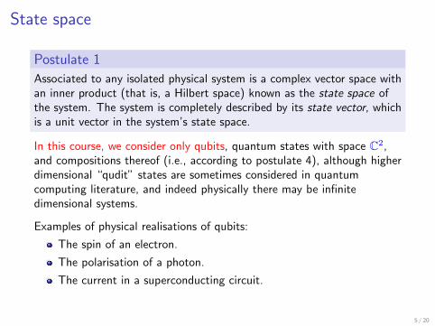
Postulate 1

Associated to any isolated physical system is a complex vector space withan inner product (that is, a Hilbert space) known as the state space ofthe system. The system is completely described by its state vector, whichis a unit vector in the system’s state space.

In this course, we consider only qubits, quantum states with space C2,and compositions thereof (i.e., according to postulate 4), although higherdimensional “qudit” states are sometimes considered in quantumcomputing literature, and indeed physically there may be infinitedimensional systems.

Examples of physical realisations of qubits:

The spin of an electron.

The polarisation of a photon.

The current in a superconducting circuit.

5 / 20

Evolution

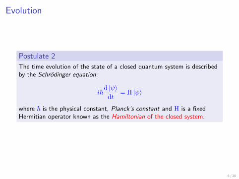
Postulate 2

The time evolution of the state of a closed quantum system is describedby the Schrodinger equation:

i~d |ψ〉dt

= H |ψ〉

where ~ is the physical constant, Planck’s constant and H is a fixedHermitian operator known as the Hamiltonian of the closed system.

6 / 20

Evolution – simplified

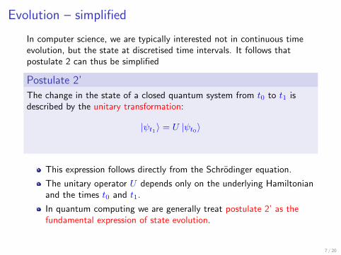
In computer science, we are typically interested not in continuous timeevolution, but the state at discretised time intervals. It follows thatpostulate 2 can thus be simplified

Postulate 2’

The change in the state of a closed quantum system from t0 to t1 isdescribed by the unitary transformation:

|ψt1〉 = U |ψt0〉

This expression follows directly from the Schrodinger equation.

The unitary operator U depends only on the underlying Hamiltonianand the times t0 and t1.

In quantum computing we are generally treat postulate 2’ as thefundamental expression of state evolution.

7 / 20

The significance of unitarity

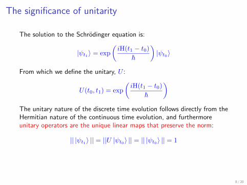
The solution to the Schrodinger equation is:

|ψt1〉 = exp

(iH(t1 − t0)

~

)|ψt0〉

From which we define the unitary, U :

U(t0, t1) = exp

(iH(t1 − t0)

~

)The unitary nature of the discrete time evolution follows directly from theHermitian nature of the continuous time evolution, and furthermoreunitary operators are the unique linear maps that preserve the norm:

|| |ψt1〉 || = ||U |ψt0〉 || = || |ψt0〉 || = 1

8 / 20

The Pauli matrices

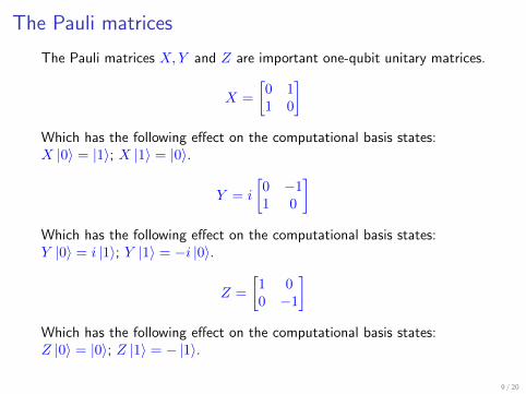
The Pauli matrices X,Y and Z are important one-qubit unitary matrices.

X =

[0 11 0

]Which has the following effect on the computational basis states:X |0〉 = |1〉; X |1〉 = |0〉.

Y = i

[0 −11 0

]Which has the following effect on the computational basis states:Y |0〉 = i |1〉; Y |1〉 = −i |0〉.

Z =

[1 00 −1

]Which has the following effect on the computational basis states:Z |0〉 = |0〉; Z |1〉 = − |1〉.

9 / 20

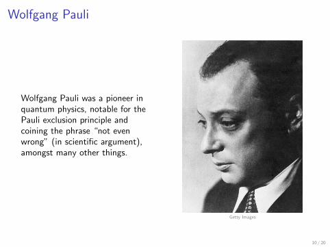
Wolfgang Pauli

Wolfgang Pauli was a pioneer inquantum physics, notable for thePauli exclusion principle andcoining the phrase “not evenwrong” (in scientific argument),amongst many other things.

Getty Images

10 / 20

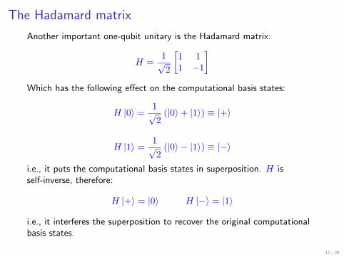
The Hadamard matrix

Another important one-qubit unitary is the Hadamard matrix:

H =1√2

[1 11 −1

]Which has the following effect on the computational basis states:

H |0〉 = 1√2(|0〉+ |1〉) ≡ |+〉

H |1〉 = 1√2(|0〉 − |1〉) ≡ |−〉

i.e., it puts the computational basis states in superposition. H isself-inverse, therefore:

H |+〉 = |0〉 H |−〉 = |1〉

i.e., it interferes the superposition to recover the original computationalbasis states.

11 / 20

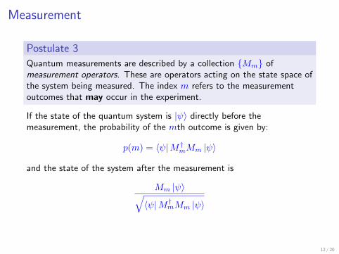
Measurement

Postulate 3

Quantum measurements are described by a collection {Mm} ofmeasurement operators. These are operators acting on the state space ofthe system being measured. The index m refers to the measurementoutcomes that may occur in the experiment.

If the state of the quantum system is |ψ〉 directly before themeasurement, the probability of the mth outcome is given by:

p(m) = 〈ψ|M†mMm |ψ〉

and the state of the system after the measurement is

Mm |ψ〉√〈ψ|M†mMm |ψ〉

12 / 20

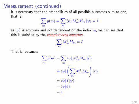
Measurement (continued)It is necessary that the probabilities of all possible outcomes sum to one,that is ∑

m

p(m) =∑m

〈ψ|M†mMm |ψ〉 = 1

as |ψ〉 is arbitrary and not dependent on the index m, we can see thatthis is satisfied by the completeness equation,∑

m

M†mMm = I

That is, because: ∑m

p(m) =∑m

〈ψ|M†mMm |ψ〉

= 〈ψ|

(∑m

M†mMm

)|ψ〉

= 〈ψ| I |ψ〉= 〈ψ|ψ〉= 1

13 / 20

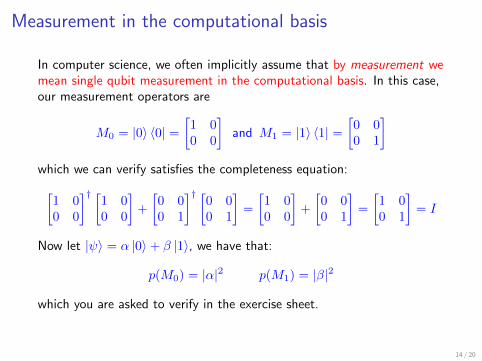
Measurement in the computational basis

In computer science, we often implicitly assume that by measurement wemean single qubit measurement in the computational basis. In this case,our measurement operators are

M0 = |0〉 〈0| =[1 00 0

]and M1 = |1〉 〈1| =

[0 00 1

]which we can verify satisfies the completeness equation:[

1 00 0

]† [1 00 0

]+

[0 00 1

]† [0 00 1

]=

[1 00 0

]+

[0 00 1

]=

[1 00 1

]= I

Now let |ψ〉 = α |0〉+ β |1〉, we have that:

p(M0) = |α|2 p(M1) = |β|2

which you are asked to verify in the exercise sheet.

14 / 20

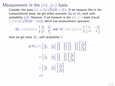
Measurement in the |+〉 , |−〉 basisConsider the state |+〉 = (1/

√2)(|0〉+ |1〉). If we measure this in the

computational basis, we get either outcome M0 or M1 each withprobability 1/2. However, if we measure in the |+〉 , |−〉 basis (recall|−〉 = (1/

√2)(|0〉 − |1〉)), which has measurement operators

M+ = |+〉 〈+| = 1

2

[1 11 1

]and M− = |−〉 〈−| = 1

2

[1 −1−1 1

]then we get state M+ with probability 1:

p(M+) =[

1√2

1√2

] [ 12

12

12

12

] [12

12

12

12

] [ 1√21√2

]

=[

1√2

1√2

] [ 12

12

12

12

] [ 1√21√2

]

=[

1√2

1√2

] [ 1√21√2

]=1

15 / 20

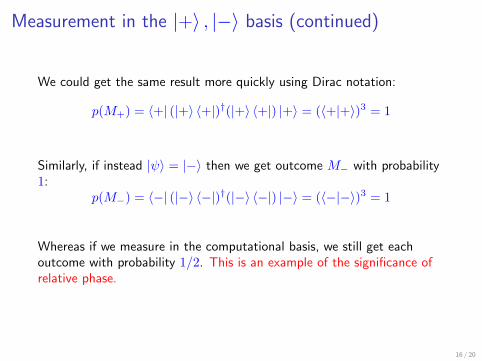
Measurement in the |+〉 , |−〉 basis (continued)

We could get the same result more quickly using Dirac notation:

p(M+) = 〈+| (|+〉 〈+|)†(|+〉 〈+|) |+〉 = (〈+|+〉)3 = 1

Similarly, if instead |ψ〉 = |−〉 then we get outcome M− with probability1:

p(M−) = 〈−| (|−〉 〈−|)†(|−〉 〈−|) |−〉 = (〈−|−〉)3 = 1

Whereas if we measure in the computational basis, we still get eachoutcome with probability 1/2. This is an example of the significance ofrelative phase.

16 / 20

Global and relative phase

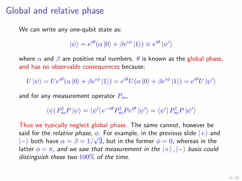
We can write any one-qubit state as:

|ψ〉 = eiθ(α |0〉+ βeiφ |1〉) ≡ eiθ |ψ′〉

where α and β are positive real numbers. θ is known as the global phase,and has no observable consequences because:

U |ψ〉 = Ueiθ(α |0〉+ βeiφ |1〉) = eiθU(α |0〉+ βeiφ |1〉) = eiθU |ψ′〉

and for any measurement operator Pm,

〈ψ|P †mP |ψ〉 = 〈ψ′| e−iθP †mPeiθ |ψ′〉 = 〈ψ′|P †mP |ψ′〉

Thus we typically neglect global phase. The same cannot, however besaid for the relative phase, φ. For example, in the previous slide |+〉 and|−〉 both have α = β = 1/

√2, but in the former φ = 0, whereas in the

latter φ = π, and we saw that measurement in the |+〉 , |−〉 basis coulddistinguish these two 100% of the time.

17 / 20

Composition

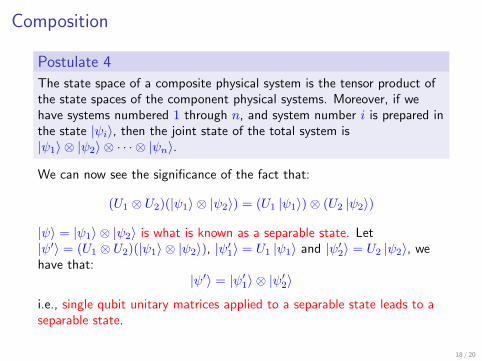
Postulate 4

The state space of a composite physical system is the tensor product ofthe state spaces of the component physical systems. Moreover, if wehave systems numbered 1 through n, and system number i is prepared inthe state |ψi〉, then the joint state of the total system is|ψ1〉 ⊗ |ψ2〉 ⊗ · · · ⊗ |ψn〉.

We can now see the significance of the fact that:

(U1 ⊗ U2)(|ψ1〉 ⊗ |ψ2〉) = (U1 |ψ1〉)⊗ (U2 |ψ2〉)

|ψ〉 = |ψ1〉 ⊗ |ψ2〉 is what is known as a separable state. Let|ψ′〉 = (U1 ⊗ U2)(|ψ1〉 ⊗ |ψ2〉), |ψ′1〉 = U1 |ψ1〉 and |ψ′2〉 = U2 |ψ2〉, wehave that:

|ψ′〉 = |ψ′1〉 ⊗ |ψ′2〉

i.e., single qubit unitary matrices applied to a separable state leads to aseparable state.

18 / 20

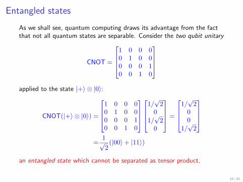
Entangled states

As we shall see, quantum computing draws its advantage from the factthat not all quantum states are separable. Consider the two qubit unitary

CNOT =

1 0 0 00 1 0 00 0 0 10 0 1 0

applied to the state |+〉 ⊗ |0〉:

CNOT(|+〉 ⊗ |0〉) =

1 0 0 00 1 0 00 0 0 10 0 1 0

1/√2

0

1/√2

0

=

1/√2

00

1/√2

=

1√2(|00〉+ |11〉)

an entangled state which cannot be separated as tensor product.

19 / 20

What to remember

Quantum mechanics specifies four postulates to which a physical theorymust adhere. You should be familiar with these, and we have alsointroduced the following important concepts in this lecture.

The Pauli matrices

The Hadamard matrix

The significance of global and relative phase

The existence of entangled states

20 / 20