Haralick feature extraction from LBP images for colortexture classification

Alice Porebski1,2, Nicolas Vandenbroucke1,2 and Ludovic Macaire2

1 Ecole d’Ingenieurs du Pas-de-Calais (EIPC)Departement Automatique - Campus de la Malassise

62967 Longuenesse Cedex - FRANCEe-mail: alice.porebski@eipc.fr, nicolas.vandenbroucke@eipc.fr

2 Laboratoire LAGIS - UMR CNRS 8146Universite des Sciences et Technologies de Lille

Cite Scientifique - Batiment P2 - 59655 Villeneuve d’Ascq - FRANCEe-mail: ludovic.macaire@univ-lille1.fr

Abstract— In this paper, we present a new approach forcolor texture classification by use of Haralick features extractedfrom co-occurrence matrices computed from Local Binary Pat-tern (LBP) images. These LBP images, which are different fromthe color LBP initially proposed by Maenpaa and Pietikainen,are extracted from color texture images, which are coded in 28different color spaces.An iterative procedure then selects among the extracted features,those which discriminate the textures, in order to build a lowdimensional feature space.Experimental results, achieved with the BarkTex database, showthe interest of this method with which a satisfying rate of well-classified images (85.6%) is obtained, with a 10-dimensionalfeature space.

Keywords— Color texture classification, Feature extraction,LBP images.

I. INTRODUCTION

Color texture classification is a major field of develop-ment for various vision applications, and particularly for theindustrial quality control where color textures have to becharacterized in order to detect defects on color texture areasand sort the products into different categories [1].

Many authors have shown that the use of color improves thecharacterization of color textures and consequently the resultsof texture classification [2], [3], [4], [5]. That is why manyrelevant texture descriptors, initially defined for grey images,have been extended to color and used to classify color textures,like Markov random fields [6], wavelet transform [7], [8], [9],co-occurrence matrices [3] or Local Binary Patterns (LBP).LBP, which have initially been proposed in 1996 by Ojala todescribe the textures present in grey level images [10], havethen been extended to color by Maenpaa and Pietikainen [2],[11].

The use of the LBP images in order to characterize colortextures is very expensive, since it requires 9 LBP imagesdeduced from the original color image. Indeed, LBP imagesare based on a scalar analysis of colors. In this paper, wepropose a new color LBP image, based on a vectorial analysisof colors. This new approach provides only one single color

LBP image which characterizes the color texture.In order to classify color textures, we propose to follow a

classical approach, defined in section III : we compute the co-occurrence matrix of this new color LBP image and extractwell-known Haralick features from this matrix.

Futhermore, the analysis of the color properties is not res-tricted to the acquisition color space (R,G,B) (see section II)and there exists a lot of color spaces which respect differentproperties [12]. None of them is adapted to the classificationof all kinds of color textures [13]. That is why we propose toselect the texture features from color texture images coded indifferent color spaces (see section IV) [14].

The selection of the Haralick features computed in differentcolor spaces significantly improves the classification qualityand also allows to work with a low-dimensional feature space[13]. This is important within the framework of industrialquality control to decrease the processing time. This discri-minating low-dimensional feature space is built by using theiterative selection procedure described in the section IV-B.

Experimental results, achieved with the BarkTex benchmarkdatabase, show the interest of this approach in the last sec-tion [15].

II. COLOR REPRESENTATION

A. Color space and texture analysis

Color analysis is not restricted to the (R,G,B) color spaceand there exists a large number of color spaces which respectdifferent properties [12]. These color spaces can be classifiedinto four families : the primary color spaces, the luminance-chrominance color spaces, the perceptual color spaces and theindependent color component spaces (see Fig. 1). Figure 1shows that these families can be divided in subfamilies too.

Furthermore, Palm, Drimbarean and Chindaro have com-pared the performances of color texture classification reachedby using color texture features extracted from images whosepixel color is represented in different color spaces [3], [4],

Image Processing Theory, Tools & Applications

978-1-4244-3321-6/08/$25.00 ©2008 IEEE

(R, G, B)

(X, Y, Z)

(x, y, z)

(r, g, b)

(A, C1, C2)

(bw, rg, by)

(Y ′, I′, Q′)

(Y ′, U ′, V ′)

(L∗, a∗, b∗)

(L∗, u∗, v∗)

(L, U, V )

(Y, x, y)

(I1, r, g)

(I1, I2, I3)

(A,CC1C2,hC1C2)

(bw,Crgby,hrgby)

(I1,CI2I3,hI2I3)

(Y ′, C′IQ, h′

IQ)

(Y ′, C′UV , h′

UV )

(L∗, C∗ab, hab)

(L∗, C∗uv , huv)

(L, CUV , hUV )

(L∗, S∗uv , huv)

(I1, S1, H3)

(I5, S4, H2)

(I4, S3, H2)

(I1, S2, H1)

(I1, S1, H1)

Primary spaces

Luminance-chrominance spaces

Independentcomponent spaces

Perceptual spaces

Real and artificialprimary spaces

Normalizedcoordinate spaces

Antagonistspaces

Televisionspaces

Perceptuallyuniform spaces

Other luminance-chrominance spaces

Polarcoordinate spaces

Perceptualcoordinate spaces

1

2

3

4

5

6

7

8

1

2

3

4

5

6

7

8

Fig. 1. Color space families.

[5]. The synthesis of these works does not allow to concludeon the definition of a single color space adapted to colortexture analysis. In order to take into account the properties ofdifferent color spaces, Chindaro proposes to merge differentclassifiers where the images are coded in different colorspaces [5]. Likewise, Vandenbroucke proposes to select localstatistical features, which are computed from different colorcomponents [16]. In this paper, we propose also to associateseveral color spaces in order to characterize the textures byextracting the color texture features from color images codedin each of the NS = 28 color spaces of Fig. 1.

B. Color order relation

In our approach, the color ranks of pixels are compared tocompute the LBP images (see section III-A.2). The color ofpixels is represented by a vector, but as there does not exist atotal order between vectors, we need to consider a partial orderrelation [18]. We choose to use for its simplicity, the partialorder relation used by vector median filters and defined asfollows :For each color space S = (C1, C2, C3) of Fig. 1, the colora = [Ca

1 Ca2 Ca

3 ] precedes the color b = [Cb1 Cb

2 Cb3], with

respect to the origin point (0, 0, 0), if√

(Ca1 )2 + (Ca

2 )2 + (Ca3 )2 ≤

√(Cb

1)2 + (Cb2)2 + (Cb

3)2.

This rule is based on the comparison of the norms of the twocolor vectors.

After having presented the NS = 28 color spaces usedto characterize more effectively the textures, and the orderrelation required to compare two colors, we explain in thenext section the computation of the color texture features.

III. COLOR TEXTURE FEATURES

In this section, we firstly explain how the LBP images arecomputed from the original color texture images. Then, wedetail the computation of the co-occurrence matrices whichare extracted from these LBP images, and finally we presentHaralick features which are used to reduce the large amountof information of the co-occurrence matrices, while preservingtheir relevance.

A. Local binary pattern images

1) Scalar LBP images: Local Binary Patterns (LBP) haveinitially been proposed in 1996 by Ojala to describe thetextures present in grey level images [10]. These texturedescriptors are very interesting because they are particularlywell-adapted to real-time quality control applications as theyare both fast and easy to implement [19]. They have thenbeen extended to color by Maenpaa and Pietikainen and usedin several color texture classification problems [2], [11].

These color texture descriptors are defined as follows :Let Ck and Ck′ , be two of the three color components ofthe color space S = (C1, C2, C3) (k, k′ ∈ {1, 2, 3}) andLBP

Ck,Ck′N [P ], be the LBP which represents the local pattern

in the neighborhood N of the pixel P , for the components Ck

and Ck′ :– first, the color component Ck′ of each pixel P ′ of the

neighborhood N is thresholded into two levels (0 and 1)by using the color component Ck(P ) of the consideredpixel P as threshold T :if Ck′(P ′) ≥ Ck(P ),then Ck′(P ′) = 1,else Ck′(P ′) = 0.

– the result of each thresholding is then coded thanks to a

weight mask :1 2 48 16

32 64 128

– the weighted values are finally summed in order to obtainthe value of the LBP LBP

Ck,Ck′N [P ].

Figure 2 illustrates the computation steps achieved toobtain the LBP images LBPC1,C1

8−N [I], LBPC1,C28−N [I] and

LBPC2,C18−N [I] extracted from the original image I, whose

the pixel color is represented by the cellC1

C2

C3

, and where

the neighborhood N here considered to compute these LBPimages is the 8-neighborhood, denoted 8 − N (see Fig. 4).

For example, for the computation of LBPC1,C28−N [P1], P1

being represented by the cell20000

in Fig. 2, the color

component C2 of each of the 8 neighboring pixels is comparedwith the color component C1(P1) = 200 = T .For the neighboring pixel located down left, for example, the

00 0

00

0

0 0

00

00

000

100

100

100100

100

100

100

100

100

200

200

200

200

200

200

200

200

200

200

255

255255255

255

50

50

505050

150

150

150 250

T T T= = =

200 0

0 1

1

0

0

1

00

1 1 1

1

111

1

1 2 4

8 16

32 64 128

0 4

0 16

0

4

0 0

0

0

200

C1,

C1

C1

,C

2 C2, C

1

0

00

0 0

0

0 0

001

0

032

4

16

1 2

8

32 64 128

LBP C1,C18−N [I]

Weight mask

Original color texture image I

LBP C1,C28−N [I] LBP C2,C1

8−N [I]

Weighting

Thresholding

Sum

20 36 255142

255 255 255 255 255 255

2 143

Fig. 2. The different steps to obtain the LBP images LBP C1,C18−N [I],

LBP C1,C28−N [I] and LBP C2,C1

8−N [I] extracted from the original image I.

result of the thresholding is 1 (200 ≥ T ). This result is thenweighted by 32.After having weighted the 8 thresholding values, we sum themand obtain LBPC1,C2

8−N [P1] = 0+0+4+0+0+32+0+0 = 36.

For a given neighborhood N , a color image I codedin the (C1, C2, C3) color space is characterized by the 9following color LBP images : LBPC1,C1

N [I], LBPC2,C2N [I],

LBPC3,C3N [I], LBPC1,C2

N I], LBPC2,C1N [I], LBPC1,C3

N [I],LBPC3,C1

N [I], LBPC2,C3N [I] et LBPC3,C2

N [I].

Pietikainen and Maenpaa propose to compute the histogramfrom each of these 9 LBP images, and to concatenate thesehistograms into a single one to characterize the color textures.They then use a log-likelihood dissimilarity measure to clas-sify the color texture images with this LBP distribution [2],[11].

2) Vectorial LBP images: Our approach differs from thisinitial definition. Indeed, instead of comparing the color com-ponents of pixels, we compare their color rank thanks to theorder relation defined in the section II-B.

00 0

00

0

0 0

00

00

000

100

100

100100

100

100

100

100

100

200

200

200

200

200

200

200

200

200

200

255

255255255

255

50

50

505050

150

150

150 250

T=

200

0 1 1

1

101

0

1 2 4

8 16

32 64 128

0 2 4

0 16

32 0 128

182 135

255 243

Original color texture image I

Weightmask

LBP image LBP C1,C2,C38−N [I]

Thresholding

Weighting

Sum

Fig. 3. The different steps done to obtain the color LBP imageLBP C1,C2,C3

8−N [I] extracted from the original image I.

This color texture descriptor is defined as follows :Let LBPS

N [P ], be the LBP image which represents the localpattern in the neighborhood N of the pixel P coded in thecolor space S :

– For each pixel P , we firstly compare the color C(P ) =[C1(P ) C2(P ) C3(P )] of this pixel with the colorC(P ′) = [C1(P ′) C2(P ′) C3(P ′)] of each neighboringpixel P ′, thanks to the color order relation :if

√(C1(P ′))2 + (C2(P ′))2 + (C3(P ′))2 ≤√

(C1(P ))2 + (C2(P ))2 + (C3(P ))2,then C(P ′) = 1,else C(P ′) = 0.

– the result of each thresholding is then coded thanks tothe weight mask proposed by Maenpaa and Pietikainen[2], [11],

– the weighted values are finally summed in order to obtainthe value of the color LBP LBPS

N [P ].

Figure 3 illustrates the computation steps done to obtain thecolor LBP image LBP

(C1,C2,C3)8−N [I] from the original image

I whose the pixel color is represented by the cellC1

C2

C3

.

For example, for the pixel P1, P1 being represented by the

cell20000

in Fig. 3, the color of each of its 8 neighbors

is compared with the threshold T =√

(200)2 + (0)2 + (0)2thanks to the following relations :

1)√

(0)2 + (0)2 + (100)2 < T2)

√(100)2 + (0)2 + (200)2 ≥ T

3)√

(255)2 + (200)2 + (0)2 ≥ T4)

√(200)2 + (100)2 + (0)2 ≥ T

5)√

(0)2 + (0)2 + (200)2 ≥ T6)

√(0)2 + (0)2 + (0)2 < T

7)√

(150)2 + (200)2 + (150)2 ≥ T8)

√(100)2 + (100)2 + (0)2 < T

The pixels whose color precedes the pixel P1 ones are labeled”0”. Otherwise they are labeled ”1” (see Fig. 3).The result of each thresholding is then coded thanksto the weight mask and the weighted values are fi-nally summed to obtain the value of LBP

(C1,C2,C3)8-neighborhood[P1] :

LBP(C1,C2,C3)8−N [P1] = 0 + 2 + 4 + 0 + 16 + 32 + 128 = 182.

The strong point of our approach is that it allows tocharacterize color textures only with one color LBP image,contrary to Maenpaa and Pietikainen’s definition where 9 LBPimages are extracted from the original image to characterizethe color textures.

Otherwise this definition of color LBP images allows toemphasize the local color variations, as we will see in thesection V-B. Therefore it is interesting to extract from theseLBP images, texture features which measure the grey scale dis-tribution and consider the spatial interactions between pixels,instead of extracting histograms, as Maenpaa and Pietikainendo. We thus choose to use Haralick features computed fromco-occurrence matrices to test the effectiveness of the LBPimages for color texture classification.

B. Haralick features extracted from co-occurrence matrices

Co-occurrence matrices, introduced by Haralick [20], arestatistical descriptors which both measure the grey scaledistribution in an image and consider the spatial interactionsbetween pixels.

These texture descriptors are defined as follows :Let MN ′ [I], the co-occurrence matrix which measures thespatial interactions between the pixels of the image I. Thecell MN ′ [I](i, j) of this matrix contains the number of timesthat a pixel P whose grey level G(P ) is equal to i, is theneighbor of a pixel Q whose grey level G(Q) is equal to j,according to the neighborhood N ′.

As they measure the local interaction between pixels, the co-occurrence matrices are sensitive to significant differences ofspatial resolution and image size. To decrease this sensitivity,it is necessary to normalize these matrices by the total co-

occurrence number∑N−1

i=0

∑N−1j=0 MN ′ [I](i, j), where N

is the quantization level number. The normalized color co-occurrence matrix mN ′ [I] is defined by :

mN ′ [I] =MN ′ [I]∑N−1

i=0

∑N−1j=0 MN ′ [I](i, j)

.

Different neighborhoods N ′ can be considered to computethe co-occurrence matrices. The first element to be consideredis the shape of the neighborhood. Figure 4 shows different 3x3neighborhood shapes.

0 ˚ direction 90 ˚ direction 45 ˚ direction 135 ˚ direction2-neighborhood 2-neighborhood 2-neighborhood 2-neighborhood

8-neighborhood 4-neighborhood 1 4-neighborhood 2

Fig. 4. Example of different 3x3 neighborhood shapes in which neighboringpixels are labeled as gray.

The choice of the neighborhood shape depending on theanalysed textures [21], we will see in section V-B that the 8-neighborhood is the best-adapted for our application since ittakes into account all directions.

The second element of the neighborhood to be consideredis the distance d between the considered pixel P and itsneighbors. Figure 5 illustrates the 8-neighborhood, for a givendistance d.

d

Fig. 5. Illustration of the neighborhood used to compute the co-occurrencematrices, for a given distance d (in number of pixels).

Palm uses different spatial city-block distances d to computeco-occurrence matrices for the classification of the BarkTexdatabase images : d = 1, 5, 10, 15, 20 [3], [15]. He obtainsthe best classification results for the distances d = 1 and d = 5.That is why we choose to consider ND = 5 different distances(d = 1, 2, 3, 4, 5) to characterize the color texture images ofthe BarkTex database.

The co-occurrence matrices characterize the textures, butthey cannot be easily exploited for color texture classificationbecause they contain a large amount of information. To reduceit, while preserving the relevance of these descriptors, Haralickproposes to use NH = 14 features, denoted f1

H to f14H ,

extracted from each matrix [20].

IV. FEATURE SELECTION

A. Candidate color texture features

For each image I coded in a color space S, we compute onesingle color LBP image LBPS

8−N [I]. Then, for each of theND = 5 neighborhoods N corresponding to the five differentdistances, we extract one co-occurrence matrix from this LBPimage (mN ′

[LBPS

8−N [I]]). Finally 14 Haralick features are

extracted from each matrix. The number of color spaces usedhere being equal to NS = 28, we examine Nf = NH ×ND ×NS = 14 × 5 × 28 = 1960 color texture features denotedxf , f = 1, . . . , Nf . Figure 6 shows how these candidate colortexture features are extracted.

f1H . . . f14

H

f1H . . . f14

Hf1

H . . . f14H

f1H . . . f14

Hf1

H . . . f14H

md=1[LBP RGB8−N [I]]

md=2[LBP RGB8−N [I]]

md=3[LBP RGB8−N [I]]

md=4[LBP RGB8−N [I]]

md=5[LBP RGB8−N [I]]

(R, G, B)

f1H . . . f14

H

f1H . . . f14

Hf1

H . . . f14H

f1H . . . f14

Hf1

H . . . f14H

md=1[LBP LUV8−N [I]]

md=2[LBP LUV8−N [I]]

md=3[LBP LUV8−N [I]]

md=4[LBP LUV8−N [I]]

md=5[LBP LUV8−N [I]]

(L, U, V )

Other color spaces. . .

Image I

LBP RGB8−N [I]

LBP LUV8−N [I]

Fig. 6. Candidate color texture features.

.

Since the total number Nf of color texture features is veryhigh, it is interesting to select the most discriminating ones inorder to reduce the size of the feature space and decrease theclassification time.

B. Iterative selection

The determination of the most discriminating feature spaceis achieved thanks to an iterative selection procedure based ona supervised learning scheme. This non-exhaustive procedurehas given very good results to select an hybrid color space forcolor image segmentation [14], [17].

In a first time, Nω learning images which are representativeof each of the NT texture classes are interactively selectedby the user. Then, the procedure selects automatically thefeatures which discriminate the NT texture classes among theNf = 1960 color texture features, thanks to the followingiterative selection procedure.At each step s of this procedure, an informational criterionJs is calculated in order to measure the discriminating powerof each candidate feature space. At the beginning of thisprocedure (s = 1), the Nf one-dimensional candidate featurespaces, defined by each of the Nf available color texture fea-tures, are considered. The candidate feature which maximizesJ1 is the best one for discriminating the texture classes. It isselected at the first step and is associated in the second stepof the procedure (s = 2) to each of the (Nf − 1) remainingcandidate color texture features in order to constitute (Nf −1)two-dimensional candidate feature spaces. We consider thatthe two-dimensional space which maximizes J2 is the bestspace for discriminating the texture classes. . .

In order to only select color texture features which arenot correlated, we measure, at each step s ≥ 2 of theprocedure, the correlation between each of the available colortexture features and each of the s − 1 other color texturefeatures constituting the selected s−1 dimensional space. Theconsidered features will be selected as candidate ones only iftheir correlation level with the color texture features alreadyselected is lower than a threshold fixed by the user [14].

We assume that the more the clusters associated to thedifferent texture classes are well separated and compact in thecandidate feature space, the higher the discriminating powerof the selected color texture features is. That leads us tochoose measures of class separability and class compactnessas measures of the discriminating power.At each step s of the procedure and for each of the (Nf−s+1)s-dimensional candidate feature spaces, we define, for theith learning image ωi,j (i = 1, . . . , Nω) associated to thetexture class Tj (j = 1, . . . , NT ), a color texture feature vectorXi,j = [x1

i,j , ..., xsi,j ]

Twhere xs

i,j is the sth color texturefeature.The measure of compactness of each texture class Tj is definedby the within-class dispersion matrix ΣC :

ΣC =1

Nω × NT×

NT∑j=1

Nω∑i=1

(Xi,j − Mj)(Xi,j − Mj)T

where Mj = [m1j , ...,m

sj ]

Tis the mean vector of the s color

texture features of the class Tj and Nω the number of imagesby class.The measure of the class separability is defined by thebetween-class dispersion matrix ΣS :

ΣS =1

NT×

NT∑j=1

(Mj − M)(Mj − M)T

where M = [m1, ...,ms]T is the mean vector of the s colortexture features for all the classes.The most discriminating feature space maximizes the infor-mation criterion :

Js = trace((ΣC + ΣS)−1ΣS

)

V. EXPERIMENTAL RESULTS

In order to show the interest of our method for colortexture classification, experimental results are achieved withthe color textures of the BarkTex database [15]. After havingdescribed this benchmark database and shown some examplesof LBP images extracted from BarkTex textures, the results ofselection and classification will be presented and analyzed.

A. BarkTex database

Color images of the BarkTex database are equally dividedinto six tree bark classes (Betula pendula (T1), Fagus silva-tica (T2), Picea abies (T3), Pinus silvestris (T4), Quercusrobus (T5), Robinia pseudacacia (T6)). Each class regroups68 images of size 128 × 192 yielding a collection of 408images.

To build the learning set, we have extracted Nω = 32learning images ωi,j of each texture class Tj .

For the classification, 36 test images for each texture classTj are used. Figure 7 illustrates a subset of learning images onthe left and a part of the images used to test our classificationmethod on the right.

These test images are classified thanks to the k-nearestneighbor classifier. We choose to use the 10-dimensionalmost discriminating feature space selected by the selectionprocedure and a number of neighbors k equal to 7 to classifythe test images, because these parameters give the best rate ofwell-classified images.

B. Examples of LBP images

Figure 8 illustrates six color texture images (coded in the(R,G,B) color space) and their associated LBP images. Wecan notice that these LBP images emphasize not only thepattern of each image, but also the local color variations.

Otherwise, contrary to the original images where the tex-tures mainly contain vertical patterns, the patterns presentin the associated LBP images have no privileged direction.So, as the choice of the neighborhood used to compute co-occurrence matrices depends on the analyzed textures [21], andas these matrices are extracted from the LBP images and notdirectly from original image, we choose the 8-neighborhoodto compute the co-occurrence matrices in order to take intoaccount all directions.

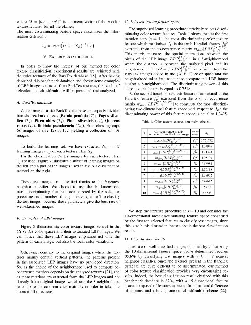
C. Selected texture feature space

The supervised learning procedure iteratively selects discri-minating color texture features. Table 1 shows that, at the firstiteration step (s = 1), the most discriminating color texturefeature which maximises J1, is the tenth Haralick feature f10

H

extracted from the co-occurrence matrix md=3[LBP(X,Y,Z)8−N ].

This matrix measures the spatial interactions between thepixels of the LBP image LBP

(X,Y,Z)8−N in a 8-neighborhood

where the distance d between the analysed pixel and itsneighbors is equal to d = 3. LBP

(X,Y,Z)8−N is extracted from the

BarkTex images coded in the (X,Y,Z) color space and theneighborhood taken into account to compute this LBP imageis also a 8-neighborhood. The discriminating power of thiscolor texture feature is equal to 0.7518.

At the second iteration step, this feature is associated to theHaralick feature f10

H extracted from the color co-occurrencematrix md=2[LBP

(Y ′,U ′,V ′)8−N ] to constitute the most discrimi-

nating two-dimensional feature space with respect to J2 : thediscriminating power of this feature space is equal to 1.3495.

Table 1. Color texture features iteratively selected.

f5H

f7H

f12H

f3H

f3H

f3H

f12H

f7H

f10H

f10Hmd=3[LBP

(X,Y,Z)8−N ]

md=2[LBP(Y ′,U′,V ′)8−N ]

md=4[LBP(L∗,S∗

uv,huv)

8−N ]

md=2[LBP(x,y,z)8−N ]

md=1[LBP(L,U,V )8−N ]

md=5[LBP(A,C1,C2)8−N ]

md=4[LBP(A,C1,C2)8−N ]

md=1[LBP(x,y,z)8−N ]

md=5[LBP(r,g,b)8−N ]

md=1[LBP(A,C1,C2)8−N ]

0.751792

1.34946

1.71323

1.95193

2.16985

2.30183

2.38972

2.47612

2.54701

2.6206

JsHaralick

featureCo-occurrence matrix

extracted from the LBP images

1

2

3

4

5

6

7

8

9

10

We stop the iterative procedure at s = 10 and consider the10-dimensional most discriminating feature space constituedby the first ten selected features to classify test images, sincethis is with this dimension that we obtain the best classificationresult.

D. Classification results

The rate of well-classified images obtained by consideringthe 10-dimensional feature space above determined reaches85.6% by classifying test images with a k = 7 nearestneighbor classifier. Since the textures present in the BarkTexdatabase are quite difficult to be discriminated, our methodof color texture classification provides very encouraging re-sults. Indeed, the best classification result obtained with thisbenchmark database is 87%, with a 15-dimensional featurespace, composed of features extracted from sum and differencehistograms, and a leaving-one-out classification scheme [22].

T6

T5

T4

T3

T2

T1

Learning images Test images

Fig. 7. Examples of BarkTex images

(a) T1 class image (b) LBP image com-puted from image (a)

(c) T2 class image (d) LBP image com-puted from image (c)

(e) T3 class image (f) LBP image com-puted from image (e)

(g) T4 class image (h) LBP image com-puted from image (g)

(i) T5 class image (j) LBP image com-puted from image (i)

(k) T6 class image (l) LBP image com-puted from image (k)

Fig. 8. Color texture images of the BarkTex database and their associated LBP images.

In order to show the interest to associate different colorspaces, we have compared the previous rate with the resultobtained by considering images only coded in the (R,G,B)space. The best classification result obtained with the Haralickfeatures extracted from co-occurrences matrices computedfrom LBP images coded in the single (R,G,B) space reaches72.7%. This rate is obtained by considering the 8-dimensionalmost discriminating feature space selected by the iterativeselection procedure, and the k = 7-nearest neighbor classifier.This experiment confirms that the association of several colorspaces improves the characterization of color textures andconsequently the results of texture classification.

VI. CONCLUSION

The originality of this work lies in the use of a new descrip-tor to characterize color textures, the color LBP images, whichdiffers from the color LBP initially proposed by Maenpaa andPietikainen. Indeed, instead of comparing the color compo-nents of pixels, we compare their color rank thanks to apartial color order relation based on euclidean distances. Thisapproach allows to consider only one LBP by image insteadof nine.

Another originality is to use Haralick features extractedfrom co-occurrence matrices computed from the color LBPimage to test the effectiveness of this descriptor for colortexture classification.

Finally, it is more interesting to extract this color LBP imagefrom color texture image coded in 28 different color spaces.

An iterative selection procedure allows then to select amongthe extracted features, those which discriminate the textures,in order to build a low dimensional feature space.

Experimental results, achieved with BarkTex database, showthe interest of this method with which a satisfying rate ofwell-classified images (85.6%) is obtained, by analysing a 10-dimensional feature space.

The perspectives of this work are firstly to find an efficientstopping criterion for the iterative selection procedure, thento determine the number k of neighbors used to classify testimages and finally, to evaluate the relevance of the color orderrelation.

Currently, we apply our approach to control the quality ofdecorated glasses which can present defects on color textureareas.

ACKNOWLEDGEMENTS

This research is funded by ”Pole de Competitivite Maud”and ”Region Nord-Pas de Calais”.

REFERENCES

[1] X. Xie. A review of recent advances in surface defect detection usingtexture analysis techniques. Computer Vision and Image Analysis, 7(3) :1-22, 2008.

[2] T. Maenpaa and M. Pietikainen. Classification with color and texture :jointly or separately ?. Pattern Recognition, 37 :629-1640, 2004.

[3] C. Palm. Color texture classification by integrative co-occurrence ma-trices. Pattern Recognition, 37 :965-976, 2004.

[4] A. Drimbarean and P.-F. Whelan. Experiments in colour texture analysis.Pattern Recognition, 22 :1161-1167, 2001.

[5] S. Chindaro, K. Sirlantzis and F. Deravi. Texture classification systemusing colour space fusion. Electronics Letters, 41 :589-590, 2005.

[6] O.J. Hernandez, J. Cook, M. Griffin, C. De Rama and M. McGovern.Classification of color textures with random field models and neuralnetworks. Journal of Computer Science & Technology, 5 :150-157, 2005.

[7] S. Arivazhagan, L. Ganesan and V. Angayarkanni. Color texture classifi-cation using wavelet transform. In Proceedings of the Sixth InternationalConference on Computational Intelligence and Multimedia Applications,315-320, 2005.

[8] A. Sengur. Wavelet transform and adaptive neuro-fuzzy inference sys-tem for color texture classification. Expert Systems with Applications,doi :10.1016/j.eswa.2007.02.032, 2007.

[9] G. Van de Wouwer, P. Scheunders, S. Livens and D. Van Dyck. Waveletcorrelation signatures for color texture characterization. Pattern Recog-nition Letters, 32 :443-451, 1999.

[10] T. Ojala, M. Pietikainen and D. Harwood. A comparative study oftexture measures with classification based on feature distributions. PatternRecognition Letters, 29(1) :51-59, 1996.

[11] M. Pietikainen, T. Maenpaa and J. Viertola Color texture classificationwith color histograms and local binary patterns In Proceedings of the2nd International Workshop on Texture Analysis and Synthesis, 109-112,2002.

[12] L. Busin, N. Vandenbroucke and L. Macaire. Color spaces and imagesegmentation. Advances in Imaging and Electron Physics, Elsevier,151(2) :65-168, 2008.

[13] A. Porebski, N. Vandenbroucke and L. Macaire. Iterative featureselection for color texture classification. In Proceeding of the 14th IEEEInternational Conference on Image Processing (ICIP’07), San Antonio,Texas, USA, 3 :509-512, 2007.

[14] N. Vandenbroucke, L. Macaire and J.-G. Postaire. Color image segmen-tation by pixel classification in an adapted hybrid color space. Applicationto soccer image analysis. Computer Vision and Image Understanding,90 :190-216, 2003.

[15] R. Picard, C. Graczyk, S. Mann, J. Wachman, L. Picard and L.Campbell. BarkTex benchmark database of color textured images. MediaLaboratory, Massachusetts Institute of Technology (MIT), Cambridge,ftp ://ftphost.uni-koblenz.de/outgoing/vision/Lakmann/BarkTex.

[16] N. Vandenbroucke, L. Macaire and J.-G. Postaire. Color image seg-mentation by supervised pixel classification in a color texture featurespace. Application to soccer image segmentation. In Proceeding of theInternational Conference on Pattern Recognition (ICPR’00), Barcelona,3 :625-628, 2000.

[17] N. Vandenbroucke, L. Macaire and J.-G. Postaire. Color pixels classifi-cation in an hybrid color space. In Proceeding of the IEEE InternationalConference on Image Processing (ICIP’98), Chicago, 1 :176-180, 1998.

[18] M. Bartkowiak and M. Domanski. Vector median filters for processingof color images in various color spaces . In Proceeding of the 5thInternational Conference on Image Processing and its Applications, 833-836, 1995.

[19] T. Maenpaa, J. Viertola and M. Pietikainen. Optimising colour andtexture features for real-time visual inspection. Pattern Analysis andApplications, 6(3) :169-175, 2003.

[20] R. Haralick, K. Shanmugan and I. Dinstein. Textural features for imageclassification. IEEE Transactions on Systems, Man and Cybernetics,3 :610-621, 1973.

[21] A. Porebski, N. Vandenbroucke and L. Macaire. Neighborhood andHaralick feature extraction for color texture analysis. In Proceeding ofthe 4th European Conference on Colour in Graphics, Image and Vision(CGIV’08), Terrassa, Spain, 316-321, 2008.

[22] C. Munzenmayer, H. Volk, C. Kublbeck, K. Spinnler and T. Wittenberg.Multispectral texture analysis using interplane sum- and difference-histograms. DAGM-Symposium, Springer, 42-49, 2002.