Artificial Intelligence in Medicine (2007) 41, 25—37

http://www.intl.elsevierhealth.com/journals/aiim

Differential diagnosis of CT focal liver lesionsusing texture features, feature selection andensemble driven classifiers

Stavroula G. Mougiakakou a,1,*, Ioannis K. Valavanis a,1,Alexandra Nikita b,2, Konstantina S. Nikita a,1

aNational Technical University of Athens, Faculty of Electrical and Computer Engineering,Biomedical Simulations and Imaging Laboratory, 9 Heroon Polytechneiou Str., 15780 Zografou,Athens, GreecebUniversity of Athens, Medical School, Department of Radiology, 20 Papadiamantopoulou Str.,15228 Athens, Greece

Received 9 January 2007; received in revised form 16 May 2007; accepted 22 May 2007

KEYWORDSLiver CT images;Computer-aideddiagnosis;Texture features;Ensembles ofclassifiers;Genetic algorithms;Bootstrap;Feature selection

Summary

Objectives: The aim of the present study is to define an optimally performingcomputer-aided diagnosis (CAD) architecture for the classification of liver tissuefrom non-enhanced computed tomography (CT) images into normal liver (C1), hepaticcyst (C2), hemangioma (C3), and hepatocellular carcinoma (C4). To this end, variousCAD architectures, based on texture features and ensembles of classifiers (ECs), arecomparatively assessed.Materials and methods: Number of regions of interests (ROIs) corresponding to C1—C4 have been defined by experienced radiologists in non-enhanced liver CT images.For each ROI, five distinct sets of texture features were extracted using first orderstatistics, spatial gray level dependence matrix, gray level difference method, Laws’texture energy measures, and fractal dimension measurements. Two different ECswere constructed and compared. The first one consists of five multilayer perceptronneural networks (NNs), each using as input one of the computed texture feature setsor its reduced version after genetic algorithm-based feature selection. The second ECcomprised five different primary classifiers, namely one multilayer perceptron NN,one probabilistic NN, and three k-nearest neighbor classifiers, each fed with thecombination of the five texture feature sets or their reduced versions. The finaldecision of each EC was extracted by using appropriate voting schemes, while

* Corresponding author. Tel.: +30 210 772 2968; fax: +30 210 772 3557.E-mail address: smougia@cc.ece.ntua.gr (S.G. Mougiakakou).

1 Tel.: +30 210 772 2968; fax: +30 210 772 3557.2 Tel.: +30 210 722 7488; fax: +30 210 729 2280.

0933-3657/$ — see front matter # 2007 Elsevier B.V. All rights reserved.doi:10.1016/j.artmed.2007.05.002

26 S.G. Mougiakakou et al.

bootstrap re-sampling was utilized in order to estimate the generalization ability ofthe CAD architectures based on the available relatively small-sized data set.Results: The best mean classification accuracy (84.96%) is achieved by the second ECusing a fused feature set, and the weighted voting scheme. The fused feature set wasobtained after appropriate feature selection applied to specific subsets of the originalfeature set.Conclusions: The comparative assessment of the various CAD architectures showsthat combining three types of classifiers with a voting scheme, fed with identicalfeature sets obtained after appropriate feature selection and fusion, may result in anaccurate system able to assist differential diagnosis of focal liver lesions from non-enhanced CT images.# 2007 Elsevier B.V. All rights reserved.

1. Introduction

One of the most common and robust imaging tech-niques for the detection of hepatic lesions is com-puted tomography (CT) [1]. Although the quality ofCT images has been significantly improved duringthe last years, it is difficult in some cases, even forexperienced doctors, to make a 100% accurate diag-nosis. In these cases, the diagnosis has to be con-firmed by administration of contrast agents, which isrelated with renal toxicity and allergic reactions, orinvasive procedures (biopsies). During the lastyears, along with the developments in image pro-cessing and artificial intelligence, computer-aideddiagnosis (CAD) systems, aiming at the character-ization of liver tissue, attract much attention, sincethey can provide diagnostic assistance to clinicians,and contribute to reduction of the number ofrequired biopsies.

Various approaches, most of them using ultra-sound B-scan and CT images, have been proposedbased on different image characteristics, such astexture features, estimated from first- and second-order gray level statistics, and fractal dimensionestimators combined with various classifiers [2—5]. Texture analysis of liver CT images based onspatial gray level dependence matrix (SGLDM), graylevel run length method (GLRLM), and gray leveldifference method (GLDM) has been proposed by Miret al. [6], in order to discriminate normal frommalignant hepatic tissue. Chen et al. [7] haveapplied SGLDM texture features to a probabilisticneural network (P-NN) for the characterization ofhepatic tissue (hepatoma and hemangioma) from CTimages. Additionally, SGLDM-based texture featuresfed to a system of three sequentially placed neuralnetworks (NNs) have been used by Gletsos et al. [8]for the classification of hepatic tissue into fourcategories. Although a lot of effort has beendevoted to liver tissue characterization, the devel-oped systems are most of the times limited to two orthree classes of liver tissue and/or do not gain from

the interaction of different texture characteriza-tion methods, or the combination of different clas-sifiers.

In order to select the most robust characteristicsfrom an initial high-dimensional feature set, thatmight be derived from different feature extractiontechniques, feature selection methods can beapplied. Deterministic, or stochastic feature selec-tion methods decrease the feature extraction costsof the classification system, and may also enhanceits performance [9]. During the last years, anincreasing number of researchers are using geneticalgorithms (GAs) for dimensionality reduction. Theuse of GAs for feature selection was first introducedin 1989 [10], and since then, GAs have been success-fully applied to a broad spectrum of dimensionalityreduction studies [11—13]. According to Ref. [8], theuse of GAs results in more robust feature vectors ascompared to other deterministic feature selectiontechniques, in problems related to liver tissue clas-sification from CT images.

In the last decade, the use of multiple classifiersystems has been proposed in order to optimize theperformance of CAD systems. A set of classifierswhose individual predictions are fused through acombining strategy, usually a voting scheme, toclassify new examples constitutes an ensemble ofclassifiers (EC) [14]. The attraction that this topicexerts on machine learning and diagnostic decisionsupport research is based on the premise that ECsare often much more accurate than any individualclassifier of the set [15,16]. Early diagnosis of mel-anoma has been facilitated by combining threetypes of classifiers, namely linear discriminant ana-lysis (LDA), k-nearest neighbor (k-NN), and a deci-sion tree, with a voting scheme [17]. A multipleclassification system based on a committee of NNs,trained by the Levenberg—Marquardt algorithm,along with a voting scheme across the NN outputshas been used by Jerebko et al. [18] for the detec-tion of colonic polyps in CT colonography data.Furthermore, a novel system for diabetes diagnosis

Differential diagnosis of CT focal liver lesions 27

has been proposed [19], which is based on retinalimages fractal characteristics and applies a votingscheme across the outputs of an EC consisting of aback-propagation trained NN, a radial basis functionNN, and a GA-based classifier. The use of texturefeatures and shape parameters along with a multi-classifier modular architecture composed from aself-organizing map (SOM) and/or k-NN classifiershas been recently proposed by Christodoulou et al.[15], aiming at the characterization of carotid pla-ques for the identification of individuals with asymp-tomatic carotid stenosis at risk of stroke.

Although previous studies [20,21] have shownthat CAD systems based on various texture featuresand ECs can enhance the diagnosis efficiency of CTfocal liver lesions, the evaluation of the proposedmethods on small-sized samples constitutes a sig-nificant drawback for these studies. To address thisdrawback, re-sampling methods like cross-valida-tion, jack-knife, and bootstrap can be applied[22—24]. In Ref. [18], cross-validation has beenapplied for sensitivity estimation of a colonic polypdetection system, while in Ref. [25] the bootstrapmethod has been used for the development of adiagnosis system able to differentiate benign andmalignant tumors from breast ultrasound images.The bootstrap method, which was introduced byEfron [22] as an approach to calculate confidenceintervals for parameters where standard methodscannot be applied, is based on re-sampling withreplacement. The comparative assessment of var-ious re-sampling methods has shown that the boot-strap method provides less biased and moreconsistent results than the jack-knife method [26].

The principal aim of the present paper is to assessthe potential of ECs in the development of a CADsystem able to discriminate four hepatic tissue types(normal liver, hepatic cyst, hemangioma, and hepa-tocellular carcinoma) from non-enhanced CTimages. Furthermore, the use of a variety of texturefeatures as input to the CAD system is examinedwhile the application of feature selection based on aGA is investigated aiming at improving the resultingclassification performance. In order to overcomeproblems with small data sets and biased classifica-

Figure 1 Generic desig

tion performances, the bootstrapmethod is applied.In this framework, five different CAD architecturesbased on the above design concepts are compara-tively assessed.

The rest of the paper is organized as follows: inSection 2, the generic system design concepts arepresented, including description of the data used,the methodology of feature extraction and selec-tion, the ECs and the applied voting schemes, aswell as the five alternative architectures of the CADsystem. In Section 3, the experimental results of thefive CAD system architectures are presented andcompared, followed by conclusions presented inSection 4.

2. Methodology

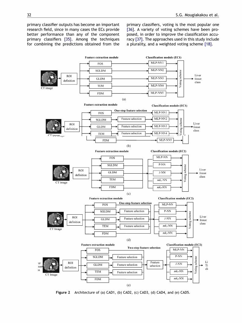
The generic design of a CAD system aiming at theclassification of CT liver tissue into one of the fourclasses: normal liver (C1), hepatic cyst (C2), heman-gioma (C3), and hepatocellular carcinoma (C4), ispresented in Fig. 1. Firstly, regions of interest (ROIs)drawn by an experienced radiologist on CT imageswere driven to a feature extraction module, wherefive different texture feature sets were obtainedusing first order statistics (FOS), spatial gray leveldependence matrices (SGLDM), gray level differ-ence matrix (GLDM), Laws’ texture energy measures(TEM), and fractal dimension measurements (FDM).Then, the full feature sets or their reduced versionsobtained after proper feature selection in the fea-ture selection module, were fed to an EC. Twoalternative approaches for constructing ECs werestudied. The primary classifiers of the first ensemble(EC1) were generated by applying a single learningalgorithm to different feature subsets, while theclassifiers of the second ensemble (EC2) were gen-erated by using different learning algorithms on theentire feature set. The predictions obtained fromthe primary classifiers of each ensemble were com-bined using appropriate voting schemes.

In the following, the modules of the CAD systemsare presented, and the five alternative CAD systemarchitectures are described.

n of CAD1, . . ., CAD5.

28 S.G. Mougiakakou et al.

2.1. Image acquisition

Abdominal non-enhanced CT images with a spatialresolution of 512 � 512 pixels and 8-bit gray level atthe W150 + 60 window taken from both patients andhealthy controls were acquired using a conventionalsingle detector CT scanner (Philips LX, Philips Med-ical Systems). The slice thickness ranged from 5 mmto 8 mm, depending on the lesion size. A total of 38healthy controls were identified by the radiologist,while the diagnosed hepatic lesions from patientswith C2 (15 patients), C3 (24 patients), and C4 (20patients), were validated by needle biopsies, den-sity measurements, and the typical pattern ofenhancement after the intravenous injection ofiodine contrast. The patient statistics is presentedin Table 1. The position, size and extent of thelesions were defined in CT images by an experiencedradiologist. For each patient a maximum of twofree-hand ROIs were taken from different slices,resulting in a total of 147 ROIs, 76 of which corre-sponded to C1, 19 to C2, 28 to C3, and 24 to C4.

2.2. Feature extraction

Five sets of texture features were calculated foreach ROI corresponding to FOS, SGLDM, GLDM, TEM,and FDM.

2.2.1. First order statisticsFeatures from FOS [27] are easily computed fromthe intensity function of the image. In our experi-ments, six features were calculated for each ROIfrom the following equations:

average gray level : avgFOS ¼Xg

gHðgÞ (1)

standard deviation : stdFOS

¼ffiffiffiffiffiffiffiffiffiffiffiffiffiffiffiffiffiffiffiffiffiffiffiffiffiffiffiffiffiffiffiffiffiffiffiffiffiffiffiffiffiffiffiffiffiXg

ðg� avgFOSÞ2HðgÞs

(2)

entropy : entFOS ¼ �X

HðgÞ lnðHðgÞÞ (3)

g

stdFOS

coefficient of variation : cvFOS ¼

avgFOS(4)

Table 1 Statistics of both healthy controls (C1) andpatients (C2—C4)

Age (years) Sex (male/female)Min Max Mean

C1 35 70 55.5 20/18C2 44 70 58.3 7/8C3 45 63 52.7 11/13C4 61 78 70.5 13/7

1 X3

skewness : skFOS ¼

std3 g

ðg� avgFOSÞ HðgÞ (5)

kurtness : kurFOS

¼ 1

std4FOS

Xg

ðg� avgFOSÞ4HðgÞ � 3 (6)

where g are the possible values of the gray level ofthe image and H(g) is the percentage of the pixels inthe image with gray level equal to g.

2.2.2. Spatial gray level dependence matricesThe texture characteristics of each ROI, whichactually correspond to second order statistics,can be derived from the SGLDM of the ROI[27,28]. The elements of the SGLDM representthe values of the probability function Pij, whichmeasure the normalized frequency in which allpixel pairs consisting of pixels with interpixel dis-tance d along a direction u andwith gray level valuesi and j, respectively, appear in the image. Thefeatures calculated in our experiments from SGLDMare given by the following equations:

angular second moment :

asmSGLDM ¼Xi

Xj

P2i j (7)

contrast :

conSGLDM ¼XNg

n¼0n2

XNg

i¼1

XNg

j¼1Pi j; ji� jj ¼ n

( )(8)

Pi

Pjði jPi jÞ � m2

correlation : corSGLDM ¼s2

(9)

variance : varSGLDM ¼XX

ði jPi jÞ � m2 (10)

i j

inverse difference moment :

idmSGLDM ¼Xi

Xj

Pi j

1þ ði� jÞ2(11)

entropy : entSGLDM ¼ �XX

Pi j lnðPi jÞ (12)

i jXX Pi j

homogeneity : hgSGLDM ¼i j

1þ ji� jj (13)

cluster tendency : cltSGLDM

¼Xi

Xj

ðiþ j� 2mÞPi j (14)

where Pij is the (i, j) element of SGLDM, m and s

are the mean value and the standard deviation ofthe elements of the matrix, respectively, and Ng isthe number of gray levels in the image. In thepresent study, four values for the angle u wereused: u = 08, 458, 908, and 1358, and the features

Differential diagnosis of CT focal liver lesions 29

were calculated for distances of 1, 2, 4, 6, 8, and12 pixels. For each distance, the final featurevalue was computed by averaging over the featurevalues corresponding to the four angular direc-tions. Thus, a total of 48 texture characteristicswas obtained for each ROI.

2.2.3. Gray level difference matrixWe consider here a class of local properties [29]based on absolute differences between the graylevels of pixels in the ROI. Let I(x, y) be the imageintensity function. For any given displacementd = (Dx, Dy) let Id(x, y) = jI(x, y) � I(x + Dx,y + Dy)j, and f(ijd) be the probability density ofId(x, y). The value of f(ijd) is obtained from thenumber of times Id(x, y) occurs for a given d, i.e.f(ijd) = P(Id(x, y) = i). If a texture is directional, thedegree of spread of the values in f(ijd) should varywith the direction of d, given that its magnitude is inthe proper range. Thus, texture directionality canbe analyzed by comparing spread measures of f(ijd)for various directions of d. In the present study, fourpossible forms of the vector d were considered: (0,d), (d, 0), (�d, d), and (�d, �d), with d being theinterpixel distance, each of which corresponds to adisplacement in vertical, horizontal, 1358 and 458direction, respectively. From each of the densityfunctions corresponding to one of the above-men-tioned directions, five texture features wereobtained:

contrast : conGLDM ¼Xi

i2 fðijdÞ (15)

mean value : mnGLDM ¼X

i fðijdÞ (16)

i

entropy : entGLDM ¼ �X

fðijdÞ log fðijdÞ (17)

i

inverse difference moment :

idmGLDM ¼Xi

fðijdÞi2 þ 1

(18)

angular second moment :

asmGLDM ¼Xi

½ fðijdÞ�2(19)

where Ng is the number of gray levels in the imageand i 2 [0, Ng � 1). The features were calculated fordistances of 1, 2, 3, and 4 pixels. The final featurevalue for each distance was computed by averagingover the feature values corresponding to the fourangular directions. Thus, from the GLDMmethod, 20texture characteristics were obtained for each ROI.

2.2.4. Laws’ texture energy measuresLaws’ TEM [30] are derived from three simple vec-tors of length three: L3 � (1, 2, 1), E3 � (�1, 0, 1),

S3 � (�1, 2, �1), which represent the one-dimen-sional operations of center-weighted local aver-aging, the symmetric first differencing for edgedetection, and the second differencing for spotdetection, respectively. If these vectors are con-volved with themselves or with each other, fivevectors of length five are obtained: L5 � L3 �L3 = (1, 4, 6, 4, 1), S5 � L3 � S3 = �E3 � E3 = (�1,0, 2, 0, �1), R5 � S3 � S3 = (1, �4, 6, �4, 1),E5 � L3 � E3 = (�1, �2, 0, 2, 1), and W5 ��E3 � S3 = (�1, 2, 0, �2, 1). Vector L5 performslocal averaging, S5 and E5 are spot and edge detec-tors, respectively, while R5 andW5 can be regardedas ‘‘ripple’’ and ‘‘wave’’ detectors, respectively. Ifwe multiply the column vectors of length five, whichare obtained after transposing L5, S5, R5, E5, andW5, by the row vectors L5, S5, R5, E5, and W5, weobtain Laws’ 5 � 5 masks. In our study, the followingfour Laws’ zero-summasks were used: L5E5 = L5TE5,E5S5 = �E5TS5, L5S5 = L5TS5, R5R5 = R5TS5.

After convolving each ROI image with each of thefour masks, the following measures were calcu-lated:

sum of absolute values

# of pixels:

asTEM ¼Xx

Xy

jILðx; yÞj# of pixels of the original image

(20)

sum of squares

# of pixels:

ssTEM ¼Xx

Xy

I2Lðx; yÞ# of pixels of the original image

(21)

entropy : entTEM ¼ �X

HLðgÞ lnHLðgÞ (22)

g

where IL(x, y) is the intensity function of the imageafter its convolution with the Law’s mask, g are thepossible values of the gray level of the convolvedimage, and HL(g) is the percentage of the pixels ofthe convolved image with gray level equal to g.Thus, twelve Laws’ energy measures (4 masks � 3statistics per mask) were calculated for each ROI.

2.2.5. Fractal dimension measurementsIn order to extract more information from the liverCT images, a feature extraction method based onthe concepts of the fractional Brownian motion(FBM) model and multiple resolution imagery wasemployed [5]. According to the FBM model devel-oped by Mandelbrot [31], the roughness of a surface,naturally occurring as the end result of randomwalks, can be characterized by its fractal dimension

30 S.G. Mougiakakou et al.

(FD). For a CT liver image, which can be consideredas such a surface, FD is estimated from the equationE(DI2) = c(Dr)6�2FD, where E(�) denotes the expecta-tion operator, DI � jI(x2, y2) � I(x1, y1)j is the inten-sity variation of two pixels, c is some constant, andDr � jj(x2, y2)�(x1, y1)jj is the spatial distance ofpixels. A simpler method is to estimate the H para-meter, which is H = 3 � FD, from the equationE(DI2) = c(Dr)2H. If we apply the log function to bothsides of the last equation we obtain:

log½EðDI2Þ� ¼ logðcÞ þ 2H logðDrÞ (23)

Given an image I, the intensity difference vector isdefined as IDV � [id(1), id(2), . . ., id(s)] where s isthe maximum inter-pixel distance depending on thesize of the image, and id(k) is the average of theabsolute intensity difference of all pixel pairs withhorizontal, vertical or diagonal distance k. Accord-ing to Eq. (23), the value of H can be obtained byusing least-squares linear regression to estimate theslope of the curve of id(k) versus k in log-log scales.Obviously, the value of H is equal to the half of theslope of the curve.

According to Ref. [5], we can obtain more textureinformation, i.e. for the lacunarity or the regularityof an image, if we calculate the values H(k), whichcorrespond to theH value of the image computed foran image resolution k. The original image corre-sponds to a k = 1 resolution, the original imagereduced to a half-sized image corresponds to ak = 2 resolution, etc. Using the pyramidal approach,described in [5], for multiresolutional analysis weobtained three features, H1FDM, H2FDM, H3FDM, foreach ROI, which correspond to theH value of the ROIat image resolutions k = 1, 2, 3.

2.3. Feature selection

For the purpose of feature selection, a GA based onRef. [32] was used in the present paper. The algo-rithm makes use of a randomly created initial popu-lation of N chromosomes. Each chromosome is abinary mask, with 1 indicating that the feature isselected, and 0 that the corresponding feature isomitted. The initial population is updated throughthe following procedure:

For Ng generations{ Calculate the fitness function of the N chromosomes

Select N/2 pairs from population using the elitistselection methodMate selected chromosomes using two-pointcrossover, with crossover probability PcSwitch value of chromosome bits, with mutationprobability PmUpdate population

Assign fitness values to new population, store bestresults }

The maximum squared Mahalanobis distancebetween classes computed for the samples belong-ing to the training set was used as fitness function[8]. Since the number of selected features is nottaken into account in computing the fitness func-tion, a ‘‘penalty’’ function for feature sets exceed-ing a given dimensionality threshold was applied.Thus, the corresponding individuals were assigned afitness value equal to 50% of the average populationfitness. The GA was run for a dimensionality thresh-old equal to 10. This threshold has been successfullyapplied in the selection of texture features usingGAs in the problem of focal liver lesion character-ization [8]. The GA run parameters, manually tunedafter a series of trials, were N = 200, Ng = 250,Pc = 0.8 and Pm = 0.008.

2.4. Classification

The estimated texture feature sets were applied toeither of two different ensembles of classifiers (EC1and EC2). EC1 was constructed by combining fivemultilayer perceptron NNs (MLP-NN), each fed withone out of the five distinct texture feature sets(MLP-NN1 with FOS, MLP-NN2 with SGLDM, MLP-NN3 with GLDM, MLP-NN4 with TEM, MPL-NN5 withFDM). EC2 was constructed by combining one MLP-NN, one probabilistic NN (P-NN), one 1-nearestneighbor (1-NN) classifier, and two modified k-NNs(mk-NN) (k > 1) classifiers, each fed with the com-bination of the five computed texture feature sets.For each EC, the final decision was generated bycombining the diagnostic outputs of the corre-sponding primary classifiers through appropriatevoting schemes. In order to obtain reliable results,in terms of classification accuracy, the develop-ment of both EC1 and EC2 was based on the boot-strap method. To this end, a training set consistingof 147 ROIs was sampled with replacement from theavailable 147 ROIs. The ROIs not appearing in thetraining set were randomly allocated into twoequally sized sets (validation and testing sets).The procedure was repeated for 50 times, resultingin 50 groups of training, validation and testing sets.For each group of sets, EC1 and EC2were developedand tested. In order to train the primary classifiersof each ensemble the training and validation setswere used. The generalization ability of both theprimary classifiers and the ECs was tested using thetesting set. The various CAD architectures wereassessed by estimating the mean classificationaccuracy and the corresponding standard deviationfor all bootstrap sets.

Differential diagnosis of CT focal liver lesions 31

2.4.1. Multilayer perceptron neural networkThe MLP-NN classifier [33] used in this study is basedon a feed-forward NN consisting of one input layerwith a number of input neurons equal to the numberof features fed into the NN, one hidden layer withvariable number of neurons, and one output layerconsisting of two output neurons, encoding thedifferent types of liver tissue. Thus, the outputs(00), (01), (10), and (11) correspond to the four livertissue classes C1, C2, C3, and C4, respectively. TheMLP-NN was fully connected with initial weightsrandomly selected in the range [�1.0, 1.0]. Thelog-sigmoid and tan-sigmoid activation functionswere employed for the hidden and the outputlayers, respectively. Because of the use of thelog-sigmoid function in the hidden layer, the valuesof the input vectors were normalized from �1.0 to1.0. The use of the tan-sigmoid function in theoutput neurons resulted in output values in therange [0.0, 1.0]: a value of less than 0.5 corre-sponded to 0, while a value greater or equal to0.5 corresponded to 1. The MLP-NN was trained,using the training set, by the batched back-propa-gation (BP) algorithm with adaptive learning rateand momentum [33]. Moreover, the optimal MLP-NNclassifier in terms of hidden neurons and internal NNparameters (appropriate values of momentum andinitial learning rate) was determined using a trial-and-error process, until no further improvement ofclassification accuracy in the validation set could beobtained.

2.4.2. Probabilistic neural networkThe P-NN performs interpolation in multidimen-sional space [2]. The P-NN consists of one inputlayer with number of neurons equal to the numberof used features, a hidden (or training pattern unit)layer, a summation unit layer, and an output layer. Inorder to classify a ROI, the corresponding feature set(X) is applied to the input layer and then into thehidden layer, followed by the summation layer. Inthe summation layer the probabilistic density func-tion p(XjCi) of the class Ci, i = 1, . . ., 4 correspondingto the four classes of hepatic tissue, is estimated:

pðXjCiÞ ¼1

ð2pÞr=2sr

1

NCi

XNCi

j¼0KðX� Xi

jÞ (24)

where r is the dimensionality of the feature vector,s is a smoothing parameter, NCi the number oftraining ROIs in each class i, Xi

j is the j pattern ofthe class Ci, and K(�) is the Gaussian basis function,output of the hidden layer, given by

KðX� XijÞ ¼ exp �

ðX� XijÞTðX� Xi

jÞ2s2

0@

1A (25)

Finally, the neuron in the output layer classifies theROI into the class with the highest probabilisticdensity function. The applied training procedure,in order to determine the value of the smoothingparameter and achieve high classification perfor-mance, is the same as in the case of the MLP-NNclassifier.

2.4.3. k-Nearest neighbor classifierThe k-NN classifier is a very popular statistical clas-sifier because of its simplicity and its easiness ofdevelopment [11,34]. In the k-NN (k � 1) classifiers,in order to classify a new feature vector, its knearest neighbors from the training set are identi-fied. The feature vector is classified to the mostfrequent class among its neighbors based on a simi-larity measure, like the Euclidian distance, which isused in the present study.

In this paper, a 1-NN classifier along with twomk-NN (modified k-NN, k > 1, classifiers) mk1-NN andmk2-NN, have been developed. The mk-NN classi-fiers are based on the use of a distance-basedweight. When a feature vector (X) is to be classified,the classifier finds the k nearest to X patterns (y1, y2,. . ., yk), which belong to the training set, based onthe Euclidian distance D. Each class Ci, i = 1, . . ., 4,corresponding to the four types (C1, C2, C3, and C4)of hepatic tissue, contests the feature vector with avoting power wi:

wi ¼Xkj¼1

D�1ðX; y jÞ fðy j;CiÞ; with i ¼ 1; :::; 4

(26)

where function f is defined as

fðy j;CiÞ ¼1; if Ci ¼ class of y j

0; else

�(27)

The feature vector is finally declared into the classthat contributes maximum weights in the neigh-bors.

The structures of mk1-NN and mk2-NN, whichparticipate in the EC2, were determined by usingthe validation set. That means that the chosenvalue of k1, predefined in our study to be in therange 2 � k1 � 5, was the value of k1 for which theclassification accuracy of the mk1-NN classifierwas maximized in the validation set. Based onthe same concept, the optimal value of k2, pre-defined to be within the range 6 � k2 � 9, waschosen.

2.4.4. Voting schemeOnce the primary classifiers of an EC have beengenerated, the issue of how to combine their pre-dictions arises. Recently, the combination of

32 S.G. Mougiakakou et al.

primary classifier outputs has become an importantresearch field, since in many cases the ECs providebetter performance than any of the componentprimary classifiers [35]. Among the techniquesfor combining the predictions obtained from the

Figure 2 Architecture of (a) CAD1, (b) CA

primary classifiers, voting is the most popular one[36]. A variety of voting schemes have been pro-posed, in order to improve the classification accu-racy [37]. The approaches used in this study includea plurality, and a weighted voting scheme [18].

D2, (c) CAD3, (d) CAD4, and (e) CAD5.

Differential diagnosis of CT focal liver lesions 33

Table 3 The 12 selected features fed into EC2 of CAD5

avgFOScvFOSkurFOScltSGLDM (d = 1)idmSGLDM (d = 2)corSGLDM (d = 8)idmGLDM (d = 1)meanGLDM (d = 4)entTEM (mask: L5E5)entTEM (mask: E5S5)H1FDMH3FDM

2.5. CAD system architectures

Five alternative architectures (CAD1, . . ., CAD5)were developed based on the generic design ofthe CAD system presented in Fig. 1. CAD1 andCAD2 were constructed using EC1, while CAD3,CAD4, and CAD5 were based on EC2. In CAD1(Fig. 2(a)), each of the full-dimensional FOS,SGLDM, GLDM, TEM, and FDM feature sets, esti-mated in the feature extraction module, is fed intoone of the five primary classifiers of EC1 (MLP-NN1,. . ., MLP-NN5). CAD2 (Fig. 2(b)) differs from CAD1 inthat feature selection is applied to the high-dimen-sionality feature vectors estimated from SGLDM,GLDM, and TEM. The selected features from theSGLDM, GLDM, and TEM sets are presented inTable 2. In CAD3 (Fig. 2(c)), each primary classifieruses as input the 89-dimensional feature set, whichresults from the combination of the full-dimensionalFOS, SGLDM, GLDM, TEM, and FDM features sets.CAD4 (Fig. 2(d)) differs from CAD3 in that featureselection is applied to SGLDM, GLDM, and TEM fea-ture sets prior to the combination with the full-dimensional FOS and FDM feature sets. The selectedSGLDM, GLDM and TEM features are identical withthe ones applied in CAD2 (Table 2). Thus, eachprimary classifier of EC2 in CAD4 uses as input a30-dimensional feature set. CAD5 (Fig. 2(e)) differsfrom CAD4 in that further feature selection isapplied to the 30-dimensional feature set used byCAD4. The resulting 12-dimensional feature set(Table 3) provides the input to each primary classi-fier of EC2 in CAD5. The final decision of each CADsystem (CAD1, . . ., CAD5) is generated by combiningthe individual predictions of the primary classifiersof EC1 and EC2 through either plurality or weightedvoting schemes.

Table 2 The selected features from the SGLDM, GLDMand TEM feature sets fed into EC1 of CAD2 and EC2 ofCAD4

SGLDM GLDM TEM

idmSGLDM (d = 1) idmGLDM

(d = 1)asTEM (mask: L5E5)

entSGLDM (d = 1) asmGLDM

(d = 1)ssTEM (mask: L5E5)

cltSGLDM (d = 1) entGLDM(d = 2)

entTEM (mask: L5E5)

corSGLDM (d = 2) meanGLDM(d = 4)

ssTEM (mask: E5S5)

idmSGLDM (d = 2) idmGLDM

(d = 4)entTEM (mask: E5S5)

conSGLDM (d = 4) asTEM (mask: L5S5)corSGLDM (d = 8) entTEM (mask: L5S5)conSGLDM (d = 12) ssTEM (mask: R5R5)

3. Results and discussion

The classification accuracies achieved by CAD1, . . .,CAD5 using the 50 groups of sets (training, validationand testing set), obtained through bootstrap re-sampling, were estimated. For each architecture,the results are presented in terms of mean valuesand standard deviations of the classification accu-racy of the primary classifiers, as well as the totalCAD system performance with use of either pluralityor weighted voting scheme.

The results for CAD1 and CAD2 are presented inTable 4. It can be observed that the use of FOS andTEM feature sets yielded to the best individualclassification accuracies. In particular, the highestclassification accuracy (78.43% 8.23) wasobtained with the use of the FOS feature vector(MLP-NN1), followed by a 70.96% 8.53% classifica-tion accuracy obtained with the use of the full TEMfeature vector (MLP-NN4 of CAD1), and a70.68% 8.64% classification accuracy achievedby using the reduced TEM feature vector (MLP-NN4 of CAD2). FDM and full or reduced SGLDMfeature sets yielded in general to worse individualclassification accuracies in the bootstrap testingsets. The feature selection module in CAD2 didnot alter significantly the performance of the pri-mary classifiers. Thus, equally performing classifierswere obtained with less computational cost.Regarding the voting schemes, it can be observedthat the weighted voting scheme outperformed theplurality voting scheme in the testing set. Similarobservations were reported in the experiments donein [15]. However, it is notable that the best of theprimary classifiers of CAD1 and CAD2 (MLP-NN1)performed slightly better than the ensemble usingthe weighted voting scheme. That is inline withmany experimental results showing that the useof fixed combining rules (e.g., voting scheme) alongwith strong primary classifiers (i.e., classifiers whichperform well by their own) results to ECs which do

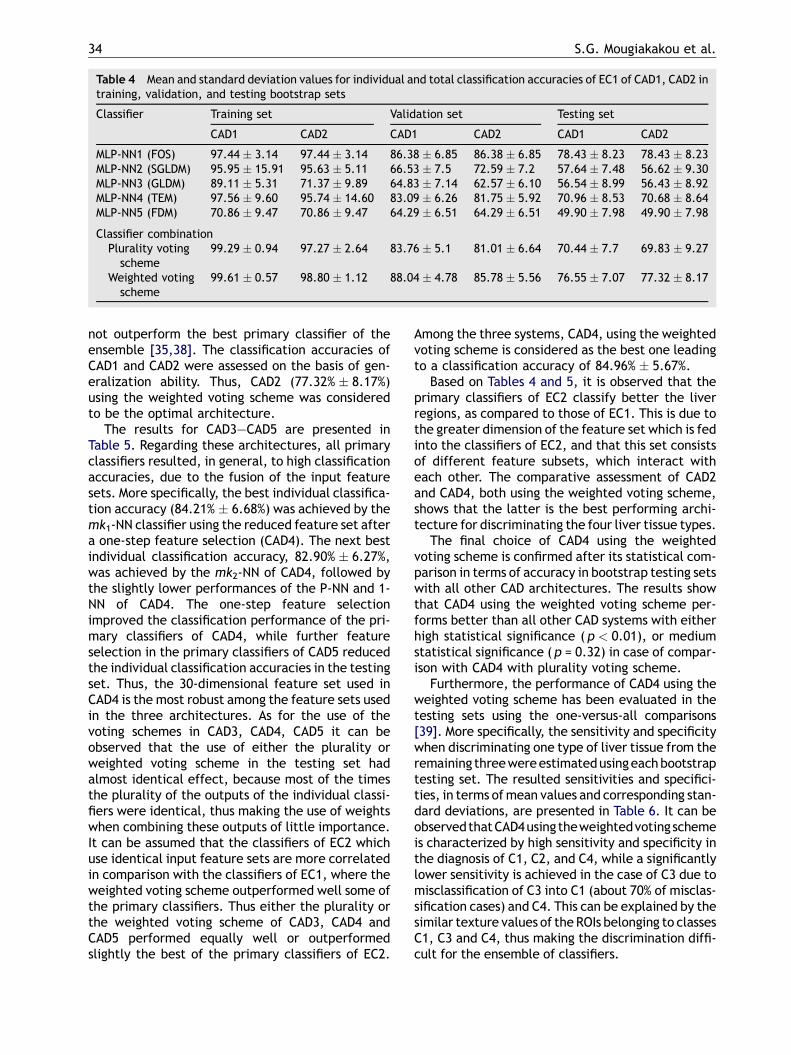
34 S.G. Mougiakakou et al.

Table 4 Mean and standard deviation values for individual and total classification accuracies of EC1 of CAD1, CAD2 intraining, validation, and testing bootstrap sets

Classifier Training set Validation set Testing set

CAD1 CAD2 CAD1 CAD2 CAD1 CAD2

MLP-NN1 (FOS) 97.44 3.14 97.44 3.14 86.38 6.85 86.38 6.85 78.43 8.23 78.43 8.23MLP-NN2 (SGLDM) 95.95 15.91 95.63 5.11 66.53 7.5 72.59 7.2 57.64 7.48 56.62 9.30MLP-NN3 (GLDM) 89.11 5.31 71.37 9.89 64.83 7.14 62.57 6.10 56.54 8.99 56.43 8.92MLP-NN4 (TEM) 97.56 9.60 95.74 14.60 83.09 6.26 81.75 5.92 70.96 8.53 70.68 8.64MLP-NN5 (FDM) 70.86 9.47 70.86 9.47 64.29 6.51 64.29 6.51 49.90 7.98 49.90 7.98

Classifier combinationPlurality votingscheme

99.29 0.94 97.27 2.64 83.76 5.1 81.01 6.64 70.44 7.7 69.83 9.27

Weighted votingscheme

99.61 0.57 98.80 1.12 88.04 4.78 85.78 5.56 76.55 7.07 77.32 8.17

not outperform the best primary classifier of theensemble [35,38]. The classification accuracies ofCAD1 and CAD2 were assessed on the basis of gen-eralization ability. Thus, CAD2 (77.32% 8.17%)using the weighted voting scheme was consideredto be the optimal architecture.

The results for CAD3—CAD5 are presented inTable 5. Regarding these architectures, all primaryclassifiers resulted, in general, to high classificationaccuracies, due to the fusion of the input featuresets. More specifically, the best individual classifica-tion accuracy (84.21% 6.68%) was achieved by themk1-NN classifier using the reduced feature set aftera one-step feature selection (CAD4). The next bestindividual classification accuracy, 82.90% 6.27%,was achieved by the mk2-NN of CAD4, followed bythe slightly lower performances of the P-NN and 1-NN of CAD4. The one-step feature selectionimproved the classification performance of the pri-mary classifiers of CAD4, while further featureselection in the primary classifiers of CAD5 reducedthe individual classification accuracies in the testingset. Thus, the 30-dimensional feature set used inCAD4 is the most robust among the feature sets usedin the three architectures. As for the use of thevoting schemes in CAD3, CAD4, CAD5 it can beobserved that the use of either the plurality orweighted voting scheme in the testing set hadalmost identical effect, because most of the timesthe plurality of the outputs of the individual classi-fiers were identical, thus making the use of weightswhen combining these outputs of little importance.It can be assumed that the classifiers of EC2 whichuse identical input feature sets are more correlatedin comparison with the classifiers of EC1, where theweighted voting scheme outperformed well some ofthe primary classifiers. Thus either the plurality orthe weighted voting scheme of CAD3, CAD4 andCAD5 performed equally well or outperformedslightly the best of the primary classifiers of EC2.

Among the three systems, CAD4, using the weightedvoting scheme is considered as the best one leadingto a classification accuracy of 84.96% 5.67%.

Based on Tables 4 and 5, it is observed that theprimary classifiers of EC2 classify better the liverregions, as compared to those of EC1. This is due tothe greater dimension of the feature set which is fedinto the classifiers of EC2, and that this set consistsof different feature subsets, which interact witheach other. The comparative assessment of CAD2and CAD4, both using the weighted voting scheme,shows that the latter is the best performing archi-tecture for discriminating the four liver tissue types.

The final choice of CAD4 using the weightedvoting scheme is confirmed after its statistical com-parison in terms of accuracy in bootstrap testing setswith all other CAD architectures. The results showthat CAD4 using the weighted voting scheme per-forms better than all other CAD systems with eitherhigh statistical significance ( p < 0.01), or mediumstatistical significance (p = 0.32) in case of compar-ison with CAD4 with plurality voting scheme.

Furthermore, the performance of CAD4 using theweighted voting scheme has been evaluated in thetesting sets using the one-versus-all comparisons[39]. More specifically, the sensitivity and specificitywhen discriminating one type of liver tissue from theremaining threewereestimatedusingeachbootstraptesting set. The resulted sensitivities and specifici-ties, in terms ofmean values and corresponding stan-dard deviations, are presented in Table 6. It can beobservedthatCAD4using theweightedvoting schemeis characterized by high sensitivity and specificity inthe diagnosis of C1, C2, and C4, while a significantlylower sensitivity is achieved in the case of C3 due tomisclassification of C3 into C1 (about 70% of misclas-sification cases) and C4. This can be explained by thesimilar texture values of the ROIs belonging to classesC1, C3 and C4, thus making the discrimination diffi-cult for the ensemble of classifiers.

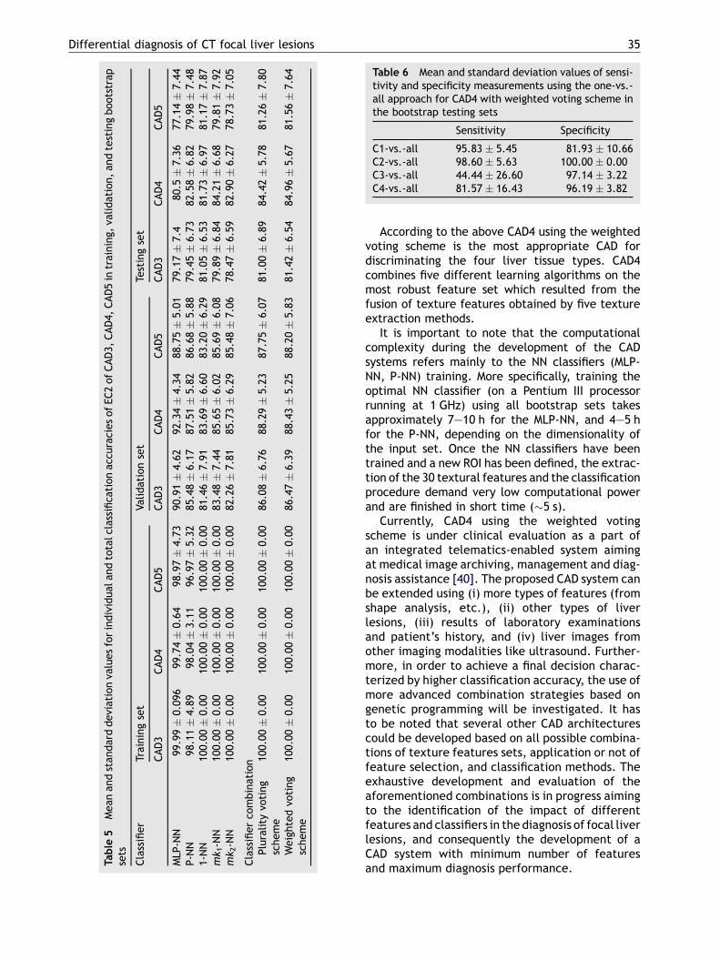
Differential diagnosis of CT focal liver lesions 35

Table 6 Mean and standard deviation values of sensi-tivity and specificity measurements using the one-vs.-all approach for CAD4 with weighted voting scheme inthe bootstrap testing sets

Sensitivity Specificity

C1-vs.-all 95.83 5.45 81.93 10.66C2-vs.-all 98.60 5.63 100.00 0.00C3-vs.-all 44.44 26.60 97.14 3.22C4-vs.-all 81.57 16.43 96.19 3.82

Table

5Mean

andstan

darddeviationva

luesforindividual

andtotalclassifica

tionac

curaciesofEC2ofCAD3,

CAD4,

CAD5in

training,

validation,an

dtestingbootstrap

sets

Classifier

Trainingset

Validationset

Testingset

CAD3

CAD4

CAD5

CAD3

CAD4

CAD5

CAD3

CAD4

CAD5

MLP

-NN

99.99

0.09

699

.74

0.64

98.97

4.73

90.91

4.62

92.34

4.34

88.75

5.01

79.17

7.4

80.5

7.36

77.14

7.44

P-NN

98.11

4.89

98.04

3.11

96.97

5.32

85.48

6.17

87.51

5.82

86.68

5.88

79.45

6.73

82.58

6.82

79.98

7.48

1-NN

100.00

0.00

100.00

0.00

100.00

0.00

81.46

7.91

83.69

6.60

83.20

6.29

81.05

6.53

81.73

6.97

81.17

7.87

mk 1-NN

100.00

0.00

100.00

0.00

100.00

0.00

83.48

7.44

85.65

6.02

85.69

6.08

79.89

6.84

84.21

6.68

79.81

7.92

mk 2-NN

100.00

0.00

100.00

0.00

100.00

0.00

82.26

7.81

85.73

6.29

85.48

7.06

78.47

6.59

82.90

6.27

78.73

7.05

Classifierco

mbination

Plurality

voting

scheme

100.00

0.00

100.00

0.00

100.00

0.00

86.08

6.76

88.29

5.23

87.75

6.07

81.00

6.89

84.42

5.78

81.26

7.80

Weightedvo

ting

scheme

100.00

0.00

100.00

0.00

100.00

0.00

86.47

6.39

88.43

5.25

88.20

5.83

81.42

6.54

84.96

5.67

81.56

7.64

According to the above CAD4 using the weightedvoting scheme is the most appropriate CAD fordiscriminating the four liver tissue types. CAD4combines five different learning algorithms on themost robust feature set which resulted from thefusion of texture features obtained by five textureextraction methods.

It is important to note that the computationalcomplexity during the development of the CADsystems refers mainly to the NN classifiers (MLP-NN, P-NN) training. More specifically, training theoptimal NN classifier (on a Pentium III processorrunning at 1 GHz) using all bootstrap sets takesapproximately 7—10 h for the MLP-NN, and 4—5 hfor the P-NN, depending on the dimensionality ofthe input set. Once the NN classifiers have beentrained and a new ROI has been defined, the extrac-tion of the 30 textural features and the classificationprocedure demand very low computational powerand are finished in short time (5 s).

Currently, CAD4 using the weighted votingscheme is under clinical evaluation as a part ofan integrated telematics-enabled system aimingat medical image archiving, management and diag-nosis assistance [40]. The proposed CAD system canbe extended using (i) more types of features (fromshape analysis, etc.), (ii) other types of liverlesions, (iii) results of laboratory examinationsand patient’s history, and (iv) liver images fromother imaging modalities like ultrasound. Further-more, in order to achieve a final decision charac-terized by higher classification accuracy, the use ofmore advanced combination strategies based ongenetic programming will be investigated. It hasto be noted that several other CAD architecturescould be developed based on all possible combina-tions of texture features sets, application or not offeature selection, and classification methods. Theexhaustive development and evaluation of theaforementioned combinations is in progress aimingto the identification of the impact of differentfeatures and classifiers in the diagnosis of focal liverlesions, and consequently the development of aCAD system with minimum number of featuresand maximum diagnosis performance.

36 S.G. Mougiakakou et al.

4. Conclusion

The aim of the present paper was to define a CADsystem architecture able to accurately classifyhepatic tissue from non-enhanced CT images asnormal liver, hepatic cyst, hemangioma, and hepa-tocellular carcinoma.

The system design was based on the use of tex-ture features, feature selection techniques, andECs. For each CT liver ROI, five types of texturefeature sets, based on first order statistics, spatialgray level dependence matrices, gray level differ-ence matrices, Laws’ texture energy measures, andfractal dimension measurements, were extractedresulting in a total of 89 features. A GA-basedfeature selection method was applied to featuresets, when dimensionality reduction was desired,while two alternative ECs were investigated con-sisting solely of NN classifiers, or of a combination ofNN and statistical classifiers. A plurality and aweighted voting scheme were used to combinethe outputs of the primary classifiers of the exam-ined CAD systems. The optimal architecture of theCAD systemwas chosen based on themean classifica-tion accuracies in 50 testing sets obtained throughthe bootstrap method. The best performing archi-tecture achieved a mean classification accuracyequal to 84.96% in the bootstrap testing sets andused (a) a fused 30-dimensional feature set obtainedafter appropriate feature selection applied in speci-fic subsets of the original 89-dimensional feature set,(b) an EC consisting of two NNs and three statisticalclassifiers, and (c) a weighted voting scheme.

The results indicate that CAD systems can providea valuable ‘‘second opinion’’ tool for the radiologistsin the differential diagnosis of focal liver lesionsfrom non-enhanced CT images, thus improving thediagnosis accuracy, and reducing the needed valida-tion time.

References

[1] Taylor HM, Ros PR. Hepatic imaging: an overview. Radiol ClinNorth Am 1998;36:237—45.

[2] Kadah YM, Frag AA, Zurada JM, Badawi AM, Youssef A-BM.Classification algorithms for quantitative tissue character-ization of diffuse liver disease from ultrasound images. IEEETrans Med Imaging 1996;15(4):466—78.

[3] Sun YN, Horng MH, Lin XZ,Wang JY. Ultrasonic image analysisfor liver diagnosis. IEEE Eng Med Biol 1996;11/12:93—101.

[4] Sujana H, Swarnamani S, Suresh S. Application of artificialneural networks for the classification of liver lesions by imagetexture parameters. Ultrasound Med Biol 1996;22(9):1177—81.

[5] Wu Ch-M, Chen Y-Ch, Sheng Hsieh K. Texture features forclassification of ultrasonic liver images. IEEE Trans MedImaging 1992;11(2):141—51.

[6] Mir AH, Hanmandlu M, Tandon SN. Texture analysis of CTimages. IEEE Eng Med Biol 1995;14(6):781—6.

[7] Chen EL, Chung P-C, Chen CL, Tsa HM, Chang CI. An auto-matic diagnostic system for CT liver image classification.IEEE Trans Biomed Eng 1998;45(6):783—94.

[8] Gletsos M, Mougiakakou SG, Matsopoulos GK, Nikita KS,Nikita A, Kelekis D. A computer-aided diagnostic systemto characterize CT focal liver lesions: design and optimiza-tion of a neural network classifier. IEEE Trans Inf Technol B2003;7(3):153—62.

[9] Jain AK, Duin RPW, Mao J. Statistical pattern recognition: areview. IEEE Trans Pattern Anal 2000;22(1):4—37.

[10] Siedlecki W, Sklansky J. A note on genetic algorithms forlarge scale feature selection. Pattern Recog Lett 1989;10:335—47.

[11] DhawanAP,ChitreY,Kaiser-BonassoCh,MoskowitzM.Analysisof mammographic microcalcifications using gray-level imagestructure features. IEEE Trans Med Imaging 1996;15(3):246—59.

[12] Handels H, Roß Th, Kreusch J, Wolff HH, Poppl SJ. Featureselection for optimized skin tumor recognition using geneticalgorithms. Artif Intell Med 1999;16:283—97.

[13] Yamany SM, Khiani KJ, Farag AA. Application of neuralnetworks and genetic algorithms in the classificationof endothelial cells. Pattern Recog Lett 1997;18:1205—10.

[14] Roli F, Giacinto G, Vernazza G. Methods for designing multi-ple classifier systems. In: Roli F, Kittler J, editors. Proceed-ings of 2nd international workshop on multiple classifiersystems in volume 2096 of lecture notes in computerscience. London, UK: Springer Verlag; 2001. p. 78—87.

[15] Christodoulou CI, Pattichis CS, Pantziaris M, Nicolaides A.Texture-based classification of atherosclerotic carotid pla-ques. IEEE Trans Med Imaging 2003;22(7):902—12.

[16] Ho TK, Hull JJ, Srihari SN. Decision combination in multipleclassifier systems. IEEE Trans Pattern Anal 1994;16(1):66—75.

[17] Sboner A, Eccher C, Blanzieri E, Bauer P, Cristofolini M,Zumiani G, et al. A multiple classifier system for earlymelanoma diagnosis. Artif Intell Med 2003;27(1):29—44.

[18] Jerebko AK, Malley JD, Franaszek M, Summers RM. Multipleneural network classification scheme for detection of colo-nic polyps in CT colonography data sets. Acad Radiol2003;10(2):154—60.

[19] Cheng S-Ch, Huang Y-M. A novel approach to diagnosediabetes based on the fractal characteristics of retinalimages. IEEE Trans Inf Technol Biomed 2003;7(3):163—70.

[20] Valavanis I, Mougiakakou SG, Nikita KS, Nikita A. Computeraided diagnosis of CT focal liver lesions by an ensemble ofneural network and statistical classifiers. In: Proceedings ofthe international joint conference on neural networks(IJCNN’04), IEEE; 2004. p. 1929—34.

[21] Mougiakakou SG, Valavanis I, Nikita KS, Nikita A, Kelekis D.Characterization of CT liver lesions based on texture fea-tures and a multiple neural network classification scheme.In: Proceedings of the engineering in medicine and biologyconference (EMBC’03), IEEE; 2003. p. 1287—90.

[22] Efron B. Bootstrap methods: another look at the jackknife.Ann Stat 1979;7:1—26.

[23] Efron B. The jackknife, the bootstrap, and other resamplingplans. In: CBMS-NSF regional conference series in appliedmathematics, society for industrial and applied mathe-matics (SIAM). Philadelphia; 1982.

[24] Chernick MR, Friis RH. Introductory biostatistics for thehealth sciences: modern applications including bootstrap.In: Hoboken NJ, editor. Wiley series in probability andstatistics. Wiley—Interscience; 2003.

Differential diagnosis of CT focal liver lesions 37

[25] Chen D-R, Kuo W-J, Chang R-F, Moon WK, Lee CC. Use of thebootstrap technique with small training sets for computer-aided diagnosis in breast ultrasound. Ultrasound Med Biol2002;28(7):897—902.

[26] Fan X, Wang L. Comparability of jackknife and bootstrapresults: an investigation for a case of canonical correlationanalysis. J Exp Educ 1996;64:173—89.

[27] Haralick RM, Shanmugan K, Dinstein I. Textural features forimage classification. IEEE Trans Syst Man Cybern 1973;3(6):610—22.

[28] Haralick RM, Shaphiro LG. Computer and robot vision, vol. I.Boston, MA, USA: Addison-Wesley Publishing Company; 1992.

[29] Weszka JS, Dryer CR, Rosenfeld A. A comparative study oftexture measures for terrain classification. IEEE Trans SystMan Cybern 1976;SMC-6:269—85.

[30] Laws KI. Rapid texture identification. In: Image processingfor missile guidance, Proceedings of the society of photo-optical instrumentation engineers conference; 1980. 238, p.376—80.

[31] Mandelbrot BB. Fractal geometry of nature. New York: W.H.Freeman and Co.; 1983.

[32] Goldberg D. Genetic algorithms in search, optimization andmachine learning. Boston, MA, USA: Addison-Wesley Publish-ing Company; 1989.

[33] Haykin S. Neural networks: a comprehensive foundation.Upper Saddle River, NJ, USA: Prentice-Hall; 1999.

[34] Wu Y, Ianakiev Kr, Govindaraju V. Improved k-nearest neigh-bor classification. Pattern Recog 2002;35:2311—8.

[35] Duin RPW. The combining classifier: to train or not to train?In: Kasturi R, Laurendeau D, Suen C, editors. ICPR16, Pro-ceedings 16th International Conference on Pattern Recogni-tion. 2002. p. 765—70.

[36] Lam L, Suen Ch. Application of majority voting to patternrecognition: an analysis of its behavior and performance.IEEE Trans Syst Man Cybern A 1997;27(5):553—68.

[37] Verikas A, Arunas L, Malmqvist K, Bacauskiene M, Gelzinis A.Soft combination of neural classifiers: a comparative study.Pattern Recog Lett 1999;20:429—44.

[38] Dzeroski S, Zenko B. Is combining classifiers better thanselecting the best one? Mach Learn 2004;54:255—73.

[39] Patel AC, Markey MK. Comparison of three-class classifica-tion performance metrics: a case study in breast cancerCAD. In: Eckstein MP, Jiang Y, editors. Medical imaging2005, image perception, observer performance, andtechnology assessment, Proceedings of SPIE 2005, 2005.5749, p. 581—89.

[40] Mougiakakou SG, Valavanis I, Mouravliansky NA, Nikita KS,Nikita A. DIAGNOSIS: a telematics enabled system for med-ical image archiving, management and diagnosis assis-tance. In: Proceedings of the 2006 IEEE internationalworkshop on imaging systems and techniques (IEEE-IST);2006. p. 43—8.