texture characterization of roller compacted concrete

TEXTURE CHARACTERIZATION OF ROLLER COMPACTED CONCRETE

PAVEMENTS BY AN IN-HOUSE DEVELOPED OPTICAL SURFACE

PROFILER

A THESIS SUBMITTED TO

THE GRADUATE SCHOOL OF NATURAL AND APPLIED SCIENCES

OF

MIDDLE EAST TECHNICAL UNIVERSITY

BY

MAHDI MAHYAR

IN PARTIAL FULFILLMENT OF THE REQUIREMENTS

FOR

THE DEGREE OF DOCTOR OF PHILOSOPHY

IN

CIVIL ENGINEERING

FEBRUARY 2021

Approval of the thesis:

TEXTURE CHARACTERIZATION OF ROLLER COMPACTED

CONCRETE PAVEMENTS BY AN IN-HOUSE DEVELOPED OPTICAL

SURFACE PROFILER

submitted by MAHDI MAHYAR in partial fulfillment of the requirements for the

degree of Doctor of Philosophy in Civil Engineering Department, Middle East

Technical University by,

Prof. Dr. Halil Kalıpçılar _____________________

Dean, Graduate School of Natural and Applied Sciences

Prof. Dr. Ahmet Türer _____________________

Head of Department, Civil Engineering

Prof. Dr. İsmail Özgür Yaman _____________________

Supervisor, Civil Engineering Dept., METU

Dr. Burhan Aleessa Alam _____________________

Co-Supervisor, Civil Engineering Dept., METU

Examining Committee Members:

Prof. Dr. Murat Güler _____________________

Civil Engineering Dept., METU

Prof. Dr. İsmail Özgür Yaman _____________________


Prof. Dr. Mustafa Şahmaran _____________________

Civil Engineering Dept., Hacettepe University

Assoc. Prof. Dr. Can Baran Aktaş _____________________

Civil Engineering Dept., TED University

Assist. Prof. Dr. Hande Işık Öztürk _____________________


Date: 15.02.2021

iv

I hereby declare that all information in this document has been obtained and

presented in accordance with academic rules and ethical conduct. I also

declare that, as required by these rules and conduct, I have fully cited and

referenced all material and results that are not original to this work.

Name, Last name : Mahdi Mahyar

Signature :

v

ABSTRACT

TEXTURE CHARACTERIZATION OF ROLLER COMPACTED

CONCRETE PAVEMENTS BY AN IN-HOUSE DEVELOPED OPTICAL

SURFACE PROFILER

Mahyar, Mahdi

Doctor of Philosophy, Department of Civil Engineering

Supervisor: Prof. Dr. İsmail Özgür Yaman

Co-Supervisor: Dr. Burhan Aleessa Alam

February 2021, 173 pages

The use of concrete instead of traditional asphalt in road construction has been a

challenge in the last century for road owners looking for a safe and sustainable

solution. Very heavy expenditures of asphalt pavement rehabilitation during its

lifetime, have made concrete the best choice for substitution. However, it is

generally accepted that the initial construction costs of conventional concrete

pavements are high. In concrete pavement construction, a competitive method for

decreasing initial cost of construction is the application of roller compacted concrete

(RCC) paving technology which carries the advantages of both methods in terms of

costs; low construction costs similar to asphalt pavement and low rehabilitation

costs similar to conventional concrete pavements.

RCC is a zero-slump concrete consisting of densely graded aggregates. Because of

its poor workability, it is usually placed with an asphalt paver, and compacted by a

vibrating roller. The most common disadvantages of RCC pavements are due to the

uncertainties in the unevenness and the skid resistance which are both related to its

surface texture. Hence, it is commonly recommended for heavy load carrying lots

and urban streets with lower traffic speeds. However, unlike mechanical properties

vi

of RCC pavements, which is almost well-understood in literature, there is not any

adequate evidence of its surface texture characteristics.

Within the framework of this study, a high accuracy 3D laser beam scanner is

developed at the METU Materials of Construction Laboratory. It has a capacity of

scanning 500x500 mm samples with a 0.010 mm accuracy in depth and MATLAB

is used for the surface texture analysis using the ISO 25178-2 international standard.

The standard defines various roughness parameters as quantitative parameters

computed from the measured 3D surface textures.

This study intended to investigate the roughness parameters of various RCC samples

prepared using different compaction methods. Superpave gyratory compactor, and

a double drum a double drum vibratory hand roller (DDVHR) to better simulate the

field compaction procedures of RCC were the two compaction procedures utilized.

Besides RCC, hot mix asphalt (HMA) specimens were also utilized. It was shown

that, super-pave gyratory compacter cannot represent the vibratory rollers in terms

of surface texture. Furthermore, it was observed that the generated texture of RCC

and HMA surface, utilizing identical aggregate gradation, type and content, is not

identical as demonstrated with 3D scanning of textures and comparing computed

roughness parameters based on ISO 25178-2. It is found that HMA texture provides

higher degree of contact with 4 to 7 times more contact points compared to RCC

texture. Shape of the contact points for the asphalt samples are 3 times pointier than

the RCC samples. As a summary, RCC suffers from producing a uniform texture

and it is prone to get waviness from compaction. However, comparisons also

showed that RCC can provide equal and greater macro-texture to HMA.

Additionally, potential correlations between micro-texture and skid resistance of the

surfaces and the surface-scaling durability of the RCC pavement samples subjected

to chemical deicers under freeze and thaw cycling was determined. Finally, two

texture modification techniques were applied on the RCC pavements and their

influence on macro-texture and micro-texture were also determined.

Keywords: Roller Compacted Concrete Pavement, Micro- and Macro-Texture

Parameters, Skid Resistance, Optical Surface Profiler

vii

ÖZ

KURUM İÇİ GELİŞTİRİLEN OPTİK YÜZEY PÜRÜZLÜLÜKÖLÇER İLE

SİLİNDİRLE SIKIŞTIRILMIŞ BETON KAPLAMALARIN YÜZEY DOKU

KARAKTERİZASYONU

Mahyar, Mahdi Doktora, İnşaat Mühendisliği

Tez Danışmanı: Prof. Dr. İsmail Özgür Yaman

Ortak Tez Danışmanı: Dr. Burhan Aleessa Alam

Şubat 2021, 173 sayfa

Yol yapımında, geleneksel asfalt yerine beton kullanımı, güvenli ve sürdürülebilir

bir çözüm arayan yol sahipleri için son yüzyılda bir zorluk olmuştur. Kullanım ömrü

boyunca çok ağır asfalt kaplama rehabilitasyonu harcamaları, betonu ikame için en

iyi seçenek haline getirmiştir. Ancak geleneksel beton kaplamaların genel olarak

ilk yapım maliyetlerinin yüksek olduğu bilinmektedir. Beton yol yapımında, maliyet

açısından her iki yöntemin avantajlarını da taşıyan silindirle sıkıştırılmış beton

(SSB) kaplama teknolojisinin uygulanması, ilk yapım maliyetini düşürmenin

rekabetçi bir yöntemidir. Başka bir ifade ile; inşa maliyeti asfalt yollar gibi az

olmasına karşın, onarım maliyeti de beton yollar gibi düşüktür.

SSB, yoğun agrega gradasyonu içeren sıfır çökme değerine sahip bir betondur. Kötü

işlenebilirliği nedeniyle, genellikle bir asfalt serici ile yerleştirilir ve bir titreşimli

silindirle sıkıştırılır. SSB kaplamaların en yaygın dezavantajı, her ikisi de yüzey

dokusuyla ilgili olan düzgünsüzlük ve kayma direncindeki belirsizliklerden

kaynaklanmaktadır. Bu nedenle, genellikle ağır yük taşıyan bölgelerde ve düşük

trafik hızına sahip şehir içi caddeler için önerilmektedir. Bununla birlikte, SSB

kaplamaların, literatürde hemen hemen iyi anlaşılan mekanik özelliklerinden farklı

olarak, yüzey dokusu özelliklerine ilişkin yeterli kanıt yoktur.

viii

Bu çalışma çerçevesinde ODTÜ Yapı Malzemeleri Laboratuvarında yüksek

hassasiyetli bir 3D lazer ışın tarayıcı geliştirilmiştir. Geliştirilen bu tarayıcının

500x500 mm büyüklüğündeki numuneleri 0,010 mm hassasiyetle tarama

kapasitesine sahiptir ve ISO 25178-2 uluslararası standardı kullanılarak yüzey

dokusu analizi için MATLAB kullanılmaktadır. Standart, çeşitli pürüzlülük

parametrelerini, ölçülen 3-boyutlu yüzey dokularından hesaplanan nicel

parametreler olarak tanımlamaktadır.

Bu çalışma, farklı sıkıştırma yöntemleri kullanılarak hazırlanan çeşitli SSB

numunelerinin pürüzlülük parametrelerini incelemeyi amaçlamıştır. Superpave

yoğurmalı sıkıştırıcı ve SSB'nin sahada sıkıştırma prosedürlerini daha iyi benzetmek

için çift tamburlu titreşimli el silindiri (ÇTTES), kullanılan iki sıkıştırma

prosedürüdür. SSB'nin yanı sıra, sıcak karışım asfalt (HMA) numuneleri de

kullanılmıştır. Süperpave yoğurmalı sıkıştırıcının yüzey dokusu açısından

ÇTTES’ni temsil edemediği gösterilmiştir. Ayrıca, aynı agrega gradasyonu, türü ve

içeriği kullanılarak oluşturulan SSB ve HMA yüzey dokusunun aynı olmadığı ISO

25178-2'ye dayalı hesaplanmış pürüzlülük parametrelerinin karşılaştırılmasıyla

görülmüştür. Asfalt dokusunun, SSB dokusuna kıyasla 4 ila 7 kat daha fazla temas

noktasıyla daha yüksek derecede temas sağladığı bulunmuştur. Asfalt numuneleri

için temas noktalarının şekli, SSB numunelerine göre 3 kat daha sivridir. Özet

olarak, SSB tek tip yüzey dokusu üretmekten muzdariptir ve sıkışmadan dolayı

düzgünsüzlük gösterme eğilimindedir. Bununla birlikte, RCC'nin asfalt’a eşit ve

daha büyük makro doku sağlayabileceği de gözlenmiştir.

Ek olarak, yüzeylerin mikro doku ve kayma direnci arasındaki potansiyel

korelasyonlar ile donma ve çözülme döngüsü altında kimyasal çözücülere tabi

tutulan SSB kaplama örneklerinin yüzey pullanma dayanıklılığı belirlendi. Son

olarak, SSB kaplamalara iki doku modifikasyon tekniği uygulanmış ve bunların

makro doku ve mikro doku üzerindeki etkileri de belirlenmiştir.

Anahtar Kelimeler: Silindirle Sıkıştırılmış Beton Kaplama, Mikro ve Makro Doku

Parametreleri, Kayma Direnci, Optik Yüzey Pürüzlülükölçer

ix

To my wife,

Nasim

x

ACKNOWLEDGMENTS

I wish to express my gratitude towards my advisor, Prof. Dr. İsmail Özgür Yaman

from METU for supervising my work. Thanks to his sincere care, trust and guidance,

understanding, motivation and support from the beginning of my Ph. D program and

during the time I worked on this thesis. I am also grateful for the great motivation

and sincere support that I got from my Co-Supervisor, Dr. Burhan Aleessa Alam

who played my best friend throughout this journey.

I am most grateful for the insightful recommendations of my committee members,

Dr. Mustafa Şahmaran, Dr. Hande Işık Öztürk, Dr. Murat Güler and Dr. Can Baran

Aktaş, who helped to improve the quality of this thesis.

I wish to thank Dr. Mustafa Tokyay and Dr. Sinan Turhan Erdoğan for their valuable

comments and contributions throughout all my education at METU.

I also want to extend my appreciation to RCCP research team Dr. Emin Şengün, Dr.

Reza Shabani, Mehmet Ali Aykutlu and Sadık Karakaç.

I am eternally indebted to all the members of the Materials of Construction

Laboratory group, of which I am honored to be a part. Special thanks to Sahra, for

her friendship and supports; Thanks to Cuma Yıldırım, Gülşah Bilici for their help

working in Lab; Ozan, Kemal, Murat for being part of one of the best times of my

life and Meltem for being a great friend and all the coffees she shared, thank you all

from the first day of the program to the last.

And finally, I am very grateful to my wife, Nasim, for her patience, support,

endurance, and her moral support encouraged me to adhere to this study, and my

son, Adrian who scarified some of his playtime with his daddy.

xi

TABLE OF CONTENTS

ABSTRACT............................................................................................................. v

ÖZ.......................................................................................................................... vii

ACKNOWLEDGMENTS....................................................................................... x

TABLE OF CONTENTS........................................................................................ xi

LIST OF TABLES................................................................................................ xvi

LIST OF FIGURES............................................................................................. xvii

CHAPTERS:

1 INTRODUCTION ............................................................................................ 1

1.1 History of road construction ...................................................................... 1

1.2 Wearing Course; Hot-Mix Asphalt vs Portland Cement Concrete ........... 3

1.3 PCC Pavements and Design Technologies ................................................ 4

1.4 RCC Pavement, The Best of the Two Worlds ........................................... 6

1.5 RCC Pavement Limitations ....................................................................... 6

1.6 Smoothness - Is It the Only Measure of Rideability? ................................ 7

1.7 Objectives .................................................................................................. 8

2 LITERATURE REVIEW ............................................................................... 11

2.1 Pavement Surface Characteristics ........................................................... 11

2.2 Unevenness and Mega-texture ................................................................ 12

2.2.1 Unevenness and Mega-Texture Measurements ............................... 13

2.3 Macro-texture .......................................................................................... 15

2.3.1 Macro-Texture Measurements ......................................................... 15

2.3.1.1 Sand patch method .................................................................... 16

2.3.1.2 Outflow meter ........................................................................... 16

xii

2.3.1.3 Circular texture meter (CT Meter) ............................................ 16

2.3.1.4 Vehicle-mounted non-contact profiler ...................................... 17

2.4 Micro-Texture .......................................................................................... 17

2.4.1 Micro-Texture Measurements .......................................................... 18

2.5 Friction ..................................................................................................... 18

2.6 Factors Affecting Road-Tire Friction ...................................................... 20

2.6.1 Skid Resistance ................................................................................. 20

2.6.1.1 British pendulum tester ............................................................. 21

2.6.1.2 Dynamic friction tester .............................................................. 21

2.6.1.3 Vehicle stopping distance tests ................................................. 21

2.6.1.4 Locked-wheel skid trailer .......................................................... 22

2.6.2 Friction Indices ................................................................................. 22

2.6.2.1 Relationship between indices .................................................... 23

2.7 Laser Texture Scanner and Friction ......................................................... 26

2.8 Concrete Surface Treatment to Enhance Macro-Texture ........................ 27

2.8.1 Tining; Broom Finish, Burlap Drag ................................................. 27

2.8.2 Diamond Grinding/Grooving ........................................................... 29

2.8.3 Abrading (Shot blasting) .................................................................. 30

2.8.4 Exposed Aggregate Texturing .......................................................... 30

2.8.5 Chip Sprinkling ................................................................................ 32

3 EXPERIMENTAL PROGRAM ..................................................................... 33

3.1 Development of the Non-Contact Laser Scanner .................................... 33

3.2 Materials and Test Specimens used in the Experiments .......................... 36

3.2.1 Material Selection and Mix Proportions .......................................... 37

3.2.2 In-Lab Produced RCC Specimens .................................................... 39

3.2.3 In-Lab Produced HMA Specimens .................................................. 42

3.3 Experimental Test Procedures ................................................................. 42

3.3.1 Measurements of Texture Depth; Sand patch method ..................... 43

xiii

3.3.2 Skid Resistance Test; Portable Pendulum Tester ............................. 43

3.3.3 Roughness Parameters ..................................................................... 44

3.3.3.1 Height parameters ..................................................................... 44

3.3.3.2 Spatial parameters ..................................................................... 47

3.3.3.3 Hybrid parameters ..................................................................... 50

3.3.3.4 Functions and related parameters ............................................. 51

3.3.3.5 Miscellaneous parameters ......................................................... 56

3.3.3.6 Feature parameters .................................................................... 56

3.3.3.7 Geometrical parameters; Fourier transform .............................. 58

3.3.3.8 Fractal Dimension ..................................................................... 59

3.3.4 Demonstration of the results ............................................................ 59

4 PHASE I, CHARACTERIZATION OF RCC PAVEMENT SURFACE

THROUGH SGC SAMPLES ................................................................................ 61

4.1 Influence of the Mixture Parameters and Compaction Methods on Surface

Texture ................................................................................................................. 61

4.1.1 Maximum peak height (Sp) .............................................................. 62

4.1.2 Maximum valley depth (Sv) ............................................................. 63

4.1.3 Maximum height (Sz) ....................................................................... 65

4.1.4 Arithmetical mean height (Sa) .......................................................... 66

4.1.5 Root mean square height (Sq) ........................................................... 68

4.1.6 Skewness (Ssk) .................................................................................. 69

4.1.7 Kurtosis (Sku) .................................................................................... 71

4.1.8 Conclusion ........................................................................................ 72

5 PHASE II, COMPARISON OF TEXTURE OF RCC AND HMA

PAVEMENTS ........................................................................................................ 73

5.1 Similarity Investigation of RCC And HMA Texture Through Roughness

Parameters ............................................................................................................ 73

5.1.1 Height Parameters ............................................................................ 73

5.1.2 Spatial Parameters ............................................................................ 75

xiv

5.1.3 Hybrid Parameters ............................................................................ 76

5.1.4 Functions and related Parameters ..................................................... 77

5.1.5 Miscellaneous Parameters ................................................................ 79

5.1.6 Feature Parameters ........................................................................... 80

5.2 Investigation of Macro-Texture ............................................................... 82

5.2.1 Mean Texture Depth, Mean Profile Depth and Mean Surface Depth ..

.......................................................................................................... 82

5.2.2 Investigation of RCC Macro-texture based on MSD ....................... 84

5.3 Investigation of Micro-Texture ................................................................ 86

5.3.1 Skid resistance and affecting variables ............................................ 87

5.3.2 Skid resistance and texture parameters ............................................ 90

6 PHASE III, DURABILITY OF RCC PAVEMENT ....................................... 95

6.1 Background .............................................................................................. 95

6.2 Materials and methods ............................................................................. 96

6.3 Results and discussions............................................................................ 96

7 PHASE IV, MODIFICATION OF TEXTURE OF RCC Pavement ............ 109

7.1 Methodology of the Experiments .......................................................... 109

7.1.1 Test Specimens for Exposed Aggregate Concrete Surface (EACS) ....

........................................................................................................ 109

7.1.2 Test Specimens for Chip Sprinkled Concrete Surface (CSCS) ...... 111

7.1.3 Experiments .................................................................................... 113

7.2 Investigating Texture Properties ............................................................ 114

7.3 Conclusion ............................................................................................. 117

8 SUMMARY AND CONCLUSIONS ........................................................... 119

8.1 Findings and Conclusions ...................................................................... 119

8.2 Suggestions for Future Studies .............................................................. 122

9 REFERENCES .............................................................................................. 125

10 APPENDICES .............................................................................................. 135

A. Roughness Parameters of The Specimens………………………………….135

xv

B. Sand Patch Test Results and Estimated Mean Texture Depth Values………163

C. The Roughness Parameters in Correlation With BPN………………………167

CURRICULUM VITAE ...................................................................................... 173

xvi

LIST OF TABLES

TABLES

Table 2-1, Commercially available road profilers .................................................. 17

Table 2-2, factors affecting tire-road friction (the more critical factors are shown in

bold ......................................................................................................................... 20

Table 3-1, Physical properties of the aggregates .................................................... 37

Table 3-2, In lab prepared mix proportions ............................................................ 39

Table 3-3, Measured properties of asphalt 50-70 ................................................... 42

Table 3-4, Height parameters of ISO 25178-2 ....................................................... 44

Table 3-5, Spatial parameters of ISO 25178-2 ....................................................... 47

Table 3-6, Hybrid parameters of ISO 25178-2 ....................................................... 50

Table 3-7, Functions and related parameters of ISO 25178-2 ............................... 51

Table 3-8, Miscellaneous parameters of ISO 25178-2 ........................................... 56

Table 3-9, Feature parameters of ISO 25178-2 ...................................................... 56

Table 7-1, Mix proportions and properties of the specimens ............................... 110

Table 7-2, Chip sprinkling gradation, coating and spread rate ............................ 112

xvii

LIST OF FIGURES

FIGURES

Figure 2-1, Illustration of the different road surface domains and some general

indicators as to which wavelengths affect which aspect of road transportation

(Henry, 2000) (Andersen, 2015). ........................................................................... 12

Figure 2-2, Reproduction of an individual present serviceability rating form. ...... 14

Figure 2-3, IRI roughness scale (replotted from Sayers, 1989). ............................ 14

Figure 2-4, Macro and Micro Texture (Flintsch, De León, McGhee, & AI-Qadi,

2003) ...................................................................................................................... 15

Figure 2-5, Friction force developed due to adhesion (on the right) and due to

hysteresis (on the left) ............................................................................................ 19

Figure 2-6, Effect of Micro-texture/Macro-texture on Pavement Friction (Noyce et

al., 2005) ................................................................................................................. 24

Figure 2-7, Recommended correlations for mean texture depth by ASTM ........... 24

Figure 3-1, The developed Non-contact 3D scanner ............................................. 34

Figure 3-2, Close up of guide frame and samples under scan ............................... 35

Figure 3-3, Schematic demonstration of the scan logic ......................................... 35

Figure 3-4, Top left; Picture of an exposed aggregate concrete surface. Top right:

Virtual image of the surface generated by MATLAB. Bottom; 3D illustration of the

surface. ................................................................................................................... 36

Figure 3-5, Aggregates gradation (Şengün, 2019) ................................................. 38

Figure 3-6 Left: The Superpave gyratory compactor, Right: schematic view of the

gyratory compaction ............................................................................................... 41

Figure 3-7, Concrete and asphalt samples compacted with SGC .......................... 41

Figure 3-8 Two-steps compaction procedure. Left: initial step; plate compactor,

Right: final step; hand roller compactor. ................................................................ 41

Figure 3-9, left: BPN measurement on disk specimen, right: BPN measurement of

asphalt block ........................................................................................................... 43

Figure 3-10, Schematic illustration of Maximum peak height (Sp), Maximum pit

depth (Sv), and Maximum height (Sz) .................................................................... 45

xviii

Figure 3-11, Physical definition of the parameters Ssk and Sku which are expressed

in 2d profiles as Rsk and Rku (Bitelli, Simone, Girardi, & Lantieri, 2012). ............ 47

Figure 3-12, a) actual Surface, b) Autocorrelation of the surface ......................... 48

Figure 3-13, Procedure to calculate Sal and Str , a) Autocorrelation function of the

surface, b) Threshold autocorrelation at s (the black spots are above the threshold),

c) Threshold boundary of the central threshold portion, d) Polar coordinates leading

to the autocorrelation lengths in different directions .............................................. 49

Figure 3-14, Demonstration of projected area and surface area in calculation of Sdr

................................................................................................................................ 50

Figure 3-15, Schematic view of cumulative probability function curve ................ 51

Figure 3-16, Areal material ratio ............................................................................ 52

Figure 3-17, Steps to draw ‘Equivalent line’ on areal material ratio curve. .......... 53

Figure 3-18, The parameters Spk and Svk each are calculated as the height of the

right-angle triangle which is constructed to have the same area as the “Peak cross-

sectional area” or “Valley cross-sectional area”. This contributes to eliminating

outlying peaks and valleys in the calculation of Spk and Svk. ................................. 54

Figure 3-19, Illustration of; a Peak extreme height (Sxp); b, Functional volume

parameters .............................................................................................................. 55

Figure 3-20, Illustration of “Density of peaks” ...................................................... 57

Figure 3-21, Components of a box-whisker plot .................................................... 59

Figure 4-1, Effect of mixture parameters (binder content, water content and

maximum aggregate size) on the Maximum peak height (Sp) ............................... 62

Figure 4-2, Effect of compaction (SGC and DDCHR) and binder types (cement and

HMA) on the maximum peak-height parameter (Sp) ............................................. 63


maximum aggregate size) on the Maximum valley depth (Sv) .............................. 64


HMA) on the Maximum valley depth (Sv) ............................................................. 64


maximum aggregate size) on the Maximum height (Sz) ........................................ 65


HMA) on the Maximum height (Sz) ....................................................................... 66

xix


maximum aggregate size) on the Arithmetical mean height (Sa) ........................... 67


HMA) on the Arithmetical mean height (Sa) ......................................................... 67


maximum aggregate size) on the Root mean square height (Sq) ........................... 68

Figure 4-10, Effect of compaction (SGC and DDCHR) and binder types (cement

and HMA) on the Root mean square height (Sq) ................................................... 69

Figure 4-11, Schematic illustration of skewness variation (in 2D profiles skewness

is denoted as Rsk) .................................................................................................... 69


maximum aggregate size) on the Skewness (Ssk) ................................................... 70


and HMA) on the Skewness (Ssk) .......................................................................... 70

Figure 4-14, Schematic illustration of kurtosis variation (in 2D profiles skewness is

denoted as Rku) ....................................................................................................... 71


maximum aggregate size) on the Kurtosis (Sku) .................................................... 71


and HMA) on the Kurtosis (Sku) ............................................................................ 72

Figure 5-1, Effect of binder type and content, and maximum aggregate size on the

Arithmetical mean height (Sa) and the Root mean square height (Sq) ................... 74


Skewness (Ssk) and the kurtosis (Sku) ..................................................................... 75


Autocorrelation length (Sal) and the Texture aspect ratio (Str) ............................... 76

Figure 5-4, A corrugated plate ............................................................................... 76


Root mean square gradient (Sdq) and the Developed interfacial area ratio (Sdr) .... 77


Core height (Sk), the Reduced peak height (Spk) and the Reduced valley height (Svk)

................................................................................................................................ 78

xx


Dale void volume (Vvv) and the Core void volume (Vvc)....................................... 79


Peak material volume (Vmp) and the Core material volume (Vmc) ......................... 79


Texture direction (Std) ............................................................................................ 80


Density of peaks (Spd) and the Arithmetic mean peak curvature (Spc) ................... 81


Mean dale area (Sda) and the Mean heal area (Sha) ................................................. 81


Mean dale volume (Sdv) and the Mean hill volume (Shv) ....................................... 82

Figure 5-13, Mean surface texture (uncorrected) correlation with sand patch test

results, Dashed line is regression of the test, Solid line gives the estimate of PIARC

model. ..................................................................................................................... 83

Figure 5-14, Mean surface texture (measured at 10% of peaks’ material ratio)

correlation with sand patch test results, the Dashed line is regression of the test,

Solid line gives the estimate of PIARC model. ...................................................... 84

Figure 5-15, Comparison of estimated mean texture depth (eMTD) on various

surfaces. .................................................................................................................. 85

Figure 5-16, Macro-texture difference between RCC texture and roller compacted

asphalt texture ......................................................................................................... 86

Figure 5-17, Skid resistance of gyratory compacted surfaces at wet and dry

conditions ............................................................................................................... 88

Figure 5-18, Skid resistance of roller compacted surfaces at wet and dry conditions

................................................................................................................................ 88

Figure 5-19, Average BPN of surfaces based on compaction method and binder type

................................................................................................................................ 89

Figure 5-20, The correlation found between BPN and fractal dimension .............. 90

Figure 5-21, Evolution of Pearson’s correlation factor with change in projected

surface area of peaks at different depths ................................................................ 91

Figure 5-22, Linear regression of dry BPNs and autocorrelation length (s=0.2) ... 92

Figure 5-23, Linear regression of wet BPNs and autocorrelation length (s=0.2) .. 93

xxi

Figure 5-24, Linear regression of wet BPNs and magnitude of 2D Fourier transform

................................................................................................................................ 93

Figure 5-25, Linear regression of dry BPNs and magnitude of 2D Fourier transform

................................................................................................................................ 93

Figure 6-1, The initial and secondary rate of water absorption for 200 kg/m3 binder

content RCC ........................................................................................................... 97


content RCC ........................................................................................................... 98


content RCC ........................................................................................................... 98

Figure 6-4, RCCP samples with 12 mm stone, before (two pictures on the left) and

after 50 cycles of freeze-thaw (two pictures on the right) ..................................... 99

Figure 6-5, RCCP samples with 19 mm stone, before (two pictures on the left) and

after 50 cycles of freeze-thaw (two pictures on the right) ................................... 100

Figure 6-6, Change in Root mean square height for RCC with 12 mm max aggregate

size ........................................................................................................................ 101

Figure 6-7, Change in Root mean square height for RCC with 19 mm max aggregate

size ........................................................................................................................ 102

Figure 6-8, Change in texture skewness of RCCs with 12 mm max aggregate size

.............................................................................................................................. 103


.............................................................................................................................. 103

Figure 6-10, Change in texture kurtosis of RCCs with 12 mm max aggregate size

.............................................................................................................................. 104


.............................................................................................................................. 104

Figure 6-12, Macro-texture change under freeze-thaw cycling influence for 12 mm

max aggregate size RCCs ..................................................................................... 105

Figure 6-13, Macro-texture change under freeze-thaw cycling influence for 19 mm

max aggregate size RCCs ..................................................................................... 106

Figure 6-14, Change in volume of valleys after freeze-thaw cycling (Dmax = 12

mm) ...................................................................................................................... 107

xxii

Figure 6-15, Change in volume of valleys after freeze-thaw cycling (Dmax = 19

mm) ...................................................................................................................... 107

Figure 6-16, Overall volume loss of the RCC samples after 50 cycles of freeze-thaw

.............................................................................................................................. 107

Figure 7-1, EACS and control specimens ............................................................ 111

Figure 7-2 a) Unchipped RCC surface. b) RCC surface sprinkled with 5.0-9.5 mm

chips. c) RCC surface sprinkled with 9.5-12.7 mm chips. d) RCC surface sprinkled

with 12.7-16 mm chips. ........................................................................................ 112

Figure 7-3, Image simulation of surface data produced by MATLAB, a,b,c) CSCS

5~9, d,e,f) CSCS 9~12, g,h,i) CSCS 12~16 ......................................................... 113

Figure 7-4, Estimated mean texture depth of surface modified RCC pavement .. 115

Figure 7-5, Estimated mean texture depth of chip sprinkled RCC pavement ...... 115

Figure 7-6, British pendulum numbers of exposed aggregate RCC pavement .... 117

Figure 7-7, British pendulum numbers of chip sprinkled RCC pavement ........... 117

1

CHAPTER 1

1 INTRODUCTION

1.1 History of road construction

Thousands of years before urban planning, motor vehicles, or even the wheel, the

first roads appeared on the landscape. Very first roads were spontaneously formed

by humans walking the same paths over and over to get water and find food. As small

groups of people combined into villages, towns and cities, networks of walking paths

became more formal roads. Following the introduction of the wheel about 7,000

years ago, the larger and heavier loads, that could be transported, showed the

limitations of dirt paths that turned into muddy bogs when it rained. The earliest

stone paved roads have been traced to about 4,000 B.C. in the Indian subcontinent

and Mesopotamia.

The earliest long-distance road was a 1,500-mile route between the Persian Gulf and

the Mediterranean Sea. It came into some use about 3500 B.C., but it was operated

in an organized way only from about 1200 B.C. by the Assyrians, who used it to join

Susa, near the Persian Gulf, to the Mediterranean ports of Smyrna (İzmir) and

Ephesus. More a track than a constructed road, the route was duplicated between 550

and 486 B.C. by the great Persian kings Cyrus II and Darius I in their famous Royal

Road (Briant, 2002). The Greek historian Herodotus, writing about 475 B.C., put the

time for the journey from Susa to Ephesus at 93 days, although royal riders traversed

the route in 20 days.

The Carthaginians are generally credited with being the first to construct and

maintain a road system about 600 B.C. (Tillson, 1900). The Romans eventually

decided that their neighbors across the Mediterranean were a bit of a threat to the

empire destroying Carthage in 146 B.C. It is suggested that the Romans took up the

2

practice of a military road system from the Carthaginians. It is estimated that the

Romans built about 87,000 km of roads within their empire.

Some of the earliest recorded information about the materials which were used in

Roman pavements concern hydraulic cement; however, in fairness, the earliest

known use of hydraulic lime was in Syria about 6,500 B.C. (over 6,000 years before

the Romans) (Brown, 1975). The Romans “discovered” that grinding volcanic tuff

with powdered hydraulic lime produced a hydraulic cement. The first known use of

hydraulic cement by the Romans occurred at about 120 B.C. The “best” variety of

volcanic tuff was found near the town of Pozzuoli (near Naples on the southwestern

coast of Italy) and the material acquired the name of pozzolana. Further, the Romans

learned a bit about the use of other additives such as blood, lard, and milk.

Apparently, blood (hemoglobin actually) is an effective air-entraining agent and

plasticizer (Jasiczak, 2006 and Akbulut, 2012).

The first recorded use of asphalt as a road building material was in Babylon around

615 BCE, in the reign of King Nabopolassa (Gillespie, 1992). Asphalt occurs

naturally in both asphalt lakes and in rock asphalt (a mixture of sand, limestone, and

asphalt). Many centuries later, Europeans exploring the New World discovered

natural deposits of asphalt. Sir Walter Raleigh (1595) described a lake of asphalt on

the Island of Trinidad, off the coast of Venezuela. Trinidad supplied about 90 percent

of all asphalt worldwide from 1875 to 1900 (Baker, 1918).

Despite these early uses of asphalt, several hundred years passed before European or

American builders tried it as a paving material. What they needed first was a good

method of road building.

Thomas Telford (born 1757) introduced relatively flat grades pavement to roads in

order to reduce the number of horses needed to haul cargos. Eventually, a Scottish

engineer, John McAdam, in the early 19th century topped multi-layer roadbeds with

a soil and crushed stone aggregate that was then packed down with heavy rollers to

lock it all together. It proved successful enough that the term “macadamized” became

a term for this type of pavement design and construction. The term “macadam” is

also used to indicate “broken stone” pavement (Baker, 1918).

3

In 1900, Frederick J. Warren filed a patent for “Bitulithic” pavement, a mixture of

bitumen and aggregate. Interestingly, portland cement concrete (PCC) was not much

used as a pavement wearing course until the 1910’s (Radford, 1940). However, it

was regularly used as a “stiff” base to support other wearing courses such as wooden

blocks, bricks, cobble stones, etc. One likely reason for this was the lack of a

consistent specification for the early cements.

According to Collins and Hart (1936), the first use of PCC as a wearing course was

in Edinburgh, U.K., in 1872 and Grenoble, France, in 1876 (H. J. Collins & Hart,

1936); however, there are evidence that the first PCC pavement was placed in

Inverness, Scotland. According to Blanchard's American Highway Engineers'

Handbook of 1919, in 1879 in Scotland, a concrete road was made with Portland

cement for binding. "The surface was very good, but when the road commenced to

break, it went to pieces very fast." (Blanchard, 1919). However, many people believe

that the history of portland cement concrete (PCC) pavements began in 1894 with

the placement in Bellefontaine, Ohio which is still in use. A considerable amount of

research and development has been done since that time in terms of concrete design,

construction technology, and road test techniques as well, to make concrete an

alternative material for road construction and pavement.

1.2 Wearing Course; Hot-Mix Asphalt vs Portland Cement Concrete

“Why still looking an alternative, while asphalt has been played a good role in road

pavement during decades?”. Answering this question is not simple without bringing

their advantages and disadvantages into a comparison.

Asphalt is more common than concrete in road pavement, it is less costly than

conventional PCC pavement, and it takes less time to build a road made of asphalt

(Horvath & Hendrickson, 1998). Nevertheless, PCC pavements have a longer

working life (approximately 20-40 years), outlasting asphalt pavement by

approximately 10 to 20 years. In addition, PCC pavements require less maintenance,

while when repairs are necessary, they are typically smaller in scope than for asphalt

pavements (Horvath & Hendrickson, 1998). Life cycle assessments reveal that PCC

4

pavements are clearly more cost-effective when results are normalized for traffic

volumes (Embacher & Snyder, 2001).

Furthermore, asphalt pavements are prone to deformations in hot climate regions and

under heavy traffic loads. PCC pavements, due to their stiffness, can withstand even

the heaviest traffic loads without suffering the distress (e.g., rutting and shoving)

common with asphalt pavements. PCC pavements continuously gain strength over

time, and quite often exceed their design life expectancy as well as the design traffic

loads (Tighe, Fung, & Smith, 2001). Moreover, restoration techniques can extend

the life of PCC pavements up to nine times their original design life (Embacher &

Snyder, 2001).

Asphalt pavement can provide a smooth and low noise driving experience as well as

better traction and skid resistance (Hayden, 1982). Nonetheless, this does not mean

it is ideal for every situation. Regions prone to heavy rains and cold, or icy winters,

experience damaged asphalt roads from extreme weather conditions and wear and

tear. Yet, PCC pavements are also not completely immune to the freeze-thaw cycles,

yet they show better performance and more resistant. Furthermore, in the presence

of heavy vehicles, asphalt pavements (so called flexible pavements) experience

greater deflections compared to PCC pavements (which can be addressed as rigid

pavements), causing 10-11% higher vehicle fuel consumption (Sumitsawan,

Ardenkani, & Romanoschi, 2009). Fuel efficiency of PCC pavement reduces its

carbon footprint and tends to make it greener than asphalt pavement, and at the same

time because its brighter in color than asphalt pavement, it has low solar absorption

during day time which contributes to its lower urban heat island effect (Kaloush,

Carlson, Golden, & Phelan, 2008) and enhances its visibility at night times (Gibbons

& Hankey, 2007). In all aspects, PCC pavement is accepted as a better sustainable

choice (Tighe et al., 2001).

1.3 PCC Pavements and Design Technologies

Since the first strip of concrete pavement was constructed, concrete has been used

extensively for paving highways and airports, as well as business and residential

5

streets. Different techniques have been developed to improve its application as roads

wearing course. It was initially placed plain, and the use of dowels was introduced

after to provide load transfer and prevent faulting. With the progress in pavement

design, conventionally reinforced PCC pavements were introduced, which contained

steel reinforcement in the road body and dowels in the contraction joints.

Continuously reinforced PCC pavements that have no contraction joints with

continuous longitudinal steel were another successful pavement construction

technology. In addition to the conventional concrete pavement methods named

above, several alternative paving technologies have emerged, which are challenging

the traditional way of constructing concrete pavements, offering some unique design

opportunities. Van Dam et al., (2011) listed those opportunities as below:

• Two-lift concrete pavement design – Two-lift pavements are constructed in

two lifts, wet on wet, using two slip form pavers one immediately following

the other. The concrete mixture in the bottom lift is often different from the

mixture in the top lift.

• Precast concrete pavement systems – Fabricated off-site in precast plants, this

type of pavement can offer many sustainability enhancements.

• Interlocking concrete pavers – Also fabricated off-site in a precast plant,

pavers provide an aesthetically pleasing surface that can also be pervious,

highly reflective, or even incorporating photocatalytic for use in streets and

local roads.

• Thin concrete pavement (TCP) design – Based on a patented Chilean design,

TCP is characterized by relatively thin slabs with short joint spacing.

• Pervious pavements – Pervious pavements allow rainwater to percolate and

replenish groundwater rather than requiring rainwater to be handled by a

stormwater or effluent system.

• Roller-Compacted Concrete (RCC) pavements – RCC pavement designs use

stiff concrete mixtures placed and densified using equipment typical of hot-

mix asphalt (HMA) construction. Traditionally used in hydraulic structures,

pavement in industrial facilities, and cargo handling areas, RCC is starting to

be used in streets and local roads.

6

1.4 RCC Pavement, The Best of the Two Worlds

Roller-compacted concrete (RCC) is a zero-slump mixture of aggregate,

cementitious materials, water, and admixtures that is compacted in place by vibratory

rollers or plate compaction equipment. The mixture is placed by a paver then

compacted by a roller with the same commonly available equipment used for asphalt

pavement construction. This construction method has the potential for savings of

one-third or more of the cost of conventional (slip-form or fixed-form) concrete

paving construction, therefore combines the more attractive features of concrete and

asphalt paving (Pittman, 1986). Advantages of RCC pavement to the conventional

portland cement pavement are its faster rate of construction, higher load bearing

capacity, resistant to freeze/thaw cycles, higher durability, reduced initial costs,

lower maintenance costs, and longer life cycle. In addition, RCC pavement can be

constructed with minimum disruption of existing traffic.

1.5 RCC Pavement Limitations

RCC is normally placed with asphalt paving machines; most contractors who

specialize in the construction of RCC pavements use high-density pavers with

vibrating screeds and oscillating tamping bars. Placement of RCC with high

performance paving machines contributes to highly uniform surfaces. However, the

available evidence in literature limits the application of RCC pavement to low-speed

traffic.

ACI 325.10R-95 reported the smoothness of RCC pavement surfaces (or lack

thereof) has been one of the primary factors limiting the use of RCC to applications

where relatively low-speed traffic is the primary user of the pavement, such as log

sorting yards, port facilities, intermodal shipping yards, and tank parking areas

(Tayabji et al., 1995). Another guide by Harrington et al., (2010) recommended low

traffic speeds (less than 30 mph [48.3 km/hr]) for unsurfaced RCC pavement.

Delatte, Amer, & Storey, (2003) stated that RCC has been a good replacement for

asphalt under conditions where rideability and smoothness are not a necessity.

7

Halsted, (2009) reported that the resulting RCC pavement surface is not as smooth

as conventional slip-form PCC paving, so a common use of RCC is to construct

pavements in industrial areas where traffic speeds are slower and there is a

requirement for a tough and durable pavement. However, the smoothness can be

improved by using a maximum aggregate size no larger than 13 mm, limiting the

pavement layer not exceeding 200 mm in thickness, using high-density pavers with

string-line grade control and be able to achieve compaction without excessive rolling

(Halsted, 2009). Canada who has the flag of RCC invention, states in its CSA A23.1

standard, that the new high-density pavers are now capable of performing the placing

and compaction operations, thereby eliminating the need for rolling, as well as

providing a surface suitable for high speed traffic.

1.6 Smoothness - Is It the Only Measure of Rideability?

The measurement of smoothness is usually expressed as the deviation in elevation

of the pavement surface at any point along a 3 m straight-edge (Halsted, 2009).

Halsted recommended surface smoothness to be checked using a straight-edge or

profilometer. An early study by Pittman et al. (1986) stated that the finished surface

of RCC pavement should not vary more than 3/8 in (9.5 mm) from the testing edge

of a 10-ft (3 m) straight-edge, and also it should resemble that of an asphaltic-

concrete pavement surface. Acceptable tolerances have generally ranged from 1/4 to

3/8 in (6.4 to 9.5 mm) deviation from a 10 or 12-ft (3 or 3.6 m) straight-edge. In

another place, Harrington et al. (2010) confirmed the acceptable surface smoothness

as 3/8 in (9.5 mm) maximum variance for a 10 ft (3 m) straight edge.

In 2009, Halsted reported that projects had been successfully constructed using a 5 to

6 mm straight-edge tolerance. However, operating speeds on RCC pavements typically

do not exceed 55 to 65 km/h, and if high-speed operations are required, a thin (50 to 75

mm) layer of asphalt or bonded concrete can be placed over the RCC slab.

8

1.7 Objectives

From what has been discussed so far, it is interpreted that smoothness is not the only

factor affecting rideability and safe operating speed of RCC roads. The existing gap

in body of knowledge related to RCC finished surface characterization is an obstacle

for understanding and improving the RCC pavement surfaces. ACI 325.10R-95

states: “Even though considerable progress has been made in RCC pavements, it is

evident that more work is needed in the development of many areas. These include:

- Improved surface texture quality and smoothness of RCC pavements,

particularly when high-speed traffic applications are considered.”

This study is aimed to take a closer look to the surface texture of RCC pavement and

bring innovative measurement tools for categorization of RCC pavement surface

texture and its quality improvement. For this purpose, a 3D profiler using a laser

beam distance sensor was developed. The surfaces of RCC samples as well as HMA

samples produced by different compaction types were scanned. Raw data were

processed in MATLAB for generation of 3D surface and standard roughness

parameters were determined. The computed parameters were analyzed to develop

measurement tools for evaluating the generated textures.

The experimental program is divided into 4 phases:

• In the phase I, super-pave gyratory compactor, as an alternative compaction

method for vibratory cylinder compactor in terms of representativeness of

surface texture is discussed. It is aimed to evaluate a readily available

compaction technique in laboratory for studying pavement texture properties.

• Phase II is divided into 2 parts. In the first part, vibratory roller compacted

RCC and HMA samples are compared based on their texture parameters. This

section aims to investigate application of a commonly used compaction

technique on two different materials in other to characterize their generated

textures. In the second part, it is tried to investigate potential correlations

between roughness parameters of the textures and their macro-texture and

micro-texture test results. The goal of this section is to estimate results of two

9

well-known pavement tests, namely Sand Patch test and British Pendulum

test, based on 3d scanning of a surface.

• Phase III has a focus on the extent of surface scaling of RCC pavement under

freeze-thaw cycling subjected to chemical deicers. It is intended to introduce

a novel technique for determination of extent of damage.

• Phase IV discusses two surface treatment methods to be applied on RCC

pavement to enhance its texture. The RCC samples are treated with exposed

aggregate concrete surface and chip sprinkled concrete surface methods and

the micro-texture and micro-textures values are determined.

This study contains seven chapters, including this one. In the second chapter, a

literature review was briefly demonstrated, explaining road texture characterization,

texture evaluation methods and how friction gains importance on road surface. In the

third chapter, materials, testing tools and techniques are explained. The fourth

chapter presents initial findings of the study, such as effect of compaction technique

and pavement materials on the achieved surface texture, as well as investigation of

correlation between computed parameters with texture physical properties. In

chapter five, durability of RCC pavement to frost damage is discussed. Two

pavement surface modification methods and their influence on texture properties are

discussed in chapter six and eventually, chapter seven is dedicated to summarize

findings of the study.

11

CHAPTER 2

2 LITERATURE REVIEW

This research is aimed to study RCC pavement surface from multiple perspectives

and develop a methodology for characterizing the surface textures to address

serviceability of the pavement. For this purpose, it is necessary to develop an

understanding of the affecting factors initially by presenting the evidence available

in literature. Therefore, this chapter provides background information about the

related topics listed below:

- Friction basics

- Parameters of road/tire interaction

- Characterization of pavements texture

- Available texture measurement methods

- Concrete pavement texturing techniques

- Surface performance of RCC pavement

2.1 Pavement Surface Characteristics

According to the United States. Federal Highway Administration (UHWA),

smoothness is a measure of the level of comfort experienced by the traveling public

while riding over a pavement surface. As an important indicator of pavement

performance, smoothness is used interchangeably with roughness as an expression

of the deviation of a surface from a true planar surface (as defined by ASTM E867).

Pavement roughness is generally defined as an expression of irregularities in the

pavement surface that adversely not only affect the ride quality of a vehicle but also

the safety of roads, the fuel consumption, the vehicle maintenance costs, and noise

pollution.

12

The first reference categorizing surface irregularities relating to their wavelengths is

a technical report by Permanent International Association of Road Congresses

(PIARC) in 1978 (Juli, 1989). According to PIARC, the road surface roughness

length scales are categorized as:

- Unevenness, with spatial wavelengths in the range of 0.5 m to 50 m

- Mega-texture, with spatial wavelengths in the range of 50 mm to 0.5 m

- Macro-texture, with spatial wavelengths in the range of 0.5 mm to 50 mm.

- Micro-texture’ with spatial wavelengths in the range of 0 mm to 0.5 mm.

PIARC also suggested that the various discrete scales of texture influence various

performance criteria such as noise, skid resistance, rolling resistance, etc., Figure

2-1.

Figure 2-1, Illustration of the different road surface domains and some general indicators as to which

wavelengths affect which aspect of road transportation (Henry, 2000) (Andersen, 2015).

2.2 Unevenness and Mega-texture

The unevenness of the road surface, with wavelengths from 0.5 m to 50 m, is

associated with longitudinal profiles larger than the tire footprint. It affects vehicle

13

dynamics, ride quality, dynamic loads, and drainage. In extreme cases, unevenness

can lead to loss of contact with the surface, and it is normally caused either by poor

initial construction or deformation caused by loading.

The road’s mega-texture refers to deviations with wavelengths from 50 mm to 500

mm. Examples of mega-texture include ruts, potholes, and major joints and cracks.

It affects vibration in the tire walls but not the vehicle suspension, and it is therefore

strongly associated with noise and rolling resistance. Although mega-texture

generally has larger dimensions than those which affect skid resistance, it is possible

that this scale of texture could influence tire/road contact.

2.2.1 Unevenness and Mega-Texture Measurements

Unevenness and mega-texture are mainly responsible for the ride quality. Ride

quality of pavement is generally the primary parameter in the “serviceability-

performance” concept developed at the AASHO Road Test in 1957. The

serviceability of a pavement is expressed in terms of the present serviceability rating,

or PSR. The PSR is a reflection of the feeling the average citizen gets as he or she

travels down the roadway and rates their ride using the quantitative scale shown in

Figure 2-2. PSR can be defined as a qualitative measure.

The second measure of ride quality is international roughness index, or IRI which

was developed by the World Bank in the 1980s. IRI is used to define a characteristic

of the longitudinal profile of a traveled wheel-track, and it constitutes a standardized

roughness measurement. As a result, the IRI is always greater than zero. The higher

the IRI, the rougher the roadway is, Figure 2-3. IRI and PSR can be derived from

each other by means of imperial correlations (Eq. 2-1;2-2) (Janisch, 2006).

Bituminous Pavements: PSR = 5.697 – (2.104 IRI½) Eq. 2-1

Concrete Pavements: PSR = 6.634 – (2.813 IRI½) Eq. 2-2

14

Figure 2-2, Reproduction of an individual present serviceability rating form.

Figure 2-3, IRI roughness scale (replotted from Sayers, 1989).

15

2.3 Macro-texture

Macro-texture is the amplitude of deviations with wavelengths from 0.5 mm to 50

mm, and it is affected by the size, shape, spacing, and arrangement of coarse

aggregate particles, Figure 2-4. Macro-texture affects mainly tire noise and water

drainage from the tire footprint. This scale of texture is thought to be important for

hysteretic friction, especially at high speed.

Pavement macro-texture provides the hysteresis component of the friction and allows

for the rapid drainage of water from the pavement. Enhanced drainage improves the

contact between the tire and the pavement surface and helps reduce the probability

of hydroplaning.

Figure 2-4, Macro and Micro Texture (Flintsch, De León, McGhee, & AI-Qadi, 2003)

2.3.1 Macro-Texture Measurements

The macro-texture of a pavement surface of HMA results from the large aggregate

particles in the mixture. For concrete pavement, since the produced surface is highly

smooth, macro-texture is obtained by tining which will be discussed later in this

chapter. Macro-texture can be measured in two different classes:

• Static measurements:

o Sand patch method

o Circular texture meter (CT Meter)

o Outflow meter

• Dynamic measurements:

o Vehicle-mounted non-contact profiler

16

2.3.1.1 Sand patch method

The sand patch method (ASTM E965 or ISO 10844) is the most common volumetric

method for macro-texture measurements. It is conducted by spreading a known

volume of spherical sand particles on a pavement surface to form a circle and

measuring the diameter of the spread to calculate the volumetric mean texture depth

(MTD) of the pavement macro-texture.

2.3.1.2 Outflow meter

The outflow meter (ASTM E2380) is an indirect method for estimating volumetric

MTD of macro-texture from the connectivity of texture. This method measures the

escape time of certain volume of water flowing from bottom of a cylinder sticking

to pavement surface. The technique is intended to provide a measure of the ability of

the pavement to relieve pressure from the face of vehicular tires and thus an

indication of hydroplaning potential under wet conditions.

2.3.1.3 Circular texture meter (CT Meter)

The Circular texture meter (ASTM E2157) rotates a displacement laser sensor on

circumference of a circle with 142 mm radius and measures the vertical macro-

texture depth of a surface in 8 segments. The collected data are processed as mean

profile depth (MPD) and/or the root mean square (RMS) for each segment. ASTM

E2157 referencing to PIARC, reports an extremely high correlation between MPD

(CT Meter) and MTD (volumetric methods). The recommended relationship for the

estimation of the MTD from the MPD is:

MTD = 0.947 MPD + 0.069 Eq. 2-3

Where MTD and MPD are expressed in millimeters.

17

2.3.1.4 Vehicle-mounted non-contact profiler

These methods typically use displacement laser measurement devices to measure

macro-textures or even mega-textures without disrupting traffic flow. An example

of a non-contact profiler for use in characterizing pavement surface texture is the

Road Surface Analyzer (ROSANV), developed by the FHWA (Hall et al., 2009). A

standard method for determining the mean profile depth (MPD) of a pavement

profiler is provided in ASTM E-1845. Table 2-1 gives some of the commercially

available profilers.

Table 2-1, Commercially available road profilers

Profiler Country of origin

ROSANV U.S.

Dynatest Road Surface Profiler Denmark

Greenwood Engineering Denmark

ARAN Automatic Road Analyzer Canada

WDM Multifunction Road Monitor U.K.

Mandli Road Surface Profiler U.S.

ARRB Australian Road Research Board Australia

SSI High Speed Profiling Systems U.S.

2.4 Micro-Texture

Micro-texture is the amplitude of deviations with wavelengths less than or equal to

0.5 mm. This scale of texture is measured on the micron scale, and it is typically

found on the surfaces of coarse aggregate particles (Figure 2-4) or the texture of the

binder mortar and fine material. Micro-texture is frequently seen on aggregate

surface; therefore, it is a function of aggregate particle mineralogy and petrology,

and it is affected by climate/weather effects and traffic action. The micro-texture of

the road surface is thought to affect skid resistance at all speeds for dry and wet

18

conditions. Micro-texture provides direct tire-pavement contact and contributes to

the adhesion component of friction.

2.4.1 Micro-Texture Measurements

Micro-texture represents a surface-roughness quality on the microscopic scale,

which is the result of the roughness of individual aggregate items used in road surface

material, and therefore, it is tightly connected to the mineralogical composition of an

aggregate (Dondi, Simone, Lantieri, & Vignali, 2010). Currently, there is no direct

way to measure micro-texture in the field. Even in the laboratory, it has only been

done with very special equipment (Hall et al., 2009). There are available researches

recommending 3D scans, digital image processing, and mathematical models to

define micro-texture measurements, but no standard method has been established yet

(Scharnigg & Schwalbe, 2010).

Micro-texture generally explained to have the greatest share on providing frictional

force between pavement surface and tire, therefore, micro-texture is often measured

indirectly based on friction or so called “skid resistance”.

2.5 Friction

Friction is basically defined as the resisting force develops from the relative motion

of material elements sliding against each other. In the context of pavement surface,

friction represents the grip developed by a tire and road surface at a particular time,

so called tire-pavement friction. It is the initial requirement to make driving possible.

For that, a sufficient tire-pavement friction must develop to permit complete control

while accelerating, cornering and decelerating. It is mainly based on two

components: adhesion and hysteresis. The adhesion coefficient (FA) is a function of

the shear forces developed at the tire-pavement interface, whereas the hysteresis

coefficient (FH) is a function of the energy losses within the rubber as it is deformed

by the textured pavement surface, Figure 2-4. The friction coefficient is the

summation of the former two coefficients (Bazlamit & Reza, 2005) (Hall et al., 2009)

19

(Mataei, Zakeri, Zahedi, & Nejad, 2016). A high adhesion coefficient exists when

shear strength and the actual contact area are high, but when the pavement is wet, a

trapped water film weakens the interface shear strength and lowers the amount of

adhesion. Hysteresis works by compressing the tire against the pavement surface,

which creates a deformation energy to be stored within the rubber, and as the tire

relaxes, part of the energy is lost in the form of heat.

Figure 2-5, Friction force developed due to adhesion (on the right) and due to hysteresis (on the left)

Due to the development of adhesion force at the pavement–tire interface, adhesion

is most responsive to the micro-level asperities (micro-texture) of the aggregate

particles contained in the pavement surface. In contrast, the hysteresis force

developed within the tire is most responsive to the macro-level asperities (macro-

texture) formed in the surface via mix design and/or construction techniques. As a

result of this phenomenon, adhesion governs the overall friction on smooth-textured

and dry pavements at lower speeds, while hysteresis is the dominant component on

wet and rough-textured pavements at higher speeds (Roberts, 1988; Hall et al., 2009).

Investigating rubber friction theory, in addition to adhesion and hysteresis

components, a third component exists which is defined as cohesion losses due to the

wearing of rubber as it slides over the pavement surface. However, it is not

insignificant when compared to the adhesion and hysteresis force components.

(Kummer, 1966).

20

2.6 Factors Affecting Road-Tire Friction

Kummer (1966) and Sandberg (1998) reported that the factors influencing road

surface friction are divided into three main categorize;

- Pavement surface texture and physical properties

- Contaminants exist on pavement surface

- Tire properties (tread pattern, rubber type, inflation pressure, sliding velocity)

Åström & Wallman, (2001) modified these affecting factors into four categories,

which are shown in Table 2-2. Among these factors, the ones considered to be within

a highway agency’s control are micro-texture, macro-texture, pavement materials

properties, and slip speed.

Table 2-2, factors affecting tire-road friction (the more critical factors are shown in bold

Pavement Surface

Characteristics

Vehicle Operating

Parameters

Tire Properties Environment

Micro-texture

Macro-texture

Mega-texture/

unevenness

Material properties

Temperature

Slipping speed:

Vehicle speed

Braking action

Driving maneuver:

Turning

Overtaking

Footprint

Tread design and

condition

Rubber composition

and hardness

Inflation pressure

Load

Temperature

Climate:

Wind

Temperature

Water (rainfall,

condensation)

Snow and Ice

Contaminants:

Anti-skid material

(salt, sand)

Dirt, mud, debris

2.6.1 Skid Resistance

Skid resistance is the force developed when a tire, that is prevented from rotating,

slides on a pavement surface (Highway Research Board, 1972). Skid resistance can

be measured by different methods; some common test methods are:

• Energy loss of a pendulum; British pendulum tester (BPT)

21

• Deceleration of a rotating wheel; dynamic friction tester (DF tester)

• Stopping distance measurement

• Drag of a locked wheel trailer; locked-wheel skid trailer test

2.6.1.1 British pendulum tester

The British pendulum tester (ASTM E303 or AASHTO T278) is a dynamic

pendulum impact-type tester used to measure the energy loss when a rubber slider

edge is propelled over a test surface. The device measures low speed friction (about

10 km/h). value produced from this device is known as British pendulum number

(BPN). UK department for international development suggested 55 as the minimum

skid resistance value for motorways, trunk and class1 roads with heavily trafficked

roads in urban areas (carrying more than 2000 vehicles per day), and 45 for all other

sites (Jones, C.R.; Rolt, J.; Smith, H.R.; Parkman, 1999).

2.6.1.2 Dynamic friction tester

The dynamic friction tester (ASTM E1911) uses a spinning disk with a plane parallel

to the test surface. Three rubber sliders are mounted on the lower surface of the disk.

The disk is brought to the desired rotational velocity, then Water is introduced in

front of the sliders and the disk is lowered to contact the test surface. The torque is

monitored continuously as the disk rotational velocity reduces due to the friction

between the sliders and the test surface. The reduction on torque is then converted to

a measurement of friction. The friction at 20, 40, 60, and 80 km/h is recorded, and

the friction-speed relationship can be then plotted.

2.6.1.3 Vehicle stopping distance tests

Stopping distance is a measure of the distance required to bring a vehicle to a stop

from a specified speed. In the test (ASTM E445), a driver attains the desired speed,

locks the brakes, and slides to a stop. The friction coefficient or skid number is the

22

square of the vehicle speed divided by the sliding distance multiplied by a constant.

Alternatively, different speeds and a fully engaged antilock braking system (ABS)

have been used. ASTM E2101 uses a similar procedure to measure deceleration rates

at lower speeds (32 to 48 km/h) in winter contaminated conditions.

2.6.1.4 Locked-wheel skid trailer

This test (ASTM E274) consists of a trailer, with wheels equipped with standard

pavement test tires, that is towed by a vehicle. The trailer is brought to the desired

test speed, then water is delivered ahead of the test tires and the braking system is

actuated to lock the tires. The skid resistance of the paved surface is determined from

the force required to slide the locked test tires at a stated speed, and the results are

reported as “Friction number or Skid number”. Testing can be done using a smooth

(ASTM E 524) or ribbed tire (ASTM E 501). The ribbed tire is insensitive to the

pavement surface water film thickness; thus, it is insensitive to the pavement macro-

texture. The smooth tire, on the other hand, is sensitive to macro-texture (Hall et al.,

2009).

2.6.2 Friction Indices

Friction indices have been changed over time. Skid number (SN) was first used by

ASTM for the coefficient of friction in 1965 (ASTM E 274). It measured friction in

a range of 0 to 100, where 100 represents complete friction, and 0 no friction. Friction

number (FN), on the other hand, was adopted by AASHTO in later years (AASHTO

E 274). FN values were designated by test speed and tire type. For instance, FN50R

= 41 is an indication of friction number of 41 at 50 mph with ribbed tire (R).

Eventually, in 1992, International Friction Index (IFI) was developed by PIARC in

order to have the terminology of friction harmonized (ASTM E1960). IFI is

composed of two components, F(60) and SP. SP (IFI speed number) is derived from

macro-texture measurement (MPD or MTD), and F(60) is the friction value at a

known speed adjusted to the friction measured at 60 km/h. IFI is reported in the

23

format of IFI (F(60) , SP). Two years later, Rado (1994) modified IFI for ABS and

developed Rado IFI model.

As an indirect measurement for the micro-texture scale of pavement, the primary

index was introduced by British Pendulum Tester (BPT) which measures low-speed

friction number (ASTM E303). Dynamic friction tester (DFT) is a newer method

that evaluates friction as a function of slip speed (ASTM E1911). Despite the fact

that DFT results have shown better reproducibility in comparison with BPT (Henry,

2000), due to portability and ease of use, BPT is still used worldwide as a measure

of friction (Hall et al., 2009).

2.6.2.1 Relationship between indices

Numerous studies have been conducted to develop relations between data obtained

from texture measurements and their frictional properties. An early study by

Hogervorst, (1974) showed variation of skid resistance on different travel speeds,

depends on both micro-texture and macro-texture. The magnitude of skid resistance

is a factor of micro-texture, whilst macro-texture influences the slope of skid

resistance as travel speed changes. In addition, macro-texture is the dominant

affecting factor on skid resistance change at high speeds by its influence on surface

water drainage. It is reported that at low speeds, micro-texture dominates and defines

the level of friction, and macro-texture has only a little effect on friction levels. (Hall

et al., 2009; Roe, Parry, & Viner, 1998; Rose, Gallaway, & Hankins, 1970). Figure

2-6 demonstrates a schematic plot of friction coefficient change by sliding velocity

for a different combination of macro and micro textures.

For macro-texture measurement, it is widely accepted that the obtained results from

volumetric measured methods (MTD) are in good correlation with non-contact

profiler-derived measurements (MPD). ASTM E1845 describes MPD as a useful

measure in predicting the speed gradient of wet pavement friction. Figure 2-7

Illustrates the correlations for the calculation of Estimated Mean Texture Depth

(EMTD).

24

Figure 2-6, Effect of Micro-texture/Macro-texture on Pavement Friction (Noyce et al., 2005)

Figure 2-7, Recommended correlations for mean texture depth by ASTM

However, McGhee & Flintsch (2003) studied the correlation between EMTD

measured from sand patch method and MPD by non-contact laser and reported a

relationship (Eq. 2-4) different than the one given in ASTM E1845.

EMTD = 0.7796 MPD – 0.379, (R2 = 0.884) Eq. 2-4

ASTM E 965 Sand patch methodMTD

(Mean Texture Depth)

ASTM E 2380Out flow

tester

OFT

(Out Flow Time)EMTD = 0.636 + 3.114/OFT

ASTM E 2157Circular track

meter

MPD

(Mean Profile Deapth)EMTD = 0.947 MPD + 0.069

ASTM E 1845Profile derived

measurments

MPD

(Mean Profile Depth)EMTD = 0.8 MPD + 0.2

25

Digging out the literature to find out studies correlating friction to texture reveals a

fluctuation in this subject. In 1982, a study conducted by Yager & Bühlmann showed

no correlation exists between macro-texture and BPN. One year after, in 1983, Henry

& Saito presented a large number of regression models, with a good coefficient of

correlation (r) values, for the prediction of SN, MTD, and BPN. A method provided

by the international friction index (IFI) gave a set of correlations (Eq. 2-5; 2-6) for

the estimation of friction number at 40 mph using BNP and MTD (Wambold, Henry,

& Blackburn, 1984).

BPN = 20 + 0.405 FN40R + 0.039 FN40S Eq. 2-5

MTD = 0.039 – 0.0029 FN40R + 0.0035 FN40S Eq. 2-6

A few years later, Forster (1989) attempted to re-correlate the BPN or SN40 with

texture shape factor but ended with the detection of problems in both texture and skid

data. Years passed until Corley-Lay found in 1998 that the variation in BPN from

section to section resembles the variation in SN. Eventually, in 2004, Olek et al.

found a linear relationship between the BPN and macro-texture on PCC surfaces.

Furthermore, in the same year, Wambold et al. presented a good correlation (Eq. 2-

7) of BPN and IFI in the international PIARC experiment.

F (60) = 0.0079 BPN + 0.0775 Eq. 2-7

ASTM E 1960 defines the requirements to obtain MPD from a surface profile and

gives a correlation (Eq. 2-8) for estimating the speed constant (SP) in km/h from

MPD, in order to calculate the IFI of pavement surface.

Sp = 14.2 + 89.7 MPD Eq. 2-8

Boscaino et al., (2004) compared mixes with different aggregate sizes and showed

that mixes with a nominal aggregate size of 10 mm have greater BPN’s compared to

the mixes with 15 mm nominal aggregate size. The BPN values were between 60 to

72 and 58 to 68, respectively. The authors reported that after a specific level a higher

26

texture does not necessarily mean a greater friction. In another complex model

developed by Ergun et al. in 2005, however, the authors themselves doubted its

reliability.

In 2001, Davis established relationship between laser measured MPD and mixture

parameters. She found linear correlation between MPD, maximum nominal

aggregate size (NMS), and voids in mineral aggregates (VMA) with an r-squared of

0.965 (Eq. 2-9).

MPD = -2896 + 0.2993 (NMS) + 0.0698 (VMA) Eq. 2-9

2.7 Laser Texture Scanner and Friction

Over the past few years, by the introduction of displacement laser sensors, high

accuracy non-contact measurements of texture have become possible. Thanks to the

high-speed reading rate of the sensors, measurements of pavement texture can be

done without disturbing traffic or conducting road closures. Saving costs, time, and

effort, obtaining frictional characteristics of pavements applying non-contact

methods have always been a subject of interest. A study by Do et al. (2007) reported

the feasibility of relating laser measured texture to BPN with a correlation factor of

0.84. It also recommended the use of a very small dot size laser for micro-texture

measurements. Moreover, Virginia Tech conducted a study on the mix design of

pavements and found that MPD and mixture parameters are in relation with frictional

parameters. A laser texture device and a locked wheel friction device were used in

this study (Meegoda, 2009). In contrast, a study by Viner et al. (2006) reported that

a correlation between skidding and texture measurements could not be developed. In

2010, Li et al. correlated laser scanned measures to the friction numbers acquired

from locked wheel trailers in both wet and dry conditions. The authors reported a

high coefficient of determination of 1 for the model. However, doubted its reliability

due to the limited number of test specimens. In 2001, a mathematical model was

developed by Persson based on his own “theory of friction” to predict skid resistance.

A study conducted by Ueckermann et al. (2015) confirmed that a close relation

27

between predicted friction coefficient and measured data can be found applying

Persson model. They put emphasis on using high resolution texture measurements

and reported that the reason behind unsuccessful approaches is either the lack of

enough resolution or excluding rubber properties. Another approach was signal

processing on generated 3D profiles from texture. Using Fourier analysis, 3D

profiles can be mathematically represented as a series of sinusoidal components of

various spatial frequencies or texture wavelengths (Zuniga-Garcia & Prozzi, 2016).

Serigos et al., (2014) extracted several spatial and spectral parameters from laser

scanned profiles in order to correlate with BPN. The authors reported that the

intercept of the linearized surface roughness power spectrum (PSD) is in good

correlation with BPN, while the slope does not. A strong correlation (R2=0.8)

between friction coefficient and top 20% portion of 3D profile is reported by Kanafi

& Tuononen (2017) using PSD.

2.8 Concrete Surface Treatment to Enhance Macro-Texture

Unlike HMA, non-texturized conventional PCC pavement surface is fairly smooth

and does not have the desired texture for providing adequate friction for safe driving.

Although adequate micro-texture generally exists on dry pavements, due to the lack

of macro-texture, the presence of water reduces the direct contact between the

pavement surface and the tire. If this film of water becomes sufficiently thick or if

vehicle speeds are sufficiently high, the tires can lose contact with the pavement

surface, resulting in a dangerous phenomenon known as hydroplaning (Dahir &

Gramling, 1990). To enhance macro-texture of PCC pavements and provide

adequate drainage to overcome hydroplaning, artificial texturing of a finished

surface is usually generated.

2.8.1 Tining; Broom Finish, Burlap Drag

Early methods for surface texturing of new PCC pavements primarily consisted of

shallow texture techniques such as broom finishing or burlap dragging. In 1963, 60%

of the United States highway departments used burlap drag, and 12% specified either

28

a burlap drag or a broom finish (Colley, Christensen, Nowlen, & Cement, 1969). By

1969, 46 states out of 50 states of the United States were using a burlap drag as their

primary texturing technique on new PCC pavements (Wu & Nagi, 1995). However,

research results from this time period indicated that although these shallow texture

techniques resulted in a very quiet riding surface, they did not provide adequate skid

resistance at high speeds. During the early 1970s, several studies demonstrated that

improved surface friction characteristics could be provided by the practice of

transverse tining (Ray & Norling, 1974; Thornton, 1974; Rugenstein, 1977;

Mahone, 1977). Texturing guidelines published by the American Concrete Paving

Association in 1975 and by AASHTO in 1976 reflected these research results as they

recognized the friction characteristic improvements of transverse tining or grooving

over the traditional practices of burlap dragging or brooming (ACPA,

1975)(AASHTO, 1976). By the end of the 1970s, more than 33 states of the United

States changed their instructions to use transverse tining as their texturing technique

on fresh PCC (Rugenstein, 1977). In 1999 the Minnesota Department of

Transportation returned to the use of a longitudinal artificial turf drag texture as the

sole texturing technique on all new PCC pavements, reporting that collected friction

and noise data indicate that the artificial turf drag texture with an MTD of 1.0 mm

provides surface friction and noise qualities equivalent to the one provided by asphalt

pavements (ACPA, 2000). However, even though longitudinal grooving is quieter

than transverse tinning, transverse tining is currently the most commonly used

surface texture method on new higher-speed PCC pavements. Transverse tining

improves a pavement’s friction characteristics since the transverse grooves are very

effective at quickly removing surface water from the driving lanes onto the

shoulders.

Although it is not as popular as transverse tining, longitudinal dragging has been

used in a fair portion of pavement construction. A study in Spain has shown that

longitudinal burlap drag followed by a plastic brush can be effective at providing

high-friction characteristics while minimizing tire-pavement noise (Hibbs & Larson,

1996).

29

Federal Highway Administration (FHWA) of the United States Department of

Transportations (1996) states that both transverse and longitudinal tining textures are

acceptable for noise and safety requirements. This requires the mix to contain at least

25 percent siliceous sand and high-quality coarse aggregate. The texturing

recommendations are uniform spacing of 20 mm for longitudinal tining. The

transverse tines should be variably spaced between 10 and 40 mm (with no more

than 50 percent of the spacing exceeding 25 mm), 3 mm wide, and 3 to 6 mm deep

(resulting in an average texture depth of 0.8 mm with no individual test less than 0.5

mm as measured by the sand patch test). Both FHWA and AASHTO currently

recommend that safety should not be compromised to obtain a slight, usually short-

term, initial reduction in noise levels. Properly constructed PCC pavement, with a

transversely tined or longitudinally tined surface, matches the performance of dense-

graded asphalt considering both safety and noise factors.

2.8.2 Diamond Grinding/Grooving

A few years after the introduction of concrete paved roads, a diamond grinder was

designed to shave high spots on the surface. For instance, in 1965, it was used on an

existing highway in Los Angeles, California to restore its surface (Roemmele, 1986).

Although diamond grinding was designed to remove surface irregularities, it was

found to be effective at improving surface friction and decreasing tire-pavement

noise. Mosher (1985) showed that diamond grinding positively affects a pavement’s

frictional characteristics by restoring surface micro-texture and providing some

macro-texture. However, a ground surface suffers from inadequate macro-texture

and respectively hydroplaning. Later, diamond grinding was replaced by diamond

grooving in order to cut grooves in hardened PCC surface using diamond saw blades.

The objective was to provide deep channels in the surface that could provide an

escape route for surface water, thereby reducing hydroplaning and wet-weather

crashes (ACPA, 2000).

30

2.8.3 Abrading (Shot blasting)

As a different texturizing technique, abrading or shot blasting is similar to

sandblasting, which shoots small abrasive media at the pavement surface in order to

remove a thin layer of mortar and aggregate. This process leaves exposed sand-sized

particles that provide good micro-texture with beneficial friction characteristics

(Hoerner, Smith, Larson, & Swanlund, 2003).

2.8.4 Exposed Aggregate Texturing

Exposed aggregate concrete surface (EACS) is the process of removing the surface

mortar of concrete in order to expose hard and polish resistant aggregates (FHWA,

2001). EACS could be regarded as a European texturing technique since it has not

been widely used in North America. A great deal of research and trials of EACS have

been undertaken in Austria. EACS is commonly accomplished by two different

techniques: (a) watering and brushing the fresh concrete surface with a rotary brush,

and (b) spraying the surface with a set retarder immediately after placement,

followed by a mechanical brushing 24 h later to remove the mortar that has not set.

The average texture depth is targeted to be 0.9 mm (0.035 in.) as measured by the

sand patch test (Descornet, Fuchs, & Buys, 1993). Though widely used in European

countries, the exposed aggregate technique has not been widely used in the United

States. Overall, the European experience has found that when exposed aggregate

surfaces are properly designed and constructed, they have performed very well. The

specific favorable characteristics include low noise (similar to porous asphalt),

excellent high-speed skidding resistance (equivalent to transversely tined

pavements), good surface durability, and low splash and spray. Disadvantages of this

method include the requirement of high-quality aggregates throughout the thickness

of the wearing course, and, although the construction of the surface is not difficult,

the learning curve experienced by contractors as they gain familiarity with the

practice (Hoerner et al., 2003).

31

In one of the conducted researches, Sommer suggests that the EACS technique is the

cheapest method of building a rigid pavement with a surface that has noise reducing,

skid resistance\ and durability features. The technique requires special adapted

pavers, tolerant retarders, and very efficient curing (Sommer, 1998). He also

emphasized that the contractor needs time to develop the correct technique for

producing an EACS. The recommendations of his work are to use a maximum

aggregate size of 8mm, a polished stone value (PSV) > 50, and that the stone count

or contact points should be at least 55 points/25cm2 of surfacing (Sommer, 1994).

Stinglhammer and Krenn also worked on the application of EACS in Austria using

a two-layer system, the top layer being placed whilst the bottom layer was still fresh.

Their experience has indicated that sand with a grading of 0-1 mm gives greater noise

reduction than sand of 0-2 mm. The coarse aggregate used had a grading of 4-8 mm.

The surface texture should be 0.9 ± 0.1mm measured by the sand patch test, and there

should be 55 profile peaks/25cm2 of surfacing. The measurement of tire road noise

at 100 km/h gave noise levels of 5 dB(A) less than conventional textured concrete.

In addition, the skid resistance was improved and winter maintenance was unaffected

(Stinglhammer, 1994).

Herrfeld (1998) indicated the requirements of surface retarders or more correctly

surface-deactivators. They should be sprayable, free of any volatile solvents, free of

any harmful chemicals, reliable during hot heather application, compatible with a

rain–protection plastic, and capable of delaying the exposure for 24 hours to

eliminate the need for night working. They should also not lead to a deeper texture

depth (Herrfeld, n.d. 1998).

Chandler et al (2003) reported that to ensure good skid resistance a coarse aggregate

with a relatively high PSV (Polished Stone Value) is required, and also that the noise

generated at the tire/road interface is lessened by reducing the maximum aggregate

size. They explained the application method as laying a concrete slab, either by slip-

forming or between forms, in one or two layers, and spraying the finished surface

with a retarder. After a suitable period of time the concrete surface is brushed or

washed with a pressure hose to remove the mortar at the surface of the slab.

32

2.8.5 Chip Sprinkling

Originating in Belgium in the early 1970s, chip sprinkling is the practice of strewing

polish-resistant stones of a specified size [e.g., 10 to 14 or 14 to 20 mm] evenly onto

the surface of the already compacted and profiled fresh concrete. The stones are then

set in such a way that they slightly protrude from the surface, thus creating macro-

texture (Fuchs, 1981). Although this practice can result in an extremely noisy

surface, the use of high-quality chippings (aggregates) can help to reduce the

associated noise while providing satisfactory surface friction (Wu & Nagi, 1995).

This technique has been further developed in France and has been used on the A26

motorway between Reims and Calais. Since 1984, it has been used in France in

combination with a chemically exposed aggregate finish (Chandler, Phillips, Roe, &

Viner, 2003).

Descornet et al. (1993) indicated that the permitted surface treatments for concrete

pavements in Belgium were transverse brushing, deep transverse grooving, chip

sprinkling, and aggregate exposure. These have all proved adequate for providing

wet skid resistance and rolling comfort (Descornet et al., 1993).

33

CHAPTER 3

3 EXPERIMENTAL PROGRAM

Before organizing the experimental program, a non-contact laser scanner and an

analysis tool is developed. Later, the experimental program is conducted which can

be divided into 4 phases. The first two phases tackle with the investigation of RCC

and HMA surface texture parameters through the developed laser-scanner. Later, the

effects of frost damage on the surface quality of RCC mixtures are investigated as

the third phase. The last phase is devoted to two surface modification techniques

utilized to improve the surface quality of RCC.

This chapter first explains the working principles of the developed non-contact laser

scanner and the analysis tool. Later, the details of the experimental program, i.e. the

materials and test methods are then described.

3.1 Development of the Non-Contact Laser Scanner

A three-dimensional non-contact scanner (Figure 3-1) was developed by the author

to record high accuracy surface profiles from the specimens. A high-resolution

computer numerical control (CNC) platform was equipped with a high accuracy

optical distance sensor to build the physical body of the scanner. The custom-made

CNC platform was capable of covering a scan area of 550 mm in X and Y directions.

The Leuze Electronics manufactured optical distance sensor measuring principle was

based on high speed (2 ms) triangulation on red laser light. For optimal performance,

scan resolution was kept constant for all profiles at 100 micrometers for X and Y

axes and 10 micrometers for Z. An algorithm for scanning pattern was developed in

G-Code, and the motion of the scanner was controlled with “MACH3” software.

34

Figure 3-1, The developed Non-contact 3D scanner

The optical distance sensor is capable of continuously reading of distance values and

storing the values as a single column of data into a text document. In order to

recognize data for each row of the scan, a guide frame was designed to be placed

over the test specimen in a known elevation range (Figure 3-2). This guide frame

acts as a physical barrier between the sensor and specimen at the beginning and end

of each row of the scan, thus, it causes a set of known distance values to be inserted

into the column of data (Figure 3-3). The number of data for a 100 x 100 mm area

with the mentioned resolution in the column exceeds one million. MATLAB was

used for processing the raw data in multiple steps. In the first step, a script selects

the values which were acquired inside the guide frame and generates rows of a scan.

Several controls are done on the next step for validation of entries of each row. Then

each row incorrect order is placed to generate a surface matrix. Then the generated

matrix is detrended, leveled, and shifted to a defined base plane.

35

Figure 3-2, Close up of guide frame and samples under scan

Figure 3-3, Schematic demonstration of the scan logic

Figure 3-4 demonstrates 3D visualization of a surface matrix produced by MATLAB

and also the actual surface picture. Dimensions of the produced matrix depend on

the scan area. For instance, from the 150 mm diameter disk specimen, a 100 mm by

100 mm area can be scanned and a 1000×1000 surface profile matrix can be obtained.

36

Figure 3-4, Top left; Picture of an exposed aggregate concrete surface. Top right: Virtual image of the surface

generated by MATLAB. Bottom; 3D illustration of the surface.

3.2 Materials and Test Specimens used in the Experiments

RCC mix is a fairly dry mixture with a zero slump. This makes the RCC mix non-

workable with conventional concrete equipment such as vibrating rods. Indeed, it is

Pix

el (

10

-5 m

)

37

designed in such a gradation that to be compactable utilizing roller compactors. Due

to the size of roller compactors and the minimum required area for proper

application, preparing RCC specimens in a lab environment for research purposes is

quite challenging. Part of the RCC specimens that were used in this study was

specifically prepared for this thesis, but the major part was prepared under an RCC

pavement research project (Project no. 116M523) funded by The Scientific and

Technological Research Council of Turkey (TÜBİTAK). For comparison purposes,

in addition to the lab prepared RCC specimens, HMA pavement specimens were

produced and tested.

3.2.1 Material Selection and Mix Proportions

CEM I 42.5 R type cement, with a specific gravity of 3.11 g/cm3 and a Blaine

fineness of ~3500 cm2/g, was selected for the mixtures. Crushed limestone aggregate

in three gradations, 0-5 mm, 5-12 mm, and 12-19 mm were chosen to produce

gradation combinations. Test results of physical properties of the aggregate in

accordance with ASTM C125, ASTM C127 and ASTM C128 are given in Table 3-1.

Table 3-1, Physical properties of the aggregates

38

Concrete proportions and mix design were engineered considering the American

Concrete Pavement Association manual and HMA gradation limits from the Turkish

General Directorate of Highways. The shared construction method of RCC and

HMA pavements was the main reason behind speculating the HMA gradation.

Şengün (2019) illustrated a comprehensive explanation and further details on the

selection of optimal aggregate combination and gradation design. Two aggregate

blends (A12 and B12) with maximum aggregate sizes of 12 mm and another two

blends (A19 and B19) with maximum aggregate sizes of 19 mm were selected for

the mixtures. The A12 blend designed to have 65% of fine aggregate (0-5 mm) and

35% coarse aggregate of size 5-12, while the A19 was consisted of 50% fine

aggregate (0-5 mm) with a coarse aggregate blend of 40% of size 5-12 mm and 10%

of size 12-19 mm. The B12 blend designed to have 54% of fine aggregate (0-5 mm)

and 46% coarse aggregate of size 5-12, while the B19 was consisted of 44% fine

aggregate (0-5 mm) with a coarse aggregate blend of 41% of size 5-12 mm and 15%

of size 12-19 mm.. Table 3-2 illustrates mix IDs with ingredients proportions.

Figure 3-5, Aggregates gradation (Şengün, 2019)

39

Table 3-2, In lab prepared mix proportions

Mix ID Cement

(kg)

Dmax

(mm)

Water

(%)

Water

(kg)

Aggregate (kg) Agg.

blend

W/C

0-5mm 5-12mm 12-19mm

SGCC-200-12-4 200 12 4 96 1424 770 0 A12 0.48

SGCC-200-12-5 200 12 5 117 1388 750 0 A12 0.59

SGCC-200-12-6 200 12 6 137 1353 731 0 A12 0.69

SGCC-200-19-4 200 19 4 96 1095 880 222 A19 0.48

SGCC-200-19-5 200 19 5 117 1067 857 216 A19 0.59

SGCC-200-19-6 200 19 6 137 1040 835 211 A19 0.69

SGCC-400-12-4 400 12 4 97 1312 709 0 A12 0.24

SGCC-400-12-5 400 12 5 118 1275 689 0 A12 0.30

SGCC-400-12-6 400 12 6 139 1240 670 0 A12 0.35

SGCC-400-19-4 400 19 4 97 1009 810 205 A19 0.24

SGCC-400-19-5 400 19 5 118 981 788 199 A19 0.30

SGCC-400-19-6 400 19 6 139 953 766 194 A19 0.35

SGCC-300-12-5 300 12 5.5 127 1095 922 0 B12 0.42

SGCC-300-19-5 300 19 5.5 128 896 820 308 B19 0.42

RCC-200-12 200 12 5 117 1157 974 0 B12 0.59

RCC-200-19 200 19 5 117 946 866 325 B19 0.59

RCC-300-12 300 12 5.5 127 1095 922 0 B12 0.42

RCC-300-19 300 19 5.5 127 896 820 308 B19 0.42

RCC-400-12 400 12 5.5 129 1048 883 0 B12 0.32

RCC-400-19 400 19 5.5 129 857 785 294 B19 0.32

Note- SGCC and RCC denote for Superpave Gyratory Compacted Concrete and Roller Compacted Concrete,

respectively.

3.2.2 In-Lab Produced RCC Specimens

The concrete was batched using a 0.35 m3 drum mixer. The mixing sequence was

consisting of adding cement after aggregates to the drum and mixing for 2 minutes,

followed by adding water and continue mixing for another 5 minutes. The mixture

consistency was determined with Vebe test, in accordance with procedure A of

ASTM C1170. The concrete was placed and compacted within 20 minutes after

mixing.

40

Two different compaction practices were implemented for the production of the

specimens:

- Superpave gyratory compactor (SGC)

- Double drum vibratory hand roller (DDVHR)

Superpave gyratory compactor (SGC) is a fairly new technique for HMA lab

environment small sample compaction (Figure 3-6), which has been proved to be

capable of simulating field compaction regime at laboratory (R. Collins et al., 1997;

Masad et al., 1999; Peterson et al., 2003). The equipment applies a constant load to

end plates of a 150 mm diameter cylindrical mold while rotating the mold with an

angle of 1.25° against its longitudinal axis. The compaction is expressed as the

number of the rotations, so called gyration number. The factors affecting compaction

such as applied energy and desired density can get under control in SGC. However,

in terms of surface texture, there is no available evidence in the literature illustrating

the closeness of developed texture in SGC to the texture which is achieved on field.

The specimens produced by SGC were cylinders with 150 mm diameter and 150 mm

height. In this study, 30 mm of the top of the cylinders were cut using a water-cooled

diamond blade for ease of transportation and testing (Figure 3-7).

In the second compaction practice, a two-step procedure was followed (Figure 3-8).

The main purpose in this practice was simulating field compaction procedure,

placing and initial compaction with paver and final compaction with rollers. To

imitate the effect of initial compaction of a paver, a flat wooden plate was placed on

the leveled concrete and a 100 kg vibratory compactor with a vibration force of 18

kN was traveled over the plate. Following removal of the plate, the final compaction

was achieved employing a 700 kg walk-behind double drum vibratory compactor in

8 passes. The first 4 passes were applied with vibration and then followed by another

4 passes without vibration. The obtained block was then moist cured and cut into

pieces for further testing.

41

Figure 3-6 Left: The Superpave gyratory compactor, Right: schematic view of the gyratory compaction

Figure 3-7, Concrete and asphalt samples compacted with SGC

Figure 3-8 Two-steps compaction procedure. Left: initial step; plate compactor, Right: final step; hand roller

compactor.

42

3.2.3 In-Lab Produced HMA Specimens

To gain a clear understanding of the compaction influence on the generated texture

with different binder types, and for comparison purposes, two HMA mixes were

designed with the super-pave method using the same aggregate types, gradations,

and nominal aggregate size of the RCC mixes. (Dmax12 and Dmax19). Mix formulae

were designed with grade 50-70 asphalt, having 4.5% and 5.0% asphalt content for

19 mm and 12 mm maximum aggregate size, respectively. 4.0% of Air void was

achieved for both mixes. Table 3-3 gives the properties of the asphalt. For the

production of the HMA specimens, compaction regimes were kept identical as RCC.

SGC and DDVHR methods were carried on for both HMA mixes.

Table 3-3, Measured properties of asphalt 50-70

Properties measured Specification value Standard

Penetration 51 (ASTM D5 2008)

Specific gravity (kg/m3) 1.025 (ASTM D36 2014)

Softening point (ring and ball method) 47.5 (ASTM D 70 2014)

Flash point (ºC) +300 (ASTM D92 2005)

Ductility (5 cm/min, 25 ºC) +100 (ASTM D113 2007)

Kinematic viscosity @135º (C.P) 372 (ASTM D445 2008)

3.3 Experimental Test Procedures

This study is aimed to investigate the intrinsic surface texture of RCC pavement to

find the main influencing factors on the texture properties in the interest of pavement

safety and rideability. In order to evaluate the macro and micro-texture of the

prepared surfaces, several measurement methods were selected from literature,

covering most aspects of surface texture properties.

43

3.3.1 Measurements of Texture Depth; Sand patch method

The sand patch method in accordance with ASTM E965 was conducted for macro-

texture measurements. This test method assesses the surface texture depth by

measuring the spread area of a known volume of spherical glass beads. This is a

suitable method for concrete and asphalt pavements with a texture depth of greater

than 0.25 mm.

3.3.2 Skid Resistance Test; Portable Pendulum Tester

The portable skid resistance tester or portable pendulum tester is designed to

determine the resistance of wet road surface to skidding. This test can provide a

measure of friction by measuring energy loss between a rubber slider and the

pavement surface and can be used in both lab and field. Portable pendulum test was

carried out on all test surfaces in both dry and wet conditions. For wet condition, in

this study water was spread on the surface using a hand spray. For consistency of

readings, the water film tried to be kept 2 mm in depth for all tests. Gyratory

compacted specimens were measured in four directions in 90° intervals. This was

limited to two directions for roller compacted specimens to match the travel direction

of the roller. Multiple readings for each direction were obtained and the mean of 5

successive readings was recorded for each surface.

Figure 3-9, left: BPN measurement on disk specimen, right: BPN measurement of asphalt block

44

3.3.3 Roughness Parameters

Roughness parameters are quantitative values derived mathematically from profiles.

They have been defined in a handful of international standards for both 2D profiles

and 3D surfaces acquired with various profilometers. ISO 25178-2 international

standard for specification and measurement of 3D surface texture (non-contact

profilometer) comprehensively illustrates 3D parameters in 6 different categories:

▪ Height parameters

▪ Spatial parameters

▪ Hybrid parameters

▪ Functional parameters

▪ Functional volume parameters

▪ Feature parameters

3.3.3.1 Height parameters

Height variants consist of 7 main parameters (Table 3-4). These parameters assess

height deviation from mean plane of a surface.

Table 3-4, Height parameters of ISO 25178-2

Height Parameters Symbol Units

Maximum peak height Sp Length (m)

Maximum valley depth Sv Length (m)

Maximum height Sz Length (m)

Arithmetical mean height Sa Length (m)

Root mean square height Sq Length (m)

Skewness Ssk (Unitless)

Kurtosis Sku (Unitless)

45

• Maximum peak height (Sp)

It is the maximum value for peak’s height. In other words, the height of the highest

peak within the defined area from mean plane (Eq. 3-1). It should be noted that this

parameter is significantly influenced by false irregularity, contamination, and

measurement noise due to the utilization of single peak height value.

𝑆𝑝 = max(𝑍(𝑥, 𝑦)) Eq. 3-1

• Maximum valley depth (Sv)

It is the maximum value for valley’s depth. In other words, the depth of the deepest

valley from mean plane within the defined area (Eq. 3-2). Similar to maximum

height, this parameter is significantly influenced by false irregularity, contamination,

and measurement noise due to the utilization of single pit depth value.

𝑆𝑣 = min | (𝑍(𝑥, 𝑦)) | Eq. 3-2

• Maximum height (Sz)

The maximum height Sz is the vertical difference between the highest and the

lowest points on the sample surface (Figure 3-10), equivalent to the sum of the

maximum peak height Sp and maximum valley depth Sv (Eq. 3-3)

𝑆𝑍 = 𝑆𝑝 + 𝑆𝑣 Eq. 3-3

Figure 3-10, Schematic illustration of Maximum peak height (Sp), Maximum pit depth (Sv), and Maximum

height (Sz)

46

• Arithmetical mean height (Sa)

It represents the arithmetic mean of the absolute ordinate Z(x, y) within the

evaluation area (Eq. 3-4). This is one of the most widely used parameters and is the

mean of the average height difference for the average plane. It provides stable results

since the parameter is not significantly influenced by the measurement noise. One of

the main criticisms of Sa is that it cannot distinguish between profiles of different

shapes. Profiles having the same Sa value may be entirely different in character.

Despite this drawback, Sa is almost a universal use for quality control, being defined

by standards.

𝑆𝑎 =1

𝐴 ∬ |𝑍(𝑥, 𝑦)|

𝐴dxdy Eq. 3-4

with A being the definition area

• Root mean square height (Sq)

Sq represents the root mean square value of ordinate values within the definition area

(Eq. 3-5). It is equivalent to the standard deviation of heights. One advantage which

the Sq parameter offers over Sa is that it appears to be more sensitive to changes in

the shape of the profile than Sa.

𝑆𝑞 = √1

𝐴 ∬ 𝑍2(𝑥, 𝑦)

𝐴dxdy Eq. 3-5

• Skewness (Ssk)

Surface skewness (Ssk) is a measure of the asymmetry of the surface deviation about

the mean plane (Eq. 3-6). For a symmetric shape of surface height distribution, the

skewness is zero (Figure 3-11). Negative values show higher height distribution

above the mean plane and positive values represent higher height distribution

beneath the mean plane.

𝑆𝑠𝑘 =1

𝑆𝑞3 [ 1

𝐴 ∬ 𝑍3(𝑥, 𝑦)

𝐴dxdy ] Eq. 3-6

47

• Kurtosis (Sku)

Kurtosis (Sku) is a measure of the sharpness of the surface height distribution. This

parameter characterizes the spread of the height distribution (Eq. 3-7). A Gaussian

surface has a kurtosis value of 3 (Figure 3-11). A centrally distributed surface has a

kurtosis value larger than 3, whereas the kurtosis of a well-spread distribution is

smaller than 3.

𝑆𝑘𝑢 =1

𝑆𝑞4 [ 1

𝐴 ∬ 𝑍4(𝑥, 𝑦)

𝐴dxdy ] Eq. 3-7

Figure 3-11, Physical definition of the parameters Ssk and Sku which are expressed in 2d profiles as Rsk and

Rku (Bitelli, Simone, Girardi, & Lantieri, 2012).

3.3.3.2 Spatial parameters

The spatial properties are described by two parameters. These parameters are the

autocorrelation length and texture aspect ratio (Table 3-5). They are used to evaluate

the horizontal size and complexity of parallel grooves and grains instead of the height

parameters.

Table 3-5, Spatial parameters of ISO 25178-2

Spatial parameters Symbol Units (Default)

Autocorrelation length Sal Length (m)

Texture aspect ratio Str (Unitless)

48

These parameters are calculated based on the autocorrelation function (ACF).

Autocorrelation function (Eq. 3-8) describes the correlation between a surface and

the same surface translated by (tx,ty). It can also evaluate the periodicity of each

surface direction. The center of the image (Figure 3-12-b) is the highest point (ACF

= 1), and ACF decays as the amount of shift away from the center increases. ACF

falls rapidly to zero along a direction where the short wavelength component is

dominant and falls slowly when shifting along a direction where a long wavelength

component is dominant.

𝑓𝐴𝐶𝐹(𝑡𝑥, 𝑡𝑦) = ∬ 𝑧(𝑥,𝑦)𝑧(𝑥−𝑡𝑥,𝑦−𝑡𝑦)𝑑𝑥𝑑𝑦𝐴

∬ 𝑧(𝑥,𝑦)𝑧(𝑥,𝑦)𝑑𝑥𝑑𝑦𝐴

Eq. 3-8

Figure 3-12, a) actual Surface, b) Autocorrelation of the surface

• Autocorrelation length (Sal)

Autocorrelation length (Sal) is described as the horizontal distance of the

autocorrelation function that has the fastest decay to a specified value s (0 ≤ s < 1).

S is assumed to be 0.2 in calculations.

𝑆𝑎𝑙 = √(𝑡𝑥2 + 𝑡𝑦

2)𝑡𝑥,𝑡𝑦∈𝑅𝑚𝑖𝑛 Eq. 3-9

where 𝑅 = {(𝑡𝑥 , 𝑡𝑦): 𝑓𝐴𝐶𝐹(𝑡𝑥, 𝑡𝑦) ≤ 𝑠}

49

• Texture aspect ratio (Str)

This parameter is defined as the ratio of the horizontal distance of the autocorrelation

function that has the fastest decay to a specified value s to the horizontal distance of

the autocorrelation function that has the slowest decay to s (0 ≤ s < 1). It indicates

the isotropic/anisotropic strength of the surface. Str value ranges from 0 to 1;

normally Str > 0.5 indicates a strong isotropy while Str < 0.3 means strongly

anisotropic.

𝑆𝑡𝑟 =

√(𝑡𝑥2+𝑡𝑦

2)𝑡𝑥,𝑡𝑦∈𝑅

𝑚𝑖𝑛

√(𝑡𝑥2+𝑡𝑦

2)𝑡𝑥,𝑡𝑦∈𝑄

𝑚𝑎𝑥 Eq. 3-9

where 𝑅 = {(𝑡𝑥, 𝑡𝑦): 𝑓𝐴𝐶𝐹(𝑡𝑥, 𝑡𝑦) ≤ 𝑠}

and 𝑄 = {(𝑡𝑥, 𝑡𝑦): 𝑓𝐴𝐶𝐹(𝑡𝑥, 𝑡𝑦) ≥ 𝑠}

Figure 3-13, Procedure to calculate Sal and Str , a) Autocorrelation function of the surface, b) Threshold

autocorrelation at s (the black spots are above the threshold), c) Threshold boundary of the central threshold

portion, d) Polar coordinates leading to the autocorrelation lengths in different directions

50

3.3.3.3 Hybrid parameters

Hybrid parameters are consisting of two parameters that focus on both the height and

the direction of the plane. These parameters are root mean square gradient (Sdq) and

developed interfacial area ratio (Sdr) (Table 3-6).

Table 3-6, Hybrid parameters of ISO 25178-2

Hybrid parameters Symbol Units (Default)

Root mean square gradient Sdq (Unitless)

Developed interfacial area ratio Sdr %

• Root mean square gradient (Sdq)

This parameter indicates the mean magnitude of the local gradient (slope) of the

surface (Eq. 3-10). The steepness of the surface can be numerically represented in

this parameter. The surface is more steeply inclined for larger values of the parameter

Sdq.

𝑆𝑑𝑞 = √(1

𝐴∬ [(

𝜕𝑧(𝑥,𝑦)

𝜕𝑥)

2

+ (𝜕𝑧(𝑥,𝑦)

𝜕𝑦)

2

]𝐴

𝑑𝑥𝑑𝑦) Eq. 3-10

• Developed interfacial area ratio (Sdr)

This signifies the rate of an increase in the surface area (Figure 3-14). Sdr values

increase as the surface texture becomes fine and rough.

𝑆𝑑𝑟 = 1

𝐴[∬ (√[1 + (

𝜕𝑧(𝑥,𝑦)

𝜕𝑥)

2

+ (𝜕𝑧(𝑥,𝑦)

𝜕𝑦)

2

] − 1)𝐴

𝑑𝑥𝑑𝑦] Eq. 3-10

Figure 3-14, Demonstration of projected area and surface area in calculation of Sdr

51

3.3.3.4 Functions and related parameters

Functional parameters are calculated using the areal material ratio function (Table

3-7). This function can be interpreted as the sample cumulative probability function

of the ordinates Z(x,y) within the evaluation area (Figure 3-15). The application of

these parameters is mostly on the evaluation of behavior of a surface that comes into

strong mechanical contacts, such as friction and abrasion.

Table 3-7, Functions and related parameters of ISO 25178-2

Functions and related parameters Symbol Units (Default)

Core height Sk Length (m)

Reduced peak height Spk Length (m)

Reduced valley height Svk Length (m)

Material ratio Smr1 %

Material ratio Smr2 %

Peak extreme height Sxp Length (m)

Dale void volume Vvv ml/m2

Core void volume Vvc ml/m2

Peak material volume Vmp ml/m2

Core material volume Vmc ml/m2

Figure 3-15, Schematic view of cumulative probability function curve

52

• Areal material ratio (Smr(c))

Areal material ratio is the ratio of the area of material at a specified height [c] from

the reference plane to the evaluation area. An areal material ratio curve represents

the heights at which the areal material ratio changes from 0% to 100%. An areal

material ratio represents the area with a specific height [c].

Figure 3-16, Areal material ratio

• Areal material ratio curve interpretation

In order to extract related parameters from the areal material ratio curve, 3 major

steps are followed as bellow (Figure 3-17):

Step 1: A secant line, covering from 0% to 40% of the areal material ratio is

drawn on the material ratio curve.

Step 2: The secant line is shifted from the areal material ratio of 0% to the

position at which the secant line has the smallest gradient. The covered

portion of the shifted secant line is called the center portion of the areal

material ratio curve.

Step 3: The equivalent line is the line where the sum of the squared deviation

in the vertical-axis direction is the smallest in the center portion.

The section of the equivalent line between the two height positions where the areal

material ratio is 0% and 100% is called a core surface. The core surface represents

53

the height of the area that makes contact with other objects after initial abrasion. The

peaks with a height above the core surface are called reduced peaks. The valleys

below the core surface are called reduced valleys.

Figure 3-17, Steps to draw ‘Equivalent line’ on areal material ratio curve.

• Core height (Sk)

Sk represents the height of the core surface and can be calculated as the difference

between the upper and lower levels of the core surface (Figure 3-18).

• Reduced peak height (Spk)

Reduced peak height is the average height of the peaks above the core surface (Figure

3-18).

• Reduced valley height (Svk)

Reduced valley height is the average depth of the valleys beneath the core surface

(Figure 3-18).

• The areal material ratio Smr1

The areal material ratio Smr1 is the ratio of area of the material at the intersection line

which separates the peaks from the core surface (Figure 3-18).

• Areal material ratio Smr2

Areal material ratio Smr2 is the ratio of area of the material at the intersection line

which separates the valleys from the core surface (Figure 3-18).

54

Figure 3-18, The parameters Spk and Svk each are calculated as the height of the right-angle triangle which is

constructed to have the same area as the “Peak cross-sectional area” or “Valley cross-sectional area”. This

contributes to eliminating outlying peaks and valleys in the calculation of Spk and Svk.

• Peak extreme height (Sxp)

This parameter is the difference of heights at the areal material ratio values of 2.5%

and 50%. Sxp represents the difference in the height between the average plane and

peaks on the surface after especially high peaks on the surface are removed (Figure

3-19, a).

Additional set of functional volume parameters can be derived from areal material

ratio curve if areal material ratios of “p” and “q” are considered. The default values

for “p” and “q” are defined as 10% and 80% respectively in accordance with ISO

25178-3 (Figure 3-19, b).

55

Figure 3-19, Illustration of; a Peak extreme height (Sxp); b, Functional volume parameters

• Dale void volume (Vvv)

Dale void volume represents the void volume of valley at areal material ratio 10%.

It can be used to quantify the magnitude of the core surface, reduced peaks, and

reduced valleys based on volume parameters (Figure 3-19-b).

• Core void volume (Vvc)

This parameter represents the difference between the void volume at areal material

ratio 10% and the void volume at areal material ratio 80%. It can also be used to

quantify the magnitude of the core surface, reduced peaks, and reduced valleys based

on volume parameters (Figure 3-19-b).

• Peak material volume (Vmp)

This parameter represents the volume of material at areal material ratio 10%. It can

also be used to quantify the magnitude of the core surface, reduced peaks, and

reduced valleys based on volume parameters (Figure 3-19-b).

• Core material volume (Vmc)

This parameter represents the difference between the material volume at areal

material ratio 80% and the material volume at areal material ratio 10%. It can also

be used to quantify the magnitude of the core surface, reduced peaks, and reduced

valleys based on volume parameters (Figure 3-19-b).

56

3.3.3.5 Miscellaneous parameters

The only parameter in this category is “Texture direction” (Std) (Table 3-8) which

indicates the direction angle of the texture (parallel groove orientation, etc.). It is

derived from the angle maximizing the spectrum angle of two-dimensional Fourier

transformation images. Std represents the angle for the strongest orientation, although

the second and third strongest angles can also be defined on the directional chart.

Table 3-8, Miscellaneous parameters of ISO 25178-2

Miscellaneous parameter Symbol Units (Default)

Texture direction Std degrees

3.3.3.6 Feature parameters

Feature parameters are defined by a multistep pattern recognition technique that is

used to characterize the specified features (Table 3-9).

Table 3-9, Feature parameters of ISO 25178-2

Feature parameters Symbol Units (Default)

Density of peaks Spd 1/m2

Arithmetic mean peak curvature Spc 1/m

Ten-point height of surface S10z Length (m)

Five-point peak height S5p Length (m)

Five-point pit height S5v Length (m)

Mean dale area Sda m2

Mean hill area Sha m2

Mean dale volume Sdv m3

Mean hill volume Shv m3

57

• Density of peaks (Spd)

The “Density of peaks”, Spd is the number of peaks per unit area within a definition

area (Figure 3-10). Only peaks that exceed a designated size are counted. The

designated size is determined to be 5% of the maximum height “Sz”.

Figure 3-20, Illustration of “Density of peaks”

• Arithmetic mean peak curvature (Spc)

Spc is the arithmetic mean of the principal curvatures of peaks within a definition

area. Only peaks that exceed a designated curvature are taken into consideration,

which is determined to be 5% of the maximum height “Sz”. A smaller value indicates

that the points of contact with other objects have rounded shapes. A larger value

indicates that the points of contact with other objects have pointed shapes.

𝑆𝑝𝑐 = −1

2

1

𝑛∑ (

𝜕2𝑧(𝑥,𝑦)

𝜕𝑥2 ) + (𝜕2𝑧(𝑥,𝑦)

𝜕𝑦2 )𝑛𝑘=1 Eq. 3-11

• Ten-point height of surface (S10z)

The ten-point height of surface is defined as the average value of the heights of the

five peaks with largest global peak height added to the average value of the heights

of the five pits with largest global pit height, within the definition area (Eq. 3-12).

𝑆10𝑧 = 𝑆5𝑝 + 𝑆5𝑣 Eq. 3-12

58

• Five-point peak height (S5p)

This parameter is defined as the average value of the heights of the five peaks with

largest global peak height, within the definition area

• Five-point pit height (S5v)

This parameter is defined as the average value of the heights of the five pits with

largest global pit height, within the definition area

• Mean dale area (Sda)

The Sda parameter is the average area of dales connected to the edge at a designated

height.

• Mean hill area (Sha)

The Sha parameter is the average area of hills connected to the edge at a designated

height.

• Mean dale volume (Sdv)

The Sdv parameter is the average volume of dales connected to the edge at a

designated height.

• Mean hill volume (Shv)

The Shv parameter is the average volume of hills connected to the edge at a designated

height.

3.3.3.7 Geometrical parameters; Fourier transform

Other than the above-mentioned parameters, ISO 25178-2 briefly points to Fourier

transformation. The 2D Fourier transform is a powerful tool in image processing that

can decompose a matrix or an image to frequency domain. Two main components

can be extracted from each image: magnitude and phase. Briefly, the magnitude tells

"how much" of a certain frequency component is present and the phase tells "where"

the frequency component is in the image.

𝐹(𝑝, 𝑞) = ∬ 𝑧(𝑥, 𝑦)𝑒−(𝑖𝑝𝑥=𝑖𝑞𝑦)𝑑𝑥𝑑𝑦𝐴

Eq. 3-13

59

3.3.3.8 Fractal Dimension

A fractal is an object that looks approximately the same over some range of scales

or magnification. The fractal dimension is a measure of the geometric complexity or

intricacy components of a fractal or partially fractal surface. The fractal dimension

increases with increasing complexity. It has a supportive application in correlations

with friction, grinding condition, adhesion and gloss. Variation method applied to

the test surfaces for calculation of fractal dimension based on international standard

ISO 25178-2.

𝐷𝑣 = lim𝑠→+0

(3 −𝑑(log𝑒[𝐹(𝑠)])

𝑑[log𝑒(𝑠)]) Eq. 3-14

3.3.4 Demonstration of the results

A script was generated in MATLAB to process the obtained surface matrices and

calculate all the above-mentioned roughness parameters. The results are summarized

in appendices A, B and C. Since this study investigates a pavement surface with a

focus on the texture quality as well as any abnormalities which may compromise the

quality and can be considered as pavement flaw, it is aimed to avoid outlier’s

removal. To simplify the demonstration of datasets, box-whisker plot system was

selected. A box-whisker plot by summarizing variation in large dataset and showing

outliers, can compare multiple distributions visually and can also indicate symmetry

and skewness of obtained results to a degree.

Figure 3-21, Components of a box-whisker plot

61

CHAPTER 4

4 PHASE I, CHARACTERIZATION OF RCC

PAVEMENT SURFACE THROUGH SGC SAMPLES

In this chapter, height parameters of RCC and HMA pavement textures prepared by

the roller compacter and the super-pave gyratory compacter are compared and

discussed. The goal that this chapter is investigating the similarity of surface texture

of pavements produced with different mixture parameters, materials and compaction

techniques.

4.1 Influence of the Mixture Parameters and Compaction Methods on

Surface Texture

The production of RCC pavement samples in lab, due to the requirement of roller

compactors, excessive size and weight of samples, and the required manpower make

it challenging to conduct studies in this field. Alternative compaction techniques,

like gyratory compaction (Superpave compactor) that facilitate the production of

samples in smaller size, are being used for studying the mechanical properties of

RCC pavements. However, the representativeness of these samples (in terms of their

surface texture) to the actual texture that is generated with roller compactors is the

point of concern. This section compares the generated texture under different

compaction methods for both RCC and HMA to verify the similarity of the surface

finish. It is also tried to seek influence of mixture parameters such as binder and

water content on surface texture investigating height parameters.

62

4.1.1 Maximum peak height (Sp)

A comparison on maximum peak height parameters is presented in Figure 4-1 and

Figure 4-2. Considering Superpave gyratory compacted concrete samples which are

denoted by SGCC, an apparent trend is seen with the change of water content inside

the mixes of the same group, which by the increase in water content, Sp tends to

decrease (Figure 4-1). Furthermore, with increase in the binder content from 200 to

400 kg/m3, a decrease in maximum peak height parameter is observed. Considering

influence of the compaction method, it is seen that all HMA samples as well as the

RCC samples, with an increase in maximum aggregate size from 12 mm to 19 mm,

a significant increase in Sp can be seen. However, this change in maximum aggregate

size does not lead to a noticeable change in Sp for the SGCC group (Figure 4-2).

Other than RCC-300-19, concrete samples have slightly lower maximum peak height

comparing to HMA samples.

Figure 4-1, Effect of mixture parameters (binder content, water content and maximum aggregate size) on the

Maximum peak height (Sp)

63

Figure 4-2, Effect of compaction (SGC and DDCHR) and binder types (cement and HMA) on the maximum

peak-height parameter (Sp)

It can be concluded that the maximum aggregate size does not play an important role

while concrete mix is being compacted with gyratory compactor. However, its effect

on roller compaction is not negligible. Considering HMA, the change in maximum

aggregate size in both compaction methods makes a difference in Sp value, and the

larger Dmax yields higher peaks.

4.1.2 Maximum valley depth (Sv)

Considering the maximum valley depth, both SGCC and RCC groups show a

decrease in Sv as water content increases (Figure 4-3). Similar to Sp, Figure 4-4

shows a jump in Sv value for RCC samples and all HMA samples with increase in

maximum aggregate size. How ever change in maximum aggregate size is not

effective for super-pave gyratory compacted concrete.

64


Maximum valley depth (Sv)

Figure 4-4, Effect of compaction (SGC and DDCHR) and binder types (cement and HMA) on the Maximum

valley depth (Sv)

65

4.1.3 Maximum height (Sz)

Maximum height is the summation of peak heights and valley depths; hence it is not

surprising to see results similar to the previous two parameters. It is seen that the

change in water content of mixes compacted by SGC shows no considerable change

in maximum height (Figure 4-5). However, the increase in cement content reduces

the maximum height. Figure 4-6 makes a comparison between compaction methods

of the RCC and HMA samples, the influence of Dmax on the maximum height of the

SGC concrete is not sensible. Nonetheless, it should be noted that Sa, Sv, and Sz are

obtained based on a single profound point of each surface and susceptible to bear

error. To achieve a definitive conclusion, further investigation is required.


Maximum height (Sz)

66

Figure 4-6, Effect of compaction (SGC and DDCHR) and binder types (cement and HMA) on the Maximum

height (Sz)

4.1.4 Arithmetical mean height (Sa)

Figure 4-7 and Figure 4-8 illustrate a comparison of Sa throughout the samples. This

parameter is prone to less error compared to Sp, Sv, and Sz, hence, provides higher

reliability. The overall view is similar to the previous comparisons, just the

uniformity in results has been increased. The water content effect is not deniable. By

the increase in water content, Sa decreases (Figure 4-7). The same trend is traceable

for the cement content increase which cause a decrease in arithmetical mean height.

However, aggregate size effect is an exception. The aggregate size influence on the

arithmetical mean height for gyratory compacted samples is negligible, while it

causes a noticeable escalation for roller compacted concrete sample as well as all

HMA samples (Figure 4-8).

67


Arithmetical mean height (Sa)

Figure 4-8, Effect of compaction (SGC and DDCHR) and binder types (cement and HMA) on the Arithmetical

mean height (Sa)

68

4.1.5 Root mean square height (Sq)

Root mean square height is one of the best measures to assess the texture height of

surfaces. It can be seen in Figure 4-10, the aggregate size does not have an influence

on the height parameter of the SGC concrete. Sq changes by the change in water

content (Figure 4-9) and cement content of the mixtures. Unlike the SGC concrete,

RCC and HMA samples show a significant increase in root mean square height by

using larger aggregate size. In addition, RCC samples with 19 mm aggregate size

show less uniformity to other samples in terms of Sq.


Root mean square height (Sq)

69

Figure 4-10, Effect of compaction (SGC and DDCHR) and binder types (cement and HMA) on the Root mean

square height (Sq)

4.1.6 Skewness (Ssk)

Figure 4-12 and Figure 4-13 illustrate a comparison in the skewness parameter of the

samples. Skewness is a measure of the asymmetry of the probability distribution of

peaks and pits about the mean plane. Negative values mean height distribution is

skewed above the mean plane. In other words, the more negative the skewness value

is, the beefier the peaks are (Figure 4-11). This parameter is suitable for evaluating

surface abrasion. It is seen that HMA samples produce better uniformity in terms of

skewness than concrete surfaces. Furthermore, the skewness decreases with an

increase in paste content (water and binder).

Figure 4-11, Schematic illustration of skewness variation (in 2D profiles skewness is denoted as Rsk)

70


Skewness (Ssk)

Figure 4-13, Effect of compaction (SGC and DDCHR) and binder types (cement and HMA) on the Skewness

(Ssk)

71

4.1.7 Kurtosis (Sku)

Figure 4-15 and Figure 4-16 give kurtosis values of compared samples. This

parameter is a measure of the sharpness of peaks and pits. A texture with an Sku value

equals to 3 is defined normal for height distribution. It is seen in Figure 4-16 that the

Sku values for all samples are greater than 3, which means the height distribution is

spiked. It is observe that HMA can produce more uniform texture in terms of

kurtosis. In addition, increase in paste content of SGC concrete samples increased

kurtosis value of the textures.

Figure 4-14, Schematic illustration of kurtosis variation (in 2D profiles skewness is denoted as Rku)


Kurtosis (Sku)

72

Figure 4-16, Effect of compaction (SGC and DDCHR) and binder types (cement and HMA) on the Kurtosis

(Sku)

4.1.8 Conclusion

The texture of study mixes in terms of height parameters were investigated and

effects of mixture parameters such as binder content, water content and maximum

aggregate size were discussed. Furthermore, the influence of two compaction method

(SGC and DDCHR) on concrete and HMA mixtures were studied. It was shown that

increase in water content of a mix, tends to decrease peaks height. A similar influence

was observed for increase in cement content. For both cases, it is contributed to

change in total paste volume which provides extra materials to fill the valleys and

decrease peak heights. As a result of having a comparison between the two different

compaction methods, it is concluded that although both methods can provide

maximum possible compaction, the generated textures are not identical and the

surface texture of SGC is not representing the DDCHR. This imposes investigation

of pavement texture to be limited on roller compaction techniques which cannot be

readily available for laboratory environment sample production.

73

CHAPTER 5

5 PHASE II, COMPARISON OF TEXTURE OF RCC

AND HMA PAVEMENTS

In this chapter, it is intended to compare RCC and HMA pavements’ textures

compacted by the DDVHR technique. Firstly, the comparison between texture

parameters is studied. The main goal at this stage is the observation of similarities

and differences of surface texture on RCC and HMA pavements. Secondly, this

comparison is extended to macro-texture and micro-texture. Finally, regressions and

data analyses are conducted to determine any possible correlation between texture

parameters and conventional macro-texture and micro-texture testing results.

5.1 Similarity Investigation of RCC And HMA Texture Through

Roughness Parameters

Conformity of RCC surfaces to HMA is the point of interest in this chapter. For this

purpose, all of the surface parameters addressed in ISO 25178-2 were computed and

brought to comparison in box-whisker graphs for better understanding of the

similarities or differences.

5.1.1 Height Parameters

Calculation of all seven height parameters was completed on roller compacted

samples. Three of these parameters, maximum peak height, maximum valley depth

and maximum height are susceptible to be influenced with isolated high or low

points, hence they were not included in the comparison. Figure 5-1 demonstrates

comparisons of Arithmetical mean height and Root mean square height parameters.

An increase in both parameters with change in maximum aggregate size is seen.

74

However, this increase is considerably significant for concrete samples. A slight

decrease trend is also seen with an increase in cement content of concrete samples.

This can be related to accumulation of excess paste in texture valleys. Another

noticeable difference is the broad range of results on concrete samples to the asphalt

samples. This can be interpreted as a lack of uniformity in terms of texture height for

RCC pavement.

Skewness was previously described as a measure of asymmetry of texture

irregularities about the mean plane and it is suitable for evaluating abrasion of

texture. As it is seen in Figure 5-2, both concrete and asphalt samples produced in

the lab show similar skewness values. It should be noted that all samples are new

and have not yet been subjected to traffic and abrasion.

Comparison of Kurtosis of textures is shown in Figure 5-2 as well. This parameter

which relates to the tip geometry of peaks and valleys is suitable for analyzing the

degree of contact between two objects. It is interpreted from the comparison that

asphalt texture shows a higher degree of contact to the concrete samples.

Figure 5-1, Effect of binder type and content, and maximum aggregate size on the Arithmetical mean height

(Sa) and the Root mean square height (Sq)

75

Figure 5-2, Effect of binder type and content, and maximum aggregate size on the Skewness (Ssk) and the

kurtosis (Sku)

5.1.2 Spatial Parameters

Str or texture aspect ratio is a measure of uniformity of spread of texture direction,

so it can be used to determine the presence of a surface pattern. Figure 5-3 shows

both asphalt and concrete pavement are similar in terms of uniformity of spread of

texture direction and both produce similar surface patterns. Sal or Autocorrelation

length determines the distance at which the autocorrelation decreases the fastest so

it can be used to determine whether there is a point at which surface height changes

suddenly and unexpectedly. It is seen in the figure that concrete pavement has a

higher tendency to show an unexpected change in height compared to asphalt

pavement and this can be even greater with an increase in maximum aggregate size.

76

Figure 5-3, Effect of binder type and content, and maximum aggregate size on the Autocorrelation length (Sal)

and the Texture aspect ratio (Str)

5.1.3 Hybrid Parameters

Hybrid parameters account for both height and direction of texture, and they are

measures for the determination of texture slope. Both Root mean square gradient, Sdq

and Developed interfacial area ratio, Sdr of a completely leveled surface is zero.

When a surface has any slope (texture), its Sdq and Sdr become larger. For instance,

a plane surface with gradient components of 45 degrees (a corrugated plate similar

to Figure 5-4) has an Sdq value of 1 and an Sdr value of 41.4 %.

Comparison of Sdq and Sdr values of concrete and asphalt pavement samples are

shown in Figure 5-5. It can be concluded from Sdq comparison that asphalt pavement

texture is more steeply inclined comparing to concrete. Furthermore, based on the

Sdr comparison, the texture asphalt pavement generated is rougher and finer than the

concrete texture.

Figure 5-4, A corrugated plate

77

Figure 5-5, Effect of binder type and content, and maximum aggregate size on the Root mean square gradient

(Sdq) and the Developed interfacial area ratio (Sdr)

5.1.4 Functions and related Parameters

Function parameters divide the total height of texture into three portions, Spk

represents the average height of reduced peaks. The reduced peaks are the areas that

are removed by initial abrasion. Sk represents the average height of core surface

which is responsible for main contact of the surface and finally, Svk represents the

reduced valley height. The reduced valleys are the untouched areas of a surface that

provides space to hold abrasion debris. It can be interpreted from Figure 5-6 concrete

pavement with greater Spk and Svk to asphalt, leaves more room for abrasion and

provides greater space to hold debris at the same time. Additionally, based on Sk

comparison, greater average core height on concrete with 19 mm stone and greater

macro-texture accordingly can be observed.

78

Figure 5-6, Effect of binder type and content, and maximum aggregate size on the Core height (Sk), the

Reduced peak height (Spk) and the Reduced valley height (Svk)

Vmp, Vmc, Vvc, and Vvv represent the volumes of the reduced peaks, core material,

core void, and valley void, respectively. Figure 5-7 and Figure 5-8 show the

normalized form of the parameters to their area. Importance of the mentioned

parameters is because of their direct relationship to macro-texture. The comparisons

clearly demonstrate that RCC can provide equal and greater macro-texture to asphalt.

Influence of maximum aggregate size in the generated macro-texture is significant,

especially for RCC pavement. It is seen that 12 mm stone for both pavement types

can produce similar macro-texture, however, the generated macro-texture with 19

mm stone is considerably greater for RCC pavement.

79

Figure 5-7, Effect of binder type and content, and maximum aggregate size on the Dale void volume (Vvv) and

the Core void volume (Vvc)

Figure 5-8, Effect of binder type and content, and maximum aggregate size on the Peak material volume (Vmp)

and the Core material volume (Vmc)

5.1.5 Miscellaneous Parameters

Std represents direction angle texture and orientation of grooves. Figure 5-9 shows

the variation in texture direction of RCC samples is wider than asphalt samples. This

shows the quality of texture is higher on asphalt compaction comparing to RCC

compaction. Asphalt produces uniform texture under cylinder compactor while RCC

is prone to get waviness from compaction.

80

Figure 5-9, Effect of binder type and content, and maximum aggregate size on the Texture direction (Std)

5.1.6 Feature Parameters

Spd or density of peaks represents the number of peaks per unit area. A large number

indicates more points of contact with other objects. The Spd comparison shown in

Figure 5-10 indicates a tremendous difference on the number of contact points

between asphalt samples and RCC. Asphalt samples produced 4 to 7 times more

contact points comparing to RCC samples. It is also observed with smaller maximum

aggregate size, higher contact points can be achieved. Points of contact are one of

the important factors on the friction of a surface.

Spc or Arithmetic mean peak curvature represents shape of the points of contact.

Larger values denote sharper shapes while smaller values indicate rounded contact

points shape. The Spc comparison given in Figure 5-10 indicates that shape of the

contact points for asphalt samples is three times pointier than RCC samples. Shape

of contact points is another effective factor on the friction of a surface.

81

Figure 5-10, Effect of binder type and content, and maximum aggregate size on the Density of peaks (Spd) and

the Arithmetic mean peak curvature (Spc)

The other three feature parameters are S5p, Spv and S10z. S5p represents average value

of the heights of five peaks with largest peak height. S5v, similar to S5p, represents

average value of the heights of five pits with largest pit height and S10z is the

summation of the mentioned values. These parameters do not represent the whole

surface and thus are not considered to be a reliable base of judgment in this study.

Finally, segmentation analysis of the test surfaces is shown in Figure 5-11 and Figure

5-12 for area and volume, respectively. It is seen that RCC samples are generating

coarser segments comparing to asphalt samples.

Figure 5-11, Effect of binder type and content, and maximum aggregate size on the Mean dale area (Sda) and

the Mean heal area (Sha)

82

Figure 5-12, Effect of binder type and content, and maximum aggregate size on the Mean dale volume (Sdv)

and the Mean hill volume (Shv)

5.2 Investigation of Macro-Texture

Macro-texture of pavement that refers to irregularities with a wavelength of 0.5 to

50 mm was mentioned previously as the main responsible factor for surface water

drainage and tire noise. It contributes to the hysteresis component of friction as well.

Macro-texture is expressed as mean texture depth (MTD) coming from sand patch

test (ASTM E965) or mean profile depth (MPD) calculated from 2D profilers such

as circular track meter (ASTM E2157). This section is allocated to investigation of

Macro-texture on the study samples.

5.2.1 Mean Texture Depth, Mean Profile Depth and Mean Surface Depth

As discussed in paragraph 2.4.1.3, ASTM E2157 referencing PIARC reports an

extremely high correlation between MPD and MTD. The test describes circular track

meter as the apparatus for scanning texture and computing a 2D MPD afterward. It

is expected that a 3D surface would give a more accurate result than a 2D profile.

For this purpose, mean depth can be achieved by dividing volume of voids to the

83

area. The obtained depth value was called mean surface depth (MSD) in this study.

For validation purpose, sand patch test was conducted on super-pave gyratory

compacted samples and MTD’s were measured. Figure 5-13 demonstrates MSD’s to

their corresponding MTD’s. It appears that MSD’s of the surfaces is greater than its

actual MTD values. In addition, a significant error on some of the measured values

is obvious. A close examination on surfaces with error revealed that any localized

feature such as a loose particle or an abnormal peak (a significantly high peak

compared to other peaks), could elevate the top plane of the measured area and

generate illogical results. It is recommended in literature to avoid abnormal chips on

surface for conducting sand patch test as well. To overcome this problem in

calculating voids volume, the top plane was shifted down based on the peaks’

material ratio, then the coefficients of determination (R2) were compared. There was

an impressive improvement in coefficient of determination while the top plane

positioned at 10% of peaks’ material ratio.

Figure 5-13, Mean surface texture (uncorrected) correlation with sand patch test results, Dashed line is

regression of the test, Solid line gives the estimate of PIARC model.

84

Figure 5-14, Mean surface texture (measured at 10% of peaks’ material ratio) correlation with sand patch test

results, the Dashed line is regression of the test, Solid line gives the estimate of PIARC model.

Measurement of MSD based on the volume of voids between 10% to 100% of peaks’

material ratio exhibits a strong correlation with MTD data. Figure 5-14 demonstrates

a strong similarity between the linear regression model (Eq. 4-1) and the one

recommended by PIARC (Eq. 4-2). The average relative errors were 12.53% and

13.31%, respectively.

Study model: eMTD = 0.909 MSD + 0.025 Eq. 4-1

PIARC model: eMTD = 0.947 MPD + 0.069 Eq. 4-2

5.2.2 Investigation of RCC Macro-texture based on MSD

Understanding the fact that how mean texture depth can be estimated from 3D

surfaces, facilitates the investigation of macro-texture of scanned surfaces and its

affecting factors.

85

Figure 5-15, Comparison of estimated mean texture depth (eMTD) on various surfaces.

Figure 5-15 presents a comparison of macro-texture between concrete and asphalt,

gyratory compaction and roller compaction, aggregate size, cement and water

content. As discussed above, samples compacted with roller compacter obviously

show macro-texture greater than the samples compacted with the gyratory

compactor. Speaking of gyratory compacted samples, it is seen that the increase in

water content of the mixes reduces the macro-texture. However, the change in the

maximum aggregate size and cement content does not change the eMTDs. This can

be associated with the high shear function of the compactor, which pushes the paste

out of the matrix and fills the gaps between aggregate on the surface of the samples.

On the flip side, roller compacted concrete samples have shown a better performance

in terms of macro-texture. At a glance, the increase in the volume of macro-texture

because of using a larger aggregate size is obvious. However, there is no intense

change seen by the change in cement content. Yet, the broader range of results for

each mix denotes weaker uniformity on RCC surface texture.

86

Figure 5-16, Macro-texture difference between RCC texture and roller compacted asphalt texture

The contrast in macro-texture of RCC and roller compacted asphalt (Figure 5-16),

sounds promising for surface water drainage. The comparison exhibits that RCC

produces a macro-texture slightly greater than the surface of asphalt pavement,

which can enhance surface water drainage and reduce the risk of hydroplaning.

However, the macro-texture of RCC shows and MTD slightly greater and less

consistent compared to the macro-texture of paved asphalt, which can affect travel

noise and tire wear.

5.3 Investigation of Micro-Texture

Previously, micro-texture that refers to the irregularities smaller than half millimeters

(which are found on surface of coarse aggregate particles or surface of binder) was

discussed. The lack of proper methods to measure and quantify micro-texture has

87

made researchers to introduce indirect methods for this purpose. Significant

dependence of road surface texture and its skid resistance with vehicle tires has given

micro-texture a friction-based definition. This section focuses on the skid resistance

measurement of the surfaces to investigate the effect of mixture proportions, nominal

aggregate size, compaction method, and binder types on the skid resistance.

Moreover, it is aimed to seek a relationship between the surface roughness

parameters and the skid resistance, in order to introduce an alternative method for

quantifying micro-texture.

5.3.1 Skid resistance and affecting variables

Figure 5-17 gives the results of the British pendulum tester that was conducted on

the surface of SGCC samples. It is obviously seen that dry skid resistance on all

surfaces is high compared to the wet condition, which is expected because a film of

water plays a lubricating role between the rubber head of the tester and the test

surface. A decrease in BPN after introducing water to the surfaces is measured to be

between 2 to 15%. The comparison of BPN within concrete samples shows a skid

resistance decrease trend with the increase in cement content of the samples. This

can be related to the paste to the aggregate ratio of the mixtures. The compaction of

mixes with higher paste content moves more paste to the top surface, hence a less

coarse aggregate surface becomes exposed. Furthermore, surprisingly, the maximum

aggregate size does not show a significant change in BPN. Moreover, by comparing

concrete and HMA results, the skid resistance of HMA stands higher by 11% on

average for both maximum aggregate sizes. The greatest BPN was achieved by HMA

samples designed with 19 mm aggregate size. It has to be noted that all the surfaces

were unexposed to any kind of wear, and the aggregates on the surface were coated

with binder, hence the type of binder contributes to the achieved skid resistance.

88

Figure 5-17, Skid resistance of gyratory compacted surfaces at wet and dry conditions

Figure 5-18, Skid resistance of roller compacted surfaces at wet and dry conditions

89

Figure 5-18 shows the result of roller compacted surfaces subjected to British

pendulum tester. It is seen that the effect of maximum aggregate size of 12 and 19

mm on the skid resistance of RCC surfaces is negligible. However, roller compacted

HMA with 12 mm aggregate size yields higher skid resistance compared to the 19

mm aggregate size. Moreover, RCC surfaces do not exhibit significant change in

BPN with the change in cement content. Comparing the skid resistance of RCC

surfaces to the roller compacted HMA surfaces shows 26% and 24% drop at dry and

wet conditions, respectively.

Another significant point is the influence of compaction method on BPN. It was

previously discussed that based on roughness parameters evaluation the surface

texture of gyratory compacted samples does not represent roller compaction

generated texture. Gyratory compactor tends to produce more uniform texture

compared to roller compactor, and this difference in texture makes a significant

variation in BPN. Figure 5-19 compares the average British pendulum numbers

achieved by gyratory compacted and roller compacted on both concrete and asphalt.

Although asphalt material gives higher BPNs for both compaction methods, roller

compacted samples have lower BPN in contrast with gyratory compacted samples.

Figure 5-19, Average BPN of surfaces based on compaction method and binder type

90

5.3.2 Skid resistance and texture parameters

In the previous section, it was shown that the skid resistances achieved by various

surfaces are different. The main reason behind this variation is the micro-texture of

surface. Answering the question that how micro-texture can be quantified based on

the geometry of texture has been investigated with different techniques. In this

section, it is aimed to make a comparison between British pendulum numbers and

roughness parameters to observe any possible correlation. In order to find out how

statistically BPN and roughness parameters are correlated, 74 various roughness

parameters were calculated. Then, for all the parameters and corresponding BPNs,

Pearson’s correlation coefficients (Eq. 4-1) were computed and compared.

𝑟𝑥𝑦 =∑ (𝑥𝑖−x)̅(𝑦𝑖−y̅)𝑛

𝑖=1

√∑ (𝑥𝑖−x)̅2𝑛𝑖=1 √∑ (𝑦𝑖−y̅)2𝑛

𝑖=1

Eq. 4-1

To narrow down the outputs for further analysis, only roughness parameters with a

coefficient factor higher than 0.5 were selected. Linear and second order polynomial

regressions were conducted for the selected 23 parameters. Four parameters (Sa, Vmc,

Sdq and Fractal dimension) showed an R-squared value of greater than 0.5 and the

greatest (with R2 = 0.54) was observed for the Fractal dimension, which is not

considered a strong correlation (Figure 5-20).

Figure 5-20, The correlation found between BPN and fractal dimension

91

Examining British pendulum test apparatus reveals that the rubber slider comes in

contact with the test surface on a narrow path for a certain depth, and the surface

characteristics beyond the effective depth cannot influence the test result

significantly. In the second step, it was aimed to determine the effective depth of

specimen surface that affects the test result. In this context, all test surfaces were

sliced horizontally with 0.2 mm increments from the top. Hence, additional 15 sub-

surfaces were generated for each surface starting with 0.2 mm height to 3 mm. The

projected area of peaks for these sub-surfaces was calculated, and the evolution of

Pearson’s correlation coefficient was investigated.

Figure 5-21, Evolution of Pearson’s correlation factor with change in projected surface area of peaks at

different depths

Figure 5-21 exhibits that Pearson’s correlation factor is a function of the projected

area of peaks, and it changes with depth change. Additionally, it can be concluded

that the depths of 0.8 to 1.0 mm tend to give the greatest correlation factor. Hence,

this depth can be accepted as the effective depth of a surface to be in correlation with

BPNs.

Based on the evaluated effective depth, all the surfaces were sliced to limit the texture

height to 1.0 mm from the top, then the roughness parameters were recalculated. The

evaluation of Pearson’s correlation factor of the new set of parameters resulted in an

92

increase for most of the parameters. However, two parameters showed significant

increase:

- Sal (autocorrelation length)

- Magnitude of 2D Fourier transform

Figure 5-22 and Figure 5-23 demonstrate the linear regression of dry and wet BPNs

with autocorrelation length calculated with “s” value of 0.2 as the default value found

in ISO 25178-3. The coefficient of determination for dry and wet BPN’s are 0.34

and 0.40, respectively, which denotes a weak to moderate correlation between the

BPNs and Sal.

Another correlation trend can be traceable in Figure 5-24 and Figure 5-25. Linear

regression of dry and wet condition BPN’s are in correlation with the magnitude of

frequency extracted from the surface by the Fourier transform function. The

coefficients of determination of the regressions, 0.74 and 0.64 for wet and dry BPNs,

stand for the probability of this parameter to predict the skid resistance, yet it is not

adequate. Moreover, larger r-squares were obtained for BPNs in a wet condition for

both parameters which demonstrates a better correlation. This can be interpreted as

an indicator of BPN measurement error, which is lower for wet conducted surfaces.

Figure 5-22, Linear regression of dry BPNs and autocorrelation length (s=0.2)

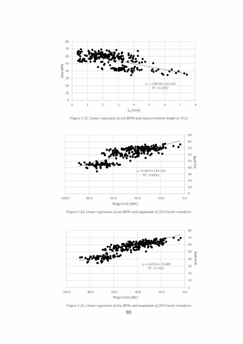
93

Figure 5-23, Linear regression of wet BPNs and autocorrelation length (s=0.2)

Figure 5-24, Linear regression of wet BPNs and magnitude of 2D Fourier transform

Figure 5-25, Linear regression of dry BPNs and magnitude of 2D Fourier transform

95

CHAPTER 6

6 PHASE III, DURABILITY OF RCC PAVEMENT

The longevity of RCC pavement, as a sustainable alternative to conventional

pavement systems, is a matter of concern for decision-makers. A key deterioration

factor for concrete pavement is frost and intensified contribution of deicers to the

factor. In this phase of the study, it is intended to investigate the durability of RCC

pavement subjected to frost and establish a novel measurement method for

determination of extent of chloride-induced deterioration of pavement surface under

freeze-thaw cycling. Moreover, the effect of salt-scaling on surface of the RCC

pavement samples is also investigated.

6.1 Background

It is well known that deicing salts have a negative impact on concrete pavement, and

it can significantly increase the freeze-thaw damage. The typical mitigation for

freeze thaw cycling damage in conventional concrete is air entrainment, however,

due to the dry nature of RCC mixture and low binder content, air entrainment of RCC

mixtures is challenging (Delagrave et al., 1997; Pigeon & Malhotra, 1995; Piggott,

1999). It is worth mentioning although there are published data indicating the high

performance of RCC pavement to freeze thaw cycling, some reports indicate

unsatisfactory resistance of RCC pavement to deicers salt scaling (Nili & Zaheri,

2011; Ragan, 1986; Vahedifard et al., 2010). Apart from the variation in results, the

mutual fact between most of these studies is the test method. ASTM C672 prescribes

a test method for scaling resistance of concrete surfaces exposed to deicing

chemicals. According to the test method, after 50 freeze-thaw cycles, a visual rating

of frost damage of pavement surface is obtained. Some countries such as Canada

96

modified this test method and added quantitative measures by determining specimen

mass loss based on mass measurement of loose materials at intervals of 5 cycles.

6.2 Materials and methods

To select test specimens, 6 RCC mixtures were considered. Three binders’ content

of 200, 300 and 400 kg/m3, nominal aggregate size of 12 mm and 19 mm. The mix

designs are given in table Table 3-2. Two cylinders with a diameter and height of

150 mm and two prisms with dimensions of 300x100x75 mm were obtained from

lab prepared roller compacted slabs.

The transport of liquids in capillary pore system of concrete is known as sorptivity.

The surface tension of capillary pores is the reason for this action. It is well-known

that the water transportability of concrete has a significant impact on its long-term

performance and durability. Additionally, the moisture state of concrete is an

effecting factor on its frost resistance. To gain a better understanding of the water

absorption rate of the produced RCCP, ASTM C1585, standard test method for

measuring the rate of water absorption by hydraulic-cement concrete was selected

for sorptivity measurement of RCCP samples. Two cylinders from each RCCP were

conditioned, sealed, and tested according to the standard. Furthermore, two RCCP

prisms from each RCCP were selected for ASTM C672, test method for scaling

resistance of concrete surfaces exposed to deicing chemicals. Cured specimens were

diked with epoxy and subjected to 50 cycles of freeze-thaw. Apart from the

requirements of ASTM C672, surfaces of all specimens were scanned at 3 stages

with the study 3D laser scanner. The first scan was conducted before start of the test

and two other scans on the 25th and 50th cycles. The scan direction and location of

each specimen were kept constant for all three rounds of scanning.

6.3 Results and discussions

Figure 6-1 gives a comparison of the rate of water absorption of RCC specimens.

The rate of water absorption or sorptivity represents the pore system and pores

97

connectivity of concrete. It is seen that sorptivity is in direct relationship with RCC

cement content, hence less cement, provides less paste and more open pores generate

for higher sorptivity. Another influencing factor is aggregate gradation and

maximum aggregate size. The test reveals, with similar cement content, RCC with

greater maximum aggregate size has lower sorptivity. Pictures of the RCC pavement

samples, before and after 50 cycles of freeze-thaw cycling are provided in Figure 6-4

and Figure 6-5. Other than discoloration of the surfaces, damage on the surface

texture of all samples can be observed. Comparing samples with 12 mm stone size

shows scaling on the surface of all samples. Furthermore, the intensity of the scaling

is greater on RCC samples with less cement content. This damage was expected

based on sorptivity results. 200-12 samples with greater sorptivity value exhibit the

greatest damage and 400-12 samples with lower sorptivity display better frost

performance. Extending the comparison to RCC samples with 19 mm stone size

gives exactly the same results, and the best performance belongs to the samples with

400 kg/m3 cement content with the lowest sorptivity value. However, the overall

performance of the RCC samples does not follow the sorptivity comparison. The

RCC samples with 12 mm maximum aggregate size performed better than their

competitors with 19 mm maximum aggregate size whilst for all samples, 12 mm

maximum aggregate size resulted in greater sorptivity value comparing to 19 mm.

Figure 6-1, The initial and secondary rate of water absorption for 200 kg/m3 binder content RCC

98



99

Figure 6-4, RCCP samples with 12 mm stone, before (two pictures on the left) and after 50 cycles of freeze-

thaw (two pictures on the right)

100

Figure 6-5, RCCP samples with 19 mm stone, before (two pictures on the left) and after 50 cycles of freeze-

thaw (two pictures on the right)

101

Inspection of the samples surface visually shows 2 different types of surface damage.

Surficial disintegration of paste, resulting in texture with deeper valleys and pop-

outs on coarse aggregates. Pop-outs are more seen on the surface of RCC samples

with 19 mm aggregate size, which represents low frost resistance of the utilized

coarse aggregates.

To gain a better understanding of the extent of surficial frost damage and change in

texture, all RCC samples were scanned and analyzed for texture parameters at cycles

zero, 25 and 50. Figure 6-6 Figure 6-7 compare Root mean square height (Sq) of the

textures as a height parameters representative. The comparison satisfies the

expecting increase in average height of texture with increase in frost cycles, however,

the point of interest is the extent of this increase. Undeniably increase in cement

content promoted the performance of RCC samples to resist frost cycles. The

comparisons reveal an increase in cement content, decreased both extent and rate of

frost damage. Furthermore, RCC with smaller maximum aggregate size samples

performed better in freeze-thaw cycling.

Figure 6-6, Change in Root mean square height for RCC with 12 mm max aggregate size

102

Figure 6-7, Change in Root mean square height for RCC with 19 mm max aggregate size

Previously it was discussed that shape texture irregularities can be assessed with

Skewness and Kurtosis parameters. Skewness which is suitable for evaluating

abrasion of texture is demonstrated in Figure 6-9 and Figure 6-8. For all RCC

samples, a decrease in skewness is seen by the increase in frost cycles. This state

abrasive influence of frost cycles on the texture of the RCC samples. In addition,

tracing the rate of the decrease in skewness shows the greater abrasive influence of

freeze-thaw cycling on RCC samples with smaller stone size.

Figure 6-10 and Figure 6-11 exhibit comparison of Kurtosis of the textures. This

parameter which relates to the tip geometry of peaks and valleys is suitable for

analyzing the degree of contact between two objects. It is seen the freeze-thaw

cycling caused a slight decrease in Kurtosis values which can be interpreted as a

decrease in the contact surface. This decrease appears to be similar for all specimens.

103



104



105

Evaluation of estimated Mean Texture Depth (eMTD) as a standard macro-texture

representative, under freeze-thaw cycling influence, is presented in Figure 6-12 and

Figure 6-13. The extent of change in macro-texture of the RCC samples shows a

variation in both magnitude and rate. Speaking of RCC samples with 19 mm

maximum aggregate, change in macro-texture magnitude remains close, however the

rate of this change slows with an increase in cement content. It worth mentioning

that pop-outs were seen on coarse aggregate of the samples. Hence, similar change

in the magnitude of eMTD can be associated with the pop-outs and a decrease in rate

of the change is due to the increase in cement content. Better performance in terms

of macro-texture change belongs to RCC samples with 12 mm maximum aggregate

size. It can be summarized that the cement content has a dramatic effect on promoting

RCC texture resistance to freeze-thaw cycling, whereas poor resistance of aggregates

to frost damage is not negligible.

Figure 6-12, Macro-texture change under freeze-thaw cycling influence for 12 mm max aggregate size RCCs

106

Figure 6-13, Macro-texture change under freeze-thaw cycling influence for 19 mm max aggregate size RCCs

Thanks to the high precision of laser scanner, volumetric parameters of scanned

texture are readily computable. Figure 6-14 and Figure 6-15 demonstrate quantitative

analysis of change in volume of valleys due to frost damage. Figure 6-16 gives a

precise comparison of overall volume loss, based on the computed volume values.

The comparison can clearly show, samples with smaller aggregate size performed

better in terms of volume loss under cycles of freeze-thaw. An increase in cement

content, increases resistance of the RCC samples to chemical deicers induced freeze-

thaw damage, and the highest performance belongs to the 400-12 RCC sample.

107

Figure 6-14, Change in volume of valleys after freeze-thaw cycling (Dmax = 12 mm)

Figure 6-15, Change in volume of valleys after freeze-thaw cycling (Dmax = 19 mm)

Figure 6-16, Overall volume loss of the RCC samples after 50 cycles of freeze-thaw

109

CHAPTER 7

7 PHASE IV, MODIFICATION OF TEXTURE OF RCC

Pavement

7.1 Methodology of the Experiments

Investigating the texture characteristics of RCC pavement in the previous chapter

demonstrated similarities to the texture of HMA pavement. Unlike conventional

Portland cement concrete pavement, which happens to have a smooth surface after

finishing and the necessity of additional texturizing, RCC surface is already

generated with a texture. However, it was shown that this texture is not identical to

HMA texture and it suffers from the lack of uniformity. Inspired by HMA

texturizing, two methods were considered for improving the surface texture of RCC:

- Exposed aggregate concrete surface (EACS)

- Chip sprinkled concrete surface (CSCS)

This chapter will discuss macro-texture, micro-texture, and skid resistance of RCC

pavement surface modified with the above-mentioned techniques.

7.1.1 Test Specimens for Exposed Aggregate Concrete Surface (EACS)

For better understanding of the influence of different variables such as compaction,

aggregate size, and the depth of exposure on EACS, two different series of EACS

specimens were prepared:

- Lab prepared gyratory compacted specimens

- Field obtained RCC specimens

110

Six mixes with three different cement contents, and two different maximum

aggregate sizes of 12 mm and 19 mm were selected (Table 7-1). Two set retarders

with various grades (elutriation depth) were also selected to stop the hydration of

surface paste. The set retarders were provided by the RECKLI company. The

products are commercially known as RECKLI-CR-Type PV (concrete surface

retarder – positive process). The grades of 25 (L) and 100 (H) were selected with

nominal elutriation depths of 2.5 mm and 4.0 mm respectively. According to the

manufacturer, the real elutriation depth of each grade may vary depending on the

cement class, water to cement ratio, shape of aggregate, and grain size distribution.

The concrete mixtures were prepared in a pan mixer. Nine specimens from each mix

were compacted with the gyratory compactor. The gyration cycles were kept at 75

cycles for all specimens. Immediately after compaction, the set retarder was brushed

on the surface of each cylindrical specimens (the dosage used is 250 g/m2). After 24

hours, the surface of the specimens was power washed to an extent that no more

paste could be cleaned off from the surface. Three replicates for each retarder grade

as well as three control specimens were prepared.

Table 7-1, Mix proportions and properties of the specimens

Mix ID Cement

(kg)

Dmax

(mm)

Water

(%)

Water

(kg)

Aggregate (kg)

W/C

Vebe

Time

(s)

Compaction

Ratio

(%)

0-5mm 5-12mm 12-19mm

SGC-200-12 200 12 5 117 1388 750 0 0.59 32 98.8

SGC-200-19 200 19 5 117 1067 857 216 0.59 32 99.5

SGC-300-12 300 12 5.5 128 1332 720 0 0.42 22 98.9

SGC-300-19 300 19 5.5 128 1024 823 208 0.42 20 98.4

SGC-400-12 400 12 6 139 1240 670 0 0.35 35 98.0

SGC-400-19 400 19 6 139 953 766 194 0.35 32 98.9

111

Figure 7-1, EACS and control specimens

7.1.2 Test Specimens for Chip Sprinkled Concrete Surface (CSCS)

Three different gradations were selected as test chips (aggregate). A substrate was

prepared from 300 kg/m3 cement RCC mixture with a Dmax of 12 mm using the same

mix design of RCC-300-12 utilized in phase II. A cement slurry with water to cement

ratio of 1 was prepared and the chips were mixed with the slurry, so the aggregate

surfaces were coated in order to enhance the penetration and adhesion of the chips.

Immediately after the initial compaction of the substrate, the fresh slurry coated chips

were placed on the surface of the substrate, and compaction with DDVHR was

carried out to reach maximum compaction. Table 7-2 gives the used gradation, ratio

of spread, and coating dosage.

112

Figure 7-2 a) Unchipped RCC surface. b) RCC surface sprinkled with 5.0-9.5 mm chips. c) RCC surface

sprinkled with 9.5-12.7 mm chips. d) RCC surface sprinkled with 12.7-16 mm chips.

Table 7-2, Chip sprinkling gradation, coating and spread rate

Sample ID Gradation

(mm)

Spread

ratio

(kg/m2)

Coating ratio

(kg per agg. kg)

Unchipped - - -

CSCS 5~9 5.0-9.5 9.6 0.25

CSCS 9~12 9.5-12.7 13.1 0.16

CSCS 12~16 12.7-16 16.9 0.12

113

Figure 7-3, Image simulation of surface data produced by MATLAB, a,b,c) CSCS 5~9, d,e,f) CSCS 9~12, g,h,i)

CSCS 12~16

7.1.3 Experiments

The core and cylinder samples obtained from exposed aggregate surfaces were cut

with a water-cooled saw to make 30 mm thick disks of the top surfaces. Chip

114

sprinkled surface samples were cut in a similar way with strips of 25 cm width. The

skid resistance of the specimens were measured under wet and dry conditions with

British Pendulum tester in 4 directions with 90-degree intervals. Then, the surfaces

of the specimens were scanned with the laser scanner developed in this work, and

3D surfaces were generated. Finally, roughness parameters were computed.

7.2 Investigating Texture Properties

To gain a clear view of how surface modification of RCC pavement affects its

performance, the obtained results were analyzed in macro-texture and micro-texture

contexts.

• Macro-texture

It was previously shown that mean texture depth as an indicator of macro-texture can

be computed from 3D surface data with high precision. Figure 7-4 demonstrates the

estimated mean texture depth (eMTD) computed from the following sample sets:

- Super-pave gyratory compacted, exposed aggregate concrete surface

o Control sample

o Low grade exposed

o High grade exposed

- Roller compacted, chip sprinkled concrete surface

o Unchipped RCC

o Chip size 5 to 9.5mm

o Chip size 9.5 to 12.7mm

o Chip size 12.7 to 16.0mm

115

Figure 7-4, Estimated mean texture depth of surface modified RCC pavement

Figure 7-5, Estimated mean texture depth of chip sprinkled RCC pavement

As expected, Figure 7-4 shows that surface modification has a tremendous influence

on macro-texture enhancement. While low-grade EACS can produce twice macro

texture compared to control samples, high-grade EACS can increase MTD up to

116

three times. What is obvious here is that the effect of set retarder varies based on

cement content. The gradation of aggregate can be considered as another affecting

factor as well. Figure 7-5 demonstrates MTD results of chip sprinkled RCC samples.

It is clearly seen that MTD increases with an increase in chip size. Spike in MTD is

tremendous and chip sprinkled surface can enhance macro-texture almost two times

of exposed aggregate concrete surface.

• Micro-texture

In a previous section, it was demonstrated that micro-texture indirectly can be

explained with skid resistance. Similar to phase one, British pendulum tester was

carried out on all of the test surfaces for the determination of skid resistance. Both

wet and dry conditions of the surfaces were assessed for skid resistance

measurements. Figure 7-6 exhibits the obtained skid numbers of test surfaces.

Surprisingly at first glance, no significant change in skid numbers was observed. As

experienced in the first phase of the study, gyratory compacted surfaces yielded

noticeably higher skid numbers in contrast to roller compacted surfaces. Speaking of

SGCC specimens, lower cement content tends to show a slightly higher skid number

compared to the high cement content mixes. In addition, skid numbers on control

surfaces show a greater fluctuation compared to the numbers obtained from exposed

aggregate surfaces. However, no significant improvement is seen for exposed

aggregate surface concrete in terms of skid numbers. Unlike exposed aggregate

surface, chip sprinkled concrete surface shows a slight improvement in skid numbers

using chip size 5 to 9.5 mm. However, an increase in chip size has a negative impact

on skid resistance. Another observation is the difference between dry and wet skid

numbers. Whilst the control RCC sample and EACS show a skid number drop of

8~14% on wet condition, CSCS samples give only 6% decrease. This shows the chip

sprinkled surfaces perform better in wet condition in terms of skid resistance.

117

Figure 7-6, British pendulum numbers of exposed aggregate RCC pavement

Figure 7-7, British pendulum numbers of chip sprinkled RCC pavement

7.3 Conclusion

In summary, two surface modification techniques were successfully implemented on

RCC pavement. To produce EACS, the pavement was power washed 24 hours after

the placement and compaction of RCC. Hydration retarders with two different

effective penetration depths were applied to stop the hardening of superficial paste.

The investigation of roughness parameters showed a significant improvement in the

118

macro-texture of the surfaces. However, no noticeable change was recorded for

micro-texture.

In CSCS, three different aggregate gradations were forced to be implanted on the

RCC pavement surface. The application was reached success after coating the

aggregate with a layer of portland cement slurry. A tremendous increase in macro-

texture was achieved. Furthermore, it was observed that the chip size is effective in

skid resistance. The surface chip sprinkled with aggregate size 5 to 9.5 mm, showed

higher BPN comparing to its substrate, RCC-300-12. However, by an increase in the

grain size of chips, a decrease in BPN was observed.

Further investigations on chips stability under loading as well as noise and tire wear

are required. To gain a better understanding of micro-texture, additional testing such

as dynamic friction tester and locked-wheel skid trailer is recommended.

119

CHAPTER 8

8 SUMMARY AND CONCLUSIONS

Drivability of road surface is affected by its texture properties in different scales.

Although available reports and studies have investigated asphalt and conventional

concrete pavement texture, however, there is not much evidence in literature

regarding RCC pavement texture. This Study utilized high precision laser

measurement technique and standard roughness parameters to provide quantitative

information of RCC pavement texture.

8.1 Findings and Conclusions

In the first phase of this study, a comparison between RCC and HMA with two

different compaction methods was made and the influencing factors were

investigated. In general, RCC and asphalt pavements are compacted with paver and

rollers on field. However, in Laboraty environment, superpave gyratory compactor

is utilized for sample preparation. This type of compaction is accepted to represent

the mechanical properties of field compaction. To extend this representativeness to

texture properties, a gyratory compactor and a walk-behind vibratory roller

compacter were used to produce the study samples.

For evaluation of the obtained surfaces, a high precision 3D laser scanner was

developed by the author. The texture of the study samples were scanned and

processed in MATLAB. ISO 25178-2, International Standard for Specification and

Measurement of 3D Surface Texture defines over 60 roughness parameters. These

parameters were computed for all the study surfaces.

120

It has shown that roughness parameters of RCC and HMA specimens made with

gyratory compactor are different than the parameters achieved from vibratory roller

compacter. Speaking of concrete samples, it was observed that:

- On both compaction methods, two main mean height parameters, Sa and Sq

tend to decrease by an increase in cement content.

- While the influence of aggregate gradation on gyratory compacted samples

is negligible, a dramatic difference available between the nominal aggregate

size of 12 mm and 19 mm on roller compacted samples.

- The skewness of all roller compacted samples are in close range to each other

varying between -1 and -2.5, however, gyratory compacted samples exhibit

great variation in results exceeding -3.5. In other words, peaks of gyratory

compacted samples are beefier.

- The kurtosis of all roller compacted samples are in the same range to each

other varying between 5 and 10, however, gyratory compacted samples show

tremendous variation in results exceeding 25, which indicates peaks on

gyratory compaction are sharper than roller compaction.

By investigating the height parameters of samples produced with these two

compacting methods, it is concluded that generated textures are not identical and

gyratory compaction is not able to represent the texture roller compaction generates.

In the lights of scanned surfaces and computed roughness parameters, the question

that to what extent roller compacted concrete and asphalt are similar in terms of

texture has been answered. Comparing both pavements:

- The RCC pavement samples showed less uniformity in terms of peaks’ height

and valleys’ depth.

- The shape and geometry of generated peaks and valleys are different in these

two different pavements.

- RCC pavement has a higher tendency to show an unexpected change in

height compared to asphalt pavement.

- Asphalt pavement generates finer texture to RCC pavement.

121

- For RCC pavement, effect of change in maximum aggregate size on macro-

texture is considerably greater to asphalt pavement.

- Asphalt produces uniform texture under cylinder compactor while RCC is

prone to get waviness from compaction.

- Shape of the contact points for asphalt pavement samples are three times

pointier than RCC pavement samples.

- RCC pavement samples are generating coarser segments comparing to

asphalt samples.

From the above-mentioned observations, it has been concluded that using the same

compaction techniques and similar effort, RCC and asphalt generate distinct textures.

Furthermore, this study has shown a good relationship between roughness

parameters and MTD resulting from the sand patch test. Although this relationship

was expected, to gain a deeper understanding of roughness parameters, all computed

parameters were checked. The study showed a strong correlation exists between

MTD and most of height and height-related parameters, however, the greatest

correlation with R2 of 0.80 was observed on Volume of Voids measured at 10% of

peaks material ratio. Considering the high precision of volume calculation from a 3D

profile, measurement error in the sand patch test can be the reason for slightly low

R2 value. Nevertheless, a model with a very small deviation from The World Road

Association model was achieved.

Additionally, investigating a relationship between computed information and

measured skid resistance has shown a weak to moderate relationship with

Autocorrelation length of texture (R2 = 0.38) and Magnitude of 2D Fourier

Transform (R2 = 0.74). The relationship was computed to be happening at only 1

millimeter depth of texture, hence, slices of only 1 mm height from top of texture

were prepared virtually for calculation of Autocorrelation length and Magnitude of

2D Fourier Transform.

The study has shown that in general, asphalt pavement can give higher skid

resistance to concrete pavement. It should be noted these results wear obtained on

122

new pavement surface where aggregate had not been exposed to traffic or other

abrasive factors, and aggregates were in binder coated condition.

In another step, the resistance of RCC pavement to chemical deicers induced freeze

and thaw cycling damage were examined. ASTM C672 defines a procedure to test

concrete for scaling resistance of concrete surfaces exposed to deicing chemicals.

This is a qualitative test method that evaluates surface scaling based on visual

observations. A novel procedure was followed to combine 3D scanning with the test

and add quantitative analysis for better evaluation of results. The surfaces were

scanned in three stages, on cycles zero, 25 and 50. And roughness parameters were

compared. Changes in macro-texture of the surfaces as well as the volume of material

loss were measured. It was observed that:

- An increase in cement content of mixtures can increase resistance to the

damage.

- Freeze-thaw has an influence on valleys depth and can increase macro-

texture depth.

- The resistance of aggregates to frost damage plays an important role in the

scaling of RCC pavement.

Moreover, two surface modification techniques were conducted on the RCC surface.

Lab prepared and field compacted RCC were subjected to set retarder immediately

after compaction and power-washed after 24 hours to achieve Exposed Aggregate

Concrete Surface. In another approach, certain gradation of aggregates was sprinkled

onto unproperly compacted RCC and compaction was carried out over the layer to

achieve Chip Sprinkled Concrete Surface. Gathered information and testing

demonstrated improvement on macro-texture of surfaces, however, no noticeable

change in skid resistance was observed.

8.2 Suggestions for Future Studies

- The findings of this thesis all depend on extensive laboratory studies. The

surface properties of RCC mixtures to include roughness or unevenness of

actual field performance can be determined.

123

- This study is focused on plain RCC without additives or admixtures. Effect

of using supplementary cementitious materials and concrete admixtures such

as air entrainment agents can be investigated.

- Skid resistance is a function of speed. British pendulum measures low-speed

friction (about 10 km/h). Investigation of micro-texture can be extended to

Dynamic Friction Tester for determination of friction index at higher speeds.

125

9 REFERENCES

AASHTO. (1976). Guidelines for Skid Resistant Pavement Design. American

Association of State Highway and Transportation Officials .

ACPA. (2000). Concrete Pavement Surface Texture,” a special report in Concrete

Pavement Technology and Research. SR902P.

Akbulut, D. E., & Akoz, F. (2012). Effects of pozzolanas and fibers on mechanical

properties of mortars in historical buildings. Struct. Anal. Hist. Constr, 1-3.

Andersen, L. G. (2015). Rolling resistance modelling: from functional data analysis

to asset management system. (Doctoral dissertation, Roskilde Universitet).

Åström, H., & Wallman, C.-G. (2001). Friction Measurement Methods And The

Correlation Between Road Friction And Traffic Safety. A Literature Review.

Baker, I. O. (1918). A treatise on roads and pavements. John Wiley & Sons.

Bazlamit, S. M., & Reza, F. (2005). Changes in asphalt pavement friction

components and adjustment of skid number for temperature. Journal of

Transportation Engineering, 131(6), 470–476.

Bitelli, G., Simone, A., Girardi, F., & Lantieri, C. (2012). Laser scanning on road

pavements: A new approach for characterizing surface texture. Sensors

(Switzerland), 12(7), 9110–9128. https://doi.org/10.3390/s120709110

Blanchard, A. H. (1919). American Highway Engineers’ Handbook. John Wiley &

Sons, Incorporated.

Board, H. R. (1972). National Cooperative Highway Research Program Synthesis of

highway practice 14: skid resistance.

Boscaino, G., Pratico, F. G., & Vaiana, R. (2004). Texture indicators and surface

performance in flexible pavements. Symposium on Pavement Surface

Characteristics [of Roads and Airports], 5th, 2004, Toronto, Ontario, Canada.

126

Briant, P. (2002). From Cyrus to Alexander: a history of the Persian Empire.

Eisenbrauns.

Brown, G. E. (1975). Mineralogical Description of Two Samples of Giza

Limestone’. Electromagnetic Sounder Experiments at The Pyramids of Giza,

Stanford Research International SRI, 119–122.

Chandler, J. W. E., Phillips, S. M., Roe, P. G., & Viner, H. E. (2003). Quieter

concrete roads: construction, texture, skid resistance and noise. TRL Report,

576.

Colley, B. E., Christensen, A. P., Nowlen, W. J., & Cement, P. (1969). Factors

Affecting Skid Resistance and Safety of Concrete Pavements. Special Report-

Highway Research Board, (101), 80.

Collins, H. J., & Hart, C. A. (1936). Principles of road engineering (Vol. 6). E.

Arnold.

Collins, R., Watson, D., Johnson, A., & Wu, Y. (1997). Effect of aggregate

degradation on specimens compacted by superpave gyratory compactor.

Transportation Research Record, 1590(1), 1–9.

Corley-Lay, J. B. (1998). Friction and surface texture characterization of 14

pavement test sections in Greenville, North Carolina. Transportation Research

Record, 1639(1), 155–161.

Dahir, S. H. M., & Gramling, W. L. (1990). NCHRP Synthesis of Highway Practice

158: Wet Pavement Safety Programs. TRB, National Research Council,

Washington, DC.

Davis, R. M. (2001). Comparison of surface characteristics of hot-mix asphalt

pavement surfaces at the Virginia Smart Road. (Doctoral dissertation, Virginia

Tech).

Delatte, N., Amer, N., & Storey, C. (2003). Improved management of RCC

pavement technology. UTCA Report, 1231, 54.

Descornet, G., Fuchs, F., & Buys, R. (1993). Noise-reducing concrete pavements.

Fifth International Conference on Concrete Pavement Design and

RehabilitationPurdue University, School of Civil Engineering; Federal

127

Highway Administration; Portland Cement Association; Transportation

Research Board; Indiana Department of Transportation; Federal Aviation

Administration; and American Concrete Pavement Association. (Vol. 2).

Do, M.-T., Tang, Z., Kane, M., & de Larrard, F. (2009). Evolution of road-surface

skid-resistance and texture due to polishing. Wear, 266(5–6), 574–577.

Dondi, G., Simone, A., Lantieri, C., & Vignali, V. (2010). Characterization of

pavement surface texture using 3D Laser scanner technique. Proceedings of the

11th International Conference on Asphalt Pavement. August, 1–6.

Embacher, R. A., & Snyder, M. B. (2001). Life-cycle cost comparison of asphalt and

concrete pavements on low-volume roads; case study comparisons.


Ergun, M., Iyinam, S., & Iyinam, A. F. (2005). Prediction of road surface friction

coefficient using only macro-and microtexture measurements. Journal of

Transportation Engineering, 131(4), 311–319.

Flintsch, G. W., De León, E., McGhee, K. K., & AI-Qadi, I. L. (2003). Pavement

surface macrotexture measurement and applications. Transportation Research

Record, 1860(1), 168–177.

Forster, S. W. (1989). Pavement microtexture and its relation to skid resistance.

Transportation Research Record, 1215, 151–164.

Fuchs, F. (1981). Texturing of cement concrete pavements by chip sprinkling the

fresh concrete. Transportation Research Record, 821, 56–60.

Gibbons, R. B., & Hankey, J. (2007). Wet night visibility of pavement markings:

dynamic experiment. Transportation Research Record, 2015(1), 73–80.

Gillespie, H. (1992). A Century of Progress: The History of Hot Mix Asphalt (1st

Ed.). Lanham, MD: National Asphalt Pavement Association.

Hall, J. W., Smith, K. L., Titus-Glover, L., Wambold, J. C., Yager, T. J., & Rado, Z.

(2009). Guide for pavement friction. Final Report for NCHRP Project, 1, 43.

Halsted, G. E. (2009). Roller-compacted concrete pavements for highways and

128

streets. 2009 Annual Conference And Exhibition Of The Transportation

Association Of Canada-Transportation In A Climate Of Change.

Harrington, D., Abdo, F., Adaska, W., Hazaree, C. V, Ceylan, H., & Bektas, F.

(2010). Guide for roller-compacted concrete pavements.

Hayden, C. M. (1982). Pavement Surface Characteristics and Materials (Vol. 763).

ASTM International.

Henry, J. J. (2000). NCHRP synthesis of highway practice 291: Evaluation of

pavement friction characteristics. TRB, National Research Council,

Washington, DC.

Henry, J. J., & Saito, K. (1983). Skid-Resistance Measurements with Blank and

Ribbed Test Tires and Their Relationship to Pavement Texture.

Herrfeld, M. (n.d.). Requirements for the application of surface retarders in whisper

concrete road proects. Proc. 8 Th International Symposium on Concrete Roads,

5, 7–8.

Hibbs, B. O., & Larson, R. M. (1996). Tire Pavement Noise and Safety Performance,

PCC Surface Texture Technical Working Group. United States. Federal

Highway Administration. Office of Engineering.

Hoerner, T. E., Smith, K. D., Larson, R. M., & Swanlund, M. E. (2003). Current

practice of portland cement concrete pavement texturing. Transportation

Research Record, 1860(1), 178–186.

Hogervorst, D. (1974). Some properties of crushed stone for road surfaces. Bulletin

of the International Association of Engineering Geology-Bulletin de

l’Association Internationale de Géologie de l’Ingénieur, 10(1), 59–64.

Horvath, A., & Hendrickson, C. (1998). Comparison of environmental implications

of asphalt and steel-reinforced concrete pavements. Transportation Research

Record, 1626(1), 105–113.

Janisch, D. (2006). An overview of Mn/DOT’s pavement condition rating

procedures and indices. Minnesota Department of Transportation, Saint Paul,

MN.

129

Jasiczak, J., & Zielinski, K. (2006). Effect of protein additive on properties of mortar.

Cement and Concrete Composites, 28(5), 451-457.

Jones, C.R.; Rolt, J.; Smith, H.R.; Parkman, C. (1999). A guide to the pavement

evaluation and maintenance of bitumen-surfaced roads in tropical and sub-

tropical countries.

Juli, D. (1989). Technical Committee Report on Surface Characteristics. RRU

Newsletter, 99, 9–11.

Kaloush, K. E., Carlson, J. D., Golden, J. S., & Phelan, P. E. (2008). The thermal

and radiative characteristics of concrete pavements in mitigating urban heat

island effects (No. PCA R&D SN2969).

Kanafi, M. M., & Tuononen, A. J. (2017). Top topography surface roughness power

spectrum for pavement friction evaluation. Tribology International, 107, 240–

249.

Kummer, H. W. (1966). Unified theory of rubber and tire friction.

Li, S., Noureldin, A. S., & Zhu, K. Q. (2011). Characterization of microtexture on

typical pavement surfaces: a pilot study (No. 11-1457).

Mahone, D. C. (1977). Texturing new concrete pavements. Virginia Transportation

Research Council.

Masad, E., Muhunthan, B., Shashidhar, N., & Harman, T. (1999). Quantifying

laboratory compaction effects on the internal structure of asphalt concrete.


Mataei, B., Zakeri, H., Zahedi, M., & Nejad, F. M. (2016). Pavement Friction and

Skid Resistance Measurement Methods: A Literature Review. Open Journal of

Civil Engineering, 06(04), 537–565. https://doi.org/10.4236/ojce.2016.64046

McGhee, K. K., & Flintsch, G. W. (2003). High-speed texture measurement of

pavements. Virginia Center for Transportation Innovation and Research.

Meegoda, J. N. (2009). Non-contact skid resistance measurement: final report,

December 2009. New Jersey. Dept. of Transportation.

130

Mosher, L. G. (1985). Restoration of Final Surface to Concrete Pavement by

Diamond Saw Grinding. Third International Conference on Concrete Pavement

Design and RehabilitationPurdue University, School of Civil Engineering;

Federal Highway Administration; Portland Cement Association;

Transportation Research Board; Federal Aviation Administration; and I, (1

Volume).

Noyce, D. A., Bahia, H. U., Yambo, J., Chapman, J., & Bill, A. (2005). Incorporating

Road Safety into Pavement Management: Maximizing Surface Friction for

Road Safety Improvements. University of Wisconsin. Retrieved from

http://www.mrutc.org/research/0404/

Olek, J., Weiss, W. J., & Garcia-Villarreal, R. (2004). Relating surface texture of

rigid pavement with noise and skid resistance.

Persson, B. N. J. (2001). Theory of rubber friction and contact mechanics. The

Journal of Chemical Physics, 115(8), 3840–3861.

Peterson, R. L., Mahboub, K. C., Michael Anderson, R., Masad, E., & Tashman, L.

(2003). Superpave® laboratory compaction versus field compaction.


Pittman, D. W. (1986). Construction of roller-compacted concrete pavements.

Transportation Research Record, 1062, 13–19.

Properties, A. C. P. A. T. S. on S. (1975). Guideline for Texturing of Portland

Cement Concrete Highway Pavements. American Concrete Paving Association.

Radford, T. A. (1940). The Construction of Roads and Pavements. McGraw Hill.

Rado, Z. (1994). Analysis of texture models. Pennsylvania Transportation Institute,

Pennsylvania State University, State College.

Ray, G. K., & Norling, L. T. (1974). More Macrotexture in Concrete Pavement for

Greater, Longer-lasting Skid Resistance. Portland Cement Association.

Roberts, A. D. (1988). Rubber adhesion at high rolling speeds.

Roe, P. G., Parry, A. R., & Viner, H. E. (1998). High and low speed skidding

131

resistance: the influence of texture depth.

Roemmele, C. F. (1986). A History of Sawing, Grinding & Grooving with Diamond.

Solutions for Pavement Rehabilitation Problems, 255–270. ASCE.

Rose, J. G., Gallaway, B. M., & Hankins, K. D. (1970). Macrotexture Measurement

and Related Skid Resistance at Speeds from 20 to 60 Miles per Hour. Highway

Research Record, (341).

Rugenstein, E. E. (1977). Summary and evaluation of concrete pavement texturing

practices. International Conference on Concrete Pavement DesignPurdue

University, School of Civil Engineering; Federal Highway Administration;

Portland Cement Association; Transportation Research Board; Federal

Aviation Administration; and Indiana Department of High.

Sandberg, U. (1998). Influence of road surface texture on traffic characteristics

related to environment, economy and safety: A state-of-the-art study regarding

measures and measuring methods. Statens väg-och transportforskningsinstitut.,

VTI notat 53A-1997.

Sayers, M. W. (1989). Two quarter-car models for defining road roughness: IRI and

HRI. Transportation Research Record, (1215).

Scharnigg, K., & Schwalbe, G. (2010). Report on knowledge gaps and proposals for

further research concerning optimisation for road surfaces and tyres for skid

resistance, rolling resistance and noise emissions TYROSAFE projecthttp.

Tyrosafe. Fehrl. Org.

Serigos, P. A., De Fortier Smit, A., & Prozzi, J. A. (2014). Incorporating surface

microtexture in the prediction of skid resistance of flexible pavements.


Sommer, H. (1994). Developments for the exposed aggregate technique in Austria.

7th International Symposium on Concrete Roads, 3(5).

Sommer, H. (1998). Longtime experience with exposed aggregate surfaces in

Austria. Theme 3-Pavement Performance and Evaluation. 8 Th International

Symposium on Concrete Roads, Lizbona, Portugalia, 117–121.

Stinglhammer, H. (1994). Noise reducing exposed aggregate surfaces experience and

132

recommendations. 1994/7th International Symposium on Concrete Roads, 137–

140.

Sumitsawan, P., Ardenkani, S. A., & Romanoschi, S. (2009). Effect of pavement

type on fuel consumption and emissions. Proceedings of the 2009 Mid-

Continent Transportation Research Symposium.

Tayabji, S. D., Sherman, T. W., Arent, W. L., Kohn, S., Piggott, R. W., Berry, J. R.,

…& Zollinger, D. G. (1995). Report on Roller-Compacted Concrete

Pavements.

Thornton, J. B. (1974). Determination of Desirable Finish for Concrete Pavement

(Publication)

Tighe, S., Fung, R., & Smith, T. (2001). Concrete pavements in Canada: State-of-

the-art practice. Seventh International Conference on Concrete Pavements. The

Use of Concrete in Developing Long-Lasting Pavement Solutions for the 21st

CenturyInternational Society for Concrete Pavements, 1.

Tillson, G. W. (1900). Street Pavements and Paving Materials: A Manual of City

Pavements: the Methods and Materials of Their Construction. J. Wiley.

Ueckermann, A., Wang, D., Oeser, M., & Steinauer, B. (2015). Calculation of skid

resistance from texture measurements. Journal of Traffic and Transportation

Engineering (English Edition), 2(1), 3–16.

Van Dam, T., Taylor, P., Fick, G., Gress, D., VanGeem, M., & Lorenz, E. (2011).

Sustainable concrete pavements: a manual of practice.

Viner, H., Abbott, P., Dunford, A., Dhillon, N., Parsley, L., & Read, C. (2006).

Surface texture measurement on local roads. Report PPR148. TRL Ltd, UK.

Wambold, J. C., Henry, J. J., & Blackburn, R. R. (1984). Evaluation Of Pavement

Surface Texture: Significance And Measurement Techniques. Volume Ii:

Comprehensive Report. Final Report.

Wambold, J. C., Henry, J. J., & Yager, T. (2004). NASA Wallops Tire/Runway

Friction Workshops 1994-2003. Proceedings of the Fifth International

Symposium on Pavement Surface Characteristics-SURF.

133

Wu, C.-L., & Nagi, M. A. (1995). Optimizing surface texture of concrete pavement

(No. RD111T).

Yager, T. J., & Bühlmann, F. (1982). Macrotexture and drainage measurements on

a variety of concrete and asphalt surfaces. In Pavement Surface Characteristics

and Materials. ASTM International.

Zuniga-Garcia, N., & Prozzi, J. A. (2016). Contribution of Micro-and Macro-

Texture for Predicting Friction on Pavement Surfaces (No. CHPP Report-

UTA# 3-2016).

135

APPENDICES

A. Roughness Parameters of The Specimens

Height Parameter

Sp Sv Sz Sa Sq Ssk Sku

Sample ID mm mm mm mm mm

SGCC-200-12-4-1 1.110 2.357 3.468 0.324 0.425 -1.227 4.781

SGCC-200-12-4-2 1.251 3.066 4.318 0.346 0.458 -1.373 5.781

SGCC-200-12-4-3 1.538 3.489 5.027 0.401 0.540 -1.077 5.555

SGCC-200-12-4-4 1.147 2.916 4.063 0.325 0.444 -1.149 5.166

SGCC-200-12-4-5 1.223 3.172 4.395 0.376 0.496 -1.379 5.439

SGCC-200-12-4-6 1.437 2.994 4.432 0.398 0.543 -1.124 5.262

SGCC-200-12-4-7 1.275 2.930 4.205 0.314 0.424 -1.470 6.364

SGCC-200-12-4-8 1.101 4.723 5.824 0.344 0.470 -1.635 7.675

SGCC-200-12-4-9 0.879 2.145 3.024 0.281 0.372 -1.346 5.262

SGCC-200-12-4-10 1.159 3.075 4.234 0.306 0.442 -1.649 8.211

SGCC-200-12-5-1 0.972 4.199 5.171 0.262 0.353 -1.580 6.962

SGCC-200-12-5-2 1.119 3.895 5.015 0.291 0.394 -1.591 6.413

SGCC-200-12-5-3 0.923 2.335 3.258 0.254 0.332 -1.396 5.273

SGCC-200-12-5-4 0.947 2.698 3.645 0.222 0.298 -1.519 6.048

SGCC-200-12-5-5 1.383 4.068 5.452 0.374 0.508 -1.563 7.066

SGCC-200-12-5-6 0.738 2.705 3.444 0.216 0.289 -1.642 6.527

SGCC-200-12-5-7 1.167 5.364 6.532 0.310 0.433 -1.721 8.145

SGCC-200-12-5-8 1.181 2.454 3.635 0.258 0.345 -1.213 5.234

SGCC-200-12-5-9 1.244 2.996 4.241 0.342 0.448 -1.010 4.286

SGCC-200-12-5-10 1.119 2.978 4.097 0.320 0.412 -0.966 4.019

SGCC-200-12-6-1 0.971 3.430 4.401 0.284 0.394 -1.827 9.056

SGCC-200-12-6-2 0.798 3.602 4.400 0.146 0.239 -3.225 25.687

SGCC-200-12-6-3 0.722 3.085 3.807 0.236 0.342 -2.001 10.932

SGCC-200-12-6-4 1.173 2.829 4.002 0.210 0.301 -1.923 10.123

SGCC-200-12-6-5 0.856 2.805 3.661 0.286 0.389 -1.510 6.866

SGCC-200-12-6-6 1.088 2.874 3.962 0.252 0.365 -1.647 8.246

SGCC-200-12-6-7 0.913 3.097 4.010 0.223 0.329 -2.181 11.760

SGCC-200-12-6-8 0.705 2.928 3.633 0.166 0.272 -2.937 18.776

SGCC-300-12-5-1 0.952 2.350 3.301 0.183 0.283 -1.940 7.988

SGCC-300-12-5-2 0.430 3.117 3.547 0.136 0.223 -2.697 14.509

SGCC-300-12-5-3 1.197 3.196 4.392 0.353 0.462 -1.184 3.525

SGCC-400-12-4-1 0.877 2.846 3.723 0.287 0.392 -1.628 6.722

SGCC-400-12-4-2 0.582 2.128 2.710 0.184 0.262 -1.862 8.508

SGCC-400-12-4-3 1.098 2.920 4.017 0.242 0.341 -1.753 7.677

136

Height Parameter



SGCC-400-12-4-4 0.922 2.685 3.608 0.160 0.232 -1.906 10.613

SGCC-400-12-4-5 0.615 2.075 2.690 0.157 0.233 -2.308 11.953

SGCC-400-12-4-6 0.954 2.278 3.232 0.204 0.304 -1.495 8.314

SGCC-400-12-4-7 1.396 3.538 4.933 0.297 0.420 -1.983 10.369

SGCC-400-12-4-8 0.727 1.944 2.671 0.176 0.249 -1.786 8.034

SGCC-400-12-4-9 0.822 2.711 3.533 0.211 0.284 -1.555 6.841

SGCC-400-12-4-10 1.136 2.817 3.953 0.257 0.355 -1.649 7.441

SGCC-400-12-5-1 1.069 2.369 3.335 0.239 0.277 -1.368 5.342

SGCC-400-12-5-2 0.860 3.996 4.564 0.225 0.295 -2.638 16.127

SGCC-400-12-5-3 0.737 3.194 3.704 0.220 0.267 -1.717 7.465

SGCC-400-12-5-4 0.951 3.725 4.422 0.235 0.296 -1.966 11.107

SGCC-400-12-5-5 0.583 2.043 2.494 0.146 0.187 -1.754 8.562

SGCC-400-12-5-6 0.948 3.049 3.810 0.235 0.294 -1.827 7.861

SGCC-400-12-5-7 0.676 2.654 3.149 0.191 0.239 -1.948 8.462

SGCC-400-12-5-8 0.703 2.108 2.688 0.183 0.223 -1.614 7.065

SGCC-400-12-5-9 1.091 2.893 3.831 0.219 0.279 -1.730 8.491

SGCC-400-12-5-10 0.871 3.045 3.721 0.235 0.302 -1.813 8.964

SGCC-400-12-6-1 0.496 1.998 2.494 0.096 0.160 -3.666 25.462

SGCC-400-12-6-2 0.882 4.229 5.110 0.196 0.288 -2.358 12.980

SGCC-400-12-6-3 0.605 3.139 3.745 0.170 0.259 -2.610 12.979

SGCC-400-12-6-4 0.801 2.148 2.949 0.164 0.237 -2.033 9.180

SGCC-400-12-6-5 0.768 2.142 2.910 0.173 0.251 -1.854 8.272

SGCC-400-12-6-6 0.799 2.651 3.449 0.166 0.242 -1.978 9.831

SGCC-400-12-6-7 0.624 2.262 2.886 0.161 0.241 -2.259 11.413

SGCC-400-12-6-8 0.960 2.184 3.144 0.166 0.239 -1.783 8.581

SGCC-400-12-6-9 0.736 2.379 3.114 0.131 0.211 -2.950 18.430

SGCC-400-12-6-10 0.855 3.234 4.089 0.131 0.201 -2.697 20.733

SGCC-200-19-4-1 1.208 2.709 3.917 0.297 0.410 -1.498 6.400

SGCC-200-19-4-2 1.607 5.225 6.832 0.408 0.594 -1.978 10.904

SGCC-200-19-4-3 0.932 3.739 4.671 0.343 0.473 -1.810 8.233

SGCC-200-19-4-4 1.162 3.028 4.190 0.299 0.402 -1.441 6.105

SGCC-200-19-4-5 1.081 2.751 3.832 0.286 0.395 -1.652 7.282

SGCC-200-19-4-6 1.259 4.883 6.142 0.334 0.475 -2.121 11.758

SGCC-200-19-4-7 0.966 2.844 3.810 0.276 0.374 -1.511 6.646

SGCC-200-19-4-8 1.328 3.241 4.569 0.351 0.488 -1.632 7.387

SGCC-200-19-4-9 1.512 5.078 6.590 0.325 0.453 -1.821 8.551

SGCC-200-19-4-10 1.107 3.472 4.579 0.366 0.516 -1.910 8.263

SGCC-200-19-5-1 0.929 3.154 4.083 0.292 0.399 -1.763 7.604

SGCC-200-19-5-2 1.249 3.588 4.837 0.400 0.541 -1.530 6.310

SGCC-200-19-5-3 0.913 3.532 4.444 0.355 0.474 -1.642 6.757

SGCC-200-19-5-4 0.970 3.932 4.903 0.326 0.445 -1.815 7.851

SGCC-200-19-5-5 1.070 3.008 4.078 0.322 0.432 -1.545 6.313

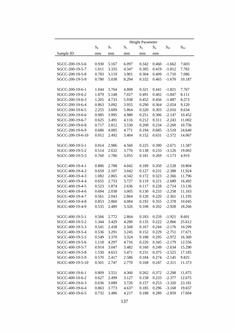
137

Height Parameter



SGCC-200-19-5-6 0.930 5.167 6.097 0.342 0.460 -1.662 7.603

SGCC-200-19-5-7 1.011 3.335 4.347 0.305 0.419 -1.812 7.782

SGCC-200-19-5-8 0.783 3.119 3.901 0.304 0.409 -1.710 7.086

SGCC-200-19-5-9 0.780 5.038 8.294 0.332 0.465 -1.670 10.187

SGCC-200-19-6-1 1.044 3.764 4.808 0.321 0.441 -1.821 7.767

SGCC-200-19-6-2 1.879 5.148 7.027 0.491 0.402 -1.847 8.111

SGCC-200-19-6-3 1.205 4.733 5.938 0.452 0.456 -1.887 8.273

SGCC-200-19-6-4 0.863 3.092 3.955 0.290 0.364 -2.024 9.120

SGCC-200-19-6-5 2.255 3.609 5.864 0.320 0.303 -2.016 8.634

SGCC-200-19-6-6 0.985 3.995 4.980 0.251 0.306 -2.147 10.452

SGCC-200-19-6-7 0.625 3.491 4.116 0.212 0.311 -2.243 11.002

SGCC-200-19-6-8 0.717 2.812 3.530 0.208 0.234 -2.260 10.756

SGCC-200-19-6-9 0.686 4.085 4.771 0.194 0.685 -3.518 24.640

SGCC-200-19-6-10 0.912 2.492 3.404 0.152 0.631 -2.572 14.067

SGCC-300-19-5-1 0.814 2.986 4.560 0.225 0.390 -2.671 11.587

SGCC-300-19-5-2 0.514 2.632 3.776 0.138 0.233 -3.126 19.002

SGCC-300-19-5-3 0.760 1.786 3.055 0.181 0.269 -1.173 4.919

SGCC-400-19-4-1 0.886 2.788 4.042 0.189 0.350 -2.528 10.804

SGCC-400-19-4-2 0.659 2.107 3.042 0.127 0.231 -2.388 11.924

SGCC-400-19-4-3 1.082 2.865 4.342 0.172 0.323 -2.366 11.796

SGCC-400-19-4-4 0.655 2.733 3.727 0.119 0.221 -2.689 16.492

SGCC-400-19-4-5 0.523 1.874 2.636 0.117 0.228 -2.724 13.136

SGCC-400-19-4-6 0.694 2.038 3.005 0.130 0.233 -2.258 11.163

SGCC-400-19-4-7 0.561 2.043 2.864 0.120 0.220 -2.361 11.195

SGCC-400-19-4-8 0.853 2.860 4.084 0.192 0.355 -2.378 10.045

SGCC-400-19-4-9 0.535 2.489 3.326 0.108 0.202 -2.928 18.266

SGCC-400-19-5-1 0.566 2.772 2.864 0.183 0.259 -1.921 8.601

SGCC-400-19-5-2 1.344 3.429 4.280 0.135 0.222 -2.866 25.612

SGCC-400-19-5-3 0.541 2.438 2.568 0.167 0.244 -2.176 10.299

SGCC-400-19-5-4 0.536 3.291 3.245 0.152 0.229 -2.751 17.671

SGCC-400-19-5-5 0.549 3.370 3.324 0.188 0.295 -2.972 16.360

SGCC-400-19-5-6 1.118 4.297 4.716 0.226 0.345 -2.179 12.556

SGCC-400-19-5-7 0.914 3.047 3.482 0.160 0.249 -2.634 15.290

SGCC-400-19-5-8 1.530 4.653 5.471 0.231 0.375 -2.525 17.185

SGCC-400-19-5-9 0.570 2.417 2.586 0.184 0.274 -2.145 9.825

SGCC-400-19-5-10 0.501 2.747 2.770 0.168 0.247 -2.311 11.373

SGCC-400-19-6-1 0.809 3.551 4.360 0.262 0.372 -2.298 11.075

SGCC-400-19-6-2 0.627 2.499 3.127 0.158 0.233 -2.377 12.675

SGCC-400-19-6-3 0.636 3.089 3.726 0.157 0.253 -3.320 23.181

SGCC-400-19-6-4 0.863 3.773 4.637 0.185 0.296 -3.168 19.657

SGCC-400-19-6-5 0.732 3.486 4.217 0.188 0.289 -2.859 17.604

138

Height Parameter



SGCC-400-19-6-6 0.606 2.878 3.485 0.151 0.226 -2.837 18.534

SGCC-400-19-6-7 0.529 2.322 2.851 0.124 0.199 -3.427 23.545

SGCC-400-19-6-8 0.882 2.818 3.700 0.146 0.251 -3.627 27.534

SGCC-400-19-6-9 0.754 2.173 2.927 0.105 0.160 -2.664 17.971

SGCC-400-19-6-10 0.467 1.091 1.558 0.083 0.116 -1.502 8.986

SGC-HMA-L-19-1 1.295 5.105 6.400 0.538 0.718 -1.538 6.332

SGC-HMA-L-19-2 1.686 7.113 8.799 0.611 0.829 -1.755 8.139

SGC-HMA-L-19-3 1.951 5.393 7.344 0.659 0.862 -1.351 5.612

SGC-HMA-L-19-4 1.689 6.290 7.978 0.523 0.703 -1.580 7.275

SGC-HMA-L-19-5 1.375 5.378 6.753 0.543 0.704 -1.340 5.408

SGC-HMA-L-19-6 1.385 5.299 6.684 0.519 0.685 -1.419 5.876

SGC-HMA-L-12-1 1.145 2.360 3.505 0.237 0.317 -1.307 6.165

SGC-HMA-L-12-2 1.128 2.726 3.854 0.251 0.334 -1.177 5.931

SGC-HMA-L-12-3 0.992 2.379 3.371 0.237 0.318 -1.331 6.269

SGC-HMA-L-12-4 1.128 2.781 3.909 0.313 0.412 -1.076 5.052

SGC-HMA-L-12-5 0.931 2.708 3.639 0.246 0.327 -1.266 5.813

SGC-HMA-L-12-6 1.309 5.088 6.397 0.317 0.437 -1.580 9.357

RCC-200-12-1 1.236 3.915 5.150 0.386 0.548 -1.961 8.703

RCC-200-12-2 1.242 2.668 3.910 0.421 0.547 -1.287 4.626

RCC-200-12-3 0.956 3.242 4.198 0.312 0.454 -2.067 9.051

RCC-200-12-4 1.110 3.233 4.343 0.353 0.493 -1.844 7.391

RCC-200-12-5 1.323 3.959 5.282 0.342 0.482 -1.996 9.614

RCC-200-12-6 1.994 4.216 6.210 0.397 0.532 -0.992 4.070

RCC-200-12-7 1.225 3.612 4.837 0.198 0.329 -1.720 6.674

RCC-200-12-8 0.707 3.013 3.720 0.267 0.366 -1.435 6.746

RCC-200-12-9 1.361 2.733 4.093 0.359 0.514 -1.970 8.624

RCC-200-12-10 0.988 4.084 5.072 0.645 0.835 -3.621 25.481

RCC-300-12-1 1.378 2.826 4.204 0.334 0.423 -1.592 7.079

RCC-300-12-2 1.673 2.638 4.312 0.327 0.430 -1.680 7.753

RCC-300-12-3 0.957 1.073 1.544 0.095 0.429 -1.735 9.821

RCC-300-12-4 0.889 2.994 3.950 0.331 0.309 -1.932 7.917

RCC-300-12-5 0.732 2.782 3.671 0.228 0.402 -2.390 9.169

RCC-300-12-6 0.638 2.825 3.557 0.305 0.224 -2.110 6.834

RCC-300-12-7 0.884 2.101 2.739 0.165 0.368 -2.450 13.460

RCC-300-12-8 0.621 2.670 3.555 0.293 0.270 -1.658 12.487

RCC-300-12-9 1.061 2.557 3.178 0.202 0.409 -2.254 12.558

RCC-300-12-10 0.471 3.414 4.476 0.298 0.121 -2.500 11.615

RCC-400-12-1 0.989 2.017 3.006 0.263 0.354 -1.927 7.538

RCC-400-12-2 0.528 1.389 1.916 0.233 0.302 -1.575 5.683

RCC-400-12-3 1.333 1.923 3.256 0.239 0.330 -1.823 7.456

RCC-400-12-4 1.232 1.945 3.177 0.278 0.363 -1.210 5.256

139

Height Parameter



RCC-400-12-5 1.090 2.403 3.493 0.308 0.419 -1.320 6.123

RCC-400-12-6 0.775 2.325 3.100 0.269 0.372 -1.988 8.491

RCC-400-12-7 0.978 2.445 3.423 0.230 0.319 -2.356 10.334

RCC-400-12-8 0.743 1.821 2.564 0.227 0.303 -1.731 7.373

RCC-400-12-9 0.579 1.819 2.397 0.228 0.292 -1.562 5.391

RCC-400-12-10 0.647 1.398 2.045 0.184 0.253 -2.114 7.705

RCC-200-19-1 2.627 6.833 9.461 0.684 0.868 -1.684 6.847

RCC-200-19-2 3.192 7.591 10.783 0.867 1.037 -1.223 4.726

RCC-200-19-3 1.735 7.136 8.871 0.571 0.725 -1.890 8.775

RCC-200-19-4 1.999 5.330 7.330 0.605 0.773 -1.721 6.752

RCC-200-19-5 3.171 7.051 10.222 0.558 0.725 -1.711 8.411

RCC-200-19-6 1.770 5.162 6.932 0.574 0.716 -1.547 6.263

RCC-200-19-7 1.686 5.695 7.381 0.667 0.851 -1.804 6.938

RCC-200-19-8 1.807 5.980 7.787 0.558 0.739 -1.905 8.271

RCC-200-19-9 2.036 5.052 7.089 0.703 0.855 -1.310 4.964

RCC-200-19-10 2.204 6.863 9.066 0.704 0.908 -1.751 7.160

RCC-300-19-1 1.945 3.408 5.352 0.476 0.661 -1.432 6.110

RCC-300-19-2 2.245 5.096 7.342 0.548 0.778 -1.829 8.493

RCC-300-19-3 1.168 6.761 7.928 0.401 0.581 -2.458 6.837

RCC-300-19-4 3.440 7.447 10.887 0.797 1.087 -1.445 8.114

RCC-300-19-5 1.944 6.643 8.586 0.687 0.967 -1.701 8.241

RCC-300-19-6 1.560 4.428 5.988 0.442 0.614 -1.834 4.880

RCC-300-19-7 3.024 5.846 8.870 0.726 0.949 -1.151 5.960

RCC-300-19-8 2.297 4.889 7.186 0.594 0.807 -1.399 5.482

RCC-300-19-9 1.739 5.232 6.971 0.607 0.814 -1.331 10.136

RCC-300-19-10 1.602 7.163 8.765 0.546 0.782 -2.071 16.028

RCC-400-19-1 3.091 7.003 10.709 0.520 0.760 -1.278 6.206

RCC-400-19-2 2.089 5.428 6.364 0.648 0.756 -1.113 5.618

RCC-400-19-3 3.076 3.128 5.953 0.797 0.966 -2.057 10.583

RCC-400-19-4 1.109 6.532 2.966 0.295 0.387 -2.751 7.563

RCC-400-19-5 2.247 5.431 6.145 0.415 0.582 -1.666 5.503

RCC-400-19-6 1.950 3.511 10.241 0.663 0.903 -1.167 6.707

RCC-400-19-7 1.721 3.135 5.167 0.557 0.673 -1.514 20.231

RCC-400-19-8 1.341 6.356 3.663 0.503 0.583 -2.691 32.951

RCC-400-19-9 1.191 10.274 3.133 0.402 0.477 -3.725 26.648

RCC-400-19-10 4.356 12.208 5.283 0.322 0.426 -3.289 18.345

RC-HMA-L-12-1 0.989 3.434 4.424 0.220 0.304 -1.728 9.824

RC-HMA-L-12-2 1.200 4.709 5.909 0.242 0.332 -1.618 8.737

RC-HMA-L-12-3 1.019 2.976 3.995 0.241 0.332 -1.653 7.891

RC-HMA-L-12-4 1.020 3.313 4.333 0.238 0.336 -1.827 8.600

RC-HMA-L-12-5 0.963 4.375 5.337 0.250 0.363 -2.216 11.810

RC-HMA-L-12-6 1.015 3.154 4.169 0.242 0.342 -1.810 8.745

140

Height Parameter



RC-HMA-L-12-7 1.310 5.017 6.327 0.322 0.460 -2.078 10.778

RC-HMA-L-12-8 1.652 4.277 5.929 0.291 0.409 -1.824 8.820

RC-HMA-L-12-9 1.102 5.367 6.469 0.322 0.457 -2.040 10.431

RC-HMA-L-12-10 1.437 5.000 6.437 0.322 0.462 -2.052 11.060

RC-HMA-L-12-11 1.273 3.139 4.412 0.296 0.419 -1.957 9.289

RC-HMA-L-12-12 1.386 4.278 5.663 0.359 0.517 -2.144 10.400

RC-HMA-L-19-1 1.690 3.959 5.648 0.359 0.508 -1.827 8.056

RC-HMA-L-19-2 1.396 4.769 6.165 0.375 0.525 -1.952 9.548

RC-HMA-L-19-3 1.397 4.828 6.225 0.387 0.551 -1.970 9.616

RC-HMA-L-19-4 1.427 4.056 5.483 0.325 0.462 -1.979 9.065

RC-HMA-L-19-5 1.280 5.182 6.462 0.380 0.539 -2.066 9.612

RC-HMA-L-19-6 1.165 5.519 6.684 0.302 0.425 -1.926 10.315

RC-HMA-L-19-7 1.261 5.136 6.398 0.340 0.486 -2.142 11.685

RC-HMA-L-19-8 1.419 4.852 6.270 0.339 0.464 -1.633 8.013

RC-HMA-L-19-9 1.401 5.105 6.507 0.371 0.528 -1.982 9.514

RC-HMA-L-19-10 1.471 6.123 7.594 0.383 0.546 -2.113 11.701

RC-HMA-L-19-11 1.533 6.596 8.130 0.461 0.669 -2.386 11.966

Spatial

Parameters

Hybrid

Parameters

Miscellaneous

Parameters

Sal Str Sdq Sdr Std

Sample ID mm (s = 0.2) % mm

SGCC-200-12-4-1 2.587 0.820 0.808 22.251 171.746

SGCC-200-12-4-2 2.877 0.903 0.837 23.853 137.509

SGCC-200-12-4-3 3.261 0.791 0.885 25.946 176.743

SGCC-200-12-4-4 2.863 0.795 0.740 19.227 176.994

SGCC-200-12-4-5 2.726 0.904 0.875 25.351 173.496

SGCC-200-12-4-6 4.007 0.810 0.845 24.271 8.485

SGCC-200-12-4-7 2.405 0.883 0.823 22.789 3.489

SGCC-200-12-4-8 2.625 0.862 0.854 23.937 50.259

SGCC-200-12-4-9 2.076 0.841 0.775 21.170 121.500

SGCC-200-12-4-10 3.854 0.652 0.708 17.945 12.249

SGCC-200-12-5-1 2.507 0.872 0.912 25.713 177.239

SGCC-200-12-5-2 3.036 0.758 0.917 25.362 17.004

SGCC-200-12-5-3 2.261 0.908 0.877 24.738 22.757

SGCC-200-12-5-4 2.095 0.880 0.834 22.838 22.243

SGCC-200-12-5-5 4.203 0.765 0.908 26.172 73.252

SGCC-200-12-5-6 1.969 0.820 0.816 21.843 173.994

SGCC-200-12-5-7 3.322 0.872 0.912 25.199 163.510

SGCC-200-12-5-8 3.401 0.861 0.715 17.925 3.492

SGCC-200-12-5-9 3.250 0.900 0.849 24.146 176.008

SGCC-200-12-5-10 3.340 0.876 0.795 21.803 176.253

141

Spatial

Parameters

Hybrid

Parameters

Miscellaneous

Parameters

Sal Str Sdq Sdr Std


SGCC-200-12-6-1 1.901 0.792 0.877 21.920 132.500

SGCC-200-12-6-2 1.809 0.774 0.601 12.198 128.749

SGCC-200-12-6-3 2.337 0.807 0.709 15.948 121.497

SGCC-200-12-6-4 1.931 0.803 0.679 15.267 163.253

SGCC-200-12-6-5 3.186 0.883 0.720 16.481 2.510

SGCC-200-12-6-6 2.642 0.768 0.719 16.080 137.015

SGCC-200-12-6-7 2.709 0.849 0.685 14.374 151.746

SGCC-200-12-6-8 1.820 0.808 0.611 12.476 42.501

SGCC-300-12-5-1 2.470 0.545 0.450 8.004 118.264

SGCC-300-12-5-2 2.406 0.809 0.432 7.220 97.509

SGCC-300-12-5-3 2.150 0.929 0.773 20.178 160.747

SGCC-400-12-4-1 3.090 0.917 0.718 18.993 3.494

SGCC-400-12-4-2 3.011 0.776 0.490 9.984 39.003

SGCC-400-12-4-3 2.539 0.796 0.653 15.999 176.503

SGCC-400-12-4-4 3.596 0.826 0.435 7.866 3.745

SGCC-400-12-4-5 3.607 0.902 0.438 7.996 11.258

SGCC-400-12-4-6 3.163 0.822 0.583 13.441 3.740

SGCC-400-12-4-7 3.196 0.777 0.705 18.154 8.491

SGCC-400-12-4-8 3.041 0.714 0.518 11.122 86.251

SGCC-400-12-4-9 2.593 0.847 0.599 14.174 140.748

SGCC-400-12-4-10 2.685 0.891 0.660 16.312 8.753

SGCC-400-12-5-1 2.436 0.847 0.753 20.566 16.250

SGCC-400-12-5-2 4.044 0.762 0.723 19.173 129.004

SGCC-400-12-5-3 2.426 0.870 0.757 20.626 28.258

SGCC-400-12-5-4 3.303 0.798 0.767 21.482 4.256

SGCC-400-12-5-5 2.546 0.842 0.538 11.335 12.747

SGCC-400-12-5-6 3.404 0.754 0.727 18.835 129.005

SGCC-400-12-5-7 2.749 0.856 0.684 17.687 176.255

SGCC-400-12-5-8 2.277 0.830 0.688 17.833 159.753

SGCC-400-12-5-9 2.798 0.842 0.742 19.589 129.249

SGCC-400-12-5-10 3.746 0.786 0.684 17.011 12.749

SGCC-400-12-6-1 1.822 0.854 0.439 7.601 92.998

SGCC-400-12-6-2 2.157 0.850 0.638 13.039 93.254

SGCC-400-12-6-3 2.428 0.803 0.553 10.768 112.747

SGCC-400-12-6-4 2.433 0.863 0.514 9.887 93.255

SGCC-400-12-6-5 2.585 0.833 0.514 10.025 163.259

SGCC-400-12-6-6 2.727 0.869 0.498 9.564 3.256

SGCC-400-12-6-7 2.806 0.776 0.501 9.173 163.999

SGCC-400-12-6-8 3.103 0.813 0.444 7.739 87.000

SGCC-400-12-6-9 2.972 0.819 0.451 7.669 106.993

SGCC-400-12-6-10 2.794 0.791 0.426 6.748 137.005

142

Spatial

Parameters

Hybrid

Parameters

Miscellaneous

Parameters

Sal Str Sdq Sdr Std


SGCC-200-19-4-1 2.406 0.893 0.825 22.469 3.998

SGCC-200-19-4-2 2.777 0.790 1.104 30.316 176.994

SGCC-200-19-4-3 2.760 0.902 0.856 23.509 16.752

SGCC-200-19-4-4 2.262 0.840 0.820 22.448 8.010

SGCC-200-19-4-5 2.360 0.749 0.804 22.276 176.255

SGCC-200-19-4-6 3.190 0.932 0.866 24.379 2.747

SGCC-200-19-4-7 2.221 0.932 0.839 23.512 148.752

SGCC-200-19-4-8 3.080 0.742 0.828 23.088 32.499

SGCC-200-19-4-9 2.580 0.874 0.909 25.820 86.495

SGCC-200-19-4-10 3.989 0.827 0.747 19.544 16.997

SGCC-200-19-5-1 2.094 0.881 0.866 23.929 171.505

SGCC-200-19-5-2 2.922 0.830 0.966 28.442 3.002

SGCC-200-19-5-3 2.688 0.872 0.907 25.737 176.754

SGCC-200-19-5-4 2.283 0.861 0.891 25.318 16.498

SGCC-200-19-5-5 2.245 0.883 0.891 25.397 163.008

SGCC-200-19-5-6 2.425 0.848 0.927 26.176 169.746

SGCC-200-19-5-7 2.368 0.847 0.844 22.939 3.502

SGCC-200-19-5-8 2.237 0.774 0.813 22.021 175.998

SGCC-200-19-5-9 2.869 0.839 0.785 20.516 19.752

SGCC-200-19-6-1 1.786 0.827 0.979 27.684 3.007

SGCC-200-19-6-2 3.403 0.780 1.131 34.152 140.744

SGCC-200-19-6-3 3.992 0.935 1.001 28.514 3.246

SGCC-200-19-6-4 1.884 0.813 0.891 23.659 3.243

SGCC-200-19-6-5 2.860 0.779 0.838 22.266 25.747

SGCC-200-19-6-6 1.813 0.905 0.831 20.969 2.742

SGCC-200-19-6-7 1.647 0.762 0.690 16.106 163.245

SGCC-200-19-6-8 1.708 0.802 0.716 16.855 16.750

SGCC-200-19-6-9 2.280 0.702 0.659 13.997 3.490

SGCC-200-19-6-10 1.800 0.787 0.565 11.584 176.502

SGCC-300-19-5-1 2.744 0.791 0.541 9.972 69.252

SGCC-300-19-5-2 2.549 0.597 0.366 5.622 50.996

SGCC-300-19-5-3 2.742 0.876 0.440 8.098 148.003

SGCC-400-19-4-1 3.732 0.792 0.518 10.499 3.011

SGCC-400-19-4-2 3.010 0.691 0.442 8.334 93.504

SGCC-400-19-4-3 2.743 0.702 0.509 10.477 154.998

SGCC-400-19-4-4 2.165 0.901 0.467 8.948 118.255

SGCC-400-19-4-5 3.148 0.753 0.405 7.026 98.498

SGCC-400-19-4-6 2.659 0.702 0.451 8.548 81.503

SGCC-400-19-4-7 2.639 0.736 0.461 8.841 113.001

SGCC-400-19-4-8 2.986 0.816 0.535 11.558 86.501

SGCC-400-19-4-9 3.250 0.771 0.410 7.294 78.251

SGCC-400-19-5-1 2.896 0.800 0.649 15.743 6.001

143

Spatial

Parameters

Hybrid

Parameters

Miscellaneous

Parameters

Sal Str Sdq Sdr Std


SGCC-400-19-5-2 2.492 0.765 0.556 11.047 86.753

SGCC-400-19-5-3 3.206 0.875 0.579 12.794 173.749

SGCC-400-19-5-4 2.804 0.623 0.594 13.481 3.762

SGCC-400-19-5-5 3.837 0.872 0.622 14.390 176.506

SGCC-400-19-5-6 3.195 0.653 0.689 15.981 176.740

SGCC-400-19-5-7 2.624 0.725 0.578 12.773 3.008

SGCC-400-19-5-8 3.103 0.645 0.708 16.610 163.006

SGCC-400-19-5-9 3.586 0.755 0.589 13.219 39.500

SGCC-400-19-5-10 3.479 0.884 0.560 12.292 137.491

SGCC-400-19-6-1 2.087 0.841 0.803 20.735 176.754

SGCC-400-19-6-2 1.734 0.853 0.603 13.353 137.501

SGCC-400-19-6-3 2.158 0.787 0.573 12.218 108.747

SGCC-400-19-6-4 1.901 0.739 0.666 14.486 99.996

SGCC-400-19-6-5 1.837 0.877 0.687 15.741 137.740

SGCC-400-19-6-6 1.875 0.842 0.588 12.909 177.002

SGCC-400-19-6-7 2.059 0.795 0.488 9.203 87.255

SGCC-400-19-6-8 3.071 0.737 0.533 10.070 97.999

SGCC-400-19-6-9 1.573 0.629 0.458 8.345 141.001

SGCC-400-19-6-10 1.397 0.747 0.416 7.574 106.997

SGC-HMA-L-19-1 2.895 0.918 1.410 50.792 39.005

SGC-HMA-L-19-2 2.310 0.747 1.941 72.587 3.755

SGC-HMA-L-19-3 3.082 0.925 1.609 59.454 14.999

SGC-HMA-L-19-4 2.096 0.859 1.909 74.966 69.753

SGC-HMA-L-19-5 2.498 0.881 1.441 52.225 20.750

SGC-HMA-L-19-6 2.345 0.879 1.804 63.170 81.750

SGC-HMA-L-12-1 1.816 0.789 0.943 29.692 93.245

SGC-HMA-L-12-2 1.571 0.884 1.139 40.129 122.498

SGC-HMA-L-12-3 1.814 0.872 0.973 31.188 163.505

SGC-HMA-L-12-4 1.952 0.849 1.279 47.805 128.995

SGC-HMA-L-12-5 1.781 0.853 1.006 33.185 3.491

SGC-HMA-L-12-6 2.098 0.823 1.475 56.985 93.753

RCC-200-12-1 2.235 0.808 0.971 25.856 13.247

RCC-200-12-2 2.989 0.740 0.828 22.874 176.263

RCC-200-12-3 3.297 0.635 0.658 15.259 30.254

RCC-200-12-4 2.477 0.643 0.821 21.265 166.503

RCC-200-12-5 2.842 0.834 0.732 17.549 140.992

RCC-200-12-6 3.202 0.663 1.117 33.745 176.000

RCC-200-12-7 2.486 0.886 0.977 28.542 171.253

RCC-200-12-8 2.858 0.920 0.456 8.291 159.002

RCC-200-12-9 2.312 0.898 0.623 14.605 137.492

RCC-200-12-10 4.442 0.845 0.918 23.549 170.744

RCC-300-12-1 2.744 0.775 1.044 27.782 176.500

144

Spatial

Parameters

Hybrid

Parameters

Miscellaneous

Parameters

Sal Str Sdq Sdr Std


RCC-300-12-2 3.183 0.852 0.924 23.502 176.752

RCC-300-12-3 3.076 0.824 0.483 7.970 132.492

RCC-300-12-4 2.722 0.915 1.039 27.666 169.999

RCC-300-12-5 2.640 0.849 0.779 17.958 3.744

RCC-300-12-6 3.065 0.921 0.944 23.775 32.001

RCC-300-12-7 2.510 0.862 0.697 15.178 98.496

RCC-300-12-8 2.545 0.771 0.956 24.963 156.501

RCC-300-12-9 2.790 0.812 0.711 15.150 3.501

RCC-300-12-10 3.074 0.698 0.899 21.596 175.745

RCC-400-12-1 2.773 0.804 0.864 24.327 147.496

RCC-400-12-2 2.691 0.867 0.785 22.056 176.505

RCC-400-12-3 2.806 0.726 0.835 21.825 152.002

RCC-400-12-4 2.907 0.917 0.891 26.678 3.747

RCC-400-12-5 3.243 0.767 0.895 26.400 137.498

RCC-400-12-6 2.969 0.845 0.877 24.173 176.750

RCC-400-12-7 3.429 0.744 0.722 18.438 3.255

RCC-400-12-8 2.594 0.833 0.776 21.094 20.503

RCC-400-12-9 2.609 0.936 0.773 21.896 12.755

RCC-400-12-10 2.611 0.919 0.673 17.611 128.995

RCC-200-19-1 3.078 0.829 1.102 32.038 86.993

RCC-200-19-2 3.804 0.825 1.255 39.845 4.244

RCC-200-19-3 3.323 0.911 0.985 27.696 7.496

RCC-200-19-4 3.665 0.907 0.947 25.899 163.250

RCC-200-19-5 3.393 0.808 0.873 21.572 140.502

RCC-200-19-6 3.224 0.967 0.883 24.847 159.500

RCC-200-19-7 3.517 0.910 0.990 27.799 132.251

RCC-200-19-8 3.223 0.785 0.931 25.414 176.757

RCC-200-19-9 3.174 0.841 1.048 32.440 140.756

RCC-200-19-10 3.805 0.839 0.953 25.607 176.494

RCC-300-19-1 3.415 0.796 0.918 24.612 50.992

RCC-300-19-2 3.449 0.822 0.966 24.022 8.498

RCC-300-19-3 3.768 0.986 0.879 18.467 16.750

RCC-300-19-4 3.364 0.767 1.404 39.968 171.246

RCC-300-19-5 3.813 0.935 1.268 32.923 42.499

RCC-300-19-6 3.281 0.859 0.864 21.252 175.746

RCC-300-19-7 3.690 0.728 1.210 32.448 86.247

RCC-300-19-8 3.416 0.907 1.155 32.761 3.502

RCC-300-19-9 3.628 0.848 1.174 33.639 171.503

RCC-300-19-10 4.290 0.881 1.097 27.946 51.006

RCC-400-19-1 3.095 0.903 1.349 37.028 47.762

RCC-400-19-2 2.940 0.812 1.399 39.651 77.007

RCC-400-19-3 3.486 0.849 1.234 33.699 86.256

RCC-400-19-4 3.245 0.795 0.865 12.429 120.504

145

Spatial

Parameters

Hybrid

Parameters

Miscellaneous

Parameters

Sal Str Sdq Sdr Std


RCC-400-19-5 3.323 0.885 1.109 23.470 132.499

RCC-400-19-6 3.787 0.858 1.482 42.775 39.245

RCC-400-19-7 3.039 0.913 1.085 28.528 39.005

RCC-400-19-8 3.685 0.855 1.074 32.022 3.499

RCC-400-19-9 2.721 0.843 0.753 19.074 166.759

RCC-400-19-10 4.369 0.873 0.943 20.506 112.501

RC-HMA-L-12-1 1.297 0.865 1.267 42.984 99.246

RC-HMA-L-12-2 1.542 0.903 1.316 45.176 119.748

RC-HMA-L-12-3 1.431 0.826 1.313 44.865 92.498

RC-HMA-L-12-4 1.523 0.839 1.313 43.465 109.257

RC-HMA-L-12-5 1.792 0.877 1.327 42.036 138.000

RC-HMA-L-12-6 1.540 0.898 1.313 42.595 109.746

RC-HMA-L-12-7 1.847 0.778 1.585 56.580 112.000

RC-HMA-L-12-8 1.546 0.866 1.497 52.615 107.499

RC-HMA-L-12-9 2.017 0.807 1.533 54.415 106.254

RC-HMA-L-12-10 1.919 0.860 1.551 53.996 144.001

RC-HMA-L-12-11 1.623 0.931 1.476 51.569 105.497

RC-HMA-L-12-12 2.090 0.856 1.652 58.991 86.753

RC-HMA-L-19-1 2.556 0.890 1.474 50.346 112.504

RC-HMA-L-19-2 2.811 0.841 1.460 49.605 79.998

RC-HMA-L-19-3 2.718 0.790 1.539 52.556 121.997

RC-HMA-L-19-4 2.050 0.766 1.440 48.694 100.746

RC-HMA-L-19-5 2.793 0.876 1.464 48.296 144.244

RC-HMA-L-19-6 1.782 0.802 1.407 46.813 99.252

RC-HMA-L-19-7 2.106 0.805 1.513 54.637 122.249

RC-HMA-L-19-8 2.104 0.856 1.470 54.421 94.496

RC-HMA-L-19-9 2.576 0.948 1.562 57.302 143.494

RC-HMA-L-19-10 2.399 0.843 1.553 56.135 113.745

RC-HMA-L-19-11 3.514 0.784 1.586 56.930 83.753

Functions and Related Parameters

Sk Spk Svk Vvv Vvc Vmp Vmc

Sample ID mm mm mm ml/m2 ml/m2 ml/m2 mm

SGCC-200-12-4-1 0.72 0.20 0.78 77.85 372.15 10.62 364.53

SGCC-200-12-4-2 0.78 0.22 0.83 83.22 390.85 11.46 385.32

SGCC-200-12-4-3 0.98 0.42 0.91 92.84 514.75 20.25 437.99

SGCC-200-12-4-4 0.75 0.32 0.84 84.54 423.17 13.89 343.17

SGCC-200-12-4-5 0.89 0.16 0.92 92.06 427.54 9.14 420.64

SGCC-200-12-4-6 0.93 0.40 0.99 99.99 506.85 19.34 420.22

SGCC-200-12-4-7 0.70 0.23 0.81 81.10 347.93 11.64 338.31

SGCC-200-12-4-8 0.81 0.20 0.91 91.67 389.63 10.82 366.19

SGCC-200-12-4-9 0.65 0.17 0.70 70.40 307.86 9.08 309.96

146




SGCC-200-12-4-10 0.71 0.32 0.88 87.18 381.96 15.16 299.03

SGCC-200-12-5-1 0.76 0.17 0.85 85.04 357.17 9.29 356.06

SGCC-200-12-5-2 0.76 0.21 0.98 98.74 375.27 11.13 389.64

SGCC-200-12-5-3 0.66 0.16 0.80 77.36 331.11 8.21 361.28

SGCC-200-12-5-4 0.56 0.18 0.74 73.36 288.10 9.01 300.23

SGCC-200-12-5-5 1.17 0.27 1.15 116.85 545.99 14.73 508.92

SGCC-200-12-5-6 0.55 0.10 0.72 71.17 272.00 5.80 296.85

SGCC-200-12-5-7 0.85 0.30 1.08 109.09 425.46 15.28 401.77

SGCC-200-12-5-8 0.73 0.30 0.79 78.96 366.12 15.13 353.17

SGCC-200-12-5-9 1.06 0.31 0.95 96.70 540.45 15.75 484.12

SGCC-200-12-5-10 1.01 0.28 0.88 89.10 479.57 15.24 449.92

SGCC-200-12-6-1 0.54 0.11 0.82 81.88 270.17 5.97 297.96

SGCC-200-12-6-2 0.30 0.11 0.54 52.29 139.54 5.11 125.47

SGCC-200-12-6-3 0.49 0.15 0.74 74.31 233.30 7.61 230.33

SGCC-200-12-6-4 0.41 0.13 0.65 65.57 203.49 6.24 208.54

SGCC-200-12-6-5 0.58 0.16 0.80 79.90 289.31 8.39 305.06

SGCC-200-12-6-6 0.50 0.26 0.79 80.22 260.63 12.60 239.24

SGCC-200-12-6-7 0.41 0.13 0.74 75.31 206.43 6.29 209.82

SGCC-200-12-6-8 0.30 0.12 0.62 62.60 145.63 5.87 136.28

SGCC-300-12-5-1 0.27 0.13 0.51 47.54 131.25 6.27 107.33

SGCC-300-12-5-2 0.22 0.07 0.39 33.98 101.92 3.50 82.41

SGCC-300-12-5-3 0.49 0.15 0.75 76.37 246.34 7.53 255.56

SGCC-400-12-4-1 0.63 0.16 0.78 78.49 306.24 8.69 308.31

SGCC-400-12-4-2 0.42 0.13 0.54 54.65 203.85 6.49 183.44

SGCC-400-12-4-3 0.52 0.18 0.71 71.54 257.88 8.90 245.34

SGCC-400-12-4-4 0.39 0.14 0.50 48.24 190.55 6.80 151.44

SGCC-400-12-4-5 0.36 0.12 0.50 49.86 164.38 5.70 148.62

SGCC-400-12-4-6 0.46 0.30 0.63 61.00 259.34 14.36 187.14

SGCC-400-12-4-7 0.70 0.19 0.81 82.02 339.26 9.39 310.94

SGCC-400-12-4-8 0.40 0.13 0.51 51.65 191.62 6.76 175.30

SGCC-400-12-4-9 0.50 0.13 0.54 53.77 231.97 6.48 227.82

SGCC-400-12-4-10 0.56 0.18 0.70 70.70 284.99 9.10 272.56

SGCC-400-12-5-1 0.65 0.18 0.76 74.89 325.07 9.65 333.51

SGCC-400-12-5-2 0.65 0.20 0.85 84.67 308.01 10.37 276.70

SGCC-400-12-5-3 0.62 0.16 0.78 78.16 300.25 8.39 286.50

SGCC-400-12-5-4 0.65 0.30 0.83 83.19 331.64 14.82 296.71

SGCC-400-12-5-5 0.41 0.20 0.56 55.18 210.68 9.93 172.20

SGCC-400-12-5-6 0.64 0.22 0.90 90.38 306.70 10.45 290.26

SGCC-400-12-5-7 0.51 0.15 0.72 72.70 248.44 7.79 236.86

SGCC-400-12-5-8 0.50 0.18 0.65 65.12 253.88 9.08 236.22

SGCC-400-12-5-9 0.62 0.31 0.82 81.22 317.38 15.25 262.37

SGCC-400-12-5-10 0.68 0.31 0.90 87.28 358.07 14.78 280.06

147




SGCC-400-12-6-1 0.22 0.08 0.36 32.34 101.44 3.99 83.72

SGCC-400-12-6-2 0.34 0.16 0.64 64.86 176.52 7.49 186.92

SGCC-400-12-6-3 0.31 0.09 0.62 61.96 150.72 4.74 148.72

SGCC-400-12-6-4 0.33 0.13 0.53 53.00 159.77 6.04 156.54

SGCC-400-12-6-5 0.34 0.17 0.57 57.36 169.35 7.98 159.76

SGCC-400-12-6-6 0.37 0.15 0.53 51.95 178.37 7.13 158.11

SGCC-400-12-6-7 0.31 0.16 0.54 53.91 157.20 7.87 146.19

SGCC-400-12-6-8 0.36 0.16 0.51 50.83 173.53 7.83 158.93

SGCC-400-12-6-9 0.29 0.14 0.47 44.22 137.85 6.68 115.16

SGCC-400-12-6-10 0.29 0.14 0.42 40.76 141.64 6.71 121.64

SGCC-200-19-4-1 0.68 0.23 0.81 81.65 332.53 11.83 308.55

SGCC-200-19-4-2 0.83 0.48 1.17 117.65 448.85 23.58 404.70

SGCC-200-19-4-3 0.78 0.17 0.92 93.25 369.84 9.21 365.21

SGCC-200-19-4-4 0.71 0.19 0.77 77.26 338.91 9.56 319.26

SGCC-200-19-4-5 0.63 0.21 0.78 78.38 311.17 10.60 299.41

SGCC-200-19-4-6 0.73 0.29 0.93 94.37 345.18 13.72 338.95

SGCC-200-19-4-7 0.65 0.18 0.71 71.91 308.43 9.60 296.90

SGCC-200-19-4-8 0.83 0.26 0.95 95.56 402.73 13.47 363.63

SGCC-200-19-4-9 0.75 0.22 0.90 90.65 344.86 10.70 336.30

SGCC-200-19-4-10 0.77 0.22 1.07 108.10 377.92 11.87 372.86

SGCC-200-19-5-1 0.59 0.17 0.80 80.07 295.73 8.61 310.90

SGCC-200-19-5-2 0.85 0.27 1.06 106.34 424.64 13.95 430.28

SGCC-200-19-5-3 0.74 0.13 0.93 92.38 365.96 7.98 390.78

SGCC-200-19-5-4 0.66 0.16 0.89 90.14 323.42 7.95 347.72

SGCC-200-19-5-5 0.69 0.20 0.84 84.23 337.18 10.19 346.59

SGCC-200-19-5-6 0.79 0.14 0.90 89.51 365.30 8.29 369.11

SGCC-200-19-5-7 0.61 0.19 0.83 83.94 302.65 9.04 323.48

SGCC-200-19-5-8 0.62 0.12 0.81 80.37 305.85 6.92 332.48

SGCC-200-19-5-9 0.69 0.38 0.91 91.28 334.30 14.31 345.30

SGCC-200-19-6-1 0.66 0.17 0.89 88.93 320.72 8.54 340.44

SGCC-200-19-6-2 1.07 0.29 1.38 139.97 514.34 14.83 506.46

SGCC-200-19-6-3 0.93 0.26 1.31 131.97 464.66 13.63 462.77

SGCC-200-19-6-4 0.57 0.13 0.81 82.29 280.75 6.76 303.47

SGCC-200-19-6-5 0.60 0.23 0.98 100.13 303.60 10.72 314.71

SGCC-200-19-6-6 0.51 0.19 0.77 77.69 257.35 9.29 245.74

SGCC-200-19-6-7 0.42 0.10 0.65 65.28 203.60 5.32 212.67

SGCC-200-19-6-8 0.44 0.14 0.66 66.62 210.06 6.93 199.51

SGCC-200-19-6-9 0.39 0.14 0.66 66.36 184.40 6.88 174.65

SGCC-200-19-6-10 0.31 0.14 0.52 51.24 151.40 6.44 137.61

SGCC-300-19-5-1 0.36 0.15 0.63 55.50 174.80 7.19 136.87

SGCC-300-19-5-2 0.25 0.09 0.34 29.45 118.12 4.45 91.61

SGCC-300-19-5-3 0.33 0.19 0.38 34.55 165.62 9.24 121.71

148




SGCC-400-19-4-1 0.42 0.11 0.66 64.26 189.82 5.32 171.61

SGCC-400-19-4-2 0.30 0.11 0.41 39.45 139.65 5.55 118.40

SGCC-400-19-4-3 0.38 0.21 0.58 56.83 178.30 9.79 151.87

SGCC-400-19-4-4 0.29 0.12 0.38 35.45 139.64 5.78 111.40

SGCC-400-19-4-5 0.27 0.12 0.45 38.13 134.31 5.74 101.94

SGCC-400-19-4-6 0.32 0.11 0.39 37.18 152.76 5.44 126.42

SGCC-400-19-4-7 0.29 0.11 0.39 36.36 134.94 5.30 113.42

SGCC-400-19-4-8 0.40 0.15 0.67 65.34 196.79 7.15 172.40

SGCC-400-19-4-9 0.27 0.10 0.36 31.45 128.00 4.77 102.00

SGCC-400-19-5-1 0.51 0.14 0.68 68.84 236.71 7.13 229.92

SGCC-400-19-5-2 0.37 0.25 0.57 55.06 177.57 11.25 148.55

SGCC-400-19-5-3 0.43 0.15 0.65 66.02 210.92 7.33 201.79

SGCC-400-19-5-4 0.45 0.13 0.60 57.61 214.62 6.44 183.90

SGCC-400-19-5-5 0.47 0.13 0.83 82.99 224.71 6.81 208.14

SGCC-400-19-5-6 0.62 0.35 0.96 92.65 307.03 16.72 250.81

SGCC-400-19-5-7 0.47 0.18 0.70 65.31 222.84 8.80 180.30

SGCC-400-19-5-8 0.57 0.39 1.01 98.32 315.18 19.56 247.02

SGCC-400-19-5-9 0.53 0.16 0.77 75.17 247.66 7.97 212.45

SGCC-400-19-5-10 0.46 0.12 0.66 66.25 216.11 6.28 201.95

SGCC-400-19-6-1 0.47 0.11 0.79 80.02 238.97 5.48 268.93

SGCC-400-19-6-2 0.34 0.11 0.49 49.03 162.55 5.46 153.54

SGCC-400-19-6-3 0.34 0.14 0.55 52.70 165.26 6.90 140.04

SGCC-400-19-6-4 0.38 0.15 0.64 63.21 178.76 7.26 165.72

SGCC-400-19-6-5 0.37 0.14 0.63 63.74 178.96 6.79 172.29

SGCC-400-19-6-6 0.33 0.11 0.46 46.14 157.71 5.13 146.97

SGCC-400-19-6-7 0.27 0.10 0.42 41.18 127.24 4.80 112.27

SGCC-400-19-6-8 0.32 0.21 0.52 46.72 167.21 10.55 125.77

SGCC-400-19-6-9 0.25 0.11 0.34 31.44 119.79 5.19 98.54

SGCC-400-19-6-10 0.23 0.09 0.21 19.95 105.92 4.24 86.12

SGC-HMA-L-19-1 1.29 0.19 1.34 134.70 597.27 12.29 592.65

SGC-HMA-L-19-2 1.42 0.27 1.58 158.87 657.87 15.65 659.80

SGC-HMA-L-19-3 1.68 0.28 1.52 153.83 750.72 16.29 732.30

SGC-HMA-L-19-4 1.29 0.27 1.28 129.93 587.69 14.85 570.09

SGC-HMA-L-19-5 1.31 0.18 1.26 126.25 602.55 11.06 612.00

SGC-HMA-L-19-6 1.24 0.24 1.26 126.23 576.07 13.42 577.18

SGC-HMA-L-12-1 0.61 0.19 0.55 55.76 282.08 9.37 260.20

SGC-HMA-L-12-2 0.70 0.20 0.56 56.37 316.93 10.13 274.04

SGC-HMA-L-12-3 0.61 0.19 0.56 56.75 282.99 9.30 257.05

SGC-HMA-L-12-4 0.89 0.22 0.69 70.54 395.46 11.88 341.11

SGC-HMA-L-12-5 0.65 0.17 0.57 57.91 297.28 8.87 268.77

SGC-HMA-L-12-6 0.87 0.27 0.79 76.31 400.38 13.64 332.82

149




RCC-200-12-1 0.68 0.33 1.14 81.59 329.28 16.37 307.66

RCC-200-12-2 0.90 0.23 1.06 72.78 389.59 10.81 378.81

RCC-200-12-3 0.68 0.20 1.00 69.55 285.24 10.14 239.95

RCC-200-12-4 0.73 0.18 1.07 76.03 305.28 9.39 278.24

RCC-200-12-5 0.69 0.21 1.00 70.68 314.37 10.43 282.11

RCC-200-12-7 0.73 0.13 1.09 75.03 342.49 7.49 348.90

RCC-200-12-8 0.44 0.21 0.66 43.87 203.11 10.12 144.99

RCC-200-12-9 0.60 0.25 0.68 48.28 268.92 12.41 228.45

RCC-200-12-10 0.75 0.22 1.10 77.61 337.76 11.00 285.51

RCC-300-12-1 0.82 0.36 1.10 85.99 377.73 15.85 343.06

RCC-300-12-2 0.84 0.42 1.18 90.47 381.01 19.02 313.64

RCC-300-12-3 0.31 0.09 0.54 21.51 130.14 4.36 97.49

RCC-300-12-4 0.74 0.26 1.23 96.89 349.26 12.00 319.86

RCC-300-12-5 0.57 0.21 0.87 66.76 255.74 9.62 214.81

RCC-300-12-6 0.74 0.19 1.13 88.14 335.82 9.39 296.88

RCC-300-12-7 0.40 0.12 0.63 48.61 180.23 5.62 157.52

RCC-300-12-8 0.72 0.28 0.98 76.11 319.54 12.37 298.97

RCC-300-12-9 0.53 0.17 0.76 57.85 234.63 7.57 193.18

RCC-300-12-10 0.82 0.26 1.17 85.61 347.98 12.03 277.97

RCC-400-12-1 0.79 0.24 1.16 100.24 341.17 11.55 342.40

RCC-400-12-2 0.79 0.15 0.92 77.93 330.00 7.79 320.61

RCC-400-12-3 0.72 0.33 1.11 96.90 313.08 14.70 297.66

RCC-400-12-4 0.96 0.39 1.04 87.92 423.92 18.07 385.24

RCC-400-12-5 1.04 0.58 1.27 110.53 462.36 18.43 395.62

RCC-400-12-6 0.82 0.35 1.23 107.73 365.06 16.39 336.63

RCC-400-12-7 0.65 0.23 1.05 90.36 281.93 10.12 299.80

RCC-400-12-8 0.84 0.23 0.90 78.96 324.64 10.67 303.47

RCC-400-12-9 0.66 0.16 0.94 75.46 292.70 7.74 320.22

RCC-400-12-10 0.48 0.14 0.91 79.67 222.52 6.60 226.57

RCC-200-19-1 1.16 0.40 1.50 135.39 630.69 17.77 630.04

RCC-200-19-2 1.74 0.33 1.56 140.96 902.03 18.52 850.71

RCC-200-19-3 0.97 0.28 1.21 109.82 530.45 14.17 529.84

RCC-200-19-4 1.08 0.28 1.36 125.53 562.27 14.11 533.34

RCC-200-19-5 0.98 0.41 1.25 114.02 531.35 19.79 496.75

RCC-200-19-6 1.07 0.27 1.15 104.51 570.91 15.16 538.39

RCC-200-19-7 1.14 0.20 1.55 141.87 588.10 11.73 593.39

RCC-200-19-8 0.91 0.41 1.31 120.94 515.39 20.39 473.77

RCC-200-19-9 1.31 0.34 1.36 122.30 705.32 18.40 672.83

RCC-200-19-10 1.19 0.41 1.61 147.09 651.73 20.83 624.28

RCC-300-19-1 1.08 0.35 1.33 131.45 562.46 15.91 480.06

RCC-300-19-2 1.08 0.41 1.56 157.48 587.46 17.80 559.56

RCC-300-19-3 0.84 0.25 1.09 109.43 476.65 10.85 414.87

RCC-300-19-4 1.69 0.59 1.99 201.91 944.91 26.35 857.81

150




RCC-300-19-5 1.30 0.58 1.88 189.34 788.91 25.16 707.63

RCC-300-19-6 0.93 0.20 1.19 119.44 487.57 9.22 470.53

RCC-300-19-7 1.68 0.38 1.63 165.94 887.23 18.78 806.15

RCC-300-19-8 1.25 0.45 1.57 158.74 660.79 20.06 618.22

RCC-300-19-9 1.28 0.34 1.59 161.08 706.75 15.72 645.97

RCC-300-19-10 1.05 0.33 1.63 164.02 577.46 15.28 542.87

RCC-400-19-1 1.30 0.48 2.04 191.21 744.88 23.81 519.08

RCC-400-19-2 1.64 0.45 1.71 171.57 720.11 22.60 800.07

RCC-400-19-4 1.01 0.26 1.13 114.32 512.75 13.02 294.01

RCC-400-19-5 1.02 0.45 1.41 139.62 569.83 20.86 443.38

RCC-400-19-6 1.78 0.35 1.84 244.39 916.66 17.89 677.57

RCC-400-19-7 1.15 0.34 1.77 175.41 716.65 17.44 662.51

RCC-400-19-8 1.17 0.45 1.36 133.57 719.52 22.51 626.96

RCC-400-19-9 0.98 0.19 1.19 118.97 548.34 9.82 490.33

RCC-400-19-10 0.83 0.25 1.06 104.65 474.18 12.63 289.14

RC-HMA-L-12-1 0.54 0.19 0.55 55.10 254.73 9.54 233.21

RC-HMA-L-12-2 0.60 0.20 0.62 61.37 278.24 9.77 256.75

RC-HMA-L-12-3 0.60 0.18 0.63 63.42 271.23 8.95 252.33

RC-HMA-L-12-4 0.55 0.18 0.68 68.35 256.61 8.98 239.60

RC-HMA-L-12-5 0.60 0.17 0.76 73.36 274.34 8.70 245.95

RC-HMA-L-12-6 0.61 0.18 0.68 66.83 274.26 9.43 245.40

RC-HMA-L-12-7 0.80 0.21 0.94 91.54 356.42 10.46 323.78

RC-HMA-L-12-8 0.72 0.22 0.82 80.33 326.52 10.55 295.67

RC-HMA-L-12-9 0.76 0.20 0.94 92.73 345.82 10.32 324.55

RC-HMA-L-12-10 0.76 0.28 0.92 91.71 352.45 13.45 321.52

RC-HMA-L-12-11 0.67 0.21 0.85 85.47 313.77 10.14 298.12

RC-HMA-L-12-12 0.78 0.24 1.09 109.58 364.76 12.07 352.25

RC-HMA-L-19-1 0.81 0.25 1.06 106.13 386.75 12.63 357.75

RC-HMA-L-19-2 0.85 0.22 1.04 104.77 407.48 11.56 385.67

RC-HMA-L-19-3 0.86 0.30 1.12 112.39 413.65 15.11 388.66

RC-HMA-L-19-4 0.71 0.22 0.97 97.17 334.47 10.99 322.87

RC-HMA-L-19-5 0.82 0.20 1.11 112.07 387.07 10.80 384.01

RC-HMA-L-19-6 0.73 0.22 0.83 82.58 339.50 10.93 310.65

RC-HMA-L-19-7 0.82 0.24 0.96 95.32 374.15 11.94 345.02

RC-HMA-L-19-8 0.87 0.24 0.88 87.37 390.74 11.96 355.83

RC-HMA-L-19-9 0.87 0.26 1.07 106.51 399.26 12.81 374.34

RC-HMA-L-19-10 0.91 0.28 1.07 106.70 424.20 14.11 389.77

RC-HMA-L-19-11 0.93 0.23 1.42 143.68 442.03 11.54 455.85

151

Functions and Related

Parameters Feature Parameters

Smr1 Smr2 Sa1 Sa2 S10z S5p S5v

Sample ID % % mm mm mm mm mm

SGCC-200-12-4-1 8.42 77.97 0.01 0.09 2.456 0.643 1.814

SGCC-200-12-4-2 7.29 78.26 0.01 0.09 2.480 0.705 1.775

SGCC-200-12-4-3 10.17 81.38 0.02 0.09 2.742 0.919 1.823

SGCC-200-12-4-4 12.25 81.04 0.02 0.08 2.217 0.651 1.566

SGCC-200-12-4-5 6.17 79.33 0.00 0.09 2.170 0.550 1.620

SGCC-200-12-4-6 11.31 81.27 0.02 0.09 1.989 0.730 1.260

SGCC-200-12-4-7 7.60 79.03 0.01 0.08 2.255 0.555 1.701

SGCC-200-12-4-8 7.47 80.40 0.01 0.09 1.900 0.593 1.307

SGCC-200-12-4-9 6.41 79.00 0.01 0.07 2.144 0.614 1.530

SGCC-200-12-4-10 11.69 82.99 0.02 0.08 2.463 0.771 1.692

SGCC-200-12-5-1 5.86 79.44 0.01 0.09 3.258 0.519 2.739

SGCC-200-12-5-2 6.41 77.46 0.01 0.11 2.648 0.536 2.112

SGCC-200-12-5-3 5.36 75.93 0.00 0.10 2.580 0.567 2.014

SGCC-200-12-5-4 7.07 76.56 0.01 0.09 2.614 0.476 2.138

SGCC-200-12-5-5 6.88 81.34 0.01 0.11 2.814 0.803 2.011

SGCC-200-12-5-6 4.74 76.08 0.00 0.09 2.366 0.460 1.906

SGCC-200-12-5-7 8.60 79.65 0.01 0.11 2.930 0.529 2.401

SGCC-200-12-5-8 8.28 78.82 0.01 0.08 2.078 0.742 1.336

SGCC-200-12-5-9 9.38 80.54 0.01 0.09 2.342 0.763 1.579

SGCC-200-12-5-10 7.53 80.63 0.01 0.09 2.654 0.767 1.886

SGCC-200-12-6-1 4.86 75.83 0.00 0.10 2.679 0.641 2.038

SGCC-200-12-6-2 7.27 81.77 0.00 0.05 1.785 0.404 1.380

SGCC-200-12-6-3 7.03 79.54 0.01 0.08 1.784 0.389 1.395

SGCC-200-12-6-4 6.90 78.16 0.00 0.07 2.204 0.425 1.780

SGCC-200-12-6-5 6.55 77.14 0.01 0.09 2.894 0.578 2.315

SGCC-200-12-6-6 9.49 79.50 0.01 0.08 2.557 0.541 2.016

SGCC-200-12-6-7 7.27 78.44 0.00 0.08 1.726 0.420 1.306

SGCC-200-12-6-8 8.20 80.01 0.00 0.06 1.725 0.435 1.290

SGCC-300-12-5-1 9.49 83.31 0.01 0.04 1.804 0.238 1.566

SGCC-300-12-5-2 7.78 85.16 0.00 0.03 1.632 0.305 1.326

SGCC-300-12-5-3 6.90 77.69 0.01 0.08 2.405 0.458 1.947

SGCC-400-12-4-1 6.95 78.71 0.01 0.08 1.853 0.535 1.318

SGCC-400-12-4-2 8.65 81.10 0.01 0.05 1.572 0.434 1.137

SGCC-400-12-4-3 8.08 79.74 0.01 0.07 2.324 0.632 1.692

SGCC-400-12-4-4 9.48 84.14 0.01 0.04 1.139 0.241 0.898

SGCC-400-12-4-5 7.07 82.11 0.00 0.05 1.288 0.359 0.929

SGCC-400-12-4-6 13.09 83.71 0.02 0.05 1.924 0.610 1.314

SGCC-400-12-4-7 7.97 80.82 0.01 0.08 2.432 0.862 1.570

SGCC-400-12-4-8 7.94 81.19 0.01 0.05 1.848 0.488 1.361

SGCC-400-12-4-9 5.55 79.97 0.00 0.05 1.696 0.450 1.246

SGCC-400-12-4-10 8.81 78.89 0.01 0.07 2.013 0.675 1.338

152





SGCC-400-12-5-1 7.21 77.41 0.01 0.09 1.910 0.578 1.333

SGCC-400-12-5-2 7.91 82.03 0.01 0.08 2.497 0.640 1.858

SGCC-400-12-5-3 7.34 80.23 0.01 0.08 2.753 0.577 2.176

SGCC-400-12-5-4 9.51 80.55 0.01 0.08 1.728 0.633 1.095

SGCC-400-12-5-5 10.64 82.40 0.01 0.05 1.563 0.458 1.104

SGCC-400-12-5-6 7.39 80.34 0.01 0.09 2.679 0.511 2.168

SGCC-400-12-5-7 7.72 79.93 0.01 0.07 1.539 0.504 1.036

SGCC-400-12-5-8 8.88 79.87 0.01 0.07 1.717 0.604 1.113

SGCC-400-12-5-9 10.39 82.23 0.02 0.07 2.225 0.696 1.529

SGCC-400-12-5-10 11.34 83.22 0.02 0.08 1.768 0.486 1.283

SGCC-400-12-6-1 8.60 84.52 0.00 0.03 1.931 0.332 1.600

SGCC-400-12-6-2 7.54 77.05 0.01 0.07 3.544 0.534 3.010

SGCC-400-12-6-3 7.52 79.22 0.00 0.06 1.885 0.352 1.533

SGCC-400-12-6-4 7.20 79.75 0.00 0.05 1.539 0.476 1.063

SGCC-400-12-6-5 8.68 79.77 0.01 0.06 1.679 0.299 1.380

SGCC-400-12-6-6 8.49 81.68 0.01 0.05 2.063 0.376 1.687

SGCC-400-12-6-7 9.01 79.92 0.01 0.05 2.044 0.442 1.602

SGCC-400-12-6-8 7.91 81.24 0.01 0.05 1.552 0.463 1.089

SGCC-400-12-6-9 9.01 83.34 0.01 0.04 2.109 0.300 1.810

SGCC-400-12-6-10 8.71 82.21 0.01 0.04 1.378 0.252 1.126

SGCC-200-19-4-1 8.23 80.50 0.01 0.08 2.240 0.643 1.598

SGCC-200-19-4-2 10.04 79.25 0.02 0.12 3.386 0.806 2.580

SGCC-200-19-4-3 6.24 79.37 0.01 0.10 3.052 0.482 2.570

SGCC-200-19-4-4 6.92 80.48 0.01 0.07 2.144 0.656 1.488

SGCC-200-19-4-5 7.76 79.53 0.01 0.08 2.040 0.440 1.600

SGCC-200-19-4-6 6.62 79.32 0.01 0.10 2.501 0.700 1.802

SGCC-200-19-4-7 7.02 80.07 0.01 0.07 1.839 0.434 1.405

SGCC-200-19-4-8 8.31 81.45 0.01 0.09 2.360 0.545 1.815

SGCC-200-19-4-9 5.84 80.37 0.01 0.09 2.414 0.688 1.726

SGCC-200-19-4-10 7.55 79.00 0.01 0.11 2.643 0.727 1.916

SGCC-200-19-5-1 6.34 76.84 0.01 0.09 2.236 0.530 1.705

SGCC-200-19-5-2 7.23 77.87 0.01 0.12 3.012 0.943 2.070

SGCC-200-19-5-3 5.31 76.65 0.00 0.11 2.485 0.608 1.877

SGCC-200-19-5-4 4.99 76.41 0.00 0.11 2.736 0.625 2.111

SGCC-200-19-5-5 6.44 77.52 0.01 0.09 2.654 0.529 2.125

SGCC-200-19-5-6 4.90 79.15 0.00 0.09 3.090 0.545 2.546

SGCC-200-19-5-7 5.78 76.25 0.01 0.10 2.858 0.485 2.374

SGCC-200-19-5-8 4.94 76.18 0.00 0.10 2.703 0.462 2.241

SGCC-200-19-5-9 5.55 78.03 0.01 0.10 2.550 0.591 1.959

SGCC-200-19-6-1 5.31 77.33 0.00 0.10 3.116 0.765 2.351

SGCC-200-19-6-2 6.58 79.10 0.01 0.14 3.515 0.826 2.690

SGCC-200-19-6-3 7.48 78.36 0.01 0.14 3.608 0.724 2.884

153





SGCC-200-19-6-4 4.97 76.03 0.00 0.10 2.549 0.608 1.941

SGCC-200-19-6-5 7.39 77.09 0.01 0.11 2.495 1.134 1.361

SGCC-200-19-6-6 8.52 78.90 0.01 0.08 3.119 0.580 2.539

SGCC-200-19-6-7 5.93 77.93 0.00 0.07 2.414 0.365 2.049

SGCC-200-19-6-8 7.49 80.15 0.01 0.07 2.378 0.422 1.956

SGCC-200-19-6-9 7.21 80.38 0.01 0.07 3.038 0.392 2.646

SGCC-200-19-6-10 8.33 80.92 0.01 0.05 1.942 0.546 1.396

SGCC-300-19-5-1 9.83 84.99 0.01 0.05 2.469 0.451 2.018

SGCC-300-19-5-2 8.94 86.39 0.00 0.02 0.994 0.350 0.644

SGCC-300-19-5-3 10.93 86.18 0.01 0.03 1.501 0.435 1.065

SGCC-400-19-4-1 6.45 82.54 0.00 0.06 1.793 0.343 1.451

SGCC-400-19-4-2 8.13 83.63 0.00 0.03 1.350 0.360 0.991

SGCC-400-19-4-3 8.62 82.81 0.01 0.05 1.616 0.436 1.180

SGCC-400-19-4-4 8.77 84.90 0.01 0.03 1.411 0.373 1.038

SGCC-400-19-4-5 10.15 85.90 0.01 0.03 1.608 0.387 1.221

SGCC-400-19-4-6 8.61 84.42 0.00 0.03 1.446 0.449 0.996

SGCC-400-19-4-7 8.16 84.12 0.00 0.03 1.661 0.377 1.284

SGCC-400-19-4-8 8.77 81.67 0.01 0.06 1.941 0.339 1.603

SGCC-400-19-4-9 8.59 85.83 0.00 0.03 1.388 0.331 1.057

SGCC-400-19-5-1 6.44 80.19 0.00 0.07 1.951 0.375 1.576

SGCC-400-19-5-2 8.39 83.18 0.01 0.05 2.088 0.565 1.523

SGCC-400-19-5-3 7.72 79.88 0.01 0.07 1.571 0.433 1.138

SGCC-400-19-5-4 8.19 83.03 0.01 0.05 1.526 0.416 1.110

SGCC-400-19-5-5 7.62 80.91 0.01 0.08 2.422 0.361 2.061

SGCC-400-19-5-6 9.66 83.05 0.02 0.08 2.512 0.380 2.132

SGCC-400-19-5-7 9.30 84.12 0.01 0.06 1.788 0.418 1.370

SGCC-400-19-5-8 12.22 82.14 0.02 0.09 2.869 0.952 1.917

SGCC-400-19-5-9 8.23 82.99 0.01 0.07 1.738 0.302 1.436

SGCC-400-19-5-10 6.87 80.99 0.00 0.06 2.100 0.213 1.887

SGCC-400-19-6-1 5.41 75.51 0.00 0.10 2.692 0.536 2.156

SGCC-400-19-6-2 7.52 80.24 0.00 0.05 1.560 0.364 1.197

SGCC-400-19-6-3 8.93 82.60 0.01 0.05 2.232 0.399 1.833

SGCC-400-19-6-4 7.44 80.79 0.01 0.06 2.417 0.370 2.047

SGCC-400-19-6-5 7.07 79.94 0.01 0.06 1.771 0.503 1.268

SGCC-400-19-6-6 6.98 80.89 0.00 0.04 1.582 0.411 1.172

SGCC-400-19-6-7 7.98 82.07 0.00 0.04 1.706 0.345 1.361

SGCC-400-19-6-8 11.04 84.71 0.01 0.04 1.607 0.258 1.350

SGCC-400-19-6-9 8.64 84.27 0.00 0.03 1.558 0.268 1.290

SGCC-400-19-6-10 8.54 85.38 0.00 0.02 0.977 0.280 0.697

SGC-HMA-L-19-1 5.22 79.75 0.00 0.14 4.021 0.863 3.158

SGC-HMA-L-19-2 5.21 79.36 0.01 0.16 4.783 1.228 3.555

SGC-HMA-L-19-3 4.29 80.85 0.01 0.15 4.524 0.848 3.676

154





SGC-HMA-L-19-4 5.46 80.51 0.01 0.13 5.317 1.169 4.147

SGC-HMA-L-19-5 3.43 78.90 0.00 0.13 4.224 0.986 3.239

SGC-HMA-L-19-6 4.96 79.37 0.01 0.13 3.837 0.939 2.898

SGC-HMA-L-12-1 6.94 81.84 0.01 0.05 2.151 0.787 1.364

SGC-HMA-L-12-2 7.13 84.40 0.01 0.04 2.238 0.805 1.433

SGC-HMA-L-12-3 6.89 82.42 0.01 0.05 2.103 0.723 1.379

SGC-HMA-L-12-4 6.94 84.61 0.01 0.05 2.680 0.907 1.774

SGC-HMA-L-12-5 6.59 82.76 0.01 0.05 2.108 0.645 1.463

SGC-HMA-L-12-6 8.10 85.02 0.01 0.06 2.707 0.882 1.824

RCC-200-12-1 8.28 75.61 0.01 0.08 3.360 0.683 2.601

RCC-200-12-2 4.16 76.47 0.00 0.07 2.572 0.641 1.860

RCC-200-12-3 6.92 81.15 0.01 0.06 1.719 0.491 1.173

RCC-200-12-4 5.18 78.91 0.00 0.07 2.615 0.555 1.998

RCC-200-12-5 7.43 78.15 0.01 0.07 2.200 0.405 1.749

RCC-200-12-6 8.23 77.77 0.02 0.10 3.512 0.992 2.410

RCC-200-12-7 4.65 73.84 0.00 0.09 3.023 0.402 2.577

RCC-200-12-8 10.55 83.09 0.01 0.03 1.641 0.415 1.179

RCC-200-12-9 8.31 79.20 0.01 0.04 1.889 0.451 1.387

RCC-200-12-10 8.27 79.68 0.01 0.07 3.063 0.606 2.390

RCC-300-12-1 7.73 76.74 0.01 0.09 3.075 0.327 2.500

RCC-300-12-2 8.92 79.48 0.01 0.09 3.363 1.087 2.354

RCC-300-12-3 8.06 83.93 0.00 0.02 1.578 0.383 1.500

RCC-300-12-4 8.07 76.63 0.01 0.10 2.779 0.687 2.141

RCC-300-12-5 8.15 79.28 0.01 0.06 2.284 0.402 1.911

RCC-300-12-6 7.67 78.05 0.01 0.09 2.501 0.473 2.062

RCC-300-12-7 7.45 78.52 0.00 0.05 2.208 0.660 1.595

RCC-300-12-8 6.48 76.71 0.01 0.08 2.157 0.265 1.910

RCC-300-12-9 8.17 79.94 0.01 0.05 1.873 0.501 1.408

RCC-300-12-10 7.44 81.76 0.01 0.07 3.028 0.873 2.217

RCC-400-12-1 7.16 76.81 0.01 0.11 3.516 0.751 2.671

RCC-400-12-2 6.16 77.69 0.01 0.08 1.926 0.365 1.515

RCC-400-12-3 8.65 78.45 0.02 0.10 2.279 0.222 2.029

RCC-400-12-4 9.26 78.67 0.02 0.09 3.387 0.999 2.263

RCC-400-12-5 10.27 80.27 0.03 0.10 3.240 1.090 2.014

RCC-400-12-6 9.39 78.41 0.02 0.11 3.077 0.707 2.282

RCC-400-12-7 6.70 75.85 0.01 0.10 2.951 0.569 2.311

RCC-400-12-8 5.99 80.40 0.01 0.07 2.262 0.576 1.614

RCC-400-12-9 4.99 73.63 0.00 0.10 2.094 0.525 1.503

RCC-400-12-10 8.46 76.28 0.01 0.09 1.933 0.258 1.643

RCC-200-19-1 6.93 78.23 0.01 0.16 4.119 1.085 3.239

RCC-200-19-2 6.17 79.64 0.01 0.16 4.444 1.301 3.368

RCC-200-19-3 7.41 77.32 0.01 0.13 3.614 0.914 2.879

155





RCC-200-19-4 6.83 79.84 0.01 0.13 2.871 0.824 2.192

RCC-200-19-5 9.24 79.77 0.02 0.12 2.776 0.908 2.011

RCC-200-19-6 8.07 79.22 0.01 0.12 3.297 0.924 2.539

RCC-200-19-7 5.41 78.90 0.01 0.16 3.700 0.897 2.986

RCC-200-19-8 10.33 79.03 0.02 0.13 3.538 0.758 2.952

RCC-200-19-9 7.71 78.63 0.01 0.14 3.696 1.053 2.829

RCC-200-19-10 8.92 79.03 0.02 0.17 3.886 1.128 2.954

RCC-300-19-1 8.25 83.40 0.01 0.11 3.187 0.979 2.429

RCC-300-19-2 7.87 79.78 0.01 0.16 3.356 0.992 2.601

RCC-300-19-3 9.53 81.25 0.01 0.10 2.495 0.827 1.983

RCC-300-19-4 9.09 80.46 0.02 0.19 4.800 1.130 3.633

RCC-300-19-5 10.43 79.22 0.03 0.20 2.700 0.708 2.732

RCC-300-19-6 5.94 80.33 0.01 0.12 3.500 0.862 1.939

RCC-300-19-7 7.50 81.49 0.01 0.15 4.215 1.305 3.201

RCC-300-19-8 7.61 80.74 0.02 0.15 4.185 1.054 3.444

RCC-300-19-9 8.62 80.60 0.01 0.15 4.025 1.304 2.993

RCC-300-19-10 8.37 79.88 0.01 0.16 3.287 0.796 2.740

RCC-400-19-1 8.84 83.45 0.02 0.17 5.671 1.169 3.449

RCC-400-19-2 6.54 78.36 0.01 0.19 5.015 1.276 3.738

RCC-400-19-3 10.67 81.91 0.04 0.22 4.705 1.154 3.551

RCC-400-19-4 8.95 80.10 0.01 0.11 2.952 0.889 2.063

RCC-400-19-5 7.05 81.24 0.02 0.13 4.385 1.089 3.296

RCC-400-19-6 5.18 84.30 0.01 0.21 4.329 1.190 3.492

RCC-400-19-7 6.81 75.47 0.01 0.22 3.837 0.958 2.879

RCC-400-19-8 7.33 76.38 0.02 0.16 3.465 0.996 2.470

RCC-400-19-9 3.89 77.96 0.00 0.13 2.824 0.734 2.090

RCC-400-19-10 7.65 81.91 0.01 0.10 4.057 0.756 3.301

RC-HMA-L-12-1 7.52 81.49 0.01 0.05 2.823 0.821 2.002

RC-HMA-L-12-2 7.02 81.46 0.01 0.06 2.952 0.999 1.953

RC-HMA-L-12-3 6.40 81.91 0.01 0.06 2.864 0.690 2.173

RC-HMA-L-12-4 6.85 81.27 0.01 0.06 3.488 0.878 2.610

RC-HMA-L-12-5 6.91 82.83 0.01 0.07 3.098 0.778 2.320

RC-HMA-L-12-6 7.00 83.06 0.01 0.06 3.044 0.783 2.261

RC-HMA-L-12-7 6.11 82.86 0.01 0.08 3.910 0.761 3.149

RC-HMA-L-12-8 6.72 82.55 0.01 0.07 3.638 1.007 2.631

RC-HMA-L-12-9 6.07 81.58 0.01 0.09 3.448 0.849 2.599

RC-HMA-L-12-10 7.15 81.81 0.01 0.08 3.857 0.664 3.192

RC-HMA-L-12-11 6.68 80.68 0.01 0.08 3.374 0.648 2.726

RC-HMA-L-12-12 6.70 80.26 0.01 0.11 2.937 0.927 2.010

RC-HMA-L-19-1 7.71 80.89 0.01 0.10 3.173 0.483 2.690

RC-HMA-L-19-2 6.95 80.19 0.01 0.10 3.913 0.844 3.069

RC-HMA-L-19-3 7.62 80.42 0.01 0.11 3.952 0.870 3.082

RC-HMA-L-19-4 6.74 80.05 0.01 0.10 3.858 1.028 2.829

156





RC-HMA-L-19-5 6.10 79.47 0.01 0.11 3.214 0.846 2.369

RC-HMA-L-19-6 6.96 81.71 0.01 0.08 4.431 0.783 3.648

RC-HMA-L-19-7 6.56 81.95 0.01 0.09 4.189 0.826 3.363

RC-HMA-L-19-8 6.37 82.60 0.01 0.08 3.866 0.994 2.872

RC-HMA-L-19-9 6.48 81.36 0.01 0.10 4.212 0.800 3.411

RC-HMA-L-19-10 6.98 81.50 0.01 0.10 4.217 1.235 2.982

RC-HMA-L-19-11 5.38 78.46 0.01 0.15 4.179 0.609 3.570

Feature Parameters

Spd Spc Sda Sha Sdv Shv

Sample ID 1/mm² 1/mm mm² mm² mm³ mm³

SGCC-200-12-4-1 0.009 1.407 13.979 17.550 0.540 0.640

SGCC-200-12-4-2 0.008 2.025 14.811 20.141 0.638 0.985

SGCC-200-12-4-3 0.005 1.218 17.558 27.187 0.909 1.443

SGCC-200-12-4-4 0.005 1.523 17.238 26.836 0.775 0.970

SGCC-200-12-4-5 0.007 1.641 16.819 23.100 0.905 1.097

SGCC-200-12-4-6 0.005 1.578 16.176 26.146 0.778 1.224

SGCC-200-12-4-7 0.007 1.478 15.423 21.318 0.763 0.825

SGCC-200-12-4-8 0.005 1.329 20.764 32.436 1.033 1.551

SGCC-200-12-4-9 0.012 1.762 11.250 13.353 0.409 0.432

SGCC-200-12-4-10 0.005 1.437 16.609 28.713 0.682 0.914

SGCC-200-12-5-1 0.006 2.695 18.457 25.296 1.054 1.315

SGCC-200-12-5-2 0.006 1.668 16.418 28.785 0.799 1.538

SGCC-200-12-5-3 0.010 1.574 11.307 15.105 0.572 0.461

SGCC-200-12-5-4 0.010 1.657 12.122 17.470 0.509 0.737

SGCC-200-12-5-5 0.004 1.683 20.069 33.634 1.049 1.729

SGCC-200-12-5-6 0.010 1.566 12.465 15.853 0.520 0.547

SGCC-200-12-5-7 0.003 1.577 23.689 63.824 1.353 3.894

SGCC-200-12-5-8 0.005 1.445 16.892 23.558 0.662 0.750

SGCC-200-12-5-9 0.008 1.790 18.613 26.613 0.830 1.040

SGCC-200-12-5-10 0.006 1.445 18.508 26.004 0.815 0.974

SGCC-200-12-6-1 0.007 2.038 18.792 35.991 0.733 1.627

SGCC-200-12-6-2 0.003 1.060 23.220 46.453 0.792 1.322

SGCC-200-12-6-3 0.007 1.654 19.115 29.559 0.622 0.971

SGCC-200-12-6-4 0.007 1.260 20.107 30.629 0.656 1.089

SGCC-200-12-6-5 0.005 1.602 20.236 30.855 0.614 1.093

SGCC-200-12-6-6 0.004 1.434 21.347 30.739 0.642 0.997

SGCC-200-12-6-7 0.004 2.066 23.268 34.991 0.660 0.980

SGCC-200-12-6-8 0.006 1.406 18.836 35.219 0.572 0.829

157

Feature Parameters



SGCC-300-12-5-1 0.005 1.793 28.236 26.667 0.625 0.430

SGCC-300-12-5-2 0.002 1.593 31.004 54.363 0.702 1.218

SGCC-300-12-5-3 0.006 1.434 16.749 29.638 0.687 1.109

SGCC-400-12-4-1 0.012 2.165 15.451 17.055 0.590 0.502

SGCC-400-12-4-2 0.013 1.351 14.015 21.011 0.373 0.394

SGCC-400-12-4-3 0.011 1.903 19.132 21.933 0.756 0.637

SGCC-400-12-4-4 0.003 1.193 25.952 40.728 0.812 0.825

SGCC-400-12-4-5 0.006 1.334 16.679 23.011 0.382 0.381

SGCC-400-12-4-6 0.011 1.540 15.562 17.669 0.524 0.473

SGCC-400-12-4-7 0.006 2.577 21.228 33.809 0.857 1.363

SGCC-400-12-4-8 0.018 2.154 12.437 12.613 0.338 0.247

SGCC-400-12-4-9 0.014 2.245 13.150 21.032 0.479 0.562

SGCC-400-12-4-10 0.010 2.367 17.085 25.061 0.654 0.784

SGCC-400-12-5-1 0.013 2.277 14.259 18.051 0.572 0.645

SGCC-400-12-5-2 0.006 2.808 18.273 28.696 0.877 0.961

SGCC-400-12-5-3 0.015 2.328 13.929 18.486 0.650 0.673

SGCC-400-12-5-4 0.007 1.993 16.335 25.548 0.901 0.904

SGCC-400-12-5-5 0.013 1.954 13.711 16.712 0.449 0.310

SGCC-400-12-5-6 0.010 2.695 17.635 24.398 0.734 0.690

SGCC-400-12-5-7 0.009 1.312 12.838 13.778 0.463 0.370

SGCC-400-12-5-8 0.016 2.272 10.961 10.653 0.355 0.252

SGCC-400-12-5-9 0.008 1.805 17.230 20.481 0.653 0.704

SGCC-400-12-5-10 0.006 1.426 16.415 30.914 0.816 0.831

SGCC-400-12-6-1 0.008 1.485 15.063 15.902 0.293 0.263

SGCC-400-12-6-2 0.002 1.180 30.921 58.083 1.063 2.333

SGCC-400-12-6-3 0.003 1.482 25.537 44.580 0.641 1.051

SGCC-400-12-6-4 0.006 1.309 19.991 26.765 0.423 0.545

SGCC-400-12-6-5 0.006 1.224 20.488 26.846 0.400 0.542

SGCC-400-12-6-6 0.003 2.081 21.112 38.326 0.424 0.872

SGCC-400-12-6-7 0.006 1.896 22.636 27.871 0.416 0.494

SGCC-400-12-6-8 0.004 1.978 29.485 36.660 0.622 0.878

SGCC-400-12-6-9 0.004 1.394 24.536 37.895 0.429 0.782

SGCC-400-12-6-10 0.002 1.840 40.681 70.302 0.854 1.644

SGCC-200-19-4-1 0.006 1.560 14.502 18.813 0.661 0.668

SGCC-200-19-4-2 0.002 2.147 21.939 45.623 1.336 4.014

SGCC-200-19-4-3 0.006 1.930 18.204 28.568 0.830 1.379

SGCC-200-19-4-4 0.008 1.681 16.220 18.781 0.717 0.789

SGCC-200-19-4-5 0.010 1.611 13.337 16.434 0.566 0.612

SGCC-200-19-4-6 0.004 1.636 19.581 34.777 0.981 1.823

SGCC-200-19-4-7 0.013 2.074 12.377 13.833 0.507 0.470

SGCC-200-19-4-8 0.010 2.729 17.739 24.512 0.871 1.005

SGCC-200-19-4-9 0.004 2.411 20.268 41.202 1.042 2.747

SGCC-200-19-4-10 0.005 1.375 20.573 34.008 0.983 1.251

158

Feature Parameters



SGCC-200-19-5-1 0.006 1.609 13.608 22.763 0.627 0.891

SGCC-200-19-5-2 0.007 1.941 16.186 26.966 0.750 1.290

SGCC-200-19-5-3 0.009 1.724 15.701 23.690 0.737 1.064

SGCC-200-19-5-4 0.009 1.723 16.570 28.309 0.809 1.423

SGCC-200-19-5-5 0.014 2.226 14.138 20.114 0.668 0.871

SGCC-200-19-5-6 0.007 2.380 19.964 35.688 1.154 2.155

SGCC-200-19-5-7 0.007 1.621 15.098 26.341 0.755 1.288

SGCC-200-19-5-8 0.010 1.528 14.358 22.761 0.596 0.918

SGCC-200-19-5-9 0.001 2.677 34.843 67.941 2.298 4.939

SGCC-200-19-6-1 0.007 1.561 15.157 25.032 0.831 1.343

SGCC-200-19-6-2 0.004 1.816 22.603 38.919 1.456 2.928

SGCC-200-19-6-3 0.005 1.515 23.159 39.168 1.196 2.400

SGCC-200-19-6-4 0.010 1.969 14.716 23.754 0.756 0.873

SGCC-200-19-6-5 0.005 3.081 25.187 46.982 1.280 2.009

SGCC-200-19-6-6 0.007 2.028 18.595 38.721 0.885 1.657

SGCC-200-19-6-7 0.007 1.290 19.827 32.742 0.784 1.049

SGCC-200-19-6-8 0.008 1.696 16.728 21.125 0.611 0.557

SGCC-200-19-6-9 0.002 1.377 25.851 52.246 1.086 1.462

SGCC-200-19-6-10 0.009 1.466 18.442 23.066 0.594 0.530

SGCC-300-19-5-1 0.004 1.740 28.131 33.503 0.673 0.712

SGCC-300-19-5-2 0.006 1.373 26.726 35.882 0.437 0.620

SGCC-300-19-5-3 0.011 1.442 14.934 14.497 0.318 0.231

SGCC-400-19-4-1 0.005 1.950 22.976 30.095 0.872 0.626

SGCC-400-19-4-2 0.011 1.797 15.883 14.466 0.344 0.237

SGCC-400-19-4-3 0.007 2.335 26.425 28.356 0.916 0.571

SGCC-400-19-4-4 0.006 1.891 21.445 19.831 0.532 0.390

SGCC-400-19-4-5 0.010 1.353 16.057 13.416 0.292 0.191

SGCC-400-19-4-6 0.008 1.538 14.208 13.468 0.263 0.232

SGCC-400-19-4-7 0.015 1.816 13.289 11.875 0.295 0.195

SGCC-400-19-4-8 0.007 2.309 21.474 21.357 0.750 0.501

SGCC-400-19-4-9 0.008 1.691 21.346 15.699 0.449 0.247

SGCC-400-19-5-1 0.010 1.897 14.478 19.604 0.546 0.430

SGCC-400-19-5-2 0.002 2.366 33.141 79.344 1.094 1.623

SGCC-400-19-5-3 0.012 2.235 15.200 20.402 0.382 0.448

SGCC-400-19-5-4 0.006 2.238 17.959 25.349 0.608 0.649

SGCC-400-19-5-5 0.006 2.300 20.641 27.850 0.658 0.765

SGCC-400-19-5-6 0.003 2.165 33.431 57.448 0.986 2.455

SGCC-400-19-5-7 0.004 1.762 23.334 30.035 0.855 0.689

SGCC-400-19-5-8 0.002 1.379 41.949 81.402 1.993 3.965

SGCC-400-19-5-9 0.009 1.851 18.484 17.944 0.538 0.350

SGCC-400-19-5-10 0.008 1.762 18.537 19.678 0.479 0.434

159

Feature Parameters



SGCC-400-19-6-1 0.004 1.786 16.770 32.584 0.772 1.123

SGCC-400-19-6-2 0.008 1.999 14.593 18.002 0.327 0.405

SGCC-400-19-6-3 0.005 1.802 19.425 28.622 0.656 0.768

SGCC-400-19-6-4 0.003 2.060 25.992 42.742 0.883 1.304

SGCC-400-19-6-5 0.004 1.840 16.988 30.062 0.626 0.927

SGCC-400-19-6-6 0.008 1.683 15.799 22.305 0.458 0.551

SGCC-400-19-6-7 0.007 1.511 17.789 21.567 0.507 0.428

SGCC-400-19-6-8 0.003 1.455 23.261 40.077 0.537 0.867

SGCC-400-19-6-9 0.005 1.612 16.123 19.643 0.350 0.379

SGCC-400-19-6-10 0.046 1.787 6.073 5.496 0.088 0.076

SGC-HMA-L-19-1 0.011 4.041 15.438 20.644 0.997 1.209

SGC-HMA-L-19-2 0.007 8.335 15.951 17.691 1.256 1.222

SGC-HMA-L-19-3 0.011 4.255 18.509 21.021 1.240 1.370

SGC-HMA-L-19-4 0.012 11.336 12.200 12.905 0.833 0.741

SGC-HMA-L-19-5 0.007 2.924 15.956 20.290 1.158 1.495

SGC-HMA-L-19-6 0.015 8.030 12.500 17.715 0.740 1.018

SGC-HMA-L-12-1 0.020 2.493 7.169 6.544 0.269 0.180

SGC-HMA-L-12-2 0.037 4.840 5.774 5.054 0.200 0.177

SGC-HMA-L-12-3 0.024 2.918 6.493 6.005 0.222 0.166

SGC-HMA-L-12-4 0.046 4.446 5.684 4.676 0.209 0.173

SGC-HMA-L-12-5 0.032 3.593 7.128 6.091 0.268 0.172

SGC-HMA-L-12-6 0.023 6.262 8.644 6.549 0.413 0.338

RCC-200-12-1 0.005 1.485 22.704 48.477 1.076 2.653

RCC-200-12-2 0.008 1.627 22.524 32.208 0.730 1.361

RCC-200-12-3 0.004 2.587 23.762 47.263 0.726 1.698

RCC-200-12-4 0.004 2.265 23.745 47.826 0.916 1.528

RCC-200-12-5 0.003 2.375 36.756 67.375 1.776 2.913

RCC-200-12-6 0.004 1.866 31.526 42.925 1.328 4.037

RCC-200-12-7 0.004 1.561 19.877 37.965 0.895 1.637

RCC-200-12-8 0.005 1.573 36.032 45.828 0.596 0.988

RCC-200-12-9 0.006 2.060 25.176 34.945 0.747 1.013

RCC-200-12-10 0.006 2.070 26.779 38.472 1.304 1.592

RCC-300-12-1 0.006 1.712 26.266 66.000 1.193 2.987

RCC-300-12-2 0.005 1.553 31.985 52.964 1.481 3.175

RCC-300-12-3 0.005 1.701 20.000 31.000 0.168 2.945

RCC-300-12-4 0.005 1.690 28.005 52.178 1.278 2.504

RCC-300-12-5 0.005 1.703 29.037 50.380 1.319 2.133

RCC-300-12-6 0.005 1.777 25.692 45.949 1.678 1.717

RCC-300-12-7 0.009 2.119 20.897 26.875 0.628 0.662

RCC-300-12-8 0.004 1.756 23.788 36.752 1.077 1.597

RCC-300-12-9 0.006 1.611 26.587 46.535 0.812 2.335

RCC-300-12-10 0.004 1.081 39.529 45.045 2.489 3.716

160

Feature Parameters



RCC-400-12-1 0.005 1.998 29.853 55.981 1.538 7.670

RCC-400-12-2 0.010 2.564 21.823 25.000 0.936 1.082

RCC-400-12-3 0.004 2.210 29.742 58.469 1.873 3.894

RCC-400-12-4 0.006 1.703 23.256 45.677 1.132 3.065

RCC-400-12-5 0.005 1.799 31.795 54.575 1.811 4.743

RCC-400-12-6 0.005 1.538 32.278 50.921 1.913 3.065

RCC-400-12-7 0.002 1.177 29.835 65.000 1.076 4.825

RCC-400-12-8 0.004 1.466 22.513 38.638 1.282 2.278

RCC-400-12-9 0.007 1.552 22.396 31.877 1.273 2.245

RCC-400-12-10 0.006 1.909 22.470 38.644 1.102 1.923

RCC-200-19-1 0.003 2.349 47.569 85.369 3.375 6.378

RCC-200-19-2 0.004 1.860 38.678 63.951 2.549 6.223

RCC-200-19-3 0.004 2.288 32.000 62.153 2.032 3.791

RCC-200-19-4 0.003 2.189 43.980 67.615 2.631 3.542

RCC-200-19-5 0.001 0.954 61.000 97.635 5.106 6.373

RCC-200-19-6 0.004 1.545 40.639 50.332 1.859 3.265

RCC-200-19-7 0.003 2.276 44.073 60.102 2.642 3.380

RCC-200-19-8 0.003 1.669 47.470 76.258 2.169 4.606

RCC-200-19-9 0.006 2.376 42.619 49.302 2.125 3.306

RCC-200-19-10 0.002 1.401 62.024 57.464 3.502 7.634

RCC-300-19-1 0.005 1.776 34.166 49.374 1.531 2.549

RCC-300-19-2 0.002 2.033 62.547 84.757 3.509 5.711

RCC-300-19-3 0.001 1.089 54.977 61.390 2.337 6,625

RCC-300-19-4 0.002 1.983 62.302 58.952 5.921 9.134

RCC-300-19-5 0.002 2.005 45.983 79.087 3.339 7.193

RCC-300-19-6 0.003 1.984 47.815 80.976 2.502 4.491

RCC-300-19-7 0.003 1.435 46.776 86.177 4.245 10.519

RCC-300-19-8 0.004 2.010 32.074 64.754 1.661 5.103

RCC-300-19-9 0.003 2.108 35.507 63.634 2.106 6.258

RCC-300-19-10 0.002 2.321 55.456 78.707 3.867 7.872

RCC-400-19-1 0.001 1.456 56.991 87.766 5.912 9.087

RCC-400-19-2 0.002 1.528 40.495 60.908 2.818 13.297

RCC-400-19-3 0.002 1.791 53.254 81.325 2.875 8.279

RCC-400-19-4 0.003 1.694 53.313 58.785 4.752 2.767

RCC-400-19-5 0.002 1.309 45.975 65.185 2.508 9.660

RCC-400-19-6 0.001 1.416 64.646 109.503 6.281 8.673

RCC-400-19-7 0.002 1.492 46.278 72.198 3.185 9.386

RCC-400-19-8 0.005 2.820 28.838 79.375 1.469 3.432

RCC-400-19-9 0.004 1.989 47.517 78.034 5.481 2.205

RCC-400-19-10 0.003 1.198 44.664 62.861 2.956 7.566

RC-HMA-L-12-1 0.038 5.025 5.590 5.617 0.215 0.217

RC-HMA-L-12-2 0.021 5.162 7.705 8.787 0.343 0.395

RC-HMA-L-12-3 0.040 5.315 5.394 5.363 0.213 0.190

RC-HMA-L-12-4 0.033 4.835 5.849 6.404 0.244 0.228

161

Feature Parameters



RC-HMA-L-12-5 0.025 4.922 8.302 8.671 0.352 0.337

RC-HMA-L-12-6 0.036 4.585 6.025 5.904 0.238 0.202

RC-HMA-L-12-7 0.021 6.666 7.803 9.261 0.403 0.439

RC-HMA-L-12-8 0.023 6.323 7.494 8.715 0.372 0.401

RC-HMA-L-12-9 0.020 5.587 8.322 10.013 0.449 0.473

RC-HMA-L-12-10 0.020 5.234 7.985 10.059 0.426 0.493

RC-HMA-L-12-11 0.033 5.536 5.568 6.263 0.267 0.224

RC-HMA-L-12-12 0.029 5.164 6.951 8.368 0.370 0.359

RC-HMA-L-19-1 0.021 6.177 8.277 9.986 0.411 0.408

RC-HMA-L-19-2 0.020 5.140 9.472 12.263 0.432 0.583

RC-HMA-L-19-3 0.018 5.435 9.593 11.773 0.481 0.503

RC-HMA-L-19-4 0.026 5.202 8.305 9.186 0.335 0.372

RC-HMA-L-19-5 0.014 4.915 11.423 13.968 0.483 0.647

RC-HMA-L-19-6 0.017 4.984 10.046 12.695 0.472 0.570

RC-HMA-L-19-7 0.019 5.721 8.868 9.423 0.391 0.424

RC-HMA-L-19-8 0.024 5.523 8.592 9.068 0.373 0.450

RC-HMA-L-19-9 0.021 6.268 8.904 10.043 0.406 0.460

RC-HMA-L-19-10 0.015 7.352 11.134 14.867 0.552 0.762

RC-HMA-L-19-11 0.010 5.858 13.049 20.611 0.669 1.186

163

B. Sand Patch Test Results and Estimated Mean Texture Depth Values

MTD

Volume of Voids /

Area

Sample ID

Sand

Patch

Test

Results

at Max

Height

Plane

at 10% of

Peaks

Material

Ratio

Plane

eMTD Relative

error

(mm) (mm) (mm) (mm) (%)

SGCC-200-12-4-1 0.47 1.11 0.45 0.43 9.27

SGCC-200-12-4-2 0.49 0.95 0.46 0.45 10.47

SGCC-200-12-4-3 0.53 1.05 0.56 0.53 1.35

SGCC-200-12-4-4 0.43 0.79 0.44 0.43 0.07

SGCC-200-12-4-5 0.51 1.19 0.52 0.50 2.87

SGCC-200-12-4-6 0.53 1.07 0.54 0.52 2.45

SGCC-200-12-4-7 0.49 0.99 0.43 0.42 18.25

SGCC-200-12-4-8 0.48 0.93 0.46 0.45 8.16

SGCC-200-12-4-9 0.44 0.90 0.39 0.38 16.37

SGCC-200-12-5-1 0.47 0.92 0.45 0.44 7.94

SGCC-200-12-5-2 0.53 0.98 0.47 0.46 16.43

SGCC-200-12-5-3 0.53 0.95 0.41 0.40 32.80

SGCC-200-12-5-4 0.48 0.79 0.37 0.36 33.76

SGCC-200-12-5-5 0.57 1.18 0.64 0.61 5.86

SGCC-200-12-5-6 0.49 0.79 0.38 0.37 33.44

SGCC-200-12-5-7 0.52 0.92 0.48 0.46 11.65

SGCC-200-12-5-8 0.49 1.31 0.48 0.46 6.89

SGCC-200-12-5-9 0.53 1.21 0.59 0.56 6.29

SGCC-200-12-6-1 0.57 2.29 0.65 0.61 6.76

SGCC-200-12-6-2 0.44 0.90 0.40 0.39 15.08

SGCC-200-12-6-3 0.26 0.80 0.20 0.20 25.69

SGCC-200-12-6-4 0.36 0.89 0.37 0.36 0.08

SGCC-200-12-6-5 0.39 0.98 0.30 0.30 32.89

SGCC-200-12-6-6 0.42 0.79 0.41 0.40 4.35

SGCC-200-12-6-7 0.44 1.04 0.38 0.37 17.49

SGCC-200-12-6-8 0.37 0.99 0.32 0.32 17.38

SGCC-200-12-6-9 0.30 0.76 0.21 0.22 37.55

SGCC-400-12-4-1 0.35 0.85 0.39 0.38 9.78

SGCC-400-12-4-2 0.26 0.49 0.24 0.25 4.25

164

MTD

Volume of Voids /

Area

Sample ID

Sand

Patch

Test

Results

at Max

Height

Plane

at 10% of

Peaks

Material

Ratio

Plane

eMTD Relative

error

(mm) (mm) (mm) (mm) (%)

SGCC-400-12-4-3 0.32 0.77 0.35 0.34 6.98

SGCC-400-12-4-4 0.23 0.96 0.24 0.24 3.97

SGCC-400-12-4-5 0.23 0.64 0.23 0.24 2.12

SGCC-400-12-4-6 0.30 0.98 0.31 0.31 3.81

SGCC-400-12-4-7 0.39 1.29 0.41 0.40 3.23

SGCC-400-12-4-8 0.25 0.82 0.27 0.27 6.21

SGCC-400-12-4-9 0.33 0.76 0.34 0.33 1.07

SGCC-400-12-5-1 0.39 1.39 0.41 0.40 0.90

SGCC-400-12-5-2 0.42 1.12 0.37 0.36 15.60

SGCC-400-12-5-3 0.41 0.91 0.37 0.36 11.99

SGCC-400-12-5-4 0.42 1.01 0.41 0.39 5.58

SGCC-400-12-5-5 0.30 0.88 0.25 0.25 17.07

SGCC-400-12-5-6 0.38 0.94 0.41 0.40 3.44

SGCC-400-12-5-7 0.36 0.86 0.33 0.33 10.70

SGCC-400-12-5-8 0.33 0.84 0.33 0.32 1.76

SGCC-400-12-5-9 0.36 1.67 0.39 0.38 5.30

SGCC-400-12-6-1 0.26 0.50 0.15 0.16 67.24

SGCC-400-12-6-2 0.33 0.90 0.33 0.32 1.28

SGCC-400-12-6-3 0.26 0.63 0.28 0.28 4.51

SGCC-400-12-6-4 0.32 0.70 0.24 0.25 30.97

SGCC-400-12-6-5 0.31 0.90 0.27 0.27 15.35

SGCC-400-12-6-6 0.27 0.68 0.26 0.26 3.73

SGCC-400-12-6-7 0.37 0.53 0.27 0.27 40.05

SGCC-400-12-6-8 0.32 0.81 0.27 0.27 18.48

SGCC-400-12-6-9 0.25 0.62 0.25 0.25 2.44

SGCC-200-19-4-1 0.44 1.03 0.42 0.40 9.42

SGCC-200-19-4-2 0.53 2.09 0.59 0.56 6.81

SGCC-200-19-4-3 0.49 0.95 0.47 0.45 7.72

SGCC-200-19-4-4 0.43 0.99 0.42 0.41 4.10

SGCC-200-19-4-5 0.42 1.14 0.41 0.39 5.50

SGCC-200-19-4-6 0.43 0.94 0.48 0.46 7.28

SGCC-200-19-4-7 0.42 0.94 0.39 0.38 9.42

SGCC-200-19-4-8 0.42 0.95 0.49 0.47 10.76

SGCC-200-19-4-9 0.46 0.92 0.45 0.44 5.79

165

MTD

Volume of Voids /

Area

Sample ID

Sand

Patch

Test

Results

at Max

Height

Plane

at 10% of

Peaks

Material

Ratio

Plane

eMTD Relative

error

(mm) (mm) (mm) (mm) (%)

SGCC-200-19-5-1 0.45 0.93 0.41 0.40 13.31

SGCC-200-19-5-2 0.52 1.22 0.53 0.51 2.16

SGCC-200-19-5-3 0.53 0.92 0.49 0.47 12.49

SGCC-200-19-5-4 0.47 0.95 0.45 0.43 7.12

SGCC-200-19-5-5 0.48 1.06 0.43 0.41 15.46

SGCC-200-19-5-6 0.49 0.98 0.49 0.47 4.20

SGCC-200-19-5-7 0.47 1.07 0.44 0.43 10.63

SGCC-200-19-5-8 0.48 0.83 0.45 0.43 11.90

SGCC-200-19-5-9 0.50 1.02 0.50 0.48 5.72

SGCC-200-19-6-1 0.51 1.08 0.42 0.41 25.77

SGCC-200-19-6-2 0.56 2.20 0.62 0.59 4.50

SGCC-200-19-6-3 0.56 1.06 0.56 0.54 4.24

SGCC-200-19-6-4 0.46 0.93 0.39 0.38 22.40

SGCC-200-19-6-5 0.46 1.93 0.42 0.41 12.29

SGCC-200-19-6-6 0.45 1.10 0.34 0.33 36.25

SGCC-200-19-6-7 0.36 0.60 0.28 0.28 28.18

SGCC-200-19-6-8 0.35 0.67 0.29 0.28 23.43

SGCC-200-19-6-9 0.33 0.61 0.25 0.25 29.01

SGCC-400-19-4-1 0.21 1.12 0.30 0.30 29.46

SGCC-400-19-4-2 0.22 0.75 0.26 0.27 15.38

SGCC-400-19-4-3 0.27 0.83 0.28 0.28 2.41

SGCC-400-19-4-4 0.21 0.70 0.25 0.26 18.80

SGCC-400-19-4-5 0.19 0.49 0.17 0.18 5.22

SGCC-400-19-4-6 0.19 0.72 0.26 0.26 28.91

SGCC-400-19-4-7 0.18 0.69 0.27 0.27 35.99

SGCC-400-19-4-8 0.26 0.79 0.31 0.30 15.18

SGCC-400-19-4-9 0.18 0.53 0.19 0.20 11.01

SGCC-400-19-5-1 0.31 0.78 0.34 0.33 7.71

SGCC-400-19-5-2 0.26 1.17 0.31 0.30 13.23

SGCC-400-19-5-3 0.25 0.76 0.34 0.33 23.49

SGCC-400-19-5-4 0.23 0.78 0.31 0.30 24.03

SGCC-400-19-5-5 0.33 0.77 0.34 0.34 2.36

SGCC-400-19-5-6 0.40 0.84 0.42 0.41 2.25

166

MTD

Volume of Voids /

Area

Sample ID

Sand

Patch

Test

Results

at Max

Height

Plane

at 10% of

Peaks

Material

Ratio

Plane

eMTD Relative

error

(mm) (mm) (mm) (mm) (%)

SGCC-400-19-5-7 0.28 0.77 0.31 0.31 9.29

SGCC-400-19-5-8 0.38 0.94 0.49 0.47 19.57

SGCC-400-19-5-9 0.32 0.86 0.34 0.33 4.88

SGCC-400-19-6-1 0.38 0.87 0.36 0.35 7.08

SGCC-400-19-6-2 0.25 0.56 0.22 0.22 12.25

SGCC-400-19-6-3 0.24 0.57 0.21 0.22 9.46

SGCC-400-19-6-4 0.29 0.61 0.26 0.26 8.52

SGCC-400-19-6-5 0.25 0.71 0.25 0.25 0.41

SGCC-400-19-6-6 0.23 0.60 0.23 0.23 0.22

SGCC-400-19-6-7 0.22 0.51 0.18 0.18 18.75

SGCC-400-19-6-8 0.20 0.50 0.22 0.22 10.60

SGCC-400-19-6-9 0.17 0.47 0.16 0.17 1.87

167

C. The Roughness Parameters in Correlation With BPN

Fractal dimension

(3D) Sal (s = 0.2000)

Magnitude of 2D

Fourier transform

Sample ID (From Full Depth) (From Top 1.0 mm) (From Top 1.0 mm)

<no unit> mm dBc

SGCC-200-12-4-1 2.690 2.569 -34.799

SGCC-200-12-4-2 2.749 2.234 -41.688

SGCC-200-12-4-3 2.535 3.025 -38.466

SGCC-200-12-4-4 2.530 2.649 -41.774

SGCC-200-12-4-5 2.598 2.272 -45.378

SGCC-200-12-4-6 2.565 3.802 -47.337

SGCC-200-12-4-7 2.763 2.088 -33.390

SGCC-200-12-4-8 2.574 2.567 -39.350

SGCC-200-12-4-9 2.779 1.949 -35.850

SGCC-200-12-4-10 2.627 3.655 -29.030

SGCC-200-12-5-1 2.499 3.058 -39.502

SGCC-200-12-5-2 2.824 1.963 -47.349

SGCC-200-12-5-3 2.521 3.212 -30.350

SGCC-200-12-5-4 2.653 1.867 -41.842

SGCC-200-12-5-5 2.516 3.664 -30.436

SGCC-200-12-5-6 2.518 3.009 -50.679

SGCC-200-12-5-7 2.451 2.871 -24.132

SGCC-200-12-5-8 2.610 2.520 -15.812

SGCC-200-12-5-9 2.609 2.146 -45.481

SGCC-200-12-5-10 2.654 2.105 -34.674

SGCC-200-12-6-1 2.000 2.725 -40.429

SGCC-200-12-6-2 2.616 2.121 -50.010

SGCC-200-12-6-3 2.797 1.571 -29.512

SGCC-200-12-6-4 2.599 2.523 -34.107

SGCC-200-12-6-5 2.773 2.374 -19.859

SGCC-200-12-6-6 2.571 3.253 -28.072

SGCC-200-12-6-7 2.727 4.267 -24.024

SGCC-200-12-6-8 2.581 2.664 -37.137

SGCC-200-12-6-9 2.632 1.511 -18.978

SGCC-400-12-4-1 2.590 2.940 -38.646

SGCC-400-12-4-2 2.680 5.253 -32.732

SGCC-400-12-4-3 2.587 4.737 -41.386

SGCC-400-12-4-4 2.617 2.412 -43.436

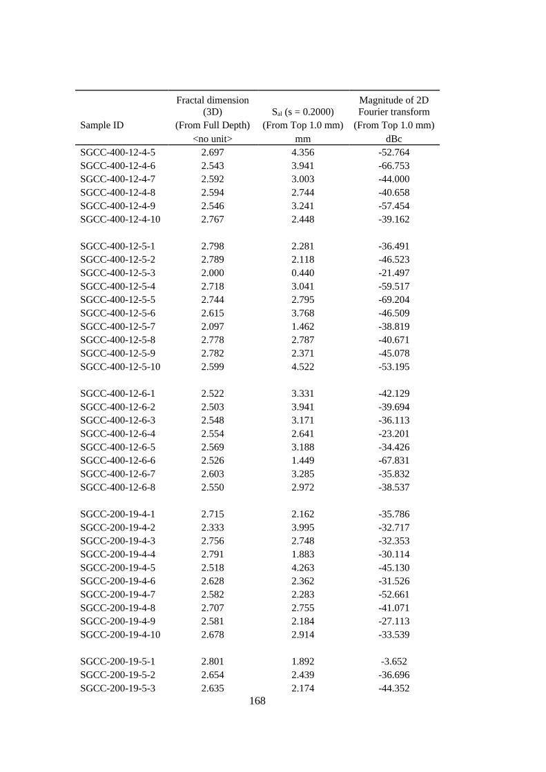
168

Fractal dimension

(3D) Sal (s = 0.2000)

Magnitude of 2D

Fourier transform


<no unit> mm dBc

SGCC-400-12-4-5 2.697 4.356 -52.764

SGCC-400-12-4-6 2.543 3.941 -66.753

SGCC-400-12-4-7 2.592 3.003 -44.000

SGCC-400-12-4-8 2.594 2.744 -40.658

SGCC-400-12-4-9 2.546 3.241 -57.454

SGCC-400-12-4-10 2.767 2.448 -39.162

SGCC-400-12-5-1 2.798 2.281 -36.491

SGCC-400-12-5-2 2.789 2.118 -46.523

SGCC-400-12-5-3 2.000 0.440 -21.497

SGCC-400-12-5-4 2.718 3.041 -59.517

SGCC-400-12-5-5 2.744 2.795 -69.204

SGCC-400-12-5-6 2.615 3.768 -46.509

SGCC-400-12-5-7 2.097 1.462 -38.819

SGCC-400-12-5-8 2.778 2.787 -40.671

SGCC-400-12-5-9 2.782 2.371 -45.078

SGCC-400-12-5-10 2.599 4.522 -53.195

SGCC-400-12-6-1 2.522 3.331 -42.129

SGCC-400-12-6-2 2.503 3.941 -39.694

SGCC-400-12-6-3 2.548 3.171 -36.113

SGCC-400-12-6-4 2.554 2.641 -23.201

SGCC-400-12-6-5 2.569 3.188 -34.426

SGCC-400-12-6-6 2.526 1.449 -67.831

SGCC-400-12-6-7 2.603 3.285 -35.832

SGCC-400-12-6-8 2.550 2.972 -38.537

SGCC-200-19-4-1 2.715 2.162 -35.786

SGCC-200-19-4-2 2.333 3.995 -32.717

SGCC-200-19-4-3 2.756 2.748 -32.353

SGCC-200-19-4-4 2.791 1.883 -30.114

SGCC-200-19-4-5 2.518 4.263 -45.130

SGCC-200-19-4-6 2.628 2.362 -31.526

SGCC-200-19-4-7 2.582 2.283 -52.661

SGCC-200-19-4-8 2.707 2.755 -41.071

SGCC-200-19-4-9 2.581 2.184 -27.113

SGCC-200-19-4-10 2.678 2.914 -33.539

SGCC-200-19-5-1 2.801 1.892 -3.652

SGCC-200-19-5-2 2.654 2.439 -36.696

SGCC-200-19-5-3 2.635 2.174 -44.352

169

Fractal dimension

(3D) Sal (s = 0.2000)

Magnitude of 2D

Fourier transform


<no unit> mm dBc

SGCC-200-19-5-4 2.656 1.878 -37.043

SGCC-200-19-5-5 2.720 2.389 -45.051

SGCC-200-19-5-6 2.771 1.915 -32.673

SGCC-200-19-5-7 2.790 1.948 -22.820

SGCC-200-19-5-8 2.636 2.143 -25.370

SGCC-200-19-5-9 2.604 2.414 -41.373

SGCC-200-19-5-10 2.640 1.919 -45.849

SGCC-200-19-6-1 2.604 1.576 -21.825

SGCC-200-19-6-2 2.732 1.677 -37.119

SGCC-200-19-6-3 2.124 2.632 -47.465

SGCC-200-19-6-4 2.542 3.822 -34.491

SGCC-200-19-6-5 2.804 1.841 -45.523

SGCC-200-19-6-6 2.776 2.239 -49.079

SGCC-200-19-6-7 2.760 2.149 -31.149

SGCC-200-19-6-8 2.588 1.732 -24.865

SGCC-200-19-6-9 2.602 1.708 -26.446

SGCC-200-19-6-10 2.581 1.956 -25.011

SGCC-400-19-4-1 2.684 4.176 -61.983

SGCC-400-19-4-2 2.533 3.851 -49.666

SGCC-400-19-4-3 2.566 3.141 -28.771

SGCC-400-19-4-4 2.754 2.307 -39.344

SGCC-400-19-4-5 2.725 3.713 -39.366

SGCC-400-19-4-6 2.539 2.756 -21.719

SGCC-400-19-4-7 2.757 2.542 -59.443

SGCC-400-19-4-8 2.684 3.794 -35.336

SGCC-400-19-5-1 2.585 2.346 -60.977

SGCC-400-19-5-2 2.560 4.115 -31.013

SGCC-400-19-5-3 2.734 3.941 -30.761

SGCC-400-19-5-4 2.768 2.736 -58.018

SGCC-400-19-5-5 2.764 3.275 -57.377

SGCC-400-19-5-6 2.724 4.094 -56.726

SGCC-400-19-5-7 2.588 3.049 -56.796

SGCC-400-19-5-8 2.594 2.598 -39.644

SGCC-400-19-5-9 2.602 3.052 -27.771

SGCC-400-19-5-10 2.730 3.615 -43.017

SGCC-400-19-6-1 2.697 1.508 -59.540

SGCC-400-19-6-2 2.575 1.878 -48.536

170

Fractal dimension

(3D) Sal (s = 0.2000)

Magnitude of 2D

Fourier transform


<no unit> mm dBc

SGCC-400-19-6-3 2.621 1.612 -49.485

SGCC-400-19-6-4 2.585 1.962 -52.428

SGCC-400-19-6-5 2.640 2.267 -18.680

SGCC-400-19-6-6 2.576 1.487 -52.661

SGCC-400-19-6-7 2.597 2.043 -33.792

SGCC-400-19-6-8 2.709 1.249 -53.170

SGC-HMA-L-12-1 2.722 0.634 -35.478

SGC-HMA-L-12-2 2.740 0.538 -26.099

SGC-HMA-L-12-3 2.780 1.061 -25.529

SGC-HMA-L-12-4 2.565 0.518 -43.048

SGC-HMA-L-12-5 2.810 1.368 -44.375

SGC-HMA-L-12-6 2.401 0.375 -34.858

SGC-HMA-L-19-1 2.491 2.389 -33.021

SGC-HMA-L-19-2 2.356 1.319 -16.402

SGC-HMA-L-19-3 2.397 2.247 -18.190

SGC-HMA-L-19-4 2.417 0.574 -9.451

SGC-HMA-L-19-5 2.518 1.730 -20.500

RCC-200-12-1 2.553 3.151 -68.874

RCC-200-12-2 2.551 3.678 -73.145

RCC-200-12-3 2.539 3.914 -64.731

RCC-200-12-4 2.538 3.860 -79.306

RCC-200-12-5 2.529 4.060 -59.779

RCC-200-12-6 2.505 3.843 -72.937

RCC-200-12-7 2.659 2.839 -79.907

RCC-200-12-8 2.547 5.274 -74.939

RCC-200-12-9 2.540 2.760 -64.056

RCC-300-12-1 2.443 4.007 -58.800

RCC-300-12-2 2.398 6.302 -68.163

RCC-300-12-3 2.661 7.434 -82.255

RCC-300-12-4 2.544 3.822 -73.401

RCC-300-12-5 2.532 5.908 -70.226

RCC-300-12-6 2.555 3.079 -64.834

RCC-300-12-7 2.530 3.874 -65.224

RCC-300-12-8 2.515 6.190 -73.806

RCC-300-12-9 2.487 6.895 -82.049

RCC-400-12-1 2.521 3.524 -68.541

171

Fractal dimension

(3D) Sal (s = 0.2000)

Magnitude of 2D

Fourier transform


<no unit> mm dBc

RCC-400-12-2 2.521 3.332 -73.895

RCC-400-12-3 2.413 3.381 -83.797

RCC-400-12-4 2.408 3.397 -65.768

RCC-400-12-5 2.401 3.573 -80.435

RCC-400-12-6 2.378 3.232 -60.074

RCC-400-12-7 2.459 5.583 -74.460

RCC-400-12-8 2.498 3.874 -86.861

RCC-400-12-9 2.539 3.008 -73.920

RCC-400-12-10 2.533 3.048 -68.740

RCC-200-19-1 2.531 2.854 -62.491

RCC-200-19-2 2.563 2.771 -67.089

RCC-200-19-3 2.538 3.322 -69.820

RCC-200-19-4 2.477 5.201 -76.846

RCC-200-19-5 2.548 3.429 -74.054

RCC-200-19-6 2.535 3.052 -76.947

RCC-200-19-7 2.614 4.221 -60.557

RCC-200-19-8 2.482 3.117 -74.370

RCC-200-19-9 2.472 3.862 -79.753

RCC-300-19-1 2.354 1.966 -79.746

RCC-300-19-2 2.413 4.502 -74.300

RCC-300-19-3 2.447 5.162 -66.004

RCC-300-19-4 2.398 4.240 -72.928

RCC-300-19-5 2.464 6.462 -88.344

RCC-300-19-6 2.000 2.101 -45.421

RCC-300-19-7 2.376 6.728 -70.590

RCC-300-19-8 2.473 7.274 -69.379

RCC-400-19-1 2.425 3.378 -73.492

RCC-400-19-2 2.655 3.637 -75.575

RCC-400-19-3 2.407 4.372 -62.609

RCC-400-19-4 2.521 4.227 -66.467

RCC-400-19-5 2.511 3.200 -67.435

RCC-400-19-6 2.367 4.005 -78.095

RC-HMA-L-12-1 2.708 0.390 -49.360

RC-HMA-L-12-2 2.717 0.492 -57.455

RC-HMA-L-12-3 2.795 1.169 -54.191

RC-HMA-L-12-4 2.784 0.798 -38.045

RC-HMA-L-12-5 2.749 1.580 -55.304

172

Fractal dimension

(3D) Sal (s = 0.2000)

Magnitude of 2D

Fourier transform


<no unit> mm dBc

RC-HMA-L-12-6 2.752 0.845 -52.657

RC-HMA-L-12-7 2.394 0.720 -59.132

RC-HMA-L-12-8 2.639 0.797 -52.550

RC-HMA-L-12-9 2.686 0.701 -56.775

RC-HMA-L-12-10 2.657 0.471 -56.631

RC-HMA-L-12-11 2.597 0.520 -46.412

RC-HMA-L-19-1 2.479 0.600 -40.258

RC-HMA-L-19-2 2.223 1.197 -51.227

RC-HMA-L-19-3 2.507 0.471 -38.631

RC-HMA-L-19-4 2.552 0.924 -49.992

RC-HMA-L-19-5 2.664 0.818 -63.224

RC-HMA-L-19-6 2.592 0.627 -47.946

RC-HMA-L-19-7 2.570 0.522 -53.538

RC-HMA-L-19-8 2.544 0.654 -45.561

173

CURRICULUM VITAE

PERSONAL INFORMATION

Surname, Name: Mahyar, Mahdi

Date and Place of Birth: 2 March 1982, Tabriz

EDUCATION

Degree Institution Year of

Graduation

MS METU Civil Engineering, Turkey 2012

BS IAU Civil Engineering, Iran 2005

High School Abouzar High School, Tabriz 1999

FOREIGN LANGUAGES

Advanced English, Fluent Turkish, Persian and Azerbaijani

PUBLICATIONS

1. Mahyar, M., Erdoğan, S.T., Tokyay, M. Extension of the chemical index

model for estimating Alkali-Silica reaction mitigation efficiency to slags

and natural pozzolans, (2018) Construction and Building Materials, 179,

pp. 587-597.

2. Mahyar, M., Uçal, G.O., Tokyay, M. Hydration of alinite cement

produced from soda waste sludge, (2018) Construction and Building

Materials, 164, pp. 178-184.

3. Mahyar, M., Uçal, G.O., Tokyay, M., Yaman, I.Ö. Low-energy alinite

cement from soda sludge waste, (2017) American Concrete Institute, ACI

Special Publication, 2017-January (SP 320), pp. 24-31.

4. Mahyar, M., Şahin, M., Erdoğan, S.T. Mutual activation of blast furnace

slag and a high-calcium fly ash rich in free lime and sulfates, (2016)

Construction and Building Materials, 126, pp. 466-475.

5. Mahyar, M., Erdoğan, S.T. Phosphate-activated high-calcium fly ash acid-

base cements, (2015) Cement and Concrete Composites, 63, pp. 96-103.

texture characterization of roller compacted concrete

Documents

Transcript of texture characterization of roller compacted concrete