Optimal Reduced Sets for Sparse Kernel Spectral

Clustering

Raghvendra Mall

ESAT/SCD

Kasteelpark Arenberg 10, bus 2446

3001 Heverlee

Email: rmall@esat.kuleuven.be

Siamak Mehrkanoon

and Rocco Langone

ESAT/SCD

Kasteelpark Arenberg 10, bus 2446

3001 Heverlee

Johan A.K. Suykens

ESAT/SCD

Kasteelpark Arenberg 10, bus 2446

3001 Heverlee

Email: johan.suykens@esat.kuleuven.be

Abstract—Kernel spectral clustering (KSC) solves a weightedkernel principal component analysis problem in a primal-dualoptimization framework. It results in a clustering model usingthe dual solution of the problem. It has a powerful out-of-sampleextension property leading to good clustering generalization w.r.t.the unseen data points. The out-of-sample extension propertyallows to build a sparse model on a small training set andintroduces the first level of sparsity. The clustering dual model isexpressed in terms of non-sparse kernel expansions where everypoint in the training set contributes. The goal is to find reducedset of training points which can best approximate the originalsolution. In this paper a second level of sparsity is introducedin order to reduce the time complexity of the computationallyexpensive out-of-sample extension. In this paper we investigatevarious penalty based reduced set techniques including the GroupLasso, L0, L1 + L0 penalization and compare the amount ofsparsity gained w.r.t. a previous L1 penalization technique. Weobserve that the optimal results in terms of sparsity correspondsto the Group Lasso penalization technique in majority of thecases. We showcase the effectiveness of the proposed approacheson several real world datasets and an image segmentation dataset.

I. INTRODUCTION

Clustering algorithms are widely used tools in fields likedata mining, machine learning, graph compression and manyother tasks. The aim of clustering is to divide data into naturalgroups present in a given dataset. Clusters are defined suchthat the data present within the group are more similar toeach other in comparison to the data between clusters. Spectralclustering methods [1], [2] and [3] are generally better thanthe traditional k-means techniques. A new Kernel SpectralClustering (KSC) algorithm based on weighted kernel PCAformulation was proposed in [4]. The method was based ona model built in a primal-dual optimization framework. Themodel had a powerful out-of-sample extension property whichallows to infer cluster affiliation for unseen data. The KSCmethodology has been extensively applied for task of dataclustering [4], [5], [6], [7] and community detection [8], [9],[10] in large scale networks.

The data points are projected to the eigenspace and theprojections are expressed in terms of non-sparse kernel expan-sions. In [5], a method to sparsify the clustering model wasproposed by exploiting the line structure of the projectionswhen the clusters are well formed and well separated. How-ever, the method fails when the clusters are overlapping and

for real world datasets where the projections in the eigenspacedo not follow a line structure as mentioned in [6]. In [6], theauthors used an L2 + L1 penalization to produce a reducedset to approximate the original solution vector. Although theauthors propose it as an L2 + L1 penalization technique, theactual penalty on the weight vectors is L1 penalty and the lossfunction is squared loss function and hence the name. There-fore in this paper we refer to the previous proposed approachas L1 penalization technique. It is well known that the L1

regularization introduces sparsity as shown in [11]. However,the resulting reduced set is neither the sparsest nor the mostoptimal w.r.t. the quality of clustering for the entire dataset. Inthis paper we propose alternative penalization techniques likeGroup Lasso [12] and [13], L0 and L1+L0 penalizations. TheGroup Lasso penalty is ideal for clusters as it results in groupsof relevant data points. The L0 regularization calculates thenumber of non-zero terms in the vector. The L0-norm results ina non-convex and NP-hard optimization problem. We modifythe convex relaxation of L0-norm based iterative sparsificationprocedure introduced in [14] for classification. We apply itto obtain the optimal reduced sets for sparse kernel spectralclustering.

The main advantage of these sparse reductions is that itresults in much simpler and faster predictive models. It allowsto reduce the time complexity for the computationally expen-sive out-of-sample extensions and also reduces the memoryrequirements for building the test kernel matrix.

II. KERNEL SPECTRAL CLUSTERING

We first provide a brief description of the kernel spectralclustering methodology according to [4].

A. Primal-Dual Weighted Kernel PCA framework

Given a dataset D = xiNtr

i=1, xi ∈ Rd, the training points

are selected by maximizing the quadratic Renyi criterion asdepicted in [6], [15] and [18]. This introduces the first levelof sparsity by building the model on a subset of the dataset.Here xi represents the ith training data point and the trainingset is represented by Xtr. The number of data points in thetraining set is Ntr. Given D and the number of clusters k, theprimal problem of the spectral clustering via weighted kernel

PCA is formulated as follows [4]:

minw(l),e(l),bl

1

2

k−1∑

l=1

w(l)⊺

w(l) − 1

2Ntr

k−1∑

l=1

γle(l)⊺

D−1Ω e(l)

such that e(l) = Φw(l) + bl1Ntr, l = 1, . . . , k − 1,

(1)

where e(l) = [e(l)1 , . . . , e

(l)Ntr

]⊺ are the projections onto theeigenspace, l = 1, . . . , k−1 indicates the number of score vari-ables required to encode the k clusters, D−1

Ω ∈ RNtr×Ntr is the

inverse of the degree matrix associated to the kernel matrix Ω.Φ is the Ntr ×nh feature matrix, Φ = [φ(x1)

⊺; . . . ;φ(xNtr)⊺]

and γl ∈ R+ are the regularization constants. We note that

Ntr ≪ N i.e. the number of points in the training set ismuch less than the total number of data points in the dataset.The kernel matrix Ω is obtained by calculating the similaritybetween each pair of data points in the training set. Eachelement of Ω, denoted as Ωij = K(xi, xj) = φ(xi)

⊺φ(xj) isobtained for example by using the radial basis function (RBF)kernel. The clustering model is then represented by:

e(l)i = w(l)⊺

φ(xi) + bl, i = 1, . . . , Ntr, (2)

where φ : Rd → R

nh is the mapping to a high-dimensionalfeature space nh, bl are the bias terms, l = 1, . . . , k − 1.

The projections e(l)i represent the latent variables of a set of

k − 1 binary cluster indicators given by sign(e(l)i ) which can

be combined with the final groups using an encoding/decodingscheme. The decoding consists of comparing the binarizedprojections w.r.t. codewords in the codebook and assigningcluster membership based on minimal Hamming distance. Thedual problem corresponding to this primal formulation is:

D−1Ω MDΩα(l) = λlα

(l), (3)

where MD is the centering matrix which is defined as MD =

INtr− (

(1Ntr1⊺

NtrD

−1Ω

)

1⊺

NtrD

−1Ω

1Ntr

). The α(l) are the dual variables and

the positive definite kernel function K : Rd × R

d → R playsthe role of similarity function. This dual problem is closelyrelated to the random walk model as shown in [4].

B. Out-of-Sample Extensions Model

The projections e(l) define the cluster indicators for thetraining data. In the case of an unseen data point x, thepredictive model becomes:

e(l)(x) =

Ntr∑

i=1

α(l)i K(x, xi) + bl. (4)

This out-of-sample extension property allows kernel spectralclustering to be formulated in a learning framework withtraining, validation and test stages for better generalization.The validation stage is used to obtain the model parameterslike the kernel parameter (σ for RBF kernel) and the numberof clusters k in the dataset. The data points corresponding tothe validation set are also selected by maximizing the quadraticRenyi entropy criterion.

C. Model Selection

The original KSC formulation in [4] works well assumingpiece-wise constant eigenvectors and using the line structureof the projections of the validation points in the eigenspace.It uses an evaluation criterion called Balanced Line Fit (BLF)for model selection i.e. for selection of k and σ for the RBFfunction. However, this criterion works well only in case ofwell separated clusters. So, we use the Balanced Angular Fit(BAF) criterion proposed in [8] and [7] for cluster evaluation.This criterion works on the principle of angular similarityand is efficient when the clusters are either well separated oroverlapping. The BAF criterion varies from [-1, 1] and highervalues are better for a given value of k.

III. SPARSE REDUCTIONS TO KSC MODEL

A. Related Work

In classical spectral clustering one needs to store the N×Nmatrix where N is the total number of points in the dataset.One then has to perform an eigen-decomposition of this matrix.The time complexity of this eigen-decomposition is O(N3).In the case of KSC we can build the training model using atraining set (Ntr ≪ N ) and use the out-of-sample extensionproperty to predict the cluster affiliation for unseen data. Thisleads to the first level of sparsity. However, the projections ofthe data points in the eigenspace are expressed in terms of non-sparse kernel expansions as reflected in (4). This non-sparsity

is a result of the KKT condition: w(l) =∑Ntr

i=1 α(l)i φ(xi).

Here w(l) represents the optimal representation of the primalweight vectors and comprises of linear combination of themapped training data points in the feature space. When usinga universal kernel like the RBF kernel the feature spacecomprises infinite dimensions. Thus, we first create an explicitfeature map using the Nystrom approximation as in [16] and[17]. This explicit feature map is created using the trainingpoints Xtr and the feature mapping becomes: φ : R

d → RNtr .

The objective is to find a reduced set of training pointsRS = xiR

i=1 such that it approximates w(l) by a new

weight vector w(l) =∑R

i=1 β(l)i φ(xi) while minimizing the

reconstruction error ||w(l) − w(l)||22 where xi is the ith pointin the reduced set RS whose cardinality is R. In [5], it wasshown by the authors that if the reduced set RS is knownthen the β(l) co-efficients can be obtained by solving the linearsystem:

Ωψψβ(l) = Ωψφα(l), (5)

where Ωψψmn = K(xm, xn), Ωψφ

mi = K(xm, xi), m,n =1, . . . , R, i = 1, . . . , Ntr and l = 1, . . . , k − 1.

In the past literature including the works in [5] and [6], itwas shown that this reduced set can be built by selecting pointswhose projections in the eigenspace occupy certain positions orby using an L1 penalization. The first method works only whenthe clusters are well formed and well separated and cannot begeneralized to real world datasets. The second method usingL1 penalization cannot introduce significant sparsity. In thispaper, we investigate other penalization techniques includingthe Group Lasso [12] and [13], L0 and L1 +L0 penalizations.

B. Group Lasso Penalization

The Group Lasso was first proposed for regression in [12]where it solves the convex optimization problem:

minβ∈Rp

‖y −L∑

l=1

Xlβl‖22 + λ

L∑

l=1

√ρl‖βl‖2,

where the√

ρl accounts for the varying group sizes, ‖ ¦ ‖2 isthe Euclidean norm. This procedure acts like Lasso [11] ata group level: depending on λ, an entire group of predictorsmay drop out of the model. We now utilize this to obtain theformulation for our optimization problem as:

minβ∈RNtr×(k−1)

‖Φ⊺α − Φ⊺β‖22 + λ

Ntr∑

l=1

√ρl‖βl‖2, (6)

where Φ = [φ(x1), . . . , φ(xNtr)], α = [α(1), . . . , α(k−1)], α ∈

RNtr×(k−1) and β = [β1, . . . , βNtr

], β ∈ RNtr×(k−1) . Here

α(i) ∈ RNtr while βj ∈ R

k−1 and we set√

ρl as the fraction of

training points belonging to the cluster to which the lth trainingpoint belongs. By varying the value of λ we control the amountof sparsity introduced in the model as it acts as a regularizationparameter. In [13], the authors show that if the initial solutions

are β1, β2, . . . , βNtrthen if ‖X⊺

l (y − ∑i6=l Xiβi)‖ < λ, then

βl is zero otherwise it satisfies: βl = (X⊺

l Xl+λ/‖βl‖)−1X⊺

l rl

where rl = y − ∑i6=l Xiβi.

Analogous to this, the solution to the group lasso penal-ization for our problem can be defined as: ‖φ(xl)(Φ

⊺α −∑i6=l φ(xi)βi)‖ < λ then βl is zero otherwise it satisfies: βl =

(Φ⊺Φ + λ/‖βl‖)−1φ(xl)rl where rl = Φ⊺α − ∑i6=l φ(xi)βi.

The Group Lasso penalization technique can be solved by ablockwise co-ordinate descent procedure as shown in [12]. Thetime complexity of the approach is O(maxiter ∗ k2N2

tr) wheremaxiter is the maximum number of iterations specified for theco-ordinate descent procedure and k is the number of clustersobtained via KSC. From our experiments we observed that onan average 10 iterations suffice for convergence.

An important point to remember here is that βl ∈ Rk−1 and

is a vector. When this βl is zero it means that it is equivalent tozero vector or the corresponding lth training point is not partof the reduced set RS. In our experiments, we set the initial

value of β as βij = αij + N (0, 1) where N (0, 1) representsGaussian noise with mean 0 and standard deviation 1.

C. L0 Penalization

We modify the iterative sparsification procedure for classi-fication as shown in [14] and use it for obtaining the reducedset. The optimization problem (J ) which is solved iterativelyis formulated as:

minβ∈RNtr×(k−1)

‖Φ⊺α − Φ⊺β‖22 + ρ

Ntr∑

i=1

ǫi + ‖Λ.β‖22

such that ‖βi‖22 ≤ ǫi, i = 1, . . . , Ntr

ǫi ≥ 0,

(7)

where Λ is matrix of the same size as the β matrix i.e.Λ ∈ R

Ntr×(k−1). The term ‖Λ.β‖22 along with the constraint

‖βi‖22 ≤ ǫi corresponds to the L0-norm penalty on β matrix.

Λ matrix is initially defined as a matrix of ones so that itgives equal chance to each element of β matrix to reduceto zero. The constraints on the optimization problem forceseach element of βi ∈ R

(k−1) to reduce to zero. This helpsto overcome the problem of sparsity per component whichis explained in [6]. The ρ variable is a regularizer whichcontrols the amount of sparsity that is introduced by solvingthis optimization problem.

The optimization problem stated in (6) is a convex Quadrat-ically Constrained Quadratic Programming (QCQP) problem.Its computational complexity is O(k3N3

tr) and we solve it iter-atively using the CVX software:[20]. We obtain a β matrix as asolution for each iteration such that βt+1

ij = arg minβJ (Λtij).

For each iteration, the Λ matrix is re-weighted as: Λtij = 1

βtij

,

∀ i = 1, . . . , Ntr, j = 1, . . . , k − 1. It was shown in [14] thatthis iterative procedure results in a convex approximation tothe L0-norm. But as the L0-norm is a non-convex problem itresults in a local minimum. We stop this iterative procedurewhen the rate of change of the β matrix is below a thresholdsuch that ‖βt+1 − βt‖2

2/Ntr < 10−4. We then select thoseindices i for which ‖βt+1

i ‖22 > 10−6 and put the corresponding

training points in the reduced set RS. In our experiments weobserve that the number of iterations required to reach thisconvergence is usually less than 20.

D. L1 + L0 Penalization

The L1 + L0 penalization formulation is quite similar tothe formulation of L1 penalization as defined in [6]. We addan additional regularization matrix Λ on the β matrix and theproblem formulation becomes:

minβ∈RNtr×(k−1)

‖Φ⊺α − Φ⊺β‖22 + ρ

Ntr∑

i=1

ǫi + ‖Λ.β‖22

such that |βi| ≤ ǫi, i = 1, . . . , Ntr

ǫi ≥ 0,

(8)

The difference between (7) and (8) is the set of constraints forboth the optimization problems. In (8) the constraint |βi| ≤ ǫi

corresponds to the L1 penalization.

This problem formulation results in a convex QuadraticProgramming (QP) problem due to linear constraints. Its com-putational complexity is O(k3N3

tr). It is also solved iterativelyusing the CVX software. We initialize Λ matrix as ones andafter each iteration we modify each element of Λt matrix suchthat Λt

ij = 1βt

ij

, ∀ i = 1, . . . , Ntr, j = 1, . . . , k − 1. We show

in the experimental results that this penalization often resultssimilarly to the L1 penalization outcomes. This suggests thatthe L1 penalization is driving the amount of sparsity in thispenalization to obtain the reduced set RS.

E. Choice of Tuning parameter

The choice of the right tuning parameter is essential toobtain optimal reduced set. The tuning parameter λ influencesthe amount of sparsity in the model for the Group Lassopenalization technique while in case of other penalizationtechniques this is handled by the tuning parameter ρ. Sparsityis defined as 1 − |RS|

Ntr.

The procedure for selection of this tuning parameter is quitesimple. For Group Lasso penalization technique, we obtainthe λmax initially which is defined as: argmax‖φ(xl)(Φ

⊺α −∑i6=l φ(xi)βi)‖, ∀ l = 1, . . . , Ntr. In order to tune the value

of the regularizer λ for varying the amount of sparsity for thereduced set RS, we use different fractional values of λmax

as λ. The values of λ are set such that the value of sparsitycovers the entire range [0, 1] i.e. we vary the value of λ suchthat there is no sparsity (sparsity= 0) in the model to the casewhen there is no data point in the reduced set RS (sparsity= 1).

For the L1, L0 and L1 + L0 penalization techniques wehave to tune the parameter ρ. To have a fair comparison weuse the same range and same values for tuning parameter ρ incase of these techniques. However, the best results for differentpenalization techniques can occur for different value of tuningparameter ρ. The choice of ρ is again dependent on the amountof sparsity it generates. We aim to select the smallest rangeof values for ρ such that the value of sparsity covers theentire range [0, 1]. From our experiments, we observe that thesmallest possible range for ρ corresponding to which sparsityvaries from [0, 1] is [1, 10]. Thus, we vary the value of ρin logarithmic steps between the range [1, 10] to obtain theoptimal reduced sets.

F. Out-of-Sample Extension Time Complexity

For the KSC method [4] we consider the entire datasetas the test set. The cardinality of the entire dataset is N . Thecomputational complexity for the out-of-sample predictions forKSC method is O(NtrN) where Ntr ≪ N . This is becausefor the out-of-sample extension we need to create the testkernel matrix of size Ntr ×N . When this kernel matrix is toolarge to be stored in memory then we divide the test data intochunks such that each chunk can fit in memory. Test clustermembership prediction is then done for each chunk.

For the reduced set based methods we can greatly reducethe computational cost for out-of-sample extensions. Let thecardinality of the reduced set corresponding to the GroupLasso, L0 and L1+L0 penalization methods be R1, R2, R3 re-spectively. Since these methods introduce sparsity, the amountof sparsity introduced corresponding to these penalizationmethods can be defined as: R1/Ntr, R2/Ntr and R3/Ntr

respectively. The cardinality of the reduced set RS is muchlesser than the size of the training set i.e. Ri ≪ Ntr,i = 1, 2, 3. Thus the time complexity for the out-of-sampleextension corresponding to the three proposed reduced sets isO(RiN), i = 1, 2, 3. This also reduces the constraint on thememory as the size of the test kernel matrix for the reducedsets becomes Ri ×N , i = 1, 2, 3 which is much less than thesize of the original test kernel matrix (Ntr × N ).

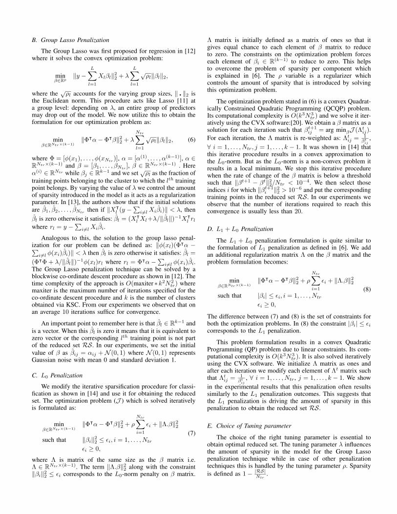
G. Synthetic Example

We show the results of an experiment on a syntheticdataset using RBF kernel in Figure 1. The dataset consistsof 3 overlapping Gaussian clouds in 2-dimensions for a totalnumber of 1, 500 data points. We select 450 data points fortraining and 600 data points for validation using the quadraticRenyi entropy criterion.

Figure 1 shows the results on this synthetic dataset cor-responding to Group Lasso, L0, L1, L1+L0 penalizations.We vary the regularization parameter λ for Group Lassoand ρ for the other penalization methods. In Figures 1b, 1d,1f and 1h, the ‘o’-shaped, red-bodied black-outlined pointscorrespond to the reduced set. In these Figures the trainingset is constant but the reduced set changes in accordance tothe penalization technique. Since the dataset is synthetic, thegroundtruth is known beforehand, the quality of the clustersare evaluated using an external quality metric - Adjusted RandIndex (ARI) as defined in [21]. The ARI metric compares thecluster memberships obtained using the reduced set w.r.t. thegroundtruth of the test points and higher value of ARI signifiesbetter match between the cluster memberships.

From Figures 1b, 1c and 1j, we observe that the best resultfor Group Lasso penalization occurs when the regularizationparameter λ = 0.8λmax. It introduces maximal amount ofsparsity (sparsity = 0.9933, cardinality of reduced set is 4)while obtaining the best generalization (ARI = 0.56). The bestresult for L0 penalization technique takes place for ρ = 10and produces a sparse reduced set (sparsity = 0.9911). But thegeneralization (ARI = 0.478) is not as good as Group Lasso.This can be observed from Figures 1d, 1e and 1k.

The L1 and L1 + L0 penalization techniques producethe same generalization and sparsity for several values ofregularizer ρ as depicted in Figures 1k and 1l. Figure 1lindicates that as we increase the value of ρ the amount ofsparsity increases. However, when we increase the value ofρ from 8 to 10, then the quality of the clusters decreaseas observed from Figure 1k. The best result for the L1 andL1 +L0 penalization techniques (sparsity = 0.93, ARI = 0.44)is worse than Group Lasso and L0 penalization technique bothin terms of quality (ARI) and amount of sparsity introduced.

IV. EXPERIMENTS ON REAL WORLD DATASETS

A. Experimental Setup

We conducted experiments on several real world datasetswhich are available at [22]. We provide a brief descriptionof these datasets in Table I. Since the cluster membershipsof these datasets are not known beforehand, we use internalclustering quality metrics for evaluation of the resulting clus-ters. These internal quality metrics include the widely usedsilhouette (sil) index and the Davies Bouldin (db) index asdescribed in [21]. Larger the values of sil better the clusteringquality and lower the value of db better the clustering quality.

Dataset Points Dimensions Clusters

Breast 699 9 2

Bridge 4096 16 -

Europe 169308 2 -

Glass 214 9 7

Iris 150 4 3

Mopsi Location Finland 13467 2 -

Mopsi Location Joensuu 6014 2 -

Thyroid 215 5 2

Wdbc 569 32 2

Wine 178 13 3

Yeast 1484 8 10

TABLE I: Real world datasets. Here ‘-’ means the number ofclusters are not known previously

(a) Synthetic Dataset (b) Best GroupLasso Penalization (c) Best GroupLasso Generalization

(d) Best L0 Penalization (e) Best L0 Generalization (f) Best L1 Penalization

(g) Best L1 Generalization (h) Best L1 + L0 Generalization (i) Best L1 + L0 Generalization

(j) Group Lasso Evaluation (k) ARI versus ρ (l) Sparsity versus ρ

Fig. 1: Results on Synthetic Dataset corresponding to the reduced sets obtained for different penalization techniques.

Group Lasso L0 Penalization L1 Penalization L1 + L0 Penalization

Dataset sil db Sparsity λ Time(secs) sil db Sparsity ρ Time(secs) sil db Sparsity ρ Time(secs) sil db Sparsity ρ Time(secs)

Breast 0.6824 0.85 99.5% 0.7λmax 0.99 0.68980.833 96.6% 7.74 19.5 0.6898 0.833 96.6% 7.74 6.7 0.6898 0.833 96.6% 7.74 20.1

Bridge 0.423 1.436 99.0% 0.7λmax 34.8 0.596 1.3 97.1% 4.642 701.0 0.559 1.72 98.5% 5.995 238.4 0.559 1.72 98.5% 5.995 702.4

Europe 0.437 2.1 99.9% 0.9λmax 4509 0.352 1.145 99.75% 10 210,512 0.352 1.148 99.7% 10 61,456 0.352 1.148 99.7% 10 220,456

Glass 0.33 3.133 14.0% 1.0λmax 0.12 0.32231.913 93.75% 2.155 2.42 0.408 1.813 96.9% 4.64 0.68 0.547 2.037 89.1% 3.593 2.64

Iris 0.611 1.333 93.33%0.9λmax 0.03 0.605 1.323 84.45% 2.78 1.02 0.61841.3063 86.67% 3.598 0.28 0.61841.3063 86.67% 3.598 1.03

Mopsi Location Finland 0.72191.2735 99.7% 0.6λmax 301.2 0.79761.142 99.6% 10 6,586 0.7946 1.158 99.5% 10 2,315 0.7946 1.158 99.5% 10 6,671

Mopsi Location Joensuu 0.911 0.64 99.5% 0.7λmax 80.2 0.88 0.67 96.5% 10 1,720 0.88140.6684 95.5% 10 612 0.88140.6684 95.5% 10 1,734

Thyroid 0.6345 0.844 98.4% 6λmax 0.13 0.538 1.04 93.75% 5.995 2.48 0.538 1.04 93.75% 5.995 0.7 0.538 1.04 93.75% 5.995 2.7

Wdbc 0.5585 1.304 96.5% 0.9λmax 0.78 0.56 1.303 97.6% 5.995 13.2 0.56 1.303 97.6% 5.995 4.11 0.56 1.303 97.6% 5.995 14.3

Wine 0.291 1.943 5.6% 1.0λmax 0.05 0.29 1.96 85.0% 1.668 1.28 0.29 1.96 86.8% 2.154 0.31 0.29 1.96 86.8% 2.154 1.3

Yeast 0.81 2.7 97.76% 0.9λmax 4.01 0.258 2.3 97.9% 7.74 79.1 0.2637 2.2 83.0% 10 25.2 0.2775 2.214 83.37% 10 82.32

TABLE II: Comparison of the sparsest feasible solution for the different penalization methods. Here we highlight the uniquebest results i.e. the best results are highlighted if they correspond to a single penalization method. In most of the cases the L1

and L1 + L0 penalization result in the same sparsest solution.

B. Experimental Results

Table II showcases the sparsest feasible solution for thedifferent penalization methods and evaluates it on quality

metrics like sil and db. We represent the amount of sparsityas percentage of sparsity rather than fractions (i.e. fraction ofsparsity ×100). By feasible solutions we refer to the caseswhen the cardinality of the reduced set |RS| > 0. Forhigher values of regularization parameters the cardinality ofthe reduced set can become zero and these solutions are notpart of the feasible solutions.

From Table II we observe that the Group Lasso penalizationintroduces the maximum amount of sparsity in general andin the obtained cases the cluster quality by correspondingreduced set is better than the other penalization methods. TheGroup Lasso penalization performs best for the Europe, MopsiLocation Joensuu (MLJ), Thyroid, Wine and Yeast datasets.We also observe that the proposed L0 penalization techniquegenerally results in sparser solution than the L1 penalizationmethod. In some cases it also results in better quality clusters,for example in the cases of Bridge, Europe and Mopsi LocationFinland (MLF) datasets. An important observation is that theresults corresponding to the proposed L1+L0 penalization arequite similar to the results of L1 penalization. This suggeststhat the L1 penalization dominates in each step of the iterativesparsification procedure for the L1 + L0 penalization method.

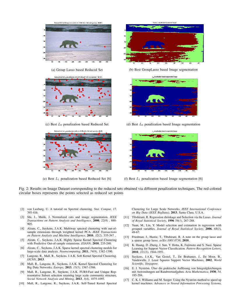
C. Real World Image Segmentation Dataset

We also perform an image segmentation experiment suchthat each pixel is transformed into a histogram and the χ2

distance is used in the RBF kernel with bandwidth σχ as shownin Figure 2. The total number of pixels is 154, 401 (321 ×481). The training set consists of Ntr = 7, 500 pixels andthe validation set consists of 10, 000 pixels. Both these setare selected by maximizing the quadratic Renyi entropy. Aftervalidation we obtain k = 3 and kernel parameter σχ = 2.807.We performed this experiment on a 2.4 GHz Core 2 Duo, 12Gb RAM machine using MATLAB 2012b.

The Group Lasso based penalization method reduces thereduced set to just two data points for λ = 0.7λmax and stillhas the best sil = 0.294 value as shown in Figure 2a. InKSC [4] there is a possibility of a null cluster i.e. the clusterwhich is beyond the generalization boundary of all the clusters.The Group Lasso penalization technique produces 2 points inthe reduced set, one corresponding to each cluster. The thirdcluster corresponds to the null cluster. Hence, it results in goodsegmentation as observed from Figure 2b.

The L0 penalization also results in a highly sparse model(sparsity = 0.9645) and has the smallest db = 0.141 value asobserved from Figure 2c.

The results corresponding to L1 and L1 + L0 penalizationtechniques are same for this image dataset. Thus, we onlyshow the result for L1 penalization technique in Figures 2eand 2f. The optimal value of the tuning parameter ρ for thesepenalization techniques was ρ = 10. From Figures 2d and2f, we observe that the best image segmentation results forthe L0 and L1 penalization technique is the same. However,the L0 penalization technique produces more sparsity (0.9645)than L1 penalization technique (0.948) to obtain the samesegmentation. We obtain good image segmentation in case ofboth the Group Lasso and the L0 penalization technique.

D. Discussion

We have used several penalization techniques to obtainoptimal reduced sets for kernel spectral clustering. We observethat the Group Lasso based penalization technique results inmaximum sparsity in many cases and is computationally themost efficient as shown in Table II. The Group Lasso basedpenalization technique is also ideal for clustering as it retainsgroups of relevant data points. The L0 penalization techniqueresults in sparser solution than L1 penalization technique ingeneral but at the expense of more computational time. Thisis because it iteratively solves a QCQP for each sparsificationstep whereas there is no such iterative procedure for L1

penalization technique. This can also be concluded from thecomputation time shown for the two methods in Table II.We also observe that as the size of the dataset increases theL0, L1 and L1 + L0 penalization based techniques becomeless feasible. This is because CVX is meant for smaller sizeoptimization problems and cannot handle very large scaleproblems efficiently.

V. CONCLUSION

We proposed several methods for obtaining sparse optimalreduced sets for kernel spectral clustering. The formulationis based on weighted kernel PCA for a specific choice ofweights. Several techniques like Group Lasso, L0, L1 + L0

penalization methods had been proposed to obtain the reducedset along with the modified weight vectors. The methodologieswere aimed to tackle different datasets in a computationallyand memory efficient way. We observed that the Group Lassoresulted in the sparsest models with good clustering qualityin least computation time followed by reduced models by theL0 penalization. The reduced models obtained by L1 + L0

penalization technique are quite similar to the reduced modelsobtained by a previous L1 penalization method.

ACKNOWLEDGMENTS

This work was supported by Research Council KUL:ERC AdG A-DATADRIVE-B, GOA/11/05 Ambiorics,GOA/10/09MaNet, CoE EF/05/006 Optimization inEngineering(OPTEC), IOF-SCORES4CHEM, severalPhD/postdoc and fellow grants; Flemish Government:FWO:PhD/postdoc grants, projects: G0226.06 (cooperativesystems & optimization), G0321.06 (Tensors), G.0302.07(SVM/Kernel), G.0320.08 (convex MPC), G.0558.08 (RobustMHE), G.0557.08 (Glycemia2), G.0588.09 (Brain-machine)G.0377. 12 (structured models) research communities(WOG:ICCoS, ANMMM, MLDM); G.0377.09 (MechatronicsMPC) IWT: PhD Grants, Eureka-Flite+, SBO LeCoPro,SBO Climaqs, SBO POM, O&O-Dsquare; Belgian FederalScience Policy Office: IUAP P6/04 ( DYSCO, Dynamicalsystems, control and optimization, 2007-2011); EU: ERNSI;FP7-HD-MPC (INFSO-ICT-223854), COST intelliCIS, FP7-EMBOCON (ICT-248940); Contract Research: AMINAL;Other:Helmholtz: viCERP, ACCM, Bauknecht, Hoerbiger.Johan Suykens is a professor at the KU Leuven, Belgium.

REFERENCES

[1] Ng, A.Y., Jordan, M.I., Weiss, Y. On spectral clustering: analysis andan algorithm, In proceedings of the Advances in Neural Information

Processing Systems; Dietterich, T.G., Becker, S., Ghahramani, Z.,editors, MIT Press: Cambridge, MA, 2002; pp. 849-856.

(a) Group Lasso based Reduced Set (b) Best GroupLasso based Image segmentation

(c) Best L0 penalization based Reduced Set (d) Best L0 penalization based Image segmentation

(e) Best L1 penalization based Reduced Set [6] (f) Best L1 penalization based Image segmentation [6]

Fig. 2: Results on Image Dataset corresponding to the reduced sets obtained via different penalization techniques. The red-coloredcircular boxes represents the points selected as reduced set points

[2] von Luxburg, U. A tutorial on Spectral clustering. Stat. Comput, 17,395-416.

[3] Shi, J., Malik, J. Normalized cuts and image segmentation. IEEE

Transactions on Pattern Analysis and Intelligence, 2000, 22(8) , 888-905.

[4] Alzate, C., Suykens, J.A.K. Multiway spectral clustering with out-of-sample extensions through weighted kernel PCA. IEEE Transactions

on Pattern Analysis and Machine Intelligence, 2010, 32(2), 335-347 .

[5] Alzate, C., Suykens, J.A.K. Highly Sparse Kernel Spectral Clusteringwith Predictive Out-of-sample extensions. ESANN, 2010, 235-240.

[6] Alzate, C., Suykens, J.A.K. Sparse kernel spectral clustering models forlarge-scale data analysis. Neurocomputing, 2011, 74(9), 1382-1390.

[7] Langone, R., Mall, R., Suykens, J.A.K. Soft Kernel Spectral Clustering.IJCNN, 2013.

[8] Mall, R., Langone, R., Suykens, J.A.K. Kernel Spectral Clustering forBig Data Networks, Entropy, 2013, 15(5), 1567-1586.

[9] Mall, R., Langone, R., Suykens, J.A.K. FURS:Fast and Unique Rep-resentative Subset selection retaining large scale community structure,Social Network Analysis and Mining, 2013, 3(4), 1075-1095.

[10] Mall, R., Langone, R., Suykens, J.A.K. Self-Tuned Kernel Spectral

Clustering for Large Scale Networks, IEEE International Conference

on Big Data (IEEE BigData), 2013, Santa Clara, U.S.A.

[11] Tibshirani, R. Regression shrinkage and Selection via the Lasso. Journalof Royal Statistical Society, 1996 58(1), 267-288.

[12] Yuan, M., Lin, Y. Model selection and estimation in regression withgrouped variables. Journal of Royal Statistical Society, 2006, 68(1),49-67.

[13] Friedman, J., Hastie, T., Tibshirani, R. A note on the group lasso anda sparse group lasso. arXiv:1001.0736, 2010.

[14] K. Huang, D. Zheng, J. Sun, Y. Hotta, K. Fujimoto and S. Naoi. SparseLearning for Support Vector Classification. Pattern Recognition Letters,2010, 31(13), 1944-1951.

[15] Suykens, J.A.K., Van Gestel, T., De Brabanter, J., De Moor, B.,Vandewalle, J. Least Squares Support Vector Machines, 2002, WorldScientific, Singapore.

[16] E. J. Nystrom. Uber die praktische Auflosung von Integralgleichungenmit Anwendungen auf Randwertaufgaben. Acta Mathematica, 1930, 54,185-204.

[17] C. K. I. Williams and M. Seeger. Using the Nystrom method to speed upkernel machines. Advances in Neural Information Processing Systems,

2001, 13, 682-688.

[18] Girolami, M. Orthogonal series density estimation and the kerneleigenvalue problem. Neural Computation, 2002, 14(3), 1000-1017.

[19] Kenney, J.F., Keeping, E.S. Linear Regression and Correlation. Chapter15 in Mathematics of Statistics, 3(1), 252-285.

[20] Grant, M., Boyd, S. CVX: Matlab software for disciplined convexprogramming. 2010, http://cvxr.com/cvx.

[21] Rabbany, R., Takaffoli, M., Fagnan, J., Zaiane, O.R., Campello R.J.G.B.Relative Validity Criteria for Community Mining Algorithms. 2012,International Conference on Advances in Social Networks Analysis and

Mining (ASONAM), 258-265.

[22] http://cs.joensuu.fi/sipu/datasets/