Discrimination of travel distances from ‘situated’ optic flow

Vision Research 43 (2003) 2173–2183

www.elsevier.com/locate/visres

Discrimination of travel distances from �situated� optic flow

Harald Frenz a, Frank Bremmer a,b, Markus Lappe a,c,*

a Allgemeine Zoologie und Neurobiologie, Ruhr-Universit€aat Bochum, D-44780 Bochum, Germanyb Fachbereich Physik, AG Neurophysik, Philipps-Universit€aat Marburg, 35032 Marburg, Germany

c Psychologisches Institut II, Westf€aalische Wilhelms-Universit€aat M€uunster, 48149 M€uunster, Germany

Received 24 December 2001; received in revised form 7 November 2002

Abstract

Effective navigation requires knowledge of the direction of motion and of the distance traveled. Humans can use visual motion

cues from optic flow to estimate direction of self-motion. Can they also estimate travel distance from visual motion?

Optic flow is ambiguous with regard to travel distance. But when the depth structure of the environment is known or can be

inferred, i.e., when the flow can be calibrated to the environmental situation, distance estimation may become possible. Previous

work had shown that humans can discriminate and reproduce travel distances of two visually simulated self-motions under the

assumption that the environmental situation and the depth structure of the scene is the same in both motions. Here we ask which

visual cues are used for distance estimation when this assumption is fulfilled. Observers discriminated distances of visually simulated

self-motions in four different environments with various depth cues. Discrimination was possible in all cases, even when motion

parallax was the only depth cue available. In further experiments we ask whether distance estimation is based directly on image

velocity or on an estimate of observer velocity derived from image velocity and the structure of the environment. By varying the

simulated height above ground, the visibility range, or the simulated gaze angle we modify visual information about the structure of

the environment and alter the image velocity distribution in the optic flow. Discrimination ability remained good. We conclude that

the judgment of travel distance is based on an estimate of observer speed within the simulated environment.

� 2003 Elsevier Ltd. All rights reserved.

Keywords: Visual motion; Optic flow; Navigation; Path integration

1. Introduction

Knowledge of travel distance is important for spatial

orientation and navigation. Classical cues to travel dis-

tance are translational vestibular signals (Berthoz, Is-

rael, Georges-Francois, Grasso, & Tsuzuku, 1995; Israel

& Berthoz, 1989), proprioception of walking movements

(Thomson, 1980), or other self-generated or ‘‘idiothetic’’

signals (Mittelstaedt & Mittelstaedt, 1973, 1980). Recent

studies in animals (Esch & Burns, 1995; Srinivasan,Zhang, & Bidwell, 1997) as well as in humans (Bremmer

& Lappe, 1999; Harris, Jenkin, & Zikovitz, 2000; Red-

lick, Jenkin, & Harris, 2001) have suggested that

self-induced visual motion signals can also be used to es-

timate travel distance. The optic flow experienced during

* Corresponding author. Address: Allgemeine Psychologie, Psycho-

logisches Institut II, Westf. Wilhelms-Universit€aat, Fliednerstrasse 21,

48149 Munster, Germany. Tel.: +49-251-83-34172; fax: +49-251-83-

34173.

E-mail address: [email protected] (M. Lappe).

0042-6989/03/$ - see front matter � 2003 Elsevier Ltd. All rights reserved.

doi:10.1016/S0042-6989(03)00337-7

self-motion carries much information that is useful for

different sub-tasks of visual navigation (Lappe, Brem-mer, & van den Berg, 1999). It can be used for the

perception of heading (Warren & Hannon, 1990) the

control of walking speed (Prokop, Schubert, & Berger,

1997), or the estimation of time to contact (Tresilian,

1999). Strictly speaking, however, optic flow does not

specify travel distance, because the image speeds in the

optic flow are mutually influenced by the speed of

the observer and the distances of the visible objects fromthe observer (Lee, 1974). For a forward moving observer

with speed V , the optical velocity h of an individual

environmental element at distance Z is

h ¼ V =Z:

Travel distance might be estimated by measuring ob-

server speed V and the duration of the movement. Butinferring observer speed V from the optic flow speed halone is impossible, as one also needs to know Z to solve

the above equation.

mail to: [email protected]

2174 H. Frenz et al. / Vision Research 43 (2003) 2173–2183

However, the respective travel distances of two suc-

cessively presented optic flow sequences can be discrim-

inated very accurately by human subjects when both

sequences simulate movement in the same environment

(Bremmer & Lappe, 1999). In this case, the distances Z of

the visible objects from the observer are the same in both

sequences. This allows observers to use optic flow speeds

h (or flow-based estimates of ego-speed V ) together withmovement duration to compare travel distances without

explicit knowledge of Z. Thus, when the two visually

simulated self-motions are from the same environmental

situation travel distances are not ambiguous. The �situ-ated� optic flow provides enough information to dis-

criminate travel distances. The initial part of the paper

describes the ability of human observers to generalize

travel distance across variations in flow speed andmovement duration provided by the same environment.

The main objective of the paper is to investigate how

the ability to estimate travel distance is affected by chan-

ges to the environment that lead to changes in the optic

flow speeds but do not change observer speed. In this case,

the relation of flow speeds to observer speed depends on

the environment. The task, then, involves a transfer of

information from one environment to another. There-fore, it requires a more general representation of travel

distance, i.e., a representation that cannot be based di-

rectly onflow speeds.We study four different variations of

the environment that affect the flow and the task in dif-

ferent ways. First, distances of objects in the environment

can be specified by a variety of cues.We use environments

that lack some of these cues but that always have the same

depth structure. In this case, the distribution of the flowspeeds is unchanged and the task can be completed as

described in the beginning, i.e., based directly on flow

speeds under the assumption that Z is always the same.

Second, we vary the height of the observer above the

ground. A change of height affects the flow speeds inde-

pendently fromobserver velocity. Thus, observers have to

register their height change and infer its consequences on

the flow field in order to make correct ego-speed anddistance judgments. Third, we vary the visibility range by

truncating the visible scene at a certain distance. This

removes slow flow speeds originating from distant objects

and modifies the distribution of flow speeds. Fourth, we

vary the viewing angle, and, respectively, the tilt of the

groundplane. This changes the distribution of flow speeds

presented on the screen. In all cases we find that observers

are able to compensate for these changes.

2. General methods

2.1. Apparatus

All stimuli were generated on a Silicon Graphics In-

digo2 workstation and back-projected on a 120� 120 cm

screen (Dataframe, type CINEPLEX) using a CRT

video projector (Electrohome ECP 4100) with a resolu-

tion of 1280� 1024 pixel. Vertical refresh rate of the

projector was locked to 72 Hz. The frame rate at which

new images were rendered was 36 Hz for textured stimuli

and 72 Hz for random dot stimuli. Subjects were seated in

front of the screen at a distance of 0.6 m. This resulted in

a 90� 90 deg field of view. Subjects were instructed tokeep the distance to the screen constant and their head

steady. Subjects viewed the stimuli binocularly.

2.2. Procedure

Each trial consisted of two visually simulated forward

movement sequences. The first sequence served as areference and was constant in velocity (2 m/s), duration

(2 s) and simulated height above the ground (2.6 m). The

second sequence varied in velocity and duration and in

experiment 2 also in height above ground. Ranges of

variation are given in the description of each experi-

ment. Usually reference and test motion of a single trial

were from within the same virtual environment. An

exception was experiment 1b in which different envi-ronments were used for reference and test in single trials.

The motion was always simulated with a rectangular

velocity profile, i.e., starting instantaneously with the

chosen velocity and terminating immediately after the

determined duration. Before the experiment the subject

was presented with an optical flow field (dot pattern)

without further information and asked about his or her

perception. All subjects reported that they perceived anego motion in the forward direction. Then the subject

was instructed that the task in the experiments was to

indicate which of two successively presented ego motion

simulations covered a greater distance. They signaled

their judgment by pressing the left mouse button if they

believed that the first ego motion simulation covered a

greater distance or the right mouse button if they be-

lieved that the second ego motion simulation covered agreater distance. Before and after each motion sequence

the environment was presented statically for 300 ms

to ensure that subjects perceived the whole motion se-

quence. After the second motion of each trial, the en-

vironment remained visible until the response of the

subject. Between the two simulations of each trial and

also between trials the screen turned black for 500 ms.

2.3. Data analysis

We determined subjective equivalence of travel dis-

tance as a function of speed ratio between the reference

and the test movement. For a given speed, the distance

of the second motion was varied by changing the du-ration of the simulation. The duration for which sub-

jects reached the point of subjective equivalence (PSE)

we estimated by an adaptive threshold estimation

H. Frenz et al. / Vision Research 43 (2003) 2173–2183 2175

procedure based on a maximum-likelihood method

(Harvey, 1986). Responses were used on-line to deter-

mine the most likely psychometric curve representing

the obtained answers. The 25% or the 75% point on the

psychometric curve was randomly chosen and presented

in the next trial. The range for the tested duration was

0.5–6 s in steps of 0.01 s with slopes between 1 and 130

in steps of 2. These ranges were based on prior tests. Theexperiment ended if a confidence interval of 95% was

reached or every condition was presented 10 times.

2.4. Participants

Ten subjects (21–29 years of age) participated in the

experiments, including the first author. All had normal

or corrected to normal vision.

2.5. Environments

2.5.1. Textured ground plane

A 8 m� 8 m texture pattern (Iris Performer type

‘‘gravel’’) was mapped on a 400 m� 400 m virtual

ground plane (Fig. 1(a)). Blue sky (rgb code: 0.1, 0.3,

0.7) was presented above the textured plane to make the

stimulus appear more realistic. The starting point for

each movement sequence was chosen at random on the

plane in order to avoid recognition of the placement of

individual texture elements in the successive movements.Mean luminance was 3.1 cd/m2. This textured ground

plane provided ample static depth cues, contained in

gradients of texture density and texture size towards the

horizon (Cutting, 1997). It also provided dynamic depth

cues in the motion sequence, most notably motion

Fig. 1. Screen shots of the four environments. (a) Textured ground plane; (b)

environments.

Table 1

Different depth cues contained in the four environments

Density gradient C

Textured ground plane + +

Dot plane 1 + )Dot plane 2 ) )Dot cloud ) )

A plus marks the presence of a cue, a minus its absence. ‘‘Density gradient’’ r

size’’ is the looming of objects as they approach the observer. ‘‘Motion paralla

observer. ‘‘Trajectories’’ means that objects can be tracked as they cross the

parallax and the change of size of texture elements as

they approach the observer. It is also conceivable that

the trajectories of the ground plane elements may be

used as a cue towards depth structure or travel distance

(Table 1).

2.5.2. Dot plane 1

This plane consisted of 3300 white light points on a

black background (Fig. 1(b)). The light points were first

set on a grating every 6 m within a distance of 30 m toeach side of the starting position of the movement and

every 2 m within 52 m in front of the observer. After-

wards they were jittered up to 5 m forward or backwards

and to one side. Therefore, on average 970 light points

were visible on the screen. During the simulation dots

stayed constant in luminance and size, eliminating size

change as a distance cue. Mean luminance was 2.0

cd/m2. Frame rate was 72 Hz.

2.5.3. Dot plane 2

For dot plane 2, 150 white light points were randomly

distributed on the lower part of the screen on a black

background (Fig. 1(c)). During the motion simulation

these dots moved as if they lay on a ground plane, i.e.,

they obeyed the pattern of motion parallax of a ground

plane. In the absence of motion, however, there was no

cue about distance of these light points from the ob-

server or about the structure of the environment. Dotsremained constant in size and luminance. Furthermore,

dots had only a limited life time so that subjects could

not obtain information about travel distance from the

trajectories of the light points. Each light point could

disappear with a probability of 10% in each frame and

dot plane 1; (c) dot plane 2; (d) cloud of dots. See text for description of

hange in size Motion parallax Trajectories

+ +

+ +

+ )+ +

efers to the increase of texture density towards the horizon. ‘‘Change of

x’’ is the scaling of visual velocity of an object with its distance from the

screen.


reappear at another position on the screen. With a frame

rate of 72 Hz the mean lifetime of each dot was 138.89

ms. The mean luminance was 0.6 cd/m2.

2.5.4. Cloud of dots

The fourth environment consisted of a random ar-

rangement of dots in three-dimensional space. This

cloud of dots was generated with 3250 white light points

on a black background (Fig. 1(d)). To each side of the

starting position the dots were set every 6 m within 30 m

and then jittered up to 5 m left/right and towards or

away from the observer. Along the frontal plane the

dots were set every 2 m within 50 m and jittered up to2 m away/towards the observer. The dots were constant

in size and luminance regardless of there distance to the

observer. Frame rate was 72 Hz. Mean luminance was

3.1 cd/m2.

3. Experiment 1a: Different velocities, same environment

In the first experiment we wished to confirm the ear-

lier finding (Bremmer & Lappe, 1999) that travel dis-

tance can be discriminated independently of velocitychanges between the first and second movement se-

quence. Furthermore we wanted to know whether the

presence or absence of depth cues in the environment

0 0.5 1 1.5 20

0.5

1

1.5

2dot plane2

0 0.5 1 1.5 20

0.5

1

1.5

2textured ground plane

velocity ratio

PS

E

Fig. 2. PSE�s as a function of velocity ratio between second and first mot

subjects, error bars give standard deviations across subjects.

influences the discrimination of the distances of two

visually simulated self-motions.

3.1. Methods

Velocity (2 m/s) and duration (2 s) of the first (refer-

ence) sequence were kept constant. The second (test)

sequence was presented with a velocity of 1.0, 1.5, 2.0,2.5, or 3.0 m/s (factors 0.5, 0.75, 1.0, 1.25, and 1.5 of the

references velocity). The duration of the test sequence

was varied in order to determine the PSE. We used the

four environments described above. In any single trial

reference and test sequence were always from within the

same virtual environment. Six subjects participated in

the experiments with the textured ground plane and dot

plane 2. Five of the six subjects also took part inthe experiments with dot plane 1 and the dot cloud. The

simulated height above the ground was 2.6 m. From the

PSE we calculated the ratio of the distances of the test

and the reference movement. We plotted this ratio as a

function of the ratio of observer velocity in the test and

the reference movement. A linear regression was fitted

on these values in order to indicate the amount of

compensation for the change in observer velocity. Fail-ure to compensate for observer velocity change would

predict a slope of one: if speed is increased, subjective

equality is reached at a greater distance. A slope of 0

0 0.5 1 1.5 20

0.5

1

1.5

2dot cloud

0 0.5 1 1.5 20

0.5

1

1.5

2dot plane1

ion sequence in four different environments. Points are means across

0 0.5 1 1.5 20

0.5

1

1.5

2

textured ground plane-dot plane2

velocity ratio

PS

E

Fig. 3. PSE�s as a function of velocity ratio between second and first

motion sequence when different environments are used in the first and

in the second sequences. Points are means across subjects, error bars

give standard deviations across subjects.


indicates perfect compensation: subjective equality is

always reached at the same distance, independent of a

change in observer speed.

3.2. Results

Fig. 2 shows the results for the four tested environ-ments. In all four environments the regression lines were

fairly flat. Slopes were )0.17, 0.1, 0.0, and 0.06 for the

textured plane, dot plane 1, dot plane 2, and the dot

cloud, respectively. t-tests revealed that all slopes were

significantly different from 1, but not from 0 (all envi-

ronments p < 0:05). A two way ANOVA gave no sig-

nificant differences for either the different velocities

(p ¼ 0:232) or the different environments (p ¼ 0:416)and no significant interaction (p ¼ 0:689). Correlationcoefficients between the PSEs of all subjects and the

velocity ratio were low ()0.219 for the textured ground

plane, 0.140 for dot plane 1, )0.003 for dot plane 2, and

0.081 for the dot cloud). This suggests that the PSE is

not correlated to the velocity ratio between the first and

the second movement sequence. Hence, compensation

for changes in velocity was good.

4. Experiment 1b: Different velocities, different environ-

ments

Information about the 3D-structure of the scene is

important to relate visual motion to travel distance. In

experiment 1a, the 3D scene in both movement se-

quences of each trial was the same and the informationabout the scene was given by the same depth cues. In

experiment 1b we tested the ability to discriminate travel

distances when depth cues differ between the two se-

quences.

4.1. Methods

The reference movement was shown on the textured

ground plane. In the test movement dot plane 2 was

used. During the scene change the screen was black for

500 ms. Velocity and duration were constant in the

reference movement and varied in the test movement.

All parameters were the same as in experiment 1a. Six

subjects participated, the same as in experiment 1a withthe textured ground plane and dot plane 2.

4.2. Results and discussion

Fig. 3 shows the results. The slope of the regression

line was 0.21. The correlation coefficient between the

PSE and the velocity factor was 0.206. The slope wassignificant different from 1 (t-test, p < 0:05) but not

from 0. Thus, the compensation for velocity changes

was almost as good as in experiment 1a. A two-way-

ANOVA gave no significant difference between the re-

sults of experiment 1a (textured ground plane, dot plane

2) and 1b (p ¼ 0:232) and the different velocities

(p ¼ 0:653). The interaction was also not significant

(p ¼ 0:378). We conclude that the change of the scenes

between the two movement sequences and the associatedchange in depth cues did not influence distance percep-

tion. Hence depth information provided by the density

gradient, the change in size of approaching objects, and

the trajectories of single objects were not necessary to

fulfill the task.

The results from experiments 1a and 1b show that

subjects can discriminate travel distance of two simu-

lated movements from visual motion cues when thedepth structure of the environment is the same in both

cases. In this situation, subjects may simply integrate the

image velocities produced by the first scene and compare

the result to that produced by the second scene. Alter-

natively, subjects may use optic flow to establish an es-

timate of observer velocity with regard to the scene and

perform the comparison on the basis of an integration of

observer velocity over time. In order to decide betweenthese two possibilities experiments 2–4 present para-

digms in which flow field speeds are altered indepen-

dently of observer speed.

5. Experiment 2: Height above ground

The elevation of the observer is one parameter thatdetermines the structure of the optic flow field. If eye

height is reduced, the velocities in the optic flow field

increase and vice versa. Travel distance, in contrast, is


independent of eye height. It depends only on the

translation velocity of the observer. When comparing

travel distances from optic flow displays with variable

eye height the observer, therefore, has to determine both

the change of flow speed resulting from a change of eye

height and the change of flow speed resulting from a

change of observer velocity. This requires extra infor-

mation about the change in eye height and the ability topredict and compensate the associated changes in flow

speed. To investigate this ability, we asked subjects to

discriminate travel distance in two displays with differ-

ent eye height. The change in eye height could either

be made explicit, thus giving extra information to the

subject, or hidden by a dark interval, in which case

predictable errors may be expected.

height velocity–1

–0.5

0

0.5

1dot plane2

Slo

pe o

f reg

ress

ion

change in darkness (A)change shown (B)

height velocity–1

–0.5

0

0.5

1textured ground plane

Slo

pe o

f reg

ress

ion


(a)

(b)

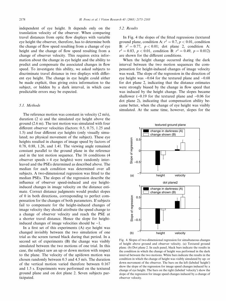
Fig. 4. Slopes of two-dimensional regression for simultaneous changes

of height above ground and observer velocity. (a) Textured ground

plane. (b) Dot plane 2. In each panel, black bars indicate the results in

the condition in which the change of height was performed in the dark

interval between the two motions. White bars indicate the results in the

condition in which the change of height was visibly simulated by up- or

down movement of the observer. The bars on the left (labeled �height�)show the slope of the regression for image speed changes induced by a

change of eye height. The bars on the right (labeled �velocity�) show the

slope of the regression for image speed changes induced by a change of

observer velocity.

5.1. Methods

The reference motion was constant in velocity (2 m/s),

duration (2 s) and the simulated eye height above theground (2.6 m). The test motion was simulated with four

different observer velocities (factors: 0.5, 0.75, 1.25 and

1.5) and four different eye heights (only visually simu-

lated; no physical movement of the subject). These eye

heights resulted in changes of image speed by factors of

0.78, 0.88, 1.26, and 1.41. The viewing angle remained

constant parallel to the ground plane in the reference

and in the test motion sequence. The 16 conditions (4observer speeds� 4 eye heights) were randomly inter-

leaved and the PSEs determined as described above. The

median for each condition was determined over all

subjects. A two-dimensional regression was fitted to the

median PSEs. The slopes of the regression describe the

influence of observer speed-induced and eye height-

induced changes in image velocity on the distance esti-

mate. Correct distance judgments would predict slopesof 0 in both directions, corresponding to perfect com-

pensation for the changes of both parameters. If subjects

fail to compensate for the height-induced changes of

image velocity they should attribute the speed change to

a change of observer velocity and reach the PSE at

a shorter travel distance. Hence the slope for height-

induced changes of image velocities should be )1.In a first set of this experiments (A) eye height was

changed invisibly between the two simulation of one

trial as the screen turned black during that period. In a

second set of experiments (B) the change was visibly

simulated between the two motions of one trial. In this

case, the subject saw an up or down motion with respect

to the plane. The velocity of the up/down motion was

chosen randomly between 0.5 and 4.5 m/s. The duration

of the vertical motion varied therefore between 0.167and 1.5 s. Experiments were performed on the textured

ground plane and on dot plane 2. Seven subjects par-

ticipated.

5.2. Results

In Fig. 4 the slopes of the fitted regressions (textured

ground plane, condition A: r2 ¼ 0:7, p < 0:01, conditionB: r2 ¼ 0:77, p < 0:01; dot plane 2, condition A:

r2 ¼ 0:83, p < 0:01, condition B: r2 ¼ 0:49, p ¼ 0:012)are shown for the different conditions.

When the height change occurred during the darkinterval between the two motion sequences the com-

pensation for height-induced changes of image velocity

was weak. The slope of the regression in the direction of

eye height was )0.64 for the textured plane and )0.68for dot plane 2, indicating that the distance estimates

were strongly biased by the change in flow speed that

was induced by the height change. The slopes became

shallower ()0.19 for the textured plane and )0.06 fordot plane 2), indicating that compensation ability be-

came better, when the change of eye height was visibly

simulated. At the same time, however, slopes for the


change of observer speed became steeper, indicating less

compensation for speed changes. For the textured plane,

the slope increased from 0.06 in condition A to 0.36 in

condition B. For dot plane 2, the slope increased from

0.33 in condition A to 0.5 in condition B. Slope de-

creases for eye height and increases for observer speed

were significant (p < 0:01) in the case of the textured

plane, only.Analysis of variance in the different conditions con-

firmed this pattern of results. When the height change

was performed in the dark interval, the parameter height

change showed a significant effect on the PSE (p < 0:01for the textured plane, p < 0:01 for dot plane 2). The

parameter speed change showed a significant effect for

dot plane 2 (p < 0:01 for dot plane 2), but not for the

textured plane. When the height change was visiblysimulated by up or down movement, height change

showed no significant effect on the PSE but speed

change did (p < 0:01 for the textured plane, p < 0:01 for

dot plane 2). A significant interaction between the height

change and speed change was observed for dot plane 2

in the dark interval condition but not in any of the other

conditions.

5.3. Discussion

Two factors influenced the visual image speeds of the

optic flow in this experiment: the speed of the observer

and the observer�s height above the ground. Therefore,in order to estimate travel distance, subjects must sepa-

rate the change of the flow speeds resulting from the

change of eye height from the change of the flow speeds

resulting from a change in observer motion. The exper-

iment presented two conditions. In the first condition,

eye height above the ground plane changed during an

interval in which the screen turned black. In the second

condition, an up or down movement simulated theheight change visibly for the subjects. When eye height

changed during the black interval, we observed a pre-

dictable error resulting from the inability to compensate

for the change in eye height. Subjects attributed almost

the entire change of the flow speeds to a change of ob-

server velocity and therefore misjudged travel distance.

Thus they did not compensate for the change of eye

height. In this condition, information about the changeof eye height was available in the accompanying change

of the position of the visible horizon on the screen and

by changing texture cues resulting from the changed

viewing angle of the ground plane. Apparently this in-

formation was not used. When subjects were afterwards

asked whether they had noticed any changes occurring

in the interval between the two motion sequences they

only reported a change of observer velocity.The results of this experiment also show that the basis

for the internal representation of the visually simulated

ego motion distance cannot be simulated ego-displace-

ment. The change of height affects visual speed but not

ego displacement. For instance, subjects would pass the

same number of texture elements regardless of the sim-

ulated eye height. Thus, if the judgment were based

on simulated ego displacement one would expect good

distance estimation regardless of whether the vertical

movement is shown or not. Because subjects failed to

compensate for the difference in eye height in the darkcondition, the internal representation does not seem to

be ego-displacement in 3D space but rather must be

perceived ego-speed.

In both conditions of the experiment a gap separated

the two forward motion simulations. In condition A the

screen turned black for 500 ms, in condition B the

display depicted an up or down motion with variable

duration between 0.167 and 1.5 s. We did not findany effect of the gap duration on the subject�s decision.Control experiments showed that also the speed of the

vertical motion had no effect on the distance perception.

The simulation of up or down movement with the

height change allowed subjects to estimate the change of

flow speeds resulting from the change of eye height.

Subjects fairly well compensated for the height change in

this condition. However, the enhanced ability to com-pensate for height changes was accompanied by an in-

creased misjudgment of the change in observer velocity.

The compensation for speed changes became weaker.

This may suggest that subjects have a limited overall

ability to compensate for changes in flow speeds when

estimating travel distance. However, because subjects

had to estimate the influence of two parameters (ob-

server velocity and eye height) the task was more dif-ficult than those of the previous experiments. The

increased difficulty may also account for the weaker

performance.

We conclude from experiment 2 that human observers

can calibrate the image velocities from the optic flow

with respect to the height above the ground to derive an

estimate of travel distance. This suggests that travel

distance is estimated not simply on the basis of imagevelocities but also takes environmental parameters into

account. However, the image velocities in the optic flow

are linearly related to the height above ground. Thus the

distance judgment may still be based on an integration

of image velocities, albeit followed by normalization

with respect to eye height, rather than an estimate of

observer velocity. Experiments 3 and 4 involve mani-

pulations of the distribution of image velocities thatfurther reduce the possibility to use image velocities

directly.

6. Experiment 3: Visibility range

If subjects were to base their discrimination of travel

distance simply on the total accumulated flow speeds in


the two movement sequences, manipulations of the

distribution of flow speeds should impair performance.

One possibility to manipulate the average flow speeds in

the display without changing observer velocity or eye

height is to restrict the visibility range. If the visibility

range is reduced, slow flow field speeds are omitted and

the average speed becomes higher. We were interested in

whether subjects are influenced by the average flowspeed or whether they are able to take changes in visi-

bility between the two motion sequences into account.

To test this, we changed the visibility range between the

two motion sequences either by adjusting the maximum

distance at which scene elements were drawn, or by in-

troducing fog of varying density.

visibility range velocity-2.5

-1.5

-0.5

0.5

1.5

2.5

Slo

pe o

f reg

ress

ion

clipped visibility range (A)fog (B)


of visibility range and observer velocity. Black bars indicate the results

in the condition in which visibility was restricted by clipping the dis-

play of the ground plane in a specified distance. White bars indicate the

results in the condition in which visibility was restricted by simulated

fog. The bars on the left (labeled �visibility range�) show the slope of the

regression for changes in average image speed induced by a change in

visibility range. The bars on the right (labeled �velocity�) show the slope

of the regression for image speed changes induced by a change of

observer velocity.

6.1. Methods

The first motion was always simulated with constantvelocity (2 m/s), duration (2 s), height above ground (2.6

m) and visibility range (20 m). The second motion was

randomly presented with four different velocities and

four visibility ranges (both with factors of: 0.5, 0.75, 1.25

and 1.5 of the first motion). For each visibility range we

calculated the associated change in the average image

velocity present on the screen. These visibility range-

induced speed changes were 0.76, 0.97, 1.05, and 1.15.Visibility range was manipulated in two ways. In the

first condition (A), the ground plane was simply trun-

cated at a certain distance from the observer. In this

case, the virtual ground plane was visible only up to the

clipping distance.

In the second condition (B), virtual fog was added to

the environment. White fog (RGB: 1.0, 1.0, 1.0) started

at the virtual position of the observer and linearly in-creased in density with distance. When the chosen visi-

bility range was reached, the fog was completely

opaque. The fog was created in the following way: First,

a color index f was determined for each pixel

f ¼ ðvisibility range� distanceÞ=ðvisibility range

� start position of fogÞ:

With this index, the new color of the pixel was calcu-

lated:

C0 ¼ f � Cr þ ð1� f Þ � Cf

where C0 ¼ new color of the pixel; Cr ¼ original color of

the pixel; Cf ¼ fog color; f ¼ color index.

Hence, fog changed the contrast of each pixel de-

pending on the pixel�s distance to the observer. The

experiments were simulated on the textured ground

plane. Seven subjects participated. For data analysis wedetermined the median over all subjects for the 16

conditions and fitted a two-dimensional linear regres-

sion on the result. The slopes of this regression indicates

the ability to compensate for the changes between the

two motion sequences.

6.2. Results

The slopes of the regressions (clipped condition (A):

r2 ¼ 0:62 and p < 0:01; fog condition (B): r2 ¼ 0:137,p ¼ 0:38) are plotted in Fig. 5.

In the clipped condition, there was no compensation

for the change of the visibility range. The slope of the

regression was )1.51. In the fog condition, compensa-

tion for the change in visibility range was better (slope of

)0.32). Compensation for changes of velocity was very

good in both conditions.

Analysis of variance showed a significant effect of

visibility range in the clipped condition (p < 0:01) butnot in the fog condition. There was no significant effect

of velocity in either condition and no interaction be-

tween velocity and visibility range.

6.3. Discussion

When the visibility range is altered, objects at greater

distances from the observer�s virtual position are re-moved from or added to the flow field. Because of mo-

tion-parallax, distant objects have a lower velocity in the

optic flow field than near objects. Thus, changing the

visibility range between the two motions caused a

change of the average velocity of flow elements. If sub-

jects base their judgment of travel distance on the av-

-0.5

0

0. 5

1

Slo

pe o

f reg

ress

ion



erage flow field velocity, and do not compensate for the

change of the different viewing distances, they should

make a predictable error. In this case, the PSE for travel

distance should decrease as flow velocity increases, i.e.,

with decreasing viewing distance. Errors in the clipped

condition followed this prediction, suggesting that sub-

jects did not compensate for the difference in visibility

range, or that they did not notice the change. In the fogcondition, however, errors were negligible and subjects

estimated travel distance correctly. This suggests that

subjects can compensate for changes in visibility range if

they notice the change. As in experiment 3, we conclude

that human observers can combine scene information

with flow information to estimate travel distance.

Bremmer and Lappe (1999) also investigated the effect

of changes in visibility range on perceived distance ofsimulated self-motion. They altered the visibility range

in an environment consisting of a three-dimensional

cloud of dots. Such an environment lacks all depth cues

beyond motion parallax. Hence the alteration of visi-

bility range is not unambiguously specified in the stim-

ulus. Their experiments revealed predictable errors that

could be explained if subjects assumed that the scene

has not changed and used the average flow velocity fortheir distance estimate. Unlike the experiment of Brem-

mer and Lappe, our experimental conditions contained

depth cues that could inform the observer about the

alteration of the visibility range independently from the

optic flow. Because our subjects were able to compen-

sate for the changes we conclude that they must not

simply rely on average optic flow speed.

A different experiment dealing with fog-limited visi-bility during simulated self-motion was described by

Snowdon, Stimpson, and Ruddle (1998). In their ex-

periment, subjects had to report perceived speed with a

virtual car in different visibility conditions. When visi-

bility was reduced, subjects experienced the velocity of

their ego-motion to be slower. In our experiment, we did

not explicitly ask for speed judgments. But effects on

speed perception could also have lead to errors in per-ceived distance. A perceptual decrease of ego-speed due

to fog might have contributed to the compensation of

the increase of average flow velocity due to decreased

visibility in that condition.

viewing angle velocity-1


of viewing angle and observer velocity. Black bars indicate the results

in the condition in which the change of viewing angle was performed in

the dark interval between the two motions. White bars indicate the

results in the condition in which the change of viewing angle was

visibly simulated by up- or down rotations of the scene. Left bars

(labeled �viewing angle�) show the slope of the regression for changes in

average image speed induced by a change of viewing angle. Right bars

(labeled �velocity�) show the slope of the regression for image speed

changes induced by a change of observer velocity.

7. Experiment 4: Viewing angle

In experiment 4, we varied the simulated angle under

which subjects view the ground plane. In the reference

movement, simulated gaze was parallel to the ground

plane. In the test movement, simulated gaze was tiltedupward or downward. This manipulation changed the

entire distribution of flow speeds on the display. In

order to perceive travel distance correctly, subjects must

estimate the orientation of the plane and calculate ego-

speed from flow speed using the plane orientation.

7.1. Methods

The reference movement was constant in velocity (2

m/s), duration (2 s) and simulated viewing angle (par-

allel to the ground plane). The test movement wassimulated with four different observer velocities (factors:

0.5, 0.75, 1.25 and 1.5) and four different viewing angles.

The different viewing angles changed image speed by

factors of 0.76, 0.97, 1.08, and 1.49. The subjects were

instructed to keep their heads upright during the ex-

periments.

In the first condition (A) viewing angle was changed

while the screen turned black between the two move-ment sequences. In the second condition (B) the change

was visibly simulated between the two movements such

that subjects saw an up or down rotation of the scene.

The velocity of the rotation was chosen randomly be-

tween 10 and 30 deg/s. This experiment used the tex-

tured ground plane. Five subjects participated.

7.2. Results

The slopes of the regressions (condition A: r2 ¼ 0:58,p < 0:01, condition B: r2 ¼ 0:5, p < 0:01) are plotted in

Fig. 6. In both conditions we found good compensation

for the change of image velocities introduced by the

change of viewing angle (condition A: 0.07, condition


B: )0.09). Compensation for changes in observer ve-

locity was less good but comparable to that observed in

experiment 3 (condition A: 0.35, condition B: 0.26).

Analysis of variance revealed a significant effect of ob-

server velocity in condition A (p < 0:01), but no other

significant effects.

7.3. Discussion

This experiment is probably the most challenging

because the change of viewing angle not only influences

the average image velocity in the flow field but the entire

distribution of image velocities. Yet, subjects were wellable to compensate for changes of the viewing angle. To

do this, they must have estimated the tilt of the plane

and used this information to estimate observer speed

with respect to the plane. This shows again that travel

distance estimation is performed from an estimate of

observer motion not image motion.

Compensation for the change in viewing angle was

possible in both conditions of experiment 4, even whenthe change occurred during the dark interval between

the movement sequences. In experiments 2 and 3, the

change of height or visibility range could only be com-

pensated when it was presented visually to the subject.

We believe that this happened because subjects did not

notice the change in those experiments. The change if

the viewing angle is possibly more salient than the

change of height in experiment 3 or the truncation of theground plane in experiment 3. Therefore, in experiment

4 subjects may have been able to notice the change of

viewing angle even when it was carried out in the dark

interval.

8. General discussion

We investigated the perception of travel distance of

visually simulated self-motion. Because of the ambiguity

of the optic flow field with respect to absolute speed

or distance we chose a comparison task in which the

distances of two movement sequences had to be dis-

criminated. The first (reference) movement was always

constant. The second (test) movement varied in duration

and observer velocity and could also vary in the numberof depth cues provided by the scene (experiments 1a and

1b), the height above the ground (experiment 2), visi-

bility range (experiment 3), or viewing angle (experiment

4). The first question we asked is whether observers can

discriminate travel distance despite variations in ob-

server speed. Experiments 1a and 1b clearly showed that

distance judgments were independent of the change of

observer velocity between the reference and the testmovement. This result corroborates earlier findings by

Bremmer and Lappe (1999) who performed similar ex-

periments but collapsed data across observer speeds in

the analysis. The second question we asked in experi-

ments 1 and 2 was about the use of various visual dis-

tance cues for discriminating travel distance from optic

flow. Systematic elimination of distance cues from the

stimulus revealed that pure visual motion, which in-

cludes motion parallax as a cue to distance, is sufficient

to discriminate travel distance.

The discrimination of travel distance of two successivemovement sequences requires the integration of the

motion signal from each sequence and a comparison of

the two results. If both movements are performed in the

same environment this comparison is sufficient. If they

are performed in different environments the motion

signals must be taken relative to the environment in

order to allow a meaningful comparison. Therefore,

travel judgments should be based on perceived ego-motion relative to the environment rather than directly

on the image velocities. Experiments 2–4 provide evi-

dence that supports this hypothesis.

In experiment 2 the simulated height of the observer

above the ground was varied. This led to an additional

variation of image motion in the flow field which is in-

dependent of the variation of the translational velocity

of the observer. When subjects experienced the changeof height by a simulated up or down movement they

were able to compensate for the associated changes in

flow speed and retain their ability to discriminate travel

distance, albeit with slightly larger errors. In experiment

3 we manipulated the distribution of image speeds in the

flow field by varying the visibility range in the test

movement. When the alteration of the visibility range

was made explicit by the introduction of fog subjectscould well compensate for the associated changes in the

distribution of image speeds. In experiment 4 we varied

the simulated viewing angle under which the scene was

presented. This manipulation again changed the distri-

bution of image velocities in the presented flow field but

subjects were able to compensate for this change. All

three experiments hence suggest that our observers did

not use image velocities directly. Rather they must haveused an estimate of observer speed with respect to the

environment.

This leads to the question of which cues subjects use

to estimate the structure of the environment. Observa-

tions from several experiments suggest that motion

parallax is a sufficient cue. Experiments 1a and 1b

showed that motion parallax is sufficient if the envi-

ronment is the same in both sequences. In experiment 2,subjects were able to compensate for visible changes in

eye height even for the limited-lifetime constant-density

ground plane (dot plane 2) in which depth is only

specified by motion parallax. This shows that motion

parallax during the up or down movement of the

observer could be used to update the observer�s repre-

sentation of the environment and the associated re-

lationship of ego-speed to flow field speed. Motion


parallax might also have been used to detect changes to

the scene in experiments 3 and 4, but other cues were

available as well in those experiments.

Our experiments provide evidence that the discrimi-

nation of travel distance from visual motion is based on

a representation of ego-speed with respect to the envi-

ronment. This representation is derived from image

motion in the optic flow together with structural cuesabout the environment provided by the visual input.

How general is this representation? Specifically, does it

pertain only to the discrimination of movement se-

quences or does it allow more abstract judgments of

travel distance? Bremmer and Lappe (1999) used a task

in which subjects had to reproduce the distance of a

visually simulated movement sequence with an active

movement simulation in which speed and duration werecontrolled by the subject with a joystick. They found

excellent distance reproduction. This suggests that the

representation of travel distance generalizes from pas-

sive judgments to active control behavior. Redlick et al.

(2001) and Harris et al. (2000) have asked subjects to

compare travel distance during a movement simulation

to the remembered distance to a previously seen static

target. Subjects had to indicate the time at which theyreached the target�s position in the simulated environ-

ment. This task requires a match of travel distance from

visual motion to distance measured from static visual

cues. Redlick et al. (2001) found that subjects indicated

the correct time of arrival at the target position for

accelerated movements but responded too early for

movements of constant velocity. They suggested that

travel distance estimates from visual motion can becompared to static distance estimates, but distances are

overestimated for movements of constant velocity. Since

our results show that travel distances of constant ve-

locity movements can be discriminated successfully, we

suggest that errors might occur in the conversion be-

tween distances obtained from static and dynamic visual

cues.

Acknowledgements

We gratefully acknowledge support from the Deut-

sche Forschungsgemeinschaft SFB 509, the Human

Frontier Science Program, the BioFuture Prize of the

German Federal Ministry for Education and Research

and the EC projects EcoVision and Eurokinesis. We

thank Bart Krekelberg for the implementation of the

maximum likelihood method and Jaap Beintema for

critical reading of the manuscript.

References

Berthoz, A., Israel, I., Georges-Francois, P., Grasso, R., & Tsuzuku,

T. (1995). Spatial memory of body linear displacement: What is

being stored? Science, 269, 95–98.

Bremmer, F., & Lappe, M. (1999). The use of optic flow for distance

discrimination and reproduction during visually simulated self

motion. Experimental Brain Research, 127, 33–42.

Cutting, J. E. (1997). How the eye measures reality and virtual reality.

Behavior Research Methods, Instruments, and Computers, 29, 27–

36.

Esch, H., & Burns, J. (1995). Honeybees use optic flow to measure the

distance of a food source. Naturwissenschaften, 82, 38–40.

Harris, L., Jenkin, M., & Zikovitz, D. (2000). Visual and non-visual

cues in the perception of linear self motion. Experimental Brain

Research, 135, 12–21.

Harvey, L. (1986). Efficient estimation of sensory thresholds. Behavior

Research Methods, Instruments, and Computers, 18, 623–632.

Israel, I., & Berthoz, A. (1989). Contribution of the otoliths to the

calculation of linear displacement. Journal of Neurophysiology, 62,

247–263.

Lappe, M., Bremmer, F., & van den Berg, A. (1999). Perception of self-

motion from visual flow. Trends in Cognitive Sciences, 9, 329–336.

Lee, D. N. (1974). Visual information during locomotion. In R. B.

MacLeod, & H. Pick (Eds.), Perception: Essays in Honor of J.J.

Gibson (pp. 250–267). Ithaca, NY: Cornell University Press.

Mittelstaedt, H., & Mittelstaedt, M. (1973). Mechanismen der Orien-

tierung ohne richtende Aussenreize. Fortschritte der Zoologie, 21,

46–58.

Mittelstaedt, M., & Mittelstaedt, H. (1980). Homing by path integra-

tion in a mammal. Naturwissenschaften, 67, 566–567.

Prokop, T., Schubert, M., & Berger, W. (1997). Visual influence on

human locomotion––modulation to changes in optic flow. Exper-

imental Brain Research, 114, 63–70.

Redlick, F., Jenkin, M., & Harris, L. (2001). Humans can use optic

flow to estimate distance of travel. Vision Research, 41, 213–219.

Snowdon, R., Stimpson, N., & Ruddle, R. (1998). Speed perception

fogs up as visibility drops. Nature, 392, 450.

Srinivasan, M., Zhang, S., & Bidwell, N. (1997). Visually mediated

odometry in honeybees. Journal of Experimental Biology, 200,

2513–2522.

Thomson, J. (1980). How do we use visual information to control

locomotion? Trends in Neurosciences, 10, 247–250.

Tresilian, J. R. (1999). Visually timed action: time-out for �tau�? Trendsin Cognitive Sciences, 3, 301–310.

Warren, W. H., & Hannon, D. J. (1990). Eye movements and optical

flow. Journal of the Optical Society of America A––Optics Image

Science and Vision, 7, 160–169.

Discrimination of travel distances from ‘situated’ optic flow

Documents

Transcript of Discrimination of travel distances from ‘situated’ optic flow