FIBER OPTIC ACOUSTIC EMISSIONS MONITORING SYSTEM

POLITECNICO DI MILANO

Polo Territoriale di Lecco

Scuola di Ingegneria Civile, Ambientale e Territoriale

Master of Science in Civil Engineering for Risk Mitigation

FIBER OPTIC ACOUSTIC EMISSIONS MONITORING SYSTEM

An experimental investigation in a laboratory application for

rainfall-induced landslides in different soil materials slope models

Supervisor: Prof.ssa Laura Longoni

Correlator: Ing. Vladislav Ivov Ivanov

Master degree thesis by:

Cerri Giulia

Matr. 920600

Academic year 2019/2020

ii

Ackonwledgements

Mi sento in dovere di dedicare questa pagina del presente elaborato alle persone che mi hanno suppor-

tato nella redazione dello stesso.

Innanzitutto, ringrazio il mio relatore Laura Longoni e il mio correlatore Vladislav Ivov Ivanov, per la loro

immensa pazienza e disponibilità, per i loro indispensabili consigli e per le conoscenze trasmesse durante

tutto il percorso di stesura dell’elaborato e durante il corso di studio.

Ringrazio infinitamente la mia famiglia che mi è sempre stata accanto e mi ha sempre sostenuto, ap-

poggiando ogni mia decisione e permettendomi di portare a termine gli studi universitari.

Grazie ai miei compagni di corso con cui ho potuto condividere questo importante percorso formativo

che ci ha visto crescere e arricchire sia dal punto di vista culturale che introspettivo.

Infine, devo riservare un pensiero al meraviglioso mondo dello sport che, oltre ad essere stato per me

fonte di sfogo e libertà, mi ha fornito la giusta grinta per non mollare mai e superare tutti gli ostacoli con la

dovuta serenità. Un sentito grazie va quindi a tutti i miei compagni di avventure ma soprattutto alla

A.S.D.Solarity, la mia squadra di calcio a 5, che durante questi cinque anni non ha mai smesso di credere in

me e ha continuato, almeno fino a quando è stato possibile, a regalarmi momenti unici di entusiasmo e

spensieratezza.

Non finirò mai di ringraziarvi per avermi permesso di arrivare fin qui.

iv

Abstract In order to overcome the shortcomings of conventional slope monitoring methods, in this document the

application of a quasi-distributed optical fiber sensing system to measure precursory acoustic emissions

(AE) preceding the release of landslides in a small-scale physical model is illustrated. The deformation pro-

cess of soil slopes during a landslide can be quantified also considering the acoustic emissions monitoring.

The implemented method based on fiber optic technology detects elastic waves transmitted within the

slope and provides AE measurements at high spatial and temporal resolution over relatively large distances.

The aim of this work is to investigate acoustic emissions as precursor of slope failure and to assess the po-

tential of the fiber optic technology for early warning in different soil slopes materials. In the present study

four shallow rainfall-induced landslides have been triggered on a small scale slope simulator accurately re-

produced in the Laboratory of Geological and Geophysical Applications (Gap2 Lab) situated in the territorial

Pole of Lecco of the Politecnico of Milan. Rainfall was artificially reproduced through a network of micro-

sprinkler irrigators. The fiber cables were deployed at a predefined depth within the slope model with pre-

selected configurations and they were interrogated through interferometry. Conventional instruments

measuring the volumetric water content and the visual inspection system for the monitoring of the surface

deformation and surface displacements were also installed along the slope for the comparison and the val-

idation of the results. The installation process of the optical fiber sensors and of the traditional instrumen-

tations is accurately explained. The experiments were conducted on slopes with different geological condi-

tions and with fiber optic cables disposed in different configurations in order to explore the ability and the

effectiveness of the fiber optical sensors in the investigation of shallow landslides behavior. The results

show that the interferometric fiber optic AE monitoring system has a good consistency with the traditional

instruments since from the different monitored quantities, all the several phases within the landslide de-

veloped during the experiments, have been clearly identified. Moreover, it is shown that, in most of the

cases, optical fibers can detect precursory signs of failure well before the collapse. It is demonstrated that

this method can effectively represents an early warning system of rainfall-triggered landslides, in particular

in layered coarser soil slopes that exhibit fluid-like rapid mass movements. In fact, it is also verified that

acoustic emissions are more pronounced in looser soil assemblies, while they are much weaker in densely

packed mixtures or cohesive uniform soil slopes, which not exhibit fluid-like motion. The present laboratory

experiments should promote in the future deeper research in the field of slope instability and further appli-

cations for risk mitigation.

v

Sommario Al fine di superare le carenze dei metodi tradizionali per il monitoraggio dei versanti, in questo elabora-

to viene illustrata su un modello fisico di pendio in scala l’applicazione di un sistema quasi-distribuito basa-

to sull’impiego della fibra ottica per misurare le emissioni acustiche che vengono emesse prima del verifi-

carsi di una frana. Il processo di deformazione dei versanti in terra durante il corso di un franamento può

essere quantificato anche grazie al monitoraggio delle emissioni acustiche. Il metodo qui utilizzato basato

sulla tecnologia a fibra ottica rileva le onde elastiche che si propagano nel suolo e fornisce le misurazioni

delle emissioni acustiche ad alta risoluzione spaziale e temporale su relativamente lunghe distanze. Lo sco-

po di questo lavoro è quello di indagare se le emissioni acustiche possano essere considerate degli affidabili

segni premonitori del cedimento di un pendio e di valutare la potenzialità della tecnologia a fibra ottica

come metodo di identificazione nei vari materiali del terreno in modo da poter essere utilizzato come esau-

stivo segnale di allarme. Nel presente studio sono state riprodotte artificialmente su piccola scala quattro

frane superficiali su un simulatore di pendio costruito nel laboratorio di Geologia e Geofisica Applicata

(Gap2 Lab) situato nel polo territoriale di Lecco del Politecnico di Milano. La pioggia è stata riprodotta artifi-

cialmente attraverso un sistema di augelli. I cavi a fibra ottica sono stati disposti nel pendio a profondità e

con configurazioni prestabilite e sono stati interrogati per interferometria. Per il confronto e la convalida

dei risultati ricavati dalla fibra ottica, sono stati inoltre installati sul simulatore altri strumenti tradizionali

mirati al monitoraggio del contenuto d’acqua del terreno e alla foto ripresa dei cinematismi superficiali del

suolo nel corso dell’evoluzione del processo di franamento. Gli strumenti e la loro installazione vengono

spiegati meticolosamente. Gli esperimenti sono stati condotti su versanti con diverse condizioni geologiche

e con i cavi della fibra ottica disposti con configurazioni differenti in modo da analizzarne l’efficienza dei

sensori nel cogliere il comportamento di una frana superficiale. I risultati ottenuti mostrano che il sistema

di monitoraggio interferometrico a fibra ottica delle emissioni acustiche è coerente con gli strumenti tradi-

zionali poiché, come da questi, tutte le diverse fasi in cui si è articolato il processo di franamento osservato

durante gli esperimenti sono state identificate. Inoltre, nella maggior parte dei casi, la fibra ottica si è dimo-

strata capace di cogliere segnali premonitori molto prima del collasso. Viene dimostrato che questo meto-

do può effettivamente rappresentare un sistema di allarme per anticipazione di frane innescate da eventi di

pioggia, in particolare in versanti stratificati di materiale più grossolano che mostra un comportamento si-

mil fluido che mobilita il suolo in maniera repentina. Infatti, viene inoltre verificato che le emissioni acusti-

che sono più pronunciate negli ammassi di suolo più poveri, mentre sono molto più deboli negli ammassi

densamente compattati o in versanti di materiale coesivo uniforme, che non hanno un comportamento si-

mile a quello di un fluido. Il presente esperimento di laboratorio dovrebbe promuovere in future e più ap-

profondite ricerche nel campo della stabilità dei pendii e in altre applicazioni da implementare per la miti-

gazione del rischio.

vii

Table of Contents

FIBER OPTIC ACOUSTIC EMISSIONS MONITORING SYSTEM ......................................................................... i

Ackonwledgements ....................................................................................................................................... ii

Abstract ........................................................................................................................................................ iv

Sommario ...................................................................................................................................................... v

Table of Contents ........................................................................................................................................ vii

INTRODUCTION ............................................................................................................................................ 1

Chapter 1: STATE OF ART OF THE FIBER OPTIC ............................................................................................ 5

1.1 The optical fiber ................................................................................................................................. 5

1.1.1 The fiber optic design ............................................................................................................ 5

1.1.2 Types of fiber optics .............................................................................................................. 5

1.1.3 The physical principles of the light observed in the fiber optic: the reflection, the

refraction and the scattering ..................................................................................................................... 6

1.2 The Fiber Optic Sensing system ......................................................................................................... 9

Chapter 2: LABORATORY AND IN-SITU APPLICATIONS OF FIBER OPTIC SENSORS IN GEOTECHNICAL FIELD

......................................................................................................................................................................... 29

Chapter 3: EXPERIMENTAL SET-UP ............................................................................................................ 38

3.1 Slope Simulator Design .................................................................................................................... 38

3.2 Instrumentation ............................................................................................................................... 40

3.2.1 Rainfall Network .................................................................................................................. 41

3.2.2 TDR (Time Domain Reflectometry) ...................................................................................... 42

3.2.3 Action Cameras .................................................................................................................... 43

3.2.4 Fiber Optic System ............................................................................................................... 44

3.3 Test procedure................................................................................................................................. 48

Chapter 4: TEST RESULTS AND DISCUSSIONS ............................................................................................. 49

4.1 TEST 1 .............................................................................................................................................. 49

4.1.1 Rainfall trend ....................................................................................................................... 49

4.1.2 Visual interpretation ............................................................................................................ 49

4.1.3 TDR results analysis ............................................................................................................. 51

4.1.4 Displacements analysis ........................................................................................................ 53

4.1.5 AE signals analysis................................................................................................................ 57

4.2 TEST 2 .............................................................................................................................................. 64

4.2.1 Rainfall trend ....................................................................................................................... 64

viii




4.2.5 AE signals analysis................................................................................................................ 71

4.3 TEST 3 .............................................................................................................................................. 77

4.3.1 Rainfall trend ....................................................................................................................... 77




4.3.5 AE signal analysis ................................................................................................................. 84

4.4 TEST 4 .............................................................................................................................................. 90

4.4.1 Rainfall trend ....................................................................................................................... 90




4.4.5 AE signals analysis.............................................................................................................. 100

4.5 Comparison of the results obtained by the different sensors in the tests .................................... 109

4.5.1 Rainfall analysis ................................................................................................................. 109

4.5.2 Visual analysis .................................................................................................................... 110

4.5.3 TDR results analysis ........................................................................................................... 114

4.5.4 Displacements of the monitoring points ........................................................................... 116

4.5.5 AE signals results ............................................................................................................... 124

4.6 Final and General Observations .................................................................................................... 130

CONCLUSIONS .......................................................................................................................................... 137

ANNEXES................................................................................................................................................... 141

ANNEX A: Table of the analyzed papers available in literature ............................................................ 141

ANNEX B: Multitaper Spectogram ........................................................................................................ 176

ANNEX C: Lead Time Analysis................................................................................................................ 180

BIBLIOGRAFY ............................................................................................................................................ 185

1

INTRODUCTION

Nowadays, rainfall is considered one of the most frequent triggering factors to natural slope failures (De

Vita and Reichenbach, 1998).

On field, hydrological conditions and geomechanical properties are key elements that control the stabil-

ity of a slope under the influence of rainfall (Huang et al. 2012).

Shallow landslides are natural geomorphological phenomena that are usually triggered by short but in-

tense rainfall events or by less intense but prolongated events.

Even though the extension of the soil mass involved in shallow landslides is limited both in terms of are-

al surface and of depth, this kind of phenomena represents important threats to people and structures that

can result in severe damages and fatalities, especially in the case of flow-like landslides, because they are

hardly predictable since they happen suddenly, with just little warning, and evolve very fast.

Typical possible causes of flow-like landsliding in granular materials and in some cohesive soils is the

partial or complete fluidization of the moving mass with the overridden bed material. In general, variously

graded and packed materials will exhibit different motion patterns depending on their ability to dissipate

the pressure excess (Hu et al., 2018).

In particular, rainfall-induced landslides in loosely packed granular deposits are highly hazardous not on-

ly for their sudden failure, but also for their fluid-like motion and for their high mobility. Starting from the

detaching area, flowslides erode and engage large amounts of soil along their path and finally discharge a

great impact energy to engineering structures (Schenato et al. 2017).

Therefore, traditional monitoring systems based on measurements of rainfall, deformation, pore water

pressure, suction or ground water level, might fail to capture precursory signals because they are limited to

some local points that are not sufficient to assure an in-depth explanation of failure trigger, and thus, time-

ly alarm cannot always be released.

As reported in the paper of Deng (2019), since the deformation of the slope is the most evident conse-

quence of landslides and from which the extend of the damage is assessed, there is an urgent requirement

to quantify the deformation process using a real-time on-line monitoring technology and to find efficient

early warning indicators for landslides.

2

When material is subjected to stress, the soil slope deforms, and because of the movement or of the

fracture of soil particles, energy is released in the form of elastic waves usually in the kilohertz to the meg-

ahertz frequency range.

Processes at different scales produce distinct frequency and energy signatures, enabling the use of AEs

to assess the mechanical state of complex materials and granular flows (Michlmayr et al., 2013).

As presented in earlier work (Michlmayr et al. 2012b), the formation of a shear zone in granular materi-

als is typically associated with significant acoustic emissions. Hence, observations of AE in unstable slopes

may provide a real time and direct indication of the imminence of a landslide and can complement existing

techniques for landslide prediction, making the acoustic emission (AE) technology a potential tool for land-

slide early warning (Michlmayr, et al., 2016).

In order to extend the spatial coverage of the monitoring, a distributed fiber-optic technique can be im-

plemented for the continuous detection of elastic waves along consecutive sections of the optical cable.

Although fiber-optic strain measurements have been used in a handful of cases for deformation meas-

urements in landslides since at the beginning of the new millennium (Iten 2008; Wang et al. 2009; Iten

2011), the firsts practical studies and tests on the application of a standard fiber-optic based technology for

the detection of acoustic emission to be used as a landslide monitoring system were conducted by

Michlmayr in 2016.

In the Michlmayr’experience it was demonstrated that fiber optic technology based on the Michelson

interferometer can effectively detect acoustic emissions on homogeneous soil slope model made of gravel.

Later on, according with Hu, the monitoring soil slopes through AEs was suggested as a low-cost and

time-effective approach for continuous monitoring and early warning of some slow movements and first-

time failures in some materials. This has been recently verified through the laboratory experience reported

in the master thesis of Bellani F. (2017) and on which this work is strictly based.

In this context, the objectives of this study are:

1) To test and evaluate the efficiency of the application of a distributed fiber optic system based on

the Michelson Interferometer (MI) technology for the acquisition of the acoustic emissions re-

leased during rainfall-induced landslides evolving processes.

2) To explore the correlation between the change in mechanical parameters, due to the possible

presence of different soil materials and also differently distributed within the slope, and the moni-

tored physical quantities including the evolution process of progressive landslides, the level of vol-

umetric water content within the slope, the evolution of the surface deformation and displace-

ments, but, above all, the AE released and detected by the fiber optic monitoring system.

3) To evaluate the effectiveness of different configurations for the installation of the fiber optic cables

within the slope.

3

4) To assess the possibility to implement the distributed fiber-optic AE measurements as an early-

warning for slope stability.

In order to study shallow landslides through the application of the fiber optic technology, a series of ex-

perimental tests have been conducted on a small-scale slope simulator reproduced in the Geological and

Geophysyscal laboratory in the territorial pole of Lecco.

The slope simulator is a steel structure facility that has been constructed in order to accommodate the

simulation of sliding soil masses (Arosio et al. 2019, Hojat et al. 2019, Ivanov et al. 2020, Hojat et al. 2020,

Papini et al. 2020) triggered by artificial rainfall and to verify the premonitory capability of the optical fiber

technology to sense in advance the imminent collapse.

For each test the slope geometry, the mechanical and the hydrological properties of the soil slope mate-

rials, the hydraulic characteristics of the artificial irrigation processes and the set-up of the traditional and

experimental monitoring systems implemented have been defined.

Since in the among the landslides monitoring systems the application of the distributed fiber optic tech-

nology for the detection of acoustic emissions released during the evolution of landslides process has been

already tested in past experiences, the present study mainly focuses on the investigation of this kind of in-

novative monitoring system in different geological conditions.

For the comparison and the validation of the results recovered by the optical system, on the simulator

other traditional instruments were installed including a couple of action cameras and the TDR (Time Do-

main Reflectometry). These conventional monitoring systems not only provided some additional infor-

mation about the type and the properties of the soil materials that were used to create the slope model,

but they also helped to characterize the fiber optic behavior at the different soil moisture and water con-

tent conditions.

Overall, the present study is developed in two main phases that can be synthetized by a first preliminary

literature research that allowed to best set-up the physical model and by the following experimental part in

which tests have been performed and results have been evaluated and discussed.

The literature research allowed to understand the physical principles that stay beyond the fiber optic

technology and to become aware of the great potentialities related to their functionalities and implemen-

tations. Moreover, the deep analysis in the laboratory and on field experiences that have been performed

all over the world since now, put the basis for the design of the landslides simulations to be carried out in

the different tests, since it allowed to understand what is the state of art of this kind of technology and

which can be the devices and the precautions to be implemented that best fit the purposes of the present

experimental investigation.

4

The structure of the thesis is developed in the following chapters:

INTRODUCTION

CHAPTER 1 – STATE OF ART OF THE FIBER OPTIC: General description of the state of art of the fiber op-

tic that develops in the illustration of the sensor’s design and in the classification of the different technolo-

gies that stay at the base of its specific functionality.

CHAPTER 2 – LABORATORY AND IN SITU APPLICATIONS OF FIBER OPTIC SENSORS IN GEOTECHNICAL

FIELD: Literature research and analysis of reported laboratory and on field applications regarding the appli-

cation of the fiber optic technology in the hydrogeological field for monitoring purposes.

CHAPTER 3 – EXPERIMENTAL SET-UP: Introduction of the laboratory physical model, description of the

monitoring systems implemented, description of the tests procedure.

CHAPTER 4 – TEST RESULTS AND DISCUSSIONS: Analysis and discussion of the results recovered from

the different tests through the comparison of the different physical quantities measured by the installed

monitoring systems in a transversal and parallel way, within each test and within each monitoring typology

respectively.

CONCLUSIONS: Summary of the presented study and of the results with the presentation of eventual

further future developments.

5

Chapter 1: STATE OF ART OF THE FIBER OPTIC

1.1 The optical fiber

1.1.1 The fiber optic design

The optical fiber is a very thin strand made of pure glass or polymeric material whose main function is

the transmission of optical signals (in the form of light) from one location to another, over long distances in

short time and with only very small losses.

Each fiber consists of a “core” made of ultra-pure glass that represents the center of the fiber in which

the light is guided. It is surrounded by a series of cylindrical layers with progressively increased thicknesses

in order to add strength to the fiber and to protect the glass from environmental damages. These coverings

are the “cladding”, the “buffer” and the “jacket”.

1.1.2 Types of fiber optics

On the base of the diameter of the core, fiber optic can be classified into two main categories:

“Single Mode Fiber” and “Multi Mode Fiber”.

Single mode fiber is characterized by core diameter of 4 μm to 10 μm. It is used especially for distributed

sensing because, due to this small dimension in comparison with the wavelength of the light travelling

through the fiber, the light can only travel in a single path or mode, limiting in this way the dispersion of the

signal and allowing its transmission over long distances. However, the small core diameter can complicate

coupling fibers together.

Multi Mode Fiber, instead, has a larger core diameter (25 µm to 150 µm) and, therefore, light can travel

in many different paths or modes. Since in this type of fiber the light is widely spread, it is mainly used for

telecommunications where it can transmit data over short distances.

Figure 2: Fiber optic design Figure 1: Cross section of a fiber optic cable

6

Figure 3: Comparison between Single Mode Fiber and Multi Mode Fiber

Since the attenuation loss depends on the wavelength, in Figure [3] can be observed that the intrinsic at-

tenuation loss is higher in a multi mode fiber than in a single mode fiber of the same length.

1.1.3 The physical principles of the light observed in the fiber optic:

the reflection, the refraction and the scattering

In the fiber optic the signal is always reflected between the core and the cladding because the core is

designed to have an index of refraction 𝑛 higher than the one of the cladding so that, up to a certain angle,

the light travelling into the core is totally reflected at the interface between the cladding and the core.

This physical principle derives from the Snell’s Law that describes the direction of propagation (𝜃𝑟𝑦) of the

light at the interface between two mediums with different indexes of refraction ( 𝑛𝑥 and 𝑛𝑦) (Figure [4]):

𝑛𝑥 ∙ cos(𝜃𝑖) = 𝑛𝑦 ∙ cos(𝜃𝑟𝑦)

where 𝑛𝑥 : index of refraction of medium of density x

𝑛𝑦 : index of refraction of medium of density y

𝜃𝑖 : angle of the incident ray

𝜃𝑟𝑦: angle of the refracted ray

Due to the Fresnel reflection, a little part of the ray is always reflected at the interface (generally less

than 4% of the incident light).

7

Figure 4: (a) Reflection; (b) Refraction of light ny > nx

If the incident angle of the light 𝜃𝑖 is greater than a particular incident angle 𝜃𝑐, called “critical angle”,

for which the corresponding refractive angle equals 90°, the ray is totally internally reflected and this is the

reason for which in optical fibers the light is trapped into the core and transmitted to the end of the fiber

without significant losses. On the other hand, for lower incident angles, the light will be refracted but not

enough so that it is lost in the cladding of the fiber (Figure [5]).

Therefore, there is a specific area of the fiber for which the incident ray must stay in order to be totally

internally reflected that is defined as “cone of acceptance”. This particular space is represented by all the

possible trajectories of the incident ray with angle equal or smaller than the “angle of acceptance”.

From the Snell’s Law can be recovered that the value of the sine of the critical angle is given by the ratio

between the indexes of refraction of the two mediums:

Figure 5: (a) Refraction; (b) critical angle; (c) reflection of light in a medium setup similar to optical fibers (ny > nx)

Another fundamental physical principle that can be observed in fiber optics is the scattering that occurs

during the interactions between the light pulse and the medium particles and acoustic waves. In a dense

and perfectly homogeneous medium, light scatters only in the forward direction (Niklès, 1997). In non-

homogeneous medium, due to the presence of imperfections in the material structure, such as dust, flaws

and other impurities, the optical properties of the medium are locally modified, and as a consequence light

can be scattered following different configurations, not only forward but also backward and laterally.

In particular, the light that is scattered in the opposite direction of the propagation direction is called

“backscattered”.

𝜃𝑐 = arcsin( 𝑛𝑦

𝑛𝑥 )

8

The spectrum of backscattered light shows three types of scattering: Rayleigh, Brillouin, and Raman

Figure 6: Rayleigh, Raman and Brillouin peaks in the electromagnetic spectrum

As illustrated in Figure [6], in the electromagnetic spectrum, light scattering in a fiber-optic cable can be

separated into three components: Rayleigh, Stokes and Anti-Stokes.

- Rayleigh scattering is directly correlated to the wavelength of the laser coming from the source and

it is very sensitive to strains induced in the fiber due to external vibrations.

- In the Stokes band, the Brillouin scattering is strain-independent while the Raman scattering is

temperature-independent.

- In the Anti-Stokes band, the Brillouin scattering is strain-dependent while the Raman scattering is

temperature-dependent.

Each of these types of scattering will be better analyzed in section (1.2.3).

The electromagnetic spectrum is generally described in terms of wavelengths. Due to a particular ab-

sorption capacity of the atoms constituting the fiber core, it could be possible that the bandwidth of the

signal transmitted in the fiber is very large. Therefore, for the transmission of the signal in the optical fiber

specific windows centered respectively on 850, 1300, 1550 μm have been identified, in order to limit the

wave attenuation within some particular ranges during its transmission (Figure [7]).

Figure 7: Transmission windows for optical fibers

9

1.2 The Fiber Optic Sensing system

1.2.1 History of fiber optic system

The era of the optical fiber sensors (OFSs) started in the 1970’s almost together with the advent of fiber-

optic communication technology from which many experiments started to be conducted by researchers in

order to realize fiber waveguides that were able to provide low losses and at the same time with larger

bandwidth allowing to carry the information at low cost.

The basic elements constituting a fiber optic sensor are:

1. Optical sources: commonly are used light sources in visible or infra-red range

(e.g. Laser, LED, Laser diode etc…)

2. Optical fiber: a sensing or modulator element which transduces the measurand to an optical signal;

Both multimode and single mode fibers are used.

3. Optical detector and processing electronics: high resolution detector used to detect light

from the sources

(e.g. oscilloscope, optical spectrum analyzer etc).

The general structure of an optical fiber sensor system is shown in Figure [8]:

Figure 8: Basic components of optical fiber sensing system

After detailed investigations of the fundamental properties of fiber optics could be understood that

losses were mostly caused by absorption and scattering, and especially the latter was predominantly

caused by impurities, in particular the presence of iron ions. With the improvement in technologies of

manufacturing, optical fiber material loss almost disappeared and the sensitivity for detection of the losses

increased. Today modern glass optical fibers of fused silica are extraordinarily transparent media with more

than 95% light transmitted after 1 km propagation, providing very high performances.

With the development in detectors able to monitor low power measurements, even small changes in

phase, intensity and wavelength of a light carried by an optical fiber due to outside perturbations on the

fiber, could be sensed resulting in geometrical (size, shape, strain) or optical (mode conversion) changes

depending on the nature and on the magnitude of these perturbations. Therefore, in fiber optic sensor

(FOS) field the resulting change in optical radiation can be used as measure of external perturbation.

Since fiber optics sensors were developed in order to detect several physical parameters including pres-

sure, strains, temperature, mechanical vibrations, accelerations, electric and magnetic fields and chemical

characteristics, through the years this advanced technology has been implemented in an increasing number

10

of applications replacing the conventional electromechanical-based methods mainly in industry but also in

transports, aerospatial field, medicine, civil engineering and environmental monitoring especially for the

exploration in harsh and difficult - to - access environments.

1.2.2 Pro & Cons

In recent years these type of technologies based on optic fibers have become widely used also in the

monitoring field because the resulting sensors have a series of characteristics that are significantly advan-

tageous compared to conventional electrical sensors.

In the following are listed some of the main advantages of FOS with respect to the conventional elec-

tronical sensors:

- Compactness and light weight (1kilometer of 200µm silica fiber weighs only 70g and occupies vol-

ume of nearly 30cm3), minimal invasiveness;

- High sensibility: the transmitted light pulses passing through the fiber are very sensitive to ambient

conditions, such as the temperature, strain and vibration;

- Sensed signal is immune to electromagnetic interference (EMF) and radio frequency interference

(RFI);

- Durability and flexibility: sensors are intrinsically robust and resistant in harsh environments (ad-

verse weather conditions, high temperature and pressure conditions);

- Fast and automatic data acquisition;

- Multifunctional sensing capabilities: sensors can monitor several parameters such as strain, pres-

sure, corrosion, temperature and acoustic signal;

- Large bandwidth signals that allow the transmission of many information that can address individ-

ually a large number of point sensors in a fiber network or distributed sensing;

- Low attenuation of the signal that allow to transfer data over long distances;

- Ability to multiplexing a number of sensors in a single optical fiber;

- Real-time and continuous monitoring;

- Remote monitoring;

These advantages were sufficient to encourage deeper and intensive research for the development of

new classes of sensors based on optic fiber, able to improve the accuracy of sensing and measurement of

physical parameters. However, during the development of different sensors, were also noticed a few disad-

vantages linked to some limitations or problems regarding FOS, that have to be taken into account in order

to preserve the correctness of the measurements acquired by fiber-optic based technologies.

In the following are listed some of the main disadvantages of FOS with respect to the conventional elec-

tronical sensors:

- Sensor installation: handling, treatment and operation of FOS require extreme care;

- Fiber break: fiber optic is extremely brittle because it is characterized by poor elastic properties;

- Interruption of the signal;

- Expensive fiber optic interrogator;

11

1.2.3 Classification of fiber optic sensors

In fiber optic sensors, information is conveyed by change either in phase, polarization, frequency, wave-

length, intensity or combination of above properties of optical fiber. However the photodetector being a

semiconductor device, it only senses the intensity of light at the detector surface, and so, in order to per-

form sensing with phase, frequency or polarization modulation, interferometric or grating based signal pro-

cessing optical circuits must be involved.

On the base of the requirements, fiber optic sensors can be designed in different ways.

The common assumption that enables the sensing feature in optical fibers is that the surrounding envi-

ronment affects the local properties of the fiber itself.

As reported in Figure [9], the optical fiber can be used to realize sensors that can be divided into two

main categories: single measurement sensors and distributed measurement sensors.

Figure 9: Scheme of three most common fiber optic sensor designs:

(a) Point sensor, (b) Distributed sensor, (c) Quasi distributed sensor

1.2.3.1 Single measurement sensors:

Single measurement sensors, if installed in strategic points, are useful to recover point-wise values of

the strains of the fiber at particular locations.

However, since on the field is not easy to localize with a great accuracy where a particular event could

happen, only approximate studies about the positioning of the sensors in the ground have been developed

leading to possible misinterpretations and misleading results.

Most of the single measurement fiber-optic sensors are based on Fiber Bragg Grating (FBG) technology

but there are also those based on interferometry (Fabry-Pérot & low coherence) that show the peculiar

characteristics of both the Bragg sensors and the distributed sensors.

12

1.2.3.1.1 Fiber Bragg Grating (FBG)

Fiber Bragg grating based sensor is a point sensor that consists of a periodic modulation of refractive in-

dex of the core’s surface of a single mode fiber along a short section, with grating period less than 100µm,

as a result of the periodical change in its density produced by exposition of the fiber to intense UV light.

Fiber gratings are optical devices that can be divided into two types depending on the grating period

and on the light’s coupling scheme (Figure [10]):

– fiber Bragg gratings also called “short period gratings” or “reflecting gratings”

– long period gratings also called “transmission gratings”

Figure 10: a) Fiber Bragg Grating and b) Long period grating

The grating period and length together with the strength of the modulation of the refractive index de-

termine whether the grating has a high or low reflectivity over a wide or narrow range of wavelengths.

When light propagates through periodically alternating regions of higher and lower refractive index, it is

partially reflected and partially refracted at each interface between those regions.

Fiber Bragg grating consists of periodic modulation of refractive index in the core of single mode fiber

along a short section, with grating period less than 100µm, produced by exposition of the fiber to intense

UV light. Usually the interesting single mode fiber section is not larger than 1cm and considering a variation

period of about 0.5µm, this little part of the fiber is characterized by approximately 20’000 changings of the

refractive index. In this way the Bragg’s grating is realized and acting as a narrow band reflection filter dur-

ing the transmission of the signal, a specific wavelength corresponding to the grating period is reflected

back at the grating, while all other wavelengths are transmitted, passing those one the grating undisturbed.

13

This specific wavelength is called Bragg’s wavelength and it is individuated by the following equation:

λ𝐵 = 2𝑛𝑒𝑓𝑓λ

Where 𝑛𝑒𝑓𝑓: is the effective refractive index of the fiber’s core

𝜆 : is the grating space that causes the variation of the refractive index

Since λ𝐵 is strain and temperature dependent, if the fiber is subjected to a particular strain and/or to

variation in temperature, corresponding variations will be observed in the grating spacing and in the effec-

tive refractive index by means of some optical effects.

Therefore sensors based on Bragg grating technology can be used to monitor temperature variations

and/or strains to which the fiber is subjected simply by monitoring the wavelength of peak of the spectrum

of the reflected light that will change due to the alterations of the initial conditions.

Depending on the spacing between the gauges of the grating, two types of FBGs can be identified:

uniform FBG characterized by grating planes perpendicular to the fiber axis and with a constant period;

chirped FBG characterized by different grating spaces and different core refractive index.

The principal difference between these two types of FBGs is that the firsts allow the reflection of one single

wavelength of the light while the second ones allow the reflection of the light at different wavelengths.

The first in-fiber Bragg grating was demonstrated by Hill et al. (1978). Today, FBG is one of the most

used type of fiber-optic strain sensor.

Since the action of a stress on the sensor implies variations in the reflected spectrum, a relationship be-

tween the spectrum characteristics and the stress need to be defined.

This relationship is explained by the photo-thermal-elastic bond. The variation of the Bragg’s wavelength

can be written as:

∆λ𝐵λ𝐵

=∆𝛬

𝛬+∆𝑛𝑒𝑓𝑓

𝑛𝑒𝑓𝑓=𝜀1 +

∆𝑛𝑒𝑓𝑓

𝑛𝑒𝑓𝑓

Where ∆𝛬: is the grating period variation

𝛬: is the undeformed grating period

𝜀1 : is the deformation to which the fiber is subjected along its axis

∆𝑛𝑒𝑓𝑓 : is the effective refraction index variation due to a mechanical or thermal action

After few mathematical passages and by means of some constants (𝐾𝜀 , 𝐾𝑇)can be obtained:

∆λ𝐵 =𝐾𝜀 𝜀 +𝐾𝑇∆𝑇

14

In order to obtain more accurate strain measurements, temperature need to be compensated through

the use of another FBG sensor located in a point nearby the sample where no mechanical strains are de-

tected and where same temperature of the first sensor is recovered. Furthermore, the signal registered by

the first FBG sensor for strain definition is then corrected by data processing.

Fiber grating technology is widely applicable in optical communication systems and sensing field since it

presents several advantages:

- the fact that is FBGs information is encoded in absolute parameter (i.e. wavelength)

- the gauge length of FBG is about 1 cm, and therefore, it is often used to replace conventional strain

gauges

- they can act as point sources

- any number of FBGs can be multiplexed in single line

- Units of measurement are also widely available for FBG, offering up to 1 με resolution and 2 με ac-

curacy (e.g. Fibersensing, 2010; Micronoptics, 2010).

- Acquisition rates in ranges of about 100 Hz which allows to use FBG for dynamic monitoring.

However, on the other side, as already mentioned before, they have to be localized in critical and

strategical points in order to provide correct information. In addition, as multiplexing is possible by tun-

ing the grating period to reflect at specific wavelengths and the gratings have to share a spectrum of

light which has a limited number of wavelengths, there is a trade-off between the number of gratings

and the dynamic range (strain and temperature variations) of the measurements on each grating.

Typically, in a single fiber is possible to combine up to 20 gratings of about 1cm gauge length.

Figure 11: Input and reflected spectra of FBG sensor

Multiplexing of several single measurement sensors, installed in series on the same fiber, leads to “qua-

si-distributed” sensors. With this type of monitoring system wider areas can be investigated, no more lim-

ited to localized single measurement points.

Each FBG sensor is identified with a particular grating period 𝛬𝑖 = 1,2,3.. and they are connect one to

the other on the same fiber optic cable so that the reflected spectrum will present several peaks each of

them associated to a particular Bragg’s wavelength given by:

λ𝐵𝑖 = 2𝑛𝑒𝑓𝑓𝛬𝑖

15

Since the signal that is reflected from each sensor FBG correspond to a specific range of wavelength, the

multiplexing of different sensors can be recovered simply by the subdivision of the wavelength (Fig. [12]).

Figure 12: Bragg gratings put in series and the spectrum representation of FBG sensors in series

With the actual available technologies, on a single fiber can be installed up to 100 FBG sensors of 1 cm

length every meter.

1.2.3.1.2 Distributed measurement sensors:

Distributed sensing systems can transform an optical fiber cable into an array of hundreds or even thou-

sands of virtual sensing devices, called “gauges”, aligned along a fiber of up to 10 km length that allow the

user to detect and monitor both strain and temperature near the cable.

The challenge has been to find a mechanism that would allow the determination of the key structural

parameters at any point along a fiber-optic cable with high sensitivity and spatial resolution, and within ac-

ceptable temporal resolution for dynamic vibration, strain and temperature detection.

Since they can provide almost continuous measurements, distributed fiber-optic sensing systems have

the potential to become one of the core technologies in collecting dynamic in-situ information (strain and

temperature) of various structures as a function of spatial distribution of the monitoring probe.

Thus, these types of sensing systems can be combined with emerging instrumentation technology to assist

people in making decisions on the safety of personnel and structures. Through the use of Internet tele-

communication devices this kind of sensing system can also establish a real-time link between the local

monitoring probe and decision makers. The real-time information on vibration and temperature can pro-

vide early warning, helping officials reduce potential failure of civil structures along with loss of lives and

injury.

16

Distributed Optical Fiber Sensors (DOFS) are based on the optical phenomenon of the scattering.

The light, constituted by photons, propagates through a generic medium interacting with the particles of

the medium and with the acoustic waves. From these interactions can be observed the absorption of the

incident photons by the particles of the medium and the emission of other photons which can have differ-

ent direction or different frequency with respect to the original ones.

The scattered light that travels in the opposite direction with respect to the direction of propagation of

the incident light is called “backscattered”. In particular the light that is backscattered along the length of

the fiber represents what is measured by distributed fiber optic sensors installed on field in order to moni-

tor the possible changes in the environment surrounding the optical fiber cable. The backscattered trace is

continuous in time, where each point in time corresponds to a particular location along the fiber. Knowing

the speed of the light in the fiber and the length of the fiber, the time information recovered can be con-

verted into distance.

The three principal scattering processes that are employed in DOFS are: Rayleigh scattering, Brillouin

scattering, and Raman scattering.

Despite the different scattering processes, the sensing mechanism is the same for all of them: the back

propagating light that is generated when an optical signal is fed into the fiber is used to probe the local

properties of the fiber, and therefore to figure out if any changes happened in the surrounding environ-

ment.

Regarding Raman and Brillouin scattering, environmental conditions directly affect the corresponding

backscattered signals used as probes. In fact, since the intensity of the anti-Stokes Raman scattered signal is

influenced by the local temperature, Raman scattering is generally used to implement Distributed Temper-

ature Sensors (DTSs) that have made significant inroads into fire alarm systems in tunnels, overheat alarms

in electrical machinery and a wide variety of similar applications. While, since the frequency and the inten-

sity of Brillouin-scattered signal is intrinsically affected by the local temperature and the strain, Brillouin

scattering is generally used to implement Distributed Temperature and Distributed Strain Sensors (DSSs).

Conversely, Rayleigh scattering is intrinsically independent of almost any external physical fields that may

affect the surrounding environment. Therefore, Rayleigh scattering is used to measure environment-

dependent propagation effects, among them the attenuation/gain, the phase interference and polarization

rotation.

The Rayleigh scattering is an elastic process 1 that involves particles smaller than the incident wave-

length (in general individual atoms and molecules).

1 (No energy is transferred in the glass, so the frequency of the Rayleigh scattering is the same as the in-

cident light pulse).

17

Since it is due to randomly-occurring inhomogeneities in the refractive index of the fiber core, scattering

can take place in any direction. The Rayleigh backscattered light has a time delay, used for spatially distrib-

uted sensing along the fiber length. In general, Rayleigh scattering provides a temperature and strain-

invariant reference attenuation distribution that is useful in order to give sense to those parameters along

the fiber that use either Raman or Brillouin scattering (Figure [13]).

At the basis of all Rayleigh DOFSs, there is the detection of the counter-propagating signal, and in turn,

of the attenuation along the fiber because Rayleigh scattering signal is temperature and strain-invariant.

To this aim, two main approaches can be followed:

• Optical Time Domain Reflectometry (OTDR) in order to determine the attenuation in the time domain

with pulse signals;

• Optical Frequency Domain Reflectometer (OFDR) in order to characterize the attenuation in the fre-

quency domain, with a frequency-modulated continuous wave signal.

Rayleigh scattering is the major source of loss in optical fibers and this effect, is especially used for opti-

cal time-domain reflectometry (OTDR) measurements.

Figure 13: Schematic of a spontaneous Rayleigh backscattering process through the core of an optical fiber cable

Spontaneous Raman scattering is an inelastic process caused by the interaction of the incident light

wave with optical phonons, thermally influenced electrons of vibrating molecules within the core material.

In particular when light is launched into a fiber to probe the Raman scattering, three spectral components

are generated: the Rayleigh scattered signal at the wavelength of input light, the Stokes component at a

higher wavelength, and the anti-Stokes component at a lower wavelength. Therefore, the Raman scattering

phenomena can be described in terms of energy exchanges between the incident phonon and a particular

particle of the fiber core, and from this interaction the resulted signal is scattered with a lower or a higher

frequency with respect to the original one.

As already explained in section 1.1.3, the main difference between Stokes and anti-Stokes components

is that the intensity of the latter signal is both strain and temperature-dependent, while the intensity of the

signal of the Stokes component is temperature insensitive and it sensitive only to strains. Therefore, the ra-

tio between the intensity of the temperature dependent anti-Stokes light and the intensity of the Stokes

light that is unaffected by temperature changes, represents a direct measurement of the local temperature

18

at which backscattered photons have been generated. Raman sensors are strain invariant and they are sen-

sitive to variation of temperature only.

Brillouin scattering is another inelastic process occurring in optical fibers that involves interactions

among the incident light wave and an acoustic wave travelling along the fiber at the speed of sound gener-

ating components with shifted frequencies. This can be interpreted as the diffraction phenomena of the

light on a moving grating generated by the acoustic wave. Since the grating propagates at the velocity of

the sound in the fiber, the diffracted signal is subjected to a frequency shift.

As occurs for Raman scattering, in this interaction two additional signals at lower frequency with respect

to the incident wave of light (Stokes component) and higher frequency with respect to the incident wave of

light (Anti-Stokes component) are symmetrically generated. Frequency shift and intensity of the generated

signals are sensitive to both strain and temperature. The effect of temperature and strain dependency

comes from the fact that the acoustic wave velocity depends on material density that again, in turn, de-

pends on temperature (thermal expansion) and deformation (strain). Thus, in correspondence of the points

along the fiber in which there are temperature or strain variations, the position of Brillouin frequency peak

is shifted. This phenomena is called the “Brillouin frequency shift” vB , which is a function of the refractive

index of the fiber n, the acoustic wave velocity vA in the fiber (≈5800 m/s), and the wavelength of the initial

light λ0, as it is shown in the following expression:

𝜈𝐵 =2𝑛𝜈𝐴

λ0

Since thermal expansions/restrictions and deformations are linear relations, the Brillouin frequency shift

is linear dependent to strain and temperature changes according to the following relationship that has

been determined experimentally:

𝜈𝐵(𝑇, 𝜀) = 𝐶𝜀(𝜀 − 𝜀0) + 𝐶𝑇(𝑇 − 𝑇0) + 𝜈𝐵0(𝑇0, 𝜀0)

where 𝐶𝜀 , 𝐶𝑇: strain and temperature coefficients respectively

𝜀, T : present strain and current temperature

𝜀0,𝑇0 : strain and temperature that correspond to the reference Brillouin frequency shift 𝜈𝐵0

respectively

Both Brillouin and Raman scatter have the benefit that they do not involve either measuring or modulat-

ing the optical loss from the fiber. Consequently, both mechanisms can be used over extremely long inter-

rogation distances, up to many tens of kilometers (≈30km). In addition to these, they are able to examine

spatial increments of the order of 1m (or less with sufficient processing) combined with temperature reso-

19

lutions of the order of 1 °C and strain resolutions measured in the order of few μm, so that they can con-

tribute to build an immensely power tool.

Over the years, all these features promoted Brillouin scattering as the most widespread and studied dis-

tributed sensing platform in many practical applications.

Brillouin scatter systems, requiring temperature measurements, generally present more complex signal

processing and, therefore, more costly than the Raman equivalent, and they have found application in par-

ticularly in monitoring fields especially for strain measurements.

The majority of distributed strain sensing technologies are based on Brillouin scattering.

Even though Brillouin scattering is capable of sensing both temperature and strain, light attenuation along

the fiber is much greater than the Rayleigh, and thus not feasible in dynamic strain measurement. So, a

combination of Rayleigh and Brillouin scattering can be used for simultaneous measurements of vibration

and temperature on single mode fiber.

Brillouin-based DOFS appeared at the end of the 1980s. More precisely the use of Brillouin scattering for

distributed optical fiber strain and temperature measurements was first demonstrated in 1989 and has

evolved towards high performance instrumentation that can achieve 1 m spatial resolution over long fiber

lengths up to 30 km with absolute strain measurements in the range of a few microstrains (µε), as previous-

ly mentioned.

At present, commercially available Brillouin sensing technology can be divided into two categories:

a) “spontaneous Brillouin scattering”, also referred to Brillouin Optical Time Domain Reflectometry

(BOTDR)

b) “stimulated Brillouin scattering”, referred to as Brillouin Optical Time Domain Analysis (BOTDA)

a) Brillouin Optical Time Domain Reflectometry (BOTDR)

The Brillouin Optical Time Domain Reflectometry technology is based on the detection of the spontane-

ous scattering that is due to the interactions among the incident light wave and thermally excited acoustic

waves that travel along the fiber at the speed of sound.

A BOTDR instrument launches an input pulse from one end into a single mode fiber and observes the

Brillouin backscattered light generated by the pulse at the same end of the fiber (Figure [14]). Therefore,

access to only one end of the fiber is required. This is an advantage because it will allow the measurements

also in case the fiber breaks in a particular point because the access to both the ends of the fiber is not re-

quired.

20

In fact, assuming Z as the distance between the position of the source of the incident light and the posi-

tion along the fiber in which the scattered signal is generated, it can be defined by the following equation:

𝑍 =𝑐𝑇

2𝑛

Where: c: velocity of the light in vacuum;

n: refractive index of the optical fiber;

T: time interval between the instant in which the wave is launched by the source and the

moment in which the scattered signal is detected at the end of the fiber

Figure 14: A typical configuration for a BOTDR measuring system

With respect to Raman, the bands generated by the spontaneous Brillouin scattering are very narrow

(approx. 30MHz vs 6THz for Raman scattering) and also the frequency shift is smaller (approx. 10 GHz vs 13

THz). In addition, the intensity of backscattered signal is substantially stronger in spontaneous Brillouin

than Raman, although it is less sensitive to temperature, making the detection less critical.

This type of Brillouin scattering is not widely used in monitoring fields since, due to the extremely low

signals that can be detected, it requires the implementation of sophisticated processing data and very

much time consuming.

a) Brillouin Optical Time Domain Analysis (BOTDA)

The Brillouin Optical Time Domain Analysis technology is based on the Stimulated Brillouin scattering

(SBS), another Brillouin scattering process that can be exploited towards the aim of distributed sensing,

that is caused by the interaction of the incident light wave (pump) with a counter-propagating continuous

light wave CW (probe signal) injected at the two ends of the fiber (Figure [15]).

Stimulation of Brillouin scattering occurs when the frequency difference of the pulse and the CW signal

corresponds to the Brillouin frequency shift.

21

The scattered light at the lower frequency is then amplified due to the energy that is transferred from

the pulse to the probe signal as a result from a larger scattering efficiency.

The result of these interactions is a very small frequency shift (approximately 11GHz at 1530nm) and

measuring this frequency shift together with knowing the acoustic wavelength (that is the optical wave-

length) immediately the acoustic velocity along the core of the fiber can be recovered. This, in turn, de-

pends on intrinsic characteristics of the fiber (the stiffness and the core refractive index), and environment

variables (temperature and strain). The interaction of the probe with the pump is recorded in the time-

domain so that the acquisition time is then converted in precise positions along the fiber.

The main difficulty is to generate a pump and a probe with a fixed and stable frequency difference (Thé-

venaz, 2010).

Figure 15: BOTDA working principle

Differently from BOTDR, in BOTDA access to both fiber ends is required and when both ends of the fiber

are accessible, the BOTDA-based technique generally shows better performance. However, as for BOTDR,

BOTDA is subject to the same limitations in spatial resolution, in a range of approximately 1m, due to the

reduced acoustic wave response time. Correspondingly, several tens of thousands of sensing points over

long distances can be measured by the BOTDA schemes (with proper implementation, it can work over a

distance of 100 km).

Over the years many optical techniques have been also introduced to ameliorate the spatial resolution.

To our knowledge, a spatial resolution of a few millimeters over a range of a few kilometers represents one

of the best results achieved so far.

22

Figure 16: A typical configuration for BOTDA interrogator (SBS: stimulated Brillouin scattering)

Stimulated Brillouin scattering can, therefore, be used to detect varying strain fields given sufficient

background knowledge of any temperature variations and for rapid measurements.

1.2.3.1 Interferometric sensors:

Interferometric sensors are intermediate sensors between the single measurement sensors and the dis-

tributed measurement sensors since they can detect pointwise strain measurements all along the fiber

whose length is limited to a few meters (up to 10m) with respect to the length of the fiber used with dis-

tributed sensors (up to some kms).

Interferometric sensors are based on the measurement of the phase difference of two separate coher-

ent optical signals that are transmitted one in a reference optical fiber, undeformed since isolated from the

sensing environment, and the other in a sensing fiber that is exposed to sensing environment and that can

undergoes a phase shift due to the variation of the physical quantity to be measured.

Interferometric sensors make use of the principle of the superposition by combining two separate

waves of equal frequency that propagate into the two different fibers (Figure [17]). Therefore, the phase

modulation is detected interferometrically by comparing the phase of the light passing through the signal

fiber to the phase of the signal passing in the reference fiber. This phase change is directly related to modi-

fications in the fiber length, refractive index of the core, and diameter of the core caused by strain, photoe-

lastic and Poisson effects resulting from any external vibration.

The physical principle on which this type of FOS is based is the principle of interferometry. Interferome-

try is the result from the interaction of two waves, not necessary of the same type but they can be also of

different nature (electromagnetic, mechanic, acoustic).

23

Figure 17: Interference between two sinusoidal periodic waves

Supposing to have two electrical fields described by generic functions αE(x1, t1) e βE(x2, t2), after their in-

terference the intensity resulted at the observation point (x,t) is given by the following relation:

𝐼(𝑥, 𝑡) = |𝛼|2𝐼(𝑥1, 𝑡1) + |𝛽|2𝐼(𝑥2, 𝑡2) + 2ℜ[αβ ∗ E(𝑥1, 𝑡1) ∗ 𝐸(𝑥2, 𝑡2)]

In which the interference term is represented by the third factor.

Since in the optical fiber Interferometer (OFI) the light propagates from points (x 1, t1) e (x2, t2) to the ob-

servation point (x, t) through the core of the optical fiber and considering two sinusoidal waves with same

amplitude, same frequency and with a phase difference of Asin (2𝜋𝑓𝑡) and Asin(2𝜋𝑓𝑡 + ϕ), the interference

phenomena is described by the following equation:

𝐴[sin(2𝜋𝑓𝑡) + sin(2𝜋𝑓𝑡 + ϕ)]

For the application of trigonometric rules the expression becomes:

𝐴[sin(2𝜋𝑓𝑡) + sin(2𝜋𝑓𝑡) cos(𝜙) + cos(2𝜋𝑓𝑡) sin(𝜙)]

And grouping common terms the obtain expression is:

𝐴{[1 +cos(𝜙)]sin(2𝜋𝑓𝑡) + cos(2𝜋𝑓𝑡) sin(𝜙)}

In interference phenomena when the phase shift is an integral multiple of wavelength, lights from the

two arms of the interferometer are “in phase” providing constructive interference and maximum intensity

at the output. If the phase shift is an integral multiple of half of the wavelength, lights from the two arms

of the interferometer are “out of phase” providing destructive interference and minimum intensity.

From the previous expression can be observed that the amplitude of the signal resulted from the inter-

ference of the two sinusoidal waves will be comprise between 0, in case that the offset is equal to (2n+1)π

(destructive interference), and 2A, in case of offset equal to 2nπ (constructive interference), with n ∈ ℕ.

24

In general, when light passes through a single mode fiber of length L at a speed of v, the phase delay ac-

cumulated during its propagation that can be detected at the other end can be expressed as:

𝜙 = 𝑛𝑘𝐿 = 𝛽𝐿

where n: core refractive index of the optical fiber

k: wave number in vacuum k=2π/λ

β: wave propagation constant

L: fiber optic length

From this relation can be seen that even very small changes in length L or in the refractive index n at

longer sections of the fiber are sufficient to produce a significant phase difference that represents the fun-

damental information monitored by the interferometric sensors. For small variations:

∆𝜙 = 𝛽∆𝑙 + 𝑙∆𝛽

Where ∆𝑙: elongation difference between the sensing fiber and the reference fiber

∆𝛽: differential variation of the wave propagating vector

Since the variation ∆𝛽 is mainly due to the variation of the refractive index n (∆𝛽 =∆𝛽

∆𝑛∆𝑛) the expression

can be approximated to: ∆𝜙 = 𝛽∆𝑙 + 𝑙𝑘∆𝑛

Generally, temperature and pressure variations or modifications in the electromagnetic fields provide a

different contribution to ∆𝑙 and ∆𝑛 resulting in a different effect on ∆𝜙 (Figure [18]).

Figure 18: Schematic of the phase change detection due to the external vibration using interferometric-based fiber optic sensing

These phase modulated FOS, depending on the sensing fiber length, are characterized by high sensitivity

and there is no limited number of wavelengths that can be used for measurements.

In recent years interferometric FOS have become to be applied in several fields since they represent a very

good compromise in terms of efficiency and costs.

There are three most commonly used interferometric configurations.

25

They are:

- Mach-Zehnder Interferometer

- Michelson Interferometer

- Fabry-Perot Interferometer

a ) Mach-Zehnder Interferometer:

Mach-Zehnder Interferometer shown in Figure [19] is a typical configuration of IFOS.

Figure 19: Schematic representation of a Mach-Zehnder Fiber Optic Interferometer (MZOFI)

It is characterized by two identical couplers. The light is launched in one of the arm and, passing through

the 1st coupler, is split into two identical beams that propagate in two different paths: one along the sens-

ing fiber that is allowed to be perturbed by a physical parameter to be measured and the other along the

reference fiber that is appropriately protected. These two beams are then combined using another coupler

and phase shift is measured through a high-speed photodetector (PD) (Figure [19], Figure [20]).

The phase shift results from changes in the length or refractive index of the sensing fiber caused by the

external excitation. If the path lengths of the sensing and reference fiber are same or differ by an integral

multiple of wavelengths, the combined beams are exactly in phase and the beam intensity is maximum.

However, if the two beams are out of phase by λ/2, the recombined beam is at its minimum value of inten-

sity. For practical purposes, a dual MZI (DMZI) configuration is widely used for vibration sensing since it can

be used to detect both the signal and its location at the same time, unlike a single MZI configuration.

Figure 20: Schematic of a simple MZI-based detection system.

DFB-Laser: Distributed Feedback-Laser, PC: Polarization Controller, OC: Optical Coupler, PD: Photodiode, and DAQ: Data Acquisition.

26

From the measured interference signal is possible to recover the phase shift induced in the sensing fiber

by the physical quantity that has to be measured.

With this sensitivity, movements in the order of the mm can be detected.

In order to be sure that the phase shift measured is referred only to the beam passing through the sens-

ing fiber, the reference fiber is positioned in a way that it can be as independent as possible.

In addition to the traditional scheme showed before, there are other two possible configurations of the

Mach-Zehnder Interferometer: the “push-pull” and the “spatially differential push-push”.

Figure 21: Alternative configurations of MZOFI: a) push-pull configuration b) push-push spatially differential configuration

Both are characterized by the presence of two sensing fibers but in the 1st case a double effect is de-

tected because the signal to be measured induced by an external excitation is equal in modulus but with

opposite sign, while in the 2nd case is recovered the real effect because both the sensing fibers return the

same response in modulus and in sign. This latter configuration is especially used for differential in space

measurements putting the sensing arms in two different environments.

27

b ) Michelson Interferometer:

Michelson Interferometer configuration is very similar to the MZI with the important difference that at

the end of both the sensing and the reference fibers there is a mirror that reflects the beam back through

the same fibers and after their combination at the initial coupler, the signal is recovered by a detector.

As in MZI, for any perturbation due to physical change, a variation in the phase of light passing through the

sensing arm can be identified and the phase shift can be detected.

Figure 22: Michelson Interferometer configuration

Is necessary to underline that in MI the optical phase shift per unit length of the fiber is doubled be-

cause the light passes in the sensing and in the reference fibers twice. Therefore, the equations and the

transfer functions previously defined with reference to MZI configuration are still valid with the difference

that for the MI configuration the phase difference will be:

∆𝜙 = 2𝑛𝑘𝐿 = 2𝛽𝐿

MI can intrinsically have better sensitivity than the one of MZI. Another advantage of MI with respect to

MZI is that the sensor can be designed with a single coupler between the source-detector module. Howev-

er, good-quality reflection mirrors are required.

The disadvantage of Michelson interferometer is that the coupler feeds light into both the detector and

laser and the feedback into the laser is source of noise especially in high performance systems.

28

c ) Fabry-Perot Interferometer:

Fabry-Perot interferometer is a type of multi beam interferometer.

As illustrated in Figure [23], It consists of two partial reflecting fiber mirrors. The injected coherent beam

is partially reflected back and partially transmitted into the interferometer. At second partial reflecting mir-

ror, again the beam is partially reflected and partially transmitted.

Figure 23: Fabry-Perot Interferometer configuration

In this type of interferometers, the light bounces back and forth many times in the fiber, increasing the

phase delay many times. This transmitted light is detected through the detector at the other end.

Successive reflection sequences will reduce the detection beam. The multiple passages of light along the

fiber increases the phase difference resulting into highly sensitive sensor.

29

Chapter 2: LABORATORY AND IN-SITU APPLICATIONS

OF FIBER OPTIC SENSORS IN GEOTECHNICAL FIELD

For decades inclinometer systems and extensometers have traditionally been used widely as conven-

tional geotechnical instruments for monitoring the ground movements of the subsurface in various applica-

tions (landslides, tunnels, foundations, etc…) providing information about the magnitude, the rate and the

location. The data produced were then used to provide design assumptions and early warnings of specific

problems. However these conventional technologies present some limitations including, for example, high

cost, poor durability, reduced accuracy when they operate in steeply inclined conditions, they are in gen-

eral difficult to install on a long array for deep depths and they are based on manual point measurements.

In recent years fiber-optic sensors (FOS) have been established as a new and innovative measurement

technology in very different fields, especially in civil engineering, light-weight structures and geotechnical

areas (Habel, 2011). FOS technology has gained popularity in structural and environmental monitoring due

to its specific advantageous characteristics, that have been already mentioned in chapter 1, providing a

non-destructive assessment of all types of geotechnical and engineering structures in which the accuracy

can be improved while the costs and the measured time are lowered.

In literature numerous experiences about the application of different fiber-optic sensor technologies in

laboratory and in-situ have been conducted for the investigation of geotechnical and hydrogeological prob-

lems. In the present study 54 scientific papers regarding the application of the FO technology, both in la-

boratory and on-site, have been analyzed.

Large part of the experiences described in the documents have been conducted in Asia and more specif-

ically in China, as it can be observed in the following plots in Figures [24] and [25].

Figure 24: Continents involved in the analyzed experiences Figure 25: Countries involved in the analyzed experiences

30

Among the experiences discussed in the considered papers the available FO technologies applied are

listed in the Table [1] and classified according to the scheme in Figure [3]. From Figure [4] can be noticed

that the most frequently studied FO technology has been the one based on the FBG sensors, followed by

the technology characterized by the implementation of the BOTDA method.

Figure 26: Scheme about the classification of the different types of FO technologies involved in the analyzed papers

Table 1: FO technology acronyms description involved in the analyzed papers

Figure 27: Types of FO technology involved in

the considered experiences

More in detail, can be observed in Figures [28,29,30] that the FBG-based technology and the OTDR

methods that have been widely applied in Asia (in particular in China), while the more recent BOTDA meth-

od has been more frequently used in Europe, in particular in Switzerland and Italy.

Figure 28: Countries of FBG technology’s applications Figure 29: Countries of OTDR technology's applications Figure 30: Countries of BOTDA technology's applications

Code Description

BOTDA Brillouin Optical Time Domain Analysis

BOTDR Brillouin Optical Time Domain Reflectometry

COTDR Coherent Optical Time Domain Reflectometry (Rayleight)

DFOS Distributed Fiber Optic Sensor

FBG Fiber Bragg Grating

FOS Fiber Optic Sensors

IFOST Integrated Fiber Optic Sensing Technology

LFOS Localized Fiber Optic Sensors

OTDR Optical Time Domain Reflectometry

PSCFODS Parallel Series Connected Fiber Optic Displacement Sensors

QDFOS Quasi-Distributed Fiber Optic Sensors

ROTDR Raman Optical Time Domain Reflectometry

SBS Stimulated Brillouin Scattering

31

From the principal publications reported on scientific journals the FO technology, tested in laboratory

and then applied on-site, have been mainly implemented for the monitoring of deep and shallow land-

slides, as it can observed in the plot in Figure [31]. In particular, from Figure [32] can be noticed that more

or less equal parts of the analyzed experiences have been only laboratory tested, or previously tested in la-

boratory and then applied on field, or directly applied on-site.

Figure 31: Monitored phenomena in the considered experiences Figure 32: Application environment of the analyzed experiences

Furthermore, as it is shown in Figure [33], the FO sensors used during the considered studies have been

in general subjected to calibration through previous laboratory tests or through the installation of conven-

tional monitoring instruments such as traditional inclinometers, GPS systems, TDR systems, microphones

and geophones, tensiometers, dial gauges and electrical strain gauges, digital cameras, etc..

Figure 33: Sensors calibration during the considered experiences

Among the different physical quantities that can be detected by the FO technology, as it has been illus-

trated in Figure [34], in the analyzed experiences, the strain has been the most frequently monitored pa-

rameter, followed by the temperature. It’s worth to underline that during the experiences often more than

one parameter has been monitored.

Figure 34: Detected measures from the analyzed experiences

32

These innovative technologies have been mainly implemented as an integration to traditional monitor-

ing instruments.

Among the available sensing methods based on fiber optic, the method based on FBG-sensors disposed

in series is one of the most popular that have been used. In particularly, the major part of the papers avail-

able in literature show the application of this fiber optic technology to conventional inclinometers inserted

in real or artificial landslides in order to detect the position of the sliding surfaces and monitor the internal

displacements of the slope over the time, as it can be demonstrated in Figure [35] and Figure [36].

Figure 35: FO technology distribution Figure 36: Application of FO technology on field

In general, the backfill between the borehole and the inclinometer casing is characterized by cement

grout and only sometimes by sand. Among the analyzed papers, as it would be later showed in Figure [40],

the FBG-based inclinometers that have been installed on-site had an average depth of 30 m and the deep-

est one has been installed in the deep-seated landslide at Five Turn Point in Taiwan during Huang’s experi-

ence in 2012 [14], with a maximum depth of 60 m.

Furthermore, form the plot in Figure [41] it could be observed that the monitoring period analyzed with

the FBG-based inclinometers has been averagely of 7 months and the longest one was carried out on a por-

tion of a roadside slope in Hong Kong during Zhu’s experience in 2012 [17] that lasted for 1 year and 3

months and in which 10 measurement sessions were performed.

One of the firsts on-site FBG-based inclinometers appeared in 2008 on the Erlangmiao landslide in Si-

chuan province (China) installed during Chen’s experience [5] and followed then by several other field ap-

plications, from the ones installed in Weijiagou valley (China) during Pei’s experience (2011) [12] to the

ones installed on an expressway slope in Sichuan province during Hu’s experience (2018) [45] in order to

study and monitor the evolution of deep landslides.

33

In case of monitoring systems for larger areas, full-distributed FO detecting technology, with cables di-

rectly embedded in the soil, have been in general preferred since they offer higher quality data with rea-

sonable costs. Data related to the distributed FO technology applications on field have been reported in

Figures [37] and [38]. Among them the most frequently used technologies were the ones based on the

principle of reflectometry, like the OTDR method and its variations, BOTDR and COTDR, and on the Brillouin

Optical Time Domain Analysis (BOTDA).

Figure 37:On field applications of OTDR Technology Figure 38: On field applications of BOTDA Technology

Interesting on-field applications of BOTDR method have been performed on the Majiagou landslide in

the Three Gorge Reservoir region in China during the experiences conducted by Sun (2012) [13] and Zhang

(2018) [43]. Similarly, several long-term field monitoring systems based on the BOTDA technology have

been installed on the Swiss mountain resort of St. Moritz starting from 2008 to monitor Brattas landslide

during the Iten’s experiences (2008 and 2011) [4] [11].

However, considering the analyzed papers, full-distributed FO technology (COTDR, BOTDR, BOTDA) has

been mainly tested in slope simulators on rainfall induced landslides and in medium-scale slope models on

artificial landslides performed during laboratory experiences, as it can be observed from Figure [39].

Figure 39: Distributed FO technology application environment in the analyzed experiences

Interesting experiments about the OTDR technology have been conducted by Yu et al. (2018) exploiting

Rayleigh backscattered signals detected from COTDR-based fiber cables embedded in a man-made land-

slide body [41], and by Schenato et al. (2017) exploiting the Brillouin backscattered signal analyzed from

BOTDR-based FO cables embedded in an artificial shallow landslide simulator in Potenza (Italy) [36, 37].

34

Looking at Figure [40] it can be noticed that among the analyzed papers, the inclinometers exploiting the

distributed FO sensing technology based on the principle of reflectometry have been installed on field with

an average depth of about 30 m and in particular the longest instrument was installed in the Majiagou

landslide (Three Gorges Reservoir region, China) within a borehole of 43 m depth [43].

The monitoring period considered for the detection of the required parameters with the ODTR-based incli-

nometers was in general of about 1 year and the longest monitoring period analyzed lasted for 5 years and

5 months during the Zhang’s experience (2012 – 2017) [52], as it is reported in Figure [41].

Figure 40: Depths of FO-based inclinometers installed on site

Figure 41: Monitoring period of FO-based inclinometers installed on site

From what is reported in literature, it can be observed that the fiber optic cables exploiting BOTDA

technology have been more frequently used embedded directly in the soil, in a S shape or longitudinally to

the slope direction, eventually fixed to geogrids or micro-anchors and with looping configurations, rather

than attached on inclinometer casings or other geotechnical reinforcement structures, as it was illustrated

in Figure [38].

35

Among the field installations, as it is reported in Figure [42], about 80 m long BOTDA-based cables have

been in general directly embedded in the soil and the longest BOTDA-based cable was installed in a trench

for approximately 90 m distance, cut in the asphalt of a road crossing the St. Moritz landslide boundary dur-

ing Iten’s experience in 2008 [4]. According with Figure [43], the monitoring results recovered by the FO

cables exploiting BOTDA technology have been analyzed for nearly two years as an average, even though

the longest monitoring period was conducted along a trench in a site at Wuxi (China) during Liu’s experi-

ence (2017) in which measurements have been carried out nine times within a period of 5 years and half

[40].

Figure 42: Length of soil-embedded FO cables installed on site

Figure 43: Monitoring period of soil-embedded FO cables installed on site

Before the application on-site, interesting laboratory experiences exploiting the BOTDA technology have

been performed in Italy, before by Minardo et al. (2014) installing a BOTDA-based PVC pipe in a slope simu-

lator in Potenza [21], and later by Zeni (2015) with soil-embedded fiber optic cables in a small-scale rainfall

induced model slope in Campania [25]. However, the distributed fiber optic technology has been more fre-

quently implemented for laboratory experiences only.

36

Instead, the FBG technology have been widely used also on-site on real slopes. In general sensors cali-

bration took place either in previous laboratory tests or directly on the field comparing the results obtained

by the fiber sensing monitoring system with the ones obtained with traditional gauges. In addition to this,

the FO technology has also been applied on geotechnical slope reinforcement elements such as soil nails,

soldier piles and geogrids in order to detect and monitor anchor deformations in difficult soil areas, as it

was demonstrated in the Zhu’s experience (2012) conducted on a roadside slope in Hong Kong [17], and

debris flows as it was demonstrated in the Pei’s experience (2011) conducted in the Weijiagou valley (Chi-

na) [12] or in the Huang’s experience (2012) conducted along two main cracks in Taiwan [15].

It’s important to underline that in order to obtain a complete picture of a landslide, or of a whatever

other application field, several complementary methods should be implemented as it was done during the

Zhang’s experience (2015) on a section of Majiagou Landslide in the Three Gorges Reservoir (China) [29].

In engineering, the fiber optic technology has been mainly used to monitor mechanical quantities such

as deformations or strains and temperature, but in some cases it has been implemented also for the detec-

tion of acoustic vibrations, water pore pressure, and for the monitoring of the overall integrity of structure

components with high level of risks or with high safety requirements, as it can be noticed looking at the fol-

lowing tables.

In fact, some interesting laboratory experiences in which acoustic emissions (AE) have been recorded

using FBG-based fiber optic measurement system have been conducted in Australia by Xi et al. (2016) for

the monitoring of crack nucleation and propagation in materials subjected to loading [32].

AE records have been detected from distributed fiber optic measurements as well during Michlmayr’s ex-

perience (Switzerland, 2016) in which a OTDR-based fiber cable has been embedded directly in the soil of

an artificial shallow landslide in order to investigate acoustic emissions as precursors of slope failure [31].

Furthermore, once they have been previously tested and calibrated in laboratory tests, FBG piezometers

arrays can be installed on PVC pipes to monitor also the level of the ground water table through the analy-

sis of the stresses, due to the pore water pressure, as it was demonstrated during the Huang et al.’s experi-

ence (2012) at a section of a deep-seated landslide at Five Turn Point in Taiwan [14]. The distributed fiber

optic technology based on Rayleigh backscattering (COTDR) can be used as well for detecting pore water

pressure as it was proved from the Kogure and Okuda’s experience (2018) in Japan [44].

37

Unfortunately, sometimes in the analyzed papers not all the required information could have been

completely recovered and the most frequently missing information have been reported in Table [2].

Table 2: Most frequently missing information in the analyzed paper

FIELD MISSING DETAILS

fiber optic

fiber installation in the slope / trench

fiber fixation on the tube / inclinometer casing / anchor / soil nail / geogrid

fiber length

fiber connections

tube tube / pipe connections

length / diameter of the inclinometer casing or the pipe

application environment depth / diameter of the borehole

depth / length of the trench

on-site monitoring period

monitoring frequency

laboratory

test duration

time needed to failure

dimensions of the slope model / specimen

In Annex A is reported the table of the analyzed papers in which the technology, the application, the

materials, the extent, and other interesting information have been specified for each of them.

38

Chapter 3: EXPERIMENTAL SET-UP

The experimental investigation conducted in laboratory on a small-scale slope model is aimed to study

in detail the stages that typically characterize the entire evolution process of a landslide, from the initial de-

formation to the final failure.

In fact, the primary objective of the monitoring activities is to explore collapse mechanisms in order to

understand which could be the possible causes that can lead to such a disaster. In general, landslides can

occur due to the presence of particular properties of the soil material, of particular predisposing factors

such as the slope and the saturation degree of the slope, and of triggering factors such as the rainfall.

The goal of this study is to investigate the capability of the optical fiber technology to become a poten-

tial monitoring system for the measurement of the acoustic emissions released during the evolution of

shallow rainfall-induced landslides and verify its efficacy on a small-scale slope model so that future appli-

cations on site could be eventually suggested.

3.1 Slope Simulator Design

As already mentioned at the beginning of the work, tests were performed on a slope simulator, a steel

structure facility constructed in order to accommodate the simulation of sliding soil masses (Arosio et al.

2019, Hojat et al. 2019, Ivanov et al. 2020, Hojat et al. 2020, Papini et al. 2020).

As it can be seen in Figure [44], it is composed of two adjustable rectangular surfaces and the upper

one, that hosts the landslide body, has dimensions of 2 m x 0.8 m and its inclination can be raised up to 45°

thanks to the an hydraulic jack positioned under the base.

The lateral sides of the flume are made of plexiglass, whose transparency allows the observation of the

internal part of the slope for the entire test duration, and that have to be protected in order to avoid

scratching by soil particles.

As it can be appreciated in Figure [54], the bottom is equipped with a geogrid in order to ensure friction

between the soil mass and the structure and avoid the collapse of the soil at a predefined failure surface.

39

The downslope boundary features an oblique finishing (c.a. 30°) with no obstructions to allow for drain-

age, as any natural slope would likely behave.

The landslide body was constructed with at least 10:1 ratio of length/depth (0.075 in the present case as

the depth of the simulated slope was limited to 15cm) in order to minimize the effect of lateral boundaries,

congruent with the infinite slope assumptions.

Three different soil mixtures were setup: in Tests 1 and 2, the slope was realized with alternating layers

of sand and gravel, in Test 3 the slope model was made of a sand and gravel mixture, while in Test 4 uni-

form sand slope was assembled.

The uniform sand used in the experiments has a characteristic grain size d50 of 0.35 mm, while the gravel

has a characteristic grain size d50 of 8mm.

Figure 44: Experimental flume

40

3.2 Instrumentation

In the following, the instruments that have been installed on the slope simulator that allowed to analyze

the trend of some physical parameters useful for the monitoring of the landslide process are presented.

Figure 45: Sensing tools

Figure 46: Sensing tools disposition on the frame

41

3.2.1 Rainfall Network

The structure features a sprinkler system designed to simulate rainfall of variable intensity. The system

consists of 6 sprinklers aligned in rows along the steel structure above the sloping surface.

The sprinklers supply a spray cone with an angle of 45° over the landslide surface at a height of 0.6 m

above. Spray-like discharge nozzles were chosen in order to avoid any erosive action of water droplets.

Sprinklers’ distance from the surface and angle of orientation was set so as to supply simulated rainfall in a

uniform manner (Figure [47]).

Figure 47: Sprinklers disposition on the frame and wet surface slope area

Rainfall intensity was then estimated through the known relationship of pressure-sprinkler discharge

represented in the table, and the surface area covered by the spray cones.

Table 3:Operative data with sprinkler at the maximum jet amplitude

Pressure [bar] Discharge [l/min]

0.6 0.33

0.7 0.34

0.9 0.36

1.1 0.38

1.5 0.42

2.1 0.47

3.1 0.55

5.1 0.69

6.5 0.77

42

For each predefined pressure value of the sprinkler, the rainfall intensity to which the slope will be sub-

jected can be calculated simply multiplying the tabulated corresponding value of the discharge by the

number of the sprinklers installed on the simulator and dividing by the wet area of the slope

(e.g. wet area = 2m x 0.8m = 1.6m2). Finally, with the appropriate transformations, the millimetres of rain-

fall intensity fallen in one hour can be recovered.

In the following table is reported an example for the sprinklers at the pressures of 0.6, 0.7 and 1 bar, as-

suming that the surface of the slope is 2m long and 0.8m width.

Table 4: Example of the sprinklers calibration for the slope simulator

Pressure [bar]

Discharge [l/min]

n° sprinklers

Total Discharge [l/min]

Wet Area [m2]

Rainfall intensity [m/min]

Rainfall intensity [mm/h]

0.6 0.33 6 1.98 1.6 0.0012375 74.25

0.7 0.34 6 2.04 1.6 0.001275 76.5

1 0.36 6 2.16 1.6 0.00135 81

3.2.2 TDR (Time Domain Reflectometry)

In order to monitor the water content in the soil, a Time Domain Reflectometry (TDR) probe has been

used.

The TDR is one of the most widely used technique for the measurement of the water content in the soil.

TDR consists of parallel rods, acting as transmission lines, where an electromagnetic impulse is launched

along the rods and reflected back to the sensor for analysis. The speed with which the signal is reflected

back along the rod is related to the dielectric permittivity of the substrate. In relatively wet soil the velocity

of the pulse is slower than in drier soil. From the propagation velocity of the electromagnetic signals

through the soil material in contact with the probe, the value of the dielectric constant of the material can

be recovered and, thanks to an empirical relation, the corresponding volumetric water content (Vw) value

can be obtained. From the volumetric water content (Vw), the saturation degree (Sr) of the slope during

the entire evolution process can be recovered simply considering the slope porosity (n) as it is shown in the

following equation: 𝑆𝑟[%] = 𝑉𝑤[%]/𝑛[−]

43

In the presented laboratory experiments a three rods TDR probe was installed in the middle part of the

slope, approximately mid depth, parallel to the surface, and returned data at 1 minute intervals (Fig. [48]).

The sensors have been calibrated using sand with increasing water content, in order to find a linear cor-

relation between the readings of the sensors and the water content given as an input, whose dielectric

constant is known.

Figure 48: Three electrodes TDR probe and TDR system calibration

3.2.3 Action Cameras

For the visual inspection and qualitative analysis of the failure process during single ongoing experiment

and for the monitoring of the displacements of predefined points on the surface of the slope, the chute ex-

periments have been documented through time lapse photography.

Two GoPro cameras have been fixed on the upper structure of the frame, without interfering with the

overhead sprinkler system, one downstream and the other upstream, so that their position with respect to

the material surface does not change at different inclination angles (Figure [49]).

The cameras have been appositively adjusted in order to have overlapping within the images collected

from downslope and from upslope, that will may help to improve the accuracy of the monitored quantities.

The trigger frequency for the time lapse photography was set to 0.2 Hz (i.e., one picture every 5 s) so as

to identify swiftly developing failure processes during the experiment.

44

The sequential images were further used in a digital image correlation (DIC) software (GOM Correlate,

https://www.gom.com/index.html) in order to estimate surface displacements during the experiments.

Figure 49: Action cameras position and prototype

3.2.4 Fiber Optic System

In order to monitor the elastic waves released within the soil during the tests, an intelligent distributed

technology sensible to acoustic emissions was employed. More precisely, this method consisted in a fiber

optic system based on the Michelson Interferometer technology that receives as input a light pulse

launched from a light source and it provides as output the phase shift induced in the sensing fiber by soil

strains. In fact, as also reported by Michlmayr (2016), when the propagating acoustic emissions, in the

form of elastic waves, hit the fiber optic cable, instantaneous distortions are produced along the optical fi-

ber, locally altering light-fiber interactions (Michlmayr, 2016).

As already introduced in Chapter 1, in the Michelson Interferometer a coherent optical signal coming

from a light source, passing through a coupler, is splitted into two identical beams that propagate in two

different paths: one in the reference optical fiber and the other in the sensing fiber. At the end of both the

sensing and the reference fibers there is a mirror that reflects the beams back through the same fibers and

after their combination at the initial coupler, the interference signal is recovered by a detector.

Any perturbation due to physical change, such as deformations, determines a variation in the phase of light

passing through the sensing arm. From the measured interference signal is possible to recover the phase

shift induced in the sensing fiber by deformation. The scheme of a typical MI configuration has been al-

ready proposed in Chapter 1 in Figure [22].

https://www.gom.com/index.html

45

This technological system is put inside special “boxes” that are realized and provided by the DEIB (De-

partment of Electronics, Information and Bioengineer). Thanks to the connection of the Michelson Interfer-

ometer to an acquisition device (DAQ2), the signals recorded by the fiber optic system are transmitted to a

computer device where they can be processed and analysed (Figure [50]).

Figure 50: Experimental set-up used for the interferometry Fiber Optic System data acquisition

The optical fiber sensors have been installed mid-depth in the slope. In order to enhance the signal ac-

curacy, the optical cables were coiled up forming focal spots and placed at three locations along the slope

(downslope, midslope, upslope), more or less at the level of the columns of the frame, with the exception

of experiment 1, which featured two coil sensors and one running longitudinally through the entire slope

(Figure [51] and [52]).

Figure 51: FO coil sensors

Figure 52: FO sensors disposition with respect to the columns of the frame

2 DAQ (Data AcQuisition) is an acquisition data system based on a group of DAQ measurement sensors, hardware components

and software programs that, working together, are aimed to collect and analyze physical signals coming from the real world. In this

work with this acronym the hardware or the measurement devices are denoted.

46

In experiments 1 and 2 the optical fibre sensors were placed in the gravel layer in order to explore the

potentially higher AE energetic imprint of the coarser material.

As it was suggested from the laboratory experience reported in the paper of Michlmayr et al. (2016), for

the signal analysis, waveforms from the channels residing within coils were averaged to retrieve three AE

virtual sensors from the distributed AE measurements. In fact, they found that this procedure reduced the

signal noise considerably when compared to single acoustic channels.

Furthermore, as illustrated in Figure [53], two different ways of installation on the slope model have

been assessed for the rests of the fiber optic cables: in experiments 1 and 3 sensing is limited to the coil,

while the rest of the cable leading to the interrogating device protrudes out of the soil body surface, while

in experiments 2 and 4 the cable leading out runs within the soil and protrudes from the upstream end of

the soil body.

Figure 53: Types of FO cable installed configurations

The sampling frequency was set to 25 kHz for the optical sensors employed in Tests 1 and 2 and to 10

kHz in Tests 3 and 4.

For the visualization of the collected time-varying signals the corresponding spectrograms have been es-

timated. In the Annex B is reported the explanation that has been followed for the creation of the Multita-

per spectrograms used for the analysis of the AE signals.

47

A schematic summary of the different experimental setups is presented in Figure [54].

In the first three tests (Test 1, Test 2 and Test 3) the fiber optic sensor cables have been differently in-

stalled in slopes of sand and gravel with an initial soil moisture at about 10% and about 20% of saturation

degree. In the last experiment (Test 4) fiber cables have been embedded in a slope of sand with an initial

soil moisture at about 20% and saturation degree of 33%.

Table 5: Initial soil parameters

Figure 54: Experimental setup of the four tests. Plan view of the experimental setup is illustrated in the upper row of images, while the lower row represents a side view. The location and different mode of deployment of the optical fibre sensors is illustrated in the upper row of images, while the lower row represents a side view. The location and different mode of deployment of the opti-cal fibre sensors is illustrated in the images. D, M, U, and L stand for downslope, midslope, upslope and longitudinal, respectively. Values of porosity, initial soil moisture, rainfall rate and dip angle are reported in the image. The different soil composition is repre-sented schematically and indicated above each section image.

Test 1 2 3 4

n [-] 0.49 0.47 0.44 0.54

θw [-] 0.12 0.09 0.1 0.18

Sr [%] 24.5 19.1 22.7 33.3

48

3.3 Test procedure

The soil was placed in the flume in layers with uniform compaction that was ensured by fitting a known

mass of soil to a certain volume in the channel.

The soil samples were compacted using wooden boards over which weight was applied until a given

mass of terrain fitted the predefined volume. The depth of the soil layer was set to 15 cm in all 4 experi-

ments. Initial soil moisture content was measured and adjusted to a predefined value at the beginning of

the experiment. After the terrain was settled, the upper platform was lifted to form the desired inclination.

Finally, rainfall was then initiated and controlled to maintain a constant value through a pressure control

valve.

Below are illustrated the steps that have been followed for the preparation of the slope models (Tests 1,4).

Figure 55: Steps for the preparation of the slope model in which different configurations for the fiber cables have been used: above the rest of the fiber cables protrudes out of the soil body surface, below the rest of the fiber cables cable leading out to the interrogating device runs within the soil and protrudes from the upstream end of the soil body.

49

Chapter 4: TEST RESULTS AND DISCUSSIONS

In the following pages the experimental results obtained from the different tests are reported.

First of all, for each single test, the results obtained from the different installed monitoring systems have

been analyzed and compared within each other, and then the monitored quantities resulted from the dif-

ferent tests have been compared in parallel.

4.1 TEST 1

4.1.1 Rainfall trend

In Test 1 a constant rainfall intensity of 82 mm/h has been applied for the whole duration of the test us-

ing 6 sprinklers that sprayed nozzles uniformly over the slope with a pressure of 0.7 bar. Overall, in Test 1

the duration of the rainfall event lasted for 35 minutes leading to a cumulative rainfall depth of 12 mm.

4.1.2 Visual interpretation

In Test 1 the soil failure initiated with the collapse of the slope toe that is the part of the slope with the

maximum inclination. The 1st crack occurred a few seconds after 13 minutes and the last crack occurred af-

ter 32 minutes from the beginning of the test. Therefore, the landslide developed in approximately 19

minutes. Only the most significant ones have been reported below in which the last fracture is identified in

red while the fractures occurred just few seconds before are identified in orange and in yellow respectively

from the closest to the furthest in time.

50

Figure 56: Some cracks observed during the landslide process

Looking at the images collected by the action cameras can be observed that, after first fracture oc-

curred, an erosion wave propagated progressively upslope inducing several collapses that involved superfi-

cial layers of the slope and that were extended just for a limited part of the whole width of the landslide. At

the bottom, some liquefaction can be noticed, representing a reliable sign of imminent collapse.

From the time laps pictures acquired, can also be observed that a lot of fractures occurred very close

one to the other, both in the time scale and in space along the slope. Furthermore, the amount of soil ma-

terial involved in the different collapses progressively increased going from downstream to upstream.

Overall, in the first test, 29 fractures have been identified with an average frequency of about 40s.

51

4.1.3 TDR results analysis

- Activation time: t0= 4 min

- Final time monitoring: tf= 26 min

- Max saturation time: tSr_max= 16 min

- Max saturation rate: from 8 min to 10 min => Δt = 2 min

- Development time interval: Δt = 12 min

- Volumetric Water Content: Vwinitial = 0.022 m3; Vwfinal = 0.06 m3; ΔVw = 0.038 m3

Figure 57: TDR results - (N.B. TDR probe located in the middle of the slope, about 1m downstream the chute head, at mid-depth)

From the analysis of the trend of the amount of water content in the soil detected by the TDR monitor-

ing system can be observed that, after the first 4 minutes in which the soil on the surface got wetted, the

water front started going deeper in the slope. This is reflected in the increments in the saturation degree

(Sr) monitored at the different time instants (Figure [57]).

In particular, at the beginning the soil began to become progressively saturated. Then, starting from the

6th minute the saturation rate considerable increased until reaching its maximum value within the time in-

terval between 8-10 min after the beginning of the test, where a sharp increase in the water content was

observed.

After that period, the saturation degree increased gentler until reaching a sort of steady state at the 12th

minute at the value of 68%.

After 16 minutes the maximum allowable water content was achieved within the soil, so that the slope

reached a condition very close to saturation (Sr=70%).

52

The trend of the water content observed can be justified considering the soil composition of the slope

that characterized Test 1. In fact, while progressively increments in water content could be detected when

the water front passed through the finer and less permeable layer of sand, the rapid increments probably

occurred when the water front, proceeding in depth, reached the coarser and more permeable layer of

gravel.

From the comparison with the visual analysis of the landslide evolution, consistent results could have

been appreciated.

As demonstrated in the following plot, in fact, when the first crack occurred, having a saturation degree

of about 70%, the soil was approaching the saturation condition so that also liquefaction at the bottom of

the slope could have been expected. Moreover, in correspondence of the following cracks the maximum

water content was already cumulated within the soil.

Figure 58: Comparison between TDR results and visual analysis in Test 1

53

4.1.4 Displacements analysis

- Point downslope:

Figure 59: Displacement of the monitored surface point downslope

From a macroscopic point of view, a slope change can be noticed from the analysis of the displacement

curve of a predefined point downslope at the time instant t=18min (Figure [59]).

Considering 1 mm as a limited threshold over which displacements can be thought meaningful, signifi-

cant displacements started being monitored from about 16 min after the beginning of the test.

From the comparison with the visual analysis, a general agreement with the displacement trend of the

point monitored in the lower part of the slope was appreciated. In fact, can be observed that the slope

change in the displacement curve, that is reflected in faster movements, occurred just after crack 4. Fur-

thermore, larger differential displacements with progressively higher velocities observed after crack 5

suggested that the monitored point has been involved in the soil collapsed.

From the comparison with the TDR results, a linear displacement has been recorded during the time in-

terval in which the saturation degree within the soil increased. In particular, a moderately large displace-

ment was observed at time t=10 min, following the time interval in which a rapid increment in water con-

tent was detected.

54

- Point midslope:

Figure 60: Displacement of the monitored surface point midslope

From a macroscopic point of view, two slope changes can be noticed from the displacement analysis of

a monitored point located in the middle of the slope respectively at time instant t=24.5min and a few sec-

onds after 26th minute (Figure [60]).

Significant displacements started being monitored from about 24.6 min after the beginning of the test.

From the comparison with the visual analysis, a general agreement with the displacement trend of the

point monitored in the middle part of the slope was appreciated.

In fact, both the slope changes noticed in the displacement curve occurred after two significant cracks

(crack 15 and crack 18). In the first case, crack 15 occurred almost 30 cm from the second column so that,

with the progress of the fractures, is reasonable that the point started moving progressively faster. In the

second case, the fact that few seconds after t=26.3min the displacement rate suddenly exponentially in-

creased, suggesting the collapse of the monitored point, is demonstrated by the fact that crack 18 occurred

almost at the level of the second column of the frame.

From the comparison with the TDR results it was verified that at the moment of the collapse, the soil,

with a saturation degree of 73%, was already approaching the saturation condition and the soil had already

cumulated almost the maximum allowable water content.

55

Summing up:

Table 6: Displacement and velocity information of the monitored downslope and midslope points on the slope surface

t_0: starting time significative displacement (d > 1mm)

t_f: collapse / stop monitoring

d_max: max displacement reached before collapse / stop monitoring (runout distance)

Δs_max: max differential displacement monitored

v_max: max displacement rate

v_av: average displacement rate

From the comparison of the displacements detected respectively downslope and midslope, as expected,

not only the monitoring of significant displacements has started and finished first downslope and then mid-

slope, but also larger relative displacements and a larger final shift from the original position has been ob-

served in the lower part of the landslide (Figures [61], [62], [63]).

However, the maximum and the average displacement rates resulted to be very similar all along the

slope as it can be appreciated in Table [6].

zone downslope midslope

16.2 24.6

(after 3° crack) (after 15° crack)

20.7 26.3


d_max [mm] 4.0 2.7

Δs_max [mm] 1.2 0.4

v_max [mm/min] 2.4 2.4

v_av [mm/min] 0.4 0.3

TEST 1

t_0 [min]

t_f [min]

56

Figure 61: Comparison between the displacements of the monitored downslope and midslope points on the slope surface

Figure 62: Comparison between the differential displacements of the monitored downslope and midslope points on the slope surface

Figure 63:Comparison between the displacement rates of the monitored downslope and midslope points on the slope surface

57

4.1.5 AE signals analysis

Figure 64: Multitaper spectrograms of Signal 1, 2 and 3 in Test 1

In Test 1, two coils and a longitudinal fiber have been installed almost in the mid-depth of the slope and

the rest of the cable leading to the interrogating device protruded out of the soil body surface. The spec-

trograms of three signals have been computed (Figure [64]). In the following pages is reported the analysis

of the spectrograms starting from “signal1”, “signal2” and “signal3” that have been recorded respectively

from the longitudinal fiber, the coil installed midslope and the coil installed downslope.

58

• Signal 1: Longitudinal Fiber Optic

- Duration: the sensor started recording signals about 12mins later the beginning of the test and

stopped working after about 28.7mins.

- Disturb: no

- High intensity signals: the most powerful signal has been detected at the time instant t=26.1 min.

- Frequency of signals: visible punctual powerful signals: 10

and windows of signals: 9 approximately

F1 F2 F3

59

Figure 65: Sections of interest of the multitaper spectrogram recovered from Signal 1

F4 F5 F6

F7 F8 F9 F10

F7

60

• Signal 2: coil midslope

- Duration: the sensor started recording signals about 24 minutes from the beginning of the test and

stopped working after about 28.3 minutes.

- Disturb: no

- High intensity signals: the most powerful signal has been detected at time instant t=28.25min.




F2 F3 F4

61

• Signal 3: coil downslope

- Duration: the sensor started recording signals about 19 minutes after the beginning of the test and

stopped working after about 23 minutes.

- Disturb: no


- Frequency of signals: visible punctual powerful signals: 4 and windows of signals: 0


62

From the analysis and the comparison of the spectrograms recovered from the three signals during Test

1, some interesting observations emerged.

From the comparison with the visual analysis, first of all, can be noticed that, in most of the cases, an in-

tense AE activity continued also after fracture formation. This is justified by the strains generated by the

soil mass movements involved in the following collapses and by the rearrangements of the soil around the

fiber cables. Another common observation that was found in all the spectrograms, is that cracks are in gen-

eral preceded or by a limited number of punctual very powerful signal or by a window of subsequent sig-

nals whose amplitude generally increased with time and peaked close or upon failure. The windows of sig-

nals can be explained with the progressive release and accumulation of energy in the soil that happens be-

fore cracks formation and failures. Punctual high intensity signals, instead, represent a sudden release of

great amount of energy in a precise time instant.

From the comparison of the spectrograms recovered from the analysis of “signal2” and “signal3”, corre-

sponding respectively to the optical fibers whose coils have been installed in the middle and in the lower

part of the slope, can be observed that, as expected, signals started to be recorded first from the coil

downslope, and only after that the latter collapsed, signals started being recorded by the midslope coil.

More precisely, considering the visual analysis, the coil installed downslope started sensing slight significant

signals about 30 seconds before the formation of crack 7, when the front of the already collapsed soil

masses was about 15 cm distant from the coil, while, the coil installed midslope started sensing slight signif-

icant signals about 20 seconds before the formation of crack 14, when the front of the already collapsed

soil masses was about 40 cm distant from the coil.

It must be said that, differently from the signal recovered from the coil installed in the middle part of

the slope in which no signals at higher frequency bands have been recorded before crack 14, in the spec-

trogram recovered by the sensor installed in the lower part of the slope, even thought with a very low in-

tensity, a series of signals, also at higher frequency bands, have been recorded even before the formation

of the first crack. This is probably due to the progressively saturation of the soil that induced since the be-

ginning some rearrangements within the soil particles to which corresponded the propagation of less ener-

getic elastic waves that were detected by the fiber optic systems but not by the visual analysis since, at that

initial moments of the test, the soil still showed sufficient resistance so that no surface fractures have been

observed. Moreover, from the pictures it was possible to demonstrate the interruption in the monitoring of

the acoustic emissions provided by signal 2, since a few seconds after crack 22 the coil was involved in the

63

collapsed mass. Instead, even though from the pictures it was observed that the optical sensor of signal 3

collapsed a few seconds after crack 11, the sensor has still continued monitoring deformations.

From the comparison of the spectrogram of “signal 1”, collected by the longitudinal fiber, with the TDR

results can be noticed that, within the time interval in which the max water content rate has been detected

by the TDR, no significant signal has been recorded by the fiber optic sensor. Instead, a punctual high am-

plitude event has been acquired by the optic sensor at time instant t=11.25 min, about 45 seconds before

that the soil reached the steady state condition close to saturation, and then starting from the 12th minute,

once that a considerable saturation degree has been reached (about 70%) , the fiber began to record sig-

nals with progressively higher intensity until the formation of the first cracks.

From the comparison between the displacements of the monitored point downslope and the spectro-

grams obtained from “signal1” and “signal3”, can be noticed that consistent results have been obtained. In

fact, the high intensity signals recorded by the longitudinal fiber and by the downslope coil, within the time

interval from 18th and 21st minute, are justified by the larger differential displacements and the increment

in the displacement rate observed from the analysis of the movements of the point located in the middle

part of the slope. Differently from the spectrogram recovered from the downslope coil, in the spectrogram

recovered from the longitudinal fiber some significant signals have been recorded even before the for-

mation of the first crack that are demonstrated by correspondent larger differential displacements and

peaks in the velocity detected during the downslope point displacement analysis. In general, it can be ob-

served that windows of AE signals with higher amplitude usually preceded the crack and the subsequent

displacements. Moreover, it can be appreciated that in the time interval preceding the maximum displace-

ment rate of the monitored point downslope, a large sequence of signals with the highest intensities has

been recorded as a warning sign of the point collapse.

From the comparison with the displacements of the monitored point located in the middle part of the

slope, considering the spectrograms of “signal1”and of “signal2”, obtained respectively from the longitudi-

nal fiber optic and from the coil installed in the middle of the slope, can be noticed that, the cracks that

caused the progressively increments in the displacement rate have been preceded by very powerful signals

or a window of signals with increasing intensity with time. Furthermore, the strongest AE signal has been

recorded at t=26.1 min (about 10s before the crack 18), can be justified by the fact that it was anticipating

the formation of a significant crack that would have lead the point to the collapse and the consequently

spreading of a great amount of energy.

64

4.2 TEST 2


In Test 2 the same rainfall conditions of Test 1 have been applied.


In Test 2 the soil failure initiated with the collapse of the slope toe. The 1st crack occurred a few seconds

after 18 minutes and the last crack occurred after 30 minutes from the beginning of the test. Therefore, the

landslide developed in approximately 12 minutes.

Unfortunately, due to the lack of available images that pictured the situation in the different time in-

stants, a properly visual interpretation couldn’t be carried out. However, given some information about

cracks occurrence and considering that slope composition and rainfall conditions were the same of Test 1,

similar failure mechanisms to the one observed in Test 1 were hypothesized.

Differently from the first test, in Test 2 only 8 fractures have been identified with an average frequency

of about 1.5 minute.

65




- Max saturation time: tSr_max=21 min

- Max saturation rate: from 6 min to 7 min => Δt = 1 min



Figure 68: TDR results

(N.B. The TDR probe was located in the middle of the slope, about 1m downstream the chute head, at mid-depth)

In the firsts minutes the soil started to become progressively wetted.

From the 3rd minute the water content sharply increased for the following 8 minutes after which the

saturation degree increased gentler until reaching a sort of steady state condition, at time instant t=21min,

that was kept until the collapse of the probe, as the soil was almost approaching saturation.

In the time interval between the 6th and the 7th minute the maximum saturation rate was reached.

Since the same slope composition was considered, the same reasons illustrated before for Test 1 can be

used to justify the trend of the volumetric water content detected by the TDR sensor in Test 2.

66

Moreover, from the comparison of the monitored crack formations can be noticed that the hydrological

results are consistent since fractures occurred once that the slope reached a saturation degree of about

75% so that the maximum water content was already cumulated within the soil.



- Point downslope:

Figure 70: Displacement of the downslope monitored surface point

Macroscopically, after crack 5 at time instant t=24.2min, a slope change can be noticed in the trend of

the displacements of the point monitored in the lower part of the slope, that represents the starting point

for the collapse (Figure [70]).

67

Figure 71: Zoom of the displacement of the monitored downslope slope surface point

Looking at the displacement curve more in the detail, in fact, after crack 1.2 (t=20.2min) the point, that un-

til this moment moved just about 1mm far from the original position, started progressively showing signifi-

cant displacements with progressively higher velocities until crack 4 (t=23 min), after which the displace-

ment rate drastically increased suggesting that the point has been involved in the soil mass collapsed (Fig-

ure [71]).

From the displacement analysis of the downslope point monitored, a runout distance of about 33 cm

has been recovered.


terval in which the saturation degree within the soil increased. In particular, when the first meaningful dis-

placement has been recorded, the soil had almost reached the maximum amount of water content.

Moreover, following the time interval in which a rapid increment in the saturation degree was detected,

a few slight increments in the displacement rate has been observed.

68

- Point midslope:

Figure 72: Displacement of the monitored midslope surface point

Macroscopically, a few minutes after crack 6 at time instant t=25.7 min, a slope change can be noticed in

the trend of the displacements of the point monitored in the middle part of the slope, that represents the

starting point for the collapse (Figure [72]).

Going deeper in the analysis of the displacement curve, after crack 3 (t=20 min) a slight increment in the

velocity of displacement could be observed taking the point, that until this moment moved just about

1.5mm far from the original position, progressively further.

Close to the failure, the maximum displacement rate was reached, leading the monitored point overall

5mm far from its original position.

From the comparison with the TDR results, similar observations to the downslope monitored point have

been appreciated.

69

Summing up:

Table 7:Displacement and velocity information of the monitored downslope and midslope points on the slope surface







From the comparison of the displacements monitored respectively downslope and midslope, plotted in

Figure [73], can be noticed that, very similar trends have been detected. However, surprisingly of what ex-

pected, in the time interval preceding the failure of the lower part of the slope, in the middle part of the

landslide have been detected larger displacements since at the beginning of the experiment that part has

been subjected to higher velocities. Another difference that can be appreciated looking at the displacement

rates is that, as soon as the lower part of the slope was approaching its failure, the velocity with which the

monitored point moved away progressively rapidly increased until the collapse, and after it exponentially

increased leading the point to a run out distance of about 34 cm (Figure [75]). Instead, in the middle part,

as it was demonstrated by a lower value of average displacement rate, a slight gentler displacement trend

was observed so that, before collapsing, a shorter final displacement was reached by the monitored point

in that part of the slope. Since the soil slope composition and the rainfall conditions were the same in both

tests, these slight differences can be probably attributed to the different initial soil moisture conditions but

also to the obviously non identical compaction given to the layers during the creation of the slope model.

From the comparison between the TDR results and the displacement curves obtained from the monitoring

of two points, one located downslope and the other midslope, in both cases slight increments in the dis-

placement velocities have been detected following the time interval in which the maximum water content

rate was reached.

zone downslope midslope

18.5 8.5

(after 1° crack) (during saturation)

23.1 26.8


d_max [mm] 334.9 5.2

Δs_max [mm] 4.9 0.6

v_max [mm/min] 29.5 3.5

v_av [mm/min] 0.7 0.3

TEST 2

t_0 [min]

t_f [min]

70

Figure 73: Comparison between the displacements of the monitored downslope and midslope points on the slope surface

Figure 74: Comparison between the differential displacements of the monitored downslope and midslope points on the slope surface

Figure 75: Comparison between the displacement rates of the monitored downslope and midslope points on the slope surface

71


Figure 76: Multitaper spectrograms recovered from Sensors 1, 2 and 3 in Test 2

In Test 2, three coils have been installed almost in the mid-depth of the slope and the rest of the cable

leading to the interrogator device run within the soil and protruded from the upstream end of the soil

body. The spectrograms of three signals have been computed. In the following pages is reported the analy-

sis of the spectrograms starting from “signal1”, “signal2” and “signal3” that have been recorded respective-

ly from the coils installed downslope, midslope and upslope.

72

• Signal1: coil downslope

- Duration: The sensor started perceiving signals about 17 minutes after the beginning of the test

and stopped working after about 25.5mins.

- Disturb: no



and windows of signals: 6

Figure 77:Sections of interest of the multitaper spectrogram recovered from Signal 1

73

• Signal2: coil in the middle

- Duration: the sensor started recording signals about 19 minutes from the beginning of the test and

stopped working after about 25.5 minutes.

- Disturb: yes, even very little – from the beginning to 18 mins

- High intensity signals: the most powerful signal has been detected at time instant t=22.1 min.




74

• Signal3: coil upslope

- Duration: the sensor started recording significant signals about 23 minutes after the beginning of

the test and stopped working after about 25.5 minutes.

- Disturb: yes – from the beginning to 23mins





75

Looking at the spectrograms recovered from the three signals during Test 2, some interesting observa-

tions emerged.

From the comparison with the spectrograms recovered from the analysis of “signal1”, “signal2” and

“signal3”, can be observed that, as expected, signals started to be recorded first from the coil downslope,

followed by the ones installed midslope and upslope respectively. In addition, as in Test 1, in the spectro-

gram recovered from the three signals, punctual high intensity signals and windows of subsequent signals

whose intensity increased with time and peaked close or upon failure, can be observed.

From the comparison of the spectrograms with the cracks occurrences, consistent results have been ap-

preciated. As already noticed in Test 1, in most of the cases, an intense AE activity continued also after fail-

ure and in all the spectrograms was observed that cracks are in general preceded or by a limited number of

punctual very powerful signal or by a window of subsequent signals whose amplitude generally increased

with time and peaked close or upon failure.

More specifically, “signal1” activated after 17 minutes from the beginning of the test, about 1 minute

before the occurrence of the first fracture, “signal2” activated at 19th minute, about 1 minute before crack

1.2, and finally “signal3” started sensing significant signals around the 23rd minute, about 35 seconds before

crack 5.

Due to the unavailability of time lapse pictures, the moment in which the coil become visible and col-

lapsed can only be assumed considering the time instant in which the most powerful signal has been rec-

orded in the different spectrograms. On the base of the hypothesis that a few seconds after the detection

of the signals with the highest intensity the coil was involved in the soil mass collapsed, it can be guess that

the optical sensor installed downslope came out after the formation of the second fracture (around 21st

minute), the sensor installed midslope after crack 3 (around 22nd minute), and the sensor installed upslope

after crack 6 (around 25th minute).

Therefore, from this analysis can be appreciated that, thanks to the distributed configuration of the fiber

cable within the slope, among the spectrograms recovered from the different signals there is a sort of over-

lapping that can improve the accuracy of the results.

However, even after the exposition of the coils, significant signals have been still recorded probably be-

cause of the distributed fiber optic cables’ configuration adopted in Test 2.

76

Furthermore, in the spectrograms recovered by the analysis of “signal3”, corresponding to the coil in-

stalled in the upper part of the slope, can be noticed that even before the formation of the first crack, sig-

nals, even if with very low intensity and mainly at the lowest frequency bands, have been recorded since

the beginning of the test and have been kept until the end.

From the comparison with the TDR results, it was noticed that, looking at the spectrogram of the signals

collected from the fiber optics installed downslope and midslope, in both cases no significant signals have

been detected during the time interval in which the saturation degree within the soil rapidly increased.

Instead, after about 17 minutes from the beginning of the test, once that an increment of about 50%

has been detected in the saturation degree and the maximum water content was cumulated in the slope,

significant signals started being recorded by the coil sensor installed downslope and a few minutes later al-

so by the coils installed respectively in the middle and in the upper part of the slope.

Therefore, the spectrograms are consistent with the monitored surface displacements recovered from

the point downslope and from the point midslope.

More precisely, from the comparison between the displacements monitored by the point downslope

and the spectrogram of “signal 1” recovered by the coil installed in the lower part of the slope, can be ob-

served that, at least for the firsts ones, the cracks to which corresponded significant variations in the sur-

face displacement, have been preceded by a window of AE signals with increasing amplitude. Moreover,

can be noticed that the signals belonging to the window preceding the crack after which the max displace-

ment velocity has been recorded, is characterize by higher intensity with respect to the others related to

lower displacement rate variations.

The same was observed comparing the spectrogram of “signal2” obtained from the coil installed in the

middle of the slope, and the monitored displacements of the point midslope.

In addition it was appreciated that the maximum displacement velocity reached by the midpoint was

justified by the fact that crack 6 has been preceded by the longest window of AE signals and a powerful

punctual signal, highlighting a great accumulation of energy.

77

4.3 TEST 3


In Test 3 the same rainfall conditions of the previous tests have been applied with the only difference

that here rainfall lasted longer.

Overall, in Test 3 the duration of the rainfall event lasted for 60 minutes leading to a cumulative rainfall

depth of 20 mm.


In Test 3 the soil failure initiated with the collapse of the slope toe. The 1st crack occurred a few seconds

after 19 minutes and the last crack occurred after 51 minutes from the beginning of the test. Therefore, the

landslide developed in approximately 32 minutes (Figure [80]).

78

Figure 80: Cracks observed during the landslide process in Test 3

Looking at the images collected by the action cameras can be observed that the first fracture involved

the right part of the toe of the slope and it was characterized by a translational mechanism. The second

crack involved the whole width of the landslide simulator and the mechanism remained still translational.

The following cracks not only involved the whole width of the landslide but they also larger portion of

soil and the mechanism become progressively rotational.

At the bottom, some liquefaction can be noticed, representing a reliable sign of imminent collapse.

Overall, in the first test, 8 fractures have been identified with an average frequency of about 4 minutes.

79



- Final time monitoring: tf= 20.3 min

- Max saturation time: tSr_max=20.3 min

- Max saturation rate: form 6 min to 8 min => Δt = 2 min

- Development time interval: Δt = 16.3 min (interrupted)



(N.B. The TDR probe was located in the middle of the slope, about 1m downstream the chute head, at mid-depth)

From the analysis of the trend of the volumetric water content detected by the TDR monitoring system,

illustrated in Figure [81], can be observed that, after the first 4 minutes in which the soil on the surface got

wetted, the water content within the slope progressively increased. This is reasonably since the slope used

in Test 3 was not stratified in layers of different soil materials as in the precedent described tests, but uni-

form layers, made of sand and gravel mixture, have been laid down carefully to create the slope.

At the 20th minute the sensor detected a rapid increment in the water content but just for a little time

interval, since few seconds later the probe stopped functioning.

80

In Test 3 the slope didn’t reach a steady state condition in terms of saturation degree. In addition to this

the saturation degree sharply decreased and this can might suggest that probably the TDR sensor was in-

volved in the collapse of the soil mass generated by crack 2. Another possibility is that the aperture of the

fracture allowed the removal of the water. However, as it was discovered during the visual analysis, the

second fracture occurred much below the second column of the frame, in which was installed the TDR

probe, without involving it at all.

Therefore, from the comparison with the visual analysis, only partially consistent results could have

been appreciated. As demonstrated in the following plot, in fact, when the first crack occurred, not only the

saturation degree within the soil had already reached a saturation degree of about 70%, so that also some

liquefaction at the bottom of the slope could have been expected, but also a second significant increment

in the volumetric water content was detected. However, as already discussed before, the monitoring of the

volumetric water content within the slope suddenly stopped a few seconds after the 20th minute without

any reasonable connection with the cracks formation, since the probe was still upstream the third crack

(t=21.9 min).


81

TEST 3

zone upslope

19.1

(at 1° crack)

51.0

(after prop. 8° crack)

d_max [mm] 3.5

Δs_max [mm] 0.2

v_max [mm/min] 1.5

v_av [mm/min] 0.2

t_0 [min]

t_f [min]


- Point upslope:

Figure 83: Displacement of the monitored upslope surface point

Macroscopically, 1 significant slope change can be identified in the trend of the displacements of the

point monitored in the upper part of the slope, occurred in correspondence of crack 7, at time instant

t=47min, in which the maximum displacement rate has been reached (Figure [83]).

However, looking at the displacement curve more in the detail, other slope changes can be seen even

before 47th min. In fact, after 16 minutes from the beginning of the test, the monitored point started mov-

ing more quickly until reaching a displacement of more than 1mm after the formation of crack 1. Then, fol-

lowing a period of rest, after crack 4 (t=23.3 min) it started moving in the opposite direction and at time in-

stant t=26min there was an increment in the displacement rate that moved the point again according to

the original direction.

As reported in Table 8, it can be observed that high displacement rates in the upper part of the slope

have been detected several minutes after the beginning of the test and overall only a limited final transla-

tion from the original position, of about 3.5mm, has been reached at the end of the monitoring period.

Table 8: Displacement and velocity information of the monitored upslope point on the slope surface


t_f: collapse / stop monitoring d_max: max displacement reached before collapse / stop

monitoring (runout distance)




82

Figure 84: Displacement of the monitored upslope point on the slope surface

Figure 85: Differential displacement of the monitored upslope point on the slope surface

Figure 86: Displacement rate of the monitored upslope point on the slope surface

1

°

2

°

6

°

3

°

4

°

5

°

83

As appreciated in Figures [84], [85], [86], increasing displacement rates have been observed starting

from more than 5 minutes before the final collapse of the slope (crack 7 at t=48.3min), and in particular,

the maximum displacement rate was reached about 4 minutes before the collapse and continued also dur-

ing the following cracks propagation. In the end, before being loose, the point monitored in the upper part

of the slope has been moved about 3.5 mm far from its original position.


terval in which the saturation degree within the soil increased. In particular, when the first meaningful dis-

placement has been recorded, a high saturation level was already reached by the soil. Moreover, the pro-

gressively larger displacement rates monitored in the last part of the experiment can be justified by the fact

that, considering the last picture available from the visual analysis, after 27 minutes from the beginning of

the test the soil mass involved in the collapses was already close to the third column of the frame, suggest-

ing that in the following time period also the very upper part of the slope could have been easily subjected

to failure.

84

4.3.5 AE signal analysis

Figure 87: Multitaper spectrograms recovered from Signals 1, 2 and 3 in Test 3

In Test 3, three coils have been installed almost in the mid depth of the slope. The spectrograms of

three signals have been computed. In the following pages is reported the analysis of the spectrograms

starting from “signal1”, “signal2” and “signal3” that have been recorded respectively from the coils in-

stalled downslope, midslope and upslope.

85

• Signal 1: coil downslope

- Duration: The sensor started perceiving signals about 18.3 minutes after the beginning of the test

and stopped working after about 20 minutes after the beginning of the test.

- Disturb: yes – in the first seconds, at t=2.3 min, at t= 6.2 min, at t=7.3 min

- High intensity signals: the most powerful signal has been detected at time instant t=19.2 min, about

6s before the occurrence of crack 1.




86

• Signal 2: coil in the middle

- Duration: the sensor started recording signals about 21.5 mins from the beginning of the test and

its monitoring analysis has been interrupted after 30 mins.

- Disturb: yes – at t=1.5min, at t=5.75min, at t=6.2min





87

• Signal 3: coil upslope

- Duration: only two significant signals have been recorded for the considered monitoring period of

30mins.

- Disturb: yes – at t=6.2min and at t=7.3min




Figure 90:Sections of interest of the multitaper spectrogram recovered from Signal 3

88


tions emerged.

From the comparison between the spectrograms recovered from the analysis of “signal1”, “signal2” and

“signal3”, reported in Figure [90], can be observed that, as expected, signals started to be recorded first

from the coil downslope, followed by the ones installed midslope and upslope respectively. In addition,

considering the fractures observed during the visual analysis, as already occurred in the previous tests, in

most of the cases, an intense AE activity continued also after failure and in all the spectrograms recovered

by the different signals it was noticed that cracks are in general preceded or by a limited number of punc-

tual very powerful signal or by a window of subsequent signals whose amplitude generally increased with

time and peaked close or upon failure.

From the comparison of the spectrograms with the cracks occurrences, at least for those of “signal 1”

and “signal 2”, consistent results have been appreciated.

More specifically, “signal1” activated after 18.3 minutes from the beginning of the test, about 1 minute

before the occurrence of the first fracture that opened at the level of the downslope coil and anticipated by

some liquefaction at the slope toe, while “signal2” activated after 21.5 minutes from the beginning, when

the already collapsed soil mass was about 30 cm downslope with respect to the midslope coil, and about 25

seconds before crack 3, that opened about 10 cm downslope from it. Instead, considering the spectrogram

recovered from the coil installed upslope, it seems that crack formation didn’t involve the upper part of the

slope in the first 30 minutes, since in the spectrogram of “signal 3” no significant signals, at high frequency

bands, have been recorded. This can be justified in part by the fact that, according with the visual analysis,

after 27 minutes from the beginning of the test, crack 6 occurred in between the middle and the upper part

of the slope, and in part by the attenuation of the higher intensities of the AE signals when propagate in a

less coarse soil.

Moreover, the abrupt interruption observed in the spectrogram of signal 1 during the recording of the

acoustic emissions released by the second crack can be demonstrated through the visual analysis since, the

coil installed downslope has been involved in the collapsed soil mass before the complete formation of the

second crack. Differently from the spectrogram recovered by the coil installed downslope in which the sen-

sor’s collapse was anticipated by a series of very powerful signals, in the spectrogram recovered from the

coil installed in the middle part of the slope it’s difficult to identify the time instant in which the sensor’s

collapse occurred because no signals of very high amplitude have been recorded after crack 3. This can be

89

justified not only by the particular fiber cable configuration adopted in Test 3 in which the rest of the cables

protruded out the slope surface, but also through the visual analysis, since from the images collected by the

action cameras it can be observed that cracks 3 and 4 took place, respectively, about 10 cm downslope and

20 cm upslope from the coil’s installation point. Furthermore, in the spectrogram of signal 2 other two

punctual powerful signals have been recorded at the time instants t=26.6 min and t=26.7 min, that can be

explained by the exposition of the coil observed during the visual analysis.

Furthermore, the lack of high intensity signals in the spectrogram recovered by the optical sensor in-

stalled upslope is demonstrated by the fact that, within the firsts 30 minutes, in the very upper part of the

slope no fractures have been identified during the visual analysis.

Therefore, from the comparison with the visual interpretation analysis emerged that some cracks have

been sightly sensed or have not been detected at all from the fiber optic sensors. This is basically due to the

fact that some fractures, such as crack 2, crack 4 and crack 6, occurred in between optical sensors and rela-

tively far from them. Moreover, the presence of lower intensity signals can probably be attributed to the

larger attenuation to which AE signals are subjected because of the propagation in a finer material.

Considering the TDR results and the spectrogram recovered by the signal recorded from the fiber optic

sensors installed downslope, can be noticed that, starting from the 18th minute, the series of subsequent AE

signals with progressively higher intensity recorded in the lower part of the slope and that preceded the

formation of the first crack reflects a sharp increment in the saturation degree detected by the soil mois-

ture probe. However, the formation of a sudden second crack, that in the TDR plot was identified by a fur-

ther sharp increment of water content occurred just a few seconds before the sensor’s collapse, has not

been accompanied by any significant AE signal, probably because located in between to the coil of signal 1

and the coil of signal 2.

With the displacement trend monitored for the point upslope and the spectrograms recovered from the

fiber optic sensors no very interesting comparisons could be performed since, in the meantime signals have

been collected, as also demonstrated through the visual analysis, the upper part of the slope has not been

subjected to any significant deformation.

90

4.4 TEST 4


In Test 4 a constant rainfall intensity of 68 mm/h has been applied for the whole duration of the test us-

ing 6 sprinklers that sprayed nozzles uniformly over the slope with a pressure of 0.7 bar. Overall, in Test 4

the duration of the rainfall event lasted for 96 minutes leading to a cumulative rainfall depth of 33 mm.


In Test 4 the soil failure initiated with the collapse of the slope toe. The 1st crack occurred after 20

minutes and the last crack occurred after 92 minutes from the beginning of the test. Therefore, the land-

slide developed in approximately 72 minutes (Figure [91]).

91

Figure 91: Cracks observed during the landslide evolution in Test 4

Looking at the images collected by the action cameras in the firsts 40 minutes of the experiment, can be

observed that the first and the second fractures involved almost the total width of the toe of the slope and

they were characterized by a translational mechanism.

The following fractures, instead, involved just a limited part of the width of the landslide and the mech-

anism become progressively a rotational one.

In general, a considerable amount of soil has been involved in the different collapses.

At the bottom, some liquefaction was noticed before cracks formation, representing a reliable sign of

imminent collapse.

Overall, in Test 4, 13 fractures have been identified with an average frequency of about 6 minutes.

Since in Test 4 the time distance between subsequent fractures was moderately high, the sand slope

was characterized by a slow failure mechanism that developed for more than one hour and half.

92




- Max saturation time: tSr_max=40 min

- Max saturation rate: form 28 min to 30 min => Δt = 2 min




From the analysis of the volumetric water content detected by the TDR monitoring system can be ob-

served that, after the firsts 4 minutes in which the soil on the surface got wetted, the water content within

the slope started increasing moderately slowly (Figure [92]). This is reasonable because of the application

of an artificial rainfall with a lower intensity, but also because the slope used in Test 4 was characterized by

three overlapped layers of uniform sand, the finest material employed in the different tests.

Only after 40 minutes the saturation degree reached an almost steady state condition meaning that the

maximum allowable amount of water within the slope was achieved.

Two time periods in which the water content increased slightly more rapidly can be identified in the

plot, respectively between the 6th min and 8th min and between the 28th min and 30th min. While in the fol-

lowing minutes the saturation degree increased slightly gentler until reaching a sort of steady state, at the

40th minute, that was kept until the collapse of the probe, as a large amount of water has already been cu-

mulated within the soil.

As can be observed in Figure [93], from the comparison with the visual analysis it was noticed that when

the first crack occurred, the soil was characterized by a saturation degree of almost 45%, showing an in-

crement of just about 15% in a time interval of 20 minutes. When the fractures (from the 2nd to the 6th) in

93

the middle part of the slope have formed, the maximum amount of allowable water content wasn’t already

cumulated within the soil. In fact, after their occurrence another increment in the volumetric water content

was observed, that lead the saturation degree to reach its maximum value around 60%. Once that the max-

imum water content was cumulated, other fractures occurred.


For the comparison with the fiber optic sensors installed in the slope, that will be discuss later, the at-

tention was focused on the trends of the saturation degree and of the water content in the firsts 30

minutes of the experiment, illustrated below.

Figure 94: TDR results in the firsts 30 minutes

From the deeper analysis of the volumetric water content detected by the TDR monitoring system, it

was observed that saturation gently increased within the sand slope.

94


- Point downslope:

Figure 95: Displacement of the monitored downslope surface point

Macroscopically the monitored point continued to oscillate all the time before collapsing. However,

a general trend has been identified in order to have an idea of the path followed by the point during

the experiment and in order to identify the time instants in which the distance from the original posi-

tion began to become more consistent. In fact, can be noticed that, although the oscillations, since the

beginning, the considering point always averagely moved in the same direction with respect to its orig-

inal position, with a progressive increment of the distance from the original position with the occurring

of the cracks.

However, can be noticed that the monitored point has never moved further than 1mm from its orig-

inal position before collapsing.

In order to have a better idea of the amount of the relative displacements occurred, the following

plots have been designed.

95

Figure 96: Differential displacement of the monitored downslope surface point

Figure 97: Displacement rate of the monitored downslope surface point

The maximum displacement was reached after crack 6, when, close to failure, the point moved away

from the original position of almost 1mm, while the maximum relative displacement, even if of relatively

small amount, has been observed at t=6.5 min.

Other significant displacements of the point monitored downslope have been observed in correspond-

ence of cracks 3, 4 and 6. In addition to these, also before the occurrence of the first crack, the point has

been subjected to some important movements since the beginning of the test.

96

Considering the saturation trend recovered from the TDR probe installed in the middle of the slope, can

be noticed that the peak in the relative displacement and the others significant displacement rates detect-

ed before the cracks formation can be justified by the continuously increment in water content in the soil.

- Point upslope:

Figure 98: Displacement of the monitored upslope surface point for the entire duration of the experiment and a zoom for the firsts

30 minutes

As observed in Figures [97] and [98] , macroscopically, the monitored point located in the upper part of the

slope was subjected to very little displacements, so that it has never moved further than 1mm from its orig-

inal position before collapsing.

Since the beginning, the monitored point continued to oscillate around its original position, but once

downslope collapses started to occur, also the considering point upslope started moving averagely in the

same single direction and progressively move slightly further from the original position going on with the

experiment. This can be justified by the progressively saturation of the soil even in the upper part of the

slope.

97

Furthermore, considering the displacement trend, it can be observed that the maximum displacement

was reached after about 60 minutes from the beginning of the test when the point moved away from the

original position for more than 0.5 mm. Other slight movements have been noticed also at the beginning of

the experiment and after crack 7. As it will be later noticed in Figure [103], the maximum displacement rate

occurred at time instant t=59min, some minutes before the collapse of the monitored point.

In order to make a comparison with the physical quantities monitored by the traditional instruments,

the following plots, representing the trends of the relative displacements and of the displacement rates,

have been designed.

Figure 99: Differential displacement of the monitored upslope surface point

Figure 100: Displacement rate of the monitored upslope surface point

98

From the comparison with the trend of the saturation degree recovered from the TDR probe installed in

the middle of the slope, it was noticed that largest relative displacements together with the largest dis-

placement rates monitored, observed in the second half of the experiment, occurred when the maximum

saturation degree was almost reached so that almost the largest allowable water content was already cu-

mulated within the soil.

As it can be noticed in the following figures, from the comparison of the displacements detected respec-

tively downslope and upslope, as expected, the monitoring of the point displacements finished downslope

before, while upslope it was appositely interrupted, since the last crack didn’t involve this very upper part

of the slope. Furthermore, larger relative movements and a larger final displacement from the original posi-

tion have been observed in the lower part of the landslide.

However, in both cases, displacements larger than 1mm have never been detected, probably due to the

strong compaction and the moderately high cohesion of the sand employed in the slope.

Overall, as it can be observed in the following table, the maximum and the average displacement rates

resulted to be quite comparable all along the slope.

Table 9: Displacement and velocity information of the monitored downslope and upslope point on the slope surface







zone downslope upslope

t_0 [min] - -

30.2

(after 6° crack)

d_max [mm] 0.9 0.6

Δs_max [mm] 0.4 0.3


v_av [mm/min] 0.3 0.2

TEST 4

-t_f [min]

99

Figure 101:Comparison between the displacements of the monitored downslope and upslope points on the slope surface

Figure 102:Comparison between the differential displacements of the monitored downslope and upslope points on the slope surface

Figure 103: Comparison between the displacement rates of the monitored downslope and upslope points on the slope surface

100


Figure 104: Multitaper spectrograms recovered from Sensors 1, 2 and 3 in Test 4

In Test 4, three coils have been installed almost in the mid-depth of the slope and the rest of the cable

leading to the interrogator device run within the soil and protruded from the upstream end of the soil

body. The spectrograms of three signals have been computed. In the following pages is reported the analy-

sis of the spectrograms starting from “signal1”, “signal2” and “signal3” that have been recorded respective-

ly from the coils installed downslope, midslope and upslope.

101

• Signal1: coil downslope

- Duration: The sensor started perceiving signals about 18.6 minutes after the beginning of the test

and its monitoring analysis has been interrupted after 28.6 mins.

- Disturb: no




F1 F2

F2 F3

102


F4

103

• Signal 2: coil in the middle

- Duration: the sensor started recording signals since the beginning, but high intensity signals at

higher frequency bands have been detected only after 18.6 minutes from the beginning of the test

and its monitoring analysis has been interrupted after 30 mins.

- Disturb: yes – from the beginning of the experiment




F1 F2

F2 F3 F4

104


F5 F6 F7 F8

105

• Signal 3: coil upslope

- Duration: the sensor has not recorded any high intensity signal for the considered monitoring peri-

od of 30 mins.

- Disturb: yes – from the beginning of the experiment




F1 F2

F2 F3 F4

106

Figure 107: Sections of interest of the multitaper spectrogram recovered from Sensor 3

F5 F6 F7

107


tions emerged.

From the comparison between the spectrograms recovered from the analysis of “signal1”, “signal2” and

“signal3”, can be observed that signals started being recorded almost simultaneously from the coils in-

stalled downslope and midslope. The optical sensor installed in the upper part of the slope didn’t record

any powerful signal at high frequency bands. According with the visual analysis, in fact, within the firsts 30

minutes, cracks’ formation didn’t involve the upper part of the slope. This is demonstrated through the vis-

ual analysis since it was observed that, after 28 minutes from the beginning of the test, crack 6 occurred in

between the second and the third column of the frame.

In general, in all the recovered spectrograms, was noticed the presence of low amplitude signals at the

higher frequency bands probably due to the attenuation of the higher intensities of the AE signals when the

elastic waves propagate in fine soil material like sand.

From the comparison with the visual analysis, as already occurred in the previous tests, even though less

marked, also in Test 4, an intense AE activity continued also after failure and in all the spectrograms recov-

ered by the different signals it was noticed that cracks are in general preceded or by a limited number of

punctual very powerful signal or by a window of subsequent signals whose amplitude generally increased

with time and peaked close or upon failure.

From the comparison of the spectrograms with the cracks occurrences, at least for those of “signal 1”

and “signal 2”, consistent results have been appreciated.

More specifically, “signal1” and “signal 2” activated after 18.6 minutes from the beginning of the test,

about 1 minute and 25 seconds before the occurrence of the first fracture that opened almost at the level

of first column of the frame, about 10 cm downslope the coil of “signal1” and about 80 cm downslope the

coil of “signal2”. Moreover, from the pictures it was possible to identify the fiber optic sensors’ collapse.

Differently from the coils installed midslope and upslope whose collapse have not been observed within

the firsts 30 minutes, from the visual analysis it was noticed that the exposition of the coil installed

downslope took place in the time interval between crack 4 and crack 5, as a demonstration of the two

punctual powerful signals detected at time instant t=25.6 min and t=26.6 min.

Another interesting feature that emerged from the analysis of the spectrograms was that since the be-

ginning of the test, some noise in the spectrograms of “signal 2” and “signal 3” was observed. This could be

108

probably attributed to a technological problem. In fact, one of the disadvantages of the Michelson Interfer-

ometer is that the coupler feeds the light into both the detector and laser, and the feedback into the laser

could be a source of noise especially in high performance systems. Nevertheless, noise could also be ex-

plained through the assumption that during the installation process some damages could have been oc-

curred to the fiber optic cables.

From the comparison between the values of the volumetric water content recovered by the TDR and the

spectrograms of the signals collected by the fiber optics installed in the different parts of the slope, differ-

ent results have been obtained. In fact, to the progressively increment in the water content in the soil de-

tected by the pressure transducer probe, in the spectrograms recovered from signal 2 and signal 3 corre-

spond a series of signals with a discrete intensity even at higher frequencies, collected by the coil installed

in the midslope, and a series of signals with high intensity only at low band frequencies, collected by the fi-

ber optic sensor whose coil was installed upslope. Instead, in the spectrogram of the signal collected from

the fiber optic whose coil was installed downslope, no significant signals have been detected during that

time interval.

Considering the visual analysis of the fractures and the displacement of the monitored point downslope,

can be noticed that the very powerful punctual signals and the window of subsequent high intensity signals

that have been recorded in the spectrogram of “signal 1”, from the coil installed in the lower part of the

slope, can be justified by the fact that in the following time period considerable collapses that involved

great amount of soil occurred and large subsequent displacements were monitored.

Furthermore, considering the spectrograms of signal 2 and 3, collected by the fiber optic sensors whose

coil was installed respectively midslope and upslope, and focusing the analysis of the monitored midslope

point in the first 30 minutes, the powerful punctual signals and windows of subsequent high intensity sig-

nals recorded by the fiber optic sensors that preceded and followed the fractures can be explained by the

moderately large entity of the displacements observed in the following time period.

109

4.5 Comparison of the results obtained by the different sensors in

the tests

In the following the analysis and the discussion of the results obtained from the different tests for each

of the monitored quantities will be exposed.

4.5.1 Rainfall analysis

In all the experiments constant rainfall intensity has been artificially applied on the slopes.

As showed in the following table, the slopes made of gravel and sand used in Test 1,2 and 3 have been

subjected to intense artificial rainfall events that lasted shorter (about 35 minutes) in the first two tests, on

slopes of alternating layers of sand and gravel, with respect to the event reproduced on slope made of sand

and gravel mixture that lasted for about 1 hour. Instead, in Test 4 a rainfall event with a lower intensity

have been artificially applied on the uniform sand slope whose duration lasted for more than 1 hour and

half. The duration of the rainfall events was influenced by the initial saturation degree and the initial geo-

logical conditions of the soil slopes.

Table 10: Rainfall data

Figure 108: Rainfall intensity trends

Test Bar Discharge [l/min] N° sprinklers Duration [min] I [mm/h]

1 0.7 0.34 6 35 82

2 0.7 0.34 6 35 82

3 0.6 0.33 6 60 82

4 0.7 0.34 6 96.3 68

110

4.5.2 Visual analysis

Due to the lack of available pictures, it was assumed that the mechanical behavior of the slope in Test 2

is the same as the one in Test 1 since they have the same soil composition and formation.

In all the tests that have been performed the soil failure initiated with the collapse of the slope toe that

is the part of the slope with the maximum inclination. However, even though some liquefaction that intro-

duced the imminent collapse was always observed at the bottom of the slopes, a first difference that can

be appreciated is that in loosely packed slopes, such as the ones made of alternating layers of sand and

gravel used in Test 1 and Test 2, the failure of the lower part of the slopes was followed by an accelerating

retrogressive failure of the material characterized by an upslope propagating erosion wave suggesting a

typical debris flow behavior. Instead, in densely packed slope, such as the one made of uniform sand used

in Test 4, a translational failure mechanism that become progressively a rotational one was observed, sug-

gesting a typical shallow landslide behavior. The slope made of sand and gravel mixture used in Test 3,

showed an intermediate behavior between a debris-flow and a shallow landslide.

These considerations are strengthened looking at the different velocities with which the fractures ap-

peared during the tests. In Test 1 and 2 fractures were very close one to the other, both in the time scale

and in the space scale, so that fast failure mechanisms have been induced, while in Test 4 the distance be-

tween two subsequent fractures was higher either in the time scale either in the space scale, generating a

slower failure mechanism. In Test 3 an intermediate situation was observed.

This is demonstrated through the comparison of the entity of the collapsed soil mass in the different

tests at almost the same time instant.

111

Figure 109: Cracks observed in Tests 1, 3 and 4 at about the same time instant from the beginning

As it can be observed in Figure [109], after 27 minutes from the beginning of the respectively tests,

while in Test 1 the collapsed soil mass was downslope the second column of the frame, in Test 3 and Test 4

the collapses already involved parts of the landslide located upslope the second column.

Moreover, a difference in the amount of soil that is mobilized by the progressively formation of the frac-

tures can be identified among the tests. In fact, the amount of soil that is involved in the collapses occurred

in the tests conducted on slopes of alternating layers of sand and gravel is smaller with respect to the one

involved in the collapses occurred on uniform sand slope and sand and gravel mixture slope.

From a macroscopic point of view, the longest laboratory experiment was carried on Test 4 in which the

last crack was observed 92 min after the beginning of the test, preceded by Test 3, that was stopped 52 min

after the beginning of the test. Instead, the experiences performed during Test 1 and Test 2 lasted less, re-

spectively about 32 and 30 minutes.

This was confirmed also by the duration of the failure processes that have been induced in the different

tests. In fact, among the failure processes, the shortest one was observed in test 2, that was conducted on

a slope made of alternating layers of sand and gravel and lasted for 12 minutes, followed by test 1, with the

same slope composition, while the longest one was observed in test 4, that was conducted on a uniform

sand slope and lasted for more than 1 hour. In between there is the failure process that was observed in

test 3, in which the experiment was conducted on a slope made of sand and gravel mixture, that lasted for

about 32 minutes.

112

These results can be explained by the different soil conditions of the slopes on which the experiments

were conducted and by the different rainfall conditions.

The presence of gravel, in fact, represents an unfavorable condition that facilitates the saturation of the

soil that results in a fast collapse mechanism. Instead, the presence of sand represents a limitation for the

saturation and, in addition to this, in Test 4 the constant intensity of the rainfall was lower than in the other

tests, that results in a slower and more controlled mechanism.

In the following table the time occurrences of the cracks for each test have been resumed and analyzed.

113

Table 11: Crack analysis

TEST

1 2 3 4

t [min] n° crack t [min] n° crack t [min] n° crack t [min] n° crack

13.3 1° 18.6 1° 19.3 1° 20.0 1°

15.3 2° 20.1 1.2° 20.8 2° 23.0 2°

16.0 3° 20.8 2° 21.9 3° 24.0 3°

17.7 4° 21.6 3° 23.3 4° 25.0 4°

18.5 5° 22.8 4° 24.1 5° 27.0 5°

19.2 6° 23.6 5° 27.1 6° 28.0 6°

19.7 7° 24.8 6° 48.3 7° 38.8 7°

20.0 8° 27.8 7° 49.6 8° cr.prop. 73.1 8°

20.2 9° 30.4 8° 51.3 8° cr.prop. 74.0 9°

20.8 10° 1.5 min average occurence 4 min. average occurence 77.0 10°

21.2 11° 11.8 process duration

[min] 32.0

process duration [min]

80.0 11°

22.5 12° retrogressive failure

type of mechanism translational -> rotational

type of mechanism 83.0 12°

23.8 13° 92.0 13°

24.3 14° 6 min. average occurence

24.7 15° 72.0 process duration

[min]

25.3 16° translational -> rotational

type of mechanism

25.7 17°

25.8 18°

26.3 19°

26.7 20°

27.3 21°

28.2 22°

28.5 23°

29.7 24°

30.0 25°

30.7 26°

31.3 27°

31.7 28°

32.2 29°

40 sec. average occurence

18.8 process duration

[min]

retrogressive failure

type of mechanism

114


In general, in all the tests conducted on the different slopes, water tended to accumulate at the base of

the landslides, firstly on the surface and more deeply later, reaching progressively the upper parts of the

slopes.

As it can be appreciated in the following tables and figures, the TDR sensor that first recorded a signifi-

cant change in the values of saturation degree was the one installed in the slope of alternating layers of

sand and gravel used in Test 2, probably because at the lowest initial moisture conditions. The slopes that

included gravel materials showed higher saturation rates and in particular the slope used in Test 1, charac-

terized by alternating layers of sand and gravel, was the one that reached high level of saturation degree

first. Instead, the uniform sand slope used in Test 4 showed a progressively soil saturation due to the lower

permeability, as a result from the smaller particles size, and to the lower rainfall intensity that has been ar-

tificially applied. As a consequence, in the slope of uniform sand employed in Test 4 was detected the low-

est increment in the amount of volumetric water content, followed by the slope of sand and gravel mixture,

while the slopes composed by layers of sand and gravel presented a larger increment. Therefore, according

to what has been said, slopes of alternating layers of sand and gravel showed faster saturation processes

that allowed the soils to reach final conditions that are very close to saturation. It must be remarked that

complete saturation is very rarely in soils since, even in very wetted soils, there is always a very small per-

centage of air that remained trapped.

Table 12: TDR results analysis

t_0 [min]: activation time

ΔT [min]: time interval of saturation increments

t_f [min]: time of stop monitoring

VWC_i [m3]: initial volumetric water content

VWC_f [m3]: final volumetric water content

Δ_VWC [m3]: volumetric water content increment

VWC rate [m3/min]: velocity with which the VWC increased within ΔT

test 1 2 3 4

t_0[min] 4 3 4 4

ΔT [min] 12 18 16.3 36

t_f [min] 26 26 20.3 96

VWC_i [m3] 0.022 0.017 0.025 0.037

VWC_f [m3] 0.060 0.059 0.057 0.067

Δ_VWC [m3] 0.038 0.042 0.032 0.030

VWC rate [m3/min] 0.0032 0.0023 0.0020 0.0008

TDR

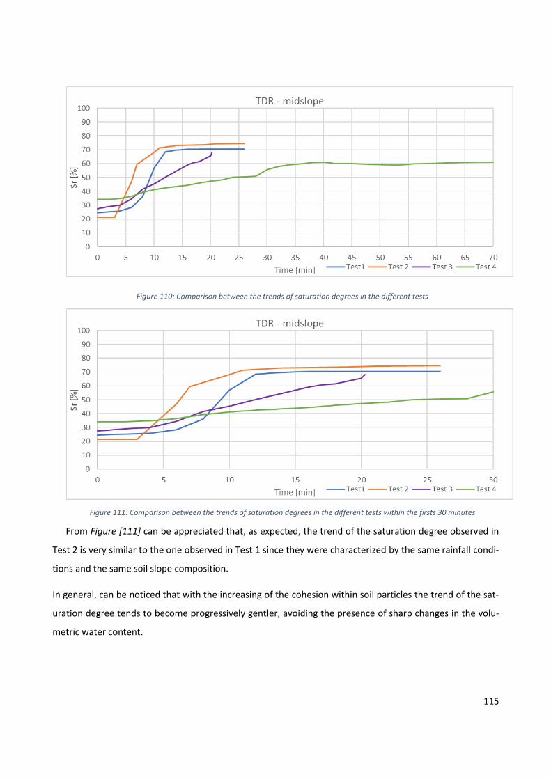
115

Figure 110: Comparison between the trends of saturation degrees in the different tests

Figure 111: Comparison between the trends of saturation degrees in the different tests within the firsts 30 minutes

From Figure [111] can be appreciated that, as expected, the trend of the saturation degree observed in

Test 2 is very similar to the one observed in Test 1 since they were characterized by the same rainfall condi-

tions and the same soil slope composition.

In general, can be noticed that with the increasing of the cohesion within soil particles the trend of the sat-

uration degree tends to become progressively gentler, avoiding the presence of sharp changes in the volu-

metric water content.

116

4.5.4 Displacements of the monitoring points

Considering the displacements of some predefined points along the slope obtained from the four differ-

ent tests, after the processing of the images acquired by the action cameras, some important observations

and verifications could be carried out.

A first common consideration that is observed in all the displacement trends recovered in the different

tests is that few seconds after a crack’s formation, the velocity with which the monitored point was moving,

increased progressively with the occurrence of other cracks.

Considering the following table and figures, starting with the analysis of the displacements of the points

downslope monitored in Tests 1, 2 and 4, the first thing that can be appreciated is that, as expected, the

duration and values of the displacements recovered form Test 4 were different from the ones recovered

from Test 1 and 2, mainly due to the different soil conditions and rainfall intensities that have been imple-

mented in the different experiments.

In fact, while in the slope of sand used in Test 4 no significant displacement have been observed before

the collapse of the point, in the slopes composed by alternating layers of sand and gravel, the point pro-

gressively moved away from its original position until, close to failure, its displacement rate exponentially

increased.

Another significant difference that can be noticed is in the trend of the velocity assumed by the point

during the experiments of Test 1 and Test 2. In fact, while in Test 2 the point moved away progressively

faster as fractures occurred, in Test 1 some great displacement rates have been observed much before the

occurrence of the cracks, and then peaked upon failure. These early increments in the velocity that deter-

mined in their turn great relative displacements, were the results of the moderately rapid increment in the

volumetric water content detected by the TDR probe some instants before.

The largest displacement of the point monitored downslope that was observed before failure was, in

both Tests 1 and 2, approximately of 5 mm. Moreover, in Test 2 also a runout distance of about 33.5 cm has

been recovered from the pictures acquired.

Without considering the displacements observed in Test 2 after failure, even though the point reached a

much higher velocity during Test 2, the average displacement rate resulted to be quite comparable to the

one of Test 1. This can be explained considering the contribution given by the movements of the point reg-

istered in Test 1 during the saturation of the slope.

117

Table 13: Analysis of the downslope point displacements observed in the tests







Figure 112: Comparison between the displacements observed for the downslope point in the tests

test 1 2 4

16.2 18.5 -


20.7 23.1 30.2

(after 9° crack) (after 4° crack) (after 6° crack)

d_max [mm] 4.0 334.9 0.9

Δs_max [mm] 1.2 4.9 0.4

v_max [mm/min] 2.4 29.5 1.6

v_av [mm/min] 0.4 0.7 0.3

point downslope

t_0 [min]

t_f [min]

118

Figure 113: Comparison between the differential displacements observed for the downslope point in the tests

Figure 114: Comparison between the displacement rates observed for the downslope point in the tests

119

Looking from a macroscopic point of view at the displacement trends of the point located in the middle

part of the slope monitored during Test 1 and Test 2, can be noticed that the points behavior was quite

similar since in both cases was observed a linear displacement of the point at an approximately constant

velocity that progressively increased approaching failure and, as a consequence, also differential displace-

ment exponentially increased (Table [14], Figures [115], [116], [117]).

However, there is also a difference that can be appreciated regarding the displacement rates since the

displacement curve observed in Test 1 is gentler and more regular than the one observed in Test 2. This is

reflected in the plot of the velocities where a linear increment in the acceleration was observed in Test 1,

while, close to failure, in Test 2 the point has been subjected to a sharp increment in the acceleration.

The largest displacement reached by the point in midslope before collapsed was about 5.2 mm and was

observed in Test 2. Moreover, in Test 1 also the runout distance of about 8.7 mm has been recovered from

the pictures acquired by the cameras.

Table 14:Analysis of the midslope point displacements observed in the tests







test 1 2

24.6 8.5

(after 15° crack) (during saturation)

26.3 26.8


d_max [mm] 2.7 5.2

Δs_max [mm] 0.4 0.6


v_av [mm/min] 0.3 0.3

t_0 [min]

t_f [min]

point midslope

120

Figure 115:Comparison between the displacements observed for the midslope point in the tests

Figure 116: Comparison between the differential displacements observed for the midslope point in the tests

Figure 117: Comparison between the displacement rates observed for the midslope point in the tests

121

In Test 3 the only point monitored during the laboratory experiment was the one located in the upper

part of the slope.

From the comparison of the movements showed by that point in Test 3 and Test 4 a first evident differ-

ence can be appreciated regarding the entity of the displacements recovered since, while in the first case

much larger displacements have been detected before collapsed, in the second case any significant dis-

placement was reached by the considered point (Table [15], Figures [118], [119], [120]). This is could be ex-

plained making the hypothesis that in Test 4, differently from Test 3, the very upper part of the slope

wasn’t involved in any failure mechanism. Unfortunately, this couldn’t be verified by the visual interpreta-

tion, since, in both tests, lasts images available pictured the situation much time before failure.

Another important difference that can be noticed is about the displacement rates with which move-

ments occurred. In fact, if in Test 4 since the beginning the monitored point continued to oscillate around

its original position with an almost constant velocity, in Test 3, instead, after a progressive linear displace-

ment that lead the point 1mm away from its original position, it followed a quiescent phase in which the

monitored point continued to oscillate with a relatively small velocity for almost 20 minutes. After that, as

the fractures continued to advance upstream, the displacement rate rapidly increased and peaked upon

failure taking progressively the point about 3.5 mm far away. This could be mainly attributed to the differ-

ent soil materials that constituted the slopes, whose mechanic properties greatly influence cracks propaga-

tion along the landslide and the propagation of the water front from the surface to depth in the slope. The

minor cohesion given by the presence of the gravel in the slope of Test 3, in fact, represent a favorable

condition for instabilities even at the surface level.

However, overall, the average and the max displacement rates in both tests were very similar as well as

the maximum relative displacements detected.

Finally, as imagined, at least for Tests 1,2 and 4, it was demonstrated that, independently by the slope

composition, in the lower part of the landslide the soil is subjected to larger displacements before collapse.

This is essentially due to the fact that downslope collapses were usually anticipated by some liquefaction at

the base, obtained as a result of the increasing moisture content that progressively decreased the soil

strength, suggesting a typical flow-like landslide behavior. Instead, the upper part of the slope often exhib-

ited sudden failure and only negligible surface displacements were recorded.

122

Table 15: Analysis of the upslope point displacements observed in the tests







Figure 118: Comparison between the displacements observed for the upslope point in the tests

test 3 4

19.1

(at 1° crack)

51.0

(after prop. 8° crack)

d_max [mm] 3.5 0.6

Δs_max [mm] 0.2 0.3


v_av [mm/min] 0.2 0.2

point upslope

t_f [min]

t_0 [min] -

-

123

Figure 119: Comparison between the differential displacements observed for the upslope point in the tests

Figure 120: Comparison between the displacement rates observed for the upslope point in the tests

124

4.5.5 AE signals results

The fiber-optic detection system reported bursts of events that were interrupted by short quiescent

phases that reflect respectively when the interferometric system recorded or not phase differences be-

tween the signals coming from the sensing and the reference fibers.

Among all the spectrograms recovered in the different tests, in most of the cases, it was observed that

cracks were in general preceded or by a small number of punctual very powerful events or by a large num-

ber of moderately strong events whose intensity increased with time and often peaked close or upon fail-

ure.

Moreover, in general, it was noticed that an intense AE activity continued also after failure since during

the mass release a decay of the AE rate and capping of event amplitudes were often observed.

From the comparison of the fiber optic detection system with the TDR sensors and the monitored dis-

placements of specific points on the slope surface, it was noticed that sometimes AE trends did not perfect-

ly follow the trends of these monitored quantities, but preceded them or occurred independently from

them.

As expected, the optical sensors whose coil was installed downslope were the ones who recorded signif-

icant signals even at larger frequency bands firsts, followed by the optical sensors whose coil was installed

midslope and upslope.

However, it can be noticed that in Test 3 and Test 4 optical sensors installed in the middle part of the

slope started recording significant signals at since the beginning of the test. In Test 3 this could be justified

assuming that the arrival of the water at the level of the embedded coil in the middle part of the slope de-

termine a redistribution of the internal stresses within the soil that act on the sensing fiber providing some

strains and, as a consequence, some phase differences. Furthermore, this assumption can be strengthened

making the hypothesis that nozzles coming from the sprinklers are more directed to the middle part of the

slope so that water can be firstly sensed by the midslope coil. The fact that water tends to accumulate on

the surface first and then to progressively filter deeper in the slope and the rapid increment in the water

content detected by the TDR probe in the first part of the experiment, contribute to support this assump-

tion. Since that phenomena was noticed in the spectrogram of “signal 2” recovered in Test 4 as well, the

hypothesis that this was related to the configuration with which the rest of fiber cables have been installed

has been discarded. Instead, the different soil slope materials and compositions, and therefore the differ-

125

ent infiltration processes, seemed to represent the most probable reasons. In fact, in Test 1, even though

the cables of sensors installed midslope and upslope protrudes out of the soil body as well as in Test 3, only

signals with very low amplitude have been recorded before cracks formation because in Test 1 the slope is

made of alternating layers of sand and gravel and, being the superficial layer of sand less permeable than

the soil made of sand and gravel mixture used in Test 3, the water front in Test 1 proceeded deeper slower

and didn’t reach the gravel layer, in which the coil was installed, before fractures formation.

In Test 4 the AE signals observed in the spectrograms of signal2 and signal3 since the beginning of the

experiment, as already mentioned before, can be justified considering the hypothesis that some damages

could eventually occurred to the fiber optic cables during the installation. In addition to this, some noise

can be noticed in the spectrogram of signal 2, that could be attributed to the presence of finer materials

that represent an unfavorable condition for the propagation of AE signals and high intensities are common-

ly attenuated.

Another possible reason that can be considered as a justification for the early detection of AE signals in

both, Test 3 and Test 4, is the fact that coils were embedded in slopes characterized by uniform layers so

that, since the beginning, the stresses related to the increasing weight of the overlaying layers with the

progressive saturation of soil, could probably act on the sensing fiber providing, as a consequence, some

strains even in the firsts minutes, when the volumetric water content was still relatively small. Differently,

in Test 1 and Test 2 the coils were embedded in the gravel layer so that a sort of attenuation of the stresses

due to the saturation of the overlaying layer of sand have been probably provided by gravel layer thanks to

its larger soil particles size.

Here are listed the analyzed features in the different spectrograms:

t_0 [min]: starting time for the detection of signals Δt [min]: time interval of signals' detection

t_f [min]: time of stop monitoring t_mps [min]: time at which the most powerful signal has been sensed

signal Freq [low,medium,high]:

signal frequency - (visually interpreted on the base of the n° of high intensity punctual signals and of windows of moderately strong signlas)

A_max [dB]: Maximum signal's amplitude detected

126

Downslope fiber optic sensor’s signal:

signal downslope

test 1 2 3 4

t_0 [min] 26 17 18 18

t_f [min] 29 25.5 30 28.6

Δt [min] 3 8.5 12 10.6

t_mps [min] 26.3 20.6 19.2 26.6

A_max [dB] 70 80 50 60

signal Freq medium medium low low

Figure 121: Spectograms and analysis of signals recovered in the different tests from the sensor installed downslope

TEST 4 – signal 1 TEST 3 – signal 1


127

Midslope fiber optic sensor’s signal:

signal midslope

test 1 2 3 4

t_0 [min] 24 18 21.5 start

t_f [min] 28.3 25.5 30 30

Δt [min] 4.3 7.5 8.5 30

t_mps [min] 28.3 22.1 27.8 26.6

A_max [dB] 60 60 60 40

signal Freq medium medium medium high

Figure 122: Spectograms and analysis of signals recovered in the different tests from the sensor installed midslope



128

Upslope fiber optic sensor’s signal:

signal upslope

test 2 3 4

t_0 [min] 23 26.5 start

t_f [min] 25.5 30 30

Δt [min] 2.5 3.5 30

t_mps [min] 24.3 28.6 22.8

A_max [dB] 50 50 40

signal Freq medium low high

Figure 123: Spectograms and analysis of signals recovered in the different tests from the sensor installed upslope


TEST 2 – signal 3

129

Excluding the spectrogram of signal 1 recovered in Test 1 by the fiber optic disposed longitudinally along

the slope, in the previous tables and figures, it can be observed that acoustic emissions were more fre-

quently sensed by the coils installed in midslope since in all the conducted tests, the formation of the frac-

tures mostly involved the lower and the middle part of the landslides. In particular, in the firsts 30 minutes,

fiber optic sensors detected the largest amount of AE signals during Test 4, even though most of them only

at very low frequency bands, probably due to the sand soil material in which cables run. This implies the ac-

cumulation and the release of a large amount of energy within the slope that is in accordance with the enti-

ty of the collapses analyzed during the visual interpretation.

Instead, in the sand and gravel mixture slope employed in Test 3 much less AE signals have been propa-

gated. This will imply that less energy was accumulated during the experience within the slope with respect

to the other tests. On one hand, this could be in part demonstrated by the restricted number of cracks that

have been identified, but, on the other hand, it could be disapproved considering the great amount of soil

material that collapsed recovered from the visual interpretation.

The most powerful AE signals have been recorded during Test 1 and Test 2, while the AE signal with the

lowest amplitudes have been recorded during Test 4. This is a confirm that in coarser materials, like gravel,

AE signals propagate with higher intensities without being attenuated as occurs in finer materials like sand.

Intermediate values of amplitudes characterized the AE signals recorded during Test 3 that propagated

within a slope made of sand and gravel mixture.

Considering the spectrograms of signal 2 recovered in Test 1 and in Test 2, whose coils were embedded

in the same soil slope composition but with a different configuration reserved for the rest of the cables, it

was noticed that in the second experiment the coil installed midslope started detecting AE signals few

minutes before than in Test 1, as a demonstration that the collapse mechanism was slightly faster in the

second test with respect to the first one.

However, once that the soil in which the coil was embedded collapsed, while the coil, whose cable run

within the soil slope in Test 1, still recorded some signals even after its exposition, the coil, whose cable

protruded out on the surface of the slope in Test 2, it suddenly stopped functioning.

130

4.6 Final and General Observations

The results obtained from the experimental tests provided an insight into some hydrologically triggered

landslides in different material soil deposits.

Overall, the progressively saturation of the soil together with a series of high intensity signals recorded

by the fiber optic sensors and the monitored displacements detected before the collapse, represent relia-

ble warning signs able to anticipate the imminent formation of cracks and the consequent failure of the

slope.

The hydrological results recovered by the TDR probe, were compatible with the hypothesis that after

the accumulation of water on the surface of the slope, the water front progressively penetrate in depth. In

fact, this phenomena is quite common in correspondence of fast and intense rainfall events, such as the

ones that were artificially applied on the different slopes during the experiments in order to minimize time

to their failures.

Given that it was demonstrated that abrupt increments in the saturation degree represent a reliable

warning of imminent landslide and considering, therefore, the hypothesis that failure was induced through

the water application by the simultaneous increment of the bulk density in the upper part of the slope and

the decrease of the effective stress at the level of the channel floor after saturation, the retrogressive fail-

ure behavior observed in Test 1 and in Test 2, suggests the localization of the shear zone at the interface

between the layer of gravel and the less permeable layer of sand below, while the rotational mechanisms

observed in the uniform sand slope in Test 4 suggest the localization of the shear zone at the material base.

In Test 3, given the slope composed by a unique stratum of sand and gravel mixture, a shear surface at the

channel floor can be assumed.

In general, it was observed that the monitored displacements of the predefined points were consistent

with the respective trend of the saturation degree and with the visual analysis.

Another common observation that was appreciated in all the performed tests was that saturation de-

gree started increasing much earlier the crack formation, followed by the detection of AE signals and only

after the occurrence of the fracture some negligible displacements were recorded, while AE signal ampli-

tudes still continued to be significant.

131

However, as anticipated at the beginning of the work, this study was mainly focused on the distributed

fiber-optic acoustic emission detection.

From a macroscopic point of view, the AE events captured by the fiber optic sensors are aligned with the

observations from the crack formations and with the displacements recovered by the pictures collected by

the action cameras and with the hydrological monitoring.

According with Michlmayr (2016), the decision to arrange fiber cables in coils on one hand allowed to

create “virtual” sensors that, averaging over individual channels, enhanced signal-to-noise ratio and greatly

improved the quality of the data, on the other hand it makes hard to determine the signal directionality

and prohibits advanced signal analysis.

However, it must be kept in mind that, during the averaging procedure could be also possible to average

out localized events.

From the analysis of the spectrograms recovered from the signals recorded by the coils of the fiber optic

sensors differently installed in the tests, it was observed that the progressive failure of the slope generates

acoustic emissions that are detected well before slope failure.

In fact, from the comparison between the monitored displacements and the recorded AE signals, can be

observed that in most of the cases the trends of the recorded AE signals with higher amplitude didn’t follow

or resembled the trends of the cracks occurrence or of the displacement rate increments, but in general

preceded them, in some cases, even more than one minute in advance.

In general, in the performed tests it was demonstrated that significant acoustic activity can be sensed

even before the monitored surface displacements. This means that also the acoustic emissions related to

the erosion and to the transport of an internally erodible granular soil fraction have been recorded by the

fiber optic sensors making this technology sensible even to particle-scale events.

Moreover, from the comparison between the visual analysis of the fractures and the spectrograms, it

was noticed that the amplitude of the AE signals usually tends to increase approaching failure.

This is reasonable because to an increase of the amplitude of the AE signals corresponds an increase of

cumulative energy released from the soil, due to internal erosion and to the structural rearrangement, that

leads successively to failures and surface displacements. However, in the present study, the deformations

132

to which the sensing fiber was subjected couldn’t be quantified since preliminary calibration tests should

have been performed before.

Nevertheless, it was demonstrated that the cumulated acoustic energy and pre-failure values of cumu-

lated energy related to powerful punctual signals, can be calibrated on field observations and serve as ear-

ly-warning thresholds.

In fact, since it was proved that to high intensity signals recorded in the spectrograms followed consid-

erable collapses that leaded to significant displacements, from the amount of energy cumulated in the time

interval preceding the crack it would be possible to have an idea of the entity of the collapse.

Furthermore, from the comparison of the spectrograms of signals acquired by optical sensors placed in

different parts of the landslide, as it was proved in the experiments, it is also possible to have an idea of the

distance at which the crack will probably occur with respect to the coil location since for each spectrogram

the higher is the intensity of the signal detected, the closer will be the crack to the point in which is in-

stalled the corresponding coil.

However, this could be a reliable early-warning method at least for coarser soil slopes, since it was

proved that in finer materials high intensity AE signals suffer important attenuations even at close distanc-

es. In addition to this, as reported in the paper written by Hu et al. (2018), this attenuation might become

even stronger when, with the soil becoming progressively saturated hydrologically triggered failure is ap-

proaching.

Therefore, the implementation of this premonitory method in densely packed soil slopes is not really

recommended and other strategies might have to be devised.

In principle, this problem can be solved by a dense network of sensors, but ambiguities would remain on

source localization and event size, and installation and management costs could limit its applicability (Dixon

et al., 2015).

Regarding the kind of installation for rest of the fiber optic cable in the slope, since they showed to be

resistant even at large deformations, the configuration in which cables were let run within the soil and pro-

trude from the upstream end of the soil body resulted to be more efficient because, in general, it allows

some overlapping between the signals in the spectrograms of subsequent coils installed along the slope,

reducing in this way the margin of error related to the AE measurements.

133

Overall, from a practical point of view, the application of a distributed fiber optic network for the moni-

toring of AE signals has shown several advantages. First of all, it can be appreciated the fact that the cables

used were relatively cheap and robust. In fact, despite the large strains to which they were subjected, they

preserved full functionality until their collapse, so that it was possible to re-use them. Another positive as-

pect that was appreciated is that distributed technologies provide a very large amount of data with high

resolution.

However, the latter, represents also a weakness of the distributed fiber optic application when the la-

boratory experiments, conducted at controlled conditions, are upscaled to full-size applications in field,

since at the present, according with Mychlmayr (2016), one of the largest challenge that have to be face is

the real time handling of the large data streams that is provided by this system.

As also reported later in the previously mentioned paper (Mychlmayr et al.,2016), it was also disclosed

that, if based on specifically designed microprocessors (e.g. embedded processors), the development of a

real time data processing is technologically feasible.

The acquisition of distributed data also allows to adjust alarm thresholds with a margin of flexibility even

after the cable installation making, at least for coarse soil slopes, the distributed fiber optic technology

based monitoring system a reliable and convenient landslide early-warning solution.

Given that, even though expeditiously, a lead time analysis has been interesting to be performed.

For this purpose, the average, the maximum and the minimum time intervals between the detection of

the firsts significant signals and the following cracks have been approximately calculated in order to have

an idea of the impact that the different soil slope compositions and the different fiber cable configurations

could have on the temporal monitoring scale.

In Annex C are reported the computed lead time intervals for each signal in the different tests.

As it can be observed in Figure [118], from the comparison between the time intervals recovered in Test

1 and Test 2, conducted on the same soil slope composition of alternating layers of sand and gravel, the

configuration for which fiber optic cables run within the slope, used in Test 2, seemed to represent a more

favorable strategy since not only allowed an earlier detection of the signals everywhere along the slope,

but also anticipate the crack formations with an average time interval of about 30 seconds and a maximum

lead time of more than 1 minute (100 s). This can be explained considering the advantages of the distribut-

ed fiber optic AE acquisition configuration that allows a continuous detection of elastic waves along con-

134

secutive sections of the optical cable providing a larger spatial coverage with respect to the configuration in

which the cables protrudes out on the body surface.

According with Michlmayr (2016), a 100 s lead time is likely to be too short for practical uses, but, con-

sidering the rapid hydromechanical loading adopted in the test and the distinctive acoustic signatures,

these results are encouraging. In fact, under realistic circumstances the time scale of the failure process is

likely to be much more extended (Michlmayr, 2016).

Instead, from the comparison between the lead time intervals observed in Tests 2 and 4 (Figure 119), in

which the same distributed configuration of fiber optic cables that run within the slope have been imple-

mented, even though different collapse mechanisms have been triggered in the different soil slope materi-

als, only slight differences could have been appreciated. This might suggest that at the time scale the soil

slope composition is less influent on the signal detection with respect to the installed cable configuration.

From a macroscopic point of view, from the comparison of the lead time intervals observed for each of

the three signals collected in all the tests respectively, it was noticed that in Test 4 failures have been antic-

ipated by signals detected averagely earlier demonstrating that lead time increases in slopes with larger ini-

tial soil moisture.

However, it must be remarked that this was a very rough analysis because it was mainly based on the

visual interpretation of the spectrograms provided by the fiber optic monitoring system.

Figure 124: Comparison between the lead time intervals observed in Test 1 and Test 2 – (D:Downslope; M:Midslope; U:Upslope)

135

Figure 125: Comparison between the lead time intervals observed in Test 2 and Test 4 - (D:Downslope; M:Midslope; U:Upslope)

In general, from the analysis of the results obtained from the different monitoring systems installed on

the slope, a great consistency has been appreciated. In particular, in all the experiments conducted, almost

the totality of the different failures that occurred have been effectively sensed by the fiber optic interfero-

metric system through the detection of a series of AE signals with increasing intensity approaching the soil’s

critical condition together with the formation of the fracture and the following slope collapse.

For the purposes of the present study’s analysis it was more interesting focusing on the trend of the

physical quantities monitored by the traditional instruments rather than on the exact values, in order to

understand when possible deformations could occur. Instead, the analysis of the spectrograms of the AE

signals recovered from fiber optic system was mainly focused on the identification of punctual high intensi-

ty signals or series of subsequent significant signals.

Finally, it must be remarked that, even though the results obtained from the different monitoring sys-

tems showed a good consistency with each other, the present analysis has been strongly influenced by the

visual and graphical interpretation given by the operator so that several approximations have been consid-

ered and, in addition to this, it must be keep in mind that the experiments have been conducted on small-

scale slope models with a limited depth of just a few centimeters (15 cm), while on site shallow landslide

usually extend for a few meters deep in the slope (in the order of the meter and in general no more than

5m).

136

Finally, in order to understand the reliability of the results obtained from the present laboratory tests, a

quick comparison with the results obtained from the Michlmyar’s experience has been performed.

However, even though a similar rainfall-induced landslide has been reproduced on an inclined chute and

monitored with similar traditional instruments, some non-negligible geological, technical and technological

differences were present. The first important difference concerned the soil material that was used to cre-

ate the slope since Michlmayr et al. considered five layers (of 0.05 − 0.10 m) of homogeneous gravel soil

while in the present experiments, in the firsts three tests, sand and gravel has been differently implement-

ed in three layers while in the last test uniform sand has been used. Other significant differences regard the

dimensions of the slope models, the inclined angle to which the chute was tilted and the intensity of the

artificial rainfall event. In fact, in the experience of Michlmayr et al. a first short intense simulated rainfall

event of approximately 30 mm has been applied before taking the chute, that held 0.6 − 0.7 m3 of soil ma-

terial, to an inclination of 26° and, after having waited for 5 minutes, they applied a second intense precipi-

tation (approx. 5 − 7 mm/min) to induce slope failure. From the technological point of view, in the experi-

ment of Michlmayr the same traditional monitoring systems have been implemented, with in addition

some piezoelectric sensors, and the same fiber optic technology based on interferometry has been consid-

ered. Even though, similarly the fiber optic cable have been coiled up, nine focal spots have been distribut-

ed longitudinally within the slope in three layers, in order to have three coils disposed at three different

depths while in the present experiments only three coils have been considered, embedded at the same

depth inside the slope, but different configurations have been tested for the rest of the fiber cables. Fur-

ther details of the Michlmayr et al.’s experience (2016) are reported in the table of Annex A in the column

[31].

Despite all the differences noticed between the two laboratory experiences, especially from the analysis of

Test 2 in which a shallow landslide has been artificially triggered on an alternating layered slope of sand and

gravel and in which coils were installed in the coarser gravel layer, very similar values of lead time intervals

before landslides has been estimated, strengthening, therefore, the general reliability of the present analy-

sis.

137

CONCLUSIONS

This experimental study investigated the potentiality of a quasi-distributed fiber optic technique based

on acoustic emission measurements to monitor crack activity during the deformation process of progres-

sive rainfall-induced landslides in flume tests.

At the beginning the fiber optic technology and its functionalities have been introduced, followed by the

analysis of the different experiences, both laboratory conducted and/or on field, in which this kind of tech-

nology has been variously implemented and tested in the geotechnical field demonstrating, in the majority

of cases, it’s reliability as a monitoring system for slope stability.

Given the level of progression of the fiber optic technology and an idea of its applications in the differ-

ent experiences in the geotechnical field, the set-up of the present laboratory flume tests have been illus-

trated and, successively, the analysis of the obtained results with the relative discussion have been con-

ducted.

Artificial shallow landslides were triggered on four slope models prepared with different soil composi-

tions through progressive water saturation. As a consequence, different behaviors have been observed:

some of them exhibited fluid-like landsliding and others sudden failures.

Together with the traditional monitoring systems regarding the imagery acquisition and the monitoring

of the hydrological conditions and of the surface displacements, the mechanical interactions within the soil

particles during the landslide process were tracked with the detection of the acoustic emissions released

through the quasi-distributed fiber optic technology.

Therefore, the volumetric water content, the visual interpretation, the displacement, the velocity and

the AE data were obtained from the four experiments and compared.

The primary goal of this analysis was to assess the feasibility of AE fiber-optic based acquisition tech-

nique for landslides early-warning in the different soil slope compositions.

Even though in all the four cases it was demonstrated that monitoring systems based on distributed fi-

ber optic technology can accurately detect failures, it was verified that this system is not very suitable for

138

soil slopes made of finer granular materials, like sand, because high intensity signals at higher frequencies

would be attenuated, while it is well recommended for soil slopes made of coarser granular materials.

From the analysis of the spectrograms it was noticed that, in general, all the stages in which the land-

slides developed, from the slope toe collapse until to the final collapse, were preceded by correspondent

significant distinct AE signals or a windows of AE signals with increasing intensity with time. Furthermore, a

linear relationship was observed between the amount of the energy cumulated before the crack and the

entity of the following collapse.

Therefore, some characteristic features of the landslide process typically observed in stratified coarser

soil slopes, like the single events related to the slope toe collapse or the material retrogressive failure,

could be clearly identified in the data recorded by the fiber optic sensors. Moreover it was also demon-

strated the ability of this kind of technology to detect signals related to acoustic emissions even released by

particle-scale events due to the rearrangement of the particles within the soil, like internal erosion or seep-

age-driven migration of the small-sized soil fraction.

Finally, the relationship between AE signal detected and the relative density of the soil material with the

different slope model compositions has been investigated remarking the potentially higher AE energetic

imprint of the coarser material.

In summary, through the comparison with traditional instrumentations, from this study it was demon-

strated that the interferometric fiber optic technique based on acoustic emission measurements may rep-

resent an innovative and more convenient method to be applied as a landslide early-warning monitoring

system especially suitable in less compacted soil slopes that exhibit fluid-like landsliding behavior.

Since this is an experimental work based on the application of the fiber optic technology as an innova-

tive monitoring system that is still being tested in the geological and geotechnical fields, further researches

and developments could be consider in the future in order to minimize noises and better understand the

great potentiality of this kind of technique so as implement it as a measure for risk reduction purposes.

At the real scale, this method should be applied to calibrate, through on field observations, the cumu-

lated acoustic energy and to establish a relationship between the detected lead time intervals and the enti-

ty of the following collapses. However, the on-site installation of fiber optic AE monitoring networks is not

an easy task since, according to Michlmayr (2012), these systems are hardly impacted by undesirable noise,

such as rain impinging on the soil surface, traffic noise or human activities, but at the moment there are still

139

other more practical issues that have to be solved each time, that spread from the most suitable fiber fixa-

tion within the slope and the most suitable depth to be put, to the most convenient monitoring period and

monitoring frequency. Therefore, on field, further research is necessary.

At the laboratory scale, it could be interesting try to define an objective method that will provide an ac-

curate estimation of the lead time. Furthermore, if possible, try to define the relationship between AE sig-

nals and the acceleration to which soil is subjected during slope deformation for the different soil materials

and composition, since are both good indicators of critical sliding. Different triggering factors could also be

considered, through the application of an artificial rainfall with time variable intensities. From the point of

view of the instrumentation, a piezoelectric AE transducers could also be installed in the slope for further

comparisons and validations with the optical fiber results, but also the possibility to apply other types of fi-

ber optic sensors could be evaluated in order to increase the sensibility of the measurements. From the

practical point of view, protective casings of different materials or alternative solutions for the protection

of the fiber optic cable could also be tested in order to find the best compromise between signals detection

and cable safety. Finally, with the changings of the boundary conditions of the landslide simulation, through

the application of the corresponding most suitable values for the characteristic parameters in the multita-

per function, analysis of different purposes could be carried out. For example, on larger-scale slope models

in which there could be very long time scale monitoring periods, data segments of larger size should be

considered, while for the monitoring of microevents, small data windows should be used and, in order to

maintained a low variance estimation, the frequency resolution should be sacrificed.

In general, this successful laboratory analysis would encourage in future larger scale testing verifications

of this fiber optic technique and on its field application.

In conclusion I can say that, thanks to the peculiar intermediate features of the quasi-distributed fiber

optic technology that allow to pass from the pointwise monitoring, typical of the traditional instrumenta-

tions, to the monitoring of a spatial measurement array without being so expensive as the purely distribut-

ed sensors, in my opinion this non-destructive technique based on the detection of the acoustic emissions

represents a good compromise for slope stability investigations, in terms of temporal and spatial resolution

and in terms of time consumption for data processing.

Given that the analysis and the interpretation of the results obtained from the four different tests were

strongly operator related, from my point of view the best conditions for the monitoring of landslide evolu-

tion processes through the implementation of the fiber optic interferometric technology have been found

140

in the slope of alternating layers of sand and gravel, with the lowest initial moisture condition, realized in

Test 2. Furthermore, the strategy adopted for the optical sensors’ installation, for which the fiber optic coils

have been embedded in the more coarser gravel layer while the rest of the cables were let run within the

slope and protrude from its upstream end, has shown to be the most efficient solution for the monitoring

of the acoustic emissions released from the mechanical interactions and from the damage accumulation

during retrogressive failure of this kind of slope. In fact, thanks to this particular solution, spectrograms

with an enhanced signal-to-noise ratio can be recovered, in which clear punctual powerful signals and se-

ries of signals, with increasing amplitude with time approaching failure, can be clearly identified even, ap-

proximately, one minute before the formation of the fracture with a sort of overlapping between signals of

consecutive installed optical sensors, improving the reliability of the analysis.

Therefore, since, at least at the small-scale, it has been proven that this kind of method can provide

more timely alarms that will allow to evacuate people probably involved in shallow landslides and saving

more lives, I strongly believe that, in the future, after many further laboratory and on field investigations,

this innovative strategy will likely to be implemented on real-scale as a winning strategy for risk mitigation.

141

ANNEXES

ANNEX A: Table of the analyzed papers available in literature

ID 1 2 3

Year 2002 2004 2006

Authors Yoshida et al. K. Higuchi, K. Fujisawa, K. Asai, A. Pasuto & G. Marcato Ho et al.

Journal Smart Structures and Materials 2002: Smart Sensor

Technology and Measurement Systems

A joint research project carried out between the Public Works Research Institute in Japan and Institute di

Recerca per la Protezione Idrogeologica, Consiglio Na-zionale delle Ricerche in Italy

Measurement science and technology

DOI https://dx.doi.org/10.1117/12.472632 http://www.cnr.it/prodotto/i/88961

https://dx.doi.org/10.1088/0957-0233/17/7/011

Country Japan Japan Taiwan (China)

Application Inclinometer Soil-embedded sensor Inclinometer

Specify appli-cation

Modular inclinometer-like device 2 lines with 18 sensors in total set up in parallel and installed in the direction of the landslide movement

Segmented device to be inserted in a conven-tional inclinometric tube

Technology FBG OTDR FBG

Specify tech-nology

in series - One set of the Borehole Inclinometer consists of 5 elastic joints at a distance of 1 m; all FBGs installed in each set are fusion-spliced in a fiber; The transducer

consists of series of unit-bars connected each other with elastic joints. FBGs were embedded on the elastic joints,and bending angles of each joint were measured

by FBGs. The transducer was set in a borehole;

distributed technology; installed at the end of the Takisaka Landslide facing the Aga River

in series

Landslide (monitored

phenomena) Embankment Takisaka Landslide Diaphragm wall

Specify Landslide

The slopes surround embankment located in western Japan (Project site of 400mx300m); embankment con-sisted in a layer of soft rocks named Kobe group (mud-stone, sandstone of Tertiary deposit) and a layer of soft

clay;

2.1 km long, 1.3 km wide, volume of the moving soil mass of 4.8×107m3, maximum depth of about 140 m;

made of granite, sandstone, tuff, mudstone, fluvial sediment, and colluvium sediment in order from the

lowest layer;

1.2 m thick, 15 m deep; The excavation side was 8.1m deep and covered a square area of

100 m x 100 m;

Application environment

Laboratory and on-site On site only Laboratory and on-site

Attached to a structure

no no yes

Material (backfill)

cement-bentonite mortar concrete

Depth (incli-nometer) /

Length/Area (distributed)

embankment: height= 43m; boreholes: depth_pipe1=22m , depth_pipe2=25m

φout=69mm Area_N.Block =250x600m Area_T.Block=200x50m depth= 14 m

Specify extent N° FBG sensors: pipe1=18 , pipe2=22

total length_FO= 4 km

Line N°1 : fiber_cable lenght=40 m with 8 sensors spacing = 5m

Line N°2 : fiber_cable lenght=50 m with 10 sensors spacing = 5m

φ_fiber_cable=2.8mm

Measurand strain strain strain

Monitoring period

4 months 9 months < 4 months

Specify period (frequency)

hourly

https://dx.doi.org/10.1117/12.472632

http://www.cnr.it/prodotto/i/88961

https://dx.doi.org/10.1088/0957-0233/17/7/011

https://dx.doi.org/10.1088/0957-0233/17/7/011

142

Calibration (yes/no) – additional monitoring

systems

yes --> conventional sensor installed along part of line N°1

yes --> 1) Strain calibration: conventional IP inclinometer spaced at 1m from the incli-

nometer casing for the FBG-SDs 2) Thermal calibration: by placing a unit of

FBG-SD in a temperature chamber where the FBG-SD was subjected to a change of tem-

perature from 0 to 40°C

Cost The cost is lower than other methods such as BOTDR, FBG and SOFO

Unspecified information

fiber installation inside the slope;

Additional notes

The transducer is composed of rigid pipes and elastic joints that connect rigid pipes each other. The rigid pipe

has hold pins at the both ends that fit the grooves of the casing-tube; plate and two small tubes: one for a

FBG and the other for passing fibers; FBG is fixed at the center of the tube filled up with adhesive; The hinge

plate supports the weight;

The slide face is near the boundary between the sand-stone and the tuff;

• A string of 11 FBG-SDs was inserted in one of the inclinometer casings;• FBG-SD consists

of a plastic rod (the flexible segment) that connects to two aluminium end pieces (the

rigid segments) that are equipped with wheeled braces so that the FBG-SD can be

fitted to the grooves in the inclinometer cas-ing; •Two FBGs are attached to the opposite sides of a the flexible segment to measure

the flexural strain;

conclusion &

results

The monitoring system proposed in the article worked correctly, and the availability of the FBG Borehole Incli-

nometer was proofed; Numerous advantages of FBG Borehole

Inclinometer against conventional electric systems has been pointed out such as: its ability of multipoint

measurement in a small diameter borehole, the light-ning impulse resistance, the unnecessity of power sup-

ply and capability of remote metering.

The tensile displacement has been detected but with an error of several mm, however the optical fiber and the

OTDR method are practical for monitoring landslide displacement in the field because behavior of landslides

can be understood more accurately and landslide blocks can be identified by installing several sensors in areas thought to be block boundaries ==> the sensor based on the OTDR method is more economical and

easier to use than those employing other methods and it was successfully tested at the Takisaka Landslide area under an international joint research program between

Italy and Japan.

The laboratory and field experiments indicat-ed that for the conditions applied, results

comparable to those of a conventional IP can be obtained with the new FBG-SD sensor and the interrogation system. Therefore, the FBG-based fibre optic sensor system is favourable

to be applied mainly for field geotechnical applications and in particularly for the moni-

toring of ground movement.

difficolties encountered

not specified

• monitoring errors caused by optical fiber cables; • Many data were missing, the cause of which was as-sumed to be the computer and/or OTDR monitor. This computer and/or OTDR trouble was identified in the

interruption of power supply in the system check

The measurement error in the FBG-SD deflec-tion angle at any given location is amplified with distance. Since the computation of lat-eral movement is based on deflection angles measured at the FBG-SD hinge locations, this drawback may limit the length of the FBG-SD

that can be used in the field.

143

ID 4 5

Year 2008 2008

Authors M. Iten et al. Chen et al.

Journal Smart Sensor Phenomena, Technology, Networks, and Systems 7th International Pipeline Conference, Alberta (Canada)

DOI https://dx.doi.org/10.1117/12.774515 https://doi.org/10.1115/IPC2008-64231

Country Switzerland China

Application Road-embedded sensor soil - embedded fiber optic cable

soil - embedded fiber optic cable

inclinometer soil - embedded fiber optic cable


An hand-coated optical fiber cable is embedded directly in a trench cut in asphalt along the road crossing the St. Moritz landslide bounda-

ry

FBG pipeline strain gages FBG earth pressure cells

4 Pipes strain gages with FBG sensors in-

serted into a borehole

buried concrete beams with FBG

sensors

Technology BOTDA FBG

Specify tech-nology

89m long fiber optic sensor; full-distributed and single-end detecting technology

6 FBG strain gages that are fixed on the surface of the steel pipe with a thin stainless steel pro-tective sheet; in each

cross section 3 longitudi-nally oriented strain gag-

es in the 90°-array are mounted in which a tem-

perature FBG sensor is mounted at 12 O'clock;

6 earth pressure cells mounted in corre-

spondance of the FBG strain gages on the surface of the pipe;

fiber cable with FBG sensors attached on the

surface of a PVC pipe;

corrugated steel bar with FBG

sensors lays in the center of the

section of the concrete beam;


phenomena)

road crossing the boundary of Brattas landslide Erlangmiao landslide in Sichuan province - China Specify

Landslide 1st trench in 2006) 89m long, 7cm deep and 1cm wide, cut in the as-

phalt 2nd trench in 2007)89m long, 9cm deep and 1cm wide, cut in the asphalt parallel about 10cm

besides the old trench

3 x 107 m3, lenght=1200m , average depth = 30m , average slope = 25° Application

environment on site only on-site experiment only


no yes - steel pipe yes - steel pipe yes - inclinometer yes - steel bar positined in the

center section of a concrete beam

Material (backfill)

epoxy adhesive + cold sealing compound grouted

Depth (incli-nometer)

/Length/Area (distributed)

trench_1: 0.7m deep, 0.1m wide trench_2: 0.9m deep, 0.1m wide

lenght_pipe= 1250 m depth_pipe = 1-1.5 m

FBG spacing = 100 - 50 m

lenght_pipe= 1250 m depth_pipe = 1 - 1.5 m spacing = 100 - 50 m

depth_#1 = 37m depth_#2 = 51m depth_#3 = 38m depth_#4 = 54m

FBG spacing = 0.5 - 5 m

lenght_1 = 153m lenght_2 = 135m

Specify extent

PVC inclinometer casing φest=80mm φint=70mm

Measurand strain and temperature strain and temperature stress, strain, tempe-rature

strain strain

Monitoring period

1st installation:7 months 2nd installation: 7 months

3 months Specify period

(frequency) every couple of months


systems

Cost


monitoring frequency; fiber fixation to the PVC tube; PVC tube connections; length of the PVC

tube segments

https://dx.doi.org/10.1117/12.774515

https://doi.org/10.1115/IPC2008-64231

144

Additional notes

• SC06 was then attached to the bottom of the trench by clips at eve-ry 2m along; • epoxy adhesive is used to fix the cable definitely at

every meter to the asphalt; • For manual integration by trained per-sonnel, these protected cables with less than 2 mm diameter seem to be sufficient. If heavy machinery is used to integrate the cables, other protection has to be applied; • road can be seen as a large scale strain

gauge: it was assumed that the road follows the movement of the ground ==> displacements in the road correspond directly to dis-

placements of the moving hillside.

conclusion &

results

In the presented case study a novel technique for the determination of a creeping landslide boundary was demonstrated by application of distributed optical fiber strain measurements using BOTDA technolo-gy; ==> The presented validation of this technology allows for a conclusion that distributed fiber optic strain sensing is a promising new tool in landslide surveil-

lance

The field experiments have demonstrated that this new system can be practical and provide ade-quate results to assess the pipeline integrity. In fact the 4 type gages can detect required defor-mation both of landslides and pipelines, so these systems based on FBG sensors can comprise a much more desirable system regarding the landslide and pipeline monitoring than the conven-

tional methods.


• At the end of 2006 cables failed and it was not possible to retrieve the 2006 cables and clean the trench so that a parallel trench was cut

beside and parallel the old trench; • Temperature measurements couldn't be repeated in Mai 2007, as the signal loss was already ex-ceeding the required level for measuring with BOTDA. Therefore, temperature compensation is not included into the results of the

strain measurements.

not specified

145

ID 6

Year 2008

Authors Hoepffner et al.

Journal Distributed Fiber Optic Strain Sensing in Hydraulic Concrete and Earth Structures Measuring Theory and Field Investigations on Dams and Landslides

DOI http://www.wb.bv.tum.de/fileadmin/w00boi/www/Publikationen/Berichtshefte/Band121.pdf

Country Germany

Application geotechnical reinforcement structure geotechnical reinforcement structure inclinometer soil-embedded


strain sensing cable installed on a rein-forced concrete beam; the cable went to

through the beam in 4 loops;

strain sensing cable installed on a rein-forced concrete column; the cable want through the beam in a loop configura-

tion

strain sensing cable installed vertically to evaluate the location of shear zones in the lower part of the landslide;

strain sensing cable installed close to the surface to monitor surface movements and for cracks moni-toring in the upper part of the landslide, starting just below the main scarp;

Technology BOTDR (DTSS) + FBG BOTDR (DTSS) BOTDR BOTDR

Specify tech-nology The cables in the compression side were

pre-strained and were attached to the rein-forcement steel with fast hardening polyes-

ter resin, while in the tension side the ca-bles were loosely attached to the steel bars with adhesive tape; 1 FBG sensor installed

in the middle of the beam on the bottom side, next to the strain sensing cable;

The cables in the compression side were pre-strained and were attached to the reinforcement steel with fast hard-

ening resin, while in the tension side the cables were loosely attached to the

steel bars with fabric tape;

strain sensing cable attached with tape to the outer surface of an inclinometer casing in a loop configuration; the cable passes the borehole twice, arranged at 90° around the inclinometer casing;

44m length of sensing cable placed in a 15 to 20 cm deep trench and additionally 23m of the same cable was loosely placed into the forest soil and, since no electricity or road access was present in that part of the landslide, the strain sensing cable was extended of about 300m towards the better accessible low-er part of the slope;


phenomena)

test site - for crack detection test site - for crack detection Aggenalm landslide, Bavarian Alps (Germany)

Specify Landslide

concrete bar placed on two rubber cush-ions on each end at the laboratory of the Technische Universität München in Ober-

nach

The column was placed into the precast foundation realized outside the labora-tory of the Technische Universität Mün-

chen in Obernach

Aggenalm slope is mainly built up by the “Kössen formation”, an alternating sequence of limestone and marl, and the overlying “Oberrhät limestone” – massive limestones and dolomites


Laboratory only Laboratory only on-site only Laboratory and on-site


yes - steel bars yes - steel bars yes - inclinometer casing yes --> small anchors driven into the soil at 1-3 m spacing

Material (backfill)

grout Trench filled up with the excavated material and compacted by hand



fiber_length = 40m fiber_length = 50 m depth = 22 m fiber_length = 62 m

trench : depth = 15 - 20 cm lenght = 370 m approx.

Specify extent Beam: length = 10 m width=30cm, height = 40 cm

Column: length = 8.6 m width=30cm, height = 30 cm

PVC inclinometer casing: depth= 22m length_fiber = 67 m approx.

Measurand strain strain strain strain

Monitoring period

4 hours 45 minutes some days


DTSS: every 4 minutes FBG: every 1 sec-ond

every 4 minutes reference measurement only taken in May 2008

reference measurement only taken in May 2008


systems

yes --> 3 ESG: 2 electrical strain gauges (ESG) attached to the reinforcement with fast hardening polyester resin in longitudi-nal direction and a third ESG was attached to the outside of the concrete beam just upon testing; A distance transducer was

installed in the middle of the beam to measure the deformation under load

yes --> 3 electrical strain gauges (ESG) attached to the reinforcement steel in the lower part of the column (2 on the tension side and 1 on the compression

side) about 1.8m above the ground

yes--> terrestric positioning system (TPS), GPS, coaxial cables for time domain re-flectometry (TDR), traditional inclinome-ter

Cost Unspecified information

diameter of the inclinometer casing and of the borehole; casing connection; mon-itoring period;

http://www.wb.bv.tum.de/fileadmin/w00boi/www/Publikationen/Berichtshefte/Band121.pdf

146

Additional notes

To achieve uniform pre-tension in the compression side, the cable was deflected on pulley wheels at one end of the beam; An empty water tank with a filling capacity of 2.2 m³ (total maximum weight ~ 25 kN)

was attached to the middle of the concrete beam and it was slowly filled until the fail-

ure of the beam (2 cycles of filling and empting were carried out)

The column was placed vertically into a precast foundation, with a depth of 1.4

m, creating a concrete column that sticks 7.2 m out of the ground; 4 rein-forcement steel bars were placed on

each edge inside a bent steel rein-forcement mesh to give basic strength to the structure; To apply load, a steel cable was also attached to the top of the column and the tensioning device was put at a distance of roughly 50 m, so that the load applied to the column

could be assumed to be horizontal; load on the column was increased in steps of

close to 500 N;

•The extended cable was embed-ded into a gel so that no strain could be transferred and to protect it form mechanical forces, it was placed in an arbored plastic tube; • For the calibration of the sensing cable, a cable piece of at least 5 to 10 m is spliced to the lower end of the extension cable and placed into a water bath next to the DTSS

conclusion &

results

The applicability of Brillouin based fiber optic strain sensing systems in concrete and soil, several installation and sensing concepts showed to work very well in terms of crack- and strain detection


• deformation below the spatial resolution of the strain sensing system - It could be shown that strain, which is applied in a 0.5 m section of a fiber cannot be measured at all ; • define the minimum section of cable that needs to be affected for accurate strain measurements.

147

ID 7 8 9 10 Year 2009 2009 2010 2011

Authors Wang et al. Lucio Olivares, Emilia Damiano, Roberto Gra-co, Luigi Zeni, Luciano

Piccarelli, Aldo Minardo, Andrea Guida, Romeo

Bernini

J. Li, R. Correia, E. Chehura, S. Staines, S.W. James

M. Iten

Journal

Landslides (2009) - © Springer-Verlag GeotechnicalTesting Journal,Vol. 32, No. 2

Proceedings of SPIE - The International Society for Optical Engineering: 4th

European Workshop on Optical Fiber Sensors · 8-10 September 2010, Porto,

Portugal

Thesis - ETH Zurich

DOI https://dx.doi.org/10.1007/s10346-008-0139-y Paper ID GTJ101366 https://dx.doi.org/10.1117/12.866334

Country China ( Nanjing) Italy (Campania)

UK (Cranfield University, Bedfordshi-re)

Switzerland

Application soil-embedded fiber optic sensor

soil-embedded fiber optic sensor

Inclinometer Soil-embedded sensor for landslide boundary

evaluation


the cable is embedded directly in soil as indicator for impending failure; sand (Xiashu soil)

the cable is embedded directly in soil (sand) as indicator for impending failure; cable glued to

1cm2 geogrids soil-embedded

Modular inclinometer-like device

trench-embedded sensor system consists of two parts: “micro-anchors” and optical cable; The

“micro-anchor” consists of three perpendicular planes

Technology BOTDR + OTDR

SBS (Stimulated Bril-louin Scattering)

FBG BOTDA

Specify tech-nology

5 lines of fiber sensors, distance between each line is 20 cm and length of each line is 1.5 m; In order to eliminate the effect of temperature, a loose-buffered fiber is planted at the height of each

above fiber sensors.

two 1m long strands of fiber placed parallel (20 cm distant) in longitudi-

nal direction

in series 80m long fiber optic sensor with "micro anchors" attached to the cable at every 2m; full-

distributed and single-end detecting technology;


phenomena)

slope simulator flume Brattas landslide, St. Moritz

Specify Landslide

1.5 m in width, 1.5 m in length, and 1.0 m in height; The stand is filled by Xiashu soil with every 10 cm

layer by layer; total height of the fillings is up to 70 cm; slope angle of 60°;

rainfall-induced flow-slides in pyroclastic soil;

the soil is laid on the flume in thin layers with a thickness of about 0.5

cm

creeping landslide


Laboratry only Laboratory only Laboratory Laboratory and on-site


yes - short-needled fabric geotextile / a type of glass-fiber geogrid

yes no micro anchors

Material (backfill)

sand



2 layers of geogrid with fiber sensors are laid at the height of 20 and 40 cm in the soil model slope; 1 layer of geotextile with fiber sensors is laid at the height of 50 cm of the model; 1 fiber sensor with

TPEE jacket is laid at the height of 60 cm;

max length = 1.90m max width = 0.50m max height = 0.50m

max slope = 65°

trench: depth=0.4m length=80m

Specify extent ABS inclinometer casing: L= 3m

φest=70mm with grooves at 90° L_fiber cable = 80m approx.

Measurand strain strain and temperature strain strain and temperature

Monitoring period

< 1 h (+/- 20 mins) 17 months


4 measurements 4 measurements


systems

yes --> Laser sensors

and Particle Image Ve-locimetetry System ,

digital camera

yes --> 4 dial gauges located in proxim-ity of the pair of FBG sensors

yes --> • 2 lab tests: 1) anchor failure test (longi-tudinal pullout) in the pullout box

2) full scale simulation of a shear zone in a large shear box; • cable without anchors was put for comparison and a loose tube cable was put for

temperature compensation;

Cost


time needed for the failure of the slope with the different loads

https://dx.doi.org/10.1007/s10346-008-0139-y

https://dx.doi.org/10.1117/12.866334

148

Additional notes

•The fiber sensors, including Types A and B, is af-fixed by Epoxy Resin on a geotextile layer; •The

monitor data obtained by BOTDR is recorded along this connected integral fiber at a designed distance (5 cm in this test). However, the maximum distance resolution of BOTDR is 1 m, which means it is diffi-

cult to locate the accurate position of the strain only from the monitor data obtained by BOTDR ==> another OTDR is used to locate the strain position. The measured signal for the OTDR is the Rayleigh backscattering which is not sensitive to strain but can monitor the powerloss and OTDR profiles are also very useful to localize breaks. • Pressures of 15, 20, 25, and 30 kN provided by a hydraulic jack are loaded step by step, and when the pressure is

greater than 30 kN, the slope failed

small geogrids are glued to the fiber in order to prevent relative move-

ments between the fiber and the surround-

ing soil

•2 FBG arrays -> 3 pairs of FBG sensors of 5 mm each and disposed at 0.5m distant one from each other; •FBG fixed diametrically opposite on the

ABS tube with cyanoacrylate adhesive; then the FBG arrays have been pro-tected with epoxy resin by covering

the entire lenght of the fibre; • deflection applied manually, in a

direction transverse to the axis of the inclinometer casing; • A tunable laser (Tunics-plus) was used to monitor the

Bragg reflection spectrum;

micro-anchors fixed to the cable with 4 screws

conclusion &

results

The test proves that the BOTDR technique can be used to ensure the stability of artificial soil slope and is useful for monitoring and early warning of the artificial soil-slope engineering since By data processing and analysis, the abnormal strains can be obtained distributively, and the position of the

abnormal strains can be located as well.

The flume is currently being used to evaluate the performance of a

TDR device and optical fibers to recognize,

respectively, the evolu-tion of the water con-tent profile and any

significant changes in the displacement field

in unsaturated soil slopes subjected to

continuous rainfall. The additional information provided by such low-cost instruments can

indeed be of great help for the rapid assess-

ment of flowslide de-velopment as well as to further clarify the phys-ical process leading to

slope failure

Laboratory based characterization showed that a fiber optic based incli-

nometer, developed by using fiber Bragg gratings attached to a conven-

tional inclinometer casing, can measure deflection accu-rately, with a resolution sufficient for the most practical applications, with

good agreement with theory and con-ventional displacement measurement

techniques

•the measured strain accurately represents the strain present in the soil; •“micro-anchor”-cable

system is more sensitive to local strain changes than the cable only; •The pre-straining was successful, as large negative strain can be

monitored; ==> The high sensitivity of the soil-embedded sensor leads to a possible application for site investigation purposes identifying poten-

tial hazardous zones quicker than conventional methods; ==> Since data acquisi-

tion in any season was possible, quasi year-round availability of field monitoring can be achieved;

==> Long term performance with no problems or breaks encountered


not specified not specified The deflection has been applied man-ually due to the limitations introduced

by the length of the bench

The goal of detecting a landslide boundary was not achieved because unfortunately, at project

planning, sufficient geodetical data was not available

and thus, the boundary was only a rough estima-tion.

149

ID 11 12 13 14 Year 2011 2011 2012 2012

Authors M. Iten Pei et al. Sun et al. Huang et al.

Journal

Thesis - ETH Zurich

J. Mt.Sc. (2011) Science Press and Institute of Mountain Hazards and

Environment, CAS and Springer-Verlag Berlin Heidelberg 2011

Hindawi Publishing Corporation, Journal of Sensors

Soils and Foundations - The Japanese Ge-otechnical Society. Production and hosting by

Elsevier B.V.

DOI https://dx.doi.org/10.1007/s11629-011-2038-2

http://dx.doi.org/10.1155/2016/9496285 http://dx.doi.org/10.1016/j.sandf.2012.07.013

Country Switzerland Weijiagou valley (China) Three Gorges Reservoir Area (China) Taiwan (China)

Application Borehole-embedded sensor for land-slide sliding surface detection

Inclinometer Inclinometer Inclinometer and piezometer


fiber-optic sensor installed inside an out-of-service inclinometer

Segmented device to be inserted in a conventional inclinometric tube

Modular inclinometer-like device Segmented device to be inserted in a conven-

tional inclinometric tube

Technology BOTDA FBG BOTDR FBG - IPI (In Place Inclinometer)

Specify tech-nology

in series full-distributed and single-end detecting

technology FBG piezometer arrays disposed in series

composed by 9 FBG sensors each


phenomena)

Brattas landslide, St. Moritz Weijiagou landslide Block1 of Majiagou landslide located in

Guizhou town of Zigui County deep seated landslide

Specify Landslide

the 2 boreholes were at about 40 m distance one from the other

It lies in the left bank of Zhaxi River; It is mainly composed of talus material and

residual deposit with loose structure and strong water permeability, the bedrock is

quartz sandstone or fine sandstone mixed with mudstone and a little silty

mudstone.

A section of Highway 18 at Five Turn Point - The slope area: approx. 1200 m x 1000 m

with about Δz = 400 m; 0–26 m of colluvial material underlain by interlayered

fractured sandstone and shale extended from below the colluvial to over 200 m below the

ground surface; Groundwater table could rise from its low level by more than 20m


Laboratory and on-site Laboratory and on-site on-site test only Laboratory and on-site


no no no no

Material (backfill)

cement-bentonite sandy-clay mixtures sand and bentonite



inclinometer casing: φext=71mm L=14.75m

depths: HA = 22m HB= 25 m

6 boreholes with depths: dB1=40 m dB2=38 m dB3=37.2m dB4= 42m

dB5=28.3m dB6= 14.2m

depth = 60 m

Specify extent L_fiber cable = 14m approx.

the block has a volume of 127.8 × 104 m3; The average slope of this landslide is

about 15°

φint=28mm thickness=4mm

Measurand strain strain strain strain and pore water pressure

Monitoring period

14 months 4 months 1 year and 4 months 10 months


3 measurements 10 measurements 6 measurements 6 measurements


systems

yes --> traditional inclinometer

yes --> rigid bar with a free end sub-jected to a displacement with 2 pairs of FBGs sensors adehered at oppo-site sides of the bar and 2 LVDTs;

yes --> traditional inclinometers were also installed to compare and validate

the results measured by the BOTDR based inclinometer tube

yes --> in a sealed chamber pressure: A pair of FBGs is fixed to the sides of the mass; The

mass is rotated away from verticality against the hinge --> FBG pair experiences elongation

strains in opposite signs but equal amount

Cost


fiber installation and fixation inside the inclinometer casing;

what was used to glue the fiber to the bar

- pipe connection - fiber connection connection of PVC pipes

Additional notes

•the cable was slightly pre-strained by attaching a weight at the sensor bottom;• No temperature compen-sation sensor was integrated, as it is

assumed that the temperature change in the ground is not signifi-

cant compared to the expected strain;• No indication about the di-rection of the displacement is ob-

tained in this measurement

• Two sets of FBG in-place inclinom-eters have been fabricated in labora-

tory; • the bars were connected using steel tubes with sliding wheels which allow the in-place inclinome-

ters to deform with the inclinometer casing installed on site.

•Tube of aluminum with φ= 75mm • Optical fibers were prestressed and then fixed on the surface of the tube with the glue of epoxy resin.• 4 optical fibers are installed on the surface of the test tube

at 4 orthogonal positions; •After the glue was solidified, the tube was protected with highstrength tape and shrink film

material to prevent the fiber from dam-age during the installation process.

•9 piezometers spaced at 5 m interval; •Small drainage holes were drilled in the PVC

pipe and wrapped with non-woven geotextile in areas surrounding the

piezometer to allow passage of water; •The piezometer was epoxied and sealed

at both ends in the PVC pipe to prevent seep-age between piezometers from

within the PVC pipe; • the FBG piezometer array, installed over 4 years ago, have contin-

ued to work until 2012

conclusion &

results

The horizontal displacements at the surface of the borehole are compa-

rable with the displacements ex-pected in that area and geodetically

measured displacements at the nearby leaning tower ==> this application is a cost-efficient and straightforward way to

reactivate old inclinometer pipes

Preliminary monitoring results show that the installed innovative sys-tems, that incorporates the FBG

in-place inclinometer and the FBG column-net, are able to detect inter-

nal movements of the slope. The overall deformation

behavior can be defined as shallow sliding. ==> The presented FBG in-

place inclinometer and the FBG col-umn-net system represent a new type of landslide and debris flow

monitoring systems.

the BOTDR based inclinometer can effec-tively access the internal deformation of the slope and help to find the position of

potential sliding surface accurately; The results

show that the BOTDR based inclinometer has a good consistency with the tradi-

tional inclinometer for the sliding zone with the

difference less than 4 mm, demonstrat-ing its high reliability and applicability.

The FBG piezometer array enables pore-water pressure profile measurements to be made at a selected location, along the borehole direc-tion => the FBG piezometer array based sys-

tem can predict the potential of an upcoming slope failure

https://dx.doi.org/10.1007/s11629-011-2038-2

https://dx.doi.org/10.1007/s11629-011-2038-2

http://dx.doi.org/10.1155/2016/9496285

http://dx.doi.org/10.1016/j.sandf.2012.07.013

150


no indication about the direction of the displacement is obtained in the measurements performed by fiber-

optic inclinometers

not specified

a limited number of boreholes could be performed => the distribution mode of sliding planes is potentially not very ac-

curate; however, it is consistent with the overall movement trend of the slope

not specified

151

ID 15 16 17 Year 2012 2012 2012 Authors Huang et al. Nother et al. Zhu et al. Journal

Sensors 2012 6th European Workshop on Structural Health Moni-

toring Smart Structures and Systems, Vol 9

DOI https://dx.doi.org/10.3390/s120505835 https://www.ndt.net/article/ewshm2012/papers/we2c4.pdf https://dx.doi.org/10.12989/sss.2012.9.5.393

Country Taiwan (China) Dresden (Germany) Hong Kong (China) Application

soil - embedded FBG accelerometers soil-embedded distributed fiber sensors integrated

in a geosynthetic soil nail inclinometer soldier pile


FBG accelerometers embedded directly in the soil; 4 reflected signals were combined into

one using a four-port (1 × 4) fiber coupler and were then sent to the demodulator.

integration of the distributed sensing fiber coated into geosynthetics in a loop configuration and with

both end connected with the read-out system

galvanized steel bars inserted into the drillhole

and instrumented with fiber optic sensors


steel column inserted into

borehole with FBG sensors

glued at the 2 fanges Technology FBG BOTDA FBG

Specify tech-nology

4 FBG accelerometers were installed in a line array along the bank of a creek

Distributed Brillouin optical frequency domain analysis

10 FBG strain sensors + 10 FBG temperature

sensors disposed in se-ries

4 optical fibers contain-ing each 10 FBG sensors

disposed in series

18 FBG strain sensors + 9 FBG

temperature sensors dis-

posed in series Landslide

(monitored phenomena)

debris flow small-scale test setup - monitoring of large ge-

otechnical structures roadside slope

Specify Landslide

Ai-Yu-Zi creek and Chu-Shui creek in Nautou County - central Taiwan; in the channel beds

of the creeks rocks, boulders and soils are loosely packed; the bed is rugged with ran-domly dispersed and variously sized rocks; the soil is maiy loam, sandy loam and sand.

a large-scale box with two sections, where one part could be moved horizontally and vertically sepa-

rately; 10cm foam mat - 3cm of sand - geocompo-site with optical fiber - 20cm gravel/sand composite

portion of a roadside slope with height=10 m, Length = 51 m, slope=35°; consists of layers of colluvium, completely de-

composed tuff, extremely weak to moderately weak siltstone, and the underlying rock layer

Application

environment Field test and On-site Laboratory test only

Laboratory and on-site


no yes - geogrid yes - steel bar yes - inclinometer ca-

sing yes - H shaped

steel pile

Material (backfill)

cement grout cement bentonite grout cement grout



FBG_accelerom. depth = 20 cm approx. depth_geogrid=20 cm approx. length = 14m depth = 15m depth = 16 m

Specify extent Lenght_AYZcreek= 625m Lenght_CScreek= 595m

length=5m width= 1m height = 0.8 m approx. φ_borehole=150 mm

φ_bar=25 mm spacing = 2m between

soil nails

φ_borehole=120 mm PVC inclinometer cas-

ing: φ_out=60mm φ_int=50mm

φ_soldier pile=550 mm

length=305mm wide=305 mm spacing = 1.8m between piles

Measurand acceleration and velocity of ground vibrations strain strain and temperature strain and temperature strain and tem-perature Monitoring

period 1 year and 4 months 1 year and 3 months

1 year and 4 months


8 measurements 10 measurements 18 measure-

ments


systems

yes --> geophones and microphones yes --> 3 digital displacement transducers

yes --> electrical strain gauges adhered on steel bars on which different loadings have been ap-plied and FBG tempera-ture sensors were im-

mersed into a tempera-ture controlled water bath, together with a type-K thermocouple

yes --> dial gauges mounted on the con-

ventional inclinometer casing instrumented

with quasi-distributed FBG sensors and on

which deflections have been applied by weight

sets in stages

yes --> electrical strain gauges adhered on

steel bars on which different loadings have been applied and FBG tem-perature sen-sors were im-mersed into a temperature

controlled wa-ter bath, to-

gether with a type-K thermo-

couple

Cost


monitoring period - frequency of the meas-urements

test duration; fiber fixation to the geogrid;

https://dx.doi.org/10.3390/s120505835

https://www.ndt.net/article/ewshm2012/papers/we2c4.pdf

https://dx.doi.org/10.12989/sss.2012.9.5.393

152

Additional notes

FBG accelerometer is mounted in a plastic box installed in the bedrock;

force applied through an hydraulic indenter load •FBG sensors fixed on the soli nail with glue; •

37 soil nails (4 rows) installed with length

varying from 12 to 14 m and uniform spacing of 2m between two adja-

cent nails; •Laboratory calibration test: tensile

strain have been applied in stages and 10 oading

and unloading cycles have been conducted; the FBG sensors have

been encapsulated in a 5mm diameter steel tube

•the 4 strain optical fibers are fixed at the orthogonal grooves of

the inclinometer casing + an additional temper-

ature optical fiber at-tached to the casing; •the optical fibers are protected by an epoxy resin cover; • FBG in-clinometer casing was assembled in the field

section by section; opti-cal adapters for cable

connections; •in order to protect the sensors and the cable plastic

and metal tubes, optical fiber splice closures and distribution boxes have

been adopted;

•2 rows of sol-dier piles in-

stalled; •H-shaped steel

column;

conclusion &

results

the proposed fiber-optic sensing system is highly promising for use in monitoring natural

disasters that generate ground vibrations (such as landslides and debris flows)

The presented laboratory test demonstrated the ability of optical fiber sensors for distributed strain

measurement integrated into geosynthetic grid structures to detect arbitrarily

oriented displacement events with a spatial accura-cy down to 1 m ==> The integration of optical fiber

sensors for distributed strain measurement into geosynthetics provides a promising, reliable and

sensitive tool for monitoring of large geotechnical structures.

slope monitoring project introduced in this paper showed the feasibil-ity of optical fibre sensing technology for use in long-term field moni-

toring of slopes. In fact, FBG not only is of high resolution and high resistance to EMI, but also coupled with multiplexible capacity, the

technology is suitable for use in slope monitoring; The slope monitor-ing results obtained from the field tests reaffirm the fact that the rain-fall infiltration and rise in groundwater pressures lead to mobilization

of tensile forces in soil nails;


the siemic signals generated by the debris flow and recorded by the FBG accelerometer were not puified by the influence of the tem-perature changes and other ambiental noises.

not specified not specified not specified

several ar-

moured cables

on the soldier

pile were se-

verely damaged

during con-

struction and

only four FBG

signals were

detected even-

tually; the com-

parison of mon-

itoring results

cannot be con-

ducted because

there was no

conventional

sensor on the

soldier pile;

153

ID 18 19 20 21 Year 2013 2013 2013 2014

Authors D. Hauswirth, M. Iten & A.M. Puzrin Pei et al. Moffat et al. A. Minardo, G. & L. Zeni et al.

Journal Geotechnical and geophysical site char-acterization 4 : Proceedings of the 4th International Conference on Site Char-

acterization ISC'4

Measurement science and technology Geo-congress 2013 2014 IEEE Geoscience and Remote Sensing

Symposium Conference in Canada

DOI http://hdl.handle.net/20.500.11850/62833

https://dx.doi.org/10.1088/0957-0233/24/9/095202

http://dx.doi.org/10.1061/ 9780784412787.151

http://dx.doi.org/10.1109/IGARSS.2014.6947382 Country Switzerland China Chile Italy (Potenza)

Application soil-embedded fiber optic strain sensors inclinometer inclinometer Inclinometer

Specify appli-cation the cable is embedded directly in soil Modular inclinometer-like device Modular inclinometer-like device Modular inclinometer-like device

Technology BOTDA FBG BOTDR BOTDA

Specify tech-nology

80m long fiber optic sensor; full-distributed and single-end detecting

technology

in series; 2 FBG tilt sensors installed one at the top and one at the toe of a dam model; 2 series of FBG sensors multiplexed and glued into the two grooves along the PVC inclinometer

casing;

standard single-mode optical fiber coated by a layer of nylon and pro-tected by a reinforced plastic and a resin coat; There are 4 lines of sen-sor fiber; upper, bottom, left, and right and 3 loops between them of approximately 0.5m long to avoid

large signal losses;

4 equally spaced fibers have been glued with epoxy adhesive along the entire length of the

PVC pipe


phenomena)

a steep slope in a Swiss mountain resort dam model - slope monitoring model for deep landslides monitor-

ing Area of a slope subjected to slow soil move-

ment

Specify Landslide

for depths 0-16m: gravelly and sandy silts (hillside waste) for depths >16 m:

heavily weathered rock

the area was already instrumented with 2 tra-ditional inclinometer tubes


Laboratory and on-site Laboratory only Laboratory only Laboratory and on-site


no yes - PVC inclinometer casing yes - PVC tube yes

Material (backfill)

Grouting (cement+sand+water) grout (cement + sand + water)



trench of 0.4m deep and 0.3m wide depth = 2m lenght_fiber = 22 m approx. depth = 7.5 m

Specify extent the cable is placed in the center of the trench with additional 40 mm block anchors attached (spacing of 2 m);

L=2m φint=58mm φext=70mm thickness=12mm

L=5m φext_1 =40mm φext_2=25mm

φint=50mm thickness =3.2mm

Measurand strain and temperature strain strain strain

Monitoring period

3 years and 3 months 4 months


9 measurements from the BOTDA; 13 measurements from the traditional IP

inclinometer

17 tests


systems

yes --> laboratory experiments yes --> 6 LVDT's yes ---> strain gauges yes --> 8 dial gauges (lab. Test); 2 traditional

inclinometers (field test)

Cost


dimension of the dam; test duration test duration

Additional notes

• In order to prevent the fiber from damage, the cables have been integrat-ed in a 0.2 m thick manually compacted sand cushion and excavation material

has been filled on top of it; • The measured Brillouin frequency shift has

to be then converted to the longitudinal strain using coefficients from laboratory tensile tests for these specific types of

cables; • 2 types of cables have been embedded in the soil: one with anchors and the other without --> The section equipped with additional anchors seems to be simply more sensi-tive, as anchors allow for a better locali-

zation of strains.

• The difference of two opposite sen-sors is taken as the strain of monitoring point with the temperature effect sub-

tracted; • A uniform force was applied onto the

lateral surface;

The sensing fiber is attached to the PVC tube with epoxy glue; The PVC tubes are subjected to controlled

displacements on 4 contact points; Displacements were applied increas-

ingly

•preliminary results show a good agreement with traditional inclinometers readings;

•The small observed differences can be at-tributed to the non perfect co-location of the devices and to the usual differences, always

present also when traditional inclinometers are installed with different grout mixes.

http://hdl.handle.net/20.500.11850/62833


https://dx.doi.org/10.1088/0957-0233/24/9/095202

https://dx.doi.org/10.1088/0957-0233/24/9/095202

http://dx.doi.org/10.1061/%209780784412787.151

http://dx.doi.org/10.1061/%209780784412787.151

http://dx.doi.org/10.1109/IGARSS.2014.6947382


154

conclusion &

results

From the results of the tests it was

demonstrated the ability of the soil-

embedded sensor to measure local

soil displacements and it was empha-

sized the advantageous effect of at-

taching small block anchors to the

cable, in order to prevent large longi-

tudinal slippage between cable and

soil and to localize strains.

==> Therefore the proposed

fiber optic sensor seems to be promis-

ing as a site investigation tool allowing

for detecting small differential soil

displacements caused by the nonuni-

form velocity field and cumulative

freezing and

thawing effects

From the tests results 3 considerations

could be done: 1) test results confirm

the feasibility and accuracy of the

newly developed tilt sensor for inclina-

tion angle measurement because

calibration results predominantly fit

well with the theoretical results with

acceptable measurement errors; 2)

the 2 mm thick PC beam is more sensi-

tive than the 3 mm thick PC beam.

However, the 2 mm thick PC beam has

bigger measurement error than the 3

mm thick PC beam. For the same PC

beam, the FBGs at the higher position

(near to the fixed point) are more

sensitive than the FBGs at the lower

position (near to the proof mass); 3)

The horizontal deflection can be di-

rectly calculated from the strains

measured by FBG strain sensors along

a standard inclinometer casing. ==>

this in-place inclinometer can be used

for measuring internal displacement of

geotechnical structures.

1) Strain measurements, in the

range of 0.01% to 0.1%, along the

sensor tube by the BOTDR optical

fiber, compares satisfactory with

measurements made by strain

gauges in the same location; 2)

Strain measured using optical fiber

compares quite well with values

predicted by considering the sensor

as a deformable beam element

(strength of materials theory) in

regions between sensor supports;

4) The tube sensor is able to cap-

ture different displacements of the

support points. Using

a 40mm diameter tube, the rec-

ommended range of supports

points displacements range from 1

to 50 cm ==> as the tube diameter

increases, the strains developed

along the sensor tube increase as

well; 5) It is shown that a back-

analysis (beam theory) can be per-

formed to estimate the displace-

ments on the support points based

on the strain measurements from

the optical fiber; 6) It is known that

the BODTR systems allows for long

distance monitoring. It is resistant

to high temperature, chemicals and

immune to electromagnetic inter-

ference, and it has a long life.

the preliminary results show a good agree-

ment with traditional inclinometers readings

==> The proposed device can be regarded as

a valid alternative to traditional inclinome-

ters offering in addition the possibility wider

displacement range and the remote interro-

gation of multiple devices with permanent

monitoring ability.

difficolties

encountered

•The cable jacket material in general

can induce additional strains due to

thermal expansion and swelling due to

water absorption which are not

caused by soil displacements. Howev-

er, in case of a soil-embedded fiber

optic sensor, these effects are at least

partially restricted by the friction be-

tween cable and soil; • The second

important issue is the possible pres-

ence of local irreversible differential

soil displacements not induced by the

moving soil mass, but by freezing and

thawing of the soil surrounding the

fiber optic sensor.

not specified not specified

non perfect co-location of the devices and

the presence of usual differences, always

present also when traditional inclinometers

are installed with different grout mixes, can

represent the causes of the small differences

in the inclinometer readings observed.

155

ID 22

23 24 Year 2014 2014 2014

Authors Huntley et al. Zhu et al. Zhu et al.

Journal Landslide Science for a Safer Geoenvironment,

Vol. 1 - Springer International Publishing Switzerland 2014

Science Press and Institute of Mountain Hazards and Environment, CAS and Springer-Verlag Berlin Heidelberg

2014 Engineering geology, published by Elsevier B.V.

DOI http://dx.doi.org/10.1007/978-3-319-04999-1_58

http://dx.doi.org/10.1007/s11629-013-2816-0 http://dx.doi.org/10.1016/j.enggeo.2014.10.012

Country Canada (British Columbia) China China Application Sensors system fully distributed fiber optic monitoring network monitoring of the stability condition of a reinforced slope

model Specify appli-

cation the cable is attached to a retaining wall strain sensing fiber buried directly in the soil in a S shape 1g physical medium-sized model test on a reinforced slope

during surcharged loading using 4 types of FBG sensors

Technology combination of FBG and BOTDR BOTDA FBG

Specify tech-nology

1.3 km long fiber optic cable + 2 FBG dis-placement sensors

• a special tight buffered single-mode optical fiber with a coated by a Nylon Jacket with 325 μm thickness was

used; • a 3 mm outer-diameter heat shrinkage tube is used to improve the surface roughness of the fiber, in

order to ensure the deformation compatibility between the fiber and soil mass; • These tubes are fixed on the sensing fiber using epoxy resin at 30 cm interval; • the

spatial resolution of the BOTDA interrogator is set as 10 cm;

quasi-distributed fiber optic sensing network based on FBG sensors connected in series: 4 types of FBG sensors

1) 4 miniature FBG temperature sensors 2) 13 FBG sensors for internal strain measurement within the

soil mass 3) 68 bare FBG strain sensors for measuring the distribution of

the strains: 4 pair of FBG's for every soil nail 4) 1 bar with 4 pairs of FBG sensors for monitoring the subsur-

face movement of the slope mass


phenomena)

Ripley Slide medium-scale model test of a soil nailed slope conducted

in a steel chamber

medium-sized slope model test conducted in a steel chamber (representing a reinforced slope) - shallow landslide monitor-

ing Specify

Landslide slow-moving retrogressive translational land-

slide; bedrock, colluvium, glaciolacustrine sediments, glaciofluvial sediments, colluvial

deposits, alluvial sediments and anthropogen-ic fill

test chamber is 3.5 m long, 1.5 m wide, and 1.5 m high. Its walls are made of steel plates; The test chamber is

divided into three sections: a central portion 3.0 m long that is used to construct the slope and left and right

chambers, each 0.25 m wide, respectively, used to supply or drain the water so that the seepage in the model slope can be controlled; soil samples used in the tests were a

mixture of 10% kaolin and 90% river sand;

test chamber is 3.5 m long, 1.5 m wide, and 1.5 m high. Its walls are made of steel plates; The test chamber is divided

into three sections: a central portion 3.0 m long that is used to construct the slope and left and right chambers, each 0.25

m wide, respectively, used to supply or drain the water so that the seepage in the model slope can be controlled; soil samples used in the tests were a mixture of 10% kaolin and

90% river sand;


on site and field test Laboratory only Laboratory only


yes no

Material (backfill)



area ca. 220 m x 150 m, volume 400,000 m3 model slope was 1.3 m high, The slope was constructed

with a slope inclination of 42° model slope was 1.5 m high, The slope was constructed with a

slope inclination of 45°

Specify extent the model slope was constructed in series of horizontal layers with a thickness of 10 cm;

the model slope was constructed in series of horizontal layers with a thickness of 10 cm;

Measurand strain and temperature strain strain and temperature

Monitoring period

3 months


4 measurements 1 measure for each loading test


systems

yes --> permanent monitoring using GPS sta-tions and piezometers, electrical resistivity tomography (ERT), electromagnetic (EM), ground penetrating radar (GPR), seismic

reflection and refraction surveys, subsurface inclinometry using ShapeAccelArray (SAA), the

installation of corner reflectors for satellite based (RADARSAT-2) interferometry, ground-

based SAR and LiDAR

yes --> LVDT's , 5 Laser displacement transducers, 2 digital cameras monitoring 3 blok markers

Cost


http://dx.doi.org/10.1007/978-3-319-04999-1_58

http://dx.doi.org/10.1007/978-3-319-04999-1_58

http://dx.doi.org/10.1007/s11629-013-2816-0

http://dx.doi.org/10.1016/j.enggeo.2014.10.012

156

Additional notes

•combination of household epoxy resins, caulking products and foam fillers were used to glue fiber optic cables and sensors to the concrete blocks; • epoxy resin and caulking

products failed during prolonged intervals of sub-zero temperatures, so that cables are no longer attached to the retaining wall in many

places

• BOTDA technology employs the stimulated Brillouin scattering (SBS) effect, that is, the Brillouin scattering is

stimulated from interaction between the two ends of the sensing fiber, leading to a much greater light intensity; •In order to conduct temperature compensation and

facilitate the identification of the boundary of each segment, several characteristic points were prepared along the fiber and for every point, a 1 meter-long segment of sensing fiber

was looped and packaged in a plastic box; • The load was applied on the top of the crest by an hydraulic jack which rested on a thick iron plate of 0.4 m wide and 1.5 m long ( loadings of 12.5 kPa, 19 kPa, 26 kPa, 32 kPa and 34 kPa

were applied in stages)

surcharge loading applied on the slope crest and gradually increased: 21kPa - 42kPa - 63kPa - 84kPa - 126kPa applied in

stages through 3 hydraulic jacks and an iron plate

conclusion &

results

•combination of household epoxy resins, caulking products and foam fillers were used to glue fiber optic cables and sensors to the concrete blocks; • epoxy resin and caulking

products failed during prolonged intervals of sub-zero temperatures, so that cables are no longer attached to the retaining wall in many

places

• BOTDA technology employs the stimulated Brillouin scattering (SBS) effect, that is, the Brillouin scattering is

stimulated from interaction between the two ends of the sensing fiber, leading to a much greater light intensity; •In order to conduct temperature compensation and

facilitate the identification of the boundary of each segment, several characteristic points were prepared along the fiber and for every point, a 1 meter-long segment of sensing fiber

was looped and packaged in a plastic box; • The load was applied on the top of the crest by an hydraulic jack which rested on a thick iron plate of 0.4 m wide and 1.5 m long ( loadings of 12.5 kPa, 19 kPa, 26 kPa, 32 kPa and 34 kPa

were applied in stages)

surcharge loading applied on the slope crest and gradually increased: 21kPa - 42kPa - 63kPa - 84kPa - 126kPa applied in

stages through 3 hydraulic jacks and an iron plate


the present paper demonstrates that distrib-uted fiber optic strain monitoring yields

meaningful results, especially when consid-ered in the context of other geological and

geophysical information

From this experimental study, the following conclusions could be obtained: 1) The embedded BOTDA strain sens-ing fiber can measure the horizontal strain distributions

within the slope mass effectively; 2) high reliability of the fiber optic sensing network has been verified since dis-

tributed strain monitoring results reflect the deformation pattern of the slope mass, which can be used to locate the potential slip surface in the slope; 3) The fiber optic

sensing results can be used to estimate the stability con-dition of the slope since an empirical relationship be-

tween the characteristic maximum strain and factor of safety for the loaded model slope was defined.

==> This study verified the effectiveness of the distribut-ed BOTDA sensing technology in performance monitoring

of slope.

From this experimental study, the following conclusions could be obtained: 1) The capability of the fiber optic sensing net-

work to monitor the stability of the model slope with high reliability and accuracy has been verified 2) When the slope has considerably large deformation, the bending stiffness of

soil nails contributed significantly to the stability of the model slope, therefore it was confirmed the fact that the soil nails

served as passive elements that provide sliding resistance by the nail–soil

interaction; 3) The embedded FBG strain sensors in the slope mass can help determine the location of the potential failure

surface since the responses of horizontally embedded FBG sensors were larger than those

vertically embedded; 4) The internal displacement of the slope mass can be measured by the FBG sensing bar since the displacement results obtained in the test were found to be in good agreement with those from slope stability analysis and

from the laser displacement transducers.

157

ID 25 26 27 28 Year 2015 2015 2015 2015

Authors Zeni et al. Picarelli et al. Y. L. Wang, B. Shi, T. L. Zhang, H. H. Zhu, Q. Jie, Q. Sun

Lienhart Journal

Journal of Rock Mechanics and Ge-otechnical Engineering

Science Press and Institute of Mountain Hazards and

Environment, CAS and Springer-Verlag Berlin Hei-

delberg 2015

Journal of Civil Structural Health Monitor-ing

Journal of Rock Mechanics and Geotechnical Engineering

DOI http://dx.doi.org/10.1016/j.jrmge.2015.01.008

http://dx.doi.org/10.1007/s11629-014-3104-3

http://dx.doi.org/10.1007/s13349-015-0129-4

http://dx.doi.org/10.1016/j.jrmge.2015.04.002 Country Italy (Campania) Italy (Campania) China (Wenzouh) Austria

Application slope monitor-ing by optical

fiber embedded in the soil

monitoring of a ground anchor

using embedded optical fiber

monitoring the reliability of fiber optic to detect soil

deformation and capture pre-failure strains

Inclinometer fiber optic rosette geogrids

Specify appli-cation single-mode optical fiber exploiting

stimulated Brillouin scattering 2 small scale model slopes

self-designed in-place inclinometer based on the FBG technology

large fiber optic rosette em-bedded in the central land-

slide area

geogrids used to rein-force earth structure

Technology BOTDA SBS (Stimulated Brillouin Scattering)

FBG SOFO BOFDA

Specify tech-nology

2 parallel cables of optical fiber sensors buried

in the soil

optical fiber dis-posed in a loop

configuration and attached with

epoxy glue inside the steel tendon of

the anchor

2 strands of the same sin-gle-mode stadard optical

fiber (25m long) were bur-ied directly in the soil at

the middle of the layer in the longitudinal direction

of the flume

in series

each LFOS rosette is com-posed by 3 SOFO sensors of 5 m length and separated by angle of 120°; SOFO sensors are based on interferometry

and consist of a stretched fiber and a loose fiber

one single 2 km sensing cable disposed in a loop

configuration with a stretched and a loose

fiber


phenomena)

small-scale rain-fall-induced model slope

Shallow landslide in Campania region

rainfall-induced shallow landslides in loose unsatu-

rated soil Wencheng landslide

Gradenbach landslide - deep seated mass

Longsgraben disposal site - reinforced earth struc-

ture (embankment)

Specify Landslide slope with:

length=1.35m thickness=10cm inclination= 40° slope is made of

volcanic ash

fractured limestone bed-rock - unsaturated pyro-

clastic deposit - alternating layers of ashes and pumic-es; 2 different pyroclastic

deposits: Cervinara ash and Monteforte Irpino ash

the landslide comprises: silty clay, com-pletely weathered tuff, weakly weath-

ered tuff and tuff underlying the bedrock

landslide area: 800m x 1800m

within the earth structure up to 5 levels of geogrids

with sensor cable are disposed


Laboratory only On site only Laboratory only on-site test only on site only on site only


yes --> a system of anchoring constitued by small plastic

grids glued eve-ry 20cm on the

fiber

no no yes -adapter's baseplate on a concrete block inserted in a

trench yes - geogrids

Material (backfill)

grout mortar soil



depth = 25 cm 9 boreholes with:average depth = 16.5 m

max depth = 21.5 depth = 2m

length=80m height=25m

Specify extent L_fiber cable = 10 m approx.

L_fiber cable =45 m approx.

Length=1.9m width=0.5m

depth=0.5m slope inclination=65°

L = 3m φint=70mm thick-ness=5mm

depth=2m width= 0.3m concrete block=0.5m

Measurand Brillouin fre-quency shift -->

strain

strain strain and temperature strain strain strain

Monitoring period

c.a. 1 hour 1 hour approx. 4 months 2 years


5 measurements at differ-ent time instants

4 measurements 3 measurement epochs montly - 3 cross sections

monitored: level 2 of CS2--> 4 measurement seg-

ments Calibration (yes/no) – additional monitoring

systems

yes --> tensiom-eters, displace-ment sensors, video cameras

yes --> 3 laser displace-ment transducers, Pore pressure transducers,

minitensiometers, TDR probe, rain gauge, stand-

ard thermocouple

yes --> Pei et al. Experiment with LVDT's yes --> GPS monitoring sy-

stem

Cost


fiber fixation to the anchor; test dura-

tion;

fiber fixation on the tube monitoring period

http://dx.doi.org/10.1016/j.jrmge.2015.01.008


http://dx.doi.org/10.1007/s11629-014-3104-3

http://dx.doi.org/10.1007/s11629-014-3104-3

http://dx.doi.org/10.1007/s13349-015-0129-4

http://dx.doi.org/10.1007/s13349-015-0129-4


158

Additional notes

same fiber was running twice

along the cable => symmetrical strain

profile; applied loadings: 50kN, 150kN, 250kN, 350kN, 450kN, 550kN, 650kN,

750kN

the system can provide an updated deformation every

about 4 mins; the slope failure is triggered by rain-fall with constant intensity

produced using some sprinklers

•3 sections - for each section 3 boreholes with 15 m distance ; •aluminum casing; during field installation, the aluminum

inclinometer is divided into several seg-ments (A, B, C, etc.), and each segment is instrumented with an optical fiber with several FBGs connected in series at an

interval of 1 m and fixed at the opposite side of an aluminum casing in U-shape; • During installation, the U-shaped plane was made parallel to the main sliding

direction.

LOFS measurements are performed automatically

every 15 min from spring to autumn

•the sensing cables are connected to the ge-

ogrids with adapters in distances >1m and

measure all the cross sections simultaneously; • During operation of the

site, the valley will be filled up to a height of 50

m and afterwards, the site will be covered with

earth and afforested.

conclusion &

results

The comparison between the

displacements retrieved by the

optical fiber sensor using a Brillouin tech-nology and the ones provided by dial gauges

distributed along the pipe has been re-

markably good;

A number of signif-icant features have been observed:(a) the strain decreas-es linearly from the ground level, van-ishing at the deep-est end of the ca-

ble: this means that the whole cable length is

involved in trans-ferring the pullout force into the soil;

(b) at larger dis-placement steps, the strain profile

propagates behind the fixation point due to slippage of the glass fiber in-

side the protection; (c) comparing Figs.

10 and 11, it is seen that there is a significant residual

strain along the fiber at the end of the pullout test:

Laboratory tests showed that the fibre can be direct-ly put into the soil and they

can easly detect internal soil deformation due to

tension cracks, volumetric collapse or shear banding; ==> the proposed system could represent a useful tool for timely alerting

landslide triggering espe-cially useful in loose soils which are susceptible to catastrophic landslides,

where the volumetric de-formation process starts quite early and could be detected in time to issue

warnings

The main findings of the paper can be summarized as: 1) The field monitoring data showed that the soil deformations above the bedrock were relatively large whereas those below the bedrock were minor ==> the potential sliding zones

were predicted to be the areas near the bedrock; 2) The factor of safety calculat-ed from the LEA was around 1.00, indi-

cating that the landslide is overall stable ==> the calculated failure surface was consistent with that predicted by the field data. 3) FBG-instrumented incli-

nometers are able to capture accurate deformations of landslides but to per-form more effective evaluation of the

instability of landslides, a combination of FBG technique and numerical analysis is

suggested.

Conventional geodetic sen-sors and fiber optic sensors complement each other : Geodetic sensors are well

suited to depicting position changes of objects whereas

fiber optic sensors are better suited to determining inter-nal strain changes. In partic-ular fiber optic sensors com-pared to traditional geodetic sensors can be embedded in the structure and therefore deliver deformation infor-

mation at locations that are otherwise not accessible.

Furthermore, in many cases deformation changes at an early stage can only be de-tected with fiber optic sen-

sors due to their high resolu-tion and high precision. ==> It is demonstrated that the developed monitoring sys-tem is well suited for as-

sessing the current state of health of reinforced earth

structures;


• the lack of standardized

procedures for sensing cables installation in large areas; •

difficulty in data interpretation;

• the lack of accurate model-

ing of ground/sensor

interaction.

presence of rela-tive displacements

probably due to the imperfect con-nection between the fiber and the soil, which deter-

mined a mismatch (2 orders of magni-tude) between the detected values of the deformation

along the slope and the deformation

normal to the slope.

data acquired by FBG-instrumented inclinome-

ters are local and are easily influenced by the selection

procedure of monitoring boreholes

since the geotextiles, in which the fiber optic had to be integrated, were not suit-

able for the Longsgraben disposal site, they had to determine the operation

grade of the specific geogrids which were used to build the structure

159

ID 29 30 31 Year 2015 2015 2016

Authors Zhang et al. Arzu et al. Michlmayr et al.

Journal Engineering Geology for Society and Territory

Engineering Geology for Society and Territory – Volume 2 Landslides, Springer-Verlag Berlin Heidelberg 2016

DOI http://dx.doi.org/10.1007/978-3-319-09057-3_13

http://dx.doi.org/10.1007/978-3-319-09057-3_ 252. http://dx.doi.org/10.1007/s10346-016-0776-5

Country China Turkey Switzerland Application Inclinometer soil-embedded Intelligent distributed acustic sensing technology

Specify appli-cation directly embedded sensing fibers into

the soil by boreholes fiber sensing cable directly embedded in the slope

fiber-optic cables embedded in the soil material at 3 different depths that provides AE measurements

across large distances

Technology IFOST OTDR OTDR-AE

Specify tech-nology

integration of BOTDA/R, FBG and ROTDR

sensors were covered by placing the cable into the mold and injecting silicone rubber

based on the principle of the time domain reflec-tometry: a continous reflection of the light along the fiber; 9 coils were formed using the optical cable from which it was recovered an average

signal; the coils were arranged in 3 levels of 3 coils each at 0.6 m distance


phenomena)

Block-1 of Majiagou Landslide in the Three Gorges Reservoir

artificial soil slope Artificial shallow landslides in a homogeneous

material - shallow landslide monitoring

Specify Landslide

the landslide is between 8.9 and 17.5 m thick, and the landslide volume is about

1.28 million m3. The average slope is about 15°; is composed by silty clay

with gravel

2 identical trays of length = 2m , width= 3m and depth that changes linearly between 0.2 and 0.4 m from the modeled toe to the scarp;

the trays are 25 cm above the ground and they could be inclined up to 45°; in order to prevent any unexpected failure due to the interaction between the material of the set-up frame and the soil, three barriers with a height of 20 mm were integrated to the base of the set-up; ,

small holes along the side panels of the set-up were designed to allow easy deployment of the optical cables;

artificial shallow landslide composed by an inclined chute (3.0 m×0.5 m×0.5 m) filled with homogene-ous soil of gravel; 5 layers of 5-10cm; slope angle

=26°


on site only Laboratory only Laboratory only


yes no no

Material (backfill) mixture of sand and in situ soil



6 boreholes with depths from 13.5m to 43m + 2 surface sensing lines in trans-

versal direction

3 different depths: on 1st, 2nd and 4th soil level

Specify extent single-mode cable for BOTDR/A based strain sensing, a multi-mode cable for

ROTDR based temperature sensing and compensation, 2–3 FBGs based pie-

zometers installed at the bottom, em-bedded directly in the boreholes; sens-ing line, S1 is located at the altitude of 204m with 183 m in length,while the other line,S2 at the altitude of 226m

with 70 m in length;

The length of one cable section is 0.5 m. With a total cable length of approximately 80 m, we ob-

tained 209 acoustic channels. Measurand strain and temperature strain acoustic emissions

Monitoring period

1 years


every 1-3 months : 5 measurements 3 landslide tests were performed


systems

yes ---> conventional inclinometer yes --> strain gauges yes --> piezometric AE transducers, tensiometers

and echo probes, cameras

Cost

Unspecified information fiber fixation on the inclinometer fiber length; test duration test duration

Additional notes

FBG based thermometers were embed-ded for temperature comparison with

ROTDR and temperature compensation for BOTDR/A.

PROBLEM_1: due to the highly fragile nature of the sensors, after they were skinned to fuse in order to combine the different fiber ca-bles having different diameters, in order to not lose their sensitivity

and gain extra strength and elasticity against any impulse during deployment and manufacturing, they were covered with silicone rubber an approach. In this way they are much more flexible without reducing their sensitivity; PROBLEM_2: each sensor leads to a considerable amount of power loss and when the total loss reaches around 10 db, this causes the OTDR to detect that

specific location as the cable termination point ==> This problem was attempted to be solved by increasing the intensity of signal by the aid

of optical amplifiers;

Distributed strain rates from consecutive cable sections are cumulated to acoustic channels

=> one acoustic channel should be understood as the mean distortion along a short cable section; The length of one cable section is 0.5 m. With a total cable length of approximately 80 m we ob-

tained 209 acoustic channels; micro-sprinkler irrigation system to mimic trigger-

ing of landslides by rainfall;

http://dx.doi.org/10.1007/978-3-319-09057-3_13

http://dx.doi.org/10.1007/978-3-319-09057-3_13

http://dx.doi.org/10.1007/978-3-319-09057-3_%20252.

http://dx.doi.org/10.1007/s10346-016-0776-5

160

conclusion &

results

The monitoring results shows that the

IFOST can identify movements of the

slope clearly, define the boundary of

the moving mass precisely and even

obtain the displacement approximative-

ly ==> The IFOST system is suitable for

early-warming and reliable monitoring

on the movement of the slope, for the

identification of the deformation pat-

tern and for the stability analysis based

on the strain distribution of the sensing

fiber.

The conducted laboratory experiments showed that the adopted

optical fiber technology is capable of determining any type of mass

movement since it can detect the changes within the soil by the aid

of sensors monitored by the OTDR; by considering the applicability

of the repeatable tests with utilization of different lithology, an em-

pirical relation between the measured decibel loss from the sensors

and observed deformation from the set-up will be constructed with

the help of strain gages. Therefore, optimum deployment geometry

of the optical fiber cables including the shape, the number of sen-

sors, the sensor properties and spacing in the soils will be deter-

mined ==>The tests show that fiber optical technology can be uti-

lized as a landslide monitoring tool and is useful in determining mass

movement throughout a fiber array

The distributed fiber-optic AE technology may

become a suitable method, to supplement exist-

ing field monitoring systems for landslide early

warning because allows the scope of monitoring

to be extended from point measurement to a

spatial measurement array. Therefore, this tech-

nology particularly attractive for risk mitigation

on infrastructure such as roads, power lines, or

railroad tracks

difficolties

encountered not precised

PROBLEM_1: due to the highly fragile nature of the sensors, after

they were skinned to fuse in order to combine the different fiber

cables having different diameters, in order to not lose their sensitivi-

ty and gain extra strength and elasticity

against any impulse during deployment and manufacturing, they

were covered with silicone rubber an approach. In this way they are

much more flexible without reducing their sensitivity; PROBLEM_2:

each sensor leads to a considerable amount of power loss and when

the total loss reaches around 10 db, this causes the OTDR to detect

that specific location as the cable termination point ==> This prob-

lem was attempted to be solved by increasing the intensity of signal

by the aid of optical amplifiers;

• Reduction of signal noise: To enhance the sig-

nal accuracy, we coiled up the fiber-optical cable

forming focal spots; then they remove constant

noise from the transient waveform generated

from other potential AE sources through the ap-

plication of a constant threshold; the averaging

over individual channels (i.e., fiber-optical cable

sections) greatly improves signal quality but at

the same time it could also average out localized

events, and this must be kept in mind during the

averaging procedure. •real time handling of the

large data streams provided by the system

161

ID 32

33 34 Year 2016

2016 2016

Authors Xi et al.

Zhang et al. Song et al.

Journal IEEE Instrumentation and Measurement Society

Sensors 2016 Bulletin of Engineering Geology and the Environment

DOI http://dx.doi.org/10.1109/SAS.2016.7479851

http://dx.doi.org/10.3390/s16091417 http://dx.doi.org/10.1007/s10064-016-0904-4

Country Australia

China China Application Micro-crack activity monitoring in civil engineering struc-

tures and sites

Artificial slope monitoring by using FBG based sen-sors

Soil-embedded fiber optic sensor

Specify appli-cation Detection of

breakage in a railway ballast

Detection of cold cracks in welding

Micro-seismic monitoring of micro cracking of rock or rock mass in a min-

ing area

4 sensors installed on a man-made slope strai-sensing cable embedded in an S shape in a soil

mass in horizontal and vertical directions: 3 horizontal layers and 4 vertical layers

Technology FBG - AE FBG PPP-BOTDA

Specify tech-nology

FBG sensors based on Acustic

Emission tech-nique - 1

FBG sensor of 10 mm long at-

tached to the lateral side of the

ballast sample

FBG sensors based on Acustic Emission technique - 1 strain FBG sensor and 1 temperature FBG

sensor

2 types of FBG based sensors: 2 "hard sensors" constitued of a high-strength reinforced steel rod and 2 FBGs and 2 "soft sensors" constitued of a

rigid plastic bar with low strength and 2 FBGs; in all of the sensors the FBGs are fixed at 50 cm and 100

cm from the top

• PulsePrePump Brillouin optical time-domain analysis (PPP-BOTDA) exploits the stimulated Brillouin scatter-ing (SBS) with a stepwise pump pulse combined with a

pre-pulse used to pre-pump the acoustic waves; • tight-buffered single-mode sensing cable—a 2 mm polyure-

thane (PU) sensing cable was used;


phenomena) Ballast sample -

crack monitoring

titanium aluminide alloy substrate - crack monitoring

A sandstone rock sample – rockfall/crack

monitoring

artificial landslide generated through machine-based and manual excavation

small-scale slope model - deep landslide monitoring

Specify Landslide

average surface area of 2537 mm2 with a

thickness of 52 mm

metal substrate dimension was 100 mm x 200 mm x 5

mm

hillrock of piled up stones and sand with high = 6.93m; stones are mainly constitued by gravel

blustones from Jiangsu

slope test chamber: width=1.5m, length=3.0m, height=1.5m, slope = 45°; made of well-graded sandy

soil;


Laboratory only Laboratory only Laboratory only Field test Laboratory test only


yes - ballast sam-ple

yes - titanium alu-minide alloy sub-

strate

yes - sandstone rock sample

yes - steel rod / plastic bar no

Material (backfill)



depth=1.5m lenght_OFiber= 20-25km

Specify extent L=1.5m; φext=80mm

Measurand acoustic emis-sions

acoustic emissions and temperature

acoustic emis-sions

strain strain

Monitoring period

few mins


4 landslides were observed 7 loading tests


systems

yes --> micropho-ne

yes --> resistance strain gauge yes --> SLOPE/W program

Cost about 20$


test duration; fiber fixation

test duration

test duration; dimension of the sample; fiber fixation

test duration;

Additional notes

Cracks were in-duced by a load-

ing machine; Acustic emissions were recorded by FBG sensor and the associated

FAESense inter-rogation system

In order to create cold cracks the Gas

Tungsten Arc Welding method

was used; fiber was fixed to the metal

substrate using glue

Cracks were induced by loading ma-

chine; the spec-imen was load-

ed across its diameter paral-

lel to the in-duced crack

•Sensors design: 1.super strong instant adhesive glue is used to fix two fiber gratings onto the rod (steel/plastic) of a sensor, 2. bare fiber is coated with epoxy resin, 3. nylon protective cloth is used to protect the rod; 4. adhesive tape is used to en-sure the smoothness of each rod; • the sensors were installed into prepared bore-holes; • the sensors were knocked into the soil with a hammer; • 3 small-scale landslides and 1 large-scale land-slide were recorded by the sensor

•The soil is positioned in series of horizontal layers with a thickness of 10 cm each and then each layer was tamped equally with a tamping rod to obtain the pre-scribed height; • In order to facilitate identification of the boundary of each segment, several characteristic points were pre-pared along the strain-sensing cable and for every point, a 1 m-long strain sensing cable segment was looped and packaged in a plastic box; • the load was applied to the slope crest using an hy-draulic jack through a thick iron plate of 0.4m wide and 1.5m long;

http://dx.doi.org/10.1109/SAS.2016.7479851

http://dx.doi.org/10.3390/s16091417

http://dx.doi.org/10.1007/s10064-016-0904-4

162

conclusion &

results

In all the three cases, it was demonstrated that FBG based

system can accurately detect the failures. The accuracy of

the results indicate that crack activities in civil

structures and sites, such as in mining, railway, and high

pressure steel structures can be monitored by measuring

the

acoustic emission using FBG sensing systems ==> The ap-

plication of fiber optic acoustic emission method has been

successfully demonstrated for the monitoring of crack

activities that can ensure the structural integrity of civil

engineering

structures.

Results of the experiment show that the costum

FBG-based sensors that were installed in bore-

holes on the landslide body to monitor an artifi-

cial landslide exhibited good accuracy and sensi-

tivity ==> hard sensors should be installed closer

to the landslide body (as opposed to soft sensors)

because they can withstand the larger stress that

is present in this area; ==> there should be a cer-

tain distance between soft sensors and the land-

slide body, and the mechanisms of inner defor-

mation in the slope can be obtained by analyzing

the tendency of the strain data collected by these

sensors

1) The results show that the specially designed strain

sensing cable is co-deformed well with the soil after a

loading of 225 kPa;

2) The soil compactness was found to have a signifi-

cant effect on the co-deformation between the sens-

ing cable and soil mass, showing that the bigger the

soil compactness, the better the sensing cable co-

deformed with the soil mass;

3) Slope cutting had a marked effect on the soil strain-

field of the model slope. Analysis of both horizontal

and vertical strain data during slope cutting could

yield an accurate predictor of slope failure or land-

slides;

4) The location of the slope sliding surface can be

monitored correctly based on optical fiber measure-

ment data of the soil strain-field;

5) A relationship between soil strain-field and slope

stability was elaborated between the horizontal char-

acteristic maximum strain and the factor of safety for

the cut slope model; ==> the distributed optical fiber

sensing technology has been validated for evaluating

slope stability and creating a warning system for land-

slides

difficolties

encountered

The recorded signal is usually a mixture of background

noise and the original acoustic emission signals ==> de-

noising methods need to be applied to extract the original

acoustic signal; a reference for the measurement of acous-

tic emission data has to be set and a signal output from a

free standing FBG with no

external disturbances has to be measured using the FAE-

Sense system.

• A suitable placement of 2 different types of FBG

sensors ("hard sensors" and "soft sensors");

• the realization of a slow landslide through the

implementation of different excavation methods:

before using an excavator that later is replaced

with manual digging;

• During the last large-scale landslide, the lower

FBG on Sensor 4 was damaged and all sensor data

was erased;

•The cost of FBG-based sensors was an issue

since FBG sensors were more expensive than

electric sensors.

A series of laboratory evaluation and calibration tests

have been performed in order to design a special

tight-buffered single-mode sensing cable that was at

the same time both strong and flexible;

163

ID 35 36 37 38 Year 2016 2017 2017 2017

Authors Xu and Yin Schenato et al. Schenato et al. Kai WANG, Shaojie ZHANG, Jiang CHEN, Pengxiao TENG,

Fangqiang WEI, and Qiao CHEN

Journal Engineering geology 25th International Conference on Optical Fiber Sensors © 2017 SPIE

Scientific Reports Sensors (Basel, Switzerland)

DOI http://dx.doi.org/10.1016/j.enggeo.2016.08.011

http://dx.doi.org/10.1117/12.2263284 http://dx.doi.org/10.1038/s41598-017-12610-1

http://dx.doi.org/10.3390/s17112486 Country Hong Kong (China) Italy (Padova) Italy (Padova) China (Three Gorges Reservoir region) Application

geotechnical reinforcement structure High density distributed strain sensing of

landslide in large scale physical model High density distributed strain sensing of

landslide in large scale physical model Inclinometer

Specify ap-plication

slope reinforcement system using glass fiber reinforced polymer (GFRP) anchors instru-

mented with fiber optic cables

Distributed optical fiber sensing system em-bedded into the soil of a large scale physical

model of landslide

Distributed optical fiber sensing system embedded into the soil of a large scale

physical model of landslide

FBG-PVC tube integrated de-vice

Technology BOTDA BOTDR BOTDR FBG

Specify technology

2 sets of strain sensors have been installed on the surface of the instrumented GFRP anchor at diametrically opposed sides==> bending strains are obtained from the dif-

ference in the measured strains; The sensors are fixed with steel clamps with screw and covered by an aluminum tube; 2 types of

standard optical fiber were used: (a) a strain sensing fiber, coated with a dual layer UV curable acrylate to provide superior envi-

ronmental protection; (b) an armored opti-cal cable with robust protections used to

measure the temperature;

•Optical cable embedded into the soil at the interface between the two layers ( approx.

60cm); • The cable outer sheath is corrugat-ed to enhance the grip with the soil and the inner fiber is hermetically sealed in a metal tube that provides also a mean of protec-tion; • the cable is deployed in meanders,

with straight sections of each meander run-ning longitudinally for 5 m down the slope

and 0.5m distant each; • the 4 strainght sections are mechanically clamped at the top of the scarp with two horizontal bars,

while they are left free at the toe; • spatial resolution of 1 cm;

•Optical cable embedded into the soil at the interface between the two layers ( approx. 60cm); • The sensing fibre is

hermetically sealed in a metal tube that provides protection and stiffness to the cable. To enhance the grip with the soil, the cable is coated with a plastic sheath

corrugated with small indentations; • the cable is about 35m long and it's deployed

in meanders, with straight sections of each meander running longitudinally for

5 m down the slope and 0.5m distant each; • the 4 strainght sections are me-

chanically clamped at the top of the scarp with two horizontal bars, while at the toe the cable is unconstrained; • spatial

resolution of 1 cm;

11 FBG sensors displaced in series on a PVC tube

Landslide (monitored phenome-

na)

Ho Man Tin slope, Hong Kong artificial shallow landslide artificial shallow landslide self-made landslide - deep

seated landslides

Specify Landslide

The slope is formed by 4 layers, including fill material, completely decomposed granite

(CDG) soil, highly decomposed granite (HDG) soil, and bedrock. The superficial soil was

weathered granite comprising fill deposits;

it's composed by a layer of permeable soil, made of uniform silty fine sand (about 60cm thick) overlying a less permeable basement

of sandy clay; slope of approx. 32°

it's composed by a layer of permeable soil, made of uniform non compacted

sand (about 60cm thick) overlying a less permeable basement of sandy clay; slope

of approx. 32°

bed rock - stable layer - sliding layer

Application environ-

ment

Laboratory and on-site Laboratory only Laboratory only Laboratory test


yes - GFRP anchors yes - fiber is anchored at the bar yes - fiber is anchored at the bar yes

Material (backfill)

grout

Depth (in-clinometer) /Length/Area (distribut-

ed)

length _fiber = 16 m appr. Area of the flume = 6mx2m Area of the flume = 6mx2m depth = 1.3 m

Specify ex-tent

lenght_anchor= 16m section Length = 5m depth = 0.6m approx. Section distance = 0.5m

section Length = 5m depth = 0.6m ap-prox. Section distance = 0.5m

L=2m φint=30mm thickness=30mm Measurand strain and temperature strain and temperature strain and temperature strain

Monitoring period

6 months 2 h 20' approx. 2 h 20' approx.

Specify pe-riod (fre-quency)

7 measurements 7 different soil conditions (dry density - compaction degree - water content) Calibration

(yes/no) – additional monitoring

systems

yes --> strain gauges ; Laboratory tests for sensors calibration in which static loads

were applied on GFRP bar with fiber optic sensors in different steps and in each step,

the load was kept constant for 5 min;

no

yes --> pullout tests; additional monitoring systems installed:

-3 pairs of tensiometers -3 pairs of water content reflectometers

probes - 2 temperature probes

- 2 tipping-bucket flow gauges

no

Cost




http://dx.doi.org/10.1117/12.2263284

http://dx.doi.org/10.1038/s41598-017-12610-1

http://dx.doi.org/10.1038/s41598-017-12610-1

http://dx.doi.org/10.3390/s17112486

http://dx.doi.org/10.3390/s17112486

164

Additional notes

A drill-and-grout installation method was used: (1) drilling holes with special casing to prevent hole collapse, (2) attaching the dis-tributed fiber sensors on the GFRP bar with well protection, (3) installing the instrumented GFRP bars in the boreholes, and (4) grouting and construction of the nail head; GFRP anchors were in-stalled with 2.0 m2 spacing in both the hori-zontal and vertical directions; Since the re-quired reinforced length of the anchor for the slope was 16 m, two GFRP bars needed to be connect-ed with a steel couple; the temperature along the GFRP anchors was separately measured using fiber type (b);

•Rayleigh shift are analyzed to calculate the strain for the four sections A, B, C and D, while the strain-free section E is used to compensate the Rayleigh shift induced by temperature fluctuation occurred during the experiment ==> it is assumed that the tem-perature fluctuation is the same for the en-tire cable, despite the different position along the flume; • Rayleigh shift measured at spans A, B, C and D were used to calculate the strain exerted by the slope, while data from span E, not subject to the slope forces, were used to compensate water-induced temperature fluctuations • the shallow land-slide is triggered by artificial rainfall pro-duced by a system of sprinklers generating uniform rainfall intensity;

•Rayleigh shift are analyzed to calculate the strain for the four sections A, B, C and D, while the strain-free section E is used to compensate the Rayleigh shift induced by temperature fluctuation occurred during the experiment ==> it is assumed that the temperature fluctuation is the same for the entire cable, despite the different position along the flume; • the shallow landslide is triggered by artificial rainfall produced by a system of sprinklers generating uniform rainfall intensity;

• FBG fibers were fixed on the outer surface of a PVC tube using quick-dry cyanoacrylate adhesive; the PVC tube is able to keep deformation compati-ble with soil mass • Soil used in the tests was silt clay; • external force applied to the upper part of the slope model using an hydraulic jack and a transfer plate; ==>The monitoring method for locat-ing slip surface is reliable

conclusion

& results

1) The measured results indicated that the GFRP anchor in the resistance zone was deformed with the slope excavations. The maximum axial tensile force occurred at one-third of the GFRP anchor length from the slope surface; 2)The theoretical analysis results were consistent with the measured data at the initial excavation stage, while at the final excavation stage where the slope undergoes plastic deformation, the theoreti-cal analysis underestimated the shear stress; 3) Laboratory calibration tests and field measurement results indicated that the BOTDA sensing technology provides an al-ternative and effective approach to identify-ing distributed strains along anchors and shear zones in reinforced slopes;

By means of this very dense optical fiber monitoring, an in-depth knowledge of the landslide mechanics is achieved. Most im-portantly, soil movements are detected well before the occurrence of the slope collapse.

The results of the experiment clearly identify several phases within the evolu-tion of the landslide and show that opti-cal fbres can detect precursory signs of failure well before the collapse, paving the way for the development of more efective early warning systems; The ex-periment also showed that fbre optic sensors are a valuable tool to calibrate early warning systems based on rain thresholds;

(1) The new device not only takes full advantage of the high sensitivity of FBG strain sensors, but also makes full use of the capacity of PVC tube to keep deformation compatible with soil mass. The installation mode of the proposed monitoring de-vice in soil mass indicates that the sensor quantity is expected to be lower than the layer-embedded method. Overall, the new device is cost-effective and convenient for field construc-tion without excavating mas-sive soil mass; 2) The monitoring method for locating slip sur-face is therefore reliable be-cause the identified slip sur-face is only 1–2 cm above the pre-set slip surface (or real sliding surface), with a moni-toring error of about 1.25– 2.5%, that is acceptable.

difficolties encounte-red

In this study the theoretical analysis results underestimated the tensile forces and shear stress along the GFRP anchors at the final excavation stage


165

ID 39 40 41 Year 2017 2017 2018

Authors Sun et al. Liu et al. Yu et al.

Journal Sensors (Basel, Switzerland) Hindawi Publishing Corporation, Journal of Sensors Optik , International Journal for light and electron optics DOI http://dx.doi.org/10.3390/s17030597 https://doi.org/10.1155/2017/6310197 https://doi.org/10.1016/j.ijleo.2017.12.013

Country China China China Application Stability analysis of a geogrids-reinforce

slope soil-embedded

high-resolution distributed strain sensing system for landslide monitoring


quasi-distributed 2 horizontal layers of geogrids made of polypropilene

optical fiber cables directly embedded in a trench to monitor ground subsidence deformation

soil-embedded fiber

Technology FBG BOTDA COTDR

Specify tech-nology

7 FBG sensors disposed in series along the ribs of the geogrid

2 optical fibers directly buried in a trench: (a) the polyurethane opti-cal fiber with diameter of 2 mm; (b) is the modified version of (a) with a 25 mm long quartz tube

glued on the fiber at every 20 cm; The distance between the 2 fibers

is 5 cm;

optical fiber fixed piecewise in piece of 200cm and protected by

a tube from the surrounding earth pressure

Rayleigh backscatter based coherent optical time domain reflectometry (COTDR) : the coherent detec-

tion is realized by optical mixing of the backscat-tered light and reference light


phenomena)

medium-sized geogrids-reinforced slope model - shallow landslide monitoring

small-scale physical model test site in Wuxi, China man-made body of landslide - deep landslide moni-

toring

Specify Landslide fine sand

Trench of 340 cm length, 75 cm width, and 80 cm depth; made of

sand and clay Trench filled with fine sand

bedrock is jurassic sandstone and sandy mudstone and conglomerate, the sliding mass is silty clay


Laboratory only Laboratory and on-site Laboratory test only


yes - ribs of the geogrid no yes - anchors yes - PVC tube

Material (backfill)



depth_LayerA = 30 cm depth_LayerB = 80 cm

fiber_lenght= 3.5m fi-ber_depth = 40cm

fiber_lenght= 72m fi-ber_depth = 60cm

depth_PVCtube= 2.5m

Specify extent slope: length = 2 m wide = 1 m

height = 1.2 m inclination = 45° depth_aribags=75cm

trench: Length= 72m depth = 75 cm width = 40cm

lenght_fiber = 4 km approx. But only the last 100 m are used; 4 fiber sections arranged as strained spots

of lenghts 3m,4m,5m,6m


Monitoring period

5 years and half


9 different situations 9 measurements


systems

yes ---> 7 electrical resistance strain gauges ; settlement gauges

yes --> 6 subsidence rulers yes --> laboratory calibration

tests no

Cost low-cost Unspecified information

fiber fixation on the geogrids ; test du-ration

test duration fiber optic cables connection;

fiber optic cable fixation to the anchors;

fiber fixation on the PVC tube

Additional notes

•load applied at the crest by an hydrau-lic jack through a thick iron plate of 0.3 m length • 3 FBG sensors disposed on layer A at distance of 35 cm , 4 FBG sensors dis-posed in series at geogrid layer B at 35 cm form each other; •the temperature effect on the FBG monitoring data is overlooked in the present paper because of the short test period

•3 inflated airbags made of rubber (with a diameter of 25 cm and a length of 32 cm) were buried in the trench to adjust the pressure ==> By reducing the pressure in the balloon at certain speed, the heterogeneous subsidence could be generated in the trench; • The subsidence rulers were in-stalled on the top of the airbag with epoxy resin paste;

•The anchor is pushed into the earth for 50 cm to ensure that it will follow the ground defor-mation; •The optical fiber end is glued to the anchor for more than 15 cm; • To compensate the effect of seasonal temperature change, a free optical fiber in a tube is in-stalled to bear the same temper-ature as the monitoring fiber;

•the sensing fiber is arranged in one-dimensional netwok, as snakelike along the landslide body from the bottom to the top; •2 deep holes with cement pile protection have been performed inside which 2 PVC tubes have been inserted; •The fiber cable have been fixed along the tubes; • outside the surface of the cable is corrugated to enhance the grip with the soil while the inner cable is hermetically sealed in a metal tube;

http://dx.doi.org/10.3390/s17030597

https://doi.org/10.1155/2017/6310197

https://doi.org/10.1016/j.ijleo.2017.12.013

166

conclusion &

results

At the beginning of the loading the ge-

ogrid A played a major role in the rein-

forcement of the slope. With the in-

crease of load, the geogrid B began to

perform a better reinforcement effect;

Using the FEM-based numerical model,

the relationship between the character-

istic strain of the geogrid and the factor

of safety of the model slope was estab-

lished: this means that the geogrid

strain can be applied to evaluate the

stability of the slope=> The analysis

results verify the effectiveness of the

FBG sensing technologies in the perfor-

mance monitoring and stability eleva-

tion of a reinforced slope.

The physical model test showed

that the distributed optical fiber

sensors can measure the strain in

soil during the ground defor-

mation process, and the strain

curve responded to the soil com-

pression and tension regions

clearly.

During field test the ground

fissures deformation area

was monitored accurately

and the trend of deformation

can also be achieved to fore-

cast and warn against the

ground fissure hazards.

Experiment results and discussions show that the

system can achieve a sensitivity resolution of 0.1 and

a spatial resolution of onemeter high sensing resolu-

tion and has good future applications.

difficolties

encountered

• only one electrical strain gauge at

location A1 survived to completion of

the experiment, while all the others

broke down; • temperature effect on

the FBG monitoring data is overlooked

in the present paper because of the

short test period; • the scale factor

effect was neglected as well.

in some locations any significant

change of subsidence could not

be observed=> This is because of

the fact that the

soil sustained itself as the airbag

got deflated

• Due to logistical constraint

the optical fiber cable could-

n't be intalled perpendicular

to the ground fissure direc-

tion, but in the 45-degree

direction; • some preventa-

tive measures have to be

taken for the optical fiber in

order to not be broken or not

fall outside the measurement

range

not specified

167

ID 42 43 44 45 Year 2018 2018 2018 2018

Authors Zheng et al. Zhang et al. T. Kogure and Y. Okuda Hu et al. Journal

Optics and Lasers in Engi-neering, published by Else-

vier B.V. in 2018

Engineering geology, published by Else-vier B.V.

AGU 100 Advancing Earth and Space Science, Geophys-

ical research letters (2018) International Journal of Distributed Sensor Networks

DOI https://doi.org/10.1016/j.optlaseng.2018.08.017

https://doi.org/10.1016/j.enggeo.2018.01.002

https://doi.org/ 10.1029/2018GL077607

http://dx.doi.org/10.1177/1550147718776228 Country China China (Three Gorges Reservoir region) Japan China

Application Inclinometer Inclinometer Inclinometer Inclinometer Soil nail



Modular inclinometer-like device FBG-PVC tube integrated

device Modular inclinometer-like device Soil nails-like device

Technology PSCFODS BOTDR DOFS with COTDR (Coherent Optical Time Domain Reflec-

tometer)

FBG FBG

Specify tech-nology

Parallel Series of COFT (combined optical fiber transducer) with OTDR

SOFs deployed along anti-sliding piles and inclinometers and directly embedded in boreholes and shallow surface trench-

es; A BOTDR readout unit was used to carry out strain measurements routinely

with a spatial resolution of 1 m and a sampling interval of 0.05 m.

analysis of the Rayleigh backscattering using a NBX-

7020 (Neubrex-Co.,Ltd.,Kobe,Japan). The instrument was set in a

house near the landslide; The fiber optic cable ran

from the instrument to the landslide mass and was then turned up at the bottom of the borehole before return-ing to the instrument in the

house.

3 inclinometer casings mounted with 2 series of FBG sensors

along the two sides; 20 FBG sen-sors - 10 on each side with a

spaing of 1m

A series of FBG sensors and a temperature sen-sor mounted on 6 soil

nails; FBG strain sensors were mounted 4, 7, 11, 15, and 19 m away from

soil nail head for all these six soil nails;


phenomena)

self-designed concrete mod-el shear apparatus with

double-shear planes - deep landslide monitoring

Majiagou landslide (Three Gorges Reser-voir region, China)

landslide in Izumo, Shimane, Japan

expressway slope (slope feature n° V5) in Sichuan Province - embankment

Specify Landslide

4 different types of test modes corresponding to 4 rock slopes failure modes

in this region there are abudant rainfalls (in the months from May to October, and

August is the wettest month

width=30m and length=60m; The bedrock around the

landslide is rhyolite from the Miocene, and it is covered

with mudstone and tuff. The upper layer of the mudstone and tuff is composed of talus

deposits (ground surface)

it is mainly composed of completely decomposed granite and highly decomposed granite; Height=39.5m and

length=130m; Inclination angle of slope=53° Application

environment Laboratory test

Laboratory (field-scale model test) and on-site

Field test only Field test only


yes yes yes yes yes

Material (backfill)

cement mortar sand–clay mixtures grout Cement Grout



depth= 0.75 m depth = 43 m depth = 16 m depth= 11m

Soil Nail lengths: L_SN1=28m L_SN2=28m L_SN3=28m L_SN4=28m L_SN5=24m L_SN6=24m

Specify extent 3 sections of L=0.25m

φest=75mm

average depth of shear zone of about 20 m (from Sliding Surface I at 12.5 m depth

to Sliding Surface II at 33.7 m depth)

larger pipe: L=16m φint=40mm thickness=8mm

smaller pipe: L=16m φint=13mm thickness=5mm

φ_int=50mm φ_ext=70mm thickness=20mm

φ_steelbar=32mm φ_drillholes=110mm

spacing= 2m inclination angle=20°

Measurand strain strain strain and pore water pres-sure

strain strain and temperature

Monitoring period

1 year (from Sept. 2012 to Sept. 2013) 4 months 6 months 6 months


8 measurements: 2 for each of the 4 loading modes

5 measurements : Nov-12, Dec-12, Mar-13, Jun-13, Sep-13

every 6 hr from 19 June 2017 to 18 October 2017

monthly --> 6 measurements monthly --> 6 measu-

rements


systems

yes -- > dial indicators

yes --> field-scale model shear test: em-bankment (half of it made of gravel and the other half of sand) + 5 extensiome-

ters

yes ---> traditional inclinom-eter and water level gauge

no no


fiber fixation on the tube fiber connection; thickness of the pile; pipe connection

https://doi.org/10.1016/j.optlaseng.2018.08.017




https://doi.org/%2010.1029/2018GL077607

https://doi.org/%2010.1029/2018GL077607

http://dx.doi.org/10.1177/1550147718776228

168

Additional notes

• The fiber is wound into a bowknot fixing its initial size with an optical fiber clamp

•Starting from 2007 some mitigation measures have been installed (anti-sliding piles and drainage channels); • The strains obtained from this bore-hole-embedded SOF were interpreted using the kinematic method - 2 kinematic models are proposed: SPM (shortest path model) and LPM (longest path model); • The SPM and LPM calculations are similar in magnitudes and agree fairly well with inclinometer measurements;

• The cable was attached ouside the surface of a smaller PVC pipe with plastic tape; • DFOS appears to success-fully measure rainfall-induced strain changes, alt-hough it might include over-estimations, especially in the near-surface zone

•prestressed FBG sensors ad-hered on inclinometer casing surface; •FBG sensors fixed by tapes; •Optical fiber cables placed in-side the plastic tubes for protec-tion; • FBG-based inclinometers were divided into a number of sections (around 3–4 m for each section) before installation (Figure 5(a)) for ease of transportation; • casing coupler for connecting two adjacent inclinometer cas-ings

• Temperature distri-bution along the soil nails is assumed to be uniformly distributed; •glue was used to ad-here the strain sensors onto the soil nail bars

conclusion &

results

Results show that the PSCFODS can accurately determine the shear-sliding surface and realize the slid-ing distance of blocks in four different test modes, which supports its applicability in civil engineering, especially for rock slopes: ==> (1) The predicted dis-placements from the PSCFODS can effectively reflect the tested shear dis-placements of the blocks with a ratio between both displacements ranging from 0.904 to 1.033, which proves that the PSCFODS can moni-tor internal deformation of rock slope; (2) The potential sliding surfaces of slope can be determined by the PSCFODS with a spatial reso-lution of 250 mm, and with more reasonable lengths of pipes and cross-section di-mension of base material, higher spatial resolution can be obtained.

The monitoring results obtained from the DFOSS technique are consistent with inclinometer measurements, demon-strating its ability to characterize the evolution of landslides;

The measurements revealed the deformation, after heavy rainfalls, of the lower section of the landslide under the slip plane composed of mud-stone despite the small strain changes; The results showed that the method produces a clear-cut vertical profile of strain changes along a borehole, even in a landslide for which coun-termeasures had been im-plemented. ==> This study demonstrat-ed that DFOS with COTDR is a promising geophysical exploration method and the applicability of this tech-nique to perform measure-ments of strain changes can facilitate the replacement of a large number of discrete sensors with DFOS.

Both the measured strain and displacement presented a pro-gressive rise as the time elapsed. The maximum magnitudes of cumulative strain and displace-ment in the present monitored expressway slope were 198 με and 5.06 mm, respectively. ==> This fiber Bragg grating–based monitoring system of soil nails and inclinometers repre-sents a real-time sensing net-work, assisting engineers to adopt quick and essential measures to deal with potential landslide risk; A number of sug-gested threshold limits for differ-ent warning levels have been also proposed ==> An optical fiber sensor–based warning method of expressway slopes is also pro-posed based on the monitored information of strain, displace-ment, and their increasing rates.


Since vibrations or movements

of bowknot will impact on the

variation of signals, the test

personal needed to be careful

in the tests in case the bow-

knot was touched==> 1) In

nature there are more land-

slides with inclined sliding

surfaces, and it is extremely

indispensable to discuss

whether the calculation based

on a particular equation de-

fined in this paper is still be

valid if the pipe is not perpen-

dicular to the sliding surface;

2) in landslides in soils, shear

displacements can also be

distributed over a certain

shear zone thickness and do

• selection of the initial length Li of SOF; • In the proposed model the shape of deformed SOF is idealized as an arc or a straight line, which appears to be compa-rable with that observed in the field shear test. However, for the monitoring of shear zones of a landslide, the actual pattern of deformed SOF can be rather complicated, which is conditioned by various factors;

The correction of possible overestimations of strain changes caused by tempera-ture changes

A limited history data for statisti-cal analysis ==> strain rate varia-tions of soil nails was not consid-ered therefore the early warning method in the present analysis was mainly developed based on the horizontal displacement rate of expressway slopes

169

not necessarily be localized,

which will be a challenge to

the PSCFODS proposed in this

paper; 3) The inner capillary

steel tube can move freely or

not; 4) The robustness and

durability of the PSCFODS in

harsh environments have to

be improved: a transparent

protective cover needs to be

designed to protect the bow-

knot in field application. 5) the

sensing points

are designed to be located near the potential sliding surface, therefore before the proposed sensor is installed in slope, the detailed geolog-ical survey should be carried out to provide the location of potential sliding surface; 6) Temperature variation will result in a little change of optical power transmitted in the fiber. However, when the fiber is bent in a certain curvature and temperature will lead to the change of the refractive index of the clad-ding, causing significant optical fiber loss.

170

ID 46 47 48 49 Year 2018 2018 2019 2019

Authors Liu et al. Mello et al.

Yong Zheng, Zheng-Wei Zhu, Quan-Xiang Deng, Feng Xiao

Yong Zheng, Zheng-Wei Zhu, Wan-Jie Li, Dong-Ming Gu, Wang Xiao

Journal

Optical Fiber Technology 40 10th International Symposium on Field Measurements

in Geomechanics - Conference in Rio de Janeiro

Optical Fiber Technology: materials, devices and systems; published by

Elsevier Measurement, Elsevier

DOI https://doi.org/10.1016/j.yofte.2017.09.003

https://doi.org/10.1016/j.yofte.2019.01.031

https://doi.org/10.1016/j.measurement.2019.106926 Country China Brazil (Rio de Janeiro) China Chongqing (China)

Application Inclinometer Horizontal inclinometer Inclinometer Inclinometer


Modular inclinometer-like devi-ce

Modular inclinometer-like device self-designed inclinometer using the

FBG technology Modular inclinometer-like device

Technology FBG FBG FBG OTDR

Specify tech-nology

4 FBG fiber optic cables glued on the surface of the guide

grooves of an ABS inclinometer casing; 3 FBG sensors for each

string; the layout spacing of the FBGs sensors of 25cm;

3 fiber optic cables attached along an horizontal profile; 13 FBG sensors installed in each profile;

ABS inclinometer tube; sections of 2m long; FBG sensors connected in series at 0.5m distance; the fiber is fixed on

the opposite sides of the ABS casing in a U-shape by using epoxy resin;

the OFS was prefabricated into a cylinder of 2m in length with ce-ment mortar at the construction

site and then it was placed into the borehole


phenomena) indoor slope model - slope

monitoring Cantagalo Park - lagoon / flat deposit

east wing of the south hot spring anti-cline of the fold-bearing geological structure in eastern Sichuan - slope

monitoring

artificial shallow slope

Specify Landslide

model box: height=1.6m, width= 2m, length= 4.5m,

slope of the toe=60°

deposit made of fill, very soft caly and sand; with ar-ea=40'000m2; depth_fill=4-16m, depth_clay = 5-30 m

monoclinic stratum with no faults, whose original geomorphology was a tectonic denuded mound landform; it was mainly composed of plain fill and the bedrock was fine sandstone with a

depth of approximately 2.0m

it was made of artificial filling and silty clay, there were some trans-vers tension cracks at the slope crest, artificial backfilling in the

middle and rear part and the fluc-tuation of river water; a supporting

system of reinforced concrete structure was taken to stabilize the

slope;


Laboratory test only Laboratry and on-site Laboratory (field-scale model test) Laboratory and on-site


yes no no no

Material (backfill)

Grouting (cement+sand+water) sand cement mortar cement mortar



depth = 2m depth = 0.45m depth = 3m depth = 2m

Specify extent φ_int=65mm φ_ext=70mm thickness=5mm

depth_guideGroove= 3mm

L_H1=50m L_H2=61m

square mound: lenght=2.26 m width=1.66m height=1.3m

L=2m φ=110mm


Monitoring period

few seconds H1: 7 months H2: 8 months 40 days


3 experiments with different loadings

H1: 14 measurements H2: 15 measurements 1 measurement for each of the 5 cas-

es 12 measurements


systems

yes --> dial gauges yes --> 2 horizontal inclinometers, 3 vertical inclinome-

ters and 15 settlement plates

yes--> L=2, 5, 10, 15, 20 m φint=65mm

thickness=5mm 2 bending types

yes: calibration + lab experiment

Cost $ 0.45/m Unspecified information





https://doi.org/10.1016/j.measurement.2019.106926


171

Additional notes

•FBG sensor glued around the ABS inclinometer casing; •when the FBG strain sensor is placed in the borehole, pour cement mortar is introduced using pres-surization from the bottom of the hole while removing the PVC tube at the same time until the borehole is filled; •The slip plane designed before the ex-periment is a precast arc shape; •The sliding bed is constructed of shale brick and cement mor-tar; •The loading is applyed through the combination of surcharge with 12 concrete sticks and 3 hydraulic jacks;

•The operational procedures for installing the optical fiber in the profilometer: cleavage, splicing, preparation of the tube, fixation of the FBG; •FBG sensors fixed on the surface of the inclinometer casing using a glue based on cyanoacrylate and then to protect is polymer-ic sealant adhesive is used; •A high strength adhesive tape with glass filament reinforcement is used to fix all optical wiring;• At the terminals of the profilometer inspection boxes were constructed with concrete blocks with the functions of allowing access and protecting the tube, the optical cable and connectors against vandal-ism; • During the execution of the landfill some FBGs or some point of the fiber were damage and therefore the corresponding channel stopped recording the signal --> in order to locate the exact point of failure the OTDR was used and that the fusion process was applied;

• borehole was drilled in the middle of the square mound and passed through the sandstone layer for a depth of 3 m; • 2 groups of 5 FBG sensors with spacing of 0.5m were fixed on the 2 opposite sides of the inclinometer tube of 3m length; • the load was applied by 2 hoisting jacks with a max range of 100 kN (5,10,15,20,25,30,35,40,45,50 kN)

at the same time a 3m long incli-nometer casing was also embed-ded in borehole (φ=110mm ) nearby the OFS for comparison monitoring

conclusion &

results

1) A new FBG strain sensor has been designed and verified using an indoor test model and the related function between the optical grating wavelength and the the sensor deflection has been established; 2) The accuracy of the theoretical for-mula has been verified by the laboratory calibration experi-ments and the model slope monitoring experiment. The model experiment results indi-cate that as the distance to the sliding plane increases, the maximum error between the theoretical and the measured displacement value decreases gradually. The error variance also decreases gradually, indi-cating that the theoretical for-mula calculation results are becoming more and more relia-ble. 3) The FBG sensor we de-signed and the theoretical for-mula we established in this paper can be used for remote, real-time, high precision and early warning monitoring of the slope

The field results, however, showed considerable disper-sion in the deformation vs. angular variation graphs ==> The laboratory experiment with the profilometer in-strumented with optical sensors according to the struc-tural model of a crimped / free beam demonstrated the possibility of its application in the instrumentation of inclinometers.

(1) Based on the principle of beam bending deformation and the conju-gate beam method, a deflection solu-tion for solving the deformation of the FBG-based inclinometer using the FBG sensing signal (wavelength) has been proposed; (2) the proposed calcula-tion method has been proved to be characterized by an high accuracy since its maximum absolute error is in general within 5%; (3) The deflection solution, proposed in this paper, for solving the deformation of a cantilever beam can be effectively used to monitor deformation of slopes using the FBG-based inclinome-ter.

From the tests carried out to de-termine the performance of the OFS for detecting the deformation of an artificial rock slope it was obrserved that the OFSs installed in slopes can report the defor-mation behavior with high accura-cy; The observation and results obtained from field tests conduct-ed on an artificial shallow slope, showed four distinct deformation stages on the monitored slope and proved that the OFS was robust and relia-ble for use in a harsh environment;


not specified

High level of pressure of the CPR technique used for installing the instrumentation, in which a mesh of PVDs along the depth of the entire saturated soft soil has been installed and then grout columns by high pressure mortar injection has been installed; The choice of the most suitable material used to fix the fiber optic cable to the tube through the conduction of laboratory exper-iments; Great difficulty in preparing the optical fiber: during the execution of the landfill, channel 3 stopped recording the seven sensors distributed in it, so the FBG associated with this channel was broken or bent; A sector of the HI, located 28.5 m from the monitoring point, was broken by a backhoe excavator near the instrumentation and, consequently, the fiber was also damaged; Another rupture occoured to the FBG 6 housed in the conduit during the excavations carried out for the construction of a multi-sport court that re-quired another intervention; ==> At the end of the work only the sensors FBG 1, 2, 9, 10, 11 and 12 were active. Therefore, due to the reduced and insufficient number of active optical sensors, 6 in total, and irregularly spaced apart, it was not possible to generate a profile of vertical displacements in a profile of 61 m in length.

not specified not specified

172

ID 50 51 52 Year 2019 2020 2020

Authors Ghazali M.F, Mohamad H Zheng et al. Zhang et al.

Journal IOP Conf. Series: Materials Science and Engineering527 (2019)

Optical Fiber Technology Bulletin of Engineering Geology and the Environment

DOI http://dx.doi.org/10.1088/1757-899X/527/1/012040

https://doi.org/10.1016/j.yofte.2020.102140 https://doi.org/10.1007/s10064-020-01749-3

Country Malaysia Chongqing (China) China Application inclinometer Inclinometer inclinometer


Modular inclinometer-like device Modular inclinometer-like device Modular inclinometer-like device + the implementation of a new deflection calculation method based on machine learn-

ing: the Back Propagation neural network algorithm Technology BOTDA OTDR BOTDR

Specify tech-nology

a pair of the optical fiber sensing with a looping configuration cables was attached along each axis and joined (spliced) exter-

nally at the top to form one continuous optical circuit with four reading direction

several fiber-optic displacement sensor (FODS) units are connected in series to form Quasi Distributes FODS

(QDFODS) using the macro-bending loss of an optical fiber for landslide monitoring; in each FODS unit the optical fiber

cable is connected by a fusion splice; each independent FODS unit is constructed with stainless steel connectors,

protective covers, ABS plastic pipes, capillary steel pipes and a single-module optical fiber with a bowknot bending modu-

lator; A single module optical fiber is passed through the capillary and is wound into a bowknot at the bottom outside

the monitored segment and placed into a stainless steel cover;

The DSS cable that was selected was a special tight-buffered single-mode sensing cable tighted in a 2- mm polyurethane cable; the DSS cable was glued symmetrically at the oppo-site sides of the inclinometer tube against the sliding direc-tion in “U” shape; distributed fiber optical (DFO) thermo-cable was installed in the same borehole; the DSS cables

were protected with shrinkable tube; All the sensing cables were introduced into a protection box; BOTDR strain ana-

lyzer, with the sampling interval of 5 cm;


phenomena)

slope in Lahat, Malaysia small-scale reinforced con-

crete shearing model artificial slope in Chong-

qing Majiagou landslide, China

Specify Landslide

next to a micro-tunnel The instrument was con-structed with four compo-

nents: sliding mass 1, sliding mass 2, sliding bed and reac-

tion frame

the rock stratum site was made of debris and a com-bination of rock formations made of an artificial plain

fill, and the underlying bedrock of mudstone and

fine sandstone;

the slope is formed by surficial deposits mainly composed of residual silty with gravels and sedimentary bedrock consti-

tuted of gray-white feldspar quartz sandstone and fine sand-stone with purple-red thin silty mudstone interbedded.


Laboratory and on-site Laboratory and on-site on site only


no yes - capillary steel pipe yes - inclinometer casing

Material (backfill)

grout cement mortar



depth = 15m FODS_length=75 cm

8 FODS units of 0.5m length connected together

to form QDFODS : QDFODS_depth= 4m

fiber_lenght = 80m

Specify extent

L=3m φint=55mm thickness=5mm L=75cm

φout=75mm

3 boreholes borehole_depth= 4 m

φ=110mm aluminium tube of: L=40 m φout=75mm


Monitoring period

20 days 6 months 5 years and 5 months


20 measurements two groups of different types

of sensors and each group had 3 sensors ==> 6 tests

13 measurements readings were recorded in March, July, and December of

each year ==> 15 measurements


systems

yes--> 1) comparison for deflection of the 3m

inclinometer casing: traditional inclinome-ter + 1 dial gauge

2) comparison for deflection of the 6m PVC casing: 3 dial gauges

yes --> dial indicators yes --> inclinometer of 8m

depth yes --> traditional inclinometer

Cost $ 0.45/m


http://dx.doi.org/10.1088/1757-899X/527/1/012040

http://dx.doi.org/10.1088/1757-899X/527/1/012040

https://doi.org/10.1016/j.yofte.2020.102140

https://doi.org/10.1007/s10064-020-01749-3

173

Additional notes

•a pair of the optical fiber sensing with a looping configuration cables was attached along each axis and joined (spliced) exter-nally at the top to form one continuous optical circuit with four reading directions •only the bottom pipe was attached with optical fibers and prepared in the laborato-ry, whereas the remaining casings and fiber attachment were assembled during field installation.

The hydraulic jack was used for loading; At the beginning of the experiment, only sliding mass 1 was loaded to move approximately half of the maximum measuring range of the sensor; then the sliding mass 1 and sliding mass 2 together were loaded until the sensor was damaged or the fiber loss signal could not be recorded in the light source detector OTDR;

FODS units were uniformly prefabricated into the cyl-inders 0.5 m in length with cement mortar at the con-struction site

a 3-layer BP network is used to establish the lateral deflec-tion calculation model: 1st layer (x1,x2,..xn) is the input depth of the inclinometer, 2dn layer (y1,y2,..yn) is the input strain difference measured by DSS cables, 3rd layer (z1,z2,..zn) is the output displacement recorded by the incli-nometer readings; 11 periods displacement and the corre-sponding strain and depth were selected as learning sam-ples, among which eight periods were used for training, the rest 3 periods (5th, 9th, 11th) were used for testing BP neu-ral network method

conclusion &

results

The fiber optic inclinometer is a cost-effective technology for applications in ground monitoring particularly when moni-toring a large number of borehole points and measurement arrays ==> DOFSS can serves as any subsurface ground monitor-ing system too as it provides real-time monitoring regardless of site conditions.

(1) The single FODSs (C1, C2, C3) could determine the mag-nitude of a rock mass slide with a ratio between both predicted and measured dis-placements ranging from 0.941 and 1.015, but not the positions of multi-slip slope surfaces, which was character-ized by the maximum meas-urement displacement and effective initial measurement displacement of 36 mm and 0.98 mm, respectively. (2) The QDFODSs (D1, D2, D3) could be effectively used for detect-ing the multi-stage sliding of the rock mass. The sliding displacements of the sliding masses can be determined by the predicted displacements by the sensors, both ratio values were between 0.926 and 1.170. The positions of the sliding planes were de-termined with a spatial resolu-tion of 250 mm, or even smaller.

From the analysis of the field test results could be observed that the QDFODS can basically reflect the internal movement of the slope, such as the position of the potential sliding surface and magnitude, which demonstrates that it is robust and capable of monitoring the field slope in actual environment;

The accuracy and feasibility of the proposed strain-deflection calculation model was verified by comparing the test data with the measuring result ==> the DFOS ML-assisted method can significantly improve the calculation accuracy and extend the measuring range of standard incli-nometer significantly.



For relatively shallow depths (<23m), with the increasing of integration length, the errors between the deflection calcu-lated by the integral method and the measured displacement begun to increase so that the integral method is no longer applicable to this case.

174

ID 53 54 Year 2020 2020

Authors Peng et al. Chen et al.

Journal Hindawi Advances in Civil Engineering

Optik – International Journal for Light and Electron Optics

DOI https://doi.org/10.1155/2020/1328945 https://doi.org/10.1016/j.ijleo.2020.164825

Country China China Application inclinometer soil-embedded


Modular inclinometer-like device optical fiber cabled directly embedded in the soli of a Slope model

Technology FBG BOTDR

Specify tech-nology The FGB monitoring equipment for landslide internal deformation mainly

includes two parts: the data acquisition equipment and the FBG sensor. -The data acquisition equipment is a convenient and dense quasi-distributed

optical fiber strain gauge. - The FBG sensor adopts a conventional grating with point string, and the point

spacing L0 is 1.0 m. Fiber grating sensor was pasted on the high-strength PVC tube with AB-type

epoxy resin glue; A temperature-compensated FBG sensor was installed along the inside of the

PVC tube;

Distributed optical fiber sensor packaged by GFRP (Glass Fiber Reinforced Polymer); 3 distributed Brillouin optical fiber strain sensors and 3 distributed Brillouin optical fiber temperature sensors were parallel installed above the sinkholes; At the end of each

sensor, it was connected to one transmission optical fiber (OF) and then accessing the distributed Brillouin measuring system. And at the other end of it, it was followed by

one optical fiber; The strain sensor was packaged by GFRP;

The temperature sensor is protected by the spiral steel strip armor;


phenomena)

Toudu landslide, in the south slope of Jinfo Mountain, Chongqing, China

small-scale sinkhole model

Specify Landslide

The landslide body is the pile-up body generated by the breaking down of the rock body in the upper part of the landslide and its accumulating in the mid-dle and lower part of the slope and at the foot of the slope; The rear edge of

the landslide body is 1035 m above sea level; The terrain slope is between 10° and 25°, and the overall slope is 13°; The right side of the landslide is bounded by the natural gully, the left side is bounded by the ridge, the trailing edge is bounded by the steep junction, and the surrounding crack can be obviously

observed; The landslide is composed by the bedrock and a multiple layers of a silty soil layer and a thin layer of silty clay.

2 test conditions; The soil used in the model was the excavation soil for the foundation of one high-rise building;


on site only Laboratory only


yes - inclinometer casing no

Material (backfill) dried and loose sand is adopted as the backfill materials



fiber grating sensors installed on the PVC tube: D1=34, D2=22, D3=30, D4=34;

Distributed Brillouin optical fiber strain sensors: l enght=500 cm distance_strainSensors=0.3m Transmission Optical Fiber connected to the BOTDR: lenght = 84m Optical Fiber at the other end: length=20m

Specify extent 4 monitoring holes: borehole_depths: D1= 34m, D2=22m, D3=26m, D4=35m

φ=110mm; steel trough: length= 4.0m, Width=1.0m, Height= 2.0 m;

Measurand strain strain and temperature

Monitoring period

3 months


D1= 9 measurements; D2= 7 measurements; D3= 7 measurements; D4= 9 measurements;


systems

yes --> tensile test is performed on the PVC tube on which the FBG sensor was attached using AB glue, under laboratory conditions


pipe connection

https://doi.org/10.1155/2020/1328945

https://doi.org/10.1016/j.ijleo.2020.164825

175

Additional notes

Assumptions: (1) the deformation of the landslide rock-soil body and the in-clinometer is coordinated; (2) the mass points in the landslide are moving in a parallel direction to the landslide slope; (3) the holes for monitoring are drilled vertically; (4) the rock-soil body below the potential sliding surface will not deform; (5) fiber grating (and the PVC pipe) is buried in the rock-soil body with the fiber bottom below the potential sliding surface; The surface of the Toudu landslide mainly includes terraced arable land, houses, and a small amount of forest land

2 test conditions: Test Condition-I :the model only bears static load --> Under this test condition, one sinkhole with an initial size of 100 cm and two sinkholes with an initial size of 50 cm and 100 cm were artificially constructed in the model; Since the test was carried out in the laboratory and ambient temperature remained constant, only the 3 distributed optical fiber strain sensors were deployed; Test Condition-II : the sub-grade model was subjected to both static load and leakage (therefore, the model col-lapsed under the combined action of the water leakage and the static loads), and one sinkhole with an initial size of 100 cm was artificially constructed in the model; the temperature distribution in the model was not uniform and changed with time, so we deployed the distributed optical fiber strain sensors and the distributed optical fiber temperature sensors simultaneously. The temperature sensors were used for tempera-ture compensation of strain measurement. The distance between the two sinkholes is 50 cm;

conclusion &

results

(1) Based on the FBG sensing technology, this research locates the position of the main slip surface of the landslide and proposes the slip surface recogni-tion method. (2) Based on the deflection curve of landslide internal deformation, the for-mula for calculating the landslide internal deformation with respect to fiber grating strain is proposed. The rationality of the formula is verified by the comparison of calculated displacement values and measured ones.

1) The distributed Brillouin optical fiber strain sensor can effectively monitor one or several sinkhole collapse at different scales with high precision. 2) The change of ambient temperature has a great influence on the strain measure-ment related to the sinkhole collapse; and the strain or the displacement can be measured correctly based on the temperature com-pensation.


Due to limited construction conditions, the monitoring hole D2 only penetrat-ed the potential slip surface S1 and did not penetrate into the bedrock; The clay and silty clay at site were hard to be compacted during backfilling pro-cess, so the dried and loose sand is adopted as the backfill materials;

not specified

176

ANNEX B: Multitaper Spectogram

In this annex is explained what is a multitaper spectrogram and the operational passages that must be

follow to compute it.

The spectrogram describes the power in the signal as a function of both frequency and time.

A spectrogram is visualized with the x-axis representing time, the y-axis representing frequency, and the

spectral power represented by the color (cool → warm :: low → high power) at each time-frequency point.

However, due to the possible presence of electrical noise that will make harder to read the time-domain

signal and thus make much more difficult to characterize the signal activity preceding and following cracks,

filtering techniques are usually applied to “clean up” the data.

Unfortunately, according with Prerau et al. (2017), simple band-pass filtering techniques are not neces-

sarily an ideal solution, since they can distort the data and can prove inadequate in removing a complex

signal. However, by using spectral analysis, no alteration of the data is necessary if the components of the

waveform reside at different frequencies.

As proposed also in the paper, the multitaper spectral estimation, which was developed in the early

1980s by David Thomson, has been used to process the signals since it is a method proven to greatly en-

hance the clarity of the spectral estimates over standard methods.

As reported by Prerau, differently form the periodogram and from the single-taper spectrogram, the

multitaper spectrum method allows to reduce the bias between the estimated spectrum of real data and

the ideal spectrogram, and simultaneously to reduce the variance due to the tapering, especially noticed in

short data sets.

In fact, the multitaper method works by averaging together multiple independent spectra estimated

from a single segment of data. It uses multiple taper functions to compute single-taper spectra, which are

averaged together.

These tapers come from a particular class of functions called the discrete prolate spheroidal sequence

(DPSS). DPSS tapers are special because they are not only optimized to reduce bias, but they also have a

special mathematical property called orthogonality, which enables them to extract uncorrelated single-

taper spectral estimates from the same data (Prerau, 2017).

177

Therefore, for the analysis and the pre-processing of the collected signals, for each set of data segments

of fixed size, the multitaper spectrum was estimated and the corresponding multitaper spctrogram was

computed using the “mtspecgramc” function in the Chronux open source library

(http://www.chronux.org/).

The Matlab software was used in order to implement the multitaper spectrogram function.

http://www.chronux.org/

178

The Multitaper Spectral Estimation operates in three main steps:

1) Generate a set of DPSS tapers given data assumptions (see procedure 2)

2) For each of the DPSS tapers, estimate a single-taper spectrum for the data

3) Compute the mean single-taper spectrum to form the multitaper spectral estimate

In practice, multitaper spectral estimates are defined by several parameters, illustrated in the following

table, which control the number of DPSS tapers and their properties.

Multitaper parame-ter

Description

N [s] Size of the data segment

TW [-] Time-half bandwidth product

L [-] Number of tapers

For the choosing of these parameter values, as suggested also in the paper written by Prearau et al., a

procedure similar to that of Babadi and Brown has been adopted.

One of the aspects that contributes to make this method so powerful is that to choose the values for

these parameters, only two things must be known: the time period over which the data are thought to be

stationary and the desired spectral resolution.

First, the data segment size N should be defined as the maximum length of time (in seconds) at which

the data are thought to be stationary.

Next, the spectral resolution (Δf), being the smallest difference in frequencies that we can resolve,

should be defined as the bandwidth (in Hz) of the main lobe in the spectral estimate, which controls the

minimum distance between peaks that we can resolve. In practice, a large Δf will produce smooth, low-

resolution peaks, whereas a small Δf will produce higher resolution peaks with greater detail (Prerau,

2017).

Once that N and Δf are given, the time-half bandwidth product TW can be computed as the product of

the window duration (N) and half the bandwidth of the main lobe (Δf /2):

𝑇𝑊 =𝑁 ∗∆𝑓

2

where TW ≥ 1 is a dimensionless parameter used in computing the DPSS tapers that relate the frequen-

cy resolution to the data window size.

179

Finally, the number of tapers (L) used in the estimate must be determined as:

𝐿 = ⌊2 ∗ 𝑇𝑊⌋ − 1

where the floor function ⌊… ⌋ rounds the 2𝑇𝑊down to the closer integer since has been proved to in-

crease the efficiency of the estimation.

As suggested in the paper the following procedure for choosing the spectral estimation parameters has

been considered:

1) Set the window size N by determining the length of time over which the signal is thought to be sta-

tionary;

2) Set the desired frequency resolution Δf given the oscillatory structure of the data;

3) Compute the time-half-bandwidth product as: 𝑇𝑊 =𝑁∗∆𝑓

2

4) Compute the number of tapers as: 𝐿 = ⌊2 ∗ 𝑇𝑊⌋ − 1

As also observed in the paper of Prerau et al., by changing the parameters, spectrograms can be de-

signed for clarity at different times scales.

Since for the purpose of the present laboratory experiments, rapidly changing dynamics within tests

over the course of 30 minutes, needed to be observed, a small data window that will improve the temporal

resolution should be chosen.

Once that, after the sensitivity analysis, the optimal compromise between the temporal and the spectral

resolution was found, for the best spectrogram visualization, the following parameters have been consid-

ered and maintained constant in all the laboratory tests:

Multitaper parameter value

N [s] 2

∆𝑓 [Hz] 1

TW [-] 1

L [-] 1

Furthermore, given the very large size of the data collected, in order to minimize the processing time

consuming, before the implementation of the multitaper function, each signal has been downsampled with

a factor of 100 and an high-pass filter with the corresponding sampling frequency has been applied.

According to Prerau, it was observed that the multitaper spectrograms had reduced variance and the

multitaper estimates, were smooth and clearly defined spectral peaks with a suitable temporal resolution

for the AE signal analysis.

180

signal 1

1 66

1.2 42

2 12

3 36

4 36 102 36 18

5 30

6 36 30 12

mean 37

max 66

min 12

48

36

12 24

30

40 22

102 30

12 12

TEST 2 Δt [s]

2 3

crac

k

signal 3

1 54 12 6

2

3

4

5

6 30 24 18

mean -

max -

min -6 18

24 27.6

54 42

24

42

TEST 3 Δt [s]

1 2

crac

k

ANNEX C: Lead Time Analysis

In this annex all the considered lead time intervals computed through the visual interpretation of the

spectrograms recovered from the three signals (Signal 1, 2 and 3) for the different tests are shown.

Table 16,15,16,17: Lead time intervals estimations preceding the corresponding cracks for each signal and in the different tests

TEST 1

signal

1

2

3

4 36 30 18

5 48 24

6

7

8

9

10 30 18

11

12 60 42 18 24 18

13 36 12

14

15

16

17

18

19

20

21 24 6

22

23 18 12

mean

max

min

24

18

36

24

27 12 20

60 24 30

12 6 6

18 12

24

12

18

30

6

18 6

18 24

18

Δt [s]

1 2 3

crac

k

36

30

signal

1 84 36 6 84 36 6 84 30 6

2 42 36 24 42

3

4

5 84 30 42

6 24 42

mean

max

min

36 18 18

41 32.0 32.4

84 84 84

6 6 6

36

24 24 24

TEST 4 Δt [s]

1 2 3

crac

k

18 18

24 18

181

Figure 126: Lead time intervals observed in the collected signals in Test 1 – (L:Longitudinal; M:Midslope; D:Downslope)

Figure 127: Lead time intervals observed in the collected signals in Test 2– (D:Downslope; M:Midslope; U:Upslope)

182



183

Figure 130: Lead time intervals detected from the signal collected by the coil installed downslope in the different tests

Figure 131: Lead time intervals detected from the signal collected by the coil installed midslope in the different tests

184

Figure 132: Lead time intervals detected from the signal collected by the coil installed upslope in the different tests

185

BIBLIOGRAFY

- Arzu A., Abdullah K.M., Mert E.A., Haluk A., and Kerem K.M., (2015), “Optical Fiber Technology

to Monitor Slope Movement”, Engineering Geology for Society and Territory – Volume 2, DOI:

http://dx.doi.org/10.1007/978-3-319-09057-3_252 .

- Aufleger, M. (2000): Verteilte faseroptische Temperaturmessungen im Wasserbau. Habilitation,

Berichte des Lehrstuhls für Wasserbau und Wasserwirtschaft. Report No. 89, Technisch Univer-

sität München, ISSN 1437-3513.

- Bao X. and Chen L., (2012), “Recent Progress in Distributed Fiber Optic Sensors”, Sensors 2012,

12, 8601-8639; DOI: http://dx.doi.org/10.3390/s120708601 .

- Bassani F., (2017), “Experimental Study for the Monitoring of Shallow Landslides through the

use of Fiber Optic Technology”, Master thesis in Environmental and Territorial Engineering.

- Chen H., He J., Xue Y., Zhang S., (2020), “Experimental study on sinkhole collapse monitoring

based on distributed Brillouin optical fiber sensor”, Optik – International Journal for Light and

Electron Optics 216 (2020) 164825 © 2020 Elsevier GmbH.,

DOI:https://doi.org/10.1016/j.ijleo.2020.164825.

- Chen P., Liu J., Hao J., Jing H., Zhao J., (2008), “A Fiber Bragg Grating Sensing System and its Ap-

plication to Monitoring Landslides and Associated Pipelines”, 7th International Pipeline Confer-

ence, Alberta (Canada) © by ASME, Proceedings of IPC2008-64231, pp. 363-368,

DOI:https://doi.org/10.1115/IPC2008-64231.

- Culshaw B. and Kersey A., (2008), “Fiber-Optic Sensing: A Historical Perspective”, Journal of

Lightwave Technology, Vol. 26, No. 9, May 1, 2008, © 2008 IEEE, DOI:

http://dx.doi.org/10.1109/JLT.0082.921915.

- Deng L., Yuan H., Chen J., Sun Z., Fu M., Zhou Y., Yan S., Zhang Z., Chen T., (2019), “Experimental

investigation on progressive deformation of soil slope using acoustic emission monitoring”, En-

gineering geology 261 (2019) 105295, 0013-7952/ © 2019 Elsevier B.V.,

DOI:https://doi.org/10.1016/j.enggeo.2019.105295.

http://dx.doi.org/10.1007/978-3-319-09057-3_252

http://dx.doi.org/10.3390/s120708601

https://doi.org/10.1016/j.ijleo.2020.164825

https://doi.org/10.1115/IPC2008-64231

http://dx.doi.org/10.1109/JLT.0082.921915

https://doi.org/10.1016/j.enggeo.2019.105295

186

- Galindez-Jamioy C.A. and López-Higuera J.M., (2012), “Brillouin Distributed Fiber Sensors: An

overview and Applications”, Journal of Sensors, vol. 2012, Article ID 204121, 17 pages,

DOI:https://doi.org/10.1155/2012/204121.

- Ghazali M.F, Mohamad H., (2019), “Monitoring subsurface ground movement using fibre optic

inclinometer sensor”, Geotropika 2019 - IOP Conference Series: Materials Science and Engineer-

ing 527 (2019) 012040, DOI: http://dx.doi.org/10.1088/1757-899X/527/1/012040 .

- Habbel W., Krebber K., (2011), “Fiber-Optic Sensor Applications in Civil and Geotechnical Engi-

neering”, Photonic Sensors, Vol. 1, No. 3: 268–280, DOI: https://dx.doi.org/10.1007/s13320-

011-0011-x .

- Hauswirth D., Iten M. & Puzrin A.M., (2013) “Detection of ground movements using soil-

embedded distributed fiber optic sensors”, Geotechnical and geophysical site characterization 4

: Proceedings of the 4th International Conference on Site Characterization ISC'4– Coutinho &

Mayne (eds) 2013 Copyright Taylor & Francis Group, London, ISBN 978-0-415-62136-6,

DOI:http://hdl.handle.net/20.500.11850/62833 .

- Higuchi K., Fujisawa K., Asai K., Pasuto A., & Marcato G., Society for study of Optical Fiber Sen-

sors, (2004) “Application of new landslide monitoring technique using optical fiber sensor at

Takisaka Landslide, Japan”, Public Works Research Institute, Japan and Istitute di Recerca per la

Protezione Idrogeologica, Consiglio Nazionale delle Ricerche, Italy ,

URL: http://www.cnr.it/prodotto/i/88961 .

- Ho Y., Huang A. and Lee J., (2006), “Development of a fiber Bragg grating sensored ground

movement monitoring system”, Measurement Science and Technology, Vol. 17 (2006) No.

1733–1740, DOI: https://dx.doi.org/10.1088/0957-0233/17/7/011 .

- Hoepffner R., (2008), “Distributed Fiber Optic Strain Sensing in Hydraulic Concrete and Earth

Structures: Measuring Theory and Field Investigations on Dams and Landslides”, Edizione 121 di

Berichte des Lehrstuhls und der Versuchsanstalt für Wasserbau und Wasserwirtschaft, Institut

für Wasserwesen Lehrstuhl für Wasserbau und Wasserwirtschaft, ISSN 1437-3513

- Hoepffner R., (2008), “Distributed Fiber Optic Strain Sensing in Hydraulic Concrete and Earth

Structures”, Techn. Univ., Lehrstuhl für Wasserbau und Wasserwirtschaft, 2008, URL:

http://www.wb.bv.tum.de/fileadmin/w00boi/www/Publikationen/Berichtshefte/Band121.pdf .

- Hu W., Scaringi G., Xu Q., and Huang R., (2018), “Acoustic Emissions and Microseismicity in

Granular Slopes Prior to Failure and Flow-Like Motion: The Potential for Early Warning”, Geo-

physical Research Letters, 45, 10,406–10,415, DOI:https://doi.org/10.1029/2018GL079724 .

https://doi.org/10.1155/2012/204121

http://dx.doi.org/10.1088/1757-899X/527/1/012040

https://dx.doi.org/10.1007/s13320-011-0011-x

https://dx.doi.org/10.1007/s13320-011-0011-x


http://www.cnr.it/prodotto/i/88961

https://dx.doi.org/10.1088/0957-0233/17/7/011

https://www.google.it/search?hl=it&tbo=p&tbm=bks&q=bibliogroup:%22Berichte+des+Lehrstuhls+und+der+Versuchsanstalt+f%C3%BCr+Wasserbau+und+Wasserwirtschaft%22&source=gbs_metadata_r&cad=3

https://www.google.it/search?hl=it&tbo=p&tbm=bks&q=bibliogroup:%22Berichte+des+Lehrstuhls+und+der+Versuchsanstalt+f%C3%BCr+Wasserbau+und+Wasserwirtschaft%22&source=gbs_metadata_r&cad=3

https://www.google.it/search?hl=it&tbo=p&tbm=bks&q=inauthor:%22Institut+f%C3%BCr+Wasserwesen+Lehrstuhl+f%C3%BCr+Wasserbau+und+Wasserwirtschaft%22&source=gbs_metadata_r&cad=3

https://www.google.it/search?hl=it&tbo=p&tbm=bks&q=inauthor:%22Institut+f%C3%BCr+Wasserwesen+Lehrstuhl+f%C3%BCr+Wasserbau+und+Wasserwirtschaft%22&source=gbs_metadata_r&cad=3

http://www.wb.bv.tum.de/fileadmin/w00boi/www/Publikationen/Berichtshefte/Band121.pdf

https://doi.org/10.1029/2018GL079724

187

- Hu Y., Hong C., Zhang Y. and Li G., (2018), “A monitoring and warning system for expressway

slopes using FBG sensing technology”, International Journal of Distributed Sensor Networks

2018, Vol. 14(5), DOI: http://dx.doi.org/10.1177/1550147718776228 .

- Huang A.B., Lee J.T., Ho Y.T., Chiu Y.F., Cheng S.Y., (2012), “Stability monitoring of rainfall-

induced deep landslides through pore pressure profile measurements”, Soils and Foundations

2012; 52(4): 737–747, DOI: http://dx.doi.org/10.1016/j.sandf.2012.07.013 .

- Huang A.B., Lee J.T., Ho Y.T., Chiu Y.F., Cheng S.Y., (2012), “Stability monitoring of rainfall-

induced deep landslides through pore pressure profile measurements”, Soils and Foundations

2012;52(4):737-747 © 2012 The Japanese Geotechnical Society,

DOI:http://dx.doi.org/10.1016/j.sandf.2012.07.013.

- Huang A.B., Wang C.C., Lee J.T., Ho Y.T., (2016), “Applications of FBG-based sensors to ground

stability monitoring”, Journal of Rock Mechanics and Geotechnical Engineering (2016),

DOI:http://dx.doi.org/10.1016/j.jrmge.2016.01.007 .

- Huang C.J., Chu C.R., Tien T.M., Yin H.Y. and Chen P.S., (2012) “Calibration and Deployment of a

Fiber-Optic Sensing System for Monitoring Debris Flows”, Sensors 2012, 12, 5835-5849,

DOI:https://dx.doi.org/10.3390/s120505835 .

- Huang, C.-J. (2012). Calibration and deployment of a Fiber-Optic Sensing System for Monitoring

Debris Flows. sensors, 5835-5849

- Huntley D., Bobrowsky P., Qing Z., Sladen W., Bunce C., Edwards T., Hendry M., Martin D., and

Choi E., (2014) “Fiber Optic Strain Monitoring and Evaluation of a Slow-Moving Landslide Near

Ashcroft, British Columbia, Canada”, Landslide Science for a Safer Geoenvironment, Vol. 1,

DOI:http://dx.doi.org/10.1007/978-3-319-04999-1_58 .

- Inaudi D., (1997), “Fiber Optic Sensor Network for the Monitoring of Civil Engineering Struc-

tures”, PhD. Thesis in Sciences Techniques, URL:https://roctest.com/wp-

content/uploads/2017/03/t01.pdf.

- Iten M., (2011), “Novel Applications of Distributed Fiber Optic Sensing in Geotechnical Engineer-

ing”, Doctorial Thesis submitted and published by ETH ZURICH, DOI:

https://doi.org/10.3929/ethz-a-6559858 .

- Iten M., Puzrin A.M., Schmid A., (2008), “Landslide monitoring using a road-embedded optical

fiber sensor”, Smart Sensor Phenomena, Technology, Networks, and Systems 2008, edited by

Wolfgang Ecke, Kara J. Peters, Norbert G. Meyendorf, Proc. of SPIE Vol. 6933, 693315, (2008) ·

0277-786X/08/$18 · DOI: https://dx.doi.org/10.1117/12.774515 .

http://dx.doi.org/10.1177/1550147718776228




https://dx.doi.org/10.3390/s120505835

http://dx.doi.org/10.1007/978-3-319-04999-1_58

https://roctest.com/wp-content/uploads/2017/03/t01.pdf

https://roctest.com/wp-content/uploads/2017/03/t01.pdf

https://doi.org/10.3929/ethz-a-6559858

https://dx.doi.org/10.1117/12.774515

188

- Kogure T. and Okuda Y., (2018), “Monitoring the Vertical Distribution of Rainfall-Induced Strain

Changes in a Landslide Measured by Distributed Fiber Optic Sensing With Rayleigh Backscatter-

ing”, Geophysical Research Letters, 45, 4033–4040,

DOI:https://doi.org/10.1029/2018GL077607.

- Li F., Zhao W., Xu H., Wang S., and Du Y., (2019), “A Highly Integrated BOTDA/XFG Sensor on a

Single Fiber for Simultaneous Multi-Parameter Monitoring of Slopes”, Sensors 2019, 19, 2132;

DOI: http://dx.doi.org/10.3390/s19092132 .

- Li J., Correia R., Chehura E., Staines S.E., James S., Tatam R.P., (2010), “A fiber Bragg grating-

based inclinometer system for ground movement measurement”, article in Proceedings of SPIE -

The International Society for Optical Engineering: 4th European Workshop on Optical Fiber Sen-

sors · 8-10 September 2010, Porto, Portugal, DOI: https://dx.doi.org/10.1117/12.866334 .

- Lienhart W., (2015), “Case studies of high-sensitivity monitoring of natural and engineered

slopes”, Journal of Rock Mechanics and Geotechnical Engineering 7 (2015) 379-384,


- Liu H.L., Zhu Z., Zheng Y., Liuc B., Xiao F., (2018), “Experimental study on a FBG strain sensor”,

Optical Fiber Technology 40 (2018) 144-151, DOI: https://doi.org/10.1016/j.yofte.2017.09.003 .

- Liu J., Wang Y., Lu Y., Wei J., and Kanungo D.P., (2017), “Application of Distributed Optical Fiber

Sensing Technique in Monitoring the Ground Deformation”, Hindawi Journal of Sensors Volume

2017, Article ID 6310197, DOI: https://doi.org/10.1155/2017/6310197 .

- Liu X., Jin B., Bai Q., Wang Y., Wang D. and Wang Y., (2016), “Distributed Fiber-Optic Sensors for

Vibration Detection”, Sensors 2016, 16, 1164; DOI: https://dx.doi.org/10.3390/s16081164 .

- Marcelo Augusto de Mello, Maria Esther Soares Marques, Luiz Augusto Cavalcante Moniz de

Aragão, (2018), “Horizontal Inclinometer with Fiber-Optic Applied in Embankment Construction

over Soft Soil at Rodrigo de Freitas Lagoon/RJ”, The paper was published in the proceedings of

10th International Symposium on Field Measurements in Geomechanics and was organized by

Prof. Pedricto Rocha Filho and downloaded from the Online Library of the International Society

for Soil Mechanics and Geotechnical Engineering (ISSMGE).

- Miah K. and Potter D.K., (2017), “A Review of Hybrid Fiber-Optic Distributed Simultaneous Vibra-

tion and Temperature Sensing Technology and Its Geophysical Applications”, Journal of Sensors

2017, 17, 2511; DOI: https://dx.doi.org/10.3390/s17112511 .

https://doi.org/10.1029/2018GL077607

http://dx.doi.org/10.3390/s19092132

https://dx.doi.org/10.1117/12.866334



https://doi.org/10.1155/2017/6310197

https://dx.doi.org/10.3390/s16081164

https://dx.doi.org/10.3390/s17112511

189

- Michlmayr G., Chalari A., Clarke A., Or D., (2016), “Fiber-optic high-resolution acoustic emission

(AE) monitoring of slope failure”, Landslides, Copyright Springer-Verlag Berlin Heidelberg 2016,

DOI: http://dx.doi.org/10.1007/s10346-016-0776-5 .

- Minardo A., Picarelli L., Avolio B., Coscetta A., Papa R., Zeni G., Di Maio C., Vassallo R., Zeni L.,

(2014), “Fiber Optic based Inclinometer for Remote Monitoring of Landslides: On Site Compari-

son with Traditional Inclinometers”, IEEE Geoscience and Remote Sensing Symposium Confer-

ence in Canada, DOI: http://dx.doi.org/10.1109/IGARSS.2014.6947382 .

- Moffat R., Beltrán J.F., and Alvarez A., (2013), “Analysis of a simple displacement sensor based

on BOTDR optical fiber”, Conference Paper of Geo-Congress 2013 © ASCE 2013, DOI:

https://dx.doi.org/10.1061/9780784412787.151 .

- Morel E.N., Torga J.R., (2012), “Spectral Low Coherence Interferometry: A Complete Analysis of

the Detection System and the Signal Processing”, in book “Interferometry - Research and Appli-

cations in Science and Technology”, DOI: https://dx.doi.org/10.5772/34947 .

- Nöther N., Glötzl R., Vollmert L., Ehrenberg H., Weisemann U., Großmann S., and Oehmichen R.,

(2012), “Displacement Monitoring in Geotechnical Applications Using Optical Fiber Sensors in

Geosynthetics”, 6th European Workshop on Structural Health Monitoring - We.2.C.4, URL:

https://www.ndt.net/article/ewshm2012/papers/we2c4.pdf .

- Olivares L., Damiano E., Greco R., Zeni L., Picarelli L., Minardo A., Guida A. and Bernini R., (2009)

“An Instrumented Flume to Investigate the Mechanics of Rainfall-Induced Landslides in Unsatu-

rated Granular Soils”, Geotechnical Testing Journal, Vol. 32, No. 2, Paper ID GTJ101366 .

- Pei H., Cui P., Yin J., Zhu H., Chen X., Pei L., Xu D., (2011), “Monitoring and Warning of Landslides

and Debris Flows Using an Optical Fiber Sensor Technology”, Article in the Journal of Mountain

Science (2011) 8: 728–738, DOI: https://dx.doi.org/10.1007/s11629-011-2038-2 .

- Pei H.F., Teng J., Yin J.H., Chen R., (2014), “A review of previous studies on the applications of

optical fiber sensors in geotechnical health monitoring”, Measurement 58 (2014) 207–214 ©

2014 Elsevier Ltd., DOI: http://dx.doi.org/10.1016/j.measurement.2014.08.013 .

- Pei H.F., Yin J.H. and Jin W., (2013), “Development of novel optical fiber sensors for measuring

tilts and displacements of geotechnical structures”, Measurement Science and Technology 24

(2013) 095202 (10pp) IOP PUBLISHING, DOI:http://dx.doi.org/10.1088/0957-0233/24/9/095202.

- Peng H., Chen B., Dong P., Chen S., Liao Y. and Guo Q., (2020), “Application of FBG Sensing

Technology to Internal Deformation Monitoring of Landslide”, Hindawi Advances in Civil Engi-

http://dx.doi.org/10.1007/s10346-016-0776-5


https://dx.doi.org/10.1061/9780784412787.151

https://dx.doi.org/10.5772/34947

https://www.ndt.net/article/ewshm2012/papers/we2c4.pdf

https://dx.doi.org/10.1007/s11629-011-2038-2

http://dx.doi.org/10.1016/j.measurement.2014.08.013

http://dx.doi.org/10.1088/0957-0233/24/9/095202

190

neering Volume 2020, Article ID 1328945, 10 pages,

DOI:https://doi.org/10.1155/2020/1328945.

- Picarelli L., Damiano E., Greco R., Minardo A., Olivares L., Zeni L., (2015), “Performance of Slope

Behavior Indicators in Unsatured Pyroclastic Soils”, Journal of Mountain Science (2015) 12(6):

1434-1447, DOI: http://dx.doi.org/10.1007/s11629-014-3104-3 .

- Picarelli L., Zeni L., (2009), “Discussion on “Test on application of distributed fibre optic sensing

technique into soil slope monitoring” by B.J. Wang, K. Li, B. Shi and G.Q. We”, Landslides (2009)

6:361–363, DOI: https://dx.doi.org/10.1007/s10346-009-0169-0 .

- Plucinski J., Hypszer R., Weirzba P., Strakowski M., Jedrzejewska-Szczerska M., Maciejewski M.,

and Kosmowski B.B., (2008), “Optical low-coherence interferometry for selected technical appli-

cations”, Bulletin of the Polish Academy of Sciences, Technical Sciences, Vol. 56, No. 2, 2008,

URL:https://www.researchgate.net/publication/233762371_Optical_low-

coherence_interferometry_for_selected_technical_applications.

- Pozzi M., Zonta D., Wu H., Inaudi D., (2008), “Development and laboratory validation of in-line

multiplexed low-coherence interferometric sensors”, Optical Fiber Technology 14 (2008) 281–

293, © 2008 Published by Elsevier Inc., DOI: https://dx.doi.org/10.1016/j.yofte.2008.01.006 .

- Prerau M.J., Brown R.E., Bianchi M.T., Ellenbogen J.M., and Purdon P.L., (2017), “Sleep Neuro-

physiological Dynamics Through the Lens of Multitaper Spectral Analysis”, PHYSIOLOGY 32: 60–

92, 2017, DOI:https://doi.org/10.1152/physiol.00062.2015 .

- Rao Y.J., Jackson D.A., (1996), “Recent progress in fiber optic low-coherence interferometry”,

Measurement Science Technology 7 (1996) 981–999, URL:http://iopscience.iop.org/0957-

0233/7/7/001 .

- Schenato L., (2017), “A Review of Distributed Fibre Optic Sensors for Geo-Hydrological Applica-

tions”, Appl. Sci. 2017, 7, 896; DOI: https://doi.org/10.3390/app7090896 .

- Schenato L., Camporese M., Bersan S., Cola S., Galtarossa A., Pasuto A., Simonini P., Salandin P.

and Palmieri L., (2017), “High density distributed strain sensing of landslide in large scale physi-

cal model”, 25th International Conference on Optical Fiber Sensors, Proc. of SPIE Vol. 10323,

1032364, DOI: http://dx.doi.org/10.1117/12.2263284 .

- Schenato L., Palmieri L., Camporese M., Bersan S., Cola S., Pasuto A., Galtarossa A., Salandin P.

and Simonini P., (2017), “Distributed optical fiber sensing for early detection of shallow land-

slides triggering”, Scientific Reports|7: 14686, DOI:http://dx.doi.org/10.1038/s41598-017-

12610-1.

https://doi.org/10.1155/2020/1328945

http://dx.doi.org/10.1007/s11629-014-3104-3

https://dx.doi.org/10.1007/s10346-009-0169-0

https://www.researchgate.net/publication/233762371_Optical_low-coherence_interferometry_for_selected_technical_applications

https://www.researchgate.net/publication/233762371_Optical_low-coherence_interferometry_for_selected_technical_applications

https://dx.doi.org/10.1016/j.yofte.2008.01.006

https://doi.org/10.1152/physiol.00062.2015

http://iopscience.iop.org/0957-0233/7/7/001

http://iopscience.iop.org/0957-0233/7/7/001

https://doi.org/10.3390/app7090896

http://dx.doi.org/10.1117/12.2263284

http://dx.doi.org/10.1038/s41598-017-12610-1

http://dx.doi.org/10.1038/s41598-017-12610-1

191

- Song Z., Shi B., Juang H., Shen M., Zhu H., (2016), “Soil strain-field and stability analysis of cut

slope based on optical fiber measurement”, Bulletin of Engineering Geology and the Environ-

ment © Springer-Verlag Berlin Heidelberg 2016, DOI:http://dx.doi.org/10.1007/s10064-016-

0904-4.

- Sun Y., Shi B., Zhang D., Tong H., Wei G., and Xu H., (2016), “Internal Deformation Monitoring of

Slope Based on BOTDR”, Hindawi Publishing Corporation Journal of Sensors Volume 2016, Arti-

cle ID 9496285, 8 pages, DOI: http://dx.doi.org/10.1155/2016/9496285 .

- Sun Y., Shi B., Zhang D., Tong H., Wei G., and Xu H., (2016), “Internal Deformation Monitoring of

Slope Based on BOTDR”, Hindawi Publishing Corporation Journal of Sensors Volume 2016, Arti-

cle ID 9496285, 8 pages, DOI: http://dx.doi.org/10.1155/2016/9496285 .

- Sun Y., Xu H., Gu P., and Hu W., (2017), “Application of FBG Sensing Technology in Stability Anal-

ysis of Geogrid-Reinforced Slope”, Sensors (Basel). 2017 Mar; 17(3): 597,

DOI:http://dx.doi.org/10.3390/s17030597 .

- Wang B.J., Li K., Shi B., Wei G.Q., (2009), “Test on application of distributed fiber optic sensing

technique into soil slope monitoring”, Landslides (2009) 6:61–68,

DOI:https://dx.doi.org/10.1007/s10346-008-0139-y .

- Wang K., Zhang S., Chen J., Teng P., Wei F. and Chen Q., (2017), “A Laboratory Experimental

Study: An FBG-PVC Tube Integrated Device for Monitoring the Slip Surface of Landslides”, Sen-

sors (Basel) 2017 Nov; 17(11): 2486, DOI: http://dx.doi.org/10.3390/s17112486 .

- Wang Y.L., B. Shi B., Zhang T.L., Zhu H.H., Jie Q., Sun Q., (2015), “Introduction to an FBG-based

inclinometer and its application to landslide monitoring”, Journal of Civil Structural Health Moni-

toring © Springer-Verlag Berlin Heidelberg 2015, DOI:http://dx.doi.org/10.1007/s13349-015-

0129-4.

- Wang Y.L., Shi B., Zhang T.L., Zhu H.H., Jie Q., Sun Q., (2015), “Introduction to an FBG-based in-

clinometer and its application to landslide monitoring”, Journal of Civil Structural Health Moni-

toring (2015) 5:645–653 © Springer-Verlag Berlin Heidelberg 2015,

DOI:http://dx.doi.org/10.1007/s13349-015-0129-4.

- Xi J., Rajan G., Jinachandran S., Vinod J.S., Moses T., Karekal S., Li H. and Prusty G.B., (2016), “Fi-

ber Optic Acoustic Emission Measurement Technique for Crack Activity Monitoring in Civil Engi-

neering Applications”, IEEE Instrumentation and Measurement Society,

DOI:http://dx.doi.org/10.1109/SAS.2016.7479851 .

http://dx.doi.org/10.1007/s10064-016-0904-4

http://dx.doi.org/10.1007/s10064-016-0904-4

http://dx.doi.org/10.1155/2016/9496285

http://dx.doi.org/10.1155/2016/9496285

http://dx.doi.org/10.3390/s17030597

https://dx.doi.org/10.1007/s10346-008-0139-y

http://dx.doi.org/10.3390/s17112486

http://dx.doi.org/10.1007/s13349-015-0129-4

http://dx.doi.org/10.1007/s13349-015-0129-4

http://dx.doi.org/10.1007/s13349-015-0129-4

http://dx.doi.org/10.1109/SAS.2016.7479851

192

- Xu D.S., Yin J.H., (2016), “Analysis of excavation induced stress distributions of GFRP anchors in a

soil slope using distributed fiber optic sensors”, Engineering Geology 213 (2016) 55–63 © 2016

Elsevier B.V., DOI: http://dx.doi.org/10.1016/j.enggeo.2016.08.011 .

- Yoshida Y., Kashiwai Y., Murakami E., Ishida S., Hashiguchi N., (2002), “Development of the Mon-

itoring System for Slope Deformations with Fiber Bragg Grating Arrays”, Smart Structures and

Materials 2002: Smart Sensor Technology and Measurement Systems Daniele Inaudi, Eric Udd,

Editors, Proceedings of SPIE Vol. 4694 (2002) © 2002 SPIE ·

DOI:https://dx.doi.org/10.1117/12.472632 .

- Yu Z., Dai H., Zhang Q., Zhang M., Liu L., Zhang J., Jin X., (2018), “High-resolution distributed

strain sensing system for landslide monitoring”, Optik 158 (2018) 91–96 © 2017 Elsevier GmbH.,

DOI: https://doi.org/10.1016/j.ijleo.2017.12.013 .

- Zeni L., Picarelli L., Avolio B., Coscetta A., Papa R., Zeni G., Di Maio C., Vassallo R., Minardo A.,

(2015), “Brillouin optical time-domain analysis for geotechnical monitoring”, Journal of Rock

Mechanics and Geotechnical Engineering 7 (2015) 458-462,


- Zhang C.C., Zhu H.H., Liu S.P., Shi B., Zhang D., (2018), “A kinematic method for calculating shear

displacements of landslides using distributed fiber optic strain measurements”, Engineering Ge-

ology 234 (2018) 83-96, DOI: https://doi.org/10.1016/j.enggeo.2018.01.002 .

- Zhang D., Shi B., Sun Y., Tong H., and Wang G., (2015), “Bank Slope Monitoring with Integrated

Fiber Optical Sensing Technology in Three Gorges Reservoir Area”, G. Lollino et al. (eds.), Engi-

neering Geology for Society and Territory – Volume 2, DOI: http://dx.doi.org/10.1007/978-3-

319-09057-3_13 .

- Zhang L., Shi B., Zhu H., Yu X., and Wei G., (2020), “A machine learning method for inclinometer

lateral deflection calculation based on distributed strain sensing technology”, Bulletin of Engi-

neering Geology and the Environment (2020) 79:3383–3401 © Springer-Verlag GmbH Germany,

part of Springer Nature 2020, DOI: https://doi.org/10.1007/s10064-020-01749-3 .

- Zhang Q., Wang Y., Sun Y., Gao L., Zhang Z., Zhang W., Zhao P. and Yue Y., (2016), “Using Custom

Fiber Bragg Grating-Based Sensors to Monitor Artificial Landslides”, Sensors 2016, 16, 1417, DOI:

http://dx.doi.org/10.3390/s16091417 .

- Zheng Y., Huang D., Zhu Z.W., (2018), “Theoretical and experimental study on fiber-optic dis-

placement sensor with bowknot bending modulation”, Optical Fiber Technology 41 (2018) 12-20

© 2017 Elsevier Inc., DOI: https://doi.org/10.1016/j.yofte.2017.12.008 .


https://dx.doi.org/10.1117/12.472632

https://doi.org/10.1016/j.ijleo.2017.12.013



http://dx.doi.org/10.1007/978-3-319-09057-3_13

http://dx.doi.org/10.1007/978-3-319-09057-3_13

https://doi.org/10.1007/s10064-020-01749-3

http://dx.doi.org/10.3390/s16091417


193

- Zheng Y., Huang D., Zhu Z.W., Li W., (2018), “Experimental study on a parallel-series connected

fiber-optic displacement sensor for landslide monitoring”, Optics and Lasers in Engineering 111

(2018) 236–245 © 2018 Elsevier Ltd., DOI: https://doi.org/10.1016/j.optlaseng.2018.08.017 .

- Zheng Y., Zhu Z.W., Deng Q.X., Xiao F., (2019), “Theoretical and experimental study on the fiber

Bragg grating-based inclinometer for slope displacement monitoring”, Optical Fiber Technology

49 (2019) 28-46 © 2019 Elsevier Inc., DOI: https://doi.org/10.1016/j.yofte.2019.01.031 .

- Zheng Y., Zhu Z.W., Li W.J., Gu D.M., Xiao W., (2019), “Experimental research on a novel optic fi-

ber sensor based on OTDR for landslide monitoring”, Measurement 148 (2019) 106926 ©2019

Elsevier Ltd., DOI: https://doi.org/10.1016/j.measurement.2019.106926 .

- Zheng Y., Zhu Z.W., Xiao W., Gu D.M., Deng Q.X., (2020), “Investigation of a quasi-distributed

displacement sensor using the macrobending loss of an optical fiber”, Optical Fiber Technology

55 (2020) 102140 © 2020 Elsevier Inc., DOI: https://doi.org/10.1016/j.yofte.2020.102140 .

- Zhu H.H., Shi B., and Zhang C.C., (2017), “FBG-Based Monitoring of Geohazards: Current Status

and Trends”, Sensors (Basel) 2017 Mar; 17(3): 452, DOI: https://doi.org/10.3390/s17030452 .

- Zhu HH, Ho ANL, Yin JH, Sun HW, Pei HF and Hong CY, (2012), “An optical fiber monitoring sys-

tem for evaluating the performance of a soil nailed slope”, Smart Structures and Systems, Vol. 9,

No. 5 (2012) 393-410, DOI: https://dx.doi.org/10.12989/sss.2012.9.5.393 .

- Zhu HH, Shi B, Zhang J, Yan JF, Zhang CC, (2014), “Distributed Fiber Optic Monitoring and Stabil-

ity Analysis of a Model Slope under Surcharge Loading”, Science Press and Institute of Mountain

Hazards and Environment, 11(4): 979-989, DOI: http://dx.doi.org/10.1007/s11629-013-2816-0 .

- Zhu HH, Shi B., Yan JF, Zhang J., Wang J., (2015), “Investigation of the evolutionary process of a

reinforced model slope using a fiber-optic monitoring network”, Engineering Geology 186 (2015)

34–43, published by Elsevier B.V., DOI: http://dx.doi.org/10.1016/j.enggeo.2014.10.012 .




https://doi.org/10.1016/j.yofte.2020.102140

https://doi.org/10.3390/s17030452

https://dx.doi.org/10.12989/sss.2012.9.5.393

http://dx.doi.org/10.1007/s11629-013-2816-0


FIBER OPTIC ACOUSTIC EMISSIONS MONITORING SYSTEM

Documents

Transcript of FIBER OPTIC ACOUSTIC EMISSIONS MONITORING SYSTEM