OPTIC GYROSCOPES USED IN AEROSPACE SYSTEMS

Eastern-European Journal of Enterprise Technologies ISSN 1729-3774 1/9 ( 85 ) 2017

44

D. Breslavsky, V. Uspensky, A. Kozlyuk, S. Pashchenko, O. Tatarinova, Yu. Kuznyetsov, 2017

1. Introduction

Fiber-optic gyroscopes (FOG) have been widely used recently in the control and navigation of aerospace systems [1]. Ensuring accuracy of measurement of external influenc-

es on instruments is an important technical problem. One of the main factors influencing FOG readings is the environ-ment temperature variation. For the instruments installed aboard flying vehicles, this temperature can vary within a wide range. For example, temperature fluctuations can range

21. Aleksandrova, T. Ye. Tsifrovyie filtryi v sistemah avtomobilnoy avtomatiki [Text] / T. Ye. Aleksandrova, I. Ye. Aleksandrova,

A. A. Lazarenko // Vestnik Moskovskogo avtomobilno-dorozhnogo gosudarstvennogo tehnicheskogo universiteta (MADI). –

2014. – Issue 1 (37). – P. 25–28.

22. Hamming, R. Numerical Methods for Scientists and Engineers [Text] / R. Hamming. – New York: McGraw-Hill, 1972. – 721 p.

23. Hamming, R. Digital Filters [Text] / R. Hamming. – New Jersey: Prentice-Hall, 1983. – 304 p.

24. Lanczos, C. Applied Analysis. Englewood Cliffs [Text] / C. Lanczos. – New York: Prentice-Hall, 1956. – 305 p.

25. Oliyarnik, B. O. Tsifrova avtomatizovana sistema kuruvannya dvigunom i transmisieyu suchasnogo tanka [Text] / B. O. Oliyar-

nik // Mizhvuzivskiy zbirnik za napryamkom «Inzhenerna mehanika». – 2006. – Issue 18. – P. 254–260.

ESTIMATION OF HEAT FIELD AND

TEMPERATURE MODELS OF ERRORS IN FIBER-OPTIC GYROSCOPES

USED IN AEROSPACE SYSTEMSD . B r e s l a v s k y

Doctor of Technical Sciences, Professor, Head of Department*E-mail: [email protected]

V . U s p e n s k yDoctor of Technical Sciences, Associate Professor*

E-mail: [email protected] . K o z l y u k

Postgraduate student*E-mail: [email protected]

S . P a s h c h e n k oPostgraduate student*

E-mail: [email protected] . T a t a r i n o v a

PhD, Associate Professor*E-mail: [email protected]

Y u . K u z n y e t s o vPhD, Associate Professor, head of laboratory

Theoretical Laboratory PJSC «HARTRON»

Akademika Proskury str., 1, Kharkiv, Ukraine, 61070E-mail: [email protected]

*Department of Computer Modeling of Processes and SystemsNational Technical University "Kharkiv Polytechnic Institute"

Kyrpychova str., 2, Kharkiv, Ukraine, 61002

Розроблено та досліджено чисельно- аналітичні моделі теплового неста-ціонарного процесу та пов'язаної з ним похибки вимірювань волоконно-оптич-них гіроскопів (ВОГ). З урахуванням значень температури, отриманих шля-хом моделювання, а також результатів калібрування конкретних ВОГ, побудо-вано прогнози величин похибок вимірю-вань. Проведено порівняння результа-тів моделювання з експериментальними даними. Наведено рекомендації з розвит-ку результатів та їхнього практичного використання

Ключові слова: гіроскоп, скінченноеле-ментна модель, нестаціонарна теплопро-відність, інструментальні похибки,тем-пературна модель, калібрування

Разработаны и исследованы числен-но–аналитические модели теплового нестационарного процесса и связанной с ним погрешности измерений волокон-но-оптических гироскопов (ВОГ). С уче-том значений температуры, полученных путем моделирования, а также резуль-татов калибровки конкретных ВОГ, выполнен прогноз величин погрешностей измерений. Проведено сравнение резуль-татов моделирования с эксперименталь-ными данными. Приведены рекомендации по развитию результатов и их практиче-скому использованию

Ключевые слова: гироскоп, конечно-элементная модель, нестационарная теплопроводность, инструментальные ошибки, температурная модель, кали-бровка

UDC 629.78DOI: 10.15587/1729-4061.2017.93320

Information and controlling systems

45

from –120 °C to +120 °C for an orbiting artificial earth sat-ellite [2]. Under these circumstances, the design of on-board gyro systems requires application of special measurement simulation models taking into account the effect of tempera-ture on the data accuracy. The matter of such model fidelity, both in terms of reproduction of thermal conditions and ad-equacy of the instrumental errors, is an open-ended question so far. In this regard, joint use of computational thermal-con-dition models and analytical instrumental-error models in which parametric setting is ensured by preliminary exper-imental studies is deemed to be promising. Parameters of the latter can be determined in the process of calibration of concrete FOG samples. Relevance of the work in this area is confirmed by the following: firstly, great attention is given recently to the issues of calibration and improvement of in-ertial system accuracy [3–5]; secondly, the demand for the study results on the part of Ukrainian space-rocket industry.

2. Literature review and problem statement

Both designing of new instruments and development of algorithms and software for processing results of mea-surements made with commercially available FOGs, are impossible without taking into account temperature effect on the instrument readings [6]. Consideration of such influ-ence is done by analytical models having phenomenological character. Parameters of such models are determined exper-imentally during so-called calibration. Above models are generally used as compensating models directly in operation of measuring gyroscopic modules (MGM) [6–8]. This error compensation is done algorithmically, using appropriate mathematical software of the system containing MGM. For this purpose, temperature variation data coming from the inboard temperature sensor of FOG is used. The studies carried out by the authors of [9, 10] have shown that the influence of the temperature change rate on the FOG mea-surement accuracy is more significant than the temperature itself. Based on this, the temperature model of the FOG instrumental errors must include not only the measured tem-perature values but also assessment of its gradient, possibly in combination with the temperature value.

Recently published works are devoted to a direct deter-mination of temperature fields in instruments, FOGs among them [6, 11]. Due to complexity of the instrument designs, use of a variety of materials in them and the need for a precise consideration of boundary conditions for numerical solution of boundary-value problems, the finite elements method (FEM) is applied To solve the initially boundary problem of non-stationary thermal conduction, difference methods are also used [12]. The resulting values of numer-ical simulation of thermal fields in instruments give just a rough estimate of their thermal state. This is due to the fact that the calculation studies cannot always be successful in setting values of thermal-physic coefficients for various ele-ments being the part of FOG. This information is not within everyone’s reach.

In this connection, experimental studies of the heat dis-tribution processes in instruments are of special importance. Comparison of experimental data with the results of numer-ical modeling enables to define more precisely source data for calculations. They help in creation of a refined model for numerous calculations of FOG thermal condition variants when designing control and navigation systems.

3. The research objective and tasks

The work objective is development of gyroscope mea-surement simulation methods close by their characteristics to real data under conditions of an extended instrument’s operating temperature range and ensuring improved pre-cision in functioning of platformless inertial navigation systems.

To achieve the objective, the following tasks were stated:– carrying out thermal experiments with FOG to study

temperature conditions of the instrument operation;– development of a computational model of nonstation-

ary thermal field in the FOG and its refinement using the experiment results;

– development of analytical models of temperature dependence of the FOG instrumental errors together with a procedure for experimental determination of their pa-rameters;

– obtaining efficiency estimates of the developed meth-ods for a concrete sample of FOG.

4. Experimental studies of thermal fields in fiber-optic gyroscopes

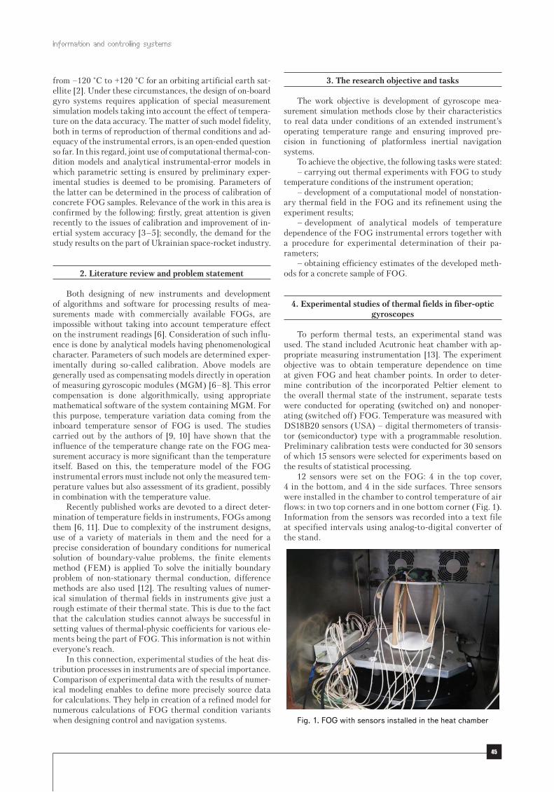
To perform thermal tests, an experimental stand was used. The stand included Acutronic heat chamber with ap-propriate measuring instrumentation [13]. The experiment objective was to obtain temperature dependence on time at given FOG and heat chamber points. In order to deter-mine contribution of the incorporated Peltier element to the overall thermal state of the instrument, separate tests were conducted for operating (switched on) and nonoper-ating (switched off) FOG. Temperature was measured with DS18B20 sensors (USA) – digital thermometers of transis-tor (semiconductor) type with a programmable resolution. Preliminary calibration tests were conducted for 30 sensors of which 15 sensors were selected for experiments based on the results of statistical processing.

12 sensors were set on the FOG: 4 in the top cover, 4 in the bottom, and 4 in the side surfaces. Three sensors were installed in the chamber to control temperature of air flows: in two top corners and in one bottom corner (Fig. 1). Information from the sensors was recorded into a text file at specified intervals using analog-to-digital converter of the stand.

Fig. 1. FОG with sensors installed in the heat chamber


46

The program of heat flow variation in the chamber was taken for the tests. It is shown in Fig. 2 by the curve of temperature variation on the internal sensor of the stand when the FOG was in operating condition. This variation was provided thru exposure of the instrument at the initial temperature T0=30 °C, further temperature setting at 0 °C, holding at this temperature and a new temperature setting at T0=30 °C.

As a result of the cycle of tests of the working and non-working FOG, temperature dependence on time was obtained at the sensor location points. One of the important results is comparison of the temperature regimes on the body of the working and non-working instrument. Tempera-tures vs. time graphs are presented in Fig. 3 for the working (curve 1) and non-working (curve 2) gyroscopes. In this and the following graphs, time keeping was done from the mo-ment of cooling. Analogous relationships with similar curve trend were obtained for the rest of sensors.

Fig. 3. Temperature (T, °C) vs. time (t, s) graphs at the bottom point: 1 – for working FOG; 2 – for non-working FOG

Comparison of the curves in Fig. 3 shows that there are no fundamental distinctions in the temperature distribution depending on time. Action of the Peltier element exerts generally smoothing effect on the distributions. At rapid overheating or cooling, temperature changes proceed more smoothly to ensure regular FOG operating mode due to the work of this element.

5. Numerical modeling of thermal fields

For the numerical solution of the problems of nonsta-tionary thermal conductivity of instrumentation, software package ANSYS Student 17.2 (USA) was used [14].

The problem of non-stationary thermal conduction was solved using the boundary condition of convective heat exchange [12] in which the ambient temperature was deter-

mined by means of internal sensor of the heat camera and 3 additional sensors installed for the experiment.

Following the analysis of the reference data and the re-sults of the experiments conducted for finite element model-ing, the following values of constants were accepted:

1) for the housing material (aluminum alloy): – density ρ=2700 kg/m3; – specific heat c=0.93 J/kg °C;

– coefficient of thermal conduc-tivity k=140 W/m∙° C;

– heat transfer coefficient α= =60 W/m2 ˚C;

2) for the coil material: – density ρ=2200 kg/m3; – specific heat c=920 J/kg∙°C; – coefficient of thermal conduc-

tivity k=1.4 W/m °C; – heat transfer coefficient α=

=60 W/m2∙°C.The coefficient of thermal con-

ductivity of the optical fiber materi-al wound on a coil is very small and

equal to 1.4 W/m∙°C (one hundred times smaller than the coefficient for the body material). This fact confirmed by nu-merical experiments permitted specification of conditions of absence of heat exchange (thermal insulation).for the surface of the FOG coil on which fiber is wound.

Thus, a simplified model was created for calculations. It consisted primarily of a housing, an internal coil on which optical fiber is wound and some elements disposed within the housing. The function of the heat source which simulates work of the Peltier element (it can provide both heating and cooling) and heat radiation from laser has been determined experimentally.

The FOG model (Fig. 4) was divided into 31882 tet-rahedral finite elements. As an initial condition, uniform distribution of temperature 30 °C corresponding to the start of the experiment has been taken.

а

b c Fig. 4. Calculation model of FOG: a – complete; b – cover;

c – FOG with the cover removed

The results of solution of the non-stationary conduction problem are shown in Fig. 5–9. Comparison of numerical and experimental results for all 12 measurement points has shown a quite satisfactory degree of their coincidence. As an

Fig. 2. Temperature (T, °С) vs. time (t, s) graph obtained in testing the stand-alone FOG

in the heat chamber


47

example, the temperature vs. time graphs for the top cover of the working (Fig. 5) and non-working (Fig. 6) FOG are giv-en. In these figures, the calculated data are represented with the solid curve and the experimental data are represented with the curve with dots.

After processing the data obtained for the working in-strument, it was established that dispersion D of experimen-tal and numerical values was as follows: D=4.256 °C for the top surface; D=1.807 °C for the side surface and D=9.143 °C for the bottom.

The same magnitudes for the nonworking FOG were as follows: D=4.764 °C for the top surface; D=3.348 °C for the side surface and D=6.361 °C for the bottom.

The comparison of data and their quite satisfactory agree-ment obtained in this comparison have led to the conclusion that there is possibility of using this model in the calculation of the instrument thermal fields. Fig. 7–9 show some results.

а b

Fig. 7. Temperature distribution on the surface: a – for non-working

instrument; b – for working instrument, t=300 s

As it might be expected, distributions were almost sym-metrical (Fig. 7, a) for the non-working device. Comparison of the temperature distribution in the non-working and working instruments shown in Fig. 6 indicates that action of the Peltier element becomes evident already at the first stag-

es of the cooling process: it is smoothing somewhat the impact of external heat variation leading to an asymmetric tem-perature field. Also, this effect is well illustrated in Fig. 8.

а b

Fig. 8. Temperature distribution for the working instrument, t=4800 s: a – on the cover; b – with the cover removed

Fig. 9 shows the temperature vs. time graph obtained for the working instrument in one of the blocks of the finite element model corresponding to the location of the FOG’s thermal sensor. This calculated temperature in conjunction with an estimate of its gradient is then used to determine temperature-dependent FOG’s instrumental errors in the problem of simulation modeling of MGM operation at an arbitrarily assigned ambient temperature.

The numerical experiments and comparison of the ob-tained data with experimental ones show quite satisfactory qualitative and quantitative coincidence of the results. Con-sequently, the developed thermal model of FOG can be used for further analysis.

6. The model of FOG measurement errors and the method of determining its parameters

This section deals with the description of the mathe-matical relationship between the FOG measurements and

Fig. 5. Temperature (T, °С) vs. time (t, s) graphs for the top cover of the working FOG

Fig. 6. Temperature (T, °С) vs. time (t, s) graphs for the top cover of the

nonworking FOG

Fig. 9. The calculated temperature (T, °C) vs. time (t, s) graph for the working FOG

at the point of location of the built-in temperature sensor


48

the value being measured taking into account instrumental errors (IE) of the instrument sensitive to the temperature factors. Parameters of this dependence (of the mathematical model) are determined from the experimental data obtained for the tested gyroscope samples through their approxi-mation with analytical functions. Use of the experimental data provides model setup for a specific type of instruments. The resulting functional dependencies of IE are used in generating data from the measuring gyroscopic module (MGM) close by their characteristics to the real ones. Such measurements enable simulation of the gyroscopic system functioning throughout the operational temperature range. It is required in the design and research works.

Measurement model. Consider a measuring gyro module comprising three FOGs and introduce two systems of coor-dinate axes:

– X, Y, Z axes of the right orthogonal instrument coor-dinate system (RCS) connected with the MGM structure;

– axes coinciding with the FOG’s sensitivity axes (SA) and close to the mutually orthogonal axes.

Let ω = ω ω ωMGU X Y Z( , , ) is a true absolute angular veloc-ity in the projections to the RCS axes and ω = ω ω ωFOG 1 2 3ˆ ( , , ) is the vector composed of the velocities measured by the first, second and third FOGs. Then the following can be written for each current time moment t:

FOG H MGUˆ (t) (E K) (F F) (t) (t),ω = + d ⋅ + d ⋅ω + dω + ξd (1)

where E is the unitary matrix (3×3); δK=diag(δk1, δk2, δk3) is the diagonal matrix of relative errors of the FOG scale factors; FH is known nominal matrix of the direction cosines (MDC) between the specified position of the FOG’s SA and RCS axes (often it is a unitary matrix); δF is such matrix (3×3) of amendments to the nominal matrix of the direction cosines that:

Н ij i,j 1,3F̂ F F {f }

=≡ + d =

is the matrix of direction cosines as well but for the actual SA location; dω is the vector composed of the drifts of the first, second and third FOGs; ξ(t) is a three-dimensional vector of the noise component of measurements with a zero mean.

Relation (1) is a standard mathematical model of per-turbed measurements made by the MGM in which param-eters δK, δF, dω, depending (in the general case) on the temperature factors correspond to the FOG instrumental errors. The reason for the introduced errors and the method of their recording in the perturbed measurement generally correspond to those which are standard in the optical gyro-scopy and inertial navigation [15].

For the subsequent solution of the problem, there is no need to separate measurement scaling and transformation by means of MDC. Therefore, introduce notation:

*HF (E K) (F F)= + d ⋅ + d

and rewrite (1) as:

ω = ⋅ω + dω + ξ*FOG MGUˆ (t) F (t) (t). (2)

Application of the model in simulation modeling. The tasks of simulation modeling using formula (2) with a re-quired time step are fulfilled by generation of the MGM measurements for an arbitrarily prescribed true rotational

speed ωMGU(t) and various temperature conditions of the instrument operation.

To do this, first the current model temperature values MiT at the points of location of the built-in temperature sen-

sors are determined for each FOG by means of the finite-el-ement calculation model of the non-stationary thermal field (Fig. 9). The matrix elements are then calculated:

==* *

ij i,j 1,3F {f } ,

using the following formula:

τ = φ + φ ⋅τ + φ ⋅τ + φ ⋅τ* (ij) (ij) (ij) 2 (ij) 3ij 0 1 i 2 i 3 if ( ) , =i, j 1,3, (3)

and the drift values using the following formula:

dω τ = + ⋅τ + ⋅τ +

+ ⋅τ + ⋅ ∆τ + ⋅τ ⋅ ∆τ =

(i) (i) (i) 2i i 00 10 i 20 i

(i) 3 (i) (i)30 i 01 i 11 i i

( ) k k k

k k k ,i 1,3, (4)

where

−τ =

ℜ

Mi 0

i

T T

and

∆∆τ =

∆

Mi

imax

TT

are normalized centered dimensionless values of temperature and the temperature gradient of the i-th FOG respectively;

+= max min

0

(T T )T

2

is mean temperature of the working temperature range [Tmin, Tmax];

−ℜ = max minT T

2

is radius of the working temperature range; ∆ MiT is the

model value of the temperature gradient calculated as a time derivative from M

iT ; ∆Tmax is its maximum possible value;

φ φ φ φ(ij) (ij) (ij) (ij)0 1 2 3, , , ; (i) (i) (i) (i) (i) (i)

00 10 20 30 01 11k ,k ,k ,k ,k ,k , =i, j 1,3

are known parameters obtained at the pre-calibration stage for concrete FOG samples.

The structure and order of analytical models (3), (4) re-lated to the instrumental errors were determined empirically in the preliminary studies [9]. It should be pointed out that for the specified FOG samples, truncated models in which there are no certain summands can be the most efficient by the results of calibration, In this case, without loss of gener-ality, the corresponding coefficients can be assumed to be zero in models (3), (4).

During simulation of real FOG measurements, a prob-lem of an adequate numerical simulation of the added noise is always taking place because the real noise component has a complex characteristic [16]. The problem disappears if the noise sample derived from the actual measurements of concrete FOG samples is used as a random component

(t).ξ For this purpose, laboratory tests are carried out in stationary thermal conditions. Measurements are done and saved with a frequency equal to the simulation frequency. The sampling duration must not be less than the duration of the subsequent modeling.


49

Thus, after calibration of MGM using formula (2), the problem of data generation to simulate functioning of the gyroscopic system is solved.

MGM calibration. The algorithm for the model parameter calculation. The central moment of the above data genera-tion procedure is obtaining coefficients of the temperature models (3), (4) which are used in it. To this end, so-called instrument calibration shall be done. Consider this problem in detail.

The problem under consideration is inverse to the problem of measurement generation and differs from the original one in that the gyroscope measurements are known and parameters of errors δK, δF, dω are the sought quantities. When doing this, the problem of calibration is solved based on the obtained experimental data and, as a rule, with the use of laboratory equipment and metrolog-ical support.

The calibration procedure includes the following:– experimental data processing algorithm;– requirements to the laboratory equipment and metro-

logical support;– schedule of carrying out calibration experiments;– criteria for assessing the calibration efficiency;– analysis of sources and the error level of the procedure

implementation.The model of MGM measurements is taken as the basis

for derivation of calculation formulas of procedure (1). As-sume that the calibration measurements are recorded at the time moments tn, n=1, 2, 3,... and performed at a constant rotational speed ωMGU and a constant FOG temperature. Since single FOG measurements have a significant noise, average them out by the formula:

− ⋅ +=

ω = ω∑N

s FOG (s 1) N kk 1

1ˆ (t ),

N (5)

where ω s is the calculated vector of the averaged measured angular velocity at the projections to the FOG’s SA; s= =1, 2, 3, ... is the number of the averaged value; N is the num-ber of counts involved in the averaging.

In this case, expression (2) for the averaged values can be represented as:

⋅ω + dω = ω* (s)MGU sF , (6)

where ω(s)MGU is the known true angular velocity in the pro-

jections to the RCS axis at the s-th interval of averaging;

* *ij i,j 1,3

F {f } ,=

= =

dω = dωi i 1,3{ }

are the sought parameters of the model.The vector equation (6) disintegrates into three indepen-

dent scalar equations:

( )dω

ω ω ω ⋅ = ω

i*i1(s) (s) (s)

MGU MGU MGU s*i2*i3

f1 [X] [Y] [Z] [i],

f

f

=i 1,3, (7)

where i is the gyroscope number;

ω ω ω(s) (s) (s)MGU MGU MGU[X], [Y], [Z]

are averaged projections of the absolute angular velocity of MGM rotation to axes X, Y, Z of RCS corresponding to the averaging interval with number s; ω s[i] are averaged mea-surements of the i-th FOG.

Obviously, to calculate four parameters δωi, *i1f , *

i2f , *i3f

one must have at least four equations of form (7) correspond-ing to various rotation modes. In this case, the determining system can be written for each =i 1,3 as (s=1, 2, 3, 4):

dω ω ω ω ω ωω ω ω ⋅ = ω ω ω ω ωω ω ω

(1) (1) (1)i 1MGU MGU MGU

*(2) (2) (2)i1 2MGU MGU MGU*(3) (3) (3)i2 3MGU MGU MGU*(4) (4) (4)i3 4MGU MGU MGU

[i]1 [X] [Y] [Z]f [i]1 [X] [Y] [Z]f [i]1 [X] [Y] [Z]f [i]1 [X] [Y] [Z]

. (8)

The sought model parameters are calculated from (8). For absence of degeneracy of system (8), specify the MGM rotation modes corresponding to different numbers s, in the form:

ω = ω(1)MGU ( ,0,0), ω = ω(2)

MGU (0, ,0),

ω = ω(3)MGU (0,0, ), ω = ω ω ω(4)

MGU 1 2 3(m ,m ,m ),

where ω, m1, m2, m3 are parameters. For these conditions, the determinant of the system (8) matrix has the following form:

∆ = + + − ⋅ω31 2 3(m m m 1) ,

which implies that for the solvability of (8) at ω ≠ 0 it is sufficient to specify:

+ + ≠1 2 3m m m 1,

or, in particular, assume:

1m 2,= 2m 0,= 3m 0,=

which corresponds to the simplest mode of rotation.Thus, to determine constant parameters:

==* *

ij i,j 1,3F {f } and

=dω = dωi i 1,3

{ }

it is enough to measure angular velocity in the four abovementioned MGM rotation modes and solve the system (8) independently for each FOG using the averaged data.

The above-mentioned requirement of the FOG tempera-ture constancy over four rotation modes can be excluded if

dω*ij if ,

parameters are sought in a form of (3), (4), i. e. in the

following form:

dω = Η τ ⋅µ

i*i1 (s)

i i*i2*i3

f( ) ,

f

f

(9)

where

==

τ = =(s) (s)i i lm l 1,4

m 1,18

H( ) H {h }

is the matrix consisting of zeros excepting the calculated elements:


50

= = τ(s)11 12 ih 1, h , = τ(s) 2

13 ih ( ) , = τ(s) 314 ih ( ) ,

= ∆τ(s)15 ih , = τ ⋅ ∆τ(s) (s)

16 i ih ;

=27h 1, = τ(s)28 ih , = τ(s) 2

29 ih ( ) , = τ(s) 32,10 ih ( ) ;

=3,11h 1, = τ(s)3,12 ih , = τ(s) 2

3,13 ih ( ) , = τ(s) 33,14 ih ( ) ;

=4,15h 1, = τ(s)4,16 ih , = τ(s) 2

4,17 ih ( ) , = τ(s) 34,18 ih ( ) ,

τ(s)i , ∆τ(s)

i are dimensionless temperature parameters of the i-th FOG in the averaging interval with number s; µi is the column vector of the sought parameters of the tempera-ture model:

µ = φ φ φ

φ φ φ φ φ φ φ φ φ

(i) (i) (i) (i) (i) (i) (i1) (i1) (i1)i 00 10 20 30 01 11 0 1 2

(i1) (i2) (i2) (i2) (i2) (i3) (i3) (i3) (i3)3 0 1 2 3 0 1 2 3

{k ,k ,k ,k ,k ,k , , , ,

, , , , , , , , }.

Substitute (9) in (7) to obtain the following scalar equa-tion:

⋅ ⋅µ = ω(s) T (s)MGU i i s(w ) H [i], (10)

where

= ω ω ω(s) (s) (s) (s)MGU MGU MGU MGUw {1, [X], [Y], [Z]}

is a column vector.To find a 18-dimensional sought vector µi using equation

(10), it is necessary to carry out at least 18 measuring ses-sions to get the system:

ω ⋅ ω⋅ ω ⋅

⋅µ = ω⋅ ω⋅

(1) T (1)1MGU i

(2) T (2)2MGU i

(3) T (3)3MGU i

(4) T (4) i4MGU i

(L) T (L)LMGU i

[i](w ) H[i](w ) H[i](w ) H

,[i](w ) H

[i](w ) H

(11)

where ≥L 18.For solvability of such system, it is sufficient to repeat

several times the above four MGM rotation modes at differ-ent FOG temperatures. The system redundancy (concern-ing the number of equations) which appears in this case is exhausted when using the least squares method whereby the following is obtained:

( )−µ = Π ⋅Π Π ⋅

1T Ti i i i iW , (12)

where Пi is designation for the block matrix in the left part of (11);

iW is designation of the vector in the right parts.Thus, determination of parameters of the FOG tempera-

ture model of measurements includes:– procedure of averaging measurements by formula (5);– composition of a redundant system of linear equa-

tions (11);– decision (12) by the method of least squares.Hardware requirements and the experiment schedule. De-

scribe conditions and procedure of the calibration experiment.To carry out the calibration experiments, it is necessary to

use a two- or three-axis motion simulator like those produced by Actidyn Systemes (France) [17]. The simulator must be mounted in a horizontal plane with an accuracy not worse

than 5² and ensure MGM rotation at a predetermined angu-lar velocity. The studied MGM is placed in the heating and cooling chamber (HCC) of Acutronic type and attached to the simulator for a conjoint motion. To account for the Earth’s rotational speed, terrestrial latitude must be known with ac-curacy better than 10² for the location where the experiment is conducted. In the course of the experiment, the gyro output data and the measurements of the embedded temperature sensors are recorded with a required update rate.

The approximate order of the experiment is as follows:0. Cool the switched off MGM down to the Tmin tem-

perature.1. Enable HCC by the programs executed sequentially

and coordinated with the operational modes of the FOG being the part of the gyroscopic system:

– external temperature varying from Tmin tо Tmax with a positive gradient Tmax;

– external temperature varying from Tmax to Tmin with a negative gradient ∆Tmax.

2. Enable MGM and data logging.3. Direct the RCS X axis vertically upwards. Spin at a

rate of +20°/s around the vertical axis for 10 minutes.4. Direct the RCS Y axis vertically upwards. Spin at a

rate of +20°/s around the vertical axis for 10 minutes.5. Direct the RCS Z axis vertically upwards. Spin at a

rate of +20°/s around the vertical axis for 10 minutes.6. Direct the RCS X axis vertically upwards. Spin a rate

of +40°/s around the vertical axis for 10 minutes.7. Repeat items 3-6 to the end of work by the HCC pro-

gram.8. Complete data logging and process the results.Remarks:a) rotation speed and duration of the modes are given

approximately. In practice, they should be adjusted taking into account the specific type of FOG;

b) items 3–6 correspond to the previously introduced four rotation modes;

c) when processing, data corresponding to the transition from one mode to another rotation mode are ignored.

The described schedule enables an adequate assessment of parameters of the temperature model of the FOG mea-surements by the method of least squares.

Criteria of calibration efficiency.Qualitative assessment of the experimental-data ap-

proximation using statistical mean value and statistical mean square deviation (MDS) of the approximation error calculated for the sample being used is well known [18]. In the problem under consideration, such assessment should be appropriately used to select the best structure of the approximating models, but objectively it does not reflect the calibration efficiency.

Efficiency of MGM calibration depends on the paramet-ric stability of temperature dependencies of the instrumental errors caused by the instrument itself. In these conditions, it is proposed to use the magnitude of the dispersion range of the FOG IE of the same name as a criterion of effectiveness. These errors are identified based on the results of several independent experiments under equivalent conditions.

This implies that for an objective appraisal of the calibra-tion efficiency, it is necessary to conduct a series of similar calibration experiments and statistically process their results.

The assessments of the relative error of the scale fac-tors collected in a matrix are the most obvious results of calibration:


51

d = d d d1 2 3K diag( k , k , k ),

assessments of the FOG SA misalignment amendments:

{ }=

d = d ij i,j 1,3F f ,

and zero drift assessment. However, within the frames of the developed procedure, the following elements alongside the dω are directly computed: *

ijf , =i, j 1,3,.Matrices F* are associated with abovementioned param-

eters by following relations:

= + d ⋅ + d* Hij i ij ijf (1 k ) (f f ),

in which Hijf are elements of the known nominal matrix of

direction cosines. Hence, it is easy to obtain the following for the sought assessments by positioning *

ijf :

d = + + −* 2 * 2 * 2i i1 i2 i3k (f ) (f ) (f ) 1,

d = −+ d

*ij H

ij iji

ff f ,

(1 k ) =i, j 1,3. (13)

At the same time, it is easy to assess non-orthogonality of the ith FOG’s sensitivity axis relative to the RCS based on dfij elements.

Assuming that the implemented IE values are “exactly” determined for each calibration experiment corresponding to one switching of the instrument, calibration efficiency is characterized by the magnitude of the similar-error scatter interval. Concrete results of the study are as follows.

Six equivalent calibration experiments have been con-ducted in stationary temperature conditions for the MGM incorporating three FOGs of a medium accuracy class hav-ing “almost orthogonal” sensitivity axes. With the use of the above-described procedure, FOG’s instrumental errors were calculated and mean values and MSD of the same-name er-rors were defined for the entire series (Table 1).

The mean error values show that the studied FOGs really correspond to the medium-class accuracy. At the same time, a high level of the estimate repeatability (as it is evidenced by the fairly small values of MSD) means that a significant (several times) improvement of the FOG accu-racy for all parameters can be achieved using algorithmic compensation taking into account mean values of the error estimates. In addition, the obtained statistical characteris-tics permit adequate simulation of the MGM functioning for various kinds of switching.

Hence, the experimental results have shown consistency of the introduced criterion of calibration efficiency.

Sources of the procedure errors and recommendations for practical application.

The main source of the method errors in the developed calibration procedure is incorrect account for the Earth’s ro-tation during result processing. This factor can be eliminat-ed by using (in the calculation formulas) the measurement values averaged within the time interval during which IGM makes a complete revolution around the rotary axis of the stand. In this case, the effect of the horizontal component of the Earth angular velocity on the FOG readings will be automatically compensated with a high accuracy. The verti-cal component of the Earth angular velocity should be taken into account in the projection to the vertical axis of the RCS vector of the true rotation velocity.

Table 1

Results of calibration experiments

FOG number

Zero drift, °/hrCorrection to the

scale factor, %

Maximal parame-ter of nonorthogo-

nality, ʹmean value

MSDmean value

MSDmean value

MSD

FОG No. 1

0.18 0.02 –0.16 0.001 14.27 0.02

FОG No. 2

–0.36 0.04 –0.24 0.001 16.47 0.63

FОG No. 3

–0.02 0.02 0.34 0.002 25.32 0.03

The procedure effectiveness can also be affected by in-strumental factors:

– nonhorizontality of the stand;– conical motion of the stand axis of rotation;– uneven rotation;– rough repeatability of angular positions of the

stand, etc.Some of these factors can be eliminated by an additional

calibration of the module using algorithms of inertial calcu-lation that goes beyond the scope of this article.

Basic recommendations for the practical application of the procedure can be stated without validation as follows:

– FOG measurement averaging should be carried out in a time interval during which the MGM makes one or more complete turns around the stand axis;

– the procedure can be applied to an arbitrary number of FOGs with axes of sensitivity randomly positioned relative to the RCS;

– the approximation problem can be solved using a re-dundant data set. Under these conditions, it is advisable to use a recursive least-squares method with a rising volume of measurements for assessment of the sought model parameters;

– the measurement error estimates obtained during cal-ibration can be used not only for simulation modeling of the MGM operation but also to compensate for the measurement errors in the course of the block operation. The correspond-ing model of restoration of the angular rotation velocity in the projections to the RCS axis has the following form:

−ω = ⋅ ω − dω*M 1 MMGU n FOG nˆ(t ) (F ) ( (t ) ), (14)

where dωM, *MF are the model values of the drift vector and the transformation matrix the elements of which are calculated according to the formulas (3), (4) with an account for current values of the FOG temperature and its gradient.

7. Discussion of the results obtained in the study of the temperature models of the FOG measurement errors

The advantage of this approach is integration of the pro-cedure for calculating the heat field in the instrument and the task of construction and use of the temperature depen-dent models of the FOG instrumental errors. This approach increases efficiency of the simulation modeling of various gyroscopic systems in the arbitrarily specified temperature conditions. In particular, the procedure for calculating heat fields provides an estimate of temperature at any time moment and anywhere in the instrument including the point of loca-tion of the built-in temperature sensor. In view of this assess-ment and the measurement error models, FOG measurements


52

are generated with their accuracy characteristics being close to real ones. These measurements are proposed to be further used in the application software (AS) of the gyroscopic sys-tem directly for the solution of functional tasks facing it. Thus, the developed approach ensures more precise consideration for the temperature dependence of the MGM measurement errors and an eventual improvement of efficiency and simulation veracity in designing gyroscopic systems.

However, the role of the proposed method is not limited thereto. In the future, it can also be used, firstly, to refine composition and location of temperature sensors in the MGM in order to improve quality of the measurement error compensation in the subsequent operation of the instrument and secondly, to improve the layout of the electronic and structural components of the MGM in terms of reducing influence of the perturbing thermal factors.

8. Conclusions

1. New experimental data of the temporal variation of temperature at various points of the fiber optic gyroscope and the heat camera were obtained.

2. Based on the finite element method, a computational model of the thermal field in the FOG at various outside tem-peratures was developed. Comparison of experimental data with the results of finite element calculation of non-station-ary heat conduction problems has demonstrated their quite

satisfactory agreement. The verification studies enabled the use of the developed calculation model for further analysis of the instrument thermal conditions. The calculation model is further used in solving the problem of simulation modeling of the FOG measurements as a part of MGM.

3. Temperature models of the FOG instrumental er-rors were considered. With their help, the MGM output data for all kinds of thermal conditions are predicted with an accuracy close to real sensor errors. For the ad-equacy of these models, their parameters are pre-defined in the course of calibration of concrete FOG samples. A procedure for calibration of the models of IGM errors was developed. It is remarkable for the possibility of joint identification of all IEs using a single redundant volume of measurements.

4. To assess the effectiveness of FOG calibration meth-ods, it was proposed to use the magnitude of the repeatabil-ity interval of the same-name errors. Such an interval can be obtained by carrying out several independent calibration experiments under equivalent conditions. Experimentally determined estimates of effectiveness of such calibration demonstrate its practical value.

Thus, the results obtained in the present study are first of all aimed at improvement of accuracy of the gyroscopic systems based on the mid-end FOGs used in aerospace engi-neering and secondly, they make the basis for further studies of thermal processes taking place in FOGs and optimization of the MGM design as a whole.

References

1. Balakrishnan, S. N. Advances in Missile Guidance, Control and Estimation [Text] / S. N. Balakrishnan, A. Tsourdos, B. A. White. – CRC Press, 2012. – 720 p.

2. Karam, R. Satellite Thermal Control for Systems Engineers [Text] / R. Karam // Progress in Astronautics and Aeronautics. American Institute of Aeronautics and Astronautics. – American Institute of Aeronautics and Astronautics, 1998. – 262 p. doi: 10.2514/4.866524

3. Shaimardanov, I. H. Methods for Calibration of Strapdown Inertial Navigation Systems (SINS) of Various Classes of Accuracy [Text] / I. H. Shaimardanov, A. A. Dzuev, V. P. Golikov // 23d Saint Petersburg International Conference on Integrated Navigation Systems, ICINS. – 2016. – P. 67–71.

4. Vavilova, N. B. Calibration of Strapdown Inertial Navigation Systems on High-Precision Turntables [Text] / N. B. Vavilova, A. A. Golovan, N. A. Parusnikov, I. A. Vasineva // 23d Saint Petersburg International Conference on Integrated Navigation Systems, ICINS. – 2016. – P. 72–75.

5. Kozlov, A. V. Calibration of Inertial Measurement Unit on Low-Grade Turntable: Estimation of Temperature Time Derivative Coefficients [Text] / A. V. Kozlov, I. E. Tarygin, A. A. Golovan // 23d Saint Petersburg International Conference on Integrated Navigation Systems, ICINS. – 2016. – P. 76–81.

6. Chen, X. Study on error calibration of fiber optic gyroscope under intense ambient temperature variation [Text] / X. Chen, C. Shen // Applied Optics. – 2012. – Vol. 51, Issue 17. – P. 3755. doi: 10.1364/ao.51.003755

7. Xiao, T. Temperature Drift Modeling and Compensating of Fiber Optic Gyroscope [Text] / T. Xiao, M. H. Pan, G. L. Zhu // Applied Mechanics and Materials. – 2012. – Vol. 220-223. – P. 1911–1916. doi: 10.4028/www.scientific.net/amm.220-223.1911

8. Meshkovsky, I. K. Investigation of the influence of thermal effects on the operation of fiber-optic angular rate sensor [Text] / I. K. Meshkovsky, G. P. Miroshnichenko, A. V. Rupasov, V. E. Strigalev, I. A. Sharkov // XXI International conference on integrated navigation systems. – 2014. – P. 191–202.

9. Kuznetsov, Yu. A. Investigation of the temperature dependence of FOG drift [Text] / Yu. A. Kuznetsov, S. V. Oleynik, V. B. Uspen-sky, N. E. Hatsko // Electronics, computer science, control systems. – 2012. – Issue 2 (27). – P. 152–156.

10. Zlatkin, O. Yu. The development of a high-precision strapdown inertial system based on medium-accuracy fiber-optic gyroscopes for rocket and space applications [Text] / O. Yu. Zlatkin, S. V. Oleynik, A. V. Chumachenko, V. B. Uspensky, A. V. Gudzenko // 21st Saint Petersburg International Conference on Integrated Navigation Systems, ICINS. – 2014.

11. Breslavsky, D. V. Development of methods for determining the temperature gradient of the fiber optic gyroscope UMAV501 [Text] / D. V. Breslavsky, S. Yu. Pogorelov, K. Yu. Schastlivets, B. I. Batyrev, Y. A. Kuznetsov, S. V. Oleinik // Mechanics and En-gineering. – 2012. – Issue 1. – P. 90–101.

12. Lewis, R. W. Fundamentals of the Finite Element Method for Heat and Fluid Flow [Text] / R. W. Lewis, P. Nithiarasu, K. Seetha-ramu. – John Wiley & Sons, Ltd, 2004. – 356 p.


53

A. Alimpiev, P. Berdnik, N. Korolyuk, O. Korshets, M. Pavlenko, 2017

1. Introduction

Defensive military doctrine of the Armed Forces of Ukraine (AFU) establishes high requirements for all el-ements of combat readiness and for training troops. The Armed Forces must be prepared to fight off aggression by

conducting defensive actions. The most important task of the headquarters under defensive nature of the military doctrine is permanent surveillance of the enemy that should provide for a timely and organized transition of troops from peace to war. The main role in this is assigned to the intelligence. A number of tasks for aerial reconnaissance can be solved

13. Acutronic [Electronic resource]. – Available at: http://www.acutronic.com/14. ANSYS Student Products [Electronic resource]. – Available at: http://www.ansys.com/products/academic/ansys-student15. Curey, R. K. Proposed IEEE inertial systems terminology standard and other inertial sensor standards [Text] / R. K. Curey, M. E. Ash,

L. O. Thielman, C. H. Barker // PLANS 2004. Position Location and Navigation Symposium (IEEE Cat. No.04CH37556). – 2004. doi: 10.1109/plans.2004.1308978

16. Krobka, N. I. Differential methods of identification gyroscope noise patterns [Text] / N. I. Krobka // Gyroscopy and navigation. – 2011. – Issue 1 (72). – P. 59–77.

17. Two- and Three-Axis Motion Simulators [Electronic resource]. – Actidyn. – Available at: http://www.actidyn.com/products/mo-tion-simulation-and-control/dual-and-tri-axis-motion-simulators/

18. Granovsky, V. A. Methods of processing of experimental data in the measurements [Text] / V. A. Granovsky, T. N. Siraya. – Lenin-grad: Energoatom, 1990. – 288 p.

SELECTING A MODEL OF UNMANNED AERIAL VEHICLE TO ACCEPT IT FOR MILITARY

PURPOSES WITH REGARD TO EXPERT DATA

A . A l i m p i e vPhD, Head of University*

E-mail: [email protected] . B e r d n i k

PhD, Senior LecturerCenter for international education

V. N. Karazin Kharkiv National UniversitySvobody ave., 4, Kharkiv, Ukraine, 61022

E-mail: [email protected] . K o r o l y u k

PhD, Associate ProfessorDepartment of combat use and operation of ASU*

E-mail: [email protected] . K o r s h e t s

PhD, Associate ProfessorDepartment of Air Force

National University of Defense of Ukraine named after Ivan Chernyakhovsky

Povitroflotsky ave., 28, Kyiv, Ukraine, 03049E-mail: [email protected]

M . P a v l e n k oDoctor of Technical Sciences, Head of Department

Department of mathematical and software*E-mail: [email protected]

*Ivan Kozhedub Kharkiv University of Air ForceSumska str., 77/79, Kharkiv, Ukraine, 61023

Проведена порівняльна характе-ристика багатокритеріальних задач оптимізації, критерії яких можуть мати кількісну і якісну природу. Обґрунтовано рішення щодо вибо-ру зразка безпілотного літального апарату для прийняття на озброєн-ня за характеристиками, значення яких прогнозуються в умовах несто-хастичної невизначеності на осно-ві експертних даних. Запропонована декомпозиція проблеми в ієрархію, що відображає зміст багатокритеріаль-ної задачі оптимізації

Ключові слова: безпілотний лі- тальний апарат, декомпозиція про-блеми в ієрархію, лінгвістична змінна

Проведена сравнительная харак-теристика многокритериальных за- дач оптимизации, критерии кото-рых могут быть количественной и качественной природы. Обоснованно решение относительно выбора об- разца беспилотного летательного аппарата для принятия на вооруже-ние с характеристиками, значения которых прогнозируются в услови-ях нестохастической неопределен-ности на основе экспертных данных. Предложена декомпозиция пробле-мы в иерархию, которая отража-ет содержание многокритериальной задачи оптимизации

Ключевые слова: беспилотный ле- тательный аппарат, декомпозиция проблемы в иерархию, лингвистиче-ская переменная

UDC 519.81DOI: 10.15587/1729-4061.2017.93179

OPTIC GYROSCOPES USED IN AEROSPACE SYSTEMS

Documents

Transcript of OPTIC GYROSCOPES USED IN AEROSPACE SYSTEMS