1

Cyclostationarity of Acoustic Emissions (AE) for monitoring bearing defects

B. KILUNDU a, X. CHIEMENTINb,1, J. DUEZa, D. MBAc

aUniversity of Mons - UMONS, Risks Research Centre, 20 Place du Parc, 7000 Mons, Belgium

bGRESPI, Groupe de Recherche En Sciences Pour l'Ingénieur, Université de Reims Champagne-Ardenne, Moulin de la

Housse, 51687 Reims Cedex 2, France.

cTurbomachinery group, School of Engineering, Cranfield University, Cranfield, Bedfordshire MK43 0AL, United Kingdom.

Abstract

Cyclostationnarity is a relatively new technique that offers diagnostic advantages for analysis of vibrations from

defective bearings. Similarly the Acoustic Emission (AE) technology has emerged as a viable tool for preventive

maintenance of rotating machines. This paper presents an experimental study that characterizes the

cyclostationary aspect of Acoustic Emission signals recorded from a defective bearing. The cyclic spectral

correlation, a property associated with cyclostationarity, was compared with a traditional technique, the envelope

spectrum. This comparison showed that the cyclic spectral correlation was most efficient for small defect

identification on outer race defects though the success was not mirrored on inner race defects. An indicator,

based to this statistical property, has been also proposed. It is concluded that its offers better sensitivity to the

continuous monitoring of defects compared to the use of traditional temporal indicators (RMS, Kurtosis, Crest

Factor).

Keywords

Acoustic Emission, Cyclostationarity, follow-up, rolling bearing.

1 Corresponding author : xavier.chiementin@univ-reims.fr

2

1 Introduction

Over the last 20 last years the Acoustic Emission (AE) has been proven as a powerful method for the detection

of incipient defects on rotating machines [1]. The technology offers several significant advantages over

conventional vibration analysis [1]. Acoustic Emission (AE) results from rapid release of strain energy which

causes transient elastic waves in a solid material [2]. In particular for bearing monitoring, AE results from micro-

shocks and friction between the rotating elements of the bearing. AE differs from vibration analysis as the

frequency band used for AE is between 100kHz to 1000kHz.

AE offers earlier detection than vibratory analysis for outer race defects [1] though this is not mirrored for inner

race defects. Some studies used the principle of AE to identifiy bearing defects over a wide range of operating

speeds. McFadden [3] showed the effectiveness of AE in detecting small defects at low speeds (10rpm) whilst

Roger [4] applied AE to monitor offshore cranes. For small defects, Tandon [5] has demonstrated the usefulness

of parameters associated with AE, such as peak amplitude or counts, especially the ringdown counts. Bansal [6]

and Choudhury [7] also exploited traditional AE analysis techniques for fault diagnosis, presenting results of AE

events and maximum amplitude (peak amplitude), or, AE events and ringdown counts.

Another advantage offered by AE is the fact that it can be employed to quantify the bearing defect size in-situ.

Al-Ghamdi [8] and Mba [9] correlated the AE burst duration with the length and width of an outer race defect;

however, such a correlation was not demonstrated for inner race defects. In another study Al-Dossary [10]

investigated the influence of the shape of the defect (length and width) on both inner and outer races and

reaffirmed the findings of Al-Ghamdi et al. It should also be noted that the application of AE does have its

challenges [21].

Over the last decade, primarily due to developments in computer hardware and storage systems, techniques

suitable for the vibration are being applied to the AE. Liu [12] used the independent components analysis, Liao

[13] employed wavelets analysis while Žvokelj [14] and Li [15] were interested in the empirical mode

decomposition and Gabor transform, respectively, on AE signals. Chiementin [16] used time domain indicators

RMS, Kurtosis, and proposes to improve the signal-to-noise ratio by applying denoising techniques (wavelet,

spectral subtraction, sanc) on experimental acquired AE data. The use of traditional methods of vibration

analysis for AE analysis offers yet further techniques for the diagnostician. This paper firstly highlights the

cyclostationary character of AE’s associated with a defective bearing, and secondly, shows the effectiveness of

3

the spectral correlation for diagnosis. Lastly, a unique indicator for monitoring bearings based on clostationnarity

characteristics is presented.

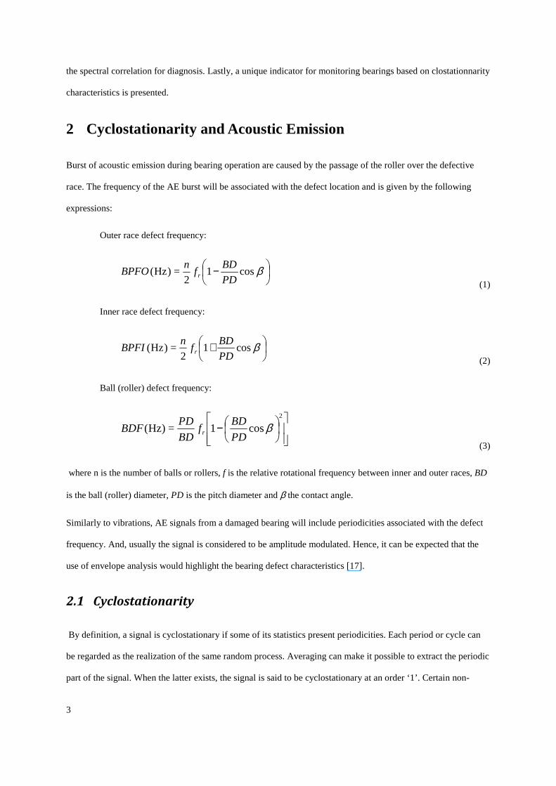
2 Cyclostationarity and Acoustic Emission

Burst of acoustic emission during bearing operation are caused by the passage of the roller over the defective

race. The frequency of the AE burst will be associated with the defect location and is given by the following

expressions:

Outer race defect frequency:

− βcos12

=)Hz(PD

BDf

nBPFO r

(1)

Inner race defect frequency:

+ βcos12

=)Hz(PD

BDf

nBPFI r

(2)

Ball (roller) defect frequency:

−2

cos1=)Hz( βPD

BDf

BD

PDBDF r

(3)

where n is the number of balls or rollers, f is the relative rotational frequency between inner and outer races, BD

is the ball (roller) diameter, PD is the pitch diameter and β the contact angle.

Similarly to vibrations, AE signals from a damaged bearing will include periodicities associated with the defect

frequency. And, usually the signal is considered to be amplitude modulated. Hence, it can be expected that the

use of envelope analysis would highlight the bearing defect characteristics [17].

2.1 Cyclostationarity

By definition, a signal is cyclostationary if some of its statistics present periodicities. Each period or cycle can

be regarded as the realization of the same random process. Averaging can make it possible to extract the periodic

part of the signal. When the latter exists, the signal is said to be cyclostationary at an order ‘1’. Certain non-

4

periodic signals can present periodic energy, i.e., they become periodic when there are squared. Such a signal

presents hidden periodicities and is said to present second-order cyclostationarity. In general terms, a signal is

cyclostationary at an order ‘2’ if its statistical properties at order ‘2’ are periodic. The cyclostationarity property

which is a particular case of non-stationarity allows discovery of hidden periodicities within a signal. As rotating

machines intrinsically generate periodicities, one may find it beneficial to exploit cyclostationarity properties for

fault detection and diagnosis. In this section, we recall the main definitions and properties of a cyclostationary

process. The reader is refered to Antoni [18] for a full explanation and definition on cyclostationarity.

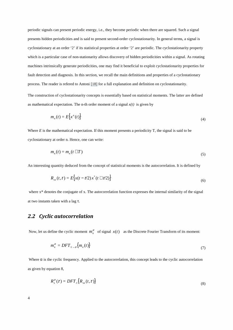
The construction of cyclostationarity concepts is essentially based on statistical moments. The latter are defined

as mathematical expectation. The n-th order moment of a signal x(t) is given by

{ })(=)( txEtm n

n (4)

Where E is the mathematical expectation. If this moment presents a periodicity T, the signal is said to be

cyclostationary at order n. Hence, one can write:

)(=)( Ttmtm nn +

(5)

An interesting quantity deduced from the concept of statistical moments is the autocorrelation. It is defined by

{ }/2)(/2)(=),( * τττ +− txtxEtRxx (6)

where x* denotes the conjugate of x. The autocorrelation function expresses the internal similarity of the signal

at two instants taken with a lag τ.

2.2 Cyclic autocorrelation

Now, let us define the cyclic moment αnm of signal )(tx as the Discrete Fourier Transform of its moment:

{ })(= / tmDFTm ntn α

α→ (7)

Where α is the cyclic frequency. Applied to the autocorrelation, this concept leads to the cyclic autocorrelation

as given by equation 8,

{ }),(=)( / ττα tRDFTR xxtx (8)

5

The cyclic autocorrelation depends on the lag τ and on the cyclic frequency α. It gives an indication of energy in

the signal due to cyclostationary components. At α=0 lies the stationary autocorrelation of the signal. If there

exists any value of α≠0 for which the cyclic correlation is non zero, then this indicates that the signal is

cyclostationary [19].

2.3 Spectral correlation

Computation of double Fourier Transform of autocorrelation along t and τ leads to the spectral correlation

density (SCD) of the signal. The SCD is given by

{ }),(=),( ,/ ταα τα tRDFTdfdfS xxftx →→

−+ )

2()

2(= * αα

fdXfdXE (9)

The spectral correlation is evaluated by extracting non zero values from SCD, and it will be noted )( fS xα .

Note that spectral correlation evaluated for α=0, gives the power spectral density (PSD) of the signal. Antoni

[20] established that the power of cyclostationary signals is distributed along spectral lines parallel to the f-axis

and positioned on the cyclic frequencies α=αi. In summary, the spectral correlation is continuous in the f-

frequency and discrete in the α-frequency.

For emphasizing correlation between components of weak energy compared to those of great energy, the concept

of spectral coherence, which is the normalized spectral correlation, may be employed. It is given by:

)2

()2

(

)(=)(

00 αα

αα

−+ fSfS

fSfC

xx

xx

(10)

Where f and α are, respectively, the spectral and cyclic frequencies.

6

2.4 Estimation of spectral correlation

The most common estimator of the spectral correlation function uses the averaged periodogram. The signal is

first segmented in K blocks by means of Hanning or Hamming window, with an overlap of 2/3 the window size

to prevent leakage. For a given cyclic frequency α, each block is multiplied by tie πα and tie πα− respectively.

Then, the inter-spectrum of the two signals deduced from a block is computed. This represents the cyclic

spectrum at the cyclic frequency α for the n -th block:

)

2().

2(=)( *

,

ααα −+ fXfXfS nx (11)

The estimator )(~

fSxα

of spectral correlation for a given α will be obtained by averaging inter-spectra for all

the K blocks. Hence, we have

)(

1=)(

~,

1=

fSK

fS nx

K

nx

αα ∑ (12)

3 Experimental study

3.1 The test rig

The test bearing was fitted on a rig that consists of a shaft driven by a motor as illustrated on figure 1. The shaft

is supported by two large slave bearings, Fig. 1.a. The test bearing is a split Cooper cylindrical roller type

01B40MEX, with a bore diameter of 40 mm, external diameter of 84 mm, pitch circle diameter of 68 mm, roller

diameter of 12 mm, and 10 rollers in total (Fig. 1.b). This bearing is selected due to its split design, which would

facilitate the assembling and disassembling of the bearing on the shaft after each test. The AE acquisition system

consists of a piezoelectric type sensor (Physical Acoustic Corporation type WD) fitted onto the top half of the

bearing housing. The transducer has an operating frequency of 100-1000 kHz. The signal from the transducer is

amplified at 40 dB and sampled at 8 MHz. The rotation speed is 1500 rpm for all signals. The bearing

characteristic frequencies at this rotational speed are respectively 147 Hz and 103 Hz for the inner race defect

and outer race defect.

7

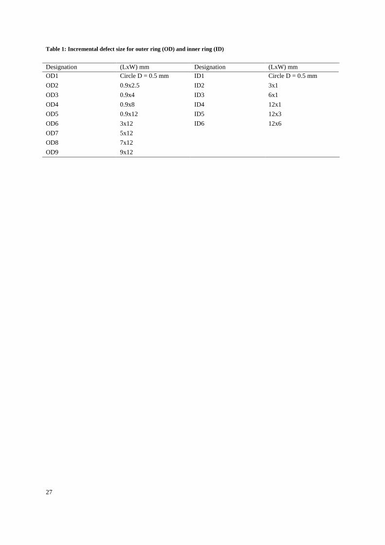
Two split Cooper bearings are used for the experiment in order to seed a variety of defects on each bearing. To

evaluate the temporal indicators largely used in vibratory analysis, the growth of the defect is simulated on outer

ring and inner ring. An isolated defect is simulated which is artificially increased in size. The defect grows in the

direction of the length of the track (L) then in the direction of the width of the track (W). All defects are grouped

in table 1. The load is set at 5.3 kN.

3.2 Spectral correlation and envelope analysis

It has been established that compared to bearing vibration monitoring, AE has the ability to detect the growth of

subsurface cracks whereas the former can detect defects only when they appear on the surface [21].

Consequently, AE offers the possibility to detect incipient bearing damage if judicious signal processing is

implemented. In this section, we compare envelope analysis and spectral correlation on AE signals for bearing

defect detection.

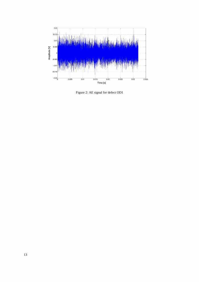
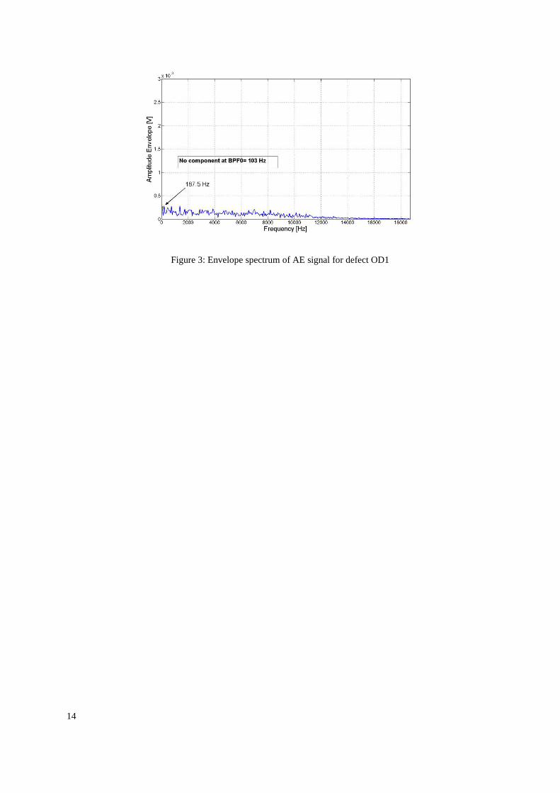
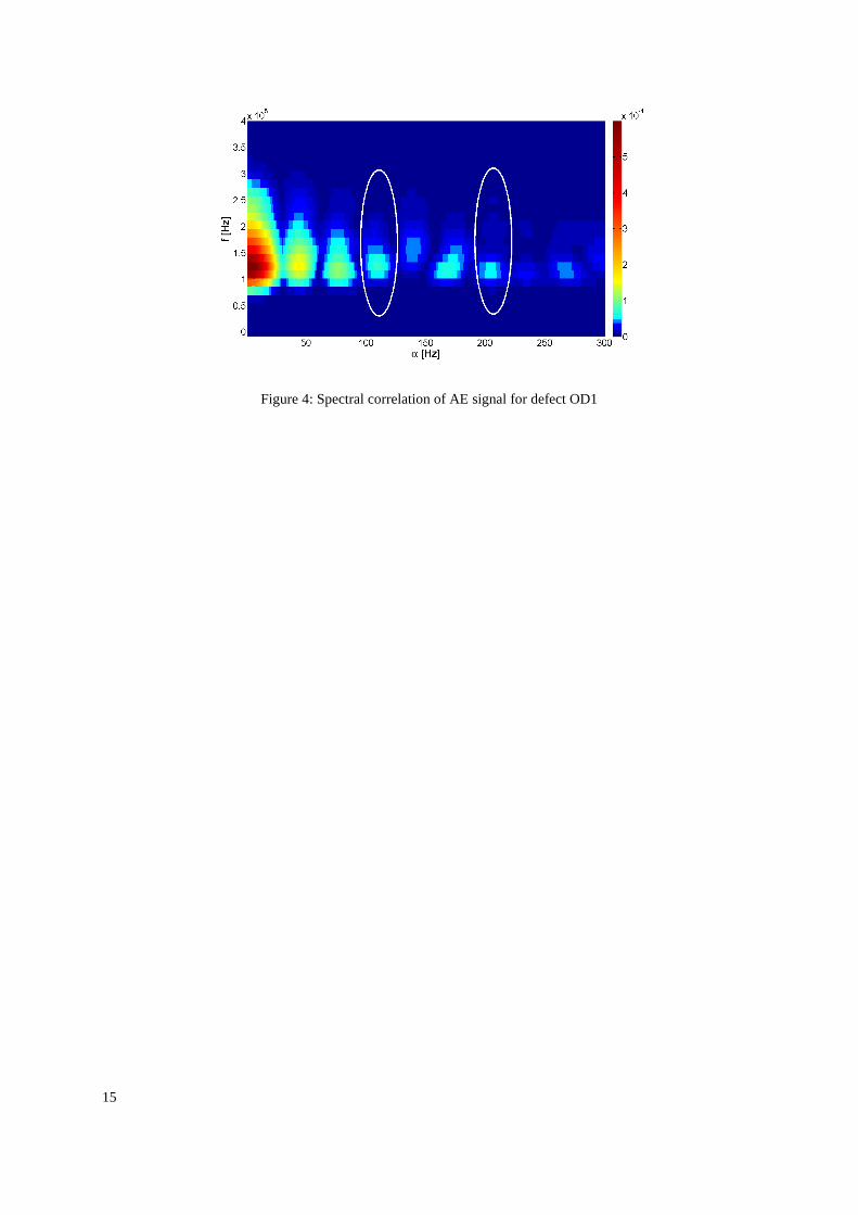
Figures 2 and 3 represent the time waveform and the envelope spectrum relative to the smallest defect size OD1

on the outer race, one can note the absence of bursts in the waveform and the absence of the BPFO (103 Hz) in

the envelope spectrum. This indicates the difficulty in detecting incipient fault by envelope analysis, however,

the spectral correlation identified the presence of such a defect, see figure 4. Envelope analysis involved

demodulating within the 50kHz-300 kHz frequency band.

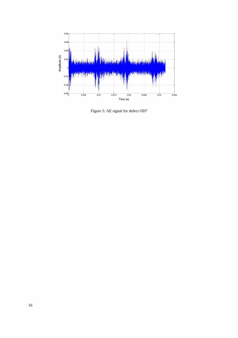
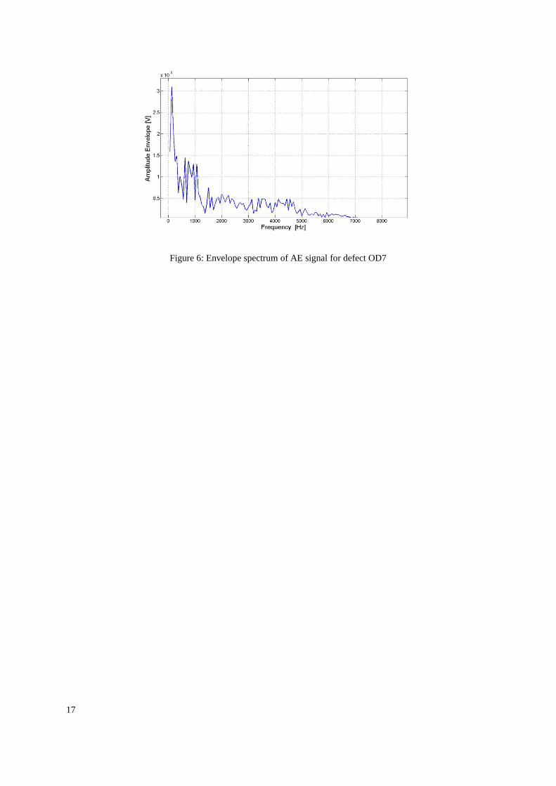
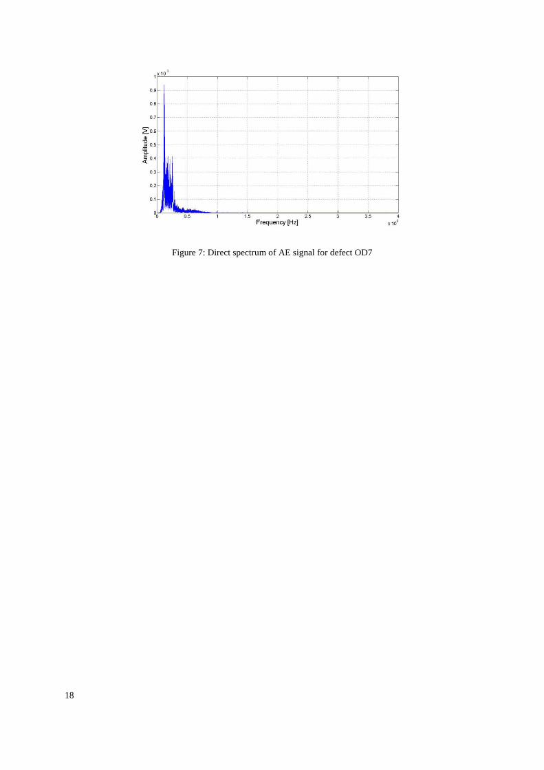
Envelope analysis proved to be effective only when the size of defect became larger. The case of OD7 shows

the presence of bursts in the time waveform (Fig.5) and that of a peak at 125 Hz in the envelop spectrum, which

can is attributed to the BPFO, see figure 6. It must be stated that a frequency spectrum of the AE waveform

offers no diagnostic information, see figure 7.

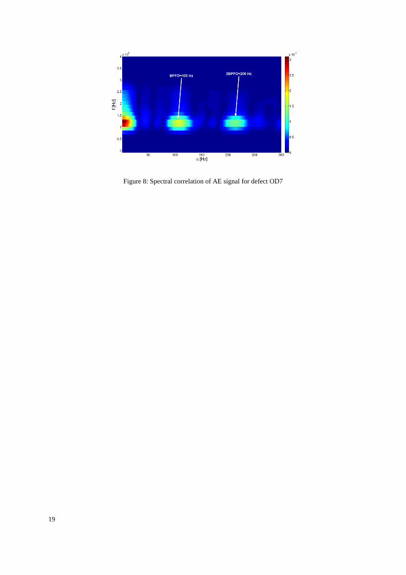
Figure 8 highlights the spectral correlation for OD7 clearly showing the manifestation of BPFO and its second

harmonic. The level of energy of the spectral correlation is, in this case, definitely larger than that of defect OD1.

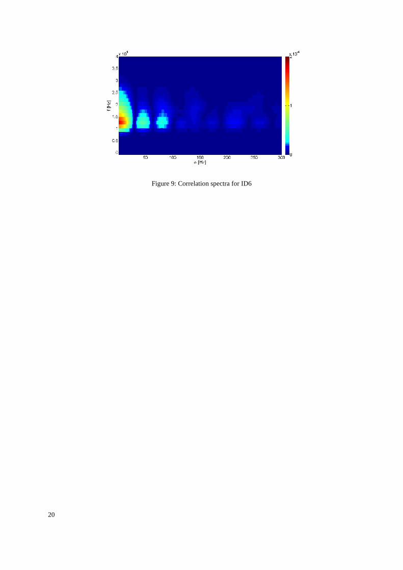
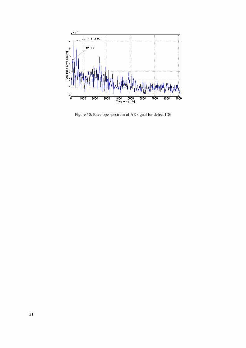
This shows its sensitivity to the outer race defect evolution. However, the envelope spectrum and the spectral

correlation do not reveal the peak of BPFI at 147 Hz, figures 9, 10.

These observations have shown AE signal from bearing are cyclostationary. The application of spectral

correlation gave better results than envelope analysis. However, it must be mentioned here that spectral

8

correlation of AE is not effective for inner race defects, nor was traditional enveloping. This is attributed to the

arduous transmission path too significant propagation path between the inner race defect and the receiving

sensor.

3.3 The" Integrated Spectral Correlation" indicator : ICS

In order to track the defect evolution, we defined an indicator that evaluates energy at α at the defect frequency

fdef from the spectral correlation. As spectral correlation is discrete along α-axis, the defect frequency does not

necessarily belong to the set of α values. Hence, the health indicator, the Integrated Spectral Correlation noted

ICS is computed by integrating the spectral correlation between α1,2≈ fdef±1 along α-axis, and for all the values

along f-axis.

dfSICS x

sf

αα

αα∫∑ 2

0

2

1=

=

(13)

3.3.1 Analysis of the outer race defect

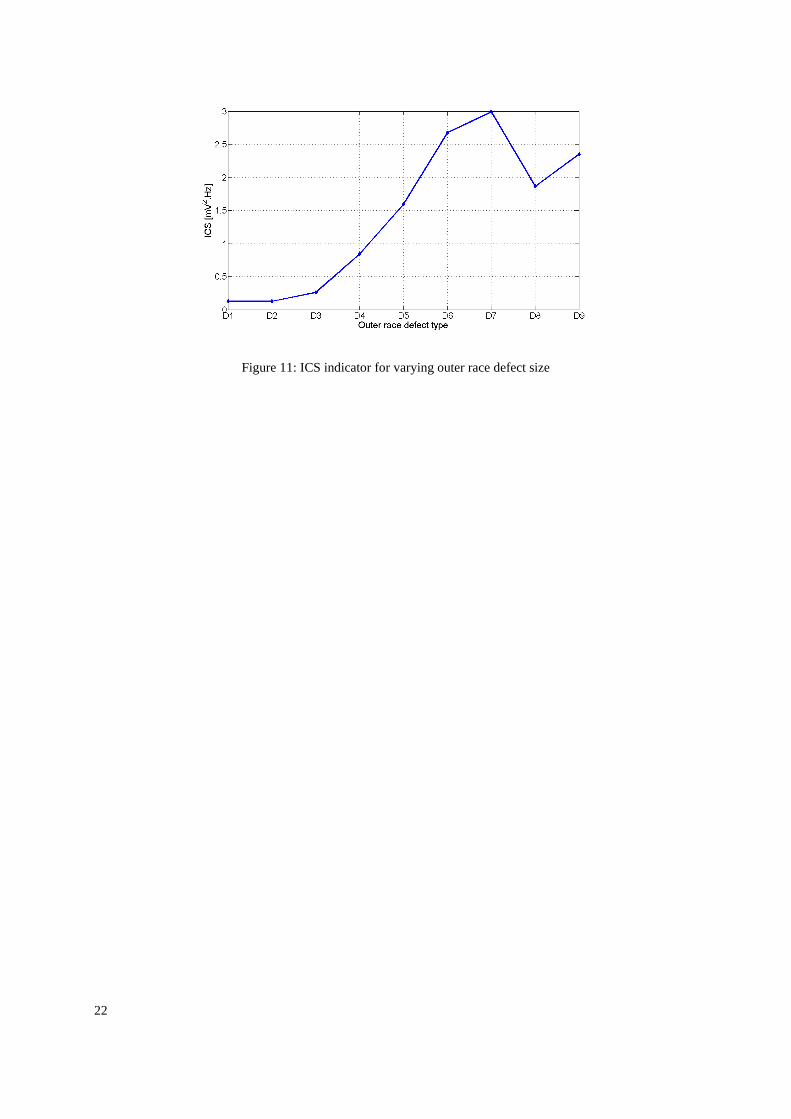
Applied to this study, the ICS indicator increased with increasing outer ring defect size as illustrated in figure

11.

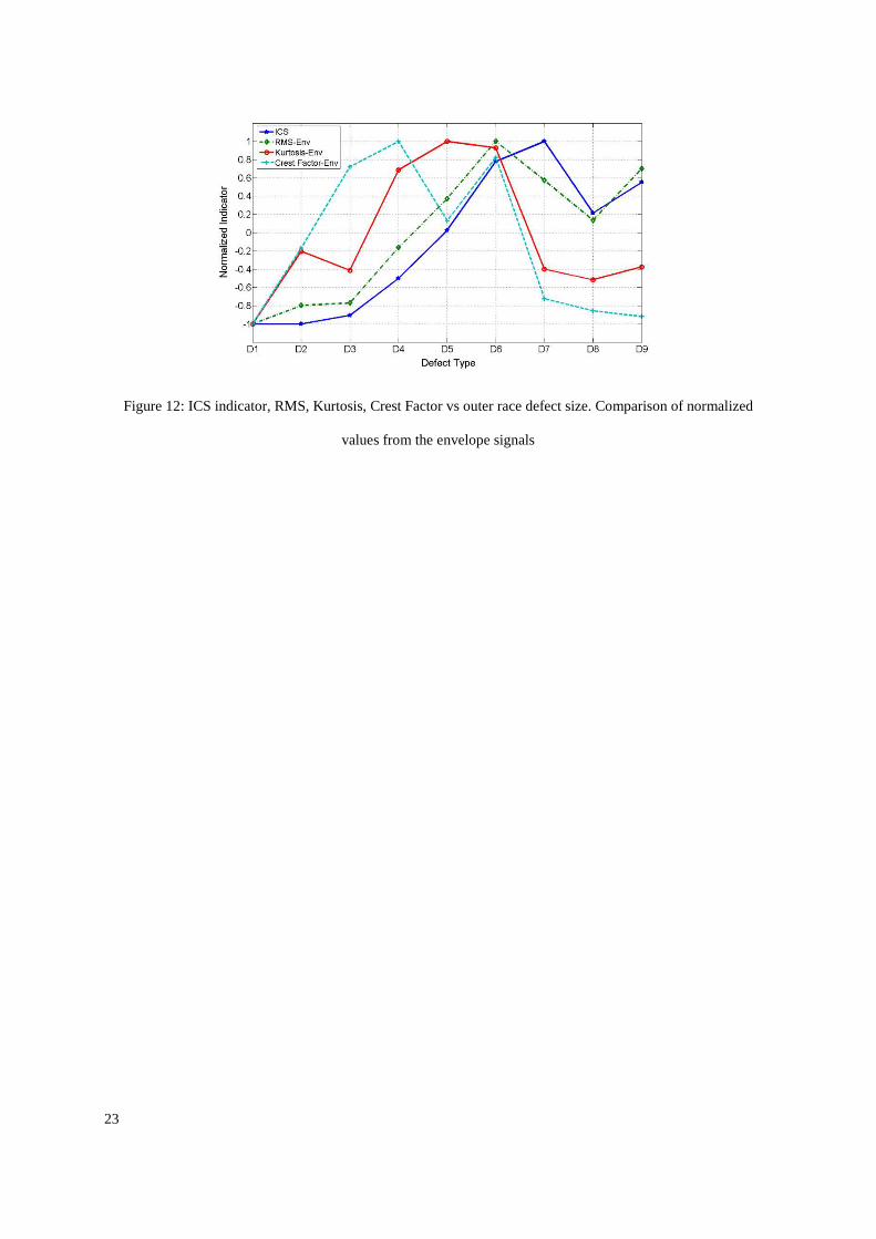
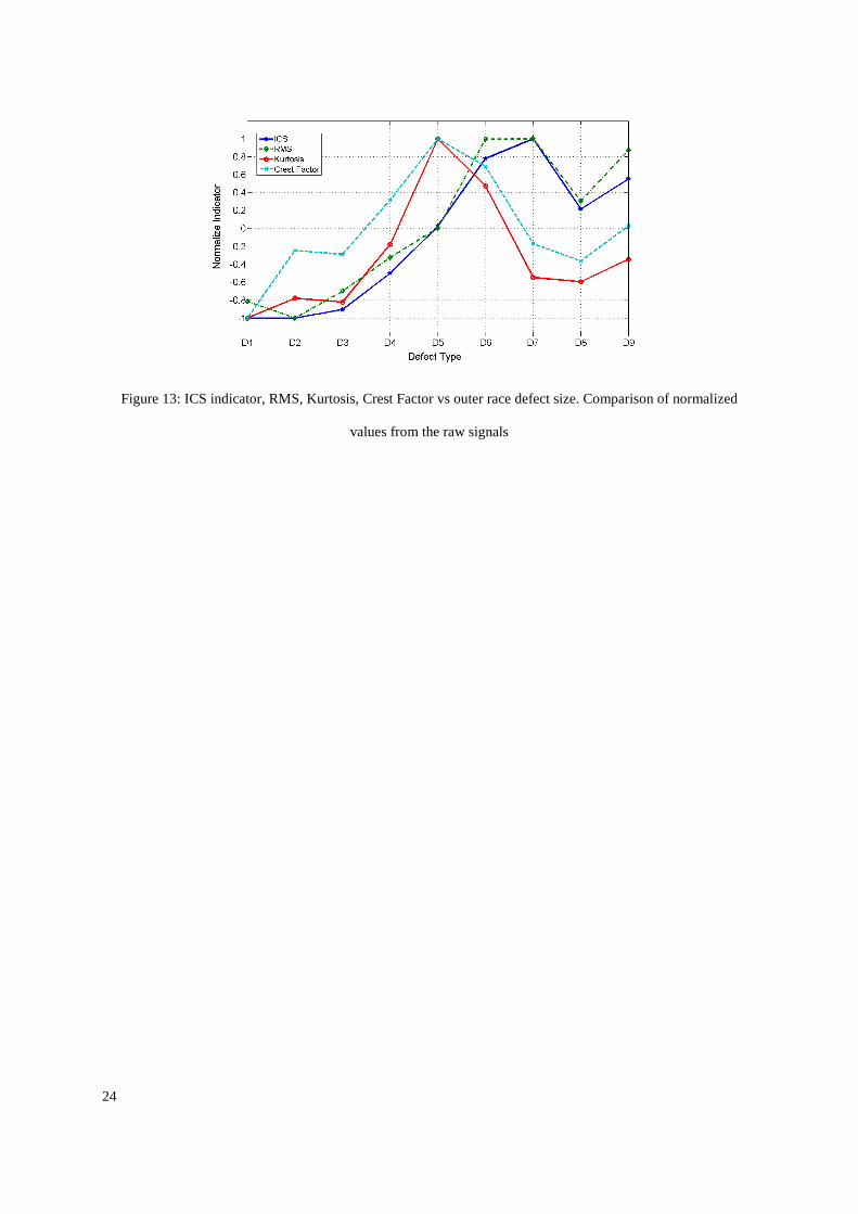
Compared to time domain indicators (RMS, Kurtosis and Crest Factor), the ICS indicator presents a good

correlation with the increasing outer race defect. Kurtosis values and Crest Factors computed for both the

envelope signals and the raw signals did not show increasing values with increasing defect size though the RMS

value of the raw signal showed close similarity with the ICS indicator (Fig. 12 and 13). The table 2 shows that

the ICS indicator offered the best correlation between its increasing value and the increasing defect size.

Interestingly, as with other indicators, the ICS indicator was affected by changes in the length of the defect

(OD6�OD9) (Fig. 12 and 13).

9

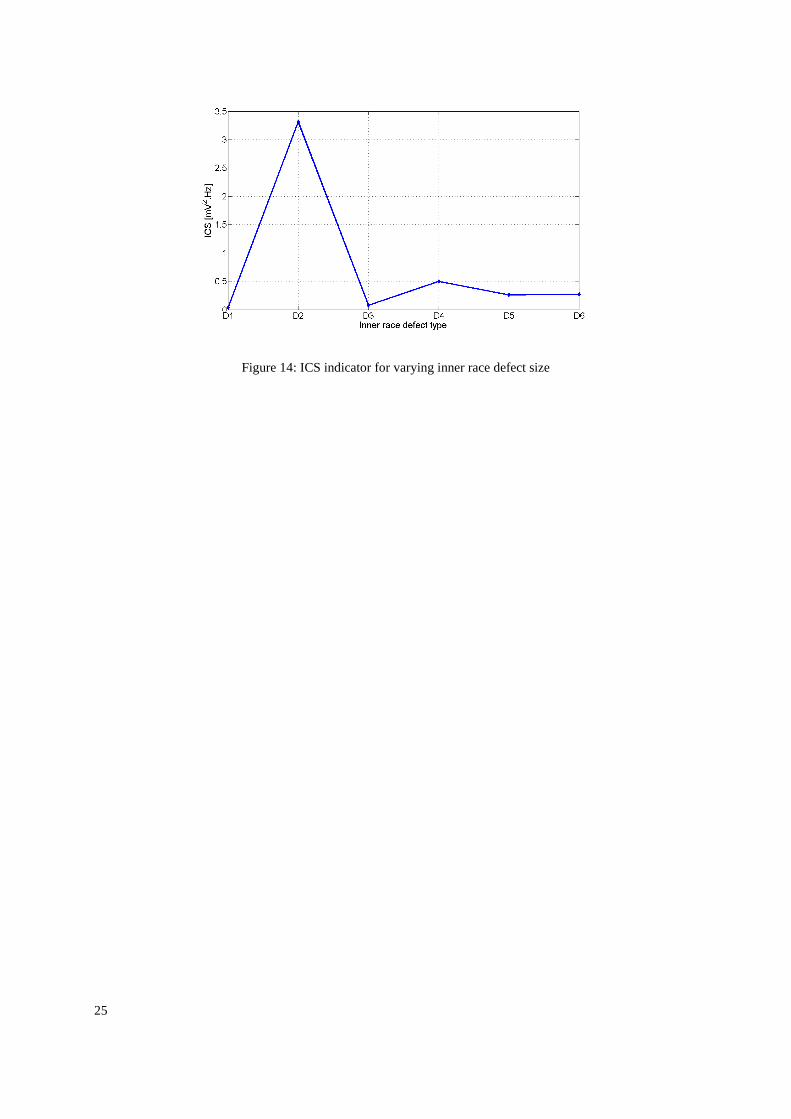
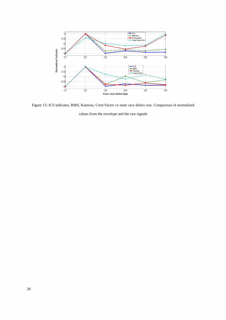
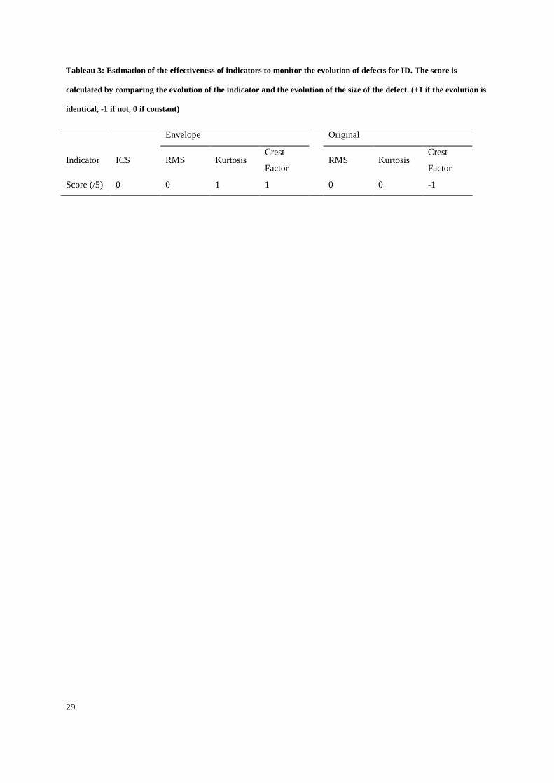
3.3.2 Analysis of the inner race defect

Contrary to the outer race defect, the ICS indicator computed from AE signals associated with the inner race

defect did not increase with the increasing of defect size (Fig. 14). The same observation was noted for other

indicators, see figure 15 and table 3. As explained earlier this was not surprising.

4 Conclusion

.This paper highlights the cyclostationary character of Acoustic Emission from bearings; it showed also the

effectiveness of the spectral correlation and the ICS indicator for monitoring bearing defects. The use of this

statistical property showed improved detection and diagnosis of defects vis-a-vis the traditional envelope

spectrum. Furthermore, the increased sensitivity of the developed indicator, ICS, over traditional indicators

(RMS, Kurtosis, and Crest Factor) was demonstrated. The use of the cyclostationarity offers an undeniable

advantage for applications of AE. However this effectiveness is valid only within the framework of an outer race

defect. Indeed, the inner race defect remains a delicate subject especially when the defect is small.

5 References

[1] D. Mba, R.B.K.N Rao, Development of acoustic emission technology for condition monitoring and

diagnosis of rotating machines: Bearings, pumps, gearboxes, engines, and rotating structures, Shock and

Vibration Digest, 38(2), (2006), 3-16.

[2] J.R. Mathews, Acoustic Emission, Gordon and Breach Science Publishers Inc., New York ISSN 0730-

7152, 1983.

[3] P.D. McFadden, J.D. Smith, Acoustic emission transducers for the vibration monitoring of bearings at low

speeds, Cambridge University, Engineering Department, (Technical Report) CUED/C-Mech, 1983.

[4] L.M. Rogers, The application of vibration signature analysis and acoustic emission source location to on-

line condition monitoring of anti-friction bearings, Tribology International, 12(2), (1979), 51-59.

[5] N. Tandon, B.C. Nakra, The application of the sound-intensity technique to defect detection in rolling-

element bearings, Applied Acoustics, 29(3), (1990), 207-217.

[6] V. Bansal, B.C. Gupta, A. Prakash, V.A. Eshwar, Quality inspection of rolling element bearing using

acousic emission technique, Journal of Acoustic Emission, 9(2), (1990), 142-146,.

10

[7] A. Choudhury, N. Tandon, Application of acoustic emission technique for the detection of defects in rolling

element bearings, Tribology International, (2003), 39–45.

[8] A.M. Al-Ghamdi, P. Cole, R. Such, D. Mba, Estimation of bearing defect size with acoustic emission,

Insight: Non-Destructive Testing and Condition Monitoring, 46(12), (2004), 758-761.

[9] D. Mba, The use of acoustic emission for estimation of bearing defect size, Journal of Failure Analysis and

Prevention, 8(2), (2008), 188-192.

[10] S. Al-Dossary, R.I.R. Hamzah, D. Mba, Observations of changes in acoustic emission waveform for

varying seeded defect sizes in a rolling element bearing, Journal of Applied Acoustics, 70(1), (2009), 58–

81.

[11] J.Z. Sikorska, D. Mba, Truth, Lies, Acoustic Emission and process machines, Journal of Mechanical

Process Engineering, Part E, IMechE, 222(1), (2008), 1-19.

[12] G.-H. Liu, P.-J. Huang, X. Gong, J. Gu, Z.-K. Zhou, Feature extraction of acoustic emission signals based

on fractal dimension and independent component analysis Journal of South China University of

Technology (Natural Science), 36 (1), (2008), 76-80.

[13] C. Liao, X. Li, D. Liu, Application of reassigned wavelet scalogram in feature extraction based on acoustic

emission signal, Journal of Mechanical Engineering, 45(2), (2009), 273-279.

[14] M. Žvokelj, S. Zupan, I. Prebil, Multivariate and multiscale monitoring of large-size low-speed bearings

using Ensemble Empirical Mode Decomposition method combined with Principal Component Analysis,

Mechanical Systems and Signal Processing , (24)4, (2010), 1049-1067 .

[15] X.-J. Li, C.-J. Liao, X.-L. Luo, Application of gabor transform in feature extraction of acoustic emission

signal, Jiliang Xuebao/Acta Metrologica Sinica, 30(3), (2009), 234-239.

[16] X. Chiementin, D. Mba, B. Charnley, S. Lignon, J.-P. Dron, Effect of the denoising on Acoustic Emission

signals, Journal of Vibration and Acoustics, In press, (2009).

[17] C. James Li, S. Li, Acoustic emission analysis for bearing condition monitoring, Wear, 185, (1995) 67-74.

[18] J. Antoni, Cyclostationarity by examples, Mechanical Systems and Signal Processing, 23, (2009) 987-

1036.

[19] A.C. McCormick, A.K. Nandi, Cyclostationarity in rotating machine vibrations, Mechanical Systems and

Signal Processing, 12(2), (1998), 225-242.

11

[20] J. Antoni, Cyclic spectral analysis in practice, Mechanical Systems and Signal Processing, 21 (2007) 597-

630.

[21] N. Tandon, A. Choudhury, A review of vibration and acoustic measurement methods for the detection of

defect in rolling element bearings, Tribology international, 32, (1999), 469-480.

12

Figure 1: (a) The test rig. (b) Bearing

13

Figure 2: AE signal for defect OD1

14

Figure 3: Envelope spectrum of AE signal for defect OD1

15

Figure 4: Spectral correlation of AE signal for defect OD1

16

Figure 5: AE signal for defect OD7

17

Figure 6: Envelope spectrum of AE signal for defect OD7

18

Figure 7: Direct spectrum of AE signal for defect OD7

19

Figure 8: Spectral correlation of AE signal for defect OD7

20

Figure 9: Correlation spectra for ID6

21

Figure 10: Envelope spectrum of AE signal for defect ID6

22

Figure 11: ICS indicator for varying outer race defect size

23

Figure 12: ICS indicator, RMS, Kurtosis, Crest Factor vs outer race defect size. Comparison of normalized

values from the envelope signals

24

Figure 13: ICS indicator, RMS, Kurtosis, Crest Factor vs outer race defect size. Comparison of normalized

values from the raw signals

25

Figure 14: ICS indicator for varying inner race defect size

26

Figure 15: ICS indicator, RMS, Kurtosis, Crest Factor vs inner race defect size. Comparison of normalized

values from the envelope and the raw signals

27

Table 1: Incremental defect size for outer ring (OD) and inner ring (ID)

Designation (LxW) mm Designation (LxW) mm OD1 Circle D = 0.5 mm ID1 Circle D = 0.5 mm

OD2 0.9x2.5 ID2 3x1

OD3 0.9x4 ID3 6x1

OD4 0.9x8 ID4 12x1

OD5 0.9x12 ID5 12x3

OD6 3x12 ID6 12x6

OD7 5x12

OD8 7x12

OD9 9x12

28

Tableau 2: Estimation of the effectiveness of indicators to monitor the evolution of defects for OD. The score is

calculated by comparing the evolution of the indicator and the evolution of the size of the defect. (+1 if the evolution is

identical, -1 if not, 0 if constant)

Envelope Original

Indicator ICS RMS Kurtosis Crest

Factor RMS Kurtosis

Crest

Factor

Score (/9) 5 3 1 1 3 2 1

29

Tableau 3: Estimation of the effectiveness of indicators to monitor the evolution of defects for ID. The score is

calculated by comparing the evolution of the indicator and the evolution of the size of the defect. (+1 if the evolution is

identical, -1 if not, 0 if constant)

Envelope Original

Indicator ICS RMS Kurtosis Crest

Factor RMS Kurtosis

Crest

Factor

Score (/5) 0 0 1 1 0 0 -1