Statistical Diagnosis of the Best Weibull Methods for ... - MDPI

Energies 2014, 7, 3056-3085; doi:10.3390/en7053056

energies ISSN 1996-1073

www.mdpi.com/journal/energies

Article

Statistical Diagnosis of the Best Weibull Methods for Wind Power Assessment for Agricultural Applications

Abul Kalam Azad 1,*, Mohammad Golam Rasul 1 and Talal Yusaf 2

1 School of Engineering and Technology, Central Queensland University, Rockhampton,

QLD 4702, Australia; E-Mail: [email protected] 2 National Centre for Engineering in Agriculture, Faculty of Engineering and Surveying,

University of Southern Queensland, Toowoomba, QLD 4350, Australia;

E-Mail: [email protected]

* Author to whom correspondence should be addressed; E-Mail: [email protected] or

[email protected]; Tel.: +61-469-235-722; Fax: +61-749-309-382.

Received: 20 February 2014; in revised form: 22 April 2014 / Accepted: 23 April 2014 /

Published: 2 May 2014

Abstract: The best Weibull distribution methods for the assessment of wind energy

potential at different altitudes in desired locations are statistically diagnosed in this study.

Seven different methods, namely graphical method (GM), method of moments (MOM),

standard deviation method (STDM), maximum likelihood method (MLM), power density

method (PDM), modified maximum likelihood method (MMLM) and equivalent energy

method (EEM) were used to estimate the Weibull parameters and six statistical tools,

namely relative percentage of error, root mean square error (RMSE), mean percentage

of error, mean absolute percentage of error, chi-square error and analysis of variance were

used to precisely rank the methods. The statistical fittings of the measured and calculated

wind speed data are assessed for justifying the performance of the methods. The capacity

factor and total energy generated by a small model wind turbine is calculated by numerical

integration using Trapezoidal sums and Simpson’s rules. The results show that MOM and

MLM are the most efficient methods for determining the value of k and c to fit Weibull

distribution curves.

Keywords: the Weibull shape factor; scale factor; probability density function; power density;

statistical tools

OPEN ACCESS

Energies 2014, 7 3057

1. Introduction

Energy and environment are the twin major crises in the world [1]. Because of this, both developed

and developing countries are becoming increasingly more interested in using pollution free, cost

effective and renewable sources of energy [2]. As a renewable and alternative energy, wind is the most

common and fastest-growing source of energy in the world [3–5]. The characteristics of wind energy

are important in different aspects regarding wind energy exploitation [6,7]. Wind is highly variable,

both in space and in time [8]. The importance of this variability becomes critical since it is amplified

by the cubic relationship of the available power to the wind speed (p = 0.5ρAV3). The wind power

production faces the fluctuation of the wind velocity [9–12]. Therefore, accurate knowledge about the

wind characteristics is needed for planning, design and operation of wind turbines [13–16]. For the

proper assessment, the variability of the wind over time can be divided into three distinct time scales.

Firstly, the large time scale variability describes the variations of the amount of wind from one year to

another, or even over periods of decades or more. Secondly, the medium time scale covers periods up

to a year. These seasonal variations of the wind are much more predictable. Finally, the short term time

scale variability covers time scales of minutes to seconds, also well known by the term “turbulence”

and which is of critical interest in the wind turbine design process [17–23]. For more than half a

century the Weibull distribution has attracted the attention of statisticians working on theory and

methods as well as various fields of statistics [22,24–27]. Hundreds of papers have been written on this

distribution; however the research is still ongoing. Together with the normal, exponential distributions,

the Weibull distribution is the most popular model in statistics [28,29]. It is of utmost interest to theory

orientated statisticians because of its great number of special features, and to practitioners because of

its ability to fit to data from various fields, ranging from life data to weather data or observations made

in economics and business administration, in health, in physical and social science, in hydrology, in

biology or in the engineering sciences [30–36].

Research is ongoing worldwide on the Weibull distribution to find the most reliable methods for

wind energy estimation. The main question is how precisely the values of the Weibull shape factor “k”

and scale factor “c” can be determined [37–39]. For this reason different scientists and engineers

have developed different methods to find the Weibull parameters for wind energy assessment. That is

why several methods are found in literature to estimate the Weibull factors [38,40–43]. Recently,

Mohammadi and Mostafaeipour [44] used two methods (STDM and PDM) for wind data assessment

in Zarrineh, Iran. In 2012, Costa Rocha et al. [45] dealt with the analysis and comparison of seven

numerical methods for the assessment of effectiveness in determining the parameters for the Weibull

distribution, using wind data collected for Camocim and Paracuru cities in the northeast region of

Brazil. Before that, Chang [41] made a statistical study to compare the performance of six numerical

methods in estimating Weibull parameters for wind energy application. Seguro and Lambert [43]

concluded that the maximum likelihood method (MLM) performs better than the popularly used

graphical method (GM). Akdağ and Dinler [40], Azad and Saha [46], and Azad and Alam [47]

reviewed three conventional methods and Akdag and Dinler [40] also proposed a new method, namely

the energy pattern factor method, for estimating the Weibull parameters. Chu and Ke [48] and

Bhattacharya and Bhattacharjee [49] examined the estimation comparison between the MLM and

the least squares method [50]. They found that the least squares method significantly outperforms

Energies 2014, 7 3058

the MLM when sample size is the same. Jowder [51] used empirical and graphical methods to analyze

the wind power density at 10, 30, and 60 m height in the Kingdom of Bahrain; two Weibull parameters

were estimated and compared. From the analysis, it was found that the empirical methods provide

more accurate prediction of average wind speed and power density than the GM. Odo et al. [52] used

the Weibull distribution based model for prediction of wind energy potential in Enugu, Nigeria over a

period of 13 years. Oyedepo et al. [53] also analyzed south-east Nigeria wind data that spans from

24 years to 37 years and was measured at 10 m height. Abbas et al. [54] statistically analyzed the wind

speed data in Pakistan to determine the best fitting distribution of wind speed. For this purpose,

two parameters Gamma, Weibull, Lognormal and Rayleigh distributions, and three parameters Burr

and Frechet distributions were fitted to data and parameters for each distribution were estimated using

the MLM [42,50,55–61].

Seguro and Lambart [43] calculated the value of the Weibull parameters by three methods. They

recommended that the MLM is useful for time series wind speed data and the modified maximum

likelihood method (MMLM) is recommended for use with wind data in frequency distribution format.

Philippopoulos and Deligiorgi [62] statistically simulated the wind speed data in Athens, Greece based

on the Weibull and autoregressive-moving average (ARMA) method. They found that ARMA methods

are superior in simulating the frequency distribution of wind speed. Karpa and Naess [63] also

analyzed the extreme value statistics of wind speed by the average conditional exceedance rate

(ACER) method. Morgan et al. [64] examined the probability distributions for offshore wind speed.

They concluded that the two-parameter lognormal distribution performs best for estimating extreme

wind speeds, but still gives estimates with significant error. Stathopoulos et al. [65] used both

numerical and statistical models for wind power prediction. Zhou et al. [66] comprehensively

evaluated wind speed distribution models for a case study of North Dakota country sites. Wind energy

estimation and analysis of wind regions through the Weibull distribution methods is widely used

nowadays [35,37,67–80].

This study summarizes the results of the 10-min time series wind speed data measured at 20 m and

30 m height in three windy sites, namely Kuakata, Kutubdia and Sitakunda, located in Bangladesh.

Table 1 shows the site information in which DL9210 anemometer used to measure wind speed at a

10-min interval. The anemometers have two sensors each of 32 KB memory and have one/two sockets.

Statistical work was involved to find the best method of Weibull distribution with high efficiency.

The assessment of wind energy potential has been done by using the best method of Weibull distribution.

Section 2 offers a detailed outline of the methodology and associated theories for the statistical analysis.

The results and discussions are presented in Section 3. Concluding remarks are presented in Section 4.

Table 1. Site name, location for wind speed measuring at 20 m and 30 m height above surface.

Wind station name Site name Latitude (°) N Longitude (°) E Height above the sea level

Reference

Station-I Kuakata 21°54.76' 90°08.24' 3 m [81] Station-II Kutubdia 21°54.71' 91°52.43' 0–4 m [82] Station-III Sitakunda 22°35.68' 91°42.52' 9 m [83]

Energies 2014, 7 3059

2. Outline of the Methodology and Associated Theories

To investigate the feasibility of the wind energy resource at any site, there are basically two ways at

present to evaluate wind power. The first and the most accurate method to calculate wind power

potential is based on measured values that are recorded at meteorological stations. The second method

to assess wind power potential is by using probability distribution functions, namely the Rayleigh

distribution, Chi-squared distribution, Normal distribution, Binomial distribution, Poisson distribution

and Weibull distribution. In this study, the authors used only the Weibull distribution for wind power

assessment as presented and discussed below.

2.1. Weibull Probability Density Function

The Weibull probability density function is a two-parameter function characterized by a dimensionless

shape parameter (k) and scale parameter (c in m/s). These two parameters determine the wind speed for

optimum performance of a wind conversion system as well as the speed range over which the device is

likely to operate [52,84–87] as given in Equation (1): ( ) = ( ) = × (1)

where v, k and c are wind speed (m/s), shape factor (dimensionless) and scale factor (m/s), respectively.

2.2. Cumulative Distribution Function or the Weibull Function

Cumulative distribution function is the integration of the Weibull density function. It is the

cumulative of relative frequency of each velocity interval [31]. The equation of the Weibull Function

is given by: ( ) = ( ́) ́ (2)

( ) = 1 − (3)

All these distributions are used to determine the probability of occurrence. The nature of the occurrence

affects the shape of the probability curve, and in the case of the wind regime, the cumulative curve

probability nature mostly fits to the Weibull Function. Several methods to estimate Weibull factors are

found in the literature. Some of these methods are:

(1) Graphical method (GM);

(2) Method of moments (MOM);

(3) Standard deviation method (STDM);

(4) Maximum likelihood method (MLM);

(5) Power density method (PDM);

(6) Modified maximum likelihood method (MMLM);

(7) Equivalent energy method (EEM).

Energies 2014, 7 3060

2.2.1. GM

The graph is constructed in such a way that the cumulative Weibull distribution becomes a straight line,

with the shape factor k as its slope. Taking the logarithm of both sides, the expression of Equation (3)

can be rewritten as: 1 − ( ) = (4)

or: − ln 1 − ( ) = ln − ln (5)

The above equation represents a relationship between ln(v) and −ln{1 − F(v)}. Therefore, the horizontal

axis of this plot on the Weibull paper is v while the vertical axis is ln(1 − F(v))−1. The result is a

straight line with slope k. For v = c, one finds F(v) = 1 − e−1 = 0.632 and t an estimation for the value

of c, by drawing a horizontal line at F(v) = 0.632. The intersection point with the Weibull line gives

the value of c.

2.2.2. MOM

The MOM is another technique commonly used in the field of parameter estimation. If the numbers

v1, v2, …, vn represent a set of data, then an unbiased estimator for the n-th origin moment is given by: = 1 (6)

where stands for the estimation of mn. In a Weibull distribution, the nth moment readily follows

from Equation (3). With an expression of the Gamma function Γ(x), the average wind speed can be

expressed as a function of c and k. The integral found cannot be solved, however it can be reduced to

a standard integral, the gamma function, as follows: Γ( ) = × (7)

where = and = ; = 1 + and, after a few manipulations:

μ = 1 Γ 1 + (8)

After a few manipulations: μ = × Γ 1 + 1 = 0.8525 + 0.0135 + ( ) (9)

This formula can easily be handled by pocket calculators in energy output calculations. The accuracy

of the approximation is within 0.5% for 1.6 < k < 3.5.Then from Equation (8) we can find the first and

the second moments as follows:

= μ = 1 Γ 1 + 1 (10)

Energies 2014, 7 3061

and:

=μ +σ = 1 Γ 1 + 2 − Γ 1 + 1 (11)

When we divide m2 by the square of m1, we get an expression which is a function of the shape

factor k only:

Γ 1 + 2 − Γ 1 + 1Γ 1 + 1 (12)

On taking the square roots of the equation, we have the coefficient of variation (COV):

= Γ 1 + 2 − Γ 1 + 1Γ 1 + 1 (13)

In this case, this method can be used as an alternative to the MLM. The value of k and c can be

easily determined by the following equations: σ = Γ 1 + 2 − Γ 1 + 1 (14)

σ̅ = 1 + 21 + 1 − 1 (15)

After some calculation we can find:

= 0.9874σ̅ . (16)

The Weibull scale factor can be calculated by: ̅ = Γ 1 + 1 (17)

2.2.3. STDM

In the STDM, the Weibull factors can be obtained as follows: = σ̅ . (18)

and: = ̅Γ 1 + 1 (19)

Energies 2014, 7 3062

where ̅ and σ are mean wind speed and standard deviation of wind speed for any specified periods of

time respectively, and can be calculated [44,88] as follows: ̅ = 1 (20)

By determining the mean wind speed ̅, the standard deviation σ of wind speed becomes:

σ = ( − ̅) (21)

or:

σ = 1− 1 ( − ̅) (22)

One can find next an expression for σ in terms of k and c with ̅ = c × Γ(1 + 1/k) and also Γ(x) is the

gamma function and is defined as: Γ( ) = exp(− ) (23)

2.2.4. MLM

Maximum likelihood estimation has been the most widely used method for estimating the

parameters of the Weibull distribution. The commonly used procedure of MLM proposed by Cohe [50],

Harter and Moore [55] and Gove [89] due to its very desirable properties. Let v1, v2, ..., vn be a random

sample of size n drawn from a probability density function f(vi, θ), where θ is an unknown parameter.

The likelihood function of this random sample is the joint density of the n random variables and is

a function of the unknown parameter [89] given as: = ( , θ) (24)

Thus, Equation (24) is the likelihood function. The maximum likelihood estimator (MLE) of θ,

sayθ, is the value of θ that maximizes L or, equivalently, the logarithm of L. Often, but not always, the

MLE of θ is a solution of (dlogL)/dθ = 0, where solutions that are not functions of the sample values

v1, v2, ..., vn are not admissible, nor are solutions which are not in the parameter space. Now, we are

going to apply the MLE to estimate the Weibull parameters, namely the shape and the scale

parameters [90]. Consider the Weibull probability density function given in Equation (3), and then the

likelihood function will be represented as: ( , , ) = − (25)

On taking the logarithms of both sides of Equation (25), we obtain the estimating

log-likelihood function:

Energies 2014, 7 3063

ln( ) = ln( ) − ln( ) + ( − 1) ln( ) − (26)

Differentiating Equation (26) with respect to k and c in turn and equating to zero, we have: ∂ln( )∂ = − + = 0 (27)

∂ ln( )∂ = + − = 0 (28)

From Equation (27):

= 1 ( ) (29)

When is obtained, then ̂ is can be determined. To solve by using the Newton-Raphson method

as given below, let f(k) be the same as Equation (28) and taking the first differential of f(k), we have: ( ) = − − (30)

Substituting Equation (29) into Equation (28) gives:

( ) = + ( )1 ∑ ( ) − ( )1 ∑ ( ) ( )1 ∑ ( ) (31)

Substituting Equation (29) into Equation (30), we get:

( ) = − + ( )1 ∑ ( ) ln ( )1 ∑ ( ) (32)

Therefore, is obtained from the equation below by carefully choosing an initial value for ki and

iterating the process until it converges:

= − + ∑ 1 ∑ ( )− + ∑ ( )1 ∑ ( ) ln ( )1 ∑ ( )

− ∑ ( )1 ∑ ( ) ln ( )1 ∑ ( )− + ∑ ( )1 ∑ ( ) ln ( )1 ∑ ( )

(33)

Energies 2014, 7 3064

2.2.5. PDM

To obtain the shape factor and scale factor through this method, firstly the energy pattern factor is

computed. The energy pattern factor usage is for turbine aerodynamic design. The energy pattern

factor is related to the averaged data of wind speed and is defined as a ratio between mean of cubic

wind speed to cube of mean wind speed. The energy pattern factor Epf is expressed as [40,45]: = Totalamount of power available in the windPowercalculated by cubing the mean wind speed

or = ∑∑ = ( ) = (34)

Once the energy pattern factor is calculated by using the above equation, the Weibull shape factor

and scale factor can be estimated from the following formulas: = 1 + 3.69 (35)

= ̅Γ 1 + 1 (36)

where Epf is the energy pattern factor; and Γ is the gamma function.

2.2.6. MMLM

The MMLM can only be considered if the available data of wind speed are already in the shape of

the Weibull distribution. The solution of the equations in the MLM requires some numerical iteration

by the Newton-Raphson method [41]. The Weibull parameters are determined by the following equations: = ∑ ( ) ( )∑ ( ) − ∑ ( ) ( )( ≥ 0) (37)

= 1( ≥ 0) ( ) ( ) (38)

where vi is the wind speed central to bin i; n is the number of bins; f(vi) represents the Weibull

frequency for the wind speed range within bin I; and f(v ≥ 0) is the probability for wind speed to equal

or exceed zero.

2.2.7. EEM

Consider a random sample of v1, v2, ..., vn by relative frequency of occurrence in a given interval

of wind speed. Then a random variable observation discrete Wv associated with wind speed can be

obtained from: = ( ) (39)

Energies 2014, 7 3065

This observation random is also related with the Weibull parameters k and c from the equation of

the probability of occurrence W. W(v) is the observed frequency of the wind speed for the interval of

(v − 1) ≤ V < v. The mathematical representation of W(v) is: ( ) = ( − 1) − ( ) (40)( ) = − (41)

where Q(v) and the probability of occurrence of wind speeds equal to or higher than v, given by

Q(v) = 1 − F(v). Then the random observation Wv can be written using Equations (39) and (41) as: = ( ) + = − + (42)

The first hypothesis says that “The energy density is a parameter that helps in the determination of

parameters of the Weibull distribution for applications in wind energy”. The related factor part

deterministic must meet the following conditions: (a) be variable with random value expected value

equal to 0: E(ε) = 0; (b) be variable random variance with constant: v(ε) = σ2; and (c) the occurrences

of ε are non-correlated: COV(εi, εj). To ensure the condition of equivalence initially proposed in the

hypothesis, it is the equality between Equation (4) and = ∑ . The equation resulting from

this transaction expresses the parameter c as a function of speed cubed average of observations and the

parameter k as:

c = v1 + 3k (43)

Substituting Equation (43) into Equation (42) gives:

= ( ) − ( ) + ε (44)

The estimate of the parameter k may be obtained from an estimator of least squares given by the

expression [45]:

− ( ) + ( ) = (ε ) (45)

where Wvi is the observed frequency of the wind speed; n is the number of intervals of the histogram

of speed; vi is the value of the upper limit of the i-th speed interval; is the mean of the cubic

wind speed; and εvi is the error of the approximation. Once the value of the parameter k is calculated,

the value of c can be obtained directly from Equation (43).

Energies 2014, 7 3066

2.3. COV

The COV is defined as the ratio between mean standard deviation to mean wind speed expressed as

a percentage. It demonstrates the mutability of wind speed and can be expressed as [29]: (%) = σ̅ × 100 (46)

2.4. Wind Speed Varies with Altitude

Wind energy is indirect solar energy because it is generated by the temperature difference between

the equator and the poles which drives the thermal system by solar radiation. It is known that wind

speed varies with altitude, however, wind blows relatively slowly at low altitude and wind speed then

increases with altitude. Different relationships are found in the literature to calculate wind speed at any

height [91–93]. The Weibull factors used for these calculations must be obtained from the best

possible method of Weibull distribution. For this purpose, the Weibull factors are initially calculated at

desired heights, then wind speed and wind power are obtained [94,95]. The calculation procedures use

the following relationships: η = 0.37 − 0.0881 ln (47)= 1 − 0.0881 ln (48)

= (49)= 1 + 1(50)

=12 ρ ̅ = 12 ρ ̅ Γ 1 + 3Γ 1 + 3 = 12ρ Γ 1 + 3 (51)

= 12ρ Γ 1 + 3 × (52)

The mean energy density over a period of time, T, is the product of mean power density and

the time period. k10 and c10 are the shape factor and scale factor at a height of 10 m and η is the power

law coefficient. kh, ch, vh, zh and Ph are shape factor, scale factor, wind speed and wind power at

the desired height, respectively. The zref is the reference height. ρ is the air density and for standard

conditions (i.e., at sea level with temperature of 15 °C and pressure of 1 atmosphere) and is equal to

1.225 kg/m3 and v is the wind speed (m/s).In this paper the authors used the Weibull factors to find

wind speed and wind power at a height of 50 m.

2.5. Statistical Error Analysis/Goodness of Fit

To find the best method for the analysis, some statistical parameters were used to analyze the

efficiency of the above mentioned methods. The following tests were used to achieve this goal:

Energies 2014, 7 3067

(a) zRelative percentage of error (RPE) = , − ,, × 100% (53)

(b) Root mean square error (RMSE)

= 1 ( , − , ) (54)

(c) Mean percentage error (MPE)

= 1 , − ,, × 100% (55)

(d) Mean absolute percentage error (MAPE)

= 1 , − ,, × 100% (56)

(e) Chi-square error χ = ∑ ( , − , ), (57)

(f) Analysis of variance or efficiency of the method = ∑ ( , − , ) − ∑ ( , − , )∑ ( , − , ) (58)

where N is the number of observations; yi,m is the frequency of observation or i-th calculated value

from measured data; xi,w is the frequency of Weibull or i-th calculated value from the Weibull distribution; , is the mean of i-th calculated value from measured data. RPE shows the percentage deviation

between the calculated values from the Weibull distribution and the calculated values from

measured data. MPE shows the average of percentage deviation between the calculated values from

the Weibull distribution and the calculated values from measured data, and MAPE shows the absolute

average of percentage deviation between the calculated values from the Weibull distribution and the

calculated values from measured data. Best results are obtained when these values are close to zero.

R2 determines the linear relationship between the calculated values from the Weibull distribution and

the calculated values from measured data. The ideal value of R2 is equal to 1 [30,44,45,96,97].

3. Results and Discussion

In this statistical analysis, data from three wind monitoring stations were used to diagnose the

best method of the Weibull distribution. The most important results of this analysis, based on hourly,

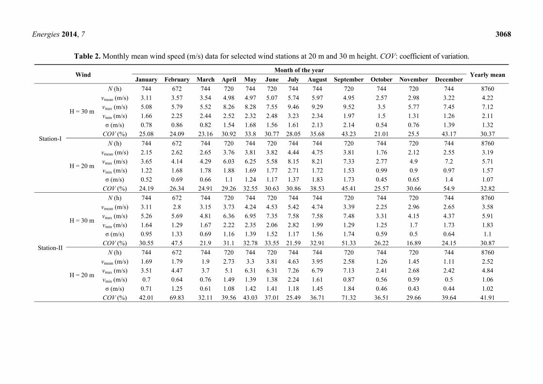
monthly, seasonal and annual figures, are presented. Table 2 shows a lot of information about the sites

based on monthly mean as well as annual mean wind speed, number of observations in hours,

maximum and minimum wind speed, standard deviation, and COV/turbulence intensity at 20 m and

30 m height.

Energies 2014, 7 3068

Table 2. Monthly mean wind speed (m/s) data for selected wind stations at 20 m and 30 m height. COV: coefficient of variation.

Wind Month of the year

Yearly mean January February March April May June July August September October November December

Station-I

H = 30 m

N (h) 744 672 744 720 744 720 744 744 720 744 720 744 8760

vmean (m/s) 3.11 3.57 3.54 4.98 4.97 5.07 5.74 5.97 4.95 2.57 2.98 3.22 4.22

vmax (m/s) 5.08 5.79 5.52 8.26 8.28 7.55 9.46 9.29 9.52 3.5 5.77 7.45 7.12

vmin (m/s) 1.66 2.25 2.44 2.52 2.32 2.48 3.23 2.34 1.97 1.5 1.31 1.26 2.11

σ (m/s) 0.78 0.86 0.82 1.54 1.68 1.56 1.61 2.13 2.14 0.54 0.76 1.39 1.32

COV (%) 25.08 24.09 23.16 30.92 33.8 30.77 28.05 35.68 43.23 21.01 25.5 43.17 30.37

H = 20 m

N (h) 744 672 744 720 744 720 744 744 720 744 720 744 8760

vmean (m/s) 2.15 2.62 2.65 3.76 3.81 3.82 4.44 4.75 3.81 1.76 2.12 2.55 3.19

vmax (m/s) 3.65 4.14 4.29 6.03 6.25 5.58 8.15 8.21 7.33 2.77 4.9 7.2 5.71

vmin (m/s) 1.22 1.68 1.78 1.88 1.69 1.77 2.71 1.72 1.53 0.99 0.9 0.97 1.57

σ (m/s) 0.52 0.69 0.66 1.1 1.24 1.17 1.37 1.83 1.73 0.45 0.65 1.4 1.07

COV (%) 24.19 26.34 24.91 29.26 32.55 30.63 30.86 38.53 45.41 25.57 30.66 54.9 32.82

Station-II

H = 30 m

N (h) 744 672 744 720 744 720 744 744 720 744 720 744 8760

vmean (m/s) 3.11 2.8 3.15 3.73 4.24 4.53 5.42 4.74 3.39 2.25 2.96 2.65 3.58

vmax (m/s) 5.26 5.69 4.81 6.36 6.95 7.35 7.58 7.58 7.48 3.31 4.15 4.37 5.91

vmin (m/s) 1.64 1.29 1.67 2.22 2.35 2.06 2.82 1.99 1.29 1.25 1.7 1.73 1.83

σ (m/s) 0.95 1.33 0.69 1.16 1.39 1.52 1.17 1.56 1.74 0.59 0.5 0.64 1.1

COV (%) 30.55 47.5 21.9 31.1 32.78 33.55 21.59 32.91 51.33 26.22 16.89 24.15 30.87

H = 20 m

N (h) 744 672 744 720 744 720 744 744 720 744 720 744 8760

vmean (m/s) 1.69 1.79 1.9 2.73 3.3 3.81 4.63 3.95 2.58 1.26 1.45 1.11 2.52

vmax (m/s) 3.51 4.47 3.7 5.1 6.31 6.31 7.26 6.79 7.13 2.41 2.68 2.42 4.84

vmin (m/s) 0.7 0.64 0.76 1.49 1.39 1.38 2.24 1.61 0.87 0.56 0.59 0.5 1.06

σ (m/s) 0.71 1.25 0.61 1.08 1.42 1.41 1.18 1.45 1.84 0.46 0.43 0.44 1.02

COV (%) 42.01 69.83 32.11 39.56 43.03 37.01 25.49 36.71 71.32 36.51 29.66 39.64 41.91

Energies 2014, 7 3069

Table 2. Cont.

Wind Month of the year

Yearly mean January February March April May June July August September October November December

Station-III

H = 30 m

N (h) 744 672 744 720 744 720 744 744 720 744 720 744 8760

vmean (m/s) 2.72 3.17 3.36 4.35 4.46 4.81 5.36 5.15 10.09 2.25 2.7 2.32 4.23

vmax (m/s) 4.16 6.21 5.14 7.36 7.55 8.16 7.59 13.76 39.2 3.48 3.69 3.67 9.16

vmin (m/s) 1.16 1.24 1.96 2.09 2.63 2.14 2.91 2.31 1.49 1.23 1.86 1.11 1.84

σ (m/s) 0.84 1.43 0.82 1.42 1.4 1.79 1.14 2.58 13.07 0.48 0.43 0.71 2.18

COV (%) 30.88 45.11 24.4 32.64 31.39 37.21 21.27 50.1 129.53 21.33 15.93 30.6 39.2

H = 20 m

N (h) 744 672 744 720 744 720 744 744 720 744 720 744 8760

vmean (m/s) 1.96 2.47 2.64 3.72 3.84 4.26 4.79 4.87 5.97 1.43 1.82 1.66 3.29

vmax (m/s) 3.36 5.61 4.35 6.62 6.86 7.34 6.89 14.35 18.58 2.6 2.67 2.7 6.83

vmin (m/s) 0.66 0.79 1.33 1.65 2.01 1.56 2.31 1.73 1.28 0.76 0.93 0.86 1.32

σ (m/s) 0.73 1.45 0.82 1.42 1.42 1.79 1.09 2.88 5.33 0.42 0.36 0.52 1.52

COV (%) 37.24 58.7 31.06 38.17 36.98 42.02 22.76 59.14 89.28 29.37 19.78 31.33 41.32

Energies 2014, 7 3070

A sample data frequency distribution and cumulative frequency distribution has been presented in

Table 3.

Table 3. Frequency distribution and cumulative frequency distribution for the selected sites

in June.

Wind speed (m/s)

Station-I Station-II Station-III

Frequency (%)

Cumulative frequency (%)

Frequency (%)


Frequency (%)


0–1 0.403 0.403 0.269 0.269 0.134 0.134 1–2 2.151 2.554 1.882 2.151 0.806 0.94 2–3 5.242 7.796 3.629 5.78 5.645 6.585 3–4 9.005 16.801 14.247 20.027 17.339 23.924 4–5 17.742 34.543 19.086 39.113 24.059 47.983 5–6 20.43 54.973 24.328 63.441 18.414 66.397 6–7 18.011 72.984 18.28 81.721 17.742 84.139 7–8 12.634 85.618 11.559 93.28 8.199 92.338 8–9 8.602 94.22 5.242 98.522 3.898 96.236

9–10 4.032 98.252 1.344 99.866 2.016 98.252 10–11 1.613 99.865 0 99.866 1.344 99.596 11–12 0.134 100 0.134 100 0.269 99.865 12–13 - - - - 0.134 100

The hourly variation of wind speed at the selected altitude has been presented in Figure 1. Wind speed

is higher during the daytime than the nighttime at every site. The COV/turbulence with the time series

is at its minimum during the higher windy periods.

Figure 1. Hourly mean wind speed at 20 m and 30 m height for the selected sites.

The hourly mean COV is presented in Figure 2. An important issue which has been clearly shown

in Figure 2 is that turbulence is comparatively low at 30 m height than at 20 m height. Therefore, at

the higher level the wind velocity stream is more uniform, i.e., the COV is lower.

Energies 2014, 7 3071

Figure 2. Hourly mean COV of turbulence at 20 m and 30 m height.

From the sample frequency distribution (Table 3), it can be clearly seen that more than 50% of the

frequency is between 5 m/s and 13 m/s of wind speed at every station. Table 3 can be used to clearly

identify the total number of hours at certain wind speed available in a month. Anyone can find monthly

wind speed scenario at a glance from the Table. The results are similar for other months at each station.

Figures 1 and 2, shows the hourly mean variations of wind speed and coefficient of variation for the

period of 24 h as a mean of a year. It has been shown that the wind speed is low until 8:00 AM to

10:00 AM, and after that it increases during the day until the maximum value is gained from 2:00 PM

to 4:00 PM, and afterwards it decrease again until the end of the day. The same wind characteristics

have been found at 20 m and 30 m height at every station. The maximum and minimum values of

hourly mean wind speeds at 30 m height are 4.95 m/s at Station-III and 3.10 m/s at Station-II. The variation

of wind speed at Station-I is lower than the others. The COV is lower when the wind speeds become a

maximum. Its values are very high at nighttime. From Table 3 and Figures 1 and 2, it is clear that 30 m

height wind speed data at Station-I shows better results than the other sites. To find the best

Weibull method, the statistical analysis of the Weibull distribution at 20 m and 30 m height is

presented in Tables 4–9.

In the statistical analysis, seven methods were used to determine the shape parameter k and scale

parameter c of the Weibull distribution. For comparison of these seven methods to each other and to

find out the efficiency of the methods, six statistical tools were used, i.e., relative percentage error (RPE),

RMSE, MPE, MAPE, chi-square error (χ2), and analysis of variance or efficiency of the method (R2).

It is important to note that only one column is required to rank the methods, since the above six criteria

all gave the same relative results. For a more precisely diagnosis, the authors used these six statistical

tools to rank the methods. The statistical analysis results for the seven numerical methods and the six

statistical test results are shown in Tables 4–9 for the three stations at 20 m and 30 m height, respectively.

The results show that the method of moments (MOM) and MLM give better results than other

methods, where the value of k and c becomes almost the same by these two methods. For MLM, RPE

and RMSE becomes zero and the value of MPE becomes negative, because, by this method, the calculated

Energies 2014, 7 3072

value becomes greater than the measured one. But the most important statistical test gives a chi-square

error of χ2 = 0.0010 and the efficiency of the method is R2 = 0.9997, where the best results are

obtained when these values are close to zero and unity, respectively. For Station-II, in Table 7,

MLM and PDM methods show better performance than others. The common factor is that the MLM

gives the better performance at every site. Therefore, it can be said that the MLM is the fisrt and MOM

is the second most efficient method for wind data assessment at 30 m height.

Table 4. The Weibull distribution analysis for Station-I at 20 m height. GM: graphical

method; MOM: method of moments; STDM: standard deviation method; MLM: maximum

likelihood method; PDM: power density method; MMLM: Modified maximum likelihood

method; and EEM: equivalent energy method.

Statistical methods

The Weibull parameters Statistical test efficiency

k (-) c (m/s) RPE (%) RMSE MPE (%) MAPE (%) χ2 R2 GM 3.63 3.55 0.0785 0.0500 0.8283 4.2571 0.1432 0.9577

MOM 3.58 3.54 −0.0523 0.0408 −0.0394 0.0394 0.0001 0.9999 STDM 3.99 4.46 26.6736 0.9219 27.9826 27.982 2.2593 0.1542 MLM 3.5 3.55 0.0000 0.0000 −0.0438 0.3700 0.0005 0.9998 PDM 3.11 3.53 −0.7845 0.1581 −0.6649 0.6648 0.0285 0.9917

MMLM 3.54 3.55 0.0784 0.0500 0.0723 0.1885 0.0002 0.9999 EEM 3.37 3.54 −0.2876 0.0957 0.1507 2.4687 0.0451 0.9866

Note: Dimensionless shape factor (k) and scale factor (c) in m/s, relative percentage error (RPE), root mean

square error (RMSE), mean percentage error (MPE), mean absolute percentage error (MAPE), chi-square

error (χ2), analysis of variance or efficiency of the method (R2).

Table 5. The Weibull distribution analysis for Station-I at 30 m height.

Statistical methods


k (-) c (m/s) RPE (%) RMSE MPE (%) MAPE (%) χ2 R2 GM 2.71 4.79 0.8880 0.1930 0.6250 1.7040 0.0350 0.9900

MOM 3.87 4.68 −0.5530 0.1530 −0.5420 0.5890 0.0023 0.9990STDM 2.64 4.78 1.7370 0.2710 2.3310 3.7180 0.2380 0.9320MLM 3.78 4.68 0.0000 0.0000 −0.0560 0.3440 0.0010 0.9997PDM 2.58 4.66 −1.2040 0.2250 −1.1870 1.2390 0.0150 0.9960

MMLM 3.18 4.67 −0.8090 0.1850 −0.9210 0.9540 0.0064 0.9980EEM 3.26 4.73 0.4930 0.1440 0.6290 1.6220 0.0290 0.9920

From Table 4, it can be clearly seen that MOM (χ2 = 0.0001, R2 = 0.9999), MLM (χ2 = 0.0005,

R2 = 0.9998) and MMLM (χ2 = 0.0002, R2 = 0.9999) give very close results and show better

performance than other methods. In Table 6, MOM and PDM methods show better results than others.

In the case of Station-III, MLM and PDM methods show better results than others in Table 8.

Summarizing these results, it can be easily said that MOM and MLM methods were applicable for

every height at any location wind data assessment. The PDM method is better for wind data

assessment at the lower height, but not perfect for the higher height.

Energies 2014, 7 3073

Table 6. The Weibull distribution analysis for Station-II at 20 m height.

Statistical methods


k (-) c (m/s) RPE (%) RMSE MPE (%) MAPE (%) χ2 R2 GM 3.11 2.70 −3.8742 0.3120 −4.1546 4.5644 0.1336 0.9787

MOM 2.82 2.81 0.0662 0.0408 0.0422 0.0422 0.0002 0.9999STDM 3.4 3.74 34.2053 0.9278 40.0035 40.003 2.8453 0.3654MLM 2.84 2.9 3.0463 0.2768 6.7823 7.0891 0.3063 0.9475PDM 2.65 2.82 0.1324 0.0577 0.1170 0.2672 0.0003 0.9999

MMLM 2.84 2.85 1.5894 0.2000 3.4823 3.6671 0.0795 0.9865EEM 2.88 2.76 −1.8212 0.2140 −1.9377 2.1966 0.0337 0.9945

Table 7. The Weibull distribution analysis for Station-II at 30 m height.

Statistical methods



MOM 3.99 3.94 −0.5820 0.1440 −0.5930 0.6490 0.0074 0.9974 STDM 4.47 4.83 22.6440 0.9004 23.8630 23.863 1.9020 0.1780 MLM 3.92 3.96 −0.0930 0.0580 −0.0920 0.5220 0.0020 0.9990 PDM 3.25 3.99 −0.2560 0.0960 −0.2560 0.2560 0.0004 0.9998

MMLM 3.59 3.98 −6.5160 0.4830 −8.3160 8.5270 2.3420 0.2280 EEM 4.23 4.39 11.1940 0.6330 11.7710 11.771 0.5180 0.7970

Table 8. The Weibull distribution analysis for Station-III at 20 m height.

Statistical methods


k (-) c (m/s) RPE (%) RMSE MPE (%) MAPE (%) χ2 R2 GM 3.04 3.66 0.0254 0.0289 −0.8825 4.4901 0.1568 0.979

MOM 3.14 3.62 −0.2536 0.0913 −0.1711 0.1711 0.0031 0.9996STDM 3.43 4.95 35.1255 1.0743 34.5353 34.535 5.7001 0.0331MLM 3.13 3.65 0.1775 0.0764 0.0826 0.4453 0.0011 0.9998PDM 2.77 3.65 −0.0507 0.0408 −0.0311 0.0311 0.0001 0.9999

MMLM 3.14 3.64 −1.1666 0.1958 −0.8205 1.4034 0.0924 0.9877EEM 2.91 3.66 0.0000 0.0000 −0.449 2.2702 0.041 0.9945

Table 9. The Weibull distribution analysis for Station-III at 30m height.

Statistical methods



MOM 3.76 4.45 0.0790 0.0580 0.1320 0.1650 0.0010 0.9999STDM 2.3 3.73 −21.540 0.9540 −11.410 13.920 20.680 0.3470MLM 3.66 4.5 −0.4730 0.1414 −0.3095 0.5340 0.0140 0.9990PDM 2.32 4.74 1.4980 0.2520 −0.0730 3.4630 0.3080 0.9740

MMLM 2.99 4.62 0.1580 0.0820 −0.4510 1.9760 0.0580 0.9950EEM 3.03 4.09 −11.845 0.7080 −6.0510 7.4310 5.9690 0.5632

Energies 2014, 7 3074

Table 10 summaries the test results of the seven methods and ranking of the methods according to

their performance and efficiency in wind data assessment. The rankings were done by considering

minimum error and maximum efficiency according to first to seventh positions respectively.

Regarding this test, six statistical tools have been used and considered four decimal places of each

value by numerical iteration methods. One test is enough to rank the methods, but for more precise

analysis, the authors used more tools which helped to verify the discussion about the best method.

In this statistical research work, it has been found that the MOM achieved the first position and the

MLM took the second position in rank. Although the PDM got the third position, this method has

better performance for low height wind data assessment. At increased height, PDM was a less efficient

method than others. But MOM and MLM methods were applicable at any altitude with minimum error

and maximum efficiency. Our first goal has been satisfied by the above statistical analysis where we

identified the best methods to determine the Weibull distribution. Another goal is to select the best

wind site by using these best methods, which has been analyzed below.

Table 10. Ranking of the methods by statistical test results.

Statistical methods

Station-I Station-II Station-III Discussion

20 m 30 m 20 m 30 m 20 m 30 m

GM Sixth Sixth Fifth Fourth Sixth Fourth - MOM First Second First Third Third First The First choice

STDM Seventh Seventh Seventh Seventh Seventh Seventh -

MLM Third First Sixth Second Second Second The second choice PDM Fourth Fourth Second First First Fifth The third choice

MMLM Second Third Fourth Sixth Fifth Third - EEM Fifth Fifth Third Fifth Fourth Sixth -

The procedure mentioned in this study is not only applicable in case study sits, it can be applied

in any climatic conditions at any site in any countries in the world. For example, Mohammadi and

Mostafaeipour [44] used STDM and PDM for wind turbine utilization in Zarriuneh at Kurdistan

mountainous province in Iran. Chang [41] used moment method, empirical method, GM, MLM,

MMLM and energy pattern factor method at three wind farms (Dayuan, Hengchun and Penghu)

experiencing different weather conditions in Taiwan. Costa Rocha et al. [45] used EEM, moment method,

MLM, etc. for wind energy generation in coastal area of the State of Ceara, located in the northeast

region of Brazil. Dorvlo [98] used moment method, Chi-square method, empirical method and

regression method for estimation of wind energy in four weather stations (Marmul, Masirah, Sur and

Thumrait) in Oman. Many authors have already used the methods at different geographical locations

for wind energy estimation [30,43,99]. The paper presented more generalized form of the Weibull

distribution methods which is validated by widely acceptable error correction methods for practical

application. This procedure is applicable at any geographical location; at any weather condition (i.e.,

summer, winter, spring etc.) at any altitude in any country in the world. The main outcome of the study

is the development of the processes for identifying best methods for wind power generation which is

applicable to any location.

Table 11 presents the variation of wind speed during different months of the year and the annual

mean values. From the average values, the variation of the maximum and minimum wind speed occurred

Energies 2014, 7 3075

in April to September and October to March respectively at every station. At Station-I, the maximum

and minimum wind speed occurred in June and October with values of 5.07 m/s and 2.57 m/s,

respectively. The COV and standard deviation at this site varies between 21.01%–35.68% and

0.54–2.13, respectively. On the other hand, Station-III has wind speeds similar to Station-I, but the

COV and standard deviation varies between 15.93%–129.53% and 0.71–13.07, respectively. In August

and September, the COV is 50.1% and 129.53%, which means that these months have some irregular

wind behavior, i.e., gusty wind exists during these months. Station-II has wind behavior (wind speed)

performance lower than other stations. Therefore, Station-I has shown better wind characteristics than

the other Stations, hence it is the selected wind site. The mean available power and energy in the wind

at 30 m height at Station-I is analyzed below.

Table 11. Monthly mean wind speed, power law coefficient (η), the Weibull shape factor

(k) and scale factor (c) at 20 m, 30 m and 50 m height.

Month Power law

coefficient η

Measured value Extrapolated value

At 20 m height At 30 m height At 50 m height

v20 k20 c20 v30 k30 c30 v50 k50 c50 January 0.262 2.15 4.33 2.35 3.11 4.42 3.40 3.55 4.63 3.89

February 0.25 2.62 4.18 2.89 3.57 4.41 3.91 4.05 4.62 4.44 March 0.251 2.65 4.12 2.91 3.54 4.41 3.87 4.02 4.62 4.4 April 0.219 3.76 3.86 4.16 4.98 3.58 5.53 5.57 3.75 6.18 May 0.219 3.81 3.45 4.25 4.97 3.30 5.55 5.58 3.46 6.21 June 0.218 3.82 3.95 4.23 5.07 3.84 5.63 5.69 4.02 6.29 July 0.207 4.44 3.41 4.93 5.74 3.82 6.34 6.39 4.00 7.05

August 0.203 4.75 2.91 5.34 5.97 3.17 6.69 6.66 3.32 7.42 September 0.218 3.81 2.4 4.31 4.95 2.52 5.60 5.56 2.64 6.26

October 0.28 1.76 4.36 1.94 2.57 5.65 2.79 2.98 5.92 3.22 November 0.266 2.12 3.06 2.34 2.98 3.70 3.26 3.37 3.87 3.73 December 0.256 2.55 1.99 2.89 3.22 2.49 3.63 3.68 2.61 4.14

The monthly mean available power is analyzed using both MOM and MLM methods in Table 12.

From this table, it can be seen that the available power from April to September was above 100 W/m2

and the maximum and minimum power occurred in August, 179.36 W/m2, and October, 11.8 W/m2,

respectively. Only two statistical tools (RMSE and Chi-square error) have been used for comparing the

MOM and MLM methods. Here, the MLM method gives better performance with minimum error.

Using the MLM method, the Weibull shape factor and scale factor vary between 2.52–5.65 and

2.79–6.69 m/s. respectively.

Therefore, the six months from April to September show more potential wind generated power than

other months in the year. In this research work, the Weibull parameters at heights of 30 m and 20 m

were determined.

Table 13 presents the seasonal analysis of wind speed, Weibull parameters and available power at

20 m and 30 m height. It also presents the extrapolated values at 50 m. The months in each season can

be classified as winter (November, December and January), spring (February, March and April),

summer (May, June and July), and autumn (August, September and October).

Energies 2014, 7 3076

Table 12. Monthly mean power based on measured data and calculated data by

statistical methods.

Month Power

(W/m2)

MOM MLM

k (-) c (m/s) P (W/m2) RMSE χ2 k (-) c (m/s) P (W/m2) RMSE χ2

January 18.75 4.50 3.41 21.84 1.7578

0.9904

4.42 3.4 21.67 1.7088

0.9724

February 27.87 4.71 3.90 32.63 2.1817 4.41 3.91 33.24 2.3173

March 26.71 4.92 3.86 31.40 2.1656 4.41 3.87 31.96 2.2913

April 73.11 3.58 5.53 97.57 4.9457 3.58 5.53 97.57 4.9457

May 71.47 3.25 5.55 101.46 5.4763 3.3 5.55 101.04 5.4378

June 75.87 3.6 5.63 102.85 5.1942 3.84 5.63 101.21 5.0339

July 110.11 3.98 6.34 143.45 5.7741 3.82 6.34 144.7 5.8813

August 123.88 3.06 6.68 181.11 7.5651 3.17 6.69 179.36 7.4485

September 70.61 2.48 5.58 118.12 6.8927 2.52 5.6 117.25 6.8293

October 10.05 5.47 2.78 11.70 1.2845 5.65 2.79 11.8 1.3229

November 16.21 4.42 3.27 19.38 1.7804 3.7 3.26 19.82 1.9000

December 20.81 2.48 3.63 32.46 3.4132 2.49 3.63 32.37 3.4000

Table 13. Seasonal mean wind speed in (m/s), the Weibull shape factor (-), scale factor (m/s)

and power density (W/m2) at 30 m and 50 m height.

Seasons η

Measured data Extrapolated data

At 20 m height At 30 m height At 50 m height

v20 k20 c20 P20 v30 k30 c30 P30 v50 k50 c50 P50

Winter 0.24 3.19 3.5 3.55 26.21 4.22 3.78 4.7 59.1 4.76 3.96 5.27 83.6 Spring 0.24 3.01 4.05 3.32 20.2 4.03 4.13 4.4 48.2 4.55 4.33 5.01 68.7

Summer 0.21 4.02 3.6 4.47 48.64 5.26 3.65 5.8 108.24 5.89 3.83 6.52 157.2 Autumn 0.23 3.44 3.22 3.86 34.1 4.5 3.78 5.1 72.3 5.07 3.96 5.63 100.67

The mean velocity, shape factor, scale factor, etc. at 50 m were extrapolated using Equations (44)–(48)

and these extrapolated results are presented in Table 14.

Table 14. Wind power classification.

Power

class Potential

Power density and wind

speed at 10 m (33 ft)





Power (W/m2) Speed (m/s) Power (W/m2) Speed (m/s) Power (W/m2) Speed (m/s)

Class-I Poor P10 ≤ 100 ≤4.4 P30 ≤ 160 ≤5.1 P50 ≤ 200 ≤5.6

Class-II Marginal P10 ≤ 150 ≤5.1 P30 ≤ 240 ≤6.0 P50 ≤ 300 ≤6.0

Class-III Moderate P10 ≤ 200 ≤5.6 P30 ≤ 320 ≤6.5 P50 ≤ 400 ≤7.0

Class-IV Good P10 ≤ 250 ≤6.0 P30 ≤ 400 ≤7.0 P50 ≤ 500 ≤7.5

Class-V Very good P10 ≤ 300 ≤6.4 P30 ≤ 480 ≤7.5 P50 ≤ 600 ≤8.0

Class-VI Excellent P10 ≤ 400 ≤7.0 P30 ≤ 640 ≤8.2 P50 ≤ 800 ≤8.8

Class-VII Excellent P10 ≤ 1000 ≤9.4 P30 ≤ 1600 ≤11.0 P50 ≤ 2000 ≤11.9

Table 15 also includes yearly or annual mean values. According to this table, the maximum and

minimum values of wind speed and wind power have been observed in summer and spring with the

values of 5.26 m/s and 4.03 m/s and the power is 108.24 W/m2 and 48.16 W/m2 respectively at 30 m

Energies 2014, 7 3077

height. In the literatures, Elliot et al. [100], Yu et al. [101], Ilinca et al. [102] and Zhou et al. [103]

classified the wind power in seven categories which are shown in Table 14. Considering these wind

power classes, it has been found that Station-I has poor wind power at every height (i.e., 20 m, 30 m

and 50 m). For a more realistic analysis, the available energy in the wind of this site was determined by

using numerical iteration methods and is presented in Table 15.

Table 15. The most frequent wind velocity (VFmax), velocity contributing the maximum

energy (VEmax), energy density (ED) and total energy intensity (EDT).

Seasons VFmax (m/s) VEmax (m/s) Energy density, ED (kW/m2) Total energy intensity, EDT (kW/m2)

Winter 4.31 5.24 0.0586 129.408

Spring 4.15 4.88 0.0492 105.082

Summer 5.35 6.58 0.1148 253.531

Autumn 4.64 5.63 0.0728 160.667

Yearly mean 4.31 5.24 0.0586 513.412

The energy estimation of wind regimes by the Weibull based approach has been presented in

Table 15. It also shows the most frequent wind speed, velocity contributing the maximum energy,

energy density and total energy intensity. From the above table, it can be clearly seen that the energy

density and total energy intensity are higher in summer than during autumn seasons and also are a

minimum in spring. Therefore, summers have more wind potential than any other seasons. To find out

the energy generated by a wind turbine, a small model wind turbine (NACA 4418 turbine power curve)

with rated power of 20 kW or 0.02 MW, rated speed of 8 m/s and hub height of 30 m has been used for

this calculation. Values of capacity factor and total energy output were obtained using numerical

integration methods of Trapezoidal Sums and Simpson’s 1/3 Rule and the values were verified to four

decimal places. From Table 16, it can be seen that, in summer, 13.2938 MW·h of energy can be

extracted by the suggested model wind turbine. This means that only 147.67 kW/day of power can be

generated by the wind turbine in summer and the value becomes 50% less in the rainy season.

Therefore, it can be finally concluded that the analytical results show that Station-I does not have the

necessary available wind power potential for large turbines but has sufficient wind power for small

wind turbine both for electricity generation and pumping water for irrigation.

Table 16. Energy generated by the wind turbine and the capacity factor by numerical

integration. The turbine rated power is 20 kW or 0.02 MW, rated speed is 8 m/s and hub

height at 30 m.

Seasons

Numerical integration

Trapezoidal sums Simpson’s rule

Capacity factor, CF Total energy output, ET (MW·h) Capacity factor, CF Total energy output, ET, (MW·h)

Winter 0.1238 5.4689 0.1238 5.4689

Spring 0.0920 3.9283 0.0920 3.9283

Summer 0.3010 13.2937 0.3010 13.2938

Autumn 0.1698 7.5005 0.1698 7.5005

Yearly mean 0.1238 21.6973 0.1238 21.6974

Energies 2014, 7 3078

4. Conclusions

In this work, statistical diagnosis of the best Weibull distribution methods for wind data analysis

is presented. By using the available wind data, the values of shape factor k and scale factor c were

determined using seven methods and were then investigated as to how efficiently the methods can

estimate the Weibull factors with minimum error. To satisfy the main objectives of this work, six

statistical tools were used to find the best method of Weibull distribution. It is important to note that

any one of these statistical tools, namely RPE, RMSE, MPE, MAPE, chi-square error (χ2), and analysis

of variance or efficiency of the method (R2) is good enough to rank the methods, however, analysis

using all of them was done to rank more precisely. The results show that the MOM and MLM are

the most efficient methods for determining the value of k and c to fit the Weibull distribution curves.

The PDM is more efficient for low altitude wind data but is not efficient for higher altitude wind data.

MOM and MLM methods are more efficient with less error and are applicable for any altitude. Other

methods such as MMLM, EEM, GM and STDM are the least efficient methods to fit the Weibull

distribution curves for the assessment of wind speed data. Another objective of this work was to find

the best wind site using the best Weibull distribution methods and calculate available wind power.

Monthly mean wind speed was found to be relatively higher in Station-I than that of the other sites.

As a result this is our selected site. The MLM method has shown better results than MOM in

calculating monthly mean wind power at Station-I. The value of shape factor, scale factor, wind speed

and power was determined at 50 m height using extrapolation of numerical equations to satisfy the

wind power classes as discussed in this paper. The poor class wind power has been found in this site in

each altitude. Furthermore, energy density and total energy intensity per unit area has been analyzed by

numerical iteration methods. Finally, the energy extracted by a small model wind turbine has been

analyzed by using numerical integration methods of Trapezoidal Sums and Simpson’s 1/3 Rule.

This study offers a new pathway on how to evaluate feasible locations for wind energy assessment

which is applicable at any windy sites in any country in the world.

Author Contributions

The major part of the works was done by corresponding author, however, co-authors also

contributed significantly. The first co-author Mohammad Golam Rasul contributed in outlining the paper,

methodology and associated theories and related description. He helped also in data some analysis.

The second co-author Talal Yusaf contributed in format of the paper and its alignment with themes of

the journal and revisions of the manuscript. Corresponding author is grateful to co-authors for their

fruitful contribution in this work.

Nomenclature

P Total power, W/m2

A Area, m2

Pe Practically extractable power, W/m2

k Dimensionless shape parameter

c Scale parameter (m/s)

Energies 2014, 7 3079

f(v) Weibull probability density function

F(v) Cumulative distribution function

C Constant

L Likelihood function

COV Coefficient of variation

vi Random sample of wind speed central to bin i

n Number of sample or bin

f(vi) Weibull frequency for wind speed ranging within bin i ( ≥ 0) Probability for wind speed ≥ 0

Wvi Observed frequency of the wind speed

Mean of the cubic wind speed, m/s

εvi Error of the approximation

zref Reference height, m

kh Weibull shape factor at desired height

ch Weibull scale factor at desired height, m/s

vh Wind speed at desired height, m/s

Ph Power at desired height, W/m2

N Total number of observations

yi,m i-th calculated value from measured data

xi,w i-th calculated value from the Weibull distribution , Mean of i-th calculated value from measured data

R2 Analysis of variance

Γ Gamma function

σ Standard deviation of wind speed, m/s

ρ Air density, kg/m3

θ Unknown parameter for maximum likelihood function

η Power law coefficient

χ2 Chi-square error

Conflicts of Interest

The authors declare no conflict of interest.

References

1. Baños, R.; Manzano-Agugliaro, F.; Montoya, F.G.; Gil, C.; Alcayde, A.; Gómez, J. Optimization

methods applied to renewable and sustainable energy: A review. Renew. Sustain. Energy Rev.

2011, 15, 1753–1766.

2. Cruz-Peragon, F.; Palomar, J.M.; Casanova, P.J.; Dorado, M.P.; Manzano-Agugliaro, F.

Characterization of solar flat plate collectors. Renew. Sustain. Energy Rev. 2012, 16, 1709–1720.

3. Acker, T.L.; Williams, S.K.; Duque, E.P.; Brummels, G.; Buechler, J. Wind resource assessment

in the state of Arizona: Inventory, capacity factor, and cost. Renew. Energy 2007, 32, 1453–1466.

Energies 2014, 7 3080

4. Munteanu, I.; Bratcu, A.I.; Cutululis, N.A.; Ceanga, E. Optimal Control of Wind Energy

Systems: Towards A Global Approach; Springer: London, UK, 2008.

5. Montoya, F.G.; Aguilera, M.J.; Manzano-Agugliaro, F. Renewable energy production in Spain:

A review. Renew. Sustain. Energy Rev. 2014, 33, 509–531.

6. Hernández-Escobedo, Q.; Manzano-Agugliaro, F.; Zapata-Sierra, A. The wind power of Mexico.

Renew. Sustain. Energy Rev. 2010, 14, 2830–2840.

7. Hernández-Escobedo, Q.; Saldaña-Flores, R.; Rodríguez-García, E.R.; Manzano-Agugliaro, F.

Wind energy resource in Northern Mexico. Renew. Sustain. Energy Rev. 2014, 32, 890–914.

8. Hernandez-Escobedo, Q.; Manzano-Agugliaro, F.; Gazquez-Parra, J.A.; Zapata-Sierra, A. Is the

wind a periodical phenomenon? The case of Mexico. Renew. Sustain. Energy Rev. 2011, 15,

721–728.

9. Vincent, C.L.; Giebel, G.; Pinson, P.; Madsen, H. Resolving nonstationary spectral information

in wind speed time series using the Hilbert-Huang transform. J. Appl. Meteorol. Climatol. 2010,

49, 253–267.

10. Huang, N.E.; Shen, Z.; Long, S.R.; Wu, M.C.; Shih, H.H.; Zheng, Q.; Yen, N.C.; Tung, C.C.;

Liu, H.H. The empirical mode decomposition and the Hilbert spectrum for nonlinear and

non-stationary time series analysis. Proc. R. Soc. Lond. Ser. A Math. Phys. Eng. Sci. 1998, 454,

903–995.

11. Chen, Z.; Gomez, S.A.; Mccormick, M. A Fuzzy Logic Controlled Power Electronic System for

Variable Speed Wind Energy Conversion Systems. In Proceedings of the 8th International

Conference on Power Electronics and Variable Speed Drives, London, UK, 18–19 September 2000;

pp. 114–119.

12. Ahmed Shata, A.; Hanitsch, R. Electricity generation and wind potential assessment at Hurghada,

Egypt. Renew. Energy 2008, 33, 141–148.

13. Akhmatov, V. Influence of wind direction on intense power fluctuations in large offshore

windfarms in the North Sea. Wind Eng. 2007, 31, 59–64.

14. Sorensen, P.; Cutululis, N.A.; Vigueras-Rodríguez, A.; Jensen, L.E.; Hjerrild, J.; Donovan, M.H.;

Madsen, H. Power fluctuations from large wind farms. IEEE Trans. Power Syst. 2007, 22,

958–965.

15. Chen, Z.; Blaabjerg, F. Wind farm—A power source in future power systems. Renew. Sustain.

Energy Rev. 2009, 13, 1288–1300.

16. Hsieh, C.-H.; Dai, C.-F. The analysis of offshore islands wind characteristics in Taiwan by

Hilbert–Huang transform. J. Wind Eng. Ind. Aerodyn. 2012, 107, 160–168.

17. Belu, R.; Koracin, D. Wind characteristics and wind energy potential in western Nevada.

Renew. Energy 2009, 34, 2246–2251.

18. Chang, T.P. Wind energy assessment incorporating particle swarm optimization method.

Energy Convers. Manag. 2011, 52, 1630–1637.

19. Adaramola, M.; Paul, S.; Oyedepo, S. Assessment of electricity generation and energy cost of

wind energy conversion systems in north-central Nigeria. Energy Convers. Manag. 2011, 52,

3363–3368.

20. Ohunakin, O.S.; Akinnawonu, O.O. Assessment of wind energy potential and the economics of

wind power generation in Jos, Plateau State, Nigeria. Energy Sustain. Dev. 2012, 16, 78–83.

Energies 2014, 7 3081

21. Ohunakin, O.S. Assessment of wind energy resources for electricity generation using WECS in

North-Central region, Nigeria. Renew. Sustain. Energy Rev. 2011, 15, 1968–1976.

22. Akpinar, E.; Akpinar, S. Statistical analysis of wind energy potential on the basis of the Weibull

and Rayleigh distributions for Agin-Elazig, Turkey. Proc. Inst. Mech. Eng. Part A J. Power Energy

2004, 218, 557–565.

23. Ahmed, A.S. Wind energy as a potential generation source at Ras Benas, Egypt. Renew. Sustain.

Energy Rev. 2010, 14, 2167–2173.

24. Fadare, D. A statistical analysis of wind energy potential in Ibadan, Nigeria, based on Weibull

distribution function. Pac. J. Sci. Technol. 2008, 9, 110–119.

25. Akpinar, E.K. A statistical investigation of wind energy potential. Energy Sources Part A

2006, 28, 807–820.

26. Ahmed Shata, A.; Hanitsch, R. Evaluation of wind energy potential and electricity generation on

the coast of Mediterranean Sea in Egypt. Renew. Energy 2006, 31, 1183–1202.

27. Akdağ, S.A.; Güler, Ö. Evaluation of wind energy investment interest and electricity generation

cost analysis for Turkey. Appl. Energy 2010, 87, 2574–2580.

28. Azad, A. Statistical Weibull distribution analysis for wind power of the two dimensional ridge areas.

Int. J. Adv. Renew. Energy Res. 2013, 1, 8–14.

29. Ahmed, S.; Mahammed, H. A statistical analysis of wind power density based on the Weibull

and Ralyeigh models of “Penjwen Region” Sulaimani/Iraq. Jordan J. Mech. Ind. Eng. 2012, 6,

135–140.

30. Celik, A.N. A statistical analysis of wind power density based on the Weibull and Rayleigh

models at the southern region of Turkey. Renew. Energy 2004, 29, 593–604.

31. Kavak Akpinar, E.; Akpinar, S. A statistical analysis of wind speed data used in installation of

wind energy conversion systems. Energy Convers. Manag. 2005, 46, 515–532.

32. Safari, B.; Gasore, J. A statistical investigation of wind characteristics and wind energy potential

based on the Weibull and Rayleigh models in Rwanda. Renew. Energy 2010, 35, 2874–2880.

33. Kose, R.; Ozgur, M.A.; Erbas, O.; Tugcu, A. The analysis of wind data and wind energy potential

in Kutahya, Turkey. Renew. Sustain. Energy Rev. 2004, 8, 277–288.

34. Zaharim, A.; Najid, S.K.; Razali, A.M.; Sopian, K. Analyzing Malaysian Wind Speed Data

Using Statistical Distribution. In Proceedings of the 4th IASME/WSEAS International

Conference on Energy and Environment, Cambridge, UK, 24–26 February 2009; pp. 360–370.

35. Islam, M.; Saidur, R.; Rahim, N. Assessment of wind energy potentiality at Kudat and Labuan,

Malaysia using Weibull distribution function. Energy 2011, 36, 985–992.

36. Daoo, V.; Panchal, N.; Sunny, F.; Sitaraman, V.; Krishnamoorthy, T. Assessment of wind energy

potential of Trombay, Mumbai (19.1 N; 72.8 E), India. Energy Convers. Manag. 1998, 39,

1351–1356.

37. Celik, A. Weibull representative compressed wind speed data for energy and performance

calculations of wind energy systems. Energy Convers. Manag. 2003, 44, 3057–3072.

38. Ulgen, K.; Hepbasli, A. Determination of Weibull parameters for wind energy analysis of Izmir,

Turkey. Int. J. Energy Res. 2002, 26, 495–506.

39. Langlois, R. Estimation of Weibull parameters. J. Mater. Sci. Lett. 1991, 10, 1049–1051.

Energies 2014, 7 3082

40. Akdağ, S.A.; Dinler, A. A new method to estimate Weibull parameters for wind energy applications.


41. Chang, T.P. Performance comparison of six numerical methods in estimating Weibull parameters

for wind energy application. Appl. Energy 2011, 88, 272–282.

42. Minami, F.; Brückner-Foit, A.; Munz, D.; Trolldenier, B. Estimation procedure for the Weibull

parameters used in the local approach. Int. J. Fract. 1992, 54, 197–210.

43. Seguro, J.V.; Lambert, T.W. Modern estimation of the parameters of the Weibull wind speed

distribution for wind energy analysis. J. Wind Eng. Ind. Aerodyn. 2000, 85, 75–84.

44. Mohammadi, K.; Mostafaeipour, A. Using different methods for comprehensive study of wind

turbine utilization in Zarrineh, Iran. Energy Convers. Manag. 2013, 65, 463–470.

45. Costa Rocha, P.A.; de Sousa, R.C.; de Andrade, C.F.; da Silva, M.E.V. Comparison of seven

numerical methods for determining Weibull parameters for wind energy generation in the

northeast region of Brazil. Appl. Energy 2012, 89, 395–400.

46. Azad, A.; Saha, M. Weibull’s analysis of wind power potential at coastal sites in Kuakata,

Bangladesh. Int. J. Energy Mach. 2011, 4, 36–45.

47. Azad, A.; Alam, M. A Statistical tools for clear energy: Weibull’s distribution for potentiality

analysis of wind energy. Int. J. Adv. Renew. Energy Res. 2012, 1, 240–247.

48. Chu, Y.-K.; Ke, J.-C. Computation approaches for parameter estimation of Weibull distribution.

Math. Comput. Appl. 2012, 17, 39–47.

49. Bhattacharya, P.; Bhattacharjee, R. A study on Weibull distribution for estimating the parameters.

Wind Eng. 2009, 33, 469–476.

50. Cohen, A.C. Maximum likelihood estimation in the Weibull distribution based on complete and

on censored samples. Technometrics 1965, 7, 579–588.

51. Jowder, F.A. Wind power analysis and site matching of wind turbine generators in Kingdom

of Bahrain. Appl. Energy 2009, 86, 538–545.

52. Odo, F.; Offiah, S.; Ugwuoke, P. Weibull distribution-based model for prediction of wind potential

in Enugu, Nigeria. Pelagia Res. Libr. Adv. Appl. Sci. Res. 2012, 3, 1202–1208.

53. Oyedepo, S.O.; Adaramola, M.S.; Paul, S.S. Analysis of wind speed data and wind energy

potential in three selected locations in south-east Nigeria. Int. J. Energy Environ. Eng. 2012, 3,

doi:10.1186/2251-6832-3-7.

54. Abbas, K.; Alamgir.; Khan, S.A.; Ali, A.; Khan, D.M.; Khalil, U. Statistical analysis of wind

speed data in Pakistan. World Appl. Sci. J. 2012, 18, 1533–1539.

55. Harter, H.L.; Moore, A.H. Maximum-likelihood estimation of the parameters of gamma and

Weibull populations from complete and from censored samples. Technometrics 1965, 7, 639–643.

56. Odell, P.M.; Anderson, K.M.; D'agostino, R.B. Maximum likelihood estimation for interval-censored

data using a Weibull-based accelerated failure time model. Biometrics 1992, 48, 951–959.

57. Choi, S.; Wette, R. Maximum likelihood estimation of the parameters of the gamma distribution

and their bias. Technometrics 1969, 11, 683–690.

58. Cacciari, M.; Mazzanti, G.; Montanari, G. Comparison of maximum likelihood unbiasing

methods for the estimation of the Weibull parameters. IEEE Trans. Dielectr. Electr. Insul. 1996,

3, 18–27.

Energies 2014, 7 3083

59. Zanakis, S.H.; Kyparisis, J. A review of maximum likelihood estimation methods for the

three-parameter Weibull distribution. J. Stat. Comput. Simul. 1986, 25, 53–73.

60. Lemon, G.H. Maximum likelihood estimation for the three parameter Weibull distribution based

on censored samples. Technometrics 1975, 17, 247–254.

61. Jiang, S.; Kececioglu, D. Maximum likelihood estimates, from censored data, for mixed-Weibull

distributions. IEEE Trans. Reliab. 1992, 41, 248–255.

62. Philippopoulos, K.; Deligiorgi, D. Statistical simulation of wind speed in Athens, Greece based

on Weibull and ARMA models. Int. J. Energy Environ. 2009, 3, 151–158.

63. Karpa, O.; Naess, A. Extreme value statistics of wind speed data by the ACER method. J. Wind

Eng. Ind. Aerodyn. 2013, 112, 1–10.

64. Morgan, E.C.; Lackner, M.; Vogel, R.M.; Baise, L.G. Probability distributions for offshore

wind speeds. Energy Convers. Manag. 2011, 52, 15–26.

65. Stathopoulos, C.; Kaperoni, A.; Galanis, G.; Kallos, G. Wind power prediction based on

numerical and statistical models. J. Wind Eng. Ind. Aerodyn. 2013, 112, 25–38.

66. Zhou, J.; Erdem, E.; Li, G.; Shi, J. Comprehensive evaluation of wind speed distribution models:

A case study for North Dakota sites. Energy Convers. Manag. 2010, 51, 1449–1458.

67. Sardar Maran, P.; Ponnusamy, R. Wind power density estimation using meteorological tower data.

Int. J. Renew. Sustain. Energy 2013, 2, 110–114.

68. Bivona, S.; Bonanno, G.; Burlon, R.; Gurrera, D.; Leone, C. Stochastic models for wind

speed forecasting. Energy Convers. Manag. 2011, 52, 1157–1165.

69. Daniel, A.; Chen, A. Stochastic simulation and forecasting of hourly average wind speed

sequences in Jamaica. Sol. Energy 1991, 46, 1–11.

70. Kamal, L.; Jafri, Y.Z. Time series models to simulate and forecast hourly averaged wind speed in

Quetta, Pakistan. Sol. Energy 1997, 61, 23–32.

71. Cadenas, E.; Rivera, W. Wind speed forecasting in the south coast of Oaxaca, Mexico.

Renew. Energy 2007, 32, 2116–2128.

72. Alexiadis, M.; Dokopoulos, P.; Sahsamanoglou, H. Wind speed and power forecasting based on

spatial correlation models. IEEE Trans. Energy Convers. 1999, 14, 836–842.

73. Keyhani, A.; Ghasemi-Varnamkhasti, M.; Khanali, M.; Abbaszadeh, R. An assessment of wind

energy potential as a power generation source in the capital of Iran, Tehran. Energy 2010, 35,

188–201.

74. Mirhosseini, M.; Sharifi, F.; Sedaghat, A. Assessing the wind energy potential locations in

province of Semnan in Iran. Renew. Sustain. Energy Rev. 2011, 15, 449–459.

75. Alamdari, P.; Nematollahi, O.; Mirhosseini, M. Assessment of wind energy in Iran: A review.

Renew. Sustain. Energy Rev. 2012, 16, 836–860.

76. Jaramillo, O.; Saldaña, R.; Miranda, U. Wind power potential of Baja California Sur, México.

Renew. Energy 2004, 29, 2087–2100.

77. Mathew, S.; Pandey, K.; Kumar, V.A. Analysis of wind regimes for energy estimation.

Renew. Energy 2002, 25, 381–399.

Energies 2014, 7 3084

78. Weisser, D. A wind energy analysis of Grenada: An estimation using the “Weibull” density function.

Renew. Energy 2003, 28, 1803–1812.

79. Chang, T.-J.; Wu, Y.-T.; Hsu, H.-Y.; Chu, C.-R.; Liao, C.-M. Assessment of wind characteristics

and wind turbine characteristics in Taiwan. Renew. Energy 2003, 28, 851–871.

80. Akpinar, S.; Akpinar, E.K. Estimation of wind energy potential using finite mixture

distribution models. Energy Convers. Manag. 2009, 50, 877–884.

81. Exif. Kutubdia in Bangladesh, 2008. Available online: https://www.flickr.com/photos/

rahmanmm/2370901630/meta/ (accessed on 15 April 2014).

82. Khadem, S.K.; Hussain, M. A pre-feasibility study of wind resources in Kutubdia Island,

Bangladesh. Renew. Energy 2006, 31, 2329–2341.

83. Rahaman, S. A Field Report Ongeoenvironmental and Biological Aspects of Sitakunda;

Jahangirnagar University: Dhaka, Bangladesh, 2010.

84. Ramírez, P.; Carta, J.A. The use of wind probability distributions derived from the maximum

entropy principle in the analysis of wind energy. A case study. Energy Convers. Manag. 2006,

47, 2564–2577.

85. Kantar, Y.M.; Usta, I. Analysis of wind speed distributions: Wind distribution function

derived from minimum cross entropy principles as better alternative to Weibull function.


86. Weibull, W. A statistical distribution function of wide applicability. J. Appl. Mech. 1951, 18,

293–297.

87. Xiao, Y.; Li, Q.; Li, Z.; Chow, Y.; Li, G. Probability distributions of extreme wind speed and its

occurrence interval. Eng. Struct. 2006, 28, 1173–1181.

88. Manwell, J.F.; Mcgowan, J.G.; Rogers, A.L. Wind Energy Explained: Theory, Design and

Application; John Wiley & Sons Ltd.: London, UK, 2002; p. 577.

89. Gove, J.H. Moment and maximum likelihood estimators for Weibull distributions under

length-and area-biased sampling. Environ. Ecol. Stat. 2003, 10, 455–467.

90. Guure, C.B.; Ibrahim, N.A. Bayesian analysis of the survival function and failure rate of Weibull

distribution with censored data. Math. Probl. Eng. 2012, 2012, doi:10.1155/2012/329489.

91. Sedefian, L. On the vertical extrapolation of mean wind power density. J. Appl. Meteorol. 1980,

19, 488–493.

92. Justel, A.; Peña, D.; Zamar, R. A multivariate Kolmogorov-Smirnov test of goodness of fit.

Stat. Probab. Lett. 1997, 35, 251–259.

93. Watson, G.S. Goodness-of-fit tests on a circle. Biometrika 1961, 48, 109–114.

94. Genest, C.; Rémillard, B.; Beaudoin, D. Goodness-of-fit tests for copulas: A review and a

power study. Insur. Math. Econ. 2009, 44, 199–213.

95. Balderrama, J.A.; Masters, F.J.; Gurley, K.R. Peak factor estimation in hurricane surface winds.

J. Wind Eng. Ind. Aerodyn. 2012, 102, 1–13.

96. Justus, C.; Mikhail, A. Height variation of wind speed and wind distributions statistics.

Geophys. Res. Lett. 1976, 3, 261–264.

Energies 2014, 7 3085

97. Justus, C.; Hargraves, W.; Mikhail, A.; Graber, D. Methods for estimating wind speed

frequency distributions. J. Appl. Meteorol. 1978, 17, 350–353.

98. Dorvlo, A.S.S. Estimating wind speed distribution. Energy Convers. Manag. 2002, 43, 2311–2318.

99. Lun, I.Y.F.; Lam, J.C. A study of Weibull parameters using long-term wind observations.

Renew. Energy 2000, 20, 145–153.

100. Elliott, D.L.; Schwartz, M.N. Wind Energy Potential in the United States. In Proceedings of the

Project Energy ’93: Real Energy Technologies—Environmentally Responsible—Ready for Today,

Independence, MO, USA, 21–23 June 1993.

101. Yu, X.; Qu, H. Wind power in China—Opportunity goes with challenge. Renew. Sustain.

Energy Rev. 2010, 14, 2232–2237.

102. Ilinca, A.; Mccarthy, E.; Chaumel, J.-L.; Rétiveau, J.-L. Wind potential assessment of

Quebec Province. Renew. Energy 2003, 28, 1881–1897.

103. Zhou, W.; Yang, H.; Fang, Z. Wind power potential and characteristic analysis of the Pearl River

Delta region, China. Renew. Energy 2006, 31, 739–753.

© 2014 by the authors; licensee MDPI, Basel, Switzerland. This article is an open access article

distributed under the terms and conditions of the Creative Commons Attribution license

(http://creativecommons.org/licenses/by/3.0/).

Statistical Diagnosis of the Best Weibull Methods for ... - MDPI

Documents

Transcript of Statistical Diagnosis of the Best Weibull Methods for ... - MDPI