Limit Theorems for the Empirical Distribution Function of ...

LIMIT THEOREMS FOR THE EMPIRICALDISTRIBUTION FUNCTION OF SCALED INCREMENTSOF ITO SEMIMARTINGALES AT HIGH FREQUENCIES

By Viktor Todorov and George Tauchen

Northwestern University and Duke University

We derive limit theorems for the empirical distribution function of“devolatilized” increments of an Ito semimartingale observed at highfrequencies. These “ devolatilized” increments are formed by suitablyrescaling and truncating the raw increments to remove the effects ofstochastic volatility and “large” jumps. We derive the limit of theempirical cdf of the adjusted increments for any Ito semimartingalewhose dominant component at high frequencies has activity index of1 < β ≤ 2, where β = 2 corresponds to diffusion. We further derivean associated CLT in the jump-diffusion case. We use the developedlimit theory to construct a feasible and pivotal test for the class ofIto semimartingales with non-vanishing diffusion coefficient againstIto semimartingales with no diffusion component.

1. Introduction. The standard jump-diffusion model used for model-ing many stochastic processes is an Ito semimartingale given by the followingdifferential equation

(1.1) dXt = αtdt+ σtdWt + dYt,

where αt and σt are processes with cadlag paths, Wt is a Brownian motionand Yt is an Ito semimartingale process of pure-jump type (i.e., semimartin-gale with zero second characteristic, Definition II.2.6 in [10]).

At high-frequencies, provided σt does not vanish, the dominant compo-nent of Xt is its continuous martingale component and at these frequenciesthe increments of Xt in (1.1) behave like scaled and independent Gaussianrandom variables. That is, for each fixed t, we have the following convergence

(1.2)1√h

(Xt+sh −Xt)L−→ σt × (Bt+s −Bs), as h→ 0 and s ∈ [0, 1],

where Bt is a Brownian motion and the above convergence is for the Sko-rokhod topology, see e.g., Lemma 1 of [19]. There are two distinctive features

AMS 2000 subject classifications: Primary 62F12, 62M05; secondary 60H10, 60J75.Keywords and phrases: Ito semimartingale, Kolmogorov-Smirnov test, high-frequency

data, stochastic volatility, jumps, stable process.

1

2 VIKTOR TODOROV AND GEORGE TAUCHEN

of the convergence in (1.2). The first is the scaling factor of the incrementson the left side of (1.2) is the square-root of the length of the high-frequencyinterval, a feature that has been used in developing tests for presence ofdiffusion. The second distinctive feature is that the limiting distribution ofthe (scaled) increments on the right side of (1.2) is mixed Gaussian (themixing given by σt). Both these features of the local Gaussianity result in(1.2) for models in (1.1) have been key in the construction of essentiallyall nonparametric estimators of functionals of volatility. Examples includethe jump-robust Bipower Variation of [5, 6] and the many other alternativemeasures of powers of volatility summarized in the recent book of [9]. An-other important example is the general approach of [15] (see also [14]) whereestimators of functions of volatility are formed by utilizing directly (1.2) andworking as if volatility is constant over a block of decreasing length.

Despite the generality of the jump-diffusion model in (1.1), however, thereare several examples of stochastic processes considered in various applica-tions that are not nested in the model in (1.1). Examples include pure-jump Ito semimartingales (i.e., the model in (1.1) with σt = 0 and jumpspresent), semimartingales contaminated with noise or more generally non-semimartingales. In all these cases, both the scaling constant on the left sideof (1.2) as well as the limiting process on the right side of (1.2) change. Ourgoal in this paper, therefore, is to derive a limit theory for a feasible ver-sion of the local Gaussianity result in (1.2) based on high-frequency recordof X. An application of the developed limit theory is a feasible and piv-otal test based on Kolmogorov-Smirnov type distance for the class of Itosemimartingales with non-vanishing diffusion component.

The result in (1.2) implies that the high-frequency increments are approx-imately Gaussian but the key obstacle of testing directly (1.2) is that the(conditional) variance of the increments, σ2

t , is unknown and further is ap-proximately constant only over a short interval of time. Therefore, on a firststep we split the high-frequency increments into blocks (with length thatshrinks asymptotically to zero as we sample more frequently) and form localestimators of volatility over the blocks. We then scale the high-frequencyincrements within each of the blocks by our local estimates of the volatil-ity. This makes the scaled high-frequency increments approximately i.i.d.centered normal random variables with unit variance. To purge further theeffect of “big” jumps, we then discard the increments that exceed a time-varying threshold (that shrinks to zero asymptotically) with time-variationdetermined by our estimator of the local volatility. We derive a (functional)Central Limit Theorem (CLT) for the convergence of the empirical cdf ofthe scaled high-frequency increments, not exceeding the threshold, to the

EMPIRICAL CDF OF SCALED INCREMENTS OF ITO SEMIMARTINGALES 3

cdf of a standard normal random variable. The rate of convergence can bemade arbitrary close to

√n, by appropriately choosing the rate of increase of

the block size, where n is the number of high-frequency observations withinthe time interval. This is achieved despite the use of the block estimatorsof volatility, each of which can estimate the spot volatility σt at a rate nofaster than n1/4.

We further derive the limit behavior of the empirical cdf described abovein two possible alternatives to the model (1.1). The first is the case whereXt does not contain a diffusive component, i.e., the second term in (1.1) isabsent. Models of these type have received a lot of attention in various fields,see e.g., [3, 4], [13], [11] and [22]. The second alternative to (1.1) is the casein which the Ito semimartingale is distorted with measurement error. In eachof these two cases, the empirical cdf of the scaled high-frequency incrementsbelow the threshold converges to a cdf of a distribution different from thestandard normal law. This is the stable distribution in the pure-jump caseand the distribution of the noise in the case of Ito semimartingale observedwith error.

The paper is organized as follows. In Section 2 we introduce the formalsetup and state the assumptions needed for our theoretical results. In Sec-tion 3 we construct our statistic and in Sections 4 and 5 we derive its limitbehavior. In Section 6 we construct the statistic using alternative local esti-mator of volatility and derive its limit behavior in the jump-diffusion case.Section 7 constructs a feasible test for local Gaussianity using our limit the-ory and in Sections 8 and 9 we apply the test on simulated and real financialdata respectively. The proofs are given in Section 10.

2. Setup. We start with the formal setup and assumptions. We willgeneralize the setup in (1.1) to accommodate also the alternative hypoth-esis in which X can be of pure-jump type. Thus, the generalized setupwe consider is the following. The process X is defined on a filtered space(Ω,F , (Ft)t≥0,P) and has the following dynamics

(2.1) dXt = αtdt+ σt−dSt + dYt,

where αt, σt and Yt are processes with cadlag paths adapted to the filtrationand Yt is of pure-jump type. St is a stable process with a characteristicfunction, see e.g., [17], given by(2.2)

log[E(eiuSt)

]= −t|cu|β (1− iγsign(u)Φ) , Φ =

tan(πβ/2) if β 6= 1,− 2π log |u|, if β = 1,


where β ∈ (0, 2] and γ ∈ [−1, 1]. When β = 2 and c = 1/2 in (2.2), werecover our original jump-diffusion specification in (1.1) in the introduction.When β < 2, X is of pure-jump type. Yt in (2.1) will play the role of a“residual” jump component at high frequencies (see assumption A2 below).We note that Yt can have dependence with St (and αt and σt), and thus Xt

does not “inherit” the tail properties of the stable process St, e.g., Xt canbe driven by a tempered stable process whose tail behavior is very differentfrom that of the stable process.

Throughout the paper we will be interested in the process X over aninterval of fixed length and hence without loss of generality we will fix thisinterval to be [0, 1]. We collect our basic assumption on the components inX next.Assumption A. Xt satisfies (2.1).A1. |σt|−1 and |σt−|−1 are strictly positive on [0, 1]. Further, there is asequence of stopping times Tp increasing to infinity and for each p a bounded

process σ(p)t satisfying t < Tp =⇒ σt = σ

(p)t and a positive constant Kp

such that

E(|σ(p)t − σ(p)

s |2|Fs)≤ Kp|t− s|, for every 0 ≤ s ≤ t ≤ 1.(2.3)

A2. There is a sequence of stopping times Tp increasing to infinity and for

each p a process Y(p)t satisfying t < Tp =⇒ Yt = Y

(p)t and a positive

constant Kp such that

E(|Y (p)t − Y (p)

s |q|Fs)≤ Kp|t− s|, for every 0 ≤ s ≤ t ≤ 1,(2.4)

and for every q ∈ (β′, 2) where β′ < β.The assumption in (2.3) can be easily verified for Ito semimartingales

which is the typical way of modeling σt, but it is also satisfied for modelsoutside of this class. The condition in (2.4) can be easily verified for pure-jump Ito semimartingales, see e.g., Corollary 2.1.9 of [9].Remark 1. Our setup in (2.1) (together with assumption A) includes themore parsimonious pure-jump models for X of the form

∫ t0 σs−dLs and LTt

where Tt is absolute continuous time-change process and Lt is a Levy process

with no diffusion component and Levy density of the formA+1x>0+A−1x<0

|x|1+β +

ν ′(x) for |ν ′(x)| ≤ K|x|1+β′ when |x| < x0 for some x0 > 0 (and assumptions

for σt and the density of the time change as in A1 above). We refer to [19]and its supplementary appendix where this is shown.


Under assumption A, we can extend the local Gaussianity result in (1.2)to

(2.5) h−1/β(Xt+sh −Xt)L−→ σt × (S′t+s − S′t), as h→ 0 and s ∈ [0, 1],

for every t and where S′t is a Levy process identically distributed to St andthe convergence in (2.5) being for the Skorokhod topology, see e.g., Lemma1 of [19]. That is, the local behavior of the increments of the process is likethat of a stable process in the more general setting of (2.1).

For deriving the CLT for our statistic (in the case of the jump-diffusionmodel in (1.1)), we need a stronger assumption which we state next.Assumption B. Xt satisfies (2.1) with β = 2, i.e., St = Wt.B1. The process Yt is of the form

(2.6) Yt =

∫ t

0

∫EδY (s, x)µ(ds, dx),

where µ is Poisson measure on R+×E with Levy measure ν(dx) and δY (t, x)is some predictable function on Ω× R+ × E.B2. |σt|−1 and |σt−|−1 are strictly positive on [0, 1]. Further, σt is an Itosemimartingale having the following representation

(2.7) σt = σ0+

∫ t

0αudu+

∫ t

0σudWu+

∫ t

0σ′udW

′u+

∫ t

0

∫Eδσ(s, x)µ(ds, dx),

where W ′t is a Brownian motion independent from Wt; αt, σt and σ′t areprocesses with cadlag paths and δσ(t, x) is a predictable function on Ω ×R+ × E.B3. σt and σ′t are Ito semimartingales with coefficients with cadlag pathsand further jumps being integrals of some predictable functions, δσ and δσ

′,

with respect to the jump measure µ.B4. There is a sequence of stopping times Tp increasing to infinity and foreach p a deterministic nonnegative function γp(x) on E, satisfying ν(x :γp(x) 6= 0) <∞ and such that |δY (t, x)| ∧ 1 + |δσ(t, x)| ∧ 1 + |δσ(t, x)| ∧ 1 +|δσ′(t, x)| ∧ 1 ≤ γp(x) for t ≤ Tp.

The Ito semimartingale restriction on σt (and its coefficients) is satisfiedin most applications. Similarly, we allow for general time-dependence inthe jumps in X which encompasses most cases in the literature. B4 is thestrongest assumption and it requires the jumps to be of finite activity.

3. Empirical CDF of the “Devolatilized” High Frequency In-crements. Throughout the paper we assume that X is observed on the


equidistant grid 0, 1n , ..., 1 with n → ∞. In the derivation of our statistic

we will suppose that St is a Brownian motion and then in the next sectionwe will derive its behavior under the more general case when St is a sta-ble process. The result in (1.2) suggests that the high-frequency increments∆ni X = X i

n− X i−1

nare approximately Gaussian with conditional variance

given by the value of the process σ2t at the beginning of the increment. Of

course, the stochastic volatility σt is not known and varies over time. Henceto test for the local Gaussianity of the high-frequency increments we firstneed to estimate locally σt and then divide the high-frequency incrementsby this estimate. To this end, we divide the interval [0, 1] into blocks eachof which contains kn increments, for some deterministic sequence kn → ∞with kn/n→ 0. On each of the blocks our local estimator of σ2

t is given by

(3.1) V nj =

π

2

n

kn − 1

jkn∑i=(j−1)kn+2

|∆ni−1X||∆n

i X|, j = 1, ..., bn/knc.

V nj is the Bipower Variation proposed by [5, 6] for measuring the quadratic

variation of the diffusion component of X. We note that an alternative mea-sure of σt can be constructed using the so-called Truncated Variation. Itturns out, however, that while the behavior of the two volatility measuresin the case of the jump-diffusion model (1.1) is the same, it differs in thecase when St is stable with β < 2. Using Truncated Variation will lead todegenerate limit of our statistic, unlike the case of using the Bipower Vari-ation estimator in (3.1). For this reason we prefer the latter in our analysisbut later in Section 6 we also derive in the jump-diffusion case the behaviorof the statistic when Truncated Variation is used in its construction.

We use the first mn increments on each block, with mn ≤ kn, to test forlocal Gaussianity. The case mn = kn amounts to using all increments inthe block and we will need mn < kn for deriving feasible CLT-s later on.Finally, we remove the high-frequency increments that contain “big” jumps.The total number of increments used in our statistic is thus given by

(3.2) Nn(α,$) =

bn/knc∑j=1

(j−1)kn+mn∑i=(j−1)kn+1

1

(|∆n

i X| ≤ α√V nj n−$),

where α > 0 an $ ∈ (0, 1/2). We note that here we use a time-varyingthreshold in our truncation to account for the time-varying σt.

The scaling of every high-frequency increment will be done after adjusting


V nj to exclude the contribution of that increment in its formation

(3.3) V nj (i) =

kn−1kn−3 V

nj − π

2n

kn−3 |∆ni X||∆n

i+1X|, for i = (j − 1)kn + 1,kn−1kn−3 V

nj − π

2n

kn−3

(|∆n

i−1X||∆ni X|+ |∆n

i X||∆ni+1X|

),

for i = (j − 1)kn + 2, ..., jkn − 1,kn−1kn−3 V

nj − π

2n

kn−3 |∆ni−1X||∆n

i X|, for i = jkn − 1.

With this, we define(3.4)

Fn(τ) =1

Nn(α,$)

bn/knc∑j=1


1

√n∆n

i X√V nj (i)

≤ τ

1|∆ni X|≤α

√V nj n

−$,

which is simply the empirical cdf of the “devolatilized” increments that donot contain “big” jumps. In the jump-diffusion case of (1.1), Fn(τ) shouldbe approximately the cdf of a standard normal random variable.

We note that all the results that follow for Fn(τ) will continue to hold ifwe do not truncate for the jumps in the construction of Fn(τ). The intuitionfor this is easiest to form in the case when X is a Levy process without

drift from the following E∣∣∣1√n∆n

i X≤τ − 1√nσ∆n

i W≤τ

∣∣∣ = O(nβ′/2−1+ι) for

β′ the constant of assumption A2 and ι > 0 arbitrary small. Our rationalfor looking at the truncated increments only is that the order of magnitudeof the above difference, i.e., the error due to the presence of jumps in X,can be slightly reduced by using truncation.

The construction of our statistic resembles the practice of standardizingincrements of the process of fixed length by a measure for volatility con-structed from high-frequency data within the interval (after correcting forjumps and leverage effect), see e.g. [2]. The main difference is that here thelength of the increments that are standardized is shrinking and further thevolatility estimator is local, i.e., over a shrinking time interval. Both thesedifferences are crucial for deriving our feasible limit theory for Fn(τ).

4. Convergence in probability of Fn(τ ). We next derive the limitbehavior of Fn(τ) both under the null of model (1.1) as well as under a setof alternatives. We start with the case when Xt is given by (2.1).

Theorem 1. Suppose assumption A holds and assume the block sizegrows at the rate

(4.1) kn ∼ nq, for some q ∈ (0, 1),

and mn →∞ as n→∞. Then if β ∈ (1, 2], we have

(4.2) Fn(τ)P−→ Fβ(τ), as n→∞,


where the above convergence is uniform in τ over compact subsets of R;

Fβ(τ) is the cdf of√

2π

S1E|S1| (S1 is the value of the β-stable process St at

time 1) and F2(τ) equals the cdf of a standard normal variable Φ(τ).

Since Fn(τ) and Fβ(τ) are cadlag and nondecreasing, the above resultholds also uniformly on R.Remark 2. The limit result in (4.2) shows that when St is stable with β < 2,Fn(τ) estimates the cdf of a β-stable random variable. We note that whenβ < 2, the correct scaling factor for the high-frequency increments is n1/β.However, in this case we need also to scale V n

j by n1/β−1/2 in order for

the latter to converge to a non-degenerate limit (that is proportional to σ2t ).

Hence the ratio

(4.3)

√n∆n

i X√V nj (i)

=n1/β∆n

i X√n2/β−1V n

j (i),

is appropriately scaled even in the case when β < 2 and importantly withoutknowing apriori the value of β. We further note that the limiting cdf, Fβ(τ),is of a random variable that has the same scale regardless of the value of β.That is, in all cases of β, Fβ(τ) corresponds to the cdf of a random variable

Z with E|Z| =√

2π . Therefore, the difference between β < 2 and the null

β = 2 will be in the relative probability assigned to “big” versus “small”values of τ .

We note further that in Theorem 1 we restrict β > 1. The reason is thatfor β ≤ 1, the limit behavior of Fn(τ) is determined by the drift term in X(when present) and not St. To allow for β ≤ 1 and still have a limit resultof the type in (4.2), we need to use ∆n

i X − ∆ni−1X in the construction of

Fn(τ) which essentially eliminates the drift term.We next derive the limiting behavior of Fn(τ) in the situation when the

Ito semimartingale X is “contaminated” by noise, which is of particularrelevance in financial applications.

Theorem 2. Suppose assumption A holds and kn ∝ nq for some q ∈(0, 1) and mn → ∞ as n → ∞. Let Fn(τ) be given by (3.4) with ∆n

i X

replaced with ∆ni X∗ for X∗i

n

= X in

+ ε in

and whereε in

i=1,...,n

are i.i.d.

random variables defined on a product extension of the original probabilityspace and independent from F . Further, suppose E|ε i

n|1+ι < ∞ for some

ι > 0. Finally, assume that the cdf of 1µ

(ε in− ε i−1

n

), Fε(τ), is continuous


where we denote µ =√

π2

√E(|ε in− ε i−1

n||ε i−1

n− ε i−2

n|)

. Then

(4.4) Fn(τ)P−→ Fε(τ), as n→∞,

where the above convergence is uniform in τ over compact subsets of R.

Remark 3. When X is observed with noise, the noise becomes the leadingcomponent at high-frequencies. Hence, our statistic recovers the cdf of the(appropriately scaled) noise component. Similar to the pure-jump alterna-tive of St with β < 2, here

√n is not the right scaling for the increments

∆ni X∗ but this is offset in the ratio in Fn(τ) by a scaling factor for the local

variance estimator V nj that makes it non-degenerate. Unlike the pure-jump

alternative, in the presence of noise the correct scaling of the numerator andthe denominator in the ratio in Fn(τ) is given by

(4.5)

√n∆n

i X∗√

V nj (i)

=∆ni X∗√

n−1V nj (i)

,

that is, we need to scale down V nj (i) to ensure it converges to non-degenerate

limit.The limit result in (4.4) provides an important insight into the noise by

studying its distribution. We stress the fact that the presence of V nj in the

truncation is very important for the limit result in (4.4). This is because itensures that the threshold is “sufficiently” big so that it does not matter inthe asymptotic limit. If, on the other hand, the threshold did not containV nj (i.e., V n

j was replaced by 1 in the threshold), then in this case the limitwill be determined by the behavior of the density of the noise around zero.

We finally note that when ε in

is normally distributed, a case that has

received a lot of attention in the literature, the limiting cdf Fε(τ) is that ofa centered normal but with variance that is below 1. Therefore, in this caseFε(τ) will be below the cdf of a standard normal variable, Φ(τ), when τ < 0and the same relationship will apply to 1−Fε(τ) and 1−Φ(τ) when τ > 0.

On a more general level, the above results show that the empirical cdfestimator Fn(τ) can shed light on the potential sources of violation of thelocal Gaussianity of high-frequency data. It similarly can provide insightson the performance of various estimators that depend on this hypothesis.

5. CLT of Fn(τ ) under Local Gaussianity.


Theorem 3. Let Xt satisfy (2.1) with St being a Brownian motion andassume that assumption B holds. Further, let the block size grow at the rate

(5.1)mn

kn→ 0, kn ∼ nq, for some q ∈ (0, 1/2), when n→∞,

such that k3nnmn

→ λ ≥ 0. We then have locally uniformly in subsets of R

Fn(τ)− Φ(τ) = Zn1 (τ) + Zn2 (τ) +1

kn

τ2Φ′′(τ)− τΦ′(τ)

8

((π2

)2

+ π − 3

)+ op

(1

kn

),

(5.2)

(5.3)(√bn/kncmnZ

n1 (τ)

√bn/kncknZn2 (τ)

)L−→ (Z1(τ) Z2(τ)) ,

where Φ(τ) is the cdf of a standard normal variable and Z1(τ) and Z2(τ)are two independent Gaussian processes with covariance functions

Cov (Z1(τ1), Z1(τ2)) = Φ(τ1 ∧ τ2)− Φ(τ1)Φ(τ2),

Cov (Z2(τ1), Z2(τ2)) =

[τ1Φ′(τ1)

2

τ2Φ′(τ2)

2

]((π2

)2

+ π − 3

), τ1, τ2 ∈ R.

(5.4)

Due to the “big” jumps, we derive the CLT only on compact sets of τsince the error in the estimation of the cdf for τ → ±∞ is affected by thetruncation.

We make several observations regarding the limiting result in (5.2)-(5.4).The first term of Fn(τ)−Φ(τ) in (5.2), Zn1 (τ), converges to Z1(τ) which is thestandard Brownian bridge appearing in the Donsker theorem for empiricalprocesses, see e.g., [21]. The second and third term on the right-hand sideof (5.2) are due to the estimation error in recovering the local variance,i.e., the presence of V n

j in Fn(τ) instead of the true (unobserved) σ2t . Z

n2 (τ)

converges to a centered Gaussian process, independent from Z1(τ), while thethird term on the right-hand side of (5.2) is an asymptotic bias. Importantly,the asymptotic bias as well as the variance of (Z1(τ) Z2(τ)) are all constantsthat depend only on τ and not the stochastic volatility σt. Therefore, feasibleinference based on (5.2) is straightforward.

We note that by picking the rate of growth of mn and kn arbitrary close to√n, we can make the rate of convergence of Fn(τ) arbitrary close to

√n. We

should further point out that this is unlike the rate of estimating the spotσ2t by V n

j (with the same choice of kn) which is at most n1/4. The reason forthe better rate of convergence of our estimator is in the integration of theerror due to the estimation V n

j .


The order of magnitude of the three components on the right-hand sideof (5.2) are different with the second term always dominated by the othertwo. Its presence should provide a better finite-sample performance of a testbased on (5.2).

Finally, we point out that a feasible CLT for Fn(τ) is available with “only”arbitrarily close to

√n rate of convergence and not exactly

√n. This is due

to the presence of the drift term in X. The latter leads to asymptotic biaswhich is of order 1/

√n and removing it via de-biasing is in general impossible

as we cannot estimate the latter from high-frequency record of X.

6. Empirical CDF of “Devolatilized” High Frequency Incrementswith an Alternative Volatility Estimator. As mentioned in Section 3,an alternative estimator of the volatility is the Truncated Variation of [12]defined as

(6.1) Cnj =n

kn

jkn∑i=(j−1)kn+1

|∆ni X|21

(|∆n

i X| ≤ αn−$), j = 1, ..., bn/knc,

where α > 0 and $ ∈ (0, 1/2) and the corresponding one excluding thecontribution of the i-th increment, for i = (j − 1)kn + 1, ..., jkn, is

(6.2) Cnj (i) =kn

kn − 1Cnj −

n

kn − 1|∆n

i X|21(|∆n

i X| ≤ αn−$).

We define the corresponding empirical cdf of the “devolatilized” (and trun-cated) high-frequency increments as(6.3)

F ′n(τ) =1

N ′n(α,$)

bn/knc∑j=1


1

√n∆n

i X√Cnj (i)

≤ τ

1|∆ni X|≤αn−$,

where for α > 0 and $ ∈ (0, 1/2)

(6.4) N′n(α,$) =

bn/knc∑j=1


1(|∆n

i X| ≤ αn−$).

In the next theorem we derive a CLT for F ′n(τ) when X is a jump-diffusion.

Theorem 4. Let Xt satisfy (2.1) with St being a Brownian motion andassume that assumption B holds. Let kn and mn satisfy (5.1). We then havelocally uniformly in subsets of R

F ′n(τ)− Φ(τ) = Zn1 (τ) + Zn2 (τ) +1

kn

τ2Φ′′(τ)− τΦ′(τ)

4+ op

(1

kn

),(6.5)


(6.6)(√bn/kncmnZ

n1 (τ)

√bn/kncknZn2 (τ)

)L−→ (Z1(τ) Z2(τ)) ,

where Φ(τ) is the cdf of a standard normal variable and Z1(τ) and Z2(τ)are two independent Gaussian processes with covariance functions

Cov (Z1(τ1), Z1(τ2)) = Φ(τ1 ∧ τ2)− Φ(τ1)Φ(τ2),

Cov (Z2(τ1), Z2(τ2)) = [τ1Φ′(τ1)τ2Φ′(τ2)] , τ1, τ2 ∈ R.(6.7)

Further, in the case when αt, σt and δY (t, x) do not depend on t, the aboveresult continues to hold even when assumption B4 is replaced with the weakercondition

∫E [|δY (x)|β′∧1]ν(dx) <∞ for some 0 ≤ β′ < 1, provided for ι > 0

arbitrary small, we have

(6.8) kn

(n1−(4−β′)$ ∨ n−

1−β′/21+β′ +ι ∨ n− 2

3 (2−β′)$+ι

)→ 0,

k3n

mnn−(4−β′)$ → 0.

The CLT for F ′n(τ) is similar to that for Fn(τ) with the only differencebeing that the asymptotic bias (the third term on the right side of (6.5))and the limiting Gaussian process Z2 are of smaller magnitude and withsmaller variance respectively. This is not surprising as the Truncated Varia-tion is known to be a more efficient estimator of volatility than the BipowerVariation.

The last part of the theorem shows that in the case when αt, σt andδY (t, x) do not depend on t, the CLT result continues to hold in presence ofjumps of infinite activity (but finite variation) provided the growth condition(6.8) holds. This condition can be simplified when one uses a value for $arbitrary close to 1/2 (as is common) and mn close to kn.

7. Test for Local Gaussianity of High-Frequency Data. We pro-ceed with a feasible test for a jump-diffusion model of the type given in(1.1) using the developed limit theory above. We will use Fn(τ) for this.The critical region of our proposed test is given by

(7.1) Cn =

supτ∈A

√Nn(α,$)|Fn(τ)− Φ(τ)| > qn(α,A)

where recall Φ(τ) denotes the cdf of a standard normal random variable,α ∈ (0, 1), A ∈ R is a finite union of compact sets with positive Lebesguemeasure, and qn(α,A) is the (1− α)-quantile of(7.2)

supτ∈A

∣∣∣∣∣Z1(τ) +

√mn

knZ2(τ) +

√mn

kn

√n

kn

τ2Φ′′(τ)− τΦ′(τ)

8

((π2

)2+ π − 3

)∣∣∣∣∣ ,


with Z1(τ) and Z2(τ) being the Gaussian processes defined in Theorem 3.We can easily evaluate qn(α,A) via simulation.

We note that in (7.1) we use Nn(α,$) as a normalizing constant. This

is justified because we have Nn(α,$)bn/kncmn

P−→ 1, both in the jump-diffusioncase as well as in the two alternative scenarios considered in Section 4. Thechoice of kn and mn in general should be dictated by how much volatility ofvolatility in X we have. We illustrate this in the next section.

The test in (7.1) resembles a Kolmogorov-Smirnov type test for equality ofcontinuous one-dimensional distributions. There are two differences betweenour test and the original Kolmogorov-Smirnov test. First, in our test we scalethe high-frequency increments by a nonparametric local estimator of thevolatility and this has an asymptotic effect on the test statistic, as evidentfrom Theorem 3. The second difference is in the region A over which thedifference Fn(τ)−Φ(τ) is evaluated. For reasons we already discussed, thatare particular to our problem here, we need to exclude arbitrary high inmagnitude values of τ .

Now, in terms of the size and power of the test, under assumptions A andB, using Theorem 1 and Theorem 3, we have

(7.3) limn

P (Cn) = α, if β = 2 and lim infn

P (Cn) = 1, if β ∈ (1, 2),

where we make also use of the fact that the stable and standard normalvariables have different cdf-s on compact subsets of R with positive Lebesguemeasure. By Theorem 2, the above power result applies also to the case whenwe observe X i

n+ ε i

n, provided of course the limiting cdf of the noise in (4.4)

differs from that of the standard normal on the set A.We note that existing tests for presence of diffusive component in X are

based only on the scaling factor of the high-frequency increments on the leftside of (2.5). However, the limiting result in (2.5) implies much more. Mainly,the distribution of the “devolatilized” increments should be stable (and inparticular normal in the jump-diffusion case). Our test in (7.1), unlike earlierwork, incorporates this distribution implication of (2.5) as well.

We finally point out that using Theorem 3, one should be able to derivealternative tests for the presence of diffusive component in X, by adoptingother measures of discrepancy between distributions like the Cramer-vonMises one.

8. Monte Carlo. We now evaluate the performance of our test on sim-ulated data. We consider the following two models. The first is

(8.1) dXt =√VtdWt+

∫Rxµ(ds, dx), dVt = 0.03(1.0−Vt)dt+0.1

√VtdBt,


where (Wt, Bt) is a vector of Brownian motions with Corr(Wt, Bt) = −0.5and µ is a homogenous Poisson measure with compensator ν(dt, dx) = dt⊗0.25e−|x|/0.4472

0.4472 dx which corresponds to double exponential jump process withintensity of 0.5 (i.e., a jump every second day on average). This model iscalibrated to financial data by setting the means of continuous and jumpvariation similar to those found in earlier empirical work. Similarly, we allowfor dependence between Xt and Vt, i.e., leverage effect. The second model isgiven by

(8.2) Xt = STt , with Tt =

∫ t

0Vsds,

where St is a symmetric tempered stable martingale with Levy measure0.1089e−|x|

|x|1+1.8 and Vt is the square-root diffusion given in (8.1). The process

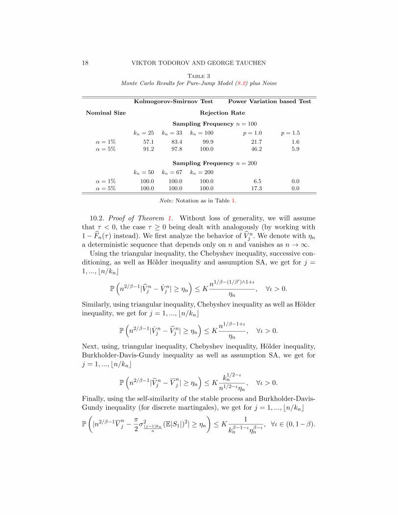
in (8.2) is a time-changed tempered stable process. The parameters of Stare chosen such that it behaves locally like 1.8-stable process and it hasvariance at time 1 equal to 1 (as the model in (8.1)). For this process thelocal Gaussianity does not hold and hence the behavior of the test on datafrom the model in (8.2) will allow us to investigate the power of the test.We also consider another alternative to the jump-diffusion, mainly the casewhen the process in (8.2) is contaminated with i.i.d. Gaussian noise. Thevariance of the noise is set to 0.01 consistent with empirical evidence in [8].

We turn next to the implementation of the test. We apply the test on oneyear worth of simulated data which consists of 252 days (our unit of timeis one trading day). We consider two sampling frequencies: n = 100 andn = 200 which correspond to sampling every 5 and 2 minutes respectivelyin a typical trading day. We experiment with 1-4 blocks per day. In eachblock we use 75% or 70% of the increments in the formation of the test, i.e.,we set bmn/knc = 0.75 for n = 100 and bmn/knc = 0.70 for n = 200. Wefound very little sensitivity of the test with respect to the choice of the ratiomn/kn. For the truncation of the increments, as typical in the literature,we set α = 3.0 and $ = 0.49. Finally, the set A over which the differenceFn(τ)− F (τ) in our test is evaluated is set to

(8.3) A = [Q(0.01) : Q(0.40)] ∪ [Q(0.60) : Q(0.99)],

where Q(α) is the α-quantile of standard normal.The results of the Monte Carlo are reported in Tables 1-3. For the smaller

sample size, n = 100, and with no blocking at all (kn = n) to account forvolatility movements over the day, there are size distortions most noticeableat the conventional 5 percent level. With three blocks (bn/knc = 3), size is


appropriate, while it is seen to have excellent power in Tables 2 and 3. Butwith four blocks on n = 100, there are size distortions because the noisyestimates of local volatility distort the test. Considering the larger samplesize (n = 200), now with three or four blocks the test’s size is approxi-mately correct while power is excellent. For larger values of kn relative ton (bn/knc = 1) the time variation in volatility over the day coupled withthe relatively high precision of estimating a biased version of local volatility,leads to departures from Gaussianity of the (small) scaled increments andhence the over-rejections.

In Tables 1-3 we also report the performance on the simulated data of atest for presence of Brownian motion in high frequency data based on (trun-cated) power variations computed on two different frequencies, proposed in[1] (see also [18]). This test, unlike the test proposed here, does not exploitthe distributional implication of the local Gaussianity result in (1.2). We cansee from Table 1 that the test based on the power variations has reasonablebehavior under the null of presence of a diffusion component in X. Table 2further shows that for the optimal choice of the power (p = 1), the test hasslightly lower power against the considered pure-jump alternative in (8.2)than the Kolmogorov-Smirnov test (when block size is chosen optimally).

When the pure-jump model is contaminated with noise, the scaling ofthe power variations is similar (for the considered frequencies) to that ofa jump-diffusion model observed without noise. Hence, Table 3 reveals rel-atively low power of the test based on the power variations against thealternative of pure-jump process contaminated with noise. By contrast, theKolmogorov-Smirnov test shows almost no change in performance comparedwith the alternative when the pure-jump process is observed without noise(Table 2). The reason is that the Kolmogorov-Smirnov test incorporates alsothe distributional implications of (1.2) and, under the pure-jump plus noisescenario, the scaled high-frequency increments have a distribution which isvery different from standard normal.

9. Empirical Illustration. We now apply our test to two differentfinancial assets, the IBM stock price and the VIX volatility index. The an-alyzed period is 2003 − 2008 and like in the Monte Carlo we consider twoand five minute sampling frequencies. The test is performed for each of theyears in the sample. We set A as in (8.3) and bn/knc = 3 for the five-minutesampling frequency and bn/knc = 4 for the two-minute frequency. As in theMonte Carlo, the ratio bmn/knc is set to 0.75 and 0.70 for the five-minuteand two-minute respectively sampling frequencies. Finally, to account forthe well-known diurnal pattern in volatility we standardize the raw high-


Table 1Monte Carlo Results for Jump-Diffusion Model (8.1)

Kolmogorov-Smirnov Test Power Variation based Test

Nominal Size Rejection Rate

Sampling Frequency n = 100

kn = 25 kn = 33 kn = 100 p = 1.0 p = 1.5

α = 1% 1.0 1.4 6.1 1.5 0.7α = 5% 13.6 5.4 20.8 7.7 5.4


kn = 50 kn = 67 kn = 200 p = 1.0 p = 1.5

α = 1% 1.7 2.2 10.6 1.4 1.3α = 5% 6.1 6.9 35.2 8.1 6.7

Note: For the cases with n = 100 we set bmn/knc = 0.75 and for the cases with n = 200we set bmn/knc = 0.70. The power variation test is a one-sided test based on Theorem 2in [1] with k = 2 and cutoff un = 7σ∆0.49

n with σ being an estimate of volatility over theday using Bipower Variation.

frequency returns by a time-of-day scale factor exactly as in [20].The results from the test are shown on Figure 1. We can see from the figure

that the local Gaussianity hypothesis works relatively well for the 5-minuteIBM returns. At 2-minute sampling frequency for the IBM stock price, how-ever, our test rejects the local Gaussianity hypothesis at conventional signif-icance levels. Nevertheless, the values of the test are not very far from thecritical ones. The explanation of the different outcomes of the test on thetwo sampling frequencies is to be found in the presence of microstructurenoise. The latter becomes more prominent at the higher frequency. Turningto the VIX index data, we see a markedly different outcome. For this dataset, the local Gaussianity hypothesis is strongly rejected at both frequencies.The explanation for this is that the underlying model is of pure-jump type,i.e., the model (2.1) with β < 2.

10. Proofs. We start with introducing some notation that we will makeuse of in the proofs.

At =

∫ t

0αsds, Bt =

∫ t

0σsdSs, σt = σt −

∑s≤t

∆σs.

V nj =n

kn − 1

π

2

jkn∑i=(j−1)kn+2

|∆ni−1A+ ∆n

i−1B||∆ni A+ ∆n

i B|,


Table 2Monte Carlo Results for Pure-Jump Model (8.2)




kn = 25 kn = 33 kn = 100 p = 1.0 p = 1.5

α = 1% 63.3 86.8 99.9 71.1 14.2α = 5% 92.8 99.1 100.0 91.3 38.4


kn = 50 kn = 67 kn = 200

α = 1% 100.0 100.0 100.0 97.7 32.1α = 5% 100.0 100.0 100.0 99.4 63.3

Note: Notation as in Table 1.

V nj =n

kn − 1

π

2

jkn∑i=(j−1)kn+2

|∆ni−1B||∆n

i B|, Vn

j = σ2(j−1)kn

n

n

kn − 1

π

2

jkn∑i=(j−1)kn+2

|∆ni−1S||∆n

i S|,

and we define V nj (i), V n

j (i) and Vnj (i) from the above as in (3.3). We also

denote

(10.1) Fn(τ) =Nn(α,$)

bn/kncmnFn(τ).

Finally, in the proofs we will denote with K a positive constant that mightchange from line to line but importantly does not depend on n and τ . We

will also use the shorthand notation Eni (·) = E(·|F (i−1)

n

).

10.1. Localization. We will prove Theorems 1-4 under the following strongerversions of assumption A and B:SA. We have assumption A with αt, σt and σ−1

t being all uniformly boundedon [0, 1]. Further, (2.3) and (2.4) hold for σt and Yt respectively.SB. We have assumption B with all processes αt, αt, σt, σ

−1t , σt, σ

′t and

the coefficients of the Ito semimartingale representations of σt and σ′t be-ing uniformly bounded on [0, 1]. Further (|δY (t, x)|+ |δσ(t, x)|+ |δσ(t, x)|+|δσ′(t, x)|) ≤ γ(x) for some non-negative valued function γ(x) on E satisfy-ing

∫E ν(x : γ(x) = 0)dx <∞ and γ(x) ≤ K for some constant K.

Extending the proofs to the weaker assumptions A and B follows by stan-dard localization techniques exactly as Lemma 4.4.9 of [9].


Table 3Monte Carlo Results for Pure-Jump Model (8.2) plus Noise




kn = 25 kn = 33 kn = 100 p = 1.0 p = 1.5

α = 1% 57.1 83.4 99.9 21.7 1.6α = 5% 91.2 97.8 100.0 46.2 5.9


kn = 50 kn = 67 kn = 200

α = 1% 100.0 100.0 100.0 6.5 0.0α = 5% 100.0 100.0 100.0 17.3 0.0

Note: Notation as in Table 1.

10.2. Proof of Theorem 1. Without loss of generality, we will assumethat τ < 0, the case τ ≥ 0 being dealt with analogously (by working with1− Fn(τ) instead). We first analyze the behavior of V n

j . We denote with ηna deterministic sequence that depends only on n and vanishes as n→∞.

Using the triangular inequality, the Chebyshev inequality, successive con-ditioning, as well as Holder inequality and assumption SA, we get for j =1, ..., bn/knc

P(n2/β−1|V n

j − V nj | ≥ ηn

)≤ Kn1/β−(1/β′)∧1+ι

ηn, ∀ι > 0.

Similarly, using triangular inequality, Chebyshev inequality as well as Holderinequality, we get for j = 1, ..., bn/knc

P(n2/β−1|V n

j − V nj | ≥ ηn

)≤ Kn1/β−1+ι

ηn, ∀ι > 0.

Next, using, triangular inequality, Chebyshev inequality, Holder inequality,Burkholder-Davis-Gundy inequality as well as assumption SA, we get forj = 1, ..., bn/knc

P(n2/β−1|V n

j − Vnj | ≥ ηn

)≤ K k

1/2−ιn

n1/2−ιηn, ∀ι > 0.

Finally, using the self-similarity of the stable process and Burkholder-Davis-Gundy inequality (for discrete martingales), we get for j = 1, ..., bn/knc

P(|n2/β−1V

nj −

π

2σ2

(j−1)knn

(E|S1|)2| ≥ ηn)≤ K 1

kβ−1−ιn ηβ−ιn

, ∀ι ∈ (0, 1−β).


2003 2004 2005 2006 2007 20080

1

2

3

4

5

IBM, 5−min

2003 2004 2005 2006 2007 20080

2

4

6

8

IBM, 2−min

Year

2003 2004 2005 2006 2007 20080

1

2

3

4

5

VIX, 5−min

2003 2004 2005 2006 2007 20080

2

4

6

8

Year

VIX, 2−min

Fig 1. Kolmogorov-Smirnov tests for local Gaussianity. The ∗ corresponds to the valueof the test supτ∈A

√Nn(α,$)|Fn(τ) − F (τ)| and the solid lines are the critical values

qn(α,A) for α = 5% and α = 1%.

Combining these results, we get altogether for ∀ι ∈ (0, 1− β)

P(|n2/β−1V n

j −π

2σ2

(j−1)knn

(E|S1|)2| ≥ ηn)

≤ K

(n1/β−(1/β′)∧1+ι

ηn

∨ k1/2−ιn

n1/2−ιηn

∨ 1

kβ−1−ιn ηβ−ιn

).

(10.2)

Using the same proofs we can show that the result above continues to holdwhen V n

j is replaced with V nj (i).

Next, for i = (j − 1)kn + 1..., (j − 1)kn + mn and j = 1, ..., bn/knc, we


denote ξni,j(1) = n1/β(

∆ni A+ ∆n

i Y +∫ i∆n

(i−1)∆n(σu− − σ (j−1)kn

n

)dSu

)ξni,j(2) = n1/βσ (j−1)kn

n

∆ni S1

|∆ni X|>α

√V nj n

−$ .

With this notation, using similar inequalities as before, we get

(10.3) P(|ξni,j(1)| ≥ ηn

)≤ K

(n1/β−(1/β′)∧1+ι

ηn

∨ kβ/2+ι/2n

nβ/2+ι/2ηβ+ιn

).

Next, using the result in (10.2) above as well as Holder inequality, we get(10.4)

P(|ξni,j(2)| ≥ ηn

)≤ Kn−(1/2−$)β+ι ∨ n1/β−(1/β′)∧1+ι ∨ (kn/n)1/2−ι ∨ k1+ι−β

n

ηιn, ∀ι > 0.

We next denote the set (note that by assumption SA, σt is strictly abovezero on the time interval [0, 1])(10.5)

Ani,j =

ω :|ξni,j(1)|+ |ξni,j(2)|√

π2E|S1|

> ηn ∪

∣∣∣∣∣∣n1/β−1/2

√V nj (i)√

π2σ (j−1)kn

n

E|S1|− 1

∣∣∣∣∣∣ > ηn

,

for i = (j − 1)kn + 1, ..., (j − 1)kn +mn and j = 1, ..., bn/knc.We now can set (recall (4.1))

(10.6) ηn = n−x, 0 < x <

[(1

β′∧ 1− 1

β

)∧ 1− q2

∧ q(β − 1)

β

],

and this choice is possible because of the restriction on the rate of increaseof the block size kn relative to n given in (4.1). With this choice of ηn, theresults in (10.2), (10.3) and (10.4) imply

(10.7)1

bn/kncmn

bn/knc∑j=1


P(Ani,j

)= o(1).

Therefore, for any compact subset A of (−∞, 0),

(10.8) supτ∈A|Fn(τ)− Gn(τ)| = op(1),

where we denote

Gn(τ) =1

bn/kncmn

bn/knc∑j=1


1

√n∆n

i X√V nj (i)

1|∆ni X|≤α

√V nj n

−$ ≤ τ

1(Ani,j)c.


Taking into account the definition of the set Ani,j , we getGn(τ) ≥ 1

bn/kncmn∑bn/knc

j=1

∑(j−1)kn+mni=(j−1)kn+1 1

n1/β∆n

i S√π2E|S1|

≤ τ(1− ηn)− ηn,

Gn(τ) ≤ 1bn/kncmn

∑bn/kncj=1

∑(j−1)kn+mni=(j−1)kn+1 1

n1/β∆n

i S√π2E|S1|

≤ τ(1 + ηn) + ηn

.

Using Glivenko-Cantelli theorem, see e.g., Theorem 19.1 of [21], we have

supτ

∣∣∣∣ 1

bn/kncmn

bn/knc∑j=1


1

n1/β∆n

i S√π2E|S1|

≤ τ(1− ηn)− ηn

− Fβ(τ(1− ηn)− ηn)

∣∣∣∣ P−→ 0,

supτ

∣∣∣∣ 1

bn/kncmn

bn/knc∑j=1


1

n1/β∆n

i S√π2E|S1|

≤ τ(1 + ηn) + ηn

− Fβ(τ(1 + ηn) + ηn

∣∣∣∣ P−→ 0,

and further using the smoothness of cdf of the stable distribution we have

supτ|Fβ(τ(1− ηn)− ηn)− Fβ(τ)| −→ 0, sup

τ|Fβ(τ(1 + ηn) + ηn)− Fβ(τ)| −→ 0.

These two results altogether imply

supτ|Gn(τ)− Fβ(τ)| P−→ 0,

and from here, using (10.8), we have supτ∈A |Fn(τ)−Fβ(τ)| = op(1) for anycompact subset A of (−∞, 0). Hence, to prove (4.2), we need only to show

(10.9)Nn(α,$)

bn/kncmn

P−→ 1, as n→∞.

We have

P(|∆n

i X| > α√V nj n

−$)≤ P

∣∣∣∣∣∣n1/β−1/2

√V nj√

π2σ (j−1)kn

nE|S1|

− 1

∣∣∣∣∣∣ > 0.5

+ P

(n1/β |∆n

i X| > 0.5α

√π

2σ (j−1)kn

nE|S1|n1/2−$

).

From here we can use the bounds in (10.2) and (10.3) to conclude(10.10)

P(|∆n

i X| > α√V nj n−$)≤ K

nι, for some sufficiently small ι > 0,

hence the convergence in (10.9) holds which implies the result in (4.2). 2


10.3. Proof of Theorem 2. The proof follows the same steps as that ofTheorem 1. We denote with ηn a deterministic sequence depending only onn and vanishing as n→∞. Then, using triangular inequality and successiveconditioning, we have

(10.11) P(∣∣∣∣ 1nV n

j − µ2

∣∣∣∣+

∣∣∣∣ 1nV nj (i)− µ2

∣∣∣∣ ≥ ηn) ≤ Kn−1/2

ηn,

(10.12) P(

(ε in− ε i−1

n)1|∆ni X|>α

√V nj n

−$ ≥ ηn

)≤ Kn$−1/2

ηιn.

We denote

Bni,j =

ω :

∣∣∣∣∣∆ni X∗1|∆ni X|≤α

√V nj n

−$ − (ε i

n− ε i−1

n)

∣∣∣∣∣ > ηn ∪

∣∣∣∣∣∣√V nj (i)√nµ

− 1

∣∣∣∣∣∣ > ηn

,

for i = (j−1)kn+1, ..., (j−1)kn+mn and j = 1, ..., bn/knc. We set ηn = n−x

for 0 < x < 1ι (1/2−$)

∧1/2. With this choice

1

bn/kncmn

bn/knc∑j=1


P(Bni,j)

= o(1).

Therefore, for any compact subset A of (−∞, 0), we have

supτ∈A|Fn(τ)− Gn(τ)| = op(1),

where we denote

Gn(τ) =1

bn/kncmn

bn/knc∑j=1


1

√n∆n

i X√V nj (i)

1|∆ni X|≤α

√V nj n

−$ ≤ τ

1(Bni,j)c.

Taking into account the definition of the set Bni,j , we get Gn(τ) ≥ 1bn/kncmn

∑bn/kncj=1

∑(j−1)kn+mni=(j−1)kn+1 1

1µ

(ε in− ε i−1

n

)≤ τ(1− ηn)− ηn

µ

,

Gn(τ) ≤ 1bn/kncmn

∑bn/kncj=1

∑(j−1)kn+mni=(j−1)kn+1 1

1µ

(ε in− ε i−1

n

)≤ τ(1 + ηn) + ηn

µ

.

From here we can proceed exactly in the same way as in the proof of Theo-

rem 1 to show that Gn(τ)P−→ Fε(τ) locally uniformly in τ . Hence we need


only show Nn(α,$)bn/kncmn

P−→ 1 as n→∞. This follows from

P(|∆n

i X∗| > α

√V nj n−$)≤ P

∣∣∣∣∣∣√V nj√nµ

∣∣∣∣∣∣ > 0.5

+ P(|∆n

i X∗| > 0.5αµn1/2−$

)≤ K

nι, for some sufficiently small ι > 0,

which can be shown using (10.11), the fact that the noise term has a finitefirst moment and the Burkholder-Davis-Gundy inequality. 2

10.4. Proof of Theorem 3. As in the proof of Theorem 1, without loss ofgenerality we will assume τ < 0. First, given the fact that mn/kn → 0, it isno limitation to assume kn −mn > 2 and we will do so henceforth. Here weneed to make some additional decomposition of the difference V n

j − Vnj . It

is given by the following

(10.13) V nj − V

nj = R

(1)j +R

(2)j +R

(3)j +R

(4)j , j = 1, ...., bn/knc,

R(1)j =

n

kn − 1

π

2

jkn∑i=(j−1)kn+2

[(|∆n

i−1B||∆ni B| − σ2

(i−2)∆n|∆n

i−1W ||∆niW |

)+ (σ(i−2)∆n

− σ (j−1)knn

)2|∆ni−1W ||∆n

iW |],

R(2)j = 2

n

kn − 1

π

2σ (j−1)kn

n

jkn∑i=(j−1)kn+2

[σ(i−2)∆n

− σ (j−1)knn−∫ i−2

n

(j−1)knn

σ (j−1)knn

dWu

−∫ i−2

n

(j−1)knn

σ′(j−1)knn

dW ′u

]|∆n

i−1W ||∆niW |,

R(3)j =

2

kn − 1

π

2σ (j−1)kn

n

jkn∑i=(j−1)kn+2

[ ∫ i−2n

(j−1)knn

σ (j−1)knn

dWu +

∫ i−2n

(j−1)knn

σ′(j−1)knn

dW ′u

]

×(n|∆n

i−1W ||∆niW | −

2

π

),

R(4)j =

2

kn − 1σ (j−1)kn

n

jkn∑i=(j−1)kn+2

[ ∫ i−2n

(j−1)knn

σ (j−1)knn

dWu +

∫ i−2n

(j−1)knn

σ′(j−1)knn

dW ′u

].

For i = (j − 1)kn + 1, ...., jkn − 2 we denote the component of R(4)j that

does not contain the increments ∆niW and ∆n

iW′ with

R(4)i,j = R

(4)j −

2

kn − 1σ (j−1)kn

n(jkn− i− 1)

[ ∫ in

i−1n

σ (j−1)knn

dWu +

∫ in

i−1n

σ′(j−1)knn

dW ′u

].


We decompose analogously the difference V nj (i) − V

nj (i) into R

(k)j (i) for

k = 1, .., 4 and R(4)i,j (i) is the component of R

(4)j (i) that does not contain the

increments ∆niW and ∆n

iW′. We further denote for i = (j−1)kn+1, ...., (j−

1)kn +mn and j = 1, ..., bn/knc,

ξnj (1) =V nj (i)− σ2

(j−1)knn

2σ2(j−1)kn

n

, ξnj (2) =

(V nj (i)− σ2

(j−1)knn

)2

8σ4(j−1)kn

n

,

ξni,j(1) =Vn

j (i) + R(4)i,j (i)− σ2

(j−1)knn

2σ2(j−1)kn

n

, ξni,j(2) =

(Vn

j (i) + R(4)i,j (i)− σ2

(j−1)knn

)2

8σ4(j−1)kn

n

,

ξn

j (1) =Vn

j +R(4)j − σ2

(j−1)knn

2σ2(j−1)kn

n

, ξn

j (2) =

(Vn

j +R(4)j − σ2

(j−1)knn

)2

8σ4(j−1)kn

n

,

ξnj (1) =Vn

j − σ2(j−1)kn

n

2σ2(j−1)kn

n

, ξnj (2) =

(Vn

j − σ2(j−1)kn

n

)2

8σ4(j−1)kn

n

,

ξni,j(3) =

√n∆n

iW

σ (j−1)knn

[σ (j−1)kn

n(W i−1

n−W (j−1)kn

n) + σ′(j−1)kn

n

(W ′i−1n

−W ′(j−1)knn

)],

ξni,j(4) = 1 +1

σ (j−1)knn

[σ (j−1)kn

n(W i−1

n−W (j−1)kn

n) + σ′(j−1)kn

n

(W ′i−1n

−W ′(j−1)knn

)].

With this notation we set for i = (j − 1)kn + 1, ...., (j − 1)kn + mn andj = 1, ...., bn/knc

χni,j(1) = −√n

1

σ (j−1)knn

(∆ni A+ ∆n

i Y +

∫ in

i−1n

(σu − σ i−1

n

)dWu

)1|∆ni X|≤α

√V nj n

−$

+ (√n∆n

iW + ξni,j(3))1|∆ni X|>α

√V nj n

−$

−

(√n∆n

iW

σ (j−1)knn

(σ i−1n− σ (j−1)kn

n)− ξni,j(3)

)1|∆ni X|≤α

√V nj n

−$,

χni,j(2) =

√V nj (i)

σ (j−1)knn

− 1− ξnj (1) + ξnj (2)

+ (ξnj (1)− ξnj (2)− ξni,j(1) + ξni,j(2)).


Finally, we denote

Gn(τ) =1

bn/kncmn

bn/knc∑j=1


1

(√n

∆ni X

σ (j−1)knn

1|∆ni X|≤α

√V nj n

−$

≤ τ

√V nj (i)

σ (j−1)knn

− χni,j(1)− τχni,j(2)

)

=1

bn/kncmn

bn/knc∑j=1


1(√

n∆niW ≤ τ + τ ξni,j(1)− τ ξni,j(2)− ξni,j(3)

).

The proof consists of three parts: the first is showing the negligibility ofkn(Fn(τ)− Gn(τ)), the second is deriving the limiting behavior of Gn(τ)−Φ(τ) and third part is showing negligibility of kn(Fn(τ)− Fn(τ)).

10.4.1. The difference Fn(τ)− Gn(τ). We first collect some preliminaryresults that we then make use of in analyzing Fn(τ)− Gn(τ). We start withmaxi=1,....,n |∆n

i B| . Using maximal inequality we have

(10.14) E( maxi=1,....,n

|∆ni B|p) ≤ Kn1−p/2, ∀p > 0.

Next, using assumption SB (in particular that jumps are of finite activity),we have

P

(∫ jknn

(j−1)knn

∫E

1(δφ(z, x) 6= 0

)µ(dz, dx) ≥ 1

)≤ Kkn

n, φ = Y , σ, σ and σ′.

(10.15)

We now provide bounds for the elements of χni,j(1) and χni,j(2). In whatfollows we denote with ηn some deterministic sequence of positive numbersthat depends only on n. We first have (recall the definition of σt)

P

(√n

∣∣∣∣∣∫ i

n

i−1n

(σu − σ i−1n

)dWu

∣∣∣∣∣ ≥ ηn)≤ P

(∫ jknn

(j−1)knn

∫E

1(δY (s, x) 6= 0

)µ(ds, dx) ≥ 1

)

+ P

(√n

∣∣∣∣∣∫ i

n

i−1n

(σu − σ i−1n

)dWu

∣∣∣∣∣ ≥ ηn).

For the second term on the right hand side of the above inequality, we canuse Chebyshev inequality as well as Burkholder-Davis-Gundy inequality, toget for ∀p ≥ 2:

P

(√n

∣∣∣∣∣∫ i

n

i−1n

(σu − σ i−1n

)dWu

∣∣∣∣∣ ≥ ηn)≤np/2E

∣∣∣∫ i∆n

(i−1)∆n(σu − σ i−1

n)2du

∣∣∣p/2ηpn

.


Therefore, applying again Burkholder-Davis-Gundy inequality, we have al-together(10.16)

P

(√n

∣∣∣∣∣∫ i

n

i−1n

(σu − σ i−1n

)dWu

∣∣∣∣∣ ≥ ηn)≤ K

[(knn

)∨(1

np/2ηpn

)], ∀p > 0.

Similar calculations (using the fact that σt and σ′t are Ito semimartingales),yields for ∀p > 0(10.17)

P

(∣∣∣∣∣√n∆n

iW

σ (j−1)knn

(σ i−1

n− σ (j−1)kn

n

)− ξni,j(3)

∣∣∣∣∣ ≥ ηn)≤ K

[(knn

)∨(knnηn

)p].

Next, applying Chebyshev inequality and the elementary |∑

i |ai||p ≤∑

i |ai|pfor p ∈ (0, 1], we get

P(√n|∆n

i Y | ≥ ηn)≤nι/2E

(∫ i∆n

(i−1)∆n

∫E |δ

Y (s, x)|µ(ds, dx))ι

ηιn

≤nι/2E

(∫ i∆n

(i−1)∆n

∫E |δ

Y (s, x)|ιµ(ds, dx))

ηιn

≤ Kn−1+ι/2η−ιn , ∀ι ∈ (0, 1).

(10.18)

Further, Chebyshev inequality and the boundedness of at easily implies

(10.19) P(√n|∆n

i A| ≥ ηn)≤ np/2E(|∆n

i A|p)ηpn

≤ K 1

np/2ηpn.

We turn next to the difference V nj − V n

j . Using triangular inequality andsuccessive conditioning, we have

P(|V nj − V nj | ≥ ηn

)≤ P

(2n

kn

π

2max

i=1,...,n|∆n

i A+ ∆ni B|

∫ jknn

(j−1)knn

∫E

(|δY (s, x)| ∨ 1)µ(ds, dx) ≥ ηn2

)+

K

nηn.

From here we have

P

(2n

kn

π

2maxi=1,...,n

|∆ni A+ ∆n

i B|∫ jkn

n

(j−1)knn

∫E

(|δY (s, x)| ∨ 1)µ(ds, dx) ≥ ηn2

)

≤ P

(∫ jknn

(j−1)knn

∫Eµ(ds, dx) ≥ 1

)≤ Kkn

n.


Thus altogether we get

(10.20) P(|V nj − V n

j | ≥ ηn)≤ K

(1

nηn

∨ knn

).

We continue next with the difference V nj − V n

j . Application of triangularinequality gives

|∆ni−1A+ ∆n

i−1B||∆ni A+ ∆n

i B| − |∆ni−1B||∆n

i B|≤ |∆n

i−1A+ ∆ni−1B||∆n

i A|+ |∆ni−1A||∆n

i B|.

Using this inequality and applying Chebyshev inequality, we get

(10.21) P(|V nj − V n

j | ≥ ηn)≤ K

(1√nηn

)p, ∀p ≥ 1,

and this inequality can be further strengthened but suffices for our analysis.

Turning next toR(1)j , using triangular inequality, Burkholder-Davis-Gundy

inequality as well as (10.15), we can easily get

P(|R(1)

j | ≥ ηn)≤ P

(|R(1)

j | ≥ ηn,∫ jkn

n

(j−1)knn

∫E

1(δσ(s, x) 6= 0)µ(ds, dx) ≥ 1

)

+ P

(|R(1)

j | ≥ ηn,∫ jkn

n

(j−1)knn

∫E

1(δσ(s, x) 6= 0)µ(ds, dx) = 0

)

≤ Kknn

+K

(1√nηn

)p+K

(knnηn

)p, ∀p ≥ 1.

Similar calculations, and utilizing the fact that σt σ′t are themselves Ito

semimartingales, yield

(10.22) P(|R(2)

j | ≥ ηn)≤ Kkn

n+K

(knnηn

)p, ∀p ≥ 1.

Next, by splitting

n|∆ni−1W ||∆n

iW |−2

π= |√n∆n

i−1W |

(|√n∆n

iW | −√

2

π

)+

√2

π

(|√n∆n

i−1W | −√

2

π

),

we can decomposeR(3)j into two discrete martingales. Then applying Burkholder-

Davis-Gundy inequality, we get

(10.23) P(|R(3)

j | ≥ ηn)≤ K

(1√nηn

)p, ∀p ≥ 2.


Next, we trivially have

(10.24)

P(|V nj − σ2

(j−1)knn

| ≥ ηn)≤ K

(1

knη2n

)p,

P(|V nj − V

n

j | ≥ 0.5σ2(j−1)kn

n

)≤ K kn

n , ∀p ≥ 2.

Further, application of Burkholder-Davis-Gundy inequality gives

(10.25)

E|V nj − σ2

(j−1)knn

|p ≤ K

kp/2n

,

En(j−1)kn(R

(4)j ) = 0, E|R(4)

j |p ≤ K(knn

)p/2, ∀p ≥ 2.

The results in (10.20)-(10.25) continue to hold when V nj , V n

j , V nj , V

nj , R

(1)j ,

R(2)j and R

(3)j are replaced with V n

j (i), V nj (i), V n

j (i), Vnj (i), R

(1)j (i), R

(2)j (i)

and R(3)j (i) respectively.

Further, using Burkholder-Davis-Gundy inequality for discrete martin-gales (note that V

nj − V

nj (i) can be decomposed into discrete martingales

and terms whose p-th moment is bounded by K/kpn), we have

(10.26) E(|R(4)

j − R(4)i,j |

p + |R(4)i,j − R

(4)i,j (i)|p

)≤ K

(1√n

)p, ∀p > 0,

(10.27)∣∣∣En(j−1)kn

(Vnj − V

nj (i)

)∣∣∣ ≤ K

k2n

, E|V nj − V

nj (i)|p ≤ K

(1

kn

)p, ∀p ≥ 1.

Now we can use the above results for the components of V nj (i)−σ2

(j−1)knn

, to

analyze the first term in χni,j(2) involving√V nj (i)− σ (j−1)kn

n

. We make use

of the following algebraic inequality∣∣∣∣√x−√y − x− y2√y

+(x− y)2

8y√y

∣∣∣∣ ≤ (x− y)4

8y7/2+|x− y|3

2y5/2,

for every x ≥ 0 and y > 0. Using this inequality with x and y replaced with

V nj (i) and σ2

(j−1)knn

respectively, as well the bounds in (10.20)-(10.27), we

get

P

∣∣∣∣∣∣√V nj (i)

σ (j−1)knn

− 1− ξnj (1) + ξnj (2)

∣∣∣∣∣∣ ≥ ηn

≤ K

[1

nη1/3n

∨ knn

∨ 1

ηp/3n [np/2 ∧ (n/kn)p/2]

∨ 1

η2p/3n kpn

],

(10.28)


for ∀p ≥ 1 and ∀ι > 0. Similarly, using the following inequality

P(|x2 − y2| ≥ ε

)≤ P

(|x− y|2 ≥ 0.5ε

)+P (2|y| ≥ K)+P (|x− y| ≥ 0.5ε/K) ,

for any random variables x and y and constants ε > 0 and K > 0, togetherwith the bounds in (10.20)-(10.27), we have

P(|ξnj (1)− ξnj (2)− ξni,j(1) + ξni,j(2)| ≥ ηn

)≤ K

[1

nηn

∨ knn

∨ 1

ηpn[np/2 ∧ (n/kn)p]

],

(10.29)

for every p ≥ 1 and arbitrary small ι > 0.We finally provide a bound for the second term in χni,j(1). We can use

Chebyshev inequality as well as Holder inequality to get

P(

(√nσ (j−1)kn

n|∆n

iW |+ |ξni,j(3)|)1(|∆n

i X| > α√V nj n

−$)≥ ηn

)

≤ K

[P(|∆n

i X| > α√V nj n

−$)]1/(1+ι)

ηιn.

(10.30)

We can further write

P(|∆n

i X| > α√V nj n−$)≤ P

(|√V nj − σ (j−1)kn

n

| ≥ 0.5σ (j−1)knn

)+ P

(|∆n

i X| > 0.5ασ (j−1)knn

n−$).

From here we can use the bounds in (10.20)-(10.27) as well as (10.18) andconclude

P(√

nσ (j−1)knn

|∆niW |1

(|∆n

i X| > α√V nj n−$)≥ ηn

)≤ K

(knn

) 11+ι 1

ηιn, ∀ι > 0.

(10.31)

Combining the results in (10.14), (10.16), (10.17), (10.18), (10.19), (10.28), (10.29)and (10.31), we get

P((|χni,j(1)|+ |χni,j(2)|) > ηn

)≤ K

[1

nηn

∨ 1

ηpn[np/2 ∧ (n/kn)p ∧ k3p/2n ]

∨(knn

) 11+ι 1

ηιn

].


From here, using the fact that the probability density of a standard normalvariable is uniformly bounded, we get

E∣∣∣∣1(√n∆n

i X1|∆ni X|≤α

√V nj n

−$ ≤ τ√V nj (i)

)

− 1

(√n

∆ni X

σ (j−1)knn

1|∆ni X|≤α

√V nj n

−$ ≤ τ

√V nj (i)

σ (j−1)knn

− χni,j(1)− τχni,j(2)

)∣∣∣∣≤ P

((|χni,j(1)|+ |χni,j(2)|) > ηn

)+ E

∣∣∣∣∣Φ(τ + τ ξni,j(1)− τ ξni,j(2) + ηn(1 + τ)

ξni,j(4)

)− Φ

(τ + τ ξni,j(1)− τ ξni,j(2)− ηn(1 + τ)

ξni,j(4)

)∣∣∣∣∣≤ KP

((|χni,j(1)|+ |χni,j(2)|) > ηn

)+Kηnτ.

Therefore, upon picking ηn ∝ n−q−ι for ι ∈ (0, 1/2 − q) sufficiently small,we get finally for any compact subset A of (−∞, 0)

(10.32) supτ∈A|Fn(τ)− Gn(τ)| = op

(1

kn

).

10.4.2. The asymptotic behavior of Gn(τ)− Φ(τ). We have(10.33)

Gn(τ)−Φ(τ) =5∑i=1

Ani , An1 =

1

bn/kncmn

bn/knc∑j=1


[1(√n∆n

iW ≤ τ)− Φ(τ)

],

An2 =1

bn/knc

bn/knc∑j=1

(Φ(τ + τξ

n

j (1)− τξnj (2))− Φ(τ)

), An3 =

1

bn/kncmn

bn/knc∑j=1


ani ,

ani = 1

(√n∆n

iW ≤τ + τ ξni,j(1)− τ ξni,j(2)

ξni,j(4)

)−1(√n∆n

iW ≤ τ)+Φ(τ)−Φ

(τ + τ ξni,j(1)− τ ξni,j(2)

ξni,j(4)

),

An4 =1

bn/kncmn

bn/knc∑j=1


[Φ

(τ+τ ξni,j(1)−τ ξni,j(2)

)−Φ

(τ+τξ

n

j (1)−τξnj (2)

)],

An5 =1

bn/kncmn

bn/knc∑j=1


[Φ


ξni,j(4)

)−Φ

(τ+τ ξni,j(1)−τ ξni,j(2)

)].

We first derive a bound for the order of magnitude of An3 , An4 and An5 andthen analyze the limiting behavior of An1 and An2 . Using the independenceof ∆n

iW , ∆nhW , ∆n

iW′, ∆n

hW′ from each other (for i 6= h) and F (j−1)kn

n

, the

fact that ξni,j(4) is adapted to Fni−1 as well as successive conditioning, we


have E (ani anh) = 0 for |i− h| > kn. For 0 < i− h ≤ kn, we can first split anh

into a component in which the summand including the i-th increment ∆niW

is removed from ξnh,j(1) and ξnh,j(2). We denote this part of anh with anh and

the residual with anh = anh − anh. We further denote with ξi,nh,j(1) and ξi,nh,j(2)

the terms ξnh,j(1) and ξnh,j(2) in which the summand corresponding to ∆niW

is removed. Then using successive conditioning, we have for (j − 1)kn + 1 ≤h < i ≤ (j − 1)kn +mn

E (ani anh) = 0, E (ani )2 ≤ K|τ |

(√knn

∨ 1√kn

).

Further, we can use triangular inequality for ani and anh, the bounds in(10.25)-(10.27), and get for n sufficiently high

E|ani anh| ≤ P

(|ξni,j(4)| >

(knn

)1/2−ι

∪ |ξnh,j(4)| >(knn

)1/2−ι)

+ P(|ξni,j(1)− ξni,j(2)| > k−1/2+ι

n

)+ P

(|ξnh,j(1)− ξi,nh,j(1)− ξnh,j(2) + ξi,nh,j(2)| > k−1+ι

n

)+ P

(√n∆n

iW ∈ 2τ(1− k−1/2+ιn , 1 + k−1/2+ι

n ) ∩√n∆n

hW ∈ 2τ(1− k−1+ιn , 1 + k−1+ι

n ))

+K|τ | ∨ τ2

kn.

Therefore, using again (10.25)-(10.27), we have

(10.34) An3 ≤ K(√|τ | ∨ τ2)×

(1√

bn/kncmn

(1

kn

)1/4∨ 1√n

).

ForAn4 , using a second-order Taylor expansion, the bounds in (10.24), (10.25)and (10.27), as well as the uniform boundedness of the probability densityof the standard normal distribution and its derivative, we get

(10.35) E|An4 | ≤ K(|τ | ∨ τ2)

(1

k3/2n

∨ 1√bn/knckn

).

Next, for An5 , we can use the boundedness of the probability density of thestandard normal as well as a second-order Taylor expansion, to get for ∀ι > 0and n sufficiently high

Φ


ξni,j(4)

)− Φ


)= bni (1) + bni (2) + bni (3),

bni (1) =

Φ


ξni,j(4)

)− Φ


)1|ξni,j(4)−1|≥( knn )

1/2−ι,


bni (2) = Φ′(τ + τ ξni,j(1)− τ ξni,j(2)

)(τ+τ ξni,j(1)−τ ξni,j(2))(ξni,j(4)−1)1|ξni,j(4)−1|<( knn )

1/2−ι,

|bni (3)| ≤ K|τ + τ ξni,j(1)− τ ξni,j(2)|2

(1− (kn/n)1/2−ι)3|ξni,j(4)− 1|2.

For bni (1) and bni (3), we have

E(|bni (1)|+ |bni (3)|) ≤ K(τ2 ∨ 1)knn.

For bni (2), by an application of Holder inequality, we first have

E∣∣∣∣bni (2)− Φ′ (τ) τ(ξni,j(4)− 1)1

|ξni,j(4)−1|<( knn )1/2−ι

∣∣∣∣ ≤ K|τ | 1√n.

Then,

E

1

bn/kncmn

bn/knc∑j=1


Φ′ (τ) τ(ξni,j(4)− 1)1|ξni,j(4)−1|<( knn )1/2−ι

2

≤ Kknmn

n2.

Therefore, altogether we get

(10.36) E|An5 | ≤ K(|τ | ∨ τ2)knn.

We turn now to An1 and An2 . Using secon-order Taylor expansion, we canextract the leading terms in A2

n. In particular, we denoteAn2 (1) = 1

bn/knc∑bn/knc

j=1 Φ′(τ)τξnj (1),

An2 (2) = 1bn/knc

∑bn/kncj=1 (0.5Φ

′′(τ)τ2(ξ

nj (1))2 − Φ′(τ)τξ

nj (2)).

With this notation, using the bounds in (10.27), as well as the boundednessof Φ

′′′, we have

(10.37) E|An2 −An2 (1)−An2 (2)| ≤ K(|τ |3 ∨ |τ |2)

[(knn

)3/2∨(1

kn

)3/2].

Further, upon denoting with An2 (1) and An2 (2) the counterparts of An2 (1)

and An2 (2) with ξnj (1) and ξ

nj (2) replaced with ξnj (1) and ξnj (2) respectively,

we have using the bounds in (10.25) (as well as the restriction on the rateof growth of kn in (5.1))

(10.38) E|An2 (1) +An2 (2)− An2 (1)− An2 (2)| ≤ K(|τ | ∨ τ2)

(1√n

∨ knn

).


Thus we are left with the terms An1 , An2 (1) and An2 (2). For An2 (2), using

En(j−1)kn

(ξnj (1)

)2= 2En(j−1)kn

(ξnj (2)) =1

4

1

kn

((π2

)2+ π − 3

)+ o

(1

kn

),

we have

(10.39) knAn2 (2)

P−→ τ2Φ′′(τ)− τΦ′(τ)

8

((π2

)2+ π − 3

),

locally uniformly in τ . We finally will show that

(10.40)(√bn/kncmnA

n1

√bn/kncknAn2 (1)

)L−→ (Z1(τ) Z2(τ)) ,

locally uniformly in τ . We have( √bn/kncmnA

n1√

bn/kncknAn2 (1)

)=

bn/knckn∑i=1

(ζni (1)

Φ′(τ)τ2 (ζni (2) + ζni (3))

)+

(0

Φ′(τ)τ2 ζn

),

with

ζni =

1√

bn/kncmn[1 (√n∆n

iW ≤ τ)− Φ(τ)]

1√bn/knckn

π2 |√n∆n

i−1W |(|√n∆n

iW | −√

2π

)1√

bn/knckn

√π2

(|√n∆n

iW | −√

2π

) , i ∈ In,

where In = i = (j − 1)kn + 1, ..., (j − 1)kn +mn, j = 1, ..., bn/knc, andfor i = 1, ...., n \ In, ζni is exactly as above with only the first element beingreplaced with zero, and finally

ζn = − (π/2)√bn/knckn

bn/knc∑j=1

[|√n∆n

(j−1)knW |

(|√n∆n

(j−1)kn+1W | −√

2

π

)

+

√2

π

(|√n∆n

jknW | −√

2

π

)],

where we set ∆n0W = 0. With this notation, we have

E(ζn)2≤ K

kn.

Further,

Eni−1(ζni ) = 0,

bn/knckn∑i=1

Eni−1||ζni ||2+ι −→ 0, ∀ι > 0,


bn/knckn∑i=1

Eni−1 [ζni (ζni )′] −→

Φ(τ)(1− Φ(τ)) 0 0

0(π2

)2 (1− 2

π

)π2

(1− 2

π

)0 π

2

(1− 2

π

)π2

(1− 2

π

) ,

because recall mn/kn → 0. Combining the last two results, we have the con-vergence in (10.40), pointwise in τ , by an application of Theorem VIII.3.32in [10]. Application of Theorem 12.3 in [7], extends the convergence to localuniform in τ .

Altogether, the limit behavior of Gn(τ)−Φ(τ) is completely characterizedby the limits in (10.39)-(10.40) and

(10.41) supτ∈A|Gn(τ)− Φ(τ)−An1 − An2 (1)− An2 (2)| = op

(1

kn

),

where A is a compact subset of (−∞, 0), with the result in (10.41) followingfrom the bounds on the order of magnitude derived above.

10.4.3. The difference Fn(τ)− Fn(τ). To analyze the difference Fn(τ)−Fn(τ), we use the following inequality

P(|∆n

i X| > α√V nj n−$)

≤ P

∣∣∣∣∣∣√V nj

σ (j−1)knn

− 1

∣∣∣∣∣∣ > 0.5

+ P(|∆n

i X| > 0.5ασ (j−1)knn

n−$).

For the first probability on the right-hand side of the above inequality we canuse the bounds in (10.24), (10.25) and (10.28), while for the second one wecan use the exponential inequality for continuous martingales with boundedvariation, see e.g., [16], as well as the algebraic inequality |

∑i ai|p ≤

∑i |ai|p

for p ∈ (0, 1], to conclude

(10.42) P(|∆n

i X| > α√V nj n−$)≤ K

[knn∨ n−1+ι$

], ∀ι > 0.

Since kn/√n→ 0 and from the result of the previous two subsections Fn(τ)−

Φ(τ) = Op

(1kn

), we get from here

(10.43) supτ∈A|Fn(τ)− Fn(τ)| = op

(1

kn

),

for any compact subset A of (−∞, 0). 2


10.5. Proof of Theorem 4. The proof follows exactly the same steps asthe proof of Theorem 3 and we use analogous notation as in that proof.The only nontrivial difference in analyzing the term F ′n(τ)− G′n(τ) regardsthe difference |Cnj − Cnj | (and |Cnj (i) − Cnj (i)|). For it, we make use of thefollowing algebraic inequality

|x21|x|≤a − y21|y|≤a| ≤ |x− y|21|x−y|≤2a + 2a|x− y|1|x−y|≤2a

+ 2|y|21|y|>a/2 + a21|x−y|>a/2.

Using the above inequality, the bound in (10.15), as well as the exponentialinequality for continuous martingales with bounded variation, see e.g., [16],we have

(10.44) P(|Cnj − Cnj | ≥ ηn

)≤ Kkn

n.

Then, upon picking ηn ∝ n−q−ι for ι ∈ (0, 1/2− q) sufficiently small, we get

supτ∈A |F ′n(τ)− G′n(τ)| = op

(1kn

)for any compact subset A of (−∞, 0).

Further, for G′n(τ) − Φ(τ) the only difference from the analysis of thecorresponding term in the proof of Theorem 3 is that now we have

knAn2 (2)

P−→ τ2Φ′′(τ)− τΦ′(τ)

4,

and further now( √bn/kncmnA

n1√

bn/kncknAn2 (1)

)=

bn/knckn∑i=1

(ζni (1)

Φ′(τ)τ2 ζni (2)

),

with

(ζni )′ =(

1√bn/kncmn

[1 (√n∆n

iW ≤ τ)− Φ(τ)] 1√bn/knckn

((√n∆n

iW )2 − 1)), i ∈ In,

where In = i = (j − 1)kn + 1, ..., (j − 1)kn +mn, j = 1, ..., bn/knc, andfor i = 1, ...., n \ In, ζni is exactly as above with only the first element being

replaced with zero. From here the analysis of G′n(τ)− Φ(τ) is done exactlyas that of the corresponding term in the proof of Theorem 3.

We are left with showing the result in the case when jumps in X canbe of infinite activity (under the conditions in the theorem). We again

follow the steps of the proof of Theorem 3. We replace R(4)j with Cnj −

Cnj in ξnj (1) and ξ

nj (2) and similarly we replace R

(4)i,j (i) with Cnj − Cnj −

(∆ni X)21|∆n

i X|≤αn−$ + |∆ni A+ ∆n

i B|2 in ξni,j(1) and ξni,j(2).


Using the inequality in (10.44), and since∫E |δ

Y (x)|β′ν(dx) < ∞ (uponlocalization that bounds the size of the jumps), we have(10.45)

E∣∣∣(∆n

i X)21|∆ni X|≤αn−$ − (∆n

i A+ ∆ni B)2

∣∣∣p ≤ Kn−1−(2p−β′)$, ∀p ≥ β′/2,

and from here

(10.46) E|Cnj − Cnj |p ≤ Knp−1−(2p−β′)$, ∀p ≥ 1.

Using the bounds in (10.45) and (10.46), we can prove exactly as in theproof of Theorem 3 for some deterministic sequence of positive numbers ηn

P((|χni,j(1)|+ |χni,j(2)|) > ηn

)≤ K

[1

ηpn[np/2 ∧ (n/kn)p ∧ k3p/2n ]

∨(knn

) 11+ι 1

ηιn

∨ n−1+β′/2

ηβ′

n

∨ n−(2−β′)$

η1/2n ∧ ηn

√kn

].

From here, using the rate of growth condition in (6.8), upon appropriatelychoosing ηn, we get

(10.47) supτ∈A|F ′n(τ)− G′n(τ)| = op

(1

kn

),

for any compact subset A of (−∞, 0).

We turn next to G′n(τ) − Φ(τ) and we derive the bounds of those termsin the decomposition of the latter which are different from the case of finitejump activity proved above (the term A5 is identically zero since σt is con-stant). First, for An3 , using (10.46) as well as the independence of Wt andYt, we have(10.48)

An3 ≤ K(√|τ |∨τ2)×

(1√

bn/kncmn

n1/2−(4−β′)$/2∨k1/4n n−1/4−(4−β′)$/4

∨ 1√n

).

Next, if we exclude Cnj − Cnj from ξnj (1) and ξ

nj (2), we get for A4, using

(10.45) and (10.46), as well as applying Holder inequality

(10.49) E|An4 | ≤ K(|τ | ∨ τ2)

(1

k3/2n

∨ 1√bn/knckn

∨ n−(2−β′)$√kn

∨n1−(4−β′)$

).

Combining the bounds in (10.48)-(10.49), and taking into account thegrowth condition in (6.8), we get

(10.50) supτ∈A|G′n(τ)− Φ(τ)−An1 − An2 (1)− An2 (2)| = op

(1

kn

),


where A is a compact subset of (−∞, 0). The limit behavior of the triple(An1 , A

n2 (1), An2 (2)) is derived as in the finite jump activity case in the first

part of the proof and this together with (10.47) and (10.50) yields the statedresult in the case of infinite variation jumps. 2

Acknowledgements. Research partially supported by NSF Grant SES-0957330. We would like to thank Dobrislav Dobrev, Jean Jacod, Per Myk-land, Mark Podolskij, Markus Reiss, Mathieu Rosenbaum and many seminarparticipants for helpful comments and suggestions. We also thank an Asso-ciate Editor and a referee for careful read and many constructive comments.

References.

[1] Ait-Sahalia, Y. and J. Jacod (2010). Is Brownian Motion Necessary to Model HighFrequency Data? Annals of Statistics 38, 3093–3128.

[2] Andersen, T., T. Bollerslev, and D. Dobrev (2007). No Arbitrage SemimartingaleRestrictions for Continuous-time Volatility Models subject to Leverage Effects, Jumpsand i.i.d. Noise: Theory and Testable Distributional Implications. Journal of Econo-metrics 138, 125–180.

[3] Andrews, B., M. Calder, and R. Davis (2009). Maximum Likelihood Estimation ofα-stable Autoregressive Processes. Annals of Statistics 37, 1946–1982.

[4] Barndorff-Nielsen, O. and N. Shephard (2001). Non-Gaussian Ornstein–Uhlenbeck-Based Models and some of Their Uses in Financial Economics. Journal of the RoyalStatistical Society Series B, 63, 167–241.

[5] Barndorff-Nielsen, O. and N. Shephard (2004). Power and Bipower Variation withStochastic Volatility and Jumps. Journal of Financial Econometrics 2, 1–37.

[6] Barndorff-Nielsen, O. and N. Shephard (2006). Econometrics of Testing for Jumps inFinancial Economics using Bipower Variation. Journal of Financial Econometrics 4,1–30.

[7] Billingsley, P. (1968). Convergence of Probability Measures. New York: Wiley.[8] Hansen, P. and A. Lunde (2006). Realized Variance and Market Microstructure Noise.

Journal of Business Economics and Statistics 24, 127–161.[9] Jacod, J. and P. Protter (2012). Discretization of Processes. Berlin: Springer-Verlag.[10] Jacod, J. and A. Shiryaev (2003). Limit Theorems For Stochastic Processes (2nd

ed.). Berlin: Springer-Verlag.[11] Kluppelberg, C., T. Meyer-Brandis, and A. Schmidt (2010). Electricity Spot Price

Modelling with a View Towards Extreme Spike Risk. Quantitative Finance 10, 963–974.[12] Mancini, C. (2009). Non-parametric Threshold Estimation for Models with Stochastic

Diffusion Coefficient and Jumps. Scandinavian Journal of Statistics 36, 270–296.[13] Mikosch, T., S. Resnick, H. Rootzen, and A. Stegeman (2002). Is Network Traffic Ap-

proximated by Stable Levy Motion or Fractional Brownian Motion? Annals of AppliedProbability 12, 23–68.

[14] Mykland, P., N. Shephard, and K. Sheppard (2012). Efficient and Feasible Infer-ence for the Components of Financial Variation using Blocked Multipower Variation.Technical report.

[15] Mykland, P. and L. Zhang (2009). Inference for Continuous Semimartingales Ob-served at High Frequency. Econometrica 77, 1403–1445.

[16] Revuz, D. and M. Yor (1999). Continuous Martingales and Brownian Motion.Springer.


[17] Sato, K. (1999). Levy Processes and Infinitely Divisible Distributions. Cambridge,UK: Cambridge University Press.

[18] Todorov, V. and G. Tauchen (2011). Limit Theorems for Power Variations of Pure-Jump Processes with Application to Activity Estimation. Annals of Applied Probabil-ity 21, 546–588.

[19] Todorov, V. and G. Tauchen (2012a). Realized Laplace Transforms for Pure-JumpSemimartingales. Annals of Statistics 40, 1233–1262.

[20] Todorov, V. and G. Tauchen (2012b). The Realized Laplace Transform of Volatility.Econometrica 80, 1105–1127.

[21] van der Vaart, A. (1998). Asymptotic Statistics. Cambridge: Cambridge UniversityPress.

[22] Woerner, J. (2007). Inference in Levy-type Stochastic Volatility Models. Advancesin Applied Probability 39, 531–549.

Department of FinanceNorthwestern UniversityEvanston, IL 60208-2001E-mail: [email protected]

Department of EconomicsDuke UniversityDurham, NC 27708-0097E-mail: [email protected]

mailto:[email protected]

mailto:[email protected]

Limit Theorems for the Empirical Distribution Function of ...

Documents

Transcript of Limit Theorems for the Empirical Distribution Function of ...