arX

iv:h

ep-t

h/95

0901

9v1

5 S

ep 1

995

PSU/TH/156UFIFT-HEP-95-16

SU-4240-598September 1995

Chern-Simons Duality and the Quantum Hall Effect

A. P. Balachandran1, L. Chandar1,2, B. Sathiapalan3

1 Department of Physics, Syracuse University,

Syracuse, NY 13244-1130, U.S.A.2 Department of Physics, University of Florida,

Gainesville, FL 32611, U.S.A.3 Department of Physics, Pennsylvania State University,

120, Ridge View Drive, Dunmore, PA 18512, U.S.A.

Abstract

In previous work on the quantum Hall effect on an annulus, we used O(d, d;Z) du-ality transformations on the action describing edge excitations to generate the Haldanehierarchy of Hall conductivities. Here we generate the corresponding hierarchy of “bulkactions” which are associated with Chern-Simons (CS) theories, the connection betweenthe bulk and edge arising from the requirement of anomaly cancellation. We also find aduality transformation for the CS theory exactly analogous to the R → 1

Rduality of the

scalar field theory at the edge.

1 Introduction

Chern Simons (CS) gauge theories are known to be particularly appropriate for describing

the quantum Hall effect (QHE) [1, 2]. The low energy effective action for the electromag-

netic vector potential, obtained by integrating out the electronic degrees of freedom in

a Hall system, is known to have a CS term. The coefficient of this term is proportional

to the Hall conductivity. This fact is easily shown as follows. Let us assume that the

effective action (apart from the usual Maxwell term) is

Seff [A] = −1

2σXY

∫

d3xǫµνλAµ∂νAλ (1.1)

Then we get for the expectation value of the current,

< jµem >A= −

δ

δAµ

Seff [A] = σXY ǫµνρ∂νAρ (1.2)

We thus see that there is a current in the X- direction when there is an electric field in

the Y- direction. This is the Hall effect, the Hall conductivity being σXY .

In studying the Hall effect, we will be interested in CS theories involving several vector

potentials (one of which is the electromagnetic field). These comprise the “statistical”

gauge fields and the fields describing excitations in the bulk [1, 2, 3, 4, 5]. The former

are introduced for the purpose of changing the statistics of the excitation fields in the

action while the latter represent collective degrees of freedom such as vortices or other

quasiparticles and can describe both bosons and fermions.

Experimentally, the Hall conductivity in certain systems is quantized in integers or

in certain definite fractions [6] corresponding respectively to integer and fractional QHE

(IQHE and FQHE). Several scenarios have been proposed to explain such quantizations.

The hierarchy schemes of Haldane [8] and Jain [9] are perhaps the most attractive, in

that they explain most of the observed experimental fractions. CS theories of the type

mentioned above, involving several vector potentials, lend themselves naturally to these

2

schemes [3, 7]. The Jain scheme has already been written in this form [3] while we will

work out a similar description of the Haldane scheme in this paper.

However, the CS action is not gauge invariant on a manifold with a boundary (like

an annulus), such a manifold being the appropriate geometry for a physical Hall sample.

One has to include non-trivial dynamical degrees of freedom at the edge [4, 10, 11, 12, 13]

to restore gauge invariance. In this way, one predicts the existence of edge states, which

nicely corroborates completely different arguments showing the existence of chiral edge

curents in a Hall sample [14]. These states have been studied in detail by many authors

[4, 10, 11, 12, 13, 15, 16, 17]. In [17], we described them by a conformal field theory of

massless chiral scalar fields taking values on a torus. The most general action for these

scalar fields contains a symmetric matrix Gij and an antisymmetric matrix Bij . In [17], we

saw that the Hall conductivity depends on Gij. In this paper, we will show, in detail, how

the anomaly cancellation argument enables us to relate this matrix to a corresponding

matrix in the bulk CS theories. Thus, once we implement the hierarchy arguments in the

CS theory, we have a rationale for particular choices of this matrix made in [17].

Now, as in string theories having torally compactified spatial dimensions, there are

certain duality transformations of the edge theory that leave the spectrum invariant [18].

These transformations change Gij and Bij in well-defined ways and hence also change

the Hall conductivity [17]. It was shown in [17] that one can reproduce most of the

conductivity fractions of the Haldane and Jain schemes by means of these generalized

duality transformations. The connection of the edge theory with the CS theory in the

bulk then suggests that similar transformations can be implemented in the bulk CS theory

also. This conjecture turns out to be at least partly realizable in that one can implement

a duality transformation of the type R → 1/R in the bulk. The demonstration of this

result is a generalization of the one that has been used in [19] to implement duality in

scalar theories. We think that both this proof and the result are interesting and could

3

have implications in many other areas as well.

This paper is organized as follows: In Section 2 we describe how to implement the

Haldane construction using CS theories. In Section 3 we describe the connection between

the bulk and edge actions. Finally, in Section 4 we show how to implement duality in the

CS theory.

2 The Haldane Hierarchy and CS Theory

In this Section we would like to describe Haldane’s construction using CS gauge fields.

Let us first recall the physical arguments. The Haldane approach exploits the superfluid

analogy and treats the Hall fluid as a bosonic condensate.

We have a system with Ne electrons per unit area in a magnetic field of strength B.

The number of flux quanta per unit area is Be/2π (in units where h = c = 1), which

we denote by Nφ. In the usual integer effect with one filled Landau level, we have the

equality

Nφ = Ne (2.1)

which tells that the degeneracy of the Landau levels is exactly equal to the number of flux

quanta piercing the Hall sample. This equation is a consequence of solving the Landau

level problem for fermions. The incompressibility follows from the existence of a gap

between Landau levels and the fermionic nature of the electrons that fixes the number of

electrons that one can place in one Landau level.

There is another way to think of the same system. According to (2.1) the number

of flux quanta is equal to the number of electrons. It is therefore like attaching one

flux quantum to each electron. The composite object behaves like a boson and can

Bose condense. The resulting superfluid is the Hall fluid. The energy gap follows from

the usual arguments for superfluidity due to Feynman [20], where he showed, using the

4

bosonic nature of the condensate, that the only low energy excitations are long wavelength

density fluctuations. However, in the Hall fluid, since the density is tied to the fixed

external magnetic field by (2.1), there are no density fluctuations. Thus we have no

massless excitations (in the bulk) at all, that is, the fluid is incompressible.

A simple generalization of the above arguments can be applied to a system that obeys

Nφ = mNe , m ∈ 2Z + 1. (2.2)

It can be interpreted as the attachment of an odd number (m) of flux tubes to each

electron. Since the composite will be bosonic, there will be bose condensation and one

can again invoke arguments from superfluidity. Thus we have a new incompressible state

at the filling fraction 1/m. These are the Laughlin fractions.

Thus in the Haldane approach, the final dynamical degrees of freedom are bosonic

objects, a circumstance which suggests that we rewrite the original action, which describes

fermions (electrons) in a magnetic field, in terms of a new set of variables that describe

these dynamical excitations. Thus we will re-express the fermionic electron field in terms

of a bosonic field and a statistical gauge field. As we shall see below, one can implement,

in this way, the ideas described in previous paragraphs, in terms of a low energy effective

field theory.

One can also proceed to generalize these ideas to get other filling fractions. The system

admits Nielsen-Olesen vortices [21] as excitations or quasiparticles. As the magnetic field

is changed, it is energetically favourable for the excess or deficit magnetic field to organize

itself as flux tubes threading vortices in the condensate, so that quasiparticles which are

one of these Nielsen-Olesen vortices are formed. At a certain point a large number of

these quasiparticles form and condense, so that we now have a finite number density of

quasiparticles and a new ground state is also created.

If one were to think of these quasiparticles or vortices as carrying a new form of charge,

then the gauge field to which they couple are in fact the duals to the Goldstone (phase)

5

mode of the condensate [3, 7]. The way one shows this point [3, 7] is by noticing that

if the electron current is represented in a dual representation using a one-form, then the

“electric field” associated to this one-form has a behaviour, outside a vortex, identical to

that of a usual electric field outside an ordinary electric charge.

Thus the flux quanta, in this dual representation, are the electrons themselves. The

quasiparticles are bosons. Clearly, their bosonic nature will be maintained if an even

number (say 2p1) of dual flux quanta (that is, electrons) get attached to each of these

quasiparticles. These statements can be summarized by the following two equations:

Nφ = mNe + N (1) (2.3)

Ne = 2|p1N(1)| (2.4)

Here N (1) is the number density of quasiparticles. Unlike Ne, it can have either sign

depending on whether the associated fluxons point in a direction parallel or antiparallel

to the original magnetic field.

If we make p1 negative whenever N1 is, then we can omit the modulus sign in equation

(2.4). In that case, we can solve these equations to get the filling fraction:

Ne

Nφ

=1

m + 12p1

(2.5)

This is the second level of the hierarchy.

We can next imagine that there are new quasiparticle excitations over the ground

state as we increase the magnetic field further. These new quasiparticles can have “flux

tubes” attached to them and can in turn condense. Now the new flux quanta are dual

representations of the quasiparticles of the first level. This process can be iterated as

many times as one wants and it generates a series of filling fractions. The equations

describing this process are the hierarchy equations of [3]:

Nφ = mNe + N (1), (2.6)

6

Ne = 2|p1N(1)| + N (2), (2.7)

N (1) = 2|p2N(2)| + N (3), (2.8)

.......

In equations (2.7), as in (2.3), the quasiparticle density N (2) can be less than zero, but

should still be such that Ne itself does not become negative.

We can in fact choose to omit the modulus signs in these equations if we allow the

pi’s also to be less than zero whenever the N i’s are, so that their product themselves

are always non-negative. We shall assume that this is done in the following, where we

implement these ideas using CS fields. The basic techniques are described in [3].

Following [3], we describe the electron by a scalar field coupled to a statistical gauge

field, aµ. Furthermore if this bosonic order parameter develops an expectation value, then

we have a massless Goldstone boson η - the phase of the original scalar field. It fulfills

the equation ∂µ∂µη = 0, being massless. The electron current ∂µη can be represented by

a dual vector field αµ defined by ∂µη = ǫµνλ∂ναλ. The field equation of η turns into an

identity in this dual representation. We can also implement a minimal coupling to the

external electromagnetic vector potential Aµ. The action thus far is

∫

(D\H)×R1

d3x [−eJµ(Aµ − aµ) −e2

4πǫµνλaµ∂νaλ],

Jµ = ǫµνλ∂ναλ (2.9)

D\H ≡ Disk D with a hole H removed (or an annulus)

where the last term is an abelian CS term for the statistical gauge field aµ and R1 accounts

for time. Its coeffecient has been chosen to ensure that it converts the boson to a fermion

as may be seen in the following way: On varying (2.9) with respect to αµ, we get

ǫµνλ∂νAλ = ǫµνλ∂νaλ. (2.10)

7

On varying with respect to aµ, we get

ǫµνλ∂ναλ =e

2πǫµνλ∂νaλ. (2.11)

so that

ǫµνλ∂ναλ =e

2πǫµνλ∂νAλ. (2.12)

This equation relates the number density J0 = Ne of electrons to the number density

Nφ = e2π

B of flux quanta 2πe

. In fact it says that Ne = Nφ. Thus there is one flux quantum

per electron which converts the latter to a fermion.

The filling fraction ν is 1 for (2.9) since Nφ = Ne. It thus describes the IQHE (see

(2.1)). We can also eliminate α and a to get an effective action dependent only on the

electromagnetic gauge field. Thus the electromagnetic current −eJµ of (2.9) is equal to

− e2

2πǫµνλ∂νAλ by (2.12) and this current is reproduced by

S = −e2

4π

∫

Md3x ǫµνλAµ∂νAλ, (2.13)

M = (D\H) × R1.

This is the electromagnetic CS term ( and a signature of the Hall effect ) for the Hall

conductivity σH = e2

2π.

One can immediately generalize (2.9) to obtain the Laughlin fractions by changing the

coefficient e2

4πto e2

4πmwith m odd:

S(0) =∫

Md3x [−eJµ(Aµ − aµ) −

e2

4πmǫµνλaµ∂νaλ], m ∈ 2Z + 1. (2.14)

This changes (2.11,2.12) to

ǫµνλ∂ναλ =e

2πmǫµνλ∂νaλ, (2.15)

ǫµνλ∂ναλ =e

2πmǫµνλ∂νAλ. (2.16)

8

Equation (2.15) says that Ne = 1m

Nφ. Since m is odd, this is the same as (2.2) and

therefore implies that the composite is bosonic, as it should be for this description of the

electron to be consistent. The filling fraction now is ν = 1m

while (2.13) is changed to

S(0)

= −e2

4πm

∫

Md3x ǫµνλAµ∂νAλ (2.17)

This is the CS action giving the first level of the Haldane hierarchy.

Next, we modify (2.14) by adding a coupling of the quasiparticle current J (1)µ to the

gauge field αµ. Thus we have the action

∫

Md3x [−eJµ(Aµ − aµ) −

e2

4πmǫµνλaµ∂νaλ + 2πJ (1)µαµ] (2.18)

The choice of the coefficient 2π in the last term can be motivated as follows. Suppose

that there is a vortex localised at z so that J (1)0(x) = δ2(x− z) while the electron density

J (0) is some smooth function. Then since J (0) = e2πm

ǫ0ij∂iaj by equations of motion,

ǫ0ij∂iaj is also smooth. Now variation of α gives 2πeJ (1)0 = ǫ0ij(∂iAj + ∂iaj) so that

the magnetic flux attached to the vortex is the flux quantum 2πe

. As this is the unit of

magnetic flux we want to attach to the vortex, the choice of 2π is seen to be correct.

Suppose next that the quasiparticles condense. Then we can write J (1)µ = ∂µη(1)

where η(1) is the Goldstone boson phase degree of freedom. As before, η(1) being massless

and hence ∂µ∂µη(1) = 0, one can write a dual version of the current by defining a field βµ

according to

J (1)µ = ∂µη(1) = ǫµνλ∂νβλ. (2.19)

We can also introduce a statistical gauge field bµ and attach flux tubes of b to the quasi-

particle. Since the quasiparticles correspond to vortices which are assumed to be bosonic,

here we attach an even number of the elementary b flux tubes to each vortex to preserve

the bosonic nature. Bearing this in mind, we add some more CS terms to (2.18) to get

S(1) =∫

M[−e(A− a)dα−

e2

4πmada + 2παdβ − ebdβ −

e2

4π(2p1)bdb], m ∈ 2Z + 1, pi ∈ Z.

(2.20)

9

[Here, we have used the form notation to save writing the antisymmetric symbol repeat-

edly. A symbol ξ = A, α, β, a or b now denotes the one-form ξµdxµ.]

The equations of motion from (2.20) are

e

2πdA =

e

2πda + dβ,

mdα =e

2πda,

dα =e

2πdb,

dβ = −e

2π(2p1)db (2.21)

The equations for α and β here are seen to be precisely the hierarchy equations (2.7) and

(2.8) [with N (2) = 0] on eliminating a and b.

Now these equations for α and β are reproduced also by

S(1)

=∫

M[−eAdα + πmαdα + 2παdβ + π(2p1)βdβ] (2.22)

=∫

M[−eAdα + π(α β)

(

m 11 2p1

)(

dαdβ

)

]. (2.23)

We have here used matrix notation to display the form of the “metric” in the CS theory.

The generalization to higher levels is as follows: Introduce d vector fields αI ; I =

1, · · · , d. [In the above example, d = 2, α1 = α, α2 = β.] Then consider the Lagrangian

form

L = −eAdα1 + παIKIJdαJ (2.24)

with

αI = αIµdxµ,

KIJ =

m 1 0 · · ·1 2p1 1 0 0 ·0 1 2p2 1 0 ·· 0 1 2p3 1 ·· · · · · ·

. (2.25)

The equation of motion for α1 gives

edA = 2πK1JdαJ (2.26)

10

while the equations of motion for the remaining αI ’s give

KIJdαJ = 0 for I 6= 1. (2.27)

These are the hierarchy equations. We can solve for the dαI ’s:

dαI =e

2π(K−1)I1dA. (2.28)

Substitute back into (2.25) to get

L = −e2

4πA(K−1)11dA. (2.29)

This is the CS Lagrangian form that gives rise to the Haldane hierarchy. Its filling fraction

ν is just (K−1)11 where KIJ is given by (2.25). ν is in fact the continued fraction obtained

in the Haldane hierarchy:

ν =1

m − 12p1−

1

2p2−1

2p3−...

. (2.30)

We can prove (2.30) easily. Let

∆(ξ1, ξ2, . . . ξn) = det

ξ1 1 0 · ·1 ξ2 1 0 ·0 1 · · ·· · · · ·· · · 1 ξn

. (2.31)

Then

∆(ξ1, ξ2, . . . ξn) = ξ1∆(ξ2, . . . ξn) − ∆(ξ3, . . . ξn), (2.32)

and

ν =∆(2p1, 2p2, . . . 2pn)

∆(m, 2p1, . . . 2pn). (2.33)

We get (2.30) from (2.32) and (2.33).

11

3 Anomaly Cancellation and the Bulk-Edge Connec-

tion

In this section we will show that the requirement of gauge invariance forces the “metric”

KIJ introduced in the previous section to be the same as the inverse of the target space

“metric” GIJ of the scalar theory describing the edge excitations. In our previous work

[17] on edge excitations, we had assumed the form (2.25) for (G−1)IJ . The results of this

and the previous section provide the necessary motivation for this assumption. Let us

consider the CS action

S =1

2

∫

Mαdα (3.1)

without any electromagnetic coupling. If M has a closed (compact and boundaryless)

spatial slice, this action has the gauge invariance

α → α + dΛ (3.2)

If M is a manifold such as M where the spatial slice Σ has a boundary like an annulus

D\H , then the gauge variation results in a surface term. For M = D\H × R1, we have,

for the variation of the action,

δS =1

2

∫

∂D×R1Λdα −

1

2

∫

∂H×R1Λdα, (3.3)

where as usual we assume that Λ vanishes in the infinite past and future. One can recover

gauge invariance at the boundary by adding to the action the following two-dimensional

action containing a new scalar field φ :

∆S = −1

2

∫

∂Mdφα +

1

4

∫

∂Md2x(Dµφ)(Dµφ) (3.4)

Here the gauge transformation law for φ is

φ → φ − Λ (3.5)

12

so that Dµφ is ∂µφ + αµ. [The coefficient 14

outside the kinetic energy term in (3.4) is

determined by requiring that the edge current be chiral, that is, that we can impose the

following condition consistently with the equations of motion:

D−φ ≡ (D0 − Dθ)φ = 0 (3.6)

(see [17]).]

The combined action S + ∆S is gauge invariant.

A more formal way of justifying the above procedure to recover gauge invariance is

to first look at the generators of the “edge” gauge transformations in the absence of the

scalar field action at tbe boundary.

The operator that generates the transformation (3.2) at a fixed time with Λ|∂D 6= 0

and Λ|∂H = 0 (Λ being a function on the annulus D\H , the choice Λ|∂H = 0 being made

for simplicity) is

Q(Λ) :=∫

D\HdΛα. (3.7)

The algebra generated by these operators is specified by ([22])

[Q(Λ), Q(Λ′)] = −i∫

∂DΛdΛ′. (3.8)

If one tries to impose the gauge invariance condition Q(Λ)|·〉 = 0 on physical states |·〉,

one is led to a contradiction because the commutator of two Q’s acting on a (physical)

state would also have to vanish, whereas (3.8) specifies the value of this commutator to

be a non-zero c-number.

However, if we now augment this action by the above action (3.4) describing new

degrees of freedom at the boundary, the generators of the “edge” gauge transformations

get modified. The modification is by the terms

q(Λ) =∫

∂DΛ(Πφ −

1

2φ′), (3.9)

13

where Πφ := 12(D0φ+Aθ), is the canonical momentum conjugate to φ and obeys the usual

commutation relations.

q(Λ) generates the transformations

φ → φ − Λ

Πφ → Πφ +1

2∂θΛ (3.10)

The algebra generated by the q(Λ)’s is given by

[q(Λ), q(Λ′)] = i∫

∂DΛdΛ′. (3.11)

Thus the new generators Q(Λ) := Q(Λ) + q(Λ) now commute amongst themselves and

can be chosen to annihilate the physical states.

Let us now attempt to couple electromagnetism to the action S in (3.1). ∗dα represents

a current so that the obvious coupling is

S1 = −q∫

MAdα (3.12)

Here A is a background electromagnetic field.

However, we run into a problem when we consider the equation of motion implied by

S + S1. On varying with respect to α, the equation of motion that we get in the bulk is

dα = qdA (3.13)

while on the boundary, it is

1

2α = qA. (3.14)

(3.13) and (3.14) are incompatible. (3.14) implies a relation between the values of the field

strengths of α and A on the boundary that differs by a factor of two from that implied

by (3.13) in the bulk whereas by continuity they should be equal.

14

There is, however, the following simple modification of the minimal coupling (3.12)

that gives a consistent set of equations. Consider the action

S2 = −1

2

∫

q(Adα + αdA) (3.15)

With this action, the boundary equation (3.14) is modified to

α = qA. (3.16)

Thus (3.13) and (3.16) together say that α = qA everywhere classically, up to gauge

transformations that vanish on the boundary. Gauge transformations that do not vanish

on the boundary and consistent with the equations of motion have the form

α → α + qdΛ , A → A + dΛ (3.17)

But while we have achieved consistency of the equations of motion at the edge and in

the bulk, the action S + S2 given by (3.1) and (3.15) is no longer gauge invariant under

(3.17). This is very similar to what happens at the edge [17], where gauge invariance

and chirality are incompatible with the equations of motion. The cure there (see [17]and

references therein), was to introduce a coupling to the bulk. Similarly, here, the cure

is to couple to degrees of freedom living only at the boundary, just as was done in the

beginning of this section for the action (3.1) (see (3.1)-(3.4)). Thus we need to introduce

a scalar field φ with a boundary action of the form

∆S2 =q

2

∫

∂MdφA +

1

4

∫

∂Md2x(Dµφ)2, (3.18)

Dµφ = ∂µφ − qAµ

to maintain invariance under (3.17), namely the electromagnetic gauge transformations.

Here φ transforms under (3.17) in the following way:

φ → φ + qΛ (3.19)

15

[Once again, we can justify this addition by noting as before that with this addition, the

generators of the “edge” gauge transformations can be required to annihilate the states.]

The full action S = S + S2 + ∆S2 is thus gauge invariant under the electromagnetic

gauge transformations. It is also easy to see that it gives equations of motion in the bulk

and the boundary that are compatible with each other. The final action is thus

S =∫

D\H×R1{1

2αdα −

q

2(Adα + αdA)} +

q

2

∫

∂D×R1dφA +

1

4

∫

∂D×R1d2x(Dµφ)2 (3.20)

Let us summarize what we have done with one CS field before we generalize to the

case of d fields. We began with a CS action for a gauge field α, where dα represents the

current of electrons or quasiparticles. We then introduced a coupling to a background

electromagnetic field. Naively, this action has a gauge invariance even without introducing

any edge degrees of freedom. However there is an inconsistency between the bulk and

the boundary equations. When the naive coupling is modified to restore consistency, the

action is no longer gauge invariant. The solution is to introduce a scalar degree of freedom

at the edge. The final action is then given by (3.20).

It is now straightforward to extend this to the case with d CS fields and the action

S = πKIJ∫

MαIdαJ (3.21)

We have introduced the “metric” KIJ that we had in the last section. This theory has d

U(1) gauge invariances:

αI → αI + dΛI (3.22)

We now introduce d background gauge fields AI , one of which represents the physical

electromagnetic field and the rest are fictitious. They can be used, for instance, to cal-

culate correlations between the different quasiparticle currents. Thus once we integrate

out the quasiparticles from the theory, the resultant action will depend on these gauge

fields. Functional differentiation with respect to these fields then gives the correlators of

16

the currents (the connected Green functions). They are, thus, a means of keeping track

of the information in the original action after integrating out the α exactly, much as the

“sources” of conventional field theory. Following the earlier procedure as earlier of first

introducing a coupling as in (3.15) and then introducing edge scalar fields for restoring

gauge invariance, the final action becomes

S =∫

M{−

1

2(AIdαI + αIdAI) + πKIJαIdαJ} +

∫

∂M

1

4π(K−1)IJφIAJ

+1

8π

∫

∂M(K−1)IJDµφ

IDµφJ (3.23)

As in (3.4), here too the coefficient of the kinetic term is fixed by requiring consistency

between the chirality of the edge currents (3.6) and the equations of motion [17].

We can also specialize to the case where only the electromagnetic background is non-

zero. Then we can set AI = qIAem and get the expression for the Hall conductivity used

in [17]. The expression used in the last section is obtained by further specializing to the

case q1 = e and q2 = q3 = ...qd = 0.

4 “T -Duality” in CS Theory

Let us first review Buscher’s duality argument [19] for the scalar field in 1+1 dimensions.

We shall later see that a straightforward generalization works for the CS theory.

Consider the action

S =R2

4π

∫

S1×R

d2x∂µφ∂µφ (4.1)

with φ identified with φ + 2π:

φ ≈ φ + 2π. (4.2)

The translational invariance φ → φ + α of (4.1) can be gauged to arrive at the action

S =R2

4π

∫

d2x(∂µφ + Wµ)2 (4.3)

17

where Wµ transforms according to

Wµ → Wµ − ∂µα. (4.4)

We now introduce a Lagrange multiplier field λ which constrains W in the following

way:

F ≡ dW = 0, (4.5)∮

CW ∈ 2πZ. (4.6)

Here C is any closed loop, space-like or time-like. [This latter possibility arises if we

identify t = −∞ with t = +∞ in the functional integral so that the transition amplitude

is between an initial state and a final state obtained after transport around a closed path

in the configuration space (of fields other than the lagrange multiplier field λ). In this

case our manifold can be thought of as T 2 = S1 × S1.] If W satisfies the conditions (4.5)

and (4.6), then it has no observable effects on any other fields and so it can be “gauged

away” [19] from (4.3) to get back S.

Let us thus consider

S ′ =R2

4π

∫

d2x(∂µφ + Wµ)2 +1

2π

∫

dλW, (4.7)

(∂µφ + Wµ)2 ≡ (∂µφ + Wµ)(∂µφ + W µ) (4.8)

where λ is a function. It follows from the equations of motion of (4.7) that the Lagrange

multiplier field λ constrains F (= dW ) to be zero. The condition (4.6) on the holonomies

to be quantized also follows [26] if we require that λ be identified with λ + 2π just as φ

itself was. (In the Appendix, we show that this latter condition is in fact necessary for

the theory to be consistent).

An alternative derivation of the quantization of the holonomies uses the functional

integral approach and is as follows. Consider the path integral

Zλ :=∫

Dλei

2π

∫

dλW (4.9)

18

(which is the part of the full path integral that involves λ). Since λ ≈ λ + 2π, we can

expand dλ according to

dλ =∑

n

αndλ(0)n + nxωx + ntωt, αn ∈ R, nx, nt ∈ Z. (4.10)

Here λ(0)n is a complete set of single-valued functions on T 2 while ωx and ωt are one-forms

such that∮

xωx =

∮

tωt = 2π, (4.11)

∮

tωx =

∮

xωt = 0 (4.12)

where∮

x and∮

t refer respectively to the integrals along the circles in x and t directions.

Thus

Zλ =∑

nx,nt

∫

∏

n

dαnei

2π[αn

∫

dλ(0)n W+nx

∫

ωxW+nt

∫

ωtW ]

∼∏

n

δ[∫

dλ(0)n W ]

∑

nx,nt

ei

2π[nx

∫

ωxW+nt

∫

ωtW ]. (4.13)

Now∑

n

einX = 2π∑

m

δ(X − 2πm). (4.14)

Therefore

Zλ ∼ δ[dW ]∑

m1,m2

δ(∫

ωx

2πW − 2πm1)δ(

∫

ωt

2πW − 2πm2) (4.15)

(where, to get the first delta functional, we have done a partial integration of the corre-

sponding term in (4.13) and used the fact that λ(0)n forms a basis).

On using (4.11), we now get

Zλ ∼ δ[dW ]∑

m1,m2

δ(∮

tW − 2πm1)δ(

∮

xW − 2πm2). (4.16)

Here we have used the fact that ωx (ωt) can be chosen to be independent of t (x) by

adding an exact form. This addition does not affect the values of the integrals in (4.15)

because of the multiplying delta functional δ[dW ].

19

Thus the conditions (4.5) and (4.6) follow.

Under these conditions, we can therefore gauge away W to get back the original action

(4.1).

If on the other hand, we decide to integrate out the W field first, then

ZW =∫

DWei[ R2

4π

∫

(∂µφ+Wµ)2+ 12π

∫

ǫµν∂µλWν ]

∼ ei[−R2

4π

∫

(∂µφ− 1R2 ǫµν∂νλ)2+ R2

4π

∫

(∂µφ)2]

∼ ei[ 12π

∫

dφdλ+ 14πR2

∫

(∂µλ)2]

∼ ei

4πR2

∫

(∂µλ)2 . (4.17)

We have used the fact here that ei

2π

∫

dφdλ = 1 which is a consequence of the identification

φ ≈ φ + 2π and λ ≈ λ + 2π.

Thus the theory we get now has the “dual” action

Sd =1

4πR2

∫

(∂µλ)2. (4.18)

This completes our review of the duality argument for the scalar field theory.

We will now repeat this argument for the CS case. To begin with we have the action

S =k

2π

∫

Mαdα, (4.19)

M being an oriented three- manifold with an annulus (say) as its spatial slice, and with

time compactified to a circle. This latter condition is equivalent to assuming that the fields

at t = ±∞ take the same values so that the path integral (restricted to the Lagrange

multiplier field that will be introduced shortly) leads to the transition amplitude between

states after transport around a closed loop in the configuration space (consisting of fields

other than the Lagrange multiplier field).

As with the scalar field, here too we need an extra condition on the α’s which disallows

arbitrary rescalings of the α. Without such a condition, k can be changed to λ2k by

20

changing α according to the scheme α → αλ , λ being a real number. The condition that

we impose is∮

C∈∂Mα ∈ 2πZ, (4.20)

where C is any closed loop on the boundary ∂M of the manifold. This condition is to be

thought of as a generalization of the condition φ ≈ φ + 2π on the scalar field.

Under the transformation

α → α + ω (4.21)

on α where ω is a closed one-form, the Lagrangean three-form is not invariant, but changes

by an exact three-form:

αdα → αdα − d(ωα) (4.22)

We can make it exactly invariant by introducing a “connection” one-form A, transforming

according to

A → A − ω (4.23)

and “gauging” S to obtain

S =k

2π

∫

αdα +k

2π

∫

Adα. (4.24)

But the action S is obviously not equivalent to the action S because the equations of

motion are different. We therefore introduce a Lagrange multiplier one-form λ as before

to constrain A by the equations

dA = 0, (4.25)∮

C∈∂MA ∈ 2πZ. (4.26)

When A fulfills (4.25) and (4.26), we can redefine α using the transformation (4.21) and

get back (4.19) and (4.20).

We thus write

S ′ =k

2π

∫

αdα +k

2π

∫

Adα +1

2π

∫

dλA, (4.27)

21

where∮

C∈∂Mλ ∈ 2πZ. (4.28)

Consider

Zλ =∫

Dλei

2π

∫

dλA. (4.29)

to see how (4.25) and (4.26) emerge when we integrate out λ. If now, each connected

component of the boundary ∂M of M , denoted by (∂M)a, contains pa cycles Cai which

can serve to define the generators of its first homology group, then there exist also pa

closed one-forms ωai (for each a) on ∂M such that

∮

Caj

ωa′i = 2πδijδaa′ , i, j = 1, 2, . . . , pa. (4.30)

[We assume that the above homology group is torsion-free.] If M is compact, as we

assume, (∂M)a is compact and has no boundaries. As M is oriented, ∂M too is oriented.

Hence each connected component (∂M)a is a sphere with handles and its homology group

has an even number of generators [27]. [When the spatial slice is an annulus (say), ∂M

is T 2 ⊔ T 2.] Hence pa has to be even. In this case we can order the ωai’s such that [27]

∫

∂Mωa,2l−1ωa′j = 4π2δ2l,jδaa′ l = 1, 2, . . . ,

pa

2. (4.31)

Given any such ω on ∂M , we can associate an ω on M by requiring [28]

∇2ω = 0. (4.32)

Here ∇2 is the Laplacian operator on one-forms on M defined using some Euclidean metric

on M . [The pull-back of this ω to ∂M must of course agree with the ω given there.] A

choice of ω⊥ (the component of ω perpendicular to ∂M) needs to be made for solving

(4.32). We can choose it to be zero.

Now, using (4.28), we can write

λ = λ(0) +∑

a,i

naiωai , nai ∈ Z (4.33)

22

where λ(0) is a one-form (on M) such that

∮

Caj

λ(0) = 0. (4.34)

Now, given any three-manifold M , the operator ∗d ∗ d (defined by choosing some

Euclidean metric on M) on the space of one-forms γ admits the following boundary

condition compatible with the self-adjointness of ∗d ∗ d (the inner product being defined

using the same Euclidean metric) [29]:

Pull-back of γ to ∂M ≡ γ|∂M = 0. (4.35)

This means that the one-form λ(0) of equation (4.33) can be expanded in a basis of one-

forms γn which satisfy the above boundary condition (as in a Fourier expansion so that

the convergence is only in the “mean-square” sense). Therefore

λ =∑

n

βnγn +∑

a,i

naiωai, γn|∂M = 0. (4.36)

Thus

Zλ =∑

nai

∫

∏

n

dβnei

2π[∑

nβn

∫

MdγnA+

∑

a,inai

∫

MdωaiA]

∼∏

n

δ(∫

dγnA)∑

nai

ei

2π

∑

a,inai

∫

MdωaiA

∼ δ[dA]∑

nai

ei

2π

∑

a,inai

∫

∂MωaiA. (4.37)

[In arriving at the delta functional here, we have done a partial integration and used the

completeness of the γn’s while to arrive at the integral in the exponent, we have again

done a partial integration and then neglected the bulk term. The latter is justified owing

to the multiplying delta functional.]

As before (see (4.14)), this means that

Zλ ∼ δ[dA]∏

a,i

(∑

mai

δ(∫

∂M

ωai

2πA − 2πmai)), mai ∈ Z. (4.38)

23

Since the delta functional above implies that A is a closed one-form, we can expand A on

the boundary ∂M as

A|∂M = dξ +∑

a,i

raiωai (4.39)

where ξ is a function on ∂M and rai are valued in reals.

Substituting (4.39) in the second delta function in (4.38), and using (4.31) and the

fact that∫

∂M ωaidξ = 0 ( ωai’s being closed one-forms at the boundary), we finally get

Zλ ∼ δ[dA]∏

a,i

(∑

mai

δ(rai − mai)). (4.40)

Thus, integrating out λ gives exactly the conditions (4.25) and (4.26) that we wanted and

shows that S is equivalent to the original action (4.19).

If on the contrary, we choose to integrate out the A field from the action S ′ in (4.27),

we get

ZA =∫

DAei[ k2π

∫

αdα+ k2π

∫

Adα+ 12π

∫

dλA]

∼ δ(k

2πdα −

1

2πdλ)ei k

2π

∫

αdα. (4.41)

Since the delta functional here implies that

dα =1

kdλ, (4.42)

we have

α =1

kλ + ω(1), (4.43)

ω(1) being a closed one-form on M .

Thus ZA can be simplified to

ZA ∼ δ(k

2πdα −

1

2πdλ)e

i2πk

∫

Mλdλ+ i

2π

∫

Mω(1)dλ (4.44)

The last term in the exponent above is a surface term because ω(1) is a closed one-form.

Hence the “dual” action obtained by integrating out A is

Sd =1

2πk

∫

Mλdλ −

1

2π

∫

∂Mω(1)λ (4.45)

24

where λ is subject to the condition

∮

C∈∂Mλ ∈ 2πZ, C = any cycle on ∂M. (4.46)

Since the second term in (4.45) is a surface term, it does not contribute to the equations

of motion. Moreover, on using the equations of motion dλ = 0 arising from the first term,

we see that the second term vanishes.

Although we have worked in this Section first with a single scalar field and then with

a single CS field, these considerations generalize (in a sense to be made precise below) to

the case with many scalar fields coupled by a matrix Gij (as in [17]) and the case with

many CS fields coupled by a matrix KIJ as in the previous Sections.

The procedure to get the dual theory is always as follows [26]:

(1) Introduce a gauge field A for some particular transformation that is a “symmetry”

of the action (be it the scalar field theory or the CS theory). (2) Introduce a Lagrange

multiplier field which constrains A by the conditions dA = 0 and∮

C A ∈ 2πZ. (3) Integrate

out the original gauge fields to obtain the “dual” theory containing the Lagrange multiplier

field.

We get different dual theories, depending on the “symmetries” we choose to gauge.

It should however be noted that the duality group that we get using this procedure is

still not the full O(d, d;Z) [18] group, because we do not have a method of incorporat-

ing antisymmetric matrices (which are needed for the O(d, d;Z) transformations) in this

approach.

5 Concluding Remarks

There is a prevalent point of view that CS theories involving several vector potentials

are quite effective in reproducing the Hall effect. In this paper we have provided further

25

evidence in support of this viewpoint by showing that the Haldane hierarchy can be

implemented using a sequence of such CS theories.

The connection of these CS theories to chiral scalar field theories at the edge has also

been demonstrated. The argument consisted of three stages. The first is that the algebra

of observables is the same for these two theories. The second is that both give rise to the

same Hall conductivity in the bulk. The third (and perhaps the most important part of

the argument) is due to the fundamental requirement of gauge invariance. The CS theory

when gauged gives rise to an effective CS theory for the electromagnetic potential. This is

not gauge invariant and requires a surface action to restore gauge invariance. The gauged

chiral scalar field theory at the boundary serves precisely as this surface action.

Another interesting result we have in this paper has to do with a generalization of

the duality transformations for scalar field theories [18, 19]. In a previous work [17], we

showed how such duality transformations relate Hall conductivities at different fractions.

There we worked purely with a chiral scalar field theory at the edge to arrive at this result.

It is therefore satisfying to note that analogous duality transformations exist also for the

CS theory in the bulk. At this point, we have only an analogue of the R → 1/R duality

for the CS theory. It would be interesting to check if we can also obtain an O(d, d;Z)

duality for the CS theory with d CS fields.

Acknowledgements

We thank T.R. Govindarajan, V. John, G. Jungman, A. Momen and S. Vaidya for

several discussions. The work of A.P.B. and L.C. was supported by a grant from DOE,

USA under contract number DE-FG02-85ER40231. The work of L.C. was supported also

by the DOE grant DE-FG05-86ER-40272.

26

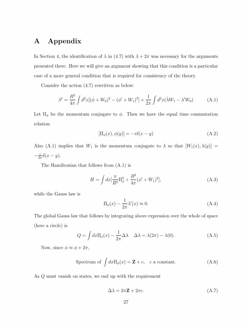
A Appendix

In Section 4, the identification of λ in (4.7) with λ + 2π was necessary for the arguments

presented there. Here we will give an argument showing that this condition is a particular

case of a more general condition that is required for consistency of the theory.

Consider the action (4.7) rewritten as below:

S ′ =R2

4π

∫

d2x[(φ + W0)2 − (φ′ + W1)

2] +1

2π

∫

d2x(λW1 − λ′W0) (A.1)

Let Πφ be the momentum conjugate to φ. Then we have the equal time commutation

relation

[Πφ(x), φ(y)] = −iδ(x − y) (A.2)

Also (A.1) implies that W1 is the momentum conjugate to λ so that [W1(x), λ(y)] =

− i2π

δ(x − y).

The Hamiltonian that follows from (A.1) is

H =∫

dx[π

R2Π2

φ +R2

4π(φ′ + W1)

2], (A.3)

while the Gauss law is

Πφ(x) −1

2πλ′(x) ≈ 0. (A.4)

The global Gauss law that follows by integrating above expression over the whole of space

(here a circle) is

Q =∫

dxΠφ(x) −1

2π∆λ ∆λ = λ(2π) − λ(0). (A.5)

Now, since φ ≈ φ + 2π,

Spectrum of∫

dxΠφ(x) = Z + c, c a constant. (A.6)

As Q must vanish on states, we end up with the requirement

∆λ = 2πZ + 2πc. (A.7)

27

With these conditions, Q generates U(1) on arbitrary states, and Gauss law picks out

singlet.

We thus see that the requirement that λ be identified with λ + 2π is natural provided

c in (A.6) vanishes.

Thus for c = 0, the λ obtained from canonical quantization has an expansion in the

form (4.33) showing that the identification of λ with λ + 2π is natural, in the canonical

approach, for this particular value of c.

Nonzero values of c too can be incorporated in the functional integral as well by

identifying λ with λ+2π(1+c). It then becomes appropriate for a scalar field canonically

quantized with c 6= 0. But we will not enter into this generalization of the functional

integral here.

References

[1] Y.N. Srivastava and A. Widom, Nuovo. Cim. Lett. 39 (1984) 285.

[2] S.C. Zhang, T.H. Hansson and S. Kivelson, Phys. Rev. Lett. 62 (1989) 82; S. Girvin

in R.E. Prange and S.M. Girvin, “The Quantum Hall Effect” [Springer-Verlag, 1990].

[3] A. Zee in Proceedings of the 1991 Kyoto Conference on “Low Dimensional Field

Theories and Condensed Matter Physics”; X.G. Wen and A. Zee, Nucl. Phys. B151

(1990) 135.

[4] J. Frohlich and T. Kerler, Nucl. Phys. B354 (1991) 369; J. Frohlich and A. Zee,

Nucl. Phys. B364 (1991) 517.

[5] E. Fradkin, “Field Theories of Condensed Matter Systems” [Addison-Wesley, 1991].

[6] G. Morandi, “Quantum Hall Effect”, Monographs and Textbooks in Physical Sci-

ence, Lecture Notes Number 10 [Bibliopolis, 1988]; A.H. MacDonald, “Quantum

28

Hall Effect: A Perspective” [Kluwer Academic Publishers, 1989]; R.E. Prange and

S.M. Girvin, “The Quantum Hall Effect” [Springer-Verlag, 1990]; A.P. Balachandran

and A.M. Srivastava, Syracuse University and University of Minnesota preprint, SU-

4288-492, TPI-MINN-91-38-T (1991), hep-th/9111006; M. Stone, “Quantum Hall Ef-

fect” [World Scientific, 1992]; F.Wilczek, IASSNS-HEP 94/58 and cond-mat/9408100

(1994); and references therein.

[7] M.P.H. Fisher and D.H. Lee, Phys. Rev. Lett. 63 (1989) 903.

[8] F.D.M. Haldane, Phys. Rev. Lett. 51 (1983) 605.

[9] J.K. Jain, Phys. Rev. Lett. 63 (1989) 199; Phys. Rev. B40 (1989) 8079.

[10] F. Wilczek, “Fractional Statistics and Anyon Superconductivity” [World Scientific,

1990].

[11] M. Stone, Ann. Phys. 207 (1991) 658.

[12] S.R. Renn, Phys. Rev. Lett. 68 (1992) 658.

[13] J. Frohlich and U.M. Studer, Rev. Mod. Phys. 65 (1993) 733; J. Frohlich and E.

Thiran, (Zurich, ETH) ETH-TH-93-22.

[14] B.I. Halperin, Phys. Rev. B25 (1982) 2185; See also R. Tao and Y.S. Wu, Phys. Rev.

B31 (1985) 6859.

[15] X.G. Wen, Phys. Rev. Lett. 64 (1990) 2206, Int. J. Mod. Phys. B6 (1992) 1711.

[16] S. Iso, D. Karabali and B. Sakita, Nucl. Phys. B338 (1992) 700; Phys. Lett. B296

(1992) 143; D. Karabali, Nucl. Phys. B419 (1994) 437, Nucl. Phys. B428 (1994)

531.

29

[17] A.P. Balachandran, L. Chandar and B. Sathiapalan, Pennsylvania State Univer-

sity and Syracuse University preprint, PSU/TH/144, SU-4240-578 (1994), hep-

th/9405141 and Nucl. Phys. B (in press).

[18] K. Kikkawa and M. Yamasaki, Phys. Lett. B149 (1984) 357; N. Sakai and I. Senda,

Prog. Th. Phys. 75 (1986) 692; V.P. Nair, A. Shapere, A. Strominger and F. Wilczek,

Nucl. Phys. B287 (1987) 402; B. Sathiapalan, Phys. Rev. Lett. 58 (1987) 1597; A.

Shapere and F. Wilczek, Nucl. Phys. B320 (1989) 669; A. Giveon, E. Rabinovici and

G. Veneziano, Nucl. Phys. B322 (1989) 167; A. Giveon and M. Rocek, Nucl. Phys.

B380 (1992) 128; J. Maharana and J.H. Schwarz, Nucl. Phys. B390 (1993) 3.

[19] T. Buscher, Phys. Lett. B194 (1987) 57, B201 (1988) 466.

[20] R.P. Feynman, “Statistical Mechanics”, Frontiers in Physics-Lecture Notes Series

[Benjamin/Cummings, 1972].

[21] H.B. Nielsen and P. Olesen, Nucl. Phys. B61 (1973) 45.

[22] A.P. Balachandran, G. Bimonte, K.S. Gupta and A. Stern, Int. J. Mod. Phys. A7

(1992) 4655 and 5855.

[23] C.G. Callan, Jr. and J.A. Harvey, Nucl. Phys. B250 (1985) 427.

[24] S.G. Naculich, Nucl. Phys. B296 (1988) 837.

[25] L. Chandar, Mod. Phys. Lett. A9 (1994) 3403.

[26] E. Alvarez, L. Alvarez-Gaume, J.L.F. Barbon and Y. Lozano, Nucl. Phys. B415

(1994) 71; E. Alvarez, L. Alvarez-Gaume and Y. Lozano, Nucl. Phys. B424 (1994)

155.

[27] R. Bott and L.W. Tu, “Differential Forms in Algebraic Topology” [Springer-Verlag,

1986].

30

[28] R. Courant and D. Hilbert, “Methods of Mathematical Physics”, Vol. II [Interscience

Publishers, 1966].

[29] A.P. Balachandran, L. Chandar, E. Ercolessi, T.R. Govindarajan and R. Shankar,

Int. J. Mod. Phys. A9 (1994) 3417; A.P. Balachandran, L. Chandar and E. Ercolessi,

Syracuse University Preprint SU-4240-574 (1994) and hep-th/9411164 (to appear in

Int. J. Mod. Phys. A).

31