Craton formation: Internal structure inherited from closing of the early oceans
Upload
khangminh22Category
view
0download
0
Glasgow Theses Service http://theses.gla.ac.uk/
Giuni, Michea (2013) Formation and early development of wingtip vortices. PhD thesis. http://theses.gla.ac.uk/3871/ Copyright and moral rights for this thesis are retained by the author A copy can be downloaded for personal non-commercial research or study, without prior permission or charge This thesis cannot be reproduced or quoted extensively from without first obtaining permission in writing from the Author The content must not be changed in any way or sold commercially in any format or medium without the formal permission of the Author When referring to this work, full bibliographic details including the author, title, awarding institution and date of the thesis must be given.
Department of Aerospace Engineering
School of Engineering
Formation and early developmentof wingtip vortices
Michea Giuni
A thesis submitted in partial fulfillment of the requirements for thedegree of Doctor of Philosophy
c© Michea Giuni, January 2013
Declaration of authorship
I herewith declare that I have produced this paper without the prohibited assistance of
third parties and without making use of aids other than those specified; notions taken
over directly or indirectly from other sources have been identified as such. This work
has not previously been presented in identical or similar form to any other Scottish or
foreign examination board.
The thesis work was conducted from January 2009 to June 2012 under the supervi-
sion of Dr. Emmanuel Benard and of Dr. Richard B. Green at the University of Glasgow,
United Kingdom.
5th October 2012, Glasgow
ii

Formation and early development of wingtip vortices
Abstract: wingtip vortices are extremely important phenomena in fluid dynamics for
their negative effects in many applications. Despite the many studies on this particular
flow, the current understanding is still poor in providing a firm base for the design
of effective tip geometry modifications and vortex control devices. A rectangular wing
with squared and rounded wingtips was tested in order to identify the main mechanisms
involved in the formation of the vortex on the wing and in its early development in the
wake. The complementarity of a number of experimental techniques adopted, such
as surface flow visualizations, wall pressure measurements, smoke visualizations and
stereoscopic particle image velocimetry (SPIV), gave a richer insight of the physics
and the basic mechanisms of the vortex development. Furthermore, a large number
of configurations were tested exploring the effects of several parameters such as wing
chord, aspect ratio, wingtip geometry, angle of attack and Reynolds number.
The development of the vortex along the wing showed the formation of several
secondary vortices which interacted with the primary vortex generating low frequency
fluctuations. The structure of the flow at this stage was analysed introducing a compact
description through characteristic lines of the vortex system defined from the velocity
vector field in the vicinity of the wing surface. The high spatial resolution achieved
by the SPIV arrangement allowed a deeper understanding of the vortex structure in
the early wake and the turbulence production and dissipation within the vortex core.
The relaminarization process of the vortex core promoted by centrifugal motion was
observed. The relation between vortex meandering, turbulence, secondary vortices and
wake sheet was discussed. A comparison of different methods for the averaging of
instantaneous planar vector fields was performed showing the effects and importance
of the meandering. An axial acceleration of the flow within the vortex was observed
and the formation of different axial flow distributions was discussed. A minimum wake–
like flow of 0.62 and a maximum jet–like flow of 1.7 times the freestream velocity were
measured and a linear relation between a vortex circulation parameter and the axial
velocity peak was found.
Keywords: wingtip vortex, wake, SPIV, relaminarization.
iii

to Rugiadaand her inspiring faith
to Darioand his exemplary strength
iv

Acknowledgments
This dissertation is actually not the fruit of just my efforts and time but it is more a
fruit of the guidance, support, patience and encouragement of other people, to whom
I am thankful.
I sincerely thank Dr. Emmanuel Benard for providing me with this opportunity to
enjoy a research in Fluid Dynamics, for believing in my abilities and for his guidance in
the experimental analysis. I also would like to thank with the same sincerity Dr. Richard
B. Green for his invaluable assistance and guidance in shaping this work and helping
me in bringing it to a closure.
I will certainly thank also all the technical support staff involved in this research,
particularly Mr. Tony Smedley, Mr. Robert Gilmour, Mr. John Kitching and Mr. Ian
Scouller.
Special thanks to my girlfriend who accepted to become my wife during this journey
and to move to Glasgow for me, to my parents and my brothers. Thanks also to my
friends and “brothers”, old and far, new and near, who encouraged me and made me
laugh and grow during these years so that I could enjoy them.
v

List of publications
The contents of this dissertation have been partially published, on in the process of
being published, in highly rated journal papers and presented in related conferences.
Journal publications
• Giuni, M., Green, R. B. & Benard, E. 2012 Unsteady flow in wingtip vortex
formation. Under preparation for submission, Journal of Fluid Mechanics.
• Giuni, M. & Green, R. B. 2012 Vortex formation on squared and rounded tip.
Under review, Aerospace Science and Technology.
Conference publications
• Giuni, M. & Benard, E. 2011 Analytical/Experimental comparison of the axial
velocity in trailing vortices. 49th AIAA Aerospace Science Meeting, 4-7 January.
Orlando, Florida.
• Giuni, M., Benard, E. & Green, R. B. 2011 Investigation of a trailing vor-
tex near field by stereoscopic particle image velocimetry. 49th AIAA Aerospace
Science Meeting, 4-7 January. Orlando, Florida.
• Giuni, M., Benard, E. & Green, R. B. 2010 Near field structure of wing tip
vortices. Experimental Fluid Mechanics Conference, 24-26 November. Liberec,
Czech Republic.
vi

list of publications vii
Presentations
• Giuni, M., Benard, E. & Green, R. B. 2010 SPIV Experiments on wing
trailing vortices. University of Glasgow: Engineering Graduate School Conference,
17-18 August. Glasgow, UK.
• Giuni, M., Benard, E. & Green, R. B. 2010 Wing trailing vortex axial ve-
locity. University of Dundee: 23rd Scottish Fluid Mechanics Meeting, 19 May.
Dundee, UK.

Table of contents
Declaration of authorship ii
Abstract iii
Acknowledgments v
List of publications vi
List of figures xiii
List of tables xx
Nomenclature xxi
viii

table of contents ix
1 Introduction 1
1 Why are wingtip vortices so important? . . . . . . . . . . . . . . . . . . 2
2 Theoretical background: why do wingtip vortices form? . . . . . . . . . 8
3 Literature review: what is the current understanding of wingtip vortices? 13
(a) Far and mid field . . . . . . . . . . . . . . . . . . . . . . . . . . . 15
(b) Formation and near field . . . . . . . . . . . . . . . . . . . . . . . 19
4 What are the scope and contributions of this work to the unresolved issues? 24
5 Structure of the thesis . . . . . . . . . . . . . . . . . . . . . . . . . . . . 26
2 Experimental apparatus and procedure 27
1 Wind tunnels . . . . . . . . . . . . . . . . . . . . . . . . . . . . . . . . . 28
(a) Argyll wind tunnel . . . . . . . . . . . . . . . . . . . . . . . . . . 28
(b) Smoke visualization wind tunnel . . . . . . . . . . . . . . . . . . 29
2 Wing models . . . . . . . . . . . . . . . . . . . . . . . . . . . . . . . . . 30
(a) M1: high aspect ratio wing . . . . . . . . . . . . . . . . . . . . . 31
(b) M2: low aspect ratio wing . . . . . . . . . . . . . . . . . . . . . 31
3 Experimental techniques . . . . . . . . . . . . . . . . . . . . . . . . . . . 33
(a) Surface oil flow visualizations . . . . . . . . . . . . . . . . . . . . 33
(b) Pressure measurements . . . . . . . . . . . . . . . . . . . . . . . 34
(c) Smoke visualizations . . . . . . . . . . . . . . . . . . . . . . . . . 39
(d) Hot film anemometry . . . . . . . . . . . . . . . . . . . . . . . . 40
(e) Stereoscopic particle image velocimetry . . . . . . . . . . . . . . 41
4 Reference systems . . . . . . . . . . . . . . . . . . . . . . . . . . . . . . 50
(a) Wake reference system . . . . . . . . . . . . . . . . . . . . . . . . 50
(b) Vortex reference system . . . . . . . . . . . . . . . . . . . . . . . 52
(c) Wing chord reference system . . . . . . . . . . . . . . . . . . . . 52
(d) Wing surface reference system . . . . . . . . . . . . . . . . . . . 53

table of contents x
3 Wingtip vortex formation 54
1 Surface oil flow visualization . . . . . . . . . . . . . . . . . . . . . . . . . 56
2 Pressure on the wing surface . . . . . . . . . . . . . . . . . . . . . . . . 59
(a) Average pressure distribution . . . . . . . . . . . . . . . . . . . . 60
(b) Pressure fluctuation at the wingtip . . . . . . . . . . . . . . . . . 64
3 Smoke visualization on the rolling up . . . . . . . . . . . . . . . . . . . . 67
(a) Rolling up on squared and rounded wingtip . . . . . . . . . . . . 67
(b) Angle of attack and Reynolds number effects . . . . . . . . . . . 71
4 Vortex characteristic lines via SPIV . . . . . . . . . . . . . . . . . . . . 75
(a) Characteristic lines definition . . . . . . . . . . . . . . . . . . . . 76
(b) Effects of the distance of the laser plane from the surface . . . . 82
(c) Reynolds number and tip geometry effects . . . . . . . . . . . . . 84
(d) Angle of attack effects . . . . . . . . . . . . . . . . . . . . . . . . 85
5 Unsteadiness of the vortex formation via hot film . . . . . . . . . . . . . 86
(a) Unsteadiness and intermittency . . . . . . . . . . . . . . . . . . . 88
(b) Signal spectra on squared tip . . . . . . . . . . . . . . . . . . . . 89
(c) Signal spectra on rounded tip . . . . . . . . . . . . . . . . . . . . 91
6 Unsteadiness of the vortex in the early wake . . . . . . . . . . . . . . . . 92
(a) Reynolds number effects . . . . . . . . . . . . . . . . . . . . . . . 94
(b) Angle of attack effects . . . . . . . . . . . . . . . . . . . . . . . . 95
(c) Downstream distance effects . . . . . . . . . . . . . . . . . . . . . 96
7 Summary . . . . . . . . . . . . . . . . . . . . . . . . . . . . . . . . . . . 97

table of contents xi
4 Wingtip vortex early wake 100
1 Localization of the vortex centre and averaging of velocity vector fields . 102
(a) Swirl velocity distribution . . . . . . . . . . . . . . . . . . . . . . 111
(b) Axial velocity distribution . . . . . . . . . . . . . . . . . . . . . . 113
(c) Turbulent quantities . . . . . . . . . . . . . . . . . . . . . . . . . 115
(d) Convergence of averages . . . . . . . . . . . . . . . . . . . . . . . 121
2 Shape of the vortex core . . . . . . . . . . . . . . . . . . . . . . . . . . . 127
(a) Vortex core shape definition . . . . . . . . . . . . . . . . . . . . . 127
(b) Vortex core shape fluctuation . . . . . . . . . . . . . . . . . . . . 130
(c) Rotation of the core . . . . . . . . . . . . . . . . . . . . . . . . . 131
(d) Vortex core shape for different tip geometries . . . . . . . . . . . 135
3 Axial flow . . . . . . . . . . . . . . . . . . . . . . . . . . . . . . . . . . . 136
(a) Shape of the axial flow . . . . . . . . . . . . . . . . . . . . . . . . 139
(b) Axial velocity at the centre of the vortex . . . . . . . . . . . . . 144
4 Turbulence in the vortex core . . . . . . . . . . . . . . . . . . . . . . . . 149
(a) Turbulent kinetic energy evolution . . . . . . . . . . . . . . . . . 150
(b) Reynolds shear stress and shear strain . . . . . . . . . . . . . . . 153
(c) Turbulence production . . . . . . . . . . . . . . . . . . . . . . . . 157
5 Early wake behind squared and rounded wingtips . . . . . . . . . . . . . 162
(a) Development of averaged properties . . . . . . . . . . . . . . . . 162
(b) Meandering and instantaneous behaviour of the vortex structure 167
(c) Turbulence and shear strain evolution . . . . . . . . . . . . . . . 169
(d) Vortex pair formation without generation of lift . . . . . . . . . . 173
6 Summary . . . . . . . . . . . . . . . . . . . . . . . . . . . . . . . . . . . 174
5 Measurement accuracy and error 177
1 Pressure, frequency and meandering . . . . . . . . . . . . . . . . . . . . 177
2 SPIV . . . . . . . . . . . . . . . . . . . . . . . . . . . . . . . . . . . . . . 178
6 Conclusions and recommendations for future work 181
1 Conclusions . . . . . . . . . . . . . . . . . . . . . . . . . . . . . . . . . . 181
2 Recommendations for future work . . . . . . . . . . . . . . . . . . . . . 184

table of contents xii
Bibliography 186
Appendices 201
A PIV: laser pulse separation and image processing 202
1 Laser pulse separation tests . . . . . . . . . . . . . . . . . . . . . . . . . 202
(a) Calculation of the pulse separation . . . . . . . . . . . . . . . . . 203
(b) Pulse separation comparison . . . . . . . . . . . . . . . . . . . . 204
2 Image processing procedure tests . . . . . . . . . . . . . . . . . . . . . . 207
(a) Interrogation window size . . . . . . . . . . . . . . . . . . . . . . 210
(b) Number of iterations . . . . . . . . . . . . . . . . . . . . . . . . . 211
(c) Interrogation window overlap . . . . . . . . . . . . . . . . . . . . 213
(d) Processing time and memory . . . . . . . . . . . . . . . . . . . . 214
(e) Conclusive remarks . . . . . . . . . . . . . . . . . . . . . . . . . . 216
B Vortex centre identification on grayscale pictures 218
1 GRAY and BW methods . . . . . . . . . . . . . . . . . . . . . . . . . . 218
(a) BW method . . . . . . . . . . . . . . . . . . . . . . . . . . . . . . 219
(b) GRAY method . . . . . . . . . . . . . . . . . . . . . . . . . . . . 219
2 Position distribution and movement frequency . . . . . . . . . . . . . . . 220
C Some equations relevant to vortices 226
1 Governing equations . . . . . . . . . . . . . . . . . . . . . . . . . . . . . 226
2 Vorticity form of the Navier–Stokes equation (or vorticity equation) . . 229
3 Reynolds–averaged Navier–Stokes equations . . . . . . . . . . . . . . . . 230
4 Conversion between cartesian and cylindrical coordinate systems . . . . 232

List of figures
1.1 Examples of wingtip vortices 1. . . . . . . . . . . . . . . . . . . . . . . . 3
1.2 Examples of wingtip vortices 2. . . . . . . . . . . . . . . . . . . . . . . . 6
1.3 Examples of wingtip vortices 3. . . . . . . . . . . . . . . . . . . . . . . . 7
1.4 Vortex systems replacing the lifting wing and its wake (Houghton & Car-
penter, 2003). . . . . . . . . . . . . . . . . . . . . . . . . . . . . . . . . . 10
1.5 Early stage of the roll up of the wake sheet. The vortex sheet element
positions are plotted on the left and an interpolating curve is plotted on
the right (Krasny, 1987). . . . . . . . . . . . . . . . . . . . . . . . . . . . 11
1.6 Pressure field interpretation of the wingtip vortex formation. . . . . . . 12
1.7 Shear layer interpretation of wingtip vortex formation. . . . . . . . . . . 13
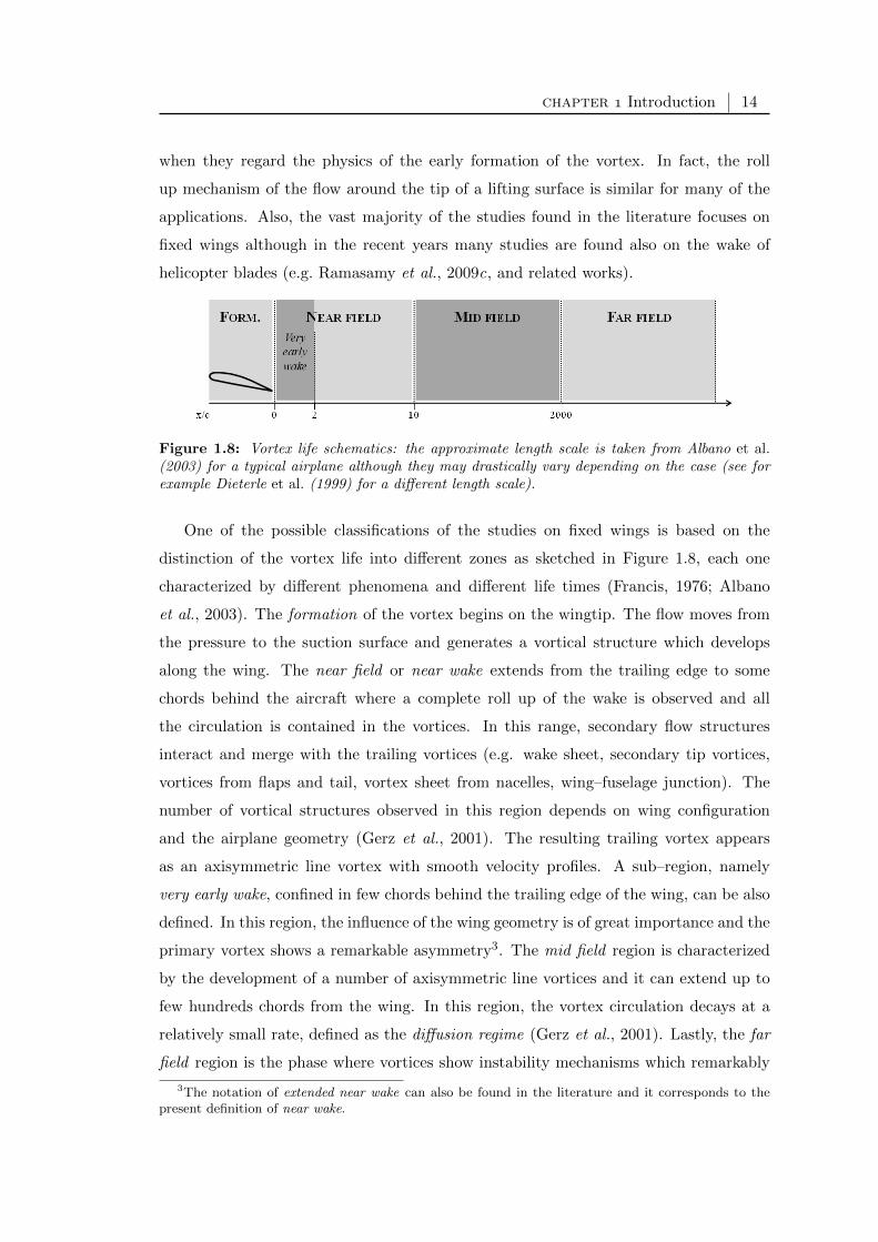
1.8 Vortex life schematics: the approximate length scale is taken from Albano
et al. (2003) for a typical airplane although they may drastically vary
depending on the case (see for example Dieterle et al. (1999) for a different
length scale). . . . . . . . . . . . . . . . . . . . . . . . . . . . . . . . . . 14
2.1 Argyll wind tunnel: top view. . . . . . . . . . . . . . . . . . . . . . . . . 29
2.2 Experimental arrangement of smoke visualizations on the vortex forma-
tion: wing M2 mounted in the flow visualization wind tunnel. . . . . . . 30
2.3 M1 wing mounted in the Argyll wind tunnel (without fixing cables). . . 31
2.4 M2 wing mounted in the Argyll wind tunnel and SPIV calibration plate. 32
2.5 Pressure tappings map and names. . . . . . . . . . . . . . . . . . . . . . 34
2.6 Pressure measurements arrangement. . . . . . . . . . . . . . . . . . . . . 38
2.7 Typical response of a pressure measurement system at an equivalent al-
titude of 2300 ft as function of the tube length and internal diameter
(Whitmore et al., 1990). . . . . . . . . . . . . . . . . . . . . . . . . . . . 39
2.8 Camera mounting and laser delivery for SPIV experiments. . . . . . . . 45
2.9 Vector field computation flow chart of a two pulses two frames SPIV. . . 49
2.10 Reference systems. . . . . . . . . . . . . . . . . . . . . . . . . . . . . . . 51
xiii

list of figures xiv
3.1 Surface flow visualizations: suction surface. . . . . . . . . . . . . . . . . 57
3.2 Surface flow visualizations: tip surface (freestream from left to right). . 58
3.3 Pressure coefficient distribution and pressure tappings at Re = 5 · 105
and α = 12: suction and pressure surface. . . . . . . . . . . . . . . . . . 61
3.4 Pressure coefficient distribution and pressure tappings at Re = 5 · 105
and α = 12: tip surface. The circles correspond to the pressure tapping
positions. . . . . . . . . . . . . . . . . . . . . . . . . . . . . . . . . . . . 62
3.5 Pressure coefficient distribution on the suction surface at Re = 5 · 105. . 63
3.6 Pressure coefficient distribution along tappings row T1 at Re = 5 · 105. . 63
3.7 McAlister & Takahashi (1991) experiments: pressure coefficient distribu-
tion at Re = 1 · 106 and α = 12. . . . . . . . . . . . . . . . . . . . . . . 64
3.8 Pressure coefficient distribution at Re = 5 · 105 and α = 12. . . . . . . 65
3.9 Pressure standard deviation. . . . . . . . . . . . . . . . . . . . . . . . . . 65
3.10 Pressure signal for α = 12. . . . . . . . . . . . . . . . . . . . . . . . . . 66
3.11 Vortex at Re = 3000, xc = 0.75 and α = 12 on rounded tip; wing section
in gray. . . . . . . . . . . . . . . . . . . . . . . . . . . . . . . . . . . . . 68
3.12 Vortex evolution at Re = 3000 and α = 12 on rounded tip; wing section
in gray. . . . . . . . . . . . . . . . . . . . . . . . . . . . . . . . . . . . . 69
3.13 Vortex evolution at Re = 3000 and α = 12 on squared tip; wing section
in gray. . . . . . . . . . . . . . . . . . . . . . . . . . . . . . . . . . . . . 70
3.14 Snapshots at f = 30 Hz, Re = 3000, α = 12 and xc = 0.7 on squared tip. 72
3.15 Vortex evolution at Re = 3000 and α = 12 on rounded tip; wing section
in gray. . . . . . . . . . . . . . . . . . . . . . . . . . . . . . . . . . . . . 73
3.16 Experimental arrangement and field of view of the SPIV cameras. . . . 75
3.17 SPIV laser sheet positions. . . . . . . . . . . . . . . . . . . . . . . . . . . 76
3.18 Mean flow plane streamlines for squared tip at α = 12, Re = 105 and
d = 3 mm. . . . . . . . . . . . . . . . . . . . . . . . . . . . . . . . . . . . 77
3.19 Characteristic lines legend for squared tip at α = 12, Re = 105 and
d = 3 mm. . . . . . . . . . . . . . . . . . . . . . . . . . . . . . . . . . . . 78
3.20 Mean flow and characteristic lines for squared tip at α = 12, Re = 105
and d = 3 mm (characteristic lines legend from the most inboard to the
nearest to the wingtip: L1 continuous line, L2 dashed–dotted line, L3
dashed line, L4 dotted line). . . . . . . . . . . . . . . . . . . . . . . . . 79
list of figures xv
3.21 Mean flow and characteristic lines for squared tip at α = 12, Re = 105
and d = 3 mm (characteristic lines legend from the most inboard to the
nearest to the wingtip: L1 continuous line, L2 dashed–dotted line, L3
dashed line, L4 dotted line). . . . . . . . . . . . . . . . . . . . . . . . . 80
3.22 Smoke visualizations at xc = 0.7, α = 12 and Re = 3000. . . . . . . . . 81
3.23 Vortex formation diagram on a rectangular wing with rounded tip. . . . 82
3.24 Schematics of the primary vortex streamlines and the evaluated reattach-
ment points positions for measurement planes at different distances from
the surface. . . . . . . . . . . . . . . . . . . . . . . . . . . . . . . . . . . 83
3.25 Characteristic lines for squared tip at α = 12. . . . . . . . . . . . . . . 83
3.26 Characteristic lines at d = 5 mm and α = 12. . . . . . . . . . . . . . . . 84
3.27 Velocity components contours for a rounded tip at Re = 106. . . . . . . 85
3.28 In–plane vorticity contours for a rounded tip at Re = 106. . . . . . . . . 86
3.29 Characteristic lines and hot film positions. . . . . . . . . . . . . . . . . . 87
3.30 Hot film signals standard deviations. . . . . . . . . . . . . . . . . . . . . 89
3.31 Square tip power spectra: Re = 105, α = 12, xs = −0.20. . . . . . . . . 90
3.32 Square tip power spectra: Re = 106, α = 12, xs = −0.20. . . . . . . . . 91
3.33 Rounded tip power spectra: Re = 106, α = 12, xs = −0.20. . . . . . . . 92
3.34 Rounded tip power spectra: Re = 106, α = 4, xs = −0.20. . . . . . . . 93
3.35 Signal spectra at xw = 1 and α = 12. . . . . . . . . . . . . . . . . . . . 94
3.36 Signal spectra at xw = 1 and Re = 10 · 105. . . . . . . . . . . . . . . . . 96
3.37 Signal spectra at α = 15 and Re = 5 · 105. . . . . . . . . . . . . . . . . 97
4.1 Instantaneous velocity vectors and vorticity at xw = 1, Re = 5 · 105 and
α = 12; projection of the trailing edge in dashed line. . . . . . . . . . . 103
4.2 Instantaneous seeding distribution at xw = 1, Re = 5 · 105 and α = 12. 104
4.3 Centering methods for an instantaneous realization at xw = 1, Re = 5·105
and α = 12. . . . . . . . . . . . . . . . . . . . . . . . . . . . . . . . . . 108
4.4 Instantaneous vortex centre positions calculated with different centering
methods at xw = 1, Re = 5 · 105 and α = 12. . . . . . . . . . . . . . . . 110
4.5 Simple averaged flow field at xw = 1, Re = 5 · 105 and α = 12; in–plane
velocity minimum (black cross), axial velocity maximum (white cross). . 112
4.6 Average swirl velocity profiles and mean values (red line) calculated with
different centering methods at xw = 1, Re = 5 · 105 and α = 12. . . . . 113

list of figures xvi
4.7 Average axial velocity profiles and mean values (red line) calculated with
different centering methods at xw = 1, Re = 5 · 105 and α = 12. . . . . 114
4.8 Velocity fluctuations at xw = 1, Re = 5 · 105 and α = 12; part 1 of 2. . 117
4.9 Velocity fluctuations at xw = 1, Re = 5 · 105 and α = 12; part 2 of 2. . 118
4.10 Instantaneous axial velocity peaks at xw = 1, Re = 5 · 105 and α = 12. 118
4.11 Turbulence at xw = 1, Re = 5 · 105 and α = 12; part 1 of 2. . . . . . . . 119
4.12 Turbulence at xw = 1, Re = 5 · 105 and α = 12; part 2 of 2. . . . . . . . 120
4.13 Swirl velocity at xw = 1, Re = 5 · 105 and α = 12. . . . . . . . . . . . . 122
4.14 Axial velocity at xw = 1, Re = 5 · 105 and α = 12. . . . . . . . . . . . . 122
4.15 Convergence and errors of velocity and core radius at xw = 1, Re = 5·105
and α = 12. . . . . . . . . . . . . . . . . . . . . . . . . . . . . . . . . . 123
4.16 Vorticity at xw = 1, Re = 5 · 105 and α = 12. . . . . . . . . . . . . . . . 123
4.17 Convergence and errors of vorticity, helicity and swirling strength at xw =
1, Re = 5 · 105 and α = 12. . . . . . . . . . . . . . . . . . . . . . . . . . 124
4.18 In–plane velocity fluctuation σv at xw = 1, Re = 5 · 105 and α = 12. . . 124
4.19 Reynolds shear stress v′w′ at xw = 1, Re = 5 · 105 and α = 12. . . . . . 125
4.20 Shear strain εyz at xw = 1, Re = 5 · 105 and α = 12. . . . . . . . . . . . 125
4.21 Convergence and errors of velocity fluctuation, Reynolds stress and shear
strain at xw = 1, Re = 5 · 105 and α = 12. . . . . . . . . . . . . . . . . 126
4.22 Swirl velocity and slicing cuts at α = 8, xw = 1 and Re = 5 · 105. . . . 128
4.23 Vortex core shape at Re = 1 · 105 and α = 12. . . . . . . . . . . . . . . 129
4.24 Vortex core shape at Re = 5 · 105 and α = 8. . . . . . . . . . . . . . . . 129
4.25 Vortex core shape at α = 12 and xw = 1. . . . . . . . . . . . . . . . . . 130
4.26 Core shape fluctuation. . . . . . . . . . . . . . . . . . . . . . . . . . . . 131
4.27 Vortex core shape for different averaging methods at α = 8, xw = 0.5
and Re = 5 · 105,. . . . . . . . . . . . . . . . . . . . . . . . . . . . . . . . 132
4.28 Axial velocity profiles. . . . . . . . . . . . . . . . . . . . . . . . . . . . . 133
4.29 Core rotation estimation as function of the angle of attack at Re = 1 · 105.134
4.30 Vortex core shape for different tip geometries at xw = 0.25 and α = 12. 135
4.31 Estimation of the vortex core structure at the trailing edge. . . . . . . . 136
4.32 Axial velocity contours and planar streamlines at xw = 1 and Re = 1 ·105
(M1 model). . . . . . . . . . . . . . . . . . . . . . . . . . . . . . . . . . 140
4.33 Schematic of generic profiles of the axial velocity across the vortex in the
early wake for different angles of attack. . . . . . . . . . . . . . . . . . . 141
list of figures xvii
4.34 Average axial velocity contours and planar streamlines at xw = 1 and
Re = 1 · 105 (M1 model). . . . . . . . . . . . . . . . . . . . . . . . . . . 142
4.35 Axial velocity, vorticity and planar streamlines at α = 15 andRe = 5·105
(M1 model). . . . . . . . . . . . . . . . . . . . . . . . . . . . . . . . . . 143
4.36 Axial velocity at the centre of the vortex as function of the circulation
parameter. . . . . . . . . . . . . . . . . . . . . . . . . . . . . . . . . . . . 146
4.37 Trendlines of the present work compared with other experimental data. 148
4.38 Velocity fluctuations in cartesian and cylindrical coordinates and turbu-
lent kinetic energy in the wake of the M1 wing at α = 12, xw = 1 and
Re = 5 · 105. . . . . . . . . . . . . . . . . . . . . . . . . . . . . . . . . . . 150
4.39 Evolution in the wake of the velocity fluctuations and turbulent kinetic
energy for α = 12 and Re = 5 · 105. . . . . . . . . . . . . . . . . . . . . 152
4.40 Turbulent kinetic energy at the centre of the vortex. . . . . . . . . . . . 153
4.41 Evolution of the shear stress v′w′ in cartesian coordinate for different
angles of attack at Re = 5 · 105. . . . . . . . . . . . . . . . . . . . . . . . 154
4.42 Evolution of the shear strain εyz in cartesian coordinate for different
angles of attack at Re = 5 · 105. . . . . . . . . . . . . . . . . . . . . . . . 155
4.43 Reynolds stresses in cartesian and cylindrical coordinates at xw = 1,
α = 12, Re = 1 · 105. . . . . . . . . . . . . . . . . . . . . . . . . . . . . 156
4.44 Evolution of the axial velocity in the wake for different angles of attack
and Re = 5 · 105. . . . . . . . . . . . . . . . . . . . . . . . . . . . . . . . 158
4.45 Radial gradient of the axial velocity at Re = 5 · 105. . . . . . . . . . . . 159
4.46 Evolution of the shear stress u′xu′r in cylindrical coordinate for different
angles of attack at Re = 5 · 105. . . . . . . . . . . . . . . . . . . . . . . . 160
4.47 Evolution of the average of the absolute value of the minimum and max-
imum peak of shear stresses in cylindrical coordinate for different angles
of attack at Re = 5 · 105. . . . . . . . . . . . . . . . . . . . . . . . . . . . 160
4.48 Evolution of the normal stress u′r2 in cylindrical coordinate for different
angles of attack at Re = 5 · 105. . . . . . . . . . . . . . . . . . . . . . . . 161
4.49 Evolution of the stresses in cylindrical coordinate for different angles of
attack at Re = 5 · 105. . . . . . . . . . . . . . . . . . . . . . . . . . . . . 161
4.50 Axial velocity at Re = 12.7 · 105 and α = 12. . . . . . . . . . . . . . . . 163
4.51 Vorticity at Re = 12.7 · 105 and α = 12. . . . . . . . . . . . . . . . . . . 164
4.52 Vorticity profiles and mean value (red line) at xw = 0.25, Re = 12.7 · 105
and α = 12. . . . . . . . . . . . . . . . . . . . . . . . . . . . . . . . . . 165

list of figures xviii
4.53 Swirl velocity profiles and mean value (continuous red line) at xw = 0.25,
Re = 12.7 · 105 and α = 12. Location of local maximum and minimum
in dashed vertical red lines; velocity profile of the Lamb–Oseen vortex in
blue. . . . . . . . . . . . . . . . . . . . . . . . . . . . . . . . . . . . . . . 166
4.54 Circulation profiles and location of local maximum and minimum of swirl
velocity (vertical red lines) at xw = 0.25, Re = 12.7 · 105 and α = 12. . 167
4.55 Instantaneous vorticity at xw = 0.25, Re = 12.7 · 105 and α = 12 for
squared wingtip. . . . . . . . . . . . . . . . . . . . . . . . . . . . . . . . 168
4.56 Vortex meandering for squared and rounded tips as function of the angle
of attack at Re = 7.4 · 105. . . . . . . . . . . . . . . . . . . . . . . . . . . 168
4.57 Evolution of the shear strain εyz for squared and rounded tip at α = 12
and Re = 12.7 · 105. . . . . . . . . . . . . . . . . . . . . . . . . . . . . . 170
4.58 Evolution of the Reynolds shear stress v′w′ for squared and rounded tip
at α = 12 and Re = 12.7 · 105. . . . . . . . . . . . . . . . . . . . . . . . 171
4.59 Turbulent kinetic energy at the centre of the vortex generated by rounded
and squared tips. . . . . . . . . . . . . . . . . . . . . . . . . . . . . . . . 171
4.60 Axial velocity at α = 0, xw = 0.25 and Re = 7.4 · 105. . . . . . . . . . . 173
4.61 Vorticity at α = 0, xw = 0.25 and Re = 7.4 · 105. . . . . . . . . . . . . . 174
A.1 Swirl velocity profiles for different laser pulse separations. . . . . . . . . 205
A.2 Axial velocity profiles for different laser pulse separations. . . . . . . . . 205
A.3 Vorticity contours for different laser pulse separations. . . . . . . . . . . 206
A.4 Velocity fluctuations for different laser pulse separations. . . . . . . . . . 206
A.5 Cross–correlation procedure scheme (DaVis, 2007). . . . . . . . . . . . . 208
A.6 Example of 50% interrogation window overlap (DaVis, 2007). . . . . . . 208
A.7 Swirl velocity profiles for different interrogation window sizes. . . . . . . 211
A.8 Axial velocity profiles for different interrogation window sizes. . . . . . . 212
A.9 Swirl velocity profiles for different numbers of iterations. . . . . . . . . . 213
A.10 Axial velocity profiles for different numbers of iterations. . . . . . . . . . 214
A.11 Swirl velocity profiles for different interrogation window overlaps. . . . . 215
A.12 Axial velocity profiles for different interrogation window overlaps. . . . . 216
B.1 Common steps. . . . . . . . . . . . . . . . . . . . . . . . . . . . . . . . . 220
B.2 BW steps. . . . . . . . . . . . . . . . . . . . . . . . . . . . . . . . . . . . 221
B.3 GRAY steps. . . . . . . . . . . . . . . . . . . . . . . . . . . . . . . . . . 222
B.4 Histogram of the light intensity for steps 1, 2 and 3. . . . . . . . . . . . 222

list of figures xix
B.5 BW method: instantaneous vortex positions (rounded tip, xw = 1, α =
12, Re = 106). . . . . . . . . . . . . . . . . . . . . . . . . . . . . . . . . 223
B.6 GRAY method: instantaneous vortex positions (rounded tip, xw = 1,
α = 12, Re = 106). . . . . . . . . . . . . . . . . . . . . . . . . . . . . . 223
B.7 BW method: vortex movement power spectra (rounded tip, xw = 1,
α = 12, Re = 106). . . . . . . . . . . . . . . . . . . . . . . . . . . . . . 224
B.8 GRAY method: vortex movement power spectra (rounded tip, xw = 1,
α = 12, Re = 106). . . . . . . . . . . . . . . . . . . . . . . . . . . . . . 225
List of tables
2.1 Summary of wing models characteristics and experiments. . . . . . . . . 32
2.2 Pressure tappings coordinates. . . . . . . . . . . . . . . . . . . . . . . . 37
2.3 Summary of SPIV experiments (79 independent tests). . . . . . . . . . . 44
4.1 Core rotation estimate: Re = 1 · 105, α = 12. . . . . . . . . . . . . . . . 133
4.2 Core rotation estimate: Re = 5 · 105, α = 8. . . . . . . . . . . . . . . . 133
4.3 Wing models characteristics and experiments of references in Figure 4.37. 148
4.4 Important production terms of the Reynolds stresses. . . . . . . . . . . . 158
4.5 Enstrophy dispersion radius in the wake of squared and rounded wingtips;
Re = 12.7 · 105 and α = 12. . . . . . . . . . . . . . . . . . . . . . . . . . 164
A.1 Summarizing table of the processing procedures tested. . . . . . . . . . . 210
A.2 Processing procedures: time and memory required. . . . . . . . . . . . . 217
xx

Nomenclature
List of symbols
Latin symbols
A anemometer constant, [V]
AR aspect ratio of the wing, =b
cb span of the wing, [m]
c chord of the wing, [m]
cP pressure coefficient, =P − P∞1
2ρU∞
2
d distance of the SPIV plane from the wing surface, [mm]
D diameter of the tube for the pressure measurement, [mm]
E anemometer output voltage, [V]
f frequency, [Hz]
f dimensionless frequency, =f c
U∞FS sampling frequency, [Hz]
Hx streamwise helicity
k turbulent kinetic energy
L1, L2, L3, L4 vortex characteristic lines
M1 high aspect ratio wing model
M2 low aspect ratio wing model
N number of measurements
Npx interrogation window size, [number of pixels]
P pressure, [Pa]
P averaged pressure, [Pa]
P∞ freestream stagnation pressure, [Pa]
xxi

nomenclature xxii
|P (f)| signal power spectral density
|Pyy(f)| power spectral density of the displacements along the y
axis
|Pzy(f)| cross spectral density of the displacements along the z and
y axes
|Pzz(f)| power spectral density of the displacements along the z
axis
Q discriminant of the characteristic equation of the velocity gradient
rEN enstrophy dispersion radius, [m]
R vortex core radius
R(θ) directional vortex core radius
S generic surface, [m2]
r, θ, x cylindrical coordinates
Re Reynolds number, =U∞ c
νu, v, w velocity in cartesian coordinates
ur, uθ, ux velocity in cylindrical coordinates
ucore core axial velocity
u velocity vector, [m/s]
u velocity vector mean, = u− u′, [m/s]
u′ velocity vector fluctuation, = u− u, [m/s]
U∞ freestream velocity, [m/s]
u′2, v′2, w′2 turbulent normal stresses in cartesian coordinates
u′2, ur ′2, uθ ′2 turbulent normal stresses in cylindrical coordinates
v′w′, u′v′, u′w′ Reynolds stresses in cartesian coordinates
u′ru′θ, u
′xu′r, u
′xu′θ Reynolds stresses in cylindrical coordinates
x, y, z dimensional cartesian coordinates
x, y, z dimensionless cartesian coordinates
x generic coordinate vector
Greek symbols
α angle of attack, [deg]
Γ vortex circulation, [m2/s]
Γ(r) vortex circulation distribution, [m2/s]

nomenclature xxiii
∆H dissipation function, [m2/s2]
∆x marker displacement, [m]
∆xw scaled distance along the streamwise direction
∆t time interval, [s]
εxx normal strain
εyy, εzz elongational strains
εyz, εzy shear strains
Θ rotation of the vortex core, [deg]
λ2 eigenvalue of the tensor Σ2 + Ω2
ν freestream kinematic viscosity, [m2/s]
ρ freestream density, [kg/m3]
σm scaled standard deviation of the vortex meandering
σr, σθ scaled root mean square of the in–plane components of the
velocity fluctuation in cylindrical coordinates
σR scaled fluctuation of the vortex core shape
σu scaled root mean square of the axial velocity fluctuation
σv, σw scaled root mean square of the in–plane components of the
velocity fluctuation in cartesian coordinates
Σ strain tensor
τw wall shear stress, [Pa]
φ rotation rate of the vortex, [rps]
ωx scaled streamwise vorticity
ω vorticity vector
Ω vorticity tensor
Subscripts
()c wing chord reference system
()i relative to measurement i
()s wing surface reference system
()v vortex reference system
()w wake reference system
()0 relative to the vortex centre

nomenclature xxiv
List of acronyms
BVI Blade Vortex Interaction
CCD Charge Coupled Device
CSD Cross Spectral Density
DNS Direct Numerical Simulation
FFT Fast Fourier Transform
LDV Laser Doppler Velocimetry
LES Large Eddy Simulation
PDV Particle Displacement Velocimetry
PIV Particle Image Velocimetry
PLV Pulsed Light Velocimetry
POD Proper Orthogonal Decomposition
PSD Power Spectral Density
RANS Reynolds–Averaged Navier–Stokes equations
RMS Root Mean Square
RSM Reynolds Stress Model
SPIV Stereoscopic Particle Image Velocimetry
2D2C Two–Dimensional Two–Components
2D3C Two–Dimensional Three–Components

chapter
Introduction
Can a mortal ask questions which God finds unanswer-
able? Quite easily, I should think. All nonsense questions
are unanswerable. How many hours are there in a mile?
Is yellow square or round? Probably half the questions
we ask - half our great theological and metaphysical prob-
lems - are like that.
Clive Staples Lewis
The greatest challenge to any thinker is stating the prob-
lem in a way that will allow a solution.
Bertrand Arthur William Russell
When an aerodynamic surface of finite span, such as an airplane wing or a helicopter
blade, moving relatively to the fluid produces lift, circular patterns of rotating fluid,
namely vortices, are formed. These vortices generally develop near the tips of the lifting
surface and they are found in the literature with different names such as wing vortices,
tip vortices or trailing vortices. They are characterized by high vorticity levels, large
regions of highly rotating fluid and a great persistence downstream of the surface. The
big interest in these vortices comes from their great importance and the large number
of applications where they can be found. An overview of the most common fields where
wingtip vortices are observed and the main problems related to them is presented in
Section 1.1. A discussion on the physical explanation of the presence of the tip vortex is
given in Section 1.2 where different and complementary approaches are presented. The
present state of the understanding of this important vortical flow is discussed in Section
1.3 where past experimental, numerical and theoretical studies are presented. Despite
the wide range and large amount of studies on wingtip vortices, the literature review
1

chapter Introduction 2
reveals key points on the formation and early development of the vortex which are still
unclear and need more attention. The position of this work in relation to the unresolved
issues is expressly addressed in Section 1.4. It is anticipated that complementary views
from different experimental techniques and a wide range of parametric and detailed
experiments make of this research a fresh and deep contribution to the understanding
of the complexity of the wingtip vortex flow. The guideline of the presentation of the
results in the following chapters is described in Section 1.5.
section
Why are wingtip vortices so important?
Wingtip vortices are most commonly related to vortices formed at the tip of air-
plane wings but they similarly occur in a variety of other situations. Moreover, the
implications and effects that these vortices bring may considerably vary depending on
the situation. For aircraft, a common mean of visualization of these vortical flows is by
condensation of water vapour in the air. In the vicinity of the centre of the vortex the
high centrifugal forces are balanced by strong radial pressure gradients. At the vortex
centre the pressure reaches a minimum value which, for certain atmospheric conditions,
causes the condensation of the water vapour. A collection of situations where the ef-
fects of wingtip vortices are particulary important is depicted in Figures 1.1, 1.2 and
1.3 which include vortices in the vicinity of airports and contrails in the sky; winglet
devices for high aspect ratio wings and delta wing vortices; vortices from tips of airplane
propellers, helicopter blades, wind turbine blades and marine propellers; vortices from
wings of cars and the effects of vortices in the V –formation.
One of the major challenges in today’s aeronautics is the problem of improving flight
safety and the airspace in the vicinity of airports is particularly challenging (Vyshinsky,
2001; Hunecke, 2001). In particular, the encounter of an aeroplane during take–off or
landing with the wake generated by a preceding aircraft can pose a serious hazard which
is particularly dangerous because it occurs near the ground. Imposed roll, loss of alti-
tude and strong structural loads are some of the dangers that the following aeroplane
will suffer. Chigier (1974) has reported that over 100 serious injuries and deaths have
occurred as a result of such encounters. To avoid such wake encounters, regulations
require aircraft to maintain set distances behind each other and set time intervals be-
tween landings and take–offs. As a result of this, the operating costs to airlines and

chapter Introduction 3
(a) Wingtip vortices from an Airbus A300 duringtake off (D. Umana, jetphotos.net).
(b) Spiroid winglets mounted on the AviationPartners Falcon 50 (planephotoman, flickr.com).
(c) Contrails behind a Boeing 747 engines en-trained by wingtip vortices (J. P. Willems, air-liners.net).
(d) i Crow instability forming in a contrail of apassing Boeing 747; ii and iii are zoomed pic-tures at different stages of the instability (her-braab, flickr.com).
(e) Bursting of delta wing vortices on Concordewings during landing (Federation of AeronauticalEngineers blogspot).
(f) Vortices from the tips of the propeller blades ofa Thunder Mustang (D. Cannon, Thunder Mus-tang blogspot).
Figure 1.1: Examples of wingtip vortices 1.
chapter Introduction 4
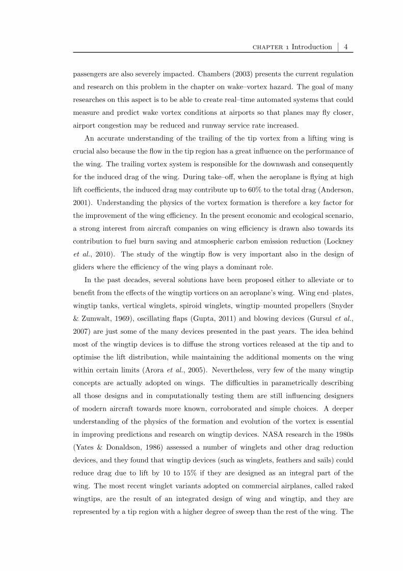
passengers are also severely impacted. Chambers (2003) presents the current regulation
and research on this problem in the chapter on wake–vortex hazard. The goal of many
researches on this aspect is to be able to create real–time automated systems that could
measure and predict wake vortex conditions at airports so that planes may fly closer,
airport congestion may be reduced and runway service rate increased.
An accurate understanding of the trailing of the tip vortex from a lifting wing is
crucial also because the flow in the tip region has a great influence on the performance of
the wing. The trailing vortex system is responsible for the downwash and consequently
for the induced drag of the wing. During take–off, when the aeroplane is flying at high
lift coefficients, the induced drag may contribute up to 60% to the total drag (Anderson,
2001). Understanding the physics of the vortex formation is therefore a key factor for
the improvement of the wing efficiency. In the present economic and ecological scenario,
a strong interest from aircraft companies on wing efficiency is drawn also towards its
contribution to fuel burn saving and atmospheric carbon emission reduction (Lockney
et al., 2010). The study of the wingtip flow is very important also in the design of
gliders where the efficiency of the wing plays a dominant role.
In the past decades, several solutions have been proposed either to alleviate or to
benefit from the effects of the wingtip vortices on an aeroplane’s wing. Wing end–plates,
wingtip tanks, vertical winglets, spiroid winglets, wingtip–mounted propellers (Snyder
& Zumwalt, 1969), oscillating flaps (Gupta, 2011) and blowing devices (Gursul et al.,
2007) are just some of the many devices presented in the past years. The idea behind
most of the wingtip devices is to diffuse the strong vortices released at the tip and to
optimise the lift distribution, while maintaining the additional moments on the wing
within certain limits (Arora et al., 2005). Nevertheless, very few of the many wingtip
concepts are actually adopted on wings. The difficulties in parametrically describing
all those designs and in computationally testing them are still influencing designers
of modern aircraft towards more known, corroborated and simple choices. A deeper
understanding of the physics of the formation and evolution of the vortex is essential
in improving predictions and research on wingtip devices. NASA research in the 1980s
(Yates & Donaldson, 1986) assessed a number of winglets and other drag reduction
devices, and they found that wingtip devices (such as winglets, feathers and sails) could
reduce drag due to lift by 10 to 15% if they are designed as an integral part of the
wing. The most recent winglet variants adopted on commercial airplanes, called raked
wingtips, are the result of an integrated design of wing and wingtip, and they are
represented by a tip region with a higher degree of sweep than the rest of the wing. The
chapter Introduction 5
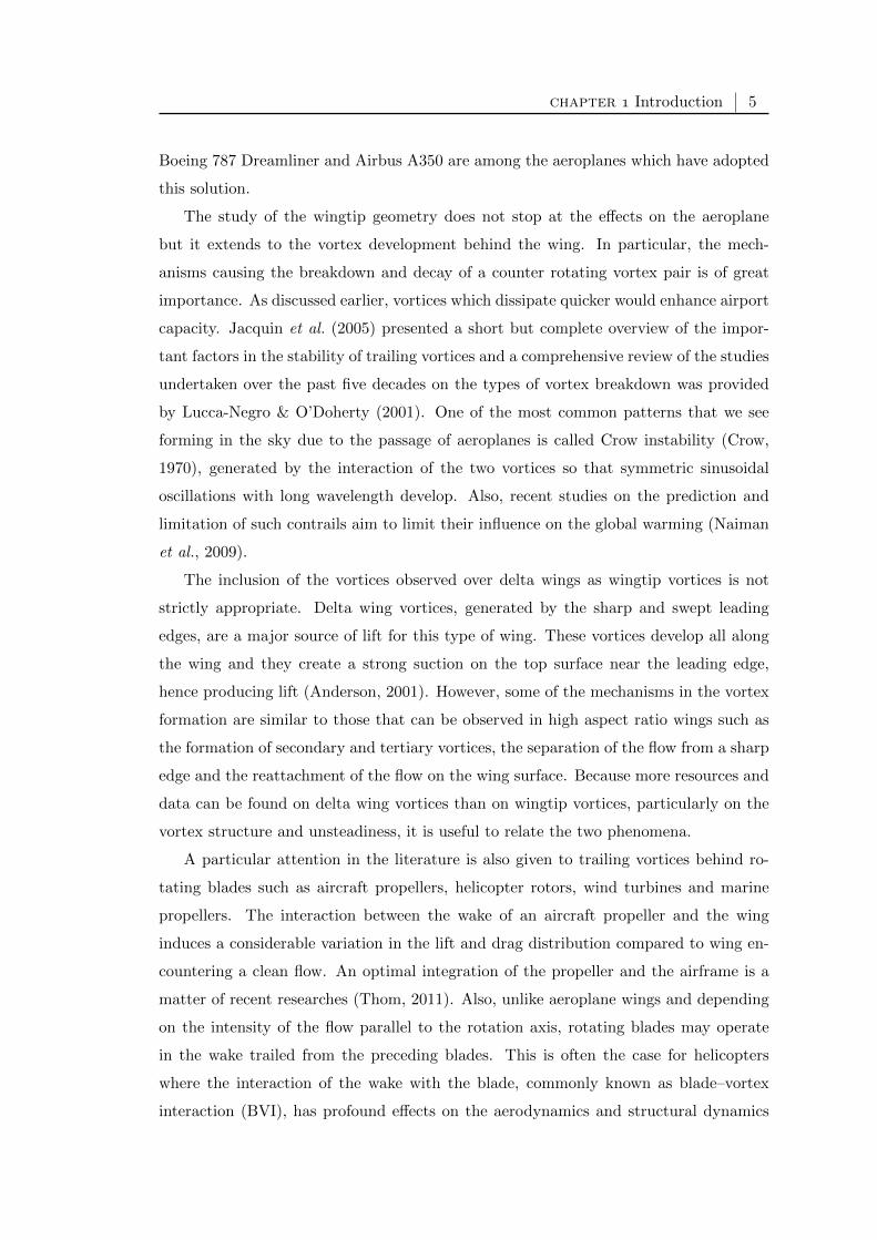
Boeing 787 Dreamliner and Airbus A350 are among the aeroplanes which have adopted
this solution.
The study of the wingtip geometry does not stop at the effects on the aeroplane
but it extends to the vortex development behind the wing. In particular, the mech-
anisms causing the breakdown and decay of a counter rotating vortex pair is of great
importance. As discussed earlier, vortices which dissipate quicker would enhance airport
capacity. Jacquin et al. (2005) presented a short but complete overview of the impor-
tant factors in the stability of trailing vortices and a comprehensive review of the studies
undertaken over the past five decades on the types of vortex breakdown was provided
by Lucca-Negro & O’Doherty (2001). One of the most common patterns that we see
forming in the sky due to the passage of aeroplanes is called Crow instability (Crow,
1970), generated by the interaction of the two vortices so that symmetric sinusoidal
oscillations with long wavelength develop. Also, recent studies on the prediction and
limitation of such contrails aim to limit their influence on the global warming (Naiman
et al., 2009).
The inclusion of the vortices observed over delta wings as wingtip vortices is not
strictly appropriate. Delta wing vortices, generated by the sharp and swept leading
edges, are a major source of lift for this type of wing. These vortices develop all along
the wing and they create a strong suction on the top surface near the leading edge,
hence producing lift (Anderson, 2001). However, some of the mechanisms in the vortex
formation are similar to those that can be observed in high aspect ratio wings such as
the formation of secondary and tertiary vortices, the separation of the flow from a sharp
edge and the reattachment of the flow on the wing surface. Because more resources and
data can be found on delta wing vortices than on wingtip vortices, particularly on the
vortex structure and unsteadiness, it is useful to relate the two phenomena.
A particular attention in the literature is also given to trailing vortices behind ro-
tating blades such as aircraft propellers, helicopter rotors, wind turbines and marine
propellers. The interaction between the wake of an aircraft propeller and the wing
induces a considerable variation in the lift and drag distribution compared to wing en-
countering a clean flow. An optimal integration of the propeller and the airframe is a
matter of recent researches (Thom, 2011). Also, unlike aeroplane wings and depending
on the intensity of the flow parallel to the rotation axis, rotating blades may operate
in the wake trailed from the preceding blades. This is often the case for helicopters
where the interaction of the wake with the blade, commonly known as blade–vortex
interaction (BVI), has profound effects on the aerodynamics and structural dynamics

chapter Introduction 6
(a) Tip vortices from the main rotor of anAH-1 Cobra in hovering flight (J. Diaz, giz-modo.com.au).
(b) Smoke visualization of wingtip vortices froma wind turbine experiment (Chattot, 2007).
(c) Cavitating tip vortices and cavitation behindthe shaft in an experiment on a marine propeller(National Research Council of Canada).
(d) Tip vortices formed over the rear wing of anF1 car (G. McCabe, McCabism blogspot).
Figure 1.2: Examples of wingtip vortices 2.
of the rotor system. The velocity induced by the unsteady wake results in impulsive
changes in the flow encountered by the rotor blades which significantly contribute to
noise and vibration (Duraisamy, 2005). Wingtip vortices are also a major source of
unsteadiness, noise and vibrations in wind turbines and the study of the structure of
wind turbine wakes is the aim of many researches (e.g. Vermeer et al., 2003; Massouh
& Dobrev, 2007; Yang et al., 2012).
Cavitation in marine propellers due to tip vortices is a very common phenomenon
and it is an important factor in propeller design. Cavitation occurs as a consequence of
the rapid growth of small bubbles that have become unstable owing to a change in the
pressure. These bubbles either can be imbedded in the flow or come from small crevices
at the bounding surfaces of the flow (Arndt, 2002). Cavitation is a significant cause of
damage to components, of noise and vibration. Also, the extent of cavitation erosion

chapter Introduction 7
can range from a minor amount of pitting after years of service to catastrophic failure
in a relatively short period of time.
(a) Pelicans flying in V –formation (fotosds,flickr.com).
(b) Delta wing type vortices generated by a spoonmoving vertically in a cup of coffee.
Figure 1.3: Examples of wingtip vortices 3.
Moreover, the control of wingtip vortices can be quite relevant in cars or sailing
competitions where the high efficiency of wings, or in general aerodynamic surfaces, is
demanded. However, it must be remembered that there are also instances where the
effects of wingtip vortices are desired and favourable. An example is the use of vortex
generators to avoid or delay flow separation, to enhance the lift of a wing or to reduce
the drag of aircraft fuselage (Lin, 2002).
Also, migrating birds are commonly seen flying in V –formation. Such formation al-
lows birds to fly in the upwash region of the wingtip vortex of the bird ahead (Hummel,
1983). The upwash assists each bird in supporting its own weight achieving a consider-
able reduction of induced drag. An extension of this concept was explored by NASA in
the Autonomous Formation Flight Project when an F/A-18 flew in the upwash of the
wingtip vortex of a DC-8 experiencing a 29% fuel savings and 14% of fuel savings was
found for an F/A-18 flying in formation with another F/A-18. For a particular fleet
configuration and wing spanload, Iglesias & Mason (2002) even predicted a negative
induced drag (which is thrust) for the following aircraft.
Lastly, the same process of formation of tip vortices from lifting surfaces can be
observed also in instances where generation of a lift force is unintentional. For example,
the author found that the vertical movement of a spoon in a cup of coffee is one of these
instances. The spoon, moving vertically at an angle with respect to the coffee surface,
generates a lift force and two counter rotating delta wing–like vortices are observed in
the cup.

chapter Introduction 8
section
Theoretical background: why do wingtip vortices
form?
The main and basic concepts of the existence of wingtip vortices are presented in this
section. The case of a rectangular fixed wing is used as a reference but these concepts
can be easily transferred to other instances. After a descriptive overview of the trailing
vortex formation and development based on established observations, different models
and mechanisms which explain the presence of the vortex will be presented. These
different approaches can be viewed as the same phenomenon described from different
perspectives.
Looking at the visualization of the flow in the vicinity of the surface of a rectangular
wing at an incidence, in a region near the tip the streamlines on the suction surface
are bent towards the root of the wing whereas the flow on the pressure surface are
bent towards the tip (Green & Acosta, 1991; Chow et al., 1997a). The roll up process
is observed to originate near the leading edge when the flow is accelerated from the
pressure side to the suction side and it wraps around the tip (Francis & Kennedy, 1979).
In detail, with the development of this process along the tip, the flow coming from the
pressure surface encounters a strong adverse pressure gradient which eventually forces
the boundary layer to a separation (Duraisamy, 2005). The lifting off of fluid by the
crossflow velocity in conjunction with the flow in the streamwise direction form a vortical
structure with a strong helical motion. The vortex so formed grows in size and strength
along the wing and secondary vortices are detected in the region of separated flow
(Chow et al., 1997a). The physics of this flow for aeronautical applications is extremely
complex since the process is largely turbulent, highly three–dimensional and involves
high velocity gradient regions with multiple flow separations (Chow et al., 1997b). This
vortical flow is convected downstream of the trailing edge and it eventually forms the
trailing vortex (Devenport et al., 1996). The flow embedded in the boundary layer
grown over the surfaces of the wing is shed downstream of the trailing edge in the form
of a thin sheet with a high level of vorticity. This wake is also entrained into the tip
vortex and, at a distance of few chords from the trailing edge, a pair of counter–rotating
axisymmetric trailing vortices is observed (Devenport et al., 1996). This system of two
parallel trailing vortices is unstable and a number of interaction mechanisms may appear
as it moves downstream of the wing (see Widnall, 1975; Devenport et al., 1997; Fabre

chapter Introduction 9
et al., 2002).
Looking at the complicated nature of the trailing vortex life, the requirement for
simple models and elementary mechanisms which are able to shed light on the key
physical factors is essential. Wu et al. (2006) explained the gap which is often found in
fluid dynamics between the formulas and the local dynamics as follows.
“Suppose one is given a set of finite–domain data for a viscous flow over
a body. One can then calculate the stress on the wall and [...] get the
force. Then one may look at various fields in the domain: streamlines,
velocity vectors, the contours of pressure and vorticity, etc. These together
form a quite complete physical picture of the flow. However, if one wishes
to identify the physical mechanisms that result in that force status, only
some qualitative assessments can be drawn from these plots. They are still
insufficient to pinpoint what flow structures have net contribution to the
force, in what way, how, and why.
[...]
Modern aerodynamics is not merely a simple combination of the flow
data and standard formulas [...]. The more complicated the flow is, the more
important role will the key physical factors play. “Bypassing flow details as
much as possible”(Wu, 2005) so as to reveal the key physical factors to
force and moment is actually the most valuable legacy of the pioneering
aerodynamicists, which should be continued and further enriched.” (Wu
et al., 2006, pp. 590-593)
A great and fundamental step forward in aeronautics came with the Lanchester–
Prandtl finite wing theory1 which showed how data from a two–dimensional aerofoil
could be used to predict the aerodynamic characteristics of a wing of finite span. Such
a model was also very important in understanding the role of trailing vortices in the
generation of the lift and the reason for their formation.
Within this model, the lifting wing and its wake are replaced by a system of vortices
that imparts to the surrounding air a motion similar to the actual flow and generates
a force equivalent to the lift. The vortex system can be divided into three main parts
which together form a vortex ring: the starting vortex, the trailing vortex system and
the bound vortex system (Houghton & Carpenter, 2003). Whereas the first two are
observable physical entities, the bound vortex system is a hypothetical arrangement of
1For an historical account of the development of the finite wing theory see Anderson (2001, p. 408).

chapter Introduction 10
a number of vortices which replace the real physical wing and where the vorticity of
each vortex filament is associated with the spanwise gradient of the wing circulation
distribution. This upstream segment of the vortex ring represents the boundary layer
of the upper and lower surfaces of the wing and it is the source of the lift and drag
through pressure and shear stress distributions. The distribution of vortex filaments
eventually merge into the trailing vortex system downstream of the wing. Moreover,
the starting vortex is soon left behind and for practical purposes the trailing vortices
are often modeled as stretching to infinity. Because of its shape, the resulting system,
which models the wing and its wake, is known as horseshoe vortex and it is sketched in
Figure 1.4(a).
(a) Horseshoe vortex. (b) Simplified horseshoe vortex.
Figure 1.4: Vortex systems replacing the lifting wing and its wake (Houghton & Carpenter,2003).
The horseshoe vortex is an important representation of the lifting wing and the
lattice method derived from this representation is a powerful numerical tool for the
investigation of the global effects of the wing configuration and geometry. For estimation
of distant phenomena such as vortex effects on flight formation (Iglesias & Mason, 2002),
a simplified horseshoe vortex model is adopted which is formed by a single bound vortex
and two trailing vortices as sketched in Figure 1.4(b). Based on Helmholtz theorems2
valid for inviscid and incompressible flows, the vortex filament replacing the wing will
continue in the wake as two infinitely long free trailing vortices and the strength of the
bound vortex is equal to the strength of the trailing vortices. Although the viscosity
2Helmholtz theorems establish basic principles on the vortex behaviour (Anderson, 2001; Wu et al.,2006):
1. the strength of a vortex filament is constant along its length;
2. a vortex filaments can not end in a fluid; it must extend to the boundaries of the fluid or form aclosed path;
3. in the absence of rotational external forces, a fluid that is initially irrotational remains irrotationalwhich is to say that the strength of a vortex filament does not vary with time.
chapter Introduction 11
plays a crucial role in the interaction of the fluid with the wing, during the vortex
formation, roll up, evolution in the wake and final dissipation, this model is able to
give accurate results on the lift generated by the wing. Furthermore, the horseshoe
vortex model explains and justifies the formation and existence of wingtip vortices with
conservation laws.
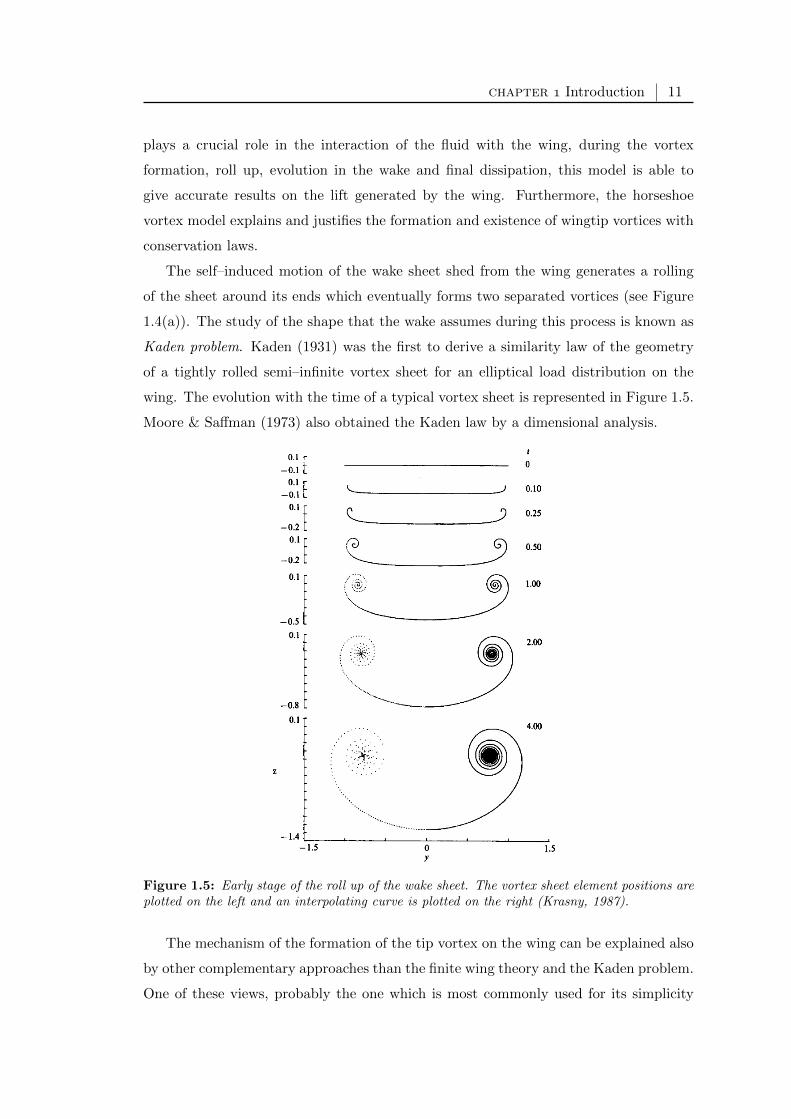
The self–induced motion of the wake sheet shed from the wing generates a rolling
of the sheet around its ends which eventually forms two separated vortices (see Figure
1.4(a)). The study of the shape that the wake assumes during this process is known as
Kaden problem. Kaden (1931) was the first to derive a similarity law of the geometry
of a tightly rolled semi–infinite vortex sheet for an elliptical load distribution on the
wing. The evolution with the time of a typical vortex sheet is represented in Figure 1.5.
Moore & Saffman (1973) also obtained the Kaden law by a dimensional analysis.
Figure 1.5: Early stage of the roll up of the wake sheet. The vortex sheet element positions areplotted on the left and an interpolating curve is plotted on the right (Krasny, 1987).
The mechanism of the formation of the tip vortex on the wing can be explained also
by other complementary approaches than the finite wing theory and the Kaden problem.
One of these views, probably the one which is most commonly used for its simplicity

chapter Introduction 12
and immediacy, is the pressure field interpretation, represented in the sketch of Figure
1.6. The physical mechanism for generating lift of the wing is the existence of a higher
pressure on the bottom surface than on the top surface (the contribution to the lift of
the shear stress is usually negligible). The net imbalance of the pressure distribution
creates the lift (Anderson, 2001). The flow near the wingtips, forced by the difference
of pressure between the two surfaces, curls from the bottom to the top side of the wing.
As a result, the flow on the lower surface of the wing presents a spanwise component
directed from the root to the the tip causing the streamlines to bend, and vice versa for
the upper surface. The crossing flow cannot move indefinitely in the spanwise direction
along the upper surface because of the gradual equalization of the pressure which,
combined with the streamwise velocity component, produces a convection of the flow in
the direction of the trailing edge in a vortical motion (Duraisamy, 2005). Moreover, the
difference of directions of the flow from the pressure and the suction surfaces results in
a thin vorticity layer which represents the wake sheet.
(a) Top view (planform). (b) Front view.
Figure 1.6: Pressure field interpretation of the wingtip vortex formation.
Another way to explain tip vortices is based on the shear layer that exists near the
wingtip (Green, 1995). The undisturbed flow on a plane some spanwise distance away
from the wing, parallel to the wing incoming flow, is sketched in Figure 1.7 along with
the projection of the flow over the wing surface (assuming no separation). The non–
parallelism of the wing surface and the freestream velocity vectors implies the existence
of vorticity approaching the wingtip. This mechanism is important because it explains
the existence of two vortices of opposite sign and same magnitude behind a wingtip also
when there is no generation of lift.
As presented, several approaches can be taken to describe the reasons of the gener-
ation of wingtip vortices and each one underlines different and complimentary physical

chapter Introduction 13
Figure 1.7: Shear layer interpretation of wingtip vortex formation.
factors of the trailing vortex life. However, much of the real flow in the early develop-
ment and formation is still hidden and in particular the role of boundary layer, viscosity
and turbulence is not described by these approaches. This lack can be justified by the
complexity needed by more comprehensive approaches and the good overall accuracy of
the present models. However, this lack of more sophisticated models comes also from a
still unsatisfactory understanding of this flow.
section
Literature review: what is the current under-
standing of wingtip vortices?
Looking at the importance of tip vortices, the number of applications where they are
found and the complexity of the flow field, it is not surprising to find a wide scientific
literature and several intensive research programs on this flow. Since the beginning of the
1960s, the aerospace industry started to understand the importance and the implications
that wingtip vortices have. Hundreds of scientists have faced the challenges of this
flow and have contributed to a deeper and clearer understanding through analytical,
experimental and numerical studies.
The experiments of the present research focus on a single vortex trailed from the tip
of a fixed wing mounted on the wall of a wind tunnel. Although this choice limits the
study to a specific field, the subjects which are addressed are general and most of the
observations and conclusions are true also for a wider range of applications, especially
chapter Introduction 14
when they regard the physics of the early formation of the vortex. In fact, the roll
up mechanism of the flow around the tip of a lifting surface is similar for many of the
applications. Also, the vast majority of the studies found in the literature focuses on
fixed wings although in the recent years many studies are found also on the wake of
helicopter blades (e.g. Ramasamy et al., 2009c, and related works).
Figure 1.8: Vortex life schematics: the approximate length scale is taken from Albano et al.(2003) for a typical airplane although they may drastically vary depending on the case (see forexample Dieterle et al. (1999) for a different length scale).
One of the possible classifications of the studies on fixed wings is based on the
distinction of the vortex life into different zones as sketched in Figure 1.8, each one
characterized by different phenomena and different life times (Francis, 1976; Albano
et al., 2003). The formation of the vortex begins on the wingtip. The flow moves from
the pressure to the suction surface and generates a vortical structure which develops
along the wing. The near field or near wake extends from the trailing edge to some
chords behind the aircraft where a complete roll up of the wake is observed and all
the circulation is contained in the vortices. In this range, secondary flow structures
interact and merge with the trailing vortices (e.g. wake sheet, secondary tip vortices,
vortices from flaps and tail, vortex sheet from nacelles, wing–fuselage junction). The
number of vortical structures observed in this region depends on wing configuration
and the airplane geometry (Gerz et al., 2001). The resulting trailing vortex appears
as an axisymmetric line vortex with smooth velocity profiles. A sub–region, namely
very early wake, confined in few chords behind the trailing edge of the wing, can be also
defined. In this region, the influence of the wing geometry is of great importance and the
primary vortex shows a remarkable asymmetry3. The mid field region is characterized
by the development of a number of axisymmetric line vortices and it can extend up to
few hundreds chords from the wing. In this region, the vortex circulation decays at a
relatively small rate, defined as the diffusion regime (Gerz et al., 2001). Lastly, the far
field region is the phase where vortices show instability mechanisms which remarkably
3The notation of extended near wake can also be found in the literature and it corresponds to thepresent definition of near wake.
chapter Introduction 15
change their shape. The vortex circulation presents a rapid decay and breakdown;
vortex interaction and dissipation are observed in this region.
Because of the different nature of the phenomena observed in each region, studies
do not usually focus on the whole vortex life but only on a limited range. Moreover,
the dual requirement of high resolution for detailed studies in the formation and near
field regions, and the large domain needed for the development of instabilities and the
observation of the decay, is usually too demanding for either experimental or numerical
studies.
(a) Far and mid field The study of far field and mid field is very important espe-
cially for problems related to the wake encountering following
airplanes. Gerz et al. (2001) present two possible strategies for the generation of less
harmful wakes, both based on the reduction of roll moments on follower aircrafts by
specific modifications during the vortex system formation. The quickly decaying vortex
strategy aims at anticipating the onset of instabilities, hence the occurrence of the far
field, which lead to an early decay of the vortex system; the low vorticity vortex strategy
aims at producing weaker vortices when observed in the mid field. These two strategies
can be seen also as two different views of the long term behaviour of trailing vortices:
predictable decay and stochastic collapse (Spalart, 1998).
A common and effective way to accelerate the dissipation of trailing vortices is to
force three–dimensional instabilities. The time required to break up the vortices under
natural conditions depends on several factors such as the strength of the atmospheric
turbulence, the number of trailing vortices, the dominant instability mechanism and
the growth rate of that particular instability. Many numerical studies and instability
criteria can be found for the far field and experimental works in this region are usually
based on flow visualizations (e.g. smoke injected in the trailing vortex). Rossow (1999)
presented an extensive review of studies on trailing vortex instabilities and several mech-
anisms of interaction between pairs of vortices. Wavelengths and amplitudes of such
instabilities are shown to be strongly affected by initial disturbances. For instance, a
typical value of the most amplified wavelength of the Crow instability behind an aircraft
(Crow, 1970) with an elliptically loaded wing is of about 8 times the vortex spacing.
Leweke & Williamson (1998) presented a well balanced theoretical and experimental
work on the interaction between short wavelength and long wavelength instabilities in
the breakdown of a vortex pair. However, more realistic airplane wakes present mul-
tiple vortex pairs (Jacquin et al., 2001) generated for instance by flaps, ailerons and

chapter Introduction 16
horizontal tail, which can reduce the time required for safe wake encounters of following
airplanes by a factor of 4 or more (Rossow, 1999) and increase the complexity in the
evolution and in the parametrization of the phenomenon. Crouch (1997) derived a set
of stability equations describing the growth of disturbances in a system composed of
two vortex pairs modeling respectively the wing tip vortices and the flap vortices. Two
instability mechanisms, with wavelengths spanning between 1.5 and 6 of the vorticity
centroid spacing, which influence the final break up of the vortices are described for
this configuration. Rennich & Lele (1999) and Fabre & Jacquin (2000), adopting Direct
Numerical Simulation (DNS) and a vortex filament method, also observed these mecha-
nisms and they showed the beneficial effects on the instability growth rate which can be
obtained by introducing long wavelength perturbations in the vortex system. Holzapfel
et al. (2001) performed a large eddy simulation (LES) of a vortex pair superimposed
with aircraft induced turbulence and atmospheric turbulence. They observed that the
short wavelength instability is triggered by atmospheric and wake turbulence and leads
to a quicker decay of the vortex circulation. Moreover, Billant et al. (1998) and Jacquin
& Pantano (2002) showed that the stability of a single vortex is strongly affected by the
swirl parameter, proportional to the ratio between the maximum swirl velocity and the
axial velocity at the centre of the vortex. Duraisamy & Lele (2008) described the mech-
anism of angular and axial momentum transport of an isolated turbulent trailing vortex
in terms of secondary turbulent structures moving radially from the vortex core to the
external flow. Moreover, Khorrami (1991) described an axisymmetric viscous mode of
trailing vortex instability which presents successive and sudden expansions (bursting)
of the vortex.
The mid field is particularly important because most of the vortex models and ana-
lytical studies refer to assumptions and approximations to the Navier–Stokes equations
which are satisfied only in this region. Axisymmetry, stationarity, incompressibility,
boundary layer–type approximation, small axial perturbation (light loading) are some
of the assumptions commonly adopted (see Hoffmann & Joubert, 1963; Batchelor, 1964;
Moore & Saffman, 1973; Phillips, 1981) and they lead to self–similar solutions of trailing
vortices (Birch, 2012). The fundamental governing equations of laminar and turbulent
isolated vortices are reported in Appendix C. Experimental studies confirmed these
assumptions to be reasonably valid (e.g. Devenport et al., 1996; Ramasamy, 2004).
However, measurements in the mid and near field are complicated by the phenomenon
of meandering (Green & Acosta, 1991; Devenport et al., 1996; Heyes et al., 2004). Me-
andering, also known as wandering, is attributed to a variety of reasons (Jacquin et al.,

chapter Introduction 17
2001) including freestream turbulence, intermittency, interference with wind tunnel un-
steadiness, amplification of vortex instabilities, perturbation due to the rolling up shear
layer and propagation of unsteadiness originating on the model. As a result, time–
averaged point measurements become weighted averages in both space and time (Green
& Acosta, 1991) so that the measured data needs to be corrected. Depending on the
measurement technique, different correction models have been suggested (e.g. Deven-
port et al., 1996; Leishman, 1998; Heyes et al., 2004; Ramasamy et al., 2011). Use of
uncorrected data gives an apparent “smeared–out” version of the actual flow field and
may contribute to large errors, especially in the vortex dimensions and swirls and axial
velocity peaks. Most experimental measurements prior to the 1990s do not account for
the effect of wandering and should therefore be interpreted with caution (Duraisamy,
2005).
A variety of analytical descriptions of vortices can be found although they may cor-
respond to real flows only in a local region or for a finite period of time (Wu et al., 2006,
chapter 6.2). Assuming laminar flow, Batchelor (1964) derived an axisymmetric simi-
larity solution for a steady incompressible isolated vortex, which has been often used as
a viscous solution suitable to describe a wake vortex in the mid field. Further, assuming
that axial gradients were much smaller than radial gradients (boundary layer–type ap-
proximation), Batchelor described the inviscid driving mechanism for the development
of the axial flow in terms of low pressure and importance of viscous effects within the
vortex core. Moore & Saffman (1973) extended the above analysis taking into account
also the roll up process of the wake and they were able to relate the mid field vortex
velocity field from a rectangular wing to the Reynolds number and the angle of attack.
Since the trailing vortex flow of most of the applications presents turbulence, a
considerable number of authors studied the Reynolds–averaged momentum equations
(presented in Appendix C) analytically and numerically. Hoffmann & Joubert (1963)
introduced isotropic eddy viscosity assumption to represent the turbulence inside a
trailing vortex. Iversen (1976) used the mixing length analogy and derived a similarity
solution using empirical inputs and he predicted the structure of a turbulent vortex as a
function of the Reynolds number for both laminar and turbulent cases. Phillips (1981)
studied the turbulent roll up of a vortex sheet and predicted in detail the structure of
the swirl velocity and the Reynolds stresses profiles. Specifically, he divided the vortex
region in three concentric regions.
1. The innermost part presents predominantly viscous effects and the swirl velocity
decreases linearly to zero in correspondence to the vortex centre. In addition,

chapter Introduction 18
approaching the centre, the rotation is close to a solid body rotation and the
Reynolds shear stress goes to zero with the square of the distance from the centre.
In this region, the stabilizing effects of the rotation of the flow are believed to
promote relaminarization.
2. The second region is located around the point of maximum swirl velocity (vortex
core radius). The viscous effects are small and in this highly strained turbulent
region a logarithmic law for the circulation applies (Hoffmann & Joubert, 1963).
3. In the outer region the flow is turbulent, the swirl velocity decays as a potential
vortex (which is as 1/r) and the Reynolds stress goes to zero as 1/r2.
Different investigations (e.g. Ramaprian & Zheng, 1997; Birch & Lee, 2005) demon-
strated that the circulation distribution in the first two regions shows a universal be-
haviour already in the very near field, which is described by semi–empirical laws. How-
ever, Birch (2012) demonstrated also that the wandering of the vortex, if is not correctly
removed, can give a strong contribution in converging the circulation profile upon the
universal profile.
The effects of turbulence in the diffusion and decay of trailing vortices are still in an
area of disagreement (Spalart, 1998), also because different sources of turbulence can be
identified such as boundary layer, viscous wake, vortex sheet rolling up and atmosphere.
Moreover, the behaviour of the turbulence within the vortex core is also a matter of many
studies. Cotel & Breidenthal (1999) used Bradshaw’s analogy (Bradshaw, 1969) between
streamline curvature and stratification to explain the possible relaminarization process
in the vortex core. Ramasamy & Leishman (2004) extended the similarity proposed by
Iversen (1976) to account for the relaminarization and they found a good correlation of
the swirl velocity profiles between the theory and the experiments. A region of transition
between laminar and turbulent flow within the vortex was predicted. Bandyopadhyay
(1990) explained a mechanism of relaminarization by centrifugal motions of patches of
turbulent flow moving from an outer annulus into the vortex core. This mechanism is
consistent with the existence of secondary structures convected along the vortex.
Whereas a number of analytical studies can be found on the evolution of vortex
properties in the far wake, the interaction between wing and flow and the complex
structure in the near wake strongly limit an analytical description. The importance
of studying the formation and early wake of a trailing vortex lies in the framework
of finding a link between the early stage and the development in the far wake. The
question on if it is possible to infer from the near field data (e.g. vortex topology,

chapter Introduction 19
spacing, circulation distribution) the behaviour in the far field is still open (Gerz et al.,
2001) and a proven method to characterize and control wake vortices is not available
yet.
(b) Formation and near
field
The assumptions adopted in the far field are violated in the
near field: the velocity field during the formation on the
wing and in the early wake is not axisymmetric; multiple
vortices and interactions with the wake sheet generate an unsteady flow; strong gradients
and axial perturbations can be observed in the vortex core; turbulence intensity is large.
Moreover, the wing geometry and the formation process strongly affect development and
characteristics of the vortex and the identification and understanding of the dominant
phenomena taking place in this region is still poor. For these reasons, a vast literature
covering the last 4 decades is found regarding the early life of wingtip vortices where
wind tunnel experiments and Computational Fluid Dynamics (CFD) have been the
main approaches4. Furthermore, the investigation techniques have greatly changed over
the years resulting in a great improvement of the accuracy of the results.
The first important investigation of the near field of tip vortices was made by Grow
(1969) using a five–hole pressure probe and a vorticity meter. He studied the effect that
the wing geometry and the boundary layer have on the trailing vortex. An increase of
vortex circulation and maximum swirl velocity was found with the increase of aspect
ratio, taper ratio and angle of attack.
Chigier & Corsiglia (1971) measured the tip flow generated by a NACA 0015 wing
with squared tip at different distances from the trailing edge and during its formation
on the surface. This investigation was based on triple–sensor hot wire velocimetry and
surface pressure measurements. A maximum axial velocity of 1.4 times the freestream
velocity was found during the formation at three quarters of chord. The axial velocity
reduced to 1.1U∞ at the trailing edge and a positive gradient in the axial direction
4Actually, the reasons of such a big number of studies on this topic can be more complex as explainedby Conlisk & Komerath (2001):
“The reasons are three–fold. The first is the omnipresence of vortices in fluid dynamics,complicated by the sheer variety of phenomena encountered when vortices interact withtheir environment, and the potential benefits in reliably controlling vortex–dominatedflows. The second is the limited opportunity (and willingness in some cases) of researchersto go beyond their application area to look for answers to problems by tying together theclues observed by others. The third is that information is not readily available in integratedform on the actual formation process of a vortex. As we demand more detailed predictionof vortex behavior, we see that it depends strongly on the formation process: the textbookmodel of solid–body–rotation in the core, and 1/r dropoff in tangential velocity outside,is not enough.”

chapter Introduction 20
was observed up to 3.75 chords downstream of the trailing edge with a final axial
velocity of 1.2U∞. This behaviour might be related to the vorticity intensification by
the mechanism of vortex stretching as presented in Appendix C.2. Moreover, from
integration of the wall pressure, generation of lift was observed in the tip region. On
a later study (Chigier & Corsiglia, 1972), they showed increasing level of turbulence at
the vortex centre line when the angle of attack was increased.
Orloff (1974) measured the mean velocity field at two chords downstream of a NACA
0015 wing with rounded tip using a two–dimensional laser velocimeter. Defect and
excess of axial velocity at the centre of the vortex with respect to the freestream velocity
was observed respectively for an angle of attack of 8 and 12. He also demonstrated
the usefulness of laser velocimetry in quantitatively assessing the relative effectiveness
of vortex alleviation devices (specifically of dissipator panels).
Thompson (1983) performed visualizations with hydrogen bubbles and dye in a water
channel to study the vortex formation for different wingtip geometries. The squared tip
produced flow separation from the sharp edges and two distinct vortices were observed
for the rounded tip. The secondary vortex, located outboard of the primary vortex, is
induced by the primary one and presents opposite sense of rotation. When the secondary
vortex rolled up and wrapped in the primary vortex, a rapid change of direction of the
primary vortex core was observed.
Francis & Katz (1988) presented the development of the tip vortex on a rectangular
wing at different Reynolds numbers and angles of attack. Illumination with a thin laser
sheet together with distribution of dye were utilized as means of observation and several
dimensions were measured off the video recordings. The flow at the squared tip was
dominated by multiple vortex structures including the main counter rotating vortex,
shear layer eddies and several other secondary structures.
A notable work was presented by McAlister & Takahashi (1991) who carried out
an extended experimental campaign on a rectangular wing as function of a number of
parameters: chord length, aspect ratio, wingtip geometry, Reynolds number and angle
of attack. They adopted pressure measurements on the wing and two–component laser
velocimetry for the evaluation of the mean flow. Trends of the main features with the
variation of the above parameters were given such as wing circulation; lift, drag and
moment coefficients and peaks and distributions of the swirl and axial velocity. The
presence of the vortex system generates regions of suction near the wingtip on the upper
surface which has the effect of producing an increase in the lift distribution over the end
part of the wing. On planes near the trailing edge, the swirl velocity profiles of a vortex

chapter Introduction 21
from a high angle of attack showed inflections which were attributed to the presence
of secondary vortices, and the initial shape of the axial velocity presented simultaneous
regions of deficit and excess compared to the freestream velocity.
Shekarriz et al. (1993) also observed that the circulation and swirl velocity profiles in
the near field are dominated by the presence of secondary vortices. They implemented
particle displacement velocimetry (PDV) to measure the global instantaneous velocity
distribution within a tip vortex. An axisymmetric vortical structure was observed at
less than 1 chord downstream of the trailing edge of the wing and a constant overall
circulation was measured in the whole range studied (up to 6.7 chords from the trailing
edge).
Another important study is the work by Chow et al. (1997a) (see also Chow et al.,
1992, 1997b) which represented a benchmark for several following numerical studies
(e.g. Dacles-Mariani et al., 1993; Dacles-Mariani & Kwak, 1996; Dacles-Mariani et al.,
1997; Kim & Rhee, 2005; Duraisamy & Iaccarino, 2005; Craft et al., 2006; Churchfield
& Blaisdell, 2009). The accuracy of the measurement technique and the detailed de-
scription of the wingtip in its formation and evolution in the near wake is still now
hardly matched. Several experimental techniques were adopted for qualitative and
quantitative measurements such as laser–illuminated smoke visualizations, surface oil
flow visualizations, surface pressure measurements, 7–hole pressure probe measurements
and triple–wire probe velocimetry. The correlation of the results from these different
techniques allowed an accurate description of the process of formation and initial roll
up of the wingtip vortex generated by a low aspect ratio wing with symmetric profile
and rounded wingtip at a fixed angle of attack and Reynolds number. Highly three–
dimensional flow was observed on the wing surface near the tip. Crossing of flow from
the pressure to the suction surface was observed as early as 30% of the chord from
the leading edge. The presence of a secondary and a tertiary vortex was indicated by
convergence lines in the surface visualizations between the main vortex separation line
and the wingtip. The pressure coefficient on the surface was minimum in correspon-
dence to the core of the main vortex. A maximum axial velocity of 1.77U∞ was found
at the vortex centre just downstream of the trailing edge followed by a slow decrease,
differently from the experiments by Chigier & Corsiglia (1971), to a value of 1.69U∞
at 0.69 chord from the trailing edge. An important achievement was the measurement
of the Reynolds stresses in the near field. The evolution and distribution of the turbu-
lent stresses and a discussion of the importance of the different terms in the Reynolds
stresses transport equations was presented. They found that the production of the tur-

chapter Introduction 22
bulence within the vortex in the early wake is associated with the high axial velocity
gradients in the vicinity of the vortex centre. However, relaminarization had a much
larger effect which resulted in a high decay rate of the overall turbulence within the
vortex core. Misalignment of the distributions of the shear stress and the mean strain
rate were measured within the vortex, which makes isotropic eddy viscosity models for
the turbulence closure of Reynolds–averaged Navier–Stokes simulations (RANS) defi-
cient in accurately representing the turbulence field (Dacles-Mariani et al., 1997). For
this reason, more recent numerical simulations adopt different models (e.g. Duraisamy
& Iaccarino, 2005; Craft et al., 2006) which better predict the early wake of a wingtip
vortex. However, simulations still find difficulties when predicting the turbulence and
the diffusion of the vortex core. Only in recent years, LES on wingtip vortices have
become feasible and they showed a better agreement with the experimental results than
RANS simulations. For instance, Jiang et al. (2007) described a primary tip vortex
originally turbulent which then rapidly relaminarized after shedding in the near field.
Moreover, Cai (2006) observed that the turbulence inside the primary vortex is caused
by the turbulent shear layer and the interaction between the primary and the secondary
vortices.
A considerable work on the vortex meandering and turbulence was presented by
Devenport et al. (1996) who studied the wingtip vortex in the wake of a rectangular
wing at a distance between 5 and 30 chords from the trailing edge. They noted that
the meander creates a smoothing effect that can make the vortex appear with a larger
diameter and reduced swirl and axial velocity peaks compared to the instantaneous vor-
tex. Moreover, artificially large values of turbulent stresses may result from experiments
that do not correct for vortex meandering. They also showed a complex structure of
the turbulence within the vortex core and in the spiral layer around it. Velocity spec-
tra measured at the vortex centre indicated that the vortex core was laminar and that
velocity fluctuations in this region were a consequence of “inactive motions” produced
by turbulence in the surrounding spiral wake. Some of the profiles, especially those
measured at upstream locations, showed a two–layered structure formed by an outer
core affected by a secondary vortex formed during the roll up process and an inner core
growing within it. These results were compared with RANS simulations by Lockard &
Morris (1998) and Spall (2001) who presented considerable discrepancies on the diffu-
sion of the vortex moving downstream (respectively overpredicting and underpredicting
the diffusion).
Stereoscopic particle image velocimetry (SPIV) on wingtip vortices was first adopted
chapter Introduction 23
by Zuhal (2001) (see also Zuhal & Gharib, 2001) who measured the three–dimensional
velocity field in the near field of a rectangular wing with squared tip. The wing generated
multiple vortices of opposite signs. Farther downstream, the vortices with opposite
direction of rotation broke up into smaller vortices which orbited around the tip vortex.
This study confirmed that the interaction of the tip vortex with satellite vortices is a
main cause of meandering generating unsteady motions of the primary vortex.
Birch et al. (2003) (see also Birch et al., 2004) presented measurements on the wing
and on the trailing vortex using PIV, a 7–hole pressure probe and a balance for force
measurements. They allowed variations of the tip geometry to establish its influence on
the growth of the main structures. Multiple vortices were observed around the main
vortical structure. The core radius, the maximum swirl velocity and the axial velocity
peak of the vortex significantly increased with the angle of attack. Also, depending on
the angle of attack, the axial velocity in the core was directed either towards the wing
or away from it.
Bailey et al. (2006) (see also Bailey & Tavoularis, 2008) studied the vortex forma-
tion and development around a squared tip up to 9 chords downstream of the wing
using a four–sensor hot–wire probe. From the analysis of the velocity fluctuations, two
kinetic energy peaks were found, one above the suction surface and another near the
tip surface. Approaching the trailing edge, the two peaks merged together and a new
smaller peak appeared on the tip surface. These three peaks were associated with re-
spectively primary, secondary and tertiary vortices and they were confirmed by flow
visualizations through dye injection. An attentive comparison of the wingtip vortex for-
mation for different freestream turbulence levels showed that, although the amplitude
of the wandering depended on freestream conditions, its wavelength is insensitive to
changes in the freestream turbulence. Recent works on the meandering were presented
by Del Pino et al. (2009) and Del Pino et al. (2010) who observed elliptical distributions
of the instantaneous vortex centre positions. They also performed proper orthogonal
decompositions (POD) of the vortex movement identifying the main frequency of the
most energetic mode (axisymmetric base vortex flow) as the frequency characterizing
the vortex meandering.
Due to its increased reliability and accuracy, PIV technique has gained the reputation
of a powerful and time effective flow diagnostic method for the quantitative whole–field
study of complex fluid flows (Scarano, 2002). In addition to the studies mentioned
above, several other experiments on wingtip vortices based on PIV measurements can
be found in the recent years. These works focus on different aspects such as effects of

chapter Introduction 24
the wing geometry, formation process, meandering structure and shape of the rolled up
vortex (e.g. Dieterle et al., 1999; Albano et al., 2003; Troolin et al., 2006; Karakus et al.,
2008; Igarashi et al., 2010; Sohn & Chang, 2011; Del Pino et al., 2011). Dieterle et al.
(1999) applied PIV on a catapult facility in order to study the far field behaviour of
trailing vortices in the wake of an aircraft model. Karakus et al. (2008) performed a PIV
on a rectangular wing with 151 mm of chord and squared tip. At a Reynolds number
of 32000 they observed the formation of three vortical structures around the tip which
merged together at around 60% of the chord. The tip region was dominated by the
stronger interaction between the multiple secondary vortices and the primary vortex.
Del Pino et al. (2011) found a good correlation between experimental data of the swirl
velocity profile and vorticity in the near field with the analytical vortex presented by
Moore & Saffman (1973).
section
What are the scope and contributions of this
work to the unresolved issues?
As shown in the literature review, a great number of authors studied the wingtip
vortex. However, this flow still presents many questions. The key points that have not
been successfully answered by previous studies and that have been addressed in the
present work are presented as follows.
• Although the work done by Chow et al. (1997a) represented an important step
forward in the understanding of the formation and early wake of wingtip vortices,
such tests were performed only at one condition (on one wing model, angle of
attack and freestream velocity). A parametric study for a range of angles of attack,
Reynolds numbers, wingtip shapes would greatly improve the understanding of the
basic mechanisms of the initial roll up, of the formation of the axial flow and of
the origin and effects of secondary vortical structures.
• In order to put the design of effective tip modifications on a firm basis and to
develop trustworthy prediction methods, more work is needed in the understanding
of the fundamental flow physics and in the characterization of the vortex formation
on the wing. Even the formation of the tip vortex on simple geometries, such as
rectangular wings with squared and rounded tips, reveals a number of peculiar and

chapter Introduction 25
very challenging phenomena which are hardly predicted by numerical simulations.
The study of the unsteadiness of the vortex system during the formation is also
very important in understanding more about meandering sources and in suggesting
tip modifications which excite instability mechanisms on particular wavelength
and so quicken the decay of the vortex in the far field.
• Whether and when the vortex core is turbulence or laminar is a matter of con-
troversy and the role of the turbulent and its effects on the early development of
wingtip vortices is not clear (Birch, 2012). Two main answers have been proposed:
the first is that the turbulence plays only a passive role in the development of the
vortex core which is subjected to a rapid relaminarization process; the second
claims the existence of convected secondary structures within the vortex core pro-
ducing high levels of turbulent stresses. More studies are needed for this question
to be better addressed and answered.
• Nowadays, CFD methods have reached a state of reliability and resources which
can give detailed descriptions of complex flows; in particular it is now common to
find RANS simulations on wings or even full aircraft. However, the approach on
the closure problem is still posing serious questions on the accuracy of such results
which is particularly true for trailing vortices. Moreover, an accurate representa-
tion of the formation and the near wake is extremely important if the aim is the
prediction of the development and decay of the trailing system or its interaction
with other bodies. Detailed experimental results on the early development of the
vortex are therefore very important not only as benchmarks for numerical simu-
lations but also for a deeper understanding of the physics and vortex dynamics in
this range so that more faithful models for the Reynolds stresses can be developed.
This research is based on an experimental study focused on the formation and very
early wake of a wingtip vortex from a rectangular wing. The effects of a number of pa-
rameters on the development of the tip vortex are addressed and a deeper understanding
of the physics involved in this flow is reached. Surface oil flow visualizations, surface
pressure measurements, laser–illuminated smoke visualizations, surface–mounted hot
film investigations and stereoscopic particle image velocimetry have been completed for
several configurations. The choice of adopting SPIV as the main experimental technique
was dictated by the need of a non intrusive, instantaneous, global and highly spatial
resolved measurement technique for the investigation of this complex flow field. These
qualities are necessary to adequately describe the mean flow structure of the vortex

chapter Introduction 26
core, the turbulent activity and secondary structure dynamics. The detail reached on
these measurements represents a unique contribution of this research to wingtip vortex
studies.
section
Structure of the thesis
The presentation of the results of this research follows the classification of the wingtip
vortex life proposed in Section 1.3. The experimental apparatus used during this work
is described in Chapter 2 where the wind tunnels used, the characteristics of the wing
models tested and the components of the experimental techniques adopted are presented.
In Chapter 3, a description of the formation of the wingtip vortex is presented
with the cooperating contribution of several experimental techniques. A model and
a characterization of the formation is proposed. Unsteadiness measurements on the
formation and in the very early wake are correlated giving insights into the effects
of secondary structures on the meandering of the vortex. Chapter 4 presents several
aspects of the early wake of the wingtip vortex such as the vortex core shape, the axial
flow development and the turbulence behaviour within the core. Due to the number
of different phenomena presented and in order to keep a general and short literature
review in this chapter, individual short introductions and specific literature reviews on
the particular topics are given at the beginning of each section. Chapter 5 presents a
discussion on the accuracy and error of the measurements with particular emphasis on
the SPIV.
Finally, Chapter 6 concludes this dissertation with a summary of the main contribu-
tions and results from this research on the various aspects of the vortex formation and
early wake. Recommendations for future work are suggested based on these conclusions.
chapter
Experimental apparatus and
procedure
When you can measure what you are speaking about,
and express it in numbers, you know something about it;
but when you cannot measure it, when you cannot ex-
press it in numbers, your knowledge is of a meager and
unsatisfactory kind: it may be the beginning of knowl-
edge, but you have scarcely, in your thoughts, advanced
to the stage of science.
Lord Kelvin (William Thomson)
A series of experiments adopting different experimental techniques were conducted
with the objective of qualitatively and quantitatively describing the initial roll up of the
tip vortex on the wing and in the early wake. Surface oil flow visualizations and pressure
measurements on the wing were performed in order to gather global and panoramic
information of the flow on the wing at different configurations. Due to its relative
simplicity in the implementation, surface flow visualizations served as a preliminary
tool for providing qualitative information of the surface flow when complex structures
are present. Moreover, smoke visualizations on the tip region were conducted to give a
deeper understanding on the structure and dynamics of the vortex development on the
wing.
A study of the unsteadiness in the formation of the trailing vortex system was accom-
plished using surface hot film anemometry and stereoscopic particle image velocimetry
(SPIV) on the flow parallel to the wing surface. Lastly, the major part of the research
was carried out performing parametric SPIV measurements in the early wake changing
a number of parameters such as wing and tip geometry, angle of attack and Reynolds
number.
The research was entirely conducted within the University of Glasgow and the ex-
27

chapter Experimental apparatus and procedure 28
periments carried out during this study were based on two wind tunnels and two wing
models. Details of experimental facilities, wing models, experimental techniques and
apparatus used during each experiment are provided in this chapter. Particular at-
tention is drawn toward the description of the stereoscopic particle image velocimetry
technique. Lastly, the reference systems adopted in the presentation of the results is
described in Section 2.4.
section
Wind tunnels
(a) Argyll wind tunnel All the experiments were carried out in the Argyll wind
tunnel with the exception of the smoke flow visualizations
of the formation of the wingtip vortex. An overview of this facility is shown in Figure
2.1.
The Argyll wind tunnel is a large facility for subsonic experiments. This is a closed–
return facility with an octagonal test section of 2.65 m width, 2.04 m height and 5.60
m length. The diameter of the fan is 3 m and it is located on the opposite side of the
circuit with respect to the test section which is vented to the atmosphere by gaps of
around 0.05 m on the walls respectively at the leading edge and at the trailing edge.
The vents keep the test section static pressure equal approximately to the atmospheric
pressure. The nominal maximum operating wind condition that the flow in the test
section can reach is 76 m/s. A Pitot tube and a thermocouple for the measurement of
the freestream speed are positioned at the test section inlet and connected to a dedicated
computer. The turbulence level, evaluated from hot wire anemometry in the centre of
the test section, is of around 0.4% in the velocity range between 10 and 25 m/s, which
corresponds to the range of the experiments presented in this study. A 3.75 m long
by 1.9 m wide moving ground, designed to operate independently from the flow at a
maximum of 60 m/s, is placed on the ground. One of the two wing models tested in
this research was mounted vertically on the floor. In order to allow this model to be
mounted on the floor, a board covering the rolling road was mounted at 0.1 m of height
from the moving ground. A rounded leading edge was adopted. The test section is
equipped with several windows allowing a wide optical access from both the sides and
from the roof.

chapter Experimental apparatus and procedure 29
Figure 2.1: Argyll wind tunnel: top view.
(b) Smoke visualization
wind tunnel
Smoke flow visualizations of the formation of the wingtip
vortex were carried out in a wind tunnel dedicated to this
kind of experiments.
The smoke visualization wind tunnel is a purpose built facility with cross section of
0.91 m by 0.91 m and maximum operating speed of 5 m/s. The working section is 4 m
long with a 9:1 contraction at the upstream end and a fan at the downstream end. A
schematic of the experimental arrangement is shown in Figure 2.2.
Flow visualization is achieved by injecting smoke through uniformly distributed
orifices of 1 mm of diameter and 6.35 mm pitch, drilled into a pipe of 12 mm diameter
positioned vertically at the test section inlet. A range of horizontal positions of the pipe
allows the smoke filaments to be released at different planes. The pressure, density and
velocity of the smoke at the orifices can be adjusted so that smoke filaments are aligned
with the freestream. Smoke tracer is generated by heating Shell Ondina EL oil which
is injected in the test section using high pressure carbon dioxide as a propellant.
The smoke lines are illuminated with a continuous laser sheet of 2 mm of thickness
from a diode laser (5 W power at 532 nm) which is shone from the top of the test section
and perpendicularly to the freestream flow. The laser is mounted on a rail so that the
laser sheet can be moved along the wind tunnel longitudinal axis.
A high resolution camera (DALSA 2M30 of 1600 by 1200 pixels) with 50 mm focal
length lens and f –number equal to 4, is used to capture instantaneous smoke realizations
with a maximum frame rate of 30 Hz. The camera is controlled by an in–built LabView

chapter Experimental apparatus and procedure 30
code which permits adjustments on the exposure time in a range between 1 and 400
ms. The camera is mounted downstream of the wing at a distance of 1.5 chords from
the trailing edge. The comparison of the vortex structure with and without the camera
showed that the flow on the wing was not sensibly affected by the presence of the camera.
Figure 2.2: Experimental arrangement of smoke visualizations on the vortex formation: wingM2 mounted in the flow visualization wind tunnel.
section
Wing models
The determination of the wing size of the model was based on the minimization of
the blockage effects while keeping a size which still allowed a detailed description of the
flow around the tip based on the resolution of the present measurement instrumentation.
The length of the test section did not limit the size of the model being only the early
wake (up to 2–3 chords) the region of interest. Two wings with different chord lengths
and aspect ratios were studied, namely M1 and M2. For both the models, a blockage
effect in the Argyll wind tunnel of less then 3% is calculated for the wing at 15. As
described by Igarashi et al. (2011), a small blockage reduces the interferences of the walls
in the wandering of the trailing vortex. The value calculated in the current investigations
ensures minimum walls effect on the tip vortex behaviour.
The interest in a better understanding of the basic physics behind wingtip vortices
leads to the choice of a widely tested and known geometry. A rectangular wing with

chapter Experimental apparatus and procedure 31
symmetric NACA profile is adopted and squared and rounded tip geometry are studied.
(a) M1: high aspect ratio
wing
A rectangular wing model with NACA 0015 profile, 0.42
m chord, 1.3 m span (corresponding to an aspect ratio
of AR = 3.1) and rectangular wingtip was tested. The
model, slid through the test chamber side wall of the Argyll wind tunnel, was mounted
on an adjustable plate which allowed the angle of attack and the model height to be
adjusted. The angle of attack of the wing was measured with a digital inclinometer
positioned on the mounting plate and it was confirmed by zero lift measurement from
surface pressure integration at an indicated angle of attack equal to zero. The wing was
positioned at the mid height of the test section and the tip was approximately along
the centerline (see Figure 2.3).
Figure 2.3: M1 wing mounted in the Argyll wind tunnel (without fixing cables).
In order to limit bending of the wing and to avoid flutter during the experiments,
two cables of adjustable length were fixed at the test section wall and at the wing shaft
from the upper and the lower surfaces. The fixing point was at 1.5 chord from the tip
so that the effect of the cables on the tip region was negligible.
(b) M2: low aspect ratio
wing
A low aspect ratio wing (AR = 0.75) was also tested.
The M2 model is a rectangular planform with NACA
0012 profile, 0.76 m chord and 0.57 m span. Squared
and rounded wingtips were tested by attaching a rounded cap. The wing area with the
round cap was around 7% greater than the wing area with squared tip. The model was
mounted vertically on a circular plate on the floor allowing the angle of attack to be
adjusted by a rotation about the quarter chord which laid on the middle plane of the test

chapter Experimental apparatus and procedure 32
section. The zero angle of attack was identified by integration of the surface pressure
along a pressure tapping array on both sides of the wing and placed at a distance of
0.10 m from the ground. A picture of the wing model and the calibration plate used for
the stereoscopic particle image velocimetry is illustrated in Figure 2.4.
Figure 2.4: M2 wing mounted in the Argyll wind tunnel and SPIV calibration plate.
A summary of the main characteristics of the two models and the experimental
techniques adopted for each wing is given in Table 2.1.
M1 M2
Aerofoil NACA 0015 NACA 0012Chord, c [m] 0.42 0.76
Span, b [m] 1.3 0.57, 0.62Aspect ratio, AR 3.1 0.75, 0.81
Tip geometry squared squared, rounded
Pressure measurements XSurface flow visualizations X
Smoke visualizations, formation XSmoke visualizations, early wake X
Hot film anemometry XSPIV, limiting flow X
SPIV, early wake X X
Table 2.1: Summary of wing models characteristics and experiments.
chapter Experimental apparatus and procedure 33
section
Experimental techniques
(a) Surface oil flow
visualizations
Oil with a fluorescent agent is used to visualize the character-
istics of the flow near the surface. Due to frictional forces the
air stream carries the oil with it. From the pattern of oil ac-
cumulation on the surface, qualitative conclusions can be drawn with respect to the
location of flow separation lines, reattachment lines and the local magnitude of skin
friction (Merzkirch, 1987; Yang, 1989). The wall shear stress is defined as the spatial
derivative normal to the surface of the velocity field at the surface. Integral curves of
the velocity in this vector field are sometimes referred to as limiting streamlines, wall
shear stress trajectories or skin friction lines. It is this vector field which produces oil
flow patterns in wind tunnel experiments (Kenwright, 1998). Whether the oil film fol-
lows the surface streamlines and whether the motion indicates the skin friction lines is
discussed by Lu (2010). The interpretation and reliability of these observations relies
on the small effects that the oil film has on the boundary conditions of the air flow near
the wall. Squire (1961) theoretically studied the motion of a thin oil sheet on a surface
under a boundary layer and he showed that the oil follows the boundary layer surface
streamlines except near flow separations where it tends to form an envelope upstream
to the true separation envelope. This effect is less marked for turbulent than for lam-
inar boundary layers and the displacement increases for thicker oil layers and smaller
Reynolds numbers.
Surface oil flow visualizations were performed on the wing model M1 using a mixture
of Ondina oil and fluorescent powder and photographed using a Nikon D70 still camera
with a 28–105 mm zoom lens. A smooth black adhesive film was applied on the model in
order to cover the pressure tappings and to create a uniform and suitable surface for the
paint. An ultraviolet lamp was used to illuminate the mixture which gave more contrast
with the background surfaces than with normal lighting. A thin layer of mixture was
uniformly brushed onto the wing surface near the tip with the wind tunnel off. The
wind tunnel was then turned on and, once the pigment was stably distributed on the
wing surface, pictures of the oil distribution were taken.
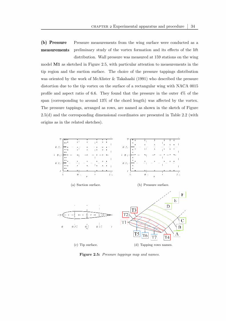
chapter Experimental apparatus and procedure 34
(b) Pressure
measurements
Pressure measurements from the wing surface were conducted as a
preliminary study of the vortex formation and its effects of the lift
distribution. Wall pressure was measured at 159 stations on the wing
model M1 as sketched in Figure 2.5, with particular attention to measurements in the
tip region and the suction surface. The choice of the pressure tappings distribution
was oriented by the work of McAlister & Takahashi (1991) who described the pressure
distortion due to the tip vortex on the surface of a rectangular wing with NACA 0015
profile and aspect ratio of 6.6. They found that the pressure in the outer 4% of the
span (corresponding to around 13% of the chord length) was affected by the vortex.
The pressure tappings, arranged as rows, are named as shown in the sketch of Figure
2.5(d) and the corresponding dimensional coordinates are presented in Table 2.2 (with
origins as in the related sketches).
(a) Suction surface. (b) Pressure surface.
(c) Tip surface. (d) Tapping rows names.
Figure 2.5: Pressure tappings map and names.
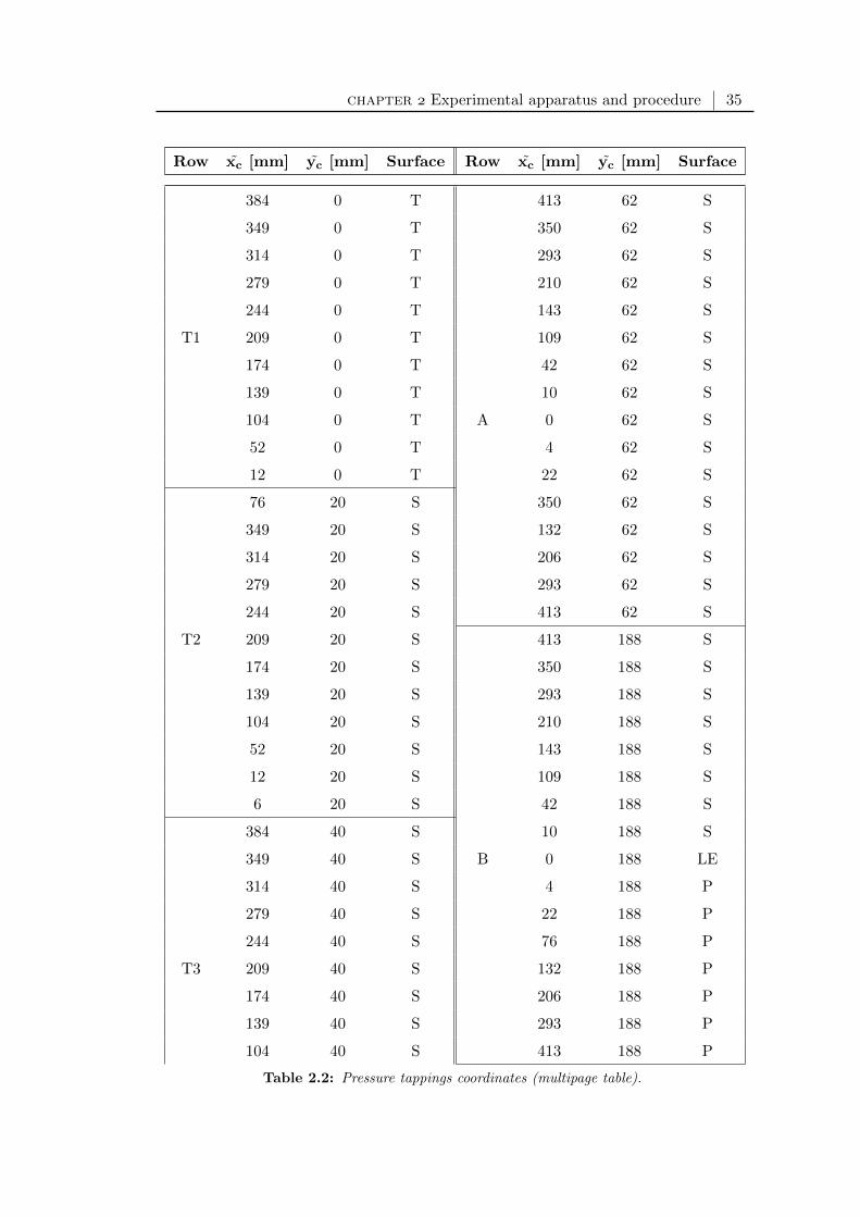
chapter Experimental apparatus and procedure 35
Row xc [mm] yc [mm] Surface Row xc [mm] yc [mm] Surface
384 0 T 413 62 S
349 0 T 350 62 S
314 0 T 293 62 S
279 0 T 210 62 S
244 0 T 143 62 S
T1 209 0 T 109 62 S
174 0 T 42 62 S
139 0 T 10 62 S
104 0 T A 0 62 S
52 0 T 4 62 S
12 0 T 22 62 S
76 20 S 350 62 S
349 20 S 132 62 S
314 20 S 206 62 S
279 20 S 293 62 S
244 20 S 413 62 S
T2 209 20 S 413 188 S
174 20 S 350 188 S
139 20 S 293 188 S
104 20 S 210 188 S
52 20 S 143 188 S
12 20 S 109 188 S
6 20 S 42 188 S
384 40 S 10 188 S
349 40 S B 0 188 LE
314 40 S 4 188 P
279 40 S 22 188 P
244 40 S 76 188 P
T3 209 40 S 132 188 P
174 40 S 206 188 P
139 40 S 293 188 P
104 40 S 413 188 P
Table 2.2: Pressure tappings coordinates (multipage table).

chapter Experimental apparatus and procedure 36
Row xc [mm] yc [mm] Surface Row xc [mm] yc [mm] Surface
52 40 S 413 318 S
12 40 S 350 318 S
6 40 S 293 318 S
384 30 P 210 318 S
349 30 P 143 318 S
314 30 P 109 318 S
279 30 P 42 318 S
244 30 P 10 318 S
T4 209 30 P C 0 318 LE
174 30 P 4 318 P
139 30 P 22 318 P
104 30 P 76 318 P
52 30 P 132 318 P
12 30 P 206 318 P
6 30 P 293 318 P
104 40 S 413 318 P
104 30 S 413 445 S
104 20 S 350 445 S
104 10 S 293 445 S
T5 104 0 Ts 210 445 S
104 0 T 143 445 S
104 0 Tp 109 445 S
104 15 P 42 445 S
104 30 P 10 445 S
104 45 P D 0 445 LE
209 40 S 4 445 P
209 30 S 22 445 P
209 20 S 76 445 P
209 10 S 132 445 P
T6 209 0 Ts 206 445 P
209 0 T 293 445 P
209 0 Tp 413 445 P
209 15 P 413 521 S
Table 2.2: Pressure tappings coordinates (multipage table).

chapter Experimental apparatus and procedure 37
Row xc [mm] yc [mm] Surface Row xc [mm] yc [mm] Surface
209 30 P 350 521 S
209 45 P 293 521 S
314 40 S 210 521 S
314 30 S 143 521 S
314 20 S 109 521 S
T7 314 10 S 42 521 S
314 0 T 10 521 S
314 15 P E 0 521 LE
314 30 P 4 521 P
314 45 P 22 521 P
76 521 P
132 521 P
206 521 P
293 521 P
413 521 P
413 572 S
350 572 S
293 572 S
210 572 S
143 572 S
109 572 S
42 572 S
10 572 S
F 0 572 LE
4 572 P
22 572 P
76 572 P
132 572 P
206 572 P
293 572 P
413 572 P
(P) Pressure surface. (S) Suction surface. (T) Tip mean line.
(Ts) Tip surface: upper half. (Tp) Tip surface: lower half. (LE) Leading edge.
Table 2.2: Pressure tappings coordinates.

chapter Experimental apparatus and procedure 38
The tubes, of 1 mm of internal diameter D, were routed from each pressure tapping
to the outside of the test section through two shafts along the wing and then connected
to 2 scanivalves. Each scanivalve contained a 20 inches of water (4977 Pa) differential–
pressure transducer and the two voltage outputs were recorded simultaneously by a
dedicated LabView code thorough a NI USB–6229 card. The opposite side of each
transducer was vented to ambient conditions outside the wind tunnel (since the Argyll
wind tunnel presents a vented test section). A calibration was carried out with a portable
pressure calibrator Druck dpi 615 and a linear relationship between pressure and output
voltage was found with sensitivity of 0.001 V/Pa. The regression coefficient, also known
as correlation coefficient, was greater than 0.99998 in the whole range of the instrument
and a resolution lower than 1 Pa could be inferred. The total distance between each
tapping and the scanivalve was approximately 3 m. The LabView code controlled
also the scanivalve switchings, the sampling frequency and the sampling time of each
recording. A delay of a tenth of a second between two successive acquisitions was set in
order to allow the switching of the scanivalve and the equalization of the pressure along
the tube.
Pictures of the pressure tubes coming from the M1 wing, the mounting plate outside
the test section, the pressure transducers and the scanivalves are presented in Figure
2.6.
(a) M1 mounting plate and tubes from pressuretappings.
(b) Pressure transducers and scanivalve.
Figure 2.6: Pressure measurements arrangement.
The response of the pressure measurement system installed as described can be
inferred from the work of Whitmore et al. (1990) and can be modeled as a second–order
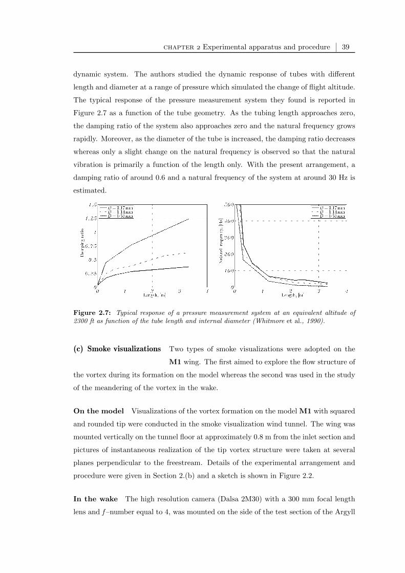
chapter Experimental apparatus and procedure 39
dynamic system. The authors studied the dynamic response of tubes with different
length and diameter at a range of pressure which simulated the change of flight altitude.
The typical response of the pressure measurement system they found is reported in
Figure 2.7 as a function of the tube geometry. As the tubing length approaches zero,
the damping ratio of the system also approaches zero and the natural frequency grows
rapidly. Moreover, as the diameter of the tube is increased, the damping ratio decreases
whereas only a slight change on the natural frequency is observed so that the natural
vibration is primarily a function of the length only. With the present arrangement, a
damping ratio of around 0.6 and a natural frequency of the system at around 30 Hz is
estimated.
Figure 2.7: Typical response of a pressure measurement system at an equivalent altitude of2300 ft as function of the tube length and internal diameter (Whitmore et al., 1990).
(c) Smoke visualizations Two types of smoke visualizations were adopted on the
M1 wing. The first aimed to explore the flow structure of
the vortex during its formation on the model whereas the second was used in the study
of the meandering of the vortex in the wake.
On the model Visualizations of the vortex formation on the model M1 with squared
and rounded tip were conducted in the smoke visualization wind tunnel. The wing was
mounted vertically on the tunnel floor at approximately 0.8 m from the inlet section and
pictures of instantaneous realization of the tip vortex structure were taken at several
planes perpendicular to the freestream. Details of the experimental arrangement and
procedure were given in Section 2.(b) and a sketch is shown in Figure 2.2.
In the wake The high resolution camera (Dalsa 2M30) with a 300 mm focal length
lens and f –number equal to 4, was mounted on the side of the test section of the Argyll
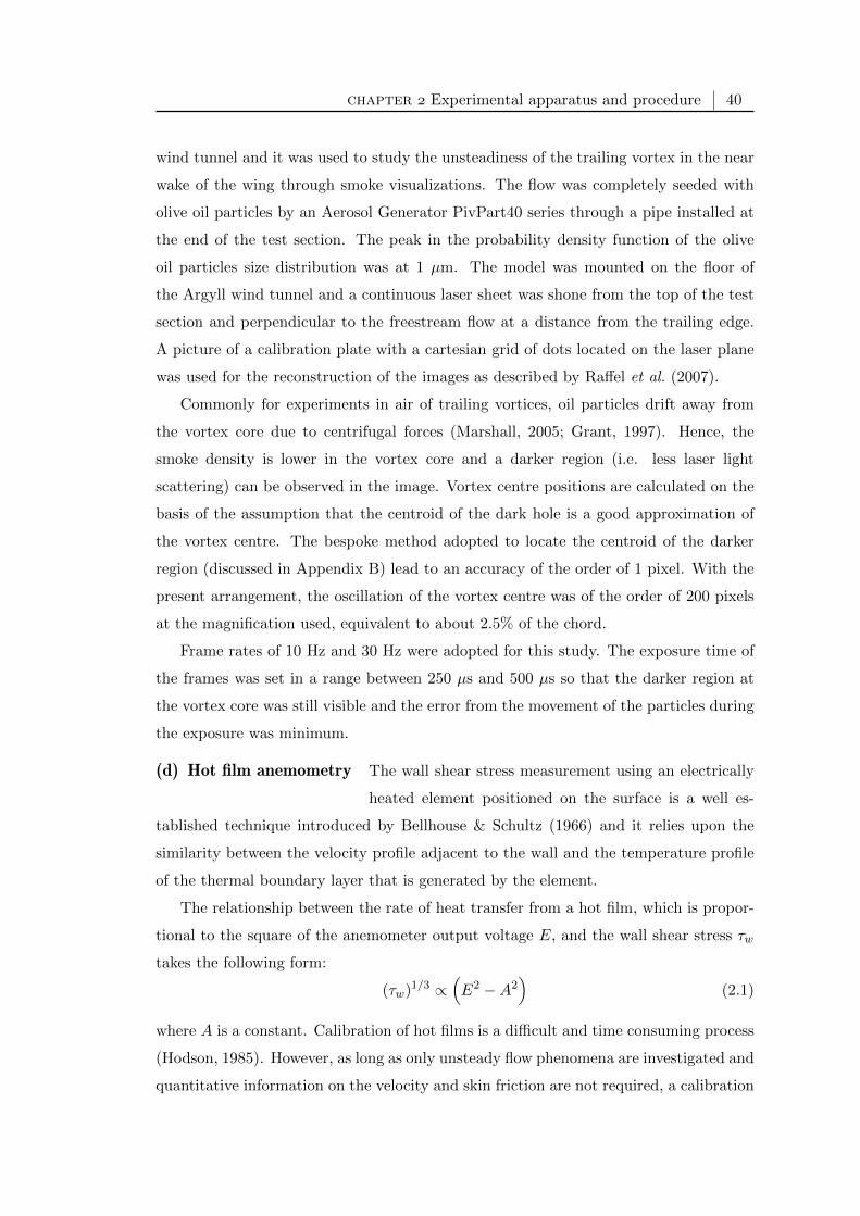
chapter Experimental apparatus and procedure 40
wind tunnel and it was used to study the unsteadiness of the trailing vortex in the near
wake of the wing through smoke visualizations. The flow was completely seeded with
olive oil particles by an Aerosol Generator PivPart40 series through a pipe installed at
the end of the test section. The peak in the probability density function of the olive
oil particles size distribution was at 1 µm. The model was mounted on the floor of
the Argyll wind tunnel and a continuous laser sheet was shone from the top of the test
section and perpendicular to the freestream flow at a distance from the trailing edge.
A picture of a calibration plate with a cartesian grid of dots located on the laser plane
was used for the reconstruction of the images as described by Raffel et al. (2007).
Commonly for experiments in air of trailing vortices, oil particles drift away from
the vortex core due to centrifugal forces (Marshall, 2005; Grant, 1997). Hence, the
smoke density is lower in the vortex core and a darker region (i.e. less laser light
scattering) can be observed in the image. Vortex centre positions are calculated on the
basis of the assumption that the centroid of the dark hole is a good approximation of
the vortex centre. The bespoke method adopted to locate the centroid of the darker
region (discussed in Appendix B) lead to an accuracy of the order of 1 pixel. With the
present arrangement, the oscillation of the vortex centre was of the order of 200 pixels
at the magnification used, equivalent to about 2.5% of the chord.
Frame rates of 10 Hz and 30 Hz were adopted for this study. The exposure time of
the frames was set in a range between 250 µs and 500 µs so that the darker region at
the vortex core was still visible and the error from the movement of the particles during
the exposure was minimum.
(d) Hot film anemometry The wall shear stress measurement using an electrically
heated element positioned on the surface is a well es-
tablished technique introduced by Bellhouse & Schultz (1966) and it relies upon the
similarity between the velocity profile adjacent to the wall and the temperature profile
of the thermal boundary layer that is generated by the element.
The relationship between the rate of heat transfer from a hot film, which is propor-
tional to the square of the anemometer output voltage E, and the wall shear stress τw
takes the following form:
(τw)1/3 ∝(E2 −A2
)(2.1)
where A is a constant. Calibration of hot films is a difficult and time consuming process
(Hodson, 1985). However, as long as only unsteady flow phenomena are investigated and
quantitative information on the velocity and skin friction are not required, a calibration

chapter Experimental apparatus and procedure 41
of the sensors is not necessary and surface mounted hot films can be satisfactorily
used to provide qualitative or semi–quantitative data (Haselback & Nitsche, 1996).
In the present work, signal frequency spectra and comparative analysis of the signal
fluctuations are presented.
Surface hot films (Dantec 55R47 glue–on probe) were deployed for the determination
of the degree of unsteadiness of the surface flow in the wingtip region. The sensors were
oriented perpendicular to the freestream direction and positioned near the wingtip.
They were operated with Dantec mini constant temperature anemometer (at a film
temperature of approximately 125C) and recorded at 1 KHz, with sampling time of 100
s and low–pass filter cutting frequency of 1 KHz. These studies focused on a frequency
range below 15 Hz and a high–pass filter cutting frequency of 0.1 Hz was employed as
a post–processing step. The film was glued for the duration of the experiment directly
onto the surface at the point of interest and the cables leading to the anemometer were
taped on the wing oriented as the freestream down to the trailing edge and then along
the trailing edge to the floor. The film was moved after each test to the next position.
(e) Stereoscopic particle
image velocimetry
In fluid dynamics history, an important evolution in the
investigation of flows was the replacement of passive ob-
servations of nature by experiments carefully planned to
extract information about a targeted phenomenon. One of the pioneers was Ludwig
Prandtl (1875–1953), who designed and utilized flow visualization techniques in a water
tunnel to study steady and unsteady separated flows behind wings and other objects.
At that time, only a qualitative description of the flow field was possible. With the sci-
entific and technical progress achieved in the last 30 years in optics, lasers, electronics,
imaging technology and computer hardware, it is now possible to extract quantitative
information on the instantaneous velocity fields exactly from the same kind of images
available more than a century ago to Prandtl (Raffel et al., 2007).
Particle image velocimetry (PIV) is part of a broader class of velocity measurement
techniques called pulsed–light velocimetry (PLV) which measures the motion of small,
marked regions of a fluid by comparing the locations of the images of the markers at
two or more times (Adrian, 1991). Such techniques can differ in many ways such as in
type, dimension and density of markers; duration and number of light pulses; type and
number of light sources; type, framing rate and number of recording devices; processing
technique of the images. The estimation of the local velocity vector u is based on the
chapter Experimental apparatus and procedure 42
(first order of the) fundamental definition of velocity
u(x, t).=
∆x(x, t)
∆t(2.2)
where ∆x is the displacement of a marker, located in x at time t, and ∆t is the time
interval separating two observations of the marker. As ∆t approaches to zero, the limit
of u is the instantaneous local velocity.
With recording and laser devices outside the tunnel, particle image velocimetry is
a non intrusive method for instantaneous velocity measurements. In contrast to more
traditional single point measurement techniques (such has with hot wires or pressure
probes), the PIV technique provides an analysis of a flow field without disturbing the
flow with probes. Furthermore, PIV is a whole field technique that allows the recording
of images of an extended region of the flow field and the extraction of the instantaneous
velocity vector information out of these images. The majority of all the other techniques
for velocity measurements only allows the measurement of the velocity of the flow at
a single point, in most cases at a high temporal resolution. The spatial resolution of
PIV can be very large, whereas the temporal resolution (frame rate of image recording)
may be limited due to current technological restrictions on laser frequency, camera
architecture or data transfer speed.
Nowadays, the PIV technique is commonly based on a planar laser light sheet, which
is pulsed twice on a wide portion of the flow. The flow is seeded with fine markers and
images of these particles lying in the light sheet are recorded on a video camera. The
displacement of the particle between the two laser pulses is measured on the image
plane and is used to determine the displacement of the particles in the flow. The most
common way to measure the particles shift is to divide the first image into small interro-
gation windows and to cross–correlate each one of them with the respective interrogation
window on the second image. The cross–correlation produces a peak corresponding to
the average displacement vector of the particles inside the interrogation cell. The ve-
locity associated with each interrogation spot is simply the displacement divided by
the time delay between the two laser pulses. Despite the recognized maturity of the
cross–correlation based methods, PIV image processing algorithms have continuously
been improved during the past decades. Comprehensive overviews of the situation were
presented by Keane & Adrian (1992), Grant (1997) and Raffel et al. (2007).
If the flow is highly three–dimensional, the velocity component perpendicular to the
laser sheet can be a source of error in the measured velocity up to more than 15% of

chapter Experimental apparatus and procedure 43
the mean flow velocity (Raffel et al., 2007). The error is due to the dependence of the
in–plane projection of the velocity vector on the viewing direction and on the out–of–
plane component. A variety of approaches capable of recovering the complete set of
velocity components have been described in the literature (Hinsch, 1995). Stereoscopic
particle image velocimetry (SPIV) is based on the same fundamental concepts of PIV
but it is capable to evaluate all the three components of the velocity vector from a two–
dimensional slice of the flow field. This method generally employs at least two imaging
systems to record simultaneous but distinct off–axis views of the same region of interest.
Two pairs of images are recorded at the same time by the two cameras. Each pair is
analysed independently to derive two in–plane velocity fields. Knowing the perspective
angles between the imaging systems and the measuring plane, the cross flow velocity
component can also be derived (see for example Lawson & Wu, 1997; Prasad, 2000).
Moreover, SPIV is known to produce more accurate measurements also of the in–plane
velocity components in the flow field than the PIV.
A commercial PIV system (LaVision) was used for experiments on model M1 and
M2 in the Argyll wind tunnel. A variety of configurations of the wings were tested
and several planes in the wake and close to the surface of the model were studied for
a detailed quantitative understanding of the evolution of the vortex system from the
model to the early wake. A summary of all the SPIV experiments is presented in Table
2.3. In the present dissertation, not all these configurations are discussed, although all
of them were analysed and compared during this study.
The general experimental setup of SPIV tests is presented here following the sub-
system sectioning proposed by Raffel et al. (2007). Some of the elements of the SPIV
system can be seen in the pictures of Figure 2.8.
Laser A Litron double cavity, Nd:YAG laser, Q–switched to produce 0.5 J pulses of
8 ns duration and 532 nm wavelength was used. The laser frequency, corresponding to
the acquisition frequency of the recorded images, was kept constant at 2 Hz.
A number of mirrors and a laser guiding arm were used for delivering the laser beam
to the divergent lens which was mounted on a camera head installed on a system of
two rails above the test section. This arrangement allows two–dimensional translations
and three–axes rotations of the laser sheet covering a wide range of the test section.
Depending on the field of view required, a divergent lens with focal length of -20 mm
or -10 mm was installed which generated a 3 mm thick lens sheet.
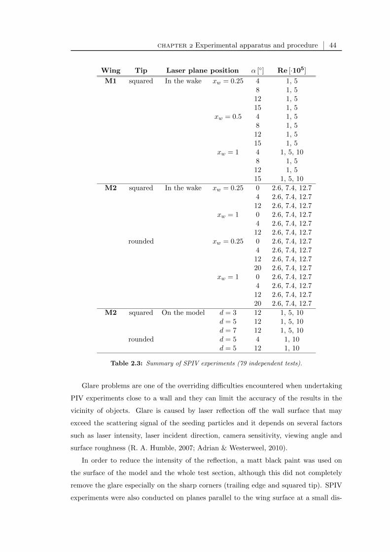
chapter Experimental apparatus and procedure 44
Wing Tip Laser plane position α [] Re [·105]
M1 squared In the wake xw = 0.25 4 1, 58 1, 512 1, 515 1, 5
xw = 0.5 4 1, 58 1, 512 1, 515 1, 5
xw = 1 4 1, 5, 108 1, 512 1, 515 1, 5, 10
M2 squared In the wake xw = 0.25 0 2.6, 7.4, 12.74 2.6, 7.4, 12.712 2.6, 7.4, 12.7
xw = 1 0 2.6, 7.4, 12.74 2.6, 7.4, 12.712 2.6, 7.4, 12.7
rounded xw = 0.25 0 2.6, 7.4, 12.74 2.6, 7.4, 12.712 2.6, 7.4, 12.720 2.6, 7.4, 12.7
xw = 1 0 2.6, 7.4, 12.74 2.6, 7.4, 12.712 2.6, 7.4, 12.720 2.6, 7.4, 12.7
M2 squared On the model d = 3 12 1, 5, 10d = 5 12 1, 5, 10d = 7 12 1, 5, 10
rounded d = 5 4 1, 10d = 5 12 1, 10
Table 2.3: Summary of SPIV experiments (79 independent tests).
Glare problems are one of the overriding difficulties encountered when undertaking
PIV experiments close to a wall and they can limit the accuracy of the results in the
vicinity of objects. Glare is caused by laser reflection off the wall surface that may
exceed the scattering signal of the seeding particles and it depends on several factors
such as laser intensity, laser incident direction, camera sensitivity, viewing angle and
surface roughness (R. A. Humble, 2007; Adrian & Westerweel, 2010).
In order to reduce the intensity of the reflection, a matt black paint was used on
the surface of the model and the whole test section, although this did not completely
remove the glare especially on the sharp corners (trailing edge and squared tip). SPIV
experiments were also conducted on planes parallel to the wing surface at a small dis-

chapter Experimental apparatus and procedure 45
(a) Imager pro X camera mounted outside the testsection.
(b) Laser beam delivery system.
Figure 2.8: Camera mounting and laser delivery for SPIV experiments.
tance from it. For this arrangement, the laser sheet was accurately positioned so that it
did not generate glare with the exception of some spots near the trailing edge. However,
the effect of the glare on the results is minimum and it is discussed in Section 3.4.
Tracer The PIV technique measures flow velocity indirectly, that is from the tracer
displacements. Therefore, the dynamics of the seeding particles has to be studied to
avoid significant errors in the velocity evaluation and the assumption that the tracer par-
ticles suspended in the flow faithfully follow the fluid motion has to be valid (Melling,
1997). Moreover, the light scattering property of the particles is another important
aspect in the selection of the tracer. Raffel et al. (2007) treat these topics remark-
ing the compromise that has to be found between a very small particle which ensures
good tracking of the fluid motion and a particle which is big enough to ensure a good
light scattering. They also present the most common solutions for several experimental
conditions and flow features.
In the current investigation, the entire flow was seeded through a pipe mounted
downstream of the test section with olive oil particles generated by the Laskin Nozzle
Aerosol Generator PivPart40 series. The nominal peak in the probability density func-
tion of the olive oil particles size distribution is at 1 µm (PIVTEC, 2007). However,
as explained by Adrian (1991), the effective particle diameter on the image plane is a
function of the physical particle diameter and the point response function of the lens.
For a reference case of the present experiments, it is found that the particle size on the

chapter Experimental apparatus and procedure 46
image plane is approximately independent of the physical particle size and it is equal
to a value around 90 µm which corresponds to a value between one and two pixels on
the object plane. This choice of seeding leads to a satisfactory behaviour of the tracer
and a good quality of the results.
Another important aspect about the seeding is the particle density. The probability
of a correct displacement evaluation is increasing with the number of particles present
in both the interrogation windows during the correlation. This number depends on the
overall particle density, the amount of in–plane displacement, the amount of out–of–
plane displacement and the image processing procedure (Keane & Adrian, 1992). A
higher number of particle pairs increases the signal strength of the correlation peak.
However, the particle density is limited to a maximum by the contrast of the PIV
recording system. In general, a densely seeded flow ensures high valid detection rate and
low measurement uncertainty. Additionally, it allows the use of smaller interrogation
windows which ensures higher spatial resolution.
Cameras Two Imager pro X, 11 Megapixel cameras (CCD chip of 4008 by 2672 pixels)
with 9 µm pixel size were used and DaVis 7.2, the software accompanying the LaVision
system, was used to synchronize laser and cameras. A range of Nikon lenses (200 mm
and 300 mm focal length with f –number equal to 4) were used to obtain the required
field of view during each test.
The cameras were mounted outside the test section and arranged in angular dis-
placement arrangement (Prasad, 2000) for greater measurement accuracy of the veloc-
ity components (Lawson & Wu, 1997). Depending on the orientation and positioning
of the laser plane, the cameras were installed on the two sides of the test section or
on the same side. Camera perspective angles were determined by DaVis 7.2 software
during the calibration procedure and the angles between cameras and the object plane
were in a range which ensures low errors in the evaluation of both the in–plane and
out–of–plane velocity components, based on Lawson & Wu (1997) analysis.
The focusing of the PIV cameras on the required region of interest was performed
manually; manual Scheimpflug adaptors were used to ensure uniform magnification
gradients across the image obtaining images in good focus over the entire image plane
(Prasad & Jensen, 1995).
Calibration of the cameras Calibration of PIV systems is accomplished to relate
the camera chip coordinate with the physical coordinates of the flow field and to pro-

chapter Experimental apparatus and procedure 47
vide transfer functions which are necessary to convert the derived pixel displacements
to physical particle displacements. LaVision FlowMaster software was used to perform
the SPIV calibration based on a three–dimensional calibration–based (pinhole) recon-
struction (Prasad, 2000; DaVis, 2007). This approach uses a spotted board (calibration
plate) with known geometrical properties. The board presents a cartesian grid of dots
positioned on two levels (three–dimensional calibration plate) in known positions and
it is located on the object plane (i.e. laser plane). With the system in the experi-
ment configuration (usually just before the measurements), a number of images is taken
from each camera. The accuracy of this calibration is improved by taking more than
one image in a neighborhood of the laser plane by slightly rotating or translating the
calibration plate. The average deviation of the dewarped marker position to the ideal
regular grid was around 0.5 pixels which is below the suggested limit for a good cali-
bration process (DaVis, 2007). Focal length of camera lenses, distance from cameras to
calibration plate and camera viewing angles of the calibration plate are all calculated
during the calibration process.
Laser pulses separation Time separation between successive laser pulses is an im-
portant parameter that has to be optimized during PIV measurements. Prior knowledge
of the flow field (i.e. maximum and minimum velocities, velocity gradients and flow di-
rection), interrogation window size, laser sheet thickness, correlation process are the
most important factors among the many involved in the calculation of the optimum
pulse separation (Raffel et al., 2007).
As described by Boillot & Prasad (1996), the restrictions change if the correlation
is an auto–correlation (two pulses on the same frame) or a cross–correlation (two pulses
on two different frames). In cross–correlations the delay time is less dependent on the
interrogation spot size because the correlation can involve interrogation window shifting
and deformation (Scarano, 2002). Furthermore Keane & Adrian (1990) showed that
generally, to achieve a valid detection probability of at least 90%, the image density
(defined as the mean number of particles per interrogation window) must be greater
than 15 and the average particle displacement must be limited to less than 30% of the
interrogation window size (Boillot & Prasad, 1996).
Although several calculation methods of the pulse separation can be found in the
literature (Adrian, 1988; Keane & Adrian, 1990; Boillot & Prasad, 1996; Raffel et al.,
2007), “it is advisible to apply a quick–look evaluation during recording for the opti-
mization of the experimental parameters” (Raffel et al., 2007, p. 95). In the current
chapter Experimental apparatus and procedure 48
study, a simple calculation method was used for a preliminary estimation of the pulse
separation which was then adjusted by observations of the resulting vector fields. In
Appendix A.1, the pulses delay calculation and optimization is applied on a reference
case of a wingtip vortex.
Image processing procedure The analysis of the recorded image is one of the most
important steps in the entire process, as it couples with the acquisition process to
determine the accuracy, reliability, and spatial resolution of the measurement; usually, it
is also the most time–consuming part of the process (Adrian, 1991). A typical procedure
for the vector field computation of a SPIV is reported in Figure 2.9. For a the stereo
cross–correlation, each acquisition consists of four images: two single–exposed frames
with a time interval ∆t from each of the two cameras. Each frame is then dewarped
through the mapping function and segmented into interrogation windows with set initial
size, weight and overlapping values. Each interrogation window is cross–correlated with
the corresponding region, shifting based on a reference vector field, on the second frame
from the same camera. The highest peak in the cross–correlation image is the most likely
displacement vector and it is used to calculate the velocity vector of that interrogation
window. After this operation, a pair of two–dimensional two–components vector fields
(2D2C) is obtained. From the two planar vector fields, the stereoscopic reconstruction of
a two–dimensional three–components vector field (2D3C) is accomplished. The vectors,
after a validation process, are then projected into planar vector fields which are used
as references for a new cross–correlation with different interrogation window size and
overlapping values. This loop is repeated accordingly to the multi–pass processing
procedure adopted. No need for vector post–processing was seen on the final vector
fields. A median filter with vector removal and iterative replacement, a fill–up process
by interpolation and a 3x3 smoothing filter on the vector field was applied only between
each step of the multi–pass iterations. This implies a good quality of the seeding and
of the images giving a high level of reliability to these experiments.
DaVis 7.2 was used for the processing of the images and the calculation of the
vector fields, whereas Matlab codes were written for the analysis of the results. The
compromise between results accuracy, spatial resolution, processing time and memory
requirement was found with a stereo cross–correlation of the image pairs composed of a
double step process on an interrogation window of 64 by 64 pixels with 25% of overlap
followed by other two steps with interrogation window of 32 by 32 pixels with 50%
of overlap. Tests on the image processing parameters (i.e. overlapping, interrogation

chapter Experimental apparatus and procedure 49
Figure 2.9: Vector field computation flow chart of a two pulses two frames SPIV.
window size, number of iterations) which led to the optimum compromise are reported
in Appendix A.2. A standard cyclic FFT–based cross–correlation algorithm was used
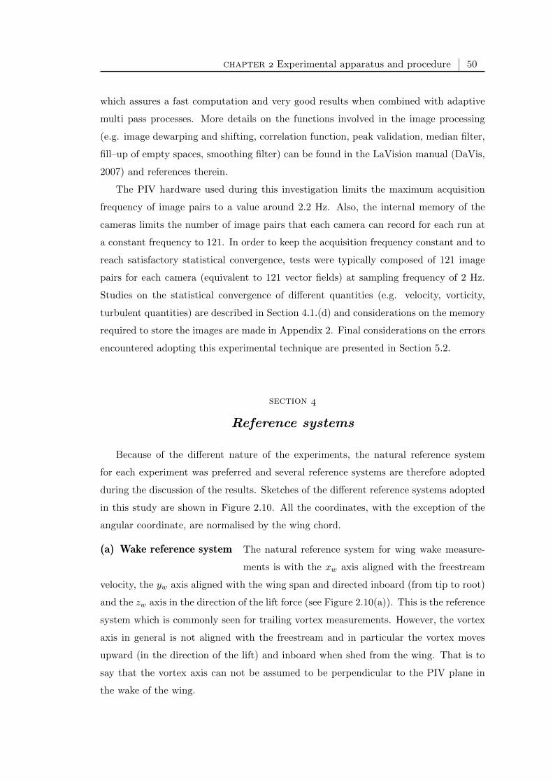
chapter Experimental apparatus and procedure 50
which assures a fast computation and very good results when combined with adaptive
multi pass processes. More details on the functions involved in the image processing
(e.g. image dewarping and shifting, correlation function, peak validation, median filter,
fill–up of empty spaces, smoothing filter) can be found in the LaVision manual (DaVis,
2007) and references therein.
The PIV hardware used during this investigation limits the maximum acquisition
frequency of image pairs to a value around 2.2 Hz. Also, the internal memory of the
cameras limits the number of image pairs that each camera can record for each run at
a constant frequency to 121. In order to keep the acquisition frequency constant and to
reach satisfactory statistical convergence, tests were typically composed of 121 image
pairs for each camera (equivalent to 121 vector fields) at sampling frequency of 2 Hz.
Studies on the statistical convergence of different quantities (e.g. velocity, vorticity,
turbulent quantities) are described in Section 4.1.(d) and considerations on the memory
required to store the images are made in Appendix 2. Final considerations on the errors
encountered adopting this experimental technique are presented in Section 5.2.
section
Reference systems
Because of the different nature of the experiments, the natural reference system
for each experiment was preferred and several reference systems are therefore adopted
during the discussion of the results. Sketches of the different reference systems adopted
in this study are shown in Figure 2.10. All the coordinates, with the exception of the
angular coordinate, are normalised by the wing chord.
(a) Wake reference system The natural reference system for wing wake measure-
ments is with the xw axis aligned with the freestream
velocity, the yw axis aligned with the wing span and directed inboard (from tip to root)
and the zw axis in the direction of the lift force (see Figure 2.10(a)). This is the reference
system which is commonly seen for trailing vortex measurements. However, the vortex
axis in general is not aligned with the freestream and in particular the vortex moves
upward (in the direction of the lift) and inboard when shed from the wing. That is to
say that the vortex axis can not be assumed to be perpendicular to the PIV plane in
the wake of the wing.
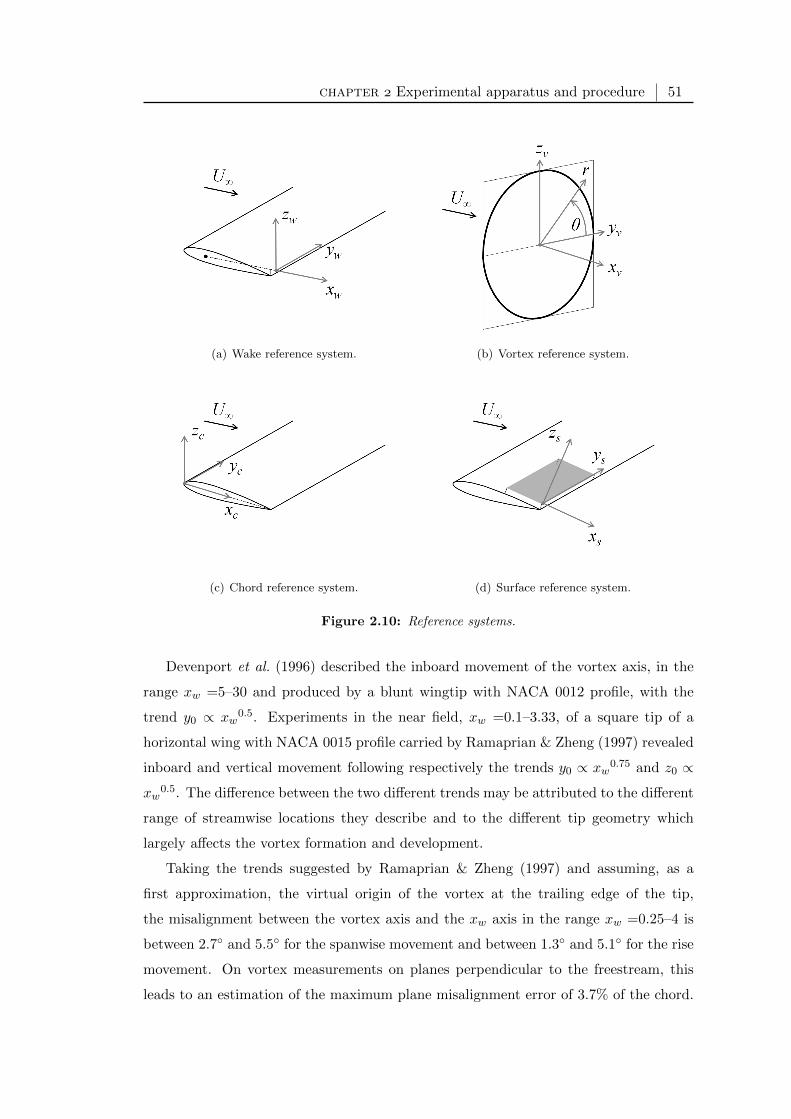
chapter Experimental apparatus and procedure 51
(a) Wake reference system. (b) Vortex reference system.
(c) Chord reference system. (d) Surface reference system.
Figure 2.10: Reference systems.
Devenport et al. (1996) described the inboard movement of the vortex axis, in the
range xw =5–30 and produced by a blunt wingtip with NACA 0012 profile, with the
trend y0 ∝ xw0.5. Experiments in the near field, xw =0.1–3.33, of a square tip of a
horizontal wing with NACA 0015 profile carried by Ramaprian & Zheng (1997) revealed
inboard and vertical movement following respectively the trends y0 ∝ xw0.75 and z0 ∝
xw0.5. The difference between the two different trends may be attributed to the different
range of streamwise locations they describe and to the different tip geometry which
largely affects the vortex formation and development.
Taking the trends suggested by Ramaprian & Zheng (1997) and assuming, as a
first approximation, the virtual origin of the vortex at the trailing edge of the tip,
the misalignment between the vortex axis and the xw axis in the range xw =0.25–4 is
between 2.7 and 5.5 for the spanwise movement and between 1.3 and 5.1 for the rise
movement. On vortex measurements on planes perpendicular to the freestream, this
leads to an estimation of the maximum plane misalignment error of 3.7% of the chord.

chapter Experimental apparatus and procedure 52
This error corresponds to the maximum displacement between the measurement plane
and the vortex plane (plane perpendicular to the vortex axis) found at a distance of
0.25 chords from the vortex centre at xw = 0.25.
Assuming an axisymmetric vortex which axis follows the analytical trends, this mis-
alignment corresponds to assume velocity vectors which are at 0.074 chords of distance
along the freestream direction as they were on the same plane (this distance rapidly
decreases moving downstream). This distance is small compared to the length scales of
the axial evolution of the vortex and therefore the misalignment error is negligible.
The origin of this reference system is at the trailing edge of the tip at an angle
of attack of α = 0 so that the actual distance from the trailing edge changes as
0.75 c · (1− cosα), which corresponds to 1.6% of the chord for an angle of attack of 12.
(b) Vortex reference
system
A vortex can be described either with a cartesian coordinate
system or a cylindrical system (see Figure 2.10(b)). The first
shows xv on the vortex axis and the yv and zv axes on the
vortex plane, the first directed as the wing span and the latter perpendicular to the
two and directed as the lift. The cylindrical coordinate r is the radial coordinate with
origin at the centre of the vortex and θ the angular coordinate which is 0 on the yv axis.
The relation between the two reference systems and the relations of velocity vectors and
Reynolds stresses expressed in the two reference frames are given in Appendix C.4.
The misalignment error between the freestream and the vortex axis is discussed in
the previous section and the assumption of local alignment of vortex axis and freestream
is used throughout, that is xw ≡ xv, yw ≡ yv and zw ≡ zv.
(c) Wing chord reference
system
For point measurements on the wing (i.e. hot film and
pressure tappings) and for measurements on planes on
the wing and perpendicular to the freestream (i.e. flow
visualizations), the reference system adopted has the origin at the leading edge of the
tip, the xc axis aligned with the chord, yc aligned with the span and pointing towards the
root and zc perpendicular to the two (see Figure 2.10(c)). This is not a fixed reference
system but is rotates with the angle of attack. The xc coordinate is 0 at the leading
edge and 1 at the trailing edge; yc is 0 at the tip and equal to the aspect ratio at the
root. Negative values of yc occur at the tip region when it is not squared.
chapter Experimental apparatus and procedure 53
(d) Wing surface reference
system
For measurements on planes parallel to the wing sur-
face, xs is the curvilinear coordinate which follows the
surface and has origin at the tip trailing edge (see Fig-
ure 2.10(d)). The ys axis is aligned with the span and zs is directed perpendicular to
the wing surface and away from it. Because the surface curvature of the last 40% of
a symmetric NACA profile is small and the tangent angle is also small, the difference
between xs and xc is below 1% in that region. Therefore, the comparison of mea-
surements on these two reference systems without a conversion can be done without
incurring significant errors.
chapter
Wingtip vortex formation
The human mind is generally far more eager to praise
and dispraise than to describe and define.
Clive Staples Lewis
The trailing vortex forms along the tip of the wing and the behaviour and charac-
teristics of the trailing vortex in the wake are strongly affected by the initial process. In
particular, the wing layout, wingtip geometry, wing load distribution, Reynolds number
and boundary layer on the wing are important factors in the formation of a trailing
vortex.
Moreover, changes in the vortex structure and decay characteristics are usually ac-
complished by changes on the wing. All the wingtip vortex control devices are related
to the vortex during its formation and development on the wing. Therefore, the effec-
tiveness of such devices depends upon a correct understanding of the physics of the flow
at the wingtip.
The wing configuration and the tip geometry have a big impact on the initial process,
particularly on the swirl and axial velocity distribution of the vortex in the very early
wake (Green, 1995). Baker et al. (1974) and Devenport et al. (1996) believe that the
vortex wandering is due to the freestream turbulence which has a beneficial effect as
it enhances the vortex rate of decay (Sharpkaya & Daly, 1987). Bailey & Tavoularis
(2008) tested several turbulence grids for the incoming flow over an airfoil and they
showed that an increase of the freestream turbulence resulted in an increase of the
amplitude of vortex wandering. Also, they observed that for the no–grid case there
could be multiple sources of the wandering, each with a different range of dominant
frequency including frequencies lower than 2 Hz. Jacquin et al. (2001) presented the
meandering as a consequence of several phenomena such as line vortex instabilities,
entrained turbulence from the rolling up or propagation of unsteadiness originated by
54
chapter Wingtip vortex formation 55
the model. Green & Acosta (1991) considered also the possibility of several vortex core
instabilities. Beresh & Henfling (2010) indicated that the meandering can be induced
by an external source to the vortex itself suggesting that the meandering is already
present on the surface, prior to vortex shedding.
Whereas several studies on the meandering of the vortex in the wake can be found,
there is obviously a lot missing on the unsteadiness of the vortex when forming on the
model and also on the possible links between the two stages. Common methods for
disturbing the vortex flow in its early stage are based on changes in the tip geometry
which result in complicated flowfields which are often too challenging for a detailed
computational study. Therefore, the study and evaluation of these devices are mainly
experimental and go usually through several adjustments based on the experience and
intuitions of the designer. A characterization method of the flow is needed for the
description of the mechanism of the formation of a tip vortex.
Moreover, understanding the relationship between meandering and unsteadiness of
the vortex in the wake with the unsteadiness of the flow on the wing is one of the key
steps of vortex control. Beside passive (static) vortex control methods based mainly on
changes in the wing configuration (vortex generators, winglets, wingtip–mounted pro-
pellers, different tip geometries), several active (dynamic) methods have been recently
deployed where continuous or periodic controls are adopted such as blowing (Heyes
& Smith, 2004; Gursul et al., 2007), oscillating flaps (Haverkamp et al., 2005; Gupta,
2011; Breitsamter & Allen, 2009), dynamic Gurney flaps (Greenblatt & Meyer, 2009),
boundary layer separation control (Greenblatt, 2005) and surface–mounted actuators
(Quackenbush et al., 1999). The often poor efficiency of control techniques can be in
great part attributed to insufficient knowledge of breakdown. Mitchell & Delery (2001)
pointed out that the difficulty in adopting periodic control devices is to identify charac-
teristic frequencies in the vortical structure in order to adjust the position and intensity
of such control actions. Information on those frequencies, which play a big role in the
excitation of vortex instabilities, is still lacking.
The aim of this chapter is to enlighten on the mechanisms that lead to the formation
of a wingtip vortex. The link between the unsteadiness of the vortex formation on the
wing and its development in the early wake is also addressed. Different experimental
techniques are applied on the wingtip vortex formation on a rectangular wing with
squared and rounded tip. A number of techniques have been adopted for these studies in
the past decades and information from each of these methods revealed different aspects
of the tip vortex flow. The combined description of different flow features provides a

chapter Wingtip vortex formation 56
greater insight into the interaction phenomena (Pagendarm & Walter, 1994) because
each technique gives a compact and meaningful representation of a selected feature in
the data.
An initial study of the vortex footprint on the wing surface is accomplished by
surface oil flow visualizations and presented in Section 3.1. In Section 3.2, pressure
measurements on the wing surface give a quantitative description of the vortex foot-
print and analysis on the unsteadiness of the pressure measurements near the wingtip
reveal the unsteady nature of the vortex system. After an overview of the vortex main
features, a bigger scale model is adopted in order to highlight the rolling up mechanism
and the dynamics of the multi–vortex structure through smoke visualizations presented
in Section 3.3. In Section 3.4 stereoscopic particle image velocimetry on planes paral-
lel to the wing surface are presented with a new method for the identification of the
vortex structure. Section 3.5 discusses the unsteadiness of the vortical structure on the
wing surface which is measured by wall–mounted hot film probes. Analysis of signal
spectra show intense contributes on the vortex movement at low frequencies. Low fre-
quencies, calculated from video recordings of smoke visualizations, are found also in the
unsteadiness of the vortex in the early wake and presented in Section 3.6.
section
Surface oil flow visualization
In order to gather general information on the limiting streamlines of a typical wingtip
vortex during its formation on the wing, surface oil flow visualizations are presented for
model M1 installed in the Argyll wind tunnel at Reynolds number of 5 · 105 and angle
of attack of 12 in Figures 3.1 and 3.2. Pictures show a darker colour where the oil
is accumulated. The assumption of oil film pattern well representing the actual wall
streamlines is valid when the pressure gradient is small compared with the skin friction
(Merzkirch, 1987). Therefore, this kind of visualization is a very good tool for a visual
understanding of the structure of the surface flow but might become not very accurate
in determining the position of separation and reattachment lines. Also, differently
from patterns observed for delta wings where convergence and divergence of wall shear
stress lines clearly show separation and reattachment lines (Taylor & Gursul, 2004),
rectangular wingtip vortices are less intense than delta wing vortices and the flow in
the tip region is dominated by the streamwise component of the velocity vector. For
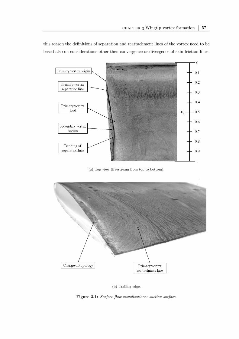
chapter Wingtip vortex formation 57
this reason the definitions of separation and reattachment lines of the vortex need to be
based also on considerations other then convergence or divergence of skin friction lines.
(a) Top view (freestream from top to bottom).
(b) Trailing edge.
Figure 3.1: Surface flow visualizations: suction surface.

chapter Wingtip vortex formation 58
Figure 3.2: Surface flow visualizations: tip surface (freestream from left to right).
A strongly three–dimensional flow is observed near the tip region. The primary
vortex origins at around xc = 0.2 (from the top view in Figure 3.1(a)) which is where
the flow crosses over the sharp edge of the tip and moves inboard. The primary vor-
tex separation line is indicated by an accumulation of pigment (convergence line) and
its distance from the tip grows linearly until xc = 0.75 where it bends toward the tip
suggesting a change of vortex structure topology. Unlike typical two–dimensional sepa-
rations, the skin friction magnitude is not zero along this line (due to the presence of a
streamwise component of the velocity). Tobak & Peake (1982) referred to this type of
line as indicative of local separations (or open separations). The peculiar characteristic
of this kind of separation is that there are no singular points in the skin friction line
topology. Additionally, there is no zone of stagnant fluid or reversed flow in the xc
direction which typically occurs in flows which are globally separated (for more details,
see for example Zilliac (1988) and Delery (2001)). The region between the primary vor-
tex separation line and the tip is occupied by a counter rotating secondary vortex. It is
the combination of the primary and secondary vortices induced flow on the surface that
produces the accumulation of pigment. The foot of the primary vortex (where the vor-
tex streamlines on the vortex plane are parallel to the surface) is identified by a region
of maximum chordwise gradient of the skin friction lines on the right of the separation
line. The primary vortex reattachment line can be identified, as a first approximation,
chapter Wingtip vortex formation 59
by the region where limiting streamlines bend toward the tip as shown in Figure 3.1(b).
Despite the simple geometry, vortices from squared tips reveal a complicated flow
structure due to the two sharp edges which induce separations of the flow. From the tip
side (Figure 3.2), the presence of a divergent and a convergent line suggests the presence
of another system of vortices which interacts with the primary and secondary vortices
on the suction surface. Both these lines start from the leading edge: the divergent line
ends on the top edge at around xc = 0.6; the convergent line ends at the trailing edge.
The region between the two lines is occupied by a vortex which grows along the chord
and, interacting with the vortices on the suction surface, contributes to the change of
topology of the vortex structure.
section
Pressure on the wing surface
Results on the effect of the angle of attack on the pressure distribution in the vicinity
of the squared wingtip of the M1 model are presented. In this section, the high aspect
ratio guarantees a vortex structure which is not influenced by the presence of the wall.
The wing is tested at angles of incidence of 0, 4, 8, 12 and 15 and Reynolds number
of 5 · 105.
Signals from the pressure tappings are recorded on a sampling window of 2 seconds
which was observed to satisfy the convergence of the average pressure. A sampling
frequency of 1 KHz was adopted and a moving average is applied as low–pass filter
with cutting frequency of 30 Hz accordingly to the estimated bandwidth of the pressure
measurement system (see Section 2.(b)). The averaged surface pressure coefficients are
calculated as follows:
cP =P − P∞1
2ρU∞
2(3.1)
Frequency studies from pressure measurements through long pipes are also presented
although they can be affected by several errors and generally they are not very reliable.
However, indications on the wall pressure unsteadiness are useful in drawing preliminary
observations on the phenomenon. The fluctuation of the signal from selected pressure
tappings indicates the unsteady nature of the vortex flow on the wing surface at low
frequencies.

chapter Wingtip vortex formation 60
(a) Average pressure
distribution
Averaged pressure coefficients contours from the pressure,
suction and tip surfaces are plotted respectively in Figures
3.3(a), 3.3(b) and 3.4 for the wing at α = 12. Cubic inter-
polation of the data is applied for such contours.
The pressure coefficient on the pressure side of the wing shows a stagnation line
(white region) nearly straight across most of the wing at an average distance from the
leading edge of 3% of the chord. The flow approaches two–dimensional behaviour from
yc > 0.5. Near the tip of the wing, the flow becomes three–dimensional; the flow in the
direction of the tip is induced by the favorable pressure gradient in the yc direction.
The sharp edge of the squared tip geometry forces the flow to separate at the tip and
to form the tip side vortex structure observed in the surface flow visualizations.
Similarly, on the suction side of the wing (Figure 3.3(b)), the pressure coefficient
contour is two–dimensional for yc > 0.5. At the leading edge, a suction peak is observed
and the minimum surface pressure coefficient is -3.11 which is found at the tapping row
F (the most inboard array). The footprint of the wingtip vortex on the wing surface
appears as a suction region which is shaped as a vertical region at around yc = 0.07.
This region widens moving toward the trailing edge and it includes pressure tapping
rows T2 and T3. The integrated effect of the vortex is to produce an increase in the
lift distribution over the region near the wingtip (McAlister & Takahashi, 1991). The
spatial resolution limitations of these measurements can not clearly confirm a secondary
suction peak due to the secondary vortex.
Because the vortex flow over a squared tip encounters abrupt separations at the
sharp edges, the resulting surface pressure distribution is not smooth when crossing
from the pressure to the tip surface and from the tip to the suction surface. Chow
et al. (1997a) described the pressure distribution over a wing with rounded tip. A
very different distribution of the pressure on the tip surface is found. The rounded tip
geometry generates a tip vortex which does not separate abruptly and the pressure on
the suction surface shows a smoother distribution.
On the tip surface (Figure 3.4) the pressure information is limited by the pressure
tappings position to a region around the symmetry plane. The low pressure region
developing from around xc = 0.3 (green colour) might indicate the growing of the tip
vortex system observed also in the surface oil flow visualization of Figure 3.2.
The effect of the angle of attack on the surface pressure is observed in Figure 3.5
where the suction surface pressure distribution is reported for angles of attack of 4,
8, 12 and 15. The increase of the suction peak at the trailing edge with the angle of

chapter Wingtip vortex formation 61
(a) Pressure surface.
(b) Suction surface.
Figure 3.3: Pressure coefficient distribution and pressure tappings at Re = 5 ·105 and α = 12:suction and pressure surface.

chapter Wingtip vortex formation 62
Figure 3.4: Pressure coefficient distribution and pressure tappings at Re = 5 ·105 and α = 12:tip surface. The circles correspond to the pressure tapping positions.
attack is clearly observed. Although the region affected by the presence of the tip vortex
shows a similar size in the yc direction at all the angles of attack, the suction peak due
to the vortex (and therefore the vortex intensity) increases from around cP = −0.5 for
α = 4 to cP = −1.5 at α = 15. Also, the extension in the xc direction grows with the
angle of incidence and it indicates an earlier initial rolling up of fluid for higher angles.
The apparent suction around the origin of the reference system is believed to be a result
of the interpolation.
The earlier initial rolling up at higher angles of attack is confirmed by the behaviour
of the pressure distribution along the pressure tappings row T1 on the mid plane of
the tip surface (Figure 3.6). Peaks are observed between xc = 0.4 and 0.6 and they
grow and move toward the leading edge as the angle of attack increases. This peak is
attributed to the suction caused by the vortex growing on the tip surface and originated
by the separation of the lower sharp edge. The peak on the pressure tapping near the
leading edge might be caused by a local separation of the flow.
McAlister & Takahashi (1991) presented a large parametric study of wing pressure
distributions for a rectangular wing with NACA 0015 profile. The pressure distribution
on a wing with aspect ratio of 3.3, chord of 0.52 m and squared tip is presented in
Figure 3.7. A gradual reduction in the suction peak as the tip of the wing is approached
is observed. A distortion over the suction surface is also observed for yc < 0.1 which
generates an increase in the lift over the region near the wingtip. In Figure 3.7(f), the
pressure curve exhibits two strong undulations which were linked to the presence of
the secondary vortex. The Reynolds number appeared to have a smaller effect on the
pressure undulations in the squared tip case than in the rounded tip case. This apparent
insensitivity is believed to be due to the transition fixing nature of the sharp edge.

chapter Wingtip vortex formation 63
(a) α = 4. (b) α = 8.
(c) α = 12. (d) α = 15.
Figure 3.5: Pressure coefficient distribution on the suction surface at Re = 5 · 105.
Figure 3.6: Pressure coefficient distribution along tappings row T1 at Re = 5 · 105.
The present experiment is similar to the one presented by McAlister & Takahashi
(1991) and reported in Figure 3.7, and the relative pressure coefficient distributions are

chapter Wingtip vortex formation 64
shown in Figure 3.8. Less intense undulations and lower values of the suction peaks
are observed and they might be caused by the lower spatial resolution of the pressure
tappings. However, the double undulation on the suction surface near the tip is observed
and similar distributions are found for yc > 0.15. The undulation at around xc = 0.4 in
Figure 3.8(f) and the undulation in Figure 3.8(e) at xc = 0.75 are believed to be related
to the suction generated by the primary vortex which moves inboard as the trailing
edge is approached. Instead, the second undulation in Figure 3.8(f) at around xc = 0.7
is generated by the secondary vortex which does not grow and move inboard enough to
affect the pressure on the tapping row T3.
(a) yc = 1.016. (b) yc = 0.749. (c) yc = 0.333.
(d) yc = 0.185. (e) yc = 0.0858. (f) yc = 0.0198.
Figure 3.7: McAlister & Takahashi (1991) experiments: pressure coefficient distribution atRe = 1 · 106 and α = 12.
(b) Pressure fluctuation at
the wingtip
Recordings at 1KHz and sampling window of 10 sec-
onds were also accomplished for the evaluation of fluc-
tuations and the same low pass filter with cutting fre-
quency of 30 Hz was applied. The unsteadiness of the pressure signals is presented in
terms of standard deviation normalised by the reference static pressure outside the test
section.
Pressure fluctuations on measurements from some of the tappings of row T2 (chord-
wise row near the tip) are reported in Figure 3.9 for different angles of attack. At
α = 0, the signal standard deviation does not change moving along the chordwise

chapter Wingtip vortex formation 65
(a) Row D: yc = 1.060. (b) Row C: yc = 0.757. (c) Row B: yc = 0.448.
(d) Row A: yc = 0.148. (e) Row T3: yc = 0.0952. (f) Row T2: yc = 0.0476.
Figure 3.8: Pressure coefficient distribution at Re = 5 · 105 and α = 12.
Figure 3.9: Pressure standard deviation.
direction. For the wing at an angle, the standard deviation trend shows a peak which
moves toward the leading edge when α is increased: at α = 4 the peak is observed at

chapter Wingtip vortex formation 66
the most downstream station (xc = 0.58) whereas at α = 15 the peak is at xc = 0.33.
Also, fluctuations are higher for higher angles of attack. The fluctuations at the pressure
tapping near the leading edge (xc = 0.029) is the same for all the angles. Looking at the
pressure contours in Figure 3.5, the maximum fluctuation is observed in the early stage
of the rolling up of the vortical flow. Downstream of the peak, the value of the fluc-
tuation decreases and it is believed that the position of maximum unsteadiness moves
inboard due to the growing of the primary vortex and therefore is not seen anymore by
the pressure tappings from row T2.
Figure 3.10: Pressure signal for α = 12.
The signal as function of the time for α = 12 is presented in Figure 3.10. The
increasing of the pressure unsteadiness moving toward the trailing edge comes primarily
from a low frequency signal of period of around 1 Hz observed for xc = 0.33, 0.41 and
0.5. At xc = 0.03, the signal does not show this low frequency disturbance and at
xc = 0.25 that disturbance is observed only for the first 5 seconds of sampling. These
observations suggest a low frequency and intermittent behaviour of the initial roll up of
fluid around the tip.
chapter Wingtip vortex formation 67
section
Smoke visualization on the rolling up
Smoke visualizations of the wingtip vortex formation were performed in the smoke
visualization wind tunnel on the M2 model with squared and rounded tip. Pictures on
laser planes perpendicular to the freestream and at different chordwise positions were
taken. The test was carried out at a low Reynolds number of 3000, corresponding to a
wind speed of 0.057 m/s, so that a laminar rolling up was observed. The wing sections
on the following pictures are added during the post–processing of the images.
(a) Rolling up on squared
and rounded wingtip
A typical smoke visualization of a wingtip vortex sys-
tem on the rounded tip is shown in Figure 3.11. The
dominant flow is perpendicular to the laser sheet and it
generates discontinuous smoke lines which are more evident where the ratio between the
cross–plane velocity and the in–plane velocity is high. The thick smoke lines coming
from the top edge of the picture are traces of the curved smoke filaments that have
left the smoke pipe upstream of the wing. If the smoke filaments did not bend, they
would appear as discrete dots on the laser plane. The primary vortex is fed by the tip–
crossing flow which moves from the pressure surface (left) to the suction surface (right)
and forms a spiral structure around the primary vortex centre. A counter–rotating sec-
ondary vortex is formed at the foot of the primary vortex and a tertiary vortex is also
observed between the secondary vortex and the tip–crossing flow.
From the evolution of the vortex along the tip in Figure 3.12, the tip–crossing flow
from the wing pressure surface can be observed as early as xc = 0.30 (Figure 3.12(a)).
However, the adverse pressure gradient is not strong enough and the tip radius is not
small enough to induce the separation of the flow from the surface (Duraisamy, 2005).
The vortex system is remarkably different at xc = 0.40 (Figure 3.12(b)), where the
separation of the crossing flow generates a vortical structure squeezed on the surface.
At xc = 0.60 (Figure 3.12(d)), the tip vortex system is composed of three vortical
structures. Along with the primary vortex, a counter–rotating second vortex and a third
vortex are formed. This vortex system is clearly seen at xc = 0.80 (Figure 3.12(f)) where
the secondary and tertiary vortices are enclosed by a bigger primary vortex and the
plane streamlines of the separated flow from the pressure side of the wing. At xc = 0.90
(Figure 3.12(g)), the reduction in the thickness of the wing and the enlargement of the
primary vortex pushes the secondary and tertiary vortices outboard. Finally, at the
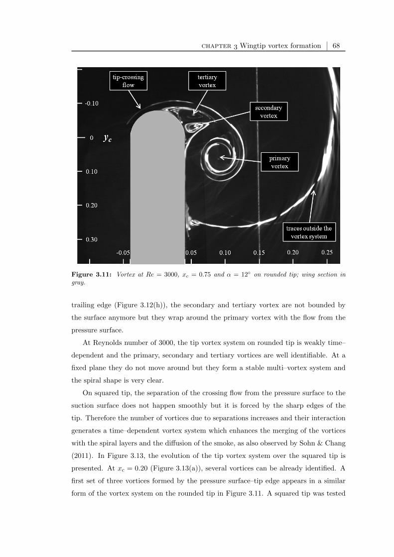
chapter Wingtip vortex formation 68
Figure 3.11: Vortex at Re = 3000, xc = 0.75 and α = 12 on rounded tip; wing section ingray.
trailing edge (Figure 3.12(h)), the secondary and tertiary vortex are not bounded by
the surface anymore but they wrap around the primary vortex with the flow from the
pressure surface.
At Reynolds number of 3000, the tip vortex system on rounded tip is weakly time–
dependent and the primary, secondary and tertiary vortices are well identifiable. At a
fixed plane they do not move around but they form a stable multi–vortex system and
the spiral shape is very clear.
On squared tip, the separation of the crossing flow from the pressure surface to the
suction surface does not happen smoothly but it is forced by the sharp edges of the
tip. Therefore the number of vortices due to separations increases and their interaction
generates a time–dependent vortex system which enhances the merging of the vortices
with the spiral layers and the diffusion of the smoke, as also observed by Sohn & Chang
(2011). In Figure 3.13, the evolution of the tip vortex system over the squared tip is
presented. At xc = 0.20 (Figure 3.13(a)), several vortices can be already identified. A
first set of three vortices formed by the pressure surface–tip edge appears in a similar
form of the vortex system on the rounded tip in Figure 3.11. A squared tip was tested

chapter Wingtip vortex formation 69
(a)xc
=0.3
0.
(b)xc
=0.4
0.
(c)xc
=0.5
0.
(d)xc
=0.6
0.
(e)xc
=0.7
0.
(f)xc
=0.8
0.
(g)xc
=0.9
0.
(h)xc
=0.9
9.
Fig
ure
3.1
2:
Vort
exev
olu
tion
atRe
=3000
an
dα
=12
on
rou
nded
tip;
win
gse
ctio
nin
gray.

chapter Wingtip vortex formation 70
(a)xc
=0.2
0.
(b)xc
=0.3
0.
(c)xc
=0.4
0.
(d)xc
=0.5
0.
(e)xc
=0.6
0.
(f)xc
=0.7
0.
(g)xc
=0.8
0.
(h)xc
=0.9
0.
(i)xc
=0.9
9.
Fig
ure
3.1
3:
Vort
exev
olu
tion
atRe
=3000
an
dα
=12
on
squ
are
dti
p;
win
gse
ctio
nin
gray.

chapter Wingtip vortex formation 71
also by Francis & Kennedy (1979) who found similar secondary structures originating
close to the leading edge at a Reynolds number of 3.85 · 105. Another set of vortices
is formed from the suction surface–tip edge which will become the main vortex system.
Initially the two sets of vortices evolve independently of each other and no sign of strong
time–dependency is observed. From xc = 0.20 to xc = 0.50 (Figures 3.13(a) to 3.13(d))
these vortices grow and the first vortex system moves towards the suction surface–tip
edge stretching over the whole tip area. At xc = 0.60 (Figure 3.13(e)) the two vortex
systems start to interact. In particular, the vortices from the first system move to
the suction surface and they interact with the primary vortex modifying its shape and
increasing the mixing of the spiral layers. At this plane, the vortices fluctuate from the
tip surface to the suction surface generating high level of unsteadiness on the primary
vortex. In Figure 3.14, a collection of snapshots is reported in order to highlight the
unsteadiness when the two vortex systems interact; position, size and shape of the
secondary vortices vary greatly with time. However, the shape and velocity field of
the inner part of the primary vortex is very little affected by secondary structures as
noted by the almost identical smoke pattern of the primary vortex core. From xc = 0.70
(Figure 3.13(f)), the primary vortex is surrounded by vortices coming from the tip which
mix with the spiral layers. At this stage there is not a stable secondary vortex between
the primary vortex and the tip edge. Several secondary structures are observed away
from the surface so that the definition of the accumulation line as the primary vortex
separation point on surface flow visualizations may not be strictly valid anymore. This
is not true for a rounded tip where the secondary vortex remains on the wing surface.
The bending of the accumulation line in Figure 3.1(a) indicates this change of topology
in the tip vortex structure. Several vortices can be counted at xc = 0.80 and xc = 0.90
(Figures 3.13(g) and 3.13(h)) and they wrap around the primary vortex. The shape
of the spiral structure is dominated by the interaction with secondary vortices. At the
trailing edge (Figure 3.13(i)), the tip vortex is shed from the wing as a strongly unsteady
vortex system which includes secondary vortices and shear layer eddies (Francis & Katz,
1988).
(b) Angle of attack and
Reynolds number effects
The effect of a change in the angle of attack (α = 4, 12)
and in the Reynolds number (Re = 3000, 7000) on the
wingtip vortex formation on the rounded tip is shown in
Figure 3.15 at 3 plane locations (xc = 0.50, 0.75 and 0.99).
As also observed in the pressure distribution, a lower angle of attack produces a

chapter Wingtip vortex formation 72
(a)N
=1.
(b)N
=2.
(c)N
=3.
(d)N
=4.
(e)N
=5.
(f)N
=6.
(g)N
=7.
(h)N
=8.
(i)N
=9.
Fig
ure
3.1
4:
Sn
apsh
ots
atf
=30
Hz,Re
=3000,α
=12
an
dxc
=0.
7on
squ
are
dti
p.

chapter Wingtip vortex formation 73
(a)xc
=0.5
0,Re
=3000,α
=4.
(b)xc
=0.7
5,Re
=3000,α
=4.
(c)xc
=0.9
9,Re
=3000,α
=4.
(d)xc
=0.5
0,Re
=3000,α
=12.
(e)xc
=0.7
5,Re
=3000,α
=12.
(f)xc
=0.9
9,Re
=3000,α
=12.
(g)xc
=0.5
0,Re
=7000,α
=12.
(h)xc
=0.7
5,Re
=7000,α
=12.
(i)xc
=0.9
9,Re
=7000,α
=12.
Fig
ure
3.1
5:
Vort
exev
olu
tion
atRe
=3000
an
dα
=12
on
rou
nded
tip;
win
gse
ctio
nin
gray.

chapter Wingtip vortex formation 74
lower lift and generates a smaller vortex with a delayed starting point. At xc = 0.75
the wing at high angle of attack already shows a clear multi–vortex structure (Figure
3.15(e)) whereas the flow visualization of the wing at low angle of attack does not show
a vortical structure (Figure 3.15(b)). An intermittent separation of the tip–crossing
flow was observed at this stage and a resulting small vortex could be only occasionally
detected. The average pressure gradient across the tip surface is not strong enough to
separate the flow and maintain a steady vortical structure. Compared to delta wing
vortices where the vortex starts from the apex of the wing, on rectangular wings the
wingtip vortex does not have a clearly defined chordwise starting point. Computational
studies by Duraisamy (2005) showed that for an early stage of a wingtip flow from a
rounded tip, the adverse pressure gradient is mild enough for the cross flow boundary
layer to remain attached on the surface without wrapping the flow around the tip.
At xc = 0.99, the vortex for the low angle of attack is observed (Figure 3.15(c)) but
it is remarkably smaller than for the high angle of attack(Figure 3.15(f)). However,
the number of turns of the spiral structure at the trailing edge of the smoke filament
coming from the pressure side is approximately the same. Assuming that the two angles
of attack generate vortices with similar swirl velocity profiles with the exception of a
scaling factor, the number of turns are directly proportional to a reference value of the
swirl velocity and the development length of the vortex, and inversely proportional to
the axial velocity within the vortex core. Also, the swirl velocity is proportional to the
pressure difference between the suction and the pressure surfaces of the wing or, in other
terms, to the circulation of the wing. This results in the following relation:
number of turns ∝swirl velocity
(wing circulation) ·development length
on the wing
core axial velocity(3.2)
Hence, at high angle of attack, the longer and more intense vortex (high swirl velocity)
has to generate a vortex axial velocity considerably higher than the wing at low angle
of attack so that the number of turns might result similar.
At a higher Reynolds number (comparing Figures 3.15(d) to 3.15(f) with Figures
3.15(g) to 3.15(i)), the vortex appears with similar sizes at all the laser planes which
indicates a similar structure to the lower Reynolds number case. Also, the traces out-
side the vortex system bend more around the vortex which indicates a sensibly higher
intensity of the vortex (higher swirl velocity). At this Reynolds number, the blurred pic-
tures are generated by the higher turbulence of the incoming flow and the more intense
mixing of the smoke filaments.

chapter Wingtip vortex formation 75
section
Vortex characteristic lines via SPIV
The vortex flow topology over wing surfaces (from rectangular to delta wings) is
often extracted from wall shear stress patterns by surface flow visualizations or from
convergence or divergence of limiting streamlines (Taylor & Gursul, 2004). Moreover,
several methods have been presented for automatic detection of the flow topology over
a surface (e.g. Kenwright, 1998; Surana et al., 2006). The literature on the description
and characterization of delta wings vortices is more vaste that on rectangular wings.
Recent PIV experiments on planes parallel to delta wing surfaces have been presented
by Taylor & Gursul (2004), Yavuz et al. (2004) and Gursul (2004). They described the
near surface topology and flow structure in terms of streamlines, vorticity and velocity
fluctuations which gave a more detailed insight of the vortex structure than surface flow
or smoke visualizations.
Figure 3.16: Experimental arrangement and field of view of the SPIV cameras.
The wing M2 was mounted on the floor of the Argyll wind tunnel (Figure 3.16)
and stereoscopic particle image velocimetry was performed on planes parallel to the
wing surface near the trailing edge where the curvature is almost zero as shown in
Figure 3.17(a). For the case of rounded tip, the laser sheet was parallel to the suction
surface and therefore at a different distance from the tip surface as sketched in Figure
3.17(b). Although glare was reduced to tolerable levels by black paint on the model
and by a high quality surface finish, wrong vectors were found in correspondence to the
trailing edge and to the sharp edge on the squared tip. However, this problem did not
influence much the measurements because of the good quality of the correlation in the
surrounding regions.
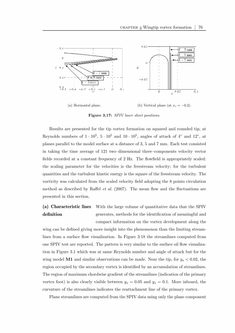
chapter Wingtip vortex formation 76
(a) Horizontal plane. (b) Vertical plane (at xc = −0.2).
Figure 3.17: SPIV laser sheet positions.
Results are presented for the tip vortex formation on squared and rounded tip, at
Reynolds numbers of 1 · 105, 5 · 105 and 10 · 105, angles of attack of 4 and 12, at
planes parallel to the model surface at a distance of 3, 5 and 7 mm. Each test consisted
in taking the time average of 121 two–dimensional three–components velocity vector
fields recorded at a constant frequency of 2 Hz. The flowfield is appropriately scaled:
the scaling parameter for the velocities is the freestream velocity; for the turbulent
quantities and the turbulent kinetic energy is the square of the freestream velocity. The
vorticity was calculated from the scaled velocity field adopting the 8 points circulation
method as described by Raffel et al. (2007). The mean flow and the fluctuations are
presented in this section.
(a) Characteristic lines
definition
With the large volume of quantitative data that the SPIV
generates, methods for the identification of meaningful and
compact information on the vortex development along the
wing can be defined giving more insight into the phenomenon than the limiting stream-
lines from a surface flow visualization. In Figure 3.18 the streamlines computed from
one SPIV test are reported. The pattern is very similar to the surface oil flow visualiza-
tion in Figure 3.1 which was at same Reynolds number and angle of attack but for the
wing model M1 and similar observations can be made. Near the tip, for ys < 0.02, the
region occupied by the secondary vortex is identified by an accumulation of streamlines.
The region of maximum chordwise gradient of the streamlines (indication of the primary
vortex foot) is also clearly visible between ys = 0.05 and ys = 0.1. More inboard, the
curvature of the streamlines indicates the reattachment line of the primary vortex.
Plane streamlines are computed from the SPIV data using only the plane component
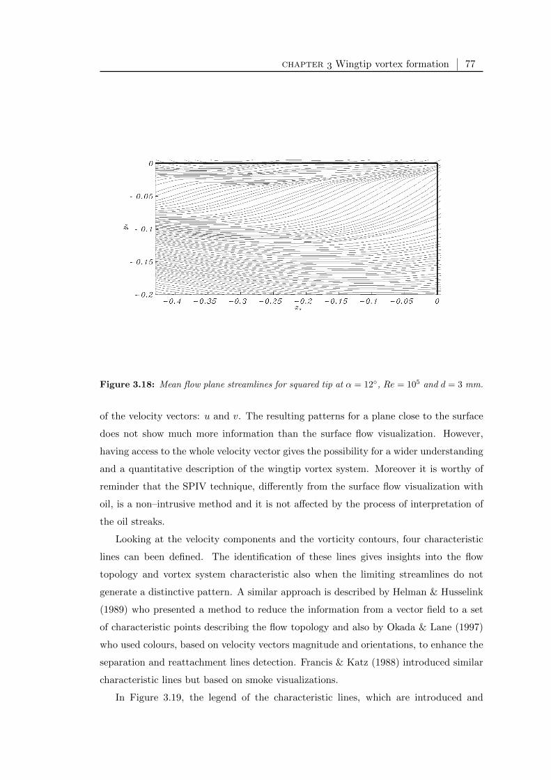
chapter Wingtip vortex formation 77
Figure 3.18: Mean flow plane streamlines for squared tip at α = 12, Re = 105 and d = 3 mm.
of the velocity vectors: u and v. The resulting patterns for a plane close to the surface
does not show much more information than the surface flow visualization. However,
having access to the whole velocity vector gives the possibility for a wider understanding
and a quantitative description of the wingtip vortex system. Moreover it is worthy of
reminder that the SPIV technique, differently from the surface flow visualization with
oil, is a non–intrusive method and it is not affected by the process of interpretation of
the oil streaks.
Looking at the velocity components and the vorticity contours, four characteristic
lines can been defined. The identification of these lines gives insights into the flow
topology and vortex system characteristic also when the limiting streamlines do not
generate a distinctive pattern. A similar approach is described by Helman & Husselink
(1989) who presented a method to reduce the information from a vector field to a set
of characteristic points describing the flow topology and also by Okada & Lane (1997)
who used colours, based on velocity vectors magnitude and orientations, to enhance the
separation and reattachment lines detection. Francis & Katz (1988) introduced similar
characteristic lines but based on smoke visualizations.
In Figure 3.19, the legend of the characteristic lines, which are introduced and

chapter Wingtip vortex formation 78
defined in this section, is reported. In Figure 3.20 the three components of the mean
velocity vector and their turbulent fluctuations (RMS) contours are reported for the case
at angle of attack of 12, Reynolds number of 105, squared tip and distance between
wing surface and laser sheet of d = 3 mm. In Figure 3.21 the in–plane vorticity (out–of–
plane component of the vorticity vector) and the turbulent kinetic energy k (which is an
indication of the overall fluctuation) are also reported. The wingtip vortex characteristic
lines are plotted on all these contours.
Figure 3.19: Characteristic lines legend for squared tip at α = 12, Re = 105 and d = 3 mm.
Referring to Figures 3.20 and 3.21, the four characteristic lines introduced in this
study are defined as follows, from the most inboard to the closest to the tip:
• L1 is the most inboard line where the v–component of the velocity is equal to
zero (from Figure 3.20(c)). This line separates the flow directed towards the
wingtip from the flow directed towards the root of the wing and it is therefore an
indication of the dimension of the primary vortex. It initially grows almost linearly
in the chord direction showing an increase of the vortical system dimension (i.e.
diameter) with the streamwise coordinate. The bump observed in the proximity
to the trailing edge is related to measurement errors due to glare and it can be
easily eliminated adopting a more sophisticated identification method.
• L2 is the line where the w–component of the velocity is equal to zero (from Figure
3.20(e)) and it corresponds to the foot of the primary vortex (where the vortex
streamlines on the vortex plane are parallel to the surface). It can be seen as a first
indication of the vortex centre position. This line lies on the region of maximum
velocity magnitude and the wall shear stress is also maximum which explains the
lighter colour at this region on the oil visualization of Figure 3.1(a). Between L1
and L2 the out–of–plane velocity component w is negative which corresponds to
flow going in the direction of the wing surface.

chapter Wingtip vortex formation 79
(a) Velocity u–component (streamwise). (b) RMS u–component.
(c) Velocity v–component (crossflow). (d) RMS v–component.
(e) Velocity w–component (out–of–plane). (f) RMS w–component.
Figure 3.20: Mean flow and characteristic lines for squared tip at α = 12, Re = 105 andd = 3 mm (characteristic lines legend from the most inboard to the nearest to the wingtip: L1continuous line, L2 dashed–dotted line, L3 dashed line, L4 dotted line).
• L3 is the line where the in–plane vorticity is maximum (from Figure 3.21(a)) and
it identifies the separation line of the primary vortex. Between L2 and L3 the
out–of–plane velocity component is positive which is flow moving away from the
surface. Maximum turbulent kinetic energy is also observed along this line (Figure

chapter Wingtip vortex formation 80
(a) In–plane vorticity. (b) k.
Figure 3.21: Mean flow and characteristic lines for squared tip at α = 12, Re = 105 andd = 3 mm (characteristic lines legend from the most inboard to the nearest to the wingtip: L1continuous line, L2 dashed–dotted line, L3 dashed line, L4 dotted line).
3.21(b)) and in particular the u–component of the fluctuations is maximum. The
region between L3 and the tip is a region of higher fluctuation of the v–component
compared to the rest of the wing surface. This indicates that the main source of the
unsteady spanwise motion of the primary vortex comes from the region occupied
by secondary vortices.
• L4 is the line where the in–plane vorticity is minimum (from Figure 3.21(a))
and it corresponds to the separation line of the secondary vortex. The sign of
the vorticity on L3 and L4, respectively positive and negative, is due to the local
minimum of the velocity u–component between the two lines. In fact, the vorticity
out–of–plane component is calculated as
ωz =∂v
∂x− ∂u
∂y(3.3)
where the gradient along the x–coordinate is much smaller than the spanwise
gradient (∂/∂y) which is negative on L3 and positive on L4. As observed in the
smoke visualization of Figure 3.13, moving toward the trailing edge secondary
vortices lift up from the wing surface around xc > 0.8 (' xs > −0.2) and the wing
tip vortex system becomes more unsteady. Therefore, for xs > −0.2, L4 does not
give anymore an accurate description of the secondary vortex structure. However,
for xs < −0.2, the presence of the secondary vortex is also seen in the negative
values of the w and v component of the velocity in the region near the tip edge.
The bending of L4, which indicates the lifting up of the secondary vortex and the

chapter Wingtip vortex formation 81
change of vortex structure topology, is observed around xs = −0.3, similarly to
the surface flow visualization of Figure 3.1(a).
(a) Square tip. (b) Rounded tip.
Figure 3.22: Smoke visualizations at xc = 0.7, α = 12 and Re = 3000.
In Figure 3.22(a), the position of the lines are sketched with respect to the smoke
visualizations of Section 3.3. The smoke visualizations refer to the position xc = 0.7,
Reynolds number of 3000 and angle of attack of 12. It is believed that the kinematics of
the tip vortex formation does not change radically for a wide range of Reynolds numbers,
especially on sharp edges where the separation points are fixed. Karakus et al. (2008)
and Bailey et al. (2006) studied a similar geometry at Reynolds numbers respectively
of 3.2 · 104 and 2.4 · 105 and they showed the same multiple vortex structures of Figure
3.22(a). Dye visualizations in a water tank were presented by Francis & Katz (1988) for
a hydrofoil with squared tip at Reynolds number in a range between 3 ·104 and 1.3 ·106;
the same multiple vortex structure and interaction was observed.
In Figure 3.22(b), the vortex characteristic lines are positioned with reference to a
typical vortex system formed over the same wing but with rounded tip. For a Reynolds
number of 4.6 ·106 on a low aspect ratio NACA 0012 rectangular wing with rounded tip,
Chow et al. (1992) showed a similar vortex structure confirming that also on rounded
tip geometries the vortex structure does not topologically change with the Reynolds
number.
In Figure 3.23 a diagram of a typical formation of the primary vortex over a rect-
angular wing with rounded tip is sketched based on the information gathered during
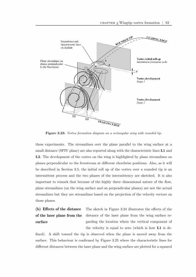
chapter Wingtip vortex formation 82
Figure 3.23: Vortex formation diagram on a rectangular wing with rounded tip.
these experiments. The streamlines over the plane parallel to the wing surface at a
small distance (SPIV plane) are also reported along with the characteristic lines L1 and
L2. The development of the vortex on the wing is highlighted by plane streamlines on
planes perpendicular to the freestream at different chordwise positions. Also, as it will
be described in Section 3.5, the initial roll up of the vortex over a rounded tip is an
intermittent process and the two phases of the intermittency are sketched. It is also
important to remark that because of the highly three–dimensional nature of the flow,
plane streamlines (on the wing surface and on perpendicular planes) are not the actual
streamlines but they are streamlines based on the projection of the velocity vectors on
those planes.
(b) Effects of the distance
of the laser plane from the
surface
The sketch in Figure 3.24 illustrates the effects of the
distance of the laser plane from the wing surface re-
garding the location where the vertical component of
the velocity is equal to zero (which is how L1 is de-
fined). A shift toward the tip is observed when the plane is moved away from the
surface. This behaviour is confirmed by Figure 3.25 where the characteristic lines for
different distances between the laser plane and the wing surface are plotted for a squared

chapter Wingtip vortex formation 83
Figure 3.24: Schematics of the primary vortex streamlines and the evaluated reattachmentpoints positions for measurement planes at different distances from the surface.
tip at two Reynolds numbers. The three planes are at a distance from the wing surface
corresponding to 0.4%, 0.65% and 0.9% of the chord and they cut the primary vortex
below the vortex centre. No particular differences on the positions of the lines are be
observed with the exception of a shifting of L1 for xs > −0.2. The closer the cutting
plane is to the surface, the more accurate is the description of the shape of L1 as the
distinctive line on the surface that divides the flow directed towards the root from the
flow directed towards the tip of the wing. It is expected therefore that the primary vor-
tex reattachment line on the surface is shifted more towards the wing root than what
observed on these near surface streamlines. For instance, assuming a linear shifting of
L1 when the plane moves closer to the surface, at xs = −0.1 the reattachment lines of
the primary vortex for Reynolds numbers of 105 and 106 are respectively at ys = 0.22
and ys = 0.17 with an error below 3% compared to the estimation on the plane at d = 3
mm.
(a) Re = 105. (b) Re = 106.
Figure 3.25: Characteristic lines for squared tip at α = 12.

chapter Wingtip vortex formation 84
(c) Reynolds number and
tip geometry effects
The characteristic lines for the two different wing tip
geometries (squared and rounded tip) at two Reynolds
numbers (105 and 106) are shown in Figure 3.26. It is
observed that the sharp geometry of the squared tip fixes the separation point of the
crossing flow and, as a consequence, the overall dimension of the primary vortex, as
indicated by L1, is the same for the two Reynolds numbers. On the squared tip, small
variations in the position of the other lines are observed which indicates the invariance of
the primary vortex position to the Reynolds number. On the rounded tip, a shift of all
the characteristic lines is detected when the Reynolds number is changed. L1, L2 and
L3 move in the direction of the tip when the Reynolds number is increased, indicating a
primary vortex around 20% smaller than the vortex formed at the low Reynolds number
(estimated as distance between the wingtip edge and L1). L4 lies outside of the wing
geometry because the secondary vortex is partially situated on the rounded edge and,
as observed in Figure 3.17(b), for ys > 0 the laser plane is not parallel to the surface.
Even though the unsteadiness, the number of vortices, the formation and the initial
roll up process are different between the squared and the rounded wingtips, the four
characteristic lines are clearly found in both cases.
(a) Squared tip. (b) Rounded tip.
Figure 3.26: Characteristic lines at d = 5 mm and α = 12.
What also appears in Figure 3.26 when comparing the characteristic lines from the
vortex systems formed on the two wingtip geometries, is that L2 lies parallel to the tip
edge (i.e. horizontal for squared tip and diagonal for rounded tip) so that the distance
between this line and the tip edge remains constant along at least the last 35 percent
of the wing (xs > −0.35). This behaviour was observed also by Yavuz et al. (2004) and
it indicates that the vortex centre moves parallel to the edge of the wing.

chapter Wingtip vortex formation 85
(a) u–component: α = 4. (b) u–component: α = 12
(c) v–component: α = 4. (d) v–component: α = 12.
(e) w–component: α = 4:. (f) w–component: α = 12.
Figure 3.27: Velocity components contours for a rounded tip at Re = 106.
(d) Angle of attack effects The vortex systems on a rounded tip wing at the two
angles of attack 4 and 12 are compared in this section
for the Reynolds number of 106. The three velocity components (Figure 3.27) and the
vorticity (Figure 3.28) are reported. At this angle, the region at the left and right edges
of the contours is not in the field of view of the cameras and presents a wrong velocity

chapter Wingtip vortex formation 86
(a) α = 4. (b) α = 12.
Figure 3.28: In–plane vorticity contours for a rounded tip at Re = 106.
field (particularly clear in Figure 3.27(e)). However, this region is included for the sake
of immediacy in comparing with previous results.
At a lower angle of attack, the pressure difference between the two surfaces of the
wing is smaller and the circulation generated by the wing is consequently smaller. As
also observed on the smoke visualizations of Figure 3.15, the vortex at lower angle of
attack is smaller and the rolling up of the vorticity sheet begins at a later stage along the
wing. As a consequence, the characteristic lines on the low angle of attack case are not
as evident as in the high angle of attack case and they are shorter. The primary vortex
reattachment line L1 appears only for xs > −0.15 and the primary vortex foot L2 for
xs > −0.25. The maximum and minimum vorticity lines, L3 and L4, are dictated by
the local minimum of the streamwise component of the velocity in correspondence to
the rounded portion of the wing.
section
Unsteadiness of the vortex formation via hot
film
Based on the preliminary information gathered from the measurement of the pressure
fluctuations in Section 3.2.(b), hot film measurements were taken on the M2 wing in
order to study the low frequency unsteadiness of the flow in the region described by the
characteristic lines which were found with the SPIV experiments in Section 3.4. The
model was mounted in the Argyll wind tunnel in the same way as the SPIV experiments.

chapter Wingtip vortex formation 87
The hot films were deployed onto the surface at several positions and recordings of
100 s at 1 KHz were taken. In Figure 3.29 the characteristic lines are sketched for
different cases (i.e. different tip geometry, Reynolds number and angle of attack) with
the positions of the hot film measurements.
(a) Squared tip at α = 12 and Re = 105. (b) Squared tip at α = 12 and Re = 106.
(c) Rounded tip at α = 4 and Re = 105. (d) Rounded tip at α = 4 and Re = 106.
(e) Rounded tip at α = 12 and Re = 105. (f) Rounded tip at α = 12 and Re = 106.
Figure 3.29: Characteristic lines and hot film positions.
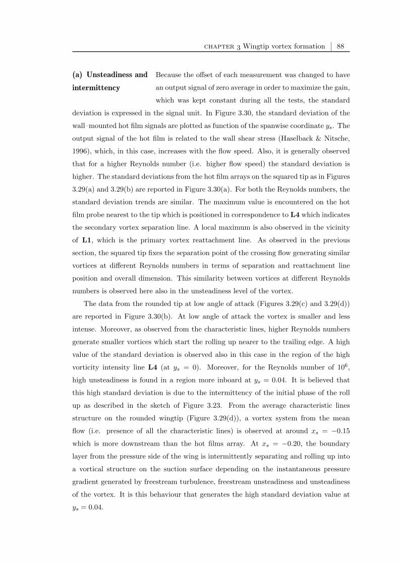
chapter Wingtip vortex formation 88
(a) Unsteadiness and
intermittency
Because the offset of each measurement was changed to have
an output signal of zero average in order to maximize the gain,
which was kept constant during all the tests, the standard
deviation is expressed in the signal unit. In Figure 3.30, the standard deviation of the
wall–mounted hot film signals are plotted as function of the spanwise coordinate ys. The
output signal of the hot film is related to the wall shear stress (Haselback & Nitsche,
1996), which, in this case, increases with the flow speed. Also, it is generally observed
that for a higher Reynolds number (i.e. higher flow speed) the standard deviation is
higher. The standard deviations from the hot film arrays on the squared tip as in Figures
3.29(a) and 3.29(b) are reported in Figure 3.30(a). For both the Reynolds numbers, the
standard deviation trends are similar. The maximum value is encountered on the hot
film probe nearest to the tip which is positioned in correspondence to L4 which indicates
the secondary vortex separation line. A local maximum is also observed in the vicinity
of L1, which is the primary vortex reattachment line. As observed in the previous
section, the squared tip fixes the separation point of the crossing flow generating similar
vortices at different Reynolds numbers in terms of separation and reattachment line
position and overall dimension. This similarity between vortices at different Reynolds
numbers is observed here also in the unsteadiness level of the vortex.
The data from the rounded tip at low angle of attack (Figures 3.29(c) and 3.29(d))
are reported in Figure 3.30(b). At low angle of attack the vortex is smaller and less
intense. Moreover, as observed from the characteristic lines, higher Reynolds numbers
generate smaller vortices which start the rolling up nearer to the trailing edge. A high
value of the standard deviation is observed also in this case in the region of the high
vorticity intensity line L4 (at ys = 0). Moreover, for the Reynolds number of 106,
high unsteadiness is found in a region more inboard at ys = 0.04. It is believed that
this high standard deviation is due to the intermittency of the initial phase of the roll
up as described in the sketch of Figure 3.23. From the average characteristic lines
structure on the rounded wingtip (Figure 3.29(d)), a vortex system from the mean
flow (i.e. presence of all the characteristic lines) is observed at around xs = −0.15
which is more downstream than the hot films array. At xs = −0.20, the boundary
layer from the pressure side of the wing is intermittently separating and rolling up into
a vortical structure on the suction surface depending on the instantaneous pressure
gradient generated by freestream turbulence, freestream unsteadiness and unsteadiness
of the vortex. It is this behaviour that generates the high standard deviation value at
ys = 0.04.
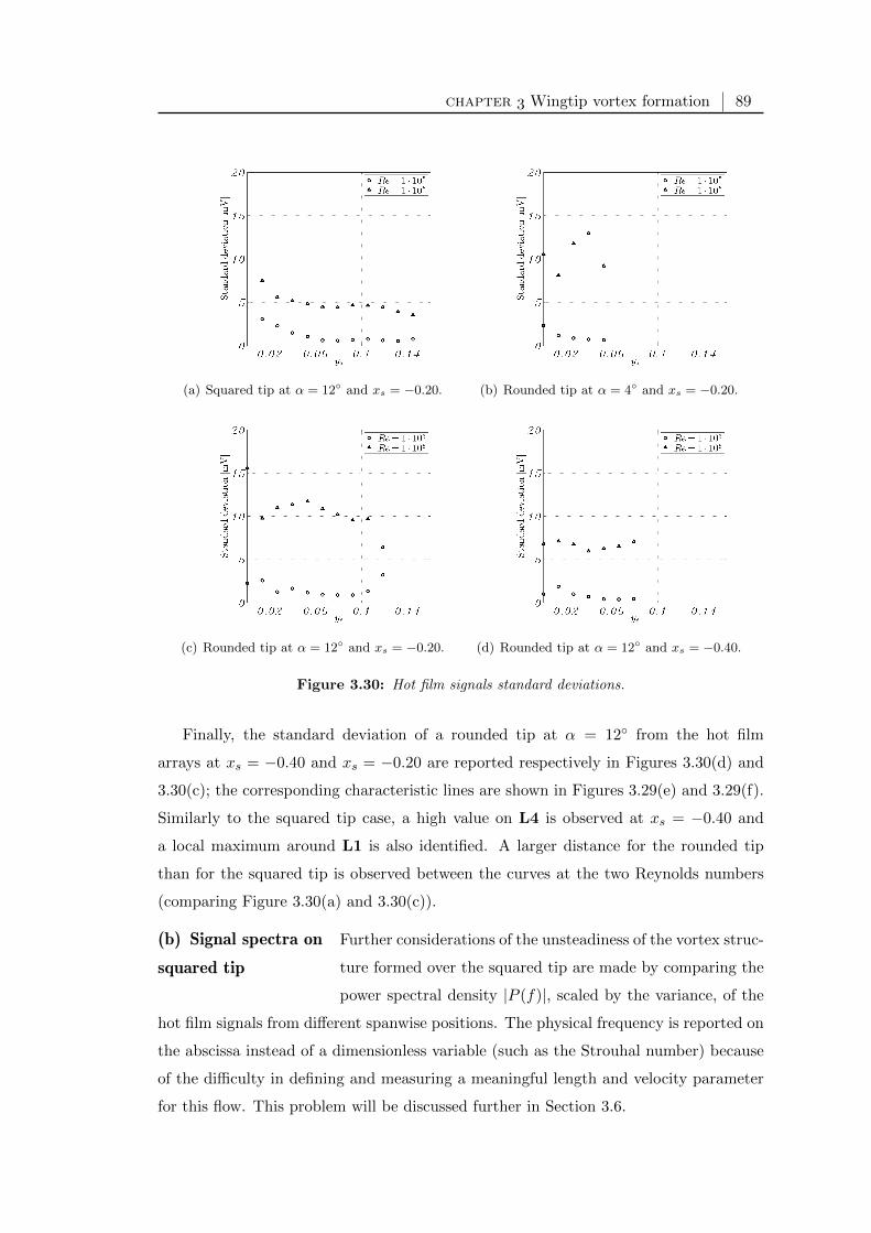
chapter Wingtip vortex formation 89
(a) Squared tip at α = 12 and xs = −0.20. (b) Rounded tip at α = 4 and xs = −0.20.
(c) Rounded tip at α = 12 and xs = −0.20. (d) Rounded tip at α = 12 and xs = −0.40.
Figure 3.30: Hot film signals standard deviations.
Finally, the standard deviation of a rounded tip at α = 12 from the hot film
arrays at xs = −0.40 and xs = −0.20 are reported respectively in Figures 3.30(d) and
3.30(c); the corresponding characteristic lines are shown in Figures 3.29(e) and 3.29(f).
Similarly to the squared tip case, a high value on L4 is observed at xs = −0.40 and
a local maximum around L1 is also identified. A larger distance for the rounded tip
than for the squared tip is observed between the curves at the two Reynolds numbers
(comparing Figure 3.30(a) and 3.30(c)).
(b) Signal spectra on
squared tip
Further considerations of the unsteadiness of the vortex struc-
ture formed over the squared tip are made by comparing the
power spectral density |P (f)|, scaled by the variance, of the
hot film signals from different spanwise positions. The physical frequency is reported on
the abscissa instead of a dimensionless variable (such as the Strouhal number) because
of the difficulty in defining and measuring a meaningful length and velocity parameter
for this flow. This problem will be discussed further in Section 3.6.

chapter Wingtip vortex formation 90
(a) ys = 0.013. (b) ys = 0.026. (c) ys = 0.040.
(d) ys = 0.053. (e) ys = 0.066. (f) ys = 0.079.
(g) ys = 0.092. (h) ys = 0.105. (i) ys = 0.118.
Figure 3.31: Square tip power spectra: Re = 105, α = 12, xs = −0.20.
The spectra from the two Reynolds numbers cases are reported in Figures 3.31
and 3.32. Peaks are observed below 5 Hz for both the cases. At the low Reynolds
number, energy peaks appear at the different spanwise positions at a frequency around
1 Hz. Also, near to the edge (ys = 0.013, 0.026, 0.040), higher energy is observed at a
frequency range between approximately 0.3 Hz and 0.9 Hz corresponding to the region
where L4 and L3 are found. At high Reynolds number (106) a high energy in the range
between 0.8 and 3 Hz is found in the region next to the tip. Also, moving towards the
root the energy decreases reflecting the same behaviour of the signal standard deviation.
This suggests a link between periodic unsteadiness on wingtip vortices and secondary
vortex movement. Strong interactions between secondary vortices and primary vortex
during the formation were described also by Karakus et al. (2008) on a rectangular wing
with squared tip.

chapter Wingtip vortex formation 91
(a) ys = 0.013. (b) ys = 0.026. (c) ys = 0.040.
(d) ys = 0.053. (e) ys = 0.066. (f) ys = 0.079.
(g) ys = 0.092. (h) ys = 0.105. (i) ys = 0.118.
Figure 3.32: Square tip power spectra: Re = 106, α = 12, xs = −0.20.
(c) Signal spectra on
rounded tip
In Figure 3.33 the power spectra are reported for the high
Reynolds number case on rounded tip at 12 and xs = −0.20.
The energy density at low frequencies at ys = 0 is higher than
at the other positions. As also observed for the squared tip, this can be linked to the
unsteadiness of the secondary vortex which dominates the unsteadiness of the entire
vortical system. Also, a double peak energy distribution (peaks at around 1 Hz and 2.5
Hz) is noted at ys = 0.013 and ys = 0.026. Taylor & Gursul (2004) observed on delta
wings similar double peak spectra and they related them to shear layer instabilities and
vortex pairing processes.
At a lower angle of attack (Figure 3.34), a peak at a frequency between 0.4 and 0.7
Hz is noted in the region near the tip and it is related to the intermittency of the initial
roll up of the boundary layer coming from the pressure surface of the wing, as discussed
earlier.

chapter Wingtip vortex formation 92
(a) ys = 0. (b) ys = 0.013. (c) ys = 0.026.
(d) ys = 0.040. (e) ys = 0.053. (f) ys = 0.066.
(g) ys = 0.079. (h) ys = 0.092. (i) ys = 0.105.
Figure 3.33: Rounded tip power spectra: Re = 106, α = 12, xs = −0.20.
section
Unsteadiness of the vortex in the early wake
The unsteadiness information gathered in the previous section are compared here
with a study on the unsteadiness of the vortex system in the near wake. When the
vortex flow seeded with smoke is illuminated, the high centrifugal forces produce a
darker region at the vortex centre which can be then located by detecting the centroid
of the darker spot. A similar problem is solved by Del Pino et al. (2009) who used an
appropriate threshold to convert the grayscale image into a binary image. However,
in the current study, a routine based on the grayscale image is preferred to a method
working on the black and white image because it avoids the problematic choice of the
threshold level when the centrifugal forces are not strong enough to produce a clear dark
region. A discussion and comparison of two different methods, respectively based on

chapter Wingtip vortex formation 93
(a) ys = 0. (b) ys = 0.013. (c) ys = 0.026.
(d) ys = 0.040. (e) ys = 0.053.
Figure 3.34: Rounded tip power spectra: Re = 106, α = 4, xs = −0.20.
binary and grayscale images, implemented on these experiments is found in Appendix B.
In the method adopted, the grayscale image is analysed through circles of diameter Npx
and iterative refinements on the position of the averaged darkest circle are performed.
Tests on the sensitivity of the interrogation circle dimensions on instantaneous vortex
position and movement frequency were carried out and a diameter of Npx = 60 was
selected for this configuration (see Appendix B). This value corresponds to a physical
size of 6 mm.
Recordings were composed of 190 pictures of smoke visualizations taken on planes in
the wake of the wing. The laser plane was perpendicular to the freestream and different
plane locations, angles of attack and Reynolds numbers were tested. The wing M2 was
mounted as in Section 3.5 and rounded tip geometry was installed. A typical meandering
of the order of 2.5% of the chord was observed for the different configurations.
In this section, the power spectral density (PSD) of the displacements along the vor-
tex plane axes yv and zv are presented, named respectively |Pyy(f)| and |Pzz(f)|. More-
over, because wandering affects the v and w component of the velocity simultaneously,
the cross spectral density (CSD) is also used in order to highlight more prominently the
overall wandering frequency (Bailey & Tavoularis, 2008). Both the PSD and the CSD
are scaled by the variance of the signal.
Based on the observations on the vortex unsteadiness dominant frequency from hot
chapter Wingtip vortex formation 94
film signals of Section 3.5, these experiments on smoke visualization recordings focus
on low frequencies. Since the maximum number of frames was limited by the hardware
to 190 and the relevant frequencies are below 5 Hz, in order to obtain a good frequency
resolution a sampling time of 19 seconds at a sampling frequency of FS = 10 Hz was
adopted. Recordings of 6.3 seconds at a frequency of FS = 30 Hz were also analysed and
they confirmed that the major contribution to the unsteadiness in these experiments is
observed at frequencies less than 5 Hz.
(a) Reynolds number
effects
In Figure 3.35, the Reynolds number effect on the vortex
meandering is presented for tests at xw = 1 and wing at
12 of incidence. A dominant peak in the PSD on both the
translation axes zv and yv for Re = 10 · 105 (Figure 3.35(c)) is seen at a frequency of
approximately 0.8 Hz. Other weaker peaks are also seen at higher frequencies but they
are not clear when the fluctuations on the yv and zv axes are correlated to form the
CSD in Figure 3.35(f). At Re = 5 · 105 a peak is observed at a frequency of 0.4 Hz
(Figure 3.35(e)) which is characterized by a predominant movement along the yv axis
(Figure 3.35(b)). For the lower Reynolds number, Re = 2 · 105, no predominant peaks
are detected in the PSD (Figure 3.35(a)); however, the CSD reveals a peak around a
frequency of 0.05 Hz (Figure 3.35(d)).
(a) PSD: Re = 2 · 105. (b) PSD: Re = 5 · 105. (c) PSD: Re = 10 · 105.
(d) CSD: Re = 2 · 105. (e) CSD: Re = 5 · 105. (f) CSD: Re = 10 · 105.
Figure 3.35: Signal spectra at xw = 1 and α = 12.
The amplitude of the peak on the CSD is higher when the PSD on the two axes show
chapter Wingtip vortex formation 95
a similar behaviour on the peak frequency which can be seen as a sign of axisymmetry
of the meandering. The lowest peak in the CSD is observed for Re = 5 · 105 where the
meandering frequency on the yv axis shows a higher energy compared to the zv axis. This
difference suggests a link between the vortex centre unsteadiness in the early wake and
the vortex unsteadiness during the roll up, particularly with the vortex movement along
the spanwise direction (ys axis). Furthermore, a similarity of the PSD along the two axes
suggests that when the Reynolds number is increased the vortex reaches a developed
meandering stage sooner, which generates a meandering not oriented predominantly
along one of the axes. Whether the meandering is axisymmetric, as observed by Beresh
& Henfling (2010), or oriented along a different axes, as presented by Del Pino et al.
(2009), is not clear from these experiments.
From the CSD plots in Figure 3.35, the frequency f of the peak increases with the
Reynolds number. A scaling of the frequency such as f = fc/U∞ would collapse the
peaks for Re = 5·105 and Re = 10·105 at the same scaled frequency of f = 0.032 and the
peak for Re = 2 · 105 at f = 0.010. Whereas Del Pino et al. (2009) found a meandering
scaled frequency of the same magnitude f ' 0.029, Bailey et al. (2006) observed a
frequency one order of magnitude higher of approximately f ' 0.35. Such a difference
can not be explained solely by the differences of those researches and the current one in
the angle of attack, Reynolds number, wing chord, wing aspect ratio, freestream velocity
or position in the wake. Although studies on low frequency unsteadiness would benefit
from comparative tests of these parameters, the scaling parameters of the dimensionless
frequency should be accurately chosen among quantities which are more characteristic
of the vortex such as vortex core diameter, maximum swirl velocity and circulation.
(b) Angle of attack effects The results of an increase of the angle of attack on signal
spectra of the vortex centre motion (Figure 3.36) show
similar trends to the increase of the Reynolds number. On the CSD, the energy peak
shifts toward a higher frequency and intensity increasing the angle of attack, from no
distinct peak at α = 4 (Figure 3.36(d)), to a peak at 0.9 Hz for α = 12 (Figure 3.36(e))
and to an intense and well defined peak at 1 Hz for α = 15 (Figure 3.36(f)). Also,
where for the low angle of attack a peak at 0.5 Hz is observed only on |Pyy(f)| (Figure
3.36(a)), a more developed and symmetric vortex movement is observed at α = 15
(i.e. similarity of the PSD on the two axes in Figure 3.36(c) and higher peak in the
CSD). This behaviour is confirmed by studies on the age and development of a trailing
vortex. Gerz et al. (2001) introduced a vortex age parameter based on the circulation

chapter Wingtip vortex formation 96
of the wing in order to properly compare trailing vortices produced by different wings.
Giuni & Benard (2011) (see also Giuni et al., 2010) studied the relationship between
the increase of the angle of attack and the increase of the vortex circulation and applied
the vortex age parameter on a test similar to the present work. They found that in the
very near wake, a higher angle of attack corresponds to an older vortex with a more
symmetric and developed structure. Also, a vortex core rotation estimation, presented
in Section 4.2, shows that increasing the angle of attack, the vortex core rotation rate
is higher which contributes to an earlier development of an axisymmetric flow.
(a) PSD: α = 4. (b) PSD: α = 12. (c) PSD: α = 15.
(d) CSD: α = 4. (e) CSD: α = 12. (f) CSD: α = 15.
Figure 3.36: Signal spectra at xw = 1 and Re = 10 · 105.
(c) Downstream distance
effects
The vortex centre fluctuation at two different planes in
the wake of the wing at Reynolds number of 5 · 105 and
angle of attack of 15 are presented in Figure 3.37. The
vortex centre movement at the furthest plane from the trailing edge of the wing appears
the same on the yv and the zv axis (Figure 3.37(b)) which suggests symmetry of the
vortex core. The peak in the CSD appears at a frequency of around 0.6 Hz (Figure
3.37(d)). At xw = 0.25, there is not a unique peak in the PSD (Figure 3.37(a)) which
can be detected but instead numerous and less intense peaks in the whole range 0–5
Hz. This is confirmed also by the almost flat distribution in the CSD (Figure 3.37(c)).
This plane is in the region where the rolling up of the vorticity sheet around the vortex
core is still very intense. Also, at xw = 0.25 the darker spot in the picture indicating

chapter Wingtip vortex formation 97
the vortex centre was very faint compared to the xw = 1 case which confirms a not fully
developed vortical structure at this early stage of the wake.
(a) PSD: xw = 0.25. (b) PSD: xw = 1.
(c) CSD: xw = 0.25. (d) CSD: xw = 1.
Figure 3.37: Signal spectra at α = 15 and Re = 5 · 105.
section
Summary
The low frequency unsteadiness in the formation and in the early wake of a rect-
angular wing was studied for Reynolds numbers between 105 and 106, angles of attack
between 4 and 15 and for squared and rounded tips. Measurements in the tip vortex
region on the wing surface and in the early wake behind the trailing edge show a low
frequency movement which links the meandering of the vortex in the wake with the
unsteady phenomenon of the cross–flow separation.
The three–dimensional vector field on a plane parallel and very close to the wing
surface near the trailing edge was calculated with stereoscopic particle image velocime-
try. The wingtip vortex structure is described on this plane by defining characteristic
lines. These characteristic lines are a good tool to describe a vortex structure and its de-
velopment along the wing. A secondary vortex is observed between the primary vortex
and the tip and maximum turbulent kinetic energy is measured at the primary vortex

chapter Wingtip vortex formation 98
separation line. The primary vortex movement on the wing is forced by the secondary
vortex which is affected by the boundary layer separation unsteadiness on the tip. The
comparison between squared and rounded tip geometry shows how the first, forcing the
separation of the flow at the sharp edges, generates a vortex which is less sensitive to
other parameters.
The wingtip unsteadiness was measured by hot film probes installed on the wing
surface and by smoke visualizations in the near wake. At the early stage on the wing,
the primary vortex intermittently rolls up to form a vortical structure depending on the
instantaneous pressure gradient so that the vortex origin is not fixed but moves in the
chordwise direction. The main source of periodic unsteadiness on the wingtip vortex
is associated with a low frequency movement of the secondary vortex which is directly
related to the separated crossing flow coming from the tip. The unsteady motion of
the vortex centre in the near field shows a similar frequency peak to the secondary
vortex movement on the wing surface and a predominantly spanwise direction pattern.
An increase in the wandering dominant frequency was observed with an increase of
Reynolds number and angle of attack suggesting a link between the wandering and the
intensity of the vortex.
Moreover, the wandering movement in the very early wake is oriented predominantly
along the spanwise direction. During the formation of the vortex on the wing, the vortex
is attached on the wall and since the movement normal to the surface is bounded, its
movement is predominantly oriented parallel to the surface. In the context of wingtip
vortices simulated with numerical methods and in particular using RANS equations,
Pettersson Reif et al. (1999) sensitized the model v2–f (where v2 is the stress component
normal to the wall and f is its source term (Durbin, 1991; Laurence et al., 2004)), which
accounts for the damping of the turbulent fluctuations in the direction normal to the
surface incorporating some near wall turbulence anisotropy, to frame rotation effects.
Duraisamy & Iaccarino (2005) implemented it on the wingtip vortex flow obtaining an
accurate prediction of the vortex physics during the formation.
Changes in the tip geometry strongly affect formation and early development of
the vortex system. The square tip presents two sharp edges and it produces a multiple
vortex structure with highly unsteady secondary structures. Secondary vortices strongly
contribute to disturb the primary vortex generating more unsteadiness on the model
and in the wake. In the present experiments on the formation and early wake of wingtip
vortices, a major source of meandering can be related to the unsteadiness of the primary
vortex generated by the interaction with secondary vortices. A vortex formed by a wing

chapter Wingtip vortex formation 99
with rounded tip reaches the axisymmetric structure at an earlier stage than one from
a squared tip.

chapter
Wingtip vortex early wake
For every complex problem there is an answer that is
clear, simple, and wrong.
Henry Louis Mencken
I have yet to see any problem, however complicated,
which, when you looked at it in the right way, did not
become still more complicated.
Poul William Anderson
The vortex system develops quickly after leaving the trailing edge of the wing and
understanding the mechanisms of the development is crucial in the prediction of the
formed trailing vortex characteristics in the far wake. The physics of the vortex flow in
the early wake is very complex and it is directly linked to the vortex formation process
on the wing surface. The wingtip geometry, the distribution of the wing circulation and
the roll up of the wake sheet are extremely vital in the setting of the early evolution
of the vortex and an asymmetric vortex flow is observed at this stage. The aim of this
chapter is to elucidate the link between aspects of this vortical flow playing significant
roles in the characterization and comparison of wingtip vortices. A more comprehensive
understanding of the mechanisms of the vortex formation is achieved in this study by
comparing several configurations of angle of attack, Reynolds number, distance from the
trailing edge, wingtip geometry, wing chord and aspect ratio (as summarized in Table
2.3). More specifically, the relations between turbulent fluctuations and the axial flow,
wingtip geometry and turbulence inside the vortex, roll up of the wake sheet and the
rotation of the vortex core are studied.
SPIV provides instantaneous and global measurements which, nowadays, are one of
the best tools for the description of wingtip vortices. Even though a widely accepted
100
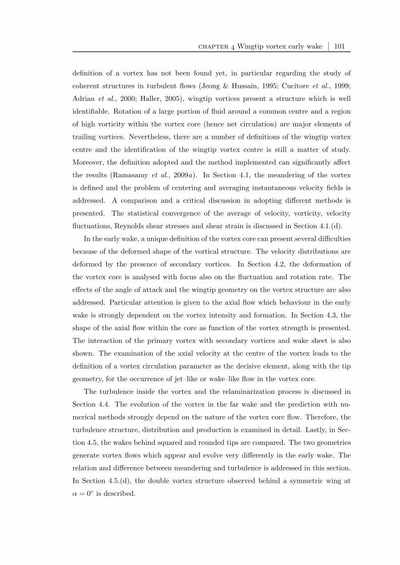
chapter Wingtip vortex early wake 101
definition of a vortex has not been found yet, in particular regarding the study of
coherent structures in turbulent flows (Jeong & Hussain, 1995; Cucitore et al., 1999;
Adrian et al., 2000; Haller, 2005), wingtip vortices present a structure which is well
identifiable. Rotation of a large portion of fluid around a common centre and a region
of high vorticity within the vortex core (hence net circulation) are major elements of
trailing vortices. Nevertheless, there are a number of definitions of the wingtip vortex
centre and the identification of the wingtip vortex centre is still a matter of study.
Moreover, the definition adopted and the method implemented can significantly affect
the results (Ramasamy et al., 2009a). In Section 4.1, the meandering of the vortex
is defined and the problem of centering and averaging instantaneous velocity fields is
addressed. A comparison and a critical discussion in adopting different methods is
presented. The statistical convergence of the average of velocity, vorticity, velocity
fluctuations, Reynolds shear stresses and shear strain is discussed in Section 4.1.(d).
In the early wake, a unique definition of the vortex core can present several difficulties
because of the deformed shape of the vortical structure. The velocity distributions are
deformed by the presence of secondary vortices. In Section 4.2, the deformation of
the vortex core is analysed with focus also on the fluctuation and rotation rate. The
effects of the angle of attack and the wingtip geometry on the vortex structure are also
addressed. Particular attention is given to the axial flow which behaviour in the early
wake is strongly dependent on the vortex intensity and formation. In Section 4.3, the
shape of the axial flow within the core as function of the vortex strength is presented.
The interaction of the primary vortex with secondary vortices and wake sheet is also
shown. The examination of the axial velocity at the centre of the vortex leads to the
definition of a vortex circulation parameter as the decisive element, along with the tip
geometry, for the occurrence of jet–like or wake–like flow in the vortex core.
The turbulence inside the vortex and the relaminarization process is discussed in
Section 4.4. The evolution of the vortex in the far wake and the prediction with nu-
merical methods strongly depend on the nature of the vortex core flow. Therefore, the
turbulence structure, distribution and production is examined in detail. Lastly, in Sec-
tion 4.5, the wakes behind squared and rounded tips are compared. The two geometries
generate vortex flows which appear and evolve very differently in the early wake. The
relation and difference between meandering and turbulence is addressed in this section.
In Section 4.5.(d), the double vortex structure observed behind a symmetric wing at
α = 0 is described.

chapter Wingtip vortex early wake 102
section
Localization of the vortex centre and averaging
of velocity vector fields
The need to identify the wingtip vortex centre comes from the fact that these vortices
are not stationary flows but they exhibit small random motions normal to the vortex
axis. This phenomenon is called meandering (or wandering) of the wingtip vortex, or
referred to as aperiodicity for rotorcraft because the motion represents the variation
or scatter in the vortex centre location from one period (rotor evolution) to another
(Ramasamy et al., 2009a).
In Figure 4.1, instantaneous velocity vectors and vorticity contours are reported on
planes perpendicular to the freestream. Assuming that it is possible to detect the vortex
core in each instantaneous frame, the wandering can be defined as the fluctuation of
these locations. The vortex meandering moves the centre by few percent of the chord
and different instantaneous positions of the vortex are observed in the four snapshots.
Whatever the source of the wandering, the vortex centre movement and the mean flow
properties are important properties to study. Moreover, centering each realization be-
fore taking the average is needed for an accurate description of the vortex structure.
The movement of the vortex introduces an artificial spreading effect when averaging,
resulting in a larger apparent vortex core size and a smaller peak swirl velocity than any
of the instantaneous measurements. Although the meandering phenomenon has more
impact on the mid field, correcting for the wandering effects is also essential when the
objective of the study is to accurately quantify the turbulence in the wake and inside the
tip vortex (Ramasamy et al., 2009b). The centering of the instantaneous realizations of
the vortex can also be seen as a filtering operation which separates the solid translation
of the vortex with the turbulent fluctuation of the vortex. The solid translation is what
is referred to as meandering.
The implementation of the method which extracts the meandering information and
the average vortex flow field requires special care. Birch (2012) proved that for isotropic
and Gaussian wandering amplitudes, within the range of those usually observed experi-
mentally, any axisymmetric flow field having zero velocity at r = 0 and r →∞ converges
upon the circulation profile obtained for the case of a Batchelor q–vortex. This means
that a good agreement of the averaged swirl velocity profile and the Batchelor q–vortex
may not necessarily imply that the instantaneous profiles also agree well with the q–
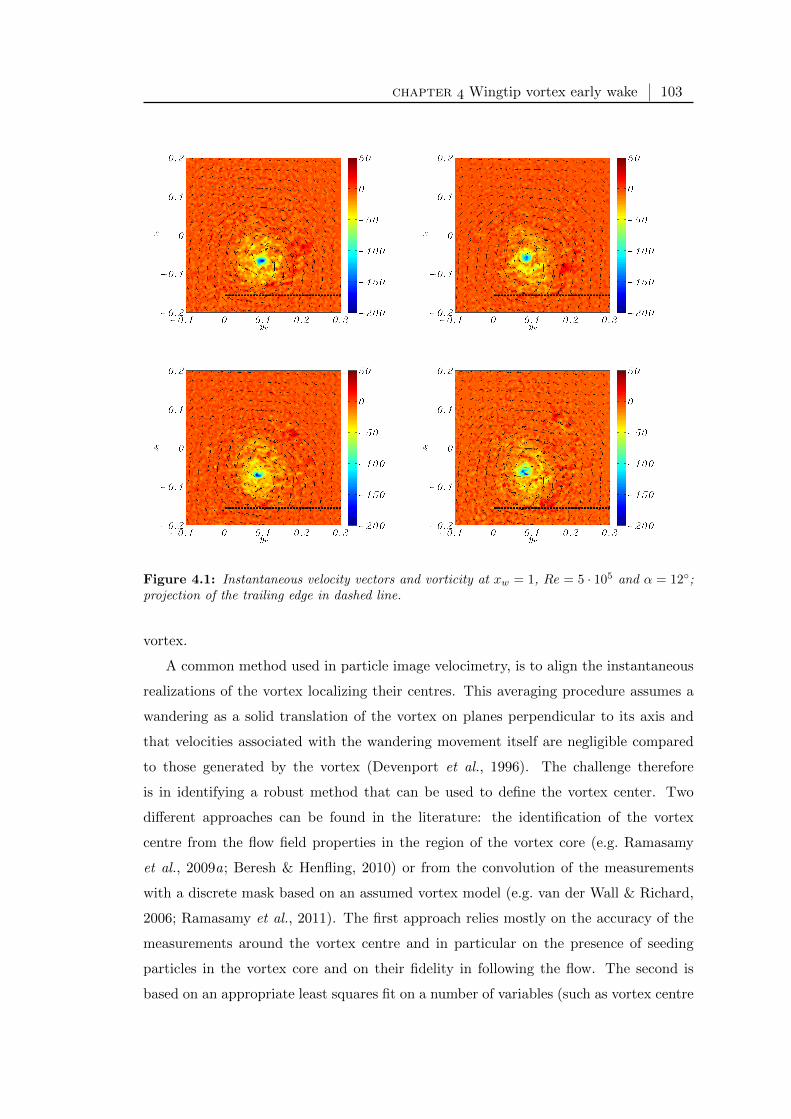
chapter Wingtip vortex early wake 103
Figure 4.1: Instantaneous velocity vectors and vorticity at xw = 1, Re = 5 · 105 and α = 12;projection of the trailing edge in dashed line.
vortex.
A common method used in particle image velocimetry, is to align the instantaneous
realizations of the vortex localizing their centres. This averaging procedure assumes a
wandering as a solid translation of the vortex on planes perpendicular to its axis and
that velocities associated with the wandering movement itself are negligible compared
to those generated by the vortex (Devenport et al., 1996). The challenge therefore
is in identifying a robust method that can be used to define the vortex center. Two
different approaches can be found in the literature: the identification of the vortex
centre from the flow field properties in the region of the vortex core (e.g. Ramasamy
et al., 2009a; Beresh & Henfling, 2010) or from the convolution of the measurements
with a discrete mask based on an assumed vortex model (e.g. van der Wall & Richard,
2006; Ramasamy et al., 2011). The first approach relies mostly on the accuracy of the
measurements around the vortex centre and in particular on the presence of seeding
particles in the vortex core and on their fidelity in following the flow. The second is
based on an appropriate least squares fit on a number of variables (such as vortex centre

chapter Wingtip vortex early wake 104
position and velocity, orientation of the vortex axis with respect to the measurement
plane, vortex circulation, vortex core radius) to a reasonable vortex analytical model.
For fixed wing tip vortices, peaks of properties such as vorticity or swirling strength
well describe the primary vortex centre in contrast to, for example, the tip vortices of
lightly loaded rotors in forward flight, especially those created on the advancing side,
which are often very weak, hard to detect and coexistent with similar secondary vortices
(van der Wall & Richard, 2006). Also, in the early wake, the vortex is not axisymmetric
and it is not well described by analytical models. Moreover, enough particles were
present in the core and the SPIV measurements resulted in a high spatial accuracy and
reliability of the data in the vortex core. Therefore, in this study, the first approach for
the vortex centre identification was adopted. In Figure 4.2, the instantaneous seeding
distribution for a reference case1 is shown along with the average core dimension for
that case. A darker region is observed at the vortex centre of size less than 2% of the
chord and less than a tenth of the vortex core diameter. However, particles are still
detected in this area which is of the order of the interrogation window size adopted and
a reliable and accurate description of the flow in the core is achieved with a measurement
grid spacing of around 3% of the core radius which is much higher than most of the
experiments on wingtip vortices found in the literature.
Figure 4.2: Instantaneous seeding distribution at xw = 1, Re = 5 · 105 and α = 12.
Methods for the detection of the vortex centre from measurements in the core can
be based on different properties of the vortex even though, for an analytical vortex, all
these methods lead to the same location of the vortex centre. A discussion of the most
common vortex centre localization methods is presented as follows.
1The reference case is the trailing vortex at 1 chord of distance from the trailing edge of the wingmodel M1, at 12 of incidence and Reynolds number of 5 · 105. This case is a medium condition interms of vortex properties and experimental arrangement of all tests.

chapter Wingtip vortex early wake 105
1. Centroid of the seed darker region. The darker region formed by centrifugal forces
on the seed particles at the vortex centre (see Figure 4.2) is only qualitative in na-
ture and it is not usually circular or in any repeatable shape in the instantaneous
pictures. It depends on several factors such as image contrast, seed particle dis-
tribution, particles mass and size, bit resolution of the camera, vortex dimension
and strength making an automatic and general method based on this concept not
very reliable compared to quantitative properties. However, these problems can
be reduced with an appropriate use of seeding and equipment.
2. Zero in–plane velocity (or swirl centre). The swirl centre represents the spatial
location at which the in–plane velocity component is zero:
√v2 + w2 = 0 (4.1)
This method can lead to erroneous results when the vortex axis is not straight and
in particular when the axis curvature is high, such as for rotor wingtips. Moreover,
the error grows if the vortex bulk motion is large or in PIV measurements if the
light sheet is misaligned. A similar approach is represented by the calculation of
the centroid of the planar streamlines.
3. Peak axial velocity. At the vortex centre, a perturbation of the axial velocity is
commonly observed and it can be either away from the wing or toward the wing
depending on the tip loading on the wing and the roll up of the wake sheet. When
this perturbation is strong, the vortex centre can be identified as the point of
maximum axial velocity perturbation.
4. Centre point between the swirl velocity peaks. The velocity profile of the component
perpendicular to a cut across the vortex core reveals two peaks on the two sides
of the centre. The centre point between these two peaks is an indication of the
vortex centre coordinate. If this process is iteratively done also on cuts at different
positions and directions, the vortex centre is identified. However, this method
addresses only the swirl velocity peaks and not also its profile within the core
and in case of asymmetry of the vortex, this procedure leads to wrong results.
Nevertheless, this technique is commonly used in point measurements such as
with pressure tubes and hot wire probes or when the accuracy of measurements
in the vortex core is low.
5. Peak of vorticity. Vorticity is a three–dimensional vector. However, PIV mea-

chapter Wingtip vortex early wake 106
surements made on a single plane can only provide the velocity gradients on that
plane. As a result, only one component of the vorticity can be calculated, that is
the streamwise component ωx when the plane is perpendicular to the freestream.
For this method, the location of the vorticity peak is taken as the vortex centre.
6. Peak of helicity. Helicity is a conserved quantity which measures the helical motion
of a vortex. It is defined as the dot product of the velocity and the vorticity so that
the result indicates the inclination between the vorticity vector and the velocity
vector. Because only the streamwise vorticity is available, only the streamwise
component of the helicity can be calculated. In these experiments, where the
wing is fixed and the vortex moves downstream with the freestream flow, a more
appropriate definition is the scalar product of the axial velocity disturbance and
the vorticity. In order to take into account either an axial velocity excess or defect,
the absolute disturbance is used:
Hx = |u− U∞| · ωx (4.2)
As for the vorticity peak method, the peak of the helicity identifies the vortex
centre.
7. Q–criterion (or peak of the swirling strength). Special singular points, typical of
vortical features of spiral or close streamlines, are mathematically described by
complex eigenvalues of the velocity gradient tensor which is composed of the strain
tensor Σ and the vorticity tensor Ω, and expressed as follows:
dV
dx= Σ + Ω =
εyy εyz
εzy εzz
+1
2
0 −ωxωx 0
=
=
∂v
∂y
1
2
(∂v
∂z+∂w
∂y
)1
2
(∂w
∂y+∂v
∂z
)∂w
∂z
+
01
2
(∂v
∂z− ∂w
∂y
)1
2
(∂w
∂y− ∂v
∂z
)0
(4.3)
A vortex is characterized by the invariance of the velocity gradient tensor (Jeong
& Hussain, 1995) which requires the discriminant Q of the characteristic equation
of the velocity tensor gradient to be below zero. It follows that the centre of the
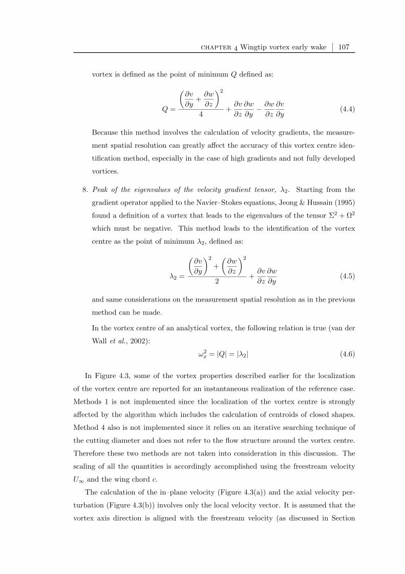
chapter Wingtip vortex early wake 107
vortex is defined as the point of minimum Q defined as:
Q =
(∂v
∂y+∂w
∂z
)2
4+∂v
∂z
∂w
∂y− ∂w
∂z
∂v
∂y(4.4)
Because this method involves the calculation of velocity gradients, the measure-
ment spatial resolution can greatly affect the accuracy of this vortex centre iden-
tification method, especially in the case of high gradients and not fully developed
vortices.
8. Peak of the eigenvalues of the velocity gradient tensor, λ2. Starting from the
gradient operator applied to the Navier–Stokes equations, Jeong & Hussain (1995)
found a definition of a vortex that leads to the eigenvalues of the tensor Σ2 + Ω2
which must be negative. This method leads to the identification of the vortex
centre as the point of minimum λ2, defined as:
λ2 =
(∂v
∂y
)2
+
(∂w
∂z
)2
2+∂v
∂z
∂w
∂y(4.5)
and same considerations on the measurement spatial resolution as in the previous
method can be made.
In the vortex centre of an analytical vortex, the following relation is true (van der
Wall et al., 2002):
ω2x = |Q| = |λ2| (4.6)
In Figure 4.3, some of the vortex properties described earlier for the localization
of the vortex centre are reported for an instantaneous realization of the reference case.
Methods 1 is not implemented since the localization of the vortex centre is strongly
affected by the algorithm which includes the calculation of centroids of closed shapes.
Method 4 also is not implemented since it relies on an iterative searching technique of
the cutting diameter and does not refer to the flow structure around the vortex centre.
Therefore these two methods are not taken into consideration in this discussion. The
scaling of all the quantities is accordingly accomplished using the freestream velocity
U∞ and the wing chord c.
The calculation of the in–plane velocity (Figure 4.3(a)) and the axial velocity per-
turbation (Figure 4.3(b)) involves only the local velocity vector. It is assumed that the
vortex axis direction is aligned with the freestream velocity (as discussed in Section
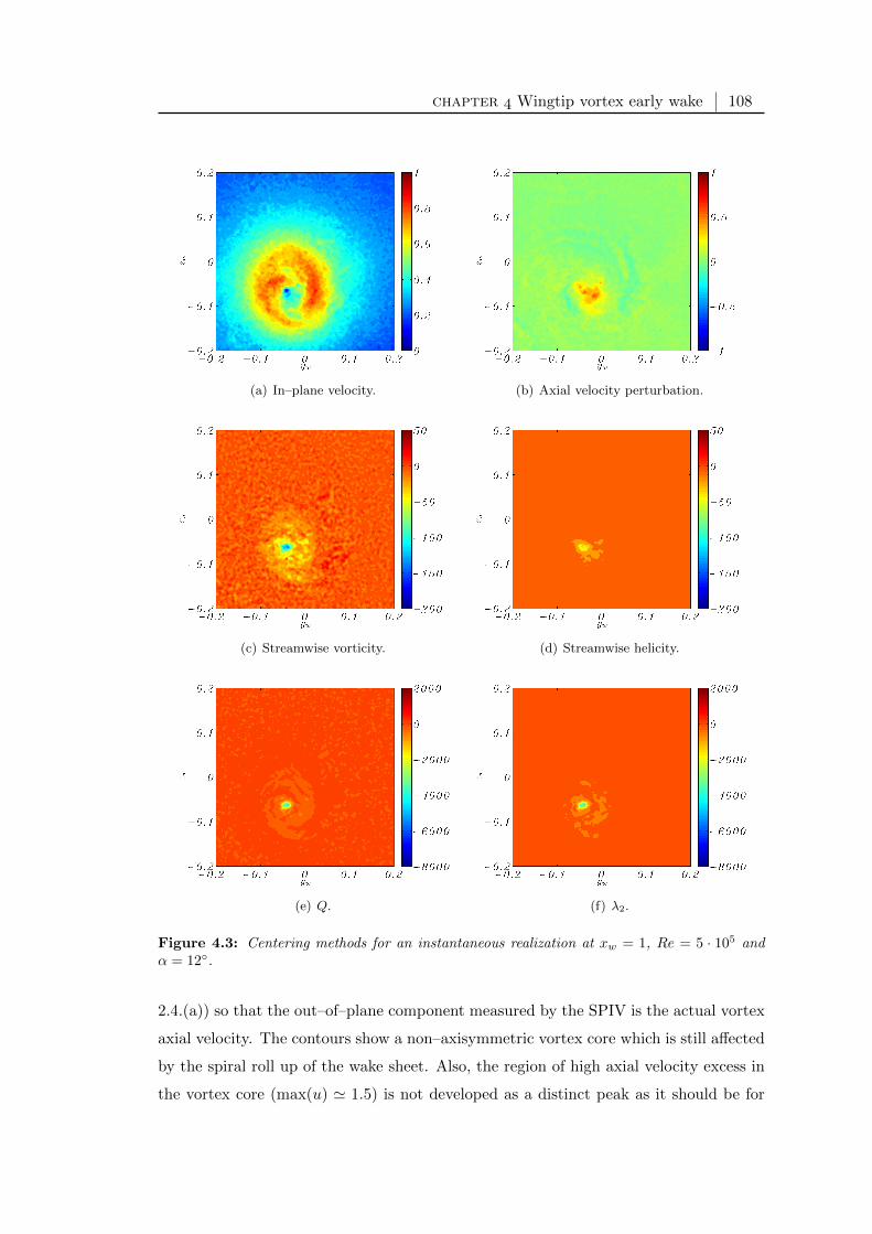
chapter Wingtip vortex early wake 108
(a) In–plane velocity. (b) Axial velocity perturbation.
(c) Streamwise vorticity. (d) Streamwise helicity.
(e) Q. (f) λ2.
Figure 4.3: Centering methods for an instantaneous realization at xw = 1, Re = 5 · 105 andα = 12.
2.4.(a)) so that the out–of–plane component measured by the SPIV is the actual vortex
axial velocity. The contours show a non–axisymmetric vortex core which is still affected
by the spiral roll up of the wake sheet. Also, the region of high axial velocity excess in
the vortex core (max(u) ' 1.5) is not developed as a distinct peak as it should be for

chapter Wingtip vortex early wake 109
fully developed trailing vortices. The streamwise vorticity (Figure 4.3(c)) is calculated
with the 8 node circulation method described by Raffel et al. (2007) which performs
better than other schemes in terms of error and smoothness of the results. A region of
high vorticity is observed in the vortex core. A similar result is observed in Figure 4.3(d)
where a concentration of helicity (calculated as the point product of streamwise vorticity
and axial velocity perturbation) is observed within the core. The helicity highlights the
vorticity peak when an axial velocity perturbation is present in the vortex core, which
exists in most of the trailing vortices. Also, the helicity is the only vortex property that
includes in its calculation all the three velocity components which are available from a
SPIV. The derivatives for the calculation of Q and λ2 (Figures 4.3(e) and 4.3(f)) are
estimated with the 4 points centered least–square approach (Raffel et al., 2007). The
two contours look very similar and around the peak in the vortex centre the shapes are
identical. This is because in the vortex core the planar elongational strains εyy, εzz are
negligible compared to the shear strains εyz, εzy and in particular, at the vortex centre:
(∂v
∂y
)2
,
(∂w
∂z
)2
,∂v
∂y
∂w
∂z ∂v
∂z
∂w
∂y(4.7)
which leads to identical definition of Q and λ2 from Equations (4.4) and (4.5) around
the vortex centre.
The 121 instantaneous vortex centre positions of the reference case are calculated
with these vortex centre localization methods and reported in Figure 4.4. The pattern
of the distribution of the instantaneous centres reveals that they are strongly affected
by the grid spacing of the vector field which is of the order of one tenth of the movement
of the centres. However, because the grid spacing is a small fraction of the core radius
(and around 0.3% of the chord), the alignment of the individual measurements with the
closest grid node does not lead to a significant error. In fact, this results in a residual
vortex wandering in the measurements which is less than half the diagonal grid spacing.
Based on analysis by Devenport et al. (1996), this would result in less than 0.8% error
in the measured peak swirl velocity and core radius. Therefore, alignment based on the
grid node closest to the vortex centre was followed in the present work.
For this case, the scattering of the vortex centres (the wandering of the vortex)
is of about 4% of the wing chord and the axial velocity perturbation method shows
the highest dispersion compared to the other methods. The Q and the λ2 methods
show identical distributions of the instantaneous centres. Analysing the vortex centre
distributions of all the configurations, no particular orientation of the meandering was
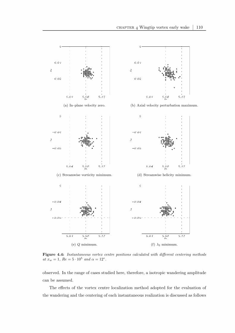
chapter Wingtip vortex early wake 110
(a) In–plane velocity zero. (b) Axial velocity perturbation maximum.
(c) Streamwise vorticity minimum. (d) Streamwise helicity minimum.
(e) Q minimum. (f) λ2 minimum.
Figure 4.4: Instantaneous vortex centre positions calculated with different centering methodsat xw = 1, Re = 5 · 105 and α = 12.
observed. In the range of cases studied here, therefore, a isotropic wandering amplitude
can be assumed.
The effects of the vortex centre localization method adopted for the evaluation of
the wandering and the centering of each instantaneous realization is discussed as follows

chapter Wingtip vortex early wake 111
with particular attention to the swirl velocity distribution, the axial velocity and the
turbulent quantities. The average of the 121 instantaneous vector fields is calculated
for each vortex centre localization method and it involves the centering of each of the
vortex realizations. The average of the instantaneous vector fields without the centering
will be referred to as simple average. The study on the statistical convergence of vortex
properties, which leads to the choice of 121 vector fields, is presented in Section 4.1.(d).
(a) Swirl velocity
distribution
As discussed earlier, without centering each instantaneous flow
field, the mean vortex shows a larger radius and a smaller maxi-
mum swirl velocity than the same mean properties when the cen-
tering is applied. This behaviour is true for a fully developed vortex, that is a wingtip
vortex in the far wake. At an early stage, as observed in these experiments, this smearing
effect is partially masked by the high asymmetry of the vortex. On the simple averaged
in–plane velocity distribution around the vortex in Figure 4.5(a), an anti–clockwise spi-
ral structure of higher velocity around the core is observed (which indicates the clockwise
rotation of the vortex). Thus, the gradient of the swirl velocity and the location of the
maximum swirl velocity (which defines the vortex radius) are expected to be different
when different directions of the cuts across the centre are done. The averaged axial
velocity distribution in Figure 4.5(b) also shows an asymmetric structure. The centres
calculated as minimum in–plane velocity and as maximum axial velocity, indicated by
respectively a black and a white cross in Figure 4.5, are positioned at a distance 1% of
the chord which corresponds to about 15% of the core radius (the origin of the reference
system of Figure 4.5 was arbitrarily chosen at the vorticity peak). This indicates that
the vortex is still strongly affected by the formation process on the wing, the rolling
up of the wake sheet and the interaction with secondary vortices. At this stage, the
effects of applying the simple average of the instantaneous flow fields or applying some
centre localization method, are small compared to the strong asymmetry of the vortex
structure.
In Figure 4.6, swirl velocity profiles calculated from the averaged vector fields after
different centering methods are shown; the velocity is calculated by a cubic interpolation
of the velocity vector field along 36 radii equispaced around the centre (although only 12
are reported in the graph) adopting a cubic interpolation from the cartesian grid of the
original velocity vectors. In Figure 4.6(a) the swirl velocity from the simple averaged
vector field is calculated. The effect of the spiral structure observed in Figure 4.5 is
observed here as a collection of profiles with very different vortex radii (from r = 0.03
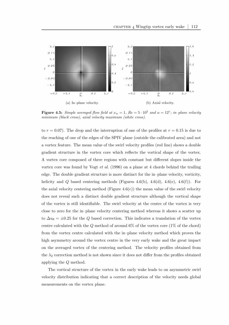
chapter Wingtip vortex early wake 112
(a) In–plane velocity. (b) Axial velocity.
Figure 4.5: Simple averaged flow field at xw = 1, Re = 5 · 105 and α = 12; in–plane velocityminimum (black cross), axial velocity maximum (white cross).
to r = 0.07). The drop and the interruption of one of the profiles at r = 0.15 is due to
the reaching of one of the edges of the SPIV plane (outside the calibrated area) and not
a vortex feature. The mean value of the swirl velocity profiles (red line) shows a double
gradient structure in the vortex core which reflects the vortical shape of the vortex.
A vortex core composed of three regions with constant but different slopes inside the
vortex core was found by Vogt et al. (1996) on a plane at 4 chords behind the trailing
edge. The double gradient structure is more distinct for the in–plane velocity, vorticity,
helicity and Q based centering methods (Figures 4.6(b), 4.6(d), 4.6(e), 4.6(f)). For
the axial velocity centering method (Figure 4.6(c)) the mean value of the swirl velocity
does not reveal such a distinct double gradient structure although the vortical shape
of the vortex is still identifiable. The swirl velocity at the centre of the vortex is very
close to zero for the in–plane velocity centering method whereas it shows a scatter up
to ∆uθ = ±0.25 for the Q based correction. This indicates a translation of the vortex
centre calculated with the Q method of around 6% of the vortex core (1% of the chord)
from the vortex centre calculated with the in–plane velocity method which proves the
high asymmetry around the vortex centre in the very early wake and the great impact
on the averaged vortex of the centering method. The velocity profiles obtained from
the λ2 correction method is not shown since it does not differ from the profiles obtained
applying the Q method.
The vortical structure of the vortex in the early wake leads to on asymmetric swirl
velocity distribution indicating that a correct description of the velocity needs global
measurements on the vortex plane.

chapter Wingtip vortex early wake 113
(a) Simple average. (b) In–plane velocity zero.
(c) Axial velocity perturbation maximum. (d) Streamwise vorticity minimum.
(e) Streamwise helicity minimum. (f) Q minimum.
Figure 4.6: Average swirl velocity profiles and mean values (red line) calculated with differentcentering methods at xw = 1, Re = 5 · 105 and α = 12.
(b) Axial velocity
distribution
Differences in the vortex description when simple average or cen-
tered average is applied, are remarkable when the axial velocity
profiles (out–of–plane component of the SPIV) are viewed. In
Figure 4.7, axial velocity profiles of the simple and corrected averaged vector fields are
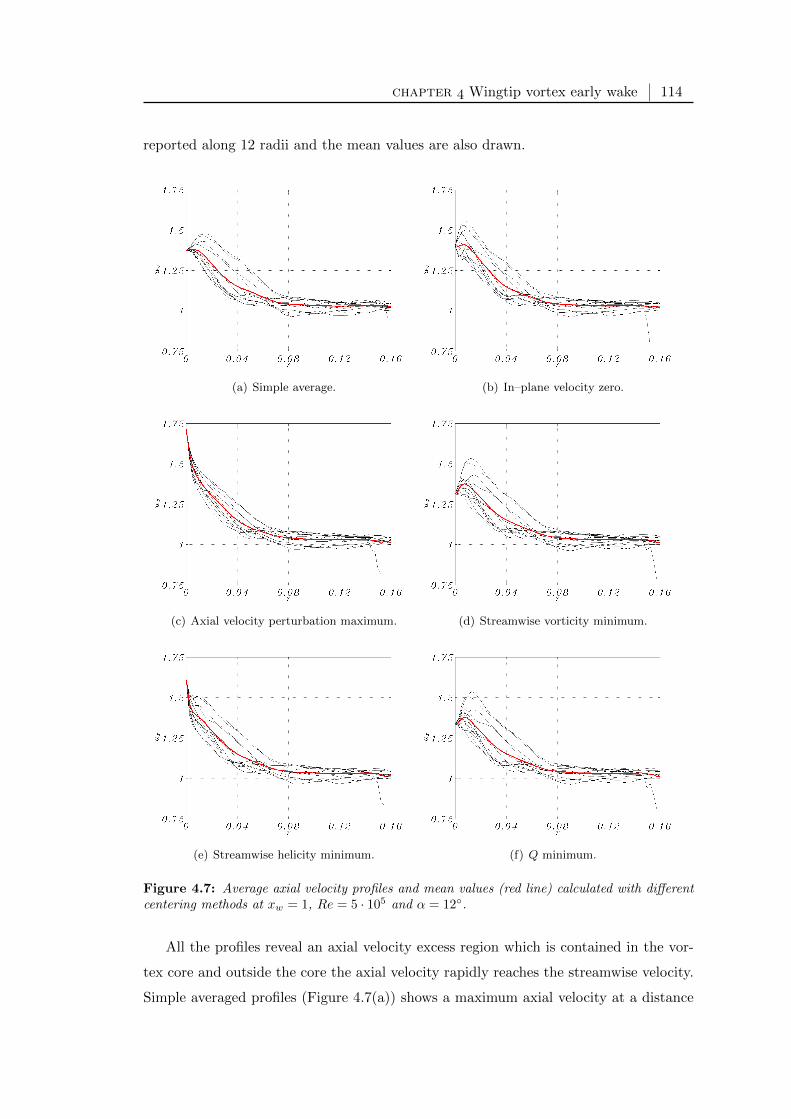
chapter Wingtip vortex early wake 114
reported along 12 radii and the mean values are also drawn.
(a) Simple average. (b) In–plane velocity zero.
(c) Axial velocity perturbation maximum. (d) Streamwise vorticity minimum.
(e) Streamwise helicity minimum. (f) Q minimum.
Figure 4.7: Average axial velocity profiles and mean values (red line) calculated with differentcentering methods at xw = 1, Re = 5 · 105 and α = 12.
All the profiles reveal an axial velocity excess region which is contained in the vor-
tex core and outside the core the axial velocity rapidly reaches the streamwise velocity.
Simple averaged profiles (Figure 4.7(a)) shows a maximum axial velocity at a distance
chapter Wingtip vortex early wake 115
of 2% of the chord from the centre. This peak, of intensity of 1.48 times the reference
velocity, is lower than the peaks observed from any other corrected profile, as a con-
sequence of the smearing effect. In contrast, the axial velocity based average (Figure
4.7(c)) show, as expected by definition, the highest axial velocity perturbation with
u0 = 1.71 located in the centre. For the in–plane velocity (Figure 4.7(b)), the vorticity
(Figure 4.7(d)) and the Q method (Figure 4.7(f)) the profiles are similar, with region
of axial velocity peak (ux =1.53–1.56) away from the centre of the vortex where the
axial velocity is u0 =1.31–1.40. It appears from these profiles that, like the swirl ve-
locity, also the axial velocity in the vortex core shows a high asymmetry. The helicity
centering method (Figure 4.7(e)) still indicates asymmetry in the vortex core but it is
the only one, besides the axial velocity method, that shows the maximum axial velocity
perturbation at the vortex centre (u0 = 1.61).
(c) Turbulent quantities Some of the turbulent quantities are also compared for
different centering methods although the discussion of the
turbulence in the vortex will be presented in a later section. The instantaneous velocity
at one point of the flow field is expressed as sum of the average velocity at that point
during the experiment and the fluctuating component:
u = u + u′ (4.8)
The root mean square of the velocity fluctuations (square root of the turbulent
normal stresses) defined as follows is scaled by the freestream velocity U∞:
σu =
√u′2 =
√(ui − u)2 (4.9)
σv =
√v′2 =
√(vi − v)2 (4.10)
σw =
√w′2 =
√(wi − w)2 (4.11)
The Reynolds stresses, scaled by U∞2, are defined as follows:
v′w′ = (vi − v) (wi − w) (4.12)
u′v′ = (ui − u) (vi − v) (4.13)
u′w′ = (ui − u) (wi − w) (4.14)
where v′w′ are the stresses on the SPIV plane.

chapter Wingtip vortex early wake 116
The shear strain εyz and the normal strain εxx are calculated with an eight point
scheme as described by Raffel et al. (2007) where, for the latter, incompressibility is
assumed:
εyz = εzy =1
2
(∂v
∂z+∂w
∂y
)(4.15)
εxx =∂u
∂x= −
(∂v
∂y+∂w
∂z
)(4.16)
The maximum Mach number found in the flow fields is of the order of M = 0.15 so that
the assumption of ∇ ·u = 0 is very reasonable. The normalisation of the strains is with
U∞/c.
The turbulent kinetic energy is also calculated and defined as half the sum of the
variance of the velocity fluctuations:
k =1
2
(u′2 + v′2 + w′2
)(4.17)
In Figures 4.8 and 4.9 the turbulent fluctuations of the three velocity components
calculated from simple averaged and centered flow fields are compared. High fluctuation
is observed within the vortex core on all the components. Both the in–plane fluctuations
σv and σw exhibit an elliptical shape, with the major axes aligned respectively along
the y axis direction and the z axis direction whereas the axial fluctuation σu shows a
circular shape. The elliptical structure of the in–plane components, which is observed
also by Ramasamy et al. (2009b), is less clear for in–plane centering method compared
to the other methods. The rolling up wake sheet also shows high fluctuations relatively
to the external flow (light blue region around the centre at radius approximately equal
to 0.1).
The peak in the fluctuation on each contour in Figures 4.8 and 4.9 is observed at the
centre of the vortex (at the origin of the reference system). The maximum peak value
of the in–plane fluctuations σv and σw is observed for the axial velocity perturbation
centering method whereas it is minimum for the in–plane velocity centering method.
Also, the maximum peak value of the axial fluctuation σu is observed for the in–plane
velocity centering method although for all the averaging methods a similar fluctuation
level is observed.
In Figure 4.10, the maximum instantaneous axial velocity ux found in the vortex
core is reported for each one of the 121 vortex realizations. The fluctuation level is very
high with velocity peak values between 1.4 and 2.1 and standard deviation of 9.5% of the

chapter Wingtip vortex early wake 117
(a) Simple average: σv. (b) Simple average: σw. (c) Simple average: σu.
(d) In–plane velocity zero: σv. (e) In–plane velocity zero: σw. (f) In–plane velocity zero: σu.
(g) Axial velocity perturbationmaximum: σv.
(h) Axial velocity perturbationmaximum: σw.
(i) Axial velocity perturbationmaximum: σu.
Figure 4.8: Velocity fluctuations at xw = 1, Re = 5 · 105 and α = 12; part 1 of 2.
freestream velocity which indicates strong turbulent fluctuations within the vortex core.
It is important to notice that these values do not correspond necessarily to the vortex
centre velocity but they refer to a point in the vortex core. They would correspond by
definition to the vortex centre in the case of adopting the peak axial velocity centering
method. Therefore, the fluctuation of these peak velocities is not directly related to
the wandering of the vortex but only to its instantaneous intensity. However, such
axial velocity are higher than most of other experiments but coherent with the results
presented by Green & Acosta (1991) and Chow et al. (1997a). Several factors influence
the development of the velocity excess including angle of attack, tip shape and Reynolds
number. The measurements of Figure 4.10 were performed at a high angle of attack, at
a relatively high Reynolds number and there was not the problem of probes affecting
the flow. These factors are shared with the studies mentioned above.
The Reynolds shear stress on the SPIV plane, the corresponding shear strain and
the turbulent kinetic energy are shown in Figures 4.11 and 4.12 for the different aver-
aging methods. The relative rotation of 45 between the Reynolds stresses and shear
stresses, observed also by Chow et al. (1997b) and Ramasamy et al. (2009b), reveals

chapter Wingtip vortex early wake 118
(a) Streamwise vorticity mini-mum: σv.
(b) Streamwise vorticity mini-mum: σw.
(c) Streamwise vorticity mini-mum: σu.
(d) Streamwise helicity mini-mum: σv.
(e) Streamwise helicity mini-mum: σw.
(f) Streamwise helicity mini-mum: σu.
(g) Q minimum: σv. (h) Q minimum: σw. (i) Q minimum: σu.
Figure 4.9: Velocity fluctuations at xw = 1, Re = 5 · 105 and α = 12; part 2 of 2.
Figure 4.10: Instantaneous axial velocity peaks at xw = 1, Re = 5 · 105 and α = 12.
the anisotropic eddy viscosity in the vortex core. Although the shear strains show the
same four lobed pattern independently from the averaging method used, the Reynolds
stresses change in magnitude when adopting different averages. As observed also for
the in–plane turbulent fluctuations earlier, the axial velocity centering method shows a
high level of turbulence in the vortex core and the in–plane velocity centering method
gives a low level of turbulence. The turbulent kinetic energy behaves in the same way.

chapter Wingtip vortex early wake 119
Also, regardless of the centering method adopted, a peak of turbulence is calculated
at the vortex centre. The peak of the turbulent kinetic energy at the vortex centre is
dictated by the high turbulence level of all the velocity components within the core. At
this stage, the turbulent fluctuations are still present in the core and the laminarization
process is not observed. More details on the relaminarization of the vortex core are
presented in the next sections.
(a) Simple average: v′w′. (b) Simple average: εyz. (c) Simple average: k.
(d) In–plane velocity zero: v′w′. (e) In–plane velocity zero: εyz. (f) In–plane velocity zero: k.
(g) Axial velocity perturbationmaximum: v′w′.
(h) Axial velocity perturbationmaximum: εyz.
(i) Axial velocity perturbationmaximum: k.
Figure 4.11: Turbulence at xw = 1, Re = 5 · 105 and α = 12; part 1 of 2.
The wingtip vortex flow in the early wake is dominated by interaction with secondary
vortices and by the rolling up of the wake sheet. Although discussions could be done
on the best and most appropriate centering method, the final decision has to take into
consideration the particular interest of the undertaken study. For instance, in order to
study the maximum axial velocity encountered in the vortex core or to study the shape
of the rolling up of the vortex sheet or the interaction between the several secondary
vortices with the primary vortex, different centering methods might be adopted before
taking the average in order to highlight the particular feature of the vortex system.
Nevertheless, vortex meandering is observed also in the early wake and centering the
instantaneous frames leads to different descriptions of the vortex velocity field and
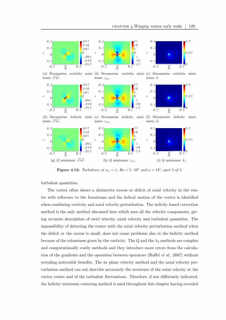
chapter Wingtip vortex early wake 120
(a) Streamwise vorticity mini-mum: v′w′.
(b) Streamwise vorticity mini-mum: εyz.
(c) Streamwise vorticity mini-mum: k.
(d) Streamwise helicity mini-mum: v′w′.
(e) Streamwise helicity mini-mum: εyz.
(f) Streamwise helicity mini-mum: k.
(g) Q minimum: v′w′. (h) Q minimum: εyz. (i) Q minimum: k.
Figure 4.12: Turbulence at xw = 1, Re = 5 · 105 and α = 12; part 2 of 2.
turbulent quantities.
The vortex often shows a distinctive excess or deficit of axial velocity in the cen-
tre with reference to the freestream and the helical motion of the vortex is identified
when combining vorticity and axial velocity perturbation. The helicity based correction
method is the only method discussed here which uses all the velocity components, giv-
ing accurate description of swirl velocity, axial velocity and turbulent quantities. The
impossibility of detecting the centre with the axial velocity perturbation method when
the deficit or the excess is small, does not cause problems also in the helicity method
because of the robustness given by the vorticity. The Q and the λ2 methods are complex
and computationally costly methods and they introduce more errors from the calcula-
tion of the gradients and the operation between operators (Raffel et al., 2007) without
revealing noticeable benefits. The in–plane velocity method and the axial velocity per-
turbation method can not describe accurately the structure of the axial velocity at the
vortex centre and of the turbulent fluctuations. Therefore, if not differently indicated,
the helicity minimum centering method is used throughout this chapter having revealed
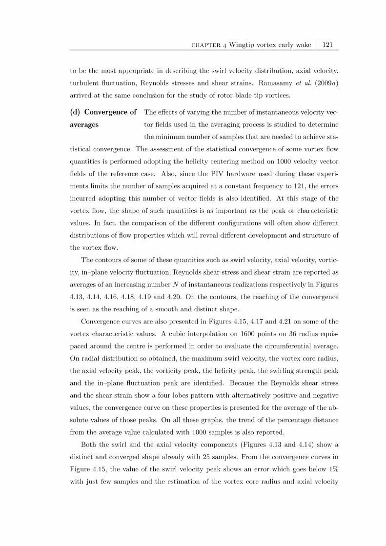
chapter Wingtip vortex early wake 121
to be the most appropriate in describing the swirl velocity distribution, axial velocity,
turbulent fluctuation, Reynolds stresses and shear strains. Ramasamy et al. (2009a)
arrived at the same conclusion for the study of rotor blade tip vortices.
(d) Convergence of
averages
The effects of varying the number of instantaneous velocity vec-
tor fields used in the averaging process is studied to determine
the minimum number of samples that are needed to achieve sta-
tistical convergence. The assessment of the statistical convergence of some vortex flow
quantities is performed adopting the helicity centering method on 1000 velocity vector
fields of the reference case. Also, since the PIV hardware used during these experi-
ments limits the number of samples acquired at a constant frequency to 121, the errors
incurred adopting this number of vector fields is also identified. At this stage of the
vortex flow, the shape of such quantities is as important as the peak or characteristic
values. In fact, the comparison of the different configurations will often show different
distributions of flow properties which will reveal different development and structure of
the vortex flow.
The contours of some of these quantities such as swirl velocity, axial velocity, vortic-
ity, in–plane velocity fluctuation, Reynolds shear stress and shear strain are reported as
averages of an increasing number N of instantaneous realizations respectively in Figures
4.13, 4.14, 4.16, 4.18, 4.19 and 4.20. On the contours, the reaching of the convergence
is seen as the reaching of a smooth and distinct shape.
Convergence curves are also presented in Figures 4.15, 4.17 and 4.21 on some of the
vortex characteristic values. A cubic interpolation on 1600 points on 36 radius equis-
paced around the centre is performed in order to evaluate the circumferential average.
On radial distribution so obtained, the maximum swirl velocity, the vortex core radius,
the axial velocity peak, the vorticity peak, the helicity peak, the swirling strength peak
and the in–plane fluctuation peak are identified. Because the Reynolds shear stress
and the shear strain show a four lobes pattern with alternatively positive and negative
values, the convergence curve on these properties is presented for the average of the ab-
solute values of those peaks. On all these graphs, the trend of the percentage distance
from the average value calculated with 1000 samples is also reported.
Both the swirl and the axial velocity components (Figures 4.13 and 4.14) show a
distinct and converged shape already with 25 samples. From the convergence curves in
Figure 4.15, the value of the swirl velocity peak shows an error which goes below 1%
with just few samples and the estimation of the vortex core radius and axial velocity

chapter Wingtip vortex early wake 122
(a) N = 5. (b) N = 25. (c) N = 100.
(d) N = 250. (e) N = 500. (f) N = 1000.
Figure 4.13: Swirl velocity at xw = 1, Re = 5 · 105 and α = 12.
(a) N = 5. (b) N = 25. (c) N = 100.
(d) N = 250. (e) N = 500. (f) N = 1000.
Figure 4.14: Axial velocity at xw = 1, Re = 5 · 105 and α = 12.
peak is below 2% with 121 samples.
The convergence of the shape of the vorticity distribution, which involve derivatives
of the velocity vector fields, (Figure 4.16) requires a higher number of samples around
100. The convergence of the peak value (Figure 4.17), found in the centre of the vortex,
also is slower than the velocity peaks and with 121 samples an error of 5% is expected.
With the same number of samples, the helicity shows an error of around 5% and the
swirling strength of around 6% which reflects the increasing number of operations needed
for their evaluation. However, the location where these peaks are found does not change
when the number of samples has reached a value of around 50.

chapter Wingtip vortex early wake 123
(a) Swirl velocity. (b) Vortex core radius.
(c) Axial velocity.
Figure 4.15: Convergence and errors of velocity and core radius at xw = 1, Re = 5 · 105 andα = 12.
(a) N = 5. (b) N = 25. (c) N = 100.
(d) N = 250. (e) N = 500. (f) N = 1000.
Figure 4.16: Vorticity at xw = 1, Re = 5 · 105 and α = 12.

chapter Wingtip vortex early wake 124
(a) Vorticity. (b) Helicity.
(c) Swirling strength.
Figure 4.17: Convergence and errors of vorticity, helicity and swirling strength at xw = 1,Re = 5 · 105 and α = 12.
(a) N = 5. (b) N = 25. (c) N = 100.
(d) N = 250. (e) N = 500. (f) N = 1000.
Figure 4.18: In–plane velocity fluctuation σv at xw = 1, Re = 5 · 105 and α = 12.
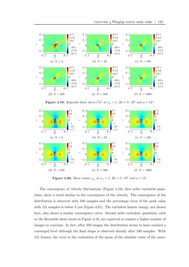
chapter Wingtip vortex early wake 125
(a) N = 5. (b) N = 25. (c) N = 100.
(d) N = 250. (e) N = 500. (f) N = 1000.
Figure 4.19: Reynolds shear stress v′w′ at xw = 1, Re = 5 · 105 and α = 12.
(a) N = 5. (b) N = 25. (c) N = 100.
(d) N = 250. (e) N = 500. (f) N = 1000.
Figure 4.20: Shear strain εyz at xw = 1, Re = 5 · 105 and α = 12.
The convergence of velocity fluctuations (Figure 4.18), first order turbulent quan-
tities, show a trend similar to the convergence of the velocity. The convergence of the
distribution is observed with 100 samples and the percentage error of the peak value
with 121 samples is below 3 (see Figure 4.21). The turbulent kinetic energy, not shown
here, also shows a similar convergence curve. Second order turbulent quantities, such
as the Reynolds shear stress in Figure 4.19, are expected to require a higher number of
images to converge. In fact, after 250 images the distribution seems to have reached a
converged level although the final shape is observed already after 100 samples. With
121 frames, the error in the evaluation of the mean of the absolute value of the maxi-
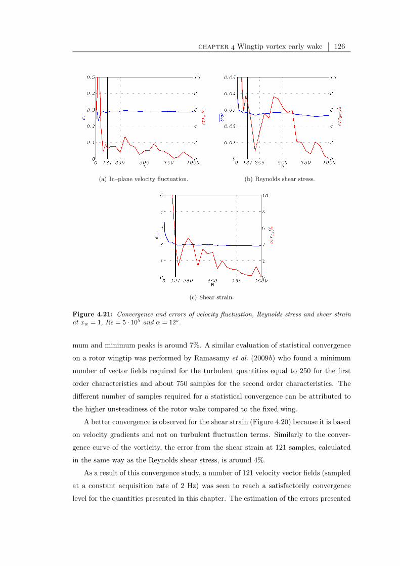
chapter Wingtip vortex early wake 126
(a) In–plane velocity fluctuation. (b) Reynolds shear stress.
(c) Shear strain.
Figure 4.21: Convergence and errors of velocity fluctuation, Reynolds stress and shear strainat xw = 1, Re = 5 · 105 and α = 12.
mum and minimum peaks is around 7%. A similar evaluation of statistical convergence
on a rotor wingtip was performed by Ramasamy et al. (2009b) who found a minimum
number of vector fields required for the turbulent quantities equal to 250 for the first
order characteristics and about 750 samples for the second order characteristics. The
different number of samples required for a statistical convergence can be attributed to
the higher unsteadiness of the rotor wake compared to the fixed wing.
A better convergence is observed for the shear strain (Figure 4.20) because it is based
on velocity gradients and not on turbulent fluctuation terms. Similarly to the conver-
gence curve of the vorticity, the error from the shear strain at 121 samples, calculated
in the same way as the Reynolds shear stress, is around 4%.
As a result of this convergence study, a number of 121 velocity vector fields (sampled
at a constant acquisition rate of 2 Hz) was seen to reach a satisfactorily convergence
level for the quantities presented in this chapter. The estimation of the errors presented
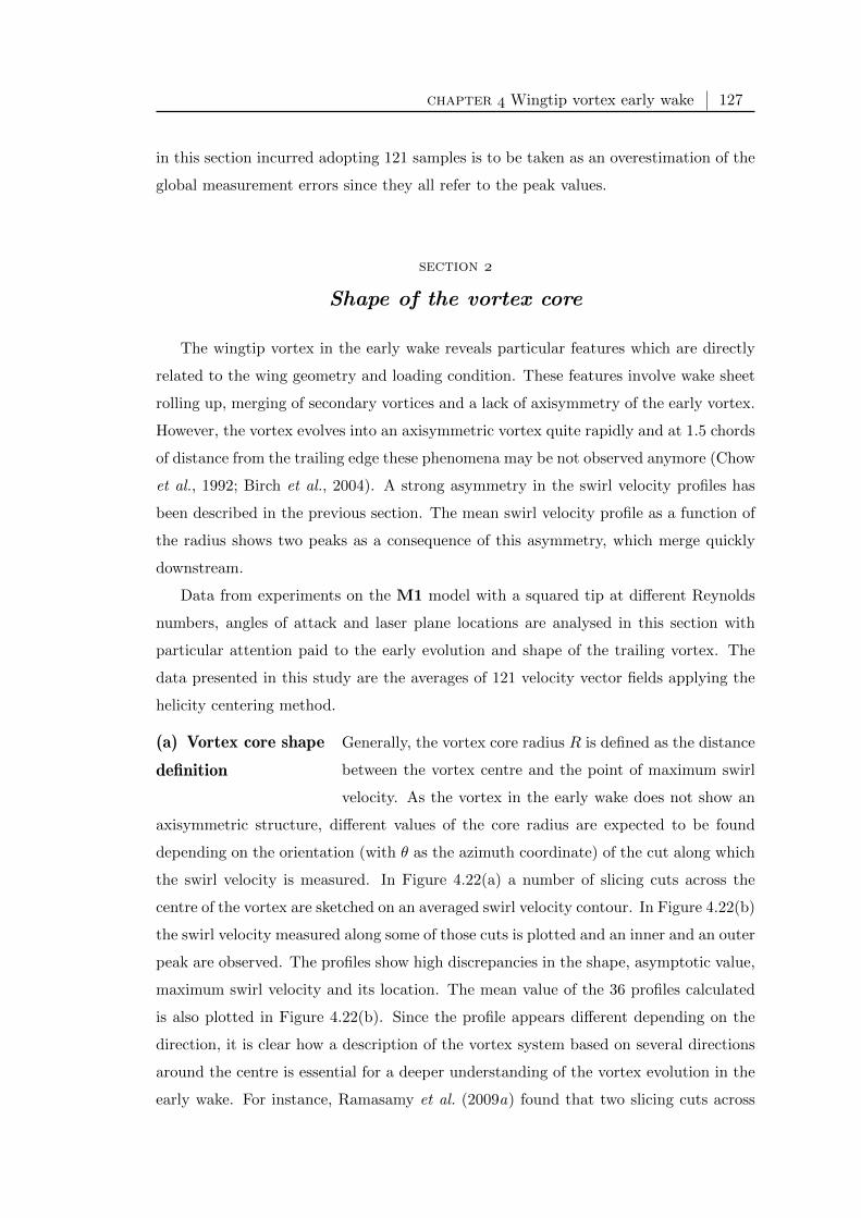
chapter Wingtip vortex early wake 127
in this section incurred adopting 121 samples is to be taken as an overestimation of the
global measurement errors since they all refer to the peak values.
section
Shape of the vortex core
The wingtip vortex in the early wake reveals particular features which are directly
related to the wing geometry and loading condition. These features involve wake sheet
rolling up, merging of secondary vortices and a lack of axisymmetry of the early vortex.
However, the vortex evolves into an axisymmetric vortex quite rapidly and at 1.5 chords
of distance from the trailing edge these phenomena may be not observed anymore (Chow
et al., 1992; Birch et al., 2004). A strong asymmetry in the swirl velocity profiles has
been described in the previous section. The mean swirl velocity profile as a function of
the radius shows two peaks as a consequence of this asymmetry, which merge quickly
downstream.
Data from experiments on the M1 model with a squared tip at different Reynolds
numbers, angles of attack and laser plane locations are analysed in this section with
particular attention paid to the early evolution and shape of the trailing vortex. The
data presented in this study are the averages of 121 velocity vector fields applying the
helicity centering method.
(a) Vortex core shape
definition
Generally, the vortex core radius R is defined as the distance
between the vortex centre and the point of maximum swirl
velocity. As the vortex in the early wake does not show an
axisymmetric structure, different values of the core radius are expected to be found
depending on the orientation (with θ as the azimuth coordinate) of the cut along which
the swirl velocity is measured. In Figure 4.22(a) a number of slicing cuts across the
centre of the vortex are sketched on an averaged swirl velocity contour. In Figure 4.22(b)
the swirl velocity measured along some of those cuts is plotted and an inner and an outer
peak are observed. The profiles show high discrepancies in the shape, asymptotic value,
maximum swirl velocity and its location. The mean value of the 36 profiles calculated
is also plotted in Figure 4.22(b). Since the profile appears different depending on the
direction, it is clear how a description of the vortex system based on several directions
around the centre is essential for a deeper understanding of the vortex evolution in the
early wake. For instance, Ramasamy et al. (2009a) found that two slicing cuts across

chapter Wingtip vortex early wake 128
the tip vortex (producing 4 profiles) provide an acceptable measurement of the vortex
core dimension.
(a) Swirl velocity contour and various slicing cutsacross the vortex.
(b) Swirl velocity profile along various cuts andmean value.
Figure 4.22: Swirl velocity and slicing cuts at α = 8, xw = 1 and Re = 5 · 105.
In the early wake, the calculation of the vortex core radius as point of maximum swirl
velocity leads to different values depending on the direction of the cut and the average
value does not contain all the information of the shape of the core. In this section, the
vortex core is presented as the locus of the points of maximum swirl velocity around
the vortex centre. In other words, the core shape is described by the directional radius
as function of the azimuth angle, that is R(θ) normalised by the chord. The directional
vortex core radius is calculated from the swirl velocity profiles along 36 directions around
the vortex centre. In Figures 4.23 and 4.24, the radius values are plotted on a polar plot
as function of θ for different Reynolds numbers, plane locations and angles of attack.
In the present reference system, the vortex rotates clockwise and the cases reported
here are chosen as the conditions where an asymmetric structure of the core is better
observed although it resembles the behaviour of all the other cases in the near wake of
the present study.
In Figure 4.23, at the closest plane to the trailing edge xw = 0.25, the peak value
of R(θ) is observed around θ = 150 and it moves to θ = 30 at xw = 0.5. An
anti–clockwise spiral is observed at xw = 1 with a discontinuity at θ = 180. The
discontinuity is due to the switch of the maximum swirl velocity from the inner to the
outer of the two peaks discussed previously. At 2 chords from the wing, very early wake
phenomena are not observed and a nearly axisymmetric shape of the core is formed. A
similar behaviour is observed for the case reported in Figure 4.24. A spiral shape of the
core is observed at planes closer than 1 chord from the trailing edge which rotates and

chapter Wingtip vortex early wake 129
(a) xw = 0.25. (b) xw = 0.5.
(c) xw = 1. (d) xw = 2.
Figure 4.23: Vortex core shape at Re = 1 · 105 and α = 12.
(a) xw = 0.25. (b) xw = 0.5.
(c) xw = 1. (d) xw = 2.
Figure 4.24: Vortex core shape at Re = 5 · 105 and α = 8.

chapter Wingtip vortex early wake 130
reaches an almost circular shape at xw = 2.
(a) Re = 1 · 105. (b) Re = 10 · 105.
Figure 4.25: Vortex core shape at α = 12 and xw = 1.
In Figure 4.25, the comparison of the vortex core shape for different Reynolds num-
bers at one chord of distance from the trailing edge and α = 12 is reported. The low
Reynolds case exhibits a slightly wider core shape (bigger vortex core) and a smaller
jump at the discontinuity (near to axisymmetry) than the high Reynolds number. The
phase difference (delay) between the two cases is of 90.
(b) Vortex core shape
fluctuation
The vortex core shape, as defined previously, highlights the
asymmetry of the vortex structure in the early wake behind
the wing where highly unsteady and asymmetric phenomena
are observed before the vortex structure develops into an axisymmetric vortex. The
fluctuation of the core shape σR is expected to be function of the azimuth angle and
it is evaluated as the root mean square of the instantaneous directional core radius,
normalised by the the average core radius.
In Figure 4.26 the core shape fluctuation is reported on polar plots for the cases
presented previously. Comparing Figures 4.26(a) and 4.26(b) respectively with Figures
4.23 and 4.24, it is noted that higher values of core shape fluctuation are found at
the position of the discontinuity of the core shape and they are proportional to the
jump of R(θ) across the discontinuity. This high fluctuation is due to the switching
of the location of maximum swirl velocity between the inner and the outer peak. The
unsteadiness of the core shape can also be expressed as a revolving fluctuation angle
that indicates an angular range around which the azimuth angle of the instantaneous
discontinuity moves. In Figure 4.26(b), σR(θ) for xw = 0.25 and xw = 0.5 shows
distinct peaks at the discontinuity of the core shape. The width of the peak increases
with the measurement plane moving downstream: a revolving fluctuation angle of 40 is
observed for xw = 0.25, an angle of 80 at xw = 0.5 and an oval shape is then observed

chapter Wingtip vortex early wake 131
at xw = 1. This indicates that for an increase of the downstream position, the revolving
fluctuation angle increases and the fluctuation level decreases. In all the cases shown
here, the fluctuation of the core shape is higher than 25% of the mean core radius.
(a) Re = 1 · 105, α = 12. (b) Re = 5 · 105, α = 8.
Figure 4.26: Core shape fluctuation.
Ramasamy et al. (2009a) studied the distribution of the average core size of a rotor
blade tip vortex showing the median of a sample set as a better descriptive measure
of the data than the mean value. When the distribution is not symmetric, the median
gives the same emphasis to all the measured core sizes, whereas the mean gives a much
greater weight to the tail of the distribution. In Figure 4.27, one core shape is reported
where the directional core radii are calculated with three different methods: from the
average flow field (Figure 4.27(a)); as the average of the 121 instantaneous directional
core radii (Figure 4.27(b)); as the median of the instantaneous directional core radii
(Figure 4.27(c)). The core shapes, and in particular around the discontinuity, appear
different when a different method is applied. The second method masks the discontinuity
observed earlier whereas the third method lies in between the other two confirming that
the fluctuation of directional core radius does not assume a normal distribution. This
suggests also the presence of outliers (very low values of R(θ) on the low side of the
discontinuity and high values on the high side) which results in an overestimation of the
discontinuity jump.
(c) Rotation of the core From the polar plots presented earlier, it is possible to re-
trieve information on the rotation of the vortex core. Be-
cause the initial stage is not axisymmetric but reveals a peculiar structure, the rotation
of the core can be evaluated by following the bump or discontinuity of the core shape.
As a first approximation, the rotation of the core in the wake Θ can be expressed as the
product between the rotation rate of the vortex φ and the time elapsed from the trailing
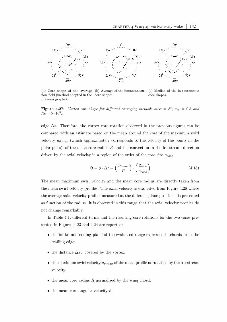
chapter Wingtip vortex early wake 132
(a) Core shape of the averageflow field (method adopted in theprevious graphs).
(b) Average of the instantaneouscore shapes.
(c) Median of the instantaneouscore shapes.
Figure 4.27: Vortex core shape for different averaging methods at α = 8, xw = 0.5 andRe = 5 · 105,.
edge ∆t. Therefore, the vortex core rotation observed in the previous figures can be
compared with an estimate based on the mean around the core of the maximum swirl
velocity uθ,max (which approximately corresponds to the velocity of the points in the
polar plots), of the mean core radius R and the convection in the freestream direction
driven by the axial velocity in a region of the order of the core size ucore.
Θ = φ ·∆t =(uθ,max
R
)·(
∆xwucore
)(4.18)
The mean maximum swirl velocity and the mean core radius are directly taken from
the mean swirl velocity profiles. The axial velocity is evaluated from Figure 4.28 where
the average axial velocity profile, measured at the different plane positions, is presented
as function of the radius. It is observed in this range that the axial velocity profiles do
not change remarkably.
In Table 4.1, different terms and the resulting core rotations for the two cases pre-
sented in Figures 4.23 and 4.24 are reported:
• the initial and ending plane of the evaluated range expressed in chords from the
trailing edge;
• the distance ∆xw covered by the vortex;
• the maximum swirl velocity uθ,max of the mean profile normalised by the freestream
velocity;
• the mean core radius R normalised by the wing chord;
• the mean core angular velocity φ;
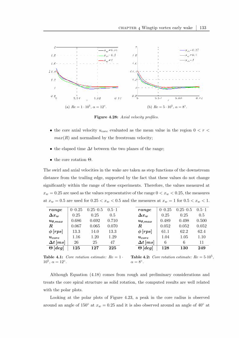
chapter Wingtip vortex early wake 133
(a) Re = 1 · 105, α = 12. (b) Re = 5 · 105, α = 8.
Figure 4.28: Axial velocity profiles.
• the core axial velocity ucore evaluated as the mean value in the region 0 < r <
max(R) and normalised by the freestream velocity;
• the elapsed time ∆t between the two planes of the range;
• the core rotation Θ.
The swirl and axial velocities in the wake are taken as step functions of the downstream
distance from the trailing edge, supported by the fact that these values do not change
significantly within the range of these experiments. Therefore, the values measured at
xw = 0.25 are used as the values representative of the range 0 < xw < 0.25, the measures
at xw = 0.5 are used for 0.25 < xw < 0.5 and the measures at xw = 1 for 0.5 < xw < 1.
range 0–0.25 0.25–0.5 0.5–1∆xw 0.25 0.25 0.5uθ,max 0.686 0.692 0.710R 0.067 0.065 0.070φ [rps] 13.3 14.0 13.3ucore 1.16 1.20 1.29∆t [ms] 26 25 47
Θ [deg] 125 127 225
Table 4.1: Core rotation estimate: Re = 1 ·105, α = 12.
range 0–0.25 0.25–0.5 0.5–1∆xw 0.25 0.25 0.5uθ,max 0.489 0.498 0.500R 0.052 0.052 0.052φ [rps] 61.1 62.2 62.4ucore 1.04 1.05 1.10∆t [ms] 6 6 11
Θ [deg] 128 130 249
Table 4.2: Core rotation estimate: Re = 5·105,α = 8.
Although Equation (4.18) comes from rough and preliminary considerations and
treats the core spiral structure as solid rotation, the computed results are well related
with the polar plots.
Looking at the polar plots of Figure 4.23, a peak in the core radius is observed
around an angle of 150 at xw = 0.25 and it is also observed around an angle of 40 at
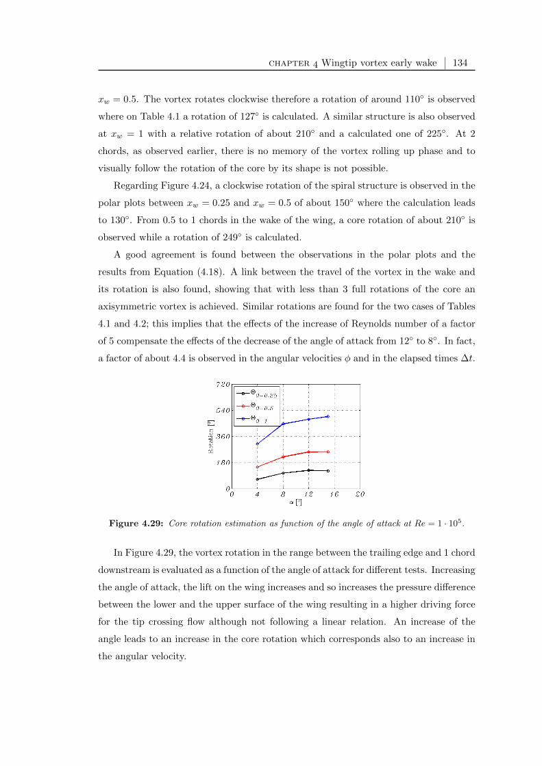
chapter Wingtip vortex early wake 134
xw = 0.5. The vortex rotates clockwise therefore a rotation of around 110 is observed
where on Table 4.1 a rotation of 127 is calculated. A similar structure is also observed
at xw = 1 with a relative rotation of about 210 and a calculated one of 225. At 2
chords, as observed earlier, there is no memory of the vortex rolling up phase and to
visually follow the rotation of the core by its shape is not possible.
Regarding Figure 4.24, a clockwise rotation of the spiral structure is observed in the
polar plots between xw = 0.25 and xw = 0.5 of about 150 where the calculation leads
to 130. From 0.5 to 1 chords in the wake of the wing, a core rotation of about 210 is
observed while a rotation of 249 is calculated.
A good agreement is found between the observations in the polar plots and the
results from Equation (4.18). A link between the travel of the vortex in the wake and
its rotation is also found, showing that with less than 3 full rotations of the core an
axisymmetric vortex is achieved. Similar rotations are found for the two cases of Tables
4.1 and 4.2; this implies that the effects of the increase of Reynolds number of a factor
of 5 compensate the effects of the decrease of the angle of attack from 12 to 8. In fact,
a factor of about 4.4 is observed in the angular velocities φ and in the elapsed times ∆t.
Figure 4.29: Core rotation estimation as function of the angle of attack at Re = 1 · 105.
In Figure 4.29, the vortex rotation in the range between the trailing edge and 1 chord
downstream is evaluated as a function of the angle of attack for different tests. Increasing
the angle of attack, the lift on the wing increases and so increases the pressure difference
between the lower and the upper surface of the wing resulting in a higher driving force
for the tip crossing flow although not following a linear relation. An increase of the
angle leads to an increase in the core rotation which corresponds also to an increase in
the angular velocity.
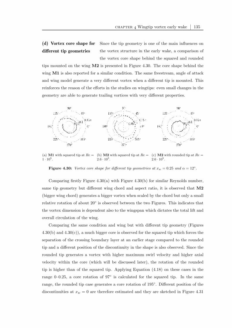
chapter Wingtip vortex early wake 135
(d) Vortex core shape for
different tip geometries
Since the tip geometry is one of the main influences on
the vortex structure in the early wake, a comparison of
the vortex core shape behind the squared and rounded
tips mounted on the wing M2 is presented in Figure 4.30. The core shape behind the
wing M1 is also reported for a similar condition. The same freestream, angle of attack
and wing model generate a very different vortex when a different tip is mounted. This
reinforces the reason of the efforts in the studies on wingtips: even small changes in the
geometry are able to generate trailing vortices with very different properties.
(a) M1 with squared tip at Re =1 · 105.
(b) M2 with squared tip at Re =2.6 · 105.
(c) M2 with rounded tip at Re =2.6 · 105.
Figure 4.30: Vortex core shape for different tip geometries at xw = 0.25 and α = 12.
Comparing firstly Figure 4.30(a) with Figure 4.30(b) for similar Reynolds number,
same tip geometry but different wing chord and aspect ratio, it is observed that M2
(bigger wing chord) generates a bigger vortex when scaled by the chord but only a small
relative rotation of about 20 is observed between the two Figures. This indicates that
the vortex dimension is dependent also to the wingspan which dictates the total lift and
overall circulation of the wing.
Comparing the same condition and wing but with different tip geometry (Figures
4.30(b) and 4.30(c)), a much bigger core is observed for the squared tip which forces the
separation of the crossing boundary layer at an earlier stage compared to the rounded
tip and a different position of the discontinuity in the shape is also observed. Since the
rounded tip generates a vortex with higher maximum swirl velocity and higher axial
velocity within the core (which will be discussed later), the rotation of the rounded
tip is higher than of the squared tip. Applying Equation (4.18) on these cases in the
range 0–0.25, a core rotation of 97 is calculated for the squared tip. In the same
range, the rounded tip case generates a core rotation of 195. Different position of the
discontinuities at xw = 0 are therefore estimated and they are sketched in Figure 4.31

chapter Wingtip vortex early wake 136
(with the current reference system, the wing is horizontal).
(a) Squared tip. (b) Rounded tip.
Figure 4.31: Estimation of the vortex core structure at the trailing edge.
This result confirms the different structure of the vortex during the formation on
the wing when the tip geometry is changed and in particular the different position of
the maximum swirl velocity. Topological differences during the formation on squared
and rounded wingtips were observed also in the smoke visualizations of Section 3.3 and
suggested by the characteristic lines in Section 3.4.
section
Axial flow
The axial flow in the core of a wingtip vortex has been intensively studied throughout
the years and has been shown to either be directed towards the wing (wake–like or
deficit, as behind a non–lifting drag–producing body) or away from the wing (jet–like
or excess). Although a number of analytical and experimental studies have presented
different models and tools to predict the axial flow, a unique solution is not present to
date. Moreover, like all the other vortex properties, the axial flow of a trailing vortex
in the near wake is influenced by several concurrent factors and presents a complex
structure.
The fact that experiments show either an excess or a deficit in the axial velocity
was explained by Spalart (1998) as the result of the acceleration of the flow described
by inviscid theory and the total pressure losses by viscosity of the boundary layer fluid
layered around the vortex. The axial velocity excess at the vortex centre can be intro-
duced in two mathematically equivalent ways: from considerations of the helical shape
of vortex lines and from equating the pressure from different points of the vortex. Both
chapter Wingtip vortex early wake 137
the approaches leads to the following equation:
d (ux2 + uθ
2)
dr+ 2
uθ2
r= 0 (4.19)
Since the circulation profile can be expressed as Γ(r) = 2πruθ, substituting uθ in Equa-
tion (4.19) withΓ(r)
2πr, the resulting equation is:
2π2r2 dux2
dr+
d Γ(r)2
dr= 0 (4.20)
Because it is generally observed that Γ increases with r, it is clear that ux increases as
the vortex axis is approached (jet–like flow). In a real flow, the fluid around the vortex
core is layered with the boundary layer fluid and the wake sheet which introduces strong
shear layers and viscous losses that contribute to the deceleration of the flow. Spalart
(1998) introduces then a circulation parameter which indicates the balance between
viscous effects and inviscid acceleration of the axial flow for each experiment. Large
values of the circulation parameter result in an excess and low values in a deficit of
axial velocity.
Bailey et al. (2006) stated that in the initial stages of the vortex formation, the pres-
sure in the vortex core gradually decreases along the vortex axis generating a favourable
axial pressure gradient that accelerates the core fluid in the streamwise direction, possi-
bly resulting in a jet–like core having an axial velocity surplus (Devenport et al., 1996).
Farther downstream, viscous actions decelerate the flow, tending to convert the core to
wake–like. It was also observed that the axial velocity gradient introduces a possible
mechanism of turbulence production in the core (Singh & Uberoi, 1976; Chow et al.,
1997a).
Although the excess or deficit of the axial velocity can be small in comparison to the
swirl velocity, its presence dictates to a large extent the stability and decay of the vortex.
Based upon previous theoretical, experimental and computational studies, Spall et al.
(1987) and Mudkavi (1993) proposed a criterion for the onset of the vortex breakdown
which is based on a swirl parameter. Such swirl parameter is evaluated from the axial
velocity, the vortex core radius and the rotation rate. Billant et al. (1998) defined a
swirl parameter as the ratio between the maximum swirl velocity and the axial velocity
in the centre of the vortex measured at an initial plane. Different magnitudes of excess
of the axial velocity were applied on a rotating fluid and the onset and structure of the
breakdown of the vortex was observed for those different values of the swirl parameter.

chapter Wingtip vortex early wake 138
They observed an earlier breakdown for higher values of the swirl parameter, which
is for weaker axial velocity excess. Hallett & Toews (1987) also deduced that a flow
exhibiting axial velocity profiles with a maximum on the axis requires a higher swirl to
produce vortex breakdown, that is a higher positive pressure gradient.
To date, there is still no established method which can reliably predict the magnitude
or even the direction of this axial velocity perturbation for a given wingtip geometry
and flow condition. Furthermore, the physical mechanism of the formation of axial flow
is still poorly understood. Batchelor (1964) proposed an analytical description of the
axial flow inside an idealized vortex and the following result was derived2:
u02 = U∞
2 +
∫ ∞r
1
4π2r2
∂Γ(r)2
∂rdr − 2∆H (4.21)
with u0 the axial velocity in the vortex centre, U∞ the freestream velocity, r the radial
cylindrical coordinate, Γ(r) the circulation profile across the vortex and ∆H an arbi-
trary function added to account for the dissipation along a streamline passing through a
viscous region of the flow (for example, the boundary layer shed from the wing trailing
edge and rolling around the tip vortex). This result was obtained from steady axisym-
metric cylindrical incompressible Navier–Stokes equations with the assumption of small
axial gradients compared with the radial gradients and small radial velocity compared
to axial and swirl velocity (boundary layer type approximation). With assumptions of a
constant dissipation term and vortex radius, Equation (4.21) shows an increase of axial
velocity with an increase of overall circulation and a velocity excess in inviscid fluids
where ∆H = 0. The presence of viscous losses competes with the inviscid acceleration
mechanism. As a result, in cases of large Reynolds numbers and high angles of attack,
the inviscid mechanism is prevailing and an axial velocity excess is expected. Under
moderate angles of attack and low Reynolds numbers, the viscous losses are dominant
and axial velocity deficits are expected.
Equation (4.21) relates the radial distribution of the circulation with the axial flow.
However, the relation between the streamwise evolution of the vortex and the axial flow
can be also quite relevant. The redistribution of the vorticity due to the development
of the vortex towards axisymmetry and the increasing of circulation due to the initial
rolling up of fluid are strongly related to the axial velocity by the mechanism called
vortex stretching (for the mathematical background of the vortex stretching and con-
siderations on the vorticity equation see Appendix C.2). As a result, a positive axial
2Equation (4.20) by Spalart (1998) can be also seen as the radial differentiation of Equation (4.21)by Batchelor (1964) when the losses term ∆H is ignored.

chapter Wingtip vortex early wake 139
gradient of the circulation will contribute to the acceleration of the axial flow. How-
ever, in the axial range of the present investigation, a remarkable effect of the vortex
stretching was not observed.
Del Pino et al. (2011) compared analytical and experimental results of the axial flow
in the range xw =0.5–16. The authors found a good agreement between experiments
and the model presented by Moore & Saffman (1973) who arrived at a more complex
equation for the axial flow in laminar trailing vortices taking also into account the
boundary layer shed by the wing and entrained in the core. In addition to the above
laminar flow studies, significant models on the development of turbulent vortices where
the axial flow is expressly addressed were presented by Govindaraju & Saffman (1971),
Saffman (1973) and Saffman (1974).
As also observed in the previous sections, the wingtip vortex in the very early wake
presents a complex structure. The axial velocity, consequently, is expected to reveal
a similarly complex structure and development. Moreover, the experimental technique
affects the description of the vortex with its measurement resolution, intrusivity and
format of the data for further processing. Recent studies (Anderson & Lawton, 2003;
Lee & Pereira, 2010) compared the wide range of results in the literature and performed
parametric experiments on the axial velocity in the vortex core. Anderson & Lawton
(2003) showed a linear trend between the axial velocity peak and the vortex circulation
strength and they suggested the presence of a maximum deficit limit for trailing vortices.
Lee & Pereira (2010) observed that the axial velocity and vorticity at the vortex centre
increase along the tip reaching their maxima in the vicinity of the trailing edge. During
the formation, they also observed a region of jet–like fluid at the vortex centre regardless
of the tip condition and the angle of attack. In the wake of a wing at small incidence,
this region was entrained by the shear layer and the wing wake resulting in a wake–like
axial flow as it progressed downstream of the wing trailing edge.
(a) Shape of the axial flow Based on considerations on smoke visualizations of the
vortex over the wing, Equation (3.2) states that the
vortex formed over a wing at a high angle of attack produces an axial flow that is
considerably higher than the vortex for a low angle of attack. In Figure 4.32, instan-
taneous and simple averaged axial velocity fields are presented for the M1 wing at 4
and 12 for two exemplifying cases. In the instantaneous flow for the wing at high angle
of attack (Figure 4.32(b)), a region of flow at higher velocity than the freestream is
observed in the vortex core with a peak of around 1.6U∞. The simple averaged velocity

chapter Wingtip vortex early wake 140
field reveals a profile which is smoother and more diffuse as effect of the meandering
and the unsteadiness of the vortex (peak of around 1.3U∞). At a lower incidence, the
instantaneous velocity field in Figure 4.32(a) shows a region of the order of the vortex
core with deficit of axial velocity which contains smaller regions of negative and positive
axial velocity perturbations. The averaged field (Figure 4.32(c)) reveals a region of axial
velocity deficit which has a circular shape.
(a) Instantaneous flow at α = 4. (b) Instantaneous flow at α = 12.
(c) Simple averaged flow at α = 4. (d) Simple averaged flow at α = 12.
Figure 4.32: Axial velocity contours and planar streamlines at xw = 1 and Re = 1 · 105 (M1model).
At low angles of attack, hence lower circulation and vortex strength, the inviscid
acceleration of the flow on the vortex axis is counterbalanced by the deceleration of the
viscous effects. The mixing of the fluid in the vortex core with the “slow” fluid from the
boundary layer and the wake sheet is more intense and generates a more complex region.
For this reason, at low angles of attack, the identification of axial velocity perturbation
peaks (either as excess of deficit with respect to the freestream velocity) is critical. This
leads the centering methods based on the solely axial velocity to a poor robustness

chapter Wingtip vortex early wake 141
and questionable results, being strongly dependent on the searching technique and peak
definition.
(a) Low angle of attack. (b) Moderate angle of attack. (c) High angle of attack.
Figure 4.33: Schematic of generic profiles of the axial velocity across the vortex in the earlywake for different angles of attack.
In Figure 4.33, illustrative axial velocity profiles across the vortex are sketched for
a low, a moderate and a high angle of attack. Based on the previous observations, it is
believed that the axial velocity at the centre of an early vortex is affected by the inviscid
acceleration mechanisms and it always appears as an excess compared to the flow in
the vortex core which might be, in some instances, lower than the freestream (Figure
4.33(a)). This last scenario is related to weak vortices interacting with large shear layers
(i.e. low wing circulation, thick boundary layer, large regions of separated flow). For
moderate angles (Figure 4.33(b)), the deficit around the centre is of the same order
of the excess at the centre. This scenario highlights the importance of high resolution
measurements in the vortex core to be able to describe the evolution of the vortex in the
early wake. At high angles of attack (Figure 4.33(c)), the axial velocity peak (jet–like) is
well defined and more intense. As the vortex progresses downstream and axisymmetry
by diffusion is reached, the axial velocity will tend to a bell–shaped profile which may
be observed either later in the wake or just downstream the trailing edge or already
during the formation of the vortex on the wing depending on the situation.
In Figure 4.34, the helicity based average method is applied on the cases of Figure
4.32. For the high incidence case, the velocity excess region appears more intense than
for the simple averaged velocity field and it shows a peak of about 1.4U∞. The low angle
of attack case reveals a small jet–like region of peak intensity equal to the freestream

chapter Wingtip vortex early wake 142
velocity at the centre of the vortex surrounded by a rounded patch of wake–like flow.
(a) Helicity average at α = 4. (b) Helicity average at α = 12.
Figure 4.34: Average axial velocity contours and planar streamlines at xw = 1 and Re = 1 ·105
(M1 model).
Following the inviscid mechanism presented by Spalart (1998), jet–like flow is in-
duced by the helical shape of the vortex lines. Hence, a second axial velocity peak can
be expected in the case of a secondary vortex of strength comparable to the primary
vortex and when viscous effects are low. In Figure 4.35, the evolution in the wake
of axial velocity, vorticity and planar streamlines are reported for the M1 wing with
squared tip at α = 15. The helicity based centering method is applied although the
same behaviour was observed also from simple averaged velocity fields.
The high angle of attack produces a strong secondary vortex which induces a sec-
ondary axial velocity peak. The two axial velocity peaks, clearly distinguishable inside
the vortex core at xw = 0.25, are merged into a unique peak at xw = 0.5 which quickly
looses strength downstream: from a maximum of about 1.7U∞ at xw = 0.25 to 1.5U∞ at
xw = 1. The deficit of axial velocity, which characterizes the wake sheet, surrounds the
vortex core and dissipates moving downstream of the wing. The axial velocity peak, the
centre of the streamlines and the vorticity peak appear at different locations because of
the distortion of the flowfield due to the interaction between primary vortex, secondary
vortices and wake sheet.
The vorticity in the core at xw = 0.25 reveals a region of positive vorticity (anti–
clockwise rotation) on the right side of the primary vortex, which is identified by the
negative vorticity peak inducing the overall clockwise rotation of the fluid. This region is
attributed to the secondary vortex generating the secondary axial velocity peak. At the
centre of the vortex the vorticity, like as the axial velocity peak, decreases in strength
moving downstream and the counter rotating secondary vortex merges with the primary
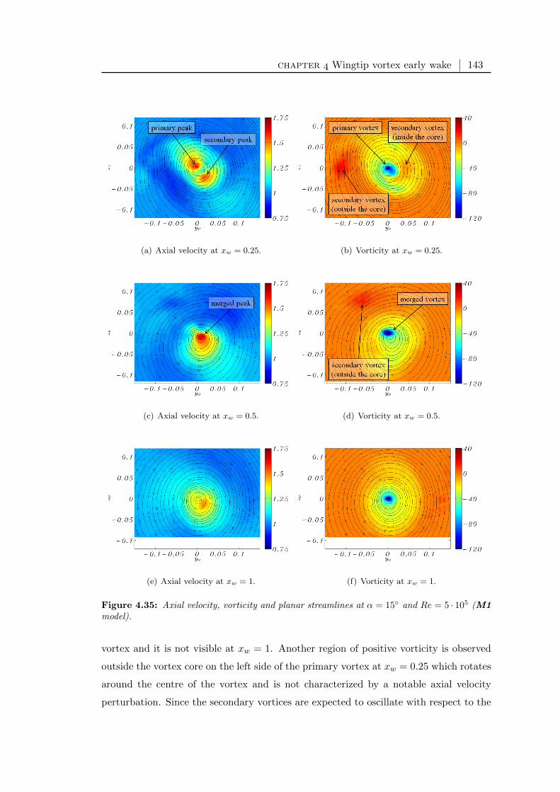
chapter Wingtip vortex early wake 143
(a) Axial velocity at xw = 0.25. (b) Vorticity at xw = 0.25.
(c) Axial velocity at xw = 0.5. (d) Vorticity at xw = 0.5.
(e) Axial velocity at xw = 1. (f) Vorticity at xw = 1.
Figure 4.35: Axial velocity, vorticity and planar streamlines at α = 15 and Re = 5 · 105 (M1model).
vortex and it is not visible at xw = 1. Another region of positive vorticity is observed
outside the vortex core on the left side of the primary vortex at xw = 0.25 which rotates
around the centre of the vortex and is not characterized by a notable axial velocity
perturbation. Since the secondary vortices are expected to oscillate with respect to the

chapter Wingtip vortex early wake 144
primary vortex, and being the centering based on the primary vortex movement only,
the secondary vortices on these contours are expected to appear wider and less intense
(smearing effect) than the instantaneous realizations.
The development of the vortex toward an axisymmetric structure is indicated by the
plane streamlines which appear more circular moving downstream. In general, the peak
of the axial velocity rapidly decreases especially when the mixing of the fluid within
the core is intense, that is when several secondary vortices interact with the primary
vortex. The vorticity shape also changes drastically within a few chords from the trailing
edge. The characteristics of the axisymmetric vortex observed in the mid wake (such as
axial velocity peak, vortex core radius, maximum swirl velocity) are therefore strongly
influenced by the vortex system dynamics during the formation on the wing and the
rolling up in the very early wake.
(b) Axial velocity at the
centre of the vortex
Recent parametric studies on the axial velocity in the cen-
tre of the vortex have allowed a deeper understanding of
the vortex axial flow although the mechanisms responsible
for the wake–like and jet–like axial flows are not fully understood.
Anderson & Lawton (2003) tested a low aspect ratio wing (AR = 0.8) with squared
and rounded tip at several downstream distances, Reynolds numbers and angles of
attack. They found a linear relationship between the scaled vortex circulationΓ
U∞band
the angle of attack. Because the circulation of a single trailing vortex is equal to the
circulation of the bound vortex at the wing root, the vortex circulation will increase
in direct proportion to the lift produced, that is to the angle of attack. Consequently,
the axial velocity at the centre of the vortex also appeared proportional to the angle of
attack with a higher gradient for the rounded tip, and greater peaks were generated by
the rounded tip than the peaks generated by the squared tip. The effects of Reynolds
number and downstream distance in the range studied were small compared to the angle
of attack and tip geometry effects.
Lee & Pereira (2010) studied the vortex generated by squared and rounded tips on
a rectangular wing with AR = 1.8 during its formation on the wing and to a maximum
distance from the trailing edge of xw = 4. They found similar vortex circulation values
for both the tip geometries although they observed a different circulation distribution
within the core. The vortex generated by a rounded tip appeared more concentrated
(smaller core radius) and more intense (higher vorticity and axial velocity peaks) than
the squared tip case. The effect of the tip shape was to change the interaction intensity

chapter Wingtip vortex early wake 145
between the vortex with the wake and secondary vortices. The axial velocity peak at
the trailing edge was similar for the two wingtips but the decrease with xw was quicker
for a squared tip than for a rounded tip. They also found a critical angle of attack of
7 below which the axial flow eventually became wake–like.
Lastly, Chow et al. (1997a) meticulously performed several measurements in the
near wake of a low aspect ratio wing with rounded tip at a Reynolds number equal to
4.6 · 106 where a jet–like axial velocity was observed with a peak of 1.77U∞.
In Figure 4.36, the axial velocity at the centre of the vortex as a function of the
circulation of all the SPIV experiments in the wake of the two wing models is presented
(test matrix in Table 2.3). The circulation is scaled by the freestream velocity and
the chord which is equivalent to the circulation parameter used by Anderson & Lawton
(2003) multiplied by the aspect ratio of the wing. The circulation profile is calculated as
the integration of the average swirl velocity profile and the vortex circulation is identified
as the maximum value of such profile. In the range of distance from the trailing edge
presented here, the axial velocity at the vortex centre did not decrease substantially
as observed also by Chow et al. (1997b). In general, the axial velocity peak increases
with the intensity of the vortex, measured by the circulation, which is directly related
to the angle of attack of the wing (Anderson & Lawton, 2003; Lee & Pereira, 2010).
The vortex circulation, which is concentrated in a region of the order of the vortex core,
is a distinctive and comparable property of vortices and it does not change with the
position downstream of the wing although it is influenced by the tip geometry (further
details on the effects of the tip geometry will be given in Section 4.5).
The two linear trendlines, sketched in Figure 4.36 and referring to the two tip ge-
ometries, show that the rounded wingtip generates a higher axial velocity in the vortex
core. A minimum axial flow deficit limit in the wing wake was suggested by Anderson
& Lawton (2003) based on the trend of their experimental results. In the current study,
although a minimum limit can not be clearly identified, it may occur at around u0 = 0.7
and it is believed to be related to the viscous deceleration effect of the boundary layer
flow developing along the wing surface and interacting with the vortex.
The results from this study are grouped in several clusters in order to make insightful
observations. Four groups corresponding to the four angles of attack tested on the wing
M1 lie on the squared tip trendline where an increase in both circulation and axial
velocity peak correspond to an increase of the incidence. Within each of these groups,
an increase of the Reynolds number coincides with an increase of the peak. However,
as discussed by Chow et al. (1997a) who empirically fitted several experimental data

chapter Wingtip vortex early wake 146
Figure 4.36: Axial velocity at the centre of the vortex as function of the circulation parameter.
with a parametric curve, the influence of the Reynolds number to the axial velocity is
negligible compared with the influence of the angle of attack.
Two other clusters refer to the two angles of attack tested on the model M2. At
the same angle of attack, the low aspect ratio wing M2 generates remarkably lower
dimensionless circulation than the high aspect ratio wing M1 mainly because of the
very different aspect ratio. In particular, wing M2 at α = 12 generates a dimensionless
circulation equivalent to M1 wing at 7 and the circulation generated at 4 by M2 is
equivalent to M1 at an incidence of about 2.
The axial velocity peaks for M2 with squared tip correlate very well with the results
for M1 which mounts the same tip geometry (see cluster of M2 at α = 12). It is
believed therefore that the effect of the different aerofoil shape (i.e. NACA 0012 and
0015) is not relevant in the current investigation.
For same dimensionless circulation, higher peaks are observed in the rounded tip
cases than for the squared tip cases particularly for α = 12 which suggests the presence
of different trendlines for different wingtip geometries. The switchover angle between
jet–like and wake–like behaviour of the axial flow is estimated to be around 4 for the
squared tip and around 7 for the rounded tip. It is important to note that the vortex
circulation is not the only parameter that dictates the intensity of the axial flow but
the formation process is equally important.

chapter Wingtip vortex early wake 147
As observed also by Lee & Pereira (2010), the tip geometry greatly influences the
strength of the axial flow but it is not itself the cause of the jet–like or wake–like flow.
The tip vortex interaction with the wing and the surrounding flow structures ultimately
determines the wake–like or jet–like nature of the axial flow and the downstream location
when the trailing vortex is fully formed. Birch et al. (2004) compared a NACA 0015
aerofoil with a cambered aerofoil showing a linear increase of the vortex circulation
with the angle of attack. However, the increase of the axial velocity centre value was
linear only for the symmetric profile; the cambered aerofoil generated an axial velocity
peak which was almost constant in the range of angles of attack between 6 and 13.
This attests that the axial velocity peak is strongly affected by the interaction between
flow and wing, that is by the tip geometry and aerofoil shape, more than by the vortex
strength and lift of the wing. Different slopes of the trendlines for different tip geometries
are therefore expected.
It is important to remind also that, for low angles of attack, the axial flow may
appear as a jet–like flow at the centre of the vortex superimposed on a region of wake–
like flow with size of the order of the vortex core. This is the case for the sub–cluster
of the M1 wing at 4 where axial velocity centre values around 1 are measured and
the axial flow shape appear as sketched in Figure 4.33(a). This sub–cluster highlights
also another important phenomenon in the development of the axial flow in the range
xw =0.25–1. In particular for the Reynolds number of 1 · 105, the two centre values at
xw = 0.5 and xw = 1 appear considerably lower than the centre value at xw = 0.25.
At the earliest stage, the axial flow appears as a small excess superimposed to a strong
deficit (as in Figure 4.33(a)), while at a later plane the axial flow has reached a bell–
shaped profile with a centre value of 0.75U∞. The axial flows of the M2 model at
α = 4 are all observed as a wake–like flow with bell–shaped profile. This suggests
that as the vortex is less intense (lower circulation and axial velocity peak), it is also
less persistent and the distance required to reach a mature phase (i.e. axisymmetric
bell–shaped profile) is shorter than a stronger vortex.
In Figure 4.37, the trendlines found in the present study are compared with similar
experimental data obtained in recent years and summarized in Table 4.3. All these
experiments are based on rectangular wings with symmetric NACA profiles and squared
or rounded wingtips. The measurements are taken in the near wake at Reynolds numbers
within the range 2.01 · 105–4.6 · 106. These data, and especially the gradients of the
experimental results, well correlate with the trendlines of both the geometries found
in this study. Particularly remarkable is the agreement of the study by Lee & Pereira

chapter Wingtip vortex early wake 148
Authors c [m] b [m] AR Aerofoil Wingtip
Lee & Pereira (2010) 0.28 0.508 1.81 NACA 0015 roundedBirch et al. (2004) 0.254 0.379 0.67 NACA 0015 squared
Anderson & Lawton (2003) 0.762 0.610 0.8 NACA 0015 rounded&squaredChow et al. (1997b) 1.22 0.91 0.75 NACA 0012 rounded
Devenport et al. (1996) 0.203 0.879 4.33 NACA 0012 squaredPresent data 0.42 1.3 3.1 NACA 0015 squared
0.76 0.57 0.75 NACA 0012 rounded&squared
Table 4.3: Wing models characteristics and experiments of references in Figure 4.37.
Figure 4.37: Trendlines of the present work compared with other experimental data.
(2010) with gradients and intercepts of both the trendlines. The experiment presented
by Chow et al. (1997b) shows the maximum average axial velocity at the centre of
the vortex which can be explained by the uniquely high Reynolds number and the
measurement plane very close to the trailing edge. A minimum deficit limit of u0 = 0.75
is suggested also by observing this collection of results and it is related to a trailing vortex
with a dimensionless circulation value very low, corresponding to low angles of attack
and intense interaction of shear layers with the vortex. The maximum dimensionless
circulation of the present experiments (for M1 at α = 15) is 25% higher than the
maximum of the experiments reported in Figure 4.37. This wider extension of the data
was made possible by the big size of the Argyll wind tunnel which gave room for the
M1 wing model. This model has a bigger span than that tested on previous similar
experiments on trailing vortices (see Table 4.3) which attests to the uniqueness of this

chapter Wingtip vortex early wake 149
work.
The dispersion of the data shown in Figures 4.36 and 4.37 around the trendlines
indicates once more the complexity of this phenomenon. The acceleration of the flow
at the centre of trailing vortices is the result of the balance of several features including
interaction between fluid and wing, induced velocity by secondary vortices, rolling up
of shear layers and turbulence within the vortex core. Particularly important in this
process is the shape and evolution of the turbulence in the core which is presented in
the next section.
section
Turbulence in the vortex core
Despite the high Reynolds numbers typically encountered in flight conditions (of the
order of 107), vortices in the far wake grow with a rate typical of laminar flows . This
explains the persistence and strength of airplane trailing vortices in the far field. The
dissipation rate follows one of a laminar flow which is much slower and less dissipative
than the turbulent flow (Cotel & Breidenthal, 2002). The strong rotation within the
core can strongly inhibit turbulent transport of fluid leading to a stratified flow (Cotel
& Breidenthal, 1999). Airplane trailing vortices, and in particular vortex cores, are
examples of relaminarization of the flow induced by rotation in which the contribution
of the turbulent fluctuation to the mean flow dynamics becomes negligible and a laminar
flow is eventually found (Narasimha & Sreenivasan, 1979).
However, as described in Chapter 3, the physics of the wingtip vortex flow is ex-
tremely complex in the near field region as the process is largely turbulent, highly
three–dimensional and involves multiple cross flow separations. Streamwise vorticity,
mainly in the form of a feeding sheet, is seen to separate from the wing surface and
roll up into the tip vortex along with a variety of minor structures. Downstream of the
trailing edge, these structures eventually evolve into the axisymmetric and coherent tip
vortex. Experimental studies on wing tip vortices (Chow et al., 1997b) have reported a
reducing turbulence level in the vortical core in the near field. This is attributed to the
laminar rotation that develops in the inner part of the vortex core as a result of pro-
gressive damping of disturbances such as turbulent fluctuations. An analytical study of
isolated vortices based on linear stability theory was performed by Jacquin & Pantano
(2002) who supported this argument. As a result, far enough from the trailing edge,

chapter Wingtip vortex early wake 150
the major diffusion mechanism appears to be driven by viscosity rather than turbulence
(Zeman, 1995).
In this section, turbulence measurements in the vortex, which benefit from the high
spatial resolution of the SPIV arrangement, are presented. The turbulent kinetic en-
ergy at the vortex centre is presented for different Reynolds numbers, angles of attack
and distances of the measurement plane from the trailing edge. The distribution of
Reynolds shear stresses and shear strains in cartesian and cylindrical coordinates is pre-
sented along with a brief discussion of the turbulent closure problem for the simulation
of wingtip vortices with RANS. The mechanism of the turbulence production and dis-
sipation in the near wake towards a laminar vortex core is also addressed. As discussed
at the beginning of this chapter, the helicity based centering method is applied on sets
of 121 instantaneous velocity vector fields.
(a) Turbulent kinetic
energy evolution
In Section 4.1.(c), the turbulent stresses were presented on
cartesian coordinates because such is the usual reference sys-
tem of PIV measurements. A concise description of the struc-
ture of the different quantities was given. However, turbulence inside the vortex in
cylindrical coordinates adds important aspects to the study. The governing equations
and the relation between velocities and Reynolds stresses in cartesian and cylindrical
coordinates are presented in Appendix C.
(a) σv. (b) σw. (c) σu.
(d) σr. (e) σθ. (f) k.
Figure 4.38: Velocity fluctuations in cartesian and cylindrical coordinates and turbulent kineticenergy in the wake of the M1 wing at α = 12, xw = 1 and Re = 5 · 105.
In Figure 4.38, the velocity fluctuations in cartesian coordinates and the relative
cylindrical fluctuations are presented for a reference case (scaled by the freestream
chapter Wingtip vortex early wake 151
velocity). The axial velocity fluctuation and the turbulent kinetic energy are the same
in both reference systems. A lower level of the axial velocity fluctuation compared to
the other components is noted so that σr > σθ > σu. The contours of the horizontal
and vertical fluctuations σv and σw are roughly elliptical in shape with major axes
respectively along the horizontal and vertical directions. These shapes, observed also
in all the other cases, represent, in cylindrical coordinates, a level of radial fluctuation
σr higher than the azimuthal fluctuation σθ. This anisotropy was explained by Chow
et al. (1997a) analysing the governing equations as consequence of the production of the
Reynolds shear stress u′ru′θ within the vortex core in the early wake. The contours of all
the velocity fluctuations show a peak at the vortex centre. Consequently, the turbulent
kinetic energy also presents a peak at the vortex centre which indicates a non–laminar
core at this stage.
The evolution of the velocity fluctuations and the turbulent kinetic energy in the
wake of the M1 wing are presented in Figure 4.39. As observed earlier, for all the
measurement planes the radial fluctuations are always higher than the azimuthal fluc-
tuations which in turn are higher than the axial fluctuations. Their shapes become
more circular and the maximum values at the vortex centre decrease as they travel
downstream. The decrease between xw = 0.25 and xw = 1 is of around 10% for the
in–plane fluctuations and around 20% for the axial fluctuation. The kinetic energy re-
flects this behaviour of the velocity fluctuations decreasing of around 50% from 0.25
to 1 chords from the trailing edge. The turbulence contained in the wake sheet and in
the secondary structures around the primary vortex at xw = 0.25 is almost completely
dissipated at xw = 1.
Although the vortex core is turbulent at the most downstream measurement plane,
the effect of the quick relaminarization of the core can be implied. The reduction of
the turbulent kinetic energy at the centre of the vortex is shown in Figure 4.40 where
k0, scaled by the square of the freestream velocity, is plotted against the plane position
and the Reynolds number for different angles of attack. A higher rate of decrease is
observed for higher angles of attack (Figure 4.40(a)) which are characterized also by
higher initial turbulence level. The level of k0 at the most upstream plane xw = 0.25
does not increase linearly with the angle of attack and the lines group together in
high angles of attack (α = 12 and 15) and low angles of attack (α = 4 and 8)
which suggests different mechanisms in the evolution of the turbulence. A quicker
increase of the turbulent kinetic energy at the centre of the vortex for higher angles of
attack is observed also by Igarashi et al. (2011) on similar experiments. Considering

chapter Wingtip vortex early wake 152
(a) σr, xw = 0.25. (b) σr, xw = 0.5. (c) σr, xw = 1.
(d) σθ, xw = 0.25. (e) σθ, xw = 0.5. (f) σθ, xw = 1.
(g) σu, xw = 0.25. (h) σu, xw = 0.5. (i) σu, xw = 1.
(j) k, xw = 0.25. (k) k, xw = 0.5. (l) k, xw = 1.
Figure 4.39: Evolution in the wake of the velocity fluctuations and turbulent kinetic energy forα = 12 and Re = 5 · 105.
the axial velocity peaks for these cases (Figure 4.36) and the axial flow schematic of
Figure 4.33, the origin and development of the turbulence of the vortex can be seen
in light of the shape and behaviour of the axial flow. For low angles of attack, the
presence of a ring of wake–like flow around the centre of the vortex acts as a buffer
region and is accompanied by low levels of turbulence at the vortex centre. On the
other hand, a vortex with intense jet–like flow is characterized by high turbulence level.
Following the trends of Figure 4.40(a), at about 2 chords of distance from the trailing
edge the vortex core is expected to be laminar (i.e. zero turbulence) for all the angles
of attack. Increasing the Reynolds number from 1 · 105 to 10 · 105 (Figure 4.40(b)), the
dimensionless turbulence kinetic energy triples for an angle of attack of 12 whereas

chapter Wingtip vortex early wake 153
(a) Evolution in the wake for different angles ofattack and Re = 5 · 105.
(b) Reynolds number effect for different angles ofattack at xw = 1.
Figure 4.40: Turbulent kinetic energy at the centre of the vortex.
for α = 4, k0 does not show any substantial increase. This can be attributed to
the interaction with secondary vortices which are stronger for the high angle of attack
than for the low angle. Secondary vortices become more intense and persistent as the
Reynolds number increases (dissipating viscous forces are less important) so that they
induce higher disturbances to the primary vortex core.
(b) Reynolds shear stress
and shear strain
The evolution and angle of attack dependency of the in–
plane Reynolds shear stress v′w′ is represented in Figure
4.41 for the M1 wing at Reynolds number of 5 ·105. The
orientation of the shear stress along axes at ±45 will be discussed later. As expected,
the shear stress intensity increases for planes closer to the trailing edge and as the angle
of attack increases. Although the tendency of these vortices to axisymmetry is visible,
they show peculiar asymmetric characteristics in the near wake. For the wing at α = 4
and 8, at xw = 1 the shear stress has decayed to almost zero. For higher angles, a
longer development range is required and the shear stress shows peak values at two
different radii, which are clearer at early planes: an inner radius of about 0.01 chords
and an outer radius of 0.06.
Although large eddy simulations (LES) are becoming more popular and feasible
also for wingtip vortices (see Jiang et al. (2007) for a study on the interaction of the
flow with the tip surface and the early development of the vortex), the high Reynolds
numbers encountered in typical flight conditions render the cost of LES on full wings
still prohibitive. Therefore, a robust and high fidelity Reynolds–averaged Navier–Stokes
(RANS) simulation is essential in studying this flow even though RANS models cannot
be expected to accurately describe all the intricate details of the turbulent flowfield. Sev-

chapter Wingtip vortex early wake 154
(a) α = 4, xw = 0.25. (b) α = 4, xw = 0.5. (c) α = 4, xw = 1.
(d) α = 8, xw = 0.25. (e) α = 8, xw = 0.5. (f) α = 8, xw = 1.
(g) α = 12, xw = 0.25. (h) α = 12, xw = 0.5. (i) α = 12, xw = 1.
(j) α = 15, xw = 0.25. (k) α = 15, xw = 0.5. (l) α = 15, xw = 1.
Figure 4.41: Evolution of the shear stress v′w′ in cartesian coordinate for different angles ofattack at Re = 5 · 105.
eral techniques can be adopted to solve the closure problem and to model the Reynolds
stresses. A common approach is the isotropic eddy viscosity model which expresses the
Reynolds shear stresses as linear functions of the shear strains. These linear functions
would be represented by the alignment of the Reynolds stresses and the shear strains.
The contours of the shear strains, corresponding to the shear stresses of Figure 4.41,
are reported in Figure 4.42. The first important observation is that they are oriented
differently from the Reynolds shear stresses and in particular they are rotated by 45.
Therefore, the first conclusion is that the linear eddy viscosity model can not be ex-
pected to be capable of describing the vortex evolution in the near wake and doubtfully
will be able to correctly link the vortex in the far wake with the wing where it was gen-

chapter Wingtip vortex early wake 155
(a) α = 4, xw = 0.25. (b) α = 4, xw = 0.5. (c) α = 4, xw = 1.
(d) α = 8, xw = 0.25. (e) α = 8, xw = 0.5. (f) α = 8, xw = 1.
(g) α = 12, xw = 0.25. (h) α = 12, xw = 0.5. (i) α = 12, xw = 1.
(j) α = 15, xw = 0.25. (k) α = 15, xw = 0.5. (l) α = 15, xw = 1.
Figure 4.42: Evolution of the shear strain εyz in cartesian coordinate for different angles ofattack at Re = 5 · 105.
erated. However, some features of the mean flow, such as the formation of a multiple
vortex system on the wing, the vortex centerline static pressure and the axial velocity
can be correctly described. However, these models can be misleading concerning the
turbulence measurements in the vortex core, as demonstrated by Churchfield & Blaisdell
(2009). Therefore, non–linear eddy viscosity models or Reynolds stress models (RSM)
have to be adopted when an accurate description of the core evolution is needed. An
example of a non–linear eddy viscosity model is the v2–f model which was applied on
wingtip vortices by Duraisamy & Iaccarino (2005) who accurately predicted formation
and early development. The structure and evolution of the tip vortex turbulence in
the far field region was accurately described with numerical simulations also by Zeman

chapter Wingtip vortex early wake 156
(1995) who adopted RSM as closure to the equations.
What also appears from the shear strains is that two radii of the local peaks can be
detected. The inner radius at about r = 0.015 does not change significantly over the
cases in Figure 4.42. The outer radius increases with the angle of attack from a value
of 0.04 for α = 4 to a value of 0.1 for α = 12. These radii do not correspond with
the position of the peaks observed in the Reynolds stresses in Figure 4.41. Also, higher
angles of attack generate vortices with a wider region of high level of shear strain. A
good symmetry at xw = 1 for all the angles is observed.
(a) v′w′. (b) u′v′. (c) u′w′.
(d) u′ru′θ. (e) u′xu′r. (f) u′xu
′θ.
(g) u′r2. (h) u′θ
2. (i) u′x2.
Figure 4.43: Reynolds stresses in cartesian and cylindrical coordinates at xw = 1, α = 12,Re = 1 · 105.
In order to understand the reasons and implications of the shape of the shear stress
v′w′ observed earlier, in Figure 4.43 the three components of the shear stress in carte-
sian and cylindrical coordinates are reported along with the normal stresses in cylindri-
cal coordinates for one case. The stresses u′v′ and u′w′ (Figures 4.43(b) and 4.43(c))
present two–lobes patterns with positive lobes respectively at −90 and 0. Equation
4.22 presents the kinematic relation between the shear stress v′w′ and the stresses in
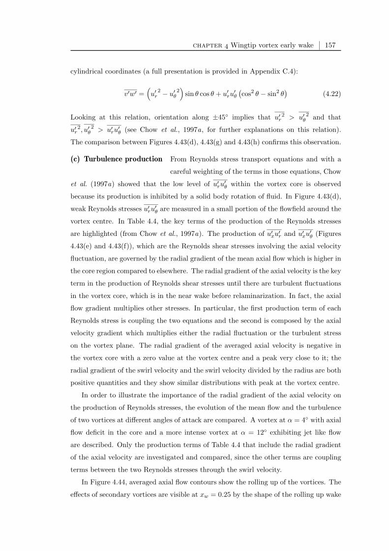
chapter Wingtip vortex early wake 157
cylindrical coordinates (a full presentation is provided in Appendix C.4):
v′w′ =(u′r
2 − u′θ2)
sin θ cos θ + u′ru′θ
(cos2 θ − sin2 θ
)(4.22)
Looking at this relation, orientation along ±45 implies that u′r2 > u′θ
2 and that
u′r2, u′θ
2 > u′ru′θ (see Chow et al., 1997a, for further explanations on this relation).
The comparison between Figures 4.43(d), 4.43(g) and 4.43(h) confirms this observation.
(c) Turbulence production From Reynolds stress transport equations and with a
careful weighting of the terms in those equations, Chow
et al. (1997a) showed that the low level of u′ru′θ within the vortex core is observed
because its production is inhibited by a solid body rotation of fluid. In Figure 4.43(d),
weak Reynolds stresses u′ru′θ are measured in a small portion of the flowfield around the
vortex centre. In Table 4.4, the key terms of the production of the Reynolds stresses
are highlighted (from Chow et al., 1997a). The production of u′xu′r and u′xu
′θ (Figures
4.43(e) and 4.43(f)), which are the Reynolds shear stresses involving the axial velocity
fluctuation, are governed by the radial gradient of the mean axial flow which is higher in
the core region compared to elsewhere. The radial gradient of the axial velocity is the key
term in the production of Reynolds shear stresses until there are turbulent fluctuations
in the vortex core, which is in the near wake before relaminarization. In fact, the axial
flow gradient multiplies other stresses. In particular, the first production term of each
Reynolds stress is coupling the two equations and the second is composed by the axial
velocity gradient which multiplies either the radial fluctuation or the turbulent stress
on the vortex plane. The radial gradient of the averaged axial velocity is negative in
the vortex core with a zero value at the vortex centre and a peak very close to it; the
radial gradient of the swirl velocity and the swirl velocity divided by the radius are both
positive quantities and they show similar distributions with peak at the vortex centre.
In order to illustrate the importance of the radial gradient of the axial velocity on
the production of Reynolds stresses, the evolution of the mean flow and the turbulence
of two vortices at different angles of attack are compared. A vortex at α = 4 with axial
flow deficit in the core and a more intense vortex at α = 12 exhibiting jet like flow
are described. Only the production terms of Table 4.4 that include the radial gradient
of the axial velocity are investigated and compared, since the other terms are coupling
terms between the two Reynolds stresses through the swirl velocity.
In Figure 4.44, averaged axial flow contours show the rolling up of the vortices. The
effects of secondary vortices are visible at xw = 0.25 by the shape of the rolling up wake
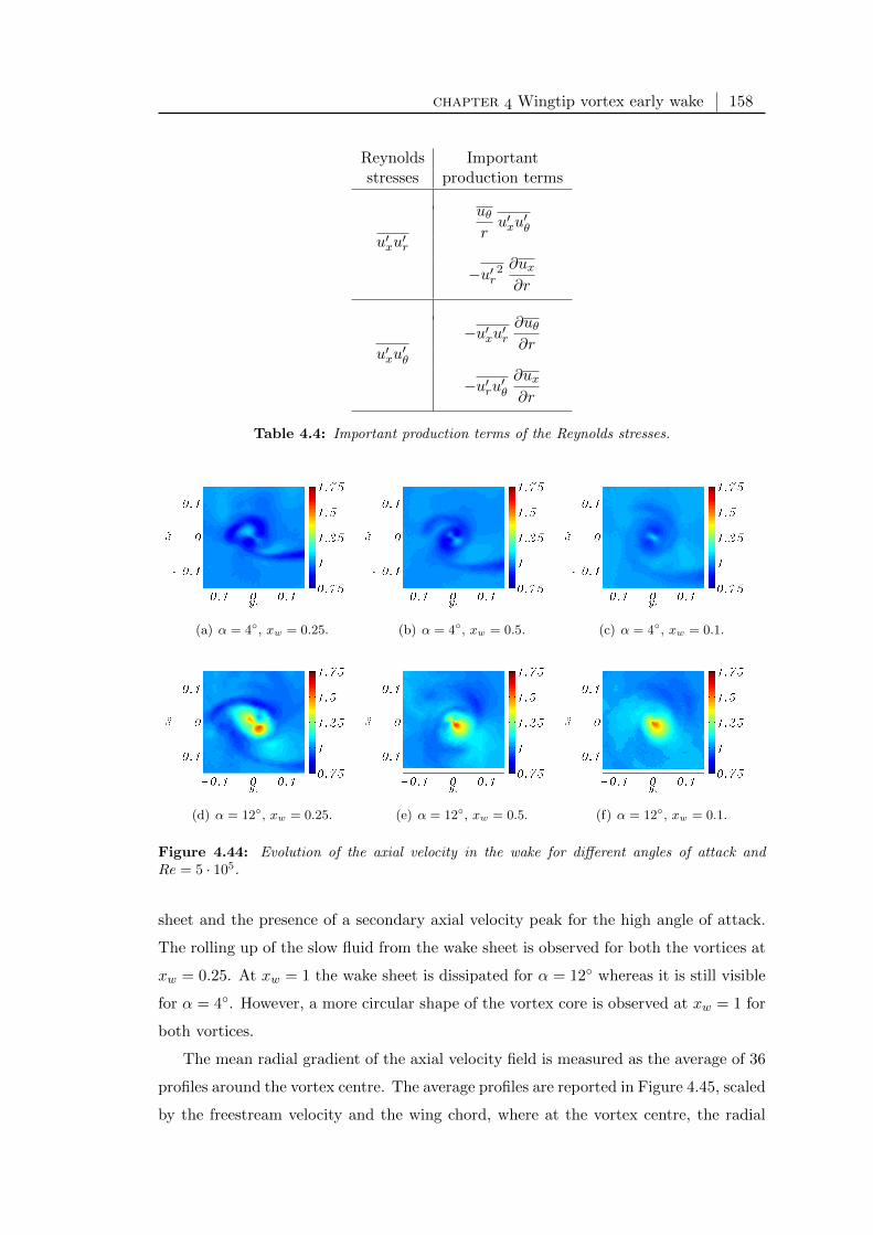
chapter Wingtip vortex early wake 158
Reynolds Importantstresses production terms
u′xu′r
uθru′xu
′θ
−u′r2 ∂ux∂r
u′xu′θ
−u′xu′r∂uθ∂r
−u′ru′θ∂ux∂r
Table 4.4: Important production terms of the Reynolds stresses.
(a) α = 4, xw = 0.25. (b) α = 4, xw = 0.5. (c) α = 4, xw = 0.1.
(d) α = 12, xw = 0.25. (e) α = 12, xw = 0.5. (f) α = 12, xw = 0.1.
Figure 4.44: Evolution of the axial velocity in the wake for different angles of attack andRe = 5 · 105.
sheet and the presence of a secondary axial velocity peak for the high angle of attack.
The rolling up of the slow fluid from the wake sheet is observed for both the vortices at
xw = 0.25. At xw = 1 the wake sheet is dissipated for α = 12 whereas it is still visible
for α = 4. However, a more circular shape of the vortex core is observed at xw = 1 for
both vortices.
The mean radial gradient of the axial velocity field is measured as the average of 36
profiles around the vortex centre. The average profiles are reported in Figure 4.45, scaled
by the freestream velocity and the wing chord, where at the vortex centre, the radial

chapter Wingtip vortex early wake 159
gradients assume a near zero value. As a consequence of the decrease of the axial velocity
fluctuations (see Figures 4.39(g), 4.39(h) and 4.39(i)), the undulations in the axial
velocity gradient profiles become weaker as the vortex progresses downstream. Although
the curves show several other local peaks which are less evident as the axisymmetric
flow is reached, the radius at which the global peak is observed is almost constant and
located at a value around 0.3% of the chord. The maximum gradient for the angle of
attack of α = 4 is approximately constant and around the dimensionless value of -8.
For α = 12, the axial flow maximum gradient increases from around -32 at xw = 0.25,
to -59 at xw = 0.5 and then to -75 at xw = 1. The increase in the axial flow gradient,
although the axial velocity peak slightly decreases, is mainly due to the redistribution
and merging of the high axial flow regions within the vortex core. The viscous dissipation
of the peak and the transfer of momentum from the high velocity in the centre to the
surrounding flow have still weak effects on the axial velocity distribution.
(a) α = 4. (b) α = 12.
Figure 4.45: Radial gradient of the axial velocity at Re = 5 · 105.
The Reynolds stress u′xu′r (left column of Table 4.4) of the study cases is reported
in Figure 4.46. The evolution of such stress in the wake of the wing is, not surprisingly,
characterized by a reshaping towards an axisymmetric pattern and a decrease of the
peak value. The low angle of attack case shows very low shear stresses at xw = 1 and
the dimensionless peak value at xw = 0.25 is much lower than the case at high incidence.
For all the cases, four lobes, alternatively positive and negative, are observed around the
vortex centre. The average of the absolute value of the minimum and maximum peak
values is reported in Figure 4.47(a) where a decrease when the vortex moves downstream
is observed. The same behaviour is observed for the Reynolds stress u′xu′θ reported in
Figure 4.47(b). It infers that, although the radial gradient of the axial velocity remains

chapter Wingtip vortex early wake 160
almost the same between xw = 0.5 and xw = 1, the production of the Reynolds stresses
in the vortex core greatly diminishes.
(a) α = 4, xw = 0.25. (b) α = 4, xw = 0.5. (c) α = 4, xw = 1.
(d) α = 12, xw = 0.25. (e) α = 12, xw = 0.5. (f) α = 12, xw = 1.
Figure 4.46: Evolution of the shear stress u′xu′r in cylindrical coordinate for different angles of
attack at Re = 5 · 105.
(a) u′xu′r. (b) u′xu′θ.
Figure 4.47: Evolution of the average of the absolute value of the minimum and maximumpeak of shear stresses in cylindrical coordinate for different angles of attack at Re = 5 · 105.
The radial velocity fluctuation u′r2 and the vortex plane Reynolds stress u′ru
′θ are the
terms that scale the axial gradient in the production terms of Table 4.4. The distribution
of the first is reported in Figure 4.48 and the evolution in the wake of both of them
is reported in Figure 4.48. For the high angle of attack, the two stresses are mainly
subjected to a reshaping in a more circular form and the peak values are approximately
constant. For the low incidence, they go to zero very quickly and at xw = 1 almost zero

chapter Wingtip vortex early wake 161
fluctuations are observed. These measurements are symptoms of a relaminarization of
the vortex core, occurring for α = 4 from xw = 0.5 to xw = 1, which inhibits turbulence
fluctuations and generates a laminar flow in the core.
(a) α = 4, xw = 0.25. (b) α = 4, xw = 0.5. (c) α = 4, xw = 1.
(d) α = 12, xw = 0.25. (e) α = 12, xw = 0.5. (f) α = 12, xw = 1.
Figure 4.48: Evolution of the normal stress u′r2 in cylindrical coordinate for different angles
of attack at Re = 5 · 105.
(a) u′r2. (b) u′ru
′θ.
Figure 4.49: Evolution of the stresses in cylindrical coordinate for different angles of attack atRe = 5 · 105.
The high radial gradient of the axial velocity and the jet–like flow in the vortex core
of a more intense vortex (α = 12) contribute to a higher turbulence production. The
higher mixing rate of fluid between vortex layers, due to the turbulence contribution,
generates mean axial flow contours which become rapidly axisymmetric (see Figure
4.44(f)). A low angle of attack (α = 4) generates a vortex which develops over a longer

chapter Wingtip vortex early wake 162
range; from Figure 4.44(c), the wake sheet is still visible at xw = 1 and not fully rolled
up around and merged with the vortex. However, the axial velocity gradient is low and
the axial velocity peak is only slightly more than the freestream. This leads to a vortex
core that presents a solid body rotation very early in the wake (i.e. at xw = 1 the vortex
core is laminar).
section
Early wake behind squared and rounded wingtips
Since a change of wingtip geometry radically affects the pressure distribution on the
wing and the behaviour of the flow in the early wake, a comparison between the tip
vortex generated by a squared tip and a rounded tip is presented in this section in order
to highlight some key mechanisms, in particular on the generation of meandering and
turbulence. Specifically, the evolution of the wingtip vortex in the early wake of the
wing M2 with squared and rounded tips is presented.
(a) Development of
averaged properties
The averaged axial velocity contours (helicity based method
applied) for the squared tip and rounded tip at xw = 0.25 and
xw = 1 are presented in Figure 4.50. The wake sheet is clearly
visible at xw = 0.25 as a horizontal line with axial velocity deficit that rolls up around
the vortex. A remarkable difference between the two geometries is the shape that the
wake sheet takes during the rolling up. For the rounded tip, the wake follows a spiral
structure, whereas for the squared geometry the induced velocity on the wake from the
vortex system is affected by the presence of an intense counter rotating secondary vortex
on the left of the primary vortex. The presence of the secondary vortex is noticeable at
xw = 0.25 where the wake sheet presents a very distinct “kink” (Chow et al., 1997a).
This structure generates a more diffuse vortex at xw = 1 than the vortex generated by
the rounded tip. The axial velocity within the core appears in all the cases as an excess
compared to the freestream velocity. These contours refer to a Reynolds number equal
to 12.7 · 105 and the results at Re = 2.6 · 105 and Re = 7.4 · 105 show the same features.
Vorticity contours are also reported in Figure 4.51 for the same cases. For the
rounded geometry, the vorticity of the wake sheet is observed at xw = 0.25 but is not
visible at xw = 1 where the vorticity is concentrated in the core. The effect of the
squared tip is to generate a region of negative vorticity which is distributed on a wider
area around the centre of the vortex. In order to quantify the dispersion of the vorticity,
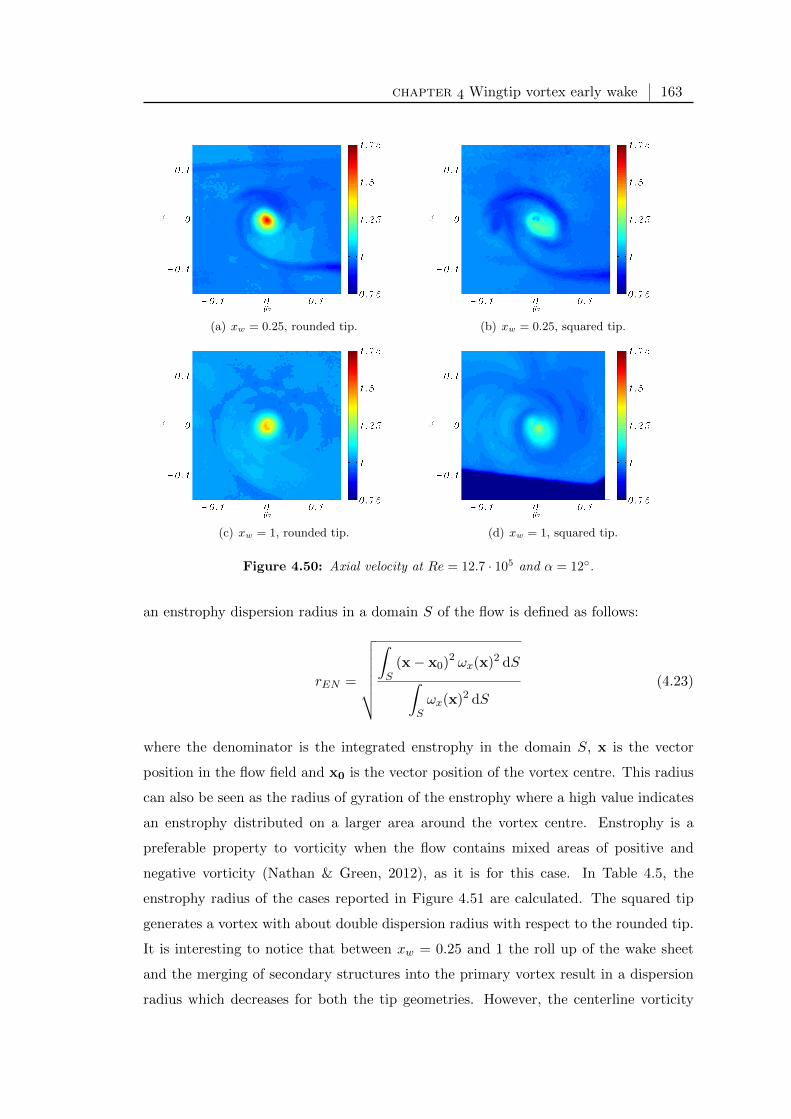
chapter Wingtip vortex early wake 163
(a) xw = 0.25, rounded tip. (b) xw = 0.25, squared tip.
(c) xw = 1, rounded tip. (d) xw = 1, squared tip.
Figure 4.50: Axial velocity at Re = 12.7 · 105 and α = 12.
an enstrophy dispersion radius in a domain S of the flow is defined as follows:
rEN =
√√√√√√√∫S
(x− x0)2 ωx(x)2 dS∫Sωx(x)2 dS
(4.23)
where the denominator is the integrated enstrophy in the domain S, x is the vector
position in the flow field and x0 is the vector position of the vortex centre. This radius
can also be seen as the radius of gyration of the enstrophy where a high value indicates
an enstrophy distributed on a larger area around the vortex centre. Enstrophy is a
preferable property to vorticity when the flow contains mixed areas of positive and
negative vorticity (Nathan & Green, 2012), as it is for this case. In Table 4.5, the
enstrophy radius of the cases reported in Figure 4.51 are calculated. The squared tip
generates a vortex with about double dispersion radius with respect to the rounded tip.
It is interesting to notice that between xw = 0.25 and 1 the roll up of the wake sheet
and the merging of secondary structures into the primary vortex result in a dispersion
radius which decreases for both the tip geometries. However, the centerline vorticity

chapter Wingtip vortex early wake 164
(a) xw = 0.25, rounded tip. (b) xw = 0.25, squared tip.
(c) xw = 1, rounded tip. (d) xw = 1, squared tip.
Figure 4.51: Vorticity at Re = 12.7 · 105 and α = 12.
increases of 22% for the squared tip and of 14% for the rounded tip as the vortex moves
downstream, which is a sign of the uncompleted roll up, as observed also by Chow et al.
(1997a).
Tip xw rEN/c%
rounded0.25 1.56
1 1.48
squared0.25 3.41
1 2.75
Table 4.5: Enstrophy dispersion radius in the wake of squared and rounded wingtips; Re =12.7 · 105 and α = 12.
As observed also in Section 4.3, a region of positive vorticity, corresponding to a
counter rotating secondary vortex, is observed on the left side of the primary vortex
at 0.25 chords from the squared tip and it contributes to the wide dispersion radius.
The fact that this secondary vortex is clearly visible in the average flow field indicates
that it is intense and persistently found in that position. The position and intensity of
other secondary vortices detected in the instantaneous fields are less persistent and they
appear in the averaged contour only as a low vorticity ring around the primary vortex.

chapter Wingtip vortex early wake 165
(a) Rounded tip. (b) Squared tip.
Figure 4.52: Vorticity profiles and mean value (red line) at xw = 0.25, Re = 12.7 · 105 andα = 12.
For a more quantitative understanding, directional vorticity profiles are reported in
Figure 4.52 as function of the distance from the vortex centre along 12 cuts around the
vortex centre at xw = 0.25. The mean value is also reported. A higher absolute value
of the vorticity in the centre is calculated for the rounded tip where a small deviation
from the mean value is also observed. A small bump at r = 0.08 is recorded and is
related to cutting across the wake sheet. For the squared tip case, the distribution of
the vorticity around the centre shows a smaller magnitude and it confirms the high
asymmetry. In the mean profile, an inner region of high gradient is followed by a region
with smaller gradient where secondary structures are indicated by drops and bumps of
the directional profiles. In particular, the bump at r = 0.11 corresponds to the main
secondary vortex on the left side of the primary vortex. As noted also from the contours
of Figure 4.51, the vorticity field for the squared case reaches the asymptotic zero value
at a considerably higher radius (r ' 0.10) than the rounded tip (r ' 0.7).
In Figure 4.53, the swirl velocity of the average velocity field at xw = 0.25 is reported
for the two tip geometries. The swirl velocity behind the squared tip shows a double–
peak profile due to the spiral shape of the vortex core discusses in Section 4.2. A wider
region of high gradient in the vortex core is observed for the rounded tip along all
the cut directions and a considerably higher swirl velocity maximum is also observed.
Even though the asymmetry is less compared to the squared tip, the difference in the
maximum swirl velocity peak around the centre is about 12% of the mean value. For
both the geometries, the swirl velocity mean profiles do not show significant changes at
xw = 1 although it reveals a smaller scatter of the directional profiles from the mean
value. For the rounded tip case, a difference between the swirl velocity maxima of 6%

chapter Wingtip vortex early wake 166
is found.
(a) Rounded tip. (b) Squared tip.
Figure 4.53: Swirl velocity profiles and mean value (continuous red line) at xw = 0.25, Re =12.7 · 105 and α = 12. Location of local maximum and minimum in dashed vertical red lines;velocity profile of the Lamb–Oseen vortex in blue.
In the same Figure, the swirl velocity profile as described in the Lamb–Oseen vortex
is also reported. The parameters needed for the definition of the analytical profile (i.e.
vortex circulation and radius) are adjusted in order to fit the inner core (r < 0.01) and
the outer core profiles (r > 0.08). The analytical profile is in good agreement with the
vortex measured behind the rounded tip at the exception of a swirl velocity peak 25%
greater. A different situation is observed looking at the vortex generated by the squared
tip where the swirl velocity profile has a different shape and it is much lower than the
analytical vortex over a large area around the vortex core. This region is affected by a
strong deformation of the vortex core shape which is far from being symmetric.
In Figure 4.54 the distribution of the vortex circulation Γ(r), calculated by integra-
tion of the swirl velocity mean values and normalised by the freestream velocity and the
chord, is presented for the two geometries. Although the circulation asymptote of the
two cases tends to the same value, which means also that a similar overall circulation
(hence lift) of the wing with the two different tips is generated, the radial distributions
are different. The vortex behind the squared tip reaches the asymptotic value at a
dimensionless radius around 0.1. A varying slope is observed within the core which
reflects the asymmetry found in the swirl velocity. The position of the local maxima
and minimum in the swirl velocity are also reported in this graph (vertical red lines)
with reference to Figure 4.53. The three lines are all found before the asymptotic value
is reached and they identify the position of a change of gradient in the circulation pro-
file. The circulation for the rounded tip case shows a first inner region of high constant

chapter Wingtip vortex early wake 167
gradient and a region of lower constant positive gradient afterwards. The maximum
swirl is found before the change of gradient occurs.
Figure 4.54: Circulation profiles and location of local maximum and minimum of swirl velocity(vertical red lines) at xw = 0.25, Re = 12.7 · 105 and α = 12.
This suggests that the rounded tip generates a wake where the circulation from the
wake sheet is gradually included into the vortex system. Also, secondary vortices found
in the wake of the squared tip accelerate the rolling up and dissipation of the wake sheet
so that the asymptotic circulation value is reached at an earlier stage. However, the
squared tip generates a vortex which has a bigger core with a more complex structure
than the rounded tip.
(b) Meandering and
instantaneous behaviour of
the vortex structure
In Figure 4.55, an instantaneous vorticity contour map
of the vortex at xw = 0.25 generated by a squared tip
is shown. Many aspects in common with the flow vi-
sualizations in Figure 3.13 are found. Several vortices
with opposite rotation can be detected by their vorticity peaks around the primary
vortex. The strong counter rotating secondary vortex also is marked on the left side of
the primary vortex. The ring of higher vorticity around the primary vortex observed in
the average field in Figure 4.51(b) is due to secondary vortices rolling up and eventually
merging with the primary vortex.
The instantaneous vorticity field of the vortex system generated by a wing with
squared tip shows an intense interaction between primary vortex, vorticity sheet and
secondary vortices. The effect is a rapid change over time of the primary vortex position
and shape. The movement of the primary vortex centre can be quantified with the
standard deviation of the distance of the instantaneous vortex centres (calculated with
the helicity based method) from the average centre, which can be seen as a definition

chapter Wingtip vortex early wake 168
Figure 4.55: Instantaneous vorticity at xw = 0.25, Re = 12.7 · 105 and α = 12 for squaredwingtip.
of the meandering intensity:
σm = std
[√(xi0 − x0
)2+(yi0 − y0
)2](4.24)
Figure 4.56: Vortex meandering for squared and rounded tips as function of the angle of attackat Re = 7.4 · 105.
In Figure 4.56, σm is plotted as a function of the angle of attack for the vortices
formed by squared and rounded wingtip at a Reynolds number of 7.4 · 105. The vortex
meandering in the early wake of a wing with rounded tip is dominated by the essentially
inviscid smoothing out process of the spiral vorticity sheet (Moore & Saffman, 1973).
On the other hand, because of the presence of stronger satellite vortices, for a squared
tip the meandering is higher than for a rounded tip. Also, as observed earlier in the
vorticity contours, at xw = 0.25 several secondary vortices are still present and not
merged with the primary vortex as one defined vortical structure. The meandering in
the early wake of the vortex from a squared tip is therefore dominated by secondary
vortex interactions as observed also by Zuhal & Gharib (2001). This system of vortices

chapter Wingtip vortex early wake 169
is the principal cause of the high meandering at this stage which decreases moving
downstream as secondary structures merge with the primary vortex.
The meandering of the vortex seems almost independent of an increase in the angle
of attack from 4 to 12. However, it changes with the distance from the trailing edge.
For a rounded tip, the meandering increases by about 50% from xw = 0.25 to 1 because
of the progressive rolling up of the vorticity sheet. For a squared tip, the meandering
observed at xw = 0.25 is double than the meandering at xw = 1 which is coherent
with the interactions of the primary vortex with satellite vortices. These interactions
are stronger at xw = 0.25 when secondary structures are not merged with the primary
vortex. The meandering of the vortex created by a rounded tip at a stall angle of
α = 20 is also reported where the values are considerably higher then at lower angles
of attack. A stalled wing creates a large region of separated flow that introduces intense
chaotic motions and a more diffused vorticity distribution in the vortex core.
(c) Turbulence and shear
strain evolution
The shear strain and the in–plane Reynolds stresses for
the vortex in the early wake of rounded and squared tip
are compared in the following Figures (respectively in
Figure 4.57 and 4.58) for the angle of attack of 12 and Reynolds number of 12.7 · 105.
The development of the four lobes pattern of the shear strain in the vortex core
is quicker for the rounded tip than for the squared tip. Apart from the presence of
the wake sheet, almost no differences in the shear strains from a rounded tip can be
seen between the two measurement planes. The wake sheet shed by the trailing edge,
characterized by a change of sign of the v–component of the velocity which results in a
region of positive∂v
∂z, is visible at xw = 0.25 and quickly dissipates by viscous effects.
For the squared tip, the shear strains at xw = 0.25 are affected by secondary vortices
which deform the four lobes pattern and create several secondary lobes around the vortex
core. A more symmetric shape is found at xw = 1. However, the size of the lobes for the
rounded tip is much larger than for the squared tip and the velocity gradients are more
intense. For a vortex from a rounded tip, the region within the core at constant and high
swirl velocity gradient is bigger because the core does not show a spiral (asymmetric)
structure like that from a squared wingtip (see Figure 4.53). The region within the
vortex core of high velocity gradients observed for the rounded tip is responsible for the
high shear strain.
Looking at Figure 4.58, higher values of Reynolds stresses are measured at xw = 1
for the rounded tip compared to the squared one (Figures 4.58(c) and 4.58(d)), and

chapter Wingtip vortex early wake 170
(a) xw = 0.25, rounded tip. (b) xw = 0.25, squared tip.
(c) xw = 1, rounded tip. (d) xw = 1, squared tip.
Figure 4.57: Evolution of the shear strain εyz for squared and rounded tip at α = 12 andRe = 12.7 · 105.
looking at the flow at xw = 0.25 (Figures 4.58(a) and 4.58(b)), a different evolution of
the stresses for the two geometries can be presumed. The rounded tip generates a vortex
with high velocity gradients within the core which in turn generate higher turbulence
stresses; the increase in the peak values of the Reynolds stress from xw = 0.25 to xw = 1
is indicative of the development of the axisymmetric vortex with a turbulent vortex core.
The squared tip generates a vortex system of multiple vortices which interact and quickly
dissipate the velocity gradients. The Reynolds stresses are higher at xw = 0.25 than at
xw = 1 which indicates a strong interaction between primary and secondary vortices.
The small Reynolds stress at the centre of the vortex at xw = 1 indicates a core in an
advanced stage of the relaminarization process. The relative rotation of 45 between
shear stresses and Reynolds stresses (and discussed in Section 4.4.(b)) is observed in
the same way for both the tip geometries.
This different evolution of the vortex cores for the two tip geometries can be observed
also by looking at the turbulent kinetic energy at the vortex centre in Figure 4.59.
Figure 4.59(a) shows the value of k0 at the two measurement planes. For the squared
tip, the same trends discussed with reference to Figure 4.40(a) are observed here: the
turbulence is higher for a higher angle of attack and decreases with the distance from
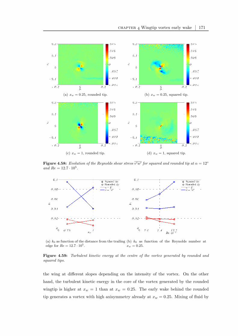
chapter Wingtip vortex early wake 171
(a) xw = 0.25, rounded tip. (b) xw = 0.25, squared tip.
(c) xw = 1, rounded tip. (d) xw = 1, squared tip.
Figure 4.58: Evolution of the Reynolds shear stress v′w′ for squared and rounded tip at α = 12
and Re = 12.7 · 105.
(a) k0 as function of the distance from the trailingedge for Re = 12.7 · 105.
(b) k0 as function of the Reynolds number atxw = 0.25.
Figure 4.59: Turbulent kinetic energy at the centre of the vortex generated by rounded andsquared tips.
the wing at different slopes depending on the intensity of the vortex. On the other
hand, the turbulent kinetic energy in the core of the vortex generated by the rounded
wingtip is higher at xw = 1 than at xw = 0.25. The early wake behind the rounded
tip generates a vortex with high axisymmetry already at xw = 0.25. Mixing of fluid by

chapter Wingtip vortex early wake 172
viscous effects and by interaction with secondary structures is very low so that strong
velocity gradients are observed around the centre, particularly the radial gradient of
the axial velocity which in turn generates turbulence within the core. However, this
is only a temporary process and the turbulence within the core will decrease moving
more downstream towards a laminar vortex core. It is believed that a similar process is
also seen in Figure 4.40(a) for the squared wingtip at α = 4. With that configuration,
similarly to the rounded tip case, secondary structures are weak and a quick development
of the vortex into an axisymmetric structure is observed. The turbulence at the vortex
centre increases between xw = 0.25 and xw = 0.5 and decreases then between xw = 0.5
and xw = 1.
The influence of the Reynolds number on the maximum turbulent kinetic energy is
reported in Figure 4.59(b) for different wing angles. As observed also in Figure 4.40(b),
for the squared tip at α = 4 the turbulence remains approximately constant but it
increases with the Reynolds number for α = 12 by the formation of stronger secondary
vortices. The rounded tip generates a vortex with fewer secondary vortices and less
intense than the squared tip so that axisymmetry is reached earlier in the wake. At
α = 12 the vortex is less turbulent than for the case with squared tip and an almost
constant turbulence is observed increasing the Reynolds number. At α = 4, with
smaller axial velocity gradients and less intense axial velocity perturbations, the effect
of increasing the Reynolds number is as of an ageing of the vortex corresponding to a
decrease of the turbulence level.
Comparing the values of k0 measured behind squared tip mounted on the different
wings, it appears that the turbulence behind the wing M1 with bigger aspect ratio
(Figure 4.40) is about double than the turbulence behind the low aspect ratio wing M2
in Figure 4.59 (the same can be said comparing the Reynolds stresses in Figures 4.41(i)
with Figure 4.58(d)). The overall circulation and its distribution is therefore strongly
connected to the vortex core turbulence.
Lastly, the turbulence values of Figure 4.59(b) for Re = 7.4 · 105 can be compared
with the meandering for the same cases in Figure 4.56 (xw = 0.25). What appears
is that rounded tips generate a vortex with lower meandering and lower turbulence
than the vortex generated by squared tips. However, the turbulence for the rounded
tip at α = 12 is higher than for the squared tip at α = 4 despite the fact that the
corresponding meandering is much lower. Meandering and turbulence, even if strongly
connected by same causes like as secondary vortices and wake sheet interactions, are
generated and evolve in different ways. The meandering is a solid movement of a big part

chapter Wingtip vortex early wake 173
of fluid (of the order of the vortex core and usually identified by the movement of the
vortex centre) dictated by disturbances on the wing and in the wake as consequence of
interactions with secondary structures. These interactions contribute to the deformation
of the velocity field within the vortex core which is balanced by asymmetric shear
stresses. Turbulence is already present during the formation of the vortex flow on
the wake surface, it is further produced in the early wake by velocity gradients and it
diminishes moving downstream as effect of the relaminarization of the vortex core by
centrifugal forces.
(d) Vortex pair formation
without generation of lift
Among the models and mechanisms of the wingtip vor-
tex formation presented in Section 1.2, the shear layer
interpretation is the only mechanism which predicts vor-
ticity formation over a wingtip without producing lift. In this section, the wake behind
the wing at no incidence is tested for the two tip geometries in order to give insights
on this mechanism of vortex formation. The axial velocity and the vorticity contours in
the wake of the M1 wing are reported respectively in Figures 4.60 and 4.61. Both the
rounded and the squared wingtips are studied at xw = 0.25 and Re = 7.4 · 105.
(a) Rounded tip. (b) Squared tip.
Figure 4.60: Axial velocity at α = 0, xw = 0.25 and Re = 7.4 · 105.
On the squared tip, the vorticity contour shows the occurrence of two counter–
rotating vortices of same magnitude. They are formed on the two wing surfaces and
they are fed by the flow on the tip side forced to a separation by the sharp edges. This
is the same mechanism seen on the wing at an incidence (smoke visualization in Figure
3.13) where the flow from the tip side separates at the sharp edge and forms the primary
vortex. For the wing at zero incidence, the flow around the wing is symmetric about
the chord plane and the flow on the tip side spills over both the wing surfaces forming
two vortices. In the wake, the consequent induced velocity field feeds the vortex pair
with the wake sheet which is identified by a region of flow with axial velocity lower

chapter Wingtip vortex early wake 174
(a) Rounded tip. (b) Squared tip.
Figure 4.61: Vorticity at α = 0, xw = 0.25 and Re = 7.4 · 105.
than the freestream flow. The flow around a rounded tip is not forced to a separation
like the flow over a squared tip. For the rounded tip, the wake shows a smaller and
weaker vortex pair than the squared tip case at the edge of the vorticity sheet and the
interaction between vortices and wake sheet is weaker. Although the geometries are
very simple, the importance of this mechanism in the initial wingtip vortex formation
may present this test as a benchmark case for numerical analysis.
section
Summary
Planar SPIV behind rectangular wings reveals that the very early wake is dominated
by the rolling up of the wake sheet and the presence of several secondary vortices which
interact with the primary vortex and strongly affect its dynamics. The vortex structure
is not axisymmetric and turbulence affects the whole vortical flow. The importance of
the centering procedure of the instantaneous vector fields is found in the clarification of
a robust vortex centre definition which can take various forms. From a comparison of
several vortex quantities such as vortex centre movement, axial velocity, swirl velocity,
velocity fluctuations, turbulent kinetic energy, Reynolds stresses and shear stresses, the
identification of the vortex centre with the peak of the streamwise helicity is found to
give the highest reliability. Moreover, among the different quantities presented here,
this is the only one which is calculated using all the three components of the velocity
vector. However, different definitions of the vortex centre can be preferred for analysis
of the flowfield which focus on specific aspects such as the rolling up of the wake sheet
or the axial velocity peak.

chapter Wingtip vortex early wake 175
The centering operation operates as a filter of the turbulent motions linked to a
solid translation of the whole vortical flow on a plane perpendicular to the vortex axis
and related to its centre position. The axial velocity flow and the turbulence level in
the vortex core are highly affected by the method adopted for the correction from this
motion. However, after such correction, the fluctuation level of the vortex core is still
high due to the presence of secondary vortices and rolling up of the wake sheet. The
introduction of a directional vortex core radius reveals the spiral structure of the vortex
core in the early stage and its development towards an axisymmetric structure. The
rotation rate of the core increases with the intensity of the vortex and an axisymmetric
vortex core is observed at 2 chords downstream of the trailing edge. The comparison
between the vortex generated by a squared wingtip with a rounded wingtip highlights
the effects of two main mechanisms in the vortex development: the rolling up of the
wake sheet and the merging of secondary vortices. The same effects can be seen from
the comparison between the development of a weak vortex (i.e. low angle of attack)
with a strong vortex (i.e. high angle of attack). During the formation of the vortex
on the wing, turbulence is already found in the rolling up spiral structure so that the
vortex core in the very early wake is turbulent for both the geometries. Jiang et al.
(2007) found that the turbulence inside the primary tip vortex is not created by the tip
vortex itself but the turbulent shear layer and the interaction between the primary and
the secondary vortices are the major sources of turbulent activity in the core.
The trailing vortex behind a squared wingtip is bigger than the vortex behind a
rounded wingtip; several secondary vortices orbits around the primary vortex and even-
tually merge with it. The interaction between these vortical structures contributes to
a high mixing of fluid between the flow in the vortex core and the external flow and a
high meandering is generated. Also, this interaction quickly dissipates the high velocity
gradients within the vortex core so that a relaminarization process is promoted at an
earlier stage. On the contrary, the rounded tip generates a vortex with an axisymmetric
shape at a more upstream plane with high velocity gradients within the core which
generate higher turbulence stresses and a later relaminarization. Also, the meandering
of the vortex behind a rounded tip is mostly dictated by the smooth and progressive
rolling up of the wake sheet.
The difference in the development processes of the trailing vortex generated by the
two different wingtip geometries gives insight on the difference between the turbulence
within the vortex core and the meandering of the vortex system. Meandering is linked
to secondary structures interacting with the vortex such as secondary vortices and wake

chapter Wingtip vortex early wake 176
sheet. Turbulence in the vortex core is generated by the high velocity and pressure
gradients and in particular by the radial gradient of the axial flow. The turbulent quan-
tities inside the vortex increase with the angle of attack and quickly become symmetric
moving downstream. The relaminarization of the vortex core is observed at a earlier
stage when the angle of attack of the wing is low and the consequent radial gradient of
the axial velocity is also low.
The axial flow in the vortex core is the result of the acceleration mechanism caused
by the spiral structure of the vortical flow and the deceleration due to the mixing of the
wake sheet and the boundary layer with the core flow. The equilibrium between these
mechanisms is dictated by the wingtip geometry and the intensity of the vortex so that
different shapes of the axial flow distribution can be observed. However, an axial velocity
excess at the vortex axis compared to the surrounding core flow is always observed in the
early wake although its magnitude might be lower than the freestream velocity for weak
vortices. The development of the axial flow is quicker than the development of the swirl
velocity and the axial velocity contours do not show the presence of secondary structures
at already one chord from the trailing edge. These findings are very important when a
centering method for the vortex in the early wake has to be selected and also when a
comparison of the axial velocity peaks is performed. In the present parametric study,
both axial velocity excess and deficit compared to the freestream velocity are observed.
A linear relation between the axial flow peak with a vortex circulation parameter is
suggested and a good correlation with other studies is found. Furthermore, different
linear trends are found for the two different wingtip geometries with the rounded tip
showing a higher gradient than the squared tip. The switchover angle between jet–like
and wake–like behaviour of the axial velocity peak is estimated to be around 4 for the
squared tip and around 7 for the rounded tip.

chapter
Measurement accuracy and error
Results from several experimental techniques have been presented and discussed in this
dissertation. Each technique contributed to create a deeper and more comprehensive
understanding of the main aspects of the formation of the wingtip vortex on the sur-
face of the wing. Moreover, a wide range of conditions have been tested which have
revealed important trends, patterns and mechanisms in the wingtip vortex formation
and early wake. Some of techniques adopted are purely qualitative, such as the smoke
and the surface oil flow visualizations, and their validity relies on a good set up of the
experimental apparatus and a sensible interpretation of the results (details in Sections
2.3.(a) and 2.3.(c)). As regards to the other experimental techniques, a discussion and
quantification of the experimental accuracy and error encountered in this work is pre-
sented in the following sections with a particular attention on the measurements using
the SPIV (Section 5.2), which played the major role in the investigation of the wingtip
vortex flow.
section
Pressure, frequency and meandering
Pressure measurements gave insight on the effects of the wingtip vortex on the pres-
sure distribution on the wing surface at different angles of attack. Pressure transducers
with very high linearity were used (see Section 2.3.(b)) and a resolution of 0.14% of
the maximum suction peak is calculated. The comparison between the results found in
this work and the results of McAlister & Takahashi (1991) revealed that a high spatial
resolution of the pressure tappings is essential for an accurate description in the region
of high gradients around the suction peak (see Section 3.2). The suction peaks found in
the present study were around 15% lower than the peaks found by McAlister & Taka-
177

chapter Measurement accuracy and error 178
hashi (1991) for a similar case. However, a similar shape of the pressure distribution
(i.e. lowering of the suction peak moving outboard and undulation generated by the
wingtip vortex suction) was found.
The dominant frequencies of the pressure measurements presented in Section 3.2.(b)
are one decade below the resonance frequency of the experimental apparatus, as dis-
cussed in Section 2.3.(b). Also, due to the small tubing diameter, the damping of the
system is very high so that the measurement errors in the pressure fluctuations presented
in this research are negligible.
As discussed in Section 2.3.(d), the hot film was used following the manufacturer
guidelines and only for frequency measurements avoiding the particularly challenging
calibration procedure needed for velocity measurements. The sampling parameters and
the filtering of the signals were set so that the measurement errors in the signal spectra
were minimized. The hot film measurements confirmed and extended the observations
from pressure fluctuations on low frequency unsteadiness on the wing surface as effect
of the initial rolling up of the vortex.
Smoke visualizations in the early wake (presented in Section 3.6) further studied
the unsteadiness of the trailing vortex and in particular the movement of the vortex
centre. Two methods for the localization of the vortex centre from smoke visualizations
were implemented and compared in Appendix B where a comparative study on the
main parameters is also presented. The procedure used in the present investigation
was then accurately chosen. The validity of this technique is based on the reliability of
the darker region centroid as a good description of the vortex centre, which is a good
assumption when smoke particles accurately follow the flow, for high smoke density, for
low buoyancy forces, for high image resolution and for darker spots of the order of the
vortex core. All these factors were satisfied for these experiments.
section
SPIV
Errors in the velocity information derived from SPIV come from a variety of sources
such as from the optical system, experimental set–up, image reconstruction method, im-
age digitisation, seeding quality, correlation process and post–processing of the images
(for some theoretical and applied accounts, see for example Raffel et al., 2007; Ra-
masamy & Leishman, 2007; Nathan, 2010; Gupta, 2011). However, some of the errors

chapter Measurement accuracy and error 179
can be rectified through implementation of post–processing algorithms and by following
guidelines from other similar experiments (Raffel et al., 2007).
The set–up of the camera position and angular displacement, the choice and posi-
tioning of the calibration plate, the focusing of the image, the calibration procedure and
the calculation of the mapping function were accomplished following the guidelines of
the PIV system manufacturer (DaVis, 2007) and adopting the relative software DaVis
7.2. The quality of the calibration process was given by the software in terms of average
deviation of the dewarped marker positions of the calibration plate to the ideal regular
grid. A value always lower then 0.3 pixel was calculated, which ensured an excellent
calibration of the system (DaVis, 2007).
The digitisation of the smoke visualizations can be one of the most limiting sources
of errors for the velocity information accuracy (Nathan, 2010). Digitisation effects in
PIV occur when the imaged flow seeding particles are too small in size to be adequately
defined as a distinctive image, which is an effect of the limited spatial resolution of the
CCD sensors used in digital cameras. The limited pixel size of these cameras results in
reduced fine detail resolution, at a given magnification. The small tracer particles in the
flowfield are thus imaged without an accurate profile (Green, 2012) and the displace-
ments derived from the correlation processes tend to be biased to integer–values resulting
in clusters of vectors in the derived velocity maps to have block–like appearances. This
phenomenon is known as peak–locking and histograms relating to the velocities will show
peaks at integer values (Raffel et al., 2007).
The camera lenses and the position of the cameras during the experiments were
accurately chosen in order to minimize the peak–locking effects and the particle size
on the image plane was between 1 and 2 pixels (Prasad et al., 1992). Errors from an
improper seeding density of the flowfield were minimized ensuring sufficiently populated
interrogation windows (Hart, 2000; Keane & Adrian, 1992). The time delay between the
two laser pulses was also accurately calculated (see Appendix A.1) and the peak–locking
effect in the velocity maps was calculated by DaVis 7.2 to have an average value well
within the acceptable range (DaVis, 2007).
The image processing procedure also can be a source of large errors in the velocity
vector evaluation. An appropriate choice of interrogation window size, overlap and
processing procedure is fundamental in the accuracy of the calculated velocity vector
field (Adrian, 1991). A study on the effects of the different parameters is presented in
Appendix A.2 and the vector field computation process used during these experiments
is described in Section 2.3.(e).

chapter Measurement accuracy and error 180
From the discussion above, the results from the cross-correlation procedure opti-
mization (in Appendix A.2) and referring to the work of Nathan & Green (2012) who
also evaluated the accuracy of the same PIV system with a similar set–up, an absolute
accuracy of the SPIV on the velocity vectors better than 2% can be claimed for the
present investigation, which is adequate for quantitative analysis of the flow. This value
has to be intended for a generalized error on the evaluation of the instantaneous veloc-
ity vector fields. From the convergence of the averages presented in Section 4.1.(d), an
accuracy better than 2% can be taken also for the averaged velocity fields based on the
121 samples used throughout this work. Nevertheless, quantities involving derivatives
and velocity fluctuations, such as vorticity, helicity, normal stress, Reynolds stress and
shear strain, are expected to exhibit lower accuracy than the velocity vectors. In Sec-
tion 4.1.(d), the highest error was equal to 7% and found for the Reynolds shear stress.
However, the averaging convergence errors were calculated on the peak values of the
quantities which leads to an overestimation of the global measurement errors.
chapter
Conclusions and recommendations
for future work
If the research that we do does not change the way people
think, the project is a fail.
George M. Whitesides
Behold, the fear of the Lord, that is wisdom, and to turn
away from evil is understanding.
Job, Bible
This chapter summarizes the major findings of the present research with reference to
the unresolved issues presented in Section 1.4 and discusses some of their implications.
In addition, recommendations are made for future research related to the wingtip vortex
flow.
section
Conclusions
The formation and the early wake of a trailing vortex behind a rectangular wing has
been studied with different experimental techniques, specifically with surface oil flow
visualization, surface pressure measurement through pressure tappings, smoke visual-
ization of the vortex formation, measurement of the unsteadiness of the surface flow
through wall pressure fluctuation and hot film mounted on the surface, stereoscopic
particle image velocimetry on planes parallel to the wing surface and on planes per-
pendicular to the freestream velocity in the wake. The integration of complementary
181

chapter Conclusions and recommendations for future work 182
results from these techniques reaches a deeper understanding of the physics and main
mechanisms of the early stage of the vortex flow. The effects of several parameters on
the interaction of these mechanisms have been addressed generating a fuller overall view
of this flow based on a wide range of experiments. In particular, two symmetric NACA
rectangular wing models with different chord (0.42 and 0.76 m) and aspect ratio (3.1
and 0.75) have been tested in a range of angle of attack of α = 0–20, Reynolds number
of Re = 3 · 103–1.27 · 106 and wake plane position of xw = 0.25–2. Also, the comparison
between the vortex flow generated by squared and rounded wingtip geometries have
been tested. The high spatial resolution on this vortex flow in the early wake achieved
by the SPIV arrangement and the largeness of this parametric study represent a unique
feature of these measurements which advances the current state of understanding on
this particular flow.
A set of characteristic lines were defined based on the three components of the ve-
locity on planes parallel to the suction surface and at a small distance from it. This
small distance (of about 7% of the chord) allowed a good correlation between the veloc-
ity field obtained by SPIV and the surface flow experiments (oil visualization and wall
pressure). These characteristic lines have been revealed to be a compact and accurate
tool in describing the vortex structure and its development along the wing. The pri-
mary vortex is created by the separation of the flow coming from pressure surface which
forms a vortical structure moving downstream along the wingtip region; depending on
the instantaneous pressure field, the vortex origin is not fixed but showed oscillations in
the chordwise direction. An intense secondary vortex is observed between the primary
vortex and the tip and a high level of turbulent kinetic energy is measured at the pri-
mary vortex separation line. The primary vortex unsteadiness is forced by the secondary
vortex dynamics which is then related to the boundary layer separation unsteadiness
on the tip. The tip geometry is a major parameter in the formation mechanism and
early development of the vortex system. The square tip presents two sharp edges and it
produces a multiple vortex structure with highly unsteady and intense secondary struc-
tures. The rounded tip does not force the flow separation and a more axisymmetric
structure of the vortical system is observed. Moreover, secondary vortices are weaker
and the process of rolling up of the wake sheet around the primary vortex is smoother.
Despite the basic geometry of a rectangular wing with squared or rounded wingtip,
the vortical flow in the early wake is extremely complex and reveals a number of pecu-
liar and very challenging phenomena which are hardly described by current numerical

chapter Conclusions and recommendations for future work 183
simulations. The vortex structure is not axisymmetric and the definition of a core shape
based on directional core radii revealed a spiral geometry which rotation rate and evo-
lution toward a circular shape are functions of wingtip geometry and vortex strength.
As commonly done nowadays in the mid field of trailing vortices, it was demon-
strated also for the early wake the importance of centering each instantaneous vector
field before the average was taken, particularly on the evaluation of the axial flow and
the turbulence within the vortex core. This operation is based on a definition of vortex
centre. Several definitions found in the literature have been compared and, for velocity
fields obtained from a SPIV, the peak of the streamwise helicity component was found
the most satisfactory. An analysis on the number of samples required for the description
of the vortex has been performed showing that a number between 100 and 150 instan-
taneous samples is enough for the statistical convergence of shapes and centre values of
most of the quantities of a trailing vortex from a fixed wing.
The comparison between the unsteadiness of the vortex system during the forma-
tion on the wing and the fluctuation of the vortex centre in the early wake revealed the
interaction between primary and secondary vortex as the major source of meandering.
The main source of periodic unsteadiness on the wingtip vortex (between 1 and 2 Hz)
is associated to a low frequency movement of the secondary vortex, predominantly in
the spanwise direction. An increase in the wandering dominant frequency was observed
with an increase of Reynolds number and angle of attack suggesting a link of the wan-
dering with the strength of the vortex. In the early wake of the wingtip vortex and its
unsteadiness, the rolling up of the wake sheet and the merging of secondary vortices
have been observed as the two main phenomena. Depending on the wingtip geometry
and the angle of attack, and so on the strength of secondary vortices, one of the two
mechanisms was predominant and a different turbulence development inside the vor-
tex was observed. Intense secondary vortices interactions (promoted by high angles of
attack and squared tip) generated a remarkable asymmetric structure and enhanced
the fluid mixing between the flow within the vortex core and the external flow which
promoted the dissipation of the turbulence near the vortex axis. An initial increase
of the turbulence at the centre of the vortex with the distance from the trailing edge
was observed in cases with high radial gradients of the axial velocity and low mixing of
fluid (which is promoted by moderate angles of attack and rounded tip). However, this
process is only temporary and a partial or complete relaminarization of the vortex core
was observed throughout the experiments depending on the radial gradient of the axial
velocity and the initial turbulence level within the core.

chapter Conclusions and recommendations for future work 184
The vortex axial flow has been deeply studied. In particular, the study of the equi-
librium between the acceleration mechanism (due to the helical shape of the vortex
lines and the radial pressure gradient balancing the centrifugal forces) and the viscous
dissipation (from the mixing of the wake sheet and the boundary layer with the flow
within the core) revealed different shapes of the axial flow distribution. The axial flow
quickly tended to a bell–shaped profile with flow in the vortex core showing either deficit
(wake–like flow) or excess (jet–like flow). However, in the very early wake, the axial
velocity at the vortex axis always appeared as an excess compared to the surrounding
flow although, for weak vortices, its magnitude was lower than the freestream velocity.
A linear relationship between the axial velocity peak with the vortex circulation pa-
rameter(
ΓU∞b
AR)
was suggested which correlated quite well also with other studies.
The gradient of this curve was found to be function of the wingtip geometry with a
higher gradient for the rounded tip intersecting the squared tip curve for a parameter
value of 0.95. Switchover angles between jet–like and wake–like flows were found of
around 4 and 7 respectively for the squared tip and the rounded tip, corresponding to
vortex circulation parameters of around 0.13 and 0.11. The maximum averaged axial
velocity found in this study was of 1.7U∞ and the maximum instantaneous velocity was
of around 2.2U∞.
section
Recommendations for future work
With the contributions of this work, the description of the vortex flow have reached
a basic understanding of the physics involved in the formation and in the development
in the early wake. While SPIV experiments provided adequate spatial resolution of the
vortex characteristic lines and the vortical system development in the near wake, the
only temporal information was recorded on the wing surface and at the vortex centre
in the wake. Additional measurements of frequency spectra during the formation of
the vortex could be performed and temporal information during the development in the
wake could be investigated. High speed SPIV measurements are now established and
could give more insights into the unsteadiness source and structure of the vortex flow.
Moreover, accurate and detailed measurements of a wide range of parameters have
built a precise qualitative and quantitative picture of the main aspects of this vortical
flow which can support the next steps in a further development of prediction methods,

chapter Conclusions and recommendations for future work 185
wingtip modifications and active control devices. The use of these data as a benchmark
for computational fluid dynamics results is advised especially regarding the vortex sys-
tem structure during the formation on the wing; the interaction between secondary
vortices, wake sheet and primary vortex in the near wake; formation of the axial ve-
locity; the shape of the Reynolds stresses in relation to the shear strains; turbulence
organization and relaminarization process within the core. Also, the formation of a pair
of vortices and their interaction with the wake sheet in the case of wing at zero angle
of attack is suggested as a benchmark test for a correct prediction of the vortex system
formation mechanism.
The relation between the structure of the vortex in the early wake, its early de-
velopment and the wingtip geometries tested was identified in terms of vortex shape,
vortex intensity, flow structure and turbulence production. It is believed that squared
and rounded tips highlight the fundamental physics of the wingtip vortex formation.
However, similar experiments on other wingtip geometries are suggested in order to
verify the fundamental mechanisms on a wider range. For such studies, wing force mea-
surements are advisable in order to relate the trailing vortex with the effect on the lift,
drag and moment coefficients.
Lastly, the information on the dominant frequency of the vortex unsteadiness and
the position of the vortical system on the wing surface offer a good base for experiments
on active control devices. The positioning, intensity and frequency of such devices can
be chosen in relation to the information gathered in this study. For example, blowing
jets or surface mounted actuators could be used to promote and excite the flow at the
unsteadiness frequency in order to enhance and accelerate the development of the vortex
or to promote the occurrence of instabilities.

Bibliography
Adrian, R. J. 1988 Double exposure, multiple-field particle image velocimetry for
turbulent probability density. Optics and Lasers Engineering 9 (3-4), 211–228.
Adrian, R. J. 1991 Particle–imaging technique for experimental fluid mechanics. An-
nual Review of Fluid Mechanics 23, 261–304.
Adrian, R. J., Christensen, K. T. & Liu, Z. C. 2000 Analysis and interpretation
of instantaneous turbulent velocity fields. Experiments in Fluids 29, 275–290.
Adrian, R. J. & Westerweel, J. 2010 Particle image velocimetry . Cambridge Uni-
versity Press.
Albano, F., De Gregorio, F. & Ragni, A. 2003 Trailing vortex detection and quan-
titative evaluation of vortex characteristics by PIV technique. In 20th International
Congress on Instrumentation in Aerospace Simulation Facilities.
Anderson, E. A. & Lawton, T. A. 2003 Correlation between vortex strength and
axial velocity in a trailing vortex. Journal of Aircraft 40 (4), 699–704.
Anderson, Jr., J. D. 2001 Fundamentals of aerodynamics, 3rd edn. Mc Graw-Hill
International Edition.
Arndt, R. E. A. 2002 Cavitation in vortical flows. Annual Review of Fluid Mechanics
34, 143–175.
Arora, P. R., Hossain, A., Edi, P., Jaafar, A. A., Younis, T. S. & Saleem,
M. 2005 Drag reduction in aircraft model using elliptical winglet. Journal of the
Institution of Engineers, Malaysia 66 (4).
Bailey, S. C. C. & Tavoularis, S. 2008 Measurements of the velocity field of a
wing-tip vortex, wandering in grid turbulence. Journal of Fluid Mechanics 601, 281–
315.
186
bibliography 187
Bailey, S. C. C., Tavoularis, S. & Lee, B. H. K. 2006 Effects of freestream
turbulence on wing–tip vortex formation and near field. Journal of Aircraf 43, 1282–
1291.
Baker, G. R., Barker, S. J., Bofah, K. K. & Saffman, P. G. 1974 Laser
anemometer measurements of trailing vortices in water. Journal of Fluid Mechanics
65 (2), 325–336.
Bandyopadhyay, P. 1990 The organized nature of a turbulent trailing vortex. In
AIAA 21st Fluid Dynamics, Plasma Dynamics and Lasers Conference, 18-20 June.
Seattle, WA.
Batchelor, G. K. 1964 Axial flow in trailing line vortices. Journal of Fluid Mechanics
20 (4), 645–658.
Bellhouse, B. J. & Schultz, D. L. 1966 Determinatino of mean and dynamic skin
friction, separation and transition in low–speed flow with a thin–film heated element.
Journal of Fluid Mechanics 24 (2), 379–400.
Beresh, S. J. & Henfling, J. F. 2010 Meander of fin trailing vortex and the origin
of its turbulence. Experiments in Fluids 49, 599–611.
Billant, P., Chomaz, J. M. & Huerre, P. 1998 Experimental study of vortex
breakdown in swirling jets. Journal of Fluid Mechanics 376, 183–219.
Birch, D. M. 2012 Self–similarity of trailing vortices. Physics of Fluids 24 (025105).
Birch, D. M. & Lee, T. 2005 Investigation of the near–field top vortex behind an
oscillating wing. Journal of Fluid Mechanics 544, 201–241.
Birch, D. M., Lee, T., Mokhatarian, F. & Kafyeke, F. 2003 Rollup and near–
field behavior of a tip vortex. Journal of Aircraft 40 (3), 603–607.
Birch, D. M., Lee, T., Mokhatarian, F. & Kafyeke, F. 2004 Structure and
induced drag of a tip vortex. Journal of Aircraft 41 (5), 1138–1145.
Boillot, A. & Prasad, A. K. 1996 Optimization procedure for pulse separation in
cross–correlation PIV. Experiments in Fluids 21, 87–93.
Bradshaw, P. 1969 The analogy between streamline curvature and buoyancy in tur-
bulent shear flow. Journal of Fluid Mechanics 36 (1), 177–191.
bibliography 188
Breitsamter, C. & Allen, A. 2009 Transport aircraft wake influenced by oscillating
winglet flaps. Journal of Aircraft 46 (1), 175–188.
Cai, J. 2006 LES for wing tip vortex around an airfoil. PhD thesis, University of Texas
at Arlington, Arlington, TX.
Chambers, J. R. 2003 Concept to reality: contribution of the NASA Langley Research
Center to U.S. civil aircraft of the 1990s. Nasa sp-2003-4529. NASA.
Chattot, J. 2007 Helicoidal vortex model for wind turbine aeroelastic simulation.
Computers and Structures 85, 1072–1079.
Chigier, N. 1974 Vortexes in aircraft wakes. Scientific American 230, 76–83.
Chigier, N. A. & Corsiglia, V. R. 1971 Tip vortices - Velocity distributions. Nasa
technical memorandum x-62,087. NASA.
Chigier, N. A. & Corsiglia, V. R. 1972 Wind–tunnel studies on wing wake turbu-
lence. Journal of Aircraft 9 (12), 820–825.
Chow, J., Zilliac, G. & Bradshaw, P. 1997a Turbulence measurements in the near
field of a wingtip vortex. Nasa technical memorandum 110418. NASA.
Chow, J. S., Zilliac, G. G. & Bradshaw, P. 1992 Initial roll–up of a wingtip vortex.
In Proceedings of the aircraft wake vortices conference, , vol. 2. Federal Aviation
Administration.
Chow, J. S., Zilliac, G. G. & Bradshaw, P. 1997b Mean and turbulence measure-
ments in the near field of a wingtip vortex. AIAA Journal 35 (10), 1561–1567.
Churchfield, M. J. & Blaisdell, G. A. 2009 Numerical simulations of a wingtip
vortex in the near field. Journal of Aircraft 46 (1), 230–243.
Conlisk, A. T. & Komerath, N. M. 2001 The origin and structure of trailing vortices
in aerodynamics. Final report. Georgia Institute of Technology.
Cotel, A. J. & Breidenthal, R. E. 1999 Turbulence inside a vortex. Physics of
Fluids 11 (10), 3026–3029.
Cotel, A. J. & Breidenthal, R. E. 2002 Turbulence inside a vortex: take two.
Physics of Fluids 14 (8), 2933–2934.

bibliography 189
Craft, T. J., Gerasimov, A. V., Launder, B. E. & Robinson, C. M. E. 2006
A computational study of the near–field generation and decay of wingtip vortices.
International Journal of Heat and Fluid Flow 27, 684–695.
Crouch, J. D. 1997 Instability and transient growth for two trailing–vortex pairs.
Journal of Fluid Mechanics 350, 311–330.
Crow, S. C. 1970 Stability theory for a pair of trailing vortices. AIAA Journal 8 (12),
2172–2179.
Cucitore, R., Quadrio, M. & Baron, A. 1999 On the effectiveness and limitations
of local criteria for the identification of a vortex. European Journal of Mechanics -
B/Fluids 18 (2), 261–282.
Dacles-Mariani, J. S. & Kwak, D. 1996 Accuracy assessment of a wingtip vortex
flowfield in the near–field region. In 34th AIAA Aerospace Sciences Meeting & Exhibit .
Reno, NV.
Dacles-Mariani, J. S., Rogers, S., Kwak, D., Zilliac, G. G. & Chow, J. S.
1993 A computational study of wingtip vortex flowfield. In 24th AIAA Fluid Dynamics
Conference. Orlando, FL.
Dacles-Mariani, J. S., Zilliac, G. G., Chow, J. S. & Bradshaw, P. 1997
Numerical/experimental study of a wingtip vortex in the near field. AIAA Journal
33 (12), 1561–1568.
DaVis 2007 DaVis 7.2 Software - Product Manual . Germany: LaVision GmbH.
Del Pino, C., Fernandez-Prats, R., Lopez-Alonso, J. M., Parras, L. &
Fernandez-Feria, R. 2010 Experimental axial evolution of the wing–tip vortex
in the near field of a NACA 0012 airfoil. In RAeS Aerodynamic Conference 2010.
Applied Aerodynamics: Capabilities and Future Requirements. Bristol, UK.
Del Pino, C., Lopez-Alonso, J. M., Parras, L. & Fernandez-Feria, R. 2009
Dynamics of the wing–tip vortex in the near field of a NACA 0012 airfoil. In CEAS
2009 European Air and Space Conference, 26-29 October . Manchester, UK.
Del Pino, C., Parras, L., Felli, M. & Fernandez-Feria, R. 2011 Structure of
traling vortices: comparison between particle image velocimetry measurements and
theoretical models. Physics of Fluids 23.
bibliography 190
Delery, J. M. 2001 Robert Legendre and Henri Werle: toward the elucidation of
three–dimensional separation. Annual Review of Fluid Mechanics 33, 129–154.
Devenport, W. J., Rife, M. C., Lipias, S. I. & Follin, G. J. 1996 The structure
and development of a wing–tip vortex. Journal of Fluid Mechanics 312, 67–106.
Devenport, W. J., Zsoldos, J. S. & Vogel, C. M. 1997 The structure and devel-
opment of a counter–rotating wing–tip vortex pair. Journal of Fluid Mechanics 332,
71–104.
Dieterle, L., Ehrenfried, K., Stuff, R., Schneider, G., Coton, P., Monnier,
J. C. & Lozier, J. F. 1999 Quantitative flow field measurements in a catapult facility
using particle image velocimetry. In 18th International Congress on Instrumentation
in Aerospace Simulation Facilities.
Duraisamy, K. 2005 Studies in tip vortex formation, evolution and control. PhD thesis,
University of Maryland, College Park, MD.
Duraisamy, K. & Iaccarino, G. 2005 Curvature correction and application of the
v2–f turbulence model to tip vortex flows. In Center for Turbulence Research, Annual
Research Briefs.
Duraisamy, K. & Lele, S. K. 2008 Evolution of isolated turbulent trailing vortices.
Physics of Fluids 20 (035102).
Durbin, P. A. 1991 Near–wall turbulence closure modelling without damping func-
tions. Theoretical and Computational Fluid Dynamics 3, 1–13.
Fabre, D. & Jacquin, L. 2000 Stability of a four–vortex aircraft wake model. Physics
of Fluids 12 (10), 2438–2443.
Fabre, D., Jacquin, L. & Loof, A. 2002 Optimal perturbations in a four–vortex
aircraft wake in counter–rotating configuration. Journal of Fluid Mechanics 451,
319–328.
Francis, M. S. 1976 An experimental investigation of wing trailing vortex formation.
Final report. United States Air Force Systems Command.
Francis, T. B. & Katz, J. 1988 Observations on the development of a tip vortex on
a rectangular hydrofoil. Journal of Fluids Engineering 110, 208–215.

bibliography 191
Francis, T. B. & Kennedy, D. A. 1979 Formation of a trailing vortex. Journal of
Aircraft 16 (3), 148–154.
Gerz, T., Holzapfel, G. & Darracq, D. 2001 Aircraft wake vortices -A position
paper-. In WakeNet Position Paper .
Giuni, M. & Benard, E. 2011 Analytical/Experimental comparison of the axial ve-
locity in trailing vortices. In 49th AIAA Aerospace Sciences Meeting . Orlando, FL.
Giuni, M., Benard, E. & Green, R. B. 2010 Near field core structure of wing tip
vortices. In Experimental Fluid Mechanics 2010 . Liberec, Czech Republic: EFM.
Govindaraju, S. P. & Saffman, P. G. 1971 Flow in a turbulent trailing vortex.
The Physics of Fluids 14 (10).
Grant, I. 1997 Particle image velocimetry: a review. In Proceedings Institute of Me-
chanical Engineers, , vol. 211, pp. 55–76.
Green, R. B. 2012 Optical methods. In Experimental Aerodynamic 5 – Lectures Notes.
Green, S. I. 1995 Fluid vortices. In Fluid Mechanics and its Applications, pp. 427–470.
Kluwer Academic Publisher.
Green, S. I. & Acosta, A. J. 1991 Unsteady flow in trailing vortices. Journal of
Fluid Mechanics 227, 107–134.
Greenblatt, G. 2005 Management of vortices trailing flapped wings via separation
control. In 43rd AIAA Aerospace Sciences Meeting and Exhibit . Reno, NV: AIAA.
Greenblatt, G. & Meyer, R. 2009 Flap vortex management using active Gurney
flaps. AIAA Journal 47 (12), 2845–2856.
Grow, T. L. 1969 Effect of a wing on its tip vortex. Journal of Aircraft 6 (1), 37–41.
Gupta, M. 2011 Investigation of active control of aircraft wing tip vortices and wake
turbulence. Master’s thesis, Auburn University, AL.
Gursul, I. 2004 Recent development in delta wing aerodynamics. The Aeronautical
Journal pp. 437–452.
Gursul, I., Vardaki, E., Margaris, P. & Wang, Z. 2007 Control of wing vortices.
In Active Flow Control , pp. 137–151. Springer.
bibliography 192
Haller, G. 2005 An objective definition of a vortex. Journal of Fluid Mechanics 525,
1–26.
Hallett, W. L. H. & Toews, D. J. 1987 The effects of inlet conditions and expansion
ratio on the onset of flow reversal in swirling flow in a sudden expansion. Experiments
in Fluids 5, 129–133.
Hart, D. P. 2000 PIV error correction. Experiments in Fluids 29, 13–22.
Haselback, F. & Nitsche, W. 1996 Calibration of single–surface hot films and in–line
hot–film arrays in laminar or turbulent flow. Measurement Science and Technology 7,
1428–1438.
Haverkamp, S., Neuwerth, G. & Jacob, D. 2005 Active and passive vortex wake
mitigation using control surfaces. Aerospace Science and Technology 9, 5–18.
Helman, J. L. & Husselink, L. 1989 Representation and display of vector field
topology in fluid flow data sets. IEEE Computer 22 (8), 27–36.
Heyes, A. L., Jones, R. F. & Smith, D. A. R. 2004 Wandering of wing–tip vor-
tices. In 12th International Symposium on Application of Laser Techniques to Fluid
Mechanics. Lisbon, Portugal.
Heyes, A. L. & Smith, D. A. R. 2004 Spatial perturbation of a wing–tip vortex using
pulsed span–wise jets. Experiments in Fluids 37, 120–127.
Hinsch, K. D. 1995 Three–dimensional particle velocimetry. Measurement Science and
Technology 6, 742–753.
Hodson, H. P. 1985 A blade to blade prediction of a wake generated unsteady flow.
ASME Journal of Engineering for Gas Turbines and Power 107.
Hoffmann, E. R. & Joubert, P. N. 1963 Turbulent line vortices. Journal of Fluid
Mechanics 16, 395–411.
Holzapfel, F., Gerz, T. & Baumann, R. 2001 The turbulent decay of trailing
vortex pairs in stably stratified environments. Aerospace Science and Technology 5,
95–108.
Houghton, E. L. & Carpenter, P. V. 2003 Aerodynamics for engineering students,
5th edn. Butterworth Heinemann.

bibliography 193
Hummel, D. 1983 Aerodynamic aspects of formation flight in birds. Journal of Theo-
retical Biology 104, 321–347.
Hunecke, K. 2001 Wake vortex control - A challenge for large transport aircraft. Air
& Space Europe 3, 209–213.
Igarashi, H., Durbin, P. A., Hu, H., Waltermire, S. & Wehrmeyer, J. 2011
The effects of wind tunnel walls on the near–field behavior of a wingtip vortex. In
49th AIAA Aerospace Sciences Meeting . Orlando, FL.
Igarashi, H., Durbin, P. A., Ma, H. & Hu, H. 2010 A stereoscopic PIV study of a
near–field wingtip vortex. In 48th AIAA Aerospace Sciences Meeting . Orlando, FL.
Iglesias, S. & Mason, W. H. 2002 Optimum spanloads in formation flight. In 40th
AIAA Aerospace Sciences Meeting . Reno, NV.
Iversen, J. D. 1976 Correlation of turbulent trailing vortex decay data. Journal of
Aircraft 13 (5), 338–342.
Jacquin, L., Fabre, D. & Geffroy, P. 2001 The properties of a transport aircraft
wake in the extended near field: an experimental study. In 39th AIAA Aeropace
Sciences Meeting & Exhibit . Reno, NV: AIAA.
Jacquin, L., Fabre, D., Sipp, D. & Coustols, E. 2005 Unsteadiness, instability
and turbulence in trailing vortices. Comptes Rendus Physique 6, 399–414.
Jacquin, L. & Pantano, C. 2002 On the persistence of trailing vortices. Journal of
Fluid Mechanics 471, 159–168.
Jeong, J. & Hussain, F. 1995 On the identification of a vortex. Journal of Fluid
Mechanics 285, 69–94.
Jiang, L., Cai, J. & Liu, C. 2007 Large eddy simulation of wing tip vortex in the
near field. Tech. Rep. 13. The University of Texas, Arlington.
Kaden, H. 1931 Aufwicklung einer unstabilen unstetigkeitsflache. Ingenieur Archiv 2,
140–168, English translation, Royal Aircraft Establishment 403.
Karakus, C., Akilli, H. & Sahin, B. 2008 Formation, structure, and development
of the near–field wing tip vortices. Proceedings of the Institution of Mechanical Engi-
neers, Part G: Journal of Aerospace Engineering 222, 13–22.

bibliography 194
Keane, R. D. & Adrian, R. J. 1990 Optimization of particle image velocimeters.
Part I: double pulsed systems. Measurements Science and Technology 1, 1202–1215.
Keane, R. D. & Adrian, R. J. 1992 Theory of cross–correlation analysis of PIV
images. Applied Scientific Research 49, 191–215.
Kenwright, D. N. 1998 Automatic detection of open and closed separation and attach-
ment lines. In IEEE Computer Society Press (ed. IEEE Visualization Proceedings),
pp. 151–158. Los Alamitos, CA.
Khorrami, M. R. 1991 On the viscous modes of instability of a trailing line vortex.
Journal of Fluid Mechanics 225, 197–212.
Kim, S. E. & Rhee, S. H. 2005 Prediction of tip–vortex flow past a finite wing. In
43th AIAA Aerospace Sciences Meeting & Exhibit . Reno, NV.
Krasny, R. 1987 Computation of vortex sheet roll–up in the Trefftz plane. Journal of
Fluid Mechanics 184, 123–155.
Laurence, D. R., Uribe, J. C. & Utyuzhnikov, S. V. 2004 A robust formulation
of the v2–f model. Flow, Turbulence and Combustion 73, 169–185.
Lawson, N. J. & Wu, J. 1997 Three–dimensional particle image velocimetry: error
analysis of stereoscopic techniques. Measurements Science and Technology 8, 894–900.
Lee, T. & Pereira, J. 2010 Nature of wakelike and jetlike axial tip vortex flows.
Journal of Aircraft 47 (6), 1946–1954.
Leishman, J. G. 1998 Measurements of the aperiodic wake of a hovering rotor. Exper-
iments in Fluids 25, 352–361.
Leweke, T. & Williamson, C. H. K. 1998 Cooperative elliptic instability of a vortex
pair. Journal of Fluid Mechanics 360, 85–119.
Lin, J. C. 2002 Review of research on low profile vortex generators to control boundary
layer separation. Progress in Aerospace Sciences 38, 389–420.
Lockard, D. P. & Morris, P. J. 1998 Wing–tip vortex calculations using high–
accuracy scheme. Journal of Aircraft 35 (5), 728–738.
Lockney, D., Schwerin, B. & Rademakers, L. 2010 Winglets save billions of
dollars in fuel costs. In Spinoff - NASA technologies benefit society .

bibliography 195
Lu, F. K. 2010 Surface oil flow visualization (still useful after all these years). The
European Physical Jounral Special Topics 182, 51–63.
Lucca-Negro, O. & O’Doherty, T. 2001 Vortex breakdown: a review. Progress in
Energy and Combustion Science 27, 431–481.
Marshall, J. S. 2005 Particle dispersion in a turbulent vortex core. Physics of Fluids
17 (025104).
Massouh, F. & Dobrev, I. 2007 Exploration of the vortex wake behind of wind
turbine rotor. In Journal of Physics: Conference Series, , vol. 75.
McAlister, K. W. & Takahashi, R. K. 1991 Wing pressure and trailing vortex
measurements. Technical report 3151. NASA.
Melling, A. 1997 Tracer particles and seeding for particle image velocimetry. Mea-
surements Science and Technology 8, 1406–1416.
Merzkirch, W. 1987 Flow visualization, 2nd edn. Academic Press.
Mitchell, A. M. & Delery, J. 2001 Research into vortex breakdown control.
Progress in Aerospace Sciences 37, 385–418.
Moore, D. W. & Saffman, P. G. 1973 Axial flow in laminar trailing vortices. Pro-
ceedings of the Royal Society A 333, 491–508.
Morton, B. R. 1969 The strength of vortex and swirling core flows. Journal of Fluid
Mechanics 38 (2), 315–333.
Mudkavi, V. Y. 1993 The phenomenon of vortex breakdown. In Proceedings of the
Fluid Dynamics Symposium in honour of Professor R. Narashima on his 60th birth-
day . Sikim, India.
Naiman, A. D., Lele, S. K., Wilkerson, J. T. & Jacobson, M. Z. 2009 A low–
order contrail model for use with global–scale climate models. In 47th AIAA Aerospace
Sciences Meeting . Orlando, FL.
Narasimha, R. & Sreenivasan, K. R. 1979 Relaminarization of fluid flows. Advances
in Applied Mechanics 19, 221–309.
Nathan, N. D. 2010 The rotor wake in ground effect and its investigation in a wind
tunnel. PhD thesis, University of Glasgow, Glasgow, UK.

bibliography 196
Nathan, N. D. & Green, R. B. 2012 The flow around a model helicopter main rotor
in ground effect. Experiments in Fluids 52, 151–166.
Okada, A. & Lane, D. 1997 Enhanced line integral convolution with flow feature
detection. SPIE 3017, 206–217.
Orloff, K. L. 1974 Trailing vortex wind–tunnel diagnostics with a laser velocimeter.
Journal of Aircraft 11 (8), 477–482.
Pagendarm, H. G. & Walter, B. 1994 Feature detection from vector quantities in
a numerically simulated hypersonic flow field in combination with experimental flow
visualization. In Proceedings of IEEE Visualization, pp. 117–123.
Pettersson Reif, B. A., Durbin, P. A. & Ooi, A. 1999 Modeling rotational effects
in eddy–viscosity closures. International Journal of Heat and Fluid Flow 20, 563–573.
Phillips, W. R. C. 1981 The turbulent trailing vortex during roll–up. Journal of Fluid
Mechanics 105, 451–467.
Phillips, W. R. C. & Graham, J. A. H. 1984 Reynolds–stress measurements in a
turbulent trailing vortex. Journal of Fluid Mechanics 147, 353–371.
PIVTEC 2007 User manual: Aerosol generator PivPart40 series. Tech. Rep.. PIVTEC
- GmbH.
Prasad, A. K. 2000 Stereoscopic particle image velocimetry. Experiments in Fluids
29, 103–116.
Prasad, A. K., Adrian, R. J., Landreth, C. C. & Offutt, P. W. 1992 Effect
of resoluation on the speed and accuracy of particle image velocimetry interrogation.
Experiments in Fluids 13, 105–116.
Prasad, A. K. & Jensen, K. 1995 Scheimpflug stereocamera for particle image ve-
locimetry in liquid flows. Applied Optics 34 (30), 7092–7099.
Quackenbush, T. R., Bilanin, A. J. & Carpenter, B. F. 1999 Test results from
an SMA–actuated vortex wake control system. In Proceedings of the society of photo-
optical instrumentation engineers The international society for optical engineering ,
p. 8494. Bellingham, WA: Society of Photo-Optical Instrumentation Engineers The
International Society for Optical Engineering.

bibliography 197
R. A. Humble, F. Scarano, B. W. van Oudheusden 2007 Particle image velocime-
try measurements of a shock wave/turbulent boundary layer interaction. Experiments
in Fluids 42, 173–183.
Raffel, M., Willert, C., Wereley, S. & Kompenhans, J. 2007 Particle image
velocimetry: a practical guide, 2nd edn. Springer.
Ramaprian, B. R. & Zheng, Y. 1997 Measurements in rollup region of the tip vortex
from a rectangular wing. AIAA Journal 35 (12).
Ramasamy, M. 2004 Contributions to the measurement and analysis of helicopter
blade tip vortices. PhD thesis, University of Maryland, College Park, MD.
Ramasamy, M., Johnson, B., Huismann, T. & Leishman, J. G. 2009a Digital par-
ticle image velocimetry measurements of tip vortex characteristic using an improved
aperiodicity correction. Journal of the American Helicopter Society 54 (012004).
Ramasamy, M., Johnson, B., Huismann, T. & Leishman, J. G. 2009b Procedures
for measuring the turbulence characteristics of rotor blade tip vortices. Journal of the
American Helicopter Society 54 (022006).
Ramasamy, M., Johnson, B. & Leishman, J. G. 2009c Turbulent tip vortex mea-
surements using dual-plane stereoscopic particle image velocimetry. AIAA Journal
47 (8).
Ramasamy, M. & Leishman, J. G. 2004 A generalized model for transitional blade
tip vortices. In American Helicopter Society 60th Annual Forum. Baltimore, MD.
Ramasamy, M. & Leishman, J. G. 2007 Benchmarking particle image velocimetry
with laser doppler velocimetry for rotor wake measurements. AIAA Journal 45 (11).
Ramasamy, M., Paetzel, R. & Bhagwat, M. J. 2011 Aperiodicity correction for
rotor tip vortex measurements. In American Helicopter Society 67th Annual Forum.
Virginia Beach, VA.
Rennich, S. C. & Lele, S. K. 1999 Method for accelerating the destruction of aircraft
wake vortices. Journal of Aircraft 36 (2), 398–404.
Rossow, V. J. 1999 Lift–generated vortex wakes of subsonic transport aircraft. Progress
in Aerospace Sciences 35, 507–660.

bibliography 198
Saffman, P. G. 1973 Structure of turbulent line vortices. The Physics of Fluids 16 (8),
1181–1188.
Saffman, P. G. 1974 The structure and decay of trailing vortices. Archives of Me-
chanics 26 (3), 423–439.
Scarano, F. 2002 Iterative image deformation methods in PIV. Measurements Science
and Technology 13, R1–R19.
Shapiro, L. G. & Stockman, G. C. 2001 Computer vision. Prentice Hall.
Sharpkaya, T. & Daly, J. J. 1987 Effect of ambient turbulence on trailing vortices.
Journal of Aircraft 24, 399–404.
Shekarriz, A., Fu, T. C. & Katz, J. 1993 Near–field behaviour of a tip vortex.
AIAA Journal 31 (1), 112–118.
Singh, P. I. & Uberoi, M. S. 1976 Experiments on vortex stability. The Physics of
Fluids 19 (12), 1858–1863.
Snyder, Jr, M. H. & Zumwalt, G. W. 1969 Effects of wingtip–mounted propellers
on wing lift and induced drag. Journal of Aircraf 6 (5), 392–397.
Sohn, M. H. & Chang, J. W. 2011 Visualization and PIV study of wing–tip vortices
for three different tip configurations. Aerospace Science and Technology in press.
Spalart, P. R. 1998 Airplane trailing vortices. Annual Review of Fluid Mechanics 30,
107–138.
Spall, R. E. 2001 Numerical study of a wing–tip vortex using the Euler equations.
Journal of Aircraft 38 (1), 22–27.
Spall, R. E., Gatski, T. B. & Grosch, C. E. 1987 On a criterion for vortex
breakdown. NASA, Langley Research Center.
Squire, L. C. 1961 The motion of a thin oil sheet under the steady boundary layer on
a body. Journal of Fluid Mechanics 11 (2), 161–179.
Surana, A., Grunberg, O. & Haller, G. 2006 Exact theory of three–dimensioanl
flow separation. Part 1. Steady separation. Journal of Fluid Mechanics 564, 57–103.
Taylor, G. S. & Gursul, I. 2004 Buffeting flows over a low–sweep delta wing. AIAA
Journal 42 (9), 1737–1745.

bibliography 199
Thom, A. D. 2011 Analysis of vortex–lifting surface interactions. PhD thesis, University
of Glasgow, Glasgow, UK.
Thompson, D. H. 1983 A flow visualisation study to tip vortex formation. Australian
Aeronautical Research Lab Aero Note 421.
Tobak, M. & Peake, D. J. 1982 Topology of three–dimensional separated flows.
Annual Review of Fluid Mechanics 14, 61–85.
Troolin, D. R., Longmire, E. K. & Lai, W. T. 2006 Time resolved PIV analysis of
flow over a NACA 0015 airfoil with Gurney flap. Experiments in Fluids 41, 241–254.
Vermeer, L. J., Sørensen, J. N. & Crespo, A. 2003 Wind turbine wake aerody-
namics. Progress in Aerospace Sciences 39, 467–510.
Vogt, A., Baumann, P., Gharib, M. & Kompenhans, J. 1996 Investigations of a
wing tip vortex in air by means of DPIV. In 19th AIAA Advanced Measurement and
Ground Testing Technology Conference. New Orleans, LA.
Vyshinsky, V. V. 2001 Flight safety, aircraft vortex wake and airport operation ca-
pacity: collection of papers. Air & Space Europe 3, 206–208.
van der Wall, B. G., Junker, B., Yu, Y. H., Burley, C. L., Brooks, T. F.,
Tung, C., Raffel, M., Richard, H., Wagner, W., Mercker, E., Pengel, K,
Holthusen, H., Beaumier, P. & Delrieux, Y. 2002 The HART II test in the
LLF of the DNW A major step towards rotor wake understanding. In 28th European
rotorcraft forum. Bristol, UK.
van der Wall, B. G. & Richard, H. 2006 Analysis methodology for 3C-PIV data
of rotary wing vortices. Experiments in Fluids 40, 798–812.
Whitmore, S. A., Lindsey, W. T., Curry, R. E. & Gilyard, G. B. 1990 Ex-
perimental characterization of the effects of pneumatic tubing on unsteady pressure
measurements. Tech. Rep..
Widnall, S. E. 1975 The structure and dynamics of vortex filaments. Annual Review
of Fluid Mechanics 7, 141–165.
Wu, J. C. 2005 Elements of vorticity aerodynamics. Tsinghua University Press.
Wu, J. Z., Ma, H. Y. & Zhou, M. D. 2006 Vorticity and vortex dynamics. Springer.

bibliography 200
Yang, W. J. 1989 Handbook of flow visualization. Hemisphere Publishing Corporation.
Yang, Z., Sarkar, P. & Hu, H. 2012 Visualization of the tip vortices in a wind
turbine wake. Journal of Visualization 12, 39–44.
Yates, J. E. & Donaldson, C. 1986 Fundamental study of drag and an assessment of
conventional drag–due–to–lift reduction devices. Nasa contractor report 4004. NASA.
Yavuz, M. M., Elkhoury, M. & Rockwell, D. 2004 Near surface topology and
flow structure on a delta wing. AIAA Journal 42 (2), 332–340.
Zeman, O. 1995 The persistence of trailing vortices: a modeling study. The Physics of
Fluids 7 (1), 135–143.
Zilliac, G. G. 1988 Computational/experimental study of the flowfield on a body of
revolution at incidence. AIAA Journal 27 (8), 1008–1016.
Zuhal, L. 2001 Formation and near–field dynamics of a wing tip vortex. PhD thesis,
California Institute of Technology, Pasadena, CA.
Zuhal, L. & Gharib, M. 2001 Near field dynamics of wing tip vortices. In 31st AIAA
Fluid Dynamics Conference & Exhibit . Anaheim, CA: AIAA.

Appendices

appendix A
PIV: laser pulse separation and
image processing
Particle image velocimetry measurements involve the choice and the finding of the best
compromise of several parameters. The sensitivity of the measurements on such param-
eters and the resulting accuracy are addressed in this appendix with particular focus on
the estimation and effect of the laser pulse separation in a double–exposure technique
and the image processing procedure for the calculation of the vector field.
In Section A.1, the flowfields corresponding to the adoption of three different laser
pulse separations of a reference wingtip vortex flow are compared in terms of averaged
velocity, vorticity and turbulent fluctuations. The searching for the best compromise
of the image processing procedure is presented in Section A.2 where the effects of the
main parameters of the procedure are also individually discussed.
section
Laser pulse separation tests
Time separation between successive laser pulses in PIV is a parameter that necessar-
ily needs to be taken into special consideration. In a simplistic way, the pulse separation
should be short enough in order to do not lose too many particles in the interrogation
window and long enough to allow the slowest particles to move a resolvable distance.
As described by Boillot & Prasad (1996), the restrictions change if the correlation
is an auto–correlation (two pulses on the same frame) or a cross–correlation (two pulses
on two different frames). In cross–correlation, the delay time is independent on the
interrogation window size dI because the image processing procedure correlates an in-
terrogation window with a second one which is displaced from the first window by an
202

appendix A PIV: laser pulse separation and image processing 203
amount equal to the local particle displacement vector ∆x and possibly deformed by
the shear stress (Scarano, 2002) as evaluated in a previous step.
Keane & Adrian (1992) showed that to achieve a valid detection probability of at
least 90%, the image density (defined as the average number of particles per interro-
gation spot) must be greater than 15 with ∆x/dI < 0.3. This means that the pulses
separation can also be seen as the time that the particles need to cover 30% of the
interrogation window. In this way it is possible to link ∆t with geometric quantities
and a pre–knowledge of the flow (i.e. maximum in–plane velocity):
∆t <0.3dI
max|uin−plane|(A.1)
When the out–of–plane velocity component is high and so is the probability of
particle not being detected in the second pulse, a second pulse separation relation can be
written changing the interrogation window dimension dI with the laser sheet thickness
dL and using the maximum out–of–plane velocity component:
∆t <0.3dL
max|uout−of−plane|(A.2)
(a) Calculation of the
pulse separation
The evaluation of the pulse separation for a reference vortex
flow is here presented. The trailing vortex behind the M1
at xw = 0.5 for α = 12 and Re = 5 · 105 is adopted as
reference. The corresponding freestream velocity is U∞ = 17.26 m/s. For such a
Reynolds number, a maximum in–plane velocity (swirl component) of around 0.9U∞
and a maximum axial velocity of around 1.6U∞ are expected (McAlister & Takahashi,
1991; Chow et al., 1997a).
For these analysis, a double step image processing on an interrogation window of 64
by 64 pixels with 25% of overlap followed by other two steps with interrogation window
of 32 by 32 pixels with 50% of overlap is adopted. The helicity peak method is applied
for the centering of 121 vector fields before the average is taken.
Equation (A.1) can be applied indifferently either on the object plane or on the image
plane (that is on the chip). In the first case, the interrogation window size will use a
scale factor of 0.07145 mm/pixels (calculated during the calibration process) whereas in
the latter case the equation will use the pixel dimension on the chip of 0.009 mm/pixel
(from camera specifications) and the magnification of the lens of 7.94 (from calibration).
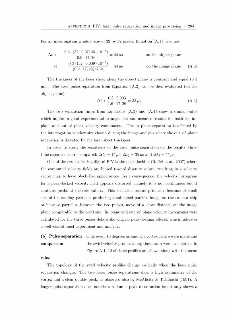
appendix A PIV: laser pulse separation and image processing 204
For an interrogation window size of 32 by 32 pixels, Equation (A.1) becomes:
∆t <0.3 · (32 · 0.07145 · 10−3)
0.9 · 17, 26= 44µs on the object plane
<0.3 · (32 · 0.009 · 10−3)
(0.9 · 17, 26)/7.94= 44µs on the image plane (A.3)
The thickness of the laser sheet along the object plane is constant and equal to 3
mm. The laser pulse separation from Equation (A.2) can be then evaluated (on the
object plane):
∆t <0.3 · 0.003
1.6 · 17, 26= 33µs (A.4)
The two separation times from Equations (A.3) and (A.4) show a similar value
which implies a good experimental arrangement and accurate results for both the in–
plane and out–of–plane velocity components. The in–plane separation is affected by
the interrogation window size chosen during the image analysis where the out–of–plane
separation is dictated by the laser sheet thickness.
In order to study the sensitivity of the laser pulse separation on the results, three
time separations are compared: ∆t1 = 15µs, ∆t2 = 35µs and ∆t3 = 55µs.
One of the error affecting digital PIV is the peak–locking (Raffel et al., 2007) where
the computed velocity fields are biased toward discrete values, resulting in a velocity
vector map to have block–like appearances. As a consequence, the velocity histogram
for a peak–locked velocity field appears distorted, namely it is not continuous but it
contains peaks at discrete values. This situation occurs primarily because of small
size of the seeding particles producing a sub–pixel particle image on the camera chip
or because particles, between the two pulses, move of a short distance on the image
plane comparable to the pixel size. In–plane and out–of–plane velocity histograms were
calculated for the three pulses delays showing no peak–locking effects, which indicates
a well–conditioned experiment and analysis.
(b) Pulse separation
comparison
Cuts every 10 degrees around the vortex centre were made and
the swirl velocity profiles along these radii were calculated. In
Figure A.1, 12 of these profiles are shown along with the mean
value.
The topology of the swirl velocity profiles change radically when the laser pulse
separation changes. The two lower pulse separations show a high asymmetry of the
vortex and a clear double peak, as observed also by McAlister & Takahashi (1991). A
longer pulse separation does not show a double peak distribution but it only shows a

appendix A PIV: laser pulse separation and image processing 205
high asymmetry. The maximum swirl velocity also changes suggesting that with a ∆t of
55 µs some faster particles are lost. It is also noted that the radius where the maximum
averaged velocity is found is around the same position of about 0.05 chords.
(a) ∆t = 15µs. (b) ∆t = 35µs. (c) ∆t = 55µs.
Figure A.1: Swirl velocity profiles for different laser pulse separations.
Axial velocity profiles are shown in Figure A.2. As for the swirl velocity, a similarity
between the profiles obtained with laser pulse separation of 15 µs and 35 µs is found.
Also, the same conclusions of loss of fast particles can be made since the longer pulse
separation case shows a velocity deficit of 0.6 at the vortex centre compared to an excess
of 0.5 for the shorter separations.
(a) ∆t = 15µs. (b) ∆t = 35µs. (c) ∆t = 55µs.
Figure A.2: Axial velocity profiles for different laser pulse separations.
Vorticity contours are compared in Figure A.3. A similar pattern is observed for all
the cases although decreasing peak values on the vortex axis are found when the pulse
separation is increased, respectively of 212, 170 and 119.
Velocity fluctuations in Figure A.4 show an increasing intensity with the increase of
the pulse separation. For ∆t = 15µs and 35 µs, the tail due to the wake sheet rolling
up around the main vortex can be clearly detected, whereas for ∆t = 55µs, contours
show intense fluctuations more spread around the centre. However, developments along
horizontal and vertical axis of σv and σw for all the cases is observed.
The results showed that a long pulses separation introduces more turbulence and
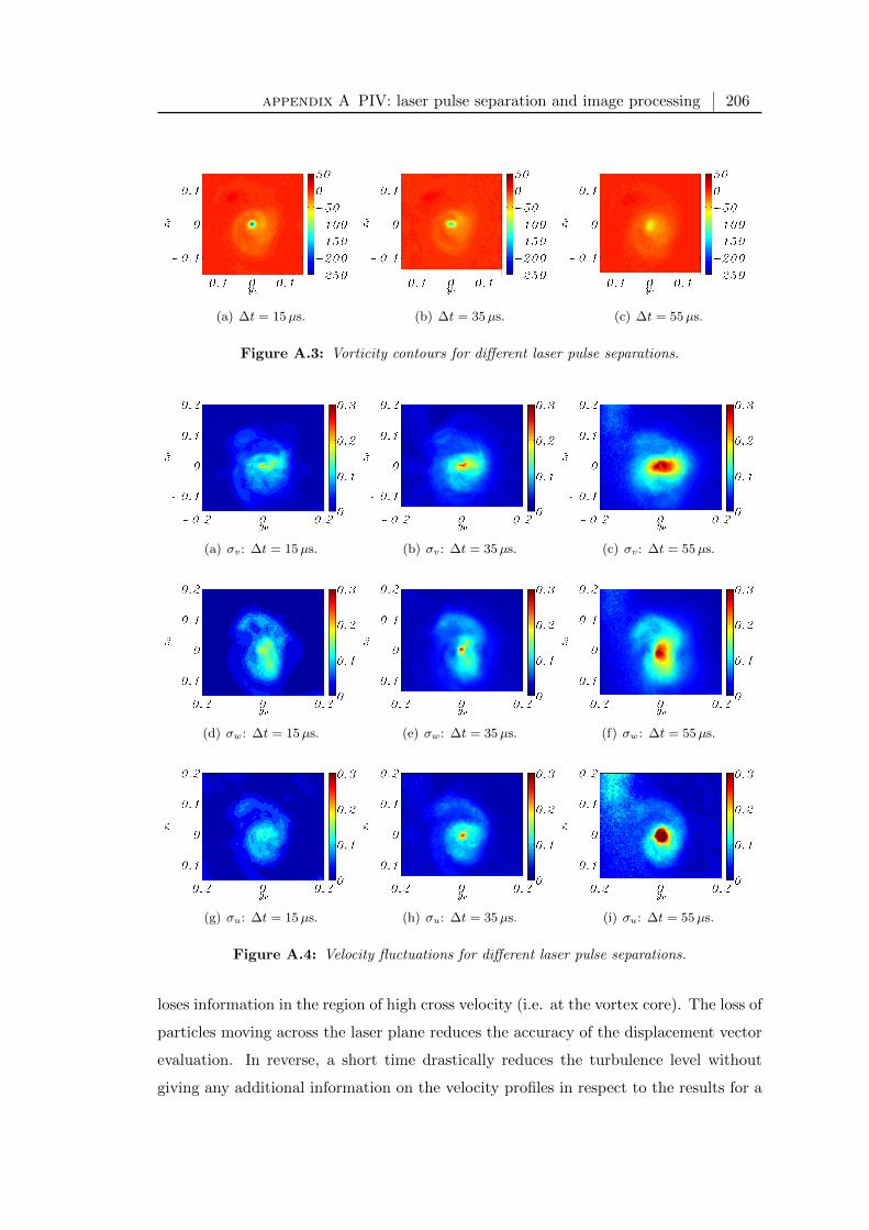
appendix A PIV: laser pulse separation and image processing 206
(a) ∆t = 15µs. (b) ∆t = 35µs. (c) ∆t = 55µs.
Figure A.3: Vorticity contours for different laser pulse separations.
(a) σv: ∆t = 15µs. (b) σv: ∆t = 35µs. (c) σv: ∆t = 55µs.
(d) σw: ∆t = 15µs. (e) σw: ∆t = 35µs. (f) σw: ∆t = 55µs.
(g) σu: ∆t = 15µs. (h) σu: ∆t = 35µs. (i) σu: ∆t = 55µs.
Figure A.4: Velocity fluctuations for different laser pulse separations.
loses information in the region of high cross velocity (i.e. at the vortex core). The loss of
particles moving across the laser plane reduces the accuracy of the displacement vector
evaluation. In reverse, a short time drastically reduces the turbulence level without
giving any additional information on the velocity profiles in respect to the results for a

appendix A PIV: laser pulse separation and image processing 207
middle pulse separation. This behaviour can be attributed to the fact that decreasing
the separation, particles move by a smaller quantity which eventually is comparable
to the uncertainty on the displacements (i.e. pixel). In other words, the minimum
detectable in–plane velocity difference is the pixel size over pulse separation so that
decreasing ∆t the minimum detectable velocity difference increases which eventually
masks the turbulent fluctuations. For the out–of–plane velocity, this mechanism is
amplified: cross displacements are detected by the camera as a shorter vector than
same in–plane displacements. It is observed that the σu fluctuation for short pulse
separation is indeed very low compared to the other cases.
section
Image processing procedure tests
For the evaluation of images via correlation, the complete image is divided into in-
terrogation windows. The correlation function operates a FFT algorithm on the light
intensity of each interrogation window and passes through the complete PIV recording
with a specified window shift. The evaluation will yield one velocity vector for each inter-
rogation window. Different type of correlations and procedures can be used in relation
of the image acquisition system as described by Adrian (1991). A stereoscopic arrange-
ment with double–pulse/double–frame mode processed with a stereo cross–correlation
is adopted in these experiments with a LaVision system. With this set–up, each sam-
ple is composed by two cameras recording two frames each in correspondence to two
laser pulses with separation of 35µs. The first frame contains the first exposure while
the second frame contains the second exposure. The algorithm computes the cross–
correlation of all the interrogation windows between frame 1 and frame 2. The highest
peak in the cross–correlation is the most likely displacement vector (see Figure A.5).
The out-of-plane component of the velocity is then calculated by a geometrical recon-
struction of the two–dimensional three-component velocity vector field from the pair of
two–dimensional two–component vector fields.
The interrogation window size defines the size in pixels of the square interrogation
window. Each correlation operates only on the intensities inside the corresponding
interrogation window. The interrogation window overlap defines the overlap among
neighboring interrogation windows (see Figure A.6). The interrogation window size
and the window overlap determine the grid size of the vector field corresponding to the

appendix A PIV: laser pulse separation and image processing 208
Figure A.5: Cross–correlation procedure scheme (DaVis, 2007).
effective spatial resolution between two neighboring vectors. The grid so formed has a
homogeneous spacing between vectors.
Figure A.6: Example of 50% interrogation window overlap (DaVis, 2007).
The calculation of the final vector field can be accomplished with a single pass pro-
cess or with a multi pass process with either constant or decreasing interrogation window
size. For the single pass process, the vector field calculation is accomplished with one
calculation directly comparing the interrogation windows on each frame. For the multi
pass process, the vector field is calculated by an arbitrary number of iterations, called
also steps, on the same image. At each step, a reference vector for each interrogation
window is calculated. Using the information of the previous step, the position of the
interrogation windows in the new step is accordingly shifted (more sophisticated pro-
cedures can for example also deform the interrogation window from the information
on the the shear). Moreover, the interrogation window size of the following step can
be reduced. In this manner, the window shift is adaptively improved to compute the
vectors in the following steps more accurately and more reliably.

appendix A PIV: laser pulse separation and image processing 209
In order to study the effects of the image processing parameters on the velocity field,
no post–processing of the final vector fields is adopted such as median filters, removal
and replacement of wrong vectors or smoothing of the vectors. Only the filling of empty
spaces through interpolation of neighbors is applied. However, empty spaces were rare
and the reduced number of particles in correspondence of the vortex centre due to
centrifugal forces did not significantly affect the vector computation in that region as it
was ensured a sufficient seeding for the correlations.
Other important aspects regarding the vector field computation are the time needed
for the processing of the images and manipulations on the vector fields and the memory
required to store the data.
In order to see how the image processing affects the results and define a satisfactory
image processing procedure, different procedures have been compared. In particular,
interrogation window size, number of iterations, interrogation window overlap, process-
ing time and memory are studied in this Appendix in relation to a reference trailing
vortex experiment. The test case is on a plane in the wake of the M1 wing at 1 chord
of distance from the trailing edge with angle of attack of 12 and Reynolds number of
Re = 5 · 105. The average vector field is calculated by applying a simple average on 121
instantaneous vector fields. The vortex centre of the average vector field is identified by
the peak of the streamwise component of the helicity.
This comparative study can be split into three sections each one focusing on one of
the aspect described earlier as summarized in Table A.1 where each case is described
with a code. For example, the case 2x64ov25%+2x32ov50% indicates a multi step
procedure composed by 2 steps with interrogation window size of 64 by 64 pixels and
overlap of 25 percent followed by other 2 steps at interrogation window size of 32 by 32
pixels with 50 percent of overlap. This case represents the processing procedure selected
at the end of these comparisons and it is present in each of the three sections.
The comparison of the different procedures is presented here through the comparison
of swirl and axial velocity profiles scaled by the freestream velocity. Cuts every 10
degrees around the vortex centre were made and the velocity profiles along these radii
were calculated. In the following Figures only 12 of these profiles are shown along with
the mean value as function of the radius scaled by the wing chord. Comparisons of
vorticity contours and turbulent quantities are not reported here as they led to same
conclusions.
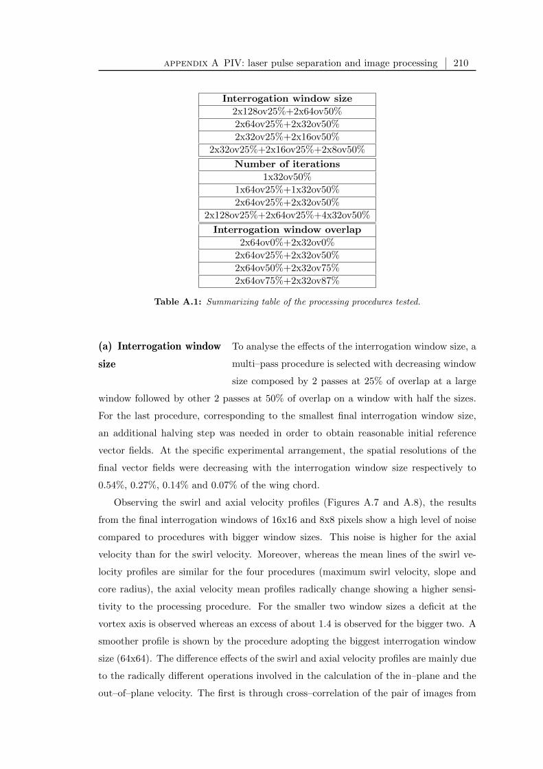
appendix A PIV: laser pulse separation and image processing 210
Interrogation window size
2x128ov25%+2x64ov50%
2x64ov25%+2x32ov50%
2x32ov25%+2x16ov50%
2x32ov25%+2x16ov25%+2x8ov50%
Number of iterations
1x32ov50%
1x64ov25%+1x32ov50%
2x64ov25%+2x32ov50%
2x128ov25%+2x64ov25%+4x32ov50%
Interrogation window overlap
2x64ov0%+2x32ov0%
2x64ov25%+2x32ov50%
2x64ov50%+2x32ov75%
2x64ov75%+2x32ov87%
Table A.1: Summarizing table of the processing procedures tested.
(a) Interrogation window
size
To analyse the effects of the interrogation window size, a
multi–pass procedure is selected with decreasing window
size composed by 2 passes at 25% of overlap at a large
window followed by other 2 passes at 50% of overlap on a window with half the sizes.
For the last procedure, corresponding to the smallest final interrogation window size,
an additional halving step was needed in order to obtain reasonable initial reference
vector fields. At the specific experimental arrangement, the spatial resolutions of the
final vector fields were decreasing with the interrogation window size respectively to
0.54%, 0.27%, 0.14% and 0.07% of the wing chord.
Observing the swirl and axial velocity profiles (Figures A.7 and A.8), the results
from the final interrogation windows of 16x16 and 8x8 pixels show a high level of noise
compared to procedures with bigger window sizes. This noise is higher for the axial
velocity than for the swirl velocity. Moreover, whereas the mean lines of the swirl ve-
locity profiles are similar for the four procedures (maximum swirl velocity, slope and
core radius), the axial velocity mean profiles radically change showing a higher sensi-
tivity to the processing procedure. For the smaller two window sizes a deficit at the
vortex axis is observed whereas an excess of about 1.4 is observed for the bigger two. A
smoother profile is shown by the procedure adopting the biggest interrogation window
size (64x64). The difference effects of the swirl and axial velocity profiles are mainly due
to the radically different operations involved in the calculation of the in–plane and the
out–of–plane velocity. The first is through cross–correlation of the pair of images from

appendix A PIV: laser pulse separation and image processing 211
(a) 2x128ov25%+2x64ov50%. (b) 2x64ov25%+2x32ov50%.
(c) 2x32ov25%+2x16ov50%. (d) 2x32ov25%+2x16ov25%+2x8ov50%.
Figure A.7: Swirl velocity profiles for different interrogation window sizes.
the same camera; the latter is through the calibration function which correlates the
two–components vector fields from the two cameras. The calibration process is usually
affected by higher errors than the cross–correlation of the images. This leads the axial
velocity to show higher errors than the swirl velocity.
Also, in order to correctly evaluate these results, it is important to point that the
interrogation window operates as an average of the velocity of the particles which are
found in it. The compromise should therefore be found between an interrogation window
which is big enough to include a number of particles that gives a statistical convergence
on the calculated velocity vector but also small enough to be able to accurately resolve
small variations of the velocity.
(b) Number of iterations To study the effect of the number of iterations in the
image processing procedure, a multi–pass scheme with
final interrogation window size of 32 by 32 pixels with 50% of overlap is adopted. As
reported in Table A.1, four different procedures are compared: a single pass, a double–

appendix A PIV: laser pulse separation and image processing 212
(a) 2x128ov25%+2x64ov50%. (b) 2x64ov25%+2x32ov50%.
(c) 2x32ov25%+2x16ov50%. (d) 2x32ov25%+2x16ov25%+2x8ov50%.
Figure A.8: Axial velocity profiles for different interrogation window sizes.
pass with 1 step each pass, a double–pass with 2 steps each pass and a triple–pass with
2 steps at 128 by 128 pixels, 2 steps at 64 by 64 pixels and 4 last steps at 32 by 32
pixels. The overlaps of the first passes are 25% and of the second passes are 50%.
The swirl velocity profiles of all the multi–pass procedures are almost identical (Fig-
ure A.9) whereas the single pass procedure is clearly not able to give accurate results.
The inaccuracy of the single pass comes from the fact that no interrogation window shift
(i.e. reference vector field) is applied between the first and the second frame on the same
camera so that loss of particles leads to wrong cross–correlations. As observed also ear-
lier, the axial velocity presents a higher sensitivity to the image processing procedure
(Figure A.10). The axial velocity for the multi–pass single–steps procedure shows an
inaccurate profile with axial velocity at the centre of the vortex 15% lower than the pro-
cedure with eight steps. The difference of the centre value between this last procedure
and the one with 4 steps is of around 1.5%.

appendix A PIV: laser pulse separation and image processing 213
(a) 1x32ov50%. (b) 1x64ov25%+1x32ov50%.
(c) 2x64ov25%+2x32ov50%. (d) 2x128ov25%+2x64ov25%+4x32ov50%.
Figure A.9: Swirl velocity profiles for different numbers of iterations.
(c) Interrogation window
overlap
On the procedure composed by 2 steps on an interroga-
tion window of 64 by 64 pixels followed by 2 steps on a
32 by 32 pixels, different window overlaps are compared.
The spatial resolution of the final vector fields are exactly the same as with the decreas-
ing of the interrogation window size, being respectively 0.54%, 0.27%, 0.14% and 0.07%
of the wing chord.
All the processes show similar swirl velocity profiles (Figure A.11). However, the
axial velocity profiles reported in Figure A.12 shows an increasing noise as the overlap
is increased. Moreover, as the overlapping is increased, the average centre value re-
markably decreases from 1.37 to 1.35, 1.27 and 1.07. As explained also by Raffel et al.
(2007), the oversampling of the data is a useful tool in order to bring out small scale
features of the flow. However, especially in regions containing high velocity gradients
and low seeding densities (which is true near the vortex centre), the neighboring veloc-
ity vectors are correlated with each other because they are estimated partially from the
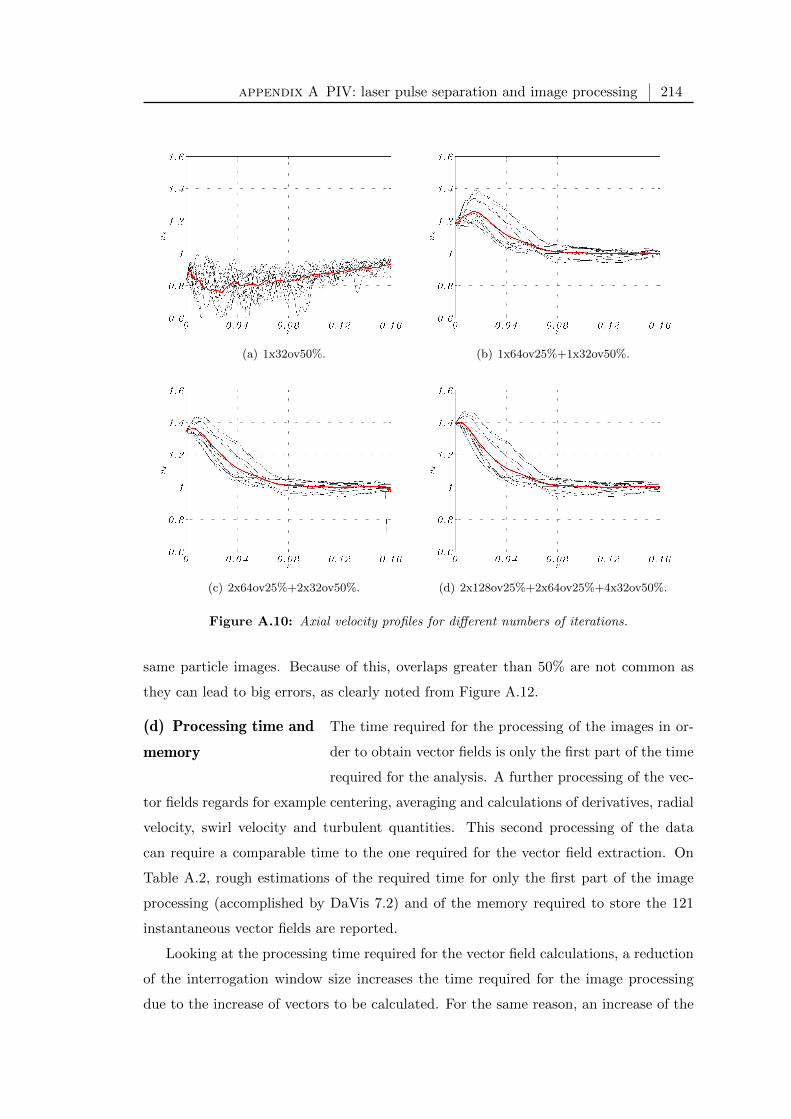
appendix A PIV: laser pulse separation and image processing 214
(a) 1x32ov50%. (b) 1x64ov25%+1x32ov50%.
(c) 2x64ov25%+2x32ov50%. (d) 2x128ov25%+2x64ov25%+4x32ov50%.
Figure A.10: Axial velocity profiles for different numbers of iterations.
same particle images. Because of this, overlaps greater than 50% are not common as
they can lead to big errors, as clearly noted from Figure A.12.
(d) Processing time and
memory
The time required for the processing of the images in or-
der to obtain vector fields is only the first part of the time
required for the analysis. A further processing of the vec-
tor fields regards for example centering, averaging and calculations of derivatives, radial
velocity, swirl velocity and turbulent quantities. This second processing of the data
can require a comparable time to the one required for the vector field extraction. On
Table A.2, rough estimations of the required time for only the first part of the image
processing (accomplished by DaVis 7.2) and of the memory required to store the 121
instantaneous vector fields are reported.
Looking at the processing time required for the vector field calculations, a reduction
of the interrogation window size increases the time required for the image processing
due to the increase of vectors to be calculated. For the same reason, an increase of the
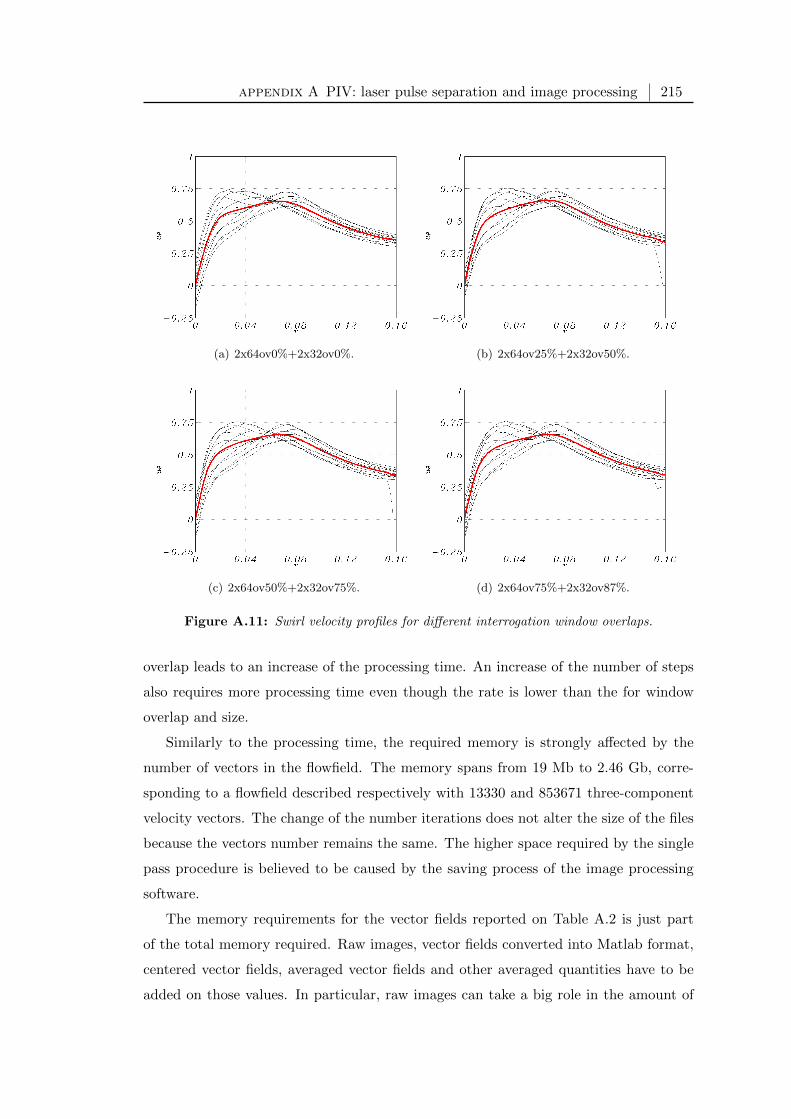
appendix A PIV: laser pulse separation and image processing 215
(a) 2x64ov0%+2x32ov0%. (b) 2x64ov25%+2x32ov50%.
(c) 2x64ov50%+2x32ov75%. (d) 2x64ov75%+2x32ov87%.
Figure A.11: Swirl velocity profiles for different interrogation window overlaps.
overlap leads to an increase of the processing time. An increase of the number of steps
also requires more processing time even though the rate is lower than the for window
overlap and size.
Similarly to the processing time, the required memory is strongly affected by the
number of vectors in the flowfield. The memory spans from 19 Mb to 2.46 Gb, corre-
sponding to a flowfield described respectively with 13330 and 853671 three-component
velocity vectors. The change of the number iterations does not alter the size of the files
because the vectors number remains the same. The higher space required by the single
pass procedure is believed to be caused by the saving process of the image processing
software.
The memory requirements for the vector fields reported on Table A.2 is just part
of the total memory required. Raw images, vector fields converted into Matlab format,
centered vector fields, averaged vector fields and other averaged quantities have to be
added on those values. In particular, raw images can take a big role in the amount of

appendix A PIV: laser pulse separation and image processing 216
(a) 2x64ov0%+2x32ov0%. (b) 2x64ov25%+2x32ov50%.
(c) 2x64ov50%+2x32ov75%. (d) 2x64ov75%+2x32ov87%.
Figure A.12: Axial velocity profiles for different interrogation window overlaps.
the memory needed for a PIV. For instance, each test of 121 sets of 4 pictures recorded
in these study required additional 4.8 Gb.
(e) Conclusive remarks Two different ways are found in order to decrease the spa-
tial resolution of the final vector field: one is decreasing the
interrogation window size and the other is increasing the overlap. The first is limited
by a minimum number of particles in each interrogation window. The second is limited
by the computational cost and by the increase of errors in the computed velocity field
as the overlap is increased. However, as shown also by van der Wall & Richard (2006)
from the analysis of PIV data on wing vortices, the interrogation window overlap is as
important as the size of the window itself for converged estimates of the core radius and
the maximum swirl velocity. From the comparison of several image processing proce-
dures, it is shown that a final interrogation window of 32 by 32 pixels gives the best
compromise between smoothness of the velocity profiles and spatial resolution. Since
the minimum cross–correlation window size is limited, the overlap must be adjusted

appendix A PIV: laser pulse separation and image processing 217
Time Memory
Interrogation window size
2x128ov25%+2x64ov50% 3 h 19 Mb
2x64ov25%+2x32ov50% 5 h 91 Mb
2x32ov25%+2x16ov50% 9 h 763 Mb
2x32ov25%+2x16ov25%+2x8ov50% 16 h 2.46 Gb
Number of iterations
1x32ov50% 2 h 263 Mb
1x64ov25%+1x32ov50% 3 h 95 Mb
2x64ov25%+2x32ov50% 5 h 91 Mb
2x128ov25%+2x64ov25%+4x32ov50% 10 h 95 Mb
Interrogation window overlap
2x64ov0%+2x32ov0% 3 h 25 Mb
2x64ov25%+2x32ov50% 5 h 91 Mb
2x64ov50%+2x32ov75% 9 h 358 Mb
2x64ov75%+2x32ov87% 18 h 1.45 Gb
Table A.2: Processing procedures: time and memory required.
in the optimization between the accuracy of the results and the time and memory re-
quired for the image processing. Moreover, the increase of the number of iterations
can increase the accuracy and the time required but it does not change the memory
required. A multi–pass procedure has revealed to be compulsory for this flow. Also,
processing time and memory requirements have revealed to be a decisive factor in the
choice of the image processing.
Following these considerations and due to the high number of different tests per-
formed in this research, an optimum compromise is found in the image processing proce-
dure 2x64ov25%+2x32ov50%. Moreover, the vector fields resulting from this procedure
do not show a significant number of wrong vectors to be removed and replaced by
interpolated value. This implies a good quality of the seeding and the experimental
arrangement giving a high level of reliability to these results.
appendix B
Vortex centre identification on
grayscale pictures
From the pictures of the smoke on planes perpendicular to the vortex axis on the wake
of a wing, is possible to identify the vortex centre and then to study the unsteadiness
of the instantaneous location. Because of the high centrifugal force within the vortex
core, the smoke particle density is lower. When the plane is illuminated a darker spot
in correspondence to the centre appears. The routine able to find the dark spot is called
here vortex centre identification method and it is used to locate the vortex of each of the
realizations. The validity of this technique is based on the reliability of the darker region
centroid as a good description of the vortex centre, which is a good assumption when
smoke particles accurately follow the flow, for high smoke density, for low buoyancy
forces, for high image resolution and for darker spots of the order of the vortex core.
In order to find a consistent and robust vortex centre identification method, the
location of the darker spots in the images, corresponding to the instantaneous vortex
centres, has been carried out with two conceptually different routines: converting the
grayscale image into a black and white image with an appropriate conversion threshold
(BW method) and mapping the grayscale of the image with rounded interrogation
windows (GRAY method).
section
GRAY and BW methods
The first three steps of the methods are common and described as follows with
reference to an image of the tip vortex at one chord behind the M1 model with rounded
tip at an angle of attack of 12 and Reynolds number of 106.
218
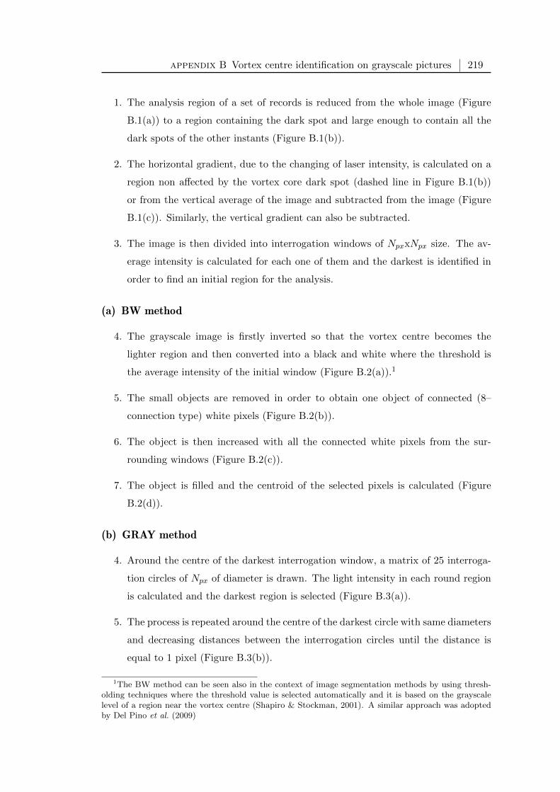
appendix B Vortex centre identification on grayscale pictures 219
1. The analysis region of a set of records is reduced from the whole image (Figure
B.1(a)) to a region containing the dark spot and large enough to contain all the
dark spots of the other instants (Figure B.1(b)).
2. The horizontal gradient, due to the changing of laser intensity, is calculated on a
region non affected by the vortex core dark spot (dashed line in Figure B.1(b))
or from the vertical average of the image and subtracted from the image (Figure
B.1(c)). Similarly, the vertical gradient can also be subtracted.
3. The image is then divided into interrogation windows of NpxxNpx size. The av-
erage intensity is calculated for each one of them and the darkest is identified in
order to find an initial region for the analysis.
(a) BW method
4. The grayscale image is firstly inverted so that the vortex centre becomes the
lighter region and then converted into a black and white where the threshold is
the average intensity of the initial window (Figure B.2(a)).1
5. The small objects are removed in order to obtain one object of connected (8–
connection type) white pixels (Figure B.2(b)).
6. The object is then increased with all the connected white pixels from the sur-
rounding windows (Figure B.2(c)).
7. The object is filled and the centroid of the selected pixels is calculated (Figure
B.2(d)).
(b) GRAY method
4. Around the centre of the darkest interrogation window, a matrix of 25 interroga-
tion circles of Npx of diameter is drawn. The light intensity in each round region
is calculated and the darkest region is selected (Figure B.3(a)).
5. The process is repeated around the centre of the darkest circle with same diameters
and decreasing distances between the interrogation circles until the distance is
equal to 1 pixel (Figure B.3(b)).
1The BW method can be seen also in the context of image segmentation methods by using thresh-olding techniques where the threshold value is selected automatically and it is based on the grayscalelevel of a region near the vortex centre (Shapiro & Stockman, 2001). A similar approach was adoptedby Del Pino et al. (2009)

appendix B Vortex centre identification on grayscale pictures 220
(a) Full grayscale image. (b) Cropped image and horizontal grayscale gra-dient.
(c) Gradient subtracted image divided into in-terrogation windows (Npx = 60).
(d) Interrogation window averaged intensitiesand identification of the darkest window.
Figure B.1: Common steps.
section
Position distribution and movement frequency
The advantage of the BW method is that it can identify the actual dark spot shape
and so a good estimation of the centrifugal forces distribution. However, the threshold
value is strongly affected by the size of the interrogation windows Npx and the rela-
tive position between the darkest window and the vortex core. Unfortunately, a fixed
threshold value method is not a feasible solution because of the movement of the vortex
in a non uniformly distributed laser intensity and because of the not clearly definable

appendix B Vortex centre identification on grayscale pictures 221
(a) Binary interrogation window. (b) Small objects removed.
(c) Object size increased. (d) Final object and centroid.
Figure B.2: BW steps.
double–peaked grayscale histogram distribution that would occur if the darker spot was
substantially darker than the surrounding region. In Figure B.4, the grayscale level
histograms are reported for the full image, the reduced image and the gradient sub-
tracted image (respectively in Figures B.1(a), B.1(b) and B.1(c)). The double–peaked
distribution of the first two (Figures B.1(a), B.1(b)) is due by the superimposition of
the vortex presence with the laser intensity changing along the image which, once the
gradient is subtracted, does not effect the histogram (Figure B.1(c)).
The GRAY method necessitates an estimate of the vortex core dimension so that
the round interrogation window diameter Npx can be set. Contrary to the BW method,
GRAY method reveals a consistency in sizes and 1 pixel accuracy in the determination
of the position. Moreover, it is observed that the shape of the darker region at 1 chord
of distance from the trailing edge was satisfactorily described by a circle.
In Figure B.5, 190 instantaneous vortex centres taken at a sampling frequency of
10 Hz of a typical case are plotted as function of the interrogation window size Npx
for the BW method. The centres distributions obtained with Npx between 20 and 60

appendix B Vortex centre identification on grayscale pictures 222
(a) Interrogation windows mapping (25 circles). (b) Initial interrogation windows and 3 steps ofrefinement (zoom in image); centre of the dark-est region at each step in red.
(c) Centre identification.
Figure B.3: GRAY steps.
Figure B.4: Histogram of the light intensity for steps 1, 2 and 3.
are very similar and the differences in positions are very small. When a value of 80
and 100 is adopted, the distributions change in sizes (less scattered) and orientation
(with a vertical principal axis). This behaviour can be explained by the presence of a
residual horizontal gradient of the background gray level. In Figure B.6, the same cases

appendix B Vortex centre identification on grayscale pictures 223
are analysed by the GRAY method. The results are very similar to the ones obtained
with the BW method with the only difference that the GRAY method gives consistent
results up to Npx = 80.
(a) Npx = 20. (b) Npx = 40. (c) Npx = 50.
(d) Npx = 60. (e) Npx = 80. (f) Npx = 100.
Figure B.5: BW method: instantaneous vortex positions (rounded tip, xw = 1, α = 12,Re = 106).
(a) Npx = 20. (b) Npx = 40. (c) Npx = 50.
(d) Npx = 60. (e) Npx = 80. (f) Npx = 100.
Figure B.6: GRAY method: instantaneous vortex positions (rounded tip, xw = 1, α = 12,Re = 106).

appendix B Vortex centre identification on grayscale pictures 224
A comparison of the two vortex identification methods and interrogation window
size was carried out also with respect to the frequency distributions of the vortex centre
movement. The frequency distributions of the vortex centre translations along the y
and z axis has been calculated and plotted in Figures B.7 and B.8, respectively adopting
BW and GRAY method. The power is scaled by the variance of the movement along
the same axis. The consistency of the results, when Npx is less than 80, appears in these
plots and no major differences can be seen between the two methods whereas, for Npx
equal or greater than 80, the frequency distributions change.
(a) Npx = 20. (b) Npx = 40. (c) Npx = 50.
(d) Npx = 60. (e) Npx = 80. (f) Npx = 100.
Figure B.7: BW method: vortex movement power spectra (rounded tip, xw = 1, α = 12,Re = 106).

appendix B Vortex centre identification on grayscale pictures 225
(a) Npx = 20. (b) Npx = 40. (c) Npx = 50.
(d) Npx = 60. (e) Npx = 80. (f) Npx = 100.
Figure B.8: GRAY method: vortex movement power spectra (rounded tip, xw = 1, α = 12,Re = 106).

appendix C
Some equations relevant to vortices
If people do not believe that mathematics is simple, it is
only because they do not realize how complicated life is.
John von Neumann
The governing equations of laminar and turbulent isolated vortices are derived after
assumptions which simplify the Navier–Stokes equations. In this appendix, the govern-
ing equations are expressed in both cartesian and cylindrical coordinates in Section C.1.
The vorticity form of the Navier–Stokes equations, which highlights important mecha-
nisms especially for trailing vortices, is also given in Section C.2. Reynolds–averaged
Navier–Stokes equations are presented in Section C.3 in order to highlight the role of
the Reynolds stresses. Some of the fundamental relations between the cartesian and
cylindrical reference frames are presented in Section C.4.
section
Governing equations
Effects due to compressibility, heat transfer, body forces and variations in fluid
properties are negligible in the present study, and thus the corresponding terms in the
continuity and Navier–Stokes equations for newtonian fluids can be neglected. The
vectorial form of the resulting continuity and momentum equations is:
∇ · u = 0 (C.1a)
∂u
∂t+ (u · ∇) u = −∇P
ρ+ ν∇2u (C.1b)
226
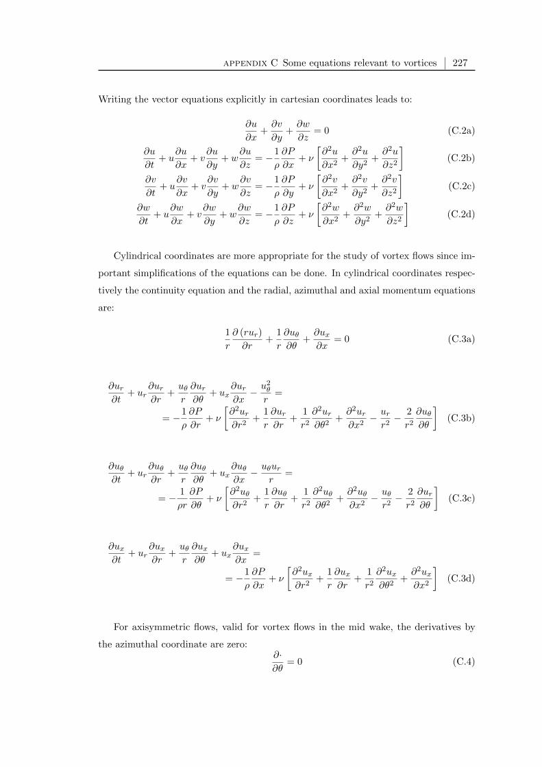
appendix C Some equations relevant to vortices 227
Writing the vector equations explicitly in cartesian coordinates leads to:
∂u
∂x+∂v
∂y+∂w
∂z= 0 (C.2a)
∂u
∂t+ u
∂u
∂x+ v
∂u
∂y+ w
∂u
∂z= −1
ρ
∂P
∂x+ ν
[∂2u
∂x2+∂2u
∂y2+∂2u
∂z2
](C.2b)
∂v
∂t+ u
∂v
∂x+ v
∂v
∂y+ w
∂v
∂z= −1
ρ
∂P
∂y+ ν
[∂2v
∂x2+∂2v
∂y2+∂2v
∂z2
](C.2c)
∂w
∂t+ u
∂w
∂x+ v
∂w
∂y+ w
∂w
∂z= −1
ρ
∂P
∂z+ ν
[∂2w
∂x2+∂2w
∂y2+∂2w
∂z2
](C.2d)
Cylindrical coordinates are more appropriate for the study of vortex flows since im-
portant simplifications of the equations can be done. In cylindrical coordinates respec-
tively the continuity equation and the radial, azimuthal and axial momentum equations
are:
1
r
∂ (rur)
∂r+
1
r
∂uθ∂θ
+∂ux∂x
= 0 (C.3a)
∂ur∂t
+ ur∂ur∂r
+uθr
∂ur∂θ
+ ux∂ur∂x−u2θ
r=
= −1
ρ
∂P
∂r+ ν
[∂2ur∂r2
+1
r
∂ur∂r
+1
r2
∂2ur∂θ2
+∂2ur∂x2
− urr2− 2
r2
∂uθ∂θ
](C.3b)
∂uθ∂t
+ ur∂uθ∂r
+uθr
∂uθ∂θ
+ ux∂uθ∂x− uθur
r=
= − 1
ρr
∂P
∂θ+ ν
[∂2uθ∂r2
+1
r
∂uθ∂r
+1
r2
∂2uθ∂θ2
+∂2uθ∂x2
− uθr2− 2
r2
∂ur∂θ
](C.3c)
∂ux∂t
+ ur∂ux∂r
+uθr
∂ux∂θ
+ ux∂ux∂x
=
= −1
ρ
∂P
∂x+ ν
[∂2ux∂r2
+1
r
∂ux∂r
+1
r2
∂2ux∂θ2
+∂2ux∂x2
](C.3d)
For axisymmetric flows, valid for vortex flows in the mid wake, the derivatives by
the azimuthal coordinate are zero:∂·∂θ
= 0 (C.4)
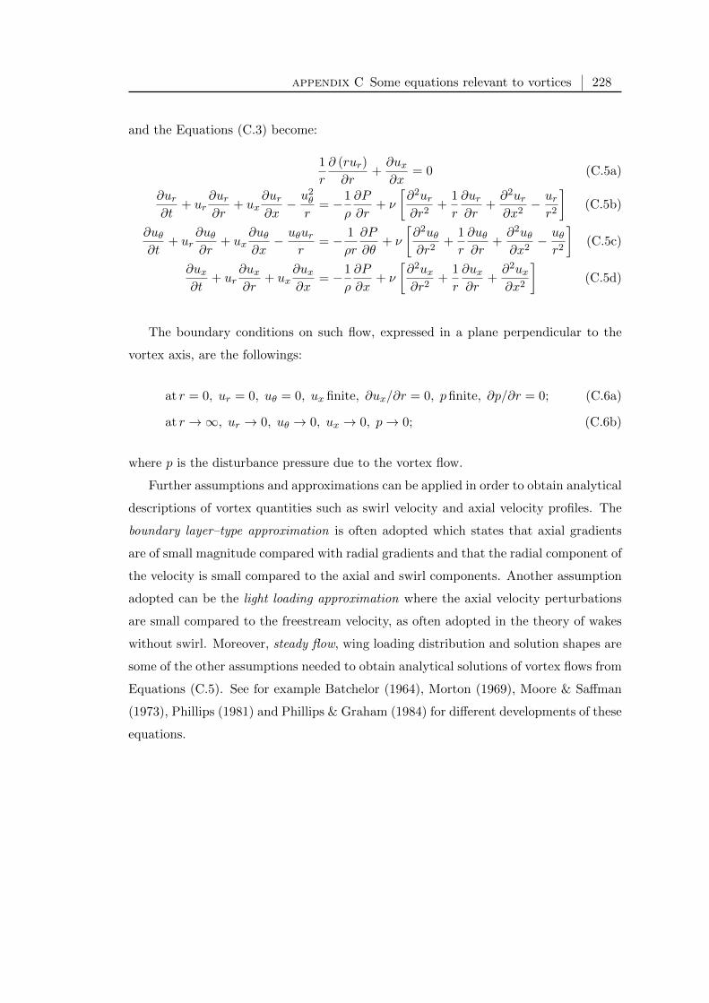
appendix C Some equations relevant to vortices 228
and the Equations (C.3) become:
1
r
∂ (rur)
∂r+∂ux∂x
= 0 (C.5a)
∂ur∂t
+ ur∂ur∂r
+ ux∂ur∂x−u2θ
r= −1
ρ
∂P
∂r+ ν
[∂2ur∂r2
+1
r
∂ur∂r
+∂2ur∂x2
− urr2
](C.5b)
∂uθ∂t
+ ur∂uθ∂r
+ ux∂uθ∂x− uθur
r= − 1
ρr
∂P
∂θ+ ν
[∂2uθ∂r2
+1
r
∂uθ∂r
+∂2uθ∂x2
− uθr2
](C.5c)
∂ux∂t
+ ur∂ux∂r
+ ux∂ux∂x
= −1
ρ
∂P
∂x+ ν
[∂2ux∂r2
+1
r
∂ux∂r
+∂2ux∂x2
](C.5d)
The boundary conditions on such flow, expressed in a plane perpendicular to the
vortex axis, are the followings:
at r = 0, ur = 0, uθ = 0, ux finite, ∂ux/∂r = 0, p finite, ∂p/∂r = 0; (C.6a)
at r →∞, ur → 0, uθ → 0, ux → 0, p→ 0; (C.6b)
where p is the disturbance pressure due to the vortex flow.
Further assumptions and approximations can be applied in order to obtain analytical
descriptions of vortex quantities such as swirl velocity and axial velocity profiles. The
boundary layer–type approximation is often adopted which states that axial gradients
are of small magnitude compared with radial gradients and that the radial component of
the velocity is small compared to the axial and swirl components. Another assumption
adopted can be the light loading approximation where the axial velocity perturbations
are small compared to the freestream velocity, as often adopted in the theory of wakes
without swirl. Moreover, steady flow, wing loading distribution and solution shapes are
some of the other assumptions needed to obtain analytical solutions of vortex flows from
Equations (C.5). See for example Batchelor (1964), Morton (1969), Moore & Saffman
(1973), Phillips (1981) and Phillips & Graham (1984) for different developments of these
equations.
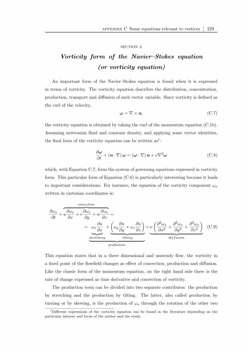
appendix C Some equations relevant to vortices 229
section
Vorticity form of the Navier–Stokes equation
(or vorticity equation)
An important form of the Navier–Stokes equation is found when it is expressed
in terms of vorticity. The vorticity equation describes the distribution, concentration,
production, transport and diffusion of such vector variable. Since vorticity is defined as
the curl of the velocity,
ω = ∇× u, (C.7)
the vorticity equation is obtained by taking the curl of the momentum equation (C.1b).
Assuming newtonian fluid and constant density, and applying some vector identities,
the final form of the vorticity equation can be written as1:
∂ω
∂t+ (u · ∇)ω = (ω · ∇) u + ν∇2ω (C.8)
which, with Equation C.7, form the system of governing equations expressed in vorticity
form. This particular form of Equation (C.8) is particularly interesting because it leads
to important considerations. For instance, the equation of the vorticity component ωx
written in cartesian coordinates is:
∂ωx∂t
+
convection︷ ︸︸ ︷u∂ωx∂x
+ v∂ωx∂y
+ w∂ωx∂z
=
= ωx∂u
∂x︸ ︷︷ ︸stretching
+
(ωy∂u
∂y+ ωz
∂u
∂z
)︸ ︷︷ ︸
tilting︸ ︷︷ ︸production
+ ν
(∂2ωx∂x2
+∂2ωx∂y2
+∂2ωx∂z2
)︸ ︷︷ ︸
diffusion
(C.9)
This equation states that in a three–dimensional and unsteady flow, the vorticity in
a fixed point of the flowfield changes as effect of convection, production and diffusion.
Like the classic form of the momentum equation, on the right hand side there is the
rate of change expressed as time derivative and convection of vorticity.
The production term can be divided into two separate contributes: the production
by stretching and the production by tilting. The latter, also called production by
turning or by skewing, is the production of ωx through the rotation of the other two
1Different expressions of the vorticity equation can be found in the literature depending on theparticular interest and focus of the author and the study.
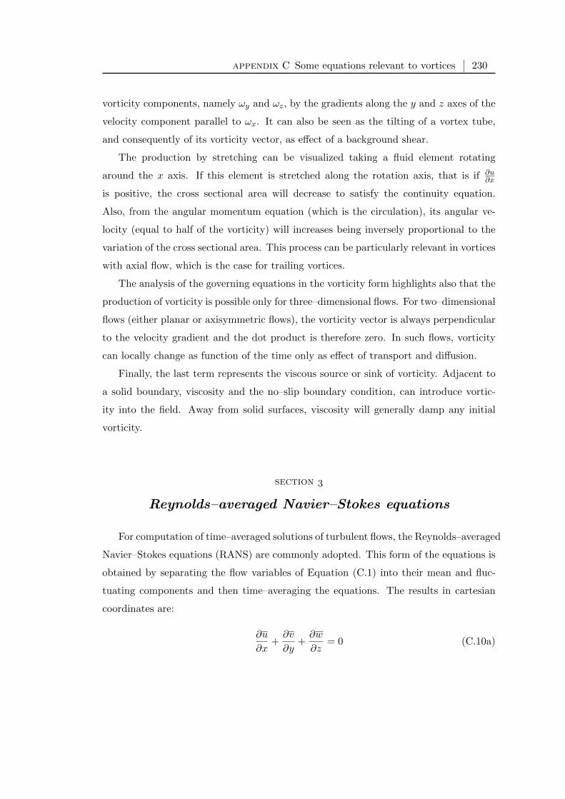
appendix C Some equations relevant to vortices 230
vorticity components, namely ωy and ωz, by the gradients along the y and z axes of the
velocity component parallel to ωx. It can also be seen as the tilting of a vortex tube,
and consequently of its vorticity vector, as effect of a background shear.
The production by stretching can be visualized taking a fluid element rotating
around the x axis. If this element is stretched along the rotation axis, that is if ∂u∂x
is positive, the cross sectional area will decrease to satisfy the continuity equation.
Also, from the angular momentum equation (which is the circulation), its angular ve-
locity (equal to half of the vorticity) will increases being inversely proportional to the
variation of the cross sectional area. This process can be particularly relevant in vortices
with axial flow, which is the case for trailing vortices.
The analysis of the governing equations in the vorticity form highlights also that the
production of vorticity is possible only for three–dimensional flows. For two–dimensional
flows (either planar or axisymmetric flows), the vorticity vector is always perpendicular
to the velocity gradient and the dot product is therefore zero. In such flows, vorticity
can locally change as function of the time only as effect of transport and diffusion.
Finally, the last term represents the viscous source or sink of vorticity. Adjacent to
a solid boundary, viscosity and the no–slip boundary condition, can introduce vortic-
ity into the field. Away from solid surfaces, viscosity will generally damp any initial
vorticity.
section
Reynolds–averaged Navier–Stokes equations
For computation of time–averaged solutions of turbulent flows, the Reynolds–averaged
Navier–Stokes equations (RANS) are commonly adopted. This form of the equations is
obtained by separating the flow variables of Equation (C.1) into their mean and fluc-
tuating components and then time–averaging the equations. The results in cartesian
coordinates are:
∂u
∂x+∂v
∂y+∂w
∂z= 0 (C.10a)
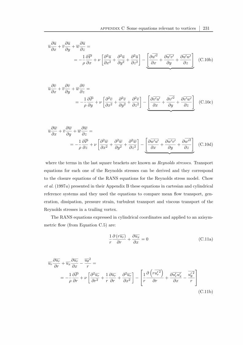
appendix C Some equations relevant to vortices 231
u∂u
∂x+ v
∂u
∂y+ w
∂u
∂z=
= −1
ρ
∂P
∂x+ ν
[∂2u
∂x2+∂2u
∂y2+∂2u
∂z2
]−
[∂u′2
∂x+∂u′v′
∂y+∂u′w′
∂z
]︸ ︷︷ ︸ (C.10b)
u∂v
∂x+ v
∂v
∂y+ w
∂v
∂z=
= −1
ρ
∂P
∂y+ ν
[∂2v
∂x2+∂2v
∂y2+∂2v
∂z2
]−
[∂v′u′
∂x+∂v′2
∂y+∂v′w′
∂z
]︸ ︷︷ ︸ (C.10c)
u∂w
∂x+ v
∂w
∂y+ w
∂w
∂z=
= −1
ρ
∂P
∂z+ ν
[∂2w
∂x2+∂2w
∂y2+∂2w
∂z2
]−
[∂w′u′
∂x+∂w′v′
∂y+∂w′2
∂z
]︸ ︷︷ ︸ (C.10d)
where the terms in the last square brackets are known as Reynolds stresses. Transport
equations for each one of the Reynolds stresses can be derived and they correspond
to the closure equations of the RANS equations for the Reynolds stress model. Chow
et al. (1997a) presented in their Appendix B these equations in cartesian and cylindrical
reference systems and they used the equations to compare mean flow transport, gen-
eration, dissipation, pressure strain, turbulent transport and viscous transport of the
Reynolds stresses in a trailing vortex.
The RANS equations expressed in cylindrical coordinates and applied to an axisym-
metric flow (from Equation C.5) are:
1
r
∂ (rur)
∂r+∂ux∂x
= 0 (C.11a)
ur∂ur∂r
+ ux∂ur∂x− uθ
2
r=
= −1
ρ
∂P
∂r+ ν
[∂2ur∂r2
+1
r
∂ur∂r
+∂2ur∂x2
]−
1
r
∂(ru′r
2)
∂r+∂u′ru
′x
∂x−u′θ
2
r
(C.11b)
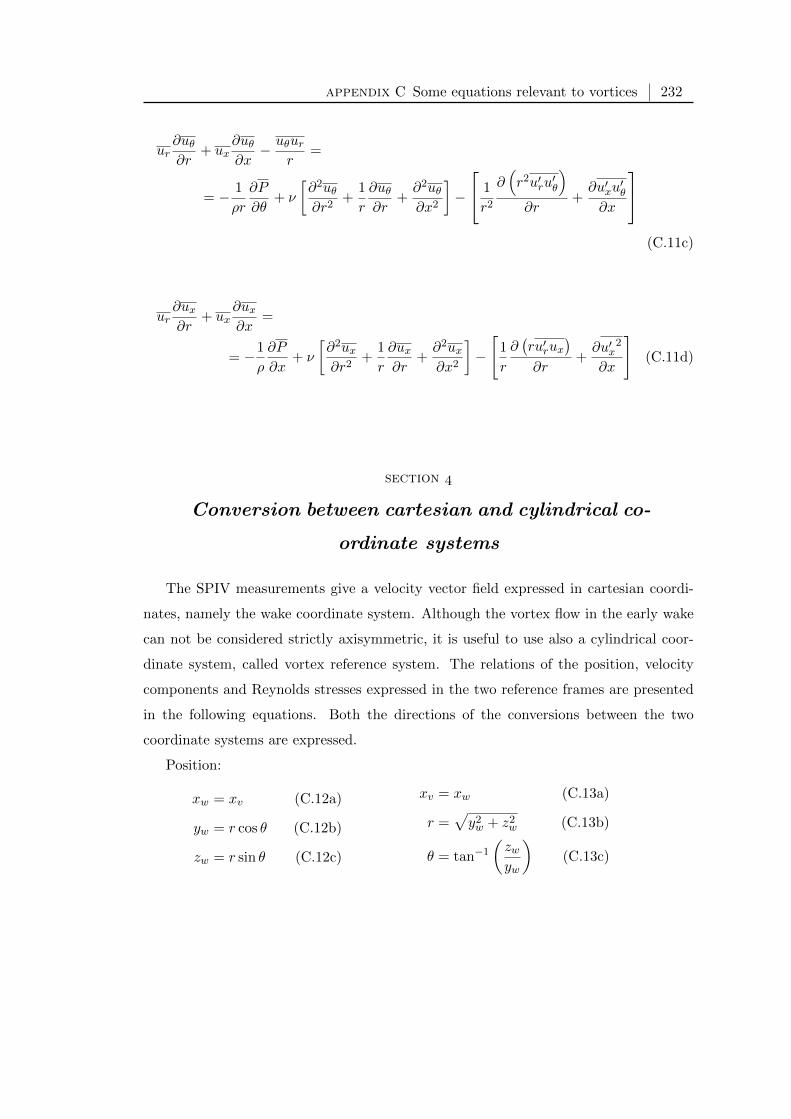
appendix C Some equations relevant to vortices 232
ur∂uθ∂r
+ ux∂uθ∂x− uθur
r=
= − 1
ρr
∂P
∂θ+ ν
[∂2uθ∂r2
+1
r
∂uθ∂r
+∂2uθ∂x2
]−
1
r2
∂(r2u′ru
′θ
)∂r
+∂u′xu
′θ
∂x
(C.11c)
ur∂ux∂r
+ ux∂ux∂x
=
= −1
ρ
∂P
∂x+ ν
[∂2ux∂r2
+1
r
∂ux∂r
+∂2ux∂x2
]−
[1
r
∂(ru′rux
)∂r
+∂u′x
2
∂x
](C.11d)
section
Conversion between cartesian and cylindrical co-
ordinate systems
The SPIV measurements give a velocity vector field expressed in cartesian coordi-
nates, namely the wake coordinate system. Although the vortex flow in the early wake
can not be considered strictly axisymmetric, it is useful to use also a cylindrical coor-
dinate system, called vortex reference system. The relations of the position, velocity
components and Reynolds stresses expressed in the two reference frames are presented
in the following equations. Both the directions of the conversions between the two
coordinate systems are expressed.
Position:
xw = xv (C.12a)
yw = r cos θ (C.12b)
zw = r sin θ (C.12c)
xv = xw (C.13a)
r =√y2w + z2
w (C.13b)
θ = tan−1
(zwyw
)(C.13c)

appendix C Some equations relevant to vortices 233
Velocity:
u
v
w
=
1 0 0
0 cos θ − sin θ
0 sin θ cos θ
ux
ur
uθ
(C.14)
ux
ur
uθ
=
1 0 0
0 cos θ sin θ
0 − sin θ cos θ
u
v
w
(C.15)
Reynolds stresses:
u′2 = u′x2 (C.16a)
v′2
w′2
v′w′
=
cos2 θ sin2 θ −2 sin θ cos θ
sin2 θ cos2 θ 2 sin θ cos θ
sin θ cos θ − sin θ cos θ cos2 θ − sin2 θ
u′r
2
u′θ2
u′ru′θ
(C.16b)
u′v′u′w′
=
cos θ − sin θ
sin θ cos θ
u′xu′ru′xu′θ
(C.16c)
u′x2 = u′2 (C.17a)
u′r2
u′θ2
u′ru′θ
=
cos2 θ sin2 θ 2 sin θ cos θ
sin2 θ cos2 θ −2 sin θ cos θ
− sin θ cos θ − sin θ cos θ cos2 θ − sin2 θ
v′2
w′2
v′w′
(C.17b)
u′xu′ru′xu′θ
=
cos θ sin θ
− sin θ cos θ
u′v′u′w′
(C.17c)
Copyright © 2022 FDOKUMEN