Experimental Detection of Optical Vortices Using a Shack-Hartmann Wavefront Sensor

Experimental detection of opticalvortices with a Shack-Hartmann

wavefront sensor

Kevin Murphy,* Daniel Burke, Nicholas Devaney, and Chris DaintyApplied Optics Group, School of Physics, National University of Ireland, Galway,

Galway, Ireland

*[email protected]

Abstract: Laboratory experiments are carried out to detect optical vorticesin conditions typical of those experienced when a laser beam is propagatedthrough the atmosphere. A Spatial Light Modulator (SLM) is used tomimic atmospheric turbulence and a Shack-Hartmann wavefront sensor isutilised to measure the slopes of the wavefront surface. A matched filteralgorithm determines the positions of the Shack-Hartmann spot centroidsmore robustly than a centroiding algorithm. The slope discrepancy is thenobtained by taking the slopes measured by the wavefront sensor away fromthe slopes calculated from a least squares reconstruction of the phase. Theslope discrepancy field is used as an input to the branch point potentialmethod to find if a vortex is present, and if so to give its position and sign.The use of the slope discrepancy technique greatly improves the detectionrate of the branch point potential method. This work shows the first time thebranch point potential method has been used to detect optical vortices in anexperimental setup.

© 2010 Optical Society of America

OCIS codes: (010.0010) Atmospheric and oceanic optics; (010.1080) Active or adaptive op-tics; (010.7350) Wave-front sensing; (080.4865) Optical vortices.

References and links1. J. F. Nye and M. V. Berry, “Dislocations in wave trains,” Proc. R. Soc. Lond. A 336, 165–190 (1974).2. D. G. Grier, “A revolution in optical manipulation,” Nature (London) 424, 810–816 (2003).3. G. Gibson, J. Courtial, and M. J. Padgett, “Free-space information transfer using light beams carrying orbital

angular momentum,” Opt. Express 12, 5448–5456 (2004).4. F. S. Roux, “Dynamical behavior of optical vortices,” J. Opt. Soc. Am. B 12, 1215–1221 (1995).5. D. L. Fried and J. L. Vaughn, “Branch cuts in the phase function,” Appl. Opt. 31, 2865–2882 (1992).6. M. C. Roggemann and B. M. Welsh, “Imaging through Turbulence”, Laser and Optical Science and Technology

(CRC Press, 1996).7. R. Mackey and C. Dainty, “Adaptive optics correction over a 3km near horizontal path,” Proc. SPIE 7108, 1–9

(2008).8. N. B. Baranova, A. V. Mamaev, N. F. Pilipetsky, V. V. Shkunov, and B. Y. Zel’dovich, “Wave-front dislocations:

topological limitations for adaptive systems with phase conjugation,” J. Opt. Soc. Am. A 73, 525–528 (1983).9. C. A. Primmerman, T. R. Price, R. A. Humphreys, B. G. Zollars, H. T. Barclay, and J. Herrmann, “Atmospheric-

compensation experiments in strong-scintillation conditions,” Appl. Opt. 34, 2081–2088 (1995).10. J. D. Barchers, D. L. Fried, and D. J. Link, “Evaluation of the performance of Hartmann sensors in strong

scintillation,” Appl. Opt. 41, 1012–1021 (2002).11. D. L. Fried, “Branch point problem in adaptive optics,” J. Opt. Soc. Am. A 15, 2759–2768 (1998).12. M. C. Roggemann and D. J. Lee, “Two-deformable-mirror concept for correcting scintillation effects in laser

beam projection through the turbulent atmosphere,” Appl. Opt. 37, 4577–4585 (1998).

#128515 - $15.00 USD Received 17 May 2010; revised 15 Jun 2010; accepted 23 Jun 2010; published 6 Jul 2010(C) 2010 OSA 19 July 2010 / Vol. 18, No. 15 / OPTICS EXPRESS 15448

13. D. L. Fried, “Adaptive optics wave function reconstruction and phase unwrapping when branch points arepresent,” Opt. Commun. 200, 43–72 (2001).

14. D. C. Ghiglia and M. D. Pritt, Two-Dimensional Phase Unwrapping (Wiley-InterScience, 1998).15. F. A. Starikov, V. P. Aksenova, V. V. Atuchind, I. V. Izmailova, F. Y. Kaneva, G. G. Kochemasov, A. V.

Kudryashovb, S. M. Kulikov, Y. I. Malakhovc, A. N. Manachinsky, N. V. Maslov, A. V. Ogorodnikov, I. S.Soldatenkovd, and S. A. Sukharev, “Wave front sensing of an optical vortex and its correction in the close-loopadaptive system with bimorph mirror,” Proc. SPIE 6747, 1–8 (2007).

16. F. A. Starikov, G. G. Kochemasov, M. O. Koltygin, S. M. Kulikov, A. N. Manachinsky, N. V. Maslov,S. A. Sukharev, V. P. Aksenov, I. V. Izmailov, F. Yu. Kanev, V. V. Atuchin, and I. S. Soldatenkov, “Correction ofvortex laser beam in a closed-loop adaptive system with bimorph mirror,” Opt. Lett. 34, 2264–2266 (2009).

17. V. E. Zetterlind III, “Distributed beacon requirements for branch point tolerant laser beam compensation inextended atmospheric turbulence,” Master’s thesis, Air Force Institute of Technology (2002).

18. K. Murphy, R. Mackey, and C. Dainty, “Branch point detection and correction using the branch point potentialmethod,” Proc. SPIE 695105, 1–9 (2008).

19. K. Murphy, R. Mackey, and C. Dainty, “Experimental detection of phase singularities using a Shack-Hartmannwavefront sensor,” Proc. SPIE 74760O, 1–9 (2009).

20. E. O. Le Bigot, W. J. Wild, and E. J. Kibblewhite, “Reconstruction of discontinuous light-phase functions,” Opt.Lett. 23, 10–12 (1998).

21. E. O. Le Bigot and W. J. Wild, “Theory of branch-point detection and its implementation,” J. Opt. Soc. Am. A16, 1724–1729 (1999).

22. W. J. Wild and E. O. Le Bigot, “Rapid and robust detection of branch points from wave-front gradients,” Opt.Lett. 24, 190–192 (1999).

23. G. A. Tyler, “Reconstruction and assessment of the least-squares and slope discrepancy components of thephase,” J. Opt. Soc. Am. A 17, 1828–1839 (2000).

24. H. H. Barrett, K. J. Myers, M. N. Devaney, and J. C. Dainty, “Objective assessment of image quality. IV. Appli-cation to adaptive optics,” J. Opt. Soc. Am. A 23, 3080–3105 (2006).

25. D. Burke, S. Gladysz, L. Roberts, N. Devaney, and C. Dainty, “An Improved Technique for the Photometry andAstrometry of Faint Companions,” Pub. Astro. Soc. Pac. 121, 767–777 (2009).

26. H. H. Barrett and K. Myres, “Foundations of Image Science” (Weily Series in Pure and Applied Optics, 2004).27. L. Caucci, H. H. Barrett, and J. J. Rodriguez, “Spatio-temporal hotelling observerfor signal detection from im-

agesequences,” Opt. Express 17, 10946–10958 (2009).28. L. A. Poyneer, “Scene-based Shack-Hartmann wave-front sensing: analysis and simulation,” Appl. Opt. 42,

5807–5815 (2003).29. C. Leroux and C. Dainty, “Estimation of centroid positions with a matched-filter algorithm: relevance for aber-

rometry of the eye,” Opt. Express 18, 1197–1206 (2010).30. L. Caucci, H. H. Barrett, N. Devaney, and J. J. Rodrı́guez, “Application of the hotelling and ideal observers to

detection and localization of exoplanets,” J. Opt. Soc. Am. A 24, B13–B24 (2007).31. L. Caucci, H. H. Barrett, N. Devaney, and J. J. Rodrı́guez, “Statistical decision theory and adaptive optics: A

rigorous approach to exoplanet detection,” in “Adaptive Optics: Analysis and Methods/Computational OpticalSensing and Imaging/Information Photonics/Signal Recovery and Synthesis Topical Meetings,” (OSA, 2007),ATuA5.

32. M. Chen, F. S. Roux, and J. C. Olivier, “Detection of phase singularities with a Shack-Hartmann wavefrontsensor,” J. Opt. Soc. Am. A 24, 1994–2002 (2007).

33. J. M. Martin and S. M. Flatte, “Simulation of point-source scintillation through three-dimensional random me-dia,” J. Opt. Soc. Am. A 7, 838–847 (1990).

34. R. A. Johnston and R. G. Lane, “Modeling scintillation from an aperiodic kolmogorov phase screen,” Appl. Opt.39, 4761–4769 (2000).

35. M. A. A. Neil, M. J. Booth, and T. Wilson, “Dynamic wave-front generation for the characterization and testingof optical systems,” Opt. Lett. 23, 1849–1851 (1998).

36. M. A. A. Neil, T. Wilson, and R. Juskaitis, “A wavefront generator for complex pupil function synthesis andpoint spread function engineering,” J. Microsc. 197, 219–223 (2000).

37. L. C. Andrews and R. L. Phillips, “Laser Beam Propagation through Random Media” (SPIE Publications, 2005).

1. Introduction

Optical vortices (also known as branch points or phase singularities) occur when the phase ofan optical field becomes undefined in a region of zero amplitude. They were comprehensivelystudied by Nye and Berry in the 70’s [1] and have continued to be a subject of interest in anumber of different fields ever since, including optical tweezers [2] and optical communica-tions [3]. There is a spiral phase change increasing from 0 to 2mπ around the undefined phase


Fig. 1. A 2π radian vortex in an atmospherically distorted phasefunction, the vertical axis isthe phase in radians and the xy plane is the space where the phase is measured. This showsthe spiral phase around the centre of the vortex as well as the wavefront dislocation createdby the vortex.

at the centre as demonstrated in Fig. 1, where m is an integer number corresponding to thecharge of the vortex. Vortices naturally occur when a laser beam propagates through the atmo-sphere and they form in pairs [4]. These pairs consist of both a positive and a negative vortex,similar to an electric dipole, with the sign determined by the direction of the rotation of thespiral phase pattern around the centre of the vortex. The wavefront dislocation which joins thetwo oppositely signed vortices is along the line where there is 2mπ jump in the phase and isreferred to as a branch cut. A paper by Fried and Vaughan in 1992 [5] showed that branch cutsare unavoidable in the phase function when a wave is distorted by the atmosphere and that theyline up along the regions of low intensity.

There is much interest in trying to correct for the distortions induced by the atmosphere on apropagating laser beam, with one the main techniques for accomplishing this being adaptiveoptics (AO). AO systems measure the wavefront and correct for its aberrations by using acontrollable optical element and they generally consist of a wavefront sensor, a deformableelement and a control system along with other static optical elements. It is now being used fora number of different applications, including imaging through the atmosphere [6] and line-of-sight optical communications [7]. Some work has highlighted a number of the difficulties thatoptical vortices can cause to adaptive optics (AO) systems for both the hardware [8–10] andcontrol system [11].

While some proposals to overcome certain hardware issues have been put forward, such aswhich deformable mirror configuration is best [12], others remain. Two major difficulties inthis field are the accurate and reliable detection of the vortices in the wavefront and the sub-sequent faithful reconstruction of the measured wavefront. Different reconstructors have beensuggested [13,14] and some of these have been shown to work in laboratory conditions [15,16],while others work in theory but are impractical in reality [17, 18].

The issues of wavefront estimation and compensation are interlinked as correct reconstruc-tion is impossible without proper sensing of the wavefront. In this paper we show that accuratedetection of optical vortices is possible with a Shack-Hartmann wavefront sensor in conditionssimilar to those experienced in the atmosphere. The detection of the Shack-Hartmann spot posi-tions, and thus the wavefront slopes, is improved by the use of a matched filter algorithm instead


of a centroiding algorithm. The vortex detection is accomplished using a technique called thebranch point potential method [19], which was first proposed by LeBigot and Wild [20–22]along with the slope discrepancy technique described by Tyler [23].

2. Shack-Hartmann wavefront sensing

2.1. Shack-Hartmann spot detection and centroiding using the Hotelling Observer

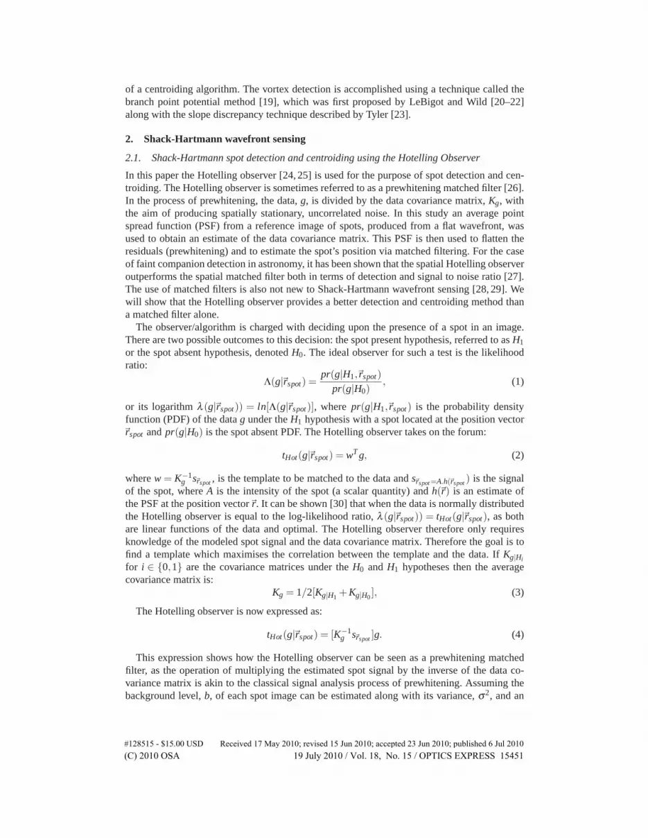
In this paper the Hotelling observer [24, 25] is used for the purpose of spot detection and cen-troiding. The Hotelling observer is sometimes referred to as a prewhitening matched filter [26].In the process of prewhitening, the data, g, is divided by the data covariance matrix, Kg, withthe aim of producing spatially stationary, uncorrelated noise. In this study an average pointspread function (PSF) from a reference image of spots, produced from a flat wavefront, wasused to obtain an estimate of the data covariance matrix. This PSF is then used to flatten theresiduals (prewhitening) and to estimate the spot’s position via matched filtering. For the caseof faint companion detection in astronomy, it has been shown that the spatial Hotelling observeroutperforms the spatial matched filter both in terms of detection and signal to noise ratio [27].The use of matched filters is also not new to Shack-Hartmann wavefront sensing [28, 29]. Wewill show that the Hotelling observer provides a better detection and centroiding method thana matched filter alone.

The observer/algorithm is charged with deciding upon the presence of a spot in an image.There are two possible outcomes to this decision: the spot present hypothesis, referred to as H1

or the spot absent hypothesis, denoted H0. The ideal observer for such a test is the likelihoodratio:

Λ(g|�rspot) =pr(g|H1,�rspot)

pr(g|H0), (1)

or its logarithm λ (g|�rspot)) = ln[Λ(g|�rspot)], where pr(g|H1,�rspot) is the probability densityfunction (PDF) of the data g under the H1 hypothesis with a spot located at the position vector�rspot and pr(g|H0) is the spot absent PDF. The Hotelling observer takes on the forum:

tHot(g|�rspot) = wT g, (2)

where w = K−1g s�rspot , is the template to be matched to the data and s�rspot=A.h(�rspot ) is the signal

of the spot, where A is the intensity of the spot (a scalar quantity) and h(�r) is an estimate ofthe PSF at the position vector�r. It can be shown [30] that when the data is normally distributedthe Hotelling observer is equal to the log-likelihood ratio, λ (g|�rspot)) = tHot(g|�rspot), as bothare linear functions of the data and optimal. The Hotelling observer therefore only requiresknowledge of the modeled spot signal and the data covariance matrix. Therefore the goal is tofind a template which maximises the correlation between the template and the data. If Kg|Hi

for i ∈ {0,1} are the covariance matrices under the H0 and H1 hypotheses then the averagecovariance matrix is:

Kg = 1/2[Kg|H1+Kg|H0

], (3)

The Hotelling observer is now expressed as:

tHot(g|�rspot) = [K−1g s�rspot ]g. (4)

This expression shows how the Hotelling observer can be seen as a prewhitening matchedfilter, as the operation of multiplying the estimated spot signal by the inverse of the data co-variance matrix is akin to the classical signal analysis process of prewhitening. Assuming thebackground level, b, of each spot image can be estimated along with its variance, σ2, and an


estimate of the PSF is known it can be shown that Kg is diagonal with it elements given by [31]:

Kg = 1/2[Kg|H1+Kg|H0

],

Kg|H0= [σ2

m +bm]δm,m′ ,

Kg|H1= [A∗hm(�rspot)+σ2

m +bm]δm,m′ .

(5)

The cross-correlation of the template vector, w, and the data, g, can be computed either in theimage plane or in the Fourier plane. In the Fourier plane the position of the spot is estimated byusing a parabolic fit to interpolate the peak of the cross-correlation [28, 29]. In this study boththe data and the template vector were zero padded to five times their original size to improvethe resolution of the cross-correlation. In the following HotMF will refer to using the Hotellingobserver in this manner and MF will refer to using a simple matched filter with this approach.In the image plane the peak of the cross-correlation is found, and hence the spot position, byshifting the position of the template spot until maximum is found. In practice this PSF fittingtype approach is carried out by an unconstrained maximisation of the Hotelling observer wherethe value of the Hotelling observer is only dependent upon the position of the test spot in thetemplate vector [25]. This image plane method will be referred to as HotML.

To test the method, ten thousand noisy spot images (size 19×19 pixels), with random spot lo-cations, were simulated using a Gaussian PSF profile with a mean full-with-half-max (FWHM)of 2.5 pixels varying normally with a standard deviation of 0.25 pixels from image to image.The noise in each image consisted of Poisson noise and normally distributed readout noise. Foreach image the three matched-filter type algorithms, as well as a classical centroiding algorithm,were tasked with locating a spot in the image. The PSF profile used in the template vectors wasalso Gaussian in shape and had the same FWHM as the mean of the data. The HotMF showedthe lowest mean error on the estimation of the position of the spot (in pixels) followed by MFand HotML, see Table 1. The centroiding algorithm faired worst; however, it should be notedthat this centroiding algorithm was not optimised as in [29]. The centroiding algorithm used inthe comparison is a simple, non-iterative centroiding algorithm. It thresholds the data and findsthe centre of mass of a spot bigger than a certain size. The threshold is specific to each lensletas it is intensity weighted for each subaperture. If two or more spots are detected above thethreshold within one subaperture the brightest one is chosen as the focused Shack-Hartmannspot.

Table 1. Summary of testing the HotMF , HotML, MF and centroiding algorithms on tenthousand simulated spot images. The HotMF showed the lowest mean error in spot positionestimation. This algorithm was also the most efficient spot detector having the highest AUCof the four tested observers.

Observer Mean Error in Spot AUC SNRPosition Estimation Pixels

HotMF 3.6×10−4 0.82 136HotML 5×10−4 0.76 206MF 4×10−4 0.80 81

Centroiding 1×10−3 40

The signal-to-noise ratios (SNR) reported in Table 1 were defined as the ratio of the meanto the standard deviation of the measured data [6]. In practice the SNRs were calculated bycomparing the peak value of the cross-correlation (or the data) to the standard deviation of the


0 0.2 0.4 0.6 0.8 10

0.1

0.2

0.3

0.4

0.5

0.6

0.7

0.8

0.9

1M F M L

( M F ) =( ) =( M L ) =

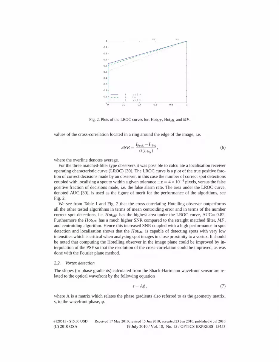
Fig. 2. Plots of the LROC curves for: HotMF , HotML and MF .

values of the cross-correlation located in a ring around the edge of the image, i.e.

SNR =IPeak − Iring

σ(Iring), (6)

where the overline denotes average.For the three matched-filter type observers it was possible to calculate a localisation receiver

operating characteristic curve (LROC) [30]. The LROC curve is a plot of the true positive frac-tion of correct decisions made by an observer, in this case the number of correct spot detectionscoupled with localising a spot to within a given tolerance ±ε = 4×10−4 pixels, versus the falsepositive fraction of decisions made, i.e. the false alarm rate. The area under the LROC curve,denoted AUC [30], is used as the figure of merit for the performance of the algorithms, seeFig. 2.

We see from Table 1 and Fig. 2 that the cross-correlating Hotelling observer outperformsall the other tested algorithms in terms of mean centroiding error and in terms of the numbercorrect spot detections, i.e. HotMF has the highest area under the LROC curve, AUC= 0.82.Furthermore the HotMF has a much higher SNR compared to the straight matched filter, MF ,and centroiding algorithm. Hence this increased SNR coupled with a high performance in spotdetection and localisation shows that the HotMF is capable of detecting spots with very lowintensities which is critical when analysing spot images in close proximity to a vortex. It shouldbe noted that computing the Hotelling observer in the image plane could be improved by in-terpolation of the PSF so that the resolution of the cross-correlation could be improved, as wasdone with the Fourier plane method.

2.2. Vortex detection

The slopes (or phase gradients) calculated from the Shack-Hartmann wavefront sensor are re-lated to the optical wavefront by the following equation

s = Aφ , (7)

where A is a matrix which relates the phase gradients also referred to as the geometry matrix,s, to the wavefront phase, φ .


The least mean square error reconstruction, φlmse, as described by Fried [11], can be writtenin the following form

φlmse = ((A†A)−1A†)s. (8)

This however does not take account of all the phase in the reconstruction process: some ofthe phase is, in essence, ignored and treated as noise. This is what Fried [11] called the hiddenphase and this is the part of the phase which is discontinuous when optical vortices are present.It can be defined as

∇φ = ∇φlmse + ∇φhid, (9)

where ∇φ is the gradient of the phase of the field, ∇φlmse is the gradient of the least-squaresphase and ∇φhid is the gradient of the hidden phase.

The hidden phase is the part of the phase which is the curl of the vector potential (the leastsquares reconstruction only looks at the scalar potential) and thus can be defined as

∇φhid = ∇ × H(r), (10)

where the H(r) above is the Hertz potential, which is defined as:

H(r) = [0,0,h(r)], (11)

where h(r) is the Hertz function. It will be this Hertz potential that we will take advantage ofwhen using the branch point potential method to detect vortices in a distorted phase function.

Although the curl component of the phase is hidden to the least squares reconstructionmethod, it can be calculated from the slope discrepancy Eq. (16) [23] of the reconstruction.This is done by calculating slopes from a wavefront reconstructed by the least squares methodand subtracting them from the slopes originally measured by the wavefront sensor. If a systemis completely noise free, then the slope discrepancy is exactly equal to the curl component ofthe phase. However, experimentally the slope discrepancy will be noisy and have fitting errorswhich were filtered out by the least squares reconstruction.

The most commonly used method to examine the curl component of the phase to find theposition and sign of optical vortices is the contour sum method of gradient circulation. Thisinvolves summing the phase gradients calculated from the wavefront sensor around in a closedloop and can be described mathematically by the following equation

∑(i, j) = −Δx(i, j)−Δy(i+1, j)+Δx(i, j +1)+Δy(i, j), (12)

where Δx() are the horizontal phase differences and Δy() are the vertical phase differences.If there are no vortices present, and thus the phase is continuous, then this sum will be equal

to zero (ignoring noise). It will also equal zero if there are two vortices of opposite sign enclosedby the loop of phase gradients, as they will cancel each other out. However if the sum aroundthe loop is equal to, or a multiple of, ±2π then there is a phase singularity enclosed in theloop. By convention the (i,j)th pixel is the top left of the four pixels and the vortex is placedthere, a more exact position of the branch point could be established by further numericalmethods but we know of no standard technique. The overall robustness of the contour summethod has been questioned under heavy noise conditions [18,21,32] making it problematic touse this with the slope discrepancy technique and therefore we have decided to use a differentmethod [21, 22]. The issue of noise with respect to the contour sum method is raised becauseit only does a gradient circulation around a closed loop of four phase gradients, whereas thebranch point potential method described below employs all of the available slope data by usinga least squares reconstruction method to calculate the potential function.


This method, called the branch point potential method, inspects the curl of the phase bydetermining the Hertz potential of the field. It is done by first rotating the phase gradientscalculated from the wavefront sensor by 90 degrees, which is accomplished by a simple matrixmultiplication.

(Rπ/2)∗ (s) =(

0 1−1 0

)∗ (s) =

(sy

−sx

), (13)

where (Rπ/2) is a 90 degree rotation, s are the slope values measured by the wavefront senorwith sx and sy the slopes x-values and y-values respectively.

Then the pseudo-inverse of the geometry matrix is calculated:

A′ = (A†A+m2)−1A†, (14)

where A† is the adjoint of the geometry matrix and the m2 value is inserted to prevent thematrix from becoming singular. The pseudo-inverse could also be calculated using a singularvalue decomposition.

The potential function, V is then calculated by multiplying the rotated slopes by the pseudo-inverse of the geometry matrix.

V = (A′)(Rπ/2 s). (15)

The potential function, V, is then reformed into a square array of the same size as the Shack-Hartmann lenslet array and the position and sign of the vortices is found by locating the peaksor valleys in the potential function. The positive vortices are designated by the peaks in thepotential plot and the negative vortices are designated by the valleys. This potential functioncan be used to locate the optical vortices because it is the Hertz potential Eq. (11) and thereforeit is able to see the hidden phase of the field.

We have found that this method can be improved upon by using it in conjunction with theslope discrepancy technique. As mentioned previously the slope discrepancy is the slope fieldobtained by subtracting the Shack-Hartmann slopes from the slopes ascertained from a leastsquares reconstruction of phase, as shown

∇φslpdis = s − ∇φlmse, (16)

where ∇φslpdis are the phase gradients of the slope discrepancy, ∇φlmse are the phase gradientsof the least-squares phase and s are the phase gradients calculated from the wavefront sensor.

The slope discrepancy phase gradients are then used as the inputs into the branch pointpotential detection method. As our results will show, when these are used instead of the Shack-Hartmann slopes we get improved vortex detection. This happens because tilts and other largeaberrations that are present in the wavefront have a strong contribution to the slope data and canmask the relatively small circulation of the slopes when a vortex is present. By removing thecontinuous part of the phase from the slope data the vortex circulation becomes more apparent.Since these large aberrations are essentially noise to our vortex detector we get increased levelsof detection. It should also be noted that the areas where we most want to evaluate the phasegradients (areas near the centre of the vortex) are the most difficult to measure due to low lightlevels. This also means that they are the slopes which are effected most by the large, turbulence-induced aberrations.


3. Laboratory experiments

3.1. Experimental method

An experimental setup was built in the laboratory to conduct practical tests of the theory out-lined above. A schematic of the setup is shown in Fig. 3. The system is configured with twoparallel beams which, after coming through a spatial filter from the laser, are split by a beam-splitter (BS1). One of these beams is a reference beam which is sent through a 4f system tothe second set of beamsplitters (BS3,BS4), through the optical trombone and back into thewavefront sensing arm. The purpose of the optical trombone is to allow for different propaga-tion distances along what is otherwise the same optical path. When Shack-Hartmann wavefrontmeasurements are being carried out this beam is blocked off somewhere in the path before itrejoins the Spatial Light Modulator (SLM) beam.

The second beam going from BS1 goes through another beamsplitter (BS2) and is directedonto the SLM. After being reflected from the SLM the beam comes back through BS2 and intoa 4f system, which has an iris placed at the focus to select only one diffraction order of the SLM.It then travels to BS4, where it rejoins the reference beam, and through the optical trombone.It then proceeds back through into the wavefront sensing arm. In the wavefront sensor itselfa lens (L8) is used to expand the beam slightly to ensure it passes through the active area ofthe Shack-Hartmann lenslet array. Due to the relatively short focal length of the lenslet array arelay lens (L9) is needed to focus the beamlets on to the camera.

Another arm is used for interferometry; this arm starts with a flip mirror (FM1). When in-terferometric images are needed this flip mirror is dropped into the path of the beam beforethe wavefront sensing arm. It redirects the beam into lenses L10 and L11 which demagnify thebeam size onto the CCD used for interferometry. When measurements involving the Shack-Hartmann sensor are needed FM1 is flipped out of the beam path and it continues into thewavefront sensing arm.

FM1

L10

L11

InterferometryCamera

Fig. 3. Schematic of experimental setup used in the laboratory.

To detect optical vortices in atmospheric like conditions we use the SLM to generate intensityscintillation and phase variations in a field typical of those encountered after the propagation ofa laser beam through the atmosphere. Turbulence degraded optical fields were first generatedby numerical simulations and the final field after the numerical propagation was encoded andapplied to the SLM. In the simulations an initially plane wave is passed through a number ofphase screens randomly generated using Kolmogorov statistics, equally spaced over the propa-gation path. The plane wave was propagated between phase screens by multiplying the Fouriertransform of the optical field by the Fresnel transfer function [33, 34].

To ensure that an optical vortex is present in the final optical field, which is applied to theSLM, the initial plane wave is seeded with an optical vortex of known sign. This vortex will stay


in the field over the total distance of the waves simulated propagation through the atmosphere.In general, a phase map with canonical vortices at locations (Xk,Yk) with charge mk can begenerated using the following product wave function, where K is the index of the vortex. In thisexperiment we seeded the initial plane wave with a single vortex, (X1,Y1), at the centre of thefield:

Ψ =K

∏k=1

{(X −Xk)+mki(Y −Yk)} , (17)

Q = arctan

(Im{Ψ}Re{Ψ}

), (18)

with Q being the resulting phase and X and Y are the coordinates of an array on a cartesiangrid and Xk and Yk defining the positions of the zero crossings. These simulations and all of theother analysis code is being implemented using MATLAB.

The desired amplitude and phase variations in the field are encoded into a binary phase maskof 0 to π radians and applied to the SLM [35, 36]. The SLM used is a ferroelectric liquid crys-tal, binary phase Spatial Light Modulator from Boulder Nonlinear Systems. It has 512× 512pixels with an active area of 7.7mm × 7.7mm and toggles between the true and inverse imagesimprinted once every cycle to prevent hardware damage. The phase and amplitude informationis carried in the first diffraction order of the phase mask. In our system Fig. 3 the iris, betweenL4 and L5, spatially filters the +1 order for further propagation through the system.

The position of the optical vortices produced by the simulations are known and therefore wecan test the efficacy of the branch point potential method against the interferometry technique ofviewing vortices. The interferometric fringes of a vortex beam combined with a reference beamwill have a fork (or a branch) present. It will be seen as one fringe splitting into two separatefringes, by pinpointing where this happens on the interferometry image and comparing it to thelocation given by the branch point potential method we can be certain of the veracity of thebranch point potential method.

3.2. Experimental results

In these set of results we will demonstrate how the branch point potential methods capacity todetect vortices is improved by using the slope discrepancy technique alongside it. The differ-ences in detection rates between two particular levels of turbulence will be highlighted. We willalso show interferometric images of optical vortices in turbulent fields and their accompanyingdetection in the potential plots.

One of the initial results we noticed in the course of the experiments was that the use ofthe slope discrepancy greatly increased the chances of a correct detection by the branch pointpotential method in the presence of turbulence. We must first define what a correct detection ofa vortex entails. A correct detection is when the vortex is seen in the correct position in the fieldand with the correct sign along with providing no other false detections in the field. Since wehave seeded the turbulence simulations with an optical vortex and then used this as the patternimprinted on the SLM, we know both the position and sign of the vortex. By examining thesimulations we can also check if any other vortices are present and therefore rule any otherdetections as false.

As we can see from Fig. 4 the use of the slope discrepancy technique improves the detectionrate approximately threefold for the scintillation indices of both σ2

I = 0.154 and σ2I = 0.652,

where σ2I is the scintillation index given by

σ2I =

⟨I2

⟩−〈I〉2

〈I〉2 , (19)


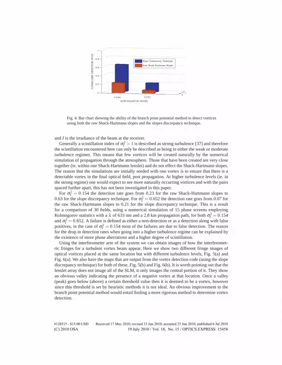
Fig. 4. Bar chart showing the ability of the branch point potential method to detect vorticesusing both the raw Shack-Hartmann slopes and the slopes discrepancy technique.

and I is the irradiance of the beam at the receiver.Generally a scintillation index of σ2

I > 1 is described as strong turbulence [37] and thereforethe scintillation encountered here can only be described as being in either the weak or moderateturbulence regimes. This means that few vortices will be created naturally by the numericalsimulation of propagation through the atmosphere. Those that have been created are very closetogether (ie. within one Shack-Hartmann lenslet) and do not effect the Shack-Hartmann slopes.The reason that the simulations are initially seeded with one vortex is to ensure that there is adetectable vortex in the final optical field, post propagation. At higher turbulence levels (ie. inthe strong regime) one would expect to see more naturally occurring vortices and with the pairsspaced further apart, this has not been investigated in this paper.

For σ2I = 0.154 the detection rate goes from 0.23 for the raw Shack-Hartmann slopes to

0.63 for the slope discrepancy technique. For σ2I = 0.652 the detection rate goes from 0.07 for

the raw Shack-Hartmann slopes to 0.21 for the slope discrepancy technique. This is a resultfor a comparison of 30 fields, using a numerical simulation of 15 phase screens employingKolmogorov statistics with a λ of 633 nm and a 2.8 km propagation path, for both σ2

I = 0.154and σ2

I = 0.652. A failure is defined as either a non-detection or as a detection along with falsepositives, in the case of σ2

I = 0.154 most of the failures are due to false detection. The reasonfor the drop in detection rates when going into a higher turbulence regime can be explained bythe existence of more phase aberrations and a higher degree of scintillation.

Using the interferometer arm of the system we can obtain images of how the interferomet-ric fringes for a turbulent vortex beam appear. Here we show two different fringe images ofoptical vortices placed at the same location but with different turbulence levels, Fig. 5(a) andFig. 6(a). We also have the maps that are output from the vortex detection code (using the slopediscrepancy technique) for both of these, Fig. 5(b) and Fig. 6(b). It is worth pointing out that thelenslet array does not image all of the SLM, it only images the central portion of it. They showan obvious valley indicating the presence of a negative vortex at that location. Once a valley(peak) goes below (above) a certain threshold value then it is deemed to be a vortex, howeversince this threshold is set by heuristic methods it is not ideal. An obvious improvement to thebranch point potential method would entail finding a more rigorous method to determine vortexdetection.


(a) (b)

Fig. 5. The interferometric fringes of a turbulent vortex beam for σ2I = 0.154 (a) and the de-

tected vortex shown as a contour plot (b). The vortex is detected as it is the only peak/valleyabove/below the threshold used to separate a vortex from noise.

(a) (b)

Fig. 6. The interferometric fringes of a turbulent vortex beam for σ2I = 0.652 (a) and the de-

tected vortex shown as a contour plot (b). The vortex is detected as it is the only peak/valleyabove/below the threshold used to separate a vortex from noise.

4. Conclusion

In this paper we have shown that it is possible to experimentally locate optical vortices in aturbulent optical field using a Shack-Hartmann wavefront sensor. The branch point potentialmethod is used to detect the vortices and it’s effectiveness is improved approximately threefoldby using the slope discrepancy technique along with it, as seen in Fig. 4. From the same figure itis also obvious that the detection rate falls with increased turbulence, this is presumably due tothe higher scintillation and larger phase aberrations across the optical field at these turbulencelevels.

We also use the Hotelling observer, a prewhitening matched filter, to give a better evaluationof Shack-Hartmann spot positions. This improves the wavefront slopes and therefore aids inthe ability to detect vortices. It is also shown, Table 1, to be more capable at spot detection andcentroiding than a straight matched filter or a common centroiding algorithm. It also retains theability to do good spot detection at low light levels, which is important when dealing with spotsclose to the vortex centre.

We feel it has been necessary to improve the Shack-Hartmann spot positioning to improve


vortex detection in turbulent optical fields. However it is equally obvious that work should con-tinue to improve the ability of the branch point potential method to detect optical vortices. Thisis especially the case when higher turbulence levels are considered, where more vortex pairs arecreated. These improvements should include a more rigorous and enhanced approach to vor-tex determination from the potential maps instead of the thresholding method currently used.Other methods to reduce the levels of noise in the potential maps are also being investigated,particularly in relation to edge effects.

Acknowledgments

We are grateful to Dr. Ruth Mackey for advice and support and to the reviewers for their com-ments. This research was funded by Science Foundation Ireland under Grant No. 07/IN.1/1906


Experimental Detection of Optical Vortices Using a Shack-Hartmann Wavefront Sensor

Documents

Transcript of Experimental Detection of Optical Vortices Using a Shack-Hartmann Wavefront Sensor