Saturn’s South Polar Vortex Compared to

Other Large Vortices in the Solar System

Ulyana A. Dyudina, a, Andrew P. Ingersoll a, Shawn P. Ewald a,

Ashwin R. Vasavada b, Robert A. West b, Kevin H Baines b,

Thomas W. Momary b, Anthony D. Del Genio c,

John M. Barbara c, Carolyn C. Porco d,

Richard K. Achterberg e, F. Michael Flasar e,

Amy A. Simon-Miller e,and Leigh N. Fletcher b

a150-21, Division of Geological and Planetary Sciences, 150-21 California

Institute of Technology, Pasadena, CA 91125 (U.S.A.)

bJet Propulsion Laboratory, California Institute of Technology, Pasadena, CA

91125 (U.S.A.)

cGoddard Institute for Space Studies, NASA, 2880 Broadway, New York, NY

10025 (U.S.A.)

dCassini Imaging Central Laboratory for Operations, Space Science Institute, 4750

Walnut Street, Suite 205, Boulder, CO 80301 (U.S.A.)

eNASA Goddard Space Flight Center, Code 693, Greenbelt, MD 20771 (U.S.A.)

Number of pages: 25, Number of tables: 1, Number of figures: 6

Temporary remarks are shown in bold font and will be removed later.

My suggestions are marked UD at the end of the note. Ulyana

For co-authors only, manuscript is not submitted yet, ignore the line below.

Preprint submitted to Icarus 27 June 2008

Proposed Running Head:

Saturn’s South Polar Vortex

Please send Editorial Correspondence to:

Ulyana A. Dyudina

150-21 Caltech, Pasadena, CA 91125, USA

E-mail: ulyana@gps.caltech.edu

Phone: (626)395-6824

Fax: (626)585-1917

2

ABSTRACT

Observations made by the imaging science experiment (ISS), visible and in-

ferred mapping spectrometer (VIMS) and the long-wavelength infrared spec-

trometer (CIRS) aboard the Cassini spacecraft reveal that the large, long-

lived cyclonic vortex at Saturn’s south pole has a 4200-km-diamter cloud-free

eye. The eye has a 4 K warm core extending from the troposphere into the

stratosphere, concentric eyewall clouds extending 70 km above the internal

clouds, and numerous external clouds whose anticyclonic vorticity suggests a

convective origin. The eye rotation speeds reach 150-190 m/s, and probably

strengthen with depth. The Saturn polar vortex has features in common with

terrestrial hurricanes and with the Venus polar vortex. Neptune and other

giant planets may also have strong polar vortices.

Keywords: SATURN, ATMOSPHERE; ATMOSPHERES, DYNAMICS ; IN-

FRARED OBSERVATIONS ; METEOROLOGY ; SPECTROSCOPY

3

1 Introduction.

Earth-based telescopic observations (Orton and Yanamandra-Fisher, 2005) re-

vealed a hot spot at Saturn’s south pole in 2003, which was observed again

by Cassini composite infrared spectrometer (CIRS) (Fletcher et al., 2008).

Cassini imaging observations (Vasavada et al., 2006; Sanchez-Lavega et al.,

2006) revealed cyclonic rotation around the spot in 2005. To explore this fea-

ture further, a series of high-resolution observations by Cassini were taken

for a three-hour period on October 11, 2006. This observtion revealed that

the hot spot is surrounded by the double cloud wall forming an “eye” of the

vortex. The eye has nearly cloud-free upper atmosphere above lower, tropo-

spheric clouds. The eye is bordered by two 20-70-km-tall cloud walls. The eye

is surrounded by the ring of high hazes (Dyudina et al., 2008).

In this paper we provide a detailed description and discussion of the October

11, 2006 imaging observations of the cyclone which were published as Science

brevia by Dyudina et al. (2008). Additionally we present simultaneous obser-

vations of the vortex by two other instruments: high-resolution infrared CIRS

maps and 5-micron VIMS moves of the Saturn’s south polar vortex (SPV).

With this data we compare SPV with large atmospheric vortices on Earth,

Venus, Jupiter, and Neptune.

Section 2 discusses morphology of the clouds and their vertical structure.

Section 3 presents our wind speed measurements. Section 4 shows the vorticity

of the wind. Section 5 discusses the heights of the two cloud walls around the

polar storm’s eye. Section 6 discribes the hot spot at the location of SPV

observed by Cassini CIRS. Section 7 compares our windspeed measurements

4

with Cassini VIMS wind measurements. Section 8 compares SPV with large

vortices on other planets.

5

2 Cloud structure.

On October 11 2006 Cassini observed South pole of Saturn with unprecedented

spatial resolution of 20 km/pixel. Figure 1 shows a mosaic from 14 images of

South pole taken within a 3-hour period. The two walls of the cyclone are the

circular structure at around -87.8 latitude and the slightly elliptical structure

at around -88.7 to -88.9 latitude. The same double-wall structure appar-

ently existed during the ∼50 km/pixel Cassini polar observations taken in

September-October 2004, two years before these ones (Vasavada et al., 2006),

and in ∼30 km/pixel observations taken in July 2004 (Sanchez-Lavega et al.,

2006). However with lower spatial resolution, slant viewing, and higher Sun

producing shorter shadows, the 2004 observations were uncapable of detecting

the steep eyewalls. The elliptical shape of the inner eyewall looks remarkably

unchanged between the 2004 and 2006 observations. There are a few small

clouds inside the inner eyewall and many small bright clouds surrounding the

eye that have the same general appearance between 2004 and 2006 observa-

tions.

From the imaging in wavelengths sensitive to different altitudes Dyudina et al.

(2008) concluded that the ”eye” of the vortex is cloud-free in the upper tro-

posphere, and that the small bright clouds both inside and outside the eye

are located in the lower tropospere (see also the description of cloud height

retrieval in Section 3).

6

3 Windspeeds.

Cassini took repeated images of the pole during the 3-hour observation. High

spatial resolution of ∼20 km/pixel and good temporal sampling of 14 images

in the continuum band filter at 750 nm (the wavelength of the best contrast for

small features) allowed tracking of clouds to obtain accurate wind velocities.

The supplementary online movie 1 combined from these images 1 shows the

winds increasing towards the pole. The cyclone’s eye rotates by ∼ 60 relative

to the planet within the 3 hours. Figure 2A shows zonal windspeeds measured

by cloud tracking. Two tracking techniques were used. Equatorward of -84.5

latitude the windspeeds were obtained by an automatic feature tracker. Pole-

ward of -84.5 latitude the automatic tracker failed to obtain accurate wind

speeds because of high speeds, curved trajectories, and multiple linear fea-

tures. For this region we manually tracked individual features using modified

movies combined from the 14 maps. In each modified movie the maps were

rotated back relative to the clouds’ zonal motion at some test angular velocity

around the pole. For each cloud there is a particular angular velocity when the

cloud’s zonal motion and the movie’s back rotation cancel out, which stops

the motion of the cloud. From the set of test angular velocities we picked the

clouds that stopped their motion in the modified movies. This produced the

data points in Fig. 2A.

The manual and automatic tracking agree equatorward from the -84.5 lat-

itude. The independent cloud tracking by two other co-authors (JMB and

ARV) agree with the windspeeds in Fig. 2A but have larger uncertainties. We

1 http://www.nasa.gov/mpg/162357main pia08332.mpg

7

do not include their data points in Fig. 2A. The wind increases towards the

pole up to the outer eyewall at -87.8 latitude. There are no trackable features

between the outer wall and latitude of -88.5, which is just outside the inner

eyewall. Between latitudes -86.5 and -89 the mean zonal velocity u reaches

its maximum of 150 ± 20 m s−1.

The winds measured using Cassini images taken in July 2004 were 160±10

m/s at -87 latitude (Sanchez-Lavega et al., 2006). This is consistent with our

measurements at this latitude. In September-October 2004 the speed of rota-

tion of the inner eyewall at -88.5 latitude was 80 to 135 m/s (Vasavada et al.,

2006). This is smaller than our u = 150 ± 20 m s−1 for this latitude (see Fig.

2A). Although this difference may be real, the uncertainty in the windspeed

measurements is rather high to assert this windspeed change with confidence.

The smooth curves in Fig. 2A assume constant absolute vorticity poleward

of latitude φ0. Absolute vorticity is related to spin about a vertical axis and

consists of two parts - a part ζ due to motion relative to the planet and a

part f due to the planet’s rotation. The curves assume ζ + f = f0 =constant,

with ζ = 0 and u = 0 at φ = φ0. The latitude φ0 is the only free parameter

of the curve. Since f ≈ f0 in the polar region, the smooth curve has ζ ≈ 0 in

this region. Up to latitude -85 the measured u increases slightly more steeply

than the constant ζ + f curve. Poleward of -85 latitude u increases more

slowly than the constant ζ +f curve. Constant absolute vorticity is consistent

with horizontal stirring by eddies. Without the frictional losses by eddies,

rings of air moving poleward would produce a profile with constant angular

momentum, which is a much steeper curve than the curve in Fig. 2A and does

8

not fit the data. Instead, angular momentum decreases toward the center.

We also measured the meridional component of the clouds’ motion which

turned out to be zero within the errors for all the clouds except the ones in

the inner eye. The clouds in the inner eye display a small radial motion, both

inward and outward, in addition to their much larger zonal motion.

The multiple-filter observations probing different cloud altitudes are repeated

four times during the three hours (see also Dyudina et al. (2008)). False-color

images are composed from the images taken with filters CB2, MT2, and MT3

(see Porco et al. (2004) for Cassini filter details). The four-frame color supple-

mentary online movie 2 2 combined from these false-coor images shows that

the clouds at different heights move at the same velocities. We estimate the

cloud heights using methane gas absorption. The continuum narrow band filter

CB2 (750 nm, red color plane) senses clouds and aerosols from the top of the

atmosphere down to the deepest levels of the troposphere. The filter at weak

methane absorption band MT2 (727 nm, green color plane) senses down to the

intermediate depths. The exact values of the atmospheric pressure where the

methane absorption reaches optical depth one for each wavelengths are usually

derived from radiative transfer models and are somewhat model-dependent.

Here we assume the penetration depths described in Tomasko et al. (1984).

According to that model, at 727 nm the gaseous absorption optical depth one

occurs at 1.2 bars at nadir viewing for a cloud-free atmosphere . At slant view-

ing (the images are observed at around 40 from horizon) the optical depth

one occurs near 800 mbar. The effect of slant illumination is even more drastic

than the effect of slant viewing. For the images composing the movie the Sun

2 http://www.gps.caltech.edu/∼ulyana/iss/polar movie/movies/color 4frm compressed.avi

9

is 15.5 above the horizon at the pole. This translates into optical depth one

for cloud-free atmosphere at ∼ 300 mbars, which would be further reduced by

haze or cloud shadowing. The illumination angle changes considerably across

the image, and so does the depth of the solar light penetration. The filter at

the strong methane absorption band MT3 (889nm, blue color plane) senses

the highest part of the atmosphere. At this wavelength the absorption opti-

cal depth one occurs at 330 mbars for nadir viewing, which corresponds to

200 mbars for slant viewing, or to 80 mbars for solar illumination. For such a

complex system the exact cloud heights can only be derived from a thorough

radiative transfer model. Such a retrieval would be uncertain with the ISS

data only and would greatly benefit from combining the ISS data with near-

infrared and infrared data from Cassini VIMS and CIRS.The accurate cloud

heigh retrieval is out of scope of this paper. However we can give qualitative

estimate of the relative cloud heights in movie 2 with low clouds appearing red

and high thin clouds appearing blue and green. The wind speeds are coherent

at all elevations whenever small clouds are available for tracking. It should

be noted though that inside -84 latitude only the deepest-probing red color

plane clouds suitable for cloud tracking. In this region near the eye it is im-

possible to tell if the windspeeds are the same at all heights. The oval shape

of the inner eye rotates coherently in all colors. It is unclear if it follows the

wind field or not: it could be a wave that propagates relative to the fluid.

10

4 Vorticity.

For an oblate spheroid the absolute vorticity of the zonal flow can be written

as

ζ =1

Rr

d

dϕ(ru)

where R is the radius of curvature in the latitudinal direction, r is the radius

of curvature in the zonal direction, and ϕ is the planetographic latitude. Plan-

etographic latitude ϕ can be converted from planetocentric latitude φ using

equatorial and polar radii Re and Rp, and their ratio ǫ = Re/Rp.

ϕ = arctan(ǫ2 tan(φ))

Radii of curvature can be expressed as follows Dowling and Ingersoll (1989).

r(ϕ) =Re

(1 + ǫ−2 tan2 ϕ)1/2

R(ϕ) =Re

ǫ2(

r

Re cos ϕ)3

The equation ζ + f = constant, which was used in Fig. 3A, can be written in

the notation of R and r, assuming ζ = 0 and u = 0 at ϕ0 = arctan(ǫ2 tan(φ0)).

ζ + f =1

Rr

d

dϕ(ru) + 2Ω sin ϕ = 2Ω sin ϕ0

The velocity curve for Fig. 3A is the result of numerical integration of the

same equation rewritten as:

u =2ΩRe

ǫ2(1 + ǫ−2 tan2 ϕ)1/2

ϕ∫

ϕo

(sin ϕ0 − sin ϕ)dϕ

(1 + ǫ−2 tan2 ϕ)2 cos2 ϕ

The solid curve for the vorticity in Fig. 3B is a finite-difference version of the

vorticity equation at the beginning of this section. For each pair of consecutive

11

points in the spline curve fitted to the points from Fig. 3A (the spline curve

is not shown in the plot) the vorticity is calculated as follows.

ζ ≈4(r1u1 − r2u2)

(r1 + r2)(R1 + R2)(ϕ1 − ϕ2)

where the subscripts correspond to the first and second point in the pair.

Multiple smaller clouds around the cyclone’s eye (see Fig. 1) show detectable

individual rotation. To determine the relative vorticity ζ of a cloud, we track

it over the 3-hour time interval and measure its angular velocity of rotation

relative to the rotating planet. Twice this angular velocity is the vorticity of

the cloud. The angular velocity was obtained by a procedure similar to the

manual feature tracking used for the zonal windspeeds, which involves picking

an appropriate stopped motion movie from the set of test movies. To obtain

each cloud’s angular velocity we first determined its drift around the pole (see

the technique described in Section 3 ). Then we made an individual cloud’s

movie from the set of 14 maps such that the movie frames track the cloud in its

motion around the pole. Finally we made a set of modified back-rotated movies

from these cloud-centered frames for a set of test angular velocities. While

simultaneously playing the set of back-rotated movies we picked the one that

stopped the apparent rotation of the cloud. Because individual clouds are not

always covered by all 14 images, some modified movies have less than 14 time

steps, down to as few as 2 time steps, which creates additional uncertainty.

Often it is uncertain which of the movies matches the rotation of the cloud. To

test the uncertainty and to increase the precision of the vorticity measurements

we measured vorticity of each cloud 3-4 times, picking the range of reasonably

good matches. The vorticity values (colors of the asterisks in Fig. 1 and points

in Fig. 2B) are the averages of those 3-4 measurements. The error bars are

12

calculated as a standard deviation of the measurements. Nearly all small clouds

rotate counterclockwise (anticyclonic vorticity). The largest features (the two

dark spots at the upper left corner of the map in Fig. 1) rotate the fastest. For

the smaller clouds the relation between the size and rotation is not systematic.

13

5 Eyewall heights.

The cyclone’s eyewalls are steep and cast shadows on the lower clouds inside

the eye (see also the brief estimate of eyewall heights in Dyudina et al. (2008)).

Figure 3 shows that the dark crescent-shaped areas inside the walls follow the

Sun in a counterclockwise direction as the planet turns during the three-hour

period. This demonstrates that the dark areas are indeed shadows and not a

dark coloration of the underlying clouds.

Figure 4 shows how we derived the height of the eyewalls from the length

of the shadows. The two maps in the figure are examples of the nine maps

from Fig. 3, which we used for the eyewall height calculation. We manually

picked the points of the apparent end of the shadow and projected these points

along the Sun’s azimuth to the edge of the eyewall. The reader may judge the

uncertainty by comparing the left panels of Fig. 4 with the right panels,

which show the same maps overlaid with our estimated shadow locations. We

assumed the clouds inside the eye are flat and horizontal. To obtain the eyewall

height we multiplied each shadow length by the tangent of the solar elevation

angle above the horizon, which is around 16 for the inner eyewall and 17 for

the outer eyewall for all the images (as the Sun is 15 above the horizon at

the pole and the eyewalls are 1 and 2 away from the pole).

Figure 5 shows the resulting heights for outer and inner eyewalls calculated

from the nine maps. The data are plotted versus the longitude where each

shadow point projects to the eyewall. The longitudes are adjusted (rotated

back) to account for the rotation of the eyewall. With such an adjustment

the shadows of particular eyewall features (e.g., the ”bulge” of the inner wall

14

oval) appear at the same longitude for all images. We assumed zero adjustment

for the first image in Fig. 3 , which is also the image in the upper panel of Fig.

4. The height of the outer wall is about 30-40 km and does not significantly

change with longitude. The height of the inner wall depends significantly on

longitude. At longitude ∼180 the shadows are shorter and the corresponding

wall height is ∼30-60 km. Shorter shadows can be seen in the upper image

in Fig. 4, which is taken at the time when the Sun illuminated the image

from longitude ∼180 (up on the map). The Sun proceeds to larger longitudes

of 350-50 with time. The last frame in the time sequence is shown in the

lower panels of Fig. 4. The shadows are longer at those longitudes and the

corresponding wall heights are ∼70-120 km. Both the upper and lower image

probe the shadows on the long sides of the inner eye’s ellipse. The eyewall on

one long side is taller than that on the opposite long side. On the short side

of the ellipse (longitude ∼270) the shadow lengths are nearly impossible to

measure because of the bright features inside the eye.

The height of the inner wall (70±30 km) is about twice the pressure scale

height (vertical e-folding distance) of Saturn’s atmosphere. The eyewalls are

consistent with rising motion above a deeper cloud layer, since clouds form on

updrafts.

Because the cloud wall is visible in the MT3 images sensitive to the highest

clouds (see Section 3) it appears that the eyewall clouds extend above the

tropopause, which is at the ∼100 mbar level (see Section 6).

15

6 Thermal data from Cassini CIRS.

The temperature distribution with latitude and height in the left panel of

Fig. 6 is derived from Cassini/CIRS spectra (Flasar et al., 2004; Irwin et al.,

2004; Fletcher et al., 2008) taken on July 30, 2005 from an orbital distance

of 28 Saturn radii. Tropospheric zonal mean temperatures in the 70-800 mbar

region (bottom left) and stratospheric zonal mean temperatures between 1-6

mbar (top left) are derived from the 600-1400 cm−1 region of CIRS mid-IR

spectra. The temperature information originates from fits to the ν4 CH4 band

and the H2-He collision-induced continuum at 15.0 cm−1 spectral resolution

(Irwin et al., 2004). The temperature minimum at ∼100 mbar indicates the

tropopause.

The right panels of Fig. 6 show the hot temperature anomaly at the pole

relative to the temperatures at same pressure levels away from the pole. The

anomaly coincides with the SPV eye (marked by dashed vertical lines in Fig.

6). The anomaly reaches the values of more than 5 K immediately below and

above the 100-mbar tropopause.

Figure 7 is derived from Cassini/CIRS data taken on October 11, 2006 from an

orbital distance of 5.6 Saturn radii simultaneously with the visible images dis-

cussed in this paper. It shows the temperatures at the 100-mbar level (Flasar

et al., 2004). This is near the tropopause, and it shows the concentration of

warm air inside the outer eyewall. The gases near the pole are ∼4 K warmer

than their surroundings. The scanning pattern did not cover the pole itself.

This 2006 warm core is consistent with the 2005 warm core in Fig. 6. The

thermal anomaly has been present since it was discovered in 2003 (Orton and

16

Yanamandra-Fisher, 2005). The visible structure of the eye has been present

at least since 2005 (Vasavada et al., 2006; Sanchez-Lavega et al., 2006), which

shows the stability of the cyclone’s motion as well as the stability of the warm

core.

The 100-mbar and 200-mbar temperature maps in Fig. 7 are taken by CIRS

simultaneously with October 11, 2006 ISS images. They show the hot anomaly

at the pole of about the same strength as in 2005. The temperature anomaly

is about 1K stronger at 100 mbar (left panel of Fig. 7) than at 200 mbar

(right panel of Fig. 7, note a different temperature scale). Stronger 100-mbar

anomaly in high-resolution mapping in 2006 is unexpected because in the

2005 low-resolution data (Fig. 6 ) the anomaly is stronger at 200 mbar. This

disagreement may be due to lower resolution of the 2005 data or may be a

real temporal change in the warm core. Both 100-mbar and 200-mbar maps

show azimuthal asymmetry of the warm core. This azimuthal asymmetry has

no obvious relation with the oblong shape of the cyclone’s inner eye (see the

ISS image at a background) or with the small clouds within the eye.

17

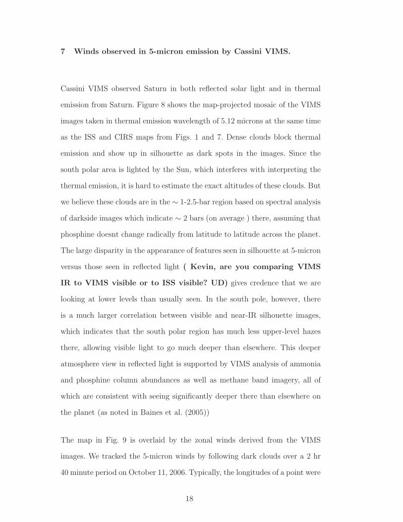
7 Winds observed in 5-micron emission by Cassini VIMS.

Cassini VIMS observed Saturn in both reflected solar light and in thermal

emission from Saturn. Figure 8 shows the map-projected mosaic of the VIMS

images taken in thermal emission wavelength of 5.12 microns at the same time

as the ISS and CIRS maps from Figs. 1 and 7. Dense clouds block thermal

emission and show up in silhouette as dark spots in the images. Since the

south polar area is lighted by the Sun, which interferes with interpreting the

thermal emission, it is hard to estimate the exact altitudes of these clouds. But

we believe these clouds are in the ∼ 1-2.5-bar region based on spectral analysis

of darkside images which indicate ∼ 2 bars (on average ) there, assuming that

phosphine doesnt change radically from latitude to latitude across the planet.

The large disparity in the appearance of features seen in silhouette at 5-micron

versus those seen in reflected light ( Kevin, are you comparing VIMS

IR to VIMS visible or to ISS visible? UD) gives credence that we are

looking at lower levels than usually seen. In the south pole, however, there

is a much larger correlation between visible and near-IR silhouette images,

which indicates that the south polar region has much less upper-level hazes

there, allowing visible light to go much deeper than elsewhere. This deeper

atmosphere view in reflected light is supported by VIMS analysis of ammonia

and phosphine column abundances as well as methane band imagery, all of

which are consistent with seeing significantly deeper there than elsewhere on

the planet (as noted in Baines et al. (2005))

The map in Fig. 9 is overlaid by the zonal winds derived from the VIMS

images. We tracked the 5-micron winds by following dark clouds over a 2 hr

40 minute period on October 11, 2006. Typically, the longitudes of a point were

18

measured 5 times. A linear fit was made to the point, where each point was

weighted by its longitudinal uncertainty. The longitudinal uncertainty is the

longitudinal width spanning ± 0.5 of a pixel. The fit to longitudinal position

changing with time gives a velocity.

Figure 9 shows that the VIMS winds measured above 1-2.5 bars generally

agree with the ISS winds measured at similar or higher altitudes with CB2

(750nm) filter, which probes deeper than ∼300 mbar, see Section 3. The peak

winds near the cyclone’s eyewalls appear to be stronger in VIMS measurements

(193±20 m/s) than in ISS measurements (150±20 m/s). This difference is

barely above the uncertainty of the wind tracking. If the difference is real it

may mean strengthening of the winds with depth (VIMS measurements may

show deeper clouds).

Another group of VIMS points may indicate stronger winds at the depth.

The large-error data points between latitudes -76 and -83 show much higher

speeds of 40-80 m/s than the VIMS points having small error at the same

latitudes, which values are below 20 m/s. The small-error VIMS points are in

perfect agreement with ISS observations, and probably result from tracking the

same clouds as ISS at similar altitudes. The 40-80 m/s points may be tracking

deeper clouds not visible to ISS. It is possible though that this discrepancy

results from uncertainties in VIMS speed measurements ( Tom or Kevin,

please give couple of sentences here explaining the uncertainty and

how much do you trust those data points. Does this idea of clouds

at different levels sound reasonable to you? Ulyana)

19

8 Comparison with vortices on other planets.

Table 1 shows a comparison of the SPV with other vortices in the solar system.

Parameter of comparison SPV Hurricane PV Venus PV Earth GRS/WO Neptune pole

diameter(km) 4200 20-100 2700 1000-2000 10000-40000 <7000

diameter(% of the planet’s radius) 7 0.3-1.5 45 15-30 14-56 <25

lifetime >2 years weeks years seasonal >300 years unknown

max. windspeeds(m s−1) 170-190 85 35 50 120 unknown

temperature anomaly warm warm warm cold cold warm

sense of rotation cyclonic cyclonic cyclonic cyclonic anticyclonic unknown

eyewall clouds yes yes unknown no unknown unknown

fixed polar location yes no yes yes no yes

convective clouds on periphery yes yes no no yes unknown

bounded by rigid surface no yes possibly yes no no

ζ/f 1 100 -100 1 -0.2 unknown

Table 1

Comparison of the Saturn south polar vortex (SPV) with terrestrial hurricanes (An-

thes, 1982; Emanuel, 2003), terrestrial Arctic and Antarctic polar vortices on Earth

(PV Earth) (Holton, 2004), Jupiter’s Great Red Spot and White Ovals (GRS/WO)

(Bagenal, 2001), South polar vortex on Venus (PV Venus) (Piccioni et al., 2007),

and the warm spot at the South Pole of Neptune (Orton et al., 2007). The “diam-

eter” refers to the major axis of the area enclosed within the maximum winds. For

the SPV and terrestrial hurricanes, this is the diameter of the eye. The “unknown”

eyewall clouds may be blocked from the view by higher clouds. The SPV peak winds

are estimated as 170 m/s in ISS observations and as 190 m/s in VIMS observations.

We did not show the North polar vortex on Venus (Taylor et al., 1979), which

is similar to the one at the south (Piccioni et al., 2007).

Terrestrial hurricanes and Venus polar vortex show the most similarities to the

20

SPV, such as cyclonic rotation, warm temperature anomaly, cloudy eyewalls

in the case of hurricane, and polar location in the case of Venus polar vortex.

Because much more is known about terrestrial hurricanes than about the

Venus polar vortices, we compare SPV to the hurricane in more details. A

hurricane (typhoon, tropical cyclone) is a warm-core vortex sustained by en-

thalpy fluxes across the air-sea interface when in-flowing air in the boundary

layer picks up water vapor from the ocean (Palmen and Newton, 1969; An-

thes, 1982; Emanuel, 2003). Saturn and the other giant planets do not have

oceans, although they do have deep, moisture-laden atmospheres below the

clouds which may act in a way similar to the terrestrial ocean interacting with

a hurricane.

A hurricane has a central low pressure at low altitudes that becomes weaker

at high altitudes due to thermal expansion of the air at the center. No direct

measurements of altitude can be done for Saturn’s polar vortex to compare

with this pressure pattern, but t is expected there due to the warm core.

Condensation and release of latent heat are greatest in a ring of clouds sur-

rounding the central eye, which is sometimes clear and sometimes partly cloud

covered. The eye of the SPV is clear at high elevations with a few deep clouds

in it. The eyewall clouds of the hurricane tower two scale heights (vertical

e-folding distance), about 15 km, above the surface. The SPV inner eyewall is

30-70 km tall, which is also about twice the scale height.

Hurricanes dissipate quickly when they leave the ocean and run over the land.

Saturn has no land, vortices usually live longer, and as of June 2008 the SPV

is still observed by Cassini, which shows that it is at least four years old, and

possibly permanent.

21

The central eye of the hurricane, typically 20-100 km in diameter, is warmer

than its surroundings to the height of the tropical tropopause, and has a

cold anomaly above the tropopause. The strongest warm core indicates the

layer of outflow just below the tropopause Emanuel (2003). SPV has a warm

anomaly extending from below to above the tropopause, which may be due to

the radiative heating from the long-lived warm core below. (Leigh, do you

have any estimates of the timescale for heating the region above

Saturnian tropopause? UD) The strongest warm cores of the SPV are

immediately below and above the tropopause (see Fig. 6)

Sometimes hurricanes have multiple concentric eyewalls which contract with

time and get replaced by the outer walls on the timescale of days. SPV’s two

walls are seen throughout the four years of observations.

In a hurricane the winds are greatest in the eyewall and can reach speeds of

85 m s−1. In SPV the winds are also greatest in the eyewall. The peak winds

range from 130 - 170 m s−1, about twice those of a terrestrial hurricane.

In both hurricane and SPV the relative vorticity ζ is large in the eye out to the

eyewall and small in the region beyond, where the tangential velocity decays

to zero. The vorticity at the center of a hurricane is cyclonic - clockwise in the

southern hemisphere and counterclockwise in the northern hemisphere. SPV

is also cyclonic.

The angular momentum in hurricanes decreases toward the center, as in the

SPV (see discussion of Fig. 2 in Section 3). On Earth, rings of air flowing

inward lose angular momentum to the lower boundary and to the outflowing

air above (Palmen and Newton, 1969; Anthes, 1982; Emanuel, 2003). On Sat-

urn there is no lower boundary, and it is possible that deep winds are even

22

stronger than at the observable level (se Section 7). The possible outflowing

air above the SPV may act as a sink for angular momentum similar to the

hurricanes.

Hurricanes are usually surrounded by heavily precipitating clouds. In this re-

spect the small bright clouds around the eye of the SPV (see Fig. 1) are like the

rain bands of a terrestrial hurricane, though rain bands usually form spirals

around the hurricane, which is not the case for the small bright clouds. How-

ever annular hurricanes Knaff et al. (2003), which are long-lived and symmetric

terrestrial hurricanes that form in unusually calm background atmosphere, do

not show spiral rain bands and are probably more similar to the polar vortex

on Saturn.

Hurricanes, Venus polar vortex, and other big planetary vortices in Table 1

display some similarity to the SPV, but there are also differences, and no close

analogue to SPV can be confidently determined.

The warm polar spot on Neptune’s South Pole is of special interest because

it may potentially be such an analogue. A hot spot similar to SPV is recently

discovered on Neptune by Orton et al. (2007). Atmospheric motion at the

pole of Neptune could be similar to Saturn’s because it is also a giant planet

with a deep atmosphere. Although Orton et al. (2007) argue that the hot spot

in Neptune’s troposphere may be due to the seasonal heating (it is in mid-

summer now), the vortex like SPV would also explain the hot spot. Cassini

CIRS measurements show similar hot spot at the north pole of Saturn(Fletcher

et al., 2008). The seasonal heating would not explain this hot spot because the

north pole is now in winter. North pole of Saturn may have a vortex similar

to the one at the south pole. This will be known during Cassini extended

23

mission when the north pole becomes illuminated by the Sun after the August

11, 2009 equinox and the winds can be measured by tracking the clouds.

It is possible that all giant planets have polar vortices but the observations are

so far insufficient for detection. The south pole of Saturn is the first pole of a

giant planet observed at adequate spatial resolution to track the clouds. More

Cassini observations will cover both Saturn’s poles. A spacecraft in a high-

inclination orbit would be needed to observe winds at the poles of Jupiter.

More high-inclination space missions would be needed to observe winds at the

poles of Jupiter, Uranus, and Neptune.

24

Acknowledgements

This research was supported by the NASA Cassini Project.

References

Anthes, R. A., 1982. Tropical Cyclones. Their Evolution, Structure and Ef-

fects. American Meteorological Society.

Bagenal, F. (Ed.), 2001. Jupiter - The Planet, Satellites and Magnetosphere.

Oxford University Press.

Baines, K. H., Drossart, P., Momary, T. W., Formisano, V., Griffith, C., Bel-

lucci, G., Bibring, J. P., Brown, R. H., Buratti, B. J., Capaccioni, F., Cer-

roni, P., Clark, R. N., Coradini, A., Combes, M., Cruikshank, D. P., Jau-

mann, R., Langevin, Y., Matson, D. L., McCord, T. B., Mennella, V., Nel-

son, R. M., Nicholson, P. D., Sicardy, B., Sotin, C., 2005. The Atmospheres

of Saturn and Titan in the Near-Infrared First Results of Cassini/VIMS.

Earth Moon and Planets 96, 119–147.

Dowling, T. E., Ingersoll, A. P., 1989. Jupiter’s Great Red Spot as a shallow

water system. Journal of Atmospheric Sciences 46, 3256–3278.

Dyudina, U. A., Ingersoll, A. P., Ewald, S., Vasavada, A., West, R. A., Del

Genio, A., Barbara, J., Porco, C. C., Achterberg, R., Flasar, F., Simon-

Miller, A., Fletcher, L., 2008. Dynamics of Saturns South Polar Vortex.

Science 319, 1801.

Emanuel, K., 2003. Tropical Cyclones. Ann. Rev. Earth Planet. Sci. 31,

75–104.

Flasar, F. M., Kunde, V. G., Abbas, M. M., Achterberg, R. K., Ade, P.,

Barucci, A., B’ezard, B., Bjoraker, G. L., Brasunas, J. C., Calcutt, S.,

25

Carlson, R., C’esarsky, C. J., Conrath, B. J., Coradini, A., Courtin, R.,

Coustenis, A., Edberg, S., Edgington, S., Ferrari, C., Fouchet, T., Gautier,

D., Gierasch, P. J., Grossman, K., Irwin, P., Jennings, D. E., Lellouch, E.,

Mamoutkine, A. A., Marten, A., Meyer, J. P., Nixon, C. A., Orton, G. S.,

Owen, T. C., Pearl, J. C., Prang’e, R., Raulin, F., Read, P. L., Romani,

P. N., Samuelson, R. E., Segura, M. E., Showalter, M. R., Simon-Miller,

A. A., Smith, M. D., Spencer, J. R., Spilker, L. J., Taylor, F. W., 2004.

Exploring The Saturn System In The Thermal Infrared: The Composite

Infrared Spectrometer. Space Sci. Rev. 115, 169–297.

Fletcher, L. N., Irwin, P. G. J., Orton, G. S., Teanby, N. A., Achterberg, R. K.,

Bjoraker, G. L., Read, P. L., Simon-Miller, A. A., Howett, C., de Kok, R.,

Bowles, N., Calcutt, S. B., Hesman, B., Flasar, F. M., 2008. Temperature

and Composition of Saturn’s Polar Hot Spots and Hexagon. Science 319,

79–82.

Holton, J. R., 2004. An Introduction to Dynamic Meteorology. Elsevier Aca-

demic Press, Amsterdam, ed. 4.

Irwin, P. G. J., Parrish, P., Fouchet, T., Calcutt, S. B., Taylor, F. W., Simon-

Miller, A. A., Nixon, C. A., 2004. Retrievals of jovian tropospheric phos-

phine from Cassini/CIRS. Icarus 172, 37–49.

Knaff, J. A., Kossin, J. P., DeMaria, M., 2003. Annular hurricanes. Weather

and Forecasting 18, 204–223.

Orton, G. S., Encrenaz, T., Leyrat, C., Puetter, R., Friedson, A. J., 2007. Evi-

dence for methane escape and strong seasonal and dynamical perturbations

of Neptune’s atmospheric temperatures. A & A 473, L5–L8.

Orton, G. S., Yanamandra-Fisher, P. A., 2005. Saturn’s Temperature Field

from High-Resolution Middle-Infrared Imaging. Science 307, 696–698.

Palmen, E., Newton, C. W., 1969. Atmospheric Circulation Systems. Aca-

26

demic Press, New York and London.

Piccioni, G., Drossart, P., Sanchez-Lavega, A., Hueso, R., Taylor, F., Wilson,

C., Grassi, D., Zasova, L., Moriconi, M., Adriani, A., Lebonnois, S., Cora-

dini, A., Bezard, B., Angrilli, F., Arnold, G., Baines, K. H., Bellucci, G.,

Benkhoff, J., Bibring, J. P., Blanco, A., Blecka, M. I., Carlson, R. W., Lel-

lis, A. D., Encrenaz, T., Erard, S., adn V. Formisano, S. F., Fouchet, T.,

Garcia, R., Haus, R., Helbert, J., Ignatiev, N. I., Irwin, P., Langevin, Y.,

Lopez-Valverde, M. A., Luz, D., Marinangeli, L., Orofino, V., Rodin, A. V.,

Roos-Serote, M. C., Saggin, B., Stam, D. M., Titov, D., Visconti, G., Zam-

belli1, M., the VIRTIS-Venus Express Technical Team, 2007. South-polar

features on venus similar to those near the north pole. Nature 450 (7170),

637–640.

Porco, C. C., West, R. A., Squyres, S., McEwen, A., Thomas, P., Murray,

C. D., Delgenio, A., Ingersoll, A. P., Johnson, T. V., Neukum, G., Vev-

erka, J., Dones, L., Brahic, A., Burns, J. A., Haemmerle, V., Knowles, B.,

Dawson, D., Roatsch, T., Beurle, K., Owen, W., 2004. Cassini Imaging Sci-

ence: Instrument Characteristics And Anticipated Scientific Investigations

At Saturn. Space Sci. Rev. 115, 363–497.

Sanchez-Lavega, A., Hueso, R., Perez-Hoyos, S., Rojas, J. F., 2006. A strong

vortex in Saturn’s South Pole. Icarus 184, 524–531.

Taylor, F. W., McCleese, D. J., Diner, D. J., 1979. Polar clearing in the venus

clouds observed from the pioneer orbiter. Nature 279, 613 – 614.

Tomasko, M. G., West, R. A., Orton, G. S., Teifel, V. G., 1984. in Saturn,

T. Gehrels, M. S. Matthews, Eds., pp. 150–194. Univ. of Arizona Press,

Tucson, AZ.

Vasavada, A. R., Horst, S. M., Kennedy, M. R., Ingersoll, A. P., Porco, C. C.,

Del Genio, A. D., West, R. A., 2006. Cassini imaging of Saturn: Southern

27

hemisphere winds and vortices. J. Geophys. Res. (Planets) 111, 5004–5017.

28

Fig. 1. Map of the SPV combined as a mosaic of 14 maps produced from individualISS images. Each image was taken in continuum band filter CB2 with the centralwavelength 750 nm (Porco et al., 2004). To reduce the effect of varying solar illu-mination across the image, each image is high-pass filtered at the spatial scale of∼200 km, or ∼0.2 latitude. The map is labeled by West longitude and planetocen-tric latitude. Asterisks show locations of the individual features for which vorticityhas been measured. The value of the vorticity is indicated by the asterisks’ color.The vorticity data are also plotted in Fig. 2 B.

29

Fig. 2. Profiles of zonal velocity (eastward) and cyclonic vorticity (clockwise) aroundSaturn’s south pole. The dashed vertical lines indicate the inner and outer eyewalls.(A) Zonal velocity measured by tracking clouds in a sequence of images over a3-hour period. The asterisks indicate data points taken from automatic trackingat latitudes equatorward from 84.5 South, or from manual feature tracking atlatitudes poleward from 84.5 South. The solid curves are for constant absolutevorticity ζ + f starting at latitude φ0 (values labeled on the curves) with u = 0 andζ = 0 at that point. (B) Relative vorticity ζ. The solid curve is a spline fit to thevelocity data of Fig. 2A. The points are the small white clouds of Fig. 1 marked byasterisks.

30

Fig. 3. A set of the maps showing how the shadow of the cyclone’s eyewall followsthe Sun. The diffuse dark band inside each of the two eyewalls is a shadow castby the eyewall on the clouds inside the eye. The first map is taken on October 11(DOY 284), 2006 at 19h. 42 min 31 s. The time on the maps increases from top tobottom panel and then from left to right, as labeled by the time in hours from thestart of the sequence. The white arrow on each panel shows the direction at whichthe Sun illuminates the planet. The arrow points from the Sun to the illuminatedscene.

31

Fig. 4. Two maps demonstrating how the length of the shadows had been estimated.The left panels show the map, the right planes show the same map with the cycloneeyewalls outlined in black and shadow lengths measured on this image shown inwhite.

32

Fig. 5. Height of the outer (upper panel) and inner (lower panel) walls of the vortex.The height is plotted versus longitude of the wall features in the first image of thesequence (first panel in Fig. 3, or upper panel of Fig. 4). The shadow lengths aretaken from all images from Fig. 3. Then the longitude of the points on the wallcasting the measured shadows is adjusted to account for the zonal velocity of thewall. The zonal velocities are 17 degrees/hr and 20 degrees/hr for the outer andinner walls respectively.

33

Temperature (K)

10

1

136

144

152

160

Anomaly (K)

-2 0

0

0

2

4

-70 -75 -80 -85 -901000

100

96

104

112

120

128136

-70 -75 -80 -85 -90

0 2 4

Planetocentric Latitude

Pre

ssur

e (m

bar)

Fig. 6. Zonal mean temperatures in Saturn’s south polar region derived from CassiniCIRS spectra (left panels) (Fletcher et al., 2008; Flasar et al., 2004; Irwin et al.,2004). The gap between the upper and lower panels arises because the CIRS instru-ment is not sensitive to the 6-70 mbar region. Temperature anomalies (right panels)are calculated by subtracting the zonal mean temperatures at -84 latitude. Thedashed vertical lines indicate the inner and outer eyewalls.

34

Fig. 7. Temperature map at the 100-mbar level (left panel) and temperature map atthe 200-mbar level (right panel) derived from the Cassini CIRS (Flasar et al., 2004)observations taken on October 11, 2006 at spatial resolution of ∼100 km/pixel. Thetemperature is shown in color. The greyscale ISS 750-nm image at the backgroundhad been taken simultaneously with the temperature map.

35

Fig. 8. A diagram that shows VIMS zonal winds overlying an image mosaic of thesouth pole of Saturn. The pole is in the lower left. The dark spots are the cloudsarranged in circular bands around the pole. The abscissa of the wind plot shows thelatitudes as they project on the map. Note that the winds are ”inverted”, with theordinate showing large winds at the bottom and small winds at the top.

36

Fig. 9. Comparison of zonal velocity (eastward) measured by ISS in CB2 filter(asterisks) with velocity measured by VIMS in 5.12 microns (error-bar-style points).The dashed vertical lines indicate the inner and outer eyewalls.

37

Movie captions

Movie 1: A movie combined from 14 maps produced from individual ISS images

taken within approximately 3 hours. Each image was taken in the continuum

band filter CB2 with the central wavelength 750 nm Porco et al. (2004).

Movie 2: A four-step movie combined from the false-color images from light at

889 nm, 727 nm, and 750 nm projected as blue, green, and red, respectively.

Images are taken within approximately 2 hr 20 min during the October 11,

2006 ISS observation.

38