hep-th/9901098

N = 1 supersymmetric SU(4)× SU(2)L × SU(2)R effective theoryfrom the weakly coupled heterotic superstring

G.K. Leontaris and J. Rizos

Physics Department, University of IoanninaIoannina, GR45110, GREECE

Abstract

In the context of the free–fermionic formulation of the heterotic superstring, we constructa three generation N = 1 supersymmetric SU(4)×SU(2)L×SU(2)R model supplementedby an SU(8) hidden gauge symmetry and five Abelian factors. The symmetry breaking tothe standard model is achieved using vacuum expectation values of a Higgs pair in (4, 2R)+(4, 2R) at a high scale. One linear combination of the Abelian symmetries is anomalousand is broken by vacuum expectation values of singlet fields along the flat directions of thesuperpotential. All consistent string vacua of the model are completely classified by solvingthe corresponding system of F− and D−flatness equations including non–renormalizableterms up to sixth order. The requirement of existence of electroweak massless doubletsfurther restricts the phenomenologically viable vacua. The third generation fermions receivemasses from the tree–level superpotential. Further, a complete calculation of all non–renormalizable fermion mass terms up to fifth order shows that in certain string vacua thehierarchy of the fermion families is naturally obtained in the model as the second and thirdgeneration fermions earn their mass from fourth and fifth order terms. Along certain flatdirections it is shown that the ratio of the SU(4) breaking scale and the reduced Planckmass is equal to the up quark ratio mc/mt at the string scale. An additional prediction ofthe model, is the existence of a U(1) symmetry carried by the fields of the hidden sector,ensuring thus the stability of the lightest hidden state. It is proposed that the hidden statesmay account for the invisible matter of the universe.

January 1999

1 Introduction

During the last decade, a lot of work has been devoted in the construction of effective lowenergy models of elementary particles from the heterotic superstring. Several old successfulN = 1 supersymmetric grand unified theories (GUTs) have been recovered through thestring approach [1, 2, 3, 4, 5, 6], however only few of them were able to rederive a numberof successful predictions of their predecessors. Yet, new avenues and radical ideas that werepreviously not considered or only poorly explored, have now been painstakingly investigatedin the context of string derived or even string inspired effective theories. Among them,the issue of the additional U(1)–symmetries which naturally appear in string models andthe systematic derivation of non–renormalizable terms boosted our understanding of theobserved mass hierarchies and impelled people to systematically classify all possible texturesconsistent with the low energy phenomenology. Further, new and astonishingly simplermechanisms of GUT symmetry breaking were introduced due to the absence of large Higgsrepresentations, at least in the simplest Kac–Moody level (k = 1) string constructions.

In addition to the above good omen, some embarrassing difficulties have also appeared,such as the existence of unconfined fractionally charged states – which belong to repre-sentations not incorporated in the usual GUTs – and the very high unification scale. Thenew representations come as a result of the breaking of the large string symmetry via theGSO projections. The appearance of such states are not necessarily an ominous warningfor a particular model, although a mechanism should be invented to make them disappearfrom the light spectrum. The real major difficulty however, was the generic property of thehigh string scale in contrast to the usual supersymmetric GUTs which unify at about twoorders of magnitude below the string mass. In the weakly coupled heterotic string theory,this problem can find a solution in specific models, when extra matter multiplets exist toproperly modify the running of the gauge couplings, or possible intermediate symmetriesand string threshold effects [7] can help gauge couplings converge to their experimentallydetermined values at low energies.

In this paper, we derive an improved version of a string model proposed in [5], based onthe observable gauge symmetry SO(6)× O(4) (isomorphic to SU(4) × SU(2)L × SU(2)RPati–Salam (PS) gauge group [8]) in the context of the free–fermionic formulation of thefour dimensional superstring. As shown in [4] this gauge symmetry breaks down to thestandard model without the use of the adjoint or any higher representation thus it can bebuilt directly at the k = 1 Kac–Moody level. (Higher Kac–Moody level models are alsopossible to build, however, they imply small unification scale values of sin2 θW [9].)

The models based on the PS gauge symmetry have also certain phenomenological ad-vantages. Among them, is the absence of coloured gauge fields mediating proton decay.This fact allows for the possibility of having a low SU(4) breaking scale compared to thatof other GUTs, provided that the Higgs coloured fields do not have dangerous Yukawa cou-plings with ordinary matter. Possible ways to avoid fast proton decay have been discussedalso recently in the literature [10].

Moreover, specific GUT relations among the Yukawa couplings, like the bottom–tauequality, give successful predictions at low energies, while at the same time such relations

1

reduce the number of arbitrary Yukawa couplings even in the field–theory version.

The above nice features are exhibited in the present string construction. Using a variantof the original string basis and the GSO projection coefficients [5], we obtain an effectivefield theory model with three generations and exactly one Higgs pair to break the SU(4)×SU(2)R gauge symmetry. The effective low energy theory is the N = 1 supersymmetricSU(3) × SU(2) × U(1) electroweak standard gauge symmetry broken to SU(3) × U(1)emby the two Higgs doublet fields. We derive the complete massless spectrum of the modeland the Yukawa interactions including non–renormalizable terms up to sixth order. Amongthe massless states, a mirror (half)–family is also obtained which acquires mass at a verylarge scale. There are also singlet fields and exotic doublet representations with a sufficientnumber of Yukawa couplings. All the observable and hidden fields appear with chargesunder five surplus U(1) factors where one linear combination of them is anomalous. Theanomalous U(1) symmetry generates a D–term contribution, which can be cancelled ifsome of the singlet fields acquire non–zero vacuum expectation values (vevs). To find thetrue vacua, we solve the F− and D−flatness conditions and classify all possible solutionsinvolving observable fields with non–zero vevs. We analyze in detail three characteristiccases where superpotential contributions up to sixth order suffice to provide fermion massterms for all generations. Phenomenologically interesting alternative solutions are alsoproposed in the case where some of the hidden fields develop vevs too.

Among the novel features of the present model is the existence of a U(1) symmetry –carried by hidden and exotic fields – which remains unbroken. As a consequence, the lightesthidden state is stable. These states form various potential mass terms in the superpotentialof the model. In our analysis, we show the existence of proper flat directions where thelightest state obtains a mass at an intermediate scale, leading to interesting cosmologicalimplications.

The paper is organized as follows: In Section 2 we give a brief description of the super-symmetric version of the model and discuss various phenomenological features, includingthe economical Higgs mechanism, the mass spectrum and the renormalization group. Inparticular we show how the Pati–Salam symmetry dispenses with the use of Higgs fields inthe adjoint of SU(4) to break down to the standard model. In Section 3, we propose thestring basis as well as the GSO projections which yield the desired gauge symmetry andthe massless spectrum. In Section 4 the gauge symmetry breaking of the string versionis analyzed. Moreover, due to the existence of additional U(1) symmetries, the issue ofnew (non–standard) hypercharge embeddings is discussed. Particular embeddings whereall fractionally charged states obtain integral charges are discussed in some detail. In Sec-tion 5 we derive the superpotential couplings and present a preliminary phenomenologicalanalysis to set the low energy constraints and reduce the number of phenomenologicallyacceptable string vacua. In Section 6 we classify all solutions of the F– and D–flatnessequations including non–renormalizable superpotential contributions up to sixth order. Adetailed phenomenological analysis of the promising string vacua in connection with theirlow energy predictions is presented in Section 7. Particular attention is given in the dou-blet higgs mass matrix, the fermion mass hierarchy and the colour triplet mass matrix.In Section 8, we present a brief discussion on the role of the hidden sector and extend

2

the solutions of string vacua including hidden field vevs. Finally, in the Appendices A–Dwe present tables with the complete string spectrum, details about the derivation of thehigher order non–renormalizable superpotential terms, the D– and F– flatness equationswith non-renormalizable contributions and the complete list of their tree–level solutions.

2 The Supersymmetric SU(4)× SO(4) Model

There is a minimal supersymmetric SU(4) × O(4) Model which can be considered as asurrogate effective GUT of the possible viable string versions, incorporating all the basicfeatures of a phenomenologically viable string model. The Yukawa couplings are determinedby the Pati–Salam (PS) gauge symmetry and possible additional U(1)–family symmetrieswhich are usually added (as in any other GUT) by phenomenological requirements, (i.e.,fermion mass hierarchy, proton stability etc). This GUT version, however, provides uswith insight in constructing the fully realistic string version. Therefore, here we brieflysummarize the parts of the model relevant for our analysis [4]. The gauge group is SU(4)×O(4), or equivalently the PS gauge symmetry [8]

SU(4)× SU(2)L × SU(2)R. (1)

The left–handed quarks and leptons are accommodated in the following representations,

F iαaL = (4, 2, 1) =

(uα νdα e

)i(2)

F ixαR = (4, 1, 2) =

(dcα ec

ucα νc

)i(3)

where α = 1, . . . , 4 is an SU(4) index, a, x = 1, 2 are SU(2)L,R indices, and i = 1, 2, 3 is afamily index. The Higgs fields are contained in the following representations,

hxa = (1, 2, 2) =

(h+

u h0d

h0u h−

d

)(4)

where hd and hu are the low energy Higgs superfields associated with the minimal super-symmetric standard model (MSSM). The two ‘GUT’ breaking higgs representations are

Hαb = (4, 1, 2) =

(uαH νHdαH eH

)(5)

and

Hαx = (4, 1, 2) =

(ucαH ecHucαH νcH

). (6)

Fermion generation multiplets transform to each other under the changes 4 → 4 and2L → 2R while the bidoublet higgs multiplet transforms to itself. However, the pair of

3

fourplet–higgs fields does not have this property, discriminating 2L and 2R. Thus, whenthey develop vevs along their neutral components νH , ν

cH ,

〈H〉 = 〈νH〉 ∼MGUT , 〈H〉 = 〈νcH〉 ∼MGUT (7)

they break the SU(4) × SU(2)R part of the gauge group, leading to the standard modelsymmetry at MGUT

SU(4)× SU(2)L × SU(2)R −→ SU(3)C × SU(2)L ×U(1)Y . (8)

Under the symmetry breaking in Eq. (8), the bidoublet Higgs field h in Eq. (4) splits intotwo Higgs doublets hu, hd whose neutral components subsequently develop weak scale vevs,

〈hd0〉 = v1, 〈hu0〉 = v2 (9)

with tan β ≡ v2/v1.

In addition to the Higgs fields in Eqs. (5),(6) the model also involves an SU(4) sextetfield D = (6, 1, 1) and four singlets φ0 and ϕi, i = 1, 2, 3. φ0 is going to acquire a vevof the order of the electroweak scale in order to realize the Higgs doublet mixing, whileϕi will participate in an extended ‘see–saw’ mechanism to obtain light majorana massesfor the left–handed neutrinos. Under the symmetry property ϕ1,2,3 → (−1) × ϕ1,2,3 andH(H) → (−1) ×H(H) the tree–level mass terms of the superpotential of the model read[4]:

W = λij1 FiLFjRh+ λ2HHD + λ3HHD + λij4 HFjRϕi + µϕiϕj + µhh (10)

where µ = 〈φ0〉 ∼ O(mW ). The last term generates the higgs mixing between the two SMHiggs doublets in order to prevent the appearance of a massless electroweak axion. Thefollowing decompositions take place under the symmetry breaking (8):

FL(4, 2, 1) → Q(3, 2,−1

6) + `(1, 2,

1

2)

FR(4, 1, 2) → uc(3, 1,2

3) + dc(3, 1,−1

3) + νc(1, 1, 0) + ec(1, 1,−1)

H(4, 1, 2) → ucH(3, 1,2

3) + dcH(3, 1,−1

3) + νcH(1, 1, 0) + ecH(1, 1,−1)

H(4, 1, 2) → uH(3, 1,−2

3) + dH(3, 1,

1

3) + νH(1, 1, 0) + eH(1, 1, 1)

D(6, 1, 1) → D3(3, 1,1

3) + D3(3, 1,−1

3)

h(1, 2, 2) → hd(1, 2,1

2) + hu(1, 2,−1

2)

where the fields on the left appear with their quantum numbers under the PS gauge sym-metry, while the fields on the right are shown with their quantum numbers under the SMsymmetry.

The superpotential Eq. (10) leads to the following neutrino mass matrix [4]

Mν,νc,ϕ =

0 miju 0

mjiu 0 MGUT

0 MGUT µ

(11)

4

in the basis (νi, νcj , ϕk). Diagonalization of the above gives three light neutrinos with masses

of the order µ(miju /MGUT )2 as required by the low energy data, and leaves right–handed

majorana neutrinos with masses of the order MGUT . Additional terms not included inEq. (10) may be forbidden by imposing suitable discrete or continuous symmetries [11, 12]which, in fact, mimic the role of various U(1) factors and string selection rules appearing inrealistic string models. The sextet field D(6, 1, 1) carries colour, while after the symmetrybreaking it decomposes in a triplet/triplet–bar pair with the same quantum numbers ofthe down quarks. Now, the terms in Eq. (10) HHD and HHD combine the uneaten(down quark–type) colour triplet parts of H , H with those of the sextet D into acceptableGUT–scale mass terms [4]. When the H fields attain their vevs at MGUT ∼ 1016 GeV,the superpotential of Eq. (10) reduces to that of the MSSM augmented by right-handedneutrinos. Below MGUT the part of the superpotential involving matter superfields is just

W = λijUQiucjh2 + λijDQid

cjh1n+ λijE`ie

cjh1 + λijNLiν

cjh2 + · · · (12)

The Yukawa couplings in Eq. (12) satisfy the boundary conditions

λij1 (MGUT ) ≡ λijU (MGUT ) = λijD(MGUT ) = λijE(MGUT ) = λijN(MGUT ). (13)

Thus, Eq. (13) retains the successful relation mτ = mb at MGUT . Moreover from therelation λijU (MGUT ) = λijN(MGUT ), and the fourth term in Eq. (10), through the see–sawmechanism we obtain light neutrino masses which satisfy the experimental limits. The U(1)symmetries imposed by hand in this simple construction play the role of family symmetriesU(1)A, broken at a scale MA > MGUT by the vevs of two SU(4)×O(4) singlets θ, θ, carryingcharge under the family symmetries and leading to operators of the form

Oij ∼ (FiFj)h

(HH

M2

)r (θnθm

M ′n+m

)+ h.c. (14)

obtained from non–renormalizable (NR) contributions to the superpotential. Here, M ′

represents a high scale M ′ > MGUT which may be identified either with the U(1)A breakingscale MA or with the string scale Mstring. Such terms have the task of filling in the entriesof fermion mass matrices, creating textures with a hierarchical mass spectrum and mixingeffects between the fermion generations.

Before we proceed to the construction of a particular string model let us examine howa three–generation SU(4)× SU(2)L × SU(2)R model can be realized. As we have alreadyexplained the fermion generations are accommodated in FL(4, 2, 1) + FR(4, 1, 2) whilethe Higgs fields are accommodated in FR(4, 1, 2) + FR(4, 1, 2) representations. In thefree–fermionic formulation the SU(2)L × SU(2)R is realized as O(4) and the 2L and 2Rrepresentations are the two spinor representations (2±) of O(4). Calling n+, n−, n+, n− thenumber of (4, 2+), (4, 2−),(4, 2+) and (4, 2−) representations we come to the conclusionthat one minimal three generation model is obtained for

~nmin = (n+, n−, n+, n−) = (3, 1, 0, 4)

where 2L is identified with 2+. A mirror minimal model can be obtained by interchangingthe two SU(2)’s, i.e. L↔ R, and identifying 2+ ∼ 2R

~nmin = (n+, n−, n+, n−) = (1, 3, 4, 0).

5

Furthermore, one can consider the existence of vector–like states that do not affect thenet number of generations since, in principle they can obtain superheavy masses. Thus ageneral three–generation SU(4)×SU(2)L×SU(2)R model corresponds to one the followingvectors

~nrs = (n+, n−, n+, n−) = (3 + r, 1 + s, r, 4 + s) , r, s = 0, 1, . . .

or~nrs = (n+, n−, n+, n−) = (1 + s, 3 + r, 4 + s, r) , r, s = 0, 1, . . .

We can rewrite the above relations in a more compact form

n+ + n− = n+ + n− = 4 + p, p = 0, 1, 2, . . .

n+ − n+ = n− − n− = ±3 (15)

Thus, there exist an infinity of three–generation SU(4)×O(4) ∼ SU(4)×SU(2)L×SU(2)Rmodels each of them uniquely characterized by an integer (p) related to the differences (15)and a sign (±). We will therefore refer to a particular model using the notation k± that isthe two minimal models will be referred as 0+ and 0−.

As stressed in the introduction, one severe problem that has to be resolved in a candidatestring model is the discrepancy between the unification scale as this is found when theminimal supersymmetric spectrum is considered, and the two orders higher string scaleimplied by theoretical calculations. In previous works, it was shown that this difficultymay be overcome in several ways [13, 14]. In particular, the class of string models as thatof Ref. [5] predict additional matter fields which can help the couplings merge at the highstring scale without disturbing the low energy values of sin2 θW and αs. Perhaps the mostelegant way to achieve this, is to make the couplings run closely from the string to thephenomenological unification scale MU ∼ 1016GeV. As a first step one may add the mirrorfields [14]

M = (4, 2, 1); M = (4, 2, 1) (16)

which guarantee the equality of the SU(2)L and SU(2)R gauge couplings gL = gR betweenthe two scales. According to the classification proposed to the previous paragraph, thismodel is classified as 1+ or 1−. The running of the SU(4) coupling can be adjusted byan additional number of extra colour sextets which are in general available in the stringversions of the present model. Indeed, with three generations and denoting collectively thenumber of fourplet sets with n4 the beta functions now become

b2L ≡ b2R = −1− 4n4; b4 = 6− n6 − 4n4 (17)

which show that a sufficient number of sextet fields may guarantee a g4 running almostidentical with that of gL,R. The string model we are proposing in the next section hasexactly one mirror pair and four sextet fields, whereas additional exotic states may alsocontribute to the beta functions if they remain in the light spectrum.

The introduction of the mirror representations (16) leads to the existence of anothersymmetry in the model: we observe that the whole spectrum now is completely symmetric

6

with respect to the two SU(2)’s in the sense that under the simultaneous change 2L ↔ 2Rand the 4 ↔ 4 of SU(4), it remains invariant. More precisely, under this symmetry therepresentations of the model are mapped as follows

FR ↔ FL

H, H ↔ M,M (18)

D, h, φi ↔ D, h, φi

This symmetry persists also in the present string model, while tree–level as well as higherorder Yukawa interactions are also invariant under these changes. As we will see, thissymmetry is broken by the vacuum which will be determined by the specific solutions ofthe flatness conditions.

After the above short description, we are ready to present the string derived modelwhere most of the above features appear naturally. In addition, novel predictions willemerge such as the appearance of exotic states with charges which are fractions of those ofordinary quarks and leptons, a hidden ‘world’ and a low energy U(1) symmetry.

3 The String Model

In the four dimensional free–fermionic formulation of the heterotic superstring, fermionicdegrees of freedom on the world sheet are introduced to cancel the conformal anomaly. Theright–moving non–supersymmetric sector in the light–cone gauge contains the two trans-verse space–time bosonic coordinates Xµ and 44 free fermions. The supersymmetric leftmoving sector, in addition to the space–time bosons Xµ and their fermionic superpartnersψµ includes also 18 real free fermions χI , yI , ωI (I = 1, ..., 6) among which supersymmetryis non–linearly realized. The world–sheet supercurrent is

TF = ψµ∂Xµ +∑I

χI yIωI (19)

Then, the theory is invariant under infinitesimal super–reparametrizations of the world–sheet as the conformal anomaly cancels separately in each sector. Each world–sheetfermion fi is allowed to pick up a phase αfi

ε(−1, 1] under parallel transport around anon–contractible loop of the world–sheet

fi → −eıπαfifi (20)

A spin structure is then defined as a specific set of phases for all world–sheet fermions,

α = [αfr1, αfr

2, . . . , αfr

k;αfc

1, αfc

2, . . . , αfc

l] (21)

where r stands for real, c for complex and k + 2l = 64. For real fermions the phases αfri

have to be integers while αψµ is independent of the space–time index µ.

The partition function is then defined as a sum over a set of spin structures (Ξ)

Z(τ) ∝ ∑α,β∈Ξ

c

(αβ

)Z

(αβ

), (22)

7

where Z(αβ

)is the contribution of the sector with boundary conditions α, β along the two

non–contractible circles of the torus and c(αβ

)a phase related to the GSO projection. Both

Ξ and c(αβ

)are subject to string constraints which guarantee the consistency of the theory.

A string model in the context of free fermionic formulation of the four–dimensionalsuperstring is constructed by specifying a set of n basis vectors 1 (b0 = 1, b1, b2, . . . , bn−1)

of the form (21) (which generate Ξ =∑imibi) and a set of n(n−1)

2+ 1 independent phases

c(bibj

). Once a consistent set of basis vectors and a choice of projection coefficients is

made, the gauge symmetry, the massless spectrum and the superpotential of the theoryare completely determined. In particular, the massless states of a certain sector α =(αL;αR) ∈ Ξ are obtained by acting on the vacuum |0〉α with the bosonic and fermionicmode operators. The massless states (M2

L = M2R = 0) are found by the Virassoro mass

formula

M2L = −1

2+αL · αL

8+∑f

frequencies

M2R = −1 +

αR · αR8

+∑f

frequencies

where the sum is over the oscillator frequencies

νf =1 + αfi

2+ integer, νf∗ =

1− αfi

2+ integer (23)

The physical states are obtained after the application of the GSO projections demanding(eıπbiFα − δαc

∗(α

bi

))|physical state〉α = 0 (24)

where δα = −1 if ψµ is periodic in the sector α and δα = +1 when ψµ is antiperiodic. Theoperator biFα is

biFα =

∑f∈left

− ∑f∈right

bi(f)Fα(f) (25)

where Fα(f) is the fermion number operator counting each fermion mode f once and itscomplex conjugate f ∗ minus once. It should be remarked that in the sector where all thefermions are antiperiodic there is always a state |µ, ν〉 = Ψµ

−1/2(∂X)ν−1 |0〉0 which survivesall projections and includes the graviton, the dilaton and the two–index antisymmetrictensor.

The present string model is defined in terms of nine basis vectors {S, b1, b2, b3, b4, b5, b6, α,ζ} and a suitable choice of the GSO projection coefficient matrix. The resulting gauge grouphas a Pati–Salam (SU(4)× SU(2)L× SU(2)R) non–Abelian observable part, accompanied

1By 1 we denote the vector where all fermions are periodic.

8

by four Abelian (U(1)) factors and a hidden SU(8) × U(1)′ symmetry. The nine basisvectors are the following

ζ = { ; Φ1...8}S = {ψµ, χ1...6, ; }b1 = {ψµ, χ12, (yy)3456, ; Ψ1...5, η1}b2 = {ψµ, χ34, (yy)12, (ωω)56 ; Ψ1...5, η2}b3 = {ψµ, χ56, (ωω)1234 ; Ψ1...5, η3}b4 = {ψµ, χ12, (yy)36, (ωω)45 ; Ψ1...5, η1}b5 = {ψµ, χ34, (yy)26, (ωω)15 ; Ψ1...5, η2}b6 = { ; Ψ1...5, η123, Φ1...4}α = { (yy)36, (ωω)36ω24 ; Ψ123, η23, Φ45}

(26)

The specific projection coefficients we are using are given in terms of the exponent coeffi-cients cij in the following matrix

cij =

z S b1 b2 b3 b4 b5 b6 α

z 1 1 1 1 1 1 1 0 0S 1 0 0 0 0 0 0 1 1b1 1 1 1 1 1 1 1 1 1b2 1 1 1 1 1 1 1 1 1b3 1 1 1 1 1 1 1 1 1b4 1 1 1 1 1 1 1 1 1b5 1 1 1 1 1 1 1 1 0b6 0 1 0 0 0 0 0 0 0α 1 1 1 1 1 1 0 1 1

(27)

where the relation of cij with c(bi, bj) is

c

(bibj

)= eıπcij

All world–sheet fermions appearing in the vectors of the above basis are assumed to have pe-riodic boundary conditions. Those not appearing in each vector are taken with antiperiodicones. We follow the standard notation used in references [3, 5]. Thus, ψµ, χ1...6, (y/ω)1...6 arereal left, (y/ω)1...6 are real right, and Ψ1...5η123Φ1...8 are complex right world sheet fermions.In the above, 1 = b1 + b2 + b3 + ζ and the basis element S plays the role of the supersym-metry generator as it includes exactly eight left movers. Further, b1,2,3 elements reduce theN = 4 supersymmetries into N = 1, while the initial O(44) symmetry of the right–movingsector results to an observable SO(10) × SO(6) gauge group at this stage. The SO(10)part corresponds to the five Ψ1...5 complex world sheet fermions while all chiral families atthis stage belong to the 16 representation of the SO(10). Vectors b4,5 reduce further thesymmetry of the left moving sector, while the introduction of the vector b6 deals with thehidden part of the symmetry. Finally, the choice of the vector α determines the final gaugesymmetry (observable and hidden sector) of the model which is

SU(4)× O(4)× U(1)4 × {U(1)′ × SU(8)}hidden. (28)

9

The observable gauge group consists of the non–Abelian SO(6) × O(4) symmetry whichis isomorphic to the left–right Pati–Salam symmetry [8]. There are also four U(1)i=1,...,4

factors related to η1,2,3-complex and the ω24-real pair of world–sheet fermions of the right–moving sector. All the superfields of the observable sector carry non–zero charges underthese four U(1) symmetries. Therefore, the latter are expected to play a very importantrole in the determination of the Yukawa couplings, the fermion mass textures, R-parityviolation and in general in all types of Yukawa interactions of the model. We note herethat the observable fields do not carry charges under U(1)′.

The Abelian part of the group deserves a separate treatment since this class of modelsin general possess U(1) symmetries which are anomalous. Indeed, while we find two ofthe U(1) factors to be traceless TrU(1)1 = TrU(1)′ = 0, the other three are traceful, withTrU(1)2 = TrU(1)3 = TrU(1)4 = 24. However, the U(1) charges can be defined in such away that only one combination is anomalous. Indeed, the linear combination

U(1)A = U(1)2 + U(1)3 + U(1)4, (29)

has TrU(1)A = 72, while there are other three combinations orthogonal to the one above,which are free of gauge and gravitational anomalies. These are,

U(1)1 = U(1)1

U(1)2 = U(1)2 − U(1)3 (30)

U(1)2 = U(1)2 + U(1)3 − 2U(1)4.

The choice of the projection coefficients shown in (27) has led to the desired threegeneration model as well as some refinements of the previously proposed theory [5] whichare phenomenologically appealing and deserve some discussion. The most important are,the new Yukawa couplings which give fermions masses, the mirror symmetry of the masslessspectrum and the number of SU(4) Higgs multiplets.

We start with the enumeration of representations candidates for families and SU(4)×SU(2)R breaking Higgs fields as they appear in Appendix A. We first note that due tothe presence of the various U(1)-factors, there is an arbitrariness in the embedding of theelectromagnetic charge operator. We will discuss this in detail in the end of this section,however, to start with, we assume first the simplest case where U(1)em is defined in thestandard way, (as in the original PS–symmetry), i.e:

Y =1√6T4 +

1

2TL +

1

2TR (31)

where T6, TL, TR are the diagonal SU(4), SU(2)L and SU(2)R generators respectively. Then,the massless spectrum is classified with respect to its group properties as follows:

• There are three copies of [(4, 2, 1) + (4, 1, 2)] representations, available to accommo-date the three generations.

• There is one [(4, 1, 2)+(4, 1, 2)] pair which is interpreted as the Higgs pair triggeringthe SU(4)× SU(2)R breaking.

10

• One pair [(4, 2, 1) + (4, 2, 1)], (mirror to each other) replaces the second Higgs pairof the old string version [5]. Clearly, since there are no mirror families observed inthe light spectrum, they should decouple at some high scale by forming a heavy massstate.

• There are a large number of singlet fields with zero electric charge, while carryingquantum numbers under the four U(1) factors. In the determination of the flatdirections of the model, their vevs have to be chosen in such a way so as to cancel theD–term. These singlets couple to ordinary matter via superpotential terms. Whenthey develop vevs along certain flat directions they may create a hierarchical fermionmass spectrum through non–renormalizable couplings.

• There are eight hidden SU(8)-octet and octet–bar superfields (charged under theU(1)4 × U(1)′), which are also neutral under the usual charge definition. They canalso acquire non–zero vevs leading to additional mass terms for ordinary or exoticmatter fields.

• The exotic states of the model fall into two categories:i) There are two SU(4) fourplets H4 = (4, 1, 1), H4 = (4, 1, 1). After the symmetrybreaking, they result to a 3 and 3 pair with charges ±1

6respectively and two singlets

with charges ±12.

ii) The second kind of exotic fields includes ten left–handed doublets XiL and anequal number of right–handed ones XiR with charges ±1

2. The presence of exotic

particles in the massless spectrum of the theory is a generic feature of level k = 1string constructions. Such states in general, are regarded as string models’ “Achillesheel” since it is likely that they remain in the light spectrum down to the electroweakscale. There are mainly three solutions to this problem : first, one may choose asuitable flat direction where all of them become massive at a relatively large scale; asa second possibility, one can properly modify the string boundary conditions on thebasis vectors, so that these states appear with non–trivial transformation propertiesunder a hidden non–Abelian group. In this latter case the exotic states are confined atthe scale where the gauge coupling of the hidden group becomes strong [15]. Clearly,for a given number of matter representations, the higher the rank of the group, thelarger the confinement scale. As a third possibility, one may consider the modificationof the charge operator (31) by the inclusion of additional U(1) factors. In the presentconstruction, we will discuss in some detail the last two possibilities. Later, we willgive a brief account for their possible relevance on recent cosmological observations.

Let us point out here that the observable spectrum of the model respects the symmetrydiscussed in Section 2 with respect to the simultaneous interchanges 2L ↔ 2R and 4 ↔ 4.In particular, left handed generation superfields are interchanged with right handed ones,while there is a similar change of roles of the SU(4) higgs and mirrors. We will also see inthe following sections that the tree–level and higher order Yukawa interactions remain alsounaltered under the above interchanges. The above symmetry is broken however, by thevacuum when consistent F– and D–flatness solutions are found. We will discuss this when

11

the superpotential of the theory is presented and the corresponding flatness conditions arederived in the next sections.

4 Symmetry breaking and hypercharge embedding in

the string model.

We will discuss now two related issues, the gauge symmetry breaking pattern and thevarious consistent embeddings of the weak hypercharge. After defining the consistent setof boundary conditions (26) described previously, one is left with an effective theory basedon the symmetry (28) with the following general characteristics. There is an effectiveunification scale, namely the string scale Mstring, where all couplings – up to thresholdcorrections – attain a common value. At this point one is left with an effective N = 1supergravity theory while the gauge group structure is of the form G =

∏nGn, containing

an ‘observable’ and a ‘hidden’ part. The two worlds are not completely decoupled. Hiddenand observable fields are charged under five Abelian factors. The first symmetry breakingoccurs when some of the singlet fields acquire vevs to cancel the D–term. Depending ofthe choice of the singlet vevs several (at most four) of the above U(1)’s break, the naturalbreaking scale MA being of the order of the D−term, i.e,

MA ∼√ξ

=

√TrQA

192

gstringπ

MP l =

√3

2πgstringMP l (32)

where TrQA = 72 is the trace of the anomalous U(1)A and MP l ≈ 4.2 × 1018GeV is thereduced Planck mass. We note here that, if only the singlets were allowed to obtain a non–vanishing vev, at most four of the U(1)’s break; no singlet is charged under the Abeliansymmetry U(1)′ which remains unbroken at this stage. The observable part SU(4) ×SU(2)L × SU(2)R has a rank larger than that of the MSSM symmetry, which breaksdown to the SM–gauge group at an intermediate scale MGUT , usually some two orders ofmagnitude below the string scale. The breaking occurs in the way described in Section2. The necessity of the SU(4) × SU(2)R symmetry breaking together with the D− andF–flatness conditions require at least two of the U(1) factors to break at a high scale.

There is finally the hidden SU(8) part. This symmetry stays intact, as long as the 8and 8 fields do not acquire vevs. Note also that the octets are charged under U(1)′. Inmany flat directions which will be discussed subsequently, phenomenological requirementsforce some of the octets to obtain vevs and the symmetry SU(8)×U(1)′ breaks to a smallerone. Now, a crucial observation (see the relevant Table in the Appendix A) is that all 8’scome with U(1)′ positive charge (+1) whilst all 8’s appear with the opposite (−1) charge.It is easy to show then, that, no matter how many of the available octet fields receive anon–zero vev, there is always a U(1)′′ unbroken which is a linear combination of the U(1)′

and one of the generators of the SU(8). Therefore, the hidden matter conserves a newU(1)′′ symmetry which stays unbroken down to low energies. Its cosmological implicationswill be discussed in a subsequent section.

12

ω sin2 θW0 3

8

1 322

Table 1: The values of the weak mixing angle at the Unification scale, for two definitionsof the weak hypercharge. In the second case, an additional U(1)-factor is assumed.

We turn now our discussion to the hypercharge embedding. As mentioned above, dueto the appearance of extra U(1)–factors, the hypercharge generator is not uniquely de-termined. It can be any linear combination of the U(1)B−L the five available U(1)’s ofthe model and possible unbroken generators of the hidden gauge symmetry, provided theminimal supersymmetric low energy particle spectrum is generated. The standard weakhypercharge assignment – as this is defined in the original PS–symmetry – does not in-volve any of the surplus U(1) factors discussed above. It is solely determined in the usualsense from the diagonal generators of the PS–symmetry as in (31). Under this definitionin addition to the representations accommodating the MSSM–fields, the states found in(4, 1, 1) + (4, 1, 1) and (1, 1, 2) + (1, 2, 1) representations obtain the exotic charges dis-cussed above, while they are rather unusual in the grand unified models.

We will discuss here in some detail another possible definition of the hypercharge oper-ator which is obtained by including the U(1)′-generator:

Y ′ =1√6T4 +

1

2TL +

1

2TR − ω

2Q′ (33)

where Q′ is related to the U(1)′ charge of the particular massless state and ω is the appro-priate normalization constant. Choosing for example ω = 1, all extra doublets XL,R obtainintegral charges (±1, 0). On the other hand, this new embedding leads to the normalizationof the hypercharge generator

k =5 + 12ω2

3. (34)

The value of the weak mixing angle at Mstring is sin2 θW (Mstring) = 11+k

. Its values for

the two lower ω’s are given in Table 1. For ω = 0, we obtain the standard GUT sin2 θWprediction but the exotic states have fractional charges, whereas for ω = 1 theXL,R doubletsas well as the (4, 1, 1) and (4, 1, 1) representations, obtain charges like those of the ordinarydown quarks and leptons. It should not escape our attention that in this new hyperchargedefinition Y ′ the octet fields now appear with fractional charges ±1/2. This is not howevera real problem. The coupling of the SU(8) group becomes strong at a high scale, leadingto a confinement (in close analogy with QCD), and forcing the octets to form boundstates with the corresponding octet–bar fields. We should note here that this situationopens up the possibility of giving vevs to these condensates at a smaller scale and createnew mass terms for the ordinary matter through their superpotential couplings. The newhypercharge definition predicts a low value for the weak mixing angle which is essentiallythe value obtained in a Kac–Moody level k = 2 string construction [9]. Starting however,

13

from such a small initial value for sin2 θW at Mstring, there is no obvious way how the largerlow energy value can be obtained in this case.

Let us close this section with a short comment on one more possibility of symmetrybreaking. One can give vevs directly to the exotic SU(2)R-doublet fields XiR. (Boththeir components are charged (Qem = ±1/2) under the standard hypercharge assignment(31)). The vev should be taken along the neutral direction defined by the proper linearcombination. This will essentially lead to a definition of the hypercharge as in the case ofω = 1. However, this approach has the advantage that the small initial value of sin2 θW isdefined now at the SU(2)R-breaking scale which can be taken to be much lower that thestring scale. This case requires a separate treatment since there are new fields entering theflatness conditions while new mass terms appear in the superpotential. Moreover, exoticdoublets now look like the ordinary electron doublets while far reaching phenomenologicalimplications appear.

5 The Superpotential of the string version.

We proceed now to the calculation of the perturbative superpotential. Clearly, the numberof fields in the string version is significantly larger than those of its surrogate GUT discussedin Section 2. In fact, in the model of Section 2, the construction of the superpotential wasrather easy since only gauge symmetries had to be respected. Here, however, not all gaugeinvariant terms are allowed; additional restrictions from world–sheet symmetries have to betaken into account since they eliminate a large portion of the gauge invariant superpotentialterms. A short description of the calculation [16, 17] of the renormalizable as well as thenon–renormalizable superpotential terms is given in the Appendix B.

The tree–level superpotential is

W3

g√

2=

F 5RF4Lh4 + F 3RF3Lh2 +1√2F 5LF4Lζ2 +

1√2F 5RF4Rζ3 +

+ F 5LF 5LD4 + F4LF4LD1 + F2LF2LD2 + F1LF1LD1 + F1LH4X7L +

+ F 1RF 1RD1 + F4RF4RD3 + F 2RF 2RD2 + F 5RF 5RD2 + F 2RH4X3R +

+1

2Φ2

(ζiζ i + ξiξi + h3h4 +H4H4

)+ Φ4

(ζ1ζ3 + ζ3ζ1

)+ Φ5

(ζ2ζ4 + ζ4ζ2

)+D1D2Φ12 +D1D4Φ

−12 +D2D3Φ

−12 +D3D4Φ12

+ h2ξ1h4 + h2ξ4h3 + h2X10LX10R + h1ξ1h3 + h1ξ4h4 + h1X9LX9R

+ Φ12

(ξ4ξ1 + h3h3 + Z3Z3

)+ Φ

−12

(ζ iζ i + ξ3ξ2 +X9RX10R

)+ Φ−

12

(ζiζi + ξ2ξ3 +X9LX10L

)+ Φ12ξ1ξ4 + Φ12h4h4 +

+1√2

(ζ1X1RX6R + ζ3Z4Z5 + ζ4X2RX5R + ζ2Z5Z4 + ζ4X1LX6L + ζ1X2LX5L

)14

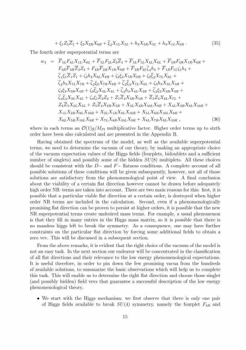
+ ξ1Z5Z5 + ξ2X2RX6R + ξ2X1LX5L + h3X2RX5L + h4X1LX6R . (35)

The fourth order superpotential terms are

w4 = F 5LF4LX1LX6L + F 5LF3LZ3Z4 + F 5LF1LX4LX6L + F 5RF4RX1RX6R +

F4RF 3RZ3Z4 + F4RF 2RX1RX8R + F 2RF2Lζ4h4 + F 1RF1Lζ1h4 +

ζ1ξ1Z1Z1 + ζ2h4X8LX8R + ζ2ξ3X7RX8R + ζ2ξ2X7LX8L +

ζ2h3X7LX7R + ζ2ξ2X7RX8R + ζ2ξ3X7LX8L + ζ3h3X3LX3R +

ζ3ξ3X3RX4R + ζ3ξ2X3LX4L + ζ3h4X4LX4R + ζ3ξ2X3RX4R +

ζ3ξ3X3LX4L + ζ4ξ1Z2Z2 + Z1Z4X3RX5R + Z2Z4X2LX7L +

Z4Z5X2LX5L + Z5Z4X2RX5R +X3LX4RX10LX9R +X4LX3RX9LX10R +

X1LX2RX9LX10R +X2LX1RX9LX10R +X5LX6RX10LX9R +

X6LX5RX10LX9R +X7LX8RX10LX9R +X8LX7RX9LX10R , (36)

where in each terms an O(1)g/MP l multiplicative factor. Higher order terms up to sixthorder have been also calculated and are presented in the Appendix B.

Having obtained the spectrum of the model, as well as the available superpotentialterms, we need to determine the vacuum of our theory, by making an appropriate choiceof the vacuum expectation values of the Higgs fields (fourplets, bidoublets and a sufficientnumber of singlets) and possibly some of the hidden SU(8) multiplets. All these choicesshould be consistent with the D− and F− flatness conditions. A complete account of allpossible solutions of these conditions will be given subsequently, however, not all of thosesolutions are satisfactory from the phenomenological point of view. A final conclusionabout the viability of a certain flat direction however cannot be drawn before adequatelyhigh order NR–terms are taken into account. There are two main reasons for this: first, it ispossible that a particular viable flat direction at a certain order, is destroyed when higherorder NR–terms are included in the calculation. Second, even if a phenomenologicallypromising flat direction can be proven to persist at higher orders, it is possible that the newNR superpotential terms create undesired mass terms. For example, a usual phenomenonis that they fill in many entries in the Higgs mass matrix, so it is possible that there isno massless higgs left to break the symmetry. As a consequence, one may have furtherconstraints on the particular flat direction by forcing some additional fields to obtain azero vev. This will be discussed in a subsequent section.

From the above remarks, it is evident that the right choice of the vacuum of the model isnot an easy task. In the next section our endeavor will be concentrated in the classificationof all flat directions and their relevance to the low energy phenomenological expectations.It is useful therefore, in order to pin down the few promising vacua from the hundredsof available solutions, to summarize the basic observations which will help us to completethis task. This will enable us to determine the right flat direction and choose those singlet(and possibly hidden) field vevs that guarantee a successful description of the low energyphenomenological theory.

• We start with the Higgs mechanism; we first observe that there is only one pairof Higgs fields available to break SU(4) symmetry, namely the fourplet F4R and

15

in general one linear combination of the fields F1,2,3,5. Thus, in order to keep F4R

massless and prevent a mass term through the tree–level coupling F4RF5Rζ3, we needto impose 〈ζ3〉 = 0.

• In addition to the three generations expected to appear at low energies, the modelpredicts also the existence of one additional (4, 2, 1) representation plus its mirrorF5L = (4, 2, 1). Since no mirror families appear in the low energy spectrum, we need amass term of the form 〈χi〉FiLF5L (where χi some of the singlets with non–zero vevs)to give a heavy mass to the mirror F5L. A candidate term could be ζ2F5LF4L whichexists already at the tree–level. At fourth order there is also the term F5LF3LZ3Z5.Thus, up to fourth order, we obtain∑

i

〈χi〉FiLF5L = (ζ2F4L + F3LZ3Z4 + · · ·)F5L (37)

where {· · ·} stand for possible higher order NR–terms involving fields that may ac-quire vevs. Clearly, if we wish to make the mirror multiplets heavy with superpo-tential terms up to fourth order, we should demand from flatness conditions eitherζ2 6= 0, or Z3Z5 6= 0. Solutions with higher order NR–terms are also possible as itwill be clear later.

• A number of sextet fields, Di, i = 1, ..., 4 containing colour triplets as well as tripletssurviving the Higgs mechanism appear also in the spectrum. In order to avoid possibleproton decay problems we need also mass terms for those coloured fields. As far asthe sextet fields are concerned, the sextet matrix at tree–level is

D1D2Φ12 +D1D4Φ−12 +D2D3Φ

−12 +D3D4Φ12 (38)

Their eigenmasses in terms of the scalar components of the singlet fields are

mDi= ±1

2

(ΣΦ2 ±

√(ΣΦ2)2 − (Φ12Φ12 − Φ−

12Φ−12)

2

)(39)

with

ΣΦ2 = Φ212 + Φ2

12 + Φ−12

2+ Φ

−12

2(40)

The above eigenvalues are all non–zero whenever the condition

Φ12Φ12 − Φ−12Φ

−12 6= 0

is fulfilled. Therefore, a satisfactory flat direction should keep the appropriate singletswith non–zero vevs. It will be clear later that in most of the phenomenologically viablestring vacua, higher order NR–contributions will prove necessary to make all sextetfields massive.

In forming the mass matrices for triplets, we should also take into account the factthat there are also coloured triplets in the Higgs pair (4, 1, 2) + (4, 1, 2). Thus,

16

recalling in mind the sextet decomposition D4 → D34 +D3

4, the term F4RF4RD4 givesa heavy mass to dc4RD

34 and the terms

F5RF5RD2 + F2RF2RD2 + F1RF1RD1

make another 3 − 3 combination massive. This linear combination depends on thechoice of the fields which are going to accommodate the families and higgses. Thiswill be precisely determined as long as a specific flat direction is chosen.

• There is a new interesting feature of this version; There are two candidate terms atfourth order to provide masses to the second generation

F1RF1Lh4ζ1 + F2RF2Lh4ζ4 (41)

They are expected to be of the right order, provided that at least one of the singletsζ1, ζ4 gets a non–zero vev.

After this preliminary analysis, we are ready now to explore other important aspects ofthe model. In the next section we will find all tree–level and higher order solutions to theflatness conditions which determine the consistent string vacua.

6 The solutions of the F– and D–flatness conditions

One of the main concerns in constructing effective supersymmetric models from super-strings, is to find the flat directions along which the scalar potential vanishes. Stringmodels in general contain several flat directions which are lifted by higher order correctionsto the superpotential and supersymmetry breaking effects. The latter set also the scale ofthe scalar potential. Another interesting fact in string model building concerning these flatdirections, is the existence of a D–term contribution [18, 19]. As has been discussed in theprevious section, there is a linear combination of the four surplus U(1) factors accompa-nying the observable gauge group of the model, which remains anomalous. The standardanomaly cancellation mechanism [19] results to a shift of the vacuum where several scalarcomponents of the singlet (and possibly hidden) superfields develop non–zero vevs. Theirmagnitude is determined by the solution(s) of the complete system of the F - and D-flatnessconstraints.

Derivation of the flatness constraints

The F -flatness equations are easily derived from the superpotential. They are the set ofequations resulting from the differentiation of W with respect to the fields of the masslessspectrum fi,

∂

∂fiW = 0

In this paper we will mainly concentrate on an analysis of the flatness conditions involvingfields only from the observable sector. For completeness, we also give in the Appendix B

17

the relevant contributions to the flatness conditions taking into account hidden field vevsas well as higher order corrections from NR–terms.

Taking the derivatives of the renormalizable superpotential W with respect to the ob-servable fields, we obtain

Φ2 : ζiζi = −ξiξi (42)

Φ4 : ζ1ζ3 = −ζ1ζ3 (43)

Φ5 : ζ2ζ4 = −ζ2ζ4 (44)

Φ12 : ξ1ξ4 = 0 (45)

Φ12 : ξ4ξ1 = 0 (46)

Φ−12 : ζiζi = −ξ2ξ3 (47)

Φ−12 : ζiζi = −ξ3ξ2 (48)

ξ1 : φ2ξ1 = −Φ12ξ4 (49)

ξ1 : φ2ξ1 = −Φ12ξ4 (50)

ξ2 : φ2ξ2 = −Φ−12ξ3 (51)

ξ2 : φ2ξ2 = −Φ−12ξ3 (52)

ξ3 : φ2ξ3 = −Φ−12ξ2 (53)

ξ3 : φ2ξ3 = −Φ−12ξ2 (54)

ξ4 : φ2ξ4 = −Φ12ξ1 (55)

ξ4 : φ2ξ4 = −Φ12ξ1 (56)

ζ1 : φ2ζ1 + Φ4ζ3 + 2Φ−12ζ1 = 0 (57)

ζ1 : φ2ζ1 + Φ4ζ3 + 2Φ−12ζ1 = 0 (58)

ζ2 : φ2ζ2 + Φ5ζ4 + 2Φ−12ζ2 + F5LF4L/

√2 = 0 (59)

ζ2 : φ2ζ2 + Φ5ζ4 + 2Φ−12ζ2 = 0 (60)

ζ3 : φ2ζ3 + Φ4ζ1 + 2Φ−12ζ3 = 0 (61)

ζ3 : φ2ζ3 + Φ4ζ1 + 2Φ−12ζ3 + F5RF4R/

√2 = 0 (62)

ζ4 : φ2ζ4 + Φ5ζ2 + 2Φ−12ζ4 = 0 (63)

ζ4 : φ2ζ4 + Φ5ζ2 + 2Φ−12ζ4 = 0 (64)

On the left of the above equations we show the field with respect to which the superpotentialis differentiated . In equations (59,62) both SU(2)L and SU(2)R fourplet fields have beenincluded to exhibit the invariance of the equations under a straightforward generalizationof the transformations (19). Indeed, it can be observed now that the F–flatness equationsas well as the Yukawa interactions remain unaltered under the interchanges mentioned inprevious sections. In particular, when 4 and 2R are interchanged with 4 and 2L respectively,it can be seen that the superpotential remains invariant under the following renaming ofthe fields

F5, F5 ↔ F4, F4 F1, F1 ↔ F2, F2 D1, D3 ↔ D2, D4 (65)

ζ1, ζ2 ↔ ζ4, ζ3 ζ1, ζ2 ↔ ζ4, ζ3 Φ1,Φ4 ↔ Φ3,Φ5 (66)

ξ2, ξ3 ↔ ξ2, ξ3 Φ−12 ↔ Φ−

12 Φ2 ↔ Φ2 (67)

18

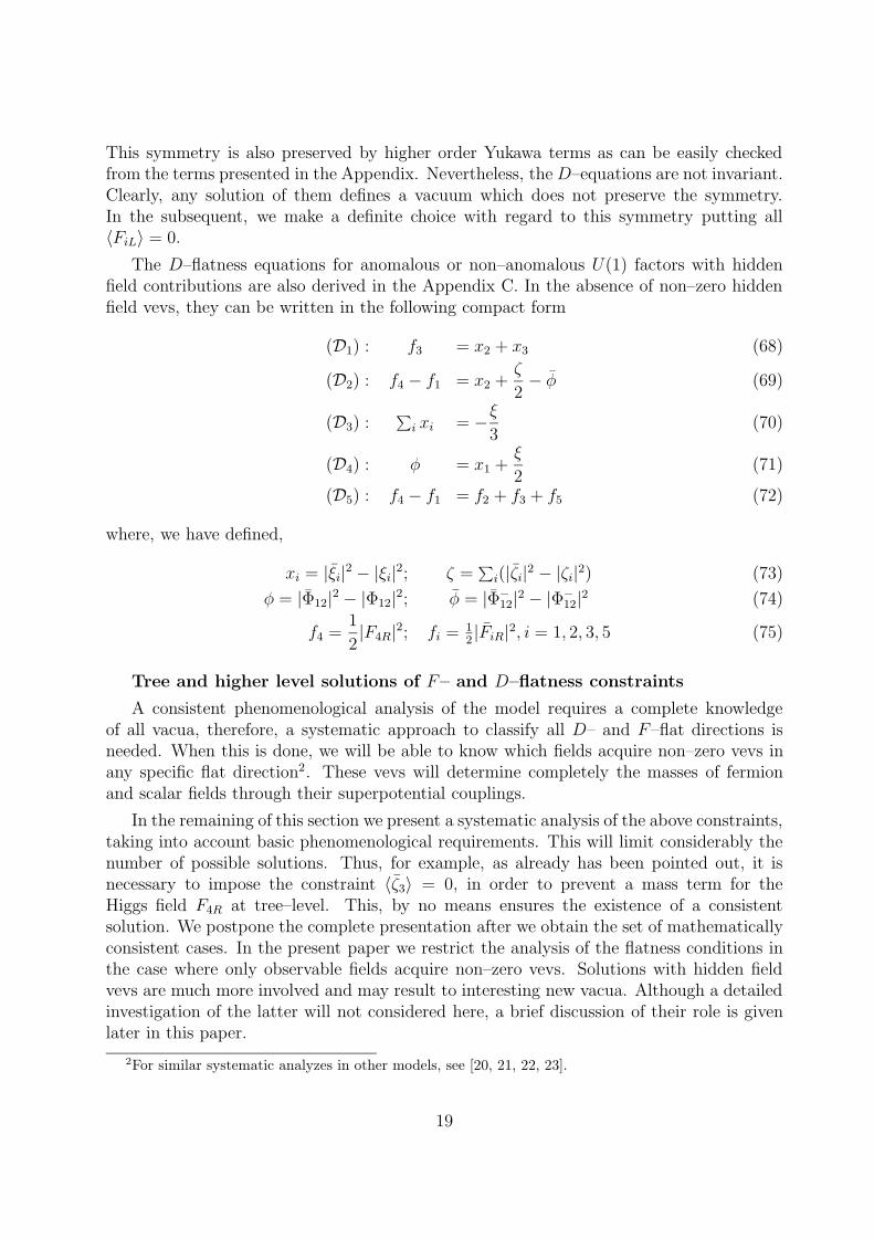
This symmetry is also preserved by higher order Yukawa terms as can be easily checkedfrom the terms presented in the Appendix. Nevertheless, theD–equations are not invariant.Clearly, any solution of them defines a vacuum which does not preserve the symmetry.In the subsequent, we make a definite choice with regard to this symmetry putting all〈FiL〉 = 0.

The D–flatness equations for anomalous or non–anomalous U(1) factors with hiddenfield contributions are also derived in the Appendix C. In the absence of non–zero hiddenfield vevs, they can be written in the following compact form

(D1) : f3 = x2 + x3 (68)

(D2) : f4 − f1 = x2 +ζ

2− φ (69)

(D3) :∑i xi = −ξ

3(70)

(D4) : φ = x1 +ξ

2(71)

(D5) : f4 − f1 = f2 + f3 + f5 (72)

where, we have defined,

xi = |ξi|2 − |ξi|2; ζ =∑i(|ζi|2 − |ζi|2) (73)

φ = |Φ12|2 − |Φ12|2; φ = |Φ−12|2 − |Φ−

12|2 (74)

f4 =1

2|F4R|2; fi = 1

2|FiR|2, i = 1, 2, 3, 5 (75)

Tree and higher level solutions of F– and D–flatness constraints

A consistent phenomenological analysis of the model requires a complete knowledgeof all vacua, therefore, a systematic approach to classify all D– and F–flat directions isneeded. When this is done, we will be able to know which fields acquire non–zero vevs inany specific flat direction2. These vevs will determine completely the masses of fermionand scalar fields through their superpotential couplings.

In the remaining of this section we present a systematic analysis of the above constraints,taking into account basic phenomenological requirements. This will limit considerably thenumber of possible solutions. Thus, for example, as already has been pointed out, it isnecessary to impose the constraint 〈ζ3〉 = 0, in order to prevent a mass term for theHiggs field F4R at tree–level. This, by no means ensures the existence of a consistentsolution. We postpone the complete presentation after we obtain the set of mathematicallyconsistent cases. In the present paper we restrict the analysis of the flatness conditions inthe case where only observable fields acquire non–zero vevs. Solutions with hidden fieldvevs are much more involved and may result to interesting new vacua. Although a detailedinvestigation of the latter will not considered here, a brief discussion of their role is givenlater in this paper.

2For similar systematic analyzes in other models, see [20, 21, 22, 23].

19

We find it convenient to start our analysis from the F–flatness conditions (44,45) whichimply four distinct cases:

(i) ξ1 = ξ1 = 0 , ξ4 6= 0; (ii) ξ1 = ξ4 = 0;(iii) ξ4 = ξ1 = 0; (iv) ξ4 = ξ1 = 0 , ξ1, ξ4 6= 0 .

From the above cases, only (iii, iv) have consistent solutions. Let’s first explain why cases(i) and (ii) are rejected.

Cases (i) and (ii)

From Eqs. (55,56) we deduce φ2 = 0, while ξ4 6= 0 in Eq. (50) imposes Φ12 = 0. Thishowever leads to inconsistency with equation D4, since the left side of the equation isnegative while the right side is positive and non–zero. Similarly case (ii) where ξ1 = ξ4 = 0,is not soluble as can be easily seen from the equation (D3)+(D1). We consider the tworemaining cases (iii) and (iv)separately.

Case (iii)

From Eq. (50), we find φ2 = 0. Further, D4–flatness tells us that ξ1 and Φ12 cannot besimultaneously zero. Then, combining this with conditions (54) and (55) we conclude that

Φ12 = 0, ξ4 = ξ4 = 0, ξ1 6= 0, φ2 = 0 (76)

while ξ1 · Φ12 = 0.

Proceeding further, we classify all solutions in this case according to their number of freeparameters and fields with zero vevs. At the tree–level, there are 17 solutions consistentwith the F– and D–flatness conditions. These are cases 1–17 of Table 9 of the Appendix D.Several of these flat directions are lifted when higher order NR–terms are included. On theother hand, other tree–level flat directions remain flat when additional constraints have areimposed on the field vevs. There are cases where a single tree–level flat direction results tomore than one distinct cases at a higher level since the solution of the constraints may besatisfied for various choices of field vevs.

When NR contributions to flatness conditions up 6th order are taken into account, theabove tree–level solutions reduce to the first thirteen cases presented in Table 2. The firstcolumn numbers the solutions, while the last one denotes the number of free (complex)parameters left. The five columns in the middle show the fields with zero vevs, where forpresentation purposes abbreviations in the field notation have been used. Thus, in thesecond row, the numbers 12, 12, 12−, 12

−, denote the fields Φ12,Φ12,Φ

−12,Φ

−12, and so on.

The fields which are forced to obtain zero vevs due to higher order NR–contributions in theYukawa potential, are included in curly brackets. Thus, for example, in the fourth columnof the first case, the symbol {2} means that 〈ξ2〉 has a zero vev due to the inclusion of NR–terms. Further, for the same reason in the fifth column we also use the notation {1}, {2}which should be translated to the conditions F1R = F2R = 0 imposed by NR–terms. Inthis notation, one can see the effect of NR–terms in the tree–level solutions presented inAppendix D. For example, the first solution in Table 9 (in the appendix) results to the firsttwo distinct cases of Table 2 and so on.

Note that in Table 2 we present only the vanishing vev’s of each particular solution.Substitution in the F– and D–flatness conditions, results to a number of constraints char-

20

acterizing each solution. These constraints are not presented in Table 2 but they havebeen taken into account in the calculation of free parameters. Specific examples will bepresented later in Section 7. Due to the existence of free parameters, each solution of Table2 can in principle generate a number of phenomenologically distinct cases. We will seein a subsequent section how some of these free parameters are forced to obtain zero vevsfollowing the requirements of low energy phenomenology.

Case (iv)

In a similar manner, we proceed also in this case where ξ1 = ξ4 = 0. Eqs. (50), (54) leadto two sub–cases depending on whether φ2 is zero or not.

• (iv)a When φ2 = 0, the analysis proceeds in analogy with case (iii). Thus, we findeight solutions at the tree–level which cases 18-25 of Table 9.

• (ivb) For the case φ2 6= 0, a tedious analysis leads to the unique tree–level solution

ξ2,3 = ξi = ζi = ζi = F3R = F5R = 0 (77)

with Φ2 = 4 Φ12 Φ12 6= 0

This is also included as case 26 in the complete list of the tree–level solutions of Table 9in Appendix D. When NR–contributions are taken into account various flat directions arelifted and the total number of solutions is reduced to 4 which are shown in Table 2 (cases(14)-(17)).

Having obtained all consistent solutions, let us try to apply the preliminary phenomeno-logical discussion of the previous section. We first point out that in eight of the cases above,all four Φ12’s fields in the second row have zero vevs. Although nothing can be definitelysaid until a complete analysis with higher NR–terms is done, we consider them as lessfavored since they leave all four sextet fields massless at tree–level. Another two solutionson the other hand, has all ζi = ζi = 0. Again, according to our previous analysis, itwould be desirable to obtain a mass term for the second generation at fourth order wherea natural fermion mass hierarchy is obtained. Such a solution should admit at least ζ1 6= 0and 〈F1R〉 = 0, or ζ4 6= 0 and 〈F2R〉 = 0. From this point of view, the cases admittingnon–zero vevs for some of the ζi, ζi are more preferable. Few of them leave only the fourpletF1R 6= 0 to be interpreted as the second SU(4)× SU(2)R breaking higgs, (the other beingdefinitely F4R), while there are several cases with 〈F3R〉 6= 0. Moreover, since in most ofthe cases 〈F5R〉 = 0, this latter field together with F4L, are suitable to accommodate thethird generation fermions who may receive a tree–level mass term via the Yukawa couplingF5RF4Lh4.

7 Higgs fields and fermion mass textures

We start our phenomenological analysis of the string model with the discussion on the Higgssector. Clearly, all the consistent solutions of the flat directions considered in the previous

21

Φ12s Φi ξi, ξi ζi, ζi Fi f.p.

1 12, 12−, 12−

2, 4, 5 4, 1, {2}, 4 3, 3 {1}, {2}, 5 6

2 12, 12−, 12−

2, 4, 5 4, 1, 4 3, 3 {1}, {3}, 5 7

3 12, 12−, 12−

2, 4, 5 4, 1, {2}, 4 1, 3 {1}, {2}, 5 6

4 12, 12−, 12−

2, 4, 5 4, 1, 4 1, 3 {1}, {3}, 5 7

5 12, 12, 12−, 12−

2, 4, 5 4, [1], {2}, 4 3, 3 {1}, {2}, 5 5

6 12, 12, 12−, 12−

2, 4, 5 4, [1], {2}, 4 1, 3 {1}, {2}, 5 6

7 12, 12−, 12−

2, 5 4, 1, 4 3, 1, 3 {1}, {3} 7

8 12, 12−, 12−

2, 5 4, 1, {2}, 4 1, 3, 1, 3 {1}, {2}, {5} 5

9 12, 12−, 12−

2, 5 4, 1, 4 {1}, 3, 1, 3 {2}, {3}, {5} 6

10 12, 12, 12−, 12−

2, 5 {2}, 4, [1], 4 {1}, 3, 1, 3 {1}, {2}, {5} 4

11 12, 12, 12−, 12−

2, 5 4, [1], {3}, 4 1, 3, 1, 3 {1}, {2}, {5} 4

12 12, 12−, 12−

2, 4 4, 1, 4 2, 3, 4, 2, 3, 4 {1}, {3}, 5 513 12 2 2, 3, 4, 1, 2, 3, 4 1, 2, 3, 4, 1, 2, 3, 4 {2}, {3}, 5 6

14 12, 12, 12−, 12−

2, 4, 5 1, {2}, 4 3, 3 {1}, 5 9

15 12, 12, 12−, 12−

2, 4, 5 1, {2}, 4 1, 3 {1}, 5 9

16 12, 12, 12−, 12−

2, 5 1, {2}, 4 3, 1, 3 {1} 917 2, 3, 1, 2, 3, 4 1, 2, 3, 4, 1, 2, 3, 4 {2}, 3, 5 7

Table 2: The solutions to the F– and D–flatness equations with contributions of NR–termsup to sixth order. The fields appearing in the table have zero vevs. Those appearing incurly brackets {} are forced to have zero vevs form NR–contributions, while those in squarebrackets [] are set to zero to ensure the existence of at least one massless Higgs doublet. Inthe last column f.p. stands for the number of free parameters.

22

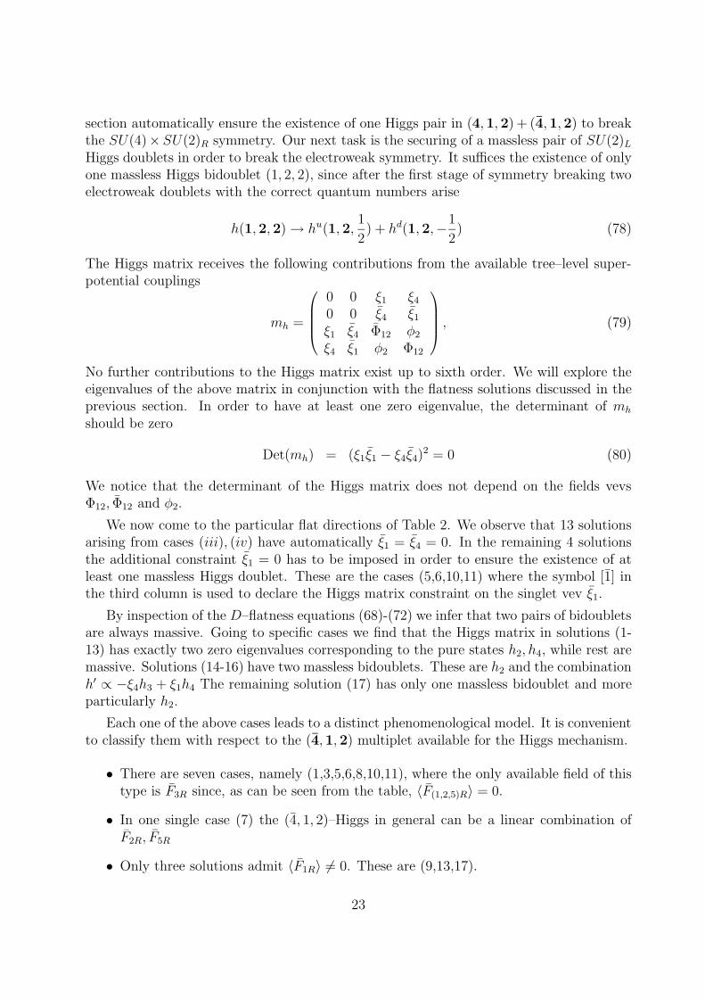
section automatically ensure the existence of one Higgs pair in (4, 1, 2) + (4, 1, 2) to breakthe SU(4)×SU(2)R symmetry. Our next task is the securing of a massless pair of SU(2)LHiggs doublets in order to break the electroweak symmetry. It suffices the existence of onlyone massless Higgs bidoublet (1, 2, 2), since after the first stage of symmetry breaking twoelectroweak doublets with the correct quantum numbers arise

h(1, 2, 2) → hu(1, 2,1

2) + hd(1, 2,−1

2) (78)

The Higgs matrix receives the following contributions from the available tree–level super-potential couplings

mh =

0 0 ξ1 ξ40 0 ξ4 ξ1ξ1 ξ4 Φ12 φ2

ξ4 ξ1 φ2 Φ12

, (79)

No further contributions to the Higgs matrix exist up to sixth order. We will explore theeigenvalues of the above matrix in conjunction with the flatness solutions discussed in theprevious section. In order to have at least one zero eigenvalue, the determinant of mh

should be zero

Det(mh) = (ξ1ξ1 − ξ4ξ4)2 = 0 (80)

We notice that the determinant of the Higgs matrix does not depend on the fields vevsΦ12, Φ12 and φ2.

We now come to the particular flat directions of Table 2. We observe that 13 solutionsarising from cases (iii), (iv) have automatically ξ1 = ξ4 = 0. In the remaining 4 solutionsthe additional constraint ξ1 = 0 has to be imposed in order to ensure the existence of atleast one massless Higgs doublet. These are the cases (5,6,10,11) where the symbol [1] inthe third column is used to declare the Higgs matrix constraint on the singlet vev ξ1.

By inspection of the D–flatness equations (68)-(72) we infer that two pairs of bidoubletsare always massive. Going to specific cases we find that the Higgs matrix in solutions (1-13) has exactly two zero eigenvalues corresponding to the pure states h2, h4, while rest aremassive. Solutions (14-16) have two massless bidoublets. These are h2 and the combinationh′ ∝ −ξ4h3 + ξ1h4 The remaining solution (17) has only one massless bidoublet and moreparticularly h2.

Each one of the above cases leads to a distinct phenomenological model. It is convenientto classify them with respect to the (4, 1, 2) multiplet available for the Higgs mechanism.

• There are seven cases, namely (1,3,5,6,8,10,11), where the only available field of thistype is F3R since, as can be seen from the table, 〈F(1,2,5)R〉 = 0.

• In one single case (7) the (4, 1, 2)–Higgs in general can be a linear combination ofF2R, F5R

• Only three solutions admit 〈F1R〉 6= 0. These are (9,13,17).

23

• There are three solutions where the higgs may be a linear combination of F(2,3)R

(14,15) or F(2,3,5)R, SU(4) (16) multiplets.

• Finally, solutions (2,4,12) admit only 〈F2R〉 6= 0.

Let us emphasize at this point that the above distinction between the solutions togetherwith the massless electroweak Higgs field classification, is in accordance with common phe-nomenological characteristics. For example, solutions of the first kind above which impose〈F3R〉 6= 0, have a rather larger number of Yukawa couplings available for fermion massgeneration, making them more appealing. Also, from a further inspection of the superpo-tential terms, the second class of solutions with 〈F5R〉 6= 0 implies a mass for the hu4 higgsvia the tree–level term 〈F5R〉F4Lh4. This fact leaves only one Yukawa coupling available forthe up quarks, up to fifth order making these solutions less interesting. In what follows,we will work out in some detail some representative cases from Table 2.

CASE 1:Let us start with the first solution in Table 2. Along this flat direction, the following 15fields are required to have zero vevs

Φ12 = Φ−12 = Φ−

12 = Φ2,4,5 = ξ4 = ξ1,2,4 = ζ3 = ζ3 = F1,2,5 = 0 . (81)

Among them, ξ2 and F5R are constrained to have zero vevs from sixth order contributions.Substituting the above condition to the full system of D– and F– flatness equations weobtain a reduced system of 9 equations for the remaining fields. These are

ξ2 ξ3 + ζ21 + ζ2

2 + ζ24 = 0 (82)

ζ21 + ζ2

2 + ζ24 = 0 (83)

ξ3ξ3 + ζ1ζ1 + ζ2ζ2 + ζ4ζ4 = 0 (84)

ζ2ζ4 + ζ4ζ2 = 0 (85)1

2|F3R|2 + |ξ2|2 + |ξ3|2 − |ξ3|2 = 0 (86)

|F3R|2 + 2 |ξ2|2 + |ζ1|2 + |ζ2|2 + |ζ4|2 − |ζ1|2 − |ζ2|2 − |ζ4|2 = 0 (87)

1

2|F3R|2 − |ξ1|2 = −ξ

3(88)

|ξ1|2 + |Φ12|2 =ξ

2(89)

|F4R|2 − |F3R|2 = 0 (90)

Taking into account that the total number of fields available to obtain vevs are 30 (assumingthat hidden sector fields do not develop vevs), we end to a 6 parameter solution. This is thenumber of free parameters (f.p.) presented in the last column of Table 2. As seen from theabove equations consistency of the solution requires a minimum number of the remaining15 fields

F3R, F4R, Φ1,3, ξ1,2,3, ξ1,2,3, ζ1,2,4, ζ1,2,4, Φ12 6= 0 (91)

24

to be non–zero. These are ξ1 , ξ3 , F3R , F4R and at least one of ζ1, ζ2, ζ4. The F4R andF3R vevs are not imposed by flatness but are required in order to obtain SU(4)× SU(2)Rbreaking. Thus the higgses in this case, in the notation of Section 2, are

F4R ≡ H(4, 1, 2); F3R ≡ H(4, 1, 2) (92)

To explore the hierarchy of the fermion mass spectrum, we note first that since 〈F3R〉 6= 0,the tree–level Yukawa coupling F3RF3Lh2 cannot be used for a fermion mass term. Clearly,F3L is more appropriate for a mirror partner for F5L. Therefore F5R and F4L are suitable toaccommodate a family and more particularly the heaviest one as indicated by the tree–levelsuperpotential term F5RF4Lh4. In this case we need to impose 〈ζ2〉 = 0, to avoid a massterm of the form 〈ζ2〉F4LF5L.

Then, condition (85) results to two distinct cases, either 〈ζ4〉 = 0, or 〈ζ2〉 = 0, each ofthem leading to a different phenomenological model. Although at this level of calculationit cannot be decided which of the two cases is appropriate, we consider the case 〈ζ4〉 6= 0as more favorable since it gives a tree–level mass term to a pair of exotic states. Thus wechoose to explore the case 〈ζ2〉 = 0.

To determine further the low energy parameters, we investigate the SU(4) breakingscale constraints as well as the singlet vevs entering the mass operators. From (88),(89) itfollows that the SU(4) breaking scale has a well defined upper limit, determined exclusivelyfrom the D-term

|F3R| ≤√ξ

3=gstring

2πMP l (93)

For perturbative values of gstring (93) gives a bound around the mass scale 1017GeV. Further,from (87) we also conclude that |ζ1| < |ζ4|. Up to fifth order, we find the following Yukawacouplings suitable for charged fermion masses

F5RF4Lh4 +¯〈ζ4〉MP l

F2RF2Lh4 +〈ζ1〉MP l

F1RF1Lh4 (94)

The last two terms appear at the fourth order, thus an additional mass parameter in theirdenominators appears. (In the Appendix B the mass parameters in the denominators areomitted in order to simplify the notation.) These two terms are obviously hierarchicallysmaller than the first term which gives masses to the third generation; further, takinginto account the flatness constraints, we infer that the second and first generations areaccommodated in F2R, F2L and F1R, F1L respectively. From the constraints above, we areable to choose ζ1 � ζ4, so that we satisfy the mass hierarchies. Moreover, this impliesthat F3R ∼ ζ4. Recalling that F3R plays the role of the SU(4)–breaking higgs at the scaleMGUT , we find that the top–charm relation will determine further these vevs to be of theorder

MGUT

MP l≡ 〈F3R〉

MP l≈ m0

c

m0t

(95)

It is worth noticing that this relation which correlates the SU(4) breaking scale with thatof the scale M ∼ MP l through the charm–top ratio at Mstring, is in excellent agreement

25

with both, the flatness condition (93) as well as the unification scale of the minimal unifi-cation scenario. We thus conclude that in the flat direction under consideration the flavorassignments of the light standard model quarks and lepton fields are as follows

F1L : (u, d), (e, νe) ; F1R : uc, dc, ec, νceF2L : (c, s), (µ, νµ) ; F2R : cc, sc, µc, νcµ (96)

F4L : (t, b), (τ, ντ ) ; F5R : tc, bc, τ c, νcτ

Up to now, we have a rather successful picture of the fermion mass spectrum which isalso in agreement with the string constraints. The above accommodation of the fermiongenerations and Higgs fields leaves no arbitrariness as far as the extra vector–like states areconcerned: these are F3L and F5L. The only mass term available at tree–level using fieldsof the observable sector, is proportional to the singlet vev 〈ζ2〉 however this is zero in thepresent case. Nevertheless, we observe that there are terms involving hidden fields whichmay acquire non–zero vevs and give a heavy mass to the mirror particles. For example,this can be obtained with a non–zero vev of the combination 〈Z3Z4〉 6= 0 while they areconstrained by the D–flatness to have equal vevs |〈Z3〉| = |〈Z4〉| 3.

We turn now to the neutrino sector. The three terms in (94) imply also Dirac massesfor the corresponding neutrinos with initial conditions at Mstring being the same as thosefor the up–quarks. Therefore a see–saw mechanism is necessary to bring them down toexperimentally acceptable scales. An available term exists already in the tree–level su-perpotential, which couples the right handed neutrino νc5 ∼ F c

5R with the singlet field ζ3via the vev 〈F4R〉. This leads to a see–saw mechanism of the type discussed in Section2. If we wish to find a final solution within the observable sector field vevs, however, acomplete account of the neutrino mass problem needs the calculation of even higher non–renormalizable terms. Restricting ourselves to contributions of NR–terms up to fifth order,the see–saw mechanism, in principle, can be effective for all neutrino species only whenadditional hidden fields acquire vevs. In this case it is easily checked that the followingadditional terms are generated

Aνc5φ2 + Bνc2φ2 + Cνc2ζ3 +Dνc1ζ2 (97)

arising from the hidden sector non–renormalizable contributions:

A = 〈F4RZ4Z5〉, B = 〈F4RZ4Z2〉, C = 〈F4RZ2Z4〉, D = 〈F4RZ1Z4〉. (98)

The terms (97) complete the mechanism for all three flavours of neutrinos and lead to anextended see–saw of the type (11). We note however that the inclusion of the above hiddenvevs requires a re–examination of the flatness conditions.

We come now to the fields having fractional charges. Since no ±1/2-charge particlehas been observed, the doublet states XL,R should also receive masses at some point,presumably higher than the electroweak scale. If we write the doublet XiR = (χ+

i , χ−i ),

3A similar mechanism has also been used in the flipped–SU(5) case [21]

26

then a possible mass term would be of the form:

WX = 〈φ〉εabXaiRX

bjR

= 〈φ〉(χ+i χ

−j − χ−i χ

+j ) (99)

where εab is the SU(2) antisymmetric tensor. φ can be any combination of fields acquiringvevs resulting to an effective singlet along the neutral direction. A similar term can alsoexist for the left doublets XL. Terms mixing left with right doublets are also possible,however, they lead to masses of the order of the electroweak scale and are not of interesthere. At the tree–level, in the present flat direction we have the following mass terms

W 3X = 〈ζ4〉X2RX5R + 〈ξ2〉X2RX6R + 〈ζ1〉X1RX6R (100)

and similarly there are two terms for the left doublet fields. Notice that we have nowmade used of the non–zero vev 〈ζ4〉 6= 0 which, according to the flatness conditions (85)implies 〈ζ2〉 = 0. There are still three and four pairs of right and left doublets respectivelyneeded to take masses at some scale well above mW . All possible terms up to fifth order,have been collected in Appendix B. By an inspection of the relevant (to this flat direction)terms up to this order, it follows that few of the octet fields Zi, Zi of the hidden sector withnon–zero vevs, are adequate to make all of them massive. As has already been pointedout, however, this will require a re–examination of the flatness conditions [24]. All thesame, the observable singlet vevs may prove to be sufficient if higher order contributionsare calculated. A similar term may also appear for the two SU(4) fourplets H4 = (4, 1, 1),H4 = (4, 1, 1).

There is finally the rather important issue concerning the triplet fields related to thestability of the proton. Recall first from the detailed analysis in Section 2 that the tripletslive only in the sextets and the fourplet Higgs fields. There are two types of terms hereto render them massive. In the present case, there is only one mass term available for thesextet fields at three level, namely Φ12D3D4, while the terms F 2

4RD3 and ζ21,4F

24RD4 offer

additional couplings with the uneaten Higgs triplet of F4R. Thus, up to fifth order, threetriplet pairs remain light. Higher order NR–terms will make them massive. In particular,an inspection of the related seventh order non–renormalizable superpotential mass termsshows that there are plenty of available couplings rendering all but one pair massive

W≤7D = D1D2ξ1Z3Z3Z5Z5 +D1D3

[ζ4ξ1Z2Z2(1 + Φ1) + ξ1Z2Z2Z5Z4

]+ D1D4

[ζ21Z5Z5ξ1 + ζ2

4ξ1Z5Z5

]. (101)

It can be checked that the only coloured field which remained uncoupled is the triplet dc3 ofthe Higgs field H ≡ F3R leading to a pair of massless triplets. This has to do with the factthat fields arising from the second b3 and being charged under peculiar U(1)4 factor makeonly few non–zero Yukawa couplings with other fields. For the same reason, quarks andlepton fields do not also have dangerous couplings with this triplet field up to this order.At higher orders, singlet fields with non–zero U(1)4 charge are expected to form NR–termmass terms for dc3 and its partner so that proton decay could be avoided.

27

CASE 7Here we have the following zero vevs

Φ−12, Φ

−12,Φ2,5, ξ4, ξ1,4, ζ3, ζ1,3, F1R, F3R = 0 (102)

Following the steps of the analysis of the previous case we find that flatness reduces to 10equations and thus the number of free parameters is 7. The SU(4)–breaking Higgs fieldsare F4R and a linear combination of the fourplets F2R and F5R. We now restrict to use thecase 〈F2R〉 = 0. Thus, the higgses are

F4R ≡ H(4, 1, 2); F5R ≡ H(4, 1, 2) (103)

Since 〈ζ2〉 6= 0, the trilinear term F5LF4Lζ2 makes massive the extra vector–like states. Onthe other hand the terms

F5RF4Lh4 + F5LF4Lζ2 → (〈νc5〉hu4 + 〈ζ2〉 ¯5)`4 (104)

mix a combination of the Higgs doublet in h4 with ¯5 in F5L leaving massless the combination

hu = cosφhu4 − sinφ¯5, tanφ =

〈ζ2〉〈νc5〉

(105)

Once we have determined the electroweak Higgs eigenstates we are in a position to examinethe available fermion mass terms. As previously, we will analyze Yukawa couplings up tofifth order. It is natural to accommodate the third generation in the representations arisingfrom the sector b3; due to the existing fermion hierarchy the heavy fermions are expectedto obtain their mass through the only available tree–level term

F3RF3Lh2 → 〈hu2〉(ttc + ντνcτ ) + 〈hd2〉(bbc + ττ c)

Then the lighter generations receive masses from non–renormalizable terms,

〈h4ζ4(1 + Φ1)〉F2RF2L + 〈h4〉〈(ζ1(1 + Φ3) + F5RF4R)〉F1RF1L (106)

where denominators of proper powers of Mstring in the various NR–contributions are omit-ted. Taking into account (105), the first term of (106) becomes

F2RF2Lh4ζ4 → cosφ〈ζ4hu′〉(Q2uc2 + νc2`2) + 〈hd4〉(Q2d

c2 + `2e

c2) (107)

and similarly for the other terms. Additional contributions may arise when higher orderNR–terms are taken into account.

The triplet mass matrix in the present case, receives contributions from terms involvingthe above non–zero vevs. Assuming the sextet decompositions Di = D3

i + D3i the triplet

matrix takes the following form in the basis D1, D2, D3, D4, dc4,

D31 D3

2 D33 D3

4 dc4(F4R)D3

1 0 x x x 0D3

2 x 0 0 F4Rζ2i F4Rζ

2i

D33 x 0 0 Φ12 F4R

D34 x 0 Φ12 0 0

dc5R(F5R)

F5Rζ2i F5R 0 0 0

(108)

28

where ζi stands for the non–vanishing vevs ζ2, ζ4. The symbol x in the first row and columnof the above matrix represents possible contributions from NR–terms involving fields fromthe hidden sector. These are

WHD = D1D2(ζ2Z3Z3Z5Z4 + ξ1Z3Z3Z5Z5) +D1D3ζ4ξ1Z2Z2

+ D1D4(ζ2ζ24Z5Z4 + ζ2

4ξ1Z5Z5 + ζ24ξ1Z5Z4)

As can be seen from the mass–matrix, observable sector contributions up to seventh ordermake all but one pair of the coloured triplets massive. If hidden fields also acquire vevsthen all triplets could become massive.

CASE 13We briefly comment now on another characteristic case of Table 2, namely solution (13).This case is distinguished by two remarkable properties which are worth mentioning:(i) First we observe that all coloured sextets become massive at tree–level. This can beseen from the mass formula (39) and the fact that only one of the four singlets involved inthe tree–level mass matrix is required to have a zero vev (namely 〈Φ12〉 = 0).(ii) Second, we point out that the two lighter generations are not pure states, since theyappear to mixing appears already at tree–level. To see this, we check first from Table 2that the solution requires 〈F2,3,5〉 = 0, thus the SU(4) × SU(2)R Higgs fields are now F4R

and F1R. A possible mass term for the mirror states may appear now at a higher order(unless – as previously – hidden fields obtain non–zero vevs). The fermion mass terms arein this case

F3RF3L〈h2〉+ F5R

(F4L〈h4〉+ F1Lh2〈F1RF4Rh4

)〉 (109)

Clearly, the right–handed fields leaving in F5R mix with both F1L and F4L. The flavorassignments are now

F1L : (u′, d′), (e′, ν ′e) ; F2R : uc′, dc

′, ec

′, νce′

F2L : (c′, s′), (µ′, ν ′µ) ; F2R : cc′, sc

′, µc

′, νc

′µ (110)

F3L : (t, b), (τ, ντ ) ; F3R : tc, bc, τ c, νcτ

where primes are used to denote that there is mixing in the two lighter generations. Weshould point out here that the third family remains essentially decoupled due to the peculiarproperties of the fourth U(1). Only very high order NR–terms are possible to mix this familywith the lighter ones. This fact of course predicts smaller mixing angles between the thirdfamily with the rest of the fermion spectrum in consistency with the phenomenologicalexpectations.

8 A brief discussion on the role of the hidden sector

fields

Up to now, we dealt with solutions of the flatness conditions considering only non–zero vevsfor observable fields. In the phenomenological analysis of the previous section, however,

29

we have seen that couplings involving only observable–sector field vevs are not adequateto make all exotic particles massive. There are mainly two important issues to be furtherinvestigated before this model is confronted with the low energy physics world. First, higherorder NR–terms have to be calculated in order to find all possible contributions to the massmatrices of fermions, triplets and other fields presented in the previous section. On theother hand, hidden fields can also play a very important role on the determination of thetrue vacuum of the model. Since they carry no charge, they can also develop non–zero vevsand contribute to the masses of the light fields through their Yukawa interactions. Thisfact has been clear already in the three examples used in the previous section. Neutrinomasses, exotic states, and few of the triplet fields become massive only when hidden fieldsare included. At the same time, in both cases, the additional terms contribute also tothe flatness conditions, thus the new non–zero vevs have to be carefully chosen so thatthey define a consistent F– and D–flat direction. For such an investigation, one has tomodify the flatness solutions, starting again from the tree level cases which are includedin Appendix D. A systematic analysis of this general case is possible, however, this goesbeyond the scope of the present work [24]. For completeness, the D−flatness conditions, inthe presence of non–zero hidden field vevs is given in Appendix C. Moreover, the F−flatnessconditions are written with the hidden fields contributions up to fourth order in the sameAppendix. Higher order NR–corrections with hidden as well as observable field vevs areeasily extracted from the terms presented in Appendix B. In the following, we give a briefaccount of the possible solutions the hidden fields may give to some of the unansweredquestions of the present string construction.

Several constraints have to be carefully derived before some of the hidden representa-tions acquire vevs. An important constraint arises from the demand of existence of masslesselectroweak Higgs doublets. Although up to sixth order we have found no extra contribu-tions to the Higgs doublet matrix, such terms may well exist in higher order, in particularwhen hidden fields are allowed to obtain non–zero vevs. It should be noted that due to theexistence of high vevs associated with the U(1)A breaking scale MA ∼ 10−1MP l securing theexistence of massless electroweak doublets is not an easy task for any superstring model.To be more specific, assume a generic form of doublet mass term

g(

Φ

MP l

)nΦh h

with Φ representing a typical singlet field obtaining a vev of the order 〈Φ〉 ∼MA. It is easyto see then that even a n = 14 order NR–term would in principle produce higgs massesabove the electroweak scale. Of course the existence of superfluous doublet fields –as is thecase of the model under consideration– provides the hope that even at this high order ofcalculation there exist flat directions that preserve at least one pair of doublets massless.

Another severe constraint arises from the necessity to keep the large SU(4) × SU(2)Rbreaking Higgs field F4R massless. Up to sixth order, this can be ensured if the followingcombinations of vevs are zero

ζ3, Z3Z4, φ2Z4Z5,

φ2Z2Z4, ζ2Z1Z4, ξ1Z1Z5,

30

Φ3Φ3Z3Z4, ζ1ζ3Z1Z4, ζ1ξ1Z1Z5. (111)

One might think that the above constraints demand most of the hidden fields Zi, Zj toobtain zero vevs. We would like to point out however that it is possible to have a conditionof the form 〈ZiZj〉 = 0, while at the same time both fields may have non–zero vevs, 〈Zi〉 6= 0and 〈Zj〉 6= 0. This happens whenever the fields Zi and Zj obtain their non–zero vevs inorthogonal to each–other directions.

When some of the SU(8) hidden fields acquire non–zero vevs, the SU(8)× U(1)′ sym-metry is broken to a smaller group. However, independently of the number of the hiddenstates which develop non–zero vevs, there is always at least one unbroken U(1)′′ generatorleft, which is in general a linear combination of the U(1)′ and one of the generators ofSU(8). On the other hand, we note that the maximum number of U(1) factors which mayremain unbroken in this model is two. Indeed, it can be checked that the breaking of theSU(4)× SU(2)R symmetry on one hand and the consistency of the flatness conditions onthe other require at least the fields F4R, F1R and Φ12, ξ1 to develop non–zero vevs. Thesevevs break three of the five Abelian factors.

The survival of U(1) symmetries in lower energies would imply the stability of lightestobservable and/or hidden fields being charged under these symmetries. In all flat directionswhich were previously analyzed, when the various singlet fields obtain their vevs, they breakfour out of five U(1) factors. Thus, only the aforementioned U(1)′′ remains at low energieswhilst, as a consequence the lightest hidden state will be stable. This fact has importantcosmological implications which we now briefly discuss:

The last few years there is accumulating evidence from astronomical observations thatthe universe is dominated by invisible non–baryonic matter. According to a recent proposal[25, 26] the dark matter of the universe –which is expected to be ten times more that theluminous one– might be composed from non–thermal superheavy states produced in theearly universe provided that the following two conditions are met: i) candidate particles Yshould have a lifetime longer that the age of the universe, τY ≥ 1010y, and ii) they shouldnot reach local thermal equilibrium with the primordial plasma. To avoid this constraintwhile having the correct number of Y to form the cold dark matter of the universe, it wassuggested that these particles are created through the interaction of the vacuum with thegravitational field. Their mass is found to be around mY ∼ 1013GeV 4.

In the string vacua found in the previous sections, a number of the hidden states Zi, Ziin the present string construction receive masses at scales which are of the order of thestring mass. There are few of Zi, Zi states however, which remain in the massless spectrumto lower scales. It is possible that in certain string vacua the lightest hidden state has amass in the range MY ∼ 1013GeV as required in the above scenario. As an example, weconstruct here the octet mass matrix for the solution 1 of Table 2. In the basis Z1,...,5, thecontributions up to sixth order involving only the non–zero vev observable fields give the

4For a similar discussion on the role of the hidden matter fields in other string models see also [27].

31

following texture ξ1ζ1 0 0 0 00 ξ1ζ4 0 0 00 0 0 F4RF3R 00 0 0 ζ2 00 0 0 0 ξ1

(112)

In this case, four out of five hidden octet/octet–bar pairs receive masses of the order of theU(1)A breaking mass scale MA ≥ MGUT . If hidden fields are also allowed to obtain vevs,then, Z4,5 are further mixed via the mass terms 〈ξ1Z1Z1〉Z4Z5 + 〈Φ3Z1Z1〉Z5Z4. There isonly one massless state (namely Z3) up to this order. It is expected that higher order termswill provide a higher order NR–contribution and make the remaining lightest hidden pairmassive at the right scale, which is of course much lower that the mass scale MA of theother Zi-fields, as required by the above cosmological scenario.

9 Conclusions

In this paper, we have worked out an SU(4) × SU(2)L × SU(2)R model derived in thecontext of the four dimensional free fermionic formulation of the heterotic superstring.Choosing a set of nine vectors of boundary conditions on the world–sheet fermion phasesand appropriate GSO projection coefficients, we derived a three–generation model sup-plemented by a mirror family and just the necessary Higgs representations to break thesymmetry down to the standard model. In addition to the observable gauge symmetry, thestring model possesses also five U(1)’s as well as a hidden SU(8) gauge group. The modelpredicts the existence of new states beyond those of the minimal supersymmetric standardmodel massless spectrum. These involve a large number of neutral singlet fields, colouredSU(4)–sextets, SU(8)-octet hidden fields and exotic states with fractional charges underthe standard hypercharge definition.

The superpotential of the model has been derived taken into account string selectionrules. All fermion mass terms have been worked out in detail up to fifth order and thefermion and Higgs mass matrix textures have been assiduously analyzed. The model isfound to possess an anomalous U(1)-symmetry implying the generation of a D–term whichis canceled by vacuum expectation values of singlet fields along D– and F–flat directionsof the superpotential.

To work out the phenomenological implications, we have performed a detailed analysis ofall D– and F– flat directions including contributions of non–renormalizable superpotentialterms up to sixth order. At tree–level, 26 solutions to the flatness conditions were foundand were classified with respect to the fields which are demanded to have zero vevs ineach particular case. It was further shown that, when sixth order NR–terms are includedthe solutions reduce to seventeen. Each solution is characterized by a the number of freeparameters which are essentially the field vevs left undetermined by the particular solution.Particular attention has been paid in the determination of those conditions necessary to

32

ensure the existence in the massless spectrum of the SU(4) breaking higgses and at leasttwo Higgs electroweak doublets in order to break the GUT and SM gauge symmetriesrespectively. These conditions have been imposed as additional constraints on the consistentD– and F–flat directions and all phenomenologically acceptable string vacua have beendetermined.

Three distinct flat directions, characterized by their SU(4)-higgs properties are investi-gated in detail and the predictions of the corresponding field theory models are discussed.a). The first of these predicts that the MGUT/Mstring–ratio is related to the up quarkmass ratio of the second and third generations. The choice of the GUT breaking Higgsrepresentations leaves a sufficient number of Yukawa couplings which produce naturally ahierarchical fermion mass spectrum for all three generations through tree–level and fourthorder non–renormalizable superpotential terms. Further, an analysis of the superpotentialNR–terms up to sixth order shows that all but one of the colour triplet fields become mas-sive. It is worth noting that there are no dangerous proton decay operators up to this orderof calculation since the massless triplet pair does not couple to ordinary matter fields up tothe sixth order. The absence of Yukawa couplings between this triplet and ordinary matterfields may be attributed to the properties of peculiar U(1)-symmetry of the specific stringbasis–vector generating this particular state. It is likely however that higher order termsmay provide a heavy mass to the remaining colour triplet pair.b). In a second case analyzed in this work, a similar hierarchical fermion mass pattern isfound, while all triplets become massive if in addition hidden fields are allowed to acquirenon–zero vevs. On the other hand, in contrast to the first model analyzed in Section 7,here the GUT scale has only an upper bound determined by the U(1)A breaking scale.c). Finally, a third effective field theory model is analyzed where all colour sextet fields be-come massive at the tree–level. This model has fewer Yukawa couplings available for masses,however, additional fermion mass terms may arise from higher order non–renormalizableterms.

A novel feature of the effective field theory is the existence of an additional U(1)-symmetry which survives down to low energies, and it is possessed by exotic states and thehidden sector fields. It is argued that if the lightest of these states receives mass at someintermediate scale, may play a role in the dark matter of the universe.

In the present paper our phenomenological explorations have been restricted mainlywith respect to the following two issues: First, while there exist various ways to define theelectric charge operator of the model (due to the existence of surplus U(1) factors), onlythe standard hypercharge embedding has been considered in the phenomenological analysis.We believe that it is worth exploring also different types of embedding although one hasto face difficulties mainly with low initial sin2 θW values. Second, the investigation of flatdirections has been limited in the cases where only ‘observable’ fields are allowed to obtainnon–zero vevs. Certainly, the inclusion of the hidden states in the analysis will lead to alarge number of new mass terms, the breaking of the hidden symmetry and modificationsof the flat directions found in this work. Yet, such a possibility has to be compared withanalogous investigations of higher order NR–terms will may or may not prove sufficient toobtain realist low energy effective theory.

33

References

[1] I. Antoniadis, C.P. Bachas, C. Kounnas and P. Windey, “Supersymmetry among freefermions and superstrings”, Phys. Lett. B 171 (1986) 51;I. Antoniadis, C.P. Bachas, and C. Kounnas, “Four dimensional superstrings”, Nucl.Phys. B 289 (1987) 87;I. Antoniadis and C. P. Bachas, “4-d fermionic superstrings with arbitrary twists”,Nucl. Phys. B 298 (1988) 586;H. Kawai, D. C. Lewellen, J. A. Schwarz, and S.–H. H. Tye, “The spin structureconstruction of string models and multiloop modular invariance”, Nucl. Phys. B 299(1988) 431.

[2] B. Greene, K. Kirlin, P. Miron and G.G. Ross, “A three generation superstring model:1. Compactification and string symmetries”, Nucl. Phys. B 278 (1986) 667;B. Greene, K. Kirlin, P. Miron and G.G. Ross, “A three generation superstring model:2. symmetry breaking and the low energy theory”, Nucl. Phys. B 292 (1987) 606;D. Bailin, A. Love and S. Tomas,“A three generation orbifold compactified superstringmodel with realistic gauge group ”, Phys. Lett. B 194 (1987) 385;A. Font, L. Ibanez, H.P. Nilles and F. Quevedo, “Yukawa couplings in degenerateorbifolds: towards a realistic SU(3)× SU(2)× U(1) superstring”, Phys. Lett. B 210(1988) 101.

[3] I. Antoniadis, J. Ellis, J. Hagelin and D. V. Nanopoulos,“The flipped SU(5) × U(1)model revambed”, Phys. Lett. B 231 (1989) 65;A. Faraggi, D.V. Nanopoulos and K. Yuan, “A standard like model in the 4–d fermionicformulation”, Nucl. Phys. B 335 (1990) 347.

[4] I. Antoniadis and G.K. Leontaris, “A supersymmetric SU(4) × O(4) model”, Phys.Lett. B 216 (1989) 333;

[5] I. Antoniadis, G.K. Leontaris and J. Rizos,“A three generation SU(4) × O(4) stringmodel”, Phys. Lett. B 245 (1990)161.

[6] D.C. Lewellen,“Embedding higher Kac–Moody algebras in heterotic string models”,Nucl. Phys. B 337 (1990) 61;Joel A. Schwartz, “Phenomenology of fermionic strings, Phys. Rev. D 42 (1990) 1777;A. Faraggi, “A new standard like model in four dimensional free fermionic formula-tion”, Phys. Lett. B 278 (1992) 131;A Faraggi, “Construction of realistic standard like models in the free fermionic formu-lation”, Nucl. Phys. B 387 (1992) 239;A. Maslikov, S. Sergeev and G. Volkov, “Grand unified string theories with non–Abeliangauge family symmetry in the free fermionic formulation”, Phys. Rev. D 50 (1994)7440;S. Chaudhuri, S.W. Chung, G. Hockney and J. Lykken,“String consistency for unifiedmodel building”, Nucl. Phys. B 456 (1995) 89;G. Aldazabal, A. Font, L. Ibanez and A.M. Uranga,“String GUTs”, Nucl. Phys. B

34

452 (1995) 3; “Building GUTs from strings”, Nucl. Phys. B 465 (1996) 34;K. Dienes and J. March–Russel, “Realising higher level gauge symmetries in stringtheory: new embeddings in string GUTs”, Nucl. Phys. B 479 (1996) 113;J. Erler, “Asymmetric orbifolds and higher level models”, Nucl. Phys. B 475 (1996)597;G.K. Leontaris, “A string model with SU(4) × O(4) × [Sp4]hidden symmetry”, Phys.Lett. B 372 (1996) 212;Z. Kakushadze and S.H.H. Tye,“Three family SO(10) grand unification in string the-ory”, Phys. Rev. Lett. 77 (1996) 2612;Z. Kakushadze, G. Shiu and S.H.Henry Tye,“Asymmetric non–Abelian orbifolds andmodel building”, Phys. Rev. D 54 (1996) 7545.

[7] V. Kaplunovsky, “One loop threshold effects in string unification”, Nucl. Phys.B 307(1988)145; Erratum-ibid.B 382 (1992) 436;I. Antoniadis, J. Ellis, R. Lacaze and D. V. Nanopoulos, “String threshold correctionsand the flipped SU(5)”, Phys. Lett. B 268 (1991) 188;P. Mayr, H–P. Nilles and S. Stieberger, “String unification, universal one–loop correc-tions and strongly coupled heterotic string theory”, Nucl. Phys. B 414 (1997)277;M. Petropoulos and J. Rizos, “Universal moduli dependent thresholds in Z2 × Z2 orb-ifolds”, Phys. Lett. B 374 (1996) 49;David Bailin, Alex Love, W.A. Sabra and S. Thomas“String loop threshold correctionsin Z(N) coxeter orbifolds”, Mod. Phys. Lett.A 9 (1994) 67;C. Bachas, C. Fabre “Threshold effects in open string theory”, Nucl. Phys. B 476(1996)418-436;E. Kiritsis, C. Kounnas, P.M. Petropoulos and J. Rizos, “String threshold correctionsin models with spontaneously broken supersymmetry”, hep-th/9807067.

[8] J. Pati and A. Salam,“Lepton number as a fourth colour”, Phys. Rev. D 10 (1974)275-289.

[9] A. Schellekens, “Electric charge of quantization in string theory”, Phys. Lett.B 237(1990)363.

[10] K.S. Babu, J. Pati and F. Wilzcek, “Suggested new models in supersymmetric protondecay”, Phys. Lett. B 423 (1998) 337;M. Gomez, J. Rizos and K. Tamvakis, “Suppressing D = 5 operators in general SU(5)models”, Phys. Rev. D 59 (1999) 015015.

[11] J.C. Pati, “Implications of the SuperKamiokande result in the nature of new physics”,hep-ph/9807315;Q. Shafi and Z. Tavartkiladze, “Large neutrino mixings and other issues in supersym-metric SU(4)C × SU(2)L × SU(2)R”, hep-ph/9811282 .

[12] K.S. Babu, J.C. Pati and F. Wilczek, “Fermion masses, neutrino oscillations, andproton decay in the light of SuperKamiokande”, hep-ph/9812538.

35

[13] I. Antoniadis, G.K. Leontaris and N.D. Tracas, “Grand unified string models and lowenergy couplings”, Phys. Lett. B 279 (1992) 58.

[14] S. King, “SU(4)× SU(2)L× SU(2)R as a surrogate GUT”, Phys. Lett. B 325 (1994)129.

[15] G.K. Leontaris, J. Rizos and K. Tamvakis, “Phenomenological constraints imposed bythe hidden sector in the flipped SU(5)× U(1)-model”, Phys. Lett. B 243 (1990) 220.

[16] J. Rizos and K. Tamvakis, “Some selection rules for non–renormalizable Yukawa cou-plings in 4–d fermionic superstring models”, Phys. Lett. B 262 (1991) 227.

[17] S. Kalara, J.L. Lopez and D.V. Nanopoulos, “Calculable non–renormalizable terms instring theory: A guide for the practicioner”, Nucl. Phys. B 353 (1991) 650.

[18] P. Fayet and J. Iliopoulos, “spontaneously broken supergauge symmetries and Gold-stone spinors”, Phys. Lett. B 51 (1974) 461-464.

[19] M. Dine, N. Seiberg and E. Witten, “Fayet-Iliopoulos terms in string theory”, NuclPhys. B 289 (1986) 585J. Atick, L. Dixon and A. Sen, “String calculation of Fayet–Iliopoulos D–terms inarbitrary supersymmetric compactifications”, Nucl. Phys. B 292 (1987) 109.

[20] J. Rizos and K. Tamvakis, “Retracing the phenomenology of the fliped SU(5) × U(1)model”, Phys. Lett. B 251 (1990) 369.

[21] I. Antoniadis, J. Rizos and K. Tamvakis, “Gauge symmetry breaking in the hiddensector of the flipped SU(5)× U(1)-model”, Phys. Lett. B 278 (1992) 257.

[22] G. Cleaver, M. Cvetic, J.R. Espinoza, L. Everett and P. Langacker, “Classification offlat directions in perturbative heterotic superstring vacua with anomalous U(1)”, Nucl.Phys. B 525 (1998) 3;G. Cleaver, M. Cvetic, J.R. Espinoza, L. Everett and P. Langacker and J. Wang,“Physics implications of flat directions in free fermionic superstring models II: Renor-malization group analysis”, hep-ph/9811355.

[23] W. Pokorski and G.G. Ross, “Flat directions, string compactification and 3 generationmodels”, hep-ph/9809537.

[24] Work in progress.

[25] D.J.H. Chung, E.W. Kold and A. Riotto, “Superheavy dark matter”, hep-ph/9802238;

[26] V. Kusmin and I. Tkachev, “Ultrahigh energy cosmic rays, superheavy long liv-ing particles and matter creation after inflation”, JETP Lett. 68 (1998) 271-275,[hep-ph/9802304].

[27] K. Benakli, J. Ellis and D.V. Nanopoulos, “Natural candidates for superheavy darkmatter in string and M–theory ”,hep-ph/9803333.

36

[28] J. Lopez and D.V. Nanopoulos, “Calculability and stability in the flipped string”, Phys.Lett. B 256 (1991) 150.

[29] A. Faraggi, “Aspects of non–renormalizable terms in superstring derived standard–likemodels”, Nucl. Phys. B 403 (1993) 101.

[30] D. Friedan, E. Martinec, S. Shenker, Nucl. Phys. B 198 (1987)474.

[31] V. A. Kostelecky, O. Lechtenfeld, W. Lerche, S. Samuel and S. Watamura, “Conformaltechniques, bosonization and tree–level string amplitudes”, Nucl. Phys. B 288 (1987)173.

[32] P. Di Francesco, H. Saleur and J. Zuber, “Generalized Coulomb gas formalism for twodimensional critical models based on SU(2) coset contruction”, Nucl. Phys. B 290(1987) 527.

[33] J. Rizos,“Construction and phenomenology of unified effective models from 4–Dfermionic superstrings”,PhD Thesis, University of Ioannina (1991).

37

10 Appendix A: The spectrum

We collect here the massless observable and hidden superfield spectrum of the model.Fermionic string models contain always an untwisted –usually called Neveu–Schwarz (NS)–sector where all world–sheet fermions are antiperiodic. In this sector, the GSO projectionsleave always in the massless spectrum the multiplet which contains the graviton, the dilatonand the two–index antisymmetric tensor. The NS–sector includes also the gauge bosonsand other Higgs and singlet fields. Twisted (R) sectors provide the generations and othermatter fields.

The states are classified in four separate tables according to their transformation prop-erties under the various parts of the gauge symmetry. In the first column of each tablewe give the symbol of the representation as this is used in the text. In the last columnwe show the relevant sector of the string basis. In all other columns we exhibit the gaugegroup properties of the states. Thus, Table 3 contains the observable fields, which havenon–trivial transformation properties under the PS–symmetry. These are obtained fromthe sectors b1,2,3,4,5 and S+b4+b5. They include the three generations, the higgses and otherfields. Table 4 includes the PS singlets with their charges under the four U(1) symmetries.In Table 5 we present the hidden SU(8) fields with the corresponding charges under thefive U(1)s. Finally, in Table 6 we collect all exotic states with fractional charges under thestandard hypercharge assignment.

field SU(4)× SU(2)L × SU(2)R U(1)1 U(1)2 U(1)3 U(1)4 sectorF 5L (4, 2, 1) 0 0 −1

20 b5

F 5R (4, 1, 2) 0 0 +12

0F4L (4, 2, 1) 0 +1

20 0 b4

F4R (4, 1, 2) 0 −12

0 0F 3R (4, 1, 2) −1

20 0 +1

2b3

F3L (4, 2, 1) +12

0 0 +12

F 2R (4, 1, 2) 0 0 +12

0 b2F2L (4, 2, 1) 0 0 +1

20

F 1R (4, 1, 2) 0 +12

0 0 b1F1L (4, 2, 1) 0 +1

20 0

D1 (6, 1, 1) 0 −1 0 0 SD2 (6, 1, 1) 0 0 −1 0D3 (6, 1, 1) 0 +1 0 0D4 (6, 1, 1) 0 0 +1 0h1 (1, 2, 2) 0 0 0 +1h2 (1, 2, 2) 0 0 0 −1h3 (1, 2, 2) 0 +1

2+1

20 S + b4 + b5

h4 (1, 2, 2) 0 −12

−12

0

Table 3: Observable sector spectrum of the SU(4)× SU(2)L × SU(2)R model.

38

field U(1)1 U(1)2 U(1)3 U(1)4 sectorΦA , A = 1, . . . , 5 0 0 0 0 SΦ12 0 +1 +1 0Φ−

12 0 +1 −1 0Φ12 0 −1 −1 0

Φ−12 0 −1 +1 0

ζi , i = 1, . . . , 4 0 −12

+12

0 S + b4 + b5ζi , i = 1, . . . , 4 0 +1

2−1

20

ξ1 0 −12

−12

−1ξ2 −1 −1

2+1

20

ξ3 −1 +12

−12

0ξ4 0 +1

2+1

2−1

ξ1 0 +12

+12

+1ξ2 +1 +1

2−1

20

ξ3 +1 −12

+12

0ξ4 0 −1

2−1

2+1

Table 4: Non–Abelian singlet fields and their U(1)4 quantum numbers (all these fields havezero U(1)′- charge).

field U(1)1 U(1)2 U(1)3 U(1)4 U(1)′ SU(8) sectorZ1 0 0 +1

2+1

2+1

28 b1 + b6(+ζ)

Z1 0 0 +12

+12

−12

8Z2 0 +1

20 +1

2+1

28 b2 + b6(+ζ)

Z2 0 +12

0 +12

−12

8Z3 −1

2+1

2+1

20 +1

28 b3 + b6(+ζ)

Z3 +12

+12

+12

0 −12

8Z4 0 0 −1

2−1

2+1

28 b4 + b6(+ζ)

Z5 0 0 +12

+12

+12

8Z4 0 −1

20 −1

2−1

28 b5 + b6(+ζ)

Z5 0 +12

0 +12

−12

8

Table 5: Hidden sector states and their U(1)4 × U(1)′ × SU(8) quantum numbers.

39

field SU(4)× SU(2)L × SU(2)R U(1)1 U(1)2 U(1)3 U(1)4 U(1)′ sectorX1L (1, 2, 1) −1

20 +1

20 −1 b1 + α

X2L (1, 2, 1) +12

0 +12

0 −1X1R (1, 1, 2) −1

20 −1

20 −1

X2R (1, 1, 2) +12

0 −12

0 −1X3L (1, 2, 1) −1

20 −1

20 +1 b4 + α

X4L (1, 2, 1) −12

0 +12

0 −1X3R (1, 1, 2) +1

20 −1

20 −1

X4R (1, 1, 2) +12

0 +12

0 +1X5L (1, 2, 1) −1

2−1

20 0 +1 b1 + b4 + b5 + α

X6L (1, 2, 1) +12

−12

0 0 +1X5R (1, 1, 2) −1

2+1

20 0 +1

X6R (1, 1, 2) +12

+12

0 0 +1X7L (1, 2, 1) −1

2−1

20 0 +1 b1 + b2 + b4 + α

X8L (1, 2, 1) −12

+12

0 0 −1X7R (1, 1, 2) +1

2−1

20 0 −1

X8R (1, 1, 2) +12

+12

0 0 +1X9L (1, 2, 1) 0 −1

2+1

2−1

2+1 b2 + b3 + b5 + α

X10L (1, 2, 1) 0 −12

+12

+12

−1X9R (1, 1, 2) 0 +1

2−1

2−1

2−1

X10R (1, 1, 2) 0 +12

−12

+12

+1H4 (4, 1, 1) −1

20 0 0 +1 S + b2 + b4 + α

H4 (4, 1, 1) +12

0 0 0 −1

Table 6: Exotic fractionally charged states and their SU(4)×SU(2)L×SU(2)R×U(1)4×U(1)′ quantum numbers.

40

11 Appendix B: Non–renormalizable contributions

In the first part of this Appendix we give a brief description of the techniques used tocalculate the tree–level and higher order NR–superpotential terms of the model. In thesecond part we give a list of the non–renormalizable superpotential terms involving massterms (up to fith order) and F–flatness conditions (up to sixth order).

1)The calculation of non–renormalizable contributions to the superpotential in the con-text of free–fermionic formulation is a straightforward but rather tedious task. The rulesfor calculation of NR terms have been presented in [17] while explicit calculation for variousmodels have been presented in [20, 28, 29]. In general, a superpotential term involving thechiral superfields Φ1,Φ2, . . . ,ΦN is proportional to the correlator

Φ1 Φ2 . . .ΦN ∼⟨V f

Φ1V f

Φ2V b

Φ3. . . V b

ΦN

⟩where V f

Φ stands for the fermionic part of the vertex operator corresponding to the field Φand V b

Φ for the bosonic part. The correlators can be calculated using conformal field theorytechniques developed in [30, 32, 31]. An important subtlety is that in order to guaranteeconformal invariance the bosonic vertex operators V b

Φ4, . . . , V b

ΦNneed to be pictured changed

to the zeroth picture.

A superpotential term vanishes if the corresponding correlator vanishes otherwise itleads to an O(1) coupling. There are two systematic sources of zeros in the superpotential.The first is group invariance, the second are the internal symmetries associated with thefermionized compactified coordinates. The former is obvious while latter has been exploredin [16] where a set of selection rules has been derived. Since these selection rules helpsignificantly to the reduction of candidate superpotential terms we summarize here thebasic results.

The fermions χ1, χ2, . . . , χ6 corresponding to the compactified coordinates can be bosonizedas follows

(χ1 ± ıχ2)/√

2 = exp{±ıS12}(χ3 ± ıχ4)/

√2 = exp{±ıS34}

(χ5 ± ıχ6)/√

2 = exp{±ıS56}

N = 2 world–sheet superconformal symmetry implies the existence of an extra current,which is expressed in terms of Sij as follows

J(q) = ı∂q(S12 + S34 + S56) (113)

and which is promoted to three U(1)’s generated by S12, S34, S56. The relevant part of thevertex operators has the form

V f

− 12

∝ e(α−12)S12e(β−

12)S34e(γ−

12)S56

V b−1 ∝ eαS12eβS34eγS56 (114)

41

N totalselection ruleinvariants

groupinvariants

final

3 73150 11719 372 664 595665 128928 339 345 16559487 2268256 10886 339

Table 7: The total number of candidate superpotential terms (for N=3,4,5) and theirnumber after application of the selection rules, group invariance and the final number aftercomplete evaluation of the correlators for the model under consideration.

where −12, (−1) are the ghost numbers for fermions and bosons respectively. Physical states

can now separated in two types NS (untwisted) and R(twisted). Each type can be further di-vided in three categories (the three orbifold planes in the orbifold language). In the notationof Eq. (114) the three categories of NS–fields have charges (α, β, γ)={(1, 0, 0), (0, 1, 0), (0, 0, 1)}while for R–fields (α, β, γ)={(0, 1

2, 1

2), (1

2, 0, 1

2), (1

2, 1

2, 0)} respectively.

Using the terminology explained above we can derive a set of selection rules based on theconservation of the three U(1) charges S12, S34, S56. These selection rules are presented inTable 8 for NR–terms up to ninth order. The notation we use is to write in square bracketsthe allowed partition of fields in each of the categories for given order N . The allowed fieldtype (NS or R) appears as a subscript. As an example let us explain the allowed fifth ordercouplings. From the table we read [3R, 2R, 0] when the number of NS–fields is zero and[2R, 2R, 1NS] when the number of NS–fields is one. The first selection rule means that inany non–vanishing coupling between twisted fields the three of them have to belong to acommon plane while the other two should both reside in one of the other planes. In thecase that one untwisted field participates in the coupling, the twisted ones should reside inthe other two planes and there should be exactly two of them in each one. As seen fromthe table, all 5th order couplings which contain more that one NS field, vanish.

In order to see the effect of the above selection rules we present in Table 7 the number ofcouplings that are eliminated (forN ≤ 5) from this source in the model under consideration.We also present the number of couplings surviving group invariance and the final numberof non–vanishing superpotential couplings. Going further to the evaluation of correlatorsone finds another source of zeros. These are the Ising type correlators arising due to theexistence of non–trivial left–right paired world–sheet fermions. For tree–level couplings,the non–vanishing Ising correlators are

〈σ+σ+〉 , 〈σ−σ−〉 , 〈σ+σ−f〉 , 〈σ+σ−f〉 (115)

for higher order terms one can follow the rules of [32].

The whole problem of deriving the superpotential terms can be automated using acomputer program [33]. The selection rules are initially used to reduce the number ofcandidate couplings, then group invariance is checked and finally all Ising type correlatorsare evaluated. The whole calculation takes a few seconds on a personal computer for N = 5and comparable time for selected N = 6 couplings.

Using this program we have calculated non–vanishing superpotential couplings.

42

N0

NS

1N

S2

NS

3N

S4

NS

3[1R,1

R,1

R]

[2R

+1 N

S,0,0

]-

[1NS,1

NS,1

NS]

·4

[2R,2

R,0

]-

--

-5

[3R,1

R,1

R]

[2R,2

R,1

NS]

--

-6

[4R,2

R,0

][3R,1

R+

1 NS,1

R]

[2R,2

R,2

NS]

··

[2R,2

R,2

R]

7[5R,1

R,1

R]

[4R,2

R,1

NS]

[3R,1

R+

2 NS,1

R]

[2R,2

R,3

NS]

-[3R,3

R,1

R]

[4R,2

R+

1 NS,0

][3R,1

R+

1 NS,1

R+

1 NS]

[2R,2

R,2

R+

1 NS]

8[6R,2

R,0

][5R,1

R+

1 NS,1

R]

[4R,2

R,2

NS]

[3R,1

R,1

R+

3 NS]

[2R,2

R,4

NS]

[4R,4

R,0

][3R,3

R,1

R+

1 NS]

[4R,2

R+

1 NS,1

NS]

[3R,1

R+

1 NS,1

R+

2 NS]

[4R,2

R,2

R]

[3R,3

R+

1 NS,1

R]

[4R,2

R+

2 NS,0

][2R

+2 N

S,2

R,2

R]

[2R

+1 N

S,2

R+

1 NS,2

R]

Tab

le8:

Non

–van

ishin

gsu

per

pot

enti

alco

uplings

up

to8th

order

.

43

2)Here we present fifth and sixth order NR–contributions to the superpotential. Forfiniteness we list only terms related to fermion masses and flatness conditions.

a)The 5th order superpotential terms involving masses for observable fields are:

w5 = F2RF2Lh4ζ4Φ1 + F1RF1Lζ1h4Φ3 + F5RF4RF1RF1Lh4

+ F 25L

((F 2

4L + F 21L + F 2

1R)Φ−12 + F 2

4RΦ12 +D1(h23 + ξ1ξ4) +D3(ζ

2i + ξ2ξ3)

)+ F5L

(F5R

(D1ζ2h3 +D3ζ2h4

)+ F4LF2RF2Lh4 + F4R(F2RF2Lζ3 + F1RF1Lζ2)

)+ F 2

5R

((F 2

4L + F 21L + F 2

1R)Φ12 + F 24RΦ−

12 +D1(ζ2i + ξ2ξ3) +D3(h

24 + ξ1ξ4)

)+ F5RF4LF3RF3Lξ1 + F4LF4R

(D2ζ3h3 +D4ζ3h4

)+ F 2

4L

((F 2

2R + F 22L)Φ12 +D2(ζ

2i + ξ2ξ3) +D4(h

24 + ξ1ξ4)

)+ F 2

2R

((F 2

1R + F 21L)Φ12 +D1(ζ

2i + ξ2ξ3) +D3(h

24 + ξ1ξ4)

)+ F 2

2L

((F 2

1R + F 21L)Φ12 +D1(ζ

2i + ξ2ξ3) +D3(h

24 + ξ1ξ4)

)+ F 2

4R

((F 2

2R + F 22L)Φ−

12 +D4(ζ2i + ξ2ξ3) +D2(h

23 + ξ1ξ4)

)+

(F 2

1L + F 21R

) (D2(ζ

2i + ξ2ξ3) +D4(h

24 + ξ1ξ4)

)(116)

b)The 5th order superpotential terms involving masses for exotic fields are:

w′5 = F 5RF4RΦ4X1RX6R + F 5RF4RΦ5X1RX6R + F 5RF4Rζ3X9RX10R + ξ2Z1Z4X4LX5L

+ F4RF 2RΦ4X1RX8R + F4RF 2RΦ5X1RX8R + F4RF 2Rζ3X6LX8L + ξ2Z2Z4X1LX7L

+ F4RF 2Rζ3X5RX7R + F4RF 1Rζ4X3RX5R + F4RF 1Rζ4X4LX6L + F4RF 1Rξ2X3RX6R

+ F4RF 1Rξ2X4LX5L + Φ1ζ2ξ2X7LX8L + Φ1ζ2ξ2X7RX8R + Φ1ζ2ξ3X7LX8L

+ Φ3ζ3ξ2X3RX4R + Φ3ζ3ξ3X3RX4R + Φ3ζ3ξ2X3LX4L + Φ3ζ3ξ3X3LX4L

+ Φ4Z1Z4X3RX5R + Φ4Z2Z4X2LX7L + Φ4Z4Z5X2LX5L + Φ4Z5Z4X2RX5R

+ Φ5Z1Z4X3RX5R + Φ5Z2Z4X2LX7L + Φ5Z4Z5X2LX5L + Φ5Z5Z4X2RX5R

+ ζ1Z2Z4X1RX8R + ζ1Z2Z4X2LX7L + ζ2Z5Z4X9RX10R + ζ2Z1Z4X3LX2L

+ ζ2Z1Z4X4RX1R + ζ3Z2Z4X6LX8L + ζ3Z2Z4X5RX7R + ζ3Z4Z5X9LX10L

+ ζ4Z1Z4X3RX5R + ζ4Z1Z4X4LX6L + ξ2Z1Z4X3RX6R + ξ2Z2Z4X2RX8R

+ ξ1Z1Z5X3LX2L + ξ1Z1Z5X4RX1R + ξ1Z2Z5X6LX8L + ξ1Z2Z5X5RX7R (117)

c) 5th and 6th order contributions to the F−flatness are 5:

w′′5 = Φ1ζ4ξ1Z2Z2 + Φ2F 5RF4RZ4Z5 + Φ2F4RF 2RZ2Z4 + Φ3ζ1ξ1Z1Z1

+ Φ12F 5RF 5RF 1RF 1R + Φ12F 2RF 2RF 1RF 1R + Φ−12Z2Z2Z4Z4 + Φ

−12Z4Z4Z5Z5

+ Φ−12F 5RF 5RF4RF4R + Φ−

12F4RF4RF 2RF 2R + Φ−12Z1Z1Z4Z4 + Φ−

12Z5Z5Z4Z4

+ F4RF 2Rζ3Z2Z4 + F4RF 1Rζ2Z1Z4 + F4RF 1Rξ1Z1Z5 + ζ2Z1Z1Z4Z4

+ ζ3Z2Z2Z4Z4 + ξ1Z1Z1Z4Z5 + ξ1Z2Z2Z5Z4 (118)

5For convenience, we include here some of the terms listed above since they can contribute in bothcategories depending on the generation assignment.

44

w6 = Φ1Φ1ζ4ξ1Z2Z2 + Φ1F4RF 2Rζ3Z2Z4 + Φ1ζ3Z2Z2Z4Z4 + Φ1ξ1Z2Z2Z5Z4

+ Φ2Φ5F4RF 2RZ2Z4 + Φ3Φ3F4RF 3RZ3Z4 + Φ3Φ3ζ1ξ1Z1Z1 + Φ3F4RF 1Rζ2Z1Z4

+ Φ3F4RF 1Rξ1Z1Z5 + Φ3ζ2Z1Z1Z4Z4 + Φ3ξ1Z1Z1Z4Z5 + Φ4Φ12F 5RF 5RF 1RF 1R

+ Φ4Φ12F 2RF 2RF 1RF 1R + Φ4Φ−12Z1Z1Z4Z4 + Φ4F4RF 1Rζ2Z1Z4 + Φ4F4RF 1Rξ1Z1Z5

+ Φ4ζ2Z1Z1Z4Z4 + Φ4ξ1Z1Z1Z4Z5 + Φ5Φ12F 2RF 2RF 1RF 1R + Φ5Φ−12Z2Z2Z4Z4

+ Φ5Φ−12Z2Z2Z4Z4 + Φ5Φ

−12F4RF4RF 2RF 2R + Φ5F4RF 2Rζ3Z2Z4 + Φ5ζ3Z2Z2Z4Z4

+ Φ5Φ−12Z2Z2Z4Z4 + Φ5Φ

−12F4RF4RF 2RF 2R + Φ5F4RF 2Rζ3Z2Z4 + Φ5ζ3Z2Z2Z4Z4

+ Φ5Φ−12Z2Z2Z4Z4 + Φ5Φ

−12F4RF4RF 2RF 2R + Φ5F4RF 2Rζ3Z2Z4 + Φ5ζ3Z2Z2Z4Z4

+ Φ5Φ−12Z2Z2Z4Z4 + Φ5Φ

−12F4RF4RF 2RF 2R + Φ5F4RF 2Rζ3Z2Z4 + Φ5ζ3Z2Z2Z4Z4

+ Φ5ξ1Z2Z2Z5Z4 + F 5RF 5RF 3RF 3Rξ1ξ2 + F4RF4RF 3RF 3Rξ4ξ2 + F4RF4RF 1RF 1Rζ1ζ3

+ F4RF4RF 1RF 1Rζ1ζ3 + F4RF 3Rζ1ζ1Z3Z4 + F4RF 3Rζ2ζ2Z3Z4 + F4RF 3Rζ3ζ3Z3Z4

+ F4RF 3Rζ3ξ1Z3Z5 + F4RF 3Rζ4ζ4Z3Z4 + F4RF 3Rξ2ξ2Z3Z4 + F4RF 3Rξ3ξ3Z3Z4

+ F4RF 3Rξ1ξ1Z3Z4 + F4RF 3Rξ4ξ4Z3Z4 + F4RF 1Rζ1ζ3Z1Z4 + F4RF 1Rζ1ζ3Z1Z4

+ F4RF 1Rζ1ξ1Z1Z5 + F 3RF 3RF 2RF 2Rξ1ξ2 + F 3RF 3RF 1RF 1Rξ1ξ3 + ζ1ζ3Z1Z1Z4Z4

+ ζ1ζ3Z1Z1Z4Z4 + ζ1ξ1Z1Z1Z4Z5 + ζ2ζ4Z2Z2Z4Z4 + ζ2ζ4Z2Z2Z4Z4

+ ζ4ξ1Z2Z2Z4Z5 + ξ2ξ4Z3Z3Z4Z4 + ξ2ξ4Z3Z3Z4Z4 (119)

12 Appendix C: F– and D–flatness equations

The identification of the flat directions in the scalar potential requires the vanishing ofthe F− and D−terms. In Section 6, the complete F−flatness conditions with tree–levelsuperpotential contributions were presented. Hidden field contributions are also easilycalculated from the superpotential (35). Fourth order contributions from both hidden andobservable sectors can also be found from the superpotential terms (36) presented in thesame section. Higher order terms have also been calculated and are given in Appendix B.For convenience, the contributing fifth and sixth order NR superpotential terms are writtenseparately in the w′′5 and w6 pieces of the NR superpotential.

D–flatnessThe D–flatness equations for the non-Anomalous U(1)i factors are given by

(Di) :∑φj

Qij |φj|2 = 0 , i = 1, 2, 3 (120)

On the other hand, the Green–Schwarz anomaly cancellation mechanism in string theorygenerates a constant Fayet-Iliopoulos contribution to the D–term of the anomalous U(1)A.This is proportional to the trace of the anomalous charge over all fields. To preservesupersymmetry the following D–flatness condition should be satisfied,

(DA) :∑φj

QAj |φj|2 = −ξ (121)

45

where the sum extends over all singlet fields (including the SU(4) × O(4) breaking ones)and ξ = 3

8π2 eΦD . If hidden fields acquire vevs, they should also be included in the above

expressions.

Taking the combinations (D1),12((D1) + (D2)),

12((D3)− (D4)),

12(D4) we obtain

1

2

∣∣∣F 3R

∣∣∣2 + |ξ2|2 −∣∣∣ξ2

∣∣∣2 + |ξ3|2 −∣∣∣ξ3

∣∣∣2 +H1 = 0 (122)

1

4

(∣∣∣F 2R

∣∣∣2 − ∣∣∣F 1R

∣∣∣2 +∣∣∣F 3R

∣∣∣2 + |F4R|2)

+ (123)

+ |ξ2|2 −∣∣∣ξ2

∣∣∣2 +∣∣∣Φ−

12

∣∣∣2 − ∣∣∣Φ−12

∣∣∣2 +1

2

4∑i=1

(|ζi|2 −

∣∣∣ζ i∣∣∣2) +H2 = 0 (124)

1

2

∣∣∣F 3R

∣∣∣2 +∣∣∣ξ1

∣∣∣2 − |ξ1|2 +∣∣∣ξ4

∣∣∣2 − |ξ4|2 +H3 = −ξ3

(125)

|ξ1|2 −∣∣∣ξ1

∣∣∣2 +∣∣∣Φ12

∣∣∣2 − |Φ12|2 +H4 =ξ

2(126)

H1,2,3,4 stand for hidden vev contributions. These are

H1 =1

2

(|Z3|2 − |Z3|2

)H2 =

1

4

(|Z2|2 + |Z2|2 + 2 |Z3|2 + |Z5|2 − |Z4|2

)H3 =

1

4

(−|Z2|2 − |Z2|2 + |Z3|2 + |Z3|2 + |Z4|2 − |Z5|2

)H4 =

1

4

(|Z1|2 + |Z1|2 + |Z2|2 + |Z2|2 − |Z4|2 − |Z4|2 + |Z5|2 + |Z5|2

)We finally have the D–flatness conditions for the non-Abelian part of the gauge symmetry.For the SU(4)× O(4), ∣∣∣F 1R

∣∣∣2 +∣∣∣F 2R

∣∣∣2 +∣∣∣F 3R

∣∣∣2 − |F4R|2 = 0 (127)

while in the presence of the hidden non-zero vevs, the SU(8) and U(1)′ D−flatness condi-tions should also be satisfied

(DU(8)) :∑5i=1

(|Zi|2 − |Zi|2

)= 0, (128)

(DU(1)′) :∑χjQ′j |χj|2 = 0 . (129)

where χj stand for all fields carrying U(1)′ charge.

F–flatnessFor completeness, we also write here the F -flatness conditions including superpotentialcontributions up to fourth order and hidden fields. Fifth and sixth order contributions areeasily calculated from the NR–terms presented in Appendix B.

Φ2 : ζiζi + ξiξi = 0 (130)

Φ4 : ζ1ζ3 + ζ1ζ3 = 0 (131)

46

Φ5 : ζ2ζ4 + ζ2ζ4 = 0 (132)

Φ12 : ξ1ξ4 = 0 (133)

Φ12 : ξ4ξ1 + Z3Z3 = 0 (134)

Φ−12 : ζiζi + ξ2ξ3 = 0 (135)

Φ−12 : ζiζi + ξ3ξ2 = 0 (136)

ξ1 : φ2ξ1 + Φ12ξ4 + Z5Z5 + ζ1Z1Z1 + ζ4Z2Z2 = 0 (137)

ξ1 : φ2ξ1 + Φ12ξ4 = 0 (138)

ξ2 : φ2ξ2 + Φ−12ξ3 = 0 (139)

ξ2 : φ2ξ2 + Φ−12ξ3 = 0 (140)

ξ3 : φ2ξ3 + Φ−12ξ2 = 0 (141)

ξ3 : φ2ξ3 + Φ−12ξ2 = 0 (142)

ξ4 : φ2ξ+Φ12ξ1 = 0 (143)

ξ4 : φ2ξ4 + Φ12ξ1 = 0 (144)

ζ1 : φ2ζ1 + Φ4ζ3 + 2Φ−12ζ1 = 0 (145)

ζ1 : φ2ζ1 + Φ4ζ3 + 2Φ−12ζ1 + ξ1Z1Z1 = 0 (146)

ζ2 : φ2ζ2 + Φ5ζ4 + 2Φ−12ζ2 + 1√

2F5LF4L = 0 (147)

ζ2 : φ2ζ2 + Φ5ζ4 + 2Φ−12ζ2 + Z5Z4/

√2 = 0 (148)

ζ3 : φ2ζ3 + Φ4ζ1 + 2Φ−12ζ3 + Z4Z5/

√2 = 0 (149)

ζ3 : φ2ζ3 + Φ4ζ1 + 2Φ−12ζ3 + F5RF4R/

√2 = 0 (150)

ζ4 : φ2ζ4 + Φ5ζ2 + 2Φ−12ζ4 + ξ1Z2Z2 = 0 (151)

ζ4 : φ2ζ4 + Φ5ζ2 + 2Φ−12ζ4 = 0 (152)

Z1 : ζ1ξ1Z1 = 0 (153)

Z1 : ζ1ξ1Z1 = 0 (154)

Z2 : ζ4ξ1Z2 = 0 (155)

Z2 : ζ4ξ1Z2 = 0 (156)

Z3 : Φ12Z3 + F5LF3LZ4 = 0 (157)

Z3 : Φ12Z3 + F4RF3RZ4 = 0 (158)

Z4 : ζ3Z5/√

2 + F4RF3RZ3 = 0 (159)

Z5 : ζ2Z4/√

2 + ξ1Z5 = 0 (160)

Z4 : ζ2Z5/√

2 = 0 (161)

Z5 : ζ3Z4/√

2 + ξ1Z5 = 0 (162)

F 5R : F4Rζ3 = 0 (163)

47

13 Appendix D: Tree–level flat directions.

We present here the tree–level flat directions of the model. As has been explained in Section6, the solutions are classified in four distinct cases according to whether the singlet vevsξ1,4, ξ1,4 are zero or non–zero. It was shown there that only the cases ξ1 = ξ4 = 0 ( assignedas case (iii) in Section 6) and ξ1 = ξ4 = 0 (with ξ1,= ξ4 6= 0, referred as case (iv) in thesame section) have solutions consistent with F− and D− flatness constraints.

Our analysis proceeded as follows: First we solved the constraints taking into accountcontributions only from the tree–level Yukawa superpotential. An exhaustive analysis showsthat at tree–level there are 17 solutions for case (iii) and 9 solutions for case (iv). Thesesolutions are presented in Tables 9. The five columns in the middle show the fields withzero vevs and the last column the number of free parameters. For further details in thenotation, see explanation in section 6. Higher order NR–contributions up to sixth order,reject several of these cases, resulting to those presented in Section 6.

The complete list of the tree–level solutions given in Table 9 is related to flatnessconstraints involving fields only from the observable sector. These are easily extended tosolutions involving hidden fields by using the flatness conditions of Appendix C. Solutionsinvolving hidden field contributions of higher NR superpotential terms are more involvedand need a separate treatment.

48

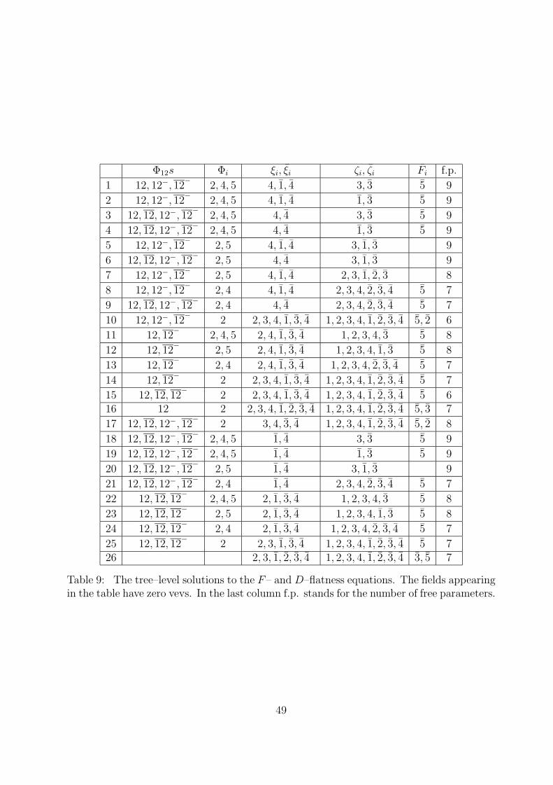
Φ12s Φi ξi, ξi ζi, ζi Fi f.p.

1 12, 12−, 12−

2, 4, 5 4, 1, 4 3, 3 5 9

2 12, 12−, 12−

2, 4, 5 4, 1, 4 1, 3 5 9

3 12, 12, 12−, 12−

2, 4, 5 4, 4 3, 3 5 9

4 12, 12, 12−, 12−

2, 4, 5 4, 4 1, 3 5 9

5 12, 12−, 12−

2, 5 4, 1, 4 3, 1, 3 9

6 12, 12, 12−, 12−

2, 5 4, 4 3, 1, 3 9

7 12, 12−, 12−

2, 5 4, 1, 4 2, 3, 1, 2, 3 8

8 12, 12−, 12−

2, 4 4, 1, 4 2, 3, 4, 2, 3, 4 5 7

9 12, 12, 12−, 12−

2, 4 4, 4 2, 3, 4, 2, 3, 4 5 7

10 12, 12−, 12−

2 2, 3, 4, 1, 3, 4 1, 2, 3, 4, 1, 2, 3, 4 5, 2 6

11 12, 12−

2, 4, 5 2, 4, 1, 3, 4 1, 2, 3, 4, 3 5 8

12 12, 12−

2, 5 2, 4, 1, 3, 4 1, 2, 3, 4, 1, 3 5 8

13 12, 12−

2, 4 2, 4, 1, 3, 4 1, 2, 3, 4, 2, 3, 4 5 7

14 12, 12−

2 2, 3, 4, 1, 3, 4 1, 2, 3, 4, 1, 2, 3, 4 5 7

15 12, 12, 12−

2 2, 3, 4, 1, 3, 4 1, 2, 3, 4, 1, 2, 3, 4 5 616 12 2 2, 3, 4, 1, 2, 3, 4 1, 2, 3, 4, 1, 2, 3, 4 5, 3 7

17 12, 12, 12−, 12−

2 3, 4, 3, 4 1, 2, 3, 4, 1, 2, 3, 4 5, 2 8

18 12, 12, 12−, 12−

2, 4, 5 1, 4 3, 3 5 9

19 12, 12, 12−, 12−

2, 4, 5 1, 4 1, 3 5 9

20 12, 12, 12−, 12−

2, 5 1, 4 3, 1, 3 9

21 12, 12, 12−, 12−

2, 4 1, 4 2, 3, 4, 2, 3, 4 5 7

22 12, 12, 12−

2, 4, 5 2, 1, 3, 4 1, 2, 3, 4, 3 5 8

23 12, 12, 12−

2, 5 2, 1, 3, 4 1, 2, 3, 4, 1, 3 5 8

24 12, 12, 12−

2, 4 2, 1, 3, 4 1, 2, 3, 4, 2, 3, 4 5 7

25 12, 12, 12−

2 2, 3, 1, 3, 4 1, 2, 3, 4, 1, 2, 3, 4 5 726 2, 3, 1, 2, 3, 4 1, 2, 3, 4, 1, 2, 3, 4 3, 5 7

Table 9: The tree–level solutions to the F– and D–flatness equations. The fields appearingin the table have zero vevs. In the last column f.p. stands for the number of free parameters.

49