Two-loop Yang-Mills diagrams from superstring amplitudes

QMUL-PH-15-06

Two-loop Yang-Mills diagrams from superstringamplitudes

Lorenzo Magnea a,1, Sam Playle a,2, Rodolfo Russo b,3, and Stefano Sciuto a,4

a Dipartimento di Fisica, Universita di Torinoand INFN, Sezione di Torino

Via P. Giuria 1, I-10125 Torino, Italy

b Centre for Research in String TheorySchool of Physics and AstronomyQueen Mary University of London

Mile End Road, London, E1 4NS, United Kingdom

Abstract

Starting from the superstring amplitude describing interactions among D-braneswith a constant world-volume field strength, we present a detailed analysis of howthe open string degeneration limits reproduce the corresponding field theory Feyn-man diagrams. A key ingredient in the string construction is represented by thetwisted (Prym) super differentials, as their periods encode the information aboutthe background field. We provide an efficient method to calculate perturbativelythe determinant of the twisted period matrix in terms of sets of super-moduli appro-priate to the degeneration limits. Using this result we show that there is a preciseone-to-one correspondence between the degeneration of different factors in the su-perstring amplitudes and one-particle irreducible Feynman diagrams capturing thegauge theory effective action at the two-loop level.

1email: [email protected]: [email protected]: [email protected]: [email protected]

arX

iv:1

503.

0518

2v1

[he

p-th

] 1

7 M

ar 2

015

1 Introduction

The study of scattering amplitudes has played a central role in the development of stringtheory since its very beginning. In the seventies and the eighties it was instrumental inshowing that superstring theories provide perturbative gravitational models that, at looplevel, are free of ultraviolet divergences and anomalies. The analysis of string amplitudeswas also crucial in the discovery of D-branes and in the development of the web of dualitiesamong different superstring theories. It is, then, not surprising that this field continuesto be under intense study. Recently, there has been renewed interest in several aspects ofstring perturbation theory in the RNS formalism, with particular focus on contributionsbeyond one loop: for example, higher-loop diagrams with Ramond external states werediscussed in Refs. [1, 2]; further, Refs. [3, 4, 5] focused on the off-shell extension of am-plitudes, studying various situations where this is necessary; finally, Ref. [6, 7] derived anexplicit result for the D6R4 term in the type-IIB effective action, checking the predictionsfollowing from S-duality and supersymmetry. Another interesting approach to the point-like limit of closed string amplitudes as a ‘tropical’ limit was discussed in [8]. For recentreviews on multiloop string amplitudes, with a more complete list of references, we referthe reader to [9, 10].

Two themes in particular have been at the center of much important progress in ourunderstanding of string interactions: the study of the mathematical properties of theworld-sheet formulation of string amplitudes, and their relation to the effective actionsdescribing the light degrees of freedom present in the theory. In this paper, we touch onboth these aspects by studying in detail the open string degeneration limits of two-loopamplitudes described by a world-sheet with three borders and no handles. In particular,we expand upon the results of [11]: starting from the Neveu-Schwarz (NS) sector ofthe open superstring partition function in the background of a constant magnetic fieldstrength, we derive the Euler-Heisenberg effective action for a gauge theory coupled toscalar fields in the ‘Coulomb phase’. The idea of using string theory to investigate effectiveactions in constant electromagnetic fields has a long history, and was studied at oneloop in [12, 13, 14], with some results for the bosonic theory at two loops given in [15].In our analysis we find exact agreement between calculations in field theory and stringtheory, in the infinite-tension limit, for the two-loop correction to the effective action.Furthermore, we find that the correspondence holds not just for the whole amplitude,but we can precisely identify the string origin of all individual one-particle irreducible(1PI) Feynman diagrams contributing to the effective action. In order to do so, on thestring theory side we need to use appropriate world-sheet super-moduli, respecting thesymmetry of the Feynman graphs, while on the field theory side we need to use a versionof the non-linear gauge condition introduced by Gervais and Neveu in [16], modified bydimensional reduction to involve the scalars also, and given here in Eq. (5.10).

On the formal side, it is advantageous to use the formalism of super Riemann sur-faces [17, 18, 19, 20, 21, 9], in which the complex structure is generalized to a super-conformal structure, with local super-conformal coordinates (z|θ). We follow this ap-proach by constructing the two-loop amplitude in the Schottky parametrization, sincethere is a close relationship between Schottky super-moduli, in particular the ‘multipli-

1

ers’, and the sewing parameters of plumbing fixtures. This in turn relates the bosonicworld-sheet moduli to the Schwinger parameters associated to the propagators in Feyn-man graphs, which provides the ideal framework for studying the connection betweenstring integrands and field theory Feynman diagrams. In the bosonic case, it is possibleto describe genus h Riemann surfaces as quotients of the Riemann sphere (with a discreteset of points removed) by a discrete (Schottky) group, freely generated by h Mobius trans-formations. Heuristically, quotienting the Riemann sphere by a Mobius transformationhas the effect of cutting out a pair of circles and gluing them to each other along theirboundaries. Schottky groups arose naturally in the early treatment of multi-loop stringamplitudes [22, 23, 24, 25, 26, 27] and remained useful [28, 18, 29, 30, 31, 32] even after al-ternative methods of analysis were found. In the supersymmetric case, higher genus superRiemann surfaces are similarly generated by quotienting the super manifold CP1|1 (witha discrete set of points removed) by a discrete group, generated by h ‘super-projective’OSp(1|2) transformations.

As is well known, the presence of a constant background field strength in the space-time description of the amplitudes translates on the world-sheet side into the presenceof non-trivial monodromies along either the a or the b cycles of the Riemann surface. Itis thus not surprising that the amplitudes we are interested in involve super 1|1-forms(sections of the Berezinian bundle) with twisted periodicities, also known as Prym dif-ferentials. The bosonic counterparts of these objects was discussed, in the Schottkyparametrization, in [33], and their periods along the untwisted cycles appear in any stringamplitude where the fields have non-trivial monodromies [34, 35, 15, 36]. We extendthese past results in two directions: first we generalise the twisted period matrix to thesupersymmetric case; then we must calculate the supersymmetric version of the twisteddeterminant to sufficiently high order in the complete degeneration limit, so as to obtainthe gauge theory Feynman graphs with multiple gluon propagators. In order to do this,we introduce an alternative formulation of the twisted super-determinant in terms of anintegral along a Pochhammer contour, and we show that this simplifies drastically itsperturbative evaluation in the Schottky parametrization.

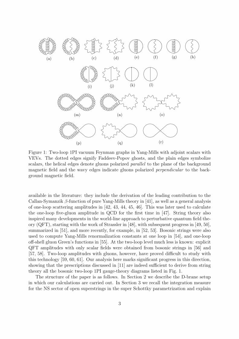
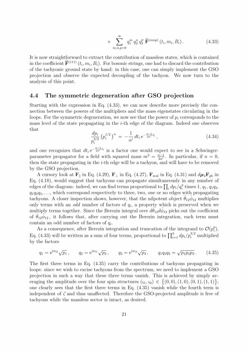
The main result of this paper is to show how the two-loop 1PI Feynman diagramslisted in Fig. 1 arise from the degeneration limits of the superstring result. The graphicalnotation for the field propagators is explained in detail in Appendix C; here we note inparticular that we are using two different types of edges to denote gluons, dependingon whether they are polarized parallel or perpendicular to the plane of the backgroundfield. We note also that some of the graphs (those in Figs. 1i–1l) include vertices with anodd number of scalars: these vertices arise because of the non-vanishing scalar vacuumexpectation values (to which these graphs are proportional); these diagrams appear auto-matically in the string calculation, and they appear on the field-theory side as a result ofhaving imposed the gauge condition of Gervais and Neveu [16] before dimensional reduc-tion. Our investigation is thus also a contribution to a long-standing program aimed to usestring theory to gain insights into field-theory amplitudes, which was started in Ref. [37]in the language of dual models, and generalized to the superstring framework in [38]. Thepractical usefulness of string theory as an organizing principle for tree-level gauge-theoryamplitudes was first noticed and applied in [39, 40]. At genus one, several results are

2

(a) (b) (c) (d) (e) (f) (g) (h)

(i) (j) (k) (l)

(m) (n) (o)

(p) (q) (r)

Figure 1: Two-loop 1PI vacuum Feynman graphs in Yang-Mills with adjoint scalars withVEVs. The dotted edges signify Faddeev-Popov ghosts, and the plain edges symbolizescalars, the helical edges denote gluons polarized parallel to the plane of the backgroundmagnetic field and the wavy edges indicate gluons polarized perpendicular to the back-ground magnetic field.

available in the literature: they include the derivation of the leading contribution to theCallan-Symanzik β-function of pure Yang-Mills theory in [41], as well as a general analysisof one-loop scattering amplitudes in [42, 43, 44, 45, 46]. This was later used to calculatethe one-loop five-gluon amplitude in QCD for the first time in [47]. String theory alsoinspired many developments in the world-line approach to perturbative quantum field the-ory (QFT), starting with the work of Strassler in [48], with subsequent progress in [49, 50],summarized in [51], and more recently, for example, in [52, 53]. Bosonic strings were alsoused to compute Yang-Mills renormalization constants at one loop in [54], and one-loopoff-shell gluon Green’s functions in [55]. At the two-loop level much less is known: explicitQFT amplitudes with only scalar fields were obtained from bosonic strings in [56] and[57, 58]. Two-loop amplitudes with gluons, however, have proved difficult to study withthis technology [59, 60, 61]. Our analysis here marks significant progress in this direction,showing that the prescriptions discussed in [11] are indeed sufficient to derive from stringtheory all the bosonic two-loop 1PI gauge-theory diagrams listed in Fig. 1.

The structure of the paper is as follows. In Section 2 we describe the D-brane setupin which our calculations are carried out. In Section 3 we recall the integration measurefor the NS sector of open superstrings in the super Schottky parametrization and explain

3

how to modify it in order to accommodate our background. In Section 4 we expandthe measure in powers the Schottky multipliers, and then we identify the appropriateparametrizations to describe the two degenerations of the Riemann surface which arerelevant for our purposes: the symmetric degeneration leading to the diagrams with thetopology of Figs. 1a–1l, and the incomplete degeneration, leading to diagrams with onlytwo field-theory propagators and a four-point vertex, depicted in Figs. 1m–1r. An analysisof the various factors contributing to the string amplitude, arising from different world-sheet conformal field theories, then enables to unambiguously identify each diagram in thefield-theory limit. In Section 5 we obtain and discuss the Lagrangian for the world-volumeQFT in the appropriate non-linear gauge, and we use it to compute example Feynmandiagrams. Finally, in Section 6.1 we compare our string-theory and QFT calculations,and in Section 6.2 we discuss the differences between the present calculation and theanalogous calculation using the bosonic string. In Appendix A we discuss super-projectivetransformations and the super Schottky group, in Appendix B we give the calculation ofthe twisted (Prym) super period matrix, and in Appendix C we list the values of all ofthe Feynman graphs in Fig. 1 with our choice of background fields.

2 The string theory setup

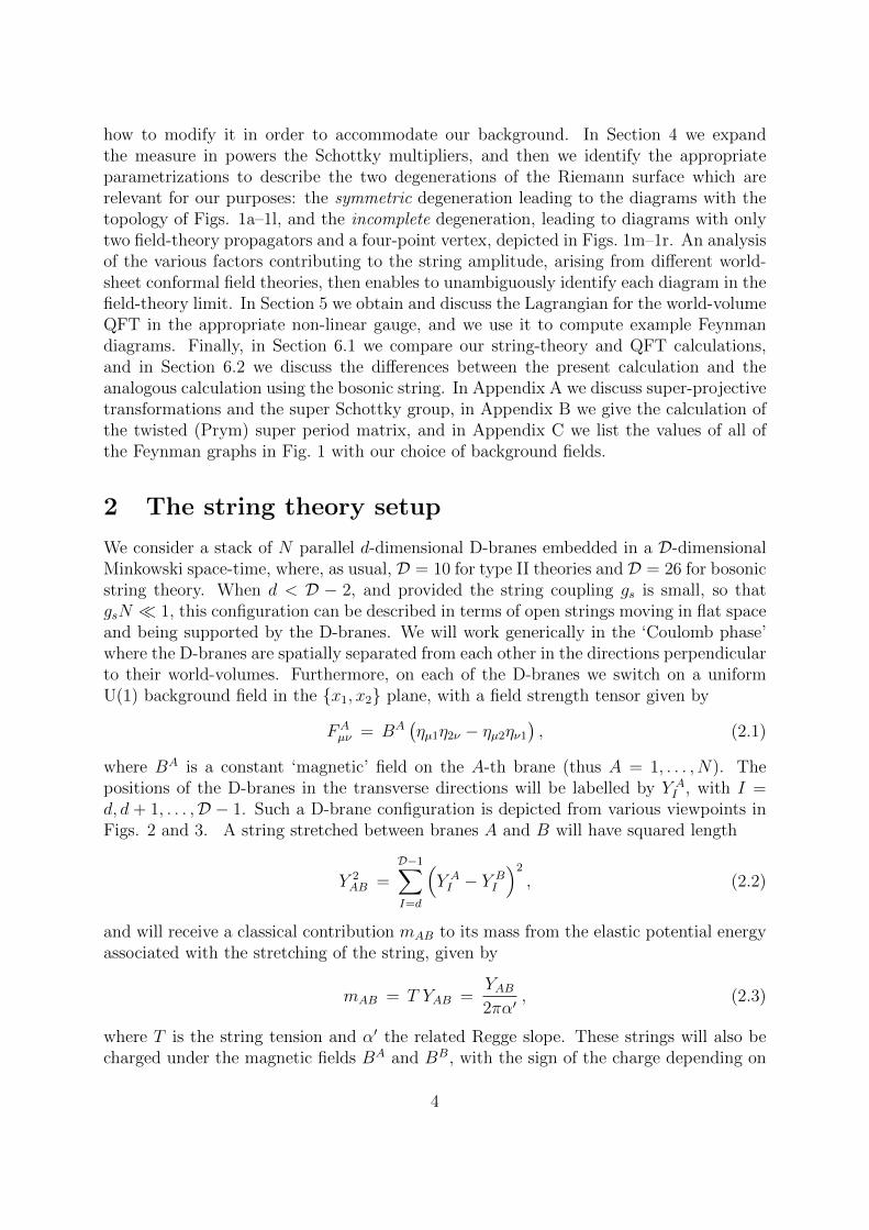
We consider a stack of N parallel d-dimensional D-branes embedded in a D-dimensionalMinkowski space-time, where, as usual, D = 10 for type II theories and D = 26 for bosonicstring theory. When d < D − 2, and provided the string coupling gs is small, so thatgsN 1, this configuration can be described in terms of open strings moving in flat spaceand being supported by the D-branes. We will work generically in the ‘Coulomb phase’where the D-branes are spatially separated from each other in the directions perpendicularto their world-volumes. Furthermore, on each of the D-branes we switch on a uniformU(1) background field in the x1, x2 plane, with a field strength tensor given by

FAµν = BA

(ηµ1η2ν − ηµ2ην1

), (2.1)

where BA is a constant ‘magnetic’ field on the A-th brane (thus A = 1, . . . , N). Thepositions of the D-branes in the transverse directions will be labelled by Y A

I , with I =d, d + 1, . . . ,D − 1. Such a D-brane configuration is depicted from various viewpoints inFigs. 2 and 3. A string stretched between branes A and B will have squared length

Y 2AB =

D−1∑I=d

(Y AI − Y B

I

)2

, (2.2)

and will receive a classical contribution mAB to its mass from the elastic potential energyassociated with the stretching of the string, given by

mAB = T YAB =YAB2πα′

, (2.3)

where T is the string tension and α′ the related Regge slope. These strings will also becharged under the magnetic fields BA and BB, with the sign of the charge depending on

4

...

...

Y 1I

Y 2I

Y AI

xI

FAµν

F 2µν

F 1µν

Y NI

FNµν

xµ

...

...

Figure 2: A stack of of spatially separated D-branes with constant gauge fields on theirworld-volumes, connected by open strings ending on three different branes, in a double-annulus configuration.

xIY 2I

DN(d−1)

Y NJ

Y AI

D1(d−1)

D2(d−1)

DA(d−1)

Y 1IY N

I

Y 1J

Y 2J

Y AJ

xJ

Figure 3: A two-dimensional section of the space transverse to the D-branes, which there-fore appear as points, connected by a web of open strings.

5

their orientation. Open strings that start and end on the same D-brane are unchargedand their mass is independent of Y A

I . For generic values of Y AI , this configuration breaks

the symmetry of the world-volume theory from U(N) to U(1)N .The theory describing open strings supported by this D-brane configuration is free [12,

13]. The constant background magnetic fields on the D-brane world-volumes manifestthemselves in the world-sheet picture by altering the boundary conditions of string coor-dinates in the magnetized plane. On the double cover of the surface, this gives twistedboundary conditions, or, in other words, non-trivial monodromies, to the zero modes inthe two magnetized space directions. To describe this setup, we will use the conventionsof Section 3 of Ref. [11], which we summarize below.

To begin with, let us briefly consider the spectrum of low-lying string excitations. Inthe bosonic case, the world-sheet theory, in a covariant approach, comprises D embeddingcoordinates Xµ and the ghost system (b, c). The holomorphic components of these fieldsadmit the mode expansions

b(z) =∑n∈Z

bnz−n−2 , c(z) =

∑n∈Z

cnz−n+1 , ∂zX

µ = − i√

2α′∑n∈Z

αµn z−n−1 . (2.4)

In the presence of constant abelian background fields, the theory remains free, but stringcoordinates in directions parallel to the magnetized plane acquire twisted boundary condi-tions and must be treated separately. Considering strings ending on branes A and B, it isconvenient to introduce the combinations Z±AB = (X1

AB± iX2AB)/

√2. These combinations

diagonalize the boundary conditions and yield the mode expansions

∂zZ±AB = − i

√2α′∑n∈Z

α±n±εAB z−n−1±εAB , (2.5)

where we definedtan (πεAB) ≡ 2πα′

(BA −BB

). (2.6)

After canonical quantization, the modes introduced above satisfy standard commutationrelations, except for magnetized directions, where one finds[

α+n+εAB

, α−m−εAB

]= (n+ εAB) δn+m . (2.7)

As usual in covariant quantization, not all states in the Fock space obtained by actingwith the creation modes on the SL(2,R)-invariant vacuum |0〉 are physical: we need toselect only the states belonging to the cohomology of the world-sheet BRST charge

QWB =

∮dz

2πic

(− 1

4α′∂XM∂XM + (∂c)b

). (2.8)

In the bosonic theory, the lowest-lying physical state is a tachyon |k〉 ≡ c1|k, 0〉, withmass-shell condition k2 = −m2 = 1/α′. The next mass level comprises (D + 2) masslessstates, which will be the focus of our analysis in the field theory limit: one finds twounphysical states, two null states, and (D−2) physical polarization states appropriate formassless gauge bosons. A crucial ingredient of our analysis is the mapping between these

6

string states and the space-time states in the limiting quantum field theory: as noticedfor instance in Chapter 4 of [62], the action of the worldsheet BRST charge (2.8) onthe (D + 2) massless states mirrors the linearized action of the space-time BRST chargefor the U(N) gauge symmetry: in particular, the states created by world-sheet ghostoscillators, c−1|k〉 and b−1|k〉, behave as the spacetime ghosts C and C. Acting with theαM−1 oscillators, on the other hand, generates d states along the D-brane, and ns = D− dstates associated to the ns directions transverse to the D-brane, representing respectivelythe d polarisations of the gauge vectors (including two unphysical ones), and ns adjointscalars. To be precise, the world-sheet BRST charge QW

B acts as

QWB b−1|k〉 =

√2α′k · α−1|k〉 ; QW

B αM−1|k〉 =

√2α′kMc−1|k〉 ; QW

B c−1|k〉 = 0 , (2.9)

while the linearised space-time BRST transformation δB acts as

δB(Ca) ∼ ∂ ·Qa ; δB

(Q aµ

)∼ ∂µC

a ; δB (Q aI ) ∼ 0; δB (C a) ∼ 0 , (2.10)

where a is an adjoint index, Q aµ and Q a

I stand for a gluon mode and a scalar, dependingon whether XM is parallel or perpendicular to the D-brane, and kM = kµ, 0.

This simple relation between world-sheet and space-time states is preserved in pertur-bation theory, when the string coupling is switched on and non-linear terms in the BRSToperators must be taken into account. This is expected, since, in a perturbative analy-sis, fields propagating between interaction vertices are free. In practice, we will test thisstatement by calculating a string diagram with the world-sheet topology of a degeneratingdouble-annulus, and identifying the contributions coming from the various massless stateslisted above, as they propagate through the diagram. We will show that each contributionmatches the gauge theory result, where the corresponding space-time fields propagate inthe matching edge of the relevant Feynman diagram, provided that the gauge used infield theory is the nonlinear Gervais-Neveu gauge, introduced in [16]. In this way, we canidentify individual Feynman diagrams in the target field theory directly at the level of thestring amplitude, picking a specific boundary of the string moduli space, and identifyingthe string states as they propagate along the degenerating surface.

A similar analysis holds also in the superstring case. In the RNS formalism one needsto introduce the extra world-sheet fields ψµ, β and γ, that are the partners under world-sheet supersymmetry of the ∂Xµ, b and c fields mentioned above. The monodromies forthese new fields will be the same as those of their partners, except for a possible extra sign,which is allowed for fields of half-integer weight, and distinguishes the Ramond from theNeveu-Schwarz sectors. In this paper we will focus on the Neveu-Schwarz contributions:the analysis of the states at the first mass level, above the tachyonic ground state |k〉,parallels that of the bosonic case. The only difference is that the relevant modes areψ−1/2, β−1/2 and γ−1/2: in the superstring partition function, the low energy limit will beperformed by focusing on the contributions of states with half-integer weight.

7

3 The superstring partition function for the NS sec-

tor

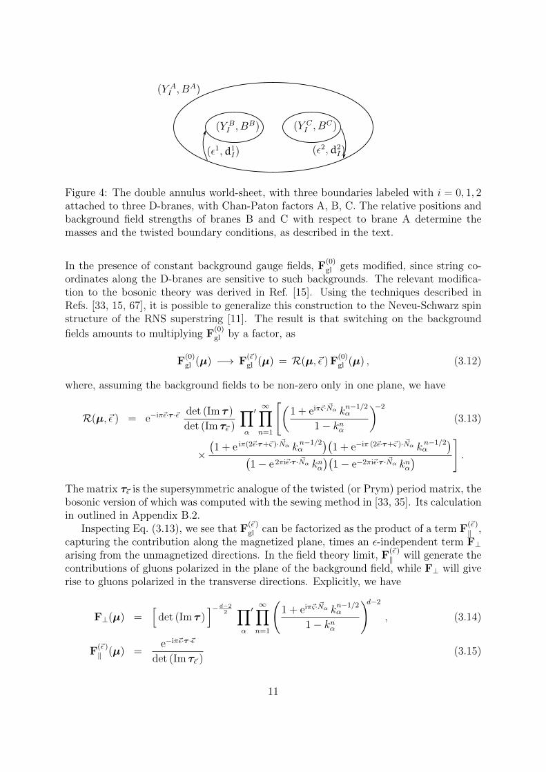
From the world-sheet point of view, the interaction among D-branes is described by thestring vacuum amplitude (the partition function) with boundaries, as depicted in Fig. 2.The case of two magnetized D-branes, corresponding to a one loop-amplitude, has beenwell studied [12, 13, 63, 14]. Here we will focus on planar world-sheets, and most of whatwe will say in this section applies to surfaces with (h + 1) borders, corresponding to h-loop open superstring diagrams, but restricted to the NS sector, where the super-Schottkyformalism described in Ref. [30] can be used. In particular, as discussed in Section 2, weconsider parallel magnetized D-branes that can be separated in the directions transverseto their world-volumes. As a consequence, and as depicted in Fig. 4 for a (two-loop)surface with three boundaries, the partition function depends on two set of variables:the relative distances among D-branes, and the magnetic field gradients between pairs ofD-branes.

To be precise, let us label the (h + 1) world-sheet borders with i = 0, 1, . . . , h. Thenwe can label the D-brane to which the i-th border is attached with the integer Ai, withAi ∈ 1, . . . , N, and Ai ≤ Ai+1. To get the full amplitude, we will have to sum over theAi’s. Having fixed A0, . . . , Ah, we can take the A0-th brane as a reference and define

diI = Y A0I − Y

AiI (I = d, . . . ,D − 1) ,

tan(πεi)

= 2πα′(BA0 −BAi

). (3.1)

The variables εi thus form an h-dimensional vector, which we will denote by ~ε ; similarly,the variables diI , which have dimension of length, form ns h-dimensional vectors, which

we will label ~dI . The classical mass of the string stretching between the A0-th brane andthe Ai-th brane is then given by

m2i =

1

(2πα′)2

D−1∑I=d

(diI)2. (3.2)

Notice finally that, for h = 2, as depicted in Fig. 4, we make a slight variation in thisnotation by flipping the sign of the second component of the two-dimensional vectors ~εand ~dI , which will be useful to take full advantage of the extra symmetry at two loops.

The string partition function in this setup can be written as follows. For our purposes,it is useful to keep separate the contributions of the different conformal field theory sectors,which leads to the expression

Zh

(~ε, ~d

)= N (~ε )

h

∫dµh Fgh (µ) F

(~d )scal (µ) F

(~ε )‖ (µ) F⊥ (µ) . (3.3)

Here N (~ε )h is a field-dependent normalization factor, to be discussed in Section 4.4, and we

denoted the contributions of the world-sheet ghost systems b, c and β, γ by Fgh, that of the

string fields XI , ψI perpendicular to the D-branes by F(~d )scal , while the contribution of the

fields along the D-branes has been separated into sectors parallel (F(~ε )‖ ) and perpendicular

8

(F⊥) to the magnetized directions. Finally, µ denotes collectively the supermoduli: herewe use the super-Schottky formalism, reviewed in Appendix A, where the supermoduliare the sewing parameters eiπςiki

1/2 (with ςi ∈ 0, 1) and the fixed points (ui|θi), (vi|φi)of h super-projective transformations i = 1, . . . , h. Note that we explicitly associate witheach Schottky multiplier ki the phase ςi associated with the NS spin structure around thebi homology cycle. In this parametrization the measure dµh reads [30]

dµh =

[√(v1 − u1)(u1 − v2)(v2 − v1)

dv1du1dv2

dΘv1u1v2

]h∏i=1

dki eiπςi

k3/2i

dui dvivi − ui

, (3.4)

where we denote superconformal coordinates in boldface, and the notation vi−ui indicatesthe supersymmetric difference

vi − ui ≡ vi − ui + θiφi . (3.5)

The square parenthesis in Eq. (3.4) takes into account the super-projective invariance ofthe integrand, which allows us to fix three bosonic and two fermionic variables. Θv1u1v2 isthe fermionic super-projective invariant which can be constructed with three fixed points,defined in Refs. [64, 20], and given explicitly in Eq. (A.12). If we specialize Eq. (3.4) toh = 2 we find

dµ2 = eiπ(ς1+ς2) dk1

k3/21

dk2

k3/22

du2 dΘv1u1v2

v2 − u2

√(u1 − v2)(v2 − v1)

v1 − u1

. (3.6)

Let us now examine in turn the various factors in the integrand of Eq. (3.3). The ghostcontribution is independent of both the magnetic fields and the D-brane separations, sowe can use the result of Ref. [30], which reads

Fgh(µ) =(1− k1)2 (1− k2)2(

1 + eiπς1k1/21

)2 (1 + eiπς2k

1/22

)2

∏α

′∞∏n=2

(1 + knα

1 + eiπ~ς· ~Nαkn− 1

2α

)2

. (3.7)

In Eq. (3.7), the notation∏′

α means that the product is over all primary classes of thesuper Schottky group: a primary class is an equivalence class of primitive super Schottkygroup elements, i.e. those elements which cannot be written as powers of another element;two primitive elements are in the same primary class if one is related to the other bya cyclic permutation of its factors, or by inversion. The vector ~Nα has h integer-valuedcomponents, and is defined as follows: the i-th entry counts how many times the generatorSi enters in the element of the super Schottky group Tα: more precisely, we define N i

α = 0for Tα = 1 and N i

α = N iβ ± 1 for Tα = S±1

i Tβ. Finally, also ~ς is a vector with hcomponents, with the i-th component denoting the spin structure along the bi cycle, asnoted above.

In fact, we need to be more precise about the notation in Eq. (3.7), because thehalf-integer powers of kα could indicate either of the two branches of the function. Thenotation is to be understood in the following way: when the spin structure is ~ς = 0, we

9

define the eigenvalue of the Schottky group element Tα with the smallest absolute value tobe −k1/2

α , see Eq (A.16). In particular, we take k1/2i to be positive5 for i = 1, . . . , h. This

corresponds to the fact that spinors are anti-periodic around a homology cycle with zerospin structure (see, for example, Ref. [65]). Furthermore, we expect the partition functionto be symmetric under the exchange of the homology cycles b1, b2 and b−1

1 · b2 (depicted in

Fig. 5), and one can verify that k1/2(S−11 S2) is always positive whenever k

1/21 and k

1/22 have

the same sign. Our convention puts all three multipliers on the same footing. Note thatk

1/2α is not in general positive when Tα is not a generator: for example, the eigenvalues of

Tα = S1S2 are positive when the spin structure is zero, so that k1/2(S1S2), as computedin Eq. (A.25), is negative.

The scalar contribution to Eq. (3.3) depends on the separation between the D-branes

in the transverse directions, as shown in Fig. 3. We can write F(~d )scal as a product over

the super Schottky group, capturing the non-zero mode contribution, times a new factorY(µ, ~d ), as

F(~d )scal(µ) = Y

(µ, ~d

) ∏α

′∞∏n=1

(1 + eiπ~ς· ~Nα k

n−1/2α

1− knα

)ns. (3.8)

The explicit form of Y can be found by repeating the calculation performed in Ref. [66]for the bosonic theory, and replacing the period matrix τ with the super-period matrix τdiscussed in Appendix A.2.2. We find

Y(µ, ~d ) ≡ns∏I=1

exp

(~dI · τ · ~dI

2πiα′

). (3.9)

It is instructive, and useful for our later implementation, to consider explicitly the h = 2case. Let the i = 0, 1, 2 borders of the world-sheet be on the D-branes labelled by A,B and C, respectively. As mentioned above, it is useful in this special h = 2 case todefine the i = 2 component d2

I with the opposite sign with respect to Eq. (3.1), so wehave d1

I = Y AI − Y B

I and d2I = Y C

I − Y AI . By so doing, we can then define an additional

(redundant) quantity, describing the displacement between the D-branes attached to thei = 1 and i = 2 borders, as d3

I = Y BI − Y C

I . Now the three distances diI for i = 1, 2, 3are on an equal footing, reflecting the symmetry of the world-sheet topology, and we haved1I+d2

I+d3I = 0 (see Fig. 4). One may easily verify that the product over the ns transverse

directions in Eq. (3.9) evaluates to a function of the squared masses m2i , defined as in

Eq. (3.2). One finds

Y(µ, ~d ) = exp

[2πiα′

(m2

1 τ11 +m22 τ22 +

(m2

3 −m21 −m2

2

)τ12

)]. (3.10)

Finally, let us turn to the contribution of the world-sheet fields Xµ, ψµ along the world-volume direction of the D-branes. In absence of magnetic fields, the result can be foundin Ref. [30] and it reads

F(0)gl (µ) =

[det (Im τ )

]−d/2 ∏α

′∞∏n=1


n−1/2α

1− knα

)d. (3.11)

5This convention is the opposite to the one used in [11].

10

(Y AI , B

A)

(Y BI , B

B) (Y CI , B

C)

(ε1,d1I) (ε2,d2

I)

Figure 4: The double annulus world-sheet, with three boundaries labeled with i = 0, 1, 2attached to three D-branes, with Chan-Paton factors A, B, C. The relative positions andbackground field strengths of branes B and C with respect to brane A determine themasses and the twisted boundary conditions, as described in the text.

In the presence of constant background gauge fields, F(0)gl gets modified, since string co-

ordinates along the D-branes are sensitive to such backgrounds. The relevant modifica-tion to the bosonic theory was derived in Ref. [15]. Using the techniques described inRefs. [33, 15, 67], it is possible to generalize this construction to the Neveu-Schwarz spinstructure of the RNS superstring [11]. The result is that switching on the background

fields amounts to multiplying F(0)gl by a factor, as

F(0)gl (µ) −→ F

(~ε )gl (µ) = R(µ,~ε ) F

(0)gl (µ) , (3.12)

where, assuming the background fields to be non-zero only in one plane, we have

R(µ,~ε ) = e−iπ~ε·τ ·~ε det (Im τ )

det (Im τ~ε )

∏α

′∞∏n=1

[(1 + eiπ~ς· ~Nα k

n−1/2α

1− knα

)−2

(3.13)

×(1 + e iπ(2~ε·τ+~ς )· ~Nα k

n−1/2α

)(1 + e−iπ (2~ε·τ+~ς )· ~Nα k

n−1/2α

)(1− e 2πi~ε·τ · ~Nα knα

)(1− e−2πi~ε·τ · ~Nα knα

) ].

The matrix τ~ε is the supersymmetric analogue of the twisted (or Prym) period matrix, thebosonic version of which was computed with the sewing method in [33, 35]. Its calculationin outlined in Appendix B.2.

Inspecting Eq. (3.13), we see that F(~ε )gl can be factorized as the product of a term F

(~ε )‖ ,

capturing the contribution along the magnetized plane, times an ε-independent term F⊥arising from the unmagnetized directions. In the field theory limit, F

(~ε )‖ will generate the

contributions of gluons polarized in the plane of the background field, while F⊥ will giverise to gluons polarized in the transverse directions. Explicitly, we have

F⊥(µ) =[

det (Im τ )]− d−2

2∏α

′∞∏n=1


n−1/2α

1− knα

)d−2

, (3.14)

F(~ε )‖ (µ) =

e−iπ~ε·τ ·~ε

det (Im τ~ε )(3.15)

11

×∏α

′∞∏n=1

(1 + e iπ(2~ε·τ+~ς)· ~Nα k

n−1/2α

)(1 + e−iπ (2~ε·τ+~ς)· ~Nα k

n−1/2α

)(1− e 2πi~ε·τ · ~Nα knα

)(1− e−2πi~ε·τ · ~Nα knα

) .

Focusing now on the h = 2 case, we can use super-projective invariance to fix three bosonicand two fermionic moduli. A convenient gauge choice in the super Schottky formalism isto specify the positions of the fixed points, given in terms of homogeneous coordinates6

on CP1|1, as

|u1〉 = (0, 1|0)t , |v1〉 = (1, 0|0)t , |u2〉 = (u, 1|θ)t , |v2〉 = (1, 1|φ)t ,(3.16)

with (0 < u < 1), which leads to

Θv1u1v2 = φ , v2 − u2 = 1− u+ θφ ,

√(u1 − v2)(v2 − v1)

v1 − u1

= 1 . (3.17)

Implementing this projective gauge fixing in Eq. (3.3), we can finally express the h = 2partition function as

Z2

(~ε, ~d

)= eiπ(ς1+ς2)

∫dk1

k3/21

dk2

k3/22

du

ydθ dφ Fgh(µ) F

(~ε )‖ (µ) F⊥(µ) F

(~d )scal(µ) , (3.18)

where we definedy ≡ (u1,v1,u2,v2) = 1− u+ θφ , (3.19)

in terms of the bosonic super-projective invariant built out of four points, (z1, z2, z3, z4),see Eq. Eq. (A.13).

4 Taking the field theory limit

4.1 Expanding in powers of the multipliers

We are interested in computing the α′ → 0 limit of the integrand of the superstringamplitude. In this limit, we expect massive string states to decouple, so that one is leftwith the massless spectrum. Possible contributions from the tachyon ground state can-cel after GSO projection in the superstring case, or should be discarded by hand in thebosonic case. It is in principle non trivial to take this limit before integration over (super)moduli, since this requires constructing a map between the dimensionless moduli of the(super) Riemann surface and the dimensionful quantities that arise in the computationof field theory Feynman diagrams. This task is considerably simplified in the Schottkyparametrization, where, as discussed for example in Ref. [11], the contributions of indi-vidual string states can be identified by performing a Laurent expansion of the integrandof the string partition function in powers of the multipliers. One finds a correspondencebetween the order of expansion and the mass level of the string, and furthermore, within

6The relation between the super-conformal and homogeneous coordinates is given in Eq. (A.5).

12

each mass level, one can track individual states by tracing the origin of each term to aspecific factor in the string integrand.

The main difference between the bosonic string and the RNS superstring is that forthe latter, which we discuss here, the expansion is in powers of k

1/2i rather than ki, as

is already apparent from our discussion in Section 3. More precisely, since the measureof integration contains a factor k

−3/2i , a term proportional to k

(n−3)/2i corresponds to a

contribution from a state belonging to the n-th mass level circulating in the i-th stringloop (where n = 0 corresponds to the tachyonic ground state). Therefore, all terms withn > 1 acquire a positive mass squared, m2 = (n − 1)/(2α′), and decouple in the limitα′ → 0. We conclude that it is necessary to expand the various factors in the integrandof Eq. (3.18) only up to terms of order ki

1/2, in order to get the complete massless fieldtheory amplitude.

This task is made possible by the fact that the multipliers of only finitely many super-Schottky group elements contribute at order k

1/21 k

1/22 . The reason is that the leading-

order behaviour of the multiplier kα = k(Tα) is related in a simple way to the index N iα

introduced in Section 3: one may verify that

k1/2(S±1i Tα

)= O

(k

1/2i k1/2

α

), (4.1)

unless of course the left-most factor of Tα is S∓1i . Thus, for every super Schottky group

element Tα not in the primary class of an element in the set S1,S2,S1S2,S−11 S2, the

multiplier k1/2α vanishes faster than k

1/2i for ki → 0. This enables us to easily compute

expressions for all the factors in Eq. (3.3), up to the relevant order.Let us begin with Fgh, defined in Eq. (3.7). One immediately sees that the expansion

of the infinite product starts at O(k3/2i ), and the numerator of the first factor can similarly

be dropped. Fgh becomes simply

Fgh(µ) =(

1− 2 eiπς1k1/21

)(1− 2 eiπς2k

1/22

)+O(ki) . (4.2)

Next, we compute F⊥, defined in Eq. (3.14). Using the expressions for the multipliersk1/2(S−1

1 S2) and k1/2(S1S2), given in Eq. (A.25), we find

F⊥(µ) =[

det (Im τ )]− d−2

2

[1 + (d− 2)

(eiπς1k

1/21 + eiπς2k

1/22

)(4.3)

+ (d− 2)(yu− y + d− 2

)eiπ(ς1+ς2)k

1/21 k

1/22

]+O(ki) .

The expansion of the determinant of the super period matrix is given in Eq. (A.33), and,substituted here, leads to the factor

[det (Im τ )

]− d−22 =

[4π2

log k1 log k2 − log2 u

] d−22

(4.4)

×

[1 + (d− 2)

y

uθφ

eiπς1k1/21 log k1 + eiπς2k

1/22 log k2

log k1 log k2 − (log u)2

]+O(ki) .

13

Notice that logarithmic dependence on (super) moduli must be retained exactly: indeed,as shown in Ref. [11] and discussed here in Section 4.3, it will turn into polynomialdependence on Schwinger parameters in the field theory limit.

The expansion of the factor F(~ε )‖ , also given in Eq. (3.14), is more intricate, as well as

more interesting, because of the dependence on the external fields. Writing

F(~ε )‖ (µ) =

e−iπ~ε·τ ·~ε

det (Im τ~ε )R(µ,~ε ) , (4.5)

where R is the background-field dependent factor of the infinite product appearing inEq. (3.15), we see that we can separately expand the three factors. The determinant ofthe twisted super period matrix is by far the most intricate contribution. It is discussed inAppendix B, and a complete expression with the exact dependence on the fields, through~ε, is very lengthy. We will see in Section 4.3, however, that in the field theory limit wemust expand in powers of the components of ~ε as well: at that stage, we will be able towrite a completely explicit expression also for det (Im τ~ε ). The exponential factor in thenumerator of Eq. (4.5) can be computed using the expression for τ in Eq. (A.32), and isgiven by

e−iπ~ε·τ ·~ε = k−ε21/21 k

−ε22/22 u−ε1ε2

[1 +

y

uθφ(

eiπς2k1/22 ε21 + eiπς1k

1/21 ε22

)]+O(ki) . (4.6)

Finally, the remaining factor in F(~ε )‖ is given by

R(µ,~ε ) = 1 + eiπς1k1/21 g+

12 + eiπς2k1/22 g+

21 (4.7)

+ eiπ(ς1+ς2)k1/21 k

1/22

[g+

12g+21 − 2 θφ

y

u

(ε1g−12 + ε2g

−21

)− 1

2

((y − y

u

)g+

12g+21 +

(y +

y

u

)g−12g

−21

)]+ O(ki) ,

where we defined the factors

g±ij = kεii uεj ± k−εii u−εj . (4.8)

The last required ingredient is F(~d )scal, defined in Eq. (3.8). Combining Eq. (3.10) with

Eq. (A.32), we get

Y(µ, ~d

)= k

α′m21

1 kα′m2

22 uα

′(m23−m2

1−m22) (4.9)

×[1− 2α′

y

u

(eiπς1k

1/21 m2

2 + eiπς2k1/22 m2

1

)]+O(ki) .

The remaining, mass-independent, factor in F(~d )scal in Eq. (3.8) is easily expanded, getting

F(0)scal(µ) = 1 + ns

(eiπς1k

1/21 + eiπς2k

1/22

)+ ns eiπ(ς1+ς2)k

1/21 k

1/22

(yu− y + ns

). (4.10)

14

b1 b2

(b−11 · b2)

(a)

(b1 · b2)

(b)

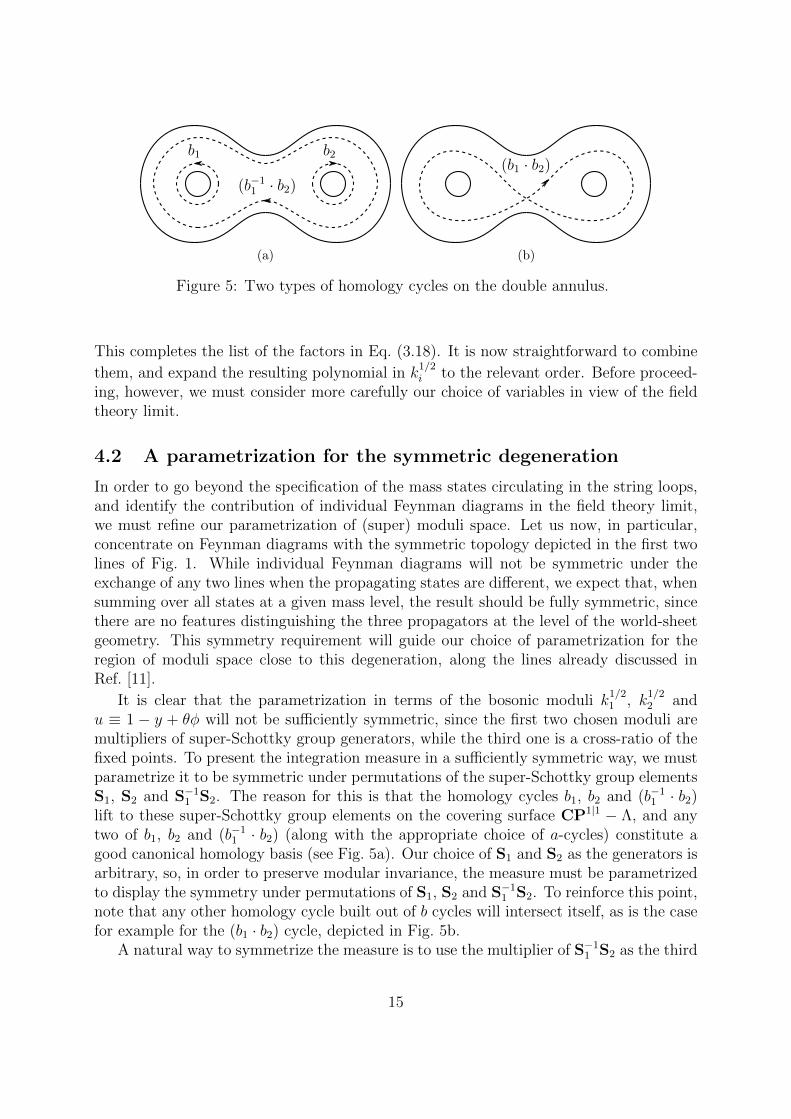
Figure 5: Two types of homology cycles on the double annulus.

This completes the list of the factors in Eq. (3.18). It is now straightforward to combine

them, and expand the resulting polynomial in k1/2i to the relevant order. Before proceed-

ing, however, we must consider more carefully our choice of variables in view of the fieldtheory limit.

4.2 A parametrization for the symmetric degeneration

In order to go beyond the specification of the mass states circulating in the string loops,and identify the contribution of individual Feynman diagrams in the field theory limit,we must refine our parametrization of (super) moduli space. Let us now, in particular,concentrate on Feynman diagrams with the symmetric topology depicted in the first twolines of Fig. 1. While individual Feynman diagrams will not be symmetric under theexchange of any two lines when the propagating states are different, we expect that, whensumming over all states at a given mass level, the result should be fully symmetric, sincethere are no features distinguishing the three propagators at the level of the world-sheetgeometry. This symmetry requirement will guide our choice of parametrization for theregion of moduli space close to this degeneration, along the lines already discussed inRef. [11].

It is clear that the parametrization in terms of the bosonic moduli k1/21 , k

1/22 and

u ≡ 1 − y + θφ will not be sufficiently symmetric, since the first two chosen moduli aremultipliers of super-Schottky group generators, while the third one is a cross-ratio of thefixed points. To present the integration measure in a sufficiently symmetric way, we mustparametrize it to be symmetric under permutations of the super-Schottky group elementsS1, S2 and S−1

1 S2. The reason for this is that the homology cycles b1, b2 and (b−11 · b2)

lift to these super-Schottky group elements on the covering surface CP1|1 − Λ, and anytwo of b1, b2 and (b−1

1 · b2) (along with the appropriate choice of a-cycles) constitute agood canonical homology basis (see Fig. 5a). Our choice of S1 and S2 as the generators isarbitrary, so, in order to preserve modular invariance, the measure must be parametrizedto display the symmetry under permutations of S1, S2 and S−1

1 S2. To reinforce this point,note that any other homology cycle built out of b cycles will intersect itself, as is the casefor example for the (b1 · b2) cycle, depicted in Fig. 5b.

A natural way to symmetrize the measure is to use the multiplier of S−11 S2 as the third

15

bosonic modulus, instead of u. Defining − eiπς3k1/23 to be the eigenvalue of S−1

1 S2 with thesmallest absolute value, so that k3 is the multiplier of that super Schottky group element,one can compute k

1/23 using Eq. (A.24). It is related to y implicitly through

y =(1− k1)(1− k2) + θφ

[(1 + eiπς1k

1/21

)(1 + eiπς2k

1/22

)(1 + eiπ(ς1+ς2)k

1/21 k

1/22

)]1 + k1k2 + k

1/21 k

1/22

(k

1/23 + k

−1/23

) . (4.11)

In these definitions, ς3 is the spin structure around the b3 ≡ b−11 · b2 homology cycle, and

therefore it is given simply by ς3 = ς1 + ς2 (mod 2). k1/23 is then positive, just as k

1/21 and

k1/22 are.

As discussed in Ref. [11], the field theory limit becomes particularly transparent ifone factors the three multipliers ki in order to assign a parameter to each section of theRiemann surface that will degenerate into an individual field theory propagator. This isdone by defining

k1/21 =

√p1√p3 k

1/22 =

√p2√p3 k

1/23 =

√p1√p2 , (4.12)

where√pi is defined to be positive. In analogy to the discussion of Ref. [11], each pi will

be interpreted, in the field theory limit, as the logarithm of the Schwinger proper timeassociated to a propagator.

For bosonic strings, the discussion leading to Eq. (4.12) was sufficient to construct asymmetric measure of integration, prepared for the symmetric degeneration in the fieldtheory limit. In the present case, instead, one must also worry about fermionic moduli:our current choice of θ and φ as moduli will not yield a symmetric measure, since theyare super-projective invariants built out of the fixed points of S1 and S2 only. In orderto find the proper Grassmann variables of integration, we take advantage of the factthat we are allowed to rescale θ and φ with arbitrary functions of the moduli, sincesuch a rescaling automatically cancels with the Berezinian of the corresponding change ofintegration variables. Such a rescaling of course leaves the integral invariant, but it canbe used to move contributions between the various factors of the integrand, in such a waythat individual factors respect the overall exchange symmetry of the diagram, as we wishto do here. In order to find a pair of odd moduli invariant under permutations of S1, S2,S−1

1 S2, we proceed as follows. Define

θij = cij Θviuiuj , φij = cij Θviuivj , (4.13)

for (ij) = (12), (23), (31). For the factors cij we make the choice

c12 =[

eiπς3 (1 + q1q2) (1− q1q3) (1− q2q3)]−1/2

, (4.14)

with c23 and c31 obtained by permuting the indices (123), and where u3 and v3 are thefixed points of the transformation S−1

1 S2. In Eq. (4.14), we have introduced the symbolsqi, i = 1, 2, 3, defined by7

q1 = eiπς2√p1 , q2 = eiπς1

√p2 , q3 = eiπς3

√p3 . (4.15)

7Note that the spin structures of q1 and q2 are swapped compared with what one might expect. This,

however, is reasonable, because the qi defined in this way factorize the NS sewing parameters eiπςi k1/2i

as follows: eiπς1 k1/21 = q1q3, eiπς2 k

1/22 = q2q3, eiπς3 k

1/23 = q1q2.

16

With this choice for cij, one can check that

eiπς3 dθ12 dφ12 = eiπς1 dθ23 dφ23 = eiπς2 dθ31 dφ31 , (4.16)

so that the Grassmann measure of integration has the required symmetry.It is not difficult to rewrite the various objects computed in Section 4.1 in terms of

the new variables, and expand the results to the required order in pi. In order to do so,we use

θφ = q3 (1 + q1q2) θ12φ12 +O(pi) , (4.17)

as well as

u = p3

[1 + θ12φ12

(q3 − q1 − q2 + q1q2q3

)]+ O

(p1, p2, p

23

).

With these results, it is straightforward to verify the symmetry of the full string integrand.In particular, we find that the product of the two-loop measure of integration times theghost factor is given by

dµ2 Fgh(µ) =3∏i=1

[dpi

p3/2i

1− eiπςik1/2i√

1 + pi

]dθ12dφ12

1√1 + p1p2p3

(4.18)

=3∏i=1

[dpiq3i

]dθ12 dφ12 (1− q1q3 − q2q3 − q1q2 ) +O(pi) ,

where the contribution of the spin structure to dµ2 in Eq. (3.6) has been absorbed indθ12 dφ12. Similarly, the contribution of the orbital modes defined in Eq. (4.7) becomes

R(µ,~ε ) = 1 +

q1q2

(pε11 p

−ε22 − p−ε11 pε22

) [1− θ12 φ12 q3 (ε1 − ε2)

]+ cyclic permutations

+O(pi) . (4.19)

Here, and in the rest of this section, we understand ‘cyclic permutations’ to mean cyclicpermutations of the indices (1, 2, 3) for pi, qi, εi and m2

i , where ε3 ≡ −ε1−ε2.8 The indicesof θ12 φ12, on the other hand, are not permuted.

In order to reconstruct the full contribution of fields in the directions parallel to themagnetized plane, we still need the other factors appearing in Eq. (4.6). The exponentialfactor takes the form

e−iπ~ε·τ ·~ε = p−ε21/21 p

−ε22/22 p

−ε23/23

[1− 1

2θ12φ12

(q1

(ε21 − ε22 − ε23

)+ q1q2q3 ε

21 + cycl. perm.

)]+O(pi) . (4.20)

8Recall that, in the h = 2 case, we define ε2 with the opposite sign with respect to Eq. (3.1), to exploitthe symmetry of the worldsheet.

17

The last factor in Eq. (4.6) is the twisted determinant det (Im τ~ε), whose calculation isdescribed in Appendix B. The result for generic values of u is a lengthy combination ofhypergeometric functions, which however simplifies drastically in the limit we are consid-ering here, where u, proportional to p3, is small.

In this limit (B.40) reads

det (Im τ~ε) =1

4π2Γ(−ε1)Γ(−ε2)Γ(−ε3)

pε1/21 p

ε2/22 p

ε3/23

(ε1 p

−ε1/21 + ε2 p

−ε2/22 + ε3 p

−ε3/23

)+ θ12φ12

[q1

(pε1/21 p

−ε2/22 p

−ε3/23 + p

−ε1/21 p

ε2/22 p

ε3/23

)pε1/21 ε2ε3 + cycl. perm.

]+ θ12φ12 q1q2q3 p

−3ε1/21 p

−3ε2/22 p

−3ε3/23

×[p2ε1

1 p2ε22 pε33

(2ε23 − ε1ε2

)+ p3ε3

3

(2ε3(p2ε1

1 ε2 + p2ε22 ε1

)− pε11 pε22 ε1ε2

)+ cycl. perm.

]+(εi ↔ −εµ

)+O(pi) . (4.21)

Next, we need the contribution of the untwisted gluon sector, given in Eq. (4.3). In thecurrent parametrization it reads

F⊥(µ) =[

det(Im τ )]−(d−2)/2

(4.22)

×[1− (d− 2)

(q1q3 + q2q3 + q1q2

)]+O(pi) ,

where the determinant of the period matrix, given by Eq. (A.33), becomes

det(Im τ ) =1

4π2

log p1 log p2 + log p2 log p3 + log p3 log p1 (4.23)

− 2 θ12φ12

[(q1 − q1q2q3

)log p1 + cycl. perm.

]+O(pi) .

Finally, we need the ingredients for the scalar sector, given above in Eq. (4.9) andEq. (4.10). The mass contribution takes the form

Y(µ, ~d

)= p

α′m21

1 pα′m2

22 p

α′m23

3

[1 + α′ θ12φ12

(q1

(m2

1 −m22 −m2

3

)(4.24)

+ q1q2q3 m21 + cycl. perm.

)]+O(pi) ,

while the mass-independent factor is given by

F(0)scal(µ) = 1 + ns

(q1q3 + q2q3 + q1q2

)+O(pi) . (4.25)

This completes the list of ingredients needed for the analysis of the symmetric degenerationof the surface. We now turn to the calculation of the α′ → 0 limit.

18

4.3 Mapping moduli to Schwinger parameters

The last, crucial step needed to take the field theory limit is the mapping between thedimensionless moduli and the dimensionful quantities that enter field theory Feynmandiagrams. This α′-dependent change of variables sets the space-time scale of the scatteringprocess and selects those terms in the string integrand that are not suppressed by powersof the string tension. The basic ideas underlying the choice of field theory variables havebeen known for a long time (see for example Ref. [68]), and were recently refined forthe case of multi-loop gluon amplitudes in Ref. [11]. The change from bosonic strings tosuperstrings does not significantly affect those arguments: in the present case we will seethat integration over odd moduli will simply provide a more refined tool to project outunwanted contributions, once the Berezin integration is properly handled.

Following Ref. [11], we introduce dimensionful field-theoretic quantities with the changeof variables

pi = exp

[− tiα′

], εi = 2α′gBi +O(α′

3) , i = 1, 2, 3 . (4.26)

These definitions make it immediately obvious that terms of the form p c εii must be treatedexactly, as we have done. On the other hand, terms proportional to high powers of εiare suppressed by powers of α′ in the field theory limit, which is the source of furthersimplifications in our final expressions.

For completeness, we give here the results for the various factors in Eq. (3.3) as Taylorexpansions powers of qi (that is, in half-integer powers of pi), but with the field- andmass-dependent coefficients of the leading terms worked out exactly. Beginning with thecontribution of gluon modes perpendicular to the magnetic fields, F⊥(µ), we find

F⊥(µ) =

[(2πα′)2

∆0

]d/2−11 + (d− 2)

[q1q2 + q2q3 + q3q1 (4.27)

−α′ θ12φ121

∆0

(t1 q1 + t2 q2 + t3 q3 + (d− 3) (t1 + t2 + t3) q1q2q3

)]+O

((α′)2, pi

)≡

[(2πα′)2

∆0

]d/2−1 ∞∑m,n,p=0

qm1 qn2 qp3 F

(mnp)⊥ (ti) ,

where we defined∆0 = t1t2 + t2t3 + t3t1 , (4.28)

which we recognize as the first Symanzik polynomial [69] of graphs with the topology ofthose in the first two lines of Fig. 1, expressed in terms of standard Schwinger parameters.

The result for the contribution of gluon modes parallel to the magnetic field is moreinteresting, as one begins to recognize detailed structures that are known to arise inthe corresponding field theory. Multiplying Eq. (4.19) by Eq. (4.20), and dividing byEq. (4.21), one finds

F(~ε )‖ (µ) =

(2πα′)2

∆B

1 + 2

[cosh

(2g (B1t1 −B2t2)

)q1q2

19

−α′ θ12φ121

∆B

sinh(gB1t1)

gB1

cosh(g (2B1t1 −B2t2 −B3t3)

)(q1 + q1q2q3

)+ cycl. perm.

]+O(α′

2) +O(pi)

(4.29)

≡ (2πα′)2

∆B

∞∑m,n,p=0

qm1 qn2 qp3 F

(mnp)‖ (ti, Bi) ,

where

∆B =cosh

[g (B1t1 −B2t2 −B3t3)

]2g2B2B3

+ cycl. perm. , (4.30)

Using the fact that B1 + B2 + B3 = 0, one can verify that ∆B can be understood asthe charged generalization of the first Symanzik polynomial for this graph topology, andindeed for vanishing fields ∆B tends to ∆0. It is then easy to see that F

(~ε )‖ (µ), in the

same limit, reproduces F⊥(µ) with the replacement d− 2→ 2, as expected.The contribution from the D-brane world-volume scalars can be obtained combining

Eq. (4.24) and Eq. (4.25). One finds

F(~d )scal(µ) = e−t1m

21 e−t2m

22 e−t3m

23

[1 + ns

(q1q2 + q2q3 + q3q1

)(4.31)

+α′ θ12φ12

((m2

1 −m22 −m2

3

)q1 −

(ns − 1

)m2

1 q1q2q3 + cycl. perm.)]

+O(pi)

≡3∏i=1

[e−tim

2i

] ∞∑m,n,p=0

qm1 qn2 qp3 F

(mnp)scal (ti,mi) ,

where one recognizes the exponential dependence on particle masses, each multipliedby the Schwinger parameter of the corresponding propagator, which is characteristic ofmassive field-theory Feynman diagrams. Note that the masses m2

i appearing in Eq. (4.31)arise via symmetry breaking from the distance between D-branes, and therefore representclassical shifts of the string spectrum: below, for brevity, we will often call ‘massless’ allstring states that would be massless in the absence of symmetry breaking.

The final factor, including the integration measure and the contribution from theghosts, can be read off Eq. (4.18), and can be organized as

dµ2 Fgh(µ) =3∏i=1

[dpiq3i

]dθ12 dφ12

∞∑m,n,p=0

qm1 qn2 qp3 F

(mnp)gh . (4.32)

The complete integrand of Eq. (3.3) is the product of F⊥ from Eq. (4.27), F‖ fromEq. (4.29), Fscal from Eq. (4.31) and dµ2 Fgh from Eq. (4.32). In the proximity of thesymmetric degeneration, it can be organized in a power series in terms of the variables qi,as we have done for individual factors. We write

dZ sym2 (µ) =

3∏i=1

[dpiq3i

e−tim2i

]dθ12 dφ12

(2πα′)d

∆d/2−10 ∆B

20

×∞∑

m,n,p=0

qm1 qn2 qp3 F(mnp) (ti,mi, Bi) . (4.33)

It is now straightforward to extract the contribution of massless states, which is containedin the coefficient F(111) (ti,mi, Bi). For bosonic strings, one had to discard the contributionof the tachyonic ground state by hand: in this case, one can simply implement the GSOprojection and observe the expected decoupling of the tachyon. We now turn to theanalysis of this point.

4.4 The symmetric degeneration after GSO projection

Starting with the expression in Eq. (4.33), we can now describe more precisely the con-nection between the powers of the multipliers and the mass eigenstates circulating in theloops. For the symmetric degeneration, we now see that the power of pi corresponds to themass level of the state propagating in the i-th edge of the diagram. Indeed one observesthat

dpi

p3/2i

(p

1/2i

)n= − 1

α′dti e

−n−12α′ ti , (4.34)

and one recognizes that dti e−n−1

2α′ ti is a factor one would expect to see in a Schwinger-parameter propagator for a field with squared mass m2 = n−1

2α′. In particular, if n = 0,

then the state propagating in the i-th edge will be a tachyon, and will have to be removedby the GSO projection.

A cursory look at F‖ in Eq. (4.29), F⊥ in Eq. (4.27), Fscal in Eq. (4.31) and dµ2Fgh inEq. (4.18), would suggest that tachyons can propagate simultaneously in any number ofedges of the diagram: indeed, we can find terms proportional to

∏i dpi/q

3i times 1, q1, q1q2,

q1q2q3, . . ., which correspond respectively to three, two, one or no edges with propagatingtachyons. A closer inspection shows, however, that the nilpotent object θ12φ12 multipliesonly terms with an odd number of factors of qi, a property which is preserved when wemultiply terms together. Since the Berezin integral over dθ12dφ12 picks out the coefficientof θ12φ12 , it follows that, after carrying out the Berezin integration, each term mustcontain an odd number of factors of qi.

As a consequence, after Berezin integration and truncation of the integrand to O(p0i ),

Eq. (4.33) will be written as a sum of four terms, proportional to∏3

i=1 dpi/p3/2i multiplied

by the factors

q1 = eiπς2√p1 , q2 = eiπς1

√p2 , q3 = eiπς3

√p3 , q1q2q3 =

√p1p2p3 . (4.35)

The first three terms in Eq. (4.35) carry the contributions of tachyons propagating inloops: since we wish to excise tachyons from the spectrum, we need to implement a GSOprojection in such a way that these three terms vanish. This is achieved by simply av-eraging the amplitude over the four spin structures (ς1, ς2) ∈

(0, 0), (1, 0), (0, 1), (1, 1)

;

one clearly sees that the first three terms in Eq. (4.35) vanish while the fourth term isindependent of ~ς and thus unaffected. Therefore the GSO-projected amplitude is free oftachyons while the massless sector is intact, as desired.

21

We are now in a position to take the field theory limit for the symmetric degeneration.The only missing ingredient is the normalization factor N (~ε )

h introduced in Eq. (3.3). Itis given by

N (~ε )2 =

C2

cos (πε1) cos (πε2), (4.36)

where Ch is the normalization factor for an h-loop string amplitude in terms of the d-dimensional Yang-Mills coupling gd, calculated in Appendix A of Ref. [68]. For h = 2 itis given by

C2 =g2d

(4π)d(α′)2

(2πα′)d. (4.37)

The denominator in Eq. (4.36) arises from the Born-Infeld contribution to the normaliza-tion of the boundary state (see for example Ref. [70]). It does not contribute to the fieldtheory limit, since cos(πε1) cos(πε2) = 1 +O(α′2), after expressing the twists εi in termsof the background field strengths via Eq. (4.26).

Applying the GSO projection to Eq. (4.33), and using dpi/pi = −dti/α′, we finallyfind that the QFT limit of the partition function can be represented succinctly by

Z sym2,QFT (mi, Bi) =

g2d

(4π)d

∫ 3∏i=1

dti e−tim2

i1

∆(d−2)/20 ∆B

× limα′→0

[− 1

α′

∫dθ12 dφ12 F(111) (ti,mi, Bi)

], (4.38)

where the limit on the second line is finite after Berezin integration. In order to see that,and in order to give our results as explicitly as possible, we define (for simplicity we omittthe arguments of the functions f)

f(mnp)gh =

− 1α′∂θ12∂φ12F

(mnp)gh if m+ n+ p is odd ,

F(mnp)gh if m+ n+ p is even ,

(4.39)

and similarly for f(mnp)‖ (ti, Bi), f

(mnp)⊥ (ti) and f

(mnp)scal (ti,mi). With our definitions, one

easily sees thatf

(000)gh = f

(000)‖ = f

(000)⊥ = f

(000)scal = 1 . (4.40)

Performing the Berezin integration is then a simple matter of combinatorics, and one finds

Z sym2,QFT (mi, Bi) =

g2d

(4π)d

∫ 3∏i=1

dti e−tim2

i1

∆(d−2)/20 ∆B

(4.41)

×[f

(111)‖ (ti, Bi) + f

(110)‖ (ti, Bi) f

(001)⊥ (ti) +

(25 more terms

)].

We can read off the various terms in the integrand by picking the coefficients of theappropriate factors of qi from F‖ in Eq. (4.29), F⊥ in Eq. (4.27), Fscal in Eq. (4.31) and

dµ2 Fgh in Eq. (4.18), and then selecting the coefficient of θ12 φ12, divided by α′. We find

f(111)‖ =

2

∆B

sinh(gB1t1

)gB1

cosh[g(2B1t1 −B2t2 −B3t3

)]+ cycl. perm. ,

22

f(110)‖ f

(001)⊥ =

2

∆0

(d− 2) t3 cosh[2g(B1t1 −B2t2

)],

f(001)‖ f

(110)⊥ =

2

∆B

(d− 2)sinh

(gB3t3

)gB3


)],

f(111)⊥ =

1

∆0

(d− 2) (d− 3)(t1 + t2 + t3

), (4.42)

f(110)gh f

(001)‖ = − 2

∆B

sinh(gB3t3

)gB3


)],

f(110)gh f

(001)⊥ = − 1

∆0

(d− 2) t3 ,

f(110)gh f

(001)scal = m2

3 −m21 −m2

2 ,

f(110)scal f

(001)‖ =

2

∆B

nssinh

(gB3t3

)gB3


)],

f(110)scal f

(001)⊥ =

1

∆0

(d− 2)ns t3 ,

f(110)‖ f

(001)scal = 2

(m2

1 +m22 −m2

3

)cosh

[2g(B1t1 −B2t2

)],

f(110)⊥ f

(001)scal = (d− 2)

(m2

1 +m22 −m2

3

),

f(111)scal = (ns − 1)

(m2

1 +m22 +m2

3

).

The other terms in the integrand can be obtained from the above by cyclic symmetry.We conclude by noting that Eq. (4.41) does not give the complete 2-loop contribu-

tion to the vacuum amplitude with this topology, since the string theory calculationdistinguishes the three D-branes where the world-sheet boundaries are attached. This isreflected in the integration region over the Schwinger parameters ti, already discussed inRef. [15]: they are not integrated directly in the interval 0 < ti <∞, as would be the casein field theory, but they are ordered, as 0 < t3 < t2 < t1 < ∞. In order to recover thefull amplitude, with the correct color factors and integration region, one must sum overall possible attachments of the string world-sheet to the D-branes, effectively summingover the different values of the background fields Bi and masses m2

i . In the absence ofexternal fields, this sum amounts just to the introduction of a symmetry and color factor;for non-vanishing Bi, it reconstructs the correct symmetry properties of the amplitudeunder permutations.

4.5 The incomplete degeneration

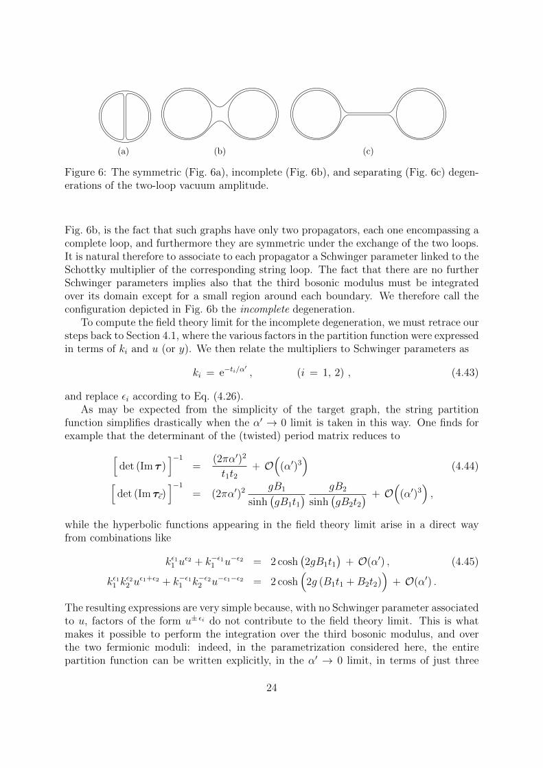
In the last three sections, 4.2, 4.3 and 4.4, we have given the tools to compute thefield theory limit of the partition function in the vicinity of the symmetric degeneration,see Fig. 6a: our final result is summarized in Eq. (4.41). The field theory two-loop effectiveaction, however, includes also the Feynman diagrams with a quartic vertex depicted inthe last two lines of Fig. 1.

The main feature of vacuum graphs with a four point vertex, which drives the cor-responding choice of parametrization for the neighborhood of moduli space depicted in

23

(a) (b) (c)

Figure 6: The symmetric (Fig. 6a), incomplete (Fig. 6b), and separating (Fig. 6c) degen-erations of the two-loop vacuum amplitude.

Fig. 6b, is the fact that such graphs have only two propagators, each one encompassing acomplete loop, and furthermore they are symmetric under the exchange of the two loops.It is natural therefore to associate to each propagator a Schwinger parameter linked to theSchottky multiplier of the corresponding string loop. The fact that there are no furtherSchwinger parameters implies also that the third bosonic modulus must be integratedover its domain except for a small region around each boundary. We therefore call theconfiguration depicted in Fig. 6b the incomplete degeneration.

To compute the field theory limit for the incomplete degeneration, we must retrace oursteps back to Section 4.1, where the various factors in the partition function were expressedin terms of ki and u (or y). We then relate the multipliers to Schwinger parameters as

ki = e−ti/α′, (i = 1, 2) , (4.43)

and replace εi according to Eq. (4.26).As may be expected from the simplicity of the target graph, the string partition

function simplifies drastically when the α′ → 0 limit is taken in this way. One finds forexample that the determinant of the (twisted) period matrix reduces to[

det (Im τ )]−1

=(2πα′)2

t1t2+ O

((α′)3

)(4.44)[

det (Im τ~ε)]−1

= (2πα′)2 gB1

sinh(gB1t1

) gB2

sinh(gB2t2

) + O(

(α′)3),

while the hyperbolic functions appearing in the field theory limit arise in a direct wayfrom combinations like

kε11 uε2 + k−ε11 u−ε2 = 2 cosh

(2gB1t1

)+ O(α′) , (4.45)

kε11 kε22 u

ε1+ε2 + k−ε11 k−ε22 u−ε1−ε2 = 2 cosh(

2g (B1t1 +B2t2))

+ O(α′) .

The resulting expressions are very simple because, with no Schwinger parameter associatedto u, factors of the form u± εi do not contribute to the field theory limit. This is whatmakes it possible to perform the integration over the third bosonic modulus, and overthe two fermionic moduli: indeed, in the parametrization considered here, the entirepartition function can be written explicitly, in the α′ → 0 limit, in terms of just three

24

simple integrals over the non-degenerating coordinates of super-moduli space. After GSOprojection, one finds

dZ inc+sep2 (µ) =

(2πα′)d

(α′)2

2∏i=1

[dti e

−tim2i gBi

td/2−1i sinh

(gBiti

)] du dθ dφ (4.46)

×

1

y

(d− 2 + 2 cosh

(2gB1t1

)+ ns − 2

)(d− 2 + 2 cosh

(2gB2t2

)+ ns − 2

)−[d− 2 + 2 cosh

(2g(B1t1 +B2t2)

)+ ns

]+

1

u

[d− 2 + 2 cosh

(2g(B1t1 −B2t2)

)+ ns

]+ O

(e−ti/α

′, α′).

As the notation suggests, Eq. (4.46) in principle contains contributions from both theincomplete and the separating degenerations, and we now turn to the problem of dis-entangling them. We also see that in order to complete the calculation one just needsto determine three numerical constants, given by the following integrals over the non-degenerating super-moduli,

I1 =

∫M1|2

du dθ dφ1

y, I2 = −

∫M1|2

du dθ dφ , I3 =

∫M1|2

du dθ dφ1

u. (4.47)

To determine the domain of integration M1|2 in Eq. (4.47), and to identify the differentdegeneration limits, note that the separating, symmetric and incomplete degenerations allcome from the region of super-moduli space in which the two Schottky multipliers k1 andk2 are small. In this limit, we can think of super moduli space as a 1|2-dimensional spaceparametrized by (u|θ, φ). The separating degeneration corresponds to the limit y → 0,while the symmetric degeneration corresponds to the limit u → 0, and the incompletedegeneration comes from the region of super moduli space interpolating between the twolimits. As pointed out in Refs. [71, 21], however, this simple characterization must bemade more precise, in particular with regards to the choice of parameters near the twodegenerations.

First of all, let us briefly consider the first term in braces on the right-hand sideof Eq. (4.46). This dominates in the limit y → 0, and we expect it to represent thecontributions of the one-particle reducible (1PR) Feynman diagrams, which we neglect.We can now concentrate on the evaluation of the integrals relevant for our purposes,which are I2 and I3 in Eq. (4.47). They can be calculated using Stokes’ theorem for asuper-manifold with a boundary (see section 3.4 of [71]), since the integrands are easilyexpressed as total derivatives. We write

− du dθ dφ ≡ dν2 , ν2 = −u dθ dφ , (4.48)

du

udθ dφ ≡ dν3 , ν3 = log(u) dθ dφ .

These expressions mean that the corresponding integrals are localized on the boundary ofM1|2, which consists of two loci associated with the two distinct ways in which the double

25

annulus world-sheet can completely degenerate: the symmetric degeneration of fig. 6a,and the separating degeneration of fig. 6c.

To use Stokes’ theorem, it is important to characterize precisely the 0|2-dimensionalboundary of the super-moduli-space region over which we are integrating. More precisely,we need to find bosonic functions of the worldsheet moduli ξi(u, θ, φ), defined near the

boundaries of M1|2, such that the vanishing of ξi defines a compactification divisor Di.Such functions are called canonical parameters in section 6.3 of [21]. It is important tonote that, for singular integrands such as those of I1 and I3, it is not sufficient to definethe canonical parameter ξ up to an overall factor, which may include nilpotent terms.For example, if we attempt to rescale ξ = (1 + θφ)ξ′, then log ξ = log ξ′+ θφ, so that theBerezin integral

∫dθ dφ log ξ does not coincide with

∫dθ dφ log ξ′.

In the small-u region, the proper choice of the canonical parameter ξsym is dictated byour parametrization of the symmetric degeneration: we must take ξsym = p3, as defined inEq. (4.12), in order to properly glue together the two regions. Although p3 and the cross-ratio u vanish at the same point, they are related by a non-trivial rescaling at leadingorder in the multipliers. Indeed

u =p3

1 + p3

(1 + θφ

)+O

(k

1/2i

), (4.49)

which affects the Berezin integral of Eq. (4.48), as discussed above. Note that, not havingintroduced a parametrization for the separating degeneration, we would not have a similarguideline in the small-y region. Furthermore, the fact that the corresponding field theorydiagram needs to be regulated9 in order to make sense of the vanishing momentum flowingin the intermediate propagator introduces an ambiguity also in the field theory result.

With this choice of parametrization, we can now use Stokes’ theorem to determinethe values of I2 and I3. Taking ξsep = y as a canonical parameter for the separatingdegeneration, we find

I2 = limε→0

[∫y=ε

ν2 −∫p3=ε

ν2

], (4.50)

= limε→0

[−∫dθ dφ

(1− ε+ θφ

)+

∫dθ dφ

ε

1 + ε

(1 + θφ

)]= 1 .

where we used∫dθ dφ θφ = −1. Similarly

I3 = limε→0

[∫y=ε

ν3 −∫p3=ε

ν3

], (4.51)

= limε→0

[∫dθ dφ log(1− ε+ θφ) −

∫dθ dφ log

[ε

1 + ε(1 + θφ)

]]= 0 .

Inserting these results into Eq. (4.46), discarding the separating degeneration, and intro-ducing the overall normalization given in Eq. (4.37), we obtain our final expression for

9Notice that in the gauge we use this Feynman diagram would not automatically vanish in a U(N)theory as the 3-point vertices contain also terms proportional to the symmetric color tensor dabc.

26

the contribution of diagrams with a four-point vertex to the field-theory effective action.It is given by

Z inc2,QFT (mi, Bi) =

g2

(4π)d

∫ ∞0

2∏i=1

[dti e

−tim2i gBi

td/2−1i sinh

(gBiti

)] (4.52)(d− 2 + 2 cosh

(2g(B1t1 +B2t2)

)+ ns

).

In order to identify the contributions of individual Feynman diagrams to Eq. (4.52), we canretrace the steps of the calculation and assign each term in our result to the appropriateworld-sheet conformal field theory, as we did for the symmetric degeneration in Eq. (4.41).We find that we can rewrite Eq. (4.52) as

Z inc2,QFT (mi, Bi) = − g2

(4π)d

∫ ∞0

2∏i=1

[dti e

−tim2i gBi

td/2−1i sinh

(gBiti

)](f11‖ + f11

⊥ + f11scal + f11

gh

), (4.53)

where here the superscripts denote the powers of k1/2i (i = 1, 2) from which the coefficients

were extracted, and we have omitted the arguments of the functions f for simplicity. Theprecise identification is

f11‖ = − 2 cosh

(2g(B1t1 +B2t2)

)f11⊥ = − (d− 2) , f11

scal = −ns , f11gh = 0 . (4.54)

A few remarks are in order. First of all we note that f11gh vanishes; this corresponds

to the fact that, in the infinite product in Fgh(ki, η) in Eq. (3.11), n ranges from 2 to∞, not from 1 to ∞ as in the case of Fgl and Fscal. As a consequence, there is no termproportional to k1/2(S1S2) in the partition function for the ghost systems. We will see thatthis corresponds to the fact that there is no quartic ghost vertex in the associated Yang-Mills theory. Next, we note that all terms associated with the four-point vertex diagramare not factorizable into the product of two contributions, proportional to k

1/21 and k

1/22

respectively. If, on the other hand, we had traced the origin of the terms associated withthe separating degeneration, and proportional to the integral I1, we would have foundthat the factor multiplying 1/y in Eq. (4.46) can be written as(

f10‖ + f10

⊥ + f10scal + f10

gh

)(f01‖ + f01

⊥ + f01scal + f01

gh

). (4.55)

This means that no contributions arise from the Schottky group elements S1S2 and S−11 S2,

which would imply a genuine correlation between the two loops. Rather, as expected, theseterms are simply the product of factors rising from individual disconnected loops. Finally,we note that the result I3 = 0 is crucial in order to recover the correct field theory limit:indeed, as will be verified in the next section and shown in Appendix C, no field theorydiagram yields hyperbolic functions with the parameter dependence displayed on the lastline of Eq. (4.46). We see once again that the field theory limit, once the contributionsof individual diagrams have been identified, provides non-trivial checks of the proceduresused to perform the integration over super-moduli.

27

5 Yang-Mills theory in the Background Field Gervais-

Neveu gauge

In order to make a precise comparison between string theory and field theory at the levelof individual Feynman diagrams, as was done in a simple case in Ref. [11], we need aprecise characterization of the field-theory Lagrangian we are working with, includinggauge fixing and ghost contributions. In principle, this presents no difficulties, since ourtarget is a U(N) Yang-Mills theory, albeit with a rather special gauge choice. There arehowever a number of subtleties, ranging from the special features of the background fieldframework, to issues of dimensional reduction, and to the need to break spontaneouslythe gauge symmetry in order to work with well-defined Feynman diagrams in the infraredlimit, which altogether lead to a somewhat complicated and unconventional field theorysetup. We will therefore devote this section to a detailed discussion of the field theoryLagrangian which arises from the field theory limit of our chosen string configuration.

The first layer of complexity is due to the fact that the string theory setup naturallycorresponds to a field theory configuration with a non-trivial background field. In general,such a background field breaks the gauge symmetry: in our case, since we are workingwith mutually commuting gauge fields with constant field strengths, and we have a stringconfiguration with separated D-brane sets, one will generically break the U(N) gaugesymmetry down to U(1)N . We will have to adjust our notation to take this into account.Notice also that our background fields break Lorentz invariance as well, since only certainpolarizations are non-vanishing. As a consequence, the polarizations of the quantum fieldwill also be distinguished as parallel or perpendicular to the given background.

Furthermore, it is interesting to work in a generic space-time dimension d, and we willfind it useful to work with massive scalar fields giving infrared-finite Feynman diagrams.We will therefore work with a d-dimensional gauge theory obtained by dimensional re-duction from the dimension D > d appropriate to the string configuration. This yieldsns = D − d adjoint scalar fields minimally coupled to the d-dimensional gauge theory,and we will choose our background fields such that these fields acquire a non-vanishingexpectation value, giving mass to some of the gauge fields.

Finally, as suggested originally in Ref. [45], and recently confirmed by the analysis ofRef. [11], covariantly quantized string theory picks a very special gauge in the field theorylimit: a background field version of the non-linear gauge first introduced by Gervais andNeveu in Ref. [16]. This gauge has certain simplifying features: for example at treelevel and at one loop it gives simplified color-ordered Feynman rules which considerablyreduce the combinatoric complexity of gauge-theory amplitudes [45]. Only at the two-loop level, however, the full complexity of the non-linear gauge fixing becomes apparent.One effect, for example, is that the diagonal U(1) ‘photon’, which ordinarily is manifestlydecoupled and never appears in ‘gluon’ diagrams, in this case has non-trivial, gauge-parameter dependent couplings to SU(N) states, and the decoupling only happens whenall relevant Feynman diagrams are summed.

In what follows, we adopt the following notations: we use calligraphic letters formatrix-valued u(N) gauge fields, and ordinary capital letters for their component fields;we use M,N, . . . = 1, . . . ,D for Lorentz indices in D-dimensional Minkowski space before

28

dimensional reduction, and µ, ν, . . . = 1, . . . , d for Lorentz indices in the d-dimensionalreduced space-time; finally, I, J, · · · = 1, . . . , ns indices enumerate adjoint scalars, andA,B, . . . = 1, . . . , N indices enumerate the components of u(N) vectors and matrices.In this language, AM will denote the D-dimensional classical background field, QM thecorresponding quantum field, while C and C are ghost and anti-ghost fields.

We will now proceed to write out the quantum lagrangian (including gauge-fixing andghost terms) in terms of matrix-valued fields. We will then comment on the form takenby various terms in component notation, which is more directly related to the verticesappearing in diagrammatic calculations.

5.1 The u(N) Lagrangian

We begin by constructing the D-dimensional Yang-Mills Lagrangian, which, in the pres-ence of a background gauge field, depends on the combination AM + QM . The field-strength tensor FMN can be expressed in terms of the covariant derivative of the quantumfield with respect to the background field, DM = ∂M + i g [AM , ·], as

FMN (A+Q) = − i

g

[DA+QM ,DA+Q

N

]= FMN (A) + DMQN −DNQM + i g [QM ,QN ] , (5.1)

where FMN (A) is the field strength tensor for the background field only, while DA+QM is

the covariant derivative with respect to the complete gauge field. The classical Lagrangianfor the quantum gauge field Q can then be written as

Lcl = Tr

[DMQNDNQM −DMQNDMQN + 2 i gFMNQMQN

+2 i gDMQN [QM ,QN ] +1

2g2 [QM ,QN ]

[QM ,QN

] ], (5.2)

where Tr here denotes the trace over the u(N) Lie algebra, and we have removed termsindependent of Q, as well as terms linear in Q, because they are not relevant for oureffective action calculation.

In anticipation of the string theory results, we now wish to fix the gauge using abackground field version of the non-linear gauge condition introduced by Gervais andNeveu in Ref. [16], setting

G (A,Q) = DMQM + i γ gQMQM = 0 , (5.3)

where γ is a gauge parameter. The gauge-fixing Lagrangian Lgf is then given by

Lgf = −Tr

[(G (A,Q)

)2]

= −Tr

[DMQMDNQN + 2 i γ gDMQMQNQN − γ2g2QMQMQNQN

]. (5.4)

29

Notice that the overall covariant gauge-fixing parameter which would appear in frontof Eq. (5.4) has been set equal to one. Note also that this gauge fixing modifies notonly the gluon propagator, as expected, but also the three- and four-gluon vertices. Inparticular, the symmetric nature of the quadratic term in the gauge-fixing function G willgenerate Feynman rules involving the symmetric u(N) tensors dabc, which in turn willinduce spurious couplings between gluons and u(1) photons.

Finally, we need the Lagrangian for the Faddeev-Popov ghost and anti-ghost fields,C and C. It is defined as usual in terms of the gauge transformation of the gauge-fixingfunction, as

Lgh = Tr[C δCG (A,Q)

], (5.5)

using C as parameter of the gauge transformation. The result is

Lgh = 2 Tr

[− CDMDMC + i gDMC

[QM , C

]− i γ g C

QM ,D

MC

+ γ g2 CQM ,

[QM , C

] ]. (5.6)

This completes the construction of the pure Yang-Mills Lagrangian in D dimensions;next, we want to dimensionally reduce it to d dimensions. The reduction splits the D-dimensional gauge fields (both classical and quantum) into a d-dimensional field andns ≡ D − d adjoint scalars, according to

AM→Aµ ,

1

gMI

,

QM

→Qµ ,ΦI

, (5.7)

with µ = 0, . . . , d−1 and I = 1, . . . , ns, and we have assumed that the classical backgroundscalars take on constant values MI , which we will use to spontaneously break the gaugesymmetry and give masses to selected components of the gauge field. Similarly, sincewe are neglecting the dependence of the fields on the reduced coordinates, the covariantderivative splits into a d-dimensional covariant derivative and a pure commutator withthe background scalar fields, as

DM

→Dµ ≡ ∂µ + i g [Aµ, ·] , i [MI , ·]

. (5.8)

Indeed, the D-dimensional d’Alembertian differs from the d-dimensional one by a massterm: for any field X,

DMDMX = DµDµX +

[MI ,

[MI , X

]]. (5.9)

Notice that in this section we work with the metric η = diag(+,−, . . . ,−). However,when summing over reduced dimensions, our summation convention does not include thenegative signature of the metric, and must be understood simply as a summation overflavor indices I. With these conventions, the gauge condition in Eq. (5.3) becomes

DµQµ + i γ gQµQµ − i[MI ,Φ

I]− i γ gΦIΦ

I = 0 . (5.10)

30

When these further changes are implemented in the Lagrangian, a number of non-trivialinteraction vertices are generated. It is then useful to organize the dimensionally-reducedLagrangian as a sum of terms with different operator content. One can write

LQ2 = Tr

[Qµ(DνD

νQµ + 4i gFµρQρ +[MI , [MI ,Qµ]

])],

LΦ2 = Tr

[− ΦIDνD

νΦI − ΦI[MJ ,

[MJ ,ΦI

]]],

LCC = Tr

[− 2 CDµD

µC − 2 C[MJ ,

[MJ , C

]]],

LQ3 = −2 i gγTr[DµQµQνQν

]− 2 i gTr

[DµQν

[Qµ,Qν

]],

LQΦ2 = 2 i gγTr[DµQµ ΦIΦ

I]

+ 2 i gTr[DµΦI

[Qµ,ΦI

]],

LCCQ = 2 i gTr[DµC

[Qµ, C

]]− 2 i γ gTr

[CQµ,DµC

], (5.11)

LΦQ2 = −2 γ gTr[[MI ,Φ

I]QµQµ

]− 2 gTr

[[MI ,Qµ

][ΦI ,Qµ

]],

LΦ3 = 2 γ g[[MI ,Φ

I]ΦJΦJ

]+ 2 gTr

[[MI ,ΦJ

][ΦI ,ΦJ

]],

LΦCC = 2 gTr[[MI , C

][ΦI , C

]]− 2 γ gTr

[C

ΦI ,[MI , C

]],

LQ4 = g2(ηρµηνσ −

(1− γ2

)ηρνησµ

)Tr[QµQνQρQσ

],

LQ2Φ2 = −2 g2Tr[ΦIQµΦIQµ

]+ 2

(1− γ2

)g2Tr

[ΦIΦ

IQµQµ],

LΦ4 = g2Tr[ΦIΦJΦIΦJ

]−(1− γ2

)g2Tr

[ΦIΦ

IΦJΦJ],

LCCQ2 = 2 γ g2Tr[CQµ, [Qµ, C]

],

LCCΦ2 = −2 γ g2Tr[C

ΦI , [ΦI , C]

].

As is typical in cases of broken symmetry, the Lagrangian in Eq. (5.11) displays a varietyof interactions, and is considerably more intricate than the combination of Eqns. (5.2),(5.4) and (5.6). In order to compute Feynman diagrams, and to compare with the stringtheory calculation, it is useful to write down an expression for the Lagrangian in terms ofcomponent fields as well. In order to do so, we now assume that the matrices Aµ andMI

are all mutually commuting: we can then pick a basis of u(N) in which they are diagonal.In this basis, we write

MI = diagmAI

, Aµ = diag

AAµ, A = 1, . . . , N . (5.12)

Similarly, we write the quantum matrix fields as[Qµ]AB

=1√2QABµ ,

[ΦI

]AB=

1√2φABI[

C]AB

=1√2cAB ,

[C]AB

=1√2cAB , (5.13)

31

all satisfying XAB = (XBA)∗, since u(N) matrices are Hermitian; the factors of 1/√

2ensure that the matrix element fields are canonically normalized. Notice that, thanks todiagonal form of the classical field Aµ, the covariant derivative Dµ does not mix matrixentries. Indeed, defining

AABµ ≡ AAµ − ABµ , (5.14)

one can write [DµX

]AB=(∂µ + i g AABµ

)XAB , (5.15)

where indices on the right-hand side are not summed. In particular, the covariant deriva-tive of diagonal entries reduces to the ordinary derivative. Motivated by this, we candefine a covariant derivative Dµ acting directly on matrix entries, as opposed to u(N)elements. Suppressing the A,B indices on the derivative symbol, we write

DµXAB =

(∂µ + i g AABµ

)XAB −→

[DµX

]AB= DµX

AB . (5.16)

Note that Dµ is a derivation, obeying the Leibnitz rule

Dµ (XY )AB =(DµX

AC

)Y CB +XA

B

(DµY

CB), (5.17)

so it can be partially integrated in any integrand with contracted color indices. Treatingthe mass matrices in a similar way, we define

mABI ≡ mA

I −mBI , m2

AB ≡ns∑I=1

(mABI

)2. (5.18)

This implies [MI , X

]AB= mAB

I XAB ,[MI ,

[MI , X

]]AB

= m2ABXAB , (5.19)

where again on the right-hand side the indices A and B are fixed and not summed. Asan example, the term quadratic in Φ in Eq. (5.11) can be written in component notationas

LΦ2 = − 1

2φABI DµD

µφBA,I − 1

2φABI m2

ij φBA,I (5.20)

= − 1

2

N∑A=1

φAAI ∂µ∂µφAA,I −

N∑1≤A<B

[ (φABI

)∗DµD

µφAB,I +m2AB

∣∣φABI ∣∣2 ] ,which is the correctly normalized quadratic part of the Lagrangian for N massless realscalar fields φAA, and 1

2N(N − 1) complex scalars φAB, A < B, with mass |mAB|. To give

a second example, the gauge-fixing condition in component notation reads

DµQABµ + i γ g QAC

µ Qµ,BC − imAB

I φABI − i γg φAI,CφCBI = 0 , (5.21)

where C is summed over but there is no summation over A or B. Note that after dimen-sional reduction and spontaneous symmetry breaking the gauge fixing has become more

32

unconventional from the d-dimensional point of view, involving scalar fields as well asgauge fields, and mass parameters.

We conclude this section by giving the explicit expression for the background fieldthat we will be working with. We choose it so that, for each A, the abelian field strengthFAµν = ∂µA

Aν − ∂νA

Aµ is a U(1) magnetic field in the x1, x2 plane. A possible choice,

already employed in Ref.[11], is

AAµ (x) = x1ηµ2BA −→ FA

µν = fµνBA , (5.22)

where we defined the antisymmetric tensor

fµν = ηµ1ην2 − ην1ηµ2 . (5.23)

We now turn to the evaluation of selected two-loop vacuum diagrams, contributing to theeffective action, which we can then compare with the corresponding expressions derivedfrom string theory. Preliminarily, we collect useful expressions for the relevant coordinate-space propagators in the presence of the background field.

5.2 Propagators in a constant background field

The quantum field theory objects that we wish to compute, in order to compare withstring theory results, are two-loop vacuum diagrams contributing to the effective action,and computed with our chosen background field, Eq. (5.22). At two loops, these diagramscan be computed in a straightforward manner in coordinate space, directly from the pathintegral definition of the generating functional,

Z[JABµ , ηAB, ηAB, JABI

]=

∫ [DQAB

µ DcABDcABDφABI]

(5.24)

× exp

[i

∫ddx

(L[QABµ , cAB, cAB, φABI

]+JABµ Qµ

BA + cBAηAB + ηABcBA + JABI φBAI

)],

where Jµ, JI , η and η are matrix sources for the fields in the complete Lagrangian L. Theonly non-trivial step is the computation of the quantum field propagators in the presenceof the background field: diagrams are then simply constructed by differentiating the freegenerating functional with respect to the external sources. For a background field of theform of Eq. (5.22), the solution is well-known for the scalar propagator (see, for example,Ref. [15]): we briefly describe it here, and discuss the generalization to vector fields.

For scalar fields, the propagator in the presence of the background in Eq. (5.22) canbe expressed in terms of a heat kernel as

GAB(x, y) =

∫ ∞0

dtKAB (x, y; t) , (5.25)

where, defining BAB ≡ BA −BB, one can write

KAB (x, y; t) =1

(4πt)d/2e−

i2gBAB(x1+y1)(x2−y2)−tm2

ABgBABt

sinh(gBABt)

33

× exp

[1

4t(xµ − yµ) Σµν

(gBABt

)(xν − yν)

]. (5.26)

In Eq. (5.26), we have introduced the tensor

Σµν

(gBABt

)=

gBABt

tanh (gBABt)η‖µν + η⊥µν , (5.27)

where the projectors ηµν‖ and ηµν⊥ identify components parallel and perpendicular to thebackground field, and are given by

ηµν‖ = fµρfρν = δ1

µδ1ν + δ2

µδ2ν , ηµν⊥ = ηµν − ηµν‖ . (5.28)

The propagator GAB(x, y) in Eq. (5.25) satisfies(D(x)µ Dµ

(x) +m2AB

)GAB(x, y) = − i δd(x− y) , (5.29)

where we noted explicitly the variable on which the derivatives act. In fact, covariantderivatives act on a propagator with color indices (AB) as

D(x)µ GAB(x, y) ≡

[∂

∂xµ+ i gAABµ (x)

]GAB(x, y) ,

D(y)µ GAB(x, y) ≡

[∂

∂yµ− i gAABµ (y)

]GAB(x, y) . (5.30)

For real scalar fields, or vanishing backgrounds, one recovers the well-known expressionfor the scalar propagator as a Schwinger parameter integral,

GAB0 (x, y) ≡ lim

BAB→0GAB(x, y) =

∫ ∞0

dte−tm

2AB

(4πt)d/2exp

[(x− y)2

4t

]. (5.31)

Ghosts fields are scalars, and they share the same propagator. For gluons, on the otherhand, the background field strength Fµρ enters the kinetic term, given in the first line ofEq. (5.11). The propagator must then satisfy[

ηµρ

(D(x)σ Dσ

(x) +m2AB

)+ 2 i g FAB

µρ

]GAB,ρν(x, y) = i δνµδ

d(x− y) . (5.32)

To diagonalize this equation, one can introduce the projection operators

(P±)ρσ =η‖ρσ ± fρσ

2, (P⊥)ρσ = η⊥ρσ , (5.33)

satisfying(P+ + P− + P⊥)µν = ηµν (P+ − P−)µν = fµν . (5.34)

It is then easy to show that the function

GAB,σα(x, y) = − ησα⊥ GAB(x, y)− P σα+ GAB

+ (x, y)− P σα− GAB

− (x, y) (5.35)

34

satisfies Eq. (5.32), provided the functions GAB± (x, y) satisfy[

D(x)µ Dµ

(x) +m2AB ± 2 i gBAB

]GAB± (x, y) = − i δd(x− y) . (5.36)

Eq. (5.36) simply gives a scalar propagator with a mass shifted by the appropriate back-ground field. It’s easy therefore to write the solution for the complete gluon propagatorexplicitly as

GABµν (x, y) = −

∫ ∞0

dt[η⊥µν + η‖µν cosh

(2gBABt

)+ fµν sinh

(2gBABt

)]KAB(x, y; t) .

(5.37)Note that this can be written also in the more compact and elegant form

GABµν (x, y) = −

∫ ∞0

dt[e− g t F

ABαβ Sαβ1

]µνKAB(x, y; t) , (5.38)

where Sαβ1 are the Lorentz generators in the spin one representation appropriate for gaugebosons, [

S αβ1

]µν

= − i(δαµδ

βν − δ

ανδβµ

). (5.39)

The propagator in Eq. (5.38) naturally generalizes to other representations of the Lorentzgroup, simply changing the form of the generators. The spin one-half case, where Sαβ1/2 =

i[γα, γβ]/4, will be useful for example when studying the gluino contribution to the effec-tive action in the supersymmetric case.

5.3 Selected two-loop vacuum diagrams

We will now illustrate the structure of the field theory calculation of the effective actionby outlining the calculation of a selection of the relevant two-loop diagrams. A completelist of the result for all 1PI diagrams depicted in Fig. 1 is given in Appendix C.

We begin by considering the ghost-gluon diagram given by the sum of Eq. (C.10)and Eq. (C.11), which we denote by Hb(BAB,mAB). The relevant interaction vertex,involving ghost, antighost and gluon fields, arises from the sixth line in Eq. (5.11), andmay be written explicitly in component language using Eq. (5.13). Upon integrating byparts, it can be rewritten as

LccQ =i g√

2

[(δBCδDEδFA − δBEδFCδDA

)Dµc

AB Qµ,CDcEF

− γ(δBCδDEδFA + δBEδFCδDA

)cAB Qµ,CDDµc

EF

]. (5.40)

Sewing two copies of this vertex together to obtain the desired diagram, one first of allobserves that terms linear in the gauge parameter γ, which involve double derivatives ofscalar propagators, cancel out upon contracting color indices. Next, one notices that someof the color contractions lead to a non-planar configuration, which would correspond to anopen string diagram with only one boundary. We are not interested in these contributions,

35

since the corresponding diagram is built of propagators which are neutral with respect tothe background field, and does not contribute to the effective action. Furthermore, wedo not expect to obtain this diagram from our string configuration, since we start witha planar worldsheet. Discarding non-planar contributions, one finds that the remainingplanar terms can be written as

Hb(BAB,mAB) = − g2 1 + γ2

4

∫ddx ddy

[D(x)µ GAB(x, y)D(y)

ν GBC(x, y)Gµν,CA(x, y)

+ (ABC)↔ (CBA)]. (5.41)

Inserting the expressions for the scalar and gluon propagators given by Eq. (5.25) andEq. (5.38), one can immediately rewrite Eq. (5.41) in terms of covariant derivatives of theheat kernels K. These, in turn, can be written as

D(x)µ KAB(x, y; t) =

Σµρ(gBABt) + i t FAB

µρ

2 t(xρ − yρ) KAB(x, y; t) , (5.42)

D(y)ν KBC(x, y; t) = −Σνσ(gBBCt)− i t FBC

νσ

2 t(xσ − yσ) KBC(x, y; t) ,

where Σ(gBt) is defined in Eq. (5.27). The integrand in Eq. (5.41) is then proportionalto the product of three heat kernels, which we write as

3∏i=1

Ki(x, y; ti) = exp

[1

4(xµ − yµ) Σµν (xν − yν)

] 3∏i=1

e−tim2i

(4πti)d2

gBitisinh(gBiti)

. (5.43)

In Eq. (5.43) we have simplified the notation by using a single index i = 1, 2, 3 in place ofthe pairs of color indices (AB), (BC), (CA), respectively. Furthermore, we have definedΣµν =

∑3i=1 Σµν(gB

iti)/ti, and we have taken advantage of the fact that the complexphases in each Ki(x, y; ti) cancel due to the fact that

∑3i=1Bi = 0. At this point one

sees that the integrand in Eq. (5.41) is translationally invariant, depending only on thecombination z = x − y. We can then, for example, replace the integral over x with anintegral over z while the integral over y gives a factor of the volume of spacetime, whichwe will not write explicitly. One needs finally to evaluate the gaussian integral∫

ddz zρzσ exp

[1

4zµ Σµν z

ν

]= −2

(Σ−1)ρσ ∫

ddz exp

[1

4zµ Σµν z

ν

]. (5.44)

Note that taking the inverse of Σµν is trivial because it is a diagonal matrix, which canbe written as

Σµν = ∆0 η⊥µν

3∏i=1

1

ti+ ∆B η

‖µν

3∏i=1

gBi

sinh(gBiti), (5.45)

where ∆0 and ∆B were defined in Eq. (4.28) and Eq. (4.30) respectively, while η⊥µν and

η‖µν are given in Eq. (5.28). One finds then∫

ddz exp

[1

4zµ Σµν z

ν

]= − i (4π)d/2 ∆

1−d/20 ∆−1

B

3∏i=1

sinh(gBiti)

gBititd/2i . (5.46)

36

Putting together all these ingredients, one may evaluate Eq. (5.41). Using the symmetryof the Schwinger parameter integrand under the exchange t1 ↔ t2 one can write

Hb(Bi,mi) = − ig2

(4π)d1 + γ2

2

∫ ∞0

3∏i=1

dtie−t1m

21−t2m2

2−t3m23

∆d/2−10 ∆B

[d− 2

∆0

t3 (5.47)

+2

∆B

sinh(gB3t3)

gB3

cosh(2gB3t3 − gB1t1 − gB2t2)

],

which can be directly matched to the string theory result.We conclude this section by briefly describing the calculation of two further Feynman

diagrams, which arise in our theory because of the pattern of symmetry breaking anddimensional reduction. First of all, there are diagrams, like Eq. (C.15), with the sametopology as Eq. (C.11), but with an odd number of scalar propagators, and verticesproportional to the scalar vacuum expectation values mij, characteristic of the brokensymmetry phase. The relevant vertex can be found by expanding LΦQ2 from Eq. (5.11)in terms of the component fields defined in the Eq. (5.13). Upon relabeling the indicesand using mCB

I +mBAI +mAC

I = 0, it reads

LQ2φ =g√2

[(1 + γ)mCB

I − (1− γ)mACI

]φAB QBC

µ Qµ,CA . (5.48)

Labeling this diagram as Hd(BAB,mAB), we find for it the coordinate space expression

Hd(BAB,mAB) =g2

4

[(1− γ)mCB

I − (1 + γ)mACI

][(1− γ)mAC

I − (1 + γ)mCBI

]×∫ddx ddy GAB(x, y)GBC

µν (x, y)Gµν,CA(x, y) , (5.49)

where we neglected non-planar contributions, and we used mBCI = −mCB

I . Manipulationssimilar to those leading to Eq. (5.47), simplified by the absence of derivative interactions,yield the result

Hd(Bi,mi) = − i

(4π)dg2

2

[(1 + γ2)m2

3 − 2 (m21 +m2

2)]

(5.50)

×∫ ∞

0

3∏i=1

dtie−t1m

21−t2m2

2−t3m23

∆d/2−10 ∆B

[d− 2 + 2 cosh(2gB1t1 − 2gB2t2)

],

where we relabeled double indices as was done for Eq. (5.47).Finally, we briefly consider a diagram with a quartic vertex: the figure-of-eight scalar

self-interaction shown in Eq. (C.23), which we label Ei(Bk,mk). The relevant interactionterm in the Lagrangian comes from LΦ4 in Eq. (5.11) and can be written as

Lφ4 =g2

4

[δKIδLJ − (1− γ2)δILδJK

]φABK φBCL φCDI φDAJ , (5.51)

which immediately gives

Ei(Bk,mk) = ig2

4

[δKIδLJ − (1− γ2)δILδJK

] ∫ddx

[GDA(x, x)GBC(x, x) δACδ

IJδLK

37

+GCD(x, x)GDA(x, x)δDBδLIδJK

]. (5.52)

Contracting flavor indices we get, as expected, the product of two one-loop integrals,

Ei(Bk,mk) = ig2

(4π)d

[1− 1− γ2

2(1 + ns)

]ns

∫ ∞0

2∏i=1

[dti

td/2−1i

g Bi e−tim2

i

sinh(gBiti)

]. (5.53)

The diagrams in Eqs. 5.1 – C.22 can be calculated similarly. One easily sees that allthese results, and those for the remaining diagrams, given in Appendix C, are directlycomparable with the ones obtained from the field theory limit of the string effective action.

6 Discussion of results

6.1 Comparison between QFT and string theory

We have now assembled all the results that we need to establish and verify a precisemapping between the degeneration limits of the string world-sheet and the 1PI Feynmandiagram topologies in the field theory limit. Furthermore, as announced, we can tracethe contributions of individual string states propagating in each degenerate surface, andthese can be unambiguously mapped to space-time states propagating in the field theorydiagrams. This diagram-by-diagram mapping allows us in particular to confirm thatcovariantly quantized superstring theory10 naturally selects a specific gauge in the fieldtheory limit, and the gauge condition is given here in Eq. (5.3).

More precisely, our string theory results for the symmetric degeneration are given inEq. (4.41) and Eq. (4.42). A careful inspection shows that these results reproduce allthe Feynman diagrams in the first two lines of Fig. 1, which are listed in Eqs. (C.6)through (C.17) in Appendix C, with the choice γ2 = 1. Similarly, our string theoryresults for the incomplete degeneration are given in Eq. (4.53) and Eq. (4.54), and onemay verify that one recovers all Feynman diagrams in the last two lines of Fig. 1, givenin Eqs. (C.18) through (C.23). It is easy to identify each term in Eq. (4.41) with aparticular Feynman diagram: for example, the term f111

⊥ in Eq. (4.42) matches the diagramresulting in Eq. (C.6), in which all three lines correspond to gluons that are polarized indirections perpendicular to the external magnetic field; on the other hand, the termf001‖ f110

⊥ , plus its cyclic permutations, matches the result of Eq. (C.7), in which one linecarries a gluon polarized in the plane parallel to the magnetic field, while the other twogluons are polarized in the directions perpendicular to the magnetic fields. One mayeasily continue through the list, identifying the other available combinations of gluons,ghosts and scalars. In a similar vein, one can associate individual Feynman graphs to eachterm in Eq. (4.53): for example, f11

‖ corresponds to Eq. (C.18), f11⊥ to Eq. (C.20), while

f11scal gives the diagram with two scalar propagators given in Eq. (C.23). Note also that

diagrams with a quartic vertex where the two propagators come from different sectors,

10On the other hand, it has been shown in Refs. [72, 73] that light-cone quantization of string theoryresults in quantum field theory amplitudes computed in a light-cone gauge.

38

such as for example Eqs. (5.1), (C.21) and (C.22), all vanish for γ2 = 1, so it comes as nosurprise that no contribution of this kind arises on the string theory side.

We finally note that we can also characterize the contributions to all 1PI Feynmandiagrams according to the Schottky multiplier they originate from. As an example, con-sider the infinite product over the Schottky group which arises from the determinant ofthe non-zero modes of the Laplacian, appearing in Eq. (3.11). Tracing the gluon contribu-tions to different Feynman diagrams back to that product, one may verify that all termsappearing in 1PI diagrams originate from at most one value of the index α in the product.More precisely, gluon contributions in Eq. (4.41) come from Tα = S1,S2,S

−11 S2, and

if, say, a factor of k1/21 =

√p1√p3 comes from the infinite product, then the necessary

factor of√p2 must come from elsewhere in the amplitude. On the other hand, all terms

in Eq. (4.53) come from Tα = S1S2. This is not surprising from a world-sheet point ofview: in fact, one may recall from Fig. 5 that S1S2 corresponds to a homology cycle whichpasses around both handles with a self-intersection between them, and furthermore thisis the only Schottky group element with this property which survives in the field theorylimit. We see that this homological property is directly related to the graphical structureof the resulting Feynman diagram.

6.2 Comparison with bosonic string theory

It is interesting to compare our results with the field theory limit of the bosonic stringeffective action which was studied in Refs. [35, 15, 67]. This comparison was discussedalso in [11], but we are now in a position to make a more detailed analysis.

Bosonic strings are clearly a simpler framework, since the world-sheet is an ordinarytwo-dimensional manifold, and not a super-manifold: one can then use the techniquesapplying to ordinary Riemann surfaces, and specifically the (purely bosonic) Schottkyparametrization discussed in detail for example in Ref. [11]. At two loops, one can usethe SL(2,R) invariance of the amplitude to choose the fixed points of the two Schottkygroup generators as

η1 = 0 , ξ1 = ∞ , η2 ≡ u , ξ2 = 1 . (6.1)

The two-loop partition function can then be written as

Z2

(~ε, ~d

)=

∫dk1 dk2 du

k21 k

22 (1− u)2

Fgh(µ)F(~ε )‖ (µ)F⊥(µ)F

(~d )scal (µ) , (6.2)

where µ denotes the set of bosonic moduli, µ = k1, k2, u, and one may compare withthe corresponding two-loop superstring expression, given in Eq. (3.18). Note that theintegration variable u is equal to the gauge-fixed value of a projective-invariant crossratio of fixed points, u = η1−η2

η1−ξ2ξ1−ξ2ξ1−η2 . The various factors in Eq. (6.2), already discussed

in [15, 11], are given by

Fgh(ki, u) = (1− k1)2 (1− k2)2∏α

′∞∏n=2

(1− knα

)2,

39

F(~ε )‖ (ki, u) = e−iπ~ε·τ ·~ε

[det (Im τ~ε)

]−1∏α

′∞∏n=1

(1− e 2πi~ε·τ · ~Nα knα

)−1 (1− e−2πi~ε·τ · ~Nα knα

)−1,

F⊥(ki, u) =[

det (Im τ)]−(d−2)/2∏

α

′∞∏n=1

(1− knα

)−d+2, (6.3)

F(~d )scal (ki, u) =

ns∏I=1

e~dI ·τ ·~dI/(2πiα′)

∏α

′∞∏n=1

(1− knα

)−ns.

Here τ is the period matrix of the Riemann surface, whose expression in the Schottkyparametrization can be found, for instance, in Eq. (A.14) of [31]. Similarly, τ~ε is thetwisted period matrix, the bosonic equivalent of τ~ε , computed here in Appendix B.

The most obvious difference between the measures in Eq. (3.18) and Eq. (6.2) is theoccurrence of half-integer powers of the multipliers in the former. In the bosonic string,the mass level of states propagating in the i-th loop increases with the power of ki, whereasin the superstring it increases with the power of k

1/2i . Necessarily, the propagation of a

massless state must correspond to terms of the form dki/ki = d log ki in the integrand,so tachyons propagating in loops correspond to terms of the form dki/k

2i in the bosonic

theory and dki/k3/2i in the superstring, as seen explicitly in Eq. (6.2) and in Eq. (3.18),

respectively. These tachyonic states must be removed by hand in the bosonic theory,whereas they are automatically eliminated from the spectrum of the superstring uponintegrating over the odd moduli and carrying out the GSO projection.

The identification of the symmetric degeneration proceeds in the same way for the twotheories: in particular, the symmetry of Fig. 6a leads to the choice of the parameters pi,defined by Eq. (4.12). The cross-ratio u can then be written as

u =(1 + p1)(1 + p2) p3

(1 + p3)(1 + p1p2p3), (6.4)

and the integration measure takes the symmetric form

dk1

k21

dk2

k22

du

(1− u)2(1− k1)2(1− k2)2 =

dp1

p21

dp2

p22

dp3

p23

(1− p2p3)(1− p1p3)(1− p1p2) . (6.5)

It is interesting to note that in the field theory limit a number of contributions arise inslightly different ways in the two approaches. As an example, let us consider the twisteddeterminant of the period matrix for the bosonic string. To lowest order in ki, it is givenby a combination of hypergeometric functions with argument u, in a manner similar towhat happens for its supersymmetric counterpart. In the neighborhood of the symmetricdegeneration, the hypergeometric functions can be expanded in powers of p3, and thebosonic string determinant reduces to

det (Im τ~ε) =1

4π2(α′)2

[∆B − 2α′p3 cosh

(g(2B3t3 −B1t1 −B2t2

)) sinh(gB3t3

)gB3

+O(p1, p2, p

23; (α′)2

)], (6.6)

40

where ∆B is defined in Eq. (4.30). We note that the term proportional to p3 in Eq. (6.6)receives a contribution from the series expansion of the hypergeometric functions, andcontributes to Feynman diagrams with a gluon polarized parallel to the magnetic fieldpropagating in the leg parametrized by t3.

For the superstring, the situation changes: one needs to keep terms only up to orderqi, which implies that all the hypergeometric functions appearing in the expression forthe supersymmetric twisted determinant can be replaced by unity. Since the first-orderterm in the expansion of the hypergeometric functions is crucial in order to get the correctcoefficient of p3 in Eq. (6.6), and in turn to match the field theory diagrams, it is necessarythat terms proportional to q3 arise from the nilpotent contributions to det (Im τ~ε). Thisis indeed what happens: expanding the supersymmetric twisted determinant in powers ofqi one finds

det (Im τ~ε) =1

4π2(α′)2

[∆B − 2α′q3 θ12φ12 cosh

(g(2B3t3 −B1t1 −B2t2

))sinh(gB3t3

)gB3

+O(q1, q2, q

23; (α′)2

)]. (6.7)

To be precise, we note that terms proportional to p3 and q3 θ12φ12 in det (Im τ~ε) anddet (Im τ~ε), respectively, also receive contributions from sources other than the ones wehave discussed, specifically from factors of the form uniεi/2, with ni integers. It is easy tosee, however, that these contribute in the same way in the two cases, since in the bosoniccase we have

uniεi/2 = pniεi/23

(1 +

niεi2

p3

)+O

(p1, p2, p

23

), (6.8)

while in the superstring case we get

uniεi/2 = pniεi/23

(1 +

niεi2

q3 θ12φ12

)+O

(q1, q2, q

23

). (6.9)

As a consequence, and as required, when all of the other factors are inserted, the coefficientof p1p2p3 in the bosonic string measure is the same as the coefficient of q1q2q3 θ12φ12 inthe superstring measure, and the same field theory amplitude is obtained for the masslesssectors of the bosonic and supersymmetric theories.

The terms computed in section 4.5, which correspond to field theory diagrams withthe topology of the diagrams in the bottom two rows of Fig. 1 as well as 1PR graphs,also appear in the bosonic theory. In fact, one gets once more an expression of the formof Eq. (4.46) in the field theory limit, but the integrals I1, I2 and I3 get replaced by

I1 =

∫ 1

0

du

(1− u)2, I2 =

∫ 1

0

du , I3 =

∫ 1

0

du

u2. (6.10)

When using the bosonic string, the integral I3 has to be discarded by hand, either byarguing that it corresponds to tachyon propagation, or by explicitly matching to thefield theory result. In the case of the superstring, on the other hand, the correct result

41

emerges automatically, provided a consistent integration procedure in super-moduli spaceis followed. The complete answer for the four-point vertex diagrams emerges in both casesfrom the terms proportional to I2 = I2 = 1. As in the superstring case, the contributionI1 is related to the sepating degeneration.

Acknowledgements

We would like to thank Paolo Di Vecchia for discussions. The work of LM was par-tially funded by MIUR (Italy), under contract 2010YJ2NYW 006, and by the Universityof Torino and the Compagnia di San Paolo under contract ORTO11TPXK. The workof SP was partially supported by an STFC studentship and partially supported by theCompagnia di San Paolo contract MAST: Modern Applications of String Theory TO-Call3-2012-0088. The work of RR was partially supported by the Science and TechnologyFacilities Council (STFC) Consolidated Grant ST/L000415/1 “String theory, gauge the-ory & duality”. We made use of the Mathematica package grassmann.m [74] in ourcomputations.

A Appendix A

In this appendix we discuss the super-Schottky parametrization of super moduli spacein the Neveu-Schwarz sector, and we compute some relevant geometric quantities in thisparametrization. Bosonic Schottky groups are discussed, for example, in Section 2 ofRef. [11]: here we focus only on the supersymmetric case.

A.1 Super-projective transformations

Super-projective transformations are automorphisms of the super-Riemann sphere CP1|1,which is defined in terms of homogeneous coordinates in C2|1 by the equivalence relation(z1, z2|θ) ∼ (λz1, λz2|λθ) for non-zero complex λ, where the bosonic coordinates z1 andz2 are not allowed to vanish simultaneously. To fix the superconformal structure, weintroduce a skew-symmetric quadratic form, using a bra-ket notation 〈u|v〉 defined by11

〈u| = (u2,−u1, θ) , |u〉 = (u1, u2|θ)t , (A.1)

satisfying 〈u|v〉 = −〈v|u〉. This bracket is related to the super-difference between twopoints, z − w, defined in Eq. (3.5), as follows: if |z〉 = (λ1z, λ1, λ1ψ)t, and |w〉 =(λ2w, λ2, λ2θ)

t, for λ1, λ2 6= 0, then

〈w|z〉 = λ1λ2(z−w) = λ1λ2(z − w − ψθ) . (A.2)

11Notice that 〈u|v〉 = −〈u,v〉 where 〈u,v〉 is the skew-symmetric quadratic form introduced inEq. (5.54) of Ref. [21].

42

The group of transformations which preserves the skew-symmetric quadratic form isOSp(1|2), which can be realised by GL(2|1) matrices of the form

S =

a b αc d βγ δ e

, (A.3)

where the five even and four odd variables are subject to the two odd and two evenconstraints,(

αβ

)=

(a bc d

)(−δγ

), ad− bc− αβ = 1 , e = 1− αβ , (A.4)

so that the group has dimension 3|2.We can define a map from homogeneous coordinates to superconformal coordinates

by

f : (z1, z2|θ)t | z2 6= 0 → C1|1 , (z1, z2|θ)t 7→ f((z1, z2|θ)t

)≡(z1

z2

∣∣∣∣ θz2

). (A.5)

Then, any other map of the form f S, with S an OSp(1|2) matrix, also defines supercon-formal coordinates. Recall [75] that two C1|1 charts (z|θ) and (z|θ) belong to the samesuperconformal class whenever Dθz = θ Dθθ, where

Dθ ≡ ∂θ + θ∂z , (A.6)

is the super derivative which satisfies D2θ = ∂z. In particular, we can cover CP1|1 with

two superconformal charts z1 = f((z1, z2|θ)t

)and z2 = (f I)

((z1, z2|θ)t

), where I is the

OSp(1|2) matrix

I =

0 −1 01 0 00 0 1

. (A.7)

In general, one can find an OSp(1|2) matrix taking two given points |u〉 = (u1, u2|θ)t

and |v〉 = (v1, v2|φ)t to |0〉 ≡ (0, 1|0)t and |∞〉 ≡ (1, 0|0)t ∼ I|0〉 respectively; one suchmatrix is

Γuv =1√〈v|u〉

u2 −u1 θ

v2 −v1 φ

u2φ−v2θ√〈v|u〉

v1θ−u1φ√〈v|u〉

√〈v|u〉 − θφ√

〈v|u〉

. (A.8)

We can further stipulate that a point |w〉 = (w1, w2|ω)t be mapped to a point equivalentto (1, 1|Θuwv)t, where now there is no freedom in choosing the fermionic co-ordinate,which is therefore a super-projective invariant built out of the triple |u〉, |v〉, |w〉. Theimage of |w〉 under Γuv is then

Γuv |w〉 =1√〈v|u〉

(〈u|w〉, 〈v|w〉

∣∣∣∣ θ〈w|v〉+ φ〈u|w〉+ ω〈v|u〉+ ωθφ√〈v|u〉

)t

. (A.9)

43

A general dilatation of the superconformal coordinates corresponds to the OSp(1|2) ma-trix12

P(ε) =

ε 0 00 ε−1 00 0 1

, (A.10)

which has |0〉 and |∞〉 as fixed points. Note that for |ε| < 1, |0〉 is an attractive fixedpoint and |∞〉 is a repulsive fixed point.

We may use such a dilatation to scale the bosonic coordinates of Γuv|w〉 as desired,obtaining for example

P

(√〈v|w〉√〈u|w〉

)Γuv|w〉 ∼

(1, 1

∣∣∣∣ θ〈v|w〉+ ω〈u|v〉+ φ〈w|u〉+ θωφ√〈u|v〉〈w|u〉〈v|w〉

)t

, (A.11)

which gives us an explicit expression for the odd super-projective invariant Θz1z2z3 , as

Θz1z2z3 =ζ1〈z3|z2〉+ ζ2〈z1|z3〉+ ζ3〈z2|z1〉+ ζ1 ζ2 ζ3√

〈z2|z1〉〈z3|z2〉〈z1|z3〉, (A.12)

where zi = (zi|ζi), as in Eq. (3.4) of [64] and Eq. (3.222) of [20].As with projective transformations, super-projective transformations preserve cross-

ratios of the form

(z1, z2, z3, z4) ≡ 〈z1|z2〉〈z3|z4〉〈z1|z4〉〈z3|z2〉

=(z1 − z2) (z3 − z4)

(z1 − z4) (z3 − z2); (A.13)

one must keep in mind, however, that the simple relations between the three possiblecross ratios that can be constructed with four points are modified by nilpotent terms. Forexample, one finds that

(z1, z2, z3, z4) + (z1, z3, z2, z4)− (z1, z3, z2, z4)1/2 Θz1z3z2 Θz1z4z2 = 1 , (A.14)

which can be checked quickly by noting that the left-hand side is OSp(1|2)-invariant, sothat one can fix 3|2 parameters, for example by choosing |z1〉 = |0〉, |z2〉 = |∞〉, and|z4〉 = (1, 1|φ)t.

With these ingredients, it is now easy to construct a super-projective transformationwith chosen fixed points and multiplier: using Γuv to map a pair of points |u〉 and |v〉 to|0〉 and |∞〉 respectively, one easily verifies that the transformation

S = Γ−1uv P

(−eiπςk1/2

)Γuv (A.15)

has |u〉 as an attractive fixed point and |v〉 as a repulsive fixed point. Here k, for whichwe take |k| < 1, is called the multiplier13 of the super-projective transformation S.

12Note that the same symbol P was used in Eq. (4.10) of Ref. [11] for a square root of this definition.13The sign eiπς is related to the spin structure: see the discussion between Eq. (3.7) and Eq. (3.8) for

the conventions.

44

To build a genus-h SRS, we may repeat this sewing procedure h times, choosing hpairs of attractive and repulsive fixed points ui = (ui|θi), vi = (vi|φi), and h multiplierski, for i = 1, . . . , h. The super-Schottky group Sh is the group freely generated by

Si = Γ−1uivi

P(− eiπςik

1/2i

)Γuivi , i = 1, . . . , h . (A.21)

We then subtract the limit set Λ (the set of accumulation points of the orbits of Sh)from CP1|1, and we quotient by the action of the super Schottky group. this leads to thedefinition

Σh =(CP1|1 − Λ

)/Sh . (A.22)

Note that the fixed points must be sufficiently far from each other, and the multiplierssufficiently small, to allow for the existence of a fundamental domain with the topology ofCP1|1 with 2h discs cut out. The fixed points ui, vi and the multipliers ki are moduli forthe surface, but for h ≥ 2 we can use the OSp(1|2) symmetry to fix 3|2 of these: in ourconventions, we take |u1〉 = |0〉, |v1〉 = |∞〉, |v2〉 = |1, 1|Θu1v2v1〉, so the super-moduli

space Mh has complex dimension 3h− 3|2h− 2.To build multi-loop open superstring world-sheets in a similar way, we should start

with the super-disc D1|1 which can be obtained by quotienting CP1|1 by the involution(z|θ) 7→ (z∗|θ), so that RP1|1 becomes the boundary of the disk. A super-projectivemap will be an automorphism of D1|1 if it preserves RP1|1, so we should build the superSchottky group from super-projective transformations whose fixed points ui, vi are inR1|1 and whose multipliers ki are real. If we quotient D1|1−Λ by h of these, then we willget a SRS with (h + 1) borders and no handles. The moduli space Mopen

h of such SRSshas real dimension 3h − 3|2h − 2. In the case of h = 2 surfaces, we use the OSp(1|2)symmetry to write the fixed points as in Eq. (3.16).

A.2.1 Multipliers

Every element Sα of a super Schottky group is similar to a matrix of the form

P(− eiπ~ς· ~Nα k1/2

α

), (A.23)

as in Eq. (A.10), for some k1/2α . We can find k

1/2α by setting the spin structure around the

b-cycles to zero, ~ς = ~0, then using the cyclic property of the supertrace14. This leads to aquadratic equation, with roots

k1/2α = −

1 + sTr (Sα)±√(

sTr(Sα)

+ 1)2 − 4

2, (A.24)

one root being the inverse of the other. We then pick k1/2α to be the root whose absolute

value satisfies |k1/2α | < 1. With this choice, we can expand the k

1/2α in powers of k

1/2i : for

h = 2, using the fixed points in Eq. (3.16), we find

k1/2 (S1S2) = − y k1/21 k

1/22 +O(ki) = − (u1,v1,u2,v2) k

1/21 k

1/22 +O(ki)

14Recall that the supertrace of a GL(2|1) matrix M = (Mij) is given by sTr(M) = M1

1 +M22 −M3

3.

46

k1/2(S−1

1 S2

)=

y

uk

1/21 k

1/22 +O(ki) = − (v1,u1,u2,v2) k

1/21 k

1/22 +O(ki) . (A.25)

where y was defined in Eq. (3.19). Note that k1/2(S−11 S2) can be obtained from k1/2(S1S2)

by swapping the attractive and repulsive fixed points of S1 in the cross-ratio, as might beexpected.

A.2.2 The super period matrix

The super abelian differentials are an h-dimensional space of holomorphic volume forms,i.e. sections of the Berezinian bundle, defined on a genus-h SRS. They are spanned by Ωi,i = 1, . . . , h, which can be normalized by their integrals around the a-cycles, according to

1

2πi

∮ai

Ωj = δij , (A.26)

while their integrals around the b-cycles define the super period matrix

1

2πi

∮bi

Ωj ≡ τij . (A.27)

Here ai and bi are closed cycles on the SRS which are projected to the usual homologycycles on the reduced space. The Ωi’s can be expressed in terms of the super Schottkyparametrization as in Eq. (21) of Ref. [30]. In our current notation

Ωi(z|ψ) = dz∑α

(i)Dψ log

〈z|Tα|ui〉〈z|Tα|vi〉

= dz∑α

(i)

[〈z|Φ Tα |ui〉〈z|Tα|ui〉

− 〈z|Φ Tα |vi〉〈z|Tα|vi〉

], (A.28)

where dz = (dz | dψ), the sum∑(i)

α is over all elements of the super-Schottky groupwhich do not have S±1

i as their right-most factor, Dψ is the superconformal derivativeDψ = ∂ψ + ψ∂z, and finally Φ is the matrix

Φ =

0 0 10 0 00 −1 0

. (A.29)

The matrix Φ has the property that, if f |z〉 = (z|ψ), then

Dψ〈w|z〉 = 〈w|Φ|z〉 , (A.30)

for any 〈w|, and furthermore for |w〉 = (w, 1|ω)t and |z〉 = (z, 1|ψ)t the map (z|ψ) 7→〈w|z〉|〈w|Φ|z〉 is superconformal. The super period matrix can be computed as

τij =1

2πi

[δij log ki − (j)

∑α

(i) log〈uj|Tα|vi〉〈vj|Tα|ui〉〈uj|Tα|ui〉〈vj|Tα|vi〉

]. (A.31)

47

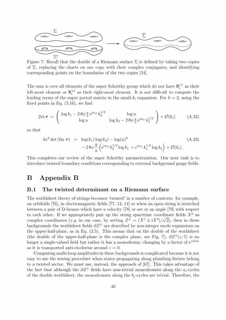
Σ

Σ∗

Σ

Figure 7: Recall that the double of a Riemann surface Σ is defined by taking two copiesof Σ, replacing the charts on one copy with their complex conjugates, and identifyingcorresponding points on the boundaries of the two copies [24].

The sum is over all elements of the super Schottky group which do not have S±1j as their

left-most element or S±1i as their right-most element. It is not difficult to compute the

leading terms of the super period matrix in the small-ki expansion. For h = 2, using thefixed points in Eq. (3.16), we find

2πi τ =

(log k1 − 2 θφ y

ueiπς2 k

1/22 log u

log u log k2 − 2 θφ yu

eiπς1 k1/21

)+O(ki) (A.32)

so that

4π2 det (Im τ ) = log(k1) log(k2)− log(u)2 (A.33)

− 2 θφy

u

(eiπς2 k

1/22 log k1 + eiπς1 k

1/21 log k2

)+O(ki) .

This completes our review of the super Schottky parametrization. Our next task is tointroduce twisted boundary conditions corresponding to external background gauge fields.

B Appendix B

B.1 The twisted determinant on a Riemann surface

The worldsheet theory of strings becomes ‘twisted’ in a number of contexts: for example,on orbifolds [76], in electromagnetic fields [77, 13, 14] or when an open string is stretchedbetween a pair of D-branes which have a velocity [78] or are at an angle [79] with respectto each other. If we appropriately pair up the string spacetime coordinate fields Xµ ascomplex coordinates (e.g. in our case, by setting Z± = (X1 ± iX2)/

√2), then in these

backgrounds the worldsheet fields ∂Z± are described by non-integer mode expansions onthe upper-half-plane, as in Eq. (2.5). This means that on the double of the worldsheet(the double of the upper-half-plane is the complex plane; see Fig. 7), ∂Z±(z, z) is nolonger a single-valued field but rather it has a monodromy, changing by a factor of e±2πiε

as it is transported anti-clockwise around z = 0.Computing multi-loop amplitudes in these backgrounds is complicated because it is not

easy to use the sewing procedure when states propagating along plumbing fixture belongto a twisted sector. We must use, instead, the approach of [67]. This takes advantage ofthe fact that although the ∂Z± fields have non-trivial monodromies along the ai-cyclesof the double worldsheet, the monodromies along the bj-cycles are trivial. Therefore, the

48

Figure 8: The same string diagram can be computed as an open string vacuum multi-loopdiagram or as the T-dual setup of a tree-level interaction between closed strings emittedfrom D-branes at angles.

idea is to build the double worldsheet by sewing along the bi cycles, and then to performthe modular transformation swapping the aj and bi cycles with each other, in order toobtain the partition function expressed in terms of the Schottky moduli which are theappropriate ones for the worldsheet degeneration we are interested in.

From a more physical point of view, we are using the fact that in a different regionof moduli space, the string diagram can be described as a tree-level interaction betweenthree closed strings being emitted or absorbed by the D-branes. In terms of the closedstring moduli, the string partition function is given by [67]

Z(Fi) =( h∏i=0

√det(1−G−1Fi)

)∫[dZ]cl

h Rh(qi,~ε ) . (B.1)

The overall factor is just the Born-Infeld lagrangian for the background fields on theD-branes, divided by

√G because all of the background-field independent factors are

included in the measure [dZ]clh .

The factor Rh(qi,~ε ), which is dependent on both the worldsheet moduli and on thebackground field strengths, has a simple form so long as it is expressed in terms of theclosed string Schottky group moduli, in other words, in terms of the multipliers of aSchottky group whose 2h Schottky circles are homotopic to the bi cycles of the worldsheetinstead of the aj cycles which we have been using. Let us denote the multipliers of theelements Tα of this Schottky group as qα, then we have

Rh(qi,~ε ) =

∏′α

∏∞n=1(1− qnα)2∏′

α

∏∞n=1(1− e−2πi ~Nα·~εqnα)(1− e2πi ~Nα·~εqnα)

, (B.2)

where the notation∏′

α has the same meaning as for the super Schottky group case, definedafter Eq. (3.7).

The modular transformation that swaps the ai- and bj-cycles, necessary to switchbetween the open string and closed string channels, acts non-analytically on the Schottkygroup multipliers.15 We need to rewrite Eq. (B.2) in terms of the open string moduli,

15This is easiest to see in the h = 1 case when the single open string multiplier k is related to thetorus period τ via k = e2πiτ , and similarly the multiplier in the closed string channel q is related to τ cl

via q = e2πiτcl

, where the closed string torus period τ cl can be obtained from the open string one τ viaτ cl = −1/τ , so (log q)(log k) = 4π2.

49

so the following strategy is used: Rh(qi,~ε ) is re-expressed in terms of functions whichtransform in simple ways under modular transformations, the modular transformationsare then carried out, and finally the results are re-expressed in terms of the open stringSchottky moduli, allowing us to investigate the field theory limit. This analysis wasperformed in [33, 35] and the results are summarized in section 2 of [15]. Assumingwithout loss of generality that the h’th twist is nonzero, εh 6= 0, the result is that

Rh(qα,~ε ) = Rh(kα,~ε · τ) e−iπ~ε·τ ·~ε det(Im τ)

det(Im τ~ε). (B.3)

whereRh(kα,~ε·τ) is the same as in Eq. (B.2) but with the closed string channel multipliersqα replaced with open string channel multipliers kα, and the twists ~ε replaced with ~ε · τ ,(τij) being the period matrix computed in the open string channel. τ~ε is the twisted periodmatrix, defined by (Eq. (3.24) of [67])

(τ~ε )ji =

1

2πi

∫ Sj(w)

wΩ~ε·τi (z) e

2πih−1

~ε·~∆(z) j 6= h 6= i

S~ε·τh −1

S~εh−1j = i = h ,

0 otherwise.

(B.4)

where

S~εi ≡ e2πiεi . (B.5)

The Prym differentials Ω~εi appearing in the integrand in the first line of Eq. (B.4) are

(h − 1) 1-forms with trivial monodromies along the ai cycles and twists along the bi-cycles, i.e. they obey

Ω~εi(Sj(z)) = S~εj Ω~ε

i(z) ; (B.6)

and they are regular everywhere.16 Assuming without loss of generality that εh 6= 0, theycan be expressed as (Eq. (3.11) of [67]):

Ω~εj(z) = ζ~εj (z)−

1− S~εj1− S~εh

ζ~εh(z) j = 1, . . . , (h− 1) . (B.7)

In Eq. (B.7) the ζ~εi are a basis of h 1-forms which are holomorphic everywhere exceptsome arbitrary base point z0, which can be computed in terms of the Schottky group as(Eq. (3.15) of [67])

ζ~εi (z) =(S~εi∑α

(i)e2πi~ε· ~Nα

[ 1

z − Tα(ηi)− 1

z − Tα(ξi)

](B.8)

+ (1− S~εi )∑α

e2πi~ε· ~Nα[ 1

z − Tα(z0)− 1

z − Tα(aαi )

])dz

16N.B. that Eq. (B.4) uses Ω~ε·τi which is obtained from Ω~εi as computed in Eqs. (B.7) and (B.8) bymaking the substitution εi 7→ (~ε · τ)i = ε1τ1i + . . .+ εhτhi.

50

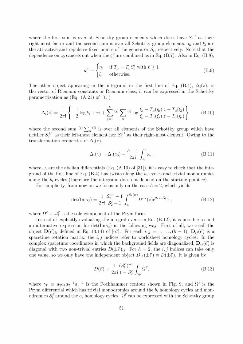
where the first sum is over all Schottky group elements which don’t have S±`i as theirright-most factor and the second sum is over all Schottky group elements. ηi and ξi arethe attractive and repulsive fixed points of the generator Si, respectively. Note that thedependence on z0 cancels out when the ζ~εi are combined as in Eq. (B.7). Also in Eq. (B.8),

aαi =

ηi if Tα = TβS

`i with ` ≥ 1

ξi otherwise.(B.9)

The other object appearing in the integrand in the first line of Eq. (B.4), ∆i(z), isthe vector of Riemann constants or Riemann class; it can be expressed in the Schottkyparametrization as (Eq. (A.21) of [31])

∆i(z) =1

2πi

−1

2log ki + πi +

h∑j=1

(j)∑α

(i) logξj − Tα(ηi)

ξj − Tα(ξi)

z − Tα(ξi)

z − Tα(ηi)

(B.10)

where the second sum (j)∑

α(i) is over all elements of the Schottky group which have

neither S±1j as their left-most element nor S±1

i as their right-most element. Owing to thetransformation properties of ∆i(z),

∆i(z) = ∆i(z0)− h− 1

2πi

∫ z

z0

ωi , (B.11)

where ωi are the abelian differentials (Eq. (A.10) of [31]), it is easy to check that the inte-grand of the first line of Eq. (B.4) has twists along the ai cycles and trivial monodromiesalong the bi-cycles (therefore the integrand does not depend on the starting point w).

For simplicity, from now on we focus only on the case h = 2, which yields

det(Im τ~ε) =1

2πi

S~ε·τ2 − 1

S~ε2 − 1

∫ S1(w)

w

Ω~ε·τ (z)e2πi~ε·~∆(z) , (B.12)

where Ω~ε ≡ Ω~ε1 is the sole component of the Prym form.

Instead of explicitly evaluating the integral over z in Eq. (B.12), it is possible to findan alternative expression for det(Im τ~ε) in the following way. First of all, we recall theobject D(~ε )ij defined in Eq. (3.14) of [67]. For each i, j = 1, . . . , (h − 1), Dij(~ε ) is aspacetime rotation matrix; the i, j indices refer to worldsheet homology cycles. In thecomplex spacetime coordinates in which the background fields are diagonalized, Dij(~ε ) isdiagonal with two non-trivial entries D(±~ε )ij. For h = 2, the i, j indices can take onlyone value, so we only have one independent object D11(±~ε ) ≡ D(±~ε ). It is given by

D(~ε ) ≡ 1

2πi

(S~ε1 )−1

1− S~ε2

∫γP

Ω~ε , (B.13)

where γP ≡ a2a1a2−1a1

−1 is the Pochhammer contour shown in Fig. 9, and Ω~ε is thePrym differential which has trivial monodromies around the bi homology cycles and mon-odromies S~εi around the ai homology cycles. Ω~ε can be expressed with the Schottky group

51

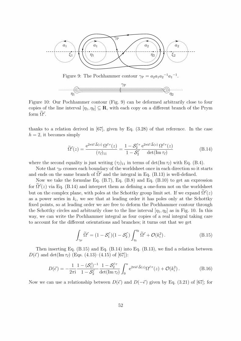
ξ1 η1 η2 ξ2

a1 a2a1 a2

γP

Figure 9: The Pochhammer contour γP = a2a1a2−1a1

−1.

γP

η1 η2

Figure 10: Our Pochhammer contour (Fig. 9) can be deformed arbitrarily close to fourcopies of the line interval [η1, η2] ⊆ R, with each copy on a different branch of the Prym

form Ω~ε.

thanks to a relation derived in [67], given by Eq. (3.28) of that reference. In the caseh = 2, it becomes simply

Ω~ε(z) =e2πi~ε·~∆(z) Ω~ε·τ (z)

(τ~ε)11

=1− S~ε·τ2

1− S~ε2e2πi~ε·~∆(z) Ω~ε·τ (z)

det(Im τ~ε)(B.14)

where the second equality is just writing (τ~ε)11 in terms of det(Im τ~ε) with Eq. (B.4).Note that γP crosses each boundary of the worldsheet once in each direction so it starts

and ends on the same branch of Ω~ε and the integral in Eq. (B.13) is well-defined.Now we take the formulae Eq. (B.7), Eq. (B.8) and Eq. (B.10) to get an expression

for Ω~ε(z) via Eq. (B.14) and interpret them as defining a one-form not on the worldsheet

but on the complex plane, with poles at the Schottky group limit set. If we expand Ω~ε(z)as a power series in ki, we see that at leading order it has poles only at the Schottkyfixed points, so at leading order we are free to deform the Pochhammer contour throughthe Schottky circles and arbitrarily close to the line interval [η1, η2] as in Fig. 10. In thisway, we can write the Pochhammer integral as four copies of a real integral taking careto account for the different orientations and branches; it turns out that we get∫

γP

Ω~ε = (1− S~ε1 )(1− S~ε2 )

∫ η2

η1

Ω~ε +O(k2i ) . (B.15)

Then inserting Eq. (B.15) and Eq. (B.14) into Eq. (B.13), we find a relation betweenD(~ε ) and det(Im τ~ε) (Eqs. (4.13)–(4.15) of [67]):

D(~ε ) = − 1

2πi

1− (S~ε1)−1

1− S~ε21− S~ε·τ2

det(Im τ~ε)

∫ u

0

e2πi~ε·~∆(z)Ω~ε·τ (z) +O(k2i ) . (B.16)

Now we can use a relationship between D(~ε ) and D(−~ε ) given by Eq. (3.21) of [67]; for

52

h = 2 it can be stated as17

D(~ε )−D(−~ε) = −2isin(πε1) sin(πε1 + πε2)

sin(πε2). (B.17)

(this can be found by cutting between the Schottky circles to get a simply-connected

fundamental domain for Σh, then using Stokes’ theorem to integrate Ω~ε ∧ Ω(−~ε), whichvanishes since it’s a (2, 0) form — see Appendix A of [36]). Inserting Eq. (B.16) inEq. (B.17), we can use the fact that det(Im τ~ε) is even under the substitution ~ε 7→ −~ε, asfollows from Eq. (B.3), and solve to find:

det(Im τ~ε) =1

4π

e−iπ(ε1+ε2)(1− S~ε·τ2 )

sin(π(ε1 + ε2))

∫ u

0

e2πi~ε·~∆(z)Ω~ε·τ (z) + (~ε→ −~ε) +O(k2i ) . (B.18)

B.2 The twisted determinant on a super Riemann surface

To compute the superstring partition function in our background, we have to find det(Im τ~ε),appearing in Eq. (3.13) and so on. det(Im τ~ε) is a modified version of det(Im τ~ε) as com-puted in the previous subsection; in this subsection we show how to modify the compu-tation for SRSs. As a starting point, we take the following formula for det(Im τ~ε) whichcan be arrived at similarly to Eq. (B.16) but without using Eq. (B.15) to deform theintegration cycle:

det(Im τ~ε) =1

4π

e−iπ(ε1+ε2)(1− S~ε·τ2 )

sin(π(ε1 + ε2))(1− S~ε1)(1− S~ε2)

∫γP

e2πi~ε·~∆(z)Ω~ε·τ (z) + (~ε→ −~ε) . (B.19)

To proceed, we replace ∆i(z) and Ωε with supersymmetric extensions ∆i(z) and Ωε re-spectively, replace the period matrix τ with the super-period matrix τ in the phasese2πi(ε·τ)i , and carry out the integration over a Pochhammer contour γP = a2a1a

−12 a−1

1 onthe SRS. The formula, then, is

det(Im τ~ε) =1

4π

e−iπ(ε1+ε2)(1− S~ε·τ2 )

sin(π(ε1 + ε2))(1− S~ε1)(1− S~ε2)

∫γP

e2πi~ε· ~∆(z)Ω~ε·τ (z) + (~ε→ −~ε) . (B.20)

The integrand in Eq. (B.20) will be locally of the form dz f(z|ψ). We can carry out thedψ integral independently and it will just yield the coefficient of ψ in the integrand. Theintegral is reduced to an ordinary line integral over a Pochhammer contour γP in thereduced space of the SRS. Then as in section B.1, we are free to expand the integrand asa power series in ki and deform γP as in Eq. (B.15) yielding

det(Im τ~ε) =1

4π

e−iπ(ε1+ε2)(1− S~ε·τ2 )

sin(π(ε1 + ε2))

∫ u

0

∂ψ

(e2πi~ε· ~∆(z|ψ)Ω~ε·τ (z|ψ)

)+ (~ε→ −~ε) +O(ki) .

(B.21)

17To get this from Eq. (3.21) of [67], we have to put εh = −ε2; the relative sign occurs because our a2and b2 homology cycles have opposite orientation.

53

Now we need to define the objects appearing in Eq. (B.21). The Prym differentials Ω~εi we

used to compute det(Im τ~ε) are holomorphic one-forms; the natural analogues on SRSsare holomorphic volume forms: sections of the Berezinian bundle. Just as holomorphicdifferentials can be written locally as dz ∂zf(z), sections of the Berezinian can be writtenlocally as dzDψ f(z|ψ), the combination being invariant under change of superconformalcoordinates [21]. We note that we can write equation Eq. (B.8) for ζ~εi as

ζεi (z) = dz∂

∂z

(S~εi∑α

(i)e2πi~ε· ~Nα log

[z − Tα(ηi)

z − Tα(ξi)

](B.22)

+ (1− S~εi )∑α

e2πi~ε· ~Nα log[ z − Tα(z0)

z − Tα(aαi )

]),

so to find the corresponding SRS volume forms we replace the expressions inside thelogarithms with their natural superconformal analogues and replace dz ∂z 7→ dzDψ. Thisyields

ζ~εi (z|ψ) = dzDψ

(S~εi∑α

(i)e2πi~ε· ~Nα log

[〈z|Tα|ui〉〈z|Tα|vi〉

](B.23)

+ (1− S~εi )∑α

e2πi~ε· ~Nα log[〈z|Tα|z0〉〈z|Tα|ai〉

])= dz

(S~εi∑α

(i)e2πi~ε· ~Nα

[〈z|ΦTα|ui〉〈z|Tα|ui〉

− 〈z|ΦTα|vi〉〈z|Tα|vi〉

](B.24)

+ (1− S~εi )∑α

e2πi~ε· ~Nα[〈z|ΦTα|z0〉〈z|Tα|z0〉

− 〈z|ΦTα|ai〉〈z|Tα|ai〉

])where we’ve used Φ defined in Eq. (A.29), |z0〉 is an arbitrary base point, and

|aαi 〉 =

|ui〉 if Tα = TβS

`i with ` ≥ 1

|vi〉 otherwise.(B.25)

Then we can write down a basis of (h − 1) holomorphic volume forms Ω~εj(z) with the

expected monodromies along the homology cycles using the analogue of Eq. (B.7), notingthat the dependence on the base point |z0〉 cancels out:

Ω~εj(z|ψ) = ζ~εj(z|ψ)−

1− S~εj1− S~εh

ζ~εh(z|ψ) j = 1, . . . , (h− 1) . (B.26)

We can calculate Ω~εj(z|ψ) as a series expansion in k

1/2i . Truncating to finite order, we only

need to sum Eq. (B.24) over finitely many terms of the super-Schottky group, because ifthe contribution from Tα is O(kα

1/2) and the left-most factor of Tα is not S±1i , then the

contribution from S±`i Tα is O(ki`/2kα

1/2). Restricting ourselves to h = 2, this means thatif we only want to compute to order ki

1/2 then we only need to sum over the super-Schottkygroup elements

Tα ∈ Id,S±11 ,S±1

2 , (S1S2)±1, (S−11 S2)±1, (S1S

−12 )±1, (S2S1)±1 . (B.27)

54

Using the fixed points given in Eq. (3.16), we obtain the following expression for Ω~ε(z) ≡Ω~ε

1(z):

Ω~ε(z|ψ) = dz[− (1− S~ε1)S~ε2θ

(1− S~ε2)(u− z)+

(1− S~ε1)φ

(1− S~ε2)(1− z)(B.28)

+

(S~ε1u(1− S~ε2)− (S~ε1 − S~ε2 − S~ε1S~ε2u+ u)z + z2(1− S~ε2)

)ψ

(1− S~ε2)(u− z)(1− z)z

+ eiπς1k1/21

− (1− S~ε1)S~ε1(S~ε2θ − φ)

(1− S~ε2)z+

(1− S~ε1)(S~ε2θ − uφ)

S~ε1(1− S~ε2)u

+ eiπς2k

1/22

− S

~ε2(1− S~ε1)θ

u− z+S~ε2(1− S~ε1u)φ

u− z− (S~ε1 − u)θ

S~ε2u(1− z)

− S~ε2(1− S~ε1u)θφψ

(u− z)2− (S~ε1 − u)θφψ

S~ε2u(1− z)2− (1− S~ε1)φ

S~ε2(1− z)

+ eiπ(ς1+ς2)k

1/21 k

1/22

S~ε1S~ε2(φ− S~ε1uφ− (1− S~ε1)θ)

z

+S~ε2(θ(1− S~ε1)− φ+ S~ε1uφ)

S~ε1u− ((u− S~ε1)θ − (1− S~ε1)uφ)

S~ε1S~ε2u

+S~ε1(uθ − S~ε1θ − uφ(1− S~ε1))

S~ε2uz+

(1− S~ε1)S~ε1(1− u)θ

(1− S~ε2)u(1− z)

− (1− S~ε1)S~ε1(1− u)φ

(1− S~ε2)S~ε2u(1− z)− (1− S~ε1)S~ε1S~ε2(1− u)(S~ε2θ − φ)

(1− S~ε2)(u− z)

− (1− S~ε1)S~ε1S~ε2(1− u)θφψ

(1− S~ε2)(u− z)2− (1− S~ε1)2(1 + S~ε1)(1− u)θφψ

S~ε1(1− S~ε2)u(1− z)2

+(1− S~ε1)(1− u)(uφ− S~ε2θ)S~ε1(1− S~ε2)S~ε2(1− z)u

+(1− S~ε1)(S~ε2)2(1− u)θ

S~ε1(1− S~ε2)u(u− z)

+(1− S~ε1)S~ε2(1− u)θφψ

S~ε1(1− S~ε2)(u− z)2− (1− S~ε1)S~ε2(1− u)φ

S~ε1(1− S~ε2)(u− z)

]+O(ki) ,

where S~εi is defined in Eq. (B.5). In our calculation of the twisted super-period matrix,the Prym differential appears not with the monodromies ~ε but with (~ε ·τ ); to find Ω~ε·τ (z)we replace S~εi in Eq. (B.28) with S~ε·τi . Using τ from Eq. (A.32), we find

S~ε·τ1 = e2πi(~ε·τ )1 = kε11 uε2(

1− 2ε1eiπς2k1/22

y

uθφ)

+O(ki) , (B.29)

S~ε·τ2 = e2πi(~ε·τ )2 = kε22 uε1(

1− 2ε2eiπς1k1/21

y

uθφ)

+O(ki) . (B.30)

To supersymmetrize the Riemann class ∆i(z), we need to replace the cross-ratios inEq. (B.10) with super-projective invariant cross-ratios, and replace the Schottky fixedpoints ηi, ξi with the super fixed points ui = ui|θi, vi = vi|φi, and replace the base pointz with a super-point z = z|ψ. The formula becomes, then,

∆i(z) =1

2πi

−1

2log ki + πi +

h∑j=1

(j)∑α

(i) log〈vj|Tα|ui〉〈vj|Tα|vi〉

〈z|Tα|vi〉〈z|Tα|ui〉

. (B.31)

55

For our purposes, we want to compute ∆i(z) for h = 2 with the fixed points given in

Eq. (3.16). At order O(k1/2i ), we find

∆1(z) =1

2πi

− 1

2log k1 + πi− log z + eiπς2k

1/22 (1− u)

(ψθ + θφ

u(1− z)+θφ− ψφu− z

)(B.32)

− eiπ(ς1+ς2)k1/21 k

1/22

1− uuz

((1− z)θψ + (u− z)ψφ)

+O(ki)

∆2(z) =1

2πi

− 1

2log k2 + πi + log

1− zu− z

+1

u− zθψ +

1

1− zψφ (B.33)

+ eiπς1k1/21

1

uz

((u− z)θψ + z(1− u)θφ+ u(1− z)ψφ

)− eiπ(ς1+ς2)k

1/21 k

1/22

(1− u)2

u

( 1

u− zθψ +

1

1− zψφ)

+O(ki) .

Exponentiating these, we get

e2πi~ε·∆(z) = eiπ(ε1+ε2)k− ε1

21 k

− ε22

2 z−ε1(

1− zu− z

)ε2× (B.34)[

1− ε1

eiπς2k1/22 (1− u)

( 1

u(1− z)θψ +

1

u− zψφ+

( 1

u− z− 1

u(1− z)

)θφ)

− eiπ(ς1+ς2)k1/21 k

1/22

1− uuz

((1− z)θψ + (u− z)ψφ

)+ ε2

1

u− zθψ +

1

1− zψφ− eiπς1k

1/21

1

uz

((u− z)θψ + z(1− u)θφ

+ u(1− z)ψφ)− eiπ(ς1+ς2)k

1/21 k

1/22

(1− u)2

u

( 1

u− zθψ +

1

1− zψφ)]

+O(ki) .

We have assembled the ingredients to compute det(Im τε). We take Ω~ε·τ1 (z|ψ) from

Eq. (B.28), the phases S~ε·τi from Eq. (B.29) and Eq. (B.30), and e2πi~ε·∆(z|ψ) from Eq. (B.34)and insert them into Eq. (B.21). We get a sum of integrals of the form

det(Im τ~ε) =∑I

fI(µ,~ε )π

sin(π(ε1 + ε2))

∫ u

0

dz znI1−ε1(1− z)n

I2+ε2(u− z)n

I3−ε2

+ (εi → −εi) +O(ki) . (B.35)

We can evaluate these integral with the substitution z = tu, getting

π

sin(π(ε1 + ε2))

∫ u

0

dzzn1−ε1(1− z)n2+ε2

(u− z)−n3+ε2=u1+n1+n3−ε1−ε3

(−1)1+n1+n3I[n1, n2, n3] , (B.36)

where

I[n1, n2, n3] ≡ Γ(1 + n1 − ε1)Γ(1 + n3 − ε2)Γ(−1− n1 − n3 + ε1 + ε2) (B.37)

× 2F1(−n2 − ε2, 1 + n1 − ε1; 2 + n1 + n3 − ε1 − ε2;u) .

The hypergeometric function is given by the integral representation

2F1(a, b; c; z) =Γ(c)

Γ(b)Γ(c− b)

∫ 1

0

tb−1(1− t)c−b−1(1− tz)−a , (B.38)

56

and we’ve used the identity Γ(x)Γ(1− x) sin(πx) ≡ π. We obtain

det(Im τ~ε) =1

4π2

2∑p,q,r=−2

1∑i,j,n=0

Aijn;pqr × (eiπς1k1/21 )i(eiπς2k

1/22 )j(θφ)n I[p, q, r]

+O(ki) + (εi ↔ −εi) . (B.39)

At lowest order in ki, det(Im τ~ε) is given as

4π2 det(Im τ~ε) =kε12

1 k− ε2

22 u−ε1 (kε22 u

ε1 − 1) I[−1,−1,−1] (B.40)

+ k− ε1

21 k

− ε22

2 uε3+1 (kε22 uε1 − 1) I[1,−1,−1]

+ k− ε1

21 k

− ε22

2 uε3(kε22 u

ε1 − kε11 uε2 + u

((k1u)ε1(k2u)ε2 − 1

))I[0,−1,−1]

− θφ ε2uε3k− ε1

21 k

− ε22

2 (kε11 uε2 − 1) (kε22 u

ε1 − 1) I[0,−1,−1] + (~ε↔ −~ε ) +O(k1/2i ) ;

our calculations require the calculation of det(Im τ~ε) to first order in k1/2i ; the neces-

sary coefficients Aijn;pqr = Aijn;pqr(k`, εm, u) for i, j, n ranging from 0 to 1 are listed in aMathematica notebook included as supplemental material on ArXiv.18

When rewriting det(Im τ ) in the pi parametrization (Eq. (4.12)) appropriate for thesymmetric degeneration (Fig. 6a), one can use

2F1 (a− ε1, b− ε2, c− ε1 − ε2, u) = 1 +(a− ε1)(b− ε2)

c− ε1 − ε2u+O(u2)

= 1 +O(pi) , (B.41)

so around the symmetric degeneration, all the 2F1 hypergeometric functions can be re-placed with 1, and so the factor I[n1, n2, n3] as defined in Eq. (B.37) depends only on thetwists ~ε and not on the worldsheet moduli.

C Appendix C

C.1 List of Feynman graphs

In this appendix we will list all of the two-loop 1-particle-irreducible planar Feynmandiagrams we get from the vertices in Eq. (5.11). To compare easily with the string theoryresults, we will order the results by the color indices, i.e., we will list all of the diagramswhose propagators have the three color indices A, B and C, say; we expect that all ofthese come from the field theory limit of the worldsheet whose boundaries are on the Ath,Bth and Cth D-branes.

Then we should sum the following diagrams, weighted appropriately, over A ≤ B ≤ C,where we write

BBA = B1 BAC = B2 BCB = B3 m2AB = m2

1 m2CA = m2

2 m2BC = m2

3 . (C.1)

18Twisted determinant coefficients.nb

57

Let us write down the Feynman diagrams with the various sectors of the QFT representedusing the following propagators:

= gluon modes polarized parallel to the background field (C.2)

= gluon modes polarized perpendicular to the background field (C.3)

= Faddeev-Popov ghosts (C.4)

= scalars (C.5)

Then we get the following Feynman graphs:

= −(3− γ2)(d− 2)(d− 3)

2

g2

(4π)d

∫ ∞0

(∏3i=1 dti e

−tim2i

∆d/2−10 ∆B

)t1 + t2 + t3

∆0

(C.6)

= −(d− 2)g2

(4π)d

∫ ∞0

(∏3i=1 dti e

−tim2i

∆d/2−10 ∆B

)1

∆B

[sinh(gB3t3)

gB3

(C.7)

×(

(1− γ2) cosh(gB2t2 − gB1t1)

+ 2 cosh(2gB3t3 − gB2t2 − gB1t1)

)+ cyclic permutations

]

= −(d− 2)g2

(4π)d

∫ ∞0

(∏3i=1 dti e

−tim2i

∆d/2−10 ∆B

)1

∆0

[(2t3 +

1− γ2

2(t1 + t2)

)

× cosh(2gB1t1 − 2gB2t2) + cyclic permutations

](C.8)

= − g2

(4π)d

∫ ∞0

(∏3i=1 dti e

−tim2i

∆d/2−10 ∆B

)1

∆B

[sinh(gB3t3)

gB3

×(2 + (1− γ2) cosh(2gB1t1 − 2gB2t2)

)× cosh(2gB3t3 − gB2t2 − gB1t1) + cyclic permutations

](C.9)

= (1 + γ2)d− 2

2

g2

(4π)d

∫ ∞0

(∏3i=1 dti e

−tim2i

∆d/2−10 ∆B

)1

∆0

[t3

+ cyclic permutations]

(C.10)

= (1 + γ2)g2

(4π)d

∫ ∞0

(∏3i=1 dti e

−tim2i

∆d/2−10 ∆B

)1

∆B

[sinh(gB3t3)

gB3

58

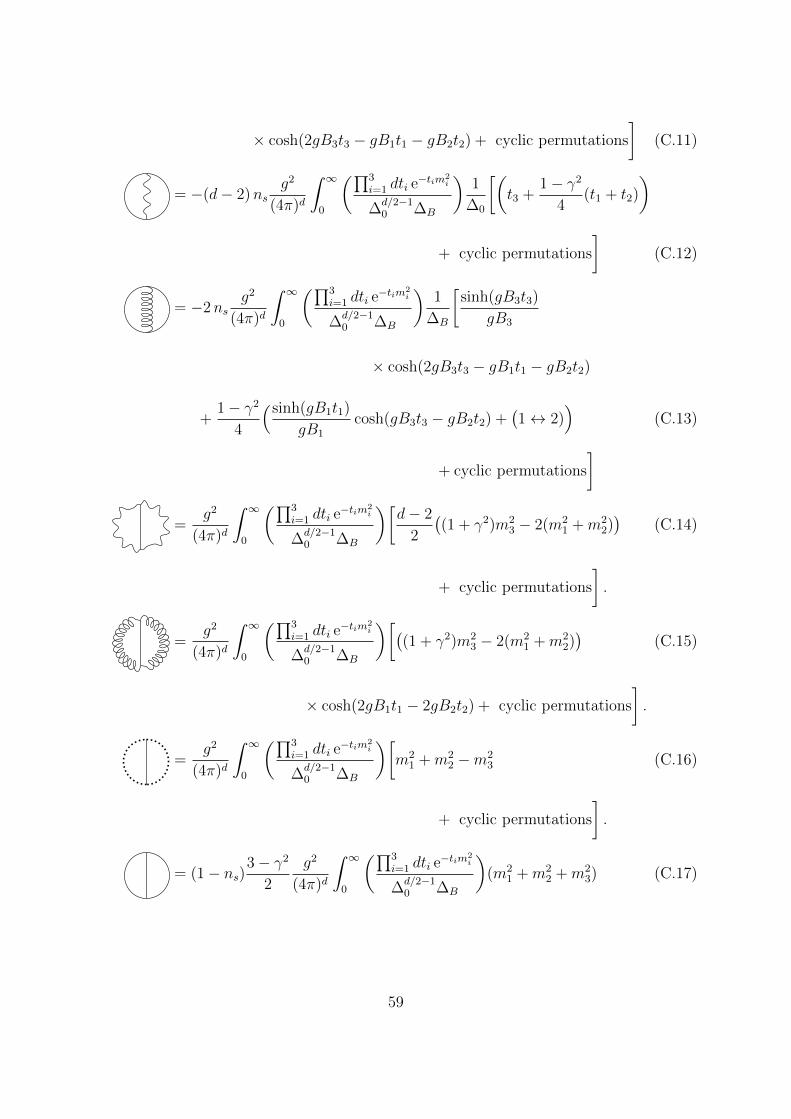
× cosh(2gB3t3 − gB1t1 − gB2t2) + cyclic permutations

](C.11)

= −(d− 2)nsg2

(4π)d

∫ ∞0

(∏3i=1 dti e

−tim2i

∆d/2−10 ∆B

)1

∆0

[(t3 +

1− γ2

4(t1 + t2)

)

+ cyclic permutations

](C.12)

= −2nsg2

(4π)d

∫ ∞0

(∏3i=1 dti e

−tim2i

∆d/2−10 ∆B

)1

∆B

[sinh(gB3t3)

gB3

× cosh(2gB3t3 − gB1t1 − gB2t2)

+1− γ2

4

(sinh(gB1t1)

gB1

cosh(gB3t3 − gB2t2) +(1↔ 2)

)(C.13)


]

=g2

(4π)d

∫ ∞0

(∏3i=1 dti e

−tim2i

∆d/2−10 ∆B

)[d− 2

2

((1 + γ2)m2

3 − 2(m21 +m2

2))

(C.14)


].

=g2

(4π)d

∫ ∞0

(∏3i=1 dti e

−tim2i

∆d/2−10 ∆B

)[((1 + γ2)m2

3 − 2(m21 +m2

2))

(C.15)

× cosh(2gB1t1 − 2gB2t2) + cyclic permutations

].

=g2

(4π)d

∫ ∞0

(∏3i=1 dti e

−tim2i

∆d/2−10 ∆B

)[m2

1 +m22 −m2

3 (C.16)


].

= (1− ns)3− γ2

2

g2

(4π)d

∫ ∞0

(∏3i=1 dti e

−tim2i

∆d/2−10 ∆B

)(m2

1 +m22 +m2

3) (C.17)

59

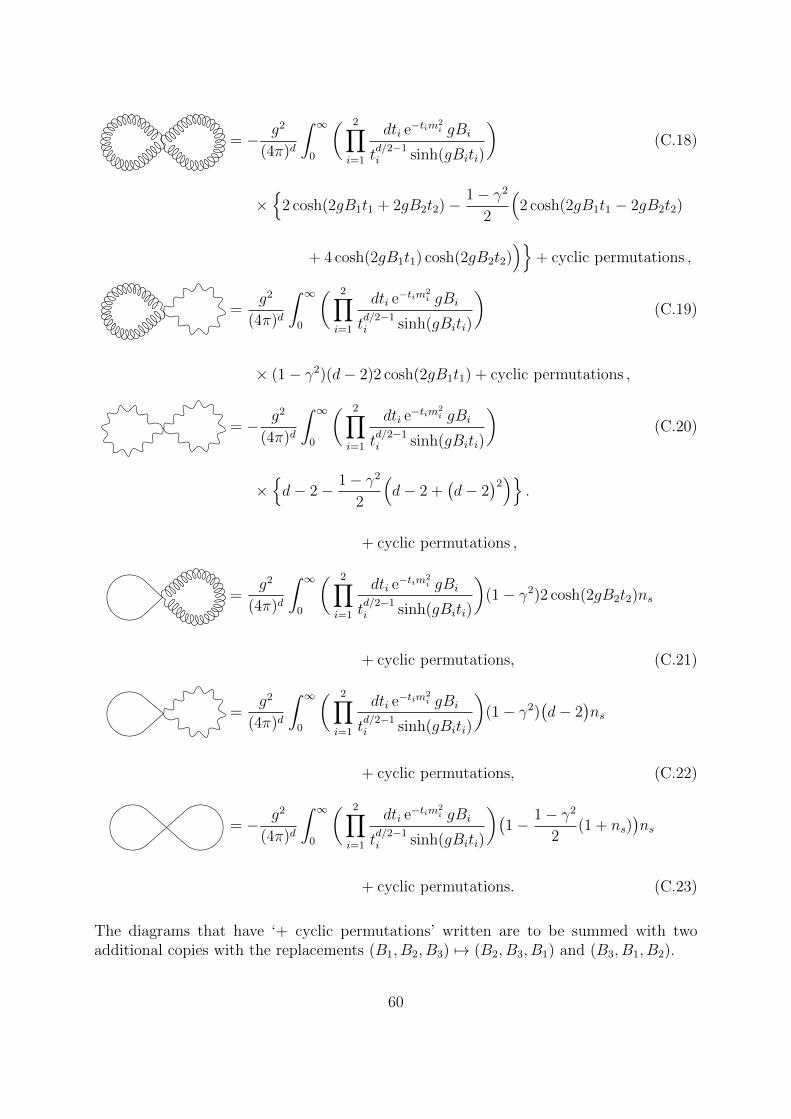
= − g2

(4π)d

∫ ∞0

( 2∏i=1

dti e−tim2

i gBi

td/2−1i sinh(gBiti)

)(C.18)

×

2 cosh(2gB1t1 + 2gB2t2)− 1− γ2

2

(2 cosh(2gB1t1 − 2gB2t2)

+ 4 cosh(2gB1t1) cosh(2gB2t2))

+ cyclic permutations ,

=g2

(4π)d

∫ ∞0

( 2∏i=1

dti e−tim2

i gBi


)(C.19)

× (1− γ2)(d− 2)2 cosh(2gB1t1) + cyclic permutations ,

= − g2

(4π)d

∫ ∞0

( 2∏i=1

dti e−tim2

i gBi


)(C.20)

×d− 2− 1− γ2

2

(d− 2 +

(d− 2

)2)

.

+ cyclic permutations ,

=g2

(4π)d

∫ ∞0

( 2∏i=1

dti e−tim2

i gBi


)(1− γ2)2 cosh(2gB2t2)ns

+ cyclic permutations, (C.21)

=g2

(4π)d

∫ ∞0

( 2∏i=1

dti e−tim2

i gBi


)(1− γ2)

(d− 2

)ns

+ cyclic permutations, (C.22)

= − g2

(4π)d

∫ ∞0

( 2∏i=1

dti e−tim2

i gBi


)(1− 1− γ2

2(1 + ns)

)ns

+ cyclic permutations. (C.23)

The diagrams that have ‘+ cyclic permutations’ written are to be summed with twoadditional copies with the replacements (B1, B2, B3) 7→ (B2, B3, B1) and (B3, B1, B2).

60

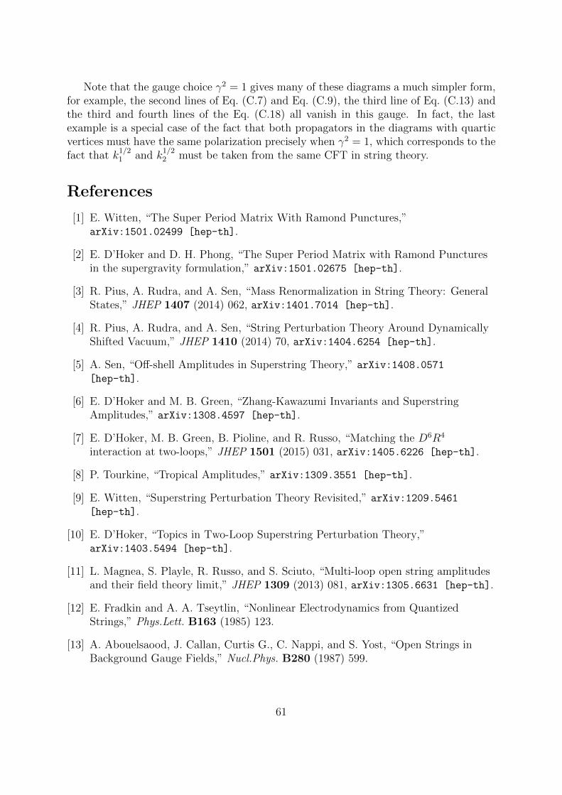
Note that the gauge choice γ2 = 1 gives many of these diagrams a much simpler form,for example, the second lines of Eq. (C.7) and Eq. (C.9), the third line of Eq. (C.13) andthe third and fourth lines of the Eq. (C.18) all vanish in this gauge. In fact, the lastexample is a special case of the fact that both propagators in the diagrams with quarticvertices must have the same polarization precisely when γ2 = 1, which corresponds to thefact that k

1/21 and k

1/22 must be taken from the same CFT in string theory.

References

[1] E. Witten, “The Super Period Matrix With Ramond Punctures,”arXiv:1501.02499 [hep-th].

[2] E. D’Hoker and D. H. Phong, “The Super Period Matrix with Ramond Puncturesin the supergravity formulation,” arXiv:1501.02675 [hep-th].

[3] R. Pius, A. Rudra, and A. Sen, “Mass Renormalization in String Theory: GeneralStates,” JHEP 1407 (2014) 062, arXiv:1401.7014 [hep-th].

[4] R. Pius, A. Rudra, and A. Sen, “String Perturbation Theory Around DynamicallyShifted Vacuum,” JHEP 1410 (2014) 70, arXiv:1404.6254 [hep-th].

[5] A. Sen, “Off-shell Amplitudes in Superstring Theory,” arXiv:1408.0571

[hep-th].

[6] E. D’Hoker and M. B. Green, “Zhang-Kawazumi Invariants and SuperstringAmplitudes,” arXiv:1308.4597 [hep-th].

[7] E. D’Hoker, M. B. Green, B. Pioline, and R. Russo, “Matching the D6R4

interaction at two-loops,” JHEP 1501 (2015) 031, arXiv:1405.6226 [hep-th].

[8] P. Tourkine, “Tropical Amplitudes,” arXiv:1309.3551 [hep-th].

[9] E. Witten, “Superstring Perturbation Theory Revisited,” arXiv:1209.5461

[hep-th].

[10] E. D’Hoker, “Topics in Two-Loop Superstring Perturbation Theory,”arXiv:1403.5494 [hep-th].

[11] L. Magnea, S. Playle, R. Russo, and S. Sciuto, “Multi-loop open string amplitudesand their field theory limit,” JHEP 1309 (2013) 081, arXiv:1305.6631 [hep-th].

[12] E. Fradkin and A. A. Tseytlin, “Nonlinear Electrodynamics from QuantizedStrings,” Phys.Lett. B163 (1985) 123.

[13] A. Abouelsaood, J. Callan, Curtis G., C. Nappi, and S. Yost, “Open Strings inBackground Gauge Fields,” Nucl.Phys. B280 (1987) 599.

61

http://arxiv.org/abs/1501.02499


http://dx.doi.org/10.1007/JHEP07(2014)062















http://dx.doi.org/10.1016/0370-2693(85)90205-9

http://dx.doi.org/10.1016/0550-3213(87)90164-7

[14] C. Bachas and M. Porrati, “Pair creation of open strings in an electric field,”Phys.Lett. B296 (1992) 77–84, arXiv:hep-th/9209032 [hep-th].

[15] L. Magnea, R. Russo, and S. Sciuto, “Two-loop Euler-Heisenberg effective actionsfrom charged open strings,” Int.J.Mod.Phys. A21 (2006) 533–558,arXiv:hep-th/0412087 [hep-th].

[16] J.-L. Gervais and A. Neveu, “Feynman rules for massive gauge fields with dualdiagram topology,” Nucl.Phys. B46 (1972) 381–401.

[17] L. Crane and J. M. Rabin, “Super Riemann Surfaces: Uniformization andTeichmuller Theory,” Commun.Math.Phys. 113 (1988) 601.

[18] E. J. Martinec, “Conformal Field Theory on a (Super)Riemann Surface,”Nucl.Phys. B281 (1987) 157.

[19] S. B. Giddings and P. C. Nelson, “The Geometry of Super Riemann Surfaces,”Commun.Math.Phys. 116 (1988) 607.

[20] E. D’Hoker and D. Phong, “The Geometry of String Perturbation Theory,”Rev.Mod.Phys. 60 (1988) 917.

[21] E. Witten, “Notes On Super Riemann Surfaces And Their Moduli,”arXiv:1209.2459 [hep-th].

[22] C. Lovelace, “M-loop generalized Veneziano formula,” Phys.Lett. B32 (1970)703–708.

[23] M. Kaku and L. Yu, “The general multi-loop Veneziano amplitude,” Phys.Lett.B33 (1970) 166–170.

[24] V. Alessandrini, “A General approach to dual multiloop diagrams,” Nuovo Cim.A2 (1971) 321–352.

[25] D. Olive, “Operator vertices and propagators in dual theories,” Nuovo Cim. A3(1971) 399–411.

[26] V. Alessandrini and D. Amati, “Properties of dual multiloop amplitudes,” NuovoCim. A4 (1971) 793–844.

[27] C. Montonen, “Multiloop amplitudes in additive dual-resonance models,” NuovoCim. A19 (1974) 69–89.

[28] P. Di Vecchia, R. Nakayama, J. Petersen, J. Sidenius, and S. Sciuto, “BRSTinvariant N -reggeon vertex,” Phys.Lett. B182 (1986) 164.

[29] P. Di Vecchia, M. Frau, A. Lerda, and S. Sciuto, “A simple expression for themultiloop amplitude in the bosonic string,” Phys.Lett. B199 (1987) 49.

62

http://dx.doi.org/10.1016/0370-2693(92)90806-F

http://arxiv.org/abs/hep-th/9209032

http://dx.doi.org/10.1142/S0217751X06025110


http://dx.doi.org/10.1016/0550-3213(72)90071-5

http://dx.doi.org/10.1007/BF01223239

http://dx.doi.org/10.1016/0550-3213(87)90252-5

http://dx.doi.org/10.1007/BF01224903

http://dx.doi.org/10.1103/RevModPhys.60.917


http://dx.doi.org/10.1016/0370-2693(70)90450-8

http://dx.doi.org/10.1016/0370-2693(70)90450-8

http://dx.doi.org/10.1016/0370-2693(70)90292-3

http://dx.doi.org/10.1016/0370-2693(70)90292-3

http://dx.doi.org/10.1007/BF02899858

http://dx.doi.org/10.1007/BF02899858

http://dx.doi.org/10.1007/BF02813700

http://dx.doi.org/10.1007/BF02813700

http://dx.doi.org/10.1007/BF02731520

http://dx.doi.org/10.1007/BF02731520

http://dx.doi.org/10.1007/BF02785444

http://dx.doi.org/10.1007/BF02785444

http://dx.doi.org/10.1016/0370-2693(86)91570-4

http://dx.doi.org/10.1016/0370-2693(87)91462-6

[30] P. Di Vecchia, K. Hornfeck, M. Frau, A. Lerda, and S. Sciuto, “N-string, g-loopvertex for the fermionic string,” Phys.Lett. B211 (1988) 301.

[31] P. Di Vecchia, F. Pezzella, M. Frau, K. Hornfeck, A. Lerda, and S. Sciuto, “N-pointg-loop vertex for a free bosonic theory with vacuum charge Q,” Nucl.Phys. B322(1989) 317.

[32] P. Di Vecchia, F. Pezzella, M. Frau, K. Hornfeck, A. Lerda, and S. Sciuto, “N-pointg-loop vertex for a free fermionic theory with arbitrary spin,” Nucl.Phys. B333(1990) 635.

[33] R. Russo and S. Sciuto, “Twisted determinants on higher genus Riemann surfaces,”Nucl.Phys. B669 (2003) 207–232, arXiv:hep-th/0306129 [hep-th].

[34] K. Aoki, E. D’Hoker, and D. Phong, “Two loop superstrings on orbifoldcompactifications,” Nucl.Phys. B688 (2004) 3–69, arXiv:hep-th/0312181[hep-th].

[35] R. Russo and S. Sciuto, “Twisted determinants and bosonic open strings in anelectromagnetic field,” Fortsch.Phys. 52 (2004) 678–683, arXiv:hep-th/0312205[hep-th].

[36] I. Antoniadis, K. Narain, and T. Taylor, “Open string topological amplitudes andgaugino masses,” Nucl.Phys. B729 (2005) 235–277, arXiv:hep-th/0507244[hep-th].

[37] J. Scherk, “Zero-slope limit of the dual resonance model,” Nucl.Phys. B31 (1971)222–234.

[38] M. B. Green, J. H. Schwarz, and L. Brink, “N=4 Yang-Mills and N=8 Supergravityas Limits of String Theories,” Nucl.Phys. B198 (1982) 474–492.

[39] M. L. Mangano, S. J. Parke, and Z. Xu, “Duality and Multi-gluon Scattering,”Nucl.Phys. B298 (1988) 653.

[40] M. L. Mangano and S. J. Parke, “Multiparton amplitudes in gauge theories,”Phys.Rept. 200 (1991) 301–367, arXiv:hep-th/0509223 [hep-th].

[41] Z. Bern and D. A. Kosower, “A New Approach to One Loop Calculations in GaugeTheories,” Phys.Rev. D38 (1988) 1888.

[42] Z. Bern and D. A. Kosower, “Efficient calculation of one loop QCD amplitudes,”Phys.Rev.Lett. 66 (1991) 1669–1672.

[43] Z. Bern and D. A. Kosower, “Color decomposition of one loop amplitudes in gaugetheories,” Nucl.Phys. B362 (1991) 389–448.

[44] Z. Bern and D. A. Kosower, “The Computation of loop amplitudes in gaugetheories,” Nucl.Phys. B379 (1992) 451–561.

63

http://dx.doi.org/10.1016/0370-2693(88)90907-0

http://dx.doi.org/10.1016/0550-3213(89)90419-7

http://dx.doi.org/10.1016/0550-3213(89)90419-7

http://dx.doi.org/10.1016/0550-3213(90)90135-Z

http://dx.doi.org/10.1016/0550-3213(90)90135-Z

http://dx.doi.org/10.1016/j.nuclphysb.2003.07.016





http://dx.doi.org/10.1002/prop.200310163






http://dx.doi.org/10.1016/0550-3213(71)90227-6

http://dx.doi.org/10.1016/0550-3213(71)90227-6

http://dx.doi.org/10.1016/0550-3213(82)90336-4

http://dx.doi.org/10.1016/0550-3213(88)90001-6

http://dx.doi.org/10.1016/0370-1573(91)90091-Y


http://dx.doi.org/10.1103/PhysRevD.38.1888

http://dx.doi.org/10.1103/PhysRevLett.66.1669

http://dx.doi.org/10.1016/0550-3213(91)90567-H

http://dx.doi.org/10.1016/0550-3213(92)90134-W

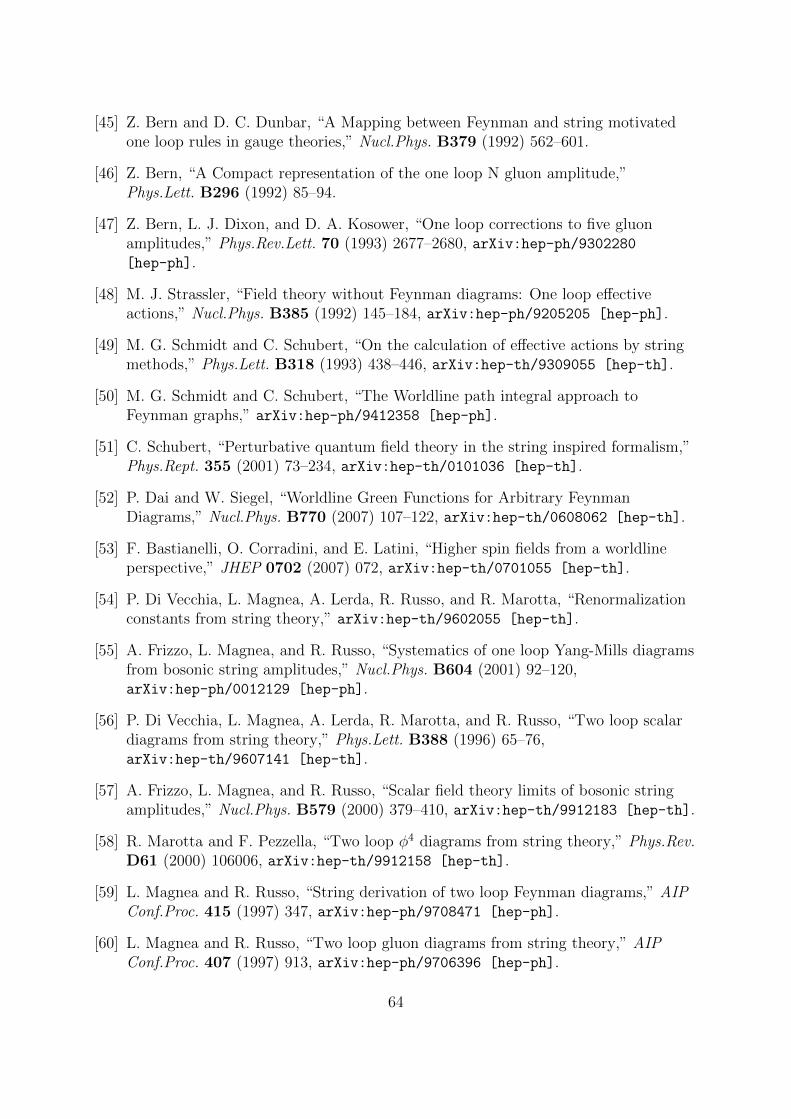
[45] Z. Bern and D. C. Dunbar, “A Mapping between Feynman and string motivatedone loop rules in gauge theories,” Nucl.Phys. B379 (1992) 562–601.

[46] Z. Bern, “A Compact representation of the one loop N gluon amplitude,”Phys.Lett. B296 (1992) 85–94.

[47] Z. Bern, L. J. Dixon, and D. A. Kosower, “One loop corrections to five gluonamplitudes,” Phys.Rev.Lett. 70 (1993) 2677–2680, arXiv:hep-ph/9302280[hep-ph].

[48] M. J. Strassler, “Field theory without Feynman diagrams: One loop effectiveactions,” Nucl.Phys. B385 (1992) 145–184, arXiv:hep-ph/9205205 [hep-ph].

[49] M. G. Schmidt and C. Schubert, “On the calculation of effective actions by stringmethods,” Phys.Lett. B318 (1993) 438–446, arXiv:hep-th/9309055 [hep-th].

[50] M. G. Schmidt and C. Schubert, “The Worldline path integral approach toFeynman graphs,” arXiv:hep-ph/9412358 [hep-ph].

[51] C. Schubert, “Perturbative quantum field theory in the string inspired formalism,”Phys.Rept. 355 (2001) 73–234, arXiv:hep-th/0101036 [hep-th].

[52] P. Dai and W. Siegel, “Worldline Green Functions for Arbitrary FeynmanDiagrams,” Nucl.Phys. B770 (2007) 107–122, arXiv:hep-th/0608062 [hep-th].

[53] F. Bastianelli, O. Corradini, and E. Latini, “Higher spin fields from a worldlineperspective,” JHEP 0702 (2007) 072, arXiv:hep-th/0701055 [hep-th].

[54] P. Di Vecchia, L. Magnea, A. Lerda, R. Russo, and R. Marotta, “Renormalizationconstants from string theory,” arXiv:hep-th/9602055 [hep-th].

[55] A. Frizzo, L. Magnea, and R. Russo, “Systematics of one loop Yang-Mills diagramsfrom bosonic string amplitudes,” Nucl.Phys. B604 (2001) 92–120,arXiv:hep-ph/0012129 [hep-ph].

[56] P. Di Vecchia, L. Magnea, A. Lerda, R. Marotta, and R. Russo, “Two loop scalardiagrams from string theory,” Phys.Lett. B388 (1996) 65–76,arXiv:hep-th/9607141 [hep-th].

[57] A. Frizzo, L. Magnea, and R. Russo, “Scalar field theory limits of bosonic stringamplitudes,” Nucl.Phys. B579 (2000) 379–410, arXiv:hep-th/9912183 [hep-th].

[58] R. Marotta and F. Pezzella, “Two loop φ4 diagrams from string theory,” Phys.Rev.D61 (2000) 106006, arXiv:hep-th/9912158 [hep-th].

[59] L. Magnea and R. Russo, “String derivation of two loop Feynman diagrams,” AIPConf.Proc. 415 (1997) 347, arXiv:hep-ph/9708471 [hep-ph].

[60] L. Magnea and R. Russo, “Two loop gluon diagrams from string theory,” AIPConf.Proc. 407 (1997) 913, arXiv:hep-ph/9706396 [hep-ph].

64

http://dx.doi.org/10.1016/0550-3213(92)90135-X

http://dx.doi.org/10.1016/0370-2693(92)90807-G

http://dx.doi.org/10.1103/PhysRevLett.70.2677

http://arxiv.org/abs/hep-ph/9302280


http://dx.doi.org/10.1016/0550-3213(92)90098-V


http://dx.doi.org/10.1016/0370-2693(93)91537-W



http://dx.doi.org/10.1016/S0370-1573(01)00013-8




http://dx.doi.org/10.1088/1126-6708/2007/02/072



http://dx.doi.org/10.1016/S0550-3213(01)00187-0


http://dx.doi.org/10.1016/0370-2693(96)01137-9


http://dx.doi.org/10.1016/S0550-3213(00)00200-5





http://dx.doi.org/10.1063/1.54495

http://dx.doi.org/10.1063/1.54495


http://dx.doi.org/10.1063/1.53731

http://dx.doi.org/10.1063/1.53731


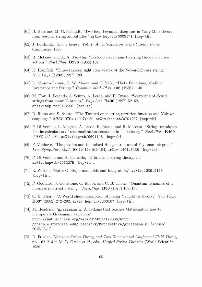
[61] B. Kors and M. G. Schmidt, “Two loop Feynman diagrams in Yang-Mills theoryfrom bosonic string amplitudes,” arXiv:hep-th/0003171 [hep-th].

[62] J. Polchinski, String theory. Vol. 1: An introduction to the bosonic string.Cambridge, 1998.

[63] R. Metsaev and A. A. Tseytlin, “On loop corrections to string theory effectiveactions,” Nucl.Phys. B298 (1988) 109.

[64] K. Hornfeck, “Three reggeon light cone vertex of the Neveu-Schwarz string,”Nucl.Phys. B293 (1987) 189.

[65] L. Alvarez-Gaume, G. W. Moore, and C. Vafa, “Theta Functions, ModularInvariance and Strings,” Commun.Math.Phys. 106 (1986) 1–40.

[66] M. Frau, I. Pesando, S. Sciuto, A. Lerda, and R. Russo, “Scattering of closedstrings from many D-branes,” Phys.Lett. B400 (1997) 52–62,arXiv:hep-th/9702037 [hep-th].

[67] R. Russo and S. Sciuto, “The Twisted open string partition function and Yukawacouplings,” JHEP 0704 (2007) 030, arXiv:hep-th/0701292 [hep-th].

[68] P. Di Vecchia, L. Magnea, A. Lerda, R. Russo, and R. Marotta, “String techniquesfor the calculation of renormalization constants in field theory,” Nucl.Phys. B469(1996) 235–286, arXiv:hep-th/9601143 [hep-th].

[69] P. Vanhove, “The physics and the mixed Hodge structure of Feynman integrals,”Proc.Symp.Pure Math. 88 (2014) 161–194, arXiv:1401.6438 [hep-th].

[70] P. Di Vecchia and A. Liccardo, “D-branes in string theory. 2.,”arXiv:hep-th/9912275 [hep-th].

[71] E. Witten, “Notes On Supermanifolds and Integration,” arXiv:1209.2199

[hep-th].

[72] P. Goddard, J. Goldstone, C. Rebbi, and C. B. Thorn, “Quantum dynamics of amassless relativistic string,” Nucl.Phys. B56 (1973) 109–135.

[73] C. B. Thorn, “A World sheet description of planar Yang-Mills theory,” Nucl.Phys.B637 (2002) 272–292, arXiv:hep-th/0203167 [hep-th].

[74] M. Headrick, “grassmann.m: A package that teaches Mathematica how tomanipulate Grassmann variables.”http://web.archive.org/web/20150317172836/http:

//people.brandeis.edu/~headrick/Mathematica/grassmann.m. Accessed:2015-03-17.

[75] D. Friedan. Notes on String Theory and Two Dimensional Conformal Field Theory,pp. 162–213 in M. B. Green et al., eds., Unified String Theories (World Scientific,1986).

65


http://dx.doi.org/10.1016/0550-3213(88)90306-9

http://dx.doi.org/10.1016/0550-3213(87)90068-X

http://dx.doi.org/10.1007/BF01210925

http://dx.doi.org/10.1016/S0370-2693(97)00331-6


http://dx.doi.org/10.1088/1126-6708/2007/04/030


http://dx.doi.org/10.1016/0550-3213(96)00141-1

http://dx.doi.org/10.1016/0550-3213(96)00141-1


http://dx.doi.org/10.1090/pspum/088/01455





http://dx.doi.org/10.1016/0550-3213(73)90223-X

http://dx.doi.org/10.1016/S0550-3213(02)00461-3

http://dx.doi.org/10.1016/S0550-3213(02)00461-3


http://web.archive.org/web/20150317172836/http://people.brandeis.edu/~headrick/Mathematica/grassmann.m

http://web.archive.org/web/20150317172836/http://people.brandeis.edu/~headrick/Mathematica/grassmann.m

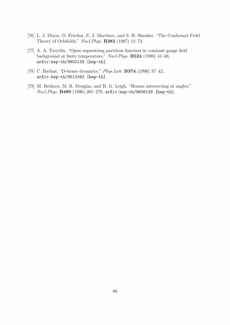
[76] L. J. Dixon, D. Friedan, E. J. Martinec, and S. H. Shenker, “The Conformal FieldTheory of Orbifolds,” Nucl.Phys. B282 (1987) 13–73.

[77] A. A. Tseytlin, “Open superstring partition function in constant gauge fieldbackground at finite temperature,” Nucl.Phys. B524 (1998) 41–68,arXiv:hep-th/9802133 [hep-th].

[78] C. Bachas, “D-brane dynamics,” Phys.Lett. B374 (1996) 37–42,arXiv:hep-th/9511043 [hep-th].

[79] M. Berkooz, M. R. Douglas, and R. G. Leigh, “Branes intersecting at angles,”Nucl.Phys. B480 (1996) 265–278, arXiv:hep-th/9606139 [hep-th].

66

http://dx.doi.org/10.1016/0550-3213(87)90676-6

http://dx.doi.org/10.1016/S0550-3213(98)00227-2


http://dx.doi.org/10.1016/0370-2693(96)00238-9


http://dx.doi.org/10.1016/S0550-3213(96)00452-X


Two-loop Yang-Mills diagrams from superstring amplitudes

Documents

Transcript of Two-loop Yang-Mills diagrams from superstring amplitudes