On the numerical integration of rigid body nonlinear dynamicsin presence of parameters singularities

Marcelo A. Trindade∗ and Rubens Sampaio†

PUC-Rio, Department of Mechanical Engineering, Rio de Janeiro, RJ 22453-900, Brazil

Abstract

One of the main complexities in the simulation of the nonlinear dynamics of rigid bodiesconsists in describing properly the finite rotations that they may undergo. It is well known that,to avoid singularities in the representation of the SO(3) rotation group, at least four parametersmust be used. However, it is computationally expensive to use a four-parameters representationsince, as only three of the parameters are independent, one needs to introduce constraint equa-tions in the model, leading to differential-algebraic equations instead of ordinary differentialones. Three-parameter representations are numerically more efficient. Therefore, the objectiveof this paper is to evaluate numerically the influence of the parametrization and its singularitieson the simulation of the dynamics of a rigid body. This is done through the analysis of a heavytop with a fixed point, using two three-parameter systems, Euler’s angles and rotation vector.Theoretical results were used to guide the numerical simulation and to assure that all possiblecases were analyzed. The two parametrizations were compared using several integrators. Theresults show that Euler’s angles lead to faster integration compared to the rotation vector. AnEuler’s angles singular case, where representation approaches a theoretical singular point, wasanalyzed in detail. It is shown that on the contrary of what may be expected, 1) the numericalintegration is very efficient, even more than for any other case, and 2) in spite of the uncertaintyon the Euler’s angles themselves, the body motion is well represented.

Key words: Finite rotations, heavy top, Euler’s angles, rotation vector, nonlinear dynamics,representation singularities

1 IntroductionThe representation of the three-dimensional motion of rigid bodies or multibodies is, commonly,the major problem in the study of their nonlinear dynamics. This difficulty is due to complexi-ties introduced by the representation of large rotations that the bodies may undergo during theirmotion. Since the modeling of multibody systems has become of great importance in areas suchas aerospace and aeronautics structures design and analysis of complex robotic manipulators, theunderstanding of the nonlinear dynamics of general bodies under large rotations has been objectof analysis and revision [5, 18]. The analysis of large displacements of flexible structures, such asbeams [3, 14] and shells [4, 9], also motivated the use of finite rotations in configuration update

∗E-mail: trindade@mec.puc-rio.br†Corresponding author. E-mail: rsampaio@mec.puc-rio.br

1

procedures. Some computational codes were developed to treat the modeling and simulation oflarge, rigid or flexible, multibody systems. It was observed that one of the major problems is tochoose the parametrization of the problem, since it determines the number of degrees of freedomthat must be calculated, i.e., the cost of modeling and simulation.

Several parameter systems can be used to represent finite three-dimensional rotations. Ap-plications of finite rotations in computational mechanics are reviewed by Atluri [2], Geradin andRixen [7] and Trindade and Sampaio [18]. Details on the parametrization of large rotations canbe found in the articles of Argyris [1] and Stuelpnagel [15], and in the classical text of Goldstein[8]. In the present work two rotation parameters systems are studied, namely Euler’s angles androtation vector, each of them composed of three parameters.

Theoretically three-parameter representations are not unique and present singular points wherethe rotation cannot be represented [15]. However, to the authors’ knowledge, the effect of thesesingularities on the numerical integration and on the representation of the rigid body motion hasnot yet been presented in the open literature. In such cases, the common solution is to use anotherparametrization composed of four parameters, like, for example, Euler’s parameters. But, the useof a four parameters system increases the number of degrees of freedom (dof) by one for eachbody and, also, includes one algebraic equation for each body. Consequently, the global equationsof motion of the system will be increased by N (number of bodies) dof and, moreover, will be asystem of differential-algebraic equations, instead of a system of ordinary differential equations(ODE), which are much more difficult to solve. Geradin [6], Rochinha and Sampaio [11] andSimo and Wong [14] studied the heavy top dynamics to show that the equations should be writtenin terms of convected operators and to analyze instabilities and dissipation of some integrators.

It is the objective of this work to present a numerical analysis of the singularities of finiterotation representation and their effect on the numerical integration of the nonlinear dynamicsof rigid bodies. This is done through the analysis of the heavy top nonlinear dynamics where therotations are represented with the Euler’s angles and the rotation vector. It is shown that the systemequations can be stiff depending on initial conditions and rotation parametrization, consequently,several integration algorithms, for stiff and non-stiff problems, are considered. The case wherethe Euler’s angles approach their singular points is analyzed in detail and it is shown that, on thecontrary of what may be expected, 1) in this particular problem, the numerical integration is veryefficient, even more than for any other case, and 2) in spite of the uncertainty on the Euler’s anglesthemselves, the body motion is well represented.

The numerical analysis of a rigid body nonlinear dynamics near the singular points of thefinite rotation representation and the study of the effect of this type of singularity on the numericalintegration are the main originalities of this work.

2 Rigid body kinematicsLet us consider the motion of a particle P of a rigid body, represented by the position of the bodyat two different instants of time, as showed in Figure 1.

We attach a fixed (inertial) frame E in the space and a moving frame b to the body. Theoperator R(t) defines the relative orientation of the frames, such that bi = R(t)Ei (i = 1,2,3),therefore the position vector of the particle P is

xP(t) = xO(t)+R(t)X (1)

2

O

O’

P’

P

x

XE

E

b

bb

1

2

3

1

2

3

xxO

P

E

Figure 1: Representation of the motion of a rigid body.

where xO is the translation of the body center of mass O and R(t) represents the body rotation.The velocity vector can be simply obtained by time-derivation

xP(t) = xO(t)+ R(t)X (2)

Solving (1) for X and replacing it in (2), we get

xP(t) = xO(t)+ w(t)(xP(t)−xO(t)) (3)

where the skew-symmetric matrix w associated with the vector w, that we denote the spatial angu-lar velocity, is defined as

w(t) = R(t)RT (t) (4)

Hence, one may write the velocity of the point P in terms of the velocity of the center of mass,the distance relative to the center of mass and the angular velocity of the body. Let us recall thefollowing isomorphism that relates the skew-symmetric matrix w and the angular velocity w,

wh=w×h , ∀ h ∈ R 3 (5)

where × represents the vector product and

w=

⎡

⎣

w1w2w3

⎤

⎦ ; w=

⎡

⎣

0 −w3 w2w3 0 −w1−w2 w1 0

⎤

⎦ (6)

Onemay also write these relations in the inertial frame E, through the definition of a convectedangular velocityW

W(t) =R(t)Tw(t) ; W(t) =R(t)T R(t) =R(t)T wR(t) (7)

3

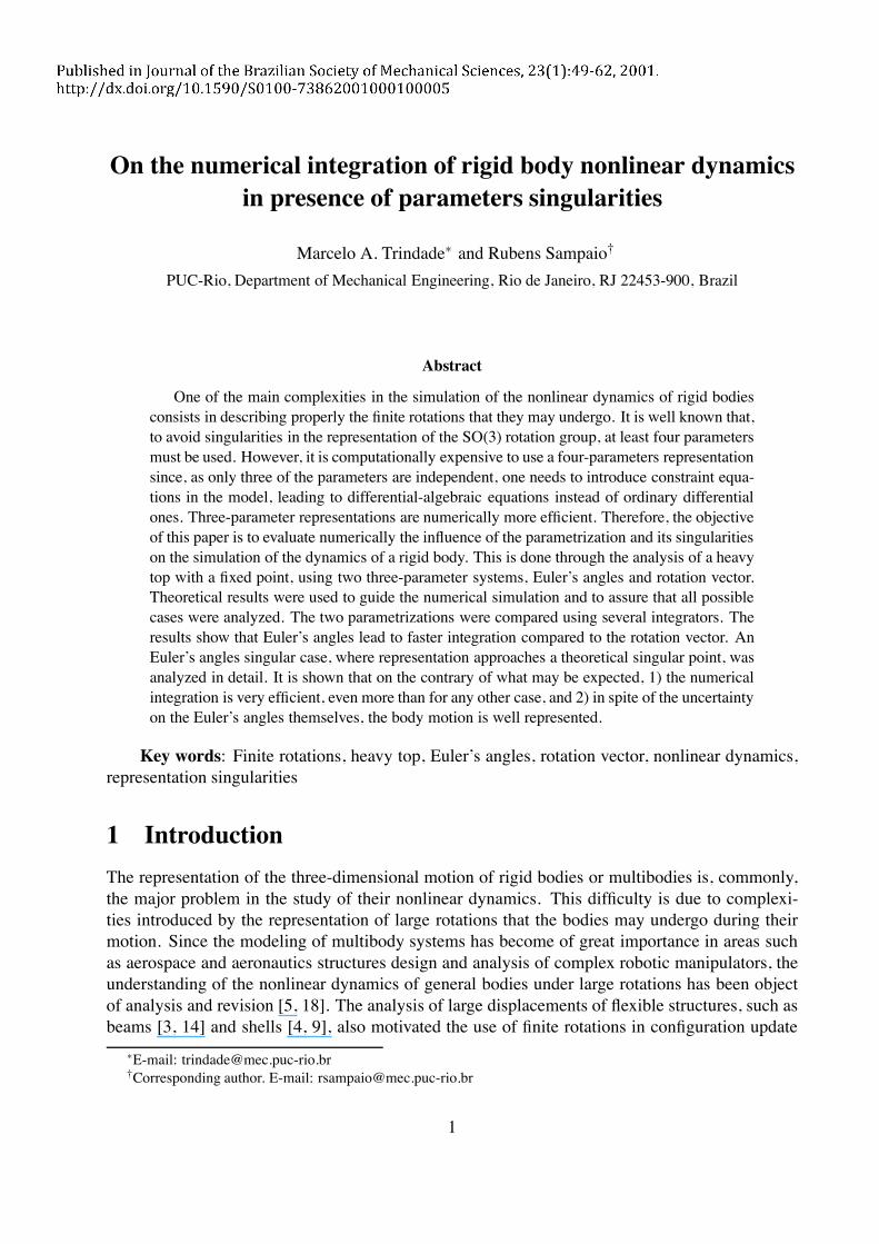
3 Representation of finite rotationsTo write the equation of motion of the body, one must represent its kinematics in terms of somechosen degrees of freedom. Therefore, the intrinsic operator R is now parametrized using two setof parameters, namely the rotation vector and the Euler’s angles. The first one, defined by Ψ= φnrepresents the rotation as a unique rotation-angle of φ in the direction of a unit vector n, that is, theaxis of rotation. Hence, the rotation-angle is the modulus of the rotation vector φ = ∥Ψ∥. Then,the rotation operator can be represented by [5, 18]

R(Ψ) = I+ sin∥Ψ∥∥Ψ∥ Ψ+

1− cos∥Ψ∥∥Ψ∥2 ΨΨ (8)

where Ψ is the skew-symmetric matrix corresponding to the rotation vector Ψ. Using (4), theangular velocity w can be written in terms of parameter Ψ as (for details see [5, 18])

w= T(Ψ)Ψ (9)

defining the tangent rotation operator T(Ψ), in terms of the parameter Ψ, as

T(Ψ) = I− cos∥Ψ∥−1∥Ψ∥2

Ψ+(

1− sin∥Ψ∥∥Ψ∥

)

ΨΨ∥Ψ∥2

(10)

Notice that R(Ψ) and T(Ψ) are not singular, for ∥Ψ∥ → 0, since it is easy to show [16, 18] thatlim∥Ψ∥→0R(Ψ) = I and lim∥Ψ∥→0T(Ψ) = I, where I is the identity operator. Hence, Ψ= 0 is nota singularity.

The Euler’s angles represent the rotation as a sequence of three elementary plane rotations,one of a precession angle ψ in E3 direction, denoted as Rψ(ψ), one of a nutation angle θ in E′1direction (Figure 2), denoted as Rθ(θ), and one of a spin angle ϕ in b3 direction, denoted asRϕ(ϕ).Therefore, one may assemble these three rotations such that the global rotation operator is writtenas

R(ψ,θ,ϕ) =Rϕ(ϕ)Rθ(θ)Rψ(ψ) (11)

or, in explicit form, in the basis bi⊗b j,

R(ψ,θ,ϕ) =

⎡

⎣

cψcϕ− sψcθsϕ −cψsϕ− sψcθcϕ sψsθsψcϕ+ cψcθsϕ −sψsϕ− cψcθcϕ −cψsθ

−sθsϕ −sθcϕ cθ

⎤

⎦ (12)

where cζ = cosζ and sζ = sinζ, (ζ = ψ,θ,ϕ). It is worthwhile to analyze the extraction of theEuler’s angles from the rotation matrix R, which may be achieved using the following relations

ϕ= tan−1(

r31r32

)

sinθ= r31 sinϕ+ r32 cosϕcosθ= r33

;

sinψ= r11 cosϕ+ r12 sinϕcosψ= r21 cosϕ− r22 sinϕ

(13)

4

ri j being the i j-th element of the matrix R. From the last relations, one may observe that thisinversion is not unique when θ= 0,π, since in these singular points

R(ψ,θ,ϕ)|θ=0,π =

⎡

⎣

cos(ψ±ϕ) −sin(ψ±ϕ) 0sin(ψ±ϕ) cos(ψ±ϕ) 0

0 0 ±1

⎤

⎦ (14)

and only the nutation angle θ and the sum or subtraction of the precession and spin angles (ψ±ϕ)can be determined, but not the precession angle nor the spin separately. This is the well-knowninversion singularity of the Euler’s angles, although, in this case, it is clear that spin and precessionangles alone have no meaning and also no use.

Thereafter, using the definition of w (4), one may write the expression of the angular velocityin terms of the Euler’s angles derivatives vector Θ= [ψ θ ϕ]T as

w= T(ψ,θ,ϕ)Θ (15)

where the tangent rotation operator T(ψ,θ,ϕ), in terms of the Euler’s angles, is written, in thebasis bi⊗b j, as

T(ψ,θ,ϕ) =

⎡

⎣

sinϕsinθ cosϕ 0cosϕsinθ −sinϕ 0cosθ 0 1

⎤

⎦ (16)

Notice that det(T) = −sinθ, hence for the singular case when θ = 0,π, det(T) = 0 so that theinverse of T is not defined.

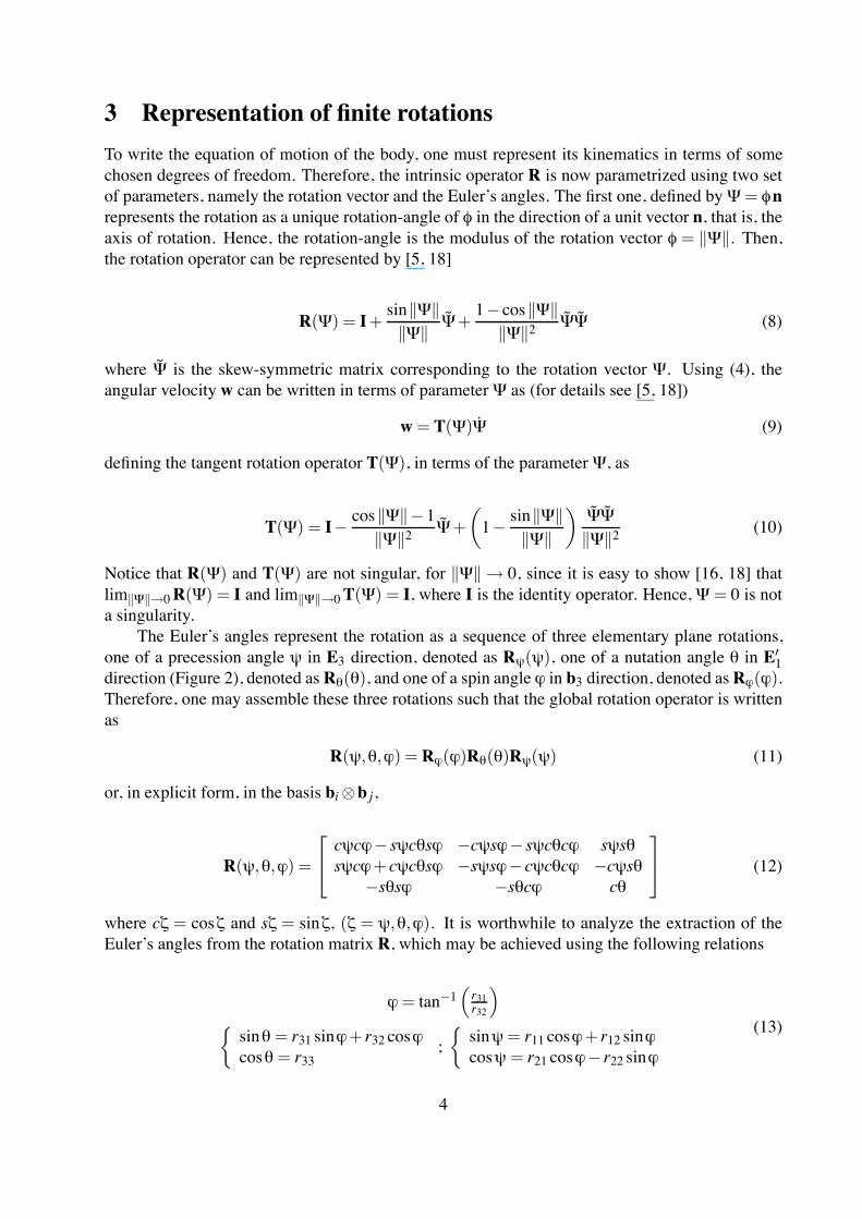
4 System modelingThe system to be analyzed, shown in Figure 2, is the heavy top with a fixed point [12, 17]. The topis characterized by a mass m and principal moments of inertia I1, I2 and I3; the distance betweenthe center of mass of the top and the fixed point (origin of the inertial frame) is L. The top is subjectto the action of gravity only.

mgθ

ϕ

φ

ψ

Ψ

E

E’

b

E

E

1

2

3

1

3

Figure 2: Representation of the heavy top (ψ,θ,ϕ - Euler’s angles; Ψ - rotation vector).

The components of the rotation vector (Ψ1,Ψ2,Ψ3), with respect to the frame b, are chosen asgeneralized coordinates and, instead of their derivatives, the components (w1,w2,w3) of the angular

5

velocity w (9) in the basis (b1,b2,b3) are assumed to be the generalized velocities. Then, velocityand acceleration of the center of mass must be written in terms of the generalized velocities, leadingto

vc = w2Lb1−w1Lb2ac = (w2+w1w3)Lb1− (w1−w2w3)Lb2− (w21+w22)Lb3

(17)

The angular acceleration, being defined as the time-derivative of the angular velocity in bi⊗b j, is simply expressed in terms of w1, w2, w3 as

w= w1b1+ w2b2+ w3b3 (18)

From (17) and (18), the inertial forces and moments are

Fc = −mac = −mL[(w2+w1w3)b1− (w1−w2w3)b2− (w21+w22)b3] (19)

M= −Jw− wJw= [−I1w1+(I2− I3)w2w3]b1+[−I2w2+(I3− I1)w1w3]b2

+[−I3w3+(I1− I2)w1w2]b3 (20)

where J is the body’s moment of inertia. The gravity force Fg = −mgE3, which is constant in theinertial frame E, can be written in the body frame b, using the relation bi =R(t)Ei, as

Fg = −mg[

(1− cosφ)φ2

Ψ1Ψ3−sinφφ

Ψ2

]

b1+[

(1− cosφ)φ2

Ψ2Ψ3+sinφφ

Ψ1

]

b2

+[

(1− cosφ)φ2

Ψ23+ cosφ]

b3

(21)

Consequently, this force is time-variant in the body frame. Then, using Kane’s procedure [10, 16],the partial Vp (p = 1,2,3) and angular partial velocities Ωp are defined as the derivative of thelinear and angular velocities, respectively. These may be written, in terms of the generalizedvelocities w1, w2, w3, as

p= 1 p= 2 p= 3Ωp b1 b2 b3Vp −Lb2 Lb1 0

(22)

The generalized inertial forces are defined as the scalar product between the partial and angu-lar partial velocities and the inertial forces and moments F∗

p =ΩTpM+VTpFc, so that

F∗1 = −I1w1+(I2− I3)w2w3−mL2(w1−w2w3)

F∗2 = −I2w2+(I3− I1)w1w3−mL2(w2+w1w3)

F∗3 = −I3w3+(I1− I2)w1w2

(23)

6

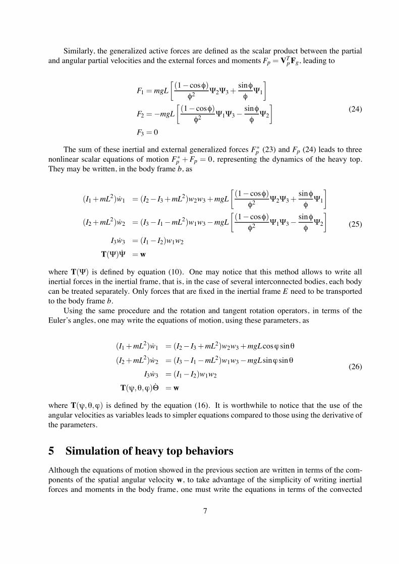
Similarly, the generalized active forces are defined as the scalar product between the partialand angular partial velocities and the external forces and moments Fp = VTpFg, leading to

F1 =mgL[

(1− cosφ)φ2

Ψ2Ψ3+sinφφ

Ψ1

]

F2 = −mgL[

(1− cosφ)φ2

Ψ1Ψ3−sinφφ

Ψ2

]

F3 = 0

(24)

The sum of these inertial and external generalized forces F∗p (23) and Fp (24) leads to three

nonlinear scalar equations of motion F∗p +Fp = 0, representing the dynamics of the heavy top.

They may be written, in the body frame b, as

(I1+mL2)w1 = (I2− I3+mL2)w2w3+mgL[

(1− cosφ)φ2

Ψ2Ψ3+sinφφ

Ψ1

]

(I2+mL2)w2 = (I3− I1−mL2)w1w3−mgL[

(1− cosφ)φ2

Ψ1Ψ3−sinφφ

Ψ2

]

I3w3 = (I1− I2)w1w2T(Ψ)Ψ = w

(25)

where T(Ψ) is defined by equation (10). One may notice that this method allows to write allinertial forces in the inertial frame, that is, in the case of several interconnected bodies, each bodycan be treated separately. Only forces that are fixed in the inertial frame E need to be transportedto the body frame b.

Using the same procedure and the rotation and tangent rotation operators, in terms of theEuler’s angles, one may write the equations of motion, using these parameters, as

(I1+mL2)w1 = (I2− I3+mL2)w2w3+mgLcosϕsinθ

(I2+mL2)w2 = (I3− I1−mL2)w1w3−mgLsinϕsinθ

I3w3 = (I1− I2)w1w2T(ψ,θ,ϕ)Θ = w

(26)

where T(ψ,θ,ϕ) is defined by the equation (16). It is worthwhile to notice that the use of theangular velocities as variables leads to simpler equations compared to those using the derivative ofthe parameters.

5 Simulation of heavy top behaviorsAlthough the equations of motion showed in the previous section are written in terms of the com-ponents of the spatial angular velocity w, to take advantage of the simplicity of writing inertialforces and moments in the body frame, one must write the equations in terms of the convected

7

angular velocityW to integrate the equations [6, 14], since the body frame varies with time andone cannot sum the components of the spatial angular velocity for different times. This can beobtained using (7).

For the integration of the equations of motion, we used the MATLAB ODESuite [13], whichcontains several ODE numerical integration algorithms, for stiff and non-stiff problems. Stiffproblems are those where some of their variables present fast dynamics and others slow dynamics.Whereas, for non-stiff problems, all variables present the same type of dynamics. The methods fornon-stiff problems are ODE45 (explicit Runge-Kutta formula of 4th/5th order), ODE23 (explicitRunge-Kutta formula of 2nd/3rd order), ODE113 (variable order formula of Adams, Bashforth andMoulton) and ADAMS (Adams predictor-corrector formula of SIMULINK); whereas the methodsfor stiff problems are ODE15s (implicit Numerical Differentiation Formula developed by Klopfen-stein and Shampine), ODE23s (implicit method based on a modified Rosenbrock formula) andGEAR (Gear’s predictor-corrector formula of SIMULINK).

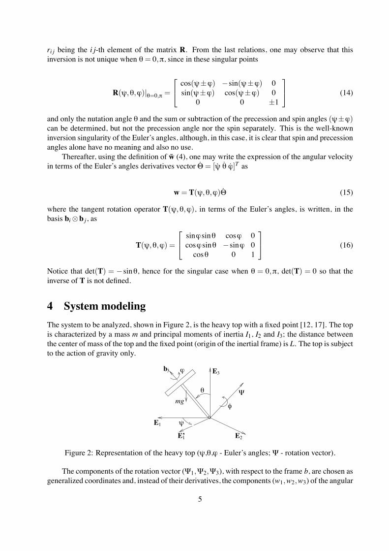
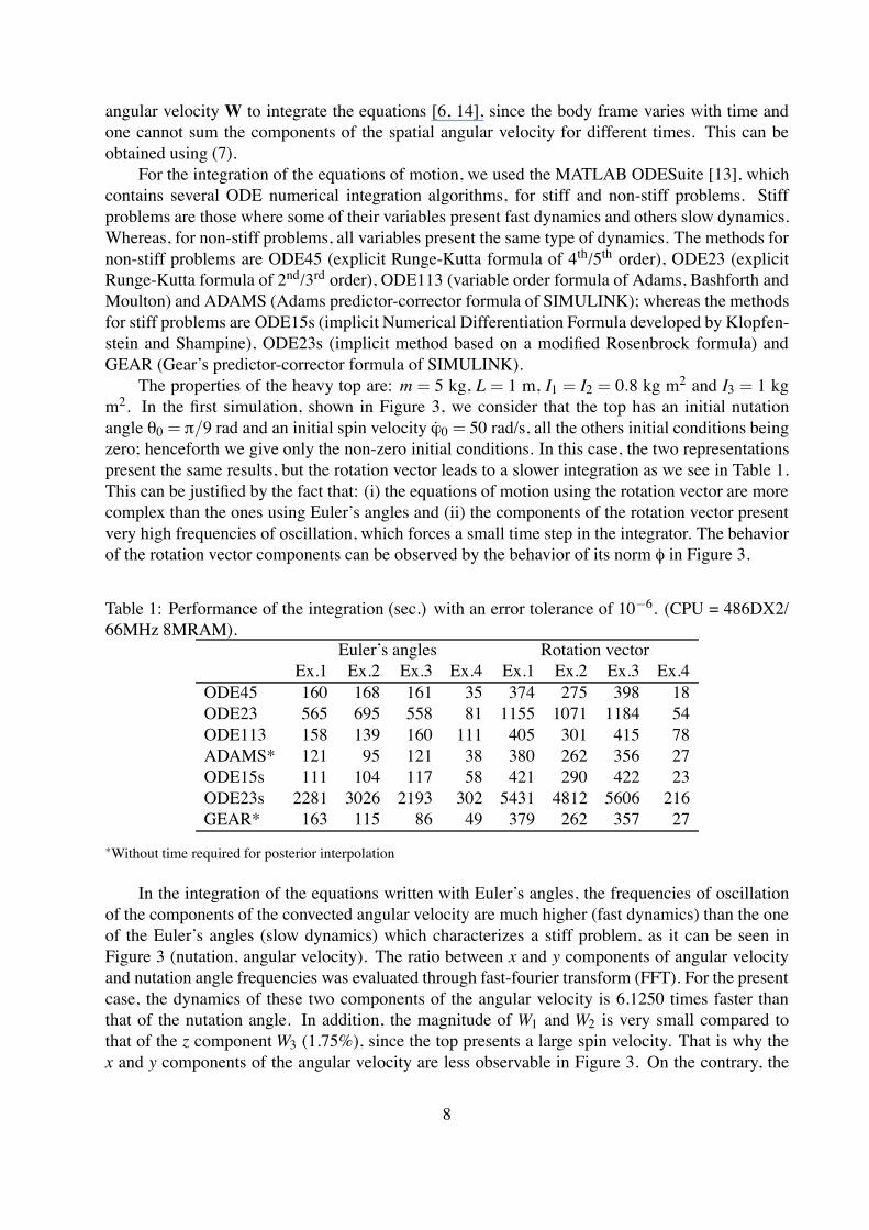
The properties of the heavy top are: m = 5 kg, L = 1 m, I1 = I2 = 0.8 kg m2 and I3 = 1 kgm2. In the first simulation, shown in Figure 3, we consider that the top has an initial nutationangle θ0 = π/9 rad and an initial spin velocity ϕ0 = 50 rad/s, all the others initial conditions beingzero; henceforth we give only the non-zero initial conditions. In this case, the two representationspresent the same results, but the rotation vector leads to a slower integration as we see in Table 1.This can be justified by the fact that: (i) the equations of motion using the rotation vector are morecomplex than the ones using Euler’s angles and (ii) the components of the rotation vector presentvery high frequencies of oscillation, which forces a small time step in the integrator. The behaviorof the rotation vector components can be observed by the behavior of its norm φ in Figure 3.

Table 1: Performance of the integration (sec.) with an error tolerance of 10−6. (CPU = 486DX2/66MHz 8MRAM).

Euler’s angles Rotation vectorEx.1 Ex.2 Ex.3 Ex.4 Ex.1 Ex.2 Ex.3 Ex.4

ODE45 160 168 161 35 374 275 398 18ODE23 565 695 558 81 1155 1071 1184 54ODE113 158 139 160 111 405 301 415 78ADAMS* 121 95 121 38 380 262 356 27ODE15s 111 104 117 58 421 290 422 23ODE23s 2281 3026 2193 302 5431 4812 5606 216GEAR* 163 115 86 49 379 262 357 27

∗Without time required for posterior interpolation

In the integration of the equations written with Euler’s angles, the frequencies of oscillationof the components of the convected angular velocity are much higher (fast dynamics) than the oneof the Euler’s angles (slow dynamics) which characterizes a stiff problem, as it can be seen inFigure 3 (nutation, angular velocity). The ratio between x and y components of angular velocityand nutation angle frequencies was evaluated through fast-fourier transform (FFT). For the presentcase, the dynamics of these two components of the angular velocity is 6.1250 times faster thanthat of the nutation angle. In addition, the magnitude of W1 and W2 is very small compared tothat of the z componentW3 (1.75%), since the top presents a large spin velocity. That is why thex and y components of the angular velocity are less observable in Figure 3. On the contrary, the

8

frequencies of oscillation of the components of the rotation vector (fast dynamics) are of the sameorder than those of the angular velocity (fast dynamics), which characterizes a non-stiff problem.Therefore, we can observe that the method ODE15s is faster than ODE45 for Euler’s angles butslower for the rotation vector.

0 2 4 6 8 100.3

0.4

0.5

t

Nut

atio

n

0 5 10−0.5

0

0.5

1

t

Posi

tion

of C

M

Px Py Pz

0 2 4 6 8 101240

1260

1280

1300

t

Ener

gy

Total Kinetic

0 5 100

20

40

60

t

Angu

lar V

eloc

ity

Wx Wy Wz

0.35 0.4 0.45−0.4−0.2

00.20.4

Nutation

Nut

atio

n Ve

loci

ty

0 5 100

5

10

15

t

Spin

−0.5 0 0.5−0.5

00.5

0.85

0.9

0.95

Trajectory of CM

0 5 100

2

4

6

t

φ

Figure 3: Heavy top. Initial conditions: θ0 = π/9 rad and ϕ0 = 50 rad/s.

This first simulation represents the most usual behavior of the heavy top. The top presents aperiodic nutation, as shown in Figure 3 (θ×θ), with a frequency higher than that of the precession,as we can see in Figure 3 (Position of CM), which is in agreement with the approximation givenby Goldstein [8] for the fast top.

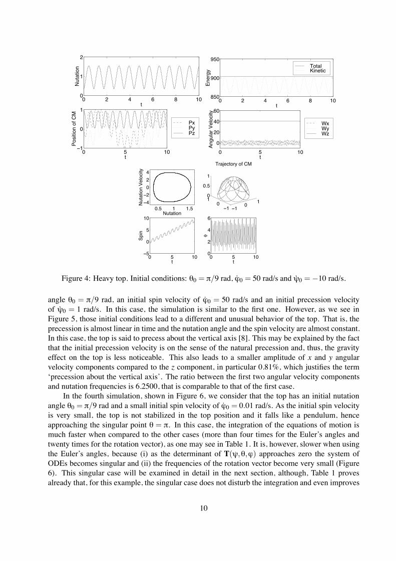
In the second simulation, shown in Figure 4, we consider that the top has an initial nutationangle θ0 = π/9 rad, an initial spin velocity of ϕ0 = 50 rad/s and an initial precession velocityof ψ0 = −10 rad/s. This simulation represents the second type of motion of the heavy top. Inthis case, the amplitudes of motion are greater, leading to a more complex overall motion. Thetop almost reaches the vertical position (θ = 0). However, the integration is faster for almost allalgorithms and for both parameters systems. One may notice that the initial precession velocity isopposite to the natural precession, due to the relation spin/gravity, leading to the loops observedin the trajectory of CM (Figure 4). This also leads to a higher nutation frequency, so that theratio between x and y angular velocity components and nutation frequencies is smaller comparedto that of the first case (5.0833, for the present case, versus 6.1250, for the previous one). Also,the relative amplitudes of W1 andW2 compared to the third componentW3 increase for this case,reaching 12.79%. Thus, they become more observable in the angular velocity plot (Figure 4).

In the third simulation, shown in Figure 5, we consider that the top has an initial nutation

9

0 2 4 6 8 100

1

2

t

Nut

atio

n

0 5 10−1

0

1

t

Posi

tion

of C

M

Px Py Pz

0 2 4 6 8 10850

900

950

t

Ener

gy

Total Kinetic

0 5 100

20

40

60

t

Angu

lar V

eloc

ity

Wx Wy Wz

0.5 1 1.5−4−2

024

Nutation

Nut

atio

n Ve

loci

ty

0 5 10−5

0

5

10

t

Spin

−1 0 1−1

010

0.5

1

Trajectory of CM

0 5 100

2

4

6

t

φ

Figure 4: Heavy top. Initial conditions: θ0 = π/9 rad, ϕ0 = 50 rad/s and ψ0 = −10 rad/s.

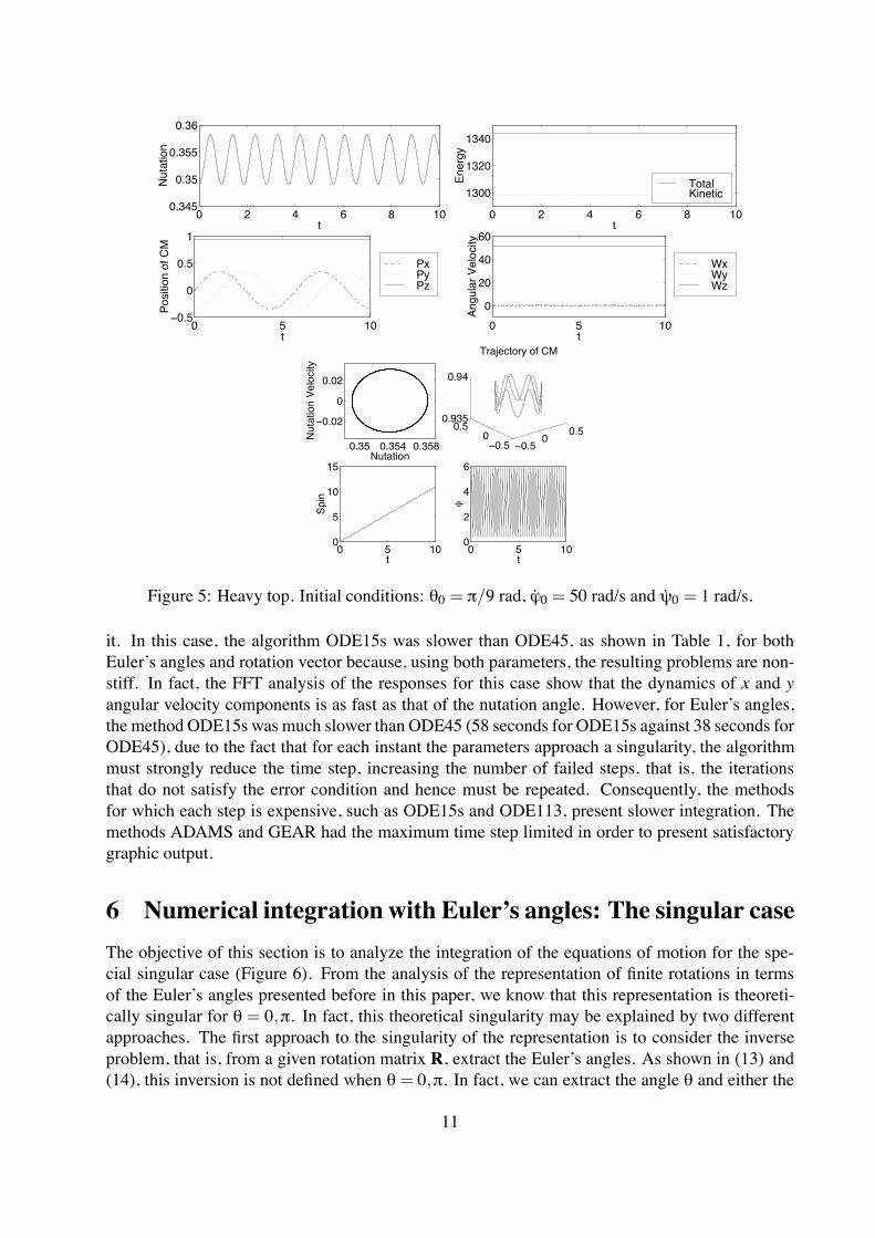
angle θ0 = π/9 rad, an initial spin velocity of ϕ0 = 50 rad/s and an initial precession velocityof ψ0 = 1 rad/s. In this case, the simulation is similar to the first one. However, as we see inFigure 5, those initial conditions lead to a different and unusual behavior of the top. That is, theprecession is almost linear in time and the nutation angle and the spin velocity are almost constant.In this case, the top is said to precess about the vertical axis [8]. This may be explained by the factthat the initial precession velocity is on the sense of the natural precession and, thus, the gravityeffect on the top is less noticeable. This also leads to a smaller amplitude of x and y angularvelocity components compared to the z component, in particular 0.81%, which justifies the term‘precession about the vertical axis’. The ratio between the first two angular velocity componentsand nutation frequencies is 6.2500, that is comparable to that of the first case.

In the fourth simulation, shown in Figure 6, we consider that the top has an initial nutationangle θ0 = π/9 rad and a small initial spin velocity of ϕ0 = 0.01 rad/s. As the initial spin velocityis very small, the top is not stabilized in the top position and it falls like a pendulum, henceapproaching the singular point θ = π. In this case, the integration of the equations of motion ismuch faster when compared to the other cases (more than four times for the Euler’s angles andtwenty times for the rotation vector), as one may see in Table 1. It is, however, slower when usingthe Euler’s angles, because (i) as the determinant of T(ψ,θ,ϕ) approaches zero the system ofODEs becomes singular and (ii) the frequencies of the rotation vector become very small (Figure6). This singular case will be examined in detail in the next section, although, Table 1 provesalready that, for this example, the singular case does not disturb the integration and even improves

10

0 2 4 6 8 100.345

0.35

0.355

0.36

t

Nut

atio

n

0 5 10−0.5

0

0.5

1

t

Posi

tion

of C

M

Px Py Pz

0 2 4 6 8 10

1300

1320

1340

t

Ener

gy

Total Kinetic

0 5 100

20

40

60

t

Angu

lar V

eloc

ity

Wx Wy Wz

0.35 0.354 0.358

−0.02

0

0.02

Nutation

Nut

atio

n Ve

loci

ty

0 5 100

5

10

15

t

Spin

−0.5 0 0.5−0.5

00.5

0.935

0.94

Trajectory of CM

0 5 100

2

4

6

t

φ

Figure 5: Heavy top. Initial conditions: θ0 = π/9 rad, ϕ0 = 50 rad/s and ψ0 = 1 rad/s.

it. In this case, the algorithm ODE15s was slower than ODE45, as shown in Table 1, for bothEuler’s angles and rotation vector because, using both parameters, the resulting problems are non-stiff. In fact, the FFT analysis of the responses for this case show that the dynamics of x and yangular velocity components is as fast as that of the nutation angle. However, for Euler’s angles,the method ODE15s was much slower than ODE45 (58 seconds for ODE15s against 38 seconds forODE45), due to the fact that for each instant the parameters approach a singularity, the algorithmmust strongly reduce the time step, increasing the number of failed steps, that is, the iterationsthat do not satisfy the error condition and hence must be repeated. Consequently, the methodsfor which each step is expensive, such as ODE15s and ODE113, present slower integration. Themethods ADAMS and GEAR had the maximum time step limited in order to present satisfactorygraphic output.

6 Numerical integration with Euler’s angles: The singular caseThe objective of this section is to analyze the integration of the equations of motion for the spe-cial singular case (Figure 6). From the analysis of the representation of finite rotations in termsof the Euler’s angles presented before in this paper, we know that this representation is theoreti-cally singular for θ = 0,π. In fact, this theoretical singularity may be explained by two differentapproaches. The first approach to the singularity of the representation is to consider the inverseproblem, that is, from a given rotation matrix R, extract the Euler’s angles. As shown in (13) and(14), this inversion is not defined when θ= 0,π. In fact, we can extract the angle θ and either the

11

0 2 4 6 8 100

2

4

t

Nut

atio

n

0 5 10−1

0

1

t

Posi

tion

of C

M

Px Py Pz

0 2 4 6 8 100

50

100

t

Ener

gy

Total Kinetic

0 5 10−10

0

10

t

Angu

lar V

eloc

ity

Wx Wy Wz

1 2 3−5

0

5

Nutation

Nut

atio

n Ve

loci

ty

0 5 100

10

20

t

Spin

−5 0 5x 10−3

−10

1−1

0

1

Trajectory of CM

0 5 100

2

4

6

t

φ

Figure 6: Heavy top. Initial conditions: θ0 = π/9 rad, ϕ0 = 0.01 rad/s.

sum ψ+ϕ or subtraction ψ−ϕ, of ψ and ϕ but not the two of them. If we could, then ψ andϕ would be determined. Therefore, we can expect that in a numerical extraction of these angles,some discontinuity in the angles ψ and ϕmay occur. However, as the sum or the subtraction ψ±ϕcan be correctly extracted, the possible discontinuity will be the same for the two angles. Thesecond approach is to think about the tangent operator T in terms of Euler’s angles. The tangentoperator T(ψ,θ,ϕ) relates the angular velocity w and the time derivatives of the Euler’s anglesψ, θ, ϕ. To integrate the equations of motion (26), we must, in some sense, invert the matrix T and,as it can be seen in (16), the matrix T is singular for θ= 0,π. Therefore, we can expect that whenθ approaches one of these values, the integration of the equations will be disturbed in some sense.Although these two approaches are equivalent in a theoretical sense, the numerical problems in-volved are different. In the case of simulation of the three-dimensional movement of a rigid bodyusing Euler’s angles parametrization, it is important to know if the possible discontinuity, that canoccurs in the singular points, can affect the representation of the motion.

The case under consideration is obtained by setting a small initial spin velocity, an initialnutation angle near π and an initial nutation velocity that forces the nutation angle to pass throughthe singular value π. The only non vanishing initial conditions are θ0 = 3.14 rad; ϕ0 = 0.01 rad/s;θ0 = 0.5 rad/s.

Although the problem was simulated with all the algorithms presented in a previous section,the results showed here corresponds to that with better performance which was, for the case pre-sented, the Runge-Kutta formula of 4th/5th order (ODE45).

12

As the initial spin velocity is very small, we can expect that the top movement will be similarto that of a pendulum with equivalent initial conditions. Moreover, as the initial angle and velocityare also small, we can expect the system to be almost linear. This means that the nutation angleθ is expect to have an almost sinusoidal response. Also, the spin ϕ and precession ψ angles areexpect to have linear responses.

0 10 20 30 40 50

3

3.2

3.4

t

Nut

atio

n

0 10 20 30 40 50

0

10

20

t

Spin

0 10 20 30 40 500

0.5

t

Spin−P

rec

0 10 20 30 40 50−1

−0.5

0

0.5

t

Posi

tion

of C

M

Px Py Pz

0 10 20 30 40 50−60−40−20

0

t

Ener

gy

Total Kinetic

0 10 20 30 40 50−0.5

0

0.5

tAn

gula

r Vel

ocity

Wx Wy Wz

Figure 7: Results of the simulation of the equations of motion with an error tolerance of 10−6.

0 10 20 30 40 50

3

3.2

3.4

t

Nut

atio

n

0 10 20 30 40 500

20

t

Spin

0 10 20 30 40 500

0.5

t

Spin−P

rec

0 10 20 30 40 50−1

−0.5

0

0.5

t

Posi

tion

of C

M

Px Py Pz

0 10 20 30 40 50−60−40−20

0

t

Ener

gy

Total Kinetic

0 10 20 30 40 50−0.5

0

0.5

t

Angu

lar V

eloc

ity

Wx Wy Wz

Figure 8: Results of the simulation of the equations of motion with an error tolerance of 10−8.

In the first simulation, presented in Figure 7, we considered an error tolerance of 10−6. We canobserve that the spin angle ϕ presents a discontinuous behavior. These jumps are of magnitude π,reflecting the error in the extraction of the angles. The same jumps are observed for the precessionangle. Each jump of the spin ϕ and precession ψ angles is accompanied by a change in the signof the nutation velocity θ, as we see in the results. The jumps in ϕ and ψ can be explained by thesingularity of the tangent operator T. Indeed, from (16), the derivatives of the Euler’s angles maybe written in terms of the material angular velocity components (W1,W2,W3) as

⎧

⎨

⎩

ψθϕ

⎫

⎬

⎭

=

⎡

⎣

sinϕ/sinθ cosϕ/sinθ 0cosϕ −sinϕ 0

−sinϕcosθ/sinθ −cosϕcosθ/sinθ 1

⎤

⎦

⎧

⎨

⎩

W1W2W3

⎫

⎬

⎭

(27)

13

so that limθ→π ψ=±∞ and limθ→π ϕ=±∞, which explains the fast increase/decrease in these twoangles. We observe that, when there are no discontinuities for the spin angle ϕ, the nutation angleθ presents the expected behavior, that is, an almost sinusoidal behavior. Moreover, from Figure7, the jumps of magnitude π in the spin and precession angles are associated to the peaks in thenutation angle. This may be explained by the following analysis of the second line of last equationfor ϕ∗ = ϕ±π, where

θ∗ = cos(ϕ±π)W1− sin(ϕ±π)W2= −cos(ϕ)W1+ sin(ϕ)W2= −θ

(28)

Hence, one may notice that an increase/decrease of π in the spin angle ϕ leads to a change in thesign of the nutation velocity θ.

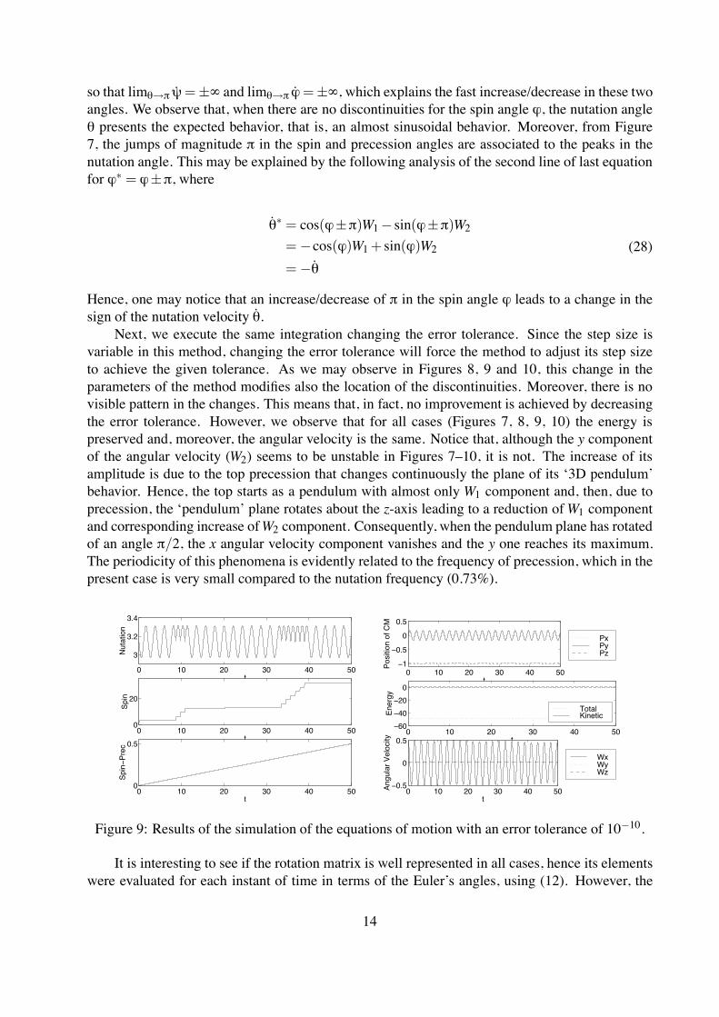
Next, we execute the same integration changing the error tolerance. Since the step size isvariable in this method, changing the error tolerance will force the method to adjust its step sizeto achieve the given tolerance. As we may observe in Figures 8, 9 and 10, this change in theparameters of the method modifies also the location of the discontinuities. Moreover, there is novisible pattern in the changes. This means that, in fact, no improvement is achieved by decreasingthe error tolerance. However, we observe that for all cases (Figures 7, 8, 9, 10) the energy ispreserved and, moreover, the angular velocity is the same. Notice that, although the y componentof the angular velocity (W2) seems to be unstable in Figures 7–10, it is not. The increase of itsamplitude is due to the top precession that changes continuously the plane of its ‘3D pendulum’behavior. Hence, the top starts as a pendulum with almost only W1 component and, then, due toprecession, the ‘pendulum’ plane rotates about the z-axis leading to a reduction ofW1 componentand corresponding increase ofW2 component. Consequently, when the pendulum plane has rotatedof an angle π/2, the x angular velocity component vanishes and the y one reaches its maximum.The periodicity of this phenomena is evidently related to the frequency of precession, which in thepresent case is very small compared to the nutation frequency (0.73%).

0 10 20 30 40 50

3

3.2

3.4

t

Nut

atio

n

0 10 20 30 40 500

20

t

Spin

0 10 20 30 40 500

0.5

t

Spin−P

rec

0 10 20 30 40 50−1

−0.5

0

0.5

t

Posi

tion

of C

M

Px Py Pz

0 10 20 30 40 50−60−40−20

0

t

Ener

gy

Total Kinetic

0 10 20 30 40 50−0.5

0

0.5

t

Angu

lar V

eloc

ity

Wx Wy Wz

Figure 9: Results of the simulation of the equations of motion with an error tolerance of 10−10.

It is interesting to see if the rotation matrix is well represented in all cases, hence its elementswere evaluated for each instant of time in terms of the Euler’s angles, using (12). However, the

14

0 10 20 30 40 50

3

3.2

3.4

t

Nut

atio

n

0 10 20 30 40 500

20

t

Spin

0 10 20 30 40 500

0.5

t

Spin−P

rec

0 10 20 30 40 50−1

−0.5

0

0.5

t

Posi

tion

of C

M

Px Py Pz

0 10 20 30 40 50−60−40−20

0

t

Ener

gy

Total Kinetic

0 10 20 30 40 50−0.5

0

0.5

t

Angu

lar V

eloc

ity

Wx Wy Wz

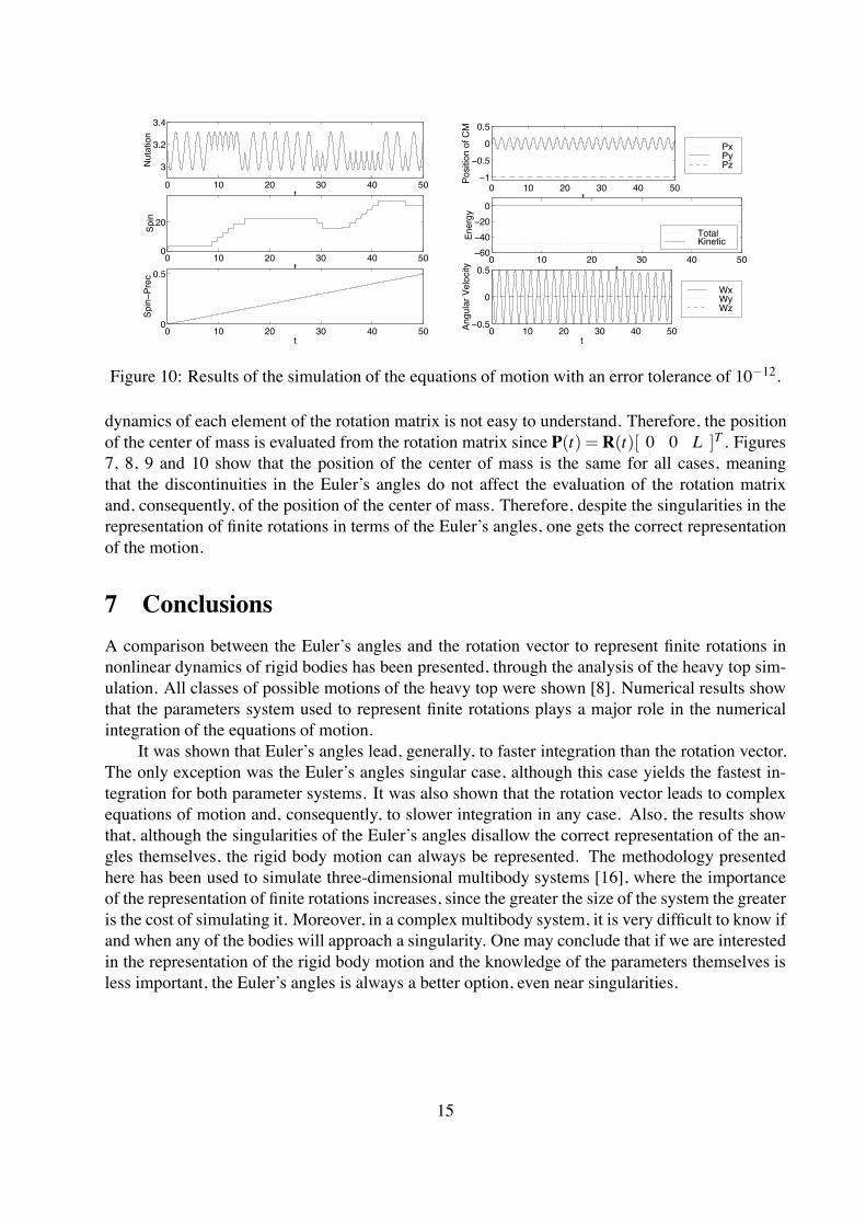
Figure 10: Results of the simulation of the equations of motion with an error tolerance of 10−12.

dynamics of each element of the rotation matrix is not easy to understand. Therefore, the positionof the center of mass is evaluated from the rotation matrix since P(t) =R(t)[ 0 0 L ]T . Figures7, 8, 9 and 10 show that the position of the center of mass is the same for all cases, meaningthat the discontinuities in the Euler’s angles do not affect the evaluation of the rotation matrixand, consequently, of the position of the center of mass. Therefore, despite the singularities in therepresentation of finite rotations in terms of the Euler’s angles, one gets the correct representationof the motion.

7 ConclusionsA comparison between the Euler’s angles and the rotation vector to represent finite rotations innonlinear dynamics of rigid bodies has been presented, through the analysis of the heavy top sim-ulation. All classes of possible motions of the heavy top were shown [8]. Numerical results showthat the parameters system used to represent finite rotations plays a major role in the numericalintegration of the equations of motion.

It was shown that Euler’s angles lead, generally, to faster integration than the rotation vector.The only exception was the Euler’s angles singular case, although this case yields the fastest in-tegration for both parameter systems. It was also shown that the rotation vector leads to complexequations of motion and, consequently, to slower integration in any case. Also, the results showthat, although the singularities of the Euler’s angles disallow the correct representation of the an-gles themselves, the rigid body motion can always be represented. The methodology presentedhere has been used to simulate three-dimensional multibody systems [16], where the importanceof the representation of finite rotations increases, since the greater the size of the system the greateris the cost of simulating it. Moreover, in a complex multibody system, it is very difficult to know ifand when any of the bodies will approach a singularity. One may conclude that if we are interestedin the representation of the rigid body motion and the knowledge of the parameters themselves isless important, the Euler’s angles is always a better option, even near singularities.

15

References[1] J.H. Argyris. An excursion into large rotations. Comput. Methods Appl. Mech. Engrg., 32:85–155,

1982.

[2] S.N. Atluri and A. Cazzani. Rotations in computational solid mechanics. Arch. Computat. MethodsEngrg., 2(1):49–138, 1995.

[3] K.J. Bathe and S. Bolourchi. Large displacement analysis of three-dimensional beam structures. Int.J. Numer. Methods Eng., 14:961–986, 1979.

[4] P. Betsch, A. Menzel, and E. Stein. On the parametrization of finite rotations in computational me-chanics: A classification of concepts with application to smooth shells. Comput. Methods Appl. Mech.Engrg., 155:273–305, 1998.

[5] A. Cardona. An integrated approach to mechanism analysis. PhD thesis, Universite de Liege, Liege(Belgium), 1989.

[6] M. Geradin. Energy conserving time integration for multibody dynamics application to top motion.Mecanica Computacional, 14:573–586, 1994.

[7] M. Geradin and D. Rixen. Parametrization of finite rotations in computational dynamics: a review.Revue Europeenne des Elements Finis, 4(5-6):497–553, 1995.

[8] H. Goldstein. Classical mechanics. Addison-Wesley, Reading (USA), 2 edition, 1980.

[9] A. Ibrahimbegovic, F. Frey, and I. Kozar. Computational aspects of vector-like parametrization ofthree-dimensional finite rotations. Int. J. Numer. Methods Eng., 38:3653–3673, 1995.

[10] T.R. Kane and D.A. Levinson. Dynamics: theory and applications. McGraw-Hill, New York, 1985.

[11] F. Rochinha and R. Sampaio. Non-linear rigid body dynamics: energy and momentum conservingalgorithm. Computer Modeling in Engineering & Sciences, 1(2):7–18, 2000.

[12] R. Sampaio and M.A. Trindade. On the simulation of the dynamics of rigid bodies. Keynote lecture tothe IV World Congress on Computational Mechanics, Buenos Aires (Argentina), in CD-ROM.

[13] L.F. Shampine and M.W. Reichelt. The MATLAB ODESuite. SIAM J. Sci. Comput., 18(1):1–22,1997.

[14] J.C. Simo and K.K. Wong. Unconditionally stable algorithms for rigid body dynamics that exactlypreserve energy and momentum. Int. J. Numer. Methods Eng., 31:19–52, 1991.

[15] J. Stuelpnagel. On the parametrization of the three-dimensional rotation group. SIAM Review, 6:422–430, 1964.

[16] M.A. Trindade. An introduction to the dynamics of multibody systems (in Portuguese). M.Sc. disserta-tion, DEM/PUC-Rio, Rio de Janeiro (Brazil), 1996. (available at http://www.mec.puc-rio.br/˜trindade)

[17] M.A. Trindade and R. Sampaio. A numerical analysis of the singularities of the Euler’s angles. InJ.M. Balthazar, P.B. Goncalves and J. Clayssen, editors, Nonlinear Dynamics, Chaos, Control andTheir Applications to Engineering Sciences, vol.2, pp.111–121, 1999.

[18] M.A. Trindade and R. Sampaio. Review on finite rotations parametrization for rigid body dynamics(in Portuguese). RBCM, Journal of the Brazilian Society of Mechanical Sciences, 22(2):341–377,2000. (available at http://www.mec.puc-rio.br/˜trindade)

16