Weighting strategies in the meta-analysis of single-case studies

1

Weighting strategies in the meta-analysis of single-case studies

Rumen Manolov1 2

, Georgina Guilera2 3

, and Vicenta Sierra1

1 ESADE Business School, Ramon Llull University.

2 Department of Behavioral Sciences Methods, Faculty of Psychology, University of Barcelona.

3 Institute for Research in Brain, Cognition, and Behavior (IR3C), University of Barcelona.

Running head: Weighting in single-case designs

Contact author

Correspondence concerning this article should be addressed to Rumen Manolov, Departament de

Metodologia de les Ciències del Comportament, Facultat de Psicologia, Universitat de

Barcelona, Passeig de la Vall d’Hebron, 171, 08035-Barcelona, Spain. Phone number:

+34934031137. Fax: +34934021359. E-mail: [email protected].

Authors’ note

This research was partially supported by the Agència de Gestió d’Ajust Universitaris i de

Recerca de la Generalitat de Catalunya grant 2009SGR1492.

2

Abstract

Establishing the evidence base of interventions taking place in areas such as psychology and

special education is one of the research aims of single-case designs in conjunction with the aim

of improving the well-being of participants in the studies. The scientific criteria for solid

evidence focus on the internal and external validity of the studies, and for both types of validity,

replicating studies and integrating the results of these replications (i.e., meta-analyzing) is

crucial. In the present study we deal with one of the aspects of meta-analysis, namely the

weighting strategy used when computing an average effect size across studies. Several weighting

strategies suggested for single-case designs are discussed and compared in the context of both

simulated and real-life data. The results indicated that there are no major differences between the

strategies and, thus we consider that it is important to choose weights with a sound statistical and

methodological basis, while scientific parsimony is another relevant criterion. More empirical

research and conceptual discussion are warranted regarding the optimal weighting strategy in

single-case designs, alongside investigation of the optimal effect size measure in these types of

design.

Key words: single-case designs; meta-analysis; weight; effect size

3

The evidence-based movement has now been salient for several years in a variety of disciplines

including psychology (APA Presidential Task Force on Evidence-Based Practice, 2006),

medicine (Sackett, Rosenberg, Gray, Hayness, & Richardson, 1996), and special education

(Odom et al., 2005). In this context, single-case designs (SCD)1 have been considered one of the

viable options for obtaining evidence that would serve as a support for interventions and

practices (Horner et al., 2005; Schlosser, 2009). Accordingly, randomized single-case trials have

been included in the new version of the classification elaborated by the Oxford Centre for

Evidence-Based Medicine regarding the methodologies providing solid evidence (Howick et al.,

2011). Thus, it is clear that one of the ways of improving methodological rigor and scientific

credibility is by incorporating randomization into the design (Kratochwill & Levin, 2010), given

the importance of demonstrating causal relations (Lane & Carter, 2013). Demonstrating cause-

effect relations is central to SCD, provided that they are “experimental” in essence (Kratochwill

et al., 2013; Sidman, 1960) and, apart from using random assignment of conditions to

measurement times, it is also favored by replication of the behavioral change contiguous with the

change in conditions (Kratochwill et al., 2013; Wolery, 2013). On the other hand, replication is

also related to generalization (Sidman, 1960), which benefits from research synthesis and meta-

analysis. In that sense, the evidence-based movement has also paid attention to the meta-

analytical integration of replications or studies on the same topic (Beretvas & Chung, 2008b;

Jenson, Clark, Kircher, & Kristjansson, 2007). The quantitative integration is deemed especially

useful when moderator variables are included in the meta-analyses (Burns, 2012; Wolery, 2013).

Finally, it has been stressed that meta-analysis and the assessment of internal and external

1 We chose the term single-case designs (SCD) in order to be consistent with the labeling used in the articles

recently published in this journal by, for instance, Baek and Ferron (2013), Shadish and Sullivan (2011), Shadish,

Rindskopf, Hedges, and Sullivan (2013), although these designs are also referred to as single-subject experimental

designs (e.g., Ugille, Moeyaert, Beretvas, Ferron, & Van den Noortgate, 2012). In any case, SCD are experimental

in nature and not to be confused with case studies (Blampied, 2000).

4

validity should not be considered separately (Burns, 2012), given that the assessment of the

methodological quality of a study is an essential part of the process of carrying out research

syntheses (Cooper, 2010; Littell, Corcoran, & Pillai, 2008; What Works Clearinghouse, 2008)

for instance using the methodological quality scale in SCD (Tate et al., 2013) or the Study DIAD

(Valentine & Cooper, 2008) as more general tools.

Despite the current prominence of hierarchical linear models (Gage & Lewis, 2012; Owens &

Ferron, 2012), more research and debate is needed regarding the optimal way in which research

synthesis ought to take place in the context of SCD (Lane & Carter, 2013; Maggin & Chafouleas,

2013). The present study represents an effort to discuss and obtain evidence regarding the meta-

analysis of single-case studies; its focus is on weighting strategies rather than on the effect size

measures that summarize the results. In that sense, it should be stressed that we do not advocate

here for or against specific procedures for SCD data analysis. We consider that, while the debate

on the optimal analytical techniques is still on-going, the methodological and statistical progress

in SCDs will benefit from parallel research on the meta-analysis of SCD data. That is, it seems

reasonable to try to solve the issue of how to combine the effect sizes from multiple studies,

while also dealing with the question of which effect size measure is optimal, especially given

that meta-analyses of SCD data are already taking place.

Study Aims

The purpose of the present study was to extend existing research on the meta-analysis of single-

case data, focusing on weighting strategies. After discussing the different weights suggested, a

comparison is performed to explore whether the choice of a weighting strategy is critical. One of

the weighting strategies studied is a proposal made here, based on considering baseline length

and variability together.

5

The comparison was carried out in two different contexts. We used data with known

characteristics (i.e., simulation) in order to study the influence of baseline and series length, data

variability, serial dependence, and trend. Simulation has already been used to compare weighting

strategies in the context of group designs (e.g., Marín-Martínez & Sánchez-Meca, 2010) and in

SCD (e.g., van den Noortgate & Onghena, 2003a). Additionally, we applied the weighting

strategies to real data sets already meta-analyzed in a previously published study (Burns et al.,

2012).

Weighting Strategies

Weighting the individual studies’ effect sizes is an inherent part of meta-analysis. When

choosing a weighting strategy, two aspects need to be taken into account – their underlying

rationale and their performance. Regarding the former aspect, in group designs, the variance of

the effect size index is considered optimal (Hedges & Olkin, 1985; Whitlock, 2005), given that it

quantifies the precision of the summary measure and is, thus, related to the confidence that a

researcher can have in the effect size value obtained. However, the choice of an effect size index

is not as straightforward in SCD as it is in group designs. Moreover, the variance has not been

derived for all effect size indices (see Hedges, Pustejovsky, and Shadish, 2012, for an example of

the complexities related to deriving the variance of a standardized mean difference). Finally,

deriving the variance of the effect size index involves assumptions such as those mentioned in

the Data analysis subsection for the indices included in this study. More discussion is necessary

in the SCD context on whether the same weighting strategy should be considered optimal,

although such practice has been recommended (Beretvas & Chung, 2008b).

6

Other suggested weighting strategies also relate to the degree to which a summary measure is

representative of the real level of behavior. On the one hand, greater data variability means that a

summary measure represents all the data less well; Parker and Vannest (2012) suggested the

inverse of data variability as a possible weight. On the other hand, when a summary measure is

obtained from a longer series, the researcher can be more confident that the data gathered

represent the actual (change in) behavior well and that the effects are not only temporary.

Accordingly, Horner and Kratochwill (2012) and Kratochwill et al. (2010) mentioned the

possibility of using series length as a weight, although its appropriateness is not beyond doubt

(Kratochwill et al., 2010; Shadish, Rindskopf, & Hedges, 2008). For instance, multiple probe

designs (unlike multiple baseline designs) are specifically intended to produce fewer baseline

phase measurements, when the pre-intervention level is stable or in the specific case zero

frequency of the behavior to be learned (Gast & Ledford, 2010). In the case of multiple probe

designs the aim is to reduce the unethical withholding of a potentially helpful intervention.

Moreover, the intervention phase measurements are only continuous until a criterion is reached.

Thus, studies using this design structure might be (unfairly) penalized (i.e., treated as

quantitatively less important) by weighting strategies based on baseline or series length.

Another possible weight related to the amount of information available is the number of

participants in a study, suggested by Kratochwill et al. (2010; 2013) and used, for instance, by

Burns (2012). Nonetheless, its proponents (Kratochwill et al., 2010) state that there is no “strong

statistical justification” (p. 24) for its use. Finally, using unweighted averages has also been

considered (Kratochwill et al., 2010; 2013) and appears to be a common practice (Schlosser, Lee,

& Wendt, 2008).

7

The proposal we make here is that, when considering the importance of data variability and

the number of measurements available, the focus should be on the baseline, consistent with the

the attention paid to it by applied researchers and methodologists. In SCD, this phase is used for

gathering information on the initial situation and is necessary for establishing a criterion against

which the effectiveness of a treatment is evaluated. On the one hand, longer baselines show more

clearly what the pre-intervention level of behavior is and this level (including any existing

trends) can be projected with a greater degree of confidence into the treatment phases and

compared with the actual measurements. Baseline length is explicitly mentioned in several SCD

appraisal tools (Wendt & Miller, 2012), with a minimum of 5 measurements for a study to

receive a high score in the standards elaborated by the What Works Clearinghouse team

(Kratochwill et al., 2010) and in the methodological quality scale for SCD (Tate et al., 2013).

On the other hand, baseline stability is critical for any further assessment of intervention

effectiveness (Kazdin, 2001; Kratochwill et al., 2010; Smith, 2012), given that consistent

responding is key to predicting how the behavior would continue in absence of intervention

(Horner et al., 2005). Finally, the focus on the baseline rather than on the whole series is

warranted, given that if the data series are considered as a whole, any potential effect will

introduce variability, as the pre-intervention and the post-intervention measurements will not

share the same level or trend. Thus, whole series variability is not an appropriate weight given

that it is confounded with intervention effectiveness. Besides the justification of the weight

chosen, it is relevant to explore the effect of using different weights when integrating SCD

studies and this is dealt with in the remainder of the article.

A Comparison of Weighting Strategies: Simulation Study

8

Method

Data generation: design. The simulation study presented here is based on multiple baseline

designs (MBD) for three reasons. Firstly, previous reviews (Hammond & Gast, 2010; Shadish &

Sullivan, 2011; Smith, 2012) suggest that this is the SCD structure used with greatest frequency

in published studies (around 50% in the former two and 69% in the latter). Secondly, in the

meta-analysis carried out by Burns et al. (2012) (and re-run here) most of the studies included in

the quantitative integration are MBD. Thirdly, MBD meet the replication criteria suggested by

Kratochwill et al. (2013) for designs allowing solid scientific evidence to be obtained.

Subsequent quantifications are based on the idea that the comparisons should be made between

adjacent phases (Gast & Spriggs, 2010; Parker & Vannest, 2012), that is, within each of the three

tiers simulated and, afterwards, that averages are obtained across tiers.

Data generation: model and data features. Data were generated using Monte Carlo

methods via the following model, presented by Huitema and McKean (2000), and used

previously in other SCD simulation studies (e.g., Beretvas & Chung, 2008a; Ferron & Sentovich,

2002; Ugille et al., 2012):

yt = β0 + β1 Tt + β2 Dt + β3 Dt [Tt – (nA + 1)] + εt.

The following variables are used in the model: T refers to time, taking the values 1, 2, …, nA +

nB (where the latter are the phase lengths), D is a dummy variable reflecting the phase (0 for

baseline and 1 for intervention) and used for modeling level change, whereas the interaction

between D and T models slope change. In this model, serial dependence can be specified via the

first-order autoregressive model for the error term εt = φ1 ∙ εt–1 + ut, with φ1 being set to either 0

(independent data), .3, or .6, and ut being a normally distributed random disturbance. These

9

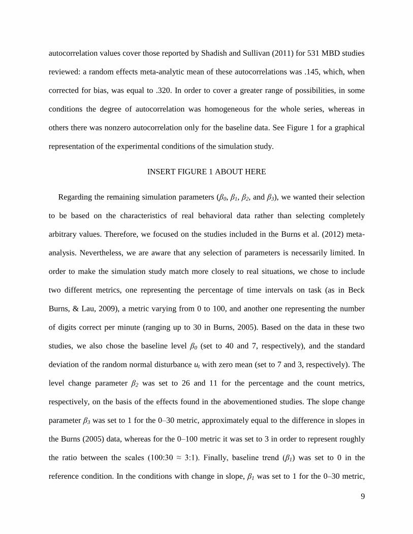
autocorrelation values cover those reported by Shadish and Sullivan (2011) for 531 MBD studies

reviewed: a random effects meta-analytic mean of these autocorrelations was .145, which, when

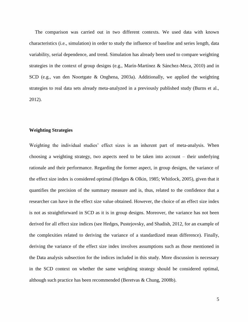
corrected for bias, was equal to .320. In order to cover a greater range of possibilities, in some

conditions the degree of autocorrelation was homogeneous for the whole series, whereas in

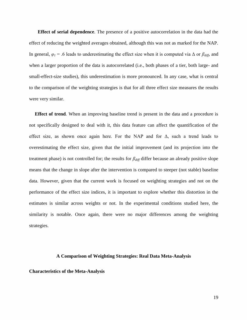
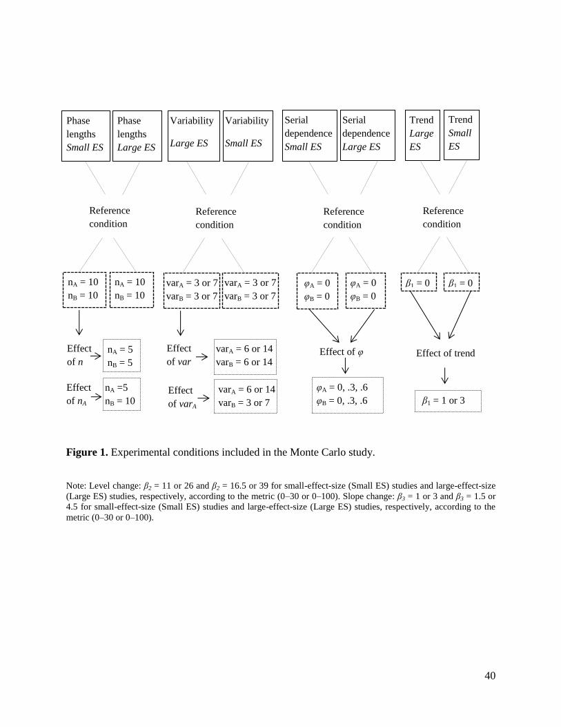
others there was nonzero autocorrelation only for the baseline data. See Figure 1 for a graphical

representation of the experimental conditions of the simulation study.

INSERT FIGURE 1 ABOUT HERE

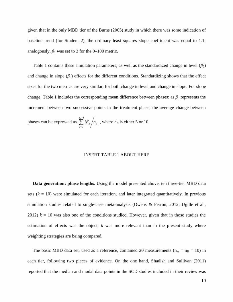
Regarding the remaining simulation parameters (β0, β1, β2, and β3), we wanted their selection

to be based on the characteristics of real behavioral data rather than selecting completely

arbitrary values. Therefore, we focused on the studies included in the Burns et al. (2012) meta-

analysis. Nevertheless, we are aware that any selection of parameters is necessarily limited. In

order to make the simulation study match more closely to real situations, we chose to include

two different metrics, one representing the percentage of time intervals on task (as in Beck

Burns, & Lau, 2009), a metric varying from 0 to 100, and another one representing the number

of digits correct per minute (ranging up to 30 in Burns, 2005). Based on the data in these two

studies, we also chose the baseline level β0 (set to 40 and 7, respectively), and the standard

deviation of the random normal disturbance ut with zero mean (set to 7 and 3, respectively). The

level change parameter β2 was set to 26 and 11 for the percentage and the count metrics,

respectively, on the basis of the effects found in the abovementioned studies. The slope change

parameter β3 was set to 1 for the 0–30 metric, approximately equal to the difference in slopes in

the Burns (2005) data, whereas for the 0–100 metric it was set to 3 in order to represent roughly

the ratio between the scales (100:30 ≈ 3:1). Finally, baseline trend (β1) was set to 0 in the

reference condition. In the conditions with change in slope, β1 was set to 1 for the 0–30 metric,

10

given that in the only MBD tier of the Burns (2005) study in which there was some indication of

baseline trend (for Student 2), the ordinary least squares slope coefficient was equal to 1.1;

analogously, β1 was set to 3 for the 0–100 metric.

Table 1 contains these simulation parameters, as well as the standardized change in level (β2)

and change in slope (β3) effects for the different conditions. Standardizing shows that the effect

sizes for the two metrics are very similar, for both change in level and change in slope. For slope

change, Table 1 includes the corresponding mean difference between phases: as β3 represents the

increment between two successive points in the treatment phase, the average change between

phases can be expressed as 1

3

0

Bn

B

i

i n

, where nB is either 5 or 10.

INSERT TABLE 1 ABOUT HERE

Data generation: phase lengths. Using the model presented above, ten three-tier MBD data

sets (k = 10) were simulated for each iteration, and later integrated quantitatively. In previous

simulation studies related to single-case meta-analysis (Owens & Ferron, 2012; Ugille et al.,

2012) k = 10 was also one of the conditions studied. However, given that in those studies the

estimation of effects was the object, k was more relevant than in the present study where

weighting strategies are being compared.

The basic MBD data set, used as a reference, contained 20 measurements (nA = nB = 10) in

each tier, following two pieces of evidence. On the one hand, Shadish and Sullivan (2011)

reported that the median and modal data points in the SCD studies included in their review was

11

20. On the other hand, Smith (2012) reported a mean of 10.4 baseline data points in MBD, which

is consistent with the Shadish and Sullivan (2011) data that (54.7%) of the SCDs had five or

more points in the first baseline.

Each generation of ten studies and posterior meta-analytical integration was iterated 1,000

times using R (R Core Team, 2013) and thus, 1,000 weighted averages were obtained for each

weighting strategy and each experimental condition (i.e., for each combination of phase lengths,

type of effect, data variability, degree of serial dependence, and trend).

Data generation: additional conditions for studying the effect of data variability and

phase length. In the simulation study, we wanted to explore the effect of data variability and

phase lengths as potentially important factors for the weighting strategies (see Figure 1). In order

to study how more variability or more data points affect the weighted average, it was necessary

to set different effect sizes in the different studies being integrated2. We decided that half of the k

= 10 studies should have the effect previously presented (β2 = 11 and β3 = 1 for the 0–30 metric,

β2 = 26 and β3 = 3 for the 0–100 metric), whereas for the other half the effects were multiplied by

the arbitrarily chosen value of 1.5 (thus β2 = 16.5 and β3 = 1.5 for the 0–30 metric, β2 = 39 and β3

= 4.5 for the 0–100 metric). The effects and their standardized versions are available in Table 1.

In order to study the effect of data variability, we doubled the standard deviation of the

random normal disturbance ut to 6 (for the 0–30 metric) and to 14 (for the 0–100 metric) for the

five studies with larger effects. Thus, we expected the weighted average to decrease. It should be

2 Otherwise, it would not be possible to study the effect of these two data features. Consider the following example,

with two studies being integrated and with the raw mean difference in both being equal to 11. If the first study is

given weight 2 (due to twice as many data points) and the second study is given weight 1, the weighted average is

still twice 11 + once 11 divided by 3, equal to 11; the same as the unweighted average. Therefore, it is necessary to

have different magnitudes of effect in order explore to what extent the weighted average moves closer to the effect

size of the study given greater weight.

12

stressed that with the simulation parameters specified in this way, the simulated data were

expected to be generally within the range of possible values, for both metrics3. The standardized

values in Table 1 are computed, on the one hand, considering the variability in the reference

condition and, on the other hand, for the conditions with greater variability.

To study the effect of phase lengths, we divided by two the number of data points in the

baseline (nA = 5) or in the whole MBD tier (nA = nB = 10) for the studies with larger effects,

expecting once again a reduction in the weighted average. Note that the multiplication factor was

the same as when studying the effect of data variability, given that the aim was to be able to

compare the changes in the weighted averages as a result of the smaller-effect-size studies

containing more measurements or presenting lower variability.

Data analysis: effect size measures. Our choice of effect size measures to include in the

present study was based on two criteria: knowledge of the expression of the index variance

(under certain assumptions) and actual use in single-case designs. Given the considerable lack of

consensus on which is the most appropriate effect size measure (Burns, 2012; Kratochwill et al.,

2013; Smith, 2012), we are aware that any choice of an analytical technique can be criticized

and, in the following, we explain our choice for this particular study, although we do not claim

that the measures included here are always the most appropriate ones.

In the review of single-case meta-analyses performed by Beretvas and Chung (2008b) the

Percentage of Nonoverlapping Data (PND; Scruggs, Mastropieri, & Casto, 1987) and the

3 For instance, for the 0–30 metric, in the treatment phase, the level of behavior expected when a large effect is

simulated is 7 (baseline level) + 16.5 (mean shift) = 23.5. Adding one standard deviation of 6 (condition of greater

variability), the greatest value expected is 29.5, which is consistent with the fact that the highest value observed in

the Burns (2005) study used as a reference was 30. For the 0–100 metric, in the treatment phase, the level of

behavior expected when there is a large effect simulated is 41 (baseline level) + 39 (mean shift) = 80. Adding one

standard deviation of 14 (condition of greater variability), the highest value expected is 94, which is consistent with

the highest possible percentage value, 100.

13

standardized mean difference were the most frequently used procedures for meta-analyzing

single-case data. Taking this into account, we chose two effect size measures for inclusion.

First, for the nonoverlap measure, we chose the Nonoverlap of All Pairs (NAP; Parker &

Vannest, 2009) rather than the PND for several reasons, despite the fact that the PND has a long

history of use and its quantifications have been validated by the researcher’s judgments on which

interventions are effective (Scruggs & Mastropieri, 2013), apart from the agreement with visual

analysis in absence of effect (Wolery, Busick, Reichow, & Barton, 2010). The reasons for

preferring the NAP are 1) it does not depend on a single extreme baseline measure; 2) in

simulation studies, the NAP has also been shown to perform well in presence of autocorrelation

(Manolov, Solanas, Sierra, & Evans, 2011), in contrast with the PND (Manolov, Solanas, &

Leiva, 2010); 3) the NAP and the PND show similar distributions of typical values according to

the review by Parker, Vannest, and Davis (2011) using real behavioral data; and 4) the critical

reason for selecting the NAP was the fact that the PND does not have a known sampling

distribution (Parker et al., 2011), which makes impossible using the most widely accepted weight

for group-design studies; in contrast, there is an expression for the variance of the NAP as shown

below. The NAP is a measure obtained as the percentage of pairwise comparisons for which the

result is an improvement after the intervention (e.g., the intervention measurement is greater than

the baseline measurement when the aim is to increase behavior). It is equivalent to an indicator

called Probability of superiority (Grissom, 1994), which is related to the common language

effect size (McGraw & Wong, 1992). Grissom and Kim (2001) provided a formula to estimate

the variance of the Probability of superiority, which is also applicable to the NAP: �̂�𝑁𝐴𝑃2 =

(1/𝑛𝐴 + 1/𝑛𝐵 + 1/𝑛𝐴𝑛𝐵)/12. Note that the Probability of superiority was originally intended to

compare two independent samples in the same way as the Mann-Whitney’s U test and, extending

14

this logic to SCD, it would be assumed that the data are independent and also that the variances

are equal. The reader should consider whether these assumptions are plausible. The NAP has

been used in single-case meta-analyses (e.g., Burns et al., 2012; Petersen-Brown, Karich, &

Symons, 2012).

Second, regarding the standardized mean difference index, according to Beretvas and Chung

(2008b), the most commonly applied version4 was the one using the standard deviation of the

baseline measurements (sA) in the denominator, which in group designs comparing a treatment

mean ( BX ) and a control group mean ( AX ) would be Glass’ Δ (Glass, McGaw, & Smith, 1981).

The index is thus defined as /B A AX X s and its variance is given by Rosenthal (1994) as

being equal to �̂�𝛥2 =

𝑛𝐴+𝑛𝐵

𝑛𝐴𝑛𝐵+

𝛥2

2(𝑛𝐴−1). Note that Δ was originally used to compare two

independent groups and is based on the assumption that the sampling distribution of Δ tends

asymptotically to normality and, thus, this formula is only an approximation. Moreover, although

it is a standardized measure of the average difference between phases, its application to SCD

data does not lead to a measure comparable to the d-statistic obtained in studies based on group

designs (see Hedges et al., 2012 for a more complete explanation). This is also a reason for not

using Cohen’s benchmarks for interpreting the index’s values (Beretvas & Chung, 2008). Once

again, we stress that we do not advocate for the use of this measure for quantifying intervention

effectiveness in all SCD data.

Three aspects should be considered with regards to these two effect size measures. First, the

fact that the first measure is expressed as a percentage of nonoverlap and the second measure is

standardized implies that they can be applied to data measured in different metrics (which is the

4 However, note that in the review by Maggin, O’Keefe, and Johnson (2011) this measure was only used in 19% of

SSED meta-analyses.

15

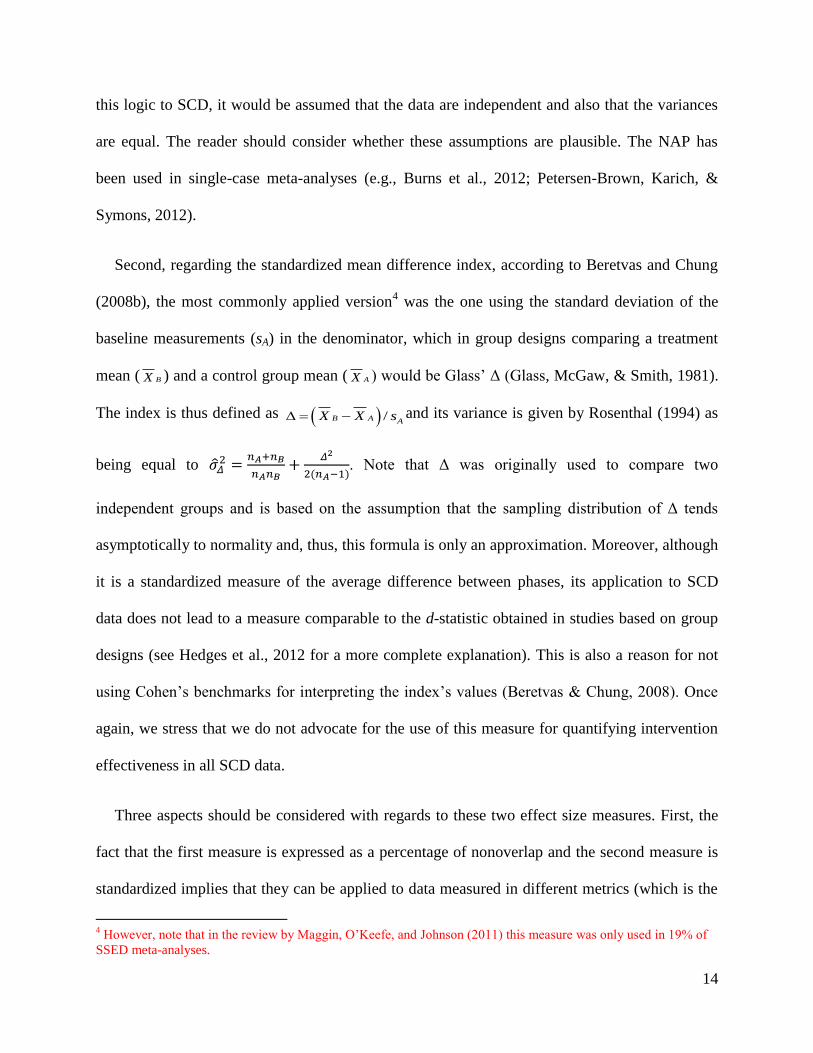
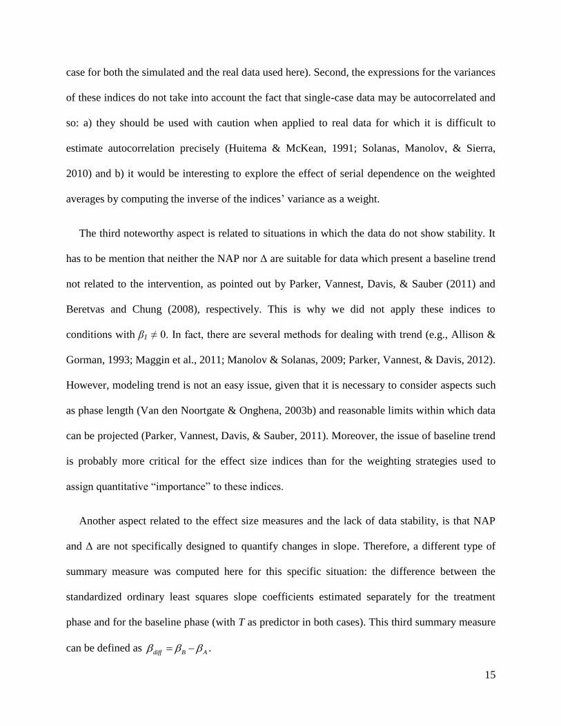
case for both the simulated and the real data used here). Second, the expressions for the variances

of these indices do not take into account the fact that single-case data may be autocorrelated and

so: a) they should be used with caution when applied to real data for which it is difficult to

estimate autocorrelation precisely (Huitema & McKean, 1991; Solanas, Manolov, & Sierra,

2010) and b) it would be interesting to explore the effect of serial dependence on the weighted

averages by computing the inverse of the indices’ variance as a weight.

The third noteworthy aspect is related to situations in which the data do not show stability. It

has to be mention that neither the NAP nor Δ are suitable for data which present a baseline trend

not related to the intervention, as pointed out by Parker, Vannest, Davis, & Sauber (2011) and

Beretvas and Chung (2008), respectively. This is why we did not apply these indices to

conditions with β1 ≠ 0. In fact, there are several methods for dealing with trend (e.g., Allison &

Gorman, 1993; Maggin et al., 2011; Manolov & Solanas, 2009; Parker, Vannest, & Davis, 2012).

However, modeling trend is not an easy issue, given that it is necessary to consider aspects such

as phase length (Van den Noortgate & Onghena, 2003b) and reasonable limits within which data

can be projected (Parker, Vannest, Davis, & Sauber, 2011). Moreover, the issue of baseline trend

is probably more critical for the effect size indices than for the weighting strategies used to

assign quantitative “importance” to these indices.

Another aspect related to the effect size measures and the lack of data stability, is that NAP

and Δ are not specifically designed to quantify changes in slope. Therefore, a different type of

summary measure was computed here for this specific situation: the difference between the

standardized ordinary least squares slope coefficients estimated separately for the treatment

phase and for the baseline phase (with T as predictor in both cases). This third summary measure

can be defined as diff B A .

16

The NAP, ∆, and βdiff were computed for each generated data set. The quantifications of the

ten studies (i = 1, 2, … 10) were then integrated via a weighted average,

10 10

1 1

,i i i

i i

NAP w NAP w

1 0 1 0

1 1

,i i i

i i

w w

or 10 10

1 1

,idiff i diff i

i i

w w

where wi denotes a

weight in the respective study I, based on either of the five strategies studied here.

Data analysis: weighting strategies. The weighting strategies included here were the

variance of the effect size indices, series length, baseline length, baseline variability, and a

proposal based on both baseline length and variability. It was expected that the data variability of

the whole series might be confounded with an intervention effect, given that a mean shift or a

change in slope both entail greater scatter. This is why it was not included as a weight. Another

possible weight not included here is the number of participants, as it is not strongly supported by

its proponents (Kratochwill et al., 2010) and raises the question of what weight should be used

when there is only one participant in the study, for instance, when an ABAB design is used or

whether in MBD across behaviors or settings, the number of tiers should also be used as a

weight.

It is important to distinguish between the weighting strategies that involve computing a

measure of variability. On the one hand, the classical option is related to the effect size index

variance (that is, the variance of its sampling distribution). In this case, the weight is the inverse

of this variance, so that a greater weight is related to greater precision of the effect size estimate.

On the other hand, the variability of the data (and not of the summary measure) is considered,

here focusing on the baseline phase. In this case, the weight is the inverse of the coefficient of

variation of the baseline measurements. The coefficient of variation is used to eliminate the

17

influence of the measurement units. In this way, studies with more stable data contribute more to

the average effect size.

Regarding series and baseline phase lengths, the weights are n and nA, respectively, giving

greater numerical importance to studies in which more measurements are available. The proposal

presented here is based on both baseline length and data variability, given that the two aspects

are related and should not be assessed separately: longer baselines are desirable given that they

provide more information and confidence about the actual initial situation, but even shorter

baselines might be sufficiently informative if the data are stable. The weight in the proposal was

defined as nA + 1/CV(A), a direct function of baseline length and inverse function of the baseline

data variability measured in terms of the coefficient of variation (a nondimensional measure that

makes data expressed in different units comparable). The proposal is well aligned with

Kratochwill et al.’s (2010) suggestion that the first step of assessing the usefulness of the single-

case data at hand for proving scientific evidence is to check whether the baseline pattern “has

sufficiently consistent level and variability”. Moreover, the same authors state that “[h]ighly

variable data may require a longer phase to establish stability” (p. 19).

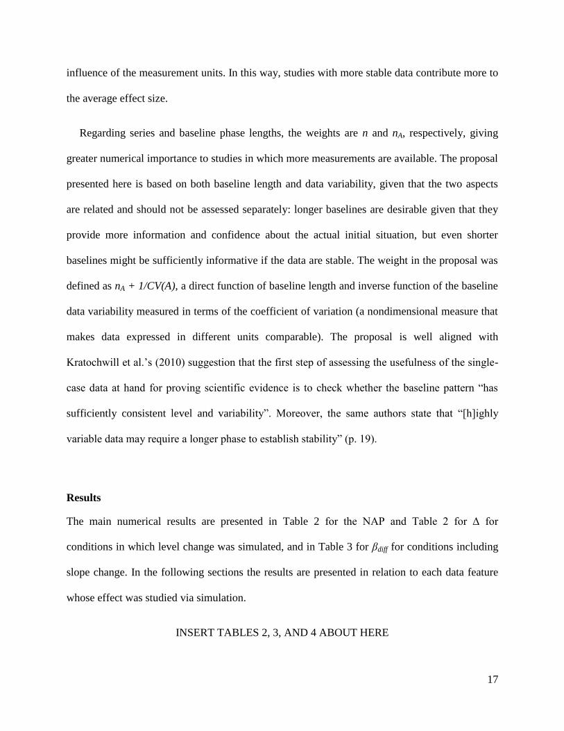
Results

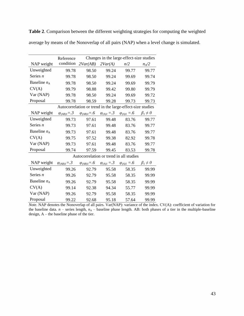
The main numerical results are presented in Table 2 for the NAP and Table 2 for Δ for

conditions in which level change was simulated, and in Table 3 for βdiff for conditions including

slope change. In the following sections the results are presented in relation to each data feature

whose effect was studied via simulation.

INSERT TABLES 2, 3, AND 4 ABOUT HERE

18

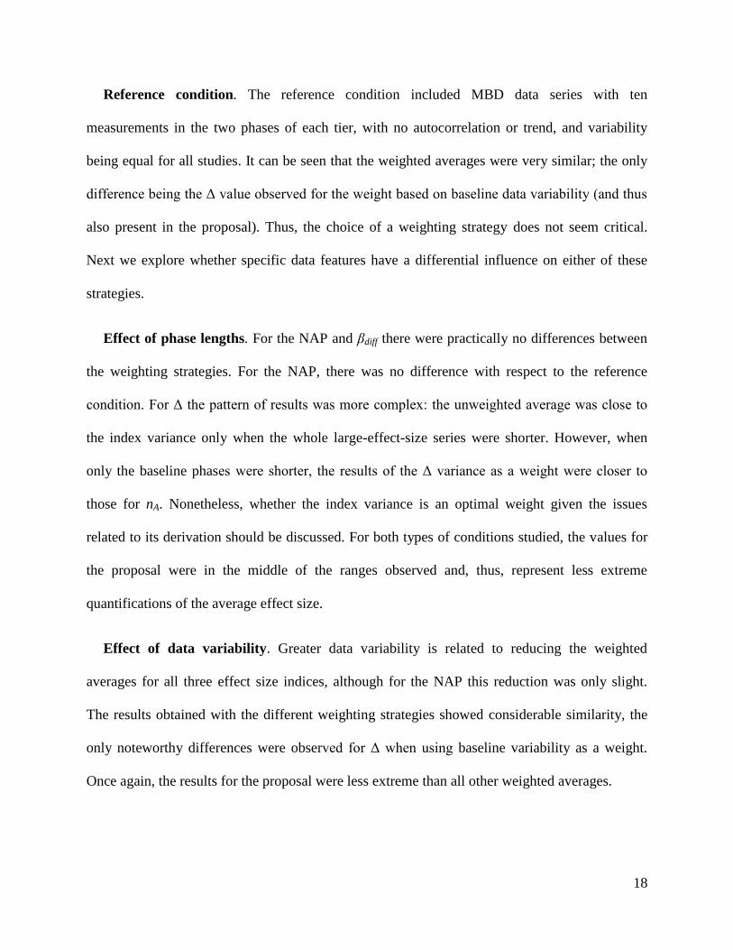
Reference condition. The reference condition included MBD data series with ten

measurements in the two phases of each tier, with no autocorrelation or trend, and variability

being equal for all studies. It can be seen that the weighted averages were very similar; the only

difference being the Δ value observed for the weight based on baseline data variability (and thus

also present in the proposal). Thus, the choice of a weighting strategy does not seem critical.

Next we explore whether specific data features have a differential influence on either of these

strategies.

Effect of phase lengths. For the NAP and βdiff there were practically no differences between

the weighting strategies. For the NAP, there was no difference with respect to the reference

condition. For Δ the pattern of results was more complex: the unweighted average was close to

the index variance only when the whole large-effect-size series were shorter. However, when

only the baseline phases were shorter, the results of the Δ variance as a weight were closer to

those for nA. Nonetheless, whether the index variance is an optimal weight given the issues

related to its derivation should be discussed. For both types of conditions studied, the values for

the proposal were in the middle of the ranges observed and, thus, represent less extreme

quantifications of the average effect size.

Effect of data variability. Greater data variability is related to reducing the weighted

averages for all three effect size indices, although for the NAP this reduction was only slight.

The results obtained with the different weighting strategies showed considerable similarity, the

only noteworthy differences were observed for Δ when using baseline variability as a weight.

Once again, the results for the proposal were less extreme than all other weighted averages.

19

Effect of serial dependence. The presence of a positive autocorrelation in the data had the

effect of reducing the weighted averages obtained, although this was not as marked for the NAP.

In general, φ1 = .6 leads to underestimating the effect size when it is computed via Δ or βdiff, and

when a larger proportion of the data is autocorrelated (i.e., both phases of a tier, both large- and

small-effect-size studies), this underestimation is more pronounced. In any case, what is central

to the comparison of the weighting strategies is that for all three effect size measures the results

were very similar.

Effect of trend. When an improving baseline trend is present in the data and a procedure is

not specifically designed to deal with it, this data feature can affect the quantification of the

effect size, as shown once again here. For the NAP and for Δ, such a trend leads to

overestimating the effect size, given that the initial improvement (and its projection into the

treatment phase) is not controlled for; the results for βdiff differ because an already positive slope

means that the change in slope after the intervention is compared to steeper (not stable) baseline

data. However, given that the current work is focused on weighting strategies and not on the

performance of the effect size indices, it is important to explore whether this distortion in the

estimates is similar across weights or not. In the experimental conditions studied here, the

similarity is notable. Once again, there were no major differences among the weighting

strategies.

A Comparison of Weighting Strategies: Real Data Meta-Analysis

Characteristics of the Meta-Analysis

20

The meta-analysis presented here is based on the meta-analysis carried out by Burns et al.

(2012),5 which integrated ten studies (k = 10; the articles marked with an asterisk in the reference

list were those included in the meta-analysis). However, the current re-analysis is not a direct

replication of the Burns et al. (2012) study, given that we did not use median NAP values, nor

convert NAP to Pearson’s phi. Most of the studies included in the meta-analysis used multiple

baseline designs, and focused on an intervention called Incremental Rehearsal, which is used for

several teaching purposes (e.g., words, mathematics) both for children with and without

disabilities.

Dealing with Dependence of Outcomes

More than one outcome can be computed for most of the single-case studies included in the

meta-analysis and it does not seem appropriate to treat each outcome as independent (Beretvas &

Chung, 2008b). Here we chose to average the effect sizes within a study, which is one of the

options used in group-designs meta-analysis (Borenstein, Hedges, Higgins, & Rothstein, 2009).

However, it is also possible to choose one of the several effect sizes reported per study according

to a substantive criterion or at random (Lipsey & Wilson, 2001).

Another issue that requires consideration is how weights are computed in order to have a

single weight per study accompanying the corresponding effect size measure. Borenstein et al.

(2009) discussed the possibility of calculating a variance of an average of effect sizes within a

study. However, their formulae require knowing or at least assuming plausible values for the

correlations between the different study outcomes. Given that we did not want to make an

assumption with no basis, we chose to obtain the average of the weights for each outcome in

5 We would like to thank Matthew K. Burns for kindly sharing his data for the analyses presented here.

21

order to have a single weight per study. This approach has been deemed a conservative solution

(Borenstein et al., 2009).

For instance, for multiple baseline designs (e.g., Burns, 2005) or multiple probe designs (e.g.,

Codding, Archer, & Connell, 2010) there is one outcome for each baseline. In such cases, it has

been suggested (Schlosser et al., 2008) that an effect size should be computed for each baseline

before computing the average of these baselines; Burns et al. (2012) also computed the NAP for

each baseline and then aggregated them. For designs with multiple treatments (e.g., Burns, 2007)

the optimal practice is not clear, but comparing each treatment with the immediately preceding

baseline seems to be the logical choice (Schlosser et al., 2008). However, given that in the Burns

(2007) study there was only one baseline (the design can be designated as ACBC) and

considering the possibility of sequence effects (Schlosser et al., 2008), we chose to include only

the comparison of this baseline with the first intervention. For the Volpe, Mulé, Briesch, Joseph,

and Burns (2011) study, each measurement obtained under the Incremental Rehearsal conditions

was compared to the corresponding measurement under the traditional drill and practice

condition, which was considered the reference, although it is not strictly speaking a baseline

condition.

Results

The effect sizes and the different weights for each of the ten studies are presented in Table 5.

Some aspects of the results should be commented upon, before discussing the weighted averages

across studies. For the Bunn, Burns, Hoffman, and Newman (2005) study, a perfectly stable

baseline (i.e., a complete lack of variability) precluded computing βdiff and also ∆, its variance, or

the weight related to baseline variability. Additionally, given that only ten studies were

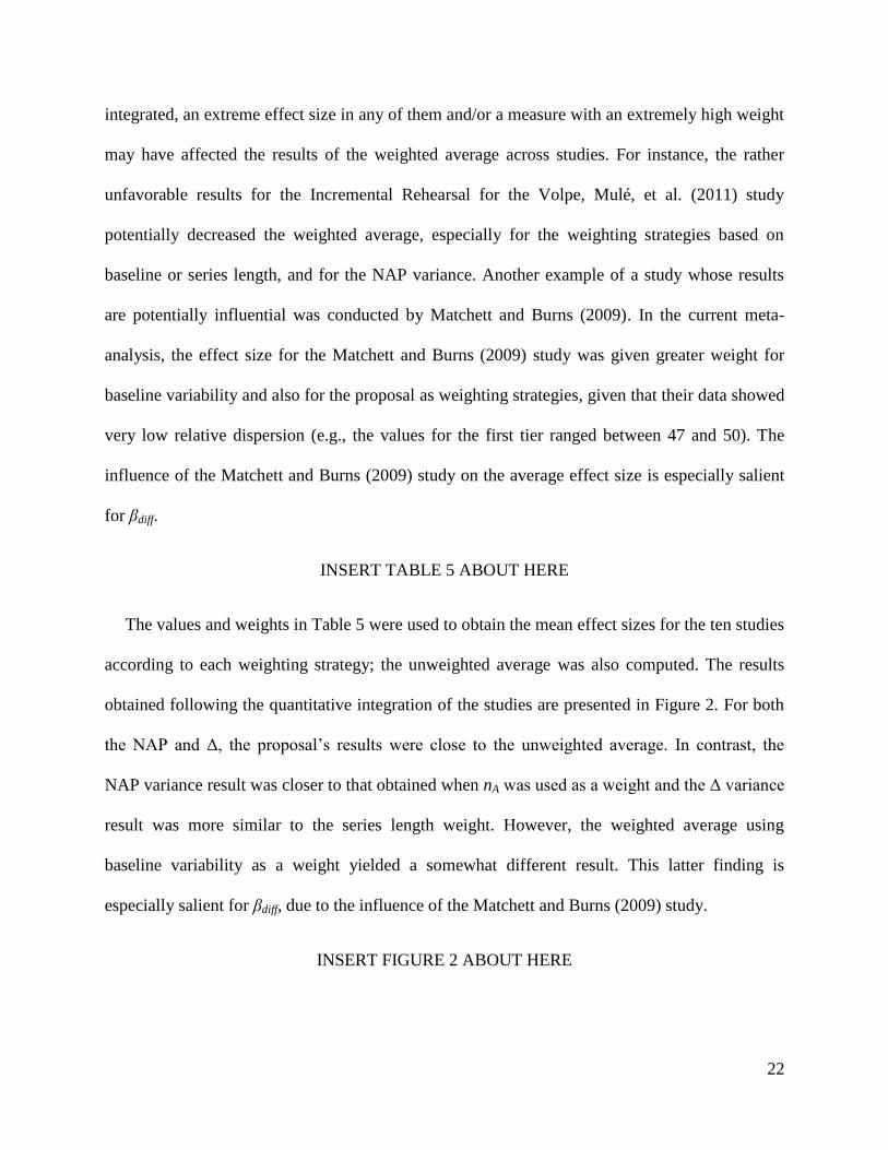
22

integrated, an extreme effect size in any of them and/or a measure with an extremely high weight

may have affected the results of the weighted average across studies. For instance, the rather

unfavorable results for the Incremental Rehearsal for the Volpe, Mulé, et al. (2011) study

potentially decreased the weighted average, especially for the weighting strategies based on

baseline or series length, and for the NAP variance. Another example of a study whose results

are potentially influential was conducted by Matchett and Burns (2009). In the current meta-

analysis, the effect size for the Matchett and Burns (2009) study was given greater weight for

baseline variability and also for the proposal as weighting strategies, given that their data showed

very low relative dispersion (e.g., the values for the first tier ranged between 47 and 50). The

influence of the Matchett and Burns (2009) study on the average effect size is especially salient

for βdiff.

INSERT TABLE 5 ABOUT HERE

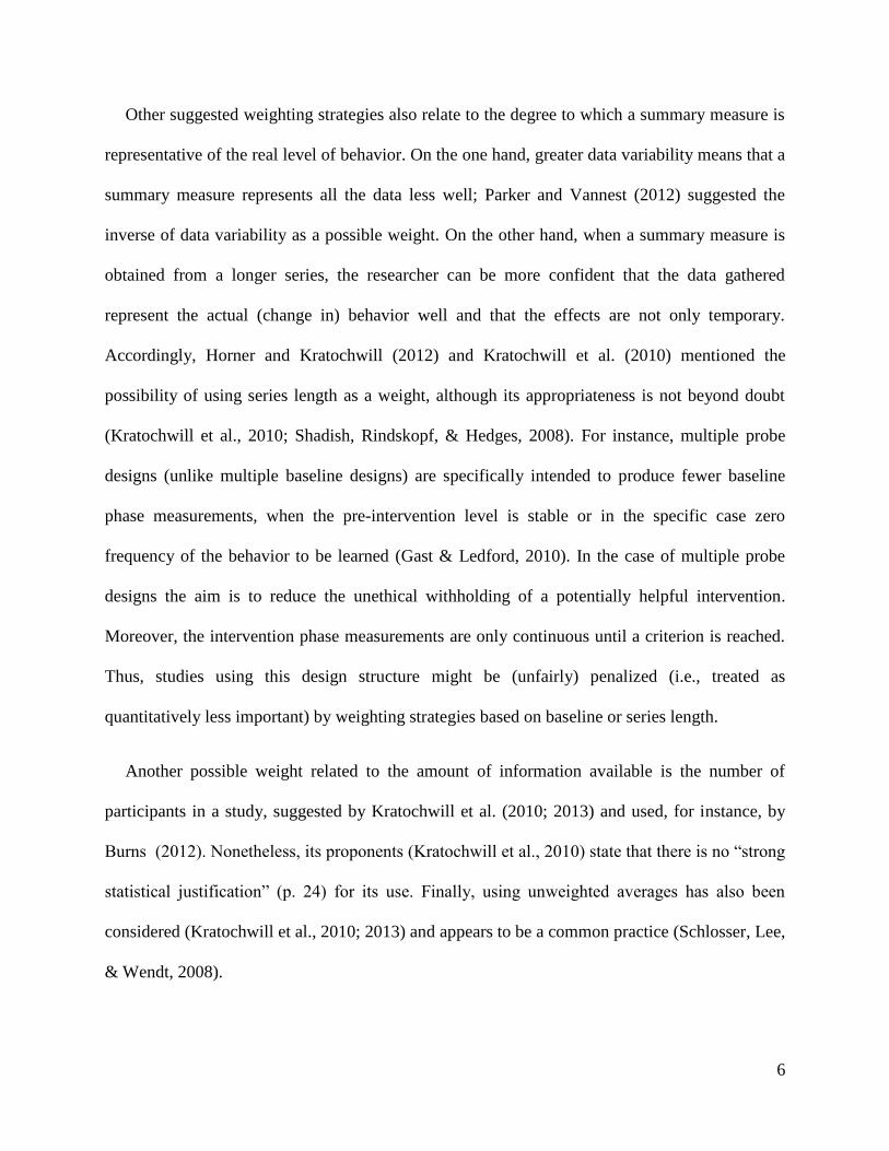
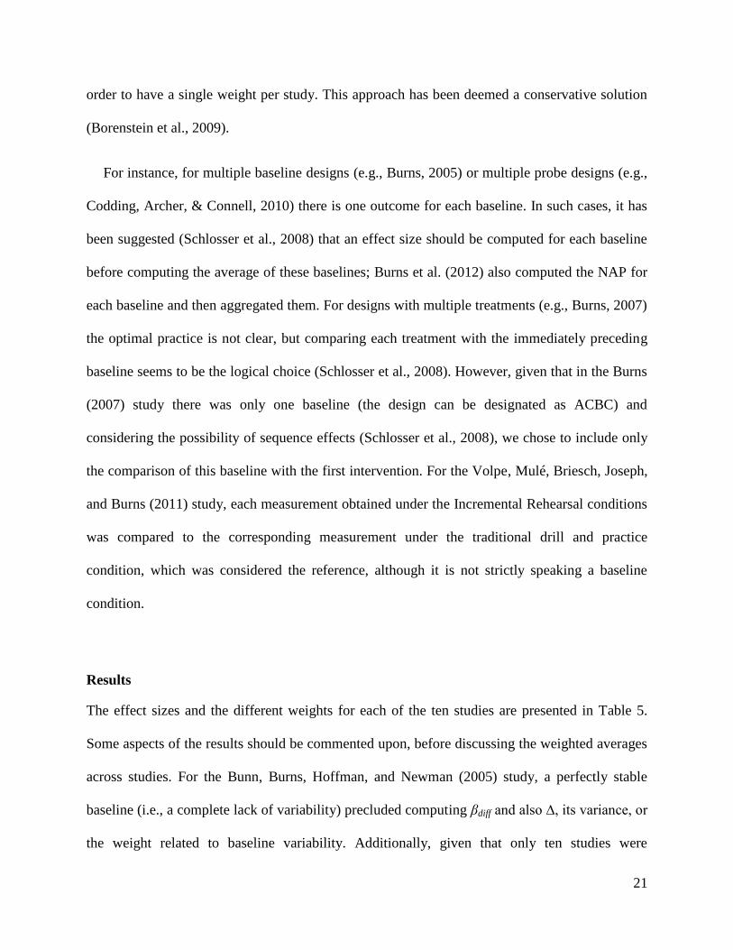
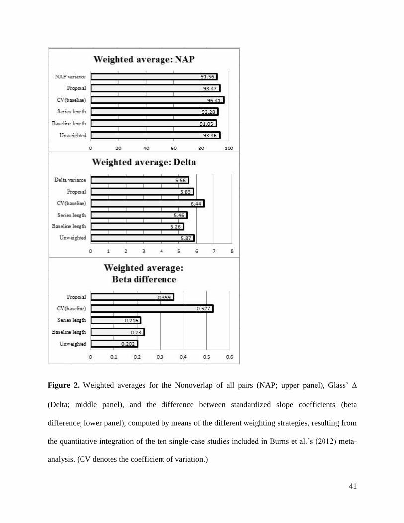
The values and weights in Table 5 were used to obtain the mean effect sizes for the ten studies

according to each weighting strategy; the unweighted average was also computed. The results

obtained following the quantitative integration of the studies are presented in Figure 2. For both

the NAP and Δ, the proposal’s results were close to the unweighted average. In contrast, the

NAP variance result was closer to that obtained when nA was used as a weight and the Δ variance

result was more similar to the series length weight. However, the weighted average using

baseline variability as a weight yielded a somewhat different result. This latter finding is

especially salient for βdiff, due to the influence of the Matchett and Burns (2009) study.

INSERT FIGURE 2 ABOUT HERE

23

Discussion

Results and Implications

The present study is, to the best of our knowledge, the first one based simultaneously on

simulation and real data comparing several weighting strategies in the context of single-case

designs’ meta-analysis. The results obtained here are restricted to the experimental conditions

studied and more extensive research and discussion are required. However, various aspects of

this work will fuel further discussion and testing with published data or via simulation.

Firstly, the issue of whether weighting is necessary when an average effect size summarizing

the results of several studies is obtained should be considered. On substantive grounds, it seems

logical to treat an outcome of a study as numerically more important (i.e., contributing to a

greater extent) when this outcome is based on a larger amount of data and/or on a clear data

pattern (i.e., with less unexplained variability). On empirical grounds, based on the results

presented here, there is not enough evidence that weighting yields markedly different results. An

implication of these findings (which should be considered taking into account the Limitations

discussed below) is that series length alone may not be a critical feature for giving more or less

weight to the results. In that sense, multiple probe designs characterized by a reduced amount of

measurements may not be treated as providing less evidence. However, note that the length of

the phases is also considered in the expressions for approximating the variance of the indices

included in this study.

Secondly, for the cases in which certain differences are observed in the weighted averages, it

is important to establish the gold standard, so that a result can be judged as more or less

desirable. It that sense, whether the variance of the effect size measure is that gold standard, and

24

whether it can be derived for single-case data, considering potential serial dependence and/or a

baseline trend, should be debated. Even in the context of simulation data, it is not easy to

determine which results show the best match for the simulation parameters, given that the

question is “what are the optimal weights?” and thus “how different from an unweighted average

should a weighted average be?”.

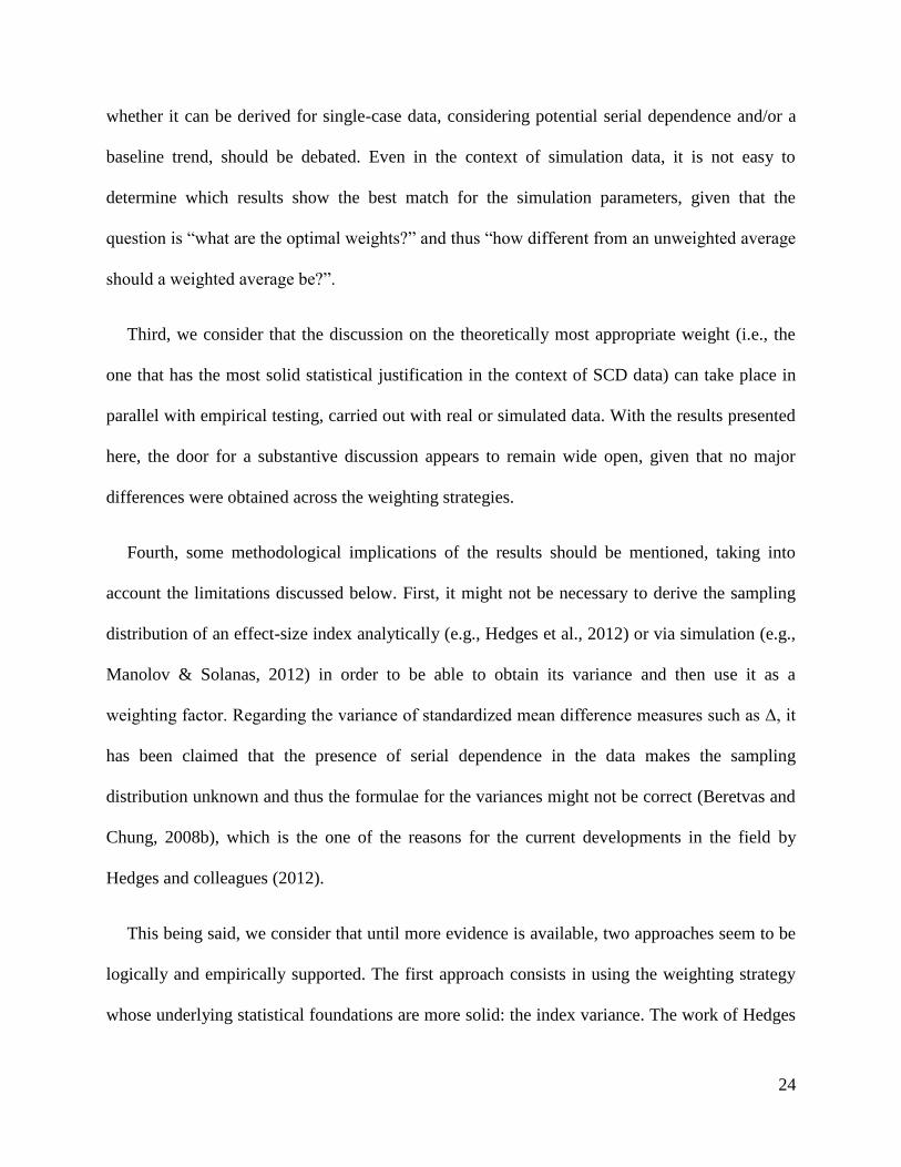
Third, we consider that the discussion on the theoretically most appropriate weight (i.e., the

one that has the most solid statistical justification in the context of SCD data) can take place in

parallel with empirical testing, carried out with real or simulated data. With the results presented

here, the door for a substantive discussion appears to remain wide open, given that no major

differences were obtained across the weighting strategies.

Fourth, some methodological implications of the results should be mentioned, taking into

account the limitations discussed below. First, it might not be necessary to derive the sampling

distribution of an effect-size index analytically (e.g., Hedges et al., 2012) or via simulation (e.g.,

Manolov & Solanas, 2012) in order to be able to obtain its variance and then use it as a

weighting factor. Regarding the variance of standardized mean difference measures such as Δ, it

has been claimed that the presence of serial dependence in the data makes the sampling

distribution unknown and thus the formulae for the variances might not be correct (Beretvas and

Chung, 2008b), which is the one of the reasons for the current developments in the field by

Hedges and colleagues (2012).

This being said, we consider that until more evidence is available, two approaches seem to be

logically and empirically supported. The first approach consists in using the weighting strategy

whose underlying statistical foundations are more solid: the index variance. The work of Hedges

25

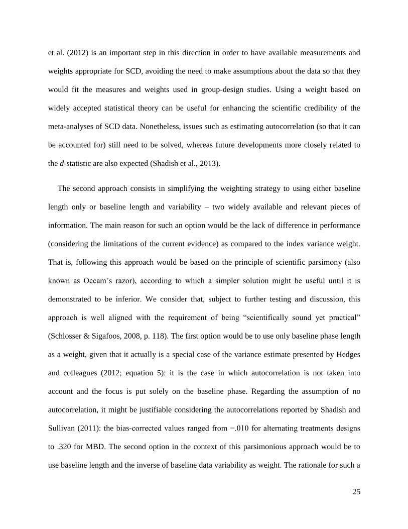
et al. (2012) is an important step in this direction in order to have available measurements and

weights appropriate for SCD, avoiding the need to make assumptions about the data so that they

would fit the measures and weights used in group-design studies. Using a weight based on

widely accepted statistical theory can be useful for enhancing the scientific credibility of the

meta-analyses of SCD data. Nonetheless, issues such as estimating autocorrelation (so that it can

be accounted for) still need to be solved, whereas future developments more closely related to

the d-statistic are also expected (Shadish et al., 2013).

The second approach consists in simplifying the weighting strategy to using either baseline

length only or baseline length and variability – two widely available and relevant pieces of

information. The main reason for such an option would be the lack of difference in performance

(considering the limitations of the current evidence) as compared to the index variance weight.

That is, following this approach would be based on the principle of scientific parsimony (also

known as Occam’s razor), according to which a simpler solution might be useful until it is

demonstrated to be inferior. We consider that, subject to further testing and discussion, this

approach is well aligned with the requirement of being “scientifically sound yet practical”

(Schlosser & Sigafoos, 2008, p. 118). The first option would be to use only baseline phase length

as a weight, given that it actually is a special case of the variance estimate presented by Hedges

and colleagues (2012; equation 5): it is the case in which autocorrelation is not taken into

account and the focus is put solely on the baseline phase. Regarding the assumption of no

autocorrelation, it might be justifiable considering the autocorrelations reported by Shadish and

Sullivan (2011): the bias-corrected values ranged from −.010 for alternating treatments designs

to .320 for MBD. The second option in the context of this parsimonious approach would be to

use baseline length and the inverse of baseline data variability as weight. The rationale for such a

26

weight would be to avoid penalizing excessively multiple probe designs in which few pre-

intervention measurements are obtained, but they show stability. Choosing either of the two

approaches can be a question of further debate.

Fifth, we would like to encourage applied researchers to publish not only their raw data in a

graphical format, but also to compute the primary summary measures such as means, medians,

and standard deviations for each phase, given that this information is useful for computing the

weights that are necessary for meta-analysis. This would help avoid any lack of precision due to

imperfect data-retrieval procedures. Meta-analysis and the identification of the conditions under

which interventions are useful would also benefit from reporting the details about the

participants, the settings, the procedures, and the operative definitions of the main study

variables (Maggin & Chafouleas, 2013).

Finally, researchers carrying out meta-analyses are encouraged to report both an unweighted

average and a weighted average based on the strategy they consider optimal. In that way, each

meta-analysis would serve as evidence based on real data regarding the impact of using

weighting in meta-analytical integrations. Furthermore, each meta-analysis would contribute not

only to substantive knowledge, but would also give added value in terms of the methodological

discussion on how to perform research synthesis in single-case designs.

Limitations and Future Research

The results of the present study are limited to the weighting strategies and the effect size

measures included. Regarding the limitations of the meta-analysis of published data, we should

mention the relatively small number of studies included, and the inability to calculate variances

27

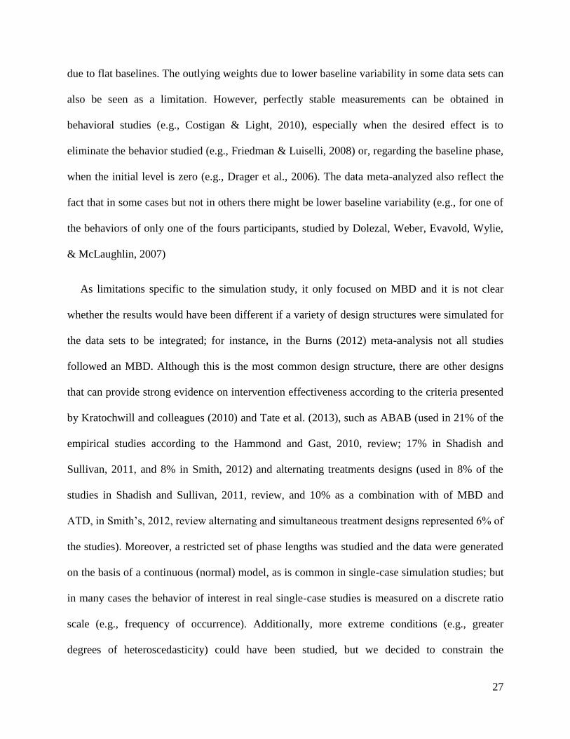
due to flat baselines. The outlying weights due to lower baseline variability in some data sets can

also be seen as a limitation. However, perfectly stable measurements can be obtained in

behavioral studies (e.g., Costigan & Light, 2010), especially when the desired effect is to

eliminate the behavior studied (e.g., Friedman & Luiselli, 2008) or, regarding the baseline phase,

when the initial level is zero (e.g., Drager et al., 2006). The data meta-analyzed also reflect the

fact that in some cases but not in others there might be lower baseline variability (e.g., for one of

the behaviors of only one of the fours participants, studied by Dolezal, Weber, Evavold, Wylie,

& McLaughlin, 2007)

As limitations specific to the simulation study, it only focused on MBD and it is not clear

whether the results would have been different if a variety of design structures were simulated for

the data sets to be integrated; for instance, in the Burns (2012) meta-analysis not all studies

followed an MBD. Although this is the most common design structure, there are other designs

that can provide strong evidence on intervention effectiveness according to the criteria presented

by Kratochwill and colleagues (2010) and Tate et al. (2013), such as ABAB (used in 21% of the

empirical studies according to the Hammond and Gast, 2010, review; 17% in Shadish and

Sullivan, 2011, and 8% in Smith, 2012) and alternating treatments designs (used in 8% of the

studies in Shadish and Sullivan, 2011, review, and 10% as a combination with of MBD and

ATD, in Smith’s, 2012, review alternating and simultaneous treatment designs represented 6% of

the studies). Moreover, a restricted set of phase lengths was studied and the data were generated

on the basis of a continuous (normal) model, as is common in single-case simulation studies; but

in many cases the behavior of interest in real single-case studies is measured on a discrete ratio

scale (e.g., frequency of occurrence). Additionally, more extreme conditions (e.g., greater

degrees of heteroscedasticity) could have been studied, but we decided to constrain the

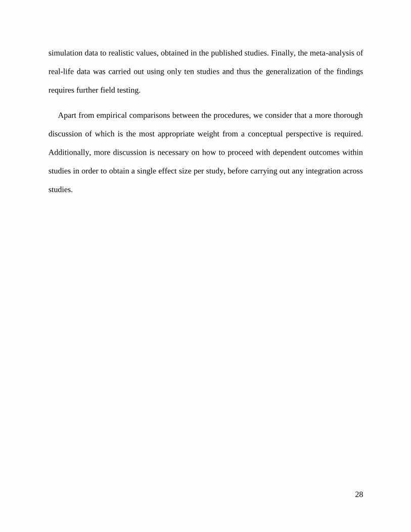
28

simulation data to realistic values, obtained in the published studies. Finally, the meta-analysis of

real-life data was carried out using only ten studies and thus the generalization of the findings

requires further field testing.

Apart from empirical comparisons between the procedures, we consider that a more thorough

discussion of which is the most appropriate weight from a conceptual perspective is required.

Additionally, more discussion is necessary on how to proceed with dependent outcomes within

studies in order to obtain a single effect size per study, before carrying out any integration across

studies.

29

References

Articles included in the meta-analysis are indicated with an asterisk (*).

APA Presidential Task Force on Evidence-Based Practice. (2006). Evidence-based practice in

psychology. American Psychologist, 61, 271-285.

Baek, E. K., & Ferron, J. M. (2013). Multilevel models for multiple-baseline data: Modeling

across-participant variation in autocorrelation and residual variance. Behavior Research

Methods, 45, 65-74.

*Beck, M., Burns, M. K., & Lau, M. (2009). Preteaching unknown items as a behavioral

intervention for children with behavioral disorders. Behavior Disorders, 34, 91-99.

Beretvas, S. N., & Chung, H. (2008a). An evaluation of modified R2-change effect size indices

for single-subject experimental designs. Evidence-Based Communication Assessment and

Intervention, 2, 120-128.

Beretvas, S. N., & Chung, H. (2008b). A review of meta-analyses of single-subject experimental

designs: Methodological issues and practice. Evidence-Based Communication Assessment

and Intervention, 2, 129-141.

Blampied, N. M. (2000). Single-case research designs: A neglected alternative. American

Psychologist, 55, 960.

Borenstein, M., Hedges, L. V., Higgins, J. P. T., & Rothstein, H. R. (2009). Introduction to meta-

analysis. Chichester, UK: John Wiley & Sons.

30

Bunn, R., Burns, M. K., Hoffman, H. H., & Newman, C. L. (2005). Using incremental rehearsal

to teach letter identification with a preschool-aged child. Journal of Evidence Based Practice

for Schools, 6, 124-134.

*Burns, M. K. (2005). Using incremental rehearsal to practice multiplication facts with children

identified as learning disabled in mathematics computation. Education and Treatment of

Children, 28, 237-249.

*Burns, M. K. (2007). Comparison of drill ratio and opportunities to respond when rehearsing

sight words with a child with mental retardation. School Psychology Quarterly, 22, 250-263.

Burns, M. K. (2012). Meta-analysis of single-case design research: Introduction to the special

issue. Journal of Behavioral Education, 21, 175-184.

*Burns, M. K., & Dean, V. J. (2005). Effect of acquisition rates on off-task behavior with

children identified as learning disabled. Learning Disability Quarterly, 28, 273-281.

*Burns, M. K., & Kimosh, A. (2005). Using incremental rehearsal to teach sight-words to adult

students with moderate mental retardation. Journal of Evidence Based Practices for Schools,

6, 135-148.

Burns, M. K., Zaslofsky, A. F., Kanive, R., & Parker, D. C. (2012). Meta-analysis of incremental

rehearsal using phi coefficients to compare single-case and group designs. Journal of

Behavioral Education, 21, 185-202.

*Codding, R. S., Archer, J., & Connell, J. (2010). A systematic replication and extension of

using incremental rehearsal to improve multiplication skills: An investigation of

generalization. Journal of Behavioral Education, 19, 93-105.

31

Cooper, H. (2010). Research synthesis and meta-analysis: A step-by-step approach. (4th Ed.).

London, UK: Sage.

Costigan, F. A., & Light, J. (2010). Effect of seated position on upper-extremity access to

augmentative communication for children with cerebral palsy: Preliminary investigation.

American Journal of Occupational Therapy, 64, 595-604.

Drager, K. D. R, Postal, V. J., Carrolus, L., Castellano, M., Gagliano, C., & Glynn, J. (2006).

The effect of aided language modeling on symbol comprehension and prodcution in 2

preschoolers with autism. American Journal of Speech – Language Pathology, 15, 112-125.

Dolezal, D. N., Weber, K. P., Evavold, J. J., Wylie, J., & McLaughlin, T. F. (2007). The effects

of a reinforcement package for on-task and reading behavior with at-risk and middle school

students with disabilities. Child and Family Therapy, 29, 9-25.

Ferron, J. M., & Sentovich, C. (2002). Statistical power of randomization tests used with

multiple-baseline designs. The Journal of Experimental Education, 70, 165-178.

Friedman, A., & Luiselli, J. K. (2008). Excessive daytime sleep: Behavioral assessment and

intervention in a child with autism. Behavior Modification, 32, 548-555.

Gage, N. A., & Lewis, T. J. (2012, May 11). Hierarchical linear modeling meta-analysis of

single-subject design research. Journal of Special Education. Advance online publication. doi:

10.1177/0022466912443894

Gast, D. L., & Ledford, J. (2010). Multiple-baseline and multiple probe designs. In D. L. Gast

(Ed.), Single subject research methodology in behavioral sciences (pp. 276-328). London,

UK: Routledge.

32

Gast, D. L., & Spriggs, A. D. (2010). Visual analysis of graphic data. In D. L. Gast (Ed.), Single

subject research methodology in behavioral sciences (pp. 199-233). London, UK: Routledge.

Glass, G. V., McGaw, B., & Smith, M. L. (1981). Meta-analysis in social research. Beverly

Hills, CA: Sage.

Grissom, R. J. (1994). Probability of the superior outcome of one treatment over another.

Journal of Applied Psychology, 79, 314-316.

Grissom, R. J., & Kim, J. J. (2001). Review of assumptions and problems in the appropriate

conceptualization of effect size. Psychological Methods, 6, 135-146.

Hammond, D., & Gast, D. L. (2010). Descriptive analysis of single subject research designs:

1983-2007. Education and Training in Autism and Developmental Disabilities, 45, 187-202.

Hedges, L. V., & Olkin, I. (1985). Statistical methods for meta-analysis. New York, NY:

Academic Press.

Hedges, L. V., Pustejovsky, J. E., & Shadish, W. R. (2012). A standardized mean difference

effect size for single case designs. Research Synthesis Methods, 3, 224-239.

Horner, R. H., Carr, E. G., Halle, J., McGee, G., Odom, S., & Wolery, M. (2005). The use of

single-subject research to identify evidence-based practice in special education. Exceptional

Children, 71, 165-179.

Horner, R. H., & Kratochwill, T. R. (2012). Synthesizing single-case research to identify

evidence-based practices: Some brief reflections. Journal of Behavioral Education, 21, 266-

272.

33

Howick, J., Chalmers, I., Glasziou, P., Greenhaigh, T., Heneghan, C., Liberati, A., et al. (2011).

The 2011 Oxford CEBM Evidence Table (Introductory Document). Oxford: Oxford Centre for

Evidence-Based Medicine. Available from: http://www.cebm.net/index.aspx?o=5653

Huitema, B. E., & McKean, J. W. (1991). Autocorrelation estimation and inference with small

samples. Psychological Bulletin, 110, 291-304.

Huitema, B. E., & McKean, J. W. (2000). Design specification issues in time-series intervention

models. Educational and Psychological Measurement, 60, 38-58.

Institute of Education Sciences. (2013). Request for applications: Statistical and research

methodology in education. Retrieved from http://ies.ed.gov/funding/pdf/2014_84305D.pdf

Jenson, W. R., Clark, E., Kircher, J. C., & Kristjansson, S. D. (2007). Statistical reform:

Evidence-based practice, meta-analyses, and single subject designs. Psychology in the

Schools, 44, 483-493.

Kazdin, A. E. (2001). Behavior modification in applied settings (6th ed.). Belmont, CA:

Wadsworth.

Kratochwill, T. R., Hitchcock, J., Horner, R. H., Levin, J. R., Odom, S. L., Rindskopf, D. M., &

Shadish, W. R. (2010). Single-case designs technical documentation [Technical Report].

Retrieved from http://ies.ed.gov/ncee/wwc/pdf/reference_resources/ wwc_scd.pdf

Kratochwill, T. R., Hitchcock, J. H., Horner, R. H., Levin, J. R., Odom, S. L., Rindskopf, D. M.,

& Shadish, W. R. (2013). Single-case intervention research design standards. Remedial and

Special Education, 34, 26-38.

34

Kratochwill, T. R., & Levin, J. R. (2010). Enhancing the scientific credibility of single-case

intervention research: Randomization to the rescue. Psychological Methods, 15, 124-144.

Lane, K. L., & Carter, E. W. (2013). Reflections on the Special Issue: Issues and advances in the

meta-analysis of single-case research. Remedial and Special Education, 34, 59-61.

Lipsey, M. W., & Wilson, D. B. (2001). Practical meta-analysis. Thousand Oaks, CA: Sage.

Littell, J. H., Corcoran, J., & Pillai, V. (2008). Systematic reviews and meta-analysis. New York,

NY: Oxford University Press.

Maggin, D. M., & Chafouleas, S. M. (2013). Introduction to the Special Series: Issues and

advance of synthesizing single-case research. Remedial and Special Education, 34, 3-8.

Maggin, D. M., O’Keeffe, B. V., & Johnson, A. H. (2011). A quantitative synthesis of

methodology in the meta-analysis of single-subject research for students with disabilities:

1985-2009. Exceptionality, 19, 109-135.

Maggin, D. M., Swaminathan, H., Rogers, H. J., O’Keefe, B. V., Sugai, G., & Horner, R. H.

(2011). A generalized least squares regression approach for computing effect sizes in single-

case research: Application examples. Journal of School Psychology, 49, 301-321.

Manolov, R., & Solanas, A. (2009). Percentage of nonoverlapping corrected data. Behavior

Research Methods, 41, 1262-1271.

Manolov, R., & Solanas, A. (2012). Assigning and combining probabilities in single-case

studies. Psychological Methods, 17, 495-509.

35

Manolov, R., Solanas, A., & Leiva, D. (2010). Comparing “visual” effect size indices for single-

case designs. Methodology, 6, 49-58.

Manolov, R., Solanas, A., Sierra, V., & Evans, J. J. (2011). Choosing among techniques for

quantifying single-case intervention effectiveness. Behavior Therapy, 42, 533-545.

Marín-Martínez, F., & Sánchez-Meca, J. (2010). Weighting by inverse variance or by sample

size in random-effects meta-analysis. Educational and Psychological Measurement, 70, 56-

73.

*Matchett, D. L., & Burns, M. K. (2009). Increasing word recognition fluency with an English

language learner. Journal of Evidence Based Practices in Schools, 10, 194-209.

Odom, S. L., Brantlinger, E., Gersten, R., Horner, R. H., Thompson, B. & Harris, K. R. (2005).

Research in special education: Scientific methods and evidence-based practices. Exceptional

Children, 71, 137-148.

Owens, C. M., & Ferron, J. M. (2012). Synthesizing single-case studies: A Monte Carlo

examination of a three-level meta-analytic model. Behavior Research Methods, 44, 795-805.

Parker, R. I., & Vannest, K. J. (2009). An improved effect size for single-case research:

Nonoverlap of all pairs. Behavior Therapy, 40, 357-367.

Parker, R. I., & Vannest, K. J. (2012). Bottom-up analysis of single-case research designs.

Journal of Behavioral Education, 21, 254-265.

Parker, R. I., Vannest, K. J., & Davis, J. L. (2011). Effect size in single-case research: A review

of nine nonoverlap techniques. Behavior Modification, 35, 303-322.

36

Parker, R. I., Vannest, K. J., & Davis, J. L. (2012, August 22). A simple method to control

positive baseline trend within data nonoverlap. Journal of Special Education. Advance online

publication. doi: 10.1177/0022466912456430.

Parker, R. I., Vannest, K. J., Davis, J. L., & Sauber, S. B. (2011). Combining nonoverlap and

trend for single-case research: Tau-U. Behavior Therapy, 42, 284-299.

Petersen-Brown, S., Karich, A. C., & Symons, F. J. (2012). Examining estimates of effect using

Non-overlap of all pairs in multiple baseline studies of academic intervention. Journal of

Behavioral Education, 21, 203-216.

R Core Team (2013). R: A language and environment for statistical computing. R Foundation for

Statistical Computing, Vienna, Austria. URL http://www.R-project.org/.

Rosenthal, R. (1994). Parametric measures of effect size. In H. Cooper & L. V. Hedges, The

handbook of research synthesis and meta-analysis (pp. 231-244). New York, NY: Russell

Sage Foundation.

Sackett, D. L., Rosenberg, W. M. C., Gray, J. A. M., Hayness, R. B., & Richardson, W. S.

(1996). Evidence based medicine: What it is and what it isn't. BMJ, 312, 71-72.

Schlosser, R. W. (2009). The role of single-subject experimental designs in evidence-based

practice times. FOCUS, 22, 1-8. Austin, TX: SEDL.

Schlosser, R. W., Lee, D. L., & Wendt, O. (2008). Application of the percentage of non-

overlapping data (PND) in systematic reviews and meta-analyses: A systematic review of

reporting characteristics. Evidence-Based Communication Assessment and Intervention, 2,

163-187.

37

Schlosser, R. W., & Sigafoos, J. (2008). Meta-analysis of single-subject experimental designs:

Why now? Evidence-Based Communication Assessment and Intervention, 2, 117-119.

Scruggs, T. E., & Mastropieri, M. A. (2013). PND at 25: Past, present, and future trends in

summarizing single-subject research. Remedial and Special Education, 34, 9-19.

Scruggs, T. E., Mastropieri, M. A., & Casto, G. (1987). The quantitative synthesis of single-

subject research: Methodology and validation. Remedial and Special Education, 8, 24-33.

Shadish, W. R., Hedges, L. V., Pustejovsky, J. E., Boyajian, J. G., Sullivan, K. J., Andrade, A. et

al. (2013, July 18). A d-statistic for single-case designs that is equivalent to the usual

between-groups d-statistic. Neuropsychological Rehabilitation. Advance online publication.

doi: 10.1080/09602011.2013.819021

Shadish, W. R., Rindskopf, D. M., & Hedges, L. V. (2008). The state of the science in the meta-

analysis of single-case experimental designs. Evidence-Based Communication Assessment

and Intervention, 2, 188-196.

Shadish, W. R., Rindskopf, D. M., Hedges, L. V., & Sullivan, K. J. (2013). Bayesian estimates of

autocorrelations in single-case designs. Behavior Research Methods, 45, 813-821.

Shadish, W. R., & Sullivan, K. J. (2011). Characteristics of single-case designs used to assess

intervention effects in 2008. Behavior Research Methods, 43, 971-980.

Sidman, M. (1960). Tactics of scientific research: Evaluating experimental data in psychology.

New York, NY: Basic Books.

Smith, J. D. (2012). Single-case experimental designs: A systematic review of published research

and current standards. Psychological Methods, 17, 510-550.

38

Solanas, A., Manolov, R., & Sierra, V. (2010). Lag-one autocorrelation in short series:

Estimation and hypothesis testing. Psicológica, 31, 357-381.

Tate, R. L., Perdices, M., Rosenkoetter, U., Wakima, D., Godbee, K., Togher, L., & McDonald,

S. (2013). Revision of a method quality rating scale for single-case experimental designs and

n-of-1 trials: The 15-item Risk of Bias in N-of-1 Trials (RoBiNT) Scale. Neuropsychological

Rehabilitation, 23, 619-638.

Ugille, M., Moeyaert, M., Beretvas, S. N., Ferron, J., & Van den Noortgate, W. (2012).

Multilevel meta-analysis of single-subject experimental designs: A simulation study.

Behavior Research Methods, 44, 1244-1254.

Valentine, J. C., & Cooper, H. (2008). A systematic and transparent approach for assessing the

methodological quality of intervention effectiveness research: The Study Design and

Implementation Assessment Device (Study DIAD). Psychological Methods, 13, 130-149.

Van den Noortgate, W., & Onghena, P. (2003a). Estimating the mean effect size in meta-

analysis: Bias, precision, and mean squared error of different weighting methods. Behavior

Research Methods, Instruments, & Computers, 35, 504-511.

Van den Noortgate, W., & Onghena, P. (2003b). Hierarchical linear models for the quantitative

integration of effect sizes in single-case research. Behavior Research Methods, Instruments, &

Computers, 35, 1-10.

*Volpe, R. J., Burns, M. K., DuBois, M., & Zaslofsky, A. F. (2011). Computer-assisted tutoring:

Teaching letter sounds to kindergarten students using incremental rehearsal. Psychology in the

Schools, 48, 332-342.

39

*Volpe, R. J., Mulé, C. M., Briesch, A. M., Joseph, L. M., & Burns, M. K. (2011). A comparison

of two flashcard drill methods targeting word recognition. Journal of Behavioral Education,

20, 117-137.

Wendt, O., & Miller, B. (2012). Quality appraisal of single-subject experimental designs: An

overview and comparison of different appraisal tools. Education and Treatment of Children,

35, 109-142.

What Works Clearinghouse. (2008). What Works Clearinghouse evidence standards for

reviewing studies, Version 1.0 Retrieved from http://ies.ed.gov/ncee/wwc/pdf/reference_

resources/wwc_version1_standards.pdf

Whitlock, M. C. (2005). Combining probability from independent tests: The weighted Z-method

is superior to Fisher’s approach. Journal of Evolutionary Biology, 18, 1368-1373.

Wolery, M. (2013). A commentary: Single-case design technical document of the What Works

Clearinghouse. Remedial and Special Education, 34, 39-43.

Wolery, M., Busick, M., Reichow, B., & Barton, E. E. (2010). Comparison of overlap methods

for quantitatively synthesizing single-subject data. Journal of Special Education, 44, 18-29.

40

Figure 1. Experimental conditions included in the Monte Carlo study.

Note: Level change: β2 = 11 or 26 and β2 = 16.5 or 39 for small-effect-size (Small ES) studies and large-effect-size

(Large ES) studies, respectively, according to the metric (0–30 or 0–100). Slope change: β3 = 1 or 3 and β3 = 1.5 or

4.5 for small-effect-size (Small ES) studies and large-effect-size (Large ES) studies, respectively, according to the

metric (0–30 or 0–100).

nA = 5

nB = 5

nA =5

nB = 10

Reference

condition

Reference

condition

Reference

condition

varA = 3 or 7

varB = 3 or 7

φA = 0

φB = 0

Reference

condition

Effect

of n

Effect

of nA

Effect

of var

Effect

of varA

Effect of φ Effect of trend

Phase

lengths

Large ES

Phase

lengths

Small ES

Variability

Large ES

Variability

Small ES

Serial

dependence

Small ES

Serial

dependence

Large ES

nA = 10

nB = 10

nA = 10

nB = 10

varA = 3 or 7

varB = 3 or 7

φA = 0

φB = 0

varA = 6 or 14

varB = 6 or 14

varA = 6 or 14

varB = 3 or 7

φA = 0, .3, .6

φB = 0, .3, .6

Trend

Large

ES

β1 = 0

β1 = 1 or 3

Trend

Small

ES

β1 = 0

41

Figure 2. Weighted averages for the Nonoverlap of all pairs (NAP; upper panel), Glass’ ∆

(Delta; middle panel), and the difference between standardized slope coefficients (beta

difference; lower panel), computed by means of the different weighting strategies, resulting from

the quantitative integration of the ten single-case studies included in Burns et al.’s (2012) meta-

analysis. (CV denotes the coefficient of variation.)

42

Table 1. Simulation parameters (β0, β1, β2, and β3) used to generate the data, expressed in the

original metrics corresponding to the behavioral data or in a standardized version.

Metric 0−100 0−30

Measure percentage of time intervals on task number of digits correct per minute

Based on Beck, Burns, & Lau (2009) Burns (2005)

β0 40 7

β1 3 1

β2 (reference) original standardized original standardized

reference SD 26.00 26/7 ≈ 3.71 SDs 11.00 11/3 ≈ 3.66 SDs

greater SD 26.00 26/14 ≈ 1.86 SDs 11.00 11/6 ≈ 1.83 SDs

β2 (larger) original standardized original standardized

reference SD 39.00 39/7 ≈ 5.57 SDs 16.50 16.5/3 = 5.50 SDs

greater SD 39.00 39/14 ≈ 2.79 SDs 16.50 16.5/6 = 2.75 SDs

β3 (reference) original standardized original standardized

reference SD 3.00 3/7 ≈ 0.43 SDs 1.00 1/3 ≈ 0.33 SDs

greater SD 3.00 3/14 ≈ 0.21 SDs 1.00 1/6 ≈ 0.17 SDs

MD for nB=5 6.00 0.86 SDs (SD=7) 2.00 0.67 SDs (SD=3)


β3 (larger) original standardized original Standardized

reference SD 4.50 4.5/7 ≈ 0.64 SDs 1.50 1.5/3 = 0.50 SDs

greater SD 4.50 4.5/14 ≈ 0.32 SDs 1.50 1.5/6 = 0.25 SDs

MD for nB=5 9.00 1.28 SDs (SD=7) 3.00 1.00 SD (SD=3)


Note. SD – standard deviation (references equal to 7 and 3 for the 0-100 and 0-30 metrics respectively; greater SD

equal to 14 and 6 for the 0-100 and 0-30 metrics respectively). MD – mean difference between phases. β0 – initial

(baseline) level. β1 – general trend not related to the intervention. β2 – change in level for the reference condition

and for the condition with larger effect size. β3 – change in slope for the reference condition and for the condition

with larger effect size.

43

Table 2. Comparison between the different weighting strategies for computing the weighted

average by means of the Nonoverlap of all pairs (NAP) when a level change is simulated.

Reference

condition

Changes in the large-effect-size studies

NAP weight 2Var(AB) 2Var(A) n/2 nA/2

Unweighted 99.78 98.50 99.24 99.77 99.77

Series n 99.78 98.50 99.24 99.69 99.74

Baseline nA 99.78 98.50 99.24 99.69 99.79

CV(A) 99.79 98.88 99.42 99.80 99.79

Var (NAP) 99.78 98.50 99.24 99.69 99.72

Proposal 99.78 98.59 99.28 99.73 99.73

Autocorrelation or trend in the large-effect-size studies

NAP weight φ(AB)1=.3 φ(AB)1=.6 φ(A)1 =.3 φ(A)1 =.6 β1 ≠ 0

Unweighted 99.73 97.61 99.48 83.76 99.77

Series n 99.73 97.61 99.48 83.76 99.77

Baseline nA 99.73 97.61 99.48 83.76 99.77

CV(A) 99.75 97.52 99.38 82.92 99.78

Var (NAP) 99.73 97.61 99.48 83.76 99.77

Proposal 99.74 97.59 99.45 83.53 99.78

Autocorrelation or trend in all studies

NAP weight φ(AB)1=.3 φ(AB)1=.6 φ(A)1 =.3 φ(A)1 =.6 β1 ≠ 0

Unweighted 99.26 92.79 95.58 58.35 99.99

Series n 99.26 92.79 95.58 58.35 99.99

Baseline nA 99.26 92.79 95.58 58.35 99.99

CV(A) 99.14 92.38 94.34 55.77 99.99

Var (NAP) 99.26 92.79 95.58 58.35 99.99

Proposal 99.22 92.68 95.18 57.64 99.99 Note. NAP denotes the Nonoverlap of all pairs. Var(NAP): variance of the index. CV(A): coefficient of variation for

the baseline data. n – series length, nA – baseline phase length. AB: both phases of a tier in the multiple-baseline

design, A – the baseline phase of the tier.

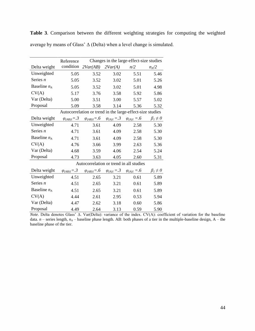
44


average by means of Glass’ Δ (Delta) when a level change is simulated.

Reference

condition


Delta weight 2Var(AB) 2Var(A) n/2 nA/2

Unweighted 5.05 3.52 3.02 5.51 5.46

Series n 5.05 3.52 3.02 5.01 5.26

Baseline nA 5.05 3.52 3.02 5.01 4.98

CV(A) 5.17 3.76 3.58 5.92 5.86

Var (Delta) 5.00 3.51 3.00 5.57 5.02

Proposal 5.09 3.58 3.14 5.36 5.32


Delta weight φ(AB)1=.3 φ(AB)1=.6 φ(A)1 =.3 φ(A)1 =.6 β1 ≠ 0

Unweighted 4.71 3.61 4.09 2.58 5.30

Series n 4.71 3.61 4.09 2.58 5.30

Baseline nA 4.71 3.61 4.09 2.58 5.30

CV(A) 4.76 3.66 3.99 2.63 5.36

Var (Delta) 4.68 3.59 4.06 2.54 5.24

Proposal 4.73 3.63 4.05 2.60 5.31


Delta weight φ(AB)1=.3 φ(AB)1=.6 φ(A)1 =.3 φ(A)1 =.6 β1 ≠ 0

Unweighted 4.51 2.65 3.21 0.61 5.89

Series n 4.51 2.65 3.21 0.61 5.89

Baseline nA 4.51 2.65 3.21 0.61 5.89

CV(A) 4.44 2.61 2.95 0.53 5.94

Var (Delta) 4.47 2.62 3.18 0.60 5.86

Proposal 4.49 2.64 3.13 0.59 5.90 Note. Delta denotes Glass’ Δ. Var(Delta): variance of the index. CV(A): coefficient of variation for the baseline

data. n – series length, nA – baseline phase length. AB: both phases of a tier in the multiple-baseline design, A – the

baseline phase of the tier.

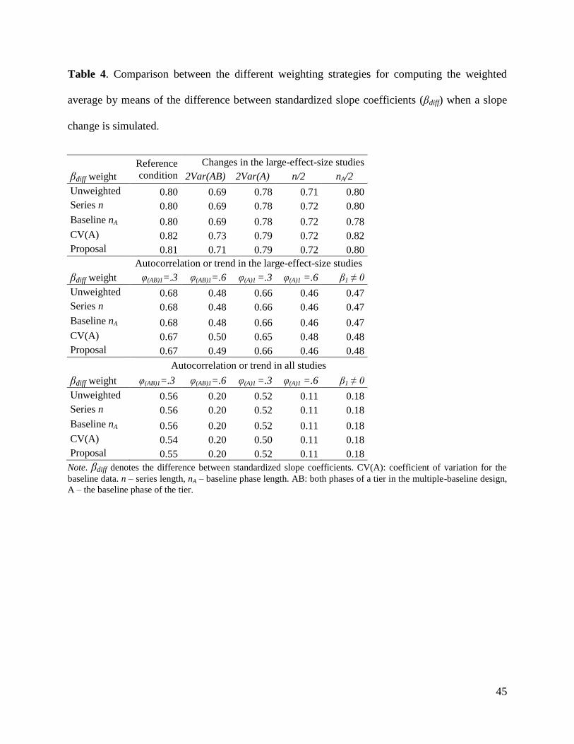
45


average by means of the difference between standardized slope coefficients (βdiff) when a slope

change is simulated.

Reference

condition


βdiff weight 2Var(AB) 2Var(A) n/2 nA/2

Unweighted 0.80 0.69 0.78 0.71 0.80

Series n 0.80 0.69 0.78 0.72 0.80

Baseline nA 0.80 0.69 0.78 0.72 0.78

CV(A) 0.82 0.73 0.79 0.72 0.82

Proposal 0.81 0.71 0.79 0.72 0.80


βdiff weight φ(AB)1=.3 φ(AB)1=.6 φ(A)1 =.3 φ(A)1 =.6 β1 ≠ 0

Unweighted 0.68 0.48 0.66 0.46 0.47

Series n 0.68 0.48 0.66 0.46 0.47

Baseline nA 0.68 0.48 0.66 0.46 0.47

CV(A) 0.67 0.50 0.65 0.48 0.48

Proposal 0.67 0.49 0.66 0.46 0.48


βdiff weight φ(AB)1=.3 φ(AB)1=.6 φ(A)1 =.3 φ(A)1 =.6 β1 ≠ 0

Unweighted 0.56 0.20 0.52 0.11 0.18

Series n 0.56 0.20 0.52 0.11 0.18

Baseline nA 0.56 0.20 0.52 0.11 0.18

CV(A) 0.54 0.20 0.50 0.11 0.18

Proposal 0.55 0.20 0.52 0.11 0.18

Note. βdiff denotes the difference between standardized slope coefficients. CV(A): coefficient of variation for the

baseline data. n – series length, nA – baseline phase length. AB: both phases of a tier in the multiple-baseline design,

A – the baseline phase of the tier.

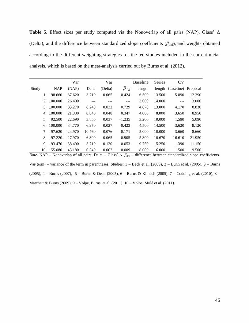
46

Table 5. Effect sizes per study computed via the Nonoverlap of all pairs (NAP), Glass’ Δ

(Delta), and the difference between standardized slope coefficients (βdiff), and weights obtained

according to the different weighting strategies for the ten studies included in the current meta-

analysis, which is based on the meta-analysis carried out by Burns et al. (2012).

Var Var Baseline Series CV

Study NAP (NAP) Delta (Delta) βdiff length length (baseline) Proposal

1 98.660 37.620 3.710 0.065 0.424 6.500 13.500 5.890 12.390

2 100.000 26.400 --- --- --- 3.000 14.000 --- 3.000

3 100.000 33.270 8.240 0.032 0.729 4.670 13.000 4.170 8.830

4 100.000 21.330 8.840 0.048 0.347 4.000 8.000 3.650 8.950

5 92.500 22.690 3.850 0.037 −1.235 3.200 10.000 1.590 5.090

6 100.000 34.770 6.970 0.027 0.423 4.500 14.500 3.620 8.120

7 97.620 24.970 10.760 0.076 0.171 5.000 10.000 3.660 8.660

8 97.220 27.970 6.390 0.065 0.905 5.300 10.670 16.610 21.950

9 93.470 38.490 3.710 0.120 0.053 9.750 15.250 1.390 11.150

10 55.080 45.180 0.340 0.062 0.009 8.000 16.000 1.500 9.500

Note. NAP – Nonoverlap of all pairs. Delta – Glass’ Δ. βdiff – difference between standardized slope coefficients.

Var(term) – variance of the term in parentheses. Studies: 1 – Beck et al. (2009), 2 – Bunn et al. (2005), 3 – Burns

(2005), 4 – Burns (2007), 5 – Burns & Dean (2005), 6 – Burns & Kimosh (2005), 7 – Codding et al. (2010), 8 –

Matchett & Burns (2009), 9 – Volpe, Burns, et al. (2011), 10 – Volpe, Mulé et al. (2011).

Weighting strategies in the meta-analysis of single-case studies

Documents

Transcript of Weighting strategies in the meta-analysis of single-case studies