Multilevel meta-analysis of single-subject experimentaldesigns: A simulation study

Maaike Ugille & Mariola Moeyaert &S. Natasha Beretvas & John Ferron &

Wim Van den Noortgate

Published online: 31 May 2012# Psychonomic Society, Inc. 2012

Abstract One way to combine data from single-subjectexperimental design studies is by performing a multilevelmeta-analysis, with unstandardized or standardized regres-sion coefficients as the effect size metrics. This study eval-uates the performance of this approach. The results indicatethat a multilevel meta-analysis of unstandardized effect sizesresults in good estimates of the effect. The multilevel meta-analysis of standardized effect sizes, on the other hand, issuitable only when the number of measurement occasionsfor each subject is 20 or more. The effect of the treatment onthe intercept is estimated with enough power when thestudies are homogeneous or when the number of studies islarge; the power of the effect on the slope is estimated withenough power only when the number of studies and thenumber of measurement occasions are large.

Keywords Meta-analysis . Multilevel . Single-subjectexperimental design . Effect size

Single-case or single-subject experimental designs (SSEDs)are used when one is interested in the effect of a treatmentfor one specific subject, a person or another entity. In the

most basic design, the time series design, the subject isobserved several times before the treatment, during the socalled baseline phase, and several times during or after thetreatment. Because it is difficult to generalize the resultsfrom such an experiment to other subjects, the experimentcan be replicated within or across studies. Next, the resultsof several single-case studies can be combined using meta-analytic techniques. There is a plethora of research indicat-ing how to perform a meta-analysis of group comparisonstudies, in which study subjects are typically measured onlyonce or a few times (e.g., Cooper, 2010; Lipsey & Wilson,2001). In contrast, procedures necessary to conduct a meta-analysis of SSEDs are not well documented, and it is notstraightforward how SSEDS should be meta-analyzed. Thisis because SSED data differ from group comparison studydata. SSEDs entail a far smaller number of subjects forwhom many repeated measures are taken. The resultingsmall-sample size and interrupted time series data mayinvolve cyclical patterns or serial dependencies (West &Hepworth, 1991).

Reviews of meta-analyses of SSEDs indicate that a mul-titude of methods are used (Beretvas & Chung, 2008;Maggin, O'Keeffe, & Johnson, 2011), each method havingits own advantages and weaknesses. Most studies about themethodology of SSED meta-analysis have focused on thequestion of which effect size should be used to describe thetreatment effect in each study being synthesized (e.g.,Campbell, 2004; Parker, Vannest, & Davis, 2011; Wolery,Busick, Reichow, & Barton, 2010). There have been manyproposals: nonparametric approaches (e.g., the percentageof nonoverlapping data statistic; Scruggs, Mastropieri, &Casto, 1987), parametric approaches (e.g., standardizedmean difference; Gingerich, 1984), and regression-basedmethods (Alison & Gorman, 1993; Center, Skiba, &Casey, 1985–1986; Van den Noortgate & Onghena, 2003a,

M. Ugille (*) :M. Moeyaert :W. Van den NoortgateFaculty of Psychology and Educational Sciences,University of Leuven,Vesaliusstraat 2,3000 Leuven, Belgiume-mail: maaike.ugille@ppw.kuleuven.be

S. N. BeretvasUniversity of Texas at Austin,Austin, TX, USA

J. FerronUniversity of South Florida,Tampa, FL, USA

Behav Res (2012) 44:1244–1254DOI 10.3758/s13428-012-0213-1

2003b). Maggin et al. (2011b) compared the weaknessesand advantages of several methods (both parametric andnonparametric), and on the basis of this overview, useof the hierarchical linear or multilevel model seemedmost promising. Use of a multilevel model is consistentwith the logic of visual analysis, can control for threatsto interpretation (e.g., autocorrelation), and has attractivestatistical properties (e.g., being able to capture differ-ences between subjects and/or studies in the magnitudeof the effect).

In this study, we will examine the effectiveness ofusing a multilevel meta-analysis to synthesize effectsizes from a set of SSEDs’ results. Van den Noortgateand Onghena (2008) illustrated this approach using areanalysis of the study results combined in the meta-analysis of Shogren, Fagella-Luby, Bae, and Wehmeyer(2004). However, an illustration using real data does notprove that the multilevel approach results in properparameter and standard error estimates for the effectsize and variance components. Simulation researchmakes it possible to investigate the latter question, be-cause population parameters are specified in advanceand, therefore, also known. First, we will discuss themultilevel approach to meta-analysis of SSEDs; next,we will present our simulation study.

Multilevel meta-analysis of SSEDs

Meta-analysis is a set of statistical methods for combiningthe results of various studies addressing the same re-search question (Glass, 1976). In order to combine theseanalysis results, study results are typically first con-verted to a common standardized effect size metric.The advantage of using effect sizes is that it is notnecessary that all raw data are available in all studies.Effect sizes may already be reported in a study, or theycan be calculated on the basis of available test statistics.One possible way to calculate effect sizes when usingSSEDs is to make use of a regression model. Center etal. (1985–1986) proposed using the following regressionmodel to analyze data from an SSED study:

Yi ¼ b0 þ b1Ti þ b2Di þ b3TiDi þ ei ð1Þwhere Yi is the score of the subject at the ith point intime, Di is a dummy variable that equals 0 in thebaseline phase and 1 in the treatment phase, and Ti isa time-related variable that equals 0 on the first day ofthe treatment phase. Therefore, β0 is the baseline inter-cept, and β1 is the linear trend during the baseline. β2refers to the treatment effect on the intercept for thetrend during the intervention phase, and β3 refers to the

effect of the treatment on the time trend. Van denNoortgate and Onghena (2003a) proposed using the lasttwo regression coefficients as effect size measures: β2for the immediate treatment effect and β3 for the treat-ment effect on the time trend.

If we can obtain, for each case, estimates for these twoeffect sizes, either by using Eq. 1 on the raw data or on thebasis of reported summary statistics or test statistics, thenthe resulting effect sizes can be combined in two separatemeta-analyses: one for the immediate treatment effect andone for the treatment effect on the time trend. There areseveral ways to do this. A three-level model presented byVan den Noortgate and Onghena (2003b, 2008) makes itpossible to model variability in effect sizes at each of thethree levels. At the first level, the effect size estimates of theimmediate treatment effect for case j from study k may bemodeled to randomly deviate from the unknown populationeffect size:

b2jk ¼ b2jk þ r2jk with r2jk � N 0;σ2r2jk

� �ð2Þ

with b2jk the ordinary least squares (OLS) estimate of β2jk.The random deviations of the observed regression coeffi-cients are assumed to be normally distributed with a vari-ance that depends on the coefficient and the subject.Because we have only one estimate per case for a coeffi-cient, this variance cannot be estimated in the three-levelanalysis. However, the sampling variance of the regressioncoefficients, σ2

r2jk, can be estimated in the original OLS

regression analysis used to estimate the regression coeffi-cient or can be derived from summary or test statisticsreported in the primary SSED study. Because thesevariances are estimated before the actual meta-analysisis performed, the three-level meta-analysis (as well asother typical meta-analyses) can be regarded as a “var-iance known problem” (Raudenbush & Bryk, 2002).

The population effect sizes β2jk from study k can bemodeled as varying over subjects around a study-specificmean effect θ20k (second level) as follows:

b2jk ¼ θ20k þ u2jk with u2jk � N 0;σ2u2jk

� �ð3Þ

and the effects for studies can vary between studies (thirdlevel):

θ20k ¼ g200 þ u20k with u20k �N 0;σ2u20k

� �ð4Þ

The same fundamental three-level model could alsobe used to model variability in the treatment’s effect onthe time trend, using the following level one, two, and threeequations,

b3jk ¼ b3jk þ r3jk with r3jk � N 0;σ2r3jk

� �ð5Þ

Behav Res (2012) 44:1244–1254 1245

b3jk ¼ θ30k þ u3jk with u3jk � N 0;σ2u3jk

� �ð6Þ

θ30k ¼ g300 þ u30k with u30k � N 0;σ2u30k

� �; ð7Þ

respectively.When the scale used is not the same for all subjects, the

effect sizes b2jk and b3jk are not comparable across subjectsand, therefore, cannot be combined. For example, if thedependent variable for a first subject can range from 0 to10 and for a second subject from 0 to 100, the expectedunstandardized effect size of the second subject may be 10times larger than the effect size of the first subject.Unstandardized effect sizes are appropriate only when thedependent variable is measured in the same way for allsubjects. In practice, this situation is rare, unless studiesare exact replications of each other. In the example, alsothe expected residual standard deviation σe will be 10 timeslarger for the second subject. Therefore, effect sizes can bemade comparable over subjects by standardizing b2jk or b3jk,by dividing them by the estimated residuals’ standard devi-ation bσeð Þ (Van den Noortgate & Onghena, 2003b, 2008).This residual standard deviation can be estimated by esti-mating the OLS regression model in Eq. 1 separately foreach subject and then finding the square root of the meansquare error or the RMSE of each separate regression. Whenthere are a lot of measurements for each subject, this stan-dard deviation can be estimated reasonably well. On the otherhand, when there are only a few measurements available foreach subject, this standard deviation might be poorly estimat-ed, resulting in poor estimates of the standardized effect size.Therefore, in this study, we are primarily interested in theperformance of a multilevel meta-analysis when there arenot many measurements for each subject.

During a single-subject experiment, subsequent measure-ments can be influenced by common (random) factors, withthe result that measurements close to each other in time maybe correlated. This phenomenon of autocorrelation can beincluded in the previous multilevel model by specifying anautoregressive covariance structure for the first-level errors(i.e., the ei from Eq. 1). In the present study, however, wewill focus on the basic model with no autocorrelation.

The parameters typically estimated in a multilevel analy-sis are the fixed effects regression coefficients (e.g., γ200

referring to the average immediate treatment effect overcases and studies and γ300 referring to the average treatmenteffect on the linear trend in Eqs. 4 and 7, respectively).Although this multilevel approach seems well suited forsingle-case data, in practice, it is seldom used. One reasonmight be that little is known about the functioning of thismodel for SSED meta-analysis. This study assesses theperformance of this method in more detail, using a set ofrealistic situations.

Method

To evaluate the performance of the three-level approach, weused a simulation study consisting of several steps. In a firststep, raw data were simulated. In a second step, the unstandard-ized regression coefficients of Eq. 1 were estimated for eachsubject, using OLS estimation. Next, these estimates were di-vided by the residual within-phase standard deviation, to obtaincorresponding standardized effect sizes. Finally, the unstandard-ized and the standardized effect sizes were separately analyzedusing the three-level meta-analytic approach (using Eqs. 2–7),and the results were compared with the parameter values used togenerate data. Despite the fact that meta-analyses with unstan-dardized effect sizes will rarely be performed in practice, theyare analyzed in this study, because if problems arise, we can findout whether these problems are due to the standardization of theeffects or to the multilevel meta-analysis itself.

To simulate the raw data, the following measurementoccasion (level one) model was used:

Yijk ¼ b0jk þ b1jkTijk þ b2jkDijk þ b3jkTijkDijk þ eijk

with eijk � N 0;σ2e

� � ð8Þ

with occasions nested within individuals at level two:

b0jk ¼ θ00k þ u0jkb1jk ¼ θ10k þ u1jkb2jk ¼ θ20k þ u2jkb3jk ¼ θ30k þ u3jk

8>><>>: with

u0jku1jku2jku3jk

2664

3775 � N 0;Σuð Þ; ð9Þ

and within studies at level three:

θ00k ¼ g000 þ u00kθ10k ¼ g100 þ u10kθ20k ¼ g200 þ u20kθ30k ¼ g300 þ u30k

with

v00kv10kv20kv30k

2664

3775

8>><>>: � N 0;Σuð Þ ð10Þ

Note that we simulated data on the same scale for eachsubject and study. However, this is not a limitation in thissimulation study. If we had simulated data using differentscales, this effect would be neutralized by the standardiza-tion (e.g., if for a specific subject we had multiplied eachscore by five, both the estimated regression coefficients andthe estimated residual standard deviations would be 5 timeslarger, so the estimated standardized coefficients wouldremain unchanged). By simulating data on the same scale,however, it is possible to evaluate the use of the multilevelmodel for SSED meta-analysis for situations in which stan-dardization is required or is not required at the same time.

The effect sizes were synthesized using the restrictedmaximum likelihood estimation procedure implemented inSAS PROC MIXED (Littell, Milliken, Stroup, Wolfinger, &Schabenberger, 2006). We used the Satterthwaite approachto estimating degrees of freedom. This approach has beenshown for two-level analyses of multiple-baseline data to

1246 Behav Res (2012) 44:1244–1254

provide relatively accurate confidence intervals for estimatesof the average treatment effect (Ferron, Bell, Hess, Rendina-Gobioff, & Hibbard, 2009), using a model without lineartrends to simulate and analyze the data. On the basis of theseresults, we expect that use of this estimation procedure forthree-level analyses would also result in relatively accurateconfidence intervals for the overall treatment effects.

The γ200 coefficient represents the shift in level thatoccurs due to the treatment. Data were generated assumingno effect (γ200 0 0) and 2 times the within-phase standarddeviation (γ200 0 2). We chose values of 0 (no effect) and0.2 times the within-phase standard deviation for the overalleffect on the slope, γ300. These values were based on rean-alyses of meta-analyses (Alen, Grietens, & Van denNoorgate, 2009; Denis, Van den Noortgate, & Maes, 2011;Kokina & Kern, 2010; Shogren et al., 2004; Wang, Cui, &Parrila, 2011). The effects of the baseline regression coef-ficients γ000 and γ100, were set at zero.

The number of studies (K) in each simulated meta-analysis was manipulated to be 10 or 30. A review of 39social science single-case meta-analyses (Farmer, Owens,Ferron, & Allsopp, 2010) showed that the number of studiesincluded in a meta-analysis ranged from 3 to 117, with 60 %of the meta-analysis including fewer than 30 studies.

We simulated studies with a multiple baseline design. Thenumber of subjects per study (J) was 3, 4, or 7. These values arebased on recommendations of Barlow and Hersen (1984) andKazdin and Kopel (1975), a survey of multiple-baseline studies(Ferron et al., 2010), a review of Farmer et al. (2010), and asurvey of single-case studies of Shadish and Sullivan (2011).

The series lengths (I) consisted of 10, 20, or 40 observa-tions. The survey of Ferron et al. (2010) found averageseries lengths that ranged from 7 to 58, with a median of24, and the survey of Shadish and Sullivan (2011) foundthat the number of data points per case ranged from 2 to 160,with median and mode equal to 20. A meta-analysis of 85single-case studies (Swanson & Sachse-Lee, 2000) foundthat 25 studies had fewer than 11 treatment sessions, 37studies had between 11 and 29 treatment sessions, and 23studies had more than 29 treatment sessions.

The intervention introductions were staggered acrosssubjects within studies. For each combination of the numberof subjects and number of data points, the moment at which

the treatment started is given in Table 1. For example, whenthere were 3 subjects and the number of measurement occa-sions for each subject equaled ten, then for the first subject,the treatment started on the fourth measurement occasion,for the second subject on the sixth measurement occasion,and for the third subject on the eighth measurement occa-sion, and for all 3 subjects the treatment lasted until the tenthmeasurement occasion.

Elements of the within-study variance matrix, Σu, weremanipulated to have conditions with relatively small andrelatively large amounts of within-study variance. For sim-plicity, covariances between regression coefficients were setto zero at the subject and study levels. Therefore, Σu is a

diagonal matrix,P

u ¼ diag σ2u0;σ2

u1;σ2

u2;σ2

u3

� �. A review of

several reanalyses indicated that the variance between sub-jects is sometimes less than the within-person variance(Ferron et al., 2009; Van den Noortgate & Onghena,2003a) and sometimes greater than the within-person vari-ance (Van den Noortgate & Onghena, 2008). If the within-person (level one) variance is set to 1.0, setting the fourdiagonal elements of Σu to values of 2, 0.2, 2, 0.2 (for thevariances in the baseline intercept, baseline slope, treatmenteffect on the intercept, and treatment effect on the sloperesiduals, respectively) represents a relatively large amountof within-study variability, while setting the four diagonalelements of Σu to values of 0.5, 0.05, 0.5, 0.05, respectively,represents a relatively small amount of within-study variability.Reanalyses of real data sets (Denis et al., 2011; Kokina &Kern, 2010; Shogren et al., 2004) indicated that the varianceof the effect of γ200 is sometimesmuch larger than the varianceof the effect of γ300. Therefore, we also set the four diagonalelements of Σu to values of 8, 0.08, 8, 0.08.

Elements of the between-study variance matrix, Σv, werealso manipulated. On the basis of reanalyses of meta-analyses (Alen et al., 2009; Denis et al., 2011; Heyvaert,Maes, Van den Noorgate, Kuppens, & Onghena, in press;Kokina &Kern, 2010; Shogren et al., 2004;Wang et al., 2011),

we setP

u ¼ diag σ2v0;σ2

v1;σ2

v2;σ2

v3

� �equal to diag( 2, 0.2, 2,

0.2), diag( 0.5, 0.05, 0.5, 0.05), and diag( 8, 0.08, 8, 0.08).Crossing the levels of the seven factors leads to a 3 × 3 ×

2 × 2 × 2 × 3 × 3 factorial design yielding 648 experimental

Table 1 The number of the measurement occasion at which the treatment started

Number of subjects

3 4 7

Total number of data points 10 4 – 6 – 8 4 – 5 – 7 – 8 4 – 5 – 5 – 6 – 7 – 7 – 8

20 7 – 11 – 15 7 – 10 – 12 – 15 7 – 9 – 9 – 11 – 13 – 13 – 15

40 11 – 21 – 31 11 – 18 – 24 – 31 11 – 15 – 15 – 21 – 27 – 27 – 31

Behav Res (2012) 44:1244–1254 1247

conditions. For each condition, 2,000 data sets were simu-lated and analyzed, with a total of 1,296,000 data sets.

Results

Wewill successively discuss the estimates of both fixed effectsused to describe an intervention’s effect (on the intercept andslope), the mean squared error, the estimation of thecorresponding standard errors, the confidence interval cover-age, the power, and the estimates of the variances. Because it isimpossible to discuss the 648 conditions separately, weexplored variation between conditions using an ANOVA,modeling main effects and two-way interaction effects, anddiscuss below only the effect for which the ANOVA showedclear evidence (p < .001). This procedure was primarily used todistinguish the most important patterns in the results.

Overall effect size estimates

In the simulation study, the mean population effect on theintercept was 0 or 2, and the effect on the time trend was 0 or0.2. In each meta-analysis, we estimated these mean effects.These estimates will likely deviate from this mean populationeffect, because of random variation at each of the three levels.

In Fig. 1, the distribution of the deviations is given for γ200

equal to 0 or 2 and the number of measurements equal to 10,20, or 40 when the unstandardized and the standardized re-gression coefficients are analyzed. For the unstandardizedeffect size estimates, close to no bias was identified.

The results differ for the standardized effect sizes. Whenγ200 equaled 0, the estimated bias was close to zero. Whenγ200 equaled 2, the estimated bias of the standardized effectsizes was 0.310 when there are only 10 measurement occa-sions, 0.110when there are 20measurements, and 0.044 when

there are 40 measurements. We also sorted all conditions bytheir estimated bias, and the 100 conditions with the largestbias all had γ200 0 2 and I 0 10. The condition with the mostbias was γ200 0 2, γ300 0 0, K 0 10, J 0 4; I 0 10, σ2

v2¼ 8;

and σ2u2¼ 0:5; in this condition, the bias equaled 0.350. The

number of studies, the number of subjects, and the true valuesof the between- and within-study variances were each foundto have no substantial effect on the estimated bias.

The results for the estimates of γ300 were similar to whatwas found for γ200. There was positive bias when standard-ized effect sizes were used if γ300 0 0.2 and I 0 10. If γ200 0

2, γ300 0 0.2, K 0 10, J 0 4; I 0 10, σ2v2¼ 2; and σ2

u2¼ 2,

the bias was 0.030, with a minimum and maximum devia-tion of −1.071 and 0.883, respectively, and with lower andupper quartiles of −0.115 and 0.178. The relative biases ofthe two estimates when a meta-analysis on standardizedeffect sizes was performed were more or less the same:The relative bias of the estimate of both γ200 and γ300 was0.155. The standard deviation of the relative deviations, onthe other hand, differed: 0.324 for the estimates of γ200 and1.090 for the estimates of γ300.

These results indicate that the positive bias when γ200

and γ300 are larger than zero and the number of measure-ments equals 10 results from the standardization of theeffects. In this simulation study, however, it is not clearwhether this positive bias is caused by calculating a weight-ed average of the individual regression coefficients orwhether these individual regression coefficients themselvesare already biased. That is why we also checked the distri-bution of the deviations from the true value of the individualregression coefficients β2jk for γ200 0 2, γ300 0 0.2, K 0 10,

J 0 4, I 0 10, σ2v2¼ 2; and σ2

u2¼ 2. In this condition, there

were 80,000 estimates of β2jk. Table 2 shows that there isalmost no bias when the effect sizes are unstandardized andthat there is a positive bias of 0.302 when the effect sizes arestandardized. This indicates that the bias of the estimatedoverall effects is mainly due to the standardization of theindividual regression coefficients and not a result of calcu-lating a weighted average.

Mean squared error

The mean squared error (MSE) is equal to the averagesquared deviation of the estimates from the true value, andtherefore, it is preferred that the MSE is as small as possible.The MSE is, as was expected, smaller when the number ofstudies, the number of cases, or the number of measurementoccasions increases. On the basis of the ANOVA, the num-ber of studies and the between-study variance seem to havethe most important influence on the MSE. This influence isillustrated in Table 3 for both the unstandardized and thestandardized effect sizes.

Fig. 1 Distribution of the deviations of the estimated mean effect onthe intercept of the treatment from its populations value (γ200) for boththe unstandardized and standardized effect sizes, for γ300 0 0.2, K 0 10,J 0 4, σ2

v2¼ 2; and σ2

u2¼ 2 conditions

1248 Behav Res (2012) 44:1244–1254

Standard error estimates

In addition to assessing parameter estimation for each of thetwo fixed effects (on the intercept and slope), we also evaluatedestimation of the standard errors of each of these effects. Thesestandard errors can be used to construct confidence intervalsand to perform tests of the statistical significance of the effects.By definition, the standard error equals the standard deviationof the sampling distribution of the estimated effects. In thissimulation study, we performed for each condition 2,000 meta-analyses, which results in 2,000 estimates of the effect. Becauseof the reasonably large number of estimates, we can regard thestandard deviations of the estimates as a good estimate of thestandard deviations of the estimator’s sampling distribution andcan, therefore, use this standard deviation to evaluate the qualityof the standard error estimates.

The median of the standard error estimates was found tobe almost equal to the standard deviation of the estimates ofthe effect for both the unstandardized and the standardizedeffects. As was expected, the standard error decreased whenthe number of studies, the number of measurement occa-sions, or the number of subjects increased or in conditionswith lower between-study or within-study variance values.

The results were similar for both the standardized and theunstandardized effect sizes. The standard error of the unstan-dardized estimate ofγ200 was slightly underestimated in 83.3%of the conditions and the relative bias over all conditions was−0.022. The difference between the median of the standarderror estimates and the standard deviation of the effect sizeestimates was greatest for γ200 0 0, γ300 0 0, K 0 10, J 0 3,I 0 10, σ2

v2¼ 8; and σ2

u2¼ 8. In this situation, the median of

the standard error equaled 1.020, and the standard deviations of

the estimates equaled 1.103. For the standardized effects, thestandard error was slightly underestimated in 86.4 % of theconditions and the relative bias over all conditions was −0.025.The difference between themedian of the standard error and thestandard deviation of the estimates was greatest in the sameconditions as for the unstandardized data, with the median ofthe standard error equal to 1.198 and the standard deviations ofthe estimates equal to 1.311. On the basis of the ANOVA, thereseemed to be only a small effect of the number of studies on thedifference between the median of the standard error and thestandard deviation of the estimates. The results were alsosimilar for the estimates of the standard error of γ300.

Confidence interval coverage

Another way to evaluate estimation of the effect sizes and oftheir corresponding standard errors is by calculating theproportion of replications in which the confidence intervalcontained the population effect size. The lower and upperlimits of the confidence intervals around the estimated effectare constructed by multiplying the estimated standard errorwith the right critical value of the z-distribution and sub-tracting from and adding this product to the point estimate ofthe effect. For a 95 % confidence interval, we expected thatthe coverage proportion would be around 95 %. Because wesimulated 2,000 data sets for each condition, the coverageproportions could be estimated accurately—more specifically,

with a standard error of 0:005 ¼ ffiffiffiffiffiffiffiffiffiffiffiffiffiffiffiffiffiffiffiffiffiffiffiffiffiffiffiffiffiffiffiffiffiffiffi0:95*0:05ð Þ 2000=

p� �—

and therefore, we expected the coverage proportion to rangefrom 94.04 % to 95.96 % (with α 0 .05).

The coverage proportions for the unstandardized estimateof γ200 ranged from 93.45 % to 97.10 %, and in 91.36 % ofthe conditions, the coverage proportion lay between94.04 % and 95.96 %. The coverage proportions for theunstandardized estimate of γ300 ranged from 93.60 % to96.85 %. In 92.90 % of the conditions, the coverage pro-portion lay between 94.04 % and 95.96 %.

The results for the standardized estimates of γ200 dif-fered. In 77.47 % of the conditions, the coverage propor-tions lay between 94.04 % and 95.95 %; however, for the

Table 2 Distribution of the deviations of the individual regressioncoefficients estimates of β2jk, for γ200 0 2, γ300 0 0.2, K 0 10, J 0 4,I 0 10, σ2

v2¼ 2; and σ2u2 ¼ 2 conditions

Mean SD Min Max

Unstandardized −0.003 2.452 −10.201 10.444

Standardized 0.302 3.123 −22.297 55.865

Table 3 Mean squared error of (MSE) γ200 and γ300, for γ200 0 2, γ300 0 0.2, J 0 4, I 0 20, and σ2u2¼ 2 conditions

K σ2v2 MSE of γ200 σ2v3 MSE of γ300

Unstandardized Standardized Unstandardized Standardized

10 0.5 0.129 0.161 0.05 0.011 0.012

2 0.261 0.307 0.08 0.015 0.017

8 0.877 0.996 0.20 0.025 0.028

30 0.5 0.041 0.059 0.05 0.004 0.004

2 0.083 0.104 0.08 0.005 0.006

8 0.302 0.347 0.20 0.008 0.010

Behav Res (2012) 44:1244–1254 1249

other conditions, the coverage proportions were often toolow, with a minimum of 70.65 % when γ200 0 2, γ300 0 0.2,K 0 30, J 0 7, I 0 10, σ2

v2¼ 0:5; and σ2

u2¼ 0:5 . There

appears to be a problem with coverage when the effect islarger than zero and when the number of measurementsoccasions is small (I 0 10); and the problem gets worsewhen the number of studies is large (K 0 30) and when the

between-study σ2v2

� �and within-study σ2

u2

� �variances are

rather small (Table 4). Figure 1 already showed that therewas positive bias when the number of measurement occa-sions is small and when the effect is larger than zero. Whenthe number of studies increases, the confidence intervalbecomes narrower, and the lower coverage proportionsmake it clear that this confidence interval varies around abiased estimator.

The 95 % coverage proportion for the standardized esti-mates ofγ300 ranged from 92.8% to 97.1%. In 88.27% of theconditions, the mean coverage proportion lay between94.04 % and 95.96 %. We already mentioned that the relativebias for the estimates of γ200 and γ300 was more or less thesame but that the standard deviation of the relative deviations

of the estimates of γ300 from the true value was larger. Thiswill result (again in relative terms) in larger estimated standarderrors and wider confidence intervals, and this results in abetter coverage proportion, as compared with the coverageproportion of the standardized estimates of γ200.

Power

In our study, we estimated the actual Type I error rate forconditions where the null hypothesis was true (i.e., γ200 0 0or γ300 0 0), by calculating the proportion of data sets forwhich the null hypothesis was rejected with α equal to .05.For γ200, this proportion is given in Table 5, in the fourththrough seventh columns, for the unstandardized estimates.The results for the standardized estimates were very similar.

When the null hypothesis is false, we want the proportionof correct rejections of the null hypothesis to be as high aspossible and, preferably, above .80. The estimated power forγ200 0 2 and α 0 .05 is given in the last four columns ofTable 5. On the basis of the ANOVA, the number of studies,the within-study variance, the between-study variance, and allthe interactions between these factors seemed to influence

Table 4 Mean coverage proportion of the 95 % confidence interval ofγ200 for both the unstandardized (U) and standardized (S) effect sizesfor γ300 0 0.2 and J 0 4 (upper section of the table) and of γ300 for both

the unstandardized (U) and standardized (S) effect sizes for γ200 0 2and J 0 4 (lower section of the table)

K I γ200 0 0 γ200 0 2

σ2v2¼ 0:5 σ2

v2¼ 8 σ2

v2¼ 0:5 σ2

v2¼ 8

σ2u2¼ 0:5 σ2

u2¼ 8 σ2

u2¼ 0:5 σ2

u2¼ 8 σ2

u2¼ 0:5 σ2

u2¼ 8 σ2

u2¼ 0:5 σ2u2 ¼ 8

U 10 10 .950 .962 .950 .953 .948 .957 .947 .949

20 .949 .962 .948 .949 .953 .960 .955 .951

30 10 .949 .954 .944 .949 .950 .957 .952 .950

20 .951 .955 .952 .953 .951 .955 .948 .949

S 10 10 .951 .963 .952 .954 .914 .944 .944 .944

20 .949 .964 .949 .951 .946 .960 .955 .948

30 10 .950 .955 .947 .952 .775 .889 .924 .935

20 .952 .957 .951 .952 .920 .945 .946 .949

K I γ300 0 0 γ300 0 0.2

σ2v3¼ 0:05 σ2

v3¼ 0:08 σ2

v3¼ 0:05 σ2

v3¼ 0:08

σ2u3¼ 0:05 σ2

u3¼ 0:08 σ2

u3¼ 0:05 σ2

u3¼ 0:08 σ2

u3¼ 0:05 σ2

u3¼ 0:08 σ2

u3¼ 0:05 σ2u3 ¼ 0:08

U 10 10 .958 .955 .952 .954 .954 .956 .952 .954

20 .952 .951 .950 .953 .952 .953 .945 .950

30 10 .950 .956 .943 .952 .952 .957 .954 .953

20 .950 .949 .948 .952 .947 .950 .948 .948

S 10 10 .961 .959 .956 .960 .954 .956 .953 .955

20 .954 .952 .951 .954 .955 .950 .946 .952

30 10 .950 .957 .944 .952 .942 .944 .941 .938

20 .953 .948 .950 .952 .942 .950 .946 .948

Coverage proportions that are significant different from .950 (α 0 .05) appear in bold

1250 Behav Res (2012) 44:1244–1254

power. For conditions in which the number of studies beingmeta-analyzed was 30, the power was high. On the other hand,when there were only 10 studies and a lot of between-studyvariability, the power was found to be much lower.

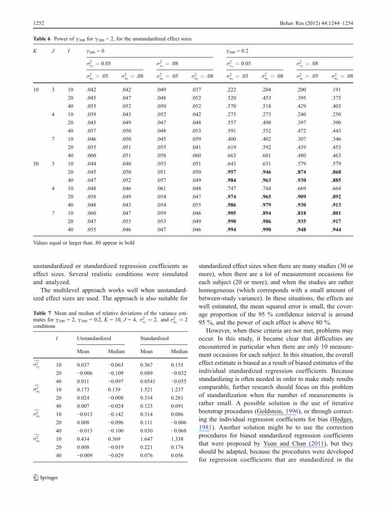
Table 6 contains the power of the estimates of γ300 for theunstandardized effects. The estimated power was lower, ascompared with the power of γ200. The power was above .80only when K 0 30 and I > 10, except if the number of casesequaled 7. Here again, the results for the estimates of thestandardized effects were very similar.

Variance estimates

In the meta-analyses, the between-study and within-studyresiduals’ variances were estimated for both the effect on theintercept and the effect on the slope parameters. We willexamine the relative deviations, which are the deviationsfrom the true value divided by the value of the populationparameter. In this study, the same problem arises for theestimates of the four variances and for the meta-analyses ofboth the unstandardized and the standardized effect sizes:namely, the distribution is positively skewed, with a long tailat the right side. For example, for the meta-analyses on thestandardized effect sizes, the relative bias (i.e., the meanrelative deviation) was larger than 100 % for 13.39 % of the

estimates of the between-study variance of the effect on theintercept, for 12.52 % of the estimates of the between-studyvariance of the effect on the slope, for 25.07% of the estimatesof the within-study variance of the effect on the intercept, andfor 26.94 % of the estimates of the within-study variance ofthe effect on the slope. Table 7 shows the mean and median ofthe relative deviations of the variance estimates.

Table 7 indicates that the relative bias of the varianceestimates was larger when the meta-analysis was performedon standardized effect sizes. The number of measurementsalso had a large effect on the bias of the four estimatedvariances. The within-study variance exhibited the highestbias when the number of measurement occasions was 10. Ingeneral, the median relative deviation of the estimates of thewithin-study variance was larger than that found for thebetween-study variance estimates. The median of the rela-tive deviation of the within-study variance of γ200 wasespecially large when the between-study variance was largeand the within-study variance was small.

Discussion

In this study, we examined whether single-case studiescan be combined using a multilevel meta-analysis, with

Table 5 Power of γ200 for γ300 0 0.2, for the unstandardized effect sizes

K J I γ200 0 0 γ200 0 2

σ2v2¼ 0:5 σ2

v2¼ 8 σ2v2 ¼ 0:5 σ2

v2¼ 8

σ2u2¼ :5 σ2

u2¼ 8 σ2u2 ¼ :5 σ2u2 ¼ 8 σ2

u2¼ :5 σ2

u2¼ 8 σ2

u2¼ :5 σ2

u2¼ 8

10 3 10 .045 .039 .047 .041 .993 .818 .467 .378

20 .041 .044 .049 .055 .998 .851 .515 .394

40 .047 .034 .051 .047 1.000 .875 .498 .389

4 10 .055 .036 .045 .054 .999 .891 .465 .402

20 .058 .033 .050 .051 1.000 .922 .506 .417

40 .059 .040 .046 .046 1.000 .937 .528 .412

7 10 .051 .042 .058 .047 1.000 .985 .480 .457

20 .056 .038 .057 .049 1.000 .988 .506 .456

40 .054 .047 .052 .050 1.000 .991 .494 .475

30 3 10 .053 .049 .049 .056 1.000 1.000 .947 .874

20 .043 .042 .045 .051 1.000 1.000 .956 .892

40 .047 .042 .054 .053 1.000 1.000 .954 .904

4 10 .050 .049 .060 .046 1.000 1.000 .950 .905

20 .052 .048 .049 .040 1.000 1.000 .959 .911

40 .052 .049 .043 .042 1.000 1.000 .956 .909

7 10 .052 .042 .059 .053 1.000 1.000 .959 .948

20 .052 .047 .049 .052 1.000 1.000 .962 .941

40 .055 .045 .054 .048 1.000 1.000 .957 .936

Values equal to or larger than .80 appear in bold

Behav Res (2012) 44:1244–1254 1251

unstandardized or standardized regression coefficients aseffect sizes. Several realistic conditions were simulatedand analyzed.

The multilevel approach works well when unstandard-ized effect sizes are used. The approach is also suitable for

standardized effect sizes when there are many studies (30 ormore), when there are a lot of measurement occasions foreach subject (20 or more), and when the studies are ratherhomogeneous (which corresponds with a small amount ofbetween-study variance). In these situations, the effects arewell estimated, the mean squared error is small, the cover-age proportion of the 95 % confidence interval is around95 %, and the power of each effect is above 80 %.

However, when these criteria are not met, problems mayoccur. In this study, it became clear that difficulties areencountered in particular when there are only 10 measure-ment occasions for each subject. In this situation, the overalleffect estimate is biased as a result of biased estimates of theindividual standardized regression coefficients. Becausestandardizing is often needed in order to make study resultscomparable, further research should focus on this problemof standardization when the number of measurements israther small. A possible solution is the use of iterativebootstrap procedures (Goldstein, 1996), or through correct-ing the individual regression coefficients for bias (Hedges,1981). Another solution might be to use the correctionprocedures for biased standardized regression coefficientsthat were proposed by Yuan and Chan (2011), but theyshould be adapted, because the procedures were developedfor regression coefficients that are standardized in the

Table 6 Power of γ300 for γ200 0 2, for the unstandardized effect sizes

K J I γ300 0 0 γ300 0 0.2

σ2v3 ¼ 0:05 σ2v3¼ :08 σ2v3 ¼ 0:05 σ2v3 ¼ :08

σ2u3 ¼ :05 σ2u3¼ :08 σ2

u3¼ :05 σ2

u3¼ :08 σ2

u3¼ :05 σ2

u3¼ :08 σ2

u3¼ :05 σ2

u3¼ :08

10 3 10 .042 .042 .049 .037 .222 .204 .200 .191

20 .045 .047 .048 .052 .520 .453 .395 .375

40 .053 .052 .050 .052 .570 .518 .429 .403

4 10 .039 .043 .052 .042 .275 .273 .240 .250

20 .045 .049 .047 .048 .557 .498 .397 .390

40 .057 .050 .048 .053 .591 .552 .472 .443

7 10 .046 .050 .045 .059 .400 .402 .307 .346

20 .055 .051 .055 .041 .619 .592 .439 .453

40 .060 .051 .058 .060 .663 .601 .480 .463

30 3 10 .044 .040 .053 .051 .643 .631 .579 .579

20 .045 .050 .051 .050 .957 .946 .874 .868

40 .047 .052 .057 .049 .984 .963 .930 .885

4 10 .048 .046 .061 .048 .747 .744 .669 .664

20 .058 .049 .054 .047 .974 .965 .909 .892

40 .048 .043 .054 .055 .986 .979 .930 .913

7 10 .060 .047 .059 .046 .905 .894 .818 .801

20 .047 .055 .053 .049 .990 .986 .935 .917

40 .055 .046 .047 .046 .994 .990 .948 .944

Values equal or larger than .80 appear in bold

Table 7 Mean and median of relative deviations of the variance esti-mates for γ200 0 2, γ300 0 0.2, K 0 10, J 0 4, σ2

v2¼ 2; and σ2

u2¼ 2

conditions

I Unstandardized Standardized

Mean Median Mean Median

cσ2v2 10 0.037 −0.063 0.367 0.155

20 −0.006 −0.109 0.089 −0.032

40 0.011 −0.097 0.0541 −0.055cσ2u2 10 0.173 0.139 1.521 1.237

20 0.024 −0.008 0.334 0.281

40 0.007 −0.024 0.123 0.091cσ2u3 10 −0.013 −0.142 0.314 0.086

20 0.008 −0.096 0.111 −0.006

40 −0.013 −0.100 0.030 −0.068cσ2u3 10 0.434 0.369 1.647 1.338

20 0.008 −0.019 0.221 0.174

40 −0.009 −0.029 0.076 0.056

1252 Behav Res (2012) 44:1244–1254

traditional way—namely, by multiplying them by the stan-dard deviation of the independent variable and then dividingby the standard deviation of the dependent variable. In thisstudy, we suggest standardizing based on the standard devi-ation of the dependent variable only, and only in so far asthis dependent variable is not explained by the predictors(i.e., we propose to use the residual standard deviation).

An important question for a researcher who wants toconduct a multilevel meta-analysis of SSEDs has to do withthe power of different scenarios. The results are the same forthe unstandardized and the standardized effect sizes. Whenthe immediate effect of the treatment is estimated, the poweris acceptable when the studies are homogeneous, regardlessof the number of studies, cases, or measurement occasions.On the other hand, when the studies’ effect sizes are moreheterogeneous, a power of 80 % or more can be reachedonly when there are a lot of studies (e.g., 30) being meta-analyzed. On the other hand, the effect of the treatment onthe slope is estimated with enough power only when thenumber of studies is 30 or more and the number of mea-surement occasions per subject is 20 or more.

The major advantage of multilevel models is that theyresult not only in an overall estimate of the effect, butalso in an estimate of the between-study and within-study variance. But these estimates are sometimes seri-ously biased. The estimates are worse for meta-analysesof standardized effects, and the estimates of the within-study variance is especially biased when the number ofmeasurements is rather small.

We should also note that the conclusions are, in principle,limited to the conditions that were simulated. These datawere balanced and were sampled from a normal distribution,there was no correlation between consecutive observations,there was no covariance, and the trajectories were not non-linear. In practice, however, data will probably not be bal-anced, autocorrelation will likely occur when observationsare taken in quick succession, there can be another underlyingdistribution, there might be correlation between the effects,and the baseline and/or intervention phase trends might benonlinear. The purpose of this study was to discover whichparameters really matter and to identify in which conditionsproblems occurred. Our aim was to get a preliminary insightinto the empirical functioning of the multilevel model forSSED meta-analysis, but in future research, we will also wantto investigate more complex situations.

In this study, we performed two separate meta-analyses forthe effects b2jk and b3jk, whereby we assumed that these twoeffects are independent of each other. This assumption maynot be realistic in applied settings. If a covariance at the secondand/or third level can be expected, a multivariate meta-analysis might be more powerful (Kalaian & Raudenbush,1996). In a pilot study, we already explored the performanceof the multivariate approach, with simulated effect sizes that

did not covary at the second and third level and showedsampling covariance only at the first level. The results weresimilar to the ones of this study. In future research, wewant to explore the operating characteristics of the multi-variate multilevel model for meta-analytic data of SSEDs insituations where there is nonzero covariance betweenparameters. We expect that the gains of such a multivariatemodel increases (e.g., higher power and accuracy) when thecovariance increases.

We also assumed that the repeated measures were uncor-related. This is probably too strong an assumption in somereal situations, because a typical characteristic of single-casedata is that the measurements are taken in rapid succession.Shadish and Sullivan (2011) showed that the size of auto-correlation varies substantially over studies. In previousresearch (Ferron et al., 2009), where a two-level modelwas used to analyze SSEDs, it was found that not modelingan existing autocorrelation results in biased parameter esti-mates. In this study, we modeled the level one errors as σ2I,but there are many other covariance structures possible, ofwhich the first-order autoregressive type is often used tomodel autocorrelation. Thus, future research should explorescenarios where the repeated measures are autocorrelatedand assess the impact of failing to model this autocorrela-tion, as well as evaluating recovery of model parameters,given the small number of data points typically encounteredin single-case design research.

Can single-case studies be combined with a multilevelmeta-analysis? The answer is yes when it is not necessary tostandardize effect sizes. And even if effect sizes should bestandardized because studies’ outcomes are on differentscales, there are no real problems as long as the studies’effects are reasonably homogeneous or when there are a lotof measurements per individual and there are a lot of studiesbeing meta-analyzed. But the method does not work well forstandardized effect sizes when there are only a few measure-ments for each subject; this situation calls for an adaptationof the method and additional research into alternative esti-mation procedures.

Author note Maaike Ugille, Faculty of Psychology and EducationalSciences, University of Leuven, Belgium; Mariola Moeyaert, Facultyof Psychology and Educational Sciences, University of Leuven,Belgium; S. Natasha Beretvas, Department of Educational Psychology,University of Texas at Austin; John Ferron, Department of EducationalMeasurement & Research, University of South Florida; Wim Van denNoortgate, Faculty of Psychology and Educational Sciences, ITEC-IBBT Kortrijk, University of Leuven, Belgium.

The research reported here was supported by the Institute of Edu-cation Sciences, U.S. Department of Education, through GrantR305D110024 to Katholieke Universiteit Leuven, Belgium. The opin-ions expressed are those of the authors and do not represent views ofthe Institute or the U.S. Department of Education. For the simulations,we used the infrastructure of the VSC–Flemish Supercomputer Center,funded by the Hercules foundation and the Flemish Government–Department EWI.

Behav Res (2012) 44:1244–1254 1253

References

Alen, E., Grietens, H., & Van den Noorgate, W. (2009). Meta-analysisof single-case studies: An illustration for the treatment of anxietydisorders. Unpublished master’s thesis, Katholieke UniversiteitLeuven, Leuven, Belgium.

Alison, D. B., & Gorman, B. S. (1993). Calculating effect sizes formeta-analysis: The case of the single case. Behaviour Researchand Therapy, 31, 621–631.

Barlow, D. H., & Hersen, M. (1984). Single-case experimentaldesigns: Strategies for studying behavior change (2nd ed.). NewYork: Pergamon.

Beretvas, S. N., & Chung, H. (2008). A review of single-subjectexperimental design meta-analyses: Methodological issues andpractice. Evidence-Based Communication and Assessment andIntervention, 2, 129–141.

Campbell, J. M. (2004). Statistical comparison of four effect sizes forsingle-subject designs. Behavior Modification, 28, 234–246.

Center, B. A., Skiba, R. J., & Casey, A. (1985–1986). A methodologyfor the quantitative synthesis of intra-subject design research.Journal of Special Education, 19, 387–400.

Cooper, H. (2010). Research synthesis and meta-analysis (4th ed.).London: Sage.

Denis, J., Van den Noortgate, W., & Maes, B. (2011). Self-injuriousbehavior in people with profound intellectual disabilities: A meta-analysis of single-case studies. Research in DevelopmentalDisabilities, 32, 911–923.

Farmer, J., Owens, C. M., Ferron, J., & Allsopp, D. (2010). A review ofsocial science single-case meta-analyses. Manuscript in preparation.

Ferron, J. M., Bell, B. A., Hess, M. F., Rendina-Gobioff, G., &Hibbard, S. T. (2009). Making treatment effect inferences frommultiple-baseline data: The utility of multilevel modelingapproaches. Behavior Research Methods, 41, 372–384.

Ferron, J. M., Farmer, J. L., & Owens, C. M. (2010). Estimatingindividual treatment effects from multiple-baseline data: AMonte Carlo study of multilevel-modeling approaches. BehaviorResearch Methods, 42, 930–943.

Gingerich, W. J. (1984). Meta-analysis of applied time-series data. TheJournal of Applied Behavioral Science, 20, 71–79.

Glass, G. V. (1976). Primary, secondary, and meta-analysis of research.Educational Researcher, 5, 3–8.

Goldstein, H. (1996). Consistent estimators for multilevel generalizedlinear models using an interated bootstrap. Multilevel ModellingNewsletter, 8, 3–6.

Hedges, L. V. (1981). Distribution theory for Glass’s estimator of effect sizeand related estimators. Journal of Educational Statistics, 6, 107–128.

Heyvaert, M., Maes, B., Van Den Noortgate, W., Kuppens, S., &Onghena, P. (in press). A multilevel meta-analysis of single-caseand small-n research on interventions for reducing challengingbehavior in persons with intellectual disabilities. Research inDevelopmental Disabilities.

Kalaian, H. A., & Raudenbush, S. W. (1996). A multivariate mixed linearmodel for meta-analysis. Psychological Methods, 1, 227–235.

Kazdin, A. E., & Kopel, S. A. (1975). On resolving ambiguities of themultiple-baseline design: Problems and recommendations.Behavior Therapy, 6, 601–608.

Kokina, A., & Kern, L. (2010). Social story interventions for studentswith autism spectrum disorders: A meta-analysis. Journal ofAutism and Developmental Disorders, 40, 812–826.

Lipsey, M., & Wilson, D. (2001). Practical meta-analysis. ThousandOaks, CA: Sage.

Littell, R. C., Milliken, G. A., Stroup, W. W., Wolfinger, R. D., &Schabenberger, O. (2006). SAS© system for mixed models (2nded.). Cary, NC: SAS Institute.

Maggin, D. M., O'Keeffe, B. V., & Johnson, A. H. (2011a). A quan-titative synthesis of methodology in the meta-analysis of single-subject reserach for students with disabilities: 1985–2009.Exceptionality, 19, 109–135.

Maggin, D. M., Swaminathan, H., Rogers, H. J., O'Keeffe, B. V., Sugai,G., & Horner, R. H. (2011b). A generalized least squares regressionapproach for computing effect sizes in single-case research:Application examples. Journal of School Psychology, 49, 301–321.

Parker, R. I., Vannest, K. J., & Davis, J. L. (2011). Effect size in single-case research: A review of nine nonoverlap techniques. BehaviorModification, 35, 303–322.

Raudenbush, S. W., & Bryk, A. S. (2002). Hierarchical linear models:Applications and data analysis methods (Vol. 2). London: Sage.

Scruggs, T. E., Mastropieri, M. A., & Casto, G. (1987). The quantita-tive synthesis of single-subject research: Methodology and vali-dation. Remedial and Special Education, 8, 24–33.

Shadish, W. R., & Sullivan, K. J. (2011). Characteristics of single-casedesigns used to assess intervention effects in 2008. BehaviorResearch Methods, 43, 971–980.

Shogren, K. A., Fagella-Luby, M. N., Bae, J. S., & Wehmeyer, M. L.(2004). The effect of choice-making as an intervention for prob-lem behavior. Journal of Positive Behavior Interventions, 6, 228–237.

Swanson, H. L., & Sachse-Lee, C. (2000). A meta-analysis of single-subject-design intervention research for students with LD.Journal of Learning Disabilities, 33, 114–136.

Van den Noortgate, W., & Onghena, P. (2003a). Combining single-caseexperimental data using hierarchical linear models. SchoolPsychology Quarterly, 18, 325–346.

Van den Noortgate, W., & Onghena, P. (2003b). Hierarchical linearmodels for the quantitative integration of effect sizes in single-case research. Behavior Research Methods, Instruments, &Computers, 35, 1–10.

Van den Noortgate, W., & Onghena, P. (2008). A multilevel meta-analysis of single-subject experimental design studies. EvidenceBased Communication Assessment and Intervention, 2, 142–151.

Wang, S., Cui, Y., & Parrila, R. (2011). Examining the effectiveness ofpeer-mediated and video-modeling social skills interventions forchildren with autism spectrum disorders: A meta-analysis insingle-case research using HLM. Research in Autism SpectrumDisorders, 5, 562–569.

West, S. G., & Hepworth, J. T. (1991). Statistical issues in the study oftemporal data: Daily experiences. Journal of Personality, 59,602–662.

Wolery, M., Busick, M., Reichow, B., & Barton, E. E. (2010).Comparison of overlap methods for quantitaively syntesizingsingle-subject data. Journal of Special Education, 44, 18–28.

Yuan, K., & Chan, W. (2011). Biases and standard errors of standard-ized regression coefficients. Psychometrika, 76, 670–690.

1254 Behav Res (2012) 44:1244–1254