Information and Software Technology 50 (2008) 1142–1154

Contents lists available at ScienceDirect

Information and Software Technology

journal homepage: www.elsevier .com/ locate / infsof

Time-line based model for software project scheduling with genetic algorithms

Carl K. Chang a, Hsin-yi Jiang a,*, Yu Di b, Dan Zhu c, Yujia Ge d

a Department of Computer Science, Iowa State University, USAb Department of Computer Science, University of Illinois at Chicago, USAc College of Business, Iowa State University, USAd Department of Computer Science, Zhejiang Gongshang University, China

a r t i c l e i n f o

Article history:Received 19 July 2007Revised 23 February 2008Accepted 2 March 2008Available online 20 March 2008

Keywords:Genetic algorithmOptimizationProject managementSchedulingTask assignment

0950-5849/$ - see front matter � 2008 Elsevier B.V. Adoi:10.1016/j.infsof.2008.03.002

* Corresponding author. Tel.: +1 5154514458.E-mail address: hsinyij@iastate.edu (H.-y. Jiang).

a b s t r a c t

Effective management of complex software projects depends on the ability to solve complex, subtle opti-mization problems. Most studies on software project management do not pay enough attention to diffi-cult problems such as employee-to-task assignments, which require optimal schedules and careful use ofresources. Commercial tools, such as Microsoft Project, assume that managers as users are capable ofassigning tasks to employees to achieve the efficiency of resource utilization, while the project continu-ally evolves. Our earlier work applied genetic algorithms (GAs) to these problems. This paper extends thatwork, introducing a new, richer model that is capable of more realistically simulating real-world situa-tions. The new model is described along with a new GA that produces optimal or near-optimal schedules.Simulation results show that this new model enhances the ability of GA-based approaches, while provid-ing decision support under more realistic conditions.

� 2008 Elsevier B.V. All rights reserved.

1. Introduction

Experienced software project managers understand the intrin-sic difficulty of managing a complex project involving a large teamof engineers and developers working together in a dynamic, ever-evolving environment with volatile project parameters. Taskassignments and scheduling have always been crucial to the soft-ware development process, and the quality of those assignmentsgreatly influences the success of a project.

The main problem with managing a large software project isthat it is tedious and error-prone [38], oftentimes requiring specificinformation to support it. Frequently, the information needed tooptimize performance is missing. Common project managementtools [1] such as Microsoft Project are not effective at managingoptimization problems. One of the main problems of these toolsis that they use schedule representations that are ‘‘inadequate tomodel the evolutionary and concurrent nature of software devel-opment” [2,3].

To the best of our knowledge, [2] represented the first attemptto develop a richer representation of software project manage-ment, one capable of supporting a genetic algorithm based optimi-zation approach. Improvements to the original model (i.e. SPM-Net[2] or PM-Net [4]) were proposed in [5]. Genetic algorithms (GAs),already commonly used in many domains of optimization research

ll rights reserved.

[6,7], provide better solutions to complex project managementproblems.

The main goal of the current work is to extend and improve themodel in [5], which will be briefly reviewed, making it more pre-cise and realistic. GA is still our choice for optimization, but theinternal ‘‘genome representation”, i.e. the model structure andparameters, has been greatly improved. Complex project manage-ment schemes that exist in the real world but were not represent-able in the old model can now be presented. The added parametersincrease the user’s control of the model. In addition, concepts fromsoftware cost estimation techniques are incorporated into themodel.

This paper is organized as follows: Section 2 introduces somebasic concepts on GA; Section 3 gives a literature review on sched-uling in software project management; Section 4 gives an overviewof the model in [5] and suggests improvements in several aspects;Section 5 describes the new and improved model in detail; Section6 explores properties of the new model and collects numericaldata; and Section 7 outlines the directions for future research.

2. Genetic algorithms

GA is a particular type of evolutionary algorithms introduced inthe 1970s by John Holland [12]. Such algorithms attempt to simu-late natural evolution and form a populous selection of possiblesolutions by exploring the search space in an attempt to findnear-optimal solutions to optimization problems. They do notexhaustively search the entire solution space, but instead start

C.K. Chang et al. / Information and Software Technology 50 (2008) 1142–1154 1143

with a small population of possible solutions and then evolve to-wards better solutions. In the end, fairly good though not necessar-ily optimal solutions for the optimization problem will beproduced. The outline of the algorithm is shown below:

1. Find representations of possible solutions, called genomes,which are composed of genes chosen so that by changing thegenes, all possible solutions can be represented.

2. Map each genome to a real number using a fitness function. Thegoal is to find a genome that maximizes the fitness function.

3. Randomly generate a set of genomes called the initialpopulation.

4. Repeat the following steps until a stopping criterion is met:(a) Selection: select a subset of the population for use in the

next steps.(b) Mutation: produce a new genome from an older one by

changing some of its genes.(c) Crossover: produce a new genome by combining genes from

two older ones.(d) Combination: build a new population using some of the old

and new genomes.Some examples of stopping criteria are:(a) A certain number of generations have been generated.(b) The best individual in the current generation has a high

enough fitness value.(c) The identity of the best individual has not changed for a

number of consecutive generations.

GAs do not guarantee the discovery of the global optimum.However, in many applications a near-optimal solution is oftenacceptable. The representation chosen for the genome is pivotalto the performance of GAs [37].

3. Related work

Generally speaking, our work is to investigate a strategy to as-sign employees to tasks, maximize the quality of project schedules,and minimize the total project cost at the same time. Benefitingfrom the computed schedule of task assignments and durations,thanks to the existence of GA, project managers can carry out thebalancing acts to minimize project costs while achieving other pro-ject objectives. We will report our survey of the related work intwo major categories: software project effort estimation, andscheduling.

3.1. Software project effort estimation

It has been extremely difficult to precisely estimate the total ef-fort demanded for sustaining the lifecycle of a software system.Until now, it is still largely an open issue for researchers althoughmany estimation models had been proposed to predict the effort toconstruct and maintain software. Among them, models designedwith Function Point Analysis (FPA) and Source Lines of Code (SLOC)are commonly seen in the literature.

As a historical note, A.J. Albrecht of IBM devised the functionpoint metric in 1979 [14,15]. FPA became a standard method rec-ognized by ISO, renamed as the Functional Size Measurement, tomeasure the functional size of an information system. It is calcu-lated based on a requirement-centered view of software and isplatform-independent [16,17]. FPA can be employed to determinethe software size for cost estimating and to find the testing effortrequired in the information system [15]. As a result, various orga-nizations adopted FPA as the designated measurement [17–20].Albrecht and Gaffney also suggested the use of function points(FPs) to estimate SLOC and then utilize SLOC to estimate the work

effort [18]. Later, Felfernig and Salbrechter described the applica-tion and extension of FPA for effort estimation in the developmentof knowledge-based configuration systems [17]. Moreover, Nies-sink and Ahn et al. proposed a model based on FPA to predict soft-ware maintenance effort [19,20].

On the other hand, SLOC is used to measure the size of a soft-ware program by counting the number of (non-commentary) linesin the text of the source code of the program. It is typically em-ployed to estimate the effort required to develop a program. Acommonly known model called COCOMO calculates the effort (inperson-months) based on SLOC [21]. Its second generation model,called COCOMO II, is an improvement of COCOMO. It employs bothSLOC and unadjusted function points to express sizes of software[22]. As exemplified from the measurements of project sizes inboth the original COCOMO and COCOMO II, most researchers be-lieve that there exists a high degree correlation between FPA andSLOC [18] [22].

Other estimation methods also exist. For example, analogy-based estimation, seen in some of the existing work, calculatesthe distance between the software project being estimatedand the historical software project data [23]. After having calcu-lated the distances, it retrieves data of the most similar projectsbased on the calculated distance, and estimates the effort basedon those similar projects [23]. In recent years, Huang and Chiu ap-plied GAs to determine the appropriate weighted similarity mea-sures of effort drivers used in analogy-based software effortestimation models [24]. Later, they proposed an adjusted anal-ogy-based software effort estimation model which adopted GA toadjust the effort based on the similarity distances [25]. The exper-imental results obtained from the work of Huang and Chiu sug-gested that such methods indeed helped improve the accuracy ofeffort estimation.

Bayesian analysis is another methodology used to predict soft-ware effort. The results in Pendharkar’s work indicated that theprobabilistic forecasting model allows managers to estimate jointprobability distribution over different software effort estimations(i.e., the effort estimations in terms of different concerns) [26]. Fol-lowing that, project managers can use the joint probability distri-bution to develop a cumulative probability distribution, which inturn helps them estimate the uncertainty of the extent as to howthe actual project effort may be greater than the estimated effort.

In fact, most of the existing software project effort estimationmodels can be employed to support the approach presented in thispaper. For the purpose of illustration, without loss of generality,COCOMO will be most often utilized for the rest of the paper.

3.2. Scheduling

Scheduling problems are NP-hard with extremely complexcombinatorial optimization issues. Research on finding solutionsof resource-constrained project scheduling problems (RCPSPs)has progressed for several decades. The methods form two distinctclasses: exact methods and heuristic methods. Exact methods in-clude backtracking, branch and bound, critical path method withits variations, dynamic programming and implicit enumeration.Heuristic methods, which are popular in scheduling, include simu-lated annealing (SA) [10], Tabu search (TS) [11], and GA [12]. All ofthese methods may be further categorized into stochastic anddeterministic approaches [13]. GA belongs to the class of stochasticsearch methods.

3.2.1. Project scheduling with genetic algorithmsIn recent years, researchers in software engineering found that

genetic algorithm (GA) is a feasible optimization method for theirproblem domains, thus it is used for an increasing number ofapplications.

1144 C.K. Chang et al. / Information and Software Technology 50 (2008) 1142–1154

Hegazy et al. proposed a model for cost optimization and dy-namic project control [36]. The model incorporates an integratedformulation for estimating, scheduling, resource management,and cash-flow analysis. GAs are applied to allocate optional con-struction methods for each activity. Although resource constraintsare also considered in this work, they did not consider much on hu-man factors. Their focus is more on the best combination of con-struction methods.

In 1996, Chan et al. suggested to solve resource schedulingproblems using genetic algorithm [8]. In their paper, an objectivefunction related to resources and constraints related to the prece-dence of tasks are formed. However, the work was emphasizedmore on the GA part, and did not discuss much on the success-ful/failed factors of projects in scheduling.

Hindi et al. demonstrated that the evolutionary algorithm iseffective to solve RCPSPs [27]. An empirical study of 2370 instanceswas conducted. The result showed that the algorithm is capable offinding the best-known solution in 68% of the instances with anaverage overall error rate of 0.95%.

Valls et al. proposed a hybrid GA for the RCPSP [28]. Although itis helpful for the scheduling problem, the focus on their work isbased on the improvement of the algorithm itself, instead of theconcerns of the factors with projects.

Alba and Chicano have shown that GAs are quite flexible andaccurate for project scheduling, and regarded as an important toolfor automatic project management [29]. They provided the basicidea on applying GA for automated task assignments. However,in their model, the experiences and skills of employees are not dis-tinguished. Moreover, changing employees are not allowed duringthe project duration.

To achieve better performance, researchers continue to focus onissues such as representation (direct and indirect) and operators(initialization, mutation, and crossover). Depending on the specificscheduling problem, the performance of GAs can vary greatly oronly by negligible amounts. Our previous model can be consideredas an early effort to apply GAs in the software project managementenvironment [5].

3.2.2. Project scheduling considering human resource factorsThe philosophy of this paper on considering and analyzing more

human resource factors is similar to Plekhanova’s work [30]. Inthat paper, it is asserted that in the mathematical theory of sched-uling, resource capability factors are not considered as the factorsthat influence the schedule since the resources are assumed tobe equal (i.e., they possess equal capabilities). However, in practice,the most effective and efficient manner of resource allocation insoftware projects should be founded on heuristic approaches thatconsider varying capabilities.

As described in this paper, our new model introduces the time-line axis, considers more human resource factors in project man-agement than our previous model, and has the potential to becomea more practical model for project managers to adopt.

4. Overview of previous model

Using a task model, Chang et al. [5] described how to apply GAsto find near-optimal schedules. In the task-based model, the repre-sentation of a problem consists of:

(1) Representation of project: TPG = (V,E)

� The project is represented as a task precedence graph.� A directed a cyclic graph where nodes (v 2 V) represent

tasks and edges (e 2 E) represent task precedence.� Each task is associated with an estimated effort and the

required skills.

2) An employee database Demp with information of skills andsalary.

3) An objective function to evaluate the performance of aschedule.

Genetic representation is an orthogonal 2D array with onedimension for tasks and the other for employees. GA operatorsare adopted from the C++ Genetic Algorithm Library (i.e. GAlib)[31]. In this approach, scheduling is a two-stage process: the firststage evaluates how a genome satisfies constraints; the secondstage evaluates the schedule performance of a genome. The sim-plest objective function for such evaluations can be defined as:

Composite objective function ¼ Validity�ðOverLoadWeight=OverLoad

þMoneyWeight=CostMoney

þ TimeWeight=CostTimeÞ:

Validity (validity of job assignments) is usually scored on a 0/1basis – 0 if the assignments are invalid and 1 if they are valid. Over-Load (minimum level of overtime) is the amount of time workedbeyond the individual overtime limit, which is summed over allemployees. CostMoney (minimum cost) is the total labor cost ofperforming the project, which is computed using the labor ratesof each resource and the hours applied to the tasks. CostTime (min-imum of time span) is the total time span required to finish theproject, from the start of the first task until the end of the last.These three objectives share the same fitness function, to minimizethe appropriate input, i.e., overload, project costs, and time. The fit-ness value is the summation of weighted component objective val-ues. The remainder of this section examines some limitations ofthe above task-based model.

4.1. Restrictions on tasks

In our earlier model, tasks were the basis of personnel assign-ments and calculation of the fitness function. The fitness functioncalculation imposed two restrictions in task assignments:

� A task must begin as early as conditions allow. That is, it beginsas soon as all preconditions are satisfied. However, in real-worldprojects, it may sometimes be advantageous to delay a task.

� A task cannot be interrupted during its execution. In real-worldprojects, however, there may be another emerging task that ismore critical to global fitness. In this case, it may be advanta-geous to refocus efforts on the other task.

4.2. Restrictions on employee assignments

In the task-based model, it was assumed that employeesworked on an assigned task from its beginning to its end. It wasfurther assumed that, once assigned, an employee’s total effortwould be applied to the task. While it is often advantageous to re-tain employees on a task to gain experience or maintain projectstability, it may sometimes be useful to remove an employee froma task where learning has been significantly slowed or skills are nota good match. The earlier model cannot support such re-assign-ments and skills are not represented in sufficient detail to facilitateassessment of skill matching.

4.3. ‘‘Mongolian Horde” strategy

Implicit in the assignment strategy of the earlier model is theassumption that an unlimited number of suitably skilled employ-ees can be applied to a task for as many hours per week as theycan legitimately work. The assumption that we can add people toaccelerate a task without any limit, also known as the Mongolian

C.K. Chang et al. / Information and Software Technology 50 (2008) 1142–1154 1145

Horde strategy, is not realistic. Therefore, the effect of differentgroups of employees and external consultants on task performanceand the impacts of coordinating their efforts must be consideredfor more realistic situations.

4.4. Skill match and experience

To assign people with the skills required to tasks, (instead ofapplying the ‘‘Mongolian Horde” strategy) the model must includea representation of the suitability of employees to perform tasks.The earlier model lacked the ability to assess workers’ expertise.That is, in our earlier work, an employee either possessed a skill ordid not, and there was no notion illustrating the level of experience.

4.5. Different scales for objectives

In the fitness calculation, the three objectives of the fitnessfunction – the amount of time for overtime, cost, and total lengthof time – are combined as a weighted sum. The weight of eachcomponent is derived from experience. However, since the scalesof the objectives are different, some objectives may be ignoredwhile GA is processed due to the small scale. The model can be en-hanced so that the three objectives are directly interpreted on acommon scale and can be simply summed with no weighting.For example, overloads for employees can directly result in in-creased cost and excessive duration (length of time) can be consid-ered with a ‘‘penalty”. Moreover, total length of time can beconverted to cost.

5. Specification of the new model

To address the aforementioned shortcomings, the task-basedmodel [5] must be changed. Some changes, e.g. the specific charac-teristics of employees and tasks, are direct enhancements to themodel and will be discussed later. A more fundamental change –introduction of a time-line – had the potential for great impactand thus will be discussed here. The ‘‘time” expands the two-dimensional (task and employee) model into a three-dimensionalone, showing the effort of each employee applied to each task ineach time unit. The time-line became necessary due to the require-ments to represent re-assignment of employees, learning, the sus-pension and resumption of tasks, and the introduction of hard andintermediate (that is, task-specific) deadlines.

5.1. Introduction of time-line and discussion of computation burden

Using a time-line (and thereby breaking down a task into smal-ler components of time-sliced activity) solves the problems de-scribed in Sections 4.1 and 4.2 by assigning employees to tasksfor discrete time units during the duration of a task, instead ofassigning them to the entire duration of the task. In this way, thecalculation of the fitness function can be performed at the timeof assignment, which allows us to incrementally update variousparameters (for example, skills of employees, cf. Section 4.4). Inimplementing the time-line based model two decisions must bemade:

1. Quantum of the time-line. In theory, the granularity of thetime-line can be arbitrarily small, and the smaller the unit, themore ‘‘precise” the model. Beyond a certain point, however, such‘‘precision” is impractical. Therefore the time unit (i.e. quantum)should not be too small; for a small project, one week or one dayis acceptable while for a large project, a month or a calendar quar-ter might be appropriate. We decided that /, time unit parameter,is to be defined as the number of time units in a month. Thus, if thetime unit is a week, / = 4.

2. Practical upper bound of the time dimension. To be realistic,an upper bound for the duration of a project should be imposed.For example, 1200 months (100 years) is definitely an upper boundof time that no project will reach. For most projects, the upperbound can be much smaller, a few years at most.

The introduction of a time-line to make the model more real-istic means it will require more extensive computation than theearlier task-based model. For the same number of tasks andemployees, the number of individual assignments in this modelwill be B/U times greater than that of the task-based model,where B is the upper bound of time, and U is the time unit.Accordingly, the amount of computation required by this modelwill also be roughly B/U times that of the task-based model. Inthe experiments described herein, time quanta of months and amaximum duration of three years were used. Smaller granulari-ties are possible, with correspondingly increased computationtime. However, the impact is only linear, so the rate of increaseof the computational burden is much less than it would be foran exhaustive search method.

5.2. Skill model

Numerical presentations represent skills similar to the modelused by Chang et al. [5]. In the new model, an employee can alsoobtain a skill during the course of a project through training. Thedefinitions of the individual properties of employees are describedin the subsequent sections.

5.3. Employee models

An employee is represented by a numerical identifier (ID) andmany properties. One property is ‘‘type”, of which there are cur-rently two values: ‘‘employee” or ‘‘contractor” (i.e., external con-sultants). A contractor cannot receive any training (see Section5.3.3). Other properties are described in the following sections.

5.3.1. Employee compensation modelA more complex compensation model is used here to convey

that employees may be paid at a different rate when working over-time. Three rates are used in this model:

� S100: The base salary for a month of work (where 100% repre-sents one month), including any training time that can becharged to the project. For training, see Section 5.3.3.

� Sover: The relative rate for overtime work.� hmax: The maximum number of hours the employee can work,

expressed as a percentage. Thus, 175 means the employee can-not work over 175%.

Thus, the total payment for h work hours (measured as a per-centage of full-time work hours in one time unit) is:

P ¼ 1/�

s100 � h% 0 6 h 6 100s100 � 100%þ sover � ðh� 100Þ% 100 6 h 6 hmax

1 h > hmax

8><>:

5.3.2. Employee skill listAn employee’s skill list is an array of proficiency score values,

with skill ID as index. A proficiency score value is a number be-tween 0 and 5, with 0 indicating the employee does not possessthe skill and 5 indicating that he or she has total mastery of it. Pro-ficiencies do not have to be integers. Fractional scores can also beused. This mechanism is used to evaluate the proficiency ofemployees in the skill areas required by a project, thus partiallysolving the problems described in Section 4.4.

1146 C.K. Chang et al. / Information and Software Technology 50 (2008) 1142–1154

5.3.3. Employee training modelIn the previous task-based model, it was assumed that the

employees’ skill levels remain constant throughout the project.The new model introduces ‘‘training” as means to improve skills,with values of 0%, 25%, 50%, 75%, and 100% allowed monthly foreach employee. At the expense of additional computation over-head, a finer grain of values is possible. Contractors cannot chargefor training in this manner. The cumulative training time of an em-ployee for a skill s at the end of time unit m, Ttrain(m, s), is definedas: Ttrainðm; sÞ ¼ 1

/�Pm

i¼0TrainHourði; sÞ. If an employee has a profi-ciency of p0 for a specific skill at the beginning, the proficiency afterT hours of training will be: p = min {p0 + l � T,5},where l is the em-ployee’s learning speed. This is a very simple model of learning[39] [40]; more complex models can be introduced without alter-ing much the nature of the time-line based model.

5.3.4. Employee experience modelAn employee may have low proficiency in a skill but if they

work on a task requiring that skill long enough, they will becomemore proficient as a result of experience. This is often referred toas ‘‘on-the-job training”. It is assumed that each employee has ‘‘Ini-tial Experience” for each skill area.

If an employee’s experience level on a task is r at the beginningof a time unit and they work for a fraction of the time (b) on thistask, then at the end of the time unit their experience will beTaskExpe ¼maxðr þ l

/� b;5Þ. Again, l is the employee’s learningspeed. The maximum value for experience is the same as that forproficiency, 5.0.

To avoid confusion, it should be noted that the time-linebased model uses the term ‘‘experience” differently from otherexisting models. For other models, the categories of experienceare very broad, fixed, and measured in years of work experienceon a certain scale (e.g. 1–7). This criterion is used to predictschedules for large, long-term activities, so this broader rangeis appropriate. In the time-line based model, experience catego-ries are specific to tasks and are used to predict completiondates for small, specific activities. Therefore, in this paper, it isappropriate that we allow the experience level to rise duringthe course of the project.

5.3.5. Employee availability modelAssociated with each employee are two dates tbegin and tend,

which represent the months they first become and then cease tobe available for the project. They can only be assigned to a taskor training in a time unit t when t

/

l mP tbegin and t

/

l m6 tend. This al-

lows the manager to move employees into and out of the projectbased on external factors and addresses the problem of restrictingemployee assignment, noted earlier in Section 4.2.

5.4. Task model

A task is also represented as a numerical identifier (ID) and a setof properties. These properties are described in the followingsections.

5.4.1. Employee effort estimationThe effort required to complete a task, measured in person-

months, must be known before employees can be assigned to thetask and the work can be scheduled. However, the experience levelof the employees assigned to a specific task will impact the effortrequired. The new model allows those experience levels to growduring the course of the tasks. Hence, models, which do not ac-count for learning, can not be used without some modification. Asolution is to make the effort parameter a variable so that the effortrequired can be adjusted based on the experience levels of employ-ees. When employees are assigned to a task, their skills, profi-

ciency, and experience levels are known. We then re-estimatethe effort using the employees’ known properties. The impact ofthe task assignment on the fitness function value will now besomewhat different, but a GA with multiple individuals in multiplepopulations will largely compensate for this effect.

5.4.2. Task importance modelDeadlines are often associated with specific tasks of the entire

project. In order to address deadline issues, the concept of ‘‘impor-tance” of tasks is introduced by assigning three properties to eachtask: Dsoft, Dhard, and P. The two deadlines are expressed in timeunits, while the penalty P is expressed as a cost per unit time. Thereis no penalty incurred if a task is finished before its soft deadline. Ifit is finished after the soft deadline but before the hard deadline, apenalty of P is paid for every time unit after the soft deadline. If thetask cannot be finished before the hard deadline, the penalty is1,which makes the schedule invalid, as any penalties will beincluded in the project cost. If Dsoft = Dhard = B (the final deadlinefor the project) for all tasks, then there are no intermediate(task-specific) deadlines.

Thus, if the task is finished on time unit M, the penalty will be:

penalty ¼0 M 6 Dsoft

P � ðM � DsoftÞ Dsoft 6 M 6 Dhard

1 M P Dhard

8><>:

5.4.3. Skill list and ancestor tasksThese are the same as in the task-based model and, indeed, as in

most scheduling models based on activity networks. A task still hasa list of required skill IDs and a list of direct ancestor task IDs. Allancestor tasks (also known as predecessor tasks) must be com-pleted before the task can begin.

5.4.4. Maximum headcountIn reality, only a limited number of employees can work effec-

tively on any given task. As employees are added, the communica-tion necessary to coordinate their mutual effort grows, usuallyresulting in lower efficiency [41]. Therefore, there should be a limitto the size of the team assigned to a task. In the new model, thislimit is set by the property MaxHead. If desired, the user can supplya value that can be used in all later steps. If not, then the limit canbe calculated using any existing model.

For instance, in the COCOMO Model [9,10,21,22], the formula tocalculate the development time for a task is: TDEV = 3 �(PM)(0.33 + 0.2�(B�1.01)) where PM is the estimated effort in person-months. Setting B = 1 in the early design model, we obtain:TDEV = 3 � PM0.328.

Therefore, the estimated average team size for a task should bePM

TDEV � 13 PM0:672. For the purpose of this study, we decided that dou-

bling this size (or 1 if PM is too small) can be used as the defaultsize limit, i.e. MaxHeaddefault ¼maxf1; roundð23 PM0:672Þg.

More elaborate models of the effort required to perform a taskcan be developed. However, replacing this algorithm with onemore appropriate to a particular type or category of tasks doesnot change the fundamental approach.

5.5. Employee-task assignment scheme

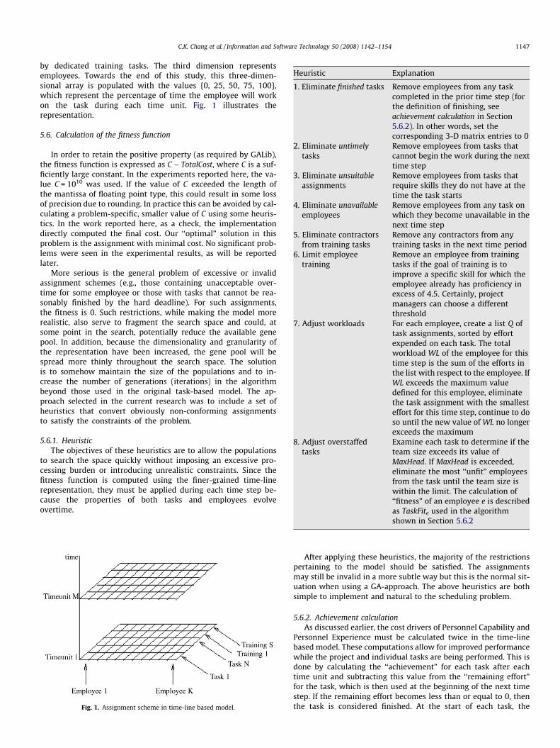
The assignment scheme in the time-line based model can berepresented by a three-dimensional array. The first dimension istime, divided into time steps, from 1 to an upper limit. Forexample, if the time step size (also called the time unit) is 1month and the upper limit is 36 months, the time dimensionwill range from 1 to 36 in units of one month. The seconddimension represents the enumerated project tasks, followed

C.K. Chang et al. / Information and Software Technology 50 (2008) 1142–1154 1147

by dedicated training tasks. The third dimension representsemployees. Towards the end of this study, this three-dimen-sional array is populated with the values {0, 25, 50, 75, 100},which represent the percentage of time the employee will workon the task during each time unit. Fig. 1 illustrates therepresentation.

5.6. Calculation of the fitness function

In order to retain the positive property (as required by GALib),the fitness function is expressed as C – TotalCost, where C is a suf-ficiently large constant. In the experiments reported here, the va-lue C = 1010 was used. If the value of C exceeded the length ofthe mantissa of floating point type, this could result in some lossof precision due to rounding. In practice this can be avoided by cal-culating a problem-specific, smaller value of C using some heuris-tics. In the work reported here, as a check, the implementationdirectly computed the final cost. Our ‘‘optimal” solution in thisproblem is the assignment with minimal cost. No significant prob-lems were seen in the experimental results, as will be reportedlater.

More serious is the general problem of excessive or invalidassignment schemes (e.g., those containing unacceptable over-time for some employee or those with tasks that cannot be rea-sonably finished by the hard deadline). For such assignments,the fitness is 0. Such restrictions, while making the model morerealistic, also serve to fragment the search space and could, atsome point in the search, potentially reduce the available genepool. In addition, because the dimensionality and granularity ofthe representation have been increased, the gene pool will bespread more thinly throughout the search space. The solutionis to somehow maintain the size of the populations and to in-crease the number of generations (iterations) in the algorithmbeyond those used in the original task-based model. The ap-proach selected in the current research was to include a set ofheuristics that convert obviously non-conforming assignmentsto satisfy the constraints of the problem.

5.6.1. HeuristicThe objectives of these heuristics are to allow the populations

to search the space quickly without imposing an excessive pro-cessing burden or introducing unrealistic constraints. Since thefitness function is computed using the finer-grained time-linerepresentation, they must be applied during each time step be-cause the properties of both tasks and employees evolveovertime.

Fig. 1. Assignment scheme in time-line based model.

Heuristic

Explanation

1. Eliminate finished tasks

Remove employees from any taskcompleted in the prior time step (forthe definition of finishing, seeachievement calculation in Section5.6.2). In other words, set thecorresponding 3-D matrix entries to 0

2. Eliminate untimelytasks

Remove employees from tasks thatcannot begin the work during the nexttime step

3. Eliminate unsuitableassignments

Remove employees from tasks thatrequire skills they do not have at thetime the task starts

4. Eliminate unavailableemployees

Remove employees from any task onwhich they become unavailable in thenext time step

5. Eliminate contractorsfrom training tasks

Remove any contractors from anytraining tasks in the next time period

6. Limit employeetraining

Remove an employee from trainingtasks if the goal of training is toimprove a specific skill for which theemployee already has proficiency inexcess of 4.5. Certainly, projectmanagers can choose a differentthreshold

7. Adjust workloads

For each employee, create a list Q oftask assignments, sorted by effortexpended on each task. The totalworkload WL of the employee for thistime step is the sum of the efforts inthe list with respect to the employee. IfWL exceeds the maximum valuedefined for this employee, eliminatethe task assignment with the smallesteffort for this time step, continue to doso until the new value of WL no longerexceeds the maximum

8. Adjust overstaffedtasks

Examine each task to determine if theteam size exceeds its value ofMaxHead. If MaxHead is exceeded,eliminate the most ‘‘unfit” employeesfrom the task until the team size iswithin the limit. The calculation of‘‘fitness” of an employee e is describedas TaskFite used in the algorithmshown in Section 5.6.2

After applying these heuristics, the majority of the restrictionspertaining to the model should be satisfied. The assignmentsmay still be invalid in a more subtle way but this is the normal sit-uation when using a GA-approach. The above heuristics are bothsimple to implement and natural to the scheduling problem.

5.6.2. Achievement calculationAs discussed earlier, the cost drivers of Personnel Capability and

Personnel Experience must be calculated twice in the time-linebased model. These computations allow for improved performancewhile the project and individual tasks are being performed. This isdone by calculating the ‘‘achievement” for each task after eachtime unit and subtracting this value from the ‘‘remaining effort”for the task, which is then used at the beginning of the next timestep. If the remaining effort becomes less than or equal to 0, thenthe task is considered finished. At the start of each task, the

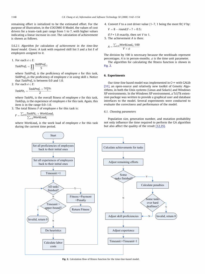
1148 C.K. Chang et al. / Information and Software Technology 50 (2008) 1142–1154

remaining effort is initialized to be the estimated effort. For thepurpose of illustration, in the COCOMO II Model, the values of costdrivers for a team–task pair range from 1 to 7, with higher valuesindicating a linear increase in cost. The calculation of achievementis shown as follows.

5.6.2.1. Algorithm for calculation of achievement in the time-linebased model. Given: A task with required skill list S and a list E ofemployees assigned to it.

1. For each e 2 E:

TaskProfe ¼Ys2S

SkillProfe;s

5

where TaskProfe is the proficiency of employee e for this task,SkillProfe,sis the proficiency of employee e in using skill s. Noticethat TaskProfe is between 0.0 and 1.0.

2. For each e 2 E:

TaskFite ¼TaskProfe þ TaskExpe

5

2

where TaskFite is the overall fitness of employee e for this task,TaskExpe is the experience of employee e for this task. Again, thisitem is in the range 0.0–1.0.

3. The total fitness F of employee e for this task is:

F ¼P

e2ETaskFite �WorkLoadePe2EWorkLoade

where WorkLoade is the work load of employee e for this taskduring the current time period.

Fig. 2. Calculation flow of fitness funct

4. Convert F to a cost driver value (1–7, 1 being the most fit) V by:

V ¼ 8� roundðF � 7þ 0:5Þ

if F = 1.0 exactly, then set V to 1.5. The achievement A is then:

A ¼P

e2EWorkLoade=100V � /

The division by 100 is necessary because the workloads representpercentages. A is in person-months. / is the time unit parameter.

The algorithm for calculating the fitness function is shown inFig. 2.

6. Experiments

Our time-line based model was implemented in C++ with GALib[31], an open-source and relatively new toolkit of Genetic Algo-rithms, in both the Unix systems (Linux and Solaris) and WindowsXP environments. In the Windows XP environment, a Tcl/Tk exten-sion package was written to provide a graphical user and databaseinterfaces to the model. Several experiments were conducted toevaluate the correctness and performance of the model.

6.1. Choosing parameters

Population size, generation number, and mutation probabilitynot only influence the time required to perform the GA algorithmbut also affect the quality of the result [12,35].

ion for the time-line-based model.

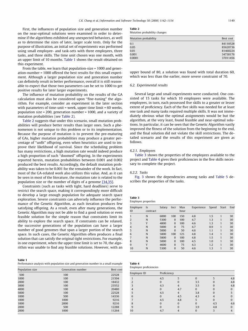
Table 2Mutation probability changes

Mutation probability Best cost

0.1 841185280.05 856207360.01 814602240.001 347381760.0001 37011456

Table 3Employee properties

EmployeeID

Iscontract

Salary Incr Maxhour

Experience Speed Start End

1 N 6000 100 150 4.8 1.5 1 302 N 5300 0 100 4.7 1.3 1 303 Y 4800 0 100 4.6 1.3 1 304 N 5000 0 75 4.7 0.9 1 305 N 5000 0 50 4.6 1.1 1 306 N 5800 100 125 4.8 1.4 1 307 N 5800 0 100 4.8 1.5 1 308 N 5000 0 100 4.5 1.0 1 309 Y 4600 0 75 4.3 1.2 1 3010 N 5300 0 50 4.6 1.3 1 30

C.K. Chang et al. / Information and Software Technology 50 (2008) 1142–1154 1149

First, the influences of population size and generation numberon the near-optimal solutions were examined in order to deter-mine if the algorithms exhibited any unexpected behaviors, as wellas to determine the sizes of later, larger scale tests. Only for thepurpose of illustration, an initial set of experiments was performedusing small employee- and task-sets with three employees, threetasks, and three skills. The time unit chosen was one month, withan upper limit of 10 months. Table 1 shows the result obtained onthis experiment.

From the table, we learn that population-size = 1000 and gener-ation-number = 1000 offered the best results for this small experi-ment. Although a larger population size and generation numbercan definitely result in better performance, overall it is still reason-able to expect that those two parameters can be set to 1000 to getpositive results for later larger experiments.

The influence of mutation probability on the results of the GAcalculation must also be considered upon ‘‘fine-tuning” the algo-rithm. For example, consider an experiment in the later sectionwith parameters of time-unit = week, upper time limit = 60 weeks,population size = 200, generation number = 1000, and a variety ofmutation probabilities (see Table 2).

Table 2 suggests that under this scenario, small mutation prob-abilities will produce better results than larger ones. Such a phe-nomenon is not unique to this problem or to its implementation.Because the purpose of mutation is to prevent the pre-maturingof GAs, higher mutation probabilities may produce a greater per-centage of ‘‘unfit” offspring, even when heuristics are used to im-prove their likelihood of survival. Since the scheduling problemhas many restrictions, a high mutation rate would indeed producea high proportion of such ‘‘doomed” offspring. In the experimentsreported herein, mutation probabilities between 0.001 and 0.002produced the best results. Accordingly, the default mutation prob-ability was taken to be 0.001 for the remainder of the work. In fact,most of the GA-related work also utilizes this value. And, as it canbe seen in most of the literature, the mutation rate is related to thepopulation size or the number of digits of a genome [34,35].

Constraints (such as tasks with tight, hard deadlines) serve torestrict the search space, making it correspondingly more difficultto develop a large enough population for adequate search spaceexploration. Severe constraints can adversely influence the perfor-mance of the Genetic Algorithm, as each iteration produces fewsatisfying offspring. As a result, even after many generations, theGenetic Algorithm may not be able to find a good solution or evenfeasible solution for the simple reason that constraints limit itsability to explore the search space. If constraints can be relaxed,the successive generations of the population can have a largernumber of good genomes that span a larger portion of the searchspace. In such cases, the Genetic Algorithm often produces a finalsolution that can satisfy the original tight restrictions. For example,in one experiment, when the upper time limit is set to 70, the algo-rithm was unable to find any feasible solutions. However, with an

Table 1Performance analysis with population size and generation number in a small example

Population size Generation number Best cost

500 100 225281000 100 215042000 100 184323000 100 235524000 100 204805000 100 225281000 500 143361000 1000 92161000 2000 92162000 500 122882000 1000 11264

upper bound of 80, a solution was found with total duration 60,which was less than the earlier, more severe constraint of 70.

6.2. Experimental results

Several large and small experiments were conducted. One con-sisted of 15 tasks for which 10 employees were available. Theemployees, in turn, each possessed five skills to a greater or lesserextent of proficiency. Each of the five skills was needed for at leastone task and many tasks required multiple skills. It was not imme-diately obvious what the optimal assignments would be but thealgorithm, at the very least, found feasible and near-optimal solu-tions. In particular, it can be seen that the Genetic Algorithm vastlyimproved the fitness of the solution from the beginning to the end,and the final solution did not violate the skill restrictions. The de-tailed scenario and the results of this experiment are given asfollows.

6.2.1. EmployeesTable 3 shows the properties of the employees available to the

project and Table 4 gives their proficiencies in the five skills neces-sary to complete the project.

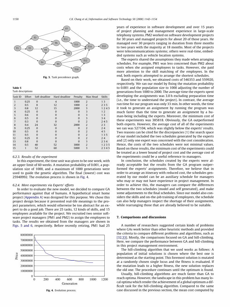
6.2.2. TasksFig. 3 shows the dependencies among tasks and Table 5 de-

scribes the properties of the tasks.

Table 4Employee proficiencies

Employee ID Proficiency

1 4.5 5 0 5 4.82 0 0 3.5 0 4.83 4.3 4 3.5 0 4.84 0 4.7 0 0 05 4.5 4 3.8 0 56 0 4.5 4.3 4 07 4.5 4.8 5 0 08 0 0 0 4.5 4.69 0 0 3.9 4.8 0

10 4.7 4 0 3 4

T11

T6

T2

T1 T3

T4

T5

T7

T8

T9

T10

T13T14

T12

T15

Fig. 3. Task precedence graph.

Table 5Task descriptions

Task ID Effort Soft deadline Hard deadline Penalty Max Head Skills

1 0.25 0 4 1000 2 1 32 0.5 8 12 1000 2 2 3 53 0.8 12 15 2000 3 1 2 4 54 0.25 0 0 0 3 1 25 0.6 0 0 0 3 1 36 0.5 0 0 0 3 3 47 0.3 0 0 0 2 2 4 58 0.4 24 32 2000 2 2 39 0.25 0 0 0 2 2 4

10 0.5 0 0 0 2 4 511 0.5 0 0 0 2 1 3 512 0.25 0 0 0 2 2 413 0.8 0 0 0 3 2 3 414 0.5 40 52 3000 2 1 2 3 515 1 52 60 5000 3 2 3 4 5

1150 C.K. Chang et al. / Information and Software Technology 50 (2008) 1142–1154

6.2.3. Results of the experimentIn this experiment, the time unit was given to be one week, with

an upper limit of 60 weeks. A mutation probability of 0.001, a pop-ulation size of 1000, and a maximum of 1000 generations wereused to guide the genetic algorithm. The final (lowest) cost was25940992. The evolution process is shown in Fig. 4.

6.2.4. More experiments via Experts’ effortsIn order to evaluate the new model, we decided to compare GA

performance against that of humans. A hypothetical smart homeproject (Appendix A) was designed for this purpose. We chose thisproject design because it presented real-life meanings to the pro-ject parameters, which would otherwise be too abstract for an ex-pert to do a good job. There are 25 tasks, 12 kinds of skills, and 15employees available for the project. We recruited two senior soft-ware project managers (PM1 and PM2) to assign the employees totasks. The results we obtained from the managers are shown inFigs. 5 and 6, respectively. Before recently retiring, PM1 had 25

0

10000000

20000000

30000000

40000000

50000000

60000000

70000000

80000000

0 200 400 600 800 1000 1200Generation

Pric

e

Fig. 4. Evolution process.

years of experience in software development and over 15 yearsof project planning and management experience in large-scaletelephony systems. PM2 worked on software development projectsfor 30 years and managed projects for about 20 of those years. Hemanaged over 30 projects ranging in duration from three monthsto two years with the majority at 18 months. Most of the projectswere telecommunications systems; others were real-time, embed-ded systems such as vehicle location systems.

The experts shared the assumptions they made when arrangingschedules. For example, PM1 was less concerned than PM2 aboutcosts when she assigned employees to tasks. However, she paidmore attention to the skill matching of the employees. In theend, both experts attempted to arrange the shortest schedules.

Based on their work, we obtained costs of 546353 and 559920,respectively. We ran our model by fixing the mutation probabilityto 0.001 and the population size to 1000 adjusting the number ofgenerations from 1000 to 2000. The average time the experts spentdeveloping the assignments was 3.0 h excluding preparation time(i.e., the time to understand the project). In contrast, the averagerun time for our program was only 33 min. In other words, the timeit took to generate an assignment by running the program wasmuch faster than the time to generate an assignment by a hu-man-being including the experts. Moreover, the minimum cost ofthese experiments was 385818. Obviously, the GA outperformedboth experts. However, the average cost of all of the experimentswe ran was 527104, which was slightly below the experts’ results.Two reasons can be cited for the discrepancies (1) the search spaceof our model included the two schedules generated by the expertsand (2) only one expert was concerned with the cost consideration.Hence, the costs of the two schedules were not minimal values.Based on these results, the minimum cost of the experiments couldbe treated as a lower bound of project cost and the average cost ofthe experiments could be a useful reference to managers.

In conclusion, the schedules created by the experts were al-ready acceptable but the results from the GA program outper-formed the experts’ assignments. Therefore, we believe that inorder to arrange an itinerary with reduced cost, the schedules gen-erated by our model can be an auxiliary schedule for managerswho may or may not have experience in project management. Inorder to achieve this, the managers can compare the differencesbetween the two schedules (model and self generated), and makesome adjustments to the final schedules. Since our model also con-siders the skills and on-the-job training of employees, the schedulecan also help managers inspect the shortage of their assignments,while rearranging those that are already believed to be suitable.

7. Comparisons and discussions

A number of researchers suggested certain kinds of problemswhere GAs work better than other heuristic methods and providedthe criteria to compare different problems and algorithms, such as[32,33]. Mostly, the comparisons focused on GA and hill-climbing.Here, we compare the performance between GA and hill-climbingin this project management environment.

The hill-climbing algorithm that we used works as follows: Apopulation of initial solutions is chosen where the best one isdetermined as the starting point. This foremost solution is mutatedat a randomly chosen single locus and the fitness is evaluated. Ifthe mutation leads to a higher fitness, the new solution replacesthe old one. The procedure continues until the optimum is found.

Usually, hill-climbing algorithms are much faster than GA toreach optima. However, the landscape in this problem has many lo-cal optima which render the achievement of a global optimum a dif-ficult task for the hill-climbing algorithm. Compared to the samecase discussed in the previous section, the mean cost computed by

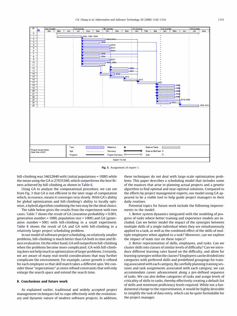
Fig. 5. Assignment of expert 1.

C.K. Chang et al. / Information and Software Technology 50 (2008) 1142–1154 1151

hill-climbing was 34622840 with (initial populations = 1000) whilethe mean using the GA is 27635360, which outperforms the best fit-ness achieved by hill-climbing as shown in Table 6.

Using GA to analyze the computational procedure, we can seefrom Fig. 3 that GA is not efficient in the later stage of computationwhich, in essence, means it converges very slowly. With GA’s abilityfor global optimization and hill-climbing’s ability to locally opti-mize, a hybrid algorithm combining the two may be the ideal choice.

The table below gives the results from the experiment with twocases. Table 7 shows the result of GA (mutation probability = 0.001,generation number = 1000, population size = 1000) and GA (gener-ation number = 500) with hill-climbing in a small experiment.Table 8 shows the result of GA and GA with hill-climbing in arelatively larger project scheduling problem.

In our model of software project scheduling, on relatively smallerproblems, hill-climbing is much better than GA both in time and fit-ness evaluation. On the other hand, GA will outperform hill-climbingwhen the problems become more complicated; GA with hill-climb-ing does not help much in optimization of larger problems. Certainly,we are aware of many real-world considerations that may furthercomplicate the environment. For example, career growth is refinedfor each employee so that skill match takes a different spin. We con-sider those ‘‘expectations” as more refined constraints that will onlyenlarge the search space and extend the search time.

8. Conclusions and future work

As explained earlier, traditional and widely accepted projectmanagement techniques fail to cope effectively with the evolution-ary and dynamic nature of modern software projects. In addition,

these techniques do not deal with large-scale optimization prob-lems. This paper describes a scheduling model that includes someof the nuances that arise in planning actual projects and a geneticalgorithm to find optimal and near-optimal solutions. Compared tothe efforts by project management experts, our model using GA ap-peared to be a viable tool to help guide project managers in theirdaily routines.

Potential topics for future work include the following improve-ments to the model:

1. Better system dynamics integrated with the modeling of pro-gress of tasks where better training and experience models are in-cluded. Can we better model the impact of the synergies betweenmultiple skills of a single individual when they are simultaneouslyapplied to a task, as well as the combined effect of the skills of mul-tiple employees when applied to a task? Moreover, can we explorethe impact of team size on these topics?

2. Better representation of skills, employees, and tasks. Can wecluster skills into classes of similar levels of difficulty? Can we intro-duce different learning rates based on the difficulty, and allow forlearning synergies within the classes? Employees can be divided intocategories with preferred skills and predefined groupings for train-ing associated with each category. By carefully planning training ses-sions and task assignments associated with each category, we canaccommodate career advancement along a pre-defined sequenceof tasks. We can also define categories of tasks and assign levels ofcriticality of skills to tasks, thereby effectively creating a default listof skills and minimum proficiency levels required. While not a fun-damental change to the representation, it would be highly desirableto simplify the task of data entry, which can be quite formidable forthe project manager.

Fig. 6. Assignment of expert 2.

Table 7Comparison between GA and GA with HC in a relative small problem (3 tasks, 3employees)

Best Mean Worst

Steady GA 8192 11298 15360Steady GA (500 generations) with HC 5286 6983 10024

Table 8Comparison between GA and GA with HC in a relative big problem (15 tasks, 10employees)

Best Mean Worst

Steady GA 25424896 27635360 29941800Steady GA (500 generations) with HC 26761000 28929233 33171600

Table 6Comparison between GA and hill-climbing

Best Mean Worst

Steady GA 25424896 27635360 29941800Hill-climbing 29883000 34622840 41868400

1152 C.K. Chang et al. / Information and Software Technology 50 (2008) 1142–1154

3. Flow of control options that allow the project manager to eas-ily explore alternative project plans needs to be examined. Someselected tasks can be immediately executable, even if their prede-cessor tasks are not complete; some selected tasks may be requiredto be re-done to recover from failure of a specific activity, such as adesign review, or a test. The concept of probability can be added tothese two options.

4. Explore more search heuristics, such as Tabu search and sim-ulated annealing, and compare their performances in software pro-ject scheduling.

5. Consider building a user interface to allow for more convenientfeedback from the manager as the project evolves, and to display thestatus of an on-going project in a manner more suitable to the model.In other words, on top of the GA engine (GALib in our implementa-tion), we can implement a suitable interface for project manage-ment. Of course this will become a very extensive project requiringknowledge in other domains such as HCI usability and design.

Acknowledgments

Dr. Mark Christensen, who retired from Northrop Grumman asVice President of the EDS division, provided very constructive com-ments during the initial stage of this study. Software project manag-ers Jean Chang, who has over 15 years of solid project planning andmanagement experience in the practitioner’s world, and Owen La-vin, who worked on software development projects for 30 yearsand managed projects for about 20 of those years, invested signifi-cant effort in submitting their favorite schedules based on our hypo-thetical smart home project. We also thank Jane Cleland-Huang forher valuable comments of revising and editing the paper.

Appendix 1. Smart home project

A.1. Purpose and overview of the project

The purpose of Smart Home Project is to develop a home wheremost devices are controlled by computers so that it can help the dis-abled or elderly people live independently without the need for an

C.K. Chang et al. / Information and Software Technology 50 (2008) 1142–1154 1153

assistant to be nearby. That is, one of the smart home’s primaryobjectives for the elderly is to enable them to retain their status asan independent homeowner for as long as possible before makingthe transition into the health care system (e.g., nursing homes). In-side the home, there are sensors to detect the activities of the home-owners and based on their specific actions, or lack thereof, the smarthome will react accordingly to deliver necessary automated assis-tances, including, but is not limited to: medicine application, cook-ing and general proactive and reactive safety measures.

One exemplary feature of the smart home is its preset automa-tion. Users and researchers alike can define specific context infor-mation (defined events, environmental fluctuations, etc.) wherethe smart home will be triggered into action. One principal exam-ple of this is the house’s lighting. Depending on the existingamount of natural and synthetic light in any given room, as wellas the preset preference of user-defined brightness, the home willadjust window coverings and synthetic light levels to accommo-date to the specifications. As a matter of fact, this feature has al-ready been designed and implemented in the Smart Home Laband at the Department of Computer Science, Iowa State University.Scenarios similar to this can be considered in many other deviceswithin the smart home.

A.2. Features of smart home framework

We focus the features of the smart home framework on three de-vices (lighting system, motion detector, and a RFID-based heart ratemonitor) and one set of actors (researchers). A key point to note isthat most of these proposed features are generic and can be easilyported to devices that will be included in future iterations. All ofthe control software will accept commands from devices such as cellphones, PCs, controllers, etc. This will ensure a greater ease of use forthe user in any scenario. Inversely, these devices will also have thecapability to receive commands from the control software.

A.2.1. Features of applicationThe following is an abbreviated list of smart home features to

illustrate the expansive breadth of control capability. The generalfeatures cover a wide spectrum such as (1) basic control of devices;(2) features on lighting, doors, administration, medication, floors,etc; (3) safety; (4) security and (5) reliability.

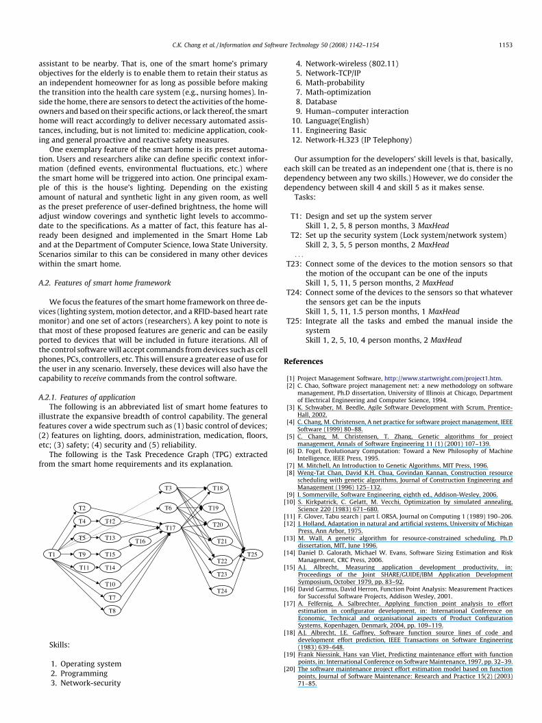
The following is the Task Precedence Graph (TPG) extractedfrom the smart home requirements and its explanation.

T1

T3

T4

T8

T9

T2

T5

T6

T7

T11

T12

T10

T18

T17

T15

T14

T13 T16

T19

T20

T21

T22

T23

T24

T25

Skills:

1. Operating system2. Programming3. Network-security

4. Network-wireless (802.11)5. Network-TCP/IP6. Math-probability7. Math-optimization8. Database9. Human–computer interaction

10. Language(English)11. Engineering Basic12. Network-H.323 (IP Telephony)

Our assumption for the developers’ skill levels is that, basically,each skill can be treated as an independent one (that is, there is nodependency between any two skills.) However, we do consider thedependency between skill 4 and skill 5 as it makes sense.

Tasks:

T1: Design and set up the system serverSkill 1, 2, 5, 8 person months, 3 MaxHead

T2: Set up the security system (Lock system/network system)Skill 2, 3, 5, 5 person months, 2 MaxHead

. . .

T23: Connect some of the devices to the motion sensors so thatthe motion of the occupant can be one of the inputsSkill 1, 5, 11, 5 person months, 2 MaxHead

T24: Connect some of the devices to the sensors so that whateverthe sensors get can be the inputsSkill 1, 5, 11, 1.5 person months, 1 MaxHead

T25: Integrate all the tasks and embed the manual inside thesystemSkill 1, 2, 5, 10, 4 person months, 2 MaxHead

References

[1] Project Management Software, http://www.startwright.com/project1.htm.[2] C. Chao, Software project management net: a new methodology on software

management, Ph.D dissertation, University of Illinois at Chicago, Departmentof Electrical Engineering and Computer Science, 1994.

[3] K. Schwaber, M. Beedle, Agile Software Development with Scrum, Prentice-Hall, 2002.

[4] C. Chang, M. Christensen, A net practice for software project management, IEEESoftware (1999) 80–88.

[5] C. Chang, M. Christensen, T. Zhang, Genetic algorithms for projectmanagement, Annals of Software Engineering 11 (1) (2001) 107–139.

[6] D. Fogel, Evolutionary Computation: Toward a New Philosophy of MachineIntelligence, IEEE Press, 1995.

[7] M. Mitchell, An Introduction to Genetic Algorithms, MIT Press, 1996.[8] Weng-Tat Chan, David K.H. Chua, Govindan Kannan, Construction resource

scheduling with genetic algorithms, Journal of Construction Engineering andManagement (1996) 125–132.

[9] I. Sommerville, Software Engineering, eighth ed., Addison-Wesley, 2006.[10] S. Kirkpatrick, C. Gelatt, M. Vecchi, Optimization by simulated annealing,

Science 220 (1983) 671–680.[11] F. Glover, Tabu search j part I. ORSA, Journal on Computing 1 (1989) 190–206.[12] J. Holland, Adaptation in natural and artificial systems, University of Michigan

Press, Ann Arbor, 1975.[13] M. Wall, A genetic algorithm for resource-constrained scheduling, Ph.D

dissertation, MIT, June 1996.[14] Daniel D. Galorath, Michael W. Evans, Software Sizing Estimation and Risk

Management, CRC Press, 2006.[15] A.J. Albrecht, Measuring application development productivity, in:

Proceedings of the Joint SHARE/GUIDE/IBM Application DevelopmentSymposium, October 1979, pp. 83–92.

[16] David Garmus, David Herron, Function Point Analysis: Measurement Practicesfor Successful Software Projects, Addison Wesley, 2001.

[17] A. Felfernig, A. Salbrechter, Applying function point analysis to effortestimation in configurator development, in: International Conference onEconomic, Technical and organisational aspects of Product ConfigurationSystems, Kopenhagen, Denmark, 2004, pp. 109–119.

[18] A.J. Albrecht, J.E. Gaffney, Software function source lines of code anddevelopment effort prediction, IEEE Transactions on Software Engineering(1983) 639–648.

[19] Frank Niessink, Hans van Vliet, Predicting maintenance effort with functionpoints, in: International Conference on Software Maintenance, 1997, pp. 32–39.

[20] The software maintenance project effort estimation model based on functionpoints, Journal of Software Maintenance: Research and Practice 15(2) (2003)71–85.

1154 C.K. Chang et al. / Information and Software Technology 50 (2008) 1142–1154

[21] Barry Boehm, Software Engineering Economics, Prentice-Hall Inc., 1981.[22] Barry Boehm et al., Software Cost Estimation with COCOMO II, Prentice-Hall

PTR, 2000.[23] Martin Shepperd, Chris Schofield, Estimating software project effort using

analogies, IEEE Transaction on Software Engineering 23 (11) (1997) 736–743.[24] Sun-Jen Huang, Nan-Hsing Chiu, Optimization of analogy weights by genetic

algorithm for software effort estimation, Information and SoftwareTechnology 48 (11) (2006) 1034–1045.

[25] Nan-Hsing Chiu, Sun-Jen Huang, The adjusted analogy-based software effortestimation based on similarity distances, Journal of Systems and Software 80(4) (2007) 628–640.

[26] Parag C. Pendharkar, Girish H. Subramanian, James A. Rodger, A probabilisticmodel for predicting software development effort, IEEE Transaction onSoftware Engineering 31 (7) (2005) 615–624.

[27] K.S. Hindi, H. Yang, K. Fleszar, An evolutionary algorithm for resource-constrained project scheduling, IEEE Transactions on EvolutionaryComputation 6 (5) (2002) 512–518.

[28] Vicente Valls, Francisco Ballestin, Sacramento Quintanilla, A hybrid geneticalgorithm for the resource-constrained project scheduling problem, EuropeanJournal of Operational Research 185 (2008) 495–508.

[29] Enrique Alba, J. Francisco Chicano, Software project management with GAs,Information Sciences 177 (2007) 2380–2401.

[30] Valentina Plekhanova, On project management scheduling where humanresource is a critical variable, in: Proceedings of the Sixth European Workshopon Software Process Technology (EWSPT-6), Lecture Notes in ComputerScience series, Springer-Verlag, London, UK, pp. 116–121.

[31] M. Wall, Lib: A C++ Library of Algorithm Components, http://lancet.mit.edu/ga/.[32] M. Mitchell, J. Holland, S. Forrest, When will a genetic algorithm

outperform hill-climbing? in: Advances in Neural InformationProcessing Systems 6 (7th NIPS Conference), Denver, Colorado, 1994,pp. 51-58.

[33] J. Horn, D. Goldberg, Genetic algorithms difficulty and the modality of fitnesslandscapes, Foundations of Genetic Algorithms 3 (1995) 243–269.

[34] Hans-Georg Beyer, Hans-Paul Schwefel, Ingo Wegener, How to analyseevolutionary algorithms, Technical Report No. CI-139/02, University ofDortmund, 2002.

[35] Jackie Rees, Gary J. Koehler, Learning genetic algorithm parameters usinghidden Markov models, European Journal of Operational Research 175 (2)(2006) 806–820.

[36] T. Hegazy, K. Petzold, Genetic optimization for dynamic project control,Journal of Construction Engineering and Management 129 (4) (2003) 396–404.

[37] David A. Coley, An Introduction to Genetic Algorithms for Scientists andEngineers, World Scientific Publishing Co. Pte. Ltd., New Jersey, 1999.

[38] Harold Kerzner, Project Management Best Practices: Achieving GlobalExcellence, John Wiley & Son, Inc., New Jersey, 2006.

[39] Harold Kerzner, Project Management: A Systems Approach to Planning,Scheduling, and Controlling, John Wiley & Son, Inc., New Jersey, 2003.

[40] G. Abu, J.W. Cangussu, A learning model for software development processes,Software Engineering (SE) (455) (2005).

[41] Frederick P. Brooks, The Mythical Man-Month: Essays on SoftwareEngineering, Addison Wesley, Boston, 1995.