Resilient scheduling algorithms for large-scale platforms
279
HAL Id: tel-02947051 https://tel.archives-ouvertes.fr/tel-02947051 Submitted on 23 Sep 2020 HAL is a multi-disciplinary open access archive for the deposit and dissemination of sci- entific research documents, whether they are pub- lished or not. The documents may come from teaching and research institutions in France or abroad, or from public or private research centers. L’archive ouverte pluridisciplinaire HAL, est destinée au dépôt et à la diffusion de documents scientifiques de niveau recherche, publiés ou non, émanant des établissements d’enseignement et de recherche français ou étrangers, des laboratoires publics ou privés. Resilient scheduling algorithms for large-scale platforms Valentin Le Fèvre To cite this version: Valentin Le Fèvre. Resilient scheduling algorithms for large-scale platforms. Distributed, Parallel, and Cluster Computing [cs.DC]. Université de Lyon, 2020. English. NNT : 2020LYSEN019. tel- 02947051
-
Upload
khangminh22 -
Category
Documents
-
view
0 -
download
0
Transcript of Resilient scheduling algorithms for large-scale platforms

HAL Id: tel-02947051https://tel.archives-ouvertes.fr/tel-02947051
Submitted on 23 Sep 2020
HAL is a multi-disciplinary open accessarchive for the deposit and dissemination of sci-entific research documents, whether they are pub-lished or not. The documents may come fromteaching and research institutions in France orabroad, or from public or private research centers.
L’archive ouverte pluridisciplinaire HAL, estdestinée au dépôt et à la diffusion de documentsscientifiques de niveau recherche, publiés ou non,émanant des établissements d’enseignement et derecherche français ou étrangers, des laboratoirespublics ou privés.
Resilient scheduling algorithms for large-scale platformsValentin Le Fèvre
To cite this version:Valentin Le Fèvre. Resilient scheduling algorithms for large-scale platforms. Distributed, Parallel,and Cluster Computing [cs.DC]. Université de Lyon, 2020. English. NNT : 2020LYSEN019. tel-02947051
Numero National de These : 2020LYSEN019
THESE de DOCTORAT de L’UNIVERSITE DE LYONoperee par
l’Ecole Normale Superieure de Lyon
Ecole Doctorale N512 :
Ecole doctorale Informatique et Mathematiques
Specialite de doctorat : Informatique
Soutenue publiquement le 18/06/2020, par :
Valentin Le Fevre
Resilient scheduling algorithms for large-scale platformsAlgorithmes d’ordonnancement tolerants aux fautes pour les plates-formes a grande echelle
Devant le jury compose de :
Olivier Beaumont Directeur de recherche INRIA, INRIA Bordeaux Sud-Ouest Examinateur
Anne Benoit Maıtresse de conferences, ENS de Lyon, LIP Co-encadrante
Henri Casanova Professeur, Universite d’Hawai’i Rapporteur
Amina Guermouche Maitresse de conferences, Telecom Sud-Paris Examinatrice
Rami Melhem Professeur, Universite de Pittsburgh Rapporteur
Yves Robert Professeur des universites, ENS de Lyon, LIP Directeur


Remerciements
Merci Sci-hub
iii

Contents
Remerciements iii
Contents v
1 Introduction 1
I Advanced checkpointing techniques 5
2 Towards optimal multi-level checkpointing 72.1 Introduction . . . . . . . . . . . . . . . . . . . . . . . . . . . . . . . . . . . 72.2 Computing the optimal pattern . . . . . . . . . . . . . . . . . . . . . . . . 10
2.2.1 Assumptions . . . . . . . . . . . . . . . . . . . . . . . . . . . . . . 112.2.2 Optimal two-level pattern . . . . . . . . . . . . . . . . . . . . . . . 11
2.2.2.1 With a single segment . . . . . . . . . . . . . . . . . . . . 112.2.2.2 With multiple segments . . . . . . . . . . . . . . . . . . . 13
2.2.3 Optimal k-level pattern . . . . . . . . . . . . . . . . . . . . . . . . 162.2.3.1 Observations . . . . . . . . . . . . . . . . . . . . . . . . . 162.2.3.2 Analysis . . . . . . . . . . . . . . . . . . . . . . . . . . . . 17
2.2.4 Optimal subset of levels . . . . . . . . . . . . . . . . . . . . . . . . 272.2.4.1 Checkpoint cost models . . . . . . . . . . . . . . . . . . 272.2.4.2 Dynamic programming algorithm . . . . . . . . . . . . 28
2.3 Simulations . . . . . . . . . . . . . . . . . . . . . . . . . . . . . . . . . . . 282.3.1 Simulation setup . . . . . . . . . . . . . . . . . . . . . . . . . . . . 292.3.2 Assessing accuracy of first-order approximation . . . . . . . . . . 29
2.3.2.1 Using set of parameters (A) . . . . . . . . . . . . . . . . 302.3.2.2 Using set of parameters (B) . . . . . . . . . . . . . . . . 31
2.3.3 Comparing performance of different approaches . . . . . . . . . 342.3.3.1 Using set of parameters (C) . . . . . . . . . . . . . . . . 342.3.3.2 Using set of parameters (D) . . . . . . . . . . . . . . . . 36
2.3.4 Summary of results . . . . . . . . . . . . . . . . . . . . . . . . . . 372.4 Related work . . . . . . . . . . . . . . . . . . . . . . . . . . . . . . . . . . . 372.5 Conclusion . . . . . . . . . . . . . . . . . . . . . . . . . . . . . . . . . . . . 38
v

vi CONTENTS
3 Comparing the performance of rigid, moldable and grid-shaped applicationson failure-prone HPC platforms 413.1 Introduction . . . . . . . . . . . . . . . . . . . . . . . . . . . . . . . . . . . 423.2 Performance model . . . . . . . . . . . . . . . . . . . . . . . . . . . . . . . 44
3.2.1 Application/platform framework . . . . . . . . . . . . . . . . . . 443.2.2 Mean Time Between Failures (MTBF) . . . . . . . . . . . . . . . . 443.2.3 Checkpoints . . . . . . . . . . . . . . . . . . . . . . . . . . . . . . . 443.2.4 Wait Time . . . . . . . . . . . . . . . . . . . . . . . . . . . . . . . . 453.2.5 Objective. . . . . . . . . . . . . . . . . . . . . . . . . . . . . . . . . 45
3.3 Expected yield . . . . . . . . . . . . . . . . . . . . . . . . . . . . . . . . . . 463.3.1 Rigid application . . . . . . . . . . . . . . . . . . . . . . . . . . . . 463.3.2 Moldable application . . . . . . . . . . . . . . . . . . . . . . . . . 473.3.3 GridShaped application . . . . . . . . . . . . . . . . . . . . . . . . 483.3.4 ABFT for GridShaped . . . . . . . . . . . . . . . . . . . . . . . . . 51
3.4 Applicative scenarios . . . . . . . . . . . . . . . . . . . . . . . . . . . . . . 543.4.1 Main scenario . . . . . . . . . . . . . . . . . . . . . . . . . . . . . . 543.4.2 Varying key parameters . . . . . . . . . . . . . . . . . . . . . . . . 573.4.3 Comparison between C/R and ABFT . . . . . . . . . . . . . . . . 62
3.5 Related work . . . . . . . . . . . . . . . . . . . . . . . . . . . . . . . . . . . 633.5.1 Moldable and GridShaped applications . . . . . . . . . . . . . . 633.5.2 ABFT . . . . . . . . . . . . . . . . . . . . . . . . . . . . . . . . . . . 64
3.6 Conclusion . . . . . . . . . . . . . . . . . . . . . . . . . . . . . . . . . . . . 64
4 A generic approach to scheduling and checkpointing workflows 674.1 Introduction . . . . . . . . . . . . . . . . . . . . . . . . . . . . . . . . . . . 674.2 Example . . . . . . . . . . . . . . . . . . . . . . . . . . . . . . . . . . . . . 704.3 Model . . . . . . . . . . . . . . . . . . . . . . . . . . . . . . . . . . . . . . . 72
4.3.1 Execution Model . . . . . . . . . . . . . . . . . . . . . . . . . . . . 724.3.2 Fault-Tolerance Model . . . . . . . . . . . . . . . . . . . . . . . . . 734.3.3 Problem Formulation . . . . . . . . . . . . . . . . . . . . . . . . . 74
4.4 Scheduling and checkpointing algorithms . . . . . . . . . . . . . . . . . . 744.4.1 Scheduling heuristics . . . . . . . . . . . . . . . . . . . . . . . . . 744.4.2 Checkpointing strategies . . . . . . . . . . . . . . . . . . . . . . . 75
4.5 Experiments . . . . . . . . . . . . . . . . . . . . . . . . . . . . . . . . . . . 784.5.1 Experimental methodology . . . . . . . . . . . . . . . . . . . . . . 784.5.2 Simulator . . . . . . . . . . . . . . . . . . . . . . . . . . . . . . . . 804.5.3 Results . . . . . . . . . . . . . . . . . . . . . . . . . . . . . . . . . . 82
4.6 Related work . . . . . . . . . . . . . . . . . . . . . . . . . . . . . . . . . . . 914.7 Conclusion . . . . . . . . . . . . . . . . . . . . . . . . . . . . . . . . . . . . 93

CONTENTS vii
II Coupling checkpointing with replication 95
5 Using Checkpointing and Replication for Reliable Execution of Linear Work-flows with Fail-Stop and Silent Errors 975.1 Introduction . . . . . . . . . . . . . . . . . . . . . . . . . . . . . . . . . . . 975.2 Model and objective . . . . . . . . . . . . . . . . . . . . . . . . . . . . . . 100
5.2.1 Application model . . . . . . . . . . . . . . . . . . . . . . . . . . . 1005.2.2 Execution platform . . . . . . . . . . . . . . . . . . . . . . . . . . . 1005.2.3 Verification . . . . . . . . . . . . . . . . . . . . . . . . . . . . . . . 1005.2.4 Checkpointing . . . . . . . . . . . . . . . . . . . . . . . . . . . . . 1015.2.5 Replication . . . . . . . . . . . . . . . . . . . . . . . . . . . . . . . 1025.2.6 Optimization problem . . . . . . . . . . . . . . . . . . . . . . . . . 104
5.3 Computing Enorep(i) and Erep(i) . . . . . . . . . . . . . . . . . . . . . . . . 1055.3.1 Computing Enorep(i) . . . . . . . . . . . . . . . . . . . . . . . . . . 1055.3.2 Computing Erep(i) . . . . . . . . . . . . . . . . . . . . . . . . . . . 106
5.4 Optimal dynamic programming algorithm . . . . . . . . . . . . . . . . . 1085.5 Experiments . . . . . . . . . . . . . . . . . . . . . . . . . . . . . . . . . . . 111
5.5.1 Scenarios with fail-stop errors only . . . . . . . . . . . . . . . . . 1125.5.1.1 Experimental setup . . . . . . . . . . . . . . . . . . . . . 1125.5.1.2 Comparison to checkpoint only . . . . . . . . . . . . . . 1135.5.1.3 Impact of error rate and checkpoint cost on the perfor-
mance . . . . . . . . . . . . . . . . . . . . . . . . . . . . . 1175.5.1.4 Impact of the number of checkpoints and replicas . . . 118
5.5.2 Scenarios with both fail-stop and silent errors . . . . . . . . . . . 1185.5.2.1 Experimental setup . . . . . . . . . . . . . . . . . . . . . 1185.5.2.2 Comparison to checkpoint only . . . . . . . . . . . . . . 1205.5.2.3 Impact of error rate and checkpoint cost on the perfor-
mance . . . . . . . . . . . . . . . . . . . . . . . . . . . . . 1235.6 Related work . . . . . . . . . . . . . . . . . . . . . . . . . . . . . . . . . . . 1255.7 Conclusion . . . . . . . . . . . . . . . . . . . . . . . . . . . . . . . . . . . . 127
6 Optimal Checkpointing Period with Replicated Execution on HeterogeneousPlatforms 1296.1 Introduction . . . . . . . . . . . . . . . . . . . . . . . . . . . . . . . . . . . 1296.2 Model . . . . . . . . . . . . . . . . . . . . . . . . . . . . . . . . . . . . . . . 1316.3 Optimal pattern . . . . . . . . . . . . . . . . . . . . . . . . . . . . . . . . . 132
6.3.1 Expected execution time . . . . . . . . . . . . . . . . . . . . . . . . 1326.3.2 Expected overhead . . . . . . . . . . . . . . . . . . . . . . . . . . . 1416.3.3 Failures in checkpoints and recoveries . . . . . . . . . . . . . . . . 143
6.4 On-failure checkpointing . . . . . . . . . . . . . . . . . . . . . . . . . . . . 1446.4.1 Expected execution time . . . . . . . . . . . . . . . . . . . . . . . . 1456.4.2 Expected overhead . . . . . . . . . . . . . . . . . . . . . . . . . . . 146
6.5 Experimental evaluation . . . . . . . . . . . . . . . . . . . . . . . . . . . . 1466.5.1 Simulation setup . . . . . . . . . . . . . . . . . . . . . . . . . . . . 146
viii CONTENTS
6.5.2 Accuracy of the models . . . . . . . . . . . . . . . . . . . . . . . . 1476.5.3 Comparison of the two strategies . . . . . . . . . . . . . . . . . . 1486.5.4 Summary . . . . . . . . . . . . . . . . . . . . . . . . . . . . . . . . 155
6.6 Conclusion . . . . . . . . . . . . . . . . . . . . . . . . . . . . . . . . . . . . 155
7 Replication is more efficient than you think 1577.1 Introduction . . . . . . . . . . . . . . . . . . . . . . . . . . . . . . . . . . . 1577.2 Model . . . . . . . . . . . . . . . . . . . . . . . . . . . . . . . . . . . . . . . 1617.3 Background . . . . . . . . . . . . . . . . . . . . . . . . . . . . . . . . . . . 163
7.3.1 With a Single Processor . . . . . . . . . . . . . . . . . . . . . . . . 1637.3.2 With N Processors . . . . . . . . . . . . . . . . . . . . . . . . . . . 165
7.4 Replication . . . . . . . . . . . . . . . . . . . . . . . . . . . . . . . . . . . . 1657.4.1 Computing the Mean Time To Interruption . . . . . . . . . . . . . 1667.4.2 With One Processor Pair . . . . . . . . . . . . . . . . . . . . . . . . 1677.4.3 With b Processor Pairs . . . . . . . . . . . . . . . . . . . . . . . . . 170
7.5 Time-To-Solution . . . . . . . . . . . . . . . . . . . . . . . . . . . . . . . . 1717.6 Asymptotic Behavior . . . . . . . . . . . . . . . . . . . . . . . . . . . . . . 1727.7 Experimental Evaluation . . . . . . . . . . . . . . . . . . . . . . . . . . . . 173
7.7.1 Simulation Setup . . . . . . . . . . . . . . . . . . . . . . . . . . . . 1747.7.2 Model Accuracy . . . . . . . . . . . . . . . . . . . . . . . . . . . . 1747.7.3 Restart-on-failure . . . . . . . . . . . . . . . . . . . . . . . . . . . . . 1777.7.4 Impact of Parameters . . . . . . . . . . . . . . . . . . . . . . . . . 1787.7.5 I/O Pressure . . . . . . . . . . . . . . . . . . . . . . . . . . . . . . 1787.7.6 Time-To-Solution . . . . . . . . . . . . . . . . . . . . . . . . . . . . 1797.7.7 When to Restart . . . . . . . . . . . . . . . . . . . . . . . . . . . . . 181
7.8 Energy consumption . . . . . . . . . . . . . . . . . . . . . . . . . . . . . . 1837.8.1 Without replication . . . . . . . . . . . . . . . . . . . . . . . . . . . 183
7.8.1.1 With a single processor . . . . . . . . . . . . . . . . . . . 1837.8.1.2 With N processors . . . . . . . . . . . . . . . . . . . . . . 184
7.8.2 With replication . . . . . . . . . . . . . . . . . . . . . . . . . . . . . 1847.8.2.1 With one processor pair . . . . . . . . . . . . . . . . . . 1847.8.2.2 With b processor pairs . . . . . . . . . . . . . . . . . . . 185
7.8.3 Experiments . . . . . . . . . . . . . . . . . . . . . . . . . . . . . . . 1867.9 Conclusion . . . . . . . . . . . . . . . . . . . . . . . . . . . . . . . . . . . . 189
III Scheduling problems 191
8 Design and Comparison of Resilient Scheduling Heuristics for Parallel Jobs 1938.1 Introduction . . . . . . . . . . . . . . . . . . . . . . . . . . . . . . . . . . . 1938.2 Models . . . . . . . . . . . . . . . . . . . . . . . . . . . . . . . . . . . . . . 195
8.2.1 Job model . . . . . . . . . . . . . . . . . . . . . . . . . . . . . . . . 1958.2.2 Error model . . . . . . . . . . . . . . . . . . . . . . . . . . . . . . . 1968.2.3 Problem statement . . . . . . . . . . . . . . . . . . . . . . . . . . . 196

CONTENTS ix
8.2.4 Expected makespan . . . . . . . . . . . . . . . . . . . . . . . . . . 1978.2.5 Static vs. dynamic scheduling . . . . . . . . . . . . . . . . . . . . 198
8.3 Resilient Scheduling Heuristics . . . . . . . . . . . . . . . . . . . . . . . . 1988.3.1 R-List scheduling heuristic . . . . . . . . . . . . . . . . . . . . . . 1988.3.2 Approximation ratios of R-List . . . . . . . . . . . . . . . . . . . . 200
8.3.2.1 Result for Reservation . . . . . . . . . . . . . . . . . . . 2008.3.2.2 Result for Greedy . . . . . . . . . . . . . . . . . . . . . . 201
8.3.3 R-Shelf scheduling heuristic . . . . . . . . . . . . . . . . . . . . . 2028.4 Performance Evaluation . . . . . . . . . . . . . . . . . . . . . . . . . . . . 204
8.4.1 Simulation setup . . . . . . . . . . . . . . . . . . . . . . . . . . . . 2058.4.2 Results for synthetic jobs . . . . . . . . . . . . . . . . . . . . . . . 2068.4.3 Results for jobs from Mira . . . . . . . . . . . . . . . . . . . . . . . 210
8.5 Background and Related Work . . . . . . . . . . . . . . . . . . . . . . . . 2128.5.1 Different scheduling flavors and strategies . . . . . . . . . . . . . 2128.5.2 Offline scheduling of rigid jobs . . . . . . . . . . . . . . . . . . . . 2138.5.3 Online scheduling of rigid jobs . . . . . . . . . . . . . . . . . . . . 2138.5.4 Batch schedulers in practical systems . . . . . . . . . . . . . . . . 214
8.6 Conclusion . . . . . . . . . . . . . . . . . . . . . . . . . . . . . . . . . . . . 214
9 I/O scheduling strategy for periodic applications 2179.1 Introduction . . . . . . . . . . . . . . . . . . . . . . . . . . . . . . . . . . . 2179.2 Model . . . . . . . . . . . . . . . . . . . . . . . . . . . . . . . . . . . . . . . 220
9.2.1 Parameters . . . . . . . . . . . . . . . . . . . . . . . . . . . . . . . . 2209.2.2 Execution Model . . . . . . . . . . . . . . . . . . . . . . . . . . . . 2219.2.3 Objectives . . . . . . . . . . . . . . . . . . . . . . . . . . . . . . . . 222
9.3 Periodic scheduling strategy . . . . . . . . . . . . . . . . . . . . . . . . . . 2239.3.1 PerSched: a periodic scheduling algorithm . . . . . . . . . . . . 2259.3.2 Complexity analysis . . . . . . . . . . . . . . . . . . . . . . . . . . 2279.3.3 High-level implementation, proof of concept . . . . . . . . . . . . 234
9.4 Evaluation and model validation . . . . . . . . . . . . . . . . . . . . . . . 2349.4.1 Experimental Setup . . . . . . . . . . . . . . . . . . . . . . . . . . 2359.4.2 Applications and scenarios . . . . . . . . . . . . . . . . . . . . . . 2359.4.3 Baseline and evaluation of existing degradation . . . . . . . . . . 2369.4.4 Comparison to online algorithms . . . . . . . . . . . . . . . . . . 2369.4.5 Discussion on finding the best pattern size . . . . . . . . . . . . . 242
9.5 Related Work . . . . . . . . . . . . . . . . . . . . . . . . . . . . . . . . . . 2439.6 Conclusion . . . . . . . . . . . . . . . . . . . . . . . . . . . . . . . . . . . . 245
10 Conclusion 247
Bibliography 251
Publications 267


Chapter 1
Introduction
In the recent years, many scientific advances in physics, chemistry, biology and morehave been achieved thanks to high performance computing (HPC). For example, tostudy magnetic field properties, physicists need to go deep into tiny details of fluiddynamics, which is an intense computational task even for current machines [138]. Inorder to compute faster, processors and more generally units of computation have seentheir number of transistors increase, as observed by Moore’s law. However, physicallimits (thermal limits, density and more [128, 123]) made constructors unable to keepincreasing the number of transistors with the same rate as before. The new plan sincereaching these limits has been to increase the number of components in a machinein order to split the computation across all the units of computation. State-of-the-art computing platforms have all grown to very large scales. For example, the currentfastest machine according to the Top500 in November 2019 [181] is Summit, a platformwith more than 2.4 millions of cores, for a peak performance of 2× 10¹⁷ Flop/s.
However, this increase in the number of components brings one major problem:resilience. It was reported to be among the top ten challenges of exascale computing(i.e., 1018 Flop/s) by the Advanced Scientific Computing Advisory Committee (AS-CAC) [135]. Resilience can be defined by “ensuring correct scientific computation inface of faults, reproducibility, and algorithm verification challenges”. Why is this chal-lenge relevant? Resilience is mandatory so that most (if not all) applications can finishand deliver non-erroneous results. Indeed, if one processor has a lifetime of 100 years(which is already optimistic), then a machine with 100,000 processors will experiencea failure every 9 hours. More generally, if we consider a mean time before failures(MTBF) µ for one processor, a machine using p such components will have a MTBFof µ
p [106, Proposition 1.2], i.e., the MTBF of the platform decreases linearly with thenumber of components. Since applications running on such systems can last for a dayup to a few weeks, solutions need to be provided to recover from two sources of errors:fail-stop and silent errors.
Silent errors are errors that strike while an application is running and are unnoticedby the system. Such errors can be bit-flips in the memory or faulty Arithmetic LogicUnits (ALU). They can be caused by lots of factors including cosmic radiation [147].
1
2 Chapter 1: Introduction
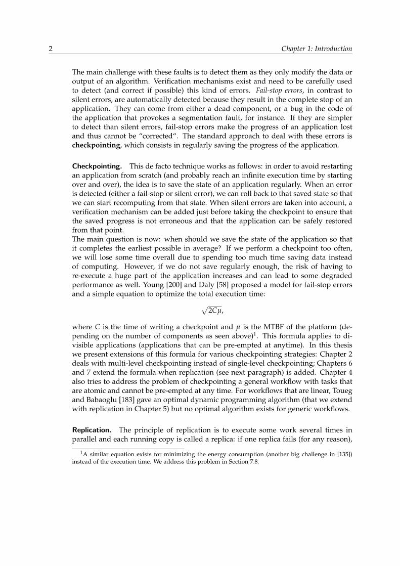
The main challenge with these faults is to detect them as they only modify the data oroutput of an algorithm. Verification mechanisms exist and need to be carefully usedto detect (and correct if possible) this kind of errors. Fail-stop errors, in contrast tosilent errors, are automatically detected because they result in the complete stop of anapplication. They can come from either a dead component, or a bug in the code ofthe application that provokes a segmentation fault, for instance. If they are simplerto detect than silent errors, fail-stop errors make the progress of an application lostand thus cannot be “corrected“. The standard approach to deal with these errors ischeckpointing, which consists in regularly saving the progress of the application.
Checkpointing. This de facto technique works as follows: in order to avoid restartingan application from scratch (and probably reach an infinite execution time by startingover and over), the idea is to save the state of an application regularly. When an erroris detected (either a fail-stop or silent error), we can roll back to that saved state so thatwe can start recomputing from that state. When silent errors are taken into account, averification mechanism can be added just before taking the checkpoint to ensure thatthe saved progress is not erroneous and that the application can be safely restoredfrom that point.The main question is now: when should we save the state of the application so thatit completes the earliest possible in average? If we perform a checkpoint too often,we will lose some time overall due to spending too much time saving data insteadof computing. However, if we do not save regularly enough, the risk of having tore-execute a huge part of the application increases and can lead to some degradedperformance as well. Young [200] and Daly [58] proposed a model for fail-stop errorsand a simple equation to optimize the total execution time:√
2Cµ,
where C is the time of writing a checkpoint and µ is the MTBF of the platform (de-pending on the number of components as seen above)1. This formula applies to di-visible applications (applications that can be pre-empted at anytime). In this thesiswe present extensions of this formula for various checkpointing strategies: Chapter 2deals with multi-level checkpointing instead of single-level checkpointing; Chapters 6and 7 extend the formula when replication (see next paragraph) is added. Chapter 4also tries to address the problem of checkpointing a general workflow with tasks thatare atomic and cannot be pre-empted at any time. For workflows that are linear, Touegand Babaoglu [183] gave an optimal dynamic programming algorithm (that we extendwith replication in Chapter 5) but no optimal algorithm exists for generic workflows.
Replication. The principle of replication is to execute some work several times inparallel and each running copy is called a replica: if one replica fails (for any reason),
1A similar equation exists for minimizing the energy consumption (another big challenge in [135])instead of the execution time. We address this problem in Section 7.8.
Introduction 3
the other replicas are still safe and can be used. Hence, an application crashes or isuncorrectable only if all the replicas have failed. By definition, this is less likely to hap-pen than when having no copy, but we still need to use a checkpoint/restart strategyto handle these cases [159, 75, 205, 82, 46, 110]. The number of replicas determine howstrong the replication is: for example, with two replicas (duplication), we can tolerateone fail-stop error on one of the two replicas and still succeed. However, if a silenterror strikes, we can detect it by looking at the results of the replicas but we would beunable to guess which replica was not corrupted by the error. Instead, if we use threereplicas (triplication), we can tolerate up to one fail-stop error on two different replicas,and we can also correct a silent error by using a majority rule. The main drawbackof replication is that it uses more components to execute the same effective amount ofwork, but we show in Part II that duplication still leads to better performance than noreplication in some cases.
In this thesis, we review a set of techniques using checkpointing in Part I. In Chap-ter 2, we derive a Young/Daly-like formula for multi-level checkpointing. Chap-ter 3 studies how enrolling more processors than necessary can be efficient for acheckpointed application, while Chapter 4 proposes a generic workflow checkpointingscheme.
We combine replication with checkpointing in Part II. In Chapter 5, we design anoptimal dynamic programming algorithm for placing checkpoints and choosing thereplicated tasks in linear workflows. Chapter 6 extends the Young/Daly formula toan application duplicated on heterogeneous platforms. Chapter 7 extends the formulafor homogeneous core-based duplication.
Finally, we investigate some scheduling results for HPC in Part III. Chapter 8 stud-ies, theoretically and experimentally, several scheduling heuristics in a non-reliablecontext. The main question is to know if algorithms that were designed for jobscheduling without failures [184] are still efficient when some tasks have to be re-executed. Another problem with the recent supercomputers is that more and moredata are produced faster while the I/O bandwidth increases at a slower pace. For in-stance, when Los Alamos National Laboratory moved from Cielo to Trinity, the peakperformance moved from 1.4 Petaflops to 40 Petaflops (×28) while the I/O bandwidthmoved to 160 GB/s to 1.45TB/s (only ×9) [124]. To tackle this challenge, Chapter 9investigates scheduling at the I/O level.

Part I
Advanced checkpointing techniques
5


Chapter 2
Towards optimal multi-level checkpointing
We provide a framework to analyze multi-level checkpointing protocols, by formallydefining a k-level checkpointing pattern. We provide a first-order approximation tothe optimal checkpointing period, and show that the corresponding overhead is in theorder of ∑k
`=1√
2λ`C`, where λ` is the error rate at level `, and C` the checkpointingcost at level `. This nicely extends the classical Young/Daly formula on single-levelcheckpointing. Furthermore, we are able to fully characterize the shape of the optimalpattern (number and positions of checkpoints), and we provide a dynamic program-ming algorithm to determine the optimal subset of levels to be used. Finally, weperform simulations to check the accuracy of the theoretical study and to confirm theoptimality of the subset of levels returned by the dynamic programming algorithm.The results nicely corroborate the theoretical study, and demonstrate the usefulness ofmulti-level checkpointing with the optimal subset of levels. The work in this chapteris joint work with Anne Benoit, Aurelien Cavelan, Yves Robert and Hongyang Sun,and has been published in Transactions on computers (TC) [J1].
2.1 Introduction
Checkpointing is the de-facto standard resilience method for HPC platforms at extreme-scale. However, the traditional single-level checkpointing method suffers from signif-icant overhead, and multi-level checkpointing protocols now represent the state-of-the-art technique. These protocols allow different levels of checkpoints to be set, eachwith a different checkpointing overhead and recovery ability. Typically, each level cor-responds to a specific fault type, and is associated to a storage device that is resilientto that type. For instance, a two-level system would deal with (i) transient memoryerrors (level 1) by storing key data in main memory; and (ii) node failures (level 2) bystoring key data in stable storage (remote redundant disks).
In this chapter, we deal with fail-stop errors only. We consider a very generalscenario, where the platform is subject to k levels of faults, numbered from 1 to k.Level ` is associated with an error rate λ`, a checkpointing cost C`, and a recoverycost R`. A fault at level ` destroys all the checkpoints of lower levels (from 1 to `− 1
7

8 Chapter 2: Towards optimal multi-level checkpointing
included) and implies a roll-back to a checkpoint of level ` or higher. Similarly, arecovery of level ` will restore data from all lower levels. Typically, fault rates aredecreasing and checkpoint/recovery costs are increasing when we go to higher levels:λ1 ≥ λ2 ≥ · · · ≥ λk, C1 ≤ C2 ≤ · · · ≤ Ck, and R1 ≤ R2 ≤ · · · ≤ Rk.
Time
Time
Time
C3 C3
C2 C2 C2
C1 C1 C1 C1 C1 C1 C1 C1
(level 3)
(level 2)
(level 1)
Figure 2.1: Independent checkpointing periods for three levels of faults: no synchro-nization between checkpoint levels.
The idea of multi-level checkpointing is that checkpoints are taken for each level offaults, but at different periods. Intuitively, the less frequent the faults, the longer thecheckpointing period: this is because the risk of a failure striking is lower when goingto higher levels; hence the expected re-execution time is lower too; one can safelycheckpoint less frequently, thereby reducing failure-free overhead (checkpointing isuseless in the absence of fault). There are several natural approaches to implementmulti-level checkpointing. The first option is to use independent checkpointing periodsfor each level, as illustrated in Figure 2.1 with k = 3 levels. This option raises severaldifficulties, the most prominent one being overlapping checkpoints. Typically, we needto checkpoint different levels in sequence (e.g., writing into memory before writingonto disk), so we would need to delay some checkpoints, which might not be possiblein some environments, and which would introduce irregular periods. The secondoption is to synchronize all checkpoint levels by nesting them inside a periodic patternthat repeats over time, as illustrated in Figure 2.2(a). In this figure, the pattern has fivecomputational segments, each followed by a level-1 checkpoint. A segment is a chunkof work between two checkpoints, and a pattern consists in segments and checkpoints.The second and fifth level-1 checkpoints are followed by a level-2 checkpoint. Finally,the pattern ends with a level-3 checkpoint. When using patterns, a checkpoint at level` is always preceded by checkpoints at all lower levels 1 to `− 1, which makes goodsense in practice (e.g., with two levels, main memory and disk, one writes the datainto memory before transferring it to disk).
Using periodic patterns simplifies the orchestration of checkpoints at all levels.In addition, repeatedly applying the same pattern is optimal for on-line schedulingproblems, or for jobs running a very long (even infinite) time on the platform. Indeed,in this scenario, we seek the best pattern, i.e., the one whose overhead is minimal. Theoverhead of a pattern is the price per work unit to pay for resilience in the pattern; henceminimizing overhead is equivalent to optimizing platform throughput. For a patternP(W) with W units of work (the cumulated length of all its segments), the overhead

2.1. INTRODUCTION 9
C1 C2 C3 C1 C1 C2 C1 C1 C1 C2 C3(a)
Time
Time
C1 C1(b)
Time
C1 C2 C1 C1 C2 C1 C1 C2(c)
Figure 2.2: Checkpointing patterns (highlighted using red bars) with (a) k = 3, (b)k = 1, and (c) k = 2 levels.
H(P(W)) is defined as the ratio of the pattern’s expected execution time E(P(W)) overits total work W minus 1:
H(P(W)) =E(P(W))
W− 1. (2.1)
If there were neither checkpoint nor fault, the overhead would be zero. Determiningthe optimal pattern (with minimal overhead), and then repeatedly using it until jobcompletion, is the optimal approach with Exponential failure distributions and long-lasting jobs. Indeed, once a pattern is successfully executed, the optimal strategy is tore-execute the same pattern. This is because of the memoryless property of exponentialdistributions: the history of failures has no impact on the solution, so if a pattern isoptimal at some point in time, it stays optimal later in the execution, because we haveno further information about the amount of work still to be executed.
The difficulty of characterizing the optimal pattern dramatically increases withthe number of levels. How many checkpoints of each level should be used, and atwhich locations inside the pattern? What is the optimal length of each segment? Withone single level (see Figure 2.2(b)), there is a single segment of length W, and the
Young/Daly formula [200, 58] gives Wopt =√
2C1λ1
. The minimal overhead is then
Hopt =√
2λ1C1 + O(λ1).With two levels, the pattern still has a simple shape, with N segments followed
by a level-1 checkpoints, and ended by a level-2 checkpoint (see Figure 2.2(c)). Re-cent work [63] shows that all segments have same length in the optimal pattern, andprovides mathematical equations that can be solved numerically to compute both theoptimal length Wopt of the pattern and its optimal number of segments. However,no closed-form expression is available, neither for Wopt, nor for the minimal overheadHopt.
With three levels, no optimal solution is known. The pattern shape becomes quitecomplicated. Coming back to Figure 2.2(a), we identify two sub-patterns ending witha level-2 checkpoint. The first sub-pattern has 2 segments while the second one has 3.The memoryless property does not imply that all sub-patterns are identical, because

10 Chapter 2: Towards optimal multi-level checkpointing
the state after completing the first sub-pattern is not the same as the initial state whenbeginning the execution of the pattern. In the general case with k levels, the shape ofthe pattern will be even more complicated, with different-shaped sub-patterns (eachended by a level k − 1 checkpoint). In turn, each sub-pattern may have different-shaped sub-sub-patterns (each ended by a level k − 2 checkpoint), and so on. Themajor contribution of this work is to provide an analytical characterization of theoptimal pattern with an arbitrary number k of checkpointing levels, with closed-formformulas for the pattern length Wopt, the number of checkpoints at each level, and theoptimal overhead Hopt. In particular, we obtain the following beautiful result:
Hopt =k
∑`=1
√2λ`C` + O(Λ), (2.2)
where Λ = ∑k`=1 λ`. However, we point out that this analytical characterization relies
on a first-order approximation, so it is valid only when resilience parameters C` andR` are small in front of the platform Mean Time Between Failures (MTBF) µ = 1/Λ.Also, the optimal pattern has rational number of segments, and we use rounding toderive a practical solution. Still, Equation (2.2) provides a lower bound on the optimaloverhead, and this bound is met very closely in all our experimental scenarios.
Finally, in many practical cases, there is no obligation to use all available check-pointing levels. For instance, with k = 3 levels, one may choose among four possibili-ties: level 3 only, levels 1 and 3, levels 2 and 3, and all levels 1, 2 and 3. Of course, westill have to account for all failure types, which translates into the following:
• level 3: use λ3 ← λ1 + λ2 + λ3;
• levels 1 and 3: use λ1 and λ3 ← λ2 + λ3;
• levels 2 and 3: use λ2 ← λ1 + λ2 and λ3;
• all levels: use λ1, λ2 and λ3.
Our analytical characterization of the optimal pattern leads to a simple dynamic pro-gramming algorithm for selecting the optimal subset of levels.
The rest of this chapter is organized as follows. Section 2.2 is the heart of thechapter and shows how to compute the optimal pattern as well as the optimal subsetof levels. Section 2.3 is devoted to simulations assessing the accuracy of the first-orderapproximation. Section 2.4 surveys the related work. Finally, Section 2.5 providesconcluding remarks and hints for future work.
2.2 Computing the optimal pattern
This section computes the optimal multi-level checkpointing pattern. We first stateour assumptions in Section 2.2.1, and then analyze the simple case with k = 2 levelsin Section 2.2.2, before proceeding to the general case in Section 2.2.3. Finally, thealgorithm to compute the optimal subset of levels is described in Section 2.2.4.
2.2. COMPUTING THE OPTIMAL PATTERN 11
2.2.1 Assumptions
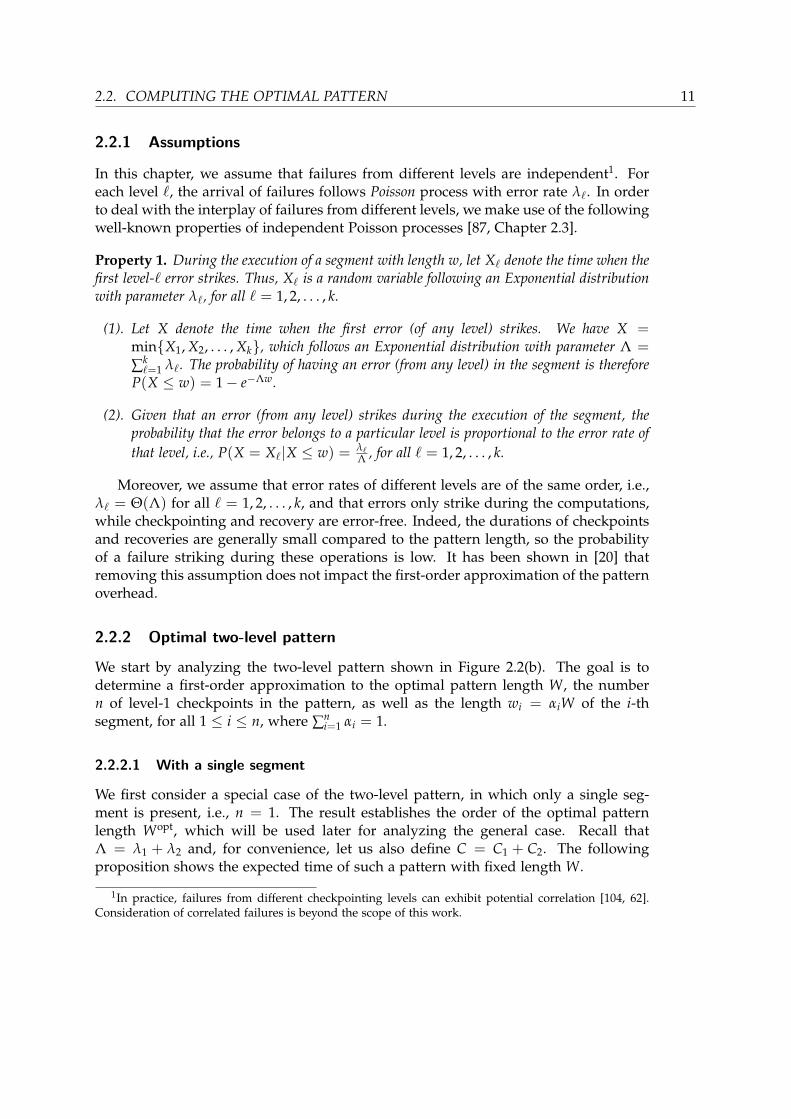
In this chapter, we assume that failures from different levels are independent1. Foreach level `, the arrival of failures follows Poisson process with error rate λ`. In orderto deal with the interplay of failures from different levels, we make use of the followingwell-known properties of independent Poisson processes [87, Chapter 2.3].
Property 1. During the execution of a segment with length w, let X` denote the time when thefirst level-` error strikes. Thus, X` is a random variable following an Exponential distributionwith parameter λ`, for all ` = 1, 2, . . . , k.
(1). Let X denote the time when the first error (of any level) strikes. We have X =minX1, X2, . . . , Xk, which follows an Exponential distribution with parameter Λ =
∑k`=1 λ`. The probability of having an error (from any level) in the segment is therefore
P(X ≤ w) = 1− e−Λw.
(2). Given that an error (from any level) strikes during the execution of the segment, theprobability that the error belongs to a particular level is proportional to the error rate ofthat level, i.e., P(X = X`|X ≤ w) = λ`
Λ , for all ` = 1, 2, . . . , k.
Moreover, we assume that error rates of different levels are of the same order, i.e.,λ` = Θ(Λ) for all ` = 1, 2, . . . , k, and that errors only strike during the computations,while checkpointing and recovery are error-free. Indeed, the durations of checkpointsand recoveries are generally small compared to the pattern length, so the probabilityof a failure striking during these operations is low. It has been shown in [20] thatremoving this assumption does not impact the first-order approximation of the patternoverhead.
2.2.2 Optimal two-level pattern
We start by analyzing the two-level pattern shown in Figure 2.2(b). The goal is todetermine a first-order approximation to the optimal pattern length W, the numbern of level-1 checkpoints in the pattern, as well as the length wi = αiW of the i-thsegment, for all 1 ≤ i ≤ n, where ∑n
i=1 αi = 1.
2.2.2.1 With a single segment
We first consider a special case of the two-level pattern, in which only a single seg-ment is present, i.e., n = 1. The result establishes the order of the optimal patternlength Wopt, which will be used later for analyzing the general case. Recall thatΛ = λ1 + λ2 and, for convenience, let us also define C = C1 + C2. The followingproposition shows the expected time of such a pattern with fixed length W.
1In practice, failures from different checkpointing levels can exhibit potential correlation [104, 62].Consideration of correlated failures is beyond the scope of this work.

12 Chapter 2: Towards optimal multi-level checkpointing
Proposition 1. The expected execution time of a two-level pattern with a single segment andfixed length W is
E = W + C +12
ΛW2 + O(maxΛ2W3, ΛW).
Proof. We can express the expected execution time of the pattern recursively as follows:
E = P
(Elost(W, Λ) +
λ1
Λ(R1 + E) +
λ2
Λ
(R2 + R1 + E
))+ (1− P) (W + C) , (2.3)
where P = 1− e−ΛW denotes the probability of having a failure (either level-1 or level-2) during the execution of the pattern based on Property 1.1, and Elost(wi, Λ) denotesthe expected time lost when such a failure occurs. In this case, and based on Property1.2, if the failure belongs to level 1, which happens with probability λ1
Λ , we can recoverfrom the latest level-1 checkpoint (R1). Otherwise, the failure belongs to level 2 withprobability λ2
Λ , and we need to first recover from the latest level-2 checkpoint (R2)before restoring the level-1 checkpoint (R1). In both cases, the entire pattern needs tobe re-executed again. Finally, if no error (of any level) strikes, which happens withprobability 1− P, the pattern is completed after W time of execution followed by thetime C to perform the two checkpoints, which are assumed to be error-free.
From [106, Equation (1.13)], the expected time lost when executing a segment oflength W with error rate Λ is
Elost(W, Λ) =1Λ− W
eΛW − 1. (2.4)
Substituting Equation (2.4) into Equation (2.3) and solving for E, we get:
E =(
eΛW − 1)( 1
Λ+ R1 +
λ2
ΛR2
)+ C1 + C2, (2.5)
which is an exact formula on the expected execution time of the pattern. Now, usingTaylor series to expand eΛW = 1 + ΛW + Λ2W2
2 + O(Λ3W3) while assuming W =Θ(Λ−x), where 0 < x < 1, we can re-write Equation (2.5) as
E = W +12
ΛW2 + C1 + C2 + O(Λ2W3)
+
(ΛW +
Λ2W2
2+ O(Λ3W3)
)(R1 +
λ2
ΛR2
).
Since recovery costs (R1, R2) are assumed to be constants, and error rates (λ1, λ2, Λ)
2.2. COMPUTING THE OPTIMAL PATTERN 13
are in the same order, the expected execution time can be expressed as follows:
E = W + C1 + C2 +12
ΛW2 + O(Λ2W3) + O(ΛW),
which completes the proof of the proposition.
From Proposition 1, the expected execution overhead of the pattern can be derivedas
H =CW
+12
ΛW + O(maxΛ2W2, Λ).
Assume that the platform MTBF µ = 1/Λ is large in front of the resilience parameters,and consider the first two terms of H: the overhead is minimized when the patternhas length W = Θ(Λ−1/2), and in that case both terms are in the order of Θ(Λ1/2), sowe have H = Θ(Λ1/2) + O(Λ). Indeed, the last term O(Λ2W2) = O(Λ) becomes neg-ligible compared to Θ(Λ1/2). Hence, the optimal pattern length Wopt can be obtainedby balancing the first two terms in H, which gives
Wopt =
√2CΛ
= Θ(Λ−1/2), (2.6)
and the optimal execution overhead becomes
Hopt =√
2ΛC + O(Λ). (2.7)
Remarks. Unlike in single-level checkpointing, the checkpoint to roll back to ina two-level pattern depends on which type of error strikes first. Under first-orderapproximation and assuming that the resilience parameters are small compared tothe platform MTBF and pattern length, the formulas shown in Equations (2.6) and(2.7) reduce exactly to Young/Daly’s classical result by aggregating the error rates andcheckpointing costs of both levels.
2.2.2.2 With multiple segments
We now consider the general two-level pattern with multiple segments, and derive theoptimal pattern parameters. As in the single-segment case, we start with a propositionshowing the expected time to execute a two-level pattern with fixed parameters.
Proposition 2. The expected execution time of a given two-level pattern is
E=W+nC1+C2 +12
(λ1
n
∑i=1
α2i + λ2
)W2 + O(Λ1/2).
Proof. We first prove the following result (by induction) on the expected time Ei toexecute the i-th segment of the pattern (up to the level-1 checkpoint at the end of the

14 Chapter 2: Towards optimal multi-level checkpointing
segment):
Ei = wi + C1 +λ1
2w2
i + λ2
(w2
i2
+i−1
∑j=1
wjwi
)+ O(Λ1/2). (2.8)
According to the result with a single segment, we know that the optimal pattern lengthand hence the segment length are in the order of O(Λ−1/2), which implies that Ei =wi + O(1).
For the ease of analysis, we assume that there is a hypothetical segment at thebeginning of the pattern with length w0 = 0 (hence no need to checkpoint). For thissegment, we have E0 = w0 = 0, satisfying Equation (2.8). Suppose the claim holds upto Ei−1. Then, Ei can be recursively expressed as follows:
Ei = Pi
(Elost(wi, Λ) +
λ1
Λ(R1 + Ei)
+λ2
Λ
(R2 + R1 +
i−1
∑j=1
Ej + Ei
))+ (1− Pi)(wi + C1), (2.9)
where Pi = 1− e−Λwi denotes the probability of having a failure (either level-1 or level-2) during the execution of the segment, and Elost(wi, Λ) denotes the expected time lostwhen such a failure occurs.
Equation (2.9) is very similar to Equation (2.3), except when a level-2 failure occurswe need to re-execute all the segments (up to segment i) that have been executedso far. Following the derivation of Proposition 1 and applying Ej = wj + O(1) forj = 1, 2, . . . , i− 1, we can derive the first-order approximation of Ei as follows:
Ei =wi+C1+12
(λ1w2
i +λ2w2i +2λ2wi
i−1
∑j=1
Ej
)+O(Λ1/2)
=wi+C1+12
(λ1w2
i +λ2w2i +2λ2wi
i−1
∑j=1
(wj+O(1)
))+O(Λ1/2)
=wi+C1+12
(λ1w2
i +λ2
(w2
i +2i−1
∑j=1
wjwi
))+O(Λ1/2). (2.10)
Since the level-2 checkpoint at the end of the pattern is also assumed to be error-
2.2. COMPUTING THE OPTIMAL PATTERN 15
free, we can compute the expected execution time of the pattern as
E =n
∑i=1
Ei + C2
= W + nC1 + C2 +12
(λ1
n
∑i=1
α2i + λ2
)W2 + O(Λ1/2),
since ∑ni=1 w2
i + 2 ∑ni=1 ∑i−1
j=1 wjwi =(∑ni=1 wi)
2=W2.
Theorem 1. A first-order approximation to the optimal two-level pattern is characterized by
nopt =
√λ1
λ2· C2
C1, (2.11)
αopti =
1nopt ∀i = 1, 2, . . . , nopt, (2.12)
Wopt =
√√√√ noptC1 + C2
12
(λ1
nopt + λ2
) , (2.13)
where nopt is the number of segments, αopti Wopt is the length of the i-th segment, and Wopt is
the pattern length.The optimal pattern overhead is
Hopt =√
2λ1C1 +√
2λ2C2 + O(Λ). (2.14)
Proof. For a given pattern with a fixed number n of segments, ∑ni=1 α2
i is minimizedsubject to ∑n
i=1 αi = 1 when αi =1n for all i = 1, 2, . . . , n. Hence, we can derive the
expected execution overhead from Proposition 2 as follows:
H =nC1 + C2
W+
12
(λ1
n+ λ2
)W + O(Λ). (2.15)
For a given n, the optimal work length can then be computed from Equation (2.15),
and it is given by Wopt =√
nC1+C212
(λ1n +λ2
) . In that case, the execution overhead becomes
H =
√2(
λ1
n+ λ2
)(nC1 + C2) + O(Λ), (2.16)
which is minimized as shown in Equation (2.14) when n satisfies Equation (2.11).Indeed, 2
(λ1
nopt + λ2
)(noptC1 + C2) = 2λ1C1 + 2λ2C2 + 4
√λ1λ2C1C2 = (
√2λ1C1 +√
2λ1C1)2. In practice, since the number of segments can only be a positive integer, the
optimal solution is either max(1, bnoptc) or dnopte, whichever leads to a smaller value

16 Chapter 2: Towards optimal multi-level checkpointing
of the convex function H as shown in Equation (2.16).
Remarks. Consider the example given in [63] with C1 = R1 = 20, C2 = R2 = 50,λ1 = 2.78× 10⁻⁴ and λ2 = 4.63× 10⁻⁵. The optimal solution2 provided by [63] givesnopt = 3.83, Wopt = 1362.49 and Hopt = 0.1879, while Theorem 1 suggests nopt = 3.87,Wopt = 1378.27 and Hopt = 0.1735, which is quite close to the exact optimum. Thedifference in overhead is due to the negligence of lower-order terms in the first-orderapproximation. We point out that the solution provided by [63] relies on numericalmethods to solve rather complex mathematical equations, whose convergence is notalways guaranteed, and it is only applicable to two levels. Our result, on the otherhand, is able to provide fast and good approximation to the optimal solution whenthe error rates are sufficiently small, and it can be readily extended to an arbitrarynumber of levels, as shown in the next section.
2.2.3 Optimal k-level pattern
In this section, we derive the first-order approximation to the optimal k-level patternby determining its length W, the number N` of level-` checkpoints for all 1 ≤ ` ≤ k,as well as the positions of all checkpoints in the pattern.
2.2.3.1 Observations
Before analyzing the optimal pattern, we make several observations. First, we canobtain the orders of the optimal length and pattern overhead as shown below (recallthat Λ = ∑k
`=1 λ`).
Observation 1. Consider the simplest k-level pattern with a single segment of length W. Wecan conduct the same analysis as in Section 2.2.2.1 to show that the optimal pattern lengthsatisfies Wopt = Θ(Λ−1/2), and the corresponding overhead satisfies Hopt = Θ(Λ1/2).
From the analysis of the two-level pattern, we can also observe that the overallexecution overhead of any pattern comes from two distinct sources defined below.
Observation 2. There are two types of execution overheads for a pattern:
(1). Error-free overhead, denoted as oef, is the total cost of all the checkpoints placed in thepattern. For a given set of checkpoints, the error-free overhead is completely determinedregardless of their positions in the pattern.
(2). Re-executed fraction overhead, denoted as ore, is the expected fraction of work thatneeds to be re-executed due to errors. The re-executed fraction overhead depends on boththe set of checkpoints and their positions.
2The original optimal solution of [63] considers faults in checkpointing but not during recoveries. Weadapt its solution to exclude faults in checkpointing so to be consistent with the model in this chapterfor a fair comparison. The results reported herein are based on this modified solution.
2.2. COMPUTING THE OPTIMAL PATTERN 17
For example, in the two-level pattern with n level-1 checkpoints and given valuesof αi for all i = 1, 2, . . . , n, the two types of overheads are given by oef = nC1 + C2 andore = 1
2
(f1 ∑n
i=1 α2i + f2
), where f` =
λ`Λ for ` = 1, 2. Assuming that checkpoints at all
levels have constant costs and that the error rates at all levels are in the same order,then both oef and ore can be considered as constants, i.e., oef = O(1) and ore = O(1).
A trade-off exists between these two types of execution overheads, since plac-ing more checkpoints generally reduces the re-executed work fraction when an errorstrikes, but it can adversely increase the overhead when the execution is error-free.Therefore, in order to achieve the best overall overhead, a resilience algorithm mustseek an optimal balance between oef and ore.
For a given pattern with fixed overheads oef and ore, we can make the followingobservation based on Propositions 1 and 2, which partially characterizes the optimalpattern.
Observation 3. For a given pattern (with fixed oef and ore), the expected execution time isgiven by
E = W + oef︸ ︷︷ ︸error-free
execution time
+ ΛW︸︷︷︸expected# errors
· oreW︸ ︷︷ ︸re-executed workin case of error
+ O(Λ1/2), (2.17)
and the optimal pattern length and the resulting expected execution overhead of the pattern are
Wopt =
√oef
Λ · ore, (2.18)
Hopt = 2√
Λ · oef · ore + O(Λ). (2.19)
Equation (2.19) shows that the trade-off between oef and ore is manifested as theproduct of the two terms. Hence, in order to determine the optimal pattern, it sufficesto find the pattern parameters (e.g., n and αi) that minimize oef · ore.
2.2.3.2 Analysis
We now extend the analysis to derive the optimal multi-level checkpointing patterns.Generally, for a k-level pattern, each computational segment s(`)ik−1,...,i`
can be uniquelyidentified by its level ` as well as its position 〈ik−1, . . . , i`〉 within the multi-level hier-archy. For instance, in a four-level pattern, the segment s(2)1,3 denotes the third level-2segment inside the first level-3 segment of the pattern (see Figure 2.3). Note that a seg-ment can contain multiple sub-segments at the lower levels (except for bottom-levelsegments) and is a sub-segment of a larger segment at a higher level (except for top-level segments). The entire pattern can be denoted as s(k), which is the only segmentat level k.
For any segment s(`)ik−1,...,i`at level `, where 1 ≤ ` ≤ k, let w(`)
ik−1,...,i`denote its length.
Hence, we have w(`+1)ik−1,...,i`+1
= ∑i` w(`)ik−1,...,i`
and w(k) = W. Also, let n(`)ik−1,...,i`
denote

18 Chapter 2: Towards optimal multi-level checkpointing
s(4)
s(3)1 s
(3)2
c4c3 c3
s(2)1,1 s
(2)1,2 s
(2)1,3 s
(2)1,4
c2
s(2)2,1 s
(2)2,2
c2 c2
c2 c2c1 c1 c1
s(1)1,3,1 s
(1)1,3,2 s
(1)1,3,3
c4
Figure 2.3: Example of a 4-level pattern. Here, we let c` = C1|C2| · · · |C` denote thesuccession of checkpoints from level 1 to level `.
the number of sub-segments contained by s(`)ik−1,...,i`at the lower level ` − 1. We have
n(1)ik−1,...,i1
= 1 for all ik−1, . . . , i1. For convenience, we further define
α(`)ik−1,...,i`
=w(`)
ik−1,...,i`W
as the fraction of the length of segment s(`)ik−1,...,i`inside the pattern, and define N` to be
the total number of level-` segments in the entire pattern. Therefore, we have Nk = 1,Nk−1 = n(k), and in general
N` = ∑ik−1,...,i +1
n( +1)ik−1,...,i +1
.
The following proposition shows the expected time to execute a given k-level pat-tern.Proposition 3. The expected execution time of a given k-level pattern is
E = W +k−1
∑`=1
N`C` + Ck
+W2
2
(k
∑`=1
λ` ∑ik−1,...,i`
(α(`)ik−1,...,i`
)2)+ O(Λ1/2).
Proof. We show that the expected time to execute any segment s(h)ik−1,...,ihat level h, where
1 ≤ h ≤ k, satisfies the following (without counting the time to execute all the check-
2.2. COMPUTING THE OPTIMAL PATTERN 19
points inside the segment):
E(h)ik−1,...,ih
= w(h)ik−1,...,ih
+W2
2
(h
∑`=1
λ` ∑ih−1,...,i`
(α(`)ik−1,...,i`
)2)
+ Λ[h+1,k]
(
w(h)ik−1,...,ih
)2
2+ w(h)
ik−1,...,ih
ih−1
∑jh=1
E(h)ik−1,...,jh
+ w(h)
ik−1,...,ih
k
∑`=h+2
Λ[`,k]
i −1−1
∑j −1=1
E( −1)ik−1,...,j −1
+O(Λ1/2), (2.20)
where Λ[x,y] = ∑y`=x λ` and, if x > y, we define Λ[x,y] = 0. The proposition can then
be proven by setting E = E(k) + ∑k−1`=1 N`C` + Ck, since checkpoints are assumed to be
error-free.
We now prove Equation (2.20) by induction on the level h. For the base case,i.e., when h = 1, consider a segment s(1)ik−1,...,i1
at the first level. Following the proof ofProposition 2 (in particular, Equation (2.9)), we can express its expected execution timeE
(1)ik−1,...,i1
, as
E(1)ik−1,...,i1
=P(1)ik−1,...,i1
(Elost(w(1)
ik−1,...,i1, Λ)
+λ1
Λ
(R1 + E
(1)ik−1,...,i1
)+
λ2
Λ
( 2
∑j=1
Rj +i1
∑j1=1
E(1)ik−1,...,j1
)+
λ3
Λ
( 3
∑j=1
Rj +i2−1
∑j2=1
E(2)ik−1,...,j2
+i1
∑j1=1
E(1)ik−1,...,j1
)...
+λk
Λ
( k
∑j=1
Rj +ik−1−1
∑jk−1=1
E(k−1)jk−1
+ik−2−1
∑jk−2=1
E(k−2)ik−1,jk−2
+ · · ·+i1
∑j1=1
E(1)ik−1,...,j1
))+(1− P(1)
ik−1,...,i1
)w(1)
ik−1,...,i1, (2.21)
where Λ = ∑k`=1 λ` is the total rate of all error sources, and P(1)
ik−1,...,i1= 1− eΛ·w(1)
ik−1,...,i1
denotes the probability of having an error (from any level) during the execution of the

20 Chapter 2: Towards optimal multi-level checkpointing
segment. Simplifying Equation (2.21) and solving for E(1)ik−1,...,i1
we get:
E(1)ik−1,...,i1
= w(1)ik−1,...,i1
+W2
2Λ[1,k]
(α(1)ik−1,...,i1
)2
+ w(1)ik−1,...,i1
k
∑`=2
Λ[`,k]
i −1−1
∑j −1=1
E( −1)ik−1,...,j −1
+ O(Λ1/2)
= w(1)ik−1,...,i1
+W2
2λ1
(α(1)ik−1,...,i1
)2
+ Λ[2,k]
(
w(1)ik−1,...,i1
)2
2+ w(1)
ik−1,...,i1
i1−1
∑j1=1
E(1)ik−1,...,j1
+ w(1)
ik−1,...,i1
k
∑`=3
Λ[`,k]
i −1−1
∑j −1=1
E( −1)ik−1,...,j −1
+O(Λ1/2),
which satisfies Equation (2.20).
Suppose Equation (2.20) holds up to any segment s(h)ik−1,...,ihat level h. Following the
proof of Proposition 2 (in particular, the derivation of Equation (2.10)), we can show byinduction that E
(h)ik−1,...,ih
= w(h)ik−1,...,ih
+ O(1). Hence, for segment s(h+1)ik−1,...,ih+1
at level h + 1,we have the Equation (2.22).
Hence, Equation (2.20) also holds for any segment at level h + 1. This completesthe proof of the proposition.
E(h+1)ik−1,...,ih+1
= ∑ih
E(h)ik−1,...,ih
= ∑ih
w(h)ik−1,...,ih
+W2
2
(h
∑`=1
λ` ∑ih,...,i`
(α(`)ik−1,...,i`
)2)
+ Λ[h+1,k] ∑ih
(
w(h)ik−1,...,ih
)2
2+w(h)
ik−1,...,ih
ih−1
∑jh=1
w(h)ik−1,...,jh
+ ∑
ih
w(h)ik−1,...,ih
k
∑`=h+2
Λ[`,k]
i −1−1
∑j −1=1
E( −1)ik−1,...,j −1
+ O(Λ1/2)

2.2. COMPUTING THE OPTIMAL PATTERN 21
E(h+1)ik−1,...,ih+1
= w(h+1)ik−1,...,ih+1
+W2
2
(h
∑`=1
λ` ∑ih,...,i`
(α(`)ik−1,...,i`
)2)+ Λ[h+1,k]
(w(h+1)
ik−1,...,ih+1
)2
2
+ w(h+1)ik−1,...,ih+1
k
∑`=h+2
Λ[`,k]
i −1−1
∑j −1=1
E( −1)ik−1,...,j −1
+ O(Λ1/2)
= w(h+1)ik−1,...,ih+1
+W2
2
(h+1
∑`=1
λ` ∑ih,...,i`
(α(`)ik−1,...,i`
)2)
+ Λ[h+2,k]
(
w(h+1)ik−1,...,ih+1
)2
2+w(h+1)
ik−1,...,ih+1
ih+1−1
∑jh+1=1
E(h+1)ik−1,...,jh+1
+ w(h+1)
ik−1,...,ih+1
k
∑`=h+3
Λ[`,k]
i −1−1
∑j −1=1
E( −1)ik−1,...,j −1
+ O(Λ1/2). (2.22)
Proposition 3 shows that, for a given k-level checkpointing pattern, the error-freeoverhead oef and the re-executed fraction overhead ore are given as follows:
oef =k−1
∑`=1
N`C` + Ck, (2.23)
ore =12
k
∑`=1
f` ∑ik−1,...,i`
(α(`)ik−1,...,i`
)2, (2.24)
where f` = λ`Λ . According to Observation 3, it remains to find parameters of the
pattern such that oef · ore is minimized.To derive the optimal pattern, we first consider the case where oef is fixed, i.e., the
set of checkpoints is given. The following proposition shows the optimal value of ore.
Proposition 4. For a k-level checkpointing pattern, suppose the number N` of checkpoints ateach level ` is given, i.e., the error-free overhead oef is fixed (as in Equation (2.23)). Then, theoptimal value of the re-executed work overhead is given by
ooptre =
12
(k−1
∑`=1
f`N`
+ fk
), (2.25)
and it is obtained when all the checkpoints of each level are equally spaced in the pattern.
Proof. According to Equation (2.24), which shows the value of ore for the entire pattern,we can define the corresponding overhead for each level-h segment s(h)ik−1,...,ih
recursively

22 Chapter 2: Towards optimal multi-level checkpointing
as follows:
ore
(s(h)ik−1,...,ih
)=
fh
2·(
α(h)ik−1,...,ih
)2+∑
ih−1
ore
(s(h−1)
ik−1,...,ih−1
),
with ore
(s(0)ik−1,...,i0
)= 0 by definition.
For each segment s(h)ik−1,...,ih, we also define N`
(s(h)ik−1,...,ih
)to be the total number of level-
` segments it contains, with ` ≤ h. We will show that the optimal value ooptre
(s(h)ik−1,...,ih
)for the segment satisfies:
ooptre
(s(h)ik−1,...,ih
)=
12
h
∑`=1
f`N`
(s(h)ik−1,...,ih
)(α
(h)ik−1,...,ih
)2, (2.26)
and it is achieved when its level-` checkpoints are equally spaced, for all ` ≤ h− 1.The proposition can then be proven by setting oopt
re = ooptre
(s(k))
, since N`
(s(k))= N`,
Nk = 1, and α(k) = 1.
Now, we prove Equation (2.26) by induction on the level h. For the base case,
i.e., when h = 1, we have ore
(s(1)ik−1,...,i1
)= f1
2 ·(
α(1)ik−1,...,i1
)2by definition, and it satisfies
Equation (2.26), because N1
(s(1)ik−1,...,i1
)= 1. Suppose Equation (2.26) holds for any
segment s(h)ik−1,...,ihat level h. Then, for segment s(h+1)
ik−1,...,ih+1at level h + 1, we have:
ore
(s(h+1)
ik−1,...,ih+1
)=
fh+1
2·(
α(h+1)ik−1,...,ih+1
)2+∑
ih
ooptre
(s(h)ik−1,...,ih
)=
fh+1
2·(
α(h+1)ik−1,...,ih+1
)2+
12
y, (2.27)
where y = ∑ihx(h)ik−1,...,ih
·(
α(h)ik−1,...,ih
)2, and x(h)ik−1,...,ih
= ∑h`=1
f`N`
(s(h)ik−1,...,ih
) . To minimize
ore
(s(h+1)
ik−1,...,ih+1
)as shown in Equation (2.27), it suffices to solve the following minimiza-
tion problem:
minimize y = ∑ih
x(h)ik−1,...,ih·(
α(h)ik−1,...,ih
)2,
subject to ∑ih
α(h)ik−1,...,ih
= α(h+1)ik−1,...,ih+1
.
Since y is clearly a convex function of α(h)ik−1,...,ih
, we can readily get, using Lagrange
2.2. COMPUTING THE OPTIMAL PATTERN 23
multiplier [32], the minimum value of y as follows:
ymin =1
∑ih1/x(h)ik−1,...,ih
·(
α(h+1)ik−1,...,ih+1
)2, (2.28)
which is obtained at
α(h)ik−1,...,ih
=1/x(h)ik−1,...,ih
∑jh 1/x(h)ik−1,...,jh
· α(h+1)ik−1,...,ih+1
. (2.29)
Let us define z = ∑ih1/x(h)ik−1,...,ih
. We now need to solve the following maximizationproblem:
maximize z = ∑ih
1
∑h`=1
f`N`
(s(h)ik−1,...,ih
) ,
subject to ∑ih
N`
(s(h)ik−1,...,ih
)=N`
(s(h+1)
ik−1,...,ih+1
), ∀` = 1, . . . , h.
Again, z is a convex function of N`
(s(h)ik−1,...,ih
), and it can be shown to be maximized
when
N`
(s(h)ik−1,...,ih
)=
N`
(s(h+1)
ik−1,...,ih+1
)n(h+1)
ik−1,...,ih+1
, ∀` = 1, . . . , h,
which gives α(h)ik−1,...,ih
= 1n(h+1)
ik−1,...,ih+1
· α(h+1)ik−1,...,ih+1
according to Equation (2.29). This implies
that all level-` checkpoints are also equally spaced inside segment s(h+1)ik−1,...,ih+1
, for all` ≤ h. The maximum value of z in this case is
zmax =1
∑h`=1
f`N`
(s(h+1)
ik−1,...,ih+1
) ,
and the optimal value of ymin according to Equation (2.28) is then given by
yoptmin =
1zmax
(α(h+1)ik−1,...,ih+1
)2
=
h
∑`=1
f`N`
(s(h+1)
ik−1,...,ih+1
)(α
(h+1)ik−1,...,ih+1
)2.
Substituting yoptmin into Equation (2.27), we get the optimal value of ore
(s(h+1)
ik−1,...,ih+1
)as
24 Chapter 2: Towards optimal multi-level checkpointing
follows:
ooptre
(s(h+1)
ik−1,...,ih+1
)=
fh+1
2·(
α(h+1)ik−1,...,ih+1
)2+
12
yoptmin
=12
h+1
∑`=1
f`N`
(s(h+1)
ik−1,...,ih
)(α
(h+1)ik−1,...,ih+1
)2.
This shows that Equation (2.26) also holds for segment s(h+1)ik−1,...,ih+1
at level h + 1 and,hence, completes the proof of the proposition.
We are now ready to characterize the optimal k-level pattern. The result is statedin the following theorem.
Theorem 2. A first-order approximation to the optimal k-level pattern and its overhead arecharacterized by
Wopt =
√√√√√2(
∑k−1`=1 Nopt
` C` + Ck
)∑k−1
`=1λ`
Nopt`
+ λk, (2.30)
Nopt` =
√λ`
C`· Ck
λk, ∀` = 1, 2, . . . , k− 1, (2.31)
Hopt =k
∑`=1
√2λ`C` + O(Λ). (2.32)
Proof. From Observation 3, Equation (2.23) and Proposition 4, we know that the opti-mal pattern can be obtained by minimizing the following function:
F = oef · ooptre =
12
(k−1
∑`=1
N`C` + Ck
)(k−1
∑`=1
f`N`
+ fk
).
We first compute the optimal number of checkpoints at each level using a two-phaseiterative method. Towards this end, let us define
oef(h) =k−1
∑`=h
N`C` + Ck,
ooptre (h) =
12
(k−1
∑`=h
f`N`
+ fk
).
In the first phase, we set initially
F(1) = oef(1) · ooptre (1).

2.2. COMPUTING THE OPTIMAL PATTERN 25
The optimal value of N1 that minimizes F(1) can then be obtained by setting
∂F(1)∂N1
= C1ooptre (1)− oef(1)
f1
2N21
= C1
(f1
2N1+ oopt
re (2))− (N1C1 + oef(2))
f1
2N21
= C1ooptre (2)− oef(2)
f1
2N21= 0,
which gives Nopt1 =
√f1C1· oef(2)
2ooptre (2)
. Substituting it into F(1) and simplifying, we can get
the value of F after the first iteration as
F(2) =12
(√f1C1 +
√oef(2) · oopt
re (2))2
.
Repeating the above process, we can get the optimal value of F after k− 1 iterations as
Fopt = F(k) =12
(k
∑`=1
√f`C`
)2
, (2.33)
and the optimal value of N` as
Nopt` =
√f`C`· oef(`+ 1)
2ooptre (`+ 1)
, ∀` = 1, 2, . . . , k− 1. (2.34)
In the second phase, we first compute from Equation (2.34)
Noptk−1 =
√fk−1
Ck−1· oef(k)
2ooptre (k)
=
√fk−1
Ck−1· Ck
fk
=
√λk−1
Ck−1· Ck
λk.

26 Chapter 2: Towards optimal multi-level checkpointing
Substituting it into Noptk−2, we obtain:
Noptk−2 =
√fk−2
Ck−2· oef(k− 1)
2ooptre (k− 1)
=
√√√√√λk−2
Ck−2· Nopt
k−1Ck−1 + Ckλk−1
Noptk−1
+ λk
=
√√√√√λk−2
Ck−2·
√λk−1
λkCk−1Ck + Ck√
λk−1λkCk−1
Ck+ λk
=
√√√√√√λk−2
Ck−2·
Ck
(√λk−1
λk· Ck−1
Ck+ 1)
λk
(√λk−1
λk· Ck−1
Ck+ 1)
=
√λk−2
Ck−2· Ck
λk.
Repeating the above process iteratively, we can compute the optimal values of Nopt` for
` = k− 3, . . . , 2, 1, as given in Equation (2.31) by using values of Noptk−1, . . . , Nopt
`+1.The optimal pattern length, according to Equation (2.18), can be expressed as
Wopt =√
oef
Λ·ooptre
, which turns out to be Equation (2.30) with the optimal values of
Nopt` .
The optimal overhead, according to Equations (2.19) and (2.33), can be expressedas Hopt = 2
√Λ · Fopt + O(Λ), which gives rise to Equation (2.32). This completes the
proof of the theorem.
Since Proposition 4 shows that all the checkpoints of each level are equally spacedin the pattern, we can readily obtain the following corollary.
Corollary 1. In an optimal k-level pattern, the number of level-` checkpoints between any twoconsecutive level-(`+ 1) checkpoints is given by
nopt` =
Nopt`
Nopt`+1
=
√λ`
λ`+1· C`+1
C`. (2.35)
for all ` = 1, . . . , k− 1.
Remarks. The optimal k-level pattern derived in this section has a rational numberof segments, while the optimal integer solution could be much harder to compute.In Section 2.3, we use rounding to derive a practical solution. Still, Equation (2.32)

2.2. COMPUTING THE OPTIMAL PATTERN 27
provides a lower bound on the optimal overhead, which is met very closely in all ourexperimental scenarios.
2.2.4 Optimal subset of levels
The preceding section characterizes the optimal pattern by using k levels of check-points. In many practical cases, there is no obligation to use all available levels. Thissection addresses the problem of selecting the optimal subset of levels in order tominimize the overall execution overhead.
2.2.4.1 Checkpoint cost models
So far, we have assumed that all the checkpoint costs are fixed under a multi-levelcheckpointing scheme. In practice, the checkpoint costs may vary depending uponthe implementation, and upon the subset of selected levels. In order to determine theoptimal subset, we identify the following two checkpoint cost models:
• Fixed independent costs. The checkpoint cost C` at level ` is the cost paid tosave data at level `, independently of the subset of levels used. In this model, thecheckpoint costs stay the same for all possible subsets.
• Incremental costs. The checkpointing cost C` at level ` is the additional cost paidto save data when going from level `− 1 to `. In this model, the checkpoint costat a particular level depends on the subset of levels selected.
For example, with k = 2 levels and C1=10, C2=20, two subsets are possible: 1, 2 and2. In the fixed independent cost model, these costs will stay unchanged regardlessof the subset chosen. In the incremental cost model, since C2 is the additional cost paidafter C1 is done, when using subset 2, i.e., only placing level-2 checkpoints in thepattern, we need to adjust its cost as C′2 = 10 + 20 = 30. In both cases, once the subsetis decided, the checkpoint costs at the selected levels can be computed and thereforeconsidered as fixed constants. The theoretical analysis presented in Section 2.2.3 canthen be used to compute the optimal pattern.
But how to determine the optimal subset of levels? Consider again the examplewith k = 2 levels. In the incremental cost model, Equation (2.32) suggests that theoptimal solution (ignoring lower-order terms) uses both levels if and only if√
2λ1C1 +√
2λ2C2 ≤√
2 (λ1 + λ2) (C1 + C2)
⇔ 0 ≤(√
λ1C2 −√
λ2C1
)2,
which is always true when assuming λ1 ≥ λ2 and C1 ≤ C2. We can easily apply thesame argument to show that the optimal subset must contain all levels available aslong as all checkpoint costs are positive.
28 Chapter 2: Towards optimal multi-level checkpointing
In the fixed independent cost model, however, it is not clear whether all availablelevels should be used. Consider the same example with k = 2 levels, and define α = λ2
λ1
and β = C2C1
. The optimal solution uses both levels if and only if
√2λ1C1 +
√2λ2C2 ≤
√2 (λ1 + λ2)C2
⇔ 4αβ ≤ (β− 1)2,
which is not true when α = 0.5 and β = 2. In this case, using only level-2 checkpointsleads to a smaller overhead.
2.2.4.2 Dynamic programming algorithm
In the fixed independent cost model, the optimal subset of levels in a general k-levelpattern could well depend on the checkpoint costs and error rates of different levels.One can enumerate all 2k−1 possible subsets and select the one that leads to the small-est overhead. The following theorem presents a more efficient dynamic programmingalgorithm when the number k of levels is large.
Theorem 3. Suppose there are k levels of checkpoints available and their costs are fixed. Then,the optimal subset of levels to use can be obtained by dynamic programming in O(k2) time.
Proof. Let Sopt(h) ⊆ 0, 1, . . . , h denote the optimal subset of levels used by a patternthat is capable of handling errors up to level h, and let Hopt(h) denote the correspond-ing optimal overhead (ignoring lower-order terms) incurred by the pattern. DefineSopt(0) = ∅ and Hopt(0) = 0. Recall that Λ[x,y] = ∑
y`=x λ`. We can compute Hopt(h)
using the following dynamic programming formulation:
Hopt(h) = min0≤`≤h−1
Hopt(`) +
√2Λ[`+1,h]Ch
, (2.36)
and the optimal subset is Sopt(h) = Sopt(`opt)⋃h, where `opt is the value of ` that
yields the minimum Hopt(h).The optimal subset of levels to handle all k levels of errors is then given by Sopt(k)
with the optimal overhead Hopt(k). The complexity is clearly quadratic in the totalnumber of levels.
2.3 Simulations
In this section, we conduct a set of simulations whose goal is threefold: (i) to ver-ify the accuracy of the first-order approximation; (ii) to confirm the optimality of thesubset of levels found by the dynamic programming algorithm; and (iii) to evaluatethe performance of our approach and to compare it with other multi-level checkpoint-ing algorithms. After introducing the simulation setup in Section 2.3.1, we proceedin two steps. First, in Section 2.3.2, we instantiate the model with realistic parameters

2.3. SIMULATIONS 29
from the literature and run simulations for all possible subsets of levels and roundings.Then, in Section 2.3.3, we instantiate the model with different test cases from the recentwork of Di et al. [62, 63] on multilevel checkpointing and compare the overheads ob-tained with three approaches: (a) Young/Daly’s classical formula; (b) our first-orderapproximation formula; and (c) Di et al.’s iterative/optimal algorithm. The simula-tor code is publicly available at http: // perso. ens-lyon. fr/ aurelien. cavelan/multilevel. zip , so that interested readers can experiment with it and instantiate themodel with parameters of their own choice.
2.3.1 Simulation setup
Checkpoint and recovery costs both depend on the volume of data to be saved, andare mostly determined by the hardware resource used at each level. As such, weassume that recovery cost for a given level is equivalent to the corresponding check-pointing cost, i.e., R` = C` for 1 ≤ ` ≤ k (unless specified otherwise). This a commonassumption [140, 62], even though in practice the recovery cost can be expected to besomewhat smaller than the checkpoint cost [62, 63]. All costs are fixed and independent(as discussed in Section 2.2.4.1).
The simulator is fed with k levels of errors and their MTBFs µ` = 1/λ`, as wellas the resilience parameters C` and R`. For each of the 2k−1 possible subsets of levels(the last level is always included), we take the optimal pattern given in Theorem 2and Corollary 1, and then try all possible roundings (floor and ceiling) based on theoptimal (rational) number of checkpoints (nopt
` given in Equation (2.35)). For eachrounding, we compare the following three overheads:
• Simulated overhead, obtained by running the simulation 10000 times and aver-aging the results;
• Corresponding theoretical overhead, obtained from Equations (2.19), (2.23) and(2.25) using the integer solution that corresponds to the rounding;
• Theoretical lower bound, obtained from Equation (2.32) with the optimal ratio-nal solution.
In the following, we associate Young/Daly’s classical formula, defined as Wopt =√2CΛ , with the highest checkpointing level available, i.e., C = Ck. Note that in this
case, Young/Daly’s formula and Equation (2.30) can be used interchangeably, and thecorresponding theoretical overhead is obtained with Hopt =
√2ΛC.
2.3.2 Assessing accuracy of first-order approximation
In this section, we run simulations with two sets of parameters, described in Table 2.1.For each set of parameters, we consider all possible subsets of levels. Then, for eachsubset, we compute the optimal pattern length and number of checkpoints to be usedat each level. We show the accuracy of our approach in both scenarios, and we confirmthe optimality of the subset of levels returned by the dynamic programming algorithm.
30 Chapter 2: Towards optimal multi-level checkpointing
Table 2.1: Sets of parameters (A) and (B) used as inputs for simulations.
Set From Level 1 2 3 4
(A)Moody C (s) 0.5 4.5 1051 -
et al. [140] MTBF (s) 5.00e6 5.56e5 2.50e6 -
(B)Balaprakash C (s) 10 30 50 150
et al. [14] MTBF (s) 3.60e4 7.20e4 1.44e5 7.20e5
2.3.2.1 Using set of parameters (A)
The first set of parameters (shown in set (A) of Table 2.1) corresponds to the Coastalplatform, a medium-sized HPC system of 1104 nodes at the Lawrence Livermore Na-tional Laboratory (LLNL). The Coastal platform has been used to evaluate the ScalableCheckpoint/Restart (SCR) library by Moody et al. [140], who provided accurate mea-surements for the checkpoint costs using real applications (given in the first row ofTable 2.1). There are k = 3 levels of checkpoints. First-level checkpoints are writtento the local RAMs of the nodes, and this is the fastest method (0.5s). Second-levelcheckpoints are also written to local RAMs, but small sets of nodes collectively com-pute and store parity redundancy data, which takes a little while longer (4.5s). Lastly,Lustre is used to store third-level checkpoints onto the parallel file system, which takessignificantly longer time (1051s). Failures were analyzed in [140], and the error ratesare given in the second row of Table 2.1. Note that the error rate at level 2 is higherthan those of levels 1 and 3.
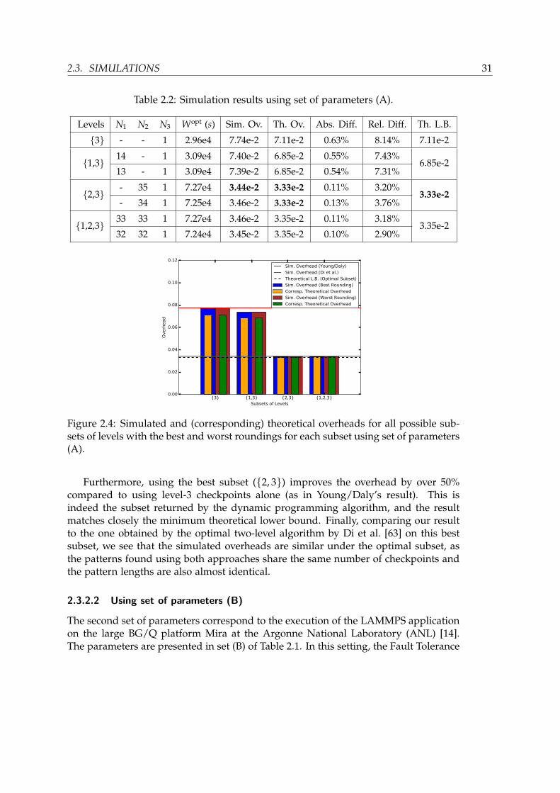
Results: Table 2.2 and Figure 2.4 present the simulation results. Table 2.2 shows,from left to right, the subset of levels used, the number of checkpoints computed byour first-order approximation formula for each possible rounding (N1, N2, N3), thecorresponding optimal pattern length (Wopt(s)), the simulated overhead (Sim. Ov.),the corresponding theoretical overhead (Th. Ov.), the absolute and relative differencesof these two overheads (Ab. Diff. = 100 × (Sim. Ov. - Th. Ov.), and Rel. Diff. = 100 ×(Sim. Ov. - Th. Ov.)/Sim. Ov.), and finally the theoretical lower bound for this subset(Th. L.B.).
With k = 3, there are four possible subsets of levels, and both the best simu-lated overhead and the corresponding theoretical overhead are achieved for the subset2, 3, with N2 = 35 and N3 = 1 (highlighted in bold in the table). First, the differ-ence between the simulated and theoretical overheads is very small, with a difference< 0.7% in absolute values, and a relative difference ranging from 2.9% (for subset1, 2, 3) to 8.14% (for subset 3), which shows the accuracy of the first-order approx-imation for this set of parameters. The simulated overhead is always higher than thetheoretical one, which is expected, because the first-order approximation ignores somelower-order terms. Next, we observe that, for each subset, all roundings of the numberof checkpoints yield similar overheads on this platform, and the difference betweenthe best and worst roundings is almost negligible.
2.3. SIMULATIONS 31
Table 2.2: Simulation results using set of parameters (A).
Levels N1 N2 N3 Wopt (s) Sim. Ov. Th. Ov. Abs. Diff. Rel. Diff. Th. L.B.
3 - - 1 2.96e4 7.74e-2 7.11e-2 0.63% 8.14% 7.11e-2
1,3 14 - 1 3.09e4 7.40e-2 6.85e-2 0.55% 7.43%6.85e-2
13 - 1 3.09e4 7.39e-2 6.85e-2 0.54% 7.31%
2,3 - 35 1 7.27e4 3.44e-2 3.33e-2 0.11% 3.20%3.33e-2
- 34 1 7.25e4 3.46e-2 3.33e-2 0.13% 3.76%
1,2,3 33 33 1 7.27e4 3.46e-2 3.35e-2 0.11% 3.18%3.35e-2
32 32 1 7.24e4 3.45e-2 3.35e-2 0.10% 2.90%
3 1,3 2,3 1,2,3Subsets of Levels
0.00
0.02
0.04
0.06
0.08
0.10
0.12
Ov
erh
ea
d
Sim. Overhead (Young/Daly)
Sim. Overhead (Di et al.)
Theoretical L.B. (Optimal Subset)
Sim. Overhead (Best Rounding)
Corresp. Theoretical Overhead
Sim. Overhead (Worst Rounding)
Corresp. Theoretical Overhead
Figure 2.4: Simulated and (corresponding) theoretical overheads for all possible sub-sets of levels with the best and worst roundings for each subset using set of parameters(A).
Furthermore, using the best subset (2, 3) improves the overhead by over 50%compared to using level-3 checkpoints alone (as in Young/Daly’s result). This isindeed the subset returned by the dynamic programming algorithm, and the resultmatches closely the minimum theoretical lower bound. Finally, comparing our resultto the one obtained by the optimal two-level algorithm by Di et al. [63] on this bestsubset, we see that the simulated overheads are similar under the optimal subset, asthe patterns found using both approaches share the same number of checkpoints andthe pattern lengths are also almost identical.
2.3.2.2 Using set of parameters (B)
The second set of parameters correspond to the execution of the LAMMPS applicationon the large BG/Q platform Mira at the Argonne National Laboratory (ANL) [14].The parameters are presented in set (B) of Table 2.1. In this setting, the Fault Tolerance

32 Chapter 2: Towards optimal multi-level checkpointing
4 1,4 2,4 3,4 1,2,4 1,3,4 2,3,4 1,2,3,4Subsets of Levels
0.00
0.02
0.04
0.06
0.08
0.10
0.12
0.14
0.16
0.18
Ov
erh
ea
d
Sim. Overhead (Young/Daly)
Sim. Overhead (Di et al.)
Theoretical L.B. (Optimal Subset)
Sim. Overhead (Best Rounding)
Corresp. Theoretical Overhead
Sim. Overhead (Worst Rounding)
Corresp. Theoretical Overhead
Figure 2.5: Simulated and (corresponding) theoretical overheads for all possible sub-sets of levels with the best and worst roundings for each subset using set of parameters(B).
Interface (FTI) [17] was used, which has four checkpoint levels (k = 4): Local check-point; Local checkpoint + Partner-copy; Local checkpoint + Reed-Solomon coding; andPFS-based checkpoint. The MTBFs correspond to the failure rates typically observedfor petascale HPC applications [140, 17, 62].
Results: Table 2.3 and Figure 2.5 present the simulation results for this set ofparameters. There are 8 possible subsets of levels. As before, we observe that thetheoretical overhead is always slightly smaller than the simulated one, with an abso-lute difference of less than 2%, and a relative difference between 6-14%, demonstratingthe accuracy of the model. Again, the results are very close to the theoretical lowerbound. For this platform, the simulated overheads vary from 9.68% (with optimal sub-set of levels 1, 3, 4 found by the dynamic programming algorithm) to 14.3% (withlevel-4 checkpoints alone). For a given subset of levels, the rounding does not playa significant role, as Wopt is also adjusted accordingly (increased or decreased) as aresult of rounding. For instance, we observe that, for subset 1, 2, 3, 4, the numbersof checkpoints at levels 1 and 2 are halved for the third rounding compared to the firstrounding in Table 2.3, but Wopt is also reduced by 31%, so that for the same amount ofwork, the number of checkpoints does not change by much. We can also see that thepattern length Wopt for the smallest overhead is around 10400s, but only 2450s for thelargest overhead. In fact, the largest pattern lengths are obtained for the highest cumu-lated checkpoint cost, which turns out to be 830s for 2, 3, 4 with N2=16, N3=4, N4=1,and for 1, 2, 3, 4 with N1 = 24, N2 = 8, N3 = 4 and N4 = 1. This is because usingmore checkpoints both increases the error-free overhead and reduces the time lost dueto re-executions upon errors. As a consequence, and to mitigate the aforementionedoverhead, the length of the pattern increases (e.g., Wopt = 17000s for 2, 3, 4 andWopt = 16600s for 1, 2, 3, 4). And the converse is also true: when using fewer check-points, the error-free overhead decreases and the time lost upon errors increases. In

2.3. SIMULATIONS 33
Table 2.3: Simulation results using set of parameters (B).
Levels N1 N2 N3 N4 Wopt (s) Sim. Ov. Th. Ov. Abs. Diff. Rel. Diff. Th. L.B.
4 - - - 1 2.45e3 1.43e-1 1.22e-1 1.9% 13.3% 1.22e-1
1,4 5 - - 1 3.79e3 1.18e-1 1.05e-1 1.3% 11.0%1.05e-1
4 - - 1 3.61e3 1.18e-1 1.05e-1 1.3% 11.0%
2,4 - 5 - 1 6.00e3 1.11e-1 1.00e-1 1.1% 9.9% 1.00e-1
3,4 - - 11 1 1.55e4 9.96e-2 9.02e-2 0.94% 9.44%9.01e-2
- - 10 1 1.44e4 9.91e-2 9.01e-2 0.90% 9.08%
1,2,4
9 3 - 1 6.41e3 1.11e-1 1.03e-1 0.8% 7.2%
1.02e-16 2 - 1 5.21e3 1.13e-1 1.04e-1 0.9% 8.0%
6 3 - 1 5.84e3 1.11e-1 1.03e-1 0.8% 7.2%
4 2 - 1 4.74e3 1.17e-1 1.05e-1 1.2% 10.3%
1,3,4
21 - 7 1 1.58e4 9.72e-2 8.99e-2 0.73% 7.51%
8.96e-218 - 6 1 1.40e4 9.82e-2 8.98e-2 0.84% 8.55%
14 - 7 1 1.04e4 9.68e-2 9.01e-2 0.67% 6.92%
12 - 6 1 1.26e4 9.85e-2 9.04e-2 0.81% 8.22%
2,3,4
- 16 4 1 1.70e4 1.07e-1 9.75e-2 0.95% 8.9%
9.68e-2- 12 3 1 1.36e4 1.04e-1 9.73e-2 0.67% 6.4%
- 12 4 1 1.47e4 1.05e-1 9.68e-2 0.82% 7.8%
- 9 3 1 1.17e4 1.05e-1 9.75e-2 0.75% 7.1%
1,2,3,4
24 8 4 1 1.66e4 1.09e-1 1.00e-1 0.9% 8.2%
9.92e-2
18 6 3 1 1.32e4 1.08e-1 9.99e-2 0.81% 7.5%
12 4 4 1 1.15e4 1.11e-1 1.03e-1 0.8% 7.2%
9 3 3 1 9.17e3 1.14e-1 1.05e-1 0.9% 7.9%
16 8 4 1 1.51e4 1.08e-1 9.95e-2 0.85% 7.9%
12 6 3 1 1.20e4 1.09e-1 1.00e-1 0.9% 8.3%
8 4 4 1 1.05e4 1.16e-1 1.05e-1 1.1% 9.5%
6 3 3 1 8.33e3 1.19e-1 1.08e-1 1.1% 9.2%

34 Chapter 2: Towards optimal multi-level checkpointing
order to compensate, the pattern length decreases (e.g., Wopt = 8330s for 1, 2, 3, 4with N1=6, N2=3, N3=3 and N4=1).
We note that, in this case, our first-order solution slightly outperforms the iterativemethod by Di et al. [62] on multi-level checkpointing (with a simulated overhead of9.68e-2 compared to 9.75e-2). The reason is that their algorithm computes a solutionunder the independent checkpointing model, i.e., checkpoints at different levels aretaken according to different independent periods. However, it is not clear how such amodel can be implemented in practice due to the difficulties as explained in Section 2.1and the different options to rollback to a checkpoint in case of a fault. Therefore, wetransformed their result to a pattern-based solution by rounding the different numbersof checkpoints obtained using their algorithm to create equal number of checkpointsat level `− 1 between two consecutive level-` checkpoints. Although the best roundingis selected here for comparison, the result can still change drastically the number ofcheckpoints computed by their initial rational solution without changing the patternlength, thus increasing the overhead.
2.3.3 Comparing performance of different approaches
In this section, we conduct simulations using settings from Di et al.’s recent work onmultilevel checkpointing, which comprises two cases with four levels [62] and eightcases with two levels [63], thus covering a wide range of configurations. For eachcase, we compare the performance of three different approaches: (a) Young/Daly’sclassical formula; (b) our first-order approximation formula; and (c) Di et al.’s iterativealgorithm.
Table 2.4: Set of parameters (C) used as input for simulations.
Set (C), from Di et al. [62]
Level 1 2 3 4
Case #A
C (s) 8 10 80 90
R (s) 8 10 80 90
MTBF (s) 2160 1440 8640 21600
Case #B
C (s) 1 20 60 70
R (s) 1 10 30 35
MTBF (s) 864 864 1080 1440
2.3.3.1 Using set of parameters (C)
We first run simulations for Cases #A and #B, whose parameters are presented inTable 2.4. These parameters are based on the FTI multilevel checkpointing model and

2.3. SIMULATIONS 35
have been used by Di et al. [62] to evaluate the performance of their approach. Notethat the recovery cost is about half that of the checkpointing cost in Case #B.
In their work, Di et al. considered independent checkpointing periods, as opposedto the nested method based on periodic patterns (as discussed in Section 2.1). Al-though they provided an optimal solution, an iterative approach was used to computeit numerically in contrast to the simple formula we propose in this work. Recall thatusing independent checkpointing periods allows checkpoints at different levels to betaken simultaneously, which can hardly be done in practice. Adapting their solutionto our model results in rational numbers of checkpoints, and we again use roundingto resolve this issue. We find that, using the best roundings for both approaches, theirsolution turns out to be very similar to ours (with the same number of checkpoints,and close periods with < 1% difference).
Results: Figure 2.6 presents the overheads for both cases. First, we observe that Diet al.’s optimal iterative algorithm has almost identical performance to our solution,with a simulated overhead around 45% for Case #A and 140% for Case #B underboth approaches. However, using Young/Daly’s formula to checkpoint only at thehighest level yields significantly worse overheads (around 90% for Case #A and 170%for Case #B). Overall, our solution is as good as Di et al.’s optimal numerical one (buthas much less complexity), and it is up to 45% better than Young/Daly’s formula inCase #A and 30% better in Case #B.
Note that the corresponding theoretical overhead of our solution is close to thesimulated one for Case #A, but starts to diverge for Case #B. This is because first-orderapproximation is only accurate when the resilience parameters and pattern length aresmall compared to the MTBF, which is no longer true for Case #B. Specifically, wehave:
• In Case #A, the optimal subset of levels is 2, 4. The optimal pattern has lengthWopt=1052s and consists of N2=8 level-2 checkpoints followed by N4=1 level-4checkpoint, meaning that we have a level-2 checkpoint every 131.5s of compu-tation. So a level-2 checkpoint is saved every 141.5s and a level-4 checkpoint issaved every 1222s. On the other hand, the combined MTBF for errors at levels1 and 2 (handled by level-2 checkpoints) is 864s and the combined MTBF forerrors at levels 3 and 4 (handled by level-4 checkpoints) is 6171s. Hence, we have141.5864 = 0.164 and 1222
6171 = 0.198, which are reasonably small, making our solutionaccurate.
• In Case #B, the optimal subset of levels is 1, 4, and the optimal pattern hasWopt = 223s, N1 = 5 and N4 = 1. Thus, we have a level-1 checkpoint every44.6s of computation. So a level-1 checkpoint is saved every 45.6s and a level-4checkpoint is saved every 298s. The MTBF for errors at level 1 is 864s and thecombined MTBF for errors at levels 2, 3 and 4 (handled by level-4 checkpoints)is 360s. Thus, we have 44.6
864 = 0.052, which is fine, but 298360 = 0.828, which is too
high and essentially makes the first-order solution inaccurate.
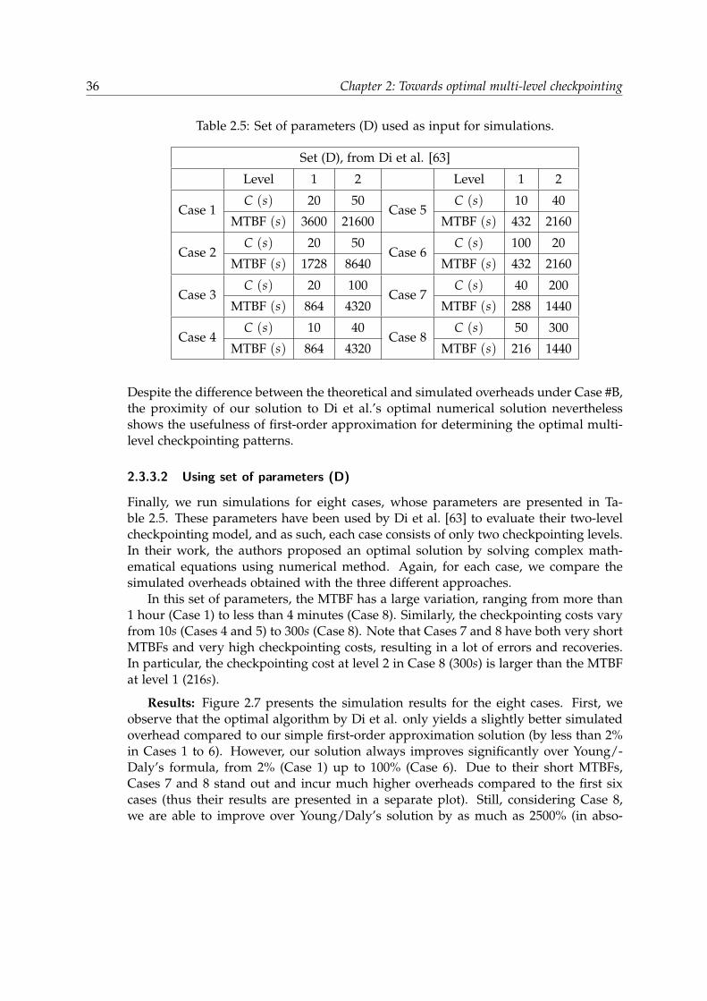
36 Chapter 2: Towards optimal multi-level checkpointing
Table 2.5: Set of parameters (D) used as input for simulations.
Set (D), from Di et al. [63]
Level 1 2 Level 1 2
Case 1C (s) 20 50
Case 5C (s) 10 40
MTBF (s) 3600 21600 MTBF (s) 432 2160
Case 2C (s) 20 50
Case 6C (s) 100 20
MTBF (s) 1728 8640 MTBF (s) 432 2160
Case 3C (s) 20 100
Case 7C (s) 40 200
MTBF (s) 864 4320 MTBF (s) 288 1440
Case 4C (s) 10 40
Case 8C (s) 50 300
MTBF (s) 864 4320 MTBF (s) 216 1440
Despite the difference between the theoretical and simulated overheads under Case #B,the proximity of our solution to Di et al.’s optimal numerical solution neverthelessshows the usefulness of first-order approximation for determining the optimal multi-level checkpointing patterns.
2.3.3.2 Using set of parameters (D)
Finally, we run simulations for eight cases, whose parameters are presented in Ta-ble 2.5. These parameters have been used by Di et al. [63] to evaluate their two-levelcheckpointing model, and as such, each case consists of only two checkpointing levels.In their work, the authors proposed an optimal solution by solving complex math-ematical equations using numerical method. Again, for each case, we compare thesimulated overheads obtained with the three different approaches.
In this set of parameters, the MTBF has a large variation, ranging from more than1 hour (Case 1) to less than 4 minutes (Case 8). Similarly, the checkpointing costs varyfrom 10s (Cases 4 and 5) to 300s (Case 8). Note that Cases 7 and 8 have both very shortMTBFs and very high checkpointing costs, resulting in a lot of errors and recoveries.In particular, the checkpointing cost at level 2 in Case 8 (300s) is larger than the MTBFat level 1 (216s).
Results: Figure 2.7 presents the simulation results for the eight cases. First, weobserve that the optimal algorithm by Di et al. only yields a slightly better simulatedoverhead compared to our simple first-order approximation solution (by less than 2%in Cases 1 to 6). However, our solution always improves significantly over Young/-Daly’s formula, from 2% (Case 1) up to 100% (Case 6). Due to their short MTBFs,Cases 7 and 8 stand out and incur much higher overheads compared to the first sixcases (thus their results are presented in a separate plot). Still, considering Case 8,we are able to improve over Young/Daly’s solution by as much as 2500% (in abso-

2.4. RELATED WORK 37
lute value of the overhead), and we are off the optimal simulated overhead by only300%. In addition, Figure 2.7 shows the theoretical overheads obtained both with ourformula and the solution provided by Di et al. in [63]. As expected, our first-orderapproximation remains accurate when the MTBF is large, as in Cases 1, 2 and 4. How-ever, it becomes less accurate with shorter MTBFs and higher error rates, especially inCases 7 and 8 (which do not represent healthy HPC platforms).
2.3.4 Summary of results
From the simulation results, we conclude that first-order approximation remains avaluable performance model for evaluating checkpointing solutions in HPC systems(as long as the error rates stay reasonably low). We have demonstrated, through anextensive set of simulations with a wide range of parameters, the usefulness of multi-level checkpointing (over using only one level of checkpoints) with significantly re-duced overheads. The results also corroborate the analytical study by showing thebenefit of selecting an optimal subset of levels among all the levels available. Overall,our approach achieves the optimal or near-optimal performance in almost all cases,except when the MTBF is too small, in which case even the optimal solution yields anunacceptably high overhead (e.g., Case 8 of Table 2.5).
2.4 Related work
Given the checkpointing cost and platform MTBF, classical formulas due toYoung [200] and Daly [58] are well known to determine the optimal checkpointing pe-riod in the single-level checkpointing scheme. However, this method suffers from theintrinsic limitation that the cost of checkpointing/recovery grows with failure proba-bility, and becomes unsustainable at large scale [82, 30] (even with diskless or incre-mental checkpointing [151]).
To reduce the I/O overhead, various two-level checkpointing protocols have beenstudied. Vaidya [185] proposed a two-level recovery scheme that tolerates a singlenode failure using a local checkpoint stored on a parter node. If more than one fail-ure occurs during any local checkpointing interval, the scheme resorts to the globalcheckpoint. Silva and Silva [164] advocated a similar scheme by using memory tostore local checkpoints, which is protected by XOR encoding. Di et al. [63] analyzeda two-level checkpointing pattern, and proved equal-length segments in the optimalsolution. They also provided mathematical equations that can be solved numericallyto compute the optimal pattern length and number of segments. Benoit et al. [20] re-lied on disk checkpoints to cope with fail-stop failures and memory checkpoints cou-pled with error detectors to handle silent data corruptions. They derived first-orderapproximation formulas for the optimal pattern length and the number of memorycheckpoints between two disk checkpoints.
Some authors have also generalized two-level checkpointing to account for an arbi-trary number of levels. Moody et al. [140] implemented this approach in a three-level

38 Chapter 2: Towards optimal multi-level checkpointing
Scalable Checkpoint/Restart (SCR) library. They relied on a rather complex Markovmodel to recursively compute the efficiency of the scheme. Bautista-Gomez et al. [17]designed a four-level checkpointing library, called Fault Tolerance Interface (FTI), inwhich partner-copy and Reed-Solomon coding are employed as two intermediate lev-els between local and global disks. Based on FTI, Di et al. [62] proposed an iterativemethod to compute the optimal checkpointing interval for each level with prior knowl-edge of the application’s total execution time. Hakkarinen and Chen [97] consideredmulti-level diskless checkpointing for tolerating simultaneous failures of multiple pro-cessors. Balaprakash et al. [14] studied the trade-off between performance and energyfor general multi-level checkpointing schemes.
While all of these works relied on numerical methods to compute the checkpoint-ing intervals at different levels, this work is the first to provide explicit formulas onthe optimal parameters in a multi-level checkpointing protocol (up to first-order ap-proximation as in Young/Daly’s classical result).
2.5 Conclusion
This chapter has studied multi-level checkpointing protocols, where different levels ofcheckpoints can be set; lower levels deal with frequent errors that can be recovered atlow cost (for instance with a memory copy), while higher levels allow us to recoverfrom all errors, such as node failures (for instance with a copy in stable storage). Weconsider a general scenario with k levels of faults, and we provide explicit formulasto characterize the optimal checkpointing pattern, up to first-order approximation.The overhead turns out to be of the order of ∑k
`=1√
2λ`C`, which elegantly extendsYoung/Daly’s classical formula.
The first-order approximation to the optimal k-level checkpointing pattern uses ra-tional numbers of checkpoints, and we prove that all segments should have equallengths. We corroborate the theoretical study by an extensive set of simulations,demonstrating that greedily rounding the rational values leads to an overhead veryclose to the lower bound. Furthermore, we provide a dynamic programming algo-rithm to determine those levels that should be selected, and the simulations confirmthe optimality of the subset of levels returned by the dynamic programming algorithm.
The problem of finding a first-order optimal pattern with an integer number ofsegments to minimize the overhead remains open. It may well be the case that suchan integer pattern is not periodic at each level and uses different-length segments.However, the good news is that the rounding of the rational solution provided in thischapter seems quite efficient in practice.

Case #A Case #B0.0
0.5
1.0
1.5
2.0
Overhead
Young/Daly's formula (Simulated)
Our first-order approx. (Simulated)
Our first-order approx. (Theoretical)
Di et al.'s algorithm (Simulated)
Figure 2.6: Performance comparison of the three different approaches using two casesfrom Di et al. [62].
Case 1 Case 2 Case 3 Case 4 Case 5 Case 60.0
0.5
1.0
1.5
2.0
Overhead
Young/Daly's formula (Simulated)
Our first-order approx. (Simulated)
Our first-order approx. (Theoretical)
Di et al.'s algorithm (Simulated)
Di et al.'s algorithm (Theoretical)
Case 7 Case 80
5
10
15
20
25
30
35
40
45
Overhead
Young/Daly's formula (Simulated)
Our first-order approx. (Simulated)
Our first-order approx. (Theoretical)
Di et al.'s algorithm (Simulated)
Di et al.'s algorithm (Theoretical)
Figure 2.7: Performance comparison of the three different approaches using 8 casesfrom Di et al. [63].

40 Chapter 2: Towards optimal multi-level checkpointing

Chapter 3
Comparing the performance of rigid, mold-able and grid-shaped applications on failure-prone HPC platforms
In this chapter, we compare the performance of different approaches to tolerate fail-ures for applications executing on large-scale failure-prone platforms. We study (i)Rigid applications, which use a constant number of processors throughout execution;(ii) Moldable applications, which can use a different number of processors after eachrestart following a fail-stop error; and (iii) GridShaped applications, which are mold-able applications restricted to use rectangular processor grids (such as many denselinear algebra kernels). We start with checkpoint/restart, the de-facto standard ap-proach. For each application type, we compute the optimal number of failures (i.e.that maximizes the yield of the application) to tolerate before relinquishing the cur-rent allocation and waiting until a new resource can be allocated, and we determinethe optimal yield that can be achieved. For GridShaped applications, we also inves-tigate Application Based Fault Tolerance (ABFT) techniques and perform the same anal-ysis, computing the optimal number of failures to tolerate and the associated yield.We instantiate our performance model with realistic applicative scenarios and make itpublicly available for further usage. We show that using spare nodes grants a muchbetter yield than currently used strategies that restart after each failure. Moreover,the yield is similar for Rigid, Moldable and GridShaped applications, while the op-timal number of failures to tolerate is very high even for a short wait time. Finally,Moldable applications have the advantage to restart less frequently than Rigid ap-plications. The work in this chapter is joint work with Thomas Herault, Yves Robert,Aurelien Bouteiller, Atsushi Hori, George Bosilca and Jack Dongarra, and has beenpublished in Parallel Computing (ParCo) [J5].
41

42Chapter 3: Comparing the performance of rigid, moldable and grid-shaped applications on
failure-prone HPC platforms
3.1 Introduction
Consider a long-running job that requests N processors from the batch scheduler.Resilience to fail-stop errors1 is typically provided by a Checkpoint/Restart (C/R)mechanism, the de-facto standard approach for High-Performance Computing (HPC)applications. After each failure on one of the nodes used by the application, theapplication restarts from the last checkpoint but the number of available processorsdecreases, assuming the application can continue execution after a failure (e.g., usingULFM [28]). Until which point should the execution proceed before requesting a newallocation with N fresh resources from the batch scheduler?
The answer depends upon the nature of the application. For a Rigid application,the number of processors must remain constant throughout the execution. The ques-tion is then to decide the number F of processors (out of the N available initially) thatwill be used as spares. With F spares, the application can tolerate F failures. The appli-cation always executes with N − F processors: after each failure, then it restarts fromthe last checkpoint and continues executing with N − F processors, the faulty proces-sor having been replaced by a spare. After F failures, the application stops when the(F + 1)st failure strikes, and relinquishes the current allocation. It then asks for a newallocation with N processors, which takes a wait time, D, to start (as other applicationsare most likely using the platform concurrently). The optimal value of F obviouslydepends on the value of D, in addition to the application and resilience parameters.The wait time typically ranges from several hours to several days if the platform isover-subscribed (up to 10 days for large applications on the K-computer [196]). Themetric to optimize here is the (expected) application yield, which is the fraction ofuseful work per second, averaged over the N resources, and computed in steady-statemode (expected value for multiple batch allocations of N resources).
For a Moldable application, the problem is different: here we assume that theapplication can use a different number of processors after each restart. The applica-tion starts executing with N processors; after the first failure, the application recoversfrom the last checkpoint and is able to continue with only N − 1 processors, albeitwith a slowdown factor N−1
N . After how many failures F should the application de-cide to stop2 and accept to produce no progress during D, in order to request a newallocation? Again, the metric to optimize is the application yield.
Finally, consider an application which must have a given shape (or a set of givenshapes) in terms of processor layout. Typically, these shapes are dictated by the ap-plication algorithm. In this chapter, we use the example of a GridShaped applica-tion, which is required to execute on a rectangular processor grid whose size candynamically be chosen. Most dense linear algebra kernels (matrix multiplication, LU,Cholesky and QR factorizations) are GridShaped applications, and perform more ef-
1We use the terms fail-stop error and failure indifferently.2Another limit is induced by the total application memory Memtot. There must remain at least ` live
processors such that Memtot ≤ `×Memind , where Memind is the memory of each processor. We ignorethis contraint in this chapter but it would be straightforward to take it into account.
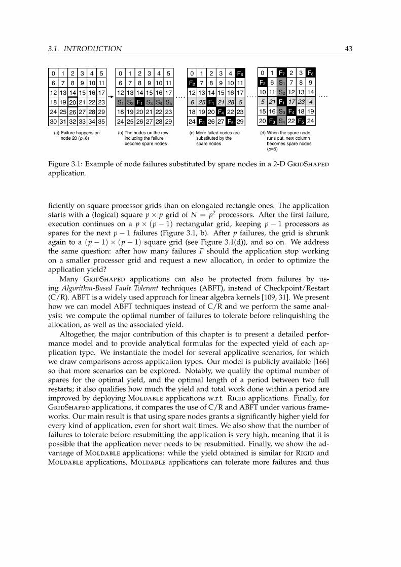
3.1. INTRODUCTION 43
Figure 3.1: Example of node failures substituted by spare nodes in a 2-D GridShaped
application.
ficiently on square processor grids than on elongated rectangle ones. The applicationstarts with a (logical) square p× p grid of N = p2 processors. After the first failure,execution continues on a p × (p − 1) rectangular grid, keeping p − 1 processors asspares for the next p − 1 failures (Figure 3.1, b). After p failures, the grid is shrunkagain to a (p − 1) × (p − 1) square grid (see Figure 3.1(d)), and so on. We addressthe same question: after how many failures F should the application stop workingon a smaller processor grid and request a new allocation, in order to optimize theapplication yield?
Many GridShaped applications can also be protected from failures by us-ing Algorithm-Based Fault Tolerant techniques (ABFT), instead of Checkpoint/Restart(C/R). ABFT is a widely used approach for linear algebra kernels [109, 31]. We presenthow we can model ABFT techniques instead of C/R and we perform the same anal-ysis: we compute the optimal number of failures to tolerate before relinquishing theallocation, as well as the associated yield.
Altogether, the major contribution of this chapter is to present a detailed perfor-mance model and to provide analytical formulas for the expected yield of each ap-plication type. We instantiate the model for several applicative scenarios, for whichwe draw comparisons across application types. Our model is publicly available [166]so that more scenarios can be explored. Notably, we qualify the optimal number ofspares for the optimal yield, and the optimal length of a period between two fullrestarts; it also qualifies how much the yield and total work done within a period areimproved by deploying Moldable applications w.r.t. Rigid applications. Finally, forGridShaped applications, it compares the use of C/R and ABFT under various frame-works. Our main result is that using spare nodes grants a significantly higher yield forevery kind of application, even for short wait times. We also show that the number offailures to tolerate before resubmitting the application is very high, meaning that it ispossible that the application never needs to be resubmitted. Finally, we show the ad-vantage of Moldable applications: while the yield obtained is similar for Rigid andMoldable applications, Moldable applications can tolerate more failures and thus

44Chapter 3: Comparing the performance of rigid, moldable and grid-shaped applications on
failure-prone HPC platforms
restart more rarely than Rigid ones. This means that a Moldable application is morelikely to terminate before being resubmitted.
The rest of the chapter is organized as follows. Section 3.2 is devoted to formallydefining the performance model. Section 3.3 provides formulas for the yield of Rigid,Moldable and GridShaped applications using the C/R approach, and for the yieldof GridShaped applications using the ABFT approach . All these formulas are instan-tiated through the applicative scenarios in Section 3.4, to compare the different results.Section 3.5 provides an overview of related work. Finally, Section 3.6 provides finalremarks and hints for future work.
3.2 Performance model
This section reviews the key parameters of the performance model. Some assumptionsare made to simplify the computation of the yield. We discuss possible extensions inSection 3.6.
3.2.1 Application/platform framework
We consider perfectly parallel applications that execute on homogeneous parallel plat-forms. Without loss of generality, we assume that each processor has unit speed: weonly need to know that the total amount of work done by p processors within T sec-onds requires p
q T seconds with q processors.
3.2.2 Mean Time Between Failures (MTBF)
Each processor is subject to failures which are IID (independent and identically dis-tributed) random variables3 following an Exponential probability distribution of meanµind, the individual processor MTBF. Then the MTBF of a section of the platform com-prised of i processors is given by µi =
µindi [106].
3.2.3 Checkpoints
Processors checkpoint periodically, using the optimal Young/Daly period [200, 58]:for an application using i processors, this period is
√2Ciµi, where Ci is the time to
checkpoint with i processors. We consider two cases to define Ci. In both cases, theoverall application memory footprint is considered constant at Memtot, so the size ofindividual checkpoints is inversely linear with the number of participating/surviv-ing processors. In the first case, the I/O bandwidth is the bottleneck (which is oftenthe case in HPC platforms – it takes only a few processors to saturate the I/O band-width); then the checkpoint cost is constant and given by Ci = Memtot
τio, where τio is
the aggregated I/O bandwidth. In the second case, the processor network card is
3In datacenters, failures can actually be correlated in space or in time. But to the best of our knowl-edge, there is no currently available method to analyze their impact without the IID assumption.

3.2. PERFORMANCE MODEL 45
the bottleneck, and the checkpoint cost is inversely proportional to number of activeprocessors: Ci =
Memtotτxnet×i , where τxnet is the available network card bandwidth, i.e. the
bandwidth available for one and only one processor, and Memtoti the checkpoint size.
We denote the recovery time with i processors as Ri. For all simulations we useRi = Ci, assuming that the read and write bandwidths are identical.
3.2.4 Wait Time
Job schedulers allocate nodes to given applications for a given time. They aim atoptimizing multiple criteria, depending on the center policy. These criteria includefairness (balancing the job requests between users or accounts), platform utilization(minimizing the number of resources that are idling), and job makespan (providingthe answer as fast as possible). Combined with a high resource utilization (nodeidleness is usually in the single digit percentage for a typical HPC platform), a job hasto wait a Wait Time (D) between its submission and the beginning of its execution.
Job schedulers implement the selection based on the list of submitted jobs, each jobdefining how many processors it needs and for how long. That definition is, in mostcases, unchangeable: an application may use less resource than what it requested,but the account will be billed for the requested resource, and it will not be able tore-dimension the allocation during the execution.
Thus, if after some failures, an application has not enough resources left to ef-ficiently complete, it will have to relinquish the allocation, and request a new one.During the wait time D, the application does not execute any computation to progresstowards completion: its yield is zero during D seconds.
3.2.5 Objective.
We consider a long-lasting application that requests a resource allocation with N pro-cessors. We aim at deriving the optimal number of failures F that should be toleratedbefore paying the wait time and requesting a new allocation. We aim at maximizingthe yield Y of the application, defined as the fraction of time during the allocationlength and wait time where the N resources perform useful work. More precisely, theyield is defined by the following formula:
Y =total time spent computing for all processors
number of processors × total execution time of application.
. Of course a spare does not perform useful work when idle, processor do not computewhen checkpointing or recovering, re-execution odes not account for actual work, andno processor is active during wait time. All this explains that the yield will always besmaller than 1. We will derive the value of F that maximizes Y for the three applicationtypes using C/R (and both C/R and ABFT for GridShaped applications).

46Chapter 3: Comparing the performance of rigid, moldable and grid-shaped applications on
failure-prone HPC platforms
3.3 Expected yield
This section is the core of the chapter. We compute the expected yield for each ap-plication type, Rigid (Section 3.3.1), Moldable (Section 3.3.2) and GridShaped (Sec-tion 3.3.3), using the C/R approach, and compare it with ABFT for GridShaped inSection 3.3.4.
3.3.1 Rigid application
We first consider a Rigid application that can be parallelized at compile-time to useany number of processors but cannot change this number until it reaches termination.There are N processors allocated to the application. We use N − F for execution andkeep F as spares. The execution is protected from failures by checkpoints of durationCN−F. Each failure striking the application will incur an in-place restart of durationRN−F, using a spare processor to replace the faulty one. However, when the (F + 1)st
failure strikes, the job will have to stop and perform a full restart, waiting for a newallocation of N processors to be granted by the job scheduler.
We define TR as the expected duration of an execution period until the (F + 1)st
failure strikes. The first failure is expected to strike after µN seconds, the second failureµN−1 seconds after the first one, and so on. We relinquish the allocation after F + 1failures and wait some time D. As faults can also happen during the checkpoint andthe recovery, this means that:
TR =N−F
∑i=N
µi + D. (3.1)
What is the total amount of work WR computed during a period TR? During thesub-period of length µi, there are µi√
2CN−FµN−Fcheckpoints, each of length CN−F. The
failure hits one of live processors, either a working processor or a spare. In both cases,the number of live processors decreases. if the failure hits a spare, it has no immediateimpact on the application, except that the number of available spares decreases. Ifthe failure hits a working processor, which happens with probability N−F
i , some workis lost, and a restart is needed. During each sub-period, and weighting the cost bythe probability of the failure hittingt a working processor during that sub-period, the
work lost by each processor by the end of the sub-period is in average√
2CN−FµN−F2 · N−F
i(see [106] for further details). Each time there is a failure, the next sub-period is thusstarted by a restart RN−F with probability N−F
i+1 , except for the first sub-period whichalways starts by a restart (it corresponds to reading input data at the beginning of theallocation). All in all, during the sub-period of length µi with i 6= N, each processorworks during
1
1 + CN−F√2CN−FµN−F
·(
µi − RN−F ·N − Fi + 1
−√
2CN−FµN−F
2· N − F
i
)

3.3. EXPECTED YIELD 47
seconds. The first fraction corresponds to the proportion of the time that isused for useful computations and not for checkpointing. This fraction is actually:
period timeperiod time+checkpoint time =
√2CN−FµN−F√
2CN−FµN−F+CN−Fwhich is equivalent to the former fraction
after simplification.Finally, each processor works during
1
1 + CN−F√2CN−FµN−F
·(
µN − RN−F −√
2CN−FµN−F
2· N − F
i
)
seconds in the first sub-period of length µN as it always starts by reading the initialdata.
There are N − F processors at work, hence, re-arranging terms, we obtain that
WR =N − F
1 + CN−F√2CN−FµN−F
·N−F
∑i=N
(µi − (RN−F +
√2CN−FµN−F
2) · N − F
i
)(3.2)
Indeed, the factor for RN−F is N−Fi+1 for all subperiods except the first one, i.e. N − F ≤
i ≤ N − 1 , which means it is equivalent to N−Fi with N − F + 1 ≤ i ≤ N. Moreover,
N−FN−F = 1 which is the corresponding factor for the first subperiod, so by summing all
the terms we get toN−F∑
i=NRN−F · N−F
i .
During the whole duration TR of the period, in the absence of failures and pro-tection techniques, the application could have used all the N processors to computecontinuously. Thus the effective yield with protection for the application during TR isreduced to YR:
YR =WR
N · TR
3.3.2 Moldable application
We now consider a Moldable application that can use a different number of proces-sors after each restart. The application starts executing with N processors. After thefirst failure, the application recovers from the last checkpoint and is able to continuewith only N− 1 processors, after paying the restart cost RN−1, albeit with a slowdownfactor N−1
N of the parallel work per time unit. After F + 1 failures, the applicationstops, just as it was the case for a Rigid application.
We define TM as the expected duration of an execution period until the (F + 1)st
failure strikes. The length of a period is
TM =N−F
∑i=N
µi + D, (3.3)

48Chapter 3: Comparing the performance of rigid, moldable and grid-shaped applications on
failure-prone HPC platforms
the same as for Rigid applications.However, for the total amount of work WM during a period, things are slightly
different. To compute the total amount of work WM during a period TM, we proceedas before and consider each sub-period. During the sub-period of length µi, there are
µi√2Ciµi
checkpoints, each of length Ci. There is also a restart Ri at the beginning of each
sub-period, and the average time lost is√
2Ciµi2 . The probability that the failure strikes
a working processor is always 1, because all alive processors are working during eachsub-period. Overall, there are i processors at work during the sub-period of length µi,and each of them actually works during
µi − Ri −√
2Ciµi2
1 + Ci√2Ciµi
seconds. Altogether, we derive that
WM =N−F
∑i=N
i× µi − Ri −√
2Ciµi2
1 + Ci√2Ciµi
(3.4)
The yield of the Moldable application is then:
YM =WM
N · TM
3.3.3 GridShaped application
Next, we consider a GridShaped application, defined as a moldable execution whichrequires a rectangular processor grid. Here we mean a logical grid, i.e. a layout ofprocesses whose communication pattern is organized as a 2D grid, not a physical pro-cessor grid where each processor has four neighbors directly connected to it. Indeed,there is little hope to use physical grids today. Some modern architectures have amulti-dimensional torus as physical interconnexion network, but the job schedulernever guarantees that allocated nodes are adjacent, let alone are organized along anactual torus. This means that the actual time to communicate with a logically adja-cent processor is variable, depending upon the length of the path that connects them,and also upon the congestion of the links within that path (these links are likely to beshared by other paths). Other architecture communicate through a hierarchical inter-connexion switch, hence a 2D processor grid is not meaningful for such architectures.Altogether, this explains that one targets logical process grids, not physical processorgrids. Now why do the application needs a process grid? State-the-art linear algebrakernels such as matrix product, LU, QR and Cholesky factorizations, are most efficientwhen the data is partitioned across a logical grid of processes, preferably a square, or

3.3. EXPECTED YIELD 49
at least a balanced rectangle of processes [150]. This is because the algorithms arebased upon outer-product matrix updates, which are most efficiently implemented on(almost) square grids. Say you start with 64 working processors, arranged as a 8× 8process grid. When one processor fails, the squarest grid would be 63 = 9× 7, andthen after a second failure we get 62 = 31× 2 which is way too elongated to be effi-cient. After the first failure, it is more efficient to use a 8× 7 grid and keep 7 spares;then we use spares for the next 7 failures, after which we shrink to a 7× 7 grid (andkeep 7 spares), and so on.
For the analysis, assume that the application starts with a square p× p grid of N =p2 processors. After the first failure, execution continues on a p× (p− 1) rectangulargrid, keeping p− 1 processors as spares for the next p− 1 failures. After p failures, thegrid is shrunk again to a (p− 1)× (p− 1) square grid, and the execution continues onthis reduced-size square grid. After how many failures F should the application stop,in order to maximize the application yield?
The derivation of the expected length of a period and of the total work is more com-plicated for GridShaped than for Rigid and Moldable. To simplify the presentation,we outline the computation of the yield only for values of F of the form F = 2p f − f 2,hence p2 = F + (p− f )2, meaning that we stop shrinking and request a new allocationwhen reaching a square grid of size (p− f )× (p− f ) for some value of f < p to bedetermined. Obviously, we could stop after any number of faults F, and the publiclyavailable software [166] shows how to compute the optimal value of F without anyrestriction.
We start by computing an auxiliary variable: on a (p1 − 1)× p2 grid with p1 ≥ p2,the expected time to move from p2 − 1 spare nodes to no spare nodes will be denotedby TG(p1, p2). It means that the number of computing nodes never changes and is(p1 − 1)p2. It always starts with a restart R(p1−1)p2
, because having p2 − 1 spare nodesmeans that a failure just occurred on one of the p1 p2 processors that were working justbefore that failure, and we had to remove a row from the process grid. As previouslythis time is the sum of all the intervals between each failure, namely:
TG(p1, p2) =(p1−1)p2
∑i=p1 p2−1
µi.
Going from p2 processors down to (p− f )2 processors thus require a time
TG = µp2 +f−1
∑g=0
(TG(p− g, p− g) + TG(p− g, p− g− 1)
)+ D.
We simply add the time before the first failure and the wait time to the time neededto move from a grid of size p2 to (p− 1)2, to (p− 2)2, . . . , to (p− f )2.
Similarly, we define the auxiliary variable WG(p1, p2) as the parallel work whenmoving from a (p1 − 1)× p2 grid with p2 − 1 spare nodes to a (p1 − 1)× p2 grid withno spare node, where p1 ≥ p2. There are (p1 − 1)p2 processors working during all

50Chapter 3: Comparing the performance of rigid, moldable and grid-shaped applications on
failure-prone HPC platforms
sub-periods. Without restart and re-execution, this work is (p1 − 1)p2 · ∑(p1−1)p2i=p1 p2−1 µi.
Any failure which hits one of the working processors calls for a restart R(p1−1)p2and
incurs some lost work:√
2C(p1−1)p22 in average. The first sub-period starts with a restart
R(p1−1)p2,because the application (distributed on a grid of p1 × p2 was previously
hit by a failure, except if this is the beginning of a new allocation (which case willbe dealt with later on). Then, for all other sub-periods, a restart is taken if one of(p1 − 1)p2 computing processors was hit by a failure. This means that the sub-periodwith i processors alive (of length µi) starts with a restart R(p1−1)p2
with probability(p1−1)p2
i+1 , for i ≤ p1 p2 − 2. Similarly, for all sub-periods with i processors alive, we
lose the expected compute time√
2C(p1−1)p2µ(p1−1)p2
2 with probability (p1−1)p2i . Finally,
the checkpoint period evolves with the number of processors, just as for Moldable
applications. We derive the following formula:
WG(p1, p2) =(p1−1)p2
1+C(p1−1)p2√
2C(p1−1)p2µ(p1−1)p2
×(
µp1 p2−1 − R(p1−1)p2−√
2C(p1−1)p2µ(p1−1)p2
2 · (p1−1)p2p1 p2−1
+ ∑(p1−1)p2i=p1 p2−2
(µi − R(p1−1)p2
· (p1−1)p2i+1 −
√2C(p1−1)p2
µ(p1−1)p22 · (p1−1)p2
i
))
Going from p2 processors down to (p− f )2 processors thus corresponds to a totalwork
WG =p2
1 +Cp2√
2Cp2 µp2
·µp2 − Rp2 −
√2Cp2 µp2
2
+
f−1
∑g=0
(WG(p− g, p− g) + WG(p− g, p− g− 1))
We use the previously computed function just as we did with the time and we add thework done during the first sub-period on the initial grid of size p2 (this is the specialcase for the beginning of an allocation that was mentioned above). Its computation issimilar to that of other subperiods.
The yield of the GridShaped application is then:
YG =WG
N · TG
where N = p2.

3.3. EXPECTED YIELD 51
3.3.4 ABFT for GridShaped
Finally, in this section, we investigate the impact of using Algorithm-Based Fault Toleranttechniques, or ABFT, instead of Checkpoint:Restart (C/R). Just as before, we build aperformance model that uses first-order approximations. In particular, we do notconsider overlapping failures, thereby allowing for a failure-free reconstruction of lostdata after a failure. This first-order approximation is accurate up to a few percent,whenever the failure rate is not too high, or more precisely, when the MTBF remains anorder of magnitude higher than resilience parameters [106]. Note that this is the casefor state-of-the-art platforms, but may prove otherwise whenever millions of nodes areassembled in the forthcoming years.
Consider a matrix factorization on a p × p grid. The matrix is of size n × n andis partitioned into tiles of size b × b. These tiles are distributed in a 2D block-cyclicfashion across processors. Letting n = pbr, each processor initially holds r2 tiles.Every set of p consecutive tiles in the matrix is checksummed into a new tile, whichis duplicated for resilience. These two new tiles are added to the right border of thematrix and will be distributed in a 2D block-cyclic fashion across processors, just asthe original matrix tiles. In other words, we add 2pr2 new tiles, extending each tilerow of the matrix (there are pr such tile rows) with 2r new tiles. Fig. 3.2 illustratesthis scheme: the white area represents the original user matrix of size n× n, split intiles of size b × b, and distributed over a p × p process grid. The number in eachtile represents the rank that hosts a given tile of the matrix. There are two groups oftile-columns of checksums: the light grey ones checksum the right end of the matrix,and the dark grey ones checksum the left part of the matrix. For a bigger matrix, moregroups would be added, each group accumulate the sum of p consecutive tile-columnsof the matrix. In each group, there are two tile-columns: the checksum and its replica.These new tiles will be treated as regular matrix tiles by the ABFT algorithm, whichcorresponds to a ratio 2pr2
p2r2 = 2p of extra work, and to a failure-free slowdown factor
1 + 2p [31].
Now, if a processor crashes, we finish the current step of the factorization on allsurviving processors, and then reconstruct the tiles of the crashed processor as follows:
• For each tile lost, there are p− 1 other tiles (the ones involved in the same check-sum as the lost tile) and at least one checksum tile (maybe two if the crashedprocessor did not hold any of the two checksum tiles for that lost tile). This iswhat is needed to enable the reconstruction. We solve a linear system of size band reconstruct the missing tile for a time proportional to b3 + pb2.
• We do this for the r2 tiles of the crashed processor, for a total time of O(r2(b3 +pb2)τa), where τa is the time to perform a floating-point operation.
Doing so, we reconstruct the same tile as if we had completed the factorization stepwithout failure.
Then, there are two cases: the ABFT algorithm relies on a process grid, so the ap-plication behaves similarly to a GridShaped application. If spare nodes are available,

52Chapter 3: Comparing the performance of rigid, moldable and grid-shaped applications on
failure-prone HPC platforms
012012
345345
678678
012012
345345
678678
012012
345345
678678
012012
+
+
=
=
b
b
p
n
p
n
Figure 3.2: Example of data redundancy and checksuming in an ABFT factorization.Each white square represents a matrix tile; numbers in the square represent the rankon which this tile is hosted; grey tiles represent the checksums and their replica (sym-bolized by the = arrow). In this case, p = 3, n = 6b.
one of them is selected and inserted within the process grid at the place of the crashedprocessor, at a cost of communicating O(r2b2) matrix coefficients (the amount of dataheld by the faulty processor). If, on the other hand, there are no spare nodes, we haveto start the redistribution of the matrix onto a p× (p− 1) grid. The distribution is op-erated in parallel across the p grid rows. Within a processor row, most of the tiles willhave to change owner to keep enforcing a 2D block-cyclic distribution, which impliesO( n2
p ) = O(r2 pb2) communications as we redistribute everything on every row. Sinceall rows operate in parallel, the time for the redistribution is O(r2 pb2τc), where τc isthe time to communicate a floating point number. Altogether, the total cost to recoverfrom a failure is O(r2b2(bτa + p(τa + τc))).
In the following, we compute the expected yield of a linear algebra kernel protectedby ABFT. Again, we consider numbers of failures of the form F = 2p f − f 2 so thatp2 = F + (p− f )2. Again, we could stop after any number of faults F, and the publiclyavailable software [166] shows how to do so.
We first compute the expected time between two full restarts:
TABFT =(p− f )2
∑i=p2
µi + D.
As previously, we tolerate failures up to reaching a processor grid size of (p − f )×(p− f ), each inter-arrival time being the MTBF of the platform with the correspondingnumber of alive processors.
Now, we define the auxiliary variable WABFT(p1, p2) as the parallel work when

3.3. EXPECTED YIELD 53
moving from a (p1 − 1)× p2 grid with p2 − 1 spare nodes to a (p1 − 1)× p2 grid withno spare node. There are (p1 − 1)p2 processors working during all sub-periods, justas it was the case for GridShaped applications. A failure-free execution would implya parallel work of 1
1+ 2p
∑(p1−1)p2i=p1 p2−1 µi which is the total time of computation divided
by overhead added with the checksum tiles. However, for each failure we need toreconstruct the lost tiles and either pay a redistribution cost (during the first sub-period where we just reduced the size of the grid because we had no spare) or acommunication cost to send data to one of the p2 − 1 spare nodes (all other sub-periods where we select a spare). This happens if and only if the failure stroke aworking processor just as in the GridShaped case, i.e. with probability (p1−1)p2
i+1 . In theend, since there are (p1 − 1)p2 processors at work, we get the following formula:
WABFT(p1, p2)=(p1 − 1)p2
1 + 2p
(µp1 p2−1−RDp1+
(p1−1)p2
∑i=p1 p2−2
(µi −RP· (p1 − 1)p2
i + 1)
),
where RP is the cost to replace a faulty processor by a spare, namely
RP = r2(b3 + pb2)τa + r2b2τc,
and RDi is the cost to reistribute data, namely
RDi = r2(b3 + pb2)τa +n2
iτc.
To compute these values, we proceed as follows:• The reconstruction of the lost tiles always takes r2(b3 + pb2) floating-point opera-
tions, and the enrollment of the spare requires that it receives r2b2 floating-pointvalues, which directly leads to the value of RP, which is independent of thenumber of processors;
• However, when we redistribute the tiles to shrink the grid, the time neededincreases as the number of processors decreases because each of them has togather more data: it requires O( n2
i ) communications when redistributing froma i× j grid of processors to a (i− 1)× j grid, or similarly from a j× i grid to aj× (i− 1) grid, where j = i or j = i− 1.
Overall, going from a p × p grid to a (p − f ) × (p − f ) grid corresponds to a totalwork of WABFT. At the beginning of the allocation, we need to read the input data,then we wait for the first failure to happen (giving a work of µp2 − Rp2 during the firstsub-period that we divide by the overhead added by the checksum tiles) and then weuse our auxiliary variables to decrease the size of the grid step by step. This leads tothe following:
WABFT =p2(µp2 − Rp2)
1 + 2p
+f−1
∑i=0
(WABFT(p− i, p− i)+WABFT(p− i, p− 1− i)) .

54Chapter 3: Comparing the performance of rigid, moldable and grid-shaped applications on
failure-prone HPC platforms
The yield of the application protected with ABFT is then:
YABFT =WABFT
N · TABFT
where N = p2.
3.4 Applicative scenarios
We consider several applicative scenarios in this section. We start with a platforminspired from existing ones in Section 3.4.1, then we study the impact of several keyparameters in Section 3.4.2. Finally, we compare ABFT and C/R for a GridShaped
application in Section 3.4.3.
3.4.1 Main scenario
As a main applicative scenario using C/R, we consider a platform with 22,250 nodes(1502), with a node MTBF of 20 years, and an application that would take 2 minutesto checkpoint (at 22,250 nodes). In other words, we let N = 22, 500, µind = 20yand Ci = C = 120s. These values are inspired from existing platforms: the Titansupercomputer at OLCF [95], for example, holds 18,688 nodes, and experiences a fewnode failures per day, implying a node MTBF between 18 and 25 years. The filesystemhas a bandwidth of 1.4TB/s, and nodes altogether aggregate 100TB of memory, thus acheckpoint that would save 30% of that system should take in the order of 2 minutesto complete. In other words, Ci = C = 120 seconds for all i ≤ 18, 688.
Figure 3.3 shows the yield that can be expected if doing a full restart after an opti-mal number of failures, as a function of the wait time, for the three kind of applicationsconsidered (Rigid, Moldable and GridShaped). We also plot the expected yield whenthe application experiences a full restart after each failure (NoSpare). First, one seesthat the three approaches that avoid paying the cost of a wait time after every fail-ure experience a comparable yield, while the performance of the NoSpare approachquickly degrades to a small efficiency (30% when the wait time is around 14h).
The zoom box to differentiate the Rigid, Moldable and GridShaped yield showsthat the Moldable approach has a slightly higher yield than the other ones, but onlyfor a minimal fraction of the yield. This is expected, as the Moldable approachtakes advantage of all living processors, while the GridShaped and Rigid approachessacrifice the computing power of the spare nodes waiting for the next failure. However,the size of the gain is small to the point of being negligible. The GridShaped approachexperiences a yield whose behavior changes in steps: it starts with a constant slope,under the Rigid yield, until the wait time reaches 8h at which point both Rigid andGridShaped yields are the same. The slope of GridShaped then becomes smaller,exhibiting a better yield than Rigid and slowly reaching the yield of Moldable. If weextend the wait time, or change the configuration to experience more phase changes (as

3.4. APPLICATIVE SCENARIOS 55
0.2
0.3
0.4
0.5
0.6
0.7
0.8
0.9
1
0 2 4 6 8 10 12 14 16 18 20
Yield
Wait Time (h)
RigidMoldable
GridShapedNoSpare
0.888 0.892 0.896
0.9 0.904 0.908
0 2 4 6 8 10 12 14 16 18 20
Yield
Wait Time (h)
Figure 3.3: Optimal yield as function of the wait time, for the different types of appli-cations.
is done in Section 3.4.2 below), the yield of GridShaped would reach the same valueas the yield of Moldable, at which point the slope of GridShaped would changeagain and become higher. This phenomenon is explained by the next figures.
Figure 3.4 shows the number of failures after which the application should do afull restart, to obtain an optimal yield, as a function of the wait time, for the three kindof applications considered. We observe that this optimal is quickly reached: even withlong wait times (e.g. 10h), 170 to 250 failures (depending on the method) should betolerated within the allocation before relinquishing it. This is small compared to thenumber of nodes: less than 1% of the resource should be dedicated as spares for theRigid approach, and after losing 1% of the resource, the Moldable approach shouldrequest a new allocation.
This is remarkable, taking into account the poor yield obtained by the approachthat does not tolerate failures within the allocation. Even with a small wait time (as-suming the platform would be capable of re-scheduling applications that experiencefailures in less than 2h), Figure 3.3 shows that the yield of the NoSpare approachwould decrease to 70%. This represents a waste of 30%, which is much higher thanthe recommended waste of 10% for resilience in the current HPC platforms recom-mendations [42, 55]. Comparatively, keeping only 1% of additional resources (withinthe allocation) would allow to maintain a yield at 90%, for every approach considered.
The GridShaped approach experiences steps that correspond to using all the sparescreated when redeploying the application over a smaller grid before relinquishing theallocation. As illustrated in Figure 3.3, the yield evolves in steps, changing the slopeof a linear approximation radically when redeploying over a smaller grid. This has

56Chapter 3: Comparing the performance of rigid, moldable and grid-shaped applications on
failure-prone HPC platforms
for consequence that the maximal yield is always at a slope change point, thus at thefrontier of a new grid size. It is still remarkable that even with very small wait times,it is more beneficial to use spares (and thus to lose a full row of processors) than toredeploy immediately.
0
50
100
150
200
250
300
350
0 2 4 6 8 10 12 14 16 18 20
Number of Failures before
Resubmission
Wait Time (h)
RigidMoldable
GridShapedNoSpare
Figure 3.4: Optimal number of failures tolerated between two full restarts, as functionof the wait time, for the different types of applications.
Figure 3.5 shows the maximal length of an allocation: after such duration, the jobwill have to fully restart in order to maintain the optimal yield. This figure illustratesthe real difference between the Rigid and Moldable approaches: although both ap-proaches are capable of extracting the same yield, the Moldable approach can do sowith significantly longer periods between full restarts. This is important when consid-ering real life applications, because this means that the applications using a Moldable
approach have a higher chance to complete before the first full restart, and overall willalways complete in a lower number of allocations than the Rigid approach.
Finally, Figure 3.6 shows an upper limit of the duration of the wait time in orderto guarantee a given yield for the three applications. In particular, we see that to reacha yield of 90%, an application which would restart its job at each fault would needthat restart to be done in less than 6 minutes whereas the Rigid and GridShaped
approaches need a full restart in less than 3 hours approximately. This bound goes upto 7 hours for the Moldable approach. In comparison, with a wait time of 1 hour, theyield obtained using NoSpare is only 80%. This shows that, using these parameters,it seems impossible to guarantee the recommended waste of 10% without tolerating (asmall) number of failures before rescheduling the job.

3.4. APPLICATIVE SCENARIOS 57
0
20
40
60
80
100
120
140
160
0 2 4 6 8 10 12 14 16 18 20
Yield-Optim
al Length
of Allocation
(days)
Wait Time (h)
RigidMoldable
GridShapedNoSpare
Figure 3.5: Optimal length of allocations, for the different types of applications.
3.4.2 Varying key parameters
We performed a full-factorial 4 level design simulation to assess the impact of keyparameters. We tried all combinations of MTBF (5 years, 10 years, 20 years, 50 years),checkpointing cost (2 minutes, 10 minutes, 30 minutes, 60 minutes) and applicationsize (50× 50 = 2500, 150× 150 = 22500, 250× 250 = 62500, 350× 350 = 122500). Notall results are presented for conciseness, but they all give very similar results comparedto the main scenario of Section 3.4.1.
Figure 3.7 shows the yield and the corresponding allocation length for differentvalues of the MTBF, when using the largest application size N = 350× 350. The topsubfigure is for µind = 5 years while the bottom subfigure is for µind = 50 years.The checkpoint cost is Ci = C = 10 minutes. As expected, the yield increases whenthe MTBF increases. However, the variation of the allocation length is a bit different.At first, it decreases with the MTBF (for example, with a wait time of 10 hours, itdecreases from around 150 days to around 100 days when µind decreases from 50 yearsto 20 years). This is because the optimal number of faults allowed is not much higherwhen µind = 20 years, thus it decreases the overall allocation length. However, whenwe reach limit behaviours with short node MTBF, the number of failures to tolerateexplodes and increases the allocation length. We can also see that the allocation lengthfor GridShaped applications tends to follow that of a Moldable application whenµind decreases.
Figure 3.8 shows the optimal number of faults to tolerate for the four differentapplication sizes (with µind = 20 years and Ci = C = 10 minutes). We can see fromthis experiment that the number of tolerated failures stays within a small percentageof the total number of processors. In particular, the optimal number of failures allowed
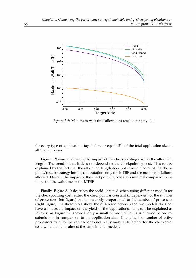
58Chapter 3: Comparing the performance of rigid, moldable and grid-shaped applications on
failure-prone HPC platforms
0.80 0.82 0.84 0.86 0.88 0.90Target Yield
10 1
100
101
102
103
Max
imum
Wai
t Tim
e (h
)RigidMoldableGridShapedNoSpare
Figure 3.6: Maximum wait time allowed to reach a target yield.
for every type of application stays below or equals 2% of the total application size inall the four cases.
Figure 3.9 aims at showing the impact of the checkpointing cost on the allocationlength. The trend is that it does not depend on the checkpointing cost. This can beexplained by the fact that the allocation length does not take into account the check-point/restart strategy into its computation, only the MTBF and the number of failuresallowed. Overall, the impact of the checkpointing cost stays minimal compared to theimpact of the wait time or the MTBF.
Finally, Figure 3.10 describes the yield obtained when using different models forthe checkpointing cost: either the checkpoint is constant (independent of the numberof processors: left figure) or it is inversely proportional to the number of processors(right figure). As these plots show, the difference between the two models does nothave a noticeable impact on the yield of the applications. This can be explained asfollows: as Figure 3.8 showed, only a small number of faults is allowed before re-submission, in comparison to the application size. Changing the number of activeprocessors by a few percentage does not really make a difference for the checkpointcost, which remains almost the same in both models.
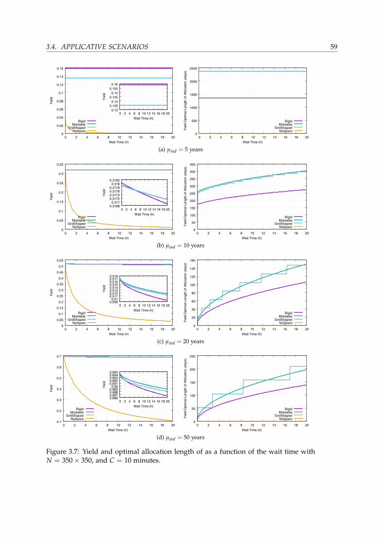
3.4. APPLICATIVE SCENARIOS 59
0
0.02
0.04
0.06
0.08
0.1
0.12
0.14
0.16
0 2 4 6 8 10 12 14 16 18 20
Yield
Wait Time (h)
RigidMoldable
GridShapedNoSpare
0.13
0.135
0.14
0.145
0.15
0.155
0.16
0 2 4 6 8 10 12 14 16 18 20
Yield
Wait Time (h)
0
500
1000
1500
2000
2500
0 2 4 6 8 10 12 14 16 18 20
Yield-Optim
al Length
of Allocation
(days)
Wait Time (h)
RigidMoldable
GridShapedNoSpare
(a) µind = 5 years
0
0.05
0.1
0.15
0.2
0.25
0.3
0.35
0 2 4 6 8 10 12 14 16 18 20
Yield
Wait Time (h)
RigidMoldable
GridShapedNoSpare
0.3168 0.317
0.3172 0.3174 0.3176 0.3178
0.318 0.3182
0 2 4 6 8 10 12 14 16 18 20
Yield
Wait Time (h)
0
50
100
150
200
250
300
350
400
450
0 2 4 6 8 10 12 14 16 18 20
Yield-Optim
al Length
of Allocation
(days)
Wait Time (h)
RigidMoldable
GridShapedNoSpare
(b) µind = 10 years
0
0.05
0.1
0.15
0.2
0.25
0.3
0.35
0.4
0.45
0.5
0.55
0 2 4 6 8 10 12 14 16 18 20
Yield
Wait Time (h)
RigidMoldable
GridShapedNoSpare
0.509 0.51
0.511 0.512 0.513 0.514 0.515 0.516 0.517 0.518
0 2 4 6 8 10 12 14 16 18 20
Yield
Wait Time (h)
0
20
40
60
80
100
120
140
160
0 2 4 6 8 10 12 14 16 18 20
Yield-Optim
al Length
of Allocation
(days)
Wait Time (h)
RigidMoldable
GridShapedNoSpare
(c) µind = 20 years
0.1
0.2
0.3
0.4
0.5
0.6
0.7
0 2 4 6 8 10 12 14 16 18 20
Yield
Wait Time (h)
RigidMoldable
GridShapedNoSpare
0.686 0.687 0.688 0.689
0.69 0.691 0.692 0.693 0.694 0.695
0 2 4 6 8 10 12 14 16 18 20
Yield
Wait Time (h)
0
50
100
150
200
250
0 2 4 6 8 10 12 14 16 18 20
Yield-Optim
al Length
of Allocation
(days)
Wait Time (h)
RigidMoldable
GridShapedNoSpare
(d) µind = 50 years
Figure 3.7: Yield and optimal allocation length of as a function of the wait time withN = 350× 350, and C = 10 minutes.
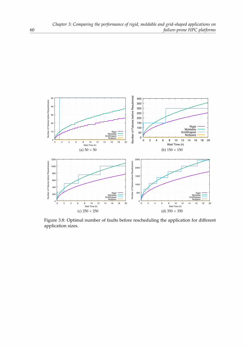
60Chapter 3: Comparing the performance of rigid, moldable and grid-shaped applications on
failure-prone HPC platforms
0
10
20
30
40
50
0 2 4 6 8 10 12 14 16 18 20
Number of Failures before
Resubmission
Wait Time (h)
RigidMoldable
GridShapedNoSpare
(a) 50× 50
0
50
100
150
200
250
300
350
400
0 2 4 6 8 10 12 14 16 18 20
Number of Failures before
Resubmission
Wait Time (h)
RigidMoldable
GridShapedNoSpare
(b) 150× 150
0
200
400
600
800
1000
1200
0 2 4 6 8 10 12 14 16 18 20
Number of Failures before
Resubmission
Wait Time (h)
RigidMoldable
GridShapedNoSpare
(c) 250× 250
0
500
1000
1500
2000
2500
0 2 4 6 8 10 12 14 16 18 20
Number of Failures before
Resubmission
Wait Time (h)
RigidMoldable
GridShapedNoSpare
(d) 350× 350
Figure 3.8: Optimal number of faults before rescheduling the application for differentapplication sizes.

3.4. APPLICATIVE SCENARIOS 61
0
20
40
60
80
100
120
140
160
0 2 4 6 8 10 12 14 16 18 20
Yield-Optim
al Length
of Allocation
(days)
Wait Time (h)
RigidMoldable
GridShapedNoSpare
(a) C = 2 min
0
20
40
60
80
100
120
140
160
0 2 4 6 8 10 12 14 16 18 20
Yield-Optim
al Length
of Allocation
(days)
Wait Time (h)
RigidMoldable
GridShapedNoSpare
(b) C = 10 min
0
20
40
60
80
100
120
140
160
0 2 4 6 8 10 12 14 16 18 20
Yield-Optim
al Length
of Allocation
(days)
Wait Time (h)
RigidMoldable
GridShapedNoSpare
(c) C = 30 min
0
20
40
60
80
100
120
140
160
0 2 4 6 8 10 12 14 16 18 20
Yield-Optim
al Length
of Allocation
(days)
Wait Time (h)
RigidMoldable
GridShapedNoSpare
(d) C = 60 min
Figure 3.9: Optimal number of faults before rescheduling the application for differentcheckpointing costs.
0
0.01
0.02
0.03
0.04
0.05
0.06
0.07
0.08
0.09
0.1
0 2 4 6 8 10 12 14 16 18 20
Yield
Wait Time (h)
RigidMoldable
GridShapedNoSpare
0.09165 0.0917
0.09175 0.0918
0.09185 0.0919
0.09195 0.092
0.09205 0.0921
0 2 4 6 8 10 12 14 16 18 20
Yield
Wait Time (h)
0
0.01
0.02
0.03
0.04
0.05
0.06
0.07
0.08
0.09
0.1
0 2 4 6 8 10 12 14 16 18 20
Yield
Wait Time (h)
RigidMoldable
GridShapedNoSpare
0.0902 0.0904 0.0906 0.0908
0.091 0.0912 0.0914 0.0916 0.0918
0.092 0.0922
0 2 4 6 8 10 12 14 16 18 20
Yield
Wait Time (h)
Figure 3.10: Constant checkpoint cost (Ci = 60 min) on the left, and increasing check-point cost (Ci =
Ni × 60 min) on the right, with µind = 5 years and N = 350× 350.

62Chapter 3: Comparing the performance of rigid, moldable and grid-shaped applications on
failure-prone HPC platforms
3.4.3 Comparison between C/R and ABFT
In this subsection, we present the results of ABFT and C/R strategies, for a GridShaped
application. In order to compare both strategies, we introduce ABFT parameters, anduse data from the Titan platform [4]:
• We use tiles of size 180× 180, i.e. we let b = 180. We set r = 325; so that a nodeholds 3252 = 105625 tiles.
• These values give a total of almost 25.5 GB used by each node, which correspondsto 80% of the memory of a node in Titan.
• Overall, the total memory of the application is 8p2r2b2 bytes, so we set the check-pointing cost to be 8p2r2b2
1.4×10244 , using 1.4 TB/s for the I/O bandwidth of the Titanplatform. With r and b set as mentioned, we get Ci = C ≈ 25.5N
1.4×1024 ≈ N56.3 .
• Titan has 18,688 cores for a peak performance of 17.59 PFlop/s. We derive aperformance per core of 987 GFlop/s, i.e. τa =
1987×10243 .
• Using the same reasoning, we derive that τc =1
87.2×10243 .
Figure 3.11 presents the yield obtained by both strategies with either no spare pro-cessors (NoSpare and NoSpare-ABFT) or with the optimal number of spare processors(GridShaped for the C/R strategy and ABFT for the ABFT strategy). In Figure 3.11 ,we use N = 150× 150 and µind = 20 years. Unsurprisingly, the ABFT strategy grants abetter yield than the C/R strategy with a yield very close to 1, compared to ≈ 0.8 forC/R. This is largely due to the fact that the overhead added by the ABFT is 2
p and so isnegligible compared to the checkpoint overhead. Moreover, the reconstruction of thetiles is done in parallel so it does not induce any significant overhead. This can also beseen when we do not use any spare: C/R and ABFT follow the same trend but ABFTis always more efficient than C/R, which exactly shows that the checkpoint overheadis larger than the ABFT overhead, since it is the only source (along with the wait time)of wasted time if F = 0. For a wait time of 10 hours the C/R strategy gives a yield of0.820 while ABFT grants a better yield of 0.973 (0.364 and 0.426 respectively with nospare processors). We can see on the right figure that the allocation lengths are similarfor both strategies. However, for some values, ABFT will have a shorter allocationlength, mostly due to the fact that its overhead is small and does not depend on thenumber of alive processors; hence loosing a few nodes implies a greater slowdownthan for the C/R strategy where the checkpointing period is adapted regularly.
The conclusion of this comparative study is that, for a GridShaped application,ABFT uses a very small percentage of spare resources and grants a better yield thanclassical C/R.

3.5. RELATED WORK 63
0.2
0.3
0.4
0.5
0.6
0.7
0.8
0.9
1
0 2 4 6 8 10 12 14 16 18 20
Yie
ld
Wait Time (h)
GridShapedNoSpare
ABFTNoSpare-ABFT
0.8 0.82 0.84 0.86 0.88 0.9 0.92 0.94 0.96 0.98 1
0 2 4 6 8 10 12 14 16 18 20
Yie
ld
Wait Time (h)
0 10 20 30 40 50 60 70 80 90
100
0 2 4 6 8 10 12 14 16 18 20
Yie
ld-O
ptim
al L
engt
h of
Allo
catio
n (d
ays)
Wait Time (h)
GridShapedNoSpare
ABFTNoSpare-ABFT
Figure 3.11: Comparison of ABFT and C/R strategies for a GridShaped application,N = 150× 150 and µind = 20 years.
3.5 Related work
We already surveyed related work on checkpoint-restart in Section 2.4. We now discussprevious contributions on Moldable applications in Section 3.5.1. Finally, we providea few references for ABFT techniques in Section 3.5.2
3.5.1 Moldable and GridShaped applications
Rigid and Moldable applications have been studied for long in the context of scien-tific applications. A detailed survey on various application types (Rigid, Moldable,malleable) was conducted in [71]. Resizing application to improve performance hasbeen investigated by many authors, including [141, 52, 176, 175] among others. A re-lated recent study is the design of a MPI prototype for enabling tolerance in Moldable
MapReduce applications [94].The TORQUE/Maui scheduler has been extended to support evolving, malleable,
and Moldable parallel jobs [153]. In addition, the scheduler may have system-widespare nodes to replace failed nodes. In contrast, our scheme does not assume a changeof behavior from the batch schedulers and resource allocators, but utilizes job-widespare nodes: a node set including potential spare nodes is allocated and dedicated toa job at the time of scheduling, that can be used by the application to restart within thesame job after a failure. At the application level, spare nodes have become common inHPC centers since more than a decade [187]. Recent work aims at sharing spare-nodesacross the whole platform to achieve a better global resource utilization [154].
An experimental validation of the feasibility of shrinking application on the flyis provided in [6]. In this paper, the authors used an iterative solver application tocompared two recovery strategies, shrinking and spare node substitution. They useULFM, the fault-tolerant extension of MPI that offers the possibility of dynamically re-sizing the execution after a failure. Finally, in [79, 107], the authors studied Moldable
and GridShaped applications that continue executing after some failures. They focuson the performance degradation incurred after shrinking or spare node substitution,

64Chapter 3: Comparing the performance of rigid, moldable and grid-shaped applications on
failure-prone HPC platforms
due to less efficient communications (and in particular collective communications). Amajor difference with our work is that these studies focus on recovery overhead anddo not address overall performance nor yield.
3.5.2 ABFT
ABFT stands for Algorithm-Based Fault Tolerant techniques. It is a widely used approachfor linear algebra kernels. Since the pioneering paper of Huang and Abraham [109],ABFT protection has been successfully applied to dense LU [69], LU with partial piv-oting [197], Cholesky [98] and QR [70] factorizations, and more recently to sparsekernels like SpMxV (matrix-vector product) and triangular solve [162].
In a nutshell, ABFT consists of adding a few checksum vectors as extra columns ofeach tile, which will be used to reconstruct data lost after a failure. The checksums aremaintained by applying the kernel operations to the extra columns, just as if they werematrix elements. The beauty of ABFT is that these checksums can be used to recoverfrom a failure, without any rollback nor re-execution, by reconstructing lost data andproceeding onward. In addition, the failure-free overhead induced by ABFT is usuallysmall, which makes it a good candidate for the design of fault-tolerant linear algebrakernels. We refer to [31, 69] for recent surveys on the approach.
Altogether, we are not aware of any previous study aiming at determining theoptimal number of spares as a function of the downtime and resilience parameters, fora general divisible-load application of either type (Rigid, Moldable or GridShaped).
3.6 Conclusion
In this chapter, we have compared the performance of Rigid, Moldable andGridShaped applications when executed on large-scale failure-prone platforms. Wehave mainly focused on the C/R approach, because it is the most widely used ap-proach for resilience. For each application type, we have computed the optimal num-ber of faults that should be tolerated before requesting a new allocation, as a functionof the wait time. Through realistic applicative scenarios inspired by state-of-the-artplatforms, we have shown that the three application types experience an optimal yieldwhen requesting a new allocation after experiencing a number of failures that repre-sents a small percentage of the initial number of resources (hence a small percentageof spares for Rigid applications), and this even for large values of the wait time. Onthe contrary, the NoSpare strategy, where a new allocation is requested after eachfailure, sees its yield dramatically decrease when the wait time increases. We also ob-served that Moldable applications enjoy much longer execution periods in betweentwo re-allocations, thereby decreasing the total execution time as compared to Rigid
applications (and GridShaped applications lying in between).GridShaped applications may also be protected using ABFT, and we have com-
pared the efficiency of C/R and ABFT for a typical dense matrix factorization prob-lem. As expected, using ABFT leads to even better yields than C/R for a wide variety

3.6. CONCLUSION 65
of scenarios, in particular for larger problem sizes for which ABFT scales remarkablywell.
Future work will be devoted to exploring more applicative scenarios, and runningactual experiments using ULFM [28]. We also intend to extend the model in several di-rections. On the application side, we aim at dealing with non-perfectly parallel appli-cations but instead with applications whose speedup profile obeys Amdahl’s law [3].On the platform side, we aim at adapting the model to heterogeneous platforms and atdoing more experiments with different values for the recovery and checkpoint costs asbandwidths are different when reading or writing data. We will also introduce a morerefined speedup profile for GridShaped applications, with an execution speed thatdepends on the grid shape (a square being usually faster than an elongated rectangle).On the resilience side, we will explore the case with different costs for checkpoint andrecovery. More importantly, we will address the combination of ABFT and C/R (in-stead of dealing with either method individually). Such a combination would allowto tolerate for several failures striking within the same computational step: the ideawould be to use ABFT to recover from a single failure and to rollback to the last check-point only in the case of multiple failures. Such a combination would enable us to gobeyond first-order approximations and single-failure scenarios.

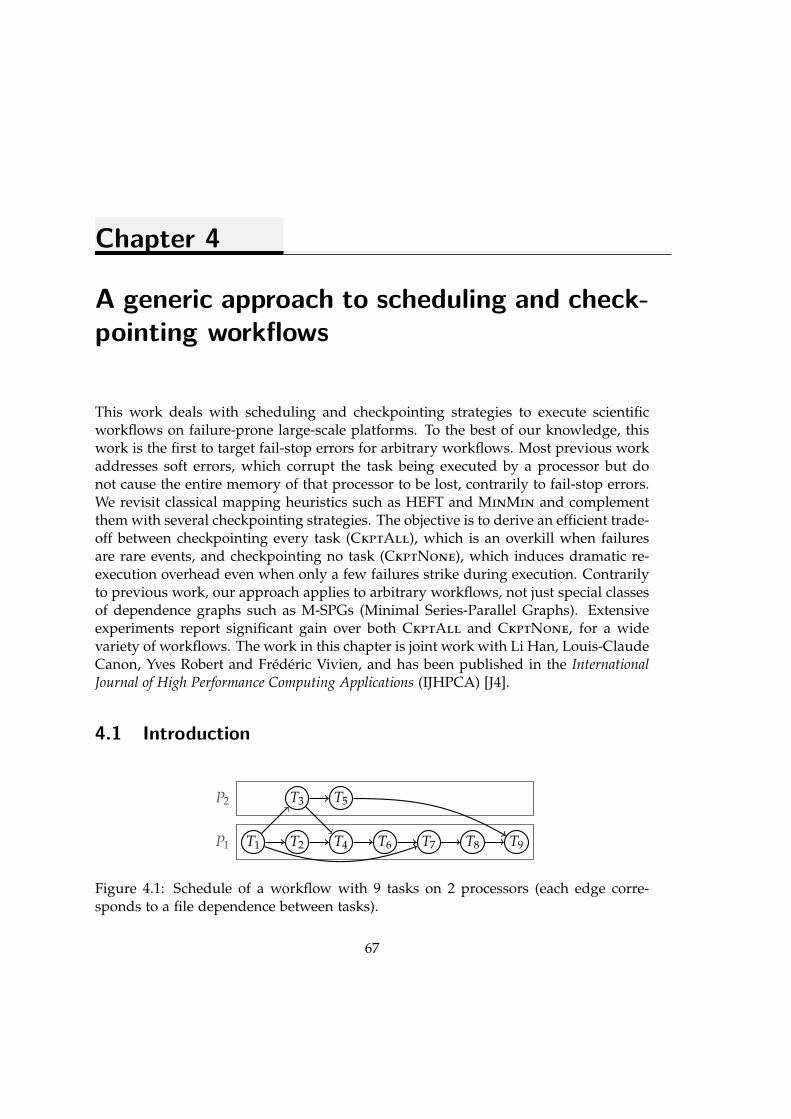
Chapter 4
A generic approach to scheduling and check-pointing workflows
This work deals with scheduling and checkpointing strategies to execute scientificworkflows on failure-prone large-scale platforms. To the best of our knowledge, thiswork is the first to target fail-stop errors for arbitrary workflows. Most previous workaddresses soft errors, which corrupt the task being executed by a processor but donot cause the entire memory of that processor to be lost, contrarily to fail-stop errors.We revisit classical mapping heuristics such as HEFT and MinMin and complementthem with several checkpointing strategies. The objective is to derive an efficient trade-off between checkpointing every task (CkptAll), which is an overkill when failuresare rare events, and checkpointing no task (CkptNone), which induces dramatic re-execution overhead even when only a few failures strike during execution. Contrarilyto previous work, our approach applies to arbitrary workflows, not just special classesof dependence graphs such as M-SPGs (Minimal Series-Parallel Graphs). Extensiveexperiments report significant gain over both CkptAll and CkptNone, for a widevariety of workflows. The work in this chapter is joint work with Li Han, Louis-ClaudeCanon, Yves Robert and Frederic Vivien, and has been published in the InternationalJournal of High Performance Computing Applications (IJHPCA) [J4].
4.1 Introduction
P1
P2
T1 T2
T3
T4
T5
T6 T7 T8 T9
Figure 4.1: Schedule of a workflow with 9 tasks on 2 processors (each edge corre-sponds to a file dependence between tasks).
67

68 Chapter 4: A generic approach to scheduling and checkpointing workflows
T1 T2 T1 T2
T3 T5 T3 T5
T4 T6 T7 T8 T9
time
P1
P2
Figure 4.2: Sample execution of the workflow in Figure 4.1 without any checkpoint,with two failures striking during the execution of T2 on P1 and during that of T5 on P2.
This work deals with scheduling techniques to deploy scientific workflows on largeparallel or distributed platforms. Scientific workflows are the archetype of HPC (HighPerformance Computing) applications, which are naturally partitioned into tasks thatrepresent computational kernels. The tasks are partially ordered because the output ofsome tasks may be needed as input to some other tasks. Altogether, the application isstructured as a DAG (Directed Acyclic Graph) whose nodes are the tasks and whoseedges enforce the dependences. Nodes are weighted by the computational require-ments (in flops) while edges are weighted by the size of communicated data (in bytes).Given a workflow and a platform, the problem of mapping the tasks onto the proces-sors and to schedule them so as to minimize the total execution time, or makespan,has received considerable attention.
This classical mapping and scheduling problem has recently been revisited to ac-count for the fact that errors and failures can strike during execution. Indeed, platformsizes have become so large that errors and failures are likely to strike at a high rateduring application execution ([42]). More precisely, the MTBF (Mean Time BetweenFailures) µP of the platform decreases linearly with the number of processors P, sinceµP = µind
P , where µind is the MTBF of each individual component (see Proposition 1.2in ([106])). Take µind = 10 years as an example. If P = 105 then µP ≈ 50 minutes andif P = 106 then µP ≈ 5 minutes: from the point of view of fault-tolerance, scale is theenemy.
Several approaches (see Section 4.6 for a review) have been proposed to mitigatethe simplest instance of the problem, that of soft and silent errors. Soft errors cause atask execution to fail but without completely losing the data present in the processormemory. Local checkpointing (or more precisely making a copy of all task input/out-put data), and task replication, are the most widely used technique to address softerrors. Silent errors represent a different challenge than soft errors, in that they donot interrupt the execution of the task but corrupt its output data. However, their neteffect is the same, since a task must be re-executed whenever a silent error is detected.A silent error detector is applied at the end of a task’s execution, and the task must bere-executed from scratch in case of an error. Again, local checkpointing (making copiesof input/output data) or replicating tasks and comparing outputs, are two commontechniques to mitigate the impact of silent errors.
Fail-stop errors, or failures, are much more difficult to deal with. In the case of afail-stop error (e.g., a crash due to a power loss or some other hardware problem) the

4.1. INTRODUCTION 69
execution of the processor stops, all the content of its memory is lost, and the compu-tations have to be restarted from scratch, either on the same processor once it rebootsor on a spare. The de-facto approach to handle such failures is Checkpoint/Restart(C/R), by which application state is saved to stable storage, such as a shared filesystem, throughout execution. The common strategy used in practice is checkpointeverything, or CkptAll: all output data of each task is saved onto stable storage (inwhich case we say “the task is checkpointed”). For instance, in production WorkflowManagement Systems (WMSs) ([2, 78, 191, 1, 192, 61]), the default behavior is thatall output data is saved to files and all input data is read from files, which is exactlythe CkptAll strategy. While this strategy leads to fast restarts in case of failures, itsdownside is that it maximizes checkpointing overhead. At the other end of the spec-trum would be a checkpoint nothing strategy, or CkptNone, by which all output datais kept in memory (up to memory capacity constraints) and no task is checkpointed.This corresponds to “in-situ” workflow executions, which has been proposed to re-duce I/O overhead ([202]). The downside is that, in case of a failure, a large numberof tasks may have to be re-executed, leading to slow restarts. The objective of thiswork is to achieve a desirable trade-off between these two extremes. To the best ofour knowledge, no general solution is available. We build upon previous work ([99])that was restricted to M-SPGs (Minimal Series-Parallel Graphs) ([186]). In ([99]), theauthors took advantage of the recursive structure of M-SPGs and used proportionalmapping ([152]) for scheduling and checkpointing M-SPG workflows as sets of super-chains. For general graphs, we have to resort to classical scheduling heuristics such asHEFT ([182]) and MinMin ([33]), two reference scheduling algorithms widely used bythe community. We provide extensions of HEFT and MinMin that allow for a smallersubset of tasks to be checkpointed and lead to better makespans than the versionswhere each task (CkptAll) or no task (CkptNone) is checkpointed.
The main contributions of this chapter are the following:• We deal with arbitrary dependence graphs, and require no graph transformation
before applying our scheduling and checkpointing algorithms.• We compare several mapping strategies and combine them with several check-
pointing strategies.• We design an event-based simulator to evaluate the makespan of the proposed
solution. Indeed, computing the expected makespan of a solution is a difficultproblem ([99]), and simple Monte-Carlo based simulations cannot be applied togeneral DAGs unless all tasks are checkpointed: otherwise, sampling the weightdistribution for each task independently is not enough to compute the makespan,since a failure may involve re-executing several tasks (as shown in Section 4.2).
• We report extensive experimental evaluation with both real-world and randomlygenerated workflows to quantify the performance gain achieved by the proposedapproach.
The rest of the chapter is organized as follows. First in Section 4.2, we work outan example to help understand the difficulty of the problem. Then we introducethe performance model in Section 6.2. We detail our scheduling and checkpointing
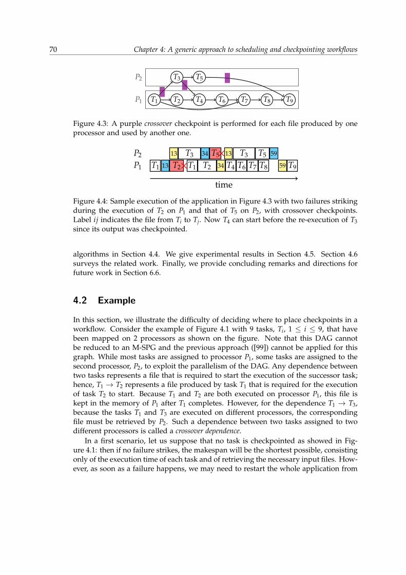
70 Chapter 4: A generic approach to scheduling and checkpointing workflows
P1
P2
T1 T2
T3
T4
T5
T6 T7 T8 T9
Figure 4.3: A purple crossover checkpoint is performed for each file produced by oneprocessor and used by another one.
T1 13 T2 T1 T2
13 T3 34 T5 13 T3 T5 59
34 T4 T6 T7 T8 59 T9
time
P1
P2
Figure 4.4: Sample execution of the application in Figure 4.3 with two failures strikingduring the execution of T2 on P1 and that of T5 on P2, with crossover checkpoints.Label ij indicates the file from Ti to Tj. Now T4 can start before the re-execution of T3since its output was checkpointed.
algorithms in Section 4.4. We give experimental results in Section 4.5. Section 4.6surveys the related work. Finally, we provide concluding remarks and directions forfuture work in Section 6.6.
4.2 Example
In this section, we illustrate the difficulty of deciding where to place checkpoints in aworkflow. Consider the example of Figure 4.1 with 9 tasks, Ti, 1 ≤ i ≤ 9, that havebeen mapped on 2 processors as shown on the figure. Note that this DAG cannotbe reduced to an M-SPG and the previous approach ([99]) cannot be applied for thisgraph. While most tasks are assigned to processor P1, some tasks are assigned to thesecond processor, P2, to exploit the parallelism of the DAG. Any dependence betweentwo tasks represents a file that is required to start the execution of the successor task;hence, T1 → T2 represents a file produced by task T1 that is required for the executionof task T2 to start. Because T1 and T2 are both executed on processor P1, this file iskept in the memory of P1 after T1 completes. However, for the dependence T1 → T3,because the tasks T1 and T3 are executed on different processors, the correspondingfile must be retrieved by P2. Such a dependence between two tasks assigned to twodifferent processors is called a crossover dependence.
In a first scenario, let us suppose that no task is checkpointed as showed in Fig-ure 4.1: then if no failure strikes, the makespan will be the shortest possible, consistingonly of the execution time of each task and of retrieving the necessary input files. How-ever, as soon as a failure happens, we may need to restart the whole application from
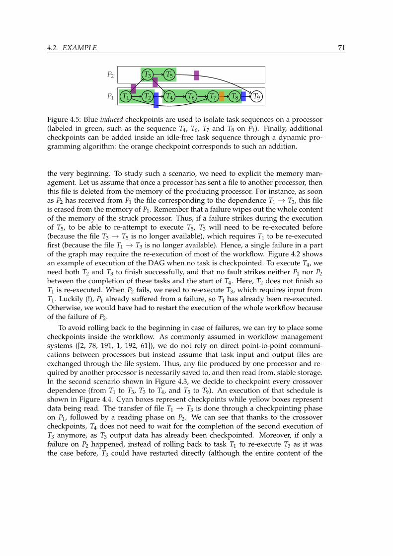
4.2. EXAMPLE 71
P1
P2
T1 T2
T3
T4
T5
T6 T7 T8 T9
Figure 4.5: Blue induced checkpoints are used to isolate task sequences on a processor(labeled in green, such as the sequence T4, T6, T7 and T8 on P1). Finally, additionalcheckpoints can be added inside an idle-free task sequence through a dynamic pro-gramming algorithm: the orange checkpoint corresponds to such an addition.
the very beginning. To study such a scenario, we need to explicit the memory man-agement. Let us assume that once a processor has sent a file to another processor, thenthis file is deleted from the memory of the producing processor. For instance, as soonas P2 has received from P1 the file corresponding to the dependence T1 → T3, this fileis erased from the memory of P1. Remember that a failure wipes out the whole contentof the memory of the struck processor. Thus, if a failure strikes during the executionof T5, to be able to re-attempt to execute T5, T3 will need to be re-executed before(because the file T3 → T5 is no longer available), which requires T1 to be re-executedfirst (because the file T1 → T3 is no longer available). Hence, a single failure in a partof the graph may require the re-execution of most of the workflow. Figure 4.2 showsan example of execution of the DAG when no task is checkpointed. To execute T4, weneed both T2 and T3 to finish successfully, and that no fault strikes neither P1 nor P2between the completion of these tasks and the start of T4. Here, T2 does not finish soT1 is re-executed. When P2 fails, we need to re-execute T3, which requires input fromT1. Luckily (!), P1 already suffered from a failure, so T1 has already been re-executed.Otherwise, we would have had to restart the execution of the whole workflow becauseof the failure of P2.
To avoid rolling back to the beginning in case of failures, we can try to place somecheckpoints inside the workflow. As commonly assumed in workflow managementsystems ([2, 78, 191, 1, 192, 61]), we do not rely on direct point-to-point communi-cations between processors but instead assume that task input and output files areexchanged through the file system. Thus, any file produced by one processor and re-quired by another processor is necessarily saved to, and then read from, stable storage.In the second scenario shown in Figure 4.3, we decide to checkpoint every crossoverdependence (from T1 to T3, T3 to T4, and T5 to T9). An execution of that schedule isshown in Figure 4.4. Cyan boxes represent checkpoints while yellow boxes representdata being read. The transfer of file T1 → T3 is done through a checkpointing phaseon P1, followed by a reading phase on P2. We can see that thanks to the crossovercheckpoints, T4 does not need to wait for the completion of the second execution ofT3 anymore, as T3 output data has already been checkpointed. Moreover, if only afailure on P2 happened, instead of rolling back to task T1 to re-execute T3 as it wasthe case before, T3 could have restarted directly (although the entire content of the

72 Chapter 4: A generic approach to scheduling and checkpointing workflows
processor memory is lost, so all inputs of T3 must be recovered from stable storageafter a downtime before the execution of T3 can restart). The motivation to checkpointall files involved in crossover dependences is to isolate the processors. Indeed, if allcrossover files are checkpointed, a failure on a processor will never lead to the re-execution of a task successfully executed on another processor. Overall, we will loseless time recomputing tasks or waiting for their second completion. However, readingfrom stable storage and checkpointing also take time. Finding the right trade-off is themain focus of this chapter: deciding which tasks should be checkpointed, so that theoverhead added by the checkpointing and reading of files is not more expensive thanthe re-execution of tasks.
We conclude by informally introducing examples of checkpointing strategies thatachieve desirable trade-offs (see Section 4.4.2 for details). Two additional checkpoints,in blue, called induced checkpoints, have been added in Figure 4.5. Their role is tosecure the fast re-execution of tasks that are the target of a crossover dependence,namely T4 and T9. The blue checkpoint after T2 isolates the execution of the task se-quence S1 = T4, T6, T7, T8 on P1. To this purpose, it is necessary to checkpoint allintermediate results that may be used after the execution of T2: these are the filesgenerated by previous tasks, namely T1 → T7 and T2 → T4, This way, when a fail-ure strikes, previous tasks do not have to be restarted and the computation may berestarted directly from T4. This way, tasks in the sequence S1 may be sequentiallyexecuted without idle time. It would not have been possible to include T1 and T2 inS1 because T4 could have waited for the completion of T3 leading to idle time in somescenarios. Similarly, the second blue checkpoint isolates the execution of T9.
Finally, once the four tasks T4, T6, T7, and T8 of the sequence S1 have been “isolated”from other tasks, it is possible to use a dynamic programming algorithm similar tothat used in ([99]) in order to introduce additional checkpoints. In the example ofFigure 4.5, a single additional checkpoint, in orange, is inserted after T7.
4.3 Model
This section details the execution and fault-tolerance models used to compare schedul-ing and checkpointing algorithms.
4.3.1 Execution Model
The execution model for a task workflow on a homogeneous system is represented as aDirected Acyclic Graph (DAG), G = (V, E), where V is the set of nodes correspondingto the tasks, and E is the set of edges corresponding to the dependences betweentasks. In a DAG, a node without any predecessor is called an entry node, while a nodewithout any successor is an exit node. For a task T in G, pred(T) and succ(T) representthe set of its immediate predecessors and successors respectively. We say that a task Tis ready if either it does not have any predecessor in the dependence graph, or if all itspredecessors have been executed. In this model, the execution time of a task Ti ∈ V

4.3. MODEL 73
is wi, i.e., its execution time in a failure-free execution. Each dependence (Ti, Tj) ∈ Eis associated with the cost ci,j to store/read the data onto/from stable storage. Beforethe execution of Tj on processor Pk, all input files needed by Tj must be present inthe local memory of Pk and absent files must be read from the stable storage, whichhappens as late as possible. We ignore direct communication between processorsbecause each data transfer between two processors (i.e., a crossover dependence) consistsin writing to and reading from the stable storage. Alternatively, we also say that thefile is checkpointed and then recovered.
4.3.2 Fault-Tolerance Model
In this work, each processor is a processing element that is subject to its own individualfailures. Failures can strike a processor at any time, during either task execution orwaiting time. Failure inter-arrival times are assumed to be Exponentially distributed.These failure-prone processors stop their execution once a failure strikes, i.e., we havefail-stop errors. When a fail-stop error strikes a processor, the whole content of itsmemory is lost and the computation it was performing must be restarted, either onthe same processor after a reboot, or on a spare processor (e.g., taken from a pool ofspare processors either specifically requested by the job submitter, or maintained bythe resource management infrastructure).
Consider a single task T, with weight w, scheduled on such a processor, and whoseinput is stored on stable storage. It takes a time r to read that input data from stablestorage, either for its first execution or after a failure. The total execution time W ofT is a random variable, because several execution attempts may be needed before thetask succeeds.
We assume that failures are i.i.d. (independent and identically distributed) acrossthe processors and that the failure inter-arrival times at each processor is Exponen-tially distributed with Mean Time Between Failures (MTBF) µ = 1/λ. Let λ 1be the Exponential failure rate of the processor. With probability e−λ(r+w), no fail-ure occurs, and W is equal to r + w. With probability (1 − e−λ(r+w)), a failure oc-curs. For Exponentially distributed failures, the expected time to failure, knowingthat a failure occurs during the task execution (i.e., in the next r + w seconds), is1/λ − (r + w)/(eλ(r+w) − 1) ([106]). After this failure, there is a downtime d, whichis (an upper bound of) the time needed to reboot the processor or migrate to aspare. Then we start the execution again, first with the recovery r and then thework w. With a general model where an unbounded number of failures can oc-cur during recovery and work, the expected time W to execute task T is given byW =
( 1λ + d
) (eλ(r+w) − 1
)([106]). Now if the output data of task T is checkpointed,
with a time c to write all of its output files onto stable storage, the total time becomes:
W =
(1λ+ d)(
eλ(r+w+c) − 1)
. (4.1)
Equation (4.1) assumes that failures can also occur during checkpoints, which is the

74 Chapter 4: A generic approach to scheduling and checkpointing workflows
most general model for failures. We also assume that failures may strike during theidle time (i.e., waiting time) of the processor (e.g., the power supply may fail). Inthe case of a sequence of non-checkpointed tasks to be executed on a processor P, theoutput data of each task resides in the memory of P for use by subsequent tasks. Whena failure strikes P, the entire memory content is lost and the whole task sequence mustbe re-executed from scratch.
4.3.3 Problem Formulation
Given a DAG and a set of processors on which fail-stop failures strike with Exponen-tially distributed inter-arrival times, the objective is to schedule the task executionsand potential checkpoints such that the expected completion time (or makespan) isminimized. Due to delays resulting from the faults, the schedule of the tasks consistsof an assignment to processors and of a task ordering. Each processor executes tasksas soon as possible and resumes their processing when a failure strikes. Finally, theschedule of the checkpoints is the (possibly empty) list of files that must be check-pointed after each task execution.
4.4 Scheduling and checkpointing algorithms
In this section, we first present heuristics to map tasks to processors. Then we proposethree different checkpointing strategies that can be used simultaneously.
4.4.1 Scheduling heuristics
We map tasks to processors and schedule them using two classical scheduling heuris-tics, HEFT ([182])† and MinMin ([33]). We run these heuristics as if the platforms werenot subject to failures, that is, without considering checkpoints. Therefore, we decidefirst on which processor a task will be executed, and the order in which a processorwill execute tasks, before deciding when and what to checkpoint (see Section 4.4.2).However, we present variants of HEFT and MinMin, named HEFTC and MinMinC,that are specifically designed for our failure-prone framework.
Heterogeneous Earliest Finish Time first (HEFT) is presented as the HEFTC variantin Algorithm 1. The original HEFT algorithm comprises two phases. In a first taskprioritizing phase, the bottom-level of all tasks is computed and tasks are ordered bynon-increasing bottom-levels. The bottom-level of a task is the maximum length ofany path starting at the task and ending in an exit task, considering that all commu-nications take place ([59]). In the second processor selection phase, the first unscheduledtask is scheduled as early as possible on a processor that minimizes its completiontime. In all cases, ties are broken arbitrarily. To these original two phases, we add athird one, the chain mapping phase (lines 7 and 8 of Algorithm 1). If the newly mappedtask T is the head of a chain in the task graph, then this whole chain is mapped on thesame processor as T, and the tasks will be executed consecutively. Ensuring that entire

4.4. SCHEDULING AND CHECKPOINTING ALGORITHMS 75
chain of tasks are scheduled on the same processor decreases the number of crossoverdependences and thus, the time to checkpoint them. HEFTC has a complexity of O(n2)for a workflow with n tasks. During the processor selection phase, the earliest finishtime of a task is computed in HEFTC while assuming that the newly mapped taskmust start after all tasks previously scheduled on that processor have completed. Onthe contrary, the original HEFT heuristic is allowed to perform backfilling following aclassical insertion-based policy, as long as the completion time of no task is delayed.Allowing backfilling is more expensive at scheduling time but should lower the exe-cution time (the complexity of HEFT with backfilling is also O(n2) with homogeneousprocessors). We do not allow backfilling for HEFTC because it could be antagonisticto the chain mapping phase if it led to backfill the head of the chain, but not the wholechain.
Algorithm 1: HEFTC
1 Compute the bottom-level of all tasks by traversing the graph from the exittasks
2 Sort the tasks by non-increasing values of their bottom-levels3 while there are unscheduled tasks do4 Select the first task Ti5 k← arg min1≤k≤p EarliestFinishTime(Ti, Pk)
6 Schedule task Ti on processor Pk7 if Ti is the head of a chain of tasks then8 Schedule the whole chain continuously on Pk
The MinMin scheduling algorithm is presented in the MinMinC variant in Al-gorithm 2. The original MinMin algorithm is a simple loop which, at each step,schedules the task that can finish the earliest among unscheduled tasks. Therefore, ateach step it considers all ready tasks and, for each of them, all the processors. We (tryto) improve this heuristic by adding a chain mapping phase exactly as previously (lines 5and 6 of Algorithm 2). MinMinC has a complexity of O(n2 p) for a workflow with ntasks and p processors.
4.4.2 Checkpointing strategies
While the previous scheduling algorithms provide mappings of tasks to processors, itremains to decide which files must be checkpointed and when. This section introducesfiner strategies than the two extremes solutions that consist of checkpointing no taskor all tasks. These two extreme solutions, CkptNone and CkptAll, are denoted withthe suffixes None and All, respectively.
In principle, our model forbids direct communications between processors (seeSection 4.3.1). However, for the sake of comparison, we make an exception for Ckpt-None: in the absence of any checkpoint with CkptNone, direct communications must

76 Chapter 4: A generic approach to scheduling and checkpointing workflows
Algorithm 2: MinMinC
1 ReadyTasks← entry tasks2 while there are unscheduled tasks do3 Pick a task T ∈ ReadyTasks and a processor P such that the completion time
of T on P is minimum among the Earliest Finish Times of all ready tasks4 Schedule task T on processor P5 if T is the head of a chain of tasks then6 Schedule the whole chain continuously on P
7 Update ReadyTasks
be performed for each crossover dependence. We assume that, in this special case,transferring a file takes half the time needed to save it to and read it from stablestorage. This special case is thus more efficient when files are large.
The minimum strategy that is required to avoid direct communications consistsof checkpointing all files that must be transferred between any pair of processors,i.e., exactly the files corresponding to crossover dependences. Moreover, in this case,any failure on a processor will not require any re-execution on other processors. Thestrategy is denoted with a “C” in the checkpoint suffix.
For the next two additional strategies, we introduce a new type of checkpoints:task checkpoints. While a simple file checkpoint consists of writing to stable storage afile that corresponds to a dependence between two tasks, a task checkpoint consists ofwriting all files that (i) reside in memory on a processor; (ii) will be used later by tasksassigned to the same processor; and (iii) have not already been checkpointed. In theexample in Section 4.2, for each crossover dependence we did a simple file checkpointrather than a full task checkpoint. A task checkpoint after task T3 would have alsocheckpointed the file corresponding to the dependence T3 → T5. A non-trivial taskcheckpoint for the example of Section 4.2 would be a task checkpoint for task T2. Thischeckpoint would require checkpointing the files corresponding to the dependencesT2 → T4 and T1 → T7.
When a task checkpoint is performed after the execution of a task, multiple filesmay be checkpointed “at the same time” (either newly created files or previouslycreated ones that will later be used). If several files are checkpointed, they are allcheckpointed after the task completion, one after the other (in any order), and they canall be read again only when the last of them has been checkpointed. When absent frommemory (following a failure or due to a crossover dependence), input files are readfrom stable storage as late as possible, just before the execution of the task that needsthem. One could imagine optimizations where files (in a task checkpoint) would becheckpointed independently and as soon as possible, or in a carefully designed order.Such optimizations could lead to lower expected makespans in some cases. However,the interplay of file checkpoints and reads that could result from these optimizationsmay lead to slowdowns. This is the reason why we prefer our simpler scheme.

4.4. SCHEDULING AND CHECKPOINTING ALGORITHMS 77
Checkpointing crossover dependences enable to isolate processors, in that there isno re-execution propagation from a processor to another. However, when a task is thetarget of a crossover dependence, its starting time is the maximum of the availabilitytimes of all its input files, and these files come from different processors. Therefore, itsstarting time may be delayed by failures occurring on other processors. Because fail-ures can strike during idle time, it may be beneficial to try to use the potential waitingtime by performing a task checkpoint of the task preceding the target task. This way,the whole content of the memory will be preserved, the cost of the checkpoint may beoffset by some waiting time, and if a failure strikes during the remaining waiting timeall input files remain available. Therefore, we propose a new checkpointing strategydenoted with “I” in the checkpoint suffix. This strategy consists of checkpointing allinduced dependences. A dependence Ti → Tj is an induced dependence if Ti and Tj arescheduled on the same processor P and there exists a crossover dependence Tk → Tlsuch that Tl is scheduled on P after Ti and before Tj (or Tl = Tj). Checkpointing theseinduced dependences is done by performing a task checkpoint of the task precedingTl on P. In the example of Section 4.2, the dependences T2 → T4 and T1 → T7 are bothinduced dependences because of the crossover dependence T3 → T4.
So far, we have only introduced checkpoints to isolate processors, either to avoidfailure propagation or to try to minimize the impact of processors having to wait fromeach other. We further consider checkpoints that more directly optimize expectedtotal execution time. We present an additional strategy, denoted by the suffix “DP”,which adds additional checkpoints through a O(n2) dynamic programming algorithm,which is a transposition of that of ([99]). This dynamic program considers a maximalsequence of consecutive tasks that are all assigned to the same processor, and that areisolated from other tasks: the sequence contains no checkpoint and none of its tasksis the target of a crossover dependence, except for its first task. Let T1, ..., Tk be such asequence of tasks. By definition, all input data produced by some previous tasks havebeen checkpointed. Then, the optimal expected time to execute this sequence is givenby Time(k) where Time is defined as follows:
Time(j) = min(
T(1, j), min1≤i<j
Time(i) + T(i + 1, j))
where T(i, j) is the expected time to execute tasks Ti to Tj provided that two taskcheckpoints are performed: one right before task Ti and one right after task Tj. Usingthe same reasoning as in Section 4.3.2, we can provide an upper bound on T(i, j) asfollows:
T(i, j) =(
1λ+ d)(
eλ(Rji+W j
i +Cji ) − 1
)where Rj
i (resp. W ji and Cj
i ) is the sum of the recovery (resp. execution and checkpoint-ing) costs of tasks Ti to Tj. The recovery costs concern all input files of these tasks thatare on the stable storage, while the checkpointing costs concern all files that will becheckpointed when a task checkpoint is done after Tj. This is an upper bound, because
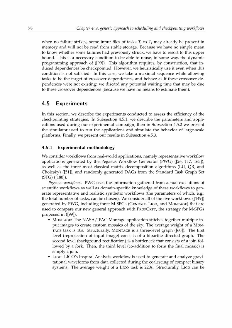
78 Chapter 4: A generic approach to scheduling and checkpointing workflows
when no failure strikes, some input files of tasks Ti to Tj may already be present inmemory and will not be read from stable storage. Because we have no simple meanto know whether some failures had previously struck, we have to resort to this upperbound. This is a necessary condition to be able to reuse, in some way, the dynamicprogramming approach of ([99]). This algorithm requires, by construction, that in-duced dependences be checkpointed. However, we heuristically use it even when thiscondition is not satisfied. In this case, we take a maximal sequence while allowingtasks to be the target of crossover dependences, and behave as if these crossover de-pendences were not existing: we discard any potential waiting time that may be dueto these crossover dependences (because we have no means to estimate them).
4.5 Experiments
In this section, we describe the experiments conducted to assess the efficiency of thecheckpointing strategies. In Subsection 4.5.1, we describe the parameters and appli-cations used during our experimental campaign, then in Subsection 4.5.2 we presentthe simulator used to run the applications and simulate the behavior of large-scaleplatforms. Finally, we present our results in Subsection 4.5.3.
4.5.1 Experimental methodology
We consider workflows from real-world applications, namely representative workflowapplications generated by the Pegasus Workflow Generator (PWG) ([26, 117, 165]),as well as the three most classical matrix decomposition algorithms (LU, QR, andCholesky) ([51]), and randomly generated DAGs from the Standard Task Graph Set(STG) ([180]).
Pegasus workflows. PWG uses the information gathered from actual executions ofscientific workflows as well as domain-specific knowledge of these workflows to gen-erate representative and realistic synthetic workflows (the parameters of which, e.g.,the total number of tasks, can be chosen). We consider all of the five workflows ([149])generated by PWG, including three M-SPGs (Genome, Ligo, and Montage) that areused to compare our new general approach with PropCkpt, the strategy for M-SPGs
proposed in ([99]).• Montage: The NASA/IPAC Montage application stitches together multiple in-
put images to create custom mosaics of the sky. The average weight of a Mon-tage task is 10s. Structurally, Montage is a three-level graph ([60]). The firstlevel (reprojection of input image) consists of a bipartite directed graph. Thesecond level (background rectification) is a bottleneck that consists of a join fol-lowed by a fork. Then, the third level (co-addition to form the final mosaic) issimply a join.
• Ligo: LIGO’s Inspiral Analysis workflow is used to generate and analyze gravi-tational waveforms from data collected during the coalescing of compact binarysystems. The average weight of a Ligo task is 220s. Structurally, Ligo can be

4.5. EXPERIMENTS 79
seen as a succession of Fork-Joins meta-tasks, that each contains either fork-joingraphs or bipartite graphs.
• Genome: The epigenomics workflow created by the USC Epigenome Center andthe Pegasus team automates various operations in genome sequence processing.The average weight of a Genome task depends on the total number of tasks andis greater than 1000s. Structurally, Genome starts with many parallel fork-joingraphs, whose exit tasks are then both joined into a new exit task, which is theroot of fork graphs.
• CyberShake: The CyberShake workflow is used by the Southern CalforniaEarthquake Center to characterize earthquake hazards in a region. The aver-age weight of a CyberShake task is 25s. Structurally, the CyberShake workflowstarts with several forks. Then each of the forked tasks has two dependences:one to a single task (join) and one to a specific task for each of the tasks. Finally,all these new tasks are joined without another dependence this time.
• Sipht: The Sipht workflow, from the bioinformatics project at Harvard, is usedto automate the search for untranslated RNAs (sRNAs) for bacterial replicons inthe NCBI database. The average weight of a Sipht task is 190s. Structurally, theSipht workflow is composed of two different parts that are joined at the end: thefirst one is a series of join/fork/join, while the other is made of a giant join.
We generate these workflows with 50, 300, and 700 tasks (these are the number oftasks given to the generator, the actual number of tasks in the generated workflowsdepend on the workflow shape). The task weights and file sizes are generated by PWG.In some instances, a single file may be used by more than one task and a dependencemay represent multiple files to transfer between two tasks. In the first case, whenevera file is common to multiple dependences, the file is only saved once. In the secondcase, files are aggregated into a single one.
Matrix factorizations. We consider the three most classical factorizations of a k× ktiled matrix: LU, QR, and Cholesky factorizations.
• The LU decomposition is the factorization of any matrix into a product of onelower-triangular (L) and one upper-triangular (U) matrices. Structurally, theDAG is made of k steps, with at step i, one task having two sets of k − i − 1children, and each pair of tasks between the two sets having another child.
• The QR decomposition is the decomposition of a matrix into a product of anorthogonal matrix (Q) and upper-triangular matrix (R), i.e., A = QR with QQT =Id. Structurally, the QR decomposition looks like the LU decomposition but ithas more complex dependences between the k− i− 1 children at step i.
• Cholesky is a factorization of a positive and definite matrix into the product ofa triangular matrix and its transpose, i.e., A = BBT where B is lower-triangularand has non-zero values of the diagonal. The Cholesky decomposition DAG isthe representation of a panel algorithm and can be constructed recursively byremoving the first row and the first column of submatrices, to keep factorizingthe trailing matrix.
For each factorization, we perform experiments with k = 6, 10, and 15, for a total
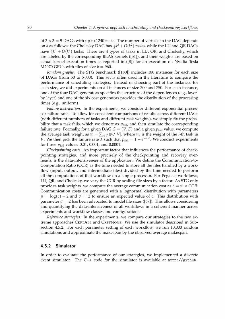
80 Chapter 4: A generic approach to scheduling and checkpointing workflows
of 3× 3 = 9 DAGs with up to 1240 tasks. The number of vertices in the DAG dependson k as follows: the Cholesky DAG has 1
3 k3 +O(k2) tasks, while the LU and QR DAGshave 2
3 k3 + O(k2) tasks. There are 4 types of tasks in LU, QR, and Cholesky, whichare labeled by the corresponding BLAS kernels ([51]), and their weights are based onactual kernel execution times as reported in ([8]) for an execution on Nvidia TeslaM2070 GPUs with tiles of size b = 960.
Random graphs. The STG benchmark ([180]) includes 180 instances for each sizeof DAGs (from 50 to 5 000). This set is often used in the literature to compare theperformance of scheduling strategies. Instead of choosing part of the instances foreach size, we did experiments on all instances of size 300 and 750. For each instance,one of the four DAG generators specifies the structure of the dependences (e.g., layer-by-layer) and one of the six cost generators provides the distribution of the processingtimes (e.g., uniform).
Failure distribution. In the experiments, we consider different exponential proces-sor failure rates. To allow for consistent comparisons of results across different DAGs(with different numbers of tasks and different task weights), we simply fix the proba-bility that a task fails, which we denote as pfail, and then simulate the correspondingfailure rate. Formally, for a given DAG G = (V, E) and a given pfail value, we computethe average task weight as w = ∑i∈V wi/|V|, where wi is the weight of the i-th task inV. We then pick the failure rate λ such that pfail = 1− e−λw. We conduct experimentsfor three pfail values: 0.01, 0.001, and 0.0001.
Checkpointing costs. An important factor that influences the performance of check-pointing strategies, and more precisely of the checkpointing and recovery over-heads, is the data-intensiveness of the application. We define the Communication-to-Computation Ratio (CCR) as the time needed to store all the files handled by a work-flow (input, output, and intermediate files) divided by the time needed to performall the computations of that workflow on a single processor. For Pegasus workflows,LU, QR, and Cholesky, we vary the CCR by scaling file sizes by a factor. As STG onlyprovides task weights, we compute the average communication cost as c = w× CCR.Communication costs are generated with a lognormal distribution with parametersµ = log(c) − 2 and σ = 2 to ensure an expected value of c. This distribution withparameter σ = 2 has been advocated to model file sizes ([67]). This allows consideringand quantifying the data-intensiveness of all workflows in a coherent manner acrossexperiments and workflow classes and configurations.
Reference strategies. In the experiments, we compare our strategies to the two ex-treme approaches CkptAll and CkptNone. We use the simulator described in Sub-section 4.5.2. For each parameter setting of each workflow, we run 10,000 randomsimulations and approximate the makespan by the observed average makespan.
4.5.2 Simulator
In order to evaluate the performance of our strategies, we implemented a discreteevent simulator. The C++ code for the simulator is available at http://github.

4.5. EXPERIMENTS 81
com/vlefevre/task-graph-simulation. To simulate the execution of applications onlarge-scale platforms, we operate in three steps:
1. We first read an input file describing the task-graph and the scheduling/map-ping strategy;
2. Then we generate a set of fail-stop error times for each processor during a timehorizon (that is set by the user);
3. Finally, we execute ready tasks by mapping them to a processor and we keepdoing this until all tasks are executed.
The first part is basically reading a file that describes the following important ele-ments for the simulation:
• For each task,– its ID,– its weight (i.e., duration),– the ID of the processor it has been mapped to,– several booleans indicating whether the task has to be checkpointed or not,
one for each checkpointing strategy.• For each dependence between two tasks,
– the ID of the parent,– the ID of the child,– the list of files with their time to be loaded/written that creates the depen-
dence (i.e., there are some of the output files of the parent and some of theinput files of the child).
• For each processor, its schedule: a list of tasks that have been mapped to it andthat respects the causal order of the task-graph.
The second part is done by using the inversion sampling method: we generateerror times according to a random variable that follows an exponential distribution,and this exponential distribution is generated from an (assumed) uniform distributionbetween 0 and 1 obtained by calling the C function rand(), and dividing its result bythe C constant RAND MAX. In our case, if U is a random variable following a uniformdistribution between 0 and 1, then − log U
λ follows an exponential distribution of pa-rameter λ. We generate errors one each processor, until the time of one error is greaterthan the horizon parameter. In the experiments, it was set to at least 2 times theexpected makespan we have with the CkptAll strategy, which we computed usingthe Monte-Carlo method. In practice, most of the simulations were done before thehorizon was reached except for None with large pfail.
For the last step, we keep a global time t on all the processors, and we generateevents happening on each processor (either a failure or the successful completion of atask). Each processor holds the time of its last event in a variable ti. At each momentof the simulation, we have ti ≥ t, ∀i. The algorithm repeats these steps until all tasksare marked executed:
• For each processor pi,– we look at the next task to be executed on pi (following the list scheduling
given as input) if the current task is finished at time t;

82 Chapter 4: A generic approach to scheduling and checkpointing workflows
– if it is ready, we compute its full execution time by computing the time ofreading the necessary input files, the weight of the task (given as input)and potentially some writing (in case of crossover dependences or if thecheckpoint strategy requires this task to be checkpointed);
– we look at the next error happening after time t: if it is before the end ofthe task then we set ti to be the time of that failure, otherwise ti is set to thetime when the task ends and the task is marked executed.
• We set t = mini
ti.
There are two more things to detail: the computation of reading times and how werollback when there is a failure. For the first problem, we keep a set of all files loadedon each processor. Before reading an input file, we check if it is already loaded (i.e.,belongs to that set). If it is already loaded, we count a cost of 0, otherwise we add thereading time for that file that is given as input. Files are added to the set wheneverthere are loaded or written (not necessarily a checkpoint). The set is cleared whenevera fail-stop error strikes on the processor or a checkpoint is performed, for simplicity.However, keeping the files needed by tasks after the checkpoint would improve evenmore the makespan.
When there is a failure, the rollback is easy because we always checkpoint crossoverdependences. This implies that a failure on a processor pi will only impact the tasksthat have been executed on pi since the last checkpointed task that was mapped topi. To rollback we explore the list of tasks backward from the current task to the lastcheckpointed one (we keep two pointers on these two tasks at each time to access theminstantaneously), we mark each task unexecuted, we clear the set of loaded files andwe can start simulating again from the last checkpointed task as if nothing happened.In the case of CkptNone, the simulation is rolled back from the first task anytime anexecution or communication is interrupted.
Finally, the simulator computes the following measures: the number of file check-points taken, the number of task checkpoints taken, the number of failures, the totaltime spent checkpointing data and the execution time of the application.
4.5.3 Results
In this section, we first compare the expected makespan of our proposed checkpointingstrategies (CDP and CIDP) over two baseline strategies (All and None) with the sametask mapping and scheduling strategy. Then, we compare the solutions (different taskmapping and scheduling heuristics combined with several checkpointing strategies)from this work with the method PropCkpt proposed in ([99]) for M-SPGs.
In Figures 4.6-4.10, we compare the four considered task mapping and schedulingstrategies: HEFT and MinMin, with their chain-mapping variants HEFTC and Min-MinC using boxplots‡. On these figures, the lower the better and the baseline at 1 is theperformance of HEFT. The chain-mapping variants have the same performance or im-prove that of their basic counterparts, especially when communications are expensive(rightmost parts of the graphs). The other conclusion is that MinMin (resp. Min-

4.5. EXPERIMENTS 83
CIDP CDP ALL
3e-0
4
0.00
1
0.00
30.
010.
03 0.1
0.3 1
3e-0
4
0.00
1
0.00
30.
010.
03 0.1
0.3 1
3e-0
4
0.00
1
0.00
30.
010.
03 0.1
0.3 1
0.6
0.8
1.0
1.2
Communication-to-Computation Ratio
Ra
tio t
o H
EF
T mapping
HEFTC
MinMin
MinMinC
Figure 4.6: Relative performance of the four task mapping and scheduling strategiesfor Cholesky.
MinC) almost always achieves same or worse performance than HEFT (resp. HEFTC).This is easily explained by the fact that HEFT and HEFTC take into account the criticalpath of workflows. These trends are representative of the trends that can be observedfor all considered graphs and workflows, but suffer from some exceptions. The chain-mapping variants can be superceded by their basic counterparts for workflows thatdo not include any chains (like LU in Figure 4.7), because the basic variants can usebackfilling. However, backfilling sometimes backfires, even in the absence of chains,like for Sipht in Figure 4.9 where HEFTC can decrease the expected makespan bymore than 30% with respect to HEFT. Overall, of the four considered task mappingand scheduling heuristics, HEFTC never achieves significantly bad performance, andmost of the time achieves the best performance. This is the reason why we focus on itin the remainder of this section.
Figures 4.11 through 4.18 present the expected makespans achieved by CDP, CIDPand None divided by that of All when the Communication-to-Computation Ratioincreases. Therefore, the lower the better and data points below the y = 1 line denotecases in which these strategies outperform the competitor All (i.e., achieve a lowerexpected makespan). Each figure shows results for workflows with different numberof tasks, ranging from 50 to 1240 tasks (each line of subfigure is for a different size,the number of tasks being reported on the rightmost column), for various number ofprocessors P (different line styles), and for the three pfail values (0.0001, 0.001, 0.01). Wereport on these figures the average number of failures that occur for the 10,000 randomtrials for each setting. These numbers are reported in black above the horizontal axisin each figure. The other two lines of numbers are the number of checkpointed tasksfor the CDP and CIDP strategies, each number is printed with the same color as thecurve of the corresponding strategy.
A clear observation is that CIDP never achieves worse performance than All: ei-
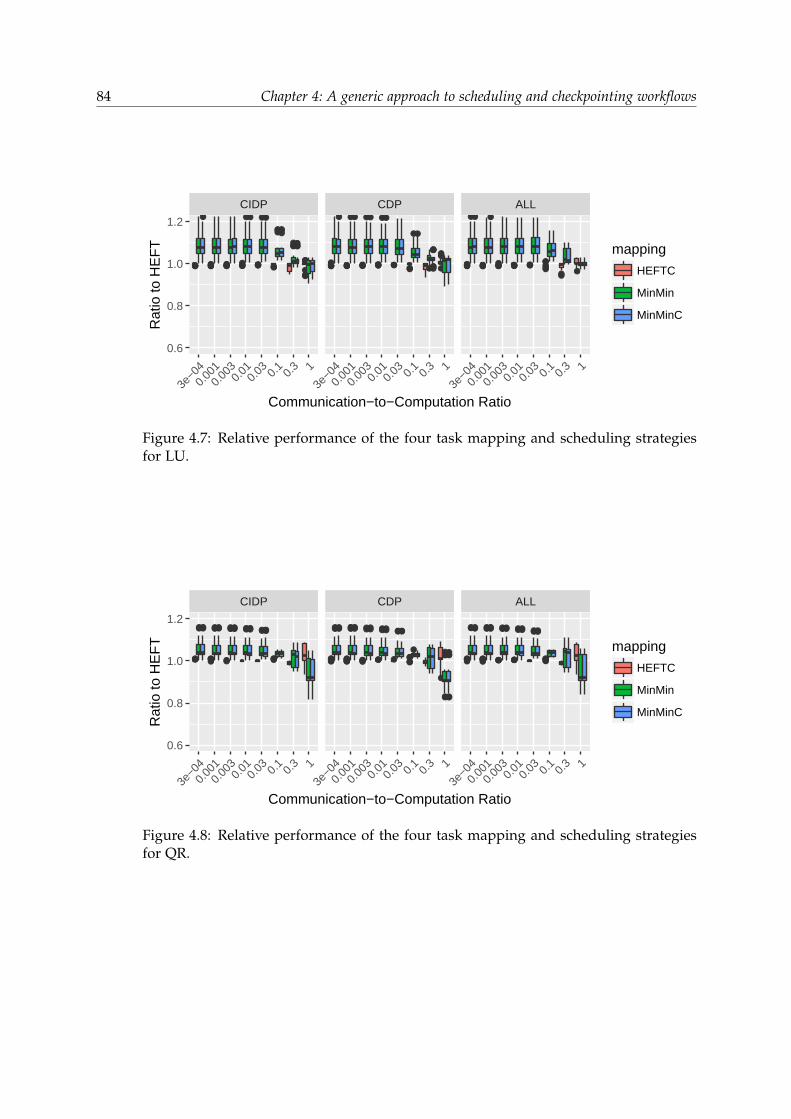
84 Chapter 4: A generic approach to scheduling and checkpointing workflows
CIDP CDP ALL
3e−0
40.
0010.
0030.
010.
03 0.1
0.3 1
3e−0
40.
0010.
0030.
010.
03 0.1
0.3 1
3e−0
40.
0010.
0030.
010.
03 0.1
0.3 1
0.6
0.8
1.0
1.2
Communication−to−Computation Ratio
Rat
io to
HE
FT mapping
HEFTC
MinMin
MinMinC
Figure 4.7: Relative performance of the four task mapping and scheduling strategiesfor LU.
CIDP CDP ALL
3e−0
40.
0010.
0030.
010.
03 0.1
0.3 1
3e−0
40.
0010.
0030.
010.
03 0.1
0.3 1
3e−0
40.
0010.
0030.
010.
03 0.1
0.3 1
0.6
0.8
1.0
1.2
Communication−to−Computation Ratio
Rat
io to
HE
FT mapping
HEFTC
MinMin
MinMinC
Figure 4.8: Relative performance of the four task mapping and scheduling strategiesfor QR.

4.5. EXPERIMENTS 85
CIDP CDP ALL
3e−0
40.
0010.
0030.
010.
03 0.1
0.3 1
3e−0
40.
0010.
0030.
010.
03 0.1
0.3 1
3e−0
40.
0010.
0030.
010.
03 0.1
0.3 1
0.6
0.8
1.0
1.2
Communication−to−Computation Ratio
Rat
io to
HE
FT mapping
HEFTC
MinMin
MinMinC
Figure 4.9: Relative performance of the four task mapping and scheduling strategiesfor Sipht.
CIDP CDP ALL
3e−0
40.
0010.
0030.
010.
03 0.1
0.3 1
3e−0
40.
0010.
0030.
010.
03 0.1
0.3 1
3e−0
40.
0010.
0030.
010.
03 0.1
0.3 1
0.6
0.8
1.0
1.2
Communication−to−Computation Ratio
Rat
io to
HE
FT mapping
HEFTC
MinMin
MinMinC
Figure 4.10: Relative performance of the four task mapping and scheduling strategiesfor CyberShake.

86 Chapter 4: A generic approach to scheduling and checkpointing workflows
ther it achieves a similar performance or it outperforms All, especially when commu-nications, and thus checkpoints, are expensive (in the rightmost parts of graphs). Itshould be noted that when checkpoints come for free (leftmost parts of graphs), All
and CIDP have the same performance as they do the same thing: they checkpoint alltasks. When the number of failures rises, the optimal solution is to checkpoint moretasks, potentially all of them, and the gain of CIDP with respect to All therefore de-creases. This can be seen, for instance, on Figure 4.12 when pfail = 0.01, n = 385 andthere are 385 tasks checkpointed.
In the majority of cases, CDP also achieves similar or better performance thanAll. As we explained in Section 4.4, the dynamic programming algorithm is well-defined for CIDP, which checkpoints all induced dependences. However, CDP triesto save some checkpointing overhead by not systematically checkpointing induceddependences. As a consequence, the dynamic programming algorithm estimationsof expected execution times may be inaccurate, which explains the sometimes badperformance of CDP. There are only a couple of CCR values for CyberShake for whichCDP achieves a significantly worse performance than All. On the contrary, CDP oftenhas better performance than CIDP when checkpointing cost is high. In all scenarios,CDP checkpoints less or the same number of tasks than CIDP. Depending on thecheckpointing cost and failure rate, CDP can lead to significant improvement overAll. For workflows as dense as LU, we save more than 10% when CCR = 1 for bothstrategies, and CDP even achieves 35% saving for Sipht. As the CCR decreases, theratio converges to 1. As already pointed out, this is because both strategies decide tocheckpoint most, if not all, tasks, when checkpointing becomes cheaper.
CDP and CIDP achieve better results than None except when (i) checkpoints areexpensive (high CCR) and/or (ii) failures are rare (low pfail). In these cases, check-pointing is a losing proposition, and yet our strategies, by design, always check-points some files (they checkpoint all crossover files and even induced dependencesfor CIDP). In practice, in such cases, the optimal approach is to bet that no failurewill happen and to restart the whole workflow execution from scratch upon the veryrare occurrence of a failure. None becomes worse whenever there are more failingtasks, i.e., when the failure rate increases (going from the leftmost column to the right-most one in the figures), and/or when the number of tasks increases (going from thetopmost row to the bottom one in the figures). When the failure rate is high andthe workflows are large (the bottom right corner of the figures), the relative expectedmakespan of None is so high that it does not appear in the plots. The above results,and our experimental methodology in general, make it possible to identify these casesso as to select which approach to use in practical situations.
Figure 4.19 presents the aggregated results for the 180 STG random DAGs withboxplots. The trends on these graphs are the same as already reported. This confirmsthe generality of our conclusions.
Finally, we compare our new general approach with PropCkpt, the approach spe-cific to M-SPGs that is proposed in ([99]). Figures 4.20-4.22 present this comparison forMontage, Ligo and Genome, which are the three M-SPGs presented in ([99]). Overall,

4.5. EXPERIMENTS 87
50 50 50 50 50 50 50 5028 25 23 23 23 23 21 171 1 1 1 1 1 1 1
210 210 210 210 210 210 210 210154 150 150 150 150 151 152 1491 1 1 1 1 1 1 1
665 665 665 665 665 665 665 665552 548 547 547 547 547 547 5471 1 1 1 1 1 1 1
51 50 50 50 50 50 50 5051 37 28 25 23 23 21 171 1 1 1 1 1 1 1
211 210 210 210 210 210 210 210211 164 154 150 150 151 152 1491 1 1 1 1 1 1 1
666 665 665 665 665 665 665 665666 573 552 548 547 547 547 5481 1 1 1 1 1 2 4
56 56 51 50 50 50 50 5056 56 51 37 29 26 26 241 1 1 1 1 1 1 3
220 220 211 210 210 210 210 211220 220 211 164 158 154 154 160
2 2 2 2 2 3 5 10
680 680 666 665 665 665 665 666680 680 666 574 571 557 563 570
6 6 6 6 7 9 14 32
pfail=0.0001 pfail=0.001 pfail=0.01
56220
680
0.01 1.00 0.01 1.00 0.01 1.00
0.00
0.25
0.50
0.75
1.00
0.00
0.25
0.50
0.75
1.00
0.00
0.25
0.50
0.75
1.00
Communication−to−Computation Ratio
Rat
io to
ALL
strategy CIDP
CDP
NONE
#proc
5
10
30
60
100
200
Figure 4.11: Performance of the different checkpointing strategies for Cholesky usingHEFTC for task mapping and scheduling.
85 85 85 85 85 85 85 8557 49 44 44 44 43 42 321 1 1 1 1 1 1 1
375 375 375 375 375 375 375 375287 277 261 261 263 264 244 2441 1 1 1 1 1 1 1
1225 1225 1225 1225 1225 1225 1225 12251045 1026 1026 1021 1024 1024 921 924
1 1 1 1 1 1 1 1
86 85 85 85 85 85 85 8586 73 58 50 44 43 42 401 1 1 1 1 1 1 1
376 375 375 375 375 375 375 375368 307 287 277 271 266 244 2471 1 1 1 1 1 1 2
1225 1225 1225 1225 1225 1225 1225 12251207 1092 1046 1026 1027 1024 924 928
2 2 2 2 2 2 3 6
91 91 86 85 85 85 85 8591 91 86 75 68 55 54 571 1 1 1 1 2 2 4
385 385 376 375 375 375 375 376385 385 376 312 293 286 263 272
4 4 4 4 4 5 8 17
1240 1240 1226 1225 1225 1225 1226 12261240 1240 1220 1092 1056 1040 937 95311 11 11 12 13 17 26 58
pfail=0.0001 pfail=0.001 pfail=0.01
91385
1240
0.01 1.00 0.01 1.00 0.01 1.00
0.00
0.25
0.50
0.75
1.00
0.00
0.25
0.50
0.75
1.00
0.00
0.25
0.50
0.75
1.00
Communication−to−Computation Ratio
Rat
io to
ALL
strategy CIDP
CDP
NONE
#proc
5
10
30
60
100
200
Figure 4.12: Performance of the different checkpointing strategies for LU using HEFTCfor task mapping and scheduling.
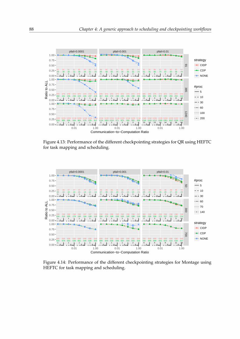
88 Chapter 4: A generic approach to scheduling and checkpointing workflows
81 81 81 81 81 82 83 8249 38 34 32 30 34 31 301 1 1 1 1 1 1 1
370 370 370 372 372 372 372 373268 251 245 238 229 225 237 2481 1 1 1 1 1 1 1
1222 1220 1219 1219 1219 1219 1220 12191011 985 966 949 963 978 979 917
1 1 1 1 1 1 1 1
86 82 81 81 81 82 83 8286 68 50 44 34 36 32 341 1 1 1 1 1 1 1
376 371 370 372 372 372 372 373367 301 274 248 235 226 238 2561 1 1 1 1 1 1 2
1224 1220 1219 1219 1219 1219 1220 12191134 1083 1018 971 975 990 982 959
2 2 2 2 2 2 3 6
91 91 86 82 82 82 83 8291 91 86 70 57 50 48 491 1 1 1 1 2 2 4
385 385 376 372 372 372 372 376385 385 376 307 283 259 264 310
4 4 4 4 5 6 8 18
1240 1240 1226 1220 1219 1220 1222 12251240 1240 1213 1080 1061 1047 1039 105613 13 13 13 14 17 26 60
pfail=0.0001 pfail=0.001 pfail=0.0191
3851240
0.01 1.00 0.01 1.00 0.01 1.00
0.00
0.25
0.50
0.75
1.00
0.00
0.25
0.50
0.75
1.00
0.00
0.25
0.50
0.75
1.00
Communication−to−Computation Ratio
Rat
io to
ALL
strategy CIDP
CDP
NONE
#proc
5
10
30
60
100
200
Figure 4.13: Performance of the different checkpointing strategies for QR using HEFTCfor task mapping and scheduling.
48 48 47 47 47 47 47 4730 16 13 14 15 14 12 141 1 1 1 1 1 1 1
298 298 298 298 298 297 297 296244 216 185 179 186 194 188 1851 1 1 1 1 1 1 1
698 698 698 698 698 698 698 698629 579 553 538 551 540 538 5051 1 1 1 1 1 1 1
48 48 48 48 48 47 47 4747 38 32 18 15 15 13 151 1 1 1 1 1 1 1
298 298 298 298 298 298 298 297298 270 248 208 189 195 188 1941 1 1 1 1 1 1 1
699 699 698 698 698 698 698 698699 649 630 588 554 544 543 5181 1 1 1 1 1 2 3
49 48 48 48 48 48 48 4849 47 47 38 29 27 23 281 1 1 1 1 1 1 2
300 299 298 298 298 298 298 298300 299 298 272 257 242 232 254
2 2 2 2 3 3 5 11
700 699 699 699 698 698 698 698700 699 699 652 626 610 618 617
5 5 5 5 6 7 11 28
pfail=0.0001 pfail=0.001 pfail=0.01
50300
700
0.01 1.00 0.01 1.00 0.01 1.00
0.00
0.25
0.50
0.75
1.00
0.00
0.25
0.50
0.75
1.00
0.00
0.25
0.50
0.75
1.00
Communication−to−Computation Ratio
Rat
io to
ALL
#proc
5
10
30
60
70
140
strategy CIDP
CDP
NONE
Figure 4.14: Performance of the different checkpointing strategies for Montage usingHEFTC for task mapping and scheduling.

4.5. EXPERIMENTS 89
13 13 13 13 14 13 12 1211 11 11 10 10 9 9 91 1 1 1 1 1 1 1
78 78 78 79 78 81 82 8471 71 70 70 68 71 73 731 1 1 1 1 1 1 1
183 183 182 182 187 189 190 190171 171 170 168 173 173 178 1771 1 1 1 1 1 1 1
14 13 13 13 14 13 12 1212 11 11 11 11 10 10 91 1 1 1 1 1 1 1
85 79 79 80 79 82 83 8478 72 72 73 72 74 74 731 1 1 1 1 1 1 1
193 192 189 187 190 191 191 191182 180 177 175 178 176 180 1801 1 1 1 1 1 2 2
24 19 15 15 15 15 14 1423 18 13 13 12 13 12 131 1 1 1 1 1 1 2
126 90 85 85 85 85 85 86125 87 82 80 80 80 81 85
4 4 4 4 4 4 5 9
339 234 199 196 197 197 197 198338 232 194 188 190 191 195 197
8 8 8 8 8 9 12 22
pfail=0.0001 pfail=0.001 pfail=0.01
47297
699
0.01 1.00 0.01 1.00 0.01 1.00
0.00
0.25
0.50
0.75
1.00
0.00
0.25
0.50
0.75
1.00
0.00
0.25
0.50
0.75
1.00
Communication−to−Computation Ratio
Rat
io to
ALL
#proc
5
10
30
60
70
140
strategy CIDP
CDP
NONE
Figure 4.15: Performance of the different checkpointing strategies for Genome usingHEFTC for task mapping and scheduling.
25 25 25 25 25 25 25 2523 22 21 19 18 18 18 171 1 1 1 1 1 1 1
151 151 150 150 150 150 150 149146 145 144 127 126 122 126 1221 1 1 1 1 1 1 1
506 502 502 503 502 502 505 504480 479 478 459 454 454 458 4601 1 1 1 1 1 1 1
36 26 26 26 26 26 25 2635 24 23 22 21 19 19 181 1 1 1 1 1 1 1
222 157 152 152 152 152 152 151216 151 146 145 144 130 128 1241 1 1 1 1 1 1 1
729 541 515 512 512 511 513 512702 503 481 479 477 472 468 4701 1 1 1 2 2 2 3
40 37 37 27 26 26 26 2639 36 36 25 23 22 22 221 1 1 1 1 1 1 2
249 226 223 161 153 153 153 153248 224 218 155 148 147 148 145
3 3 4 4 4 4 5 9
837 747 731 549 521 521 521 521826 727 707 512 482 483 484 48710 11 10 11 11 12 16 28
pfail=0.0001 pfail=0.001 pfail=0.01
50300
1000
0.01 1.00 0.01 1.00 0.01 1.00
0.00
0.25
0.50
0.75
1.00
0.00
0.25
0.50
0.75
1.00
0.00
0.25
0.50
0.75
1.00
Communication−to−Computation Ratio
Rat
io to
ALL
strategy CIDP
CDP
NONE
#proc
5
10
30
60
100
200
Figure 4.16: Performance of the different checkpointing strategies for Ligo usingHEFTC for task mapping and scheduling.

90 Chapter 4: A generic approach to scheduling and checkpointing workflows
47 47 47 47 46 44 32 3215 18 16 17 12 17 12 121 1 1 1 1 1 1 1
288 288 288 288 288 278 278 277178 183 171 168 170 165 188 1351 1 1 1 1 1 1 1
671 671 671 671 671 658 648 648493 442 455 472 450 430 441 3651 1 1 1 1 1 1 1
48 47 47 47 46 46 34 3418 20 16 17 14 19 12 121 1 1 1 1 1 1 1
288 288 288 288 288 288 288 287187 192 178 169 179 174 190 1361 1 1 1 1 1 1 1
671 671 671 671 671 672 671 671520 464 475 476 462 452 450 3681 1 1 1 1 1 1 2
48 48 48 47 46 46 34 3421 24 21 21 17 20 15 151 1 1 1 1 1 1 2
290 289 288 288 288 288 288 287225 209 195 188 198 190 209 156
3 3 4 4 4 4 5 8
677 674 671 671 671 672 671 671562 504 511 519 504 492 496 414
8 7 8 8 8 9 11 18
pfail=0.0001 pfail=0.001 pfail=0.0148
290677
0.01 1.00 0.01 1.00 0.01 1.00
0.00
0.25
0.50
0.75
1.00
0.00
0.25
0.50
0.75
1.00
0.00
0.25
0.50
0.75
1.00
Communication−to−Computation Ratio
Rat
io to
ALL
#proc
5
10
30
60
70
140
strategy CIDP
CDP
NONE
Figure 4.17: Performance of the different checkpointing strategies for Sipht usingHEFTC for task mapping and scheduling.
47 45 45 46 45 45 45 4138 35 33 32 29 27 32 291 1 1 1 1 1 1 1
299 296 297 297 294 267 266 268235 215 214 215 215 203 191 1821 1 1 1 1 1 1 1
700 697 697 695 689 652 654 618556 494 495 493 501 490 470 4251 1 1 1 1 1 1 1
50 49 47 46 47 49 49 4550 44 38 34 33 29 34 331 1 1 1 1 1 1 1
300 300 299 298 295 296 298 298300 276 238 216 217 212 216 2131 1 1 1 1 1 1 1
700 699 699 696 696 697 697 696699 631 563 495 502 505 499 4971 1 1 1 1 1 1 2
50 50 50 49 49 49 49 4650 50 50 43 41 36 37 361 1 1 1 1 1 1 2
300 300 300 300 297 298 300 299300 300 300 282 245 225 219 223
4 4 4 4 4 4 4 7
700 700 700 699 697 699 699 696700 700 699 634 583 522 502 515
8 8 8 8 8 8 10 15
pfail=0.0001 pfail=0.001 pfail=0.01
50300
700
0.01 1.00 0.01 1.00 0.01 1.00
0.00
0.25
0.50
0.75
1.00
0.00
0.25
0.50
0.75
1.00
0.00
0.25
0.50
0.75
1.00
Communication−to−Computation Ratio
Rat
io to
ALL
#proc
5
10
30
60
70
140
strategy CIDP
CDP
NONE
Figure 4.18: Performance of the different checkpointing strategies for CyberShake us-ing HEFTC for task mapping and scheduling.

4.6. RELATED WORK 91
1 1 1 1 1 1 1 2 1 1 1 1 2 3 7 21 8 8 9 10 14 29 77 294
pfail=0.0001 pfail=0.001 pfail=0.01
3e-0
4
0.00
1
0.00
30.
010.
03 0.1
0.3 1
3e-0
4
0.00
1
0.00
30.
010.
03 0.1
0.3 1
3e-0
4
0.00
1
0.00
30.
010.
03 0.1
0.3 1
0.00
0.25
0.50
0.75
1.00
Communication-to-Computation Ratio
Ra
tio t
o A
LL strategy
CIDP
CDP
NONE
Figure 4.19: Average performance of the different checkpointing strategies for the STGtask graphs using HEFTC for task mapping and scheduling.
the new approaches perform better than PropCkpt.
4.6 Related work
Checkpointing workflows has received considerable attention in the recent years, butno satisfactory solution has yet been proposed for fail-stop failures and general DAGs.
Many authors ([115, 39, 118]) have considered soft errors, by which a task executionfails but does not lead to completely losing the data present in the processor memory.Fail-stop errors have far more drastic consequences than soft errors as they induce theloss of all data present in memory. Therefore they require different solutions.
As discussed in Section 6.1, silent errors represent do not interrupt the executionof the task but corrupt its output data. Their net effect is the same, since a task mustbe re-executed whenever a silent error is detected. Their detection requires the use ofsome silent error detectors at the end of a task’s execution. Two well-known examplesof fault detectors are Algorithm-Based Fault Tolerance (ABFT) (see Section 3.5.2) andsilent error detectors based on domain-specific data analytics ([15, 16, 25]). As we onlyconsider fail-stop errors we do not need to use fault detectors.
Relatively few published works have studied fail-stop failures, rather than soft andsilent errors, in the context of workflow applications. When the workflow consists ofa linear chain of tasks, the problem of finding the optimal checkpoint strategy, i.e., de-termining which tasks to checkpoint, has been solved by Toueg and Babaoglu ([183])using a dynamic programming algorithm. The algorithm of ([183]) was later extendedin ([23]) to cope with both fail-stop and silent errors simultaneously. When the work-flow is general but comprised of parallel tasks that each executes on the whole plat-form, the problem of placing checkpoints is NP-complete for simple join graphs ([11])(this is because the original workflow is not a chain but must be linearized). In the

92 Chapter 4: A generic approach to scheduling and checkpointing workflows
CIDP CDP ALL
3e-0
4
0.00
1
0.00
30.
010.
03 0.1
0.3 1
3e-0
4
0.00
1
0.00
30.
010.
03 0.1
0.3 1
3e-0
4
0.00
1
0.00
30.
010.
03 0.1
0.3 1
0.95
1.00
1.05
1.10
Communication-to-Computation Ratio
Ra
tio t
o H
EF
T mapping
HEFTC
MinMin
MinMinC
Prop
Figure 4.20: Relative performance of the four task mapping and scheduling strategiesand of PropCkpt for Montage.
CIDP CDP ALL
3e−0
40.
0010.
0030.
010.
03 0.1
0.3 1
3e−0
40.
0010.
0030.
010.
03 0.1
0.3 1
3e−0
40.
0010.
0030.
010.
03 0.1
0.3 1
0.6
0.8
1.0
1.2
Communication−to−Computation Ratio
Rat
io to
HE
FT mapping
HEFTC
MinMin
MinMinC
Prop
Figure 4.21: Relative performance of the four task mapping and scheduling strategiesand of PropCkpt for Ligo.

4.7. CONCLUSION 93
CIDP CDP ALL
3e−0
40.
0010.
0030.
010.
03 0.1
0.3 1
3e−0
40.
0010.
0030.
010.
03 0.1
0.3 1
3e−0
40.
0010.
0030.
010.
03 0.1
0.3 1
0.4
0.6
0.8
1.0
1.2
Communication−to−Computation Ratio
Rat
io to
HE
FT mapping
HEFTC
MinMin
MinMinC
Prop
Figure 4.22: Relative performance of the four task mapping and scheduling strategiesand of PropCkpt for Genome.
most general case, tasks of a workflow do not necessarily span the whole platformwhen executing. Existing work in this most general context diverges from ours asfollows: either there is a limit to the number of failures that an execution can copewith ([188]), or the optimization objective is reliability ([7]), meaning that the appli-cation execution can fail altogether. The only exception that we are aware of is someprevious work ([99]). The limitation of that work was different: the proposed solutioncould only deal with workflows whose structure was a Minimal Series-Parallel Graph(a generalization of Series-Parallel Graph).
To the best of our knowledge, this work is the first approach (beyond application-specific solutions) that (i) does not resort to linearizing the entire workflow as a chainof (parallel) tasks; (ii) can be applied to any workflow; (iii) can cope with an arbitrarynumber of failures; (iv) always guarantees a successful application execution; and (v)minimizes the (expectation of) the application execution time. As a result, we proposethe first DAG scheduling/checkpointing algorithm that allows arbitrary workflowsto execute concurrently on multiple failure-prone processors in standard task-parallelfashion.
4.7 Conclusion
This work tackles the challenging problem of executing arbitrary workflows on homo-geneous processors, with reasonable performance in presence of failures but withoutincurring a prohibitive cost when no failure strikes. While CkptAll meets the first ob-jective by expensively checkpointing every task and CkptNone meets the second oneby avoiding any checkpoint at all, we propose new strategies that provide differenttrade-offs between these two extremes. First, all crossover dependences, correspond-ing to file transfers between processors, are checkpointed, which prevents re-execution
94 NOTES
propagation between processors in case of failure. Then, a DP (Dynamic Program-ming) solution is used to insert additional checkpoints to minimize the expected com-pletion time. Additional (induced) checkpoints may be added prior to the DP exe-cution to provide it with more accurate information. Moreover, different mappingstrategies that extend classical ones to reduce the number of checkpoints were alsoproposed. To the best of our knowledge, these new strategies are the first to be tunedto minimize the need for checkpointing while mapping tasks. Extensive experimentswith a discrete event simulator, conducted for both synthetic and realistic instances,show that our approaches significantly outperform CkptAll and CkptNone in mostscenarios.
Future work will aim at extending our approach to workflows with parallel mold-able tasks ([68]). Such an extension raises yet another significant challenge: now thenumber of processors assigned to each task becomes a parameter to the proposedsolutions, with a dramatic impact on both performance and resilience.
Notes†In fact, because we have homogeneous processors, we use MCP (Modified Critical Path) ([194]) with
backfilling, which is exactly HEFT in this context.‡Each boxplot consists of a bold line for the median, a box for the quartiles, whiskers that extend at
most to 1.5 times the interquartile range from the box and additional points for outliers.

Part II
Coupling checkpointing with replication
95


Chapter 5
Using Checkpointing and Replication for Re-liable Execution of Linear Workflows with Fail-Stop and Silent Errors
Large-scale platforms currently experience errors from two different sources, namelyfail-stop errors (which interrupt the execution) and silent errors (which strike unno-ticed and corrupt data). This work combines checkpointing and replication for thereliable execution of linear workflows on platforms subject to these two error types.While checkpointing and replication have been studied separately, their combinationhas not yet been investigated despite its promising potential to minimize the exe-cution time of linear workflows in error-prone environments. Moreover, combinedcheckpointing and replication has not yet been studied in the presence of both fail-stop and silent errors. The combination raises new problems: for each task, we have todecide whether to checkpoint and/or replicate it to ensure its reliable execution. Weprovide an optimal dynamic programming algorithm of quadratic complexity to solveboth problems. This dynamic programming algorithm has been validated through ex-tensive simulations that reveal the conditions in which checkpointing only, replicationonly, or the combination of both techniques, lead to improved performance. The workin this chapter is joint work with Anne Benoit, Aurelien Cavelan, Florina M. Ciorbaand Yves Robert, and has been published in the International Journal of Networking andComputing (IJNC) [J3].
5.1 Introduction
Several high-performance computing (HPC) applications are designed as a successionof (typically large) tightly-coupled computational kernels, or tasks, that should beexecuted in sequence [37, 119, 57]. These parallel tasks are executed on the entireplatform, and they exchange data at the end of their execution. In other words, thetask graph is a linear chain, and each task (except maybe the first one and the lastone) reads data from its predecessor and produces data for its successor. Such linear
97
98Chapter 5: Using Checkpointing and Replication for Reliable Execution of Linear Workflows with
Fail-Stop and Silent Errors
chains of tasks also appear in image processing applications [137], and are usuallycalled linear workflows [177].
The first objective when considering linear workflows is to ensure their efficient ex-ecution, which amounts to minimizing the total parallel execution time, or makespan.However, a reliable execution is also critical to performance. Indeed, large-scale plat-forms are increasingly subject to errors [41, 42]. Scale is the enemy here: even if eachcomputing resource is very reliable, with, say, a Mean Time Between Errors (MTBE) often years, meaning that each resource will experience an error only every 10 years onaverage, a platform composed of 100, 000 of such resources will experience an errorevery fifty minutes [106]. Hence, fault-tolerance techniques to mitigate the impact oferrors are required to ensure a correct and uninterrupted execution of the applica-tion [135]. To further complicate matters, several types of errors need to be consideredwhen computing at scale. In addition to the classical fail-stop errors (such as hardwarefailures or crashes), silent errors (also known as silent data corruptions) constitute an-other threat that can no longer be ignored [147, 208, 209, 210, 140]. There are severalcauses of silent errors, such as cosmic radiation, packaging pollution, among others.Silent errors can strike the cache and memory (bit flips) components as well as theCPU operations; in the latter case they resemble floating-point errors due to improperrounding, but have a dramatically larger impact because any bit of the result, not onlylow-order mantissa bits, can be corrupted.
The standard approach to cope with fail-stop errors is checkpoint with rollbackand recovery [47, 74]: in the context of linear workflow applications, each task candecide to take a checkpoint after it has correctly executed. A checkpoint is simply afile including all intermediate results and associated data that is saved on a storagemedium resilient to errors; it can be either the memory of another processor, a localdisk, or a remote disk. This file can be recovered if a successor task experiences anerror later in the execution. If there is an error while some task is executing, theapplication has to roll back to the last checkpointed task (or to start recomputingagain from scratch if no checkpoint was taken). Then the checkpoint is read from thestorage medium (recovery phase), and execution resumes from that task onward. If thecheckpoint was taken many tasks before an error strikes, there is a lot of re-executioninvolved, which calls for more frequent checkpoints. However, checkpointing incurs asignificant overhead, and is a mere waste of resources if no error strikes. Altogether,there is a trade-off to be found, and one may want to checkpoint only carefully selectedtasks.
While checkpoint/restart [47, 73, 74] is the de-facto recovery technique for ad-dressing fail-stop errors, there is no widely adopted general-purpose technique tocope with silent errors. The challenge with silent errors is detection latency: contrarilyto a fail-stop error whose detection is immediate, a silent error is identified only whenthe corrupted data is activated and/or leads to an unusual application behavior. How-ever, checkpoint and rollback recovery assumes instantaneous error detection, and thisraises a new difficulty: if the error stroke before the last checkpoint, and is detectedafter that checkpoint, then the checkpoint is corrupted and cannot be used to restore
5.1. INTRODUCTION 99
the application. To address the problem of silent errors, many application-specific de-tectors, or verification mechanisms, have been proposed. We apply such a verificationmechanism after each task in this chapter. Our approach is agnostic of the nature ofthe verification mechanism (checksum, error correcting code, coherence test, etc.). Inthis context, if the verification succeeds, then the output of the task is correct, andone can safely either proceed to the next task directly, or save the result beforehandby taking a checkpoint. Otherwise, if verification fails we have to rollback to the lastsaved checkpoint and re-execute the work since that point on. However, and contrarilyto fail-stop errors, silent errors do not cause the loss of the entire memory content ofthe affected processor. To account for this difference, we use a two-level checkpointingscheme: the checkpoint file is saved in the main memory of the processor before beingtransferred to some storage (disk) that is resilient to fail-stop errors. This allows forrecovering faster after a silent error than after a fail-stop error.
Replication is a well-known, but costly, method to deal with both, fail-stop er-rors [159, 75, 205, 76, 82, 72, 172, 46] and silent errors [145, 21]. While both checkpoint-ing and replication have been extensively studied separately, their combination hasnot yet been investigated in the context of linear workflows, despite its promising po-tential to minimize the execution time in error-prone environments. The contributionsof this work are the following:
• We provide a detailed model for the reliable execution of linear workflows,where each task can be replicated or not, and with a two-level checkpoint/recov-ery mechanism whose cost depends both on the number of processors executingthe task, and on whether the task is replicated or not.
• We address both fail-stop and silent errors. We perform a verification after eachtask to detect silent errors and recover from the last in-memory checkpoint afterdetecting one. We recover from the last disk checkpoint after a fail-stop error. Ifa task is replicated, we do not need to roll back and we can directly proceed tothe next task, unless both replicas have been affected (by either error type).
• We design an optimal dynamic programming algorithm that minimizes themakespan of a linear workflow with n tasks, with a quadratic complexity, inthe presence of fail-stop and silent errors.
• We conduct extensive experiments to evaluate the impact of using both repli-cation and checkpointing during execution, and compare them to an executionwithout replication.
• We provide guidelines about when it is beneficial to employ checkpointing only,replication only, or to combine both techniques together.
The chapter is organized as follows. Section 5.2 details the model and formalizesthe objective function and the optimization problem. Section 5.3 presents a prelim-inary result for the dynamic programming algorithm: we explain how to computethe expected time needed to execute a single task (replicated or not), assuming thatits predecessor has been checkpointed. The proposed optimal dynamic programmingalgorithm is outlined in Section 5.4. The experimental validation is provided in Sec-tion 5.5. Finally, related work is discussed in Section 5.6, and the work is concluded in
100Chapter 5: Using Checkpointing and Replication for Reliable Execution of Linear Workflows with
Fail-Stop and Silent Errors
Section 5.7.
5.2 Model and objective
This section details the framework of this study. We start with the application andplatform models, then we detail the verification, checkpointing and replication, andfinally we state the optimization problem.
5.2.1 Application model
We target applications whose workflows represent linear chains of parallel tasks. Moreprecisely, for one application, consider a chain T1 → T2 → · · · → Tn of n parallel tasksTi, 1 ≤ i ≤ n. Hence, T1 must be completed before executing T2, and so on.
Here, each Ti is a parallel task whose speedup profile obeys Amdahl’s law [3]: thetotal work, wi, consists of a sequential fraction αiwi, 0 ≤ αi ≤ 1, and the remainingfraction (1− αi)wi perfectly parallel. The (error-free) execution time, Ti, using qi pro-cessors is thus wi
(αi +
1−αiqi
). Without loss of generality, we assume that processors
execute the tasks at unit speed, and we use time units and work units interchangeably.While our study is agnostic of task granularity, it applies primarily to frameworkswhere tasks represent large computational entities whose execution takes from a fewminutes up to tens of minutes. In such frameworks, it may be worthwhile to replicateor to checkpoint tasks to mitigate the impact of errors.
5.2.2 Execution platform
We target a homogeneous platform with p processors Pi, 1 ≤ i ≤ p. We assume thatthe platform is subject to fail-stop and silent errors whose inter-arrival times followan Exponential distribution. More precisely, let λF
ind be the fail-stop error rate of eachindividual processor Pi: the probability of having a fail-stop error striking Pi withinT time-units is P(X ≤ T) = 1− e−λF
indT. Similarly, let λSind be the silent error rate of
each individual processor Pi: the probability of having a silent error striking Pi withinT time-units is P(Y ≤ T) = 1− e−λS
indT. Then, a computation on q ≤ p processors hasan error rate qλF
ind for fail-stop errors, and qλSind for silent errors. The probability of
having a fail-stop error within T time-units and with q processors becomes 1− e−qλFindT
(and 1− e−qλSindT for a silent error) [106].
5.2.3 Verification
To detect silent errors, we add a verification mechanism at the end of each task. Thisensures that the error will be detected as soon as possible. The verification followingtask Ti has a cost Vi. We assume that the verification mechanism has a perfect recall(it detects all errors). This guarantees that all taken checkpoints are correct, because

5.2. MODEL AND OBJECTIVE 101
they are always preceded by a verification. Similarly, we assume that no silent errorcan strike during the verification.
The cost Vi depends upon the detector and can thereby take a wide range of values.In this work, we adopt a quite general formula and use
Vi(qi) = ui +vi
qi(5.1)
to model the cost of verifying task Ti when executed with qi processors, where uiand vi denote the sequential and parallel cost of the verification, respectively. In theexperiments (Section 5.5.2), we instantiate the model with two cases:
• We use ui = βwi and vi = 0, where β is a small parameter (around 1%). Thismeans that the cost of the verification is proportional to the sequential cost wi ofTi. It corresponds to the case of data-oriented kernels processing large files andchecksumming for verification in a centralized location (hence sequentially) [23].
• We use ui = 0 and vi = βwi. This means that the cost of the verification is propor-tional to the parallel fraction of Ti. It corresponds to the same scenario as above,but where checksumming is performed in parallel on all enrolled processors.
5.2.4 Checkpointing
The output of each task Ti can be checkpointed in time Ci. We use a two-level check-point protocol where the checkpoint is first saved locally (memory checkpoint) beforebeing transferred to a slower but reliable storage like a filesystem (disk checkpoint).The memory checkpoint will be lost when a fail-stop error strikes a processor (andits local data), whereas the disk checkpoint will always remain available to restart theapplication.
When a fail-stop error strikes during the execution of Ti, we first incur a downtimeD, and then we must start the execution from the task following the last checkpoint.Hence, if Tj is the last checkpointed task, the execution starts again at task Tj+1, andthe recovery cost is RD
j+1, which amounts to reading the disk checkpoint of task Tj.When a silent error is detected at the end of Ti by the verification mechanism, we alsoroll back to the last checkpointed task Tj, but (i) we do not pay the downtime D; and(ii) the recovery cost is RM
j+1, which amounts to reading the memory checkpoint oftask Tj (hence at a much smaller cost than for a fail-stop error).
The checkpoint cost Ci, and both recovery costs RDj+1 and RM
j+1 clearly dependupon the checkpoint protocol and storage medium, as well as upon the number qi ofenrolled processors. In this work, we adopt a quite general formula for checkpointtimes and use
Ci(qi) = ai +bi
qi+ ciqi (5.2)

102Chapter 5: Using Checkpointing and Replication for Reliable Execution of Linear Workflows with
Fail-Stop and Silent Errors
to model the time to save a checkpoint after Ti executed with qi processors. Here, ai +biqi
represents the I/O overhead to write the task output file Mi to the storage medium.
For in-memory checkpointing [204], ai +biqi
is the communication time, in which ai
denotes the latency to access the storage system; then we have biqi
= Miτnetqi
, where
τnet is the network bandwidth (each processor stores Miqi
data items). For coordinatedcheckpointing to stable storage, there are two cases: if the I/O bottleneck is the storagesystem’s bandwidth, then ai = β + Mi
τioand bi = 0, where β is a start-up time and τio is
the I/O bandwidth; otherwise, if the I/O bottleneck is the network latency, we retrievethe same formula as for in-memory checkpointing. Finally, ciqi represents the messagepassing overhead that grows linearly with the number of processors, in order for allprocessors to reach a global consistent state [74, 206].
For the cost of recovery (from memory or from disk), we assume similar formulas:
RMi (qi) = aM
i +bM
iqi
+ cMi qi; RD
i (qi) = aDi +
bDi
qi+ cD
i qi. (5.3)
The coefficients depend on the type of recovery: again, a memory recovery is muchfaster than a disk recovery. If we further assume that reading and writing from/to thesame storage medium (memory or disk) have same cost, we have
Ci(qi) = RDi+1(qi) + RM
i+1(qi)
since recovering for task Ti+1 amounts to reading the checkpoint from task Ti.Finally, we assume that there is a fictitious task T0 of zero weight (w0 = 0) that
is always checkpointed, so that RD1 (q1) represents the time for I/O input from the
external world. Similarly, we systematically checkpoint the last task Tn, in order toaccount for the I/O output time Cn(qn).
5.2.5 Replication
When executing a task, we envision two possibilities: either the task is not replicated,or it is replicated. To explain the impact of replication, we momentarily assume thatwe consider fail-stop errors only. Then we return to the scenario with both fail-stopand silent errors.
With fail-stop errors only, consider a task Ti, and assume for simplicity that thepredecessor Ti−1 of Ti has been checkpointed. If it is not the case, i.e., if the predecessorTi−1 of Ti is not checkpointed, we have to roll back to the last checkpointed task, sayTk where k < i− 1, whenever an error strikes, and re-execute the entire segment fromTk+1 to Ti instead of just Ti.
Without replication, a single copy of Ti is executed on the entire platform, hencewith qi = p processors. Then we let Enorep(i) denote the expected execution time ofTi when accounting for errors. We attempt a first execution, which takes Tnorep
i =
wi
(αi +
1−αip
)if no fail-stop error strikes. But if a fail-stop error does strike, we must

5.2. MODEL AND OBJECTIVE 103
account for the time that has been lost (between the beginning of the execution andthe fail-stop error), then perform a downtime D, a recovery Ri(p) (since we use theentire platform for Ti), and then re-execute Ti from scratch. Similarly, if we decide tocheckpoint after Ti, we need Ci(p) time units. We explain how to compute Enorep(i) inSection 5.3.
With replication, two copies of Ti are executed in parallel, each with qi = p2
processors. If no fail-stop error strikes, both copies finish execution in time Trepi =
wi
(αi +
1−αip2
), since each copy uses p
2 processors. If a fail-stop error strikes one copy,
we proceed as before, account for the downtime D, recover (in time Ri(p2 ) now), and
restart execution with that copy. Then there are two cases: (i) if the second copysuccessfully completes its first execution, the fail-stop error has no impact and theexecution time remains the same as the error-free execution time; (ii) however, if thesecond copy also fails to execute, we resume its execution, and iterate until one copysuccessfully completes. Of course, case (ii) is less likely to happen than case (i), whichexplains why replication can be useful. Finally, if we decide to checkpoint after Ti, thefirst successful copy will take the checkpoint in time Ci(
p2 ).
Replication raises several complications in terms of checkpoint and recovery costs.When a replicated task Ti is checkpointed, we can enforce that only one copy (the firstone to complete execution) would write the output data onto the storage medium,hence with a cost Ci(
p2 ), as stated above. Similarly, when a single copy of a replicated
task Ti performs a recovery after a fail-stop error, the cost would be Ri(p2 ). However,
in the unlikely event where both copies are struck by a fail-stop error at close timeinstances, their recoveries would overlap, and the cost can vary anywhere betweenRi(
p2 ) and 2Ri(
p2 ), depending upon the amount of contention, the length of the overlap
and where the I/O bottleneck lies. We will experimentally evaluate the impact of therecovery cost with replication in Section 5.5.1. For simplicity, in the rest of the chapter,we use Crep
i for the checkpoint cost of Ti when it is replicated, and Cnorepi when it is
not. Similarly, we use RDrepi or RMrep
i for the recovery costs (disk or memory) when Ti
is replicated, and RDnorepi or RMnorep
i when it is not. Note that the recovery cost of Tidepends upon whether it is replicated or not, but does not depend upon whether thecheckpointed task Ti−1 was replicated or not, since we need to read the same file fromthe storage medium in both cases. The values of Crep
i and Cnorepi can be instantiated
from Equation (5.2) and those of RDrepi , RDnorep
i , RMrepi and RMnorep
i can be instantiatedfrom Equation (5.3). We let Erep(i) denote the expected execution time of Ti withreplication and when accounting for fail-stop errors, when Ti−1 is checkpointed. Thederivation of Erep(i) is significantly more complicated than for Enorep(i) and representsa new contribution of this work, detailed in Section 5.3.2.
We now detail the impact of replication when both fail-stop and silent errors canstrike. First, we have to state how the verification cost Vi of task Ti depends uponwhether Ti is replicated or not. For the analysis, we keep a general model and let Vrep
ibe the cost when Ti is replicated, and Vnorep
i when it is not. However, as explainedlater in the experimental evaluation (Section 5.5.2), we use two different instantiations

104Chapter 5: Using Checkpointing and Replication for Reliable Execution of Linear Workflows with
Fail-Stop and Silent Errors
of Equation (5.1), which directly give the two (possibly different) values of Vrepi and
Vnorepi as a function of parameter β.
Next, consider again a task Ti, and still assume for simplicity that the predecessorTi−1 of Ti has been checkpointed. The impact of fail-stop errors is the same as before,and depends upon how many replicas of Ti are executed. The only difference is thatthe fail-stop error can now strike either during the execution of a replica or during itsverification. But if no fail-stop error strikes, we still have to perform the verification todetect a possible silent error, whose probability depends upon the error-free executiontime of that replica. Recall that no silent error can strike during the verification (but afail-stop can strike). If a silent error is detected, we have to re-execute the task, in whichcase we recover from the memory checkpoint instead of from the disk checkpoint.
Finally, we extend the definition of Enorep(i) and Erep(i) to account for both fail-stop and silent errors, when Ti−1 is checkpointed. We explain how to compute bothquantities in Section 5.3.2.
5.2.6 Optimization problem
The objective of this work is to minimize the expected makespan of the linear workflow inthe presence of fail-stop and silent errors. For each task, we have four choices: eitherwe replicate the task or not, and either we checkpoint it or not. More formally, foreach task Ti we need to decide: (i) if it is checkpointed or not; and (ii) if it is replicatedor not, (meaning that there are 4n combinations for the whole workflow) with theobjective to minimize the total execution time of the workflow. We point out thatnone of these decisions can be made locally. Instead, we need to account for previousdecisions and optimize globally. Our major contribution of this work is to provide anoptimal dynamic programming algorithm to solve this problem, which we denote asChainsRepCkpt.
We point out that ChainsCkpt, the simpler problem without replication, i.e., op-timally placing checkpoints for a chain of tasks, has been extensively studied. Thefirst dynamic programming algorithm to solve ChainsCkpt appears in the pioneer-ing paper of Toueg and Babaoglu [183] back in 1984, for the scenario with fail-stoperrors only (see Section 5.6 on related work for further references). Adding replica-tion significantly complicates the solution. Here is an intuitive explanation: When thealgorithm recursively considers a segment of tasks from Ti to Tj, where Ti−1 and Tjare both checkpointed and no intermediate task Tk, i ≤ k < j is checkpointed, thereare many cases to consider to account for possible different values in: (i) executiontime, since some tasks in the segment may be replicated; (ii) checkpoint, whose costdepends upon whether Tj is replicated or not; and (iii) recovery, whose cost dependsupon whether Ti is replicated or not. We provide all details in Section 5.4.
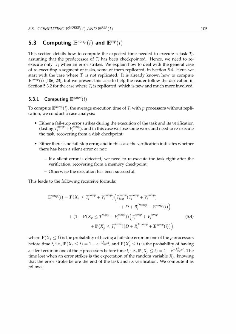
5.3. COMPUTING ENOREP(I) AND EREP(I) 105
5.3 Computing Enorep(i) and Erep(i)
This section details how to compute the expected time needed to execute a task Ti,assuming that the predecessor of Ti has been checkpointed. Hence, we need to re-execute only Ti when an error strikes. We explain how to deal with the general caseof re-executing a segment of tasks, some of them replicated, in Section 5.4. Here, westart with the case where Ti is not replicated. It is already known how to computeEnorep(i) [106, 23], but we present this case to help the reader follow the derivation inSection 5.3.2 for the case where Ti is replicated, which is new and much more involved.
5.3.1 Computing Enorep(i)
To compute Enorep(i), the average execution time of Ti with p processors without repli-cation, we conduct a case analysis:
• Either a fail-stop error strikes during the execution of the task and its verification(lasting Tnorep
i +Vnorepi ), and in this case we lose some work and need to re-execute
the task, recovering from a disk checkpoint;
• Either there is no fail-stop error, and in this case the verification indicates whetherthere has been a silent error or not:
– If a silent error is detected, we need to re-execute the task right after theverification, recovering from a memory checkpoint;
– Otherwise the execution has been successful.
This leads to the following recursive formula:
Enorep(i) = P(Xp ≤ Tnorepi + Vnorep
i )(
Tnoreplost (Tnorep
i + Vnorepi )
+ D + RDnorepi + Enorep(i)
)+ (1−P(Xp ≤ Tnorep
i + Vnorepi ))
(Tnorep
i + Vnorepi (5.4)
+ P(X′p ≤ Tnorep
i )(D + RMnorepi + Enorep(i))
),
where P(Xp ≤ t) is the probability of having a fail-stop error on one of the p processorsbefore time t, i.e., P(Xp ≤ t) = 1− e−λF
ind pt, and P(X′p ≤ t) is the probability of having
a silent error on one of the p processors before time t, i.e., P(X′p ≤ t) = 1− e−λS
ind pt. Thetime lost when an error strikes is the expectation of the random variable Xp, knowingthat the error stroke before the end of the task and its verification. We compute it asfollows:

106Chapter 5: Using Checkpointing and Replication for Reliable Execution of Linear Workflows with
Fail-Stop and Silent Errors
Tnoreplost (Tnorep
i + Vnorepi ) =
+∞∫0
xP(Xp = x|Xp ≤ Tnorepi + Vnorep
i )dx
=1
P(Xp ≤ Tnorepi + Vnorep
i )
Tnorepi +Vnorep
i∫0
xP(Xp = x)dx
=1
P(Xp ≤ Tnorepi + Vnorep
i )
Tnorepi +Vnorep
i∫0
xdP(Xp ≤ x)
dxdx
After integration, we get the formula:
Tnoreplost (Tnorep
i + Vnorepi ) =
1λF
ind p− Tnorep
i + Vnorepi
eλFind p(Tnorep
i +Vnorepi ) − 1
. (5.5)
Replacing the left hand side term of Equation (5.5) in Equation (5.4) and solving, wederive:
Enorep(i) =
(1
λFind p
+ D + RDnorepi
)ep((λF
ind+λSind)T
norepi +λF
indVnorepi ) (5.6)
−(
1λF
ind p+ (RDnorep
i − RMnorepi )
)eλS
ind pTnorepi − (D + RMnorep
i ).
Recall that Tnorepi = wi
(αi +
1−αip
)in Equation (5.6). Finally, if we decide to checkpoint
Ti, we simply add Cnorepi to Enorep(i).
5.3.2 Computing Erep(i)
We now discuss the case where Ti is replicated; each copy executes with p2 processors.
To compute Erep(i), the expected execution time of Ti with replication, we conduct acase analysis similar to that of Section 5.3.1:
• Either two fail-stop errors strike before the end of the task and its verification(lasting Trep
i + Vrepi ), with one fail-stop error striking each copy. Then we have
lost some work and need to re-execute the task from a disk checkpoint;
• Or at least one copy is not hit by any fail-stop error. Then we need to accountfor two different cases in the analysis:
– Both copies have survived: then we need to re-execute the task (recoveringfrom a memory checkpoint) only if both copies are hit by a silent error.
– Only one replica survived: then we need to re-execute the task if this replicais hit by a silent error.
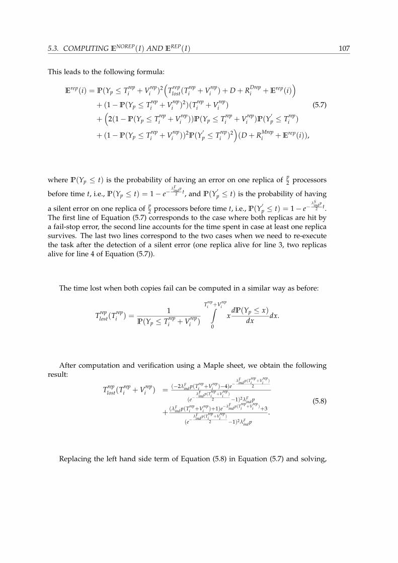
5.3. COMPUTING ENOREP(I) AND EREP(I) 107
This leads to the following formula:
Erep(i) = P(Yp ≤ Trepi + Vrep
i )2(
Treplost(T
repi + Vrep
i ) + D + RDrepi + Erep(i)
)+ (1−P(Yp ≤ Trep
i + Vrepi )2)(Trep
i + Vrepi ) (5.7)
+(
2(1−P(Yp ≤ Trepi + Vrep
i ))P(Yp ≤ Trepi + Vrep
i )P(Y′p ≤ Trep
i )
+ (1−P(Yp ≤ Trepi + Vrep
i ))2P(Y′p ≤ Trep
i )2)(D + RMrep
i + Erep(i)),
where P(Yp ≤ t) is the probability of having an error on one replica of p2 processors
before time t, i.e., P(Yp ≤ t) = 1− e−λF
ind p2 t, and P(Y
′p ≤ t) is the probability of having
a silent error on one replica of p2 processors before time t, i.e., P(Y
′p ≤ t) = 1− e−
λSind p2 t.
The first line of Equation (5.7) corresponds to the case where both replicas are hit bya fail-stop error, the second line accounts for the time spent in case at least one replicasurvives. The last two lines correspond to the two cases when we need to re-executethe task after the detection of a silent error (one replica alive for line 3, two replicasalive for line 4 of Equation (5.7)).
The time lost when both copies fail can be computed in a similar way as before:
Treplost(T
repi ) =
1P(Yp ≤ Trep
i + Vrepi )
Trepi +Vrep
i∫0
xdP(Yp ≤ x)
dxdx.
After computation and verification using a Maple sheet, we obtain the followingresult:
Treplost(T
repi + Vrep
i ) =(−2λF
ind p(Trepi +Vrep
i )−4)e−λF
ind p(Trepi +Vrep
i )
2
(e−λF
ind p(Trepi +Vrep
i )
2 −1)2λFind p
+(λF
ind p(Trepi +Vrep
i )+1)e−λFind p(Trep
i +Vrepi )+3
(e−λF
ind p(Trepi +Vrep
i )
2 −1)2λFind p
.(5.8)
Replacing the left hand side term of Equation (5.8) in Equation (5.7) and solving,

108Chapter 5: Using Checkpointing and Replication for Reliable Execution of Linear Workflows with
Fail-Stop and Silent Errors
we get:
Erep(i) = − (4 + 2λFind p(RDrep
i − RMrepi ))ep(
λFind(T
repi +Vrep
i )
2 +λSindTrep
i )
(2epλF
ind(Trepi +Vrep
i )+λSindTrep
i2 − 1) · λF
ind p(5.9)
+(1 + λF
ind p(RDrepi − RMrep
i ))eλSind pTrep
i
(2epλF
ind(Trepi +Vrep
i )+λSindTrep
i2 − 1) · λF
ind p
+(3 + λF
ind p(D + RDrepi ))ep(λF
ind(Trepi +Vrep
i )+λSindTrep
i )
(2epλF
ind(Trepi +Vrep
i )+λSindTrep
i2 − 1) · λF
ind p− (D + RMrep
i )
Recall that Trepi = wi
(αi +
1−αip2
)in Equation (5.9). Finally, if we decide to checkpoint
Ti, we simply add Crepi to Erep(i).
5.4 Optimal dynamic programming algorithm
In this section, we provide an optimal dynamic programming (DP) algorithm to solvethe ChainsRepCkpt problem for a linear chain of n tasks.
Theorem 4. The optimal solution to the ChainsRepCkpt problem can be obtained using adynamic programming algorithm in O(n2) time, where n is the number of tasks in the chain.
Proof. The algorithm recursively computes the expectation of the optimal time re-quired to execute tasks T1 to Ti and then checkpoint Ti. As already mentioned, weneed to distinguish two cases, according to whether Ti is replicated or not, becausethe cost of the final checkpoint depends upon this decision. Hence, we recursivelycompute two different functions:
• Trepopt(i), the expectation of the optimal time required to execute tasks T1 to Ti,
knowing that Ti is replicated;• Tnorep
opt (i), the expectation of the optimal time required to execute tasks T1 to Ti,knowing that Ti is not replicated.
Note that checkpoint time is not included in Trepopt(i) nor Tnorep
opt (i). The solution toChainsRepCkpt will be given by
min
Trepopt(n) + Crep
n , Tnorepopt (n) + Cnorep
n
. (5.10)
We start with the computation of Trepopt(j) for 1 ≤ j ≤ n, hence assuming that the

5.4. OPTIMAL DYNAMIC PROGRAMMING ALGORITHM 109
last task Tj is replicated. We express Trepopt(j) recursively as follows:
Trepopt(j)= min
1≤i<j
Trepopt(i) + Crep
i + Trep,repNC (i + 1, j),
Trepopt(i) + Crep
i + Tnorep,repNC (i + 1, j),
Tnorepopt (i) + Cnorep
i + Trep,repNC (i + 1, j),
Tnorepopt (i)+Cnorep
i +Tnorep,repNC (i + 1, j),
RDrep1 + Trep,rep
NC (1, j),
RDnorep1 + Tnorep,rep
NC (1, j)
(5.11)
In Equation (5.11), Ti corresponds to the last checkpointed task before Tj, and wetry all possible locations Ti for taking a checkpoint before Tj. The first four linescorrespond to the case where there is indeed an intermediate task Ti between T1 andTj that is checkpointed, while the last two lines correspond to the case where nocheckpoint at all is taken until after Tj.
The first two lines of Equation (5.11) apply to the case where Ti is replicated. Line1 is for the case when Ti+1 is replicated, and line 2 when it is not. In the first lineof Equation (5.11), Trep,rep
NC (i + 1, j) denotes the optimal time to execute tasks Ti+1 to Tjwithout any intermediate checkpoint, knowing that Ti is checkpointed, and both Ti+1and Tj are replicated. If Ti+1 is not replicated, we use the second line of Equation (5.11),where Tnorep,rep
NC (i + 1, j) is the counterpart of Trep,repNC (i + 1, j), except that it assumes that
Ti+1 is not replicated. This information on Ti+1 (replicated or not) is needed to computethe recovery cost when executing tasks Ti+1 to Tj and experiencing an error.
Lines 3 and 4 apply to the case where Ti is not replicated, with similar notation asbefore. In the first four lines, no task between Ti+1 and Tj−1 is checkpointed, hence thenotation NC for no checkpoint.
If no checkpoint at all is taken before Tj (this corresponds to the case i = 0), weuse the last two lines of Equation (5.11): we include the cost to read the initial input,which depends whether T1 is replicated (in line 5) or not (in line 6) of Equation (5.11).
We have a very similar equation to express Tnorepopt (j) recursively, with intuitive no-
tation:
Tnorepopt (j) = min
1≤i<j
Trepopt(i) + Crep
i + Trep,norepNC (i + 1, j),
Trepopt(i) + Crep
i + Tnorep,norepNC (i + 1, j),
Tnorepopt (i) + Cnorep
i + Trep,norepNC (i + 1, j),
Tnorepopt (i)+Cnorep
i +Tnorep,norepNC (i + 1, j),
RDrep1 + Trep,norep
NC (1, j),
RDnorep1 + Tnorep,norep
NC (1, j)
(5.12)
To synthesize the notation, we have defined TA,BNC (i + 1, j), with A, B ∈ rep, norep,
as the optimal time to execute tasks Ti+1 to Tj without any intermediate checkpoint,knowing that Ti is checkpointed, Ti+1 is replicated if and only if A = rep, and Tj is

110Chapter 5: Using Checkpointing and Replication for Reliable Execution of Linear Workflows with
Fail-Stop and Silent Errors
replicated if and only if B = rep. In a nutshell, we have to account for the possiblereplication of the first task Ti+1 after the last checkpoint, and of the last task Tj, hencethe four cases.
There remains to compute TA,BNC (i, j) for all 1 ≤ i, j ≤ n and A, B ∈ rep, norep.
This is still not easy, because there remains to decide which intermediate tasks shouldbe replicated. In addition to the status of Tj (replicated or not, according to the valueof B), the only thing we know so far is that the only checkpoint that we can recoverfrom while executing tasks Ti to Tj is the checkpoint taken after task Ti−1, hence weneed to re-execute from Ti whenever an error strikes. Furthermore, Ti is replicated ifand only if A = rep, hence we know the corresponding cost for recovery, RA
i . LettingTA,B
NC (i, j) = 0 whenever i > j, we can express TA,BNC (i, j) for 1 ≤ i ≤ j ≤ n as follows:
TA,BNC (i, j) = min
TA,rep
NC (i, j− 1), TA,norepNC (i, j− 1)
+ TA,B(j | i).
Here the new (and final) notation TA,B(j | i) is simply the time needed to executetask Tj, knowing that an error during Tj implies to recover from Ti. Indeed, to executetasks Ti to Tj, we account recursively for the time to execute Ti to Tj−1; Ti−1 is stillcheckpointed; Ti is replicated if and only if A = rep, Tj is replicated if and only ifB = rep, and we consider both cases whether Tj−1 is replicated or not. The time lostin case of an error during Tj depends whether Tj is replicated or not, and we need torestart from Ti in case of error, hence the notation TA,B(j | i), representing the expectedexecution time for task Tj with or without replication (depending on B), given that weneed to restart from Ti if there is an error (and Ti is replicated if and only if A = rep).
The last step is hence to express these execution times. We start with the casewhere Tj is not replicated:
TA,norep(j | i) =(
1− e−λFind p(Tnorep
j +Vnorepj )
) (Tnorep
lost (Tnorepj + Vnorep
j ) + D + RD Ai
+min
TA,repNC (i, j− 1), TA,norep
NC (i, j− 1)+ TA,norep(j | i)
)+ e−λF
ind p(Tnorepj +Vnorep
j )(
Tnorepj + Vnorep
j +(
1− e−λSind pTnorep
j)(D + RM A
i
+min
TA,repNC (i, j− 1), TA,norep
NC (i, j− 1)+ TA,norep(j | i))
).
The term in e−λFind p(Tnorep
j +Vnorepj ) represents the case without fail-stop error, where the
execution time is simply Tnorepj +Vnorep
j . If a silent error is detected after the verification,we pay a downtime and a memory recovery (with a cost depending on A). Next, weneed to re-execute all the tasks since the last checkpoint (Ti to Tj−1) and take theminimal value obtained out of the execution where Tj−1 is replicated or not; finally,we execute Tj again (with a time TA,norep(j | i)) from last checkpoint. When a fail-stop

5.5. EXPERIMENTS 111
error strikes, we account for Tnoreplost (Tnorep
j + Vnorepj ), the time lost within Tj, and whose
value is given by Equation (5.5). Then we pay a downtime and a disk recovery (witha cost depending on A). Finally, we re-execute all the tasks from last checkpoint andthat is similar to the previous case.
The formula is similar with replication of Tj, where the probability of error ac-counts for the fact that we need to recover only if both replicas fail for the fail-stoperrors and accounts for the number of living replicas in the case where a silent erroris detected (see Section 5.3.2 for the details):
TA,rep(j | i) =
(1− e−
λFind p(Trep
j +Vrepj )
2
)2 (Trep
lost(Trepj + Vrep
j ) + D + RD Ai
+min
TA,repNC (i, j− 1), TA,norep
NC (i, j− 1)+ TA,rep(j | i)
)+
1−(
1− e−λF
ind p(Trepj +Vrep
j )
2
)2(Trep
j + Vrepj
)+((1− e−
λFind p(Trep
j +Vrepj )
2 )e−λF
ind p(Trepj +Vrep
j )
2 (1− e−λS
ind pTrepj
2 )
+e−λFind p(Trep
j +Vrepj )(1− e−
λSind pTrep
j2 )2
)(D + RM A
i
+min
TA,repNC (i, j− 1), TA,norep
NC (i, j− 1)+ TA,rep(j | i)
).
Note that the value of Treplost(T
repj ) is given by Equation (5.8). Overall, we need to
compute the O(n2) intermediate values TA,B(j | i) and TA,BNC (i, j) for 1 ≤ i, j ≤ n
and A, B ∈ rep, norep, and each of these take constant time. There are O(n) valuesTA
opt(i), for 1 ≤ i ≤ n and A ∈ rep, norep, and these perform a minimum over atmost 6n elements, hence they can be computed in O(n). The overall complexity istherefore O(n2).
5.5 ExperimentsIn this section, we evaluate the advantages of adding replication to checkpointingin the presence of both, fail-stop and silent errors. We point out that the simulatorthat implements the proposed DP algorithm is publicly available at http://graal.ens-lyon.fr/˜yrobert/chainsrep.zip so that interested readers can instantiate theirpreferred scenarios and repeat the same simulations for reproducibility purpose. Thecode is written in-house in C++ and does not use any library other than the STL.
We start by assessing scenarios with fail-stop errors only in Section 5.5.1. We firstdescribe the evaluation framework in Section 5.5.1.1, then we compare checkpoint withreplication to checkpoint only in Section 5.5.1.2. In Section 5.5.1.3, we assess the impactof the different model parameters on the performance of the optimal strategy. Finally,Section 5.5.1.4 compares the performance of the optimal solution to alternative sub-optimal solutions.

112Chapter 5: Using Checkpointing and Replication for Reliable Execution of Linear Workflows with
Fail-Stop and Silent Errors
Then we assess scenarios with both fail-stop and silent errors in Section 5.5.2. Wefirst describe the few modifications of the evaluation framework in Section 5.5.2.1, thenwe compare checkpoint with replication to checkpoint only in Section 5.5.2.2. Finally, Sec-tion 5.5.2.3 assesses the impact of the different model parameters on the performanceof the optimal strategy.
5.5.1 Scenarios with fail-stop errors only
5.5.1.1 Experimental setup
We fix the total work in the chain to W = 10, 000 seconds. The choice of this valueis less important than the duration of the tasks compared to the error rate. For thisreason, we rely on five different work distributions, where all tasks are fully parallel(αi = 0):
• Uniform: every task i is of length wi =Wn , i.e., identical tasks.
• Increasing: the length of the tasks constantly increases, i.e., task Ti has lengthwi = i 2W
n(n+1) .
• Decreasing: the length of the tasks constantly decreases, i.e., task Ti has lengthwi = (n− i + 1) 2W
n(n+1) .
• HighLow: the chain is formed by long tasks followed by short tasks. The longtasks represent 60% of the total work and there are d n
10e such tasks. Short tasksrepresent the remaining 40% of the total work and consequently there are n −d n
10e small tasks.
• Random: task lengths are uniformly chosen at random between W2n and 3W
2n . Ifthe total work of the first i tasks reaches W, the weight of each task is multipliedby i
n so that we can continue adding the remaining tasks.
Experiments with increasing sequential part (αi) for the tasks are available in thecompanion research report [22]. Setting αi = 0 amounts to being in the worse pos-sible case for replication, since the tasks will fully benefit of having twice as muchprocessors when not replicated.
For simplicity, we assume that checkpointing costs are equal to the correspondingrecovery costs, assuming that read and write operations take approximately the sameamount of time, i.e., RDnorep
i+1 = Cnorepi . For replicated tasks, we set Crep
i = αCnorepi and
RDrepi = αRDnorep
i , where 1 ≤ α ≤ 2, and we assess the impact of parameter α in Sec-tion 5.5.2.3. In the following experiments, we measure the performance of a solutionby evaluating the associated normalized expected makespan, i.e., the expected execu-tion time needed to compute all the tasks in the chain, with respect to the executiontime without errors, checkpoints, or replicas.
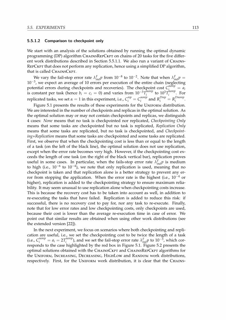
5.5. EXPERIMENTS 113
5.5.1.2 Comparison to checkpoint only
We start with an analysis of the solutions obtained by running the optimal dynamicprogramming (DP) algorithm ChainsRepCkpt on chains of 20 tasks for the five differ-ent work distributions described in Section 5.5.1.1. We also run a variant of Chains-RepCkpt that does not perform any replication, hence using a simplified DP algorithm,that is called ChainsCkpt.
We vary the fail-stop error rate λFind p from 10−8 to 10−2. Note that when λF
ind p =10−3, we expect an average of 10 errors per execution of the entire chain (neglectingpotential errors during checkpoints and recoveries). The checkpoint cost Cnorep
i = aiis constant per task (hence bi = ci = 0) and varies from 10−3Tnorep
i to 103Tnorepi . For
replicated tasks, we set α = 1 in this experiment, i.e., Crepi = Cnorep
i and RDrepi = RDnorep
i .Figure 5.1 presents the results of these experiments for the Uniform distribution.
We are interested in the number of checkpoints and replicas in the optimal solution. Asthe optimal solution may or may not contain checkpoints and replicas, we distinguish4 cases: None means that no task is checkpointed nor replicated, Checkpointing Onlymeans that some tasks are checkpointed but no task is replicated, Replication Onlymeans that some tasks are replicated, but no task is checkpointed, and Checkpoint-ing+Replication means that some tasks are checkpointed and some tasks are replicated.First, we observe that when the checkpointing cost is less than or equal to the lengthof a task (on the left of the black line), the optimal solution does not use replication,except when the error rate becomes very high. However, if the checkpointing cost ex-ceeds the length of one task (on the right of the black vertical bar), replication provesuseful in some cases. In particular, when the fails-stop error rate λF
ind p is mediumto high (i.e., 10−6 to 10−4), we note that only replication is used, meaning that nocheckpoint is taken and that replication alone is a better strategy to prevent any er-ror from stopping the application. When the error rate is the highest (i.e., 10−4 orhigher), replication is added to the checkpointing strategy to ensure maximum relia-bility. It may seem unusual to use replication alone when checkpointing costs increase.This is because the recovery cost has to be taken into account as well, in addition tore-executing the tasks that have failed. Replication is added to reduce this risk: ifsuccessful, there is no recovery cost to pay for, nor any task to re-execute. Finally,note that for low error rates and low checkpointing costs, only checkpoints are used,because their cost is lower than the average re-execution time in case of error. Wepoint out that similar results are obtained when using other work distributions (seethe extended version [22]).
In the next experiment, we focus on scenarios where both checkpointing and repli-cation are useful, i.e., we set the checkpointing cost to be twice the length of a task(i.e., Cnorep
i = ai = 2Tnorepi ), and we set the fail-stop error rate λF
ind p to 10−3, which cor-responds to the case highlighted by the red box in Figure 5.1. Figure 5.2 presents theoptimal solutions obtained with the ChainsCkpt and ChainsRepCkpt algorithms forthe Uniform, Increasing, Decreasing, HighLow and Random work distributions,respectively. First, for the Uniform work distribution, it is clear that the Chains-

114Chapter 5: Using Checkpointing and Replication for Reliable Execution of Linear Workflows with
Fail-Stop and Silent Errors
1.0e− 034.0e− 031.6e− 026.4e− 022.6e− 011.0e
+ 004.1e
+ 001.6e
+ 016.6e
+ 012.6e
+ 021.0e
+ 03
Checkpoint/Recovery cost over task length ratio
1.00e− 08
4.00e− 08
1.60e− 07
6.40e− 07
2.56e− 06
1.02e− 05
4.10e− 05
1.64e− 04
6.55e− 04
2.62e− 03
1.05e− 02
Err
orR
ate
NoneCheckpointing OnlyReplication OnlyCheckpointing+Replication
Figure 5.1: Impact of checkpoint/recovery cost and error rate on the usage of check-pointing and replication. Total work is fixed to 10, 000s and is distributed uniformlyamong n = 20 tasks (i.e., T1 = T2 = · · · = T20 = 500s). Each color shows the presenceof checkpoints and/or replicas in the optimal solution. Results corresponding to thecase highlighted with a red square are presented in Figure 5.2.

5.5. EXPERIMENTS 115
T2 T4 T6 T8 T10 T12 T14 T16 T18 T20
CHAINSCKPT (Checkpointing Only)
T2 T4 T6 T8 T10 T12 T14 T16 T18 T20
CHAINSREPCKPT (Checkpointing and Replication)
(a) Uniform
T2 T4 T6 T8 T10 T12 T14 T16 T18 T20
CHAINSCKPT (Checkpointing Only)
T2 T4 T6 T8 T10 T12 T14 T16 T18 T20
CHAINSREPCKPT (Checkpointing and Replication)
(b) Increasing
T2 T4 T6 T8 T10 T12 T14 T16 T18 T20
CHAINSCKPT (Checkpointing Only)
T2 T4 T6 T8 T10 T12 T14 T16 T18 T20
CHAINSREPCKPT (Checkpointing and Replication)
(c) Decreasing
T2 T4 T6 T8 T10 T12 T14 T16 T18 T20
CHAINSCKPT (Checkpointing Only)
T2 T4 T6 T8 T10 T12 T14 T16 T18 T20
CHAINSREPCKPT (Checkpointing and Replication)
(d) HighLow
T2 T4 T6 T8 T10 T12 T14 T16 T18 T20
CHAINSCKPT (Checkpointing Only)
T2 T4 T6 T8 T10 T12 T14 T16 T18 T20
CHAINSREPCKPT (Checkpointing and Replication)
NoneCheckpointing OnlyReplication OnlyCheckpointing+Replication
(e) Random
Figure 5.2: Optimal solutions obtained with the ChainsCkpt algorithm (top) and theChainsRepCkpt algorithm (bottom) for the five work distributions.
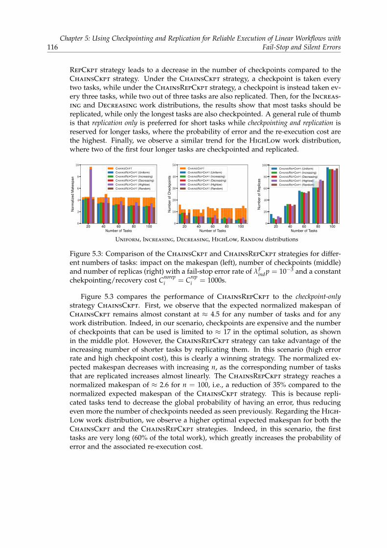
116Chapter 5: Using Checkpointing and Replication for Reliable Execution of Linear Workflows with
Fail-Stop and Silent Errors
RepCkpt strategy leads to a decrease in the number of checkpoints compared to theChainsCkpt strategy. Under the ChainsCkpt strategy, a checkpoint is taken everytwo tasks, while under the ChainsRepCkpt strategy, a checkpoint is instead taken ev-ery three tasks, while two out of three tasks are also replicated. Then, for the Increas-ing and Decreasing work distributions, the results show that most tasks should bereplicated, while only the longest tasks are also checkpointed. A general rule of thumbis that replication only is preferred for short tasks while checkpointing and replication isreserved for longer tasks, where the probability of error and the re-execution cost arethe highest. Finally, we observe a similar trend for the HighLow work distribution,where two of the first four longer tasks are checkpointed and replicated.
20 40 60 80 100Number of Tasks
0
2
4
6
8
10
Nor
mal
ized
Mak
espa
n
CHAINSCKPT
CHAINSREPCKPT (Uniform)CHAINSREPCKPT (Increasing)CHAINSREPCKPT (Decreasing)CHAINSREPCKPT (Highlow)CHAINSREPCKPT (Random)
20 40 60 80 100Number of Tasks
0
10
20
30
40
50N
umbe
rofC
heck
poin
tsCHAINSCKPT
CHAINSREPCKPT (Uniform)CHAINSREPCKPT (Increasing)CHAINSREPCKPT (Decreasing)CHAINSREPCKPT (Highlow)CHAINSREPCKPT (Random)
20 40 60 80 100Number of Tasks
0
20
40
60
80
100
Num
bero
fRep
licas
CHAINSREPCKPT (Uniform)CHAINSREPCKPT (Increasing)CHAINSREPCKPT (Decreasing)CHAINSREPCKPT (Highlow)CHAINSREPCKPT (Random)
Uniform, Increasing, Decreasing, HighLow, Random distributions
Figure 5.3: Comparison of the ChainsCkpt and ChainsRepCkpt strategies for differ-ent numbers of tasks: impact on the makespan (left), number of checkpoints (middle)and number of replicas (right) with a fail-stop error rate of λF
ind p = 10−3 and a constantchekpointing/recovery cost Cnorep
i = Crepi = 1000s.
Figure 5.3 compares the performance of ChainsRepCkpt to the checkpoint-onlystrategy ChainsCkpt. First, we observe that the expected normalized makespan ofChainsCkpt remains almost constant at ≈ 4.5 for any number of tasks and for anywork distribution. Indeed, in our scenario, checkpoints are expensive and the numberof checkpoints that can be used is limited to ≈ 17 in the optimal solution, as shownin the middle plot. However, the ChainsRepCkpt strategy can take advantage of theincreasing number of shorter tasks by replicating them. In this scenario (high errorrate and high checkpoint cost), this is clearly a winning strategy. The normalized ex-pected makespan decreases with increasing n, as the corresponding number of tasksthat are replicated increases almost linearly. The ChainsRepCkpt strategy reaches anormalized makespan of ≈ 2.6 for n = 100, i.e., a reduction of 35% compared to thenormalized expected makespan of the ChainsCkpt strategy. This is because repli-cated tasks tend to decrease the global probability of having an error, thus reducingeven more the number of checkpoints needed as seen previously. Regarding the High-Low work distribution, we observe a higher optimal expected makespan for both theChainsCkpt and the ChainsRepCkpt strategies. Indeed, in this scenario, the firsttasks are very long (60% of the total work), which greatly increases the probability oferror and the associated re-execution cost.

5.5. EXPERIMENTS 117
10−5 10−4 10−3 10−2
Error rate λindp
0
2
4
6
8
10
Nor
mal
ized
Mak
espa
n
CHAINSREPCKPT (C = R = 1000)CHAINSCKPT (C = R = 1000)
0 1 2 3 4 5Checkpoint/Recovery cost over task length ratio
0
2
4
6
8
10
Nor
mal
ized
Mak
espa
n
CHAINSREPCKPT
CHAINSCKPT
0 20 40 60 80 100Number of Tasks
0
1
2
3
4
5
Nor
mal
ized
Mak
espa
n
CHAINSREPCKPT (Crep = Cnorep)CHAINSREPCKPT (Crep = 1.5 Cnorep)CHAINSREPCKPT (Crep = 2 Cnorep)
Figure 5.4: Impact of fail-stop error rate λFind p (left), checkpoint cost (middle), and
ratio α between the checkpointing cost for replicated task Crepi over non-replicated
tasks Cnorepi (right).
0 2000 4000 6000 8000 10000Number of Processors
0
1
2
3
4
5
Nor
mal
ized
Mak
espa
n
CHAINSREPCKPT
CHAINSCKPT
(a) (100, 10000, 1)
0 2000 4000 6000 8000 10000Number of Processors
0
1
2
3
4
5
Nor
mal
ized
Mak
espa
n
CHAINSREPCKPT
CHAINSCKPT
(b) (100, 100000, 0.1)
0 2000 4000 6000 8000 10000Number of Processors
0
1
2
3
4
5
Nor
mal
ized
Mak
espa
nCHAINSREPCKPT
CHAINSCKPT
(c) (100, 1000000, 0.01)
Figure 5.5: Comparison of the ChainsCkpt and ChainsRepCkpt strategies for differ-ent numbers of processors, with different model parameter values for the checkpoint-ing cost (ai, bi, ci).
5.5.1.3 Impact of error rate and checkpoint cost on the performance
Figure 5.4 shows the impact of three of the model parameters on the optimal expectednormalized makespan of both ChainsCkpt and ChainsRepCkpt. First, we show theimpact of the fail-stop error rate λF
ind p on the performance. The ChainsRepCkpt algo-rithm improves the ChainsCkpt strategy for large values of λF
ind p: replication starts tobe used for λF
ind p > 2.6× 10⁻⁴ and it reduces the makespan by ≈ 16% for λFind p = 10−3
and by up to ≈ 40% when λFind p = 10−2, where all tasks are checkpointed and repli-
cated.Then, we investigate the impact of the checkpointing cost with respect to the task
length. As shown in Figure 5.1, replication is not needed for low checkpointing costs,i.e., when the checkpointing cost is between 0 and 0.8 times the cost of one task: in thisscenario, all tasks are checkpointed and both strategies lead to the same makespan.When the checkpointing cost is between 0.9 and 1.6 times the cost of one task, Chains-RepCkpt checkpoints and replicates half of the tasks. Overall, the ChainsRepCkpt
strategy improves the optimal normalized expected makespan by ≈ 11% for a check-pointing cost ratio of 1.6, and by as much as ≈ 36% when the checkpointing cost is

118Chapter 5: Using Checkpointing and Replication for Reliable Execution of Linear Workflows with
Fail-Stop and Silent Errors
five times the length of one task.We now investigate the impact of the ratio between the checkpointing and recov-
ery cost for replicated tasks and non-replicated tasks α and we present the results forα = 1 (Crep
i = RDrepi = Cnorep
i = RDnorepi ), α = 1.5 (Crep
i = RDrepi = 1.5Cnorep
i = 1.5RDnorepi )
and α = 2 (Crepi = RDrep
i = 2Cnorepi = 2RDnorep
i ). As expected, the makespan in-creases with α, but it is interesting to note that the makespan converges towards asame lower-bound as the number of (shorter) tasks increases. As shown previously,when tasks are smaller, ChainsRepCkpt favors replication over checkpointing, espe-cially when the checkpointing cost is high, which means less checkpoints, recoveriesand re-executions.
Finally, we evaluate the efficiency of both strategies when the number of processorsincreases. For this experiment, we instantiate the model using variable checkpointingcosts, i.e., we do not use bi = ci = 0 anymore, so that the checkpointing/recoverycost depends on the number of processors. We set n = 50, λF
ind = 10−7 and we makep vary from 10 to 10,000 (i.e., the global error rate varies between 10−6 and 10−3).Figure 5.5 presents the results of the experiment using three different sets of values forai, bi and ci. We see that when bi increases while ci decreases, the replication becomesuseless, even for the larger error rate values. However, when the term ci p becomeslarge in front of bi
p , we see that ChainsRepCkpt is much better than ChainsCkpt,as the checkpointing costs tend to decrease, in addition to all the other advantagesinvestigated in the previous sections. With p = 10, 000, the three different experimentsshow an improvement of 80.5%, 40.7% and 0% (from left to right, respectively).
5.5.1.4 Impact of the number of checkpoints and replicas
Figure 5.6 shows the impact of the number of checkpoints and replicas on the nor-malized expected makespan for different checkpointing costs and fail-stop error ratesλF
ind p under the Uniform work distribution. We show that the optimal solution withChainsRepCkpt (highlighted by the green box) always matches the minimum valueobtained in the simulations, i.e., the optimal number of checkpoints, number of repli-cas, and expected execution times are consistent. In addition, we show that in sce-narios where both the checkpointing cost and the error rate are high, even a smalldeviation from the optimal solution can quickly lead to a large overhead.
5.5.2 Scenarios with both fail-stop and silent errors
In this section we evaluate the power of replication in addition to checkpointing onplatforms subject to both fail-stop and silent errors.
5.5.2.1 Experimental setup
All the model parameters are instantiated as before, with the following changes toaccount for the presence of silent errors. Unless stated otherwise, the fail-stop error

5.5. EXPERIMENTS 119
1 2 4 5 10 20#Checkpoints
0
2
4
5
10
20
#Rep
licas
1.0
1.5
2.0
2.5
3.0
3.5
4.0
4.5
5.0
1 2 4 5 10 20#Checkpoints
0
2
4
5
10
20
#Rep
licas
1.0
1.5
2.0
2.5
3.0
3.5
4.0
4.5
5.0
1 2 4 5 10 20#Checkpoints
0
2
4
5
10
20
#Rep
licas
1.0
1.5
2.0
2.5
3.0
3.5
4.0
4.5
5.0
1 2 4 5 10 20#Checkpoints
0
2
4
5
10
20
#Rep
licas
1.0
1.5
2.0
2.5
3.0
3.5
4.0
4.5
5.0
1 2 4 5 10 20#Checkpoints
0
2
4
5
10
20
#Rep
licas
1.0
1.5
2.0
2.5
3.0
3.5
4.0
4.5
5.0
1 2 4 5 10 20#Checkpoints
0
2
4
5
10
20
#Rep
licas
1.0
1.5
2.0
2.5
3.0
3.5
4.0
4.5
5.0
1 2 4 5 10 20#Checkpoints
0
2
4
5
10
20
#Rep
licas
1.0
1.5
2.0
2.5
3.0
3.5
4.0
4.5
5.0
1 2 4 5 10 20#Checkpoints
0
2
4
5
10
20
#Rep
licas
1.0
1.5
2.0
2.5
3.0
3.5
4.0
4.5
5.0
1 2 4 5 10 20#Checkpoints
0
2
4
5
10
20#R
eplic
as
1.0
1.5
2.0
2.5
3.0
3.5
4.0
4.5
5.0
Figure 5.6: Impact of the number of checkpoints and replicas on the normalized ex-pected makespan for fail-stop error rates of λF
ind = 10−4 (top), λ = 10−3 (middle) andλ = 10−2 (bottom) and for checkpointing costs of 0.5× Tnorep
i (left), 1× Tnorepi (middle)
and 2× Tnorepi (right), with Cnorep
i = Crepi under Uniform work distribution. The opti-
mal solution obtained with ChainsRepCkpt always matches the minimum simulationvalue and is highlighted by the green box.
rate has been set to 1.28e-3s−1 and the silent error rate has been set to 5.48e-3s−1.The silent error rate has been computed from real measures [18]: we derived a non-corrected silent error rate per core of 5.48e-9s−1. Similarly, the fail-stop error rateper core considered was 1.28e-9s−1, which corresponds to a core lifetime of 25 years.Finally, we considered a platform of 1 million cores which tends to be the trend forcurrent Top500 machines [181].
As for other parameters, we considered a verification cost of 1% of the correspond-ing task length. The cost of memory recovery was set to 5% of that of a disk recovery,considering an average between different measured values from [140].
For simplicity, we assume that checkpointing costs are equal to the sum of the

120Chapter 5: Using Checkpointing and Replication for Reliable Execution of Linear Workflows with
Fail-Stop and Silent Errors
corresponding recovery costs, assuming that read and write operations take approxi-mately the same amount of time, i.e., RDnorep
i+1 + RMnorepi+1 = Cnorep
i . For replicated tasks,
we set Crepi = αCnorep
i , RDrepi = αRDnorep
i and RMrepi = αRMnorep
i , where 1 ≤ α ≤ 2, andwe assess the impact of parameter α in Section 5.5.2.3. As in the previous section, wemeasure the performance of a solution by evaluating the associated normalized ex-pected makespan, i.e., the expected execution time needed to compute all the tasks inthe chain, with respect to the execution time without errors, checkpoints, or replicas.
5.5.2.2 Comparison to checkpoint only
We start with an analysis of the solutions obtained by running the optimal dynamicprogramming (DP) algorithm ChainsRepCkpt on chains with 20 tasks for the fivedifferent work distributions described in Section 5.5.1.1. We also run a variant ofChainsRepCkpt that does not perform any replication, hence using a simplified DPalgorithm, that is called ChainsCkpt.
We vary the fail-stop error rate λFind p from 10−8 to 10−2, without changing the
silent error rate λSind. The disk checkpoint/recovery cost is constant per task and varies
from 10−3Tnorepi to 103Tnorep
i (hence, the memory checkpoint/recovery cost varies from5× 10−5Tnorep
i to 50Tnorepi ). Overall, all checkpoints have a cost from 1.05× 10⁻³Tnorep
i to1.05× 103Tnorep
i as we always perform both types of checkpoints. For replicated tasks,we set α = 1 in this experiment, i.e., Crep
i = Cnorepi , RDrep
i = RDnorepi and RMrep
i = RMnorepi .
In another experiment, we also make the silent error rate λSind p vary from 10−8 to
10−2 without changing the fail-stop error rate of 1.28e-3, with the same range for thecheckpoint cost.
s1.0e− 034.0e− 031.6e− 026.4e− 022.6e− 011.0e
+ 004.1e
+ 001.6e
+ 016.6e
+ 012.6e
+ 021.0e
+ 03
Checkpoint/Recovery cost over task length ratio
1.00e− 08
4.00e− 08
1.60e− 07
6.40e− 07
2.56e− 06
1.02e− 05
4.10e− 05
1.64e− 04
6.55e− 04
2.62e− 03
1.05e− 02
Fail-
stop
Err
orR
ate
Checkpointing OnlyCheckpointing+Replication
1.0e− 034.0e− 031.6e− 026.4e− 022.6e− 011.0e
+ 004.1e
+ 001.6e
+ 016.6e
+ 012.6e
+ 021.0e
+ 03
Checkpoint/Recovery cost over task length ratio
1.00e− 08
4.00e− 08
1.60e− 07
6.40e− 07
2.56e− 06
1.02e− 05
4.10e− 05
1.64e− 04
6.55e− 04
2.62e− 03
1.05e− 02
Sile
ntE
rror
Rat
e
Checkpointing OnlyCheckpointing+Replication
Figure 5.7: Impact of checkpoint/recovery cost and error rates on the usage of check-pointing and replication. Total sequential work is fixed to 10, 000s and is distributeduniformly among n = 20 tasks (i.e., T1 = T2 = · · · = T20 = 500s). Each color showsthe presence of checkpoints and/or replicas in the optimal solution.
Figure 5.7 presents the results of these experiments for the Uniform distribution.

5.5. EXPERIMENTS 121
The colors are the same as in Figure 5.1, with Checkpointing Only meaning that sometasks are checkpointed but no task is replicated and Checkpointing+Replication mean-ing that some tasks are checkpointed and some tasks are replicated. The left figurepresents the results when the silent error rate is fixed but the fail-stop error rate varies.The right figure presents the results of the other experiment with a fixed fail-stop errorrate and different silent error rates.
First, we observe that with silent errors, checkpointing becomes mandatory. Toomany failures can strike during the execution, and checkpointing helps reducing thetime spent on rollbacks and re-executions. However, as soon as the cost of a checkpointexceeds the length of a task, replication becomes useful and this remains true even forlow error rates. This holds for both fail-stop errors (left) and silent errors (right). Thereis one exception: when the fail-stop error rate is lower than 10−5 and the checkpointingcost is less than twice the length of a task, checkpoints are sufficient and is replicationis not needed. Replication is overall not needed under good conditions, however forour real setup, indicated by the red box, using both checkpointing and replication is abetter solution. We point out that similar results are obtained when using other workdistributions (see the extended version [22]).
In the next experiment, we focus on scenarios where both checkpointing and repli-cation are useful, i.e., we set the checkpointing cost to be twice the length of a task(i.e., Cnorep
i = ai = 2Tnorepi ), keeping λF
ind p = 1.28e-3 and λSind p = 5.48e-3, for the fail-
stop and silent error rates, respectively, which corresponds to the case highlighted bythe red box in Figure 5.7. Figure 5.8 presents the optimal solutions obtained withthe ChainsCkpt and ChainsRepCkpt algorithms for the Uniform, Increasing, De-creasing, HighLow and Random work distributions, respectively. With two sourcesof errors, the solution is straightforward: almost every task must be checkpointed,with the exception of one (short) task for the Decreasing and Increasing distribu-tions. However almost every task is also replicated (20 tasks out of 20 for the Uniform
distribution compared to only 13 in the experiments of Section 5.5.1.2), showing oncemore that replication grants better protection to failures even if it increases the failure-free execution time. Checkpoints are being taken the same way as in our previousexperiments: long tasks are systematically checkpointed while shorter tasks are ei-ther unprotected or replicated, as can be seen with the first tasks of the Increasing
distribution and the last task of the Decreasing distributions.Figure 5.9 compares the performance of ChainsRepCkpt to the checkpoint-only
strategy ChainsCkpt with fail-stop and silent errors. First, we observe that longtasks, being more likely to fail than shorter tasks, introduce a high overhead. As aconsequence, with 20 tasks, the normalized makespan is too high and the execution ofsuch applications is not possible, independently of the work distribution and the cho-sen checkpointing strategy. With more tasks however, the ChainsRepCkpt strategyalways yield a shorter makespan compared to the ChainsCkpt strategy. For example,with 100 tasks, the normalized makespan obtained with the ChainsRepCkpt strategyis as high as ≈ 8.5 (and much more for the HighLow distribution), compared to ≈ 13for ChainsCkpt. Indeed, with such high error rates, all tasks are replicated under

122Chapter 5: Using Checkpointing and Replication for Reliable Execution of Linear Workflows with
Fail-Stop and Silent Errors
T2 T4 T6 T8 T10 T12 T14 T16 T18 T20
CHAINSCKPT (Checkpointing Only)
T2 T4 T6 T8 T10 T12 T14 T16 T18 T20
CHAINSREPCKPT (Checkpointing and Replication)
(a) Uniform
T2 T4 T6 T8 T10 T12 T14 T16 T18 T20
CHAINSCKPT (Checkpointing Only)
T2 T4 T6 T8 T10 T12 T14 T16 T18 T20
CHAINSREPCKPT (Checkpointing and Replication)
(b) Increasing
T2 T4 T6 T8 T10 T12 T14 T16 T18 T20
CHAINSCKPT (Checkpointing Only)
T2 T4 T6 T8 T10 T12 T14 T16 T18 T20
CHAINSREPCKPT (Checkpointing and Replication)
(c) Decreasing
T2 T4 T6 T8 T10 T12 T14 T16 T18 T20
CHAINSCKPT (Checkpointing Only)
T2 T4 T6 T8 T10 T12 T14 T16 T18 T20
CHAINSREPCKPT (Checkpointing and Replication)
(d) HighLow
T2 T4 T6 T8 T10 T12 T14 T16 T18 T20
CHAINSCKPT (Checkpointing Only)
T2 T4 T6 T8 T10 T12 T14 T16 T18 T20
CHAINSREPCKPT (Checkpointing and Replication)
NoneCheckpointing OnlyReplication OnlyCheckpointing+Replication
(e) Random
Figure 5.8: Optimal solutions obtained with the ChainsCkpt algorithm (top) and theChainsRepCkpt algorithm (bottom) for the five work distributions.

5.5. EXPERIMENTS 123
20 40 60 80 100Number of Tasks
0
10
20
30
40
50
60
Nor
mal
ized
Mak
espa
n
CHAINSCKPT
CHAINSREPCKPT (Uniform)CHAINSREPCKPT (Increasing)CHAINSREPCKPT (Decreasing)CHAINSREPCKPT (Highlow)CHAINSREPCKPT (Random)
20 40 60 80 100Number of Tasks
0
20
40
60
80
100
Num
bero
fChe
ckpo
ints
CHAINSCKPT
CHAINSREPCKPT (Uniform)CHAINSREPCKPT (Increasing)CHAINSREPCKPT (Decreasing)CHAINSREPCKPT (Highlow)CHAINSREPCKPT (Random)
20 40 60 80 100Number of Tasks
0
20
40
60
80
100
Num
bero
fRep
licas
CHAINSREPCKPT (Uniform)CHAINSREPCKPT (Increasing)CHAINSREPCKPT (Decreasing)CHAINSREPCKPT (Highlow)CHAINSREPCKPT (Random)
Uniform, Increasing, Decreasing, HighLow, Random distributions
Figure 5.9: Comparison of the ChainsCkpt and ChainsRepCkpt strategies for differ-ent numbers of tasks: impact on the makespan (left), number of checkpoints (mid-dle) and number of replicas (right) with a fail-stop error rate of λF
ind p = 1.28e-3,a silent error rate of λS
ind p = 5.48e-3 and a constant chekpointing/recovery costCnorep
i = Crepi = 1000s.
the ChainsRepCkpt strategy, as can be seen on the right plot, but fewer tasks needto be be checkpointed (up to 50% fewer checkpoints with 100 tasks and the Uniform
distribution).The improvement is comparable to the 35% improvement observed with only fail-
stop errors. Once again, replicated tasks tend to decrease the global probability of hav-ing an error, thus slightly reducing the number of checkpoints needed, while reducingthe re-execution costs that can be very important with late-detected silent errors. Re-garding the HighLow work distribution, we again observe a higher optimal expectedmakespan for both the ChainsCkpt and the ChainsRepCkpt strategies. Indeed, inthis scenario, the first tasks are very long (60% of the total work), which greatly in-creases the error probability and the associated re-execution cost. Overall, for suchapplications on platforms subject to both, fail-stop and silent errors, replication ap-pears to be mandatory and allows a reduction of the makespan of at least 30% if tasksare not too large (i.e. the probability of completing the task is not close to 1).
5.5.2.3 Impact of error rate and checkpoint cost on the performance
Figure 5.10 shows the impact of four of the model parameters on the optimal expectednormalized makespan of both ChainsCkpt and ChainsRepCkpt, using the Uniform
distribution. First, we show the impact of the fail-stop error rate λFind p on the perfor-
mance. The ChainsRepCkpt strategy always yields shorter makespans compared tothe ChainsCkpt strategy. All tasks are always replicated, reducing the probability ofhaving an error for each task, and each task is also checkpointed. The normalizedmakespan for ChainsCkpt is 19.5 for λF
ind p = 10−5, compared to 19.2 for Chains-RepCkpt, i.e. a reduction of only 1.7%, but this goes up to 50.3 for λF
ind p = 1.14e-3compared to 35.2 when using replication, i.e. a reduction of 30%. The results are sim-ilar when we vary the silent error rate: when λS
ind p = 10−5, ChainsRepCkpt results in

124Chapter 5: Using Checkpointing and Replication for Reliable Execution of Linear Workflows with
Fail-Stop and Silent Errors
10−5 10−4 10−3 10−2
Fail-stop error rate λFindp
0
5
10
15
20
25
30
35
40
Nor
mal
ized
Mak
espa
n
CHAINSREPCKPT (C = R = 1000)CHAINSCKPT (C = R = 1000)
10−5 10−4 10−3 10−2
Silent error rate λSindp
0
2
4
6
8
10
12
14
16
18
20
Nor
mal
ized
Mak
espa
n
CHAINSREPCKPT (C = R = 1000)CHAINSCKPT (C = R = 1000)
0.0 1.05 2.1 3.15 4.2 5.25Checkpoint/Recovery cost over task length ratio
0
10
20
30
40
50
60
70
80
Nor
mal
ized
Mak
espa
n
CHAINSREPCKPT
CHAINSCKPT
0 20 40 60 80 100Number of Tasks
0
1
2
3
4
5
Nor
mal
ized
Mak
espa
n
CHAINSREPCKPT (Crep = Cnorep)CHAINSREPCKPT (Crep = 1.5 Cnorep)CHAINSREPCKPT (Crep = 2 Cnorep)
Figure 5.10: Impact of fail-stop error rate λFind p (top left), silent error rate λS
ind p (topright), checkpoint cost (bottom left) and ratio α between the checkpointing cost forreplicated task Crep
i over non-replicated tasks Cnorepi (bottom right) for the Uniform
distribution.
0 500000 1000000 1500000 2000000Number of Processors
0
10
20
30
40
50
Nor
mal
ized
Mak
espa
n
CHAINSREPCKPT
CHAINSCKPT
(a) (105, 1050000, 0.0105)
0 500000 1000000 1500000 2000000Number of Processors
0
5
10
15
20
25
30
Nor
mal
ized
Mak
espa
n
CHAINSREPCKPT
CHAINSCKPT
(b) (105, 10500000, 0.00105)
0 500000 1000000 1500000 2000000Number of Processors
0
2
4
6
8
10
12
14
Nor
mal
ized
Mak
espa
n
CHAINSREPCKPT
CHAINSCKPT
(c) (105, 105000000, 0.000105)
Figure 5.11: Comparison of the ChainsCkpt and ChainsRepCkpt strategies for differ-ent numbers of processors, with different model parameter values for the checkpoint-ing cost (ai, bi, ci).

5.6. RELATED WORK 125
a normalized makespan of 4.60 compared to 5.55 with ChainsCkpt, i.e. a reductionof 17%, and this goes up to more than 30% when λS
ind p > 5× 10⁻³.Then, we investigate the impact of the checkpointing cost with respect to the task
length. The results are slightly different now that we have silent errors: Chains-Ckpt and ChainsRepCkpt behave similarly only for small values of checkpoint cost.ChainsRepCkpt becomes better than ChainsCkpt for C ≥ 0.525, thus reducing themakespan obtained using only checkpoints. Both strategies yield a makespan thatincreases linearly with the checkpointing cost, however the ChainsRepCkpt strat-egy needs less checkpoints, and the makespan increases slower. This means that thecostlier the checkpoints the better the improvement thanks to replication. Overall, theexecution under the ChainsRepCkpt strategy is 1.17 times faster than ChainsCkpt fora checkpointing cost of 1.05Tnorep
i , 1.66 times faster for a checkpoint cost of 3.15Tnorepi ,
and this goes up to 1.95 times faster when the checkpointing cost is 5.25Tnorepi .
We now investigate the impact of the ratio α between the checkpointing and recov-ery cost for replicated tasks and non-replicated tasks and we present the results forα = 1, α = 1.5 and α = 2. As expected, the makespan increases with α, but it is interest-ing to note that the makespan converges towards a same lower-bound as the numberof (shorter) tasks increases. As shown previously, when tasks are smaller, ChainsRep-Ckpt favors replication over checkpointing, especially when the checkpointing cost ishigh, which means fewer checkpoints, recoveries and re-executions.
Finally, we evaluate the efficiency of both strategies when the number of processorsincreases. For this experiment, we instantiate the model using variable checkpointingcosts, i.e., we do not use bi = ci = 0 anymore, so that the checkpointing/recov-ery cost depends on the number of processors. We set n = 50, λF
ind = 1.28× 10⁻⁹,λS
ind = 5.48× 10⁻⁹ and we make p vary from 1000 to 2,000,000 (i.e., the error ratesvary between 10−6 and 10−2 approximately). Figure 5.11 presents the results of theexperiment using three different sets of values for ai, bi and ci. The trend is the sameas previously with fail-stop errors: when bi increases and ci decreases, the advantageof using replication becomes less clear. However, on every plot, ChainsCkpt andChainsRepCkpt grants the same makespan only when using a few cores. Every plotshows that, with the increasing number of cores on nowadays platforms, Chains-RepCkpt will behave better and better compared to ChainsCkpt. In particular, theimprovement for each set of parameters (from left to right) is 69%, 30% and 0% forp = 500000, and is 76%, 60% and 16% for p = 1500000.
5.6 Related work
In this section, we discuss the work related to replication. For related work on check-pointing, refer to Section 2.4. Each of these mechanisms has been studied for copingwith fail-stop errors and/or with silent errors. The present work combines check-pointing and replication for linear workflows in the presence of fail-stop and silenterrors.
As mentioned earlier, this work only considers task duplication. Triplication [136]
126Chapter 5: Using Checkpointing and Replication for Reliable Execution of Linear Workflows with
Fail-Stop and Silent Errors
(three replicas per task) is also possible yet only useful with extremely high error rates,which are unlikely in HPC systems. The use of redundant MPI processes is analyzedin [76, 82, 46]. In particular, Ferreira et al. [82] studied the use of process replication forMPI applications, using two replicas per MPI process. They provide a theoretical anal-ysis of parallel efficiency, an MPI implementation that supports transparent processreplication (including error detection, consistent message ordering among replicas,etc.), and a set of experimental and simulation results. Thread-level replication hasalso been investigated [155, 56, 201]. The present work targets selective task replica-tion as opposed to full task replication in conjunction with selective task checkpointingto cope with fail-stop and silent errors and minimize makespan.
Partial redundancy was also studied (in combination with coordinated checkpoint-ing) to decrease the overhead of full replication [72, 172, 174]. Recently, Hussain etal. [110] have demonstrated the usefulness of partial redundancy for platforms whereindividual node failure distributions are not identical. They numerically determine theoptimal partial replication degree. Adaptive redundancy is introduced in [91], wherea subset of processes is dynamically selected for replication. Earlier work [21] consid-ered replication in the context of divisible load applications. In the present work, taskreplication (including work and data) is studied in the context of linear workflows,which represent a harder case than that of divisible load applications as tasks cannotarbitrarily be divided and are executed non-preemptively.
In contrast to fail-stop errors whose detection is immediate, silent errors are identi-fied only when the corrupted data leads to an unusual application behavior, and sev-eral works use replication to detect and/or correct silent errors. For instance, thread-level replication has been investigated in [155, 56, 201], which target process-levelreplication in order to detect (and correct) silent errors striking in all communication-related operations. Ni et al. [145] introduce process duplication to cope both withfail-stop and silent errors. Their pioneering paper contains many interesting results. Itdiffers from this work in that they only consider perfectly parallel applications whilewe investigate herein per task speedup profiles that obey Amdahl’s law. Recently,Subasi et al. [173] proposed a software-based selective replication of task-parallel ap-plications with both, fail-stop and silent errors. In contrast, the present work (i) con-siders dependent tasks such as found in applications consisting of linear workflows;and (ii) proposes an optimal dynamic programming algorithm to solve the combinedselective replication and checkpointing problem. More recently, Benoit et al. [21] ex-tended these work to general applications, and compare traditional process replicationwith group replication, where the whole application is replicated as a black box. Theyanalyze several scenarios with duplication or triplication. Combining replication withcheckpointing has also been proposed in [159, 75, 205] for HPC platforms, and in [127,198] for grid computing.

5.7. CONCLUSION 127
5.7 Conclusion
In this chapter, we studied the combination of checkpointing and replication to min-imize the execution time of linear workflows in environments prone to both fail-stopand silent errors. We introduced a sophisticated dynamic programming algorithm thatsolves the combined problem optimally, by determining which tasks to checkpoint andwhich tasks to replicate, in order to minimize the total execution time. This dynamicprogramming algorithm was validated through extensive simulations that reveal theconditions in which checkpointing, replication, or both lead to improved performance.We have observed that the gain over the checkpoint-only approach is quite significant,in particular when checkpointing is costly and error rates are high.
Future work will address workflows whose dependence graphs are more complexthan linear chains of tasks. Although an optimal solution seems hard to reach, thedesign of efficient heuristics that decide where to locate checkpoints and when to usereplication, would prove highly beneficial for the efficient and reliable execution ofHPC applications on current and future large-scale platforms.

Chapter 6
Optimal Checkpointing Period with ReplicatedExecution on Heterogeneous Platforms
In this chapter, we design and analyze strategies to replicate the execution of an appli-cation on two different platforms subject to failures, using checkpointing on a sharedstable storage. We derive the optimal pattern size W for a periodic checkpointingstrategy where both platforms concurrently try and execute W units of work beforecheckpointing. The first platform that completes its pattern takes a checkpoint, and theother platform interrupts its execution to synchronize from that checkpoint. We com-pare this strategy to a simpler on-failure checkpointing strategy, where a checkpoint istaken by one platform only whenever the other platform encounters a failure. We usefirst or second-order approximations to compute overheads and optimal pattern sizes,and show through extensive simulations that these models are very accurate. The sim-ulations show the usefulness of a secondary platform to reduce execution time, evenwhen the platforms have relatively different speeds: in average, over a wide range ofscenarios, the overhead is reduced by 30%. The simulations also demonstrate that theperiodic checkpointing strategy is globally more efficient, unless platform speeds arequite close. The work in this chapter is joint work with Anne Benoit, Aurelien Cavelanand Yves Robert, and has been published in the workshop on Fault Tolerance for HPCat eXtreme Scale (FTXS) [W3].
6.1 Introduction
One of the most important challenges faced by large-scale computing systems is thefrequent occurence of failures (a.k.a. fails-top errors) [42, 169]. Platform sizes havebecome so large that failures are likely to strike during the execution of an application.Consider the mean time between failures µ (usually denoted as MTBF) of a platformwith p processors: µ decreases linearly with p, since µ = µind
p , where µind is the MTBFof each individual component (see Proposition 1.2 in [106]). For instance, with µind =10 years and p = 105, we have µ ≈ 50 minutes, and it goes down to a failure every 5minutes for p = 106.
129

130 Chapter 6: Optimal Checkpointing Period with Replicated Execution on Heterogeneous Platforms
The classical technique to deal with failures is to use a checkpoint-restart mecha-nism: the state of the application is periodically checkpointed on stable storage, andwhen a failure occurs, we can recover from the last valid checkpoint and resumethe execution, rather than starting again from scratch. Checkpointing policies havebeen widely studied, see [106] for a survey of various protocols and the derivationof the Young/Daly formula [200, 58] for the optimal checkpointing period. Recentadvances include multi-level approaches, or the use of SSD or NVRAM as secondarystorage [42].
Another technique that has been advocated to deal with failures is process replica-tion, where each process in a parallel MPI (Message Passing Interface) application isduplicated to increase the mean-time to interruption. More precisely, each processorof the platform is paired with a replica so that the execution can continue wheneverone of them is struck by a failure. Given the high rate of failures expected in cur-rent systems, process replication is usually combined with a periodic checkpointingmechanism, as proposed in [159, 75, 205] for HPC platforms, and in [127, 198] for gridcomputing. These approaches use process replication: each processor of the platform ispaired with a replica so that the execution can continue whenever one is struck by afailure.
Another approach introduced in [45] is group replication, a technique that can beused whenever process replication is not available. Group replication is agnostic tothe parallel programming model, and thus views the application as an unmodifiedblack box. Group replication consists in executing multiple application instances con-currently. For example, two distinct p-process application instances could be executedon a 2p-processor platform. Once an instance saves a checkpoint, the other instancecan use this checkpoint immediately to “jump ahead” in its execution. Hence, groupreplication is more efficient than the mere independent execution of two instances:each time one instance successfully completes a given “chunk of work”, the otherinstance immediately benefits from this success.
In this work, we extend group replication to the case of two different computingplatforms executing concurrently and cooperating to the success of a given applica-tion. To the best of our knowledge, this scenario has not been explored yet. Thetwo platforms share a set of remote disks, used as a stable storage for checkpointing.Typically, these platforms would be clusters, which may have different number of pro-cessors, and hence different MTBFs and execution speeds. Our goal is to determinethe best way to have both platforms cooperate so that the execution time of the appli-cation is minimized. We design and analyze two strategies:1. A periodic checkpointing strategy, where both platforms checkpoint periodicallyonce they have executed a chunk of work of size W. Both platforms synchronizethrough the shared storage as soon as one of them has completed the execution ofa chunk (at the time of the checkpoint). We provide a thorough analysis to expressthe overhead given the checkpointing period W, and we derive the size of the optimalpattern.2. An on-failure checkpointing strategy, where each platform progresses at its own

6.2. MODEL 131
speed, and checkpoints only when a failure occurs on the other platform. Hence, whena failure occurs on one of the platforms (say platform A), the other one (platform B)checkpoints, and platform A gets a copy of this checkpoint to restart its executionat this point. Intuitively, if both platforms have the same speed, we will never rollback with this strategy, unless a failure occurs during checkpoint. We compare bothstrategies through extensive simulations, and show the gain (or the absence thereof)compared to using a single platform. We also assess the accuracy of the model and ofour first or second-order approximations.
The rest of the chapter is organized as follows. We introduce the execution modelin Section 6.2, and derive the optimal pattern for the periodic checkpointing strategy inSection 6.3. The analysis for the checkpoint-on-failure strategy is given in Section 6.4.Section 6.5 is devoted to the experimental evaluation. Finally, we provide concludingremarks and directions for future work in Section 6.6.
6.2 Model
We consider a black-box application and replicate its execution on two different com-puting platforms P1 and P2. The platforms may well be heterogeneous, with differentprocessor numbers, different MTBF values and different execution speeds. Both plat-forms use the same stable storage system. A typical instance is the case of two clustersthat share a set of storage disks. We assume that both executions can synchronizethrough checkpointing. Checkpoint time is C on either platform, and this includes thetime to update the state of the application on the other platform. We make no furtherhypothesis: The checkpointing protocol can be single-level or multi-level, and the up-date of the application state on the other platform can take place either through thenetwork or via the file system. Recovery time is R, independently of which platformhas taken the last checkpoint.
We partition the execution of the application into periodic patterns, i.e., computa-tional units that repeat over time. Each pattern includes W units of work (we alsosay a chunk of size W) and ends with a checkpoint. With a single platform, the opti-mal pattern length is well-known and obeys the Young/Daly formula [200, 58]. Withtwo platforms executing concurrently, both platforms execute the pattern concurrently,and repeat until success. Once a platform succeeds, the other one stops executing andsynchronizes on checkpoint. Computing the optimal pattern length turns out a chal-lenging problem in this case.
We assume that failures independently strike the platforms with an Exponentialdistribution. Platform P1 has failure rate λ1, which means its MTBF (Mean TimeBetween Failures) is µ1 = 1
λ1. Similarly, P2 has failure rate λ2, and MTBF µ2 = 1
λ2. We
let σ1 be the execution speed of the application on platform P1, and σ2 be the speed onP2. We assume that P1 is the fast platform, so that σ1 ≥ σ2.
The expected execution time of the pattern is E(P): we have to take expectations,as the computation time is not deterministic. Letting T1 = W
σ1, we note that E(P) >
T1 + C, the failure-free time on the fast platform. An optimal pattern is defined as

132 Chapter 6: Optimal Checkpointing Period with Replicated Execution on Heterogeneous Platforms
the one minimizing the ratio E(P)T1
, or equivalently the ratio H(P) = E(P)T1− 1. This
latter ratio is the relative overhead paid for executing the pattern. The smaller thisoverhead, the faster the progress of the execution. For the theoretical analysis, weassume that checkpoint and recovery are failure-free, because this assumption doesnot modify the dominant terms of the overhead (see Section 6.3.3 for details), but forthe simulations, we do account for failures striking anytime. Finally, to be able towrite Taylor expansions, we also let λ be the global failure rate and write λ1 = α1λand λ2 = α2λ, with α1 + α2 = 1.
6.3 Optimal pattern
In this section, we show how to derive the optimal pattern length. The derivation isquite technical, and the reader may want to skip the proofs.
6.3.1 Expected execution time
Consider a pattern P of size W, and let E(P) denote the expected execution time ofthe pattern. Because we assume that checkpoints are failure-free, we have E(P) =E(W) + C, where E(W) is the expected time to execute a chunk of size W.
We start with some background on well-known results on E(W) with a singleplatform P1, before moving on to our problem with two platforms. With a singleplatform P1, let T1 = W
σ1and p1 = 1− e−λ1T1 be the probability of a failure on P1 while
attempting to execute the chunk of size W. We can write
E(W) = (1− p1)T1 + p1(Elost + R + E(W)).
The first term corresponds to a successful execution, while the second term accountsfor a failure striking during execution, with expected time lost Elost, recovery time Rand calling E(W) recursively to restart from scratch. We know from [106] that Elost =1
λ1− T1
eλ1T1−1, and after simplification we get E(W) = ( 1
λ1+ R)(eλ1T1 − 1) (see [106]for
details). We aim at minimizing the pattern overhead H(P) = E(P)T1− 1. To get a
first-order approximation, we assume that λ1W is small so that we can expand p1 =1− eλ1T1 into
p1 = λ1Wσ1
+12
(λ1
Wσ1
)2
+ o
((λ1
Wσ1
)2)
.
We then derive that H(P) = Cσ1W + λ1W
2σ1+ o(√
λ1). The first two-terms show that
Wopt = Θ(λ−1/21 ) and we retrieve the Young/Daly formula Wopt = σ1
√2Cλ1
. For the
optimal pattern, we have Hopt =√
2Cλ1 + o(√
λ1).Equipped with these results for a single platform, we can now tackle the problem

6.3. OPTIMAL PATTERN 133
with two platforms. We will need a second-order approximation of the form
H(P) =Cσ1
W+ β
(λ
Wσ1
)+ γ
(λ
Wσ1
)2
+ δλ + o((λW)2
),
where λ = λ1 + λ2 is the total failure rate, and β, γ and δ are constants that wederive below. With a single platform, we had β = 1
2 . With two platforms, we obtain acomplicated expression for β, whose value will always be nonnegative. If β is strictlypositive and above a reasonable threshold, we will proceed as above and be satisfied
with the first-order approximation that gives Wopt = σ1
√Cβλ = Θ(λ−1/2). However,
if β is zero or close to zero, we will need to resort to the second-order expansion toderive an accurate approximation of Wopt. In particular, when P1 and P2 are same-speed platforms, we will find that β = 0, γ > 0 and Wopt = Θ(λ−2/3).
As above, let E(W) be the expected time to execute a chunk of size W with bothplatforms. Let T1 = W
σ1and p1 = 1− e−λ1T1 as before. We write:
E(W) =∞
∑i=0
pi1(1− p1)Ei ,
where Ei denotes the expected time to execute W successfully, knowing that therewere i failures on P1 before P1 executes the chunk successfully. We point out that wecondition Ei on the number of failures on P1, independently on what is happening onP2. In other words, we let P1 execute until success, but we do account for the fact thatP2 may have completed before P1 when computing Ei. Similarly, letting T2 = W
σ2and
p2 = 1− e−λ2T2 be the probability of a failure on P2, we write
Ei =∞
∑j=0
pj2(1− p2)Ei,j ,
where Ei,j denotes the expected execution time of the pattern, knowing there were ifailures on P1 and j failures on P2 before both platforms execute successfully.
Theorem 5. The expected execution time of a pattern E(P), whose execution is replicated ontwo platforms P1 and P2, is
E(P) = (1− p1)T1 + p1(1− p1 − p2)E1,0
+ p1 p2E1,1 + p21E2,0 + C + o(λ2W3) ,
where p1 and p2 denote the probability of having a failure during the execution of the patternon P1 or P2, respectively.
Proof. We aim at deriving a second-order approximation of E. When i = 0, there is nofailure on P1, and the execution takes time T1, regardless of the number of failures on

134 Chapter 6: Optimal Checkpointing Period with Replicated Execution on Heterogeneous Platforms
P2. Therefore:
E(W) = (1− p1)T1 + p1(1− p1)E1 + p21(1− p1)E2 + p3
1E3+
where E3+ denote the expected time to execute the pattern successfully, knowing thatthere were at least 3 failures on P1. The rationale to introduce E3+ is that it representsa lower-order term that can be neglected. Indeed, we have E3+ ≤ 3W
σ1+ 3R +E. To see
that: for each failure, we lose at most T1 + R; in the worst case, the three failures strikeright before the checkpoint on P1, and for each of them we lose the entire pattern timeT1 plus the recovery R (and P2 has not completed execution yet). Then we re-executethe application once more, which is accounted for in re-introducing E. Similarly, wecan write E1 and E2 as follows:
E1 = (1− p2)E1,0 + p2(1− p2)E1,1 + p22E1,2+
E2 = (1− p2)E2,0 + p2E2,1+ ,
where E1,2+ ≤ Wσ1+ R + E1 and E2,1+ ≤ 2W
σ1+ 2R + E2. Then, we use Taylor series to
approximate p1 and p2 to α1λσ1
W +O(λ2W2) and α2λσ2
W + o(λ2W2), respectively. Solvingfor E1 and E2, we derive that:
E1 ≤1
1− p22
((1− p2)E1,0 + p2(1− p2)E1,1 + p2
2
(1Wσ1
+ 1R))
E2 ≤1
1− p2
((1− p2)E2,0 + p2
(2Wσ1
+ 2R))
.
Note that 11−p2
2= 1+O(λ2W2) and that 1
1−p2= 1+O(λW). Altogether, p2
2
(Wσ1+ R
)=
O(λ2W3) and p2
(2Wσ1
+ 2R)= O(λW2). Therefore, we derive that:
E1 = (1− p2)E1,0 + p2E1,1 + O(λ2W3)
E2 = E2,0 + O(λW2) .
Then, putting E1, E2, and E3+ back into E and solving for E, we obtain:
E(W) ≤ 11− p3
((1− p1)T1
+ p1(1− p1)((1− p2)E1,0 + p2E1,1 + O(λ2W3)
)+ p2
1(1− p1)(E2,0 + O(λW2)
)+ p3
1
(3Wσ1
+ 3R))
.

6.3. OPTIMAL PATTERN 135
Time
Time
C1 T1 C1
C1 T2 C1
(P1)
(P2)
Figure 6.1: I0 – no failure on P1 (there can be failures on P2); P1 always finishes first.
Finally, note that 11−p3 = 1 + O(λ3W3) and p3
1
(3Wσ1
+ 3R)= O(λ3W4).
Therefore, keeping second-order terms only, we obtain
E(W) = (1− p1)T1 (I0)+ p1(1− p1 − p2)E1,0 (I1)+ p1 p2E1,1 (I2)
+ p21E2,0 (I3)
+ O(λ3W4) ,
where I0, I1, I2 and I3 denote the four possible outcomes of the execution (up to twofailures), with their associated probability. Finally, plugging E(W) back into E(P) =E(W) + C, we retrieve the equation of Theorem 5.
Computing I0 (Figure 6.1). Let I0 denote the expected execution time associated withhaving no failures on P1. With probability (1− p1), P1 finishes faster than P2 in T1time, and we can write:
I0 = (1− p1)T1 .
Using Taylor expansions to approximate p1 to λ1T1 +λ2
1T21
2 + o(λ2T21 ), we can write:
I0 =
(1− λ1T1 −
λ21T2
12
+ o(λ2T21 )
)T1
= T1 − λ1T21 −
λ2T31
2+ o(λ2T3
1 ) .
Computing I1 (Figure 6.2). Let I1 denote the expected execution time when havingexactly one failure on P1. Letting X ∼ exp(λ1) denote the failure inter-arrival time, wehave:
I1 = p1(1− p1 − p2)∫ ∞
0P(X = t|X ≤ T1)min(t + R + T1, T2)dt
= p1(1− p1 − p2)1
P(X ≤ T1)
∫ T1
0P(X = t)min(t + R + T1, T2)dt .

136 Chapter 6: Optimal Checkpointing Period with Replicated Execution on Heterogeneous Platforms
Time
Time
C1 t1 R T1 C1
C1 T2 C1
(P1)
(P2)(a)
Time
Time
C1 t1 R T1 C1
C1 T2 C1
(P1)
(P2)(b)
Figure 6.2: I1 – there is one failure on P1; depending on the failure arrival time t1, P1finishes either first (a) or last (b).
By definition, P(X ≤ T1) = p1 and P(X = t) = λ1e−λ1t, therefore:
I1 = (1− p1 − p2)∫ T1
0λ1e−λ1t min(t + R + T1, T2)dt .
Note that min(t + R + T1, T2) is in order of O(W). Using Taylor series to approximatep1 to λ1T1 + o(λW), p2 to λ2T2 + o(λW), e−λ1t to 1− λ1t + o(λt) and keeping second-order terms only, we can get:
I1 = λ1(1− λ1T1 − λ2T2)∫ T1
0(1− λ1T1)min(t + R + T1, T2)dt
+ o(λ2W3) .
The minimum depends on which platform finishes first. We know that t + R + T1 ≤T2 ⇐⇒ t ≤ T2 − T1 − R, so that we break the integral into two parts to address bothcases, as follows:
I1 = λ1(1− λ1T1 − λ2T2)
( ∫ T2−T1−R
0(1− λ1t)(t + R + T1)dt
+∫ T1
T2−T1−R(1− λ1t)T2
)dt + o(λ2W3) ,
where T2−T1−R must be both positive and less that T1. Finally, let r1 = max(min(T2−T1 − R, T1), 0), and we can write:
I1 = λ1(1− λ1T1 − λ2T2)
( ∫ r1
0(1− λ1t)(t + R + T1)dt
+∫ T1
r1
(1− λ1t)T2dt
)+ o(λ2W3) .

6.3. OPTIMAL PATTERN 137
Time
Time
C1 t1 R T1 C1
C1 t2 R T2 C1
(P1)
(P2)(a)
Time
Time
C1 t1 R T1 C1
C1 t2 R T2 C1
(P1)
(P2)(b)
Figure 6.3: I2 – there is one failure on P1 and one failure on P2; depending on thefailure arrival times t1 and t2, P1 finishes either first (a) or last (b).
Finally, note that I1 depends on the value of r1 as follows:
r1 =
T2 − T1 − R, if 0 ≤ T2 − T1 − R ≤ T1
T1, if T2 − T1 − R > T1
0, otherwise.
Assuming R is small in front of T1 and T2, we derive:
r1 =
T2 − T1 − R, if 1 ≤ σ1
σ2≤ 2
T1, if 2 < σ1σ2
.
Computing I2 (Figure 6.3). Let I2 denote the expected execution time when havingone failure in P1 and one failure in P2. Let X1 ∼ exp(λ1) and X2 ∼ exp(λ2) denote thefailure arrival time in P1 and P2, respectively. We can write:
I2 = p1 p2
( ∫ ∞
0P(X1 = t1|X1 ≤ T1)P(X2 = t2|X2 ≤ T2)
min(t1 + R + T1, t2 + R + T2)dt1dt2
)
=p1 p2
P(X1 ≤ T1)P(X2 ≤ T2)
( ∫ T1
0
∫ T2
0P(X1 = t1)P(X2 = t2)
min(t1 + R + T1, t2 + R + T2)dt1dt2
).
Again, we have P(X1 ≤ T1) = p1 and P(X2 ≤ T2) = p2, as well as P(X1 = t1) =λ1e−λ1t1 and P(X2 = t2) = λ2e−λ2t2 . Therefore, we can write:
I2 =∫ T1
0
∫ T2
0λ1e−λ1t1 λ2e−λ2t2 min(t1+R+T1, t2+R+T2)dt1dt2 .

138 Chapter 6: Optimal Checkpointing Period with Replicated Execution on Heterogeneous Platforms
Using Taylor series to approximate the Exponential terms to 1 + o(1) and keepingsecond-order terms only, we can get:
I2 = λ1λ2
∫ T1
0
∫ T2
0min(t1+R+T1, t2+R+T2)dt1dt2 + o(λ2W3) .
As before, platform P2 finishes faster ⇐⇒ t2 + R + T2 ≤ t1 + R + T1 ⇐⇒ t2 ≤t1 + T1 − T2. Therefore, we can can break the second integral into two parts, and weget:
I2 = λ1λ2
∫ T1
0e−λ1t1
( ∫ t1+T1−T2
0(t2 + R + T2)dt2
+∫ T2
t1+T1−T2
(t1 + R + T1)dt2
)dt1 + o(λ2W3) ,
where t1 + T1 − T2 must be both positive and less than T2. We find that t1 + T1 − T2 ≤T2 ⇐⇒ t1 ≤ 2T2 − T1, which is always true, since t1 is comprised between 0 and T1.There remains one condition, and we find that t1 + T1 − T2 ≤ 0 ⇐⇒ t1 ≥ T2 − T1,so that we can break the first integral into parts. Let r2 = min(T2 − T1, T1) (note thatT2 − T2 is always positive), and we can write:
I2 = λ1λ2
( ∫ r2
0
∫ T2
0(t1 + R + T1)dt2dt1
+∫ T1
r2
( ∫ t1+T1−T2
0(t2 + R + T2)dt2
+∫ T2
t1+T1−T2
(t1 + R + T1)dt2
)dt1
)+ o(λ2W3) .
Finally, note that, similarly to I1, I2 depends on the value of r2, which can be either:
r2 =
T2 − T1, if T1 − T2 ≤ T1
T1, otherwise.
Simplifying, we find that:
r2 =
T2 − T1, if 1 ≤ σ1
σ2≤ 2
T1, if 2 < σ1σ2
.
Computing I3 (Figure 6.4). Let I3 denote the expected execution time when havingtwo failures on P1. Let X1 ∼ exp(λ1) and X2 ∼ exp(λ1) denote the failure arrival time

6.3. OPTIMAL PATTERN 139
Time
Time
C1 t1 R t2 R T1 C1
C1 T2 C1
(P1)
(P2)(a)
Time
Time
C1 t1 R t2 R T1 C1
C1 T2 C1
(P1)
(P2)(b)
Figure 6.4: I3 – there are two failures on P1; depending on the failure arrival times t1and t2, P1 finishes either first (a) or last (b).
of each failure relative to their execution. We can write:
I3 = p1 p1
( ∫ ∞
0P(X1 = t1|X1 ≤ T1)
∫ ∞
0P(X2 = t2|X2 ≤ T1)
min(t1 + t2 + 2R + T1, T2)dt1dt2
)
=p1 p1
P(X1 ≤ T1)P(X2 ≤ T1)
( ∫ T1
0P(X1 = t1)
∫ T1
0P(X2 = t2)
min(t1 + t2 + 2R + T1, T2)dt1dt2
),
where P(X1 ≤ T1) = P(X2 ≤ T1) = p1, and P(X1 = t1) = λ1e−λ1t1 and P(X2 = t2) =λ1e−λ1t2 . Therefore, we can get:
I3 =∫ T1
0λ1e−λ1t1
∫ T1
0λ1e−λ1t2 min(t1 + t2 + 2R + T1, T2)dt1dt2
=∫ T1
0λ1e−λ1t1
∫ t1+R+T1
t1+Rλ1e−λ1t2 min(t2 + R + T1, T2)dt1dt2 .
Using Taylor series to approximate e−λ1t to 1 + o(1) and keeping second-order termsonly, we can get:
I3 = λ21
∫ T1
0
∫ t1+R+T1
t1+Rmin(t2 + R + T1, T2)dt1dt2 + o(λ2W3) .
We find that t2 + R+ T1 ≤ T2 ⇐⇒ t2 ≤ T2− T1− R, and we break the second integral
140 Chapter 6: Optimal Checkpointing Period with Replicated Execution on Heterogeneous Platforms
into two parts, as follows:
I3 = λ21
∫ T1
0
( ∫ T2−T1−R
t1+R(t2 + R + T1)dt2
+∫ t1+R+T1
T2−T1−RT2dt2
)dt1 + o(λ2W3) ,
where T2 − T1 − R must be both greater than t1 + R and less than t1 + R + T1. Again,we find that T2− T1− R ≤ t1 + R + T1 ⇐⇒ t1 ≤ T2− 2T1− 2R, and we can break thefirst integral into two parts again, as follows:
I3 = λ21
( ∫ T2−2T1−2R
0
∫ t1+R+T1
t1+R(t2 + R + T1)dt2dt1
+∫ T1
T2−2T1−2R
( ∫ T2−T1−R
t1+R(t2 + R + T1)dt2
+∫ t1+R+T1
T2−T1−RT2dt2
)dt1
)+ o(λ2W3) ,
where T2 − 2T1 − 2R must be both positive and less than T1. Let r3,1 = max(min(T2 −2T1 − 2R, T1), 0). Then, thanks to the last step, we know that the condition T2 − T1 −R ≤ t1 + R + T1 is always verified, but there remains t1 + R ≤ T2 − T1 − R ⇐⇒ t1 ≤T2 − T1 − 2R. Therefore, we can break the second term into parts, as follows:
I3 = λ21
( ∫ r3,1
0
∫ t1+R+T1
t1+R(t2 + R + T1)dt2dt1
+∫ T2−T1−2R
r3,1
( ∫ T2−T1−R
t1+R(t2 + R + T1)dt2 +
∫ t1+R+T1
T2−T1−RT2dt2
)dt1
+∫ T1
T2−T1−2R
∫ t1+R+T1
t1+RT2dt2dt1
)+ o(λ2W3) ,
where T2 − T1 − 2R must be both greater than r3,1, and less than T1. Let r3,2 =

6.3. OPTIMAL PATTERN 141
max(min(T2 − T1 − 2R, T1), 0), and we can write:
I3 = λ21
( ∫ r3,1
0
∫ t1+R+T1
t1+R(t2 + R + T1)dt2dt1
+∫ r3,2
r3,1
( ∫ T2−T1−R
t1+R(t2 + R + T1)dt2 +
∫ t1+R+T1
T2−T1−RT2dt2
)dt1
+∫ T1
r3,2
∫ t1+R+T1
t1+RT2dt2dt1
)+ o(λ2W3) .
Finally, and similarly to I1 and I2 before, I3 depends on the value of r3,1 and r3,2, whichare as follows:
r3,1 =
T2 − 2T1 − 2R, if 0 ≤ T2 − 2T1 − 2R ≤ T1
T1, if T2 − 2T1 − 2R > T1
0, otherwise.
r3,2 =
T2 − T1 − 2R, if 0 ≤ T2 − T1 − 2R ≤ T1
T1, if T2 − T1 − 2R > T1
0, otherwise.
Asymptotically, the constant R is small in front of T1 and T2, which tend to infinitywhen λ tends to zero, and we derive:
r3,1 =
0, if 1 ≤ σ1
σ2< 2.
T2 − 2T1 − 2R, if 2 ≤ σ1σ2≤ 3
T1, if 3 ≤ σ1σ2
r3,2 =
T2 − T1 − 2R, if 1 ≤ σ1
σ2≤ 2
T1, if 2 < σ1σ2
.
6.3.2 Expected overhead
Theorem 6. The expected overhead of a pattern H(P), whose execution is replicated on twoindependent platforms P1 and P2 is
H(P) =Cσ1
W+ β
(λ
Wσ1
)+ γ
(λ
Wσ1
)2
+ δλ + o((λW)2
), (6.1)
where λ1 = α1λ and λ2 = α2λ with α1 + α2 = 1. The values of the constants β, γ and δ areprovided by the following case analysis:

142 Chapter 6: Optimal Checkpointing Period with Replicated Execution on Heterogeneous Platforms
Case 1: 1 ≤ σ1σ2≤ 2.
β =α1
2−σ2
1 + 4σ1σ2 − 3σ22
σ22
,
γ =α2
12
σ21 − 3σ1σ2 + 2σ2
2
σ22
+α1α2
32σ3
1 − 9σ21 σ2 + 12σ1σ2
2 − 4σ32
σ32
,
δ = Rσ1 − σ2
σ2.
Case 2: 2 ≤ σ1σ2
< 3.
β =α1
2
γ =α2
16
σ31 − 9σ2
1 σ2 + 27σ1σ22 − 26σ3
2
σ32
δ = α1R .
Case 3: 3 ≤ σ1σ2
.
β =α1
2γ = α2
1
δ = α1R .
The optimal checkpointing period Wopt can be obtained by solving the following third-degreeequation numerically:
∂H(P)∂W
= −Cσ1
W2 + βλ
σ1+ 2γ
λWσ2
1= 0 . (6.2)
Proof. Let H(P) = E(P)T1− 1. We can write:
H(P) =σ1CW
+ σ1I0 + I1 + I2 + I3
W− 1 + o(λ2W2) .
Then, computing I0, I1, I2 and I3 according to the values of r1, r2, r3,1 and r3,2 presentedin Section 6.3.1, we need to consider three cases, depending upon the ratio σ1
σ2. The
values of β, γ and δ for each of the three cases are reported above. Finally, in order toget the corresponding optimal period, we need to solve ∂H(P)
∂W = 0, which amounts tosolve Equation (6.2). This can be done numerically.
For cases 2 and 3 (where σ1 ≥ 2σ2), we have β = α12 . If we use the first-order
approximation, we neglect the last two terms with γ and δ in H(P). Then we obtain
Wopt = σ1
√Cβλ , a similar formula as with a single platform. We experimentally check

6.3. OPTIMAL PATTERN 143
the accuracy of the first-order approximation in Section 6.5.On the contrary for case 1 (where σ1 ≥ 2σ2), we have β = α1
2 (σ1σ2− 1)(3− σ1
σ2) ≥ 0 but
β = 0 ⇐⇒ σ1 = σ2. We can still use the first-order approximation when β is not tooclose to 0. For same-speed platforms, we need to use the second-order approximation:
Theorem 7. For same-speed platforms (σ2 = σ1), the expected overhead is
H(P) =Cσ1
W+
α1α2λ2W2
3σ21
+ o(λ2W2) . (6.3)
and the associated optimal checkpointing period is
Wopt = σ13
√3C
2α1α2λ2 . (6.4)
Proof. With two same-speed platforms, we have σ2 = σ1. This corresponds to case 1with β = δ = 0 and γ = α1α2
3 , hence we retrieve Equation (6.3). Then, differentiatingand solving for W, we obtain Equation (6.4).
It is striking to note that Wopt = Θ(λ−2/3) for same speed platforms, instead ofWopt = Θ(λ−1/2). Finally, with two identical platforms (α1 = α2 = 1
2 and λ = 2λ1), we
obtain Wopt = σ1 3√
3C2λ2
1.
6.3.3 Failures in checkpoints and recoveries
So far, we have assumed that failures do not strike during checkpoints and recoveries.In this section, we show how to handle failures during these operations, and that theapproximations derived in the preceding section remain valid as long as the platformMTBF µ = 1/λ is large in front of the other resilience parameters.
Let E(R) and E(C) denote the expected time to perform a recovery and a check-point, respectively. The probability of a failure occurring during a process of length L
on platform Pi is given by pLi = 1− e−λi
Lσi . If a failure strikes during the recovery, we
lose ElostR time due to the failure, and we account for the time to try again by calling
E(R) recursively. If a failure strikes during the checkpoint, we lose ElostC time due to
the failure, we account for the recovery time E(R), and we then need to re-execute theentire pattern, which is accounted for by calling E(W) and E(C), recursively. Alto-gether, we have:
E(R) = pRi
(Elost
R + E(R))+ (1− pR
i )R ,
E(C) = pCi
(Elost
C + E(R) + E(W) + E(C))+ (1− pC
i )C .

144 Chapter 6: Optimal Checkpointing Period with Replicated Execution on Heterogeneous Platforms
We know from [106] that ElostL = 1
λi− L
eλi L−1. Solving the above equations and simpli-
fying, we derive that:
E(R) =eλi R − 1
λi, (6.5)
E(C) =eλiC − 1
λ1+ (eλiC − 1) (E(R) + E(W)) . (6.6)
Now, recall from our previous analysis in Section 6.3 that the optimal pattern lengthsatisfies Wopt = Θ(λ−1/2) and that Hopt(P) = Θ(λ1/2). Hence, in an optimized pat-tern, we will have E(W) ≤ E(P) = Wopt
σi
(1 + Hopt(P)
)= Θ(λ−1/2). Then, using Taylor
expansions to approximate Equations 6.5 and 6.6, we can derive the following results:
E(R) = R + O(λ) ,
E(C) = C + O(√
λ) .
This suggests that the expected costs to perform checkpoints and recoveries are domi-nated by their original costs, under the assumption of a large MTBF. Intuitively, this isdue to the small probability of encountering a failure during these operations. Thus,in Section 6.3, replacing R and C by their expected values does not affect the expectedexecution time of the pattern, neither in the first-order nor second-order approxima-tions.
6.4 On-failure checkpointing
In this section, we present another strategy. Contrarily to the approach of Section 6.3,the work is not divided into periodic patterns. We only checkpoint when a failurestrikes either platform. More precisely, when a failure f strikes one platform, we usethe other platform to checkpoint the work, so that both platforms can resume theirexecution from this checkpoint, in a synchronized fashion. This scheme is exposed tothe risk of having a second failure f ′ striking the other platform during its checkpoint,which would cause to roll-back and re-execute from the previous checkpoint (whichwas taken right after the failure preceding f , which may be a long time ago). Such arisk can be neglected in most practical settings. As before, we will assume that failuresdo not strike during checkpoints.
Intuitively, this checkpoint-on-failure strategy is appealing, because we checkpointa minimum number of times. And when a failure strikes the slow platform P2, we donot roll-back. However, when a failure strikes the fast platform P1, we have to roll-backto the state of P2. Altogether, we expect this strategy to work better when platformspeeds are close. We will experimentally assess the checkpoint-on-failure strategy inSection 6.5.

6.4. ON-FAILURE CHECKPOINTING 145
6.4.1 Expected execution time
Let E(A) denote the expected time needed to execute the application successfully, andlet Tbase =
Wbaseσ1
denote the total execution time of the application on the fast platformP1, without any resilience mechanism nor failures. Here Wbase denotes the total amountof work of the application.
Theorem 8. The expected execution time of the application is
E(A) = Tbase +Tbase
µ
(C + α1
(µ
σ1 − σ2
σ1
)). (6.7)
where µ = 1λ is the MTBF.
Proof. We first consider the case of two identical platforms, i.e. σ1 = σ2 and λ1 =λ2 = λ
2 . In this case, as soon as a failure occurs on either platform, the other oneimmediately checkpoints, and both platforms synchronize on this checkpoint, beforeresuming execution. In other words, the execution never rolls back, and no work isever lost.
Now, in order to compute the expected execution time, we need to account forthe time needed to execute the entire application Tbase, as well as the time lost due tofailures. When a failure occurs, we only need to account for the time C to checkpointand synchronize. In addition, we can estimate the expected number of failures as Tbase
µ
in average, and we write:
E(A) = Tbase +Tbase
µC .
This is fine for two identical platforms. However, when failure rates and speedsdiffer, there are two cases: (i) a failure strikes the fast platform P1. Then platform P2checkpoints, but because it is slower than P1, P1 needs to rollback and we lose the extraamount of work that P1 has computed since the last failure and synchronization; (ii) afailure strikes the slow platform P2. Then platform P1 checkpoints, and because it isfaster, P2 will roll-forward instead, catching up with the execution of P1.
Assuming failures are Exponentially distributed, and given that a failure (fromeither platform) strikes during the execution of the segment, the probability that thefailure belongs to a particular platform is proportional to the failure rate of that plat-form [139], i.e. the probability that the failure belongs to P1 and P2 are λ1
λ = α1 andλ2λ = α2, respectively.
In order to compute the expected execution time, we first need to account for Tbase,which is the time to execute the application once, without failures. Then, when afailure strikes, either it strikes P2, with probability α2, and we only lose the time tocheckpoint C; or it strikes P1, with probability α1, and we lose the difference betweenthe amount of work executed on P1 and P2 since the last synchronization. In average,the last synchronization was when the last failure occurred, that is µ time-steps ago.

146 Chapter 6: Optimal Checkpointing Period with Replicated Execution on Heterogeneous Platforms
Name Titan Cori K computer Trinity Theta
Speed (PFlops) 17.6 14.0 10.5 8.1 5.1
MTBF (s) 50,000 100,000
Table 6.1: Summary of parameters used for simulations for each platform.
During that time, P1 and P2 have executed µσ1 and µσ2 units of work, respectively, andwe have lost µ σ1−σ2
µ due to the failure. Altogether, we can write:
E(A) = Tbase +Tbase
µ
(C + α1
(µ
σ1 − σ2
σ1
)).
6.4.2 Expected overhead
Theorem 9. The expected overhead is
H(A) =Cµ+ α1
(σ1 − σ2
σ1
). (6.8)
Proof. Let H(A) = E(A)Tbase− 1. We write:
H(A) =1µ
(C + α1
(µ
σ1 − σ2
σ1
)).
Then, simplifying, we obtain Equation (6.8).
6.5 Experimental evaluation
In this section, we conduct a set of simulations, whose goal is three-fold: (i) assess theaccuracy of the proposed models; (ii) compare the performance of the two replicationstrategies in different scenarios; and (iii) evaluate the performance improvement of theapproach over classical periodic checkpointing with a single platform.
6.5.1 Simulation setup
This section describes the parameters used for the simulations. First, we set R = C inall cases. Indeed, the recovery time and checkpointing time are equivalent to a read(recovery) and a write (checkpoint) operation, and they take approximately the sameamount of time. Then, we set the other parameters according to real behaviors on

6.5. EXPERIMENTAL EVALUATION 147
today’s supercomputers. Because the typical failure rate for the most powerful Top500platforms [181] is around 1 or 2 failures per day, we choose µ1 = 50, 000s ≈ 14hand µ2 = 100, 000s ≈ 28h. The speeds were set using the Rmax value (maximumperformance achieved when executing LINPACK) in PFlops of Top500 platforms (listof November 2016). We always set σ1 = 17.6 (units in Petaflops, corresponding tothe Titan platform), and we build four different cases aiming at having different σ1
σ2ratios: σ2 can be either 14.0 (Cori), 10.5 (K computer), 8.1 (Trinity) or 5.1 (Theta). Wealso have two possible configurations for the checkpointing (and recovery) time: asmall checkpoint of 60 seconds and a large checkpoint of 1800 seconds. Overall, theparameters used by default for each platform are summarized in Table 6.1.
For each experiment, we setup the simulator with the resilience parameters λ1, λ2, Cand R, and we compute the optimal pattern length Wopt, which is obtained by solv-ing Equation 6.1 numerically. The total amount of work in the simulation is fixedto be 1000Wopt, and each simulation is repeated 1000 times. All the figures reportthe optimal overhead Hopt as a function of some parameter. The solid lines are sim-ulation results: green for the fastest machine alone (with Young/Daly period), bluefor the periodic checkpoint strategy, red for the on-failure checkpoint strrtegy. Thedashed lines are model predictions: blue for the periodic checkpoint strategy, redfor the on-failure checkpoint strategy. The simulator is publicly available at http://perso.ens-lyon.fr/aurelien.cavelan/replication-ftxs.zip.
6.5.2 Accuracy of the models
In this section, we study the accuracy of the models and we assess the usefulness ofthe second-order approximation by comparing the results obtained with both first andsecond-order formulas. We take the fastest machine Titan and let its speed σ1 vary,while keeping all other parameters fixed. Hence we always have µ1 = 50, 000s andfour possible second platforms (Cori, K-computer, Trinity, Theta) whose parametersare given in Table 6.1.
Figures 6.5 and 6.6 present the evolution of the overhead as a function of σ1 vary-ing from σ2 to 5σ2, and using a checkpointing time of 60s (Figure 6.5), and 1800s (Fig-ure 6.6). We observe that the model matches very well the results of the simulations:the maximum relative error is 5% with C = 1800s, and is within 0.2% with C = 60s.The latter result is expected: we do not account for failures during checkpoints t in theanalysis, hence the approximation gets less accurate as checkpoint time increases.
For each value of σ1 varying from σ2 to 5σ2, we set β, γ and δ in Equation 6.1,according to the ratio σ1
σ2, which shows the accuracy of the formula in all three cases.
Finally, we note that the overhead increases with larger speeds σ1, but the expectedthroughput (time per unit of work) keeps decreasing.
Regarding on-failure checkpointing, we observe that the precision of the formulaquickly degrades with larger σ1, because it does not take into account failures thatcan occur during the re-execution work, which corresponds to the factor µ( σ1−σ2
σ1) in
Equation 6.8. Note that this factor grows when σ1 increases (or when σ2 decreases),

148 Chapter 6: Optimal Checkpointing Period with Replicated Execution on Heterogeneous Platforms
20 30 40 50 60 70
σ1
0.0
0.2
0.4
0.6
0.8
1.0
1.2
H(P)
σ1 variation (Titan/Cori, C,R=60)
Simulated periodic
Theoretical periodic
Simulated on-failure
Theoretical on-failure
Simulated Titan
15 20 25 30 35 40 45 50
σ1
0.0
0.2
0.4
0.6
0.8
1.0
1.2
H(P)
σ1 variation (Titan/K, C,R=60)
Simulated periodic
Theoretical periodic
Simulated on-failure
Theoretical on-failure
Simulated Titan
10 15 20 25 30 35 40
σ1
0.0
0.2
0.4
0.6
0.8
1.0
1.2
H(P)
σ1 variation (Titan/Trinity, C,R=60)
Simulated periodic
Theoretical periodic
Simulated on-failure
Theoretical on-failure
Simulated Titan
10 15 20 25
σ1
0.0
0.2
0.4
0.6
0.8
1.0
1.2
H(P)
σ1 variation (Titan/Theta, C,R=60)
Simulated periodic
Theoretical periodic
Simulated on-failure
Theoretical on-failure
Simulated Titan
Figure 6.5: Evolution of overhead when σ1 varies with C = R = 60s.
and it is not surprising to find that the overhead is always underestimated when thetwo speeds are quite different.
Next in Figures 6.7 and 6.8, we compare the simulated and theoretical overheadsobtained with the first and second-order approximations. Note that the plot colorshave a different meaning in this figure. The difference is small when using smallcheckpoint time (Figure 6.7), but when the two speeds get close and the checkpointcost is high (Figure 6.8), the first-order approximation collapses and the theoreticaloverhead increases dramatically (Hopt = 0.5). This is because the coefficient in O(λW)tends to 0, and the first-order approximation used to get Wopt is not valid anymore.However, we show that using the second-order approximation, (i.e. considering addi-tional terms in O(λ2W2)) still yields good results (Hopt = 0.128).6.5.3 Comparison of the two strategies
In this section, we compare the overhead with the two strategies against that with asingle platform. Coming back to Figures 6.5 and 6.6, we make two observations. First,when the ratio between σ1 and σ2 is large (greater than 2 with a small checkpoint C,somewhat higher when C increases), using a periodic pattern with replication is thesame as using the fast platform only: the slow platform is not useful. Second, whenthis ratio between between σ1 and σ2 increases, the on-failure checkpointing strategybecomes worst than using the fast platform alone, especially with small checkpointcosts (left). This can be explained as follows: we wait for a failure on the slow platformto checkpoint the work done by the fast platform. But given the value of µ2, the slow

6.5. EXPERIMENTAL EVALUATION 149
20 30 40 50 60 70
σ1
0.0
0.2
0.4
0.6
0.8
1.0
1.2
1.4
H(P)
σ1 variation (Titan/Cori, C,R=1800)
Simulated periodic
Theoretical periodic
Simulated on-failure
Theoretical on-failure
Simulated Titan
15 20 25 30 35 40 45 50
σ1
0.0
0.2
0.4
0.6
0.8
1.0
1.2
1.4
H(P)
σ1 variation (Titan/K, C,R=1800)
Simulated periodic
Theoretical periodic
Simulated on-failure
Theoretical on-failure
Simulated Titan
10 15 20 25 30 35 40
σ1
0.0
0.2
0.4
0.6
0.8
1.0
1.2
1.4
H(P)
σ1 variation (Titan/Trinity, C,R=1800)
Simulated periodic
Theoretical periodic
Simulated on-failure
Theoretical on-failure
Simulated Titan
10 15 20 25
σ1
0.0
0.2
0.4
0.6
0.8
1.0
1.2
1.4
H(P)
σ1 variation (Titan/Theta, C,R=1800)
Simulated periodic
Theoretical periodic
Simulated on-failure
Theoretical on-failure
Simulated Titan
Figure 6.6: Evolution of overhead when σ1 varies with C = R = 1800s.
20 30 40 50 60 70
σ1
0.00
0.01
0.02
0.03
0.04
0.05
0.06
H(P)
σ1 variation (Titan/Cori, C,R=60)
Simulated second-order
Theoretical second-order
Simulated first-order
Theoretical first-order
15 20 25 30 35 40 45 50
σ1
0.00
0.01
0.02
0.03
0.04
0.05
0.06
H(P)
σ1 variation (Titan/K, C,R=60)
Simulated second-order
Theoretical second-order
Simulated first-order
Theoretical first-order
10 15 20 25 30 35 40
σ1
0.00
0.01
0.02
0.03
0.04
0.05
0.06
H(P)
σ1 variation (Titan/Trinity, C,R=60)
Simulated second-order
Theoretical second-order
Simulated first-order
Theoretical first-order
10 15 20 25
σ1
0.00
0.01
0.02
0.03
0.04
0.05
0.06
H(P)
σ1 variation (Titan/Theta, C,R=60)
Simulated second-order
Theoretical second-order
Simulated first-order
Theoretical first-order
Figure 6.7: Comparison of overhead using first-order approximation and second-orderapproximation when σ1 varies, with C = R = 60s.

150 Chapter 6: Optimal Checkpointing Period with Replicated Execution on Heterogeneous Platforms
20 30 40 50 60 70
σ1
0.00
0.05
0.10
0.15
0.20
0.25
0.30
0.35
0.40
H(P)
σ1 variation (Titan/Cori, C,R=1800)
Simulated second-order
Theoretical second-order
Simulated first-order
Theoretical first-order
15 20 25 30 35 40 45 50
σ1
0.0
0.1
0.2
0.3
0.4
0.5
H(P)
σ1 variation (Titan/K, C,R=1800)
Simulated second-order
Theoretical second-order
Simulated first-order
Theoretical first-order
10 15 20 25 30 35 40
σ1
0.00
0.05
0.10
0.15
0.20
0.25
0.30
0.35
0.40
0.45
H(P)
σ1 variation (Titan/Trinity, C,R=1800)
Simulated second-order
Theoretical second-order
Simulated first-order
Theoretical first-order
10 15 20 25
σ1
0.05
0.10
0.15
0.20
0.25
0.30
0.35
0.40
H(P)
σ1 variation (Titan/Theta, C,R=1800)
Simulated second-order
Theoretical second-order
Simulated first-order
Theoretical first-order
Figure 6.8: Comparison of overhead using first-order approximation and second-orderapproximation when σ1 varies, with C = R = 1800s.

6.5. EXPERIMENTAL EVALUATION 151
1000
0
2000
0
3000
0
4000
0
5000
0
6000
0
7000
0
8000
0
9000
0
1000
00
µ1
0.00
0.05
0.10
0.15
0.20
0.25
H(P)
µ1 variation (Titan/Cori, C,R=60)
Simulated periodic
Theoretical periodic
Simulated on-failure
Theoretical on-failure
Simulated Titan
1000
0
2000
0
3000
0
4000
0
5000
0
6000
0
7000
0
8000
0
9000
0
1000
00
µ1
0.0
0.1
0.2
0.3
0.4
0.5
0.6
H(P)
µ1 variation (Titan/K, C,R=60)
Simulated periodic
Theoretical periodic
Simulated on-failure
Theoretical on-failure
Simulated Titan
1000
0
2000
0
3000
0
4000
0
5000
0
6000
0
7000
0
8000
0
9000
0
1000
00
µ1
0.0
0.2
0.4
0.6
0.8
1.0
H(P)
µ1 variation (Titan/Trinity, C,R=60)
Simulated periodic
Theoretical periodic
Simulated on-failure
Theoretical on-failure
Simulated Titan10
000
2000
0
3000
0
4000
0
5000
0
6000
0
7000
0
8000
0
9000
0
1000
00
µ1
0.0
0.5
1.0
1.5
2.0
H(P)
µ1 variation (Titan/Theta, C,R=60)
Simulated periodic
Theoretical periodic
Simulated on-failure
Theoretical on-failure
Simulated Titan
Figure 6.9: Evolution of overhead when µ1 varies with C = R = 60s.
1000
0
2000
0
3000
0
4000
0
5000
0
6000
0
7000
0
8000
0
9000
0
1000
00
µ1
0.0
0.2
0.4
0.6
0.8
1.0
1.2
1.4
H(P)
µ1 variation (Titan/Cori, C,R=1800)
Simulated periodic
Theoretical periodic
Simulated on-failure
Theoretical on-failure
Simulated Titan
1000
0
2000
0
3000
0
4000
0
5000
0
6000
0
7000
0
8000
0
9000
0
1000
00
µ1
0.0
0.2
0.4
0.6
0.8
1.0
1.2
1.4
H(P)
µ1 variation (Titan/K, C,R=1800)
Simulated periodic
Theoretical periodic
Simulated on-failure
Theoretical on-failure
Simulated Titan
1000
0
2000
0
3000
0
4000
0
5000
0
6000
0
7000
0
8000
0
9000
0
1000
00
µ1
0.2
0.4
0.6
0.8
1.0
1.2
1.4
1.6
H(P)
µ1 variation (Titan/Trinity, C,R=1800)
Simulated periodic
Theoretical periodic
Simulated on-failure
Theoretical on-failure
Simulated Titan
1000
0
2000
0
3000
0
4000
0
5000
0
6000
0
7000
0
8000
0
9000
0
1000
00
µ1
0.0
0.5
1.0
1.5
2.0
2.5
3.0
H(P)
µ1 variation (Titan/Theta, C,R=1800)
Simulated periodic
Theoretical periodic
Simulated on-failure
Theoretical on-failure
Simulated Titan
Figure 6.10: Evolution of overhead when µ1 varies with C = R = 1800s.

152 Chapter 6: Optimal Checkpointing Period with Replicated Execution on Heterogeneous Platforms
0
2000
00
4000
00
6000
00
8000
00
1000
000
µ2
0.00
0.05
0.10
0.15
0.20
0.25
H(P)
µ2 variation (Titan/Cori, C,R=60)
Simulated periodic
Theoretical periodic
Simulated on-failure
Theoretical on-failure
Simulated Titan
0
2000
00
4000
00
6000
00
8000
00
1000
000
µ2
0.0
0.1
0.2
0.3
0.4
0.5
0.6
0.7
H(P)
µ2 variation (Titan/K, C,R=60)
Simulated periodic
Theoretical periodic
Simulated on-failure
Theoretical on-failure
Simulated Titan
0
2000
00
4000
00
6000
00
8000
00
1000
000
µ2
0.0
0.2
0.4
0.6
0.8
1.0
1.2
H(P)
µ2 variation (Titan/Trinity, C,R=60)
Simulated periodic
Theoretical periodic
Simulated on-failure
Theoretical on-failure
Simulated Titan
0
2000
00
4000
00
6000
00
8000
00
1000
000
µ2
0.0
0.5
1.0
1.5
2.0
2.5
H(P)
µ2 variation (Titan/Theta, C,R=60)
Simulated periodic
Theoretical periodic
Simulated on-failure
Theoretical on-failure
Simulated Titan
Figure 6.11: Evolution of overhead when µ2 varies with C = R = 60s.
platform is struck less frequently than the fast one, hence we often lose a lot of workin expectation (remember we lose µ(σ1 − σ2) units of work when a failure strikes onP1).
Figures 6.9 to 6.13 show the evolution of the overhead when parameters µ1, µ2and C, R vary. Overall, we observe again that the work lost when a failure occurs onP1 is important with the on-failure checkpointing strategy, whose overhead stronglydepends upon on the second platform used. For instance, the overhead for µ1 =10, 000s and C = 60s goes from 0.236 (using Cori) to 1.81 (using Theta), whereas theoverhead of the periodic checkpointing remains small (between 0.074 and 0.125). Thisobservation is confirmed by Figures 6.11 and 6.12, where the overhead increases whenthe number of faults actually decreases on the slow platform!
We see the benefits of using replication when looking at Figures 6.9 and 6.10. Whenµ1 becomes small (10, 000s, or 8.6 failures per day), the overhead with a single platform(green) increases a lot, while the overhead with the periodic strategy (blue) increasesonly a little, even when the second platform is twice slower than the first one. Forinstance we have an overhead of 1.36 for P1 alone when C = 1800s, whereas we get0.894 when using P1 in conjunction with Trinity, i.e. a reduction of 34%. However,when the second platform gets too slow, the improvement brought by the use of P2 isonly meaningful when the checkpointing cost is large: on Figure 6.13, we get 15% of
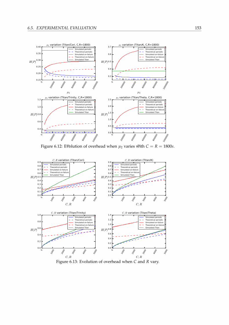
6.5. EXPERIMENTAL EVALUATION 153
0
2000
00
4000
00
6000
00
8000
00
1000
000
µ2
0.15
0.20
0.25
0.30
0.35
0.40
H(P)
µ2 variation (Titan/Cori, C,R=1800)
Simulated periodic
Theoretical periodic
Simulated on-failure
Theoretical on-failure
Simulated Titan
0
2000
00
4000
00
6000
00
8000
00
1000
000
µ2
0.3
0.4
0.5
0.6
0.7
H(P)
µ2 variation (Titan/K, C,R=1800)
Simulated periodic
Theoretical periodic
Simulated on-failure
Theoretical on-failure
Simulated Titan
0
2000
00
4000
00
6000
00
8000
00
1000
000
µ2
0.4
0.6
0.8
1.0
1.2
H(P)
µ2 variation (Titan/Trinity, C,R=1800)
Simulated periodic
Theoretical periodic
Simulated on-failure
Theoretical on-failure
Simulated Titan0
2000
00
4000
00
6000
00
8000
00
1000
000
µ2
0.0
0.5
1.0
1.5
2.0
2.5
H(P)
µ2 variation (Titan/Theta, C,R=1800)
Simulated periodic
Theoretical periodic
Simulated on-failure
Theoretical on-failure
Simulated Titan
Figure 6.12: Evolution of overhead when µ2 varies with C = R = 1800s.
0
1000
2000
3000
4000
5000
C,R
0.0
0.1
0.2
0.3
0.4
0.5
0.6
0.7
0.8
0.9
H(P)
C,R variation (Titan/Cori)
Simulated periodic
Theoretical periodic
Simulated on-failure
Theoretical on-failure
Simulated Titan
0
1000
2000
3000
4000
5000
C,R
0.0
0.1
0.2
0.3
0.4
0.5
0.6
0.7
0.8
0.9
H(P)
C,R variation (Titan/K)
Simulated periodic
Theoretical periodic
Simulated on-failure
Theoretical on-failure
Simulated Titan
0
1000
2000
3000
4000
5000
C,R
0.0
0.2
0.4
0.6
0.8
1.0
H(P)
C,R variation (Titan/Trinity)
Simulated periodic
Theoretical periodic
Simulated on-failure
Theoretical on-failure
Simulated Titan
0
1000
2000
3000
4000
5000
C,R
0.0
0.2
0.4
0.6
0.8
1.0
1.2
1.4
H(P)
C,R variation (Titan/Theta)
Simulated periodic
Theoretical periodic
Simulated on-failure
Theoretical on-failure
Simulated Titan
Figure 6.13: Evolution of overhead when C and R vary.
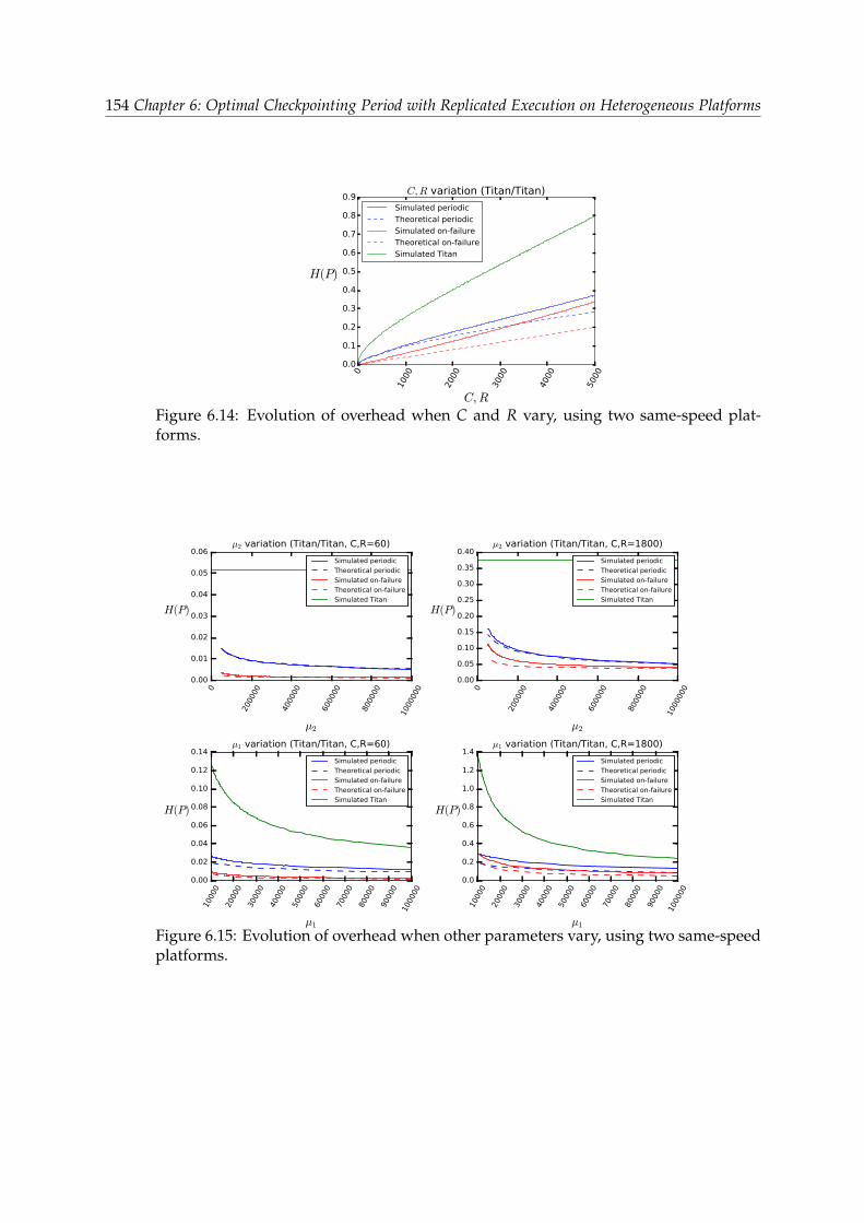
154 Chapter 6: Optimal Checkpointing Period with Replicated Execution on Heterogeneous Platforms
0
1000
2000
3000
4000
5000
C,R
0.0
0.1
0.2
0.3
0.4
0.5
0.6
0.7
0.8
0.9
H(P)
C,R variation (Titan/Titan)
Simulated periodic
Theoretical periodic
Simulated on-failure
Theoretical on-failure
Simulated Titan
Figure 6.14: Evolution of overhead when C and R vary, using two same-speed plat-forms.
0
2000
00
4000
00
6000
00
8000
00
1000
000
µ2
0.00
0.05
0.10
0.15
0.20
0.25
0.30
0.35
0.40
H(P)
µ2 variation (Titan/Titan, C,R=1800)
Simulated periodic
Theoretical periodic
Simulated on-failure
Theoretical on-failure
Simulated Titan
0
2000
00
4000
00
6000
00
8000
00
1000
000
µ2
0.00
0.01
0.02
0.03
0.04
0.05
0.06
H(P)
µ2 variation (Titan/Titan, C,R=60)
Simulated periodic
Theoretical periodic
Simulated on-failure
Theoretical on-failure
Simulated Titan
1000
0
2000
0
3000
0
4000
0
5000
0
6000
0
7000
0
8000
0
9000
0
1000
00
µ1
0.0
0.2
0.4
0.6
0.8
1.0
1.2
1.4
H(P)
µ1 variation (Titan/Titan, C,R=1800)
Simulated periodic
Theoretical periodic
Simulated on-failure
Theoretical on-failure
Simulated Titan
1000
0
2000
0
3000
0
4000
0
5000
0
6000
0
7000
0
8000
0
9000
0
1000
00
µ1
0.00
0.02
0.04
0.06
0.08
0.10
0.12
0.14
H(P)
µ1 variation (Titan/Titan, C,R=60)
Simulated periodic
Theoretical periodic
Simulated on-failure
Theoretical on-failure
Simulated Titan
Figure 6.15: Evolution of overhead when other parameters vary, using two same-speedplatforms.

6.6. CONCLUSION 155
improvement if C ≥ 10s with Cori, if C ≥ 760s with K, if C ≥ 4460s with Trinity, andmore than 5000s with Theta.
Figures 6.14 and 6.15 present the case of same-speed platforms. In this case, for allparameter choices (C, R, µ1, µ2), it is interesting to see that on-failure checkpointingis the best strategy, while it was less efficient than periodic checkpointing in almostall the other scenarios that we considered. This can be explained by the fact thatthere is no work lost at all with this strategy, except when there is a failure during acheckpoint.
6.5.4 Summary
We summarize simulation results as follows:• The model is very accurate, as long as the resilience parameters remain reason-
ably small.• On-failure checkpointing is generally less efficient than periodic checkpointing,
except when the speeds of the two platforms are equal (σ2 = σ1).• If P2 is really too slow compared to P1 (σ2 < σ1
2 ) or if the checkpointing cost issmall, there is little reason to use a second platform.
• In all other cases ( σ12 ≤ σ2 < σ1), the periodic checkpointing strategy reduces the
overhead by 30% in average, and up to 90% in some particular cases.
6.6 Conclusion
This work has addressed group replication for a black-box application executing ontwo heterogeneous platforms. We designed and thoroughly analyzed two strategies,periodic checkpointing and on-failure checkpointing. For periodic checkpointing, wehave been able to analytically derive the best pattern length, using either first-order orsecond-order approximations. These results nicely extend the Young/Daly formula.
Simulations show that the model is quite accurate. As expected, when the platformspeeds have different orders of magnitude, it is better to use only the fast platform.However, periodic checkpointing is useful for a wide range of speeds, and generallymore efficient than on-failure checkpointing. The latter strategy is to be preferred onlywhen the platform speeds are close.
Future work will be devoted to extending replication with heterogeneous platformsto deal with more complex applications, such as scientific workflows arranged as linearchains or fork-join graphs. Another interesting direction is to study the bi-criteriaproblem with energy consumption as a second metric, in addition to total executiontime, in order to better assess the cost of replication.

Chapter 7
Replication is more efficient than you think
This chapter revisits replication coupled with checkpointing for fail-stop errors. Repli-cation enables the application to survive many fail-stop errors, thereby allowing forlonger checkpointing periods. Previously published works use replication with theno-restart strategy, which works as follows: (i) compute the application Mean Time ToInterruption (MTTI) M as a function of the number of processor pairs and the indi-vidual processor Mean Time Between Failures (MTBF); (ii) use checkpointing periodTno
MTTI =√
2MC a la Young/Daly, where C is the checkpoint duration; and (iii) neverrestart failed processors until the application crashes. We introduce the restart strategywhere failed processors are restarted after each checkpoint. We compute the optimalcheckpointing period Trs
opt for this strategy, which is much larger than TnoMTTI, thereby
decreasing I/O pressure. We show through simulations that using Trsopt and the restart
strategy, instead of TnoMTTI and the usual no-restart strategy, significantly decreases the
overhead induced by replication. The work in this chapter is joint work with AnneBenoit, Thomas Herault and Yves Robert, and has been published in Supercomputing(SC) 2019 [C2].
7.1 Introduction
Current computing platforms have millions of cores: the Summit system at the OakRidge National Laboratory (ORNL) is listed at number one in the TOP500 rank-ing [181], and it has more than two million cores. The Chinese Sunway TaihuLight(ranked as number 3) has even more than 10 million cores. These large-scale com-puting systems are frequently confronted with failures, also called fail-stop errors.Indeed, even if individual cores are reliable, for instance if the Mean Time Between Fail-ures (MTBF) for a core is µ = 10 years, then the MTBF for a platform with a millioncores (N = 106) becomes µN = µ
N ≈ 5.2 minutes, meaning that a failure strikes theplatform every five minutes, as shown in [106].
The classical technique to deal with failures consists of using a checkpoint-restartmechanism: the state of the application is periodically checkpointed, and when afailure occurs, we recover from the last valid checkpoint and resume the execution
157
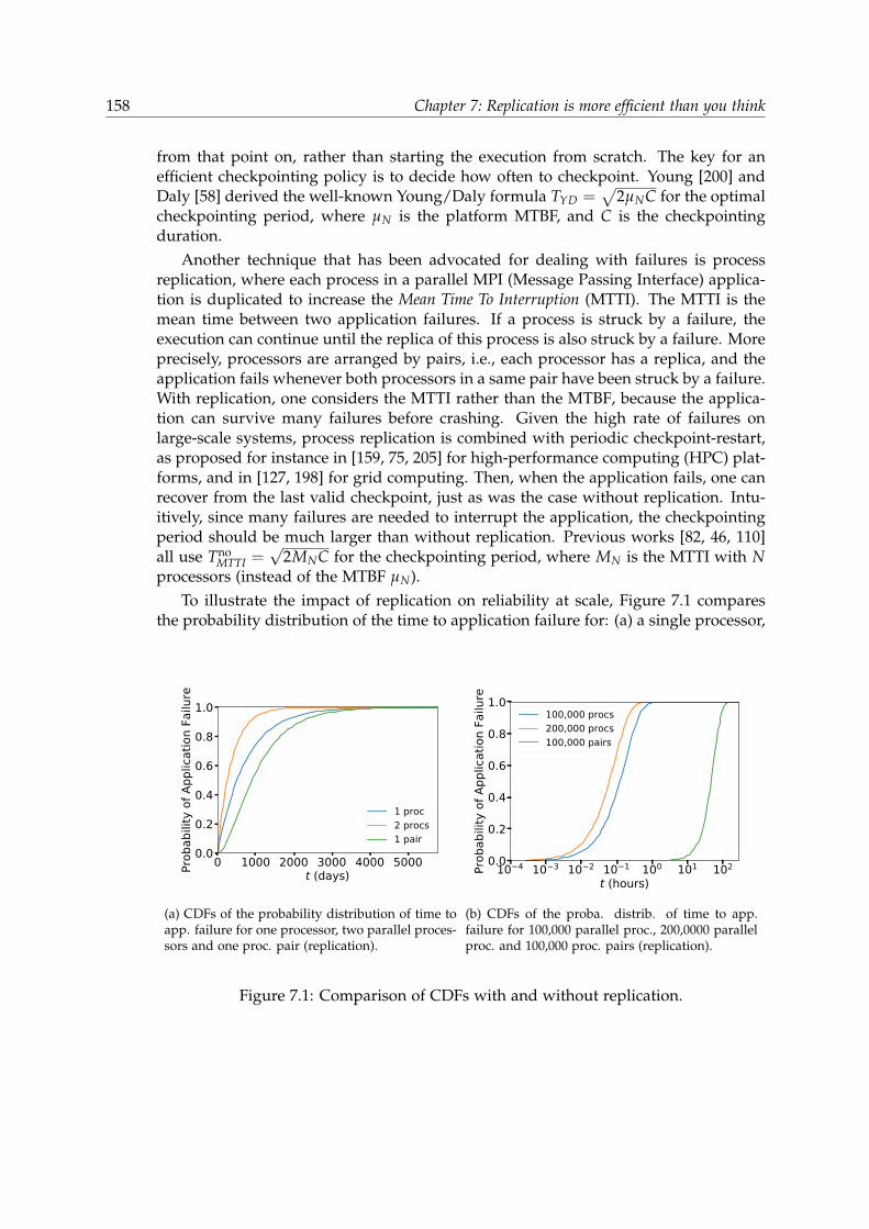
158 Chapter 7: Replication is more efficient than you think
from that point on, rather than starting the execution from scratch. The key for anefficient checkpointing policy is to decide how often to checkpoint. Young [200] andDaly [58] derived the well-known Young/Daly formula TYD =
√2µNC for the optimal
checkpointing period, where µN is the platform MTBF, and C is the checkpointingduration.
Another technique that has been advocated for dealing with failures is processreplication, where each process in a parallel MPI (Message Passing Interface) applica-tion is duplicated to increase the Mean Time To Interruption (MTTI). The MTTI is themean time between two application failures. If a process is struck by a failure, theexecution can continue until the replica of this process is also struck by a failure. Moreprecisely, processors are arranged by pairs, i.e., each processor has a replica, and theapplication fails whenever both processors in a same pair have been struck by a failure.With replication, one considers the MTTI rather than the MTBF, because the applica-tion can survive many failures before crashing. Given the high rate of failures onlarge-scale systems, process replication is combined with periodic checkpoint-restart,as proposed for instance in [159, 75, 205] for high-performance computing (HPC) plat-forms, and in [127, 198] for grid computing. Then, when the application fails, one canrecover from the last valid checkpoint, just as was the case without replication. Intu-itively, since many failures are needed to interrupt the application, the checkpointingperiod should be much larger than without replication. Previous works [82, 46, 110]all use Tno
MTTI =√
2MNC for the checkpointing period, where MN is the MTTI with Nprocessors (instead of the MTBF µN).
To illustrate the impact of replication on reliability at scale, Figure 7.1 comparesthe probability distribution of the time to application failure for: (a) a single processor,
0 1000 2000 3000 4000 5000t (days)
0.0
0.2
0.4
0.6
0.8
1.0
Prob
abilit
y of
App
licat
ion
Failu
re
1 proc2 procs1 pair
(a) CDFs of the probability distribution of time toapp. failure for one processor, two parallel proces-sors and one proc. pair (replication).
10 4 10 3 10 2 10 1 100 101 102
t (hours)0.0
0.2
0.4
0.6
0.8
1.0
Prob
abilit
y of
App
licat
ion
Failu
re
100,000 procs200,000 procs100,000 pairs
(b) CDFs of the proba. distrib. of time to app.failure for 100,000 parallel proc., 200,0000 parallelproc. and 100,000 proc. pairs (replication).
Figure 7.1: Comparison of CDFs with and without replication.

7.1. INTRODUCTION 159
two parallel processors and a pair of replicated processors; and (b) a platform ofN = 100, 000 parallel processors, N = 200, 000 parallel processors without replication,and b = 100, 000 processor pairs with replication. In all cases, the individual MTBFof a single processor is µ = 5 years. The time to reach 90% chances of having a fatalfailure is: (a) 1688 days for one processor, 844 days for two processors and 2178 daysfor a processor pair; and (b) 24 minutes for 100,000 processors, 12 minutes for 200,000processors and 5081 minutes (almost 85 hours) for 100,000 processor pairs. We seethat replication is key to safe application progress at scale! Again, the cost is that halfof the resources are doing redundant work, hence time-to-solution is increased. Wecompare time-to-solution with and without replication in Section 7.7.6. We also seethat in heavily failure-prone environments (small MTBF values), checkpoint/restartalone cannot ensure full reliability, and must be complemented by replication.
One major contribution of this chapter is to introduce a new approach that mini-mizes the overhead incurred by the checkpoint-restart mechanism when coupled withreplication. Previous works [82, 46, 110] use the no-restart strategy: if a processor wasstruck by a failure (but not its replica), then the processor remains failed (no recovery)until the whole application fails. Hence, there is a recovery only every MN secondson average, whenever the application fails. Many periodic checkpoints are taken inbetween two application crashes, with more and more processors failing on the fly.To the best of our knowledge (i) all related works use the no-restart strategy and (ii)analytically computing the optimal period for no-restart is an open problem (see Sec-tion 7.4.2 for more details, where we also show that non-periodic strategies are moreefficient for no-restart), but simulations can help assess this approach.
The study of the no-restart strategy raises an important question: should failedprocessors be restarted earlier on in the execution? Instead of waiting for an appli-cation crash to rejuvenate the whole platform, a simple approach would be to restartprocessors immediately after each failure. Let restart-on-failure denote this strategy. Itensures that all processor pairs involve two live processors throughout execution, andwould even suppress the notion of checkpointing periods. Instead, after each failurestriking a processor, its replica would checkpoint immediately, and the spare processorreplacing the failed processor would read that checkpoint to resume execution. Thereis a small risk of fatal crash if a second failure should strike the replica when writingits checkpoint, but (i) the risk is very small because the probability of such a cascadeof two narrowly spaced failures is quite low; and (ii) if the checkpoint protocol is scal-able, every other processor can checkpoint in parallel with the replica, and there isno additional time overhead. With tightly coupled applications, the other processorswould likely have to wait until the spare is able to restart, and they can checkpointinstead of idling during that wait. While intuitively appealing, the restart-on-failurestrategy may lead to too many checkpoints and restarts, especially in scenarios whenfailures strike frequently. However, frequent failures were exactly the reason to deployreplication in the first place, precisely to avoid having to restart after each failure.
In this work, we introduce the restart strategy, which requires any failed processorto recover each time a checkpoint is taken. This ensures that after any checkpoint at the

160 Chapter 7: Replication is more efficient than you think
end of a successful period, all processors are alive. This is a middle ground betweenthe no-restart and restart-on-failure strategies, because failed processors are restarted atthe end of each period with restart. On the one hand, a given period may well includemany failures, hence restart restarts processors less frequently than restart-on-failure.On the other hand, there will be several periods in between two application crashes,hence restart restarts processors more frequently than no-restart.
Periodic checkpointing is optimal with the restart strategy: the next period shouldhave same length as the previous one, because we have the same initial conditionsat the beginning of each period. Restarting failed processors when checkpointingcan introduce additional overhead, but we show that it is very small, and even non-existent when in-memory (a.k.a. buddy) checkpointing is used as the first-level ofa hierarchical multi-level checkpointing protocol (such state-of-the-art protocols areroutinely deployed on large-scale platforms [140, 17, 40]). A key contribution of thischapter is a mathematical analysis of the restart strategy, with a closed-form formulafor its optimal checkpointing period. We show that the optimal checkpointing periodfor the restart strategy has the order Θ(µ
23 ), instead of the Θ(µ
12 ) used in previous
works for no-restart as an extension of the Young/Daly formula [82, 46, 110]. Hence,as the error rate increases, the optimal period becomes much longer than the value thathas been used in all previous works (with no-restart). Consequently, checkpoints aremuch less frequent, thereby dramatically decreasing the pressure on the I/O system.
The main contributions in this chapter are the following:• We provide the first closed-form expression of the application MTTI MN with repli-cation;• We introduce the restart strategy for replication, where we recover failed processorsduring each checkpoint;• We formally analyze the restart strategy, and provide the optimal checkpointing pe-riod with this strategy;•We apply these results to applications following Amdahl’s law, i.e., applications thatare not fully parallel but have an inherent sequential part, and compare the time-to-solution achieved with and without replication;•We validate the model through comprehensive simulations, by showing that analyti-cal results, using first-order approximations and making some additional assumptions(no failures during checkpoint and recovery), are quite close to simulation results; forthese simulations, we use both randomly generated failures and log traces.• We compare through simulations the overhead obtained with the optimal strategyintroduced in this work (restart strategy, optimal checkpointing period) to those usedin all previous works (no-restart strategy, extension of the Young/Daly checkpoint-ing period), as well as with strategies that use partial replication or that restart onlyat some of the checkpoints, and demonstrate that we can significantly decrease bothtotal execution time and utilization of the I/O file system.
The chapter is organized as follows. We first describe the model in Section 7.2. Werecall how to compute the optimal checkpointing period when no replication is usedin Section 7.3. The core contribution is presented in Section 7.4, where we explain how

7.2. MODEL 161
to compute the MTTI with b (= N2 ) processor pairs, detail the restart strategy, and show
how to derive the optimal checkpointing period with this restart strategy. Results areapplied to applications following Amdahl’s law in Section 7.5. An asymptotic analysisof no-restart and restart is provided in Section 7.6. The experimental evaluation in Sec-tion 7.7 presents extensive simulation results, demonstrating that replication is indeedmore efficient than you think, when enforcing the restart strategy instead of the no-restartstrategy. Finally, we extend the analysis and experiments to energy consumption inSection 7.8, and conclude in Section 7.9.
7.2 Model
This section describes the model, with an emphasis on the cost of a combinedcheckpoint-restart operation.
Fail-stop errors. Throughout the text, we consider a platform with N identical pro-cessors. The platform is subject to fail-stop errors, or failures, that interrupt the ap-plication. Similarly to previous work [82, 72, 110], for the mathematical analysis, weassume that errors are independent and identically distributed (IID), and that theystrike each processor according to an exponential probability distribution exp(λ) withsupport [0, ∞), probability density function (PDF) f (t) = λe−λt and cumulative distri-bution function (CDF) F(T) = P(X ≤ T) = 1− e−λT. We also introduce the reliabilityfunction G(T) = 1− F(T) = e−λT. The expected value µ = 1
λ of the exp(λ) distri-bution is the MTBF on one processor. We lift the IID assumption in the performanceevaluation section by using trace logs from real platforms.
Checkpointing. To cope with errors, we use periodic coordinated checkpointing. Weassume that the divisible application executes for a very long time (asymptoticallyinfinite) and we partition the execution into periods. Each period P consists of a worksegment of duration T followed by a checkpoint of duration C. After an error, thereis a downtime of duration D (corresponding to the time needed to migrate to a spareprocessor), a recovery of size R, and then one needs to re-execute the period from itsbeginning.
Replication. We use another fault tolerance technique, namely replication. Each pro-cess has a replica, which follows the exact same states in its execution. To ensure this,when a process receives a message, its replica also receives the same message, andmessages are delivered in the same order to the application (an approach called activereplication; see [92, 82]). If a crash hits a process at any time, and its replica is stillalive, the replica continues the execution alone until a new process can replace thedead one.
We rely on the traditional process allocation strategy that assigns processes andtheir replicas on remote parts of the system (typically different racks) [34]. This strat-

162 Chapter 7: Replication is more efficient than you think
egy mitigates the risk that a process and its replica would both fail within a short timeinterval (much shorter than the expected MTTI). As stated in [158], when failure cor-relations are observed, their correlation diminishes when the processes are far awayfrom each other in the memory hierarchy, and becomes undistinguishable from thenull hypothesis (no correlation) when processes belong to different racks.
Combined checkpoint-restart. In this chapter, we propose the restart strategy wherefailed processes are restarted as soon as the next checkpoint wave happens. Whenthat happens, and processes need to be restarted, the cost of a checkpoint and restartwave, CR, is then increased: one instance of each surviving process must save theirstate, then processes for the missing instances of the replicas must be allocated; thenew processes must load the current state, which has been checkpointed, and join thesystem to start acting as a replica. The first part of the restart operation, allocatingprocesses to replace the failed ones, can be managed in parallel with the checkpoint ofthe surviving processes. Using spare processes, this allocation time can be very smalland we will consider it negligible compared to the checkpoint saving and loadingtimes. Similarly, integrating the newly spawned process inside the communicationsystem when using spares is negligible when using mechanisms such as the onesdescribed in [29].
There is a large variety of checkpointing libraries and approaches to help applica-tions save their state. [140, 17, 40] are typically used in HPC systems for coordinatedcheckpointing, and use the entire memory hierarchy to speed up the checkpointingcost: the checkpoint is first saved on local memory, then uploaded onto local storage(SSD, NVRAM if available), and eventually to the shared file system. As soon as acopy of the state is available on the closest memory, the checkpoint is considered astaken. Loading that checkpoint requires that the application state from the closestmemory be sent to the memory of the new hosting process.
Another efficient approach to checkpoint is to use in-memory checkpoint replica-tion using the memory of a ’buddy’ process (see [204, 146]). To manage the risk oflosing the checkpoint in case of failure of two buddy processes, the checkpoint mustalso be saved on reliable media, as is done in the approaches above. Importantly, in-memory checkpointing is particularly fitted for the restart strategy, because the buddyprocess and the replica are the same process: in that case, the surviving processes up-load their checkpoint directly onto the memory of the newly spawned replicas; as soonas this communication is done, the processes can continue working. Contrary to tradi-tional buddy checkpointing, it is not necessary to exchange the checkpoints betweena pair of surviving buddies since, per the replication technique, both checkpoints areidentical.
In the worst case, if a sequential approach is used, combining checkpointing andrestart takes at most twice the time to checkpoint only; in the best case, using buddycheckpointing, the overhead of adding the restart to the checkpoint is negligible. Weconsider the full spectrum C ≤ CR ≤ 2C in the simulations.
As discussed in [148, 82], checkpoint time varies significantly depending upon the

7.3. BACKGROUND 163
target application and the hardware capabilities. We will consider a time to checkpointwithin two reasonable limits: 60s ≤ C ≤ 600s, following [110].
First-order approximation. Throughout the chapter, we are interested in first-orderapproximations, because exact formulas are not analytically tractable. We carefullystate the underlying hypotheses that are needed to enforce the validity of first-orderresults. Basically, the first-order approximation will be the first, and most meaningful,term of the Taylor expansion of the overhead occurring every period when the errorrate λ tends to zero.
7.3 Background
In this section, we briefly summarize well-known results on the optimal checkpointingperiod when replication is not used, starting with a single processor in Section 7.3.1,and then generalizing to the case with N processors in Section 7.3.2.
7.3.1 With a Single Processor
We aim at computing the expected time E(T) to execute a period of length P = T +C.The optimal period length will be obtained for the value of T, minimizing the overhead
H(T) =E(T)
T− 1. (7.1)
We temporarily assume that fail-stop errors strike only during work T and notduring checkpoint C nor recovery R. The following recursive equation is the key tomost derivations:
E(T) = (1− F(T))(T + C) + F(T)(Tlost(T) + D + R + E(T)). (7.2)
Equation (7.2) reads as follows: with probability 1− F(T), the execution is successfuland lasts T +C seconds; with probability F(T), an error strikes before completion, andwe need to account for time lost Tlost(T), downtime D and recovery R before startingthe computation anew. The expression for Tlost(T) is the following:
Tlost(T) =∫ ∞
0tP(X = t|X ≤ T)dt =
1F(T)
∫ T
0t f (t)dt.
Integrating by parts and re-arranging terms in Equation (7.2), we derive
E(T) = T + C +F(T)
1− F(T)(Tlost(T) + D + R)
and H(T) = CT + F(T)
T(1−F(T)) (D + R) +∫ T
0 G(t)dtT(1−F(T)) − 1. Now, if we instantiate the value of

164 Chapter 7: Replication is more efficient than you think
F(T) = 1− G(T) = 1− e−λT, we obtain
H(T) =CT+
eλT − 1T
(D + R +1λ)− 1.
We can find the value Topt by differentiating and searching for the zero of thederivative, but the solution is complicated as it involves the Lambert function [58, 106].Instead, we use the Taylor expansion of e−λT = ∑∞
i=0(−1)i (λT)i
i! and the approximation
e−λT = 1− λT + (λT)2
2 + o(λ2T2). This makes sense only if λT tends to zero. It isreasonable to make this assumption, since the length of the period P must be muchsmaller than the error MTBF µ = 1
λ . Hence, we look for T = Θ(λ−x), where 0 < x < 1.Note that x represents the order of magnitude of T as a function of the error rate λ.We can then safely write
H(T) =CT+
λT2
+ o(λT). (7.3)
Now, CT = Θ(λx) and λT
2 = Θ(λ1−x), hence the order of magnitude of the overheadis H(T) = Θ(λmax(x,1−x)), which is minimum for x = 1
2 . Differentiating Equation (7.3),we obtain
Topt =
√2Cλ
= Θ(λ−12 ), and Hopt =
√2Cλ + o(λ
12 ) = Θ(λ
12 ) (7.4)
which is the well-known and original Young formula [200].
Variants of Equation (7.4) have been proposed in the literature, such as Topt =√2(µ + R)C in [58] or Topt =
√2(µ− D− R)C− C in [106]. All variants are approxi-
mations that collapse to Equation (7.4). This is because the resilience parameters C, D,and R are constants and thus negligible in front of Topt when λ tends to zero. This alsoexplains that assuming that fail-stop errors may strike during checkpoint or recoveryhas no impact on the first-order approximation of the period given in Equation (7.4).For instance, assuming that fail-stop errors strike during checkpoints, we would mod-ify Equation (7.2) into
E(T + C) = (1− F(T + C))(T + C) + F(T + C)(Tlost(T + C) + D + R + E(T + C))
and derive the same result as in Equation (7.4). Similarly, assuming that fail-stop errorsstrike during recovery, we would replace R with E(R), which can be computed via anequation similar to that for E(T), again without modifying the final result.
Finally, a very intuitive way to retrieve Equation (7.4) is the following: consider aperiod of length P = T + C. There is a failure-free overhead C
T , and a failure-inducedoverhead 1
µ × T2 , because with frequency 1
µ an error strikes, and on average it strikes inthe middle of the period and we lose half of it. Adding up both overhead sources gives
CT+
T2µ
, (7.5)

7.4. REPLICATION 165
which is minimum when T =√
2µC. While not fully rigorous, this derivation helpsunderstand the tradeoff related to the optimal checkpointing frequency.
7.3.2 With N Processors
The previous analysis can be directly extended to multiple processors. Indeed, iffail-stop errors strike each processor according to an exp(λ) probability distribution,then these errors strike the whole platform made of N identical processors accordingto an exp(Nλ) probability distribution [106]. In other words, the platform MTBFis µN = µ
N , which is intuitive: the number of failures increases linearly with thenumber of processors N, hence the mean time between two failures is divided by N.All previous derivations apply, and we obtain the optimal checkpointing period andoverhead:
Topt =
√2CNλ
= Θ(λ−12 ), and Hopt =
√2CNλ + o(λ
12 ) = Θ(λ
12 ) (7.6)
This value of Topt can be intuitively retrieved with the same (not fully rigorous)reasoning as before (Equation (7.5)): in a period of length P = T + C, the failure-freeoverhead is C
T , and the failure-induced overhead becomes 1µN× T
2 : we factor in an
updated value of the failure frequency, using 1µN
= Nµ instead of 1
µ . Both overheadsources add up to
CT+
T2µN
=CT+
NT2µ
, (7.7)
which is minimum when T =√
2µCN .
7.4 Replication
This section deals with process replication for fail-stop errors, as introduced in [82] andrecently revisited by [110]. We consider a platform with N = 2b processors. Exactlyas in Section 7.3, each processor fails according to a probability distribution exp(λ),and the platform MTBF is µN = µ
N . We still assume that checkpoint and recovery areerror-free: it simplifies the analysis without modifying the first-order approximationof the optimal checkpointing period.
Processors are arranged by pairs, meaning that each processor has a replica. Theapplication executes as if there were only b available processors, hence with a reducedthroughput. However, a single failure does not interrupt the application, because thereplica of the failed processor can continue the execution. The application can thussurvive many failures, until both replicas of a given pair are struck by a failure. Howmany failures are needed, in expectation, to interrupt the application? We computethis value in Section 7.4.1. Then, we proceed to deriving the optimal checkpointingperiod, first with one processor pair in Section 7.4.2, before dealing with the generalcase in Section 7.4.3.
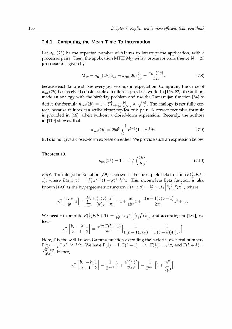
166 Chapter 7: Replication is more efficient than you think
7.4.1 Computing the Mean Time To Interruption
Let nfail(2b) be the expected number of failures to interrupt the application, with bprocessor pairs. Then, the application MTTI M2b with b processor pairs (hence N = 2bprocessors) is given by
M2b = nfail(2b) µ2b = nfail(2b)µ
2b=
nfail(2b)2λb
, (7.8)
because each failure strikes every µ2b seconds in expectation. Computing the value ofnfail(2b) has received considerable attention in previous work. In [156, 82], the authorsmade an analogy with the birthday problem and use the Ramanujan function [84] to
derive the formula nfail(2b) = 1 + ∑bk=0
b!(b−k)!b;k ≈
√πb2 . The analogy is not fully cor-
rect, because failures can strike either replica of a pair. A correct recursive formulais provided in [46], albeit without a closed-form expression. Recently, the authorsin [110] showed that
nfail(2b) = 2b4b∫ 1
2
0xb−1(1− x)bdx (7.9)
but did not give a closed-form expression either. We provide such an expression below:
Theorem 10.
nfail(2b) = 1 + 4b /(
2bb
). (7.10)
Proof. The integral in Equation (7.9) is known as the incomplete Beta function B( 12 , b, b+
1), where B(z, u, v) =∫ z
0 xu−1(1 − x)v−1dx. This incomplete Beta function is also
known [190] as the hypergeometric function B(z, u, v) = zu
u × 2F1
[u, 1−v
u+1 ; z]
, where
2F1
[u, vw
; z]=
∞
∑n=0
〈u〉n〈v〉n〈w〉n
zn
n!= 1 +
uv1!w
z +u(u + 1)v(v + 1)
2!wz2 + . . .
We need to compute B( 12 , b, b + 1) = 1
b2b × 2F1
[b, −bb+1 ; 1
2
], and according to [189], we
have
2F1
[b, − bb + 1
;12
]=
√π Γ(b + 1)
2b+1
[ 1Γ(b + 1)Γ( 1
2 )+
1Γ(b + 1
2 ))Γ(1)
].
Here, Γ is the well-known Gamma function extending the factorial over real numbers:Γ(z) =
∫ ∞0 xz−1e−xdx. We have Γ(1) = 1, Γ(b + 1) = b!, Γ( 1
2 ) =√
π, and Γ(b + 12 ) =√
π(2b)!4bb! . Hence,
2F1
[b, − bb + 1
;12
]=
12b+1
[1 +
4b(b!)2
(2b)!
]=
12b+1
[1 +
4b
(2bb )
].

7.4. REPLICATION 167
For the last equality, we observe that (2bb ) =
(2b)!(b!)2 . We derive B( 1
2 , b, b + 1) = 12b4b
[1 +
4b
(2bb )
], and finally nfail(2b) = 1 + 4b
(2bb )
, which concludes the proof.
Using Sterling’s formula, we easily derive that nfail(2b) ≈√
πb, which is 40% more
than the value√
πb2 used in [156, 82].
Plugging the value of nfail(2b) back in Equation (7.8) gives the value of the MTTIM2b. As already mentioned, previous works [82, 46, 110] all use the checkpointingperiod
TnoMTTI =
√2M2bC (7.11)
to minimize execution time overhead. This value follows from the same derivation asin Equations (7.5) and (7.7). Consider a period of length P = T + C. The failure-freeoverhead is still C
T , and the failure-induced overhead becomes 1M2b× T
2 : we factor in anupdated value of the failure frequency, which now becomes the fatal failure frequency,namely 1
M2b. Both overhead sources add up to
CT+
T2M2b
, (7.12)
which is minimum when T =√
2M2bC.In the following, we analyze the restart strategy. We start with one processor pair
(b = 1) in Section 7.4.2, before dealing with the general case in Section 7.4.3.
7.4.2 With One Processor Pair
We consider two processors working together as replicas. The failure rate is λ = 1µ
for each processor, and the pair MTBF is µ2 = µ2 , while the pair MTTI is M2 = 3µ
2because nfail(2) = 3. We analyze the restart strategy, which restarts a (potentially)failed processor at every checkpoint. Hence, the checkpoint has duration CR andnot C. Consider a period of length P = T + CR. If one processor fails before thecheckpoint but the other survives until reaching it, the period is executed successfully.The period is re-executed only when both processors fail within T seconds. Let p1(T)denote the probability that both processors fail during T seconds: p1(T) = (1− e−λT)2.We compute the expected time E(T) for period of duration P = T + CR using thefollowing recursive equation:
E(T) = (1− p1(T))(T + CR) + p1(T)(Tlost(T) + D + R + E(T)). (7.13)
Here, CR denotes the time to checkpoint, and in addition, to recover whenever one ofthe two processors had failed during the period. As discussed in Section 7.2, we haveC ≤ CR ≤ C + R: the value of CR depends upon the amount of overlap between thecheckpoint and the possible recovery of one processor.
Consider the scenario where one processor fails before reaching the end of theperiod, while the other succeeds and takes the checkpoint. The no-restart strategy

168 Chapter 7: Replication is more efficient than you think
continues execution, hence pays only for a regular checkpoint of cost C, and when thelive processor is struck by a failure (every M2 seconds on average), we roll back andrecover for both processors [82, 46, 110]. However, the new restart strategy requiresany failed processor to recover whenever a checkpoint is taken, hence at a cost CR.This ensures that after any checkpoint at the end of a successful period, we have twolive processors, and thus the same initial conditions. Hence, periodic checkpointingis optimal with this strategy. We compare the restart and no-restart strategies throughsimulations in Section 7.7.
As before, in Equation (7.13), Tlost(T) is the average time lost, knowing that bothprocessors have failed before T seconds. While Tlost(T) ∼ T
2 when considering a singleprocessor, it is no longer the case with a pair of replicas. Indeed, we compute Tlost(T)as follows:
Tlost(T) =∫ ∞
0tP(X = t|t ≤ T)dt =
1p1(T)
∫ T
0tdP(X ≤ t)
dtdt
=2λ
(1− e−λT)2
∫ T
0t(e−λt − e−2λt)dt.
After integration, we find that
Tlost(T) =(2e−2λT − 4e−λT)λT + e−2λT − 4e−λT + 3
2λ(1− e−λT)2 =1
2λ
u(λT)v(λT)
,
with u(y) = (2e−2y − 4e−y)y + e−2y − 4e−y + 3 and v(y) = (1− e−y)2.
Assuming that T = Θ(λ−x) with 0 < x < 1 as in Section 7.3.1, then Taylor ex-pansions lead to u(y) = 4
3 y3 + o(y3) and v(y) = y2 + y3 + o(y3) for y = λT = o(1),
meaning that Tlost(T) = 12λ
4λT3 +o(λT)
1+λT+o(λT) . Using the division rule, we obtain Tlost(T) =1
2λ (4λT
3 + o(λT)) = 2T3 + o(T). Note that we lose two thirds of the period with a pro-
cessor pair rather than one half with a single processor. Plugging back the value ofTlost(T) and solving, we obtain:
E(T) = T + CR + (D + R +(2e−2λT − 4e−λT)λT + e−2λT − 4e−λT + 3
2λ(1− e−λT)2 ) · (eλT − 1)2
2eλT − 1. (7.14)
We then compute the waste Hrs(T) of the restart strategy as follows:
Hrs(T) =E(T)
T− 1 =
CR
T+
23
λ2T2 + o(λ2T2). (7.15)
Moreover, with T = Θ(λ−x), we have CR
T = Θ(λx) and 23 λ2T2 = Θ(λ2−2x), hence
Hrs(T) = Θ(λmax(x,2−2x)), which is minimum for x = 23 . Differentiating, we readily
obtain:
Topt =
(3CR
4λ2
) 13
= Θ(λ−23 ), (7.16)

7.4. REPLICATION 169
Hrs(Topt) =
(3CRλ√
2
) 23
+ o(λ23 ) = Θ(λ
23 ). (7.17)
Note that the optimal period has the order Topt = Θ(λ−23 ) = Θ(µ
23 ), while the exten-
sion√
2M2C of the Young/Daly formula has the order Θ(λ−12 ) = Θ(µ
12 ). This means
that the optimal period is much longer than the value that has been used in all previ-ous works. This result generalizes to several processor pairs, as shown in Section 7.4.3.We further discuss asymptotic results in Section 7.6.
For an intuitive way to retrieve Equation (7.16), the derivation is similar to thatused for Equations (7.5), (7.7) and (7.12). Consider a period of length P = T +CR. Thefailure-free overhead is still CR
T , and the failure-induced overhead becomes 1µ
Tµ × 2T
3 :
we factor in an updated value of the fatal failure frequency 1µ
Tµ : the first failure strikes
with frequency 1µ , and then with frequency T
µ , there is another failure before the end
of the period. As for the time lost, it becomes 2T3 , because in average the first error
strikes at one third of the period and the second error strikes at two-third of the pe-riod: indeed, we know that there are two errors in the period, and they are equallyspaced in average. Altogether, both overhead sources add up to
CR
T+
2T2
3µ2 , (7.18)
which is exactly Equation (7.15).
We conclude this section with a comment on the no-restart strategy. The intuitivederivation in Equation (7.12) leads to Hno(T) = C
T + T2M2b
. We now understand thatthis derivation is accurate if we have Tlost(T) = T
2 + o(T). While this latter equality isproven true without replication [58], it is unknown whether it still holds with repli-cation. Hence, computing the optimal period for no-restart remains an open problem,even with a single processor pair.
Going further, Figure 7.2 shows that periodic checkpointing is not optimal forno-restart with a single processor pair, which provides another hint of the diffi-culty of the problem. In the figure, we compare four approaches: in addition toRestart(Trs
opt) and NoRestart(TnoMTTI), we use two non-periodic variants of no-restart,
Non-Periodic(T1, T2). In both variants, we use a first checkpointing period T1 whileboth processors are alive, and then a shorter period T2 as soon as one processor hasbeen struck by a failure. When an application failure occurs, we start anew with pe-riods of length T1. For both variants, we only restart processors after an applicationfailure, just as no-restart does. The first variant uses T1 = Tno
MTTI =√
3µC (the MTTI is
M2 = 3 µ2 ) and the second variant uses T1 = Trs
opt =( 3
4 Cµ2) 13 . We use the Young/Daly
period T2 =√
2µC for both variants, because there remains a single live processorwhen period T2 is enforced. The figure shows the ratio of the time-to-solution for thetwo non-periodic approaches over that of periodic no-restart (with period Tno
MTTI). Notethat the application is perfectly parallel, and that the only overhead is for checkpoints

170 Chapter 7: Replication is more efficient than you think
10 1 100
MTBF (days)
0.4
0.6
0.8
1.0
Ratio
to N
oRes
tart(
Tno MTT
I)Non-Periodic(Tno
MTTI, TYD)Non-Periodic(Trs
opt, TYD)Restart(Trs
opt)
Figure 7.2: Ratio of time-to-solution of two non-periodic strategies and restart overtime-to-solution of no-restart (one processor pair, C = CR = 60).
and re-executions after failures. Both non-periodic variants are better than no-restart,the first one is within 98.3% of no-restart, and the second one is even better (95% ofno-restart) when the MTBF increases. We also see that restart is more than twice betterthan no-restart with a single processor pair. Note that results are averaged over 100,000simulations, each lasting for 10,000 periods, so that they are statistically guaranteed tobe accurate.
7.4.3 With b Processor Pairs
For b pairs, the reasoning is the same as with one pair, but the probability of hav-ing a fatal error (both processors of a same pair failing) before the end of the periodchanges. Letting pb(T) be the probability of failure before time T with b pairs, wehave pb(T) = 1− (1− (1− e−λT)2)b. As a consequence, computing the exact value ofTlost(T) becomes complicated: obtaining a compact closed-form is not easy, becausewe would need to expand terms using the binomial formula. Instead, we directly usethe Taylor expansion of pb(T) for λT close to 0. Again, this is valid only if T = Θ(λ−x)with x < 1. We have pb(T) = 1 − (1 − (λT + o(λT))2)b = bλ2T2 + o(λ2T2) andcompute Tlost(T) with b pairs as Tlost(T) = 1
pb(T)
∫ T0 t dP(X≤t)
dt dt = 2T3 + o(T). As be-
fore, Tlost(T) ∼ 2T3 . Also, as in Section 7.4.2, we analyze the restart strategy, which
requires any failed processor to recover whenever a checkpoint is taken. We comeback to the difference with the no-restart strategy after deriving the period for therestart strategy. We compute the expected execution time of one period: E(T) =
pb(T)(Tlost(T) + D + R + E(T)
)+ (1− pb(T))
(T + CR) = T + 2bλ2T3
3 + o(λ2T3), and
7.5. TIME-TO-SOLUTION 171
Hrs(T) =E(T)
T− 1 =
CR
T+
2bλ2T2
3+ o(λ2T2). (7.19)
We finally derive the expression of the optimal checkpointing period with b pairs:
Trsopt =
(3CR
4bλ2
) 13
= Θ(λ−23 ). (7.20)
When plugging it back in Equation (7.19), we get
Hrs(Trsopt) =
(3CR√
bλ√2
) 23
+ o(λ23 ) = Θ(λ
23 ). (7.21)
for the optimal overhead when using b pairs of processors.The derivation is very similar to the case with a single pair, and the result is essen-
tially the same, up to factoring in the number of pairs to account for a higher failurerate. However, the difference between the no-restart and the restart strategies gets moreimportant. Indeed, with the no-restart strategy, several pairs can be struck once (andeven several times if the failures always strike the failed processor) before a pair finallygets both its processors killed. While the no-restart strategy spares the cost of severalrestarts, it runs at risk with periods whose length has been estimated a la Young/Daly,thereby assuming an identical setting at the beginning of each period.
Finally, for the intuitive way to retrieve Equation (7.20), it goes as for Equation (7.18),multiplying the frequency of fatal failures 1
µTµ by a factor b to account for each of the
b pairs possibly experiencing a fatal failure.
7.5 Time-To-Solution
So far, we have focused on period length. In this section, we move to actual workachieved by the application. Following [110], we account for two sources of overheadfor the application. First, the application is not perfectly parallel and obeys Amdahl’slaw [3], which limits its parallel speedup. Second, there is an intrinsic slowdown dueto active replication related to duplicating every application message [82, 110].
First, for applications following Amdahl’s law, the total time spent to compute Wunits of computation with N processors is TAmdahl = γW + (1− γ)W
N = (γ + 1−γN )W,
where γ is the proportion of inherently sequential tasks. When replication is used,this time becomes TAmdahl = (γ + 2(1−γ)
N )W. Following [110], we use γ = 10−5 in Sec-tion 7.7. Second, as stated in [82, 110], another slowdown related to active replicationand its incurred increase of communications writes Trep = (1 + α)TAmdahl, where α issome parameter depending upon the application and the replication library. Follow-ing [110], we use either α = 0 or α = 0.2 in Section 7.7.
All in all, once we have derived Topt, the optimal period between two check-points without replication (see Equation (7.6)), and Trs
opt, the optimal period betweentwo checkpoints with replication and restart (see Equation (7.20)), we are able tocompute the optimal number of operations to be executed by an application be-

172 Chapter 7: Replication is more efficient than you think
tween two checkpoints as Wopt =Topt
(γ+ 1−γN )
for an application without replication, and
Wrsopt =
Trsopt
(1+α)(γ+ 1−γb )
=Trs
opt
(1+α)(
γ+ 2(1−γ)N
) for an application with replication and the restart
strategy. Finally, for the no-restart strategy, using TnoMTTI (see Equation (7.11)), the num-
ber of operations becomes WnoMTTI =
TnoMTTI
(1+α)(γ+ 1−γb )
=Tno
MTTI
(1+α)(
γ+ 2(1−γ)N
) .
To compute the actual time-to-solution, assume that we have a total of Wseq op-erations to do. With one processor, the execution time is Tseq = Wseq (assuming unitexecution speed). With N processors working in parallel (no replication), the failure-free execution time is Tpar = (γ + 1−γ
N )Tseq. Since we partition the execution intoperiods of length T, meaning that we have Tpar
T periods overall, the time-to-solution isTfinal =
TparT E(T) = Tpar(H(T) + 1), hence
Tfinal =
(γ +
1− γ
N
)(H(T) + 1)Tseq. (7.22)
If we use replication with b pairs of processors (i.e., N2 pairs) instead, the difference is
that Tpar = (1 + α)(
γ + 1−γb
)Tseq, hence
Tfinal = (1 + α)
(γ +
2(1− γ)
N
)(γ +
2(1− γ)
N
)(H(T) + 1)Tseq. (7.23)
Without replication, we use the optimal period T = Topt. For the restart strategy, weuse the optimal period T = Trs
opt, and for no-restart, we use T = TnoMTTI, as stated above.
7.6 Asymptotic Behavior
In this section, we compare the restart and no-restart strategies asymptotically. Bothapproaches (and, as far as we know, all coordinated rollback-recovery approaches) aresubject to a design constraint: if the time between two restarts becomes of same mag-nitude as the time to take a checkpoint, the application cannot progress. Therefore,when evaluating the asymptotic behavior (i.e., when the number of nodes tends toinfinity, and hence the MTTI tends to 0), a first consideration is to state that none ofthese techniques can support infinite growth, under the assumption that the check-point time remains constant and that the MTTI decreases with scale. Still, in that case,because the restart approach has a much longer checkpointing period than no-restart,it will provide progress for lower MTTIs (and same checkpointing cost).
However, we can (optimistically) assume that checkpointing technology will evolve,and that rollback-recovery protocols will be allowed to scale infinitely, because thecheckpoint time will remain a fraction of the MTTI. In that case, assume that with anynumber N of processors, we have C = xMN for some small constant x < 1 (whereMN is the MTTI with N processors). Consider a parallel and replicated application

7.7. EXPERIMENTAL EVALUATION 173
that would take a time Tapp to complete without failures (and with no fault-toleranceoverheads). We compute the ratio R, which is the expected time-to-solution using therestart strategy divided by the expected time-to-solution using the no-restart strategy:
R =(Hrs(Trs
opt) + 1)Tapp
(Hno(TnoMTTI) + 1)Tapp
=
3√
98 πx2 + 1√
2x + 1.
Because of the assumption C = xMN , both the number of nodes N and the MTBF µsimplify out in the above ratio. Under this assumption, the restart strategy is up to8.4% faster than the no-restart strategy if x is within the range [0, 0.64], i.e., as long asthe checkpoint time takes less than 2/3 of the MTTI.
In the next section, we consider realistic parameters to evaluate the performance ofvarious strategies through simulations, and we also provide results when increasingthe number of processors N or reducing the MTBF.
7.7 Experimental Evaluation
In this section, we evaluate the performance of the no-restart and restart strategiesthrough simulations. Our simulator is publicly available [24] so that interested read-ers can instantiate their preferred scenarios and repeat the same simulations for repro-ducibility purpose. The code is written in-house in C++ and does not use any libraryother than the Standard Template Library (STL).
We compare different instances of the models presented above. We let Restart(T)denote the restart strategy with checkpointing period T, and NoRestart(T) denote theno-restart strategy with checkpointing period T. In most figures, we present the over-head as given by Equation (7.1): it is a relative time overhead, that represents the timespent tolerating failures divided by the duration of the protected application. Recallpreviously introduced notations:• For Restart(T), the overhead Hrs(T) is predicted by the model according to Equa-tion (7.19);• For NoRestart(T), the overhead Hno(T) is estimated in the literature according toEquation (7.12);• Trs
opt denotes the optimal period for minimizing the time overhead for the restart strat-egy, as computed in Equation (7.20);• Tno
MTTI from Equation (7.11) is the standard period used in the literature for theno-restart strategy, after an analogy with the Young/Daly formula.
The no-restart strategy with overhead Hno(TnoMTTI) represents the state of the art
for full replication [82]. For completeness, we also compare the no-restart and restartstrategies with several levels of partial replication [72, 110].
We describe the simulation setup in Section 7.7.1. We assess the accuracy of ourmodel and of first-order approximations in Section 7.7.2. We compare the performanceof restart with restart-on-failure in Section 7.7.3. In Section 7.7.4, we show the impact ofkey parameters on the difference between the checkpointing periods of the no-restartand restart strategies, and on the associated time overheads. Section 7.7.5 discusses the

174 Chapter 7: Replication is more efficient than you think
impact of the different strategies on I/O pressure. Section 7.7.6 investigates in whichscenarios a smaller time-to-solution can be achieved with full or partial replication.Section 7.7.7 explores strategies that restart after a given number of failures.
7.7.1 Simulation Setup
To evaluate the performance of the no-restart and restart strategies, we use a pub-licly available simulator [24] that generates random failures following an exponentialprobability distribution with a given mean time between individual node failures andnumber of processor pairs. Then, we set the checkpointing period, and checkpointingcost. Default values are chosen to correspond to the values used in [110], and are de-fined as follows. For the checkpointing cost, we consider two default values: C = 60seconds corresponds to buddy checkpointing, and C = 600 seconds corresponds tocheckpointing on remote storage. We let the MTBF of an individual node be µ = 5years, and we use N = 200, 000, hence having b = 100, 000 pairs when replication isused. We then simulate the execution of an application lasting for 100 periods (totalexecution time 100T) and we average the results on 1000 runs. We measure two mainquantities: time overhead and optimal period length. For simplicity, we always as-sume that R = C, i.e., read and write operations take (approximately) the same time.We cover the whole range of possible values for CR, using either C, 1.5C or 2C. Thiswill show the impact of overlapping checkpoint and processor restart.
7.7.2 Model Accuracy
0 500 1000 1500 2000 2500 3000 3500Checkpoint duration (s)
0.00
0.02
0.04
0.06
0.08
0.10
0.12
0.14
0.16
Tim
e ov
erhe
ad
Restart(Trsopt)
rs(Trsopt)
Restart(TnoMTTI)
rs(TnoMTTI)
NoRestart(TnoMTTI)
no(TnoMTTI)
Figure 7.3: Evaluation of model accuracyfor time overhead. µ = 5 years, b = 105.
Figure 7.3 compares three different waysof estimating the time overhead of anapplication running on b = 105 proces-sor pairs. Solid lines are measurementsfrom the simulations, while dashed linesare theoretical values. The red coloris for Restart(Trs
opt), the blue color is forRestart(Tno
MTTI) and the green color is forNoRestart(Tno
MTTI). For the restart strategy,CR = C in this figure.
For the restart strategy, the resultsfrom simulation match the results fromthe theory quite accurately. Because ourformula is an approximation valid whenT C, the difference between simulatedtime overhead and Hrs(Trs
opt) slightly in-creases when the checkpointing cost be-comes greater than 1500 seconds. We also verify that Restart(Trs
opt) has smaller overheadthan Restart(Tno
MTTI) in the simulations, which nicely corroborates the model.

7.7. EXPERIMENTAL EVALUATION 175
We also see that Hno(TnoMTTI) is a good estimate of the actual simulated overhead of
NoRestart(TnoMTTI) only for C < 500. Larger values of C induce a significant deviation
between the prediction and the simulation. Values given by Hno(T) underestimate theoverheads for lower values of C more than Hrs(T), even when using the same Tno
MTTIperiod to checkpoint. As described at the end of Section 7.4.1, the Hno(T) formula isan approximation whose accuracy is unknown, and when C scales up, some elementsthat were neglected by the approximation become significant. The formula for Trs
opt, onthe contrary, remains accurate for higher values of C.
0 500 1000 1500 2000 2500 3000 3500Checkpoint duration (s)
0.00
0.02
0.04
0.06
0.08
0.10
0.12
0.14
Tim
e ov
erhe
ad
Restart(Trsopt)
rs(Trsopt)
Restart(TnoMTTI)
rs(TnoMTTI)
NoRestart(TnoMTTI)
no(TnoMTTI)
0 1000 2000 3000Checkpoint duration (s)
0.000
0.025
0.050
0.075
0.100
0.125
0.150
0.175
Tim
e ov
erhe
ad
Restart(Trsopt)
rs(Trsopt)
Restart(TnoMTTI)
rs(TnoMTTI)
NoRestart(TnoMTTI)
no(TnoMTTI)
Figure 7.4: Evaluation of model accuracy for time overhead with two trace logs(LANL#18 on the left, and LANL#2 on the right).
Figure 7.4 is the exact counterpart of Figure 7.3 when using log traces from realplatforms instead of randomly generated failures with an exponential distribution. Weuse the two traces featuring the largest number of failures from the LANL archive [125,120], namely LANL#2 and LANL#18. According to the detailed study in [12], failuresin LANL#18 are not correlated while those in LANL#2 are correlated, providing per-fect candidates to experimentally study the impact of failure distributions. LANL#2has an MTBF of 14.1 hours and is composed of 5350 failures, while LANL#18 has anMTBF of 7.5 hours and is composed of 3899 failures. For the sake of comparing withFigure 7.3 that used a processor MTBF of 5 years (and an exponential distribution), wescale both traces as follows:•We target a platform of 200,000 processors with an individual MTBF of 5 years. Thusthe global platform MTBF needs to be 64 times smaller than the MTBF of LANL#2,and 32 times smaller than the MTBF of LANL#18. Hence we partition the global plat-form into 64 groups (of 3,125 processors) for LANL#2, and into 32 groups (of 6,250processors) for LANL#18;•Within each group, the trace is rotated around a randomly chosen date, so that eachtrace starts independently;• We generate 200 sets of failures for each experiment and report the average timeoverhead.
We observe similar results in Figure 7.3 and Figure 7.4. For LANL#18, the exper-

176 Chapter 7: Replication is more efficient than you think
imental results are quite close to the model. For LANL#2, the model is slightly lessaccurate because of some severely degraded intervals with failure cascades. However,the restart strategy still grants lower time overheads than the no-restart strategy. For anexponential distribution, only 15% of the runs where an application failure was expe-rienced did experience two or more failures. This ratio increases to 20% for LANL#18and reaches 50% for LANL#2; this leads to a higher overhead than estimated for IIDfailures, but this is true for all strategies, and restart remains the best one.
0 10000 20000 30000 40000Period length T (s)
0.00
0.01
0.02
0.03
0.04
0.05
0.06
0.07
0.08
Tim
e ov
erhe
ad
Restart(T) (CR = C)Restart(T) (CR = 1.5C)Restart(T) (CR = 2C)
rs(T)NoRestart(T)OptimumsTno
MTTI
0 20000 40000 60000 80000 100000Period length T (s)
0.0
0.1
0.2
0.3
0.4
0.5
0.6
Tim
e ov
erhe
ad
Restart(T) (CR = C)Restart(T) (CR = 1.5C)Restart(T) (CR = 2C)
rs(T)NoRestart(T)OptimumsTno
MTTI
Figure 7.5: Time overhead as a function of the checkpointing period T for C = 60seconds (left) or C = 600 seconds (right), MTBF of 5 years, IID failures and b = 105
processor pairs.
Next, on both graphs in Figure 7.5, we present the details of the evolution of thetime overhead as a function of the period length for C = 60s and C = 600s. Here,we compare the overhead of the restart strategy obtained through simulations (solidred, orange and yellow lines for different values of CR), the overhead of the restartstrategy obtained through the theoretical model with CR =C (dashed blue line), andthe overhead of the no-restart strategy obtained through simulations (solid green line).In each case, a circle denotes the optimal period, while Tno
MTTI (the MTTI extension ofthe Young/Daly formula for no-restart) is shown with a vertical bar.
Hrs(Trsopt) perfectly matches the behavior of the simulations, and the optimal value
is very close to the one found through simulations. The simulated overhead ofNoRestart(T) is always larger than for Restart(T), with a significant difference as Tincreases. Surprisingly, the optimal value for the simulated overhead of NoRestart(T)is obtained for a value of T close to Tno
MTTI, which shows a posteriori that the approxi-mation worked out pretty well in this scenario. The figure also shows that the restartstrategy is much more robust than the no-restart one: in all cases, Restart(T) providesa lower overhead than NoRestart(T) throughout the spectrum, even when CR = 2C.More importantly, this overhead remains close to the minimum for a large range ofvalues of T: when CR = C = 60s, for values of T between 21,000s and 25,000s, theoverhead remains between 0.39% (the optimal), and 0.41%. If we take the same tol-erance (overhead increased by 5%), the checkpointing period must be between 6,000s
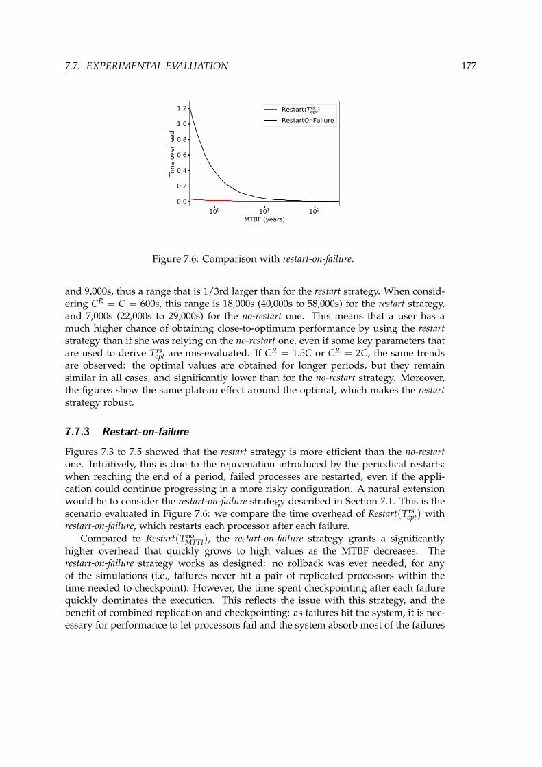
7.7. EXPERIMENTAL EVALUATION 177
100 101 102
MTBF (years)
0.0
0.2
0.4
0.6
0.8
1.0
1.2
Tim
e ov
erhe
ad
Restart(Trsopt)
RestartOnFailure
Figure 7.6: Comparison with restart-on-failure.
and 9,000s, thus a range that is 1/3rd larger than for the restart strategy. When consid-ering CR = C = 600s, this range is 18,000s (40,000s to 58,000s) for the restart strategy,and 7,000s (22,000s to 29,000s) for the no-restart one. This means that a user has amuch higher chance of obtaining close-to-optimum performance by using the restartstrategy than if she was relying on the no-restart one, even if some key parameters thatare used to derive Trs
opt are mis-evaluated. If CR = 1.5C or CR = 2C, the same trendsare observed: the optimal values are obtained for longer periods, but they remainsimilar in all cases, and significantly lower than for the no-restart strategy. Moreover,the figures show the same plateau effect around the optimal, which makes the restartstrategy robust.
7.7.3 Restart-on-failure
Figures 7.3 to 7.5 showed that the restart strategy is more efficient than the no-restartone. Intuitively, this is due to the rejuvenation introduced by the periodical restarts:when reaching the end of a period, failed processes are restarted, even if the appli-cation could continue progressing in a more risky configuration. A natural extensionwould be to consider the restart-on-failure strategy described in Section 7.1. This is thescenario evaluated in Figure 7.6: we compare the time overhead of Restart(Trs
opt) withrestart-on-failure, which restarts each processor after each failure.
Compared to Restart(TnoMTTI), the restart-on-failure strategy grants a significantly
higher overhead that quickly grows to high values as the MTBF decreases. Therestart-on-failure strategy works as designed: no rollback was ever needed, for anyof the simulations (i.e., failures never hit a pair of replicated processors within thetime needed to checkpoint). However, the time spent checkpointing after each failurequickly dominates the execution. This reflects the issue with this strategy, and thebenefit of combined replication and checkpointing: as failures hit the system, it is nec-essary for performance to let processors fail and the system absorb most of the failures

178 Chapter 7: Replication is more efficient than you think
100 101 102
MTBF (years)
0.00
0.02
0.04
0.06
0.08
0.10Ti
me
over
head
Restart(Trsopt) (CR = C)
Restart(Trsopt) (CR = 2C)
NoRestart(TnoMTTI)
100 101 102
MTBF (years)
0.0
0.1
0.2
0.3
0.4
Tim
e ov
erhe
ad
Restart(Trsopt) (CR = C)
Restart(Trsopt) (CR = 2C)
NoRestart(TnoMTTI)
Figure 7.7: Time overhead as a function of MTBF, with C = 60s (left) or C = 600s(right), b = 105 processor pairs.
using the replicates. Combining this result with Figure 7.5, we see that it is critical forperformance to find the optimal rejuvenation period: restarting failed processes toofrequently is detrimental to performance, as is restarting them too infrequently.
7.7.4 Impact of Parameters
The graphs in Figure 7.7 describe the impact of the individual MTBF of the proces-sors on the time overhead. We compare Restart(Trs
opt), Restart(TnoMTTI) (both in the most
optimistic case when CR = C and in the least optimistic case when CR = 2C) andNoRestart(Tno
MTTI). As expected, when CR increases, the time overhead increases. How-ever, even in the case CR = 2C, both restart strategies outperform the no-restart strategy.As the MTBF increases, the overhead of all strategies tends to be negligible, since along MTBF has the cumulated effect that the checkpointing period increases and therisk of needing to re-execute decreases. The longer the checkpoint time C, the higherthe overheads, which is to be expected; more interestingly, with higher C, the restartstrategy needs CR to remain close to C to keep its advantage against the no-restart strat-egy. This advocates for a buddy checkpointing approach with restart strategy whenconsidering replication and checkpointing over unreliable platforms.
7.7.5 I/O Pressure
Figure 7.8 reports the difference between Trsopt and Tno
MTTI. We see that Trsopt increases
faster than TnoMTTI when the MTBF decreases. This is due to the fact that the processors
are restarted at each checkpoint, hence reducing the probability of failure for each pe-riod; it mainly means that using the restart strategy (i) decreases the total applicationtime, and (ii) decreases the I/O congestion in the machine, since checkpoints are lessfrequent. This second property is critical for machines where a large number of appli-cations are running concurrently, and for which, with high probability, the checkpoint

7.7. EXPERIMENTAL EVALUATION 179
100 101 102
MTBF (years)0
2
4
6
9
Perio
d le
ngth
(day
s)
Trsopt (CR = C)
Trsopt (CR = 1.5C)
Trsopt (CR = 2C)
TnoMTTI
100 101 102
MTBF (years)0
2
4
6
9
Perio
d le
ngth
(day
s)
Trsopt (CR = C)
Trsopt (CR = 1.5C)
Trsopt (CR = 2C)
TnoMTTI
Figure 7.8: Period length T as function of MTBF, with C = 60s (left) or C = 600s(right), b = 105 processor pairs.
100 101 102
MTBF (years)
5
10
50
Tim
e to
Sol
utio
n (d
ays)
100 101 102
MTBF (years)
5
10
50
Tim
e to
Sol
utio
n (d
ays)
No replicationRestart(Trs
opt) (CR = C)Partial90(Trs
opt) (CR = C)Partial50(Tno
MTTI) (CR = C)
NoRestart(TnoMTTI)
Lower bound with full replicationLower bound without replication
Figure 7.9: Time-to-solution for N = 2× 10⁵ standalone proc. against full and partialreplication approaches, as a function of MTBF, with CR = C = 60s (left) or CR = C =600s (right), γ = 10−5, α = 0.2.
times are longer than expected because of I/O congestion.
7.7.6 Time-To-Solution
Looking at the time overhead is not sufficient to evaluate the efficiency of replication.So far, we only compared different strategies that all use full process replication. Wenow compare the restart and no-restart strategies to the approach without replication,and also to the approach with partial replication [72, 110]. Figure 7.9 shows the corre-sponding time-to-solution for γ = 10−5 and α = 0.2 (values used in [110]), and CR = C
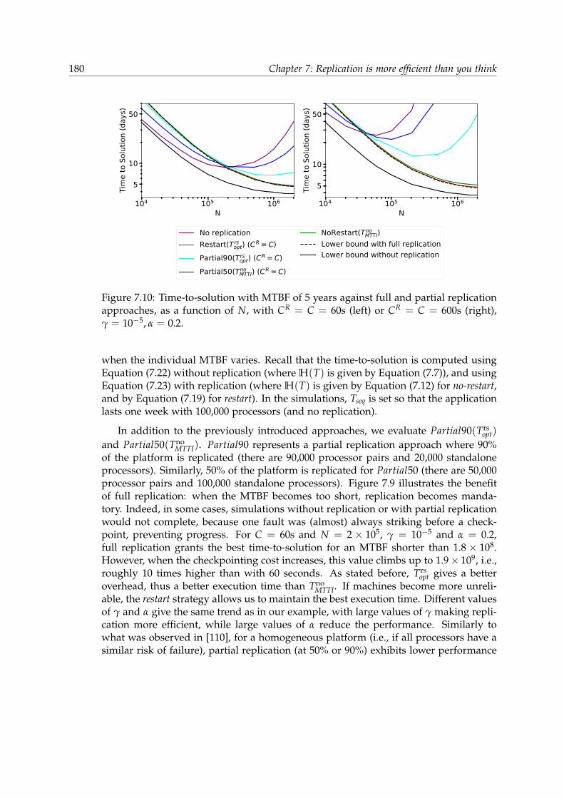
180 Chapter 7: Replication is more efficient than you think
104 105 106
N
5
10
50Ti
me
to S
olut
ion
(day
s)
104 105 106
N
5
10
50
Tim
e to
Sol
utio
n (d
ays)
No replicationRestart(Trs
opt) (CR = C)Partial90(Trs
opt) (CR = C)Partial50(Tno
MTTI) (CR = C)
NoRestart(TnoMTTI)
Lower bound with full replicationLower bound without replication
Figure 7.10: Time-to-solution with MTBF of 5 years against full and partial replicationapproaches, as a function of N, with CR = C = 60s (left) or CR = C = 600s (right),γ = 10−5, α = 0.2.
when the individual MTBF varies. Recall that the time-to-solution is computed usingEquation (7.22) without replication (where H(T) is given by Equation (7.7)), and usingEquation (7.23) with replication (where H(T) is given by Equation (7.12) for no-restart,and by Equation (7.19) for restart). In the simulations, Tseq is set so that the applicationlasts one week with 100,000 processors (and no replication).
In addition to the previously introduced approaches, we evaluate Partial90(Trsopt)
and Partial50(TnoMTTI). Partial90 represents a partial replication approach where 90%
of the platform is replicated (there are 90,000 processor pairs and 20,000 standaloneprocessors). Similarly, 50% of the platform is replicated for Partial50 (there are 50,000processor pairs and 100,000 standalone processors). Figure 7.9 illustrates the benefitof full replication: when the MTBF becomes too short, replication becomes manda-tory. Indeed, in some cases, simulations without replication or with partial replicationwould not complete, because one fault was (almost) always striking before a check-point, preventing progress. For C = 60s and N = 2× 10⁵, γ = 10−5 and α = 0.2,full replication grants the best time-to-solution for an MTBF shorter than 1.8× 10⁸.However, when the checkpointing cost increases, this value climbs up to 1.9× 10⁹, i.e.,roughly 10 times higher than with 60 seconds. As stated before, Trs
opt gives a betteroverhead, thus a better execution time than Tno
MTTI. If machines become more unreli-able, the restart strategy allows us to maintain the best execution time. Different valuesof γ and α give the same trend as in our example, with large values of γ making repli-cation more efficient, while large values of α reduce the performance. Similarly towhat was observed in [110], for a homogeneous platform (i.e., if all processors have asimilar risk of failure), partial replication (at 50% or 90%) exhibits lower performance

7.7. EXPERIMENTAL EVALUATION 181
100 101 102
MTBF (years)
0.00
0.02
0.04
0.06
0.08
0.10
Tim
e ov
erhe
ad
Restart(Trsopt)
Restart-2(Trsopt)
Restart-2(TnoMTTI)
Restart-6(Trsopt)
Restart-6(TnoMTTI)
Restart-12(Trsopt)
Restart-12(TnoMTTI)
Restart-56(Trsopt)
Restart-56(TnoMTTI)
Restart-112(Trsopt)
Restart-112(TnoMTTI)
Restart-281(Trsopt)
Restart-281(TnoMTTI)
NoRestart(TnoMTTI)
Figure 7.11: Comparison of restart strategy with restart only every 2, 6, 12, 56, 112, or281 dead proc., with Trs
opt and TnoMTTI.
than no replication for long MTBF, and lower performance than the no-restart strategy(hence even lower performance than the restart strategy) for short MTBF. This confirmsthat partial replication has potential benefit only for heterogeneous platforms, whichis outside the scope of this study.
We now further focus on discussing when replication should be used. Figure 7.10shows the execution time of an application when the number of processors N varies.Each processor has an individual MTBF of 5 years. The same general comments can bemade: Restart(Trs
opt) always grants a slightly lower time-to-solution than NoRestart(TnoMTTI),
because it has a smaller overhead. As before, when N is large, the platform is less reli-able and the difference between Restart(Trs
opt) and NoRestart(TnoMTTI) is higher compared
to small values of N. We see that replication becomes mandatory for large platforms:without replication, or even with 50% of the platform replicated, the time-to-solutionis more than 10 times higher than the execution time without failures. With γ = 10−5
and α = 0.2, replication becomes more efficient than no replication for N ≥ 2× 10⁵
processors when C = 60s. However, when C = 600s, it starts being more efficientwhen N ≥ 2.5× 10⁴, i.e., roughly 10 times less processors when C is 10 times longer.This study further confirms that partial replication never proved to be useful through-out our experiments.
7.7.7 When to Restart
In this section, we consider a natural extension of the restart approach: instead ofrestarting failed processors at each checkpoint, the restart can be delayed until the

182 Chapter 7: Replication is more efficient than you think
next checkpoint where the number of accumulated failures reaches or exceeds a givenbound nbound, thereby reducing the frequency of the restarts.
The restart strategy assumes that after a checkpoint, the risk of any processor fail-ing is the same as in the initial configuration. For the extension, there is no guaranteethat Trs
opt remains the optimal interval between checkpoints; worse, there is no guar-antee that periodic checkpointing remains optimal. To evaluate the potential gain ofreducing the restart frequency, we consider the two proposed intervals: Trs
opt and TnoMTTI.
And, since most checkpoints will not incur a restart, we assume CR = C when com-puting Trs
opt. However, checkpoints where processes are restarted have a cost of twicethe cost of a simple checkpoint in the simulation: this is the worst case for the restartstrategy. We then simulate the execution, including restarts due to reaching nboundfailures and due to application crashes. With b = 100, 000 processor pairs, we expectnfail(2b) = 561 failures before the application is interrupted; so we will consider alarge range of values for nbound: from 2, 6, 12, to cover cases where few failures areleft to accumulate, to 56, 112, or 281, that represent respectively 10%, 20% and 50% ofnfail(2b), to cover cases where many failures can accumulate.
The results are presented in Figure 7.11, for a variable node MTBF. The time over-head of the extended versions is higher than the time overhead of the restart approachusing Trs
opt as a checkpointing (and restarting) interval. The latter is also lower than theoverhead of the no-restart strategy, which on average corresponds to restarting afternbound = nfail(2b) = 561 failures. This shows that restarting the processes after eachcheckpoint consistently decreases the time overhead. Using the optimal checkpointingperiod for restart Trs
opt, increasing nbound also increases the overhead. Moreover, whenusing small values (such as 2 and 6) for nbound, we obtain exactly the same results asfor the restart strategy. This is due to the fact that between two checkpoints, the restartstrategy usually looses around 6 processors, meaning that restart is already the samestrategy as accumulating errors up to 6 (or less) before restarting. With nbound =12, onaverage the restart happens every two checkpoints, and the performance is close, butslightly slower than the restart strategy.
Finally, an open problem is to determine the optimal checkpointing strategy for theextension of restart tolerating nbound failures before restarting failed processors. Thisoptimal strategy could render the extension more efficient than the baseline restartstrategy. Given the results of the simulations, we conjecture this optimal number to be0, i.e., restart would be the optimal strategy.
Summary. Overall, we have shown that the restart strategy with period Trsopt is indeed
optimal and that our model is realistic. We showed that restart decreases time over-head, hence time-to-solution, compared to using no-restart with period Tno
MTTI. The nextsection shows similar gains in energy overheads. The main decision is still to decidewhether the application should be replicated or not. However, whenever it should be(which is favored by a large ratio of sequential tasks γ, a large checkpointing cost C,or a short MTBF), we are now able to determine the best strategy: use full replication,restart dead processors at each checkpoint (overlapped if possible), and use Trs
opt for

7.8. ENERGY CONSUMPTION 183
the checkpointing period.
7.8 Energy consumption
In this last section, we extend the approach to a different objective function: the goal isnow to minimize the energy overhead. If E(T) is the expected energy consumption ofa period of length P = T +C, the energy overhead with a single processor is expressedas:
Henergy(T) =E(T)
T(Pcomp + Pstatic)− 1, (7.24)
where Pcomp is the dynamic power consumption of a processor when computing, andPstatic denotes the static power, which is paid when the processor is kept idle, but stillturned on.
We also denote by PI/O the dynamic power when performing I/O operations,which has to be accounted for when checkpointing, hence in the expression of E(T).We express below E(T) and Henergy(T) in the cases without replication (single pro-cessor or N processors, Section 7.8.1) and with replication (one pair or b pairs, Sec-tion 7.8.2), and derive in each case the optimal period, and the optimal energy over-head. Finally, we present comprehensive simulation results in Section 7.8.3.
7.8.1 Without replication
7.8.1.1 With a single processor
In this case, we use the same approach as in Section 7.3.1 and we write a recursiveformula similar to Equation (7.2):
E(T) = (1− F(T))(T(Pcomp + Pstatic) + C(PI/O + Pstatic))
+ F(T)(ElostT(Pcomp + Pstatic) + DPstatic + R(PI/O + Pstatic)
+ E(T)) (7.25)
If the computation is successful, then we compute at power Pcomp + Pstatic during atime T and use the power PI/O + Pstatic during the checkpoint. However if a failurestrikes, the machine is used at power Pcomp + Pstatic for ElostT seconds, then used atpower Pstatic for the downtime, and used at power PI/O + Pstatic during the recoverybefore starting the period anew. Finally, we obtain:
E(T) =(
C + (eλT − 1)R)(PI/O + Pstatic)
+ (eλT − 1)DPstatic +eλT − 1
λ(Pcomp + Pstatic).
184 Chapter 7: Replication is more efficient than you think
Using the Taylor expansion as previously, we obtain the overhead
Henergy(T) =C(PI/O + Pstatic)
T(Pcomp + Pstatic)+
λT2
+ o(λT). (7.26)
Again, this overhead is minimized for T = Θ(λ−12 ). By differentiating Equa-
tion (7.26), we get the optimal period minimizing energy consumption:
Tenergyopt =
√2C(PI/O + Pstatic)
λ(Pcomp + Pstatic)= Θ(λ−
12 ). (7.27)
Plugging it back into Equation (7.26), we get the optimal energy overhead:
Henergyopt =
√2Cλ(PI/O + Pstatic)
Pcomp + Pstatic+ o(λ
12 ) = Θ(λ
12 ). (7.28)
7.8.1.2 With N processors
We can generalize the previous result for the case with N processors, as done in Sec-tion 7.3.2 for the time overhead. We obtain another similar formula:
Tenergyopt =
√√√√ 2C(P(N)I/O + NPstatic)
N2λ(Pcomp + Pstatic)= Θ(λ−
12 ) (7.29)
for the optimal checkpointing period, while the overhead becomes:
Henergyopt =
√√√√2Cλ(P(N)I/O + NPstatic)
Pcomp + Pstatic+ o(λ
12 ) = Θ(λ
12 ). (7.30)
The main difference between Equations (7.27), (7.28) and Equations (7.29), (7.30) is thatthe dynamic power and the static power is multiplied by N, the number of processors,as more processors consume more energy. Similarly, PI/O becomes P(N)
I/O = PI/O,static +NPI/O,comm to take into account that more nodes are sending data to the externalstorage.
7.8.2 With replication
7.8.2.1 With one processor pair
We now compute the expected energy consumption E(T) of a period of length P =T + CR. We use the same approach as in Section 7.8.1.1 and aim at minimizing the

7.8. ENERGY CONSUMPTION 185
energy overhead
Henergy(T) =E(T)
2T(Pcomp + Pstatic)− 1 (7.31)
We write a recursive formula similar to Equation (7.13):
E(T) = (1− p1(T))(
T(2Pcomp + 2Pstatic) + CR(P(2)I/O + 2Pstatic)
)+ p1(T)
(ElostT(2Pcomp + 2Pstatic) + 2DPstatic
+ R(P(2)I/O + 2Pstatic) + E(T)
). (7.32)
After solving, we obtain:
E(T) = T(2Pcomp + 2Pstatic) + CR(P(2)I/O + 2Pstatic)
+(eλT − 1)2
2eλT − 1
( (2e−2λT − 4e−λT)λT + e−2λT − 4e−λT + 32λ(1− e−λT)2 (2Pcomp + 2Pstatic)
+ 2DPstatic + R(P(2)I/O + 2Pstatic)
).
After Taylor expansion, we derive the overhead Henergy(T):
Henergy(T) =CR(P(2)
I/O + 2Pstatic)
2T(Pcomp + Pstatic)+
2λ2T2
3+ o(λ2T2) (7.33)
The computations are similar to Section 7.4.2 and we find the following optimal valuesfor Tenergy
opt and Henergyopt :
Tenergyopt =
3CR(P(2)I/O + 2Pstatic)
8λ2(Pcomp + Pstatic)
13
= Θ(λ−23 ). (7.34)
Henergyopt =
3CRλ(P(2)I/O + 2Pstatic)
2√
2(Pcomp + Pstatic)
23
+ o(λ23 ) = Θ(λ
23 ). (7.35)
7.8.2.2 With b processor pairs
As previously, we compute the energy consumption for the execution of one period ofduration P = T + CR using the following recursion:
E(T) = pb(T)(ElostT(2bPcomp + 2bPstatic) + D2bPstatic
+ R(P(N)I/O + 2bPstatic) + E(T)
)+ (1− pb(T))
(T(2bPcomp + 2bPstatic) + CR(P(N)
I/O + 2bPstatic)).
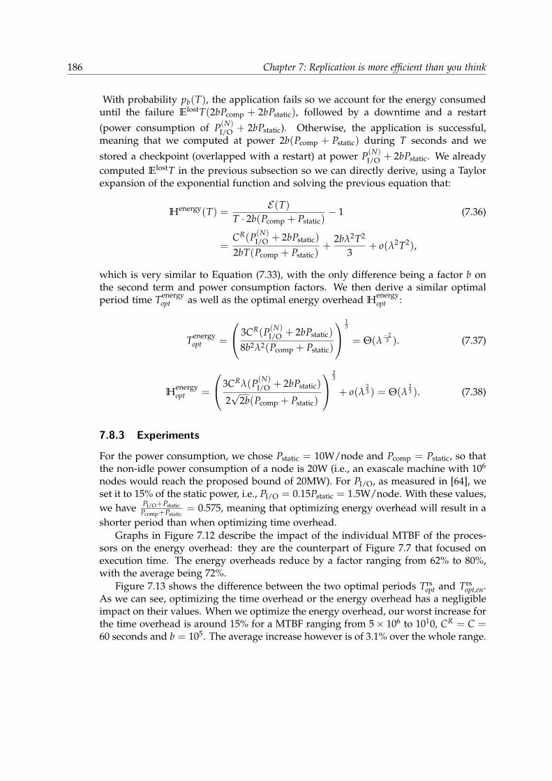
186 Chapter 7: Replication is more efficient than you think
With probability pb(T), the application fails so we account for the energy consumeduntil the failure ElostT(2bPcomp + 2bPstatic), followed by a downtime and a restart
(power consumption of P(N)I/O + 2bPstatic). Otherwise, the application is successful,
meaning that we computed at power 2b(Pcomp + Pstatic) during T seconds and we
stored a checkpoint (overlapped with a restart) at power P(N)I/O + 2bPstatic. We already
computed ElostT in the previous subsection so we can directly derive, using a Taylorexpansion of the exponential function and solving the previous equation that:
Henergy(T) =E(T)
T · 2b(Pcomp + Pstatic)− 1 (7.36)
=CR(P(N)
I/O + 2bPstatic)
2bT(Pcomp + Pstatic)+
2bλ2T2
3+ o(λ2T2),
which is very similar to Equation (7.33), with the only difference being a factor b onthe second term and power consumption factors. We then derive a similar optimalperiod time Tenergy
opt as well as the optimal energy overhead Henergyopt :
Tenergyopt =
3CR(P(N)I/O + 2bPstatic)
8b2λ2(Pcomp + Pstatic)
13
= Θ(λ−23 ). (7.37)
Henergyopt =
3CRλ(P(N)I/O + 2bPstatic)
2√
2b(Pcomp + Pstatic)
23
+ o(λ23 ) = Θ(λ
23 ). (7.38)
7.8.3 Experiments
For the power consumption, we chose Pstatic = 10W/node and Pcomp = Pstatic, so thatthe non-idle power consumption of a node is 20W (i.e., an exascale machine with 106
nodes would reach the proposed bound of 20MW). For PI/O, as measured in [64], weset it to 15% of the static power, i.e., PI/O = 0.15Pstatic = 1.5W/node. With these values,we have PI/O+Pstatic
Pcomp+Pstatic= 0.575, meaning that optimizing energy overhead will result in a
shorter period than when optimizing time overhead.Graphs in Figure 7.12 describe the impact of the individual MTBF of the proces-
sors on the energy overhead: they are the counterpart of Figure 7.7 that focused onexecution time. The energy overheads reduce by a factor ranging from 62% to 80%,with the average being 72%.
Figure 7.13 shows the difference between the two optimal periods Trsopt and Trs
opt,en.As we can see, optimizing the time overhead or the energy overhead has a negligibleimpact on their values. When we optimize the energy overhead, our worst increase forthe time overhead is around 15% for a MTBF ranging from 5× 10⁶ to 1010, CR = C =60 seconds and b = 105. The average increase however is of 3.1% over the whole range.

7.8. ENERGY CONSUMPTION 187
100 101 102
MTBF (years)
0.00
0.02
0.04
0.06
0.08
Ener
gy o
verh
ead
Restart(Trsopt) (CR = C)
Restart(Trsopt) (CR = 2C)
NoRestart(TnoMTTI)
100 101 102
MTBF (years)
0.0
0.1
0.2
0.3
Ener
gy o
verh
ead
Restart(Trsopt) (CR = C)
Restart(Trsopt) (CR = 2C)
NoRestart(TnoMTTI)
Figure 7.12: Influence of the MTBF on the energy overhead for the Ra nd no-restartstrategies. Checkpointing time set to 60 seconds (left) or 600 seconds (right), with 105
pairs of processors.
106 107 108 109 1010
MTBF (s)
0.000
0.005
0.010
0.015
0.020
0.025
0.030
0.035
0.040
0.045
Tim
e o
verh
ead
Restart(T rsopt) (CR =C)
Restart(T rsopt, en) (CR =C)
106 107 108 109 1010
MTBF (s)
0.000
0.005
0.010
0.015
0.020
0.025
0.030
0.035
Energ
y o
verh
ead
Restart(T rsopt) (CR =C)
Restart(T rsopt, en) (CR =C)
Figure 7.13: Impact of optimizing the time overhead or the energy overhead on thetime overhead (left) or the energy overhead (right) as a function of the MTBF (C = 60s,105 pairs of processors).

188 Chapter 7: Replication is more efficient than you think
105 106 107 108
PI/O
10-3
10-2
10-1
100Tim
e o
verh
ead
Restart(T rsopt) (CR =C)
Restart(TnoMTTI) (CR =C)
Restart(T rsopt) (CR =C+R)
Restart(TnoMTTI) (CR =C+R)
NoRestart(TnoMTTI)
105 106 107 108
PI/O
10-3
10-2
10-1
100
Energ
y o
verh
ead
Restart(T rsopt) (CR =C)
Restart(TnoMTTI) (CR =C)
Restart(T rsopt) (CR =C+R)
Restart(TnoMTTI) (CR =C+R)
NoRestart(TnoMTTI)
Figure 7.14: Time and energy overheads when varying PI/O (MTBF 5 years, C = 60s,b = 105) when optimizing the time overhead.
105 106 107 108
PI/O
10-3
10-2
10-1
100
Tim
e o
verh
ead
Restart(T rsopt, en) (CR =C)
Restart(TnoMTTI, en) (CR =C)
Restart(T rsopt, en) (CR =C+R)
Restart(TnoMTTI, en) (CR =C+R)
NoRestart(TnoMTTI, en)
105 106 107 108
PI/O
10-3
10-2
10-1
100
Energ
y o
verh
ead
Restart(T rsopt, en) (CR =C)
Restart(TnoMTTI, en) (CR =C)
Restart(T rsopt, en) (CR =C+R)
Restart(TnoMTTI, en) (CR =C+R)
NoRestart(Tno, enMTTI )
Figure 7.15: Time and energy overheads when varying PI/O (MTBF 5 years, C = 60s,b = 105) when optimizing the energy overhead.
When optimizing the time overhead, we measured a maximum of 23% improvementunder the same conditions with the average increase being 4.2%. Overall, with ourvalues we do not need to specifically optimize the energy overhead, except if the ratiobetween PI/O + Pstatic and Pcomp + Pstatic is much greater or much smaller than 1, wherethe difference between the two optimal periods might differ more than that.
Finally, Figures 7.14 and 7.15 show the impact of varying PI/O on both time andenergy overheads, the former when optimizing the time overhead, the latter whenoptimizing the energy overhead. We once again show that the Rs trategy with thecorresponding optimal period is the best one, with the only exception being whenPI/O is high (more than 107W, i.e. 10 times the value set in the previous experiments).If we want to optimize the energy consumption, then using Tno
MTTI,en can lower thetime overhead (and only increases a bit the energy overhead).
7.9. CONCLUSION 189
7.9 Conclusion
In this work, we have revisited process replication combined with checkpointing, anapproach that has received considerable attention from the HPC community in re-cent years. Opinion is divided about replication. By definition, its main drawbackis that 50% of platform resources will not contribute to execution progress, and sucha reduced throughput does not seem acceptable in many scenarios. However, check-point/restart alone cannot ensure full reliability in heavily failure-prone environments,and must be complemented by replication in such unreliable environments. Previousapproaches all used the no-restart strategy. In this work, we have introduced a newrollback/recovery strategy, the restart strategy, which consists of restarting all failedprocesses at the beginning of each period. Thanks to this rejuvenation, the systemremains in the same conditions at the beginning of each checkpointing period, whichallowed us to build an accurate performance model and to derive the optimal check-pointing period for this strategy. This period turns out to be much longer than theone used with the no-restart strategy, hence reducing significantly the I/O pressureintroduced by checkpoints, and improving the overall time-to-solution. To validatethis approach, we have simulated the behavior of realistic large-scale systems, withfailures either IID or from log traces. We have compared the performance of restartwith the state-of-the-art strategies. Another key advantage of the restart strategy is itsrobustness: the range of periods in which its performance is close to optimal is muchlarger than for the no-restart strategy, making it a better practical choice to target un-reliable platforms where the key elements (MTBF and checkpoint duration) are hardto estimate. In the future, we plan to evaluate, at least experimentally, non-periodiccheckpointing strategies that rejuvenate failed processors after a given number of fail-ures is reached or after a given time interval is exceeded.


Part III
Scheduling problems
191

Chapter 8
Design and Comparison of Resilient Schedul-ing Heuristics for Parallel Jobs
This chapter focuses on the resilient scheduling of parallel jobs on high-performancecomputing (HPC) platforms to minimize the overall completion time, or makespan.We revisit the classical problem while assuming that jobs are subject to transient orsilent errors, and hence may need to be re-executed each time they fail to completesuccessfully. This work generalizes the classical framework where jobs are known of-fline and do not fail: in the classical framework, list scheduling that gives priority tolongest jobs is known to be a 3-approximation when imposing to use shelves, and a 2-approximation without this restriction. We show that when jobs can fail, using shelvescan be arbitrarily bad, but unrestricted list scheduling remains a 2-approximation.The chapter focuses on the design of several heuristics, some list-based and someshelf-based, along with different priority rules and backfilling strategies. We assessand compare their performance through an extensive set of simulations, using bothsynthetic jobs and log traces from the Mira supercomputer. The work in this chapteris joint work with Anne Benoit, Hongyang Sun and Yves Robert, and will be pub-lished in the workshop on Advances in Parallel and Distributed Computational Models(APDCM) [W7].
8.1 Introduction
One of the main challenges faced by today’s HPC platforms is resilience, since suchplatforms are confronted with many failures or errors due to their large scale [169].Indeed, the number of failures is known to grow proportionally with the number ofnodes on a platform [106], and the largest supercomputers today experience severalfailures per day. There are two main classes of errors that can cause failures in anapplication’s execution, namely, fail-stop and silent errors. While fail-stop errors causethe execution to terminate (e.g., due to hardware fault), large-scale platforms are alsoconfronted with silent errors, or silent data corruptions (SDCs). Such errors are causedby cosmic radiation or packaging pollution, striking either the cache or memory units
193
194 Chapter 8: Design and Comparison of Resilient Scheduling Heuristics for Parallel Jobs
(bit flips), or the CPU operations [147, 210]. Even though any bit can be corrupted, theexecution continues (unlike fail-stop errors), hence the error is transient, but it maydramatically impact the result of a running application. Many silent errors can beaccurately detected by verifying the data using dedicated, lightweight detectors (e.g.,[195, 50, 93, 49]). In this work, we focus on job failures caused by silent errors, and weaim to design resilient scheduling heuristics while assuming the availability of ad-hocdetectors to detect such errors.
The problem of scheduling a set of independent jobs on parallel platforms withthe goal of minimizing the total completion time, or makespan, has been extensivelystudied (see Section 8.5). Jobs may be parallel and should be executed on a givennumber of processors for a certain duration; both the processor requirement and theexecution time of each job are known at the beginning. Such jobs are called rigidjobs, contrarily to moldable or malleable jobs, whose processor allocations can varyat launch time or during execution [80]. While moldable or malleable jobs offer moreflexibility in the execution, rigid jobs remain the most prevalent form of parallel jobssubmitted on today’s HPC systems, and we focus on rigid jobs in this chapter.
Unlike the classical scheduling problem without job failures, we consider failure-prone platforms subject to silent errors. Hence, at the end of each job’s execution, anSDC detector will flag if a silent error has occurred during its execution. In this case,the job must be re-executed until it has been successfully completed without errors.For a set of jobs, each execution may lead to a different failure scenario, dependingupon the jobs that have experienced failures as well as the number of such failures.The objective is to minimize the makespan under any failure scenario, as well as theexpected makespan, averaged over all possible failure scenarios, where each scenario isweighted by a probability that governs its occurrence under certain failure assump-tions. Since a failure scenario is unknown a priori, the scheduling decisions must bemade dynamically on-the-fly, whenever an error has been detected. As a result, even forthe same set of jobs, different schedules may be produced, depending on the failurescenario that occurred in a particular execution.
Building upon the existing framework for scheduling parallel jobs without failures,we propose two scheduling strategies, namely, a list-based strategy and a shelf-basedstrategy. While list-based schedules have no restrictions on the starting times of thejobs, shelf-based schedules group all jobs into subsets of jobs having the same startingtime (called shelves); a shelf of jobs can start its execution once the longest job from theprevious shelf has completed. For list-based scheduling, practical systems also employa combination of reservation and backfilling strategies with different job priority rulesto increase the system utilization. On platforms with no failures, variants for all ofthese strategies exist that could achieve constant approximations for the makespan(see Section 8.5 for details). The main focus of this chapter is to extend these existingheuristics to execution scenarios with job failures, and to experimentally compare theirperformance using a variety of job and platform configurations.
Our main contributions are the following:• We propose a formal model for the problem of resilient scheduling of parallel
8.2. MODELS 195
jobs on failure-prone platforms. The model formulates the performance of analgorithm under both worst-case and expected executions.
• We design a resilient list-based strategy, and prove that its greedy variant achieves(2− 1
P )-approximation, and its reservation variant is (3− 4P+1 )-approximation,
where P is the total number of processors. These results apply to both worst-caseand expected makespans.
• We design a resilient shelf-based strategy, but we show that, under some failurescenarios, any shelf-based algorithm has an unbounded approximation ratio,thus having a makespan that is arbitrarily higher than the optimal makespan inthe worst case.
• We conduct an extensive set of simulations to evaluate and compare differentvariants of these heuristics using both synthetic jobs and log traces from theMira supercomputer. The results show that the performance of these resilientscheduling heuristics is close to the optimal in practice, even when confrontedwith failures.
The rest of this chapter is organized as follows: The formal models and the prob-lem statement are presented in Section 8.2. The key contributions of the chapter arepresented in Section 8.3, where we describe both list-based and shelf-based strategies,and analyze their performance. Section 8.4 presents an extensive set of simulationresults and highlights the main findings. Section 8.5 describes the background of par-allel job scheduling and presents some related work. Finally, Section 8.6 concludes thechapter and discusses future directions.
8.2 Models
In this section, we formally present the models, the problem statement, and the mainassumptions we make in the chapter.
8.2.1 Job model
We consider a set J = J1, J2, . . . , Jn of n parallel jobs to be executed on a platformconsisting of P identical processors. All jobs are released at the same time, correspond-ing to the batch scheduling scenario in an HPC environment. We focus on rigid jobs,which must be executed with a fixed number of processors set by the user when thejob is submitted1. For each job Jj ∈ J , let pj ∈ 1, 2, . . . , P denote its fixed (integral)processor allocation, and let tj denote its error-free execution time. The area of the jobis defined as aj = pj × tj.
1Other parallel job models include moldable and malleable models, which allow the processor allocationof a job to vary at launch time or during execution [80]. Considering alternative job models will be partof our future work.
196 Chapter 8: Design and Comparison of Resilient Scheduling Heuristics for Parallel Jobs
8.2.2 Error model
We consider failures that manifest as silent errors or silent data corruptions (SDCs) [169]that could corrupt a job during execution. A silent error detector is assumed to beavailable for each job, which is triggered at the end of the job’s execution. If an erroris detected, the job needs to be re-executed, followed by another error detection. Thisprocess repeats until the job completes successfully without errors. Current state-of-the-art SDC detectors are typically lightweighted (e.g., ABFT for matrix computations[195, 50], data analytics for scientific applications [93, 49]), and hence incur a negligiblecost compared to the job’s overall execution time.
All the list-based and shelf-based scheduling heuristics introduced and comparedin this chapter are agnostic of the probability of each job to fail any given number oftimes. Specifically, for a job Jj, consider a particular run where it fails f j times beforesucceeding on the ( f j + 1)-th execution. The probability that this happens is denotedas qj( f j). Let f = ( f1, f2, . . . , fn) denote a failure scenario, i.e., a vector of the numberof failed execution attempts for all jobs, during a particular run. Assuming that er-rors occur independently for different jobs, the probability that this combined failurescenario happens can be computed as Q(f) = ∏j=1...n qj( f j). The failure scenario f, aswell as the associated probabilities qj( f j) and Q(f) may be unknown to the scheduler.
8.2.3 Problem statement
We study the following resilient scheduling problem: Given a set J of paralleljobs, find a schedule for J on P identical processors under any failure scenariof = ( f1, f2, . . . , fn). Here, a schedule for f is defined by a collection s = (~s1,~s2, . . . ,~sn) of
starting time vectors for all jobs, where vector ~sj = (s(1)j , s(2)j , . . . , s( f j+1)j ) specifies the
starting times for job Jj at different execution attempts until success.The objective is to minimize the overall completion time of all jobs, or the makespan.
Suppose an algorithm Alg makes scheduling decision s during a failure scenario f,then the makespan of the algorithm for this scenario is defined as:
TAlg(f, s) = maxj=1...n
(s( f j+1)j + tj
). (8.1)
All scheduling decisions should be made while satisfying the following two con-straints:
1. Processor constraint: The number of processors used at any time t by the set Jtof running jobs should not exceed the total number P of available processors onthe platform, i.e., ∑Jj∈Jt
pj ≤ P, ∀t.
2. Re-execution constraint: A job cannot be re-executed if its previous execution at-tempt has not yet been completed, i.e., s(i+1)
j ≥ s(i)j + tj, ∀j = 1 . . . n, ∀i ≥ 1.
This scheduling problem, encompassing the failure-free problem as a special case,is clearly NP-hard. A scheduling algorithm Alg is said to be c-approximation if its

8.2. MODELS 197
makespan is at most c times that of an optimal scheduler for all possible sets of jobsunder all possible failure scenarios, i.e.,
TAlg(f, s) ≤ c · TOpt(f, s∗) , (8.2)
where TOpt(f, s∗) denotes the optimal makespan with scheduling decision s∗ underfailure scenario f. Clearly, this optimal makespan admits the following two lowerbounds:
TOpt(f, s∗) ≥ tmax(f) , (8.3)
TOpt(f, s∗) ≥ A(f)P
, (8.4)
where tmax(f) = maxj=1...n( f j + 1) · tj is the maximum cumulative execution time ofany job under f, and A(f) = ∑n
j=1( f j + 1) · aj is the total cumulative area.In Section 8.3, we establish several approximation results, which are valid for any
failure scenario regardless of its individual probability. This is the strongest result thatcan be obtained from a theoretical perspective. However, from a practical perspective,given a set of jobs, it is not easy to assess the performance of a scheduling heuristicif the probability Q(f) = ∏j=1...n qj( f j) of each failure scenario f is not known. Thus,for the experiments in Section 8.4, we report the expected makespan of each heuristicunder the standard Exponential probability distribution, as explained below.
8.2.4 Expected makespan
Suppose the occurrence of silent errors striking the jobs follows an Exponential proba-bility distribution, and that the mean time between error (MTBE) of an individual pro-cessor is µ, so the error rate of the processor is given by λ = 1/µ. For a job Jj executedon pj processors, the probability that the job is struck by a silent error during executionis then given by qj = 1− e−λpj·tj = 1− e−λaj [106]. Then, the probability for job Ji to
fail f j times before succeeding on the ( f j + 1)-th execution is qj( f j) = qf jj (1− qj).
Given a set J of jobs, we can now define the expected makespan of an algorithmAlg, taken over all possible failure scenarios weighted by their probabilities, as:
E(TAlg) = ∑f Q(f) · TAlg(f, s) . (8.5)
In this case, an algorithm is a c-approximation if we have:
E(TAlg) ≤ c ·E(TOpt) , (8.6)
for all possible sets of jobs, where E(TOpt) denotes the optimal expected makespan.This is because the inequality is true for each failure scenario, hence for the weightedsum. Obviously, the converse is not true: an algorithm could satisfy Equation (8.6)(thus achieving c-approximation in expectation) but be arbitrarily worse than the op-

198 Chapter 8: Design and Comparison of Resilient Scheduling Heuristics for Parallel Jobs
timal on some (low probability) failure scenarios. Still, expected makespan providesa synthetic indicator on the performance of an algorithm under study, enabling easyand quantitative comparisons. Thus, we use it for the experimental evaluations inSection 8.4.
8.2.5 Static vs. dynamic scheduling
As all the information regarding the set of jobs (except the failure scenario f) is avail-able, one approach would be to make all scheduling decisions (i.e., starting times s)statically at the beginning, and then execute the jobs according to this static schedule.While this approach works for failure-free executions, it is problematic when jobs canfail and re-execute. In particular, a static schedule needs to pre-compute a (possiblyinfinite) sequence of starting times for all jobs to account for every possible failure sce-nario, while ensuring the satisfaction of the constraints. Pre-computing such a staticschedule would be computationally intractable, especially when there turn out to beonly a few failures in a run.
In contrast, another more flexible approach is to make scheduling decisions dynam-ically depending on the particular failure scenario that is unveiled from an execution.For example, a scheduling algorithm may decide the starting time for the next exe-cution attempt of a job depending on the failure scenario and schedule so far. As aresult, even for the same set of jobs, the algorithm may produce different schedules inresponse to the different failure scenarios that could arise at runtime. In this chapter,we adopt this dynamic approach.
8.3 Resilient Scheduling Heuristics
In this section, we present a resilient list-based heuristic (R-List) and a resilient shelf-based heuristic (R-Shelf) for scheduling rigid parallel jobs that could fail due tosilent errors. We show that the greedy variant of R-List without reservation is 2-approximation, and a variant with reservations is 3-approximation. For R-Shelf, eventhough it achieves 3-approximation in the failure-free case, we show through an ex-ample that any resilient shelf-based algorithm may have an approximation ratio ofΩ(ln P) compared to the optimal in some failure scenario.
8.3.1 R-List scheduling heuristic
We first present a resilient list-based scheduling heuristic, called R-List, that sched-ules any set of jobs with the capability to handle failures. Algorithm 3 shows thepseudocode of R-List. It extends the classical batch scheduler that combines reser-vation and backfilling strategies. The algorithm first organizes all jobs in a list (or aqueue) based on some priority rule. Then, whenever an existing job Jk completes andhence releases processors (at time 0, a virtual job J0 can be considered to complete), thealgorithm schedules the remaining jobs in the queue. First, it checks if job Jk completes

8.3. RESILIENT SCHEDULING HEURISTICS 199
Algorithm 3: R-List
Input: a set J = J1, J2, · · · , Jn of rigid jobs, with processor allocation pj and error-freeexecution time tj for each job Jj ∈ J , a platform with P identical processors, parameterm;
Output: a list schedule with starting times for all jobs in J till they complete successfully.begin
Insert all jobs into a queue Q according to some priority rule;whenever an existing job Jk completes do
if error detected for Jk thenQ.insert with priority(Jk);
// schedule high-priority jobs using reservationfor j = 1, 2 . . . , min(m, |Q|) do
Jj ← Q(j);Give job Jj an earliest possible reservation without delaying the reservation of job
Jj′ , ∀j′ = 1, . . . , j− 1;
// schedule low-priority jobs using backfillingfor j = m + 1, . . . , |Q| do
Jj ← Q(j);if Job Jj can be scheduled at the current time without delaying the reservation of
job Jj′ , ∀j′ = 1 . . . m thenexecute job Jj at the current time;
with error. If so, the job will be inserted back into the queue, based on its priority, tobe rescheduled later. All jobs in the queue are divided into two groups: the first mjobs with the highest priorities are each given a reservation at the earliest possibletime, provided that any reservation made should not delay the starting times of thehigher-priority jobs; the subsequent jobs in the queue (if any) are then examined oneby one and backfilled to start at the current time, again if such backfilling does notaffect any reservations for the higher-priority jobs.2
The R-List heuristic takes a parameter m, and depending on the value of m chosen,it resembles several scheduling strategies known in theory and practice:
• m = |Q| (Conservative backfilling [142]): this strategy makes reservations for allpending jobs in the queue;
• m = 1 (Aggressive or EASY backfilling [129, 168]): this strategy makes a reser-vation only for the job at the head of the queue, and uses backfilling to scheduleall remaining jobs in the queue;
• m = 0 (Greedy scheduler [88, 184, 81]): this strategy does not make any reserva-tion, and uses backfilling to schedule all jobs in the queue.
Note that, when m > 0 and when a job Jk with high priority fails, it may be re-inserted back into the first part of the queue (i.e., among the top m jobs). This mayrequire recomputing the existing reservations (made previously) for some jobs thathave lower priority than Jk. From an analysis point of view, we can think of eachjob completion as a trigger, which deletes all previous reservations and makes a fresh
2For practical schedulers, this is typically implemented using two separate job queues, one for reser-vation and one for backfilling.

200 Chapter 8: Design and Comparison of Resilient Scheduling Heuristics for Parallel Jobs
round of reservation and backfilling decisions based on the updated queue.In the following, we denote by Reservation this variant of R-List with reservations
(m > 0), and by Greedy the variant with m = 0.
8.3.2 Approximation ratios of R-List
We show that, under any failure scenario, Reservation with a particular priority ruleis a (3 − 4
P+1 )-approximation, and that Greedy with any priority rule is a (2 − 1P )-
approximation. According to Equation (8.6), these results directly imply the sameapproximation ratios for the respective heuristic variants in terms of the expectedmakespan.
8.3.2.1 Result for Reservation
We first consider the Reservation variant, while applying a priority rule that favorslarge jobs and uses any priority for small jobs. We call this rule Large Job First (LJF).Specifically, a job is said to be large if its processor allocation is at least P+1
2 , and smallotherwise. The LJF rule specifies that: (1) all large jobs have higher priority than allsmall jobs; (2) the priorities for large jobs are based on decreasing processor allocation;and (3) the priorities for small jobs are defined arbitrarily.
The following proposition shows the performance of Reservation in any failurescenario using the above LJF rule. The result matches the 3-approximation ratio [13,184] known for failure-free jobs.
Proposition 5. For any set of rigid parallel jobs under any failure scenario f, the makespan ofReservation with the LJF priority rule satisfies:
TR(f, s) ≤ (3− 4P + 1
) · TOpt(f, s∗) . (8.7)
Proof. Let Jj be a last successfully completed job in the schedule. We divide the setI = I1, I2, . . . , Iv of all intervals into two disjoint subsets I1 and I2, where I1 containsthe intervals in which job Jj is executing (including all of its execution attempts), andI2 = I\I1. Let T1 = ∑I∈I1
|I| and T2 = ∑I∈I2|I| denote the total lengths of all intervals
in I1 and I2, respectively. Based on Equation (8.3), we have T1 = ( f j + 1) · tj(pj) ≤tmax(f) ≤ Topt(f, s∗).
We will show that the processor utilization in any interval I ∈ I2 satisfies p(I) ≥P+1
2 . First, we observe that all large jobs are completed sequentially (in decreasingorder of processor allocation) at the beginning of the entire schedule, since no twolarge jobs can be scheduled at the same time, and no small (backfilling) jobs can delaytheir executions because large jobs have higher priority based on the LJF rule. Thus, ifan interval I ∈ I2 contains a large job, its processor allocation must satisfy p(I) ≥ P+1
2 .Now, consider any interval I ∈ I2 after all the large jobs have completed, and sup-
pose I lies in between the i-th execution attempt and the (i + 1)-th execution attemptof Jj, where 0 ≤ i ≤ f j. Hence, if such an interval exists, it means that Jj is a small job

8.3. RESILIENT SCHEDULING HEURISTICS 201
(with pj ≤ P+12 ), as well as all remaining jobs that are to be executed. Let t be the time
at the beginning of this interval I. Recall that we can consider Reservation to make afresh round of reservations and backfillings based on the current job queue Q at timet. Let Jk be the first job in Q that cannot be scheduled (either reserved or backfilled)to run at t. We know that such a job always exists because of the (i + 1)-th executionattempt of Jj, which is scheduled to run at a later time. Let Jt be the set of jobs alreadyrunning at time t or just scheduled to run at time t before job Jk, and let p(Jt) be thetotal processor allocation of all jobs in Jt. As Jk cannot be scheduled to run at time t,it must be due to p(Jt) + pk ≥ P + 1. Since Jk is a small job, i.e., pk ≤ P+1
2 , it impliesthat p(I) ≥ p(Jt) ≥ P+1
2 .Thus, based on Equation (8.4) and since pj ≥ 1, we have P · Topt(f, s∗) ≥ A(f) ≥
P+12 · T2 + pj · T1 ≥ P+1
2 · T2 + T1. The overall execution time of Reservation with theLJF priority rule therefore satisfies:
TR(f, s) = T1 + T2
≤ T1 + 2 · P · Topt(f, s∗)− T1
P + 1
=2P
P + 1· Topt(f, s∗) +
(1− 2
P + 1
)· T1
≤ (3− 4P + 1
) · Topt(f, s∗) .
8.3.2.2 Result for Greedy
We now consider the Greedy variant. The following proposition shows the perfor-mance of Greedy in any failure scenario regardless of the priority rule. The resultgeneralizes the 2-approximation ratio [88, 184, 81] known for failure-free jobs.
Proposition 6. For any set of rigid parallel jobs under any failure scenario f, the makespan ofGreedy regardless of the priority rule satisfies:
TG(f, s) ≤ (2− 1P) · TOpt(f, s∗) . (8.8)
Proof. Given the set I = I1, I2, . . . , Iv of all intervals in the schedule, let pmin =min1≤`≤v p(I`) denote the minimum processor utilization among them. Since the algo-rithm never idles all processors unless all jobs complete successfully, we have pmin ≥ 1.We consider two cases:
Case 1: pmin ≥ P+12 . In this case, we have p(I`) ≥ pmin ≥ P+1
2 for all 1 ≤ ` ≤ v.Hence, based on Equation (8.4), we get P · Topt(f, s∗) ≥ A(f) = ∑`=1,...,v |I`| · p(I`) ≥P+1
2 · TG(f, s). This implies:
TG(f, s) ≤ 2PP + 1
· Topt(f, s∗) ≤ (2− 1P) · Topt(f, s∗) .
202 Chapter 8: Design and Comparison of Resilient Scheduling Heuristics for Parallel Jobs
Case 2: pmin < P+12 . In this case, let Imin denote the last-executed interval that has
processor utilization pmin. Consider a job Jj that is running during interval Imin. Nec-essarily, we have pj ≤ pmin. We divide the set I of intervals into two disjoint subsetsI1 and I2, where I1 contains the intervals in which job Jj is executing (including all ofits execution attempts), and I2 = I\I1. Let T1 = ∑I∈I1
|I| and T2 = ∑I∈I2|I| denote
the total lengths of all intervals in I1 and I2, respectively. Based on Equation (8.3), wehave T1 = ( f j + 1) · tj(pj) ≤ tmax(f) ≤ Topt(f, s∗).
For any interval I ∈ I2 that lies between the i-th execution attempt and the (i + 1)-th execution attempt of Jj in the schedule, where 0 ≤ i ≤ f j, the processor utilizationof I must satisfy p(I) ≥ P − pmin + 1, since otherwise there are at least pmin ≥ pjavailable processors during interval I and hence the (i + 1)-th execution attempt of Jjwould have been scheduled at the beginning of I.
For any interval I ∈ I2 that lies after the ( f j + 1)-th (last) execution attempt of Jj,there must be a job Jk running during I and that was not running during Imin (mean-ing no attempt of executing Jk was made during Imin). This is because p(I) > pmin,hence the job configuration must differ between I and Imin. The processor utilizationduring interval I must also satisfy p(I) ≥ P− pmin + 1, since otherwise the processorallocation of Jk will be pk ≤ p(I) ≤ P− pmin, implying that the first execution attemptof Jk after interval Imin would have been scheduled at the beginning of Imin.
Thus, for all I ∈ I2, we have p(I) ≥ P − pmin + 1. Based on Equation (8.4), wehave P · Topt(f, s∗) ≥ A(f) ≥ (P− pmin + 1) · T2 + pmin · T1. Since pmin ≥ 1, the overallexecution time of Greedy therefore satisfies:
TG(f, s) = T1 + T2
≤ T1 +P · Topt(f, s∗)− pmin · T1
P− pmin + 1
=P
P− pmin + 1· Topt(f, s∗) +
P− 2pmin + 1P− pmin + 1
· T1
≤ 2P− 2pmin + 1P− pmin + 1
· Topt(f, s∗)
≤ (2− 1P− pmin + 1
) · Topt(f, s∗)
≤ (2− 1P) · Topt(f, s∗) .
8.3.3 R-Shelf scheduling heuristic
We now present a shelf-based scheduling heuristic, called R-Shelf, that schedules anyset of parallel jobs onto a series of shelves while handling job failures.
Heuristic description Algorithm 4 shows the pseudocode of R-Shelf. As in R-List,the algorithm starts by organizing all jobs in a queue based on some priority rule.Whenever the jobs in the preceding shelf all complete (at time 0, a virtual shelf S0 with

8.3. RESILIENT SCHEDULING HEURISTICS 203
Algorithm 4: R-Shelf
Input: a set J = J1, J2, · · · , Jn of rigid jobs, with processor allocation pj and error-freeexecution time tj for each job Jj ∈ J , a platform with P identical processors, parameter b;
Output: a shelf schedule with starting times for all jobs in J till they complete successfully.begin
Insert all jobs into a queue Q according to some priority rule;i← 0, Si ← ∅;whenever all jobs in Si complete do
if error detected for Jk ∈ Si thenQ.insert with priority(Jk);
i← i + 1 and Si ← ∅; // start a new shelffor j = 1, 2 . . . , |Q| do
Jj ← Q(j);if Job Jj can fit in shelf Si then
Si ← Si⋃Jj;
else if b = 0 thenbreak ; // no backfilling
execute all jobs in Si at the current time;
no job in it can be considered to complete), the algorithm builds a new shelf and addsthe remaining jobs to it. First, any job in the preceding shelf that completes with errorwill be inserted back into the queue based on its priority. Then, the algorithm scansthe queue and adds a job to the new shelf if the job can fit in without violating theprocessor constraint. R-Shelf takes a binary parameter b that determines if backfillingis used in the process:
• b = 0 (No backfilling): the heuristic closes the new shelf upon encountering thefirst job in the queue that does not fit in the shelf. This resembles the Next-Fit(NF) strategy for bin-packing.
• b = 1 (Backfilling): the heuristic scans all the jobs in the queue until no morejob can be added to the new shelf. This resembles the First-Fit (FF) strategy forbin-packing.
Once the jobs in the new shelf have been selected, they will simultaneously starttheir executions.
Inapproximability result For failure-free jobs, the variant of R-Shelf without back-filling and considering jobs in the non-increasing execution time order is equivalentto the Next-Fit Decreasing Height (NFDH) [53] algorithm for strip packing. The algo-rithm starts with the longest job J1, which is put on the first shelf, whose height is t1.Then, the next job J2 is put on the same shelf if it fits in, meaning that p1 + p2 ≤ P,otherwise a new shelf is started for J2, whose height is t2. The algorithm proceeds likethis, either putting the next job on the last shelf if it fits in, or creating a new shelfotherwise. Despite its simplicity, the algorithm is shown to be a 3-approximation forfailure-free jobs [53, 184].
Now, when jobs can fail, we show that there exists a job instance J and a failurescenario f such that any shelf-based algorithm has a makespan TS(f, s) that is arbitrar-
204 Chapter 8: Design and Comparison of Resilient Scheduling Heuristics for Parallel Jobs
ily higher than the optimal makespan TOpt(f, s∗) regardless of the job priority used.This is in clear contrast with the 3-approximation result for the failure-free case. Notethat TOpt(f, s∗) is not necessarily the optimal makespan of a shelf-based schedule.
Proposition 7. There exists a job instance and a failure scenario such that any shelf-basedalgorithm has an approximation ratio of Ω(ln P).
Proof. Consider a set J = J1, . . . , JP of P uniprocessor jobs, where tj = P/j andpj = 1 for 1 ≤ j ≤ P. For the failure scenario f, we let f j = j− 1 for 1 ≤ j ≤ P; hencejob J1 does not fail, job J2 fails once before success, and job JP fails fP = P− 1 timesbefore success.
We first consider the R-Shelf algorithm. Because the problem instance above hasonly P uniprocessor jobs, R-Shelf has no freedom at all: it schedules the first executionof all P jobs in the first shelf of height t1, then the second execution of jobs J2 to JP inthe second shelf of height t2, and so on until the last shelf of height tP, which includesonly the P-th execution of job JP. Therefore, the makespan of R-Shelf is TS(f, s) = P +P2 + · · ·+ 1 = P ∑P
j=11j , while the optimal algorithm schedules the different executions
of all jobs right after each other, thus having a makespan of TOpt(f, s∗) = P. The ratioTS(f,s)
TOpt(f,s∗) tends to ln(P) when P tends to infinity, hence it is not bounded.
Furthermore, since the P jobs have decreasing execution time and increasing num-ber of failures, any shelf-based algorithm will have at least one shelf of height tj, forall 1 ≤ j ≤ P, thus having a makespan that is at least TS(f, s). Therefore, the sameratio applies to any shelf-based algorithm.
We conclude this section with an open problem. Instead of a single failure sce-nario, consider an Exponential probability distribution and the expected makespan asdefined in Section 8.2.4. Will R-Shelf or any shelf-based algorithm admit a constantapproximation ratio in expectation? To answer this question seems difficult, becausecomputing the expected makespan seems out of reach analytically. Given P = 10 inthe above example, we find numerically (using a computer program) that the expectedmakespan ratio of R-Shelf is 1.00005 for λ = 10−7 and 1.07 for λ = 10−3. We havenot been able to build an example where this ratio (computed numerically) is greaterthan 3.
8.4 Performance Evaluation
We now evaluate and compare the performance of all heuristics presented in Sec-tion 8.3, using different job priority rules and backfilling strategies. The evaluationis performed by simulation using both synthetic jobs and jobs extracted from the logtraces of the Mira supercomputer.

8.4. PERFORMANCE EVALUATION 205
8.4.1 Simulation setup
We compare five different heuristics combined with seven different priority rules. Thefive heuristics are:
• R-List-0: The list-based algorithm with m = 0;• R-List-1: The list-based algorithm with m = 1;• R-List-Q: The list-based algorithm with m = |Q|;• R-Shelf-B: The shelf-based algorithm with b = 1.• R-Shelf-NB: The shelf-based algorithm with b = 0.
For each of these five heuristics, we consider seven different job priority rules:• Lpt/Spt (Longest/Shortest Processing Time): a job with a longer/shorter pro-
cessing time will have higher priority;• Hpa/Lpa (Highest/Lowest Processor Allocation): a job with a higher/lower
number of requested processors will have higher priority;• La/Sa (Largest/Smallest Area): a job with a larger/smaller area will have higher
priority;• Random (Random): the priorities are determined randomly for all jobs.
We simulate two different settings, one using synthetic jobs and the other usingreal job traces from the Mira logs.
• Synthetic jobs: We generate 30 different job sets, each containing 100 jobs. Foreach job, the processor allocation is generated uniformly at random between 50and 2000, while the execution time is generated uniformly at random between100 and 20000 seconds. The total number of processors is set to be P = 10000. Inthe experiments, we also vary P to study its impact.
• Jobs from Mira logs: We generate jobs by extracting from the log traces [5] (of June2019) of the Mira supercomputer, which has P = 49152 compute nodes. Therewere 4699 jobs submitted in June 2019, and we group the ones submitted eachday as a set to form 30 sets of jobs. Figure 8.1(a) plots the number of jobs in eachday of the month, varying between 66 and 277. The processor allocations of thejobs vary between 512 and 49152, and the execution times vary between 37 and86494 seconds. Figure 8.1(b) plots these two parameters for all jobs in the month(with each point representing a job).
In both settings, silent errors are injected to the jobs based on the Exponentialdistribution as described in Section 8.2.4. To study the impact of error rate, we furtherdefine the average failure probability for a set of jobs to be q = 1 − e−λa, wherea = ∑n
j=1 aj/n is the average area of all jobs in the set. Intuitively, q represents theprobability that a job with the average area over all jobs would fail due to silent errors.For a given value of q, we can compute the error rate as λ = − ln(1− q)/a, and hencethe failure probability of any job Jj with area aj to be qj = 1− e−λaj = 1− (1− q)aj/a.Based on this q, we then randomly generate 1000 failure scenarios for the set of jobsfollowing the probabilities. For each failure scenario f, we evaluate the makespans ofthe heuristics, normalized by the lower bound L(f) = max(tmax(f), A(f)/P) as definedin Equations (8.3) and (8.4). The normalized makespans are then averaged over the
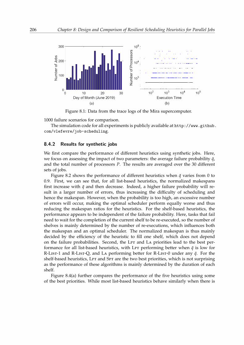
206 Chapter 8: Design and Comparison of Resilient Scheduling Heuristics for Parallel Jobs
(a) (b)
Figure 8.1: Data from the trace logs of the Mira supercomputer.
1000 failure scenarios for comparison.The simulation code for all experiments is publicly available at http://www.github.
com/vlefevre/job-scheduling.
8.4.2 Results for synthetic jobs
We first compare the performance of different heuristics using synthetic jobs. Here,we focus on assessing the impact of two parameters: the average failure probability q,and the total number of processors P. The results are averaged over the 30 differentsets of jobs.
Figure 8.2 shows the performance of different heuristics when q varies from 0 to0.9. First, we can see that, for all list-based heuristics, the normalized makespansfirst increase with q and then decrease. Indeed, a higher failure probability will re-sult in a larger number of errors, thus increasing the difficulty of scheduling andhence the makespan. However, when the probability is too high, an excessive numberof errors will occur, making the optimal scheduler perform equally worse and thusreducing the makespan ratios for the heuristics. For the shelf-based heuristics, theperformance appears to be independent of the failure probability. Here, tasks that failneed to wait for the completion of the current shelf to be re-executed, so the number ofshelves is mainly determined by the number of re-executions, which influences boththe makespan and an optimal scheduler. The normalized makespan is thus mainlydecided by the efficiency of the heuristic to fill one shelf, which does not dependon the failure probabilities. Second, the Lpt and La priorities lead to the best per-formance for all list-based heuristics, with Lpt performing better when q is low forR-List-1 and R-List-Q, and La performing better for R-List-0 under any q. For theshelf-based heuristics, Lpt and Spt are the two best priorities, which is not surprisingas the performance of these algorithms is mainly determined by the duration of eachshelf.
Figure 8.4(a) further compares the performance of the five heuristics using someof the best priorities. While most list-based heuristics behave similarly when there is
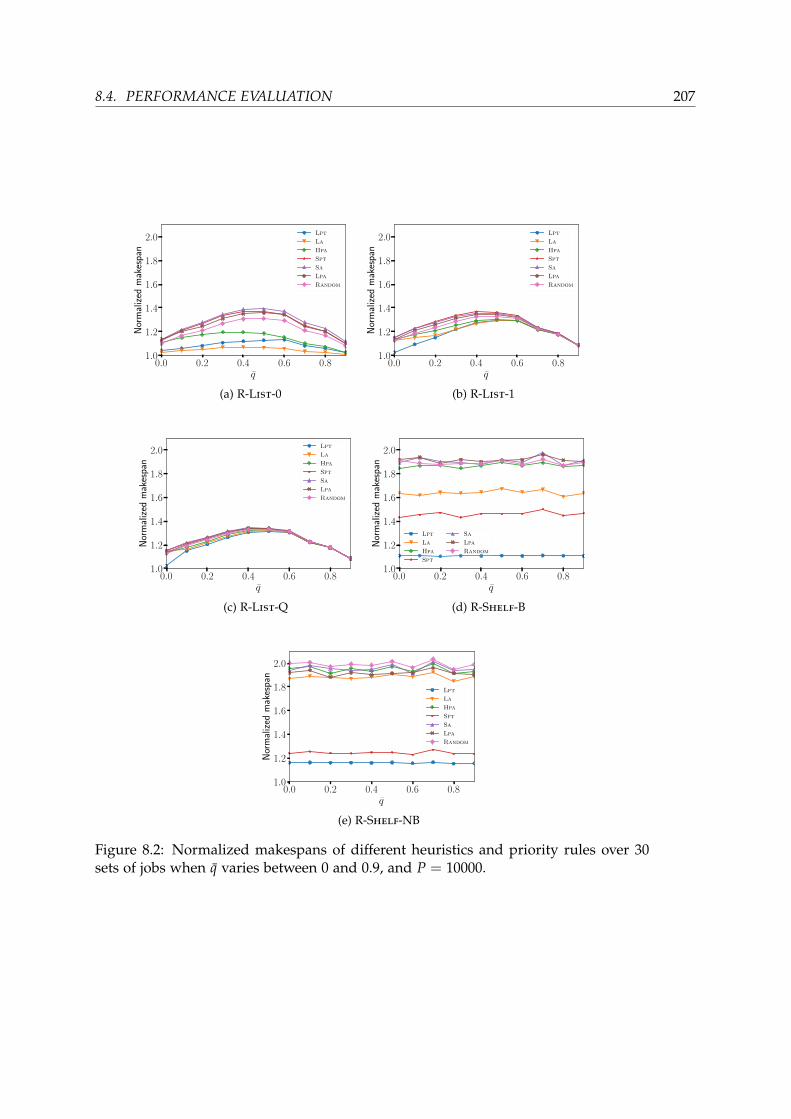
8.4. PERFORMANCE EVALUATION 207
0.0 0.2 0.4 0.6 0.8q
1.0
1.2
1.4
1.6
1.8
2.0
Nor
mal
ized
mak
espa
n
Lpt
La
Hpa
Spt
Sa
Lpa
Random
(a) R-List-0
0.0 0.2 0.4 0.6 0.8q
1.0
1.2
1.4
1.6
1.8
2.0
Nor
mal
ized
mak
espa
n
Lpt
La
Hpa
Spt
Sa
Lpa
Random
(b) R-List-1
0.0 0.2 0.4 0.6 0.8q
1.0
1.2
1.4
1.6
1.8
2.0
Nor
mal
ized
mak
espa
n
Lpt
La
Hpa
Spt
Sa
Lpa
Random
(c) R-List-Q
0.0 0.2 0.4 0.6 0.8q
1.0
1.2
1.4
1.6
1.8
2.0
Nor
mal
ized
mak
espa
n
Lpt
La
Hpa
Spt
Sa
Lpa
Random
(d) R-Shelf-B
0.0 0.2 0.4 0.6 0.8q
1.0
1.2
1.4
1.6
1.8
2.0
Nor
mal
ized
mak
espa
n
Lpt
La
Hpa
Spt
Sa
Lpa
Random
(e) R-Shelf-NB
Figure 8.2: Normalized makespans of different heuristics and priority rules over 30sets of jobs when q varies between 0 and 0.9, and P = 10000.

208 Chapter 8: Design and Comparison of Resilient Scheduling Heuristics for Parallel Jobs
5000 10000 15000 20000P
1.00
1.25
1.50
1.75
2.00
Nor
mal
ized
mak
espa
n
Lpt
La
Hpa
Spt
Sa
Lpa
Random
(a) R-List-0
5000 10000 15000 20000P
1.00
1.25
1.50
1.75
2.00
Nor
mal
ized
mak
espa
n
Lpt
La
Hpa
Spt
Sa
Lpa
Random
(b) R-List-1
5000 10000 15000 20000P
1.00
1.25
1.50
1.75
2.00
Nor
mal
ized
mak
espa
n
Lpt
La
Hpa
Spt
Sa
Lpa
Random
(c) R-List-Q
5000 10000 15000 20000P
1.00
1.25
1.50
1.75
2.00
Nor
mal
ized
mak
espa
n
Lpt
La
Hpa
Spt
Sa
Lpa
Random
(d) R-Shelf-B
5000 10000 15000 20000P
1.00
1.25
1.50
1.75
2.00
Nor
mal
ized
mak
espa
n
Lpt
La
Hpa
Spt
Sa
Lpa
Random
(e) R-Shelf-NB
Figure 8.3: Normalized makespans of different heuristics and priority rules over 30sets of jobs when P varies between 5000 and 20000, and q = 0.3.

8.4. PERFORMANCE EVALUATION 209
0.0 0.2 0.4 0.6 0.8q
1.0
1.2
1.4
1.6
Nor
mal
ized
mak
espa
n
R-List-0 / Lpt
R-List-0 / La
R-List-1 / Lpt
R-List-1 / La
R-List-Q / Lpt
R-List-Q / La
R-Shelf-B / Lpt
R-Shelf-NB / Lpt
(a)
5000 10000 15000 20000P
1.0
1.2
1.4
1.6
Nor
mal
ized
mak
espa
n
R-List-0 / Lpt
R-List-0 / La
R-List-1 / Lpt
R-List-1 / La
R-List-Q / Lpt
R-List-Q / La
R-Shelf-B / Lpt
R-Shelf-NB / Lpt
(b)
Figure 8.4: Comparison of different heuristics with the best priority rules Lpt and/orLa when: (a) q varies between 0 and 0.9, and P = 10000; and (b) P varies between 5000and 20000, and q = 0.3.
no failure (i.e., q = 0), R-List-0 clearly outperforms the rest when jobs can fail. Thiscorroborates the theoretical result that R-List-0 (i.e., Greedy) has the lowest approxi-mation ratio regardless of the priority rule and failure scenario. Moreover, R-List-0 isalso the heuristic that is least affected by job failures, with an increase in normalizedmakespan by less than 10% compared to the case of q = 0, while the other heuristicsexperience 20-30% increase in normalized makespan. Finally, R-Shelf-NB appears tobe the worst heuristic for small and high probabilities of failure with a makespan thatis up to 15% higher than that of R-List-0 (when q = 0.9), while R-List-Q is the worstfor medium probabilities (e.g., 26% higher than that of R-List-0 for q = 0.5). Theresults are likely due to: (i) the restriction of R-Shelf-NB for building shelves in aschedule, which leads to poor performance for some failure scenarios (such as the onediscussed in Section 8.3.3), and hence an increase in the expected makespan, and (ii)the fact that R-List-Q is more affected by the increasing failure probability.
Figure 8.3 shows the performance of different heuristics when the number of pro-cessors P varies from 5000 to 20000 while the failure probability is fixed at q = 0.3.Again, we can see that La and Lpt are the two best priority rules for all heuristics,with La performing better for R-List-0 and R-List-1, and Lpt performing better forother heuristics under all P. Also, the normalized makespans of the heuristics first in-crease with the number of processors and then tend to decrease. This is because whenP is either too small (i.e., total resource is constrained) or too big (i.e., total resource isalmost unconstrained), the optimal scheduler tends to have very similar performanceas the heuristics.
We further compare the performance of the five heuristics using some of the bestpriorities in Figure 8.4(b). As in the previous experiment, the best heuristic is R-List-0with the La priority, which is the least impacted by the total number of processors(with < 10% variations in normalized makespan). Also, R-List-Q gives the worstperformance (with a 23% increase in makespan compared to R-List-0 with La when

210 Chapter 8: Design and Comparison of Resilient Scheduling Heuristics for Parallel Jobs
Table 8.1: Performance of different heuristics using Lpt priority for all 30 days (sets)of jobs from June 2019 on the Mira supercomputer.
q Average#failures
Average makespan ratio Standard deviation Maximum makespan ratio
R-List R-Shelf R-List R-Shelf R-List R-Shelf
0 1 Q B NB 0 1 Q B NB 0 1 Q B NB
0 0 1.067 1.051 1.051 1.407 1.441 8.78× 10⁻² 8.19× 10⁻² 8.23× 10⁻² 1.29× 10⁻¹ 1.45× 10⁻¹ 1.425 1.425 1.425 1.633 1.760
0.05 15.2913 1.031 1.049 1.061 1.129 1.141 6.72× 10⁻² 6.87× 10⁻² 7.76× 10⁻² 1.30× 10⁻¹ 1.40× 10⁻¹ 1.278 1.292 1.292 1.489 1.510
0.1 254.453 1.016 1.025 1.028 1.071 1.073 4.66× 10⁻² 4.54× 10⁻² 4.97× 10⁻² 1.03× 10⁻¹ 1.06× 10⁻¹ 1.249 1.224 1.245 1.398 1.413
P = 15000) and has the largest variation (∼20%) in normalized makespan as thenumber of processors changes.
From these experiments, we can see that job failures and processor variations dohave an impact on the relative performance of different heuristics. Nevertheless, themakespans of all the heuristics (with good priorities) are never more than 40% worsethan the theoretical lower bound, which can be much less than the optimal makespan.The results suggest the robustness of these heuristics, and that they should actuallyperform really well in practice, even with job failures.
8.4.3 Results for jobs from Mira
We now evaluate the performance of different heuristics using real jobs from the Miratrace logs. Figures 8.5 and 8.6 show the normalized makespans of all heuristics andpriority rules under all 30 days (sets) of jobs with and without failures. We observethat the Lpt and La priorities again offer the best performance, with Lpt performingbetter this time for most job sets. This holds for every heuristic on average, especiallywhen there is no failure (i.e., q = 0). As the failure probability increases, both Lpt
and La (and even Hpa) give similar performance. The reason is that the processorallocations and execution times of the jobs in Mira are more skewed than those ofthe synthetic ones. Here, some jobs use a very large number of processors and havelong execution times, which make them fail more often even with small values of q.As a result, the makespan lower bound is largely determined by the total executiontimes of these jobs, thus any priority rule that favors these jobs will achieve similarperformance. Comparing different heuristics, we can see that R-List-0 again performsthe best and R-Shelf-B the worse, especially with higher failure probability (q = 0.1).This is consistent with the previous findings and corroborates the analysis.
Table 8.1 summarizes the results of the five heuristics using the Lpt priority (whichis overall the best one) over 30 days (sets) of jobs, which have an average of 157.63jobs per day (set). As q increases to 0.05 and 0.1, the average number of failuresrises to around 15 and 254, respectively. All list-based heuristics have good averagemakespan ratios that are very close to 1 (with low standard deviations), as well asgood maximum makespan ratios that are lower than 1.5, while the two shelf-basedheuristics have worse performance in comparison, even when failures are not present.The maximum makespans, however, are never more than 80% of the theoretical lowerbound. This again corroborates the results in Section 8.4.2.
Overall, these results confirm the efficacy and robustness of the resilient scheduling

8.4. PERFORMANCE EVALUATION 211
5 10 15 20 25 30
Set
1.0
1.2
1.4
1.6
1.8
Nor
mal
ized
mak
espa
n
0.0
0.0
0.0
0.0
0.0
0.0
0.0
0.0
0.0
0.0
0.0
0.0
0.0
0.0
0.0
0.0
0.0
0.0
0.0
0.0
0.0
0.0
0.0
0.0
0.0
0.0
0.0
0.0
0.0
0.0
Lpt
La
Hpa
Spt
Sa
Lpa
Random
(a) R-List-0 (with q = 0)
5 10 15 20 25 30
Set
1.0
1.1
1.2
1.3
1.4
1.5
Nor
mal
ized
mak
espa
n
4.75
14.
469
4.88
914
.002
5.71
922
.897
4.59
48.
429
4.88
913
.361
12.6
6111
.852
21.1
799.
105
18.0
1421
.772
6.25
411
.228
15.6
0416
.188
47.5
469.
337
10.2
4713
.155
59.2
9424
.504
11.3
9222
.481
16.6
9912
.228
Lpt
La
Hpa
Spt
Sa
Lpa
Random
(b) R-List-0 (with q = 0.05)
5 10 15 20 25 30
Set
1.0
1.1
1.2
1.3
1.4
Nor
mal
ized
mak
espa
n
11.0
7811
.546
11.8
5560
.598
22.9
7330
1.05
14.7
8355
.143
11.8
5558
.554
66.2
5364
.126
0.04
22.6
2911
8.37
614
4.57
314
.734
38.3
275
.687
44.8
7220
10.4
629
.393
24.6
7573
.006
3374
.84
296.
649
78.0
6525
3.00
952
.782
31.6
89
Lpt
La
Hpa
Spt
Sa
Lpa
Random
(c) R-List-0 (with q = 0.1)
5 10 15 20 25 30
Set
1.0
1.5
2.0
2.5
Nor
mal
ized
mak
espa
n
0.0
0.0
0.0
0.0
0.0
0.0
0.0
0.0
0.0
0.0
0.0
0.0
0.0
0.0
0.0
0.0
0.0
0.0
0.0
0.0
0.0
0.0
0.0
0.0
0.0
0.0
0.0
0.0
0.0
0.0
Lpt
La
Hpa
Spt
Sa
Lpa
Random
(d) R-List-1 (with q = 0)
5 10 15 20 25 30
Set
1.0
1.2
1.4
1.6
Nor
mal
ized
mak
espa
n
4.75
14.
469
4.88
914
.002
5.71
922
.897
4.59
48.
429
4.88
913
.361
12.6
6111
.852
21.1
799.
105
18.0
1421
.772
6.25
411
.228
15.6
0416
.188
47.5
469.
337
10.2
4713
.155
59.2
9424
.504
11.3
9222
.481
16.6
9912
.228
Lpt
La
Hpa
Spt
Sa
Lpa
Random
(e) R-List-1 (with q = 0.05)
5 10 15 20 25 30
Set
1.0
1.1
1.2
1.3
1.4
Nor
mal
ized
mak
espa
n
11.0
7811
.546
11.8
5560
.598
22.9
7330
1.05
14.7
8355
.143
11.8
5558
.554
66.2
5364
.126
0.04
22.6
2911
8.37
614
4.57
314
.734
38.3
275
.687
44.8
7220
10.4
629
.393
24.6
7573
.006
3374
.84
296.
649
78.0
6525
3.00
952
.782
31.6
89
Lpt
La
Hpa
Spt
Sa
Lpa
Random
(f) R-List-1 (with q = 0.1)
5 10 15 20 25 30
Set
1.0
1.5
2.0
2.5
Nor
mal
ized
mak
espa
n
0.0
0.0
0.0
0.0
0.0
0.0
0.0
0.0
0.0
0.0
0.0
0.0
0.0
0.0
0.0
0.0
0.0
0.0
0.0
0.0
0.0
0.0
0.0
0.0
0.0
0.0
0.0
0.0
0.0
0.0
Lpt
La
Hpa
Spt
Sa
Lpa
Random
(g) R-List-Q (with q = 0)
5 10 15 20 25 30
Set
1.0
1.2
1.4
1.6
1.8
Nor
mal
ized
mak
espa
n
4.75
14.
469
4.88
914
.002
5.71
922
.897
4.59
48.
429
4.88
913
.361
12.6
6111
.852
21.1
799.
105
18.0
1421
.772
6.25
411
.228
15.6
0416
.188
47.5
469.
337
10.2
4713
.155
59.2
9424
.504
11.3
9222
.481
16.6
9912
.228
Lpt
La
Hpa
Spt
Sa
Lpa
Random
(h) R-List-Q (with q = 0.05)
5 10 15 20 25 30
Set
1.0
1.1
1.2
1.3
1.4
1.5
Nor
mal
ized
mak
espa
n
11.0
7811
.546
11.8
5560
.598
22.9
7330
1.05
14.7
8355
.143
11.8
5558
.554
66.2
5364
.126
0.04
22.6
2911
8.37
614
4.57
314
.734
38.3
275
.687
44.8
7220
10.4
629
.393
24.6
7573
.006
3374
.84
296.
649
78.0
6525
3.00
952
.782
31.6
89
Lpt
La
Hpa
Spt
Sa
Lpa
Random
(i) R-List-Q (with q = 0.1)
Figure 8.5: Performance of list-based heuristics for 30 job sets using the Mira tracelogs (June 2019) with and without failures. Each row represents a different heuris-tic (R-List-0, R-List-1 and R-List-Q), and each column represents a different failureprobability (q = 0, q = 0.05 and q = 0.1). The average number of failures for each jobset is indicated on top of each plot.

212 Chapter 8: Design and Comparison of Resilient Scheduling Heuristics for Parallel Jobs
5 10 15 20 25 30
Set
1
2
3
4
5
6
7N
orm
aliz
edm
akes
pan
0.0
0.0
0.0
0.0
0.0
0.0
0.0
0.0
0.0
0.0
0.0
0.0
0.0
0.0
0.0
0.0
0.0
0.0
0.0
0.0
0.0
0.0
0.0
0.0
0.0
0.0
0.0
0.0
0.0
0.0
Lpt
La
Hpa
Spt
Sa
Lpa
Random
(a) R-Shelf-B (with q = 0)
5 10 15 20 25 30
Set
1.0
1.5
2.0
2.5
Nor
mal
ized
mak
espa
n
4.75
14.
469
4.88
914
.002
5.71
922
.897
4.59
48.
429
4.88
913
.361
12.6
6111
.852
21.1
799.
105
18.0
1421
.772
6.25
411
.228
15.6
0416
.188
47.5
469.
337
10.2
4713
.155
59.2
9424
.504
11.3
9222
.481
16.6
9912
.228
Lpt
La
Hpa
Spt
Sa
Lpa
Random
(b) R-Shelf-B (with q = 0.05)
5 10 15 20 25 30
Set
1.00
1.25
1.50
1.75
2.00
2.25
Nor
mal
ized
mak
espa
n
11.0
7811
.546
11.8
5560
.598
22.9
7330
1.05
14.7
8355
.143
11.8
5558
.554
66.2
5364
.126
0.04
22.6
2911
8.37
614
4.57
314
.734
38.3
275
.687
44.8
7220
10.4
629
.393
24.6
7573
.006
3374
.84
296.
649
78.0
6525
3.00
952
.782
31.6
89
Lpt
La
Hpa
Spt
Sa
Lpa
Random
(c) R-Shelf-B (with q = 0.1)
5 10 15 20 25 30
Set
1
2
3
4
5
6
7
Nor
mal
ized
mak
espa
n0.
00.
00.
00.
00.
00.
00.
00.
00.
00.
00.
00.
00.
00.
00.
00.
00.
00.
00.
00.
00.
00.
00.
00.
00.
00.
00.
00.
00.
00.
0
Lpt
La
Hpa
Spt
Sa
Lpa
Random
(d) R-Shelf-NB (with q = 0)
5 10 15 20 25 30
Set
1.0
1.5
2.0
2.5
Nor
mal
ized
mak
espa
n
4.75
14.
469
4.88
914
.002
5.71
922
.897
4.59
48.
429
4.88
913
.361
12.6
6111
.852
21.1
799.
105
18.0
1421
.772
6.25
411
.228
15.6
0416
.188
47.5
469.
337
10.2
4713
.155
59.2
9424
.504
11.3
9222
.481
16.6
9912
.228
Lpt
La
Hpa
Spt
Sa
Lpa
Random
(e) R-Shelf-NB (with q = 0.05)
5 10 15 20 25 30
Set
1.00
1.25
1.50
1.75
2.00
2.25
Nor
mal
ized
mak
espa
n
11.0
7811
.546
11.8
5560
.598
22.9
7330
1.05
14.7
8355
.143
11.8
5558
.554
66.2
5364
.126
0.04
22.6
2911
8.37
614
4.57
314
.734
38.3
275
.687
44.8
7220
10.4
629
.393
24.6
7573
.006
3374
.84
296.
649
78.0
6525
3.00
952
.782
31.6
89
Lpt
La
Hpa
Spt
Sa
Lpa
Random
(f) R-Shelf-NB (with q = 0.1)
Figure 8.6: Performance of shelf-based heuristics for 30 job sets using the Mira tracelogs (June 2019) with and without failures. Each row represents a different heuristic (R-Shelf-B and R-Shelf-NB), and each column represents a different failure probability(q = 0, q = 0.05 and q = 0.1). The average number of failures for each job set isindicated on top of each plot.
heuristics, not only for synthetic jobs, but also for real sets of jobs. In particular, boththeory and practice have suggested that R-List-0 is the best heuristic when silenterrors are present, and Lpt and La are the two best priorities for most cases. In allexperiments we have conducted, this heuristic achieves a makespan that is within afew percent of the lower bound on average, and never more than 50% in the worstcase.
8.5 Background and Related Work
This section describes the background of scheduling rigid parallel jobs and reviewssome related work.
8.5.1 Different scheduling flavors and strategies
Historically, scheduling parallel jobs comes in two flavors: if a job requests p proces-sors, either any subset of p processors can be assigned, or only subsets of p contiguousprocessors can be chosen. In the latter case, processors are organized as a linear ar-ray and labeled from 1 to P, where P is the total number of processors; then only
8.5. BACKGROUND AND RELATED WORK 213
neighboring processors (whose labels differ by one) can be assigned to a job. The con-tiguous variant is equivalent to the rectangle strip packing problem, where rectangles areto be stacked (without rotation) within a strip of width P: rectangle widths representprocessor numbers, and rectangle heights represent execution times.
Most scheduling strategies also come in two flavors: either the schedule is re-stricted to building shelves (also referred to as levels in some literature), or it is unre-stricted, in which case the jobs are often scheduled based on an ordered list. Shelvesare subsets of jobs with the same starting time, and for which each of the P proces-sors is used at most once: the height of a shelf is the length of its longest job; whenthe shorter jobs complete, their processors become idle, but these processors are notreassigned to other jobs until the completion of the longest job of the shelf. Thus, ashelf resembles a bookshelf, hence the name. Shelf-based schedules play an importantrole in HPC, because they correspond to batched execution scenarios, where jobs aregrouped into batches that are scheduled one after another. Note that for shelf-basedalgorithms, the contiguous and non-contiguous variants collapse.
8.5.2 Offline scheduling of rigid jobs
To minimize the makespan for a set of rigid jobs that are known statically and availableinitially (i.e., offline), the problem is obviously NP-complete, as it generalizes the prob-lem of scheduling independent jobs on two processors, a variant of the 2-PARTITIONproblem [89]. Coffman et al. [53] showed that the Next-Fit Decreasing Height (NFDH)algorithm is 3-approximation, and the First-Fit Decreasing-Height (FFDH) algorithm is2.7-approximation. Both algorithms are shelf-based. See the survey by Lodi et al. [132]for more results and lower bounds on the best possible approximation ratio for shelf-based algorithms, and see Han et al. [100] for the intricate relationship between strippacking and bin packing.
For list-based scheduling, Baker et al. [13] showed that the Bottom-up Left-justified(BL) heuristic while ordering the jobs in decreasing processor requirement achieves3-approximation. Turek et al. [184] showed that ordering jobs in decreasing execu-tion time is also 3-approximation. Moreover, both algorithms guarantee contiguousprocessor allocations for all jobs. Without the contiguous processor constraint, sev-eral works [88, 184, 81] showed that the greedy list-scheduling heuristic achieves 2-approximation. Finally, Jansen [114] presented a (3/2 + ε)-approximation algorithmfor any fixed ε > 0. This is the best result possible, since a lower bound on theapproximation ratio is 3/2, which holds even when considering asymptotic perfor-mance [116].
8.5.3 Online scheduling of rigid jobs
In the online problem, a set of rigid jobs arrive dynamically over time and informationof a job is not known until the job has arrived. In this case, the list-based greedyalgorithm maintains a competitive ratio of 2 [144, 116]. Chen and Vestjens [48] showeda 1.3473 lower bound on the competitive ratio of any deterministic online algorithm

214 Chapter 8: Design and Comparison of Resilient Scheduling Heuristics for Parallel Jobs
even when all jobs are sequential. Shmoys et al. [163] showed that by collecting alljobs that arrive during a batch and then scheduling them together in the next batch,one can transform any c-approximation offline algorithm into a 2c-competitive onlinealgorithm. We point out that this technique, however, does not apply to the modelconsidered in this chapter, because it relies on jobs having fixed, although unknown,release times, whereas the “new job arrivals” in our model (corresponding to failedjobs restarting) depend on the decisions made on-the-fly by the schedulers.
8.5.4 Batch schedulers in practical systems
In practical systems, parallel jobs are often scheduled by batch schedulers [113, 199,171] that use a combination of reservation and backfilling strategies: while high-priorityjobs are scheduled by reserving processors in advance, low-priority ones are used tofill in the “holes” to improve system utilization. Two popular backfilling strategies areconservative [142] and aggressive (a.k.a. EASY) [129, 168]. The former gives a reserva-tion for every job in the queue, and a lower-priority job is moved forward as long as itdoes not delay the reservation for any higher-priority job. The latter only gives reser-vation to the job at the head of the queue (i.e., the one with the highest priority), andbackfilling is allowed without delaying this highest-priority job. As jobs arrive overtime, most practical schedulers use First-Come First-Serve (FCFS) in conjunction withthese strategies to prevent job starvation, but no worst-case performance guaranteeis known. Various priority rules have been empirically evaluated to characterize andtune their performance for different metrics (e.g., [170, 193, 90]).
8.6 Conclusion
In this chapter, we have investigated the problem of scheduling rigid jobs onto a par-allel platform subject to silent errors. We have revisited the classical scheduling al-gorithms in this new framework, where jobs that have been struck by errors must bere-executed (possibly many times) until success. We designed resilient list-based andshelf-based scheduling heuristics, along with different priority rules and backfillingstrategies. On the theoretical side, we proved that variants of the list-based heuris-tic achieve a constant approximation ratio (2 or 3 depending whether reservation isused or not). We also showed that any shelf-based heuristic is no longer a constant-factor approximation, while a failure-free variant was known to be a 3-approximation.Extensive simulations conducted using both synthetic jobs and real traces from theMira supercomputer demonstrate that these heuristics are quite robust, and achievemakespans close to the optimal. As highlighted by the theoretical analysis, the beststrategy remains the unrestricted greedy list-based scheduling with no reservations,and good results are obtained in practice when job priorities are assigned by process-ing times (favoring jobs with long execution times) or by areas (favoring jobs withmany processors and/or long execution times).
8.6. CONCLUSION 215
Some problems remain open, in particular for the study of shelf-based algorithms,whose expected makespan under the Exponential probability distribution is not knownto be bounded by a constant factor of the optimal or not. A natural extension of thiswork would be to consider moldable jobs, whose processor allocations can be de-cided at launch time. However, for jobs with nonlinear speedup curves, changing thenumber of processors assigned to a job also changes its error probability under theExponential probability distribution, thereby severely complicating the problem, andthus calling for the design of novel heuristics.


Chapter 9
I/O scheduling strategy for periodic applica-tions
With the ever-growing need of data in HPC applications, the congestion at the I/Olevel becomes critical in supercomputers. Architectural enhancement such as burstbuffers and pre-fetching are added to machines, but are not sufficient to prevent con-gestion. Recent online I/O scheduling strategies have been put in place, but they addan additional congestion point and overheads in the computation of applications.
In this work, we show how to take advantage of the periodic nature of HPC ap-plications in order to develop efficient periodic scheduling strategies for their I/Otransfers. Our strategy computes once during the job scheduling phase a patternwhich defines the I/O behavior for each application, after which the applications runindependently, performing their I/O at the specified times. Our strategy limits theamount of congestion at the I/O node level and can be easily integrated into currentjob schedulers. We validate this model through extensive simulations and experi-ments on an HPC cluster by comparing it to state-of-the-art online solutions, showingthat not only does our scheduler have the advantage of being de-centralized and thusovercoming the overhead of online schedulers, but also that it performs better thanthe other solutions, improving the application dilation up to 16% and the maximumsystem efficiency up to 18%. The work in this chapter is joint work with GuillaumePallez and Ana Gainaru, and has been published in Transactions on Parallel Computing(TOPC) [J2].
9.1 Introduction
Nowadays, supercomputing applications create or process TeraBytes of data. Thisis true in all fields: for example LIGO (gravitational wave detection) generates1500TB/year [126], the Large Hadron Collider generates 15PB/year, light sourceprojects deal with 300TB of data per day and climate modeling are expected to haveto deal with 100EB of data [102].
Management of I/O operations is critical at scale. However, observations on the
217
218 Chapter 9: I/O scheduling strategy for periodic applications
Intrepid machine at Argonne National Lab show that I/O transfer can be slowed downup to 70% due to congestion [85]. For instance, when Los Alamos National Labora-tory moved from Cielo to Trinity, the peak performance moved from 1.4 Petaflops to40 Petaflops (×28) while the I/O bandwidth moved to 160 GB/s to 1.45TB/s (only×9) [124]. The same kind of results can be observed at Argonne National Labora-tory when moving from Intrepid (0.6 PF, 88 GB/s) and to Mira (10PF, 240 GB/s).While both peak performance and peak I/O improve, the reality is that I/O through-put scales worse than linearly compared to performance, and hence, what should benoticed is a downgrade from 160 GB/PFlop (Intrepid) to 24 GB/PFlop (Mira).
With this in mind, to be able to scale, the conception of new algorithms has tochange paradigm: going from a compute-centric model to a data-centric model.
To help with the ever growing amount of data created, architectural improvementssuch as burst buffers [130, 9] have been added to the system. Work is being done totransform the data before sending it to the disks in the hope of reducing the I/O [65].However, even with the current I/O footprint burst buffers are not able to completelyhide I/O congestion. Moreover, the data used is always expected to grow. Recentworks [85] have started working on novel online, centralized I/O scheduling strategiesat the I/O node level. However, one of the risks noted on these strategies is thescalability issue caused by potentially high overheads (between 1 and 5% dependingon the number of nodes used in the experiments) [85]. Moreover, it is expected thatthis overhead will increase at larger scale since it need centralized information aboutall applications running in the system.
In this chapter, we present a decentralized I/O scheduling strategy for supercom-puters. We show how to take known HPC application behaviors (namely their peri-odicity) into account to derive novel static scheduling algorithms. This chapter is anextended version of our previous work [W2]. We improve the main algorithm witha new loop aiming at correcting the size of the period at the end. We also added adetailed complexity analysis and more simulations on synthetic applications to showthe wide applicability of our solution. Overall we consider that close to 50% of thetechnical content is new material.
Periodic Applications Many recent HPC studies have observed independent patternsin the I/O behavior of HPC applications. The periodicity of HPC applications hasbeen well observed and documented [43, 66, 85, 108]: HPC applications alternatebetween computation and I/O transfer, this pattern being repeated over-time. Carnset al. [43] observed with Darshan [43] the periodicity of four different applications(MADBench2 [44], Chombo I/O benchmark [54], S3D IO [157] and HOMME [143]).Furthermore, in a previous work [85], the authors were able to verify the periodicity ofgyrokinetic toroidal code (GTC) [77], Enzo [36], HACC application [96] and CM1 [35].Furthermore, fault-tolerance techniques (such as periodic checkpointing [58, 105]) alsoadd to this periodic behavior.
The key idea in this project is to take into account those known structural behaviorsof HPC applications and to include them in scheduling strategies.

9.1. INTRODUCTION 219
Using this periodicity property, we compute a static periodic scheduling strategy(introduced in our previous work [W2]), which provides a way for each application toknow when it should start transferring its I/O (i) hence reducing potential bottlenecksdue to I/O congestion, and (ii) without having to consult with I/O nodes every timeI/O should be done and hence adding an extra overhead. The main contributions ofthis chapter are:
• A novel light-weight I/O algorithm that looks at optimizing both application-oriented and platform-oriented objectives;
• The full details of this algorithm and its implementation along with the fullcomplexity analysis;
• A set of extensive simulations and experiments that show that this algorithmperforms as well or better than current state of the art heavy-weight online algo-rithms.
• More simulations to show the performance at scale and a full evaluation to un-derstand how each parameter of the algorithm impacts its performance
Of course, not all applications exhibit a perfect periodic behavior, but based on ourexperience, many of the HPC scientific applications have this property. This work ispreliminary in the sense that we are offering a proof of concept in this chapter and weplan to tackle more complex patterns in the future. In addition, future research willbe done for including dynamic schedules instead of only relying on static schedules.This work aims at being the basis of a new class of data-centric scheduling algorithmsbased on well-know characteristics of HPC applications.
The algorithm presented here is done as a proof of concept to show the efficiency ofthese light-weight techniques. We believe our scheduler can be implemented naturallyinto a data scheduler (such as Clarisse [112]) and we provide experimental resultsbacking this claim. We also give hints of how this could be naturally coupled with non-periodic applications. However, this integration is beyond the scope of this chapter.For the purpose of this chapter the applications are already scheduled on the systemand are able to receive information about their I/O scheduling. The goal of our I/Oscheduler is to eliminate congestion points caused by application interference whilekeeping the overhead seen by all applications to the minimum. Computing a fullI/O schedule over all iterations of all applications is not realistic at today’s scale. Theprocess would be too expensive both in time and space. Our scheduler overcomes thisby computing a period of I/O scheduling that includes different number of iterationsfor each application.
The rest of the chapter is organized as follows: in Section 9.2 we present the appli-cation model and optimization problem. In Section 9.3 we present our novel algorithmtechnique as well as a brief proof of concept for a future implementation. In Section 9.4we present extensive simulations based on the model to show the performance of ouralgorithm compared to state of the art. We then confirm the performance by perform-ing experiments on a supercomputer to validate the model. We give some backgroundand related work in Section 9.5. We provide concluding remarks and ideas for futureresearch directions in Section 9.6.

220 Chapter 9: I/O scheduling strategy for periodic applications
b=0.1Gb/s/Node
=B
Figure 9.1: Model instantiation for Intrepid [85].
9.2 Model
In this section we use the model introduced in the previous work [85] that has beenverified experimentally to be consistent with the behavior of Intrepid and Mira, super-computers at Argonne.
We consider scientific applications running at the same time on a parallel platform.The applications consist of series of computations followed by I/O operations. On asupercomputer, the computations are done independently because each applicationuses its own nodes. However, the applications are concurrently sending and receivingdata during their I/O phase on a dedicated I/O network. The consequence of this I/Oconcurrency is congestion between an I/O node of the platform and the file storage.
9.2.1 Parameters
We assume that we have a parallel platform made up of N identical unit-speed nodes,composed of the same number of identical processors, each equipped with an I/Ocard of bandwidth b (expressed in bytes per second). We further assume having acentralized I/O system with a total bandwidth B (also expressed in bytes per second).This means that the total bandwidth between the computation nodes and an I/O nodeis N · b while the bandwidth between an I/O node and the file storage is B, withusually N · b B. We have instantiated this model for the Intrepid platform onFigure 9.1.
We have K applications, all assigned to independent and dedicated computationalresources, but competing for I/O. For each application App(k) we define:
• Its size: App(k) executes with β(k) dedicated processors;• Its pattern: App(k) obeys a pattern that repeats over time. There are n(k)
tot instancesof App(k) that are executed one after the other. Each instance consists of twodisjoint phases: computations that take a time w(k), followed by I/O transfers fora total volume vol(k)io . The next instance cannot start before I/O operations forthe current instance are terminated.
We further denote by rk the time when App(k) is executed on the platform and dk the

9.2. MODEL 221
App(1) w(1) w(1) w(1)
App(2) w(2) w(2) w(2)App(3) w(3) w(3) w(3)
Bandwidth
Time00
B
Figure 9.2: Scheduling the I/O of three periodic applications (top: computation, bot-tom: I/O).
time when the last instance is completed. Finally, we denote by γ(k)(t), the bandwidthused by a node on which application App(k) is running, at instant t. For simplicity weassume just one I/O transfer in each loop. However, our model can be extended towork with multiple I/O patterns as long as these are periodic in nature or as long asthey are known in advance. In addition, our scheduler can complement I/O prefetch-ing mechanisms like [38, 103] that use the regular patterns within each data access(contiguous/non-contiguous, read or write, parallel or sequential, etc) to avoid con-gestion.
9.2.2 Execution Model
As the computation resources are dedicated, we can always assume without loss ofgenerality that the next computation chunk starts immediately after completion ofthe previous I/O transfers, and is executed at full (unit) speed. On the contrary, allapplications compete for I/O, and congestion will likely occur. The simplest case isthat of a single periodic application App(k) using the I/O system in dedicated modeduring a time-interval of duration D. In that case, let γ be the I/O bandwidth used byeach processor of App(k) during that time-interval. We derive the condition β(k)γD =
vol(k)io to express that the entire I/O data volume is transferred. We must also enforcethe constraints that (i) γ ≤ b (output capacity of each processor); and (ii) β(k)γ ≤ B(total capacity of I/O system). Therefore, the minimum time to perform the I/O
transfers for an instance of App(k) is time(k)io =vol(k)io
min(β(k)b,B). However, in general many
applications will use the I/O system simultaneously, and the bandwidth capacity Bwill be shared among all applications (see Figure 9.2). Scheduling application I/Owill guarantee that the I/O network will not be loaded with more than its designedcapacity. Figure 9.2 presents the view of the machine when 3 applications are sharingthe I/O system. This translates at the application level to delays inserted before I/Obursts (see Figure 9.3 for application 2’s point of view).
This model is very flexible, and the only assumption is that at any instant, allprocessors assigned to a given application are assigned the same bandwidth. This

222 Chapter 9: I/O scheduling strategy for periodic applications
App(2) w(2) IO D IO w(2) IO w(2) IOBandwidth
Time
Figure 9.3: Application 2 execution view (D represents the delay in I/O operations)
assumption is transparent for the I/O system and simplifies the problem statementwithout being restrictive. Again, in the end, the total volume of I/O transfers for aninstance of App(k) must be vol(k)io , and at any instant, the rules of the game are simple:never exceed the individual bandwidth b of each processor (γ(k)(t) ≤ b for any k and
t), and never exceed the total bandwidth B of the I/O system (K∑
k=1β(k)γ(k)(t) ≤ B for
any t).
9.2.3 Objectives
We now focus on the optimization objectives at hand. We use the objectives introducedin [85].
First, the application efficiency achieved for each application App(k) at time t is de-fined as
ρ(k)(t) =∑i≤n(k)(t) w(k,i)
t− rk,
where n(k)(t) ≤ n(k)tot is the number of instances of application App(k) that have been
executed at time t, since the release of App(k) at time rk. Because we execute w(k,i)
units of computation followed by vol(k,i)io units of I/O operations on instance I (k)i of
App(k), we have t− rk ≥ ∑i≤n(k)(t)
(w(k,i) + time(k,i)
io
). Due to I/O congestion, ρ(k) never
exceeds the optimal efficiency that can be achieved for App(k), namely
ρ(k) =w(k)
w(k) + time(k)io
The two key optimization objectives, together with a rationale for each of them,are:
• SysEff: maximize the peak performance of the platform, namely maximizing theamount of operations per time unit:
maximize1N
K
∑k=1
β(k)ρ(k)(dk). (9.1)
The rationale is to squeeze the most flops out of the platform aggregated com-putational power. We say that this objective is CPU-oriented, as the schedule

9.3. PERIODIC SCHEDULING STRATEGY 223
will give priority to compute-intensive applications with large w(k)and smallvol(k)io values.
• Dilation: minimize the largest slowdown imposed to each application (henceoptimizing fairness across applications):
minimize maxk=1..K
ρ(k)
ρ(k)(dk). (9.2)
The rationale is to provide more fairness across applications and corresponds tothe stretch in classical scheduling: each application incurs a slowdown factor dueto I/O congestion, and we want the largest slowdown factor to be kept minimal.We say that this objective is user-oriented, as it gives each application a guaranteeon the relative rate at which the application will progress.
We can now define the optimization problem:
Definition 1 (Periodic [85]). We consider a platform of N processors, a set of applications∪K
k=1(App(k), β(k), w(k), vol(k)io ), a maximum period Tmax, we want to find a periodic scheduleP of period T ≤ Tmax, in order to optimize one of the following objectives:
1. SysEff
2. Dilation
Note that it is known that both problems are NP-complete, even in an (easier)offline setting [85].
9.3 Periodic scheduling strategy
In general, for an application App(k), n(k)tot the number of instances of App(k) is very
large and not polynomial in the size of the problem. For this reason, online scheduleshave been preferred until now. The key novelty of this chapter is to introduce periodicschedules for the K applications. Intuitively, we are looking for a computation and I/Opattern of duration T that will be repeated over time (except for initialization and cleanup phases), as shown on Figure 9.4a. In this section, we start by introducing the notionof periodic schedule and a way to compute the application efficiency differently. Wethen provide the algorithms that are at the core of this work.
Because there is no competition on computation (no shared resources), we canconsider that a chunk of computation directly follows the end of the I/O transfer,hence we need only to represent I/O transfers in this pattern. The bandwidth usedby each application during the I/O operations is represented over time, as shown inFigure 9.4b. We can see that an I/O operation can overlap with the previous patternor the next pattern, but overall, the pattern will just repeat.
To describe a pattern, we use the following notations:• n(k)
per: the number of instances of App(k) during a pattern.

224 Chapter 9: I/O scheduling strategy for periodic applications
Bw
Time
Init
· · ·
Pattern Clean up
c T+c 2T+c 3T+c (n−2)T+c (n−1)T+c nT+c
(a) Periodic schedule (phases)
Bw
Time00
T
B
vol(1)io vol(1)io vol(1)io
vol(2)io vol(2)io vol(2)iovol(3)io vol(3)iovol(4)io
initW(4)1endW(4)1 initIO(4)1
(b) Detail of I/O in a period/pattern
Figure 9.4: A schedule (above), and the detail of one of its regular pattern (below),where (w(1) = 3.5; vol(1)io = 240; n(1)
per = 3), (w(2) = 27.5; vol(2)io = 288; n(2)per = 3), (w(3) =
90; vol(3)io = 350; n(3)per = 1), (w(4) = 75; vol(4)io = 524; n(4)
per = 1), and c is the duration ofthe initilization phase.
• I (k)i : the i-th instance of App(k) during a pattern.
• initW(k)i : the time of the beginning of I (k)i . So, I (k)i has a computation interval
going from initW(k)i to endW(k)i = initW(k)i + w(k) mod T.
• initIO(k)i : the time when the I/O transfer from the i-th instance of App(k) starts
(between endW(k)i and initIO(k)i , App(k) is idle). Therefore, we have
∫ initW(k)(i+1)%n(k)per
initIO(k)i
β(k)γ(k)(t)dt = vol(k)io .
Globally, if we consider the two instants per instance initW(k)i and initIO(k)i , thatdefine the change between computation and I/O phases, we have a total of S ≤∑K
k=1 2n(k)per distinct instants, that are called the events of the pattern.
We define the periodic efficiency of a pattern of size T:
ρ(k)per =
n(k)perw(k)
T. (9.3)
For periodic schedules, we use it to approximate the actual efficiency achieved for eachapplication. The rationale behind this can be seen in Figure 9.4. If App(k) is releasedat time rk, and the first pattern starts at time rk + c, that is after an initialization phaseof duration c, then the main pattern is repeated n times (until time n · T + rk + c),
9.3. PERIODIC SCHEDULING STRATEGY 225
and finally App(k) ends its execution after a clean-up phase of duration c′ at timedk = rk + c + n · T + c′. If we assume that n · T c + c′, then dk − rk ≈ n · T. Then thevalue of the ρ(k)(dk) for App(k) is:
ρ(k)(dk) =
(n · n(k)
per + δ)
w(k)
dk − rk=
(n · n(k)
per + δ)
w(k)
c + n · T + c′
≈ n(k)perw(k)
T= ρ
(k)per
where δ can be 1 or 0 depending whether App(k) was executed or not during theclean-up or init phase.
9.3.1 PerSched: a periodic scheduling algorithm
For details in the implementation, we refer the interested reader to the source code availableat [83].
The difficulties of finding an efficient periodic schedule are three-fold:• The right pattern size has to be determined;• For a given pattern size, the number of instances of each application that should
be included in this pattern need to be determined;• The time constraint between two consecutive I/O transfers of a given application,
due to the computation in-between makes naive scheduling strategies harder toimplement.
Finding the right pattern size A solution is to find schedules with different patternsizes between a minimum pattern size Tmin and a maximum pattern size Tmax.
Because we want a pattern to have at least one instance of each application, wecan trivially set up Tmin = maxk(w(k) + time(k)io ). Intuitively, the larger Tmax is, themore possibilities we can have to find a good solution. However this also increasesthe complexity of the algorithm. We want to limit the number of instances of allapplications in a schedule. For this reason we chose to have Tmax = O(maxk(w(k) +
time(k)io )). We discuss this hypothesis in Section 9.4, where we give better experimentalintuition on finding the right value for Tmax. Experimentally we observe (Section 9.4,Figure 9.11) that Tmax = 10Tmin seems to be sufficient.
We then decided on an iterative search where the pattern size increases exponen-tially at each iteration from Tmin to Tmax. In particular, we use a precision ε as inputand we iteratively increase the pattern size from Tmin to Tmax by a factor (1 + ε). Thisallows us to have a polynomial number of iterations. The rationale behind the ex-ponential increase is that when the pattern size gets large, we expect performance toconverge to an optimal value, hence needing less the precision of a precise pattern size.Furthermore while we could try only large pattern sizes, it seems important to finda good small pattern size as it simplifies the scheduling step. Hence a more precisesearch for smaller pattern sizes. Finally, we expect the best performance to cycle with

226 Chapter 9: I/O scheduling strategy for periodic applications
the pattern size. We verify these statements experimentally in Section 9.4 (Figure 9.10).Determining the number of instances of each application By choosing Tmax = O(maxk(w(k)+
time(k)io )), we guarantee the maximum number of instances of each application that fit
into a pattern is O(
maxk(w(k)+time(k)io )
mink(w(k)+time(k)io )
).
Instance scheduling Finally, our last item is, given a pattern of size T, how to sched-ule instances of applications into a periodic schedule.
To do this, we decided on a strategy where we insert instances of applications ina pattern, without modifying dates and bandwidth of already scheduled instances.Formally, we call an application schedulable:
Definition 2 (Schedulable). Given an existing pattern
P = ∪Kk=1
(n(k)
per ,∪n(k)per
i=1initW(k)i , initIO(k)i , γ(k)())
, we say that an application App(k) is
schedulable if there exists 1 ≤ i ≤ n(k)per , such that:
∫ initIO(k)i −w(k)
initW(k)i +w(k)min
(β(k)b, B−∑
lβ(l)γ(l)(t)
)dt ≥ vol(k)io (9.4)
To understand Equation (9.4): we are checking that during the end of the compu-tation of the ith instance (initW(k)i + w(k)), and the beginning of the computation of thei + 1th instance to be, there is enough bandwidth to perform at least a volume of I/Oof vol(k)io . Indeed if a new instance is inserted, initIO(k)i −w(k) would then become thebeginning of computation of the i + 1th instance. Currently it is just some time beforethe I/O transfer of the ith instance. We represent it graphically on Figure 9.5.
Bw
Time00
B
vol(1)io 1 vol(1)io 2
vol(2)io 1 vol(2)io 2 vol(2)io 3
vol(3)io
initW(2)2 +w(2) initIO(2)2 −w(2)
Figure 9.5: Graphical description of Definition 2: two instances of App(1) and App(2)
are already scheduled. To insert a third instance of App(2), we need to check that theblue area is greater than vol(2)io with the bandwidth constraint (because an instance ofApp(1) is already scheduled, the bandwidth is reduced for the new instance of App(2)).The red area is off limit for I/O (used for computations).
With Definition 2, we can now explain the core idea of the instance scheduling part

9.3. PERIODIC SCHEDULING STRATEGY 227
of our algorithm. Starting from an existing pattern, while there exist applications thatare schedulable:
• Amongst the applications that are schedulable, we choose the application thathas the worst Dilation. The rationale is that even though we want to increaseSysEff, we do it in a way that ensures that all applications are treated fairly;
• We insert the instance into an existing scheduling using a procedure Insert-In-Pattern such that (i) the first instance of each application is inserted usingprocedure Insert-First-Instance which minimizes the time of the I/O transferof this new instance, (ii) the other instances are inserted just after the last insertedone.
Note that Insert-First-Instance is implemented using a water-filling algorithm [86]and Insert-In-Pattern is implemented as described in Algorithm 5 below. We use adifferent function for the first instance of each application because we do not have anyprevious instance to use the Insert-In-Pattern function. Thus, the basic idea wouldbe to put them at the beginning of the pattern, but it will be more likely to createcongestion if all applications are “synchronized” (for example if all the applicationsare the same, they will all start their I/O phase at the same time). By using Insert-First-Instance, every first instance will be at a place where the congestion for it isminimized. This creates a starting point for the subsequent instances.
The function addInstance updates the pattern with the new instance, given a listof the intervals (El , El′ , bl) during which App(k) transfers I/O between El and El′ usinga bandwidth bl .
Correcting the period size In Algorithm 6, the pattern sizes evaluated are determinedby Tmin and ε. There is no reason why this would be the right pattern size, and onemight be interested in reducing it to fit precisely the instances that are included in thesolutions that we found.
In order to do so, once a periodic pattern has been computed, we try to improvethe best pattern size we found in the first loop of the algorithm, by trying new patternsizes, close to the previous best one, Tcurr. To do this, we add a second loop whichtries 1/ε uniformly distributed pattern sizes from Tcurr to Tcurr/(1 + ε).
With all of this in mind, we can now write PerSched (Algorithm 6), our algorithmto construct a periodic pattern. For all pattern sizes tried between Tmin and Tmax, wereturn the pattern with maximal SysEff.
9.3.2 Complexity analysis
In this section we show that our algorithm runs in reasonable execution time. Wedetail theoretical results that allowed us to reduce the complexity. We want to showthe following result:
Theorem 11. Let nmax =
(maxk(w(k)+time(k)io )
mink(w(k)+time(k)io )
),
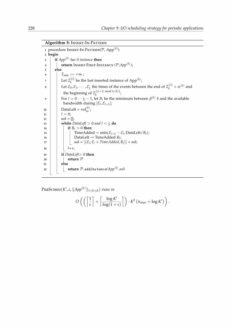
228 Chapter 9: I/O scheduling strategy for periodic applications
Algorithm 5: Insert-In-Pattern
1 procedure Insert-In-Pattern(P , App(k))2 begin3 if App(k) has 0 instance then4 return Insert-First-Instance (P ,App(k));5 else6 Tmin := +∞ ;
7 Let Iik be the last inserted instance of App(k);
8 Let E0, E1, · · · , Eji the times of the events between the end of Iik + w(k) and
the beginning of I(i+1) mod lT(k)k ;
9 For l = 0 · · · ji − 1, let Bl be the minimum between β(k) b and the availablebandwidth during [El , El+1];
10 DataLeft = vol(k)io ;11 l = 0;12 sol = [];13 while DataLeft > 0 and l < ji do14 if Bl > 0 then15 TimeAdded = min(El+1 − El , DataLeft/Bl);16 DataLeft -= TimeAdded·Bl ;17 sol = [(El , El + TimeAdded, Bl)] + sol;
18 l++;
19 if DataLeft> 0 then20 return P21 else22 return P .addInstance(App(k),sol)
PerSched(K′, ε, App(k)1≤k≤K) runs in
O((⌈
1ε
⌉+
⌈log K′
log(1 + ε)
⌉)· K2 (nmax + log K′
)).

9.3. PERIODIC SCHEDULING STRATEGY 229
Algorithm 6: Periodic Scheduling heuristic: PerSched
1 procedure PerSched(K′, ε, App(k)1≤k≤K)2 begin3 Tmin ← maxk(w(k) + time(k)io );4 Tmax ← K′ · Tmin;5 T = Tmin;6 SE← 0;7 Topt ← 0;8 Popt ← ;9 while T ≤ Tmax do
10 P = ;11 while exists a schedulable application do12 A = App(k)|App(k) is schedulable;13 Let App(k) be the element of A minimal with respect to the lexicographic
order(
ρ(k)
ρ(k)per
, w(k)
time(k)io
);
14 P←Insert-In-Pattern(P , App(k));
15 if SE < SysEff(P) then16 SE← SysEff(P);17 Topt ← T;18 Popt ← P19 T ← T · (1 + ε);
20 T ← Topt;21 while true do22 P = ;23 while exists a schedulable application do24 A = App(k)|App(k) is schedulable;25 Let App(k) be the element of A minimal with respect to the lexicographic
order(
ρ(k)
ρ(k)per
, w(k)
time(k)io
);
26 P←Insert-In-Pattern(P , App(k));
27 if SysEff(P) = ToptT · SE then
28 Popt ← P ;
29 T ← T − (Topt − Topt1+ε )/b1/εc
30 else31 return Popt
We estimate SysEff of a periodic pattern, by replacing ρ(k)(dk) by ρ(k)per in Equation (9.1)

230 Chapter 9: I/O scheduling strategy for periodic applications
Some of the complexity results are straightforward. The key results to show are:
• The complexity of the tests “while exists a schedulable application” on lines 11and 23
• The complexity of computing A and finding its minimum element on line 13and 25.
• The complexity of Insert-In-Pattern
To reduce the execution time, we proceed as follows: instead of implementing theset A, we implement a heap A that could be summarized as
App(k)|App(k) is not yet known to not be schedulable
sorted following the lexicographic order:(
ρ(k)
ρ(k)per
, w(k)
time(k)io
). Hence, we replace the while
loops on lines 11 and 23 by the algorithm snippet described in Algorithm 7. The ideais to avoid calling Insert-In-Pattern after each new inserted instance to know whichapplications are schedulable.
Algorithm 7: Schedulability snippet
11 A = ∪kApp(k) (sorted by(
ρ(k)
ρ(k)per
, w(k)
time(k)io
));
12 while A 6= ∅ do13 Let App(k) be the minimum element of A;14 A ← A \ App(k);15 Let P ′ =Insert-In-Pattern(P , App(k));16 if P ′ 6= P then17 P ← P ′;18 Insert App(k) in A following
(ρ(k)
ρ(k)per
, w(k)
time(k)io
);
We then need to show that they are equivalent:
• At all time, the minimum element of A is minimal amongst the schedulable
applications with respect to the order(
ρ(k)
ρ(k)per
, w(k)
time(k)io
)(shown in Lemma 4);
• If A = ∅ then there are no more schedulable applications (shown in Corollary 3).
To show this, it is sufficient to show that (i) at all time, A ⊂ A, and (ii) A is always
sorted according to(
ρ(k)
ρ(k)per
, w(k)
time(k)io
).

9.3. PERIODIC SCHEDULING STRATEGY 231
Definition 3 (Compact pattern).
We say that a pattern P = ∪Kk=1
(n(k)
per ,∪n(k)per
i=1initW(k)i , initIO(k)i , γ(k)())
is compact if for
all 1 ≤ i < n(k)per , either initW(k)i + w(k) = initIO(k)i , or for all t ∈ [initW(k)i , initIO(k)i ],
∑l β(l)γ(l)(t) = B.
Intuitively, this means that, for all applications App(k), we can only schedule a newinstance between I (k)
n(k)per
and I (k)1 .
Lemma 1. At any time during PerSched, P is compact.
Proof. For each application, either we use Insert-First-Instance to insert the firstinstance (so P is compact as there is only one instance of an application at this step),or we use Insert-In-Pattern which inserts an instance just after the last inserted one,which is the definition of being compact. Hence, P is compact at any time duringPerSched.
Lemma 2. Insert-In-Pattern(P , App(k)) returns P , if and only if App(k) is not schedula-ble.
Proof. One can easily check that Insert-In-Pattern checks the schedulability of App(k)
only between the last inserted instance of App(k) and the first instance of App(k).Furthermore, because of the compactness of P (Lemma 1), this is sufficient to test theoverall schedulability.
Then the test is provided by the last condition Dataleft > 0.• If the condition is false, then the algorithm actually inserts a new instance, so it
means that one more instance of App(k) is schedulable.• If the condition is true, it means that we cannot insert a new instance after the
last inserted one. Because P is compact, we cannot insert an instance at anotherplace. So if the condition is true, we cannot add one more instance of App(k) inthe pattern.
Corollary 2. In Algorithm 7, an application App(k) is removed from A if and only if it is notschedulable.
Lemma 3. If an application is not schedulable at some step, it will not be either in the future.
Proof. Let us suppose that App(k) is not schedulable at some step. In the future, newinstances of other applications can be added, thus possibly increasing the total band-width used at each instant. The total I/O load is non-decreasing during the executionof the algorithm. Thus if for all i, we had
∫ initIO(k)i −w(k)
initW(k)i +w(k)min
(β(k)b, B−∑
lβ(l)γ(l)(t)
)dt < vol(k)io ,
232 Chapter 9: I/O scheduling strategy for periodic applications
then in the future, with new bandwidths used γ′(l)(t) > γ(l)(t), we will still have thatfor all i, ∫ initIO(k)i −w(k)
initW(k)i +w(k)min
(β(k)b, B−∑
lβ(l)γ′(l)(t)
)dt < vol(k)io .
Corollary 3. At all time,
A = App(k)|App(k) is schedulable ⊂ A.
This is a direct corollary of Corollary 2 and Lemma 3
Lemma 4. At all time, the minimum element of A is minimal amongst the schedulable appli-
cations with respect to the order(
ρ(k)
ρ(k)per
, w(k)
time(k)io
)(but not necessarily schedulable).
Proof. First see that App(k)|App(k) is schedulable ⊂ A. Furthermore, initially theminimality property is true. Then the set A is modified only when a new instanceof an application is added to the pattern. More specifically, only the application thatwas modified has its position in A modified. One can easily verify that for all other
applications, their order with respect to(
ρ(k)
ρ(k)per
, w(k)
time(k)io
)has not changed, hence the set
is still sorted.
This concludes the proof that the snippet is equivalent to the while loops. With allthis we are now able to show timing results for the version of Algorithm 6 that usesAlgorithm 7.
Lemma 5. The loop on line 21 of Algorithm 6 terminates in at most d1/εe steps.
Proof. The stopping criteria on line 27 checks that the number of instances did notchange when reducing the pattern size. Indeed, by definition for a pattern P ,
SysEff(P) = ∑k
β(k)ρ(k)per =
∑k β(k)n(k)perw(k)
T.
Denote SE the SysEff reached in Topt at the end of the while loop on line 9 ofAlgorithm 6. Let SysEff(P) be the SysEff obtained in Topt/(1 + ε). By definition,
SysEff(P) < SE andTopt
1 + εSysEff(P) < ToptSE.
Necessarily, after at most d1/εe iterations, Algorithm 6 exits the loop on line 21.

9.3. PERIODIC SCHEDULING STRATEGY 233
Proof of Theorem 11. There are bmc pattern sizes tried where Tmin · (1 + ε)m = Tmax inthe main “while” loop (line 9), that is
m =log Tmax − log Tmin
log(1 + ε)=
log K′
log(1 + ε).
Furthermore, we have seen (Lemma 5) that there are a maximum of d1/εe patternsizes tried of the second loop (line 21).
For each pattern size tried, the cost is dominated by the complexity of Algorithm 7.Let us compute this complexity.
• The construction of A is done in O(K log K).
• In sum, each application can be inserted a maximum of nmaxtimes in A (maxi-mum number of instances in any pattern), that is the total of all insertions has acomplexity of O(K log Knmax).
We are now interested in the complexity of the different calls to Insert-In-Pattern.First one can see that we only call Insert-First-Instance K times, and in particular
they correspond to the first K calls of Insert-In-Pattern. Indeed, we always chooseto insert a new instance of the application that has the largest current slowdown. Theslowdown is infinite for all applications at the beginning, until their first instance isinserted (or they are removed from A) when it becomes finite, meaning that the K firstinsertions will be the first instance of all applications.
During the k-th call, for 1 ≤ k ≤ K, there will be n = 2(k − 1) + 2 events (2 foreach previously inserted instances and the two bounds on the pattern), meaning thatthe complexity of Insert-First-Instance will be O(n log n) (because of the sorting ofthe bandwidths available by non-increasing order to choose the intervals to use). Sooverall, the K first calls have a complexity of O(K2 log K).
Furthermore, to understand the complexity of the remaining calls to Insert-In-Pattern we are going to look at the end result. In the end there is a maximum ofnmaxinstance of each applications, that is a maximum of 2nmaxK events. For all appli-cation App(k), for all instance I (k)i k, 1 < i ≤ n(k), the only events considered in Insert-
In-Pattern when scheduling I (k)i k were the ones between the end of initW(i)k + w(k)
and initW(i)k+1. Indeed, since the schedule has been able to schedule vol(k)io , Insert-In-Pattern will exit the while loop on line 13. Finally, one can see that the events con-sidered for all instances of an application partition the pattern without overlapping.Furthermore, Insert-In-Pattern has a linear complexity in the number of events con-sidered. Hence a total complexity by application of O(nmaxK). Finally, we have Kapplications, the overall time spent in Insert-In-Pattern for inserting new instancesis O(K2nmax).
Hence, with the number of different pattern tried, we obtain a complexity of
O((dme+
⌈1ε
⌉) (K2 log K + K2nmax
)).

234 Chapter 9: I/O scheduling strategy for periodic applications
In practice, both K′ and K are small (≈ 10), and ε is close to 0, hence making thecomplexity O
( nmaxε
).
9.3.3 High-level implementation, proof of concept
We envision the implementation of this periodic scheduler to take place at two levels:1) The job scheduler would know the applications profiles (using solutions such as
Omnisc’IO [66]). Using profiles it would be in charge of computing a periodic patternevery time an application enters or leaves the system.
2) Application-side I/O management strategies (such as [133, 203, 112, 179]) thenwould be responsible to ensure the correct I/O transfer at the right time by limitingthe bandwidth used by nodes that transfer I/O. The start and end time for each I/Oas well as the used bandwidth are described in input files.
To deal with the fact that some applications may not be fully-periodic, severaldirections could be encompassed:
• Dedicating some part of the IO bandwidth to non-periodic applications depend-ing on the respective IO load of periodic and non-periodic applications;
• Coupling a dynamic I/O scheduler to the periodic scheduler;
• Using burst buffers to protect from the interference caused by non-predictableI/O.
Note that these directions are out of scope for this chapter, as the goal of this chapteraims to show a proof-of-concept. Although future work will be devoted to the studyof those directions.
9.4 Evaluation and model validation
Note that the data used for this section and the scripts to generate the figures are available athttps: // github. com/ vlefevre/ IO-scheduling-simu .
In this section, (i) we assess the efficiency of our algorithm by comparing it to a re-cent dynamic framework [85], and (ii) we validate our model by comparing theoreticalperformance (as obtained by the simulations) to actual performance on a real system.
We perform the evaluation in three steps: first we simulate behavior of applicationsand input them into our model to estimate both Dilation and SysEff of our algorithm(Section 9.4.4) and evaluate these cases on an actual machine to confirm the validity ofour model. Finally, in Section 9.4.5 we confirm the intuitions introduced in Section 9.3to determine the parameters used by PerSched.

9.4. EVALUATION AND MODEL VALIDATION 235
9.4.1 Experimental Setup
The platform available for experimentation is Jupiter at Mellanox, Inc. To be ableto verify our model, we use it to instantiate our platform model. Jupiter is a DellPowerEdge R720xd/R720 32-node cluster using Intel Sandy Bridge CPUs. Each nodehas dual Intel Xeon 10-core CPUs running at 2.80 GHz, 25 MB of L3, 256 KB unified L2and a separate L1 cache for data and instructions, each 32 KB in size. The system hasa total of 64GB DDR3 RDIMMs running at 1.6 GHz per node. Jupiter uses MellanoxConnectX-3 FDR 56Gb/s InfiniBand and Ethernet VPI adapters and Mellanox SwitchXSX6036 36-Port 56Gb/s FDR VPI InfiniBand switches.
We measured the different bandwidths of the machine and obtained b = 0.01GB/sand B = 3GB/s. Therefore, when 300 cores transfer at full speed (less than half of the640 available cores), congestion occurs.
Implementation of scheduler on Jupiter We simulate the existence of such a sched-uler by computing beforehand the I/O pattern for each application and providing it asan input file. The experiments require a way to control for how long each applicationuses the CPU or stays idle waiting to start its I/O in addition to the amount of I/O itis writing to the disk. For this purpose, we modified the IOR benchmark [161] to readthe input files that provide the start and end time for each I/O transfer as well as thebandwidth used. Our scheduler generates one such file for each application. The IORbenchmark is split in different sets of processes running independently on differentnodes, where each set represents a different application. One separate process actsas the scheduler and receives I/O requests for all groups in IOR. Since we are inter-ested in modeling the I/O delays due to congestion or scheduler imposed delays, themodified IOR benchmarks do not use inter-processor communications. Our modifiedversion of the benchmark reads the I/O scheduling file and adapts the bandwidthused for I/O transfers for each application as well as delaying the beginning of I/Otransfers accordingly.
We made experiments on our IOR benchmark and compared the results betweenperiodic and online schedulers as well as with the performance of the original IORbenchmark without any extra scheduler.
9.4.2 Applications and scenarios
In the literature, there are many examples of periodic applications. Carns et al. [43]observed with Darshan [43] the periodicity of four different applications (MAD-Bench2 [44], Chombo I/O benchmark [54], S3D IO [157] and HOMME [143]). Fur-thermore, in a previous work [85], the authors were able to verify the periodicity ofEnzo [36], HACC application [96] and CM1 [35].
Unfortunately, few documents give the actual values for w(k), vol(k)io and β(k). Liuet al. [130] provide different periodic patterns of four scientific applications: Plasma-Physics, Turbulence1, Astrophysics and Turbulence2. They were also the top four

236 Chapter 9: I/O scheduling strategy for periodic applications
App(k) w(k)(s) vol(k)io (GB) β(k)
Turbulence1 (T1) 70 128.2 32,768
Turbulence2 (T2) 1.2 235.8 4,096
AstroPhysics (AP) 240 423.4 8,192
PlasmaPhysics (PP) 7554 34304 32,768
Table 9.1: Details of each application.
Set # T1 T2 AP PP
1 0 10 0 0
2 0 8 1 0
3 0 6 2 0
4 0 4 3 0
5 0 2 0 1
Set # T1 T2 AP PP
6 0 2 4 0
7 1 2 0 0
8 0 0 1 1
9 0 0 5 0
10 1 0 1 0
Table 9.2: Number of applications ofeach type launched at the same timefor each experiment scenario.
write-intensive jobs run on Intrepid in 2011. We chose the most I/O intensive patternsfor all applications (as they are the most likely to create I/O congestion). We presentthese results in Table 9.1. Note that to scale those values to our system, we dividedthe number of processors β(k) by 64, hence increasing w(k)by 64. The I/O volume staysconstant.
To compare our strategy, we tried all possible combinations of those applicationssuch that the number of nodes used equals 640. That is a total of ten different scenariosthat we report in Table 9.2.
9.4.3 Baseline and evaluation of existing degradation
We ran all scenarios on Jupiter without any additional scheduler. In all tested scenarioscongestion occurred and decreased the visible bandwidth used by each applicationsas well as significantly increased the total execution time. We present in Table 9.3the average I/O bandwidth slowdown due to congestion for the most representativescenarios together with the corresponding values for SysEff. Depending on the I/Otransfers per computation ratio of each application as well as how the transfers of mul-tiple applications overlap, the slowdown in the perceived bandwidth ranges between25% to 65%.
Interestingly, set 1 presents the worst degradation. This scenario is running con-currently ten times the same application, which means that the I/O for all applica-tions are executed almost at the same time (depending on the small differences inCPU execution time between nodes). This scenario could correspond to coordinatedcheckpoints for an application running on the entire system. The degradation in theperceived bandwidth can be as high as 65% which considerably increases the time tosave a checkpoint. The use of I/O schedulers can decrease this cost, making the entireprocess more efficient.
9.4.4 Comparison to online algorithms
In this subsection, we present the results obtained by running PerSched and the onlineheuristics from recent work [85]. Because in [85], the authors had different heuristics tooptimize either Dilation or SysEff, in this work, the Dilation and SysEff presented

9.4. EVALUATION AND MODEL VALIDATION 237
Set # Application BW slowdown SysEff
1 Turbulence 2 65.72% 0.064561
2 Turbulence 2 63.93% 0.250105
AstroPhysics 38.12%
3 Turbulence 2 56.92% 0.439038
AstroPhysics 30.21%
4 Turbulence 2 34.9% 0.610826
AstroPhysics 24.92%
6 Turbulence 2 34.67% 0.621977
AstroPhysics 52.06%
10 Turbulence 1 11.79% 0.98547
AstroPhysics 21.08%
Table 9.3: Bandwidth slowdown, performance and application slowdown for each setof experiments
are the best reached by any of those heuristics. This means that there are no onlinesolution able to reach them both at the same time! We show that even in this scenario, ouralgorithm outperforms simultaneously these heuristics for both optimization objectives!
The results presented in [85] represent the state of the art in what can be achievedwith online schedulers. Other solutions show comparable results, with [207] present-ing similar algorithms but focusing on dilation and [65] having the extra limitation ofallowing the scheduling of only two applications.
PerSched takes as input a list of applications, as well as the parameters, presentedin Section 9.3, K′ = Tmax
Tmin, ε. All scenarios were tested with K′ = 10 and ε = 0.01.
Simulation results We present in Table 9.4 all evaluation results. The results obtainedby running Algorithm 6 are called PerSched. To go further in our evaluation, we alsolook for the best Dilation obtainable with our pattern (we do so by changing line 15of PerSched). We call this result min Dilation in Table 9.4. This allows us to estimatehow far the Dilation that we obtain is from what we can do. Furthermore, we cancompute an upper bound to SysEff by replacing ρ(k) by ρ(k) in Equation (9.1):
Upper bound =1N
K
∑k=1
β(k)w(k)
w(k) + time(k)io
. (9.5)
The first noticeable result is that PerSched almost always outperforms (when itdoes not, it matches) both the Dilation and SysEff attainable by the online scheduling

238 Chapter 9: I/O scheduling strategy for periodic applications
SetMin Upper bound PerSched Online
Dilation SysEff Dilation SysEff Dilation SysEff
1 1.777 0.172 1.896 0.0973 2.091 0.0825
2 1.422 0.334 1.429 0.290 1.658 0.271
3 1.079 0.495 1.087 0.480 1.291 0.442
4 1.014 0.656 1.014 0.647 1.029 0.640
5 1.010 0.816 1.024 0.815 1.039 0.810
6 1.005 0.818 1.005 0.814 1.035 0.761
7 1.007 0.827 1.007 0.824 1.012 0.818
8 1.005 0.977 1.005 0.976 1.005 0.976
9 1.000 0.979 1.000 0.979 1.004 0.978
10 1.009 0.988 1.009 0.986 1.015 0.985
Table 9.4: Best Dilation and SysEff for our periodic heuristic and online heuristics.
algorithms! This is particularly impressive as these objectives are not obtained by thesame online algorithms (hence conjointly), contrarily to the PerSched result.
While the gain is minimal (from 0 to 3%, except SysEff increased by 7% for case6) when little congestion occurs (cases 4 to 10), the gain is between 9% and 16% forDilation and between 7% and 18% for SysEff when congestion occurs (cases 1, 2, 3)!
The value of ε has been chosen so that the computation stays short. It seems to bea good compromise as the results are good and the execution times vary from 4 ms(case 10) to 1.8s (case 5) using a Intel Core I7-6700Q. Note that the algorithm is easilyparallelizable, as each iteration of the loop is independent. Thus it may be worthconsidering a smaller value of ε, but we expect no big improvement on the results.
Model validation through experimental evaluation We used the modified IOR bench-mark to reproduce the behavior of applications running on HPC systems and ana-lyze the benefits of I/O schedulers. We made experiments on the 640 cores of theJupiter system. Additionally to the results from both periodic and online heuristics,we present the performance of the system with no additional I/O scheduler.
Figure 9.6 shows the SysEff (normalized using the upper bound in Table 9.4) andDilation when using the periodic scheduler in comparison with the online scheduler.The results when applications are running without any scheduler are also shown. Asobserved in the previous section, the periodic scheduler gives better or similar resultsto the best solutions that can be returned by the online ones, in some cases increasingthe system performance by 18% and the dilation by 13%. When we compare to thecurrent strategy on Jupiter, the SysEff reach 48%! In addition, the periodic schedulerhas the benefit of not requiring a global view of the execution of the applications at
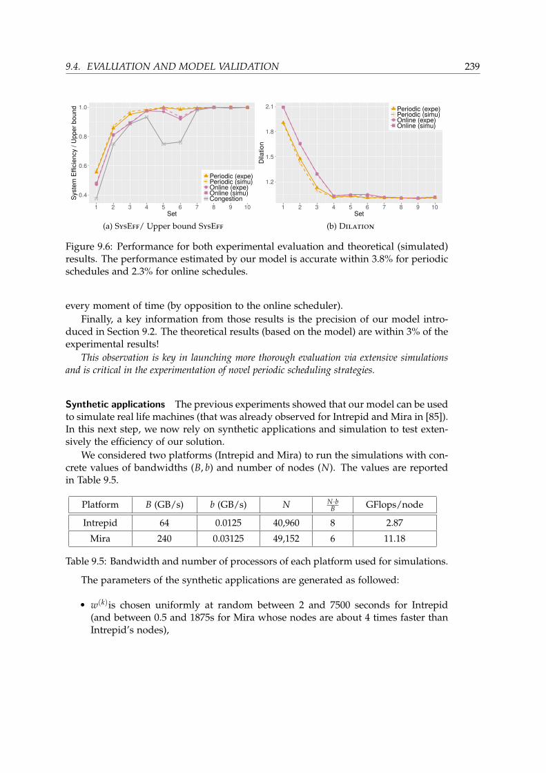
9.4. EVALUATION AND MODEL VALIDATION 239
0.4
0.6
0.8
1.0
1 2 3 4 5 6 7 8 9 10Set
Syst
em E
ffici
ency
/ U
pper
bou
nd
Periodic (expe)Periodic (simu)Online (expe)Online (simu)Congestion
(a) SysEff/ Upper bound SysEff
1.2
1.5
1.8
2.1
1 2 3 4 5 6 7 8 9 10Set
Dila
tion
Periodic (expe)Periodic (simu)Online (expe)Online (simu)
(b) Dilation
Figure 9.6: Performance for both experimental evaluation and theoretical (simulated)results. The performance estimated by our model is accurate within 3.8% for periodicschedules and 2.3% for online schedules.
every moment of time (by opposition to the online scheduler).Finally, a key information from those results is the precision of our model intro-
duced in Section 9.2. The theoretical results (based on the model) are within 3% of theexperimental results!
This observation is key in launching more thorough evaluation via extensive simulationsand is critical in the experimentation of novel periodic scheduling strategies.
Synthetic applications The previous experiments showed that our model can be usedto simulate real life machines (that was already observed for Intrepid and Mira in [85]).In this next step, we now rely on synthetic applications and simulation to test exten-sively the efficiency of our solution.
We considered two platforms (Intrepid and Mira) to run the simulations with con-crete values of bandwidths (B, b) and number of nodes (N). The values are reportedin Table 9.5.
Platform B (GB/s) b (GB/s) N N·bB GFlops/node
Intrepid 64 0.0125 40,960 8 2.87
Mira 240 0.03125 49,152 6 11.18
Table 9.5: Bandwidth and number of processors of each platform used for simulations.
The parameters of the synthetic applications are generated as followed:
• w(k)is chosen uniformly at random between 2 and 7500 seconds for Intrepid(and between 0.5 and 1875s for Mira whose nodes are about 4 times faster thanIntrepid’s nodes),

240 Chapter 9: I/O scheduling strategy for periodic applications
• the volume of I/O data vol(k)io is chosen uniformly at random between 100 GB and35 TB.
These values where based on the applications we previously studied.We generate the different sets of applications using the following method: let n be
the number of unused nodes. At the beginning we set n = N.1. Draw uniformly at random an integer number x between 1 and max(1, n
4096 − 1)(to ensure there are at least two applications).
2. Add to the set an application App(k) with parameters w(k) and vol(k)io set as pre-viously detailed and β(k) = 4096x.
3. n← n− 4096x.4. Go to step 1 if n > 0.
We then generated 100 sets for Intrepid (using a total of 40,960 nodes) and 100 setsfor Mira (using a total of 49,152 nodes) on which we run the online algorithms (eithermaximizing the system efficiency or minimizing the dilation) and PerSched. The re-sults are presented on Figures 9.7a and 9.7b for simulations using the Intrepid settingsand Figures 9.8a and 9.8b for simulations using the Mira settings.
0.6
0.8
1.0
0 25 50 75 100Set
Syst
em E
ffici
ency
/ U
pper
bou
nd
PeriodicOnline (best)
(a) SysEff/ Upper bound SysEff
1.0
1.2
1.4
1.6
0 25 50 75 100Set
Dila
tion
PeriodicOnline (best)
(b) Dilation
Figure 9.7: Comparison between online heuristics and PerSched on synthetic appli-cations, based on Intrepid settings.
We can see that overall, our algorithm increases the system efficiency in almostevery case. On average the system efficiency is improved by 16% on intrepid (32%on Mira) with peaks up to 116%! On Intrepid the dilation has overall similar values(an average of 0.6% degradation over the best online algorithm, with variation be-tween 11% improvement and 42% degradation). However on Mira in addition to theimprovement in system efficiency, PerSched improves on average by 22% the dilation!
The main difference between Intrepid and Mira is the ratio compute (= N ·GFlops/node) over I/O bandwidth (B). In other terms, that is the speed at which datais created/used over the speed at which data is transferred. Note that as said earlier,the trend is going towards an increase of this ratio. This ratio increases a lot (andhence incurring more I/O congestion) on Mira. To see if this indeed impacts the per-
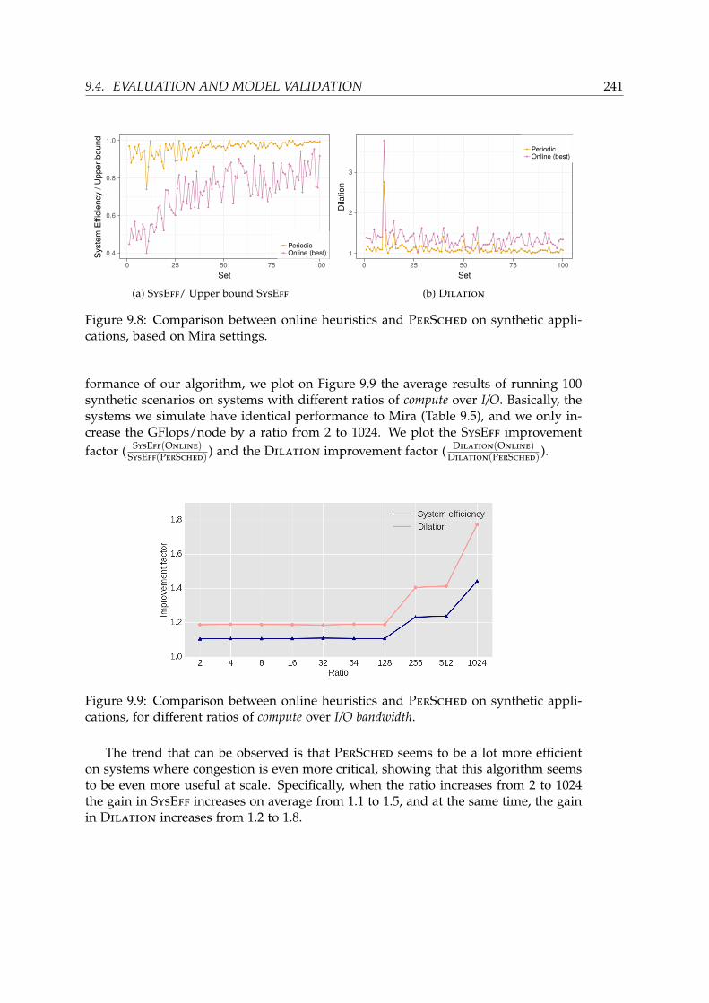
9.4. EVALUATION AND MODEL VALIDATION 241
0.4
0.6
0.8
1.0
0 25 50 75 100Set
Syst
em E
ffici
ency
/ U
pper
bou
nd
PeriodicOnline (best)
(a) SysEff/ Upper bound SysEff
1
2
3
0 25 50 75 100Set
Dila
tion
PeriodicOnline (best)
(b) Dilation
Figure 9.8: Comparison between online heuristics and PerSched on synthetic appli-cations, based on Mira settings.
formance of our algorithm, we plot on Figure 9.9 the average results of running 100synthetic scenarios on systems with different ratios of compute over I/O. Basically, thesystems we simulate have identical performance to Mira (Table 9.5), and we only in-crease the GFlops/node by a ratio from 2 to 1024. We plot the SysEff improvementfactor ( SysEff(Online)
SysEff(PerSched)) and the Dilation improvement factor ( Dilation(Online)
Dilation(PerSched)).
Figure 9.9: Comparison between online heuristics and PerSched on synthetic appli-cations, for different ratios of compute over I/O bandwidth.
The trend that can be observed is that PerSched seems to be a lot more efficienton systems where congestion is even more critical, showing that this algorithm seemsto be even more useful at scale. Specifically, when the ratio increases from 2 to 1024the gain in SysEff increases on average from 1.1 to 1.5, and at the same time, the gainin Dilation increases from 1.2 to 1.8.
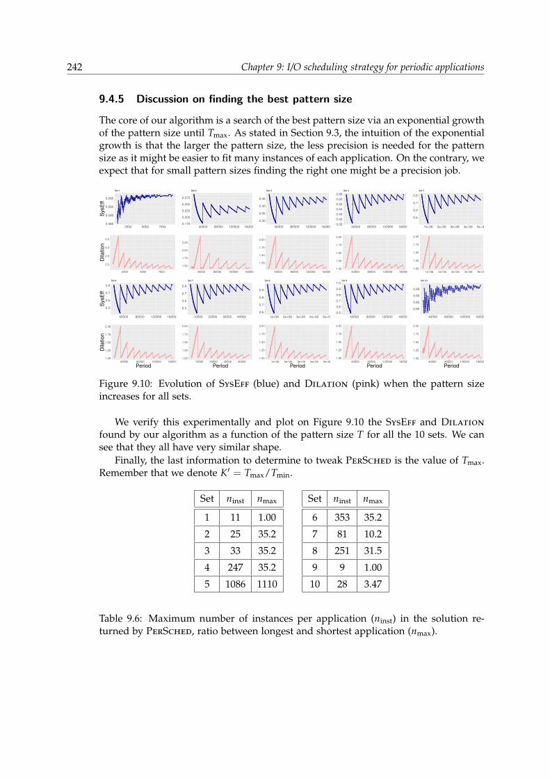
242 Chapter 9: I/O scheduling strategy for periodic applications
9.4.5 Discussion on finding the best pattern size
The core of our algorithm is a search of the best pattern size via an exponential growthof the pattern size until Tmax. As stated in Section 9.3, the intuition of the exponentialgrowth is that the larger the pattern size, the less precision is needed for the patternsize as it might be easier to fit many instances of each application. On the contrary, weexpect that for small pattern sizes finding the right one might be a precision job.
0.080
0.085
0.090
0.095
2500 5000 7500
SysE
ff
Set 1
2.0
2.5
3.0
3.5
2500 5000 7500
Dila
tion
0.175
0.200
0.225
0.250
0.275
40000 80000 120000 160000
Set 2
1.50
1.75
2.00
2.25
40000 80000 120000 160000
0.30
0.35
0.40
0.45
40000 80000 120000 160000
Set 3
1.25
1.50
1.75
2.00
40000 80000 120000 160000
0.350.400.450.500.550.600.65
40000 80000 120000 160000
Set 4
1.00
1.25
1.50
1.75
2.00
40000 80000 120000 160000
0.5
0.6
0.7
0.8
1e+06 2e+06 3e+06 4e+06 5e+06
Set 5
1.00
1.25
1.50
1.75
2.00
1e+06 2e+06 3e+06 4e+06 5e+06
0.5
0.6
0.7
0.8
40000 80000 120000 160000
SysE
ff
Set 6
1.00
1.25
1.50
1.75
2.00
40000 80000 120000 160000Period
Dila
tion
0.5
0.6
0.7
0.8
10000 20000 30000 40000
Set 7
1.00
1.25
1.50
1.75
2.00
10000 20000 30000 40000Period
0.6
0.7
0.8
0.9
1e+06 2e+06 3e+06 4e+06 5e+06
Set 8
1.00
1.25
1.50
1.75
2.00
1e+06 2e+06 3e+06 4e+06 5e+06Period
0.5
0.6
0.7
0.8
0.9
1.0
40000 80000 120000 160000
Set 9
1.00
1.25
1.50
1.75
2.00
40000 80000 120000 160000Period
0.80
0.85
0.90
0.95
40000 80000 120000 160000
Set 10
1.00
1.25
1.50
1.75
2.00
40000 80000 120000 160000Period
Figure 9.10: Evolution of SysEff (blue) and Dilation (pink) when the pattern sizeincreases for all sets.
We verify this experimentally and plot on Figure 9.10 the SysEff and Dilation
found by our algorithm as a function of the pattern size T for all the 10 sets. We cansee that they all have very similar shape.
Finally, the last information to determine to tweak PerSched is the value of Tmax.Remember that we denote K′ = Tmax/Tmin.
Set ninst nmax
1 11 1.00
2 25 35.2
3 33 35.2
4 247 35.2
5 1086 1110
Set ninst nmax
6 353 35.2
7 81 10.2
8 251 31.5
9 9 1.00
10 28 3.47
Table 9.6: Maximum number of instances per application (ninst) in the solution re-turned by PerSched, ratio between longest and shortest application (nmax).
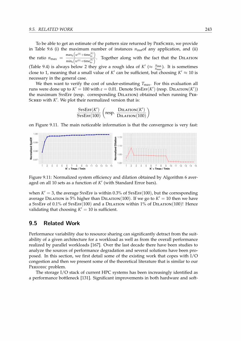
9.5. RELATED WORK 243
To be able to get an estimate of the pattern size returned by PerSched, we providein Table 9.6 (i) the maximum number of instances ninstof any application, and (ii)
the ratio nmax =maxk
(w(k)+time(k)io
)mink
(w(k)+time(k)io
) . Together along with the fact that the Dilation
(Table 9.4) is always below 2 they give a rough idea of K′ (≈ ninstnmax
). It is sometimesclose to 1, meaning that a small value of K′ can be sufficient, but choosing K′ ≈ 10 isnecessary in the general case.
We then want to verify the cost of under-estimating Tmax. For this evaluation allruns were done up to K′ = 100 with ε = 0.01. Denote SysEff(K′) (resp. Dilation(K′))the maximum SysEff (resp. corresponding Dilation) obtained when running Per-Sched with K′. We plot their normalized version that is:
SysEff(K′)SysEff(100)
(resp.
Dilation(K′)Dilation(100)
)on Figure 9.11. The main noticeable information is that the convergence is very fast:
0.97
0.98
0.99
1.00
1 2 3 4 5 6 7 8 9 10 11 12 13 14 15K' = Tmax / Tmin
Nor
mal
ized
Sys
Eff
1.00
1.05
1.10
1.15
1 2 3 4 5 6 7 8 9 10 11 12 13 14 15K' = Tmax / Tmin
Nor
mal
ized
Dila
tion
Figure 9.11: Normalized system efficiency and dilation obtained by Algorithm 6 aver-aged on all 10 sets as a function of K′ (with Standard Error bars).
when K′ = 3, the average SysEff is within 0.3% of SysEff(100), but the correspondingaverage Dilation is 5% higher than Dilation(100). If we go to K′ = 10 then we havea SysEff of 0.1% of SysEff(100) and a Dilation within 1% of Dilation(100)! Hencevalidating that choosing K′ = 10 is sufficient.
9.5 Related Work
Performance variability due to resource sharing can significantly detract from the suit-ability of a given architecture for a workload as well as from the overall performancerealized by parallel workloads [167]. Over the last decade there have been studies toanalyze the sources of performance degradation and several solutions have been pro-posed. In this section, we first detail some of the existing work that copes with I/Ocongestion and then we present some of the theoretical literature that is similar to ourPeriodic problem.
The storage I/O stack of current HPC systems has been increasingly identified asa performance bottleneck [131]. Significant improvements in both hardware and soft-

244 Chapter 9: I/O scheduling strategy for periodic applications
ware need to be addressed to overcome oncoming scalability challenges. The studyin [111] argues for making data staging coordination driven by generic cross-layermechanisms that enable global optimizations by enforcing local decisions at nodegranularity at individual stack layers.
I/O congestion While many other studies suggest that I/O congestion is one of themain problems for future scale platforms [27, 134], few papers focus on finding a so-lution at the platform level. Some papers consider application-side I/O managementand transformation (using aggregate nodes, compression etc) [133, 203, 179]. We con-sider those work to be orthogonal to our work and able to work jointly. Recently,numerous works focus on using machine learning for auto tuning and performancestudies [19, 122]. However these solutions also work at the application level and donot have a global view of the I/O requirements of the system and they need to besupported by a platform level I/O management for better results.
Some paper consider the use of burst buffers to reduce I/O congestion by delayingaccesses to the file storage, as they found that congestion occurs on a short period oftime and the bandwidth to the storage system is often underutilized [130]. Note thatbecause the computation power increases faster than the I/O bandwidth, this assump-tion may not hold in the future and the bandwidth may tend to be saturated moreoften and thus decreasing the efficiency of burst buffers. Kougas et al. [121] present adynamic I/O scheduling at the application level using burst buffers to stage I/O andto allow computations to continue uninterrupted. They design different strategies tomitigate I/O interference, including partitioning the PFS, which reduces the effectivebandwidth non-linearly. Note that their strategy only consider two applications. Tanget al. [178] consider the use of Burst-Buffers to serve the I/O bursts of HPC applica-tions. They prove that a basic reactive draining strategy that empties the burst bufferas soon as possible can lead to a severe degradation of the aggregate I/O through-put. On the other hand, they advocate for a proactive draining strategy, where datais divided into draining segments which are dispersed evenly over the I/O interval,and the burst buffer draining throughput is controlled through adjusting the numberof I/O requests issued each time. Recently, Aupy et al. [10] have started discussingcoupling of IO scheduling and buffers partitionning to improve data scheduling. Theypropose an optimal algorithm that determines the minimum buffer size needed toavoid congestion altogether.
The study from [160] offers ways of isolating the performance experienced by ap-plications of one operating system from variations in the I/O request stream char-acteristics of applications of other operating systems. While their solution cannot beapplied to HPC systems, the study offers a way of controlling the coarse grain alloca-tion of disk time to the different operating system instances as well as determining thefine-grain interleaving of requests from the corresponding operating systems to thestorage system.
Closer to this work, online schedulers for HPC systems were developed such asprevious work [85], the study by Zhou et al [207], and a solution proposed by Dorieret al [65]. In [65], the authors investigate the interference of two applications and

9.6. CONCLUSION 245
analyze the benefits of interrupting or delaying either one in order to avoid congestion.Unfortunately their approach cannot be used for more than two applications. Anothermain difference with our previous work is the light-weight approach of this studywhere the computation is only done once.
The previous study [85] is more general by offering a range of options to scheduleeach I/O performed by an application. Similarly, the work from [207] also utilizes aglobal job scheduler to mitigate I/O congestion by monitoring and controlling jobs’I/O operations on the fly. Unlike online solutions, this paper focuses on a decentral-ized approach where the scheduler is integrated into the job scheduler and computesahead of time, thus overcoming the need to monitor the I/O traffic of each applicationat every moment of time.
Periodic schedules As a scheduling problem, our problem is somewhat close to thecyclic scheduling problem (we refer to Hanen and Munier [101] for a survey). Namelythere are given a set of activities with time dependency between consecutive tasksstored in a DAG that should be executed on p processors. The main difference is thatin cyclic scheduling there is no consideration of a constant time between the end ofthe previous instance and the next instance. More specifically, if an instance of anapplication has been delayed, the next instance of the same application is not delayedby the same time. With our model this could be interpreted as not overlapping I/Oand computation.
9.6 Conclusion
Performance variation due to resource sharing in HPC systems is a reality and I/Ocongestion is currently one of the main causes of degradation. Current storage systemsare unable to keep up with the amount of data handled by all applications running onan HPC system, either during their computation or when taking checkpoints. In thisdocument we have presented a novel I/O scheduling technique that offers a decen-tralized solution for minimizing the congestion due to application interference. Ourmethod takes advantage of the periodic nature of HPC applications by allowing thejob scheduler to pre-define each application’s I/O behavior for their entire execution.Recent studies [66] have shown that HPC applications have predictable I/O patternseven when they are not completely periodic, thus we believe our solution is generalenough to easily include the large majority of HPC applications. Furthermore, withthe integration of burst buffers in HPC machines [130, 9] periodic schedules could al-low to stage data from non periodic applications in Application-side burst buffers, andempty those buffers periodically to avoid congestion. This is the strategy advocatedby Tang et al. [178].
We conducted simulations for different scenarios and made experiments to validateour results. Decentralized solutions are able to improve both total system efficiencyand application dilation compared to dynamic state-of-the-art schedulers. Moreover,they do not require a constant monitoring of the state of all applications, nor do theyrequire a change in the current I/O stack. One particularly interesting result is for

246 Chapter 9: I/O scheduling strategy for periodic applications
scenario 1 with 10 identical periodic behaviors (such as what can be observed withperiodic checkpointing for fault-tolerance). In this case the periodic scheduler showsa 30% improvement in SysEff. Thus, system wide applications taking global check-points could benefit from such a strategy. Our scheduler performs better than existingsolutions, improving the application dilation up to 16% and the maximum system effi-ciency up to 18%. Moreover, based on simulation results, our scheduler shows an evengreater improvement for future systems with increasing ratios between the computingpower and the I/O bandwidth.
Future work: we believe this work is the initialization of a new set of techniques todeal with the I/O requirements of HPC system. In particular, by showing the efficiencyof the periodic technique on simple pattern, we expect this to serve as a proof ofconcept to open a door to multiple extensions. We give here some examples that wewill consider in the future. The next natural directions is to take more complicatedperiodic shapes for applications (an instance could be composed of sub-instances) aswell as different points of entry inside the job scheduler (multiple I/O nodes). Weplan to also study the impact of non-periodic applications on this schedule and howto integrate them. This would be modifying the Insert-In-Pattern procedure andwe expect that this should work well as well. Another future step would be to studyhow variability in the compute or I/O volumes impact a periodic schedule. Thisvariability could be important in particular on machines where the inter-processorcommunication network is shared with the I/O network. Indeed, in those case, I/Owould likely be delayed. Finally we plan to model burst buffers and to show how touse them conjointly with periodic schedules, specifically if they allow to implementasynchrone I/O.
Chapter 10
Conclusion
Summary of results
In this thesis, we have addressed several challenges related to exascale computing,more particularly resilience. We have presented some algorithms that allow applica-tions to complete in a failure-prone environment. Moreover, we have been able toderive optimal solutions to minimize the execution time (or the energy consumptionin some cases, as it remains one of the big challenges of exascale computing).
In Part I, we have presented an extension of Young and Daly’s formula for a multi-level checkpointing scheme, which targets fail-stop errors. In particular, we have beenable to derive the optimal (rational) number of checkpoints for each level and that theyare equally spaced. We have also provided a dynamic programming algorithm thatselects the optimal subset of levels to be used. We have compared the performance ofRigid, Moldable and GridShaped applications with checkpoint/restart (and ABFTfor GridShaped applications), and showed that the yield can be improved a lot byrequesting a new allocation after a number of failures corresponding to a small per-centage of the total resources, even for large values of wait time. Finally, we havedesigned the first (for fail-stop errors) heuristic for checkpointing generic workflowswhile mapping tasks to processors. This heuristic achieves a trade-off between check-pointing every task (which is secure but long) and checkpointing no task (which mightimply too many re-executions).
Part II deals with problems related to replication. We first proposed an optimaldynamic programming algorithm to decide which tasks are duplicated and/or check-pointed in a linear workflow. The algorithm runs in O(n2) and applies to both silentand fail-stop errors. We then studied a divisible application executed on two hetero-geneous platforms and we derived the optimal checkpointing period (more exactly, afirst or second-order approximation) for a periodic strategy and we compared it to an-other strategy: on-failure checkpointing. One striking result is that when the speedsof both machines are the same, the optimal checkpointing period is proportional toλ−
23 instead of λ−
12 as it is classically. We find this result again in our study of process
duplication on homogeneous processors with our restart strategy. All previous worksused the no-restart strategy, and we showed that our approach can be significantly bet-
247

248 Chapter 10: Conclusion
ter in terms of execution time, energy consumption, robustness as regard to the periodchoice or I/O utilization.
Finally, we studied two scheduling problems in Part III. We first extended approx-imation results on list scheduling heuristics to a context where tasks can fail and weget constant approximation ratios. We also showed that shelf-based algorithms can nolonger be constant-factor approximation algorithms. Then, to tackle the problem ofI/O congestion (computational power increases faster than bandwidths), we designeda nice I/O scheduling algorithm at the platform level. We relied on applications thathave a periodic behavior to compute a periodic schedule, each time a new applicationis launched. We were able to improve two metrics: SysEff and Dilation, and weprovided a additional scenario to show even more the benefits of I/O scheduling inthe future.
For each theoretical result, we validated our model and solution with extensivesets of simulations. These simulations have been helpful in two major ways: assessingthe accuracy of our first-order (or second-order) approximations and measuring thepractical impact of the proposed solutions. When possible, we used numbers comingfrom real applications to further strengthen the analysis (for example, we used reallogs from Mira [5] in Chapter 8) instead of using only randomly generated input data,which, in some cases, may not reflect the same exact behavior of our algorithms.
Future work and perspectives
On-going work includes two different problems. We first plan to extend the re-sults described in Chapter 8 to moldable jobs, i.e., jobs that do not require a fixednumber of processors to run. We consider several models (Amdahl’s law, rooftop,communication-bound jobs, ...) and design a new algorithm for attributing the re-sources to each job before scheduling them. We expect to have higher approximationratios compared to rigid jobs, as it is already the case when considering jobs thatcannot fail [184].
Another study that we target is a comparison of residual checking and ABFT forcorrecting silent data corruptions (SDC). Residual checking is an ABFT-like techniquethat has one major asset: while ABFT uses embedded checksums that are transmittedthrough the computation (for example, for a matrix-matrix product, some rows andcolumns are added, then the multiplication is done as if these rows and columns arepart of the orignal matrices thanks to linear properties), residual checking consists indoing this check only at the end of the computation. This is easier for a developer toimplement even for complex transformations like LU and Cholesky. The challengingpart in this problem is to detect where the SDCs strike and to find a way to correctthem. To the best of our knowledge, using residual checking has only been used todetect errors so far, and preliminary results seem to indicate that it can have a loweroverhead than ABFT for matrix-matrix multiplication.
In the long term, future work is composed of several perspectives, as most chapterscan be extended with a more complex framework. In Chapter 3, we considered only

Conclusion 249
perfectly divisible applications, ABFT and checkpoint/restart separately and homoge-neous platforms. It would be natural to see if similar results can be derived for jobsobeying Amdahl’s law [3], heterogeneous platforms, and check what happens whenboth ABFT and checkpoint/restart are applied (to deal with both fail-stop and silenterrors for example). As we saw in Chapter 4, it is already difficult to select which tasksshould be checkpointed in a generic workflow. A challenging extension for Chapter 5would be to find which tasks should be replicated and/or checkpointed in such aworkflow. Finally, an interesting perspective found in Chapter 7 could be to studynon-periodic checkpointing periods for a replicated divisible application. Indeed, weprovided an example where periodic checkpointing is not optimal with one pair ofprocessors, and we believe that this result holds for several pairs of processors.


Bibliography
[1] M. Albrecht, P. Donnelly, P. Bui, and D. Thain. “Makeflow: A portable abstrac-tion for data intensive computing on clusters, clouds, and grids.” In: 1st ACMSWEET SIGMOD. ACM. 2012.
[2] I. Altintas, C. Berkley, E. Jaeger, M. Jones, B. Ludascher, and S. Mock. “Kepler:an extensible system for design and execution of scientific workflows.” In: Proc.of 16th SSDBM. IEEE, 2004, pp. 423–424.
[3] G. Amdahl. “The validity of the single processor approach to achieving largescale computing capabilities.” In: AFIPS Conference Proceedings. Vol. 30. AFIPSPress, 1967, pp. 483–485.
[4] APEX. APEX Workflows. Research report SAND2016-2371 and LA-UR-15-29113.LANL, NERSC, SNL, 2016.
[5] Argonne Leadership Computing Facility. Mira log traces. https://reports.alcf.anl.gov/data/mira.html.
[6] R. A. Ashraf, S. Hukerikar, and C. Engelmann. “Shrink or Substitute: HandlingProcess Failures in HPC Systems using In-situ Recovery.” In: CoRR abs/1801.04523(2018). arXiv: 1801.04523.
[7] I. Assayad, A. Girault, and H. Kalla. “A Bi-Criteria Scheduling Heuristic forDistributed Embedded Systems under Reliability and Real-Time Constraints.”In: Dependable Systems Networks (DSN). IEEE, 2004.
[8] C. Augonnet, S. Thibault, R. Namyst, and P.-A. Wacrenier. “StarPU: a unifiedplatform for task scheduling on heterogeneous multicore architectures.” In:Concur. and Comp.: Pract. and Exp. 23.2 (2011), pp. 187–198.
[9] G. Aupy, O. Beaumont, and L. Eyraud-Dubois. “What size should your Buffersto Disk be?” In: Proceedings of the 32nd International Parallel Processing Sympo-sium, (IPDPS’18). IEEE. 2018.
[10] G. Aupy, O. Beaumont, and L. Eyraud-Dubois. “Sizing and Partitioning Strate-gies for Burst-Buffers to Reduce IO Contention.” In: Proceedings of the 33rd In-ternational Parallel Processing Symposium, (IPDPS’19). IEEE. 2019.
[11] G. Aupy, A. Benoit, H. Casanova, and Y. Robert. “Scheduling computationalworkflows on failure-prone platforms.” In: Int. J. of Networking and Computing6.1 (2016), pp. 2–26.
251

252 Bibliography
[12] G. Aupy, Y. Robert, and F. Vivien. “Assuming failure independence: are weright to be wrong?” In: FTS’2017, the Workshop on Fault-Tolerant Systems, in con-junction with Cluster’2017. IEEE Computer Society Press, 2017.
[13] B. S. Baker, E. G. Coffman, and R. L. Rivest. “Orthogonal Packings in TwoDimensions.” In: SIAM Journal on Computing 9.4 (1980), pp. 846–855.
[14] P. Balaprakash, L. A. B. Gomez, M.-S. Bouguerra, S. M. Wild, F. Cappello, andP. D. Hovland. “Analysis of the Tradeoffs Between Energy and Run Time forMultilevel Checkpointing.” In: Proc. PMBS’14. 2014.
[15] L. Bautista Gomez and F. Cappello. “Detecting Silent Data Corruption ThroughData Dynamic Monitoring for Scientific Applications.” In: SIGPLAN Notices49.8 (2014), pp. 381–382.
[16] L. Bautista Gomez and F. Cappello. “Detecting and Correcting Data Corruptionin Stencil Applications through Multivariate Interpolation.” In: FTS. IEEE, 2015.
[17] L. Bautista-Gomez, S. Tsuboi, D. Komatitsch, F. Cappello, N. Maruyama, andS. Matsuoka. “FTI: High Performance Fault Tolerance Interface for Hybrid Sys-tems.” In: Proc. SC’11. 2011.
[18] L. Bautista-Gomez, F. Zyulkyarov, O. Unsal, and S. McIntosh-Smith. “Unpro-tected Computing: A Large-scale Study of DRAM Raw Error Rate on a Su-percomputer.” In: Proceedings of the International Conference for High PerformanceComputing, Networking, Storage and Analysis. SC ’16. Salt Lake City, Utah: IEEEPress, 2016, 55:1–55:11. isbn: 978-1-4673-8815-3.
[19] Behzad et al. “Taming parallel I/O complexity with auto-tuning.” In: SC13.2013.
[20] A. Benoit, A. Cavelan, Y. Robert, and H. Sun. “Optimal Resilience Patterns toCope with Fail-Stop and Silent Errors.” In: 2016 IEEE International Parallel andDistributed Processing Symposium (IPDPS). May 2016, pp. 202–211. doi: 10.1109/IPDPS.2016.39.
[21] A. Benoit, A. Cavelan, F. Cappello, P. Raghavan, Y. Robert, and H. Sun. “Cop-ing with silent and fail-stop errors at scale by combining replication and check-pointing.” In: J. Parallel and Distributed Computing 122 (2018), pp. 209–225.
[22] A. Benoit, A. Cavelan, F. Ciorba, V. L. Fevre, and Y. Robert. Combining check-pointing and replication for reliable execution of linear workflows. Research reportRR-9152. INRIA, 2018.
[23] A. Benoit, A. Cavelan, Y. Robert, and H. Sun. “Assessing General-Purpose Al-gorithms to Cope with Fail-Stop and Silent Errors.” In: ACM Trans. ParallelComput. 3.2 (July 2016), 13:1–13:36. issn: 2329-4949. doi: 10.1145/2897189.
[24] A. Benoit, T. Herault, V. L. Fevre, and Y. Robert. Replication Is More EfficientThan You Think: Code and Technical Report. https://doi.org/10.5281/zenodo.3366221. Aug. 2019.
Bibliography 253
[25] E. Berrocal, L. Bautista-Gomez, S. Di, Z. Lan, and F. Cappello. “LightweightSilent Data Corruption Detection Based on Runtime Data Analysis for HPCApplications.” In: HPDC. ACM, 2015.
[26] S. Bharathi, A. Chervenak, E. Deelman, G. Mehta, M.-H. Su, and K. Vahi. “Char-acterization of scientific workflows.” In: Workflows in Support of Large-Scale Sci-ence (WORKS). IEEE, 2008, pp. 1–10.
[27] R. Biswas, M. Aftosmis, C. Kiris, and B.-W. Shen. “Petascale computing: Impacton future NASA missions.” In: Petascale Computing: Architectures and Algorithms(2007), pp. 29–46.
[28] W. Bland, A. Bouteiller, T. Herault, G. Bosilca, and J. Dongarra. “Post-failurerecovery of MPI communication capability: Design and rationale.” In: Interna-tional Journal of High Performance Computing Applications 27.3 (2013), pp. 244–254.doi: 10.1177/1094342013488238. eprint: http://hpc.sagepub.com/content/27/3/244.full.pdf+html.
[29] W. Bland, A. Bouteiller, T. Herault, J. Hursey, G. Bosilca, and J. J. Dongarra.“An evaluation of User-Level Failure Mitigation support in MPI.” In: Computing95.12 (2013), pp. 1171–1184.
[30] G. Bosilca, A. Bouteiller, E. Brunet, F. Cappello, J. Dongarra, A. Guermouche,T. Herault, Y. Robert, F. Vivien, and D. Zaidouni. “Unified model for assess-ing checkpointing protocols at extreme-scale.” In: Concurrency and Computation:Practice and Experience (2013). issn: 1532-0634. doi: 10.1002/cpe.3173.
[31] G. Bosilca, R. Delmas, J. Dongarra, and J. Langou. “Algorithm-based fault tol-erance applied to high performance computing.” In: J. Parallel Distrib. Comput.69.4 (2009), pp. 410–416.
[32] S. Boyd and L. Vandenberghe. Convex Optimization. New York, NY, USA: Cam-bridge University Press, 2004. isbn: 0521833787.
[33] T. D. Braun, H. J. Siegel, N. Beck, L. L. Boloni, M. Maheswaran, A. I. Reuther,J. P. Robertson, M. D. Theys, B. Yao, D. Hensgen, et al. “A comparison of elevenstatic heuristics for mapping a class of independent tasks onto heterogeneousdistributed computing systems.” In: Journal of Parallel and Distributed computing61.6 (2001), pp. 810–837.
[34] R. Brightwell, K. Ferreira, and R. Riesen. “Transparent Redundant Computingwith MPI.” In: EuroMPI. Springer, 2010.
[35] G. H. Bryan and J. M. Fritsch. “A benchmark simulation for moist nonhydro-static numerical models.” In: Monthly Weather Review 130.12 (2002).
[36] G. L. Bryan et al. “Enzo: An Adaptive Mesh Refinement Code for Astrophysics.”In: arXiv:1307.2265 (2013).
[37] E. S. Buneci. “Qualitative Performance Analysis for Large-Scale Scientific Work-flows.” PhD thesis. Duke University, 2008.

254 Bibliography
[38] S. Byna, Y. Chen, X. Sun, R. Thakur, and W. Gropp. “Parallel I/O prefetchingusing MPI file caching and I/O signatures.” In: SC ’08: Proceedings of the 2008ACM/IEEE Conference on Supercomputing. Nov. 2008, pp. 1–12. doi: 10.1109/SC.2008.5213604.
[39] C. Cao, T. Herault, G. Bosilca, and J. Dongarra. “Design for a Soft Error ResilientDynamic Task-Based Runtime.” In: IPDPS. IEEE, 2015, pp. 765–774.
[40] F. Cappello, K. Mohror, et al. VeloC: Very Low Overhead Checkpointing System.https://veloc.readthedocs.io/en/latest/. Mar. 2019.
[41] F. Cappello, A. Geist, W. Gropp, S. Kale, B. Kramer, and M. Snir. “Toward Ex-ascale Resilience.” In: Int. J. High Performance Computing Applications 23.4 (2009),pp. 374–388.
[42] F. Cappello, A. Geist, W. Gropp, S. Kale, B. Kramer, and M. Snir. “TowardExascale Resilience: 2014 update.” In: Supercomputing frontiers and innovations1.1 (2014).
[43] P. Carns, R. Latham, R. Ross, K. Iskra, S. Lang, and K. Riley. “24/7 characteri-zation of petascale I/O workloads.” In: Cluster Computing and Workshops, 2009.CLUSTER’09. IEEE International Conference on (Jan. 2009), pp. 1–10.
[44] J. Carter, J. Borrill, and L. Oliker. “Performance characteristics of a cosmologypackage on leading HPC architectures.” In: HiPC. Springer, 2005, pp. 176–188.
[45] H. Casanova, M. Bougeret, Y. Robert, F. Vivien, and D. Zaidouni. “Using groupreplication for resilience on exascale systems.” In: Int. Journal of High Perfor-mance Computing Applications 28.2 (2014), pp. 210–224.
[46] H. Casanova, Y. Robert, F. Vivien, and D. Zaidouni. “On the impact of processreplication on executions of large-scale parallel applications with coordinatedcheckpointing.” In: Future Gen. Comp. Syst. 51 (2015), pp. 7–19.
[47] K. M. Chandy and L. Lamport. “Distributed Snapshots: Determining GlobalStates of Distributed Systems.” In: ACM Transactions on Computer Systems 3.1(1985), pp. 63–75.
[48] B. Chen and A. P. Vestjens. “Scheduling on identical machines: How good isLPT in an on-line setting.” In: Operations Research Letters 21.4 (1997), pp. 165–169.
[49] C. Chen, G. Eisenhauer, M. Wolf, and S. Pande. “LADR: Low-cost Application-level Detector for Reducing Silent Output Corruptions.” In: HPDC. Tempe, Ari-zona, 2018, pp. 156–167.
[50] Z. Chen. “Online-ABFT: An Online Algorithm Based Fault Tolerance Schemefor Soft Error Detection in Iterative Methods.” In: SIGPLAN Not. 48.8 (2013),pp. 167–176.
[51] J. Choi, J. J. Dongarra, L. S. Ostrouchov, A. P. Petitet, D. W. Walker, and R. C.Whaley. “Design and implementation of the ScaLAPACK LU, QR, and Choleskyfactorization routines.” In: Scientific Programming 5.3 (1996), pp. 173–184.

Bibliography 255
[52] W. Cirne and F. Berman. “Using Moldability to Improve the Performance ofSupercomputer Jobs.” In: J. Parallel Distrib. Comput. 62.10 (2002), pp. 1571–1601.
[53] E. G. Coffman, M. R. Garey, D. S. Johnson, and R. E. Tarjan. “PerformanceBounds for Level-Oriented Two-Dimensional Packing Algorithms.” In: SIAM J.Comput. 9.4 (1980), pp. 808–826.
[54] P. Colella et al. Chombo infrastructure for adaptive mesh refinement. https://seesar.lbl.gov/ANAG/chombo/. 2005.
[55] CORAL: Collaboration of Oak Ridge, Argonne and Livermore National Lab-oratorie. DRAFT CORAL-2 BUILD STATEMENT OF WORK. Tech. rep. LLNL-TM-7390608. Lawrence Livermore National Laboratory, Mar. 2018.
[56] S. P. Crago, D. I. Kang, M. Kang, R. Kost, K. Singh, J. Suh, and J. P. Walters.“Programming Models and Development Software for a Space-Based Many-Core Processor.” In: 4th Int. Conf. on Space Mission Challenges for InformationTechnology. IEEE, 2011, pp. 95–102.
[57] V. Cuevas-Vicenttın, S. C. Dey, S. Kohler, S. Riddle, and B. Ludascher. “Scien-tific Workflows and Provenance: Introduction and Research Opportunities.” In:Datenbank-Spektrum 12.3 (2012), pp. 193–203.
[58] J. T. Daly. “A higher order estimate of the optimum checkpoint interval forrestart dumps.” In: Future Generation Comp. Syst. 22.3 (2006), pp. 303–312.
[59] A. Darte, Y. Robert, and F. Vivien. Scheduling and automatic parallelization. Birkhauser,2000. isbn: 978-3-7643-4149-7.
[60] E. Deelman, G. Singh, M.-H. Su, J. Blythe, Y. Gil, C. Kesselman, G. Mehta, K.Vahi, G. B. Berriman, J. Good, et al. “Pegasus: A framework for mapping com-plex scientific workflows onto distributed systems.” In: Scientific Programming13.3 (2005), pp. 219–237.
[61] E. Deelman, K. Vahi, G. Juve, M. Rynge, S. Callaghan, P. J. Maechling, R.Mayani, W. Chen, R. Ferreira da Silva, M. Livny, and K. Wenger. “Pegasus, aWorkflow Management System for Science Automation.” In: Future GenerationComputer Systems 46 (2015), pp. 17–35.
[62] S. Di, M. S. Bouguerra, L. Bautista-Gomez, and F. Cappello. “Optimizationof multi-level checkpoint model for large scale HPC applications.” In: Proc.IPDPS’14. 2014.
[63] S. Di, Y. Robert, F. Vivien, and F. Cappello. “Toward an Optimal Online Check-point Solution under a Two-Level HPC Checkpoint Model.” In: IEEE Trans.Parallel & Distributed Systems (2016).
[64] M. e. M. Diouri, O. Gluck, L. Lefevre, and F. Cappello. “Energy considerationsin checkpointing and fault tolerance protocols.” In: IEEE/IFIP International Con-ference on Dependable Systems and Networks Workshops (DSN 2012). June 2012,pp. 1–6. doi: 10.1109/DSNW.2012.6264670.
256 Bibliography
[65] M. Dorier, G. Antoniu, R. Ross, D. Kimpe, and S. Ibrahim. “CALCioM: Miti-gating I/O Interference in HPC Systems through Cross-Application Coordina-tion.” In: IPDPS’14. 2014.
[66] M. Dorier, S. Ibrahim, G. Antoniu, and R. Ross. “Omnisc’IO: a grammar-basedapproach to spatial and temporal I/O patterns prediction.” In: SC. IEEE Press.2014, pp. 623–634.
[67] A. B. Downey. “The structural cause of file size distributions.” In: MASCOTS2001. IEEE. 2001, pp. 361–370.
[68] M. Drozdowski. Scheduling for Parallel Processing. Computer Communicationsand Networks. Springer, 2009.
[69] P. Du, A. Bouteiller, G. Bosilca, T. Herault, and J. Dongarra. “Algorithm-basedFault Tolerance for Dense Matrix Factorizations.” In: PPoPP. ACM. 2012, pp. 225–234.
[70] P. Du, P. Luszczek, S. Tomov, and J. Dongarra. “Soft error resilient QR fac-torization for hybrid system with GPGPU.” In: Journal of Computational Science4.6 (2013). Scalable Algorithms for Large-Scale Systems Workshop (ScalA2011),Supercomputing 2011, pp. 457–464. issn: 1877-7503.
[71] P.-F. Dutot, G. Mounie, and D. Trystram. “Scheduling Parallel Tasks Approxi-mation Algorithms.” In: Handbook of Scheduling - Algorithms, Models, and Perfor-mance Analysis. Ed. by J. Y.-T. Leung. CRC Press, 2004.
[72] J. Elliott, K. Kharbas, D. Fiala, F. Mueller, K. Ferreira, and C. Engelmann. “Com-bining partial redundancy and checkpointing for HPC.” In: ICDCS. IEEE, 2012.
[73] E. N. ( Elnozahy, L. Alvisi, Y.-M. Wang, and D. B. Johnson. “A survey ofrollback-recovery protocols in message-passing systems.” In: ACM ComputingSurvey 34 (3 2002), pp. 375–408.
[74] E. Elnozahy and J. Plank. “Checkpointing for peta-scale systems: a look intothe future of practical rollback-recovery.” In: IEEE Trans. Dependable and SecureComputing 1.2 (2004), pp. 97–108.
[75] C. Engelmann, H. H. Ong, and S. L. Scorr. “The case for modular redundancyin large-scale high performance computing systems.” In: PDCN. IASTED, 2009.
[76] C. Engelmann and B. Swen. “Redundant execution of HPC applications withMR-MPI.” In: PDCN. IASTED, 2011.
[77] S. Ethier, M. Adams, J. Carter, and L. Oliker. “Petascale parallelization of thegyrokinetic toroidal code.” In: VECPAR (2012).
[78] T. Fahringer, R. Prodan, R. Duan, J. Hofer, F. Nadeem, F. Nerieri, S. Podlipnig,J. Qin, M. Siddiqui, H.-L. Truong, et al. “Askalon: A development and gridcomputing environment for scientific workflows.” In: Workflows for e-Science.Springer, 2007, pp. 450–471.

Bibliography 257
[79] A. Fang, H. Fujita, and A. A. Chien. “Towards Understanding Post-recovery Ef-ficiency for Shrinking and Non-shrinking Recovery.” In: Euro-Par 2015: ParallelProcessing Workshops. Springer, 2015, pp. 656–668.
[80] D. G. Feitelson, L. Rudolph, U. Schwiegelshohn, K. C. Sevcik, and P. Wong.“Theory and Practice in Parallel Job Scheduling.” In: JSSPP. 1997, pp. 1–34.
[81] A. Feldmann, J. Sgall, and S.-H. Teng. “Dynamic scheduling on parallel ma-chines.” In: Theoretical Computer Science 130.1 (1994), pp. 49–72.
[82] K. Ferreira, J. Stearley, J. H. I. Laros, R. Oldfield, K. Pedretti, R. Brightwell, R.Riesen, P. G. Bridges, and D. Arnold. “Evaluating the Viability of Process Repli-cation Reliability for Exascale Systems.” In: Proceedings of 2011 International Con-ference for High Performance Computing, Networking, Storage and Analysis. Seattle,WA, 2011, 44:1–44:12.
[83] V. L. Fevre. source code. https://github.com/vlefevre/IO-scheduling-simu.2017.
[84] P. Flajolet, P. J. Grabner, P. Kirschenhofer, and H. Prodinger. “On Ramanujan’sQ-Function.” In: J. Computational and Applied Mathematics 58 (1995), pp. 103–116.
[85] A. Gainaru, G. Aupy, A. Benoit, F. Cappello, Y. Robert, and M. Snir. “Schedul-ing the I/O of HPC applications under congestion.” In: IPDPS. IEEE. 2015,pp. 1013–1022.
[86] R. G. Gallager. Information theory and reliable communication. Vol. 2. Springer,1968.
[87] R. G. Gallager. Stochastic Processes: Theory for Applications. New York, NY, USA:Cambridge University Press, 2014.
[88] M. R. Garey and R. L. Graham. “Bounds for multiprocessor scheduling withresource constraints.” In: SIAM J. Comput. 4.2 (1975), pp. 187–200.
[89] M. R. Garey and D. S. Johnson. Computers and Intractability, a Guide to the Theoryof NP-Completeness. W.H. Freeman and Company, 1979.
[90] E. Gaussier, J. Lelong, V. Reis, and D. Trystram. “Online Tuning of EASY-Backfilling using Queue Reordering Policies.” In: IEEE Transactions on Paralleland Distributed Systems 29.10 (2018), pp. 2304–2316.
[91] C. George and S. S. Vadhiyar. “ADFT: An Adaptive Framework for Fault Toler-ance on Large Scale Systems using Application Malleability.” In: Procedia Com-puter Science 9 (2012), pp. 166–175.
[92] R. Guerraoui and A. Schiper. “Fault-tolerance by replication in distributed sys-tems.” In: Reliable Software Technologies — Ada-Europe ’96. Ed. by A. Strohmeier.1996, pp. 38–57.
[93] P.-L. Guhur, H. Zhang, T. Peterka, E. Constantinescu, and F. Cappello. “Lightweightand Accurate Silent Data Corruption Detection in Ordinary Differential Equa-tion Solvers.” In: Euro-Par. 2016.
258 Bibliography
[94] Y. Guo, W. Bland, P. Balaji, and X. Zhou. “Fault tolerant MapReduce-MPI forHPC clusters.” In: Proceedings of the International Conference for High PerformanceComputing, Networking, Storage and Analysis, SC 2015, Austin, TX, USA, November15-20, 2015. 2015, 34:1–34:12.
[95] S. Gupta, T. Patel, C. Engelmann, and D. Tiwari. “Failures in Large Scale Sys-tems: Long-term Measurement, Analysis, and Implications.” In: Proceedings ofthe International Conference for High Performance Computing, Networking, Storageand Analysis. SC ’17. Denver, Colorado, 2017, 44:1–44:12. isbn: 978-1-4503-5114-0.
[96] S. Habib et al. “The universe at extreme scale: multi-petaflop sky simulation onthe BG/Q.” In: SC12. IEEE Computer Society. 2012, p. 4.
[97] D. Hakkarinen and Z. Chen. “Multilevel Diskless Checkpointing.” In: IEEETransactions on Computers 62.4 (2013), pp. 772–783.
[98] D. Hakkarinen, P. Wu, and Z. Chen. “Fail-Stop Failure Algorithm-Based FaultTolerance for Cholesky Decomposition.” In: Parallel and Distributed Systems,IEEE Transactions on 26.5 (May 2015), pp. 1323–1335. issn: 1045-9219.
[99] L. Han, L.-C. Canon, H. Casanova, Y. Robert, and F. Vivien. “Checkpointingworkflows for fail-stop errors.” In: IEEE Transactions on Computers (2018).
[100] X. Han, K. Iwama, D. Ye, and G. Zhang. “Strip Packing vs. Bin Packing.” In:Algorithmic Aspects in Information and Management. Ed. by M.-Y. Kao and X.-Y.Li. Springer, 2007, pp. 358–367.
[101] C. Hanen and A. Munier. Cyclic scheduling on parallel processors: an overview.Citeseer, 1993.
[102] B. Harrod. Big data and scientific discovery. 2014.
[103] J. He, J. Bent, A. Torres, G. Grider, G. Gibson, C. Maltzahn, and X.-H. Sun. “I/OAcceleration with Pattern Detection.” In: Proceedings of the 22Nd InternationalSymposium on High-performance Parallel and Distributed Computing. HPDC ’13.New York, New York, USA: ACM, 2013, pp. 25–36. isbn: 978-1-4503-1910-2.doi: 10.1145/2493123.2462909.
[104] E. Heien, D. Kondo, A. Gainaru, D. LaPine, B. Kramer, and F. Cappello. “Mod-eling and tolerating heterogeneous failures in large parallel systems.” In: Proc.ACM/IEEE Supercomputing’11. ACM Press, 2011.
[105] T. Herault, Y. Robert, A. Bouteiller, D. Arnold, K. Ferreira, G. Bosilca, and J.Dongarra. “Optimal Cooperative Checkpointing for Shared High-PerformanceComputing Platforms.” In: APDCM 2018, Vancouver, Canada, May 2018. 2018.
[106] T. Herault and Y. Robert, eds. Fault-Tolerance Techniques for High-PerformanceComputing. Computer Communications and Networks. Springer Verlag, 2015.

Bibliography 259
[107] A. Hori, K. Yoshinaga, T. Herault, A. Bouteiller, G. Bosilca, and Y. Ishikawa.“Sliding Substitution of Failed Nodes.” In: Proceedings of the 22Nd European MPIUsers’ Group Meeting. EuroMPI ’15. Bordeaux, France: ACM, 2015, 14:1–14:10.isbn: 978-1-4503-3795-3. doi: 10.1145/2802658.2802670.
[108] W. Hu, G.-m. Liu, Q. Li, Y.-h. Jiang, and G.-l. Cai. “Storage wall for exascale su-percomputing.” In: Journal of Zhejiang University-SCIENCE 2016 (2016), pp. 10–25.
[109] K.-H. Huang and J. A. Abraham. “Algorithm-Based Fault Tolerance for MatrixOperations.” In: IEEE Trans. Comput. 33.6 (1984), pp. 518–528.
[110] Z. Hussain, T. Znati, and R. Melhem. “Partial Redundancy in HPC Systemswith Non-uniform Node Reliabilities.” In: SC ’18. IEEE, 2018.
[111] F. Isaila and J. Carretero. “Making the case for data staging coordination andcontrol for parallel applications.” In: Workshop on Exascale MPI at Supercomput-ing Conference. 2015.
[112] F. Isaila, J. Carretero, and R. Ross. “Clarisse: A middleware for data-stagingcoordination and control on large-scale hpc platforms.” In: Cluster, Cloud andGrid Computing (CCGrid), 2016 16th IEEE/ACM International Symposium on. IEEE.2016, pp. 346–355.
[113] D. B. Jackson, Q. Snell, and M. J. Clement. “Core Algorithms of the Maui Sched-uler.” In: JSSPP. 2001, pp. 87–102.
[114] K. Jansen. “A (3/2+ε) Approximation Algorithm for Scheduling Moldable andNon-moldable Parallel Tasks.” In: SPAA. Pittsburgh, Pennsylvania, USA, 2012,pp. 224–235.
[115] H. Jin, X.-H. Sun, Z. Zheng, Z. Lan, and B. Xie. “Performance Under Failuresof DAG-based Parallel Computing.” In: CCGRID ’09. IEEE Computer Society,2009.
[116] B. Johannes. “Scheduling Parallel Jobs to Minimize the Makespan.” In: J. ofScheduling 9.5 (2006), pp. 433–452.
[117] G. Juve, A. Chervenak, E. Deelman, S. Bharathi, G. Mehta, and K. Vahi. “Char-acterizing and profiling scientific workflows.” In: Future Generation ComputerSystems 29.3 (2013), pp. 682–692.
[118] E. Kail, P. fchtpen, and M. Kozlovszky. “A novel adaptive checkpointing methodbased on information obtained from workflow structure.” In: Computer Science17.3 (2016).
[119] G. Kandaswamy, A. Mandal, and D. A. Reed. “Fault Tolerance and Recoveryof Scientific Workflows on Computational Grids.” In: Proceedings of the 2008Eighth IEEE International Symposium on Cluster Computing and the Grid. CCGRID’08. Washington, DC, USA: IEEE Computer Society, 2008, pp. 777–782. isbn:978-0-7695-3156-4. doi: 10.1109/CCGRID.2008.79.

260 Bibliography
[120] D. Kondo, B. Javadi, A. Iosup, and D. Epema. “The Failure Trace Archive: En-abling Comparative Analysis of Failures in Diverse Distributed Systems.” In:Cluster Computing and the Grid, IEEE International Symposium on (2010), pp. 398–407. doi: http://doi.ieeecomputersociety.org/10.1109/CCGRID.2010.71.
[121] A. Kougkas, M. Dorier, R. Latham, R. Ross, and X.-H. Sun. “Leveraging BurstBuffer Coordination to Prevent I/O Interference.” In: IEEE International Confer-ence on eScience. IEEE. 2016.
[122] S. Kumar et al. “Characterization and modeling of PIDX parallel I/O for per-formance optimization.” In: SC. ACM. 2013.
[123] S. Kumar. “Fundamental limits to Moore’s law.” In: arXiv preprint arXiv:1511.05956(2015).
[124] A. N. Lab. The Trinity project. http://www.lanl.gov/projects/trinity/.
[125] LANL. Computer Failure Data Repository. https://www.usenix.org/cfdr-data.2006.
[126] A. Lazzarini. Advanced LIGO Data & Computing. 2003.
[127] T. Leblanc, R. Anand, E. Gabriel, and J. Subhlok. “VolpexMPI: An MPI Libraryfor Execution of Parallel Applications on Volatile Nodes.” In: 16th EuropeanPVM/MPI Users’ Group Meeting. Springer-Verlag, 2009, pp. 124–133.
[128] Y. LI and L. B. KISH. “HEAT, SPEED AND ERROR LIMITS OF MOORE’SLAW AT THE NANO SCALES.” In: Fluctuation and Noise Letters 06.02 (2006),pp. L127–L131. doi: 10.1142/S0219477506003215. eprint: https://doi.org/10.1142/S0219477506003215.
[129] D. A. Lifka. “The ANL/IBM SP Scheduling System.” In: JSSPP. 1995, pp. 295–303.
[130] N. Liu et al. “On the Role of Burst Buffers in Leadership-Class Storage Sys-tems.” In: MSST/SNAPI. 2012.
[131] G. K. Lockwood, S. Snyder, T. Wang, S. Byna, P. Carns, and N. J. Wright. “A yearin the life of a parallel file system.” In: Proceedings of the International Conferencefor High Performance Computing, Networking, Storage, and Analysis. IEEE Press.2018, p. 74.
[132] A. Lodi, S. Martello, and M. Monaci. “Two-dimensional packing problems: Asurvey.” In: European Journal of Operational Research 141.2 (2002), pp. 241–252.
[133] J. Lofstead et al. “Managing variability in the IO performance of petascale stor-age systems.” In: SC. IEEECS. 2010.
[134] J. Lofstead and R. Ross. “Insights for exascale IO APIs from building a petascaleIO API.” In: SC13. ACM. 2013, p. 87.
[135] R. Lucas, J. Ang, K. Bergman, S. Borkar, W. Carlson, L. Carrington, G. Chiu,R. Colwell, W. Dally, J. Dongarra, et al. “Top ten exascale research challenges.”In: DOE ASCAC subcommittee report (2014), pp. 1–86.

Bibliography 261
[136] R. E. Lyons and W. Vanderkulk. “The use of triple-modular redundancy toimprove computer reliability.” In: IBM J. Res. Dev. 6.2 (1962), pp. 200–209.
[137] D. P. Mehta, C. Shetters, and D. W. Bouldin. “Meta-Algorithms for Schedulinga Chain of Coarse-Grained Tasks on an Array of Reconfigurable FPGAs.” In:VLSI Design (2013).
[138] P. Mendygral, N. Radcliffe, K. Kandalla, D. Porter, B. O’Neill, C. Nolting, P. Ed-mon, J. Donnert, and T. Jones. “WOMBAT: A Scalable and High-performanceAstrophysical Magnetohydrodynamics Code.” In: The Astrophysical Journal Sup-plement Series 228 (Feb. 2017), p. 23. doi: 10.3847/1538-4365/aa5b9c.
[139] M. Mitzenmacher and E. Upfal. Probability and Computing: Randomized Algo-rithms and Probabilistic Analysis. Cambridge University Press, 2005.
[140] A. Moody, G. Bronevetsky, K. Mohror, and B. R. d. Supinski. “Design, Model-ing, and Evaluation of a Scalable Multi-level Checkpointing System.” In: Proc.of the ACM/IEEE SC Conf. 2010, pp. 1–11.
[141] J. E. Moreira and V. K. Naik. “Dynamic resource management on distributedsystems using reconfigurable applications.” In: IBM Journal of Research and De-velopment 41.3 (1997), pp. 303–330.
[142] A. W. Mu’alem and D. G. Feitelson. “Utilization, Predictability, Workloads, andUser Runtime Estimates in Scheduling the IBM SP2 with Backfilling.” In: IEEETrans. Parallel Distrib. Syst. 12.6 (2001), pp. 529–543.
[143] R. Nair and H. Tufo. “Petascale atmospheric general circulation models.” In:Journal of Physics: Conference Series. Vol. 78. IOP Publishing. 2007, p. 012078.
[144] E. Naroska and U. Schwiegelshohn. “On an On-line Scheduling Problem forParallel Jobs.” In: Inf. Process. Lett. 81.6 (2002), pp. 297–304.
[145] X. Ni, E. Meneses, N. Jain, and L. V. Kale. “ACR: Automatic Checkpoint/Restartfor Soft and Hard Error Protection.” In: Proc. SC’13. ACM, 2013.
[146] X. Ni, E. Meneses, and L. V. Kale. “Hiding checkpoint overhead in HPC ap-plications with a semi-blocking algorithm.” In: Cluster Computing (CLUSTER),2012 IEEE International Conference on. IEEE Computer Society, 2012, pp. 364–372.
[147] T. O’Gorman. “The effect of cosmic rays on the soft error rate of a DRAM atground level.” In: IEEE Trans. Electron Devices 41.4 (1994), pp. 553–557.
[148] R. Oldfield, S. Arunagiri, P. Teller, S. Seelam, M. Varela, R. Riesen, and P. Roth.“Modeling the Impact of Checkpoints on Next-Generation Systems.” In: Proc.of IEEE MSST. 2007, pp. 30–46. doi: 10.1109/MSST.2007.4367962.
[149] Pegasus. Pegasus Workflow Generator. https://confluence.pegasus.isi.edu/display/pegasus/WorkflowGenerator. 2014.

262 Bibliography
[150] A. Petitet, H. Casanova, J. Dongarra, Y. Robert, and R. C. Whaley. “Paralleland Distributed Scientific Computing: A Numerical Linear Algebra ProblemSolving Environment Designer’s Perspective.” In: Handbook on Parallel and Dis-tributed Processing. Ed. by J. Blazewicz, K. Ecker, B. Plateau, and D. Trystram.Available as LAPACK Working Note 139. Springer Verlag, 1999.
[151] J. Plank, K. Li, and M. Puening. “Diskless checkpointing.” In: IEEE Trans. Par-allel Dist. Systems 9.10 (1998), pp. 972–986. issn: 1045-9219.
[152] A. Pothen and C. Sun. “A mapping algorithm for parallel sparse Choleskyfactorization.” In: SIAM J. on Scientific Computing 14.5 (1993), pp. 1253–1257.
[153] S. Prabhakaran. “Dynamic Resource Management and Job Scheduling for HighPerformance Computing.” PhD thesis. Technische Universitat Darmstadt, 2016.
[154] S. Prabhakaran, M. Neumann, and F. Wolf. “Efficient Fault Tolerance ThroughDynamic Node Replacement.” In: 18th Int. Symp. on Cluster, Cloud and GridComputing CCGRID. IEEE Computer Society, 2018, pp. 163–172.
[155] M. W. Rashid and M. C. Huang. “Supporting highly-decoupled thread-levelredundancy for parallel programs.” In: 14th Int. Conf. on High-Performance Com-puter Architecture (HPCA). IEEE, 2008, pp. 393–404.
[156] R. Riesen, K. Ferreira, and J. Stearley. “See applications run and throughputjump: The case for redundant computing in HPC.” In: Proc. of the DependableSystems and Networks Workshops. 2010, pp. 29–34.
[157] Sankaran et al. “Direct numerical simulations of turbulent lean premixed com-bustion.” In: Journal of Physics: conference series. Vol. 46. IOP Publishing. 2006,p. 38.
[158] N. El-Sayed and B. Schroeder. “Reading between the lines of failure logs: Un-derstanding how HPC systems fail.” In: 2013 43rd Annual IEEE/IFIP Interna-tional Conference on Dependable Systems and Networks (DSN). June 2013, pp. 1–12.doi: 10.1109/DSN.2013.6575356.
[159] B. Schroeder and G. A. Gibson. “Understanding Failures in Petascale Comput-ers.” In: Journal of Physics: Conference Series 78.1 (2007).
[160] S. R. Seelam and P. J. Teller. “Virtual I/O Scheduler: A Scheduler of Sched-ulers for Performance Virtualization.” In: Proceedings VEE. San Diego, Califor-nia, USA: ACM, 2007, pp. 105–115.
[161] H. Shan and J. Shalf. “Using IOR to Analyze the I/O Performance for HPCPlatforms.” In: Cray User Group (2007).
[162] M. Shantharam, S. Srinivasmurthy, and P. Raghavan. “Fault Tolerant Precondi-tioned Conjugate Gradient for Sparse Linear System Solution.” In: ICS. ACM,2012.
[163] D. B. Shmoys, J. Wein, and D. P. Williamson. “Scheduling Parallel MachinesOn-line.” In: SIAM J. Comput. 24.6 (1995), pp. 1313–1331.

Bibliography 263
[164] L. Silva and J. Silva. “Using two-level stable storage for efficient checkpointing.”In: IEE Proceedings - Software 145.6 (1998), pp. 198–202.
[165] R. F. da Silva, W. Chen, G. Juve, K. Vahi, and E. Deelman. “Community re-sources for enabling research in distributed scientific workflows.” In: e-Science(e-Science), 2014 IEEE 10th International Conference on. Vol. 1. IEEE. 2014, pp. 177–184.
[166] Simulation Software. Computing the yield. https : / / zenodo . org / record /2159761#.XA51mhCnfCJ. 2018.
[167] D. Skinner and W. Kramer. “Understanding the Causes of Performance Vari-ability in HPC Workloads.” In: IEEE Workload Characterization Symposium (2005),pp. 137–149.
[168] J. Skovira, W. Chan, H. Zhou, and D. A. Lifka. “The EASY - LoadLeveler APIProject.” In: JSSPP. 1996, pp. 41–47.
[169] M. Snir and et al. “Addressing Failures in Exascale Computing.” In: Int. J. HighPerform. Comput. Appl. 28.2 (2014), pp. 129–173.
[170] S. Srinivasan, R. Kettimuthu, V. Subramani, and P. Sadayappan. “Character-ization of backfilling strategies for parallel job scheduling.” In: InternationalConference on Parallel Processing Workshop. 2002.
[171] G. Staples. “TORQUE Resource Manager.” In: Proceedings of the ACM/IEEE Con-ference on Supercomputing. Tampa, Florida, 2006.
[172] J. Stearley, K. B. Ferreira, D. J. Robinson, J. Laros, K. T. Pedretti, D. Arnold,P. G. Bridges, and R. Riesen. “Does partial replication pay off?” In: FTXS. IEEE,2012.
[173] O. Subasi, G. Yalcin, F. Zyulkyarov, O. Unsal, and J. Labarta. “Designing andModelling Selective Replication for Fault-Tolerant HPC Applications.” In: Proc.CCGrid’2017. May 2017, pp. 452–457. doi: 10.1109/CCGRID.2017.40.
[174] O. Subasi, J. Arias, O. Unsal, J. Labarta, and A. Cristal. “Programmer-directedPartial Redundancy for Resilient HPC.” In: Computing Frontiers. ACM, 2015.
[175] R. Sudarsan and C. J. Ribbens. “Design and performance of a scheduling frame-work for resizable parallel applications.” In: Parallel Computing 36.1 (2010),pp. 48–64.
[176] R. Sudarsan, C. J. Ribbens, and D. Farkas. “Dynamic Resizing of Parallel Scien-tific Simulations: A Case Study Using LAMMPS.” In: Int . Conf . ComputationalScience ICCS. Procedia, 2009, pp. 175–184.
[177] D. Talia. “Workflow Systems for Science: Concepts and Tools.” In: ISRN SoftwareEngineering (2013).
[178] K. Tang, P. Huang, X. He, T. Lu, S. S. Vazhkudai, and D. Tiwari. “Toward Man-aging HPC Burst Buffers Effectively: Draining Strategy to Regulate Bursty I/OBehavior.” In: MASCOTS. IEEE. 2017, pp. 87–98.

264 Bibliography
[179] F. Tessier, P. Malakar, V. Vishwanath, E. Jeannot, and F. Isaila. “Topology-awaredata aggregation for intensive I/O on large-scale supercomputers.” In: FirstWorkshop on Optimization of Communication in HPC. IEEE Press. 2016, pp. 73–81.
[180] T. Tobita and H. Kasahara. “A standard task graph set for fair evaluationof multiprocessor scheduling algorithms.” In: Journal of Scheduling 5.5 (2002),pp. 379–394.
[181] Top500. Top 500 Supercomputer Sites. https://www.top500.org/lists/2018/11/. Nov. 2019.
[182] H. Topcuoglu, S. Hariri, and M.-y. Wu. “Performance-effective and low-complexitytask scheduling for heterogeneous computing.” In: IEEE transactions on paralleland distributed systems 13.3 (2002), pp. 260–274.
[183] S. Toueg and O. Babaoglu. “On the Optimum Checkpoint Selection Problem.”In: SIAM J. Comput. 13.3 (1984), pp. 630–649.
[184] J. Turek, J. L. Wolf, and P. S. Yu. “Approximate Algorithms Scheduling Paral-lelizable Tasks.” In: SPAA. San Diego, California, USA, 1992.
[185] N. H. Vaidya. “A Case for Two-level Distributed Recovery Schemes.” In: SIG-METRICS Perform. Eval. Rev. 23.1 (1995), pp. 64–73.
[186] J. Valdes, R. E. Tarjan, and E. L. Lawler. “The Recognition of Series ParallelDigraphs.” In: Proc. of STOC’79. ACM, 1979, pp. 1–12.
[187] C. Wang, F. Mueller, C. Engelmann, and S. L. Scott. “Proactive process-levellive migration in HPC environments.” In: SC ’08: Proc.ACM/IEEE Conference onSupercomputing. ACM Press, 2008.
[188] P. Wang, K. Zhang, R. Chen, H. Chen, and H. Guan. “Replication-Based Fault-Tolerance for Large-Scale Graph Processing.” In: 2014 44th Annual IEEE/IFIPInternational Conference on Dependable Systems and Networks. June 2014, pp. 562–573.
[189] E. Weisstein. Gauss hypergeometric function. From MathWorld–A Wolfram Web Re-source. http://functions.wolfram.com/HypergeometricFunctions/Hypergeometric2F1/03/04/02/.
[190] E. Weisstein. Incomplete Beta Function. From MathWorld–A Wolfram Web Resource.http://mathworld.wolfram.com/IncompleteBetaFunction.html.
[191] M. Wilde, M. Hategan, J. M. Wozniak, B. Clifford, D. S. Katz, and I. Foster.“Swift: A language for distributed parallel scripting.” In: Parallel Computing37.9 (2011), pp. 633–652.
[192] K. Wolstencroft, R. Haines, D. Fellows, A. Williams, D. Withers, S. Owen, S.Soiland-Reyes, I. Dunlop, A. Nenadic, P. Fisher, et al. “The Taverna workflowsuite: designing and executing workflows of Web Services on the desktop, webor in the cloud.” In: Nucleic acids research (2013), gkt328.

Bibliography 265
[193] A. K. L. Wong and A. M. Goscinski. “Evaluating the EASY-backfill Job Schedul-ing of Static Workloads on Clusters.” In: CLUSTER. 2007.
[194] M. Y. Wu and D. D. Gajski. “Hypertool: a programming aid for message-passing systems.” In: IEEE Trans. Parallel Distributed Systems 1.3 (1990), pp. 330–343.
[195] P. Wu, C. Ding, L. Chen, F. Gao, T. Davies, C. Karlsson, and Z. Chen. “Fault Tol-erant Matrix-matrix Multiplication: Correcting Soft Errors On-line.” In: ScalA’11.Seattle, Washington, USA, 2011, pp. 25–28.
[196] K. Yamamoto, A. Uno, H. Murai, T. Tsukamoto, F. Shoji, S. Matsui, R. Sek-izawa, F. Sueyasu, H. Uchiyama, M. Okamoto, N. Ohgushi, K. Takashina, D.Wakabayashi, Y. Taguchi, and M. Yokokawa. “The K computer Operations: Ex-periences and Statistics.” In: Procedia Computer Science (ICCS) 29 (2014), pp. 576–585.
[197] E. Yao, J. Zhang, M. Chen, G. Tan, and N. Sun. “Detection of soft errors in LUdecomposition with partial pivoting using algorithm-based fault tolerance.”In: International Journal of High Performance Computing Applications 29.4 (2015),pp. 422–436.
[198] S. Yi, D. Kondo, B. Kim, G. Park, and Y. Cho. “Using Replication and Check-pointing for Reliable Task Management in Computational Grids.” In: SC’10.ACM, 2010.
[199] A. B. Yoo, M. A. Jette, and M. Grondona. “SLURM: Simple Linux Utility forResource Management.” In: JSSPP. 2003, pp. 44–60.
[200] J. W. Young. “A first order approximation to the optimum checkpoint interval.”In: Comm. of the ACM 17.9 (1974), pp. 530–531.
[201] J. Yu, D. Jian, Z. Wu, and H. Liu. “Thread-level redundancy fault tolerant CMPbased on relaxed input replication.” In: ICCIT. IEEE, 2011.
[202] F. Zhang, C. Docan, M. Parashar, S. Klasky, N. Podhorszki, and H. Abbasi.“Enabling In-situ Execution of Coupled Scientific Workflow on Multi-core Plat-form.” In: Proc. 26th IEEE IPDPS. 2012, pp. 1352–1363.
[203] X. Zhang, K. Davis, and S. Jiang. “Opportunistic data-driven execution of par-allel programs for efficient I/O services.” In: IPDPS’12. IEEE. 2012, pp. 330–341.
[204] G. Zheng, L. Shi, and L. V. Kale. “FTC-Charm++: an in-memory checkpoint-based fault tolerant runtime for Charm++ and MPI.” In: Cluster Computing,2004 IEEE International Conference on. IEEE Computer Society, 2004, pp. 93–103.
[205] Z. Zheng and Z. Lan. “Reliability-aware scalability models for high perfor-mance computing.” In: Cluster Computing. IEEE, 2009.
[206] Z. Zheng, L. Yu, and Z. Lan. “Reliability-Aware Speedup Models for ParallelApplications with Coordinated Checkpointing/Restart.” In: IEEE Trans. Com-puters 64.5 (2015), pp. 1402–1415.

266 Bibliography
[207] Z. Zhou, X. Yang, D. Zhao, P. Rich, W. Tang, J. Wang, and Z. Lan. “I/O-AwareBatch Scheduling for Petascale Computing Systems.” In: Cluster15. Sept. 2015,pp. 254–263. doi: 10.1109/CLUSTER.2015.45.
[208] J. F. Ziegler, H. W. Curtis, H. P. Muhlfeld, C. J. Montrose, and B. Chin. “IBMExperiments in Soft Fails in Computer Electronics.” In: IBM J. Res. Dev. 40.1(1996), pp. 3–18.
[209] J. Ziegler, H. Muhlfeld, C. Montrose, H. Curtis, T. O’Gorman, and J. Ross. “Ac-celerated testing for cosmic soft-error rate.” In: IBM J. Res. Dev. 40.1 (1996),pp. 51–72.
[210] J. Ziegler, M. Nelson, J. Shell, R. Peterson, C. Gelderloos, H. Muhlfeld, and C.Montrose. “Cosmic ray soft error rates of 16-Mb DRAM memory chips.” In:IEEE Journal of Solid-State Circuits 33.2 (1998), pp. 246–252.
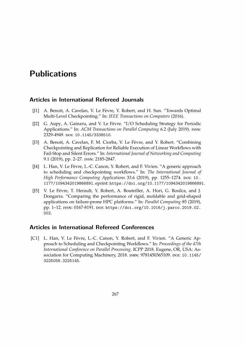
Publications
Articles in International Refereed Journals
[J1] A. Benoit, A. Cavelan, V. Le Fevre, Y. Robert, and H. Sun. “Towards OptimalMulti-Level Checkpointing.” In: IEEE Transactions on Computers (2016).
[J2] G. Aupy, A. Gainaru, and V. Le Fevre. “I/O Scheduling Strategy for PeriodicApplications.” In: ACM Transactions on Parallel Computing 6.2 (July 2019). issn:2329-4949. doi: 10.1145/3338510.
[J3] A. Benoit, A. Cavelan, F. M. Ciorba, V. Le Fevre, and Y. Robert. “CombiningCheckpointing and Replication for Reliable Execution of Linear Workflows withFail-Stop and Silent Errors.” In: International Journal of Networking and Computing9.1 (2019), pp. 2–27. issn: 2185-2847.
[J4] L. Han, V. Le Fevre, L.-C. Canon, Y. Robert, and F. Vivien. “A generic approachto scheduling and checkpointing workflows.” In: The International Journal ofHigh Performance Computing Applications 33.6 (2019), pp. 1255–1274. doi: 10.1177/1094342019866891. eprint: https://doi.org/10.1177/1094342019866891.
[J5] V. Le Fevre, T. Herault, Y. Robert, A. Bouteiller, A. Hori, G. Bosilca, and J.Dongarra. “Comparing the performance of rigid, moldable and grid-shapedapplications on failure-prone HPC platforms.” In: Parallel Computing 85 (2019),pp. 1–12. issn: 0167-8191. doi: https://doi.org/10.1016/j.parco.2019.02.002.
Articles in International Refereed Conferences
[C1] L. Han, V. Le Fevre, L.-C. Canon, Y. Robert, and F. Vivien. “A Generic Ap-proach to Scheduling and Checkpointing Workflows.” In: Proceedings of the 47thInternational Conference on Parallel Processing. ICPP 2018. Eugene, OR, USA: As-sociation for Computing Machinery, 2018. isbn: 9781450365109. doi: 10.1145/3225058.3225145.
267

268 Publications
[C2] A. Benoit, T. Herault, V. Le Fevre, and Y. Robert. “Replication is More Effi-cient than You Think.” In: Proceedings of the International Conference for HighPerformance Computing, Networking, Storage and Analysis. SC ’19. Denver, Col-orado: Association for Computing Machinery, 2019. isbn: 9781450362290. doi:10.1145/3295500.3356171.
Articles in International Refereed Workshops
[W1] A. Benoit, A. Cavelan, V. Le Fevre, Y. Robert, and H. Sun. “A Different Re-execution Speed Can Help.” In: 2016 45th International Conference on ParallelProcessing Workshops (ICPPW). Aug. 2016, pp. 250–257. doi: 10.1109/ICPPW.2016.45.
[W2] G. Aupy, A. Gainaru, and V. Le Fevre. “Periodic I/O Scheduling for Super-Computers.” In: High Performance Computing Systems. Performance Modeling, Bench-marking, and Simulation. Ed. by S. Jarvis, S. Wright, and S. Hammond. Cham:Springer International Publishing, 2017, pp. 44–66. isbn: 978-3-319-72971-8.
[W3] A. Benoit, A. Cavelan, V. Le Fevre, and Y. Robert. “Optimal Checkpointing Pe-riod with Replicated Execution on Heterogeneous Platforms.” In: Proceedings ofthe 2017 Workshop on Fault-Tolerance for HPC at Extreme Scale. FTXS ’17. Wash-ington, DC, USA: Association for Computing Machinery, 2017, pp. 9–16. isbn:9781450350013. doi: 10.1145/3086157.3086165.
[W4] A. Benoit, A. Cavelan, F. M. Ciorba, V. Le Fevre, and Y. Robert. “CombiningCheckpointing and Replication for Reliable Execution of Linear Workflows.” In:2018 IEEE International Parallel and Distributed Processing Symposium Workshops(IPDPSW). May 2018, pp. 793–802. doi: 10.1109/IPDPSW.2018.00126.
[W5] V. Le Fevre, L. Bautista-Gomez, O. Unsal, and M. Casas. “Approximating aMulti-Grid Solver.” In: 2018 IEEE/ACM Performance Modeling, Benchmarking andSimulation of High Performance Computer Systems (PMBS). Nov. 2018, pp. 97–107.doi: 10.1109/PMBS.2018.8641651.
[W6] V. Le Fevre, G. Bosilca, A. Bouteiller, T. Herault, A. Hori, Y. Robert, and J.Dongarra. “Do Moldable Applications Perform Better on Failure-Prone HPCPlatforms?” In: Euro-Par 2018: Parallel Processing Workshops. Ed. by G. Mencagli,D. B. Heras, V. Cardellini, E. Casalicchio, E. Jeannot, F. Wolf, A. Salis, C. Schi-fanella, R. R. Manumachu, L. Ricci, M. Beccuti, L. Antonelli, J. D. Garcia Sanchez,and S. L. Scott. Cham: Springer International Publishing, 2018, pp. 787–799.isbn: 978-3-030-10549-5.
[W7] A. Benoit, V. Le Fevre, P. Raghavan, Y. Robert, and H. Sun. “Design and Com-parison of Resilient Scheduling Heuristics for Parallel Jobs.” In: 2020 IEEE In-ternational Parallel and Distributed Processing Symposium Workshops (IPDPSW).2020.