ww

w.in

l.g

ov

RNEDE: Resilient Network Design Environment

Venkat Venkatasubramanian

Tanu Malik, Prasad Raghavendra, Aviral Shukla and Kris Villez

Purdue

Craig Rieger, Keith Daum, and Miles McQueenINL

Aug 9, 2010

Motivation

• The nation’s critical infrastructure is increasingly characterized by large networks

– electrical power grids

– road and airline systems

– biological pathways

– chemical plants

– Internet

Problem: Design of Resilient Topologies

• Topology governs operational efficiency and resiliency

• How to optimize topology in the event of threats and disruptions?

– Which remedial action must be taken?

– Where in the current network remedial actions should be taken?

– Whether remedial actions are even worth taking?

• Distance:– d (i, j) = length of the shortest path between i and j

• Average Path Length

ni,j1,

2

)1n(n

)j,i(d

APSPAveragedj,i

1

2• Interaction Efficiency– “Time or Effort” required for an exchange between agents

i and j

– Measured by Path length

– Smaller average path length, higher efficiencyd

Eff1

Efficiency of interaction

• Failure of one or more nodes/edges

– Structural robustness:

• Number of resulting component(s)

• Resulting graph connected: perfectly robust

– Functional robustness:

• Efficiency of resulting component(s)

• Average path length of resulting graph unchanged: perfectly robust

– Worst-case versus average-case

Overall Robustness: combination of above

Robustness of Interaction

• They are often conflicting Objectives

– Increasing efficiency often implies reducing robustness for the same cost

– And vice versa

• Efficiency : A measure of short-term performance or survival

• Robustness: A measure of long-term performance or survival

Efficiency and Robustness

• MST: e = emin = n – 1

– No redundancy or excess connectivity

• CG: e = emax = n(n-1)/2

– Maximum redundancy

• Redundancy coefficient

mstcg

mst

ee

ee0 ≤ ≤ 1

• Structural and Functional Redundancies

• Cost: measure of the economy of design– Assumption: All nodes and edges have equal importance

– Cost per edge = 1, Total cost C = e

Redundancy and Cost

• For a given environment , design a net to maximize survival fitness G

1

2

1 2

is the efficiency

is the robustness

is a constant, 0 1

is the cost function related to the addition of edges

is the cost function related to the addition of nod

max (1 ) ( , ) ( )

E

R

E R

c

c

G c k c n

es

is the vertex degree of the node to which a new edge is being added

is the redundancy coefficient

is the number of nodes

k

n Principle of Maximum Harmony

Harmony Function G

Optimization Formalism

Different ‘Survival’ Environments

• = 0

– Only Robustness matters for survival

• = 1

– Only Efficiency matters

• = 0.5

– Both matter equally

• Other values are possible

Network Topologies

(a) Star (b) Line (c) Circle (d) Triangular Hub (e) Pentagonal Hub (f) Perfect Hub

San Francisco Airport

Perfect Hub, Alpha = 0.5

RNEDE: Resilient Network Design Environment

• Visualize, Create, Edit and Analyze

large complex networks/graphs

• Dynamic simulation platform for the

development and evaluation of

methods for control of networked

systems

• Object Oriented system

• Prototype version in Python

RNEDE

RNEDESim: A Simulator for Resilient Network Design

• Key Features

–Replays various threat and disruption scenarios

–Suggests various remedial options

–Provides a visual guide of the network

–Scalable for large networks consisting of thousands of nodes and edges

–Application-independent

A Formal Description

• Topology T = (V,E)

• T satisfies set of constraints C = {c1,…,cn}

• Cost function for maintaining T, S : T → R+

• Set of incidents (disruptions), I = {i1,…,in}

• Compromised topology, T’ = (V’,E’) or (V, E’) or (V’,E); May not satisfy C

• Amount of compromise: F: (T, T’) → R+

• Set of remedial actions, A = {a1,…,an}, and a cost function, Q: A → R+

Resilient Control of Topology

Obtain a set of remedial actions such that the compromise is minimized

i.e., F(T’’, T) < ϵ

Given the disruptions, minimize the cost of maintaining the compromised topology and the cost of making the change

Optimizer and Simulator

• Optimizer: Minimizes the difference in the value of the objective function, F,on the original topology and the compromised topology by choosing a set of remedial actions

• Simulator: Given a network specification, it calculates the value of the objective function F

RNEDE Architecture

1

2

3

RNEDE In-Action

Decision-Controller

• Determines if it is beneficial to transition to T’’ or remain in T’

• The decision is based on

– the incoming sequence of disruptions,

– the transition cost

• associated with remaining in the current topology and the cost of transitioning between T’ and T’’.

• Adopts a rent-vs-buy model

– staying in the current topology corresponds to renting and moving to another topology corresponds to buying

– Several known algorithms, greedy and worst-case.

A Case Study: Supply Chain Networks

Supply chain involves both flow of physical products and information

Conventional objective for supply chain network design is optimizing efficiency (fulfillment of objective with minimum cost)

A crucial objective is the maximization of robustness: the ability of the supply chain to resist shocks

Supply Chain Data

• 1 Manufacturing Centre in Detroit • 50 Customer Zones (US States)

• Delivery to State Capitals

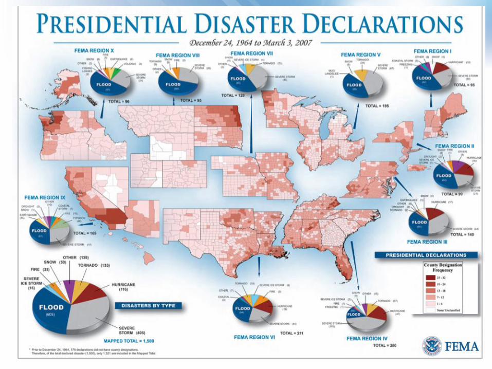
• 10 candidates for warehouse locations:• One in each FEMA region• Boston, NYC, Philadelphia, Jacksonville, Chicago,

Houston, Kansas City, Denver, LA, Seattle

• Demand for each state proportional to the state population

• The distance between the manufacturing centers, warehouses and customer zones is road distance from GoogleTM Maps

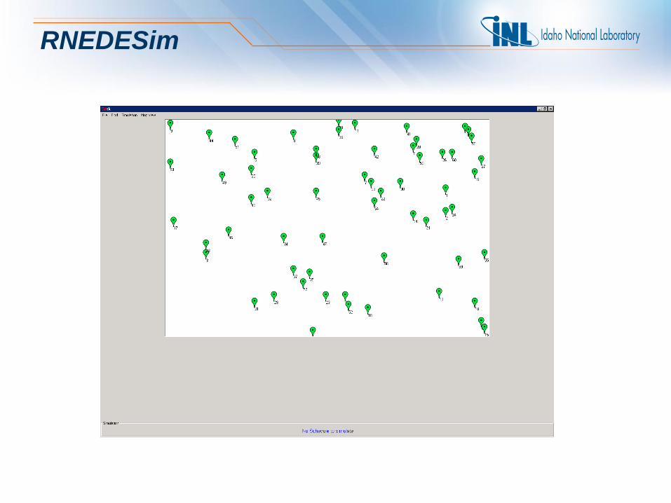
RNEDESim

RNEDESim: Producers/Consumers

RNEDESim: Optimized

RNEDESim: View on the Map

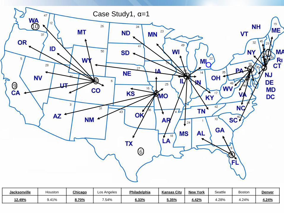
α=1

Jacksonville Houston Chicago Los Angeles Philadelphia Kansas City New York Seattle Boston Denver

12.49% 9.41% 8.70% 7.54% 6.33% 5.35% 4.42% 4.28% 4.24% 4.24%

Case Study1, α=1

α=1

Jacksonville Houston Chicago Los Angeles Philadelphia Kansas City New York Seattle Boston Denver

12.49% 9.41% 8.70% 7.54% 6.33% 5.35% 4.42% 4.28% 4.24% 4.24%

Case Study1, α=0.8

30

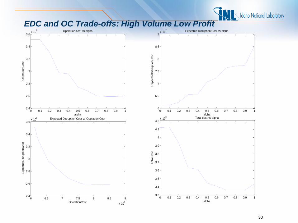
EDC and OC Trade-offs: High Volume Low Profit

0 0.1 0.2 0.3 0.4 0.5 0.6 0.7 0.8 0.9 13.3

3.4

3.5

3.6

3.7

3.8

3.9

4

4.1

4.2x 10

8

alpha

Tota

lCost

Total cost vs alpha

6 6.5 7 7.5 8 8.5 9

x 107

2.4

2.6

2.8

3

3.2

3.4

3.6x 10

8

OperationCost

Expecte

dD

isru

ptionC

ost

Expected Disruption Cost vs Operation Cost

0 0.1 0.2 0.3 0.4 0.5 0.6 0.7 0.8 0.9 12.4

2.6

2.8

3

3.2

3.4

3.6x 10

8

alpha

Opera

tionC

ost

Operation cost vs alpha

0 0.1 0.2 0.3 0.4 0.5 0.6 0.7 0.8 0.9 16

6.5

7

7.5

8

8.5

9x 10

7

alpha

Expecte

dD

isru

ptionC

ost

Expected Disruption Cost vs alpha

Summary

• Resilient Network Design Environment

• Trade-offs between efficiency and robustness and their connection to topologies

• Re-optimize the topology when subject to disruptions for resileint control

• Python and GAMS

• Resilient Supply Chain Case Study