
Multitree-Multiobjective Multicast Routing for Traffic Engineering
A review and evaluation of multi-objective algorithms
for the flowshop scheduling problem
Gerardo Minella1, Rubén Ruiz1∗, Michele Ciavotta2†
1 Grupo de Sistemas de Optimización Aplicada, Instituto Tecnológico de Informática,
Universidad Politécnica de Valencia, Valencia, Spain. [email protected], [email protected]
2 Dipartimento di Informatica e Automazione, Università degli studi Roma Tre, Roma, Italy.
March 29, 2007
Abstract
This paper contains a complete and updated review of the literature for multi-
objective flowshop problems which are among the most studied environments in the
scheduling research area. No previous comprehensive reviews exist in the literature.
Papers about lexicographical, goal programming, objective weighting and Pareto ap-
proaches have been reviewed. Exact, heuristic and metaheuristic methods have been
surveyed. Furthermore, a complete computational evaluation is also carried out. A
total of 23 different algorithms including both flowshop-specific methods as well as
general multi-objective optimization approaches have been tested under three differ-
ent two-criteria combinations with a comprehensive benchmark. All methods have
been studied under recent state-of-the-art quality measures. Parametric and non-
parametric statistical testing is profusely employed to support the observed perfor-
mance of the compared methods. As a result, we have identified the best performing
methods from the literature which, along with the review, constitutes a reference
work for further research.
Keywords: scheduling, flowshop, multi-objective, review, evaluation
∗Corresponding author. Tel: +34 96 387 70 07, ext: 74946. Fax: +34 96 387 74 99†This research was carried out while M. Ciavotta was visiting the Grupo de Sistemas de Optimización
Aplicada.
1
1. Introduction
In the field of scheduling, the flowshop problem has been thoroughly studied for decades. The
flowshop problem is defined by a set of N = 1, 2, . . . , n jobs that have to be processed on a set
of M = 1, 2, . . . ,m machines. The processing time of each job j ∈ N on each machine i ∈ M is
known in advance and is denoted by pij. All N jobs visit the machines in the same order, which,
without loss of generality, can be assumed to be 1, 2, . . . ,m. The objective is to find a processing
sequence of the jobs so that a given criterion is optimized. In general, the number of possible
solutions results from the product of all possible job permutations across all machines, i.e. (n!)m
solutions or “schedules”. However, in the flowshop literature it is very common to restrict the
solution space by having the same permutation of jobs for all machines. The resulting problem
is referred to as Permutation Flowshop Problem or PFSP in short where n! schedules are possible.
The majority of the literature for the PFSP is centered around a single optimization criterion
or objective. However, a single criterion is deemed as insufficient for real and practical applica-
tions. Multi-objective optimization is without a doubt a very important research topic not only
because of the multi-objective nature of most real-world problems, but also because there are
still many open questions in this area. Over the last decade, multi-objective optimization has
received a big impulse in Operations Research. Some new techniques have been developed in
order to deal with functions and real-world problems that have multiple objectives, and many
approaches have been proposed.
The easiest way of dealing with a multi-objective problem is the so called “a priori” approach
where two or more objectives are weighted and combined into a single measure, usually linear.
For example, given two optimization criteria F1 and F2, a single-objective problem is derived
with a combined αF1 + (1 − α)F2 function, where 0 ≤ α ≤ 1. However, the major drawback in
this approach is that α must be given a priori. If α is not known, an alternative is to obtain
several solutions with varying values of α but even in this case, if F1 and F2 are measured in
different scales, this approach might be challenging.
A more desirable approach is the “a posteriori” method. In this case, the aim is to obtain many
solutions with as many associated values as objectives. In such cases, the traditional concept
of “optimum” solution does not apply. A given solution A might have a better F1 value than
another solution B, but at the same time worse F2 value. In this context, a set of solutions is
obtained where their objective values form what is referred to as the Pareto front. In the Pareto
front all solutions are equally good, since there is no way of telling which one is better or worse.
In other words, all solutions belonging to a Pareto front are the “best” solutions for the problem
in a multi-objective sense.
There are no comprehensive reviews in the literature about multi machine flowshops with
several objectives. In the past years a number of interesting algorithms have been proposed.
2
However, new proposals are hardly validated against the existing literature and when done, the
quality indicators used are not appropriate. Additionally, the multi-objective literature is rich on
advanced methods that have not been applied to the PFSP before. Therefore, the objective of
this paper is to give an up-to-date review and evaluation of many existing metaheuristics for solv-
ing the multi-objective PFSP. A second objective is to adapt proposed methods from the general
multi-objective optimization field to the PFSP. As we will see, the literature is marred with dif-
ferent multi-objective proposals, many of which have not been tested for scheduling problems. As
a result we identify the most promising methods for the most common criteria combination. We
evaluate a total of 23 methods, from local search metaheuristics such as tabu search or simulated
annealing to evolutionary approaches like genetic algorithms. Furthermore, we use the latest
Pareto-compliant quality measures for assessing the effectiveness of the tested methods. Careful
and comprehensive statistical testing is employed to ensure the accuracy of the conclusions.
The remainder of this paper is organized as follows: In Section 2 we further introduce the
single and multi-objective PFSP, along with some notation and complexity results. In Section 3
we review the general literature on multi-objective optimization as well as the existing results
for the PFSP. Section 4 examines the different available quality measures for comparing multi-
objective methods. Section 5 deals with the comparative evaluation of all the studied algorithms.
Finally in Section 6 some conclusions and further research topics are given.
2. Single and Multi-objective optimization
Single optimization criteria for the PFSP are mainly based on the completion times for the jobs
at the different machines which are denoted by Cij , i ∈ M, j ∈ N . Given a permutation π of n
jobs, where π(j) denotes the job in the j-th position of the sequence, the completion times are
calculated with the following expression:
Ci,π(j)= max
{
Ci−1,π(j), Ci,π(j−1)
}
+ piπ(j)(1)
where C0,π(j)= 0 and Ci,π(0)
= 0, ∀i ∈ M,∀j ∈ N . Additionally, the completion time of job j
equals to Cmj and is commonly denoted as Cj in short.
By far, the most thoroughly studied single criterion is the minimization of the maximum comple-
tion time or makespan, denoted as Cmax = Cm,π(n). Under this objective, the PFSP is referred to
as F/prmu/Cmax according to Graham et al. (1979) and was shown by Garey et al. (1976) to be
NP-Hard in the strong sense for more than two machines (m > 2). Recent reviews and compar-
ative evaluations of heuristics and metaheuristics for this problem are given in Framinan et al.
(2004); Ruiz and Maroto (2005) and in Hejazi and Saghafian (2005). The second most stud-
ied objective is the total completion time or TCT =∑n
j=1 Cj. The PFSP with this objective
(F/prmu/∑
Cj) is already NP-Hard for m ≥ 2 according to Gonzalez and Sahni (1978). Some
recent results for this problem can be found in El-Bouri et al. (2005) or Rajendran and Ziegler
3
(2005). If there are no release times for the jobs, i.e., rj = 0,∀j ∈ N , then the total or average
completion time equals the total or average flowtime, denoted as F in the literature.
Probably, the third most studied criterion is the total tardiness minimization. Given a due
date dj for job j, we denote by Tj the measure of tardiness of job j, which is defined as
Tj = max{Cj − dj , 0}. As with the other objectives, total tardiness minimization results in
a NP-Hard problem in the strong sense for m ≥ 2 as shown in Du and Leung (1990). A recent
review for the total tardiness version of the PFSP (the F/prmu/∑
Tj problem) can be found in
Vallada et al. (2007).
Single and multi-objective scheduling problems have been studied extensively. However, in the
multi-objective case, the majority of studies use the simpler “a priori” approach where multiple
objectives are weighted into a single one. As mentioned, the main problem in this method is
that the weights for each objective must be given. The “a posteriori” multi-objective approach is
more complex since in this case, there is no single optimum solution, but rather lots of “optimum”
solutions. For example, given two solutions x1 and x2 for a given problem with two minimization
objectives f1 and f2 and being f1(·) and f2(·) the objective values for a given solution. Is x1
better than x2 if f1(x1) < f1(x2) but at the same time f2(x1) > f2(x2)? It is clear than in a multi-
objective scenario, neither solution is better than the other. However, given a third solution x3
we can say than x3 is worse than x1 if f1(x1) < f1(x3) and f2(x1) < f2(x3). In order to properly
compare two solutions in a Multi-Objective Optimization Problem (MOOP) some definitions are
needed. Without loss of generality, let us suppose that there are M minimization objectives in
a MOOP. We use the operator ⊳ as “better than”, so that the relation x1 ⊳ x2 implies that x1 is
better than x2 for any minimization objective.
Zitzler et al. (2003) present a much more extensive notation which is later extended in Paquete
(2005) and more recently in Knowles et al. (2006). For the sake of completeness, some of this
notation is also introduced here:
Strong (or strict) domination: A solution x1 is said to strongly dominate a solution x2
(x1 ≺≺ x2) if:
fj(x1) ⊳ fj(x2) ∀j = 1, 2, . . . ,M ; x1 is better than x2 for all the objective values.
Domination: A solution x1 is said to dominate a solution x2 (x1 ≺ x2) if the following conditions
are satisfied:
(1) fj(x1) 6 ⊲ fj(x2) for j = 1, 2, . . . ,M ; x1 is not worse than x2 for all the objective values
(2) fj(x1) ⊳ fj(x2) for at least one j = 1, 2, . . . ,M
Weak domination: A solution x1 is said to weakly dominate a solution x2 (x1 � x2) if:
fj(x1) 6 ⊲fj(x2) for all j = 1, 2, . . . ,M ; x1 is not worse than x2 for all the objective values
4
Incomparable solutions: Solutions x1 and x2 are incomparable (x1‖x2 or x2‖x1) if:
fj(x1) 6� fj(x2) nor fj(x2) 6� fj(x1) for all j = 1, 2, . . . ,M
These definitions can be extended to sets of solutions. Being A and B two sets of solutions for a
given MOOP, we further define:
Strong (or strict) domination: Set A strongly dominates set B (A ≺≺ B) if:
Every xi ∈ B ≻≻ by at least one xj ∈ A
Domination: Set A dominates set B (A ≺ B) if:
Every xi ∈ B ≻ by at least one xj ∈ A
Better: Set A is better than set B (A ⊳ B) if:
Every xi ∈ B � by at least one xj ∈ A and A 6= B
Weakly domination: A weakly dominates B (A � B) if:
Every xi ∈ B � by at least one xj ∈ A
Incomparability: Set A is incomparable with set B (A‖B) if:
Neither A � B nor B � A
Non-dominated set: Among a set of solutions A, we refer to the non-dominated subset A′ such
as xA′
∈ A′ ≺ xA with xA′
6= xA and A′ ⊂ A.
Pareto global optimum solution: a solution x ∈ A (being A a set of all feasible solutions
of a problem) is a Pareto global optimum solution if and only if there is no x′ ∈ A such that
f(x′) ≺ f(x).
Pareto global optimum set: a set A′ ∈ A (being A a set of solutions of a problem) is a Pareto
global optimum set if and only if it contains only and all Pareto global optimum solutions This
set is commonly referred to as Pareto front.
In multi-objective optimization, two goals are usually aimed at. An approximation of the
Pareto global optimum set is deemed good if it is close to this set. Additionally, a good spread of
solutions is also desirable, i.e., an approximation set is good if the whole Pareto global optimum
front is sufficiently covered.
One important question is concerned about the complexity of multi-objective flowshop scheduling
problems. As mentioned above, the PFSP is already NP-Hard under any of three commented
5
single objectives (makespan, total completion time or total tardiness). Therefore, in a multi-
objective PFSP, no matter if the approach is “a priori” or “a posteriori”, the resulting problem is
also NP-Hard if it contains one or more NP-Hard objectives.
3. Literature review on multi-objective optimization
The literature on multi-objective optimization is plenty. However, the multi-objective PFSP field
is relatively scarce, specially when compared against the number of papers published for this
problem that consider one single objective. The few proposed multi-objective methods for the
PFSP are mainly based on evolutionary optimization and some in local search methods like sim-
ulated annealing or tabu search.
It could be argued that many reviews have been published about multi-objective scheduling.
However we find that little attention has been paid to the flowshop scheduling problem. For
example, the review by Nagar et al. (1995b) is mostly centered around single machine problems.
As a matter of fact there are only four survey papers related with flowshop. In another review
by T’kindt and Billaut (2001) we find about 15 flowshop papers reviewed where most of them
are about the specific two machine case. Another review is given by Jones et al. (2002). How-
ever, this is more a quantification of papers in multi-objective optimization. Finally, the more
recent review of Hoogeveen (2005) contains mainly results for one machine and parallel machines
scheduling problems. The papers reviewed about flowshop scheduling are all restricted to the
two machine case. For all these reasons, in this paper we provide a complete and comprehen-
sive review about multi-objective flowshop. However, note that we restrict ourselves to the pure
flowshop setting, i.e., with no additional constraints. In the following, we will use the notation
of T’kindt and Billaut (2002) to specify the technique and objectives studied by each reviewed
paper. For example, a weighted makespan and total tardiness bi-criteria flowshop problem is de-
noted as F//Fl(Cmax, T ). For more details, the reader is referred to T’kindt and Billaut (2001)
or T’kindt and Billaut (2002).
3.1. Lexicographical and ε-constraint approaches
Lexicographical approaches have been also been explored in the literature. Daniels and Chambers
(1990) proposed a constructive heuristic for the m machine flowshop where makespan is mini-
mized subject to a maximum tardiness threshold, a problem denoted by F/prmu/ε(Cmax/Tmax).
This heuristic along with the one of Chakravarthy and Rajendran (1999) (see next section) are
compared with a method recently proposed in Framinan and Leisten (2006). In this later pa-
per, the newly proposed heuristic is shown to outperform the methods of Daniels and Chambers
(1990) and Chakravarthy and Rajendran (1999) both on quality and on the number of feasible
solutions found. A different set of objectives is considered in Rajendran (1992) were the authors
minimize total flowtime subject to optimum makespan value in a two machine flowshop. Such
6
an approach is valid for the PFSP problem since the optimum makespan can be obtained by
applying the well known algorithm of Johnson (1954). Rajendran proposes a branch and bound
(B&B) method together with some heristics for the problem. However, the proposed methods
are shown to solve 24 jobs maximum.
In Neppalli et al. (1996) two genetic algorithms were proposed for solving the two machine bi-
criteria flowshop problem also in a lexicographical way as in Rajendran (1992). The first algo-
rithm is based in the VEGA (Vector Evaluated Genetic Algorithm) of Schaffer (1985). In this
algorithm, two subpopulations are maintained (one for each objective) and are combined by the
selection operator for obtaining new solutions. In the second GA, referred to as the weighted
criteria approach, a linear combination of the two criteria is considered. This weighted sum of
objectives is used as the fitness value. The same problem is studied by Gupta et al. (1999) where
a tabu search is employed. This algorithm is finely-tuned by means of statistical experiments
and shown to outperform some of the earlier existing methods. Gupta et al. (2002) present some
local search procedures and three metaheuristics for a two machine flowshop. The methods de-
veloped are simulated annealing, threshold accepting and tabu search. The criteria to optimize
are composed of several lexicographic pairs involving makespan, weighted flowtime and weighted
tardiness. The proposed methods are compared against the GA of Neppalli et al. (1996) and the
results discussed.
Gupta et al. (2001) proposed nine heuristics for the two machine case minimizing flowtime sub-
ject to optimum makespan, i.e., Lex(Cmax, F ). The authors identify some polynomially solvable
cases and carry out a comprehensive analysis of the proposed heuristics. Insertion based methods
are shown to give the best results. The same problem is approached by T’kindt et al. (2002)
where the authors propose an ant colony optimization (ACO) algorithm. The method is com-
pared against a heuristic from T’kindt et al. (2003) and against other single objective methods
form the literature. Although in some cases is slower, the proposed ACO method is shown to give
higher quality results. T’kindt et al. (2003) work with the same problem. The authors propose a
B&B method capable of solving instances of up to 35 jobs in a reasonable time. Some heuristics
are also provided.
3.2. Weighted objectives
As mentioned, most studies make use of the “a priori” approach. This means that objectives are
weighted (mostly linearly) into a single combined criterion. After this conversion, most single
objective algorithms can be applied.
Nagar et al. (1995a) proposed a B&B procedure for solving a two machine flowshop problem
with a weighted combination of flowtime and makespan as objective. The algorithm initializes
the branch and bound tree with an initial feasible solution and an upper bound, both obtained
from a greedy heuristic. This algorithm was able to find the optimal solutions of problems with
two machines and up to 500 jobs but only under some strong assumptions and data distribu-
7

tions. The same authors use this branch and bound in Nagar et al. (1996) as a tool for providing
the initial population in a genetic algorithm. The hybrid B&B+GA approach is tested for the
same two-job bi-criteria flowshop and it is shown to outperform the pure B&B and GA algo-
rithms. Another genetic algorithm is presented in Sridhar and Rajendran (1996) for makespan
and flowtime, including also idle time as a third criterion. The algorithm uses effective heuristics
for initialization. Cavalieri and Gaiardelli (1998) study a realistic production problem that they
modelize as a flowshop problem with makespan and tardiness criteria. Two genetic algorithms
are proposed where many of their parameters are adaptive. Yeh (1999) proposes another B&B
method that compares favorably against that of Nagar et al. (1995a). For un-structured prob-
lems, Yeh’s B&B is able to solve up to 14-job instances in less time than the B&B of Nagar et al.
(1995a). The same author improved this B&B in Yeh (2001) and finally proposed a hybrid GA in
Yeh (2002) showing the best results among all previous work. Note that all these papers of Yeh
deal with the specific two machine case only. Lee and Chou (1998) proposed heuristic methods
and a mixed integer programming model for the m machine problem combining makespan and
flowtime objectives. Their study shows that the integer programming approach is only valid for
very small instances. A very similar work and results was given in a paper by the same authors
(see Chou and Lee, 1999).
Sivrikaya-Şerifoğlu and Ulusoy (1998) presented three B&B algorithms and two heuristics for the
two machine flowshop with makespan and flowtime objectives. All these methods are compared
among them in a series of experiments. The largest instances solved by the methods contain 18
jobs. A linear combination of makespan and tardiness is studied in Chakravarthy and Rajendran
(1999) but in this case a Simulated Annealing (SA) algorithm is proposed. Chang et al. (2002)
study the gradual-priority weighting approach in place of the variable weight approach for genetic
and genetic local search methods. These two methods are related to those of Murata et al. (1996)
and Ishibuchi and Murata (1998), respectively. In numerical experiments, the gradual-priority
weighting approach is shown superior. Framinan et al. (2002) proposed several heuristics along
with a comprehensive computational evaluation for the m machine makespan and flowtime flow-
shop problem. Allahverdi (2003) also studies the same objectives. A total of 10 heuristics are
comprehensively studied in a computational experiment. Among the studied methods, three pro-
posed heuristics from the author outperform the others. Several dominance relations for special
cases are proposed as well.
A different set of objectives, namely makespan and maximum tardiness, are studied by Allahverdi
(2004). Two variations are tested, in the first one, a weighted combination of the two objectives
subject to a maximum tardiness value is studied. In the second, the weighted combination of
criteria is examined. The author proposes a heuristic and compares it against the results of
Daniels and Chambers (1990) and Chakravarthy and Rajendran (1999). The proposed method
is shown to outperform these two according to the results. Ponnambalam et al. (2004) proposed a
genetic algorithm that uses some ideas from the Traveling Salesman Problem (TSP). The imple-
8
mented GA is a straightforward one that just uses a weighted combination of criteria as the fitness
of each individual in the population. The algorithm is not compared against any other method
from the literature and just some results on small flowshop instances are reported. Lin and Wu
(2006) focuses on the two machine case with a weighted combination of makespan and flowtime.
The authors present a B&B method that is tested against a set of small instances. The proposed
method is able to find optimum solutions to instances of up to 15 jobs in all cases. Lemesre et al.
(2007) have studied the m machine problem with makespan and total tardiness criteria. A spe-
cial methodology based on a B&B implementation, called two-phase method is employed. Due
to performance reasons, the method is parallelized. As a result, some instances of up to 20 jobs
and 20 machines are solved to optimality. However, the reported solving times for these cases are
of seven days in a cluster of four parallel computers.
3.3. Pareto approaches
When focusing on the “a posteriori” approach the number of existing studies drops significantly.
In the previously commented work of Daniels and Chambers (1990), the authors also propose
a B&B procedure for the Cmax and Tmax objectives that computes the pareto global front for
the case of two machines. A genetic algorithm was proposed by Murata et al. (1996) which was
capable of obtaining a pareto front for makespan and total tardiness. This algorithm, referred to
as MOGA, applies elitism by copying a certain number of individuals in the non-dominated set
to the next generation. The non-dominated solutions are kept externally in an archive. The algo-
rithm selection is based on a fitness value given to each solution on the basis of a weighted sum of
the objective’s values. The weights for each objective are randomly assigned at each iteration of
the algorithm. The authors also test their proposed GA with three objectives including flowtime.
Later, in Ishibuchi and Murata (1998) the algorithm is extended by using a local search step that
is applied to every new solution, after the crossover and mutation procedures.
Sayın and Karabatı (1999) studied a B&B algorithm that generates the optimum pareto front
for a two machine flowshop with makespan and flowtime objectives. The experimental evalua-
tion compares only against heuristics like those of Johnson (1954) and Rajendran (1992). Some
instances of up to 24 jobs are solved to optimality. Liao et al. (1997) proposed a B&B algo-
rithm for the two machine bi-criteria optimization problem, with the objectives of minimizing
makespan and number of tardy jobs and also with the objectives of makespan and total tardiness.
The lower bound values are obtained by means of the Johnson algorithm for makespan, and the
Moore’s EDD (Early Due Date) algorithm for the number of tardy jobs. For each node of the
partial schedules, two lower bounds are calculated using the above heuristics. The accepted non-
dominated schedules are kept in an external set. At the end of the algorithm, this set contains
optimal Pareto front for the problem. Lee and Wu (2001) also studies the two machine case
with B&B methods but with a combination of flowtime and total tardiness criteria. The authors
do not compare their proposed approach with the literature and just report the results of their
9
algorithm. A new type of genetic algorithm is shown by Bagchi (2001). This method is based
on the NSGA method by Srinivas and Deb (1994). Some brief experiments are given for a sin-
gle flowshop instance with flowtime and makespan objectives. Murata et al. (2001) improve the
earlier MOGA algorithm of Murata et al. (1996). This new method, called CMOGA, refines the
weight assignment. A few experiments with makespan and total tardiness criteria are conducted.
The new CMOGA outperforms MOGA in the experiments carried out.
Ishibuchi et al. (2003) present a comprehensive study about the effect of adding local search to
their previous algorithm (Ishibuchi and Murata, 1998). The local search is only applied to good
individuals and by specifying search directions. This form of local search was shown to give bet-
ter solutions for many different multi-objective genetic algorithms. In Loukil et al. (2000) many
different scheduling problems are solved with different combinations of objectives. The main
technique used is a multi-objective tabu search (MOTS). The paper contains a general study
involving single and parallel machine problems as well. Later, in Loukil et al. (2005), a similar
study is carried out, but in this case the multi-objective approach employed is the simulated
annealing algorithm (MOSA).
A B&B approach is also shown by Toktaş et al. (2004) for the two machine case under makespan
and maximum earliness criteria. To the best of our knowledge, such combination of objectives
has not been studied in the literature before. The procedure is able to solve problems of up
to 25 jobs. The authors also propose a heuristic method. Suresh and Mohanasundaram (2004)
propose a Pareto-based simulated annealing algorithm for makespan and total flowtime criteria.
The proposed method is compared against that of Ishibuchi et al. (2003) and against an early
version of the SA proposed later by Varadharajan and Rajendran (2005). The results, shown
only for small problems of up to 20 jobs, show the proposed algorithm to be better on some
specific performance metrics. Arroyo and Armentano (2004) studied heuristics for several two
and three objective combinations among makespan, flowtime and maximum tardiness. For two
machines, the authors compare the heuristics proposed against the existing B&B methods of
Daniels and Chambers (1990) and Liao et al. (1997). For the general m machine case, the au-
thors compare the results against those of Framinan et al. (2002). The results favor the proposed
method that is also shown to improve the results of the GA of Murata et al. (1996) if used as
a seed sequence. The same authors developed a tabu search for the makespan and maximum
tardiness objectives in Armentano and Arroyo (2004). The algorithm includes several advanced
features like diversification and local search in several neighborhoods. For the two machine case,
again the proposed method is compared against Daniels and Chambers (1990) and for more than
two machines against Ishibuchi and Murata (1998). The proposed method is shown to be com-
petitive in numerical experiments. In a more recent paper Arroyo and Armentano (2005) carry
out a similar study but in this case using genetic algorithms as solution tools. Although shown
to be better than other approaches, the authors do not compare this GA with their previous
methods.
10

Makespan and total flowtime are studied by Varadharajan and Rajendran (2005) with the help
of simulated annealing methods. These algorithms start from heuristic solutions that are further
enhanced by improvement schemes. Two versions of these SA (MOSA and MOSA-II) are shown
to outperform the GA of Ishibuchi and Murata (1998). Pasupathy et al. (2006) have proposed a
Pareto-archived genetic algorithm with local search and have tested it with the makespan and
flowtime objectives. The authors test this approach against Ishibuchi and Murata (1998) and
Chang et al. (2002). Apparently, the newly proposed GA performs better under some limited
tests. Melab et al. (2006) propose a grid-based parallel genetic algorithm aimed at obtaining
an accurate Pareto front for makespan and total tardiness criteria. While the authors do not
test their approach against other existing algorithms, the results appear promising. However,
the running days are of 10 days in a set of computers operating as a grid. More recently,
Rahimi-Vahed and Mirghorbani (2007) have proposed a complex hybrid multi-objective particle
swarm optimization (MOPS) method. The considered criteria are flowtime and total tardiness.
In this method, a elite tabu search algorithm is used as an initialization of the swarm. A parallel
local search procedure is employed as well to enhance the solution represented by each particle.
This complex algorithm is compared against the SPEAII multi-objective genetic algorithm of
Zitzler et al. (2001). MOPS yields better results than SPEAII according to the reported compu-
tational experimentation albeit at a higher CPU time requirements. Finally, Geiger (2007) has
published an interesting study where the topology of the multi-objective flowshop problem search
space is examined. Using several local search algorithms, the author analyzes the distribution of
several objectives and tests several combinations of criteria.
3.4. Goal Programming and other approaches
There are some cases of other multi-objective methodologies like goal programming. For example,
Selen and Hott (1986) proposed a mixed-integer goal programming formulation for a bi-objective
PFSP dealing with makespan and flowtime criteria. As with every goal programming method, a
minimum desired value for each objective has to be introduced. Later, Wilson (1989) proposed
a different model with fewer variables but a larger number of constraints. However, both models
have the same number of binary variables. The comparison between both models results in the
one of Selen and Hott (1986) being better for problems with n ≥ 15.
Many algorithms in the literature have been proposed that do not explicitly consider many ob-
jectives as in previous sections. For example, Ho and Chang (1991) propose a heuristic that
is specifically devised for minimizing machine idle time in a m machine flowshop. Although
the heuristic does not allow for setting weights or threshold values and does not work with the
Pareto approach either, the authors test it against a number of objectives. A similar approach
is followed by Gangadharan and Rajendran (1994) where a simulated annealing is proposed for
the m machine problem and evaluated under makespan and flowtime criteria. Along with the
SA method, two heuristics are also studied. Rajendran (1995) proposes a heuristic for the same
11
problem dealt with in Ho and Chang (1991). After a comprehensive numerical experimentation,
the new proposed heuristic is shown to be superior to that of Ho and Chang’s. A very similar
study is also presented by the same author in Rajendran (1994). Ravindran et al. (2005) present
three heuristics aimed at minimizing makespan and flowtime. The authors test the three pro-
posed method against the heuristic of Rajendran (1995) but using only very small instances of 20
jobs and 20 machines maximum. The three heuristics appear to outperform Rajendran’s albeit
slightly. It is difficult to draw a line in these type of papers since many authors test a given
proposed heuristic under different objectives. However, the heuristics commented above were
designed with several objectives in mind and therefore we have included them in the review.
To sum up, Table 1 contains, in chronological order, the reviewed papers along with the
number of machines (2 or m), the multi-objective approach along with the criteria as well as the
type of method used.
[Insert Table 1 about here]
In total, 54 papers have been reviewed. Among them, 21 deal with the specific two machine case.
From the remaining 33 that study the more general m machines, a total of 16 use the “a posteriori”
or Pareto based approach. The results of these methods are not comparable for several reasons.
First, the authors do not always deal with the same combination of criteria. Second, comparisons
are many times carried out with different benchmarks and against heuristics or older methods.
Last and most importantly, the quality measures employed are not appropriate as recent studies
have shown. Next Section deals with these measures.
4. Multi-objective quality measures
As commented in previous sections, comparing the solutions of two different Pareto approxima-
tions coming from two algorithms is not straightforward. Two approximation sets A and B can
be even incomparable. Recent studies like those of Zitzler et al. (2003), Paquete (2005) or more
recently, Knowles et al. (2006) are an example of the enormous effort being carried out in order
to provide the necessary tools for a better evaluation and comparison of multi-objective algo-
rithms. However, the multi-objective literature for the PFSP frequently uses quality measures
that have been shown to be misleading. For example, in the two most recent papers reviewed
(Rahimi-Vahed and Mirghorbani, 2007 and Geiger, 2007) some metrics like generational distance
or maximum deviation from the best Pareto front are used. These metrics, among other ones
are shown to be non Pareto-compliant in the study of Knowles et al. (2006), meaning that they
can give a better metric for a given Pareto approximation front B and worse for another front A
even in a case where A ≺ B. What is worse, in the comprehensive empirical evaluation of quality
measures given in Knowles et al. (2006), it is shown that the most frequently used measures are
12
non Pareto-compliant and are demonstrated to give wrong and misleading results more often
than not. Therefore, special attention must be given to the choice of quality measures to ensure
sound and generalizable results.
Knowles et al. (2006) propose three main approaches that are safe and sound. The first one
relies on the Pareto dominance relations among sets of solutions. It is possible to rank a given
algorithm over another based on the number of times the resulting Pareto approximation fronts
dominate (strong, regular or weakly) each other. The second approach relies on quality indi-
cators, mainly the hypervolume IH and the Epsilon indicators that were already introduced in
Zitzler and Thiele (1999) and Zitzler et al. (2003), respectively. Quality indicators usually trans-
form a full Pareto approximation set into a real number. Lastly, the third approach is based on
empirical attainment functions. Attainment functions give, in terms of the objective space, the
relative frequency that each region is attained by the approximation set given by an algorithm.
These three approaches range from straightforward and easy to compute in the case of dominance
ranking to the not so easy and computationally intensive attainment functions.
In this paper, we choose the hypervolume (IH) and the unary multiplicative Epsilon (I1ε ) indi-
cators. The choice is first motivated by the fact that dominance ranking is best observed when
comparing one algorithm against another. By doing so, the number of times the solutions given
by the first algorithm strongly, regularly or weakly dominate those given by the second gives
a direct picture of the performance assessment among the two. The problem is that with 23
algorithms compared in this paper (see next Section) the possible two-algorithms pairs is 253 and
therefore this type of analysis becomes unpractical. The same conclusion can be reached for the
empirical attainment functions because these have to be compared in pairs. Furthermore, the
computation of attainment functions is costly and the outcome has to be examined graphically
one by one. As a result, such type of analysis is not useful in our case.
According to Knowles et al. (2006), IH and I1ε are Pareto-compliant and represent the state-of-
the-art as far as quality indicators are concerned. Additionally, combining the analysis of these
two indicators is a powerful approach since if the two indicators provide contradictory conclusions
for two algorithms, it means that they are incomparable. In the following we give some additional
details on how these two indicators are calculated.
The hypervolume indicator IH , first introduced by Zitzler and Thiele (1999) just measures the
area (in the case of two objectives) covered by the approximated Pareto front given by one al-
gorithm. A reference point is used for the two objectives in order to bound this area. A greater
value of IH indicates both a better convergence to as well as a good coverage of the optimal
Pareto front. Calculating the hypervolume can be costly and we use the algorithm proposed in
Deb (2001). This algorithm already calculates a normalized and scaled value.
The binary epsilon indicator Iε proposed initially by Zitzler et al. (2003) is calculated as follows:
Given two approximation sets A and B produced by two algorithms, the binary multiplicative
13

epsilon indicator Iε(A,B) equals to maxxBminxA
max1≤j≤Mfj(xA)fj(xB) , where xA and xB are each
of the solutions given by algorithms A and B, respectively. Notice that such a binary indicator
would require to calculate all possible pairs of algorithms. However, in Knowles et al. (2006), a
unary I1ε version is proposed where the approximation set B is substituted by the best known
Pareto front. This is an interesting indicator since it tells us how much worse (ε) an approxima-
tion set is w.r.t. the best known Pareto front in the best case. Therefore “ε” gives us a direct
performance measure. Note however that in our case some objectives might take a value of zero
(for example tardiness). Also, objectives must be normalized. Therefore, for the calculation of
the I1ε indicator, we first normalize and translate each objective, i.e., in the previous calculation,
fj(xA) and fj(xB) are replaced byfj(xA)−f−
j
f+j −f−
j
+ 1 andfj(xB)−f−
j
f+j −f−
j
+ 1, respectively, where f+j and
f−j are the maximum and minimum known values for a given objective j, respectively. As a
result, our normalized I1ε indicator will take values between 1 and 2. A value of one for a given
algorithm means that its approximation set is not dominated by the best known one.
5. Computational Evaluation
In this work we have implemented not only algorithms specifically proposed for the multi-objective
PFSP but also many other multi-objective optimization algorithms. In these cases, some adap-
tation has been necessary. In the following we go over the algorithms that have been considered.
5.1. Pareto approaches for the flowshop problem
We now detail the algorithms that have been re-implemented and tested among those proposed
specifically for the flowshop scheduling problem. These methods have been already reviewed in
Section 3 and here we extend some details about them and about their re-implementation.
The MOGA algorithm of Murata et al. (1996) was designed to tackle the multi objective flow-
shop problem. It is a simple genetic algorithm with a modified selection operator. During this
selection, a set of weights for the objectives are generated. In this way the algorithm tends to dis-
tribute the search toward different directions. The authors also incorporate an elite preservation
mechanism which copies several solutions from the actual Pareto front to the next generation.
We will refer to our MOGA implementation as MOGA_Murata. Chakravarthy and Rajendran
(1999) presented a simple simulated annealing algorithm which tries to minimize the weighted
sum of two objectives. The best solution between those generated by the Earliest Due Date
(EDD), Least Static Slack (LSS) and NEH (from the heuristic of Nawaz et al., 1983) methods is
selected to be the initial solution. The adjacent interchange scheme (AIS) is used to generate a
neighborhood for the actual solution. Notice that this algorithm, referred to as SA_Chakravarty,
is not a real Pareto approach since the objectives are weighted. However, we have included it
in the comparison in order to have an idea of how such methods can perform in practice. We
14
“simulate” a Pareto approach by running SA_Chakravarty 100 times with different weight combi-
nations of the objectives. All the 100 resulting solutions are analyzed and the best non dominated
subset is given as a result.
Bagchi (2001) proposed a modification of the well known NSGA procedure (see next section) and
adapted it to the flowshop problem. This algorithm, referred to as ENGA, differentiates from
NSGA in that it incorporates elitism. In particular, the parent and offspring populations are com-
bined in a unique set, then a non-dominated sorting is applied and the 50% of the non-dominated
solutions are copied to the parent population of the following generation. Murata et al. (2001)
enhanced the original MOGA of Murata et al. (1996). A different way of distributing the weights
during the run of the algorithm is presented. The proposed weight specification method makes
use of a cellular structure which permits to better select weights in order to find a finer approxi-
mation of the optimal Pareto front. We refer to this later algorithm as CMOGA.
Suresh and Mohanasundaram (2004) proposed a Pareto archived simulated annealing (PASA)
method. A new perturbation mechanism called “segment-random insertion (SRI)” scheme is used
to generate the neighborhood of a given sequence. An archive containing the non-dominated
solution set is used. A randomly generated sequence is used as an initial solution. The SRI is
used to generate a neighborhood set of candidate solutions and each one is used to update the
archive set. A fitness function that is a scaled weighted sum of the objective functions is used
to select a new current solution. A restart strategy and a re-annealing method are also imple-
mented. We refer to this method as MOSA_Suresh. Armentano and Arroyo (2004) developed
a multi-objective tabu search method called MOTS. The algorithm works with several paths of
solutions in parallel, each with its own tabu list. A set of initial solutions is generated using a
heuristic. A local search is applied to the set of current solutions to generate several new solu-
tions. A clustering procedure ensures that the size of the current solution set remains constant.
The algorithm makes also use of an external archive for storing all the non-dominated solutions
found during the execution. After some initial experiments we found that under the considered
stopping criterion (to be detailed later), less than 12 iterations were carried out. This together
with the fact that the diversification method is not sufficiently clear from the original text has re-
sulted in our implementation not including this procedure. The initialization procedure of MOTS
takes most of the allotted CPU time for large values of n. Considering the large neighborhood
employed, this all results in extremely lengthy computations for larger n values.
Arroyo and Armentano (2005) proposed a genetic local search algorithm with the following fea-
tures: preservation of population’s diversity, elitism (a subset of the current Pareto front is directly
copied to the next generation) and usage of a multi-objective local search. The concept of Pareto
dominance is used to assign fitness (using the non-dominated sorting procedure and the crowding
measure both proposed for the NSGAII) to the solutions and in the local search procedure. We
refer to this method as MOGALS_Arroyo. A multi-objective simulated annealing (MOSA) is
presented in Varadharajan and Rajendran (2005). The algorithm starts with an initialization
procedure which generates two initial solutions using simple and fast heuristics. These sequences
are enhanced by three improvement schemes and are later used, alternatively, as the solution of
the simulated annealing method. MOSA tries to obtain non dominated solutions through the
implementation of a simple probability function that attempts to generate solutions on the Pareto
optimal front. The probability function is varied in such a way that the entire objective space
is covered uniformly obtaining as many non-dominated and well dispersed solutions as possible.
We refer to this algorithm as MOSA_Varadharajan.
Pasupathy et al. (2006) proposed a genetic algorithm which we refer to as PGA_ALS. This
algorithm uses an initialization procedure which generates four good initial solutions that are
introduced in a random population. PGA_ALS handles a working population and an external
one. The internal one evolves using a Pareto-ranking based procedure similar to that used in
NSGAII. A crowding procedure is also proposed and used as a secondary selection criterion. The
non-dominated solutions are stored in the external archive and two different local searches are
then applied to half of archive’s solutions for improving the quality of the returned Pareto front.
Finally, we have also re-implemented PILS from Geiger (2007). This new algorithm is based on
iterated local search which in turn relies on two main principles, intensification using a variable
neighborhood local search and diversification using a perturbation procedure. The Pareto domi-
nance relationship is used to store the non-dominated solutions. This scheme is repeated through
successive iterations to reach favorable regions of the search space. Notice that at the time of the
writing of this paper, this last algorithm has not even been published yet.
Notice that among the 16 multi-objective PFSP specific papers reviewed in Section 3, we are
re-implementing a total of 10. We have chosen not to re-implement the GAs of Ishibuchi and Murata
(1998) and Ishibuchi et al. (2003) since they were shown to be inferior to the multi-objective tabu
search of Armentano and Arroyo (2004) and some others. Loukil et al. (2000) and Loukil et al.
(2005) have presented some rather general methods applied to many scheduling problems. This
generality and the lack of details have deterred us from trying a re-implementation. Arroyo and Armentano
(2004) proposed just some heuristics and finally, the hybrid Particle Swarm Optimization (PSO)
proposed by Rahimi-Vahed and Mirghorbani (2007) in incredibly complex, making use of parallel
programming techniques and therefore we have chosen not to implement it.
5.2. Other general Pareto algorithms
The multi-objective literature is marred with many interesting proposals, mainly in the form of
evolutionary algorithms, that have not been applied to the PFSP before. Therefore, in this sec-
tion we review some of these methods that have been re-implemented and adapted to the PFSP.
Srinivas and Deb (1994) proposed the well known non-dominated sorting genetic algorithm, re-
ferred to as NSGA. This method differs from a simple genetic algorithm only for the way the
selection is performed. The non-dominated Sorting procedure (NDS) iteratively divides the en-
16
tire population into different Pareto fronts. The individuals are assigned a fitness value that
depends on the Pareto front they belong to. Furthermore, this fitness value is modified by a
factor that is calculated according to the number of individuals crowding a portion of the ob-
jective space. A sharing parameter σshare is used in this case. All other features are similar
to a standard genetic algorithm. Zitzler and Thiele (1999) presented another genetic algorithm
referred to as SPEA. The most important characteristic of this method is that all non-dominated
solutions are stored in an external population. Fitness evaluation of individuals depend on the
number of solutions from the external population they dominate. The algorithm also incorpo-
rates a clustering procedure to reduce the size of the non-dominated set without destroying its
characteristics. Finally, population’s diversity is maintained by using the Pareto dominance re-
lationship. Later, Zitzler et al. (2001) proposed an improved SPEAII version that incorporates
a different fine-grained fitness strategy to avoid some drawbacks of the SPEA procedure. Other
improvements include a density estimation technique that is an adaptation of the k-th nearest
neighbor method, and a new complex archive truncation procedure.
Knowles and Corne (2000) presented another algorithm called PAES. This method employs lo-
cal search and a population archive. The algorithm is composed of three parts, the first one
is the candidate solution generator which has an archive of only one solution and generates a
new one making use of random mutation. The second part is the candidate solution acceptance
function which has the task of accepting or discarding the new solution. The last part is the
non-dominated archive which contains all the non-dominated solutions found so far. According
to the authors, this algorithm represents the simplest nontrivial approach to a multi-objective
local search procedure. In the same paper, the authors present an enhancement of PAES referred
to as (µ + λ)−PAES. Here a population of µ candidate solutions is kept. By using a binary tour-
nament, a single solution is selected and λ mutant solutions are created using random mutation.
Hence, a µ + λ population is created and a dominance score is calculated for each individual.
µ individuals are selected to update the candidate population while an external archive of non-
dominated solutions is maintained. Another genetic algorithm is proposed by Corne et al. (2000).
This method, called PESA uses an external population EP and an internal one IP to pursuit
the goal of finding a well spread Pareto front. A selection and replacement procedure based on
the degree of crowding is implemented. A simple genetic scheme is used for the evolution of IP
while EP contains the non-dominated solutions found. The size of the EP is upper bounded
and a hyper-grid based operator eliminates the individuals in the more crowded zones. Later,
in Corne et al. (2001) a enhanced PESAII method is provided. This algorithm differs from the
preceding one only in the selection technique in which the fitness value is assigned according to
a hyperbox calculation in the objective space. In this technique, instead of assigning a selective
fitness to an individual, it is assigned to the hyperboxes in the objective space which are occu-
pied by at least one element. During the selection process, the hyperbox with the best fitness is
selected and an individual is chosen at random among all inside the selected hyperbox.
17
In Deb (2002) an evolution of the NSGA was presented. This algorithm, called NSGAII, uses
a new Fast Non-Dominated Sorting procedure (FNDS). Unlike the NSGA, here a rank value
is assigned to each individual of the population and there is no need for a parameter to achieve
fitness sharing. Also, a crowding value is calculated with a fast procedure and assigned to each
element of the population. The selection operator uses the rank and the crowding values to select
the better individuals for the mating pool. An efficient procedure of elitism is implemented by
comparing two successive generations and preserving the best individuals. This NSGAII method
is extensively used in the multi objective literature for the most varied problem domains. Later,
Deb et al. (2002) introduced yet another GA called CNSGAII. Basically, in this algorithm the
crowding procedure is replaced by a clustering approach. The rationale is that once a generation
is completed, the previous generation has a size of Psize (parent set) and the current one (off-
spring set) is also of the same size. Combining both populations yields a 2Psize set but only half
of them are needed for the next generation. To select these solutions the non-dominated sorting
procedure is applied first and the clustering procedure second.
Deb et al. (2002) studied another different genetic algorithm. This method, called ε−MOEA uses
two co-evolving populations, the regular one called P and an archive A. At each step, two parent
solutions are selected, the first from P and the second from A. An offspring is generated, and it
is compared with each element of the population P . If the offspring dominates at least a single
individual in P then it replaces this individual. The offspring is discarded if it is dominated by P .
The offspring individual is also checked against the individuals in A. In the archive population
the ε−dominance is used in the same way. For example, and using the previous notation, a
solution x1 strongly ε−dominates another solution x2 (x1 ≺ε x2) if fj(x1) − ε ⊳ fj(x2).
Zitzler and Künzli (2004) proposed another method called B−IBEA. The main idea in this
method is defining the optimization goal in terms of a binary quality measure and directly using
it in the selection process. B-IBEA performs binary tournaments for mating selection and imple-
ments environmental selection by iteratively removing the worst individual from the population
and updating the fitness values of the remaining individuals. An ε−indicator is used. In the same
work, an adaptive variation called A−IBEA is also presented. An adapted scaling procedure is
proposed with the goal of making the algorithm’s behavior independent from the tuning of the
parameter k used in the basic B−IBEA version. Finally, Kollat and Reed (2005) proposed also
a NSGAII variation referred to as ε−NSGAII by adding ε−dominance archiving and adaptive
population sizing. The ε parameter establishes the size of the grid in the objective space. Inside
each cell of the grid no more than one solution is allowed. Furthermore, the algorithm works
by alternating two phases. It starts using a very small population of 10 individuals and several
runs of NSGAII are executed. During these runs all the non-dominated solutions are copied to
an external set. When there are no further improvements in the current Pareto front, the second
phase starts. In this second phase the ε−dominance procedure is applied on the external archive.
The 23 re-implemented algorithms, either specific for the PFSP or general multi-objective
18
proposals, are summarized in Table 2.
[Insert Table 2 about here]
5.3. Benchmark and computational evaluation details
Each one of the 23 proposed algorithms is tested against a new benchmark set. There are no
known comprehensive benchmarks in the literature for the multi-objective PFSP. The only refer-
ence we know of is the work of Basseur (2005) where a small set of 14 instances is proposed. In
order to carry out a comprehensive and sound analysis, a much larger set is needed. We augment
the well known instances of Taillard (1993). This benchmark is organized in 12 groups with
10 instances each. The groups contain different combinations of the number of jobs n and the
number of machines m. The n × m combinations are: {20, 50, 100} × {5, 10, 20}, 200 × {10, 20}
and 500 × 20. The processing times (pij) in Taillard’s instances are generated from a uniform
distribution in the range [1, 99]. We take the first 110 instances and drop the last 10 instances
in the 500 × 20 group since this size is deemed as too large for the experiments. As regards
the due dates for the tardiness criterion we use the same approach of Hasija and Rajendran
(2004). In this work, a tight due date dj is assigned to each job j ∈ N following the expression:
dj = Pj × (1 + random · 3) where Pj =∑m
i=1 pij is the sum of the processing times over all
machines for job j and random is a random number uniformly distributed in [0, 1]. This method
of generating due dates results in very tight to relatively tight due dates depending on the actual
value of random for each job, i.e., if random is close to 0, then the due date of the job is going
to be really tight as it would be more or less the sum of its processing times. As a result, the job
will have to be sequenced very early to avoid any tardiness. These 110 augmented instances can
be downloaded from http://www.upv.es/gio/rruiz.
Each algorithm has been carefully re-implemented following all the explanations given by
the authors in the original papers. We have re-implemented all the algorithms in Delphi 2006.
It should be noted that all methods share most structures and functions and the same level of
coding has been used, i.e., all of them contain most common optimizations and speed-ups. Fast
Non-Dominated Sorting (FNDS) is frequently used for most methods. Unless indicated differ-
ently by the authors in the original papers, the crossover and mutation operators used for the
genetic methods are the two point order crossover and insertion mutation, respectively. Unless
explicitly stated, all algorithms incorporate a duplicate-deletion procedure in the populations as
well as in the non-dominated archives.
The stopping criterion for most algorithms and is given by a time limit depending on the size of
the instance. The algorithms are stopped after a CPU running time of n · m/2 · t milliseconds,
where t is an input parameter. Giving more time to larger instances is a natural way of separating
the results from the lurking “total CPU time” variable. Otherwise, if worse results are obtained
19

for large instances, it would not be possible to tell if it is due to the limited CPU time or due
to the instance size. Every algorithm is run 10 different independent times (replicates) on each
instance with three different stopping criteria: t = 100, 150 and 200 milliseconds. This means
that for the largest instances of 200 × 20 a maximum of 400 seconds of real CPU time (not wall
time) are allowed. For every instance, stoping time and replicate we use the same random seed
as a common variance reduction technique.
We run every algorithm on a cluster of 12 identical computers with Intel Core 2 Duo E6600
processors running at 2.4 GHz with 1 Gbyte of RAM. For the tests, each algorithm and in-
stance replicate is randomly assigned to a single computer and the results are collected at the
end. According to Section 2, the three most common criteria for the PFSP are makespan, total
completion time and total tardiness. All these criteria are of the minimization type. Therefore,
all experiments are conducted for the three following criteria combinations: 1) makespan and
total tardiness, 2) total completion time and total tardiness and finally, 3) makespan and total
completion time.
A total of 75,900 data points are collected per criteria combination if we consider the 23 algo-
rithms, 110 instances, 10 replicates per instance and three different stopping time criteria. In
reality, each data point is an approximated Pareto front containing a set of vectors with the
objective values. In total there are 75, 900 · 3 = 227, 700 Pareto fronts taking into account the
three criteria combinations. The experiments have required approximately 5,100 CPU hours.
From the 23 · 10 · 3 = 690 available Pareto front approximations for each instance and criteria
combination, a FNDS is carried out and the best non-dominated Pareto front is stored. These
“best” 110 Pareto fronts for each criteria combination are available for future use of the research
community and are also downloadable from http://www.upv.es/gio/rruiz. Additionally, a set
of best Pareto fronts are available for the three different stopping time criteria. These last Pareto
fronts are also used for obtaining the reference points for the hypervolume (IH) indicator and are
fixed to 1.2 times the worst known value for each objective. Also, these best Pareto fronts are
also used as the reference set in the multiplicative epsilon indicator (I1ε ).
5.4. Makespan and total tardiness results
According to the review carried out in previous sections, makespan and total tardiness are two
common criteria. Furthermore, a low makespan increases machine utilization and throughput.
However, the best possible makespan might sacrifice due dates and therefore both objectives are
not correlated. We test all 23 re-implemented methods for these two criteria. Table 3 shows the
average hypervolume (IH) and epsilon indicator (I1ε ) values for all the algorithms. Notice that
the results are divided into the three different stopping criteria. Also, the methods are sorted in
descending order of hypervolume value.
[Insert Table 3 about here]
20
Although later we will conduct several statistical experiments, we proceed now to comment on
the results. First and foremost, both quality indicators are contradictory in very few cases. We
can observe that as hypervolume values decrease, the epsilon indicator increases. There are just
some exceptions and these occur between consecutive algorithms with very similar hypervolume
values, like for example SPEA and CNSGAII in positions 10 and 11 in the 200ms time columns.
Another interesting result is that the ranking of the algorithms does not practically change as
the allowed CPU time is increased and when it does it is motivated by small differences to start
with. However, these are the observed average values across all instances and as we will mention
later, there are more pronounced differences when focusing on specific instance sizes.
Since the objective values are normalized and the worst solutions are multiplied by 1.2, the
maximum hypothetical hypervolume is 1.22 = 1.44. As we can see, MOSA_Varadharajan is
very close to this value in all three stopping criteria. Similarly, the minimum, possible epsilon
indicator is one. Most interestingly, PESA and PESAII algorithms outperform PGA_ALS and
MOTS by a noticeable margin. It has to be reminded that PESA and PESAII have just been
re-implemented and adapted to the PFSP problem since both methods were proposed in the gen-
eral multi-objective optimization literature, i.e., they were not built for the PFSP. GA_ALS and
MOTS are PFSP-specific algorithms and in the case of MOTS, even for the same two objectives
that have been tested. It is also interesting how MOGA_Murata, is the 7th best performer in
the comparison, although it is more than 10 years old and one of the first multi-objective algo-
rithms proposed for the PFSP. This algorithm manages to outperform CMOGA, proposed also
by the same authors and claimed to be better to MOGA_Murata. It has to be reminded that
our re-implementations have been carried out according to the details given in all the reviewed
papers. CMOGA might result to be better to MOGA_Murata under different CPU times or
under specific optimizations. However, for the careful and comprehensive testing in this paper,
this is not the case.
In a much more unfavorable position are the remaining PFSP-specific methods (MOSA_Suresh,
SA_Chakravarthy, PILS and ENGA). The bad performance of SA_Chakravarthy is expected,
since it has to be recalled that this method uses the “a priori” approach by weighting the objectives
and here we have run it for 100 different times with varying weights. Therefore, using this type
of methods in such a way for obtaining a Pareto front is not advisable. ENGA is, as indicated by
the original authors, better than NSGA but overall significantly worse than earlier methods like
MOGA_Murata. Another striking result is the poor performance of the recent PILS method.
Basically PILS is an iterative improvement procedure and is extremely costly in terms of CPU
time. Therefore, in our experimental setting, it is outperformed by most other methods.
It should be specified that not all methods stop by the allotted CPU time as a stopping
criterion. Some methods carry out some local searches after completing the iterations and some
others just cannot be properly modified to stop at a given point in time. In any case, all CPU
21
times stay within a given acceptable interval. For example, for 100 milliseconds stopping time
and for the largest 200 × 20 instances tested, all methods should stop at 3.33 minutes. How-
ever, SA_Chakravarty stopped at 1.39 minutes. MOGALS_Arroyo at 3.36, MOTS at 3.52,
PILS at 3.36, MOSA_Suresh at 12.8 and MOSA_Varadharajan at 2.23. For 200 millisec-
onds stopping time all methods should stop at 6.67 minutes for the largest instances. In this
case, MOTS required 7.05 minutes, PILS 6.72, SA_Chakravarty 1.39, MOSA_Suresh 12.92 and
MOSA_Varadharajan 2.16. Interestingly, MOSA_Varadharajan, the best performer of the test
is actually a fast method and other not so well performers like MOSA_Suresh take a much longer
time. All other methods can be controlled to stop at the specified time. These discrepancies in
stopping times are only important for the largest instances as for the smallest ones more or less
all CPU times are similar.
Table 3 contains just average values and many of them are very similar. Although each
average is composed of a very large number of data points, it is still necessary to carry out a
comprehensive statistical experiment to assess if the observed differences in the average values
are indeed statistically significant. A total of 12 different experiments are carried out. We do
design of experiments (DOE) and parametric ANOVA analyses as well as non-parametric Fried-
man rank-based tests on both quality indicators and for the three different stopping criteria.
The utility of showing both parametric as well as non-parametric tests is threefold. First, in
the Operations Research and Computer Science literature it is common to disregard parametric
testing due to the fact that this type of tests are based on assumptions that the data has to
satisfy. Non-parametric testing is many times preferred since it is “distribution-free”. However,
non-parametric testing is nowhere as powerful as parametric testing. Second, in non-parametric
testing a lot of information is lost since the data has to be ranked and the differences in the values
(be these large or small) are transformed into a rank value. Third, ANOVA techniques allow for
a much deeper and richer study of the data. Therefore we also compare both techniques in this
paper to support these claims. For more information the reader is refereed to Conover (1999)
and Montgomery (2004). We carry out six multi-factor ANOVAS where the type of instance is a
controlled factor with 11 levels (instances from 20×5 to 200×20). The algorithm is another con-
trolled factor with 23 levels. The response variable on each experiment is either the hypervolume
or the epsilon indicator. Lastly, there is one set of experiments for each stopping time. Consid-
ering that each experiment contains 25,300 data points, the three main hypotheses of ANOVA:
normality, homocedasticity and independence of the residuals are easily satisfied. To compare
results, a second set of six experiments are performed. In this case, non-parametric Friedman
rank-based tests are carried out. Since there are 23 algorithms and 10 different replicates, the
results for each instance are ranked between 1 and 230. A rank of one represents the best result
for hypervolume or epsilon indicator. We are performing four different statistical tests on each
set of results (for example, for 100 CPU time we are testing ANOVA and Friedman on both
22

quality indicators). Therefore, a correction on the confidence levels must be carried out since the
same set of data is being used to make more than one inference. We take the most conservative
approach, which is the Bonferroni adjustment, and we set the adjusted significance level αs toα4 = 0.05
4 ≃ 0.01. This means that all the tests are carried out at a 0.01 adjusted confidence level
for a real confidence level of 0.05.
Figures 1 and 2 show the means plot for the factor algorithm in the ANOVA for the epsilon
indicator response variable and the means plot for the ranks of the epsilon indicator, respec-
tively. Both figures refer to the 100 CPU time stopping criterion. For the parametric tests we
use Tukey’s Honest Significant Difference (HSD) intervals which counteract the bias in multiple
pairwise comparisons. Similar Honest Significant Difference (HSD) intervals are used for the
non-parametric tests.
[Insert Figures 1 and 2 about here]
As can be seen, the non-parametric test is less powerful. Not only are the intervals much wider
(recall that overlapping intervals indicate a non-statistically significant difference) but ranking
neglects the differences in the response variables. PILS is shown to be better in rank than
MOSA_Suresh and SA_Chakravarthy when we have already observed that it has worse average
hypervolume and epsilon indicator values. The reason behind this behavior is that PILS is better
for many small instances with a small difference in epsilon indicator than MOSA_Suresh and
SA_Chakravarthy. However, it is much worse for some other larger instances. When one trans-
forms this to ranks, PILS obtains a better rank more times and hence it appears to be better,
when in reality is is marginally better more times but significantly worse many times as well.
Concluding the discussion about parametric vs. non-parametric, if the parametric hypothesis are
satisfied (even if they are not strictly satisfied, as thoroughly explained in Montgomery, 2004) it
is much better to use parametric statistical testing. Notice that we are using a very large dataset,
with medium or smaller datasets, the power of non-parametric tests drops significantly.
The relative ordering, as well as most observed differences of the algorithms are statistically sig-
nificant as we can see from Figure 1. As a matter of fact, the only non-statistically significant
differences are those between (µ + λ)−PAES and ε−NSGAII and between the algorithms CNS-
GAII, SPEA and NSGAII. MOGALS_Arroyo, PESA and PESAII are also equivalent.
Figure 3 shows the parametric results also for CPU time of 100 but for the hypervolume quality
indicator.
[Insert Figure 3 about here]
Notice that the Y-axis is now inverted since a larger hypervolume indicates better results. The
relative ordering of the algorithms is almost identical to that of Figure 1, the only difference be-
ing MOGALS_Arroyo PESA and PESAII. This means that these algorithms show a very similar
performance and on average are incomparable. A more in depth instance-by-instance analysis
23

would be needed to tell them apart.
As we have shown, increasing CPU time does not change, on average, the relative ordering of
the algorithms. Figure 4 shows the parametric results for the epsilon indicator and for 200 CPU
time.
[Insert Figure 4 about here]
We can observe the slight improvement on PILS but although there is an important relative
decrease on the average epsilon indicator, it is not enough to improve the results to a significant
extent. More or less all other algorithms maintain their relative positions with little differences.
We commented before that the average performance is not constant for all instance sizes. For
example, PILS can be a very good algorithm for small problems. Figure 5 shows the parametric
results for the epsilon indicator and for 200ms CPU time but focused on the 50 × 5 instances.
[Insert Figure 5 about here]
As we can see, this group of instances is “easy” in the sense that a large group of algorithms
is able to give very low epsilon indicator values. Most notably, PILS statistically outperforms
MOSA_Varadharajan albeit by a small margin. This performance however is not consistent. For
instances of the size 50 × 10, PILS is the third best performer and for instances if size 100 × 5
PILS results to be the worst algorithm in the comparison. A worthwhile venue of research would
be to investigate the strengths of PILS and to speed it up so that the performance is maintained
for a larger group of instances.
5.5. Total completion time and total tardiness results
Total completion time criterion is related to the amount of work-in-progress or WIP. A low total
completion time minimizes WIP and cycle time as well. As it was the case with the makespan
criterion, total completion time is not correlated with total tardiness. Therefore, in this section
we report the results for these two objectives.
Table 4 shows the corresponding average hypervolume and epsilon indicator values.
[Insert Table 4 about here]
One should expect that different criteria combinations should result in different performance for
the algorithms tested. However, comparing the results of Tables 3 and 4 gives a different picture.
MOSA_Varadhrajan and MOGALS_Arroyo produce the best results with independence of the
allowed CPU time. MOGA_Murata as well as many others keep their relative position and most
other PFSP-specific methods are still on the lower positions despite the new criteria combination.
The only noteworthy exception is the (µ + λ)−PAES method which is ranking 7th where for the
other criteria combinations it was ranking around 12th. As it was the case with the previous
makespan and total tardiness criteria combination, both quality indicators and both parametric
24
as well as non-parametric statistics give consistent results. For example, Figure 6 shows the
parametric results for the epsilon indicator and for 200ms CPU time across all instances.
[Insert Figure 6 about here]
As can be seen, most of the observed differences from Table 4 are indeed statistically significant.
5.6. Makespan and total completion time results
Finally, we study the combination of makespan and total completion time. Contrary to the two
previous criteria combinations, these two objectives are correlated. It is straightforward to see
that a low makespan value will also result in a reduced total completion time. However, there
are some scheduling scenarios where this is not true. In our case, the best approximated Pareto
fronts obtained throughout the tests contain several points and in the case of large instances,
Pareto fronts are composed of hundreds of points. Therefore, it seems that these two objectives
are not as correlated as they seem. Table 4 shows the observed average values.
[Insert Table 5 about here]
Once again, the results are remarkably similar with respect to the other criteria combinations.
MOSA_Varadhrajan and MOGALS_Arroyo are the best performers for the three criteria combi-
nations and the non PFSP-specific methods PESA and PESAII are very good performers as well.
As in the other cases, most observed differences in the average values are statistically significant
as shown in Figure 7.
[Insert Figure 7 about here]
6. Conclusions and future research
In this paper we have conducted a comprehensive survey of the multi-objective literature for the
flowshop, one of the most common and thoroughly studied problems in the scheduling field. This
survey complements others like by those of Nagar et al. (1995b), T’kindt and Billaut (2001) or
Hoogeveen (2005) that did not deal with multi machine flowshops. The papers surveyed include
exact as well as heuristic techniques for many different multi-objective approaches.
Another important contribution is this paper is a complete and comprehensive computational
evaluation of 23 different metaheuristics proposed for the Pareto or “a posteriori” multi-objective
approach. Recent and state-of-the-art quality measures have been employed in an extensive ex-
periment where makespan, total completion time and total tardiness criteria have been studied in
three different two-criteria combinations. The comparative evaluation not only includes flowshop-
specific algorithms but also adaptations of other general methods proposed in the multi-objective
optimization literature. A new set of benchmark instances, based on the well known benchmark
of Taillard (1993) has been proposed and is currently available online along with the best known
25

Pareto fronts for the tested objectives.
A comprehensive statistical analysis of the results has been conducted with both parametric as
well as non-parametric techniques. We have shown the preferred qualities of the parametric tests
over the non-parametric counterparts, contrary to what is mainstream in the literature. The array
of statistical analyses soundly support the observed performances of the evaluated algorithms.
As a result, we have identified the best algorithms from the literature, which, along with the
survey, constitute an important study and reference work for further research. Overall, the multi-
objective simulated algorithm of Varadharajan and Rajendran (2005), MOSA_Varadharajan can
be regarded as the best performer under our experimental settings. Another consistent performer
is the genetic local search method MOGALS_Arroyo of Arroyo and Armentano (2005). Our
adapted versions of PESA and PESAII from Corne et al. (2000) and Corne et al. (2001), respec-
tively, have shown a very good performance over many other flowshop-specific algorithms. The
recent PILS method from Geiger (2007) has shown a promising performance for small instances.
In our study we have also shown that different stopping criteria as well as different criteria com-
binations result in little changes, i.e., the algorithms that give best results do so in a wide array
of circumstances.
Further research stems from the possibility of devising new methods containing characteristics
of the best observed methods like MOSA_Varadharajan or MOGALS_Arroyo. Finally, multi-
objective studies for more complex flowshop problems with additional characteristics like setup
times or parallel machines are scarce and new algorithms for such problems are desirable in
practice.
References
Allahverdi, A. 2003. The two- and m-machine flowshop scheduling problems with bicriteria of
makespan and mean flowtime. European Journal of Operational Research 147 373–396.
Allahverdi, A. 2004. A new heuristic for m-machine flowshop scheduling problem with bicriteria
of makespan and maximum tardiness. Computers & Operations Research 31 157–180.
Armentano, V. A., J. E. C. Arroyo. 2004. An application of a multi-objective tabu search algo-
rithm to a bicriteria flowshop problem. Journal of Heuristics 10 463–481.
Arroyo, J. E. C., V. A. Armentano. 2004. A partial enumeration heuristic for multi-objective
flowshop scheduling problems. Journal of the Operational Research Society 55 1000–1007.
Arroyo, J. E. C., V. A. Armentano. 2005. Genetic local search for multi-objective flowshop
scheduling problems. European Journal of Operational Research 167 717–738.
Bagchi, T. P. 2001. Pareto-optimal solutions for multi-objective production scheduling prob-
lems. E. Zitzler, K. Deb, L. Thiele, Carlos A. Coello Coello, D. Corne, eds., Evolutionary
Multi-Criterion Optimization, First International Conference, EMO 2001, Zurich, Switzer-
26
land, March 7-9, 2001, Proceedings, Lecture Notes in Computer Science, vol. 1993. Springer,
458–471.
Basseur, M. 2005. Conception d’algorithmes coopératifs pour l’optimisation multi-objectif: Ap-
plication aux problèmes d’ordonnancement de type flow-shop. Ph.D. thesis, Laboratoire
d’Informatique Fondamentale de Lille. Lille, France. In French.
Cavalieri, S., P. Gaiardelli. 1998. Hybrid genetic algorithms for a multiple-objective scheduling
problem. Journal of Intelligent Manufacturing 9 361–367.
Chakravarthy, K., C. Rajendran. 1999. A heuristic for scheduling in a flowshop with the bicriteria
of makespan and maximum tardiness minimization. Production Planning and Control 10
707–714.
Chang, P. C., J. C. Hsieh, S. G. Lin. 2002. The development of gradual-priority weighting
approach for the multi-objective flowshop scheduling problem. International Journal of Pro-
duction Economics 79 171–183.
Chou, F. D., C. E. Lee. 1999. Two-machine flowshop scheduling with bicriteria problem. Com-
puters & Industrial Engineering 36 549–564.
Conover, W. 1999. Practical Nonparametric Statistics. 3rd ed. John Wiley & Sons, New York.
Corne, D. W., Nick R. Jerram, Joshua D. Knowles, Martin J. Oates. 2001. PESA-II: Region-based
selection in evolutionary multiobjective optimization. L. Spector, E. D. Goodman, A. Wu,
W. B. Langdon, H. M. Voigt, M. Gen, S. Sen, M. Dorigo, S. Pezeshk, Max H. Garzon, E. Burke,
eds., Proceedings of the Genetic and Evolutionary Computation Conference (GECCO-2001).
Morgan Kaufmann, San Francisco, California, USA, 283–290.
Corne, D. W., J. D. Knowles, M. J. Oates. 2000. The pareto envelope-based selection algorithm
for multiobjective optimization. M. Schoenauer, K. Deb, G. Rudolph, X. Yao, E. Lutton,
Juan J. Merelo Guervós, H. P. Schwefel, eds., Parallel Problem Solving from Nature - PPSN
VI, 6th International Conference, Paris, France, September 18-20, 2000, Proceedings, Lecture
Notes in Computer Science, vol. 1917. Springer, 839–848.
Daniels, R. L., R. J. Chambers. 1990. Multiobjective flow-shop scheduling. Naval research logistics
37 981–995.
Deb, K. 2001. Multi-Objective Optimization Using Evolutionary Algorithms. John Wiley & Sons,
West Sussex, England.
Deb, K. 2002. A fast and elitist multiobjective genetic algorithm: NSGA-II. IEEE Transactions
on Evolutionary Computation 6 182–197.
Deb, K., M. Mohan, S Mishra. 2002. A fast multi-objective evolutionary algorithm for finding well-
spread pareto-optimal solutions. Tech. Rep. 2003002, Kanpur Genetic Algorithms Laboratory
(KanGAL), Kampur, India.
Du, J., J. Y.-T. Leung. 1990. Minimizing total tardiness on one machine is NP-hard. Mathematics
of Operations Research 15 483–495.
El-Bouri, A., S. Balakrishnan, N. Popplewell. 2005. A neural network to enhance local search in
27
the permutation flowshop. Computers & Industrial Engineering 49 182–196.
Framinan, J. M., R. Leisten, R. Ruiz-Usano. 2002. Efficient heuristics for flowshop sequencing
with the objectives of makespan and flowtime minimisation. European Journal of Operational
Research 141 559–569.
Framinan, Jose M., J. N. D. Gupta, R. Leisten. 2004. A review and classification of heuristics
for permutation flow-shop scheduling with makespan objective. Journal of the Operational
Research Society 55 1243–1255.
Framinan, Jose M., R. Leisten. 2006. A heuristic for scheduling a permutation flowshop with
makespan objective subject to maximum tardiness. International Journal of Production Eco-
nomics 99 28–40.
Gangadharan, R., C. Rajendran. 1994. A simulated annealing heuristic for scheduling in a
flowshop with bicriteria. Computers & Industrial Engineering 27 473–476.
Garey, M. R., D. S. Johnson, Ravi Sethi. 1976. The complexity of flowshop and jobshop schedul-
ing. Mathematics of Operations Research 1 117–129.
Geiger, M. J. 2007. On operators and search space topology in multi-objective flow shop schedul-
ing. European Journal of Operational Research In press.
Gonzalez, T., S. Sahni. 1978. Flowshop and jobshop schedules: Complexity and approximation.
Operations Research 26 36–52.
Graham, R. L., E. L. Lawler, J. K. Lenstra, A. H. G. Rinnooy Kan. 1979. Optimization and
approximation in deterministic sequencing and scheduling: A survey. Annals of Discrete Math-
ematics 5 287–326.
Gupta, J. N. D., K. Hennig, F. Werner. 2002. Local search heuristics for two-stage flow shop
problems with secondary criterion. Computers & Operations Research 29 123–149.
Gupta, J. N. D., V. R. Neppalli, F. Werner. 2001. Minimizing total flow time in a two-machine
flowshop problem with minimum makespan. International Journal of Production Economics
69 323–338.
Gupta, J. N. D., N. Palanimuthu, C. L. Chen. 1999. Designing a tabu search algorithm for
the two-stage flow shop problem with secondary criterion. Production Planning & Control 10
251–265.
Hasija, S., C. Rajendran. 2004. Scheduling in flowshops to minimize total tardiness of jobs.
International Journal of Production Research 42 2289–2301.
Hejazi, S. R., S. Saghafian. 2005. Flowshop-scheduling problems with makespan criterion: a
review. International Journal of Production Research 43 2895–2929.
Ho, Johnny C., Yih-Long Chang. 1991. A new heuristic for the n-job, M-machine flow-shop
problem. European Journal of Operational Research 52 194–202.
Hoogeveen, H. 2005. Multicriteria scheduling. European Journal of Operational Research 167
592–623.
Ishibuchi, H., T. Murata. 1998. A multi-objective genetic local search algorithm and its ap-
28
plication to flowshop scheduling. IEEE Transactions on Systems Man and Cybernetics 28
392–403.
Ishibuchi, H., T. Yoshida, T. Murata. 2003. Balance between genetic search and local search in
memetic algorithms for multiobjective permutation flowshop scheduling. IEEE Transactions
on Evolutionary Computation 7 204–223.
Johnson, S. M. 1954. Optimal two- and three-stage production schedules with setup times in-
cluded. Naval Research Logistics Quarterly 1 61–68.
Jones, D. F., S. K. Mirrazavi, M. Tamiz. 2002. Multi-objective meta-heuristics: An overview of
the current state-of-the-art. European Journal of Operational Research 137 1–9.
Knowles, J., D. W. Corne. 2000. Approximating the nondominated front using the pareto archived
evolution strategy. Evolutionary Computation 8 149–172.
Knowles, J., L. Thiele, E. Zitzler. 2006. A tutorial on the performance assessment of stochastic
multiobjective optimizers. Tech. Rep. 214, Computer Engineering and Networks Laboratory
(TIK), ETH Zurich, Switzerland. Revised version.
Kollat, J. B., P. M. Reed. 2005. The value of online adaptive search: A performance comparison
of nsgaii, ε−nsgaii and ε−moea. Carlos A. Coello Coello, A. Hernández Aguirre, E. Zitzler,
eds., Evolutionary Multi-Criterion Optimization, Third International Conference, EMO 2005,
Guanajuato, Mexico, March 9-11, 2005, Proceedings , Lecture Notes in Computer Science, vol.
3410. Springer, 386–398.
Lee, C. E., F. D. Chou. 1998. A two-machine flowshop scheduling heuristic with bicriteria
objective. International Journal of Industrial Engineering 5 128–139.
Lee, W. C., C. C. Wu. 2001. Minimizing the total flow time and the tardiness in a two-machine
flow shop. International Journal of Systems Science 32 365–373.
Lemesre, J., C. Dhaenens, E. G. Talbi. 2007. An exact parallel method for a bi-objective permu-
tation flowshop problem. European Journal of Operational Research 177 1641–1655.
Liao, C.-J., W.-C. Yu, C.-B. Joe. 1997. Bicriterion scheduling in the two-machine flowshop.
Journal of the Operational Research Society 48 929–935.
Lin, B. M. T., J. M. Wu. 2006. Bicriteria scheduling in a two-machine permutation flowshop.
International Journal of Production Research 44 2299–2312.
Loukil, T., J. Teghem, P. Fortemps. 2000. Solving multi-objective production scheduling problems
with tabu search. Control and Cybernetics 29 819–828.
Loukil, T., J. Teghem, D. Tuyttens. 2005. Solving multi-objective production scheduling problems
using metaheuristics. European Journal of Operational Research 161 42–61.
Melab, N., M. Mezmaz, E. G. Talbi. 2006. Parallel cooperative meta-heuristics on the computa-
tional grid. a case study: the bi-objective flow-shop problem. Parallel Computing 32 643–659.
Montgomery, DC. 2004. Design and Analysis of Experiments. sixth ed. John Wiley & Sons, New
York.
Murata, T., H. Ishibuchi, M. Gen. 2001. Specification of genetic search directions in cellular multi-
29

objective genetic algorithms. E. Zitzler, K. Deb, L. Thiele, Carlos A. Coello Coello, D. Corne,
eds., Evolutionary Multi-Criterion Optimization, First International Conference, EMO 2001,
Zurich, Switzerland, March 7-9, 2001, Proceedings , Lecture Notes in Computer Science, vol.
1993. Springer, 82–95.
Murata, T., H. Ishibuchi, H. Tanaka. 1996. Multi-objective genetic algorithm and its applications
to flowshop scheduling. Computers & Industrial Engineering 30 957–968.
Nagar, A., S. S. Heragu, J. Haddock. 1995a. A branch-and-bound approach for a two-machine
flowshop scheduling problem. Journal of the Operational Research Society 46 721–734.
Nagar, A., S. S. Heragu, J. Haddock. 1995b. Mutiple and bicriteria scheduling: A lierature survey.
European Journal of Operational Research 81 88–104.
Nagar, A., S. S. Heragu, J. Haddock. 1996. A combined branch-and-bound and genetic algorithm
based approach for a flowshop scheduling problem. Annals of Operations Research 63 397–414.
Nawaz, Muhammad, E. Emory. Enscore, Jr, Inyong Ham. 1983. A heuristic algorithm for the
m-machine, n-job flow-shop sequencing problem. OMEGA, The International Journal of Man-
agement Science 11 91–95.
Neppalli, V. R., C.-L. Chen, J. N. D. Gupta. 1996. Genetic algorithms for the two-stage bicriteria
flowshop problem. European Journal of Operational Research 95 356–373.
Paquete, Luis F. 2005. Stochastic local search algorithms for multiobjective combinatorial op-
timization: Method and analysis. Ph.D. thesis, Computer Science Department. Darmstadt
University of Technology. Darmstadt, Germany.
Pasupathy, T., C. Rajendran, R. K. Suresh. 2006. A multi-objective genetic algorithm for schedul-
ing in flow shops to minimize the makespan and total flow time of jobs. The International
Journal of Advanced Manufacturing Technology 27 804–815.
Ponnambalam, S. G., H. Jagannathan, M. Kataria, A. Gadicherla. 2004. A TSP-GA multi-
objective algorithm for flow-shop scheduling. The International Journal of Advanced Manu-
facturing Technology 23 909–915.
Rahimi-Vahed, A. R., S. M. Mirghorbani. 2007. A multi-objective particle swarm for a flow shop
scheduling problem. Journal of Combinatorial Optimization 13 79–102.
Rajendran, C. 1992. Two-stage flowshop scheduling problem with bicriteria. Journal of the
Operational Research Society 43 871–884.
Rajendran, C. 1994. A heuristic for scheduling in flowshop and flowline-based manufacturing cell
with multicriteria. International Journal of Production Research 32 2541–2558.
Rajendran, C. 1995. Heuristics for scheduling in flowshop with multiple objectives. European
Journal of Operational Research 82 540–555.
Rajendran, C., H. Ziegler. 2005. Two ant-colony algorithms for minimizing total flowtime in
permutation flowshops. Computers & Industrial Engineering 48 789–797.
Ravindran, D., A. N. Haq, S. J. Selvakuar, R. Sivaraman. 2005. Flow shop scheduling with
multiple objective of minimizing makespan and total flow time. The International Journal of
30
Advanced Manufacturing Technology 25 1007–1012.
Ruiz, R., C. Maroto. 2005. A comprehensive review and evaluation of permutation flowshop
heuristics. European Journal of Operational Research 165 479–494.
Sayın, S., S. Karabatı. 1999. A bicriteria approach to the two-machine flow shop scheduling
problem. European Journal of Operational Research 113 435–449.
Schaffer, J. D. 1985. Multiple objective optimization with vector evaluated genetic algorithms.
Proceedings of the 1st International Conference on Genetic Algorithms. Lawrence Erlbaum
Associates, Inc., Mahwah, NJ, USA, 93–100.
Selen, W. J., D. D. Hott. 1986. A mixed-integer goal-programming formulation of the standard
flowshop scheduling problem. Journal of the Operational Research Society 37 1121–1128.
Sivrikaya-Şerifoğlu, F., G. Ulusoy. 1998. A bicriteria two-machine permutation flowshop problem.
European Journal of Operational Research 107 414–430.
Sridhar, J., C. Rajendran. 1996. Scheduling in flowshop and cellular manufacturing systems
with multiple objectives: A genetic algorithmic approach. Production Planning & Control 7
374–382.
Srinivas, N., K. Deb. 1994. Multiobjective optimization using nondominated sorting in genetic
algorithms. Evolutionary Computation 2 221–248.
Suresh, R. K., K. M. Mohanasundaram. 2004. Pareto archived simulated annealing for permu-
tation flow shop scheduling with multiple objectives. IEEE Conference on Cybernetics and
Intelligent Systems (CIS), Singapore, December 1-3, 2004, Proceedings, vol. 2. 712–717.
Taillard, E. 1993. Benchmarks for basic scheduling problems. European Journal of Operational
Research 64 278–285.
T’kindt, V., J.-C. Billaut. 2001. Multicriteria schduling problems: A survey. RAIRO Recherche
opérationnelle - Operations Research 35 143–163.
T’kindt, V., J.-C. Billaut. 2002. Multicriteria scheduling: Theory, models and algorithms .
Springer, Berlin.
T’kindt, V., J. N. D. Gupta, J.-C. Billaut. 2003. Two-machine flowshop scheduling with a sec-
ondary criterion. Computers & Operations Research 30 505–526.
T’kindt, V., N. Monmarché, F. Tercinet, D. Laügt. 2002. An ant colony optimization algorithm
to solve a 2-machine bicriteria flowshop scheduling problem. European Journal of Operational
Research 142 250–257.
Toktaş, Berkin, Meral Azizoğlu, Suna Kondakcı Köksalan. 2004. Two-machine flow shop schedul-
ing with two criteria: Maximum earliness and makespan. European Journal of Operational
Research 157 286–295.
Vallada, E., R. Ruiz, G. Minella. 2007. Minimising total tardiness in the m-machine flowshop
problem: A review and evaluation of heuristics and metaheuristics. Computers & Operations
Research In press.
Varadharajan, T.K., C. Rajendran. 2005. A multi-objective simulated-annealing algorithm for
31
scheduling in flowshops to minimize the makespan and total flowtime of jobs. European Journal
of Operational Research 167 772–795.
Wilson. 1989. Alternative formulations of a flowshop scheduling problem. Journal of the Opera-
tional Research Society 40 395–399.
Yeh, W.-C. 1999. A new branch-and-bound approach for the n/2/flowshop/αF +βCmax. Com-
puters & Operations Research 26 1293–1310.
Yeh, W.-C. 2001. An efficient branch-and-bound algorithm for the two-machine bicriteria flowshop
scheduling problem. Journal of Manufacturing Systems 20 113–123.
Yeh, W.-C. 2002. A memetic algorithm for the n/2/flowshop/αF + βCmax scheduling problem.
The International Journal of Advanced Manufacturing Technology 20 464–473.
Zitzler, E., S. Künzli. 2004. Indicator-based selection in multiobjective search. 8th International
Conference on Parallel Problem Solving from Nature (PPSN VIII). Springer-Verlag, Berlin,
Germany, Birmingham, UK, 832–842.
Zitzler, E., M. Laumanns, L. Thiele. 2001. SPEA2: Improving the strength pareto evolutionary
algorithm. Tech. Rep. 103, Computer Engineering and Networks Laboratory (TIK), ETH
Zurich, Switzerland.
Zitzler, E., L. Thiele. 1999. Multiobjective evolutionary algorithms: A comparative case study
and the strength pareto approach. IEEE Transactions on Evolutionary Computation 3 257–
271.
Zitzler, E., L. Thiele, M. Laumanns, C. M. Fonseca, V. G. da Fonseca. 2003. Performance assess-
ment of multiobjective optimizers: an analysis and review. IEEE, Transactions on Evolutionary
Computation 7 117–132.
32
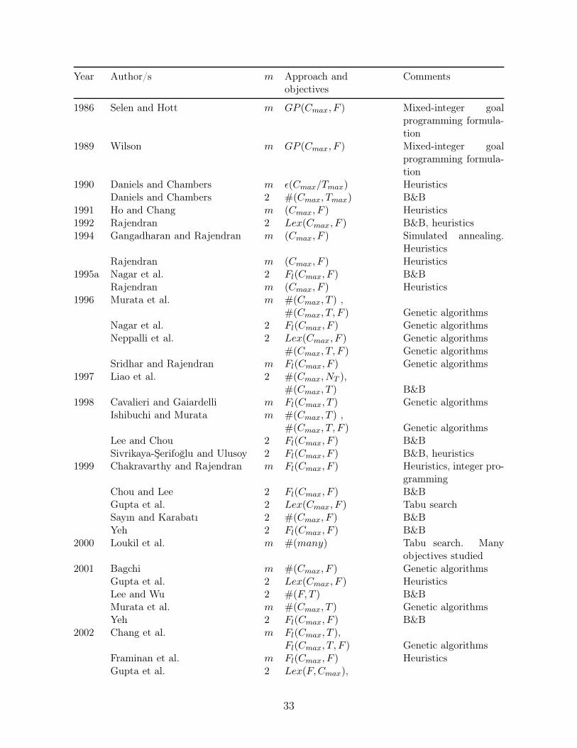
Year Author/s m Approach and Commentsobjectives
1986 Selen and Hott m GP (Cmax, F ) Mixed-integer goalprogramming formula-tion
1989 Wilson m GP (Cmax, F ) Mixed-integer goalprogramming formula-tion
1990 Daniels and Chambers m ǫ(Cmax/Tmax) HeuristicsDaniels and Chambers 2 #(Cmax, Tmax) B&B
1991 Ho and Chang m (Cmax, F ) Heuristics1992 Rajendran 2 Lex(Cmax, F ) B&B, heuristics1994 Gangadharan and Rajendran m (Cmax, F ) Simulated annealing.
HeuristicsRajendran m (Cmax, F ) Heuristics
1995a Nagar et al. 2 Fl(Cmax, F ) B&BRajendran m (Cmax, F ) Heuristics
1996 Murata et al. m #(Cmax, T ) ,#(Cmax, T, F ) Genetic algorithms
Nagar et al. 2 Fl(Cmax, F ) Genetic algorithmsNeppalli et al. 2 Lex(Cmax, F ) Genetic algorithms
#(Cmax, T, F ) Genetic algorithmsSridhar and Rajendran m Fl(Cmax, F ) Genetic algorithms
1997 Liao et al. 2 #(Cmax, NT ),#(Cmax, T ) B&B
1998 Cavalieri and Gaiardelli m Fl(Cmax, T ) Genetic algorithmsIshibuchi and Murata m #(Cmax, T ) ,
#(Cmax, T, F ) Genetic algorithmsLee and Chou 2 Fl(Cmax, F ) B&BSivrikaya-Şerifoğlu and Ulusoy 2 Fl(Cmax, F ) B&B, heuristics
1999 Chakravarthy and Rajendran m Fl(Cmax, F ) Heuristics, integer pro-gramming
Chou and Lee 2 Fl(Cmax, F ) B&BGupta et al. 2 Lex(Cmax, F ) Tabu searchSayın and Karabatı 2 #(Cmax, F ) B&BYeh 2 Fl(Cmax, F ) B&B
2000 Loukil et al. m #(many) Tabu search. Manyobjectives studied
2001 Bagchi m #(Cmax, F ) Genetic algorithmsGupta et al. 2 Lex(Cmax, F ) HeuristicsLee and Wu 2 #(F, T ) B&BMurata et al. m #(Cmax, T ) Genetic algorithmsYeh 2 Fl(Cmax, F ) B&B
2002 Chang et al. m Fl(Cmax, T ),Fl(Cmax, T, F ) Genetic algorithms
Framinan et al. m Fl(Cmax, F ) HeuristicsGupta et al. 2 Lex(F,Cmax),
33
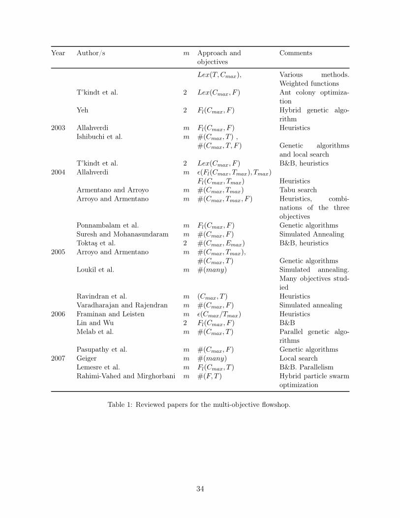
Year Author/s m Approach and Commentsobjectives
Lex(T,Cmax), Various methods.Weighted functions
T’kindt et al. 2 Lex(Cmax, F ) Ant colony optimiza-tion
Yeh 2 Fl(Cmax, F ) Hybrid genetic algo-rithm
2003 Allahverdi m Fl(Cmax, F ) HeuristicsIshibuchi et al. m #(Cmax, T ) ,
#(Cmax, T, F ) Genetic algorithmsand local search
T’kindt et al. 2 Lex(Cmax, F ) B&B, heuristics2004 Allahverdi m ǫ(Fl(Cmax, Tmax), Tmax)
Fl(Cmax, Tmax) HeuristicsArmentano and Arroyo m #(Cmax, Tmax) Tabu searchArroyo and Armentano m #(Cmax, Tmax, F ) Heuristics, combi-
nations of the threeobjectives
Ponnambalam et al. m Fl(Cmax, F ) Genetic algorithmsSuresh and Mohanasundaram m #(Cmax, F ) Simulated AnnealingToktaş et al. 2 #(Cmax, Emax) B&B, heuristics
2005 Arroyo and Armentano m #(Cmax, Tmax),#(Cmax, T ) Genetic algorithms
Loukil et al. m #(many) Simulated annealing.Many objectives stud-ied
Ravindran et al. m (Cmax, T ) HeuristicsVaradharajan and Rajendran m #(Cmax, F ) Simulated annealing
2006 Framinan and Leisten m ǫ(Cmax/Tmax) HeuristicsLin and Wu 2 Fl(Cmax, F ) B&BMelab et al. m #(Cmax, T ) Parallel genetic algo-
rithmsPasupathy et al. m #(Cmax, F ) Genetic algorithms
2007 Geiger m #(many) Local searchLemesre et al. m Fl(Cmax, T ) B&B. ParallelismRahimi-Vahed and Mirghorbani m #(F, T ) Hybrid particle swarm
optimization
Table 1: Reviewed papers for the multi-objective flowshop.
34
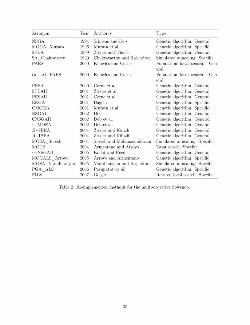
Acronym Year Author/s Type
NSGA 1994 Srinivas and Deb Genetic algorithm. GeneralMOGA_Murata 1996 Murata et al. Genetic algorithm. SpecificSPEA 1999 Zitzler and Thiele Genetic algorithm. GeneralSA_Chakravarty 1999 Chakravarthy and Rajendran Simulated annealing. SpecificPAES 2000 Knowles and Corne Population local search. Gen-
eral(µ + λ)−PAES 2000 Knowles and Corne Population local search. Gen-
eralPESA 2000 Corne et al. Genetic algorithm. GeneralSPEAII 2001 Zitzler et al. Genetic algorithm. GeneralPESAII 2001 Corne et al. Genetic algorithm. GeneralENGA 2001 Bagchi Genetic algorithm. SpecificCMOGA 2001 Murata et al. Genetic algorithm. SpecificNSGAII 2002 Deb Genetic algorithm. GeneralCNSGAII 2002 Deb et al. Genetic algorithm. Generalε−MOEA 2002 Deb et al. Genetic algorithm. GeneralB−IBEA 2004 Zitzler and Künzli Genetic algorithm. GeneralA−IBEA 2004 Zitzler and Künzli Genetic algorithm. GeneralMOSA_Suresh 2004 Suresh and Mohanasundaram Simulated annealing. SpecificMOTS 2004 Armentano and Arroyo Tabu search. Specificε−NSGAII 2005 Kollat and Reed Genetic algorithm. GeneralMOGALS_Arroyo 2005 Arroyo and Armentano Genetic algorithm. SpecificMOSA_Varadharajan 2005 Varadharajan and Rajendran Simulated annealing. SpecificPGA_ALS 2006 Pasupathy et al. Genetic algorithm. SpecificPILS 2007 Geiger Iterated local search. Specific
Table 2: Re-implemented methods for the multi-objective flowshop.
35
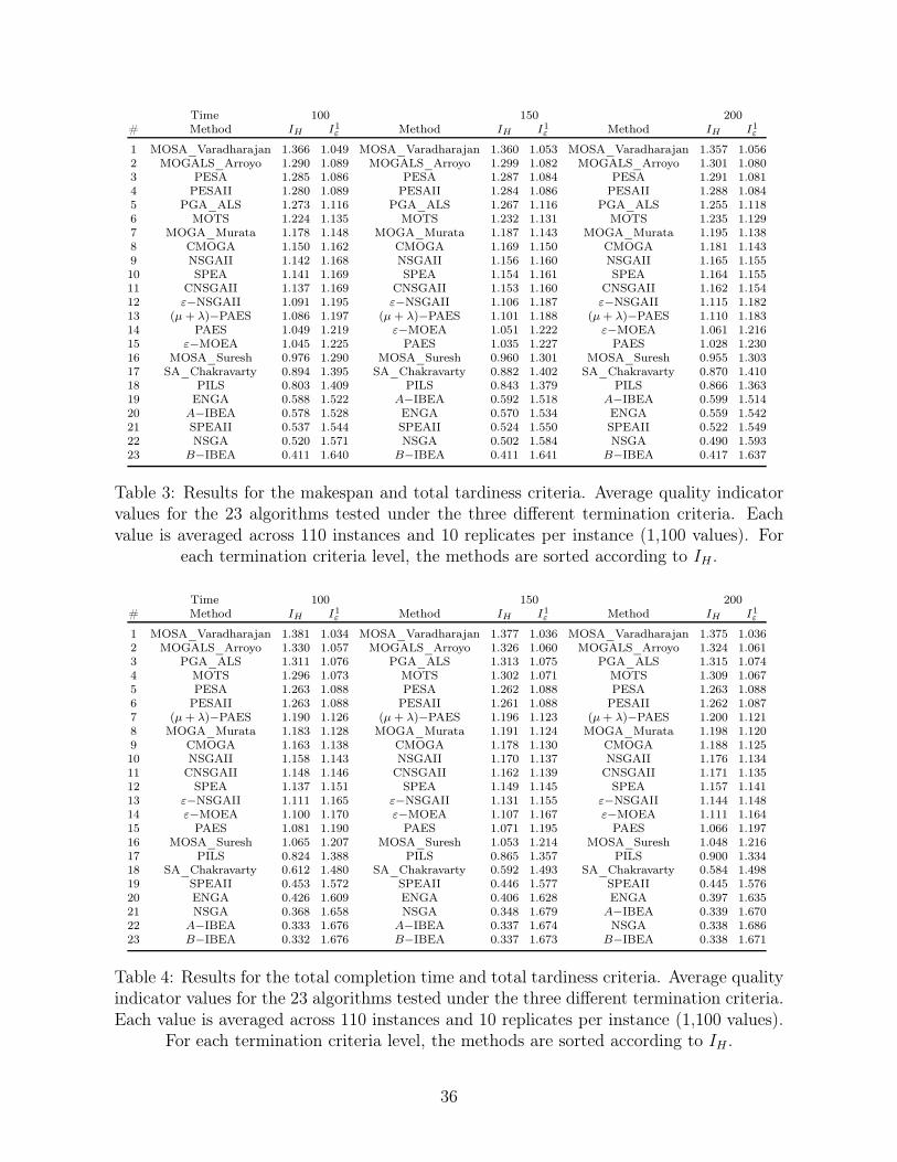
Time 100 150 200# Method IH I1
ε Method IH I1ε Method IH I1
ε
1 MOSA_Varadharajan 1.366 1.049 MOSA_Varadharajan 1.360 1.053 MOSA_Varadharajan 1.357 1.0562 MOGALS_Arroyo 1.290 1.089 MOGALS_Arroyo 1.299 1.082 MOGALS_Arroyo 1.301 1.0803 PESA 1.285 1.086 PESA 1.287 1.084 PESA 1.291 1.0814 PESAII 1.280 1.089 PESAII 1.284 1.086 PESAII 1.288 1.0845 PGA_ALS 1.273 1.116 PGA_ALS 1.267 1.116 PGA_ALS 1.255 1.1186 MOTS 1.224 1.135 MOTS 1.232 1.131 MOTS 1.235 1.1297 MOGA_Murata 1.178 1.148 MOGA_Murata 1.187 1.143 MOGA_Murata 1.195 1.1388 CMOGA 1.150 1.162 CMOGA 1.169 1.150 CMOGA 1.181 1.1439 NSGAII 1.142 1.168 NSGAII 1.156 1.160 NSGAII 1.165 1.15510 SPEA 1.141 1.169 SPEA 1.154 1.161 SPEA 1.164 1.15511 CNSGAII 1.137 1.169 CNSGAII 1.153 1.160 CNSGAII 1.162 1.15412 ε−NSGAII 1.091 1.195 ε−NSGAII 1.106 1.187 ε−NSGAII 1.115 1.18213 (µ + λ)−PAES 1.086 1.197 (µ + λ)−PAES 1.101 1.188 (µ + λ)−PAES 1.110 1.18314 PAES 1.049 1.219 ε−MOEA 1.051 1.222 ε−MOEA 1.061 1.21615 ε−MOEA 1.045 1.225 PAES 1.035 1.227 PAES 1.028 1.23016 MOSA_Suresh 0.976 1.290 MOSA_Suresh 0.960 1.301 MOSA_Suresh 0.955 1.30317 SA_Chakravarty 0.894 1.395 SA_Chakravarty 0.882 1.402 SA_Chakravarty 0.870 1.41018 PILS 0.803 1.409 PILS 0.843 1.379 PILS 0.866 1.36319 ENGA 0.588 1.522 A−IBEA 0.592 1.518 A−IBEA 0.599 1.51420 A−IBEA 0.578 1.528 ENGA 0.570 1.534 ENGA 0.559 1.54221 SPEAII 0.537 1.544 SPEAII 0.524 1.550 SPEAII 0.522 1.54922 NSGA 0.520 1.571 NSGA 0.502 1.584 NSGA 0.490 1.59323 B−IBEA 0.411 1.640 B−IBEA 0.411 1.641 B−IBEA 0.417 1.637
Table 3: Results for the makespan and total tardiness criteria. Average quality indicatorvalues for the 23 algorithms tested under the three different termination criteria. Eachvalue is averaged across 110 instances and 10 replicates per instance (1,100 values). For
each termination criteria level, the methods are sorted according to IH .
Time 100 150 200# Method IH I1
ε Method IH I1ε Method IH I1
ε
1 MOSA_Varadharajan 1.381 1.034 MOSA_Varadharajan 1.377 1.036 MOSA_Varadharajan 1.375 1.0362 MOGALS_Arroyo 1.330 1.057 MOGALS_Arroyo 1.326 1.060 MOGALS_Arroyo 1.324 1.0613 PGA_ALS 1.311 1.076 PGA_ALS 1.313 1.075 PGA_ALS 1.315 1.0744 MOTS 1.296 1.073 MOTS 1.302 1.071 MOTS 1.309 1.0675 PESA 1.263 1.088 PESA 1.262 1.088 PESA 1.263 1.0886 PESAII 1.263 1.088 PESAII 1.261 1.088 PESAII 1.262 1.0877 (µ + λ)−PAES 1.190 1.126 (µ + λ)−PAES 1.196 1.123 (µ + λ)−PAES 1.200 1.1218 MOGA_Murata 1.183 1.128 MOGA_Murata 1.191 1.124 MOGA_Murata 1.198 1.1209 CMOGA 1.163 1.138 CMOGA 1.178 1.130 CMOGA 1.188 1.12510 NSGAII 1.158 1.143 NSGAII 1.170 1.137 NSGAII 1.176 1.13411 CNSGAII 1.148 1.146 CNSGAII 1.162 1.139 CNSGAII 1.171 1.13512 SPEA 1.137 1.151 SPEA 1.149 1.145 SPEA 1.157 1.14113 ε−NSGAII 1.111 1.165 ε−NSGAII 1.131 1.155 ε−NSGAII 1.144 1.14814 ε−MOEA 1.100 1.170 ε−MOEA 1.107 1.167 ε−MOEA 1.111 1.16415 PAES 1.081 1.190 PAES 1.071 1.195 PAES 1.066 1.19716 MOSA_Suresh 1.065 1.207 MOSA_Suresh 1.053 1.214 MOSA_Suresh 1.048 1.21617 PILS 0.824 1.388 PILS 0.865 1.357 PILS 0.900 1.33418 SA_Chakravarty 0.612 1.480 SA_Chakravarty 0.592 1.493 SA_Chakravarty 0.584 1.49819 SPEAII 0.453 1.572 SPEAII 0.446 1.577 SPEAII 0.445 1.57620 ENGA 0.426 1.609 ENGA 0.406 1.628 ENGA 0.397 1.63521 NSGA 0.368 1.658 NSGA 0.348 1.679 A−IBEA 0.339 1.67022 A−IBEA 0.333 1.676 A−IBEA 0.337 1.674 NSGA 0.338 1.68623 B−IBEA 0.332 1.676 B−IBEA 0.337 1.673 B−IBEA 0.338 1.671
Table 4: Results for the total completion time and total tardiness criteria. Average qualityindicator values for the 23 algorithms tested under the three different termination criteria.Each value is averaged across 110 instances and 10 replicates per instance (1,100 values).
For each termination criteria level, the methods are sorted according to IH .
36

Time 100 150 200# Method IH I1
ε Method IH I1ε Method IH I1
ε
1 MOSA_Varadharajan 1.362 1.054 MOSA_Varadharajan 1.356 1.058 MOSA_Varadharajan 1.350 1.0612 MOGALS_Arroyo 1.337 1.066 MOGALS_Arroyo 1.337 1.064 MOGALS_Arroyo 1.336 1.0643 MOTS 1.309 1.087 MOTS 1.312 1.085 MOTS 1.312 1.0834 PGA_ALS 1.271 1.120 PESA 1.273 1.091 PESA 1.275 1.0915 PESA 1.269 1.092 PGA_ALS 1.272 1.121 PGA_ALS 1.272 1.1226 PESAII 1.262 1.095 PESAII 1.267 1.093 PESAII 1.268 1.0937 MOGA_Murata 1.160 1.154 MOGA_Murata 1.171 1.148 MOGA_Murata 1.176 1.1468 CMOGA 1.134 1.167 CMOGA 1.155 1.155 CMOGA 1.167 1.1499 CNSGAII 1.111 1.180 CNSGAII 1.126 1.171 CNSGAII 1.133 1.16810 NSGAII 1.106 1.184 NSGAII 1.121 1.177 NSGAII 1.128 1.17311 SPEA 1.099 1.186 SPEA 1.116 1.176 SPEA 1.122 1.17312 (µ + λ)−PAES 1.059 1.206 (µ + λ)−PAES 1.071 1.199 (µ + λ)−PAES 1.077 1.19613 ε−NSGAII 1.051 1.213 ε−NSGAII 1.068 1.204 ε−NSGAII 1.077 1.19914 ε−MOEA 1.027 1.233 ε−MOEA 1.036 1.228 ε−MOEA 1.040 1.22615 PAES 1.005 1.238 PAES 0.992 1.244 PAES 0.980 1.25216 MOSA_Suresh 0.950 1.296 MOSA_Suresh 0.936 1.303 MOSA_Suresh 0.922 1.31417 SA_Chakravarty 0.813 1.410 PILS 0.836 1.383 PILS 0.861 1.36718 PILS 0.794 1.413 SA_Chakravarty 0.798 1.422 SA_Chakravarty 0.781 1.43119 ENGA 0.512 1.575 ENGA 0.492 1.590 ENGA 0.477 1.60420 SPEAII 0.475 1.586 SPEAII 0.467 1.590 SPEAII 0.458 1.60021 NSGA 0.446 1.625 A−IBEA 0.426 1.626 B−IBEA 0.425 1.63122 A−IBEA 0.416 1.634 NSGA 0.426 1.642 A−IBEA 0.424 1.63123 B−IBEA 0.416 1.634 B−IBEA 0.423 1.629 NSGA 0.409 1.658
Table 5: Results for the makespan and total completion time. Average quality indicatorvalues for the 23 algorithms tested under the three different termination criteria. Eachvalue is averaged across 110 instances and 10 replicates per instance (1,100 values). For
each termination criteria level, the methods are sorted according to IH .
37
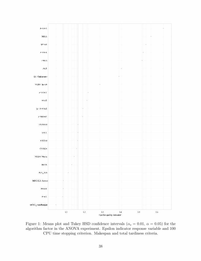
������������� ��� ��� ���������������������������������������������������� ��������ε−�������
µ�λ�−�� ��� �ε−�� ���������������������������� ����−� ��� �������!
−� �
"#" "#$ "#% "#& "#' "#()*+,-./ 012-,34 ,/5,623.7Figure 1: Means plot and Tukey HSD confidence intervals (αs = 0.01, α = 0.05) for thealgorithm factor in the ANOVA experiment. Epsilon indicator response variable and 100
CPU time stopping criterion. Makespan and total tardiness criteria.
38
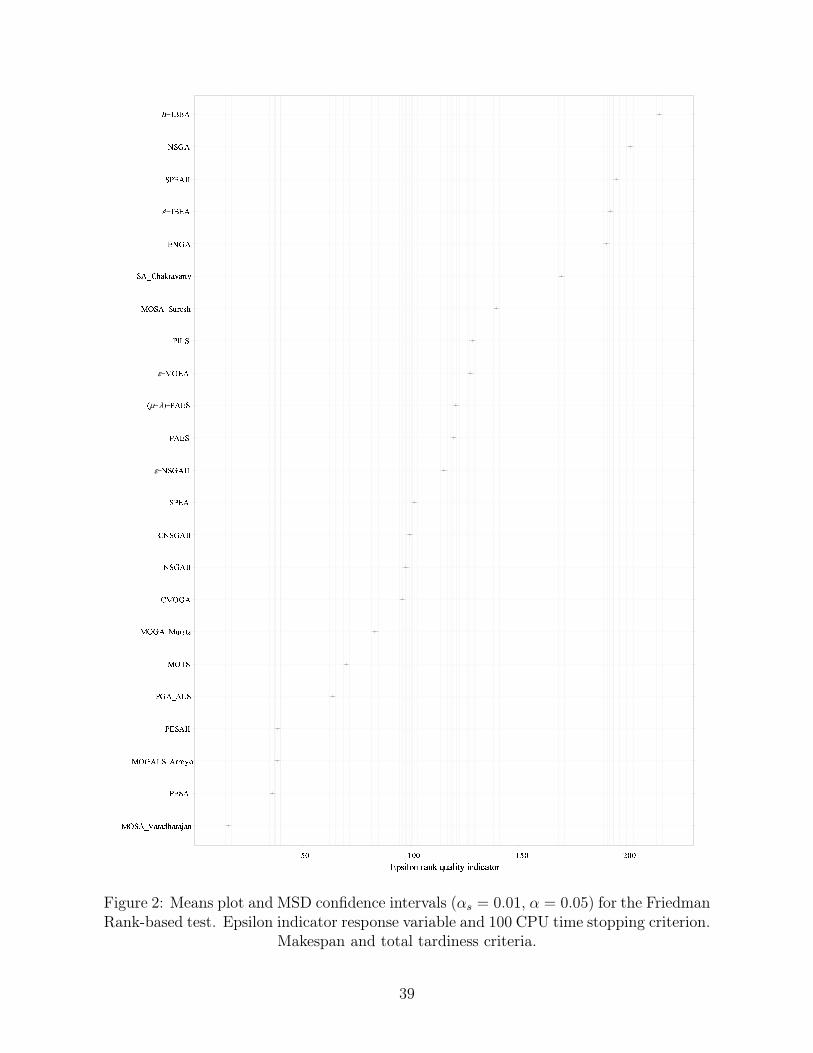
89:;<=>?>@A>?>B >CDE:;89F;G:<;??HIHDE:;JJDF;<;G:89K:89F;<8L?>M>N89F;O:F;JJNO:F;JJ:DE;ε−O:F;JJD;E:P
µQλR−D;E:ε−89E;DJG:89:;<:L?STA:;<NA>U?>V>?MIEOF;W−JXE;:DE;JJO:F;Y
−JXE;
Z[ \[[ \Z[ ][[^_ abcd efdg hifbajk adlamfjceFigure 2: Means plot and MSD confidence intervals (αs = 0.01, α = 0.05) for the FriedmanRank-based test. Epsilon indicator response variable and 100 CPU time stopping criterion.
Makespan and total tardiness criteria.
39
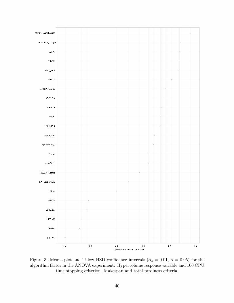
n− opqrsturtvqroow− opqrqsurvoxttryz{|}~|�|~����tryt�~��{ε−��qrvrqt�
µ�λ�−vrqtε−sturoozsturootvqrsturooz��ur��ury��~|�|���tvuryrxtvqtroovqtr��urxtyr~~�����try�|~|�{|~|� |�
��� ��� ��� ��� ��� ������������ � ¡�¢�£¤� £¥¦£§¢¤��Figure 3: Means plot and Tukey HSD confidence intervals (αs = 0.01, α = 0.05) for thealgorithm factor in the ANOVA experiment. Hypervolume response variable and 100 CPU
time stopping criterion. Makespan and total tardiness criteria.
40
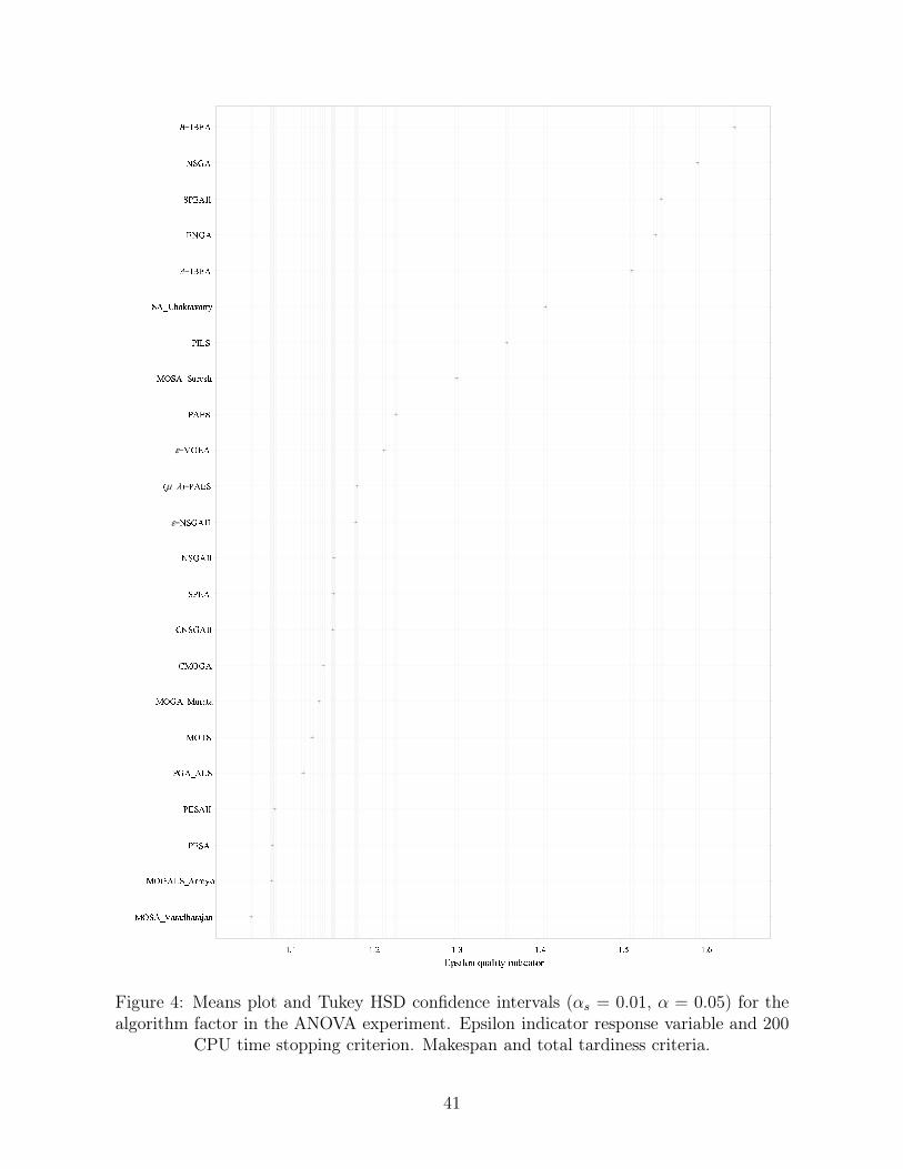
¨©ª«¬®¯®°±®¯®² ®³¨©´«µª¬«¯¯¶·¶¸¹ª«¸¹ª«ºº¸´«¬«µª¨©»ª¨©´«¬¨¼¯®½®¾¨©´«¾¿ª´«ººª¸¹«¿ª´«ººε−¿ª´«ººÀ
µÁλÂ−¸«¹ªε−¨©¹«¸«¹ª¨©ª«¬ª¼¯Ãı¸ºµªª«¬¾±®Å¯®Æ®¯½·Ç−ºÈ¹«¹¿´«ª¸¹«ºº¿ª´«É
−ºÈ¹«
ÊËÊ ÊËÌ ÊËÍ ÊËÎ ÊËÏ ÊËÐÑÒÓÔÕÖ× ØÙÚÕÔÛÜ Ô×ÝÔÞÚÛÖßFigure 4: Means plot and Tukey HSD confidence intervals (αs = 0.01, α = 0.05) for thealgorithm factor in the ANOVA experiment. Epsilon indicator response variable and 200
CPU time stopping criterion. Makespan and total tardiness criteria.
41
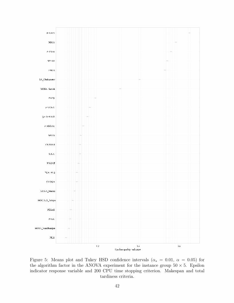
àáâãäåãæçèéêéëìéêéí éîàïãæàïãæááäåðæâãçæêêñòñäåðæçäóêéôéõäåðæàðæçæâãöãðæááãàïæõöãðæááäå÷ãε−öãðæááø
µùλú−àæïãε−äåïæàæïãäåãæçãóêûüìãæçõìéýêéþéêôòïöðæãàïæááÿ−á�ïæöãðæ�
−á�ïæ
��� ��� ������� ������ ������Figure 5: Means plot and Tukey HSD confidence intervals (αs = 0.01, α = 0.05) forthe algorithm factor in the ANOVA experiment for the instance group 50 × 5. Epsilonindicator response variable and 200 CPU time stopping criterion. Makespan and total
tardiness criteria.
42
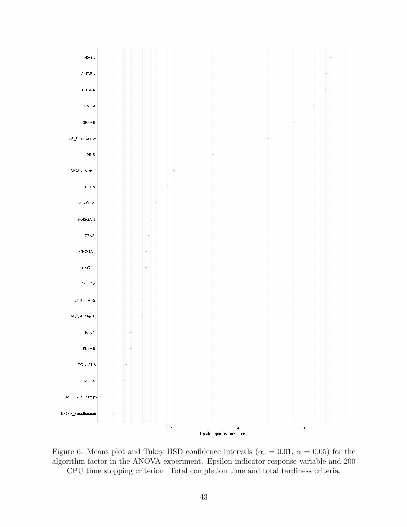
�������������� �!��"�#�����$%$��&�'"���# �'(��))'(����"���*��+�,µ-λ.−'�(�/��"�0�"�))/0�"�))�'(�ε−
0�"�))ε−��(�'�(�������*�12�')# ����/��3��4��+%�'(�))(0"�5−
)6(�7−
)6(�0�"�
89: 89; 89<=>?@ABC DEFA@GH @CI@JFGBKFigure 6: Means plot and Tukey HSD confidence intervals (αs = 0.01, α = 0.05) for thealgorithm factor in the ANOVA experiment. Epsilon indicator response variable and 200
CPU time stopping criterion. Total completion time and total tardiness criteria.
43
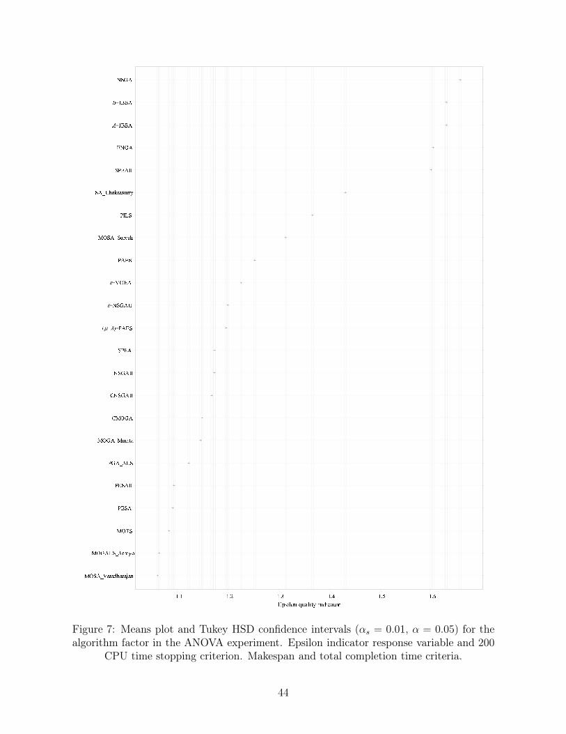
LMNOPQRSRTURSRV RWLMXOYNPOSSZ[ZLM\N]^NO]^NO__]XOPOY NLMXOPL`SRaRbLMXObcNXO__cNXO__N]^Odµeλf−]O^Nε−
cNXO__ε−LM^O]O^NLMNOPN SghU]_Y NNOPbURiSRjRSa[N]^O__^cXOk−
_l^Om−
_l^OcNXO
non nop noq nor nos notuvwxyz{ |}~yx�� x{�x�~�z�Figure 7: Means plot and Tukey HSD confidence intervals (αs = 0.01, α = 0.05) for thealgorithm factor in the ANOVA experiment. Epsilon indicator response variable and 200
CPU time stopping criterion. Makespan and total completion time criteria.
44
Copyright © 2022 FDOKUMEN