HEURISTICS FOR FLEXIBLE FLOWSHOP

SCHEDULING PROBLEMS

by

CHERNG-YEE LEUNG, B.S., M.S.I.E.

A DISSERTATION

IN

INDUSTRIAL ENGINEERING

Submitted to the Graduate Faculty of Texas Tech University in

Partial Fulfillment of the Requirements for

the Degree of

DOCTOR OF PHILOSOPHY

Approved

August, 1993

^

""-' .. ACKNOWLEDGMENTS J7k^ ^V?// / *•-'

\ln ">^ i ' I am deeply indebted to Dr. Milton L. Smith for his

guidance through all phases of this research, to Dr. Richard

A. Dudek for his direction, and to Surya Liman for his help

in the preparation of this research. Also appreciation is

gratefully expressed to Dr. Kamal C. Chanda and Dr. Hossein

S. Mansouri for their support. I am grateful to my wife

Su-Chen Chuang for her encouragement and patience while the

research was being conducted. My thanks are extended to my

son Edmund for his inspiration during the research.

11

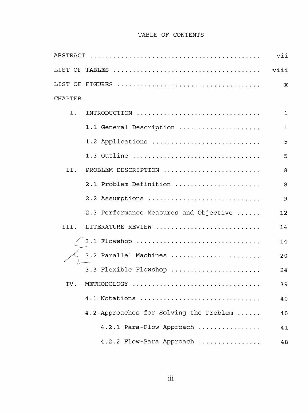
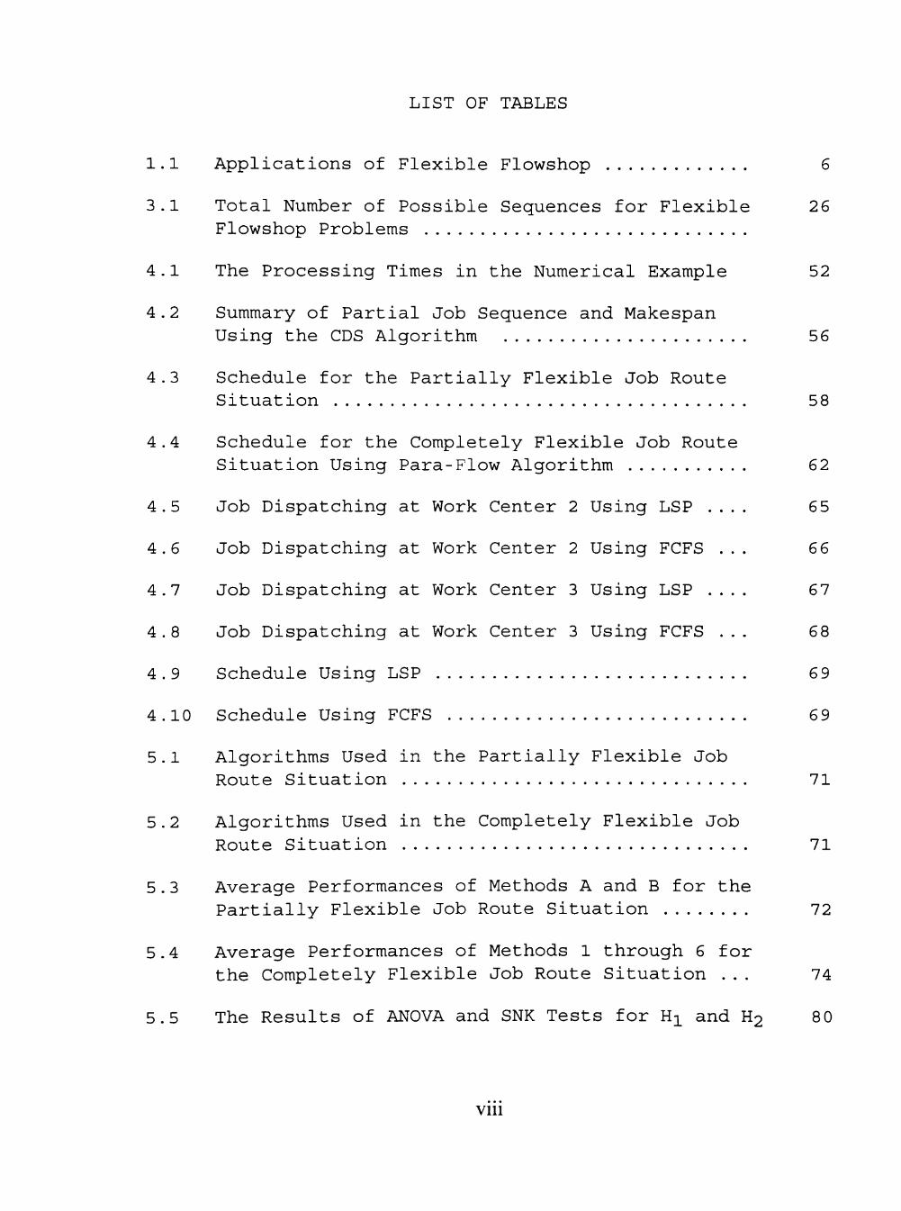
TABLE OF CONTENTS

ABSTRACT vii

LIST OF TABLES viii

LIST OF FIGURES x

CHAPTER

I. INTRODUCTION 1

1.1 General Description 1

1.2 Applications 5

1. 3 Outline 5

II. PROBLEM DESCRIPTION 8

2.1 Problem Definition 8

2.2 Assumptions 9

2.3 Performance Measures and Objective 12

III . LITERATURE REVIEW 14

3 .1 Flowshop 14

3.2 Parallel Machines 20

3.3 Flexible Flowshop 24

IV. METHODOLOGY 3 9

4 .1 Notations 40

4.2 Approaches for Solving the Problem 4 0

4.2.1 Para-Flow Approach 41

4.2.2 Flow-Para Approach 48

111

4.3 Numerical Example 51

4.3.1 Illustration of the Para-Flow Approach 52

4.3.2 Illustration of the Flow-Para

Approach 63

V. COMPUTER EXPERIMENTS AND COMPUTATION RESULTS 70

5.1 Computer Experiment 70

5.2 Computation Results 71

5.3 Statistical Analysis 78

5 . 4 Discussion 79

5.4.1 The Partially Flexible Job Route

Situation 83 5.4.2 The Completely Flexible Job Route

Situation 86

5.4.3 The Comparison of Performance of Algorithms for the Partially Flexible Job Route Situation and Algorithms for the Completely Flexible Job Route Situation 91

VI . TREND ANALYSIS 95

6.1 Parallel Machine Trend Analysis 96

6.1.1 Settings 96

6.1.2 Computation Results 97

6.1.3 Observations 97

6.1.4 Discussion 105

6 .2 Job Trend Analysis Ill

6.2.1 Settings Ill

IV

6.2.2 Computation Results Ill

6.2.3 Observations 113

6.2.4 Discussion 118

6 .3 Work Center Trend Analysis 122

6.3.1 Settings 122

6.3.2 Computation Results 122

6.3.3 Observations 122

6.3.4 Discussion 130

VII. CONCLUSIONS AND FURTHER STUDIES 13 5

7 .1 Conclusions 135

7.1.1 Conclusions for the Problem under the Partially Flexible Job Route Situation 137

7.1.2 Conclusions for the Problem under the Completely Flexible Job Route Situation 138

7.1.3 Conclusions for the Comparison of the Problem under the Partially Flexible Job Route Situation and under the Completely Flexible Job Route Situation 140

7.1.4 Conclusions for Parallel Machine

Trend Analysis 141

7.1.5 Conclusions for Job Trend Analysis 143

7.1.6 Conclusions for Work Center Trend

Analysis 143

7 . 2 Further Studies 145

REFERENCES 14 8

APPENDIX: COMPUTER PROGRAMS 16 0

VI

\

ABSTRACT

A flexible flowshop consists of a number of work

centers, each having one or more parallel machines. A set

of immediately available jobs has to be processed through

the ordered work centers. A job is processed on any and

only one of the parallel machines at each of the work

centers?) Structurally, a flexible flowshop represents a

generalization of the simple flowshop and the identical

parallel machine shop. For the case of having the same

number of identical parallel machines at every work center,

two approaches are developed: the para-flow approach and

the flow-para approach. Two situations regarding the job

route are examined. These are the partially flexible job

route situation and the completely flexible job route

situation. (The objective of this research is to find

heuristics that minimize the makespan of the problem in

reasonable computation time. A computer experiment verifies

that the para-flow approach and the flow-para approach

outperform published algorithms. Problem size includes

three elements: the number of jobs, the number of work

centers, and the number of parallel machines at each work

center. By fixing any two of the three elements, the trend

caused by the third element can be analyzed. / A trend

analysis of the proposed algorithms has been conducted.

Vll

LIST OF TABLES

1.1 Applications of Flexible Flowshop 6

3.1 Total Number of Possible Sequences for Flexible 26 Flowshop Problems

4.1 The Processing Times in the Numerical Example 52

4.2 Summary of Partial Job Sequence and Makespan Using the CDS Algorithm 56

4.3 Schedule for the Partially Flexible Job Route Situation 58

4.4 Schedule for the Completely Flexible Job Route Situation Using Para-Flow Algorithm 62

4.5 Job Dispatching at Work Center 2 Using LSP .... 65

4.6 Job Dispatching at Work Center 2 Using FCFS ... 66

4.7 Job Dispatching at Work Center 3 Using LSP .... 67

4.8 Job Dispatching at Work Center 3 Using FCFS ... 68

4.9 Schedule Using LSP 69

4.10 Schedule Using FCFS 69

5.1 Algorithms Used in the Partially Flexible Job Route Situation 71

5 .2 Algorithms Used in the Completely Flexible Job Route Situation 71

5.3 Average Performances of Methods A and B for the Partially Flexible Job Route Situation 72

5.4 Average Performances of Methods 1 through 6 for the Completely Flexible Job Route Situation ... 74

5.5 The Results of ANOVA and SNK Tests for H^ and H2 80

Vlll

5.6 The Results of ANOVA and SNK Tests for H3 and H4 81

5.7 The Results of ANOVA and SNK Tests for H5 and Hg 82

5.8 Makespan Improvement Percentages 84

6.1 Average Makespan in Parallel Machine Trend Analysis 98

6.2 Average CPU Time (Seconds) in Parallel Machine Trend Analysis 99

6.3 Marginal Makespan Decrement Percentage in Parallel Machine Trend Analysis 102

6.4 Marginal CPU Time Increment Percentage in

Parallel Machine Trend Analysis 104

6.5 Average Makespan in Job Trend Analysis 112

6.6 Average CPU Time (Seconds) in Job Trend Analysis 112

6.7 Makespan Increment Percentage in Job Trend Analysis 116

6.8 CPU Time Increment Percentage in Job Trend Analysis 117

6.9 Average Makespan in Work Center Trend Analysis 123

6.10 Average CPU Time (Seconds) in Work Center Trend Analysis 124

6.11 Marginal Makespan Increment Percentage in Work Center Trend Analysis 128

6.12 Marginal CPU Time Increment Percentage in Work Center Trend Analysis 129

IX

LIST OF FIGURES

1.1 The Machine Configuration of Flexible Flowshop 2

2.1 An Example of the Partially Flexible Job Route 10

2.2 An Example of the Completely Flexible Job Route 10

3.1 The Machine Configuration of a Simple Flowshop 15

3.2 The Machine Configuration of Identical Parallel Machines 21

4.1 (s + 1) Para-Subproblems Partitioned from the Original Problem 43

4.2 m(s + 1) Flow-Subproblems with Partially Job Assignment Jobsj j Obtained from Phase I 44

4.3 The Flow-Subproblem in Flow-Para Approach .... 49

6.1 Average Makespan in Parallel Machine Trend Analysis (30 Jobs, 3 Work Centers) 10 0

6.2 Average CPU Time in Parallel Machine Trend Analysis (30 Jobs, 3 Work Centers) 10 0

6.3 Average Makespan in Parallel Machine Trend Analysis (50 Jobs, 6 Work Centers) 101

6.4 Average CPU Time in Parallel Machine Trend Analysis (50 Jobs, 6 Work Centers) 101

6.5 Average Makespan in Job Trend Analysis (3 Work Centers, Each Having 3 Parallel Machines) .... 114

6.6 Average CPU Time in Job Trend Analysis (3 Work Centers, Each Having 3 Parallel Machines) .... 114

6.7 Average Makespan in Job Trend Analysis (6 Work Centers, Each Having 6 Parallel Machines) .... 115

6.8 Average CPU Time in Job Trend Analysis (6 Work Centers, Each Having 6 Parallel Machines) .... 115

X

6.9 Average Makespan in Work Center Trend Analysis (30 Jobs, 3 Parallel Machines) 125

6.10 Average CPU Time in Work Center Trend Analysis (30 Jobs, 3 Parallel Machines) 125

6.11 Average Makespan in Work Center Trend Analysis (50 Jobs, 6 Parallel Machines) 126

6.12 Average CPU Time in Work Center Trend Analysis (50 Jobs, 6 Parallel Machines) 126

XI

CHAPTER I

INTRODUCTION

1.1 General Description

This research discusses scheduling algorithms for a

certain kind of manufacturing environment. "Scheduling"

refers to the timing of arrival of jobs requiring service,

and "sequencing" refers to the order in which jobs will be

processed (Churchman et al., 1967). These terms can be used

interchangeably (Dudek et al., 1974). A job is considered

as a collection of a set of operations each being processed

on different machines (Baker, 1974). The system being

introduced is made up of a number of different work centers,

each of which consists of one or more parallel machines. At

each work center, the parallel machines can perform the same

operation. A set of jobs has to be processed through the

system. Because of technological restrictions on the order

in which jobs can be performed, jobs pass through the work

centers in the same order. At each work center, each job

can be processed on any and only one of the parallel

machines. Jobs may skip a work center. This system is

referred to as a "multi-stage parallel-processor flowshop"

(Rajendran and Chaudhuri, 19 92), a "flowshop with multiple

processors" (Brah and Hunsucker, 1991; Deal and Hunsucker,

1991), a "flexible flowshop" (Sriskandarajah and Sethi,

1989), a "hybrid flowshop" (Gupta and Tunc, 1991; Gupta,

1988; Narasimhan and Mangiameli, 1987), a "flexible flow

line" (Raban and Nagel, 1991; Kochhar et al., 1988;

Wittrock, 1985 and 1988; Kochhar and Morris, 1987), and a

"network flowshop" (kuriyan and Reklaitis, 1989; Salvador,

1973). In this paper flexible flowshop will be used to

represent this kind of system. Figure 1.1 illustrates the

machine configuration of a flexible flowshop.

Jobs

Start ^ WCi • > WC'

M 11

^ • >

wc

M 21

• > Finish

Msl

M 12

J^lm^

.

M 22

M2m2

Hs2

M siric

Figure 1.1. The Machine Configuration of Flexible Flowshop

In Figure 1.1, WCi and M^j denote Work Center i and

Machine j at work center i (i = 1, 2, ..., s,

j = 1, 2, ..., mi), respectively. A set of jobs is

available to be processed at the starting point. All the

jobs go through the system from the starting point to the

finishing point. After being completed at work center 1, a

job is moved to work center 2, then to work center 3, and so

3 on until it is moved to the work center which is the last

work center to process the job. When a job is completed at

the last work center, it is then collected to the finishing

point. Each job is processed through these work centers in

the same order, thus the shop is called a "flowshop." After

getting into the system, at each work center, a job can

visit any one of the parallel machines at the work center.

In this flow, if the processing time of a job is zero at a

work center, the job might skip this work center. After

visiting the last work center, the job goes to the finishing

point.

At any one of the work centers, e.g., work center i

(i = 1, 2, ..., s), there are m^ parallel machines. Since

these m-L parallel machines perform the same operation, a job

can be executed on any one of these m^ machines. If the m^

parallel machines have the same production rate, they are

called identical parallel machines, i.e., a job processed on

any one of these m^ parallel machines at work center i will

have the same processing time. On the other extreme, if the

m-L parallel machines have different production rates, then

they are called heterogeneous parallel machines, i.e., the

processing time of a job at work center i may be different

if it is processed on different parallel machines.

In this system, the jobs have the flexibility to skip a

work center if the processing time of a job at the work

center is zero; otherwise the job has to be processed at the

4 work center. At each work center a job can be processed on

any one of the parallel machines. With the properties

above, this kind of flowshop is called a "flexible

flowshop."

Structurally, the flexible flowshop, when reduced to

its elementary and restrictive forms, resembles two common

scheduling systems: the parallel machine scheduling system

and the simple flowshop scheduling system. The parallel

machine scheduling system involves the scheduling of a set

of immediately available jobs, each on one of the parallel

machines. There is only one work center, and that work

center consists of two or more parallel machines. The

simple flowshop scheduling system is described as the

sequencing of a set of immediately available jobs through

each of the ordered work centers. There are two or more

work centers in this system but only one machine at each

work center. Many papers dealing with parallel machine

scheduling problem have been published. Also, the simple

flowshop scheduling problem has been studied extensively in

the literature. As the research interest in the field of

flexible manufacturing has grown rapidly, the combination of

these two scheduling problems, namely a flowshop having one

or more parallel machines at each work center has been a

topic of frequent study.

1.2 Applications

Brah and Hunsucker (1991) stated that the application

of the flexible flowshop occurs more often than one could

imagine. Many high volume production facilities consist of

several independent production lines each of which can be

considered as a flowshop. In almost all of these

configurations the nature of the machines at each work

center is such that they are effectively identical and hence

interchangeable, i.e., the jobs can practically be processed

on any one of the machines at each work center of the

processing (Salvador, 1973; Sriskandarajah, 1988). The

running of a program on a computer with a language like

FORTRAN is another example of the application of flexible

flowshop (Brah and Hunsucker, 1991). The three steps of

compiling, linking and running are performed in a fixed

sequence. If there are multiple jobs (computer programs)

requiring all of these facilities (steps), each having

multiple processors (softwares), the process resembles that

of a flexible flowshop. More applications in different

fields have been mentioned in several papers. Some of these

are summarized in Table 1.1.

1.3 Outline

The outline of this research is as follows. The next

chapter defines the problem to be studied and specifies the

objective of this research and the measures of performance.

Table 1.1. Applications of Flexible Flowshop

Author (Year) Applications Objective Brah and Hunsucker (19 91)

Assembly lines, reduce bottle neck pressure, increase production capacity, FORTRAN, electronics manufacturing

Minimize makespan and reduce effect of setup and blocking and starvation

Gupta and Tunc (1991)

One expensive machine at the 1^^ work center or average processing times on the 2^^ work center much more than average processing times on the 1^^ work center

Minimize makespan

Zijm and Nelissen Metal cutting machining Minimize maximal (1990) center in car factory lateness

Yanney and Kuo (1989)

Rubber tire industry Minimize number of quality violations

Gupta (1988)

Sriskandaraj ah (1988)

One expensive machine Minimize makespan at the 2^^ work center

Chemical process, hot Minimize makespan metal rolling industries

Wittrock (1985 and 1988)

Buten and Shen (1973)

Salvador (1973)

Printed circuit cards Minimize makespan and reduce queue

Computing systems (two Minimize makespan classes of processors)

Chemical, polymer. Minimize makespan process, petrochemical, synthetic fibers industries

7 Chapter III reviews the related literature. In Chapter IV

the algorithms proposed for solving the studied problem are

presented. A numerical example illustrates the proposed

algorithms. Chapter V compares the proposed algorithms with

some published algorithms. Trend analysis for the proposed

algorithms is discussed in Chapter VI. The last chapter

states the conclusion and makes recommendations for further

study.

CHAPTER II

PROBLEM DESCRIPTION

2,1 Problem Definition

The problem to be addressed in this research is a

special case of flexible flowshop. In this problem jobs

pass through ordered work centers, each of which consists of

the same number of identical parallel machines. Jobs are

processed on any and only one of the parallel machines at

each work center in ascending order of work center numbers.

The machine configuration of this special case is almost the

same as the diagram shown in Figure 1.1 except that

m]_ = m2 = • • • = mg = m.

Regarding job route, the proposed problem is considered

under two situations: the partially flexible job route

situation and the completely flexible job route situation.

In both situations, jobs can be processed on any one of the

parallel machines at the first work center. When the jobs

go to the following work centers, these two situations may

lead to different results.

For the problem under the partially flexible job route

situation, once a job is assigned to a machine at work

center one, this job must be processed on a specific machine

at each of the following work centers. These specific

machines bear the same machine number as the machine

processing this job at the first work center does. Jobs

8

9

have flexibility to visit any one of the parallel machines

at the first work center but have to follow the same machine

number through the second work center to the last work

center. Each job route is only flexible at the entry work

center.

For the problem under the completely flexible job route

situation, even when a job is assigned to a specific machine

at the first work center, the job still can be processed on

any one of the parallel machines at each of the following

work centers. Jobs have the flexibility to visit any one of

the parallel machines at each of the work centers. Each job

route is completely flexible at all of the work centers.

After having been processed at the last work center, all the

jobs are collected at a finishing point in both situations.

A simple example containing three work centers each having

two parallel machines illustrates the proposed problem under

these two situations. Figure 2.1 illustrates the problem

under the partially flexible job route situation, and Figure

2.2 depicts the system under the completely flexible job

route situation.

2-2 Assumptions

To characterize the proposed problem, the following

assumptions are held throughout:

1. A set of jobs is available for processing at the

beginning.

10

Jobs

WC

Jobs ->

Jobs ^ Mi2

WC2

Mil ^ ^21 ^ M31

->

WC3

M 22 ^ ^32

^ Finish

Figure 2.1. An Example of the Partially Flexible Job Route

WC WC WC'

Jobs

• ^ Mil

- M12

M21 r— f M31

M 22 M 32

> Finish

Figure 2.2. An Example of the Completely Flexible Job Route

2. Every job passes through the system in the same

work center sequence.

3. Every work center has the same number of identical

parallel machines.

4. Each job requires s operations, and each operation

requires a different machine.

5. Machines at different work centers perform

different operations.

6. Jobs are mutually independent, i.e., a partial

ordering among jobs based on a precedence relation

does not exist

11

7. The processing of one job by one machine is

nonpreemptive, i.e., once a machine starts

processing a job, the machine must finish

processing this job before it can start processing

another.

8. No job can be split on any work center.

9. A job does not become available to the next work

center until it completes its work at the current

work center.

10. Set up times for the jobs at each work center are

sequence independent and are included in processing

times.

11. All processing times are known and deterministic

for each job at each work center.

12. All machines are available at the beginning and do

not break down through the processing.

13. In the partially flexible job route situation,

jobs can be processed on any one of the parallel

machines at the first work center. Once a job is

assigned to a machine, at each of the following

work centers the job must be processed on specific

machines which bear the same machine number as the

assigned machine at the first work center.

14. In the completely flexible job route situation,

jobs can be processed on any one of the parallel

machines at each work center.

12

The number of jobs to be scheduled is greater than the

number of parallel machines at each work center. Otherwise

it is a trivial problem. For this trivial case, an optimal

schedule is very obvious. That is, every machine processes

at most one job, and every job is processed on only one

machine at each work center. The makespan is equal to the

total processing time of the bottle neck job which has the

largest total processing time over the jobs. This trivial

case does not need to be studied.

2.3 Performance Measures and Objective

Schedules are generally evaluated by aggregate

quantities that involve information about all jobs,

resulting in one-dimensional performance measures. These

measures are usually expressed as a function of the set of

job completion times (Baker, 1974). Makespan, average

completion time, production throughput, lateness, lateness

penalties, and total flowtime are examples of performance

measures. One of the most frequently used performance

measures is makespan which is the time required to process

all jobs on machines at all work centers. Since makespan

minimization also can minimize machine idle times, increase

machine utilization, and reduce production lead time, the

makespan is used as the major performance measure in this

research.

13

Efficient optimizing algorithms for minimizing makespan

in a flexible flowshop are not likely to exist since the

problem belongs to the class of NP-complete problems

(Sriskandarajah and Sethi, 1989; Gupta, 1988;

Sriskandarajah, 1988; Sriskandarajah and Ladet, 1986; Rock,

1984; Garey and Johnson, 1979; Garey et al., 1976). The NP-

complete problems cannot be solved by any efficient

(polynomial-time) algorithm. While it is possible to design

an algorithm using branch-and-bound technique, as in

Salvador (1973) and in Brah and Hunsucker (1991), such

algorithms are time consuming even for moderate size

problems. Thus instead of looking for exact optimizing

algorithms, heuristics which hopefully obtain good solutions

in reasonable computing times are sought. Therefore,

computing time is used as another performance measure in

this research.

The objective of this research is to develop heuristics

to schedule a set of immediately available jobs through the

flexible flowshop in order to minimize the makespan in

reasonable computing time.

CHAPTER III

LITERATURE REVIEW

Because the configuration of the flexible flowshop

includes two elementary forms—parallel machines and simple

flowshop—this chapter not only reviews the literature

related to flexible flowshop but also looks at the

properties of simple flowshops and parallel machines. Since

Johnson (1954) used makespan minimization as an objective in

scheduling problem, a considerable number of researchers

have been attracted to this field, and several analytical

techniques have been developed to solve various problems.

Rather than giving a complete survey of what is known for

the scheduling problem, this chapter instead gives some

samples of typical results.

3•1 Flowshop

The flowshop is characterized by a flow of work that is

unidirectional. A job is considered to be a collection of

operations in which a special precedence structure applies.

A work center contains only one machine; thus the work

center is referred to as a machine in the flowshop problem.

Figure 3.1 represents the flow of work in a simple flowshop

in which all jobs require one operation on each machine.

14

15

Jobs - >

Start • > WC

• > WC'

• > -> WC, -> Finish

Figure 3.1. The Machine Configuration of a Simple Flowshop

The general simple flowshop problem can be

characterized with the following six conditions (Baker,

1974) :

1. A set of n multi-operation jobs is available for

processing at time zero.

2. Each job requires s operations and each operation

requires a different machine.

3. Set-up times for the operations are sequence-

independent and are included in processing times.

4. Job descriptions are known in advance.

5. s different machines are continuously available.

6. Individual operations are not preemptable.

In the flowshop problem, for a set of n jobs, n!

different job sequences are possible for each machine,

therefore (n!)^ different schedules would be examined. The

insertion of idle time on a machine may be necessary if the

order of jobs is changed from one machine to the next

machine and if no job is available to be processed on a

machine when the machine is ready to process. However, when

two machines or three machines are considered, Baker (1974)

has proved that in regard to makespan minimization, it is

16

sufficient to consider only permutation schedules. A

permutation schedule is a schedule with the same job

processing order on all machines. In this case, Johnson's

rule (1954) and its extensions state that job i precedes job

j in an optimal sequence if min{t-i_i, tj2} ^ min{ti2/ ^jl)'

where t^b is the processing time of job a (a = 1, 2, ..., n)

on machine b (b = 1, 2). This rule is implemented by the

following algorithm (Baker, 1974):

Step 1. Let U = {j|tji < tj2} and V = {j|tji > tj2}-

Step 2. Arrange the members of set U in nondecreasing

order of tj^, and arrange the members of set

V in nonincreasing order of tj2.

Step 3. An optimal sequence is the ordered set U

followed by the ordered set V.

Even though the set of permutation schedules may not

form a dominant set for makespan minimization problems when

the flowshop has more than three machines, it is intuitively

plausible that the best permutation schedule should be at

least very close to the true optimum (Baker, 1974) . A

common approach for solving small flowshop sequencing

problems is branch-and-bound algorithms studied by Little et

al. (1963), Lomnicki (1964), Brooks and White (1965), Ignall

and Schrage (1965), and Bestwick and Hastings (1976) among

others. Although this method is the best optimizing

technique available, the computation time requirement

increases exponentially with increasing the number of jobs

17

or the number of machines. The alternatives are heuristics

which can obtain nearly optimum solutions to large size N

problems with limited computational effort.

For the case where intermediate queues are allowed,

i.e., the storage space in front of each machine is

unlimited, a number of heuristics are available to find a

job sequence to minimize makespan. Park et al. (1984)

divided the heuristics into three categories: (1) the

application of Johnson's two-machine algorithm (e.g., the

Campbell, Dudek, and Smith heuristic (1970)), (2) the

generation of a slope index for the job processing times

(e.g., the Palmer heuristic (1965)), and (3) the

minimization of the total idle time on machines (e.g, the

King and Spachis heuristic (1980)).

Given a set of n jobs. Palmer (1965) gave priority to

the jobs having the strongest tendency to progress from

short times to long times in the sequence of processes. He

proposed a numerical "slope index", SIi (i = 1, 2, ..., n),

for each job in an s-machine flowshop, where

SI- = Z(2j - 1 - s)tij. Then a permutation schedule is

j=l

constructed in nonincreasing order of Sli.

Gupta (1972) extended a sorting function for Johnson's

two- and three-machine cases to an approximate function for

the general s-machine case. He proposed that the job index

18

e * to be calculated is SIi = j—^ r, where

min (tij + ti^j + ij l<j<(s-l)

ei = i 1, if t-i T <t-; Q „, . , , .

•^•^ -^ Then a permutation schedule is -1, if tii>ti s

constructed in nonincreasing order of SI- .

Campbell, Dudek, and Smith (1970), Dannenbring (1977),

and Karimi and Ku (1988) developed some other heuristics

which are basically an extension of the Johnson's algorithm

Given a set of n immediately available jobs, for an s-

machine flowshop the Campbell, Dudek, and Smith (CDS)

heuristic generates a job sequence through the following

steps:

1. Generate a set of (s - 1) artificial two-machine

problems from the original s-machine problem. For

the kth subproblem (k = 1, 2, ..., (s - 1))), the

artificial processing time for the i^^ job

(i = 1, 2, ..., n) on the first artificial machine

k is defined as t^H = Ztij, and on the second

j = l

s artificial machine is t] i2 = ^ ^ij •

j=s-k+l

2. Each of the (s - 1) subproblems is then solved by

using Johnson's two-machine algorithm (1954).

19

3. The minimum makespan among the (s - 1) schedules is

identified. The corresponding job order is chosen

to be the best job sequence for the original s-

machine problem.

A rapid access heuristic (RA) was first developed by

Dannenbring (1977) and then modified by Karimi and Ku

(1988) . The Modified Rapid Access (MRA) devises a single

two-machine approximation to the s-machine flowshop. The

artificial processing time for the i^h job

(i = 1, 2, ..., n) on the first artificial machine is

defined as t^^ = S (s - j)tij, and on the second artificial

j = l V

machine i s t^^ = S (j - D t i j . Then the job sequence i s j = l

generated from the artificial two-machine problem which is

solved by Johnson's algorithm (1954). The makespan is

computed accordingly.

The case where no intermediate queues are allowed,

i.e., there is no storage space in front of every machine,

is proved to be an NP-complete problem when more than three

machines are under considered (Papadimitriou and Kanellakis,

1980). Wismer (1972) constructed a heuristic to solve this

problem. He set up a delay matrix whose elements represent

the delays that would be incurred between two adjacent jobs

in sequence. By regarding the jobs as cities and the

20

elements of the delay matrix as distances, this problem is

formulated as a Traveling Salesman Problem (TSP). A TSP

technique is applied to this delay matrix in order to find

the best job sequence. Reddi and Ramamoorthy (1972)

proposed the similar algorithm. Gupta (1976) provided a

theoretical foundation of these methods.

Papadimitriou and Kanellakis (1980) examined the

scheduling problem in a two-machine flowshop with limited

intermediate queue allowed between two consecutive machines.

They proved this is an NP-complete problem and suggested an

approach to minimize the makespan. If the size of the

intermediate queue is b, their approach can be carried out

in the following two steps: (1) Treat this b-buffer problem

as a 0-buffer problem. Use the Gilmore-Gomory algorithm

(1964) to obtain a job sequence. (2) According to this job

sequence, assign the jobs sequentially to the earliest

available machines at work center 1, then do the same

procedure at work center 2. The corresponding schedule is

determined, yet the usefulness of the approach decreases as

b grows.

3.2 Parallel Machines

A single work center consists of more than one machine.

All the machines are capable of performing the same

operation, and all have the same production rate. This

21

system is called an identical parallel machine system and is

illustrated in Figure 3.2:

Jobs • ^

Figure 3.2

• ^ Machine 1

• ^ Machine 2

^ Machine • •

Machine m

The Machine Configuration of Identical Parallel Machines

The identical parallel machine shop can be

characterized with the following conditions:

1. A set of n single operation jobs is available for

processing at time zero.

There are m identical parallel machines 2.

3.

continuously available for processing.

A job can be processed by at most one machine at a

time.

4. Set-up times for the operation on each machine are

sequence independent and are included in processing

times.

5. Job descriptions are known in advance.

Advantages of this parallelism are that several jobs

can be processed simultaneously and no idle times are needed

between any two consecutive jobs. Therefore, for minimizing

22

the makespan, workload is the only factor to be considered.

For each machine, its workload is the sum of the processing

times of the jobs assigned to it. In order to minimize

makespan, the workloads among the parallel machines should

be as balanced as possible. The lowest conceivable maximum

workload would be obtained if all of the machines were given

equal workloads. If the jobs are preemptable, McNaughton

(1959) stated that either the machines will be fully

utilized throughout an optimal schedule or else the largest

processing time among the jobs will determine the makespan.

If job preemption is prohibited, it usually is not possible

to find an equalized workload (Baker, 1974), and the problem

is NP-complete (Lenstra et al., 1990; Rock and Schmidt,

1983; Lawler et al., 1982; Garey, 1979; Graham et al., 1979;

Lenstra et al. , 1977; Graham, 1969). No direct algorithm is

possible for calculating the optimal makespan or for

constructing an optimal schedule. To find nearly balanced

workloads, a heuristic procedure, the Longest Processing

Time First (LPTF), is used as a dispatching mechanism.) For

a set of immediately available jobs, LPTF performs the job

assignment through the following steps:

1. Sort jobs in nonincreasing order of processing

time, i.e., the Longest Processing Time (LPT)

order.

2. According to the LPT order, assign one job at a

time to the machine with least accumulative

23

processing time. Thus, on each of the m parallel

machines, a partial job assignment is determined.

A whole parallel job assignment which consists of

the m partial job assignments is also determined.

Several other heuristics based on the idea of "bin

packing problem" are developed to make parallel machine

assignment (Graham et al., 1979; Coffman et al., 1978; Garey

and Johnson, 1976; Graham, 1976, Johnson et al. , 1974;

Johnson, 1973 and 1974). First-Fit (FF) algorithm, Best-Fit

(BF) algorithm, First-Fit Decreasing (FFD) algorithm, and

Best-Fit Decreasing (BED) algorithm among others are used to

pack items into bins?J Based on FFD algorithm, Coffman et

al. (1978) developed a MULTIFIT heuristic. Processor j

(j = 1, 2, ..., m) is regarded as binj, and job i

(i = 1, 2, ..., n) as itemi of size t^ which is the

processing time of job i. To complete a schedule by time t

can be considered as the successful packing of the n items

into m bins of capacity t. FFD algorithm arrange the jobs

in LPT order, then it packs the jobs sequentially into the

lowest numbered bin in which the job will validly fit. An

upper bound (CU = max 2^-; — 1 i / \ ^-^^ , maxi [ ti j

m V

) and a lower bound

y

/

(CL = max ^i = l \

m — , maxi (ti ) ) initialize a binary search in

order to minimize bin size t. At each step of the binary

24

CU + CL search FFD is run for a bin size of C = . Whenever

2

all the jobs can fit into the m bins, CU is updated by C;

otherwise, CL is updated by C. FFD repeatedly run for the

update C. These steps are iterated until a pre-set number

of iterations is reached. The value of C at this point is

the value of t, i.e., the makespan of the parallel machine

problem.

Tit has been shown that LPTF algorithm always finds a

schedule having makespan within 1.33 of the minimum possible

makespan (Graham, 1969 and 1976). Coffman et al. (1978)

showed MUTIFIT algorithm can reduce this number to 1.22.

Friesen (1984) decreased this number to 1.20 by using

tighter bounds for the MULTIFIT algorithm

3.3 Flexible Flowshop

In the context of flexible flowshops, a complete

schedule includes a job sequence, job route, machine

allocation, a priority dispatching rule, and job timing. A

job sequence is the order in which the jobs enter the system

and in which the jobs visit each of the parallel machines at

each work center. Job route describes the exact route of

each job to go through the system, i.e., the sequence of

machines processing the job. Machine allocation is the

specification of which jobs will visit each individual

machine at each work center. A priority dispatching rule is

specified to choose the job to be processed next when one of

25

the parallel machines at a work center becomes available and

there is more than one job waiting in its queue. Job timing

indicates the times at which each job should start being

processed and be completed on each machine at each work

center.

The general flexible flowshop has been described in

s Chapter I. A set of n jobs can take n

^n - 1 ^ n!

possible sequence combinations for a schedule (Brah and

Hunsucker, 1991). Table 3.1 gives the total number of

combinations for several sizes of problems.

This makes the enumeration method almost totally

impractical and virtually impossible. Though it is an NP-

complete problem, some heuristics have been published to

deal with different restricted situations.

Gupta and Tunc (1991), Gupta (1988), Mittal and Bagga

(1973), Buten and Shen (1973), and Arthanari and Ramamurthy

(1971) studied several different two-work-center flexible

flowshop problems. When the second work center has only one

machine, the branch-and-bound algorithm of Arthanari and

Ramamurthy (1971) for m identical parallel machines at the

first work center and that of Mittal and Bagga (1973) for

two identical parallel machines at the first work center can

be applied to minimize makespan. Since Murthy (1974) has

shown that Mittal and Bagga's procedure is not an optimum

26

Table 3.1. Total Number of Possible Sequences for Flexible Flowshop Problems

Number of

Jobs

6

6

6

6

8

8

8

8

10

10

10

10

Number of Work

Centers

4

4

5

5

4

4

5

5

4

4

5

5

Number Machines Work

of per

Center

2

3

2

3

2

3

2

3

2

3

2

3

Numbe Possi

r of .ble

Sequenc

1.04976

2.07360

1.88957

2.48832

3.96601

3.96601

5.59684

5.59684

7.11053

2.24728

1.16112

4.89295

*

•

*

•

*

*

*

*

•

*

*

•

es 10-L-^

10l2

10l6

10l5

1020

1020

1025

1025

1028

1029

1036

1036

algorithm, Gupta (1988) suggested a heuristic to deal with

the same problem. A job with minimum processing time at

work center 1 is placed in the first sequence position. The

remaining jobs are sequenced by Johnson's rule. According

to this job sequence, assign the jobs to the latest

available machine at work center 1 such that minimum idle

time is incurred at work center 2.

27

Buten and Shen (1973) used Modified Johnson Ordering

(MJO) to find a permutation schedule for the problem with m

machines at the first work center and n machines at the

second work center. MJO can be stated as follows: job i

precedes job j (i T j) if tnin ^Dl ti2 til tj2 /

\ m n ; < m m

V ^ n y

where tij^ is the processing time of job i (i = 1, 2, ..., n)

at work center k (k = 1, 2).

Gupta and Tunc (1991) considered the problem with only

one machine at work center 1 and m identical parallel

machines at work center 2. If the average processing time

at work center 2 is greater than that at work center 1, a

job sequence at work center 1 is formed by the LPT order of

their processing times at work center 2. Otherwise,

Johnson's Rule (1954) is employed to obtained a job sequence

for work center 1. Then the jobs are assigned to the latest

available machine at work center 2.

When no intermediate queue is allowed, Salvador (1973)

suggested a branch-and-bound approach to solve a flowshop

with multiple processors (FSMP). A best permutation job

sequence is obtained. When intermediate queues are

unlimited, Brah and Hunsucker (1991) presented a branch-and-

bound algorithm to solve the scheduling problem of FSMP for

minimizing makespan. However, these branch-and-bound

algorithms are time-consuming methods.

28

Kochhar and Morris (1987) reported work on the

development of heuristics. In their case, setup times,

finite buffers, blocking and starvation, machine down time,

and current and subsequent state of the flexible flow line

(FFL) are taken into account. The heuristics use a local

search technique to set up the entry point sequences. Then

dispatching rules which try to minimize the effect of setup

times and blocking/starvation determine machine allocation.

A deterministic simulator evaluates the costs associated

with the entry point sequences. An optimal job sequence is

then chosen. Kochhar et al. (1988) have done similar work.

Wittrock (1985) proposed a Flexible Flow Line Loading

(FFLL) algorithm to maximize throughput, i.e., minimize

makespan or total completion time of a whole daily part mix.

The problem is divided into three subproblems: machine

allocation, sequencing, and timing. The whole daily part

mix is divided into F Minimum Part Sets (MPS). The MPS is

the smallest possible set of parts in the same proportion as

the whole daily part mix. F is the maximum factor among the

numbers of each part. After the machine allocation has been

determined by the LPTF heuristic, FFLL uses "periodic

scheduling" to do the sequencing and timing. In Wittrock's

paper, the idea of periodic scheduling is used to schedule

the MPS and repeat this schedule F times at regular interval

called period. The period is equal to the bottleneck

workload which is the largest workload in MPS. Then the

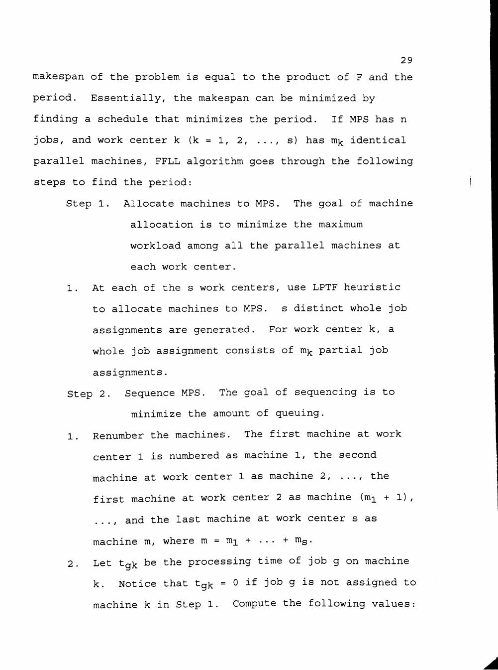
29

makespan of the problem is equal to the product of F and the

period. Essentially, the makespan can be minimized by

finding a schedule that minimizes the period. If MPS has n

jobs, and work center k (k = 1, 2, ..., s) has mj identical

parallel machines, FFLL algorithm goes through the following

steps to find the period:

Step 1. Allocate machines to MPS. The goal of machine

allocation is to minimize the maximum

workload among all the parallel machines at

each work center.

1. At each of the s work centers, use LPTF heuristic

to allocate machines to MPS. s distinct whole job

assignments are generated. For work center k, a

whole job assignment consists of mj partial job

assignments.

Step 2. Sequence MPS. The goal of sequencing is to

minimize the amount of queuing.

1. Renumber the machines. The first machine at work

center 1 is numbered as machine 1, the second

machine at work center 1 as machine 2, ..., the

first machine at work center 2 as machine (m^ + 1),

and the last machine at work center s as

machine m, where m = m^ + ... + nig.

2. Let tg]^ be the processing time of job g on machine

k. Notice that tg^ = 0 if job g is not assigned to

machine k in Step 1. Compute the following values:

30

(1) Ik = Z2_i tg] = workload of machine k, (2) y J. -3

tg = Si?_-, tg] = total processing time of job g in

MPS, (3) T = ZjJ^^^lk= total workload of MPS, and

(4) hgk = tgk -glk

= overload of job g on machine

3. Let g* be the last job in the partial sequence

determined so far. A myopic heuristic adds to the

end of the sequence the job g, which minimizes

m m . .+ I H , = I iHg*k + hgkj / where

k=l ^ k=l

H , = max gk (Hgk'O), and Hgk = S hg'k g'esg

Hg]^ measures

how overloaded machine k is when job g enters the

system and Sg is the set of jobs in the sequence

through job g.

4_ Repeat (3) until all the jobs in MPS are sequenced.

Step 3. Compute loading times for MPS. The goal is to

find a minimum period schedule whose period

is equal to the bottleneck workload.

1. According to the sequence obtained from Step 2, let

all the jobs of the MPS enter the system as rapidly

as possible. Consider the machines, one at a time,

in an order consistent with the machine number.

31

2. At each machine, process the job in the order in

which they arrive. Begin processing each job as

soon as the machine is available.

3. For each machine, its workspan is the elapsed time

between the time it starts processing its first job

and the time it completes work on its last job.

Thus a machine's workspan is equal to its workload

plus any idle time it incurs. After considering

all jobs of the MPS that visit the machine, if the

workspan of the machine exceeds its workload, delay

processing the first job by the difference. All

subsequent jobs are still processed in order,

starting as soon as the machine is available.

4. After considering all machines, the schedule for

MPS is determined.

In 1988 Wittrock approached the same problem with a

non-periodic scheduling method which is called Workload

Approximation (WLA) heuristic. WLA seeks a sequence that

comes close to balanced workloads. Given a set of n jobs,

and s work centers each having m]^ (k = 1, 2, ..., s)

identical parallel machines, WLA employs the following three

primary steps to solve the problem.

Step 1. Determine which jobs will visit each

individual machine at each work center.

1. At each of the s work centers, use LPTF heuristic

to allocate machines to the jobs. s distinct whole

32

job assignments are generated. For work center k,

a whole job assignment consists of m]^^ partial job

assignments.

Step 2. Specify the order in which the jobs should

enter the line.

1. Renumber the machines. This is done as in Step 2

in FFLL algorithm.

2. Let V(k) be the set of the jobs that visit machine

k, k'(g,k) be the predecessor machine to machine k

for job g e V(k), R(g) be the set of machines that

job g visits, excluding its first machine, p(g,k)

be transportation time from machine k'(g,k) to

machine k in R(g), g(f) be the f^h job in the

sequence, G = {l, 2, ..., n} be the set of all job

indices, T(f) = S(f-l) be the set of the first

(f _ 1) jobs loaded, and t(g,k) be the processing

time of job g on machine k. Notice that t(g,k) = 0

if job g ^ V(k) . Compute the following values:

(1) l(k) = Z^_T t(g,k) = workload of machine k, (2)

1* = maxi<k<sl(k) = bottleneck workload, (3)

3.

7C

i (n \r) = -—-—-— = the allocation of idle time to ^^' |V(k)|

job g e V(k) , where |v(k) I is the number of jobs

in the set of V(k) ,

The WLA heuristic considers each sequence index, f

(f = 1, 2, ..., n), in order, and selects a job,

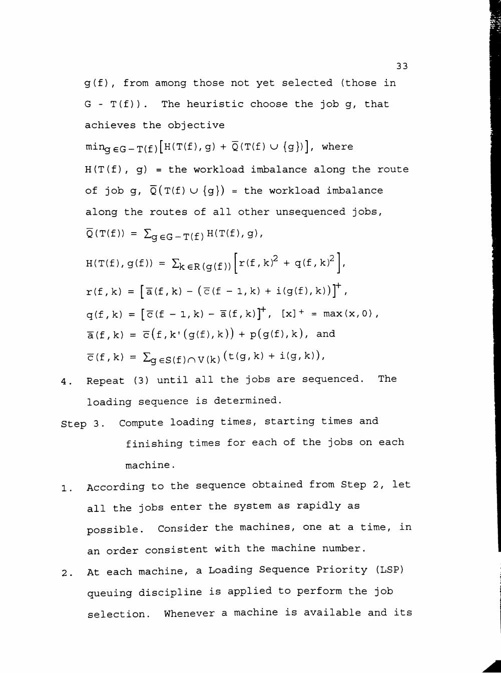
33

g(f), from among those not yet selected (those in

G - T(f)). The heuristic choose the job g, that

achieves the objective

mingeG-T(f)[H(T(f), g) + Q(T(f) u {g})], where

H(T(f), g) = the workload imbalance along the route

of job g, Q(T(f) U {g}) = the workload imbalance

along the routes of all other unsequenced jobs,

Q(T(f)) = Ig^Q_T(f)H(T(f),g),

r(f,k)2 + q(f,k)2

1+

H(T(f),g(f)) = ZkeR(g(f))

r(f,k) = [a(f,k) - (c(f - l,k) + i(g(f),k))f ,

q(f, k) = [c(f - 1, k) - a(f, k)]" , [x] + = max(x,0) ,

a(f,k) = c(f ,k'(g(f),k)) + p(g(f),k), and

c(f,k) = Iges(f)nv(k)(t(g,k) + i(g,k)),

4. Repeat (3) until all the jobs are sequenced. The

loading sequence is determined.

Step 3. Compute loading times, starting times and

finishing times for each of the jobs on each

machine.

1. According to the sequence obtained from Step 2, let

all the jobs enter the system as rapidly as

possible. Consider the machines, one at a time, in

an order consistent with the machine number.

2. At each machine, a Loading Sequence Priority (LSP)

queuing discipline is applied to perform the job

selection. Whenever a machine is available and its

34

buffer is occupied, it begins processing that job

which appears earliest in the loading sequence.

After considering all the machines, an initial set

of loading times, starting times and finishing

times for each of the jobs on each machine is

found.

Delay the loading time of each job as much as

possible as long as: (a) the makespan is not

increased, and (b) the schedule of all the other

jobs is unaltered. The delaying is carried out by

the following steps:

4.1. Consider the jobs, one at a time, in an order

consistent with the loading sequence obtained

from Step 2, and consider the machines, one

at a time, in an order that the job visits.

4.2. At each machine, if the job queues, the

queuing time cancels out with some or all the

delay. The delay is set equal to the idle

time that the machine incurs between

processing the current job and the next job.

4.3. After considering all machines that the job

visits, if the resulting final delay causes

the job to leave the line at a time later

than the makespan, this delay is reduced

accordingly.

35

4.4. After considering all jobs, the schedule for

the problem is determined.

From Wittrock's point of view, the job sequence cannot

change the job route. The job route is decided by the

parallel machine assignments. In applying the FFLL

algorithm, the makespan is decided by the period of MPS

which is equal to the bottleneck workload of MPS. This

period is also decided by the parallel machine assignment.

The job sequence cannot change the makespan. Wittrock

treated the job sequence as a means of minimizing the amount

of queuing, not as a means of minimizing the makespan.

The case with every work center having the same number

of identical parallel machines has been given less

attention. Except for the heuristic solutions suggested by

Deal and Hunsucker (1991), and by Sriskandarajah and Sethi

(1989), this problem has not been reported.

A lower bound (LB) which is the maximum value among

LBl, LB2 and LB3 was developed by Deal and Hunsucker for a

two work center problem. LBl is the maximum total

processing time over all jobs. LB2 is equal to

max< n 1 ^

i f ai + mini<i<n(t)i)''i^ini<i<n(ai) + - I bi m . ^ -i - 1

, where n I

i=l i=l

a- and bi are the processing times of job i at work centers

1 and 2, respectively, and m is the number of machines at

each work center. LB3 is equal to

36

(i) m

th

maxs n m n m Sbi+ Zti(j); Iai+ Zt2(j) i=l j=l i=l j=l

, where ty^ij) is the

j ^ " - smallest processing time at work center k (k = 1, 2) .

The Deal and Hunsucker heuristic utilizes Johnson's

algorithm to create a single queue in front of the first

work center. Jobs then are assigned sequentially to the

earliest available machine at work center 1. When a queue

of jobs for the next available machine at work center 2

exists, jobs are processed in first-come-first-serve

sequence.

The Sriskandarajah and Sethi's algorithm is first

developed for a two work center problem then extended to an

s work center problem. Bounds are given which show how

close the heuristic solutions are to the true optimal

solution in the worst case. A permutation schedule is

generated from the following steps:

1. Generate an artificial m-parallel machine problem

from the original s work center problem. The

artificial processing time for each job is the

total processing time of this job in this system,

i.e., for job i (i = 1, 2, ..., n) the artificial

2.

processing time is S tij . j = l

With the artificial processing times obtained from

(1), use LPTF heuristic to perform machine

37

allocation. A whole job assignment that consists

of m partial job assignments is obtained.

3. Determine the job sequence:

3.1. If only two work centers are considered, m-

partial job sequences are generated by

Johnson's rule (1954) for the case with

unlimited buffer, or by Gilmore and Gomory's

algorithm (1964) for the no-wait case for

each partial job assignment obtained from

(2) .

3.2. If more than two work centers are considered,

m-partial job sequences are generated by

arranging the jobs in each partial job

assignment in the LPT order of their

artificial processing times.

4. Impose each of the partial job sequences to the

corresponding parallel machines to every work

center. The job sequence for the problem is then

determined.

5. Compute the starting time and finishing time for

each job on each assigned machine at each work

center. The largest finishing time among the jobs

at the last work center is the makespan for the

problem.

Sriskandarajah and Sethi also use parallel machine

assignment to determine the job route. In the algorithm.

38

every work center must have the same machine allocation,

i.e., at every work center the machines bearing the same

machine number must have the same partial job assignment and

the same partial job sequence. They showed that even if an

optimal algorithm is employed to do parallel machine

assignment, the worst case bound of this heuristic is less

than or equal to ( \

s + 1 V my

times the true optimal

makespan.

CHAPTER IV

METHODOLOGY

It is of interest to note that a flexible flowshop

represents a generalization of the simple flowshop and the

identical parallel machine shop. For a given set of jobs,

the approaches used to minimize the makespan in the simple

flowshop and in the identical parallel machine shop are

different from each other. Since the insertion of idle

times is needed when a machine is ready but no jobs are

available for processing, in the simple flowshop, the main

concern is to find a job sequence and reduce the total

machine idle time. In the identical parallel machine shop,

because no idle time is needed between any pair of adjacent

jobs, the main concern is to dispatch jobs to the parallel

machines and balance the workloads among the parallel

machines. The two concerns mentioned above have to be

considered together in flexible flowshop scheduling

problems. Many algorithms have been developed to solve the

simple flowshop scheduling problem. Identical parallel

machine shop scheduling problems have been solved by several

different heuristics. By combining the characteristics of

the simple flowshop and the identical parallel machine, in

this research two different approaches are developed to find

a schedule for a set of immediately available jobs in the

flexible flowshop to minimize makespan.

39

40

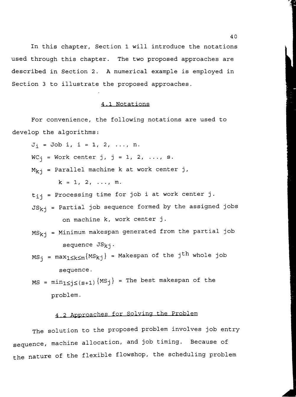
In this chapter. Section 1 will introduce the notations

used through this chapter. The two proposed approaches are

described in Section 2. A numerical example is employed in

Section 3 to illustrate the proposed approaches.

4.1 Notations

For convenience, the following notations are used to

develop the algorithms:

Ji = Job i, i = 1, 2, ..., n.

WCj = Work center j, j = 1, 2, ..., s.

M] j = Parallel machine k at work center j ,

k = 1, 2, ..., m.

tij = Processing time for job i at work center j.

jS] j = Partial job sequence formed by the assigned jobs

on machine k, work center j.

MS}rj = Minimum makespan generated from the partial job

sequence JSj j .

MSj = maxi<k<Tn{MSkj} = Makespan of the jth whole job

sequence.

MS = mini<j<(s + l) {J Sj} = The best makespan of the

problem.

4 7 ^pp-rnRche^ for Solving the Problem

The solution to the proposed problem involves job entry

sequence, machine allocation, and job timing. Because of

the nature of the flexible flowshop, the scheduling problem

41

of the proposed problem can be broken down into simple

flowshop scheduling problems and identical parallel machine

scheduling problems. That is, the problem is one of

developing a job sequence for each of the parallel machines

and a whole job assignment for each of the work centers. To

determine the schedule in the partially flexible job route

situation, an approach called the para-flow algorithm is

used. In the completely flexible job route situation, two

approaches are employed to find the schedule. In addition

to the para-flow algorithm, the second approach is called

flow-para algorithm. Both of the algorithms can utilize the

combination of all the existing flowshop scheduling

algorithms and the identical parallel machine scheduling

algorithms to solve the flexible flowshop scheduling

problem.

4•2.1 Para-Flow Approach

As the name connotes, the problem to be investigated is

approached by solving the identical parallel machine

assignments first. Then it is approached by solving the

flowshop problem. When the system consists of s work

centers, each having m identical parallel machines and a set

of n jobs is available to be processed, the para-flow

approach can be summarized in a four-phase algorithm. The

results of each phase are used as input for the next phase.

In both situations, the steps used in Phases I, II, and III

42

are the same. For the problem under the partially flexible

job route situation. Phase IV simply determines the final

schedule which is a permutation schedule. For the problem

under the completely flexible job route situation, at each

work center workspans among the parallel machines can be

adjusted by a balancing routine. After balancing the

workspans at the last work center. Phase IV generates the

final schedule which is a non-permutation schedule.

Phase I : Parallel Machine Assignment

The purpose of this phase is to find a whole job

assignment for each of the para-subproblem of machines. For

each of the para-subproblems, a whole job assignment is

defined to be the machine allocation of the set of n jobs.

Nearly balanced workload can be achieved and the maximum

workload among all of the parallel machines in a para-

subproblem can be minimized.

Step 1. Partition the problem into (s + 1) parallel machine

subproblems each having exactly one work center

with m identical parallel machines. The

processing time of job i (i = 1, 2, ..., n) in the

first s para-subproblems is tij

(j = 1, 2, ..., s). In the (s + l)th para-

subproblem the artificial processing time of job i

s is S tij. Figure 4.1 shows these (s + 1) para-

j=l

subproblems:

43

WCi WC

Jobs -—

—

M l

M2

• • •

Mm

J o b s

Ml

M2

• • •

Mm

WCc WCs+1

Jobs -

M l

M2

Jobs • • •

Mm

• M l

M2

• • •

Mm

Figure 4.1. (s + 1) Para-Subproblems Partitioned from the Original Problem

Step 2. Each of the para-subproblems is considered

separately. Start at work center 1, i.e., the

first para-subproblem. Apply a parallel machine

assignment heuristic, e.g., LPTF (the Longest

Processing Time First) , to dispatch jobs to the

parallel machines. Each of the parallel machines

is assigned one or more jobs. A partial job

assignment is formed by the jobs assigned to the

same machine. A whole job assignment is formed by

the m partial job assignments.

Step 3. If this is the last para-subproblem, then move to

Phase II. Otherwise, go back to step 2 to deal

with the next para-subproblem.

44

Phase II; Flowshop Sequencing

The purpose of this phase is to find the best partial

job sequences which have minimum makespan for each of the

partial job assignments.

Step 1. Partition the problem into m(s + 1) simple flowshop

problems, each having s work centers, each having

exactly one machine. Each of the flow-subproblems

has a partial job assignment Jobs} j

(k = 1, 2, ..., m, j = 1, 2, ..., (s + 1)) and is

considered separately. Figure 4.2 shows these

m(s + 1) flow-subproblems:

•I?

F l o w - s u b p r o b l e m 1:

M i l

Jobs 1^1

- > Ml2 -^ • - ^ Ml

F l o w - s u b p r o b l e m 2 :

M 21

Jobs2 1

- ^ M 22 ^ • •

- ^

^ M 2s

F l o w - s u b p r o b l e m m ( s + l ) : J°^^m,(s-H) • ^

M ml - > M m2 - > • ^ M ms

Figure 4.2. m(s + 1) Flow-subproblems with Partial Job Assignment Jobsj j Obtained from Phase I

45

Step 2. Start at machine 1 in the para-subproblem 1, i.e.,

the first flow-subproblem. Consider the jobs

assigned to this machine in Phase I. Apply a

flowshop scheduling algorithm, e.g., the CDS

algorithm, to this flow-subproblem. Determine a

partial job sequence JS} j (k = 1, 2, ..., m,

j = 1, 2, ..., (s + 1)) and compute its

corresponding makespan for the partial job

assignment. This makespan is considered as MS] j .

Step 3. If this is the last flow-subproblem, then move to

Phase III. Otherwise go back to step 2 to deal

with the next flow-subproblem.

Phase III: Sequence Selection

The purpose of this phase is to choose a whole job

sequence from the (s + 1) whole job sequences that has the

minimum makespan.

Step 1. For each of the para-subproblems, there are m

makespans, each generated by a partial job

sequence obtained from Phase II. Among these m

makespans, the maximum value is the makespan of

this para-subproblem, i.e., the value of MSj

(j = 1, 2, . . . , (s + 1) ) .

Step 2. Find the minimum value from these MSj and assign

this value to MS.

Step 3. Identify a whole job sequence whose makespan is

equal to MS. In case that more than one whole job

46

sequence has the same value as MS, break the tie

by arbitrarily choosing one of the tied whole job

sequences; then advance to Phase IV.

Phase IV; Scheduling

For the problem under the partially flexible job route

situation, the purpose of this phase is to determine the

start times and finish times of each job on each assigned

machine at each work center, i.e., the final schedule. For

the problem under the completely flexible job route

situation, at each work center the chosen whole job sequence

may not have a balanced workspan. This phase not only

determines the final schedule but also balances workspans

among the parallel machines at each work center.

Step 1. If the problem is under the completely flexible job

route situation, then go to Step 4. If a

partially flexible job route situation is

considered, then go to Step 2.

Step 2. Impose each of the partial job sequences of the

chosen whole job sequence to the corresponding

machines at every work center. Thus every work

center has the same whole job assignment and every

machine bearing the same machine number has the

same partial job sequence. This is the job

sequence and machine allocations for the problem

under the partially flexible job route situation.

47

Step 3. Consider the work centers in order. Start at work

center 1. Compute the job timing for each job on

the assigned machine. The value of MS is the

makespan of this schedule. Then stop.

Step 4. Consider the work centers in order. Start this

phase at work center 1. According to the chosen

whole job sequence, assign each of the partial job

sequences to the corresponding machines at the

work center. Then compute the start times and

finish times of each job on the assigned machine.

At this point, all the m parallel machines are

classified as unadjusted machines whose workspans

have not been balanced and whose partial job

sequence have not been adjusted.

Step 5. Among unadjusted machines, identify the machine

with the largest workspan and the machine with the

smallest workspan.

Step 6. Select adjustable jobs. A job is said to be an

adjustable job if the job meets the fololowing

three conditions: (1) the job is on the machine

with the largest workspan, (2) the start time of

the job is larger than the finish time of the last

job on the machine with the smallest workspan, and

(3) there exists a time lag between the finish

time of the job at previous work center and the

start time of the job at the current work center.

48

Move the adjustable jobs to the end of the partial

job sequence on the machine with the smallest

workspan. Then change the start times and finish

times of the adjusted jobs accordingly.

Step 7. The machine which was labeled as the one with the

largest workspan is then classified as an adjusted

machine. Go back to step 4 until only one machine

is left unadjusted.

Step 8. If this is not the last work center, then move to

next work center and go back to Step 4.

Otherwise, stop; the complete schedule has been

obtained. The largest finish time among the jobs

at the last work center is the makespan for the

problem under the completely flexible job route

situation.

4 2.2 F]nw-Para Approach

This approach allows jobs to be processed on any one of

the parallel machines at each work center. Therefore, it is

only suitable for the problem under the completely flexible

job route situation. As the name connotes, the problem is

approached by solving the flowshop problem first. Then it

is approached by solving the identical parallel machine

assignments. This approach can be summarized in the

following two-phase algorithm:

49 Phase T; Flowshop Seguenr-ing

The purpose of this phase is to find a job entry

sequence that determines the loading sequence priority of

each job.

Step 1. Take the problem as a simple flowshop problem,

i.e., each of the work centers has only one

machine. This flow-subproblem is illustrated in

Figure 4.3.

Jobs -^

WCi -^ WC' ^ . . . - ^ WC.

Figure 4.3. The Flow-subproblem in Flow-para Approach.

Step 2. Apply a flowshop scheduling algorithm, e.g., the

CDS algorithm, to this flow-subproblem. Determine

a job sequence which has minimum makespan obtained

from the flowshop algorithm.

Phase II: Job Assignment and Scheduling

The purpose of this phase is to perform the machine

allocation and determine the start times and finish times of

each job on each of the parallel machines at each work

center.

Step 1. Start at work center 1. From the beginning of the

job entry sequence obtained from Phase I, assign

the jobs one by one to the earliest available

machine at work center 1. Repeat this step until

step 2

Step 3

50

all the jobs are assigned to the parallel machines

at work center 1. Then go to Step 2 to deal with

the following work centers.

Upon arriving at a work center, a job is put to the

end of the queue in front of the work center.

When a machine completes one job, this machine

becomes available. If more than one machine is

available, arbitrarily assign a chosen job to one

of the available machines. Under different

situations, the job to be processed next is

decided by one of the following rules.

Rule 1. If there are no waiting jobs in the

buffer of this work center, set the

machine idle until a job arrives from

the previous work center. The arriving

job is processed next.

Rule 2. If there is only one waiting job in the

buffer of this work center, then choose

this waiting job to be processed next.

Rule 3. If there is more than one waiting job in

the buffer of this work center, a

priority dispatching rule must be

employed to choose a job to be processed

next.

Go back to Step 2 until all the jobs have been

completed at this work center.

51

Step 4. If this is not the last work center, then move to

next work center and go back to Step 2.

Otherwise, stop and the complete schedule is

obtained. The largest finish time among the jobs

at the last work center is the makespan for the

problem under the completely flexible job route

situation.

4.3 Numerical Example

By specifying a simple flowshop scheduling algorithm, a

parallel machine assignment heuristic and a priority

dispatching rule, the para-flow approach and the flow-para

approach stated above can be realized. For the para-flow

approach, LPTF heuristic will be used in Phase I to make

parallel machine assignments and the CDS algorithm will be

used in Phase II to sequence the jobs. For the flow-para

approach, the CDS algorithm will be employed to find the

entry job sequence in Phase I, and Loading Sequence Priority

(LSP) queuing discipline and First-Come-First-Serve (FCFS)

queuing discipline will be used as a priority dispatching

rule in Phase II. LPTF heuristic and the CDS algorithm are

referred to in Sections 3.2 and 3.1, respectively. LSP

queuing discipline is described as follows: when a machine

is available and there is more than one waiting job in

queue, among the queuing jobs, the job appearing earliest in

the loading sequence at the first work center is selected to

52

be processed next. FCFS queuing discipline is the first

come, first served rule.

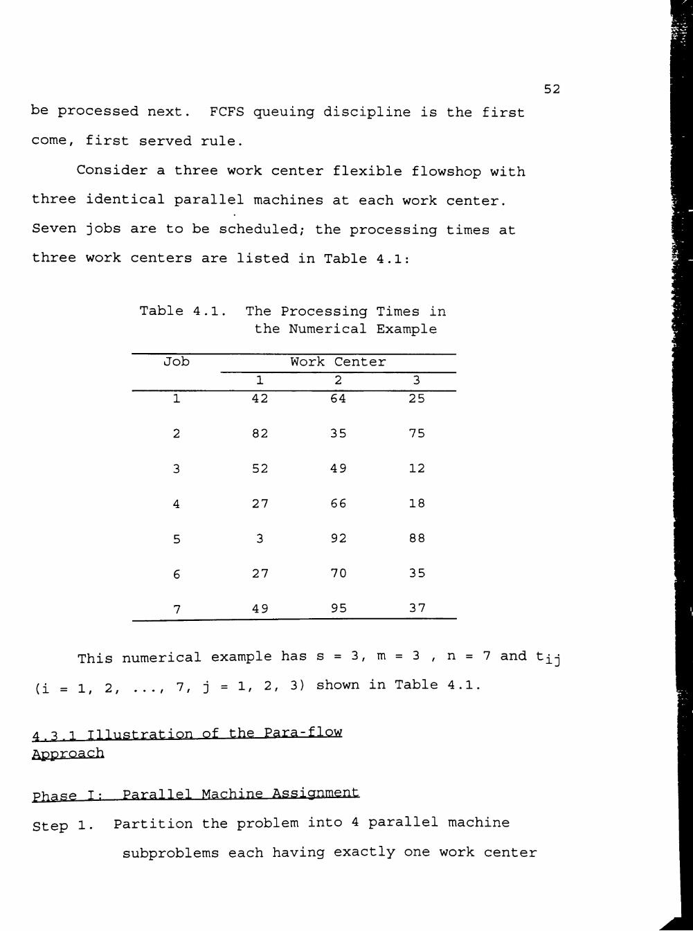
Consider a three work center flexible flowshop with

three identical parallel machines at each work center.

Seven jobs are to be scheduled; the processing times at

three work centers are listed in Table 4.1:

Table 4.1.

Job

1

2

3

4

5

6

7

The the

1

42

82

52

27

3

27

49

Processing Numerical

Work Cent*

2

64

35

49

66

92

70

95

Times in Example

sr

3

25

75

12

18

88

35

37

This numerical example has s = 3, m = 3 , n = 7 and t- j

( i = l , 2, ...,7, j = l , 2, 3) shown in Table 4.1.

4 ^ 1 Tl]nP!tration of the Para-flow Approach

pv .cp T: Parallel Machine Assignment

Step 1. Partition the problem into 4 parallel machine

subproblems each having exactly one work center

53

with 3 identical parallel machines. The

processing time of job i (i = 1, 2, ..., 7) in the

first 3 para-subproblems is t^j (j = 1 , 2, 3) as

shown in Table 4.1. That is, the processing times

of jobs 1 through 7 are 42, 82, 52, 27, 3, 27, and

49, respectively in the 1^^ para-subproblem, 64,

35, 49, 66, 92, 70, and 95, respectively in the

2^^ para-subproblem, and 25, 75, 12, 18, 88, 35,

and 37 respectively in the 3^^ para-subproblem.

In the 4th para-subproblem the artificial

processing times are Z ti j which are 131, 192,

j = l

113, 111, 183, 132, and 181 for jobs 1 through 7,

respectively.

Step 2. Each of the para-subproblems is considered

separately. For the first para-subproblem. LPTF

heuristic is applied as follows: (1) Arrange the

jobs in nonincreasing order of their processing

time. The LPT order is 2-3-7-1-4-6-5. (2) Assign

the jobs in order, one at a time, to the machine

having the least accumulative processing times.

The partial job assignments are (2,5), (3,4,6),

and (7,1) on machines 1, 2, and 3, respectively.

A whole job assignment is formed by the 3 partial

job assignments.

54

Step 3. Repeat Step 2 for para-subproblems 2, 3, and 4.

The LPT orders are 7-5-6-4-1-3-2, 5-2-7-6-1-4-3,

and 2-5-7-6-1-3-4 for para-subproblems 2, 3, and

4, respectively. The partial job assignments on

machines 1, 2, and 3 are (7,3), (5,1), and

(6,4,2), respectively for para-subproblem 2,

(5,3), (2,4), and (7,6,1), respectively for para-

subproblem 3, and (2,3,4), (5,1) and (7,6),

respectively for para-subproblem 4. Then move to

Phase II.

Phase II: Flowshop Sequencing

Step 1. Partition the problem into 12 simple flowshop

problems, each having 3 work centers, each having

exactly one machine. Each of the flow-subproblems

has a partial job assignment Jobsj j (k = 1, 2, 3,

j = 1, 2, 3, 4). JobS]_i, Jobs2i/ ..., and Jobs34

are {2,5}, {3,4,6}, {7,l}, {7,3}, {5,l}, {6,4,2},

{5,3}, {2,4}, {7,6,1}, {2,3,4}, {5,1} and {7,6},

respectively. Each flow-subproblem is considered

separately.

Step 2. Start at machine 1 in the para-subproblem 1, i.e.,

the first flow-subproblem. Apply the CDS

algorithm to this flow-subproblem with

Jobsii = {2,5}. (1) Generate 2 artificial two-

machine subproblems. For the first subproblem,

the artificial processing times: ti2i/ ^22'

55 ti5i/ and ti52 are equal to 82, 75, 3, and 88,

respectively. For the second subproblem, the

artificial processing times: t22i, t222' t25i,

and t252 are equal to (82 + 35), (75 + 35),

(3 + 92), and (88 + 92), respectively which are

117, 110, 95, and 180 accordingly. (2) Apply

Johnson's algorithm to the first subproblem.

Since ti5i < ti52, U = {5} and since ti2i > ti22.

V = {2}. The partial job sequence is 5-2 with

makespan 2 58. (3) Apply Johnson's algorithm to

the second subproblem. Since t25i < ^252/ U = {5}

and since t22i > t222' V = {2}. The partial job

sequence is 5-2 with makespan 258. (4) Then

MSii = min(258,258) = 258. The partial job

sequence is 5-2 for the partial job assignment

{2,5}.

Step 3. Repeat Step 2 for all the flow-subproblems. The

computation results are summarized in Table 4.2.

Then go to Phase III.

Phase III: Sequence Selection

Step 1. Determine the makespan for each of the para-

subproblems MSj (j = 1, 2, 3, 4).

MSi = max{258,224,233} = 258.

MS2 = max{205,208,237} = 237.

MS3 = max{l95,210,28l} = 281.

MS4 = max{245,208,229} = 245.

56

Table 4.2.

Partial Job Assignment

{2,51

{3,4,6}

{7,1}

{7,3}

{5,1}

{6,4,2}

{5,3}

{2,4}

{7,6,1}

{2,3,4} \ *

{1,5}

{7,6}

Summary of Using the

CDS

Partia 1 Job Se CDS Algorithm

U Subproblem

First Second

First Second

First Second

First Second

First Second

First Second

First Second

First Second

First Second

First Second

First Second

First Second

{5} {5}

{6} {6}

0 0

0 0

{5} {5}

{6} {6}

{5} {5}

0 0

{6} {6}

0 0

{5} {5}

{6} {6}

V

{2} {2}

{3,4} {3,4}

{1,7} {1,7}

{3,7} {3,7}

{1} {1}

{2,4} {2,4}

{3} {3}

{2,4} {2,4}

{1,7} {1,7}

{2,3,4} {2,3,4}

{1} {1}

{7} {7}

quence and Makespan

Partial Job Makespan Sequence

5-2 5-2

6-4-3 6-4-3

7-1 7-1

7-3 7-3

5-1 5-1

6-2-4 6-2-4

5-3 5-3

2-4 2-4

6-7-1 6-7-1

2-4-3 2-4-3

5-1 5-1

6-7 6-7

258 258

224 224

233 233

205 205

208 208

237 237

195 195

210 210

281 281

245 245

208 208

229 229

57

Step 2. MS = min{258,237,281,245} = 237.

Step 3. The whole job sequence with makespan 237 consists

of the three partial job sequences: 7-3 on

machine 1, 5-1 on machine 2, and 6-2-4 on machine

Phase XV; Scheduling

Step 1. If the problem is under the completely flexible job

route situation, then go to Step 4. If a

partially flexible route situation is considered,

then go to Step 2.

Step 2. Impose each of the partial job sequences of the

chosen whole job sequence on the corresponding

machines at every work center. That is, at every

work center 7-3 are on machine 1, 5-1 are on

machine 2, and 6-2-4 are on machine 3. This is

the job sequence and machine allocation for the

problem under the partially flexible job route

situation.

Step 3. The schedule is shown in Table 4.3 in which

i(ts,tf) represents the start time and finish time

of job i. The makespan of this schedule is 237.

Then stop.

Step 4. According to the chosen whole job sequence, assign

each of the partial job sequences to the

corresponding machines at work center 1. Then

determine the start times and finish times of each

58

Table 4.3. Schedule for the Partially Flexible Job Route Situation

Machine Work Center

7(0,49) 3 (49,101)

5(0,3) 1(3,45)

6 (0,27) 2 (27,109) 4(109,136)

7(49,144) 3(144,193)

5 (3,95) 1(95,159)

6(27,97) 2 (109,144) 4 (144,210)

7(144,181) 3(193,205)

5 (95,183) 1(183,208)

6(97,132) 2 (144,219) 4 (219,237)

job on the assigned machine. The initial

condition is as follows.

Machine 1: 7(0,49), 3(49,101).

Machine 2: 5(0,3), 1(3,45).

Machine 3: 6(0,27), 2(27,109), 4(109,136).

Unadjusted machines: {1,2,3}.

Adjusted machines: 0.

Step 5. Machine 3 has the largest workspan of 136. Machine

2 has the smallest workspan of 45.

Step 6. Since job 4 is on machine 3 and its start time of

109 is greater than 45, job 4 is selected as an

adjustable job. Move job 4 to the end of job 1 on

machine 2. Then the partial job sequence, the

sets of adjusted machines and unadjusted machines

are updated as follows.

59

Machine 1: 7(0,49), 3(49,101).

Machine 2: 5(0,3), 1(3,45), 4(45,72).

Machine 3: 6(0,27), 2(27,109).

Unadjusted machines: {1,2} .

Adjusted machines: {3}.

Step 7. Between machines 1 and 2, machine 1 has larger

workspan of 101. Machine 2 has smaller makespan

of 72. Since the start times of all the jobs on

machine 1 are less than 72, there are no

adjustable jobs. The partial job sequence on each

machine is unchanged. The sets of adjusted

machines and unadjusted machines are updated as

follows.

Unadjusted machines: {l}-

Adjusted machines: {3,2}.

Since only machine 1 is left unadjusted, stop the

balancing routine at work center 1 and go to work

center 2.

Step 8. Repeat Step 4 through Step 7 for work centers 2 and

3. At work center 2, the initial condition is:

Machine 1: 7(49,144), 3(144,193).

Machine 2: 5(3,95), 1(95,159).

Machine 3: 6(27,97), 2(109,144), 4(144,210).

Unadj usted machines: {1,2,3}.

Adjusted machines: 0.

60

Among the unadjusted machines, machine 3 has the

largest workspan of 210 and machine 2 has the

smallest workspan of 159. Since the start times

of all the jobs on machine 3 are less than 159,

there are no adjustable jobs. The partial job

sequence on each machine is unchanged. The set of

adjusted machines and unadjusted machines are

updated as follows.

Unadjusted machines: {1,2}.

Adjusted machines: {3}.

Between machines 1 and 2, machine 1 has larger

workspan of 193. Machine 2 has smaller makespan

of 159. Since the start times of all the jobs on

machine 1 are less than 159, there are no

adjustable jobs. The partial job sequence on each

machine is unchanged. The sets of adjusted

machines and unadjusted machines are updated as

follows.

Unadjusted machines: {l} .

Adjusted machines: {3,2}.

Since only machine 1 is left unadjusted, stop the

balancing routine at work center 2 and go to work

center 3.

At work center 3, the initial condition is:

61

Machine 1: 7(144,181), 3(193,205).

Machine 2: 5(95,183), 1(183,208).

Machine 3: 6(97,132), 2(144,219), 4(219,237).

Unadj usted machines: {1,2,3}.

Adjusted machines: 0.

Among the unadjusted machines, machine 3 has the

largest workspan of 23 7 and machine 1 has the

smallest workspan of 205. Job 4 is on machine 3,

its start time at work center 3 is 219, and its

finish time at work center 2 is 210. A time lag,

9, exists between 210 and 219. Therefore, job 4

is selected as an adjustable job. Move job 4 to

the end of job 3 on machine 1. Then the partial

job sequence, the sets of adjusted machines and

unadjusted machines are updated as follows.

Machine 1: 7(144,181), 3(193,205), 4(210,228).

Machine 2: 5(95,183), 1(183,208).

Machine 3: 6(97,132), 2(144,219).

Unadj usted machines: {1/2}.

Adjusted machines: {3}.

Between machines 1 and 2, machine 1 has larger

workspan of 228. Machine 2 has smaller makespan

of 208. Job 4 with start time of 210 is the only

job on machine 1 whose start time is greater than

208. The finish time of job 4 at work center 2

also is 210. There is no time lag between the

62

finish time of job 4 at work center 2 and the

start time of job 4 at work center 3. Therefore,

there are no adjustable jobs. The partial job

sequence on each machine is unchanged. The sets

of adjusted machines and unadjusted machines are

updated as follows.

Unadjusted machines: {2}.

Adjusted machines: {3,1}.

Since only machine 2 is left unadjusted, stop the

balancing routine. The schedule is determined and

is given in Table 4.4. The makespan for the

problem under the completely flexible job route

situation is the largest finish time among the

jobs at work center 3 which is 228.

Table 4.4. Schedule for the Completely Flexible Job Route Situation Using Para-flow Algorithm

Machine Work Center

7(0,49) 3 (49,101)

5(0,3) 1(3,45) 4 (45,72)

6 (0,27) 2 (27,109)

7 (49,144) 3 (144,193)

5(3,95) 1 (95,159)

6(27,97) 2 (109,144) 4 (144,210)

7(144,181) 3 (193,205) 4 (210,228)

5(95,183) 1(183,208)

6 (97,132) 2(144,219)

63

4.3.2 Illustration of the Flow-Para Approach

Phase I ; Flowshop Sequencing

Step 1. Take the problem as a simple flowshop problem which

has 3 work centers. Each work center has exactly

one machine.

Step 2. Apply the CDS algorithm to this flow-subproblem

with jobs 1 through 7 having processing times

shown in Table 4.1. (1) Generate 2 artificial

two-machine subproblems. For the first

subproblem, the artificial processing times:

till, tii2, ti2i, ti22, •••/ and ti72 are equal to

42, 25, 82, 75, ..., 49, and 37, respectively.

For the second subproblem, the artificial

processing times: t2ii/ t2i2/ ^221/ ^222' •••/

and t272 are equal to (42 + 64), (64 + 25),

(82 + 35), (75+35), ..., (49 + 95), and

(95 + 37), respectively which are 106, 89, 117,

110, , ..., 144, and 132 accordingly. (2) Apply

Johnson's algorithm to the first subproblem.

Since tisi < ti52 and tigi < ti62' U = {5,6} and

V = {1,2,3,4,7}. Arrange jobs 5 and 6 in

nondecreasing order of t^si and t^gi and arrange

jobs 1, 2, 3, 4, and 7 in nonincreasing order of

tii2' ^122/ ti32, ti42r and ti72. The job

sequence is 5-6-2-7-1-4-3 with makespan 486. (3)

64

Apply Johnson's algorithm to the second

subproblem. Since t25i < t252 and t26i < t262'

U = {5,6} and V = {1,2,3,4,7}. Arrange jobs 5 and

6 in nondecreasing order of t25i and t26i and

arrange jobs 1, 2, 3, 4, and 7 in nonincreasing

order of t2i2/ t222' t232, t242/ and t272. The

job sequence is 5-6-7-2-1-4-3 with makespan 486.

Though the job sequences obtained from both

subproblems are different, the makespans obtained

from both subproblems are the same. Arbitrarily

choose one job sequence to advance to Phase II.

5-6-2-7-1-4-3 is chosen to be the loading job

sequence.

Phase II: Job Assignment and Scheduling

Step 1. From the beginning of the job entry sequence

obtained from Phase I, assign the jobs one by one

to the earliest available machine at work center

1. This results in the following.

Machine 1: 5(0,3), 7(3,52), 4(52,79).

Machine 2: 6(0,27), 1(27,69), 3(69,121).

Machine 3: 2 (0,82) .

Step 2. Worksheets for dispatching jobs to parallel

machines at work center 2 are shown in Table 4.5

and Table 4.6 by using LSP and by using FCFS as a

priority dispatching rule, respectively. In both

tables, "*" means a priority dispatching rule is

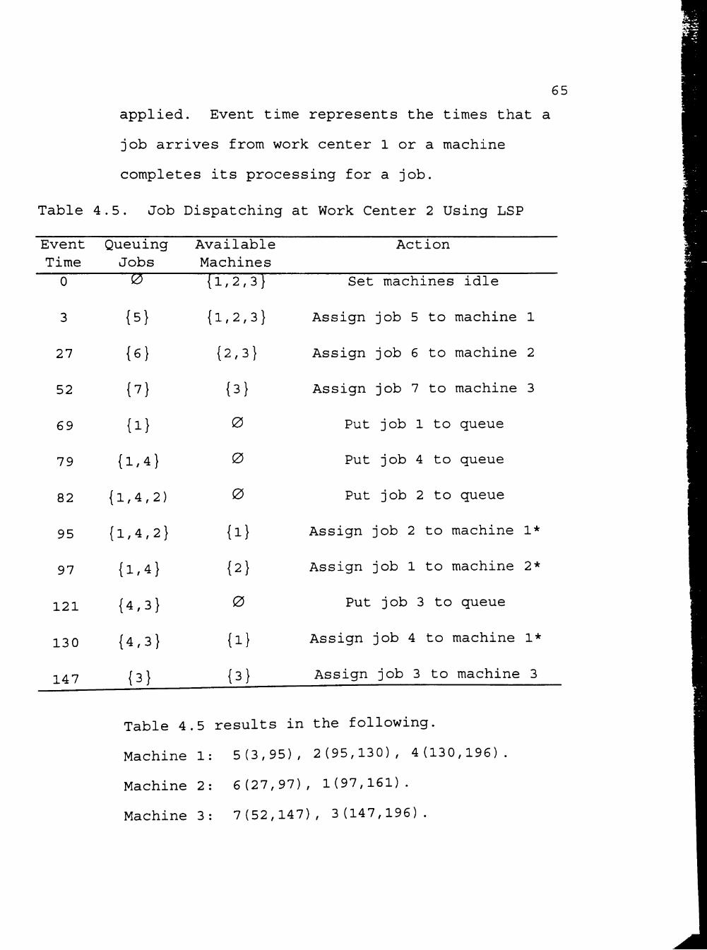
65

applied. Event time represents the times that a

job arrives from work center 1 or a machine

completes its processing for a job.

Table 4.5. Job Dispatching at Work Center 2 Using LSP

Event Queuing Time Jobs

0

Available Machines

{1,2,3}

{1,2,3}

{2,3}

{3}

0

0

0

{1}

{2}

0

{1}

{3}

Action

0

27

52

69

79

82

95

97

121

130

147

{5}

{6}

{7}

{1}

{1,4}

{1,4,2)

{1,4,2}

{1,4}

{4,3}

{4,3}

{3}

Set machines idle

Assign job 5 to machine 1

Assign job 6 to machine 2

Assign job 7 to machine 3

Put job 1 to queue

Put job 4 to queue

Put job 2 to queue

Assign job 2 to machine 1*

Assign job 1 to machine 2*

Put job 3 to queue

Assign job 4 to machine 1*

Assign job 3 to machine 3

Table 4.5 results in the following.

Machine 1: 5(3,95), 2(95,130), 4(130,196)

Machine 2: 6(27,97), 1(97,161).

Machine 3: 7(52,147), 3(147,196).

66

Table 4.6. Job Dispatching at Work Center 2 Using FCFS

Event Time

Queuing Jobs 0

{5}

{6}

{V}

{1}

{1,4}

{1,4,2)

{1,4,2}

{4,2}

{2,3}

{2,3}

{3}

Available Machines {1,2,3}

Action

0

27

52

69

79

82

95

97

121

147

159

Set machines idle

{1,2,3} Assign job 5 to machine 1

{2,3}

{3}

0

0

0

{1}

{2}

0

{3}

{3}

Assign job 6 to machine 2

Assign job 7 to machine 3

Put job 1 to queue

Put job 4 to queue

Put job 2 to queue

Assign job 1 to machine 1*

Assign job 4 to machine 2*

Put job 3 to queue

Assign job 2 to machine 3*

Assign job 3 to machine 1

Table 4.6 results in the following.

Machine 1: 5(3,95), 1(95,159), 3(159,208).

Machine 2: 6(27,97), 4(97,163).

Machine 3: 7(52,147), 2(147,182).

Worksheets for dispatching jobs to parallel

machines at work center 3 are shown in Table 4.7

and Table 4.8 by using LSP and by using FCFS as a

dispatching rule, respectively. In both tables,

"*" means a priority dispatching rule is applied.

67 Event time represents the time that a job arrives

from work center 2, or a machine completes its

processing for a job.

Table 4.7. Job Dispatching at Work Center 3 Using LSP

Event Time

0

95

97

130

132

147

161

183

Queuing Jobs

^

{5}

{6}

{2}

0

{7}

{D

{1}

Available Machines {1,2,3}

{1,2,3}

{2,3}

{3}

{2}

{2}

0

{1)

Action

Set machines idle

Assign

Assign

Assign

Set

Assign

Put

Assign

job 5 to machine

job 6 to machine

job 2 to machine

machine 2 idle

job 7 to machine

job 1 to queue

job 1 to machine

1

2

3

2

1

184

196

205

0

{4,3}

{3}

{2}

{2}

{3}

Set machine 2 idle

Assign job 4 to machine 2*

Assign job 3 to machine 3

Table 4.7 results in the following.

Machine 1: 5(95,183), 1(183,208).

Machine 2: 6(97,132), 7(147,184), 4(196,214)

Machine 3: 2(130,205), 3(205,217).

Table 4.8. Job Dispatching at Work Center 3 Using FCFS

68

Event Time 0

95

97

147

132

159

163

182

183

184

201

208

Queuing Jobs 0

{5}

{6}

{7}

0

{1}

{4)

{4,2}

{4,2}

{2}

0

{3}

Available Machines {1,2,3}

{1,2,3}

{2,3}

{3}

{2}

{2}

0

0

{1}

{2,3}

{3,1}

{3,1}

Action

Set machines idle

Assign job 5 to machine 1

Assign job 6 to machine 2

Assign job 7 to machine 3

Set machine 2 idle

Assign job 1 to machine 2

Put job 4 to queue

Put job 2 to queue

Assign job 4 to machine 1*

Assign job 2 to machine 2

Set machine 1 idle

Assign job 3 to machine 3

Table 4.8 results in the following.

Machine 1: 5(95,183), 4(183,201).

Machine 2: 6(97,132), 1(159,184), 2(184,259).

Machine 3: 7(147,184), 3(208,220).

Step 3. The schedules are determined and listed in Table

4.9 and Table 4.10 for using LSP as the priority

dispatching rule and using FCFS as the priority

dispatching rule, respectively. The makespan for

the problem under the completely flexible job

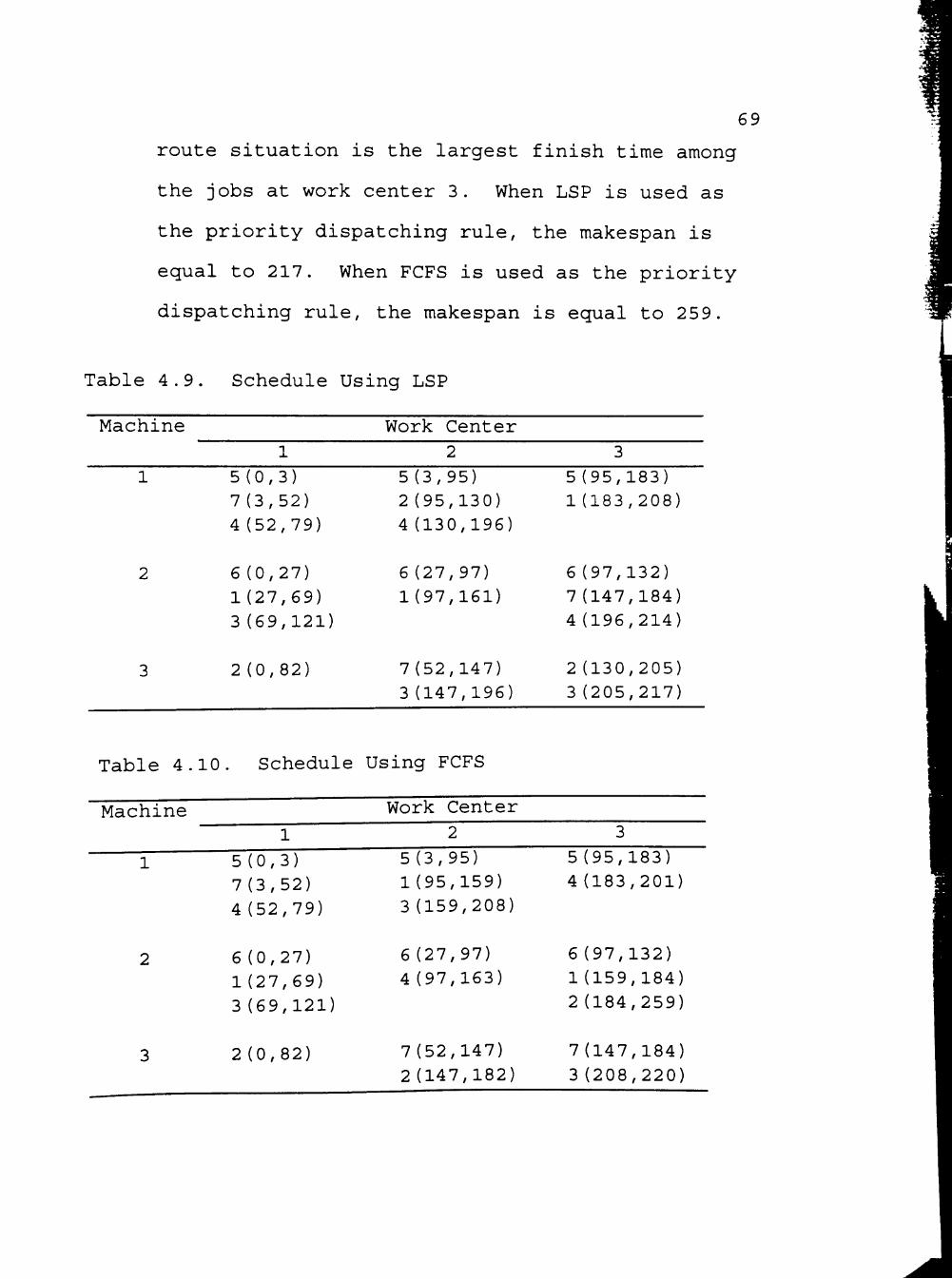
69

route situation is the largest finish time among

the jobs at work center 3. When LSP is used as

the priority dispatching rule, the makespan is

equal to 217. When FCFS is used as the priority

dispatching rule, the makespan is equal to 259.

Table 4.9. Schedule Using LSP

Machine Work Center

5(0,3) 7(3,52) 4 (52,79)

6 (0,27) 1(27,69) 3 (69,121)

2 (0,82)

5(3,95) 2 (95,130) 4 (130,196)

6 (27,97) 1(97,161)

7(52,147) 3 (147,196)

5 (95,183) 1 (183,208)

6 (97,132) 7 (147,184) 4 (196,214)

2(130,205) 3(205,217)

Table 4.10. Schedule Using FCFS

Machine

5(0,3) 7(3,52) 4 (52,79)

6(0,27) 1(27,69) 3(69,121)

2 (0,82)

Work Center

5(3,95) 1(95,159) 3 (159,208)

6 (27,97) 4 (97,163)

7(52,147) 2 (147,182)

5 (95,183) 4 (183,201)

6(97,132) 1(159,184) 2(184,259)

7(147,184) 3 (208,220)

CHAPTER V

COMPUTER EXPERIMENTS AND COMPUTATION

RESULTS

5.1 Computer Experiment

A computer experiment is employed to test the

effectiveness of the proposed algorithms. This test is

conducted by comparing makespan and CPU time between the

proposed algorithms and the published algorithms. Table 5.1

and Table 5.2 list the algorithms used for the problem under

the partially flexible job route situation and for the

problem under the completely flexible job route situation,

respectively.

Methods A, 1, 2, and 3 have been demonstrated in

Chapter IV. Method B is the same as Method 4 which has been

reviewed in Section 3.3. Methods 5 and 6 are developed by

Wittrock in 1985, and 1988, respectively, and are also

mentioned in Section 3.3. A symbol, (i,j,k), is used to

describe the size of the problem. (i,j,k) represents i

jobs, j work centers, and k identical parallel machines per

work center. Twenty-two different sizes of the problem are

employed, varying from (5,3,3) to (30,6,6), each having

twenty random sample problems for the problem under both

situations. The processing times for each of the problems

are randomly generated from a uniform distribution between 1

and 100. A computer program in GW-BASIC and compiled in

70

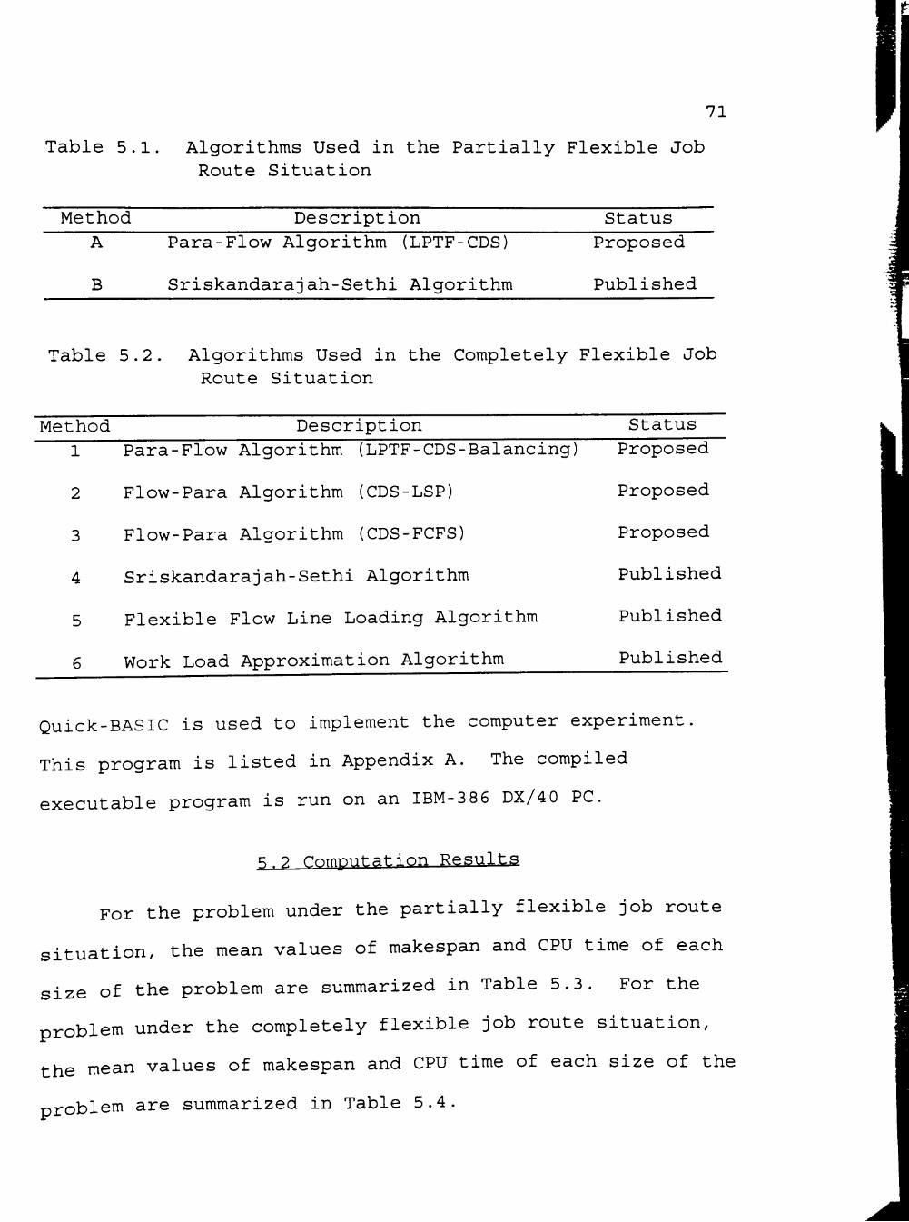
71

Table 5.1. Algorithms Used in the Partially Flexible Job Route Situation

Method Description Status

B

Para-Flow Algorithm (LPTF-CDS)

Sriskandarajah-Sethi Algorithm

Proposed

Published

Table 5.2. Algorithms Used in the Completely Flexible Job Route Situation

Method Description Status Para-Flow Algorithm (LPTF-CDS-Balancing) Proposed

2

3

4

5

6

Flow-Para Algorithm (CDS-LSP)

Flow-Para Algorithm (CDS-FCFS)

Sriskandarajah-Sethi Algorithm

Flexible Flow Line Loading Algorithm

Work Load Approximation Algorithm

Proposed

Proposed

Published

Published

Published

Quick-BASIC is used to implement the computer experiment.

This program is listed in Appendix A. The compiled

executable program is run on an IBM-386 DX/40 PC.

q.? romputatinn Results

For the problem under the partially flexible job route

situation, the mean values of makespan and CPU time of each

size of the problem are summarized in Table 5.3. For the

problem under the completely flexible job route situation,

the mean values of makespan and CPU time of each size of the

problem are summarized in Table 5.4.

72

Table 5.3. Average Performances of Methods A and B for the Partially Flexible Job Route Situation

Problem Size Method A B

A B

A B

A B

A B

A B

A B

A B

A B

A B

A B

Makespan 224.50* 237.85

299.95* 361.30

373.25* 469.40

475.10* 587.05

539.20* 658.95

641.65* 762.90

235.95* 248.75

265.70* 309.05

321.05* 383.60

349.45* 419.05

392.80* 477.45

CPU Time (Seconds)

( 5,3,3)

(10,3,3)

(15,3,3)

(20,3,3)

(25,3,3)

(30,3,3)

(10,3,6)

(15,3,6)

(20,3,6)

(25,3,6)

(30,3,6)

2.16 1.67*

2.56 1.80*

3.20 2.20*

3.91 2.46*

4.70 2.78*

5.59 3.22*

2.52 1.81*

3.08 2.20*

3.69 2.47*

4.32 2.79*

5.19 3.36*

Table 5.3. Continued

73

Problem Size Method Makespan CPU Time (Seconds)

( 5,6,3)

(10,6,3)

(15,6,3)

(20,6,3)

(25,6,3)

(30,6,3)

(10,6,6)

(15,6,6)

(20,6,6)

(25,6,6)

(30,6,6)

A B

A B

A B

A B

A B

A B

A B

A B

A B

A B

A B

382.75* 413.00

471.80* 544.00

579.80* 687.30

669.90* 822.10

757.00* 936.25

871.15* 1056.05

409.31* 423.05

459.55* 507.10

509.85* 574 .35

549.75* 662.95

605.15* 724.60

3 . 1 .

5 . 2 .

8 . 2 .

1 1 . 3 .

1 4 . 3

17 4

5 2

7 2

10 3

12 3

15 4

63 7 5 *

82 0 3 *

26 6 4 *

22 2 1 *

44 8 9 *

. 83

. 9 1 *

. 6 5

. 0 3 *

. 9 1

. 6 6 *

. 2 3

. 2 2 *

. 8 4

. 9 0 *

. 6 9

. 9 4 *

* marks the smaller average value between A and B.

74

Table 5.4 Average Performances of Methods 1 through 6 for Completely Flexible Job Route Situation

Problem Size Method Makespan CPU Time (Seconds) ( 5,3,3)

(10,3,3)

(15,3,3)

(20,3,3)

(25,3,3)

(30,3,3)

1 2 3 • 4 5 6

1 2 3 4 5 6

1 2 3 4 5 6

1 2 3 4 5 6

1 2 3 4 5 6

1 2 3 4 5 6

224.35* 224.45 225.80 237.85 244.65 234.35

291.35 290.45* 291.70 361.30 353.45 329.65

365.55 347.70* 349.25 469.40 451.00 410.50

470.30 456.60* 458.80 587.05 572.65 517.35

529.95 516.25* 517.20 658.95 648.60 577.50

627.35 610.75* 611.65 762.90 748.95 683.60

2.11 1.13 1.06* 1.67 1.59 5.86

2.61 1.48 1.44* 1.80 2.01

24.83

3.26 1.79 1.62* 2.20 2.87

81.05

3.98 2.40 2.12* 2.46 3.87

201.23

4.76

2.95 2.71* 2.78 5.34

418.49

5.63 3.63 3.23 3.22* 7.27

774.45

75

Fable 5.4. Cont

Problem Size

(10,3,6)

(15,3,6)

(20,3,6)

(25,3,6)

(30,3,6)

inued

Method

1 2 3 4 5 6

1 2 3 4 5 6

1 2 3 4 5 6

1 2 3 4 5 6

1 2 3 4 5 6

Makespan

234.40* 236.10 236.75 248.75 255.15 247.50

261.50 249.90* 251.40 309.05 304.75 293.25

315.00 299.85* 301.70 383.60 374.30 356.10

332.70 317.45 317.25* 419.05 412.95 384.70

381.35 353.25* 353.80 477.45 473.10 428.00

CPU Time (Seconds)

2.65 1.51 1.48* 1.81 2.29

44.72

3.25 1.81 1.66* 2.20 3 .41

153.59

3 .85 2.41 2.17* 2.47 4.91

388.83

4.50 2.99 2.78* 2.79 6.82

815.33

5.32

3.68 3.29* 3.36 9.26

1515.65

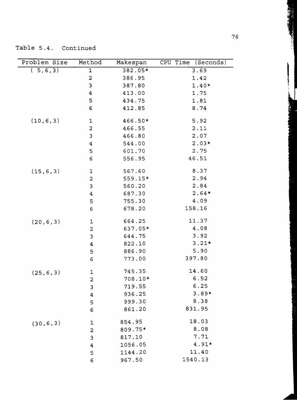
T a b l e 5 . 4 . C o n t i n u e d

76

Problem Size

( 5,6,3)

(10,6,3)

(15,6,3)

(20,6,3)

(25,6,3)

(30,6,3)

Method

1 2 3 4 5 6

1 2 3 4 5 6

1 2 3 4 5 6

1 2 3 4 5 6

1 2 3 4 5 6

1 2 3 4 5 6

Makespan

382.05* 386.95 387.80 413.00 434.75 412.85

466.50* 466.55 466.80 544.00 601.70 556.95

567.60 559.15* 560.20 687.30 755.30 678.20

664.25 637.05* 644.75 822.10 886.90 773.00

745.35 708.10* 719.55 936.25 999.30 861.20

854.95

809.75* 817.10 1056.05 1144.20 967.50

CPU Time (Seconds)

3.69 1.42 1.40* 1.75 1.81 8.74

5.92 2.11 2.07 2.03* 2.75

46.51

8.37 2.94 2.84 2.64* 4.09

158.16

11.37 4.08 3.92 3.21* 5.90

397.80

14.60

6.52 6.25 3.89* 8.38

831.95

18.03

8.08 7.71 4.91* 11.40

1540.13

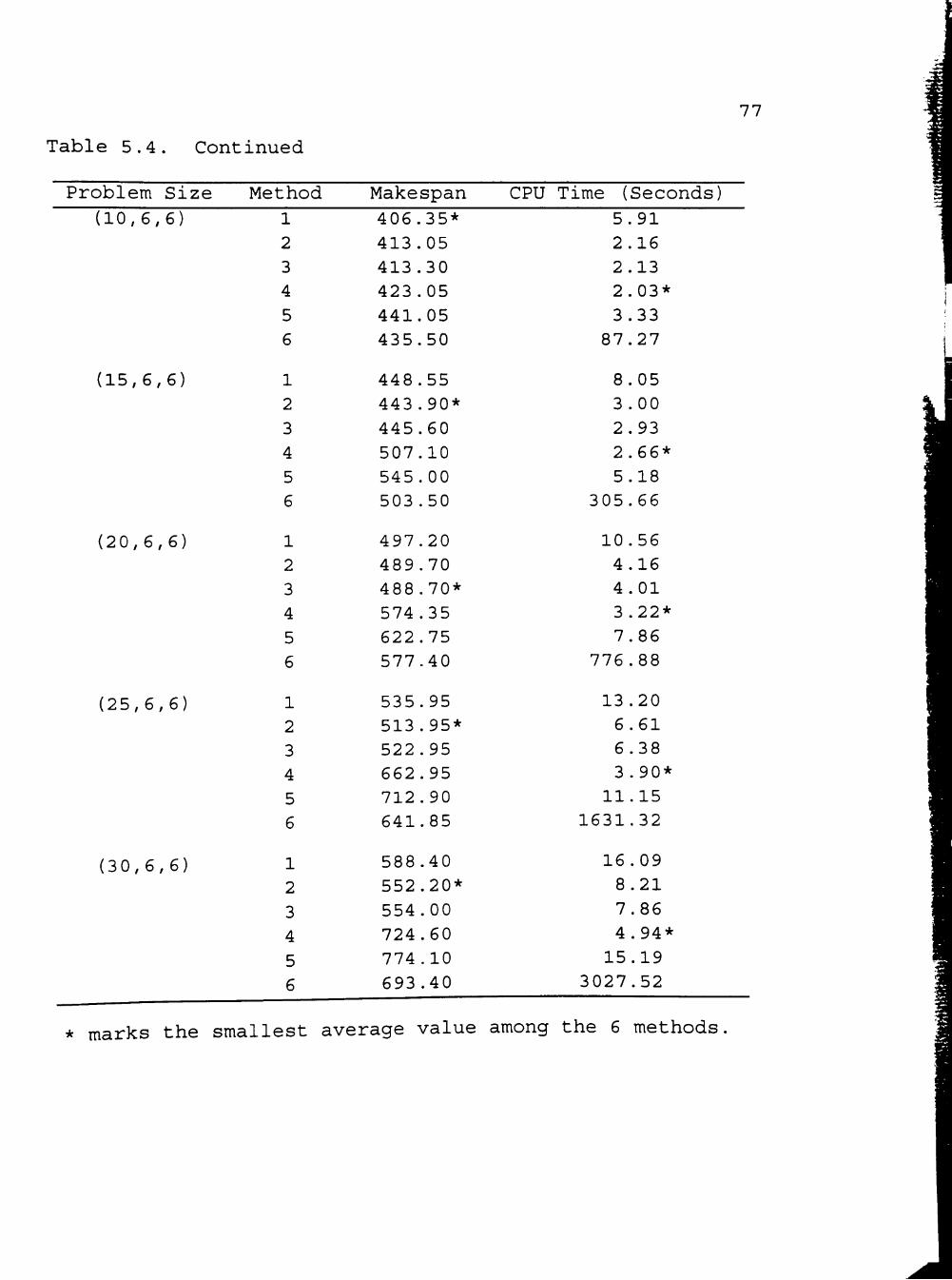
77

Fable 5.4. Cont

Problem Size

(10,6,6)

(15,6,6)

(20,6,6)

(25,6,6)

(30,6,6)

inued

Method

1 2 3 4 5 6

1 2 3 4 5 6

1 2 3 4 5 6

1 2 3 4 5 6

1 2 3 4 5 6

Makespan

406.35* 413.05 413.30 423.05 441.05 435.50

448.55 443.90* 445.60 507.10 545.00 503.50

497.20 489.70 488.70* 574.35 622.75 577-40

535.95 513.95* 522.95 662.95 712.90 641.85

588.40 552.20* 554.00 724.60 774.10 693.40

CPU Time (Seconds)

5.91 2.16 2.13 2.03* 3.33

87.27

8.05 3.00 2.93 2.66* 5.18

305.66

10.56 4.16 4.01 3.22* 7.86

776.88

13.20 6.61 6.38 3.90*

11.15 1631.32

16.09

8.21 7.86 4.94* 15.19

3027.52

* marks the smallest average value among the 6 methods.

78

5.3 Statistical Analysis

A series of hypothesis tests are conducted to provide a

more stringent examination of the performance of the

heuristics. These tests can be stated in six general

hypotheses, each testing 22 different sizes of the problem.

In the following, H^ represents the i^h general null

hypothesis (i = 1, 2, ..., 6).

Hi: For the partially flexible job route situation,

the average makespan obtained from Method A is the same as

that from Method B.

H2: For the partially flexible job route situation,

the average CPU time from Method A is the same as that from

y

Method B.

H3: For the completely flexible job route situation,

the average makespans obtained from Methods 1 through 6 are

the same.

H4: For the completely flexible job route situation,

the average CPU times from Methods 1 through 6 are the same.

H5: The average makespans obtained from Method A for

the partially flexible job route situation, and from Methods

1, 2, and 3 for the completely flexible job route situation

are the same.

Hg: The average CPU times from Method A for the

partially flexible job route situation, and from Methods 1,

2, and 3 for the completely flexible job route situation are

the same.

79

Analysis of variance (ANOVA) is employed to perform

these hypothesis tests. At 0.05 significance level, if a

null hypothesis is rejected by the ANOVA, then the Student-

Newman-Keuls' (SNK) multiple range test is applied to do the

multi-comparison test. Tables 5.5, 5.6, and 5.7 list the

results of the hypothesis tests and the results of SNK tests

for Hi and H2, for H3 and H4, and for H5 and Hg,

respectively. In these three tables, '*' means the null

hypothesis is rejected at 0.05 significance level. Under

the column title "SNK Rank," methods are arranged in

nonincreasing order of their average performances. Methods

within the same parenthesis have no significant difference

in their average performances, but methods between

parentheses have significant difference in their average

performances.

5.4 Discussion

This section consists of three subsections: discussion

for the problem under the partially flexible job route

situation, discussion for the problem under the completely

flexible job route situation, and the comparison of the

performance of the proposed algorithms for the problem under

these two situations. Each of the three subsections states

the results of the computer experiment regarding the

makespan and CPU time. Then the results of ANOVA and SNK

tests are addressed. The last part in each subsection

Table 5.5. The Results of ANOVA and SNK Tests for Hi and H2

80

Problem

Size

( 5,3,3)

(10,3,3)

(15,3,3)

(20,3,3)

(25,3,3)

(30,3,3)

(10,3,6)

(15,3,6)

(20,3,6)

(25,3,6)

(30,3,6)

( 5,6,3)

(10,6,3)

(15,6,3)

(20,6,3)

(25,6,3)

(30,6,3)

(10,6,6)

(15,6,6)

(20,6,6)

(25,6,6)

(30,6,6)

Makespan

Pr > F

0.0988

0.0001*

0.0001*

0.0001*

0.0001*

0.0001*

0.1787

0.0001*

0.0001*

0.0001*

0.0001*

0.0236*

0.0001*

0.0001*

0.0001*

0.0001*

0.0001*

0.1918

0.0002*

0.0001*

0.0001*

0.0001*

SNK Rank

(A) (B)

(A) (B)

(A) (B)

(A) (B)

(A) (B)

(A) (B)

(A) (B)

(A) (B)

(A) (B)

(A) (B)

(A) (B)

(A) (B)

(A) (B)

(A) (B)

(A) (B)

(A) (B)

(A) (B)

(A) (B)

(A) (B)

CPU Time

Pr > F

0.0001*

0.0001*

0.0001*

0.0001*

0.0001*

0.0001*

0.0001*

0.0001*

0.0001*

0.0001*

0.0001*

0.0001*

0.0001*

0.0001*

0.0001*

0.0001*

0.0001*

0.0001*

0.0001*

0.0001*

0.0001*

0.0001*

(Seconds)

SNK Rank

(B) (A)

(B) (A)

(B) (A)

(B) (A)

(B) (A)

(B) (A)

(B) (A)

(B) (A)

(B) (A)

(B) (A)

(B) (A)

(B) (A)

(B) (A)

(B) (A)

(B) (A)

(B) (A)

(B) (A)

(B) (A)

(B) (A)

(B) (A)

(B) (A)

(B) (A)

81

Table 5.6. The Results of ANOVA and SNK Tests for H3 and H4

Problem

Size ( 5,3,3

(10,3,3

(15,3,3

(20,3,3

(25,3,3

(30,3,3

(10,3,6

(15,3,6

(20,3,6

(25,3,6

(30,3,6

( 5,6,3

(10,6,3

(15,6,3

(20,6,3

(25,6,3

(30,6,3

(10,6,6

(15,6,6

(20,6,6

(25,6,6

(30,6,6

Makespan

Pr > F SNK Rank

0.1902

0.0001*

0.0001*

0.0001*

0.0001*

0.0001*

0.2273

0.0001*

0.0001*

0.0001*

0.0001*

0.0021*

0.0001*

0.0001*

0.0001*

0.0001*

0.0001*

0.0181*

0.0001*

0.0001*

0.0001*

0.0001*

2,1,3) (6,5) (5,4)

2,3,1) (6) (5,4)

2,3,1) (6) (5,4)

2,3,1) (6) (5,4)

2,3,1) (6) (5,4)

2,3,1) (6,5,4)

2,3,1) (6,5) (5,4)

3,2,1) (6) (5,4)

2,3) (1) (6) (5,4)

1,2,3,6,4) (6,4,5)

1,2,3) (4,6) (5)

2,3,1) (6,4) (5)

2,3,1) (6) (4) (5)

2,3,1) (6) (4) (5)

2,3,1) (6) (4) (5)

1,2,3,4,6) 2,3,4,6,5)

2,3,1) (6,4) (5)

2,3,1) (4,6) (5)

2,3,1) (6,4) (5)

2,3,1) (6) (4) (5)

CPU Time (Seconds) • Pr > F SNK Rank 0.0001* (3,2) (5) (4) (1) (6)

0.0001*

0.0001*

0.0001*

0.0001*

0.0001*

0.0001*

0.0001*

0.0001*

0.0001*

0.0001*

0.0001*

0.0001*

0.0001*

0.0001*

0.0001*

0.0001*

0.0001*

0.0001*

0.0001*

0.0001*

0.0001*

3) (2) (4) (5) (1) (6)

3) (2) (4) (5) (1) (6)

3) (2,4) (5) (1) (6)

3,4) (2) (1) (5) (6)

4,3) (2) (1) (5) (6)

3,2) (4) (5) (1) (6)

3) (2) (4) (1) (5) (6)

3) (2,4) (5) (1) (6)

3,4,2) (1) (5) (6)

3,4,2) (1) (5) (6)

3) (2) (4) (5) (1) (6)

4) (3) (2) (5) (1) (6)

4) (3) (2) (5) (1) (6)

4) (3) (2) (5) (1) (6)

4) (3) (2) (5) (1) (6)

4) (3) (2) (5) (1) (6)

4) (3,2) (5) (1) (6)

4) (3,2) (5) (1) (6)

4) (3,2) (5) (1) (6)

4) (3,2) (5) (1) (6)

4) (3,2) (5) (1) (6)

82

Table 5.7. The Results of ANOVA and SNK Tests for H5 and Hg

Problem

Size

( 5,3,3)

(10,3,3)

(15,3,3)

(20,3,3)

(25,3,3)

(30,3,3)

(10,3,6)

(15,3,6)

(20,3,6)

(25,3,6)

(30,3,6)

( 5,6,3)

(10,6,3)

(15,6,3)

(20,6,3)

(25,6,3)

(30,6,3)

(10,6,6)

(15,6,6)

(20,6,6)

(25,6,6)

(30,6,6)

Makespan

Pr > F

0.9987

0.8231

0.0879

0.4036

0.1108

0.1330

0.9967

0.1257

0.0222*

0.0001*

0.0001*

0.9687

0.9629

0.1616

0.0816

0.0011*

0.0006*

0.9191

0.4382

0.3514

0.0051*

0.0001*

(2,

(3,

(2,

(2

(2

(2

(2

SNK

3,1)

Rank

(1,A)

2) (1) (A)

3) (1

3) (3

,3) (1

,A)

,1)(1,A)

,A)

,3,1)(1,A)

,3) (1 ,A)

CPU Time (Seconds)

Pr > F

0.0001*

0.0001*

0.0001*

0.0001*

0.0001*

0.0001*

0.0001*

0.0001*

0.0001*

0.0001*

0.0001*

0.0001*

0.0001*

0.0001*

0.0001*

0.0001*

0.0001*

0.0001*

0.0001*

0.0001*

0.0001*

0.0001*

(3)

(3)

(3)

(3)

(3)

(3)

(3)

(3)

(3)

(3)

(3)

(3)

(3)

(3;

(3;

(3

(3

(3

(3

(3

(3

(3

SNK Rank

(2) (A) (1)

(2) (A) (1)

(2) (A) (1)

(2) (A) (1)

(2) (A) (1)

(2) (A) (1)

(2) (A) (1)

(2) (A) (1)

(2) (A) (1)

(2) (A) (1)

(2) (A) (1)

(2) (A) (1)

(2) (A) (1)

(2) (A) (1)

1 (2) (A) (1)

> (2) (A) (1)

) (2) (A) (1)

) (2) (A) (1)

) (2) (A) (1)

) (2) (A) (1)

) (2) (A) (1)

) (2) (A) (1)

83

analyzes the causes why the null hypotheses are rejected or

why the null hypotheses are not rejected.

5.4.1 The Partially Flexible Job Route Situation

The results of the computer experiments for the

partially flexible job route situation are summarized in

Table 5.3. For all of the 22 problem sizes, the para-flow

algorithm (Method A) has better average makespan performance

than does the Sriskandarajah-Sethi algorithm (Method B). In

other words, the average makespan generated from Method A is

smaller than that from Method B. In order to compare the

average makespan performances between these two methods, a

makespan improvement percentage is calculated by the

following formula:

Makespan(B)- Makespan(A) Makespan Im provement% = — — — * 100-c

Makespan(B

•o

where Makespan(A) and Makespan(B) represent the average

makespan obtained from Methods A and B, respectively. This

percentage describes how much the average makespan

performance from Method A is better than that from Method B

The second column in Table 5.8 shows the makespan

improvement percentages of Method A versus Method B. The

average of these makespan improvement percentages is 14.31%

The results of ANOVA are shown in Table 5.5. At 0.05

significance level, ANOVA shows that the null hypothesis Hi

is rejected in 19 (or 86.36%) of the 22 problem sizes. The

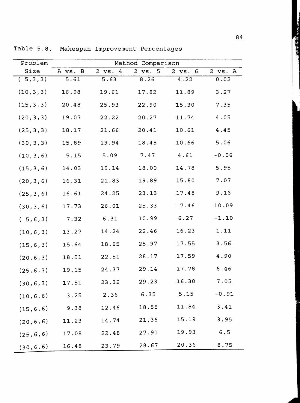
Table 5.8. Makespan Improvement Percentages

84

P r o b l e m

S i z e

( 5 , 3 , 3 )

( 1 0 , 3 , 3 )

( 1 5 , 3 , 3 )

( 2 0 , 3 , 3 )

( 2 5 , 3 , 3 )

( 3 0 , 3 , 3 )

( 1 0 , 3 , 6 )

( 1 5 , 3 , 6 )

( 2 0 , 3 , 6 )

( 2 5 , 3 , 6 )

( 3 0 , 3 , 6 )

( 5 , 6 , 3 )

( 1 0 , 6 , 3 )

( 1 5 , 6 , 3 )

( 2 0 , 6 , 3 )

( 2 5 , 6 , 3 )

( 3 0 , 6 , 3 )

( 1 0 , 6 , 6 )

( 1 5 , 6 , 6 )

( 2 0 , 6 , 6 )

( 2 5 , 6 , 6 )

( 3 0 , 6 , 6 )

A v s . B

5 . 6 1

1 6 . 9 8

2 0 . 4 8

1 9 . 0 7

1 8 . 1 7

1 5 . 8 9

5 . 1 5

1 4 . 0 3

1 6 . 3 1

1 6 . 6 1

1 7 . 7 3

7 . 3 2

1 3 . 2 7

1 5 . 6 4

1 8 . 5 1

1 9 . 1 5

1 7 . 5 1

3 . 2 5

9 . 3 8

1 1 . 2 3

1 7 . 0 8

1 6 . 4 8

M e t h o d Compar ;

2 v s . 4

5 . 6 3

1 9 . 6 1

2 5 . 9 3

2 2 . 2 2

2 1 . 6 6

1 9 . 9 4

5 . 0 9

1 9 . 1 4

2 1 . 8 3

2 4 . 2 5

2 6 . 0 1

6 . 3 1

1 4 . 2 4

1 8 . 6 5

2 2 . 5 1

2 4 . 3 7

2 3 . 3 2

2 . 3 6

1 2 . 4 6

1 4 . 7 4

2 2 . 4 8

2 3 . 7 9

2 v s . 5

8 . 2 6

1 7 . 8 2

2 2 . 9 0

2 0 . 2 7

2 0 . 4 1

1 8 . 4 5

7 . 4 7

1 8 . 0 0

1 9 . 8 9

2 3 . 1 3

2 5 . 3 3

1 0 . 9 9

2 2 . 4 6

2 5 . 9 7

2 8 . 1 7

2 9 . 1 4

2 9 . 2 3

6 . 3 5

1 8 . 5 5

2 1 . 3 6

2 7 . 9 1

2 8 . 6 7

Lson

2 v s . 6

4 . 2 2

1 1 . 8 9

1 5 . 3 0

1 1 . 7 4

1 0 . 6 1

1 0 . 6 6

4 . 6 1

1 4 . 7 8

1 5 . 8 0

1 7 . 4 8

1 7 . 4 6

6 . 2 7

1 6 . 2 3

1 7 . 5 5

1 7 . 5 9

1 7 . 7 8

1 6 . 3 0

5 . 1 5

1 1 . 8 4

1 5 . 1 9

1 9 . 9 3

2 0 . 3 6

2 v s . A

0 . 0 2

3 . 2 7

7 . 3 5

4 . 0 5

4 . 4 5

5 . 0 6

- 0 . 0 6

5 . 9 5

7 . 0 7

9 . 1 6

1 0 . 0 9

- 1 . 1 0

1 . 1 1

3 . 5 6

4 . 9 0

6 . 4 6

7 . 0 5

- 0 . 9 1

3 . 4 1

3 . 9 5

6 . 5

8 . 7 5

85

null hypothesis Hi is not rejected for the problems with the

size of (5,3,3), (10,3,6), and (10,6,6). For all the

problem sizes in which the null hypothesis Hi is rejected,

SNK tests show that Method A has smaller average makespans

than does Method B, and Table 5.8 shows the average makespan

improvement percentage by using Method A instead of Method B

is 15.84

In comparison with the average CPU time. Table 5.3

shows Method B spends less CPU time than does Method A. The

results of ANOVA and SNK tests in Table 5.5 also show that

the CPU times spent by Method A and by Method B are

significantly different at 0.05 significance level and that

Method B does require less CPU time.

In Sections 4.2 and 4.3, it was shown that the makespan

obtained from Method A is selected from m(s + 1) makespans

which were determined by the LPTF heuristic and the CDS

algorithm. A min-max method is used to find the best

makespan. In each of the (s + 1) para-subproblems, the

maximum value among m makespans is identified. Among the

(s + 1) maximum values, a minimum value is chosen to be the

makespan for the problem. Therefore, a multi-comparison

process has to be performed. As it is described in Section

3.3, makespan obtained from Method B is generated directly

from the LPTF list. There is only one choice, and that is

why Method B consumes less CPU time.

86

Method B has better performance in CPU time, but worse

performance in makespan. A detailed examination of the

average CPU time shows that in 11 (or 50%) problem sizes

Method A requires less than 5 seconds. In 5 (or 22.73%)

problem sizes Method A requires between 5 and 10 seconds,

and for 4 (or 18.18%) problem sizes CPU time is between 10

and 15 seconds. For the remaining 2 (or 9.09%) problem

sizes Method A takes between 15 and 18 seconds to find a

solution. These CPU times are not thought to be excessive

for industrial applications. Compared with Method B, Method

A yields solutions with nearly 16% smaller makespan with

only a moderate increase in CPU time. To assure this is

also true for large problem sizes, twenty problems with size

of (100,6,6) are tested. The average makespans yielded by

using Methods A and B are 1274.60 and 1510.40, respectively.

The average CPU times required by using Methods A and B are

77.24 and 33.75 seconds, respectively. The makespan

improvement is 15.61% and the CPU time of 77.24 seconds is

not excessive. Therefore, for the problem under the

partially flexible job route situation. Method A, the para-

flow algorithm, appears to be a better choice.

R 4,2 The Completely Flexible Job Route ,c!iMiation

The results of the computer experiments for the

completely flexible job route situation are summarized in

Table 5.4. In comparison with the makespan, the para-flow

87

algorithm (Method 1) has the smallest average makespan in 5

(or 22.73%) of the 22 problem sizes: (5,3,3), (10,3,6),

(5,6,3), (10,6,3), and (10,6,6). The flow-para algorithm

with priority dispatching rule LSP (Method 2) has the

smallest average makespan in 15 (or 68.18%) of the 22

problem sizes: (10,3,3), (15,3,3), (20,3,3), (25,3,3),

(30,3,3), (15,3,6), (20,3,6), (30,3,6), (15,6,3), (20,6,3),

(25,6,3), (30,6,3), (15,6,6), (25,6,6), and (30,6,6), and

the flow-para algorithm with the priority dispatching rule

FCFS (Method 3) has the smallest average makespan in 2 (or

9.09%) of the problem sizes: (25,3,6) and (20,6,6). The

flow-para algorithms (Method 2 and Method 3) have

outstanding performance. The para-flow algorithm (Method 1)

also has good performance, especially when the number of

jobs is less than or equal to 10. Each of the proposed

algorithms performs better than do the three published

algorithms. The third, fourth, and fifth columns in Table

5.8 show the makespan improvement percentages of Method 2

versus Method 4, Method 2 versus Method 5, and Method 2

versus Method 6, respectively. The averages of these

makespan improvement percentages are 18.02%, 20.49%, and

13.58%, respectively.

The results obtained from ANOVA are summarized in Table

5.6. At 0.05 significance level, this analysis shows that

the null hypothesis H3 is rejected in 20 (or 90.9%) of the

22 problem sizes. Only in the problems of the small size.

88

(5,3,3) and (10,3,6), the null hypothesis H3 is not

rejected. Among the 20 problem sizes in which the null

hypothesis H3 is rejected, SNK tests reveal that the average

makespans obtained from Methods 1, 2, and 3 are smaller than

those from Methods 4, 5, and 6. The makespan performances

between Method 2 and Method 3 have no significant difference

in all (or 100%) of the 20 problem sizes. The makespan

performances among Methods 1, 2, and 3 have no significant

difference in 19 (or 95%) out of these 20 problem sizes.

The average makespan performances among Methods 1, 2, 3, 4,

and 6 have no significant difference in 2 (or 10%) of these

20 problem sizes: (5,6,3) and (10,6,6). Method 5 performs

significantly different from the proposed algorithms in all

of the 2 0 problem sizes. That is, when the number of jobs

is less than or equal to 10, the proposed algorithms'

performances are not significantly different from that of

Method 4 and Method 6. However when the number of jobs is

greater than 10, the proposed algorithms have better average

makespan performance than the published algorithms have.

In comparison of average CPU time. Table 5.4 shows that

the flow-para algorithm using FCFS as priority dispatching

rule (Method 3) spends the least amount of CPU time in 11

(or 50%) out of the 22 problem sizes, especially when the

number of work centers is not large. The Sriskandarajah-

Sethi algorithm (Method 4) spends the least amount of CPU

time in the remaining 11 (or 50%) problem sizes. However,

89

average CPU times spent by the flow-para algorithm using LSP

as priority dispatching rule (Method 2) are also attractive.

In 10 (or 45.45%) out of the 22 problem sizes, there is no

significant difference in CPU time required by Method 2 and

by Method 3. Comparing with WLA algorithm (Method 6), the

para-flow algorithm (Method 1) spends relatively small CPU

time.

As described in Section 4.1 and illustrated in Section

4.3, Method 1 goes through the same procedures as Method A

does to generate a solution, but includes a balancing

routine. For the same reason stated in Section 5.4.2,

Method 1 spends some CPU time to accomplish a multi-

comparison process but yields smaller makespans than do

published algorithms (Methods 4, 5, and 6) .

When Methods 2 and 3 are applied, the flexible flowshop

problem is treated as a simple flowshop problem and solved

by the CDS algorithm. Then the jobs are dispatched to the

parallel machines at each work center by the priority

dispatching rule LSP in using Method 2, and FCFS in using

Method 3. As illustrated in Section 4.3, there is only one

job sequence plus a priority dispatching rule under

consideration. Therefore, Methods 2 and 3 spend less CPU

time than do Methods 1, 5, and 6.

Makespan obtained from Method 4 is directly generated

from the LPTF list as mentioned in Section 3.3. Method 4

only considers the workload balance, not the workspan

90

balance. That is why this method has the faster speed but

larger makespans than do the proposed algorithms (Methods 1,

2, and 3).

Method 5 and Method 6 were developed by Wittrock in

1985, and in 1988, respectively. As reviewed in Section

3.3, Wittrock applied the LPTF heuristic to allocate jobs to

the parallel machines at each work center. Once a job is

assigned to a machine at a work center, the job cannot be

processed on other machines even when the other machines are

available and the assigned machine is busy. The job must

follow the fixed job route. Wittrock claims that the

makespan is decided by the machine allocation, thus choosing

a job sequence has no strong effect on the makespan. That

is why Method 5 and Method 6 have larger makespan than the

proposed algorithms.

When considering both the measures of performance,

makespan and CPU time. Method 3 is the best choice for the

completely flexible job route situation. However, from

Table 5.6, it can be seen that the proposed algorithms

(Methods 1, 2, and 3) generate smaller makespans than do the

other three published algorithms (Method 4, Method 5, and

Method 6) and spend reasonable CPU times. Among Methods 1

through 6, Method 4 requires the smallest CPU time for

problems with large size. To assure that the makespan

improvement using Method 3 instead of using Method 4

justifies the additional CPU time, twenty problems with size

91

of (100,6,6) are tested. The average makespans yielded by

using Methods 3 and 4 are 1138.70 and 1510.40, respectively.

The average CPU times required by using Methods 3 and 4 are

50.15 and 33.75 seconds, respectively. The makespan

improvement is 24.61%; the CPU time of 50.15 seconds is not

excessive.

5.4.3 The Comparison of Performance of Algorithms for the Partially Flexible Job Route Situation and Algorithms for the Completely Flexible Job Route Situation

Since the proposed problem is considered in the

partially flexible job route situation and in the completely

flexible job route situation, the makespan performance

between these two situations should be examined. As

illustrated in Section 4.3, Methods A and 1 are used to

realize the para-flow approach for the partially flexible

job route situation and the complete flexible job route

situation, respectively. The difference between Method A

and Method 1 is that Method 1 includes an additional

balancing routine. It is of interest to examine the impact

of the balancing routine on makespan and CPU time

performance. In Section 4.3, Methods 2 and 3 are used to

demonstrate the flow-para approach. The priority

dispatching rule employed in Method 2 is LSP and in Method 3

is FCFS. The impact of using the different priority

dispatching rules on makespan and CPU time performance

92

should be investigated. Therefore, this subsection

discusses the performance of Methods A, 1, 2, and 3.

The results of ANOVA and SNK tests for the null

hypotheses H5 and Hg are summarized in Table 5.7. In

comparison with the average makespan, out of the 22 problem

sizes, in 7 (or 31.82%) problem sizes the null hypothesis H5

is rejected at 0.05 significance level. Among these 7

problem sizes, SNK tests show that the average makespans

obtained from Methods 2 and 3 are smaller than those from

Methods A and 1. For the problems with size of (25,3,6),

Method 1 has better makespan performance than Method A has.

Except this problem size. Method 1 and Method A have no

significant differences in makespan performance. For the

completely flexible job route situation. Method 2 generates

the smallest makespan among Methods 1, 2 and 3, and Method A

is used for the partially flexible job route situation.

Between these two situations, the sixth column in Table 5.8

shows that the average makespan improvement percentages of

Method 2 versus Method A is 4.55%.

In comparison with average CPU time, the null

hypothesis Hg is rejected in all (or 100%) of the 22

problem sizes. SNK tests show that Method 3 spends the

least CPU time. Method 2 spends the second least CPU time,

and Method 1 spends the largest CPU time in all of the 22

problem sizes.

93

For the completely flexible job route situation, the

job route is completely flexible at every work center. The

machine that processes a job at a work center does not have

to bear the same machine number as the machines processing

this job at previous and subsequent work centers. For the

partially flexible job route situation, the job route is

flexible at the first work center but fixed at the following

work centers. At the first work center, a job can visit any

one of the parallel machines. But at each of the following

work centers, this job must be processed on the machine

bearing the same machine number as at the first work center.

When a machine at a work center is available and one or more

jobs are waiting in front of this work center, these two

situations may yield different results. In the completely

flexible job route situation, immediately a priority

dispatching rule is applied to choose one of the waiting

jobs to be processed next. Thus, the jobs have more

flexibility and can be processed on the earliest available

machine. But in the partially flexible job route situation,

each machine has in its queue only those jobs being

processed by machines having the same machine number. If

the queue is empty, the available machine is set to be idle

even though jobs are waiting for machines at the work

center. This is the reason why the makespan obtained from

Method 2 and from Method 3 are smaller than the makespan

obtained from Method A. The results of this computer

94

experiment are consistent with this statement. Regarding

the measurement of makespan, the completely flexible job

route situation has better performance than does the

partially flexible job route situation.

As illustrated in Section 4.3 and explained in Sections

5.4.1 and 5.4.2, a multi-comparison process has to be

performed in both Methods A and 1. As illustrated in

Section 4.3 and mentioned in Section 5.4.2, when Methods 2,

and 3 are applied, only one job sequence plus a priority

dispatching rule is under consideration. Therefore, CPU

times required using Methods 2 and 3 are less than those

using Methods A and 1. Method 1 has to perform the

additional balancing task, so Method 1 spends more CPU time

than does Method A.

Furthermore, the difference between Methods 2 and 3 is

the priority dispatching rule used in job selection process.

Method 2 uses LSP as priority dispatching rule while Method

3 uses FCFS as priority dispatching rule. Once a machine is

available and there is more than one job in queue, the job

to be processed next has to be selected. Before making the

selection. Method 2 has to check the loading sequence

priority of the queuing jobs, but Method 3 just simply

selects the first job in the queue as the job to be

processed next. Thus Method 3 spends less CPU time than

does Method 2.

CHAPTER VI

TREND ANALYSIS

Problem size is described by three elements: the

number of jobs, the number of work centers, and the number

of parallel machines at each work center. Intuitively,

increasing the number of jobs or increasing the number of

work centers would increase the CPU time to generate a

solution, and might result in a larger makespan. Increasing

the number of parallel machines at each work center would

reduce the makespan since more jobs could be processed on

different machines at the same time. Thus as the problem

size changes, the value of performance measure also changes.

It may be of interest to examine this trend. By fixing any

two of the three elements of the problem size, the trend

resulting from changes in the third element can be analyzed.

It has been shown in Chapter V that the proposed

algorithms outperform the published algorithms. This

chapter presents the trend analysis for the Methods A, 1, 2,

and 3. Method A (LPT-CDS algorithm) uses the para-flow

approach for the problem under the partially flexible job

route situation. Methods 1, 2, and 3 are used for the

problem under the completely flexible job route situation.

Method 1 (LPT-CDS-Balancing algorithm) uses the para-flow

approach , Method 2 (CDS-LSP algorithm) and Method 3 (CDS-

FCFS) use the flow-para approach with the priority

95

96

dispatching rule LSP and with the priority dispatching rule

FCFS, respectively.

This chapter includes three sections: parallel machine

trend analysis, job trend analysis, and work center trend

analysis. In each of the three sections, two settings which

describe the values of the two fixed elements of the problem

size are given. Different values of the analyzed element

per setting are chosen to perform the trend analysis. The

combination of settings and values of the analyzed element

forms different problem sizes. For each problem size, 20

problems are considered. Every sample problem is solved by

the four methods. Data are collected from the output of a

compiled executable GW-BASIC program. ANOVA is employed to

test the average performance of makespans and CPU times

among the four solution methods. The SNK test conducts the

multiple comparison test among the four solution methods if

performances are shown to be significantly different in

ANOVA at 0.05 significance level. Observations and

discussions are stated following the computation results.

fi.l Parallel Machine Trend Analysis

^.1,1 .qettinas

For the parallel machine trend analysis the two

settings are: (1) 30 jobs and 3 work centers, and (2) 50

jobs and 6 work centers. Ten different numbers of parallel

machines per work center are assigned to each setting. The

97

numbers of parallel machines per work center are 1, 2, 3, 4,

5, 6, 7, 8, 9, and 10. Therefore, the combination of

settings and the numbers of parallel machines per work

center produces twenty different problem sizes.

6.1.2 Computation Resnlt.c!

The average makespans and average CPU times along with

ANOVA results are listed in Tables 6.1 and 6.2,

respectively. Figures 6.1 and 6.3 show the graphs of the

average makespans for settings 1 and 2, respectively.

Figures 6.2 and 6.4 show the graphs of the average CPU times

for settings 1 and 2, respectively.

6.1.3 Observations

Some observations obtained from the tables and figures

above are stated in the following:

1. In both settings, all the solution methods have the

same parallel machine trend for makespan. With the same set

of jobs and the same number of work centers, the makespan

decreases as the number of parallel machines per work center

increases. A marginal makespan decrement percentage is

calculated by the following formula:

Makespan(i) - Makespand + 1) Marginal Makespan% = * 100

Makespand) where makespand) is the average makespan obtained from a

schedule when there are i parallel machines at each work

center. This percentage represents the percentage of

98

Table 6.1. Average Makespan in Parallel Machine Trend Analysis

Number of Setting Method

Parallel Machines A

1 1 1687.55 1687.55 1687.55 1687.55 2 3057.95 3057.95 3057.95 3057.95

2 1 890.20 881.00 873.50 874.35 2 1682.05 1675.45 1631.30 1632.70

3 1 635.95 624.90 602.80 604.55 2* 1247.50 1222.15 1158.00 1168.50

4 1* 518.60 502.25 478.35 481.55 2* 1020.05 991.40 925.55 936.85

5 1* 442.40 429.35 407.30 408.80 2* 881.35 861.05 796.05 800.20

6 1* 391.25 380.05 360.05 364.70 2* 797.50 769.75 708.40 719.55

7 1* 361.75 348.55 327.90 329.95 2* 730.75 705.65 651.35 658.65

8 1* 338.20 327.45 308.55 309.30 2* 685.50 662.25 610.40 618.05

9 1* 315.65 303.70 291.20 293.30 2* 647.65 623.45 576.60 589.80

10 1* 300.15 291.35 280.20 280.75 2* 621.40 595.30 552.05 562.60

* means the performances among the methods are

significantly different at 0.05 level.

99

Table 6.2. Average CPU Time (Seconds) in Parallel Machine Trend Analysis

Number of Setting Method Parallel Machines A i '-

1* 7 . 8 0 7 . 7 9 3 . 5 9 3 . 1 8 2 * 6 2 . 3 2 6 2 . 2 0 1 6 . 6 0 1 5 . 4 5

1* 6 . 0 9 6 . 1 5 3 . 6 0 3 . 1 9 2 * 4 2 . 8 6 4 2 . 9 3 1 6 . 6 6 1 5 . 5 6

1* 5 . 5 8 5 . 6 3 3 . 6 1 3 . 2 3 2 * 3 6 . 3 8 3 6 . 5 7 1 6 . 7 2 1 5 . 6 7

1* 2 *

1* 2 *

1* 5 . 1 9 5 . 3 4 3 . 6 4 3 . 3 0 2 * 3 0 . 0 9 3 0 . 5 1 1 6 . 8 9 1 5 . 9 0

5.42 33 .21

5.28 31.32

5.41 33 .47

5.39 31.63

3.62 16.76

3 .62 16.83

3.25 15.75

3 .28 15.83

5. 29

5. 28

12 .24

07 .64

5.35 29.69

5.36 29.21

3.66 16.97

3 .67 17.03

3.32 16.00

3.35 16.08

7 1* 2 *

8 1* 2 *

9 1* 5 . 0 3 5 . 3 6 3 . 6 9 3 . 3 8 2* 28.19 28.92 17.09 16.15

10 1* 5.03 5.38 3.70 3.39 2* 27.80 28.58 17.16 16.24

* means the performances among the methods are significantly different at 0.05 level.

100

CO CO "O Q

1650 -1550 -1450 -1350 . 1250 . 1150 . 1050 . 950 -850 . 750 . 650 -550 . 450 . 350 . 250 . 1

x_ ^-O;^ -~ r

— 1 1

8 10

Number of Parallel Machines per Work Center

Figure 6.1. Average Makespan in Parallel Machine Trend Analysis (30 Jobs, 3 Work Centers)

3 CD

'GO" CD <~) O

<^ 4 5 .. CO **•-» +

4 ..

3.5 .:

3

2 3

8 10

Number of Parallel Machines per Work Center

Figure 6.2. Average CPU Time in Parallel Machine Trend Analysis (30 Jobs, 3 Work Centers)

101

3050

2550 ..

2050 .. CO CO

Q

^ 1550 ..

1050 ..

550

A 1 3 2

1 2 3 4 5 6 7 8 9 10

Number of P a r a l l e l Machines p e r Work C e n t e r

F i g u r e 6 . 3 . Average Makespan i n P a r a l l e l Machine Trend A n a l y s i s (50 J o b s , 6 Work C e n t e r s )

2 3

1 2 3 4 5 6 7 8 9

Number of Parallel Machines per Work Center

Figure 6.4. Average CPU Time in Parallel Machine Trend Analysis (50 Jobs, 6 Work Centers)

10

102

makespan reduction when the number of parallel machines per

work center increases from i to (i + 1). Table 6.3 shows

the marginal makespan decrement percentages in the parallel

machine trend analysis.

Table 6.3. Marginal Makespan Decrement Percentage in Parallel Machine Trend Analysis

Machine Increment Setting Method

(from -> to) A 1 2 3

1 ^ 2 1 47.25 47.79 48.24 48.19 2 44.99 45.21 46.65 46.60

2 -> 3 1 28.56 29.07 30.99 30.86 2 25.83 27.05 29.01 28.43

3 -> 4 1 18.45 19.63 20.65 20.35 2 18.23 18.88 20.07 19.82

4 ^ 5 1 14.69 14.51 14.85 15.11 2 13.59 13.14 13.99 14.58

6 1 11.56 11.48 11.60 10.79 2 9.51 10.60 11.01 10.07

7 ^ 8

8

9 -^ 10

1 2

1 2

1 2

1 2

7 . 5 0 8 . 3 7

6 . 5 1 6 . 1 9

6 . 6 7 5 . 5 2

4 . 9 1 4 . 0 5

8 . 2 9 8 . 3 3

6 . 0 5 6 . 1 5

7 . 2 5 5 . 8 6

4 . 0 7 4 . 5 2

8 . 9 3 8 . 0 5

6 . 2 7

6 . 2 9

5 . 6 2 5 . 5 4

3 . 7 8 4 . 2 6

9 . 5 3 8 . 4 6

6 . 2 6 6 . 1 6

5 . 1 7 4 . 5 7

4 . 2 8 4 . 6 1

2. For Methods 2 and 3, when the number of parallel

machines per work center increases from 1 to 10, the CPU

time increases from 3.59 to 3.70 and from 3.10 to 3.39,

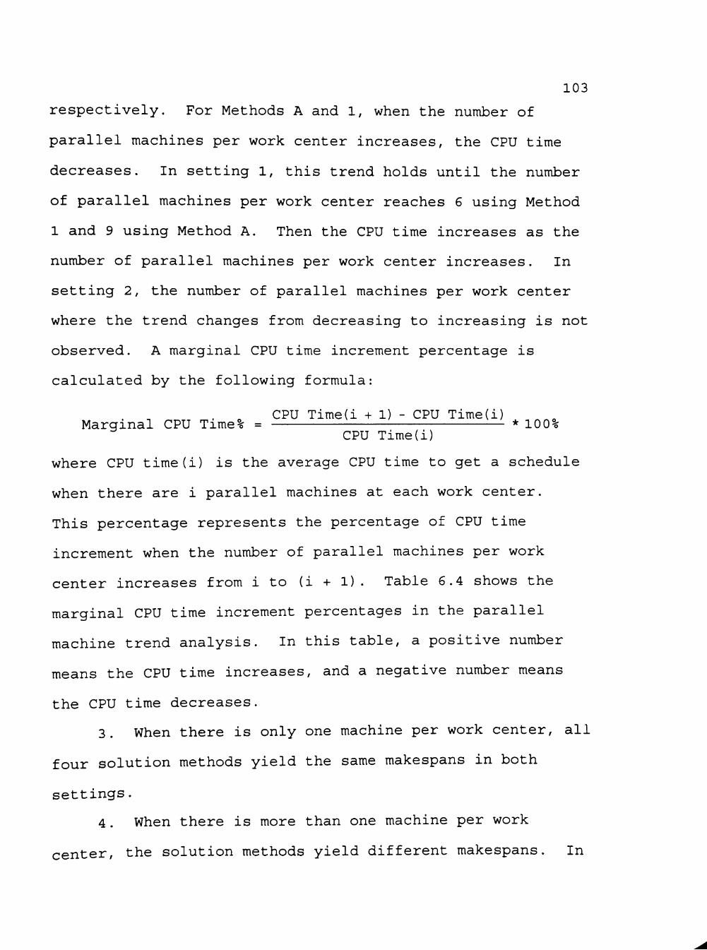
103

respectively. For Methods A and 1, when the number of

parallel machines per work center increases, the CPU time

decreases. In setting 1, this trend holds until the number

of parallel machines per work center reaches 6 using Method

1 and 9 using Method A. Then the CPU time increases as the

number of parallel machines per work center increases. In

setting 2, the number of parallel machines per work center

where the trend changes from decreasing to increasing is not

observed. A marginal CPU time increment percentage is

calculated by the following formula:

CPU Timed + 1) - CPU Time(i) Marginal CPU Time% = * 100%

CPU Timed)

where CPU time(i) is the average CPU time to get a schedule

when there are i parallel machines at each work center.

This percentage represents the percentage of CPU time

increment when the number of parallel machines per work

center increases from i to (i + 1). Table 6.4 shows the

marginal CPU time increment percentages in the parallel

machine trend analysis. In this table, a positive number

means the CPU time increases, and a negative number means

the CPU time decreases.

3. When there is only one machine per work center, all

four solution methods yield the same makespans in both settings.

4. When there is more than one machine per work

center, the solution methods yield different makespans. In

104

Table 6.4. Marginal CPU Time Increment Percentage in Parallel Machine Trend Analysis

Machine Increment Setting Method (from -^ to) A i '

2 -> 3

4 -> 5

6 -> 7

7 ^ 8

8

9 -^ 10

1 2

1 2

1 2

1 2

1 2

1 2

1 2

1 2

1 2

- 2 1 . 9 2 - 3 1 . 2 3

- 8 . 3 7 - 1 5 . 1 2

- 2 . 8 7 - 8 . 7 1

- 2 . 5 8 - 5 . 6 9

- 1 . 7 0 - 3 . 9 3

- 1 . 3 5 - 2 . 8 2

- 0 . 9 8 - 2 . 0 5

- 0 . 7 9 - 1 . 5 7

0 . 0 0 - 1 . 3 8

- 2 1 . 0 5 - 3 0 . 9 8

- 8 . 4 6 - 1 4 . 8 1

- 3 . 9 1 - 8 . 4 8

- 0 . 3 7 - 5 . 5 0

- 0 . 9 3 - 3 . 5 4

0 . 1 9 - 2 . 6 9

0 . 1 9 - 1 . 6 2

0 . 0 0 - 0 . 9 9

0 . 3 7 - 1 . 1 8

0 . 2 8 0 . 3 6

0 . 2 8 0 . 3 6

0 . 2 8 0 . 3 0

0 . 0 0 0 . 4 2

0 . 5 5 0 . 3 6

0 . 5 5 0 . 4 7

0 . 5 4 0 . 3 5

0 . 5 4 0 . 3 5

0 . 2 7 0 . 4 1

0 . 3 1 0 . 7 1

1 . 2 5 0 . 7 1

0 . 6 2 0 . 5 1

0 . 9 2 0 . 5 1

0 . 2 8 0 . 4 4

0 . 6 1 0 . 6 3

0 . 9 0 0 . 5 0

0 . 9 0 0 . 4 4

0 . 3 0 0 . 5 6

setting 1, at 0.05 significance level, ANOVA shows that the

average makespans obtained from Methods A, 1, 2, and 3 are

different when the number of parallel machines per work

center is greater than 3. The SNK tests show the makespans

between Methods 2 and 3 are not significantly different.

The makespans between Method A and Method 1 are not

significantly different either. The makespans obtained from

105

Methods 2 and 3 are smaller than those from Methods A and 1.

In setting 2, at 0.05 significance level, ANOVA shows that

the average makespans obtained from Methods A, 1, 2, and 3

are different when the number of parallel machines per work

center is greater than 2. The SNK tests show no significant

difference between the makespans from Methods 2 and 3.

Between Methods A and 1, the SNK test shows the makespans

are significantly different. The makespans obtained from

Methods 2 and 3 are smaller than those from Method 1.

Method A produces sequences with the largest makespans.

5. For both settings, in all the cases ANOVA and the

SNK test show that the performances of CPU time among the

four solution methods are significantly different from one

another. The order of the CPU time performance from the

best to the worst is: Method 3, Method 2, Method A, and

Method 1. One more observation is that CPU times spent by

Method A and by Method 1 are close to each other, so are

those by Method 2 and by Method 3 . But the latter two

solution methods have shorter CPU times.

6.1.4 Discussion

1. A parallel machine trend is observed and can be

stated as follows: if a set of jobs and the number of work

centers are given, all of the four solution methods result

in smaller makespans when the number of parallel machines

per work center increases. With more parallel machines at

106

each work center more jobs can be processed at the same time

on different machines at a work center. This results in a

shorter makespan to finish a given set of jobs.

2. If the number of parallel machines per work center

is doubled or tripled, the makespan is expected to reduce

about 50% and 66% , respectively. Table 6.3 shows that when

the number of parallel machines per work center increases

from 1 to 2, the makespans reduce nearly 48% in setting 1,

and 46% in setting 2. When the number of parallel machines

per work center increases from 2 to 3, the makespans reduce

nearly 30% in setting 1, and 28% in setting 2; i.e., when

the number of parallel machines per work center increases

from 1 to 3, the makespans reduce nearly 64% in setting 1,

and 61% in setting 2. However, with more than 3 parallel

machines the marginal makespan decrement percentage

decreases when the number of parallel machines per work

center increases, but some improvement still can be

observed. This trend is maintained until the number of

parallel machines per work center becomes close to the

number of jobs.

3. When there is only one machine at each work center,

this flexible flowshop problem is exactly the same as a

simple flowshop problem. Since all four solution methods

utilize the CDS algorithm, for the case of one machine at

each work center, the results are identical to that of the

107

CDS algorithm. Therefore, these four solution methods can

yield the same solution.

4. When there is more than one machine at each work

center, the solution to the completely flexible job route

situation has better makespan performance than does the

solution to the partially flexible job route situation.

Jobs in the completely flexible job route situation can be

processed on any one of the parallel machines within a work

center, but in the partially flexible job route situation,

once a job has been assigned to a machine at the first work

center, at the following work centers, this job has to be

processed on the machine bearing the same machine number as

it being at the first work center. Therefore, there are

more opportunities to reduce job waiting time in the

completely flexible job route situation. Consequently,

methods for the completely flexible job route situation can

get solution with lower makespans than those for the

partially flexible job route situation.

5. Methods A and 1 use the para-flow approach. These

two solution methods apply the CDS algorithm m(s + 1) times,

where m is the number of parallel machines per work center,

and s is the number of work centers. Methods 2 and 3 use

the flow-para approach and apply the CDS algorithm only

once. That is why Methods 2 and 3 require less CPU time

than does Methods A and 1.

108

6. Method 1 has better makespan performance than

Method A has; the difference is significant when the number

of parallel machines is greater than 4 in setting 2. Method

1 has worse CPU time performance than Method A has; the

difference is significant in most of the cases. Since

Method 1 is based on Method A and has the balancing routine

added. Method 1 requires more time to get a schedule. The

workspans are more balanced at each work center using Method

1 than those are using Method A. The balancing routine has

a strong effect on CPU time for all of the cases and has a

strong effect on makespan for the cases with larger number

of parallel machines per work center.

7. The difference between Method 2 and Method 3 is in

job selection. Whenever a machine is available and there is

more than one waiting job, one job must be selected to be

processed next. Method 2 applies the priority dispatching

rule LSP to choose the job with the earliest starting

position in the entry sequence at work center 1. Method 3

employs the priority dispatching rule FCFS to choose the job

with the earliest arrival time at current work center.

Before making a selection. Method 2 has to check the

position of each waiting jobs in the entry sequence at work

center 1, but Method 3 just simply selects the earliest

arriving job at current work center. The difference between

these two job selection processes results in method 3

requiring less CPU time than does Method 2.

109

8. Although Method 2 has better makespan performance

than Method 3 in most of the cases, the difference is not

significant. Regarding the CPU time performance. Method 3

has better performance than Method 2 has, and the difference

is significant in most of the cases. This implies that the

priority dispatching rules applied with these two methods do

not result in a significant difference between the makespans

obtained from Methods 2 and 3 but result in a significant

difference between the CPU time required by Methods 2 and 3.

9. For Method 2 and Method 3, increasing the number of

parallel machines per work center does not have much effect

on CPU time. In both settings Table 6.4 shows the CPU time

increment percentages are around 0.41% using Method 2 and

0.95% using Method 3. This implies that as long as the

number of jobs and the number of work centers are fixed, for

Method 2 and Method 3, increasing the number of parallel

machines at each work center does not have a significant

effect on CPU time.

10. For both Methods A and 1, there is an interesting

effect related to the number of parallel machines per work

center. From the experiments, it is apparent that CPU times

decrease as the number of parallel machines per work center

increases up to a critical number of parallel machines per

work center; beyond that point CPU times increase with

increasing the number of parallel machines per work center.

When the number of parallel machines per work center

110

increases from 1 to 2, the CPU time is reduced 21.49% in

setting 1 and 31.10% in setting 2. When the number of

parallel machines per work center increases from 2 to 3, the

CPU time is reduced 8.42% in setting 1 and 14.97% in setting

2. Beyond this critical number, an increase in the number

of parallel machines at each work center will increase the

CPU time. This critical number is 6 for Method 1 and 9 for

Method A in setting 1, but in setting 2, more data have to

be collected in order to find the critical number. The CPU

time reduction in setting 2 is larger than its counterpart

in setting 1.

11. Because of the nature of Methods A and 1, this

pattern of change in CPU time observed in (10) will be find

consistently. Methods A and 1 use para-flow approach and

employ the CDS algorithm. For n jobs and s work centers,

when there is only one machine at each work center, these

two methods have to run (s + 1) sub-problems on the CDS

algorithm; each sub-problem has n jobs. If there are two

machines per work center, on the average, these two methods

have to run 2(s + 1) sub-problems on the CDS algorithm; each

sub-problem has ^ jobs. If there are m machines per work

center, on the average, these two methods have to run

m(s + 1) sub-problems on the CDS algorithm; each sub-problem

has — jobs. Whenever one machine is added, the number of m

jobs dispatched to each machine may be reduced, so is the

number of jobs of each sub-problem running on the CDS

Ill

algorithm. However, these two methods have to run (s + 1)

additional sub-problems on the CDS algorithm; each problem

has . , P', . less jobs. There is a trade off between the id + 1) -

number of jobs of each sub-problem running on the CDS

algorithm and the number of parallel machines per work

center. That is why when the number of parallel machines

per work center increases, the CPU time decreases in the

beginning, but after some critical number, the CPU time

begins to increase.

6.2 Job Trend Analysis

6.2.1 Settings

For the job trend analysis, the two settings are: (1)

3 work centers, each having 3 parallel machines, and (2) 6

work centers, each having 6 parallel machines. Five

different numbers of jobs are assigned to each setting. The

numbers of jobs are 10, 20, 30, 40, and 50. Therefore, the

combination of settings and the numbers of jobs produces ten

different problem sizes.

fi 2 2 Computation Results

The average makespans and the average CPU times along

with their ANOVA results are listed in Tables 6.5 and 6.6,

respectively.

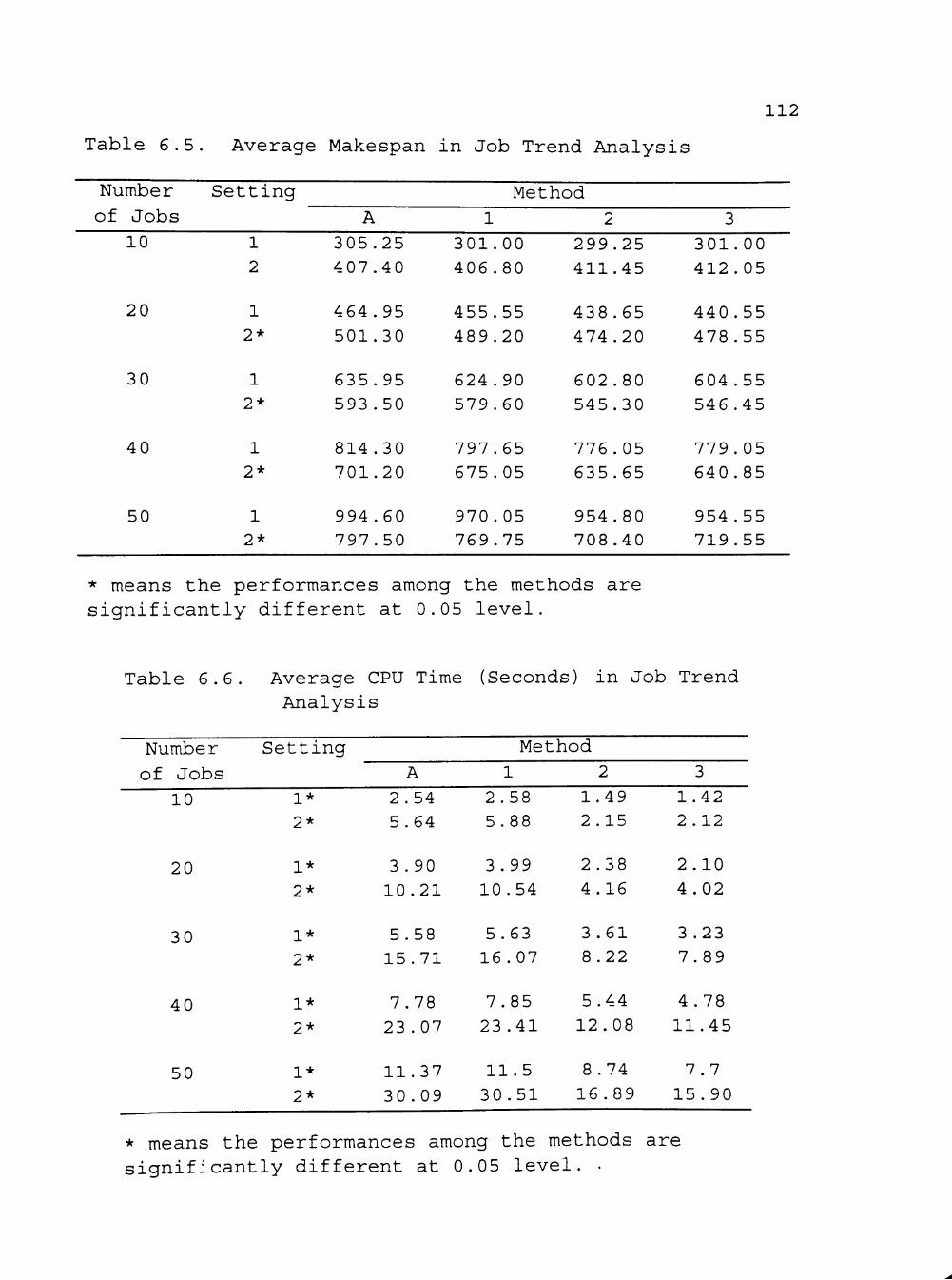
112

Table 6.5. Average Makespan in Job Trend Analysis

Number

of Jobs

10

20

30

40

50

Setting

1 2

1 2*

1 2*

1 2*

1 2*

A

305.25 407.40

464.95 501.30

635.95 593.50

814.30 701.20

994 .60 797.50

Method

1

301.00 406.80

455.55 489.20

624.90 579.60

797.65 675.05

970.05 769.75

2

299.25 411.45

438.65 474.20

602.80 545.30

776.05 635.65

954.80 708.40

3

301.00 412.05

440.55 478.55

604.55 546.45

779.05 640.85

954.55 719.55

* means the performances among the methods are significantly different at 0.05 level.

Table 6.6. Average CPU Time (Seconds) in Job Trend Analysis

Number

of Jobs

10

20

30

40

50

Setting

1* 2*

1* 2*

1* 2*

1* 2*

1* 2*

A

2 .54 5.64

3.90 10.21

5.58 15.71

7.78 23 .07

11.37 30.09

Method

1

2.58 5.88

3.99 10.54

5.63 16.07

7.85 23.41

11.5 30.51

2

1.49 2 .15

2.38 4 .16

3.61 8.22

5.44 12.08

8.74 16.89

3

1.42 2.12

2.10 4.02

3.23 7.89

4.78 11.45

7.7 15.90

* means the performances among the methods are significantly different at 0.05 level. •

113

Figures 6.5 and 6.7 show the graphs of the average

makespans for settings 1 and 2, respectively. Figures 6.6

and 6.8 show the graphs of the average CPU times for

settings 1 and 2, respectively.

6.2.3 Observations

Some observations obtained from the preceding tables

and figures are stated in the following:

1. In both settings, all the solution methods have the

same job trend for makespan. With the same number of work

centers and the same number of parallel machines at each

work center, the makespan increases as the number of jobs to

be processed increases. A makespan increment percentage is

calculated by the following formula:

Makespand + 1) - Makespand) Makespan Increment % = * 100-?

Makespand)

where makespand) is the average makespan obtained from a

schedule when there are JB- jobs to be processed and JB^ is

10, 20, 30, 40, and 50 for i being 1, 2, 3, 4, and 5,

respectively. This percentage represents the percentage of

makespan increasing when the number of jobs to be processed

increases from JB^ to JBi+i. Table 6.7 shows the makespan

increment percentages in the job trend analysis.

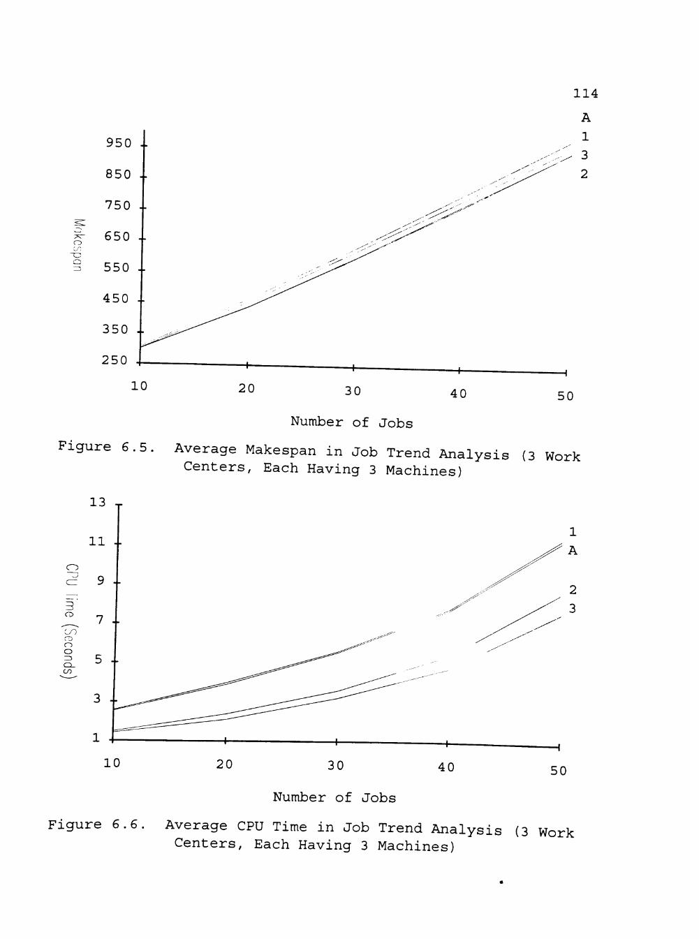
114

s :^^

~c ^

950 ..

850 ..

750 ..

650 ..

550 ..

450 ..

350 ..

250 L

A 1 3 2

30 40

Number of Jobs

Figure 6.5 Average Makespan in Job Trend Analysis (3 Work Centers, Each Having 3 Machines)

10 20 30

Number of Jobs

40 50

Figure 6.6. Average CPU Time in Job Trend Analysis (3 Work Centers, Each Having 3 Machines)

115

CO

o

800 J

750 ..

700 ..

650 -.

600 ..

550 ..

500 ..

450 ..

400 ^

10

Figure 6.7

20 30 40

Number of Jobs

A 1

3 2

50

Average Makespan in Job Trend Analysis (6 Work Centers, Each Having 6 Machines)

10

Figure 6.8

20 30

Number of Jobs

40 50

Average CPU Time in Job Trend Analysis (6 Work Centers, Each Having 6 Machines)

116

Table 6.7. Makespan Increment Percentage in Job Trend Analysis

Job Increment Setting Method (from -^ to) A 1 2 3 10 -> 20 1 52.32 51.35 46.58 46.36

2 23.05 20.26 15.25 16.14

20 ^ 30 1 36.78 37.17 37.42 37.23 2 18.39 18.48 14.99 14.19

30 ^ 40 1 28.04 27.64 28.74 28.86 2 18.15 16.47 16.57 17.28

40 ^ 50 1 22.14 21.61 23.03 22.53 2 13.73 14.03 11.44 12.28

2. In both settings, all the solution methods have the

same job trend for CPU time. With the same number of work

centers and the same number of parallel machines at each

work center, the CPU times increase as the number of jobs to

be processed increases. A CPU time increment percentage is

calculated by the following formula:

CPU Timed + 1) - CPU Timed) CPU Time Increment % = ; 77- * 10 0

CPU Timed)

where CPU timed) is the average CPU time required to get a

schedule when there are JBi jobs to be processed, and JB^ is

10, 20, 30, 40, and 50 for i being 1, 2, 3, 4, and 5,

respectively. This percentage represents the percentage

increase in CPU time as the number of jobs increases from

JBi to JBi+i. Table 6.8 shows the CPU time increment

percentages in the job trend analysis.

117

Table 6.8. CPU Time Increment Percentage in Job Trend Analysis

Job I]

(f ron 10

20

30

40

Qcrement

1 -> to) ->

^ •

->

->

20

30

40

50

Setting

1 2

1 2

1 2

1 2

A

53, 81,

43, 53,

39 46,

46 30

.54

.03

.08

.87

.43

.85

.14

.43

Method

1

54, 79,

41, 52,

39 45

46 30

.65

.25

.10

.47

.43

.68

.50

.33

2

59. 93,

51, 97,

50, 46,

60, 39,

.73

.49

.68

.60

.69

.96

.66

.82

3

47. 89.

53. 96.

47. 45.

61. 38.

,89 .62

.81

.27

.99 ,12

.09

.86

3. All the cases in setting 1 and the cases of 10 jobs

and 2 0 jobs in setting 2, ANOVA shows the performances of

makespan among the four solution methods having no

significant difference. For cases of 30 jobs, 40 jobs and

5 0 jobs in setting 2, ANOVA shows the performances of

makespan among the four solution methods have significant

difference. Among the significant cases, the SNK test shows

the makespans between Method 2 and Method 3 have no

significant difference, and those from Methods 2 and 3 are

better than those from Methods A and 1. For the case of 3 0

jobs in setting 2, the makespans between Methods A and 1 are

not significantly different, but for cases of 40 jobs and 50

jobs in setting 2, the makespans obtained from Method 1 are

better than those from Method A.

4. For both settings, in all the cases ANOVA and the

SNK test show that the performances of CPU time among the

118

four solution methods are significantly different from one

another. The order of the CPU time performance from the

best to the worst is: Method 3, Method 2, Method A, and

Method 1. One more observation is that CPU times spent by

Method A and by Method 1 are close as are those by Methods 2

and 3. However, Methods 2 and 3 have shorter CPU times than

those from Methods A, and 1.

6.2.4 Discussion

1. A job trend is observed and can be stated as

follows: if the number of work centers and the number of

parallel machines per work center are fixed, all the four

solution methods get larger makespans when the number of

jobs to be processed increases. This is just as expected.

2. Table 6.7 shows that the makespan increment

percentages using Methods A and 1 are close to each other as

are those using Methods 2 and 3. For Methods A and 1, when

the number of jobs increases from 10 to 20, the makespan

increases nearly 51.84% in setting 1, and 21.66% in setting

2. When the number of jobs increases from 2 0 to 30, the

makespan increases nearly 37.03% in setting 1, and 18.44% in

setting 2; i.e., when the number of jobs increases from 10

to 30, the makespan increases nearly 108.07% in setting 1,

and 44.09% in setting 2. For Methods 2 and 3, when the

number of jobs increases from 10 to 20, the makespan

increases nearly 47% in setting 1 and 16% in setting 2.

119

When the number of jobs increases from 2 0 to 30, the

makespan increases nearly 37% in setting 1, and 15% in

setting 2; i.e., when the number of jobs increases from 10

to 30, the makespan increases nearly 101% in setting 1 and

33% in setting 2. Thus the makespan increases when the

number of jobs to be processed is doubled or tripled, but

the increasing amount is not doubled or tripled. The

makespan obtained from a set of n jobs is less than the sum

of the makespans obtained from two sets of ^ jobs and is

even relatively smaller than the sum of the makespans from

three sets of ^ jobs. This effect is more significant in

setting 2 and in combining two or more sets of smaller

numbers of jobs into a single set since the makespan

increment percentage is getting smaller in setting 2 and

when the number of jobs to be processed is getting larger.

This implies that instead of processing several smaller sets

of jobs separately, if it is possible, it is better to

process all the jobs together in a single set to generate a

smaller makespan.

3. In setting 2 for the cases of 30 jobs, 40 jobs, and

5 0 jobs, the problem under the completely flexible job route

situation has better makespan performance than does it under

the partially flexible job route situation. Jobs in the

completely flexible job route situation can be processed on

any one of the parallel machines at each work center, but in

the partially flexible job route situation, once a job has

120

been assigned to a machine in the first work center, at the

following work centers, this job has to be processed on the

machine bearing the same machine number as it being at the

first work center. Therefore, there are more opportunities

to reduce job waiting time in the completely flexible job

route situation. Consequently, the problem under the

completely flexible job route situation may have a smaller

makespan than it can under the partially flexible job route

situation. However, this difference is not significant in

setting 1 for all the cases and in setting 2 for the cases

of 10 jobs and 2 0 jobs.

4. Methods A and 1 follow para-flow approach. These

two solution methods apply the CDS algorithm m(s + 1) times,

where m is the number of parallel machines per work center,

and s is the number of work centers. Methods 2, and 3

follow flow-para approach. They apply the CDS algorithm

only once. That is why Methods 2 and 3 spend less CPU time

than do Methods A and 1.

5. Method 1 has better makespan performance than

Method A has, and the difference is significant in setting 2

for the cases of 40 jobs and 50 jobs. However, Method 1 has

higher CPU time requirement than Method A has and the

difference is significant in most of the cases. This is to

be expected since Method 1 is based on Method A and has the

balancing routine added. Therefore, the balancing routine

has a significant effect on CPU time for all of the cases

121

and has a significant effect on makespan for the cases with

large number of jobs.

6. As discussed in (7), Section 6.1.4, Method 2

applies the priority dispatching rule LSP to choose the job

with the earliest starting position in the entry sequence at

work center 1. Method 3 employs the priority dispatching

rule FCFS to choose the job with the earliest arrival time

at current work center. The difference between these two

job selection processes results in method 3 requiring less

CPU time than does Method 2.

7. As discussed in (8), in Section 6.1.4, the priority

dispatching rules applied with Methods 2 and 3 do not result

in a significant difference between the makespan obtained

from Methods 2 and 3, but result in a significant difference

between the CPU time required by Methods 2 and 3.

8. For the four solution methods, increasing the

number of jobs has a big effect on CPU time. Table 6.8

shows the CPU time increment percentages range from 3 9.43%

to 61.09% in setting 1 and from 30.33% to 93.49% in setting

2. This implies that when the number of work centers and

the number of parallel machines at each work center are

fixed, increasing the number of jobs results in larger CPU

time.

122

6.3 Work Center Trend Analysis

6.3.1 Settings

For the work center trend analysis, the two settings

are: (1) 30 jobs and 3 parallel machines at each work

center, and (2) 50 jobs and 6 parallel machines at each work

center. Ten different numbers of work centers are assigned

to each setting. The numbers of work centers are 1, 2, 3,

4, 5, 6, 7, 8, 9, and 10. Therefore, the combination of

settings and numbers of work centers produces twenty

different problem sizes.

6.3.2 Computation Results

The average makespans and average CPU times along with

their ANOVA results are listed in Tables 6.9 and 6.10,

respectively. Figures 6.9 and 6.11 show the graphs of the

average makespans for settings 1 and 2, respectively.

Figures 6.10 and 6.12 show the graphs of the average CPU

times for settings 1 and 2, respectively.

6.3.3 Ob.servations

Some observations obtained from the preceding tables

and figures are in the following:

1. In both settings, all the solution methods have the

same work center trend for makespan. With the same set of

jobs and the same number of parallel machines at each work

center, the makespan increases as the number of work centers

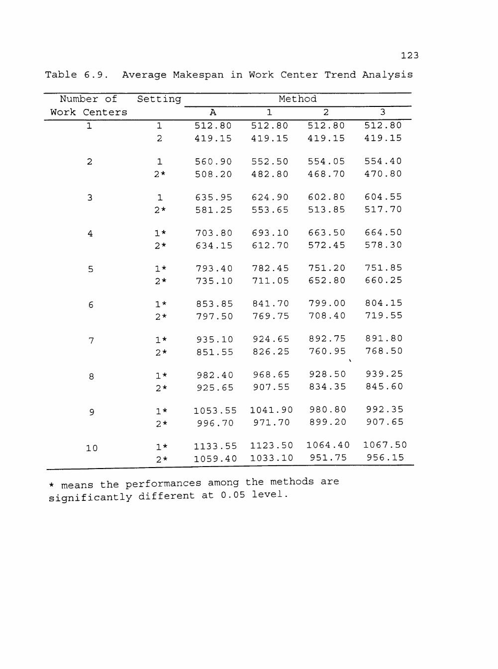
123

Table 6.9. Average Makespan in Work Center Trend Analysis

Number of Setting Method Work Centers

8

1

2

1

2*

1

2*

1*

2*

1*

2*

1*

2*

1*

2*

1*

2*

1*

2*

A

512.

419.

560.

508.

635.

581.

703 .

634.

793 .

735.

853 ,

797,

935,

851

982

925

1053

996

80

15

90

20

95

25

,80

,15

,40

,10

.85

.50

.10

.55

.40

.65

.55

.70

1

512 .

419.

552 .

482.

624 .

553.

693.

612.

782.

711.

841.

769.

924,

826,

968,

907

1041

971

80

15

50

80

90

65

10

70

,45

,05

,70

.75

.65

.25

.65

.55

.90

.70

2

512.

419.

554.

468.

602.

513 .

663 .

572.

751.

652.

799,

708,

892,

760

928

834

980

899

80

15

,05

,70

,80

.85

,50

,45

.20

.80

.00

.40

.75

.95

.50

.35

.80

.20

3

512.

419.

554.

470.

604.

517.

664.

578 .

751.

660.

804,

719,

891,

768

939

845

992

907

,80

,15

,40

,80

,55

,70

,50

,30

.85

.25

.15

.55

.80

.50

.25

.60

.35

.65

10 1* 1133.55 1123.50 1064.40 1067.50 2* 1059.40 1033.10 951.75 956.15

* means the performances among the methods are significantly different at 0.05 level.

124

Table 6.10. Average CPU Time (Seconds) in Work Center Trend Analysis

Number of

Work Center

1

2

3

4

5

6

7

8

9

10

Setting

1*

2*

1*

2*

1*

2*

1*

2*

1*

2*

1*

2*

1*

2*

1*

2*

1*

2*

1*

2*

A

0,

1.

3 .

5.

5

9.

8.

14

12

21

17

30

25

40

33

53

43

69

54

88

.45

18

52

91

.58

99

65

.92

.65

.50

.84

.09

.14

.86

.62

.97

.37

.81

.82

.57

Method

1

0.

1.

3.

5.

5.

10

8.

15

12

21

18

30

25

41

33

54

43

70

55

89

44

18

58

86

63

.23

77

.28

.78

.81

. 02

.51

.17

.40

.79

.53

.56

.49

.02

.31

0.

0.

2.

5.

3.

8.

4 .

11

6.

14

8.

16

9.

19

10

22

11

25

13

28

2

25

65

54

07

61

77

68

.39

94

.15

11

.89

32

.75

.59

.79

.87

.72

.18

.80

0.

0.

2.

4 .

3.

7.

4 .

10

6.

13

7.

15

8.

18

10

21

11

24

12

27

3

25

66

16

07

23

82

31

.44

57

.15

72

.90

94

.78

.18

.77

.45

.72

.78

.79

* means the performances among the methods are significantly different at 0.05 level.

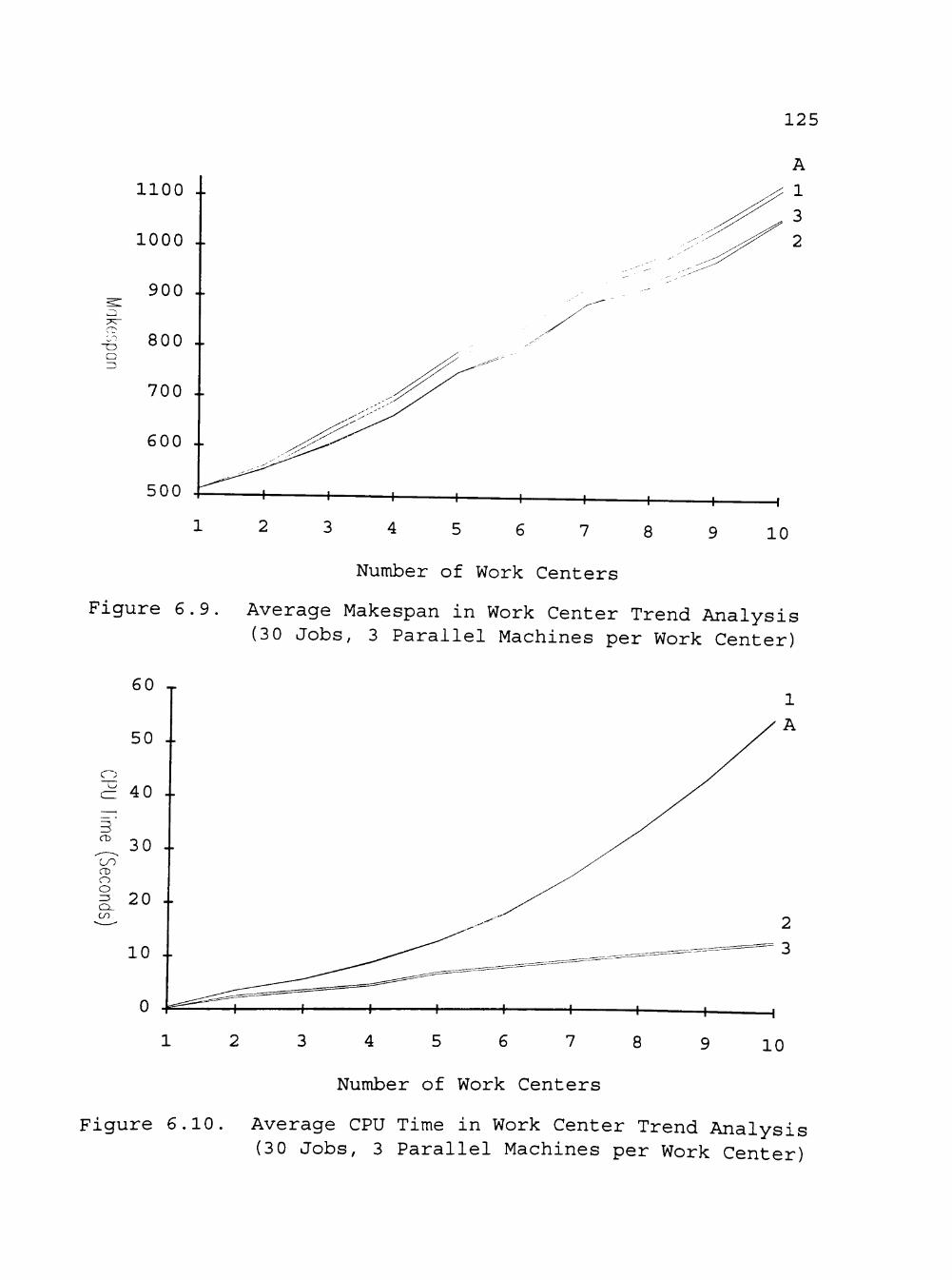
125

o

o

1100 ..

1000 ..

900 ..

800 ..

700 ..

600 ..

500

F i g u r e

C^U

firne S

econds

60 .

50 -

40 .

30 -

20 .

6 9

10 -.

0

8 10

Number of Work Centers

Average Makespan in Work Center Trend Analysis (30 Jobs, 3 Parallel Machines per Work Center)

8 10

Number of Work Centers

Figure 6.10. Average CPU Time in Work Center Trend Analysis (30 Jobs, 3 Parallel Machines per Work Center)

126

1000 ..

900 ..

4 5 6 7 8

Number of Work Centers

10

Figure 6.11

90 J

80 ..

70 ..

Average Makespan in Work Center Trend Analysis (50 Jobs, 6 Parallel Machines per Work Center)

r 60 ..

1 A

2 3

3 4 5 6 7 8

Number of Work Centers

10

Figure 6.12. Average CPU Time in Work Center Trend Analysis (50 Jobs, 6 Parallel Machines per Work Center)

127

increases. A marginal makespan increment percentage is

calculated by the following formula:

«>, • n », 1 o Makespand + 1) - Makespand) Marginal Makespan% = ^ ^ ^ ^ * ioo%

Makespand)

where makespand) is the average makespan obtained from a

schedule when there are i work centers. This percentage

represents the percentage of makespan increasing when the

number of work centers increases from i to (i + 1). Table

6.11 shows the marginal makespan increment percentages in

the work center trend analysis.

2. In both settings, all the solution methods have the

same work center trend for CPU time. With the same set of

jobs and the same number of parallel machines at each work

center, the CPU time increases as the number of work centers

increases. A CPU time increment percentage is calculated by

the following formula:

CPU Timed + 1) - CPU Time(i) CPU Time Increment % = * 100%

CPU Timed)

where CPU time(i) is the average CPU time to get a schedule

when there are i work centers. This percentage represents

the percentage of CPU time increasing when the number of

work centers increases from i to (i + 1). Table 6.12 shows

the CPU time increment percentages in the work center trend

analysis.

3. When there is only one work center, all of the four

solution methods yield the same makespans in both settings.

128

Table 6.11. Marginal Makespan Increment Percentage in Work Center Trend Analysis

Work Center Increment Setting Method (from -> to) A 1 '

^ 1 9.38 7.74 8.04 8.11 2 2 1 . 2 4 1 5 . 1 9 1 1 . 8 2 1 2 . 3 2

2 ^ 3 1 1 3 . 3 8 1 3 . 1 0 8 . 8 0 9 . 0 5 2 1 4 . 3 7 1 4 . 6 7 9 . 6 3 9 . 9 6

3 ^ 4 1 1 0 . 6 7 1 0 . 9 1 1 0 . 0 7 9 . 3 0 2 9 . 1 0 1 0 . 6 7 1 1 . 4 0 1 1 . 7 1

4 ^ 5 1 1 2 . 7 3 1 2 . 8 9 1 3 . 2 2 1 3 . 1 5 2 1 5 . 9 2 1 6 . 0 5 1 4 . 0 4 1 4 . 1 7

6

6 ^ 7

8

8

9 ^ 10

1 2

1 2

1 2

1 2

1 2

7 . 6 2 8 . 4 9

9 . 5 2 6 . 7 8

5 . 0 6 8 . 7 0

7 . 2 4 7 . 6 8

7 . 5 9 6 . 2 9

7 . 5 7 8 . 2 5

9 . 8 6 7 . 3 4

4 . 7 6 9 . 9 6

7 . 5 6 7 . 0 7

7 . 8 3 6 . 3 2

6 . 3 6 8 . 5 2

1 1 . 7 3 7 . 4 2

4 . 0 0 9 . 6 5

5 . 6 3 7 . 7 7

8 . 5 2 5 . 8 4

6 . 9 6 8 . 9 8

1 0 . 9 0 6 . 8 0

5 . 3 2 1 0 . 0 3

5 . 6 5 7 . 3 4

7 . 5 7 5 . 3 4

4. When there is more than one work center, the

solution methods yield different makespans. In setting 1,

ANOVA shows significant difference among makespans obtained

from the four solution methods when the number of work

centers is greater than 3. The SNK test shows the makespans

between Methods 2 and 3 have no significant difference,

neither do those between Methods A and 1. Makespans

129

Table 6.12. Marginal CPU Time Increment Percentage in Work Center Trend Analysis

Work Center Increment Setting " Method" (from -> to) A 1

^ 1 682.22 713.63 916.00 764.00 2 400.85 396.61 680.00 516.67

2 -> 3 1 58.52 57.26 42.13 49.54 2 69.04 74.57 72.98 92.14

3 - ^ 4 1 55.02 55.77 29.64 33.44 2 49.35 49.36 29.87 33.50

4 ^ 5 1 46.24 45.72 48.29 52.44 2 44.10 42.74 24.23 25.96

5 -> 6 1 41.03 41.00 16.86 17.50 2 39.95 39.89 19.36 20.91

6 - ^ 1 1 40.92 39.68 14.92 15.80 2 35.79 35.69 16.93 18.11

7 ^ 8 1 33.73 34.25 13.63 13.87 2 32.09 31.71 15.39 15.92

8 -> 9 1 29.00 28.91 12.09 12.48 2 29.35 29.27 12.86 13.55

9 -> 10 1 26.40 26.31 11.04 11.62 2 26.87 26.70 11.98 12.42

obtained from Methods 2 and 3 are smaller than those from

Methods A and 1. In setting 2, ANOVA shows significant

difference among makespans obtained from the four solution

methods when the number of work centers is greater than 1.

The SNK tests show the makespans between Methods 2 and 3

have no significant difference, but the makespans between

Methods A and 1 are significantly different in all cases

130

where ANOVA indicates rejection of the null hypothesis. The

makespans obtained from Methods 2 and 3 are smaller than

those from Method 1. Method A yields the largest makespans.

5. For both settings, in the case of one work center,

the performances of CPU time between Methods 2 and 3 have no

significant difference, neither do those between Methods A

and 1. The CPU times required by Methods 2 and 3 are

smaller than those required by Methods A and 1. Except for

the case of one work center, ANOVA and the SNK test show

that the performances of CPU time among the four solution

methods are significantly different from one another. The

order of the CPU time performance from the best to the worst

is: Method 3, Method 2, Method A, and Method 1. One more

observation is that CPU times spent by Methods A and 1 are

close to each other as are those by Methods 2 and 3.

However, the Methods 2 and 3 require less CPU times than do

Methods A and 1.

6.3.4 Discussion

1. A work center trend is observed and can be stated

as follows: if a set of jobs and the number of parallel

machine per work center are fixed, all of the four solution

methods get larger makespans when the number of work centers

increases. A set of given jobs has to go through more

processing with more work centers. This results in a larger

makespan to finish a set of given jobs.

131

2. Table 6.11 shows that when the number of work

centers increases from 1 to 2, the makespan increases nearly

8% in setting 1, and 15% in setting 2. When the number of

work centers increases from 2 to 3, the makespan increases

nearly 11% in setting 1, and 12% in setting 2; i.e., when

the number of work centers increases from 1 to 3, the

makespan increases nearly 20% in setting 1, and 29% in

setting 2. This means when the number of work centers is

doubled or tripled, the makespan increases some percentage

but the increasing amount is not doubled or tripled. On the

average. Table 6.11 shows a 10% increase in makespan as one

more work center added.

3. When there is only one work center, this flexible

flowshop problem is exactly the same as an m-parallel

machine assignment problem. Methods A and 1 utilize the

LPTF heuristic to do the job assignment. The makespans

obtained from these two methods and the CPU time spent by

these two methods should be the same. Methods 2 and 3

utilize the CDS algorithm to form an entry job sequence then

dispatch the jobs to the parallel machines according this

CDS entry sequence. The makespans obtained from these two

methods and the CPU time spent by these two methods should

be the same.

4. When there is more than one work center, the

problem under the completely flexible job route situation

has better makespan performance than it has under the

132

partially flexible job route situation. Jobs in the

completely flexible job route situation can be processed on

any one of the parallel machines at a work center, but in

the partially flexible job route situation, once a job has

been assigned to a machine at the first work center, at the

following work centers this job has to be processed on the

machine bearing the same machine number as it being at the

first work center. Therefore, there are more opportunities

to reduce job waiting time in the completely flexible job

route situation. Consequently, the problem under the

completely flexible job route situation can result in

smaller makespan than it can under the partially flexible

job route situation.

5. Methods A and 1 follow the para-flow approach.

These two solution methods apply the CDS algorithm m(s + 1)

times, where m is the number of parallel machines per work

center, and s is the number of work centers. Methods 2 and

3 follow the flow-para approach. They apply the CDS

algorithm only once. That is why Methods 2 and 3 spend less

CPU time than do Methods A and 1.

6. Method 1 has better makespan performance than

Method A has and the difference is significant when the

number of work centers is greater than 3 in setting 1 and

greater than 1 in setting 2. However, Method 1 has worse

CPU time performance than Method A has and the difference is

significant in most of the cases. This is as expected.

133

since Method 1 is based on Method A and has the balancing

routine added. Therefore, the balancing routine has a

significant effect on CPU time for all of the cases and has

a significant effect on makespan for the cases with larger

number of work centers.

7. As discussed in (7), Section 6.1.4, Method 2

applies the priority dispatching rule LSP to choose the job

with the earliest starting position in the entry sequence at

work center 1. Method 3 employs the priority dispatching

rule FCFS to choose the job with the earliest arrival time

at current work center. The difference between these two

job selection processes is the reason why method 3 requires

less CPU time than does Method 2.

8. As discussed in (8), Section 6.1.4, the priority

dispatching rules applied with Methods 2 and 3 do not result

in significant difference between the makespan obtained from

Methods 2 and 3, but make significant difference between the

CPU time spent by Method 2 and by Method 3.

9. For the four solution methods, increasing the

number of work centers has a strong effect on CPU time,

especially when the number of work centers increases from 1

to 2; the CPU time for these cases increases over 400%.

Except for this case. Methods A and 1 have similar CPU time

increment percentages. Methods 2 and 3 have similar CPU

time increment percentages. For Methods A and 1, Table 6.12

shows the CPU time increment percentages range from 26.40^ I o, •©

134

to 58.52% in setting 1 and from 26.70% to 74.57% in setting

2. For Methods 2 and 3, the CPU time increment percentages

range from 11.04% to 52.44% in setting 1 and from 11.98% to

92.14% in setting 2. For all the solution methods, when the

number of work centers increases, the CPU time increment

percentage decreases. This implies that when the number of

jobs and the number of parallel machines at each work center

are fixed, increasing the number of work centers requires

more CPU time to get a schedule but the CPU time increment

percentage decreases.

CHAPTER VII

CONCLUSIONS AND FURTHER STUDIES

This research studies the scheduling problem in the

flexible flowshop system. This system includes a number of

work centers, each having one or more parallel machines. A

set of immediately available jobs has to be processed

through the ordered work centers. A job is processed on at

most one of the identical parallel machines at each of the

work centers. For the case of having the same number of

identical parallel machines at every work center, this

research proposes two approaches to do the scheduling: the

para-flow approach and the flow-para approach. Regarding

the job route, this problem is discussed under two

situations: the partially flexible job route situation and

the completely flexible job route situation. The objective

of this research is to find the heuristics to minimize the

makespan of the problem in reasonable computational time.

7.1 Conclusions

It is of interest to note that a flexible flowshop

represents a generalization of the simple flowshop and the

identical parallel machine shop. For a set of given jobs,

the way used to minimize the makespan in the simple flowshop

and in the identical parallel machine shop is different from

each other. In the simple flowshop, the main concern is to

find a job sequence and reduce the total idle time of

135

136

machines. In the identical parallel machine shop, the main

concern is to dispatch jobs into the parallel machines and

balance the workloads among the parallel machines. The two

concerns mentioned above have to be considered together in a

flexible flowshop scheduling problem. Numerous algorithms

have been developed to solve the simple flowshop scheduling

problems. Identical parallel machine shop scheduling

problems have been solved by several different heuristics.

By combining the characteristics of the simple flowshop and

the identical parallel machine, this research recommends two

different approaches to find a schedule for a set of

immediately available jobs in the flexible flowshop in order

to minimize the makespan.

This research verifies that to solve the scheduling

problem in the flexible flowshop the para-flow approach and

the flow-para approach outperform the published algorithms.

The comparisons among the proposed algorithms and the

published algorithms are summarized in this section. Since

the problem is considered under two situations, the

comparisons within each situation will be stated first then

the comparisons between these two situations are summarized.

The size of the problem includes three elements: the number

of jobs, the number of work centers, and the number of

parallel machines at each work center. By fixing any two of

the three elements, the trend caused by the third element

can be analyzed. The last three sub-sections state the

137

trend analysis of the three elements of the size of the

problem. These three sub-sections present the trend

analysis for the four proposed algorithms: Method A, Method

1, Method 2, and Method 3.

7.1.1 Conclusions for the Problem under the Partially Flexible Job Route Situation

Two algorithms are used for the problem under the

partially flexible job route situation: the para-flow

algorithm (LPTF-CDS algorithm) and the Sriskandarajah-Sethi

algorithm. The first algorithm is the proposed algorithm

which utilizes the LPTF heuristic and the CDS algorithm.

The second is an algorithm published in 1989 by

Sriskandarajah and Sethi. For convenience, the proposed

algorithm is called Method A and the published algorithm is

called Method B.

1. Method A has better makespan performance than

Method B has; thus the LPTF-CDS algorithm can generate

smaller makespan than the Sriskandarajah Sethi algorithm

can. The average of the makespan improvement percentages of

Method A versus Method B is about 16%.

2. Method B has better CPU time performance than

Method A has; thus the LPTF-CDS algorithm spends more CPU

time to generate a schedule than the Sriskandarajah-Sethi

algorithm does.

138

3. Since Method A can generate a smaller makespan in

reasonable time, the para-flow approach is a better choice

to set up a schedule for the problem under the partially

flexible job route situation.

7.1.2 Conclusions for the Problem under the Completely Flexible Job Route Situation

Six algorithms are used for the problem under the

completely flexible job route situation: the para-flow

algorithm (LPTF-CDS-Balancing algorithm), the flow-para

algorithms (CDS-LSP algorithm and CDS-FCFS algorithm), the

Sriskandarajah-Sethi algorithm and the Wittrock algorithms

(FFLL algorithm and LPTF-WLA algorithm). The first

algorithm utilizes the LPTF heuristic and the CDS algorithm.

The second and the third utilize the CDS algorithm to

determine a loading sequence, then the Loading Sequence

Priority (LSP) queuing principle and the First Come First

Serve (FCFS) queuing principle are employed as priority

dispatching rules, respectively. The fourth was published

in 1989 by Sriskandarajah and Sethi. The Flexible Flow Line

Loading (FFLL) algorithm and LPTF-Working Loading

Approximation (WLA) algorithm were published in 1985 and

1988, respectively, by Wittrock. For convenience, in the

following the three proposed algorithms are called Method 1,

Method 2, and Method 3, respectively. The three published

139

algorithms are called Method 4, Method 5, and Method 6,

respectively.

1. Each of the proposed algorithms has better makespan

performance than each of the published algorithms has.

Makespans generated by Methods 1, 2, and 3 are smaller than

those generated by Methods 4, 5, and 6. The averages of the

makespan improvement percentages of Method 2 versus Methods

4, 5 and 6 are about 18%, 20%, and 14%, respectively.

2. Methods 3 and 4 have better CPU time performance

than do the other four methods. When the number of work

centers is small. Method 3 spends less CPU time than Method

4 does. CPU time spent by method 2 is close to that spent

by Method 3. When Method 1 compares with Method 6, Method 1

spends relatively little CPU time.

3. The difference between Methods 2 and 3 is the

priority dispatching rule used in job selection. Although

Method 2 generates the smallest makespan among the six

methods, the makespan generated by Method 3 has no

significant difference from that generated by Method 2. The

CPU time required by Method 3 is less than that required by

Method 2, and the difference is significant. This implies

that the priority dispatching rules applied with Methods 2

and 3 do not result in significant difference in the

makespan performance but result in significant difference in

the CPU time performance.

140

4. Since Method 3 spends less CPU time than Method 2

does and yields smaller makespan than the other four methods

do, the flow-para approach using FCFS queuing principle as

priority dispatching rule is the best choice to set up a

schedule for the problem under the completely flexible job

route situation.

7.1.3 Conclusions for the Comparison of the Problem under the Partially Flexible Job Route Situation and under the Completely Flexible Job Route Situation

Four algorithms are discussed in this section: Method

A, Method 1, Method 2, and Method 3. Method A is used for

the problem under the partially flexible job route

situation. Methods 1, 2, and 3 are used for the problem

under the completely flexible job route situation.

1. The para-flow approach can be applied in the

partially flexible job route situation and in the completely

flexible job route situation. The flow-para approach can be

applied only in the completely flexible job route situation.

2. The schedule of the problem under the partially

flexible job route situation is a permutation schedule. The

schedule of the problem under the completely flexible job

route situation is a non-permutation schedule.

3. The makespan of the problem generated in the

completely flexible job route situation is smaller than that

generated in the partially flexible job route situation.

141

4. The makespans yielded by using Methods A and 1 are

close to each other, so are those yielded by using Methods 2

and 3 .

5. CPU time spent by Method A is larger than that

spent by Methods 2 and 3. That is if Method 2 or Method 3

is used in the completely flexible job route situation, and

Method A is used in the partially flexible job route

situation, the CPU time needed to set up a schedule for the

problem under the completely flexible job route situation is

less than that needed for the problem under the partially

flexible job route situation.

6. Except for the additional balancing routine used in

Method 1, Method 1 goes through the same procedure as Method

A does to set up a schedule. Therefore, Method A spends

less CPU time than Method 1 does, but this difference is not

significant. Since the workspans are more balanced at each

work center using Method 1 than those using Method A, Method

1 may generate solutions with smaller makespan than Method A

does. This difference is significant for large problem

size. This implies that the balancing routine has no impact

on CPU time but has impact on makespan when the size of the

problem is large.

7.1.4 Conclusion for Parallel Machine Trend Analysis

1. All the four proposed methods have similar parallel

machine trends. If a set of jobs and the number of work

142

centers are fixed, a smaller makespan is obtained when the

number of parallel machines per work center increases. This

trend is maintained until the number of parallel machines

per work center becomes close to the number of jobs.

2. If the number of parallel machines per work center

increases from 1 to 2 and from 1 to 3, the makespan reduces

about 47% and 63%, respectively.

3. When there is only one machine at each work center,

the flexible flowshop is exactly the same as a simple

flowshop. The four solution methods get the same makespan.

4. When there is more than one parallel machine per

work center, the problem under the completely flexible job

route situation has better makespan performance than does it

under the partially flexible job route situation.

5. As long as the number of jobs and the number of

work centers are fixed, for Methods 2 and 3, increasing the

number of parallel machines at each work center does not

have significant effect on CPU time.

6. For Methods A and 1, there is a critical number of

parallel machines per work center. Below this critical

number, increasing the number of parallel machines per work

center will reduce the CPU time; but beyond this critical

number, increasing the number of parallel machines at each

work center will increase the CPU time.

143

7.1.5 Conclusion for Job Trend Analysis

1. The four proposed methods have similar job trend.

If the number of work centers and the number of parallel

machines per work center are fixed, a larger makespan is

obtained when the number of jobs to be processed increases.

2. The makespan increases when the number of jobs to

be processed is doubled or tripled, but the increasing

amount is not doubled or tripled. The makespan obtained

from a set of n jobs is less than the sum of the makespans

obtained from two sets of ^ jobs and even relatively

smaller than the sum of the makespans from three sets of ^

jobs. This effect is more significant in combining two or

more sets of smaller number of jobs into a single set when

the number of jobs to be processed is large. This implies

that instead of processing several smaller sets of jobs

separately, if it is possible, it is better to process all

jobs together in a single set to generate a smaller

makespan.

7.i.f connin.qion for Work Center Trend Analysis

1. All of the four proposed methods have similar work

center trend. If a set of jobs and the number of parallel

machines per work center are fixed, a larger makespan is

obtained when the number of work centers increases.

144

2. When the number of work centers is doubled or

tripled, the makespan increases some percentage but the

increasing amount is not doubled or tripled. On the

average, the makespan increases 10.12% as one more work

center added.

3. When there is only one work center, this flexible

flowshop problem is exactly the same as an m-parallel

machine assignment problem. Methods A and 1 utilize the

LPTF heuristic to do the job assignment. The makespans

obtained from these two methods and the CPU time spent by

these two methods should be the same. Methods 2 and 3

utilize the CDS algorithm to form an entry job sequence then

dispatch the jobs to the earliest available parallel

machines according this CDS entry sequence. The makespans

obtained from these two methods and the CPU time spent by

these two methods should be the same.

4. When there is more than one work center, the

problem under the completely flexible job route situation

has better makespan performance than it does under the

partially flexible job route situation.

5. For the four proposed methods, increasing the

number of work centers has a strong effect on CPU time,

especially, when the number of work centers increases from 1

to 2; for this case the CPU time increases over 400%.

Except for this case. Methods A and 1 have similar CPU time

increment percentages. These percentages are 26% or higher.

145

Methods 2 and 3 have similar CPU time increment percentages

that are 11% or higher. For all the solution methods, when

the number of work centers increases, the CPU time spending

increases but the increment percentage decreases. This

implies that when the number of jobs and the number of

parallel machines at each work center are fixed, increasing

the number of work centers results in larger CPU time but

the increasing rate of CPU time is getting smaller.

7.2 Further Studies

In this research the scheduling problem in the flexible

flowshop with the same number of identical parallel machines

at every work center has been examined. The two recommended

approaches have been developed; these approaches outperform

the published algorithms. The results of this research can

encourage the following further studies:

1. Generalize the flow-para approach to solve the

scheduling problem in the flexible flowshop with different

numbers of parallel machines at each work center.

2. Instead of using the LPTF heuristic, use different

heuristics to do parallel machine assignment in order to

find the best heuristic for the para-flow approach.

3. Instead of using the CDS flowshop scheduling

algorithm, use different flowshop algorithms to do job

sequencing in the para-flow approach and in the flow-para

approach.

146

4. Instead of using the LSP queuing discipline or FCFS

queuing discipline as the priority dispatching rule, use

different priority dispatching rules in the job selection

process to find the best priority dispatching rule for the

flow-para approach.

5. Use the flow-para approach and/or the para-flow

approach to solve the scheduling problem in the flexible

flowshop with the same or different number of heterogeneous

parallel machines at each work center.

6. Develop solution methods when the storage space in

front of each work center is limited.

7. Apply the para-flow approach and the flow-para

approach when the storage space in front of each work center

is not allowed.

8. After the completion of the processing of a set of

jobs, the jobs may be sent to several different

destinations. There are a number of sub-sets of jobs, each

of them having the same destination. Instead of minimizing

makespan of the whole job set, develop algorithms to

minimize makespans of each sub-set of jobs.

10. Apply the para-flow approach and the flow-para

approach to the situation that set up times are dependent on

the job sequence.

11. Apply the para-flow approach and the flow-para

approach to a set of jobs with stochastic processing times

147

12. Instead of minimizing makespan, apply the para-

flow approach and the flow-para approach to achieve

different goals.

13. When there is a processing time relationship among

jobs or among work centers, e.g., the ordered processing

time matrix (Smith et al. 1975 and 1976), solve the

scheduling problem by using the para-flow approach and the

flow-para approach.

REFERENCES

Adolphson, D. L., "Single Machine Job Sequencing with Precedence Constraints," SIAM Journal on Computing. Vol. 6, No. 1, Mar. 1977, pp. 40-54.

Adolphson, D. L., and Hu, T. C., "Optimal Linear Ordering," SIAM Journal on Applied Mathematics. Vol. 25, No. 3, Nov. 1973, pp. 403-423.

Agnetis, A. C. A., and Stecke, K. E., "Optimal Two-Machine Scheduling in a Flexible Flow System," Proceedings: Rensselarer's Second International Conference on Computer Integrated Manufacturing. Rensselarer Polytechnic Institute, N. Y., May 21-23, 1990, pp. 47-54.

Ahuja, R. K. , Orlin, J. B., and Tarjan, R. E., "Improved Time Bounds for the Maximum Flow Problem," SIAM Journal on Computing. Vol. 18, No. 5, Oct. 1989, pp. 939-954.

Alidaee, B., "A Heuristic Solution Procedure to Minimize Makespan on a Single Machine with Non-Linear Cost," Journal of the Operational Research Society. Vol. 41, No. 11, Nov. 1990, pp. 1065-1068.

Arneson, G., "Introduction to Dynamic Scheduling," Metal Finishing. Vol. 86, Nov. 1988, pp. 19-22.

Arthanari, T. S., and Ramamurthy, K. G., "An Extension of Two Machines Sequencing Problem," Opsearch. Vol. 8, 1971, pp. 10-22.

Baker, K. R., introduction to Seauencincr and Scheduling. 1974, John Wiley & Sons, Inc., New York.

Bansal, S. P., "Minimizing the Sum of Completion Times of n Jobs over m Machines in a Flowshop—A Branch and Bound Approach," ATTF Transactions. Vol. 9, No. 3, Sept. 1977, pp. 306-311.

Bestwick, P. F., and Hastings, N. A. J., "A New Bound for Machine Scheduling," Operational Research Quarterly. Vol. 27, No. 2, 1976.

148

149

Brah, S. A., and Hunsucker, J. L., "Branch and Bound Algorithm for the Flow Shop with Multiple Processors," European Journal of Operational Research. Vol. 51, No. 1, Mar. 1991, pp. 88-99.

Brooks, G. H., and White, C. R., "An Algorithm for Finding Optimal and Near Optimal Solutions to the Production Scheduling Problem," Journal of Industrial Engineering. Vol. 16, No. 2, 1965.

Buten, R. E., and Shen, V. Y., "A Scheduling Model for Computer Systems with Two Classes of Processors," Proceedings of Sagamore Computer Conference on Parallel Processing. 1973, pp. 130-138.

Campbell, H. G. , Dudek, R. A., and Smith, M. L., "A Heuristic Algorithm for the n Job, m Machine Sequencing Problem," Management Science. Vol. 16, No. 10, June 1970, pp. B-630-B-637.

Churchman, C. W. , Ackoff, R. L., and Arnoff, E. L. ,

Introduction to Operations Research. Wiley, New York, 1969.

Coffman, E. G., Jr., Computer and Job-Shop Scheduling Theory. Wiley, New York, 1976.

Coffman, E. G., Jr., Garey, M. R., and Johnson, D. S., "An Application of Bin-Packing to Multiprocessor Scheduling," SIAM Journal of Computing. Vol. 7, No. 1, Feb. 1978, pp. 1-17.

Coffman, E. G., Jr., and Graham, R. L., "Optimal Scheduling for Two-Processor Systems," Acta Informatica. Vol. 1, 1972, pp. 200-213.

Conway, R. W., Maxwell, W. L., and Miller, L. W., Theory o£ .qrheduling. Addison-Wesley, Reading, MA., 1967.

Dannenbring, D. G., "An Evaluation of Flowshop Sequencing

Heuristics," Management Science. Vol. 23, No. 11, July 1977, pp. 1174-1182.

150

Deal, D. E., and Hunsucker, J. L., "The Two-Stage Flowshop Scheduling Problem with M Machines at each Stage," JOUrna] o£ Information Ff Ontimizatinn Sc-ienrP.c;. Vol. 12, No. 3, Sept. 1991, pp. 407-417.

Dudek, R. A., Panwalkar, S. S., and Smith, M. L., "The Lessons of Flowshop Scheduling Research," Operations Research, Vol. 40, No. l, Jan.-Feb. 1992, pp. 7-13.

Dudek, R. A., Smith, M. L., and Panwalkar, S. S., "Use of a Case Study in Sequencing/Scheduling Research," Omega. Vol. 2, No. 2, 1974, pp. 253-261.

Dudek, R. A., and Teuton, 0. F., Jr., "Development of M-Stage Decision Rule for Scheduling n Jobs Through M Machines," Operations Researrh, Vol. 12, No. 3, May-June 1964, pp. 471-497.

Friesen, D. K. , "Tighter Bounds for the MULTIFIT Processor Scheduling Algorithm," SIAM Journal of CnmputiTig. Vol. 13, No. 1, Feb. 1984, pp. 170-181.

Garey, M. R. , and Johnson D. S., Computers and Intractability; A guide to the Theory of NP-Completeness. Freeman, San Francisco, 1979.

Garey, M. R., and Johnson D. S., "Scheduling Tasks with Nonuniform Deadlines on Two Processors," Journal of Association of Computing Machinery. March 1976, pp. 461-467.

Garey, M. R., and Johnson D. S., "Approximation Algorithms for Combinatorial Problems: An Annotated Bibliography," in: Traub, J. F., ed., Algorithms and Complexity: New Directions and Recent Results, Academic, New York, 1976, pp. 41-52.

Garey, M. R., Johnson D. S., and Sethi, R., "The Complexity of Flowshop and jobshop Scheduling," Mathematics nf Operational Research. Vol. 1, 1976, pp. 117-129.

Garey, M. R., Johnson, D. S., and Tarjan, r. E., "The Complexity of Flowshop and Jobshop Scheduling," Mathematics of Operational Research. Vol. 1, No. 2, 1974, pp. 117-128.

151

Gilmore, P. G-, and Gomory, R. E., "Sequencing a One State-Variable Machine: A solvable Case of the Traveling Salesman Problem," Operations Research. Vol. 12, 1964, pp. 655-679.

Gonzalez, T., and Sahni, S., "Flowshop and Jobshop Schedules: Complexity and Approximation," Operations Research. Vol. 26, No. 1, Jan.-Feb. 1978, pp. 36-52.

Graham, R. L., "Bounds on the Performance of Scheduling Algorithms," in: Coffman, E. G., ed.. Computer and Job-Shop Scheduling Theory. Wiley, New York, 1976, pp. 165-227.

Graham, R. L., "Bounds on Multiprocessing Timing Anomalies," SIAM Journal of Applied Mathematics. Vol. 17, No. 2, Mar. 1969, pp. 416-429.

Graham, R. L., "Bounds for Certain Multiprocessing

Anomalies," The Bell System Technical Journal. Vol. 45, Nov. 1966, pp. 1563-1581.

Graham, R. L., Lawler, E. L., Lenstra, J. K., and Rinnooy Kan, A. H. G., "Optimization and Approximation in Deterministic Sequencing and Scheduling: A Survey", Annals of Discrete Mathematics. Vol. 5, 1979, pp. 287-326 .

Grolmusz, V., "Large Parallel machines Can Be Extremely Slow for Small Problems," Algorithmica. Vol. 6, No. 4, 1991, pp. 479-489.

Guinet, A., "Textile Production Systems: A Succession of

Non-Identical Parallel Processor Shops," Journal of the

Operational Research Society. Vol. 42, No. 8, Aug.

1991, pp. 655-671.

Gupta, J. N. D., "Two-Stage, Hybrid Flowshop Scheduling

Problem," Journal of the Operational Research Society.

Vol. 39, No. 4, 1988, pp. 359-364.

Gupta, J. N. D., "Optimal Flowshop Schedules with No Intermediate Storage Space," Naval Research Logistics Quarterly. Vol. 23, No. 2, June 1976, pp. 235-243.

152

Gupta, J. N. D., "Heuristic Algorithms for Multistage Flow Shop Problem," AIIE Transactions. Vol. 4, No. 1, Mar. 1972, pp. 11-18.

Gupta, J. N. D., and Dudek, R. A., "Optimality Criteria for Flowshop Schedules," AIIE Transactions. Vol. 3, No. 3, Sept. 1971, pp. 199-205.

Gupta, J. N. D., and Tunc, E. A., "Scheduling for a Two-Stage Hybrid Flowshop with Parallel Machines at the Second Stage," International Journal of Production Research, vol. 29, No. 7, July 1991, pp. 1489-1502.

Hariri, A. M. A., and Potts, C. N., "Heuristics for Scheduling Unrelated Parallel Machines," Computers & Operations Research. Vol. 18, No. 3, 1991, pp. 323-331.

Ho, J. C , and Chang, Y.-L., "A New Heuristic for the n-Job, M-Machine Flow-Shop Problem," European Journal of Operational Research. Vol. 52, No. 2, May 19 91, pp. 194-202 .

Hochbaum, D. S., and Shmoys, D. B., "Using Dual Approximation Algorithms for Scheduling Problems: Theoretical and Practical Results," Journal of the Association for Computing Machinery. Vol. 34, No. 1, Jan. 1987, pp. 144-162.

Ignall, E., and Schrage, L., "Application of the Branch and Bound Technique to Some Flow-Shop Scheduling Problems," Operations Research. Vol. 13, No. 3, May-June 1965, pp. 400-412 .

Jo, K. Y., and Maimon, 0. Z., "Optimal Dynamic Load Distribution in a Class of Flow-Type Flexible Manufacturing Systems," European Journal of Operational Research. Vol. 55, No. 1, Nov. 1991, pp. 71-81.

Johnson, D- S., "Fast Algorithms for Bin Packing," Journal

of Computing System Sciences. Vol. 8, 1974, pp. 272-

314.

Johnson, D. S., "Near-Optimal Bin Packing Algorithms," Report MAC TR-109. Massachusetts Institute of Technology, Cambridge, MA, 1973.

153

Johnson, D. S., Demers, A., Ullman, J. D., Garey, M. R., Graham, R. L., "Worst-Case Performance Bounds for Simple One-Dimensional Packing Algorithms," SIAM Journal of Computing, Vol. 3, 1974, pp. 299-325.

Johnson, S. M., "Optimal Two- and Three-Stage Production Schedules with Setup Times Included," Naval Research Logistics Quarterly. Vol. 1, No. 1, Mar. 1954, pp. 61-68.

Kang, B.-S., and Markland, R. E., "Solving the No-Intermediate Storage Flowshop Scheduling Problem," International Journal of Operations and Production Management. Vol. 9, No. 3, 1989, pp. 48-59.

Kang, B.-S., and Markland, R. E., "Evalution of Scheduling Techniques for Solving Flowshop Problems with No Intermediate Storage," Journal Qt Operations Management. Vol. 7, No. 3, Dec. 1988, pp. 1-24.

Karimi, I., and Ku, H.-M., "A Modified Heuristic for an Initial Sequence in Flowshop Scheduling," Industrial and Engineering Chemistry Research. Vol. 27, Sept. 1988, pp. 1654-1658.

Karush, W., "A Counterexample to a Proposed Algorithm for Optimal Sequencing of Jobs," Operations Research. Vol. 13, 1965, pp. 323-325.

King, J. R., and Spachis, A. S., "Heuristics for Flow-Shop Scheduling," International Journal of Production Research. Vol. 19, No. 3, 1980.

Kochhar, S., and Morris, R. J. T., "Heuristic Methods for Flexible Flow Line Scheduling," Journal of Manufactur-Hna Systems. Vol. 6, No. 4, 1987, pp. 209-314.

Kochhar, S., Morris, R. J. T., and Wong, W. S., "The Local Search Approach to Flexible Flow Line Scheduling," F.ngineer-ing Costs and Production Economics. Vol. 14, 1988, pp. 25-37.

154

Kuriyan, K., and Reklaitis, G. V., "Scheduling Network Flowshops so as to Minimize Makespan," Computers & Chemical Engineering. Vol. 13, No. 1/2, Jan. 1989, pp. 187-200.

Langston, M. A., "Interstage Transportation Planning in the Deterministic Flow-shop Environment," Operations Research/ vol. 35, No. 4, July-Aug. 1987, pp. 556-564.

Langston, M. A., "Improved LPT Scheduling for Identical Processor Systems," RAIRO—^Technique et Science Informatiques. Vol. 1, Jan.-Feb. 1982, pp. 69-75.

Law, A. M., and Kelton, W. D., Simulation Medeling & Analysis. 2nd ed., 1991, McGraw-Hill, Inc., New York.

Lawer, E. L., Lenstra J. K., and Rinnooy Kan, A. H. G., "Recent Development in Deterministic Sequencing and Scheduling: A Survey," in: Dempster, M. A. H. et al., Eds., Deterministic and Stochastic Scheduling. D. Reidel Publishing Co., Boston, MA, 1982, pp. 35-78.

Lenstra, J. K. , Rinnooy Kan, A. H. G., and Brucker, P., "Complexity of Machine Scheduling Problems," Annals of Discrete Mathematics. Vol. 1, No. 4, 1977, pp. 343-362.

Lenstra, J. K. , Shmoys, D. S., and Tardos, E., "Approximation Algorithms for Scheduling Unrelated Parallel Machines," Mathematical Programming. Vol. 46, No. 3, Apr. 1990, pp. 259-271.

Little, J., Murty, K., Sweeney, D., and Karel, C., "An Algorithm for the Traveling Salesman Problem," Qperational Research Quarterly, Vol. 11, No. 6, 1963.

Liu, C. L., "Optimal Scheduling on Multi-Processor Computing Systems," Proceedings of the 1 3 ^ Annual IEEE Symposium nn Switching and Automata Theory. Oct. 25-27, 1972, pp. 155-160.

Liu, J. W. S., and Liu, C. L., "Performance Analysis of Heterogeneous Multiprocessor Computing Systems," In: E. Gelenbe, R. Mahl (eds.). Computer Architechtures and Networks. North Holland, Amsterdam, 1974, pp. 331-343.

155

Liu, J. W. S., and Liu, C. L., "Bounds on Scheduling Algorithms for Heterogeneous Computing Systems," In: J. L. Rosenfeld (ed.). Information Processing 74: Proceedings of IFIP Congress 74, North Holland, Amsterdam, 1974, pp. 349-353.

Lomnicki, Z., "A Branch and Bound Algorithm for the Exact Solution of the Three Machine Scheduling Problem," Operational Research Quarterly. Vol. 16, No. 1, 1964, pp. 89-100.

McNaughton, R. , "Scheduling with Deadlines and Loss Functions," Management Science. Vol. 6, No. 1, Oct. 1959, pp.1-12.

Mittal, B. S., and Bagga, P. C , "Two Machine Sequencing Problem with Parallel Machines," Opsearch. Vol. 10, 1973, pp. 50-61.

Murthy, R. N., "On Two Machine Sequencing with Parallel Processors," Opsearch. Vol. 11, 1974, pp. 42-44.

Narasimhan, S. L., and Mangiameli, P. M., "A Comparison of Sequencing Rule for a Two-stage Hybrid Flow Shop," Decision Sciences. Vol. 18, No. 2, Spring 1987, pp. 250-265.

Nowicki, E., and Smutnicki, C , "Worst-Case Analysis of Dannenbring's Algorithm for Flow-Shop Scheduling," Operations Research Letters. Vol. 10, No. 8, Nov. 1991, pp. 473-480.

Nowicki, E., and Smutnicki, C , "Worst-Case Analysis of an Approximation Algorithm for Flow-Shop Scheduling," Operations Research Letters. Vol. 8, No. 3, June 1991, pp. 171-177.

Palmer, D. S., "Sequencing Jobs Through a Multi-Stage Process in the Minimum Total Time—A Quick Method of

Obtaining a Near Optimum," Operational Research Quarterly. Vol. 16, No. 1, Mar. 1965, pp. 101-107.

156

Panwalkar, S. S., "Scheduling of a Two-machine Flowshop with Travel Time between Machines," Journal nf Operational Research Society, Vol. 42, No. 7, July 1991, pp. 609-613.

Panwalkar, S. S., Dudek, R. A., and Smith M. L., "Sequencing Research and the Industrial Scheduling Problem," PrCCeedings of Symposium on Theory of Scheduling and Its Applications, Raleigh. North rar-n1in;=| May 1972. pp. 29-38.

Panwalkar, S. S., and Iskander, W., "A Survey of Scheduling Rules," Operations Research. Vol. 25, No. 1, Jan.-Feb. 1977, pp. 45-61.

Panwalkar, S. S., and Khan, A. W., "An Improved Branch and Bound Procedure for n x m flow Shop Problems," Naval Research Logistics Quarterly. Vol. 22, No. 4, Dec. 1975, pp. 787-790.

Panwalkar, S. S., and Woolam, C. R., "Ordered Flow Shop Problems with No In-Process Waiting: Further Results," Journal of the Operational Research Society. Vol. 31, No. 7, Nov. 1980, pp. 1039-1043.

Papadimitriou, C. H., and Kanellakis, P. C., "Flowshop Scheduling with Limited Temporary Storage," Journal of the Association for Computing Machinery. Vol. 27, No. 3, July 1980, pp. 533-549.

Park, Y. B., Pegden, C. D., and Enscore, E. E., "A Survey and Evaluation of Static Flowshop Scheduling Heuristics," International Journal of Production Research. Vol. 22, No. 1, 1984, pp. 127-141.

Parker, G. R., "Using Combinatorics to Solve Production Scheduling Problems in Matching Jobs and Machines," Industrial Engineering. Vol. 16, June 1984, pp. 22-25.

Paul, R. J., "A Production Scheduling Problem in the Glass-Container Industry," Operations Research. Vol. 27, No. 2, Mar.-Apr. 1979, pp. 290-302.

Petrov, V. A., Flowline Group Production Planning, Business Publications Limited, London, 1968.

157

Potts, C. N., "Analysis of a Heuristic for One Machine Sequencing with Release Dates and Delivery," Operations Research, vol. 28, No. 6, Nov.-Dec. 1980, pp. 19-25.

Potts, C. N., Shmoys, D. B., and Williamson, D. P., "Permutation vs. Non-Permutation Flow Shop Schedules," Operations Research Letters, Vol. 10, No. 5, July 1991, pp. 281-284.

Raban, S., and Nagel, R. N., "Constraint-Based Control of Flexible Flow Lines," International Journal of Production Quarterly. Vol. 29, No. 10, Oct. 1991, pp. 1941-1951.

Rajendran, C , and Chaudhuri, D., "A Multi-stage Parallel-Processor Flowshop Problem with Minimum Flowtime," European Journal of Operational Research. Vol. 57, No. 1, Feb. 1992, pp. 111-122.

Rao, T. B. K., "Sequencing in the Order A, B with Multiplicity of Machines for a Single Operation," Opsearch. Vol. 7, 1970, pp. 135-144.

Reddi, S. S., and Ramamoorthy, C. V., "On the Flowshop Sequencing Problem with No Wait in Process," Qperational Research Quarterly. Vol. 23, No. 3, 1972, pp. 323-331.

Rinnooy Kan, A. H. G., Lageweg, B. J., and Lenstra, J. K., "Minimizing Total Costs in One-machine Scheduling," Operations Research. Vol. 23, No. 5, Sept.-Oct. 1975, pp. 908-927.

Rock, H., "The Three-Machine No-Wait Flow Shop Is NP-Complete," Journal of the Association for Computing Machinery. Vol. 31, No. 2, Apr. 1984, pp. 336-345.

Rock, H., and Schmidt, G., "Machine Aggregation Heuristics in Shop-Scheduling," Methods of Operations Research. Vol. 45, 1983, pp. 303-314.

Sahni, S., and Cho, Y, "Nearly on Line Scheduling of a Uniform Processor System with Release Times," 31MI •Tnnrnal of Computing. Vol. 18, No. 2, May 1979, pp. 275-285.

158

Salvador, M. S., "A solution to a Special Class of Flow Shop Scheduling Problems," Proceedings of the Symposium nn the Thecrv of Scheduling and its Applications. 1973, Spring-Verlag, Berlin, pp. 83-91.

Shen, V. Y. , and Chen, Y. E., "A Scheduling Strategy for the Flow-Shop Problem in a System with Two Classes of Processors," Proceedings of the Annual Conference on Information Sciences and Systems, 1972, pp. 645-649.

Sherali, H. D-, Sarin, S. C , and Kodialam, M. S., "Models and Algorithms for a Two-Stage Production Process," Production Planning & Control. Vol. 1, No. 1, 1990, pp. 27-39.

Smith, M. L., "A Critical Analysis of Flow-Shop Sequencing," Unpublished Doctorial Dissertation, Texas Tech University, 1968.

Smith, M. L., Panwalkar, S. S., and Dudek, R. A., "Flowshop Sequencing Problem with Ordered Processing Time Matrices," Management Science. Vol. 23, No. 3, Sept. 1976, pp. 481-486.

Smith, M. L., Panwalkar, S. S., and Dudek, R. A., "Flowshop Sequencing Problem with Ordered Processing Time Matrices: A General Case," Naval Research Logistics Quarterly. Vol. 21, No. 5, Jan. 1975, pp. 544-549.

Smith, R. D., and Dudek, R. A., "A General Algorithm for Solution of the n-Job, M-Machine Sequencing Problem of

the Flow Shop," Operations Research. Vol. 15, 1967, pp.

71-82.

So, K. C , "Some Heuristics for Scheduling Jobs on Parallel Machines with Setups," Management Science. Vol. 36, No. 4, Apr. 1990, pp. 467-475.

Sriskandarajah, C., "Performance of Scheduling Algorithms for Flowshops No-Wait with Parallel Machines," Ice n^Y^ii-yc, du GFRAD group d' e' tudes et de recherche en analyse des de'cisions. G-88-37, Nov. 1988.

159

Sriskandarajah, C , and Ladet, P., "Some No-Wait Shops Scheduling Problems: Complexity Aspect," European Journal of Operational T sp arrh Vol. 24, Mar. 1986, pp. 424-438.

Sriskandarajah, C , and Sethi, S. P., "Scheduling Algorithms for Flexible Flowshops: Worst and Average Case Performance," European Journal of Operational Research. Vol. 43, 1989, pp. 143-160.

Stern, H. I., and Vitner, G., "Scheduling Parts in a Combined Production-Transportation Work Cell," Journal of the Operational Research Society. Vol. 41, No. 7, July 1990, pp. 625-632.

Stecke, K. E., and Kim, I., "A Flexible Approach to Part Type Selection in Flexible Flow Systems Using Part Mix," International Journal of Production Research. Vol. 29, No. 1, Jan. 1991, pp. 53-75.

Szwarc, W. , "Optimal Elimination Methods in the m x n Flow-Shop Scheduling Problem," Operations Research. Vol. 21, 1973, pp. 1250-1259.

Wismer, D. A., "Solution of the Flowshop-Scheduling Problem with No Intermediate Queues," Operations Research. Vol. 20, No. 3, May-June 1972, pp. 689-697.

Wittrock, R. J., "An Adaptable Scheduling Algorithm for Flexible Flow Lines," Operations Research. Vol. 36, No. 3, May-June 1988, pp. 445-453.

Wittrock, R. J., "Scheduling Algorithms for Flexible Flow Lines," TBM Journal of Research and Development. Vol. 29, No. 4, July 1985, pp. 401-412.

Yanney, J. D. , and Kuo, W. , "A Practical Approach to Scheduling a Multistage, Multiprocessor Flow-shop Problem," international Journal of Production Research. Vol. 27, No. 10, 1989, pp. 1733-1742.

Zijm, W. H. M., and Nelissen, E. H. L. B., "Scheduling a Flexible Machining Centre," Engineering Costs and Pr-oduction Economics. Vol. 19, 1990, pp. 249-258.

APPENDIX

COMPUTER PROGRAMS

160

y ^'

161

10 REM *********************•*•••••••••*•*••*••••••••*•••**•

20 REM *** Flexible Flow Shop Scheduling Problems *** 30 REM ***********************••••***•*****••**•*•***•*••**•

4 0 REM *** Algorithm Menu *** 50 REM *** 1. LPT_CDS (Complete flexible job route) *** 6 0 REM *** 2. CDS_Sequence_priority *** 70 REM *** 3. CDS_First_come_first_serve *** 80 REM *** 4. LPT_List (Sriskandarajh & Sethi, 1989) *** 90 REM *** 5. Flexible Flow Line Loading (FFLL; Wittrock,***

1985) *** 100 REM *** 6. Flexible Flow Line Workload Approximation ***

Sequence_priority) *** 110 REM *** 7. LPT_CDS (Partial flexible job route) *** 12 0 REM **************************************************** 13 0 COMMON CHAINLINE$, COST(), CPUS, CPUTIME$, DEL(), FFSMAK ESPAN, INDEX 0, INDEXl() , INDEX2() , INDRIVE$, JOBCONSIDER() , JOBINMC () , JOBMC() , JOBN() , JOBS, LOADDRIVE$, LOADOFMC() , LO ADOFNECK, MCN(), MCS, MCTN, METHODNO, METHODTYPE(), METHOD$ 14 0 COMMON NECKMC, NOMETHOD, NOPROBLEM, NOSETTING, ORDER(), OUTDRIVE$, PROBLEMNOO, PROBNO, PROBNOl, PT(), PTM(), PTT(), RUNTYPE$, SAMPLENO, SAMPLESIZE, SAVEDRIVE$, SETTINGNO, TIMEl , WCNO , WCS, WCSl 15 0 KEY OFF 160 REM ******** Chained to the Related Program ************ 170 IF CHAINLINE$ = "MAIN" THEN 3530 180 IF CHAINLINE$ = "JOB_TREND" THEN 1560 190 IF CHAINLINE$ = "WC_TREND" THEN 2300 2 00 IF CHAINLINE$ = "MC_TREND" THEN 3 08 0 210 IF CHAINLINE$ = "MIX_TREND" THEN 346 0 220 REM COMMON CHAINLINE$, CPUS, CPUTIME$, FFSMAKESPAN, INDR IVE$, JOBS, LOADDRIVE$, LOADOFNECK, MCS, MCTN, METHODNO, MET HOD$, NECKMC, NOMETHOD, NOPROBLEM, NOSETTING 230 REM COMMON OUTDRIVE$, PROBNO, PROBNOl, RUNTYPE$, SAMPLEN O, SAMPLESIZE, SAVEDRIVE$, SETTINGNO, TIMEl, WCS, WCSl 24 0 REM $DYNAMIC 250 DIM C0ST(3, 3), DEL(3, 3), INDEX(3), INDEXl(3), INDEX2(3 ), JOBCONSIDER(3, 3), J0BINMC(3, 3, 3), J0BMC(3, 3), J0BN(3) JOBN(3), LOADOFMC(3), MCN(3), METHODTYPE(3), ORDER(3), PROBL EMN0(3), PT(3, 3), PTM(3, 3), PTT(3), WCN(3) 26 0 REM *** Indicate Loading, Input and Output Drive ******* 2 70 CLS 280 LOCATE 3, 15: PRINT "Indicate the following drives (A, B , or C) "

162

290 LOCATE 5, 20: INPUT "Program is loading from drive --> " , A$ 300 IF A$ = "A" OR A$ = "a" OR A$ = "B" OR A$ = "b" OR A$ = "C" OR A$ = "c" THEN 320 310 BEEP: LOCATE 23, 20: PRINT "Wrong input, enter again.": GOTO 2 90 320 LOADDRIVE$ = A$ + "": " 330 LOCATE 7, 20: INPUT "Data file is entered from drive --> ", A$ 340 IF A$ = "A" OR A$ = "a" OR A$ = "B" OR A$ = "b" OR A$ = "C" OR A$ = "c" THEN 360 350 BEEP: LOCATE 23, 20: PRINT "Wrong input, enter again.": GOTO 33 0 3 60 INDRIVE$ = A$ + ":" 3 70 LOCATE 9, 20: INPUT "Data file is saved in drive --> ",

A$ 380 IF A$ = "A" OR A$ = "a" OR A$ = "B" OR A$ = "b" OR A$ = "C" OR A$ = "c" THEN 400 390 BEEP: LOCATE 23, 20: PRINT "Wrong input, enter again.":

GOTO 3 70 400 SAVEDRIVE$ = A$ + ":" 410 LOCATE 11, 20: INPUT "Results are saved in drive --> ",

A$ 420 IF A$ = "A" OR A$ = "a" OR A$ = "B" OR A$ = "b" OR A$ = "C" OR A$ = "c" THEN 44 0 430 BEEP: LOCATE 23, 20: PRINT "Wrong input, enter again.":

GOTO 410 44 0 OUTDRIVE$ = A$ + ":" 450 REM ******* Running Type Selection Menu ****************

460 CLS 470 LOCATE 3, 15: PRINT "*** Flexible Flow Shop Scheduling P roblems ***" 480 LOCATE 5, 20: PRINT "*** Running Type Selection Menu *** II

490 LOCATE 7, 2 0 500 LOCATE 8, 20 510 LOCATE 9, 20

PRINT "1. Case by case" PRINT "2. Series of samples"

PRINT "3. Main menu"

520 LOCATE 10, 20: PRINT "4. Exit" 530 LOCATE 20, 25: INPUT "Your option is --> ", RUNTYPEINPUT 540 ON RUNTYPEINPUT GOTO 570, 710, 3530, 3990 550 BEEP: LOCATE 23, 20: PRINT "Wrong input, enter again.": GOTO 53 0 56 0 REM *************** Data Input Menu ********************

163

570 CHAINLINE$ = "MAIN" 58 0 RUNTYPE$ = "CASE" 590 CLS 6 00 LOCATE 3, roblems ***" 610 LOCATE 5,

7, 8, 9, 10

15: PRINT "*** Flexible Flow Shop Scheduling P

62 0 LOCATE 63 0 LOCATE 64 0 LOCATE 650 LOCATE 66 0 LOCATE 11 670 LOCATE 2 0

27 20 20 20 20 20 25

PRINT PRINT PRINT "2. PRINT "3. PRINT "4 PRINT "5

"*** Data Input Menu ***" "1. Keyboard Input"

File Input" Random Number Generator Input" Main Menu" Exit"

INPUT "Your option is --> , DATAINPUT 680 ON DATAINPUT GOTO 4320, 4490, 4640, 3530, 3990 690 BEEP: LOCATE 23, 20: PRINT "Wrong input, enter again.": GOTO 670 700 REM ************* Run a Series of Samples ************** 710 RUNTYPE$ = "SAMPLES" 720 CLS 730 LOCATE 12, 20: INPUT "Number of methods to be tested (1-7)--> ", NOMETHOD 74 0 IF NOMETHOD < 1 OR NOMETHOD > 7 THEN 73 0 750 ERASE METHODTYPE 760 DIM METHODTYPE(NOMETHOD + 1) 770 REM COMMON METHODTYPE() 780 GOTO 3690 790 CLS 800 LOCATE 5, 25 810 LOCATE 7, 20 82 0 LOCATE 8, 2 0 83 0 LOCATE 9, 2 0 84 0 LOCATE 10, 2 0

LOCATE 11, 2 0 LOCATE 12, 2 0 LOCATE 20, 2 5

850 860 870 880 890

PRINT "*** Trend Analysis Menu ***" PRINT "1. Job Trend Analysis" PRINT "2. Work Center Trend Analysis" PRINT "3. Parallel Machine Trend Analysis" PRINT "4. Mixed Trend Random Samples" PRINT "5. Main Menu" PRINT "6. Exit" INPUT "Your option is --> " , TRENDINPUT

ON TRENDINPUT GOTO 910, 1650, 2390, 3170, 3530, 3990 BEEP: LOCATE 23, 20: PRINT "Wrong input, enter ag ain.":

GOTO 870

900 REM ************ Job Trend Analysis ******************** 910 CHAINLINE$ = "JOB_TREND" 92 0 CLS 93 0 INPUT "Number of settings NOSETTING 94 0 IF NOSETTING < 1 THEN 93 0

for job trend analysis -->

164

950 ERASE MCN, PROBLEMNO, WON 960 DIM PROBLEMNO(NOSETTING), MCN(NOSETTING), WON(NOSETTING) 970 REM COMMON MCN(), PROBLEMNOO, WON() 980 PRINT "Setting No. # of Work Centers # of Machines/Work Center # of problems" 990 PRINT "

II

10 0 0 NOPROBLEM = 0 1010 FOR I = 1 TO NOSETTING 1020 LOCATE , 5: PRINT I 103 0 LOCATE CSRLIN - 1, 21: INPUT " ", WON(I) 1040 IF WCN(I) < 1 THEN 1030 1050 LOCATE CSRLIN - 1, 47: INPUT " ", MCN(I) 1060 IF MCN(I) < 1 THEN 1050 1070 LOCATE CSRLIN - 1, 68: INPUT " ", PROBLEMNO(I) 1080 IF PROBLEMNO(I) < 1 THEN 1070 10 9 0 NOPROBLEM = NOPROBLEM + PROBLEMNO(I)

110 0 NEXT I 1110 ERASE JOBN 112 0 DIM JOBN(NOPROBLEM) 113 0 REM COMMON JOBN() 1140 PRINT 1150 INPUT "Sample size/problem --> ", SAMPLESIZE 1160 IF SAMPLESIZE < 1 THEN 1150 1170 PRINT 1180 IF CSRLIN > 19 THEN CLS 1190 PRINT "Enter number of jobs for each problem:" 12 0 0 PROBNO = 0 1210 PRINT 122 0 FOR I = 1 TO NOSETTING 1230 IF CSRLIN > 21 THEN CLS

1240 PRINT "Setting"; I; ":"; WCN(I); "Work centers, each having"; MCN(I); "parallel machines" 1250 J2 = CSRLIN 12 60 PRINT "Problem" 1270 LOCATE , 3: PRINT "Jobs" 1280 Jl = 7 12 90 FOR J = 1 TO PROBLEMNO(I) 1300 Jl = Jl + 3 1310 PROBNO = PROBNO + 1 13 2 0 LOCATE J2, Jl: PRINT J 13 3 0 LOCATE , Jl: INPUT " ", JOBN(PROBNO) 1340 IF JOBN(PROBNO) < 1 THEN 1330

165 1350 IF Jl < 79 THEN 1430 1360 IF CSRLIN <= 21 THEN 1390 1370 CLS

1380 PRINT "Setting"; I; ":"; WCN(I); "Work centers, e ach having"; MCN(I); "parallel machines" 1390 J2 = CSRLIN

1400 LOCATE J2: PRINT "Problem" 1410 LOCATE , 3: PRINT "Jobs" 1420 Jl = 7 143 0 NEXT J 144 0 NEXT I

1450 PROBNO = 0

14 6 0 SETTINGNO = 1

1470 WCS = WCN(SETTINGNO)

14 8 0 MCS = MCN(SETTINGNO)

14 90 PROBNOl = 1 150 0 PROBNO = PROBNO + 1 1510 JOBS = JOBN(PROBNO) 152 0 SAMPLENO = 1 153 0 METHODNO = 0

1540 GOSUB 4210

1550 GOSUB 4650

156 0 METHODNO = METHODNO + 1

1570 ON METHODTYPE(METHODNO) GOTO 3910, 3920, 3930,

3940, 3950, 3960, 3970

158 0 SAMPLENO = SAMPLENO + 1

1590 IF SAMPLENO <= SAMPLESIZE THEN 1530 16 0 0 PROBNOl = PROBNOl + 1

1610 IF PROBNOl <= PROBLEMNO(SETTINGNO) THEN 1500

162 0 SETTINGNO = SETTINGNO + 1 163 0 IF SETTINGNO > NOSETTING THEN 3 53 0 ELSE 14 70 164 0 REM ********* Work Center Trend Analysis ************** 1650 CHAINLINE$ = "WC_TREND" 1660 CLS 1670 INPUT "Number of settings for work center trend a nalys is --> ", NOSETTING 1680 IF NOSETTING < 1 THEN 1670 1690 ERASE JOBN, MCN, PROBLEMNO 1700 DIM JOBN(NOSETTING), MCN(NOSETTING), PROBLEMNO(NOSETTIN G) 1710 REM COMMON JOBN(), MCN(), PROBLEMNOO 172 0 PRINT "Setting No. # of Jobs # of Machines/Work Cente r # of problems"

166

173 0 PRINT

174 0 NOPROBLEM = 0 1750 FOR I = 1 TO NOSETTING 1760 LOCATE , 5: PRINT I 1770 LOCATE CSRLIN - 1, 18: INPUT " ", JOBN(I) 1780 IF JOBN(I) < 1 THEN 1770 1790 LOCATE CSRLIN - 1, 37: INPUT " ", MCN(I) 1800 IF MCN(I) < 1 THEN 1790 1810 LOCATE CSRLIN - 1, 59: INPUT " ", PROBLEMNO(I) 1820 IF PROBLEMNO(I) < 1 THEN 1810 183 0 NOPROBLEM = NOPROBLEM + PROBLEMNO(I) 184 0 NEXT I 1850 ERASE WCN 186 0 DIM WCN(NOPROBLEM) 1870 REM COMMON WCN() 188 0 PRINT 1890 INPUT "Sample size/problem --> ", SAMPLESIZE 1900 IF SAMPLESIZE < 1 THEN 1890 1910 PRINT 1920 IF CSRLIN > 19 THEN CLS 1930 PRINT "Enter number of work centers for each problem:" 194 0 PROBNO = 0 1950 PRINT 196 0 FOR I = 1 TO NOSETTING 1970 IF CSRLIN > 21 THEN CLS 1980 PRINT "Setting"; I; ":"; JOBN(I); "Jobs,"; MCN(I); " Parallel Machines/Work Center" 1990 J2 = CSRLIN 2 00 0 PRINT " Problem" 2010 PRINT "Work Centers"

2020 Jl = 12 2 03 0 FOR J = 1 TO PROBLEMNO(I) 2040 Jl = Jl + 3 2 05 0 PROBNO = PROBNO + 1 2 060 LOCATE J2, Jl: PRINT J 2 070 LOCATE , Jl: INPUT " ", WCN(PROBNO) 2080 IF WCN(PROBNO) < 1 THEN 2070 2090 IF Jl < 78 THEN 2170 2100 IF CSRLIN <= 21 THEN 2130 2110 CLS 2120 PRINT "Setting"; I; ":"; JOBN(I); "Jobs,"; MCN(I) • "Parallel Machines/Work Center"

167 2130 J2 = CSRLIN

2140 LOCATE J2, 3: PRINT "Problem" 2150 PRINT "Work Centers" 2160 Jl = 12 2170 NEXT J 2180 NEXT I 2190 PROBNO = 0 22 00 SETTINGNO = 1 2210 JOBS = JOBN(SETTINGNO) 2220 MCS = MCN(SETTINGNO) 223 0 PROBNOl = 1 224 0 PROBNO = PROBNO + 1 22 5 0 WCS = WCN(PROBNO) 2260 SAMPLENO = 1 22 7 0 METHODNO = 0

2280 GOSUB 4210

2290 GOSUB 4650

23 0 0 METHODNO = METHODNO + 1

2310 ON METHODTYPE(METHODNO) GOTO 3 910, 3 920, 3930,

3940, 3950, 3960, 3970

23 2 0 SAMPLENO = SAMPLENO + 1

2330 IF SAMPLENO <= SAMPLESIZE THEN 2270 234 0 PROBNOl = PROBNOl + 1

2350 IF PROBNOl <= PROBLEMNO(SETTINGNO) THEN 2240 23 6 0 SETTINGNO = SETTINGNO + 1

2370 IF SETTINGNO > NOSETTING THEN 3530 ELSE 2210

2380 REM ****** Parallel Machine Trend Analysis ************

23 90 CHAINLINE$ = "MC_TREND" 2400 CLS 2410 INPUT "Number of settings for parallel machine trend an alysis --> ", NOSETTING 2420 IF NOSETTING < 1 THEN 2410 24 3 0 ERASE JOBN, PROBLEMNO, WCN 244 0 DIM JOBN(NOSETTING), PROBLEMNO(NOSETTING), WCN(NOSETTIN G) 2450 REM COMMON JOBN(), PROBLEMNOO, WCN() 2460 PRINT "Setting No. # of Jobs # of Work Centers # of problems" 2470 PRINT "

24 8 0 NOPROBLEM = 0 24 90 FOR I = 1 TO NOSETTING 250 0 LOCATE , 5: PRINT I

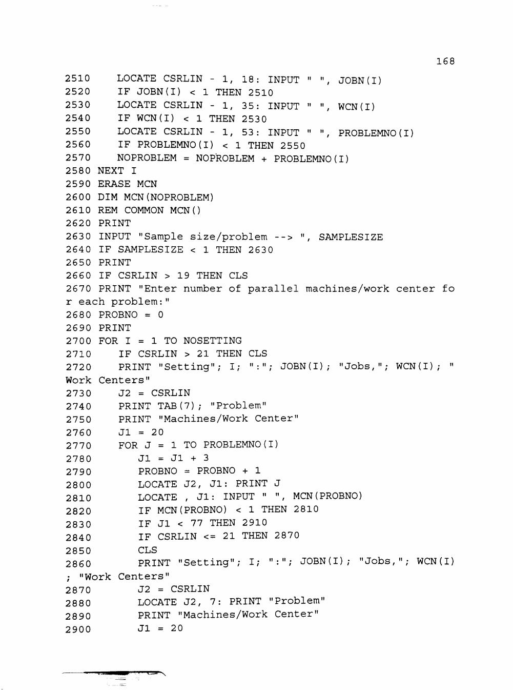
168

2510 LOCATE CSRLIN - 1, 18: INPUT " ", JOBN(I) 2520 IF JOBN(I) < 1 THEN 2510 253 0 LOCATE CSRLIN - 1, 35: INPUT " ", WCN(I) 254 0 IF WCN(I) < 1 THEN 253 0 2550 LOCATE CSRLIN - 1, 53: INPUT " ", PROBLEMNO(I) 2560 IF PROBLEMNO(I) < 1 THEN 2550 2570 NOPROBLEM = NOPROBLEM + PROBLEMNO(I) 2580 NEXT I 2590 ERASE MCN 2600 DIM MCN(NOPROBLEM) 2610 REM COMMON MCN() 2620 PRINT 263 0 INPUT "Sample size/problem --> ", SAMPLESIZE 2640 IF SAMPLESIZE < 1 THEN 2630 2650 PRINT 2660 IF CSRLIN > 19 THEN CLS 2670 PRINT "Enter number of parallel machines/work center fo r each problem:" 2680 PROBNO = 0 26 90 PRINT 2700 FOR I = 1 TO NOSETTING 2710 IF CSRLIN > 21 THEN CLS 272 0 PRINT "Setting"; I; ":"; JOBN(I); "Jobs,"; WCN(I); " Work Centers" 273 0 J2 = CSRLIN 2740 PRINT TAB(7); "Problem" 2750 PRINT "Machines/Work Center" 2760 Jl = 20 2770 FOR J = 1 TO PROBLEMNO(I) 2780 Jl = Jl + 3 2790 PROBNO = PROBNO + 1 28 0 0 LOCATE J2, Jl: PRINT J 2810 LOCATE , Jl: INPUT " ", MCN(PROBNO) 2820 IF MCN(PROBNO) < 1 THEN 2810 2830 IF Jl < 77 THEN 2910 2840 IF CSRLIN <= 21 THEN 2870 2850 CLS 2860 PRINT "Setting"; I; ":"; JOBN(I); "Jobs,"; WCN(I) ; "Work Centers" 2870 J2 = CSRLIN 2880 LOCATE J2, 7: PRINT "Problem" 2890 PRINT "Machines/Work Center"

2900 Jl = 20

'liJJB \

169 2910 NEXT J 292 0 NEXT I 2 93 0 SETTINGNO = 1 294 0 JOBS = JOBN(SETTINGNO) 2950 WCS = WCN(SETTINGNO) 2 960 SAMPLENO = 1 2970 GOSUB 4210 2980 GOSUB 4650 2990 PROBNO = 0 3 000 FOR I = 1 TO SETTINGNO - 1 3 010 PROBNO = PROBNO + PROBLEMNO(I) 3 02 0 NEXT I 3 03 0 PROBNOl = 1

3 04 0 PROBNO = PROBNO + 1

3 05 0 MCS = MCN(PROBNO)

3 06 0 GOSUB 42 6 0

3 070 METHODNO = 0

3 080 METHODNO = METHODNO + 1 3 090 ON METHODTYPE(METHODNO) GOTO 3 910, 3 920, 39

30, 3940, 3950, 3960, 3970

310 0 PROBNOl = PROBNOl + 1 3110 IF PROBNOl <= PROBLEMNO(SETTINGNO) THEN 3 04 0 312 0 SAMPLENO = SAMPLENO + 1 313 0 IF SAMPLENO <= SAMPLESIZE THEN 2 970 314 0 SETTINGNO = SETTINGNO + 1 3150 IF SETTINGNO > NOSETTING THEN 3530 ELSE 2940 3160 REM ********** Mixed Trend Random Samples ************* 3170 CHAINLINE$ = "MIX_TREND" 3180 CLS 3190 INPUT "Number of problems to be run --> ", NOPROBLEM 32 00 IF NOPROBLEM < 1 THEN 3190 3210 ERASE JOBN, MCN, WCN 3220 DIM JOBN(NOPROBLEM), MCN(NOPROBLEM), WCN(NOPROBLEM) 3230 REM COMMON JOBN(), MCN(), WCN() 3240 INPUT "Sample size/problem --> ", SAMPLESIZE 3250 IF SAMPLESIZE < 1 THEN 3240 3260 PRINT "Enter the problem size:" 3270 PRINT "Problem No. # of Jobs # of Work Centers # of Machines/Work Center" 3280 PRINT "

II

32 9 0 FOR I = 1 TO NOPROBLEM 33 00 LOCATE , 5: PRINT I

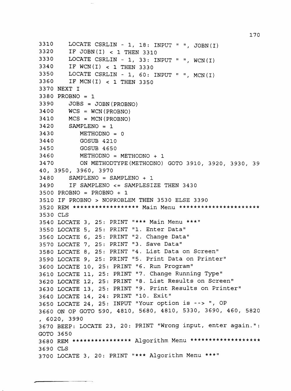
170

JOBN(I)

WCN(I)

MCN(I)

3310 LOCATE CSRLIN - 1, 18: INPUT " " 3320 IF JOBN(I) < 1 THEN 3310

3330 LOCATE CSRLIN - 1, 33: INPUT " " 3340 IF WCN(I) < 1 THEN 3330 3350 LOCATE CSRLIN - 1, 60: INPUT " " 3360 IF MCN(I) < 1 THEN 3350 3370 NEXT I 33 80 PROBNO = 1

33 90 JOBS = JOBN(PROBNO) 34 00 WCS = WCN(PROBNO) 3410 MCS = MCN(PROBNO) 3420 SAMPLENO = 1 343 0 METHODNO = 0 3440 GOSUB 4210 3450 GOSUB 4650 346 0 METHODNO = METHODNO + 1 3470 ON METHODTYPE(METHODNO) GOTO 3910, 3920, 3930, 39 40, 3950, 3960, 3970 3480 3490 3500 3510 3520 3530 354 0 LOCATE 3 550 LOCATE 3 56 0 LOCATE 3 570 LOCATE 3 58 0 LOCATE 3590 LOCATE 360 0 LOCATE 3 610 LOCATE 3 62 0 LOCATE 3 63 0 LOCATE 3 64 0 LOCATE 3 650 LOCATE

SAMPLENO = SAMPLENO + 1 IF SAMPLENO <= SAMPLESIZE THEN 343 0

PROBNO = PROBNO + 1 IF PROBNO > NOPROBLEM THEN 3 53 0 ELSE 33 90 REM ****************** Main Menu **********************

CLS "*** Main Menu ***" "1. Enter Data"

. Change Data"

. Save Data"

. List Data on Screen"

. Print Data on Printer" Run Program" Change Running Type" List Results on Screen" Print Results on Printer" Exit"

"Your option is --> ", OP 5680, 4810, 5330, 3690, 460, 5820

3, 5, 6, 7, 8, 9, 10,

11, 12, 13, 14, 24,

25 25 25 25 25 25 25 25 25 25 24 25

PRINT PRINT PRINT PRINT PRINT PRINT PRINT PRINT PRINT PRINT PRINT INPUT . 4810

"2 "3 "4 "5 "6. "7. "8. "9. "10

20: PRINT "Wrong input, enter again.":

3660 ON OP GOTO 590, , 6020, 3990 3670 BEEP: LOCATE 23, GOTO 3650 368 0 REM **************** Algorithm Menu *******************

3690 CLS 3 700 LOCATE 3, 20: PRINT "*** Algorithm Menu ***"

171

jo

6 7

20: 20: 20: 20: 20

PRINT "2. PRINT "3. PRINT "4. PRINT "5. PRINT "6

CDS_Sequence_priority" CDS_First_come_first_serve" LPT_List" Flexible Flow Line Loading" Flexible Flow Line Workload Ap

20: PRINT "7. LPT_CDS (Partially flexible jo

20 PRINT "8. Main menu" "CASE" THEN 3 870

3710 LOCATE 5, 20: PRINT "1. LPT_CDS (Completely flexible b route)" 3 72 0 LOCATE 373 0 LOCATE 3 74 0 LOCATE 8, 3750 LOCATE 9, 3760 LOCATE 10, proximation" 3 770 LOCATE 11, b route)" 3780 LOCATE 12, 3 790 IF RUNTYPE$ = 3 800 FOR I = 1 TO NOMETHOD 3 810 LOCATE 23, 20: PRINT "The"; I; "th method to be test ed is (1-7) "; 3 82 0 INPUT " --> ", METHODTYPE(I) 3 83 0 IF METHODTYPE(I) < 1 OR METHODTYPE(I) 3 84 0 LOCATE CSRLIN - 1, 55: PRINT " 3850 NEXT I 3860 GOTO 790 3870 LOCATE 24, 25: INPUT "Your option is --> " 3 880 ON METHODINPUT GOTO 3 910, 3 920, 3930, 3940 3970, 3530 3890 BEEP: LOCATE 23, 20: PRINT "Wrong input, enter again.": GOTO 3870 3 900 REM ************** Chain Sub_Programs *****************

> 8 THEN 3 810

METHODINPUT 3950, 3960,

3 910 METHOD$ 3 92 0 METHOD$ 3 93 0 METHOD$ 3 94 0 METHOD$ 3 950 METHOD$ 3 96 0 METHOD$ 3 970 METHOD$

LPT_CDS": CHAIN LOADDRIVE$ CDS_S": CHAIN LOADDRIVE$ + CDS_F": CHAIN LOADDRIVE$ + LPT_LIST": CHAIN LOADDRIVE$ + LPT LOAD": CHAIN LOADDRIVE$ +

+ "LPTFFS" "FFSFPCDS" "FFSFPCDS"

"LPTFFSl" "LPTFFS"

LPT_WLA": CHAIN LOADDRIVE$ + "LPTFFS" LPT CDSP": CHAIN LOADDRIVE$ + "LPTFFS"

******************** Goodbye * * * * * * * * * * * * * * * * * * * * * * 3980 REM 3990 CLS 4 00 0 LOCATE 10 20* PRINT "******************************" 4010 4020 4030 4040 4050 4060 4070

LOCATE LOCATE LOCATE LOCATE LOCATE KEY ON END

, 20 , 20 , 20 , 20 23

PRINT PRINT PRINT PRINT

II * * *

II * * *

II * * *

II * * *

Have a nice day!!!

* * * II

* * * II

* * * II

I I * * * * * * * * * * * * * * * * * * * * * * * * * * * * * * "

172

4080 REM ************** Continue Subroutine ****************

4090 LOCATE 24, 25: PRINT "< Press any key to continue ... > II

410 0 A$ = INKEY$ 4110 IF A$ = "" THEN 4100 412 0 RETURN

4130 REM *** Enter Problem Size(# of Jobs, Work Centers, & Parallel Machines) ** 414 0 CLS 4150 LOCATE 10, 25: INPUT "Number of jobs --> ", JOBS 4160 IF JOBS < 1 THEN 4150 4170 LOCATE 12, 25: INPUT "Number of work centers --> ", WCS 4180 IF WCS < 1 THEN 4170 4190 LOCATE 14, 25: INPUT "Number of parallel machines/work center --> ", MCS 4200 IF MCS < 1 THEN 4190 4210 WCSl = WCS + 1 422 0 ERASE PTM 4230 DIM PTM(JOBS, WCSl) 424 0 REM COMMON PTM() 4250 IF CHAINLINE$ = "MC_TREND" THEN RETURN 42 6 0 MCTN = MCS * WCS 42 70 ERASE COST, DEL, INDEX, INDEXl, INDEX2, JOBCONSIDER, JO BINMC, JOBMC, LOADOFMC, ORDER, PT, PTT 42 8 0 DIM COST(JOBS, JOBS), DEL(JOBS, WCS), INDEX(JOBS + 1 ) , INDEXl(JOBS + 1), INDEX2(JOBS) , JOBCONSIDER(MCS, WCSl), JQBI NMC(MCS, WCSl, JOBS), JOBMC(JOBS, WCS), LOADOFMC(MCTN), ORDE R(JOBS), PT(JOBS, MCTN), PTT(JOBS) 42 9 0 REM COMMON COST() , DEL() , INDEX() , INDEXl() , INDEX2() , JOBCONSIDER 0 , JOBINMCO, JOBMC () , LOADOFMC () , ORDER () , PT () , PTT() 43 0 0 RETURN 4310 REM **************** Keyboard Input ******************* 4320 GOSUB 4140 4330 CLS 4340 PRINT TAB(20); JOBS; "jobs,"; WCS; "work centers,"; MCS ; "parallel machines" 43 50 PRINT 4360 PRINT TAB(15); "Job No. Work Center No. P recessing Time" 4370 PRINT TAB(15) ; "

II

4380 FOR I = 1 TO JOBS

-««i

173

4390 PRINT TAB(17); I; 44 0 0 FOR J = 1 TO WCS 4410 LOCATE , 3 8 4420 PRINT J; TAB(57); 443 0 INPUT " ", PTM(I, J) 4440 IF PTM(I, J) < 0 THEN 4430 4450 NEXT J 44 6 0 NEXT I 4470 GOTO 4730 4480 REM ****************** File Input ********************* 4490 CLS 4500 LOCATE 10, 30: INPUT "File name --> ", FILENAME$ 4510 FILENAME$ = INDRIVE$ + FILENAME$ 452 0 OPEN FILENAME$ FOR INPUT AS #1 4530 LOCATE 23, 25: PRINT "Data is reading from <"; FILENAME

$; " > "

4540 INPUT #1, JOBS, WCS, MCS 4550 GOSUB 4210 456 0 FOR I = 1 TO JOBS 4570 FOR J = 1 TO WCS 4580 INPUT #1, PTM(I, J) 4590 NEXT J 4600 NEXT I 4610 CLOSE #1 4620 GOTO 4730 463 0 REM ********* Random Number Generator Input ***********

4640 GOSUB 4140 4 650 RANDOMIZE TIMER 4660 FOR I = 1 TO JOBS 4670 FOR J = 1 TO WCS 4680 PTMd, J) = INT(RND * 100) + 1 4690 NEXT J 4700 NEXT I 4710 GOTO 4730 4 72 0 REM **** Compute Total Processing Time for Each Job *** 473 0 FOR I = 1 TO JOBS 4740 PTMd, WCSl) = 0 4750 FOR J = 1 TO WCS 4760 PTMd, WCSl) = PTM (I, WCSl) + PTM (I, J)

4 770 NEXT J 4780 NEXT I 4 79 0 IF RUNTYPE$ = "SAMPLES" THEN RETURN ELSE 3 53 0 4800 REM ***** List Processing Time Matrix on Screen *******

174

4810 CLS 4820 IF JOBS < 20 THEN PSl = INT(JOBS / 2) ELSE PSl = 10 4830 IF WCS < 22 THEN 4870 4840 PS2 = 11 4850 JF = 22 4860 GOTO 4890 4870 PS2 = INT (WCS / 2)" 4880 JF = WCS 4890 LOCATE 11 - PSl: PRINT "Processing Time Matrix:"; JOBS; "jobs,"; WCS; "work centers, each having"; MCS; "parallel ma chines" 4900 JB = 1 4 910 PRINT 4920 LOCATE , 34 - 3 * PS2: PRINT "Job/Center "; 4 93 0 FOR J = JB TO JF 4940 PRINT USING "###"; J; 4950 NEXT J 4 96 0 PRINT 4 970 ROWCHECKER = 0 4980 FOR I = 1 TO JOBS 4990 LOCATE , 38 - 3 * PS2: PRINT USING "##"; I; 5000 PRINT " "; 5010 FOR J = JB TO JF 5020 PRINT USING "###"; PTM(I, J); 503 0 NEXT J 5040 PRINT 5050 ROWCHECKER = ROWCHECKER + 1 5060 IF ROWCHECKER < 20 THEN 5100 5070 GOSUB 4090 508 0 ROWCHECKER = 0 50 90 PRINT 5100 NEXT I 5110 IF JF >= WCS THEN 5150 5120 JB = JF + 1 5130 JF = WCS 5140 GOTO 4910 5150 GOSUB 4090 5160 IF OP <> 2 THEN 3530 5170 REM ****************** Data Change ******************** 5180 LOCATE 24, 14: INPUT "Number of processing times to be changed"; II 5190 IF II = 0 THEN 3530 5200 IF II < 0 OR II > JOBS * WCS THEN 5180

"'•". » H -Lx

175

5210 FOR 12 = 1 TO II 5220 LOCATE , 10: PRINT "The"; 12; 5230 INPUT "th data to be changed is for job ", I 5240 IF I < 1 OR I > JOBS THEN 5230 5250 LOCATE CSRLIN - 1, 56: INPUT "work center ", J 5260 IF J < 1 OR J > WCS THEN 5250 5270 PRINT TAB(20); "Old data -->"; PTM(I, J); TAB(40); 528 0 INPUT "New data --> ", PTM(I, J) 5290 IF PTMd, J) < 0 THEN 5280 5300 NEXT 12 5310 GOTO 4810 5320 REM *** Print Processing Time Matrix on Printer ******* 5330 IF WCS < 22 THEN 5370 5340 PS2 = 11 5350 JF = 22 5360 GOTO 5390 5370 PS2 = INT(WCS / 2) 5380 JF = WCS 5390 LPRINT 54 0 0 LPRINT 5410 LPRINT "Processing Time Matrix:"; JOBS; "jobs,"; WCS; " work centers, each having"; MCS; "parallel machines" 5420 JB = 1 543 0 LPRINT 5440 FOR I = 1 TO 34 - 3 * PS2 54 50 LPRINT " "; 54 6 0 NEXT I 5470 LPRINT "Job/Center ";

54 8 0 FOR J = JB TO JF

5490 LPRINT USING "###"; J;

5500 NEXT J

5510 LPRINT

552 0 FOR I = 1 TO JOBS 5530 FOR II = 1 TO 38 - 3 * PS2

554 0 LPRINT " ";

5550 NEXT II 5560 LPRINT USING "##"; I;

5570 LPRINT " ";

5580 FOR J = JB TO JF

5590 LPRINT USING "###"; PTM(I, J ) ;

5600 NEXT J

5610 LPRINT

5620 NEXT I

-^tx

176

5630 IF JF >= WCS THEN 3530 5640 JB = JF + 1 5650 JF = WCS 5660 GOTO 5430 5670 REM ***************** Save File *********************** 5680 CLS 56 90 LOCATE 10, 30: INPUT "File name --> ", FILENAME$ 5700 FILENAME$ = SAVEDRIVE$ + FILENAME$ 5710 OPEN FILENAME$ FOR OUTPUT AS #1 5720 LOCATE 23, 20: PRINT "Data is saving to <"; FILENAME$; II ^ II

573 0 PRINT #1, JOBS, WCS, MCS 574 0 FOR I = 1 TO JOBS 5750 FOR J = 1 TO WCS 5760 PRINT #1, PTMd, J); 5770 NEXT J 5780 NEXT I 5790 CLOSE #1 5800 GOTO 3530 5810 REM ************ List Results on Screen *************** 5820 CLS 583 0 IF RUNTYPE$ = "SAMPLES" THEN 5870 5840 LOCATE 12: PRINT "Method/# of Jobs/Work Centers/Paralle 1 Machines/Makespan/CPU Time (Seconds)" 5850 LOCATE 14: PRINT METHOD$; JOBS; WCS; MCS; FFSMAKESPAN;

CPUTIME$; " ("; CPUS; " ) " 5860 GOTO 5990 5870 OPEN "FFSOUT.DAT" FOR INPUT AS #1 588 0 II = NOPROBLEM * SAMPLESIZE * NOMETHOD 5890 PRINT "Method/# of Jobs/Work Centers/Parallel Machines/ Makespan/CPU Time (Seconds)" 5900 FOR I = 1 TO II 5910 INPUT #1, METHOD$, JOBS, WCS, MCS, FFSMAKESPAN, CPUS

5920 PRINT METHOD$, JOBS, WCS, MCS, FFSMAKESPAN, CPUS 5930 IF CSRLIN < 24 THEN 5970 5940 GOSUB 4090 5950 CLS 5960 PRINT "Method/# of Jobs/Work Centers/Parallel Machin es/Makespan/CPU Time (Seconds)" 5970 NEXT I 5980 CLOSE #1 5990 GOSUB 4090 6000 GOTO 3 53 0

^tJ""*W .1.-'

177

6010 REM ************ Print Results on Printer ************* 602 0 LPRINT 6030 LPRINT "Method/# of Jobs/Work Centers/Parallel Machines /Makespan/CPU Time (Seconds)" 604 0 LPRINT 6050 IF RUNTYPE$ = "SAMPLES" THEN 6080 6060 LPRINT METHOD$; JOBS; WCS; MCS; FFSMAKESPAN; CPUTIME$; " ("; CPUS; " ) " 6070 GOTO 3530 6 08 0 OPEN "FFSOUT.DAT" FOR INPUT AS #1 6090 II = NOPROBLEM * SAMPLESIZE * NOMETHOD 6100 FOR I = 1 TO II 6110 INPUT #1, METHOD$, JOBS, WCS, MCS, FFSMAKESPAN, CPUS 612 0 LPRINT METHOD$, JOBS, WCS, MCS, FFSMAKESPAN, CPUS 613 0 NEXT I 6140 CLOSE #1 6150 GOTO 3530

w;.,. ||J >j. !» ,s^

178

10 REM ******* Longest Processing Time First *************** 20 REM ********* Chained by <FLEXFLOW.BAS> ***************** 3 0 COMMON CHAINLINE$, COST(), CPUS, CPUTIME$, DEL(), FFSMAKE SPAN, INDEX 0, INDEXl0, INDEX2() , INDRIVE$, JOBCONSIDER0 , JOBINMCO, JOBMC0, JOBN(), JOBS, LOADDRIVE$, LOADOFMC0, LO ADOFNECK, MCN(), MCS, MCTN, METHODNO, METHODTYPE(), METHOD$ 40 COMMON NECKMC, NOMETHOD, NOPROBLEM, NOSETTING, ORDER 0 , 0 UTDRIVE$, PROBLEMNOO, PROBNO, PROBNOl, PT () , PTM () , PTT () , RUNTYPE$, SAMPLENO, SAMPLESIZE, SAVEDRIVE$, SETTINGNO, TIMEl , WCNO , WCS, WCSl 50 DIM ORDERLPT(JOBS, WCSl) 60 REM * Arrange Jobs in Nonincreasing Processing Time Order 70 REM *** ORDERLPTd, j) =ith job in LPT sequence at w/c j, I NDEX(i)=processing time of ith job in LPT sequence ********* 8 0 TIME$ = "00:00:00" 90 TIMEl = TIMER 100 CLS 110 IF METHOD$ = "LPT_LIST" THEN IWCS = WCSl ELSE IWCS = 1 12 0 IF METHOD$ = "LPT_CDS" OR METHOD$ = "LPT_CDSP" THEN IWCS 1 = WCSl ELSE IWCSl = WCS 13 0 FOR I = IWCS TO IWCSl 14 0 FOR J = 1 TO JOBS 150 INDEX(J) = PTM(J, I) 160 ORDERLPT(J, I) = J

170 NEXT J 180 Kl = JOBS - 1 190 FOR K = Kl TO 1 STEP -1 200 FOR J = 1 TO K 210 IF INDEX(J) >= INDEX(J + 1) THEN 240 220 SWAP INDEX(J), INDEX(J + 1) 230 SWAP ORDERLPT(J, I), ORDERLPT(J + 1, I)

24 0 NEXT J 250 NEXT K 260 NEXT I 270 IF WCS > 1 THEN 320

2 80 IWCS = 1 290 IWCSl = 1 300 REM ********** Parallel Machine Assignment ************* 310 REM *** JOBINMC(i,j,k)=kth job on m/c i, w/c j, JOBCONSI DER(i,j)=# of jobs on m/c i, w/c j, LOADOFMC(i)=cumulative w ork load in m/c i ****************************************** 320 FOR I = IWCS TO IWCSl 33 0 FOR J = 1 TO MCS

179

340 JOBCONSIDER(J, I) = 0 3 50 LOADOFMC(J) = 0 360 NEXT J

370 FOR J = 1 TO JOBS 380 COST = 999999! 3 90 FOR K = 1 TO MCS

400 IF LOADOFMC(K) >= COST THEN 430 410 COST = LOADOFMC(K) 42 0 NEXTMC = K 43 0 NEXT K

440 LOADOFMC(NEXTMC) = LOADOFMC(NEXTMC) + PTM(ORDERLPT (J, I), I)

450 JOBCONSIDER(NEXTMC, I) = JOBCONSIDER(NEXTMC, I) + 1

460 JOBINMC(NEXTMC, I, JOBCONSIDER(NEXTMC, I)) = ORDER LPT(J, I) 470 NEXT J 480 NEXT I 490 IF WCS > 1 THEN 870

500 REM *** When only one work center is under considered ** 510 FFSMAKESPAN = 0 52 0 FOR J = 1 TO MCS

530 IF LOADOFMC(J) >= FFSMAKESPAN THEN FFSMAKESPAN = LOAD OFMC(J) 54 0 NEXT J 550 CPUTIME$ = TIME$ 560 TIME2 = TIMER 570 CPUS = INTdOOOO * (TIME2 - TIMED) / 10000 580 REM ******* Print Parallel Machine Assignment ********** 590 PRINT "*** Flexible Flowshop Scheduling Problem solved b y "; METHOD$ 600 PRINT TAB(5); JOBS; "jobs,"; WCS; "work centers, each ha ving"; MCS; "parallel machines" 610 PRINT "Parallel machine assignment for:" 62 0 FOR I = IWCS TO IWCSl 630 PRINT "Work center"; I; ":" 64 0 FOR J = 1 TO MCS 650 JOBCONSIDER = JOBCONSIDER(J, I) 66 0 PRINT " Machine"; J; ":"; 670 FOR K = 1 TO JOBCONSIDER 680 PRINT JOBINMC(J, I, K ) ; 690 IF K = JOBCONSIDER THEN PRINT ELSE PRINT "-"; 700 NEXT K

180

710 NEXT J 72 0 NEXT I

730 PRINT "CPU time = "; CPUTIME$; " ("; CPUS; "seconds)" 740 PRINT "Makespan ="; FFSMAKESPAN 750 REM *** Save Makespan and CPU Time on FFSOUT.DAT ******* 760 OPEN OUTDRIVE$ + "FFSOUT.DAT" FOR APPEND AS #1 770 PRINT #1, METHOD$, JOBS; WCS; MCS, FFSMAKESPAN, CPUS 780 CLOSE #1 790 IF RUNTYPE$ = "SAMPLES" THEN 85 0 800 REM ************** Continue Subroutine ***************** 810 LOCATE 24, 25: PRINT "< Press any key to continue ... >" ,

82 0 A$ = INKEY$ 83 0 IF A$ = "" THEN 820 84 0 REM ************ Chain FLEXFLOW Program **************** 85 0 CHAIN LOADDRIVE$ + "FLEXFLOW" 86 0 REM ************** Chain Sub-Programs ****************** 870 IF METHOD$ = "LPT_CDS" OR METHOD$ = "LPT_CDSP" THEN CHAI N LOADDRIVE$ + "FFSCDS" 880 CHAIN LOADDRIVE$ + "FFLLOAD"

•s

181

10 REM *** Longest Processing Time for CDS_1 Algorithm ***** 2 0 REM ************ Chained by <FLEXFLOW.BAS> ************** 3 0 COMMON CHAINLINE$, COST(), CPUS, CPUTIME$, DEL(), FFSMAKE SPAN, INDEX(), INDEXl(), INDEX2(), INDRIVE$, JOBCONSIDER(), JOBINMCO, JOBMC 0, JOBN () , JOBS, LOADDRIVE$, LOADOFMC 0 , LO ADOFNECK, MCN(), MCS, MCTN, METHODNO, METHODTYPE(), METHOD$ 4 0 COMMON NECKMC, NOMETHOD, NOPROBLEM, NOSETTING, ORDER 0 , 0 UTDRIVE$, PROBLEMNO(), PROBNO, PROBNOl, PT(), PTM(), PTT(), RUNTYPE$, SAMPLENO, SAMPLESIZE, SAVEDRIVE$, SETTINGNO, TIMEl , WCNO , WCS, WCSl 50 DIM ORDERLPT(JOBS, WCSl) 60 TIME$ = "00:00:00" 70 TIMEl = TIMER 8 0 CLS 90 REM ************** Compute Dummy processing time for each iob *************** 100 REM *** ORDERLPT(i,WCSl)=ith job in LPT, PTT(i)=total pr ocessing time of ith job in LPT **************************** 110 FOR I = 1 TO JOBS 12 0 PTT(I) = 0 13 0 FOR J = 1 TO WCS 14 0 PTT(I) = PTT(I) + PTMd, J) 150 NEXT J 16 0 ORDERLPTd, WCSl) = I 170 NEXT I 180 REM ****** Longest Processing Time First Sequence ****** 190 Kl = JOBS - 1 200 FOR K = Kl TO 1 STEP -1 210 FOR J = 1 TO K 220 IF PTT(J) >= PTT(J + 1) THEN 250 230 SWAP PTT(J), PTT(J + 1) 240 SWAP ORDERLPT(J, WCSl), ORDERLPT(J + 1, WCSl)

250 NEXT J 26 0 NEXT K 270 FOR I = 1 TO JOBS 280 INDEX (I) = ORDERLPTd, WCSl)

290 NEXT I 300 REM *** jobinmc(i,WCSl, j)=jth job in m/c i, jobconsider( i,WCSl)=# of jobs in m/c i, LOADOFMC(i)=dummy cumulative wor kload in m/c i ********************************************* 310 FOR J = 1 TO MCS 320 JOBCONSIDER(J, WCSl) = 0 330 LOADOFMC(J) = 0

""•iP

182 34 0 NEXT J 350 FOR J = 1 TO JOBS 3 60 COST = 999999! 370 FOR K = 1 TO MCS 380 IF LOADOFMC(K) >= COST THEN 410 3 90 COST = LOADOFMC(K) 4 00 NEXTMC = K 410 NEXT K

420 LOADOFMC(NEXTMC) = LOADOFMC(NEXTMC) + PTT(J) 430 JOBCONSIDER(NEXTMC, WCSl) = JOBCONSIDER(NEXTMC, WCSl) + 1

440 JOBINMC(NEXTMC, WCSl, JOBCONSIDER(NEXTMC, WCSl)) = OR DERLPT(J, WCSl) 450 NEXT J 46 0 IF WCS > 1 THEN CHAIN LOADDRIVE$ + "FFSCDSl" 470 REM *** When only one work center is under considered ** 480 FFSiyiAKESPAN = 0 490 FOR J = 1 TO MCS 500 IF LOADOFMC(J) >= FFSMAKESPAN THEN FFSMAKESPAN = LOAD OFMC(J) 510 NEXT J 52 0 CPUTIME$ = TIME$ 53 0 TIME2 = TIMER 540 CPUS = INTdOOOO * (TIME2 - TIMEl)) / 10000 550 REM ********* Print Parallel Machine Assignment ******** 560 PRINT "*** Flexible Flowshop Scheduling Problem solved b y "; METHOD$ 570 PRINT TAB(5); JOBS; "jobs"; WCS; "work centers, each hav ing"; MCS; "parallel machines" 580 PRINT "Parallel machine assignment:" 590 FOR J = 1 TO MCS 600 JOBCONSIDER = JOBCONSIDER(J, WCSl) 610 PRINT " Machine"; J; ":"; 62 0 FOR K = 1 TO JOBCONSIDER 630 PRINT JOBINMC(J, WCSl, K); 64 0 IF K = JOBCONSIDER THEN PRINT ELSE PRINT "-"; 650 NEXT K 660 NEXT J 670 PRINT "CPU time = "; CPUTIME$; " ("; CPUS; "seconds)" 680 PRINT "Makespan ="; FFSMAKESPAN 690 REM *** Save Makespan and CPU Time on FFSOUT.DAT ******* 70 0 OPEN OUTDRIVE$ + "FFSOUT.DAT" FOR APPEND AS #1 710 PRINT #1, METHOD$, JOBS; WCS; MCS, FFSMAKESPAN, CPUS

^

183

720 CLOSE #1 73 0 IF RUNTYPE$ = "SAMPLES" THEN 790 740 REM ************** Continue Subroutine ***************** 750 LOCATE 24, 25: PRINT "< Press any key to continue ... >"

760 A$ = INKEY$ 770 IF A$ = "" THEN 760 780 REM ************* Chain FLEXFLOW Program *************** 790 CHAIN LOADDRIVE$ + "FLEXFLOW"

AM-

184

10 REM ******** Flexible Flowshop (CDS Algorithm) ********** 2 0 REM ********** Chained by <LPTFFS.BAS> ****************** 3 0 COMMON CHAINLINE$, COST(), CPUS, CPUTIME$, DEL(), FFSMAKE SPAN, INDEX 0 , INDEXl0, INDEX2() , INDRIVE$, JOBCONSIDER() , JOBINMCO, JOBMC 0 , JOBN () , JOBS, LOADDRIVE$, LOADOFMC () , LO ADOFNECK, MCN(), MCS, MCTN, METHODNO, METHODTYPE(), METHOD$ 4 0 COMMON NECKMC, NOMETHOD, NOPROBLEM, NOSETTING, ORDER 0 , O UTDRIVE$, PROBLEMNOO, PROBNO, PROBNOl, PT () , PTM () , PTT () , RUNTYPE$, SAMPLENO, SAMPLESIZE, SAVEDRIVE$, SETTINGNO, TIMEl , W C N O , WCS, WCSl 50 CLS 60 DIM IDX(JOBS, 2 ) , IDXl(JOBS), IPLACE(JOBS, 2 ) , V(JOBS, 2) , VEC(JOBS) 70 DIM FLAG(MCS), FTIME(JOBS, WCS), QUEAVE(WCS), QUEMAX(WCS1 1 ) , STIME(JOBS, WCS), STIMEMC(MCS, WCS) 8 0 REM *** FFSMAKESPAN=temporary best makespan, FFSWC=w/c FF SMAKESPAN occurs at, COST=min makespan from CDS for m/c i, J OBCONSIDERd, j) =JOBCONSIDER=# of jobs considered in m/c i, w /c i ******************************************************* 90 REM *** INDEX(k)=JOBINMC(i,j,k)=kth job on m/c i, w/c j, V(i,j)=dummy processing time of ith job at jth dummy w/c, QU EMAX(i)=maxmin makespan obtaines at w/c i ****************** 100 FFSMAKESPAN = 99999! 110 FOR IW = 1 TO WCSl 12 0 QUEMAX(IW) = 0 13 0 FOR R = 1 TO MCS 140 COST = 99999! 150 JOBCONSIDER = JOBCONSIDER(R, IW) 160 FOR I = 1 TO JOBCONSIDER 170 INDEXd) = JOBINMC(R, IW, I) 180 V d , 1) = 0 190 V d , 2) = 0 200 NEXT I 210 NS = WCS - 1 22 0 FOR ICY = 1 TO NS 230 GOSUB 910 24 0 REM *** Compute Makespan when Running CDS ************** 250 FOR I = 1 TO JOBCONSIDER 260 FOR J = 1 TO WCS 270 K = INDEX(ORDER(I)) 280 IF DELd, J - 1) <= DELd - 1, J) THEN DE L d , J) = DELd - 1, J) + PTM(K, J) ELSE DEL (I, J) = DEL (I, J - 1) + PTM(K, J)

185

290 NEXT J 3 00 NEXT I

310 IF DEL(JOBCONSIDER, WCS) >= COST THEN 360 32 0 FOR I = 1 TO JOBCONSIDER 330 IDXld) = INDEX (ORDER (I) ) 34 0 NEXT I

350 COST = DEL(JOBCONSIDER, WCS)

36 0 NEXT ICY 3 70 FOR I = 1 TO JOBCONSIDER 380 JOBINMC(R, IW, I) = IDXl(I) 3 90 NEXT I 4 00 IF COST > QUEMAX(IW) THEN QUEMAX(IW) = COST 410 NEXT R 42 0 IF QUEMAX(IW) > FFSMAKESPAN THEN 450 43 0 FFSMAKESPAN = QUEMAX(IW) 440 FFSWC = IW 4 50 NEXT IW 46 0 REM *** Impose chosen whole job sequence into correspond ing m/c at every w/c 470 FOR I = 1 TO WCS 480 IF I = FFSWC THEN 550 490 FOR J = 1 TO MCS 500 JOBCONSIDER(J, I) = JOBCONSIDER(J, FFSWC) 510 FOR K = 1 TO JOBCONSIDER(J, I) 520 JOBINMC(J, I, K) = JOBINMC(J, FFSWC, K) 53 0 NEXT K 54 0 NEXT J 550 NEXT I 560 GOSUB 2690 570 CPUTIME$ = TIME$ 580 TIME2 = TIMER 590 CPUS = INTdOOOO * (TIME2 - TIMED) / 10000 600 REM **************** Print Results ********************* 610 PRINT "*** Flexible Flowshop (LPT_CDS Algorithm) "; 620 IF METHOD$ = "LPT_CDS" THEN PRINT "(Complete Flexible Job Route) ***" ELSE PRINT "(Partial Flexible Job Route) *** II

630 PRINT TAB(5); JOBS; "jobs,"; WCS; "work centers, each ha ving"; MCS; "parallel machines" 640 PRINT "Job (Start time. Finish time):" 650 FOR I = 1 TO WCS 660 PRINT "Work Center"; I; ": " 6 7 0 FOR J = 1 TO MCS

^i9mma " ^

^ . /

186

680 PRINT " Machine"; J; ":"; 6 90 JOBCONSIDER = JOBCONSIDER(J, I) 700 FOR K = 1 TO JOBCONSIDER 710 Kl = JOBINMC(J, I, K) 720 PRINT Kl; "("; STIME(K1, I); ","; FTIME(K1, I); II ) ,1 .

730 NEXT K 74 0 PRINT 750 NEXT J 76 0 NEXT I 770 PRINT "CPU time = "; CPUTIME$; " ("; CPUS; "seconds)" 780 PRINT "Makespan ="; FFSMAKESPAN 790 REM *** Save Makespan and CPU Time on FFSOUT.DAT ******* 80 0 OPEN OUTDRIVE$ + "FFSOUT.DAT" FOR APPEND AS #1 810 PRINT #1, METHOD$, JOBS; WCS; MCS, FFSMAKESPAN, CPUS 82 0 CLOSE #1 83 0 IF RUNTYPE$ = "SAMPLES" THEN 890 84 0 REM ************** Continue Subroutine ***************** 850 LOCATE 24, 25: PRINT "< Press any key to continue ... >"

86 0 A$ = INKEY$ 870 IF A$ = "" THEN 860 880 REM ************* Chain FLEXFLOW Program *************** 890 CHAIN LOADDRIVE$ + "FLEXFLOW" 900 REM **************** CDS Algorithm ********************* 910 I = WCS - ICY + 1 920 REM *** Arrange jobs in non-decreasing processing time o rder ******************************************************* 93 0 REM *** IPLACE(i,j)=the order of job i at jth dummy w/c, IDX(i,j)=the ith job at jth dummy w/c ********************** 94 0 FOR L = 1 TO JOBCONSIDER 950 V(L, 1) = V(L, 1) + PTM(INDEX(L), ICY) 960 V(L, 2) = V(L, 2) + PTM(INDEX(L), I)

970 NEXT L 980 FOR J = 1 TO 2 990 FOR L = 1 TO JOBCONSIDER 1000 VEC(L) = V(L, J) 1010 IDX(L, J) = L 1020 NEXT L 103 0 K = JOBCONSIDER - 1 104 0 FOR L = K TO 1 STEP -1 1050 FOR I = 1 TO L 1060 IF VECd) <= VECd + 1) THEN 1090

^ /

187

1070 SWAP IDXd, J), IDXd + 1, J) 1080 SWAP VECd), VECd + 1) 10 9 0 NEXT I 110 0 NEXT L 1110 FOR L = 1 TO JOBCONSIDER 1120 IPLACE(IDX(L, J), J) = L 113 0 NEXT L 114 0 NEXT J 1150 REM *** Sequencing ************************************ 1160 JO = 1 1170 KO = 1 1180 Jl = 1 1190 J2 = JOBCONSIDER 120 0 FOR I = 1 TO JOBCONSIDER 1210 REM *** Find the job with the smallest processing time 1220 MO = IDX(JO, 1) 1230 IF MO >= 0 THEN 1260 124 0 JO = JO + 1 1250 GOTO 1220 1260 NO = IDX(KO, 2) 1270 IF NO >= 0 THEN 1300 12 8 0 KO = KO + 1 1290 GOTO 1260 1300 IF I = JOBCONSIDER THEN 2210 1310 W = V(MO, 1) - V(NO, 2) 1320 IF W < 0 THEN 1530 1330 IF W > 0 THEN 2100 134 0 REM *** Tie breaker (when there is a tie between two du mmy w/c) *************************************************** 1350 IF ICY = 1 THEN 1440 1360 IH = ICY - 1 1370 FOR MP = 1 TO IH 13 8 0 MR = ICY - MP + 1 13 90 MS = WCS - MR + 1 1400 MM = PTM(INDEX(MO), MR) - PTM(INDEX(NO), MS) 1410 IF MM < 0 THEN 1530 1420 IF MM > 0 THEN 2100 143 0 NEXT MP 1440 IH = ICY + 1 1450 IF IH = WCS THEN 1530 14 6 0 FOR MR = IH TO NS 14 70 MS = WCS - MR + 1 1480 MN = PTM(INDEX(MO), MR) - PTM(INDEX(NO), MS)

188

1490 IF MN < 0 THEN 1530 1500 IF MN > 0 THEN 2100 1510 NEXT MR 1520 REM *** Sequencing when the smallest processing time is at 1st dummy w/c ******************************************* 1530 IC = JO + 1 1540 MR = IDXdC, 1) 1550 IF MR >= 0 THEN 1600 1560 IC = IC + 1 1570 NIC = JOBCONSIDER - IC 1580 IF NIC < 0 THEN 2210 1590 IF NIC >= 0 THEN 1540 1600 A = V(MO, 1) 1610 B = V(MR, 1) 1620 AB = A - B 1630 IF AB >= 0 THEN 1750 1640 REM *** Assign the chosen job to the earliest available position *************************************************** 1650 ORDER(Jl) = MO 1660 Jl = Jl + 1 1670 MP = IPLACE(MO, 1) 1680 IDX(MP, 1) = -7 1690 MP = IPLACE(MO, 2) 1700 IDX(MP, 2) = -7 1710 JO = JO + 1 1720 GOTO 2650 1730 REM ***Tie breaker (when there is a tie at the 1st dumm y w/c) ***************************************************** 1740 REM *** Search backward to break the tie ************** 1750 AA = V(MO, 1) 1760 BB = V(MR, 1) 1770 IH = ICY - 1 1780 IF IH = 0 THEN 1880 1790 FOR IC = 1 TO IH 1800 IJ = ICY + 1 - IC 1810 AA = AA - PTM(INDEX(MO), IJ) 1820 BB = BB - PTM(INDEX(MR), IJ) 1830 AB = AA - BB 1840 IF AB < 0 THEN 1650 1850 IF AB > 0 THEN 2020 I860 NEXT IC 1870 REM *** Search forward to break the tie *************** 1880 AA = V(MO, 1)

X

+

+ -

0 0

PTM(INDEX(MO), PTM(INDEX(MR), BB THEN 1650 THEN 202 0

IC) IC)

189 1890 BB = V(MR, 1) 1900 IH = ICY + 1 1910 IF IH = WCS THEN 1990 1920 FOR IC = IH TO NS 1930 AA = AA 1940 BB = BB 1950 AB = AA 1960 IF AB < 1970 IF AB > 1980 NEXT IC 1990 AB = PTM(INDEX(MO), WCS) - PTM(INDEX(MR), WCS) 2000 IF AB >= 0 THEN 1650 2010 REM *** Assign the chosen job to the earliest available position *************************************************** 2020 ORDER(Jl) = MR 2030 MP = IPLACE(MR, 2) 2040 IDX(MP, 2) = -7 2050 MP = IPLACE(MR, 1) 2060 IDX(MP, 1) = -7 2070 Jl = Jl + 1 2080 GOTO 2650 2090 REM *** Sequencing when the smallest processing time is at 2nd dummy w/c ******************************************* 2100 IC = KO + 1 2110 MR = IDXdC, 2) 2120 IF MR >= 0 THEN 2170 2130 IC = IC + 1 214 0 NIC = JOBCONSIDER - IC 2150 IF NIC < 0 THEN 2210 2160 IF NIC >= 0 THEN 2110 2170 A = V(NO, 2) 2180 B = V(MR, 2) 2190 IF A - B >= 0 THEN 2310 2200 REM *** Assign the chosen job to the latest available p OSition **************************************************** 2210 ORDER(J2) = NO 2220 J2 = J2 - 1 2230 MP = IPLACE(NO, 1) 2240 IDX(MP, 1) = -7 2250 MP = IPLACE(NO, 2) 2260 IDX(MP, 2) = -7 2270 KO = KO + 1 2280 GOTO 2650

^ /

190

22 90 REM *** Tie breaker (when there is a tie at the 2nd dum my w/c) ****************************************************

2300 REM *** Search backward to break the tie ************** 2310 AA = V(NO, 2) 2320 BB = V(MR, 2) 2330 IH = ICY - 1 2340 IF IH = 0 THEN 2440 2350 FOR IC = IH TO 1 STEP -1 2360 IJ = WCS - IC 2370 AA = AA - PTM(INDEX(NO), IJ) 2380 BB = BB - PTM(INDEX(MR), IJ) 2390 AB = AA - BB 2400 IF AB < 0 THEN 2210 2410 IF AB > 0 THEN 2590 2420 NEXT IC 2430 REM *** Search forward to break the tie *************** 2440 AA = V(NO, 2) 2450 BB = V(MR, 2) 2460 IH = ICY + 1 2470 IF IH = WCS THEN 2560 24 8 0 FOR IC = IH TO NS 2490 IJ = WCS - IC + 1 2500 AA = AA 2510 BB = BB 2520 AB = AA 2530 IF AB < 2540 IF AB > 2550 NEXT IC 2560 AB = PTM(INDEX(MO), 1) - PTM(INDEX(MR), 1) 2570 IF AB >= 0 THEN 2210 2580 REM *** Assign the chosen job to the latest available p OSition **************************************************** 2590 ORDER(J2) = MR 2600 J2 = J2 - 1 2610 MP = IPLACE(MR, 1) 2620 IDX(MP, 1) = -7 2630 MP = IPLACE(MR, 2) 2640 IDX(MP, 2) = -7 2650 NEXT I 266 0 RETURN 2 670 REM ******************* Timing ************************ 2680 REM *** STIMEMCd, j) =start time on m/c i, w/c j, STIME ( i,j)/FTIME(i,j)=start/finish time of job i at w/c j, MAXMC/M

+

+ -

0 0

PTM(INDEX(NO), PTM(INDEX(MR), BB THEN 2210 THEN 2590

IJ) IJ)

191

INMC=max/min workspan m/c, FLAG=0/1=jobs moved from maxmc to minmc no/yes, FLAG(j)=0/l=m/c j adjusted no/yes ************ 2690 FOR J = 1 TO MCS 2700 FLAG(J) = 0 2710 FOR I = 1 TO WCS 2720 STIMEMC(J, I) = 0 2730 NEXT I 274 0 NEXT J 2750 FOR I = 1 TO JOBS 2760 FTIMEd, 0) = 0 2770 NEXT I 2 78 0 FOR I = 1 TO WCS 2790 REM *** Set up temporary start/finish time for jobs on m/c j, w/c i *********************************************** 2800 FOR J = 1 TO MCS 2810 Jl = JOBCONSIDER(J, I) 2820 FOR K = 1 TO Jl 2830 Kl = JOBINMC(J, I, K) 2840 IF FTIME(Kl, I - 1) > STIMEMC(J, I) THEN STIME MC(J, I) = FTIME(K1, I - 1) 2850 STIME(Kl, I) = STIMEMC(J, I) 2860 FTIME(Kl, I) = STIME(Kl, I) + PTM(K1, I) 2870 STIMEMC(J, I) = FTIME(K1, I) 2880 NEXT K 2890 NEXT J 2 90 0 IF METHOD$ = "LPT_CDSP" THEN 3 310 2 910 REM *** Balance workspans among m/cs ******************

2 92 0 FOR K2 = 1 TO MCS

2 93 0 COST = -1

2 94 0 FOR J = 1 TO MCS 2950 IF FLAG(J) = 1 OR STIMEMC(J, I) <= COST THEN 2

980

2960 COST = STIMEMC(J, I)

2970 MAXMC = J

2 980 NEXT J 2 990 COST = 99 9999! 3000 FOR J = 1 TO MCS 3010 IF FLAG(J) = 1 OR STIMEMC(J, I) >= COST THEN 3 040 3020 COST = STIMEMC(J, I) 3030 MINMC = J 3 04 0 NEXT J 3050 IF MAXMC = MINMC THEN 3310

"X

192

3060 FLAG = 0 3 070 REM *** Move jobs from m/c with max workspan to m/c wit h min workspan *********************************************

3080 FOR J = 1 TO JOBCONSIDER(MAXMC, I) 3090 IF STIME(JOBINMC(MAXMC, I INMC, I) THEN 3270 3100 IF FTIME (-JOBINMC (MAXMC, I JOBINMC(MAXMC, I, J), I) THEN 3270

J),

J),

I) <= STIMEMC(M

I - 1) = STIME(

3110 3120 3130 3140 3150 3160 D) 3170 3180 3190 I, J) 3200 3210

FLAG = 1 J2 = JOBCONSIDER(MAXMC, I) K = JOBCONSIDER(MINMC, I) JOBCONSIDER(MINMC, I) = K + JOBCONSIDER(MAXMC, I) = J -JOBMOVE = JOBINMC(MAXMC, I,

- J + 1

J2 1 JOBCONSIDER(MAXMC,

STIMEMC(MAXMC, I) = FTIME(JOBMOVE, I) FOR Jl = 1 TO J2

JOBINMC(MINMC, I, K + Jl) = JOBINMC(MAXMC,

K + Jl) STIMEMC(MINMC, I) TH

Kl = JOBINMC(MINMC, I IF FTIME(Kl, I - 1) >

EN STIMEMC(MINMC, I) = FTIME(Kl, I - 1) 3220 STIME(Kl, I) = STIMEMC(MINMC, I) 3230 FTIME(K1, I) = STIME(K1, I) + PTM(K1, I) 3240 STIMEMC(MINMC, I) = FTIME(Kl, I) 3250 J = J + 1 326 0 NEXT Jl 3270 NEXT J 3280 IF FLAG = 1 THEN 2930 3290 FLAG(MAXMC) = 1 33 00 NEXT K2 3310 FOR J = 1 TO MCS 3320 FLAG(J) = 0 333 0 NEXT J 3340 NEXT I 335 0 IF METHOD$ = "LPT_CDSP" THEN RETURN 33 60 REM *********** Compute FFS_CDS Makespan ************** 33 70 FFSMAKESPAN = 0 3380 FOR I = 1 TO MCS 33 90 IF STIMEMCd, WCS) > FFSMAKESPAN THEN FFSMAKESPAN = STIMEMCd, WCS) 34 0 0 NEXT I 3410 RETURN

fWtOf ^\

193

10 REM *** Flexible Flowshop (CDS Algorithm) (Flow-Para Appr oach) ****************************************************** 2 0 REM ************* Chained by <FLEXFLOW.BAS> ************* 3 0 COMMON CHAINLINE$, COST(), CPUS, CPUTIME$, DEL(), FFSMAKE SPAN, INDEX(), INDEXl(), INDEX2(), INDRIVE$, JOBCONSIDER(), JOBINMCO, JOBMC 0, JOBN () , JOBS, LOADDRIVE$, LOADOFMC () , LO ADOFNECK, MCN(), MCS, MCTN, METHODNO, METHODTYPE(), METHOD$ 4 0 COMMON NECKMC, NOMETHOD, NOPROBLEM, NOSETTING, ORDER(), O UTDRIVE$, PROBLEMNOO, PROBNO, PROBNOl, PT () , PTM () , PTT () , RUNTYPE$, SAMPLENO, SAMPLESIZE, SAVEDRIVE$, SETTINGNO, TIMEl , WCNO , WCS, WCSl 50 IF WCS = 1 THEN CHAIN LOADDRIVE$ + "LPTFFS" 60 TIME$ = "00:00:00" 70 TIMEl = TIMER 80 CLS 90 DIM IDX(JOBS, 2), IDXl(JOBS), IPLACE(JOBS, 2), V(JOBS, 2) , VEC(JOBS) 100 PRINT "*** Flexible Flowshop (CDS Algorithm) (Flow-Para Approach) ***" 110 PRINT TAB(5); JOBS; "jobs,"; WCS; "work centers, each ha ving"; MCS; "parallel machines" 120 REM *** COST=min dummy makespan from CDS, INDEX(k)/IDXl( k)=kth job in final/CDS sequence, V(i,j)/PT(i,j)=dummy proce ssing time of job i at dummy w/c j/w/c j, DEL(i,j)=finish ti me of job i at w/c j, ORDER(i)=order of job i in sequence ** 130 COST = 99999! 14 0 FOR I = 1 TO JOBS 150 INDEXd) = I 160 V d , 1) = 0 170 V d , 2) = 0 18 0 NEXT I 190 NS = WCS - 1 2 00 FOR ICY = 1 TO NS 210 GOSUB 430 22 0 REM *** Compute Makespan when Running CDS ************** 230 FOR I = 1 TO JOBS 240 FOR J = 1 TO WCS 250 IF DELd, J - 1) <= DELd - 1, J) THEN DEL (I, J ) = DELd - 1, J) + PTM(ORDER(I), J) ELSE DEL (I, J) = DEL (I, J - 1) + PTM(ORDER(I), J) 260 NEXT J 270 NEXT I 280 IF DEL(JOBS, WCS) >= COST THEN 330

194

290 FOR I = 1 TO JOBS 3 00 IDXld) = INDEX (ORDER (I) ) 310 NEXT I 32 0 COST = DEL(JOBS, WCS) 33 0 NEXT ICY 340 PRINT "Job sequence:"; 3 50 FOR I = 1 TO JOBS 360 INDEXd) = IDXld) 370 ORDER(INDEX(I)) = I 380 PRINT INDEX(I); 390 IF I = JOBS THEN PRINT ELSE PRINT "-"; 400 NEXT I 410 CHAIN LOADDRIVE$ + "FFSFPQUE" 42 0 REM ******************* CDS Algorithm ****************** 430 I = WCS - ICY + 1 44 0 REM *** Arrange jobs in non-decreasing processing time o rder ******************************************************* 4 50 REM *** IDX(i,j)=the order of job i at dummy w/c j, IPLA CE(i,j)=ith job at dummy w/c j, VEC(i)=temporary for V(i,j) 460 470 480 490 500 510 520 530 540 550 560 570 580 590 600 610 620 630 640 650 660

FOR L = 1 TO JOBS V(L, 1) = V(L, 1) + V(L, 2) = V(L, 2) +

NEXT L FOR J = 1 TO 2

FOR L = 1 TO JOBS VEC(L) = V(L, J) IDX(L, J) = L

NEXT L K = JOBS - 1 FOR L = K TO 1 STEP

FOR I = 1 TO L

PTM(L, ICY) PTM(L, I)

-1

IF VECd) <= VECd + 1) THEN 610 SWAP IDXd, J) 1 , IDXd + 1, J)

SWAP VECd) , VECd + 1) NEXT I

NEXT L FOR L = 1 TO JOBS

IPLACE(IDX(L, J) .

NEXT L NEXT J

, J) = L

670 REM *** Sequencing ************************************* 680 JO = 1 6 90 KO = 1

195

700 Jl = 1 710 J2 = JOBS 72 0 FOR I = 1 TO JOBS 730 REM *** Find the job with the smallest processing time * 740 MO = IDX(JO, 1) 750 IF MO >= 0 THEN 780 76 0 JO = JO + 1 770 GOTO 74 0 780 NO = IDX(KO, 2) 790 IF NO >= 0 THEN 820 800 KO = KO + 1 810 GOTO 780 820 IF I = JOBS THEN 1730 830 W = V(MO, 1) - V(NO, 2) 840 IF W < 0 THEN 1050 850 IF W > 0 THEN 1620 860 REM *** Tie breaker (When there is a tie between two dum my w/cs) *************************************************** 870 IF ICY = 1 THEN 960 880 IH = ICY - 1 890 FOR MP = 1 TO IH 900 MR = ICY - MP + 1 910 MS = WCS - MR + 1 92 0 MM = PTM(MO, MR) - PTM(NO, MS) 930 IF MM < 0 THEN 1050 94 0 IF MM > 0 THEN 162 0 950 NEXT MP 960 IH = ICY + 1 970 IF IH = WCS THEN 1050 98 0 FOR MR = IH TO NS 990 MS = WCS - MR + 1 1000 MN = PTM(MO, MR) - PTM(NO, MS) 1010 IF MN < 0 THEN 1050 1020 IF MN > 0 THEN 1620

103 0 NEXT MR 1040 REM *** Sequencing when the smallest processing time is at 1st dummy w/c *******************************************

1050 IC = JO + 1 1060 MR = IDXdC, 1) 1070 IF MR >= 0 THEN 1120 1080 IC = IC + 1 1090 NIC = JOBS - IC 1100 IF NIC < 0 THEN 1730

^x uj'l '• ,-T-

196

1110 IF NIC >= 0 THEN 1060 1120 A = V(MO, 1) 1130 B = V(MR, 1) 1140 AB = A - B 1150 IF AB >= 0 THEN 1270 1160 REM *** Assign the chosen job to the earliest available position *************************************************** 1170 ORDER(Jl) = MO 1180 Jl = Jl + 1 1190 MP = IPLACE(MO, 1) 1200 IDX(MP, 1) = -7 1210 MP = IPLACE(MO, 2) 1220 IDX(MP, 2) = -7 1230 JO = JO + 1 1240 GOTO 2170 1250 REM *** Tie breaker (When there is a tie at the 1st dum my w/c) **************************************************** 1260 REM *** Search backward to break the tie ************** 1270 AA = V(MO, 1) 1280 BB = V(MR, 1) 1290 IH = ICY - 1 1300 IF IH = 0 THEN 1400 1310 FOR IC = 1 TO IH 1320 IJ = ICY + 1 - IC 1330 AA = AA - PTM(MO, IJ) 1340 BB = BB - PTM(MR, IJ) 1350 AB = AA - BB 1360 IF AB < 0 THEN 1170 1370 IF AB > 0 THEN 1540 1380 NEXT IC 1390 REM *** Search forward to break the tie *************** 1400 AA = V(MO, 1) 1410 BB = V(MR, 1) 1420 IH = ICY + 1 1430 IF IH = WCS THEN 1510 1440 FOR IC = IH TO NS 1450 AA = AA + PTM(MO, IC) 1460 BB = BB 1470 AB = AA 1480 IF AB < 1490 IF AB > 1500 NEXT IC 1510 AB = PTM(MO, WCS) - PTM(MR, WCS)

+ -

0 0

PTM(MR, IC) BB THEN 1170 THEN 154 0

197

1520 IF AB >= 0 THEN 1170 1530 REM *** Assign the chosen job to the earliest available position *************************************************** 154 0 ORDER(Jl) = MR 1550 MP = IPLACE(MR, 2) 1560 IDX(MP, 2) = -7 1570 MP = IPLACE(MR, 1) 1580 IDX(MP, 1) = -7 1590 Jl = Jl + 1 1600 GOTO 2170

1610 REM *** Sequencing when the smallest processing time is at 2nd dummy w/c ******************************************* 1620 IC = KO + 1 1630 MR = IDXdC, 2) 1640 IF MR >= 0 THEN 1690 1650 IC = IC + 1 1660 NIC = JOBS - IC 1670 IF NIC < 0 THEN 1730 1680 IF NIC >= 0 THEN 1630 1690 A = V(NO, 2) 1700 B = V(MR, 2) 1710 IF A - B >= 0 THEN 1830 1720 REM *** Assign the chosen job to the latest available p OSition **************************************************** 173 0 ORDER(J2) = NO 1740 J2 = J2 - 1 1750 MP = IPLACE(NO, 1) 1760 IDX(MP, 1) = -7 1770 MP = IPLACE(NO, 2) 1780 IDX(MP, 2) = -7 1790 KO = KO + 1 1800 GOTO 2170 1810 REM *** Tie breaker (When there is a tie at the 2nd dum my w/c) **************************************************** 1820 REM *** Search backward to break the tie ************** 1830 AA = V(NO, 2) 1840 BB = V(MR, 2) 1850 IH = ICY - 1 1860 IF IH = 0 THEN 1960 1870 FOR IC = IH TO 1 STEP -1 1880 IJ = WCS - IC 1890 AA = AA - PTM(NO, IJ) 1900 BB = BB - PTM(MR, IJ)

^ A

198

1910 AB = AA - BB 1920 IF AB < 0 THEN 1730 1930 IF AB > 0 THEN 2110 1940 NEXT IC 1950 REM *** Search forward to break the tie *************** 1960 AA = V(NO, 2) 1970 BB = V(MR, 2) 1980 IH = ICY + 1 1990 IF IH = WCS THEN 2080 2000 FOR IC = IH TO NS 2010 IJ = WCS - IC + 1 2020 AA = AA + PTM(NO, IJ) 2030 BB = BB + PTM(MR, IJ) 2040 AB = AA - BB 2050 IF AB < 0 THEN 1730 2060 IF AB > 0 THEN 2110 2070 NEXT IC 2080 AB = PTM(MO, 1) - PTM(MR, 1) 2090 IF AB >= 0 THEN 1730 2100 REM *** Assign the chosen job to the latest available p osition **************************************************** 2110 ORDER(J2) = MR 2120 J2 = J2 - 1 2130 MP = IPLACE(MR, 1) 2140 IDX(MP, 1) = -7 2150 MP = IPLACE(MR, 2) 2160 IDX(MP, 2) = -7 2170 NEXT I 2180 RETURN

~N

199

10 REM *** Flexible Flowshop: Timing (Queueing Principle) (F low-Para Approach) ***************************************** 2 0 COMMON CHAINLINE$, COST() , CPUS, CPUTIME$, DEL() , FFSMAKE SPAN, INDEX 0, INDEXl0, INDEX2() , INDRIVE$, JOBCONSIDER0 , JOBINMC() , JOBMC() , JOBN() , JOBS, LOADDRIVE$, LOADOFMC 0 , LO ADOFNECK, MCN(), MCS, MCTN, METHODNO, METHODTYPE(), METHOD$ 3 0 COMMON NECKMC, NOMETHOD, NOPROBLEM, NOSETTING, ORDER 0 , O UTDRIVE$, PROBLEMNOO, PROBNO, PROBNOl, PT () , PTM () , PTT () , RUNTYPE$, SAMPLENO, SAMPLESIZE, SAVEDRIVE$, SETTINGNO, TIMEl , WCNO , WCS, WCSl 40 DIM FTIME(JOBS, WCS), ISW(JOBS), QUEAVE(WCS), QUEMAX(WCS) , STIME(JOBS, WCS), STIMEMC(MCS, WCS) 50 REM *** Chained by <LPTFFS.BAS> and by <FFSFPCDS.BAS> *** 60 REM *** STIMEMCd, j) =start time on m/c i, w/c j, STIME (i, j)=start time of job i at w/c j, FTIME(i,j)=finish time of j ob i at w/c i ********************************************** 70 REM *** INDEX2(i)=ith job in queue, ISW(i)=order of ith j ob in original sequence, QUEMAX(i)/QUEAVE(i)=max/average que ue at w/c i ************************************************ 80 FOR I = 1 TO WCS 90 FOR J = 1 TO MCS 100 STIMEMC(J, I) = 0 110 JOBCONSIDER(J, I) = 0 12 0 NEXT J 13 0 NEXT I 14 0 FOR I = 1 TO JOBS 150 FTIMEd, 0) = 0 160 INDEXl (I) = INDEXd) 170 NEXT I 18 0 FOR I = 1 TO WCS 190 QUEMAX(I) = 0 200 QUEAVE(I) = 0 210 IF I = 1 THEN 290 220 Jl = JOBS - 1 230 FOR J2 = Jl TO 1 STEP -1 24 0 FOR J = 1 TO J2 250 IF FTIME(INDEXl(J), I - 1) <= FTIME(INDEXl(J + 1), I - 1) THEN 2 70 260 SWAP INDEXl(J), INDEXl(J + 1) 270 NEXT J 280 NEXT J2 2 90 IF METHOD$ = "CDS_F" THEN 790 300 REM *** Sequence Priority Queueing Principle ***********

"x

200

310 FOR K2 = 1 TO JOBS

320 REM *** Chose a m/c with least amount of workspan has be

en assigned ************************************************ 330 COST = 999999! 34 0 FOR J = 1 TO MCS 350 IF STIMEMC(J, I) >= COST THEN 380 36 0 COST = STIMEMC(J, I) 3 70 NEXTMC = J 380 NEXT J 3 90 REM *** Compute the queue length *********************** 400 QUE = 0 410 QUE2 = 0 420 FOR J = K2 TO JOBS 430 IF FTIME(INDEXl(J), I - 1) > COST THEN 480 44 0 QUE2 = QUE2 + 1 450 INDEX2(QUE2) = INDEXl(J) 460 ISW(QUE2) = J 470 IF FTIME(INDEXl(J), I - 1) < COST THEN QUE = QU E + 1 4 80 NEXT J 490 QUEAVE(I) = QUEAVE(I) + QUE 500 IF QUE > QUEMAX(I) THEN QUEMAX(I) = QUE 510 IF QUE2 > 0 THEN 580 52 0 REM *** When there is no queue the very 1st coming job i s chosen ***************************************************

53 0 K = INDEXl(K2) 540 J2 = K2 550 STIMEMC(NEXTMC, I) = FTIME(K, I - 1)

560 GOTO 660 570 REM *** When there is a queue, a job having sequence pri ority is chosen ********************************************

580 Jl = 999999! 590 FOR J = 1 TO QUE2 600 IF 0RDER(INDEX2(J)) > Jl THEN 630 610 Jl = 0RDER(INDEX2(J)) 620 J2 = ISW(J)

63 0 NEXT J 640 K = INDEXl(J2) 650 REM *** Compute starting/finishing time of the chosen jo J-) **********************************************************

660 STIME(K, I) = STIMEMC(NEXTMC, I) 670 FTIME(K, I) = STIME(K, I) + PTM(K, I) 680 STIMEMC(NEXTMC, I) = FTIME(K, I)

201

690 JOBCONSIDER(NEXTMC, I) = JOBCONSIDER(NEXTMC I) + 1

700 JOBINMC(NEXTMC, I, JOBCONSIDER(NEXTMC, I)) = K 710 REM *** Remove the chosen job from the list ************ 720 IF J2 = K2 THEN 760 730 FOR J = J2 TO K2 + 1 STEP -1 740 SWAP INDEXl(J), INDEXl(J - 1) 75 0 NEXT J 76 0 NEXT K2 770 GOTO 1040 780 REM *** First come first serve queueing principle ****** 790 FOR K2 = 1 TO JOBS

800 REM *** Chose a m/c with least amount of workspan has be en assigned ************************************************ 810 COST = 999999! 82 0 FOR J = 1 TO MCS 830 IF STIMEMC(J, I) >= COST THEN 860 840 COST = STIMEMC(J, I) 85 0 NEXTMC = J 86 0 NEXT J 870 REM *** Compute the queue length *********************** 880 QUE = 0 890 FOR J = K2 TO JOBS 900 IF FTIME(INDEXl(J), I - 1) < COST THEN QUE = QU E + 1 910 NEXT J 92 0 QUEAVE(I) = QUEAVE(I) + QUE 93 0 IF QUE > QUEMAX(I) THEN QUEMAX(I) = QUE 940 K = INDEXl(K2) 950 REM *** Compute starting/finishing time of the earliest arrival job ************************************************ 960 IF FTIME(K, I - 1) > STIMEMC(NEXTMC, I) THEN STIME MC(NEXTMC, I) = FTIME(K, I - 1) 970 STIME(K, I) = STIMEMC(NEXTMC, I) 980 FTIME(K, I) = STIME(K, I) + PTM(K, I) 990 STIMEMC(NEXTMC, I) = FTIME(K, I) 1000 J = NEXTMC - INT((NEXTMC - 1) / MCS) * MCS 1010 JOBCONSIDER(NEXTMC, I) = JOBCONSIDER(NEXTMC, I) + 1 1020 JOBINMC(NEXTMC, I, JOBCONSIDER(NEXTMC, I)) = K 103 0 NEXT K2 104 0 QUEAVE(I) = QUEAVE(I) / JOBS 1050 NEXT I

202

1060 REM ************** Compute Makespan ******************* 1070 FFSMAKESPAN = 0 10 8 0 FOR I = 1 TO JOBS 1090 IF FTIMEd, WCS) > FFSMAKESPAN THEN FFSMAKESPAN = FT IMEd, WCS) 1100 NEXT I 1110 CPUTIME$ = TIME$ 1120 TIME2 = TIMER 1130 CPUS = INTdOOOO * (TIME2 - TIMED) / 10000 1140 REM **************** Print Results ******************** 1150 PRINT "Job (Start time. Finish time):" 1160 FOR I = 1 TO WCS 1170 PRINT "Work Center"; I; ": "; 1180 PRINT "Maximum queue = "; QUEMAX(I); ", Average queu e = "; QUEAVE(I) 1190 FOR J = 1 TO MCS 1200 PRINT " Machine"; J; ":"; 1210 JOBCONSIDER = JOBCONSIDER(J, I) 122 0 FOR K = 1 TO JOBCONSIDER 1230 Kl = JOBINMC(J, I, K) 1240 PRINT Kl; "("; STIME(K1, I); ","; FTIME(K1, I)

II \ II .

125 0 NEXT K 1260 PRINT 12 70 NEXT J 128 0 NEXT I 1290 PRINT "CPU time = "; CPUTIME$; " ("; CPUS; "seconds)" 1300 PRINT "Makespan ="; FFSMAKESPAN

1310 REM *** Save Makespan and CPU Time on FFSOUT.DAT ****** 1320 OPEN OUTDRIVE$ + "FFSOUT.DAT" FOR APPEND AS #1 1330 PRINT #1, METHOD$, JOBS; WCS; MCS, FFSMAKESPAN, CPUS 1340 CLOSE #1 1350 IF RUNTYPE$ = "SAMPLES" THEN 1410

13 6 0 REM *************** Continue Subroutine ***************

1370 LOCATE 24, 25: PRINT "< Press any key to continue... >" •

13 80 A$ = INKEY$ 1390 IF A$ = "" THEN 1380

14 00 REM ************* Chain FLEXFLOW Program ************** 1410 CHAIN LOADDRIVE$ + "FLEXFLOW"

iT

203

10 REM ***** Flexible Flowshop (Flexible Flow Line Loading A Igorithm) ************************************************** 20 REM *************** Chained by <LPTFFS.BAS> ************* 30 COMMON CHAINLINE$, COST(), CPUS, CPUTIME$, DEL(), FFSMAKE SPAN, INDEX 0, INDEXl0, INDEX2() , INDRIVE$, JOBCONSIDER() , JOBINMCO, JOBMC 0, JOBN () , JOBS, LOADDRIVE$, LOADOFMC () , LO ADOFNECK, MCN() , MCS, MCTN, METHODNO, METHODTYPE() , METHOD$ 4 0 COMMON NECKMC, NOMETHOD, NOPROBLEM, NOSETTING, ORDER(), O UTDRIVE$, PROBLEMNO(), PROBNO, PROBNOl, PT(), PTM(), PTT(), RUNTYPE$, SAMPLENO, SAMPLESIZE, SAVEDRIVE$, SETTINGNO, TIMEl , WCNO , WCS, WCSl 50 CLS 60 REM DIM JOBMC(JOBS, WCS), LOADOFMC(MCTN), PT(JOBS, MCTN) 70 REM ********* Sequence (by Using Dynamic Balancing Heuris tic) *******************************************************

80 REM *** PT(i,j)=processing time of job i on m/c j, LOADOF MC(I)=workload on m/c i, LOADOFNECK=workload of bottleneck m /c, NECKMC=bottleneck m/c, COST=total processing time of all jobs on all m/cs ******************************************* 90 FOR I = 1 TO JOBS 100 FOR J = 1 TO MCTN 110 PTd, J) = 0 12 0 NEXT J 13 0 NEXT I 14 0 COST = 0 15 0 LOADOFNECK = 0 16 0 FOR I = 1 TO WCS 170 FOR J = 1 TO MCS 18 0 JOBCONSIDER = JOBCONSIDER(J, I)

190 K2 = J + MCS * (I - 1) 200 LOADOFMC(K2) = 0 210 FOR K = 1 TO JOBCONSIDER 220 Kl = JOBINMC(J, I, K) 230 J0BMC(K1, I) = K2 240 PT(K1, K2) = PTM(K1, I) 250 LOADOFMC(K2) = LOADOFMC(K2) + PT(K1, K2)

260 NEXT K

270 COST = COST + LOADOFMC(K2) 28 0 IF LOADOFMC(K2) < LOADOFNECK THEN 310 2 90 LOADOFNECK = LOADOFMC(K2) 3 00 NECKMC = K2 310 NEXT J 32 0 NEXT I

I^ITN

.^ /

204

33 0 IF METHOD$ = "LPT_WLA" THEN CHAIN LOADDRIVE$ + "FFLWLA" 340 DIM FTIME(JOBS, WCS), OVLOAD(JOBS, MCTN), QUEMAX(WCS), Q UEAVE(WCS), STIME(JOBS, WCS), STIMEMC(MCTN) 350 REM *** OVLOADd, j) =overload of job i on m/c j, Il=total processing time of job i *********************************** 36 0 FOR I = 1 TO JOBS 370 II = 0 380 FOR J = 1 TO WCS 390 II = II + PTMd, J) 400 NEXT J 410 FOR J = 1 TO MCTN 420 OVLOADd, J) = PT (I, J) - II * LOADOFMC(J) / COST 43 0 NEXT J 44 0 NEXT I 450 REM *** DEL(i,j)=ith job at jth w/c, STIMEMC(j)=penalty on m/c j ************************************************** 460 FOR I = 0 TO MCTN 4 70 STIMEMCd) = 0 480 NEXT I 4 90 FOR I = 1 TO JOBS 500 510 520 530 540 550 560 570 580 590 600 610 620 630 640 650 660 670 680 690 700 710 720

11 = 999999! FOR 12 = 1 TO JOBS

Jl = 0 FLAG = 0 Kl = I - 1 FOR 13 = 1 TO Kl

IF 12 <> DEL(13, 1) THEN 590

FLAG = 1 13 = Kl

NEXT 13 IF FLAG = 1 THEN 690 FOR J = 1 TO MCTN

J2 = STIMEMC(J) + 0VL0AD(I2, J)

IF J2 < 0 THEN J2 = 0

Jl = Jl + J2

NEXT J IF Jl >= 11 THEN 690

11 = Jl K = 12

NEXT 12 DELd, 1) = K ORDER(K) = I FOR J = 1 TO MCTN

"lif I dlL \

Af

205

730 STIMEMC(J) = STIMEMC(J) + OVLOAD(K, J) 74 0 NEXT J 750 REM PRINT 760 NEXT I

770 REM *********** Timing (by Using Delay Skill) ********** 780 REM *** STIMEMC(i)=start time on m/c i, STIME(i,j)/FTIME (i,j)=start/finish time of job i at w/c j, QUEMAX(i)/QUEAVE( i) =maxi/average queue at w/c i ***************************** 790 FOR I = 1 TO MCTN 800 STIMEMCd) = 0 810 NEXT I 82 0 FOR I = 1 TO JOBS 830 FTIMEd, 0) = 0 84 0 NEXT I 850 FOR I = 1 TO WCS

GOSUB 176 0 REM *** Reconstruct job starting time by Delay skill ***

FOR J = 1 TO MCS Jl = JOBCONSIDER(J, I) - 1 FOR J2 = Jl TO 1 STEP -1

FOR K = 1 TO J2 IF ORDER(JOBINMC(J, I

1)) THEN 94 0 SWAP JOBINMC(J,

NEXT K NEXT J2

K = J + MCS * (I - 1) J2 = FTIME(JOBINMC(J,

1) , I) IF J2 <= LOADOFMC(K) THEN 1000

860 870 880 890 900 910 920

, I,

930 940 950 960 970 MC(J, 980 990 ), I) 1000 1010 1020

K + K)

K)) < ORDER(JOBINMC(J

JOBINMC(J, I, K + 1)

I, Jl + 1), I) - STIME(JOBIN

STIME(JOBINMC(J, J2 - LOADOFMC(K) NEXT J FOR J = 1 TO MCS

STIMEMC(J + MCS

I, 1), I) = STIME(JOBINMC(J, I, 1

* (I - D ) = STIME (JOBINMC (J, I

1) , I) 1030 NEXT J 104 0 REM *** Compute the length of queue and job schedule

1050 QUEMAX(I) = 0 1060 QUEAVE(I) = 0 1070 FOR J = 1 TO JOBS 1080 Kl = 0 1090 FOR K = J TO JOBS

* *

1100 (K, I) 1110 1120 1130 1140 1150 1160 1170 1180 1190 1200 1210 1220 1230 1240 1250 I + 1) 1260 1270 + D) 1280 1290

206

IF FTIME(DEL(K, I), I - 1) < STIMEMC(JOBMC(DEL I)) THEN Kl = Kl + 1

NEXT K QUEAVE(I) = QUEAVE(I) + Kl IF Kl > QUEMAX(I) THEN QUEMAX(I) = Kl GOSUB 1760

NEXT J QUEAVE(I) = QUEAVE(I) / JOBS

REM *** Find the job arrival sequence at (i+l)th w/c ** IF I = WCS THEN 13 0 0 FOR J = 1 TO JOBS

DEL(J, I + 1) = DEL(J, I) NEXT J Jl = JOBS - 1 FOR J2 = Jl TO 1 STEP

FOR J = 1 TO J2 IF FTIME(DEL(J,

I) THEN 12 8 0 SWAP DEL(J, I +

-1

I + 1), I) <= FTIME(DEL(J + 1,

1), SWAP ORDER(DEL(J, I

DEL(J + 1 , I + 1) + 1)), ORDER(DEL(J + 1, I

NEXT J NEXT J2

13 0 0 NEXT I 1310 REM *** Compute Makespan by Using FFLL Algorithm ****** 132 0 FFSMAKESPAN = 0 1330 K = MCS * (WCS - 1) + 1 1340 FOR I = K TO MCTN 1350 IF STIMEMCd) > FFSMAKESPAN THEN FFSMAKESPAN = STIME MCd) 13 6 0 NEXT I 13 70 CPUTIME$ = TIME$ 1380 TIME2 = TIMER 1390 CPUS = INTdOOOO * (TIME2 - TIMED) / 10000 1400 REM ****************** Print Results ****************** 1410 PRINT "*** Flexible Flowshop (Flexible Flow Line Loadin g Algorithm) ***" 1420 PRINT TAB(5); JOBS; "jobs,"; WCS; "work centers, each h aving"; MCS; "parallel machines" 1430 PRINT "Job (Start time. Finish time):" 144 0 FOR I = 1 TO WCS 1450 PRINT "Work center"; I; ": Maximum queue ="; QUEMAX( I); ", Average queue ="; QUEAVE(I)

• ^

•S~rrm

207

14 60 PRINT " Job sequence:"; 14 70 FOR J = 1 TO JOBS 1480 PRINT DEL(J, I); 1490 IF J = JOBS THEN PRINT ELSE PRINT "-"; 1500 NEXT J 1510 FOR J = 1 TO MCS 1520 PRINT " Machine"; J; ":"; 153 0 JOBCONSIDER = JOBCONSIDER(J, I) 154 0 FOR K = 1 TO JOBCONSIDER 1550 Kl = JOBINMC(J, I, K) 1560 PRINT Kl; "("; STIME(K1, I); ","; FTIME(K1, I)

II \ II .

1570 NEXT K 1580 PRINT 1590 NEXT J 16 00 NEXT I 1610 PRINT "CPU time = "; CPUTIME$; " ("; CPUS; "seconds)" 1620 PRINT "Makespan ="; FFSMAKESPAN 1630 PRINT "Bottleneck machine: machine"; NECKMC - MCS * INT ((NECKMC - 1) / MCS); "on work center"; INT((NECKMC - 1) / M CS) + 1; "with work load"; LOADOFNECK 164 0 REM **** Save Makespan and CPU Time in FFSOUT.DAT ***** 1650 OPEN OUTDRIVE$ + "FFSOUT.DAT" FOR APPEND AS #1 166 0 PRINT #1, METHOD$, JOBS; WCS; MCS, FFSMAKESPAN, CPUS 1670 CLOSE #1 16 8 0 IF RUNTYPE$ = "SAMPLES" THEN 174 0 16 9 0 REM **************** Continue Subroutine ************** 1700 LOCATE 24, 25: PRINT "< Press any key to continue ... > II .

1710 A$ = INKEY$ 1720 IF A$ = "" THEN 1710 173 0 REM *************** Chain FLEXFLOW Program ************ 174 0 CHAIN LOADDRIVE$ + "FLEXFLOW" 1750 REM *** Subroutine: Compute Job Starting and Finishing Time ******************************************************* 1760 FOR J = 1 TO JOBS 1770 Jl = DEL(J, I) 1780 J2 = JOBMC(Jl, I) 1790 IF FTIME(J1, I - 1) > STIMEMC(J2) THEN STIMEMC(J2) = FTIME(Jl, I - 1) 1800 STIME(Jl, I) = STIMEMC(J2) 1810 FTIME(J1, I) = STIME(J1, I) + PTM(J1, I) 1820 STIMEMC(J2) = FTIME(Jl, I)

208

1 8 3 0 NEXT J 184 0 RETURN

^\

. -* ' *: f? *SLiL«Pa»MH#J-aj^MUU JPJ pgw^y-—^

209

10 REM ********** Flexible Flowshop (Work Load Approximation AlQorithm) ************************************************* 2 0 REM ************* Chained by <FFLLOAD.BAS> ************** 3 0 COMMON CHAINLINE$, COST() , CPUS, CPUTIME$, DEL() , FFSMAKE SPAN, INDEX 0, INDEXl0 , INDEX2() , INDRIVE$, JOBCONSIDER0 , JOBINMCO, JOBMC 0, JOBN () , JOBS, LOADDRIVE$, LOADOFMC () , LO ADOFNECK, MCN() , MCS, MCTN, METHODNO, METHODTYPE() , METHOD$ 4 0 COMMON NECKMC, NOMETHOD, NOPROBLEM, NOSETTING, ORDER 0 , O UTDRIVE$, PROBLEMNOO, PROBNO, PROBNOl, PT () , PTM () , PTT () , RUNTYPE$, SAMPLENO, SAMPLESIZE, SAVEDRIVE$, SETTINGNO, TIMEl , WCNO , WCS, WCSl 50 DIM ABAR(JOBS + 1, MCTN), CBAR(JOBS + 1, MCTN), FLAG(JOBS ), H(JOBS + 1, JOBS), IDLE(JOBS, MCTN), ISW(JOBS), Q(JOBS + 1, MCTN), R(JOBS + 1, MCTN), T(JOBS, MCTN) 60 DIM FTIME(JOBS, WCS), QUEAVE(WCS), QUEMAX(WCS), STIME(JOB S, WCS), STIMEMC(MCTN) 70 CLS 80 FOR I = 1 TO JOBS 90 JOBMC(I, 0) = 0 10 0 CBARd, 0) = 0 110 INDEXd) = 0 12 0 FOR J = 1 TO MCTN 130 T d , J) = 0 140 IDLEd, J) = 0 15 0 NEXT J 16 0 NEXT I 170 FOR I = 1 TO WCS 180 FOR J = 1 TO MCS 190 K = J + MCS * (I - 1) 200 CBAR(0, K) = 0 210 JOBCONSIDER = JOBCONSIDER(J, I) 22 0 FOR Jl = I TO JOBCONSIDER 230 IDLE(JOBINMC(J, I, Jl), K) = (LOADOFNECK - LOAD OFMC(K)) / JOBCONSIDER 24 0 NEXT Jl 250 NEXT J 260 NEXT I 270 REM ************** Job Sequence Computation ************ 28 0 REM *** INDEX(i)=ith job in sequence, ORDER(i)=order of job i in sequence, FLAG(i)=0/1=job i is unsequenced/sequence ^ * * * * * * * * * * * * * * * * * * * * * * * * * * * * * * * * * * * * * * * * * * * * * * * * * * * * * * * * * *

2 90 FOR I = 1 TO JOBS 300 FLAGd) = 0

ML^ ^n^^'K'srm

210

310 NEXT I 32 0 FOR I = 1 TO JOBS 330 COST = 99999999# 34 0 FOR J = 1 TO JOBS 350 IF FLAG(J) = 1 THEN 540 360 INDEX(I) = J 370 12 = I 380 FLAG(J) = 1 390 GOSUB 1810 400 13 = I + 1 410 INDEXl(13) = 0 42 0 FOR Jl = 1 TO JOBS 430 IF FLAG(Jl) = 1 THEN 480 440 INDEX(13) = Jl 450 12 = 13 460 GOSUB 1810

470 INDEXl(13) = INDEXl(13) + H(I3, INDEX(13)) 4 80 NEXT Jl 490 FLAG(J) = 0 500 J2 = H(I, INDEXd)) + INDEXl (13) 510 IF J2 >= COST THEN 54 0 52 0 COST = J2 53 0 Kl = INDEXd) 54 0 NEXT J 55 0 INDEXd) = Kl 560 ORDER(Kl) = I 570 FLAG(Kl) = 1 580 NEXT I 590 REM ********** Timing (by using Delay skill) *********** 600 REM *** STIMEMCd)=start time on m/c i, STIME(i,j)=start time of job i at w/c j, FTIME(i,j)=finish time of job i on w IQ -i *******************************************************

610 REM *** INDEX2(i)=ith job in queue, ISW(i)=order of ith job in original sequence, QUEMAX(i)/QUEAVE(i)=max/average qu eue at w/c i ***********************************************

62 0 FOR I = 1 TO MCTN 63 0 STIMEMCd) = 0 64 0 NEXT I 650 FOR I = 1 TO JOBS 660 FTIMEd, 0) = 0 670 INDEXl (I) = INDEXd) 680 NEXT I 6 90 FOR I = 1 TO WCS

.^ if \- >'•

211

700 QUEMAX(I) = 0 710 QUEAVE(I) = 0 720 IF I = 1 THEN 810 73 0 Jl = JOBS - 1 74 0 FOR J2 = Jl TO 1 STEP -1 75 0 FOR J = 1 TO J2 760 IF FTIME(INDEXl(J), I - 1) <= FTIME(INDEXl(J + 1) , I - 1) THEN 78 0 770 SWAP INDEXl(J), INDEXl(J + 1) 780 NEXT J 790 NEXT J2 800 REM *** Sequence Priority Queueing Principle *********** 810 FOR K2 = 1 TO JOBS 82 0 REM *** Compute the queue length *********************** 83 0 QUE = 0 84 0 QUE2 = 0 850 FOR J = K2 TO JOBS 860 IF FTIME(INDEXl(J), I - 1) > STIMEMC(JOBMC(INDE XI(J), I)) THEN 910 870 QUE2 = QUE2 + 1 880 INDEX2(QUE2) = INDEXl(J) 890 ISW(QUE2) = J 900 IF FTIME(INDEXl(J), I - 1) < STIMEMC(JOBMC(INDE XI(J), D ) THEN QUE = QUE + 1 910 NEXT J 92 0 QUEAVE(I) = QUEAVE(I) + QUE 93 0 IF QUE > QUEMAX(I) THEN QUEMAX(I) = QUE 940 IF QUE2 > 0 THEN 1010 95 0 REM *** When there is no queue, the very 1st coming job

is chosen ************************************************** 960 K = INDEXl(K2) 970 J2 = K2 980 STIMEMC(JOBMC(K, I)) = FTIME(K, I - 1) 990 GOTO 1090

1000 REM *** When there is a queue, sequence priority job is chosen ***************************************************** 1010 Jl = 999999! 1020 FOR J = 1 TO QUE2 1030 IF 0RDER(INDEX2(J)) > Jl THEN 1060 1040 Jl = 0RDER(INDEX2(J)) 1050 J2 = ISW(J) 1060 NEXT J 1070 K = INDEXl(J2)

kt^ MSL- — *••««•»»-" X-'T:.^ -\'^*mVW19 J JJI ll»H^M

212

1080 REM *** Compute start/finish time of the chosen job *** 1090 STIME(K, I) = STIMEMC(JOBMC(K, I)) 1100 FTIME(K, I) = STIME(K, I) + PTM(K, I) 1110 STIMEMC(JOBMC(K, I)) = FTIME(K, I) 1120 REM *** Remove the chosen job from the list *********** 1130 IF J2 = K2 THEN 1170 114 0 FOR J = J2 TO K2 + 1 STEP -1 1150 SWAP INDEXl(J), INDEXl(J - 1) 116 0 NEXT J 1170 NEXT K2 1180 QUEAVE(I) = QUEAVE(I) / JOBS 1190 REM *** ISW(i)=temporary memory for start time of ith j ob in m/c ************************************************** 12 0 0 FOR J = 1 TO MCS 1210 JOBCONSIDER = JOBCONSIDER(J, I) 1220 REM *** Rearrange jobs in m/c according to their start time ******************************************************* 123 0 FOR K = 1 TO JOBCONSIDER 1240 ISW(K) = STIME(JOBINMC(J, I, K), I) 1250 NEXT K 126 0 J2 = JOBCONSIDER - 1 1270 FOR Jl = J2 TO 1 STEP -1 12 8 0 FOR K = 1 TO Jl

1290 IF ISW(K) <= ISW(K + 1) THEN 1320

1300 SWAP ISW(K), ISW(K + 1)

1310 SWAP JOBINMC(J, I, K ) , JOBINMC(J, I, K + 1)

132 0 NEXT K 133 0 NEXT Jl 134 0 NEXT J 13 5 0 NEXT I 1360 REM * Makespan: Using Work Load Approximation Algorithm 13 70 FFSMAKESPAN = 0 13 80 FOR I = 1 TO JOBS 1390 IF FTIMEd, WCS) > FFSMAKESPAN THEN FFSMAKESPAN = FT IMEd, WCS) 14 0 0 NEXT I 1410 CPUTIME$ = TIME$ 1420 TIME2 = TIMER 1430 CPUS = INTdOOOO * (TIME2 - TIMED) / 10000 1440 REM ****************** Print Results ****************** 14 50 PRINT "*** Flexible Flowahop (Work Load Approximation A Igorithm) ***"

•»rW V^--?*

213

1460 PRINT TAB(5); JOBS; "jobs,"; WCS; "work centers, each h aving"; MCS; "parallel machines" 1470 PRINT "Job sequence :"; 14 8 0 FOR I = 1 TO JOBS 1490 PRINT INDEX(I); 1500 IF I = JOBS THEN PRINT ELSE PRINT "-"; 1510 NEXT I

1520 PRINT "Job (Start time. Finish time):" 153 0 FOR I = 1 TO WCS 1540 PRINT "Work Center"; I; ": "; 1550 PRINT "Maximum queue = "; QUEMAX(I); " e = "; QUEAVE(I)

FOR J = 1 TO MCS PRINT " Machine"; J; ":"; JOBCONSIDER = JOBCONSIDER(J, I) FOR K = 1 TO JOBCONSIDER

Kl = JOBINMC(J, I, K) PRINT Kl; "("; STIME(Kl, I); ","

Average queu

1560 1570 1580 1590 1600 1610 ; ") "

1620 1630 1640

FTIME(Kl, I)

CPUTIME$; ' FFSMAKESPAN

("; CPUS; "seconds)"

NECKMC - MCS * INT((NECKMC - 1)

NEXT K PRINT

NEXT J 1650 NEXT I 16 6 0 PRINT "CPU time = " 1670 PRINT "Makespan ="; 1680 PRINT "Bottleneck machine: machine"; INT((NECKMC - 1) / MCS); "on work center" / MCS) + 1; "with work load"; LOADOFNECK 16 90 REM *** Save Makespan and CPU Time on FFSOUT.DAT ****** 170 0 OPEN OUTDRIVE$ + "FFSOUT.DAT" FOR APPEND AS #1 1710 PRINT #1, METHOD$, JOBS; WCS; MCS, FFSMAKESPAN, CPUS 1720 CLOSE #1 1730 IF RUNTYPE$ = "SAMPLES" THEN 1790 174 0 REM ************ Continue Subroutine ****************** 1750 LOCATE 24, 25: PRINT "< Press any key to continue... >"

176 0 A$ = INKEY$ 1770 IF A$ = "" THEN 1760 1780 REM ************** Chain FLEXFLOW Program ************* 179 0 CHAIN LOADDRIVE$ + "FLEXFLOW" 1800 REM **** Subroutine: Compute the Violation Penalty **** 1810 FOR K = 1 TO MCTN 1820 CBAR(I2, K) = 0

MTk

214

1830 FOR II = 1 TO 12 1840 K2 = INDEX (ID 1850 CBAR(I2, K) = CBAR(I2, K) + PT(K2, K) + IDLE(K2,

K) 1860 NEXT II 1870 NEXT K 1880 K2 = INDEX(12) 1890 H(I2, K2) = 0 1900 FOR K = 1 TO MCTN 1910 WCNO = INT((K - 1) / MCS) 1920 ABAR(I2, K) = CBAR(I2, J0BMC(K2, WCNO)) + T(K2, K) 1930 R(I2, K) = ABAR(I2, K) - CBAR(I2 - 1, K) - IDLE(K2,

K) 1940 IF R(I2, K) < 0 THEN R(I2, K) = 0 1950 Q(I2, K) = CBAR(I2 - 1, K) - ABAR(I2, K) 1960 IF Q(I2, K) < 0 THEN Q(I2, K) = 0 1970 H(I2, K2) = H(I2, K2) + R(I2, K) " 2 + Q(I2, K) " 2

198 0 NEXT K 19 90 RETURN

215

10 REM ******* Flexible Flowshop (CDS_1 Algorithm) ********* 2 0 REM ************* Chained by <LPTFFS1.BAS> ************** 3 0 COMMON CHAINLINE$, COST(), CPUS, CPUTIME$, DEL(), FFSMAKE SPAN, INDEX() , INDEXl() , INDEX2() , INDRIVE$ , JOBCONSIDER() , JOBINMCO, JOBMC 0, JOBN () , JOBS, LOADDRIVE$, LOADOFMC () , LO ADOFNECK, MCN() , MCS, MCTN, METHODNO, METHODTYPE() , METHOD$ 4 0 COMMON NECKMC, NOMETHOD, NOPROBLEM, NOSETTING, ORDER 0 , 0 UTDRIVE$, PROBLEMNO() , PROBNO, PROBNOl, PT () , PTM() , PTT() , RUNTYPE$, SAMPLENO, SAMPLESIZE, SAVEDRIVE$, SETTINGNO, TIMEl , WCNO , WCS, WCSl 50 DIM IDX(JOBS, 2), IDXl(JOBS), IPLACE(JOBS, 2), V(JOBS, 2) , VEC(JOBS) 60 DIM FTIME(JOBS, WCS), QUEAVE(WCS), QUEMAX(WCS), STIME(JOB S, WCS), STIMEMC(MCS, WCS) 70 REM *** JOBMC(i,j)=m/c job i is on at w/c j ************* 8 0 FOR J = 1 TO MCS 90 JOBCONSIDER = JOBCONSIDER(J, WCSl) 100 FOR K = 1 TO JOBCONSIDER 110 FOR I = 1 TO WCS 120 JOBMC(JOBINMC(J, WCSl, K), I) = J 13 0 NEXT I 14 0 NEXT K 150 NEXT J 16 0 REM ******************** TIMING ************************ 170 REM *** STIMEMCd) =start time on m/c i, STIME (i, j)/FTIME (i,j)=start/finish time of job i at w/c j, QUEMAX(i)/QUEAVE( i)lmax/average queue at w/c i ****************************** 180 FOR I = 1 TO WCS 190 FOR J = 1 TO MCS 200 STIMEMC(J, I) = 0 210 NEXT J 220 NEXT I 230 FOR I = 1 TO JOBS 240 FTIMEd, 0) = 0 250 NEXT I 260 FOR I = 1 TO WCS 270 QUEMAXd) = 0 280 QUEAVE(I) = 0 290 IF I = 1 THEN 380 300 Jl = JOBS - 1 310 FOR J2 = Jl TO 1 STEP -1 320 FOR J = 1 TO J2

216

330 IF FTIME(INDEX(J), I - i) <= FTIME(INDEX(J + 1), I - 1) THEN 350 340 SWAP INDEX(J), INDEX(J + 1) 350 NEXT J 3 60 NEXT J2 370 REM *** First come first serve queueing principle ****** 3 80 FOR K2 = 1 TO JOBS 3 90 QUE = 0 400 FOR J = K2 TO JOBS 410 IF FTIME(INDEX(J), I - 1) < STIMEMC(JOBMC(INDEX (J) , I) , I) THEN QUE = QUE + 1 42 0 NEXT J 430 QUEAVE(I) = QUEAVE(I) + QUE 44 0 IF QUE > QUEMAX(I) THEN QUEMAX(I) = QUE 450 K = INDEX(K2) 460 Jl = JOBMC(K, I) 470 IF FTIME(K, I - 1) > STIMEMC(J1, I) THEN STIMEMC(J 1, I) = FTIME(K, I - 1) 480 STIME(K, I) = STIMEMC(Jl, I) 490 FTIME(K, I) = STIME(K, I) + PTM(K, I) 500 STIMEMC(Jl, I) = FTIME(K, I) 510 NEXT K2 52 0 QUEAVE(I) = QUEAVE(I) / JOBS 53 0 NEXT I 54 0 REM *** Compute makespan ******************************* 55 0 FFSMAKESPAN = 0 56 0 FOR I = 1 TO JOBS 570 IF FTIMEd, WCS) > FFSMAKESPAN THEN FFSMAKESPAN = FTI ME(I, WCS) 58 0 NEXT I 590 CPUTIME$ = TIME$ 600 TIME2 = TIMER 610 CPUS = INTdOOOO * (TIME2 - TIMED) / 10000 620 REM **************** Print Results ********************* 63 0 PRINT "*** Flexible Flowshop ("; METHOD$; " Algorithm) * * * II

640 PRINT TAB(5); JOBS; "jobs,"; WCS; "work centers, each ha ving"; MCS; "parallel machines" 650 PRINT "Machine Job sequence" 660 FOR I = 1 TO MCS 670 PRINT " "; : PRINT USING "##"; I; : PRINT " 68 0 JOBCONSIDER = JOBCONSIDER(I, WCSl) 6 90 FOR J = 1 TO JOBCONSIDER

wi^ •• -iMi' '-^

217

700 PRINT JOBINMC(I, WCSl, J); 710 IF J = JOBCONSIDER THEN PRINT 72 0 NEXT J 73 0 NEXT I 740 PRINT "Job (Start time. Finish time):" 750 FOR I = 1 TO WCS 760 PRINT "Work Center"; I; ": "; 770 PRINT "Maximum queue = "; QUEMAX(I);

QUEAVE(I) FOR J = 1 TO MCS

PRINT " Machine"; J; ":"; JOBCONSIDER = JOBCONSIDER(J, WCSl) FOR K = 1 TO JOBCONSIDER

Kl = JOBINMC(J, WCSl, K) PRINT Kl; "("; STIME(Kl

ELSE PRINT "-"

Average queue _ II

780 790 800 810 820 830 II \ II

840 850 860

I); FTIME(Kl, I);

NEXT K PRINT

NEXT J 870 NEXT I 88 0 PRINT "CPU time = " 890 PRINT "Makespan =";

("; CPUS; "seconds)" CPUTIME$; FFSMAKESPAN

900 REM *** Save Makespan and CPU Time on FFSOUT.DAT ******* 910 OPEN OUTDRIVE$ + "FFSOUT.DAT" FOR APPEND AS #1 92 0 PRINT #1, METHOD$, JOBS; WCS; MCS, FFSMAKESPAN, CPUS 93 0 CLOSE #1 94 0 IF RUNTYPE$ = "SAMPLES" THEN 10 0 0 950 REM ************ Continue Subroutine ******************* 960 LOCATE 24, 25: PRINT "< Press any key to continue ... >"

970 A$ = INKEY$ 98 0 IF A$ = "" THEN 970 990 REM ************* Chain FLEXFLOW Program *************** 10 0 0 CHAIN LOADDRIVE$ + "FLEXFLOW"

\:Si£M

\ •?-• --rni,'mm%\\MUnil ilii ' " 1 — "