Scholars' Mine Scholars' Mine

Doctoral Dissertations Student Theses and Dissertations

1970

Synthesis heuristics for large asynchronous sequential circuits Synthesis heuristics for large asynchronous sequential circuits

Robert Judson Smith

Follow this and additional works at: https://scholarsmine.mst.edu/doctoral_dissertations

Part of the Electrical and Computer Engineering Commons

Department: Electrical and Computer Engineering Department: Electrical and Computer Engineering

Recommended Citation Recommended Citation Smith, Robert Judson, "Synthesis heuristics for large asynchronous sequential circuits" (1970). Doctoral Dissertations. 2047. https://scholarsmine.mst.edu/doctoral_dissertations/2047

This thesis is brought to you by Scholars' Mine, a service of the Missouri S&T Library and Learning Resources. This work is protected by U. S. Copyright Law. Unauthorized use including reproduction for redistribution requires the permission of the copyright holder. For more information, please contact scholarsmine@mst.edu.

SYNTHESIS HEURISTICS FOR LARGE ASYNCHRONOUS SEQUENTIAL CIRCUITS

by

ROBERT JUDSON SMITH II, 1944-

A DISSERTATION

Presented to the Faculty of the Graduate School of the

UNIVERSITY OF MISSOURI - ROLLA

In Partial Fulfillment of the Requirements for the Degree

DOCTOR OF PHILOSOPHY

in

ELECTRICAL ENGINEERING

1970 T2369 c.l 88 pages

:190822

ABSTRACT

Many well-known synthesis procedures for asynchronous sequential

circuits produce minimal or near-minimal results, but are practical

only for very small problems. These algorithms become unwieldy when

applied to "large'' circuits with, for example, three or more input

variables and twenty or more internal states.

New heuristic procedures are described which permit the syn-

thesis of very large machines. Although the resulting designs are

generally not minimal, the heuristics are able to produce near­

minimal solutions orders of magnitude more rapidly than the minimal

algorithms.

A method for specifying sequential circuit behavior is presented.

Input-output sequences define submachines or modules. Hhen 1•roperly

interconnected, these modules form the required sequential circuit.

It is shown that the waveform and interconnection specifications may

easily be translated into flm.v table form.

A large flow table simplification heuristic is developed. The

algorithm may be applied to tables having hundreds of rows, and handles

both normal and non-normal mode circuit specifications.

Nonstandard state assignment procedures for normal, fundamental

mode asynchronous sequential circuits are examined. An algorithm for

rapidly generating large flow table internal state assignments is pro­

posed.

The algorithms described have been programmed in PL/1 and incor­

porated into an automated design system for asynchronous circuits;

the system also includes minimum and near-minimum variable state

assignment generators, a code evaluation routine, a design equation

ii

generator, and two Boolean equation simplification procedures. Large

sequential circuits designed using the system illustrate the utility

of the heuristic procedures.

iii

ACKNOWLEDGEMENTS

The author \o~ould like to express his appreciation to Dr . J . II .

Tracey for his guidance , advice and patience during the studies v:hi ch

led to this dissertation. Thanks are also extended to the author's

wife, Jean-Marie, and to Sandra Wilson for their diligen t typinf. of

this manuscript.

The research described in this dissertation was supported in par L

by National Science Foundation Grant GK 2017 .

iv

v

TABLE OF CONTENTS

Page ABSTRACT .. .. .. . .... . ......... . ... . .. . . . . . ...... . . ... . ..... . .. . .. . .. . . ii

ACKNOWLEDGENENTS .... . . . ...... .. . . ... .. . . . .. . .. ... .. .. . . .. . .. ... .. .. . . i v

LIST OF ILLUSTRATIONS ... . ... . .... . ... . . .. . .. . . .. . .. . .. . . ..... . ... . .. vii

LIST OF TABLES . ... . ...... .. ... . ... ... .... . . . .. . . ... ... .. . .. . . . . . . . .. . ix

I . INTRODUCTION .. . . . . . .. . ... . . . . . ....... . .. . . . .. . . . . .. ... . .. .. . . . 1

II . A SPECIFICATION TECHNIQUE FOR LARGE ASYNCHRONOUS SEQUENTIAL

CIRCUITS . . .. . .. . .. . . .. . ..... .... .... ... . .. . . .. . . ... . ... . . . . .. . 9

A. Background . ........ . .. . ....... . . .. . . ... . .. .. . .. ... ... ..... 9

B. Sequential Circuit Specification Using Input/Output

Sequences ... . . .. . . . . . . . .. .. . . . . . .. .. . . .. .. . . .... . .. . .... . 10

C. Conve r sion to Flow Table Form .. ... . . . . . . .... .. . . . .. . . ... . 15

D. A Sequen ce Tr anslation Compute r Program .. .. . . . . . . . .... . .. 19

E . Exten sions and Results . .. .. . .. . . .. . .. . .. ... . . . .. .... . .. . . 20

II I. REDUCTION OF LARGE INCO:t1PLETELY SPECIFIED FLOH TABLES . .. .. .. . 22

A. Backgr ound . ...... . ... . . .. .. .. ... . . . .. . .. .. . . ..... .. . . . .. . 22

B. A Flow Table Simplification He uristic .... . .... . . . .. . .. . . . 30

C. Programmed Implementation and Results . .... . . . . .. . . .... .. . 43

IV . STATE ASSIGNMENTS FOR LARGE ASYNCHRONOUS SEQUENTIAL

CIRCUITS ..... .. . . ..... . .. . . .. . . .. . . . .... . ...... . . . . . . . . . ... . . 50

A. Ba c k gr ound . . ... . . ... ... . .. . ........ . . . . . ... .. . . .. . . . ... .. 50

B. A Nonstandard State Assignmen t Procedure for Large Flow

Tables .... . ... . . ... .. . .. . .... .. .... · · · · · · · · · · · · . · · · · · · · · ·55

C. An Example .. .. . . . .. ... . . . . . ... . . .. . · · · · · · · · · · · · · · · · · · · · · · 59

D. A Pr ogrammed Implementation of the Procedure . . .. ... . . .. . . 61

E. Summary ... . .. .. . ....... . .... ·. · · ···· · ·· ·· ·· · ··· · ·· ·· · · · · .65

vl

Page V. AN AUTOMATED DESIGN SYSTEM ............ . . ... .... . ... . ... . .... . 66

A. System Over vie'l.v . . .. . .... . . .. . ... . .. ...... . . .. . . . . . . . . . ... 66

B. State Assignment Generation and Evaluation Routines . . .... 69

C. Design Equation Generation and Red uction ... . . . . . .. ... .... 70

D. Conclu sions ............. .. ..... . ..... ... . .. ... . .... ... . .. 71

APPENDIX 1 . Exper imental Flow Tab le Simplification . . ...... . . . .. .. . . 72

APPENDIX 2 . Summary o f State Assignment Exper iments . . . . . . ...... . . . . 75

BIBLIOGRAPHY .. .. .. . .. ...... . . . . . .. .. .. . ....... . .. . . . . . .. . . · · · · · · · · · · · 7 7

VITA .. ...... . .. .. . . .. . . ........... . . ...... . ....... . .. . .. ... .. . ... . . .. 79

vii

LIST OF ILLUSTRATIONS

Figures Page

1. A Typical Flow Table -- Example A ... ... . ......... ............ 1

2. Asynchronous Sequential Circuit Model .... .. ............ ...... 2

3. A Typical Sequence Specification .................... .... .. .. 12

4 . Sequence Description Example B .. .. ........... ............... 15

5 . Translation of a Sequence into a Flow Table Segment ......... 16

6. Sequence Flow Table Segments for Example B .................. 17

7. The Module Flow Table for Example B ..•.•...•................ 18

8. Flow Table Representation of Example B . .. ....... . ........... 18

9. Modular Organization of Example B ........................... 20

10. Implication Table for Flow Table A .......................... 24

11. Flow Table and Corresponding Representation . .............. .. 29

12. Discovery of a New Compatibility Class ........ .............. 34

13. Formation of the New Class .................................. 34

14. Addition of a Row to the New Class ....... ... ........... .... . 35

15. A Recheck Opportunity ... ... . ....... . .......... .. .. ... ....... 3 7

16. Flow Table Segment After Rechecking ............ ..... ... ..... 38

17. Partial Flow Table and Single Implication Chain ............. 39

18 . Flow Table Simplification Using Single Implication Chains ... 41

19. Reorganization of a Reduced Flow Table ...................... 42

20a. The Flow Table Simplification Heuristic ..... ..... .. ......... 44

20b. The Flow Table Simplification Heuristic (Recheck, Chaining and Reorganization) ........ . ... .... · · .. · · · · · · · · · · · · · · · · ..... 45

21. An Example of the Effect of Look Ahead on Simplification .... 47

22. State Assignment Containing a Critical Race ................. 51

viii

Figures Pagv

23 . Flow Table Size Versus Typical State Assignment Time -- Tracey Methods . .... . ... . .. . ... . ........ .. .. . . .. . .. . . 54

24a . The Large Flow Table State Assignment Procedure (K-set Partitions) . ...... ........ . .. . .. .. ..... . . ...... ... . .. 57

24b . The Large Flow Table S t ate Assignment Procedure (Row Partitions) ..... . .. . .... . .. . .. ....... ..... .... . .. .. . .. . 58

25. Flow Table D ... . ... ... ........ .. . ... .... .. . . . . . .. .... ... .... 59

26. K-set Partition List for Flow Table D ..... . .... . . . . . ... ..... 60

27. State Assignment for Flow Table D . ... . . .... . ............... . 61

28. The Effect of Segment Size on Assignment Generation Time ........... .... .... . . ......... ..... ..... . ..... .......... 6 3

29 . Comparison of Four State Assignment Techniques ... . .......... 64

30a . The SHADE Sys tern ............... .. . . . ... · · . · · · · · · · · · · · · · · · · · · 6 7

30b . The SHADE System (continued) .. ... .... .... ...... . ...... ..... . 68

ix

LIST OF TABLES

Page I. Simplification of Several Large Flow Tables .................. 49

II. Varying Look Ahead in Simplification of a 193 x 4 Flow Table ................................................... 73

III. Experimental Flow Table Simplification Results ............... 74

IV. State Assignment Experiments ................................. 76

I. INTRODUCTION

Sequential circuits which operate without synchronizing (or

clock) signals are commonl y called asynchronous sequential circuits.

An important advantage of asynchronous design is that the circuit

may respond to input changes at basic device speed, rather than

awaiting the arrival of clock pulses.

The operation of an asynchronous sequential circuit is often

desc r ibed by means of a flow table (see figure 1). The flow table

1

2

3

4

5

6

{1)!00

1

~/10

4

1

2

{3)!11

6

6

{])!10

{])!01

{1) 111

4

1

{!)!10

1

6

3

<1}100

6

6

~/00

Figure 1 . A Typical Flow Table -- Example A

columns represent input states , while the rows represent internal

states assumed by the machine. Each flow table entry specifies the

next-state resulting from a given input and internal state.

1

A circuit is said to be operating in the fundamental mode if no

change in input state is allowed unless the circuit is stable, i.e .,

the next- state of the circuit is the present state. Output specifi-

cations are usually associated with stable next states. If the next-

2

state is not the present state , the latter is terme d unstable and im-

plies a transition to another state. In normal mode circuits, transi -

tions must b e made directly to a stable state . This work is largely

concerned with normal, fundamental mode asynchronous sequential cir-

cuits .

The circuit model to be used throughout is shown in fi gure 2 .

The sequential cir cuit i s composed of a set of inputs I 1 , . .. , In , pre-

sent state variables y 1 , . . . ,ym, outputs o1 , ... ,0k , and next-state

var iables Y1, .. . ,Ym, which after passing through asynchr onous delays

d 1 , ... ,dm become present state variables . The delays usually represen t

Il 0 1 . . .

I n . . ok

COMBINATIONAL

. LOGIC yl . . y

1 . y

Ym m

dl

.

.

.

d m

Figure 2 . Asynchr onous Se quential Circuit Model .

3

the propagation times of next-state signals through the combinational

logic.

A commonly employed manual synthesis procedure1 begins with the

formulation of a verbal or diagrammatic circuit behavior description .

The circuit description is translated into the form of a flow table,

usually employing a non-algorithmic procedure . The flow table is then

minimized or simplified using one of several available algori­

thms2,3,4,5.

A satisfactory internal state assignment must then be found fo r

the reduced flow table. The greatest difficulty in making an asynchro-

nous sequential circuit state assignment is avoiding critical races .

A critical race exists when , due to unequal signal transmission de-

lays, there is a possibility that the stable state reached is not the

intended one. Huffman6 , Liu7 , and others have described universal

state assignments which depend only on flow table size. Universal,

or standard assignments, are relatively easy to construct and are

independent of flow table structure. 8 Tracey has shown how to con-

struct nonstandard codes (dependent on flow table structure) which

permit no critical races. Nonstandard codes generally have fewer

state variables and yield simpler circuits than standard codes.

Once a critical-race-free code has been generated, the designer

forms a transition table by substituting internal state codes for

next-state entries in the flow table. Excitation and output Boolean

equations are then derived from the transition table. Finally, these

design equations are simplified and converted to hardware imple-

mentation form.

The above manual synthesis procedure is practical only when

4

applied to quite small circuits . For larger sequential circuits,

s everal authors have described automated design systems which perform

steps o f the manual procedure.

Elsey9 in 1963 described a machine language computer program

which accepted a primitive (one stable state per row) flow table.

Very elementary simplification procedures were applied to the flow

table and a non-normal mode standard assignment was generated . Un­

simplified design equations were produced by reading directly from

the transition table . Although Elsey's program produced design

equations with a large amount of simplification still required , it

was able to synthesize extremely large flow tables: a 117 column by

33 row flow table design was produced in 213 seconds .

Smith, et. al., have written a PL/1 program10 \.Jhich accepts a

simplified flow table description of an asynchronous sequential cir­

cuit . Either minimum or near-minimum variable state assignments may

be generated . An assignment evaluation algorithm predicts which of

several codes generated will yield the simplest design equations. A

complete set of design equations is then produced without cons tructing

transition or excitation tables. Each design equation is simplified

to an irredundant sum of prime implicants, and static hazards are

r emoved . This automated design system functions \.Jell fo r flow tables

of up to about 15 rows by four columns, but becomes prohib itively

slow for larger flmv tables .

Burton and Noak.s, in a recent paper, 11 have briefly menti0ned

any asynchronous design automation program under development . Given

a simplified flow table, a r edundant state assignment is generated

which allows the excitation equations to be readily derived. The

code is then simplified by examining the design equations resulting

from the redundant assignmen t . The program does not presently

generate output equations . Since the system is still under develop-

ment , no performance data have been published .

12 Tan recently described a computer aided procedure for reali-

zation of asynchronous sequential circuits. The circuit to be

synthesized is described by a simplified flow table and several

state assignments are constructed . The code exhibiting the least

amount of state variable dependency is selected for use. Design

equations are not gener ated or simplified .

All of the synthesis procedures described above--both manual

and programmed--have serious limitations. The manual procedure can

be used only on flow tab les having fifty or less next-state entries .

Manually exercised minimum or near-minimum variable state assignment

algorithms become unmanageable for flow tables of more than eight

rows. Manual simplification (or minimization) of Boolean equations

of more than seven variables is generally difficult.

None of the automated design systems described adequately deal

5

with the highly significant probl em of flow table simplification . The

nonstandard state assignment techniques described in (6 , 7 , 8) all

appear to be unsuitable for large flow tables because they require

the manipulation of extremely large amounts of data . Elsey ' s non-

normal mode realizations lead to unnecessarily complex exci tation

equations. None of the systems cited are capable of simplifying

large sys t ems of Boolean equations .

This dissertation describes several algorithms which have been

6

developed expressly to synthesiz e very large asynchronous sequential

circuits. Emphasis has been placed on reducing synthesis costs with·-

out introducing large amounts of hardware redundancy. Heuristic

procedures have been used to improve synthesis speed , at the cost of

circuit minimality . Since minimal solutions for designs of the size

considered are unknown it is not possible to evaluate heuristic

solutions in terms of minimal designs . The p rocedures described herein

will rather be justified by comparing their performance on medium and

small circuits with previously known algorithms, and by demonstratin g

their capabil ity to synthesize circuits f ar larger than the capacity

of other algorithms.

A design automation system has been developed to facilitate com-

parison of various synthesis procedures . With this system, problem

descriptions may be entered at any of six stages in the automated de­

sign procedure, and synthesis may be interrupted at any later stage .

Several of the minimal or near-minimal techniques employed in the

system are adoptions of programs previously developed by the author. 1 0

Other routines , which will not be described in detail, include a

state assignment evaluation programl3, a Boolean equation sum of pro­

ducts simplification routinel4 , and a stati c hazard removal program .

Although the programming system currently operates in a batch pro­

cessing environment, it is intended to eventually be available in

conversational mode.

The asynchronous sequential circuit design programs previously

developed require that the circuit be initially described in the form

of a flow table. However , complex sequential circuits are usually not

perceived initially as flow tables . Often designers think first of

of responses to specific sequences of input state s . A specification

for the r e quired circui t is then derived by assembling the sequence

specifications in some desired manner . The result- -us ually a very

informal description--must then be t r anslated into flow table form.

7

For lar ge circuits (with perhaps five or more inputs and many out puts ),

t he task of writing a f l ow table descr iption may become quit e for­

midable--a flow table repres enting a circui t with five input variables

has 32 column s .

Chapter Two desc r ibes a sequential ci rcuit s peci fica tion t ech­

nique which c l osely resembles the informal " r esponse to input se-

quences " approach which prece des flow table construction . It is

shown t h at the resul ting specification may be translat e d into eit her

a single flow table , or into a network o f interconnected , relatively

simpl e module descriptions .

The simplification of large flow tables i s not performed by any

of the normal mode design automation systems cited . Since large

sequential circuit flow tables are almost always gene rated in non­

minimal form , simplification is desirable in order to reduce large

flow t a hle synthesis cos t s and hardwar e complexity . Much VJOrk has

been done in the area of flow tabl e minimization; however , it is shown

t hat minimization is impractical for large flow tab l es . Little has

been published concerning simplifica tion of large flow tables .

Chapter Three describes a heuristic f low table simplifi ca tion

a l gorithm. It i s based on easily detected compatibility r elationships

and immediate table r eduction. A programmed vers ion of the algorithm

a l lows the user to i nfluence the " cost" (i.e . , computer t ime consumed)

o f a f l ow tab l e simplification . The procedure may be applied to

either normal or non-nor mal flow t ables .

State assignment techniques incorporated in known synthesis

systems hav e been found inadequate for large flow tables . Chapter

Four examines presently available coding procedur es and proposes an

extension of Tracey's method two8 for use on large flow tables .

II. A SPECIFI CATION TECHNIQUE FOR LARGE

ASYNCHRONOUS SEQUENTIAL CIRCUITS

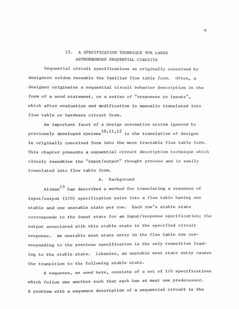
Sequential circuit specifications as originally conceived by

designers seldom resembl e the familiar flm" table form . Often , a

designer originates a sequential circuit behavior description in the

form of a word statement, or a series of "responses to inputs",

which af t e r evaluation and modification is manually translated into

flow table o r hardwar e c ircuit form .

An important face t of a design automation system ignored by

10 11 12 p r eviously developed sys tems ' ' is the translat ion of designs

9

in originally conceived form into the more tractable flow table form.

This chapter presents a s equential circuit description technique which

closely resembles the "input/output " thought process and is easily

translated into flow table form .

A. Background

15 Altman has described a method for translating a seq uence of

input/output (I/0) specification pairs into a flow table having one

stable and one unstable s tate per row. Each r ow ' s stable s tate

corresponds to the input state for an input/respon se specificat ion; the

output associated with this stable stat e is the specified circuit

respons e . An unstable next state entry in the flow table row cor-

r esponding to the previous specification is the only transition lead-

ing to the s tabl e state . Likewise, an unstable next state e ntry causes

the transition t o the fo llowing s table state .

A sequence , as used he r e , consis t s of a se t of I/0 specifications

which fol low one an other such that each has at mos t one predecessor .

A problem with a seq uence description of a sequential circuit is the

10

possibility of having to repeat long lists of specifications in order

to express alternate behaviors at a "branch point;" each string of

inputs to which the circuit is to react in a specified manner must be

explicitly recorded.

Furthermore, not every sequential circuit can be specified by a

finite list of I/0 pairs. For example, any circuit which is to pro­

duce a repeated sequence of outputs in response to inputs until a

certain series of inputs is applied cannot be specified by a single

I/O sequence.

A more general formulation of the above problem is the in­

ability of single sequence specifications to describe cyclic be­

haviors of indeterminate duration.

An input/response description method will next be described

which overcomes the above difficulties. It will be shown that this

extension of the previously described method increases only slightly

the effort required to translate I/0 specifications into flow table

form.

B. Sequential Circuit Specification Using Input/Output Sequences

The sequence may be used as a building block to describe more

complex circuit behavior. The first I/0 pair of a sequence will be

called the head of the sequence, and the last specification the tail.

At some point in the I/0 description of a sequential circuit, it may

be desirable to indicate that one of two or more alternate sequences

will be followed, depending on the next circuit input. At such a

branch point, the sequence previously under development is terminated

and the heads of the alternate sequences follow its tail.

Since the sequences are often developed and recorded serially, it

11

is convenient to introduce the "FOLLOWS" note. This device is used

to record, for appropriate sequence heads, the labels associated with

preceding sequence tails. Note that a sequence may FOLLOW more than

one tail. Conversely, more than one sequence may FOLLOW a tail

specification (or a group of them), so long as each head input state

is not the head of another of the following sequences.

Figure 3 illustrates the terminology introduced above by showing

the sequence representation of a circuit described with a series of

I/0 pairs.

It is sometimes inconvenient to use "FOLLOWS" notation to de­

scribe sequence relationships. For example, the tail of sequence

four of figure 3 may be FOLLOWed by HEADl, but at the time sequence

one is recorded the preceding tail name may not be known. A "GO TO"

note is provided to simplify such cases. The GO TO instruction,

applied to sequence tail specifications, merely lists the labels of

the following sequence heads.

Certain other notation conveniences for recording sequences are

also adopted. A "*" or "-" in any position indicates that an input

or output line is unspecified for an I/O pair. A blank in any

position indicates that the value of the corresponding line has not

changed; the last specified value for the variable thus replaces the

blank. The latter feature eliminates the needless reproduction of

long strings of unchanging variables.

The possibility of leaving some variables unspecified complicates

the problem of detecting improper sequences: no specification may re­

quire or imp~ a change in output without a change in input. Two

tests have been devised to detect improper sequences.

13

Let the first I/O specification w1

be composed of input state

N1 and circuit response (output) o1

; likewise the second specification

is denoted w2

, composed of N and 0 2 2· w2

may properly follow w1

if:

1.

2.

At least one input variable specified in both N1

and N2

is 1 in one case and 0 in the other.

If 1) is not satisfied and w1

is not a sequence tail , then

all of the following must be satisfied: a) Each variable

specified in N1

must correspond to either an identical

specified value or a don't care in N2 ; b) Each variable

not specified in N1

must also be unspecified in N2 ; c) All

output variables specified in o2 must be specified in 0 1

and both must have a common value; d) Output values not

specified in o2

may correspond to either specified or

unspecified variables in 01 .

Rule 2 applies only to input state transitions within a sequence,

and reduces to the requirement that w1 and w2 be indistinguishable.

Consider the possibly improper sequence (4 inputs, two outputs)

0*01 11

0101 00,

which fails Test 1. Assuming w1

is not a sequence tail, application

of Test 2a indicates this is an improper sequence--for input state

0101, the specification requires outputs of first 11 then 00 . For the

pair

0101 00

0*01 11,

Test 1 fails. Tests 2a and 2b are satisfied, but Tes t 2c indicates

h 'f' t' ~or ~nput 0101 , the t at this is also an improper spec~ ~ca ~on. c •

output is required to be 00 then 11. All parts of Test 2 are ,

however , satisfied by

0101 00

0*01 *0

Another potential source of difficulty under the proposed

description method is the need for unique labels on sequence heads

a nd tails . In order to simplify modification of previously re­

corded sequences (as design progresses), each I/0 specification

should have a unique name .

The beginning of a new sequence is implied by a "FOLLOWS"

notat i on . Likewise , a " GO TO" note indica tes the end of a seq­

uence . It is not, however, necessary to use a " FOLLOWS" at the

start , and a "GO TO" at the end of each sequence . The note " BEGIN"

has been adopted to indicate the start of a new sequence; end of

]4

a sequence is indicated simply by "END". Sequence heads and tails

noted in this manner are assumed to have predecessors and successors

which are specified elsewhere.

These notation conventions do not cover the case of a sequence

which is i mplicitly begun or terminated by an explicit reference to,

respectively , end of the previous sequence , or beginning of a follow­

ing sequence. In situations where no notation explicitly indicates a

sequence begins or ends , a " FOLLOWS" o r "GO TO" instruction referring

to the preceding or next sequence is assumed by default. Figure 4

shows a thirteen pair sequence which illustrates the descriptive

method presented here .

LABEL Il I2 I3 01 NOTES

Sequence 1 I ONE 0 * * 1

TWO 1 * * 1

BEGIN

2 I THREE 0 1 1 1 ( i mplie d sequen ce e nd)

FOUR 0 0 1 0 FOLLOWS TWO

3 FIVE 1 1 0 FOLLOWS TWO, THREE

SIX 0 1 1

SEVEN 1 1 1 GO TO ONE

4 EIGHT 0 1 0 1 FOLLOWS TWO

NINE 0 0 0 0 FOLLOWS TWO , EIGHT

TEN 1 0 0

5 ELEVEN 0 0 0

TWELVE 1 0 0

THIRTEEN 0 0 0 1 GO TO ONE

Figure 4. Sequence Description Example B.

It will next be shown that this type of sequential circuit

specification may easily be c onverted into conventional flow tabl e

representation .

C. Conve rsion to Flow Table Form

The procedure previously described for conve rting a s eque nce

t o flow t able form r equires little modification fo r us e unde r the

present scheme. Each input/output pair corresponds t o a row of

the f low table. Stable state entries (with the spec ified o u tpu t s)

appear in a ll columns co rresponding to the input state specifi­

cation. Thus n unspecified input line value s res ult in 2n stable

state entries in the appropriat e row.

Unstable next-state entries are placed in the preceding row

15

for each stable state. Since the preceding flow table row r e presents

the last specification in the h sequence, t e sequence head stable

states do not have any unstable next-state entries leading to th em .

Consecutive I/0 specifications to which proper sequence rule #2

applies are a special case. If there is no stable state in a column

of the row w1 , the next-state entry for the 1 I/0 · owe r pa1r w2

must be

copied into the preceding row position .

Figure 5 shows the flow table segment which exhibits be ha vior

specified by sequence 5 of fig ure 4.

11 12 13 01 STATE 000 001 010 011 100 101 110 lll

0 0 0 0 A G);o B

0 1 0 0 B c G);o 0 0 0 0 c @ !o D

0 1 0 0 D E @ ;o 0 0 0 1 E @ 11

Figure 5. Translation of a Sequence into a Flow Tabl e Segment .

Sequence relationship data provided by "FOLLO\.JS" and "GO TO"

instructions are conveniently r ecorded in a Module Flow Table (}WT).

16

Each sequence corre sponds to a single r ow of the HFT . Stable states in

the MFT r ecord sequence entry input states (obtained f r om the head I/0

pair specification). Unstable next-state entries i n exit (tail) input

state columns indicate the next sequence to be fo llowe d for various

input values . A stable and unstable state entry both in the same r ow

and column indicate s that an entry input state is also an exit s ta t e .

In this case , the unstable entry is simply tagged with a minus sign .

Each sequence is translated to flow table segment form and the

MFT is completed. A single flow table description of the sequential

circuit is then obtained by concatenating all sequence flow table

segments. Unstable next-states corresponding to FOLLOWing sequence

entry rows are added to the last (tail) row of each segment and

17

flow table translation is completed. Note that the unstable states of

a row of the MFT correspond to the unstable states added to the last

row of each segment.

Figure 6 shows the flow table segments which are obtained from

the circuit description of figure 4.

0 1

1

2 0

0

0 3

0

0

4 0

0

0

5 0

0

0

.,.,

* 1

0

1

0

1

1

0

1

0

1

0

.,.,

1

1

1

1

1

0

0

0

0

0

0

1

1

1

0

0

1

1

1

0

0

0

0

1

A

B

c

D

E

F

G

H

J

K

L

M

N

INPUT STATE

000 001 010 011 100 101 110 111

J D

D

@;o F

Q)!l A A

J

Q)!l L

@!o N

@11 A

B B B B

H c @ll @ll @11 @!1

@!l E

@;o G

A @11

G)/1 K

@;o M

@;o A A

Figure 6. Sequence Flow Table Segments for Example B.

18

The Module Flow Table for figure 4 is shown in figure 7; the

segments and the MFT have been combined as described into a single

flow table shown in figure 8.

Il I2 I3 04 INPUT STATE

000 001 010 011 100 101 110 111

0 * * 1 1 -, 5 - , 3 -, 4 -,2

0 1 1 1 2 3 0 0 0 1 0 3 1 -,1 1 1

0 1 0 1 4 5 0 0 0 0 0 5 -,1 1 1 1

Figure 7 . The Module Flow Table for Example B.

INTERNAL STATE INPUT STATE

000 001 010 011 100 101 110 111

1 <2) /1 C!)/1 C!)/1 {2) !1 2 2 2 2

2 9 4 8 3 ~/1 ~/1 ~/1 ~/1

3 4 G)/1

4 @ !o 5

5 6 G)!o

6 @ ll 7

7 1 1 1 (j)!l 8 9 @ !l

9 0 Jo 10

10 11 @ !o

11 @ !o 1 2

12 13 @ !o

1 3 QJ /1 1 1 1

Figure 8. Flow Table Representation of Example B.

19

D. A sequence Translation Computer Program

A PL/1 program, WAVEFM, has been written which accepts I/O

sequential circuit specifications of the type described. The program

also incorporates several useful error detection and editing features.

The improper sequence tests have been incorporated; they produce

error messages and terminate translation if an improper list of

specifications is presented .

Each specification is required to have a unique 4-character label.

If the I/0 pair name has been previously used, an error message is

produced and processing ends.

The program accepts "FOLL XXXX,YYYY , . .. " as FOLLOWS instructions,

where XXXX and YYYY are 4-character labels previously used in the

description . The GO TO instruction is identical, except for the

nmemonic "GOTO". "BEGN" and ''END" mark the beginning and end of

sequences , while "STOP" in the label field indicates end of the cir­

cuit description .

Althou gh now operat i ng in a batch mode environment, the de­

scription and translation methods used by WAVEFN should prove most

useful in interactive use by circuit designers. Limited text

editing features were incl uded in order to provide some "psuedo­

interactive" processing by the present version of the program . Thus

a " 4. " causes deletion of a single character immediately to the left

of the character deletion symbol and "/" causes the deletion of an

entire input record (line) .

Another feature incorporated into the program is the capability

to provide, on request, an error-free copy of the partial list of

circuit spec ifications a nd/or the module flow tabl e .

Finally , the program may optionally be requested to prepare

a list of all branch points for which action in response to some

input is not specified.

E. Extensions and Results

An alternate representation of the desired sequential circuit

may be obtained by considering each sequence (or a collection of

sequences) as a submachine or module . Each module has one or more

entry internal states , and a single exit state. Each module

realizes a portion of the sequential behavior required of the de­

sired circuit .

Only one module at a time responds to input stimulii . The

active module is selected by a control module which r esponds t o

inputs as well as " module exit state" signal s . It is interesting

to note that the previously developed MFT closely resembles a flow

table description of the control module . Figure 9 shows a block

diagram of one modular realization of example B of this chapter.

ENTRY CONTROL ENTRY MODULE:

MFT

,, 4 ~ .. ~ 'II.

MODULE A EXIT EXIT MODULE B:

SEQUENCES SEQUENCES

2&3 4&5

Figure 9 . Modular Organization of Example B.

A flow table translation program for modularly organized

circuits has not been written , because t he design aut oma t ion system

20

r e l a t ed to the programming effort pres e ntly synthesizes only single

f low tables . Little difficulty should be e n countered in adopting

the t ransla tion algorithm to t he modular case . Investigation will ,

however, be required to develop heuristics for det e rmining modular

par t itionin g . The decomposi t ion of a very large sequential circuit

description into several smaller ones is a powerful synthesis aid .

2J

The single flow table translation program has been applied to

only a few long specification lists. A typical description involved

22 sequences containing a total of 158 fo ur-input, three-outpu t

specifications . The 158 row by sixteen column flow table was pro­

duced in only 65 seconds .

Th e flow tables produced by the methods described in this

chapter gen erally can be g reatly s i mplified . Indeed , if these tables

are t o be used to actually syn thes ize circuits , it is impo rtan t to

reduce (if poss ible) the number of inte rnal s tates (rows) in the

flow table . Chapt er III is devoted to the problem of simplifying

v e ry large flow tables .

22

III. REDUCTION OF LARGE INCOMPLETELY SPECIFIED FLOW TABLES

Flow tables often contain more internal states than are required

to specify the desired circuit behavior . In such cases it is ad­

vantageous to reduce the flow table to more compact form, for synthe­

sis costs increase with flow table size, and circuit complexity is

roughly proportional to flow table size. The simplification of

completely specified flow tables is much less difficult than that for

incompletely specified tables.l6 Since practical asynchronous se­

quential circuit descriptions are seldom formulated as completely

specified tables, the more general , incompletely specified case is

treated here.

A. Background

The following defintiions are useful in this chapter. If a

sequence of inputs is applied to flow tab le P when it is initially

in internal state r, then this sequence is said to be applicable to

r if the state of the flow table is specified after each input, ex­

cept possibly the last . Thus , when an applicable sequence of inputs

is applied, no unspecified next-state entries are encountered , except

possibly after the final input . Unspecified flow table entries are

taken to imply that behavior of the machine ceases to be of interest

once the unspecified state is entered. Stable states which have no

output specified imply that circuit outputs will be ignored so long

as the output remains unspecified.

Two output states are comparable if they are identical whenever

both a re specified. Two internal states sa and sb are compatible

if they yield comparable output sequences for all possible input

sequences . It is clear that sa and sb are compatable only if for

2J

each input state t h eir outputs are identical whenever both are

specified , and their next-state entries are compatable whenever both

n e xt-states are specified.

A compatibility class C is a set of internal states which are all

pairwise compatible . A set of states Q is implied by a set o f states

R if , for all inputs, Q is the set of all specified next-state entries

for R. As used herein, this definition will be slightly modified

when applied to compatibility class candidates. Ca implies Cbi if

for each input state Ii either all next-state entries are in Ca o r

all n ext-states are in an implied class Cbi· Using the latter concept

o f implication , it may be seen that a single class Ca may imply one

or more classes Cbi· Since each of the Cbi may in turn imply other

classes, an implication chain may be fo rmed. All compatibility c lass

candidates Ca which imply others are termed conditionally compatibl~ ,

since the implied classes of the chain must be subsets of known com­

patibility classes before compatibility can be established f or Ca .

A maximal compatible (or maximum compatibility class) is one

which is not contained in any other compatibility class.

A set of compatibility c l asses c ove rs a f low t able i f every

state of the flow table is contained in one or more classes o f the

s e t.

A set of compatibility classes is closed if for every input

state the set of next-states implied by each class Ci in the s e t is

contained in at least one of the classes of the s e t .

It can easily be shown that a reduced flow table which covers

the original one may be fo rmed from a closed set o f compatibility

classes which contains each state of the original table . Each row

24

of the reduced table corresponds to a compatibility class.

Paull and Unger, in a classic paper2, presented an algorithm for

obtaining maximum compatibility classes for incompletely specified

flow tables. An implication table is formed, recording pairwise com-

patibility. Figure 10 illustrates the implication table for flow

table A of figure 1. Dash entries indicate state pairs which are

5 X

4 1,4 5,6

3 5,6 1,4 - 3,6 3 6

1,4 3,6 1,4

X X 2,6 216 2

1,4 2,6 3,6 2,6 2,5 X 3,6 1,4 1

6 5 4 3 2

Figure 10. Implication Table for Flow Table A.

compatible, while X's indicate pairs which are incompatible. State

pairs which are conditionally compatible have the implied pairs enter-

ed in the appropriate cell. Conditional compatibility chains are

systematically examined and the final implication table contains no

implied pair entries which are not conditionally compatible.

A systematic method is described for obtaining the set of all

maximal compatibles from the implication table. The Paull-Unger

maximal compatible algorithm is well known and will not be presented

here.

Paull and Unger were unable to present a systematic procedure

(other than complete enumeration) for obtaining a minimum closed

25

collection of compatibility classes. They pointed out that an upper

bound on the number of states in the minimized flow table is the

number of maximal compatibles--but this number is usually greater

than the number of rows in the original flow table. Several sugges-

tions are offered for manual minimization of flow tables of up to

fifteen rows.

Grasselli and Luccio have published an algorithm3 which solves

the cover and closure problem without resorting to complete enu­

meration. The incompatibility table is formed and used to produce the

set of all maximal compatibles.

A procedure is described for obtaining the collection of all

compatibility classes which can be used to construct a minimal flow

table. This set of compatibility classes is much smaller than the

set of all maximal compatibility classes and their included sub­

classes. A significant reduction in intermediate data is achieved,

but only through increased computation.

The final step in Grasselli's flow table minimization procedure

is the construction and reduction of a cover and closure (CC) table,

used to select closed sets of compatibility classes which cover the

original flow table. The CC table is very similar to a prime im-

plicant table, but is somewhat more difficult to reduce.

Kella5 recently developed a procedure for finding all minimal

covers for an incompletely specified flow table. The generation

of all prime compatibility classes is avoided by generating reduced

26

machines by recursively adding new states, rather than starting with

a set of compatibility classes which cover the original flow table.

Only reduced machines with the minimum number of states are considered

as new states are added, thus avoiding non-minimal reductions.

A sequential machine Ma is a partial machine of machine Mb if the

state table of Ma is included in but less than Mb· Every transition

in Mb not covered by Ma is considered unspecified in Mb. A reduced

machine Mb is based on a reduced machine Ma if Ma is a partial

Kella's procedure begins by finding all state pairs of the

original flow table which are pairwise incompatible. An algorithm

is then presented for finding all reduced machines M for the first a

(i+l) rows of the original table M, which are based on theM of M(i). a

Thus the consideration of each row of M in turn leads to the pro-

duction of all minimal flow tables. The procedure involves finding

all maximum compatibility classes for the partial table M(i+l) which

include state si+l; using the list of incompatible states this process

is much less difficult than finding the set of all maximum compatibili-

ty classes for the original machine.

The three algorithms outlined above have been examined in some

detail in order to emphasize the amount of effort required to mini-

mize very large flow tables. For an N-row table, the amount of data

and effort required to produce pairwise compatibility or incom­

patibility information is in general proportional to N2 for large

tables. The amount of computation involved in generating maximum

compatibility classes is rather problem dependent, but is roughly

27

proportional to N6.* Effort expended in developing prime com-

patibility classes and reducing a CC table also increases approxi-

mately exponentially .

The Kella algorithrn,while in general requiring less effort than

the Grasselli-Luccio procedure, is still far too cumbersome to

economically reduce extremely large flow tables.

None of the methods outlined are well suited to automated flow

table reduction . All require that an extremely large amount of

int ermediate data be preserved. Another disadvantage of these tech-

niques is that they produce all minimal flow tables; for large tables

it becomes impractical to produce more than a single reduced flow

table. Furthermore , experience with other switching theory mini-

mization problems·--Boolean fun ctions and asynchronous state assign-

ments , to name just two--has shown that minimization becomes pro-

hibitively costly fo r very large problems. Although they do not in

general produce minimal results, it is clear that economical flow

table reduction procedures must simplify rather than minimize large

tables .

*There are P = (N2-N)/2 row-pair comparisons to be made in form­ing a compatibility or incompatibility table. Suppose that 1-1/r of the row pairs are incompatible. Consider only attempting to form three member compatibility (or incompatibility) classes : three two­sets must be examined for each three-set . There are R = P/r possible two-sets. The number of pair comparison look-ups re~uired is W = (~) = (P~r) = (N2 3-N)/2r , which is proportional toN . For example ,

with N = 10 and r = 4, W = 155; however , for N = 100 and r = 4 , W = 3xl08. This very rapid increase in effort required to produce maximal compatible generator routines for minimum variable state assignments descr ibed in (10 and 17). Also see Chapter IV .

28

One of the least complicated simplification procedures is mcrg-

ing. 18 Two flow table states may be merged if their next-state

entries are the same state whenever both are specified. The state

resulting from the merger has a stable state or output specification

wherever either of the original states had a stable state or an out-

put specification. Merging thus does not remove redundant stable

states; however if there are no redundant stable states, merging pro-

duces a minimal flow table. Although merging usually prevents a re-

duction of large flow tables to minimal form, it is based on a simple

relationship between rows which is easily detected.

Two rows of a flow table are equivalent unless in some flow

table column a) their outputs are specified to be different, b) the

output or next-state of one row is specified and the other is not,

) h . f h . 1 19 or c t e next-state entr1es o t e two rows are not equ1va ent

Only one of the two or more equivalent rows need be included in a

simplified flow table.

B. A Flow Table Simplification Heuristic

The operating speed or amount of effort required by a large

flow table simplification procedure is related to the simplicity of

the state relationships detected. It is also affected by the volume

of intermediate data which is required to be generated and evaluated.

Conversely, the amount of simplification achieved (compared to minimal

reduction) is in general improved by detecting complex compatibility

relationships and using large amounts of intermediate data.

The algorithm presented below is intended to rapidly produce a

simplified--but in general non-minimal--flow table. The table to be

simplified is assumed to be incompletely specified, with many next-

29

state entries unspecified. The simplification method is independent

of flow table source; the method described in Chapter II might, for

example, be employed to produce such tables. The procedure is de-

signed to be most economical when applied to extremely large (up to

several hundred state) flow tables, and is intended primarily for

automated design applications.

Two important considerations affect the design of a flow

table simplification heuristic. First, the procedure must not require

exhaustive computations or comparisons. The effort expended in

economically simplifying large flow tables must be literally orders of

magnitude less than that characteristic of known minimization pro­

cedures.

Digital computer main memory size limitations restrict the

volume of data immediately accessible to a simplification program.

(Secondary storage is uneconomical for frequently accessed data).

The generation of massive blocks of intermediate data is also ex-

pensive. Thus a modest amount of data should be utilized by the

successful flow table simplification heuristic.

These two constraints have led to the adoption of a simple

strategy: only a single set of compatibility classes, representing

the reduced table, is generated. Cover is insured by insisting that

each state of the original machine be a member of one and only one

compatibility class. Closure is preserved by continuously updating

next-state and output specifications for the compatibility classes;

current closure requirements thus reduce to satisfying compatibility

requirements for the partially reduced machine.

The partial machine next-state entries are stored in a two-

30

dimensional array wherein each row is reserved for a compatibility

class, and columns correspond to input states. A Boolean matrix is

utilized to store output states associated with stable states. A

tag number is associated with each flow table state; if zero, the

state is either a single element compatibility class or has not yet

been added to the reduced machine. If the tag is negative, the state

represents a compatibility class containing two or more elements

(states). A positive tag points to the state number (in the reduced

machine) which corresponds to the compatibility class containing the

row in question; positive tags thus map original machine states into

compatibility classes, and eventually into states of the reduced

machine.

Il 12 13 14

1 @;ooo G)/111 2 *

2 1 @!010 Q)/011 3

3 8 9 i~ G)/101

4 * 2 @1011 3

5 1 G)/111 4 '1c

1 1 1 2 0 000 111 -1

2 1 2 2 3 010 011 -1

3 8 9 0 3 101 0

4 0 2 4 3 011 +2

5 1 5 4 0 111 +1

Next States Output States Tags

Figure 11. Flow Table and Corresponding Representation.

31

Next-state zero indicates that the flow table entry is not

specified. Row 4 has been combined with row 2, and the resulting

compatibility class has been stored in row 2; likewise, rows 1 and 5

have been combined and the resulting class is in row 1.

Each state of the original flow table is considered in turn.

To reduce the number of row-pair comparisons performed, row i is

compared only with compatibility classes--or rows---in the limited

range (i-p) 4 i <. (i+q). Because of this 'look-ahead' provision in the

range of comparison for row i, the current status of state (i+q) is

used. Thus prior to examining state (i+q) from the original table,

the tag numbers must be used to map next-state entries for original

row (i+q) into compatibility class references if appropriate.-~

The limited flow table examination range employed here may also

be visualized as a "window" which moves down the flow table. Only

rows currently exposed in the window are used in flow table sim-

plification.

To minimize the amount of intermediate data, only four simple

types of row-pair compatibility test are utilized; this arrangement

also improves the operating speed of the simplification procedure

drastically.

Consider row i from the unsimplified flow table as it is being

added to the reduced table. An attempt is first made to add the row

*This action is actually performed for rows (q+l) and on--the first q rows of the original table 'prime' the reduction procedure and require no updating.

J2

to a compatibility class within the examination range having a

negative tag (implying two or more original states in the class).

Since the compatibility class is represented by its resulting flow

table row, i can be added to class j if it is compatible \vith (com--

patibility class) flow table row j.

Two flow table rows are compatible, written x 'Vy, if for each

input state having specified next-state in both rows, 1) both next-

state entries are identical or 2) both next-state entries are stable

states and the output states agree whenever both are specified.*

Row i is immediately added to the first compatibility class j

with which it is compatible. The resulting compatibility class has

a stable state and output specification whe rever either of the

previous rows tvas stable . If both were stable for some input, only

the outputs are combined. For convenience, the new class is placed

in the same location as the old compatibility class; this practice

generally reduces the number of next-state entries \vhich must be

changed , since next-state i is likely to appear l ess frequently than

j. The tag for row i is set equal to j, and known (i.e . , wi t hin the

range "window") next-state entries corresponding to stable states i

a re changed to j.

Next , an attempt is made to add each lower (k > j) compatibility

class to the new class containing state i . Any classes which can be

*This definition is much more restrictive than that usually en­counte red in the literature. A third condition, that the next-states themselves be compatible, has been discar ded in order to develop an economical simplification heuristic. All compatibility c lasses de­veloped under the restricted definition also satisfy the more general

case.

added to the new class j are included inunediately by updating the

appropriate tag, next-state and output entries.

JJ

Finally, the new class j is checked for compatibility 'vlith any

single member classes--rows which have previously been found incom­

patible with all others in the known segment of the reduced table.

The new compatibility class expansion procedure causes com­

patibility classes which may contain many original table rows to

grow quite rapidly; this is advantageous because it quickly decreases

the size of the partially reduced table and thus reduces the number of

row pair comparisons performed in each step.

If a newly considered flow table row is incompatible with all

known compatibility classes (i.e., those in range) with two or more

elements, an attempt is made to combine that row with each known

single element compatibility class. These classes correspond to rows

of the original flow table which have been found incompatible with

all known rows. If a single row j is discovered to be compatible

with i, a new compatibility class is formed and recorded in the old

compatibility class position j as outlined above; the remaining single

element classes are also checked for compatibility with new class j,

as in the previous new class case.

Figure 12 illustrates the formation of a new compatibility class.

Row 6 of the original table is added to the partially reduced table

composed of classes 1,2, and 3.

Row 6 is incompatible with classes 1 and 2 which represent two or

more rows of the original table. Row 6 is conditionally compatible

with row 3. With a look-ahead factor of 3, rows 7,8, and 9 are then

considered. Rows 6 and 7 are conditionally compatible; then row 8 is

34

discovered to be compatible with row 6. A new two element class is

then formed in row 8. The tag and next-state entry modifications

which occur are shown in Figure 13.

1

2

3

4

5

i=6

7

j=8

9

@;ooo

1

8

* 1

@/111

* @!111

6

Q)/111

G)/010

9

2

@/111

@1ooo

1

G);ooo

2

@/011

@/011

4

7

G);ooo

7

3

G)/101

3

10

3

3

Tag

-1

-1

0

+2 Partially Reduced

+1 t 0

0

0

0

F ·g re 12 Dl·scovery of a New Compatibility Class. l u .

1

2

3

4

5

i=6

7

j=8

k=9

/000

1

8

1

@/111

* @/111

8

1 /111

0.)/010

9

2

G)/111

@;ooo

1

(D;ooo

G);ooo

2

G)/011

G)/011

4

7

(i)/100

7

3

G)/101

3

10

3

3

F . 13 Formation of the New Class lgure .

Tag

-1

-1

0

+2

+1

+8

0

-1

0

35

An attempt is then made to add remaining classes or rows to the

new class formed in row 8 . Row 9 is found to be compatible with

class 8 and is thus included in the new class , as shown in figure 14.

Il I2 13 I4 Tag

1 @ !000 Q)/111 2 * -1

2 1 @ !010 @ /011 3 -1

3 8 8 * G)/101 0

4 * 2 G)/011 3 +2

5 1 G)/111 4 * +1

6 G)/111 @ !000 7 * +8

7 * 1 G)/100 10 0

j=8 @ /111 @ !000 7 3 -1

9 8 G)/000 * 3 +8

Figure 14. Addition of a Row to the New Class.

It has been found that for partially reduced incompletely

specified flow tables, row pair (i,j) is sometimes the only implicant

for class pair (m , n) . In this case , the compatibility of pair (i,j)

implies that of pair (m,n). However, this situation does not occur

frequently enough to justify rechecking the compatibility of each

row pair after formation of each new compatibility class . To do so

would increase manyfold the amount of effort expended in flow table

reduction.

It can be shown , however, that in general only a small fraction

of row pairs need be rechecked. Furthermore , these pairs can be

easily located during the process of next-state entry updating after

36

formation of the new compatibility class (i,j).

Theorem: If row pair (k,j) is an implicant of pair (m,n) then

both i and j must have stable states under some input state(s), and

fo r at least one of these inputs, both i and j must appear as explicit

next-state entries in rows m and n.

Proof : If (m, n) implies (i,j) then i and j must be next-state

entries under at least one input state of pair (m,n) . Normal mode

operation require s that transitions lead directly to stable states,

so both i and j must be stable for the given input.

It is clear that the above theorem dramatically reduces the

amount of rechecking which needs to be done after compatibility class

format ion . Rechecking does, however represent a significant increase

in computational effort, and should be further justified.

First consider two relatively small compatibility classes i and

j. In a large table, it is quite likely that the number of unstable

next-state entries leading to them will be small. Rechecking in this

case is inexpensive, especially since the number of stable states per

r ow may be small, further reducing the likelihood of both being

s tabl e in the same column .

If on the other hand i and j are large compatibility classes

having many stable state columns, rechecking may involve a large

number of row pairs and thus become less desirable.

In the format ion of new compatibility classes described above,

at least one of the constituents of the new class is always a single

row from the original flow table, i. Rechecking is performed after

forma tion of new classes resulting from the construction of class

(i,j) . If rechecking discovers compatible state pairs (m ,n), they

are immediately combined, but further r echecking based on these

II d II • secon ary new classes 1s not performed.*

Figur e 15 s hows t he reduced flow table resulting from the sim-

plification illustrated in figure 14 . Notice that as new class 8

1

2

3

7

8

@ ;ooo

1

8

* @ /111

(D /111

@ 1010

8

1

@ ;ooo

Tag

2 'lc -1

@ 1011 3 -1

* G)/101 0

G)/100 10 0

7 3 -1

Figure 15. A Recheck Opportunity .

Recheck

0

0

1

0

1

was constructed , the recheck flag for row 3 was set due to rows 8

and 9 having stable states under r 2 , and row 3 having a n ext-state

entry l eading to the new stable state .

Rechecking pair (3 , 8) results in the formation of a new class

(3 , 8) which is placed in row 3 . Figure 16 shows the flow table

segment after rechecking is completed.

37

*Experimenta l simplification of large randomly redundant tables

has shown that locating implicants of secondary new classes , al­

though cos t ly, results in little if any increase in overall flow

table simplification.

38

Il 12 I3 I4 Tag

1 ~/000 ~/111 2 * -1

2 1 ~/010 ~/011 3 -1

3 8 8 * ~/101 +8

7 * 1 {2)/100 10 0

8 ~/111 ~/000 7 ~/101 -1

Figure 16 . Flow Table Segment After Rechecking .

A row i from the original table is not considered further unless,

after the processes described , it is found to be incompatible with all

known (in range) c lasses. Since the amount of reduc tion achieved may

be significantly decreased by such rows, another attempt is made to

f ind compatibility classes containing i.

A single implication chain consists of a collection of state

pairs suc h that each pair of states (excluding perhaps the last) is

conditionally compatible and implies only the next pair in the chain .

Figure 17 shows a partial flow table containing a single im-

plication chain.

Sin ce the generation and use of implication data is expensive in

terms of both storage and computation, only single implication chains

are used in the flow table simplification heuristic. Additional con-

straints restrict the consideration of implication relations to those

situations most likely to produce economical simpli fi cation.

J9

Il I2 I3

1 @!1 6 4 (1,2)~

2 @!1 6 5 ~~ 3 Q)!l G);o

(3,6) 1

4 1 3 @!1 5 1 6 G)/1

6 2 @!1 3

Figure 17. Partial Fl ow Table and Single Implication Chain.

As has already been implied , a row pair (i,j) is used as the

first element in an implication chain only if 1) one of the two states

is incompatible with a l l known stat es, and 2) only a single pair of

states (p,q) is implied by (i , j) . These pairs are detected as the

pair compatibility process previously described is executed : as s t ate

j is considered for compatibility with state i , if i and j are con-

ditionally compatible and imply only a single pair of s tat es (im-

plicants) p and q , j is marked. If i is not found compatible with

any known state, t hen an attempt is made to build a singl e implication

chain based on (i,j) implies (p , q) .

Implication chains which may be used to find valid compatibility

classes terminate in several ways . If the final implicant pair p and

q are uncond i tionally compatible, then all pairs in the chain are

compatible. If a pair already in the chain is the only implicant of

the last pair (i.e., the chain closes on itself) then all pairs in

the chain are compatible.

A chain building attempt fails if some chain implicant pair

(p,q) has two or more implicants, if a pair of implied states are

incompatible, or if the chain length exceeds some threshold. The

latter has experimentally been shown to be unimportant;the restricted

implications considered cause almost all chains to be very short.

A fourth type of chain failure closely resembles a closed chain: if

one state but not both of an implicant pair has previously appeared

in a chain, the chain fails.

If a chain is successfully completed, compatibility classes

are calculated in reverse order, beginning with the last class added

to the chain. Rechecking may be performed after this operation is

completed for all implicant pairs. The advisability of rechecking

here is highly problem dependent but usually yields little additional

simplification--at a relatively high cost.

Figure 18 illustrates the simplification obtained by reducing

the single implication chain shown in figure 17.

After the process described above has been completed for each

original flow table row, the flow table must be reorganized to

eliminate the rows with positive tags and to complete the updating of

next state entries.

Each row is considered in turn, until all rows have been pro-

cessed. If row i has a positive tag (indicating inclusion of i in a

compatibility class stored elsewhere) the flow table portion con­

sisting of zero or negatively tagged rows above the "known'; part of

the table (with the window of the known rows based on row i) is

41

11 12 13 Tag

1 @ !1 3 4 -1

2 @ 11 6 5 +1

3 1 Q)!l Q);o -1

4 1 3 G)/1 -1

5 1 6 @ !1 +4

6 2 @ 11 3 +3

Figure 18. Flow Table Simplification Using Single Implication Chains.

examined for unstable entries valued i. These next-state entries are

changed to the appropriate state number of the class containing row i .

A search is then made to find a rmv j > i with a zero or negative

tag to "fill" the space occupied by the eliminated row i . If such a

row is f ound, next-state entries are changed to reflect the re-

location of row j to position i . If no rows are available to fill

state i, the flow table reorganization process is complete.

Figure 19 illustrates the flow table reorganization for the

reduced table shown in figure 18 . Notice that the second row,

42

11 12 13 Tag

@ 11 2

1 3 I. -1

2 @ 11 6 5 +1

3 1 G)ll @Ia -1

4 1 3 0 11 -1

5 1 6 0 11 +4

6 2 @ 11 3 +3

Before Reorganization .

11 12 13

1 @ 11 3 2

2 1 3 @11

3 1 @11 Q)lo

Final Form

Figure 19. Reorganization of a Reduced Flow Table.

having a positive tag, is replaced by the lowest row 4 having a

negative tag.

4J

The procedure outlined produces excellent simplification if a

large portion of the flow table is in the range of consideration .

However , the effort implied by such a large range is considerable.

Thus, it is recommended that the procedure presented here be applied

iteratively using a mor e economical range . Simplification process ing

ceases when a simplification yield requirement is not met.

Figure 20 is a brief flow diagram of the flow table simplifi­

cation heuristic presented here .

C. Programmed Implementation and Results

The flow table simplification heuristic described has been

programmed in PL/1. Although the program will not be described in

detail, the performance of the programmed procedure illustrates the

utility of the simplification heuristic itsel f . It should be noted

that the program was written in a high level language and emphasized

algorithm clarity rather than execution efficiency .

Experience gained in several previously developed flo\~ table

simplification algorithms led to a program implementation of the

procedure containing several minor modifications of the simpli fication

heuristic described here . These changes permitted the evaluation of

constraint placed on various phases of the simplification process.

A rather trivial assumption was also made to allow an experi­

mental simplification routine to be developed more rapidly. It was

assumed that, as flow table simplification proceeds, enough memory is

available to store all of the partially reduced machine. Thus as

row i of the original flow table is added to the reduced machine, it

Begin

Attempt To Form New CC

Record Implication Chain Data

I

'

Reor ganize Simplified Flow Table

Yes Acquire >-----. .. Firs t q

Finished

Rows Of Input Table

Loop J Through All Known Rows

44

Finished

Loop I Through Original Rows

Acquire a New Original Row

--- .... -._- --------,

No

For m New CC And Update Tables

Attempt To Expand Previous cc

Single Row CC' s Are Considered Last

Add J To New Compatibility Class

Figure 20a. The Flow Table Simplification Heuristic.

Recheck For New CC's

Loop Thru Input States

No

Attempt Chaining

45

Finished

Yes

Loop Thru Recheckable Pairs In Column

Form New Compatibility Class & Updat Tables

Finish

Form All

Add Row Pair To Implication Chain

New Compatibility Classes

Figure 20b. The Flow Table Simplification Heuristic

(Recheck, Chaining and Reorganization).

46

is assumed that all compat ibility classes containing ro\vS 1 through

i-1 are stored in main memory. This programming convenience elim­

inated the need for a partially reduced flow table segment paging and

bookkeeping scheme--which although involving very significant extra

programming effort is not technically important .

An interesting experimental modification of the program was a

provision fo r varying the degree of "look ahead" used in the pro­

cedure. Although computer time cos ts have restricted experimentation

with this parameter, some preliminary results can be reported.

Figure 21 shows a plot of look ahead versus simplification time (using

a S/360-50) fo r a single 193 rows by four column flmv table. Also

shown on the same graph is the degree of simplification achieved in

each case. Although the effects of various degrees of look ahead are

highly problem dependent, processing times generally increase as look

ahead incr eases beyond about 10%. The degree of reduction achieved may

be less dependent on look ahead, especially fo r values greater than 10%

The examination of an extr emely large number of single im­

plication chains may be undersirable. The programmed simplification

procedure thus contained a provision fo r halting the chain building

process afte r a variable number of chain failures . A variable maxi­

mum chain length test was also incorporated (i.e., fail all chains

longer than the length limit) . Both of these provisions were found to

have almost no effect on either the degree of reduction obtained or

execution time required . This result is due to the extremely lmv in­

cidence of long single implication chains in the examples used, and the

surprisingly small number of single implication chains discovered.

0\ t 0

(/') I ..... 3

"0 1-' ..... H'l ..... () Cll rt ..... 0 :I

t-1 ~ I-'• Vl 3 ro ~

(/')

ro ()

0 :I 0.. (/)

. w 0

0

The effect of look ahead on simplification of a 193 x 4

flow table

• + ~

• • • w

~

• • • . rows

• 0 time + ~

50 100 150

Look ahead-- rows

Figure 21 . An Example of the Effect of Look Ahead on Flow Table Simplification

:::0 0 ~ (/)

..... :I

(/') ..... a

"0 1-' ..... H'l ..... ro 0..

~ Cll cr 1-' ro

~ -...J

48

The programmed routine also contained an option for suppression

of the iterated simplification feature. It was found that the in--

creased simplification obtained was highly problem dependent. In many

instances, virtually no simplification was achieved after the first

pass. For other tables, significant reduction was obtained for up to

three passes. In all cases, the amount of time required to complete

a simplification cycle decreased markedly for successive passes.

The recheck performed after formation of new compatibility classes

could also be bypassed in the programmed flow table simplification

routine. It was found that rechecking contributes significantly to

table reduction, especially on the first iteration.

As has been pointed out previously, minimization procedures for

the large flow tables considered here are impractical. Thus no

attempt has been made to program a flow table minimization algorithm.

Still, some means of evaluating the performance of the heuristic is

essential.

The evaluation method selected consisted of constructing a

completely simplified flow table by insuring that no two rows were

compatible. A random number generator was then used to introduce

redundant rows having at least one stable state. Other next-state

entries in the redundant rows were randomly determined to be specified

or unspecified. Finally, the rows of the redundant flow table were

randomly reordered, and the table was prepared for simplification.

Several very large flow tables prepared in this manner have

been reduced by the simplification heuristic program. Table I

summarizes results obtained using these and other examples. Appendix

I contains more detailed information on trial flow table reductions,

49

including input and output flow table characteristics, simplification

mechanism, etc .

Table I. Simplification of Several Large Flow Tables

Example Number of Rows Number Simp. Number Input Simp . Min . Columns Time . Sec .

1 193 32 23 4 40.8

2 75 28 23 4 18

3 115 25 UNK 8 49

4 217 38 23 8 82

5 158 37 UNK 16 93

6 96 26 UNK 16 31.5

The performance of the programn1ed version of the flow table

simplification heuristic illustrates the utility of the method.

Although the reduced tables are not minimal, considerable reduction

is achieved at v ery low cost.

The availability of a practical flow table reduction method

represents a furthe r step toward the economical synthesis of large

asynchronous sequential circuits . Chapter IV examines the problem

of constructing state assignments for reduced tables which specify

large sequential circuits.

50

IV. STATE ASSIGNMENTS FOR LARGE ASYNCHRONOUS SEQUENTIAL CIRCUITS

The selection of a satisfactory state assignment for an asynchro-

nous sequential circuit is one of the most difficult tasks in the

synthesis procedure. This chapter considers the state assignment

problem for circuits operating in the normal fundamental mode and

describes a method especially suited to the automated design of very

large circuits. Operation of the machine is assumed to be described

by a previously simplified flow table.

A. Background

The complexity of the state assignment problem for asynchronous

sequential circuits stems from the necessity of avoiding critical

races which may cause the machine to malfunction. A critical race

exists when, because of the asynchronous nature of state transitions,

internal state variables may change values in an order which causes

the circuit to reach a final (stable) state other than the desired one.

Figure 22 shows a portion of a flow table and a state assignment which

contains a critical race. If the circuit is stable in state 1 under

input I2

, assume the input then changes to I1

. The desired final

state is 3, but if y2

changes state before y1

, stable state 2 is

reached, causing a malfunction.

One method which has been used to avoid critical races is the

application of a standard state assignment, i.e. one which does not

depend on flow table structure. The number of state variables re-

quired for standard state assignments has been the topic of several

7,20 papers The least number of standard assignment variables for

20 s normal, fundamental mode circuits reported to date is s0 + C20) +

(~0), where for ann row flow table, s0 = [Log2 n].

51

Yl y2 y3 Il I2 Desired Operation Critical Race

0 0 0 3 @;o 0 0 0 }

0 0 0) 0 1 0 (j) /0 0 1 0) 0 1 0

1 1 0 G)!l 1 1 0

Figure 22. State Assignment Containing a Critical Race.

The complexity (and, to an extent , r eliability and cost) of se-

quential circuit hardware is roughly proportional to the number of in-

ternal state variables. Standard assignmen ts frequently conta in an

unnecessarily large number of variables. Quite often, it can be shown

that a given flow table can be satisfactorily coded using a nonstan-

dard assignment with significantly fewer variables than the corre-

spending standard assignment. Conversely, standard assignments can be

generated orders of magnitude more rapidly than critical-race-free non-

standard codes, and thus lower synthesis costs.

Nonstandard state assignments for asynchronous sequential circuits

have received much attention in recent years . In an early paper, C.N .

Liu showed that a critical-race-free assignment could be fo rmed by

combining individual column codes which are themselves critical race

f ree. 7 The column codes are obtained by considerin g transitions f rom

unstable to stable states within a colunm.

A k-set is composed of a stable state in a flow table column,

together with all states in the column that have unst able nex t state

en tries whic h lead to the stable state. Li u shows tha t for N stable

states in a row, [log2 N]*variables may be used to form a cri tical-

*In this paper [x] is used to denote the nearest integer which is greater than or equal to X.

52

race-free column code. Howe er f t bl · l v , or a es Wlt 1 many colunms, the

number of variables in the state assignment may approach or even

exceed that required for a standard assignment.

Tracey later described a method for finding minimum variable

assignments for normal, fundamental mode asynchronous sequential cir­

cuits.8 A list of constraints (two block partitions) is constructed

according to the following theorem: A row assignment with one state

per row can be used for the realization of normal mode flow tables

without critical races if and only if for every transition (Si, Sj):

a) if (Sm, Sn) is another transition in the same column, then at

least one internal state variable partitions the pair (Si, s.) and J

(Sm, Sn) into separate blocks, b) if Sk is a stable state in the same

column, at least one variable partitions (Si, Sj) and (Sm, Sn) into

separater blocks, and c) fori# j, Si and Sj are in separate blocks

of a state variable partition.

Tracey's state assignment algorithm requires that the partition

list be translated into a Boolean matrix; each row represents a con-

straint and each column corresponds to a flow table row.

Two rows of a Boolean matrix are intersectable if and only if

they agree whenever both are specified. A Boolean matrix roH may be

added to an intersectable R only if that row is intersectable with

every element in R. An intersectable which cannot be enlarged is

called a maximal compatible. Each maximal compatible may be thought

of as a largest possible collection of non-conflicting constraints.

A minimum variable code which satisfies each of the constraints thus

corresponds to a minimum number of maximal compatibles which cover the

constraint list.

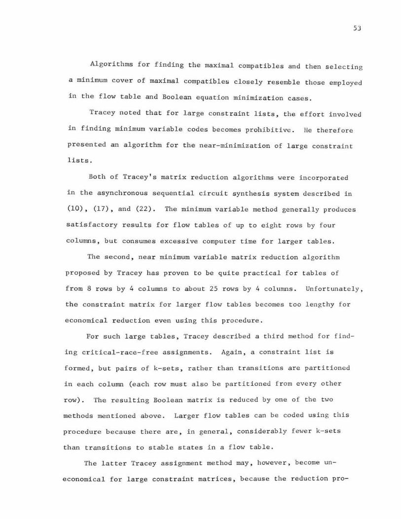
53

Algorithms for finding the maximal compatibles and then selecting

a minimum cover of maximal compatibles closely resemb l e those employed

in the flow table and Boolean equation minimizat ion cases .

Tracey noted that for large constraint lists, the effort involved

in finding minimum variable codes becomes prohibitive . He therefore

presented an algorithm for the near-minimization of large constraint

lists .

Both of Tracey's matrix reduction algorithms were incorporated

in the asynchronous sequential circuit synthesis system described in

(10), (17), and (22) . The minimum variable method generally produces

satisfactory results for flow tables of up to eight ro,~s by four

colunms, but consumes excessive computer time for larger tables.

The second, near minimum variable matrix reduction algorithm

proposed by Tracey has proven to be quite practical fo r tables of

from 8 rows by 4 columns to about 25 rows by 4 columns. Unfortunately,

the constraint matrix for larger flow tables becomes too lengthy for

economical reduction even using this procedure.

For such large tables, Tracey described a third method for f ind­

ing critical-race-free assignments . Again , a constraint list is

f ormed, but pairs of k-sets , rather than transitions are partitioned

in each column (each row must also be partitioned f rom eve ry other

row). The resulting Boolean matrix is reduced by one of the two

methods mentioned above . Larger flow tables can be coded using this

procedure because there are, in general, considerably fewer k-sets

than transitions to stable states in a flow table.

The latter Tracey assignment method may , however, become un­

economical for large constraint matrices, because the reduction pro-

54

co

...-I N ("') ~ ~ ~

>. :>. Q) Q) (J (,) C1S C1S ,., ...

E-< E-< (I) Q) ~ ~ s::

orf I: .. Q)

s ...-4 ~ -.:r ~ s:: Q) a 00

orf (I) (I)

C1S

Q) ~ C1S ~ Ul

N

0 25 50 75 100

Flow table size , rows x columns

Figure 23 . Flow Table Size versus Typical State Assignment Time--

Tracey Methods .

55

cedures become impractical for matrices exceeding certain sizes. The

minimum reduction procedure matrix size limit has been found experi-

17 mentally to be about 50 rows by 8 to 12 columns. The near-minimum

matrix reduction method size limit has been found to be about 200

rows by 30 columns.

Figure 23 shows a comparison of flow table size versus state

assignment generation time for programmed versions of the three Tracey

state assignment methods.

Because of the exponentially increasing computation times for

larger tables, none of the Tracey assignment methods appear to be

suitable for flow tables of 20 rows by 8 columns or larger. The re-

mainder of this chapter describes a modification of Tracey's k-set

partition assignment algorithm which permits the economical generation

of codes for extremely large tables.

B. A Nonstandard State Assignment Procedure for Large Flmv Tables

The generation of either transition or k-set partitions is not

particularly difficult or time consuming even for large flow tables.

As previously pointed out, the difficulty centers around the reduction

of very large constraint matrices. A method is described here which

avoids reducing large Boolean matrices, thus allowing nonstandard

codes to be found for very large flow tables.

The strategy used is a simple one: k-set partition constraints

are found. (The use of k-set partitions reduces the number of con-

straints which must be satisfied.) A constraint list is only

allowed to grow to a predetermined size limit, then is partially re-

duced. This strategy will, in general, produce assignments having at

least as many variables as the Tracey methods. However, the proposed

56

method will bP- shown to be much faster and hence more economical for

large circuits.

An example, shown in figures 25, 26, and 27, illustrates the

following discussion.

The new state assignment procedure begins by finding k-set

partitions for each flow table column. When the partition matrix

reaches the size limit, the matrix is partially reduced, yielding

state variables and a small number of constraints not satisfied by the

variables generated.

K-set partition generation then resumes. However, a k-set par­

tition is not added to the constraint list if it can be satisfied by

a previously calculated state variable. The constraint matrix thus

contains only those k-set partitions which remain to be satisfied.

When this constraint list again reaches the size limit, the partial

matrix reduction procedure is repeated.

After all k-set partitions have been found, the state variable

and partition lists must be checked to insure that each flow table

row is partitioned by some variable from every other flow table row.

Any constraints needed to satisfy this requirement are added to the

partition matrix, and it is completely reduced.

A flow diagram of the large flow table state assignment procedure

is shown in figure 24. The matrix reduction scheme is not detailed

since it is identical to Tracey's method two. 21

The state assignment method outlined above produces codes more

economically than the Tracey algorithms because the amount of com­

putation required to reduce a Boolean matrix is much greater for

schemes which consider the entire matrix than for methods which re-

Begin

Loop I Through

Flow Table Columns

Add K-set (I,J) To List In

Position H

Add (H.K) To Partition

List

Not Full

Full

Loop J Through

Flow Table Rows

Loop K Through

Flow Table Rows

Finish

Call Hatrix Reducer

Yes

Loop L Through Existing Variables

Finish

Add Partition

(M,K) To List

Figure 24a. The Large Flow Table State Assignment Procedure

(K-set Partitions).

57

Begin Check For All Row Pairs Partitioned

Loop K Through All State Variables

Finish

Loop K Through All State Variables

Finish

Add (I,J) To The Partition List

Finish

Loop I Through All But Last Row

No

No

Not Full

Yes

Yes

Call Hatrix Reducer

Loop J Through All Rows

Call !·1atrix Reducer

Figure 24b. The Large Flow Table State Assignment Procedure

(Row Partitions).

58

Il

1 @/11

2 @/01

3 G);oo

4 @/10

5 3

6 1

7 3

8 4

9

10

11 2

12 4

I2

G);oo

6

1

6

(D;o1

@Ill

(2)/10

7

5

7

Figure 25. Flow

I3

9

10

G);oo

9

5

@/11

0/01

@)!10

10

8

Table D.

11

12

11

12

12

11

11

12

11

@ /11

GV ;oo

duce relatively small matrix segments. It is, for example, much

59

simpler to reduce four matrix segments of 50 rows each than to reduce

one 200 row matrix.

C. An Example

Figure 25 shows a 12 row by 4 column flow table which will be

used to illustrate the state assignment procedure for large flow

tables. It should be noted that the algorithm is not particularly

well suited to tables as small as the one considered; this example

is presented primarily to illustrate the algorithm.

Figure 26 shows the k-set partition list for flow table D.

This table requires 61 transition partitions, compared to the 21 k-set

partitions shown.

Column 11

(1,6;2,11)

(1,6;3,5,7)

(2,11;3,5,7)

(1,6;4,8,12)

(2,11;4,8,12)

(3,5,7;4,8,12)

Column 13

(5,7;8,12)

(5,7;1,6,9)

(8,12;1,6,9)

(5,7;2,10,11)

(8,12;2,10,11)

(1,6,9;2,10,11)

Column r2

(1,3;5,9)

(1,3;2,4,6)

(5,9;2,4,6)

(1,3;7,8,10)

(5,9;7,8,10)

(2,4,6;7,8,10)

Column r4

bO

(1,3,6,8,10,11;2,4,5,9,12)

Rows

(4;12)

(10; 11)

Figure 26. K-set Partition List for Flow Table D.

The state assignment found by reducing the above k-set partition

list is shown in figure 27. Tracey's second, near-minimal, matrix

reduction technique was used. (For this example the constraint matrix

size limits were set at 10 rows maximum and 2 rows minimum).

The preceding example is too small to illustrate many advantages

of the segment matrix reduction procedure. Experience with larger

matrices has been gained through the use of a programmed version of

the large flow table state assignment procedure.

01

Row Number K-set Partition Code

1 1111--1

2 00011-0

3 110---1

4 0011010

5 1001010

6 0111--1

7 100001-

8 0010--1

9 1011000

10 -000101

11 000-111

12 0010--0 ~igure 27. State Assignment for Flow Table D.

D. A Programmed Implementation of the Procedure

The algorithm outlined above was programmed in PL/1. The pro-

gram (actually two subroutines) consists of about 325 statements.

Both segment maximum and minimum sizes are input parameters.

Subprogram KPI generates k-set partitions and adds them to the

constraint matrix if they cannot be satisfied by previously determined

state variables. hfhen the list reaches maximum size or all con-

straints have been generated, routine CODE partially reduces the re-

sulting Boolean matrix.

CODE extracts state variables from the constraint matrix using

62

a procedure closely resembling Tracey's reduction method two 21

However, when extraction of a state variable causes the constraint

list to become shorter than the minimum length, control is returned to

KPI and constraint generation continues. The minimum length of the

last constraint matrix segment is always zero.

The programmed implementation of the state assignment method was

used to investigate the effect of varying the values of the maximum

and minimum segment size limits. Although the results appear to be

problem dependent, preliminary conclusions can be drawn. Figure 28

shows the relationship between maximum segment size and the amount

of computation time required to find a single state assignment for

several large flow tables. (More extensive descriptions of these and

other state assignment experiments are found in Appendix 2.) Based

on the (computer time cost) limited number of experiments performed,

it appears that the upper matrix size limit should be about 20 rows.

Results appear to be rather insensitive to minimum matrix size limits

between 2 and 5 rows.

Figure 29 clearly shows the utility of the state assignment

technique described in this chapter (a more extensive list of ex-

periments appears in Appendix 2). The same flow tables have, wher-

ever possible, been coded with Tracey's three methods and the tech­

nique developed here. The latter clearly may be used to economically

code large tables for which the three Tracey methods are not practical.

The largest flow table for which a state assignment has been

generated has 37 rows and 16 columns. A 27 variable state assignment

was found for this table in less than 17 minutes. (A standard assign-

ment for the same table would have 41 state variables.)

63

29 X 4 Table,

0 Single Code

0 (Minimum Matrix C") . Size = 3 rows).

C) <l)

C/)

~

<l)

s •--" E-< ...., 0 >::: 0 <l) C"J

§ Ol)

•--" (/) (/)

<t: <l) ...., ttl ....,

C/) 0 0 .-i

10 20 30

Constraint Matrix Maximum Size, Rows

Figure 28. The Effect of Segment Size on Assignment Generation Time.

64

• I I I I

Lf"'l

I .-i

I I

.-i N I ("")

~ ~ I ~

:>.. ~I :>.. tl) QJ QJ ,.r:: QJ C) ~I C) +-1 +-1 C\1 C\1 .,.; ~ 1-1 1-1 1-1 E s:: E-1 E-< E-< U'l ..... s -QJ

s -M +-1

s:: 0 0 .-i ..... +-1 C\1 +-1 ~ p. E 0 C)

+-1 s:: QJ

~ bO ..... tl) tl)

C\1

QJ +-1 C\1 +-1 Lf"'l tl)

.-i C\1 C) ..... p. :>..

E-1

0 200 400 600

Flow table sizeJ rows x columns

Figure 29. Comparison of Four State Assignment Techniques.

65

E. Sununary

The large flow table state assignment procedure presented here

was developed after recognizing that constraint matrix reduction

techniques used in well-known algorithms are inadequate for extremely

large constraint matrices. The number of constraints (or matrix rows)

to be satisfied by a code is first lowered by using k-set partitions.

The maximum matrix size which can be efficiently reduced is then used

as a matrix segment size limit; matrices which exceed this length are

partially reduced by sections.

A programmed realization of the assignment procedure has econom­

ically produced state assignments for flow tables far larger than

those which could be coded by more nearly minimum variable techniques.

Chapter V briefly describes the characteristics of an experi­

mental automated design system which incorporates the new synthesis

techniques described in Chapters II, III, and IV.

6h

V. AN AUTOMATED DESIGN SYSTEM .

The synthesis h e uris t ics developed here have been incorporat e d

in a programmed asyn chronous sequential circuit sys t em unde r deve l op­

ment at the University of Missouri - Ro lla . Although det ailed discus­

sion of the SHADE (~nthesis Heuristics for Automated DEsign) sys tem

is n ot appropriate t o this dissertation , a summar y of the sys t em will

illustrate the utility of the algorithms presented h ere . SHADE has

been used to verify programmed versions of the heuristics and to

demonstrate the economical synthes i s of large asynchronous sequential

circuits .

A. System Overview

Figure 30 shows a f lowchart representation of the SHADE

(~nthesis Heuris tics fo r Automated DEsi gn) system which is useful in

the discussion which follows .

The SHADE user may enter a p roblem at any of six steps in the

synthesis pro cedure. Pr ocessing then continues th r ough one or more

s teps f ollowing the selected entry point. The av a ilable e ntry point s

precede t hese synthesis steps:

1) I/O sequence translation to flow table form .

2) Flow table simplification.

3) Int e rnal stat e assignment gen eration .

4) State assignment evaluation.

5) Design equation generation .

6) Boolean equation simplification and hazard r emoval.

SHADE is capable of processin g multiple problems witho ut re­

initialization of the system.

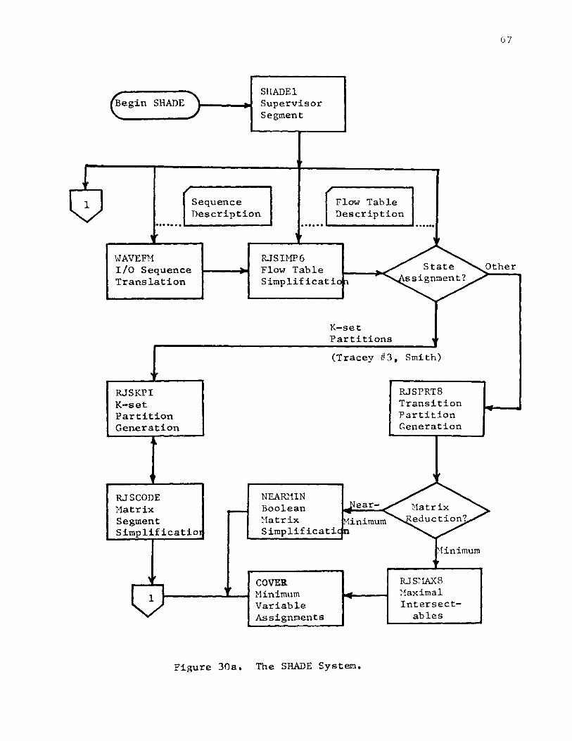
Begin SHADE J

Sequence Description

SHADEl Supervisor Segment

Flow Table Description ....... .._ ______ _. ...... . .....

WAVEFl1 I/O Sequence Translation

RJSKPI K-set Partition Generation

RJSCODE Matrix Segment Simplificatio1

.. ' 1

RJSIMP6 Flow Table .. State

Simplificatio p. ssignment?

K-set Partitions 1

(Tracey #3, Smith)

NEARlUN Boolean .,liear-

~1atrix 1inimum Simplificaticn

RJSPRT8 Transition Partition Generation

aatrix eduction?

1inirnurn , RJS~1AX8

;1axirnal Intersect-

ables

Figure 30a. The SHADE System.

G7

Other

...

~>----......... L/

SHADE2 Supervisor Segment

Flow Table & Assignment(s)

................... '---------1 .................. .

RJSEVAL State Assignment Evaluation

EQNSIMP (Hodified Breuer)

RJSOUT2 Remove All Static Hazards

SHADE3 Supervisor Segment

RJSHKI Next-State Equations

/

Boolean Equations

.................. ··L-------...1

Equation Reduction?

Simplify Minimize

RJSCBS Iterative Con census

..

Figure 30b.

RJSOUTl Remove Remaining Static Hazards

End SHADE)

RJSPIT Prime Implicant Table

The SHADE System (continued).

68

69

All data input operations are handled via supervisory programs

SHADEl , SHADE2 and SHADE3 . These supervisory routines also , at user

request , print intermediate resul t s and punch c heckpoint data after

each synthesis step .

As shown in figure 30 , the system user may choose from several

modes of operation. For example, by specifying appropriate options

and parameters, state assignments may be generated by any of the three

Tracey methods, or by using the procedure described in this disserta-

t ion . Designs may be generated using all state assignments discove r ed

by a particular method , or only the predicted "bes t" assignment may

be used . Boolean equations may be minimized using either of two

methods .

The supervisory programs determine synthesis routine sequencing

from a user supplied opti on card . The supervisor also manages all

data passed between synthesis programs.

The I/0 sequence trans l ation and flow table s impli fication

programs have been described, so will not be presented here.

B. State Assignment Generation and Evaluation Routines.

As mentioned previously, four s tate assignment algorithms are

availabl e in the SHADE system. The programmed implementation of the

method of Chapter IV has been described and will not be reviewed

here .

Programmed versions of Tracey ' s methods 1 and 2 a r e adaptations

f d S . hl0 , 17 , 22

of the programs pr eviously developed by Schoe fel an m1 t .

These s ubroutines generate minimum and near-minimum variable state

assignments using transition partition constraint lists. These

routines have proven to be economical only for small to medium size

flow tables (see Appendix 2) and are included in the SHADE system

primarily for comparison purposes .

70

Tracey ' s method 3, utilizing k-set partition constraint lis t s

and near-minimum matrix reduction, can be shown to be a special case

of the procedure described in Chapter IV. In fact , the two methods

are identical if the entire constraint matrix is taken as the first

matrix segment . In the SHADE system , this is achieved by making the

segment size limit (an input parameter) larger than the matrix size .

Thus the program described i n Chapter IV may be used to generate

Tracey method 3 state assignments .

SHADEl , the supervisory section covering int e rnal state ass i gn­

ment generation , is capable of selecting any of the four algorithms

if none is specified by the user .

The state assignment evaluation subroutine is based on that

described in (13). If two or more codes are generated , the routine

attempts to predict which will yield simplest design equations .

C. Design Equation Generation and Reduction .

RJSMKI, the design equation gen e ration program to be used in

the SHADE sys tem, is a modification of the one desc ribed i n (22).

It is interesting to note that this algorithm has proven to b e

economical fo r quite large flow tables .

Design equations , in the form of Boolean equations for next

state variables , are obtained in unsimplified form . Two Boolean

equation reduction procedures are available . The first, developed

some time ago (10,22), produces minimal equations containing no

static hazards . Unfortunately, expe rience has shown thi s g roup of

subroutines to be extreme ly t ime consuming for large systems of

Boolean equatio ns .

71

In order to improve the performance of the SHADE system, a fast

Boolean e quation simplification routine has been adde d. The program ,

14 based on an algorithm described by Breuer , produces irre dunda nt

sums of products using only one pass thro ugh the input exp ression. A

static hazard removal routine (under deve lopment) completes the

processing of large systems of design equations .

D. Conclusions.

The synthesis heuristics developed in this dissertation s u ccess-

fully avoid the prohibitively expensive data storage and computation

requirements associated wi th previously used algorithms . Thei r

inco rporation into an automated design sys tem makes possibl e the

synthesis of qui t e large circuits . The examples cited throughout

this dissertat ion fur the r illus trate the low cos t of such an app r oach .

Inves tigations i n sever al areas may , however , lead to furthe r

performance improvements . New methods fo r specifyin g sequential

circuit s should be expl ored . The r elationship be t ween state

assignments and next s tate equations should be reviewed; perhaps

efficient new s tate assignment methods could be found wh ich directly

yield design equations . Finally , t he implications of modular real -

izations of asynchronous sequential cir cuits could be furthe r

developed.

72

APPENDIX 1 : EXPERIMENTAL FLOW TABLE SIMPLIFICATION

The following tables s ummarize the results obtained in several

flow table simplification expe rime nts performed using the algorithm

presented in Chapter III. The PL/1 programmed implementation was

run on an IBM S/360-50 as part of the SHADE system discussed in

Chapter V.

The large flow tables were obtained from randomly gene rated I/0

pair specifications or by randomly introducing redundant rows into

completely simplified f low tables.

Table II shows the effect of varying look ahead on simplifica­

tion of a 193 row by four column table . For this particular example,

it was concluded that look ahead of 10 to 20 rows ( 5 to 10%)

produced satisfactory simplification .

Table III details several flow table simplification experiments .

Reduction mechanism entries sho\Yn in Table III reflect the number of

compatibili t y class enlargeme nts produced by each of the listed

methods.

...

Table II.

Look Ahead, Rmvs

5

10

15

20

25

35

so

75

100

150

190

VARYING LOOK AHEAD IN SD1PLIFICATION OF A 193x4 FLOH TABLE

Simplification Time Sec.

45

40

40

41

45

48

47

52

53

53

53

Output Table Size RovJs

35

34

33

32

33

36

35

35

34

35

32

73

74

Table III . EXPERIMENTAL FLO\-/ TARLE SHtPLI FICATimi RESVLTS.

No . INPUT Fl..OH TABLE SIHPLI FIED FLOH TABLE

Rows Cols . Stable Unspec. Rmvs Cols. Stahle Unspcc. States Entries States Ent ries

1 193 4 193 185 3'• 4 49 I)

2 75 4 75 57 28 4 40 2

3 115 8 115 685 25 8 100 32

4 217 8 217 38 8 93 20

5 158 16 287 1968 37 16 268 137

6 96 16 194 1139 26 16 175 102

No . PROGRAM PERFORMANCE REDUCTION MECHAN I S.'1S

Time Number Look Minimum Row Row & New CC Chain-Required , of Ahead , Table, Pair cc Enlarge- ing Sec Itera- Ro~vs Rows Comb ina- Combo. ment

tions tions

1 40 2 10 23 34 68 56 6

2 18 2 10 23 17 1o 13 2

3 49 2 10 Unk . 27 14 43 6

4 82 2 10 23 36 3 79 2

5 93 1 10 Unk.

6 32 1 35 Unk. 18 6 43 0

75

APPENDIX 2: SUMMARY OF STATE ASSIGNMENT EXPERIMENTS

Table IV summarizes the results of a set of state assignment

experiments conducted to evaluate four non-standard state assignment

techniques for normal, fundamental mode asynchronous sequential

circuits.

1.

The methods (and identification numbers) used were:

Tracey's method one, which finds minimum variable state

assignments by finding transition partitions, then

minimizing the resulting constraint (Boolean) matrix.

2. Tracey's second method, which finds near-minimum variable

assignments by reducing the transition partition matrix

to near-minimum size.

3. Tracey's third state assignment technique, which requires

the computation of K-set partitions and near-minimum

reduction of the resulting constraint matrix.

4. The new state assignment algorithm proposed in this

dissertation, which involves near-minimum reduction of

K-set partition matrix segments.

The timing data was obtained by executing PL/1 implementations

of the state assignment procedures on a S/360-50 computer.

Entries indicated by "*" are approximations (in most cases

necessitated by premature termination of the programs).

No. Rows Columns

1 6 3

2 6 4

6 4

3 12 4

12 4

12 4

12 4

4 18 4

18 4

18 4

5 23 4

6 26 16

7 28 4

8 29 4

9 34 4

10 38 8

11 37 16

Table IV. STATE ASSIGNMENT EXPERIMENTS.

FLOW TABLE STATE ASSIGNMENT

Stable States Unspec. Entries Method Time Sec. Number Variables

9 3 1 1.8 4

12 0 1 36 5

12 0 2 21 5

14 6 1 104* 4

14 6 2 20 5

14 6 3 22 7

14 6 4 22 7

20 12 2 171 7

20 12 3 106 8

20 12 4 74 9

34 0 4 154 14

175 102 4 375* 27*

40 3 4 1000* 12

34 24 4 135 10

49 0 4 464 16

98 20 4 840 28

268 137 4 1040 28

' i I I

I

-....! 0\

BIBLIOGRAPHY

1. McCluskey, E.J., Introduction to the Theory of Switching Circuits. New York: McGraw-Hill Book Company, 1965.

2. Paull, M.C. and S.H. Unger, "Minimizing the Number of States in Incompletely Specified Sequential Switching Functions," IRETEC, EC-8 (September, 1959), 356-367.

3. Grasselli, A. and F. Luccio, "A Method for Minimizing the Number of Internal States in Incompletely Specified Sequential Networks," IEEETEC, EC-14 (June, 1965), 350-359.

4. Ginsburg, S., "On the Reduction of Superfluous States in a Sequential Machine," J. ACH, Vol. 6 (September, 1959), 252-282.

5. Kella, J., "State Minimization of Incompletely Specified Sequential Machines," IEEETEC, C-19, No. 4 (April, 1970), 342-349.

77

6. Huffman, D.A., "The Synthesis of Sequential Switching Circuits," J. of the Franklin Institute, Vol. 257 (Harch and April, 1954), 161-190 and 257-303.

7. Liu, C.N., "A State Variable Assignment Method for Asynchronous Sequential Switching Circuits," J. ACM, Vol. 10 (1963), 209-216.

8. Tracey, J.H., "Internal State Assignments for Asynchronous Sequential Machines," IEEETEC, EC-15 (August, 1966), 551-560.

9. Elsey, John, "An Algorithm for the Synthesis of Large Sequential Switching Circuits," Report R-169, Coordinated Science Laboratory, University of Illinois, Urbana, 1963.

10. Smith. R.J., et al., "Automation in the Design of Asynchronous Sequential Circuits," Proc. AFIPS SJCC, 1968, 55-60.

11. Burton, D.P. and D.R. Noaks, "Complement Free S.T.T. State Assignments for Asynchronous Sequential Machines," Paper read at the Second National Symposium on Logic Design, University of Reading, Reading, Penn., March 28, 1969.

12. Tan, C.J., "Synthesis of Asynchronous Sequential Switching Circuits," Dr. Engr. Sc. Dissertation, Columbia University, June, 1969.

13. Maki, G.K., "Minimization and Generation of Next-State Expres­sions for Asynchronous Sequential Circuits," Hasters Thesis, University of Missouri - Rolla, 1967.

78

2

14. Breuer, M.A., "Heuristic Switching Expression Simplification," Proc. 1968 ACM National Conference, 241-250.

15. Altman, R.A., "The Computer Aided Generation of Flow Tables for Asynchronous Sequential Circuits," Masters Thesis, University of Missouri - Rolla, 1968.

16. Unger, S.H., "Flow Table Simplification-- Some Useful Aids," IEEETEC, EC-14 (June, 1965), 472.

17. Schoeffel, W.L., "Programmed State Assignment Algorithms for Asynchronous Sequential Machines," Masters Thesis, University of Missouri- Rolla, 1967.

18. Huffman, D.A., "The Synthesis of Sequential Switching Circuits," J. of the Franklin Institute, Vol. 257 (March, 1954), 176.

19. Unger, S. H., "Flow Table Simplification - Some Useful Aids," IEEETEC, EC-14 (June, 1965), 473.

20. Mago, Gyula, "Universal State Assignment for Asynchronous Sequential Circuits," Unpublished Manuscript R-69-6, IEEE Computer Group Repository, 1969.

21. Tracey, J.H., "Internal State Assignments for Asynchronous Sequential Machines," IEEETEC, EC-15 (August, 1966), 552.

22. Smith, R.J., "A Programmed Synthesis Procedure for Asynchronous Sequential Circuits," Masters Thesis, University of Missouri­Rolla, 1967.

79

VITA

Robert Judson Smith II was born May 12 , 1944, in San Francisco ,

California . He received his primary and secondary education in

Wichita, Kansas . He has r eceived his college education from Wichita

State Unive rsity and the Uni versity of Missouri - Rolla. He earned

a Bachelor of Science degree in Electrical Engineering (Cum Laude)

from Wichita State University in June 1966 , and a Master of Science

degree in Electrical Engineering from the Unive rsity of Missouri -

Rolla in January 1968.

Mr. Smith has b een enroll ed in the Graduate School of the

University of Missouri - Rolla since Septembe r 1966; he held an NDEA

fellowship from that time until June 1969. He was an instructor in

Electrical En gineering from Sep t ember 1969 unt i l February 1970 .

Mr. Smith is presently involved in clinical data p r ocessing res earch

at the Missouri I nstitute o f Psychiatry , University of Hissouri School

of Medicine.

.1908ZZ