arX

iv:1

103.

1711

v1 [

cs.A

I] 9

Mar

201

1Journal of Artificial Intelligence Research 26 (2006) 35-99 Submitted 8/05; published 5/06

Planning Graph Heuristics for Belief Space Search

Daniel Bryce DAN .BRYCE@ASU.EDU

Subbarao Kambhampati, RAO@ASU.EDU

Department of Computer Science and EngineeringIra A. Fulton School of EngineeringArizona State University, Brickyard Suite 501699 South Mill Avenue, Tempe, AZ 85281

David E. Smith DE2SMITH@EMAIL .ARC.NASA.GOV

NASA Ames Research CenterIntelligent Systems Division, MS 269-2Moffett Field, CA 94035-1000

Abstract

Some recent works in conditional planning have proposed reachability heuristics to improveplanner scalability, but many lack a formal description of the properties of their distance estimates.To place previous work in context and extend work on heuristics for conditional planning, weprovide a formal basis for distance estimates between belief states. We give a definition for thedistance between belief states that relies on aggregating underlying state distance measures. Wegive several techniques to aggregate state distances and their associated properties. Many existingheuristics exhibit a subset of the properties, but in order to provide a standardized comparison wepresent several generalizations of planning graph heuristics that are used in a single planner. Wecompliment our belief state distance estimate framework byalso investigating efficient planninggraph data structures that incorporate BDDs to compute the most effective heuristics.

We developed two planners to serve as test-beds for our investigation. The first, CAltAlt ,is a conformant regression planner that uses A* search. The second,POND, is a conditionalprogression planner that uses AO* search. We show the relative effectiveness of our heuristictechniques within these planners. We also compare the performance of these planners with severalstate of the art approaches in conditional planning.

1. Introduction

Ever since CGP (Smith & Weld, 1998) and SGP (Weld, Anderson, &Smith, 1998) a series of plan-ners have been developed for tackling conformant and conditional planning problems – includingGPT (Bonet & Geffner, 2000), C-Plan (Castellini, Giunchiglia, & Tacchella, 2001), PKSPlan (Pet-rick & Bacchus, 2002), Frag-Plan (Kurien, Nayak, & Smith, 2002), MBP (Bertoli, Cimatti, Roveri,& Traverso, 2001b), KACMBP (Bertoli & Cimatti, 2002), CFF (Hoffmann & Brafman, 2004), andYKA (Rintanen, 2003b). Several of these planners are extensions of heuristic state space plannersthat search in the space of “belief states” (where a belief state is a set of possible states). Withoutfull-observability, agents need belief states to capture state uncertainty arising from starting in anuncertain state or by executing actions with uncertain effects in a known state. We focus on thefirst type of uncertainty, where an agent starts in an uncertain state but has deterministic actions.We seek strong plans, where the agent will reach the goal withcertainty despite its partially knownstate. Many of the aforementioned planners find strong plans, and heuristic search planners are

c©2006 AI Access Foundation. All rights reserved.

BRYCE, KAMBHAMPATI , & SMITH

currently among the best. Yet a foundation for what constitutes a good distance-based heuristic forbelief space has not been adequately investigated.

Belief Space Heuristics: Intuitively, it can be argued that the heuristic merit of a belief state dependson at least two factors–the size of the belief state (i.e., the uncertainty in the current state), and thedistance of the individual states in the belief state from a destination belief state. The question ofcourse is how to compute these measures and which are most effective. Many approaches estimatebelief state distances in terms of individual state to statedistances between states in two beliefstates, but either lack effective state to state distances or ways to aggregate the state distances. Forinstance the MBP planner (Bertoli et al., 2001b) counts the number of states in the current beliefstate. This amounts to assuming each state distance has unitcost, and planning for each state can bedone independently. The GPT planner (Bonet & Geffner, 2000)measures the state to state distancesexactly and takes the maximum distance, assuming the statesof the belief state positively interact.

Heuristic Computation Substrates: We characterize several approaches to estimating belief statedistance by describing them in terms of underlying state to state distances. The basis of our in-vestigation is in adapting classical planning reachability heuristics to measure state distances anddeveloping state distance aggregation techniques to measure interaction between plans for states ina belief state. We take three fundamental approaches to measure the distance between two beliefstates. The first approach does not involve aggregating state distance measures, rather we use aclassical planning graph to compute a representative statedistance. The second retains distinctionsbetween individual states in the belief state by using multiple planning graphs, akin to CGP (Smith& Weld, 1998), to compute many state distance measures whichare then aggregated. The thirdemploys a new planning graph generalization, called the Labelled Uncertainty Graph (LUG), thatblends the first two to measure a single distance between two belief states. With each of these tech-niques we will discuss the types of heuristics that we can compute with special emphasis on relaxedplans. We present several relaxed plan heuristics that differ in terms of how they employ state dis-tance aggregation to make stronger assumptions about how states in a belief state can co-achievethe goal through action sequences that are independent, positively interact, or negatively interact.

Our motivation for the first of the three planning graph techniques for measuring belief statedistances is to try a minimal extension to classical planning heuristics to see if they will work for us.Noticing that our use of classical planning heuristics ignores distinctions between states in a beliefstate and may provide uninformed heuristics, we move to the second approach where we possiblybuild exponentially many planning graphs to get a better heuristic. With the multiple planninggraphs we extract a heuristic from each graph and aggregate them to get the belief state distancemeasure. If we assume the states of a belief state are independent, we can aggregate the measureswith a summation. Or, if we assume they positively interact we can use a maximization. However,as we will show, relaxed plans give us a unique opportunity tomeasure both positive interaction andindependence among the states by essentially taking the union of several relaxed plans. Moreover,mutexes play a role in measuring negative interactions between states. Despite the utility of havingrobust ways to aggregate state distances, we are still facedwith the exponential blow up in thenumber of planning graphs needed. Thus, our third approach seeks to retain the ability to measurethe interaction of state distances but avoid computing multiple graphs and extracting heuristicsfrom each. The idea is to condense and symbolically represent multiple planning graphs in a singleplanning graph, called a Labelled Uncertainty Graph (LUG). Loosely speaking, this single graphunions the causal support information present in the multiple graphs and pushes the disjunction,

36

PLANNING GRAPH HEURISTICS FORBELIEF SPACE SEARCH

describing sets of possible worlds (i.e., initial literal layers), into “labels”. The planning graphvertices are the same as those present in multiple graphs, but redundant representation is avoided.For instance an action that was present in all of the multipleplanning graphs would be present onlyonce in theLUG and labelled to indicate that it is applicable in a planning graph projection fromeach possible world. We will describe how to extract heuristics from theLUG that make implicitassumptions about state interaction without explicitly aggregating several state distances.

Ideally, each of the planning graph techniques considers every state in a belief state to computeheuristics, but as belief states grow in size this could become uninformed or costly. For example,the single classical planning graph ignores distinctions between possible states where the heuristicbased on multiple graphs leads to the construction of a planning graph for each state. One way tokeep costs down is to base the heuristics on only a subset of the states in our belief state. We evaluatethe effect of such a sampling on the cost of our heuristics. With a single graph we sample a singlestate and with multiple graphs and theLUG we sample some percent of the states. We evaluatestate sampling to show when it is appropriate, and find that itis dependent on how we computeheuristics with the states.

Standardized Evaluation of Heuristics: An issue in evaluating the effectiveness of heuristic tech-niques is the many architectural differences between planners that use the heuristics. It is quite hardto pinpoint the global effect of the assumptions underlyingtheir heuristics on performance. Forexample, GPT is outperformed by MBP–but it is questionable as to whether the credit for this effi-ciency is attributable to the differences in heuristics, ordifferences in search engines (MBP uses aBDD-based search). Our interest in this paper is to systematically evaluate a spectrum of approachesfor computing heuristics for belief space planning. Thus wehave implemented heuristics similarto GPT and MBP and use them to compare against our new heuristics developed around the notionof overlap (multiple world positive interaction and independence). We implemented the heuristicswithin two planners, the Conformant-AltAlt planner (CAltAlt) and the Partially-Observable Non-Deterministic planner (POND). POND does handle search with non-deterministic actions, butfor the bulk of the paper we discuss deterministic actions. This more general action formulation, aspointed out by Smith and Weld (1998), can be translated into initial state uncertainty. Alternatively,in Section 8.2 we discuss a more direct approach to reason with non-deterministic actions in theheuristics.

External Evaluation: Although our main interest in this paper is to evaluate the relative advan-tages of a spectrum of belief space planning heuristics in a normalized setting, we also comparethe performance of the best heuristics from this work to current state of the art conformant andconditional planners. Our empirical studies show that planning graph based heuristics provide ef-fective guidance compared to cardinality heuristics as well as the reachability heuristic used by GPTand CFF, and our planners are competitive with BDD-based planners such as MBP and YKA, andGraphPlan-based ones such as CGP and SGP. We also notice thatour planners gain scalability withour heuristics and retain reasonable quality solutions, unlike several of the planners we compareagainst.

The rest of this paper is organized as follows. We first present theCAltAlt andPOND plannersby describing their state and action representations as well as their search algorithms. To understandsearch guidance in the planners, we then discuss appropriate properties of heuristic measures forbelief space planning. We follow with a description of the three planning graph substrates used tocompute heuristics. We carry out an empirical evaluation inthe next three sections, by describing

37

BRYCE, KAMBHAMPATI , & SMITH

our test setup, presenting a standardized internal comparison, and finally comparing with severalother state of the art planners. We end with related research, discussion, prospects for future work,and various concluding remarks.

2. Belief Space Planners

Our planning formulation uses regression search to find strong conformant plans and progressionsearch to find strong conformant and conditional plans. A strong plan guarantees that after a finitenumber of actions executed from any of the many possible initial states, all resulting states are goalstates. Conformant plans are a special case where the plan has no conditional plan branches, as inclassical planning. Conditional plans are a more general case where plans are structured as a graphbecause they include conditional actions (i.e. the actionshave causative and observational effects).In this presentation, we restrict conditional plans to DAGs, but there is no conceptual reason whythey cannot be general graphs. Our plan quality metric is themaximum plan path length.

We formulate search in the space of belief states, a technique described by Bonet and Geffner(2000). The planning problemP is defined as the tuple〈D,BSI , BSG〉, whereD is a domaindescription,BSI is the initial belief state, andBSG is the goal belief state (consisting of all statessatisfying the goal). The domainD is a tuple〈F,A〉, whereF is a set of fluents andA is a set ofactions.

Logical Formula Representation: We make extensive use of logical formulas overF to representbelief states, actions, andLUG labels, so we first explain a few conventions. We refer to everyfluent inF as either a positive literal or a negative literal, either ofwhich is denoted byl. Whendiscussing the literall, the opposite polarity literal is denoted¬l. Thus if l = ¬at(location1), then¬l = at(location1). We reserve the symbols⊥ and⊤ to denote logical false and true, respectively.Throughout the paper we define the conjunction of an empty setequivalent to⊤, and the disjunctionof an empty set as⊥.

Logical formulas are propositional sentences comprised ofliterals, disjunction, conjunction, andnegation. We refer to the set of models of a formulaf asM(f). We consider the disjunctive normalform of a logical formulaf , ξ(f), and the conjunctive normal form off , κ(f). The DNF is seen asa disjunction of “constituents”S each of which is a conjunction of literals. Alternatively the CNFis seen as a conjunction of “clauses”C each of which is a disjunction of literals.1 We find it usefulto think of DNF and CNF represented as sets – a disjunctive setof constituents or a conjunctive setof clauses. We also refer to the complete representationξ(f) of a formulaf as a DNF where everyconstituent – or in this case stateS – is a model off .

Belief State Representation: A world state,S, is represented as a complete interpretation overfluents. We also refer to states as possible worlds. A belief stateBS is a set of states and is symbol-ically represented as a propositional formula overF . A stateS is in the set of states represented bya belief stateBS if S ∈ M(BS), or equivalentlyS |= BS.

For pedagogical purposes, we use the bomb and toilet with clogging and sensing problem,BTCS, as a running example for this paper.2 BTCS is a problem that includes two packages, one of

1. It is easy to see thatM(f) andξ(f) are readily related. Specifically each constituent contains k of the |F | literals,corresponding to2|F |−k models.

2. We are aware of the negative publicity associated with theB&T problems and we do in fact handle more interestingproblems with difficult reachability and uncertainty (e.g.Logistics and Rovers), but to simplify our discussion wechoose this small problem.

38

PLANNING GRAPH HEURISTICS FORBELIEF SPACE SEARCH

which contains a bomb, and there is also a toilet in which we can dunk packages to defuse potentialbombs. The goal is to disarm the bomb and the only allowable actions are dunking a package inthe toilet (DunkP1, DunkP2), flushing the toilet after it becomes clogged from dunking (Flush), andusing a metal-detector to sense if a package contains the bomb (DetectMetal). The fluents encodingthe problem denote that the bomb is armed (arm) or not, the bomb is in a package (inP1, inP2) ornot, and that the toilet is clogged (clog) or not. We also consider a conformant variation on BTCS,called BTC, where there is no DetectMetal action.

The belief state representation of the BTCS initial condition, in clausal representation is:

κ(BSI) = arm∧¬clog∧ (inP1∨ inP2)∧ (¬inP1∨¬inP2),

and in constituent representation is:

ξ(BSI) = (arm∧¬ clog∧ inP1∧¬inP2)∨ (arm∧¬ clog∧¬inP1∧ inP2).

The goal of BTCS has the clausal and constituent representation:

κ(BSG) = ξ(BSG) = ¬arm.

However, the goal has the complete representation:

ξ(BSG) = (¬arm∧ clog∧ inP1∧¬inP2)∨ (¬arm∧ clog∧¬inP1∧ inP2)∨(¬arm∧¬clog∧ inP1∧¬inP2)∨ (¬arm∧¬clog∧¬inP1∧ inP2)∨(¬arm∧ clog∧¬inP1∧¬inP2)∨ (¬arm∧ clog∧ inP1∧ inP2)∨(¬arm∧¬clog∧¬inP1∧¬inP2)∨ (¬arm∧¬clog∧ inP1∧ inP2).

The last four states (disjuncts) in the complete representation are unreachable, but consistent withthe goal description.

Action Representation: We represent actions as having both causative and observational effects.All actionsa are described by a tuple〈ρe(a),Φ(a),Θ(a)〉 whereρe(a) is an execution precondition,Φ(a) is a set of causative effects, andΘ(a) is a set of observations. The execution precondition,ρe(a), is a conjunction of literals that must hold for the action tobe executable. If an action is exe-cutable, we apply the set of causative effects to find successor states and then apply the observationsto partition the successor states into observational classes.

Each causative effectϕj(a) ∈ Φ(a) is a conditional effect of the formρj(a) =⇒ εj(a), wherethe antecedentρj(a) and consequentεj(a) are both a conjunction of literals. We handle disjunctionin ρe(a) or aρj(a) by replicating the respective action or effect with different conditions, so with outloss of generality we assume conjunctive preconditions. However, we cannot split disjunction in theeffects. Disjunction in an effect amounts to representing aset of non-deterministic outcomes. Hencewe do not allow disjunction in effects thereby restricting to deterministic effects. By conventionϕ0(a) is an unconditional effect, which is equivalent to a conditional effect whereρ0(a) = ⊤.

The only way to obtain observations is to execute an action with observations. Each observationformula oj(a) ∈ Θ(a) is a possible sensor reading. For example, an actiona that observes thetruth values of two fluentsp andq definesΘ(a) = {p ∧ q,¬p ∧ q, p ∧ ¬q,¬p ∧ ¬q}. This differsslightly from the conventional description of observations in the conditional planning literature.Some works (e.g., Rintanen, 2003b) describe an observationas a list of observable formulas, thendefine possible sensor readings as all boolean combinationsof the formulas. We directly define thepossible sensor readings, as illustrated by our example. Wenote that our convention is helpful inproblems where some boolean combinations of observable formulas will never be sensor readings.

The causative and sensory actions for the example BTCS problem are:

39

BRYCE, KAMBHAMPATI , & SMITH

DunkP1:〈ρe = ¬clog,Φ = {ϕ0 = clog,ϕ1 = inP1 =⇒ ¬arm},Θ = {}〉,DunkP2:〈ρe = ¬clog,Φ = {ϕ0 = clog,ϕ1 = inP2 =⇒ ¬arm},Θ = {}〉,Flush:〈ρe = ⊤, Φ = {ϕ0 = ¬clog},Θ = {}〉, andDetectMetal:〈ρe = ⊤,Φ = ∅,Θ = {o0 = inP1,o1 = ¬inP1}〉.

2.1 Regression

We perform regression in the CAltAlt planner to find conformant plans by starting with the goalbelief state and regressing it non-deterministically overall relevant actions. An action (withoutobservations) is relevant for regressing a belief state if (i) its unconditional effect is consistent withevery state in the belief state and (ii) at least one effect consequent contains a literal that is present ina constituent of the belief state. The first part of relevancerequires that every state in the successorbelief state is actually reachable from the predecessor belief state and the second ensures that theaction helps support the successor.

Following Pednault (1988), regressing a belief stateBS over an actiona, with conditionaleffects, involves finding the execution, causation, and preservation formulas. We define regressionin terms of clausal representation, but it can be generalized for arbitrary formulas. The regressionof a belief state is a conjunction of the regression of clauses inκ(BS). Formally, the resultBS′ ofregressing the belief stateBS over the actiona is defined as:3

BS′ = Regress(BS, a) = Π(a) ∧

∧

C∈κ(BS)

∨

l∈C

(Σ(a, l) ∧ IP (a, l))

Execution formula (Π(a)) is the execution preconditionρe(a). This is what must hold inBS′ fora to have been applicable.Causation formula (Σ(a, l)) for a literal l w.r.t all effectsϕi(a) of an actiona is defined as theweakest formula that must hold in the state beforea such thatl holds inBS. The intuitive meaningis thatl already held inBS′, or the antecedentρi(a) must have held inBS′ to makel hold inBS.FormallyΣ(a, l) is defined as:

Σ(a, l) = l ∨∨

i:l∈εi(a)

ρi(a)

Preservation formula (IP (a, l)) of a literal l w.r.t. all effectsϕi(a) of actiona is defined as theformula that must be true beforea such thatl is not violated by any effectεi(a). The intuitivemeaning is that the antecedent of every effect that is inconsistent withl could not have held inBS′.FormallyIP (a, l) is defined as:

IP (a, l) =∧

i:¬l∈εi(a)

¬ρi(a)

Regression has also been formalized in the MBP planner (Cimatti & Roveri, 2000) as a symbolicpre-image computation of BDDs (Bryant, 1986). While our formulation is syntactically different,both approaches compute the same result.

3. Note thatBS′ may not be in clausal form after regression (especially whenan action has multiple conditional effects).

40

PLANNING GRAPH HEURISTICS FORBELIEF SPACE SEARCH

BSG

BS2

BS4

BS9

DunkP1

Flush

BS1

Flush

BS3

DunkP2

BS5

DunkP1

BS6

DunkP2

BS7

Flush

BS8

DunkP1 DunkP2

Figure 1: Illustration of the regression search path for a conformant plan in theBTC problem.

2.2 CAltAlt

The CAltAlt planner uses the regression operator to generate children in an A* search. Regressionterminates when search node expansion generates a belief stateBS which is logically entailed bythe initial belief stateBSI . The plan is the sequence of actions regressed fromBSG to obtain thebelief state entailed byBSI .

For example, in the BTC problem, Figure 1, we have:

BS2 =Regress(BSG, DunkP1) =¬clog∧ (¬arm∨ inP1).

The first clause is the execution formula and the second clause is the causation formula for theconditional effect of DunkP1 and¬arm.

RegressingBS2 with Flush gives:

BS4 = Regress(BS2, Flush) = (¬arm∨ inP1).

ForBS4, the execution precondition of Flush is⊤, the causation formula is⊤ ∨ ¬clog= ⊤, and(¬arm∨ inP1) comes by persistence of the causation formula.

Finally, regressingBS4 with DunkP2 gives:

BS9 = Regress(BS4, DunkP2) =¬clog∧ (¬arm∨ inP1∨ inP2).

We terminate atBS9 becauseBSI |= BS9. The plan is DunkP2, Flush, DunkP1.

2.3 Progression

In progression we can handle both causative effects and observations, so in general, progressing theactiona over the belief stateBS generates the set of successor belief statesB. The set of beliefstatesB is empty when the action is not applicable toBS (BS 6|= ρe(a)).

Progression of a belief stateBS over an actiona is best understood as the union of the result ofapplyinga to each model ofBS but we in fact implement it as BDD images, as in the MBP planner

41

BRYCE, KAMBHAMPATI , & SMITH

(Bertoli et al., 2001b). Since we compute progression in twosteps, first finding a causative succes-sor, and second partitioning the successor into observational classes, we explain the steps separately.The causative successorBS′ is found by progressing the belief stateBS over the causative effectsof the actiona. If the action is applicable, the causative successor is thedisjunction of causativeprogression (Progressc) for each state inBS overa:

BS′ = Progressc(BS, a) =

⊥ : BS 6|= ρe(a)∨

S∈M(BS)

Progressc(S, a) : otherwise

The progression of an actiona over a stateS is the conjunction of every literal that persists (noapplicable effect consequent contains the negation of the literal) and every literal that is given as aneffect (an applicable effect consequent contains the literal).

S′ = Progressc(S, a) =∧

l:l∈S and

¬∃j S|=ρj(a) and

¬l∈εj(a)

l ∧∧

l:∃j S|=ρj(a) and

l∈εj(a)

l

Applying the observations of an action results in the set of successorsB. The set is found (inProgresss) by individually taking the conjunction of each sensor reading oj(a) with the causativesuccessorBS′. Applying the observationsΘ(a) to a belief stateBS′ results in a setB of beliefstates, defined as:

B = Progresss(BS′, a) =

⊥ : BS′ =⊥{BS′} : Θ(a) = ∅{BS′′|BS′′ = oj(a) ∧BS′} : otherwise

The full progression is computed as:

B = Progress(BS, a) = Progresss(Progressc(BS, a), a).

2.4 POND

We use top down AO* search (Nilsson, 1980), in thePOND planner to generate conformant andconditional plans. In the search graph, the nodes are beliefstates and the hyper-edges are actions.We need AO* because applying an action with observations to abelief state divides the belief stateinto observational classes. We use hyper-edges for actionsbecause actions with observations haveseveral possible successor belief states, all of which mustbe included in a solution.

The AO* search consists of two repeated steps: expand the current partial solution, and thenrevise the current partial solution. Search ends when everyleaf node of the current solution is abelief state that satisfies the goal and no better solution exists (given our heuristic function). Expan-sion involves following the current solution to an unexpanded leaf node and generating its children.Revision is a dynamic programming update at each node in the current solution that selects a besthyper-edge (action). The update assigns the action with minimum cost to start the best solutionrooted at the given node. The cost of a node is the cost of its best action plus the average cost of itschildren (the nodes connected through the best action). When expanding a leaf node, the childrenof all applied actions are given a heuristic value to indicate their estimated cost.

42

PLANNING GRAPH HEURISTICS FORBELIEF SPACE SEARCH

The main differences between our formulation of AO* and thatof Nilsson (1980) are that wedo not allow cycles in the search graph, we update the costs ofnodes with an average rather than asummation, and use a weighted estimate of future cost. The first difference is to ensure that plansare strong (there are a finite number of steps to the goal), thesecond is to guide search toward planswith lower average path cost, and the third is to bias our search to trust the heuristic function. Wedefine our plan quality metric (maximum plan path length) differently than the metric our searchminimizes for two reasons. First, it is easier to compare to other competing planners because theymeasure the same plan quality metric. Second, search tends to be more efficient using the averageinstead of the maximum cost of an action’s children. By usingaverage instead of maximum, themeasured cost of a plan is lower – this means that we are likelyto search a shallower search graphto prove a solution is not the best solution.

Conformant planning, using actions without observations,is a special case for AO* search,which is similar to A* search. The hyper-edges that represent actions are singletons, leading to asingle successor belief state. Consider the BTC problem (BTCS without the DetectMetal action)with the future cost (heuristic value) set to zero for every search node. We show the search graph inFigure 2 for this conformant example as well as a conditionalexample, described shortly. We canexpand the initial belief state by progressing it over all applicable actions. We get:

B1 = {BS10} = Progress(BSI , DunkP1)= {(inP1∧¬inP2∧ clog∧¬arm)∨ (¬inP1∧ inP2∧ clog∧ arm)}

and

B3 = {BS20} = Progress(BSI , DunkP2)= {(inP1∧¬inP2∧ clog∧ arm)∨ (¬inP1∧ inP2∧ clog∧¬arm)}.

Since¬clog already holds in every state of the initial belief state, applying Flush toBSI leads toBSI creating a cycle. Hence, a hyper-edge for Flush is not added to the search graph forBSI . Weassign a cost of zero toBS10 andBS20, update the internal nodes of our best solution, and addDunkP1 to the best solution rooted atBSI (whose cost is now one).

We expand the leaf nodes of our best solution, a single nodeBS10, with all applicable actions.The only applicable action is Flush, so we get:

B3 = {BS30} = Progress(BS10, Flush)= {(inP1∧¬inP2∧¬clog∧¬arm)∨ (¬inP1∧ inP2∧¬clog∧ arm)}.

We assign a cost of zero toBS30 and update our best solution. We choose Flush as the best actionfor BS10 (whose cost is now one), and choose DunkP2 as the best action for BSI (whose cost isnow one). DunkP2 is chosen forBSI because its successorBS20 has a cost of zero, as opposed toBS10 which now has a cost of one.

Expanding the leaf nodeBS20 with the only applicable action, Flush, we get:

B4 = {BS40} = Progress(BS20, Flush)= {(¬inP1∧ inP2∧¬clog∧arm)∨ (inP1∧¬inP2∧¬clog∧¬ arm)}.

We updateBS40 (to have cost zero) andBS20 (to have a cost of one), and choose Flush as the bestaction forBS20. The root nodeBSI has two children, each with cost one, so we arbitrarily chooseDunkP1 as the best action.

We expandBS30 with the relevant actions to getBSG with the DunkP2 action. DunkP1 createsa cycle back toBS10 so it is not added to the search graph. We now have a solution where all leafnodes are terminal. While it is only required that a terminalbelief state contains a subset of the

43

BRYCE, KAMBHAMPATI , & SMITH

B2

B1

B3

B7

B5

BSI

BS10

BS50

BS51BS

20

BSG

BS70

B6

DunkP1

Detect

MetalDunkP2

DunkP1

DunkP1

DunkP2

inP1 :inP1

BS30

Flush

B4

BS40

Flush

DunkP2

BS60

DunkP2

DunkP1

Figure 2: Illustration of progression search for a conformant plan (bold dashed edges) and a condi-tional plan (bold solid edges) in the BTCS problem.

states inBSG, in this case the terminal belief state contains exactly thestates inBSG. The cost ofthe solution is three because, through revision,BS30 has a cost of one, which setsBS10 to a costof two. However, this means now thatBSI has cost of three if its best action is DunkP1. Instead,revision sets the best action forBSI to DunkP2 because its cost is currently two.

We then expandBS40 with DunkP1 to find that its successor isBSG. DunkP2 creates a cycleback toBS20 so it is not added to the search graph. We now have our second valid solution becauseit contains no unexpanded leaf nodes. Revision sets the costof BS40 to one,BS20 to two, andBSI to three. Since all solutions starting atBSI have equal cost (meaning there are now cheapersolutions), we can terminate with the plan DunkP2, Flush, DunkP1, shown in bold with dashed linesin Figure 2.

As an example of search for a conditional plan inPOND, consider the BTCS example whosesearch graph is also shown in Figure 2. Expanding the initialbelief state, we get:

B1 = {BS10} = Progress(BSI , DunkP1),

B2 = {BS20} = Progress(BSI , DunkP2),

and

B5 = {BS50, BS51} = Progress(BSI ,DetectMetal)= {inP1∧¬inP2∧¬clog∧ arm,¬inP1∧ inP2∧¬clog∧ arm}.

Each of the leaf nodes is assigned a cost of zero, and DunkP1 ischosen arbitrarily for the bestsolution rooted atBSI because the cost of each solution is identical. The cost of including eachhyper-edge is the average cost of its children plus its cost,so the cost of using DetectMetal is (0+0)/2+ 1 = 1. Thus, our rootBSI has a cost of one.

44

PLANNING GRAPH HEURISTICS FORBELIEF SPACE SEARCH

As in the conformant problem we expandBS10, giving its child a cost of zero andBS10 a costof one. This changes our best solution atBSI to use DunkP2, and we expandBS20, giving its childa cost of zero and it a cost of one. Then we choose DetectMetal to start the best solution atBSI

because it givesBSI a cost of one, where using either Dunk action would giveBSI a cost of two.We expand the first child of DetectMetal,BS50, with DunkP1 to get:

{inP1∧¬inP2∧ clog∧¬arm},

which is a goal state, and DunkP2 to get:

B6 = {BS60} = Progress(BS50,DunkP2) ={inP1∧¬inP2∧clog∧ arm}.

We then expand the second child,BS51, with DunkP2 to get:

{¬inP1∧ inP2∧ clog∧¬arm},

which is also a goal state and DunkP1 to get:

B7 = {BS70} = Progress(BS51,DunkP1) ={¬inP1∧ inP2∧clog∧ arm}.

While none of these new belief states are not equivalent toBSG, two of them entailBSG, so wecan treat them as terminal by connecting the hyper-edges forthese actions toBSG. We chooseDunkP1 and DunkP2 as best actions forBS50 andBS51 respectively and set the cost of each nodeto one. This in turn sets the cost of using DetectMetal forBSI to (1+1)/2 + 1 = 2. We terminatehere because this plan has cost equal to the other possible plans starting atBSI and all leaf nodessatisfy the goal. The plan is shown in bold with solid lines inFigure 2.

3. Belief State Distance

In both the CAltAlt andPOND planners we need to guide search node expansion with heuristicsthat estimate the plan distancedist(BS,BS′) between two belief statesBS andBS′. By conven-tion, we assumeBS precedesBS′ (i.e., in progressionBS is a search node andBS′ is the goalbelief state, or in regressionBS is the initial belief state andBS′ is a search node). For simplicity,we limit our discussion to progression planning. Since a strong plan (executed inBS) ensures thatevery stateS ∈ M(BS) will transition to some stateS′ ∈ M(BS′), we define the plan distancebetweenBS andBS′ as the number of actions needed to transition every stateS ∈ M(BS) to astateS′ ∈ M(BS′). Naturally, in a strong plan, the actions used to transitiona stateS1 ∈ M(BS)may affect how we transition another stateS2 ∈ M(BS). There is usually some degree of positiveor negative interaction betweenS1 andS2 that can be ignored or captured in estimating plan dis-tance.4 In the following we explore how to perform such estimates by using several intuitions fromclassical planning state distance heuristics.

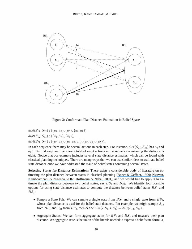
We start with an example search scenario in Figure 3. There are three belief statesBS1 (con-taining statesS11 andS12), BS2 (containing stateS21), andBS3 (containing statesS31 andS32).The goal belief state isBS3, and the two progression search nodes areBS1 andBS2. We want toexpand the search node with the smallest distance toBS3 by estimatingdist(BS1, BS3) – denotedby the bold, dashed line – anddist(BS2, BS3) – denoted by the bold, solid line. We will assume fornow that we have estimates of state distance measuresdist(S, S′) – denoted by the light dashed andsolid lines with numbers. The state distances can be represented as numbers or action sequences. Inour example, we will use the following action sequences for illustration:

4. Interaction between states captures the notion that actions performed to transition one state to the goal may interfere(negatively interact) or aid with (positively interact) transitioning other states to goals states.

45

BRYCE, KAMBHAMPATI , & SMITH

S31

S32

S11

S12

S21

BS3

BS1

BS2 8

10

14

5

3

7

Figure 3: Conformant Plan Distance Estimation in Belief Space

dist(S11, S32) : ({a1, a2}, {a5}, {a6, a7}),

dist(S12, S31) : ({a1, a7}, {a3}),

dist(S21, S31) : ({a3, a6}, {a9, a2, a1}, {a0, a8}, {a5}).

In each sequence there may be several actions in each step. For instance,dist(S21, S31) hasa3 anda6 in its first step, and there are a total of eight actions in the sequence – meaning the distance iseight. Notice that our example includes several state distance estimates, which can be found withclassical planning techniques. There are many ways that we can use similar ideas to estimate beliefstate distance once we have addressed the issue of belief states containing several states.

Selecting States for Distance Estimation: There exists a considerable body of literature on es-timating the plan distance between states in classical planning (Bonet & Geffner, 1999; Nguyen,Kambhampati, & Nigenda, 2002; Hoffmann & Nebel, 2001), and we would like to apply it to es-timate the plan distance between two belief states, sayBS1 andBS3. We identify four possibleoptions for using state distance estimates to compute the distance between belief statesBS1 andBS3:

• Sample a State Pair: We can sample a single state fromBS1 and a single state fromBS3,whose plan distance is used for the belief state distance. For example, we might sampleS12

from BS1 andS31 from BS3, then definedist(BS1, BS3) = dist(S12, S31).

• Aggregate States: We can form aggregate states forBS1 andBS3 and measure their plandistance. An aggregate state is the union of the literals needed to express a belief state formula,

46

PLANNING GRAPH HEURISTICS FORBELIEF SPACE SEARCH

which we define as:

S(BS) =⋃

l:l∈S,S∈ξ(BS)

l

Since it is possible to express a belief state formula with every literal (e.g., using(q ∨¬q)∧ p

to express the belief state wherep is true), we assume a reasonably succinct representation,such as a ROBDD (Bryant, 1986). It is quite possible the aggregate states are inconsis-tent, but many classical planning techniques (such as planning graphs) do not require con-sistent states. For example, with aggregate states we wouldcompute the belief state distancedist(BS1, BS3) = dist(S(BS1), S(BS3)).

• Choose a Subset of States: We can choose a set of states (e.g.,by random sampling) fromBS1 and a set of states fromBS3, and then compute state distances for all pairs of statesfrom the sets. Upon computing all state distances, we can aggregate the state distances (as wewill describe shortly). For example, we might sample bothS11 andS12 from BS1 andS31

fromBS3, computedist(S11, S31) anddist(S12, S31), and then aggregate the state distancesto definedist(BS1, BS3).

• Use All States: We can use all states inBS1 andBS3, and, similar to sampling a subset ofstates (above), we can compute all distances for state pairsand aggregate the distances.

The former two options for computing belief state distance are reasonably straightforward, giventhe existing work in classical planning. In the latter two options we compute multiple state distances.With multiple state distances there are two details which require consideration in order to obtain abelief state distance measure. In the following we treat belief states as if they contain all statesbecause they can be appropriately replaced with the subset of chosen states.

The first issue is that some of the state distances may not be needed. Since each state inBS1

needs to reach a state inBS3, we should consider the distance for each state inBS1 to “a” state inBS3. However, we don’t necessarily need the distance for every state inBS1 to “every” state inBS3. We will explore assumptions about which state distances need to be computed in Section 3.1.

The second issue, which arises after computing the state distances, is that we need to aggregatethe state distances into a belief state distance. We notice that the popular state distance estimatesused in classical planning typically measure aggregate costs of state features (literals). Since weare planning in belief space, we wish to estimate belief state distance with the aggregate cost ofbelief state features (states). In Section 3.2, we will examine several choices for aggregating statedistances and discuss how each captures different types of state interaction. In Section 3.3, weconclude with a summary of the choices we make in order to compute belief state distances.

3.1 State Distance Assumptions

When we choose to compute multiple state distances between two belief statesBS and BS′,whether by considering all states or sampling subsets, not all of the state distances are important.For a given state inBS we do not need to know the distance to every state inBS′ because eachstate inBS need only transition to one state inBS′. There are two assumptions that we can makeabout the states reached inBS′ which help us define two different belief state distance measures interms of aggregate state distances:

47

BRYCE, KAMBHAMPATI , & SMITH

• We can optimistically assume that each of the earlier statesS ∈ M(BS) can reach the closestof the later statesS′ ∈ M(BS′). With this assumption we compute distance as:

dist(BS,BS′) = ▽S∈M(BS) minS′∈M(BS′)

dist(S, S′).

• We can assume that all of the earlier statesS ∈ M(BS) reach the same later stateS′ ∈M(BS′), where the aggregate distance is minimum. With this assumption we compute dis-tance as:

dist(BS,BS′) = minS′∈M(BS′)

▽S∈M(BS)dist(S, S′),

where▽ represents an aggregation technique (several of which we will discuss shortly).Throughout the rest of the paper we use the first definition forbelief state distance because it is

relatively robust and easy to compute. Its only drawback is that it treats the earlier states in a moreindependent fashion, but is flexible in allowing earlier states to transition to different later states.The second definition measures more dependencies of the earlier states, but restricts them to reachthe same later state. While the second may sometimes be more accurate, it is misinformed in caseswhere all earlier states cannot reach the same later state (i.e., the measure would be infinite). We donot pursue the second method because it may return distance measures that are infinite when theyare in fact finite.

As we will see in Section 4, when we discuss computing these measures with planning graphs,we can implicitly find for each state inBS the closest state inBS′, so that we do not enumerate thestatesS′ in the minimization term of the first belief state distance (above). Part of the reason we cando this is that we compute distance in terms of constituentsS′ ∈ ξ(BS′) rather than actual states.Also, because we only consider constituents ofBS′, when we discuss sampling belief states to in-clude in distance computation we only sample fromBS. We can also avoid the explicit aggregation▽ by using theLUG, but describe several choices for▽ to understand implicit assumptions madeby the heuristics computed on theLUG.

3.2 State Distance Aggregation

The aggregation function▽ plays an important role in how we measure the distance between beliefstates. When we compute more than one state distance measure, either exhaustively or by samplinga subset (as previously mentioned), we must combine the measures by some means, denoted▽.There is a range of options for taking the state distances andaggregating them into a belief statedistance. We discuss several assumptions associated with potential measures:

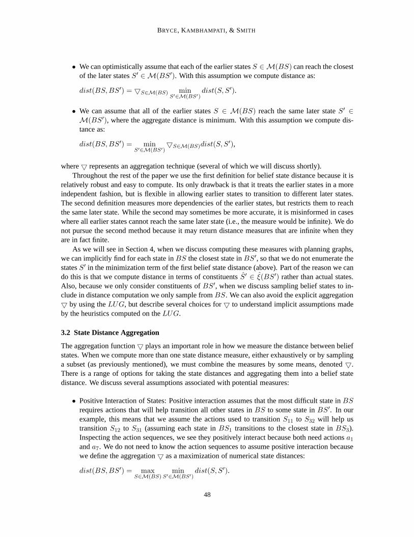
• Positive Interaction of States: Positive interaction assumes that the most difficult state inBS

requires actions that will help transition all other statesin BS to some state inBS′. In ourexample, this means that we assume the actions used to transition S11 to S32 will help ustransitionS12 to S31 (assuming each state inBS1 transitions to the closest state inBS3).Inspecting the action sequences, we see they positively interact because both need actionsa1anda7. We do not need to know the action sequences to assume positive interaction becausewe define the aggregation▽ as a maximization of numerical state distances:

dist(BS,BS′) = maxS∈M(BS)

minS′∈M(BS′)

dist(S, S′).

48

PLANNING GRAPH HEURISTICS FORBELIEF SPACE SEARCH

The belief state distances aredist(BS1, BS3) = max(min(14, 5), min(3, 7)) = 5 anddist(BS2, BS3) = max(min(8, 10)) = 8. In this case we preferBS1 to BS2. If eachstate distance is admissible and we do not sample from beliefstates, then assuming positiveinteraction is also admissible.

• Independence of States: Independence assumes that each state inBS requires actions that aredifferent from all other states inBS in order to reach a state inBS′. Previously, we foundthere was positive interaction in the action sequences to transitionS11 to S32 andS12 to S31

because they shared actionsa1 anda7. There is also some independence in these sequencesbecause the first containsa2, a5, anda6, where the second containsa3. Again, we do not needto know the action sequences to assume independence becausewe define the aggregation▽as a summation of numerical state distances:

dist(BS,BS′) =∑

S∈M(BS)

minS′∈M(BS′)

dist(S, S′).

In our example,dist(BS1, BS3) = min(14, 5) + min(3, 7) = 8, anddist(BS2, BS3) =min(8, 10) = 8. In this case we have no preference overBS1 andBS2.

We notice that using the cardinality of a belief state|M(BS)| to measuredist(BS,BS′) isa special case of assuming state independence, where∀S, S′dist(S, S′) = 1. If we use cardi-nality to measure distance in our example, then we havedist(BS1, BS3) = |M(BS1)| = 2,anddist(BS2, BS3) = |M(BS2)| = 1. With cardinality we preferBS2 overBS1 becausewe have better knowledge inBS2.

• Overlap of States: Overlap assumes that there is both positive interaction and independencebetween the actions used by states inBS to reach a state inBS′. The intuition is that someactions can often be used for multiple states inBS simultaneously and we should count theseactions only once. For example, when we computeddist(BS1, BS3) by assuming positiveinteraction, we noticed that the action sequences fordist(S11, S32) anddist(S12, S31) bothuseda1 anda7. When we aggregate these sequences we would like to counta1 anda7 eachonly once because they potentially overlap. However, trulycombining the action sequencesfor maximal overlap is a plan merging problem (Kambhampati,Ihrig, & Srivastava, 1996),which can be as difficult as planning. Since our ultimate intent is to compute heuristics,we take a very simple approach to merging action sequences. We introduce a plan mergingoperator⋒ for ▽ that picks a step at which we align the sequences and then unions the alignedsteps. We use the size of the resulting action sequence to measure belief state distance:

dist(BS,BS′) = ⋒S∈M(BS) minS′∈M(BS′)

dist(S, S′).

Depending on the type of search, we define⋒ differently. We assume that sequences used inprogression search start at the same time and those used in regression end at the same time.Thus, in progression all sequences are aligned at the first step before we union steps, and inregression all sequences are aligned at the last step beforethe union.

For example, in progressiondist(S11, S32) ⋒ dist(S12, S31) = ({a1, a2}, {a5}, {a6, a7}) ⋒({a1, a7}, {a3}) = ({a1, a2, a7}, {a5, a3}, {a6, a7}) because we align the sequences at theirfirst steps, then union each step. Notice that this resultingsequence has seven actions, giving

49

BRYCE, KAMBHAMPATI , & SMITH

dist(BS1, BS3) = 7, whereas defining▽ as maximum gave a distance of five and as sum-mation gave a distance of eight. Compared with overlap, positive interaction tends to underestimate distance, and independence tends to over estimatedistance. As we will see dur-ing our empirical evaluation (in Section 6.5), accounting for overlap provides more accuratedistance measures for many conformant planning domains.

• Negative Interaction of States: Negative interaction between states can appear in our exampleif transitioning stateS11 to stateS32 makes it more difficult (or even impossible) to transitionstateS12 to stateS31. This could happen if performing actiona5 for S11 conflicts with actiona3 for S12. We can say thatBS1 cannot reachBS3 if all possible action sequences that startin S11 andS12, respectively, and end in anyS ∈ M(BS3) negatively interact.

There are two ways negative interactions play a role in belief state distances. Negative in-teractions can allow us to prove it is impossible for a beliefstateBS to reach a belief stateBS′, meaningdist(BS,BS′) = ∞, or they can potentially increase the distance by a finiteamount. We use only the first, more extreme, notion of negative interaction by computing“cross-world” mutexes (Smith & Weld, 1998) to prune belief states from the search. If wecannot prune a belief state, then we use one of the aforementioned techniques to aggregatestate distances. As such, we do not provide a concrete definition for ▽ to measure negativeinteraction.

While we do not explore ways to adjust the distance measure for negative interactions, wemention some possibilities. Like work in classical planning (Nguyen et al., 2002), we canpenalize the distance measuredist(BS1, BS3) to reflect additional cost associated with se-rializing conflicting actions. Additionally in conditional planning, conflicting actions can beconditioned on observations so that they do not execute in the same plan branch. A distancemeasure that uses observations would reflect the added cost of obtaining observations, aswell as the change in cost associated with introducing plan branches (e.g., measuring averagebranch cost).

The above techniques for belief state distance estimation in terms of state distances provide thebasis for our use of multiple planning graphs. We will show inthe empirical evaluation that thesemeasures affect planner performance very differently across standard conformant and conditionalplanning domains. While it can be quite costly to compute several state distance measures, un-derstanding how to aggregate state distances sets the foundation for techniques we develop in theLUG. As we have already mentioned, theLUG conveniently allows us to implicitly aggregate statedistances to directly measure belief state distance.

3.3 Summary of Methods for Distance Estimation

Since we explore several methods for computing belief statedistances on planning graphs, we pro-vide a summary of the choices we must consider, listed in Table 1. Each column is headed with achoice, containing possible options below. The order of thecolumns reflects the order in which weconsider the options.

In this section we have covered the first two columns which relate to selecting states from beliefstates for distance computation, as well as aggregating multiple state distances into a belief statedistance. We test options for both of these choices in the empirical evaluation.

50

PLANNING GRAPH HEURISTICS FORBELIEF SPACE SEARCH

State State Distance Planning Mutex Mutex HeuristicSelection Aggregation Graph Type Worlds

Single + Interaction SG None Same MaxAggregate Independence MG Static Intersect Sum

Subset Overlap LUG Dynamic Cross LevelAll - Interaction Induced Relaxed Plan

Table 1: Features for a belief state distance estimation.

In the next section we will also expand upon how to aggregate distance measures as well asdiscuss the remaining columns of Table 1. We will present each type of planning graph: the singleplanning graph (SG), multiple planning graphs (MG), and the labelled uncertainty graph (LUG).Within each planning graph we will describe several types ofmutex, including static, dynamic,and induced mutexes. Additionally, each type of mutex can becomputed with respect to differentpossible worlds – which means the mutex involves planning graph elements (e.g., actions) whenthey exist in the same world (i.e., mutexes are only computedwithin the planning graph for a singlestate), or across worlds (i.e., mutexes are computed between planning graphs for different states)by two methods (denoted Intersect and Cross). Finally, we can compute many different heuristicson the planning graphs to measure state distances – max, sum,level, and relaxed plan. We focusour discussion on the planning graphs, same-world mutexes,and relaxed plan heuristics in the nextsection. Cross-world mutexes and the other heuristics are described in appendices.

4. Heuristics

This section discusses how we can use planning graph heuristics to measure belief state distances.We cover several types of planning graphs and the extent to which they can be used to computevarious heuristics. We begin with a brief background on planning graphs.

Planning Graphs: Planning graphs serve as the basis for our belief state distance estimation. Plan-ning graphs were initially introduced in GraphPlan (Blum & Furst, 1995) for representing an op-timistic, compressed version of the state space progression tree. The compression lies in unioningthe literals from every state at subsequent steps from the initial state. The optimism relates to un-derestimating the number of steps it takes to support sets ofliterals (by tracking only a subset of theinfeasible tuples of literals). GraphPlan searches the compressed progression (or planning graph)once it achieves the goal literals in a level with no two goal literals marked infeasible. The searchtries to find actions to support the top level goal literals, then find actions to support the chosenactions and so on until reaching the first graph level. The basic idea behind using planning graphsfor search heuristics is that we can find the first level of a planning graph where a literal in a stateappears; the index of this level is a lower bound on the numberof actions that are needed to achievea state with the literal. There are also techniques for estimating the number of actions required toachieve sets of literals. The planning graphs serve as a way to estimate the reachability of state liter-als and discriminate between the “goodness” of different search states. This work generalizes suchliteral estimations to belief space search by considering both GraphPlan and CGP style planninggraphs plus a new generalization of planning graphs, calledtheLUG.

Planners such as CGP (Smith & Weld, 1998) and SGP (Weld et al.,1998) adapt the GraphPlanidea of compressing the search space with a planning graph byusing multiple planning graphs, one

51

BRYCE, KAMBHAMPATI , & SMITH

None

Positive

Interaction

Independence

Overlap

Sta

te D

ista

nce

Aggre

gat

ion

NG LUG

Planning Graph Type

hMGm-RP

hMGs-RP

hLUGRPhMG

RPU

hcard

GPT

n-distances

CFF

MBP

h0hSG

RP

1

SG MG

hSGRP

U

KACMBP

YKA

Figure 4: Taxonomy of heuristics with respect to planning graph type and state distance aggrega-tion. Blank entries indicate that the combination is meaningless or not possible.

for each possible world in the initial belief state. CGP and SGP search on these planning graphs,similar to GraphPlan, to find conformant and conditional plans. The work in this paper seeks toapply the idea of extracting search heuristics from planning graphs, previously used in state spacesearch (Nguyen et al., 2002; Hoffmann & Nebel, 2001; Bonet & Geffner, 1999) to belief spacesearch.

Planning Graphs for Belief Space: This section proceeds by describing four classes of heuristicsto estimate belief state distanceNG,SG,MG, andLUG. NG heuristics are techniques existing inthe literature that are not based on planning graphs,SG heuristics are techniques based on a singleclassical planning graph,MG heuristics are techniques based on multiple planning graphs (similarto those used in CGP) andLUG heuristics use a new labelled planning graph. TheLUG combinesthe advantages ofSG andMG to reduce the representation size and maintain informedness. Notethat we do not include observations in any of the planning graph structures as SGP (Weld et al.,1998) would, however we do include this feature for future work. The conditional planning formu-lation directly uses the planning graph heuristics by ignoring observations, and our results show thatthis still gives good performance.

In Figure 4 we present a taxonomy of distance measures for belief space. The taxonomy alsoincludes related planners, whose distance measures will becharacterized in this section. All of therelated planners are listed in theNG group, despite the fact that some actually use planning graphs,because they do not clearly fall into one of our planning graph categories. The figure shows how

52

PLANNING GRAPH HEURISTICS FORBELIEF SPACE SEARCH

different substrates (horizontal axis) can be used to compute belief state distance by aggregatingstate to state distances under various assumptions (vertical axis). Some of the combinations arenot considered because they do not make sense or are impossible. The reasons for these omissionswill be discussed in subsequent sections. While there are a wealth of different heuristics one cancompute using planning graphs, we concentrate on relaxed plans because they have proven to be themost effective in classical planning and in our previous studies (Bryce & Kambhampati, 2004). Weprovide additional descriptions of other heuristics like max, sum, and level in Appendix A.

Example: To illustrate the computation of each heuristic, we use an example derived from BTCcalled Courteous BTC (CBTC) where a courteous package dunker has to disarm the bomb andleave the toilet unclogged, but some discourteous person has left the toilet clogged. The initialbelief state of CBTC in clausal representation is:

κ(BSI) = arm∧ clog∧ (inP1∨ inP2)∧ (¬inP1∨¬inP2),

and the goal is:

κ(BSG) = ¬clog∧¬arm.

The optimal action sequences to reachBSG from BSI are:

Flush, DunkP1, Flush, DunkP2, Flush,

and

Flush, DunkP2, Flush, DunkP1, Flush.

Thus the optimal heuristic estimate for the distance between BSI and BSG, in regression, ish∗(BSG) = 5 because in either plan there are five actions.

We use planning graphs for both progression and regression search. In regression search theheuristic estimates the cost of the current belief state w.r.t. the initial belief state and in progressionsearch the heuristic estimates the cost of the goal belief state w.r.t. the current belief state. Thus,in regression search the planning graph(s) are built (projected) once from the possible worlds ofthe initial belief state, but in progression search they need to be built at each search node. Weintroduce a notationBSi to denote the belief state for which we find a heuristic measure, andBSP

to denote the belief state that is used to construct the initial layer of the planning graph(s). In thefollowing subsections we describe computing heuristics for regression, but they are generalized forprogression by changingBSi andBSP appropriately.

In the previous section we discussed two important issues involved in heuristic computation:sampling states to include in the computation and using mutexes to capture negative interactions inthe heuristics. We will not directly address these issues inthis section, deferring them to discussionin the respective empirical evaluation sections, 6.4 and 6.2. The heuristics below are computedonce we have decided on a set of states to use, whether by sampling or not. Also, as previouslymentioned, we only consider sampling states from the beliefstateBSP because we can implicitlyfind closest states fromBSi without sampling. We only explore computing mutexes on the planninggraphs in regression search. We use mutexes to determine thefirst level of the planning graph wherethe goal belief state is reachable (via the level heuristic described in Appendix A) and then extract arelaxed plan starting at that level. If the level heuristic is∞ because there is no level where a beliefstate is reachable, then we can prune the regressed belief state.

We proceed by describing the various substrates used for computing belief space distance esti-mates. Within each we describe the prospects for various types of world aggregation. In addition toour heuristics, we mention related work in the relevant areas.

53

BRYCE, KAMBHAMPATI , & SMITH

4.1 Non Planning Graph-based Heuristics (NG)

We group many heuristics and planners into theNG group because they are not usingSG, MG,or LUG planning graphs. Just because we mention them in this group does not mean they are notusing planning graphs in some other form.

No Aggregation: Breadth first search uses a simple heuristic,h0 where the heuristic value is setto zero. We mention this heuristic so that we can gauge the effectiveness of our search substratesrelative to improvements gained through using heuristics.

Positive Interaction Aggregation: The GPT planner (Bonet & Geffner, 2000) measures beliefstate distance as the maximum of the minimum state to state distance of states in the source anddestination belief states, assuming optimistic reachability as mentioned in Section 3. GPT measuresstate distances exactly, in terms of the minimum number of transitions in the state space. Takingthe maximum state to state distance is akin to assuming positive interaction of states in the currentbelief state.

Independence Aggregation: The MBP planner (Bertoli et al., 2001b), KACMBP planner (Bertoli& Cimatti, 2002), YKA planner (Rintanen, 2003b), and our comparablehcard heuristic measurebelief state distance by assuming every state to state distance is one, and taking the summation ofthe state distances (i.e. counting the number of states in a belief state). This measure can be usefulin regression because goal belief states are partially specified and contain many states consistentwith a goal formula and many of the states consistent with thegoal formula are not reachable fromthe initial belief state. Throughout regression, many of the unreachable states are removed frompredecessor belief states because they are inconsistent with the preconditions of a regressed action.Thus, belief states can reduce in size during regression andtheir cardinality may indicate they arecloser to the initial belief state. Cardinality is also useful in progression because as belief statesbecome smaller, the agent has more knowledge and it can be easier to reach a goal state.

In CBTC,hcard(BSG) = 4 becauseBSG has four states consistent with its complete represen-tation:

ξ(BSG) = (¬inP1∧¬inP2∧¬clog∧¬arm)∨ (¬inP1∧ inP2∧¬clog∧¬arm)∨(inP1∧¬inP2∧¬clog∧¬arm)∨ (inP1∧ inP2∧¬clog∧¬arm).

Notice, this may be uninformed forBSG because two of the states inξ(BSG) are not reachable,like: (inP1∧ inP2∧¬clog∧¬arm). If there aren packages, then there would be2n−1 unreachablestates represented byξ(BSG). Counting unreachable states may overestimate the distance estimatebecause we do not need to plan for them. In general, in addition to the problem of counting unreach-able states, cardinality does not accurately reflect distance measures. For instance, MBP reverts tobreadth first search in classical planning problems becausestate distance may be large or small butit still assigns a value of one.

Overlap Aggregation: Rintanen (2004) describes n-Distances which generalize the belief statedistance measure in GPT to consider the maximum n-tuple state distance. The measure involves,for each n-sized tuple of states in a belief state, finding thelength of the actual plan to transition then-tuple to the destination belief state. Then the maximum n-tuple distance is taken as the distancemeasure.

For example, consider a belief state with four states. With an n equal to two, we would definesix belief states, one for each size two subset of the four states. For each of these belief states wefind a real plan, then take the maximum cost over these plans tomeasure the distance for the original

54

PLANNING GRAPH HEURISTICS FORBELIEF SPACE SEARCH

clog

inP1

¬inP1

inP2

¬inP2

arm

¬clog

clog

inP1

¬inP1

inP2

¬inP2

arm

Flush

¬arm

¬clog

clog

inP1

¬inP1

inP2

¬inP2

arm

DunkP1

DunkP2

Flush

L1

A1

E1

L2L

0A0

E0

ϕ1(DunkP2)

ϕ0(Flush)

ϕ0(DunkP2)

j1(DunkP1)

ϕ0(DunkP1)

j0(Flush)

Figure 5: Single planning graph for CBTC, with relaxed plan components in bold. Mutexes omit-ted.

four state belief state. When n is one, we are computing the same measure as GPT, and when n isequal to the size of the belief state we are directly solving the planning problem. While it is costlyto compute this measure for large values of n, it is very informed as it accounts for overlap andnegative interactions.

The CFF planner (Hoffmann & Brafman, 2004) uses a version of arelaxed planning graph toextract relaxed plans. The relaxed plans measure the cost ofsupporting a set of goal literals from allstates in a belief state. In addition to the traditional notion of a relaxed planning graph that ignoresmutexes, CFF also ignores all but one antecedent literal in conditional effects to keep their relaxedplan reasoning tractable. The CFF relaxed plan does captureoverlap but ignores some subgoals andall mutexes. The way CFF ensures the goal is supported in the relaxed problem is to encode therelaxed planning graph as a satisfiability problem. If the encoding is satisfiable, the chosen numberof action assignments is the distance measure.

4.2 Single Graph Heuristics (SG)

The simplest approach for using planning graphs for belief space planning heuristics is to use a“classical” planning graph. To form the initial literal layer from the projected belief state, we couldeither sample a single state (denotedSG1) or use an aggregate state (denotedSGU ). For example,in CBTC (see Figure 5) assuming regression search withBSP = BSI , the initial levelL0 of theplanning graph forSG1 might be:

55

BRYCE, KAMBHAMPATI , & SMITH

L0 = {arm, clog, inP1,¬inP2}

and forSGU it is defined by the aggregate stateS(BSP ):

L0 = {arm, clog, inP1, inP2,¬inP1,¬inP2}.

Since these two versions of the single planning graph have identical semantics, aside from the initialliteral layer, we proceed by describing theSGU graph and point out differences withSG1 wherethey arise.

Graph construction is identical to classical planning graphs (including mutex propagation) andstops when two subsequent literal layers are identical (level off). We use the planning graph formal-ism used in IPP (Koehler, Nebel, Hoffmann, & Dimopoulos, 1997) to allow for explicit represen-tation of conditional effects, meaning there is a literal layer Lk, an action layerAk, and an effectlayerEk in each levelk. Persistence for a literall, denoted bylp, is represented as an action whereρe(lp) = ε0(lp) = l. A literal is in Lk if an effect from the previous effect layerEk−1 contains theliteral in its consequent. An action is in the action layerAk if every one of its execution preconditionliterals is inLk. An effect is in the effect layerEk if its associated action is in the action layerAk andevery one of its antecedent literals is inLk. Using conditional effects in the planning graph avoidsfactoring an action with conditional effects into a possibly exponential number of non-conditionalactions, but adds an extra planning graph layer per level. Once our graph is built, we can extractheuristics.

No Aggregation: Relaxed plans within a single planning graph are able to measure, under themost optimistic assumptions, the distance between two belief states. The relaxed plan represents adistance between a subset of the initial layer literals and the literals in a constituent of our beliefstate. In theSGU , the literals from the initial layer that are used for support may not hold in asingle state of the projected belief state, unlike theSG1. The classical relaxed plan heuristichSGRP

finds a set of (possibly interfering) actions to support the goal constituent. The relaxed planRP is asubgraph of the planning graph, of the form{ARP

0 , ERP0 , LRP

1 , ...,ARPb−1, E

RPb−1, L

RPb }. Each of the

layers contains a subset of the vertices in the corresponding layer of the planning graph.More formally, we find the relaxed plan to support the constituentS ∈ ξ(BSi) that is reached

earliest in the graph (as found by thehSGlevel(BSi) heuristic in Appendix A). Briefly,hSGlevel(BSi)returns the first levelb where a constituent ofBSi has all its literals inLb and none are markedpair-wise mutex. Notice that this is how we incorporate negative interactions into our heuristics.We start extraction at the levelb, by definingLRP

b as the literals in the constituent used in the levelheuristic. For each literall ∈ LRP

b , we select a supporting effect (ignoring mutexes) fromEb−1

to form the subsetERPb−1. We prefer persistence of literals to effects in supportingliterals. Once a

supporting set of effects is found, we createARPb−1 as all actions with an effect inERP

b−1. Then theneeded preconditions for the actions and antecedents for chosen effects inARP

b−1 andERPb−1 are added

to the list of literals to support fromLRPb−2. The algorithm repeats until we find the needed actions

from A0. A relaxed plan’s value is the summation of the number of actions in each action layer. Aliteral persistence, denoted by a subscript “p”, is treatedas an action in the planning graph, but in arelaxed plan we do not include it in the final computation of| ARP

j |. The single graph relaxed planheuristic is computed as

hSGRP (BSi) =

b−1∑

j=0

| ARPj |

56

PLANNING GRAPH HEURISTICS FORBELIEF SPACE SEARCH

For the CBTC problem we find a relaxed plan from theSGU , as shown in Figure 5 as the boldedges and nodes. Since¬arm and¬clog are non mutex at level two, we can use persistence tosupport¬clog and DunkP1 to support¬arm inLRP

2 . In LRP1 we can use persistence for inP1, and

Flush for¬clog. Thus,hSGRP (BSG) = 2 because the relaxed plan is:

ARP0 = {inP1p, Flush},

ERP0 = {ϕ0(inP1p), ϕ0(Flush)},

LRP1 = {inP1,¬clog},

ARP1 = {¬clogp, DunkP1},

ERP1 = {ϕ0(¬clogp), ϕ1(DunkP1)},

LRP2 = {¬arm,¬clog}.

The relaxed plan does not use both DunkP2 and DunkP1 to support ¬arm. As a result¬arm isnot supported in all worlds (i.e. it is not supported when thestate where inP2 holds is our initialstate). Our initial literal layer threw away knowledge of inP1 and inP2 holding in different worlds,and the relaxed plan extraction ignored the fact that¬arm needs to be supported in all worlds. Evenwith anSG1 graph, we see similar behavior because we are reasoning withonly a single world. Asingle, unmodified classical planning graph cannot capturesupport from all possible worlds – hencethere is no explicit aggregation over distance measures forstates. As a result, we do not mentionaggregating states to measure positive interaction, independence, or overlap.

4.3 Multiple Graph Heuristics (MG)

Single graph heuristics are usually uninformed because theprojected belief stateBSP often cor-responds to multiple possible states. The lack of accuracy is because single graphs are not able tocapture propagation of multiple world support information. Consider the CBTC problem where theprojected belief state isBSI and we are using a single graphSGU . If DunkP1 were the only actionwe would say that¬arm and¬clog can be reached at a cost of two, but in fact the cost is infinite(since there is no DunkP2 to support¬arm from all possible worlds), and there is no strong plan.

To account for lack of support in all possible worlds and sharpen the heuristic estimate, a set ofmultiple planning graphsΓ is considered. Eachγ ∈ Γ is a single graph, as previously discussed.These multiple graphs are similar to the graphs used by CGP (Smith & Weld, 1998), but lack themore general cross-world mutexes. Mutexes are only computed within each graph, i.e. only same-world mutexes are computed. We construct the initial layerLγ

0 of each graphγ with a different stateS ∈ M(BSP ). With multiple graphs, the heuristic value of a belief stateis computed in terms ofall the graphs. Unlike single graphs, we can compute different world aggregation measures with themultiple planning graphs.

While we get a more informed heuristic by considering more ofthe states inM(BSP ), incertain cases it can be costly to compute the full set of planning graphs and extract relaxed plans.We will describe computing the full set of planning graphs, but will later evaluate (in Section 6.4)the effect of computing a smaller proportion of these. The single graphSG1 is the extreme case ofcomputing fewer graphs.

To illustrate the use of multiple planning graphs, considerour example CBTC. We build twographs (Figure 6) for the projectedBSP . They have the respective initial literal layers:

L10 = {arm, clog, inP1,¬inP2} and

L20 = {arm, clog,¬inP2, inP2}.

57

BRYCE, KAMBHAMPATI , & SMITH

clog

inP1

¬inP2

arm

¬ clog

clog

inP1

¬inP2

arm

Flush

¬arm

¬ clog

clog

inP1

¬inP2

arm

DunkP1

DunkP2

Flush

clog

¬inP1

inP2

arm

¬clog

clog

¬inP1

inP2

arm

Flush

¬arm

¬clog

clog

¬inP1

inP2

arm

DunkP1

DunkP2

Flush

1

2

L1

A1

E1

L2L

0A0

E0

ϕ0(Flush)

ϕ1(DunkP1)

ϕ0(DunkP1)

ϕ0(DunkP2)

ϕ0(Flush)ϕ0(Flush)

ϕ0(DunkP1)

ϕ1(DunkP2)

ϕ0(DunkP2)

ϕ0(Flush)

ϕ1(DunkP2)

ϕ1(DunkP1)

Figure 6: Multiple planning graphs for CBTC, with relaxed plan components bolded. Mutexesomitted.

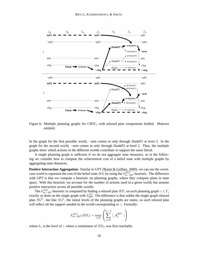
In the graph for the first possible world,¬arm comes in only through DunkP1 at level 2. In thegraph for the second world,¬arm comes in only through DunkP2 at level 2. Thus, the multiplegraphs show which actions in the different worlds contribute to support the same literal.

A single planning graph is sufficient if we do not aggregate state measures, so in the follow-ing we consider how to compute the achievement cost of a belief state with multiple graphs byaggregating state distances.

Positive Interaction Aggregation: Similar to GPT (Bonet & Geffner, 2000), we can use the worst-case world to represent the cost of the belief stateBSi by using thehMG

m−RP heuristic. The differencewith GPT is that we compute a heuristic on planning graphs, where they compute plans in statespace. With this heuristic we account for the number of actions used in a given world, but assumepositive interaction across all possible worlds.

ThehMGm−RP heuristic is computed by finding a relaxed planRPγ on each planning graphγ ∈ Γ,

exactly as done on the single graph withhSGRP . The difference is that unlike the single graph relaxedplanSGU , but like SG1, the initial levels of the planning graphs are states, so each relaxed planwill reflect all the support needed in the world corresponding toγ. Formally:

hMGm−RP (BSi) = max

γ∈Γ

bγ−1∑

j=0

| ARPγ

j |

wherebγ is the level ofγ where a constituent ofBSG was first reachable.

58

PLANNING GRAPH HEURISTICS FORBELIEF SPACE SEARCH

Notice that we are not computing all state distances betweenstates inBSP andBSi. Eachplanning graphγ corresponds to a state inBSP , and from eachγ we extract a single relaxed plan.We do not need to enumerate all states inBSi and find a relaxed plan for each. We instead support aset of literals from one constituent ofBSi. This constituent is estimated to be the minimum distancestate inBSi because it is the first constituent reached inγ.

For CBTC, computinghMGm−RP (BSG) (Figure 6) finds:

RP 1 =

ARP1

0 = {inP1p, Flush},

ERP1

0 = {ϕ0(inP1p), ϕ0(Flush)},

LRP1

1 = {inP1,¬clog},

ARP1

1 = {¬clogp, DunkP1},

ERP1

1 = {ϕ0(¬clogp), ϕ1(DunkP1)},

LRP1

2 = {¬arm,¬clog}

andRP 2 =

ARP2

0 = {inP2p, Flush},

ERP2

0 = {ϕ0(inP2p), ϕ0(Flush)},

LRP2

1 = {inP2,¬clog},

ARP2

1 = {¬clogp, DunkP2},

ERP2

1 = {ϕ0(¬clogp), ϕ1(DunkP2)},

LRP2

2 = {¬arm,¬clog}.

Each relaxed plan contains two actions and taking the maximum of the two relaxed plan valuesgiveshMG

m−RP (BSG) = 2. This aggregation ignores the fact that we must use different Dunk actionseach possible world.

Independence Aggregation: We can use thehMGs−RP heuristic to assume independence among the

worlds in our belief state. We extract relaxed plans exactlyas described in the previous heuristicand simply use a summation rather than maximization of the relaxed plan costs. Formally:

hMGs−RP (BSi) =

∑

γ∈Γ

bγ−1∑

j=0

| ARPγ

j |

wherebγ is the level ofγ where a constituent ofBSG was first reachable.For CBTC, if computinghMG

s−RP (BSG), we find the same relaxed plans as in thehMGm−RP (BSG)

heuristic, but sum their values to get 2 + 2 = 4 as our heuristic. This aggregation ignores the factthat we can use the same Flush action for both possible worlds.

State Overlap Aggregation: We notice that in the two previous heuristics we are either taking amaximization and not accounting for some actions, or takinga summation and possibly accountingfor extra actions. We present thehMG

RPU heuristic to balance the measure between positive interactionand independence of worlds. Examining the relaxed plans computed by the two previous heuristicsfor the CBTC example, we see that the relaxed plans extractedfrom each graph have some overlap.Notice, that bothARP1

0 andARP2

0 contain a Flush action irrespective of which package the bomb isin – showing some positive interaction. Also,ARP1

1 contains DunkP1, andARP2

1 contains DunkP2

59

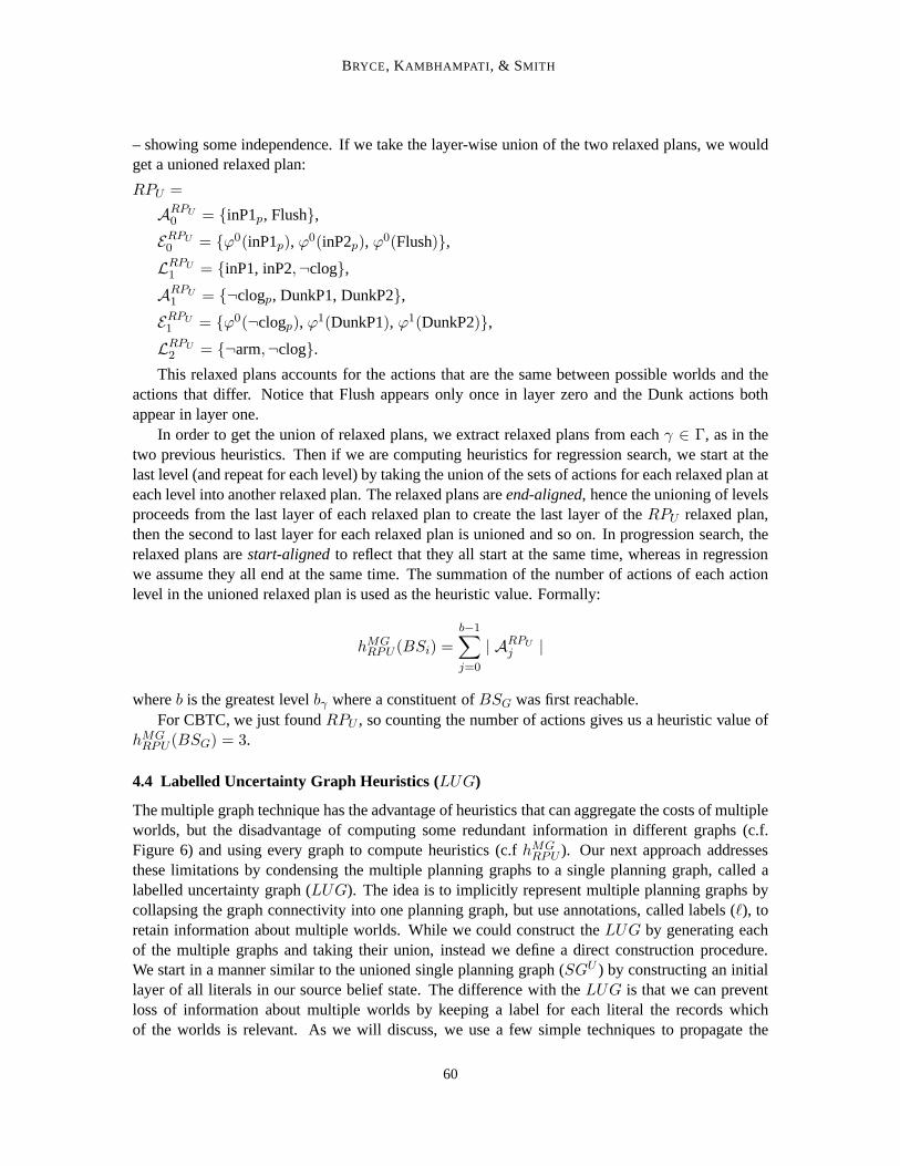
BRYCE, KAMBHAMPATI , & SMITH

– showing some independence. If we take the layer-wise unionof the two relaxed plans, we wouldget a unioned relaxed plan:

RPU =

ARPU0 = {inP1p, Flush},

ERPU0 = {ϕ0(inP1p), ϕ0(inP2p), ϕ0(Flush)},

LRPU

1 = {inP1, inP2,¬clog},

ARPU1 = {¬clogp, DunkP1, DunkP2},

ERPU1 = {ϕ0(¬clogp), ϕ1(DunkP1), ϕ1(DunkP2)},

LRPU2 = {¬arm,¬clog}.

This relaxed plans accounts for the actions that are the samebetween possible worlds and theactions that differ. Notice that Flush appears only once in layer zero and the Dunk actions bothappear in layer one.

In order to get the union of relaxed plans, we extract relaxedplans from eachγ ∈ Γ, as in thetwo previous heuristics. Then if we are computing heuristics for regression search, we start at thelast level (and repeat for each level) by taking the union of the sets of actions for each relaxed plan ateach level into another relaxed plan. The relaxed plans areend-aligned, hence the unioning of levelsproceeds from the last layer of each relaxed plan to create the last layer of theRPU relaxed plan,then the second to last layer for each relaxed plan is unionedand so on. In progression search, therelaxed plans arestart-alignedto reflect that they all start at the same time, whereas in regressionwe assume they all end at the same time. The summation of the number of actions of each actionlevel in the unioned relaxed plan is used as the heuristic value. Formally:

hMGRPU (BSi) =

b−1∑

j=0

| ARPU

j |

whereb is the greatest levelbγ where a constituent ofBSG was first reachable.For CBTC, we just foundRPU , so counting the number of actions gives us a heuristic valueof

hMGRPU (BSG) = 3.

4.4 Labelled Uncertainty Graph Heuristics (LUG)

The multiple graph technique has the advantage of heuristics that can aggregate the costs of multipleworlds, but the disadvantage of computing some redundant information in different graphs (c.f.Figure 6) and using every graph to compute heuristics (c.fhMG

RPU ). Our next approach addressesthese limitations by condensing the multiple planning graphs to a single planning graph, called alabelled uncertainty graph (LUG). The idea is to implicitly represent multiple planning graphs bycollapsing the graph connectivity into one planning graph,but use annotations, called labels (ℓ), toretain information about multiple worlds. While we could construct theLUG by generating eachof the multiple graphs and taking their union, instead we define a direct construction procedure.We start in a manner similar to the unioned single planning graph (SGU ) by constructing an initiallayer of all literals in our source belief state. The difference with theLUG is that we can preventloss of information about multiple worlds by keeping a labelfor each literal the records whichof the worlds is relevant. As we will discuss, we use a few simple techniques to propagate the

60

PLANNING GRAPH HEURISTICS FORBELIEF SPACE SEARCH

labels through actions and effects and label subsequent literal layers. Label propagation relies onexpressing labels as propositional formulas and using standard propositional logic operations. Theend product is a single planning graph with labels on all graph elements; labels indicate which ofthe explicit multiple graphs (if we were to build them) contain each graph element.

We are trading planning graph structure space for label storage space. Our choice of BDDs torepresent labels helps lower the storage requirements on labels. The worst-case complexity of theLUG is equivalent to theMG representation. TheLUG’s complexity savings is not realized whenthe projected possible worlds and the relevant actions for each are completely disjoint; however, thisdoes not often appear in practice. The space savings comes intwo ways: (1) redundant represen-tation of actions and literals is avoided, and (2) labels that facilitate non-redundant representationare stored as BDDs. A nice feature of the BDD package (Brace, Rudell, & Bryant, 1990) we useis that it efficiently represents many individual BDDs in a shared BDD that leverages common sub-structure. Hence, in practice theLUG contains the same information asMG with much lowerconstruction and usage costs.

In this section we present construction of theLUG without mutexes, then describe how tointroduce mutexes, and finally discuss how to extract relaxed plans.

4.4.1 LABEL PROPAGATION

Like the single graph and multiple graphs, theLUG is based on theIPP (Koehler et al., 1997)planning graph. We extend the single graph to capture multiple world causal support, as present inmultiple graphs, by adding labels to the elements of the actionA, effectE , and literalL layers. Wedenote the label of a literall in level k asℓk(l). We can build theLUG for any belief stateBSP ,and illustrateBSP = BSI for the CBTC example. A label is a formula describing a set of states (inBSP ) from which a graph element is (optimistically)reachable. We say a literall is reachable froma set of states, described byBS, afterk levels, ifBS |= ℓk(l). For instance, we can say that¬armis reachable after two levels ifL2 contains¬arm andBSI |= ℓ2(¬arm), meaning that the models ofworlds where¬arm holds after two levels are a superset of the worlds in our current belief state.

The intuitive definition of theLUG is a planning graph skeleton, that represents causal relations,over which we propagate labels to indicate specific possibleworld support. We show the skeletonfor CBTC in Figure 7. Constructing the graph skeleton largely follows traditional planning graphsemantics, and label propagation relies on a few simple rules. Each initial layer literal is labelled,to indicate the worlds ofBSP in which it holds, as the conjunction of the literal withBSP . Anaction is labelled, to indicate all worlds where its execution preconditions can be co-achieved, asthe conjunction of the labels of its execution preconditions. An effect is labelled, to indicate allworlds where its antecedent literals and its action’s execution preconditions can be co-achieved, asthe conjunction of the labels of its antecedent literals andthe label of its associated action. Finally,literals are labelled, to indicate all worlds where they aregiven as an effect, as the disjunction overall labels of effects in the previous level that affect the literal. In the following we describe labelpropagation in more detail and work through the CBTC example.

Initial Literal Layer: TheLUG has an initial layer consisting of every literal with a non false (⊥)label. In the initial layer the labelℓ0(l) of each literall is identical tol∧BSP , representing the statesof BSP in which l holds. The labels for the initial layer literals are propagated through actions andeffects to label the next literal layer, as we will describe shortly. We continue propagation until nolabel of any literal changes between layers, a condition referred to as “level off”.

61

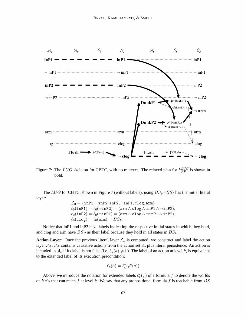
BRYCE, KAMBHAMPATI , & SMITH

inP1

: inP1

inP2

: inP2

arm

clog

: clog

DunkP1

DunkP2

Flush

inP1

: inP1

inP2

: inP2

arm

: arm

clog

: clog

L1

A1

E1

L2

inP1

: inP1

inP2

: inP2

arm

clog

Flush

L0

A0

E0

ϕ0(DunkP1)

j1(DunkP1)

j1(DunkP2)

ϕ0(Flush)

ϕ0(DunkP2)

ϕ0(Flush)

Figure 7: TheLUG skeleton for CBTC, with no mutexes. The relaxed plan forhLUGRP is shown in

bold.

TheLUG for CBTC, shown in Figure 7 (without labels), usingBSP=BSI has the initial literallayer:

L0 = {inP1,¬inP2, inP2,¬inP1, clog, arm}ℓ0(inP1) = ℓ0(¬inP2) = (arm ∧ clog ∧ inP1 ∧ ¬inP2),ℓ0(inP2) = ℓ0(¬inP1) = (arm ∧ clog ∧ ¬inP1 ∧ inP2),ℓ0(clog) = ℓ0(arm) = BSP

Notice that inP1 and inP2 have labels indicating the respective initial states in which they hold,and clog and arm haveBSP as their label because they hold in all states inBSP .

Action Layer: Once the previous literal layerLk is computed, we construct and label the actionlayerAk. Ak contains causative actions from the action setA, plus literal persistence. An action isincluded inAk if its label is not false (i.e.ℓk(a) 6=⊥). The label of an action at levelk, is equivalentto the extended label of its execution precondition:

ℓk(a) = ℓ∗k(ρe(a))

Above, we introduce the notation for extended labelsℓ∗k(f) of a formulaf to denote the worldsof BSP that can reachf at levelk. We say that any propositional formulaf is reachable fromBS

62

PLANNING GRAPH HEURISTICS FORBELIEF SPACE SEARCH

after k levels if BSi |= ℓ∗k(f). Since we only have labels for literals, we substitute the labels ofliterals for the literals in a formula to get the extended label of the formula. The extended label of apropositional formulaf at levelk, is defined:

ℓ∗k(f ∧ f ′) = ℓ∗k(f) ∧ ℓ∗k(f′),

ℓ∗k(f ∨ f ′) = ℓ∗k(f) ∨ ℓ∗k(f′),

ℓ∗k(¬(f ∧ f ′)) = ℓ∗k(¬f ∨ ¬f ′),ℓ∗k(¬(f ∨ f ′)) = ℓ∗k(¬f ∧ ¬f ′),

ℓ∗k(⊤) = BSP ,

ℓ∗k(⊥) =⊥,

ℓ∗k(l) = ℓk(l)

The zeroth action layer for CBTC is:

A0 = {Flush, inP1p,¬inP2p, inP2p,¬inP1p, clogp, armp}ℓ0(Flush) = BSP ,

ℓ0(inP1p) = ℓ0(¬inP2p) = (arm ∧ clog ∧ inP1 ∧ ¬inP2),ℓ0(inP2p) = ℓ0(¬inP1p) = (arm ∧ clog ∧ ¬inP1 ∧ inP2),ℓ0(clogp) = ℓ0(armp) = BSP

Each literal persistence has a label identical to the label of the corresponding literal from theprevious literal layer. The Flush action hasBSP as its label because it is always applicable.

Effect Layer: The effect layerEk depends both on the literal layerLk and action layerAk. Ekcontains an effectϕj(a) if the effect has a non false label (i.e.ℓk(ϕj(a)) 6=⊥). Because both theaction and an effect must be applicable in the same world, thelabel of the effect at levelk is theconjunction of the label of the associated action with the extended label of the antecedent

ℓk(ϕj(a)) = ℓk(a) ∧ ℓ∗k(ρ

j(a))

The zeroth effect layer for CBTC is:

E0 = {ϕ0(Flush), ϕ0(inP1p), ϕ0(¬inP2p), ϕ

0(inP2p),ϕ0(¬inP1p), ϕ

0(clogp), ϕ0(armp)}

ℓ0(ϕ0(Flush)) = BSP

ℓ0(ϕ0(inP1p)) = ℓ0(ϕ

0(¬inP2p)) = (arm ∧ clog ∧ inP1 ∧ ¬inP2),ℓ0(ϕ

0(inP2p)) = ℓ0(ϕ0(¬inP1p)) = (arm ∧ clog ∧ ¬inP1 ∧ inP2),

ℓ0(ϕ0(clogp)) = ℓ0(ϕ

0(armp)) = BSP

Again, like the action layer, the unconditional effect of each literal persistence has a label iden-tical to the corresponding literal in the previous literal layer. The unconditional effect of Flush hasa label identical to the label of Flush.

Literal Layer: The literal layerLk depends on the previous effect layerEk−1, and contains onlyliterals with non false labels (i.e.ℓk(l) 6=⊥). An effectϕj(a) ∈ Ek−1 contributes to the label of aliteral l when the effect consequent contains the literall. The label of a literal is the disjunction ofthe labels of each effect from the previous effect layer thatgives the literal:

ℓk(l) =∨

ϕj(a):l∈εj(a),ϕj(a)∈Ek−1

ℓk−1(ϕj(a))

63

BRYCE, KAMBHAMPATI , & SMITH

The first literal layer for CBTC is:

L1 = {inP1,¬inP2, inP2,¬inP1,¬clog, clog, arm}ℓ1(inP1) = ℓ1(¬inP2) = (arm ∧ clog ∧ inP1 ∧ ¬inP2),ℓ1(inP2) = ℓ1(¬inP1) = (arm ∧ clog ∧ ¬inP1 ∧ inP2),ℓ1(¬clog) = ℓ1(clog) = ℓ1(arm) = BSP

This literal layer is identical to the initial literal layer, except that¬clog goes from having a falselabel (i.e. not existing in the layer) to having the labelBSP .

We continue to the level one action layer becauseL1 does not indicate thatBSG is reachablefrom BSP (¬arm 6∈ L1). Action layer one is defined:

A1 = {DunkP1, DunkP2, Flush, inP1p,¬inP2p, inP2p,¬inP1p, clogp, armp,¬clogp}ℓ1(DunkP1) = ℓ1(DunkP2) = ℓ1(Flush) = BSP ,

ℓ1(inP1p) = ℓ1(¬inP2p) = (arm ∧ clog ∧ inP1 ∧ ¬inP2),ℓ1(inP2p) = ℓ1(¬inP1p) = (arm ∧ clog ∧ ¬inP1 ∧ inP2),ℓ1(clogp) = ℓ1(armp) = ℓ1(¬clogp) = BSP

This action layer is similar to the level zero action layer. It adds both Dunk actions because theyare now executable. We also add the persistence for¬clog. Each Dunk action gets a label identicalto its execution precondition label.

The level one effect layer is:

E1 = {ϕ0(DunkP1), ϕ0(DunkP2), ϕ1(DunkP1), ϕ1(DunkP2), ϕ0(Flush), ϕ0(inP1p),ϕ0(¬inP2p), ϕ

0(inP2p), ϕ0(¬inP1p), ϕ

0(clogp), ϕ0(armp), ϕ

0(¬clogp)}ℓ1(ϕ

0(DunkP1)) = ℓ1(ϕ0(DunkP2)) = ℓ1(ϕ

0(Flush)) = BSP

ℓ1(ϕ1(DunkP1)) = (arm ∧ clog ∧ inP1 ∧ ¬inP2),

ℓ1(ϕ1(DunkP2)) = (arm ∧ clog ∧ ¬inP1 ∧ inP2),

ℓ1(ϕ0(¬inP2p)) = ℓ1(ϕ

0(inP1p)) = (arm ∧ clog ∧ inP1 ∧ ¬inP2),ℓ1(ϕ

0(¬inP1p)) = ℓ1(ϕ0(inP2p)) = (arm ∧ clog ∧ ¬inP1 ∧ inP2),

ℓ1(ϕ0(clogp)) = ℓ1(ϕ

0(armp)) = ℓ1(ϕ0(¬clogp)) = BSP

The conditional effects of the Dunk actions in CBTC (Figure 7) have labels that indicate thepossible worlds in which they will give¬arm because their antecedents do not hold in all possibleworlds. For example, the conditional effectϕ1(DunkP1) has the label found by taking the conjunc-tion of the action’s labelBSP with the antecedent labelℓ∗1(inP1) to obtain(arm ∧ clog ∧ inP1 ∧¬inP2).

Finally, the level two literal layer:

L2 = {inP1,¬inP2, inP2,¬inP1,¬clog, clog, arm,¬arm}ℓ2(inP1) = ℓ2(¬inP2) = (arm ∧ clog ∧ inP1 ∧ ¬inP2),ℓ2(inP2) = ℓ2(¬inP1) = (arm ∧ clog ∧ ¬inP1 ∧ inP2),ℓ2(¬clog) = ℓ2(clog) = ℓ2(arm) = ℓ2(¬arm) = BSP

The labels of the literals for level 2 of CBTC indicate that¬arm is reachable fromBSP be-cause its label is entailed byBSP . The label of¬arm is found by taking the disjunction ofthe labels of effects that give it, namely,(arm ∧ clog ∧ inP1 ∧ ¬inP2) from the conditional

64

PLANNING GRAPH HEURISTICS FORBELIEF SPACE SEARCH

effect of DunkP1 and(arm ∧ clog ∧ ¬inP1 ∧ inP2) from the conditional effect of DunkP2,which reduces toBSP . Construction could stop here becauseBSP entails the label of the goalℓ∗k(¬arm∧¬clog)= ℓk(¬arm) ∧ ℓk(¬clog) = BSP ∧ BSP = BSP . However, level off occurs atthe next level because there is no change in the labels of the literals.

When level off occurs at level three in our example, we can saythat for anyBS, whereBS |=BSP , that a formulaf is reachable ink steps ifBS |= ℓ∗k(f). If no such levelk exists, thenf is notreachable fromBS. If there is some levelk, wheref is reachable fromBS, then the first suchk isa lower bound on the number of parallel plan steps needed to reachf from BS. This lower boundis similar to the classical planning max heuristic (Nguyen et al., 2002). We can provide a moreinformed heuristic by extracting a relaxed plan to supportf with respect toBS, described shortly.

4.4.2 SAME-WORLD LABELLED MUTEXES

There are several types of mutexes that can be added to theLUG. To start with, we only concentrateon those that can evolve in a single possible world because same-world mutexes are more effectiveas well as relatively easy to understand. We extend the mutexpropagation that was used in themultiple graphs so that the mutexes are on one planning graph. The savings of computing mutexeson theLUG instead of multiple graphs is that we can reduce computationwhen a mutex exits inseveral worlds. In Appendix B we describe how to handle cross-world mutexes, despite their lack ofeffectiveness in the experiments we conducted. Cross-world mutexes extend theLUG to computethe same set of mutexes found by CGP (Smith & Weld, 1998).

Same-world mutexes can be represented with a single label,ℓk(x1, x2), between two elements(actions, effect, or literals). The mutex holds between elementsx1 andx2 in all worldsS whereS |= ℓk(x1, x2). If the elements are not mutex in any world, we can assume the label of a mutexbetween them is false⊥. We discuss how the labelled mutexes are discovered and propagated foractions, effect relations, and literals.

By using mutexes, we can refine what it means for a formulaf to be reachable from a set ofworldsBSP . We must ensure that for every state inBSP , there exists a state off that is reachable.A stateS′ of f is reachable from a stateS of BSP when there are no two literals inS′ that aremutex in worldS andBSP |= ℓ∗k(S).

In each of the action, effect, and literal layers there are multiple ways for the same pair ofelements to become mutex (e.g. interference or competing needs). Thus, the mutex label for a pairis the disjunction of all labelled mutexes found for the pairby some means.

Action Mutexes: The same-world action mutexes at a levelk are a set of labelled pairs of actions.Each pair is labelled with a formula that indicates the set ofpossible worlds where the actions aremutex. The possible reasons for mutex actions are interference and competing needs.

• Interference Two actionsa, a′ interfere if (1) the unconditional effect consequentε0(a) ofone is inconsistent with the execution preconditionρe(a′) of the other, or (2) vice versa.They additionally interfere if (3) both unconditional effect consequentsε0(a) andε0(a′) areinconsistent, or (4) both execution preconditionsρe(a) andρe(a′) are inconsistent. The mutexwill exist in all possible world projectionsℓk(a, a′) = BSP . Formally,a anda′ interfere if

65

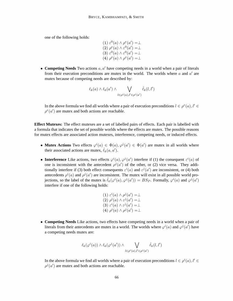
BRYCE, KAMBHAMPATI , & SMITH

one of the following holds:(1) ε0(a) ∧ ρe(a′) =⊥(2) ρe(a) ∧ ε0(a′) =⊥(3) ε0(a) ∧ ε0(a′) =⊥(4) ρe(a) ∧ ρe(a′) =⊥

• Competing Needs Two actionsa, a′ have competing needs in a world when a pair of literalsfrom their execution preconditions are mutex in the world. The worlds wherea anda′ aremutex because of competing needs are described by:

ℓk(a) ∧ ℓk(a′) ∧

∨

l∈ρj(a),l′∈ρj(a′)

ℓk(l, l′)

In the above formula we find all worlds where a pair of execution preconditionsl ∈ ρe(a), l′ ∈ρe(a′) are mutex and both actions are reachable.

Effect Mutexes: The effect mutexes are a set of labelled pairs of effects. Each pair is labelled witha formula that indicates the set of possible worlds where theeffects are mutex. The possible reasonsfor mutex effects are associated action mutexes, interference, competing needs, or induced effects.

• Mutex Actions Two effectsϕi(a) ∈ Φ(a), ϕj(a′) ∈ Φ(a′) are mutex in all worlds wheretheir associated actions are mutex,ℓk(a, a

′).

• Interference Like actions, two effectsϕi(a), ϕj(a′) interfere if (1) the consequentεi(a) ofone is inconsistent with the antecedentρj(a′) of the other, or (2) vice versa. They addi-tionally interfere if (3) both effect consequentsεi(a) andεj(a′) are inconsistent, or (4) bothantecedentsρi(a) andρj(a′) are inconsistent. The mutex will exist in all possible worldpro-jections, so the label of the mutex isℓk(ϕi(a), ϕj(a′)) = BSP . Formally,ϕi(a) andϕj(a′)interfere if one of the following holds:

(1) εi(a) ∧ ρj(a′) =⊥(2) ρi(a) ∧ εj(a′) =⊥(3) εi(a) ∧ εj(a′) =⊥(4) ρi(a) ∧ ρj(a′) =⊥

• Competing Needs Like actions, two effects have competing needs in a world when a pair ofliterals from their antecedents are mutex in a world. The worlds whereϕi(a) andϕj(a′) havea competing needs mutex are:

ℓk(ϕi(a)) ∧ ℓk(ϕ

j(a′)) ∧∨

l∈ρi(a),l′∈ρj(a′)

ℓk(l, l′)

In the above formula we find all worlds where a pair of execution preconditionsl ∈ ρi(a), l′ ∈ρj(a′) are mutex and both actions are reachable.

66

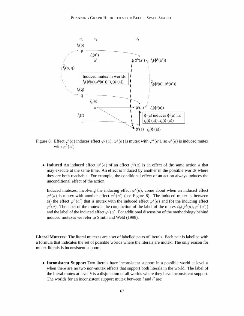
PLANNING GRAPH HEURISTICS FORBELIEF SPACE SEARCH

a

a’

ϕj(a)

ϕh(a’)

ϕi(a) induces ϕj(a) in:

lk(ϕi(a))∧l

k(ϕj(a))

lk(ϕj(a), ϕh(a’))

Induced mutex in worlds:

lk(ϕj(a),ϕh(a’))∧l

k(ϕi(a))

p

q

lk(p)

lk(q)

lk(p, q)

r

lk(r)

lk(a’)

lk(a)

lk(ϕh(a’))

lk(ϕj(a))

lk(ϕi(a))

Lk

Ak

Ek

ϕi(a)

∧

∧∧

Figure 8: Effectϕi(a) induces effectϕj(a). ϕj(a) is mutex withϕh(a′), soϕi(a) is induced mutexwith ϕh(a′).

• Induced An induced effectϕj(a) of an effectϕi(a) is an effect of the same actiona thatmay execute at the same time. An effect is induced by another in the possible worlds wherethey are both reachable. For example, the conditional effect of an action always induces theunconditional effect of the action.

Induced mutexes, involving the inducing effectϕi(a), come about when an induced effectϕj(a) is mutex with another effectϕh(a′) (see Figure 8). The induced mutex is between(a) the effectϕh(a′) that is mutex with the induced effectϕj(a) and (b) the inducing effectϕi(a). The label of the mutex is the conjunction of the label of the mutex ℓk(ϕj(a), ϕh(a′))and the label of the induced effectϕj(a). For additional discussion of the methodology behindinduced mutexes we refer to Smith and Weld (1998).

Literal Mutexes: The literal mutexes are a set of labelled pairs of literals. Each pair is labelled witha formula that indicates the set of possible worlds where theliterals are mutex. The only reason formutex literals is inconsistent support.

• Inconsistent Support Two literals have inconsistent support in a possible world at level kwhen there are no two non-mutex effects that support both literals in the world. The label ofthe literal mutex at levelk is a disjunction of all worlds where they have inconsistent support.The worlds for an inconsistent support mutex betweenl andl′ are:

67

BRYCE, KAMBHAMPATI , & SMITH

∨

S:∀ϕi(a),ϕj(a′)∈Ek−1,

where l∈εi(a),l′∈εj(a′),

S|=ℓk−1(ϕi(a),ϕj (a′))

S

The meaning of the above formula is that the two literals are mutex in all worldsS where allpairs of effects that support the literals inS are mutex inS.

4.4.3 LUG HEURISTICS

The heuristics computed on theLUG can capture measures similar to theMG heuristics, but thereexists a new opportunity to make use of labels to improve heuristic computation efficiency. A singleplanning graph is sufficient if there is no state aggregationbeing measured, so we do not mentionsuch measures for theLUG.

Positive Interaction Aggregation: Unlike MG heuristics, we do not compute positive interactionbased relaxed plans on theLUG. TheMG approach to measure positive interaction across eachstate in a belief state is to compute multiple relaxed plans and take their maximum value. To get thesame measure on theLUG we would still need to extract multiple relaxed plans, the situation we aretrying to avoid by using theLUG. While the graph construction overhead may be lowered by usingtheLUG, the heuristic computation could take too long. Hence, we donot compute relaxed planson theLUG to measure positive interaction alone, but we do compute relaxed plans that measureoverlap (which measures positive interaction).

Independence Aggregation: Like positive interaction aggregation, we need a relaxed plan for everystate in the projected belief state to find the summation of the costs. Hence, we do not computerelaxed plans that assume independence.

State Overlap Aggregation: A relaxed plan extracted from theLUG to get thehLUGRP heuristic

resembles the unioned relaxed plan in thehMGRPU heuristic. Recall that thehMG

RPU heuristic extractsa relaxed plan from each of the multiple planning graphs (onefor each possible world) and unionsthe set of actions chosen at each level in each of the relaxed plans. TheLUG relaxed plan heuristicis similar in that it counts actions that have positive interaction in multiple worlds only once andaccounts for independent actions that are used in subsets ofthe possible worlds. The advantage ofhLUGRP is that we find these actions with a single pass on one planninggraph.

We are trading the cost of computing multiple relaxed plans for the cost of manipulatingLUG

labels to determine what lines of causal support are used in what worlds. In the relaxed plan wewant to support the goal with every state inBSP , but in doing so we need to track which states inBSP use which paths in the planning graph. A subgoal may have several different (and possiblyoverlapping) paths from the worlds inBSP .

A LUG relaxed plan is a set of layers:{ARP0 , ERP

0 ,LRP1 , ..., ARP

b−1, ERPb−1, L

RPb }, whereARP

r

is a set of actions,ERPr is a set of effects, andLRP

r+1 is a set of clauses. The elements of the layersare labelled to indicate the worlds ofBSP where they are chosen for support. The relaxed plan isextracted from the levelb = hLUG

level (BSi) (i.e., the first level whereBSi is reachable, also describedin Appendix A).

Please note that we are extracting the relaxed plan forBSi in terms of clauses, and not liter-als, which is different than theSG andMG versions of relaxed plans. Previously we found the

68

PLANNING GRAPH HEURISTICS FORBELIEF SPACE SEARCH

constituent ofBSi that was first reached on a planning graph and now we do not commit to anyone constituent. Our rationale is that we were possibly using different constituents in each of themultiple graphs, and in this condensed version of the multiple graphs we still want to be able tosupport different constituents of theBSi in different worlds. We could also use the constituent rep-resentation ofBSi in defining the layers of the relaxed plan, but choose the clausal representationof BSi instead because we know that we have to support each clause. However with constituentswe know we only need to support one (but we don’t need to know which one).

The relaxed plan, shown in bold in Figure 7, forBSI to reachBSG in CBTC is listed as follows:

ARP0 = {inP1p, inP2p, Flush},ℓRP0 (inP1p) = (arm ∧ ¬clog ∧ inP1 ∧ ¬inP2),ℓRP0 (inP2p) = (arm ∧ ¬clog ∧ ¬inP1 ∧ inP2),ℓRP0 (Flush) = BSP ,

ERP0 = {ϕ0(inP1p), ϕ

0(inP2p), ϕ0(Flush)},

ℓRP0 (ϕ0(inP1p)) = (arm ∧ ¬clog ∧ inP1 ∧ ¬inP2),ℓRP0 (ϕ0(inP2p)) = (arm ∧ ¬clog ∧ ¬inP1 ∧ inP2),ℓRP0 (ϕ0(Flush)) = BSP ,

LRP1 = {inP1, inP2,¬clog},ℓRP1 (inP1) = (arm ∧ ¬clog ∧ inP1 ∧ ¬inP2),ℓRP1 (inP2) = (arm ∧ ¬clog ∧ ¬inP1 ∧ inP2),ℓRP1 (¬clog) = BSP ,

ARP1 = {DunkP1, DunkP2,¬clogp},ℓRP1 (DunkP1) = (arm ∧ ¬clog ∧ inP1 ∧ ¬inP2),ℓRP1 (DunkP2) = (arm ∧ ¬clog ∧ ¬inP1 ∧ inP2),ℓRP1 (¬clogp) = BSP ,

ERP1 = {ϕ1(DunkP1), ϕ1(DunkP2), ϕ0(¬clogp)},ℓRP1 (ϕ1(DunkP1)) = (arm ∧ ¬clog ∧ inP1 ∧ ¬inP2),ℓRP1 (ϕ1(DunkP2)) = (arm ∧ ¬clog ∧ ¬inP1 ∧ inP2),ℓRP1 (ϕ0(¬clogp)) = BSP ,

LRP2 = {¬arm,¬clog},ℓRP2 (¬arm) = BSP ,

ℓRP2 (¬clog) = BSP

We start by formingLRP2 with the clauses inκ(BSG), namely¬arm and¬clog; we label the

clauses withBSP because they need to be supported by all states in our belief state. Next, wesupport each clause inLRP

2 with the relevant effects fromE1 to form ERP1 . For ¬clog we use

persistence because it supports¬clog in all worlds described byBSP (this is an example of positiveinteraction of worlds). For¬arm the relevant effects are the respectiveϕ1 from each Dunk action.We choose both effects to support¬arm because we need to support¬arm in all worlds ofBSP , andeach effect gives support in only one world (this is an example of independence of worlds). We theninsert the actions associated with each chosen effect intoARP

1 with the appropriate label indicating

69

BRYCE, KAMBHAMPATI , & SMITH

the worlds where it wasneeded, which in general is fewer worlds than where it isreachable(i.e.it is always the case thatℓRP

r (·) |= ℓr(·)). Next we formLRP1 with the execution preconditions of

actions inARP1 and antecedents of effects inERP

1 , which are¬clog, inP1, and inP2, labelled withall worlds where an action or effect needed them. In the same fashion as level two, we support theliterals at level one, using persistence for inP1 and inP2, and Flush for¬clog. We stop here, becausewe have supported all clauses at level one.

For the general case, extraction starts at the levelb whereBSi is first reachable fromBSP .The first relaxed plan layers we construct areARP

b−1, ERPb−1,L

RPb , whereLRP

b contains all clausesC ∈ κ(BSi), labelled asℓRP

k (C) = BSP .For each levelr, 1 ≤ r ≤ b, we support each clause inLRP

r by choosing relevant effects fromEr−1 to form ERP

r−1. An effectϕj(a) is relevant if it is reachable in some of the worlds where weneed to supportC (i.e. ℓr−1(ϕ

j(a)) ∧ ℓRPr (C) 6=⊥) and the consequent gives a literall ∈ C. For

each clause, we have to choose enough supporting effects so that the chosen effect worlds are asuperset of the worlds we need to support the clause, formally:

∀C∈LRPr

ℓRPr (C) |=

∨

ϕj(a):l∈εj(a),l∈C,

ϕj(a)∈Er−1

ℓRPr−1(ϕ

j(a))

We think of supporting a clause in a set of worlds as a set coverproblem where effects coversubsets of worlds. Our algorithm to cover the worlds of a clause with worlds of effects is a variantof the well known greedy algorithm for set cover (Cormen, Leiserson, & Rivest, 1990). We firstchoose all relevant persistence effects that can cover worlds, then choose action effects that coverthe most new worlds. Each effect we choose for support is added toERP

r−1 and labelled with the newworlds it covered forC. Once all clauses inLRP

r are covered, we form the action layerARPr−1 as all

actions that have an effect inERPr−1. The actions inARP

r−1 are labelled to indicate all worlds whereany of their effects were labelled inERP

r−1.We obtain the next subgoal layer,LRP

r−1, by adding literals from the execution preconditions ofactions inARP

r−1 and antecedents of effects inERPr−1. Each literall ∈ LRP

r−1 is labelled to indicate allworlds where any action or effect requiresl. We support the literals inLRP

r−1 in the same fashionasLRP

r . We continue to support literals with effects, insert actions, and insert action and effectpreconditions until we have supported all literals inLRP

1 .Once we get a relaxed plan, the relaxed plan heuristic,hLUG

RP (BSi), is the summation of thenumber of actions in each action layer, formally:

hLUGRP (BSi) =

b−1∑

i=0

| ARPi |

Thus in our CBTC example we havehLUGRP (BSG) = 3. Notice that if we construct theLUG

without mutexes for CBTC we reach the goal after two layers. If we had included mutexes theLUG, then it would reach the goal after three layers. The way we use mutexes will not change ourrelaxed plan because we do not use mutexes to influence relaxed plan extraction. Mutexes only helpto identify when a the belief stateBSi is not reachable fromBSP .

70

PLANNING GRAPH HEURISTICS FORBELIEF SPACE SEARCH

Search Engine

(HSP-r: CAltAlt/

LAO*: POND)

Heuristics

Planning

Graph(s)

(IPP)Belief

StatesBDDs

(CUDD)

PDDL Parser

(IPC)

Labels

Actions

(POND only)

Problem

Figure 9: The implementations of CAltAlt andPOND rely on many existing technologies. Thesearch engine is guided by heuristics extracted from planning graphs.

5. Empirical Evaluation: Setup

This section presents our implementation of theCAltAlt andPOND planners and the domains weuse in the experiments. All tests were run in Linux on an x86 machine with a 2.66GHz P4 processorand 1GB RAM with a timeout of 20 minutes. Both CAltAlt andPOND used a heuristic weightof five in the, respective, A* and AO* searches. We compare with the competing approaches (CGP,SGP, GPT v1.40, MBP v0.91, KACMBP, YKA, and CFF) on several domains and problems. Ourplanners and all domain and problem files for all of the compared planners can be found in theonline appendix.

5.1 Implementation

The implementation of CAltAlt uses several off-the-shelf planning software packages. Figure 9shows a diagram of the system architecture for CAltAlt andPOND. While CAltAlt extends thename ofAltAlt, it relies on a limited subset of the implementation. The components of CAltAltare the IPC parser for PDDL 2.1 (slightly extended to allow uncertain initial conditions), the HSP-r search engine (Bonet & Geffner, 1999), the IPP planning graph (Koehler et al., 1997), and theCUDD BDD package (Brace et al., 1990) to implement theLUG labels. The custom parts of theimplementation include the action representation, beliefstate representation, regression operator,and the heuristic calculation.

The implementation ofPOND is very similar to CAltAlt aside from the search engine, andstate and action representation.POND also uses the IPP source code for planning graphs.POND

uses modified LAO* (Hansen & Zilberstein, 2001) source code from Eric Hansen to perform AO*

71

BRYCE, KAMBHAMPATI , & SMITH

Problem Initial Goal Fluents Causative Observational Optimal OptimalStates Literals Actions Actions Parallel Serial

Rovers1 1 1 66 88 0 {12} 5 {5} 5 {5}Rovers2 2 1 66 88 0 {12} 8 {7} 8 {7}Rovers3 3 1 66 88 0 {12} 10{?} 10{8}Rovers4 4 1 66 88 0 {12} 13{?} 13{10}Rovers5 16 3 71 97 0 {12} ? {?} 20{?}Rovers6 12 3 119 217 0 {18} ? {?} ? {?}

Logistics1 2 1 29 70 0 {10} 6 {6} 9 {7}Logistics2 4 2 36 106 0 {20} 6 {?} 15{12}Logistics3 2 1 58 282 0 {21} 8 {?} 11{8}Logistics4 4 2 68 396 0 {42} 8 {?} 18{?}Logistics5 8 3 78 510 0 {63} ? {?} 28{?}

BT(n) n 1 n+1 n 0 {n} 1 {1} n {n-1}BTC(n) n 1 n+2 n+1 0 {n} 2n-1 {2} 2n-1 {n-1}

CubeCenter(n) n3 3 3n 6 0 (3n-3)/2 (9n-3)/2Ring(n) n3n n 4n 4 0 3n-1 3n-1

Table 2: Features of test domains and problems - Number of initial states, Number of goal liter-als, Number of fluents, Number of causative actions, Number of Observational Actions,Optimal number of parallel plan steps, Optimal number of serial plan steps. Data for con-ditional versions of domains is in braces; plan lengths for conditional plans are maximumconditional branch length.

search, and CUDD (Brace et al., 1990) to represent belief states and actions. Even with deterministicactions it is possible to obtain cycles from actions with observations because we are planning inbelief space.POND constructs the search graph as a directed acyclic graph by employing a cycle-checking algorithm. If adding a hyper-edge to the search graph creates a cycle, then the hyper-edgecannot represent an action in a strong plan and is hence not added to the graph.

5.2 Domains

Table 2 shows some of the relative features of the different problems we used to evaluate our ap-proach. The table shows the number of initial states, goal literals, fluents, actions, and optimalplan lengths. This can be used as a guide to gauge the difficulty of the problems, as well as ourperformance.

Conformant Problems In addition to the standard domains used in conformant planning–suchas Bomb-in-the-Toilet, Ring, and Cube Center, we also developed two new domains Logistics andRovers. We chose these new domains because they have more difficult subgoals, and have manyplans of varying length.

The Ring domain involves a ring ofn rooms where each room is connected to two adjacentrooms. Each room has a window which can be open, closed, or locked. The goal is to have everywindow locked. Initially, any state is possible – we could bein any room and each window could bein any configuration. There are four actions: move right, move left, close the window in the current

72

PLANNING GRAPH HEURISTICS FORBELIEF SPACE SEARCH

room, and lock the window in the current room. Closing a window only works if the window isopen, and locking a window only works if the window is closed.A good conformant plan involvesmoving in one direction closing and locking the window in each room.

The Cube Center domain involves a three-dimensional grid (cube) where there are six actions –it is possible to move in two directions along each dimension. Each dimension consists ofn possiblelocations. Moving in a direction along which there are no more grid points leaves one in the sameposition. Using this phenomena, it is possible to localize in each dimension by repeatedly movingin the same direction. Initially it is possible to be at any location in the cube and the goal is to reachthe center. A good conformant plan involves localizing in a corner and then moving to the center.

The Rovers domain is a conformant adaptation of the analogous domain of the classical planningtrack of the International Planning Competition (Long & Fox, 2003). The added uncertainty tothe initial state uses conditions that determine whether animage objective is visible from variousvantage points due to weather, and the availability of rock and soil samples. The goal is to upload animage of an objective and some rock and soil sample data. Thusa conformant plan requires visitingall of the possible vantage points and taking a picture, plusvisiting all possible locations of soil androck samples to draw samples.

The first five Rovers problems have 4 waypoints. Problems one through four have one throughfour locations, respectively, at which a desired imaging objective is possibly visible (at least one willwork, but we don’t know which one). Problem 5 adds some rock and soil samples as part of the goaland several waypoints where one of each can be obtained (again, we don’t know which waypointwill have the right sample). Problem 6 adds two more waypoints, keeps the same goals as Problem5 and changes the possible locations of the rock and soil samples. In all cases the waypoints areconnected in a tree structure, as opposed to completely connected.

The Logistics domain is a conformant adaptation of the classical Logistics domain where trucksand airplanes move packages. The uncertainty is the initiallocations of packages. Thus, any actionsrelating to the movement of packages have a conditional effect that is predicated on the packageactually being at a location. In the conformant version, thedrivers and pilots cannot sense or com-municate a package’s actual whereabouts. The problems scale by adding packages and cities.

The Logistics problems consist of one airplane, and cities with an airport, a post office, and atruck. The airplane can travel between airports and the trucks can travel within cities. The firstproblem has two cities and one package that could start at either post office, and the goal is to getthe package to the second city’s airport. The second problemadds another package at the samepossible starting points and having the same destination. The third problem has three cities withone package that could be at any post office and has to reach thethird airport. The fourth problemadds a second package to the third problem with the same starting and ending locations. The fifthproblem has three cities and three packages, each at one of two of the three post offices and havingto reach different airports.

Conditional Problems For conditional planning we consider domains from the literature: Bomb-in-the-Toilet with sensing BTS, and Bomb-in-the-Toilet with clogging and sensing BTCS. We alsoextend the conformant Logistics and Rovers to include sensory actions.

The Rovers problem allows for the rover, when it is at a particular waypoint, to sense the avail-ability of image, soil, or rock data at that location. The locations of the collectable data are expressedas one-of constraints, so the rover can deduce the locationsof collectable data by failing to sensethe other possibilities.

73

BRYCE, KAMBHAMPATI , & SMITH

Logistics has observations to determine if a package at a location exists, and the observation isassumed to be made by a driver or pilot at the particular location. Since there are several drivers anda pilot, different agents make the observations. The information gained by the agents is assumed tobe automatically communicated to the others, as the planneris the agent that has all the knowledge.5

6. Empirical Evaluation: Inter-Heuristic Comparison

We start by comparing the heuristic approaches within our planners. In the next section, we continueby describing how our planners, using the best heuristics, compare against other state of the artapproaches. In this section we intend to validate our claimsthat belief space heuristics that measureoverlap perform well across several domains. We further justify using theLUG over multipleplanning graphs and applying mutexes to improve heuristicsin regression through pruning beliefstates.

We compare many techniques within CAltAlt andPOND on our conformant planning do-mains, and in addition we test the heuristics inPOND on the conditional domains. Our perfor-mance metrics include the total planning time and the numberof search nodes expanded. Addi-tionally, when discussing mutexes we analyze planning graph construction time. We proceed byshowing how the heuristics perform in CAltAlt and then how various mutex computation schemesfor theLUG can affect performance. Then we present howPOND performs with the differentheuristics in both conformant and conditional domains, explore the effect of sampling a proportionof worlds to buildSG1, MG, andLUG graphs, and compare the heuristic estimates inPOND

to the optimal plan length to gauge heuristic accuracy. We finish with a summary of importantconclusions.

We only compute mutexes in the planning graphs for CAltAlt because the planning graph(s) areonly built once in a search episode and mutexes help prune theinconsistent belief states encounteredin regression search. We abstain from computing mutexes inPOND because in progression webuild new planning graphs for each search node and we want to keep graph computation time low.With the exception of our discussion on sampling worlds to construct the planning graphs, theplanning graphs are constructed deterministically. This means that the single graph is the unionedsingle graphSGU , and theMG andLUG graphs are built for all possible worlds.

6.1 CAltAlt

The results for CAltAlt in the conformant Rovers, Logistics, BT, and BTC domains, interms oftotal time and number of expanded search nodes, are presented in Table 3. We show the number ofexpanded nodes because it gives an indication of how well a heuristic guides the planner. The totaltime captures the amount of time computing the heuristic andsearching. A high total time with ahigh number of search nodes indicates a poor heuristic, and ahigh total time and low number ofsearch nodes indicates an expensive but informed heuristic.

We do not discuss the Ring and Cube Center domains for CAltAlt because it cannot solveeven the smallest instances. Due to implementation detailsthe planner performs very poorly whendomains have actions with several conditional effects and hence does not scale. The trouble stems

5. This problem may be interesting to investigate in a multi-agent planning scenario, assuming no global communication(e.g. no radio dispatcher).

74

PLANNING GRAPH HEURISTICS FORBELIEF SPACE SEARCH

Problem h0 hcard hSGRP hMGm−RP hMG

RPU hLUG(FX)RP

Rovers 1 2255/5 18687/14 543/5 542/5 185/5 15164/52 49426/8 TO 78419/8 8327/8 29285/9 32969/83 TO - 91672/10 20162/10 2244/11 16668/104 - - TO 61521/16 3285/15 31584/135 - - - TO TO TO6 - - - - - -

Logistics 1 1108/9 4268/9 198/9 183/9 1109/9 1340/92 TO TO 7722/15 15491/15 69818/19 18535/153 - - 3324/14 70882/14 TO 16458/154 - - 141094/19 TO - 178068/195 - - TO - - TO

BT 2 19/2 14/2 18/2 20/2 21/2 12/210 4837/10 56/10 5158/10 8988/10 342/10 71/1020 TO 418/20 TO TO 2299/20 569/2030 - 1698/30 - - 9116/30 2517/3040 - 5271/40 - - 44741/40 7734/4050 - 12859/50 - - TO 18389/5060 - 26131/60 - - - 37820/6070 - 48081/70 - - - 70538/7080 - 82250/80 - - - 188603/80

BTC 2 30/3 16/3 16/3 33/3 23/3 18/310 15021/19 161/19 15679/19 41805/19 614/19 1470/1920 TO 1052/39 TO TO 2652/39 51969/3930 - 3823/59 - - 9352/59 484878/5940 - 11285/79 - - 51859/79 TO50 - 26514/99 - - TO -60 - 55687/119 - - - -70 - 125594/140 - - - -

Table 3: Results for CAltAlt for conformant Rovers, Logistics, BT, and BTC. The data is TotalTime / # Expanded Nodes, “TO” indicates a time out (20 minutes) and “-” indicates noattempt.

from a weak implementation for bringing general propositional formulas (obtained by regressionwith several conditional effects) into CNF.

We describe the results from left to right in Table 3, comparing the different planning graphstructures and relaxed plans computed on each planning graph. We start with the non-planninggraph heuristicsh0 andhcard. As expected,h0, breadth-first search, does not perform well in alarge portion of the problems, shown by the large number of search nodes and inability to scale tosolve larger problems. We notice that with thehcard heuristic performance is very good in the BTand BTC problems (this confirms the results originally seen by Bertoli, Cimatti, & Roveri, 2001a).However,hcard does not perform as well in the Rovers and Logistics problemsbecause the size of abelief state, during planning, does not necessarily indicate that the belief state will be in a good plan.Part of the reasonhcard works so well in some domains is that it measures knowledge, and plansfor these domains are largely based on increasing knowledge. The reasonhcard performs poorlyon other domains is that finding causal support (which it doesnot measure) is more important thanknowledge for these domains.

75

BRYCE, KAMBHAMPATI , & SMITH

Next, for a single planning graph (SGU ), CAltAlt does reasonably well with thehSGRP heuristic inthe Rovers and Logistics domains, but fails to scale very well on the BT and BTC domains. Roversand Logistics have comparatively fewer initial worlds thanthe BT and BTC problems. Moreoverthe deterministic plans, assuming each initial state is thereal state, are somewhat similar for Roversand Logistics, but mostly independent for BT and BTC. Therefore, approximating a fully observ-able plan with the single graph relaxed plan is reasonable when plans for achieving the goal fromeach world have high positive interaction. However, without high positive interaction the heuristicdegrades quickly when the number of initial worlds increases.

With multiple planning graphs, CAltAlt is able to perform better in the Rovers domain, but takesquite a bit of time in the Logistics, BT, and BTC domains. In Rovers, capturing distance estimatesfor individual worlds and aggregating them by some means tends to be better than aggregatingworlds and computing a single distance estimate (as in a single graph). In Logistics, part of thereason computing multiple graphs is so costly is that we are computing mutexes on each of theplanning graphs. In BT and BTC, the total time increases quickly because the number of planninggraphs, and number of relaxed plans for every search node increase so much as problems get larger.

Comparing the two multiple graph heuristics6 in CAltAlt namelyhMGm−RP andhMG

RPU , we cansee the effect of our choices for state distance aggregation. The hMG

m−RP relaxed plan heuristicaggregates state distances, as found on each planning graph, by taking the maximum distance. ThehMGRPU unions the relaxed plans from each graph, and counts the number of actions in the unioned

relaxed plan. As with the single graph relaxed plan, thehMGm−RP relaxed plan essentially measures

one state to state distance; thus, performance suffers on the BT and BTC domains. However, usingthe unioned relaxed plan heuristic, we capture the independence among the multiple worlds so thatwe scale up better in BT and BTC. Despite the usefulness of theunioned relaxed plan, it is costly tocompute and scalability is limited, so we turn to theLUG version of this same measure.

With theLUG, we use thehLUG(FX)RP heuristic in CAltAlt . This heuristic uses aLUG with

full cross-world mutexes (denoted byFX). As in the similarhMGRPU heuristic, measuring overlap is

important, and improving the speed of computing the heuristic tends to improve the scalability ofCAltAlt . While CAltAlt is slower in the Rovers and BTC domains when using theLUG, we notethat it is because of the added cost of computing cross-worldmutexes – we are able to improve thespeed by relaxing the mutexes, as we will describe shortly.

6.2 Mutexes

Mutexes are used to help determine when a belief state is unreachable. Mutexes improve the pruningpower of heuristics by accounting for negative interactions. The mutexes are only used to improveour heuristics, so it is reasonable to compute only a subset of the mutexes. We would like to knowwhich mutexes are the most cost effective because the numberof possible mutexes we can find isquite large.

We can use several schemes to compute a subset of the mutexes.The schemes combine differenttypes of mutexes with types of cross-world checking. The mutex types are: computing no mutexes(NX), computing only static interference mutexes (StX), computing (StX) plus inconsistent sup-port and competing needs mutexes – dynamic mutexes (DyX), and computing (DyX) plus inducedmutexes – full mutexes (FX). The cross-world checking (see appendix B) reduction schemes are:

6. We showhMGs−RP with POND.

76

PL

AN

NIN

GG

RA

PH

HE

UR

IST

ICS

FO

RBE

LIE

FS

PA

CE

SE

AR

CH

Problem hLUG(NX)RP h

LUG(StX)RP h

LUG(DyX)RP h

LUG(FX)RP h

LUG(DyX−SX)RP h

LUG(DyX−IX)RP h

LUG(FX−SX)RP h

LUG(FX−IX)RP

Rovers 1 13/1112/51 19/1119/51 15453/89/6 15077/87/6 15983/87/6 15457/87/6 15098/86/6 15094/85/62 20/904/41 16/903/41 13431/138/8 32822/147/8 10318/139/8 10625/134/8 10523/138/8 14550/138/83 13/8704/384 17/8972/384 17545/185/10 16481/187/10 10643/185/10 11098/209/10 10700/191/10 11023/184/104 TO TO 32645/441/14 31293/291/14 14988/291/14 16772/291/14 14726/290/14 16907/290/145 - - 698575/3569/45 TO 61373/3497/45 379230/3457/45 60985/3388/45 378869/3427/456 - - TO - 217507/3544/37 565013/3504/37 225213/3408/37 588336/3512/37

Logistics 1 5/868/81 10/868/81 1250/117/9 1242/98/9 791/116/9 797/117/9 796/115/9 808/115/92 10/63699/1433 88/78448/1433 16394/622/15 18114/421/15 2506/356/15 7087/428/15 2499/352/15 6968/401/153 TO TO 17196/1075/15 16085/373/15 10407/403/15 10399/408/15 10214/387/15 10441/418/154 - - 136702/1035/19 176995/1073/19 24214/648/19 71964/871/19 23792/642/19 71099/858/195 - - TO TO 52036/2690/41 328114/4668/52 52109/2672/41 324508/4194/52

BT 2 1/34/2 0/13/2 0/13/2 0/12/2 0/16/2 0/15/2 0/25/2 0/13/210 4/72/10 4/56/10 13/57/10 13/58/10 12/59/10 14/59/10 13/59/10 14/56/1020 19/452/20 22/448/20 120/453/20 120/449/20 102/450/20 139/454/20 105/444/20 137/454/2030 62/1999/30 59/1981/30 514/1999/30 509/2008/30 421/1994/30 600/2007/30 413/1986/30 596/2002/3040 130/6130/40 132/6170/40 1534/6432/40 1517/6217/40 1217/6326/40 1822/6163/40 1196/6113/40 1797/6127/4050 248/14641/50 255/14760/50 3730/14711/50 3626/14763/50 2866/14707/50 4480/14676/50 2905/14867/50 4392/14683/5060 430/30140/60 440/29891/60 7645/30127/60 7656/30164/60 5966/30017/60 9552/30337/60 5933/30116/60 9234/29986/6070 680/55202/70 693/55372/70 15019/55417/70 14636/55902/70 11967/55723/70 18475/55572/70 11558/55280/70 18081/55403/7080 1143/135760/80 1253/140716/80 26478/132603/80 26368/162235/80 21506/136149/80 32221/105654/80 21053/139079/80 32693/109508/80

BTC 2 0/62/3 1/16/3 0/15/3 4/14/3 0/16/3 1/14/3 1/13/3 2/14/310 4/93/19 4/77/19 14/78/19 1388/82/19 13/76/19 16/75/19 14/75/19 440/81/1920 21/546/39 32/545/39 139/553/39 51412/557/39 105/546/39 140/549/39 110/555/39 19447/568/3930 58/2311/59 61/2293/59 543/2288/59 482578/2300/59 427/2294/59 606/2300/59 444/2287/59 199601/2401/5940 133/6889/79 149/6879/79 1564/6829/79 TO 1211/6798/79 1824/6816/79 1253/6830/79 1068019/6940/7950 260/15942/99 261/16452/99 TO - 2890/16184/99 4412/16414/99 2926/16028/99 TO60 435/32201/119 443/32923/119 - - 6045/32348/119 9492/32350/119 6150/32876/119 -70 742/62192/139 745/61827/139 - - TO TO TO -

Table4:

Results

forCA

ltAlt

usinghLUG

RP

with

mutex

schemes.

The

datais

Graph

Construction

Tim

e(m

s)/AllO

therTim

e(m

s)/#E

xpandedN

odes,“TO

”indicates

atim

eout(20

minutes)

and“-”

indicatesno

attempt.

77

BRYCE, KAMBHAMPATI , & SMITH

computing mutexes across same-worlds (SX) and computing mutexes across pairs of worlds in theintersection (conjunction) of element labels (IX).

Table 4 shows that within CAltAlt , using the relaxed plan heuristic and changing the way wecompute mutexes on theLUG can drastically alter performance. Often, the cross-worldmutexesare so numerous that building theLUG takes too much time. To see if we could reduce graphconstruction overhead without hindering performance, we evaluatedhLUG

RP when the LUG is built(a) considering all cross-world relations, for the schemes(NX), (StX), (DyX), and (FX); and (b)same-world relations for the schemes (DyX-SX) and (FX-SX),and (c) cross-world relations for allpossible worlds pairs in the intersection of element’s labels (DyX-IX) and (FX-IX).

The results show that simpler problems like BT and BTC do not benefit as much from advancedcomputation of mutexes beyond static interference. However, for the Rovers and Logistics prob-lems, advanced mutexes play a larger role. Mainly, interference, competing needs, and inconsistentsupport mutexes are important. The competing needs and inconsistent support mutexes seem tohave a large impact on the informedness of the guidance givenby theLUG, as scalability improvesmost here. Induced mutexes don’t improve search time much, and only add to graph computationtime. A possible reason induced mutexes don’t help as much inthese domains is that all the actionshave at most two effects, an unconditional and conditional effect. Reducing cross-world mutexchecking also helps quite a bit. It seems that only checking same-world mutexes is sufficient tosolve large problems. Interestingly, theMG graphs compute same-world interference, competingneeds, and inconsistent support mutexes within each graph,equating to the same scenario as (DyX-SX), however, the LUG provides a much faster construction time, evidenced by theLUG’s abilityto out-scaleMG.

6.3 POND

We show the total time and the number of expanded nodes forPOND solving the conformantproblems (including Ring and Cube Center) in Table 5, and forPOND solving the conditionalproblems in Table 6. As with CAltAlt we show the total time and number of expanded nodes foreach test. We also add thehMG

s−RP heuristic, not implemented in CAltAlt , that takes the summationof the values of relaxed plans extracted from multiple planning graphs. We do not compute mutexeson any of the planning graphs used for heuristics inPOND mainly because we build planninggraphs for each search node. We proceed by first commenting onthe performance ofPOND, withthe different heuristics, in the conformant domains, then discuss the conditional domains.

In the conformant domains,POND generally does better than CAltAlt . This may be attributedin part to implementation-level details.POND makes use of an existing (highly optimized) BDDpackage for belief state generation in progression, but as previously mentioned, CAltAlt relies on aless optimized implementation for belief state generationin regression. As we will see in the nextsection, regression planners that employ a more sophisticated implementation perform much better,but could still benefit from our heuristics. Aside from a few differences that we will mention, we seesimilar trends in the performance of the various heuristicsin both CAltAlt andPOND. Namely,theNG andSG heuristics have limited ability to help the planner scale, theMG heuristics helpthe planner scale better but are costly, and theLUG provides the best scalability. The differencebetween theMG and theLUG are especially pronounced in Cube Center and Ring, where thesizeof the initial belief state is quite large as the instances scale. Interestingly in Ring, breadth firstsearch and the single graph relaxed plan are able to scale dueto reduced heuristic computation time

78

PLANNING GRAPH HEURISTICS FORBELIEF SPACE SEARCH

Problem h0 hcard hSGRP hMGm−RP hMG

s−RP hMGRPU hLUG

RP

Rovers 1 540/36 520/21 590/6 580/6 580/6 580/6 590/62 940/249 790/157 700/15 1250/32 750/10 830/13 680/113 3340/1150 2340/755 3150/230 3430/77 1450/24 1370/23 850/164 TO 14830/4067 13480/1004 10630/181 7000/163 2170/34 1130/285 - TO TO 85370/452 12470/99 31480/73 2050/366 - - - 180890/416 15780/38 31950/73 9850/147

Logistics 1 560/169 530/102 680/46 970/58 730/21 650/9 560/92 TO TO TO 2520/32 6420/105 2310/20 910/153 - - - 27820/927 4050/83 2000/15 1130/144 - - - 5740/27 29180/211 53470/382 3180/465 - - - 42980/59 51380/152 471850/988 6010/42

BT 2 450/3 460/2 460/3 450/2 450/2 500/2 460/210 760/1023 590/428 1560/1023 6200/428 820/10 880/10 520/1020 TO TO TO TO 6740/20 6870/20 1230/2030 - - - - 41320/30 44260/30 4080/3040 - - - - 179930/40 183930/40 11680/4050 - - - - 726930/50 758140/50 28420/5060 - - - - TO TO 59420/6070 - - - - - - 113110/7080 - - - - - - 202550/80

BTC 2 460/5 460/4 450/5 460/4 460/3 470/3 460/310 1090/2045 970/1806 3160/2045 18250/1806 980/19 990/19 540/1920 TO TO TO TO TO 9180/39 1460/3930 - - - - - 54140/59 4830/5940 - - - - - 251140/79 14250/7950 - - - - - 1075250/99 34220/9960 - - - - - TO 71650/11970 - - - - - - 134880/139

CubeCenter 3 10/184 30/14 90/34 1050/61 370/9 0430/11 70/115 180/3198 20/58 3510/1342 60460/382 11060/55 14780/82 1780/2057 1940/21703 40/203 46620/10316 TO 852630/359 1183220/444 27900/17749 TO 70/363 333330/46881 - TO TO 177790/722611 - 230/1010 TO - - - 609540/1702713 - 700/2594 - - - - TO

Ring 2 20/15 20/7 30/15 80/8 80/7 80/8 30/83 20/59 20/11 70/59 1500/41 500/8 920/19 70/104 30/232 20/15 350/232 51310/77 6370/11 19300/40 250/245 160/973 20/19 2270/973 TO 283780/16 TO 970/446 880/4057 30/23 14250/4057 - TO - 4080/987 5940/16299 40/27 83360/16299 - - - 75020/5748 39120/64657 40/31 510850/64657 - - - 388300/9029 251370/261394 50/35 TO - - - TO10 TO 70/39 - - - - -

Table 5: Results forPOND for conformant Rovers, Logistics, BT, BTC, Cube Center, andRing.The data is Total Time (ms)/# Expanded Nodes, “TO” indicatesa time out and “-” indicatesno attempt.

and the low branching factor in search. TheLUG is able to provide good search guidance, but tendsto take a long time computing heuristics in Ring.

We are also now able to compare the choices for aggregating the distance measures from re-laxed plans for multiple graphs. We see that taking the maximum of the relaxed plans,hMG

m−RP , inassuming positive interaction among worlds is useful in Logistics and Rovers, but loses the indepen-dence of worlds in the BT and BTC domains. However, taking thesummation of the relaxed plan

79

BRYCE, KAMBHAMPATI , & SMITH

Problem h0 hcard hSGRP hMGm−RP hMG

s−RP hMGRPU hLUG

RP

Rovers 1 550/36 480/21 580/6 570/6 570/6 580/6 580/62 1030/262 550/36 780/15 760/14 710/12 730/12 730/133 1700/467 590/48 3930/248 830/15 830/15 910/17 810/164 5230/1321 620/58 6760/387 1020/20 1040/21 1070/21 910/215 TO TO TO 16360/175 11100/232 12810/209 7100/1746 - - - 31870/173 24840/159 30250/198 13560/174

Logistics 1 530/118 TO 740/46 580/10 570/10 600/10 570/102 TO - TO 1630/30 1300/36 1360/36 1250/363 - - - 1360/20 1250/19 1290/19 1210/194 - - - 4230/59 3820/57 3940/57 4160/575 - - - 27370/183 19620/178 20040/178 20170/178

BT 2 460/5 460/3 450/3 460/3 450/3 470/3 460/310 TO 470/19 111260/7197 970/19 970/19 1020/19 550/1920 - 510/39 TO 9070/39 9060/39 9380/39 1610/3930 - 620/59 - 52410/59 52210/59 55750/59 5970/5940 - 850/79 - 207890/79 206830/79 233720/79 17620/7950 - 1310/99 - 726490/99 719000/99 TO 43020/9960 - 2240/119 - TO TO - 91990/11970 - 24230/139 - - - - 170510/13980 - 45270/159 - - - - 309940/159

BTC 2 450/6 460/3 470/5 470/3 460/3 470/3 470/310 TO 480/19 271410/10842 1150/19 1140/19 1200/19 590/1920 - 510/39 TO 11520/39 TO 11610/39 1960/3930 - 660/59 - 62060/59 - 64290/59 6910/5940 - 970/79 - 251850/79 - 274610/79 19830/7950 - 1860/99 - 941220/99 - TO 49080/9960 - 4010/119 - TO - - 103480/11970 - 7580/139 - - - - 202040/139

Table 6: Results forPOND for conditional Rovers, Logistics, BTS, BTCS. The data is Total Time(ms)/# Expanded Nodes, “TO” indicates a time out (20 minutes) and “-” indicates noattempt.

values for different worlds,hMGs−RP is able to capture the independence in the BT domain. We notice

that the summation does not helpPOND in the BTC domain; this is because we overestimate theheuristic value for some nodes by counting the Flush action once for each world when it in factonly needs to be done once (i.e. we miss positive interaction). Finally, using thehMG

RPU heuristicwe do well in every domain, aside from the cost of computing multiple graph heuristics, becausewe account for both positive interaction and independence by taking the overlap of relaxed plans.Again, with theLUG relaxed plan, analogous to the multiple graph unioned relaxed plan,POND

scales well because we measure overlap and lower the cost of computing the heuristic significantly.

The main change we see in usingPOND versus CAltAlt is that the direction of search isdifferent, so thehcard heuristic performs unlike before. In the BT and BTC domains cardinalitydoes not work well in progression because the size of belief states does not change as we get closerto the goal (it is impossible to ever know which package contains the bomb). However, in regressionwe start with a belief state containing all states consistent with the goal and regressing actions limits

80

PLANNING GRAPH HEURISTICS FORBELIEF SPACE SEARCH

our belief state to only those states that can reach the goal through those actions. Thus in regressionthe size of belief states decreases, but in progression remains constant.

The performance ofPOND in the conditional domains exhibits similar trends to the confor-mant domains, with a few exceptions. Like the conformant domains, theMG relaxed plans tend tooutperform theSG relaxed plan, but theLUG relaxed plan does best overall. Unlike the conformantdomains, ThehMG

m−RP performs much better in BTS and BTCS over BT and BTC partly becausethe conditional plans have a lower average cost. Thehcard heuristic does better in BTS and BTCSover BT and BTC because the belief states actually decrease in size when they are partitioned bysensory actions.

6.4 Sampling Worlds

Our evaluations to this point have considered the effectiveness of different heuristics, each com-puted with respect to all possible worlds of a belief state. While we would like to use as many ofthe possible worlds as we can, we can reduce computation costand hopefully still get reasonableheuristics by considering a subset of the worlds. Our schemefor considering subsets of worlds inthe heuristics is to sample a single world (SG1), or sample a given percentage of the worlds andbuild multiple graphs, or theLUG.

With these sampling approaches, we use thehSGRP , hMGRPU , andhLUG

RP relaxed plans. We buildtheMG andLUG for 10%, 30%, 50%, 70%, and 90% of the worlds in each belief state, sampledrandomly. In Figure 10, we show the total time taken (ms) to solve every problem in our test set(79 problems over 10 domains). Each unsolved problem contributed 20 minutes to the total time.For comparison we show the previously mentioned heuristics: hSGRP computed on a unioned singlegraphSGU , denoted as “Unioned” compared to the sampled single graphSG1 denoted as “Single”,andhMG

RPU andhLUGRP computed for all worlds denoted as “100%”. The total time forany heuristic

that samples worlds is averaged over ten runs.There are two major points to see in Figure 10. First, thehSGRP heuristic is much more effective

when computed onSG1 versusSGU . This is because theSG1 is less optimistic. It builds aplanning graph for a real world state, as opposed to the unionof literals in all possible world states,as inSGU . Respecting state boundaries and considering only a singlestate is better than ignoringstate boundaries to naively consider all possible states. However, as we have seen with theMG

andLUG heuristics, respecting state boundaries and considering several states can be much better,bringing us to the second point.

We see very different performance when using more possible worlds to build multiple graphscompared to theLUG. We are better off using fewer worlds if we have to build multiple graphsbecause they can become very costly as the number of worlds increases. In contrast, performanceimproves with more possible worlds when we use theLUG. Using more possible worlds to computeheuristics is a good idea, but it takes a more efficient substrate to exploit them.

6.5 Accuracy

The heuristics that account for overlap in the possible worlds should be more accurate than theheuristics that make an assumption of full positive interaction or full independence. To check ourintuitions, we compare the heuristic estimates for the distance between the initial belief state andthe goal belief state for all the heuristics used in conformant problems solved byPOND. Figure11 shows the ratio of the heuristic estimate forh(BSI) to the optimal serial plan lengthh∗(BSI) in

81

BRYCE, KAMBHAMPATI , & SMITH

0

2

4

6

8

10

12

14

16

Unioned Single 10% 30% 50% 70% 90% 100%

SG

MG

LUG

Figure 10: Total Time (hours) forPOND to solve all conformant and conditional problems whensampling worlds to use in heuristic computation.

several problems. The points below the line (where the ratiois one) are under-estimates, and thoseabove are over-estimates. Some of the problem instances arenot shown because no optimal planlength is known.

We note that in all the domains thehLUGRP andhMG

RPU heuristics are very close toh∗, confirmingour intuitions. Interestingly,hMG

s−RP and hMGm−RP are both close toh∗ in Rovers and Logistics;

whereas the former is close in the BT and BTC problems, and thelatter is close in CubeCenterand Ring. As expected, assuming independence (using summation) tends to over-estimate, andassuming positive interaction (using maximization) tendsto under-estimate. ThehSGRP heuristictends to under-estimate, and in some cases (CubeCenter and Ring) gives a value of zero (becausethere is an initial state that satisfies the goal). Thehcard heuristic is only accurate in BT and BTC,under-estimates in Rovers and Logistics, and over-estimates in Cube Center and Ring.

The accuracy of heuristics is in some cases disconnected from their run time performance. Forinstancehcard highly overestimates in Ring and Cube Center, but does well because the domainsexhibit special structure and the heuristic is fast to compute. On the other hand,hLUG

RP andhMGRPU

82

PLANNING GRAPH HEURISTICS FORBELIEF SPACE SEARCH

0.001

0.01

0.1

1

10

100

1000

10000

R10R2C13C3BC70BC10B80B10L5L1Rv4Rv1

Problem

hcard

3333 33333

333333333333333

3

33333

3

3

3

3

3

3

3

3

3

hSGRP

++++ +++

++

++++++++

+++++++

+

hMGm−RP

2222

22222

22222222

2222222

2

22

2222

2

hMGs−RP

×××× ×××

××

×××××××××××××××

×

××

×

×

×

×

×

hMGRPU

△△△△ △△△△△ △△△△△△△△△△△△△△△ △△△ △△△△

△

hLUGRP

⋆⋆⋆⋆ ⋆⋆⋆⋆⋆ ⋆⋆⋆⋆⋆⋆⋆⋆⋆⋆⋆⋆⋆⋆⋆ ⋆⋆⋆⋆⋆⋆

⋆⋆⋆⋆⋆⋆⋆⋆

⋆

0.001

0.01

0.1

1

10

100

1000

10000

R10R2C13C3BC70BC10B80B10L5L1Rv4Rv1

Problem

0.001

0.01

0.1

1

10

100

1000

10000

R10R2C13C3BC70BC10B80B10L5L1Rv4Rv1

Problem

0.001

0.01

0.1

1

10

100

1000

10000

R10R2C13C3BC70BC10B80B10L5L1Rv4Rv1

Problem

0.001

0.01

0.1

1

10

100

1000

10000

R10R2C13C3BC70BC10B80B10L5L1Rv4Rv1

Problem

0.001

0.01

0.1

1

10

100

1000

10000

R10R2C13C3BC70BC10B80B10L5L1Rv4Rv1

Problem

0.001

0.01

0.1

1

10

100

1000

10000

R10R2C13C3BC70BC10B80B10L5L1Rv4Rv1

Problem

Figure 11: Ratio of heuristic estimates for distance between BSI andBSG to optimal plan length.Rv = Rovers, L = Logistics, B = BT, BC = BTC, C = Cube Center, R = Ring.

are very accurate in many domains, but suffer in Ring and CubeCenter because they can be costlyto compute.

6.6 Inter-Heuristic Conclusions

Our findings fall into two main categories: one, what are effective estimates for belief state distancesin terms of state to state distances, and two, how we can exploit planning graphs to support thecomputation of these distance measures.

In comparing ways to aggregate state distance measures to compute belief state distances, wefound that measuring no interaction as in single graph heuristics tends to poorly guide planners,measuring independence and positive interaction of worldsworks well in specific domains, andmeasuring overlap (i.e. a combination of positive interaction and independence) tends to work wellin a large variety of instances. By studying the accuracy of our heuristics we found that in somecases the most accurate were not the most effective. We did however find that the most accurate didbest over the most cases.

Comparing graph structures that provide the basis for belief state distance measures, we foundthat the heuristics extracted from the single graph fail to systematically account for the indepen-dence or positive interaction among different possible worlds. Despite this lack in the distancemeasure, single graphs can still identify some structure indomains like Rovers and Logistics. Tomore accurately reflect belief state distances, multiple graphs reason about reachability for eachworld independently. This accuracy comes at the cost of computing a lot of redundantMG struc-ture and is limiting in instances with large belief states. We can reduce the cost of theMG structure

83

BRYCE, KAMBHAMPATI , & SMITH

Planner Search Space Search Direction Conditional Heuristic ImplementationCAltAlt Belief Space Backward Planning Graph CPOND Belief Space Forward

√Planning Graph C

MBP Belief Space Forward/Backward√

Cardinality CKACMBP Belief Space Forward Cardinality CCGP Planning Graph Backward Planning Graph LispSGP Planning Graph Backward

√Planning Graph Lisp

GPT Belief Space Forward√

State Space Plans CYKA Belief Space Backward

√Cardinality C

CFF Belief Space Forward Planning Graph C

Table 7: Comparison of planner features.

by sampling worlds used in its construction. However planners are able to exhibit better scalabilityby considering more worlds through optimizing the representation of the redundant structure as intheLUG. The improvement in scalability is attributed to lowering the cost of heuristic computa-tion, but retaining measures of multiple state distances. TheLUG makes a trade-off of using anexponential time algorithm for evaluation of labels instead of building an exponential number ofplanning graphs. This trade-off is justified by our experiments.

7. Empirical Evaluation: Inter-Planner Comparison

We first compare CAltAlt andPOND with several planners on our conformant domains, thencomparePOND with the conditional planners on the conditional domains. Our purpose in thissection is to identify the advantages of our techniques overthe state of the art planners. We end thesection with a discussion of general conclusions drawn fromthe evaluation.

7.1 Conformant Planning

Although this work is aimed at giving a general comparison ofheuristics for belief space planning,we also present a comparison of the best heuristics within CAltAlt andPOND to some of theother leading approaches to conformant planning. Table 7 lists several features of the evaluatedplanners, such as their search space, their search direction, whether they are conditional, the type ofheuristics, and the implementation language. Note, since each approach uses a different planningrepresentation (BDDs, GraphPlan, etc.), not all of which even use heuristics, it is hard to get astandardized comparison of heuristic effectiveness. Furthermore, not all of the planners use PDDL-like input syntax; MBP, and KACMBP use AR encodings which maygive them an advantage inreducing the number of literals and actions. We gave the MBP planners the same grounded andfiltered action descriptions that we used in CAltAlt andPOND. We also tried, but do not reportresults, giving the MBP planners the full set of ground actions without filtering irrelevant actions. Itappears that the MBP planners do not use any sort of action pre-processing because performance wasmuch worse with the full grounded set of actions. Nevertheless, Table 8 compares MBP, KACMBP,GPT, CGP, YKA, and CFF withhLUG(DyX−SX)

RP in CAltAlt andhLUGRP in POND with respect to

run time and plan length.

MBP: The MBP planner uses a cardinality heuristic that in many cases overestimates plan distances(as per our implementation withhcard). MBP uses regression search for conformant plans, butprogression search for conditional plans. It is interesting to note that in the more difficult problem

84

PLANNING GRAPH HEURISTICS FORBELIEF SPACE SEARCH

Problem CAltAlt POND MBP KACMBP GPT CGP YKA CFF

hLUG(DyX−SX)RPU hLUG

RP

Rovers 1 16070/5 590/5 66/5 9293/5 3139/5 70/5 1220/7 70/52 10457/8 680/9 141/8 9289/15 4365/8 180/8 2050/10 30/83 10828/10 850/11 484/10 9293/16 5842/10 460/10 1740/12 10/104 15279/13 1130/16 3252/13 9371/18 7393/13 1860/13 2010/16 10/135 64870/29 2050/25 OoM 39773/40 399525/20 OoM 7490/27 18/226 221051/25 8370/25 727/32 TO TO - 24370/26 21/23

Logistics 1 907/9 560/9 37/9 127/12 916/9 60/6 250/13 10/92 2862/15 910/15 486/24 451/19 1297/15 290/6 670/19 12/153 10810/15 1130/14 408/14 1578/18 1711/11 400/8 20280/21 14/124 24862/19 3180/22 2881/27 8865/22 9828/18 1170/8 17530/27 12/185 54726/34 6010/29 OoM 226986/42 543865/28 TO 141910/40 25/28

BT 2 16/2 460/2 6/2 10/2 487/2 20/1 0/2 0/210 71/10 520/10 119/10 16/10 627/10 520/1 0/10 30/1020 552/20 1230/20 80/20 84/20 472174/20 3200/1 20/20 4400/2030 2415/30 4080/30 170/30 244/30 TO 10330/1 80/30 4500/3040 7543/40 11680/40 160/40 533/40 - 24630/1 160/40 26120/4050 17573/50 28420/50 300/50 1090/50 - 49329/1 250/50 84730/5060 35983/60 59420/60 480/60 2123/60 - 87970/1 420/60 233410/6070 67690/70 113110/70 730/70 3529/70 - 145270/1 620/70 522120/7080 157655/80 202550/80 1080/80 1090/80 - TO 3310/80 979400/80

BTC 2 16/3 460/3 8/3 18/3 465/3 0/3 10/3 10/310 89/19 540/19 504/19 45/19 715/19 39370/19 30/19 57/1920 651/39 1460/39 98/39 211/39 - - 240/39 2039/3930 2721/59 4820/59 268/59 635/59 - - 1210/59 23629/5940 8009/79 14250/79 615/79 1498/79 - - 3410/79 116156/7950 19074/99 34220/99 1287/99 10821/99 - - 8060/50 334879/9960 38393/119 71650/119 2223/119 5506/119 - - 15370/119 TO70 65448/139 134880/139 3625/139 2640/139 - - 27400/139 -

CubeCenter 3 TO 70/9 10/9 20/9 40/9 28990/3 0/9 20/155 - 1780/18 16/18 20/18 363/18 TO 0/19 28540/457 - 27900/29 35/27 70/27 4782/27 - 20/34 TO9 - 177790/36 64/36 120/36 42258/36 - 80/69 -11 - 609540/47 130/45 230/45 26549/45 - 190/68 -

Ring 2 TO 30/6 0/5 0/5 31/5 TO 0/5 360/123 - 70/8 0/8 40/8 35/8 - 0/8 TO4 - 250/13 10/11 30/11 60/11 - 20/11 -5 - 970/17 20/14 50/14 635/14 - 80/14 -6 - 4080/22 30/17 120/18 51678/17 - 110/17 -7 - 75020/30 80/20 230/21 TO - 300/20 -8 - 388300/29 160/23 600/24 - - 480/23 -

Table 8: Results for CAltAlt usinghLUG(DyX−SX)RP , POND usinghLUG

RP , MBP, KACMBP, GPT,CGP, YKA, and CFF for conformant Rovers, Logistics, BT, BTC,Cube Center, and Ring.The data is Total Time / # Plan Steps, “TO” indicates a time out(20 minutes), “OoM”indicates out of memory (1GB), and “-” indicates no attempt.

instances in the Rovers and Logistics domains MBP and KACMBPtend to generate much longerplans than the other planners. MBP does outperformPOND in some cases but does not findsolutions in certain instances (like Rovers 5), most likelybecause of its heuristic. We note thatKACMBP and MBP are quite fast on the Cube Center and Ring domains, but have more trouble ondomains like Rovers and Logistics. This illustrates how a heuristic modeling knowledge as opposedto reachability can do well in domains where the challenge isuncertainty not reachability.

85

BRYCE, KAMBHAMPATI , & SMITH

Optimal Planners: The optimal approaches (CGP and GPT) tend not to scale as well, despite theirgood solutions. CGP has trouble constructing its planning graphs as the parallel conformant plandepth increases. CGP spends quite a bit of time computing mutexes, which increases the planningcost as plan lengths increase. CGP does much better on shallow and parallel domains like BT, whereit can find one step plans that dunk every package in parallel.

GPT performs progression search that is guided by a heuristic that measures the cost of fullyobservable plans in state space. GPT finds optimal serial plans but is not as effective when the sizeof the search space increases. GPT fails to scale with the search space because it becomes difficultto even compute its heuristic (due to a larger state space as well).

YKA: YKA, like CAltAlt is a regression planner, but the search engine is very different and YKAuses a cardinality heuristic. YKA performs well on all the domains because of its search enginebased on BDDs. We notice a difference in progression and regression by comparingPOND toYKA, similar to trends found in the comparison betweenPOND and CAltAlt . Additionally, itseems YKA has a stronger regression search engine than CAltAlt . POND is able to do better thanYKA in the Rovers and Logistics domains, but it is unclear whether that it is because of the searchdirection or heuristics.

CFF: Conformant FF, a progression planner using a relaxed plan similar to theLUG relaxed plan,does very well in the Rovers and Logistics domains because ituses the highly optimized FF searchengine as well as a cheap to compute relaxed plan heuristic. However, CFF does not do as well inthe BT, BTC, Cube Center, and Ring problems because there arenot as many literals that will beentailed by a belief state. CFF relies on implicitly representing belief states in terms of the literalsthat are entailed by the belief state, the initial belief state, and the action history. When there arevery few literals that can be entailed by the belief state, reasoning about the belief state requiresinference about the action history. Another possible reason CFF suffers is our encodings. TheCube Center and Ring domains are naturally expressed with multi-valued state features, and in ourtransformation to binary state features we describe the values that must hold but also the values thatmust not hold. This is difficult for CFF because the conditional effect antecedents contain severalliterals and its heuristic is restricted to considering only one such literal. It may be that CFF ischoosing the wrong literal or simply not enough literals to get effective heuristics. However in BTand BTC where we used only one literal in effect antecedents CFF still performs poorly.

7.2 Conditional Planning

Table 9 shows the results for testing the conditional versions of the domains onPOND, MBP, GPT,SGP, and YKA.

MBP: ThePOND planner is very similar to MBP in that it uses progression search. POND

uses an AO* search, whereas the MBP binary we used uses a depthfirst And-Or search. The depthfirst search used by MBP contributes to highly sub-optimal maximum length branches (as muchas an order of magnitude longer thanPOND). For instance, the plans generated by MBP forthe Rovers domain have the rover navigating back and forth between locations several times beforedoing anything useful; this is not a situation beneficial foractual mission use. MBP tends to not scaleas well asPOND in all of the domains we tested. A possible reason for the performance of MBPis that the Logistics and Rovers domains have sensory actions with execution preconditions, whichprevent branching early and finding deterministic plan segments for each branch. We experimented

86

PLANNING GRAPH HEURISTICS FORBELIEF SPACE SEARCH

Problem POND MBP GPT SGP YKAhLUGRP

Rovers 1 580/5 3312/11 3148/5 70/5 3210/52 730/8 4713/75 5334/7 760/7 6400/73 810/8 5500/119 7434/8 TO 7490/84 910/10 5674/146 11430/10 - 11210/105 7100/19 16301/76 TO - TO6 13560/22 OoM - - -

Logistics 1 570/7 41/16 1023/7 5490/6 1390/82 1250/12 22660/177 5348/12 TO TO3 1210/9 2120/45 2010/8 - TO4 4160/15 OoM TO - -5 20170/22 - - - -

BT 2 460/2 0/2 510/2 0/1 0/210 550/10 240/10 155314/10 70/1 20/1020 1610/20 OoM OoM 950/1 60/2030 5970/30 - - 4470/1 200/3040 17620/40 - - 13420/1 400/4050 43020/50 - - 32160/1 810/5060 91990/60 - - 90407/1 1350/6070 170510/70 - - 120010/1 2210/7080 309940/80 - - TO 3290/80

BTC 2 470/2 20/2 529/2 10/2 0/410 590/10 280/10 213277/10 TO 210/1220 1960/20 OoM TO - 2540/2230 6910/30 - - - 13880/3240 19830/40 - - - 46160/4250 49080/50 - - - 109620/5260 103480/60 - - - 221460/6270 202040/70 - - - 41374/72

Table 9: Results forPOND usinghLUGRP , MBP, GPT, SGP, and YKA for conditional Rovers, Lo-

gistics, BT, and BTC. The data is Total Time / # Maximum possible steps in a execution,“TO” indicates a time out (20 minutes), “OoM” indicates out of memory (1GB), and “-”indicates no attempt.

with MBP using sensory actions without execution preconditions and it was able to scale somewhatbetter, but plan quality was much longer.

Optimal Planners: GPT and SGP generate better solutions but very slowly. GPT does better onthe Rovers and Logistics problems because they exhibit somepositive interaction in the plans, butSGP does well on BT because its planning graph search is well suited for shallow, yet broad (highlyparallel) problems.

YKA: We see that YKA fares similar to GPT in Rovers and Logistics, but has trouble scaling forother reasons. We think that YKA may be having trouble in regression because of sensory actionssince it was able to scale reasonably well in the conformant version of the domains. Despite this,YKA proves to do very well in the BT and BTC problems.

87

BRYCE, KAMBHAMPATI , & SMITH

7.3 Empirical Evaluation Conclusions

In our internal comparisons of heuristics within CAltAlt andPOND, as well as external com-parisons with several state of the art conformant and conditional planners we have learned manyinteresting lessons about heuristics for planning in belief space.

• Distance based heuristics for belief space search help control conformant and conditional planlength because, as opposed to cardinality, the heuristics model desirable plan quality metrics.

• Planning graph heuristics for belief space search scale better than planning graph search andadmissible heuristic search techniques.

• Of the planning graph heuristics presented, relaxed plans that take into account the overlapof individual plans between states of the source and destination belief states are the mostaccurate and tend to perform well across many domains.

• The LUG is an effective planning graph for both regression and progression search heuristics.

• In regression search, planning graphs that maintain only same-world mutexes provide the besttrade-off between graph construction cost and heuristic informedness.

• Sampling possible worlds to construct planning graphs doesreduce computational cost, butconsidering more worlds by exploiting planning graph structure common to possible worlds(as in theLUG), can be more efficient and informed.

• The LUG heuristics help our conditional planner,POND, to scale up in conditional domains,despite the fact that the heuristic computation does not model observation actions.

8. Related Work & Discussion

We discuss connections with several related works that involve heuristics and/or conditional plan-ning in the first half of this section. In the second part of thesection we discuss how we can extendour work to directly handle non-deterministic outcomes of actions in heuristic computation.

8.1 Related Work

Much interest in conformant and conditional planning can betraced to CGP (Smith & Weld, 1998), aconformant version of GraphPlan (Blum & Furst, 1995), and SGP (Weld et al., 1998), the analogousconditional version of GraphPlan. Here the graph search is conducted on several planning graphs,each constructed from one of the possible initial states. More recent work on C-plan (Castelliniet al., 2001) and Frag-Plan (Kurien et al., 2002) generalizethe CGP approach by ordering thesearches in the different worlds such that the plan for the hardest to satisfy world is found first,and is then extended to the other worlds. AlthoughCAltAlt andPOND utilize planning graphssimilar to CGP and Frag-plan it only uses them to compute reachability estimates. The search itselfis conducted in the space of belief states.

Another strand of work models conformant and conditional planning as a search in the spaceof belief states. This started with Genesereth and Nourbakhsh (1993), who concentrated on formu-lating a set of admissible pruning conditions for controlling search. There were no heuristics forchoosing among unpruned nodes. GPT (Bonet & Geffner, 2000) extended this idea to consider a

88

PLANNING GRAPH HEURISTICS FORBELIEF SPACE SEARCH

simple form of reachability heuristic. Specifically, in computing the estimated cost of a belief state,GPT assumes that the initial state is fully observable. The cost estimate itself is done in terms ofreachability (with dynamic programming rather than planning graphs). GPT’s reachability heuristicis similar to ourhMG

m−RP heuristic because they both estimate the cost of the farthest (maximum dis-tance) state by looking at a deterministic relaxation of theproblem. In comparison to GPT,CAltAltandPOND can be seen as using heuristics that do a better job of considering the cost of the beliefstate across the various possible worlds.

Another family of planners that search in belief states is the MBP-family of planners—MBP(Bertoli et al., 2001b), and KACMBP (Bertoli & Cimatti, 2002). In contrast toCAltAlt but sim-ilar to POND, the MBP-family of planners all represent belief states in terms of binary decisiondiagrams. Action application is modeled as modifications tothe BDDs. MBP supports both pro-gression and regression in the space of belief states, whileKACMBP is a pure progression planner.Before computing heuristic estimates, KACMBP pro-actively reduces the uncertainty in the beliefstate by preferring uncertainty reducing actions. The motivation for this approach is that applyingcardinality heuristics to belief states containing multiple states may not give accurate enough direc-tion to the search. While reducing the uncertainty seems to be an effective idea, we note that (a)not all domains may contain actions that reduce belief stateuncertainty and (b) the need for uncer-tainty reduction may be reduced when we have heuristics thateffectively reason about the multipleworlds (viz., our multiple planning graph heuristics). Nevertheless, it could be very fruitful to inte-grate knowledge goal ideas of KACMBP and the reachability heuristics ofCAltAlt andPOND tohandle domains that contain both high uncertainty and costly goals.

In contrast to these domain-independent approaches that only require models of the domainphysics, PKSPlan (Petrick & Bacchus, 2002) is a forward-chaining knowledge-based plannerthatrequires richer domain knowledge. The planner makes use of several knowledge bases, as opposedto a single knowledge base taking the form of a belief state. The knowledge bases separate binaryand multi-valued variables, and planning and execution time knowledge.

YKA (Rintanen, 2003b) is a regression conditional planner using BDDs that uses a cardinal-ity heuristic. Recently Rintanen has also developed related reachability heuristics that considerdistances for groups of states, which do not rely on planninggraphs (Rintanen, 2004).

More recently, there has been closely related work on heuristics for constructing conformantplans within the CFF planner (Hoffmann & Brafman, 2004). Theplanner represents belief statesimplicitly through a set of known facts, the action history (leading to the belief state), and the initialbelief state. CFF builds a planning graph forward from the set of known literals to the goal literalsand backwards to the initial belief state. In the planning graph, conditional effects are restrictedto single literals in their antecedent to enable tractable 2-cnf reasoning. From this planning graph,CFF extracts a relaxed plan that represents supporting the goal belief state from all states in theinitial belief state. The biggest differences between theLUG and the CFF technique are that theLUG reasons only forward from the source belief state (assumingan explicit, albeit symbolic, beliefstate), and theLUG does not restrict the number of literals in antecedents. As aresult, theLUG

does not lose the causal information nor perform backward reasoning to the initial belief state.Our handling of uncertainty through labels and label propagation is reminiscent of and related to

de Kleer’s assumption based truth maintenance system (ATMS) (de Kleer, 1986). Where an ATMSuses labels to identify the assumptions (contexts) where a particular statement holds, a traditionaltruth maintenance system requires extensive backtrackingand consistency enforcement to identifyother contexts. Similarly, where we can reason about multiple possible worlds (contexts) with the

89

BRYCE, KAMBHAMPATI , & SMITH

LUG simultaneously, the MG approach requires, not backtracking, but reproduction of planninggraphs for other possible worlds.

Finally, CAltAlt andPOND are also related to, and an adaptation of the work on reachabilityheuristics for classical planning, includingAltAlt (Nguyen et al., 2002), FF (Hoffmann & Nebel,2001) and HSP-r (Bonet & Geffner, 1999).CAltAlt is the conformant extension toAltAlt that usesregression search (similar to HSP-r) guided by planning graph heuristics.POND is similar to FFin that it uses progression search with planning graph heuristics.

8.2 Extension to Non-Deterministic Actions

While the scope of our presentation and evaluation is restricted to planning with initial state uncer-tainty and deterministic actions, some of the planning graph techniques can be extended to includenon-deterministic actions of the type described by Rintanen (2003a). Non-deterministic actionshave effects that are described in terms of a set of outcomes.For simplicity, we consider Rintanen’sconditionality normal form, where actions have a set of conditional effects (as before) and eachconsequent is a mutually-exclusive set of conjunctions (outcomes) – one outcome of the effect willresult randomly. We outline the generalization of our single, multiple, and labelled planning graphsto reason with non-deterministic actions.

Single Planning Graphs: Single planning graphs, that are built from approximate belief states ora sampled state, do not lend themselves to a straight-forward extension. A single graph ignoresuncertainty in a belief state by unioning its literals or sampling a state to form the initial planninggraph layer. Continuing with the single graph assumptions about uncertainty, it makes sense to treatnon-deterministic actions as deterministic. Similar to how we approximate a belief state as a set ofliterals to form the initial literal layer or sample a state,we can assume that a non-deterministic effectadds all literals appearing in the effect or samples an outcome as if the action were deterministic(i.e. gives a set of literals). Single graph relaxed plan heuristics thus remain unchanged.

Multiple Planning Graphs: Multiple planning graphs are very much like Conformant GraphPlan(Smith & Weld, 1998). We can generalize splitting the non-determinism in the current belief stateinto multiple initial literal layers to splitting the outcomes of non-deterministic effects into multipleliteral layers. The idea is to root a set of new planning graphs at each level, where each has aninitial literal layer containing literals supported by an interpretation of the previous effect layer. Byinterpretations of the effect layer we mean every possible set of joint effect outcomes. A set of effectoutcomes is possible if no two outcomes are outcomes of the same effect. Relaxed plan extractionstill involves finding a relaxed plan in each planning graph.However, since each planning graph issplit many times (in a tree-like structure) a relaxed plan isextracted from each “path of the tree”.

We note that this technique is not likely to scale because of the exponential growth in redundantplanning graph structure over time. Further, in our experiments CGP has enough trouble with initialstate uncertainty. We expect that we should be able to do muchbetter with theLUG.

Labelled Uncertainty Graph: With multiple planning graphs we are forced to capture non–determinism through splitting the planning graphs not onlyin the initial literal layer, but also eachliteral layer that follows at least one non-deterministic effect. We saw in theLUG that labels cancapture the non-determinism that drove us to split the initial literal layer in multiple graphs. Assuch, these labels took on a syntactic form that describes subsets of the states in our source beliefstate. In order to generalize labels to capture non-determinism resulting from uncertain effects, we

90

PLANNING GRAPH HEURISTICS FORBELIEF SPACE SEARCH

need to extend their syntactic form. Our objective is to havea label represent which sources ofuncertainty (arising from the source belief state or effects) causally support the labelled item. Wealso introduce a graph layerOk to represent outcomes and how they connect effects and literals.

It might seem natural to describe the labels for outcomes in terms of their affected literals, butthis can lead to trouble. The problem is that the literals in effect outcomes are describing states at adifferent time than the literals in the projected belief state. Further, an outcome that appears in twolevels of the graph is describing a random event at differenttimes. Using state literals to describeall labels will lead to confusion as to which random events (state uncertainty and effect outcomes atdistinct steps) causally support a labelled item. A pathological example is when we have an effectwhose set of outcomes matches one-to-one with the states in the source belief state. In such a case,by using labels defined in terms of state literals we cannot distinguish which random event (the stateuncertainty or the effect uncertainty) is described by the label.

We have two choices for describing effect outcomes in labels. In both choices we introduce anew set of label variables to describe how a literal layer is split. These new variables will be usedto describe effect outcomes in labels and will not be confused with variables describing initial stateuncertainty. In the first case, these variables will have a one-to-one matching with our original setof literals, but can be thought of as time-stamped literals.The number of variables we add to thelabel function is on the order of 2F per level (the number of fluent literals – assuming booleanfluents). The second option is to describe outcomes in labelswith a new set of fluents, where eachinterpretation over the fluents is matched to a particular outcome. In this case, we add on the orderof log |Ok| variables, whereOk is thekth outcome layer. It would actually be lower if many ofthe outcomes were from deterministic effects because thereis no need to describe them in labels.The former approach is likely to introduce fewer variables when there are a lot of non-deterministiceffects and they affect quite a few of the same literals. The latter will introduce fewer variableswhen there are relatively few non-deterministic effects whose outcomes are fairly independent.

With the generalized labelling, we can still say that an itemis reachable from the source beliefstate when its label is entailed by the source belief state. This is because even though we are addingvariables to labels, we are implicitly adding the fluents to the source belief state. For example, saywe add a fluentv to describe two outcomes of an effect. One outcome is labelled v, the other¬v.We can express the source belief stateBSP that is projected by theLUG with the new fluent asBSP ∧ (v ∨ ¬v) = BSP . An item labelled asBSP ∧ v will not be entailed by the projected beliefstate (i.e. is unreachable) because only one outcome causally supports it. If both outcomes supportthe item, then it will be reachable.

Given our notion of reachability, we can determine the levelfrom which to extract a relaxedplan. The relaxed plan procedure does not change much in terms of its semantics other than havingthe extra graph layer for outcomes. We still have to ensure that literals are causally supported in allworlds they are labelled with in a relaxed plan, whether or not the worlds are from the initial stateuncertainty or supporting non-deterministic effects.

9. Conclusion

With the intent of establishing a basis for belief state distance estimates, we have:

• Discussed how heuristic measures can aggregate state distance measures to capture positiveinteraction, negative interaction, independence, and overlap.

91

BRYCE, KAMBHAMPATI , & SMITH

• Shown how to compute such heuristic measures on planning graphs and provided empiricalcomparisons of these measures.

• Found that exploiting planning graph structure to reduce the cost of considering more possiblestates of a belief state is preferable to sampling a subset ofthe states for the heuristics.

• Shown that a labelled uncertainty graph can capture the samesupport information as multiplegraphs, and reduces the cost of heuristic computation.

• Shown that the labelled uncertainty graph is very useful forconformant planning and, withoutconsidering observational actions and knowledge, can perform well in conditional planning.

Our intent in this work was to provide a formal basis for measuring the distance between beliefstates in terms of underlying state distances. We investigated several ways to aggregate the statedistances to reflect various assumptions about the interaction of state to state trajectories. The bestof these measures turned out to measure both positive interaction and independence, what we calloverlap. We saw that planners using this notion of overlap tend to do well across a large variety ofdomains and tend to have more accurate heuristics.

We’ve also shown that planning with a Labelled Uncertainty planning GraphLUG, a condensedversion of the multiple graphs is useful for encoding conformant reachability information. Our maininnovation is the idea of “labels” – labels are attached to all literals, actions, effect relations, andmutexes to indicate the set of worlds in which those respective elements hold. Our experimentalresults show that theLUG can outperform the multiple graph approach. In comparison to otherapproaches, we’ve also been able to demonstrate the utilityof structured reachability heuristics incontrolling plan length and boosting scalability for both conformant and conditional planning.

We intend to investigate three additions to this work. The first, is to incorporate sensing andknowledge into the heuristics. We already have some promising results without using these featuresin the planning graphs, but hope that they will help the approaches scale even better on conditionalproblems. The second addition will be to consider heuristics for stochastic planning problems. Themajor challenges here are to associate probabilities with labels to indicate the likelihood of eachpossible world and integrate reasoning about probabilistic action effects.

Lastly, we have recently extended theLUG within the framework of state agnostic planninggraphs (Cushing & Bryce, 2005), and hope to improve the technique. A state agnostic planninggraph is essentially a multiple source planning graph, where by analogy a conventional planninggraph has a single source. Planning graphs are already multiple destination, so in our generalizationthe state agnostic planning graph allows us to compute the distance measure between any pair ofstates or belief states. TheLUG seeks to avoid redundancy across the multiple planning graphsbuilt for states in the same belief state. We extended this notion to avoid redundancy in planninggraphs built for every belief state. We have shown that the state agnosticLUG (SLUG) which isbuilt once per search episode (as opposed to aLUG at each node) can reduce heuristic computationcost without sacrificing informedness.

Acknowledgments We would like to thank Minh B. Do, Romeo Sanchez, Terry Zimmermam,Satish Kumar Thittamaranahalli, and Will Cushing for helpful discussions and feedback, Jussi Rin-tanen for help with the YKA planner, and Piergiorgio Bertolifor help with the MBP planner. Thiswork was supported in part by NASA grants NCC2-1225 and NAG2-1461, the NSF grant IIS-0308139, the 2003 NASA RIACS SSRP, the ARCS Foundation, and an IBM faculty award.

92

PLANNING GRAPH HEURISTICS FORBELIEF SPACE SEARCH

Appendix A. Additional Heuristics

For completeness, we present some additional heuristics adapted from classical planning to reasonabout belief state distances in each type of planning graph.Many of these heuristics appeared in ourprevious work (Bryce & Kambhampati, 2004). We show how to compute the max, sum, and levelheuristics on the single graphSG, multiple graphsMG, and the labelled uncertainty graphLUG.While these heuristics tend to be less effective than the relaxed plan heuristics, we provide them asreference. As with Section 4, we describe the heuristics in terms of regression search.

A.1 Single Planning Graph Heuristics (SG)

Like, the relaxed plan for the single unmodified planning graph, we cannot aggregate state distancesbecause all notion of separate states is lost in forming the initial literal layer, thus we only computeheuristics that do not aggregate state distances.

No State Aggregation:

• Max In classical planning, the maximum cost literal is used to get a max heuristic, but we useformulas to describe our belief states, so we take the maximum cost clause as the cost of thebelief state to find the max heuristichSGmax. The maximum cost clause of the belief state, withrespect to a single planning graph, is:

hSGmax(BSi) = maxC∈κ(BSi)

cost(C)

where the cost of a clause is:cost(C) = min

l∈Cmink:l∈Lk

k

Here we find the cheapest literal as the cost of each clause to find the maximum cost clause.This is an underestimate of the closest state to our current belief state.

• Sum Like the classical planning sum heuristic, we can take the sum hSGsum of the costs of theclauses in our belief state to estimate our belief state distance

hSGsum(BSi) =∑

C∈κ(BSi)

cost(C)

This heuristic takes the summation of costs of literals in the closest estimated state in thebelief state, and is inadmissible because there may be a single action that will support everyclause, and we could count it once for each clause.

• Level When we have mutexes on the planning graph, we can compute a level heuristichSGlevel(without mutexes the level heuristic is equivalent to the max heuristic). The level heuristicmaintains the admissibility of the max heuristic but improves the lower bound by consideringwhat level of the planning graph all literals in a constituent are non-pairwise mutex. Thelevel heuristic is computed by taking the minimum among theS ∈ ξ(BSi), of the first level(lev(S)) in the planning graph where literals ofS are present with none of them markedpairwise mutex. Formally:

hSGlevel(BSi) = minS∈ξ(BSi)

lev(S)

93

BRYCE, KAMBHAMPATI , & SMITH

A.2 Multiple Planning Graph Heuristics (MG)

Similar to the various relaxed plan heuristics for the multiple graphs, we can compute a max, sum,or level heuristic on each of the multiple planning graphs and aggregate them with a maximumor summation to respectively measure positive interactionor independence. The reason we cannotaggregate the individual graph heuristics to measure overlap is that they are numbers, not sets ofactions. Measuring overlap involves taking the union of heuristics from each graph and the unionof numbers is not meaningful like the union of action sets from relaxed plans. Like before, there isno reason to use multiple graphs if there is no state distanceaggregation.

Positive Interaction Aggregation:

• Max The max heuristichMGm−max is computed with multiple planning graphs to measure pos-

itive interaction in thehMGm−max heuristic. This heuristic computes the maximum cost clause

in κ(BSi) for each graphγ ∈ Γ, similar to howhSGm−max(BSi) is computed, and takes themaximum. Formally:

hMGm−max(BSi) = max

γ∈Γ(hγmax(BSi))

ThehMGm−max heuristic considers the minimum cost, relevant literals ofa belief state (those that

are reachable given a possible world for each graphγ) to get state measures. The maximumis taken because the estimate accounts for the worst (i.e., the plan needed in the most difficultworld to achieve the subgoals).

• Sum The sum heuristic that measures positive interaction for multiple planning graphs ishMGm−sum. It computes the summation of the cost of the clauses inκ(BSi) for each graph

γ ∈ Γ and takes the maximum. Formally:

hMGm−sum(BSi) = max

γ∈Γ(hγsum(BSi))

The heuristic considers the minimum cost, relevant literals of a belief state (those that arereachable given the possible worlds represented for each graphγ) to get state measures. Aswith hMG

m−max, the maximum is taken to estimate for the most costly world.

• Level Similar tohMGm−max andhMG

m−sum, thehMGm−level heuristic is found by first findinghγlevel

for each graphγ ∈ Γ to get a state distance measure, and then taking the maximum acrossthe graphs.hγlevel(BSi) is computed by taking the minimum among theS ∈ ξ(BSi), of thefirst level levγ(S) in the planning graphγ where literals ofS are present with none of themmarked mutex. Formally:

hγlevel(BSi) = min

S∈ξ(BSi)levγ(S)

andhMGm−level(BSi) = max

γ∈Γ(hγlevel(BSi))

Note that this heuristic is admissible. By the same reasoning as in classical planning, the firstlevel where all the subgoals are present and non-mutex is an underestimate of the true cost ofa state. This holds for each of the graphs. Taking the maximumaccounts for the most difficult

94

PLANNING GRAPH HEURISTICS FORBELIEF SPACE SEARCH

world in which to achieve a constituent ofBSi and is thus a provable underestimate ofh∗.GPT’s max heuristic (Bonet & Geffner, 2000) is similar tohMG

m−level, but is computed withdynamic programming in state space rather than planning graphs.

Independence Aggregation: All heuristics mentioned for Positive Interaction Aggregation canbe augmented to take the summation of costs found on the individual planning graphs rather thanthe maximum. We denote them as:hMG

s−max, hMGs−sum, andhMG

s−level. None of these heuristics areadmissible because the same action may be used in all worlds,but we count its cost for every worldby using summation.

A.3 Labelled Uncertainty Graph (LUG)

The max, sum, and level heuristics for theLUG are similar to the analogous multiple graph heuris-tics. The main difference with these heuristics for theLUG is that it is much easier to computepositive interaction measures than independence measures. The reason positive interaction is easierto compute is that we find the cost of a clause for all states in our belief state at once, rather than oneach of multiple planning graphs. Like before, we do not consider heuristics that do not aggregatestate distances.

Positive Interaction Aggregation:

• Max The max heuristichLUGm−max for theLUG finds the maximum clause cost across clauses

of the current belief stateBSi. The cost of a clause is the first level it becomes reachable.Formally:

hLUGm−max(BSi) = max

C∈κ(BSi)

(

mink:BSP |=ℓ∗

k(C)

k

)

• Sum The sum heuristichLUGm−sum for theLUG sums the individual levels where each clause

in κ(BSi) is first reachable. Formally:

hLUGm−sum(BSi) =

∑

C∈κ(BSi)

(

mink:BSP |=ℓ∗

k(C)

k

)

• Level The level heuristichLUGm−level is the index of the first level whereBSi is reachable.

Formally:

hLUGm−level(BSi) = min

k:BSP |=ℓ∗k(BSi)

i

Independence Aggregation: All heuristics mentioned for positive interaction aggregation can beaugmented to take the summation of costs for each state in ourbelief state. This may be inefficientdue to the fact that we lose the benefit of having aLUG by evaluating a heuristic for each state ofourBSP , rather than all states at once as in the positive interaction aggregation. In such a case weare doing work similar to the multiple graph heuristic extraction, aside from the improved graphconstruction time. The positive interaction aggregation is able to implicitly calculate the maximumover all worlds for most of the heuristics, whereas for the sum heuristic we need to explicitly find acost for each world. We denote the sum heuristics as:hLUG

s−max, hLUGs−sum, andhLUG

s−level.

95

BRYCE, KAMBHAMPATI , & SMITH

Appendix B. Cross-World Mutexes

Mutexes can develop not only in the same possible world but also between two possible worlds,as described by Smith and Weld (1998). Cross-world mutexes are useful to capture negative in-teractions in belief state distance measures (mentioned inSection 3). The representation of cross-world mutexes requires another generalization for the labelling of mutexes. Same world mutexesrequire keeping only one label for the mutex to signify all same possible worlds for which the mu-tex holds. The extended representation keeps a pair of labels, one for each element in the mutex;if x in possible worldS is mutex withx′ in possible worldS′, we denote the mutex as the pair(ℓk(x) = S, ℓk(x

′) = S′).We can compute cross-world mutexes between several worlds of elementsx andx′. For exam-

ple, if ℓk(x) = S1∨S2∨S3 andℓk(x′) = S2∨S3, then to check for all cross-world mutexes we needto consider mutexes for the world pairs(S1, S2), (S1, S3), (S2, S2), (S2, S3), (S3, S2), and(S3, S3).We can also check for mutexes in the intersection of the element labelsℓk(x) ∧ ℓk(x

′) = S2 ∨ S3,meaning the only cross world pairs we check for mutexes are(S2, S2), (S2, S3), (S3, S2), and(S3, S3).

We can say that a formulaf is reachable from our projected belief stateBSP , when consideringcross-world mutexes, if for every pair of states inBSP , f is reachable. For a pair of statesS andS′, f is reachable ifS ∧ S′ |= ℓ∗k(f) and for every pair of constituentsS′′, S′′′ ∈ f such thatS |= ℓ∗k(S

′′) andS′ |= ℓ∗k(S′′′), there are no two literals in eitherS′′ or S′′′ that are same-world

mutex whenS = S′, and there is not a mutex between literals inS′′ andS′′′, across the respectiveworldsS andS′ whenS 6= S′. There is a mutex between a pair literalsl andl′, respectively fromS′′ andS′′′ if there is a mutex(ℓk(l), ℓk(l′)) such thatS |= ℓk(l) andS′ |= ℓk(l

′).The computation of cross-world mutexes requires changes tosome of the mutex formulas, as

outlined next. The major change is to check, instead of all the single possible worldsS, all pairs ofpossible worldsS andS′ for mutexes.

Action Mutexes: The action mutexes can now hold for actions that are executable in differentpossible worlds.

• Interference Interference mutexes do not change for cross-world mutexes, except that thereis a pair of labels where (ℓk(a) = BSP , ℓk(a

′) = BSP ), instead of a single label.

• Competing Needs Competing needs change mutexes for cross-world mutexes because twoactionsa anda′, in worldsS andS′ respectively, could be competing. Formally, a cross-world competing needs mutex ((ℓk(a) = S, ℓk(a

′) = S′) exists betweena anda′ in worldsSandS′ if:

∃l∈ρe(a),l′∈ρe(a′)(ℓk(l) = S, ℓk(l′) = S′)

Effect Mutexes: The effect mutexes can now hold for effects that occur in different possible worlds.

• Interference Effect interference mutexes do not change for cross-world mutexes, except thatthere is a pair of labels where (ℓk(ϕ

i(a)) = BSP , ℓk(ϕj(a′)) = BSP ), instead of a single

label.

96

PLANNING GRAPH HEURISTICS FORBELIEF SPACE SEARCH

a

a’

ϕj(a)

ϕh(a’)

ϕi(a) induces ϕj(a) in:

lk(ϕi(a))∧l

k(ϕj(a))

(lk(ϕj(a)), l

k(ϕh(a’)))

Induced mutex across worlds:

(lk(ϕj(a))∧l

k(ϕi(a)), l

k(ϕh(a’)))

p

q

lk(p)

lk(q)

(lk(p), l

k(q))

r

lk(r)

lk(a’)

lk(a)

lk(ϕh(a’))

lk(ϕj(a))

lk(ϕi(a))

Lk

Ak

Ek

ϕi(a)

∧

∧∧

∧

∧∧

Figure 12: Example of a cross-world induced effect mutex.

• Competing Needs Effect competing needs mutexes change for cross-world mutexes becausetwo effectsϕi(a) andϕj(a′), in worldsS andS′ respectively, could be competing. Formally,a cross-world competing needs mutex (ℓk(ϕ

i(a)) = S, ℓk(ϕj(a′)) = S′) exists betweenϕi(a)

andϕj(a′) in worldsS andS′ if:

∃l∈ρi(a),l′∈ρj(a′)(ℓk(l) = S, ℓk(l′) = S′)

• Induced Induced mutexes change slightly for cross-world mutexes. The worlds where oneeffect induces another, remains the same, but the mutex changes slightly.

If ϕj(a) in ℓk(ϕj(a)) is mutex withϕh(a′) in ℓk(ϕ

h(a′)), andϕi(a) induces effectϕj(a)in the possible worlds described byℓk(ϕi(a)) ∧ ℓk(ϕ

j(a)), then there is an induced mutexbetweenϕi(a) in ℓk(ϕ

j(a)) ∧ ℓk(ϕi(a)) andϕh(a′) in ℓk(ϕ

h(a′)) (see Figure 12).

Literal Mutexes: The literal mutexes can now hold for literals that are supported in different pos-sible worlds.

• Inconsistent Support changes for cross-world mutexes. A mutex (ℓk(l) = S, ℓk(l′) = S′)

holds forl in S andl′ in S′ if ∀ϕi(a), ϕj(a′) ∈ Ek−1 wherel ∈ εi(a), l′ ∈ εj(a′), there is amutexℓk−1(ϕ

i(a)) = S, ℓk−1(ϕj(a′)) = S′).

97

BRYCE, KAMBHAMPATI , & SMITH

References

Bertoli, P., & Cimatti, A. (2002). Improving heuristics forplanning as search in belief space. InProceedings of AIPS’02.

Bertoli, P., Cimatti, A., & Roveri, M. (2001a). Heuristic search + symbolic model checking =efficient conformant planning. InProceedings of IJCAI’01.

Bertoli, P., Cimatti, A., Roveri, M., & Traverso, P. (2001b). Planning in nondeterministic domainsunder partial observability via symbolic model checking. In Proceedings of IJCAI’01.

Blum, A., & Furst, M. (1995). Fast planning through planninggraph analysis. InProceedings ofIJCAI’95.

Bonet, B., & Geffner, H. (1999). Planning as heuristic search: New results. InProceedings ofECP’99.

Bonet, B., & Geffner, H. (2000). Planning with incomplete information as heuristic search in beliefspace. InProceedings of AIPS’00.

Brace, K., Rudell, R., & Bryant, R. (1990). Efficient implementation of a bdd package. InProceed-ings of the 27th ACM/IEEE design automation conference.

Bryant, R. (1986). Graph-based algorithms for Boolean function manipulation.IEEE Transactionson Computers, C-35(8), 677–691.

Bryce, D., & Kambhampati, S. (2004). Heuristic guidance measures for conformant planning. InProceedings of ICAPS’04.

Castellini, C., Giunchiglia, E., & Tacchella, A. (2001). Improvements to sat-based conformantplanning. InProceedings of ECP’01.

Cimatti, A., & Roveri, M. (2000). Conformant planning via symbolic model checking.Journal ofArtificial Intelligence Research, 13, 305–338.

Cormen, T. H., Leiserson, C. E., & Rivest, R. L. (1990).Introduction to Algorithms. McGraw-Hill.

Cushing, W., & Bryce, D. (2005). State agnostic planning graphs. InProceedings of AAAI’05.

de Kleer, J. (1986). An Assumption-Based TMS.Artificial Intelligence, 28(2), 127–162.

Genesereth, M. R., & Nourbakhsh, I. R. (1993). Time-saving tips for problem solving with incom-plete information. InProceedings of AAAI’93.

Hansen, E., & Zilberstein, S. (2001). LAO: A heuristic-search algorithm that finds solutions withloops.Artificial Intelligence, 129(1–2), 35–62.

Hoffmann, J., & Brafman, R. (2004). Conformant planning viaheuristic forward search: A newapproach. InProceedings of ICAPS’04.

Hoffmann, J., & Nebel, B. (2001). The FF planning system: Fast plan generation through heuristicsearch.Journal of Artificial Intelligence Research, 14, 253–302.

Kambhampati, S., Ihrig, L., & Srivastava, B. (1996). A candidate set based analysis of subgoalinteractions in conjunctive goal planning. InProceedings of AIPS’96.

Koehler, J., Nebel, B., Hoffmann, J., & Dimopoulos, Y. (1997). Extending planning graphs to anadl subset. InProceedings of ECP’97.

98

PLANNING GRAPH HEURISTICS FORBELIEF SPACE SEARCH

Kurien, J., Nayak, P., & Smith, D. (2002). Fragment-based conformant planning. InProceedings ofAIPS’02.

Long, D., & Fox, M. (2003). The 3rd international planning competition: Results and analysis.Journal of Artificial Intelligence Research, 20, 1–59.

Nguyen, X., Kambhampati, S., & Nigenda, R. (2002). Planninggraph as the basis for derivingheuristics for plan synthesis by state space and CSP search.Artificial Intelligence, 135(1-2),73–123.

Nilsson, N. (1980).Principles of Artificial Intelligence. Morgan Kaufmann.

Pednault, E. P. D. (1988). Synthesizing plans that contain actions with context-dependent effects.Computational Intelligence, 4, 356–372.

Petrick, R., & Bacchus, F. (2002). A knowledge-based approach to planning with incomplete infor-mation and sensing. InProceedings of AIPS’02.

Rintanen, J. (2003a). Expressive equivalence of formalisms for planning with sensing. InProceed-ings of ICAPS’03.

Rintanen, J. (2003b). Product representation of belief spaces in planning under partial observability.In Proceedings of IJCAI’03.

Rintanen, J. (2004). Distance estimates for planning in thediscrete belief space. InProceedings ofAAAI’04.

Smith, D., & Weld, D. (1998). Conformant graphplan. InProceedings of AAAI’98.

Weld, D., Anderson, C., & Smith, D. (1998). Extending graphplan to handle uncertainty and sensingactions. InProceedings of AAAI’98.

99