Neural Networks 27 (2012) 32–37

Contents lists available at SciVerse ScienceDirect

Neural Networks

journal homepage: www.elsevier.com/locate/neunet

Asynchronous frameless event-based optical flowRyad Benosman a,∗, Sio-Hoi Ieng a, Charles Clercq b, Chiara Bartolozzi b, Mandyam Srinivasan c

a Vision Institute, University Pierre and Marie Curie-UPMC/CNRS UMR7222, Paris, Franceb Italian Institute of Technology, Genova, Italyc University of Queensland at the Queensland Brain Institute, Australia

a r t i c l e i n f o

Article history:Received 9 July 2011Received in revised form 3 October 2011Accepted 2 November 2011

Keywords:Asynchronous acquisitionSpikesTemporal dynamicsEvent-based visionFrameless visionOptical flow

a b s t r a c t

This paper introduces a process to compute optical flow using an asynchronous event-based retina at highspeed and low computational load. A new generation of artificial vision sensors has now started to rely onbiologically inspired designs for light acquisition. Biological retinas, and their artificial counterparts, aretotally asynchronous and data driven and rely on a paradigm of light acquisition radically different frommost of the currently used frame-grabber technologies. This paper introduces a framework for processingvisual data using asynchronous event-based acquisition, providing a method for the evaluation of opticalflow. The paper shows that current limitations of optical flow computation can be overcome by usingevent-based visual acquisition, where high data sparseness and high temporal resolution permit thecomputation of optical flow with micro-second accuracy and at very low computational cost.

© 2011 Elsevier Ltd. All rights reserved.

1. Introduction

Asynchronous event-based artificial retinas are beginning toprovide a paradigm shift in the current approaches to tacklingvisual signal processing (Lichtsteiner, Posch, & Delbruck, 2008;Posch, 2010). Conventional, frame-based image acquisition andprocessing technologies are not computationally efficient becausethey are not designed to take full advantage of the dynamiccharacteristics of visual scenes. Event-based dynamic visionsensors, on the other hand, provide a novel and efficient wayfor encoding light and its temporal variations by registering andtransmitting only the changes at the exact time atwhich they occur(Lenero-Bardallo, Serrano-Gotarredona, & Linares-Barranco, 2011;Lichtsteiner et al., 2008; Posch, Matolin, &Wohlgenannt, 2011). Aswe shall show in this paper, the technique of event-based lightencoding enables us to derive an event-based methodology forthe computation of optical flow at high speed and at a very lowcomputational cost.

There is no notion of frames in biological visual systems: theretina’s outputs are massively parallel, asynchronous and data-driven. Neurons fire in an unsynchronized manner according tothe information retrieved in scenes (Roska, Alyosha, & Werblin,2006). Event-based retinas sense and encode the spatial locations(addresses) and times of changes in light intensity at the pixel level(Boahen, 2005). The resulting data is sparse and asynchronous.

∗ Corresponding author.E-mail addresses: ryad.benosman@upmc.fr (R. Benosman),

sio-hoi.ieng@upmc.fr (S.-H. Ieng), charles.clercq@iit.it (C. Clercq),chiara.bartolozzi@iit.it (C. Bartolozzi), M.Srinivasan@uq.edu.au (M. Srinivasan).

0893-6080/$ – see front matter© 2011 Elsevier Ltd. All rights reserved.doi:10.1016/j.neunet.2011.11.001

Unlike the situation in frame-based imaging, event-based pixelshandle their own information and provide their location in thearray, and a predefined indication of light change (Lichtsteineret al., 2008). The notion of a general synchronous time applied toa set of pixels is replaced by a spatio-temporal record of events inwhich space and time are the encoded parameters. Consequently,event-based retinas’ pixels have a very high temporal resolutionof the order of thousand to tens of thousands of frames persecond, thus exceeding the speed of most conventional framebased cameras by many orders of magnitude.

Optical flow computation is crucial for navigation, obstacleavoidance, distance regulation, and tracking moving targets. Anefficient implementation is particularly important for mobilerobots with limited power and tight payload constraints.

Optical flow estimation has been intensively studied for overtwo decades. State-of-the-art methods allow a robust calculationfor a variety of applications, but are still far from being fullysatisfactory, as the estimation of dense flow fields for fast motionsin real world environments cannot be achieved reliably. Existingoptical flow techniques originate from two main concepts: theenergy minimization framework proposed by Horn and Schunck(1980), and the coarse-to-fine image warping introduced by Lucasand Kanade (1981a) to handle large displacements. These ideashave been extended by using statistical techniques to lower theimpact of outliers to yield reliable results even in situations thatinvolve occlusions or motion discontinuities (Black & Anandan,1996; Memin & Perez, 1998). Some techniques are even robust toillumination changes by introducing gradient consistency (Brox,Bruhn, Papenberg, & Weickert, 2004), with the constraint of smalldisplacements.

R. Benosman et al. / Neural Networks 27 (2012) 32–37 33

In order to tackle large displacements, some methods rely onmulti-scales techniques. The flow is computed from coarse-to-finescales, allowing the coarser scales to provide an initialization ofthe global computation. However, these downscaling techniquesperform spatial smoothing, which means that the computed flowis dominated by the motion of large structures and does notaccurately estimate the motion of small structures undergoinglarge motions (Fransens, Strecha, & Gool, 2007).

Techniques based on the matching of sparse descriptors arerobust to large displacements at the cost of lower accuracy.The main advantage of such techniques is to provide a reliableinitial match, taking into account small scale structures missedby the coarse-to-fine optical flow. The initial set of sparsehypotheses is then integrated into variational approaches toguide local optimizations taking into account large displacements(Alexander, Arteaga, David, & Tomas, 2008; Amiaz, Lubetzky, &Kiryati, 2007; Brox et al., 2004). Variational optimizations providedense estimates with subpixel accuracy, estimates making use ofgeometric constraints and all available image information (Liu,Hong, Herman, Camus, & Chellappa, 1998). Their main drawbackis the influence of outliers and the dependence on the choiceof the initialization scale. The high computational cost of the allof the approaches described above requires power hungry andtime consuming software implementations, which are not adaptedfor real-time applications such as mobile autonomous robotics.The frame-based optical flow’s computations remain linked to thefrequency of the camera used, they usually do not exceed 60 Hz.

2. Neuromorphic silicon retina

2.1. State of the art

In the late 1980s, it was shown (Mead, 1989) that standardsemiconductor technology can be used for implementing cir-cuits that mimic neural functions and realize building blocks thatemulate the operation of their biological models, i.e. neurons,axons, synapses, photoreceptors, etc., thus enabling the construc-tion of biomimetic artifacts that combine the assets of siliconVLSI technology with the processing paradigms of biology. Thenotion that binds work on such neuromorphic systems is a de-sire to emulate Nature’s use of asynchronous, exceedingly sparse,data-driven digital signaling as a core aspect of its computationalarchitecture. Neuromorphic systems, as the biological systemstheymodel, process information using energy-efficient, oftenmas-sively parallel, event-driven methods. Since the seminal imple-mentation of a ‘‘silicon retina’’ by Mahowald and Mead (1991)in 1989, a variety of biomimetic vision devices has been de-veloped (Boahen, 2005; Lichtsteiner et al., 2008). Neuromorphicvision sensors feature massively parallel pre-processing of the vi-sual information at the pixel level, combined with highly efficientasynchronous, event-based information encoding and data com-munication. Event-based sensors allow a radical new variety ofprocessing (Braddick, 2001; Chicca, Lichtsteiner, Delbruck, Indi-veri, & Douglas, 2006; Choi, Merolla, Arthur, Boahen, & Shi, 2005;Serrano-Gotarredona et al., 2009; Serrano-Gotarredona, Serrano-Gotarredona, Acosta-Jimenez, & Linares-Barranco, 2006).

2.2. The visual input events

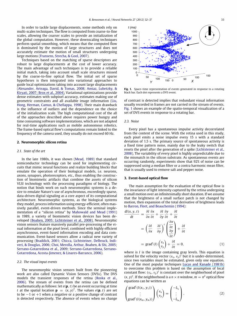
The neuromorphic vision sensors built from the pioneeringwork are also called Dynamic Vision Sensors (DVSs). The DVSmodels the transient responses of the retina (Roska et al.,2006). The stream of events from the retina can be definedmathematically as follows: let e(p, t) be an event occurring at timet at the spatial location p = (x, y)T . The values e(p, t) are setto be −1 or +1 when a negative or a positive change of contrastis detected respectively. The absence of events when no change

Fig. 1. Space–time representation of events generated in response to a rotatingblack bar. Each dot represents a DVS event.

of contrast is detected implies that redundant visual informationusually recorded in frames are not carried in the stream of events.Fig. 1 shows an example of the spatio-temporal visualization of aset of DVS events in response to a rotating bar.

2.3. Noise

Every pixel has a spontaneous impulse activity decorrelatedfrom the content of the scene. With the retina used in this study,each pixel emits a noise impulse every 15 s with a standarddeviation of 1.5 s. The primary source of spontaneous activity isa fixed time pattern noise, mainly due to the leaky switch thatresets the pixel after the generation of a spike (Lichtsteiner et al.,2008). The variability of every pixel is highly unpredictable due tothe mismatch in the silicon substrate. As spontaneous events areoccurring randomly, experiments show that 92% of noise can besuppressed using a median filter or a contra harmonic mean filter,that is usually used to remove salt and pepper noise.

3. Event-based optical flow

The main assumption for the evaluation of the optical flow isthe invariance of light intensity captured by the retina undergoinga small motion over an infinitesimally short duration. If we assumethat the brightness of a small surface patch is not changed bymotion, then expansion of the total derivative of brightness leadsto Barron, Fleet, and Beauchemin (1994):dI(x, y, t)

dt=

∂ I∂x

∂x∂t

+∂ I∂y

∂y∂t

+∂ I∂t

=

∂ I∂x

∂ I∂y

t

∂x∂t∂y∂t

+∂ I∂t

= gradt(I)

vxvy

+

∂ I∂t

= 0, (1)

where is I is the image containing gray levels. This equation issolved for the velocity vector (vx, vy)

t but it is under-determined,since two variables must be estimated, given only one equation.One of the most popular techniques Lucas and Kanade (1981b)to overcome this problem is based on the assumption of localconstant flow: (vx, vy)

t is constant over the neighborhood of pixel(x, y)t . If the neighborhood is a n× nwindow,m = n2 optical flowequations can be written as gradt(I(x1, y1))

...

gradt(I(xm, ym))

vxvy

=

−It1...

−Itm

, (2)

34 R. Benosman et al. / Neural Networks 27 (2012) 32–37

Fig. 2. Bar orientation estimated by the events-based (+) and by the frame-based (∗) optical flow algorithms versus the true bar orientation over the time (−) for the inputshown in Fig. 1.

with gradt(I) being the spatial gradient and It the partial temporalderivative of I . The equation system can then be solved using leastsquare error minimization techniques.

This constraint can be formulated in an event-based manner.The main difficulty being that event-based retinas do not providegray levels. The absence of gray levels makes it difficult to providea spatial gradient computation. Nevertheless for adjacent activepixels it is possible to provide an estimation of the spatial gradientby comparing their instantaneous activities:

∂e(x, y, t)∂x

∼

tt−1t

e(x, y, t) −

tt−1t

e(x − 1, y, t)

∂e(x, y, t)∂y

∼

tt−1t

e(x, y, t) −

tt−1t

e(x, y − 1, t).

(3)

1t is a temporal interval of few µs it is generally set to 50 µs.The estimation of the temporal gradient is expected to be moreprecise than in the frame-based framework due to the temporalprecision of the DVS. It can be written as

∂e(x, y, t)∂t

∼

t1t−1t

e(x, y, t) −

tt−1t

e(x, y, t)

t − t1, with t1 < t. (4)

By substituting Eqs. (3) and (4) into Eq. (2), the jth line of thematrixequality can be reformulated using events:

tt−1t

e(xj, yj, t) −

tt−1t

e(xj − 1, yj, t)

vx

+

t

t−1t

e(xj, yj, t) −

tt−1t

e(xj, yj − 1, t)

vy

=

tt1

e(xj, yj, t)

t − t1(5)

sincet1

t−1t

e(x, y, t) −

tt−1t

e(x, y, t) =

tt1

e(x, y, t).

The general optic flow algorithm is detailed by Algorithm 1.

4. Experiments

Experiments use the DVS that has a temporal resolution of 1µs.The optical flow is computed using a neighborhood of 5× 5 pixelsfor a 1t = 50 µs.

Algorithm 1 Event-based optical flowFor each incoming e(x,y,t):Define a (n × n × 1t) neighborhood around (x, y, t)TCompute the partial derivatives:

•∂e(x,y,t)

∂x ,∂e(x,y,t)

∂y ,∂e(x,y,t)

∂t

Solve Eq. (2) written using Eq. (5) for (vx, vy)t

4.1. Orientation

The first experiment uses a black bar painted on a white disk,rotating with a constant angular velocity of ω ∼ 13.6 rad/s. It isused as input to the DVS, as shown in Fig. 1. The events-basedoptical flow is computed in real-time using the continuous trainof output events. The frame-based optical flow is computed fora 60 fps emulated camera, obtained by accumulating eventsfor a duration of 16.7 ms. Fig. 2 shows the orientation of thebar computed from the flow obtained by the two techniquesand is plotted versus the ground truth orientation of the bar.The event-based computation takes full advantage of the hightemporal accuracy of the sensor, by providing a dense and accurateestimation of the rotation angles in real time.

4.2. Amplitude

The amplitudes of the estimated optical flow are computed fora moving pattern of bars presented on a moving conveyor beltwhose translational speed can be accurately set by adjusting thesupply voltage of a DC motor that drives the system (Fig. 3). Inthis experiment the magnitudes of the optical flow are computedfor different known belt speeds obtained by driving the DC motorwith supply voltages ranging from 500 to 1500 mV correspondingto a range of velocities of 30.83–83.05 cm/s. Fig. 3 shows themean estimated amplitudes of the bars for a range of voltages, asexpected, there is a linear relationship between the actual speedsand the velocity amplitudes.

4.3. Temporal precision

The experiment consists of the observation of a regular planargrid of LEDs with a precisely adjustable illumination frequency(see Fig. 4(a)). The panel has been designed so that each LEDswitches on and off sequentially and individually in time. Theprocess starts from the first one located at the top left cornerof the panel, and then proceeds progressively through every rowuntil reaching the final LED in the bottom right-hand corner.The illumination sequence then commences again. The distance

R. Benosman et al. / Neural Networks 27 (2012) 32–37 35

Fig. 3. (Top) Experimental device: a translating pattern of vertical bars on a beltmoved by a DC is acquired by the DVS. (Bottom) Estimated amplitudes of the opticalflow versus the DC voltage ranging from 500 to 1500 mV and corresponding to arange of velocities of 30.83–83.05 cm/s.

between LEDs is known to be 3.4 cm. The time interval betweenthe switching of successive LEDs is adjustable from 1ms to 1 s andis set to 16 ms in the current experiment.

The aim of the experiment is to estimate the rate of switchingon of successive LEDs on the panel. The principle is to detect when

two consecutive LEDs switch on. The speed can then be computedfrom the knowledge of this temporal interval, and the distancebetween successive LEDs. The switching on of an LED is detected bysensing the characteristic divergent pattern of the optical flow thatit creates, as shown in Fig. 4(b). This divergent pattern of opticalflow is created because, as the LED turns on, the pixel that viewsthe brightest point in the LED reaches a threshold of activity first,followed later by the surrounding pixels.

In the experiment the DVS observes the panel continuously andfor every incoming event the optical flow is computed. In a secondstage, in order to detect precisely the exact timing of the LED’sactivation, a spatial vector pattern similar to Fig. 4(b) is used as atemplate and correlated with the measured optic flow pattern inthe neighborhood of the active pixel’s location. In the experiment,the vector flow pattern of activation is set to a size of 5 × 5vectors.

Once the location of the active LED is located, its positionon the panel is retrieved and the estimation of the speed ofactivation of pixels can then be performed. The precise momentof switching on of an LED is established by detecting the divergentpattern of optic flow that will initially cover a small area and thengrow continuously. The instant of switching on is then definedas the time when the central pixel is first detected and hasreached threshold. Fig. 4(c) shows the distribution of estimatedspeeds for a 2 s sequence, giving an estimated mean speed of2.169m/swhile the ground truth speed is 2.125m/s. The observedestimation errors are due to small misalignments of individualLEDs in the panel, small geometrical imperfections in the retinaand distortions in the optics of the camera.

4.4. Computational cost

Tests were performed to compare the computational timesrequired by the frame-based and the event-based methods forcomputing optic flow. These results were obtained using a C++implementation of the algorithm, on an Intel Core 2 Duo 2.40 GHzprocessor.

The optical flow was computed for a rotating bar as shown inFig. 1. The event-based method uses raw events, while the frame-based method uses frames acquired at a rate of 60 Hz created bysumming events. The following computation timeswere obtained:

a

b

c

Fig. 4. Computation of the optical flow generated by sequential activation of LEDs on a panel. Long exposure of this image shows four LEDS that have been turned onsuccessively from left to right (a). (b) Switching on of a single LED generates a characteristic, expansional pattern of optic flow. (c) Distribution of estimated speeds of movingdisplay created by sequential switching of LEDs in m/s, giving a mean value of 2.16 m/s, compared to an actual speed of 2.12 m/s.

36 R. Benosman et al. / Neural Networks 27 (2012) 32–37

Fig. 5. Computation time of event-based (triangles) vs. frame based (squares) forthe same observed sequence. The event-basedmethod delivers flowmeasurementsat a cost that is approximately 25 times lower than does the frame-based method.

• frame-based, 60 fps (16.7 ms): the number of processed pixelsat each step is 16384, and amean computation time is 251.7ms,

• event-based (1e−3 ms): computation time for a period of16.7ms corresponding to amean number of events of 1340, thecomputation time is 9.65ms, while themean computation timeof an event is 7.2e−3 ms.

It takes 251.7 ms to compute the optical flow between twosuccessive frames on a time interval between successive framesof 16.7 ms. This means that in the absence of any optimization,the optical flow can be computed only at a rate of 4 fps. Theoptical flow computation is taking as long as 251.7 ms becausewe are computing the flow at all of the 16384 pixel locations inthe imager without any optimization in both frame and event-based. The event-based optical flow requires 7.2 µs to computethe optical flow for each event, thus leading to a total time of1340 × (7.2e − 3) = 9.65 ms. Fig. 5 shows that the event-basedmethoddelivers flowmeasurements at a cost that is approximately25 times lower than does the frame-based method.

4.5. Samples of computed flows

This section presents examples of optic flow computedusing the events-based method developed in this paper. Fig. 6presents the decomposition of fast arms movements and theircorresponding estimated optical flows. Fig. 7 shows the optic flowassociated with a bouncing ball.

5. Conclusions

This paper presented an alternative framework for the compu-tation of optical flow based on an asynchronous spiking vision sen-sor that responds to temporal variations of contrast of the visual

Fig. 6. Optic flow for curved motion: (up) decomposition of the movement oftwo hands moving from the bottom to the sides of the scene and its (down)corresponding cumulative estimated optic flow over a time period of 1.5 s on allthe focal plane.

input. The experiments showed that asynchronous event-based ac-quisition allows for high dynamic, fast and low cost computationof the optical flow for many different stimuli.

The results presented here fully exploit the high temporalresolution and high dynamic range of event-based cameras, andoutperform existing frame-based camera techniques, overcomingtheir limitations in relation to large displacements and limitedaccuracy in the calculation of the optical flow. The proposedparadigm should be valuable in a number of applications thatrequire rapid, real-time analysis of high-speed events such as inimaging moving projectiles, or in vision-based guidance of high-speed autonomous aircraft.

Acknowledgments

The authors would like to thank T. Delbruck, R. Berner,P. Lichtsteiner, S.C. Liu and P. Rogister, for their help, time,availability and for allowing to use and share their knowledge inusing AER cameras. This work was supported by the EU eMorphgrant #ICT-231467, and partially by the Australian ResearchCouncil Centre of Excellence in Vision Science (CE0561903), by aQueensland Smart State Premier’s Fellowship, and by US AOARDAward no. FA4869-07-1-0010.

The authors are also grateful to both the CapoCaccia andTelluride neuromorphic workshops for their important role insetting up the indispensable community gathering efforts at thecore of this collaborative work.

Appendix. Supplementary data

Supplementary material related to this article can be foundonline at doi:10.1016/j.neunet.2011.11.001.

R. Benosman et al. / Neural Networks 27 (2012) 32–37 37

Fig. 7. Optic flow for curved motion: (up) decomposition of the movement of abouncing ball, (down) corresponding cumulative estimated optic flow over a timeperiod of 0.8 s on all the focal plane.

References

Alexander, S., Arteaga, G., David, J., & Tomas, W. (2008). A discrete search methodfor multi-modal non-rigid image registration. In NORDIA 2008: proceedings ofthe 2008 IEEE CVPR workshop on non-rigid shape analysis and deformable imagealignment (pp. 6).

Amiaz, T., Lubetzky, E., & Kiryati, N. (2007). Coarse to over-fine optical flowestimation. Pattern Recognition, 40, 2496–2503.

Barron, J., Fleet, D., & Beauchemin, S. (1994). Performance of optical flow techniques.International Journal of Computer Vision, 12(1), 43–77.

Black, M., & Anandan, P. (1996). The robust estimation of multiple motions:parametric and piecewise-smooth flow fields. Computer Vision and ImageUnderstanding, CVIU , 75–104.

Boahen, K. (2005). Neuromorphic microchips. Scientific American, 292, 55–63.Braddick, O. (2001). Neural basis of visual perception: Vol. 0. Elsevier Ltd.,

pp. 16269–16274.Brox, T., Bruhn, A., Papenberg, N., & Weickert, J. (2004). High accuracy optical

flow estimation based on a theory for warping. In LNCS: Vol. 3024. Europeanconference on computer vision, ECCV, (pp. 25–36). Prague, Czech Republic:Springer.

Chicca, E., Lichtsteiner, P., Delbruck, T., Indiveri, G., & Douglas, R. (2006). Modelingorientation selectivity using a neuromorphic multichip system. In Proc. IEEE int.symp. circuits syst. Press (pp. 1235–1238).

Choi, T. Y. W., Merolla, P., Arthur, J., Boahen, K., & Shi, B. E. (2005). Neuromorphicimplementation of orientation hypercolumns. IEEE Transactions on Circuits andSystems, 52, 1049–1060.

Fransens, R., Strecha, C., & Gool, L. V. (2007). Optical flow based super-resolution: aprobabilistic approach. Computer Vision and Image Understanding, CVIU , 106(1),106–115.

Horn, B., & Schunck, B. (1980). Determining optical flow. Tech. Rep. Cambridge, MA,USA.

Lenero-Bardallo, J. A., Serrano-Gotarredona, T., & Linares-Barranco, B. (2011).A 3.6us asynchronous frame-free event-driven dynamic-vision-sensor. IEEEJournal of Solid-State Circuits, 46, 1443–1455.

Lichtsteiner, P., Posch, C., & Delbruck, T. (2008). A 128 128 120 dB 15 s latencyasynchronous temporal contrast vision sensor. IEEE Journal of Solid-StateCircuits, 43(2), 566–576. doi:10.1109/JSSC.2007.914337.

Liu, H., Hong, T., Herman, M., Camus, T., & Chellappa, R. (1998). Accuracy vs.efficiency trade-offs in optical flow algorithms. Computer Vision and ImageUnderstanding , 72(3), 271–286.

Lucas, B., & Kanade, T. (1981a). An iterative image registration technique with anapplication to stereo vision (IJCAI). in: Proceedings of the 7th international jointconference on artificial intelligence. IJCAI’81 (pp. 674–679).

Lucas, B., & Kanade, T. (1981b). An iterative image registration technique with anapplication to stereo vision. In Imaging understanding workshop (pp. 121–120).

Mahowald, M., & Mead, C. (1991). The silicon retina. Scientific American,.Mead, C. (1989). Adaptive retina. In C. Mead, & M. Ismail (Eds.), Analog VLSI

implementation of neural systems.Memin, E., & Perez, P. (1998). Joint estimation-segmentation of optic flow. In

ECCV’98.Posch, C. (2010). High-DR frame-free PWM imaging with asynchronous aer

intensity encoding and focal-plane temporal redundancy suppression, in:ISCAS.

Posch, C., Matolin, D., & Wohlgenannt, R. (2011). A QVGA 143 dB dynamic rangeframe-free PWM image sensor with lossless pixel-level video compression andtime-domain CDS. IEEE Journal of Solid-State Circuits, 46, 259–275.

Roska, B., Alyosha, M., & Werblin, F. (2006). Parallel processing in reti-nal ganglion cells: how integration of space–time patterns of excita-tion and inhibition form the spiking output. Journal of Neurophysiology,95(6), 3810–3822. arXiv:http://jn.physiology.org/cgi/reprint/95/6/3810.pdf,doi:10.1152/jn.00113.2006, URL:http://jn.physiology.org/cgi/content/abstract/95/6/3810.

Serrano-Gotarredona, R., Oster, M., Lichtsteiner, P., Linares-Barranco, A., Paz-Vicente, R., & Gomez-Rodriguez, F. (2009). Caviar: a 45k-neuron, 5m-synapse,12g-connects/sec aer hardware sensory-processing-learning-actuating systemfor high speed visual object recognition and tracking. IEEE Transactions onNeuralNetworks, 20, 1417–1438.

Serrano-Gotarredona, R., Serrano-Gotarredona, T., Acosta-Jimenez, A., & Linares-Barranco, B. (2006). A neuromorphic cortical-layer microchip for spike-basedevent processing vision systems. IEEE Transactions on Circuits and System, 53,2548–2566.