Scholars' Mine Scholars' Mine

Masters Theses Student Theses and Dissertations

1970

Fault detection in asynchronous sequential circuits Fault detection in asynchronous sequential circuits

Jeng-Chuan Kau

Follow this and additional works at: https://scholarsmine.mst.edu/masters_theses

Part of the Electrical and Computer Engineering Commons

Department: Department:

Recommended Citation Recommended Citation Kau, Jeng-Chuan, "Fault detection in asynchronous sequential circuits" (1970). Masters Theses. 7132. https://scholarsmine.mst.edu/masters_theses/7132

This thesis is brought to you by Scholars' Mine, a service of the Missouri S&T Library and Learning Resources. This work is protected by U. S. Copyright Law. Unauthorized use including reproduction for redistribution requires the permission of the copyright holder. For more information, please contact scholarsmine@mst.edu.

FAULT DETECTION IN ASYNCHRONOUS

SEQUENTIAL CIRCUITS

BY

JENG-CHUAN KAU, 1944-

A

THESIS

submitted to the faculty of

UNIVERSITY OF MISSOURI - ROLLA

in partial fulfillment of the requirements for the

Degree of

MASTER OF SCIENCE IN ELECTRICAL ENGINEERING

Rollar Missouri

1970

Approved by

~£12::j~~~~advisor) . r~ 2ez-:ra,L ~~J)fl

ii

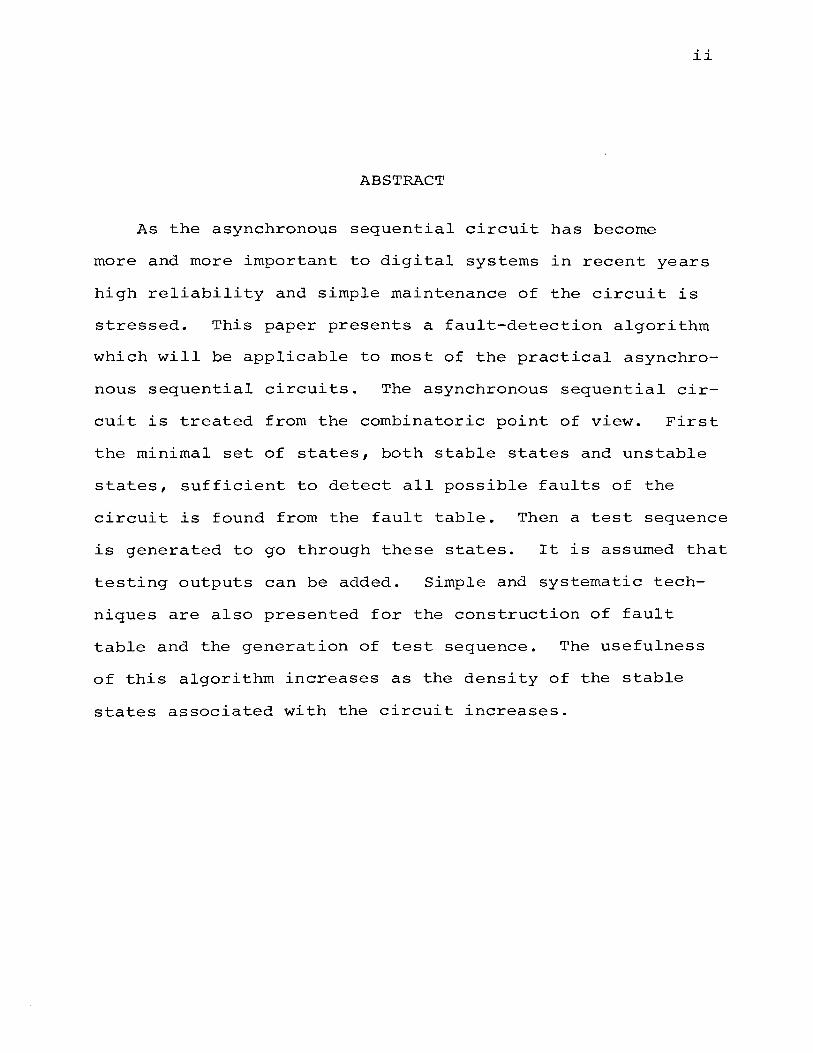
ABSTRACT

As the asynchronous sequential circuit has become

more and more important to digital systems in recent years

high reliability and simple maintenance of the circuit is

stressed. This paper presents a fault-detection algorithm

which will be applicable to most of the practical asynchro­

nous sequential circuits. The asynchronous sequential cir­

cuit is treated from the combinatoric point of view. First

the minimal set of states, both stable states and unstable

states, sufficient to detect all possible faults of the

circuit is found from the fault table. Then a test sequence

is generated to go through these states. It is assumed that

testing outputs can be added. Simple and systematic tech-

niques are also presented for the construction of fault

table and the generation of test sequence. The usefulness

of this algorithm increases as the density of the stable

states associated with the circuit increases.

iii

ACKNOWLEDGEMENT

The author wishes to express his sincere appreciation

and gratitude to Dr. J.H. Tracey, for his guidance and

assistance during the entire course of this investigation.

iv

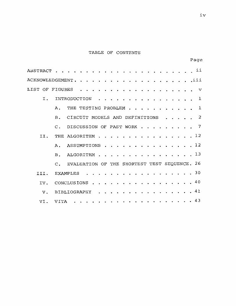
TABLE OF CONTENTS

Page

ABSTRACT . . . . . . . . . . . . . . . . . . . ii

. .iii ACKNOWLEDGEMENT.

LIST OF FIGURES v

I. INTRODUCTION

A. THE TESTING PROBLEM

1

1

B. CIRCUIT MODELS AND DEFINITIONS • • . 2

C. DISCUSSION OF PAST WORK . . . . . 7

II. THE ALGORITHM . . ...•.... 12

A. ASSUMPTIONS . . . . . . . . . . . . . 12

B. ALGORITHM . . . . . . . . . . . . 13

C. EVALUATION OF THE SHORTEST TEST SEQUENCE. 26

III. EXAMPLES . . . . . . . . . . . . 3 0

IV.

v.

CONCLUSIONS .

BIBLIOGRAPHY

VI. VITA

• • • 4 0

41

43

LIST OF FIGURES

Figures

1 The synchronous sequential circuit .

2 The fundamental-mode asynchronous sequential circuit

3

4

5

6

7

8

9

10

11

12

13

14

15

16

17

18

Circuit for illustrating algorithm .

Fault table for Figure 3 .

The transition table for xl s-a-1

The transition table for yl s-a-0

Stable state conditions for the output net-work of Figure 3 . The transition table for Figure 3

State-transition tree for Figure 8 •

Circuit for evaluating the shortest test sequence .

Fault table for Figure 10

State-transition tree for Figure 10

The transition table for e s-a-1 .

Circuit for example 1

Fault table for Figure 14

Transition table and state-transition tree for Figure 14

Circuit for example 2

Fault table for Figure 17

v

Page

3

4

14

16

18

20

21

22

23

27

28

29

30

31

32

34

36

37

1

I. INTRODUCTION

A. The Testing Problem

As the range of problems to which digital computing

systems have been applied has widened, the task of

ensuring that a computing system is operating correctly

has become steadily more important. Incorrect computer

operation in some applications such as the control of

chemical process units and nuclear reactors, and military

command and control, can be potentially disastrous. In

many practical situations the synchronizing clock pulses

are not available and asynchronous circuits must be

designed. Moreover, within large synchronous systems it

is often desirable to allow certain subsystems to operate

asynchronously, thereby increasing the overall speed of

operation. In this paper the methods to diagnose the

asynchronous circuits are investigated.

The testing problem for sequential circuits may be

stated as follows: given a circuit$ find a testing pro­

cedure which determines whether the circuit is performing

correctly by applying signals to and measuring signals

on the terminals of the circuit. There are two kinds of

experiments: 1) simple experiments, which are performed

on a single copy of the machine, and 2) multiple experiments 1

which are performed on two or more identical copies of the

2

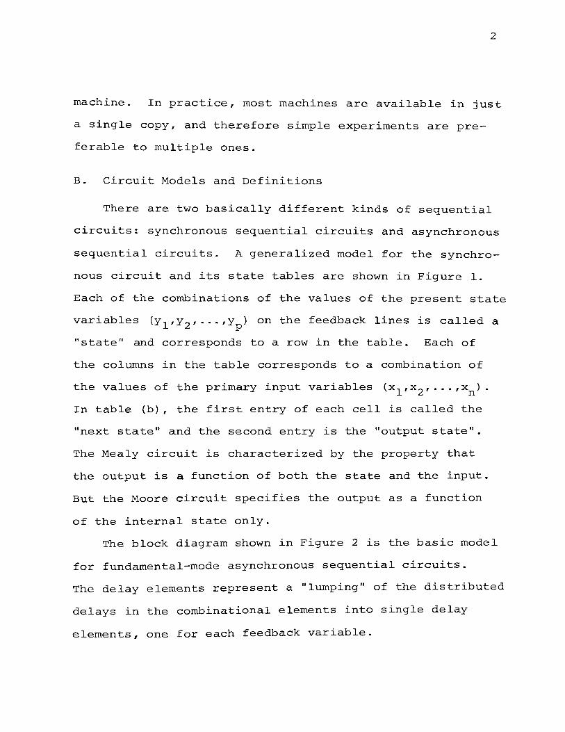
machine. In practice, most machines are available in just

a single copy, and therefore simple experiments are pre­

ferable to multiple ones.

B. Circuit Models and Definitions

There are two basically different kinds of sequential

circuits: synchronous sequential circuits and asynchronous

sequential circuits. A generalized model for the synchro-

nous circuit and its state tables are shown in Figure 1.

Each of the combinations of the values of the present state

variables (y 1 ,y2 , ... ,yp) on the feedback lines is called a

"state" and corresponds to a row in the table. Each of

the columns in the table corresponds to a combination of

the values of the primary input variables Cx1 ,x2 , ... ,xn).

In table (b) , the first entry of each cell is called the

"next state" and the second entry is the "output state".

The Mealy circuit is characterized by the property that

the output is a function of both the state and the input.

But the Moore circuit specifies the output as a function

of the internal state only.

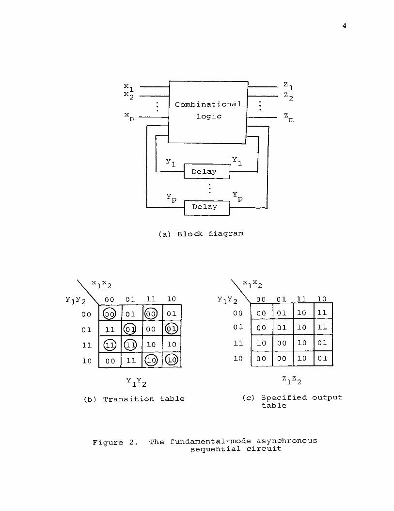
The block diagram shown in Figure 2 is the basic model

for fundamental-mode asynchronous sequential circuits.

The delay elements represent a "lumping" of the distributed

delays in the combinational elements into single delay

elements, one for each feedback variable.

yly2

00

01

11

10

~ 00

1 3.0

2 2.1

3 1.0

4 4.0

X n

. Combinational . . . . . logic

- -

yl yl I I I Memory I

• . . yp y

I Memory 1 p I r

(a) Block diagram

xlx2

~ 01 11 10 yly2

1.1 2.0 3.1 00 1

3.0 1.0 1.0 01 2

3.1 4.1 2.0 11 3

1.1 3.1 2.1 10 4

00

3

2

1

4

z m

x1x2

01 11

4 2

3 1

3 4

1 3

10

3

1

2

2

(b) State table of Mealy circuit

(c) State table of Moore circuit

Figure 1. The synchronous sequential circuit

3

z

0

1

1

0

xlx2

2 00

00 @ 01 11

11 @ 10 00

X n

01

01

@ @ 11

11

~ 00

10

@

. Combinational . . . . . logic

,..__ -

yl yl I Delay

-, I I . .

yp . y

p I Delay I L J

(a) Block diagram

xlx2

10 2 00

01 00 00

@ 01 00

10 11 10

@ 10 00

01

01

01

00

00

z m

11 10

10 11

10 11

10 01

10 01

(b) Transition table (c) Specified output table

Figure 2. The fundamental-mode asynchronous sequential circuit

4

5

In table (b) of Figure 2, the rows are defined by the

signals at the output of the delay elements and the

columns are defined by the combinations of the values of

the primary input variables. A state of the circuit is a

combination of the values of the variables (x1 ,x2 , •.• ,xn,

y 1 ,y2 , .•. ,yp) and denotes a cell of the table. A row state

consists of the values of the variables (y1 ,y2 , ... ,yp) only.

If the next row state is the same as the present row state

for a given input combination, then the entry is circled and

is said to be stable. If the next row state is different

from the present one, then the entry is not circled and is

said to be unstable. The table (c) is same as table (b)

except that the cells in this table represent the primary

outputs of the circuit.

Before proceeding to discuss the literature a number

of definitions are presented first.

A failure (fault) In a logic circuit, any transformation

of hardware that changes the logical

character of the function realized by

the hardware.

A primary input In a logical circuit, a line that is

not fed by any other line in that

circuit.

6

A primary output In a logical circuit 1 a line whose

signal is accessible to the exterior

of the circuit.

A test (for a failure) A pattern of signals on primary

Experiment

inputs such that the value of the

signal on some primary output will

differ according to the presence or

absence of that failure.

The application of input sequences to the

input terminals of a sequential

machine and the observation of the

corresponding output sequences in

order to conclude something about

the machine.

Distinguishing sequence An input sequence which when

Homing sequence

applied to a sequential machine

allows the initial state of the

machine to be determined by observa­

tion of the corresponding output

sequence.

An input sequence which allows the

final state of the given machine to

be determined by observation of the

corresponding output sequence.

Preset experiment

Adaptive experiment

7

An experiment such that the input

sequence to be applied is comple­

tely determined in advance.

An experiment such that the input

sequence consists of subsequences

which are selected by observing

the response to previously applied

subsequences.

C. Discussion of Past Work

For a combinational network a test is just an input

combination. A test detects a fault if the network output

differs from the correct output when the test is applied

and the fault is present. The simplest way of constructing

the fault-detection tests is the use of fault tables. A

fault table is a table in which there is a row for every

possible test (i.e. 1 input combination) and a column for

each possible fault. A 1 is entered at the intersection

of a row and column if the corresponding test detects the

corresponding fault; otherwise a 0 is entered. The problem

of finding a minimal set of tests then reduces to the

problem of finding a minimal set of rows in the table such

that they include at least one 1 in every column. In order

to handle networks with larger number of variables a more

systematic method of deriving the minimal test set is

developed by Kautz (1) .

8

For large networks the previously described procedure

becomes prohibitive because of the size of the fault

table. Armstrong (2) then provides a short-cut procedure

based on the 11 path-sensitizing" technique. By sensitizing

all the paths of the network under test, all faults in

the entire network will be detected. This procedure also

appears to ensure finding a sufficient set of tests to

detect all detectable faults. But it may become cumbersome

when the number of paths through out the network is large.

Another well-known procedure of fault detection is the

D-algorithm (3) . If a test exists for a given failure the

algorithm will find such a test. The method is to find

the D-cube chains, which extends from the primary inputs to

the outputsJ necessarily to detect all possible faults.

The fault detection of sequential networks is more

difficult than that of combinational networks. Bennie

introduced the transition checking approach by use of the

distinguishing sequences. Rennie's approach yields good

results for machines that possess distinguishing sequences,

and when the actual circuit has no more states than the

correctly operating circuit. For machines which do not

have a distinguishing sequence, Rennie's approach yields

very long experiments .1 which are impractical. Further

development of this approach was done by Kime (4) . When

the machine has no distinguishing sequence, Kime makes two

modifications: the addition of testing points and the

9

addition of logic. Nevertheless, the length of experiments

is still very long and the experiments are extremely hard

to apply in any practical situation. Kohavi and Lavallee

(5) then present a method for designing sequential circuits

in such a way that they will be made to possess dis­

tinguishing sequences with repeated symbols by use of the

additional output logic if the circuits do not have such a

distinguishing sequence. The circuits thus modified have

shorter fault-detection experiments than those of the

original circuits.

The distinguishing sequences just discussed are the

preset fixed-length distinguishing sequences (FLDS). A

variable-length distinguishing sequence (VLDS) is a preset

distinguishing sequence X such that, if the machine is 0

started is an unknown state, the output response of the

machine to some prefix of X (i.e., some subsequence of 0

X ) will identify the initial state. The length of the 0

required prefix is a function of the initial state.

I. Kohavi and z. Kohavi (6) apply VLDS to the construction

of fault-detection experiments. Consequently, the machine

will have shorter and more efficient experiments when VLDS

is used, provided the average length of the VLDS of the

machine is shorter than that of the FLDS, and provided that

a larger number of states possess the shorter prefixes of

X . 0

10

The above fault-detection approaches for sequential

circuits generally lead to long testing sequence. One

reason these sequences are so long is that these approaches

are actually doing machine identification rather than

simply fault detection. Based on Armstrong's theory,

Kohavi (7) finds the minimal fault-detection tests set

of the combinational networks from their Karnaugh maps.

Kohavi then applies his approach to the generation of

testing sequence for the sequential networks.

Let the experiment for sequential networks be divided

into two parts: the first part identifies that the given

n-state machine has n states and the second part disting­

uishes between the given n-state machine and those n-state

machines which the given machine can be transformed into

as a result of some fault. Kohavi's method generates a

much shorter test sequence for the second part of the

experiment than previously discussed methods. The class

of n-state machines that the given machine can be trans­

formed into as a result of some malfunction form a subset

of all n-state machines. In order to distinguish between

the given machine and the above subset of machines, shorter

experiments are required than in the case of distinguishing

between the given machine and the entire set of n-state

machines. In other words, one need not identify the n

distinct states of the machine and check all the transitions

according to the given state table.

Based on the above idea and Hughes' method (8), a

fault-detection algorithm for asynchronous sequential

circuits is presented in the following chapter.

11

12

II. THE ALGORITHM

A. Assumptions

The asynchronous sequentia~ circuit presents a some­

what more difficult testing problem. In general, an

asynchronous circuit is not as well behaved as the corres­

ponding synchronous circuit. Before going into the details,

it is necessary to make some assumptions.

1) The circuits considered here are fundamental­

mode asynchronous sequential circuits. The

inputs are levels, and are never changed unless

the circuit is internally stable. It is

required that only one input is changed at a

time.

2) The machines are strongly connected. This

provides the capability of always establishing

the feedback variables to be zero before begin­

ning the test.

3) The circuitry must be irredundant. A circuit is

irredundant if its Boolean expressions are in

minimal forms. The redundant circuit consists

of redundant literals,where by literal we mean

an appearance of a variable or its complement.

Without this restriction, the function realized

with a fault in the redundant circuitry is

equal to the function realized without the fault.

4) The flow table is free from critical races and

oscillations.

5) Only single faults are considered.

6) The faults are permanent faults due to component

failures and manifest themselves as stuck-at-one

(s-a-l) or stuck-at-zero (s-a-o).

l3

In treating the single fault case one implies that

fault-detection test will be run frequently enough so that,

in generalr multiple faults will not occur. From a prac-

tical point of view this is not a severe limitation, since

most circuits are reliable enough so that the probability

of occurrence of multiple faults is very small. Other

assumptions will be given as the discussion progresses.

B. Algorithm

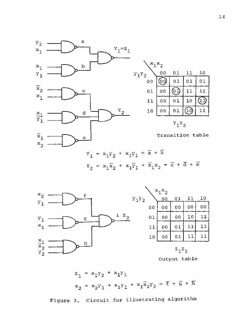
The asynchronous sequential circuit shown in Figure

3, with x1

x 2 as primary inputs and z1 z2 as primary outputs,

will be used to illustrate the algorithm. For convenience,

the output portion (without feedbacks) of the circuit will

be considered as the output network although it is regarded

as part of the single block of the combinational logic as

shown in Figure 2. Thusr the lower part of the circuit in

Figure 3 will be called the output network.

14

xlx2

2 00 01 11 10

00 @ 01 01 01

c 01 00 @ 11 11

11 00 01 10 @ 10 00 01 @ 11

yly2

e Transition table

yl = xly2 + xlyl = a + b

- -y2 = xlx2 + xlyl + xlx2 = c + d + e

x2 f yl

yly2

xlx2

00 01 11 10

00 00 00 00 00

yl g i z2 01 00 00 10 11

xl 11 00 01 11 11

10 00 01 11 11 xl h x2 y2

zl = xly2 + xlyl

z2 = x2yl + xlyl + xlx2y2 = f + g + h

Figure 3. Circuit for illustrating algorithm

In the remainder of this paper when input and output are

spoken of, they will mean primary input and primary

output respectively unless otherwise specified. Since

the delay is not a physical element, they are not shown

15

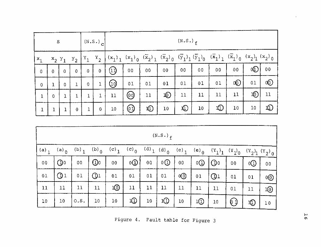
in the circuit and will not be shown on subsequent figures.

Figure 4 is the frult table of Figure 3 under stable

state conditions.

is as follows:

The meaning of each column in the table

S all stable state conditions; and, under

stable state conditions;

(N. S • ) c

(N.S.)f

the correct values of next state variables;

the values of next state variables for

the s-a-1 and s-a-o faults designated by

the subscript;

the correct outputs;

the values of the outputs under s-a-1 and

s-a-o faults of those lines related to

the outputs.

In constructing the fault table, all possible faults of

the lines that are related to the next state variables should

be included in column (N.S.)f. Only those faults associated

with the output network and not included in column (N.S.)f

are contained in column zf. The values of the next state

variables under (N.S.)f are circled whenever they are dif­

ferent from the correct values under (N.S.)c of the same row.

s (N. S.) c

xl x2 Y1 y2 yl y2

0 0 0 0 0 0

0 1 0 1 0 1

1 0 1 1 1 1

1 1 1 0 1 0

(a) 1 (a}o (b) 1 (b)o

00 (]o 00 G)o

01 Q)l 01 (Dl

11 11 11 11

10 10 o.s. 10

(N.S.)f

Cxl)l Cxl)o (x2)1 cx2)o Cyl)l(yl)O Cxl)l (xl)o Cx2)1 Cx2)o

@ 00 00 00 00 00 00 00 ~ 00

@ 01 01 01 01 01 01 ~ 01 ~

11 @ 11 1(Q) 11 11 11 11 1@ 11

10 @ 1(D 10 JC) 10 JQ) 10 10 llD

(N. S. ) f

(c)l (c)o (d)l (d)o (e) 1 (e)o (Y 1 )1 (Y 1)0 (Y 2 )1 (Y 2) 0

00 o(D 00 o(D 00 oQ) Q)o 00 o(D 00

01 01 01 01 o@ 01 (Dl 01 01 o@

1@ 11 11 11 ll 11 11 01 11 1@

10 1(D 10 l(D 10 1@ 10 0 1© 10

Figure 4. Fault table for Figure 3

I

I-' 0'1

l7

z zf c

z2 (f) 1 (f) 0

(g) 1 (g)o (h) 1 (h) 0

(i) 1 (i) 0

0 0 CD 0 CD 0 CD CD 0

0 0 CD 0 CD 0 CD CD 0

1 1 1 1 1 1 1 1 @

1 1 1 1 1 1 1 1 @

Figure 4. Fault table for Figure 3 (cont.)

The same is true for zf. It should be emphasized that the

values in the table are all in steady states, except the

entry "O.S." under column (b) 1 . The symbol "O.S." indi­

cates that the circuit will oscillate if one tries to put

it in stable state x1

x2

y 1y 2 = 1110 under s-a-1 fault on b.

A suggested short-cut technique for deriving the entries

under (N.S.)f consists of writing the state equation as a

function of the inputs and internal state variables for

the fault specified, then forming the transition table.

By comparing this faulty transition table with the original

table, one can determine the proper entry. For example,

the column (x1

)1

(x1

s-a-1) is found from the equations:

yl = ly2 + lyl = y2 + yl

y2 = lx2 + lyl + Ox2 = x2 + yl.

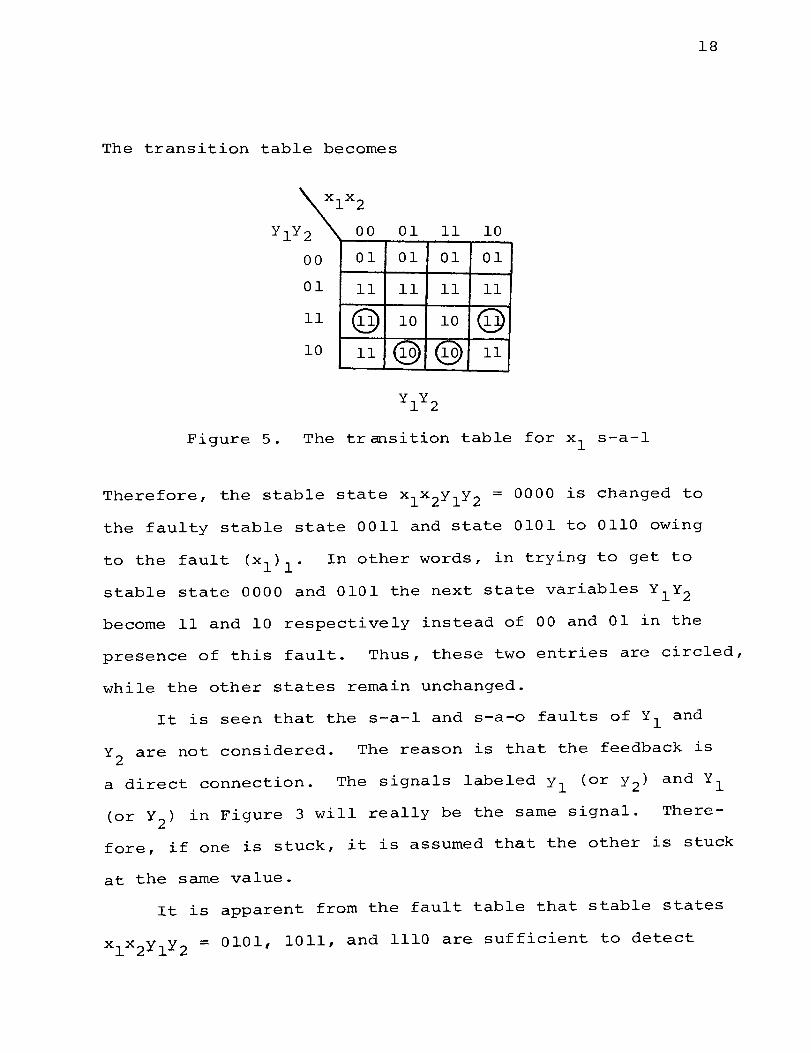
18

The transition table becomes

xlx2

2 00 01 ll 10

00 01 01 01 01

01 ll ll ll ll

ll @ 10 10 @ 10 ll @ @ ll

Figure 5. The transition table for x1

s-a-l

Therefore, the stable state x 1 x 2y 1y 2 = 0000 is changed to

the faulty stable state 0011 and state 0101 to 0110 owing

In other words, in trying to get to

stable state 0000 and 0101 the next state variables Y1 Y2

become ll and 10 respectively instead of 00 and 01 in the

presence of this fault. Thus, these two entries are circled,

while the other states remain unchanged.

It is seen that the s-a-l and s-a-o faults of Y1 and

Y2

are not considered. The reason is that the feedback is

a direct connection. The signals labeled y 1 (or y 2 ) and Y1

(or Y2

) in Figure 3 will really be the same signal. There-

fore, if one is stuck, it is assumed that the other is stuck

at the same value.

It is apparent from the fault table that stable states

x1

x2

y1

y2

= 0101, lOll, and 1110 are sufficient to detect

l9

all faults except (y1 )0

, (a) 1 , (d) 1 , (f) 1 , (g}1

, and (h}1

•

If the fault table is much larger, Kautz's method (1)

should be applied to simplify the fault table for obtaining

the minimal set of test states.

When a circuit has a fault some of the following con-

ditions may occur.

1) Some stable states become unstable.

2) Some unstable states become stable.

3) The circuit is oscillating after some

input sequence is applied.

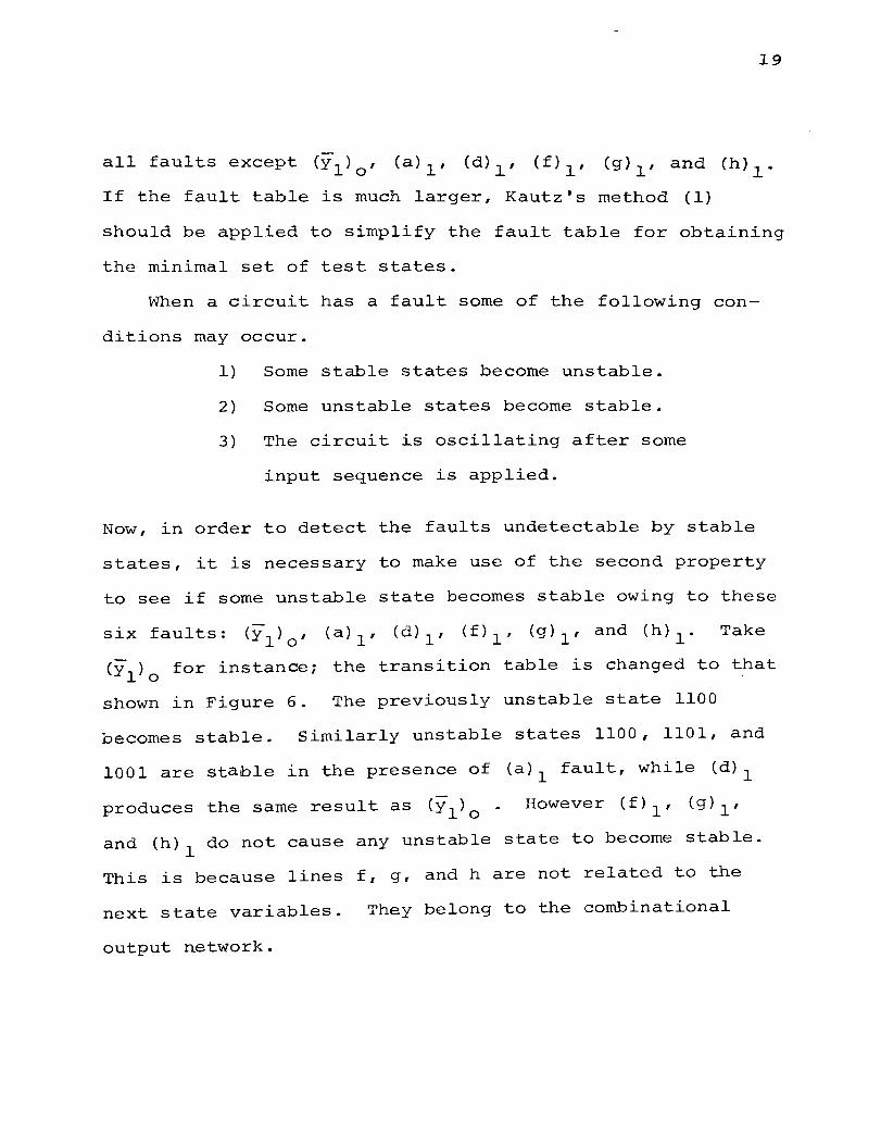
Now, in order to detect the faults undetectable by stable

states, it is necessary to make use of the second property

to see if some unstable state becomes stable owing to these

Take

Cy1

)0

for instance; the transition table is changed to that

shown in Figure 6. The previously unstable state 1100

becomes stable. Similarly unstable states 1100, 1101, and

1001 are stable in the presence of (a) 1 fault, while (d) 1

produces the same result as (y 1 )0

• However (f) 1 , (g) 1 ,

and (h) 1

do not cause any unstable state to become stable.

This is because lines f, g, and h are not related to the

next state variables. They belong to the combinational

output network.

Figure 6.

Attention is

f = x2 +

g = xl + h = xl +

xlx2

00 01 11 10

00 @ 01 @ 01

01 00 @ lQ 11

11 OQ 01 10 @ 10 oo· 01 @ 11

Yl = xly2 + xlyl

Y2 = xlx2 + xlx2

The transition table for y1

s-a-o

now given to the equations:

yl

yl

x2 + y2.

20

Under stable state conditions f, g, and h assume values

of 0 and 1 as shown in Figure 7. To illustrate how one can

detect these faults, the variable f will be examined. When

f is s-a-1 and the stable state 1110 is reached, the value

on f differs according to the presence or absence of the

fault. If f is made a testing output, the undetectable

fault (f}1

can now be detected. The same is true for (g) 1

and (h)1

faults. As a result, the two stable states 1011

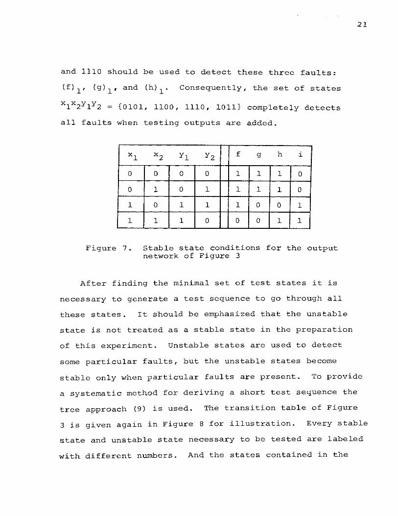
and 1110 should be used to detect these three faults:

Consequently, the set of states

xlx2yly2 = {0101, 1100, 1110, lOll} completely detects

all faults when testing outputs are added.

xl

0

0

1

1

Figure 7.

x2 yl y2 f g h i

0 0 0 1 1 1 0

1 0 1 1 1 1 0

0 1 1 1 0 0 1

1 1 0 0 0 1 1

Stable state conditions for the output network of Figure 3

After finding the minimal set of test states it is

necessary to generate a test sequence to go through all

these states. It should be emphasized that the unstable

state is not treated as a stable state in the preparation

of this experiment. Unstable states are used to detect

some particular faults, but the unstable states become

21

stable only when particular faults are present. To provide

a systematic method for deriving a short test sequence the

tree approach (9) is used. The transition table of Figure

3 is given again in Figure 8 for illustration. Every stable

state and unstable state necessary to be tested are labeled

with different numbers. And the states contained in the

22

test set are marked with "*". The state-transition tree

is shown in Figure 9. The circuit is first reset to the

yly2 11 10 YC

013 01

11 11

11 00 01 10

10 00 01

yly2

Figure 8. The transition table for Figure 3

If the circuit

can not be reset to a starting state by a homing sequence,

either preset sequence or adaptive sequence, we may conclude

that there exists a fault and thus complete the experiment

without any further test. The state at a particular level,

say J, will be a terminal state whenever it appeared at the

level less than J. Starting from state 1, the circuit goes

to state 2 after inputs x 1 x 2 = 01 are applied. Then it goes

to state 1 if next inputs are 00. Now this branch is ter-

minated since state 1 had appeared at level 1. In the same

manner the whole tree will be generated.

23

1 level 1

01

I 2* level 2

11 I 00

4* 1 level 3

~ 2 5* level 4

00 I 11

I 1 4 level 5

Figure 9. State-transition tree for Figure 8

As shown in the tree every state has only two possible

next states since there are two inputs associated with

the circuit and one input change is allowed at a time.

The unstable state, if any, will be put directly above its

stable state and bracketed in order to distinguish it from

stable state. By inspection, it is quite straightforward

to generate a test sequence to go through the desired

states. Unfortunately, state 3 cannot be reached because

of the limitation that multiple input changes are not

allowed. As stated before, state 3 is used to detect

It is, therefore, necessary

24

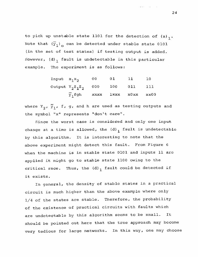
to pick up unstable state 1101 for the detection of (a)1

.

Note that (y 1 )0

can be detected under stable state 0101

(in the set of test states) if testing output is added.

However, (d) 1 fault is undetectable in this particular

example. The experiment is as follows:

Input x 1 x 2

Output Y2 z1 z2

ylfgh

00

000

xxxx

01

100

lxxx

11 10

011 111

xOxx xxOO

where Y2 , y 1 , f, g, and h are used as testing outputs and

the symbol "x" represents "don't care".

Since the worst case is considered and only one input

change at a time is allowed, the (d) 1 fault is undetectable

by this algorithm. It is interesting to note that the

above experiment might detect this fault. From Figure 6

when the machine is in stable state 0101 and inputs 11 are

applied it might go to stable state 1100 owing to the

critical race. Thus, the (d) 1 fault could be detected if

it exists.

In general, the density of stable states in a practical

circuit is much higher than the above example where only

1/4 of the states are stable. Therefore, the probability

of the existence of practical circuits with faults which

are undetectable by this algorithm seems to be small. It

should be pointed out here that the tree approach may become

very tedious for large networks. In this way, one may choose

the "trial and error" procedure to derive the test

sequence.

The testing procedure can be listed now as follows.

It is assumed that a circuit and its transition table

and output table are given, and that testing outputs can

be added.

1) Construct the fault table under stable state

conditions, simulating s-a-o and s-a-1 faults

on each line.

2) Under column (N.S.)f of the fault table if not

all faults are detected under stable state

conditions, find the unstable states which will

become stable in the presence of the undetectable

faults.

3) If not all faults in columns(N.S.)f and Zf are

detected, find the stable states which will

indicate the faults when testing outputs are

added to those lines.

4) Find the minimal set of test states sufficient

to detect all faults.

5) Generate the state-transition tree to derive a

shortest test sequence to go through the states

found in 4) .

25

There exists a subset of the former class of asynchronous

sequential circuits. They are the circuits with the outputs

26

identical to the next state variables. In this case,

step 3) of the above procedure is unnecessary. An example

in the next chapter is presented to illustrate this case.

C. Evaluation of the Shortest Test Sequence

In this section the minimization of test sequences is

investigated. In a circuit which has some particular fault

some stable states become unstable and some unstable states

become stable. If all unstable states are included in the

fault table and optimun use is made of the fault table, it

is possible to find a shorter test sequence for some cir-

cuit. The algorithm discussed previously is used to con-

struct the fault table under stable state conditions onlyi

if all stable states or some subset of them are sufficient

to detect all faults, then the test sequence is generatedi

otherwise the necessary unstable states are added to the

test sequence to detect the faults undetectable by stable

states~ or testing outputs are added.

To illustrate the idea presented above consider the

following example taken from Hughes (8). Each decimal

number in the transition table identifies a state.

The fault table is shown in Figure 11. The minimal

set of test states for this circuit is

011* 110* 100 } 001

101

The meaning of the above notation is that the states marked

with "*" are essential and that one state out of lOOr 001,

xl

x2

x2 y

y =

Figure 10.

xlx2

Y=Z y 00 01 11 10

0 @1 ®; 1 X ®7 5

1 0 2 * <D4 <D6 0 8

Y(=Z)

a + b

Circuit for evaluating the shortest test sequence

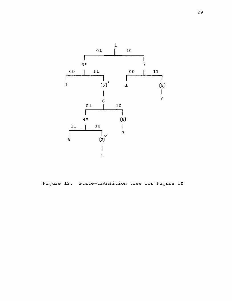
and 101 can be selected. The state-transition tree is

shown in Figure 12. From it the shortest test sequence

x 1 x 2 = 00 01 11 01 00 is found. When the algorithm

described in last section is applied, the state 100

will be selected. Thus, the test sequence becomes

Note that the length of this

test sequence is longer than the former. However, it

must be pointed out that not all circuits have this

property (i.e., their test sequence can be further mini-

mized) and that the length can not be made much shorter

by this method although it causes the fault table to be

more cumbersome. For example, this method is not useful

to the two examples in the next chapter.

27

28

s z zf c

xl x2 y z (xl)l (xl)O (x2)1 (x2)0 (a) 1 (a)o (b) 1

0 0 0 0 0 0 0 0 0 (1) 0

0 1 0 0 CD 0 0 0 0 (1) 0

1 0 0 0 0 0 CD 0 0 Q) 0

0 1 1 1 1 1 1 @ 1 1 @

1 1 1 1 1 1 1 @ 1 1 1

1 1 0 1 1 @ 1 @ @ 1 1

0 0 1 0 0 0 CD 0 0 Q) 0

1 0 1 0 0 0 CD 0 0 CD 0

'

zf

(b)o (Y) 1 (Y) 0

(1) (1) 0

(1) (1) 0

(1) <D 0

1 1 @

1 1 @

1 1 @

Q) <D 0

Q) <D 0

Figure 11. Fault table for Figure 10

29

1 01 I 10

3* 7

00 11 00 11

I * (s) 1 (5) 1

I 6 6

01 I 10

I 4* (8)

11 00 I 1 ..... 7

6 (2)

I 1

Figure 12. State-transition tree for Figure 10

30

III. EXAMPLES

In this chapter two examp~es are presented to illus­

trate the a~gorithm in more detail.

Example 1

The circuit in Figure 14 (taken from Kime (4)) has

the outputs identical to next state variables. Step 3)

of the testing procedure is to be omitted. The fault

table is shown in Figure 15. It is seen from the fault

table that the (e) 1 fault can not be detected under stable

state conditions. But when ~ine e is stuck at one the

transition table becomes that shown in Figure 13.

yly2 01 11 10

01 01

01 11 @) @ ~1 @ 10 10

10 10 @ @

yly2 (=ZlZ2)

yl = xlx2y2 + x2y~ + x~yl

y2 = x2y2 + x2yl

Figure 13. The transition tab~e for e s-a-1

31

Figure 14. Circuit for example 1

I

s z c

xl x2 yl y2 zl z2

0 0 0 0 0 0

0 0 1 1 1 1

0 1 0 1 0 1

0 1 1 0 1 0

1 1 0 1 0 1

1 1 1 0 1 0

1 0 0 1 0 1

1 0 1 1 1 1

1 0 1 0 1 0 I-- - ......

zf

(xl)l (xl)o (x2)1 (x2)o (yl)l (yl)o (x2)1 (x2)o (xl)l (xl)o

oQ) <(D '

00 00 00 00 00 00 00 00

11 @1 11 0 11 11 1@ 11 11 11 I 01 01 <1)1 01 01 o@ (})1

l 01 01 01 I

10 10 10 10 lG) 10 10 @o 10 10

01 01 01 01 01 <@ 01 01 01 01

10 10 10 10 lQ') 10 10 l(j) 10 10

G)l 01 01 01 01 01 01 01 01 0)1

11 11 11 1@ 11 11 1@ 11 11 11

10 10 10 10 l(D 10 10 lQ) 10 @o

Figure 15. Fault table for Figure 14

w [\)

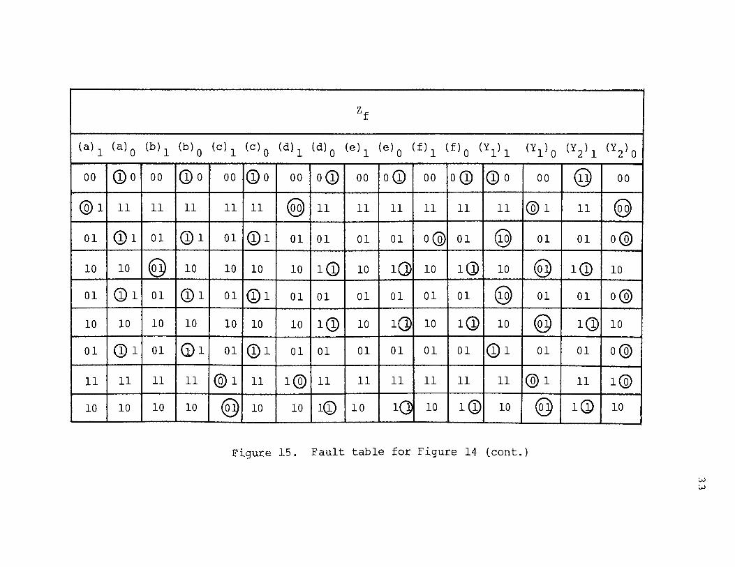
zf

(a)1 (a)o (b)1 (b)o (c)1 (c)o (d)1 (d)o (e)1 (e)o (f)1 (f)o (Y1)1 (Y1) 0 (Y2) 1 (Y2) 0

00 Q)o 00 (Yo 00 Q)o 00 o(D 00 o(D 00 oQ) Q)o 00 @ 00

@1 11 11 11 11 11 @ 11 11 11 11 11 11 @1 11 @

01 Q)1 01 Q)1 01 @1 01 01 01 01 o@ 01 @ 01 01 o@

10 10 @ 10 10 10 10 1@ 10 1Q) 10 1G) 10 @ 1Q) 10

01 G)1 01 Q)1 01 @1 01 01 01 01 01 01 @ 01 01 o@

10 10 10 10 10 10 10 1Q) 10 1(]} 10 1(j) 10 @ 1Q) 10

01 {1)1 01 (j)l 01 Q)l 01 01 01 01 01 01 Q)l 01 01 o@

11 11 11 11 @1 11 1@ 11 11 11 11 11 11 @1 11 1@

10 10 10 10 <§ 10 10 l(j) 10 lQ 10 lQ) 10 <§ lG) 10 -- ·--

~-

Figure 15. Fault table for Figure 14 (cont.)

I

w w

34

Therefore, unstable state x 1 x 2y 1y 2 = 1000 is included in

the set of test states x 1 x 2y 1 y 2 = {0000, 0011, 0101,

0110, 1001, lOll, 1000}. Figure 16 shows the transition

table with desired states marked and the state-transition

tree.

1* 10 01

I [7) * 3*

I 00

8* I 11

01 11 10 n 2*

10 01

5

01 10

'i<

00 01 01 01 2 5

9* I

4 3

01 11 @ 11 @ ~

1 6 ~ 2 6

10 00

YlY2(=ZlZ2) f-U--lo

4* 10

~ 1 6

Figure 16. Transition table and state-transition tree for Figure 14

The shortest test sequence is

Input xlx2 00 10 11 01 00 10 11 01

Output zlz2 00 01 01 01 11 11 10 10.

In order to place the circuit in initial state x1X2Y1Y2 =

0000 an adaptive homing sequence should be used. First,

I 8

35

apply 00. If the output is 00, we then start the test se-

quence; otherwise another input sequence, 01 00, must be

applied before beginning the test.

In his paper Kime obtained a experiment for this cir-

cuit. It required 31 input symbols in spite of the fact

that numerous short cuts and tricks were used in its con-

struction. This is almost 4 times longer than the above

result which requires 8 symbols.

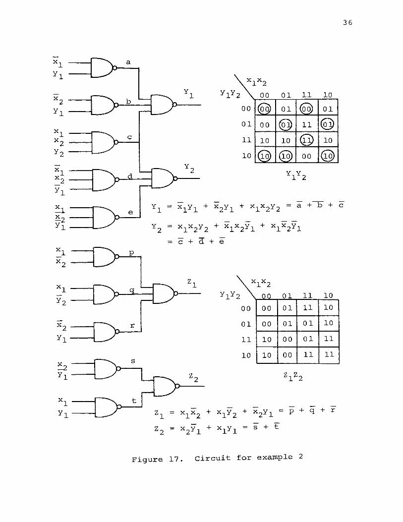
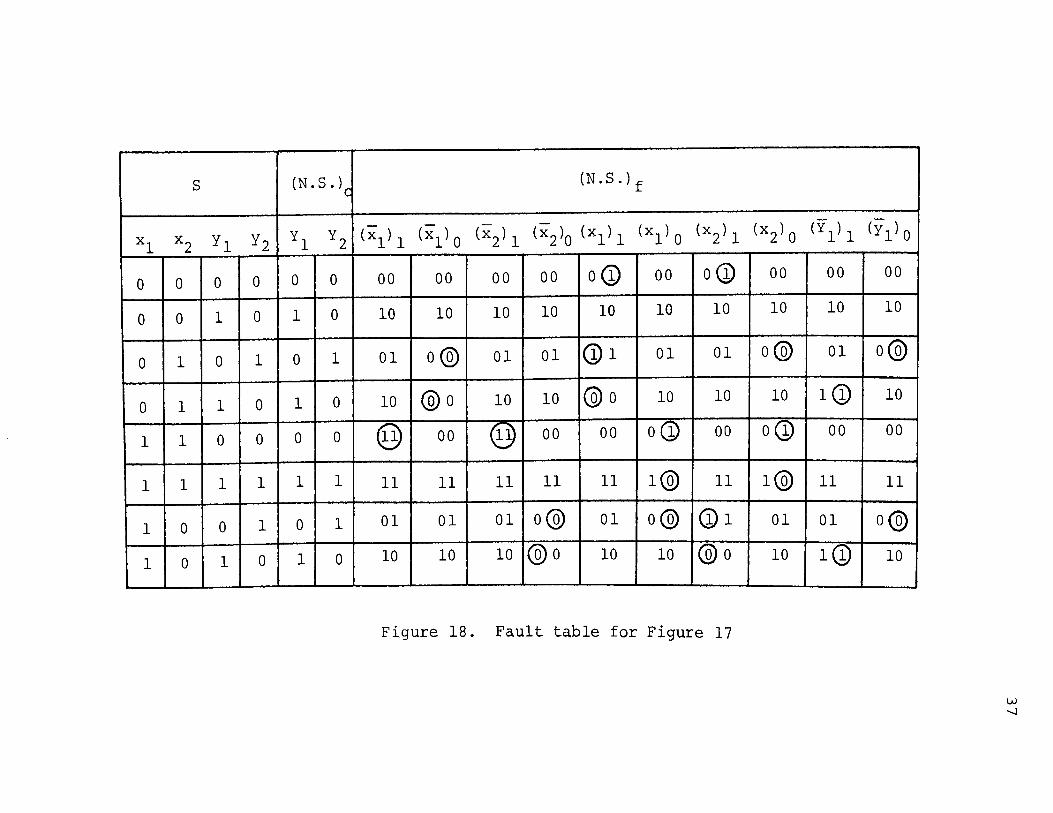
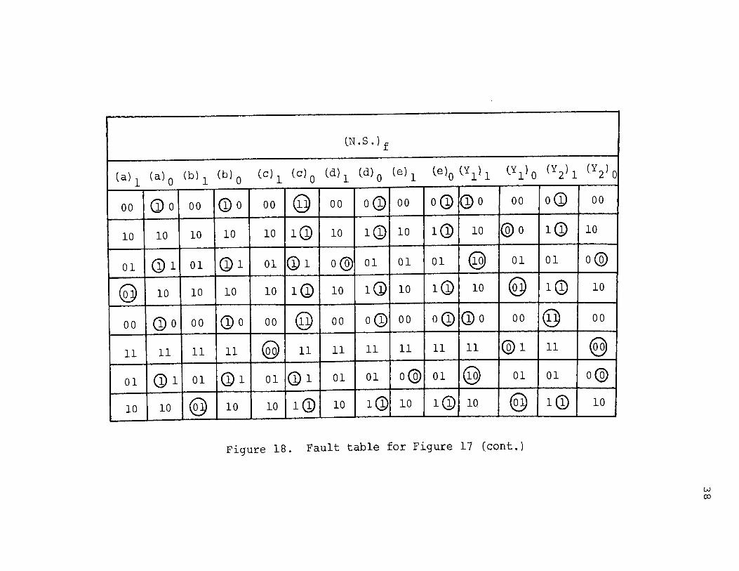
Example 2

Since the circuit shown in Figure 17 is a conventional

asynchronous sequential circuit, all steps of the proce-

dure should be applied. Figure 18 is its fault table.

From it the set of test states x 1 x 2y 1y 2 = {0010, 0101,

0110, 1100, 1111, 1001, 1010} is found. Note that all

stable states except 0000 are included in this set. There-

fore it is unnecessary to construct the state-transition

tree. The test sequence is the following:

Input x 1 x 2

Output Y1 Y2 z1 z2

00 10 11 10 00 01 11 01

0000 0110 1101 lOll 1010 1000 0011 0101

where Y1

and Y2

are testing outputs. Again, an adaptive

homing sequence (x1 x 2 = 00 or 00 01 11 01 00) is used to

put the circuit in the starting state x 1x 2y 1 y 2 = 0000.

36

a

c

xl yl + + - b -

= xlyl x2yl xlx2y2 = a + + c e

x2 ---1

y 1 ----~------ y2 = xlx2y2 + xlx2yl + xlx2yl

- d -= c + + e

p

xlx2

2 00 01 11 10

00 00 01 11 10

r 01 00 01 01 10

11 10 00 01 11

10 10 00 11 11

-x1x2 + x1y2 + x2yl = P + q + r

z2 = x2yl + x1yl = s + t

Figure 17. Circuit for example 2

s (N.S.)c

xl x2 yl y2 yl y2

0 0 0 0 0 0

0 0 1 0 1 0

0 1 0 1 0 1

0 1 1 0 1 0

1 1 0 0 0 0

1 1 1 1 1 1

1 0 0 1 0 1

1 0 1 0 1 0

(N.S.)f

<xl)l (xl)o (x2)1 <x2)o (xl)l <xl)o <x2)1 (x2)o (Yl)l (yl)O

00 00 00 00 oQ) 00 oQ) 00 00 00

10 10 10 10 10 10 10 10 10 10

01 o@ 01 01 @1 01 01 o@ 01 o@

10 @o 10 10 @o 10 10 10 10) 10

@ 00 @ 00 00 o(D 00 oQ) 00 00

11 11 11 11 11 1@ 11 1@ 11 11

01 01 01 o@ 01 o@ G)l 01 01 o@

10 10 10 @o 10 10 @o 10 1@ 10

Figure 18. Fault table for Figure 17

w -.J

lN. S.) f

(a)l (a)o (b)l (b)o (c)1

(c}0

(d)1

(d)0

le) 1 (elo (Yl)l (Yl}O (Y2)1 (Y2)C

00 G)o 00 (Do 00 @ 00 oQ) 00 o0) Q)o 00 oG) 00

10 10 10 10 10 lG) 10 l(D 10 lQ) 10 @o lG) 10

01 G)l 01 Q)l 01 G)l o@ 01 01 01 @ 01 01 o@

@ 10 10 10 10 lG) 10 lG) 10 lG) 10 @ lQ) 10 I

00 (Do 00 (Do 00 @ 00 o0) 00 oQ) (Do 00 @ 00

11 11 11 11 @ 11 11 11 11 11 11 @1 11 @

01 G)l 01 (1)1 01 Q)l 01 01 o@ 01 @ 01 01 o@

10 10 @ 10 10 1(1) 10 1(1) 10 1@ 10 @ 1@ 10

Figure 18. Fault table for Figure 17 (cont.)

w (X)

z c

zl z2

0 0

1 0

0 1

0 0

1 1

0 1

1 0

1 1

zf

(y2)1 Cy2}o (P}l (P}o (q}l (q}o Cr}l Crlo (s}l Cslo (t}l (t)o (Zl}l ('1_}o Cz21 (Zjo

00 00 00 KDo 00 Q)o 00 (Do 00 oG) 00 oQ) (Do 00 o(D oo

10 10 10 10 10 10 @o 10 10 lQ) 10 1{1) 10 @o 1{1) 10

01 01 01 (Dl 01 (Dl 01 Q)l o@ 01 01 01 Q)l 01 01 a@

00 00 00 1 0 00 (Do 00 (Do 00 o(D 00 oQ) Q)o 00 oQ) 00

11 @1 11 11 @1 11 11 11 1@ 11 11 11 11 @1 11 1@

(1)1 01 01 Q)l 01 Q)l 01 (})1 01 01 o@ 01 (1)1 01 01 o@

10 10 @o 10 10 10 10 10 10 lQ;} 10 1(1) 10 @o 1(1) 10

11 11 11 11 11 11 11 11 1 1 11 1@ 11 11 @1 11 1@

Figure 18. Fault table for Figure 17 (cont.)

1

w ~

40

IV. CONCLUSIONS

The algorithm developed in this paper presents a

method for detecting a single failure in an asynchronous

sequential circuit which is treated from the combinatoric

point of view. Since the states sufficient to detect all

possible faults of the circuit form a subset of the total

states, the experiments are to check only this subset of

states rather than all the transitions of the states. In

this way, a very short test sequence can be generated.

The effectiveness of the algorithm depends on the density

of stable states. Attempts at finding a practical cir­

cuit with faults which are undetectable by this algorithm

have been unsuccessful. The only disadvantage, and one

which is common to most of the fault-detection methods,

is that when the circuit has a large number of inputs and

state variables the procedures of the algorithm may become

quite lengthy.

41

V. BIBLIOGRAPHY

1. Kautz, W.H. "Fault Testing and Diagnosis in Combina­

tional Digital Circuits", IEEE Trans. on Computers,

Vol. C-17, No. 4, pp. 352-366, April 1968.

2. Armstrong, D.B., ''On Finding a Nearly Minimal Set of

Fault Detection Tests for Combinational Logic Nets",

IEEE Trans. on Electronic Computers, Vol. EC-15,

pp. 66-73, February 1966.

3. Roth, P.J., "Diagnosis of Automata Failures: A

Calculus and a Method", IBM Journal, Vol. 10,

No. 4, pp. 278-291, July 1966.

4. Kime, C.R., ''A Failure Detection Method for Sequential

Circuits", Dept. Elec. Engrg., Univ. of Iowa, Iowa

City, Tech. Report 66-13, January 1966.

5. Kohavi, Z. and Lavallee, P., ''Design of Sequential

Machine with Fault Detection Capabilities", IEEE

Trans. on Computers, Vol. EC-16, No. 4, pp. 473-484,

August 1967.

6. Kohavi, I. and Kohavi, z., "Variable-Length Disting­

uishing Sequences and Their Application to the

Design of Fault Detection Experiments", IEEE Trans.

on Computers, Vol. C-17, pp. 792-795, August 1968.

7. Kohave, I., "Fault Diagnosis of Logical Circuits",

IEEE Conference Record of 1969 lOth Annual

Symposium on Switching and Automata Theory, pp.

166-173.

8. Hughes, V.W., Jr., "Fault Diagnosis of Sequential

Circuits", M.S. Thesis, University of Missouri­

Rolla. T2272, 1969.

42

9. Booth, T.L., Seguential Machines and Automata Theory,

New York: John Wiley and Sons, Inc., 1968.

VI. VITA

Jeng-Chuan Kau was born on December 20, 1944, in

Taipei, Taiwan, Republic of China. He received his

primary and secondary education there and obtained his

Bechelor of Science Degree in Electrical Engineering

in 1967 from Tatung Institute of Technology in Taiwan,

Republic of China.

He has been enrolled in the Graduate School of the

University of Missouri-Rolla since September, 1969.

43