A Comprehensive Review and Evaluation of

Permutation Flowshop Heuristics

Ruben Ruiz∗, Concepcion Maroto

Dpto. de Estadıstica e Investigacion Operativa Aplicadas y Calidad

Universidad Politecnica de Valencia

6th January 2004

Abstract

In this work we present a review and comparative evaluation of

heuristics and metaheuristics for the well known permutation flow-

shop problem with the makespan criterion. A number of reviews and

evaluations have already been proposed. However, the evaluations do

not include the latest heuristics available and there is still no compari-

son of metaheuristics. Furthermore, since no common benchmarks and

computing platforms are used, the results cannot be generalised. We

propose a comparison of 25 methods, ranging from the classical John-

son’s algorithm or dispatching rules to the most recent metaheuristics,

including tabu search, simulated annealing, genetic algorithms, iter-

ated local search and hybrid techniques. For the evaluation we use the

∗Corresponding author: Ruben Ruiz Garcıa. Universidad Politecnica de Valencia.Departamento de Estadıstica e Investigacion Operativa Aplicadas y Calidad. Camino deVera S/N, 46021, Valencia, SPAIN. Tel: +34 96 387 70 07, ext: 74946. Fax: +34 96 38774 99. e-mail: rruiz@eio.upv.es

1

standard test of Taillard (1993) composed of 120 instances of differ-

ent sizes. In the evaluations we use the experimental design approach

to obtain valid conclusions on the effectiveness and efficiency of the

different methods tested.

Keywords: Flowshop, Scheduling, Heuristics, Metaheuristics.

1 Introduction

In a flowshop scheduling problem there is a set of n jobs, tasks or items

(1, . . . , n) to be processed in a set of m machines or processors (1, . . . ,m)

in the same order, i.e. first in machine 1 then on machine 2 and so on until

machine m. The objective is to find a sequence for the processing of the jobs

in the machines so that a given criterion is optimised. In the literature, the

most common criterion is the minimisation of the total completion time or

makespan of the schedule (Cmax), this is sometimes referred to as maximum

flow time or Fmax. The processing times needed for the jobs on the machines

are noted as pij, where i = 1, . . . , n and j = 1, . . . ,m, these times are fixed,

known in advance and nonnegative. There are several assumptions that are

commonly made regarding this problem (Baker, 1974):

• Each job i can be processed at most on one machine j at the same

time.

• Each machine m can process only one job i at a time.

• No preemption is allowed, i.e. the processing of a job i on a machine j

can not be interrupted.

• All jobs are independent and are available for processing at time 0.

2

• The set-up times of the jobs on machines are negligible and therefore

can be ignored.

• The machines are continuously available.

• In-process inventory is allowed. If the next machine on the sequence

needed by a job is not available, the job can wait and joins the queue

at that machine.

This problem was initially classified as n/m/F/Fmax following the four pa-

rameter notation A/B/C/D by Conway et al. (1967) and then as F//Cmax

following the three parameter notation α/β/γ introduced by Graham et al.

(1979). Although the flowshop scheduling problem is solvable to optimality

in polynomial time when m = 2 (Johnson, 1954), it is known to be NP-

Complete in the strong sense when m ≥ 3 (see Garey et al., 1976). In

general (n!)m schedules have to be considered. This is why the problem is

further restricted in the literature by not allowing job passing, i.e. the pro-

cessing sequence of the jobs is the same for all the machines, so no job can

pass another in the following machine. In this case “only” n! schedules have

to be considered and the problem is then known as permutation flowshop and

is classified as n/m/P/Fmax or as F/prmu/Cmax (see Pinedo, 2002). In this

work we will concentrate on this last type of flowshop environment.

In the literature of flowshop scheduling there are various reviews (for exam-

ple, Dudek et al., 1992 or Reisman et al., 1994), and also there are some

comparative evaluations available. In Ponnambalam et al. (2001), five dif-

ferent heuristics are compared against only 21 typical test problems. Turner

and Booth (1987) compare two famous heuristics with a set of 350 random

problems. In the work of Byung Park et al. (1984), a total of 16 heuris-

tics are compared against 1,500 random generated problems of a maximum

size of 30 jobs and 20 machines. Dannenbring (1977) evaluated 11 different

3

heuristics with a benchmark set of 1,580 random problems of various sizes

and characteristics. Finally, Ashour (1970), compared some of the earliest

methods for the permutation flowshop problem.

As we can see, all these evaluations have several shortcomings; usually no

common data sets and/or computer mainframes are used for the results to

be generalised. The comparisons are usually performed between no more

than a few heuristics and, furthermore, no comparison deals with the most

recent heuristics available. It is also difficult to find comparative evaluations

between advanced metaheuristics such as Simulated Annealing or Genetic

Algorithms.

For all aforementioned reasons, today it is impossible to make a global com-

parative evaluation of the different methods proposed in the literature, since

the evaluations are partial and the benchmarks used are not standard, there-

fore the results are not reproducible.

The objective of this paper is to give an up to date comprehensive review

and evaluation of many existing heuristics and metaheuristics for the per-

mutation flowshop. We evaluate a total of 25 heuristics, from the classical

methods to the most recent heuristics and advanced metaheuristics. The

comparisons are made against Taillard (1993)’s famous benchmarks.

The rest of the paper is organised as follows. In section 2 the most well-known

heuristics for the permutation flowshop (PFSP from now on) are reviewed.

Section 3 deals with metaheuristics for the PFSP, from Simulated Annealing

to complex hybrid techniques. A comparison of the various heuristics and

metaheuristics can be seen in Section 4. Finally, in Section 5 some conclu-

sions are given.

4

2 Heuristics for the flowshop scheduling prob-

lem

The complexity of the flowshop scheduling problem renders exact solution

methods impractical for instances of more than a few jobs and/or machines.

This is the main reason for the various heuristic methods proposed in the

literature, some of which will be explained here. The heuristics can be di-

vided in either constructive heuristics or improvement heuristics, the former

are heuristics that build a feasible schedule from scratch and the latter are

heuristics that try to improve a previously generated schedule by normally

applying some form of specific problem knowledge.

2.1 Constructive Heuristics

Johnson’s algorithm (1954) is the earliest known heuristic for the PFSP,

which provides an optimal solution for two machines. Moreover, it can be

used as a heuristic for the m machine case by clustering the m machines into

two “virtual” machines. The computational complexity of this heuristic is

O(n log n). Other authors have used the general ideas of Johnson’s rule in

their algorithms, for example, Dudek and Teuton (1964) developed an m-

stage rule for the PFSP that minimises the idle time accumulated on the last

machine when processing each job by using Johnson’s approach. Campbell

et al. (1970) developed a heuristic algorithm which is basically an exten-

sion of Johnson’s algorithm. In this case, several schedules are constructed

and the best one is given as a result. The heuristic is known as CDS and

builds m − 1 schedules by clustering the m original machines into two vir-

tual machines and solving the generated two machine problem by repeatedly

using Johnson’s rule. The CDS heuristic has a computational complexity of

O(m2n + mn log n).

5

In a more recent work, Koulamas (1998) reported a new two phase heuristic,

called HFC. In the first phase, the HFC heuristic makes extensive use of

Johnson’s algorithm. The second phase improves the resulting schedule from

the first phase by allowing job passing between machines, i.e. by allowing

non-permutation schedules. This is a very interesting idea, since it is known

that permutation schedules are only dominant for the three-machine case. In

the general m machine case, a permutation schedule is not necessarily opti-

mal anymore (Potts et al., 1991). Although this heuristic departs from the

PFSP problem by allowing job passing, we have included it in the review for

comparison reasons since we believe that some instances might benefit from

job passing. Taking into account both phases, the general computational

complexity of this heuristic is roughly O(m2n2).

Another approach is to assign a weight or “index” to every job and then ar-

range the sequence by sorting the jobs according to the assigned index. This

idea was first exploited by Palmer (1965) when he developed a very simple

heuristic in which for every job a “slope index” is calculated and then the

jobs are scheduled by non-increasing order of this index, which leads to a

computational complexity of O(nm + n log n). This idea has been used in

later papers, for example Gupta (1971) proposed a modification of Palmer’s

slope index which exploited some similarities between scheduling and sorting

problems. Similarly, Bonney and Gundry (1976) worked on the idea of using

the geometrical properties of the cumulative process times of the jobs and

a slope matching method for scheduling the PFSP. Hundal and Rajgopal

(1988) proposed a very simple extension to Palmer’s heuristic by exploiting

the fact that when m is an odd number, Palmer’s slope index returns the

value 0 for the machine (m + 1)/2 and consequently ignores it. In order

to overcome this, two more slope indexes are calculated and with these two

slope indexes and the original Palmer’s slope index, three schedules are cal-

6

culated and the best one is given as a result. Since the procedure consists

in calculating three indexes, the computational complexity is the same of

Palmer’s O(nm + n log n).

Dannenbring (1977)’s Rapid Access (RA) heuristic is a mixture of the pre-

vious ideas of Johnson’s algorithm and Palmer’s slope index. In this case a

virtual two machine problem is defined as it is in the CDS heuristic, but in-

stead of directly applying Johnson’s algorithm over the processing times, two

weighting schemes are calculated, one for each machine, and then Johnson’s

algorithm is applied. The weighting schemes give the processing times for

the jobs in the two virtual machines. As the name of the heuristic implies,

RA provides a good solution in a very quick and easy way O(mn + n log n).

Since all the jobs in a PFSP form a permutation, many proposed methods

work with the idea of exchanging the position of the jobs in the sequence

or inserting jobs at different locations to obtain better results. Page (1961)

proposed three heuristic methods based on the similarities of the PFSP with

sorting methods. The idea is to obtain a good ordering of the jobs and to

subsequently improve this order by means of job exchanges.

Nawaz et al. (1983)’s NEH heuristic is regarded as the best heuristic for the

PFSP (see Taillard, 1990). It is based on the idea that jobs with high pro-

cessing times on all the machines should be scheduled as early in the sequence

as possible. The procedure is straightforward:

1. The total processing times for the jobs are calculated using the formu-

lae: ∀ job i, i = 1, . . . , n, Pi =∑m

j=1 pij.

2. The jobs are sorted in non-increasing order of Pi. Then the first two

jobs (those two with higher Pi) are taken and the two possible schedules

containing them are evaluated.

3. Take job i, i = 3, . . . , n and find the best schedule by placing it in all the

7

possible i positions in the sequence of jobs that are already scheduled.

For example, if i = 4, the already constructed sequence would contain

the first three jobs of the sorted list calculated in step 2, then the fourth

job could be placed either in the first, in the second, in the third or in

the last position of the sequence. The best sequence of the four would

be selected for the next iteration.

As we have seen, the NEH heuristic is based neither on Johnson’s algorithm

nor on slope indexes. The only drawback is that a total of [n(n + 1)/2] − 1

schedules have to be evaluated, being n of those schedules complete se-

quences. This makes the complexity of NEH rise to O(n3m) which can be

lengthy for big problem instances. However, Taillard (1990) reduced NEH’s

complexity to O(n2m) by calculating all the partial schedules in a given it-

eration in a single step.

Sarin and Lefoka (1993) exploited the idea of minimising idle time on the last

machine since any increase in the idle time on the last machine will translate

into an increase in the total completion time or makespan. In this way, the

sequence is completed by inserting one job at a time and priority is given

to the job that, once added to the sequence, would result in minimal added

idle time on machine m. The method proposed compares well with the NEH

heuristic but only when the number of machines in a problem exceeds the

number of jobs. Davoud Pour (2001) proposed another insertion method.

This new heuristic is based on the idea of job exchanging and is similar to

the NEH method. The performance of this method is evaluated against the

NEH, CDS and Palmer’s heuristics showing better effectiveness only when

a big number of machines is considered, and being the computational com-

plexity O(n3m). More recently, Framinan et al. (2003) have published a

study about the NEH heuristic where different initialisations and orderings

are considered. The study also includes different objective functions.

8

Other authors have proposed heuristics that use one or more of the pre-

vious ideas, for example, Gupta (1972) proposed three heuristic methods,

named minimum idle time (MINIT), minimum completion time (MICOT)

and MINIMAX algorithms, the first two are based on job pair exchanges

and the MINIMAX is based on Johnson’s rule. These three algorithms were

tested with the objectives of Cmax and mean flowtime (F ) and compared

with the CDS algorithm, proving to be superior only when considering the

F objective.

Additionally, there are many other methods available that are not based

on Johnson’s or Palmer’s ideas and that do not construct sequences by job

exchanges and/or insertions only. For example, King and Spachis (1980)

evaluated various heuristics for the PFSP and for the flowshop with no job

waiting (no-wait flowshop). For the PFSP, a total of five heuristics based on

dispatching rules were developed. A different approach is shown in Stinson

and Smith (1982) where the authors solve the permutation flowshop problem

by using a well known heuristic for the Travelling Salesman Problem (TSP).

2.2 Improvement Heuristics

Contrary to constructive heuristics, improvement heuristics start from an al-

ready built schedule and try to improve it by some given procedure. Dannen-

bring (1977) proposed two simple improvement heuristics, these are Rapid

Access with Close Order Search (RACS) and Rapid Access with Extensive

Search (RAES). The reason behind these two heuristics is that Dannenbring

found that simply swapping two adjacent jobs in a sequence obtained by

the RA heuristic resulted in an optimal schedule. RACS works by swapping

every adjacent pair of jobs in a sequence (this is n−1 steps). The best sched-

ule among the n − 1 generated is then given as a result. In RAES heuristic,

RACS is repeatedly applied while improvements are found. Both RACS and

9

RAES heuristics start from a schedule generated with the RA constructive

heuristic.

Ho and Chang (1991) developed a method that works with the idea of min-

imising the elapsed times between the end of the processing of a job in a

machine and the beginning of the processing of the same job in the following

machine in the sequence. The authors refer to this time as “gap”. The al-

gorithm calculates the gaps for every possible pair of jobs and machines and

then by a series of calculations, the heuristic swaps jobs depending on the

value of the gaps associated with them. The heuristic starts from the CDS

heuristic by Campbell et al.

Recently, Suliman (2000) developed an improvement heuristic. In the first

phase, a schedule is generated with the CDS heuristic method. In the second

phase, the schedule generated is improved with a job pair exchange mech-

anism. In order to reduce the computational burden of an exhaustive pair

exchange mechanism, a directionality constraint is imposed to reduce the

search space. For example, if by moving a job forward, a better schedule is

obtained, it is assumed that better schedules can be achieved by maintaining

the forward movement and not allowing a backward movement.

3 Metaheuristics for the flowshop scheduling

problem

Metaheuristics are general heuristic procedures that can be applied to many

problems, and, in our case, to the PFSP. These methods normally start from

a sequence constructed by heuristics and iterate until a a stopping criterion is

met. There is plenty of research work done for the PFSP and metaheuristics.

In this section, we will point out a few noteworthy papers mainly dealing with

Simulated Annealing (SA), Tabu Search (TS), Genetic Algorithms (GA) and

10

other metaheuristics, as well as hybrid methods.

Osman and Potts (1989) proposed a simple Simulated Annealing algorithm

using a shift neighbourhood and a random neighbourhood search. In the

same year Widmer and Hertz (1989) presented a method called SPIRIT,

which is a two phase heuristic. In the first phase, a problem is generated

with an analogy with the Open Travelling Salesman Problem (OTSP) and

then, this problem is solved with an insertion method to obtain an initial

solution. In the second phase, a Tabu Search metaheuristic with standard

parameters and exchange neighbourhood is used to improve the incumbent

solution. Taillard (1990) also presented a similar procedure to that of Wid-

mer and Hertz. A Tabu Search technique is applied to a schedule generated

by an improved NEH heuristic. Taillard tested various types of neighbour-

hoods and the neighbourhood resulting from changing the position of one

job proved to be the best.

Ogbu and Smith (1990a) proposed a Simulated Annealing approach to the

PFSP which involved an initialisation with the Palmer and Dannenbring

heuristics. The choice of a large neighbourhood and an acceptance proba-

bility function independent of the change in the makespan of the schedule

resulted in near-optimal schedules for the problems tested. In a later work

(Ogbu and Smith, 1990b) compared this Simulated Annealing with that of

Osman and Potts. The results show a tie between the two metaheuristics

with a slight advantage on the part of Osman and Potts’s one.

Werner (1993) constructed a fast iterative method which obtained very good

results by generating restricted numbers of paths in a search neighbourhood

built upon the path structure of a feasible schedule. It is interesting to re-

mark that while local search or fast iterative methods operate in a very small

neighbourhood, Werner’s path algorithm operates with a rather large neigh-

bourhood but only evaluates the most interesting solutions in each step.

11

Reeves (1993) modified the SPIRIT algorithm and introduced several en-

hancements, such as the initialisation by the NEH heuristic and the insertion

neighbourhood. The author compared this algorithm with the SA of Osman

and Potts showing better results.

Chen et al. (1995) developed a simple Genetic Algorithm for the PFSP with

various enhancements. The initial population is generated with the CDS and

RA heuristics and also from simple job exchanges of some of the individuals.

Only the crossover operator is applied (no mutation), and the crossover used

is the Partially mapped crossover or PMX. Reeves (1995) also developed a

Genetic Algorithm. In this case, the offspring generated in each step of the

algorithm do not replace their parents but individuals from the generation

that have a fitness value below average. Reeves used a crossover operator

called C1, which is equivalent to the One Point Order Crossover. Another

remarkable feature of the algorithm is that it uses an adaptive mutation rate.

The algorithm uses a shift mutation which simply changes the position of one

job. Reeves also chose to seed the initial population with a good sequence

among randomly generated ones. This good sequence is obtained with the

NEH heuristic. Also, the selection of the parents is somewhat different from

what is common in genetic algorithms; parent 1 is selected using a fitness

rank distribution whereas parent 2 is chosen using a uniform distribution.

This Genetic Algorithm was one of the first methods to be tested against

Taillard (1993)’s famous benchmark instances.

Ishibuchi et al. (1995) presented two Simulated Annealing algorithms charac-

terized by having robust performance with respect to the temperature cooling

schedule. Their results showed that their algorithms were comparable to the

SA of Osman and Potts. Zegordi et al. (1995) demonstrated a hybrid tech-

nique by introducing problem domain knowledge into a Simulated Annealing

algorithm. Their algorithm, called SA-MDJ, uses a “Move desirability for

12

Jobs” table which incorporates several rules that facilitate the annealing

process. This way, fewer control parameters are needed. The algorithm is

compared with Osman and Potts’s SA algorithm proving to be slightly infe-

rior but much faster in the instances tested.

The Tabu Search of Moccellin (1995) is mainly based on Widmer and Hertz’s

SPIRIT heuristic. The only difference exists in the step of calculating the

initial solution for the problem. The analogy with the Travelling Salesman

Problem is maintained, but the way the distance between jobs is calculated

differs from that of Widmer and Hertz. Also, how the TSP problem is

solved is different, since Moccellin uses the farthest Insertion Travelling Sales-

man Procedure (FITSP). The rest of the algorithm is essentially similar to

SPIRIT.

The genetic algorithms proposed by Murata et al. (1996) use the two-point

crossover operator and a shift mutation along with an elitist strategy to

obtain good solutions for the PFSP. The algorithm performed worse than

implementations of Tabu Search, Simulated Annealing and local search, so

the authors implemented two hybrid versions of the Genetic Algorithm; Ge-

netic Simulated Annealing and Genetic Local Search. In these algorithms,

an “improvement” phase is performed before selection and crossover and this

improvement is made with local search and simulated annealing algorithms

respectively. The hybrid algorithms performed better than the non hybrid

Genetic Algorithm, implementations of Tabu Search, Simulated Annealing

and local search.

Nowicki and Smutnicki (1996) proposed a Tabu Search metaheuristic where

once again, a reduced part of the neighbourhood is evaluated along with

a fast method for obtaining the makespan. The neighbourhood is reduced

with the idea of blocks of jobs, where jobs are clustered and the movements

are made on a block-by-block basis instead of just moving single jobs. This

13

algorithm has proved to be one of the finest metaheuristics for the PFSP

and the authors were then able to lower the best upper bounds for Taillard’s

benchmark instances.

Another hybrid Genetic Algorithm is that of Reeves and Yamada (1998),

the idea behind this algorithm is the Multi-step crossover fusion or MSXF

operator which coalesces a crossover operator with local search. The MSXF

operator carries a biased local search from one parent using the other parent

as a reference. The MSXF operator is defined by a neighbourhood struc-

ture and a measure of distance, which has some similarities with simulated

annealing but with a constant temperature parameter. The results given

outperform other metaheuristics and the authors also found new lower upper

bounds for Taillard’s benchmark instances. Another metaheuristic is given

by Stutzle (1998), and is given the name “Iterated Local Search” or ILS. In

some way or another, the ideas behind ILS are those of descent search, local

search, Simulated Annealing or Tabu Search; An initial solution is obtained

and a LocalSearch procedure is executed over this initial solution, then a

Modify procedure that slightly modifies the current solution is carried out.

Then, LocalSearch is called again and the resulting schedule is deemed as the

new current solution only if a certain acceptance criterion is met (procedure

AcceptanceCriterion). The ILS procedure may also work with a list called

history that works similarly to the tabu list in Tabu Search. The exper-

imental results given in the paper show some very interesting conclusions.

According to the tests conducted by Stutzle, the ILS algorithm is much bet-

ter than the Tabu Search of Taillard (1990) and also better than the Tabu

Search of Nowicki and Smutnicki (1996).

Ben-Daya and Al-Fawzan (1998) implemented a Tabu Search algorithm with

some extra features such as intensification and diversification schemes that

provide better moves in the tabu search process. The algorithm proposed

14

provides similar results as the TS of Taillard and slightly better results than

the SA of Ogbu and Smith. Moccellin and dos Santos (2000) presented a

hybrid Tabu Search-Simulated Annealing heuristic that is compared with

simple Tabu Search and simple Simulated Annealing implementations from

the same authors, showing advantages for the hybrid approach.

Ponnambalam et al. (2001) evaluate a Genetic Algorithm which uses the

GPX crossover (Generalised Position Crossover) and other features like shift

mutation and a randomized initial solution.

Wodecki and Bozejko (2002) have recently proposed a SA algorithm that is

run in a parallel computing environment. The authors compare the proposed

algorithm with the NEH heuristic, the former showing better results. Finally,

Wang and Zheng (2003) have presented a complex hybrid genetic algorithm

in which the initialisation of the population uses the NEH heuristic and the

mutation operator is replaced by a SA algorithm. The proposed algorithm

also uses multicrossover operators that are applied to subpopulations in the

original population.

4 Comparative Evaluation of Heuristics and

Metaheuristics

Table 1 shows a summary of the different constructive and improvement

heuristics reviewed in chronological order, and Table 2 shows information

about the reviewed metaheuristics. In order to evaluate the different heuris-

tics, a broad number of them have been coded, these are: Johnson’s algorithm

(extended to the m machine case) (Johns), Page’s pairing sorting algorithm

(Page), Palmer’s “slope index” heuristic (Palme), the Campbell et al. and

Gupta’s heuristics (CDS and Gupta). The three heuristics by Dannenbring

(RA, RACS and RAES), Nawaz et al. NEH heuristic (NEH), Hundal and

15

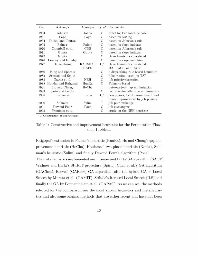
Year Author/s Acronym Type∗ Comments

1954 Johnson Johns C exact for two machine case1961 Page Page C based on sorting1964 Dudek and Teuton C based on Johnson’s rule1965 Palmer Palme C based on slope indexes1970 Campbell et al. CDS C based on Johnson’s rule1971 Gupta Gupta C based on slope indexes1972 Gupta C three heuristics considered1976 Bonney and Gundry C based on slope matching1977 Dannenbring RA,RACS, C/ three heuristics considered:

RAES I RA, RACS, and RAES1980 King and Spachis C 5 dispatching rule based heuristics1982 Stinson and Smith C 6 heuristics, based on TSP1983 Nawaz et al. NEH C job priority/insertion1988 Hundal and Rajgopal HunRa C Palmer’s based1991 Ho and Chang HoCha I between-jobs gap minimisation1993 Sarin and Lefoka C last machine idle time minimisation1998 Koulamas Koula C/ two phases, 1st Johnson based, 2nd

I phase improvement by job passing2000 Suliman Sulim I job pair exchange2001 Davoud Pour Pour C job exchanging2003 Framinan et al. C study on the NEH heuristic∗C: Constructive, I: Improvement

Table 1: Constructive and improvement heuristics for the Permutation Flow-shop Problem.

Rajgopal’s extension to Palmer’s heuristic (HunRa), Ho and Chang’s gap im-

provement heuristic (HoCha), Koulamas’ two-phase heuristic (Koula), Suli-

man’s heuristic (Sulim) and finally Davoud Pour’s algorithm (Pour).

The metaheuristics implemented are: Osman and Potts’ SA algorithm (SAOP),

Widmer and Hertz’s SPIRIT procedure (Spirit), Chen et al.’s GA algorithm

(GAChen), Reeves’ (GAReev) GA algorithm, also the hybrid GA + Local

Search by Murata et al. (GAMIT), Stutzle’s Iterated Local Search (ILS) and

finally the GA by Ponnambalam et al. (GAPAC). As we can see, the methods

selected for the comparison are the most known heuristics and metaheuris-

tics and also some original methods that are either recent and have not been

16

Year Author/s Acronym Type Comments

1989 Osman and Potts SAOP SAWidmer and Hertz Spirit TS initial solution based on

the OTSP1990 Taillard TS

Ogbu and Smith SA1993 Werner other path algorithms

Reeves TS1995 Chen et al. GAChen GA PMX crossover

Reeves GAReev GA adaptive mutation rateIshibuchi et al. SA two SA consideredZegordi et al. SA combines sequence knowledge

Moccellin TS based on SPIRIT1996 Murata et al. GAMIT hybrid GA+Local Search/SA

Nowicki and Smutnicki TS neighbourhood by blocks of jobs1998 Stutzle ILS other Iterated Local Search

Ben-Daya and Al-Fawzan TS intensification + diversificationReeves and Yamada GA GA operators with problem

knowledge2000 Moccellin and dos Santos hybrid TS + SA2001 Ponnambalam et al. GAPAC GA GPX crossover

Wodecki and Bozejko SA parallel simulated annealing2003 Wang and Zheng hybrid GA + SA, multicrossover operators

Table 2: Metaheuristics for the Permutation Flowshop Problem.

evaluated before or some that incorporate new ideas not previously used by

other algorithms.

All efforts to code the complex TSAB algorithm of Nowicki and Smutnicki

(1996) were unsuccessful. We tried several times to contact the authors but

were unable to obtain the code for help. However, Stutzle showed his ILS

algorithm to be superior to the published results of the TSAB. Note that,

however, the implementations that have been carried out in this work come

from the explanations given in the original papers which could sometimes dif-

fer slightly from the original authors’ implementations. All algorithms and

methods (25 total) are coded in Delphi 6.0 and run in an Athlon XP 1600+

computer (1400 MHz) with 512 MBytes of main memory.

17

In order to make a fair comparison, the stopping criterion for all the meta-

heuristics tested is a maximum of 50,000 makespan evaluations where every

algorithm is run five independent times to obtain a final average of the re-

sults. For comparison reasons, we have also included a random procedure

that evaluates random schedules and returns the best one (RAND). Fur-

thermore, three common dispatching rules have been implemented, these are

FCFS (First Come, First Served), SPT (Shortest Processing Time First) and

LPT (Longest Processing Time First). The reason behind this is that dis-

patching rules are commonly used in practice. Note that SPT and LPT rules

can produce non-permutation schedules where job passing is permitted.

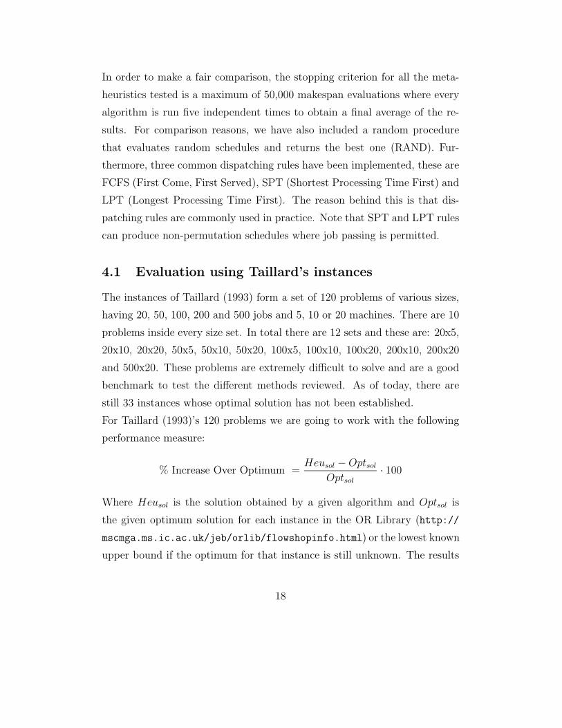
4.1 Evaluation using Taillard’s instances

The instances of Taillard (1993) form a set of 120 problems of various sizes,

having 20, 50, 100, 200 and 500 jobs and 5, 10 or 20 machines. There are 10

problems inside every size set. In total there are 12 sets and these are: 20x5,

20x10, 20x20, 50x5, 50x10, 50x20, 100x5, 100x10, 100x20, 200x10, 200x20

and 500x20. These problems are extremely difficult to solve and are a good

benchmark to test the different methods reviewed. As of today, there are

still 33 instances whose optimal solution has not been established.

For Taillard (1993)’s 120 problems we are going to work with the following

performance measure:

% Increase Over Optimum =Heusol − Optsol

Optsol

· 100

Where Heusol is the solution obtained by a given algorithm and Optsol is

the given optimum solution for each instance in the OR Library (http://

mscmga.ms.ic.ac.uk/jeb/orlib/flowshopinfo.html) or the lowest known

upper bound if the optimum for that instance is still unknown. The results

18

of the different heuristics can be seen in Table 3. Note that for every problem

size we have averaged the 10 corresponding instances. As is shown in Ta-

Problem RAND FCFS SPT LPT Johns Page Palme CDS Gupta

20x5 5.79 24.98 20.44 47.66 12.78 15.15 10.58 9.54 12.45

20x10 9.47 28.77 24.74 46.38 19.97 20.43 15.28 12.13 24.48

20x20 7.76 21.43 23.17 34.27 16.47 16.18 16.34 9.64 22.53

50x5 4.74 15.32 16.21 48.33 10.43 10.14 5.34 6.10 12.43

50x10 14.00 25.05 26.51 51.23 21.90 20.47 14.01 12.98 22.05

50x20 16.31 29.59 29.38 48.08 22.81 23.12 15.99 13.85 23.66

100x5 3.70 13.63 17.98 45.19 6.84 7.98 2.38 5.01 6.02

100x10 10.31 20.92 24.63 47.27 15.01 15.79 9.20 9.15 15.12

100x20 16.28 25.36 28.93 47.01 21.15 21.68 14.41 13.12 22.68

200x10 8.39 15.67 20.25 45.54 11.47 12.74 5.13 7.38 11.80

200x20 15.32 22.10 25.94 51.10 18.93 19.43 13.17 12.08 19.67

500x20 11.45 15.99 23.04 48.01 14.07 14.05 7.09 8.55 13.66

Average 10.29 21.57 23.44 46.67 15.99 16.43 10.74 9.96 17.21

Problem RA RACS RAES NEH HunRa HoCha Koula Sulim Pour

20x5 8.86 7.71 4.95 3.35 9.35 6.94 7.68 4.46 12.05

20x10 15.40 10.66 8.62 5.02 13.34 10.51 11.82 7.84 12.34

20x20 16.35 8.16 6.41 3.73 13.47 8.30 11.89 6.69 10.71

50x5 6.30 5.40 3.28 0.84 4.21 3.33 4.03 2.20 6.58

50x10 15.05 12.19 10.41 5.12 13.35 11.29 12.13 8.46 14.44

50x20 18.88 12.86 10.00 6.20 14.99 12.40 14.93 9.62 14.87

100x5 3.54 4.58 3.25 0.46 1.99 2.70 3.12 1.28 4.06

100x10 10.48 8.72 7.31 2.13 8.12 7.96 7.50 5.75 7.82

100x20 16.96 12.48 10.56 5.11 13.65 11.10 14.04 9.28 13.18

200x10 6.17 7.11 6.16 1.43 4.50 5.11 5.09 4.09 5.52

200x20 12.67 11.83 10.39 4.37 12.59 9.99 11.60 8.85 11.50

500x20 8.34 8.38 7.77 2.24 6.75 7.14 6.82 6.06 7.69

Average 11.58 9.17 7.43 3.33 9.69 8.06 9.22 6.21 10.07

Table 3: Average percentage increase over the best solution known for theheuristic algorithms.

ble 3, the worst performing algorithms are the three dispatching rules, with

the LPT being close to a 50% increase over the best known solution. The

other two dispatching rules achieve over 21% (FCFS) and over 23% (SPT)

increase respectively. This is an interesting result, since dispatching rules are

the most used algorithms in professional sequencing and scheduling software,

despite their very poor performance. We would like to point out that it is

even better to use the RAND algorithm than to use dispatching rules by

19

a significant margin, so there is no reason for professional software to keep

using these kinds of methods.

For a better analysis of the results we have performed a design of experi-

ments and an analysis of variance (ANOVA) (see Montgomery, 2000) where

we consider the different algorithms as a factor and all the instances solved

as treatments. We have chosen to take the three dispatching rules out of the

experiment since it is clear that their performance is very poor. This way we

have 15 different algorithms and 1,800 treatments. It is important to note

that in an ANOVA it is necessary to check the model’s adequacy to the data

and there are three important hypotheses that should be carefully checked:

normality, homogeneity of variance (or homocedasticity) and independence

of the residuals. We carefully checked all these three hypotheses and we

found no basis for questioning the validity of the experiment.

The results indicate that there are statistically significant differences between

the different algorithms with a p-value very close to zero. Figure 1 shows

the means plot with LSD intervals (at the 95% confidence level) for the dif-

ferent algorithms. After analysing the means and intervals we can form nine

homogeneous groups where within each group no statistically significant dif-

ferences can be found. For example, the two lowest performers, the heuristics

of Gupta and Page are, at the 95% confidence level, similar. The same ap-

plies for the Johnson rule and Page’s heuristic. After these three heuristics

we can see that the RA method and Palmer’s heuristic are similar, and at

the same time, this last algorithm is similar to many other methods (RAND,

Pour, CDS and HunRa).

Interestingly enough, Gupta’s heuristic is over 17% increase, despite the au-

thor’s claims about being superior to Palmer’s index algorithm (the author

used a different benchmark from us). Moreover, Palmer’s heuristic is supe-

rior to Gupta’s in every problem size and it is clear from the experiment that

20

ALGORITHM

Avera

ge %

increa

se ov

er op

timum

CDSGupta

HoChaHunRa

JohnsKoula

NEHPage

PalmePour

RARACS

RAESRAND

Sulim0

3

6

9

12

15

18

Figure 1: Means plot and LSD intervals for the Algorithm factor in theexperiment.

there are statistically significant differences between the two methods.

In a better position are the RACS algorithm and the improvement heuris-

tic of Ho and Chang (HoCha), although there is no clear difference between

them. The RAES algorithm is better than the RACS with a 7.42% average

percentage increase over the best solution.

The best two heuristics are the improvement method of Suliman and the

NEH heuristic, although there are differences between the two which favour

the second. Clearly, the NEH heuristic is, by far, the best heuristic among

those tested. In some instances it even manages a mere increase of under 1%

which is significantly better than every other method.

Some interesting results can be drawn from the study, first, among the

most recent heuristics, Koulamas’s two phase method has an average per-

formance, despite being a remarkably sophisticated heuristic and permitting

job-passing, thus allowing potentially better schedules. From the study no

21

statistically significant differences were obtained between this method and

other older (and simpler) algorithms like the CDS or the RAND rule.

Davoud Pour’s (Pour) heuristic performance can also be compared to the

CDS or to the Hundal and Rajgopal (HunRa) heuristics. This is a negative

result since the Hundal and Rajgopal heuristic evaluates only three different

schedules and Davoud Pour’s evaluates a total of [n(n + 1)/2] − 1 schedules

which is very slow for big instances. The results obtained by the author

claiming to be a better heuristic than NEH, clearly do not hold with this

benchmark.

In order to analyse the influence of the number of jobs (n) and number of

machines (m) in the effectiveness of all algorithms we conducted a second

experimental design where n and m are also considered as factors. As with

the algorithm factor, n and m turned out to be statistically significant with

real low p-values. In this case, in order to study the different interactions,

the instances of more than 100 jobs had to be taken out of the experiment

to maintain the necessary orthogonality in the experiment (i.e. there are no

200x5, 500x5 500x10 instances in Taillard’s benchmark). In Figure 2 we can

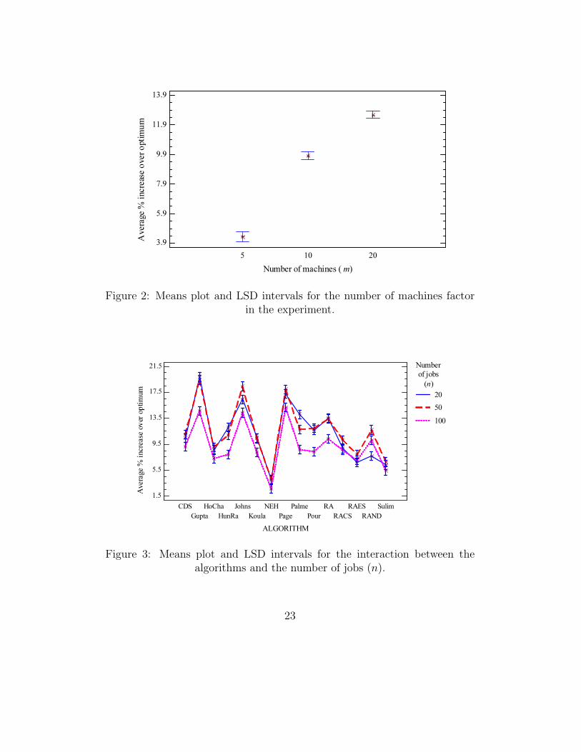
see the effect that the number of machines has over all algorithms. As we can

see, more machines lead to worse results, meaning that generally, instances

with 20 machines are harder than instances with only five or 10 machines.

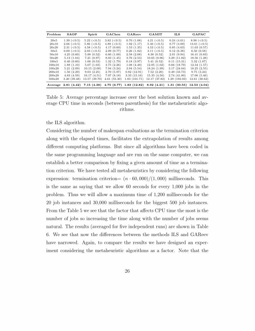
No clear trend was observed for the factor n. There are, however, some inter-

esting interactions, such as the one concerning the different algorithms and

n that is shown in Figure 3. It can be observed that the NEH heuristic per-

forms very well regardless of the number of jobs involved. Some algorithms,

such as HoCha, CDS or Sulim are robust and show a statistically similar

performance no matter how many jobs, whereas Johnson’s rule or Palmer’s

heuristic are sensitive to the number of jobs. The situation is very similar

for the interaction between the number of machines (m) and the different

22

Number of machines (m)

Avera

ge %

increa

se ov

er op

timum

5 10 203.9

5.9

7.9

9.9

11.9

13.9

Figure 2: Means plot and LSD intervals for the number of machines factorin the experiment.

ALGORITHM

Avera

ge %

increa

se ov

er op

timum

Numberof jobs

(n)2050100

1.5

5.5

9.5

13.5

17.5

21.5

CDSGupta

HoChaHunRa

JohnsKoula

NEHPage

PalmePour

RARACS

RAESRAND

Sulim

Figure 3: Means plot and LSD intervals for the interaction between thealgorithms and the number of jobs (n).

23

algorithms, where the best results for the different methods are obtained in

the five machine instances. Finally, it is worth noting the interaction between

the factors (n) and (m), which is shown in Figure 4. It is clear that the most

Number of jobs ( n)

Avera

ge %

increa

se ov

er op

timum

Number ofmachines

(m)51020

2.5

4.5

6.5

8.5

10.5

12.5

14.5

16.5

20 50 100

Figure 4: Means plot and LSD intervals for the interaction between thenumber of jobs (n) and the number of machines (m).

difficult instances are those with 50 jobs and 20 machines and those with 100

jobs and 20 machines. As a matter of fact, these 20 instances are still open

and no optimal solution has been established so far.

It is also interesting to analyse the efficiency of the different heuristics when

evaluating the different instances. We have measured the time (in seconds)

that a given method needs in order to provide a solution. The results for the

classical heuristics are straightforward, the RAND, FCFS, SPT, LPT, John-

son, Page, Palmer, CDS, Gupta, RA and RACS heuristics all needed less

than 0.5 seconds on average for all problem sizes. For the remaining heuris-

tics, the times were similar for problem sizes up to 100x5. From that point,

the times needed for solving the instances started to increase (Table 4). We

can see that the RAES method is very fast, needing less than five seconds

on average but only for the biggest instances. The NEH and Hundal and

24

Problem RAND RAES NEH HunRa HoCha Koula Sulim Pour

100x5 0.58 <0.5 <0.5 <0.5 <0.5 <0.5 <0.5 0.86

100x10 1.08 <0.5 <0.5 <0.5 <0.5 <0.5 <0.5 1.54

100x20 2.02 <0.5 <0.5 <0.5 <0.5 0.70 <0.5 2.92

200x10 2.26 <0.5 <0.5 <0.5 <0.5 1.04 <0.5 13.81

200x20 4.50 <0.5 <0.5 <0.5 <0.5 4.52 <0.5 26.00

500x20 22.38 4.67 <0.5 <0.5 1.18 64.55 13.61 532.61

Average 2.95 <0.5 <0.5 <0.5 <0.5 5.93 1.20 48.20

Table 4: Average CPU time in seconds used by the different heuristics.

Rajgopal, as well as Ho and Chang are also very efficient. It is important to

note that the NEH heuristic has been implemented with the speed improve-

ment suggested by Taillard (1990), otherwise, the classical NEH without this

improvement, is very slow and almost impracticable for large instances. The

most recent constructive and improvement heuristics, such as Koulamas’s

method take more than one minute in the 500x20 instances, whereas Suli-

man’s is faster with less than 20 seconds.

Davoud Pour’s heuristic times grow exponentially with the size of the prob-

lem considered, reaching almost nine minutes on average for the biggest in-

stances. This is due to the extensive work needed in each iteration. We think

these time requirements are unbearable, especially considering this method’s

low performance. In this situation it is much better to use the simple RAND

method, which needs little more than 20 seconds to evaluate 50,000 ran-

dom makespans and the solution obtained is of the same quality as that of

Davoud Pour’s heuristic.

Now we are going to analyse the effectiveness and efficiency of the differ-

ent metaheuristics reviewed. The results for the metaheuristics can be seen

in Table 5. The first conclusion that could be drawn is that the ILS and

GAReev methods are the most effective and the GA of Ponnambalam et al.

(GAPAC) the least. However, the CPU times range from little more than

four seconds on average for the Spirit method to more than half a minute for

25

Problem SAOP Spirit GAChen GAReev GAMIT ILS GAPAC

20x5 1.39 (<0.5) 5.22 (<0.5) 3.82 (<0.5) 0.70 (1.08) 4.21 (<0.5) 0.24 (4.01) 8.98 (<0.5)20x10 2.66 (<0.5) 5.86 (<0.5) 4.89 (<0.5) 1.92 (1.17) 5.40 (<0.5) 0.77 (4.09) 13.61 (<0.5)20x20 2.31 (<0.5) 4.58 (<0.5) 4.17 (0.60) 1.53 (1.35) 4.53 (<0.5) 0.85 (4.63) 11.03 (0.57)50x5 0.69 (<0.5) 2.03 (<0.5) 2.09 (0.77) 0.26 (1.82) 3.11 (<0.5) 0.12 (6.38) 6.50 (0.58)50x10 4.25 (0.60) 5.88 (0.52) 6.60 (1.00) 2.58 (2.08) 8.38 (0.52) 2.01 (9.94) 16.41 (0.83)50x20 5.13 (1.04) 7.21 (0.97) 8.03 (1.45) 3.76 (2.53) 10.65 (0.96) 3.29 (11.82) 18.56 (1.28)100x5 0.40 (0.60) 1.06 (0.53) 1.32 (1.79) 0.18 (3.97) 5.41 (0.52) 0.11 (15.31) 5.32 (1.07)100x10 1.88 (1.10) 5.07 (1.03) 3.75 (2.26) 1.08 (4.49) 12.05 (1.02) 0.66 (18.79) 12.34 (1.57)100x20 5.21 (2.09) 10.15 (2.00) 7.94 (3.24) 3.94 (5.54) 18.24 (1.99) 3.17 (24.04) 18.25 (2.55)200x10 1.56 (2.29) 9.03 (2.25) 2.70 (5.97) 0.82 (12.91) 7.52 (2.20) 0.49 (33.73) 9.75 (3.24)200x20 4.83 (4.59) 16.17 (4.51) 7.07 (8.18) 3.33 (15.16) 15.35 (4.50) 2.74 (41.80) 17.06 (5.46)500x20 3.40 (39.48) 13.57 (39.70) 4.61 (55.30) 1.83 (101.71) 12.17 (37.82) 1.29 (192.03) 12.61 (30.62)

Average 2.81 (4.42) 7.15 (4.38) 4.75 (6.77) 1.83 (12.82) 8.92 (4.21) 1.31 (30.55) 12.53 (4.04)

Table 5: Average percentage increase over the best solution known and av-erage CPU time in seconds (between parenthesis) for the metaheuristic algo-

rithms.

the ILS algorithm.

Considering the number of makespan evaluations as the termination criterion

along with the elapsed times, facilitates the extrapolation of results among

different computing platforms. But since all algorithms have been coded in

the same programming language and are run on the same computer, we can

establish a better comparison by fixing a given amount of time as a termina-

tion criterion. We have tested all metaheuristics by considering the following

expression: termination criterion= (n · 60, 000)/(1, 000) milliseconds. This

is the same as saying that we allow 60 seconds for every 1,000 jobs in the

problem. Thus we will allow a maximum time of 1,200 milliseconds for the

20 job instances and 30,000 milliseconds for the biggest 500 job instances.

From the Table 5 we see that the factor that affects CPU time the most is the

number of jobs so increasing the time along with the number of jobs seems

natural. The results (averaged for five independent runs) are shown in Table

6. We see that now the differences between the methods ILS and GAReev

have narrowed. Again, to compare the results we have designed an exper-

iment considering the metaheuristic algorithms as a factor. Note that the

26

Problem SAOP Spirit GAChen GAReev GAMIT ILS GAPAC

20x5 1.47 2.14 3.67 0.71 3.28 0.29 8.26

20x10 2.57 3.09 5.03 1.97 5.53 1.26 12.88

20x20 2.22 2.99 4.02 1.48 4.33 1.04 10.62

50x5 0.52 0.57 2.31 0.23 1.96 0.12 7.19

50x10 3.65 4.08 6.65 2.47 6.25 2.38 16.53

50x20 4.97 4.78 7.92 3.89 7.53 4.19 18.84

100x5 0.42 0.32 1.18 0.18 1.33 0.12 5.21

100x10 1.73 1.69 3.91 1.06 3.66 0.85 12.38

100x20 4.90 4.49 7.82 3.84 9.70 3.92 17.88

200x10 1.33 0.95 2.70 0.85 6.47 0.54 9.94

200x20 4.40 3.85 7.01 3.47 14.56 3.34 16.83

500x20 3.48 2.17 5.62 1.98 12.47 1.82 12.67

Average 2.64 2.60 4.82 1.84 6.42 1.65 12.44

Table 6: Average percentage increase over the best solution known for themetaheuristic algorithms. Maximum elapsed time stopping criterion.

GAPAC algorithm gives very poor results and has been disregarded in the

experiment. Again, the ANOVA results indicate that there are statistically

significant differences between the algorithms considered, with the p-value

being almost zero. To evaluate which algorithms perform better than others

we focus on the means plot shown in Figure 5. We can see that there are

four clear homogeneous groups, (ILS, GAReev), (SAOP, Spirit), (GAChen)

and (GAMIT). The two best metaheuristics are the ILS and the GAReev

methods and the worst is the GAMIT algorithm. We consider the result of

the GAMIT algorithm rather poor as it is a complex hybrid algorithm. Also,

it is worthwhile to note that the GAPAC’s effectiveness is even lower than

the much more simplistic RAND rule. This conclusion is different to that of

the authors’, who claimed their algorithm to be better than the NEH or the

CDS heuristics. This is clearly not the case for the benchmarks and evalu-

ations shown here. SAOP and Spirit’s effectiveness is very similar although

the implementation of the SAOP method is much simpler. Finally, we think

that the ILS method compares better since, even though it is similar to the

GAReev in terms of effectiveness, it is very simple to code, and it is much

simpler than a Genetic Algorithm. Furthermore, the ILS algorithm can be

27

METAHEURISTIC

Avera

ge %

increa

se ov

er op

timum

GAChen GAMIT GAReev ILS SAOP Spirit1

2

3

4

5

6

7

Figure 5: Means plot and LSD intervals for the Metaheuristic factor in theexperiment.

coupled with a more powerful Local Search phase than the one used here. If

we analyse again the influence of the number of jobs (n) and number of ma-

chines (m) in the effectiveness of the different metaheuristics we find almost

identical results to those obtained when evaluating the heuristic methods.

For example, in Figure 6 we can observe the interaction between the differ-

ent metaheuristics and the number of jobs. As we can see, the profile of the

different algorithms is almost the same regardless of the number of jobs in

the instance, although there are some aspects worth noting. For example,

the SAOP algorithm is more adequate than the Spirit for instances with 20

jobs and the ILS algorithm is also better than the GAReev for the instances

with this same number of jobs.

28

METAHEURISTIC

Avera

ge %

incre

ase ov

er op

timum

Numberof jobs

(n)2050100

0.51

1.52

2.53

3.54

4.55

5.56

GAChen GAMIT GAReev ILS SAOP Spirit

Figure 6: Means plot and LSD intervals for the interaction between themetaheuristics and the number of jobs (n).

5 Conclusions

In this paper we have given an extensive review and evaluation of many

heuristics and metaheuristics for the permutation flow shop scheduling prob-

lem, also known as n/m/P/Fmax or as F/prmu/Cmax. A total of 25 al-

gorithms have been coded and tested against Taillard’s (1993) famous 120

instance benchmark.

As a conclusion, we can now say that Nawaz et al.’s (1983) algorithm (NEH)

is the best heuristic for Taillard’s benchmarks. The performance of this

heuristic, if implemented as in Taillard (1990) is outstanding, with CPU

times below 0.5 seconds even for the largest 500x20 instances.

From the metaheuristics tested, Stutzle’s (1998) Iterated Local Search (ILS)

method, and the genetic algorithm of Reeves are better than the other algo-

rithms evaluated.

We would like to point out that dispatching rules have shown a very poor

performance in Taillard’s benchmarks, worse even than a simplistic RAN-

29

DOM rule, by a significant margin. However, these rules are still used in

practice in professional software and by production managers in many indus-

trial sectors. More elaborated heuristics outperform dispatching rules to a

significant degree.

We have also shown that Tabu Search, Simulated Annealing and Genetic Al-

gorithms are good metaheuristics for this problem, although the latter type

needs a good initialisation of the population and/or problem domain knowl-

edge in order to achieve a good performance. This result leads to the same

conclusion reached by Murata et al. (1996).

Acknowledgments

This work is funded by the Polytechnic University of Valencia, Spain, under

an interdisciplinary project, and by the Spanish Department of Science and

Technology (research project ref. DPI2001-2715-C02-01).

The authors would like to thank the two anonymous referees for their in-

sightful comments in a previous version of this paper and also to the ACLE

office.

References

Ashour, S. (1970). An Experimental Investigation and Comparative Evalua-

tion of Flow-Shop Scheduling Techniques. Operations Research, 18(3):541–

549.

Baker, K. R. (1974). Introduction to Sequencing and Scheduling. John Wiley

& Sons, New York.

Ben-Daya, M. and Al-Fawzan, M. (1998). A tabu search approach for the

flow shop scheduling problem. European Journal of Operational Research,

109:88–95.

Bonney, M. and Gundry, S. (1976). Solutions to the Constrained Flowshop

Sequencing Problem. Operational Research Quarterly, 27(4):869–883.

30

Byung Park, Y., Pegden, C. D., and Enscore, E. E. (1984). A survey and

evaluation of static flowshop scheduling heuristics. International Journal

of Production Research, 22(1):127–141.

Campbell, H. G., Dudek, R. A., and Smith, M. L. (1970). A Heuristic

Algorithm for the n Job, m Machine Sequencing Problem. Management

Science, 16(10):B630–B637.

Chen, C.-L., Vempati, V. S., and Aljaber, N. (1995). An application of ge-

netic algorithms for flow shop problems. European Journal of Operational

Research, 80:389–396.

Conway, R. W., Maxwell, W. L., and Miller, L. W. (1967). Theory of Schedul-

ing. Addison-Wesley, Reading, MA.

Dannenbring, D. G. (1977). An Evaluation of Flow Shop Sequencing Heuris-

tics. Management Science, 23(11):1174–1182.

Davoud Pour, H. (2001). A new heuristic for the n-job, m-machine flow-shop

problem. Production Planning and Control, 12(7):648–653.

Dudek, R. A., Panwalkar, S. S., and Smith, M. L. (1992). The Lessons of

Flowshop Scheduling Research. Operations Research, 40(1):7–13.

Dudek, R. A. and Teuton, Jr, O. F. (1964). Development of m-Stage decision

Rule for Scheduling n Jobs Through m Machines. Operations Research,

12(3):471–497.

Framinan, J. M., Leisten, R., and Rajendran, C. (2003). Different ini-

tial sequences for the heuristic of Nawaz, Enscore and Ham to minimize

makespan, idletime or flowtime in the static permutation flowshop sequenc-

ing problem. International Journal of Production Research, 41(1):121–148.

Garey, M., Johnson, D., and Sethi, R. (1976). The Complexity of Flowshop

and Jobshop Scheduling. Mathematics of Operations Research, 1(2):117–

129.

Graham, R., Lawler, E., Lenstra, J., and Rinnooy Kan, A. (1979). Opti-

mization and Approximation in Deterministic Sequencing and Scheduling:

A Survey. Annals of Discrete Mathematics, 5:287–326.

Gupta, J. N. (1971). A Functional Heuristic Algorithm for the Flowshop

Scheduling Problem. Operational Research Quarterly, 22(1):39–47.

Gupta, J. N. D. (1972). Heuristic Algorithms for Multistage Flowshop

31

Scheduling Problem. AIIE Transactions, 4(1):11–18.

Ho, J. C. and Chang, Y.-L. (1991). A new heuristic for the n-job, M-machine

flow-shop problem. European Journal of Operational Research, 52:194–202.

Hundal, T. S. and Rajgopal, J. (1988). An Extension of Palmer’s Heuristic for

the Flow Shop Scheduling Problem. International Journal of Production

Research, 26(6):1119–1124.

Ishibuchi, H., Misaki, S., and Tanaka, H. (1995). Modified simulated anneal-

ing algorithms for the flow shop sequencing problem. European Journal of

Operational Research, 81:388–398.

Johnson, S. (1954). Optimal Two- and Three-Stage Production Schedules

with Setup Times Included. Naval Research Logistics Quarterly, 1:61.

King, J. R. and Spachis, A. S. (1980). Heuristics for flow-shop scheduling.

International Journal of Production Research, 18(3):345–357.

Koulamas, C. (1998). A new constructive heuristic for the flowshop schedul-

ing problem. European Journal of Operational Research, 105:66–71.

Moccellin, J. a. V. (1995). A New Heuristic Method for the Permutation Flow

Shop Scheduling Problem. Journal of the Operational Research Society,

46:883–886.

Moccellin, J. a. V. and dos Santos, M. O. (2000). An adaptive hybrid meta-

heuristic for permutation flowshop scheduling. Control and Cybernetics,

29(3):761–771.

Montgomery, D. C. (2000). Design and Analysis of Experiments. John Wiley

& Sons, fifth edition.

Murata, T., Ishibuchi, H., and Tanaka, H. (1996). Genetic algorithms

for flowshop scheduling problems. Computers & Industrial Engineering,

30(4):1061–1071.

Nawaz, M., Enscore, Jr, E. E., and Ham, I. (1983). A Heuristic Algorithm

for the m-Machine, n-Job Flow-shop Sequencing Problem. OMEGA, The

International Journal of Management Science, 11(1):91–95.

Nowicki, E. and Smutnicki, C. (1996). A fast tabu search algorithm for

the permutation flow-shop problem. European Journal of Operational Re-

search, 91:160–175.

Ogbu, F. and Smith, D. (1990a). The application of the simulated annealing

32

algorithms to the solution of the n/m/Cmax flowshop problem. Computers

& Operations Research, 17(3):243–253.

Ogbu, F. and Smith, D. (1990b). Simulated Annealing for the Permutation

Flowshop Problem. OMEGA, The International Journal of Management

Science, 19(1):64–67.

Osman, I. and Potts, C. (1989). Simulated Annealing for Permutation Flow-

Shop Scheduling. OMEGA, The international Journal of Management

Science, 17(6):551–557.

Page, E. S. (1961). An Approach to the Scheduling of Jobs on Machines.

Journal of the Royal Statistical Society, B Series, 23(2):484–492.

Palmer, D. (1965). Sequencing Jobs through a Multi-Stage Process in the

Minimum Total Time - A Quick Method of Obtaining a Near Optimum.

Operational Research Quarterly, 16(1):101–107.

Pinedo, M. (2002). Scheduling: Theory, Algorithms and Systems. Prentice

Hall, New Jersey, second edition.

Ponnambalam, S. G., Aravindan, P., and Chandrasekaran, S. (2001). Con-

structive and improvement flow shop scheduling heuristics: an extensive

evaluation. Production Planning and Control, 12(4):335–344.

Potts, C. N., Shmoys, D. B., and Williamson, D. P. (1991). Permutation

vs. non-permutation flow shop schedules. Operations Research Letters,

10:281–284.

Reeves, C. and Yamada, T. (1998). Genetic Algorithms, Path Relinking, and

the Flowshop Sequencing Problem. Evolutionary Computation, 6(1):45–60.

Reeves, C. R. (1993). Improving the Efficiency of Tabu Search for Ma-

chine Scheduling Problems. Journal of the Operational Research Society,

44(4):375–382.

Reeves, C. R. (1995). A Genetic Algorithm for Flowshop Sequencing. Com-

puters & Operations Research, 22(1):5–13.

Reisman, A., Kumar, A., and Motwani, J. (1994). Flowshop Schedul-

ing/Sequencing Research: A Statistical Reeview of the Literature, 1952-

1994. IEEE Transactions on Engineering Management, 44(3):316–329.

Sarin, S. and Lefoka, M. (1993). Scheduling Heuristic for the n-Job m-

Machine Flow Shop. OMEGA, The International Journal of Management

33

Science, 21(2):229–234.

Stinson, J. P. and Smith, A. W. (1982). A heuristic programming procedure

for sequencing the static flowshop. International Journal of Production

Research, 20(6):753–764.

Stutzle, T. (1998). Applying Iterated Local Search to the Permutation Flow

Shop Problem. Technical report, AIDA-98-04, FG Intellektik,TU Darm-

stadt.

Suliman, S. (2000). A two-phase heuristic approach to the permutation flow-

shop scheduling problem. International Journal of production economics,

64:143–152.

Taillard, E. (1990). Some efficient heuristic methods for the flow shop se-

quencing problem. European Journal of Operational Research, 47:67–74.

Taillard, E. (1993). Benchmarks for basic scheduling problems. European

Journal of Operational Research, 64:278–285.

Turner, S. and Booth, D. (1987). Comparison of Heuristics for Flow Shop

Sequencing. OMEGA, The International Journal of Management Science,

15(1):75–78.

Wang, L. and Zheng, D. Z. (2003). An Effective Hybrid Heuristic for Flow

Shop Scheduling. The International Journal of Advanced Manufacturing

Technology, 21:38–44.

Werner, F. (1993). On the heuristic solution of the permutation flow

shop problem by path algorithms. Computers & Operations Research,

20(7):707–722.

Widmer, M. and Hertz, A. (1989). A new heuristic method for the flow shop

sequencing problem. European Journal of Operational Research, 41:186–

193.

Wodecki, M. and Bozejko, W. (2002). Solving the Flow Shop Problem by Par-

allel Simulated Annealing. In Wyrzykowski, R., Dongarra, J., Paprzycki,

M., and Wasniewski, J., editors, Parallel Processing and Applied Mathe-

matics, 4th International Conference, PPAM 2001, volume 2328 of Lecture

Notes in Computer Science, pages 236–244. Springer-Verlag.

Zegordi, S. H., Itoh, K., and Enkawa, T. (1995). Minimizing makespan for

flowshop scheduling by combining simulated annealing with sequencing

knowledge. European Journal of Operational Research, 85:515–531.

34