PERMUTATION FLOW-SHOP SCHEDULING USING A GENETIC ...
134
PERMUTATION FLOW-SHOP SCHEDULING USING A GENETIC ALGORITHM-BASED ITERATIVE METHOD A Thesis Submitted to the Faculty of Graduate Studies and Research In Partial Fulfillment of the Requirements for the Degree of Master of Applied Science in Industrial Systems Engineering University of Regina by Mandi Eskenasi Regina, Saskatchewan July, 2006 Copyright 2006: Mandi Eskenasi Reproduced with permission of the copyright owner. Further reproduction prohibited without permission. PERMUTATION FLOW-SHOP SCHEDULING USING A GENETIC ALGORITHM-BASED ITERATIVE METHOD A Thesis Submitted to the Faculty of Graduate Studies and Research In Partial Fulfillment of the Requirements for the Degree of Master of Applied Science in Industrial Systems Engineering University of Regina by Mahdi Eskenasi Regina, Saskatchewan July, 2006 Copyright 2006: Mahdi Eskenasi Reproduced with permission of the copyright owner. Further reproduction prohibited without permission.
-
Upload
khangminh22 -
Category
Documents
-
view
4 -
download
0
Transcript of PERMUTATION FLOW-SHOP SCHEDULING USING A GENETIC ...
PERMUTATION FLOW-SHOP SCHEDULING USING
A GENETIC ALGORITHM-BASED ITERATIVE METHOD
A Thesis
Submitted to the Faculty of Graduate Studies and Research
In Partial Fulfillment of the Requirements
for the Degree of
Master of Applied Science in
Industrial Systems Engineering
University of Regina
by
Mandi Eskenasi
Regina, Saskatchewan
July, 2006
Copyright 2006: Mandi Eskenasi
Reproduced with permission of the copyright owner. Further reproduction prohibited without permission.
PERMUTATION FLOW-SHOP SCHEDULING USING
A GENETIC ALGORITHM-BASED ITERATIVE METHOD
A Thesis
Submitted to the Faculty o f Graduate Studies and Research
In Partial Fulfillment o f the Requirements
for the Degree o f
Master o f Applied Science in
Industrial Systems Engineering
University o f Regina
by
Mahdi Eskenasi
Regina, Saskatchewan
July, 2006
Copyright 2006: Mahdi Eskenasi
Reproduced with permission of the copyright owner. Further reproduction prohibited without permission.

1+1 Library and Bibliotheque et Archives Canada Archives Canada
Published Heritage Direction du Branch Patrimoine de redition
395 Wellington Street Ottawa ON KlA ON4 Canada
395, rue Wellington Ottawa ON KlA ON4 Canada
NOTICE: The author has granted a non-exclusive license allowing Library and Archives Canada to reproduce, publish, archive, preserve, conserve, communicate to the public by telecommunication or on the Internet, loan, distribute and sell theses worldwide, for commercial or non-commercial purposes, in microform, paper, electronic and/or any other formats.
The author retains copyright ownership and moral rights in this thesis. Neither the thesis nor substantial extracts from it may be printed or otherwise reproduced without the author's permission.
Your file Votre reference ISBN: 978-0-494-20208-1 Our file Notre reference ISBN: 978-0-494-20208-1
AVIS: L'auteur a accord& une licence non exclusive permettant a la Bibliotheque et Archives Canada de reproduire, publier, archiver, sauvegarder, conserver, transmettre au public par telecommunication ou par ('Internet, preter, distribuer et vendre des theses partout dans le monde, a des fins commerciales ou autres, sur support microforme, papier, electronique et/ou autres formats.
L'auteur conserve la propriete du droit d'auteur et des droits moraux qui protege cette these. Ni la these ni des extraits substantiels de celle-ci ne doivent etre imprimes ou autrement reproduits sans son autorisation.
In compliance with the Canadian Privacy Act some supporting forms may have been removed from this thesis.
While these forms may be included in the document page count, their removal does not represent any loss of content from the thesis.
1*1
Canada
Conformement a la loi canadienne sur la protection de la vie privee, quelques formulaires secondaires ont ete enleves de cette these.
Bien que ces formulaires aient inclus dans la pagination, it n'y aura aucun contenu manquant.
Reproduced with permission of the copyright owner. Further reproduction prohibited without permission.
Library and Archives Canada
Bibliotheque et Archives Canada
Published Heritage Branch
395 Wellington Street Ottawa ON K1A 0N4 Canada
Your file Votre reference ISBN: 978-0-494-20208-1 Our file Notre reference ISBN: 978-0-494-20208-1
Direction du Patrimoine de I'edition
395, rue Wellington Ottawa ON K1A 0N4 Canada
NOTICE:The author has granted a nonexclusive license allowing Library and Archives Canada to reproduce, publish, archive, preserve, conserve, communicate to the public by telecommunication or on the Internet, loan, distribute and sell theses worldwide, for commercial or noncommercial purposes, in microform, paper, electronic and/or any other formats.
AVIS:L'auteur a accorde une licence non exclusive permettant a la Bibliotheque et Archives Canada de reproduire, publier, archiver, sauvegarder, conserver, transmettre au public par telecommunication ou par I'lnternet, preter, distribuer et vendre des theses partout dans le monde, a des fins commerciales ou autres, sur support microforme, papier, electronique et/ou autres formats.
The author retains copyright ownership and moral rights in this thesis. Neither the thesis nor substantial extracts from it may be printed or otherwise reproduced without the author's permission.
L'auteur conserve la propriete du droit d'auteur et des droits moraux qui protege cette these.Ni la these ni des extraits substantiels de celle-ci ne doivent etre imprimes ou autrement reproduits sans son autorisation.
In compliance with the Canadian Privacy Act some supporting forms may have been removed from this thesis.
While these forms may be included in the document page count, their removal does not represent any loss of content from the thesis.
Conformement a la loi canadienne sur la protection de la vie privee, quelques formulaires secondaires ont ete enleves de cette these.
Bien que ces formulaires aient inclus dans la pagination, il n'y aura aucun contenu manquant.
i * i
CanadaReproduced with permission of the copyright owner. Further reproduction prohibited without permission.

UNIVERSITY OF REGINA
FACULTY OF GRADUATE STUDIES AND RESEARCH
SUPERVISORY AND EXAMINING COMMITTEE
Mandi Eskenasi, candidate for the degree of Master of Applied Science, has presented a thesis
titled, The Permutation Flow-Shop Scheduling Using a Genetic Algorithm-Based Iterative
Method, in an oral examination held on May 26, 2006. The following committee members
have found the thesis acceptable in form and content, and that the candidate demonstrated
satisfactory knowledge of the subject material.
External Examiner: Dr. Stephen O'Leary, Faculty of Engineering
Supervisor: Dr. Mehran Mehrandezh, Faculty of Engineering
Committee Member: Dr. Nader Mahinpey, Faculty of Engineering
Committee Member: Dr. Rene Mayorga, Faculty of Engineering
Chair of Defense: Dr. Wojciech Ziarko, Department of Computer Science
Reproduced with permission of the copyright owner. Further reproduction prohibited without permission.
UNIVERSITY OF REGINA
FACULTY OF GRADUATE STUDIES AND RESEARCH
SUPERVISORY AND EXAMINING COMMITTEE
Mahdi Eskenasi, candidate for the degree o f Master o f Applied Science, has presented a thesis
titled, The Permutation Flow-Shop Scheduling Using a Genetic Algorithm-Based Iterative
Method, in an oral examination held on May 26, 2006. The following committee members
have found the thesis acceptable in form and content, and that the candidate demonstrated
satisfactory knowledge o f the subject material.
External Examiner: Dr. Stephen O'Leary, Faculty o f Engineering
Supervisor: Dr. Mehran Mehrandezh, Faculty o f Engineering
Committee Member: Dr. Nader Mahinpey, Faculty o f Engineering
Committee Member: Dr. Rene Mayorga, Faculty o f Engineering
Chair o f Defense: Dr. Wojciech Ziarko, Department o f Computer Science
Reproduced with permission of the copyright owner. Further reproduction prohibited without permission.
ABSTRACT
The purpose of this research is to investigate one well-known type of scheduling
problem, the Permutation Flow-Shop Scheduling Problem, with the makespan as the
objective function to be minimized. During the last four decades, the permutation flow-
shop scheduling problem has received considerable attention. Various techniques,
ranging from the simple constructive algorithm to the state-of-the-art techniques, such as
Genetic Algorithms, have been proposed for this scheduling problem.
The development of a solution methodology based on genetic algorithms, yielding
(near) optimal makespans, has been investigated in this thesis. In order to improve the
performance of the search technique, the proposed genetic algorithm is hybridized with
an Iterated Greedy Search Algorithm.
The parameters of both the hybrid and the non-hybrid genetic algorithms were
tuned using the Full Factorial Experimental Design and Analysis of Variance. The
performance of the tuned hybrid and non-hybrid algorithms are finally examined on the
existing standard benchmark problems cited in the literature, and it is shown that the
proposed hybrid genetic algorithm performs well on those benchmark problems. In
addition, it is demonstrated that the hybrid proposed algorithm is robust with respect to
problem parameters, such as population size, crossover type, and crossover probability.
i
Reproduced with permission of the copyright owner. Further reproduction prohibited without permission.
A bst r a c t
The purpose o f this research is to investigate one well-known type o f scheduling
problem, the Permutation Flow-Shop Scheduling Problem, with the makespan as the
objective function to be minimized. During the last four decades, the permutation flow-
shop scheduling problem has received considerable attention. Various techniques,
ranging from the simple constructive algorithm to the state-of-the-art techniques, such as
Genetic Algorithms, have been proposed for this scheduling problem.
The development o f a solution methodology based on genetic algorithms, yielding
(near) optimal makespans, has been investigated in this thesis. In order to improve the
performance o f the search technique, the proposed genetic algorithm is hybridized with
an Iterated Greedy Search Algorithm.
The parameters o f both the hybrid and the non-hybrid genetic algorithms were
tuned using the Full Factorial Experimental Design and Analysis o f Variance. The
performance o f the tuned hybrid and non-hybrid algorithms are finally examined on the
existing standard benchmark problems cited in the literature, and it is shown that the
proposed hybrid genetic algorithm performs well on those benchmark problems. In
addition, it is demonstrated that the hybrid proposed algorithm is robust with respect to
problem parameters, such as population size, crossover type, and crossover probability.
i
Reproduced with permission of the copyright owner. Further reproduction prohibited without permission.

ACKNOWLEDGMENTS
I would like to extend my hearty appreciation to Dr. Mehran Mehrandezh for his
invaluable guidance in conducting the research reported in this thesis. I am indebted to
him for both his time and insights over the course of conducting this thesis.
I am very grateful to the Faculty of Graduate Studies and Research for their
financial support. In addition, the financial support provided through the John Spencer
Middleton and Jack Spencer Gordon Scholarship is greatly acknowledged.
The help provided by Mr. Shaahin Rushan on implementing my proposed
algorithm in Java is acknowledged.
ii
Reproduced with permission of the copyright owner. Further reproduction prohibited without permission.
A c k n o w l e d g m e n t s
I would like to extend my hearty appreciation to Dr. Mehran Mehrandezh for his
invaluable guidance in conducting the research reported in this thesis. I am indebted to
him for both his time and insights over the course o f conducting this thesis.
I am very grateful to the Faculty of Graduate Studies and Research for their
financial support. In addition, the financial support provided through the John Spencer
Middleton and Jack Spencer Gordon Scholarship is greatly acknowledged.
The help provided by Mr. Shaahin Rushan on implementing my proposed
algorithm in Java is acknowledged.
ii
Reproduced with permission of the copyright owner. Further reproduction prohibited without permission.

DEDICATION
This thesis is dedicated to my parents. Without their
devotion, support and above all love, the completion
of this work would not have been possible.
iii
Reproduced with permission of the copyright owner. Further reproduction prohibited without permission.
D ed ic a t io n
This thesis is dedicated to my parents. Without their
devotion, support and above all love, the completion
of this work would not have been possible.
iii
Reproduced with permission of the copyright owner. Further reproduction prohibited without permission.
TABLE OF CONTENTS
ABSTRACT I
ACKNOWLEDGMENTS II
DEDICATION III
TABLE OF CONTENTS IIV
LIST OF TABLES VI
LIST OF FIGURES VII
LIST OF APPENDICES VIII
LIST OF ACRONYMS IIX
CHAPTER 1: INTRODUCTION TO SCHEDULING 1
1.1 FLOW-SHOP SCHEDULING PROBLEM 1 1.2 RESEARCH OBJECTIVES 8 1.3 RESEARCH CONTRIBUTIONS 8
CHAPTER 2: REVIEW OF LITERATURE 10
2.1 JOHNSON'S ALGORITHM 12 2.2 THE ALGORITHM OF NAWAZ, ENSCORE AND HAM 13 2.3 TAILLARD'S ALGORITHM 15 2.4 TAILLARD'S BENCHMARK PROBLEMS 18
CHAPTER 3: GENETIC ALGORITHMS (AN OVERVIEW) AND THEIR APPLICATIONS IN THE PFSP 21
3.1 REPRESENTATION AND INITIAL POPULATION 25 3.2 EVALUATION 26 3.3 SELECTION 26
3.3.1 Roulette Wheel Selection 27 3.3.2 Rank-Based Selection 28 3.3.3 Tournament Selection 30 3.3.4 Elitist Selection 30
3.4 CROSSOVER OPERATORS 30 3.4.1 Longest Common Subsequence Crossover (LCSX) 32 3.4.2 Similar Block Order Crossover (SBOX) 34
3.5 MUTATION OPERATORS 35 3.5.1 Insertion Mutation (Shift Change Mutation) 37 3.5.2 Reciprocal Exchange Mutation (Swap Mutation) 36 3.5.3 Transpose Mutation 36 3.5.4 Inversion Mutation 37
CHAPTER 4: SOLUTION METHODOLOGY 39
4.1 THE STRUCTURE OF THE PROPOSED GA 39
iv
Reproduced with permission of the copyright owner. Further reproduction prohibited without permission.
Ta b l e o f C o n ten t s
ABSTRACT........................................................................................................................ I
ACKNOWLEDGMENTS............................................................................................... IIDEDICATION.................................................................................................................IllTABLE OF CONTENTS............................................................................................. IIVLIST OF TABLES..........................................................................................................VI
LIST OF FIGURES...................................................................................................... VIILIST OF APPENDICES.............................................................................................VIII
LIST OF ACRONYMS................................................................................................ IIXCHAPTER 1: INTRODUCTION TO SCHEDULING..................................................1
1.1 Flo w -S hop Sc h ed u lin g Pr o b l e m .............................................................................................. 11.2 Resea r c h O b je c t iv e s ....................................................................................................................... 81.3 Re se a r c h Co n t r ib u t io n s ................................................................................................................8
CHAPTER 2: REVIEW OF LITERATURE................................................................102.1 Jo h n s o n ’s A l g o r it h m .................................................................................................................... 122 .2 The A lgorithm of N a w a z , En sc o r e a n d H a m .................................................................132.3 Ta il l a r d ’s A lg o r ith m ...................................................................................................................152 .4 Ta il l a r d ’s B en c h m a r k Pr o bl em s ...........................................................................................18
CHAPTER 3: GENETIC ALGORITHMS (AN OVERVIEW) AND THEIR APPLICATIONS IN THE PFSP....................................................................................21
3.1 Repr esen ta tio n a n d Initia l Po p u l a t io n ............................................................................253 .2 Ev a l u a t io n ......................................................................................................................................... 263.3 S el e c t io n .............................................................................................................................................. 26
3.3.1 Roulette Wheel Selection..........................................................................................273.3.2 Rank-Based Selection............................................................................................... 283.3.3 Tournament Selection.............................................................................................. 303.3.4 Elitist Selection ......................................................................................................... 30
3.4 C r o sso v e r O p e r a t o r s .................................................................................................................. 303.4.1 Longest Common Subsequence Crossover (LCSX)............................................. 323.4.2 Similar Block Order Crossover (SBOX)................................................................34
3.5 M u t a t io n Op e r a t o r s .....................................................................................................................353.5.1 Insertion Mutation (Shift Change M utation)........................................................ 373.5.2 Reciprocal Exchange Mutation (Swap Mutation).................................................363.5.3 Transpose M utation ..................................................................................................363.5.4 Inversion Mutation....................................................................................................37
CHAPTER 4: SOLUTION METHODOLOGY.......................................................... 394.1 T he Str u c tu r e of the Pro po sed G A .................................................................................. 39
iv
Reproduced with permission of the copyright owner. Further reproduction prohibited without permission.
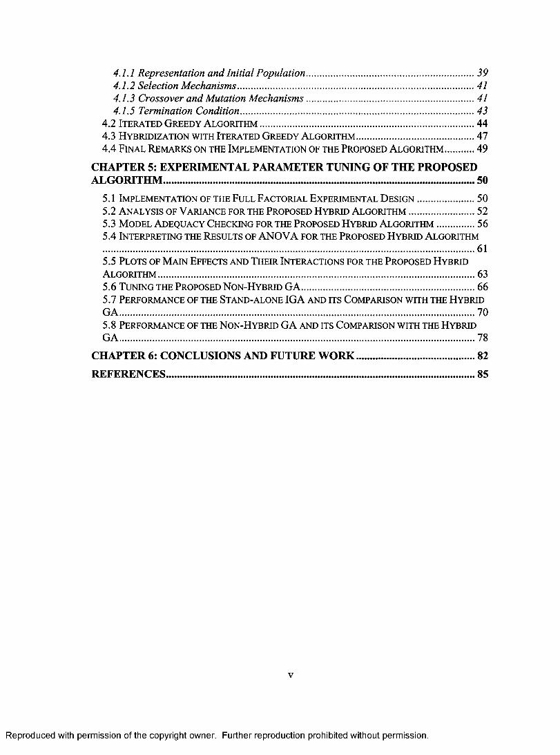
4.1.1 Representation and Initial Population 39 4.1.2 Selection Mechanisms 41 4.1.3 Crossover and Mutation Mechanisms 41 4.1.5 Termination Condition 43
4.2 ITERATED GREEDY ALGORITHM 44 4.3 HYBRIDIZATION WITH ITERATED GREEDY ALGORITHM 47 4.4 FINAL REMARKS ON THE IMPLEMENTATION OF THE PROPOSED ALGORITHM 49
CHAPTER 5: EXPERIMENTAL PARAMETER TUNING OF THE PROPOSED ALGORITHM 50
5.1 IMPLEMENTATION OF THE FULL FACTORIAL EXPERIMENTAL DESIGN 50 5.2 ANALYSIS OF VARIANCE FOR THE PROPOSED HYBRID ALGORITHM 52 5.3 MODEL ADEQUACY CHECKING FOR THE PROPOSED HYBRID ALGORITHM 56 5.4 INTERPRETING THE RESULTS OF ANOVA FOR THE PROPOSED HYBRID ALGORITHM 61 5.5 PLOTS OF MAIN EFFECTS AND THEIR INTERACTIONS FOR THE PROPOSED HYBRID ALGORITHM 63 5.6 TUNING THE PROPOSED NON-HYBRID GA 66 5.7 PERFORMANCE OF THE STAND-ALONE IGA AND ITS COMPARISON WITH THE HYBRID GA 70 5.8 PERFORMANCE OF THE NON-HYBRID GA AND ITS COMPARISON WITH THE HYBRID GA 78
CHAPTER 6: CONCLUSIONS AND FUTURE WORK 82
REFERENCES 85
v
Reproduced with permission of the copyright owner. Further reproduction prohibited without permission.
4.1.1 Representation and Initial Population................................................................... 394.1.2 Selection Mechanisms.............................................................................................. 414.1.3 Crossover and Mutation M echanisms................................................................... 414.1.5 Termination Condition........................................................................................... 43
4.2 Ite r a t ed G r ee d y A l g o r it h m .................................................................................................... 444.3 Hy b r id iza t io n w ith Iter ated G r ee d y A lg o r ith m ....................................................... 474 .4 Fin a l Rem a r k s o n the Im plem en ta tio n of the Pr o po sed A lg o r it h m 49
CHAPTER 5: EXPERIMENTAL PARAMETER TUNING OF THE PROPOSED ALGORITHM................................................................................................................. 50
5.1 Im plem en ta tio n of the Fu ll Facto rial Ex per im en ta l D e s ig n ........................... 505.2 A n a l y sis of V a r ia n c e for the Pro po sed H y b r id A l g o r it h m ............................... 525.3 M o d el A d e q u a c y Check ing for the Pr o po sed H y b r id A l g o r it h m .................. 565.4 In terpr etin g the Re su l t s of A N O V A for the Pr o po sed H y b r id A lgorithm 615.5 Plo ts of M a in E ffects a n d T heir In te r a c tio n s for the Pr o po sed H y br id A l g o r ith m ....................................................................................................................................................635 .6 Tu n in g the Pr o po sed N o n -H y br id G A ................................................................................. 665.7 Per fo r m a n c e of the St a n d -a lo n e IG A a n d its Co m pa r iso n w ith the Hy br id G A ..................................................................................................................................................................... 705.8 Per fo r m a n c e of the N o n -H y b r id G A a n d its C o m pa r iso n w ith the H y br id G A ..................................................................................................................................................................... 78
CHAPTER 6: CONCLUSIONS AND FUTURE WORK............................................82REFERENCES.................................................................................................................85
v
Reproduced with permission of the copyright owner. Further reproduction prohibited without permission.
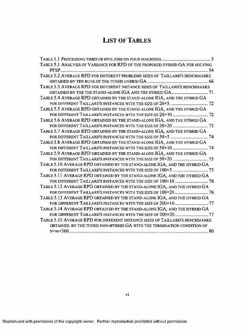
LIST OF TABLES
TABLE 1.1 PROCESSING TIMES OF FIVE JOBS ON FOUR MACHINES. 5 TABLE 5.1 ANALYSIS OF VARIANCE FOR RPD OF THE PROPOSED HYBRID GA FOR SOLVING
PFSP 54 TABLE 5.2 AVERAGE RPD FOR DIFFERENT PROBLEMS SIZES OF TAILLARD'S BENCHMARKS
OBTAINED BY TEN RUNS OF THE TUNED HYBRID GA 66 TABLE 5.3 AVERAGE RPD FOR DIFFERENT INSTANCE SIZES OF TAILLARD'S BENCHMARKS
OBTAINED BY THE THE STAND-ALONE IGA AND THE HYBRID GA 71 TABLE 5.4 AVERAGE RPD OBTAINED BY THE STAND-ALONE IGA, AND THE HYBRID GA
FOR DIFFERENT TAILLARD'S INSTANCES WITH THE SIZE OF 20x5. 72 TABLE 5.5 AVERAGE RPD OBTAINED BY THE STAND-ALONE IGA, AND THE HYBRID GA
FOR DIFFERENT TAILLARD'S INSTANCES WITH THE SIZE OF 20x 10 72 TABLE 5.6 AVERAGE RPD OBTAINED BY THE STAND-ALONE IGA, AND THE HYBRID GA
FOR DIFFERENT TAILLARD'S INSTANCES WITH THE SIZE OF 20x20 73 TABLE 5.7 AVERAGE RPD OBTAINED BY THE STAND-ALONE IGA, AND THE HYBRID GA
FOR DIFFERENT TAILLARD'S INSTANCES WITH THE SIZE OF 50x5 74 TABLE 5.8 AVERAGE RPD OBTAINED BY THE STAND-ALONE IGA, AND THE HYBRID GA
FOR DIFFERENT TAILLARD'S INSTANCES WITH THE SIZE OF 50x 10 74 TABLE 5.9 AVERAGE RPD OBTAINED BY THE STAND-ALONE IGA, AND THE HYBRID GA
FOR DIFFERENT TAILLARD'S INSTANCES WITH THE SIZE OF 50x20 75 TABLE 5.10 AVERAGE RPD OBTAINED BY THE STAND-ALONE IGA, AND THE HYBRID GA
FOR DIFFERENT TAILLARD'S INSTANCES WITH THE SIZE OF 100x5 75 TABLE 5.11 AVERAGE RPD OBTAINED BY THE STAND-ALONE IGA, AND THE HYBRID GA
FOR DIFFERENT TAILLARD'S INSTANCES WITH THE SIZE OF 100x 10 76 TABLE 5.12 AVERAGE RPD OBTAINED BY THE STAND-ALONE IGA, AND THE HYBRID GA
FOR DIFFERENT TAILLARD'S INSTANCES WITH THE SIZE OF 100x20 76 TABLE 5.13 AVERAGE RPD OBTAINED BY THE STAND-ALONE IGA, AND THE HYBRID GA
FOR DIFFERENT TAILLARD'S INSTANCES WITH THE SIZE OF 200x 10 77 TABLE 5.14 AVERAGE RPD OBTAINED BY THE STAND-ALONE IGA, AND THE HYBRID GA
FOR DIFFERENT TAILLARD'S INSTANCES WITH THE SIZE OF 200x20 77 TABLE 5.15 AVERAGE RPD FOR DIFFERENT INSTANCE SIZES OF TAILLARD'S BENCHMARKS
OBTAINED BY THE TUNED NON-HYBRID GA WITH THE TERMINATION CONDITION OF NxMx360 80
vi
Reproduced with permission of the copyright owner. Further reproduction prohibited without permission.
L ist o f Ta b l e s
Ta ble 1.1 Pr o c essin g tim es of five jobs o n fo u r m a c h in e s .....................................................5T a ble 5.1 A n a l y sis of V a r ia n c e for RPD of the pro po sed h y b r id G A for so lv in g
PF SP .............................................................................................................................................................54Ta b l e 5 .2 A v er a g e R PD for different problem s sizes of Ta il l a r d 's ben c h m a r k s
OBTAINED BY TEN RUNS OF THE TUNED HYBRID G A .................................................................66T a ble 5.3 A v er a g e R PD for different in st a n c e sizes of Ta il l a r d 's be n c h m a r k s
OBTAINED BY THE THE STAND-ALONE IG A AND THE HYBRID G A .......................................71Ta b l e 5 .4 A v er a g e RPD o b ta in ed b y the s t a n d -a lo n e IG A, a n d the h y br id G A
FOR DIFFERENT TAILLARD'S INSTANCES WITH THE SIZE OF 2 0 x 5 ......................................... 72Ta b l e 5.5 A v er a g e R PD o b ta in ed b y the s t a n d -a lo n e IG A, a n d the h y br id G A
FOR DIFFERENT TAILLARD'S INSTANCES WITH THE SIZE OF 2 0 x 1 0 ......................................72Ta ble 5 .6 A v er a g e RPD o b ta in ed b y the s t a n d -a lo n e IG A, a n d th e h y br id G A
FOR DIFFERENT TAILLARD'S INSTANCES WITH THE SIZE OF 2 0 x 2 0 ......................................73Ta b l e 5 .7 A v er a g e RPD o b ta in ed b y the s t a n d -a lo n e IG A, a n d th e h y br id G A
FOR DIFFERENT TAILLARD'S INSTANCES WITH THE SIZE OF 5 0 x 5 ........................................ 74Ta b l e 5 .8 A v er a g e RPD o b ta in ed b y the s t a n d -a lo n e IG A, a n d the h y br id G A
FOR DIFFERENT TAILLARD'S INSTANCES WITH THE SIZE OF 5 0x 1 0 ......................................74Ta b l e 5 .9 A v er a g e RPD o b ta in ed b y the s t a n d -a lo n e IG A, a n d the h y br id G A
FOR DIFFERENT TAILLARD'S INSTANCES WITH THE SIZE OF 5 0 x 2 0 ......................................75Ta ble 5 .10 A v er a g e RPD o b ta in ed b y the s t a n d -a l o n e IG A, a n d the h y b r id G A
FOR DIFFERENT TAILLARD'S INSTANCES WITH THE SIZE OF 1 0 0 x 5 ......................................75Ta b l e 5.11 A v er a g e R PD o b ta in ed b y the s t a n d -a l o n e IG A, a n d the h y br id G A
FOR DIFFERENT TAILLARD'S INSTANCES WITH THE SIZE OF 100x 1 0 ................................... 76Ta b l e 5 .12 A v er a g e R PD o b ta in ed b y the s t a n d -a lo n e IG A , a n d the h y br id G A
FOR DIFFERENT TAILLARD'S INSTANCES WITH THE SIZE OF 1 0 0 x 2 0 ................................... 76Ta ble 5 .13 A v er a g e R PD o b ta in ed b y the s t a n d -a lo n e IG A , a n d the h y br id G A
for d ifferent Ta ill a r d 's in st a n c e s w ith the SIZE OF 2 0 0 X1 0 ................................... 77Ta b l e 5 .14 A v er a g e R PD o b ta in ed b y the s t a n d -a l o n e IG A , a n d the h y br id G A
FOR DIFFERENT TAILLARD'S INSTANCES WITH THE SIZE OF 2 0 0 x 2 0 ................................... 77Ta b l e 5 .15 A v er a g e R PD for d ifferent in st a n c e sizes of Ta il l a r d 's be n c h m a r k s
OBTAINED BY THE TUNED NON-HYBRID G A WITH THE TERMINATION CONDITION OF NXMX360....................................................................................................................................................80
vi
Reproduced with permission of the copyright owner. Further reproduction prohibited without permission.
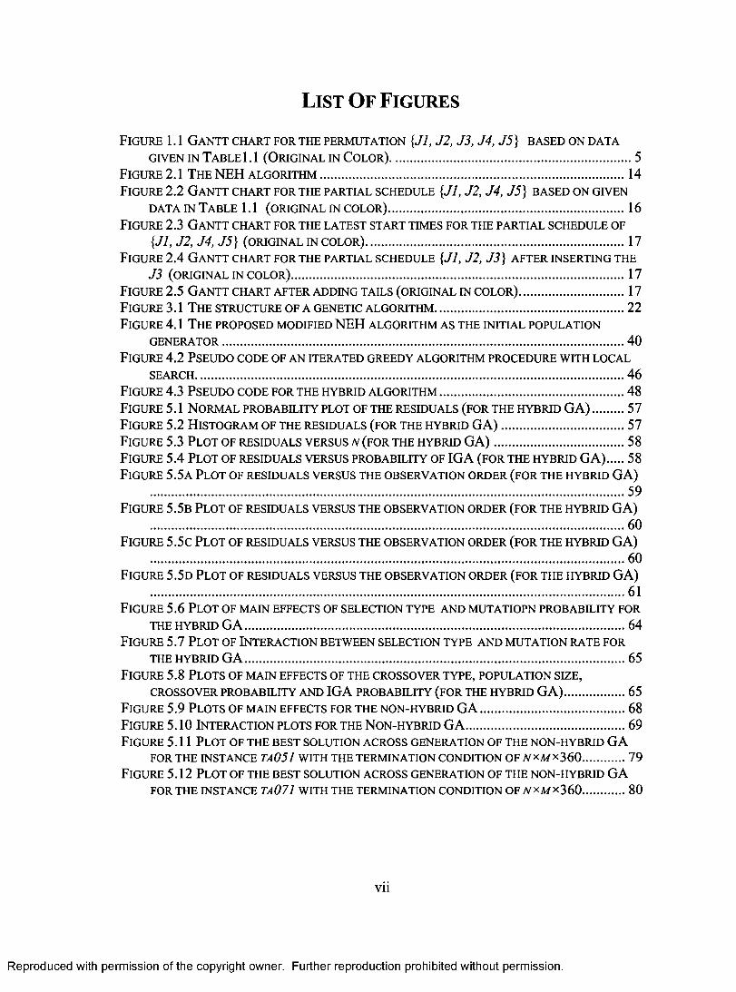
LIST OF FIGURES
FIGURE 1.1 GANTT CHART FOR THE PERMUTATION {J1, J2, J3, J4, J5} BASED ON DATA GIVEN IN TABLE1.1 (ORIGINAL IN COLOR). 5
FIGURE 2.1 THE NEH ALGORITHM 14 FIGURE 2.2 GANTT CHART FOR THE PARTIAL SCHEDULE {J1, J2, J4, J.5} BASED ON GIVEN
DATA IN TABLE 1.1 (ORIGINAL IN COLOR) 16 FIGURE 2.3 GANTT CHART FOR THE LATEST START TIMES FOR THE PARTIAL SCHEDULE OF
{J1, J2, J4, J.5} (ORIGINAL IN COLOR). 17 FIGURE 2.4 GANTT CHART FOR THE PARTIAL SCHEDULE {J1, J2, J3} AFTER INSERTING THE
J3 (ORIGINAL IN COLOR) 17 FIGURE 2.5 GANTT CHART AFTER ADDING TAILS (ORIGINAL IN COLOR) 17 FIGURE 3.1 THE STRUCTURE OF A GENETIC ALGORITHM. 22 FIGURE 4.1 THE PROPOSED MODIFIED NEH ALGORITHM AS THE INITIAL POPULATION
GENERATOR 40 FIGURE 4.2 PSEUDO CODE OF AN ITERATED GREEDY ALGORITHM PROCEDURE WITH LOCAL
SEARCH. 46 FIGURE 4.3 PSEUDO CODE FOR THE HYBRID ALGORITHM 48 FIGURE 5.1 NORMAL PROBABILITY PLOT OF THE RESIDUALS (FOR THE HYBRID GA) 57 FIGURE 5.2 HISTOGRAM OF THE RESIDUALS (FOR THE HYBRID GA) 57 FIGURE 5.3 PLOT OF RESIDUALS VERSUS N (FOR THE HYBRID GA) 58 FIGURE 5.4 PLOT OF RESIDUALS VERSUS PROBABILITY OF IGA (FOR THE HYBRID GA) 58 FIGURE 5.5A PLOT OF RESIDUALS VERSUS THE OBSERVATION ORDER (FOR THE HYBRID GA)
59 FIGURE 5.5B PLOT OF RESIDUALS VERSUS THE OBSERVATION ORDER (FOR THE HYBRID GA)
60 FIGURE 5.5C PLOT OF RESIDUALS VERSUS THE OBSERVATION ORDER (FOR THE HYBRID GA)
60 FIGURE 5.5D PLOT OF RESIDUALS VERSUS THE OBSERVATION ORDER (FOR THE HYBRID GA)
61 FIGURE 5.6 PLOT OF MAIN EFFECTS OF SELECTION TYPE AND MUTATIOPN PROBABILITY FOR
THE HYBRID GA 64 FIGURE 5.7 PLOT OF INTERACTION BETWEEN SELECTION TYPE AND MUTATION RATE FOR
THE HYBRID GA 65 FIGURE 5.8 PLOTS OF MAIN EFFECTS OF THE CROSSOVER TYPE, POPULATION SIZE,
CROSSOVER PROBABILITY AND IGA PROBABILITY (FOR THE HYBRID GA) 65 FIGURE 5.9 PLOTS OF MAIN EFFECTS FOR THE NON-HYBRID GA 68 FIGURE 5.10 INTERACTION PLOTS FOR THE NON-HYBRID GA 69 FIGURE 5.11 PLOT OF THE BEST SOLUTION ACROSS GENERATION OF THE NON-HYBRID GA
FOR THE INSTANCE TAOS 1 WITH THE TERMINATION CONDITION OF NxM x360 79 FIGURE 5.12 PLOT OF THE BEST SOLUTION ACROSS GENERATION OF THE NON-HYBRID GA
FOR THE INSTANCE TA071 WITH THE TERMINATION CONDITION OF NxMx 360 80
vii
Reproduced with permission of the copyright owner. Further reproduction prohibited without permission.
L ist O f F ig u r e s
F ig u r e 1.1 G a n t t c h a r t f o r t h e p e r m u ta t io n {Jl, J2, J3, J4, J5 } b a s e d o n d a t ag iv e n in Ta b l e 1.1 (O riginal in Co lor) ...................................................................................... 5
F igure 2.1 T he NEH a l g o r it h m ............................................................................................................ 14F ig u r e 2 .2 G a n t t c h a r t f o r t h e p a r t i a l s c h e d u le {Jl, J2, J4, J5} b a s e d o n g iv e n
d a t a in T a b l e 1.1 (original in color) .................................................................................... 16F igure 2 .3 G a n t t c h a r t for the la test start tim es for the pa r tia l sc h ed u l e of
{Jl, J2, J4, J5} (ORIGINAL IN COLOR).......................................................................................... 17F ig u r e 2 .4 G a n t t c h a r t f o r t h e p a r t i a l s c h e d u le {Jl, J2, J3} a f t e r in s e r t in g t h e
J3 ( o r ig in a l in c o l o r ) .......................................................................................................................17F igure 2 .5 G a n t t c h a r t a fter a d d in g tails (o rig inal in co lo r ) ...................................... 17F igure 3.1 T he str uc tur e of a genetic alg o rith m ....................................................................22F igure 4.1 T he pr o po sed m o dified NEH a lgo rithm a s the in itial po pu la tio n
GENERATOR.............................................................................................................................................. 40F igure 4 .2 P se u d o c o d e of a n iterated g r eed y a lgo rithm pr o c ed u re w ith lo cal
SEARCH........................................................................................................................................................46F igure 4 .3 P se u d o c o d e for the h y br id a l g o r it h m ..................................................................48F igure 5.1 N o r m a l pr o ba bility plot of the r e sid u a l s (for th e h y b r id G A )............57F igure 5 .2 H isto g ra m of the r esid u a l s (fo r the h y br id G A ) ............................................ 57F ig u r e 5.3 P l o t o f r e s id u a l s v e r s u s n ( f o r t h e h y b r id G A ) ...............................................58F igure 5 .4 Plot of r esid u a l s v e r su s pr o ba bility of IG A (for the h y b r id G A ).......58F igure 5 .5 a Plot of r e sid u a l s v e r su s the o b se r v a tio n o r d er (fo r the h y br id G A )
........................................................................................................................................................................59F igure 5 .5 b Plot of r esid u a l s v e r su s the o b se r v a tio n o r d er (for the h y br id G A )
60F igure 5 .5 c Plot of r esid u a l s v e r su s the o b se r v a tio n o r d er (for the h y br id G A )
60F igure 5 .5 d Plot of r esid u a l s v e r su s the o b se r v a t io n o r d er (fo r the h y br id G A )
61F igure 5 .6 Plot of m a in effects of selection ty pe a n d m u t a t io pn pr o ba bility for
THE HYBRID G A .......................................................................................................................................64F igure 5 .7 Plot of In te r a c tio n betw een selection ty pe a n d m u t a t io n rate for
THE HYBRID G A .......................................................................................................................................65F igure 5 .8 Plo ts of m a in effects of the c r o sso v er t y p e , po pu la tio n size ,
CROSSOVER PROBABILITY AND IG A PROBABILITY (FOR THE HYBRID G A )...................... 65F igure 5 .9 Plo ts of m a in effects for the n o n -h y br id G A ....................................................68F igure 5 .10 In te r a c tio n plots for the N o n -h y br id G A .........................................................69F igure 5.11 Plot of the b e st so lu tio n a c r o ss g ener atio n of the n o n -h y br id G A
FOR THE INSTANCE TA051 WITH THE TERMINATION CONDITION OF VXM><360................79F igure 5 .12 Plot of the b e st so lu tio n a c r o ss g ener atio n of th e n o n -h y br id G A
FOR THE INSTANCE TA071 WITH THE TERMINATION CONDITION OF N*M><3 6 0 ................80
vii
Reproduced with permission of the copyright owner. Further reproduction prohibited without permission.

LIST OF APPENDICES
APPENDIX 90
APPENDIX A. PLOT OF RESIDUALS VERSUS FACTORS 91 APPENDIX B. ANOVA TABLE FOR THE NON-HYBRID GA 94 APPENDIX C. RESIDUALS PLOTS FOR THE NON-HYBRID GA 95 APPENDIX D. BEST-KNOWN MAKESPAN FOR TAILLARD'S STANDARD BENCHMARK ROBLEMS 96 APPENDIX E. JAVA CODE 98
viii
Reproduced with permission of the copyright owner. Further reproduction prohibited without permission.
L ist o f A ppe n d ic e s
APPENDIX.......................................................................................................................90A ppen d ix A . Plot of Re sid u a l s v e r su s Fa c t o r s ................................................................... 91A p pen d ix B . A N O V A Ta b l e for the N o n -H y br id G A .........................................................94A p pen d ix C. Re sid u a l s Plots for the N o n -H y b r id GA......................................... 95A ppen d ix D . b e st -k n o w n m a k e spa n for Ta il l a r d 's s t a n d a r d be n c h m a r k
ROBLEMS..........................................................................................................................................................96A ppen d ix E. Ja v a Co d e ..........................................................................................................................98
viii
Reproduced with permission of the copyright owner. Further reproduction prohibited without permission.

LIST OF ACRONYMS
ANOVA: Analysis of Variance
CPU: Central Processing Unit
DOE: Design of Experiments
EP: Evolution Programs
FSP: Flow-Shop Scheduling Problem
GA: Genetic Algorithms
IGA: Iterated Greedy Algorithm
ILS: Iterated Local Search
LCSX: Longest Common Subsequence Crossover
NEH: Nawaz, Enscore and Ham's Algorithm
PFSP: Permutation Flow-Shop Scheduling Problem
RPD: Relative Percentage Deviation
SA: Simulated Annealing
SBOX: Similar Block Order Crossover
TS: Tabu Search
TSP: Traveling Salesman Problem
ix
Reproduced with permission of the copyright owner. Further reproduction prohibited without permission.
L ist o f A c r o n y m s
ANOVA: Analysis o f Variance
CPU: Central Processing Unit
DOE: Design o f Experiments
EP: Evolution Programs
FSP: Flow-Shop Scheduling Problem
GA: Genetic Algorithms
IGA: Iterated Greedy Algorithm
ILS: Iterated Local Search
LCSX: Longest Common Subsequence Crossover
NEH: Nawaz, Enscore and Ham’s Algorithm
PFSP: Permutation Flow-Shop Scheduling Problem
RPD: Relative Percentage Deviation
SA: Simulated Annealing
SBOX: Similar Block Order Crossover
TS: Tabu Search
TSP: Traveling Salesman Problem
Reproduced with permission of the copyright owner. Further reproduction prohibited without permission.
CHAPTER 1: INTRODUCTION To SCHEDULING
Scheduling can simply be defined as "the allocation of resources over time to perform a
collection of tasks" [2]. It is a decision-making process in which one or more objectives
should be optimized [39].
Different forms of resources and tasks in manufacturing systems or service
industries can result in different classifications of scheduling. As Pinedo states, the
resources can take many forms such, as machines in a workshop, crews of an airplane or
a ship, processing units in a network of computers, and so on [39]. The tasks may be
operations on an assembly line, take-offs and landings at an airport, phases of a
construction project, etc. [39]. Therefore, according to the different types of resources
and tasks, and also considering the technological constraints that exist, various classical
scheduling problems can be defined and formulated, such as flow-shop scheduling, job
shop scheduling, open shop scheduling, etc.
1.1 Flow-Shop Scheduling Problem (FSP)
A well-known class of scheduling problems, the flow-shop scheduling problem, is of
interest in this thesis. In assembly lines of many manufacturing companies, there are a
number of operations that have to be performed on every job. Frequently, these jobs can
follow the same route in an assembly line, meaning that the processing order of the jobs
on machines should remain the same. The machines are normally set up in series, which
constitutes a flow-shop [39], and the scheduling of the jobs in this environment is
1
Reproduced with permission of the copyright owner. Further reproduction prohibited without permission.
C h a p t e r 1: In t r o d u c t io n To Sc h e d u l in g
Scheduling can simply be defined as “the allocation of resources over time to perform a
collection o f tasks” [2]. It is a decision-making process in which one or more objectives
should be optimized [39].
Different forms o f resources and tasks in manufacturing systems or service
industries can result in different classifications o f scheduling. As Pinedo states, the
resources can take many forms such, as machines in a workshop, crews o f an airplane or
a ship, processing units in a network o f computers, and so on [39], The tasks may be
operations on an assembly line, take-offs and landings at an airport, phases o f a
construction project, etc. [39]. Therefore, according to the different types o f resources
and tasks, and also considering the technological constraints that exist, various classical
scheduling problems can be defined and formulated, such as flow-shop scheduling, job
shop scheduling, open shop scheduling, etc.
1.1 Flow-Shop Scheduling Problem (FSP)
A well-known class o f scheduling problems, the flow-shop scheduling problem, is of
interest in this thesis. In assembly lines o f many manufacturing companies, there are a
number o f operations that have to be performed on every job. Frequently, these jobs can
follow the same route in an assembly line, meaning that the processing order o f the jobs
on machines should remain the same. The machines are normally set up in series, which
constitutes a flow-shop [39], and the scheduling of the jobs in this environment is
1
Reproduced with permission of the copyright owner. Further reproduction prohibited without permission.

commonly referred to as flow-shop scheduling. An apparent example for such a shop is
an assembly line, where the workers (or workstations) represent the machines and a
unidirectional conveyer performs the materials handling for machines [7]. In this
particular example, operations are performed on materials. A job in the aforementioned
environment is accomplished the moment the material of interest leaves the last machine.
The flow-shop scheduling problem can be mathematically described as follows,
[15]:
• There are n jobs to be processed on m machines.
• Each job has to be processed on all machines in the order 1, 2, ..., m.
• The processing time, pi,;, of job i on machine] is known.
• Every machine can handle at most one job at a time.
• Each job can be processed on one machine at a time.
• The operations, once started, cannot be preempted.
• The set-up times for operations are sequence-independent and are included
in the processing times.
• It is assumed that there is an unlimited storage (buffer) capacity in
between the successive machines.
• All jobs are available for processing on the machines at time zero.
• Machines never breakdown and are available throughout the scheduling
period.
2
Reproduced with permission of the copyright owner. Further reproduction prohibited without permission.
commonly referred to as flow-shop scheduling. An apparent example for such a shop is
an assembly line, where the workers (or workstations) represent the machines and a
unidirectional conveyer performs the materials handling for machines [7]. In this
particular example, operations are performed on materials. A job in the aforementioned
environment is accomplished the moment the material o f interest leaves the last machine.
The flow-shop scheduling problem can be mathematically described as follows,
[15]:
• There are n jobs to be processed on m machines.
• Each job has to be processed on all machines in the order 1 ,2 , m.
• The processing time, ptj, o f job i on machine j is known.
• Every machine can handle at most one job at a time.
• Each job can be processed on one machine at a time.
• The operations, once started, cannot be preempted.
• The set-up times for operations are sequence-independent and are included
in the processing times.
• It is assumed that there is an unlimited storage (buffer) capacity in
between the successive machines.
• All jobs are available for processing on the machines at time zero.
• Machines never breakdown and are available throughout the scheduling
period.
2
Reproduced with permission of the copyright owner. Further reproduction prohibited without permission.
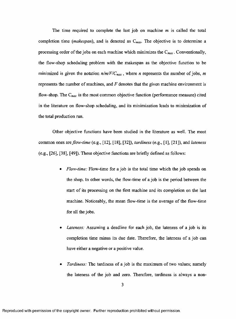
The time required to complete the last job on machine m is called the total
completion time (makespan), and is denoted as C max. The objective is to determine a
processing order of the jobs on each machine which minimizes the Cmax . Conventionally,
the flow-shop scheduling problem with the makespan as the objective function to be
minimized is given the notation n/m/F/Cmax , where n represents the number of jobs, m
represents the number of machines, and F denotes that the given machine environment is
flow-shop. The C max is the most common objective function (performance measure) cited
in the literature on flow-shop scheduling, and its minimization leads to minimization of
the total production run.
Other objective functions have been studied in the literature as well. The most
common ones are flow-time (e.g., [12], [18], [32]), tardiness (e.g., [1], [21]), and lateness
(e.g., [26], [38], [49]). These objective functions are briefly defined as follows:
• Flow-time: Flow-time for a job is the total time which the job spends on
the shop. In other words, the flow-time of a job is the period between the
start of its processing on the first machine and its completion on the last
machine. Noticeably, the mean flow-time is the average of the flow-time
for all the jobs.
• Lateness: Assuming a deadline for each job, the lateness of a job is its
completion time minus its due date. Therefore, the lateness of a job can
have either a negative or a positive value.
• Tardiness: The tardiness of a job is the maximum of two values; namely
the lateness of the job and zero. Therefore, tardiness is always a non-
3
Reproduced with permission of the copyright owner. Further reproduction prohibited without permission.
The time required to complete the last job on machine m is called the total
completion time (makespan), and is denoted as Cmax. The objective is to determine a
processing order o f the jobs on each machine which minimizes the Cmax. Conventionally,
the flow-shop scheduling problem with the makespan as the objective function to be
minimized is given the notation n/m/F/Cmax, where n represents the number o f jobs, m
represents the number o f machines, and F denotes that the given machine environment is
flow-shop. The Cmax is the most common objective function (performance measure) cited
in the literature on flow-shop scheduling, and its minimization leads to minimization of
the total production run.
Other objective functions have been studied in the literature as well. The most
common ones are flow-time (e.g., [12], [18], [32]), tardiness (e.g., [1], [21]), and lateness
(e.g., [26], [38], [49]). These objective functions are briefly defined as follows:
• Flow-time: Flow-time for a job is the total time which the job spends on
the shop. In other words, the flow-time of a job is the period between the
start o f its processing on the first machine and its completion on the last
machine. Noticeably, the mean flow-time is the average of the flow-time
for all the jobs.
• Lateness: Assuming a deadline for each job, the lateness of a job is its
completion time minus its due date. Therefore, the lateness o f a job can
have either a negative or a positive value.
• Tardiness: The tardiness o f a job is the maximum o f two values; namely
the lateness of the job and zero. Therefore, tardiness is always a non-
3
Reproduced with permission of the copyright owner. Further reproduction prohibited without permission.
negative number. The interpretation behind defining the tardiness as an
objective function is that one may be simply interested in meeting due
dates without being concerned about their actual start times.
Most of the literature on the flow-shop scheduling is limited to a special case
called the permutation flow-shop scheduling (e.g., [23], [42], [45], [46], [47], and [50]).
In this particular case of flow-shop, machines must process the jobs in the very same
order. In other words, in permutation flow-shop scheduling, sequence change is not
allowed between the machines, and once the sequence of jobs is scheduled on the first
machine, this sequence remains unchanged on the other machines [3].
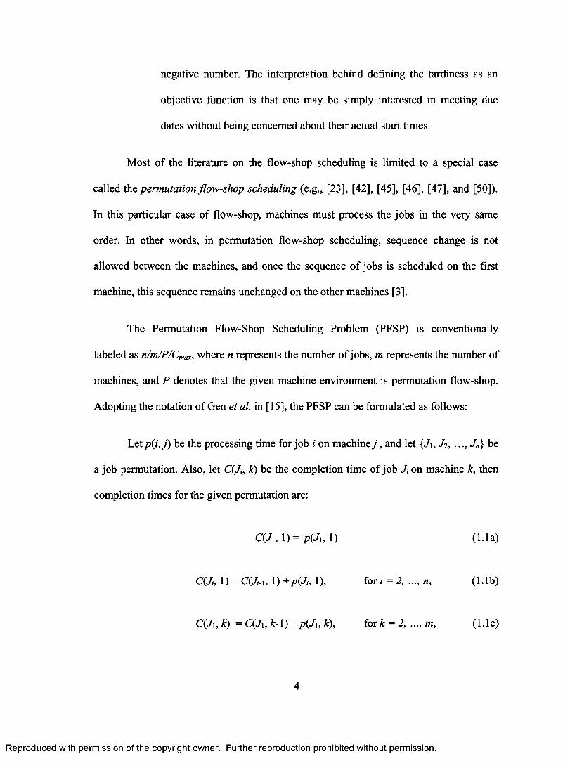
The Permutation Flow-Shop Scheduling Problem (PFSP) is conventionally
labeled as n/m/P/Cmax, where n represents the number of jobs, m represents the number of
machines, and P denotes that the given machine environment is permutation flow-shop.
Adopting the notation of Gen et al. in [15], the PFSP can be formulated as follows:
Let p(i, j) be the processing time for job i on machine j , and let {Ji, J2, ..., 4} be
a job permutation. Also, let C(Ji, k) be the completion time of job on machine k, then
completion times for the given permutation are:
C(11,1)= p(41) (1.1a)
C(Ji, 1) = C(41, 1) + p(J i, 1), for i = 2, ..., n, (1.1b)
C(J1, k) = C(J1, k-1) + p(Ji, k), for k = 2, ..., m, (1.1c)
4
Reproduced with permission of the copyright owner. Further reproduction prohibited without permission.
negative number. The interpretation behind defining the tardiness as an
objective function is that one may be simply interested in meeting due
dates without being concerned about their actual start times.
Most o f the literature on the flow-shop scheduling is limited to a special case
called the permutation flow-shop scheduling (e.g., [23], [42], [45], [46], [47], and [50]).
In this particular case o f flow-shop, machines must process the jobs in the very same
order. In other words, in permutation flow-shop scheduling, sequence change is not
allowed between the machines, and once the sequence o f jobs is scheduled on the first
machine, this sequence remains unchanged on the other machines [3].
The Permutation Flow-Shop Scheduling Problem (PFSP) is conventionally
labeled as n/m/P/Cmax, where n represents the number o f jobs, m represents the number of
machines, and P denotes that the given machine environment is permutation flow-shop.
Adopting the notation of Gen et al. in [15], the PFSP can be formulated as follows:
Let p(i, j ) be the processing time for job i on machine j , and let {J\, Ji, ..., Jn) be
a job permutation. Also, let C(Jt, k) be the completion time o f job J\ on machine k, then
completion times for the given permutation are:
C(JU 1) = p (Ju 1) (1.1a)
C(Jh 1) = C(J,.U 1 )+ p (Jh 1), for i = 2, .... n, ( 1.1b)
C(J\, k) = C(Ji, £-1) + p(J\, k), for k = 2, .... m, (1.1c)
4
Reproduced with permission of the copyright owner. Further reproduction prohibited without permission.

C(Ji, k) = max {C(Ji_i, k), C(Ji, k-1)} + p(J,, k),
for i = 2, ..., n; for k = 2, ..., m (1.1d)
The makespan for the given permutation is obtained through:
Cma., = m). (1.1e)
In the following illustrative example for the PFSP, there are five jobs to be
processed on four machines. The processing times of each job on different machines are
given in Table 1.1:
Cable 1.1 Processing times of five jobs on four machines [391
J.5
jobs processing times Jl J2 J3 J4
P(Jill) 5 5 3 6 3
P(Ji,2) 4 4 2 4 4
P(Ji,3) 4 4 3 4 1
P64,49 3 6 3 2 5
The following Gantt chart (Figure 1.1) illustrates how the makespan 34 for the
permutation of {Ji, J2, J3, J4, J5} is derived from data given in Table 1.1.
In addition to makespan, Figure 1.1 illustrates the earliest completion time for
each job on different machines. For example, the earliest completion time of J4 on
machine 1 to machine 4 are respectively 19, 23, 27, 29.
J1
J1
J3 J5
J3 J5
J5
1 2 3 4 5 6 7 8 9 10 11 12 13 14 15 16 17 18 19 20 21 22 23 24 25 26 27 28 29 30 31 32 33 34
Figure 1.1 Gantt chart for the permutation {J1, J2, J3, J4, J5} based on data given in Table1.1 (Original in Color).
5
Reproduced with permission of the copyright owner. Further reproduction prohibited without permission.
C(J\, k) = max{C(J,-.i, k), C(J, ft-1)} + p(Jt, k),
for / = 2 , n; for k = 2 , m ( 1.1 d)
The makespan for the given permutation is obtained through:
Cmax = C(Jn, m). ( l .le )
In the following illustrative example for the PFSP, there are five jobs to be
processed on four machines. The processing times o f each job on different machines are
given in Table 1.1:
Table 1.1 Processing times o f five jobs on four machines [391.jobs
processing times'""— Ji J 2 Ji J 4 Js
P ( J i J ) 5 5 3 6 3
p (J i> 2 ) 4 4 2 4 4
p ( J t ,3 ) 4 4 3 4 1
p (J i> 4 ) 3 6 3 2 5
The following Gantt chart (Figure 1.1) illustrates how the makespan 34 for the
permutation o f {J], J 2, J 3, J4, J 5 } is derived from data given in Table 1.1.
In addition to makespan, Figure 1.1 illustrates the earliest completion time for
each job on different machines. For example, the earliest completion time o f J 4 on
machine 1 to machine 4 are respectively 19, 23, 27, 29.
1 2 3 4 5 6 7 8 9 10 11 12 13 14 15 16 17 18 19 20 21 22 23 24 25 26 27 28 29 30 31 32 33 34
Figure 1.1 Gantt chart for the permutation {Jl, J2, J3, J4, J5} based on data given in Tablel.l (Original in Color).
5
Reproduced with permission of the copyright owner. Further reproduction prohibited without permission.
The permutation flow-shop scheduling problem, as presented above, is a
combinatorial optimization problem and the size of its search space is n!. According to
Reeves, [43] any improvement in the quality of the solution (i.e., the makespan) obtained
for the general flow-shop scheduling (n/m/F/Cmax) is rather small compared with that of
permutation flow-shop scheduling. On the other hand, general flow-shop scheduling
causes the size of the search space to increase considerably, from n! to (n!)" . Therefore,
in the general form of flow-shop scheduling (where the permutation of jobs is allowed to
be different on each machine) one might obtain a slightly better makespan at the cost of
much higher computation time.
One of the most frequently cited papers in the field of the flow-shop scheduling
problem, which is also referred to as the first paper in that area, dates back to 1954 [25].
In that paper, Johnson proposed a constructive algorithm which can find the optimal
solution for the two-machine permutation flow-shop scheduling problem (2/m/P/Cm„,).
However, the PFSP (i.e., n/m/P/C„,„,) is known to be Non-deterministic Polynomial-time
hard (NP-hard') if the number of machines are greater than two [14], [44].
As mentioned earlier, scheduling problems can take many forms in industry.
Before closing the introductory notes on scheduling, the definitions of other important
machine scheduling problems that may arise in a shop environment are given according
to Pinedo [39]:
According to Weisstein, a problem is NP-hard if an algorithm for solving it can be translated into one for solving any NP-problem (nondeterministic polynomial time problem). NP-hard, therefore, means at least as hard as any NP-problem, although it might, in fact, be harder [63]. In addition, he defines NP-problems as follows: "A problem is assigned to the NP class if it is solvable in polynomial time by a nondeterministic Turing machine. A nondeterministic Turing machine is a "parallel" Turing machine that can take many computational paths simultaneously, with the restriction that the parallel Turing machines cannot communicate" [63].
6
Reproduced with permission of the copyright owner. Further reproduction prohibited without permission.
The permutation flow-shop scheduling problem, as presented above, is a
combinatorial optimization problem and the size o f its search space is n!. According to
Reeves, [43] any improvement in the quality o f the solution (i.e., the makespan) obtained
for the general flow-shop scheduling (n/m/F/Cmax) is rather small compared with that of
permutation flow-shop scheduling. On the other hand, general flow-shop scheduling
causes the size o f the search space to increase considerably, from n! to (n!)m. Therefore,
in the general form of flow-shop scheduling (where the permutation o f jobs is allowed to
be different on each machine) one might obtain a slightly better makespan at the cost of
much higher computation time.
One o f the most frequently cited papers in the field o f the flow-shop scheduling
problem, which is also referred to as the first paper in that area, dates back to 1954 [25].
In that paper, Johnson proposed a constructive algorithm which can find the optimal
solution for the two-machine permutation flow-shop scheduling problem (2/m/P/Cmax ).
However, the PFSP (i.e., n/m/P/Cmax) is known to be Non-deterministic Polynomial-time
hard (NP-hard1) if the number o f machines are greater than two [14], [44].
As mentioned earlier, scheduling problems can take many forms in industry.
Before closing the introductory notes on scheduling, the definitions o f other important
machine scheduling problems that may arise in a shop environment are given according
to Pinedo [39]:
1 According to Weisstein, a problem is NP-hard if an algorithm for solving it can be translated into one forsolving any NP-problem (nondeterministic polynomial time problem). NP-hard, therefore, means at least ashard as any NP-problem, although it might, in fact, be harder [63]. In addition, he defines NP-problems asfollows: “A problem is assigned to the NP class if it is solvable in polynomial time by a nondeterministicTuring machine. A nondeterministic Turing machine is a "parallel" Turing machine that can take many computational paths simultaneously, with the restriction that the parallel Turing machines cannot communicate” [63].
6
Reproduced with permission of the copyright owner. Further reproduction prohibited without permission.

Flexible Flow-Shop Scheduling: A flexible flow-shop makes use of parallel
machines. Instead of having m machines working in series, there would exist c stages
(work centers) in series with a number of identical machines working in parallel at each
stage. Each job must be performed first at Stage 1, then at Stage 2, and so on. Each stage
can provide us with some parallel machines and a job can be processed on any idle
machine at each stage.
Job-Shop Scheduling: In a job shop environment, each job has its own pre-
specified route of machines to follow. These routes are fixed but they are not necessarily
the same for each job. The job shop scheduling problem itself can be classified into two
sub-categories based on whether recirculation is allowed or not. Recirculation occurs
when a job visits certain machines more than once.
Flexible Job-Shop Scheduling: A flexible job shop is a generalization of the job
shop scheduling by making use of parallel machines. Each job has its own pre-specified
route of machines to follow. But similar to the flexible flow-shop environment, there are
c work centers with a number of identical machines at each work center. The work
centers can provide us with parallel machines, and each job can be processed on any idle
machine at each work center.
Open-Shop Scheduling: Similar to flow-shop scheduling, each job has to be
processed on each of the m machines. However, there are no technological constraints
with respect to the routing of each job through the machines. In other words, the
scheduler can specify a route for each job, and different jobs are allowed to have different
routes.
7
Reproduced with permission of the copyright owner. Further reproduction prohibited without permission.
Flexible Flow-Shop Scheduling: A flexible flow-shop makes use o f parallel
machines. Instead o f having m machines working in series, there would exist c stages
(work centers) in series with a number o f identical machines working in parallel at each
stage. Each job must be performed first at Stage 1, then at Stage 2, and so on. Each stage
can provide us with some parallel machines and a job can be processed on any idle
machine at each stage.
Job-Shop Scheduling: In a job shop environment, each job has its own pre
specified route o f machines to follow. These routes are fixed but they are not necessarily
the same for each job. The job shop scheduling problem itself can be classified into two
sub-categories based on whether recirculation is allowed or not. Recirculation occurs
when a job visits certain machines more than once.
Flexible Job-Shop Scheduling: A flexible job shop is a generalization of the job
shop scheduling by making use o f parallel machines. Each job has its own pre-specified
route of machines to follow. But similar to the flexible flow-shop environment, there are
c work centers with a number o f identical machines at each work center. The work
centers can provide us with parallel machines, and each job can be processed on any idle
machine at each work center.
Open-Shop Scheduling: Similar to flow-shop scheduling, each job has to be
processed on each o f the m machines. However, there are no technological constraints
with respect to the routing o f each job through the machines. In other words, the
scheduler can specify a route for each job, and different jobs are allowed to have different
routes.
7
Reproduced with permission of the copyright owner. Further reproduction prohibited without permission.
1.2 Research Objectives
As Pinedo states, efficient scheduling has become crucial for the survival of companies in
the marketplace [39]. Scheduling systems can be considered as sub-systems that interact
with other sub-systems in an enterprise, such as logistics, supplier, and marketing
systems. The overall system, which integrates all those sub-systems, is typically known
as an enterprise-wide information system. Jessup defines enterprise-wide information
system as "information systems that allow companies to integrate information across
operations on a company-wide basis" [24].
The purpose of this research is to investigate one well-known form of the
scheduling problems, the permutation flow-shop scheduling problem, with the makespan
minimization as the objective function. Development of a new algorithm based on
genetic algorithms to find solutions fast (and reliably) has been investigated.
Efficiency of the permutation flow-shop scheduling in manufacturing systems is
affected by the decisions made with respect to the sequence of jobs. Makespan
minimization, as mentioned earlier, leads to a minimization of the total production run.
The literature on the PFSP employing this objective function is vast. Therefore, proposed
algorithms can be extensively evaluated and compared with the wide range of heuristic
algorithms that already exist in the literature.
1.3 Research Contributions
A genetic algorithm-based solution methodology is developed and implemented in this
thesis. More specifically, the performance of two versions of the proposed algorithm,
namely, a stand-alone genetic algorithm (referred to as the non-hybrid genetic algorithm
8
Reproduced with permission of the copyright owner. Further reproduction prohibited without permission.
1.2 Research Objectives
As Pinedo states, efficient scheduling has become crucial for the survival o f companies in
the marketplace [39]. Scheduling systems can be considered as sub-systems that interact
with other sub-systems in an enterprise, such as logistics, supplier, and marketing
systems. The overall system, which integrates all those sub-systems, is typically known
as an enterprise-wide information system. Jessup defines enterprise-wide information
system as “information systems that allow companies to integrate information across
operations on a company-wide basis” [24].
The purpose o f this research is to investigate one well-known form of the
scheduling problems, the permutation flow-shop scheduling problem, with the makespan
minimization as the objective function. Development o f a new algorithm based on
genetic algorithms to find solutions fast (and reliably) has been investigated.
Efficiency of the permutation flow-shop scheduling in manufacturing systems is
affected by the decisions made with respect to the sequence o f jobs. Makespan
minimization, as mentioned earlier, leads to a minimization o f the total production run.
The literature on the PFSP employing this objective function is vast. Therefore, proposed
algorithms can be extensively evaluated and compared with the wide range o f heuristic
algorithms that already exist in the literature.
1.3 Research Contributions
A genetic algorithm-based solution methodology is developed and implemented in this
thesis. More specifically, the performance o f two versions o f the proposed algorithm,
namely, a stand-alone genetic algorithm (referred to as the non-hybrid genetic algorithm
8
Reproduced with permission of the copyright owner. Further reproduction prohibited without permission.
in this thesis) and a hybrid genetic algorithm (merging the GA with iterated greedy search
algorithm) are thoroughly investigated in this thesis. As for the comparative experimental
results, the standard benchmarks proposed by Taillard [53] are employed. Experimental
results, presented in this thesis, demonstrate that the proposed hybridized genetic
algorithm outperforms the stand-alone genetic algorithm.
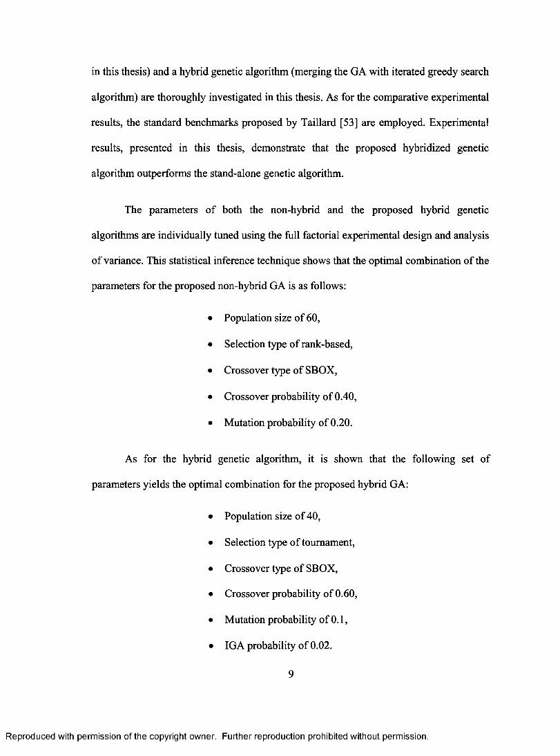
The parameters of both the non-hybrid and the proposed hybrid genetic
algorithms are individually tuned using the full factorial experimental design and analysis
of variance. This statistical inference technique shows that the optimal combination of the
parameters for the proposed non-hybrid GA is as follows:
• Population size of 60,
• Selection type of rank-based,
• Crossover type of SBOX,
• Crossover probability of 0.40,
• Mutation probability of 0.20.
As for the hybrid genetic algorithm, it is shown that the following set of
parameters yields the optimal combination for the proposed hybrid GA:
• Population size of 40,
• Selection type of tournament,
• Crossover type of SBOX,
• Crossover probability of 0.60,
• Mutation probability of 0.1,
• IGA probability of 0.02.
9
Reproduced with permission of the copyright owner. Further reproduction prohibited without permission.
in this thesis) and a hybrid genetic algorithm (merging the GA with iterated greedy search
algorithm) are thoroughly investigated in this thesis. As for the comparative experimental
results, the standard benchmarks proposed by Taillard [53] are employed. Experimental
results, presented in this thesis, demonstrate that the proposed hybridized genetic
algorithm outperforms the stand-alone genetic algorithm.
The parameters o f both the non-hybrid and the proposed hybrid genetic
algorithms are individually tuned using the full factorial experimental design and analysis
o f variance. This statistical inference technique shows that the optimal combination o f the
parameters for the proposed non-hybrid GA is as follows:
• Population size o f 60,
• Selection type o f rank-based,
• Crossover type o f SBOX,
• Crossover probability o f 0.40,
• Mutation probability o f 0.20.
As for the hybrid genetic algorithm, it is shown that the following set of
parameters yields the optimal combination for the proposed hybrid GA:
• Population size o f 40,
• Selection type o f tournament,
• Crossover type o f SBOX,
• Crossover probability o f 0.60,
• Mutation probability o f 0.1,
• IGA probability o f 0.02.
Reproduced with permission of the copyright owner. Further reproduction prohibited without permission.
CHAPTER 2: REVIEW OF LITERATURE
The motivation for solving the PFSP over the last four decades stems not only from its
practical relevance, but also from its misleading simplicity and challenging difficulties
[28].
The proposed methods for the PFSP can be divided into two main categories;
namely, exact methods and heuristic methods. French refers to exact methods as
enumerative algorithms [13]. According to French, enumerative algorithms can be
described as algorithms which "generate schedules one by one, searching for an optimal
solution. Often, they use 'clever' elimination procedures to see if the non-optimality of a
schedule implies the non-optimality of many others not yet generated. Thus, the methods
may not search the whole set of feasible solutions. Nonetheless, they are considered as
methods that proceed through exhaustive enumeration and, hence, require much
computation time".
Enumerative algorithms, such as integer programming, and branch and bound
techniques, can be theoretically applied to find the optimal solution for the permutation
flow-shop scheduling problem [13], [28]. However, these methods are not practical for
large-sized or even mid-sized problems. Ruiz et al. [46] states that exact methods are
only applicable for small instances, when the number of jobs is roughly less than 20.
Therefore, researchers have focused on applying heuristic methods to the PFSP in order
10
Reproduced with permission of the copyright owner. Further reproduction prohibited without permission.
C h a p t e r 2: R e v ie w O f L ite r a tu r e
The motivation for solving the PFSP over the last four decades stems not only from its
practical relevance, but also from its misleading simplicity and challenging difficulties
[28].
The proposed methods for the PFSP can be divided into two main categories;
namely, exact methods and heuristic methods. French refers to exact methods as
enumerative algorithms [13]. According to French, enumerative algorithms can be
described as algorithms which “generate schedules one by one, searching for an optimal
solution. Often, they use ‘clever’ elimination procedures to see if the non-optimality o f a
schedule implies the non-optimality o f many others not yet generated. Thus, the methods
may not search the whole set o f feasible solutions. Nonetheless, they are considered as
methods that proceed through exhaustive enumeration and, hence, require much
computation time”.
Enumerative algorithms, such as integer programming, and branch and bound
techniques, can be theoretically applied to find the optimal solution for the permutation
flow-shop scheduling problem [13], [28]. However, these methods are not practical for
large-sized or even mid-sized problems. Ruiz et al. [46] states that exact methods are
only applicable for small instances, when the number o f jobs is roughly less than 20.
Therefore, researchers have focused on applying heuristic methods to the PFSP in order
10
Reproduced with permission of the copyright owner. Further reproduction prohibited without permission.
to find near-optimal solutions in much shorter time. The heuristics proposed for the PFSP
can fall into either constructive or improvement heuristics.
According to French [13], a constructive heuristic for a scheduling problem can
be defined as an algorithm that builds up a schedule from the given data of the problem
by following a simple set of rules (e.g., First-In-First-Out) which exactly determines the
processing order. Later on, a constructive heuristic will be discussed, and it can be
observed that this algorithm can optimally solve the two-machine flow-shop scheduling
problem.
Improvement heuristics, as contrasted to constructive heuristics, start from a
previously generated schedule and try to iteratively modify it. Meta-heuristics (modem
heuristics), such as Genetic Algorithms, Simulated Annealing, Iterated Local Search,
Iterated Greedy Search, etc., fall in the category of improvement heuristics.
An extensive literature review on the proposed heuristics for the PFSP can be
found in [15] and [45]. The heuristics by Johnson [25], Campel et al. [4], Dannenbring
[8], Palmer [37], Gupta [17], Nawaz et al. [58], Taillard [52], Hundal et al. [22],
Koulamas [27], and Davoud Pour [10] are instances of constructive heuristics in the
literature. The most cited existing improvement heuristics in the literature are Simulated
Annealing (SA) of Osman et al. [36], SA of Ogbu et al. [60], Genetic Algorithm (GA) of
Chen et al. [5], GA of Reeves [42], GA of Murata et al. [33], Iterated Local Search of
Stiizle [50], GA of Ponnambalom et al. [40], GA of Iyer et al. [23], GA of Ruiz et al.
[46], Iterated Greedy Search of Ruiz et al. [47].
11
Reproduced with permission of the copyright owner. Further reproduction prohibited without permission.
to find near-optimal solutions in much shorter time. The heuristics proposed for the PFSP
can fall into either constructive or improvement heuristics.
According to French [13], a constructive heuristic for a scheduling problem can
be defined as an algorithm that builds up a schedule from the given data o f the problem
by following a simple set o f rules (e.g., First-In-First-Out) which exactly determines the
processing order. Later on, a constructive heuristic will be discussed, and it can be
observed that this algorithm can optimally solve the two-machine flow-shop scheduling
problem.
Improvement heuristics, as contrasted to constructive heuristics, start from a
previously generated schedule and try to iteratively modify it. Meta-heuristics (modem
heuristics), such as Genetic Algorithms, Simulated Annealing, Iterated Local Search,
Iterated Greedy Search, etc., fall in the category o f improvement heuristics.
An extensive literature review on the proposed heuristics for the PFSP can be
found in [15] and [45]. The heuristics by Johnson [25], Campel et al. [4], Dannenbring
[8], Palmer [37], Gupta [17], Nawaz et al. [58], Taillard [52], Hundal et al. [22],
Koulamas [27], and Davoud Pour [10] are instances o f constructive heuristics in the
literature. The most cited existing improvement heuristics in the literature are Simulated
Annealing (SA) o f Osman et al. [36], SA of Ogbu et al. [60], Genetic Algorithm (GA) of
Chen et al. [5], GA of Reeves [42], GA of Murata et al. [33], Iterated Local Search of
Stuzle [50], GA o f Ponnambalom et al. [40], GA of Iyer et al. [23], GA of Ruiz et al.
[46], Iterated Greedy Search o f Ruiz et al. [47].
11
Reproduced with permission of the copyright owner. Further reproduction prohibited without permission.
In this chapter, three most important constructive heuristics; namely, Johnson's
algorithm, the heuristic of Nawaz et al. [58] (referred to as the NEH Algorithm), and
Taillard's algorithm [52] (which is an accelerated form of the NEH algorithm) are
described. The improvement heuristics of interest in this thesis, the genetic algorithms,
are briefly introduced in the next chapter.
2.1 Johnson's Algorithm
Johnson has been recognized as the pioneer in the research of the PFSP [25]. The
significance of his proposed algorithm is that it can provide an optimal solution for the
two-machine flow-shop scheduling problem in polynomial time. However, where the
number of machines is greater than two, the PFSP is known to be NP-hard [14].
Johnson's algorithm is described as follows according to Pinedo [39]: The jobs
are first split into two sets; namely, Set #1 that contains all the jobs with pi] < pi2, and
Set #2 that contains all the jobs with pH > Pi2 (where pee is the processing time of the i-th
job on the first machine, and pee is the processing time of the i-th job on the second
machine). The jobs in Set #1 are scheduled first and they are sequenced in increasing
order of pee (Shortest Processing Times (SPT) first); then the jobs in Set #2 are scheduled
in decreasing order of pi2 (Longest Processing Times (LPT) first). Ties can be broken
randomly (e.g., if the processing times of two jobs in Set #1 are equal, each of them can
be arbitrarily scheduled first). Any schedule constructed through the aforementioned
method is typically known as a SPT(1)-LPT(2) schedule. Johnson proved that any
SPT(1)-LPT(2) is optimal for the two-machine flow-shop scheduling problem.
12
Reproduced with permission of the copyright owner. Further reproduction prohibited without permission.
In this chapter, three most important constructive heuristics; namely, Johnson’s
algorithm, the heuristic o f Nawaz et al. [58] (referred to as the NEH Algorithm), and
Taillard’s algorithm [52] (which is an accelerated form o f the NEH algorithm) are
described. The improvement heuristics o f interest in this thesis, the genetic algorithms,
are briefly introduced in the next chapter.
2.1 Johnson’s Algorithm
Johnson has been recognized as the pioneer in the research of the PFSP [25]. The
significance o f his proposed algorithm is that it can provide an optimal solution for the
two-machine flow-shop scheduling problem in polynomial time. However, where the
number o f machines is greater than two, the PFSP is known to be NP-hard [14].
Johnson’s algorithm is described as follows according to Pinedo [39]: The jobs
are first split into two sets; namely, Set #1 that contains all the jobs with pu < pi2, and
Set #2 that contains all the jobs with pu > pt2 (where pu is the processing time of the z'-th
job on the first machine, and pi2 is the processing time of the z'-th job on the second
machine). The jobs in Set #1 are scheduled first and they are sequenced in increasing
order of pu (Shortest Processing Times (SPT) first); then the jobs in Set #2 are scheduled
in decreasing order o f pi2 (Longest Processing Times (LPT) first). Ties can be broken
randomly (e.g., if the processing times o f two jobs in Set #1 are equal, each of them can
be arbitrarily scheduled first). Any schedule constructed through the aforementioned
method is typically known as a SPT(1)-LPT(2) schedule. Johnson proved that any
SPT(1)-LPT(2) is optimal for the two-machine flow-shop scheduling problem.
12
Reproduced with permission of the copyright owner. Further reproduction prohibited without permission.
Although it has been proven that when m > 3 (where m is the number of
machines), the PFSP turns into a NP-hard problem, some efforts have been made to
propose a modification of Johnson's rule for permutation flow-shop scheduling problem
for more than two machines (e.g., [4]).
2.2 The Algorithm of Nawaz, Enscore and Ham
The algorithm of Nawaz et al. [58] is commonly referred to as the NEH algorithm in the
literature. The NEH algorithm has been given considerable attention in the literature of
the PFSP, because it has been unanimously referred to as the best constructive method for
the permutation flow-shop scheduling problem among the constructive heuristics in the
literature; (see, for example: [40], [45], [52], [55], and [57]). Among the aforementioned
references, the work of Ruiz et al. (i.e., [45]) is the most comprehensive, since they have
compared fifteen constructive heuristics extensively.
In the NEH algorithm, first the jobs are sorted by a decreasing sum of the
processing times on machines (the sum of the processing times for job J, is denoted by
TPi and is calculated using the formula TP, = EAJ,k), where k represents the machine k=1
number on which the job is being processed). Then, the first two jobs with highest sum of
processing times on the machines are considered for partial scheduling. The best partial
schedule of those two jobs (i.e., one that produces lower partial makespan) is selected.
This partial sequence is fixed in a sense that the relative order of those two jobs will not
change until the end of the procedure. In the next step, the job with the third highest sum
of processing times is selected and three possible partial schedules are generated through
placing the third chosen job at the beginning, in the middle, and at the end of the fixed
13
Reproduced with permission of the copyright owner. Further reproduction prohibited without permission.
Although it has been proven that when m > 3 (where m is the number of
machines), the PFSP turns into a NP-hard problem, some efforts have been made to
propose a modification of Johnson’s rule for permutation flow-shop scheduling problem
for more than two machines (e.g., [4]).
2.2 The Algorithm of Nawaz, Enscore and Ham
The algorithm of Nawaz et al. [58] is commonly referred to as the NEH algorithm in the
literature. The NEH algorithm has been given considerable attention in the literature of
the PFSP, because it has been unanimously referred to as the best constructive method for
the permutation flow-shop scheduling problem among the constructive heuristics in the
literature; (see, for example: [40], [45], [52], [55], and [57]). Among the aforementioned
references, the work o f Ruiz et al. (i.e., [45]) is the most comprehensive, since they have
compared fifteen constructive heuristics extensively.
In the NEH algorithm, first the jobs are sorted by a decreasing sum of the
processing times on machines (the sum of the processing times for job Ji is denoted by
m
TPi and is calculated using the formula 77* = t ,k) , where k represents the machinek=1
number on which the job is being processed). Then, the first two jobs with highest sum of
processing times on the machines are considered for partial scheduling. The best partial
schedule o f those two jobs (i.e., one that produces lower partial makespan) is selected.
This partial sequence is fixed in a sense that the relative order o f those two jobs will not
change until the end o f the procedure. In the next step, the job with the third highest sum
of processing times is selected and three possible partial schedules are generated through
placing the third chosen job at the beginning, in the middle, and at the end o f the fixed
13
Reproduced with permission of the copyright owner. Further reproduction prohibited without permission.
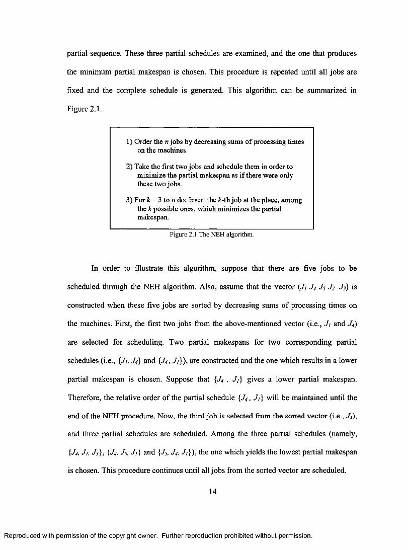
partial sequence. These three partial schedules are examined, and the one that produces
the minimum partial makespan is chosen. This procedure is repeated until all jobs are
fixed and the complete schedule is generated. This algorithm can be summarized in
Figure 2.1.
1) Order the n jobs by decreasing sums of processing times on the machines.
2) Take the first two jobs and schedule them in order to minimize the partial makespan as if there were only these two jobs.
3) For k = 3 to n do: Insert the k-th job at the place, among the k possible ones, which minimizes the partial makespan.
Figure 2.1 The NEH algorithm.
In order to illustrate this algorithm, suppose that there are five jobs to be
scheduled through the NEH algorithm. Also, assume that the vector (.11 J4 J5 J2 J3) is
constructed when these five jobs are sorted by decreasing sums of processing times on
the machines. First, the first two jobs from the above-mentioned vector (i.e., J i and J 4)
are selected for scheduling. Two partial makespans for two corresponding partial
schedules (i.e., {.//, J 4} and {J4, Ji}), are constructed and the one which results in a lower
partial makespan is chosen. Suppose that {J4 , gives a lower partial makespan.
Therefore, the relative order of the partial schedule {J4 , J will be maintained until the
end of the NEH procedure. Now, the third job is selected from the sorted vector (i.e., J 5),
and three partial schedules are scheduled. Among the three partial schedules (namely,
{J4, Jl, J5}, {J4, J5, J1} and {J5, J 4, Ji }), the one which yields the lowest partial makespan
is chosen. This procedure continues until all jobs from the sorted vector are scheduled.
14
Reproduced with permission of the copyright owner. Further reproduction prohibited without permission.
partial sequence. These three partial schedules are examined, and the one that produces
the minimum partial makespan is chosen. This procedure is repeated until all jobs are
fixed and the complete schedule is generated. This algorithm can be summarized in
Figure 2.1.
1) Order the n jobs by decreasing sums of processing timeson the machines.
2) Take the first two jobs and schedule them in order tominimize the partial makespan as if there were only these two jobs.
3) For k = 3 to n do: Insert the A>th job at the place, amongthe k possible ones, which minimizes the partial makespan.
Figure 2.1 The NEH algorithm.
In order to illustrate this algorithm, suppose that there are five jobs to be
scheduled through the NEH algorithm. Also, assume that the vector (J4 J 4 J 5 J2 J 3) is
constructed when these five jobs are sorted by decreasing sums o f processing times on
the machines. First, the first two jobs from the above-mentioned vector (i.e., Jj and J4)
are selected for scheduling. Two partial makespans for two corresponding partial
schedules (i.e., {J/, J4] and {J4, J/}), are constructed and the one which results in a lower
partial makespan is chosen. Suppose that {J4 , J/} gives a lower partial makespan.
Therefore, the relative order o f the partial schedule {J4, J{) will be maintained until the
end of the NEH procedure. Now, the third job is selected from the sorted vector (i.e., J5),
and three partial schedules are scheduled. Among the three partial schedules (namely,
{J4, J 1, J5}, {J4, J$, Jj} and {J5, J4, Jj}), the one which yields the lowest partial makespan
is chosen. This procedure continues until all jobs from the sorted vector are scheduled.
14
Reproduced with permission of the copyright owner. Further reproduction prohibited without permission.
2.3 Taillard's Algorithm
Taillard investigated some of the above-mentioned constructive algorithms and he
showed that the performance of the NEH algorithm is superior in terms of the achieved
makespan through some experimental results. Moreover, he proposed a method which
reduces the complexity of the NEH algorithm, and consequently accelerates the original
NEH algorithm. Using his proposed technique, the order of the NEH algorithm decreases
from 0(n3 nz)to 0(n2 m) . One should note that Taillard's algorithm achieves the very
same results that the NEH algorithm does, in lower CPU time [52].
Taillard's procedure is illustrated through Figures 2.2 to 2.5. For the previously
given processing times of five jobs on four machines summarized in
Table 1.1, suppose that four jobs have been sequenced according to the NEH algorithm
and that the partial schedule {Jj, J2, J 4, J 5} has been constructed as the best partial
schedule so far with the makespan of 31 (see Figure 2.2). Preserving the relative order of
the best partial schedule, J3 (i.e., the only job which has not been scheduled yet) is going
to be inserted at five possible positions. Consequently, the makespan for five schedules
should be calculated and the one with the lowest makespan is considered as the best
complete schedule. According to the original NEH algorithm, the makespan for those five
schedules should be calculated from scratch; but Taillard proposed a method where the
makespan for those five schedules can be obtained from the best partial schedule of four
jobs, which is achieved already in the previous step.
For instance, suppose that J3 is going to be inserted at the 3rd position (i.e.,
between J2 and J4 of the partial schedule {Jj, J2, J4, J5}). Based on Taillard's algorithm,
15
Reproduced with permission of the copyright owner. Further reproduction prohibited without permission.
2.3 Taillard’s Algorithm
Taillard investigated some o f the above-mentioned constructive algorithms and he
showed that the performance o f the NEH algorithm is superior in terms o f the achieved
makespan through some experimental results. Moreover, he proposed a method which
reduces the complexity o f the NEH algorithm, and consequently accelerates the original
NEH algorithm. Using his proposed technique, the order o f the NEH algorithm decreases
from 0 ( n 3m)to 0 ( n 2m ) . One should note that Taillard’s algorithm achieves the very
same results that the NEH algorithm does, in lower CPU time [52].
Taillard’s procedure is illustrated through Figures 2.2 to 2.5. For the previously
given processing times o f five jobs on four machines summarized in
Table 1.1, suppose that four jobs have been sequenced according to the NEH algorithm
and that the partial schedule {Ji, J 2, J 4, J 5 } has been constructed as the best partial
schedule so far with the makespan o f 31 (see Figure 2.2). Preserving the relative order of
the best partial schedule, J 3 (i.e., the only job which has not been scheduled yet) is going
to be inserted at five possible positions. Consequently, the makespan for five schedules
should be calculated and the one with the lowest makespan is considered as the best
complete schedule. According to the original NEH algorithm, the makespan for those five
schedules should be calculated from scratch; but Taillard proposed a method where the
makespan for those five schedules can be obtained from the best partial schedule o f four
jobs, which is achieved already in the previous step.
For instance, suppose that J 3 is going to be inserted at the 3rd position (i.e.,
between J2 and J4 o f the partial schedule {Ji, J 2, J 4, J 5 )). Based on Taillard’s algorithm,
15
Reproduced with permission of the copyright owner. Further reproduction prohibited without permission.
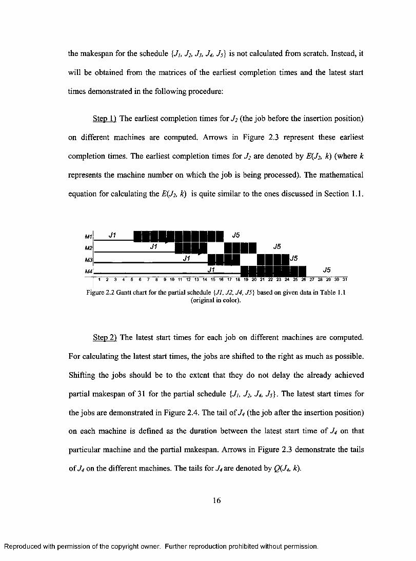
the makespan for the schedule 1.11, J2, J3, J4, J5} is not calculated from scratch. Instead, it
will be obtained from the matrices of the earliest completion times and the latest start
times demonstrated in the following procedure:
Step 1) The earliest completion times for J2 (the job before the insertion position)
on different machines are computed. Arrows in Figure 2.3 represent these earliest
completion times. The earliest completion times for J2 are denoted by E(J2, k) (where k
represents the machine number on which the job is being processed). The mathematical
equation for calculating the E(J2, k) is quite similar to the ones discussed in Section 1.1.
M1
M2
M3
M4
111111111111111111111 j5J5
J1 111111 IMP J1
1 2 3 4 5 6 7 8 9 10 11 12 13 14 15 16 17 18 19 20 21 22 23 24 25 26 27 28 29 30 31
Figure 2.2 Gantt chart for the partial schedule {J1, J2, J4, J5} based on given data in Table 1.1 (original in color).
Step 2) The latest start times for each job on different machines are computed.
For calculating the latest start times, the jobs are shifted to the right as much as possible.
Shifting the jobs should be to the extent that they do not delay the already achieved
partial makespan of 31 for the partial schedule J2, J4, J5}. The latest start times for
the jobs are demonstrated in Figure 2.4. The tail of J 4 (the job after the insertion position)
on each machine is defined as the duration between the latest start time of J4 on that
particular machine and the partial makespan. Arrows in Figure 2.3 demonstrate the tails
of J 4 on the different machines. The tails for J4 are denoted by Q(J4, k).
16
Reproduced with permission of the copyright owner. Further reproduction prohibited without permission.
the makespan for the schedule {Ji, J2, J3, J4, J5} is not calculated from scratch. Instead, it
will be obtained from the matrices o f the earliest completion times and the latest start
times demonstrated in the following procedure:
Step 1) The earliest completion times for J 2 (the job before the insertion position)
on different machines are computed. Arrows in Figure 2.3 represent these earliest
completion times. The earliest completion times for J2 are denoted by E(J2, k) (where k
represents the machine number on which the job is being processed). The mathematical
equation for calculating the E{J2, k) is quite similar to the ones discussed in Section 1.1.
M1
M2
M3
M4
■■— ■■■■■IJ1
J5
J1
1 2 3 4 5 6 7 8 9 10 11 12 13 14 15 16 17 18 19 20 21 22 23 24 25 26 27 28 29 30 31
Figure 2.2 Gantt chart for the partial schedule {JI, J2, J4, J5} based on given data in Table 1.1(original in color).
Step 2) The latest start times for each job on different machines are computed.
For calculating the latest start times, the jobs are shifted to the right as much as possible.
Shifting the jobs should be to the extent that they do not delay the already achieved
partial makespan o f 31 for the partial schedule {Ji, J2, J4, J5}. The latest start times for
the jobs are demonstrated in Figure 2.4. The tail of J4 (the job after the insertion position)
on each machine is defined as the duration between the latest start time o f J 4 on that
particular machine and the partial makespan. Arrows in Figure 2.3 demonstrate the tails
of J4 on the different machines. The tails for J 4 are denoted by Q(J4, k).
16
Reproduced with permission of the copyright owner. Further reproduction prohibited without permission.
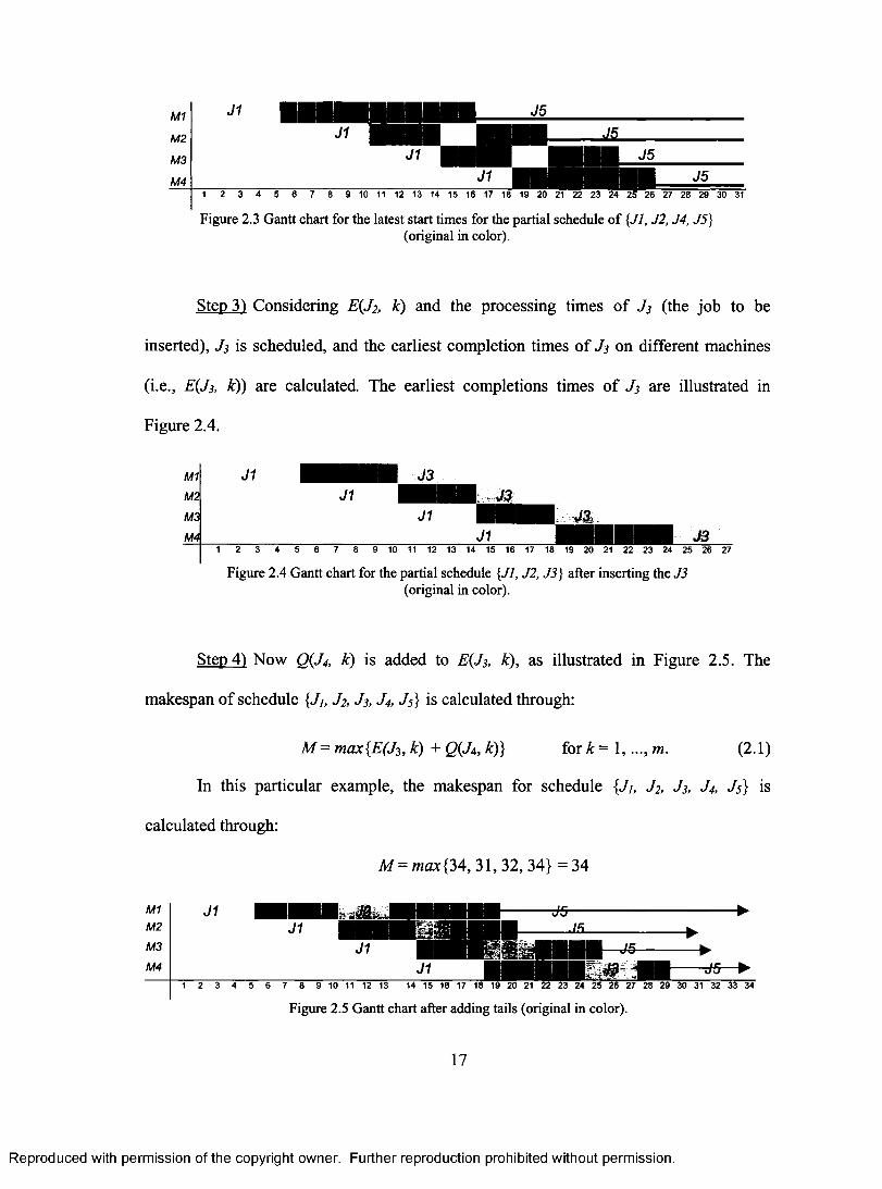
M1
M2
M3
M4
J1
J1
J1
J1
J5
1 2 3 4 5 6 7 8 9 10 11 12 13 14 15 16 17 18 19 20 21 22 23 24 2 26 27 28 29 30 31
Figure 2.3 Gantt chart for the latest start times for the partial schedule of {J1, J2, J4, J5} (original in color).
Step 3) Considering E(J2, k) and the processing times of J3 (the job to be
inserted), J3 is scheduled, and the earliest completion times of J3 on different machines
(i.e., E(J3, k)) are calculated. The earliest completions times of J3 are illustrated in
Figure 2.4.
M1 J1
M2
M3
M4
1111.1111 J3 J1 ...11
J1J1
2 3 4 5 6 7 8 9 10 11 12 13 14 15 16 17 18 19 20 21 22 23 24 25 26 27
Figure 2.4 Gantt chart for the partial schedule {J1, J2, J3} after inserting the J3 (original in color).
Step 4) Now Q(J4, k) is added to E(J3, k), as illustrated in Figure 2.5. The
makespan of schedule J2, J3, 4, ‘15} is calculated through:
M= mcvc{E(J3, k) + Q(J4, k)} for 1, ...,m. (2.1)
In this particular example, the makespan for schedule {J1, J2, J3, J4, J 5} is
calculated through:
M= max {34, 31, 32, 34} = 34
5 6 7 8 9 10 11 12 13 14 15 16 17 18 19 20 21 22 23 24 25 26 27 28 29
Figure 2.5 Gantt chart after adding tails (original in color).
17
Reproduced with permission of the copyright owner. Further reproduction prohibited without permission.
1 2 3 4 5 6 7 8 9 10 11 12 13 14 15 16 17 18 19 20 21 22 23 24 25 26 27 28 29 30 31
Figure 2.3 Gantt chart for the latest start times for the partial schedule o f {JI, J2, J4, J5}(original in color).
Step 3) Considering E(J2, k) and the processing times o f J 3 (the job to be
inserted), J 3 is scheduled, and the earliest completion times of J 3 on different machines
(i.e., E(J3, k)) are calculated. The earliest completions times o f J 3 are illustrated in
Figure 2.4.
1 2 3 4 5 6 7 8 9 10 11 12 13 14 15 16 17 18 19 20 21 22 23 24 25 26 27
Figure 2.4 Gantt chart for the partial schedule {JI, J2, J3} after inserting the J3(original in color).
Step 4) Now Q(J4, k) is added to E(J3, A), as illustrated in Figure 2.5. The
makespan of schedule {Ji, J2, J3, J4, J5) is calculated through:
M = max{E(J-3, k) + Q(Ja, A)} for k = 1,..., m. (2.1)
In this particular example, the makespan for schedule {Ji, J2, J3, J4, J5) is
calculated through:
M = m a x{34 ,31 ,32 , 34} = 34
1 2 3 4 5 6 7 8 9 10 11 12 13 14 15 16 17 18 19 20 21 22 23 24 25 26 27 28 29 30 31 32 33 34
Figure 2.5 Gantt chart after adding tails (original in color).
17
Reproduced with permission of the copyright owner. Further reproduction prohibited without permission.
One should note that if J3 is inserted into any other position in the partial schedule
{JI, J2, J4, J.5}, a similar procedure can be followed for calculating the makespan. For
example, the makespan of schedule {J], J2, J4, J.3, ../.5} can be obtained through the partial
schedule of {Jj, J2, J 4, J.5} and there is no need to calculate the makespan from scratch.
Taillard [52] concluded that the NEH algorithm-based solution can be obtained by
order of 0(n2m). In his paper, Taillard also addressed the concept of neighborhood in
the PFSP. This concept will be discussed in Chapter 3.
2.4 Taillard's Benchmark Problems
Most of the researchers in the area of machine scheduling in the 80s and 90s have tested
their heuristic approaches on randomly generated problems separately. Those problem
instances were never published. To solve this problem, Taillard has proposed a set of 120
test problems, denoted by ta001 to ta120, ranging from small instances with 20 jobs on 5
machines to large ones with 500 jobs on 20 machines as standard test benchmarks for the
PFSP [53]. Fortunately, Taillard's benchmarks for the PFSP are being widely used
recently by a wide range of researchers. For each problem size, ten instances are
available. The processing times of each instance are integers between 1 and 100 and they
were randomly generated with a uniform probability distribution. In fact, these 120
instances were selected by Taillard from a bigger set of generated instances. According to
Ruiz et al., some of them have been proven to be very difficult to solve over the past 10
years, [46].
18
Reproduced with permission of the copyright owner. Further reproduction prohibited without permission.
One should note that if J 3 is inserted into any other position in the partial schedule
{ J i , J 2 , J 4 , J s ) , a similar procedure can be followed for calculating the makespan. For
example, the makespan o f schedule {Ji, J 2 , J 4 , J 3 , J 5 } can be obtained through the partial
schedule o f { J i , J 2 , J 4, Js) and there is no need to calculate the makespan from scratch.
Taillard [52] concluded that the NEH algorithm-based solution can be obtained by
order of 0 (n 2m) . In his paper, Taillard also addressed the concept o f neighborhood in
the PFSP. This concept will be discussed in Chapter 3.
2.4 Taillard’s Benchmark Problems
Most o f the researchers in the area o f machine scheduling in the 80s and 90s have tested
their heuristic approaches on randomly generated problems separately. Those problem
instances were never published. To solve this problem, Taillard has proposed a set o f 120
test problems, denoted by taOOl to tal20, ranging from small instances with 20 jobs on 5
machines to large ones with 500 jobs on 20 machines as standard test benchmarks for the
PFSP [53]. Fortunately, Taillard’s benchmarks for the PFSP are being widely used
recently by a wide range of researchers. For each problem size, ten instances are
available. The processing times o f each instance are integers between 1 and 100 and they
were randomly generated with a uniform probability distribution. In fact, these 120
instances were selected by Taillard from a bigger set o f generated instances. According to
Ruiz et al., some o f them have been proven to be very difficult to solve over the past 10
years, [46].
18
Reproduced with permission of the copyright owner. Further reproduction prohibited without permission.
Global optima have been obtained for Taillard's small benchmarks, ranging from
20 x 5 ( n = 20, m = 5) to 50 x10 ( n = 50, m =10). But the optimal solutions for some of
the larger problem instances are still unknown.
By making use of Taillard's instances, researchers normally address the relative
percentage deviation of their solutions from the best-known solutions as the performance
measure. The best-known solution for an instance is denoted by Bestsoi and is either the
known optimal solution or the lowest-known upper bound (when the optimal solution is
still unknown). Denoting the achieved makespan of a given heuristic by Heusoi, the
relative percentage deviation (RPD) of that heuristic from the best-known solution can be
calculated through the following expression:
(Heu — Best sol ) RPD so. x100
Best so,
(2.2)
The optimal solutions or (upper bounds) are mainly found by branch and bound
technique which requires high CPU times [13], [28], [43]. Recently, the best-known
solutions for larger instances with unknown optimal solutions are being replaced by the
solutions found using meta-heuristics, such as Genetic Algorithms, Tabu Search, Iterated
Greedy Algorithm, and so on. The latest information on those solutions is updated by
Taillard on his website [54].
In this chapter, two constructive heuristic algorithms, namely the Johnson and the
NEH algorithms, were discussed. The improvement heuristics of interest in this thesis,
namely the genetic algorithms (GAs) and their applications in the PFPS are investigated
19
Reproduced with permission of the copyright owner. Further reproduction prohibited without permission.
Global optima have been obtained for Taillard’s small benchmarks, ranging from
2 0 x 5 {n = 20, m = 5) to 5 0 x l0 (n = 50,m = 10). But the optimal solutions for some of
the larger problem instances are still unknown.
By making use o f Taillard’s instances, researchers normally address the relative
percentage deviation o f their solutions from the best-known solutions as the performance
measure. The best-known solution for an instance is denoted by BestS0i and is either the
known optimal solution or the lowest-known upper bound (when the optimal solution is
still unknown). Denoting the achieved makespan of a given heuristic by Heusoi, the
relative percentage deviation (RPD) o f that heuristic from the best-known solution can be
calculated through the following expression:
RPD = (HeUs°l ~ Best™>) x 100 2̂ '2)Bestsol
The optimal solutions or (upper bounds) are mainly found by branch and bound
technique which requires high CPU times [13], [28], [43]. Recently, the best-known
solutions for larger instances with unknown optimal solutions are being replaced by the
solutions found using meta-heuristics, such as Genetic Algorithms, Tabu Search, Iterated
Greedy Algorithm, and so on. The latest information on those solutions is updated by
Taillard on his website [54].
In this chapter, two constructive heuristic algorithms, namely the Johnson and the
NEH algorithms, were discussed. The improvement heuristics o f interest in this thesis,
namely the genetic algorithms (GAs) and their applications in the PFPS are investigated
19
Reproduced with permission of the copyright owner. Further reproduction prohibited without permission.

in Chapter 3. The number of the proposed GAs to solve the PFSP is numerous. Therefore,
many of them will merely be mentioned for interested readers. In Chapter 4, the proposed
genetic algorithm is explained and its performance is tested on Taillard's benchmark
problems.
20
Reproduced with permission of the copyright owner. Further reproduction prohibited without permission.
in Chapter 3. The number o f the proposed GAs to solve the PFSP is numerous. Therefore,
many of them will merely be mentioned for interested readers. In Chapter 4, the proposed
genetic algorithm is explained and its performance is tested on Taillard’s benchmark
problems.
20
Reproduced with permission of the copyright owner. Further reproduction prohibited without permission.
CHAPTER 3: GENETIC ALGORITHMS (AN OVERVIEW)
AND THEIR APPLICATIONS IN THE PFSP
In this chapter, the general notion of Genetic Algorithms (GAs) is briefly discussed and
then it is explained that how genetic algorithms can be customized for the PFSP.
Genetic algorithms are stochastic search and optimization techniques developed
based on the mechanism of Darwinian 'natural evolution' and 'survival of the fittest'
[20]. The probabilistic search method in Genetic Algorithms, along with natural selection
and reproduction methods, mimic the process of biological evolution [20].
GAs can be applied to a wide range of optimization problems that cannot be
easily solved by conventional optimization algorithms, including problems in which the
objective function is discontinuous, fuzzy, non-differentiable, or highly nonlinear. For
various applications of GAs, see [6], [15], [19], [31], and [48].
Davis has been recognized as the pioneer in the application of genetic algorithms
in scheduling problems [63]. Since he proposed a methodology to solve the Job Shop
Scheduling problem through the genetic algorithms in 1985, the application of genetic
algorithms to different scheduling problems have been extensively investigated.
The general structure of the GA suggested by Michalewicz [31] is illustrated in
Figure 3.1. According to Michalewicz, a GA is a probabilistic algorithm which maintains
21
Reproduced with permission of the copyright owner. Further reproduction prohibited without permission.
C h a p t e r 3: G e n e t ic A l g o r it h m s (A n o v e r v ie w )
A n d T h e ir A pplic a tio n s In Th e PFSP
In this chapter, the general notion o f Genetic Algorithms (GAs) is briefly discussed and
then it is explained that how genetic algorithms can be customized for the PFSP.
Genetic algorithms are stochastic search and optimization techniques developed
based on the mechanism o f Darwinian ‘natural evolution’ and ‘survival o f the fittest’
[20]. The probabilistic search method in Genetic Algorithms, along with natural selection
and reproduction methods, mimic the process o f biological evolution [20],
GAs can be applied to a wide range o f optimization problems that cannot be
easily solved by conventional optimization algorithms, including problems in which the
objective function is discontinuous, fuzzy, non-differentiable, or highly nonlinear. For
various applications o f GAs, see [6], [15], [19], [31], and [48].
Davis has been recognized as the pioneer in the application o f genetic algorithms
in scheduling problems [63], Since he proposed a methodology to solve the Job Shop
Scheduling problem through the genetic algorithms in 1985, the application of genetic
algorithms to different scheduling problems have been extensively investigated.
The general structure o f the GA suggested by Michalewicz [31] is illustrated in
Figure 3.1. According to Michalewicz, a GA is a probabilistic algorithm which maintains
21
Reproduced with permission of the copyright owner. Further reproduction prohibited without permission.
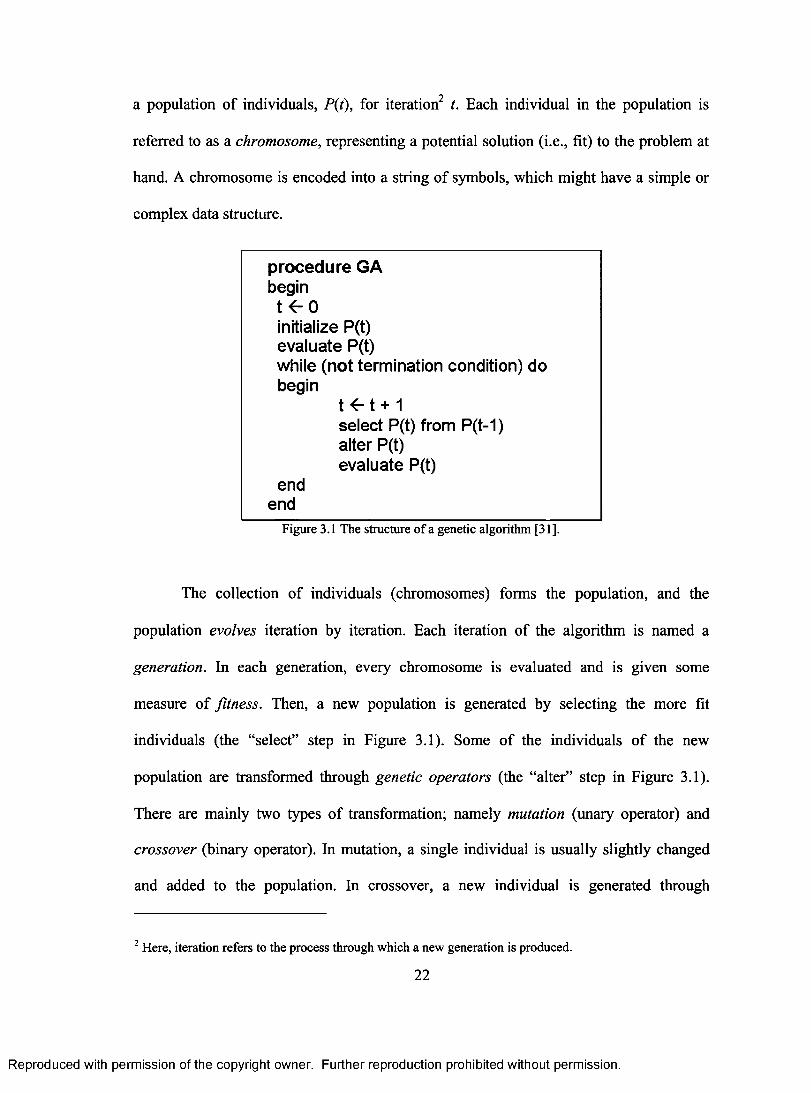
a population of individuals, P(t), for iteration t. Each individual in the population is
referred to as a chromosome, representing a potential solution (i.e., fit) to the problem at
hand. A chromosome is encoded into a string of symbols, which might have a simple or
complex data structure.
procedure GA begin t 0 initialize P(t) evaluate P(t) while (not termination condition) do begin
t t + 1 select P(t) from P(t-1) alter P(t) evaluate P(t)
end end
Figure 3.1 The structure of a genetic algorithm [31].
The collection of individuals (chromosomes) forms the population, and the
population evolves iteration by iteration. Each iteration of the algorithm is named a
generation. In each generation, every chromosome is evaluated and is given some
measure of fitness. Then, a new population is generated by selecting the more fit
individuals (the "select" step in Figure 3.1). Some of the individuals of the new
population are transformed through genetic operators (the "alter" step in Figure 3.1).
There are mainly two types of transformation; namely mutation (unary operator) and
crossover (binary operator). In mutation, a single individual is usually slightly changed
and added to the population. In crossover, a new individual is generated through
2 Here, iteration refers to the process through which a new generation is produced.
22
Reproduced with permission of the copyright owner. Further reproduction prohibited without permission.
a population o f individuals, P(t), for iteration t. Each individual in the population is
referred to as a chromosome, representing a potential solution (i.e., fit) to the problem at
hand. A chromosome is encoded into a string o f symbols, which might have a simple or
complex data structure.
procedure GA begin
t < -0initialize P(t) evaluate P(t)while (not termination condition) do begin
t ^ t + 1select P(t) from P(t-1) alter P(t) evaluate P(t)
endend
Figure 3.1 The structure o f a genetic algorithm [31].
The collection o f individuals (chromosomes) forms the population, and the
population evolves iteration by iteration. Each iteration of the algorithm is named a
generation. In each generation, every chromosome is evaluated and is given some
measure o f fitness. Then, a new population is generated by selecting the more fit
individuals (the “select” step in Figure 3.1). Some o f the individuals o f the new
population are transformed through genetic operators (the “alter” step in Figure 3.1).
There are mainly two types o f transformation; namely mutation (unary operator) and
crossover (binary operator). In mutation, a single individual is usually slightly changed
and added to the population. In crossover, a new individual is generated through
2 Here, iteration refers to the process through which a new generation is produced.
22
Reproduced with permission of the copyright owner. Further reproduction prohibited without permission.
exchanging the information between two individuals. These selection, alteration, and
evaluation steps are repeated for a pre-set number of generations. At the final generation,
the algorithm converges to the best chromosome, which 'hopefully' represents a near-
optimal solution to the problem (with the highest fit value) [31].
According to Goldberg [16], GAs differ from conventional optimization and
search methods in several primary aspects:
• GAs work with a coding of the solutions sets rather than solutions
themselves.
• GAs start searching from a population of solutions, instead of a single
solution (robustness of the solution).
• GAs use the fitness function as payoff information. Whereas in
conventional algorithms, derivatives/gradients or other auxiliary
knowledge is normally applied.
• Genetic algorithms use probabilistic rules, whereas in conventional
algorithms, deterministic rules are applied.
In recent years, other terms, such as 'evolutionary computing', 'evolutionary
algorithms', and 'evolutionary programs' have been widely discussed by many
researchers. Michalewicz uses a common term, Evolution Programs (EPs), for all
evolution based systems. In addition, he states the fundamental differences between
classical GAs and EPs as follows:
23
Reproduced with permission of the copyright owner. Further reproduction prohibited without permission.
exchanging the information between two individuals. These selection, alteration, and
evaluation steps are repeated for a pre-set number o f generations. At the final generation,
the algorithm converges to the best chromosome, which ‘hopefully’ represents a near-
optimal solution to the problem (with the highest fit value) [31].
According to Goldberg [16], GAs differ from conventional optimization and
search methods in several primary aspects:
• GAs work with a coding o f the solutions sets rather than solutions
themselves.
• GAs start searching from a population o f solutions, instead o f a single
solution (robustness o f the solution).
• GAs use the fitness function as payoff information. Whereas in
conventional algorithms, derivatives/gradients or other auxiliary
knowledge is normally applied.
• Genetic algorithms use probabilistic rules, whereas in conventional
algorithms, deterministic rules are applied.
In recent years, other terms, such as ‘evolutionary computing’, ‘evolutionary
algorithms’, and ‘evolutionary programs’ have been widely discussed by many
researchers. Michalewicz uses a common term, Evolution Programs (EPs), for all
evolution based systems. In addition, he states the fundamental differences between
classical GAs and EPs as follows:
23
Reproduced with permission of the copyright owner. Further reproduction prohibited without permission.
"Classical genetic algorithms, which operate on binary strings, require
a modification of an original problem into appropriate (suitable for GA) form;
this would include mapping between potential solutions and binary
representation, taking care of decoders or repair algorithms, etc. This is not
usually an easy task. On the other hand, evolution programs would leave the
problem unchanged, modifying a chromosome representation of potential
solution (using "natural" data structures), and applying appropriate "genetic"
operators. In other words, to solve a nontrivial problem using an evolution
program, we can either transform the problem into a form appropriate for
genetic algorithm, or we can transform the genetic algorithm to suit the
problem. Clearly, classical GAs take the former approach, EPs the later. So
the idea behind evolution programs is quite simple and is based on the
following motto: if the mountain will not come to Mohammed, then
Mohammed will go to the mountain." [31].
However, Michalewicz [31] emphasizes that it is difficult to draw a precise line
between genetic algorithms and evolution programs. Therefore, the aforementioned
classification might not be followed by all researchers. In this thesis, the term 'genetic
algorithms' is used as a general term that embraces the concept of evolution programs, as
well. As a result, the binary representation of data is not necessarily intended in this
thesis by making use of genetic algorithms in the PFPS.
The effectiveness of GAs fundamentally depends on the proper choice of
encoding (representation), population size, selection type, crossover and mutation
operators, in addition to the probabilities that are assigned to crossover and mutation
24
Reproduced with permission of the copyright owner. Further reproduction prohibited without permission.
“Classical genetic algorithms, which operate on binary strings, require
a modification o f an original problem into appropriate (suitable for GA) form;
this would include mapping between potential solutions and binary
representation, taking care o f decoders or repair algorithms, etc. This is not
usually an easy task. On the other hand, evolution programs would leave the
problem unchanged, modifying a chromosome representation o f potential
solution (using “natural” data structures), and applying appropriate “genetic”
operators. In other words, to solve a nontrivial problem using an evolution
program, we can either transform the problem into a form appropriate for
genetic algorithm, or we can transform the genetic algorithm to suit the
problem. Clearly, classical GAs take the former approach, EPs the later. So
the idea behind evolution programs is quite simple and is based on the
following motto: if the mountain will not come to Mohammed, then
Mohammed will go to the mountain.” [31].
However, Michalewicz [31] emphasizes that it is difficult to draw a precise line
between genetic algorithms and evolution programs. Therefore, the aforementioned
classification might not be followed by all researchers. In this thesis, the term ‘genetic
algorithms’ is used as a general term that embraces the concept o f evolution programs, as
well. As a result, the binary representation o f data is not necessarily intended in this
thesis by making use o f genetic algorithms in the PFPS.
The effectiveness o f GAs fundamentally depends on the proper choice of
encoding (representation), population size, selection type, crossover and mutation
operators, in addition to the probabilities that are assigned to crossover and mutation
24
Reproduced with permission of the copyright owner. Further reproduction prohibited without permission.
operations. The crossover and mutation operators, which will be discussed in this chapter,
are mainly appropriate for the PFSP (or some other combinatorial optimization problems
such as traveling salesman problem). However, the selection operators are problem
independent, thus they can be applied to any problem at hand. The structure of the rest of
this chapter is as follows: first, the most common way of individual representation for the
PFSP is explained. Then four well-known GAs' selection mechanisms are discussed.
Finally, the crossover and mutation operators customized for the PFSP are investigated.
3.1 Representation and Initial Population
As mentioned earlier, in the GAs each individual, as a potential solution, is encoded into
a string of symbols. In the classical GAs proposed by Holland [20], the binary
representation of individuals has been applied. This, however, does not suit the
representation of schedules in a PFSP. In practice, the binary representation for the PFSP
needs special repair algorithms, because the change of a single bit of the binary string,
from zero to one (or vice versa), may produce an illegal schedule (a schedule which is not
a permutation of jobs). Instead, the most frequently applied encoding scheme, and
perhaps the most 'natural' representation of a schedule for the PFSP, is a permutation of
jobs. A permutation of jobs determines the relative order that the jobs should be
performed on machines. As an example, the schedule {J6, J.3, J 1, J4, J2, J5} is simply
represented in the majority of the GAs proposed for the PFSP by means of the following
data structure: (6, 3, 1, 4, 2, 5). Clearly, a permutation of jobs is a candidate solution and
plays the role of a chromosome (or possible solution) in the GAs proposed for the PFSP.
25
Reproduced with permission of the copyright owner. Further reproduction prohibited without permission.
operations. The crossover and mutation operators, which will be discussed in this chapter,
are mainly appropriate for the PFSP (or some other combinatorial optimization problems
such as traveling salesman problem). However, the selection operators are problem
independent, thus they can be applied to any problem at hand. The structure o f the rest of
this chapter is as follows: first, the most common way of individual representation for the
PFSP is explained. Then four well-known GAs’ selection mechanisms are discussed.
Finally, the crossover and mutation operators customized for the PFSP are investigated.
3.1 Representation and Initial Population
As mentioned earlier, in the GAs each individual, as a potential solution, is encoded into
a string o f symbols. In the classical GAs proposed by Holland [20], the binary
representation o f individuals has been applied. This, however, does not suit the
representation o f schedules in a PFSP. In practice, the binary representation for the PFSP
needs special repair algorithms, because the change o f a single bit o f the binary string,
from zero to one (or vice versa), may produce an illegal schedule (a schedule which is not
a permutation o f jobs). Instead, the most frequently applied encoding scheme, and
perhaps the most ‘natural’ representation o f a schedule for the PFSP, is a permutation of
jobs. A permutation o f jobs determines the relative order that the jobs should be
performed on machines. As an example, the schedule {J* J3, Jj, J4 , J 2, Js) is simply
represented in the majority of the GAs proposed for the PFSP by means o f the following
data structure: (6 , 3, 1, 4, 2, 5). Clearly, a permutation o f jobs is a candidate solution and
plays the role o f a chromosome (or possible solution) in the GAs proposed for the PFSP.
25
Reproduced with permission of the copyright owner. Further reproduction prohibited without permission.
The initial population of a GA can be a collection of random permutation of jobs,
collection of permutations, which have already been obtained through heuristic
approaches, and/or any combinations of these two methods. Obviously, high-quality
solutions generated by some heuristic method(s) might help a genetic algorithm find
near-optimal solutions more efficiently. However, on the flip side, one should note that
starting the GA with a homogeneous population might result in a premature convergence
[46].
3.2 Evaluation
As stated in the previous chapter, the makespan in a PFSP is considered as the objective
function to be minimized. Consequently, the fitness value of an individual should be
calculated based on its makespan. In Section 1.1, the way one can obtain the makespan of
a given permutation of jobs in a PFSP was formulated and illustrated.
3.3 Selection
The selection operator provides the driving force in a genetic algorithm [15]. From a
biological point of view, Darwinian natural selection results in the survival of the fittest.
Similarly, in the selection phase of the genetic algorithms, the fitter an individual, the
higher is the chance of being selected for the next generation.
It should be noted, however, that an appropriate selection method gives at least
some chance of competing for survival to the individuals having lower fitness values.
Otherwise, a few super individuals (highly fit individuals) will dominate the population
after a few generations, and the GA will terminate prematurely [15]. As stated by Whitley
[56], there are two significant and interrelated factors in the evolutionary process of GAs;
26
Reproduced with permission of the copyright owner. Further reproduction prohibited without permission.
The initial population o f a GA can be a collection of random permutation of jobs,
collection o f permutations, which have already been obtained through heuristic
approaches, and/or any combinations o f these two methods. Obviously, high-quality
solutions generated by some heuristic method(s) might help a genetic algorithm find
near-optimal solutions more efficiently. However, on the flip side, one should note that
starting the GA with a homogeneous population might result in a premature convergence
[46],
3.2 Evaluation
As stated in the previous chapter, the makespan in a PFSP is considered as the objective
function to be minimized. Consequently, the fitness value o f an individual should be
calculated based on its makespan. In Section 1.1, the way one can obtain the makespan of
a given permutation o f jobs in a PFSP was formulated and illustrated.
3.3 Selection
The selection operator provides the driving force in a genetic algorithm [15]. From a
biological point o f view, Darwinian natural selection results in the survival o f the fittest.
Similarly, in the selection phase of the genetic algorithms, the fitter an individual, the
higher is the chance o f being selected for the next generation.
It should be noted, however, that an appropriate selection method gives at least
some chance o f competing for survival to the individuals having lower fitness values.
Otherwise, a few super individuals (highly fit individuals) will dominate the population
after a few generations, and the GA will terminate prematurely [15]. As stated by Whitley
[56], there are two significant and interrelated factors in the evolutionary process o f GAs;
26
Reproduced with permission of the copyright owner. Further reproduction prohibited without permission.
namely population diversity and selective pressure3. On one hand, strong selective
pressure can lead to premature convergence because the search focuses on the top
individuals in the population and genetic diversity is lost and on the other hand, a weak
selective pressure causes the GAs to progress slowly and therefore it makes the search
less effective. A balance between these two factors is essential for GAs in order to have
an efficient search mechanism. This is another interpretation of the idea of striking a
balance between exploitation and exploration.
The most popular selection methods are investigated in this chapter. However, an
extensive literature review on selections strategies can be found in [15] and [31]:
3.3.1 Roulette Wheel Selection
The classical selection method proposed by Holland [20] is referred to as roulette wheel
selection or fitness proportionate selection. The idea behind this selection scheme is that
the survival chance of each individual is proportional to its fitness value. Roulette wheel
technique can be implemented as follows [11]:
1. The selection probability for each individual is obtained. Let f i be the
fitness value of individual i, and let n be the population size. The selection
probability of individual i is:
0 ,/“1 (3.1)
3 Selective pressure can be defined as the ratio of the probability of the best individual being selected to the average probability of selection of all individuals [62]. 4 The survival chance can be defined as the chance of being selected for next generation.
27
Reproduced with permission of the copyright owner. Further reproduction prohibited without permission.
namely population diversity and selective pressure3. On one hand, strong selective
pressure can lead to premature convergence because the search focuses on the top
individuals in the population and genetic diversity is lost and on the other hand, a weak
selective pressure causes the GAs to progress slowly and therefore it makes the search
less effective. A balance between these two factors is essential for GAs in order to have
an efficient search mechanism. This is another interpretation o f the idea o f striking a
balance between exploitation and exploration.
The most popular selection methods are investigated in this chapter. However, an
extensive literature review on selections strategies can be found in [15] and [31]:
3.3.1 Roulette Wheel Selection
The classical selection method proposed by Holland [20] is referred to as roulette wheel
selection or fitness-proportionate selection. The idea behind this selection scheme is that
the survival chance4 of each individual is proportional to its fitness value. Roulette wheel
technique can be implemented as follows [11]:
1. The selection probability for each individual is obtained. Let f be the
fitness value o f individual i, and let n be the population size. The selection
probability o f individual i is:
n - f ‘Pi~~n 0 < Pi <1 (3.1)Z/,j=1
3 Selective pressure can be defined as the ratio o f the probability o f the best individual being selected to the average probability o f selection o f all individuals [62].4 The survival chance can be defined as the chance o f being selected for next generation.
27
Reproduced with permission of the copyright owner. Further reproduction prohibited without permission.
2. The cumulative selection probabilities of individuals are calculated.
3. A random number is generated and its position among the obtained
cumulative selection probabilities determines which chromosome is
selected. This process is repeated until the required number of individuals
is obtained.
One of the disadvantages of roulette wheel selection is the likelihood of
encountering early convergence during the evolution process. In other words, highly fit
individuals might take over the entire population rapidly if the rest of the population is
much less fit [11]. The other problem associated with roulette wheel selection arises at
the end of runs of a GA, where the fitness values of individuals are rather close. In this
case, GA loses its selection pressure, and therefore its effectiveness.
3.3.2 Rank-Based Selection
Rank-based selection method is an attempt to remove the problems of roulette wheel
selection method [11]. In rank-based selection, the raw fitness values of the individuals
are weighted based on their ranks. The rank of an individual is its position in the sorted
vector of fitness values. More explicitly, the rank of the fittest individual is n (where n is
the number of individuals in a generation), the rank of the second fittest individual
is (n —1) , and so on. These ranks are used for selection of individuals instead of their
actual fitness values. Obviously, rank-based selection imposes an overhead of sorting
individuals on the algorithm.
28
Reproduced with permission of the copyright owner. Further reproduction prohibited without permission.
2. The cumulative selection probabilities o f individuals are calculated.
3. A random number is generated and its position among the obtained
cumulative selection probabilities determines which chromosome is
selected. This process is repeated until the required number o f individuals
is obtained.
One o f the disadvantages o f roulette wheel selection is the likelihood of
encountering early convergence during the evolution process. In other words, highly fit
individuals might take over the entire population rapidly if the rest o f the population is
much less fit [11]. The other problem associated with roulette wheel selection arises at
the end o f runs o f a GA, where the fitness values o f individuals are rather close. In this
case, GA loses its selection pressure, and therefore its effectiveness.
3.3.2 Rank-Based Selection
Rank-based selection method is an attempt to remove the problems o f roulette wheel
selection method [11]. In rank-based selection, the raw fitness values o f the individuals
are weighted based on their ranks. The rank of an individual is its position in the sorted
vector o f fitness values. More explicitly, the rank of the fittest individual is n (where n is
the number o f individuals in a generation), the rank of the second fittest individual
i s ( n - l ) , and so on. These ranks are used for selection of individuals instead o f their
actual fitness values. Obviously, rank-based selection imposes an overhead of sorting
individuals on the algorithm.
28
Reproduced with permission of the copyright owner. Further reproduction prohibited without permission.
The linear rank-based selection, as a simple form of rank-based selection, is
described here according to [56]. Suppose that n denotes the number of individuals in the
population, and ri denotes the rank of individual i in the current population (where, l< ri <
n). Then, the fitness value for individual i is calculated as:
= 2 _ sp + 2(sp —1)(1; —1)
(n —1)
where sp is the selective pressure.
(3.2)
The selective pressure of twos is typically employed for the linear rank-based
selection [56]. With this selective pressure, Eq.(3.2) takes the following simple form:
2(ri
—1) f = (n-1)
(3.3)
which indicates that the value of fi for the best and worst individuals in the population
will be two and zero, respectively. Additionally, the fitness value of any other individual
in the population is linearly mapped between the values of zero and two (i.e., 0 2 ).
After scaling the fitness values through the linear ranking method, the roulette
wheel mechanism (described in 3.3.1) is applied to assign a probability to each
individual. The assigned probabilities to individuals are finally employed to generate the
next generation. It is worth mentioning that since the fitness values of the individuals are
linearly mapped according to above-mentioned technique, the chance that highly fit
individuals dominate the population is removed.
5 Here the selective pressure of two indicates that the ratio of the probability of the best individual being selected to the probability of the selection of the individual ranked as the median of the population is equal to two.
29
Reproduced with permission of the copyright owner. Further reproduction prohibited without permission.
The linear rank-based selection, as a simple form o f rank-based selection, is
described here according to [56]. Suppose that n denotes the number o f individuals in the
population, and r, denotes the rank o f individual i in the current population (where, 1 < r, <
n). Then, the fitness value for individual i is calculated as:
f , = 2 - s p + 2^ P ~ l)^ ‘ ~ X) , (3.2){ n - 1)
where sp is the selective pressure.
The selective pressure o f two5 is typically employed for the linear rank-based
selection [56]. With this selective pressure, Eq.(3.2) takes the following simple form:
/ , = ^ , (3.3)' (n -1 )
which indicates that the value o f f for the best and worst individuals in the population
will be two and zero, respectively. Additionally, the fitness value o f any other individual
in the population is linearly mapped between the values o f zero and two (i.e., o<y;. <2) .
After scaling the fitness values through the linear ranking method, the roulette
wheel mechanism (described in 3.3.1) is applied to assign a probability to each
individual. The assigned probabilities to individuals are finally employed to generate the
next generation. It is worth mentioning that since the fitness values o f the individuals are
linearly mapped according to above-mentioned technique, the chance that highly fit
individuals dominate the population is removed.
5 Here the selective pressure o f two indicates that the ratio o f the probability o f the best individual being selected to the probability o f the selection o f the individual ranked as the median o f the population is equal to two.
29
Reproduced with permission of the copyright owner. Further reproduction prohibited without permission.
3.3.3 Tournament Selection
In tournament selection, a group of k individuals (where, 2 < k n) are randomly picked
from the population. k is called the size of the tournament. The best individual from the
group is then selected. This process is repeated until the required number of individuals is
obtained at each iteration. Tournament selection is a selection with replacement process
(i.e., the individual which is selected is not excluded from the next tournament). In
tournament selection, the population does not need to be sorted based on the fitness
values of its individuals.
3.3.4 Elitist Selection
The purpose of elitism is to preserve at least one copy of the fittest k individuals in the
population in order to pass onto the next generation, where k could be any number less
than the population size. The elitist model is usually applied along with one of the
aforementioned selection strategies.
3.4 Crossover Operators
Crossover operator is devised in GAs in order to exchange information between
randomly selected parents with the aim of producing better offspring and exploring the
search space [23]. Crossover operators mimic the reproduction mechanism in nature.
One should note that when a permutation of jobs in a PFSP represents a
chromosome in the population, classical crossover operators, which are suitable for
binary representation, cannot be applied. The reason is that the classical crossover
operators will often produce offspring which is not a permutation of jobs. One should
30
Reproduced with permission of the copyright owner. Further reproduction prohibited without permission.
3.3.3 Tournament Selection
In tournament selection, a group of k individuals (where, 2 < k < ri) are randomly picked
from the population, k is called the size of the tournament. The best individual from the
group is then selected. This process is repeated until the required number o f individuals is
obtained at each iteration. Tournament selection is a selection with replacement process
(i.e., the individual which is selected is not excluded from the next tournament). In
tournament selection, the population does not need to be sorted based on the fitness
values o f its individuals.
3.3.4 Elitist Selection
The purpose o f elitism is to preserve at least one copy of the fittest k individuals in the
population in order to pass onto the next generation, where k could be any number less
than the population size. The elitist model is usually applied along with one o f the
aforementioned selection strategies.
3.4 Crossover Operators
Crossover operator is devised in GAs in order to exchange information between
randomly selected parents with the aim of producing better offspring and exploring the
search space [23]. Crossover operators mimic the reproduction mechanism in nature.
One should note that when a permutation o f jobs in a PFSP represents a
chromosome in the population, classical crossover operators, which are suitable for
binary representation, cannot be applied. The reason is that the classical crossover
operators will often produce offspring which is not a permutation o f jobs. One should
30
Reproduced with permission of the copyright owner. Further reproduction prohibited without permission.
also note that in an offspring, each job must be represented only one time. Otherwise, the
produced offspring is named illegal (inadmissible). Therefore, a customized crossover
operator is needed for the problem at hand.
The most popular crossover operators applied for the PFSP are Order Crossover
[9], Position-Based Crossover [51], Order-Based Crossover [51], Cycle Crossover [35],
Partially-Mapped Crossover [16], Precedence Preservation Crossover [59], Two-Point
Crossover I [33], Two-Point Crossover II [33], One-Point Crossover [33], Longest
Common Subsequence Crossover [23], Similar Job Order Crossover [46], Similar Block
Order Crossover [46], Similar Job 2-Point Order Crossover [46], and Similar Block 2-
Point Order Crossover [46].
It is noteworthy that some of these crossover operators have not been exclusively
used for the PFSP. Some were originally proposed for the Traveling Salesman Problem
(TSP), which is another well-known combinatorial optimization problem.
Ruiz et al. [46] have investigated the performance of the above-mentioned
crossover operators except for the Longest Common Subsequence Crossover (LCSX). In
their survey, it is shown that the Similar Block Order Crossover (SBOX) outperforms
other crossover operators (excluding the LCSX, which was not considered in their
survey).
Iyer et al. proposed the LCSX and showed that LCSX outperform One-Point
Crossover (OPX) through experimental results [23]. Furthermore, in their experiments
the standard benchmarks of Taillard were not used. In fact, the performance of their
algorithm is tested on some randomly generated problem instances of the PFPS [23].
31
Reproduced with permission of the copyright owner. Further reproduction prohibited without permission.
also note that in an offspring, each job must be represented only one time. Otherwise, the
produced offspring is named illegal (inadmissible). Therefore, a customized crossover
operator is needed for the problem at hand.
The most popular crossover operators applied for the PFSP are Order Crossover
[9], Position-Based Crossover [51], Order-Based Crossover [51], Cycle Crossover [35],
Partially-Mapped Crossover [16], Precedence Preservation Crossover [59], Two-Point
Crossover I [33], Two-Point Crossover II [33], One-Point Crossover [33], Longest
Common Subsequence Crossover [23], Similar Job Order Crossover [46], Similar Block
Order Crossover [46], Similar Job 2-Point Order Crossover [46], and Similar Block 2-
Point Order Crossover [46].
It is noteworthy that some of these crossover operators have not been exclusively
used for the PFSP. Some were originally proposed for the Traveling Salesman Problem
(TSP), which is another well-known combinatorial optimization problem.
Ruiz et al. [46] have investigated the performance o f the above-mentioned
crossover operators except for the Longest Common Subsequence Crossover (LCSX). In
their survey, it is shown that the Similar Block Order Crossover (SBOX) outperforms
other crossover operators (excluding the LCSX, which was not considered in their
survey).
Iyer et al. proposed the LCSX and showed that LCSX outperform One-Point
Crossover (OPX) through experimental results [23], Furthermore, in their experiments
the standard benchmarks o f Taillard were not used. In fact, the performance of their
algorithm is tested on some randomly generated problem instances o f the PFPS [23].
31
Reproduced with permission of the copyright owner. Further reproduction prohibited without permission.
Consequently, the comparison of LCSX and SBOX on standard benchmarks of Taillard
seems necessary. In the following sections, the LCSX and SBOX are described. In
Chapter 5, the performance of LCSX and SBOX utilized in the proposed hybrid GA is
extensively studied and compared.
3.4.1 Longest Common Subsequence Crossover (LCSX)
The LCSX preserves the longest relative orders of the jobs which are common in both
parents [23]. This concept is illustrated via an example. In the following example, two
parents (schedules), P1 and P2, mate to produce two offspring, 01 and 02, via the
LCSX6:
P1 = (123456789)
P2 = (476289153)
Step 1) First, the longest common subsequence of jobs is found in the parents. In
this particular example, one can find several common subsequences. For instance (4, 7) is
a common subsequence between P1 and P2, since the relative order of these two jobs in
both parents remains the same. Another common subsequence between P1 and P2 is (4,
7, 8). After a simple investigation, one can readily realize that the longest common
subsequence between P1 and P2 is (4, 7, 8, 9).
The jobs belonging to the longest common subsequence are underlined in parents.
P1=(1234567$9)
6 The pseudo code for the obtaining the longest common subsequence can be obtained through [29]
32
Reproduced with permission of the copyright owner. Further reproduction prohibited without permission.
Consequently, the comparison of LCSX and SBOX on standard benchmarks o f Taillard
seems necessary. In the following sections, the LCSX and SBOX are described. In
Chapter 5, the performance of LCSX and SBOX utilized in the proposed hybrid GA is
extensively studied and compared.
3.4.1 Longest Common Subsequence Crossover (LCSX)
The LCSX preserves the longest relative orders of the jobs which are common in both
parents [23], This concept is illustrated via an example. In the following example, two
parents (schedules), P I and P2, mate to produce two offspring, O l and 02 , via the
LCSX6:
P I = (1 2 3 4 5 6 7 8 9)
P2 = (4 7 6 2 8 9 1 5 3)
Step 1) First, the longest common subsequence o f jobs is found in the parents. In
this particular example, one can find several common subsequences. For instance (4, 7) is
a common subsequence between P I and P2, since the relative order o f these two jobs in
both parents remains the same. Another common subsequence between P I and P2 is (4,
7, 8). After a simple investigation, one can readily realize that the longest common
subsequence between P I and P2 is (4, 7, 8, 9).
The jobs belonging to the longest common subsequence are underlined in parents.
■Pi = (1 2 3 4 5 6 2S2)
6 The pseudo code for the obtaining the longest common subsequence can be obtained through [29]
32
Reproduced with permission of the copyright owner. Further reproduction prohibited without permission.
P2 = (416282153)
Step 2) The underlined jobs are directly copied from P1 into the 01 by preserving
their positions in Pl. Likewise, the underlined jobs in P2 are directly copied into the 02
(`x's in the offspring 01 and 02 represent unknown jobs (open positions) at the current
step):
01=(xxx4xx782)
02= (47 xxa9xx x)
Step 3) The jobs in P2 which are not underlined (i.e., the jobs in P2 which are not
in longest common subsequence) will fill the open positions of 01 from left to right. One
should note that the relative order of jobs which are not in longest common in P2 is
preserved as the open positions of 01 are being filled. Likewise, the open positions of 02
will be filled.
01=(6214532a 2)
02= (42 1 2 a 2356)
Iyer et al. proposed LCSX since they assume that the relative positions of the jobs
constitute the building block of the parent chromosomes. Consequently, they proposed a
crossover operator that maintains the locations of those jobs whose relative positions in
both parents are identical. More specifically, LCSX preserves only the longest common
According to [19], a building block can be defined as the patterns that give a chromosome a high fitness and increase in number as the GA progresses (also, see the schema theorem in [31]).
33
Reproduced with permission of the copyright owner. Further reproduction prohibited without permission.
P2 = ( 4 2 6 2 1 2 1 53)
Step 2) The underlined jobs are directly copied from P I into the O l by preserving
their positions in P l. Likewise, the underlined jobs in P2 are directly copied into the 0 2
( ‘x ’s in the offspring O l and 0 2 represent unknown jobs (open positions) at the current
step):
07 = ( x x x 4 x x 2 S 2 )
0 2 = ( 4 2 x x £ g x x x )
Step 3) The jobs in P2 which are not underlined (i.e., the jobs in P2 which are not
in longest common subsequence) will fill the open positions o f O l from left to right. One
should note that the relative order o f jobs which are not in longest common in P2 is
preserved as the open positions o f 01 are being filled. Likewise, the open positions o f 0 2
will be filled.
01 = { 6 2 1 4 5 3 2 S 2)
0 2 = (4 2 1 2 3 5 6)
Iyer et al. proposed LCSX since they assume that the relative positions o f the jobs
n
constitute the building block o f the parent chromosomes. Consequently, they proposed a
crossover operator that maintains the locations o f those jobs whose relative positions in
both parents are identical. More specifically, LCSX preserves only the longest common
7According to [19], a building block can be defined as the patterns that give a chromosome a high fitness
and increase in number as the GA progresses (also, see the schema theorem in [31]).
33
Reproduced with permission of the copyright owner. Further reproduction prohibited without permission.
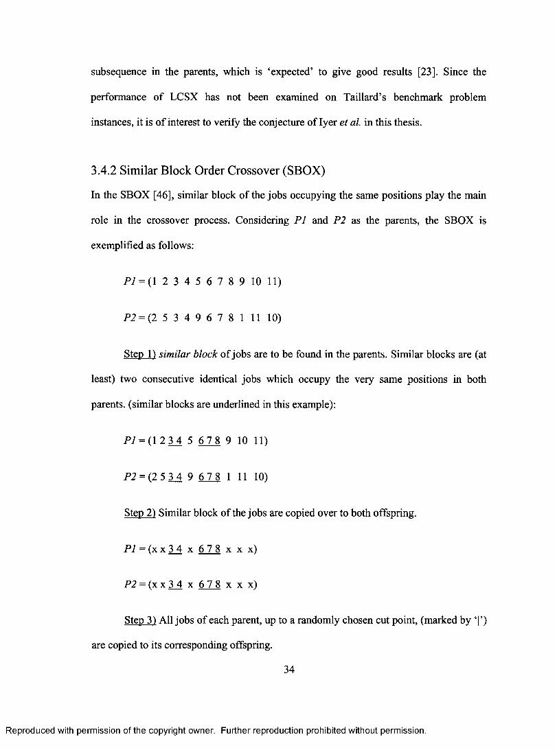
subsequence in the parents, which is 'expected' to give good results [23]. Since the
performance of LCSX has not been examined on Taillard's benchmark problem
instances, it is of interest to verify the conjecture of Iyer et al. in this thesis.
3.4.2 Similar Block Order Crossover (SBOX)
In the SBOX [46], similar block of the jobs occupying the same positions play the main
role in the crossover process. Considering P1 and P2 as the parents, the SBOX is
exemplified as follows:
P1= (1 2 3 4 5 6 7 8 9 10 11)
P2 = (2 5 3 4 9 6 7 8 1 11 10)
Step 1) similar block of jobs are to be found in the parents. Similar blocks are (at
least) two consecutive identical jobs which occupy the very same positions in both
parents. (similar blocks are underlined in this example):
P1 = (1 2 3 4 5 678 9 10 11)
P2 = (2 5 3 4 9 6 7 8 1 11 10)
Step 2) Similar block of the jobs are copied over to both offspring.
P1 = (xx34 x 678 x x x)
P2 = (xx34 x 678 xxx)
Step 31 All jobs of each parent, up to a randomly chosen cut point, (marked by 'I')
are copied to its corresponding offspring.
34
Reproduced with permission of the copyright owner. Further reproduction prohibited without permission.
subsequence in the parents, which is ‘expected’ to give good results [23]. Since the
performance o f LCSX has not been examined on Taillard’s benchmark problem
instances, it is o f interest to verify the conjecture o f Iyer et al. in this thesis.
3.4.2 Similar Block Order Crossover (SBOX)
In the SBOX [46], similar block of the jobs occupying the same positions play the main
role in the crossover process. Considering P I and P2 as the parents, the SBOX is
exemplified as follows:
P l = {\ 2 3 4 5 6 7 8 9 10 11)
P2 = (2 5 3 4 9 6 7 8 1 11 10)
Step 11 similar block o f jobs are to be found in the parents. Similar blocks are (at
least) two consecutive identical jobs which occupy the very same positions in both
parents, (similar blocks are underlined in this example):
P l = {\ 2 3 4 5 6 2 8 9 10 11)
P2 = (2 5 3_4 9 62_8 1 11 10)
Step 2) Similar block o f the jobs are copied over to both offspring.
P I = (x x 3 4 x 6 7 8 x x x)
P2 = ( x x 3_4 x 6 7 8 x x x)
Step 31 All jobs o f each parent, up to a randomly chosen cut point, (marked by ‘|’)
are copied to its corresponding offspring.
34
Reproduced with permission of the copyright owner. Further reproduction prohibited without permission.
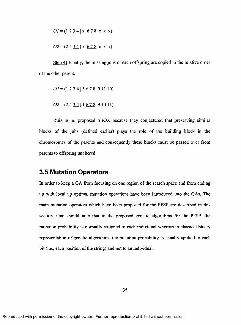
0/=(1234 Ix 678 x x x)
02 = (25341x 678 xxx)
Step 4) Finally, the missing jobs of each offspring are copied in the relative order
of the other parent.
0/ = (1 2 3 415 6 7 8 9 11 10)
02 = (2 5 3 41 1 6 7 8 9 10 11)
Ruiz et al. proposed SBOX because they conjectured that preserving similar
blocks of the jobs (defined earlier) plays the role of the building block in the
chromosomes of the parents and consequently these blocks must be passed over from
parents to offspring unaltered.
3.5 Mutation Operators
In order to keep a GA from focusing on one region of the search space and from ending
up with local up optima, mutation operations have been introduced into the GAs. The
main mutation operators which have been proposed for the PFSP are described in this
section. One should note that in the proposed genetic algorithms for the PFSP, the
mutation probability is normally assigned to each individual whereas in classical binary
representation of genetic algorithms, the mutation probability is usually applied to each
bit (i.e., each position of the string) and not to an individual.
35
Reproduced with permission of the copyright owner. Further reproduction prohibited without permission.
01 = (\ 2 3 4 | x 67_8 x x x)
0 2 = (2 5 3_4 | x 6 7 8 x x x)
Step 4) Finally, the missing jobs o f each offspring are copied in the relative order
o f the other parent.
01 = (1 2 3 4 | 5 6 7 J 9 11 10)
0 2 = (2 5 3_4 | 1 67_8 9 10 11)
Ruiz et al. proposed SBOX because they conjectured that preserving similar
blocks o f the jobs (defined earlier) plays the role o f the building block in the
chromosomes o f the parents and consequently these blocks must be passed over from
parents to offspring unaltered.
3.5 Mutation Operators
In order to keep a GA from focusing on one region o f the search space and from ending
up with local up optima, mutation operations have been introduced into the GAs. The
main mutation operators which have been proposed for the PFSP are described in this
section. One should note that in the proposed genetic algorithms for the PFSP, the
mutation probability is normally assigned to each individual whereas in classical binary
representation o f genetic algorithms, the mutation probability is usually applied to each
bit (i.e., each position o f the string) and not to an individual.
35
Reproduced with permission of the copyright owner. Further reproduction prohibited without permission.
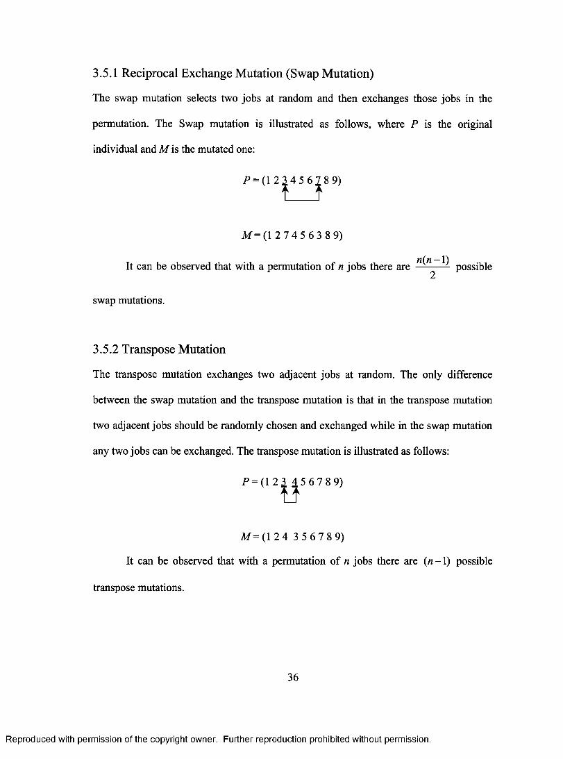
3.5.1 Reciprocal Exchange Mutation (Swap Mutation)
The swap mutation selects two jobs at random and then exchanges those jobs in the
permutation. The Swap mutation is illustrated as follows, where P is the original
individual and M is the mutated one:
P=(123456789)
t t
M= (127456389)
n — e It can be observed that with a permutation of n jobs there are n( 2 possible
swap mutations.
3.5.2 Transpose Mutation
The transpose mutation exchanges two adjacent jobs at random. The only difference
between the swap mutation and the transpose mutation is that in the transpose mutation
two adjacent jobs should be randomly chosen and exchanged while in the swap mutation
any two jobs can be exchanged. The transpose mutation is illustrated as follows:
P= (123 456789)
11
M=(124 356789)
It can be observed that with a permutation of n jobs there are (n —1) possible
transpose mutations.
36
Reproduced with permission of the copyright owner. Further reproduction prohibited without permission.
3.5.1 Reciprocal Exchange Mutation (Swap Mutation)
The swap mutation selects two jobs at random and then exchanges those jobs in the
permutation. The Swap mutation is illustrated as follows, where P is the original
individual and M is the mutated one:
P = (l 2 3 4 5 6 7 8 9)
M = (1 2 7 4 5 6 3 8 9)
It can be observed that with a permutation o f n jobs there are ^ possible
swap mutations.
3.5.2 Transpose Mutation
The transpose mutation exchanges two adjacent jobs at random. The only difference
between the swap mutation and the transpose mutation is that in the transpose mutation
two adjacent jobs should be randomly chosen and exchanged while in the swap mutation
any two jobs can be exchanged. The transpose mutation is illustrated as follows:
P = (1 2 3 4 5 6 7 8 9 )
M = ( l 2 4 3 5 6 7 8 9)
It can be observed that with a permutation o f n jobs there are (n - 1) possible
transpose mutations.
36
Reproduced with permission of the copyright owner. Further reproduction prohibited without permission.
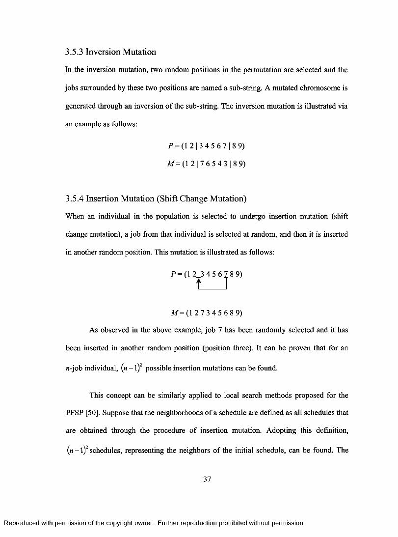
3.5.3 Inversion Mutation
In the inversion mutation, two random positions in the permutation are selected and the
jobs surrounded by these two positions are named a sub-string. A mutated chromosome is
generated through an inversion of the sub-string. The inversion mutation is illustrated via
an example as follows:
P = (12134567189)
M= (12176543189)
3.5.4 Insertion Mutation (Shift Change Mutation)
When an individual in the population is selected to undergo insertion mutation (shift
change mutation), a job from that individual is selected at random, and then it is inserted
in another random position. This mutation is illustrated as follows:
P=(12_3456789)
I'
M = (127345689)
As observed in the above example, job 7 has been randomly selected and it has
been inserted in another random position (position three). It can be proven that for an
n-job individual, (n —1)2 possible insertion mutations can be found.
This concept can be similarly applied to local search methods proposed for the
PFSP [50]. Suppose that the neighborhoods of a schedule are defined as all schedules that
are obtained through the procedure of insertion mutation. Adopting this definition,
(n — 1)2 schedules, representing the neighbors of the initial schedule, can be found. The
37
Reproduced with permission of the copyright owner. Further reproduction prohibited without permission.
3.5.3 Inversion Mutation
In the inversion mutation, two random positions in the permutation are selected and the
jobs surrounded by these two positions are named a sub-string. A mutated chromosome is
generated through an inversion of the sub-string. The inversion mutation is illustrated via
an example as follows:
P = (l 2 | 3 4 5 6 7 | 8 9)
M = ( 1 2 | 7 6 5 4 3 | 8 9)
3.5.4 Insertion Mutation (Shift Change Mutation)
When an individual in the population is selected to undergo insertion mutation (shift
change mutation), a job from that individual is selected at random, and then it is inserted
in another random position. This mutation is illustrated as follows:
P = (l 2_3 4 5 6 7 8 9)
t _______
M = (1 2 7 3 4 5 6 8 9)
As observed in the above example, job 7 has been randomly selected and it has
been inserted in another random position (position three). It can be proven that for an
H-job individual, (n - 1)2 possible insertion mutations can be found.
This concept can be similarly applied to local search methods proposed for the
PFSP [50]. Suppose that the neighborhoods o f a schedule are defined as all schedules that
are obtained through the procedure o f insertion mutation. Adopting this definition,
(n - 1)2 schedules, representing the neighbors o f the initial schedule, can be found. The
37
Reproduced with permission of the copyright owner. Further reproduction prohibited without permission.
makespan for each neighborhood can be obtained in the order of 0(nm), and since there
are (n —1)2 neighbors (schedules), the makespan of all these schedules can be calculated
in the order of 0(n3m). By adopting Taillard's approach, discussed in the preceding
chapter, the makespan for these schedules can be calculated in the order of 0(n 2m).
It has been experimentally shown that the insertion mutation outperforms other
above-mentioned mutation operations [42], [46]. In Chapter 4, a new mutation named
destruction-construction is employed in the proposed genetic algorithm. In addition, the
comparative performance of the insertion mutation and destruction-construction mutation
is discussed in that chapter.
38
Reproduced with permission of the copyright owner. Further reproduction prohibited without permission.
makespan for each neighborhood can be obtained in the order o f 0 (nm) , and since there
are (n - 1)2 neighbors (schedules), the makespan o f all these schedules can be calculated
in the order o f 0 (n 3m ). By adopting Taillard’s approach, discussed in the preceding
chapter, the makespan for these schedules can be calculated in the order o f 0 (n 2m ) .
It has been experimentally shown that the insertion mutation outperforms other
above-mentioned mutation operations [42], [46]. In Chapter 4, a new mutation named
destruction-construction is employed in the proposed genetic algorithm. In addition, the
comparative performance of the insertion mutation and destruction-construction mutation
is discussed in that chapter.
38
Reproduced with permission of the copyright owner. Further reproduction prohibited without permission.
CHAPTER 4: SOLUTION METHODOLOGY
The organization of this chapter is as follows: first, the proposed GA-based algorithm to
solve the PFSP is described. The concept of the Iterated Greedy Algorithm (IGA) of Ruiz
et al. [47] is also discussed, and then the hybrid method, combining the proposed GA
with the IGA, yielding favorable results over each individual technique, is explained.
4.1 The Structure of the Proposed GA
4.1.1 Representation and Initial Population
Similar to the existing GAs cited in the literature (e.g., [5], [23], [33], [40], [42], [46]), a
permutation of jobs is adopted to represent an individual in the population. The initial
population is recommended to be a collection of permutations that have already been
obtained through heuristic approaches [5], [46]. In the proposed GA, the initial
population is generated through a slight modification of the NEH algorithm.
The original NEH algorithm (described in Section 2.2) can be observed as a
function that initially gets a permutation of jobs and returns a new permutation based on
its input. More specifically, in the first step of the algorithm, the jobs are sorted by
decreasing sum of their processing times. Then in the steps that follow, the NEH changes
the permutation constructed in step one.
In the proposed modification of the NEH algorithm, a slight change is made in the
first step of the original NEH to produce an initial population for the genetic algorithm
39
Reproduced with permission of the copyright owner. Further reproduction prohibited without permission.
C h a p t e r 4: So l u t io n M e t h o d o l o g y
The organization o f this chapter is as follows: first, the proposed GA-based algorithm to
solve the PFSP is described. The concept o f the Iterated Greedy Algorithm (IGA) of Ruiz
et al. [47] is also discussed, and then the hybrid method, combining the proposed GA
with the IGA, yielding favorable results over each individual technique, is explained.
4.1 The Structure of the Proposed GA
4.1.1 Representation and Initial Population
Similar to the existing GAs cited in the literature (e.g., [5], [23], [33], [40], [42], [46]), a
permutation o f jobs is adopted to represent an individual in the population. The initial
population is recommended to be a collection o f permutations that have already been
obtained through heuristic approaches [5], [46]. In the proposed GA, the initial
population is generated through a slight modification o f the NEH algorithm.
The original NEH algorithm (described in Section 2.2) can be observed as a
function that initially gets a permutation o f jobs and returns a new permutation based on
its input. More specifically, in the first step of the algorithm, the jobs are sorted by
decreasing sum of their processing times. Then in the steps that follow, the NEH changes
the permutation constructed in step one.
In the proposed modification of the NEH algorithm, a slight change is made in the
first step o f the original NEH to produce an initial population for the genetic algorithm
39
Reproduced with permission of the copyright owner. Further reproduction prohibited without permission.
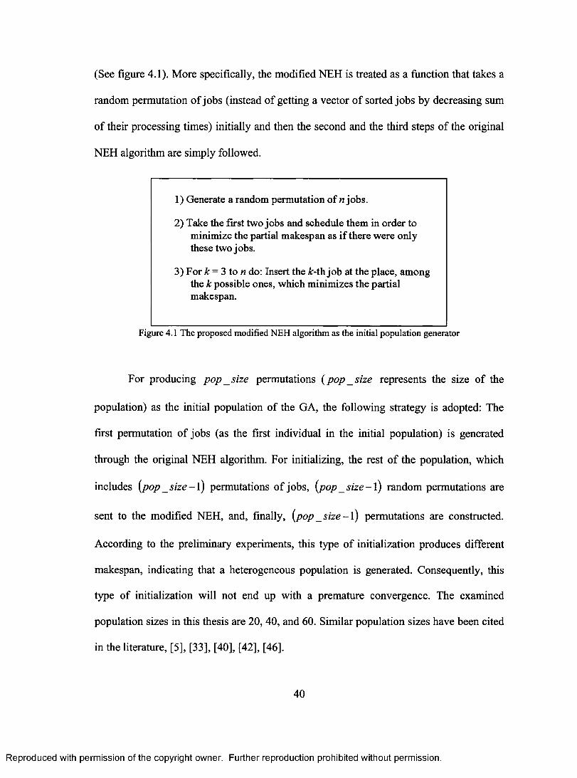
(See figure 4.1). More specifically, the modified NEH is treated as a function that takes a
random permutation of jobs (instead of getting a vector of sorted jobs by decreasing sum
of their processing times) initially and then the second and the third steps of the original
NEH algorithm are simply followed.
1) Generate a random permutation of n jobs.
2) Take the first two jobs and schedule them in order to minimize the partial makespan as if there were only these two jobs.
3) For k = 3 to n do: Insert the k-th job at the place, among the k possible ones, which minimizes the partial makespan.
Figure 4.1 The proposed modified NEH algorithm as the initial population generator
For producing pop _ size permutations (pop _ size represents the size of the
population) as the initial population of the GA, the following strategy is adopted: The
first permutation of jobs (as the first individual in the initial population) is generated
through the original NEH algorithm. For initializing, the rest of the population, which
includes (pop _ size —1) permutations of jobs, (pop _ size —1) random permutations are
sent to the modified NEH, and, finally, (pop _ size —1) permutations are constructed.
According to the preliminary experiments, this type of initialization produces different
makespan, indicating that a heterogeneous population is generated. Consequently, this
type of initialization will not end up with a premature convergence. The examined
population sizes in this thesis are 20, 40, and 60. Similar population sizes have been cited
in the literature, [5], [33], [40], [42], [46].
40
Reproduced with permission of the copyright owner. Further reproduction prohibited without permission.
(See figure 4.1). More specifically, the modified NEH is treated as a function that takes a
random permutation o f jobs (instead of getting a vector o f sorted jobs by decreasing sum
of their processing times) initially and then the second and the third steps o f the original
NEH algorithm are simply followed.
1) Generate a random permutation of n jobs.
2) Take the first two jobs and schedule them in order tominimize the partial makespan as if there were only these two jobs.
3) For k = 3 to n do: Insert the k-tb. job at the place, amongthe k possible ones, which minimizes the partial makespan.
Figure 4.1 The proposed modified NEH algorithm as the initial population generator
For producing pop_size permutations (p o p _ size represents the size o f the
population) as the initial population o f the GA, the following strategy is adopted: The
first permutation of jobs (as the first individual in the initial population) is generated
through the original NEH algorithm. For initializing, the rest o f the population, which
includes (pop _ s iz e -1 ) permutations o f jobs, (pop s iz e - \ ) random permutations are
sent to the modified NEH, and, finally, (pop size - l ) permutations are constructed.
According to the preliminary experiments, this type o f initialization produces different
makespan, indicating that a heterogeneous population is generated. Consequently, this
type of initialization will not end up with a premature convergence. The examined
population sizes in this thesis are 20, 40, and 60. Similar population sizes have been cited
in the literature, [5], [33], [40], [42], [46],
40
Reproduced with permission of the copyright owner. Further reproduction prohibited without permission.
4.1.2 Selection Mechanisms
Elitist selection is employed in the GA in a way that the top ten percent of individuals in
every generation are directly copied into the next generation.
Two classical selection types are examined for the selection of parents; namely
rank-based selection and tournament selection (described in Sections 3.3.2 and 3.3.3,
respectively). Regardless of the adopted selection type, the selection mechanism produces
a set of permutations (referred to as candidacy list hereinafter) with the size of
0.90 x pop _size.
In rank-based selection, the notion of linear rank scaling with the selective
pressure of two is applied. The rationale behind this selection type was described in
Section 3.3.2.
The other implemented selection type is the tournament selection. A tournament
size of two, as cited in the literature is used [19], [30]. For implementing the tournament
selection mechanism, 0.90 x pop _ size tournaments will be performed. In each
tournament, two individuals are selected at random from the population (i.e., a selection
procedure with replacement), and one which has the lower makespan is selected and
added to the candidacy list.
4.1.3 Crossover and Mutation Mechanisms
When a candidacy list is thoroughly produced through selection, its individuals are paired
according to their order in the list. It is noteworthy that regardless of the selection type
employed, the candidacy list is filled with individuals in a way that every two
41
Reproduced with permission of the copyright owner. Further reproduction prohibited without permission.
4.1.2 Selection Mechanisms
Elitist selection is employed in the GA in a way that the top ten percent o f individuals in
every generation are directly copied into the next generation.,
Two classical selection types are examined for the selection o f parents; namely
rank-based selection and tournament selection (described in Sections 3.3.2 and 3.3.3,
respectively). Regardless o f the adopted selection type, the selection mechanism produces
a set o f permutations (referred to as candidacy list hereinafter) with the size of
0.90x pop size.
In rank-based selection, the notion of linear rank scaling with the selective
pressure o f two is applied. The rationale behind this selection type was described in
Section 3.3.2.
The other implemented selection type is the tournament selection. A tournament
size of two, as cited in the literature is used [19], [30]. For implementing the tournament
selection mechanism, 0.90 x pop _size tournaments will be performed. In each
tournament, two individuals are selected at random from the population (i.e., a selection
procedure with replacement), and one which has the lower makespan is selected and
added to the candidacy list.
4.1.3 Crossover and Mutation Mechanisms
When a candidacy list is thoroughly produced through selection, its individuals are paired
according to their order in the list. It is noteworthy that regardless o f the selection type
employed, the candidacy list is filled with individuals in a way that every two
41
Reproduced with permission of the copyright owner. Further reproduction prohibited without permission.

consecutive individuals in the list are statistically independent. In other words, there is no
need to perform an additional procedure to pair the individuals from the candidacy list at
random.
size x pop _ According to the aforementioned selection strategy,
0.90 pairs of
2
consecutive individuals exist in the candidacy list (i.e., the first and second individuals as
the first pair, the third and fourth individuals as the second pair, and so on). A fraction of
these pairs are randomly chosen (with the probability of pc) to undergo crossover
operation in the next step. Each pair which undergoes crossover operation produces two
offspring that replace the parents in the candidacy list. If a pair is not chosen for
crossover, they will remain intact in the candidacy list. Consequently, after applying the
crossover, the number of individuals in the candidacy list remains unchanged. LCSX and
SBOX, described in Sections 3.4.1 and 3.4.2, are examined as the crossover operators.
As stated in Section 3.4, Ruiz et al. [46] have recently shown that SBOX
outperforms One Point Crossover, Order Crossover, Partially-Mapped Crossover, Two
Point Crossover, Similar Job Order Crossover, Similar Job 2-Point Order Crossover,
Similar Block 2-Point Order Crossover operators cited in the literature. However, Ruiz
et al. have not tested the performance of LCSX in their algorithm. Furthermore, the
performance of the LCSX on standard benchmarks of Taillard has not been investigated
in the literature. The performance of the SBOX and LCSX in the proposed algorithm is
extensively studied in this thesis.
After applying the crossover operators, a fraction of individuals in the candidacy
list are randomly chosen to undergo mutation operator. More specifically, the mutation
42
Reproduced with permission of the copyright owner. Further reproduction prohibited without permission.
consecutive individuals in the list are statistically independent. In other words, there is no
need to perform an additional procedure to pair the individuals from the candidacy list at
random.
According to the aforementioned selection strategy, ^ x P°P - iS7ze pajrs 0f
consecutive individuals exist in the candidacy list (i.e., the first and second individuals as
the first pair, the third and fourth individuals as the second pair, and so on). A fraction of
these pairs are randomly chosen (with the probability of p c) to undergo crossover
operation in the next step. Each pair which undergoes crossover operation produces two
offspring that replace the parents in the candidacy list. If a pair is not chosen for
crossover, they will remain intact in the candidacy list. Consequently, after applying the
crossover, the number o f individuals in the candidacy list remains unchanged. LCSX and
SBOX, described in Sections 3.4.1 and 3.4.2, are examined as the crossover operators.
As stated in Section 3.4, Ruiz et al. [46] have recently shown that SBOX
outperforms One Point Crossover, Order Crossover, Partially-Mapped Crossover, Two
Point Crossover, Similar Job Order Crossover, Similar Job 2-Point Order Crossover,
Similar Block 2-Point Order Crossover operators cited in the literature. However, Ruiz
et al. have not tested the performance o f LCSX in their algorithm. Furthermore, the
performance o f the LCSX on standard benchmarks o f Taillard has not been investigated
in the literature. The performance o f the SBOX and LCSX in the proposed algorithm is
extensively studied in this thesis.
After applying the crossover operators, a fraction o f individuals in the candidacy
list are randomly chosen to undergo mutation operator. More specifically, the mutation
42
Reproduced with permission of the copyright owner. Further reproduction prohibited without permission.
operator, with a probability of pm, is applied to each individual of the candidacy list. Two
mutation operators are examined in the proposed algorithm; namely insertion mutation
and destruction-construction mutation. The destruction-construction mutation operation is
the same as destruction and construction phases of the Iterated Greedy Algorithm, which
will be discussed later on. The preliminary tests show that the destruction-construction
mutation is clearly superior to the insertion mutation. Therefore, the insertion mutation
will not be considered in design of experiments (to be discussed in Chapter 5). Three
levels are considered for the mutation rate, namely, 0.10, 0.15, and 0.20.
4.1.5 Termination Condition
A time dependent termination condition of n x m x 90 milliseconds is adopted, where n
and m are the number of jobs and machines, respectively. The proposed GA is
implemented in Java (J2SE8) and is run on a personal computer with 1.4 GHz Pentium III
processor, and 2 GB of RAM. The aforementioned period (as the termination condition)
is twice the duration that Ruiz et al. [46] used in their proposed GA. In fact, Ruiz et al.
employed faster computer9 with Athlon XP 1600+ processor (running at 1400 MHz) and
512 MB of RAM (See [46] for detail).
The hybrid method based on the GA and the IGA is addressed in the next
sections. An overview of the IGA is given in Section 4.2, and the proposed hybrid
solution technique is addressed in Section 4.3.
8 Java 2 Platform, Standard Edition
9 One should admit, that it is not easy to compare the performance of these two different types of computers precisely.
43
Reproduced with permission of the copyright owner. Further reproduction prohibited without permission.
operator, with a probability o f p m, is applied to each individual o f the candidacy list. Two
mutation operators are examined in the proposed algorithm; namely insertion mutation
and destruction-construction mutation. The destruction-construction mutation operation is
the same as destruction and construction phases o f the Iterated Greedy Algorithm, which
will be discussed later on. The preliminary tests show that the destruction-construction
mutation is clearly superior to the insertion mutation. Therefore, the insertion mutation
will not be considered in design o f experiments (to be discussed in Chapter 5). Three
levels are considered for the mutation rate, namely, 0.10, 0.15, and 0.20.
4.1.5 Termination Condition
A time dependent termination condition of n x m x 90 milliseconds is adopted, where n
and m are the number o f jobs and machines, respectively. The proposed GA is
implemented in Java (J2SE8) and is run on a personal computer with 1.4 GHz Pentium III
processor, and 2 GB of RAM. The aforementioned period (as the termination condition)
is twice the duration that Ruiz et al. [46] used in their proposed GA. In fact, Ruiz et al.
employed faster computer9 with Athlon XP 1600+ processor (running at 1400 MHz) and
512 MB of RAM (See [46] for detail).
The hybrid method based on the GA and the IGA is addressed in the next
sections. An overview o f the IGA is given in Section 4.2, and the proposed hybrid
solution technique is addressed in Section 4.3.
8 Java 2 Platform, Standard Edition
9 One should admit, that it is not easy to compare the performance o f these two different types o f computers precisely.
43
Reproduced with permission of the copyright owner. Further reproduction prohibited without permission.
4.2 Iterated Greedy Algorithm
Ruiz et al. [47] have proposed an Iterated Greedy Algorithm for the PFSP recently, which
is easy to implement.
The central idea behind any Iterated Greedy Algorithm (IGA) is to iteratively
apply two main stages to the current solution (e.g., permutation, etc.); namely destruction
stage and construction stage. These two stages are problem specific and in the case of the
PFSP they are tuned by Ruiz et al. as follows: in the destruction stage, some jobs are
removed at random from the current solution, and in the construction stage, those
removed jobs are added again to the sequence in a certain pattern which will be described
later on.
The Iterated Greedy algorithm (IGA) of Ruiz et al., which is similar to the
Iterated Local Search (ILS) of Stiitzle [50] to some extent, has five components, namely,
initial solution generation, destruction, construction, local search, and acceptance
criterion.
The initial solution is found through the NEH heuristics, which is followed by a
local search. The local search, which will be described later on, explores and finds local
optimal solution in the neighborhood of the initial solution. After finding the local
optimal solution, four components, namely destruction, construction, local search, and
acceptance criterion are iteratively applied to the incumbent solution, as illustrated in the
pseudo code of the IGA in Figure 4.1.
In the destruction phase, d jobs (without repetition) are randomly removed from
the current solution, it. Removing d jobs from a permutation of n jobs, yields two partial
44
Reproduced with permission of the copyright owner. Further reproduction prohibited without permission.
4.2 Iterated Greedy Algorithm
Ruiz et al. [47] have proposed an Iterated Greedy Algorithm for the PFSP recently, which
is easy to implement.
The central idea behind any Iterated Greedy Algorithm (IGA) is to iteratively
apply two main stages to the current solution (e.g., permutation, etc.); namely destruction
stage and construction stage. These two stages are problem specific and in the case o f the
PFSP they are tuned by Ruiz et al. as follows: in the destruction stage, some jobs are
removed at random from the current solution, and in the construction stage, those
removed jobs are added again to the sequence in a certain pattern which will be described
later on.
The Iterated Greedy algorithm (IGA) o f Ruiz et al., which is similar to the
Iterated Local Search (ILS) o f Stiitzle [50] to some extent, has five components, namely,
initial solution generation, destruction, construction, local search, and acceptance
criterion.
The initial solution is found through the NEH heuristics, which is followed by a
local search. The local search, which will be described later on, explores and finds local
optimal solution in the neighborhood of the initial solution. After finding the local
optimal solution, four components, namely destruction, construction, local search, and
acceptance criterion are iteratively applied to the incumbent solution, as illustrated in the
pseudo code o f the IGA in Figure 4.1.
In the destruction phase, d jobs (without repetition) are randomly removed from
the current solution, n. Removing d jobs from a permutation o f n jobs, yields two partial
44
Reproduced with permission of the copyright owner. Further reproduction prohibited without permission.
sequences; namely ltD which contains (n — d) jobs, and 7ER which has d jobs. Needles to
say, the order in which those d jobs are removed from It is important, because this order
provides the 7ER, which is one of the two mentioned partial schedules.
In the construction phase, the jobs of ltR are re-inserted to ltD one by one
according to the 3rd step of the NEH algorithm. Thus, the first job of ltR has
(n — d +1) possible positions for insertion to RD (see the NEH algorithm in Section 2.1).
All these positions are examined and the position which yields the best makespan is
chosen. After fixing the position of the first job of 7tR in irD, the best position for the
second job of 1ER is investigated. The second job of ltR has (n — d + 2) possible positions
for insertion to nro. This procedure is repeated until the last job of ltR is inserted to irD.
One should note that Taillard's acceleration investigated in Section 2.3 is applied in
construction phase.
After the construction phase, the current solution can undergo a local search (this
can be optional). In fact, Ruiz et al. realized that this step improves the overall
performance of the IGA. The insertion-move, which is similar to the insertion mutation
operator described in Section 3.5.4, is applied as a local search technique. As mentioned
in that section, (n —1)2 possible neighborhoods can be scanned for a given permutation.
Ruiz et al. follow the strategy in which the first randomly chosen neighborhood (among
(n — 0 2 possible neighborhoods) that improves the makespan of the current solution is
applied as the output of the local search procedure [47]. In this thesis, however, a
45
Reproduced with permission of the copyright owner. Further reproduction prohibited without permission.
sequences; namely 7Ud which contains ( n - d ) jobs, and 7Er which has d jobs. Needles to
say, the order in which those d jobs are removed from it is important, because this order
provides the 7Tr , which is one o f the two mentioned partial schedules.
In the construction phase, the jobs of 7Tr are re-inserted to 7Td one by one
according to the 3rd step of the NEH algorithm. Thus, the first job of 7Tr has
( n - d + 1)possible positions for insertion to 7Td (see the NEH algorithm in Section 2.1).
All these positions are examined and the position which yields the best makespan is
chosen. After fixing the position of the first job o f 7Ir in 7tD, the best position for the
second job o f 7Cr is investigated. The second job o f 7Er has ( n - d + 2) possible positions
for insertion to 7to. This procedure is repeated until the last job o f 71r is inserted to jId.
One should note that Taillard’s acceleration investigated in Section 2.3 is applied in
construction phase.
After the construction phase, the current solution can undergo a local search (this
can be optional). In fact, Ruiz et al. realized that this step improves the overall
performance o f the IGA. The insertion-move, which is similar to the insertion mutation
operator described in Section 3.5.4, is applied as a local search technique. As mentioned
in that section, (n - 1)2 possible neighborhoods can be scanned for a given permutation.
Ruiz et al. follow the strategy in which the first randomly chosen neighborhood (among
(n - 1)2 possible neighborhoods) that improves the makespan of the current solution is
applied as the output o f the local search procedure [47]. In this thesis, however, a
45
Reproduced with permission of the copyright owner. Further reproduction prohibited without permission.
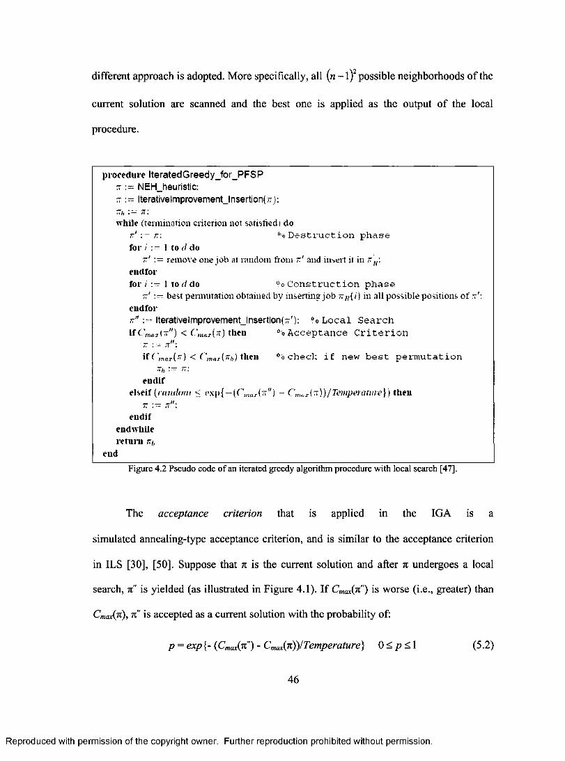
different approach is adopted. More specifically, all (n —1)2 possible neighborhoods of the
current solution are scanned and the best one is applied as the output of the local
procedure.
procedure Iterated Greedy jor_PFSP := NEH_Meuristic;
IterativelmprovemenUnsertion(7): Th
while (termination criterion not satisfied) do := Tr: % Destruction phase
for 1 to d do := remove one job at random from 771 and insert it in T fi;
endfor for i := I to d do 4 -0 Construction phase
7 1 := best permutation obtained by inserting job r R(i) in all possible positions of 7 ' :
endfor Jr" := lterativelmprovement Insertion(7'): ?-o Local Search if ( ;mu I 7 " ) < 'mar ) then
:=
if Cma.r(Tr) < rmax("A-10 then 7t, = 77:
endif elseif (random vxp{ 7" ) — Crimx ( )V TeMpOra Mi' I) then
endif endwhile return 171,
% Acceptance Criterion
end
% check. if new best permutation
Figure 4.2 Pseudo code of an iterated greedy algorithm procedure with local search [47].
The acceptance criterion that is applied in the IGA is a
simulated annealing-type acceptance criterion, and is similar to the acceptance criterion
in ILS [30], [50]. Suppose that it is the current solution and after IE undergoes a local
search, 7E" is yielded (as illustrated in Figure 4.1). If Cmax(n") is worse (i.e., greater) than
C.(n), 1E" is accepted as a current solution with the probability of:
p = exp {- (Cmax(e) - Cmax(7t))1Temperature} 0 p 1 (5.2)
46
Reproduced with permission of the copyright owner. Further reproduction prohibited without permission.
different approach is adopted. More specifically, all (n - 1)2 possible neighborhoods o f the
current solution are scanned and the best one is applied as the output o f the local
procedure.
procedure lteratedGreedy_for_PFSP 7T := NEH_heuristic: rrIterativelmprovementJnsertion(Tr):~i, n';while (termination criterion not satisfied) do
rd := ,v: °oDestruction phasefor / 1 to d do
:= remove one job at random from and insert it in ~ {(\eudforfor i 1 to d do ° o Construction phase
tt' best pennutation obtained by inserting job in all possible positions o f tt' :
eudfortr" := lterativelmprovement_lnsertion{-'): °o Local Searchif t ’mnji'") < f mrtxl'T) then °o Acceptance Criterion
t t n " :
if ( ' m u r i x ) < ( 'max( ~ h ) then 06 check if new best permutationttfc
endifelseif {ran dom < oxp{ —(CmnJ.(^") - C nuis(tt) ) / Tcinpeitiniit?}) theu
__ ._fi , — il .
eudif endwhile retttru rr,,
end
Figure 4.2 Pseudo code o f an iterated greedy algorithm procedure with local search [47].
The acceptance criterion that is applied in the IGA is a
simulated annealing-type acceptance criterion, and is similar to the acceptance criterion
in ILS [30], [50]. Suppose that 7t is the current solution and after 7t undergoes a local
search, Tt" is yielded (as illustrated in Figure 4.1). If Cmax(n") is worse (i.e., greater) than
Cmax(n), Tt" is accepted as a current solution with the probability of:
p = exp{- (Cmaxiti") - Cmax(n))/Temperature) 0 < p < 1 (5.2)
46
Reproduced with permission of the copyright owner. Further reproduction prohibited without permission.
If C'„,„,(7r") is better than Cm (7t), 7C" is then accepted. Temperature in the
implementation of Ruiz et al. is a constant parameter that should be tuned offline. One
should note that 7rb in Figure 4.2 keeps track of the best visited solution. 7rb is returned
after the termination condition is satisfied.
Two parameters of IGA, namely T and d (where T and d represent the
Temperature and the number of jobs to be removed in the destruction phase,
respectively), were tuned by Ruiz et al. through the design of experiments. As a result of
experimental analysis, they found that the IGA with d = 4 and T = 0.4 yields the best
results in terms of the relative percentage deviation from best-known solution of
Taillard's instances.
Before dealing with the hybridization of the GA, it is noteworthy that the
mutation operation considered for the proposed GA consists of two phases, namely the
destruction and the construction phases of the IGA with d = 4.
4.3 Hybridization with Iterated Greedy Algorithm
The idea of hybridization of the GA with other heuristics has been investigated for
solving the PFPS in the literature. Murata et al. examined genetic local search and genetic
simulated annealing as two hybridization of genetic algorithm [33]. They showed that a
genetic local search outperforms the non-hybrid genetic algorithms and genetic simulated
annealing. In their genetic local search, the local search is added as an improvement
phase. In that improvement phase, all individuals of the current population of the GA
iteratively undergo a local search before going through the selection phase. The
disadvantage of their approach is that the local search becomes very time consuming.
47
Reproduced with permission of the copyright owner. Further reproduction prohibited without permission.
If Cmax(n") is better than Cmax(n), % is then accepted. Temperature in the
implementation o f Ruiz et al. is a constant parameter that should be tuned offline. One
should note that 7Tb in Figure 4.2 keeps track o f the best visited solution. 7tb is returned
after the termination condition is satisfied.
Two parameters o f IGA, namely T and d (where T and d represent the
Temperature and the number o f jobs to be removed in the destruction phase,
respectively), were tuned by Ruiz et al. through the design of experiments. As a result of
experimental analysis, they found that the IGA with d = 4 and T = 0.4 yields the best
results in terms o f the relative percentage deviation from best-known solution of
Taillard’s instances.
Before dealing with the hybridization o f the GA, it is noteworthy that the
mutation operation considered for the proposed GA consists o f two phases, namely the
destruction and the construction phases o f the IGA with d = 4.
4.3 Hybridization with Iterated Greedy Algorithm
The idea of hybridization o f the GA with other heuristics has been investigated for
solving the PFPS in the literature. Murata et al. examined genetic local search and genetic
simulated annealing as two hybridization o f genetic algorithm [33]. They showed that a
genetic local search outperforms the non-hybrid genetic algorithms and genetic simulated
annealing. In their genetic local search, the local search is added as an improvement
phase. In that improvement phase, all individuals o f the current population of the GA
iteratively undergo a local search before going through the selection phase. The
disadvantage o f their approach is that the local search becomes very time consuming.
47
Reproduced with permission of the copyright owner. Further reproduction prohibited without permission.
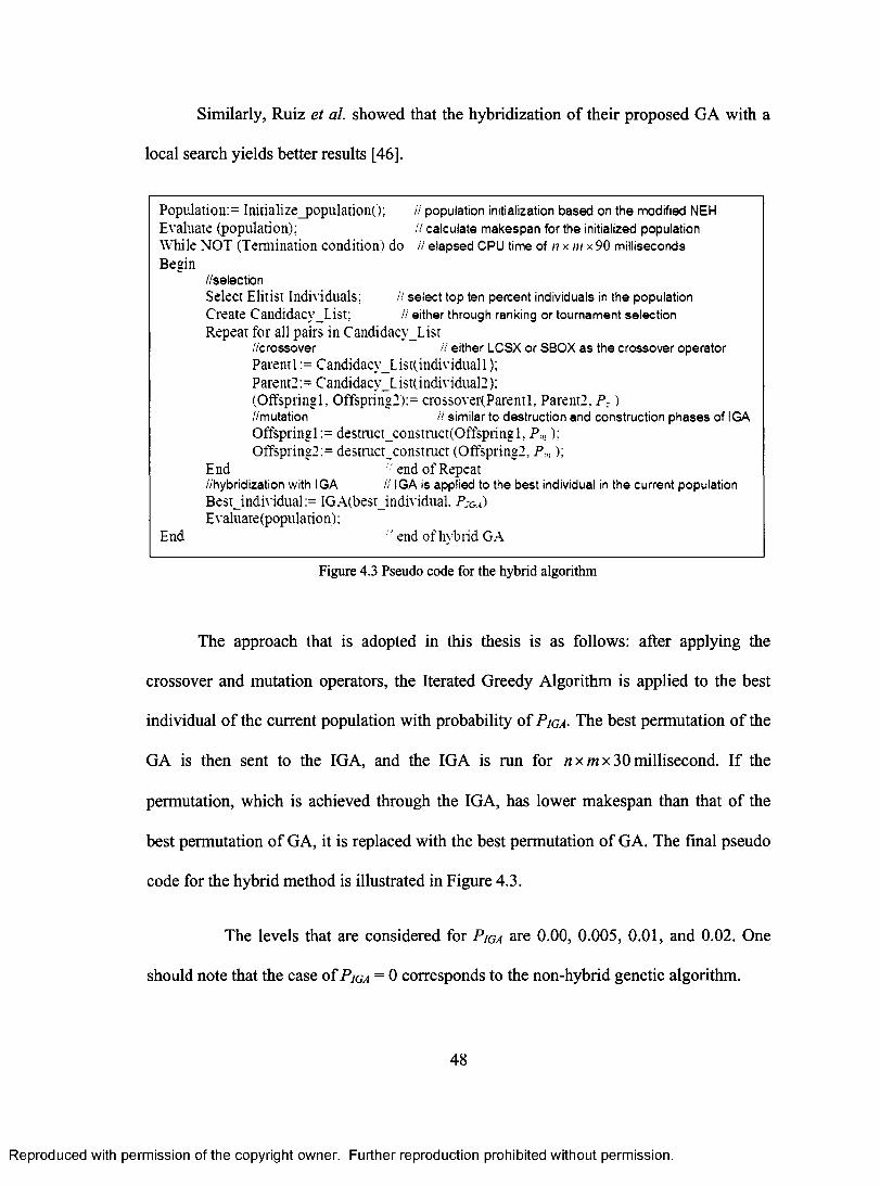
Similarly, Ruiz et al. showed that the hybridization of their proposed GA with a
local search yields better results [46].
Population:= Initialize_population(); if population initialization based on the modified NEH Evaluate (population); II calculate makespan for the initialized population While NOT (Termination condition) do elapsed CPU time of 11 x in x 90 milliseconds Begin
//selection Select Elitist Individuals: // select top ten percent individuals in the population Create Candidacy_List; either through ranking or tournament selection Repeat for all pairs in Candidacy_List
//crossover /I either LCSX or SBOX as the crossover operator Parentl:= CandidacyList(individuall); Pare nt2 = List(individual2): ndividual2 (Offspringl. Offspring2):= crossover(Parentl. Parent?, P,) //mutation similar to destruction and construction phases of IGA Offspringl := destmct_consttuct(Offspring 1, P„,); Offspring2:= destruct_constmct (Offspring2, P„,);
End end of Repeat //hybridization with IGA /1 IGA is applied to the best individual in the current population Best_individual:= IGA(best_individual, PIGA) Evaluate(population);
End " end of hybrid GA
Figure 4.3 Pseudo code for the hybrid algorithm
The approach that is adopted in this thesis is as follows: after applying the
crossover and mutation operators, the Iterated Greedy Algorithm is applied to the best
individual of the current population with probability of PIGA. The best permutation of the
GA is then sent to the IGA, and the IGA is run for n x m x 30 millisecond. If the
permutation, which is achieved through the IGA, has lower makespan than that of the
best permutation of GA, it is replaced with the best permutation of GA. The final pseudo
code for the hybrid method is illustrated in Figure 4.3.
The levels that are considered for PIGA are 0.00, 0.005, 0.01, and 0.02. One
should note that the case of PIGA = 0 corresponds to the non-hybrid genetic algorithm.
48
Reproduced with permission of the copyright owner. Further reproduction prohibited without permission.
Similarly, Ruiz et al. showed that the hybridization of their proposed GA with a
local search yields better results [46],
Population:^ Initialize_population(); // population initialization based on the modified NEH Evaluate (population); // calculate makespan for the initialized populationWhile NOT (Termination condition) do ii elapsed CPU time of n x m x 90 milliseconds Begin
//selectionSelect Elitist Individuals; // select top ten percent individuals in the populationCreate Candidacy List; ii either through ranking or tournament selectionRepeat for all pairs in Candidacv_List
//crossover ii either LCSX or SBOX as the crossover operatorParentl := Candidacv_List(individuall);Parent2:= Candidacy_List(individual2):(Offspring 1. Offspring2):= crossover(Parentlr Parent2. P : )//mutation it similar to destruction and construction phases of IGAOffspringl:= destmct_construct(Offspringl. P ,n );Offspring2:= destruct_construct (Offspring2. P ,„);
End end of Repeat//hybridization with IGA ii IGA is applied to the best individual in the current populationBest_individual:= IGA(best_individuaL PIGA)Evaluate (popula tio n);
End end of hvbrid GA
Figure 4.3 Pseudo code for the hybrid algorithm
The approach that is adopted in this thesis is as follows: after applying the
crossover and mutation operators, the Iterated Greedy Algorithm is applied to the best
individual o f the current population with probability o f P i g a- The best permutation o f the
GA is then sent to the IGA, and the IGA is run for n x m x 30 millisecond. If the
permutation, which is achieved through the IGA, has lower makespan than that o f the
best permutation o f GA, it is replaced with the best permutation o f GA. The final pseudo
code for the hybrid method is illustrated in Figure 4.3.
The levels that are considered for Piga are 0.00, 0.005, 0.01, and 0.02. One
should note that the case o f Piga = 0 corresponds to the non-hybrid genetic algorithm.
48
Reproduced with permission of the copyright owner. Further reproduction prohibited without permission.
4.4 Final Remarks on the Implementation of the Proposed Algorithm
The proposed algorithm was first implemented in MATLAB 7 using its Genetic
Algorithm and Direct Search Toolbox. Since MATLAB is a high-level programming
language, it does not need an intensive effort for implementing the proposed algorithm.
However, the drawback is that the implemented code in MATLAB needs a long time to
run as compared to low-level programming languages, such as C++, Delphi, and Java.
In order to compare the performance of the proposed algorithm with the
algorithms published in recent papers10 from a CPU time point of view, the proposed
algorithm was implemented in Java and the Java-based version of the proposed algorithm
was tested across the benchmarks of Taillard.
In Chapter 5, the tuning of the algorithm with the aforementioned parameters
through the Design of Experiments and Analysis of Variance is discussed, and the
performance of the algorithm is discussed.
10 Such as GA of Ruiz et al. [46], and IGA of Ruiz et al. [47], which are both implemented in Delphi.
49
Reproduced with permission of the copyright owner. Further reproduction prohibited without permission.
4.4 Final Remarks on the Implementation of the Proposed Algorithm
The proposed algorithm was first implemented in MATLAB 7 using its Genetic
Algorithm and Direct Search Toolbox. Since MATLAB is a high-level programming
language, it does not need an intensive effort for implementing the proposed algorithm.
However, the drawback is that the implemented code in MATLAB needs a long time to
run as compared to low-level programming languages, such as C++, Delphi, and Java.
In order to compare the performance o f the proposed algorithm with the
algorithms published in recent papers10 from a CPU time point o f view, the proposed
algorithm was implemented in Java and the Java-based version o f the proposed algorithm
was tested across the benchmarks of Taillard.
In Chapter 5, the tuning of the algorithm with the aforementioned parameters
through the Design o f Experiments and Analysis o f Variance is discussed, and the
performance o f the algorithm is discussed.
10 Such as GA o f Ruiz et al. [46], and IGA o f Ruiz et al. [47], which are both implemented in Delphi.
49
Reproduced with permission of the copyright owner. Further reproduction prohibited without permission.
CHAPTER 5: EXPERIMENTAL PARAMETER TUNING OF
THE PROPOSED ALGORITHM
In this chapter, the impact of the factors described in Chapter 4 on the performance of the
proposed GA-based algorithms to solve the PFSP is investigated through full factorial
experimental design and Analysis of Variance (ANOVA). The RPD is used as the
performance measure for this purpose. In the Design of Experiments (DOE), it is of
interest to determine which factors affect the proposed algorithms (both hybrid and non-
hybrid GA) the most. Moreover, the performances of the hybrid and non-hybrid GA are
extensively compared, and it is shown through experimental results that the hybridization
of the GA with the IGA (i.e., the hybrid GA) yields better results in terms of the RPD. It
is also shown that the proposed hybrid GA is robust".
5.1 Implementation of the Full Factorial Experimental Design
In the full factorial experimental design [61], all possible combinations of the levels
(treatments12) of the factors that are anticipated to be influential to the end results are
investigated. In this chapter, a combination of the following factors and their associated
RPDs is referred to as observations:
II According to Montgomery, the term robust algorithm is applied to an algorithm, which is influenced very slightly by the external source of variability [61].
12 In the design of experiments, every level of a factor is called a treatment.
50
Reproduced with permission of the copyright owner. Further reproduction prohibited without permission.
C h a p t e r 5: E x pe r im e n t a l Pa r a m e t e r T u n in g O f
T h e Pr o po se d A l g o r it h m
In this chapter, the impact o f the factors described in Chapter 4 on the performance of the
proposed GA-based algorithms to solve the PFSP is investigated through fu ll factorial
experimental design and Analysis o f Variance (ANOVA). The RPD is used as the
performance measure for this purpose. In the Design o f Experiments (DOE), it is of
interest to determine which factors affect the proposed algorithms (both hybrid and non
hybrid GA) the most. Moreover, the performances o f the hybrid and non-hybrid GA are
extensively compared, and it is shown through experimental results that the hybridization
o f the GA with the IGA (i.e., the hybrid GA) yields better results in terms o f the RPD. It
is also shown that the proposed hybrid GA is robustn .
5.1 Implementation of the Full Factorial Experimental Design
In the full factorial experimental design [61], all possible combinations o f the levels
(treatments12) o f the factors that are anticipated to be influential to the end results are
investigated. In this chapter, a combination o f the following factors and their associated
RPDs is referred to as observations'.
11 According to Montgomery, the term robust algorithm is applied to an algorithm, which is influenced very slightly by the external source o f variability [61].
12 In the design o f experiments, every level o f a factor is called a treatment.
50
Reproduced with permission of the copyright owner. Further reproduction prohibited without permission.
• Population size: 20, 40, and 60;
• Selection type13: tournament and rank-based selections,
• Crossover type14: LCSX and SBOX,
• Crossover probability: 0.4, 0.6, and 0.8,
• Mutation probability: 0.1, 0.15, and 0.20,
• P IGA (IGA Probability): 0.005, 0.010, and 0.020.
One should note that the population size, selection type, crossover probability,
mutation probability, and IGA probability are controllable factors in the full factorial
experimental design. In addition to those controllable factors, there are two
uncontrollable factors in the DOE, namely the number of jobs (i.e., n) and the number of
machines (i.e., m). As a result, eight factors altogether are examined in the full factorial
experimental design.
For tuning of the proposed hybrid algorithm, the set of Taillard's benchmarks (see
Section 2.4) is used. The preliminary results show that any treatment combination of the
proposed hybrid algorithm to find the optimal solution for almost all small instances
(namely, the instances with the sizes of 20 x 5 , 20 x10 , 20 x 20 and 50 x 5 , which are
labeled as ta001 to ta040 in the literature). Therefore, in the design of experiments these
instances are not used. In addition, instances with the size of 100 x 5 (labeled as ta061 to
ta070) are not considered in the design of experiment for the same reason.
13 Hereinafter, tournament and rank-based selections will be denoted in the DOE by selection type 1 and 2, respectively.
14 Hereinafter, LCSX and SBOX will be denoted by crossover type 1 and 2, respectively.
51
Reproduced with permission of the copyright owner. Further reproduction prohibited without permission.
• Population size: 20,40, and 60;
• Selection type13: tournament and rank-based selections,
• Crossover type14: LCSX and SBOX,
• Crossover probability: 0.4,0.6, and 0.8,
• Mutation probability: 0.1, 0.15, and 0.20,
• P ig a (IGA Probability): 0.005, 0.010, and 0.020.
One should note that the population size, selection type, crossover probability,
mutation probability, and IGA probability are controllable factors in the full factorial
experimental design. In addition to those controllable factors, there are two
uncontrollable factors in the DOE, namely the number o f jobs (i.e., n) and the number of
machines (i.e., m). As a result, eight factors altogether are examined in the full factorial
experimental design.
For tuning of the proposed hybrid algorithm, the set of Taillard’s benchmarks (see
Section 2.4) is used. The preliminary results show that any treatment combination o f the
proposed hybrid algorithm to find the optimal solution for almost all small instances
(namely, the instances with the sizes o f 2 0 x 5 ,2 0 x 1 0 , 20x20 and 50x 5 , which are
labeled as taOOl to ta040 in the literature). Therefore, in the design of experiments these
instances are not used. In addition, instances with the size of 100 x 5 (labeled as ta061 to
ta.070) are not considered in the design o f experiment for the same reason.
13 Hereinafter, tournament and rank-based selections will be denoted in the DOE by selection type 1 and 2, respectively.
14 Hereinafter, LCSX and SBOX will be denoted by crossover type 1 and 2, respectively.
51
Reproduced with permission of the copyright owner. Further reproduction prohibited without permission.

The instances used in the design of experiment are as follows: five out of ten
instances with the size of 50 x10 (namely, ta041, ta043, ta045, ta047, and ta049), five
out of ten instances with the size of 50 x 20 (namely, ta051, ta053, ta055, ta057, and
ta059), five out of ten instances with the size of 100 x10 (namely, ta071, ta073, ta075,
ta077, and ta079), five out of ten instances with the size of 100x 20 (namely, ta081,
ta083, ta085, ta087, and ta089), five out of ten instances with the size of
200 x10 (namely, ta091, ta093, ta095, ta097, and ta099), and finally five out of ten
instances with the size of 200 x 20 (namely, ta101, ta103, ta105, ta107, and ta109).
Noticeably, 324 combinations of the controllable factors should be employed for
each of 30 above-mentioned instances. Consequently, 9,720 observations are needed to
conduct all possible combinations of the factors for 30 chosen instances. Since four
replicates15 are carried out for the hybrid GA, 38,880 observations are totally needed. In
short, for the implementation of full factorial experimental design the effects of these
38,880 observations were investigated on their corresponding RPDs as the response
variable, and the results will be discussed in the next section.
5.2 Analysis of Variance for the Proposed Hybrid Algorithm
The full factorial design with aforementioned characteristics is conducted in MINITAB
Statistical Software. MINITAB generates an ANOVA table as the output of factorial
design. ANOVA is a statistical inference technique through tests of hypotheses. Each of
15 The number of runs of the DOE on the same treatment combination is referred to as the number of replicates. The replication allows the experimenter to obtain a more precise estimate of the effect of factors [61].
52
Reproduced with permission of the copyright owner. Further reproduction prohibited without permission.
The instances used in the design of experiment are as follows: five out o f ten
instances with the size o f 50x10 (namely, ta041, ta043, ta045, ta047, and ta049), five
out o f ten instances with the size of 50x 20 (namely, ta051, ta053, ta055, ta057, and
ta059), five out o f ten instances with the size o f 100x10 (namely, ta071, ta073, ta.075,
ta077, and ta079), five out o f ten instances with the size o f 100x20 (namely, ta081,
ta083, ta085, ta087, and ta089), five out o f ten instances with the size of
200x10 (namely, ta091, ta093, ta095, ta097, and ta099), and finally five out o f ten
instances with the size o f 200x20 (namely, talO l, ta!03, tal05, ta!07, and tal09).
Noticeably, 324 combinations o f the controllable factors should be employed for
each of 30 above-mentioned instances. Consequently, 9,720 observations are needed to
conduct all possible combinations o f the factors for 30 chosen instances. Since four
replicates15 are carried out for the hybrid GA, 38,880 observations are totally needed. In
short, for the implementation of full factorial experimental design the effects of these
38,880 observations were investigated on their corresponding RPDs as the response
variable, and the results will be discussed in the next section.
5.2 Analysis of Variance for the Proposed Hybrid Algorithm
The full factorial design with aforementioned characteristics is conducted in MINITAB
Statistical Software. MINITAB generates an ANOVA table as the output o f factorial
design. ANOVA is a statistical inference technique through tests o f hypotheses. Each of
15 The number o f runs o f the DOE on the same treatment combination is referred to as the number of replicates. The replication allows the experimenter to obtain a more precise estimate o f the effect o f factors [61].
52
Reproduced with permission of the copyright owner. Further reproduction prohibited without permission.
the tests comprises two hypotheses: the null hypothesis (indicated by Ho), and the
alternative hypothesis (indicated by H1).
In the null hypothesis, it is assumed that the effects of different levels of a factor
are equal on the response variable. In the null hypothesis, it is claimed that the difference
in the average response across different levels of a factor is not statistically significant. In
the alternative hypothesis, it is assumed that at least two levels of a factor are not equal in
terms of the obtained response variable.
In addition, if the number of factors involved in the experiment is more than one,
it might be of interest to detect a possible interaction between two (or among more than
two) factors through hypothesis tests. Statistically speaking, the probability of rejection
of the null hypothesis when it is true is called the level of significance (also it is referred
to as the probability of committing type I error), [61]. On the other hand, acceptance of
the null hypothesis when it is false is called a type II error.
In the proposed algorithm, several hypotheses tests were performed. More
specifically, the effects of each of the eight16 aforementioned factors are individually
investigated using hypotheses tests. Furthermore, all possible interactions of two factors,
and all possible interactions of three factors are examined using hypotheses tests. As a
result, in this statistical model 92 hypotheses tests (i.e., (0+ (82 )+ (83 ) = 92) are
conducted. ANOVA table generated by MINITAB is illustrated in Table 5.1.
16 These eight factors consist of six controllable and two uncontrollable factors that are mentioned in Section 5.1.
53
Reproduced with permission of the copyright owner. Further reproduction prohibited without permission.
the tests comprises two hypotheses: the null hypothesis (indicated by Ho), and the
alternative hypothesis (indicated by H }).
In the null hypothesis, it is assumed that the effects o f different levels o f a factor
are equal on the response variable. In the null hypothesis, it is claimed that the difference
in the average response across different levels o f a factor is not statistically significant. In
the alternative hypothesis, it is assumed that at least two levels o f a factor are not equal in
terms o f the obtained response variable.
In addition, if the number of factors involved in the experiment is more than one,
it might be o f interest to detect a possible interaction between two (or among more than
two) factors through hypothesis tests. Statistically speaking, the probability o f rejection
o f the null hypothesis when it is true is called the level o f significance (also it is referred
to as the probability o f committing type I error), [61]. On the other hand, acceptance of
the null hypothesis when it is false is called a type I I error.
In the proposed algorithm, several hypotheses tests were performed. More
specifically, the effects o f each of the eight16 aforementioned factors are individually
investigated using hypotheses tests. Furthermore, all possible interactions o f two factors,
and all possible interactions o f three factors are examined using hypotheses tests. As a
result, in this statistical model 92 hypotheses tests (i.e., ( f )+ ( | )+ (3) = 92) are
conducted. ANOVA table generated by MINITAB is illustrated in Table 5.1.
16 These eight factors consist o f six controllable and two uncontrollable factors that are mentioned in Section 5.1.
53
Reproduced with permission of the copyright owner. Further reproduction prohibited without permission.
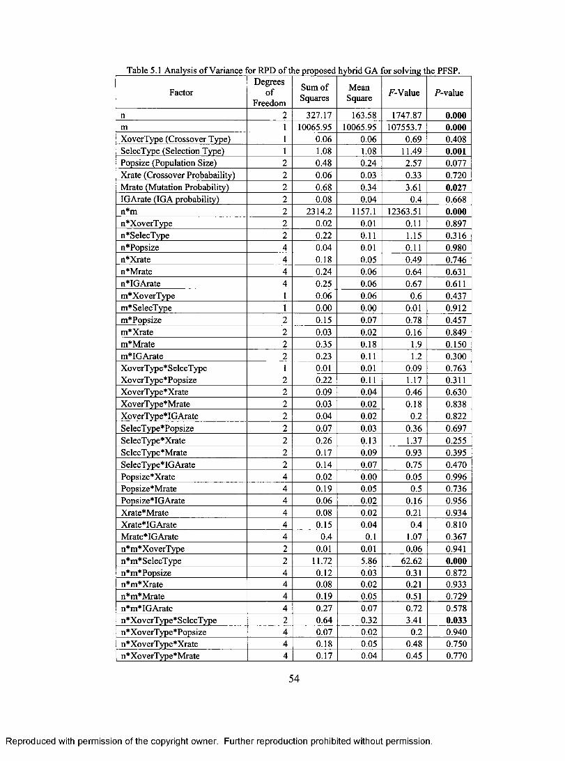
Table 5.1 Analysis of Variance for RPD of the proposed hybrid GA for solving the PFSP.
Factor Degrees
of Freedom
Sum of Squares
Mean Square
F-Value P-value
n 2 327.17 163.58 1747.87 0.000 m 1 10065.95 10065.95 107553.7 0.000 XoverType (Crossover Type) 1 0.06 0.06 0.69 0.408 SelecType (Selection Type) 1 1.08 1.08 11.49 0.001 Popsize (Population Size) 2 0.48 0.24 2.57 0.077 Xrate (Crossover Probabaility) 2 0.06 0.03 0.33 0.720 Mrate (Mutation Probability) 2 0.68 0.34 3.61 0.027 IGArate (IGA probability) 2 0.08 0.04 0.4 0.668 n*m 2 2314.2 1157.1 12363.51 0.000 n*XoverType 2 0.02 0.01 0.11 0.897 n*SelecType 2 0.22 0.11 1.15 0.316 n*Popsize 4 0.04 0.01 0.11 0.980 n*Xrate 4 0.18 0.05 0.49 0.746 n*Mrate 4 0.24 0.06 0.64 0.631 n*IGArate 4 0.25 0.06 0.67 0.611 m*XoverType 1 0.06 0.06 0.6 0.437 m*SelecType 1 0.00 0.00 0.01 0.912 m*Popsize 2 0.15 0.07 0.78 0.457 m*Xrate 2 0.03 0.02 0.16 0.849 m*Mrate 2 0.35 0.18 1.9 0.150 m*IGArate 2 0.23 0.11 1.2 0.300 XoverType*SelecType 1 0.01 0.01 0.09 0.763 XoverType*Popsize 2 0.22 0.11 1.17 0.311 XoverType*Xrate 2 0.09 0.04 0.46 0.630 XoverType*Mrate 2 0.03 0.02 0.18 0.838 XoverType*IGArate 2 0.04 0.02 0.2 0.822 SelecType*Popsize 2 0.07 0.03 0.36 0.697 SelecType*Xrate 2 0.26 0.13 1.37 0.255 SelecType*Mrate 2 0.17 0.09 0.93 0.395 SelecType*IGArate 2 0.14 0.07 0.75 0.470 Popsize*Xrate 4 0.02 0.00 0.05 0.996 Popsize*Mrate 4 0.19 0.05 0.5 0.736 Popsize*IGArate 4 0.06 0.02 0.16 0.956 Xrate*Mrate 4 0.08 0.02 0.21 0.934 Xrate*IGArate 4 0.15 0.04 0.4 0.810 Mrate*IGArate 4 0.4 0.1 1.07 0.367 n*m*XoverType 2 0.01 0.01 0.06 0.941 n*m*SelecType 2 11.72 5.86 62.62 0.000 n*m*Popsize 4 0.12 0.03 0.31 0.872 n*m*Xrate 4 0.08 0.02 0.21 0.933 n *Mrate 4 0.19 0.05 0.51 0.729 n*m*IGArate 4 0.27 0.07 0.72 0.578 n*XoverType*SelecType 2 0.64 0.32 3.41 0.033 n*XoverType*Popsize 4 0.07 0.02 0.2 0.940 n*XoverType*Xrate 4 0.18 0.05 0.48 0.750 n*XoverType*Mrate 4 0.17 0.04 0.45 0.770
54
Reproduced with permission of the copyright owner. Further reproduction prohibited without permission.
Table 5.1 Analysis o f Variance for RPD o f the proposed hybrid GA for solving the PFSP.
FactorDegrees
o fFreedom
Sum of Squares
MeanSquare
F-Value F-value
n 2 327.17 163.58 1747.87 0.000m 1 10065.95 10065.95 107553.7 0.000XoverType (Crossover Type) 1 0.06 0.06 0.69 0.408SelecType (Selection Type) 1 1.08 1.08 11.49 0.001Popsize (Population Size) 2 0.48 0.24 2.57 0.077Xrate (Crossover Probabaility) 2 0.06 0.03 0.33 0.720Mrate (Mutation Probability) 2 0.68 0.34 3.61 0.027IGArate (IGA probability) 2 0.08 0.04 0.4 0.668n*m 2 2314.2 1157.1 12363.51 0.000n*XoverType 2 0.02 0.01 0.11 0.897n*SelecType 2 0.22 0.11 1.15 0.316n*Popsize 4 0.04 0.01 0.11 0.980n*Xrate 4 0.18 0.05 0.49 0.746n*Mrate 4 0.24 0.06 0.64 0.631n*IGArate 4 0.25 0.06 0.67 0.611m*XoverType 1 0.06 0.06 0.6 0.437m*SelecType 1 0.00 0.00 0.01 0.912m*Popsize 2 0.15 0.07 0.78 0.457m*Xrate 2 0.03 0.02 0.16 0.849m*Mrate 2 0.35 0.18 1.9 0.150m* IGArate 2 0.23 0.11 1.2 0.300XoverType*SelecType 1 0.01 0.01 0.09 0.763XoverType*Popsize 2 0.22 0.11 1.17 0.311XoverType*Xrate 2 0.09 0.04 0.46 0.630XoverType*Mrate 2 0.03 0.02 0.18 0.838XoverType*IGArate 2 0.04 0.02 0.2 0.822SelecType*Popsize 2 0.07 0.03 0.36 0.697SelecType*Xrate 2 0.26 0.13 1.37 0.255SelecType*Mrate 2 0.17 0.09 0.93 0.395SelecType*IGArate 2 0.14 0.07 0.75 0.470Popsize*Xrate 4 0.02 0.00 0.05 0.996Popsize*Mrate 4 0.19 0.05 0.5 0.736Popsize*IGArate 4 0.06 0.02 0.16 0.956Xrate*Mrate 4 0.08 0.02 0.21 0.934Xrate*IGArate 4 0.15 0.04 0.4 0.810Mrate*IGArate 4 0.4 0.1 1.07 0.367n*m*XoverType 2 0.01 0.01 0.06 0.941n*m*SelecType 2 11.72 5.86 62.62 0.000n*m*Popsize 4 0.12 0.03 0.31 0.872n*m*Xrate 4 0.08 0.02 0.21 0.933n*m*Mrate 4 0.19 0.05 0.51 0.729n*m*IGArate 4 0.27 0.07 0.72 0.578n*XoverType*SelecType 2 0.64 0.32 3.41 0.033n*XoverType*Popsize 4 0.07 0.02 0.2 0.940n*XoverType*Xrate 4 0.18 0.05 0.48 0.750n*XoverType*Mrate 4 0.17 0.04 0.45 0.770
54
Reproduced with permission of the copyright owner. Further reproduction prohibited without permission.
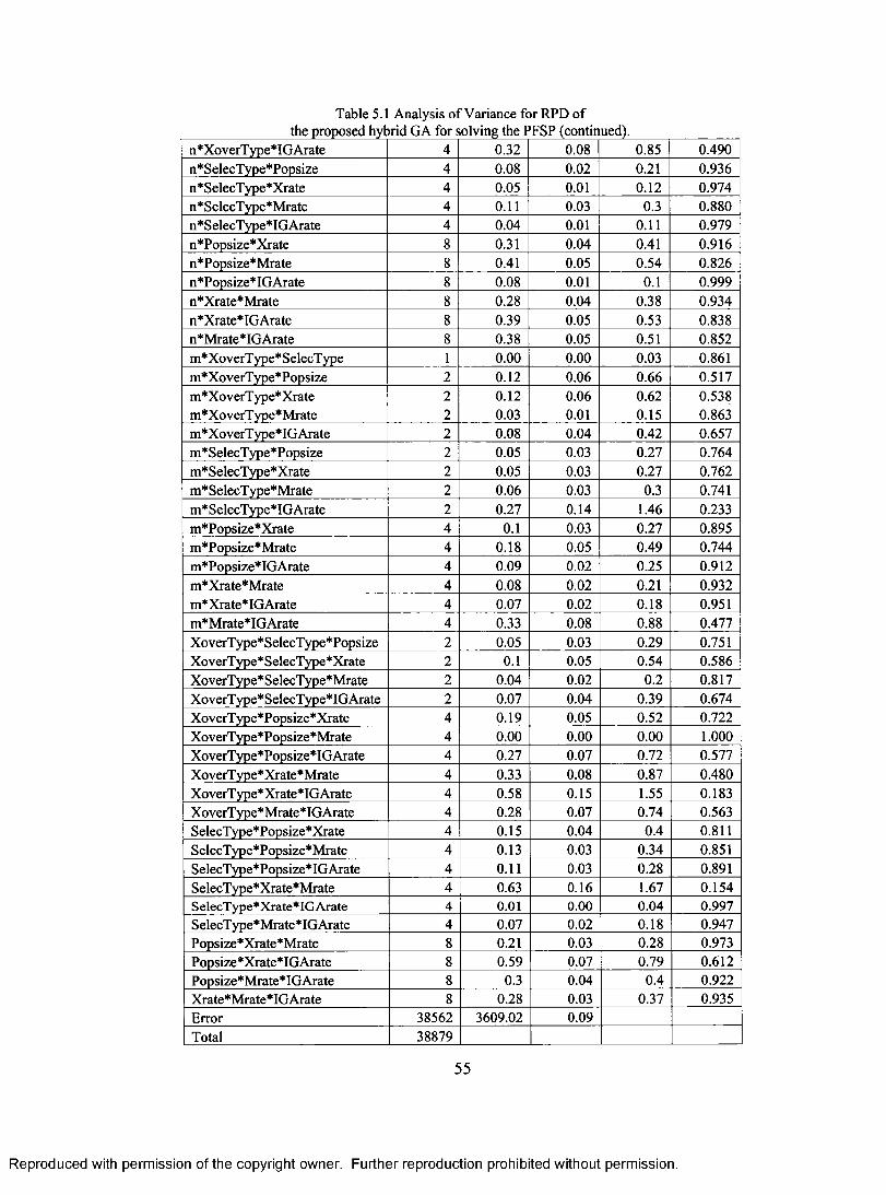
Table 5.1 Analysis of Variance for RPD of the nronosed hybrid GA for solving the PFSP (continued).
n*XoverType*IGArate 4 0.32 0.08 0.85 0.490 n*SelecType*Popsize 4 0.08 0.02 0.21 0.936 n*SelecType*Xrate 4 0.05 0.01 0.12 0.974 n*SelecType*Mrate 4 0.11 0.03 0.3 0.880 n*SelecType*IGArate 4 0.04 0.01 0.11 0.979 n*Popsize*Xrate 8 0.31 0.04 0.41 0.916 n*Po size*Mrate 8 0.41 0.05 0.54 0.826 n*Popsize*IGArate 8 0.08 0.01 0.1 0.999 n*Xrate*Mrate 8 0.28 0.04 0.38 0.934 n*Xrate*IGArate 8 0.39 0.05 0.53 0.838 n*Mrate*IGArate 8 0.38 0.05 0.51 0.852 m*XoverType*SelecType 1 0.00 0.00 0.03 0.861 m*XoverType*Popsize 2 0.12 0.06 0.66 0.517 m*XoverType*Xrate 2 0.12 0.06 0.62 0.538 m*XoverType*Mrate 2 0.03 0.01 0.15 0.863 m*XoverType*IGArate 2 0.08 0.04 0.42 0.657 m*SelecType*Popsize 2 0.05 0.03 0.27 0.764 m*SelecType*Xrate 2 0.05 0.03 0.27 0.762 m*SelecType*Mrate 2 0.06 0.03 0.3 0.741 m*SelecType*IGArate 2 0.27 0.14 1.46 0.233 m*Popsize*Xrate 4 0.1 0.03 0.27 0.895 m*Popsize*Mrate 4 0.18 0.05 0.49 0.744 m*Popsize*IGArate 4 0.09 0.02 0.25 0.912 m*Xrate*Mrate 4 0.08 0.02 0.21 0.932 m*Xrate*IGArate 4 0.07 0.02 0.18 0.951 m*Mrate*IGArate 4 0.33 0.08 0.88 0.477 XoverType*SelecType*Popsize 2 0.05 0.03 0.29 0.751 XoverType*SelecType*Xrate 2 0.1 0.05 0.54 0.586 XoverType*SelecType*Mrate 2 0.04 0.02 0.2 0.817 XoverType*SelecType*IGArate 2 0.07 0.04 0.39 0.674 XoverType*Popsize*Xrate 4 0.19 0.05 0.52 0.722 XoverType*Popsize*Mrate 4 0.00 0.00 0.00 1.000 XoverType*Popsize*IGArate 4 0.27 0.07 0.72 0.577 XoverType*Xrate*Mrate 4 0.33 0.08 0.87 0.480 XoverType*Xrate*IGArate 4 0.58 0.15 1.55 0.183 XoverType*Mrate*IGArate 4 0.28 0.07 0.74 0.563 SelecType*Popsize*Xrate 4 0.15 0.04 0.4 0.811 SelecType*Popsize*Mrate 4 0.13 0.03 0.34 0.851 SelecType*Popsize*IGArate 4 0.11 0.03 0.28 0.891 SelecType*Xrate*Mrate 4 0.63 0.16 1.67 0.154 SelecType*Xrate*IGArate 4 0.01 0.00 0.04 0.997 SelecType*Mrate*IGArate 4 0.07 0.02 0.18 0.947 Popsize*Xrate*Mrate 8 0.21 0.03 0.28 0.973 Popsize*Xrate*IGArate 8 0.59 0.07 0.79 0.612 Popsize*Mrate*IGArate 8 0.3 0.04 0.4 0.922 Xrate*Mrate*IGArate 8 0.28 0.03 0.37 0.935 Error 38562 3609.02 0.09 Total 38879
55
Reproduced with permission of the copyright owner. Further reproduction prohibited without permission.
Table 5.1 Analysis o f Variance for RPD o fthe proposed hybrid GA for solving the PFSP (continued).
n*XoverType*IGArate 4 0.32 0.08 0.85 0.490n*SelecType*Popsize 4 0.08 0.02 0.21 0.936n*SelecType*Xrate 4 0.05 0.01 0.12 0.974n*SelecType*Mrate 4 0.11 0.03 0.3 0.880n*SelecType*IGArate 4 0.04 0.01 0.11 0.979n*Popsize*Xrate 8 0.31 0.04 0.41 0.916n*Popsize*Mrate 8 0.41 0.05 0.54 0.826n*Popsize*IGArate 8 0.08 0.01 0.1 0.999n*Xrate*Mrate 8 0.28 0.04 0.38 0.934n*Xrate*IGArate 8 0.39 0.05 0.53 0.838n*Mrate*IGArate 8 0.38 0.05 0.51 0.852m* XoverType* SelecType 1 0.00 0.00 0.03 0.861m*XoverType*Popsize 2 0.12 0.06 0.66 0.517m*XoverType* Xrate 2 0.12 0.06 0.62 0.538m*XoverType*Mrate 2 0.03 0.01 0.15 0.863m*XoverType*IGArate 2 0.08 0.04 0.42 0.657m*SelecType*Popsize 2 0.05 0.03 0.27 0.764m*SelecType*Xrate 2 0.05 0.03 0.27 0.762m*SelecType*Mrate 2 0.06 0.03 0.3 0.741m*SelecType*IGArate 2 0.27 0.14 1.46 0.233m*Popsize*Xrate 4 0.1 0.03 0.27 0.895m*Popsize*Mrate 4 0.18 0.05 0.49 0.744m*Popsize*IGArate 4 0.09 0.02 0.25 0.912m*Xrate*Mrate 4 0.08 0.02 0.21 0.932m*Xrate*IGArate 4 0.07 0.02 0.18 0.951m*Mrate*IGArate 4 0.33 0.08 0.88 0.477XoverType*SelecType*Popsize 2 0.05 0.03 0.29 0.751XoverType*SelecType*Xrate 2 0.1 0.05 0.54 0.586XoverType*SelecType*Mrate 2 0.04 0.02 0.2 0.817XoverType*SelecType*IGArate 2 0.07 0.04 0.39 0.674XoverType*Popsize*Xrate 4 0.19 0.05 0.52 0.722XoverType*Popsize*Mrate 4 0.00 0.00 0.00 1.000XoverType*Popsize*IGArate 4 0.27 0.07 0.72 0.577XoverType * Xrate * Mrate 4 0.33 0.08 0.87 0.480XoverType*Xrate*IGArate 4 0.58 0.15 1.55 0.183XoverType*Mrate*IGArate 4 0.28 0.07 0.74 0.563SelecType*Popsize*Xrate 4 0.15 0.04 0.4 0.811SelecType*Popsize*Mrate 4 0.13 0.03 0.34 0.851SelecType*Popsize*IGArate 4 0.11 0.03 0.28 0.891SelecType*Xrate*Mrate 4 0.63 0.16 1.67 0.154SelecType*Xrate*IGArate 4 0.01 0.00 0.04 0.997SelecType*Mrate*IGArate 4 0.07 0.02 0.18 0.947Popsize*Xrate*Mrate 8 0.21 0.03 0.28 0.973Popsize*Xrate*IGArate 8 0.59 0.07 0.79 0.612Popsize*Mrate*IGArate 8 0.3 0.04 0.4 0.922Xrate*Mrate*IGArate 8 0.28 0.03 0.37 0.935Error 38562 3609.02 0.09Total 38879
55
Reproduced with permission of the copyright owner. Further reproduction prohibited without permission.
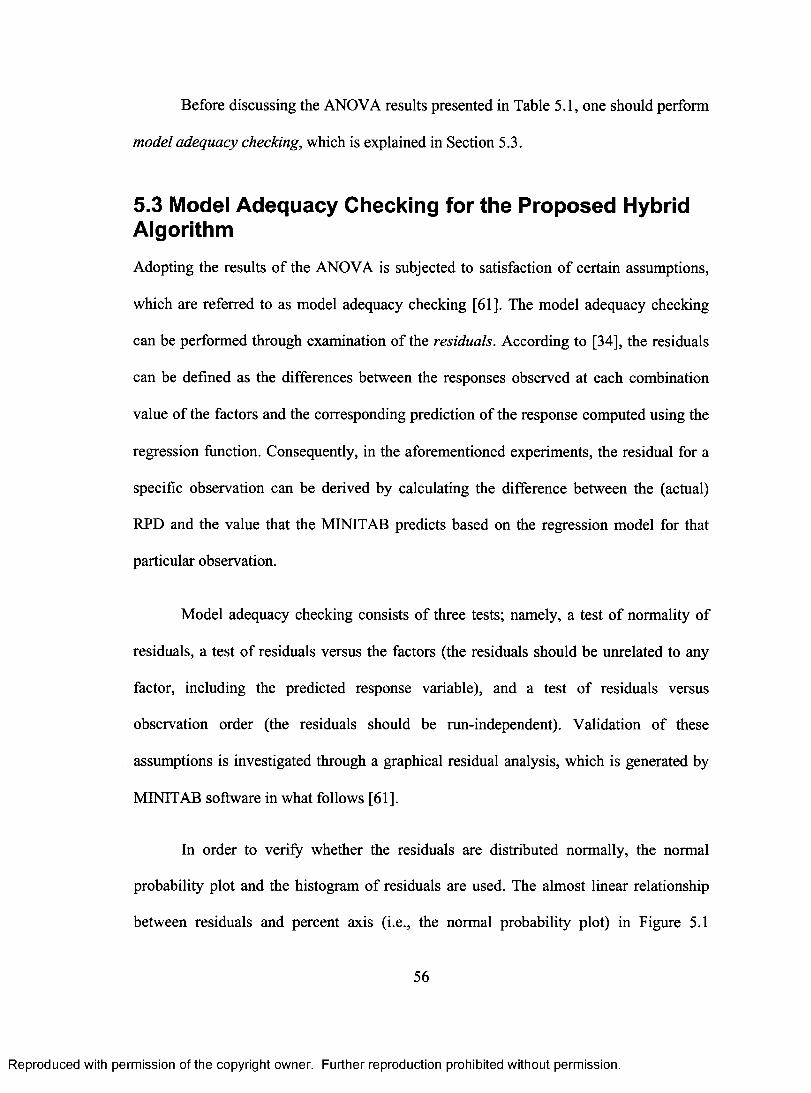
Before discussing the ANOVA results presented in Table 5.1, one should perform
model adequacy checking, which is explained in Section 5.3.
5.3 Model Adequacy Checking for the Proposed Hybrid Algorithm
Adopting the results of the ANOVA is subjected to satisfaction of certain assumptions,
which are referred to as model adequacy checking [61]. The model adequacy checking
can be performed through examination of the residuals. According to [34], the residuals
can be defined as the differences between the responses observed at each combination
value of the factors and the corresponding prediction of the response computed using the
regression function. Consequently, in the aforementioned experiments, the residual for a
specific observation can be derived by calculating the difference between the (actual)
RPD and the value that the MINITAB predicts based on the regression model for that
particular observation.
Model adequacy checking consists of three tests; namely, a test of normality of
residuals, a test of residuals versus the factors (the residuals should be unrelated to any
factor, including the predicted response variable), and a test of residuals versus
observation order (the residuals should be run-independent). Validation of these
assumptions is investigated through a graphical residual analysis, which is generated by
MINITAB software in what follows [61].
In order to verify whether the residuals are distributed normally, the normal
probability plot and the histogram of residuals are used. The almost linear relationship
between residuals and percent axis (i.e., the normal probability plot) in Figure 5.1
56
Reproduced with permission of the copyright owner. Further reproduction prohibited without permission.
Before discussing the ANOVA results presented in Table 5.1, one should perform
model adequacy checking, which is explained in Section 5.3.
5.3 Model Adequacy Checking for the Proposed Hybrid Algorithm
Adopting the results o f the ANOVA is subjected to satisfaction o f certain assumptions,
which are referred to as model adequacy checking [61]. The model adequacy checking
can be performed through examination of the residuals. According to [34], the residuals
can be defined as the differences between the responses observed at each combination
value of the factors and the corresponding prediction o f the response computed using the
regression function. Consequently, in the aforementioned experiments, the residual for a
specific observation can be derived by calculating the difference between the (actual)
RPD and the value that the MINITAB predicts based on the regression model for that
particular observation.
Model adequacy checking consists o f three tests; namely, a test o f normality of
residuals, a test o f residuals versus the factors (the residuals should be unrelated to any
factor, including the predicted response variable), and a test o f residuals versus
observation order (the residuals should be run-independent). Validation o f these
assumptions is investigated through a graphical residual analysis, which is generated by
MINITAB software in what follows [61].
In order to verify whether the residuals are distributed normally, the normal
probability plot and the histogram of residuals are used. The almost linear relationship
between residuals and percent axis (i.e., the normal probability plot) in Figure 5.1
56
Reproduced with permission of the copyright owner. Further reproduction prohibited without permission.
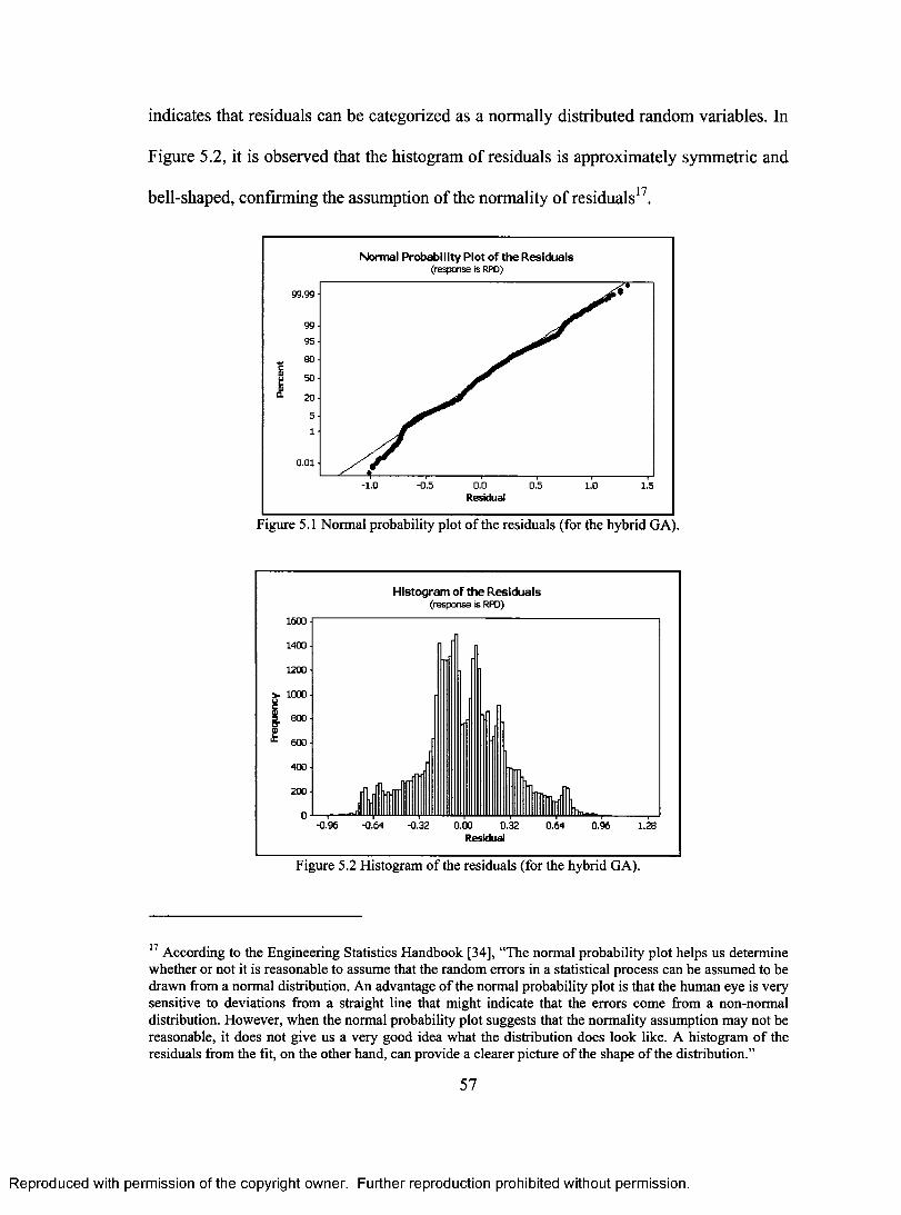
indicates that residuals can be categorized as a normally distributed random variables. In
Figure 5.2, it is observed that the histogram of residuals is approximately symmetric and
bell-shaped, confirming the assumption of the normality of residuals17.
Normal Probability Plot of the Residuals (response is RPD)
a
99.99 -
99 -
95 - eo - so - 20 -
5 -
1 -
0.01-
•
-1.0 -0.5 0.0 Residual
0,5 1.0 1.5
Figure 5.1 Normal probability plot of the residuals (for the hybrid GA).
Histogram of the Residuals (response is RPD)
1600 -
1400 -
1200 -
1000 -
= 800 - er
600 -
400 -
200 -
-0 64 -0.32 0 00 032 0.64 0.96 Residual
1.28
Figure 5.2 Histogram of the residuals (for the hybrid GA).
17 According to the Engineering Statistics Handbook [34], "The normal probability plot helps us determine whether or not it is reasonable to assume that the random errors in a statistical process can be assumed to be drawn from a normal distribution. An advantage of the normal probability plot is that the human eye is very sensitive to deviations from a straight line that might indicate that the errors come from a non-normal distribution. However, when the normal probability plot suggests that the normality assumption may not be reasonable, it does not give us a very good idea what the distribution does look like. A histogram of the residuals from the fit, on the other hand, can provide a clearer picture of the shape of the distribution."
57
Reproduced with permission of the copyright owner. Further reproduction prohibited without permission.
indicates that residuals can be categorized as a normally distributed random variables. In
Figure 5.2, it is observed that the histogram of residuals is approximately symmetric and
bell-shaped, confirming the assumption o f the normality o f residuals17.
Normal Probability Plot of the Residuals(response is RPD)
§£
0.01
- 1.0 -0.5 0.0 0.5 1.0 1.5Residual
Figure 5.1 Normal probability plot o f the residuals (for the hybrid GA).
Histogram of the Residuals(response is RPD)
1600
1400
1200
1000
5 8000)4 600
400
200
-0.96 -0.64 -0.32 0.00 0.32 0.64 0.96 1.28Residual
Figure 5.2 Histogram o f the residuals (for the hybrid GA).
17 According to the Engineering Statistics Handbook [34], “The normal probability plot helps us determine whether or not it is reasonable to assume that the random errors in a statistical process can be assumed to be drawn from a normal distribution. An advantage o f the normal probability plot is that the human eye is very sensitive to deviations from a straight line that might indicate that the errors come from a non-normal distribution. However, when the normal probability plot suggests that the normality assumption may not be reasonable, it does not give us a very good idea what the distribution does look like. A histogram o f the residuals from the fit, on the other hand, can provide a clearer picture o f the shape o f the distribution.”
57
Reproduced with permission of the copyright owner. Further reproduction prohibited without permission.
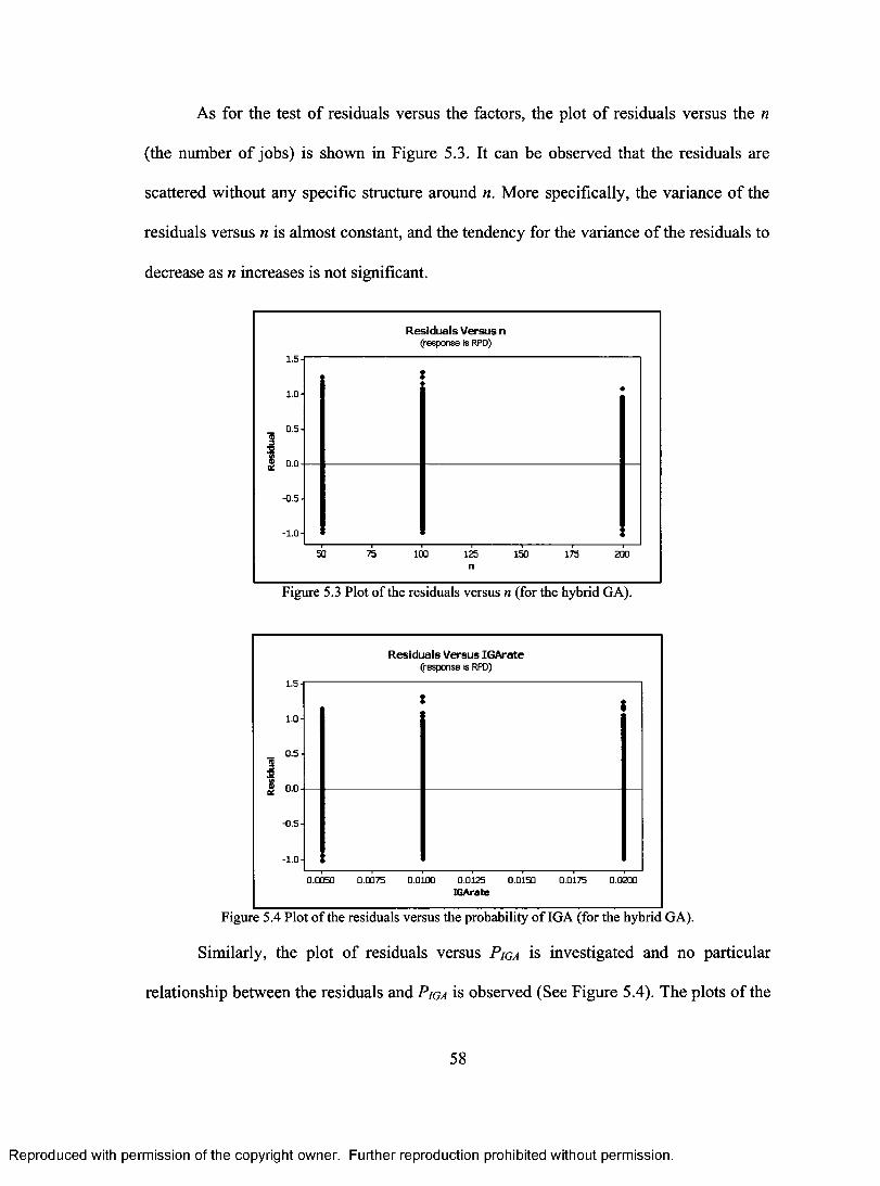
As for the test of residuals versus the factors, the plot of residuals versus the n
(the number of jobs) is shown in Figure 5.3. It can be observed that the residuals are
scattered without any specific structure around n. More specifically, the variance of the
residuals versus n is almost constant, and the tendency for the variance of the residuals to
decrease as n increases is not significant.
Residuals Versus n (response is RPD)
1.5
1.0
0.5
0.0
-0.5
-1.0
•
50 75 100 125 n
150 175 200
Figure 5.3 Plot of the residuals versus n (for the hybrid GA).
1.5
1.0
0.5
1
1 0.0
-0.5
-1.0
Residuals Versus IGArate (response is RPD)
$
0.0050 0.0075 0.0100 0.0125 0.0150 IGArate
0.0175 0.0200
Figure 5.4 Plot of the residuals versus the probability of IGA (for the hybrid GA).
Similarly, the plot of residuals versus PIGA is investigated and no particular
relationship between the residuals and PIGA is observed (See Figure 5.4). The plots of the
58
Reproduced with permission of the copyright owner. Further reproduction prohibited without permission.
As for the test o f residuals versus the factors, the plot o f residuals versus the n
(the number o f jobs) is shown in Figure 5.3. It can be observed that the residuals are
scattered without any specific structure around n. More specifically, the variance o f the
residuals versus n is almost constant, and the tendency for the variance o f the residuals to
decrease as n increases is not significant.
Residuals Versus n(response is RPD)
115 o.o
-0.5-
50 75 100 125 150 175 200n
Figure 5.3 Plot o f the residuals versus n (for the hybrid GA).
Residuals Versus IGArate (response is RPD)
1.5 A
1s*
-0.5-
0.02000.0050 0.0100 0.0125 0.0150 0,0175IGArate
Figure 5.4 Plot o f the residuals versus the probability o f IGA (for the hybrid GA).
Similarly, the plot o f residuals versus P ig a is investigated and no particular
relationship between the residuals and P ig a is observed (See Figure 5.4). The plots o f the
58
Reproduced with permission of the copyright owner. Further reproduction prohibited without permission.

residuals versus other factors, including the predicted response variable (which is
statistically referred to as the fitted value) were investigated and none of them depicted a
particular relationship (see Appendix A).
The last step in model adequacy checking is the test of residuals versus the
observation order. In Figures 5.5a through 5.5d, the plot of residuals versus the
observation order is presented. Since no tendency1 8 to have runs of positive and negative
residuals is observed in this plot, it can be stated that no clear pattern is observed in this
plot, and consequently, the residuals are run-independent.
Residuals Versus the Order of the Data
0.5
ed 3 0
a
w
Ce
-0.5
-1
1 i I I 1 I 1000 5000 6000 7000 W 0OO 90D3 1001 0 11001 0
Observation Figure 5.5a Plot of the residuals versus the observation order (for the hybrid GA).
18 Since the number of observations is 38,880, representing all observations in one single plot will not be illustrative enough to detect the possible structure of residuals versus their order. Therefore, the plot of the residuals versus the observation order was divided into four groups. The results are shown in Figures 5.5a-5.5d.
59
Reproduced with permission of the copyright owner. Further reproduction prohibited without permission.
residuals versus other factors, including the predicted response variable (which is
statistically referred to as the fitted value) were investigated and none of them depicted a
particular relationship (see Appendix A).
The last step in model adequacy checking is the test o f residuals versus the
observation order. In Figures 5.5a through 5.5d, the plot o f residuals versus the
observation order is presented. Since no tendency18 to have runs o f positive and negative
residuals is observed in this plot, it can be stated that no clear pattern is observed in this
plot, and consequently, the residuals are run-independent.
Residuals Versus the Order of the DataT I I I I I I I------------------1----------------- 1----------------- T
-1 -
_______ I__________ I__________ I__________ I__________ I__________ I__________ I__________ I__________ I__________ I__________ l_1000 2000 3000 4000 5000 6000 7000 8000 9000 10000 11000
ObservationFigure 5.5a Plot o f the residuals versus the observation order (for the hybrid GA).
18 Since the number o f observations is 38,880, representing all observations in one single plot will not be illustrative enough to detect the possible structure o f residuals versus their order. Therefore, the plot o f the residuals versus the observation order was divided into four groups. The results are shown in Figures 5.5a- 5.5d.
59
Reproduced with permission of the copyright owner. Further reproduction prohibited without permission.
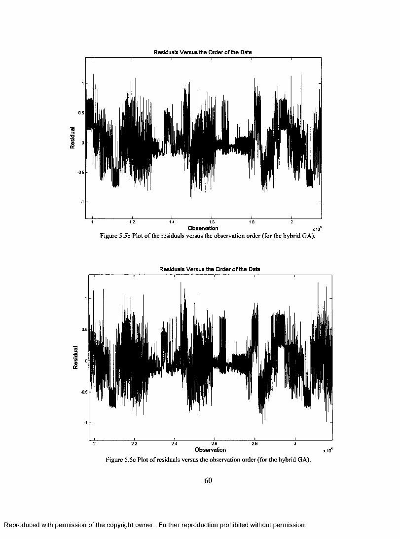
Residuals Versus the Order of the Data
0.5
-0.5
-1
0.5
-0.5
1.2 1.4 1.6
Observation x idsFigure 5.5b Plot of the residuals versus the observation order (for the hybrid GA).
1.8
Residuals Versus the Order of the Data
2
2.2 2.4 2.6 2.8
Observation
Figure 5.5c Plot of residuals versus the observation order (for the hybrid GA).
60
3
x
Reproduced with permission of the copyright owner. Further reproduction prohibited without permission.
Res
idua
l
Residuals Versus the Order of the Datat--------------------------- 1--------------------------- 1----------------------------1--------------------------- 1--------------------------- r
-1 -
j ____________________i___________________ i____________________i____________________i___________________ i_______________1 1.2 1.4 1.6 1.8 2
Observation x 104
Figure 5.5b Plot o f the residuals versus the observation order (for the hybrid GA).
Residuals Versus the Order of the Data1 I I 1 I T
-1 -
2.2 2.4 2.6 2.8Observation
Figure 5.5c Plot o f residuals versus the observation order (for the hybrid GA).
60
Reproduced with permission of the copyright owner. Further reproduction prohibited without permission.
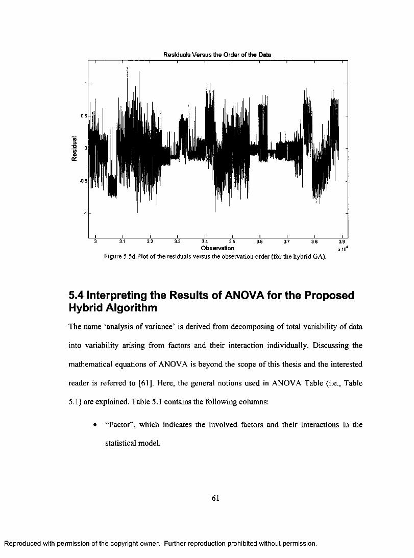
Residuals Versus the Order of the Data
7 :0
0.5
-0.5
I I 3.1
1 1 1 1 3.2 3.3 3.4 3.5 3.6 3.7
3.8 3.9
Observation x le Figure 5.5d Plot of the residuals versus the observation order (for the hybrid GA).
5.4 Interpreting the Results of ANOVA for the Proposed Hybrid Algorithm
The name 'analysis of variance' is derived from decomposing of total variability of data
into variability arising from factors and their interaction individually. Discussing the
mathematical equations of ANOVA is beyond the scope of this thesis and the interested
reader is referred to [61]. Here, the general notions used in ANOVA Table (i.e., Table
5.1) are explained. Table 5.1 contains the following columns:
• "Factor", which indicates the involved factors and their interactions in the
statistical model.
61
Reproduced with permission of the copyright owner. Further reproduction prohibited without permission.
Residuals Versus the Order of the DataT-----------------1-----------------1-----------------1-----------------1-----------------1-----------------1-----------------1-----------------1-----------------T
-1 -
J ____________I____________I____________I____________I____________I____________I____________I____________ I____________l_ l3 3.1 3.2 3.3 3.4 3.5 3.6 3.7 3.8 3.9
Observation x 104
Figure 5.5d Plot o f the residuals versus the observation order (for the hybrid GA).
5.4 Interpreting the Results of ANOVA for the Proposed Hybrid Algorithm
The name ‘analysis o f variance’ is derived from decomposing o f total variability o f data
into variability arising from factors and their interaction individually. Discussing the
mathematical equations o f ANOVA is beyond the scope o f this thesis and the interested
reader is referred to [61]. Here, the general notions used in ANOVA Table (i.e., Table
5.1) are explained. Table 5.1 contains the following columns:
• “Factor”, w h ich indicates the involved factors and their interactions in the
statistical m odel.
61
Reproduced with permission of the copyright owner. Further reproduction prohibited without permission.
• "Sum of Squares", which denotes the measure of variability in data arising
from each factor. The sum of Squares for the "Error" denotes how much of
the variance in the data is accounted for random error. (see [61] for detail).
• "Degrees of Freedom", which indicates the number of degrees of freedom of
the sum of squares associated with each factor (see [61] for detail).
• "Mean Square", which is obtained through dividing the sum of squares by its
associated number of degrees of freedom.
• "F-value", which is equal to the mean square for the factor divided by the
mean square for the error. The F-value (also referred to as F-statistic) follows
an F distribution (see [61] for detail). The value of this statistic signifies
whether the null or the alternative hypothesis is accepted. As a substitute, the
column "P-value" can be employed in hypothesis-testing (see [61] for detail).
In order to recognize whether the null or alternative hypothesis is accepted for
each factor, the associated P-value of Table 5.1 is employed here. The P-value can be
defined as the smallest level of significance19 that would lead to rejection of the null
hypothesis. The predetermined level of significance of 0.05 is normally applied in
hypothesis testing, which is adopted in this thesis as well.
As it can be observed from Table 5.1, the P-values for factors n, m,
SelectionType, and MutationProbability are smaller than 0.05 (the predetermined level of
significance). Also, the P-values for some interactions, namely ( n x m ),
(nxCrossoverTypexSelectionType) and (n x m x SelectionType) are less than 0.05.
19 As stated earlier, the level of significance is the probability of rejection of the null hypothesis when it is true [61].
62
Reproduced with permission of the copyright owner. Further reproduction prohibited without permission.
• “Sum of Squares”, which denotes the measure o f variability in data arising
from each factor. The sum of Squares for the “Error” denotes how much of
the variance in the data is accounted for random error, (see [61] for detail).
• “Degrees o f Freedom”, which indicates the number o f degrees o f freedom of
the sum of squares associated with each factor (see [61] for detail).
• “Mean Square”, which is obtained through dividing the sum of squares by its
associated number o f degrees o f freedom.
• “F-value”, which is equal to the mean square for the factor divided by the
mean square for the error. The F-value (also referred to as F-statistic) follows
an F distribution (see [61] for detail). The value o f this statistic signifies
whether the null or the alternative hypothesis is accepted. As a substitute, the
column “F-value” can be employed in hypothesis-testing (see [61] for detail).
In order to recognize whether the null or alternative hypothesis is accepted for
each factor, the associated P-value of Table 5.1 is employed here. The P-value can be
defined as the smallest level o f significance19 that would lead to rejection o f the null
hypothesis. The predetermined level o f significance o f 0.05 is normally applied in
hypothesis testing, which is adopted in this thesis as well.
As it can be observed from Table 5.1, the P-values for factors n, m,
SelectionType, and MutationProbability are smaller than 0.05 (the predetermined level of
significance). Also, the P-values for some interactions, namely ( n x m ),
(nxCrossoverTypexSelectionType) and (nxm xSelectionType) are less than 0.05.
19 As stated earlier, the level o f significance is the probability o f rejection o f the null hypothesis when it is true [61].
62
Reproduced with permission of the copyright owner. Further reproduction prohibited without permission.
Therefore, null hypotheses are rejected for these terms, indicating that factors n, m,
SelectionType, and MutationProbability are influential on RPD. It is noteworthy that n
and m are uncontrollable factors and they are directly related to the problem at hand.
Furthermore, the three aforementioned terms, namely ( n x m),
(n x CrossoverType x SelectionType), and (n x mx SelectionType) are uncontrollable,
since they contain at least one of the two uncontrollable factors. In the next section, the
impact of SelectionType and MutationProbability will be investigated on the response
variable.
As for the remaining factors and their interactions, it can be observed that their
corresponding P-values are greater than 0.05, indicating that the null hypothesis should
be accepted for them. The statistical interpretation behind the acceptance of the null
hypothesis is that the obtained observations do not give enough evidence in support of
significant difference in the average RPD across the levels of those factors and their
interactions. Therefore, it can be concluded that the factors, or terms that have P-values
of greater than 0.05, are not influential on the overall performance of the proposed hybrid
genetic algorithm.
5.5 Plots of Main Effects and Their Interactions for the Proposed Hybrid Algorithm
In this section, SelectionType and MutationProbability are tuned by making use of the
plots of main effects and their interactions. The procedure for tuning these two
parameters is as follows: between these two factors, SelectionType (the factor that has a
lower P-value), is tuned first. In fact, the lower the P-value is, the more impact that factor
can have on the response variable.
63
Reproduced with permission of the copyright owner. Further reproduction prohibited without permission.
Therefore, null hypotheses are rejected for these terms, indicating that factors n, m,
SelectionType, and MutationProbability are influential on RPD. It is noteworthy that n
and m are uncontrollable factors and they are directly related to the problem at hand.
Furthermore, the three aforementioned terms, namely ( n x m ) ,
( n x CrossoverType x Selection Type), and ( n x m x Selection Type) are uncontrollable,
since they contain at least one o f the two uncontrollable factors. In the next section, the
impact o f SelectionType and MutationProbability will be investigated on the response
variable.
As for the remaining factors and their interactions, it can be observed that their
corresponding P-values are greater than 0.05, indicating that the null hypothesis should
be accepted for them. The statistical interpretation behind the acceptance of the null
hypothesis is that the obtained observations do not give enough evidence in support of
significant difference in the average RPD across the levels o f those factors and their
interactions. Therefore, it can be concluded that the factors, or terms that have P-values
o f greater than 0.05, are not influential on the overall performance o f the proposed hybrid
genetic algorithm.
5.5 Plots of Main Effects and Their Interactions for the Proposed Hybrid Algorithm
In this section, SelectionType and MutationProbability are tuned by making use o f the
plots o f main effects and their interactions. The procedure for tuning these two
parameters is as follows: between these two factors, SelectionType (the factor that has a
lower P-value), is tuned first. In fact, the lower the P-value is, the more impact that factor
can have on the response variable.
63
Reproduced with permission of the copyright owner. Further reproduction prohibited without permission.
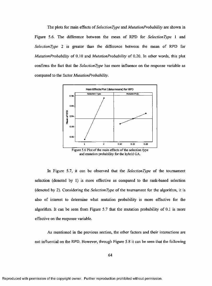
The plots for main effects of SelectionType and MutationProbability are shown in
Figure 5.6. The difference between the mean of RPD for SelectionType 1 and
SelectionType 2 is greater than the difference between the mean of RPD for
MutationProbability of 0.10 and MutationProbability of 0.20. In other words, this plot
confirms the fact that the SelectionType has more influence on the response variable as
compared to the factor MutationProbability.
Main Effects Plot (data means) for RPD
0.96
0.95
0.94
0.93
0.92
Selection Type Mutaion Prob.
2 0.10 0.15 0.20
Figure 5.6 Plot of the main effects of the selection type and mutation probability for the hybrid GA.
In Figure 5.7, it can be observed that the SelectionType of the tournament
selection (denoted by 1) is more effective as compared to the rank-based selection
(denoted by 2). Considering the SelectionType of the tournament for the algorithm, it is
also of interest to determine what mutation probability is more effective for the
algorithm. It can be seen from Figure 5.7 that the mutation probability of 0.1 is more
effective on the response variable.
As mentioned in the previous section, the other factors and their interactions are
not influential on the RPD. However, through Figure 5.8 it can be seen that the following
64
Reproduced with permission of the copyright owner. Further reproduction prohibited without permission.
The plots for main effects of SelectionType and MutaiionProbability are shown in
Figure 5.6. The difference between the mean o f RPD for SelectionType 1 and
SelectionType 2 is greater than the difference between the mean o f RPD for
MutationProbability o f 0.10 and MutationProbability o f 0.20. In other words, this plot
confirms the fact that the SelectionType has more influence on the response variable as
compared to the factor MutationProbability.
Main Effects Plot (data means) for RPDSelection Type Mutaion Prob.
0.96
0.95
'S 0.94
0.93
0.92
2 0.10 0.201 0.15
Figure 5.6 Plot o f the main effects o f the selection type and mutation probability for the hybrid GA.
In Figure 5.7, it can be observed that the SelectionType o f the tournament
selection (denoted by 1) is more effective as compared to the rank-based selection
(denoted by 2). Considering the SelectionType o f the tournament for the algorithm, it is
also of interest to determine what mutation probability is more effective for the
algorithm. It can be seen from Figure 5.7 that the mutation probability o f 0.1 is more
effective on the response variable.
As mentioned in the previous section, the other factors and their interactions are
not influential on the RPD. However, through Figure 5.8 it can be seen that the following
64
Reproduced with permission of the copyright owner. Further reproduction prohibited without permission.
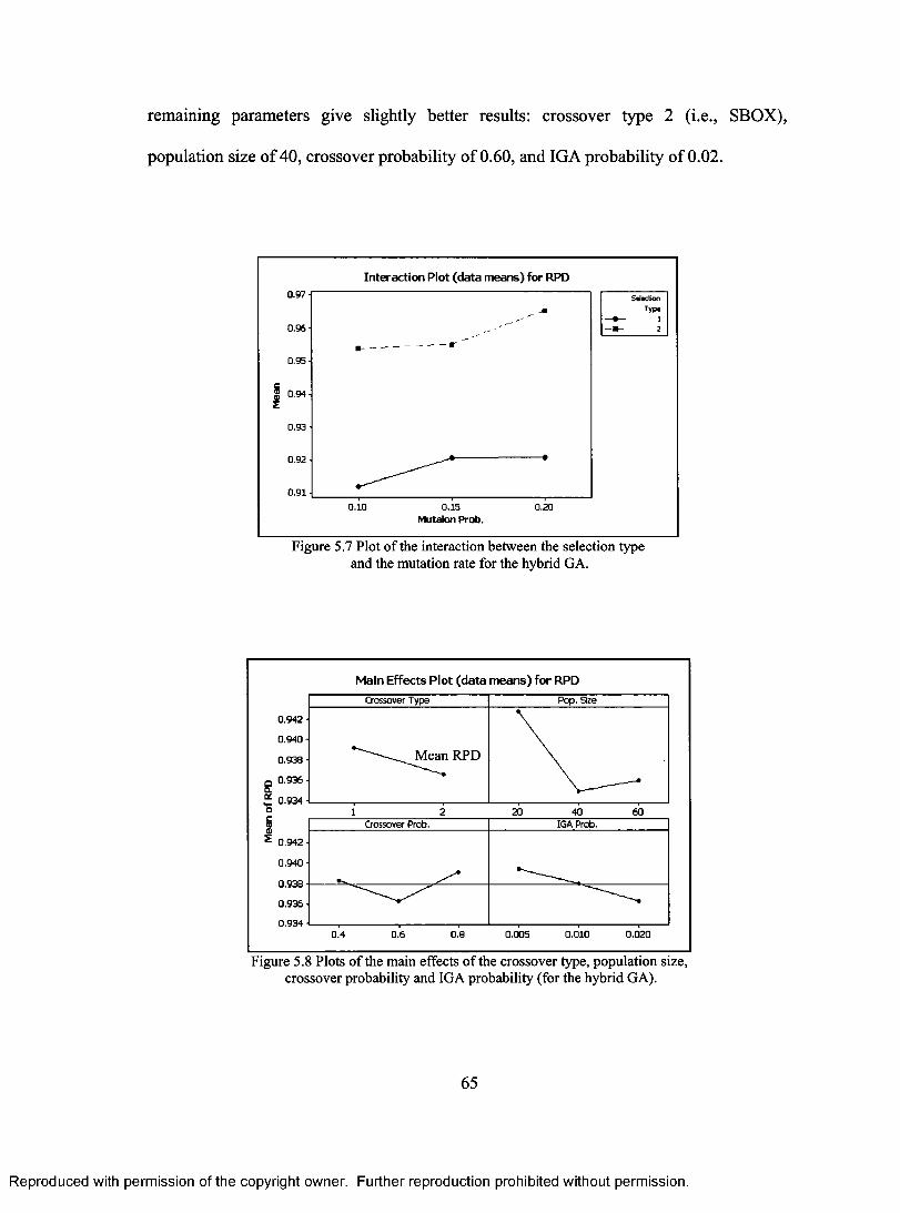
remaining parameters give slightly better results: crossover type 2 (i.e., SBOX),
population size of 40, crossover probability of 0.60, and IGA probability of 0.02.
Interaction Plot (data means) for RPD 0.97 -
0.96
0.95 -
0.94 -
0.93 -
0.92 •
0.91 -
-
•
0.10 0.15 Mutaion Prob.
0.20
Selection Type
—0— 1 — 2 M--
Figure 5.7 Plot of the interaction between the selection type and the mutation rate for the hybrid GA.
Main Effects Plot (data means) for RPD
Crossover Type Pop. Size
0.942
0.940
0.938 Mean RPD
p 0.936 0.
0.934 0 1 2 20 40 60 C ao Crossover Prob. IGA Prob. to
0.942
0.940
0.938
0.936
0.934 0.4 0.6 0.8 0.005 0.010 0.020
Figure 5.8 Plots of the main effects of the crossover type, population size, crossover probability and IGA probability (for the hybrid GA).
65
Reproduced with permission of the copyright owner. Further reproduction prohibited without permission.
remaining parameters give slightly better results: crossover type 2 (i.e., SBOX),
population size o f 40, crossover probability of 0.60, and IGA probability o f 0.02.
Interaction Plot (data means) for RPD0.97
0.96
0.95
| 0.94
0.93
0.92
0.910.10 0.15 0.20
SelectionTyp«1
2
Mutaion Prob.
Figure 5.7 Plot o f the interaction between the selection type and the mutation rate for the hybrid GA.
Main Effects Plot (data m eans) for RPD
0.942
0.940 H
0.938
0.936
0.934
0.942
0.940
0.938
0.936
0.934
Crossover Type Pop. Size
Mean RPD\
1 2 20 40 60Crossover Prob. IGA Prob.
•
0.4 0.6 0.8 0.005 0.010 0.020
Figure 5.8 Plots o f the main effects o f the crossover type, population size, crossover probability and IGA probability (for the hybrid GA).
65
Reproduced with permission of the copyright owner. Further reproduction prohibited without permission.
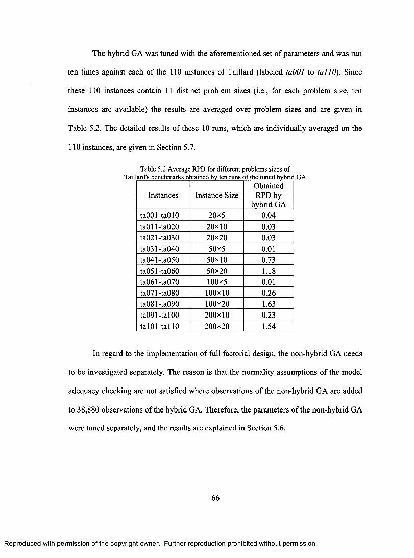
The hybrid GA was tuned with the aforementioned set of parameters and was run
ten times against each of the 110 instances of Taillard (labeled ta001 to tal 10). Since
these 110 instances contain 11 distinct problem sizes (i.e., for each problem size, ten
instances are available) the results are averaged over problem sizes and are given in
Table 5.2. The detailed results of these 10 runs, which are individually averaged on the
110 instances, are given in Section 5.7.
Table 5.2 Average RPD for different problems sizes of Taillard's benchmarks obtained by ten runs of the tuned hybrid GA.
Instances Instance Size Obtained RPD by
hybrid GA ta001-ta010 20x5 0.04
ta011-ta020 20 x10 0.03 ta021-ta030 20x20 0.03 ta031-ta040 50x5 0.01
ta041-ta050 50x 10 0.73 ta051-ta060 50x20 1.18
ta061-ta070 100x5 0.01 ta071-ta080 100x10 0.26 ta081-ta090 100x20 1.63 ta091-ta100 200x 10 0.23
ta101-ta1 10 200x20 1.54
In regard to the implementation of full factorial design, the non-hybrid GA needs
to be investigated separately. The reason is that the normality assumptions of the model
adequacy checking are not satisfied where observations of the non-hybrid GA are added
to 38,880 observations of the hybrid GA. Therefore, the parameters of the non-hybrid GA
were tuned separately, and the results are explained in Section 5.6.
66
Reproduced with permission of the copyright owner. Further reproduction prohibited without permission.
The hybrid GA was tuned with the aforementioned set o f parameters and was run
ten times against each o f the 110 instances of Taillard (labeled taOOl to ta llO ). Since
these 110 instances contain 11 distinct problem sizes (i.e., for each problem size, ten
instances are available) the results are averaged over problem sizes and are given in
Table 5.2. The detailed results o f these 10 runs, which are individually averaged on the
110 instances, are given in Section 5.7.
Table 5.2 Average RPD for different problems sizes o f Taillard's benchmarks obtained by ten runs o f the tuned hybrid GA.
Instances Instance SizeObtained RPD by
hybrid GAtaOOl-taOlO 20x5 0.04ta011-ta020 20x10 0.03ta021-ta030 20x20 0.03ta031-ta040 50x5 0.01ta041-ta050 50x10 0.73ta051-ta060 50x20 1.18ta061-ta070 100x5 0.01ta071-ta080 100x10 0.26ta081-ta090 100x20 1.63ta091-tal00 200x10 0.23talO l-tallO 200x20 1.54
In regard to the implementation o f full factorial design, the non-hybrid GA needs
to be investigated separately. The reason is that the normality assumptions o f the model
adequacy checking are not satisfied where observations o f the non-hybrid GA are added
to 38,880 observations o f the hybrid GA. Therefore, the parameters o f the non-hybrid GA
were tuned separately, and the results are explained in Section 5.6.
66
Reproduced with permission of the copyright owner. Further reproduction prohibited without permission.

5.6 Tuning the Proposed Non-Hybrid GA
In this section, the case of PIGA = 0 is individually investigated (i.e., the non-hybrid GA).
The rationale behind considering this case individually is that by adding the observations
associated with PIGA = 0 to the observations of the hybrid algorithm, the model adequacy
checking of ANOVA (discussed in Section 5.3) is not satisfied.
In order to tune the parameters of the non-hybrid GA, the full factorial
experimental design for all possible combinations of the following factors is carried out:
population size (20, 40, and 60), selection type (rank-based selection, and tournament),
crossover type (SBOX, and LCSX), crossover probability (0.4, 0.6, and 0.8), and
mutation probability (0.1, 0.15, and 0.20). PIGA
combinations are investigated.
is set to zero and, therefore, 108
The same thirty instances of Taillard, which were employed in the
implementation of the full factorial experimental design of the hybrid algorithm, were
used here as well. Three replicates, with the aforementioned combination of parameters,
were considered and consequently 9,720 observations were carried out. Similarly, the
analysis of variance, and the model adequacy checking were investigated. The ANOVA
table and the plots of residuals for the non-hybrid GA are given in Appendix B and
Appendix C, respectively. It can be observed that the residuals follow a normal
distribution. Additionally, the residuals are not related to any factor and they are run-
independent. Therefore, one can rely on the obtained observations of the non-hybrid GA.
The P-values of the ANOVA table for the non-hybrid GA (given in Appendix B)
are zero for all factors, meaning that all factors are statistically influential on the response
67
Reproduced with permission of the copyright owner. Further reproduction prohibited without permission.
5.6 Tuning the Proposed Non-Hybrid GA
In this section, the case o f P i g a - 0 is individually investigated (i.e., the non-hybrid GA).
The rationale behind considering this case individually is that by adding the observations
associated with P i g a = 0 to the observations o f the hybrid algorithm, the model adequacy
checking o f ANOVA (discussed in Section 5.3) is not satisfied.
In order to tune the parameters o f the non-hybrid GA, the full factorial
experimental design for all possible combinations o f the following factors is carried out:
population size (20, 40, and 60), selection type (rank-based selection, and tournament),
crossover type (SBOX, and LCSX), crossover probability (0.4, 0.6, and 0.8), and
mutation probability (0.1, 0.15, and 0.20). P i g a is set to zero and, therefore, 108
combinations are investigated.
The same thirty instances of Taillard, which were employed in the
implementation o f the full factorial experimental design of the hybrid algorithm, were
used here as well. Three replicates, with the aforementioned combination of parameters,
were considered and consequently 9,720 observations were carried out. Similarly, the
analysis o f variance, and the model adequacy checking were investigated. The ANOVA
table and the plots of residuals for the non-hybrid GA are given in Appendix B and
Appendix C, respectively. It can be observed that the residuals follow a normal
distribution. Additionally, the residuals are not related to any factor and they are run-
independent. Therefore, one can rely on the obtained observations o f the non-hybrid GA.
The P-values o f the ANOVA table for the non-hybrid GA (given in Appendix B)
are zero for all factors, meaning that all factors are statistically influential on the response
67
Reproduced with permission of the copyright owner. Further reproduction prohibited without permission.
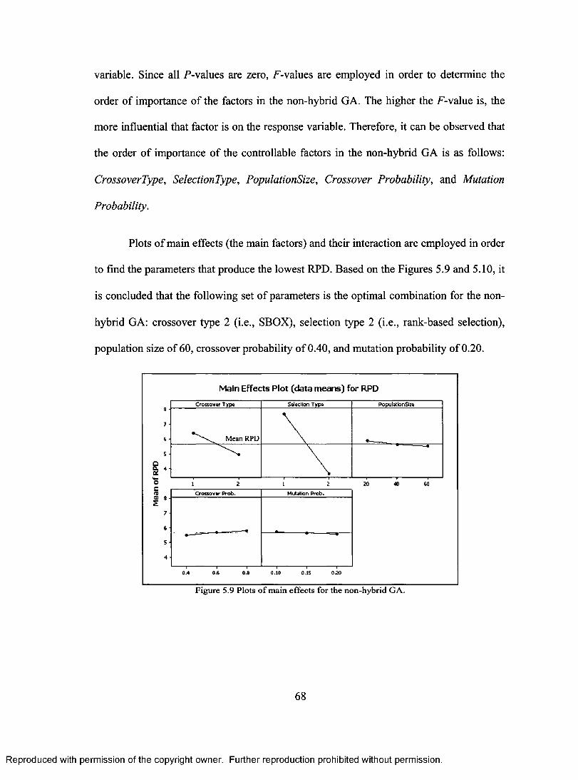
variable. Since all P-values are zero, F-values are employed in order to determine the
order of importance of the factors in the non-hybrid GA. The higher the F-value is, the
more influential that factor is on the response variable. Therefore, it can be observed that
the order of importance of the controllable factors in the non-hybrid GA is as follows:
CrossoverType, SelectionType, PopulationSize, Crossover Probability, and Mutation
Probability.
Plots of main effects (the main factors) and their interaction are employed in order
to find the parameters that produce the lowest RPD. Based on the Figures 5.9 and 5.10, it
is concluded that the following set of parameters is the optimal combination for the non-
hybrid GA: crossover type 2 (i.e., SBOX), selection type 2 (i.e., rank-based selection),
population size of 60, crossover probability of 0.40, and mutation probability of 0.20.
Main Effects Plot (data means) for RPD
Mean o
f RP
D
8
7
6
5
4
8
7
6
5
4
Crossover Type Selection Type PopulationSize
Mean RPD •—_____ ie---_.
2 2
Crossover Prob. Mutation Prob.
rr
0.4 0.6 0.8 0.10 0.15 0.20
20 40
Figure 5.9 Plots of main effects for the non-hybrid GA.
68
60
Reproduced with permission of the copyright owner. Further reproduction prohibited without permission.
variable. Since all P-values are zero, F-values are employed in order to determine the
order of importance o f the factors in the non-hybrid GA. The higher the F-value is, the
more influential that factor is on the response variable. Therefore, it can be observed that
the order o f importance o f the controllable factors in the non-hybrid GA is as follows:
CrossoverType, SelectionType, PopulationSize, Crossover Probability, and Mutation
Probability.
Plots o f main effects (the main factors) and their interaction are employed in order
to find the parameters that produce the lowest RPD. Based on the Figures 5.9 and 5.10, it
is concluded that the following set o f parameters is the optimal combination for the non
hybrid GA: crossover type 2 (i.e., SBOX), selection type 2 (i.e., rank-based selection),
population size o f 60, crossover probability o f 0.40, and mutation probability o f 0.20.
Main Effects Plot (data means) for RPDSelection TypeCrossover Type
Mean RPD
C rossover Prob.
0.4 0.$ 0.10 0.15 0.20
Figure 5.9 Plots o f m ain effects for the non-hybrid GA.
68
Reproduced with permission of the copyright owner. Further reproduction prohibited without permission.
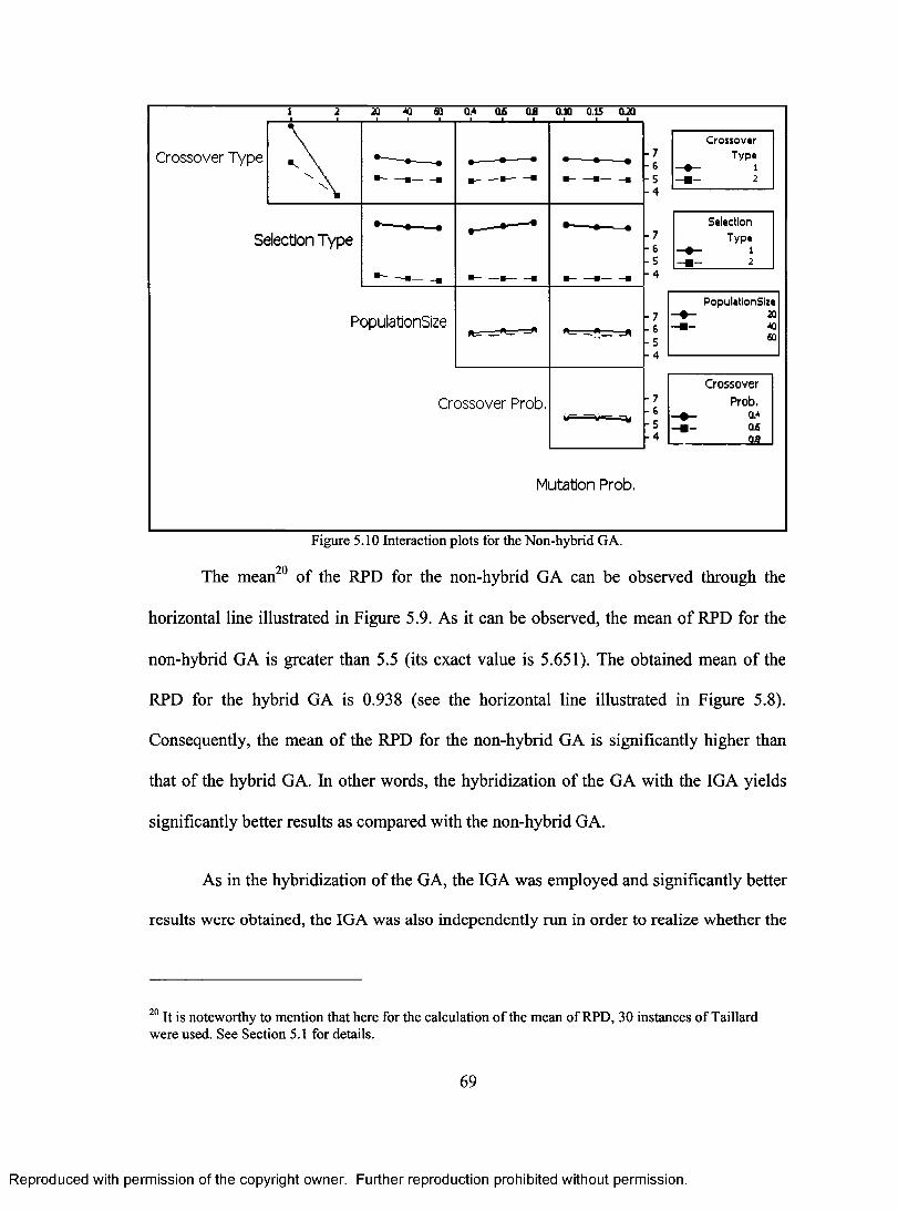
1 2 3? 19 61? OA 0)5 011 0.10 0.15 0.20
Crossover
Crossover Type -7 -6 —0-
Type 1
•-- —s— -s M— — -5 --MI— 2 -4
Selection
Selection Type - 7 -6
Type 1
-5 2
— ♦ — —II —M — —IN -4
PopulationSize
PopulationSize -7 -6 —a-
20
-5 -4
Crossover
Crossover Prob. -7 -6
- a -Prob,
OA -5 -a— 0,6 -4 02
Mutation Prob.
Figure 5.10 Interaction plots for the Non-hybrid GA.
The mean20 of the RPD for the non-hybrid GA can be observed through the
horizontal line illustrated in Figure 5.9. As it can be observed, the mean of RPD for the
non-hybrid GA is greater than 5.5 (its exact value is 5.651). The obtained mean of the
RPD for the hybrid GA is 0.938 (see the horizontal line illustrated in Figure 5.8).
Consequently, the mean of the RPD for the non-hybrid GA is significantly higher than
that of the hybrid GA. In other words, the hybridization of the GA with the IGA yields
significantly better results as compared with the non-hybrid GA.
As in the hybridization of the GA, the IGA was employed and significantly better
results were obtained, the IGA was also independently run in order to realize whether the
20 It is noteworthy to mention that here for the calculation of the mean of RPD, 30 instances of Taillard were used. See Section 5.1 for details.
69
Reproduced with permission of the copyright owner. Further reproduction prohibited without permission.
CrossoverTypeCrossover Type
SelectionTypeSelection Type
PopulationSize
CrossoverProb,
Q.AQjfi
______Q£
Crossover Prob.
Mutation Prob.
Figure 5.10 Interaction plots for the Non-hybrid GA.
70The mean o f the RPD for the non-hybrid GA can be observed through the
horizontal line illustrated in Figure 5.9. As it can be observed, the mean o f RPD for the
non-hybrid GA is greater than 5.5 (its exact value is 5.651). The obtained mean o f the
RPD for the hybrid GA is 0.938 (see the horizontal line illustrated in Figure 5.8).
Consequently, the mean of the RPD for the non-hybrid GA is significantly higher than
that of the hybrid GA. In other words, the hybridization of the GA with the IGA yields
significantly better results as compared with the non-hybrid GA.
As in the hybridization of the GA, the IGA was employed and significantly better
results were obtained, the IGA was also independently run in order to realize whether the
20 It is noteworthy to mention that here for the calculation o f the mean o f RPD, 30 instances o f Taillard were used. See Section 5.1 for details.
69
Reproduced with permission of the copyright owner. Further reproduction prohibited without permission.
GA played any role in the overall performance of the proposed hybrid algorithm21. If
employing the GA has not been helpful at all, one would prefer to allocate all the
mentioned CPU time to the IGA. The other question that arises is on the performance of
the stand-alone GA (the proposed non-hybrid GA) in the long run. In other words, the
GA has been run on a relatively short CPU time, and since the GA is a population based
search technique, it might not be fair to compare its results with those of IGA over the
same CPU time. These two issues will be addressed in the next sections. More
specifically, in Section 5.7 the performance of the stand-alone IGA is tested on the
benchmarks of Taillard. Then, this performance is compared with that of the hybrid GA.
In Section 5.8 the performance of the non-hybrid GA is investigated over a long period of
time.
5.7 Performance of the stand-alone IGA and its Comparison with the Hybrid GA
A time-dependent termination condition of n x m x 90 milliseconds is considered for the
implemented IGA, where n and m are the number of jobs and machines, respectively. In
fact, this is the same termination condition adopted for the hybrid GA (discussed in
Section 4.1.5). The stand-alone IGA was run ten times for each of the 110 instances of
Taillard and the results, which are averaged on problem size, are given in Table 5.3. In
this table, the results of hybrid GA (discussed in Section 5.5) are also presented for the
sake of comparison.
21 It is worth mentioning that the IGA of Ruiz et al. [47] has been experimentally proven to be very effective. In fact, Ruiz et al. compared the IGA against the other twelve algorithms, and they showed that their IGA outperformed all of them.
70
Reproduced with permission of the copyright owner. Further reproduction prohibited without permission.
0 1GA played any role in the overall performance o f the proposed hybrid algorithm . If
employing the GA has not been helpful at all, one would prefer to allocate all the
mentioned CPU time to the IGA. The other question that arises is on the performance of
the stand-alone GA (the proposed non-hybrid GA) in the long run. In other words, the
GA has been run on a relatively short CPU time, and since the GA is a population based
search technique, it might not be fair to compare its results with those of IGA over the
same CPU time. These two issues will be addressed in the next sections. More
specifically, in Section 5.7 the performance o f the stand-alone IGA is tested on the
benchmarks o f Taillard. Then, this performance is compared with that o f the hybrid GA.
In Section 5.8 the performance o f the non-hybrid GA is investigated over a long period of
time.
5.7 Performance of the stand-alone IGA and its Comparison with the Hybrid GA
A time-dependent termination condition o f n x m x 90 milliseconds is considered for the
implemented IGA, where n and m are the number o f jobs and machines, respectively. In
fact, this is the same termination condition adopted for the hybrid GA (discussed in
Section 4.1.5). The stand-alone IGA was run ten times for each o f the 110 instances of
Taillard and the results, which are averaged on problem size, are given in Table 5.3. In
this table, the results o f hybrid GA (discussed in Section 5.5) are also presented for the
sake of comparison.
21 It is worth mentioning that the IGA o f Ruiz et al. [47] has been experimentally proven to be very effective. In fact, Ruiz et al. compared the IGA against the other twelve algorithms, and they showed that their IGA outperformed all o f them.
70
Reproduced with permission of the copyright owner. Further reproduction prohibited without permission.
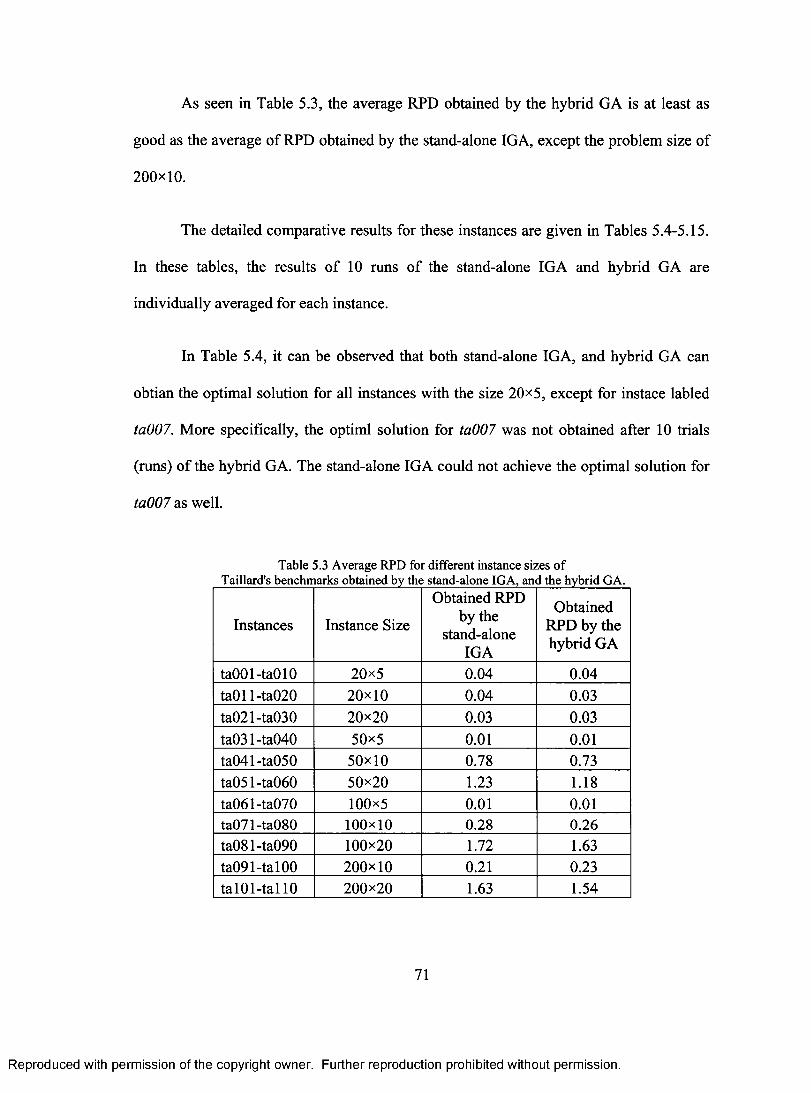
As seen in Table 5.3, the average RPD obtained by the hybrid GA is at least as
good as the average of RPD obtained by the stand-alone IGA, except the problem size of
200x10.
The detailed comparative results for these instances are given in Tables 5.4-5.15.
In these tables, the results of 10 runs of the stand-alone IGA and hybrid GA are
individually averaged for each instance.
In Table 5.4, it can be observed that both stand-alone IGA, and hybrid GA can
obtian the optimal solution for all instances with the size 20x5, except for instace Tabled
ta007. More specifically, the optiml solution for ta007 was not obtained after 10 trials
(runs) of the hybrid GA. The stand-alone IGA could not achieve the optimal solution for
ta007 as well.
Table 5.3 Average RPD for different instance sizes of Taillard's benchmarks obtained by the stand-alone IGA, and the hybrid GA.
Instances Instance Size
Obtained RPD by the
stand-alone IGA
Obtained RPD by the hybrid GA
ta001-ta010 20x5 0.04 0.04
ta011-ta020 20x10 0.04 0.03
ta021-ta030 20x20 0.03 0.03
ta031-ta040 50x5 0.01 0.01 ta041-ta050 50x 10 0.78 0.73
ta051-ta060 50x20 1.23 1.18
ta061-ta070 100x5 0.01 0.01 ta071-ta080 100x10 0.28 0.26 ta081-ta090 100x20 1.72 1.63 ta091-ta100 200x 10 0.21 0.23 ta101-tall0 200x20 1.63 1.54
71
Reproduced with permission of the copyright owner. Further reproduction prohibited without permission.
As seen in Table 5.3, the average RPD obtained by the hybrid GA is at least as
good as the average o f RPD obtained by the stand-alone IGA, except the problem size of
200x10.
The detailed comparative results for these instances are given in Tables 5.4-5.15.
In these tables, the results o f 10 runs o f the stand-alone IGA and hybrid GA are
individually averaged for each instance.
In Table 5.4, it can be observed that both stand-alone IGA, and hybrid GA can
obtian the optimal solution for all instances with the size 20x5, except for instace labled
ta007. More specifically, the optiml solution for ta007 was not obtained after 10 trials
(runs) o f the hybrid GA. The stand-alone IGA could not achieve the optimal solution for
ta007 as well.
Table 5.3 Average RPD for different instance sizes o f Taillard's benchmarks obtained by the stand-alone IGA, and the hybrid GA.
Instances Instance Size
Obtained RPD by the
stand-alone IGA
Obtained RPD by the hybrid GA
taOOl-taOlO 20x5 0.04 0.04ta011-ta020 20x10 0.04 0.03ta021-ta030 20x20 0.03 0.03ta031-ta040 50x5 0.01 0.01ta041-ta050 50x10 0.78 0.73ta051-ta060 50x20 1.23 1.18ta061-ta070 100x5 0.01 0.01ta071-ta080 100x10 0.28 0.26ta081-ta090 100x20 1.72 1.63ta091-tal00 200x10 0.21 0.23talO l-tallO 200x20 1.63 1.54
71
Reproduced with permission of the copyright owner. Further reproduction prohibited without permission.
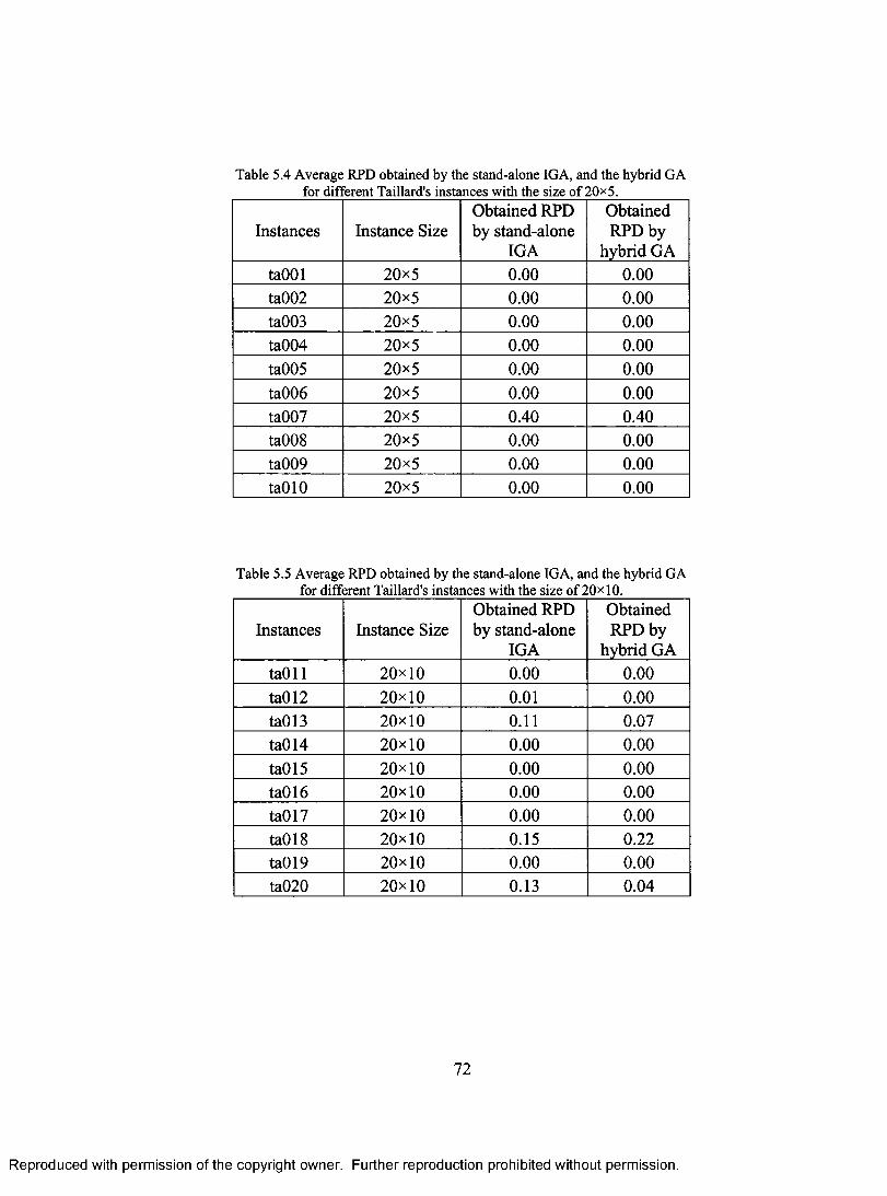
Table 5.4 Average RPD obtained by the stand-alone IGA, and the hybrid GA for different Taillard's instances with the size of 20x5.
Instances Instance Size Obtained RPD by stand-alone
IGA
Obtained RPD by
hybrid GA
ta001 20x5 0.00 0.00 ta002 20x5 0.00 0.00 ta003 20x5 0.00 0.00 ta004 20x5 0.00 0.00
ta005 20x5 0.00 0.00
ta006 20x5 0.00 0.00 ta007 20x5 0.40 0.40 ta008 20x5 0.00 0.00
ta009 20x5 0.00 0.00
ta010 20x5 0.00 0.00
Table 5.5 Average RPD obtained by the stand-alone IGA, and the hybrid GA for different Taillard's instances with the size of 20x10.
Instances Instance Size Obtained RPD by stand-alone
IGA
Obtained RPD by
hybrid GA ta011 20x 10 0.00 0.00
ta012 20x10 0.01 0.00
ta013 20x10 0.11 0.07 ta014 20x10 0.00 0.00
ta015 20x10 0.00 0.00
ta016 20x10 0.00 0.00
ta017 20x10 0.00 0.00
ta018 20x 10 0.15 0.22 ta019 20x10 0.00 0.00
ta020 20 x10 0.13 0.04
72
Reproduced with permission of the copyright owner. Further reproduction prohibited without permission.
Table 5.4 Average RPD obtained by the stand-alone IGA, and the hybrid GAfor different Taillard's instances with the size o f 20x5.
Instances Instance SizeObtained RPD by stand-alone
IGA
Obtained RPD by
hybrid GAtaOOl 20x5 0.00 0.00ta002 20x5 0.00 0.00ta003 20x5 0.00 0.00ta004 20x5 0.00 0.00ta005 20x5 0.00 0.00ta006 20x5 0.00 0.00ta007 20x5 0.40 0.40ta008 20x5 0.00 0.00ta009 20x5 0.00 0.00taOlO 20x5 0.00 0.00
Table 5.5 Average RPD obtained by the stand-alone IGA, and the hybrid GA for different Taillard's instances with the size o f 20x10.
Instances Instance SizeObtained RPD by stand-alone
IGA
Obtained RPD by
hybrid GAtaOll 20x10 0.00 0.00ta012 20x10 0.01 0.00ta013 20x10 0.11 0.07ta014 20x10 0.00 0.00ta015 20x10 0.00 0.00ta016 20x10 0.00 0.00ta017 20x10 0.00 0.00ta018 20x10 0.15 0.22ta019 20x10 0.00 0.00ta020 20x10 0.13 0.04
72
Reproduced with permission of the copyright owner. Further reproduction prohibited without permission.
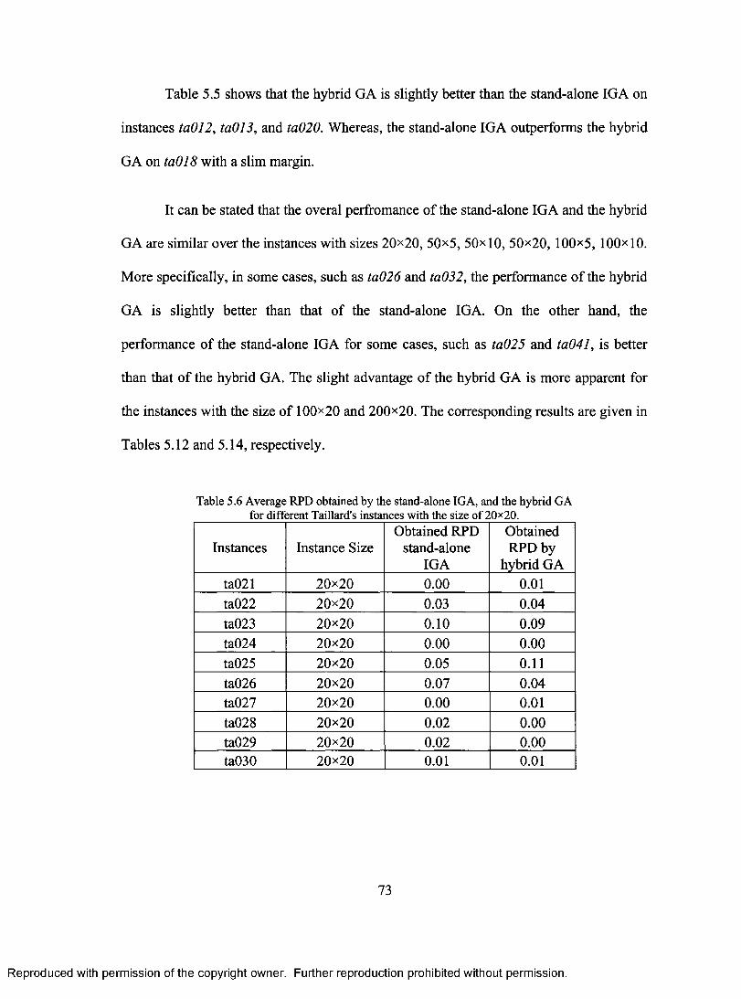
Table 5.5 shows that the hybrid GA is slightly better than the stand-alone IGA on
instances ta012, ta013, and ta020. Whereas, the stand-alone IGA outperforms the hybrid
GA on ta018 with a slim margin.
It can be stated that the overal perfromance of the stand-alone IGA and the hybrid
GA are similar over the instances with sizes 20x20, 50x5, 50x10, 50x20, 100x5, 100x10.
More specifically, in some cases, such as ta026 and ta032, the performance of the hybrid
GA is slightly better than that of the stand-alone IGA. On the other hand, the
performance of the stand-alone IGA for some cases, such as ta025 and ta041, is better
than that of the hybrid GA. The slight advantage of the hybrid GA is more apparent for
the instances with the size of 100x20 and 200x20. The corresponding results are given in
Tables 5.12 and 5.14, respectively.
Table 5.6 Average RPD obtained by the stand-alone IGA, and the hybrid GA for different Taillard's instances with the size of 20x20.
Instances Instance Size Obtained RPD
stand-alone IGA
Obtained RPD by
hybrid GA ta021 20x20 0.00 0.01
ta022 20x20 0.03 0.04
ta023 20x20 0.10 0.09 ta024 20x20 0.00 0.00
ta025 20x20 0.05 0.11
ta026 20x20 0.07 0.04 ta027 20x20 0.00 0.01
ta028 20x20 0.02 0.00 ta029 20x20 0.02 0.00 ta030 20x20 0.01 0.01
73
Reproduced with permission of the copyright owner. Further reproduction prohibited without permission.
Table 5.5 shows that the hybrid GA is slightly better than the stand-alone IGA on
instances ta012, taOl 3, and ta020. Whereas, the stand-alone IGA outperforms the hybrid
GA on ta018 with a slim margin.
It can be stated that the overal perffomance of the stand-alone IGA and the hybrid
GA are similar over the instances with sizes 20x20, 50x5, 50x10, 50x20, 100x5, 100x10.
More specifically, in some cases, such as ta026 and ta032, the performance o f the hybrid
GA is slightly better than that of the stand-alone IGA. On the other hand, the
performance o f the stand-alone IGA for some cases, such as ta025 and ta041, is better
than that o f the hybrid GA. The slight advantage o f the hybrid GA is more apparent for
the instances with the size o f 100x20 and 200x20. The corresponding results are given in
Tables 5.12 and 5.14, respectively.
Table 5.6 Average RPD obtained by the stand-alone IGA, and the hybrid GA for different Taillard's instances with the size o f 20x20.
Instances Instance SizeObtained RPD
stand-alone IGA
Obtained RPD by
hybrid GAta021 20x20 0.00 0.01ta022 20x20 0.03 0.04ta023 20x20 0.10 0.09ta024 20x20 0.00 0.00ta025 20x20 0.05 0.11ta026 20x20 0.07 0.04ta027 20x20 0.00 0.01ta028 20x20 0.02 0.00ta029 20x20 0.02 0.00ta030 20x20 0.01 0.01
73
Reproduced with permission of the copyright owner. Further reproduction prohibited without permission.
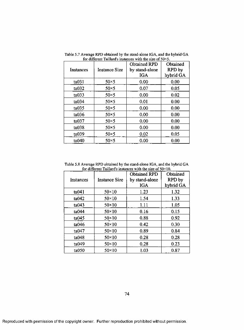
Table 5.7 Average RPD obtained by the stand-alone IGA, and the hybrid GA for different Taillard's instances with the size of 50x5.
Instances Instance Size Obtained RPD by stand-alone
IGA
Obtained RPD by
hybrid GA
ta031 50x5 0.00 0.00 ta032 50x5 0.07 0.05
ta033 50x5 0.00 0.02 ta034 50x5 0.01 0.00 ta035 50x5 0.00 0.00
ta036 50x5 0.00 0.00 ta037 50x5 0.00 0.00 ta038 50x5 0.00 0.00
ta039 50x5 0.02 0.05
ta040 50x5 0.00 0.00
Table 5.8 Average RPD obtained by the stand-alone IGA, and the hybrid GA for different Taillard's instances with the size of 50x10.
Instances Instance Size Obtained RPD by stand-alone
IGA
Obtained RPD by
hybrid GA
ta041 50x10 1.23 1.32
ta042 50x10 1.54 1.33 ta043 50x10 1.11 1.05 ta044 50x10 0.16 0.15 ta045 50x10 0.88 _ 0.92 ta046 50x10 0.42 0.30
ta047 50x10 0.89 0.84
ta048 50x10 0.28 0.28 ta049 50x10 0.28 0.23 ta050 50x10 1.03 0.87
74
Reproduced with permission of the copyright owner. Further reproduction prohibited without permission.
Table 5.7 Average RPD obtained by the stand-alone IGA, and the hybrid GAfor different Taillard's instances with the size o f 50x5.
Instances Instance SizeObtained RPD by stand-alone
IGA
Obtained RPD by
hybrid GAta031 50x5 0.00 0.00ta032 50x5 0.07 0.05ta033 50x5 0.00 0.02ta034 50x5 0.01 0.00ta035 50x5 0.00 0.00ta036 50x5 0.00 0.00ta037 50x5 0.00 0.00ta038 50x5 0.00 0.00ta039 50x5 0.02 0.05ta040 50x5 0.00 0.00
Table 5.8 Average RPD obtained by the stand-alone IGA, and the hybrid GA for different Taillard's instances with the size o f 50x10.
Instances Instance SizeObtained RPD by stand-alone
IGA
Obtained RPD by
hybrid GAta041 50x10 1.23 1.32ta042 50x10 1.54 1.33ta043 50x10 1.11 1.05ta044 50x10 0.16 0.15ta045 50x10 0.88 0.92ta046 50x10 0.42 0.30ta047 50x10 0.89 0.84ta048 50x10 0.28 0.28ta049 50x10 0.28 0.23ta050 50x10 1.03 0.87
74
Reproduced with permission of the copyright owner. Further reproduction prohibited without permission.
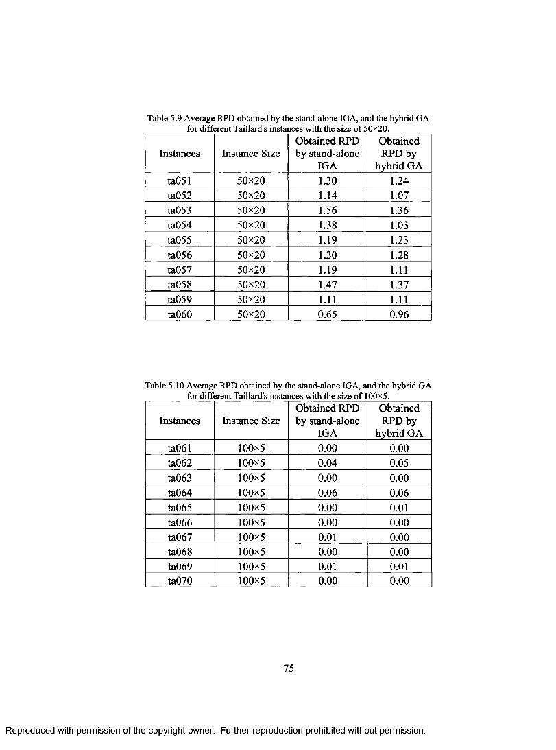
Table 5.9 Average RPD obtained by the stand-alone IGA, and the hybrid GA for different Taillard's instances with the size of 50x20.
Instances Instance Size Obtained RPD by stand-alone
IGA
Obtained RPD by
hybrid GA ta051 50x20 1.30 1.24 ta052 50x20 1.14 1.07
ta053 50x20 1.56 1.36 ta054 50x20 1.38 1.03
ta055 50x20 1.19 1.23
ta056 50x20 1.30 1.28
ta057 50x20 1.19 1.11
ta058 50x20 1.47 1.37 ta059 50x20 1.11 1.11 ta060 50x20 0.65 0.96
Table 5.10 Average RPD obtained by the stand-alone IGA, and the hybrid GA for different Taillard's instances with the size of 100x5.
Instances Instance Size Obtained RPD by stand-alone
IGA
Obtained RPD by
hybrid GA ta061 100x5 0.00 0.00 ta062 100x5 0.04 0.05
ta063 100x5 0.00 0.00
ta064 100x5 0.06 0.06
ta065 100x5 0.00 0.01
ta066 100x5 0.00 0.00 ta067 100x5 0.01 0.00 ta068 100x5 0.00 0.00 ta069 100x5 0.01 0.01 ta070 100x5 0.00 0.00
75
Reproduced with permission of the copyright owner. Further reproduction prohibited without permission.
Table 5.9 Average RPD obtained by the stand-alone IGA, and the hybrid GAfor different Taillard's instances with the size o f 50><20.
Instances Instance SizeObtained RPD by stand-alone
IGA
Obtained RPD by
hybrid GAta051 50x20 1.30 1.24ta052 50x20 1.14 1.07ta053 50x20 1.56 1.36ta054 50x20 1.38 1.03ta055 50x20 1.19 1.23ta056 50x20 1.30 1.28ta057 50x20 1.19 1.11ta058 50x20 1.47 1.37ta059 50x20 1.11 1.11ta060 50x20 0.65 0.96
Table 5.10 Average RPD obtained by the stand-alone IGA, and the hybrid GA for different Taillard's instances with the size o f 100*5.
Instances Instance SizeObtained RPD by stand-alone
IGA
Obtained RPD by
hybrid GAta061 100x5 0.00 0.00ta062 100x5 0.04 0.05ta063 100x5 0.00 0.00ta064 100x5 0.06 0.06ta065 100x5 0.00 0.01ta066 100x5 0.00 0.00ta067 100x5 0.01 0.00ta068 100x5 0.00 0.00ta069 100x5 0.01 0.01ta070 100x5 0.00 0.00
75
Reproduced with permission of the copyright owner. Further reproduction prohibited without permission.
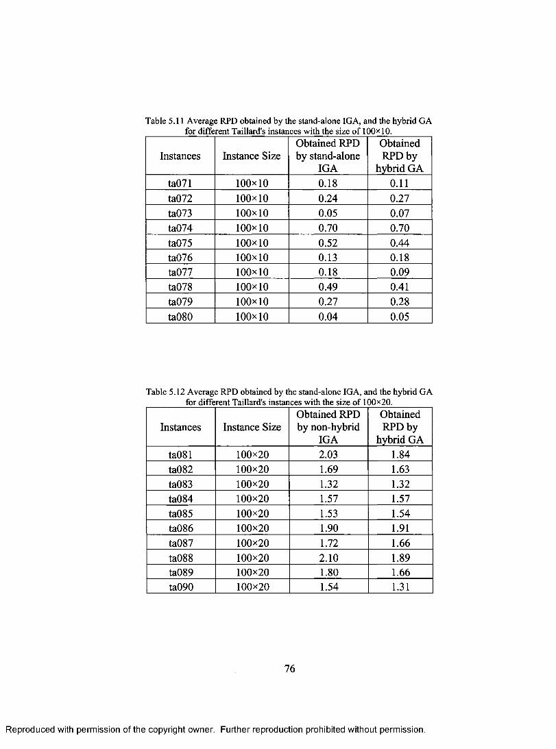
Table 5.11 Average RPD obtained by the stand-alone IGA, and the hybrid GA for different Taillard's instances with the size of 100x10.
Instances Instance Size Obtained RPD by stand-alone
IGA
Obtained RPD by
hybrid GA ta071 100x10 0.18 0.11
ta072 100x10 0.24 0.27
ta073 100x10 0.05 0.07 ta074 100x10 0.70 0.70
ta075 100x10 0.52 0.44 ta076 100x10 0.13 0.18 ta077 100x10 0.18 0.09 ta078 100x10 0.49 0.41
ta079 100x10 0.27 0.28
ta080 100x10 0.04 0.05
Table 5.12 Average RPD obtained by the stand-alone IGA, and the hybrid GA for different Taillard's instances with the size of 100x20.
Instances Instance Size Obtained RPD by non-hybrid
IGA
Obtained RPD by
hybrid GA
ta081 100x20 2.03 1.84
ta082 100x20 1.69 1.63
ta083 100x20 1.32 1.32
ta084 100x20 1.57 1.57
ta085 100x20 1.53 1.54
ta086 100x20 1.90 1.91
ta087 100x20 1.72 1.66
ta088 100x20 2.10 1.89 ta089 100x20 1.80 1.66 ta090 100x20 1.54 1.31
76
Reproduced with permission of the copyright owner. Further reproduction prohibited without permission.
Table 5.11 Average RPD obtained by the stand-alone IGA, and the hybrid GAfor different Taillard's instances with the size o f 100x 10.
Instances Instance SizeObtained RPD by stand-alone
IGA
Obtained RPD by
hybrid GAta071 100x10 0.18 0.11ta072 100x10 0.24 0.27ta073 100x10 0.05 0.07ta074 100x10 0.70 0.70ta075 100x10 0.52 0.44ta076 100x10 0.13 0.18ta077 100x10 0.18 0.09ta078 100x10 0.49 0.41ta079 100x10 0.27 0.28ta080 100x10 0.04 0.05
Table 5.12 Average RPD obtained by the stand-alone IGA, and the hybrid GA for different Taillard's instances with the size o f 100x20.
Instances Instance SizeObtained RPD by non-hybrid
IGA
Obtained RPD by
hybrid GAta081 100x20 2.03 1.84ta082 100x20 1.69 1.63ta083 100x20 1.32 1.32ta084 100x20 1.57 1.57ta085 100x20 1.53 1.54ta086 100x20 1.90 1.91ta087 100x20 1.72 1.66ta088 100x20 2.10 1.89ta089 100x20 1.80 1.66ta090 100x20 1.54 1.31
76
Reproduced with permission of the copyright owner. Further reproduction prohibited without permission.
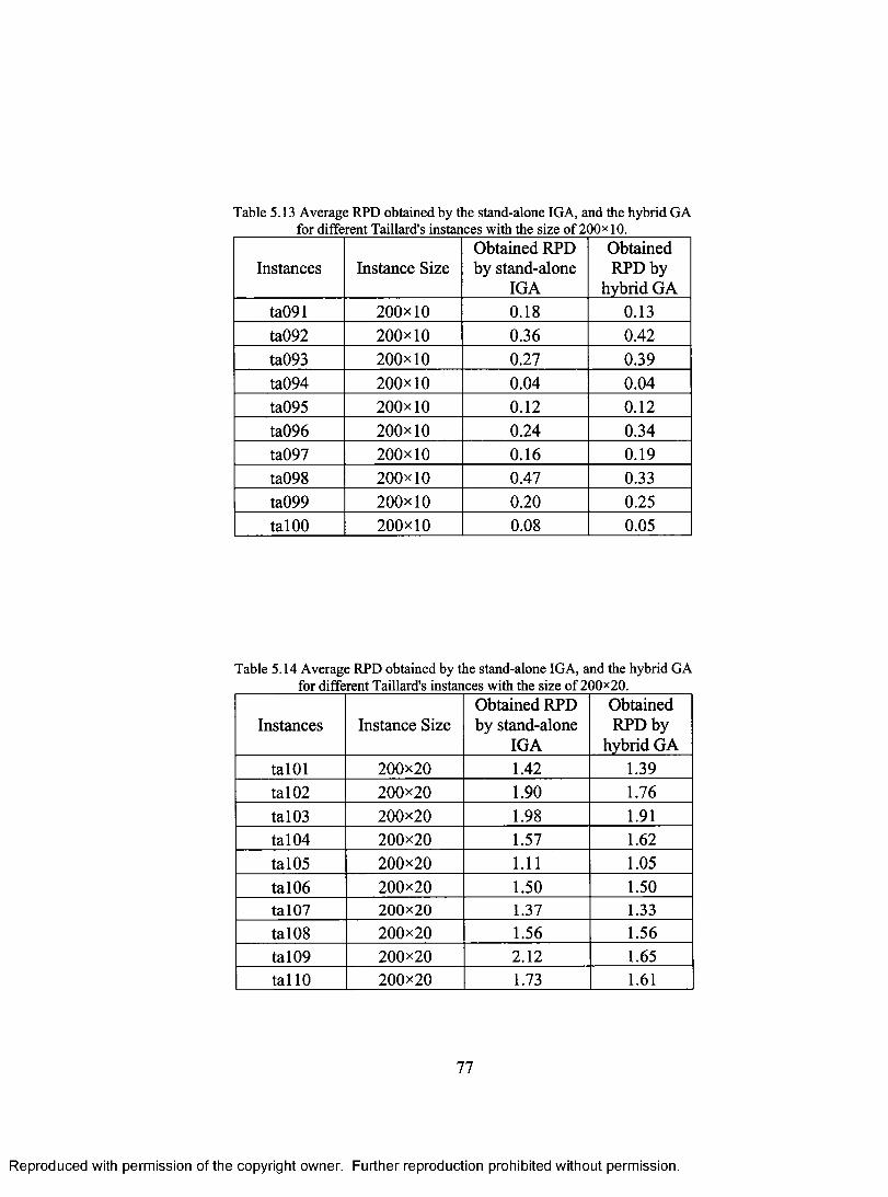
Table 5.13 Average RPD obtained by the stand-alone IGA, and the hybrid GA for different Taillard's instances with the size of 200x10.
Instances Instance Size Obtained RPD by stand-alone
IGA
Obtained RPD by
hybrid GA ta091 200x10 0.18 0.13 ta092 200x10 0.36 0.42
ta093 200x10 0.27 0.39
ta094 200x10 0.04 0.04 ta095 200x10 0.12 0.12
ta096 200x10 0.24 0.34 ta097 200x10 0.16 0.19
ta098 200x10 0.47 0.33
ta099 200x10 0.20 0.25
ta100 200x10 0.08 0.05
Table 5.14 Average RPD obtained by the stand-alone IGA, and the hybrid GA for different Taillard's instances with the size of 200x20.
Instances Instance Size Obtained RPD by stand-alone
IGA
Obtained RPD by
hybrid GA
ta101 200x20 1.42 1.39
ta102 200x20 1.90 1.76
ta103 200x20 1.98 1.91 ta104 200x20 1.57 1.62
ta105 200x20 1.11 1.05
ta106 200x20 1.50 1.50 ta107 200x20 1.37 1.33
ta108 200x20 1.56 1.56
ta109 200x20 2.12 1.65 tall° 200x20 1.73 1.61
77
Reproduced with permission of the copyright owner. Further reproduction prohibited without permission.
Table 5.13 Average RPD obtained by the stand-alone IGA, and the hybrid GAfor different Taillard's instances with the size o f 200x10.
Instances Instance SizeObtained RPD by stand-alone
IGA
Obtained RPD by
hybrid GAta091 200x10 0.18 0.13ta092 200x10 0.36 0.42ta093 200x10 0.27 0.39ta094 200x10 0.04 0.04ta095 200x10 0.12 0.12ta096 200x10 0.24 0.34ta097 200x10 0.16 0.19ta098 200x10 0.47 0.33ta099 200x10 0.20 0.25talOO 200x10 0.08 0.05
Table 5.14 Average RPD obtained by the stand-alone IGA, and the hybrid GA for different Taillard's instances with the size o f 200x20.
Instances Instance SizeObtained RPD by stand-alone
IGA
Obtained RPD by
hybrid GAtalOl 200x20 1.42 1.39tal02 200x20 1.90 1.76tal03 200x20 1.98 1.91tal04 200x20 1.57 1.62tal05 200x20 1.11 1.05tal06 200x20 1.50 1.50tal07 200x20 1.37 1.33tal08 200x20 1.56 1.56tal09 200x20 2.12 1.65tallO 200x20 1.73 1.61
77
Reproduced with permission of the copyright owner. Further reproduction prohibited without permission.

5.8 Performance of the Non-Hybrid GA and its Comparison with the Hybrid GA
The performance of the non-hybrid GA, which was discussed and tuned in Section 5.7, is
investigated here over the long CPU time. It is of interest to realize whether the non-
hybrid GA can obtain results similar to the hybrid GA when run for a longer period of
time. A time-dependent termination condition, of n x m x 360 milliseconds, was
considered for the non-hybrid GA, which is three times greater than that of the CPU time
allocated to the hybrid GA discussed in Section 4.1.5.
In Figures 5.11 and 5.12, the plots of the best solution of the non-hybrid GA for
the instances ta051 and ta071 are given. These plots typically show how the best fitness
value (makespan) of the PFSP evolves across the aforementioned time period (which is
approximately equal to evolution over 2.5x10⁴ generations).
After approximately 2.5x 10⁴ generations, the best obtained solution for the
instances ta051 and ta071 are 3977 and 5834, respectively. The best-known solutions
cited in the literature for these two instances are 3850 and 5770, respectively (see
Appendix D). Therefore, the final RPDs through the non-hybrid GA for the instances
ta051 and ta071 are 3.30 and 1.11, respectively.
It can be observed in Figures 5.11 and 5.12, that the best obtained solutions by the
non-hybrid GA do not evolve significantly after 1000 generations. Similar trends are
observed typically for other instances of Taillard's benchmarks, meaning that the non-
hybrid GA stalls quickly.
78
Reproduced with permission of the copyright owner. Further reproduction prohibited without permission.
5.8 Performance of the Non-Hybrid GA and its Comparison with the Hybrid GA
The performance o f the non-hybrid GA, which was discussed and tuned in Section 5.7, is
investigated here over the long CPU time. It is o f interest to realize whether the non
hybrid GA can obtain results similar to the hybrid GA when run for a longer period of
time. A time-dependent termination condition, o f n x m x 360 milliseconds, was
considered for the non-hybrid GA, which is three times greater than that o f the CPU time
allocated to the hybrid GA discussed in Section 4.1.5.
In Figures 5.11 and 5.12, the plots o f the best solution o f the non-hybrid GA for
the instances ta051 and ta.071 are given. These plots typically show how the best fitness
value (makespan) o f the PFSP evolves across the aforementioned time period (which is
approximately equal to evolution over 2.5 xlO4 generations).
After approximately 2.5*104 generations, the best obtained solution for the
instances ta051 and ta071 are 3977 and 5834, respectively. The best-known solutions
cited in the literature for these two instances are 3850 and 5770, respectively (see
Appendix D). Therefore, the final RPDs through the non-hybrid GA for the instances
ta.051 and ta071 are 3.30 and 1.11, respectively.
It can be observed in Figures 5.11 and 5.12, that the best obtained solutions by the
non-hybrid GA do not evolve significantly after 1000 generations. Similar trends are
observed typically for other instances o f Taillard’s benchmarks, meaning that the non
hybrid GA stalls quickly.
78
Reproduced with permission of the copyright owner. Further reproduction prohibited without permission.
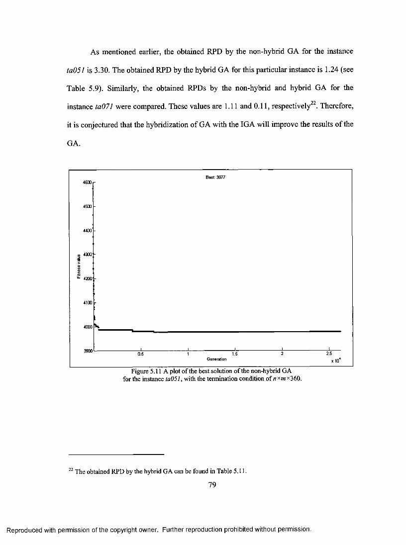
As mentioned earlier, the obtained RPD by the non-hybrid GA for the instance
ta051 is 3.30. The obtained RPD by the hybrid GA for this particular instance is 1.24 (see
Table 5.9). Similarly, the obtained RPDs by the non-hybrid and hybrid GA for the
instance ta071 were compared. These values are 1.11 and 0.11, respectively22. Therefore,
it is conjectured that the hybridization of GA with the IGA will improve the results of the
GA.
Best: 3977
4500
4333 3
4200
4100
40013 6
0.5 1 Generation
5
Figure 5.11 A plot of the best solution of the non-hybrid GA for the instance ta051, with the termination condition of n xm x360.
22 The obtained RPD by the hybrid GA can be found in Table 5.11.
79
2.5
x 104
Reproduced with permission of the copyright owner. Further reproduction prohibited without permission.
As mentioned earlier, the obtained RPD by the non-hybrid GA for the instance
ta051 is 3.30. The obtained RPD by the hybrid GA for this particular instance is 1.24 (see
Table 5.9). Similarly, the obtained RPDs by the non-hybrid and hybrid GA for the
• 22instance ta071 were compared. These values are 1.11 and 0.11, respectively . Therefore,
it is conjectured that the hybridization o f GA with the IGA will improve the results o f the
GA.
Best: 39774600
4500
4400
4300 -
4200
4100
4000
3900 2.50.5Generation x104
Figure 5.11 A plot o f the best solution o f the non-hybrid GAfor the instance ta051, with the termination condition o f n x/n*360.
22 The obtained RPD by the hybrid GA can be found in Table 5.11.
79
Reproduced with permission of the copyright owner. Further reproduction prohibited without permission.
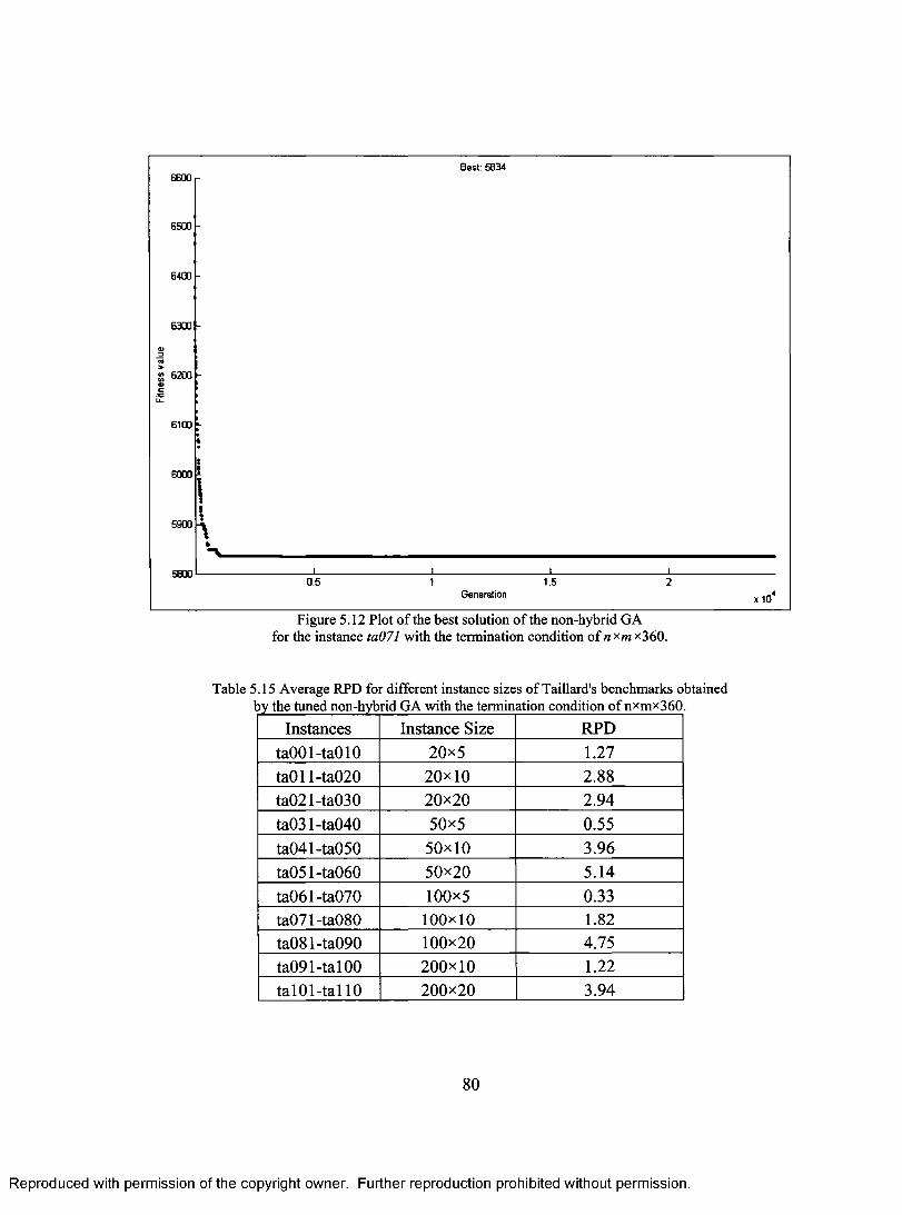
Best: 5834 6600 —
6500'
64E10
6300
a)
6200
Co
U-
6100
6000
5900
5800
■
1
0.5 1 1.5 2 Generation
Figure 5.12 Plot of the best solution of the non-hybrid GA for the instance ta07 1 with the termination condition of n xm x360.
Table 5.15 Average RPD for different instance sizes of Taillard's benchmarks obtained by the tuned non-hybrid GA with the termination condition of nxmx360.
Instances Instance Size RPD
ta001-ta010 20x5 1.27
ta011-ta020 20x 10 2.88
ta021-ta030 20x20 2.94
ta031-ta040 50x5 0.55
ta041-ta050 50x 10 3.96
ta051-ta060 50x20 5.14
ta061-ta070 100x5 0.33
ta071-ta080 100 x 10 1.82
ta081-ta090 100x20 4.75
ta091-ta100 200x10 1.22
ta101-ta1 10 200x20 3.94
80
le
Reproduced with permission of the copyright owner. Further reproduction prohibited without permission.
Best: 58348600
6500
6400
6300 -
X 6200 -
6100
6000
5900
58000.5
Generation x 10
Figure 5.12 Plot o f the best solution o f the non-hybrid GAfor the instance ta071 with the termination condition o f n *m x360.
Table 5.15 Average RPD for different instance sizes o f Taillard's benchmarks obtained by the tuned non-hybrid GA with the termination condition o f nxmx360.
Instances Instance Size RPDtaOOl-taOlO 20x5 1.27ta011-ta020 20x10 2.88ta021-ta030 20x20 2.94ta031-ta040 50x5 0.55ta041-ta050 50x10 3.96ta051-ta060 50x20 5.14ta061-ta070 100x5 0.33ta071-ta080 100x10 1.82ta081-ta090 100x20 4.75ta091-tal00 200x10 1.22talO l-tallO 200x20 3.94
80
Reproduced with permission of the copyright owner. Further reproduction prohibited without permission.
Finally, in order to investigate the superiority of the hybridization of the proposed
GA further, the non-hybrid GA is run ten times over the aforementioned CPU time for all
the instances of Taillard and the obtained RPDs are given in Table 5.15. Comparison of
the Table 5.15 and Table 5.3 substantiates the conjecture that hybridization of the GA
with the IGA are beneficial, for all instance sizes.
The other advantage of the proposed hybrid GA is its robustness. This can be
realized through Figures 5.6 through 5.10. In Figures 5.6-5.8, it can be observed that
different treatments of the factors do not change the obtained RPDs to a great extent.
More specifically, the difference of the worst and best values for the RPDs in Figures
5.6-5.8 are not greater than 0.1. Whereas, the non-hybrid GA shows much higher
variation in terms of the RPD. Figures 5.9 and 5.10 show that these variations could reach
up to 4. Therefore, it can be concluded that the proposed hybrid GA is robust with respect
to its parameters. Moreover, according to Table 5.3, it can be concluded that the hybrid
GA outperforms the stand-alone IGA.
81
Reproduced with permission of the copyright owner. Further reproduction prohibited without permission.
Finally, in order to investigate the superiority o f the hybridization o f the proposed
GA further, the non-hybrid GA is run ten times over the aforementioned CPU time for all
the instances o f Taillard and the obtained RPDs are given in Table 5.15. Comparison of
the Table 5.15 and Table 5.3 substantiates the conjecture that hybridization o f the GA
with the IGA are beneficial, for all instance sizes.
The other advantage o f the proposed hybrid GA is its robustness. This can be
realized through Figures 5.6 through 5.10. In Figures 5.6-5.8, it can be observed that
different treatments o f the factors do not change the obtained RPDs to a great extent.
More specifically, the difference o f the worst and best values for the RPDs in Figures
5.6-5.8 are not greater than 0.1. Whereas, the non-hybrid GA shows much higher
variation in terms o f the RPD. Figures 5.9 and 5.10 show that these variations could reach
up to 4. Therefore, it can be concluded that the proposed hybrid GA is robust with respect
to its parameters. Moreover, according to Table 5.3, it can be concluded that the hybrid
GA outperforms the stand-alone IGA.
81
Reproduced with permission of the copyright owner. Further reproduction prohibited without permission.
CHAPTER 6: CONCLUSIONS AND FUTURE WORK
The goal of this thesis was to survey one of the most well-known scheduling problems,
the permutation flow-shop scheduling problem. Makespan, as the most common
objective function (i.e., performance measure) to be minimized, was considered for
evaluation of the proposed algorithms in this thesis.
A genetic algorithm-based solution methodology was developed and implemented
in this thesis. More specifically, the performance of two versions of the proposed
algorithm, namely the stand-alone genetic algorithm (referred to as the non-hybrid
genetic algorithm) and the hybrid genetic algorithm (its hybridization with the iterated
greedy search algorithm) were extensively studied in this thesis. As for the comparative
experimental results, Taillard's standard benchmarks were employed. Experimental
results presented in this thesis showed that the performance of the search for near optimal
solutions was highly increased where the proposed genetic algorithm is hybridized with
an iterated greedy search algorithm.
The parameters of both the hybrid and the non-hybrid proposed genetic
algorithms were individually tuned using the full factorial experimental design. As a
result, it was shown that the following set of parameters yields the optimal combination
for the proposed hybrid GA: population size of 40, selection type of tournament,
crossover type SBOX, crossover probability of 0.60, mutation probability of 0.1, and
IGA probability of 0.02.
82
Reproduced with permission of the copyright owner. Further reproduction prohibited without permission.
C h a p t e r 6: C o n c l u sio n s A n d Fu t u r e W o r k
The goal o f this thesis was to survey one o f the most well-known scheduling problems,
the permutation flow-shop scheduling problem. Makespan, as the most common
objective function (i.e., performance measure) to be minimized, was considered for
evaluation of the proposed algorithms in this thesis.
A genetic algorithm-based solution methodology was developed and implemented
in this thesis. More specifically, the performance o f two versions o f the proposed
algorithm, namely the stand-alone genetic algorithm (referred to as the non-hybrid
genetic algorithm) and the hybrid genetic algorithm (its hybridization with the iterated
greedy search algorithm) were extensively studied in this thesis. As for the comparative
experimental results, Taillard’s standard benchmarks were employed. Experimental
results presented in this thesis showed that the performance of the search for near optimal
solutions was highly increased where the proposed genetic algorithm is hybridized with
an iterated greedy search algorithm.
The parameters o f both the hybrid and the non-hybrid proposed genetic
algorithms were individually tuned using the full factorial experimental design. As a
result, it was shown that the following set o f parameters yields the optimal combination
for the proposed hybrid GA: population size of 40, selection type o f tournament,
crossover type SBOX, crossover probability o f 0.60, mutation probability o f 0.1, and
IGA probability o f 0.02.
82
Reproduced with permission of the copyright owner. Further reproduction prohibited without permission.
As for the non-hybrid genetic algorithm, it was shown that the optimal
combination of parameters for the proposed non-hybrid GA is: population size of 60,
selection type of rank-based, crossover type of SBOX, crossover probability of 0.40, and
mutation probability of 0.20.
Furthermore, it was shown that the hybrid genetic algorithm performs very well
on the benchmark problems of Taillard. More specifically, the hybrid genetic algorithm
obtains optimal solutions for a large number of the small instances of Taillard (namely,
instances with the size of 20x5, 20x10, 20x20, 50x5, and 100x5). The hybrid genetic
algorithm performs well for larger instances as well. In the worst case, the relative
percentage deviation from the best-known solution for instances with the size of 200x20
is less than two (see Table 5.14). In addition, it was shown that the proposed hybrid
genetic algorithm is robust with respect to its parameters.
The non-hybrid genetic algorithm is not as effective as the hybrid one in terms of
the obtained relative percentage deviation from the best-known solution. As it was seen,
the performance of the non-hybrid genetic algorithm was always worse than the hybrid
genetic algorithm. Even allocating longer CPU time to the non-hybrid genetic algorithm
did not result in achieving the same results obtained by the hybrid genetic algorithm.
Finally, it was shown that the hybrid genetic algorithm performs slightly better
than the iterative greedy search algorithm of Ruiz et al. It is noteworthy to mention that
Ruiz et al. compared their iterative greedy search algorithm against other existing
algorithms and concluded that their algorithm outperforms them.
83
Reproduced with permission of the copyright owner. Further reproduction prohibited without permission.
As for the non-hybrid genetic algorithm, it was shown that the optimal
combination o f parameters for the proposed non-hybrid GA is: population size o f 60,
selection type o f rank-based, crossover type of SBOX, crossover probability o f 0.40, and
mutation probability o f 0.20.
Furthermore, it was shown that the hybrid genetic algorithm performs very well
on the benchmark problems o f Taillard. More specifically, the hybrid genetic algorithm
obtains optimal solutions for a large number o f the small instances o f Taillard (namely,
instances with the size o f 20x5, 20x10, 20x20, 50x5, and 100x5). The hybrid genetic
algorithm performs well for larger instances as well. In the worst case, the relative
percentage deviation from the best-known solution for instances with the size o f 200x20
is less than two (see Table 5.14). In addition, it was shown that the proposed hybrid
genetic algorithm is robust with respect to its parameters.
The non-hybrid genetic algorithm is not as effective as the hybrid one in terms o f
the obtained relative percentage deviation from the best-known solution. As it was seen,
the performance o f the non-hybrid genetic algorithm was always worse than the hybrid
genetic algorithm. Even allocating longer CPU time to the non-hybrid genetic algorithm
did not result in achieving the same results obtained by the hybrid genetic algorithm.
Finally, it was shown that the hybrid genetic algorithm performs slightly better
than the iterative greedy search algorithm of Ruiz et al. It is noteworthy to mention that
Ruiz et al. compared their iterative greedy search algorithm against other existing
algorithms and concluded that their algorithm outperforms them.
83
Reproduced with permission of the copyright owner. Further reproduction prohibited without permission.

Future work for this research could be a parallel implementation of the genetic
algorithm and the iterative greedy search algorithm. In a parallel implementation, the
genetic algorithm and the iterative greedy search algorithm can be run on two separate
processing units, where both algorithms have their own evolution but they exchange their
best solutions in different intervals during the time that the algorithms are being run on
two computers.
Applications of the proposed hybrid GA on the Traveling Salesman Problem is
another application domain that has been drawing attention recently.
84
Reproduced with permission of the copyright owner. Further reproduction prohibited without permission.
Future work for this research could be a parallel implementation of the genetic
algorithm and the iterative greedy search algorithm. In a parallel implementation, the
genetic algorithm and the iterative greedy search algorithm can be run on two separate
processing units, where both algorithms have their own evolution but they exchange their
best solutions in different intervals during the time that the algorithms are being run on
two computers.
Applications o f the proposed hybrid GA on the Traveling Salesman Problem is
another application domain that has been drawing attention recently.
84
Reproduced with permission of the copyright owner. Further reproduction prohibited without permission.
REFERENCES
[1] Allahverdi A., Two-machine proportionate flowshop scheduling with breakdowns to minimize maximum lateness, Computers and Operations Research 1996, 23(10):909-916,.
[2] Baker K.R., Introduction to Sequencing and Scheduling, Wiley & Sons, 1974.
[3] Blazewicz J., Ecker K., Pesch E., Schmidt G., and Weglarz J., Scheduling Computer and Manufacturing Processes, 2nd editions, Springer-Verlag, 2001.
[4] Campbell H.G., Dudek R.A., Smith M.L., A heuristic algorithm for the n-job, m-machine sequencing problem. Management Science 1970; 16(B):630-637.
[5] Chen C.L., Vempati, V.S., Aljaber, N., An application of genetic algorithms for flow shop problems. European Journal of Operational Research 1995; 80:389-396.
[6] Coley D.A., An Introduction to Genetic Algorithms for Scientists and Engineers, World Scientific Publishing Company, 1997.
[7] Conway R.W., Maxwell W.L., Miller, L.W., Theory of Scheduling, Addison-Wellesley, 1967.
[8] Dannenbring D.G., An evaluation of flow shop sequencing heuristics. Management Science 1977; 23(11):1174-1182.
[9] Davis L., Applying adaptative algorithms to epistatic domains, in: Proceedings of the International joint conference on artificial intelligence 1985, 162-164.
[10] Davoud Pour H., A new heuristic for the n-job, m-machine flow-shop problem. Production Planning and Control 2001, 12(7):648-653.
[11] Eiben A.E., and Smith J.E., Introduction to Evolutionary Computing, Springer-Verlag, 2003.
[12] Framinan J.M., Leisten R, Ruiz-Usano R., Efficient heuristics for flow shop sequencing with the objectives of makespan and flowtime minimization, European Journal of Operational Research 2002, 141:559-569.
[13] French S., Sequencing and Scheduling: An Introduction to the Mathematics of Job-Shop, John Wiley, New York, 1982.
[14] Garey M.R., Johnson D.S., Sethi R., The complexity of flow shop and job shop scheduling, Mathematics of Operations Research 1976:117-129.
85
Reproduced with permission of the copyright owner. Further reproduction prohibited without permission.
R e f e r e n c e s
[1] Allahverdi A., Two-machine proportionate flowshop scheduling with breakdowns to minimize maximum lateness, Computers and Operations Research 1996, 23(10):909-916„
[2] Baker K.R., Introduction to Sequencing and Scheduling, Wiley & Sons, 1974.
[3] Blazewicz J., Ecker K., Pesch E., Schmidt G., and Weglarz J., Scheduling Computer and Manufacturing Processes,2nd editions, Springer-Verlag, 2001.
[4] Campbell H.G., Dudek R.A., Smith M.L., A heuristic algorithm for the n-job, m-machine sequencing problem. Management Science 1970; 16(B):630-637.
[5] Chen C.L., Vempati, V.S., Aljaber, N., An application o f genetic algorithms for flow shop problems. European Journal o f Operational Research 1995; 80:389-396.
[6] Coley D.A., An Introduction to Genetic Algorithms for Scientists and Engineers, World Scientific Publishing Company, 1997.
[7] Conway R.W., Maxwell W.L., Miller, L.W., Theory o f Scheduling, Addison- Wellesley, 1967.
[8] Dannenbring D.G., An evaluation o f flow shop sequencing heuristics. Management Science 1977; 23(11): 1174-1182.
[9] Davis L., Applying adaptative algorithms to epistatic domains, in: Proceedings of the International joint conference on artificial intelligence 1985, 162-164.
[10] Davoud Pour H., A new heuristic for the «-job, m-machine flow-shop problem. Production Planning and Control 2001, 12(7):648-653.
[11] Eiben A.E., and Smith J.E., Introduction to Evolutionary Computing, Springer- Verlag, 2003.
[12] Framinan J.M., Leisten R, Ruiz-Usano R., Efficient heuristics for flow shop sequencing with the objectives o f makespan and flowtime minimization, European Journal o f Operational Research 2002, 141:559-569.
[13] French S., Sequencing and Scheduling: An Introduction to the Mathematics of Job-Shop, John Wiley, New York, 1982.
[14] Garey M.R., Johnson D.S., Sethi R., The complexity o f flow shop and job shop scheduling, Mathematics o f Operations Research 1976:117-129.
85
Reproduced with permission of the copyright owner. Further reproduction prohibited without permission.
[15] Gen M., Cheng R., Genetic Algorithms and Engineering Design, New York: Wiley, 1997.
[16] Goldberg D.E., Genetic Algorithms in Search, Optimization, and Machine Learning. Addison Wesley, 1989.
[17] Gupta J.N.D., A functional heuristic algorithm for the flow shop scheduling problem. Operational Research Quarterly 1971; 22(1):39-47.
[18] Gupta J.N.D., Heuristic algorithms for multistage flowshop scheduling problem, AIIE Transactions 4 (1972) 11-18.
[19] Haupt R.L. and Haupt S.E., Practical Genetic Algorithms, Second Edition, John Wiley & Sons, 2004.
[20] Holland J.H., Adaptation in Natural and Artificial Systems, University of Michigan Press, Ann Arbor, 1975.
[21] Dileepan P., Sen T., Job lateness in a two-machine flowshop with setup times separated, Computers and Operations Research, v.18 n.6, p.549-556, 1991.
[22] Hundal T.S., Rajgopal J. "An extension of Palmer heuristic for the flow-shop scheduling problem", International Journal of Production Research, 26 (1988), 1119-1124.
[23] Iyer S.K., Saxena B., Improved genetic algorithm for the permutation flowshop scheduling problem, Computers & Operations Research 31 (2004) 593-606.
[24] Jessup L.M., Valacich J.S., Information Systems Today, Prentice Hall; 1st edition 2002.
[25] Johnson S.M., Optimal two- and three-stage production schedules with setup times included, Naval Research Logistics Quarterly, 1954, Vol. 1, pp. 61-68.
[26] Kim Y., Minimizing total tardiness in permutation flowshops. European Journal of Operational Research 1993; 20:391-401.
[27] Koulamas C., 1998. A new constructive heuristic for the flowshop scheduling problem. European Journal of Operational Research Society 105,66-71.
[28] Ladhari T., Haouar M., A computational study of the permutation flow shop problem based on a tight lower bound; Computers & Operations Research 32 (2005) 1831-1847.
86
Reproduced with permission of the copyright owner. Further reproduction prohibited without permission.
[15] Gen M., Cheng R., Genetic Algorithms and Engineering Design, New York: Wiley, 1997.
[16] Goldberg D.E., Genetic Algorithms in Search, Optimization, and Machine Learning. Addison Wesley, 1989.
[17] Gupta J.N.D., A functional heuristic algorithm for the flow shop scheduling problem. Operational Research Quarterly 1971; 22(l):39-47.
[18] Gupta J.N.D., Heuristic algorithms for multistage flowshop scheduling problem, AIIE Transactions 4 (1972) 11-18.
[19] Haupt R.L. and Haupt S.E., Practical Genetic Algorithms, Second Edition, John Wiley & Sons, 2004.
[20] Holland J.H., Adaptation in Natural and Artificial Systems, University of Michigan Press, Ann Arbor, 1975.
[21] Dileepan P., Sen T., Job lateness in a two-machine flowshop with setup times separated, Computers and Operations Research, v.18 n.6, p.549-556,1991.
[22] Hundal T.S., Rajgopal J. “An extension of Palmer heuristic for the flow-shop scheduling problem”, International Journal o f Production Research, 26 (1988), 1119- 1124.
[23] Iyer S.K., Saxena B., Improved genetic algorithm for the permutation flowshop scheduling problem, Computers & Operations Research 31 (2004) 593-606.
[24] Jessup L.M., Valacich J.S., Information Systems Today, Prentice Hall; 1st edition 2002.
[25] Johnson S.M., Optimal two- and three-stage production schedules with setup times included, Naval Research Logistics Quarterly, 1954, Vol. 1, pp. 61-68.
[26] Kim Y., Minimizing total tardiness in permutation flowshops. European Journal o f Operational Research 1993; 20:391-401.
[27] Koulamas C., 1998. A new constructive heuristic for the flowshop scheduling problem. European Journal o f Operational Research Society 105, 66-71.
[28] Ladhari T., Haouar M., A computational study o f the permutation flow shop problem based on a tight lower bound; Computers & Operations Research 32 (2005) 1831-1847.
86
Reproduced with permission of the copyright owner. Further reproduction prohibited without permission.
[29] Stasko J.T, Longest Common Subsequence Pseudo Code, http://www.cc.gatech.edu/classes/cs3158 98_fall/lcs.html, last accessed February 5, 2006.
[30] Lourenco H.R., Martin 0.C., Stiitzle T., 2000. "Iterated Local Search," Economics Working Papers 513, Department of Economics and Business, Universitat Pompeu Fabra.
[31] Michalewicz Z., Genetic Algorithms + Data Structures = Evolution Programs, 3rd Revised Eedition, New York: Springer-Verlag, 1998.
[32] Miyazaki S., Nishiyama N., Hashimoto F., An adjacent pairwise approach to the mean flowtime scheduling problem, Journal of the Operations Research Society of Japan 21 (1978) 287-299.
[33] Murata T., Ishibuchi H., Takana H., Genetic algorithm for flow shop scheduling problems. Computers and Industrial Engineering 1996; 30 (4): 1061-1071.
[34] NIST/SEMATECH e-Handbook of Statistical Methods, http://www.itl.nist.gov/div898/handbook/, last visited: February 24,2006.
[35] Oliver I.M., Smith D.J., Holland J.R.C., A study of permutation crossover operators on the traveling salesman problem, Proceedings of the Second International Conference on Genetic Algorithms on and their application, p.224-230, October 1987, Cambridge, Massachusetts, United States.
[36] Osman LH., Potts C.N., Simulated annealing for permutation flow-shop scheduling. OMEGA, The International Journal of Management Science 1989; 17(6): 551-557.
[37] Palmer D.S., Sequencing jobs through a multistage process in the minimum total time: A quick method of obtaining a near-optimum, Operational Research Quarterly 16 (1965) 101-107.
[38] Pan J.C.H., Fan E.T., Two-machine flow-shop scheduling to minimize total tardiness. International Journal of Systems Science 1997; 28:405-14.
[39] Pinedo M., Scheduling: Theory, Algorithms, and Systems, 2nd Edition, Prentice Hall; 2001.
[40] Ponnambalam S.G., Aravindan P., Chandrasekaran S., 2001. Constructive and improvement flow shop scheduling heuristics: An extensive evaluation, Production Planning and Control 12 (4), 335-344.
[41] Reeves C.R., Improving the efficiency of tabu search in machine sequencing problems, Journal of Operations research society, 1993, 44: 375-382.
87
Reproduced with permission of the copyright owner. Further reproduction prohibited without permission.
[29] Stasko J.T, Longest Common Subsequence Pseudo Code, http://www.cc.gatech.edu/classes/cs3158 98 fall/lcs.html. last accessed February 5, 2006.
[30] Lourenpo H.R., Martin O.C., Stutzle T., 2000. "Iterated Local Search," Economics Working Papers 513, Department o f Economics and Business, Universitat Pompeu Fabra.
[31] Michalewicz Z., Genetic Algorithms + Data Structures = Evolution Programs, 3rd Revised Eedition, New York: Springer-Verlag, 1998.
[32] Miyazaki S., Nishiyama N., Hashimoto F., An adjacent pairwise approach to the mean flowtime scheduling problem, Journal o f the Operations Research Society of Japan 21 (1978) 287-299.
[33] Murata T., Ishibuchi H., Takana H., Genetic algorithm for flow shop scheduling problems. Computers and Industrial Engineering 1996; 30 (4): 1061-1071.
[34] NIST/SEMATECH e-Handbook o f Statistical Methods, http://www.itl.nist.gov/div898/handbook/, last visited: February 24,2006.
[35] Oliver I.M., Smith D.J., Holland J.R.C., A study o f permutation crossover operators on the traveling salesman problem, Proceedings o f the Second International Conference on Genetic Algorithms on and their application, p.224-230, October 1987, Cambridge, Massachusetts, United States.
[36] Osman I.H., Potts C.N., Simulated annealing for permutation flow-shop scheduling. OMEGA, The International Journal o f Management Science 1989; 17(6): 551-557.
[37] Palmer D.S., Sequencing jobs through a multistage process in the minimum total time: A quick method of obtaining a near-optimum, Operational Research Quarterly 16(1965) 101-107.
[38] Pan J.C.H., Fan E.T., Two-machine flow-shop scheduling to minimize total tardiness. International Journal o f Systems Science 1997; 28:405-14.
[39] Pinedo M., Scheduling: Theory, Algorithms, and Systems, 2nd Edition, Prentice Hall; 2001.
[40] Ponnambalam S.G., Aravindan P., Chandrasekaran S., 2001. Constructive and improvement flow shop scheduling heuristics: An extensive evaluation, Production Planning and Control 12 (4), 335-344.
[41] Reeves C.R., Improving the efficiency o f tabu search in machine sequencing problems, Journal o f Operations research society, 1993, 44: 375-382.
87
Reproduced with permission of the copyright owner. Further reproduction prohibited without permission.
[42] Reeves C.R., A genetic algorithm for flowshop sequencing. Computers & Operations Research 1995, 22, pp. 5-13.
[43] Reeves C.R., Yamada T., Genetic Algorithms, Path Relinking and the Flowshop Sequencing Problem; Evolutionary Computation journal (MIT press), Vol.6 No.1, pp. 230-234 Spring 1998.
[44] Rinnooy Kan A.H.G., Machine Scheduling Problems: Classification, Complexity, and Computations, Nijhoff, The Hague, 1976.
[45] Ruiz R., Maroto C., A comprehensive review and evaluation of permutation flowshop heuristics, European Journal of Operational Research 2005; 165: 479-94.
[46] Ruiz R., Maroto C., Alcaraz J., Two new robust genetic algorithms for the flowshop scheduling problem OMEGA: International Journal of Management Science, In Press, Corrected Proof, Available online 9 April 2005,
[47] Ruiz R., Stiitzle T., A Simple and Effective Iterated Greedy Algorithm for the Flowshop Scheduling Problem. European Journal of Operational Research 2005, (accepted for publication).
[48] Sakawa M., Genetic Algorithms and Fuzzy Multiobjective Optimization, Kluwer Academic Publishers, 2002.
[49] Sem T., Dileepan P., Jatinder N. D., The two-machine flowshop scheduling problem with total tardiness, Computers and Operations Research, v.16 n.4, p.333-340, July 1989.
[50] Stilzle T., 1998. Applying Iterated Local Search to the permutation flow shop problem. Technical Report, AIDA-98-04, FG Intellektik,TU Darmstadt
[51] Syswerda G., Schedule Optimisation Using Genetic Algorithms. In Davis L. editor. Handbook of Genetic Algorithms, London: International Thomson Computer Press, 1991: 335-349.
[52] Taillard E. Some efficient heuristic methods for the flow shop sequencing problem. European Journal of Operational Research 1990;47:65-74.
[53] Taillard E., Benchmark for basic scheduling problems, European Journal of Operational Research 64 (1993) 278-285.
[54] Taillard E, http ://ina. eivd. ch/collaborateurs/etd/probl ernes . dir/ordonnancement. dir/ordonnanceme nt.html, last accessed February 7, 2005.
88
Reproduced with permission of the copyright owner. Further reproduction prohibited without permission.
[42] Reeves C.R., A genetic algorithm for flowshop sequencing. Computers & Operations Research 1995, 22, pp. 5-13.
[43] Reeves C.R., Yamada T., Genetic Algorithms, Path Relinking and the Flowshop Sequencing Problem; Evolutionary Computation journal (MIT press), Vol.6 N o.l, pp. 230-234 Spring 1998.
[44] Rinnooy Kan A.H.G., Machine Scheduling Problems: Classification, Complexity, and Computations, Nijhoff, The Hague, 1976.
[45] Ruiz R., Maroto C., A comprehensive review and evaluation o f permutation flowshop heuristics, European Journal o f Operational Research 2005; 165: 479-94.
[46] Ruiz R., Maroto C., Alcaraz J., Two new robust genetic algorithms for the flowshop scheduling problem OMEGA: International Journal o f Management Science, In Press, Corrected Proof, Available online 9 April 2005,
[47] Ruiz R., Stutzle T., A Simple and Effective Iterated Greedy Algorithm for the Flowshop Scheduling Problem. European Journal o f Operational Research 2005, (accepted for publication).
[48] Sakawa M., Genetic Algorithms and Fuzzy Multiobjective Optimization,Kluwer Academic Publishers, 2002.
[49] Sem T., Dileepan P., Jatinder N. D., The two-machine flowshop scheduling problem with total tardiness, Computers and Operations Research, v.16 n.4, p.333- 340, July 1989.
[50] Stiizle T., 1998. Applying Iterated Local Search to the permutation flow shop problem. Technical Report, AIDA-98-04, FG Intellektik,TU Darmstadt
[51] Syswerda G., Schedule Optimisation Using Genetic Algorithms. In Davis L. editor. Handbook of Genetic Algorithms, London: International Thomson Computer Press, 1991: 335-349.
[52] Taillard E. Some efficient heuristic methods for the flow shop sequencing problem. European Journal o f Operational Research 1990;47:65-74.
[53] Taillard E., Benchmark for basic scheduling problems, European Journal of Operational Research 64 (1993) 278-285.
[54] Taillard E,http://ina.eivd.ch/collaborateurs/etd/problemes.dir/ordonnancement.dir/ordonnanceme nt.html, last accessed February 7, 2005.
88
Reproduced with permission of the copyright owner. Further reproduction prohibited without permission.
[55] Turner S., Booth D., Comparison of heuristics for flowshop sequencing, OMEGA: International Journal of Management Science, 15 (1987) 75-85.
[56] Whitley D., The GENITOR Algorithm and Selection Pressure: Why Rank-Based Allocation of Reproductive Trials is Best, Proceedings of the Third International Conference on Genetic Algorithms, 1989.
[57] Widmer M., Hertz A., A new heuristic for the flow shop sequencing problem, European Journal of Operational Research 1989; 41:186-93. Winston ML., The Biology of the Honey Bee, Harvard University Press 1987.
[58] Nawaz M., Enscore E.E.J., Ham I., A heuristic algorithm for the m-machine, n-job flow shop sequencing problem. OMEGA: International Journal of Management Science, 1983;11 (1):91-5.
[59] Bierwirth C., Mattfeld D.C., Kopfer H., On Permutation Representations for Scheduling Problems, Proceedings of the 4th International Conference on Parallel Problem Solving from Nature, p.310-318, September 22-26,1996
[60] Ogbu F.A., Smith D.K., The application of the simulated annealing algorithms to the solution of the n/m/Cmax flowshop problem. Computers & Operations Research 1990;17(3):243-53.
[61] Montgomery D.C., Design and analysis of experiments, 5th Ed., New York: Wiley; 2000.
[62] Baker J.E., Adaptive Selection Methods for genetic Algorithms, in Proceedings of the 1st International Conference on Genetic Algorithms, Lawrence Erlbaum Associates, Inc. Hillsdale, NJ, 1985, pp. 101-111.
[63] Weisstein E.W., "NP-Hard Problem." From Math World-- A Wolfram Web Resource. http://mathworld.wolfram.com/NP-HardProblem.html, last accessed March 31,2006.
89
Reproduced with permission of the copyright owner. Further reproduction prohibited without permission.
[55] Turner S., Booth D., Comparison of heuristics for flowshop sequencing, OMEGA: International Journal o f Management Science, 15 (1987) 75-85.
[56] Whitley D., The GENITOR Algorithm and Selection Pressure: Why Rank- Based Allocation o f Reproductive Trials is Best, Proceedings o f the Third International Conference on Genetic Algorithms, 1989.
[57] Widmer M., Hertz A., A new heuristic for the flow shop sequencing problem, European Journal o f Operational Research 1989; 41:186-93.Winston ML., The Biology of the Honey Bee, Harvard University Press 1987.
[58] Nawaz M., Enscore E.E.J., Ham I., A heuristic algorithm for the m-machine, n- job flow shop sequencing problem. OMEGA: International Journal o f Management Science, 1983;11 (l):91-5.
[59] Bierwirth C., Mattfeld D.C., Kopfer H., On Permutation Representations for Scheduling Problems, Proceedings of the 4th International Conference on Parallel Problem Solving from Nature, p.310-318, September 22-26,1996
[60] Ogbu F.A., Smith D.K., The application o f the simulated annealing algorithms to the solution o f the n/m/Cmax flowshop problem. Computers & Operations Research 1990; 17(3):243-53.
[61] Montgomery D.C., Design and analysis o f experiments, 5th Ed., New York: Wiley; 2000.
[62] Baker J.E., Adaptive Selection Methods for genetic Algorithms, in Proceedings o f the 1st International Conference on Genetic Algorithms, Lawrence Erlbaum Associates, Inc. Hillsdale, NJ, 1985, pp. 101-111.
[63] Weisstein E.W., "NP-Hard Problem.” From MathWorld- A Wolfram Web Resource. http://mathworld.wolfram.com/NP-HardProblem.html. last accessed March 31,2006.
89
Reproduced with permission of the copyright owner. Further reproduction prohibited without permission.
APPENDIX
Appendix A: Residuals Plots for the Hybrid GA
Appendix B: ANOVA Table for the Non-Hybrid GA
Appendix C: Residuals Plots for the Non-Hybrid GA
Appendix D: Best-known makespan for Taillard's standard benchmark problems
Appendix E: Java Code
90
Reproduced with permission of the copyright owner. Further reproduction prohibited without permission.
A p pe n d ix
Appendix A: Residuals Plots for the Hybrid GA
Appendix B: ANOVA Table for the Non-Hybrid GA
Appendix C: Residuals Plots for the Non-Hybrid GA
Appendix D: Best-known makespan for Taillard's standard benchmark problems
Appendix E: Java Code
90
Reproduced with permission of the copyright owner. Further reproduction prohibited without permission.
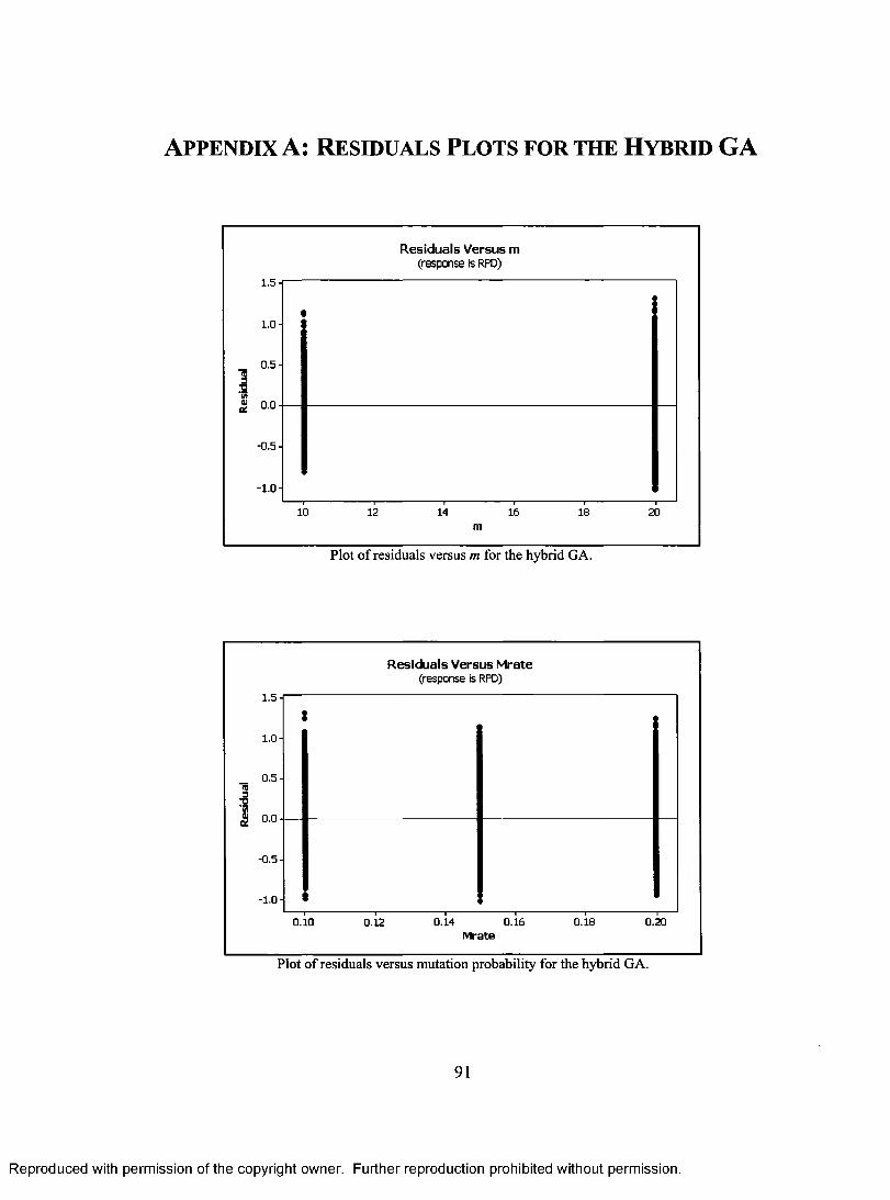
APPENDIX A: RESIDUALS PLOTS FOR THE HYBRID GA
Residuals Versus m (response is RPD)
1.5
1.0
-0.5
-1.0
1.5
1.0
-0.5
-1.0
10 12 14 m
16 18
Plot of residuals versus m for the hybrid GA.
Residuals Versus Mrate (response is RPD)
20
t
$ t
0.10 0.12 0.14 0.16 Mrate
0.18 0.20
Plot of residuals versus mutation probability for the hybrid GA.
91
Reproduced with permission of the copyright owner. Further reproduction prohibited without permission.
A p pe n d ix A: R e sid u a l s Plo t s f o r th e H y b r id GA
1 .5 -
1.0 -
_ 0 .5 -(0 3
■o'B
s 0.0-
-0 .5 -
- 1.0 -
10 12 14 16 18 20m
Plot o f residuals versus m for the hybrid GA.
1.5
1.0
_ 0 ,5(0 3■o*5S. o.o
-0 .5
- 1,0
Plot o f residuals versus mutation probability for the hybrid GA.
91
Reproduced with permission of the copyright owner. Further reproduction prohibited without permission.
Residuals Versus Mrate(resp o n se is RPD)
0.10 0.12 0 .14 0.16 0.18 0.20Mrate
Residuals Versus m(re sp o n se is RPD)
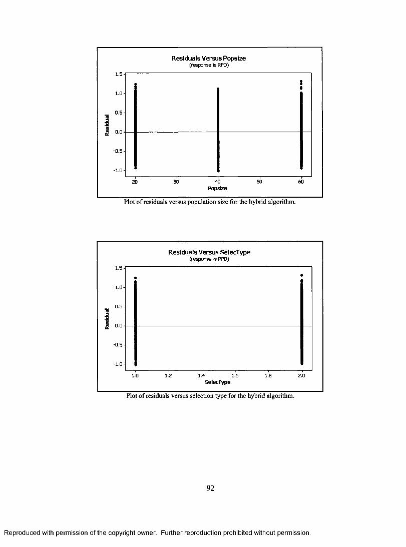
Residuals Versus Popsize (response is RPD)
1.5
1.0
-0.5
-1.0
1.5
1.0
-0.5
-1.0
• : •
20 30 40 Popsize
50
Plot of residuals versus population size for the hybrid algorithm.
Residuals Versus SelecType (response is RPD)
60
• •
1.0 1.2 1.4 1.6 SelecType
1.8
Plot of residuals versus selection type for the hybrid algorithm.
92
2.0
Reproduced with permission of the copyright owner. Further reproduction prohibited without permission.
Residuals Versus Popsize(response is RPD)
1.5 -{
1.0 -
_ 0.5-<o3■o‘3& o.o-
-0.5-
- 1.0 -
30 40 50 6020Popsize
Plot o f residuals versus population size for the hybrid algorithm.
Residuals Versus SelecType(re s p o n se is RPD)
1.5-1-------------------------------------------------------------------
1.0 -
0.5-TS3■o'3£ o.o-
-0.5-
- 1.0 -
1.0 1.2 1.4 1.6 1.8 2.0SelecType
Plot o f residuals versus selection type for the hybrid algorithm.
92
Reproduced with permission of the copyright owner. Further reproduction prohibited without permission.
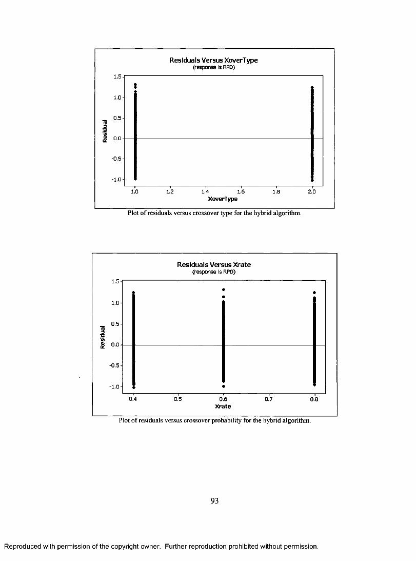
Residuals Versus XoverType (response is RPD)
1.5
! 1.0
-0.5
-1.0
1,5
1.0
0.5
-0.5
-1.0
I 1.0 1.2 1.4 1.6
XoverType 1,8
Plot of residuals versus crossover type for the hybrid algorithm.
Residuals Versus Xrate (response is RPD)
2.0
• • • •
I •
0.4 0.5 0.6 Xrate
0.7 0.
Plot of residuals versus crossover probability for the hybrid algorithm.
93
Reproduced with permission of the copyright owner. Further reproduction prohibited without permission.
1.0 -
_ 0.5-<0 s ■o ■«« 0 .0 -
-0.5-
- 1.0 -
1.0 1.2 1.4 1.6 1.8 2.0XoverType
Plot o f residuals versus crossover type for the hybrid algorithm.
Residuals Versus Xrate( r e s p o n s e is RPD)
1.5-
1.0 -
0.5-133 ■D'Si2 o.o-
-0.5-
- 1.0 -
Plot o f residuals versus crossover probability for the hybrid algorithm.
0.4 0.5 0.6X rate
0.7 0.8
Residuals Versus XoverType(response is RPD)
I
Reproduced with permission of the copyright owner. Further reproduction prohibited without permission.
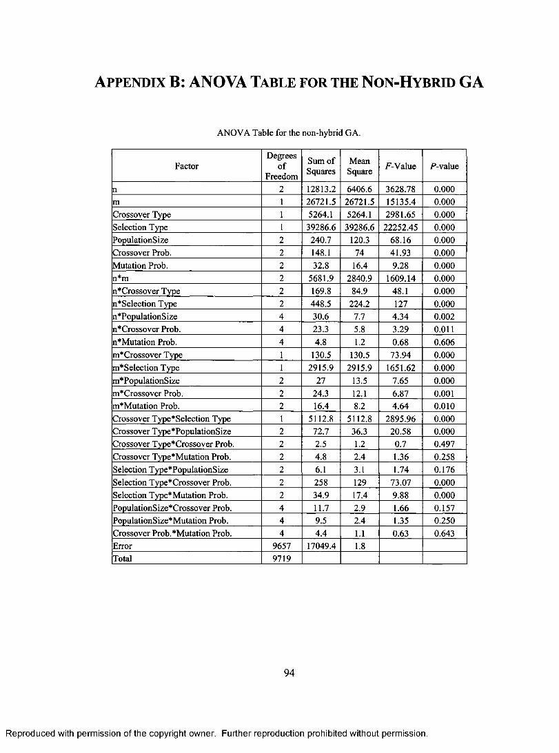
APPENDIX B: ANOVA TABLE FOR THE NON-HYBRID GA
ANOVA Table for the non-hybrid GA.
Factor Degrees
of Freedom
Sum of Squares
Mean Square
F-Value P-value
n 2 12813.2 6406.6 3628.78 0.000
m 1 26721.5 26721.5 15135.4 0.000
Crossover Type 1 5264.1 5264.1 2981.65 0.000
Selection Type 1 39286.6 39286.6 22252.45 0.000
PopulationSize 2 240.7 120.3 68.16 0.000
Crossover Prob. 2 148.1 74 41.93 0.000
Mutation Prob. 2 32.8 16.4 9.28 0.000
n*m 2 5681.9 2840.9 1609.14 0.000
n*Crossover Type 2 169.8 84.9 48.1 0.000
n*Selection Type 2 448.5 224.2 127 0.000
n*PopulationSize 4 30.6 7.7 4.34 0.002 n*Crossover Prob. 4 23.3 5.8 3.29 0.011
n*Mutation Prob. 4 4.8 1.2 0.68 0.606
m*Crossover Type 1 130.5 130.5 73.94 0.000
m*Selection Type 1 2915.9 2915.9 1651.62 0.000
m*Po ulationSize 2 27 13.5 7.65 0.000
m*Crossover Prob. 2 24.3 12.1 6.87 0.001 m*Mutation Prob. 2 16.4 8.2 4.64 0.010
Crossover Type*Selection Type 1 5112.8 5112.8 2895.96 0.000 Crossover Type*PopulationSize 2 72.7 36.3 20.58 0.000 Crossover Type*Crossover Prob. 2 2.5 1.2 0.7 0.497
Crossover Type*Mutation Prob. 2 4.8 2.4 1.36 0.258
Selection Type*PopulationSize 2 6.1 3.1 1.74 0.176
Selection T e*Crossover Prob. 2 258 129 73.07 0.000
Selection Type*Mutation Prob. 2 34.9 17.4 9.88 0.000
PopulationSize*Crossover Prob. 4 11.7 2.9 1.66 0.157 PopulationSize*Mutation Prob. 4 9.5 2.4 1.35 0.250
Crossover Prob.*Mutation Prob. 4 4.4 1.1 0.63 0.643 Error 9657 17049.4 1.8 Total 9719
94
Reproduced with permission of the copyright owner. Further reproduction prohibited without permission.
A p pe n d ix B: ANOVA Ta ble f o r th e N o n -H y b r id G A
ANOVA Table for the non-hybrid GA.
FactorDegrees
o fFreedom
Sum of Squares
MeanSquare F-Value P-value
n 2 12813.2 6406.6 3628.78 0.000m 1 26721.5 26721.5 15135.4 0.000Crossover Type 1 5264.1 5264.1 2981.65 0.000Selection Type 1 39286.6 39286.6 22252.45 0.000PopulationSize 2 240.7 120.3 68.16 0.000Crossover Prob. 2 148.1 74 41.93 0.000Mutation Prob. 2 32.8 16.4 9.28 0.000n*m 2 5681.9 2840.9 1609.14 0.000n*Crossover Type 2 169.8 84.9 48.1 0.000n*Selection Type 2 448.5 224.2 127 0.000n*PopulationSize 4 30.6 7.7 4.34 0.002n*Crossover Prob. 4 23.3 5.8 3.29 0.011n*Mutation Prob. 4 4.8 1.2 0.68 0.606m*Crossover Type 1 130.5 130.5 73.94 0.000m*Selection Type 1 2915.9 2915.9 1651.62 0.000m*PopulationSize 2 27 13.5 7.65 0.000m*Crossover Prob. 2 24.3 12.1 6.87 0.001m*Mutation Prob. 2 16.4 8.2 4.64 0.010Crossover Type*Selection Type 1 5112.8 5112.8 2895.96 0.000Crossover Type*PopulationSize 2 72.7 36.3 20.58 0.000Crossover Type*Crossover Prob. 2 2.5 1.2 0.7 0.497Crossover Type*Mutation Prob. 2 4.8 2.4 1.36 0.258Selection Type*PopulationSize 2 6.1 3.1 1.74 0.176Selection Type*Crossover Prob. 2 258 129 73.07 0.000Selection Type*Mutation Prob. 2 34.9 17.4 9.88 0.000PopulationSize*Crossover Prob. 4 11.7 2.9 1.66 0.157PopulationSize*Mutation Prob. 4 9.5 2.4 1.35 0.250Crossover Prob.*Mutation Prob. 4 4.4 1.1 0.63 0.643Error 9657 17049.4 1.8Total 9719
94
Reproduced with permission of the copyright owner. Further reproduction prohibited without permission.
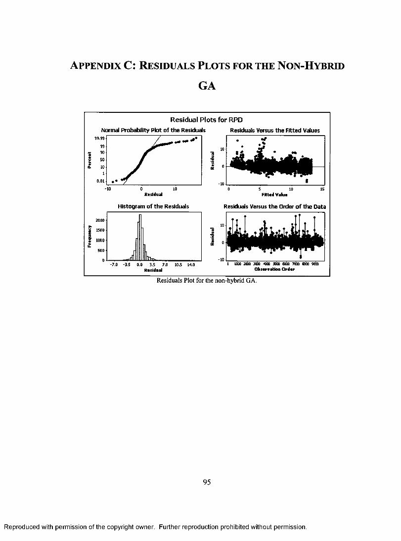
APPENDIX C: RESIDUALS PLOTS FOR THE NON-HYBRID
GA
Residual Plots for RPD
Normal Probability Plot of the Residuals 99.99
99
90
50
0. • 10
0.01
10 a O
72 o
-10 0 Residual
10
Histogram of the Residuals
2000 -
'6" ▪ 1500 •
0 er ▪ 1000 - IL
500 -
a 0
72
at
-7.0 -3.5 0.0 3.5 7.0 10.5 14.0 Residual
-10 0
Residuals Versus the Fitted Values
5 10 Fitted Value
15
Residuals Versus the Order of the Data
10
0
-10 1 1020 2000 MOO 4030 5000 6073 7033 e000 9000
Observation Order
Residuals Plot for the non-hybrid GA.
95
Reproduced with permission of the copyright owner. Further reproduction prohibited without permission.
A p pe n d ix C: Re sid u a l s Pl o t s f o r th e N o n -H y b r id
GA
Normal Probability Plot of the Residuals39.99
Residual P lo ts for RPDResiduals Versus the Fitted Values
99
c 90S 50
a 10l
0.01
2000
1500
1000
500
0
-10 0 10Residual
Histogram of the Residuals
—«-rlf-7.0 -3.5 0.0 3.5 7.0 10.5 14.0
Residual
10
•/
t i
0 5 10 15Fitted Value
Residuals Versus the Order of the Data
1 1QM 2000 XOQ 4QQQ 5GQQ «UQ 7000 9XU 9000 Observation O rder
Residuals Plot for the non-hybrid GA.
95
Reproduced with permission of the copyright owner. Further reproduction prohibited without permission.
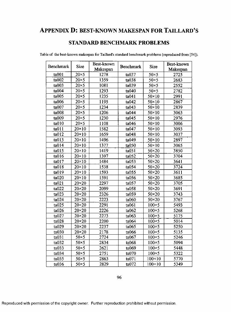
APPENDIX D: BEST-KNOWN MAKESPAN FOR TAILLARD'S
STANDARD BENCHMARK PROBLEMS
Table of the best-known makespan for Taillard's standard benchmark problems (reproduced from [54]).
Benchmark Size Best-known Makespan Benchmark Size Best-known
Makespan ta001 20x5 1278 ta037 50x5 2725 ta002 20x5 1359 ta038 50x5 2683 ta003 20x5 1081 ta039 50x5 2552 ta004 20x5 1293 ta040 50x5 2782 ta005 20x5 1235 ta041 50x10 2991 ta006 20x5 1195 ta042 50 x 10 2867 ta007 20x5 1234 ta043 50x10 2839 ta008 20x5 1206 ta044 50x10 3063 ta009 20x5 1230 ta045 50x10 2976 ta010 20x5 1108 ta046 50x10 3006 ta011 20x10 1582 ta047 50x10 3093 ta012 20x10 1659 ta048 50x10 3037 ta013 20x10 1496 ta049 50 x 10 2897 ta014 20x10 1377 ta050 50x10 3065 ta015 20x10 1419 ta051 50x20 3850 ta016 20x10 1397 ta052 50x20 3704 ta017 20x10 1484 ta053 50x20 3641 ta018 20x10 1538 ta054 50x20 3724 ta019 20x10 1593 ta055 50x20 3611 ta020 20x10 1591 ta056 50x20 3685 ta021 20x20 2297 ta057 50x20 3705 ta022 20x20 2099 ta058 50x20 3691 ta023 20x20 2326 ta059 50x20 3743 ta024 20x20 2223 ta060 50x20 3767 ta025 20x20 2291 ta061 100)(5 5493 ta026 20x20 2226 ta062 100 x 5 5268 ta027 20x20 2273 ta063 100)(5 5175 ta028 20x20 2200 ta064 100 x 5 5014 ta029 20x20 2237 ta065 100x5 5250 ta030 20x20 2178 ta066 100x5 5135 ta031 50x5 2724 ta067 100 x 5 5246 ta032 50x5 2834 ta068 100 x 5 5094 ta033 50x5 2621 ta069 100x5 5448 ta034 50x5 2751 ta070 100 x 5 5322 ta035 50x5 2863 ta071 100x10 5770 ta036 50x5 2829 ta072 100x10 5349
96
Reproduced with permission of the copyright owner. Further reproduction prohibited without permission.
A p pe n d ix D: best-k n o w n m a k espa n f o r Ta il l a r d ’s
STANDARD BENCHMARK PROBLEMS
Table o f the best-known makespan for Taillard's standard benchmark problems (reproduced from [54]).
Benchmark Size Best-knownMakespan Benchmark Size Best-known
MakespantaOOl 20x5 1278 ta037 50x5 2725ta002 20x5 1359 ta038 50x5 2683ta003 20x5 1081 ta039 50x5 2552ta004 20x5 1293 ta040 50x5 2782ta005 20x5 1235 ta041 50x10 2991ta006 20x5 1195 ta042 50x10 2867ta007 20x5 1234 ta043 50x10 2839ta008 20x5 1206 ta044 50x10 3063ta009 20x5 1230 ta045 50x10 2976taOlO 20x5 1108 ta046 50x10 3006taOll 20x10 1582 ta047 50x10 3093ta012 20x10 1659 ta048 50x10 3037ta013 20x10 1496 ta049 50x10 2897ta014 20x10 1377 ta050 50x10 3065ta015 20x10 1419 ta051 50x20 3850ta016 20x10 1397 ta052 50x20 3704ta017 20x10 1484 ta053 50x20 3641ta018 20x10 1538 ta054 50x20 3724ta019 20x10 1593 ta055 50x20 3611ta020 20x10 1591 ta056 50x20 3685ta021 20x20 2297 ta057 50x20 3705ta022 20x20 2099 ta058 50x20 3691ta023 20x20 2326 ta059 50x20 3743ta024 20x20 2223 ta060 50x20 3767ta025 20x20 2291 ta061 100x5 5493ta026 20x20 2226 ta062 100x5 5268ta027 20x20 2273 ta063 100x5 5175ta028 20x20 2200 ta064 100x5 5014ta029 20x20 2237 ta065 100x5 5250ta030 20x20 2178 ta066 100x5 5135ta031 50x5 2724 ta067 100x5 5246ta032 50x5 2834 ta068 100x5 5094ta033 50x5 2621 ta069 100x5 5448ta034 50x5 2751 ta070 100x5 5322ta035 50x5 2863 ta071 100x10 5770ta036 50x5 2829 ta072 100x10 5349
96
Reproduced with permission of the copyright owner. Further reproduction prohibited without permission.
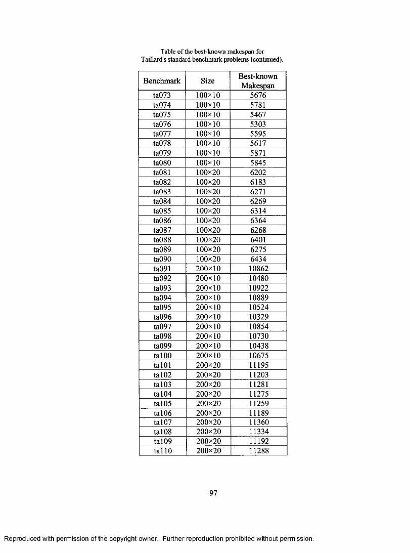
Table of the best-known makespan for Taillard's standard benchmark problems (continued).
Benchmark Size Best-known Makespan
ta073 100x10 5676 ta074 100x10 5781 ta075 100x10 5467 ta076 100x10 5303 ta077 100x10 5595 ta078 100x10 5617 ta079 100x10 5871 ta080 100x10 5845 ta081 100x20 6202 ta082 100x20 6183 ta083 100x20 6271 ta084 100x20 6269 ta085 100x20 6314 ta086 100x20 6364 ta087 100x20 6268 ta088 100x20 6401 ta089 100x20 6275 ta090 100x20 6434 ta091 200x10 10862 ta092 200x10 10480 ta093 200x10 10922 ta094 200x10 10889 ta095 200x10 10524 ta096 200x10 10329 ta097 200x10 10854 ta098 200x10 10730 ta099 200x10 10438 ta100 200x10 10675 ta101 200x20 11195 ta102 200x20 11203 ta103 200x20 11281 ta104 200x20 11275 ta105 200x20 11259 ta106 200x20 11189 ta107 200x20 11360 ta108 200x20 11334 ta109 200x20 11192 tall0 200x20 11288
97
Reproduced with permission of the copyright owner. Further reproduction prohibited without permission.
Table o f the best-known makespan for Taillard's standard benchmark problems (continued).
Benchmark Size Best-knownMakespan
ta073 100x10 5676ta074 100x10 5781ta075 100x10 5467ta076 100x10 5303ta077 100x10 5595ta078 100x10 5617ta079 100x10 5871ta080 100x10 5845ta081 100x20 6202ta082 100x20 6183ta083 100x20 6271ta084 100x20 6269ta085 100x20 6314ta086 100x20 6364ta087 100x20 6268ta088 100x20 6401ta089 100x20 6275ta090 100x20 6434ta091 200x10 10862ta092 200x10 10480ta093 200x10 10922ta094 200x10 10889ta095 200x10 10524ta096 200x10 10329ta097 200x10 10854ta098 200x10 10730ta099 200x10 10438talOO 200x10 10675talOl 200x20 11195tal02 200x20 11203tal03 200x20 11281tal04 200x20 11275tal05 200x20 11259tal06 200x20 11189tal07 200x20 11360tal08 200x20 11334tal09 200x20 11192tallO 200x20 11288
97
Reproduced with permission of the copyright owner. Further reproduction prohibited without permission.
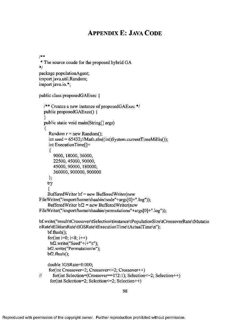
APPENDIX E: JAVA CODE
/** * The source coude for the proposed hybrid GA */
package populationAgent; import java.util.Random; import java.io.*;
public class proposedGAExec
/** Creates a new instance of proposedGAExec */ public proposedGAExec() } public static void main(String[] args) {
Random r = new Random(); int seed = 65432;//Math.abs((int)System.currentTimeMillis()); int ExecutionTime[]= {
9000, 18000, 36000, 22500, 45000, 90000, 45000, 90000, 180000, 360000, 900000, 900000
1; try { BufferedWriter bf = new BufferedWriter(new
FileWriter("/export/home/shaahin/node"+args[0]+".log")); BufferedWriter bf2 = new BufferedWriter(new
FileWriter("/export/home/shaahin/permutations"+args[0]+".log"));
bfwrite("result\tCrossover\tSelection\tinstance\tPopulationSize\tCrossoverRate\tMutatio nRate\tElitismRate\tIGSRate\tExecutionTime\tActualTime\n");
bfflush(); for(int i=0; i<8; i++) bf2.write("Seed"+i+"\t");
bf2.write("Permutation\n"); bf2.flush();
double IGSRate=0.000; for(int Crossover=2; Crossover<=2; Crossover++)
// for(int Selection=(Crossover==1?2:1); Selection<=2; Selection++) for(int Selection=2; Selection<=2; Selection++)
98
Reproduced with permission of the copyright owner. Further reproduction prohibited without permission.
A p pe n d ix E: Java C o de
/* *
* The source coude for the proposed hybrid GA*/package populationAgent; import j ava.util .Random; import java.io.*;
public class proposedGAExec {
/** Creates a new instance o f proposedGAExec */ public proposedGAExec() {}public static void main(String[] args){
Random r = new Random();int seed = 65432;//Math.abs((int)System.currentTimeMillis()); int ExecutionTime[]={
9000, 18000, 36000,22500,45000, 90000,45000, 90000,180000,360000, 900000, 900000
};try{BufferedWriter b f = new BufferedWriter(new
FileWriter("/export/home/shaahin/node"+args[0]+".log"));BufferedWriter bf2 = new BufferedWriter(new
FileWriter("/export/home/shaahin/permutations"+args[0]+".log"));
bf.write("result\tCrossover\tSelection\tinstance\tPopulationSize\tCrossoverRate\tMutationRate\tElitismRate\tIGSRate\tExecutionTime\tActualTime\n");
bf.flush();for(int i=0; i<8; i++)
bf2. write(" Seed"+i+"\t"); bf2.write("Permutation\n"); bf2.flush();
double IGSRate=0.000;for(int Crossover=2; Crossover<=2; Crossover++)
// for(int Selection=(Crossover=l?2:l); Selection<=2; Selection++) for(int Selection=2; Selection<=2; Selection++)
98
Reproduced with permission of the copyright owner. Further reproduction prohibited without permission.
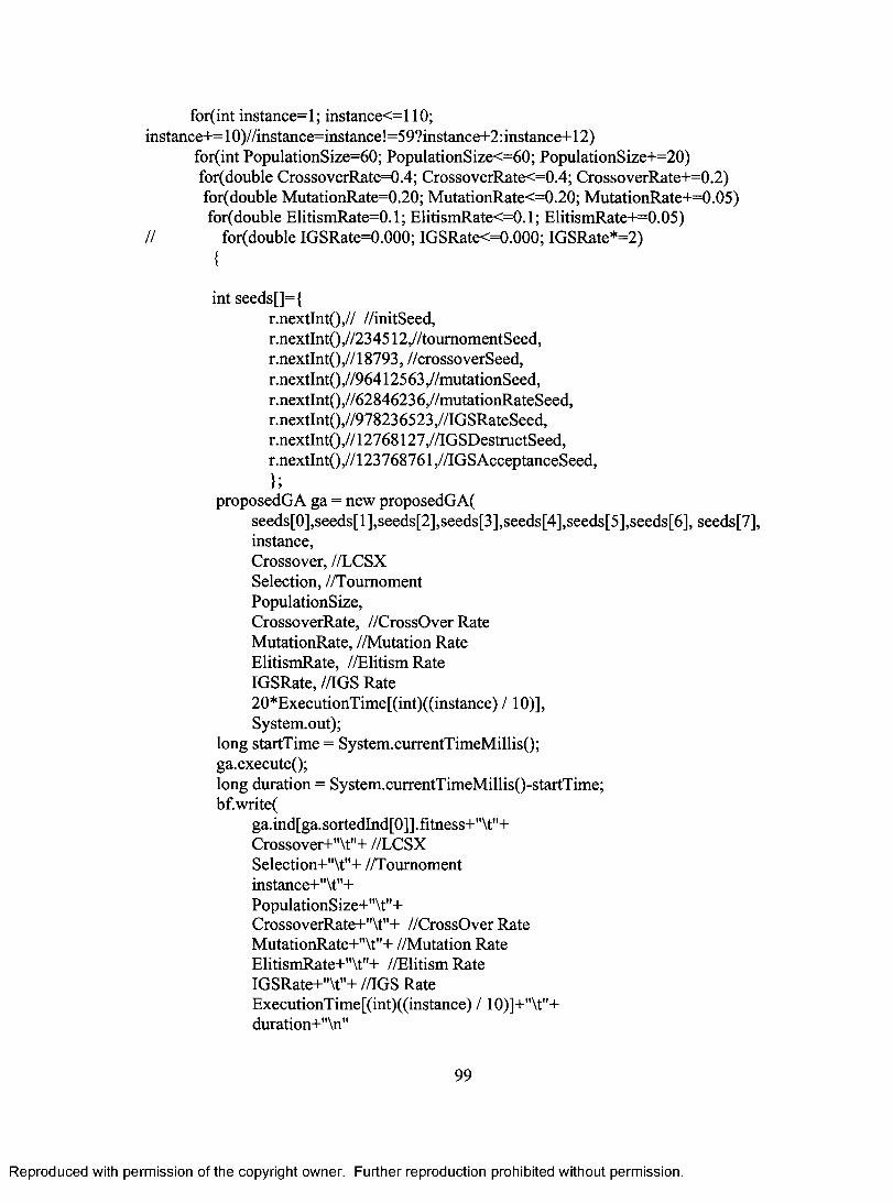
for(int instance=1; instance<=110; instance+=10)//instance=instance!=59?instance+2:instance+12)
for(int PopulationSize=60; PopulationSize<=60; PopulationSize+=20) for(double CrossoverRate=0.4; CrossoverRate<=0.4; CrossoverRate+=0.2) for(double MutationRate=0.20; MutationRate<=0.20; MutationRate+=0.05) for(double ElitismRate=0.1; ElitismRate<=0.1; ElitismRate+=0.05)
// for(double IGSRate=0.000; IGSRate<=0.000; IGSRate*=2) {
int seeds[]={ r.nextInt(),// //initSeed, r.nextInt(),//234512,//tournomentSeed, r.nextInt(),//18793, //crossoverSeed, r.nextInt(),//96412563,//mutationSeed, r.nextInt(),//62846236,//mutationRateSeed, r.nextInt(),//978236523,HIGSRateSeed, r.nextInt(),//12768127,//IGSDestructSeed, r.nextInt(),//123768761,//IGSAcceptanceSeed, 1,
proposedGA ga = new proposedGA( seeds[0],seeds[1],seeds[2],seeds[3],seeds[4],seeds[5],seeds[6], seeds[7], instance, Crossover, //LCSX Selection, //Tournoment PopulationSize, CrossoverRate, //CrossOver Rate MutationRate, //Mutation Rate ElitismRate, //Elitism Rate IGSRate, //IGS Rate 20*ExecutionTime[(int)((instance) / 10)], System.out);
long startTime = System.currentTimeMillis(); ga.execute(); long duration = System.currentTimeMillis()-startTime; bf.write(
ga.ind[ga.sortedInd[0]].fitness+"\t"+ Crossover+"\t"+ //LCSX Selection+"\t"+ //Tournoment instance+"\t"+ PopulationSize+"\t"+ CrossoverRate+"\t"+ //CrossOver Rate MutationRate+"\t"+ //Mutation Rate ElitismRate+"\t"+ //Elitism Rate IGSRate+"\t"+ //IGS Rate ExecutionTime[(int)((instance) / 10)]+"\t"+ duration+"\n"
99
Reproduced with permission of the copyright owner. Further reproduction prohibited without permission.
for(int instance=l; instance<=l 10; instance+= 10)//instance=instance! =59?instance+2: instance+12)
for(int PopulationSize=60; PopulationSize<=60; PopulationSize+=20) for(double CrossoverRate=0.4; CrossoverRate<=0.4; CrossoverRate+=0.2) for(double MutationRate=0.20; MutationRate<=0.20; MutationRate+=0.05) for(double ElitismRate=0.1; ElitismRate<=0.1; ElitismRate+=0.05)
// for(double IGSRate=0.000; IGSRate<=0.000; IGSRate*=2){
int seeds[]={r.nextlnt(),// //initSeed, r.nextInt(),//234512,//toumomentSeed, r.nextlnt(),//l 8793, //crossoverSeed, r.nextInt(),//96412563,//mutationSeed, r.nextInt(),//62846236,//mutationRateSeed, r.nextInt(),//978236523,//IGSRateSeed, r.nextInt(),//12768127,//IGSDestructSeed, r.nextlnt(),//123768761 ,//IGSAcceptanceSeed,};
proposedGA ga = new proposedGA(seeds[0],seeds[l],seeds[2],seeds[3],seeds[4],seeds[5],seeds[6], seeds[7], instance,Crossover, //LCSX Selection, //Toumoment PopulationSize,CrossoverRate, //CrossOver Rate MutationRate, //Mutation Rate ElitismRate, //Elitism Rate IGSRate, //IGS Rate20*ExecutionTime[(int)((instance) /10)],System.out);
long startTime = System.currentTimeMillis(); ga.execute();long duration = System.currentTimeMillis()-startTime; bf.write(
ga.ind[ga.sortedInd[0]].fitness+"\t"+Crossover+"\t"+ //LCSX Selection+"\t"+ //Toumoment instance+"\t"+PopulationSize+"\t"+CrossoverRate+"\t"+ //CrossOver Rate MutationRate+"\t"+ //Mutation Rate ElitismRate+"\t"+ //Elitism Rate IGSRate+"\t"+ //IGS Rate ExecutionTime[(int)((instance) / 10)]+"\t"+ duration+"\n"
99
Reproduced with permission of the copyright owner. Further reproduction prohibited without permission.
); bf.flush(); for(int i=0; i<8; i++) bf2.write(seeds[i]+"\t");
for(int i=0; i<ga.jobCount; i++) bf2.write(gaind[ga.sortedInd[0]].gene[i]+",");
bf2.newLine(); } bf2.flush();
} catch(IOException e) { }
} }
/* * proposedGAExec.java *
*1
package populationAgent; import j ava. io.PrintStream; import java.util.Random; 1**
* * @author Mandi Eskenasi/Shahin Rushan *1
public class proposedGA {
/** Creates a new instance of proposedGA */ int randSeed; int benchmark; int crossoverType; //1:LCSX 2:SBOX int selectionType; //1:Tournoment 2:Ranking public int tournomentSize = 2; int populationSize; double crossoverRate; double mutationRate; double elitismRate; double igsRate; long runDuration; public individual ind[]; public int sortedInd[]; public individual candidate[]; public int candidatelndex[]; public evaluator ev;
100
Reproduced with permission of the copyright owner. Further reproduction prohibited without permission.
);bf.flush();for(int i=0; i<8; i++)
bf2.write(seeds[i]+"\t"); for(int i=0; i<ga.jobCount; i++)
bf2.write(ga.ind[ga.sortedlnd[0]].gene[i]+","); bf2.newLine();}bf2.flush();
}catch(IOException e){}
}}
/** proposedGAExec.java*
*/package populationAgent;import j ava.io.PrintStream;import java.util.Random;/**** @author Mahdi Eskenasi/Shahin Rushan */
public class proposedGA {
/** Creates a new instance of proposedGA */ int randSeed; int benchmark;int crossoverType; //1:LCSX 2:SBOXint selectionType; //l:Toumoment 2:Rankingpublic int toumomentSize = 2;int populationSize;double crossoverRate;double mutationRate;double elitismRate;double igsRate;long runDuration;public individual ind[];public int sortedInd[];public individual candidate[];public int candidatelndex[];public evaluator ev;
100
Reproduced with permission of the copyright owner. Further reproduction prohibited without permission.
public int jobCount; public int machineCount; public Random rinit,
rTournoment, rCrossover, rMutation, rMutationRate, rIGSRate, rIGSDestructSeed, rIGSAcceptanceSeed;
public PrintStream printStr; int generation = 0; public proposedGA(
int initSeed, int tournomentSeed, int crossoverSeed, int mutationSeed, int mutationRateSeed, int IGSRateSeed, int IGSDestructSeed, int IGSAcceptanceSeed, int aBenchmark, int aCrossoverType, //1:LCSX 2:SBOX int aSelectionType, //1:Tournoment 2:Ranking int aPopulationSize, double aCrossoverRate, double aMutationRate, double anElitismRate, double anIGSRate, long aRunDuration, PrintStream aPrintStr ) {
benchmark = aBenchmark; crossoverType = aCrossoverType; selectionType = aSelectionType; populationSize = aPopulationSize; crossoverRate = aCrossoverRate; mutationRate = aMutationRate; elitismRate = anElitismRate; runDuration = aRunDuration; igsRate = anIGSRate; ind = new individual[populationSize]; sortedlnd = new int[populationSize]; candidate = new individual[populationSize]; candidatelndex = new int[populationSize]; ev = new evaluator(benchmark);
101
Reproduced with permission of the copyright owner. Further reproduction prohibited without permission.
public int jobCount; public int machineCount; public Random rlnit,
rToumoment, rCrossover, rMutation, rMutationRate, rIGSRate, rIGSDestructSeed, rIGSAcceptanceSeed;
public PrintStream printStr; int generation = 0; public proposedGA(
int initSeed, int toumomentSeed, int crossoverSeed, int mutationSeed, int mutationRateSeed, int IGSRateSeed, int IGSDestructSeed, int IGSAcceptanceSeed, int aBenchmark,int aCrossoverType, //1:LCSX 2:SBOXint aSelectionType, //l:Toumoment 2:Rankingint aPopulationSize,double aCrossoverRate,double aMutationRate,double anElitismRate,double anIGSRate,long aRunDuration,PrintStream aPrintStr ){
benchmark = aBenchmark; crossoverType = aCrossoverType; selectionType = aSelectionType; populationSize = aPopulationSize; crossoverRate = aCrossoverRate; mutationRate = aMutationRate; elitismRate = anElitismRate; runDuration = aRunDuration; igsRate = anIGSRate; ind = new individual[populationSize]; sortedlnd = new int[populationSize]; candidate = new individual[populationSize]; candidatelndex = new int[populationSize]; ev = new evaluator(benchmark);
101
Reproduced with permission of the copyright owner. Further reproduction prohibited without permission.
jobCount = ev.jobCount; machineCount = ev.machineCount;
// r = new Random(randSeed); rinit = new Random(initSeed); rTournoment = new Random(tournomentSeed); rCrossover = new Random(crossoverSeed); rMutation = new Random(mutationSeed); rMutationRate = new Random(mutationRateSeed); rIGSRate = new Random(IGSRateSeed); rIGSDestructSeed = new Random(IGSDestructSeed); rIGSAcceptanceSeed = new Random(IGSAcceptanceSeed);
printStr = aPrintStr; }
public void init() {
for(int i=1; i<populationSize; i++) {
ind[i] = new individual(jobCount, rInit); candidate[i] = new individual(jobCount); NEH neh = new NEH(ev, ind[i]); neh.CalculateReduced(); ind[i].copy(neh.getInd()); sortedlnd[i] = i;
} sortedlnd[0] = 0; NEH neh = new NEH(ev); neh.CalculateReduced(); ind[0] = new individual(jobCount); ind[0].copy(neh.getInd()); candidate[0] = new individual(jobCount);
}
public void sort() {
int itj, temp; for(i=0; i<populationSize; i++)
for(j=i+1 j<populationSize; j++) if(ind[sortedlnd[i]].fitness > ind[sortedInd[j]].fitness) {
temp = sortedlnd[i]; sortedInd[i]=sortedInd[j]; sortedlnd[j ]=temp;
} }
102
Reproduced with permission of the copyright owner. Further reproduction prohibited without permission.
jobCount = ev.jobCount; machineCount = ev.machineCount;
// r = new Random(randSeed); rlnit = new Random(initSeed); rToumoment - new Random(toumomentSeed); rCrossover = new Random(crossoverSeed); rMutation = new Random(mutationSeed); rMutationRate = new Random(mutationRateSeed); rIGSRate = new Random(IGSRateSeed); rIGSDestructSeed = new Random(IGSDestructSeed); rIGSAcceptanceSeed = new Random(IGSAcceptanceSeed);
printStr = aPrintStr;}
public void init(){
for(int i= l; i<populationSize; i++){
ind[i] = new individual^obCount, rlnit); candidate[i] = new individual(jobCount);NEH neh = new NEH(ev, ind[i]); neh.CalculateReduced(); ind[i].copy(neh.getInd()); sortedInd[i] = i;
}sortedlnd[0] = 0;NEH neh = new NEH(ev);neh.CalculateReduced();ind[0] = new individual^ obCount);ind[0].eopy(neh.getlnd());candidate[0] = new individual^obCount);
}
public void sort(){
int i j , temp;for(i=0; i<populationSize; i++)
for(j=i+l y<populationSize; j++)if(ind[sortedInd[i]].fitness > ind[sortedInd[j]]. fitness){
temp = sortedlndfi]; sortedInd[i]=sortedInd[j ]; sortedInd[j ]=temp;
}}
102
Reproduced with permission of the copyright owner. Further reproduction prohibited without permission.
public void evaluate() {
for(int i=0; i<populationSize; i++) {
ev.evaluate(ind[i]); } sort();
}
public void tournomentSelection() {
for(int i=0; i< (int)(populationSize*(1-elitismRate)); i++) {
int bestIndex = rTournoment.nextInt(populationSize); int randlndex=0; for(int j=1; j<tournomentSize; j++) {
randlndex = rTournoment.nextlnt(populationSize); if(ind[bestIndex].fitness>ind[randIndex].fitness)
bestIndex = randlndex; } candidatelndex[i]=randlndex;
} } public void rankingSelection() {
candidatelndex = new int[populationSize]; // Random r = new Random();
int j; float tempSum, totalSum=0.0f, k;
for(int i=0; i<populationSize; i++) {
ind[sortedInd[i]].rank = 2*(populationSize - i+1)/(population Size-1); totalSum +=ind[sortedInd[i]].rank;
}
for(int i=0; i<populationSize; i++) {
k = rTournoment.nextFloat(rtotalSum; j=0; tempSum = 0; whilea<populationSize) {
tempSum += 1/(ind[j].rank);
103
Reproduced with permission of the copyright owner. Further reproduction prohibited without permission.
public void evaluate(){
for(int i=0; i<populationSize; i++){
ev.evaluate(ind[i]);}sort();
}
public void toumomentSelection(){
for(int i=0; i< (int)(populationSize*(l-elitismRate)); i++){
int bestlndex = rToumoment.nextlnt(populationSize); int randlndex=0;for(int j= 1; j<toumomentSize; j++){
randlndex = rToumoment.nextInt(populationSize); if(ind[bestlndex] .fitness>ind[randlndex] .fitness)
bestlndex = randlndex;}candidatelndex[i]=randlndex;
}}public void rankingSelection(){
candidatelndex = new int[populationSize];// Random r - new Random();
int j;float tempSum, totalSum=0.0f, k;
for(int i=0; i<populationSize; i++){
ind[sortedInd[i]].rank = 2*(populationSize - i+l)/(populationSize-l); totalSum +=ind[sortedInd[i]].rank;
}
for(int i=0; i<populationSize; i++){
k = rToumoment.nextFloat()*totalSum; j=0;tempSum = 0; while(j<populationSize){
tempSum += l/(ind[j].rank);
103
Reproduced with permission of the copyright owner. Further reproduction prohibited without permission.
if(k>tempSum) j++;
else break;
} candidateIndex[i] = j;
} return;
}
public individual[] LCSXCrossover(int indexl, int index2)
{ boolean indl []= new boolean[jobCount]; boolean ind2[]= new boolean[jobCount]; int opt[][]=new int[jobCount+1][jobCount+1];
individual offspring[] = new individual[2]; offspring[0] = new individual(jobCount); offspring[1] = new individual(jobCount); int j,k; for(j=0;j<jobCount; j++)
{ indl[j]=false; ind2[j]=false;
} for(j=jobCount - 1; j>=0; j--)
for(k=jobCount - 1; k>=0; k--) { if(ind[indexl].gene[j]==ind[index2].gene[k])
opt[j][k]=opt[j+1][k+1]+1; else
opt[j][k]= Math.max(opt[j+1][k],opt[j][k+1]); }
j=0; k=0; while(j<jobCount & k<jobCount)
{ if(ind[indexl].gene[j]==ind[index2].gene[k])
{ indl[j]=true; ind2 [k]=true, j++; k++;
} else
if(opt[j+1][k]>=opt[j][k+1]) j++;
104
Reproduced with permission of the copyright owner. Further reproduction prohibited without permission.
if(k>tempSum)j++;
elsebreak;
}candidatelndex[i] = j;
}return;
public individual [] LCSXCrossover(int index 1, int index2){
boolean indl []= new boolean[jobCount]; boolean ind2[]= new boolean[jobCount]; int opt[][]=new int[jobCount+l][jobCount+l];
individual offspring[] = new individual[2]; offspring[0] = new individual^obCount); offspring[l] = new individual(jobCount); int j,k;for(j=0;j<jobCount; j++){
indl[j]=false;ind2[j]=false;
}for(j=jobCount -1 ; j>=0; j - )
for(k=jobCount -1 ; k>=0; k—){if(ind[indexl].gene[j]==ind[index2].gene[k])
opt □ ] [k]=opt □+1 ] [k+1 ]+1; else
opt[j ] [k]= Math.max(opt[j+1 ] [k] ,opt [j ] [k+1 ]);}
j=0;k=0;while(j<jobCount & kcjobCount){
if(ind[index 1 ] .gene[j ]==ind[index2] .gene[k]){
indl[j]=true;ind2[k]=true;j++;k++;
}else
if(opt[j+1 ] [k]>=opt[j][k+l ]) j++;
104
Reproduced with permission of the copyright owner. Further reproduction prohibited without permission.
else k++; I k=0; int 1=0; for(j=0ij<jobCount; j++) {
if(indl [j]) offspring[0].geneW=ind[index1].gene[j];
else {
while(ind2[k]) k++; offspring[0].gene[Thind[index2].gene[k++];
} if(ind2W)
offspring[1].geneW=ind[index2].gene[j]; else
{ while(indl[1]) I++;
offspring[1].gene[j]=ind[indexl].gene [1+-1];
I I
return offspring;
I
public individual[] SBOXCrossover(int indexl, int index2)
{ boolean[J block = new boolean[obCount]; boolean[J blockl --- new boolean[jobCount]; Boolean[] block2 = new boolean[jobCount];
for(int i=0; i< jobCount; i++) {
block[i]—(ind[candidateIndex[indexl]].gene[i]==ind[candidateindex[index2]].gene[i]);
I
block[0] = block[0] & block[1]; for(int i=1; i< jobCount-1; i++) { block[i]=(block[i-1] & block[i])1(block[i] & block[i+1]);
}
block[jobCount-1] = block[jobCount-2] & block[jobCount-1]; individual[] offspring = new individual[2];
offspring[0]= new individual(jobCount);
105
Reproduced with permission of the copyright owner. Further reproduction prohibited without permission.
else k++;}k=0; int 1=0;for(j=0y<jobCount; j++){
if(indl[j])offspring[0] .gene[j ]=ind[index 1 ] .gene[j ];
else {
while(ind2[k]) k++;offspring[O].gene0]=ind[index2].gene[k++];
}if(ind2[j])
offspring[l].gene{j]=ind[index2].gene(j];else{
while(indl[lj) 1++; offspring[ 1 ].gene[j]=ind[index 1 ].gene[l++];
}}
return offspring;
public individual^ SBOXCrossover(int index 1, int index2){
booleanf] block = new boolean[jobCount]; boolean[] blockl = new boolean[jobCount]; boolean[] block2 = new boolean[jobCount];
for(int i=0; i< jobCount; i++){
block[i]=(ind[candidateIndex[indexl]].gene[i]==ind[candidateIndex[index2]].gene[i]);}
block[0] = block[0] & block[lj; for(int i= l; i< jobCount-1; i++){block[i]-(block[i-l] & block[i])|(block[i] & block[i+lJ);
}
block{jobCount-l] = bIock[jobCount-2] & block[jobCount-l]; individual[] offspring = new individual[2];
offspring[0]= new individual(jobCount);
105
Reproduced with permission of the copyright owner. Further reproduction prohibited without permission.

offspring[11= new individual(jobCount);
for(int i=0; i<jobCount; i++)
{ blockl [i]=block[i]; block2 [i]=block[i] ; if(block[i])
{ offspring[0].gene[i]=ind[candidateIndex[index1]].gene[i]; offspring[1].gene[i]=ind[candidateIndex[index2]].gene[i];
} }
int cPoint = rCrossover.nextInt(jobCount); for(int i=0; i<=cPoint; i++)
{ if(!block[i])
{ offspring[0].gene[i]=ind[candidateIndex[index1]].gene[i]; for(int j=0; j<jobCount; j++)
{ if( !block2 [j ] &&
(offspring[0].gene[i]==ind[candidateIndex[index2]].gene[j])) {
block2[j] = true; break;
}
} } if(!block[i])
{ offspring[1].gene[i]=ind[candidateIndex[index2]].gene[i]; for(int j=0; j<jobCount; j++)
{ if(!b1ock 1 [j] &&
(offspring[ l ] . gene [i] ==ind[candidateIndex [indexl] ] . gene [j ]))
{ blockl [j] = true; break;
}
} }
}
106
Reproduced with permission of the copyright owner. Further reproduction prohibited without permission.
offspring[l]= new individual(jobCount);
for(int i=0; i<j obCount; i++){
block 1 [i]=block[i]; block2 [i]=block[i]; if(block[i]){
ofTspring[0].gene[i]=ind[candidateIndex[indexl]].gene[i];offspring[l].gene[i]=ind[candidateIndex[index2]].gene[i];
}}
int cPoint = rCrossover.nextInt(jobCount); for(int i=0; i<=cPoint; i++){
if(!block[i]){
offspring[0] .gene[i]=ind[candidatelndex[index 1 ]] .gene[i]; for(int j=0; j<jobCount; j++){
if(!block2[j] && (offspring[0].gene[i]==ind[candidatelndex[index2]].gene[j]))
{block2[j] = true; break;
}
}}if(!block[i]){
offspring[l].gene[i]=ind[candidateIndex[index2]].gene[i]; for(int j=0; j<jobCount; j++){
if(!blockl[j] && (offspring[l].gene[i]==ind[candidateIndex[indexl]].gene[j]))
{blockl [j] = true; break;
}
}}
}
106
Reproduced with permission of the copyright owner. Further reproduction prohibited without permission.
int i = cPoint+1; int j =0; while(true) {
if(i>=jobCount II j >= jobCount) break;
while(block[i] && i< (jobCount-1)) i-F-F;
while(block2[j] && j< (jobCount-1)) jam;
if(i< jobCount && j< jobCount) offspring[0].gene[i]=ind[candidateIndex[index2]].gene[j];
else break;
i++; j++;
} i = cPoint+1; j =0; while(true) {
if(i>=johCount II j >= jobCount) break;
while(block[i] && i< (jobCount-1)) i-H-;
while(blockl[j] && j< (jobCount-1)) j++;
if(i< jobCount && j< jobCount) offspring[1].gene[i]=ind[candidateIndex[indexl]].gene[j];
else break;
i++; j++;
}
return offspring; }
public void doCrossover() {
individual offspring[] = new individual[2]; offspring[0] = new individual(jobCount); offspring[1] = new individual(jobCount);
for(int i=0; i< (int)(populationSize*(1-elitismRate)); i+=2) {
107
Reproduced with permission of the copyright owner. Further reproduction prohibited without permission.
int i = cPoint+1; int j =0; while(true){
if(i>=jobCount || j >= jobCount) break;
while(block[i] && i< (jobCount-1)) i++;
while(block2[j] && j< (jobCount-1))j++;
if(i< jobCount && j< jobCount) offspring[0].gene[i]=ind[candidatelndex[index2]].gene[j];
else break;
i++;j++;
}i = cPoint+1;j =0;while(true){
if(i>=jobCount || j >= jobCount) break;
while(block[i] && i< (jobCount-1)) i++;
while(blockl [j] && j< (jobCount-1))j++;
if(i< jobCount & & j< jobCount)offspring[ 1 ] ,gene[i]=ind[candidatelndex[index 1 ]] .gene[j];
else break;
i++;j++;
return offspring;
public void doCrossover(){
individual offspring[] = new individual[2]; offspring[0] = new individual^obCount); offspring[l] = new individual(jobCount);
for(int i=0; i< (int)(populationSize*(l-elitismRate)); i+=2) {
107
Reproduced with permission of the copyright owner. Further reproduction prohibited without permission.
if(rCrossover.nextFloat()<=crossoverRate) {
if(crossoverType==2) offspring = SBOXCrossover(candidateIndex[i], candidateIndex[i+1]);
else offspring = LC SXCrossover(candidateIndex [i] , candidateIndex[i+1]);
} else {
offspring[0].copy(ind[candidateIndex[i]]); offspring[1].copy(ind[candidateIndex[i+1]]);
} candidate[i].copy(offspring[0]); candidate [i+1].copy(offspring[1]);
} }
public void doMutation() {
int pl, p2, temp; evaluator ev = new evaluator(benchmark); IGS igs = new IGS(ind[0], ev, rMutation, runDuration, printStr); for(int i=0; i<populationSize*(1-elitismRate); i++) {
if(rMutationRate.nextFloat()<=mutationRate) candidate[i].copy(igs.CalculateReduced(candidate[i]));
} }
public void doElitism() {
int elitSize = (int)(populationSize*elitismRate); int j = populationSize -elitSize; int i=0; while(j < populationSize) {
candidate[j].copy(ind[sortedInd[i++]]); j++;
} evaluator ev= new evaluator(benchmark);
/* i = 0; while(ind[sortedInd[i]].igsDone & i<elitSize)
i-H-;
if(i==elitSize) i = r.nextlnt(populationSize - elitSize);
else
108
Reproduced with permission of the copyright owner. Further reproduction prohibited without permission.
if(rCrossover.nextFloat()<=crossoverRate){
if(crossoverType==2) offspring = SBOXCrossover(candidateIndex[i], candidatelndex[i+l]);
elseoffspring = LCSXCrossover(candidateIndex[i], candidatelndex[i+l]);
}else{
offspring[0].copy(ind[candidateIndex[i]]); offspring[ 1 ] .copy(ind[candidateIndex[i+1 ]]);
}candidate[i].copy(offspring[0]); candidate [i+1 ] .copy(offspring[ 1 ]);
}
public void doMutation(){
int p i, p2, temp;evaluator ev = new evaluator(benchmark);IGS igs = new IGS(ind[0], ev, rMutation, runDuration, printStr); for(int i=0; i<populationSize*(l-elitismRate); i++){
if(rMutationRate.nextFloat()<=mutationRate)candidate[i].copy(igs.CalculateReduced(candidate[i]));
}}
public void doElitism(){
int elitSize = (int)(populationSize*elitismRate); int j = populationSize -elitSize; int i=0;while(j < populationSize){
candidate[j].copy(ind[sortedInd[i++]]);j++;
}evaluator ev= new evaluator(benchmark);
/* i = 0;while(ind[sortedInd[i]].igsDone & i<elitSize)
i++; if(i==elitSize)
i = r.nextInt(populationSize - elitSize); else
108
Reproduced with permission of the copyright owner. Further reproduction prohibited without permission.
i = populationSize - elitSize + i; *1
i = populationSize - elitSize; IGS igs = new IGS(ind[sortedInd[0]],ev , rIGSDestructSeed,
rIGSAcceptanceSeed, runDuration/3, System.out); if(rIGSRate.nextDouble()< igsRate) {
candidate[i].copy(igs.AlgIGS(candidate[i],2)); // candidate[i].copy(igs.AlgIGS(ind[sortedInd[0]],2));
candidate[i].igsDone = true; // runDuration += runDuration/2;
} }
public void evolve() {
if(selectionType=2) rankingSelection();
else tournomentSelection();
doCrossover(); doMutation(); doElitism(); for(int i=0; i<populationSize; i++)
ind[i]=candidate[i]; generation++; evaluate();
} public void execute() {
init(); evaluate(); float best = ind[sortedlnd[0]].fitness; int bestgen=0;
long startTime = System.currentTimeMillis(); while (System.currentTimeMillis() <= (startTime + runDuration)) {
evolve(); if (best > ind[sortedlnd[0]].fitness) {
best = ind[sortedlnd[0]].fitness; bestgen = generation;
} if(best<=ev.optimal[benchmark-1]) {
109
Reproduced with permission of the copyright owner. Further reproduction prohibited without permission.
i = populationSize - elitSize + i;*/
i = populationSize - elitSize;IGS igs = new IGS(ind[sortedInd[0]],ev , rIGSDestructSeed,
rIGSAcceptanceSeed, runDuration/3, System.out); if(rIGSRate.nextDouble()< igsRate){
candidate [i] .copy(igs. AlgIGS(candidate[i] ,2));// candidate[i].copy(igs.AlgIGS(ind[sortedInd[0]],2));
candidate [ij.igsDone = true;// runDuration += runDuration/2;
}}
public void evolve(){
if(selectionType=2)rankingSelection();
elsetoumomentSelection();
doCrossover();doMutation();doElitism();for(int i=0; i<populationSize; i++)
ind[i]=candidate[i]; generation++; evaluate();
}public void execute(){
init();evaluate();float best = ind[sortedlnd[0]].fitness; int bestgen=0;
long startTime = System.currentTimeMillis(); while (System.currentTimeMillis() <= (startTime + runDuration)) {
evolve();if (best > ind[sortedlnd[0]]. fitness){
best = ind[sortedlnd[0]].fitness; bestgen = generation;
}if(best<=ev.optimal[benchmark-1 ]){
109
Reproduced with permission of the copyright owner. Further reproduction prohibited without permission.
long total_time=System.currentTimeMillis()-startTime; printStr.println("Time: "+ total_time); break;
} printStr.println(generation+":"+best);
} for(int i=0; i<jobCount; i++)
printStr.print(ind[sortedInd[0]].gene[i]+"/"); printStr.println(); printStr.println("best fitness:" +best +" Total generation:"+generation+" Best
Generation: "+bestgen); long total_time=System.currentTimeMillisO-startTime; printStr.println("Total Time: "+ total_time);
}
}
/* * IGS.java
*/
package populationAgent; import j ava. io.PrintStream ; import java.util.Random;
import populationAgent.*; 1** *
* @author Mandi Eskenasi/Shahin Rushan */
public class IGS {
individual Ind; evaluator Eval; int aux_formin; float Mneh[]; float[][] Eneh,Qneh,Fneh; /** Creates a new instance of IGS */ int partialPermutation[]; int finalPermutation[];
int number_ of_ swaps=2; int removed_job_count = 4; int p; int[] removed; int[] partial; long Duration;
110
Reproduced with permission of the copyright owner. Further reproduction prohibited without permission.
long total_time=System.currentTimeMillis()-startTime;printStr.println("Time: "+ total time);break;
}printStr.println(generation+": "+best);
}for(int i=0; i<jobCount; i++)
printStr.print(ind[sortedInd[0]].gene[i]+"/");printStr.printlnO;printStr.println("best fitness:" +best +" Total generation:"+generation+" Best
Generation: "+bestgen);long total_time=System.currentTimeMillis()-startTime; printStr.println("Total Time: "+ total time);
}
}
/** IGS.java
*/package populationAgent; import java.io.PrintStream; import java.util.Random;
import populationAgent.*;/**** @author Mahdi Eskenasi/Shahin Rushan */
public class IGS {
individual Ind; evaluator Eval; int auxform in; float Mneh[]; float[][] Eneh,Qneh,Fneh;/** Creates a new instance o f IGS */ int partialPermutation[]; int finalPermutation[];
int number_of_swaps=2; int removed j o b count = 4; int p;int[] removed; int[] partial; long Duration;
110
Reproduced with permission of the copyright owner. Further reproduction prohibited without permission.
Random r; Random rAcc; PrintStream printStr;
public IGS(individual anlnd, evaluator anEval, Random rand, long aDuration, PrintStream aPrintStr) {
Ind = anlnd; Eval = anEval; aux_formin=0; Eneh = new float[Eval.jobCount+1][Eval.machineCount+1]; Qneh = new float[Eval.jobCount+1] [Eval.machineCount+2]; Fneh = new float[Eval.jobCount+1] [Eval.machineCount+1]; Mneh = new float [Eval.jobCount+1]; removed = new int[removed_job_count]; partial = new int[Eval.jobCount];
partialPermutation = new int[Eval.jobCount]; finalPermutation = new int[Eval.jobCount]; r = rand; Duration = aDuration; printStr = aPrintStr;
} public IGS(individual anlnd, evaluator anEval, Random randDestruct,
Random randAccept, long aDuration, PrintStream aPrintStr)
Ind = anlnd; Eval = anEval; aux_formin=0; Eneh = new float[Eval.jobCount+1] [Eval.machineCount+1]; Qneh = new float[Eval.jobCount+1][Eval.machineCount+2] ; Fneh = new float[Eval.jobCount+1][Eval.machineCount+1]; Mneh = new float [Eval.jobCount+1]; removed = new int[removed_job_count]; partial = new int[Eval.jobCount];
partialPermutation = new int[Eval.jobCount]; finalPermutation = new int[Eval.jobCount]; r = randDestruct; rAcc = randAccept; Duration = aDuration; printStr = aPrintStr;
} private void Zero(float M[], float E[][], float Q[][], float F[][]) {
111
Reproduced with permission of the copyright owner. Further reproduction prohibited without permission.
Random r;Random rAcc;PrintStream printStr;
public IGS(individual anlnd, evaluator anEval, Random rand, long aDuration, PrintStream aPrintStr) {
Ind = anlnd;Eval = anEval; aux_formin=0;Eneh = new float[Eval.jobCount+l][Eval.machineCount+l];Qneh = new float[Eval.jobCount+l][Eval.machineCount+2];Fneh = new float[Eval.j obCount+1 ] [Eval.machineCount+1 ];Mneh = new float [Eval.jobCount+1]; removed = new int[removed_job_count]; partial = new int[Eval.j obCount];
partialPermutation = new int[Eval .jobCount]; fmalPermutation = new int[Eval.jobCount]; r = rand;Duration = aDuration; printStr = aPrintStr;
}public IGS(individual anlnd, evaluator anEval, Random randDestruct,
Random randAccept, long aDuration, PrintStream aPrintStr) {
Ind - anlnd;Eval = anEval; aux_formin=0;Eneh = new float[Eval.jobCount+l][Eval.machineCount+l];Qneh = new float[Eval.jobCount+l][Eval.machineCount+2];Fneh = new float[Eval.jobCount+l][Eval.machineCount+l];Mneh = new float [Eval.jobCount+1]; removed = new int[removedJob_count]; partial = new int[Eval.jobCount];
partialPermutation = new int[Eval.jobCount]; fmalPermutation = new int[Eval.jobCount]; r - randDestruct; rAcc = randAccept;Duration = aDuration; printStr = aPrintStr;
}private void Zero(float M[], float E[][], float Q[][], float F[][]){
111
Reproduced with permission of the copyright owner. Further reproduction prohibited without permission.

for(int i=0; i< Eval.jobCount+1; i++) {
M[i] = 0.0f; for(int j=0; j< Eval.machineCount+1; j++) {
E[i][j]=0.0f; Q[i][j]=0.0f; F[i][j]=0.0f;
} Q[i] [Eval.machineCount+1]=0.0f;
} }
public individual A1gIGS(individual Ord, int LocalType) {
int i, j; individual best, OrdAux; float T, makespans,makespanaux,delta,bestmakespan; int ite; int JobCount, MachineCount; JobCount = Eval.jobCount; MachineCount = Eval.machineCount;
OrdAux = new individual(JobCount); best = new individual(JobCount); best.copy(Ord); ite = 0; //inicializamos la temperatura //vamos a calcular los tiempos totales de todos los trabajos y todas las maquinas // we initialized the temperature // we are going to calculate the total times of all the works and all the machines T=O; for(i=0; i< JobCount; i++) for(j=0;j<MachineCount;j++)
T += Eval.p[j][i]; T = 0.66P(T/(JobCount*MachineCount*10.00);
//ILS //LOCALSEARCH if(LocalType-1) Ord.copy(ILSLocal(Ord));
else Ord.copy(ILSLocalComplete(Ord));
makespans=Makespan(Ord); bestmakespan=makespans;
112
Reproduced with permission of the copyright owner. Further reproduction prohibited without permission.
for(int i=0; i< Eval.jobCount+1; i++){
M[i] = O.Of;for(int j=0; j< Eval.machineCount+1; j++){
E[i][j]=O.Of;Q[i]U]=O.Of;F[i][j]=O.Of;
}Q[i][Eval.machineCount+l]=O.Of;
}}
public individual AlgIGS(individual Ord, int LocalType){
int i, j;individual best, OrdAux;float T, makespans,makespanaux,delta,bestmakespan; int ite;int JobCount, MachineCount;JobCount = Eval.jobCount;MachineCount = Eval.machineCount;
OrdAux = new individual(JobCount); best = new individual(JobCount); best.copy(Ord); ite - 0;//inicializamos la temperatura//vamos a calcular los tiempos totales de todos los trabajos y todas las maquinas // we initialized the temperature// we are going to calculate the total times o f all the works and all the machines T=0;for(i=0; i< JobCount; i++)
for(j=0;j<MachineCount;i++)T += Eval.p[j][i];
T = 0.66fl‘(T/(JobCount*MachineCount*10.0f));
//ILS//LOCALSEARCH if(LocalType== 1)
Ord.copy(ILSLocal(Ord));else
Ord.copy(ILSLocalComplete(Ord));
makespans=Makespan(Ord); bestmakespan=makespans;
112
Reproduced with permission of the copyright owner. Further reproduction prohibited without permission.
OrdAux.copy(Ord); long EndTime = System.currentTimeMillis()+Duration;
while(System.currentTimeMillis()<=EndTime) {
OrdAux.copy(CalculateReduced(OrdAux)); Ord.evaluated = false;
11*****************************************/
//LOCALSEARCH if(LocalType=1) OrdAux.copy(ILSLocal(OrdAux));
else OrdAux.copy(ILSLocalComplete(OrdAux));
++ite; //ACCEPTANCECRITERION
makespanaux = Makespan(OrdAux); delta = makespans-makespanaux; if (delta>=0) //nueva mejor solucion // new better solution { makespans = makespanaux; if (makespans<bestmakespan) {
bestmakespan = makespans; best.copy(OrdAux); Eval.evaluate(best); printStr.println("best:"+bestmakespan+" cycle: "
+ite+" steps: "+ite); for(i=0; i<Ord.size; i++)
printStr.print(best.gene[i]+"/"); printStr.println(); if(best.fitness<=Eval.optimal[Eval.instance-1]) {
break; }
Ord.copy(OrdAux); }
} else //no es mejor solucion, hay que ver si se acepta // it is not better solution, is
necessary to see if it is accepted { if(rAcc.nextFloat()<=Math.exp((delta/T))) { makespans = makespanaux; Ord.copy(OrdAux);
113
Reproduced with permission of the copyright owner. Further reproduction prohibited without permission.
OrdAux.copy(Ord);long EndTime = System.currentTimeMillis()+Duration;
while(System.currentTimeMillis()<=EndTime){
OrdAux.copy(CalculateReduced(OrdAux));Ord.evaluated = false;
//LOCALSEARCH if(LocalT y p e = 1)
OrdAux.copy(ILSLocal(OrdAux));else
OrdAux.copy(ILSLocalComplete(OrdAux));-H-ite;//ACCEPT ANCECRITERION
makespanaux = Makespan(OrdAux); delta = makespans-makespanaux;if (delta>=0) //nueva mejor solucion // new better solution{makespans - makespanaux; if (makespans<bestmakespan){
bestmakespan = makespans; best.copy(OrdAux);Eval.evaluate(best);printstr.println("best:"+bestmakespan+" cycle: "
+ite+" steps: "+ite); for(i=0; i<Ord.size; i++)
printStr.print(best.gene[i]+"/");printStr.println();if(best.fitness<=Eval.optimal[Eval.instance-1 ]){
break;}
Ord.copy(OrdAux);}
}else //no es mejor solucion, hay que ver si se acepta // it is not better solution,
necessary to see if it is accepted{if(rAcc.nextFloat()<=Math.exp((delta/T))){makespans = makespanaux;Ord.copy(OrdAux);
113
Reproduced with permission of the copyright owner. Further reproduction prohibited without permission.
} else { OrdAux.copy(Ord);
} I if(ite%1000==0)
printStr.println(ite); } // del while return best;
} private float MinArray(float[] Mneh,int start,int end) {
float MinPoint= 10000000;; for(int i=start; i<=end; i++)
if(Mneh[i]<MinPoint) {
aux_formin = i; MinPoint = Mneh[i];
} return MinPoint;
1 public individual ILSLocalComplete(individual Ord) {
int point1j jobaux; float makel; int JobCount = Eval.jobCount; individual Ordaux;
Ordaux = new individual(JobCount); individual OrdBest = new individual(JobCount); OrdBest.copy(Ord); Eval.evaluate(OrdBest); float bestMakeSpan = OrdBest.fitness;
// Random r = new Random(); int lastpoint = -1;
// do { // pointl = r.nextInt(Ord. size); // while(pointl=lastpoint) // pointl = r.nextInt(Ord. size);
for(point1=0; pointl<Ord. size ; pointl++) {
lastpoint = pointl; jobaux = Ord.gene[pointl];
114
Reproduced with permission of the copyright owner. Further reproduction prohibited without permission.
}else{OrdAux.copy(Ord);
}}if(ite% 1000= 0)
printStr.println(ite);} // del while return best;
}private float MinArray(float[] Mneh,int start,int end) {
float MinPoint= 10000000;; for(int i=start; i<=end; i++)
if(Mneh[i]<MinPoint){
aux formin -- i;MinPoint = Mneh[i];
}return MinPoint;
}public individual ILSLocalComplete(individual Ord){
int pointl j jobaux; float makel;int JobCount = Eval.jobCount; individual Ordaux;
Ordaux = new individual JobCount); individual OrdBest = new individual(JobCount); OrdBest.copy(Ord);Eval.evaluate(OrdBest);float bestMakeSpan = OrdBest.fitness;
// Random r - new Random(); int lastpoint = -1;
// do{// pointl = r.nextlnt(Ord.size);// w hile(pointl=lastpoint)// pointl = r.nextlnt(Ord.size);
for(pointl=0; pointl<Ord.size; pointl-H-){
lastpoint = pointl; jobaux = Ord.gene[pointl];
114
Reproduced with permission of the copyright owner. Further reproduction prohibited without permission.
Zero(Mneh, Eneh, Qneh, Fneh); fora =0;j<=point1-1;j++) Ordaux.gene[j] = Ord.gene[j];
for(j=point1+1; j<Ord. size; j++) Ordaux.gene[j-1] = Ord.gene[j];
NEHMakespans(Eneh,Qneh,Fneh,Ordaux,jobaux); makel = MinAmay(Mneh,l,JobCount);
for(j=1; j<=aux_formin-1; j++) Ord.gene[j-1] = Ordaux.gene[j-1];
Ord.gene[aux_formin-l] = jobaux;
j=(aux_formin+1); while(j <= JobCount) { Ord.gene[j-1] = Ordaux.gene[j-2]; j++;
} Eval.evaluate(Ord); make1=Ord. fitness; if(makel<bestMakeSpan) {
OrdBest.copy(Ord); bestMakeSpan = makel;
} // else // break;
}//while(true); /* if(makel<makeini)
{ Ord. copy(Ordaux); return Ord;
} else*/
return OrdBest; } public individual ILSLocal(individual Ord) {
int pointl,j ijobaux; //float[][] Eneh,Qneh,Fneh; //float[] Mneh; float makel; int JobCount = Eval.jobCount;
115
Reproduced with permission of the copyright owner. Further reproduction prohibited without permission.
Zero(Mneh, Eneh, Qneh, Fneh); for(j=0;j<=pointl-1 ;j++)
Ordaux.gene[j] = Ord.gene[j]; for(j=pointl+l; j<Ord.size; j++)
Ordaux.gene[j-l] = Ord.gene[j];
NEFIMakespans(Eneh,Qneh,Fneh,Ordauxjobaux); makel = MinArray(Mneh,l,JobCount);
for(j= l; j<=aux_formin-1; j++)Ord.gene[j-l] = Ordaux.gene[j-l];
Ord.gene[aux_formin-1 ] = jobaux;
j=(aux_formin+1); while(j <= JobCount){Ord.gene[j-l] = Ordaux.gene[j-2];j++;
}Eval.evaluate(Ord); make 1 =Ord. fitness; if(make 1 <bestMakeSpan){
OrdBest.copy(Ord); bestMakeSpan = makel;
}// else // break;
}//while(true);/* if(makel<makeini)
{Ord. copy (Ordaux); return Ord;
}else*/
return OrdBest;}public individual ILSLocal(individual Ord){
int pointl jjobaux;//float[][] Eneh,Qneh,Fneh;//float[] Mneh; float makel;int JobCount = Eval JobCount;
115
Reproduced with permission of the copyright owner. Further reproduction prohibited without permission.
individual Ordaux; Ordaux = new individual(JobCount); individual OrdBest = new individual(JobCount); OrdBest.copy(Ord); Eval.evaluate(OrdBest); float bestMakeSpan = OrdBest.fitness;
// Random r = new Random(); int lastpoint = -1;
do { pointl = r.nextlnt(Ord.size); while(point1==lastpoint)
pointl = r.nextlnt(Ord.size); lastpoint = pointl; jobaux = Ord.gene[pointl];
Zero(Mneh, Eneh, Qneh, Fneh); for(j=0;j<=point1-1;j++) Ordaux.gene[j] = Ord.gene[j];
for(j=pointl+1; j<Ord.size; j++) Ordaux.gene[j-1] = Ord.gene[j];
NEHMakespans(Eneh,Qneh,Fneh,Ordaux,j obaux); makel = MinArray(Mneh,l,JobCount);
for(j=1; j<=aux_formin-1; j++) Ord.gene[j-1] = Ordaux.gene[j-1];
Ord.gene[aux_formin-l] = jobaux;
j=(aux_formin+1); while(j <= JobCount) { Ord.gene[j-1] = Ordaux.gene[j-2]; j++;
} Eval.evaluate(Ord); make1=Ord.fitness; if(makel<bestMake Span) {
OrdBest.copy(Ord); bestMakeSpan = makel;
} else
break; } while(true);
/* if(make 1 <makeini)
116
Reproduced with permission of the copyright owner. Further reproduction prohibited without permission.
individual Ordaux;Ordaux = new individual JobCount); individual OrdBest = new individual(JobCount); OrdBest.copy(Ord);Eval .evaluate(OrdBest);float bestMakeSpan = OrdBest.fitness;
// Random r - new Random(); int lastpoint = -1;
do{pointl = r.nextlnt(Ord.size); while(point 1 ==lastpoint)
pointl = r.nextlnt(Ord.size); lastpoint = pointl; jobaux = Ord.gene[pointl];
Zero(Mneh, Eneh, Qneh, Fneh); for(j=0;j<=pointl-l;j++)
Ordaux.gene[j] = Ord.gene[j]; for(j=pointl+l; j<Ord.size; j++)
Ordaux.gene[j-l] - Ord.gene[j];
NEHMakespans(Eneh,Qneh,Fneh,Ordauxjobaux); makel = MinArray(Mneh,l, JobCount);
for(j=1; j<=aux_formin-1; j++)Ord.gene[j-l] = Ordaux.gene[j-l];
Ord.gene[aux_formin-l] = jobaux;
j=(aux_formin+1); while(j <= JobCount){Ord.gene[j-l] = Ordaux.gene[j-2];j++;
}E val. evaluate(Ord); make 1 =Ord.fitness; if(make 1 <bestMakeSpan){
OrdBest.copy(Ord); bestMakeSpan = makel;
}else
break;}while(true);
/* if(makel<makeini)
116
Reproduced with permission of the copyright owner. Further reproduction prohibited without permission.
{ Ord. copy(Ordaux); return Ord;
} else*/
return OrdBest; }
public void NEHMakespans( float Eneh[][], float Qneh[][], float Fneh[][],
individual Orden, int job) { int 1, j; float makel, aux; float eidle[][]; int JobCount = Eval.jobCount; int MachineCount= Eval.machineCount; int i=JobCount;
eidle = new float[JobCount][JobCount]; //MEJORAS DE TAILLARD //Tipo 0 (flowshop estandar) // TAILLARD IMPROVEMENTS// Type 0 (flowshop standard)
//Calculamos E for(1=1; l<=i-1;1++)
for(j=1; j<=MachineCount; j++) Eneh[l][j]=Math.max(Eneh[l][j-1],Eneh[1-1][j]) + Eval.p[j-1][Orden.gene[1-11-1];
//Calculamos Q for(1=i-1;1>=1;1--) for(j=MachineCount; j>= 1; j--)
Qneh[l][j]=Math.max(Qneh[l][j+1],Qneh[1+1][j])+Eval.p[j-1][Orden.gene[1-1]-1]; //Calculamos F for(1=1;1<=i; l++) for(j=1;j<=MachineCount;j++)
Fneh[1] [j]=Math.max(Fneh[1] [j-1] ,Eneh[1-1] [j])+Eval.p [j -1] [j ob-1];
//calulamos los partial makespans for(1=1;1<=i;1++) { make1=-10000; for(j=1;j<=MachineCount;j++)
{
117
Reproduced with permission of the copyright owner. Further reproduction prohibited without permission.
{Ord.copy(Ordaux); return Ord;
}else*/
return OrdBest;
public void NEHMakespans( float Eneh[][], float Qneh[][], float Fneh[][],
individual Orden, int job){int 1, j;float m akel, aux; float eidle[][];int JobCount = Eval.jobCount;int MachineCount= Eval.machineCount;int i=JobCount;
eidle = new float[JobCount] [JobCount];//MEJORAS DE TAILLARD //Tipo 0 (flowshop estandar)// TAILLARD IMPROVEMENTS// Type 0 (flowshop standard)
//Calculamos E for(l= 1; l<=i-1 ;1++)
for(j=l; j<=MachineCount; j++)Eneh[l][j]=Math.max(Eneh[l][j-1 ],Eneh[l-1 ][j]) + Eval.p[j-1 ][Orden.gene[l-1 ]-l ];
//Calculamos Q for(l=i-l;l>=l;l--)
for(j=MachineCoimt; j>= 1; j —)Qneh[l][j]=Math.max(Qneh[l][j+l],Qneh[l+l ][j])+Eval.p[j - 1 ][Orden.gene[l-1 ]-l ];
//Calculamos F for(l=l;l<=i; 1++)
for(j=l ;j<=MachineCount;j++)Fneh[l][j]=Math.max(Fneh[l][j-1 ],Eneh[l- l][j])+Eval.p[j-1 ] [j ob-1 ];
//calulamos los partial makespans for(l=l;l<=i;l++){makel =-10000;for(j=1 ;j<=MachineCount;j++){
117
Reproduced with permission of the copyright owner. Further reproduction prohibited without permission.
aux = Fneh[l][j]+Qneh[l][j]; if (aux>make 1)
make 1=aux; } Mneh[1]=make1;
} }
public float Makespan(individual Ord) { Ord.evaluated = false; Eval.evaluate(Ord); return Ord.fitness;
}
public float PartialMakeSpan(int partialSize) {
float C[][]= new float[Eval.machineCount][partialSize]; C[0][0] = Eval.p[0][partialPermutation[0]-1]; int i,j; for(i=1;i<partialSize;i++)
C[0][i] = C[0][i-1]+ Eval.p[0][partialPermutation[i]-1]; for(j=1;j<Eval.machineCount;j++)
C [j] [0] = CU-1] [0] + Eval.p[j] [partialPermutation [0]-1] ; for(i=1;i<partialSize;i++)
for(j=1;j<Eval.machineCount;j++) C[j][i] =
Math.max(C[j ] [i-1],C[j -1] [i]) + Eval.p[j][partialPermutation[i]-1];
return C[Eval.machineCount-1][partialSize-1]; }
public individual CalculateReduced(individual Ord) {
int i, j , k, 1; int tempBestPermutation[] = new int[Eval.jobCount]; int JobCount, MachineCount; JobCount = Eval.jobCount; MachineCount = Eval.machineCount; Random r = new Random(); p = r.nextlnt(JobCount); removed[0]=p; boolean flag=true,
for(i=1;i<removed_job_count; i++) {
while(flag)
118
Reproduced with permission of the copyright owner. Further reproduction prohibited without permission.
aux = Fneh[l][j]+Qneh[l][j]; if (aux>makel)
makel=aux;}Mneh[l]=makel;
}
public float Makespan(individual Ord) {Ord.evaluated = false;Eval. e valuate(Ord); return Ord.fitness;
}
public float PartialMakeSpan(int partialSize){
float C[][]= new float[Eval.machineCount] [partialSize]; C[0][0] = Eval.p[0][partialPermutation[0]-l]; int i j ;for(i= 1 ;i<partialSize;i-H-)
C[0][i] = C[0][i-1]+ Eval.p[0][partialPermutation[i]-l]; for(j=l ;j<Eval.machineCount;j-H-)
C[j][0] = C[j-1][0] + Eval.p[j][partialPermutation[0]-l]; for(i=l ;i<partialSize;i-H-)
for(j=1 ;j<Eval.machineCount;j++)CD][i] =
Math.max(C[j][i-l],C[j-l][i])+ Eval .p[j ] [partialPermutation[i] -1 ];
return C[Eval.machineCount-1 ] [partialSize-1 ];
public individual CalculateReduced(individual Ord){
int i, j , k, 1;int tempBestPermutation[] = new int[Eval.jobCount]; int JobCount, MachineCount;JobCount = Eval.jobCount;MachineCount = Eval.machineCount;
// Random r = new Random();p = r.nextlnt( JobCount); removed[0]=p; boolean flag=true;
for(i= 1 ;i<removed_job_count; i++){
while(flag)
118
Reproduced with permission of the copyright owner. Further reproduction prohibited without permission.
flag = false; p = r.nextInt(JobCount); fora =0;j<i ;j ++)
flag = flag I (p==removed[j]); } removed[i]=p; flag = true;
} k=0; for(i=0; i<JobCount; i++) {
flag = true; for(j=0; j< removed.length; j++)
if(i==removed[j])
I flag = false; break;
} if(flag)
partial[k++]=i; }
float E[][]= new float[JobCount+1][MachineCount+1]; float Q[][]= new float[JobCount+1][MachineCount+2]; float F[][]= new float[JobCount+1][MachineCount+1]; float M[]=new float[JobCount+1];
II
counter++)
int j, k; float tempMakeSpan, tempSum; float MinPoint=0;
for(i = 0; i<(Eval.jobCount-removed job_count); i++) tempBestPermutation[i]=Ord.gene[partial[i]];
for(int counter=JobCount-removed job_count; counter<JobCount;
{ Zero(M, E, Q, F); for(1=1; l<=counter;1++)
for(j=1; j<=MachineCount; j++) E[1][j]=Math.max(E[1] [j -1], E [1- 1] [j ])
+ Eval .p [j -1] [tempB estPermutation[1-1]-1] ;
for(1=counter;1>=1;1--) for(j=MachineCount; j>= 1; j--)
119
Reproduced with permission of the copyright owner. Further reproduction prohibited without permission.
//
counter-H-)
{flag = false;p = r.nextlnt(JobCount); for(j=0;j<i;j++)
flag = flag | (p==removed[j]);}removed[i]=p; flag = true;
}k=0;for(i=0; i<JobCount; i++){
flag = true;for(j=0; j< removed.length; j++)
if(i==removed[j]){
flag = false; break;
}if(flag)
partial[k++]=i;}
float E[][]= new float[JobCount+l][MachineCount+l]; float Q[][]= new float[JobCount+l][MachineCount+2]; float F[][]= new float[JobCount+l][MachineCount+l]; float M[]=new float[JobCount+l];
int j, k;float tempMakeSpan, tempSum; float MinPoint=0;
for(i = 0; i<(Eval.jobCount-removedJob_count); i++) tempBestPermutation[i]=Ord.gene[partial[i]];
for(int counter=JobCount-removed_job_count; counter<JobCount;
{Zero(M, E, Q, F); for(l=l; l<=counter;l++)
for(j= l; j<=MachineCount; j++)E[l][j]=Math.max(E[l] [j - 1 ],E[l-l][j])
+ Eval.p[j-1 ] [tempBestPermutation[l-1 ]-1 ];
for(l=counter;l>= 1 ;1—)for(j=MachineCount; j>= 1; j —)
119
Reproduced with permission of the copyright owner. Further reproduction prohibited without permission.
Q[1][j]=Math.max(Q[1][j+1],Q[1+1][j]) +Eval.p[j-1][tempBestPermutation[1-1]-1];
for(1=1;1<=counter+1; 1++) for(j=1 <=MachineCount;j++)
F[1][j]=Math.max(F[1][0],E[1-1][j]) +Eval.p[j-l][Ord.gene[removed[counter-
JobCount+removed job_count]]-1];
for(1=1;1<=counter+1;1++) {
tempMakeSpan=-10000; for(j =1 ;j <=MachineCount ;j ++) {
tempSum = F[1][j]+Q[1][j]; if (tempSum>tempMakeSpan)
tempMakeSpan=tempSum; } M[1]=tempMakeSpan;
}
MinPoint= 10000000; int index=-1; for(i=1; i<=counter+1; i++)
if(M[i]<MinPoint) {
index = i; MinPoint = M[i];
}
partialPermutation [index-1]=Ord. gene [removed [counter-JobCount+removed job_count]];
1=0; for(k=0; k<=counter ; k++) {
if (k!= (index-1)) {
partialPermutation[k]=tempBestPermutation[1]; 1++;
} } for(k=0; k<=counter; k++)
tempBestPermutation[k]=partialPermutation[k]; } for(int counter=0; counter<JobCount; counter++)
finalPermutation[counter]=partialPermutation[counter];
120
Reproduced with permission of the copyright owner. Further reproduction prohibited without permission.
Q[l]D]=Math.max(Q[l][j+l],Q[l+l][j])+Eval.p[j-1 ] [tempBestPermutation[l-1 ]-1 ];
for(l= 1 ;l<=counter+1; 1++)for(j=l ;j<=MachineCount;j++)
F[l][j]=Math.max(F[l]D-l],E[l-l]D])+Eval.p[j-1 ] [Ord.gene[removed[counter-
JobCount+removedJ ob_count] ]-1 ];
for(l= 1; l<=counter+1; 1++){
tempMakeSpan=-10000; for(j=l ;j<=MachineCount;j++){
tempSum = F[l][j]+Q[l][j]; if (tempSum>tempMakeSpan)
tempMakeSpan=tempSum;}M[l]=tempMakeSpan;
}
MinPoint= 10000000; int index—1;for(i=l; i<=counter+l; i++)
if(M[i]<MinPoint){
index = i;MinPoint = M[i];
}
partialPermutation[index-1 ]=Ord.gene[removed[counter- JobCount+removedjob_count]];
1=0 ;for(k=0; k<=counter; k++){
if (k!= (index-1)){
partialPermutation[k]=tempBestPermutation[l];1++;
}}for(k=0; k<=counter; k++)
tempBestPermutation[k]=partialPermutation[k];}for(int counter=0; counter<JobCount; counter++)
finalPermutation[counter]=partialPermutation[counter];
120
Reproduced with permission of the copyright owner. Further reproduction prohibited without permission.
// System.out.println(bestMakeSpan); for(i=0;i<JobCount; i++)
Ord.gene[i]=finalPermutation[i]; return Ord;
}
public individual Calculate(individual Ord) {
int i, j , k, 1; int tempBestPermutation[] = new int[Eval.jobCount]; float bestMakeSpan, MakeSpan; int JobCount, MachineCount; JobCount = Eval.jobCount; MachineCount = Eval.machineCount;
// Random r = new Random();
p = r.nextInt(JobCount); removed[0]=p; boolean flag=true,
for(i=1;i<removed job_count; i++)
{ while(flag)
{ flag = false; p = r.nextInt(JobCount); for(j =0;j <i ;j ++)
flag = flag I (p==removed[j]); } removed[i]=p; flag = true;
} k=0; for(i=0; i<JobCount; i++)
{ flag = true; for(j=0; j< removed.length; j++)
if(i==removed[j]) {
flag = false; break;
} if(flag)
partial[k++]=i; }
121
Reproduced with permission of the copyright owner. Further reproduction prohibited without permission.
// System.out.println(bestMakeSpan);for(i=0;i<JobCount; i++)
Ord.gene[i]=fmalPermutation[i]; return Ord;
}
public individual Calculate(individual Ord){
int i, j , k, 1;int tempBestPermutation[] = new int[Eval.jobCount]; float bestMakeSpan, MakeSpan; int JobCount, MachineCount;JobCount = Eval.jobCount;MachineCount = Eval.machineCount;
// Random r = new Random();
p = r.nextlnt(JobCount); removed[0]=p; boolean flag=true;
for(i=l ;i<removed_job_count; i++){
while(flag){flag = false;p = r.nextlnt(JobCount); for(j=0;j<i;j++)
flag = flag | (p=rem oved[j]);}removed[i]=p; flag = true;
}k=0;for(i=0; i<JobCount; i++){
flag = true;for(j=0; j< removed, length; j++)
if(i==removed[j ]){
flag = false; break;
}if(flag)
partial[k++]=i;}
121
Reproduced with permission of the copyright owner. Further reproduction prohibited without permission.
for(i = 0; i<(Eval.jobCount-removed job_count); i++) tempBestPermutation[i]=Ord.gene[partial[i]];
bestMakeSpan = 1000000000.0f; for(i=0; i<removed job_count; i++) {
bestMakeSpan = 1000000000.0f; for(j = 0; j<=(Eval.jobCount-removed job_count+i); j++)
partialPermutation[j]=Ord.gene[removed[i]]; 1=0; for(k=0; k<=(Eval.jobCount-removed job_count+i) ; k++) {
if (k!= j)
partialPermutation[k]=tempBestPermutation[1]; 1++;
} } MakeSpan = PartialMakeSpan(Eval.jobCount-removed job_count+i+1); if(MakeSpan<bestMakeSpan) {
for(int counter=0; counter<=Eval.jobCount-removed job_count+i; counter++)
finalPermutation[counter]=partialPermutation[counter]; bestMakeSpan = MakeSpan;
}
} for(int counter=0; counter<=Eval.jobCount-removed job_count+i; counter++)
tempBestPermutation[counter]=finalPermutation[counter]; }
// System.out.println(bestMakeSpan); for(i=0;i<JobCount; i++)
Ord.gene[i]=finalPermutation[i]; Ord.evaluated = true; Ord.fitness = bestMakeSpan; return Ord;
}
}
122
Reproduced with permission of the copyright owner. Further reproduction prohibited without permission.
for(i = 0; i<(Eval.jobCount-removedJob_count); i++) tempBestPermutation[i]=Ord.gene[partial[i]];
bestMakeSpan = lOOOOOOOOO.Of; for(i=0; i<removedJob_count; i++){
bestMakeSpan = lOOOOOOOOO.Of;for(j = 0; j<=(Eval.jobCount-removed_job_count+i); j++){
partialPermutation[j ]=Ord.gene [removed[i] ];1=0 ;for(k=0; k<=(Eval.jobCount-removedJob_count+i); k++){
if (k!= j){
partialPermutation[k]=tempBestPermutation[l];1++;
}}MakeSpan = PartialMakeSpan(Eval.jobCount-removedjob_count+i+l); if(MakeSpan<bestMakeSpan){
for(int counter=0; counter<=Eval.jobCount-removedJob_count+i;counter++)
finalPermutation[counter]=partialPermutation[counter]; bestMakeSpan = MakeSpan;
}
}for(int counter=0; counteK=Eval.jobCount-removedJob_count+i; counter++)
tempBestPermutation[counter]=flnalPermutation[counter];}
// System.out.println(bestMakeSpan); for(i=0;i<JobCount; i++)
Ord.gene[i]=finalPermutation[i];Ord.evaluated = true;Ord.fitness = bestMakeSpan; return Ord;
}
}
122
Reproduced with permission of the copyright owner. Further reproduction prohibited without permission.