Approximation Schemes for Flow Shop Scheduling Problems

with Machine Availabilty Constraints

Mikhail A. KubzinSchool of Computing and Mathematical Sciences,University of Greenwich, London SE10 9LS, U.K.

Chris N. PottsFaculty of Mathematical Studies, University of Southampton,

Southampton SO17 1BJ, U.K.

Vitaly A. StrusevichSchool of Computing and Mathematical Sciences,University of Greenwich, London SE10 9LS, U.K.

May 1, 2010

Abstract

This paper considers two-machine flow shop scheduling problems with machine avail-ability constraints. When the processing of a job is interrupted by an unavailabilityperiod of a machine, we consider both the resumable scenario in which the processingcan be resumed when the machine next becomes available, and the semi-resumable sce-narios in which some proportion of the processing is repeated but the job is otherwiseresumable. For the resumable scenario, problems with non-availability intervals on oneof the machines are shown to admit fully polynomial-time approximation schemes thatare based on an extended dynamic programming algorithm. For the problem with sev-eral non-availability intervals on the first machine, we present a fast 3/2-approximationalgorithm. For the problem with one non-availability interval under the semi-resumablescenario, polynomial-time approximation schemes are developed.(Production-Scheduling; Flow-Shop; Analysis of Algorithms; Computational Complex-ity; Suboptimal Algorithms)

This paper has appeared as a journal publication in:Computers & Operations Research, Volume 36, Issue 2, pages 379-390, February 2009.For information about the journal, see:http://www.elsevier.com/wps/find/journaldescription.cws home/300/description#description

1 Introduction

In real industrial settings, it is often necessary to address situations where the machines usedfor processing become unavailable during the planning period due to planned maintenance,machine breakdowns, or the use of such facilities for other activities that conflict withplanning decisions. Relevant scheduling models with machine non-availability periods haverecently been studied in numerous papers. For recent surveys of the related results, werefer to Sanlaville and Schmidt [16] and Schmidt [17].

1

This paper studies the two-machine flow shop scheduling problem under various as-sumptions about the jobs affected by a non-availability period, and the structure of non-availability intervals.

In the classical two-machine flow shop scheduling problem, we are given a set of n jobsand two machines. Each job has to be processed on the first machine and then on thesecond machine. We refer to the processing of a job on a machine as an operation. Theprocessing times of all operations are known. Every job is to be processed on at most onemachine at a time, and each machine processes no more than one job at a time. In themodels studied in this paper, the machines are not continuously available for processing.Further, the precise time of each interval of machine unavailability is known in advance.In all problems discussed in this paper, the goal is to minimize the makespan, i.e., themaximum completion time of all jobs on all machines.

Henceforth, we often refer to a non-availability period on a machine as a hole. As intro-duced by Lee [14], we consider various scenarios relating to the processing of an operationthat is interrupted by a hole.

Resumable Scenario. In this case, the total processing time of the operation interrupted bya non-availability interval remains equal to its original processing time, i.e., the processingof the operation is interrupted by the hole and is resumed when the machine next becomesavailable. For example, this scenario applies to a typist who has gone to a lunch break andthen resumes the typing of a manuscript from the last typed page.

Semi-Resumable Scenario. This case is similar to the resumable scenario, but the portion ofan operation performed before the hole has to be partially reprocessed after the hole. Thus,the total processing time of an operation becomes greater than its original processing time.This scenario is applicable if, for example, the machine must heat the job to the requiredtemperature, so that the cooling of the job during the non-availability period necessitatesre-heating to the temperature at the point of interruption.

Non-Resumable Scenario. For this scenario, after an interruption the total processing of theinterrupted operation is equal to its original processing time, so effectively the operationrestarts from scratch. We can regard this is a special case of the semi-resumable scenariowhen an operation has to be completely reprocessed. An example where such a situationarises is in situations related to downloading files from the Internet: if the connection islost during the download, the process must be restarted when the connection is restored.

It is well-known that the two-machine flow shop problem with no availability constraintsis solvable in O(n log n) time by an algorithm of Johnson [8]. However, the complexity of theproblem changes if the machines are not continuously available. Lee (1997, 1999) studiesthe problem with a single hole for all three scenarios: resumable, non-resumable and semi-resumable. He proves that the problem is NP-hard for each of these scenarios, and presentspseudopolynomial dynamic programming algorithms. For the resumable scenario, Kubiaket al. [9] show that the problem with a variable number of holes on one of the machinesis NP-hard in the strong sense. For the both the semi-resumable scenario and the non-resumable scenario, Lee [12] shows that minimizing the makespan on a single machine witha variable number of holes is NP-hard in the strong sense.

The complexity status of scheduling with machine unavailability has stimulated researchon approximability of the problems. It appears that for the problem under consideration,as well as some other scheduling problems with machine availability constraints, there is asharp borderline between those variants of the problem for which it is possible to designfast algorithms that provide a provably close approximation to the optimum, and thosevariants for which finding an approximate solution that is close enough to the optimum is

2

theoretically no easier than determining the optimum exactly.A polynomial-time algorithm that creates a schedule with the makespan that is at most

ρ times the optimal value (where ρ ≥ 1), is called a ρ-approximation algorithm; the value ofρ is called a worst-case ratio bound. If a problem admits a ρ-approximation algorithm, thenit is said to be approximable within a factor ρ. A family of ρ-approximation algorithms iscalled a polynomial-time approximation scheme, or a PTAS, if ρ = 1 + ε for any fixed ε > 0and the running time is polynomial in the length of the problem input. If additionally therunning time of a PTAS is polynomial with respect to 1/ε, it is called a fully polynomial-timeapproximation scheme, or an FPTAS.

The resumable two-machine flow shop problem becomes non-approximable within afixed factor in polynomial time, unless P = NP, provided that there are either two holeson the second machine or one hole on each machine (Lee 1999, Kubiak et al. 002). Breitet al. (2001) show that for the semi-resumable scenario as well as for the non-resumablescenario, the single machine problem with two holes is non-approximable within a fixedfactor, unless P = NP. This implies that the two-machine flow shop problem may admita ρ-approximation algorithm for finite ratio ρ only if there is exactly one hole (for allscenarios), or if there are several holes on the first machine for the resumable scenario only.

The following approximation results for the two-machine flow shop problem with a singlehole on one of the machines are known. For the resumable scenario, Lee [13] gives a (4/3)-approximation algorithm if the hole is on the second machine, and a (3/2)-approximationalgorithm if the hole is on the first machine. For the former problem, Breit (2004) devel-ops an improved (5/4)-approximation algorithm, while for the latter problem, Cheng andWang [3] propose an improved (4/3)-approximation algorithm. Finally, it has been shownthat the two-machine flow shop with a single hole under the resumable scenario admits aPTAS [1] and an FPTAS [?].

For the semi-resumable scenario (and also the non-resumable scenario), Lee [14] gives a(3/2)-approximation algorithm if the hole is on the second machine and a 2-approximationalgorithm if the hole is on the first machine. If there are two holes, one on the first and theother on the second machine, and these holes are consecutive, i.e., the second hole startsexactly when the first hole ends, Cheng and Wang [2] give a (5/3)-approximation algorithm.

Our contribution ...The remainder of this paper is organized as follows. Section 2 contains a formal de-

scription of the two-machine flow shop problem under consideration, and introduces somenotation and terminology. In Section ??, a dynamic programming algorithm for the resum-able scenario and several holes on one of the machines is presented. Section ?? demonstrateshow to use the available dynamic programming algorithms to create FPTAS’s. Since therunning time of these FPTAS’s is fairly large, in Section ?? a fast heuristic algorithm witha worst-case ratio of 3/2 is presented for the problem with holes on the first machine andthe semi-resumable scenario. Section 4 describes a PTAS for the problem with a single holeon one of the machines under the semi-resumable scenario. Some concluding remarks aregiven in Section 5.

2 Preliminaries

In this section, we formally describe the problem under consideration and introduce therequired notation and terminology.

We are given a set of jobs N = {J1, J2, . . . , Jn}. Each job Jj , for j = 1, 2, . . . , n, consistsof two operations OjA and OjB to be performed on machines A and B, respectively. Wedenote the processing time of operations OjA and OjB by aj and bj , respectively. We

3

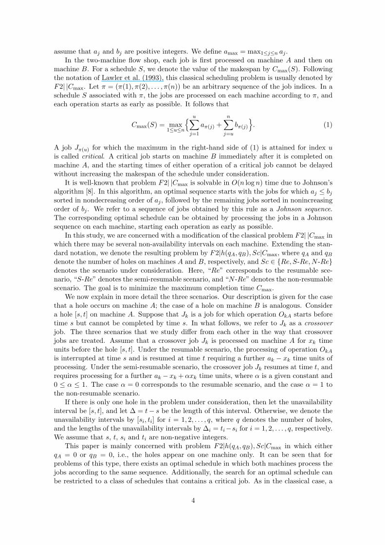
assume that aj and bj are positive integers. We define amax = max1≤j≤n aj .In the two-machine flow shop, each job is first processed on machine A and then on

machine B. For a schedule S, we denote the value of the makespan by Cmax(S). Followingthe notation of Lawler et al. (1993), this classical scheduling problem is usually denoted byF2| |Cmax. Let π = (π(1), π(2), . . . , π(n)) be an arbitrary sequence of the job indices. In aschedule S associated with π, the jobs are processed on each machine according to π, andeach operation starts as early as possible. It follows that

Cmax(S) = max1≤u≤n

{ u∑j=1

aπ(j) +n∑

j=u

bπ(j)

}. (1)

A job Jπ(u) for which the maximum in the right-hand side of (1) is attained for index uis called critical. A critical job starts on machine B immediately after it is completed onmachine A, and the starting times of either operation of a critical job cannot be delayedwithout increasing the makespan of the schedule under consideration.

It is well-known that problem F2| |Cmax is solvable in O(n log n) time due to Johnson’salgorithm [8]. In this algorithm, an optimal sequence starts with the jobs for which aj ≤ bj

sorted in nondecreasing order of aj , followed by the remaining jobs sorted in nonincreasingorder of bj . We refer to a sequence of jobs obtained by this rule as a Johnson sequence.The corresponding optimal schedule can be obtained by processing the jobs in a Johnsonsequence on each machine, starting each operation as early as possible.

In this study, we are concerned with a modification of the classical problem F2| |Cmax inwhich there may be several non-availability intervals on each machine. Extending the stan-dard notation, we denote the resulting problem by F2|h(qA, qB), Sc|Cmax, where qA and qB

denote the number of holes on machines A and B, respectively, and Sc ∈ {Re, S-Re,N -Re}denotes the scenario under consideration. Here, “Re” corresponds to the resumable sce-nario, “S-Re” denotes the semi-resumable scenario, and “N -Re” denotes the non-resumablescenario. The goal is to minimize the maximum completion time Cmax.

We now explain in more detail the three scenarios. Our description is given for the casethat a hole occurs on machine A; the case of a hole on machine B is analogous. Considera hole [s, t] on machine A. Suppose that Jk is a job for which operation OkA starts beforetime s but cannot be completed by time s. In what follows, we refer to Jk as a crossoverjob. The three scenarios that we study differ from each other in the way that crossoverjobs are treated. Assume that a crossover job Jk is processed on machine A for xk timeunits before the hole [s, t]. Under the resumable scenario, the processing of operation OkA

is interrupted at time s and is resumed at time t requiring a further ak − xk time units ofprocessing. Under the semi-resumable scenario, the crossover job Jk resumes at time t, andrequires processing for a further ak − xk + αxk time units, where α is a given constant and0 ≤ α ≤ 1. The case α = 0 corresponds to the resumable scenario, and the case α = 1 tothe non-resumable scenario.

If there is only one hole in the problem under consideration, then let the unavailabilityinterval be [s, t], and let ∆ = t− s be the length of this interval. Otherwise, we denote theunavailability intervals by [si, ti] for i = 1, 2, . . . , q, where q denotes the number of holes,and the lengths of the unavailability intervals by ∆i = ti−si for i = 1, 2, . . . , q, respectively.We assume that s, t, si and ti are non-negative integers.

This paper is mainly concerned with problem F2|h(qA, qB), Sc|Cmax in which eitherqA = 0 or qB = 0, i.e., the holes appear on one machine only. It can be seen that forproblems of this type, there exists an optimal schedule in which both machines process thejobs according to the same sequence. Additionally, the search for an optimal schedule canbe restricted to a class of schedules that contains a critical job. As in the classical case, a

4

critical job starts on machine B immediately after it is completed on machine A and cannotbe delayed. The makespan of a schedule that contains a critical job Ju is determined bythe length of the critical path, which is the sum of the following components:

(i) the processing time of both operations of Ju;

(ii) the total processing time of all jobs that precede Ju on machine A;

(iii) total processing time of all jobs that follow Ju on machine B;

(iv) total length of all holes either before Ju on machine A or after Ju on machine B.

We exclude from further consideration the situation that all jobs complete before thefirst hole since in this case an optimal schedule can be found by Johnson’s algorithm.

For any non-empty set Q ⊆ N , we define

a(Q) =∑j∈Q

aj , b(Q) =∑j∈Q

bj ,

and denote a(∅) = b(∅) = 0.

3 Resumable Scenario

In this section, we develop a fast heuristic algorithm that guarantees a solution fairly closeto the optimum. For this problem with only one hole on machine A, Lee (1997) presents a(3/2)−approximation algorithm. We extend his heuristic to the case of several holes andsimplify both the algorithm and the proof. Note that, to date, no approximation algorithmfor the flow shop problems with more than one hole has been developed.

Our algorithm creates two schedules and outputs the better of them as a heuristicsolution.

Algorithm H

1. Select a job with the largest processing time on machine B and place it into the firstposition in the processing sequence, followed by all other jobs in an arbitrary order.Let S1 denote the schedule associated with that sequence.

2. Sequence all jobs j in non-increasing order of bj/aj and let S2 denote the scheduleassociated with that sequence.

3. If Cmax(S1) ≤ Cmax(S2), then set SH = S1 as the heuristic schedule; otherwise, setSH = S2.

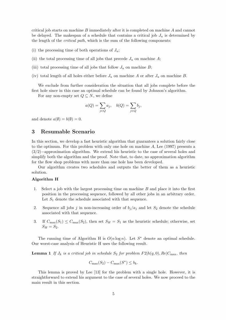
The running time of Algorithm H is O(n log n). Let S∗ denote an optimal schedule.Our worst-case analysis of Heuristic H uses the following result.

Lemma 1 If Jk is a critical job in schedule S2 for problem F2|h(q, 0), Re|Cmax, then

Cmax(S2) − Cmax(S∗) ≤ bk.

This lemma is proved by Lee [13] for the problem with a single hole. However, it isstraightforward to extend his argument to the case of several holes. We now proceed to themain result in this section.

5

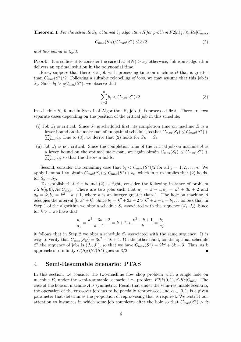
Theorem 1 For the schedule SH obtained by Algorithm H for problem F2|h(q, 0), Re|Cmax,

Cmax(SH)/Cmax(S∗) ≤ 3/2 (2)

and this bound is tight.

Proof. It is sufficient to consider the case that a(N) > s1; otherwise, Johnson’s algorithmdelivers an optimal solution in the polynomial time.

First, suppose that there is a job with processing time on machine B that is greaterthan Cmax(S∗)/2. Following a suitable relabelling of jobs, we may assume that this job isJ1. Since b1 > 1

2Cmax(S∗), we observe that

n∑j=2

bj < Cmax(S∗)/2. (3)

In schedule S1 found in Step 1 of Algorithm H, job J1 is processed first. There are twoseparate cases depending on the position of the critical job in this schedule.

(i) Job J1 is critical. Since J1 is scheduled first, its completion time on machine B is alower bound on the makespan of an optimal schedule, so that Cmax(S1) ≤ Cmax(S∗)+∑n

j=2 bj . Due to (3), we derive that (2) holds for SH = S1.

(ii) Job J1 is not critical. Since the completion time of the critical job on machine A isa lower bound on the optimal makespan, we again obtain Cmax(S1) ≤ Cmax(S∗) +∑n

j=2 bj , so that the theorem holds.

Second, consider the remaining case that bj < Cmax(S∗)/2 for all j = 1, 2, . . . , n. Weapply Lemma 1 to obtain Cmax(S2) ≤ Cmax(S∗) + bk, which in turn implies that (2) holds.for Sh = S2.

To establish that the bound (2) is tight, consider the following instance of problemF2|h(q, 0), Re|Cmax. There are two jobs such that a1 = k + 1, b1 = k2 + 3k + 2 anda2 = k, b2 = k2 + k + 1, where k is an integer greater than 1. The hole on machine Aoccupies the interval [k, k2 + k]. Since b1 = k2 + 3k + 2 > k2 + k + 1 = b2, it follows that inStep 1 of the algorithm we obtain schedule S1 associated with the sequence (J1, J2). Sincefor k > 1 we have that

b1

a1=

k2 + 3k + 2k + 1

= k + 2 >k2 + k + 1

k=

b2

a2,

it follows that in Step 2 we obtain schedule S2 associated with the same sequence. It iseasy to verify that Cmax(SH) = 3k2 + 5k + 4. On the other hand, for the optimal scheduleS∗ the sequence of jobs is (J2, J1), so that we have Cmax(S∗) = 2k2 + 5k + 3. Thus, as kapproaches to infinity C(SH)/C(S∗) goes to 3/2.

4 Semi-Resumable Scenario: PTAS

In this section, we consider the two-machine flow shop problem with a single hole onmachine B, under the semi-resumable scenario, i.e., problem F2|h(0, 1), S-Re|Cmax. Thecase of the hole on machine A is symmetric. Recall that under the semi-resumable scenario,the operation of the crossover job has to be partially reprocessed, and α ∈ [0, 1] is a givenparameter that determines the proportion of reprocessing that is required. We restrict ourattention to instances in which some job completes after the hole so that Cmax(S∗) > t;

6

otherwise, the problem is trivially solved by sequencing the jobs according to Johnson’srule.

For each problem F2|h(0, 1), S-Re|Cmax and F2|h(1, 0), S-Re|Cmax, we problem aPTAS. The best known results in this area available to date are a (3/2)-approximationalgorithm for problem F2|h(0, 1), S-Re|Cmax and a 2-approximation algorithm for problemF2|h(1, 0), S-Re|Cmax [14].

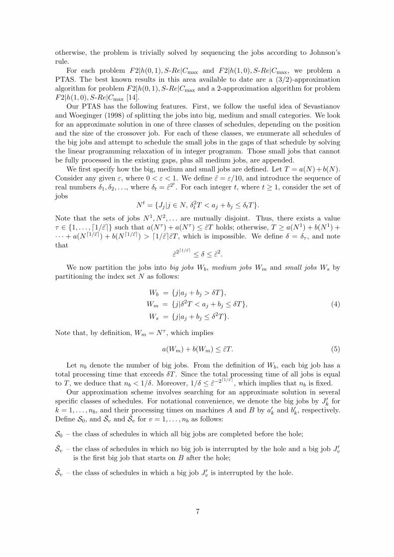
Our PTAS has the following features. First, we follow the useful idea of Sevastianovand Woeginger (1998) of splitting the jobs into big, medium and small categories. We lookfor an approximate solution in one of three classes of schedules, depending on the positionand the size of the crossover job. For each of these classes, we enumerate all schedules ofthe big jobs and attempt to schedule the small jobs in the gaps of that schedule by solvingthe linear programming relaxation of in integer programm. Those small jobs that cannotbe fully processed in the existing gaps, plus all medium jobs, are appended.

We first specify how the big, medium and small jobs are defined. Let T = a(N) + b(N).Consider any given ε, where 0 < ε < 1. We define ε = ε/10, and introduce the sequence ofreal numbers δ1, δ2, . . ., where δt = ε2t

. For each integer t, where t ≥ 1, consider the set ofjobs

N t = {Jj |j ∈ N, δ2t T < aj + bj ≤ δtT}.

Note that the sets of jobs N1, N2, . . . are mutually disjoint. Thus, there exists a valueτ ∈ {1, . . . , d1/εe} such that a(N τ ) + a(N τ ) ≤ εT holds; otherwise, T ≥ a(N1) + b(N1) +· · · + a(N d1/εe) + b(N d1/εe) > d1/εeεT , which is impossible. We define δ = δτ , and notethat

ε2d1/εe ≤ δ ≤ ε2.

We now partition the jobs into big jobs Wb, medium jobs Wm and small jobs Ws bypartitioning the index set N as follows:

Wb = {j|aj + bj > δT},Wm = {j|δ2T < aj + bj ≤ δT}, (4)

Ws = {j|aj + bj ≤ δ2T}.

Note that, by definition, Wm = N τ , which implies

a(Wm) + b(Wm) ≤ εT. (5)

Let nb denote the number of big jobs. From the definition of Wb, each big job has atotal processing time that exceeds δT . Since the total processing time of all jobs is equalto T , we deduce that nb < 1/δ. Moreover, 1/δ ≤ ε−2d1/εe

, which implies that nb is fixed.Our approximation scheme involves searching for an approximate solution in several

specific classes of schedules. For notational convenience, we denote the big jobs by J ′k for

k = 1, . . . , nb, and their processing times on machines A and B by a′k and b′k, respectively.Define S0, and Sv and Sv for v = 1, . . . , nb as follows:

S0 – the class of schedules in which all big jobs are completed before the hole;

Sv – the class of schedules in which no big job is interrupted by the hole and a big job J ′v

is the first big job that starts on B after the hole;

Sv – the class of schedules in which a big job J ′v is interrupted by the hole.

7

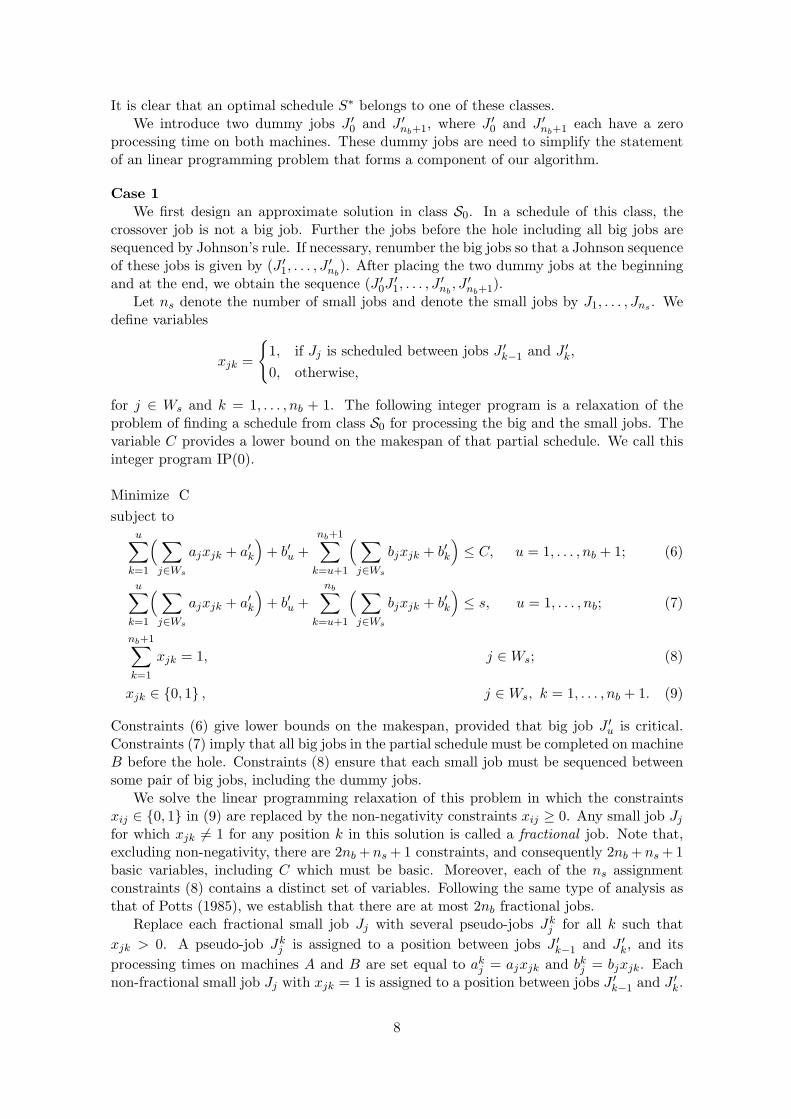
It is clear that an optimal schedule S∗ belongs to one of these classes.We introduce two dummy jobs J ′

0 and J ′nb+1, where J ′

0 and J ′nb+1 each have a zero

processing time on both machines. These dummy jobs are need to simplify the statementof an linear programming problem that forms a component of our algorithm.

Case 1We first design an approximate solution in class S0. In a schedule of this class, the

crossover job is not a big job. Further the jobs before the hole including all big jobs aresequenced by Johnson’s rule. If necessary, renumber the big jobs so that a Johnson sequenceof these jobs is given by (J ′

1, . . . , J′nb

). After placing the two dummy jobs at the beginningand at the end, we obtain the sequence (J ′

0J′1, . . . , J

′nb

, J ′nb+1).

Let ns denote the number of small jobs and denote the small jobs by J1, . . . , Jns . Wedefine variables

xjk =

{1, if Jj is scheduled between jobs J ′

k−1 and J ′k,

0, otherwise,

for j ∈ Ws and k = 1, . . . , nb + 1. The following integer program is a relaxation of theproblem of finding a schedule from class S0 for processing the big and the small jobs. Thevariable C provides a lower bound on the makespan of that partial schedule. We call thisinteger program IP(0).

Minimize Csubject to

u∑k=1

( ∑j∈Ws

ajxjk + a′k

)+ b′u +

nb+1∑k=u+1

( ∑j∈Ws

bjxjk + b′k

)≤ C, u = 1, . . . , nb + 1; (6)

u∑k=1

( ∑j∈Ws

ajxjk + a′k

)+ b′u +

nb∑k=u+1

( ∑j∈Ws

bjxjk + b′k

)≤ s, u = 1, . . . , nb; (7)

nb+1∑k=1

xjk = 1, j ∈ Ws; (8)

xjk ∈ {0, 1} , j ∈ Ws, k = 1, . . . , nb + 1. (9)

Constraints (6) give lower bounds on the makespan, provided that big job J ′u is critical.

Constraints (7) imply that all big jobs in the partial schedule must be completed on machineB before the hole. Constraints (8) ensure that each small job must be sequenced betweensome pair of big jobs, including the dummy jobs.

We solve the linear programming relaxation of this problem in which the constraintsxij ∈ {0, 1} in (9) are replaced by the non-negativity constraints xij ≥ 0. Any small job Jj

for which xjk 6= 1 for any position k in this solution is called a fractional job. Note that,excluding non-negativity, there are 2nb + ns + 1 constraints, and consequently 2nb + ns + 1basic variables, including C which must be basic. Moreover, each of the ns assignmentconstraints (8) contains a distinct set of variables. Following the same type of analysis asthat of Potts (1985), we establish that there are at most 2nb fractional jobs.

Replace each fractional small job Jj with several pseudo-jobs Jkj for all k such that

xjk > 0. A pseudo-job Jkj is assigned to a position between jobs J ′

k−1 and J ′k, and its

processing times on machines A and B are set equal to akj = ajxjk and bk

j = bjxjk. Eachnon-fractional small job Jj with xjk = 1 is assigned to a position between jobs J ′

k−1 and J ′k.

8

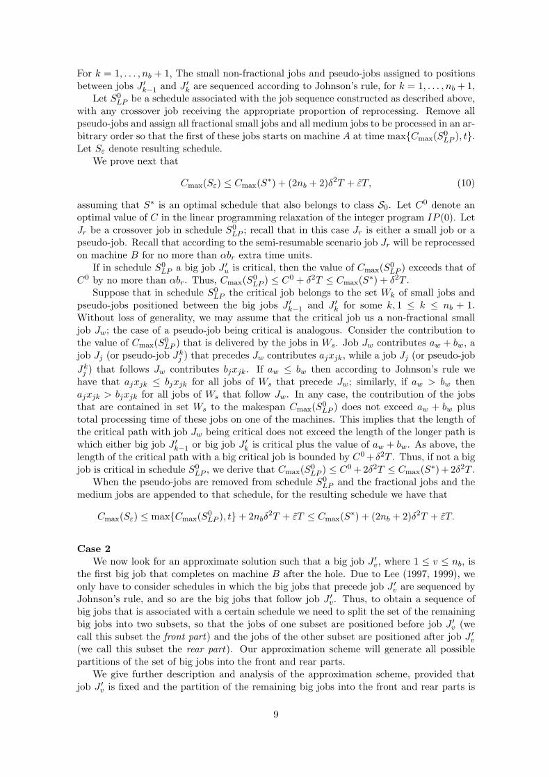
For k = 1, . . . , nb + 1, The small non-fractional jobs and pseudo-jobs assigned to positionsbetween jobs J ′

k−1 and J ′k are sequenced according to Johnson’s rule, for k = 1, . . . , nb + 1,

Let S0LP be a schedule associated with the job sequence constructed as described above,

with any crossover job receiving the appropriate proportion of reprocessing. Remove allpseudo-jobs and assign all fractional small jobs and all medium jobs to be processed in an ar-bitrary order so that the first of these jobs starts on machine A at time max{Cmax(S0

LP ), t}.Let Sε denote resulting schedule.

We prove next that

Cmax(Sε) ≤ Cmax(S∗) + (2nb + 2)δ2T + εT, (10)

assuming that S∗ is an optimal schedule that also belongs to class S0. Let C0 denote anoptimal value of C in the linear programming relaxation of the integer program IP (0). LetJr be a crossover job in schedule S0

LP ; recall that in this case Jr is either a small job or apseudo-job. Recall that according to the semi-resumable scenario job Jr will be reprocessedon machine B for no more than αbr extra time units.

If in schedule S0LP a big job J ′

u is critical, then the value of Cmax(S0LP ) exceeds that of

C0 by no more than αbr. Thus, Cmax(S0LP ) ≤ C0 + δ2T ≤ Cmax(S∗) + δ2T .

Suppose that in schedule S0LP the critical job belongs to the set Wk of small jobs and

pseudo-jobs positioned between the big jobs J ′k−1 and J ′

k for some k, 1 ≤ k ≤ nb + 1.Without loss of generality, we may assume that the critical job us a non-fractional smalljob Jw; the case of a pseudo-job being critical is analogous. Consider the contribution tothe value of Cmax(S0

LP ) that is delivered by the jobs in Ws. Job Jw contributes aw + bw, ajob Jj (or pseudo-job Jk

j ) that precedes Jw contributes ajxjk, while a job Jj (or pseudo-jobJk

j ) that follows Jw contributes bjxjk. If aw ≤ bw then according to Johnson’s rule wehave that ajxjk ≤ bjxjk for all jobs of Ws that precede Jw; similarly, if aw > bw thenajxjk > bjxjk for all jobs of Ws that follow Jw. In any case, the contribution of the jobsthat are contained in set Ws to the makespan Cmax(S0

LP ) does not exceed aw + bw plustotal processing time of these jobs on one of the machines. This implies that the length ofthe critical path with job Jw being critical does not exceed the length of the longer path iswhich either big job J ′

k−1 or big job J ′k is critical plus the value of aw + bw. As above, the

length of the critical path with a big critical job is bounded by C0 + δ2T . Thus, if not a bigjob is critical in schedule S0

LP , we derive that Cmax(S0LP ) ≤ C0 + 2δ2T ≤ Cmax(S∗) + 2δ2T .

When the pseudo-jobs are removed from schedule S0LP and the fractional jobs and the

medium jobs are appended to that schedule, for the resulting schedule we have that

Cmax(Sε) ≤ max{Cmax(S0LP ), t} + 2nbδ

2T + εT ≤ Cmax(S∗) + (2nb + 2)δ2T + εT.

Case 2We now look for an approximate solution such that a big job J ′

v, where 1 ≤ v ≤ nb, isthe first big job that completes on machine B after the hole. Due to Lee (1997, 1999), weonly have to consider schedules in which the big jobs that precede job J ′

v are sequenced byJohnson’s rule, and so are the big jobs that follow job J ′

v. Thus, to obtain a sequence ofbig jobs that is associated with a certain schedule we need to split the set of the remainingbig jobs into two subsets, so that the jobs of one subset are positioned before job J ′

v (wecall this subset the front part) and the jobs of the other subset are positioned after job J ′

v

(we call this subset the rear part). Our approximation scheme will generate all possiblepartitions of the set of big jobs into the front and rear parts.

We give further description and analysis of the approximation scheme, provided thatjob J ′

v is fixed and the partition of the remaining big jobs into the front and rear parts is

9

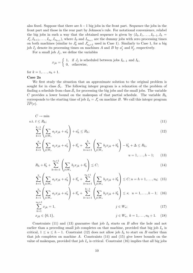
also fixed. Suppose that there are h− 1 big jobs in the front part. Sequence the jobs in thefront part and those in the rear part by Johnson’s rule. For notational convenience, relabelthe big jobs in such a way that the obtained sequence is given by (I0, I1, . . . , Ih−1, Ih =J ′

v, Ih+1, . . . , Inb, Inb+1

), where I0 and Inb+1are the dummy jobs with zero processing times

on both machines (similar to J ′0 and J ′

nb+1 used in Case 1). Similarly to Case 1, for a bigjob Ij denote its processing times on machines A and B by a′j and b′j , respectively.

For a small job Jj , we define the variables

xjk ={

1, if Jj is scheduled between jobs Ik−1 and Ik,0, otherwise,

for k = 1, . . . , nb + 1.Case 2a

We first study the situation that an approximate solution to the original problem issought for in class Sv. The following integer program is a relaxation of the problem offinding a schedule from class Sv for processing the big jobs and the small jobs. The variableC provides a lower bound on the makespan of that partial schedule. The variable Rh

corresponds to the starting time of job Ih = J ′v on machine B. We call this integer program

IP (v).

C → mins.t. t ≤ Rh; (11)

h−1∑k=1

∑j∈Ws

ajxjk + a′k

+ a′h ≤ Rh; (12)

u∑k=1

∑j∈Ws

ajxjk + a′k

+ b′u +h∑

k=u+1

∑j∈Ws

bjxjk + b′k

− b′h + ∆ ≤ Rh,

u = 1, . . . , h− 1; (13)

Rh + b′h +nb+1∑

k=h+1

∑j∈Ws

bjxjk + b′k

≤ C; (14)

u∑k=1

∑j∈Ws

ajxjk + a′k

+ b′u +nb+1∑

k=u+1

∑j∈Ws

bjxjk + b′k

≤ C; u = h + 1, . . . , nb; (15)

u∑k=1

∑j∈Ws

ajxjk + a′k

+ b′u +h−1∑

k=u+1

∑j∈Ws

bjxjk + b′k

≤ s; u = 1, . . . , h− 1; (16)

nb+1∑k=1

xjk = 1, j ∈ Ws; (17)

xjk ∈ {0, 1}, j ∈ Ws, k = 1, . . . , nb + 1. (18)

Constraints (11) and (13) guarantee that job Ih starts on B after the hole and notearlier than a preceding small job completes on that machine, provided that big job Iu iscritical, 1 ≤ u ≤ h − 1. Constraint (12) does not allow job Ih to start on B earlier thanthat job completes on machine A. Constraints (14) and (15) give lower bounds on thevalue of makespan, provided that job Iu is critical. Constraint (16) implies that all big jobs

10

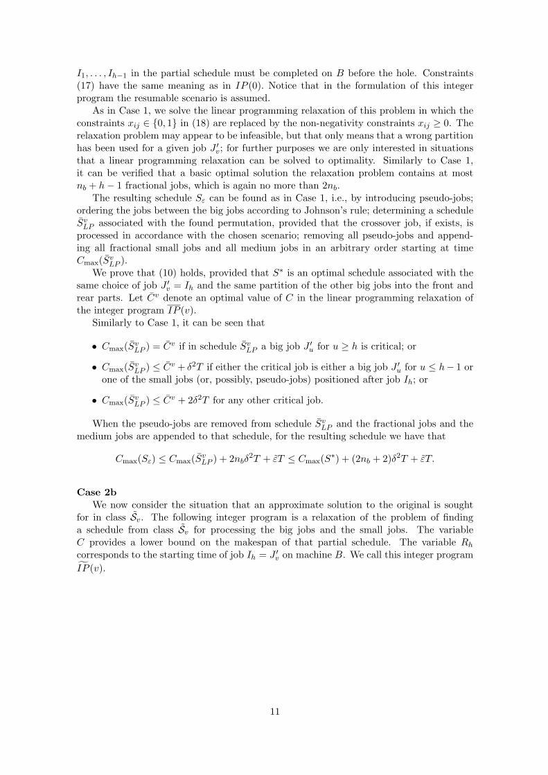
I1, . . . , Ih−1 in the partial schedule must be completed on B before the hole. Constraints(17) have the same meaning as in IP (0). Notice that in the formulation of this integerprogram the resumable scenario is assumed.

As in Case 1, we solve the linear programming relaxation of this problem in which theconstraints xij ∈ {0, 1} in (18) are replaced by the non-negativity constraints xij ≥ 0. Therelaxation problem may appear to be infeasible, but that only means that a wrong partitionhas been used for a given job J ′

v; for further purposes we are only interested in situationsthat a linear programming relaxation can be solved to optimality. Similarly to Case 1,it can be verified that a basic optimal solution the relaxation problem contains at mostnb + h− 1 fractional jobs, which is again no more than 2nb.

The resulting schedule Sε can be found as in Case 1, i.e., by introducing pseudo-jobs;ordering the jobs between the big jobs according to Johnson’s rule; determining a scheduleSv

LP associated with the found permutation, provided that the crossover job, if exists, isprocessed in accordance with the chosen scenario; removing all pseudo-jobs and append-ing all fractional small jobs and all medium jobs in an arbitrary order starting at timeCmax(Sv

LP ).We prove that (10) holds, provided that S∗ is an optimal schedule associated with the

same choice of job J ′v = Ih and the same partition of the other big jobs into the front and

rear parts. Let Cv denote an optimal value of C in the linear programming relaxation ofthe integer program IP (v).

Similarly to Case 1, it can be seen that

• Cmax(SvLP ) = Cv if in schedule Sv

LP a big job J ′u for u ≥ h is critical; or

• Cmax(SvLP ) ≤ Cv + δ2T if either the critical job is either a big job J ′

u for u ≤ h− 1 orone of the small jobs (or, possibly, pseudo-jobs) positioned after job Ih; or

• Cmax(SvLP ) ≤ Cv + 2δ2T for any other critical job.

When the pseudo-jobs are removed from schedule SvLP and the fractional jobs and the

medium jobs are appended to that schedule, for the resulting schedule we have that

Cmax(Sε) ≤ Cmax(SvLP ) + 2nbδ

2T + εT ≤ Cmax(S∗) + (2nb + 2)δ2T + εT.

Case 2bWe now consider the situation that an approximate solution to the original is sought

for in class Sv. The following integer program is a relaxation of the problem of findinga schedule from class Sv for processing the big jobs and the small jobs. The variableC provides a lower bound on the makespan of that partial schedule. The variable Rh

corresponds to the starting time of job Ih = J ′v on machine B. We call this integer program

IP (v).

11

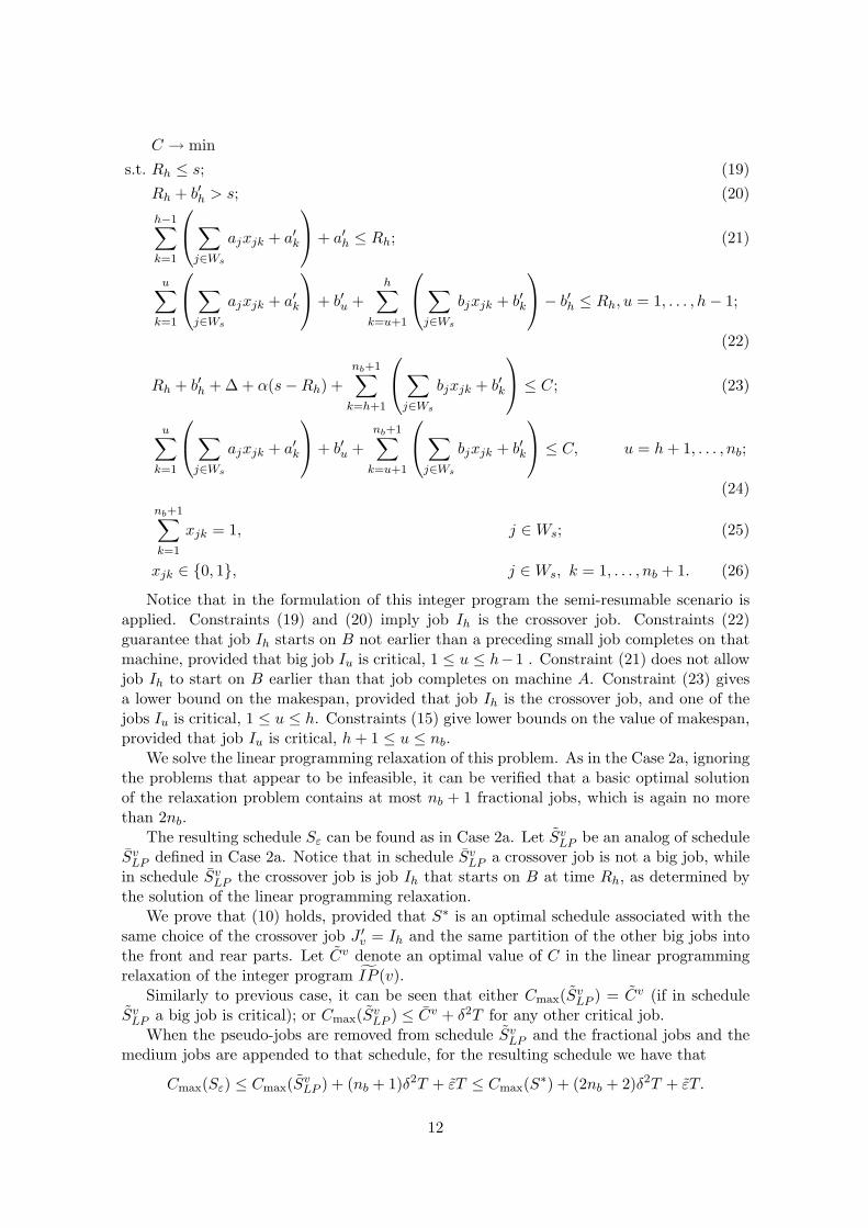
C → mins.t. Rh ≤ s; (19)

Rh + b′h > s; (20)

h−1∑k=1

∑j∈Ws

ajxjk + a′k

+ a′h ≤ Rh; (21)

u∑k=1

∑j∈Ws

ajxjk + a′k

+ b′u +h∑

k=u+1

∑j∈Ws

bjxjk + b′k

− b′h ≤ Rh, u = 1, . . . , h− 1;

(22)

Rh + b′h + ∆ + α(s−Rh) +nb+1∑

k=h+1

∑j∈Ws

bjxjk + b′k

≤ C; (23)

u∑k=1

∑j∈Ws

ajxjk + a′k

+ b′u +nb+1∑

k=u+1

∑j∈Ws

bjxjk + b′k

≤ C, u = h + 1, . . . , nb;

(24)nb+1∑k=1

xjk = 1, j ∈ Ws; (25)

xjk ∈ {0, 1}, j ∈ Ws, k = 1, . . . , nb + 1. (26)

Notice that in the formulation of this integer program the semi-resumable scenario isapplied. Constraints (19) and (20) imply job Ih is the crossover job. Constraints (22)guarantee that job Ih starts on B not earlier than a preceding small job completes on thatmachine, provided that big job Iu is critical, 1 ≤ u ≤ h−1 . Constraint (21) does not allowjob Ih to start on B earlier than that job completes on machine A. Constraint (23) givesa lower bound on the makespan, provided that job Ih is the crossover job, and one of thejobs Iu is critical, 1 ≤ u ≤ h. Constraints (15) give lower bounds on the value of makespan,provided that job Iu is critical, h + 1 ≤ u ≤ nb.

We solve the linear programming relaxation of this problem. As in the Case 2a, ignoringthe problems that appear to be infeasible, it can be verified that a basic optimal solutionof the relaxation problem contains at most nb + 1 fractional jobs, which is again no morethan 2nb.

The resulting schedule Sε can be found as in Case 2a. Let SvLP be an analog of schedule

SvLP defined in Case 2a. Notice that in schedule Sv

LP a crossover job is not a big job, whilein schedule Sv

LP the crossover job is job Ih that starts on B at time Rh, as determined bythe solution of the linear programming relaxation.

We prove that (10) holds, provided that S∗ is an optimal schedule associated with thesame choice of the crossover job J ′

v = Ih and the same partition of the other big jobs intothe front and rear parts. Let Cv denote an optimal value of C in the linear programmingrelaxation of the integer program IP (v).

Similarly to previous case, it can be seen that either Cmax(SvLP ) = Cv (if in schedule

SvLP a big job is critical); or Cmax(Sv

LP ) ≤ Cv + δ2T for any other critical job.When the pseudo-jobs are removed from schedule Sv

LP and the fractional jobs and themedium jobs are appended to that schedule, for the resulting schedule we have that

Cmax(Sε) ≤ Cmax(SvLP ) + (nb + 1)δ2T + εT ≤ Cmax(S∗) + (2nb + 2)δ2T + εT.

12

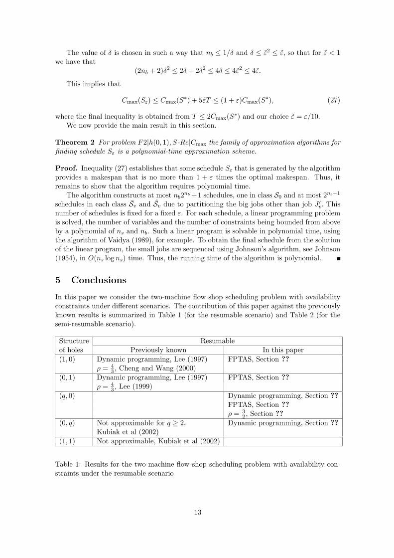
The value of δ is chosen in such a way that nb ≤ 1/δ and δ ≤ ε2 ≤ ε, so that for ε < 1we have that

(2nb + 2)δ2 ≤ 2δ + 2δ2 ≤ 4δ ≤ 4ε2 ≤ 4ε.

This implies that

Cmax(Sε) ≤ Cmax(S∗) + 5εT ≤ (1 + ε)Cmax(S∗), (27)

where the final inequality is obtained from T ≤ 2Cmax(S∗) and our choice ε = ε/10.We now provide the main result in this section.

Theorem 2 For problem F2|h(0, 1), S-Re|Cmax the family of approximation algorithms forfinding schedule Sε is a polynomial-time approximation scheme.

Proof. Inequality (27) establishes that some schedule Sε that is generated by the algorithmprovides a makespan that is no more than 1 + ε times the optimal makespan. Thus, itremains to show that the algorithm requires polynomial time.

The algorithm constructs at most nb2nb +1 schedules, one in class S0 and at most 2nb−1

schedules in each class Sv and Sv due to partitioning the big jobs other than job J ′v. This

number of schedules is fixed for a fixed ε. For each schedule, a linear programming problemis solved, the number of variables and the number of constraints being bounded from aboveby a polynomial of ns and nb. Such a linear program is solvable in polynomial time, usingthe algorithm of Vaidya (1989), for example. To obtain the final schedule from the solutionof the linear program, the small jobs are sequenced using Johnson’s algorithm, see Johnson(1954), in O(ns log ns) time. Thus, the running time of the algorithm is polynomial.

5 Conclusions

In this paper we consider the two-machine flow shop scheduling problem with availabilityconstraints under different scenarios. The contribution of this paper against the previouslyknown results is summarized in Table 1 (for the resumable scenario) and Table 2 (for thesemi-resumable scenario).

Structure Resumableof holes Previously known In this paper(1, 0) Dynamic programming, Lee (1997) FPTAS, Section ??

ρ = 43 , Cheng and Wang (2000)

(0, 1) Dynamic programming, Lee (1997) FPTAS, Section ??ρ = 4

3 , Lee (1999)(q, 0) Dynamic programming, Section ??

FPTAS, Section ??ρ = 3

2 , Section ??(0, q) Not approximable for q ≥ 2, Dynamic programming, Section ??

Kubiak et al (2002)(1, 1) Not approximable, Kubiak et al (2002)

Table 1: Results for the two-machine flow shop scheduling problem with availability con-straints under the resumable scenario

13

Strucure Semi-resumableof holes Previously known In this paper(1, 0) Dynamic programming, Lee (1999) PTAS, Section 4

ρ = 2, Lee (1999)(0, 1) Dynamic programming, Lee (1999) PTAS, Section 4

ρ = 32 , Lee (1999)

(q, 0) Not approximable for q ≥ 2, Lee (1996), Breit et al (2003)(0, q) Not approximable for q ≥ 2, Lee (1996), Breit et al (2003)(1, 1) Not approximable, Lee (1996), Breit et al (2003)

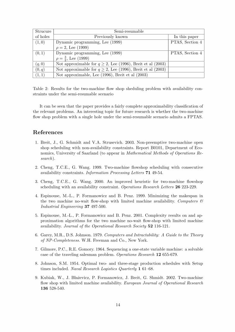
Table 2: Results for the two-machine flow shop sheduling problem with availability con-straints under the semi-resumable scenario

It can be seen that the paper provides a fairly complete approximability classification ofthe relevant problems. An interesting topic for future research is whether the two-machineflow shop problem with a single hole under the semi-resumable scenario admits a FPTAS.

References

1. Breit, J., G. Schmidt and V.A. Strusevich. 2003. Non-preemptive two-machine openshop scheduling with non-availability constraints. Report B0101, Department of Eco-nomics, University of Saarland (to appear in Mathematical Methods of Operations Re-search).

2. Cheng, T.C.E., G. Wang. 1999. Two-machine flowshop scheduling with consecutiveavailability constraints. Information Processing Letters 71 49-54.

3. Cheng, T.C.E., G. Wang. 2000. An improved heuristic for two-machine flowshopscheduling with an availability constraint. Operations Research Letters 26 223-229.

4. Espinouse, M.-L., P. Formanowicz and B. Penz. 1999. Minimizing the makespan inthe two machine no-wait flow-shop with limited machine availability. Computers &Industrial Engineering 37 497-500.

5. Espinouse, M.-L., P. Formanowicz and B. Penz. 2001. Complexity results on and ap-proximation algorithms for the two machine no-wait flow-shop with limited machineavailability. Journal of the Operational Research Society 52 116-121.

6. Garey, M.R., D.S. Johnson. 1979. Computers and Intractability: A Guide to the Theoryof NP-Completeness. W.H. Freeman and Co., New York.

7. Gilmore, P.C., R.E. Gomory. 1964. Sequencing a one-state variable machine: a solvablecase of the traveling salesman problem. Operations Research 12 655-679.

8. Johnson, S.M. 1954. Optimal two- and three-stage production schedules with Setuptimes included. Naval Research Logistics Quarterly 1 61–68.

9. Kubiak, W., J. B lazevicz, P. Formanowicz, J. Breit, G. Shmidt. 2002. Two-machineflow shop with limited machine availability. European Journal of Operational Research136 528-540.

14

10. Kubzin, M.A., V.A. Strusevich. 2002. Two-machine flow shop no-wait scheduling witha non-availability interval. Paper 02/IM/99, CMS Press, University of Greenwich, Lon-don, U.K.

11. Lawler, E.L., J.K. Lenstra, A.H.G. Rinnooy Kan, D.B. Shmoys. 1993. “Sequencingand scheduling: algorithms and complexity,” in Handbooks in Operations Researchand Management Science, vol. 4, Logistics of Production and Inventory, S.C. Graves,A.H.G. Rinnooy Kan, P.H. Zipkin (Editors), North–Holland, Amsterdam. 455-522.

12. Lee, C.-Y. 1996. Machine scheduling with an availability constraint. Journal of GlobalOptimization 9 395–416.

13. Lee, C.-Y. 1997. Minimizing the makespan in the two-machine flowshop schedulingproblem with an availability constraint. Operations Research Letters 20 129-139.

14. Lee, C.-Y. 1999. Two-machine flowshop scheduling with availability constraints. Euro-pean Journal of Operations Research 114 420-429.

15. Potts, C.N. 1985. Analysis of a linear programming heuristic for scheduling unrelatedparallel machines, Discrete Applied Mathematics 10 155–164.

16. Sanlaville, E., G. Schmidt. 1998. Machine scheduling with availability constraints. ActaInformatica 35 795-811.

17. Schmidt, G. 2000. Scheduling with limited machine availability. European Journal ofOperations Research 121 1-15.

18. Sevastianov, S.V., G.J. Woeginger. 1998. Minimizing makespan in open shops: A poly-nomial time approximation scheme, Mathematical Programming 82 191–198.

19. Vaidya, P.M. 1989. Speeding up linear programming using fast matrix multiplication.In: Proceedings of IEEE 30th Annual Symposium on Foundations of Computer Science.332–337.

20. Wang, G., T.C.E. Cheng. 2001. Heuristics for two-machine no-wait flowshop schedulingwith an availability constraint. Information Processing Letters 80 305-309.

15