Computers & Operations Research 36 (2009) 1110–1121www.elsevier.com/locate/cor

Metaheuristics for scheduling a non-permutation flowlinemanufacturing cell with sequence dependent family setup times

Shih-Wei Lina,b, Kuo-Ching Yingc,∗, Zne-Jung Leeb

aDepartment of Information Management, Chang Gung University, Tao-Yuan, Taiwan, ROCbDepartment of Information Management, Huafan University, No. 1, Huafan Road, Taipei, Taiwan, ROC

cDepartment of Industrial Engineering and Management Information, Huafan University, No. 1, Huafan Road, Taipei, Taiwan, ROC

Available online 28 January 2008

Abstract

The broad applications of cellular manufacturing make flowline manufacturing cell scheduling problems with sequence depen-dent family setup times a core topic in the field of scheduling. Due to computational complexity, almost all published studiesfocus on using permutation schedules to deal with this problem. To explore the potential effectiveness of treating this argumentusing non-permutation schedules, three prominent types of metaheuristics—a simulated annealing, a genetic algorithm and a tabusearch—are proposed and empirically evaluated. The experimental results demonstrate that in general, the improvement made bynon-permutation schedules over permutation schedules for the due-date-based performance criteria were significantly better thanthat for the completion-time-based criteria. The results of this study will provide practitioners a guideline as to when to adopt anon-permutation schedule, which may exhibit better performance with additional computational efforts.� 2008 Elsevier Ltd. All rights reserved.

Keywords: Scheduling; Non-permutation flowline manufacturing cell; Simulated annealing; Genetic algorithm; Tabu search

1. Introduction

Cellular manufacturing (CM) is one of the most important applications of group technology in today’s small-to-medium lot production environment. Since CM combines the flexibility of jobshops while retaining the efficiencyof flowshops, it allows small batch production to gain economic advantages similar to those of mass production [1].Relevant studies have found that CM has many advantages, including shortened setup times, reduced work-in-process(WIP), less material handling and simplified production planning and control [2]. These inherent advantages of CMhave to it being broadly applied in many industries, such as the electronics industry as well as numerically controlledmanufacturing.

Due to the wide applications of CM, the manufacturing cell scheduling problem (MCSP) has become a matter ofgreat concern in the field of scheduling. In a CM environment, a variety of machines and/or parts (jobs) are groupedtogether into part families, each of which is then assigned to a manufacturing cell (MC) [3]. Therefore, MCSPs arechiefly concerned with sequencing part families and parts within families where each MC is dedicated to producing aspecific number of part families.

∗ Corresponding author. Tel.: +886 2 2663 2102; fax: +886 2 2663 3981.E-mail address: kcying@cc.hfu.edu.tw (K.-C. Ying).

0305-0548/$ - see front matter � 2008 Elsevier Ltd. All rights reserved.doi:10.1016/j.cor.2007.12.010

S.-W. Lin et al. / Computers & Operations Research 36 (2009) 1110–1121 1111

When each part is processed on each machine in the same technological order of an MC, this is called a flowlineMC [4]. Since parts are assigned to part families based on similar characteristics and operation requirements, in practice,it is quite often the case that prior to processing each part family, major sequence dependent family setup times (SDFSTs)will arise on each machine. Thus, in this study we consider flowline MCSPs with SDFSTs.

Since the seminal work of Mitrofanov [5] and Burbidge [6], a considerable amount of research has been done inthe field of MCSPs. Currently available algorithms for solving MCSPs can be broadly classified into two categories:exact methods and approximation heuristics. For exact methods, some papers [7–12] have been proposed for differentMCSPs. While relatively easy to conceptualize, a flowline MCSP with SDFSTs is NP-hard in the strong sense evenfor a two-machine case [13]. As the computational requirements necessary to obtain an optimal solution increaseexponentially as problem size increases, in view of the combinatorial complexity and time constraints, practitionersoften seek approximation heuristics that generate near-optimum solutions at relatively minor computational expenses.

Vast amounts of near-optimal algorithms have been presented for various MCSPs. Experimental comparisons of thesealgorithms can be found in investigations by Askin and Iyer [14], Frazier [15], Schaller et al. [4], and Logendran et al.[16]. Recent interest in developing efficient improvement heuristics has gained considerable attention for metaheuristicsthat are extremely efficient for large problems. Examples of metaheuristics for MCSPs with SDFSTs include geneticalgorithms [17], tabu searches [13,18], memetic algorithms [17], and hybrid metaheuristics [19]. The relevant literatureindicates that some of these metaheuristics do provide excellent results and constitute state-of-the-art available methods.

Although flowline MCSPs with SDFSTs have recently become of great concern in the field of scheduling, thereis little information available regarding the use of non-permutation schedules (NPSs). According to Hendizadeh etal. [13] and França et al. [17], near-optimal solutions can be obtained for the scheduling of flowline MCSPs withSDFSTs under the assumption of a permutation schedule (PS), which limits the search space. However, reduction ofthe NPSs in regards to the PSs is sometimes achieved at the price of significantly inferior performance. If the operationalefficiency can be improved significantly by using an NPS within a reasonable computational effort, this is usually seenas acceptable in most practical situations.

In this paper, we provide justifications for considering flowline MCSPs with SDFSTs under NPSs. The problemaddressed involves the minimization of one of the completion-time-based or the due-date-based performance criteriafor the NPSs of this problem. To fully explore the potential effectiveness of the NPSs for flowline MCSPs with SDFSTs,three prominent types of metaheuristics—a simulated annealing, a genetic algorithm, and a tabu search—are proposedand empirically evaluated. The remainder of this paper is organized as follows. In the next section, the problemsare formulated. The proposed metaheuristics are presented in Section 3. The computational results of applying theproposed metaheuristics to a benchmark problem set are provided in Section 4. Finally, this study concludes withrecommendations for future research.

2. Problem formulation

To formulate the flowline MCSP with SDFSTs, consider a set N = {P1, P2, . . . , Pn} of n given parts (jobs) tobe processed on m machines in the same technological order. All parts to be processed are classified into one of Fmutually and collectively exhaustive part families f = {f1, f2, . . . , fF } with nk parts belonging to part family fk

(k = 1, 2, . . . , F ). Let the parts be numbered sequentially such that the first n1 parts belong to the first family f1,the next n2 parts belong to f2, and so on until finally nF parts belong to fF . Therefore, n = n1 + · · · + nF . Priorto processing each part family, the SDFSTs s

jxy take place when part family fy is processed immediately after part

family fx on machine j, where sjyy = 0 for allfy . Let pij be the processing time of each part Pi (i = 1, 2, . . . , n) at

machine j. The individual part setup times are small compared with the family setup times and are included in the partprocessing time.

With these definitions, the objective is to find a permutation or a non-permutation schedule for the part familiesand parts within each family that minimizes one of the completion-time-based or due-date-based performance criteria.The completion-time-based performance criteria include makespan (Cmax), total completion time (

∑Ci), and total

weighted completion time (∑

wiCi), while the due-date-based performance criteria include maximum tardiness (Tmax),total tardiness (

∑Ti), and total weighted tardiness (

∑wiTi). In this study, the NPSs only allow the part families’

sequence to be changed between different machines, while the parts’ sequence within each family remains unchangedbetween different machines. Furthermore, the flowline MCSP with SDFSTs considered in this study satisfies the

1112 S.-W. Lin et al. / Computers & Operations Research 36 (2009) 1110–1121

following major assumptions:

• The analysis is limited to static flowline MCSP wherein the number of parts, their processing times, the number ofpart families, and their setup times are known in advance and are non-negative integers.• The ready time of each part is zero, meaning all parts are available for processing at the start time.• The exhaustive rule is applied—that is all parts in a part family are processed consecutively and once the processing

of a part family starts, it cannot be interrupted until all parts of that family are processed.• Every part can be processed by at most one machine at any given time without preemption. Furthermore, each

machine can handle only one part at a time and is persistently available to process all scheduled parts when required.

3. The proposed metaheuristics

In terms of dealing with the flowline MCSP with SDFSTs using the three proposed metaheuristics, the solutionrepresentations for both the PS and the NPS are described in Section 3.1. Section 3.2 defines the neighborhood solutionof this study. The proposed simulated annealing, genetic algorithm, and tabu search approaches are developed inSections 3.3, 3.4 and 3.5, respectively.

3.1. Solution representation

An NPS is required to represent not only the operation sequence between part families in each machine but also theoperation sequence of parts within each family. Suppose there are F part families to be processed on m machines. Then,the solution representation will consist of m + F segments. The first m segment represents the operation sequenceof part families on each machine, and the other F segments correspond to the operation sequence of parts withineach part family. Supposing there are three machines, four families and a total of 22 parts to be scheduled, a solutionrepresentation as shown in Fig. 1 can be decoded as follows. The operation sequences of the part families for machines1, 2, and 3 are 3-4-2-1, 3-4-1-2, and 3-4-2-1, respectively. Meanwhile, the operation sequences for parts in part families1, 2, 3, and 4 are 1-3-5-4-6-2-8-7, 11-9-10-12-13, 17-14-16-15, and 20-18-21-22-19, respectively.

As for a PS, because the operation sequence of part families is the same for all machines, the solution representationonly consists of 1+F segments. The first segment represents the operation sequence of part families for all machines,and the other F segments correspond to the operation sequence of parts within each part family.

3.2. Neighborhood solution definition

Given a solution X, the neighborhood solution of X, denoted as N(X), can be obtained by either a swap or insertionoperation on the sequence of part families in one machine and the sequence of the parts within one family. By randomlyselecting the sequence of parts within a part family, N(X) is sampled by randomly selecting one part of this part familyand another part of the same part family in order to swap the two parts directly, or by randomly selecting one part ofthis part family and inserting the chosen part immediately before another part in the same part family. Similar to thesequence of part families in machines, N(X) is obtained by randomly selecting one part family and another part familyin a sequence of part families on a machine in order to swap the two families directly, or randomly selecting one partfamily and inserting the chosen part family immediately before another part family in the sequence of part families.Since an NPS solution consists of m + F segments, the probabilities of changing a sequence of part families in one

Fig. 1. An example of a solution representation.

S.-W. Lin et al. / Computers & Operations Research 36 (2009) 1110–1121 1113

machine and changing a sequence of parts in each part family are both set to 1/(m+F ′) in an NPS schedule, where mis the number of machines, and F ′ is the number of part families whose number of parts is greater than 1. Evidently,the swap and insertion cannot be done when there is only one part in a part family. As for a PS, because the operationalsequences of part families are the same in all machines, m should be set to 1 in the probability formulae.

3.3. Simulated annealing approach

Introduced by Metropolis et al. [20] and popularized by Kirkpatrick et al. [21], the concept of simulated annealing(SA) is taken from nature. Annealing is the process through which the slow cooling of metal produces good and lowenergy state crystallization, whereas fast cooling produces poor crystallization.

The proposed SA approach is described as follows. First, the current temperature T is set to an initial temperatureT0. The initial solution is generated randomly for the PS and the solution obtained by the PS is then used as the initialsolution of the NPS.

For each iteration, the next solution Y is chosen from N(X). Let obj(X) denote the calculation of the objectivefunction value of X, and �E denote the difference between obj(X) and obj(Y ); that is �E = obj(Y ) − obj(X).As reported by Tiwari et al. [22], the Cauchy function can replace the Boltzmann function (commonly used in SA) inthe annealing process and give the SA more opportunities to escape from the local minima. Thus, this study adoptsthe Cauchy function instead of the Boltzmann function. The probability of replacing X with Y, where X is the currentsolution andY is the next solution, given that �E > 0, is T/(T 2+(�E)2). This is accomplished by generating a randomnumber r ∈ [0, 1] and replacing the solution X with Y if r < T/(T 2+ (�E)2). Meanwhile, if �E�0 , the probability ofreplacing X with Y is 1. T is decreased after running Iiter iterations from the previous decrease, according to the formulaT ← �T , where 0 < � < 1. If T is lower than TF , the algorithm is terminated. Xbest records the best solution as theproposed approach progresses. Following the termination of the SA procedure, the (near) global optimal schedule canthus be derived by Xbest.

3.4. Genetic algorithm approach

Genetic algorithms (GAs) were introduced by Holland [23] and the application of GAs was accelerated by thepublication of a textbook by Goldberg [24]. GAs are search procedures based on natural selection. Unlike neighbor-hood search methods, GAs deal with multiple solutions simultaneously and compute fitness function values for thesesolutions.

In terms of application of the GA approach to a flowline MCSP with SDFSTs, the chromosome presentation, initialpopulation, selection scheme, crossover operator, mutation operator, and termination condition(s) are described asfollows.

• Chromosome representation and initial population—The chromosome representation is the same as the solutionrepresentation described in Section 3.1. The initial population for the PS is generated randomly. One of the initialsolutions for the NPS adopts the best solution obtained by the PS, while other initial solutions are generated randomly.That is, the best solution of the non-permutation problem is, at least, equal to the best solution of the associatedpermutation problem. A collection of Psize such individuals forms a population.• Selection scheme—The likelihood that an individual will be selected as parent increases with the individual’s fitness

value. Given a population P and an objective function value vj for each j ∈ P , the fitness value fj for each j ∈ P

is defined as fj = 1/(1+ vj ). This study uses a tournament selection, which randomly selects two individuals andthen picks the one with the higher fitness value as parent. The smaller the objective function value an individual has,the higher fitness value it has.• Crossover—Two parents have a probability pc of undergoing crossover. The newly generated individual has chro-

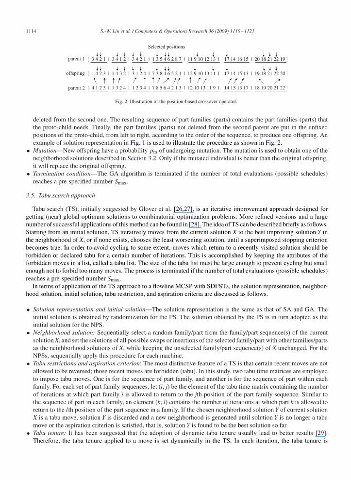
mosomes consisting of genes from either of its parents. If the newly generated individual is better than the worstparent, it will replace that parent; otherwise, it will be discarded. This study uses the position-based crossover, whichis essentially a kind of uniform crossover for literal permutations encoding incorporated with a repairing procedure[25]. Position-based crossover can be described as follows. At first, a set of positions from one parent are selected atrandom. Second, a proto-child is produced by copying part families (parts) at these positions into the correspondingpositions of the proto-child. Third, the part families (parts) that have already been selected from the first parent are

1114 S.-W. Lin et al. / Computers & Operations Research 36 (2009) 1110–1121

parent 1

Selected positions

offspring

parent 2

Fig. 2. Illustration of the position-based crossover operator.

deleted from the second one. The resulting sequence of part families (parts) contains the part families (parts) thatthe proto-child needs. Finally, the part families (parts) not deleted from the second parent are put in the unfixedpositions of the proto-child, from left to right, according to the order of the sequence, to produce one offspring. Anexample of solution representation in Fig. 1 is used to illustrate the procedure as shown in Fig. 2.• Mutation—New offspring have a probability pm of undergoing mutation. The mutation is used to obtain one of the

neighborhood solutions described in Section 3.2. Only if the mutated individual is better than the original offspring,it will replace the original offspring.• Termination condition—The GA algorithm is terminated if the number of total evaluations (possible schedules)

reaches a pre-specified number Smax.

3.5. Tabu search approach

Tabu search (TS), initially suggested by Glover et al. [26,27], is an iterative improvement approach designed forgetting (near) global optimum solutions to combinatorial optimization problems. More refined versions and a largenumber of successful applications of this method can be found in [28]. The idea of TS can be described briefly as follows.Starting from an initial solution, TS iteratively moves from the current solution X to the best improving solution Y inthe neighborhood of X, or if none exists, chooses the least worsening solution, until a superimposed stopping criterionbecomes true. In order to avoid cycling to some extent, moves which return to a recently visited solution should beforbidden or declared tabu for a certain number of iterations. This is accomplished by keeping the attributes of theforbidden moves in a list, called a tabu list. The size of the tabu list must be large enough to prevent cycling but smallenough not to forbid too many moves. The process is terminated if the number of total evaluations (possible schedules)reaches a pre-specified number Smax.

In terms of application of the TS approach to a flowline MCSP with SDFSTs, the solution representation, neighbor-hood solution, initial solution, tabu restriction, and aspiration criteria are discussed as follows.

• Solution representation and initial solution—The solution representation is the same as that of SA and GA. Theinitial solution is obtained by randomization for the PS. The solution obtained by the PS is in turn adopted as theinitial solution for the NPS.• Neighborhood solution: Sequentially select a random family/part from the family/part sequence(s) of the current

solution X, and set the solutions of all possible swaps or insertions of the selected family/part with other families/partsas the neighborhood solutions of X, while keeping the unselected family/part sequence(s) of X unchanged. For theNPSs, sequentially apply this procedure for each machine.• Tabu restrictions and aspiration criterion: The most distinctive feature of a TS is that certain recent moves are not

allowed to be reversed; those recent moves are forbidden (tabu). In this study, two tabu time matrices are employedto impose tabu moves. One is for the sequence of part family, and another is for the sequence of part within eachfamily. For each set of part family sequences, let (i, j) be the element of the tabu time matrix containing the numberof iterations at which part family i is allowed to return to the jth position of the part family sequence. Similar tothe sequence of part in each family, an element (k, l) contains the number of iterations at which part k is allowed toreturn to the lth position of the part sequence in a family. If the chosen neighborhood solution Y of current solutionX is a tabu move, solution Y is discarded and a new neighborhood is generated until solution Y is no longer a tabumove or the aspiration criterion is satisfied, that is, solution Y is found to be the best solution so far.• Tabu tenure: It has been suggested that the adoption of dynamic tabu tenure usually lead to better results [29].

Therefore, the tabu tenure applied to a move is set dynamically in the TS. In each iteration, the tabu tenure is

S.-W. Lin et al. / Computers & Operations Research 36 (2009) 1110–1121 1115

generated from a uniform distribution between MINT and MAXT , which are the minimal and maximal tenure oftabu moves, respectively.

4. Computational results

The three proposed metaheuristics were implemented using C language and run on a PC with an Intel Pentium 4(2.4 GHz) CPU and 512 MB memory. As parameter selection may influence the quality of results, based on extensivecomputational testing, the following parameters were used for the results reported in this paper: T0 = 1000, Iiter =(F × m + n) × 1000, � = 0.90, and TF = 10 for SA, where F is the number of families, n is the number of parts tobe scheduled, m is the number of machines (m is set to be 1 in the permutation schedule); Psize = 1000, pc = 0.95and pm = 0.1 for GA; MINT = 3 and MAXT = 5 for TS. The proposed SA approaches were terminated after 44(1000 × 0.944 < 10) temperature reductions and the proposed GA and TS approaches were terminated if the numberof total evaluations (possible schedules) Smax reached 44× Iiter.

4.1. Test problems

The test problems used in this study are from Schaller et al. [4] and França et al. [17]. Briefly, the processing times ateach stage have been randomly generated using a uniform distribution in the range of [1,10]. Problem hardness is likelyto depend on whether there is a balance between average processing times and the average setup times. Therefore, threedifferent classes of setup times were generated as random integers from the following uniform distributions:

• Small setups (SSU): U[1, 20].• Medium setups (MSU): U[1, 50].• Large setups (LSU): U[1, 100].

A family setup time distribution of U[1, 20], U[1, 50] and U[1, 100] implies that the ratio of mean family setup timeto mean part processing time is approximately 2:1 (10.5:5.5), 5:1 (25.5:5.5), and 10:1 (50.5:5.5) for the instances ofSSU, MSU and LSU, respectively. The number of families varied between 3 and 10, the number of parts between 1and 10, and the number of machines between 3 and 10. For each combination of problem parameters, 30 problem setswere generated, and 30 problem instances were generated for each problem set. Thus, the test bed was composed ofa total of 900 test instances. These 30 problem sets covered a spectrum from loosely to tightly constrained probleminstances.

Since the benchmark problems mentioned above lacked due date information, we added weight (wi) and due date(di) data for each problem instance. The weights were randomly generated using a discrete uniform distribution in therange of [1, 10]. The due dates are integers which were generated from a uniform distribution in the range [0.7P, P ],where P is a parameter known as tightness parameter given by

P =⎧⎨⎩

m∑j=1

[n∑

i=1

pij

]+ (n− 1) max

1� j �m

[n∑

i=1

pij

]⎫⎬⎭

/n+

⎧⎨⎩

m∑j=1

⎧⎨⎩

F∑x=0

⎡⎣ F∑

y=1

sjxy

⎤⎦

⎫⎬⎭

⎫⎬⎭

/{m(F − 1)}.

This tightness parameter setting will bring out the better relative performance of the NPS with respect to the PSunder evaluation for the due-date-based criteria. For each of the six performance criteria, each of the 900 test instanceswas solved once by each of the three proposed metaheuristics for the NPSs and the PSs, respectively. Consequently,there were a total of 6× 900× 3× 2= 32 400 trials in our experiment.

4.2. Results and discussion

The performance evaluations regarding NPSs vs. PSs were conducted using six of the most general criteria including:makespan (Cmax), total completion time (

∑Ci), total weighted completion time (

∑wiCi), maximum tardiness (Tmax),

total tardiness (∑

Ti), and total weighted tardiness (∑

wiTi). To get positive proof that the proposed SA, GA, and TSalgorithms are effective approaches for a flowline MCSP with SDFSTs, their computational results for permutationschedules with respect to the Cmax criterion were compared with the results of two state-of-the-art approaches cited

1116 S.-W. Lin et al. / Computers & Operations Research 36 (2009) 1110–1121

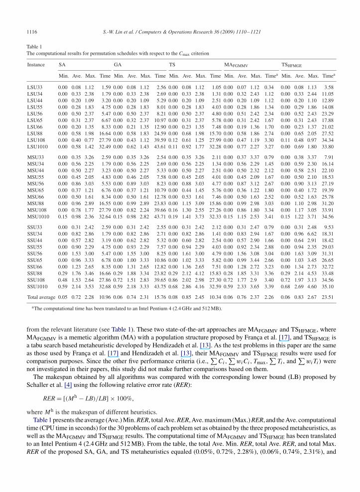
Table 1The computational results for permutation schedules with respect to the Cmax criterion

Instance SA GA TS MAFGMMV TSHFMGE

Min. Ave. Max. Time Min. Ave. Max. Time Min. Ave. Max. Time Min. Ave. Max. Timea Min. Ave. Max. Timea

LSU33 0.00 0.08 1.12 1.59 0.00 0.08 1.12 2.56 0.00 0.08 1.12 1.05 0.00 0.07 1.12 0.34 0.00 0.08 1.13 3.58LSU34 0.00 0.33 2.38 1.79 0.00 0.33 2.38 2.69 0.00 0.33 2.38 1.31 0.00 0.32 2.43 1.12 0.00 0.33 2.44 11.05LSU44 0.00 0.20 1.09 3.20 0.00 0.20 1.09 5.29 0.00 0.20 1.09 2.51 0.00 0.20 1.09 1.12 0.00 0.20 1.10 12.89LSU55 0.00 0.28 1.83 4.75 0.00 0.28 1.83 8.01 0.00 0.28 1.83 4.03 0.00 0.28 1.86 1.34 0.00 0.29 1.86 14.08LSU56 0.00 0.50 2.37 5.47 0.00 0.50 2.37 8.21 0.00 0.50 2.37 4.80 0.00 0.51 2.42 2.34 0.00 0.52 2.43 23.29LSU65 0.00 0.31 2.37 6.67 0.00 0.32 2.37 10.97 0.00 0.31 2.37 5.78 0.00 0.31 2.42 1.67 0.00 0.31 2.43 17.88LSU66 0.00 0.20 1.35 8.33 0.00 0.21 1.35 12.90 0.00 0.23 1.35 7.48 0.00 0.19 1.36 1.70 0.00 0.23 1.37 21.02LSU88 0.00 0.58 1.98 16.64 0.00 0.58 1.83 24.59 0.00 0.68 1.98 15.70 0.00 0.58 1.86 2.74 0.00 0.65 2.05 27.52LSU108 0.00 0.40 0.77 27.79 0.00 0.43 1.12 39.59 0.12 0.61 1.25 27.99 0.00 0.47 1.19 3.30 0.11 0.48 0.97 34.34LSU1010 0.00 0.58 1.42 32.49 0.00 0.62 1.43 43.61 0.11 0.92 1.77 32.28 0.00 0.77 2.27 3.27 0.00 0.69 1.80 33.80

MSU33 0.00 0.35 3.26 2.59 0.00 0.35 3.26 2.54 0.00 0.35 3.26 2.11 0.00 0.37 3.37 0.79 0.00 0.38 3.37 7.91MSU34 0.00 0.56 2.25 1.79 0.00 0.56 2.25 2.69 0.00 0.56 2.25 1.34 0.00 0.56 2.29 1.45 0.00 0.59 2.30 16.14MSU44 0.00 0.50 2.27 3.23 0.00 0.50 2.27 5.33 0.00 0.50 2.27 2.51 0.00 0.50 2.32 2.12 0.00 0.58 2.51 22.10MSU55 0.00 0.45 2.05 4.83 0.00 0.46 2.05 7.58 0.00 0.45 2.05 4.01 0.00 0.45 2.09 1.67 0.00 0.50 2.10 18.53MSU56 0.00 0.86 3.03 5.53 0.00 0.89 3.03 8.23 0.00 0.88 3.03 4.77 0.00 0.87 3.12 2.67 0.00 0.90 3.13 27.19MSU65 0.00 0.37 1.21 6.76 0.00 0.37 1.21 10.79 0.00 0.44 1.45 5.76 0.00 0.36 1.22 1.80 0.00 0.40 1.72 19.39MSU66 0.00 0.50 1.61 8.34 0.00 0.50 1.61 12.78 0.00 0.53 1.61 7.46 0.00 0.50 1.63 2.52 0.00 0.52 1.63 25.78MSU88 0.00 0.96 2.89 16.55 0.00 0.99 2.89 23.83 0.00 1.15 3.09 15.86 0.00 0.99 2.98 3.03 0.00 1.10 2.98 31.20MSU108 0.00 0.78 1.77 27.79 0.00 0.82 2.24 39.66 0.16 1.30 2.55 27.26 0.00 0.86 1.80 3.34 0.00 1.17 3.05 33.91MSU1010 0.15 0.98 2.36 32.64 0.15 0.98 2.82 43.71 0.19 1.41 3.73 32.33 0.15 1.15 2.53 3.41 0.15 1.22 3.71 34.56

SSU33 0.00 0.31 2.42 2.59 0.00 0.31 2.42 2.55 0.00 0.31 2.42 2.12 0.00 0.31 2.47 0.79 0.00 0.31 2.48 9.53SSU34 0.00 0.82 2.86 1.79 0.00 0.82 2.86 2.71 0.00 0.82 2.86 1.41 0.00 0.83 2.94 1.67 0.00 0.96 6.62 18.31SSU44 0.00 0.57 2.82 3.19 0.00 0.62 2.82 5.32 0.00 0.60 2.82 2.54 0.00 0.57 2.90 1.66 0.00 0.64 2.91 18.42SSU55 0.00 0.90 2.29 4.75 0.00 0.93 2.29 7.57 0.00 0.94 2.29 4.03 0.00 0.92 2.34 2.88 0.00 0.94 2.35 29.03SSU56 0.00 1.53 3.00 5.47 0.00 1.55 3.00 8.25 0.00 1.61 3.00 4.79 0.00 1.56 3.08 3.04 0.00 1.63 3.09 31.31SSU65 0.00 0.96 3.33 6.78 0.00 1.00 3.33 10.86 0.00 1.02 3.33 5.82 0.00 0.99 3.44 2.66 0.00 1.03 3.45 26.65SSU66 0.00 1.23 2.65 8.35 0.00 1.31 2.65 12.82 0.00 1.36 2.65 7.51 0.00 1.28 2.72 3.23 0.00 1.34 2.73 32.72SSU88 0.29 1.76 3.46 16.66 0.29 1.88 3.34 23.82 0.29 2.12 4.12 15.83 0.28 1.85 3.31 3.36 0.29 2.14 4.53 33.48SSU108 0.48 1.53 2.64 27.86 0.72 1.51 2.83 39.65 0.86 2.02 2.98 27.30 0.72 1.77 2.9 3.40 0.72 1.97 3.13 34.56SSU1010 0.59 2.14 3.53 32.68 0.59 2.18 3.33 43.75 0.68 2.86 4.16 32.59 0.59 2.33 3.65 3.39 0.68 2.69 4.60 35.10

Total average 0.05 0.72 2.28 10.96 0.06 0.74 2.31 15.76 0.08 0.85 2.45 10.34 0.06 0.76 2.37 2.26 0.06 0.83 2.67 23.51

aThe computational time has been translated to an Intel Pentium 4 (2.4 GHz and 512 MB).

from the relevant literature (see Table 1). These two state-of-the-art approaches are MAFGMMV and TSHFMGE, whereMAFGMMV is a memetic algorithm (MA) with a population structure proposed by França et al. [17], and TSHFMGE isa tabu search based metaheuristic developed by Hendizadeh et al. [13]. As the test problems in this paper are the sameas those used by França et al. [17] and Hendizadeh et al. [13], their MAFGMMV and TSHFMGE results were used forcomparison purposes. Since the other five performance criteria (i.e.,

∑Ci,

∑wiCi, Tmax,

∑Ti , and

∑wiTi) were

not investigated in their papers, this study did not make further comparisons based on them.The makespan obtained by all algorithms was compared with the corresponding lower bound (LB) proposed by

Schaller et al. [4] using the following relative error rate (RER):

RER= [(Mh − LB)/LB] × 100%,

where Mh is the makespan of different heuristics.Table 1 presents the average (Ave.) Min. RER, total Ave. RER, Ave. maximum (Max.) RER, and the Ave. computational

time (CPU time in seconds) for the 30 problems of each problem set as obtained by the three proposed metaheuristics, aswell as the MAFGMMV and TSHFMGE results. The computational time of MAFGMMV and TSHFMGE has been translatedto an Intel Pentium 4 (2.4 GHz and 512 MB). From the table, the total Ave. Min. RER, total Ave. RER, and total Max.RER of the proposed SA, GA, and TS metaheuristics equaled (0.05%, 0.72%, 2.28%), (0.06%, 0.74%, 2.31%), and

S.-W. Lin et al. / Computers & Operations Research 36 (2009) 1110–1121 1117

Table 2The improvement rates (%) of NPSs vs. PSs by the proposed SA approach

Instance F M Cmax∑

Ci

∑wiCi Tmax

∑Ti

∑wiTi Ave. time

N Ave. Max. N Ave. Max. N Ave. Max. N Ave. Max. N Ave. Max. N Ave. Max.

LSU33 3 3 8 2.34 37.80 6 2.07 32.22 6 2.51 34.12 6 10.93 100.00 6 13.66 100.00 6 15.08 100.00 1.99LSU34 3 4 7 2.52 27.89 5 0.92 13.17 4 0.89 17.34 8 16.87 100.00 6 16.73 100.00 7 18.41 100.00 2.62LSU44 4 4 17 4.20 14.44 13 1.88 13.69 13 1.95 14.60 16 32.20 100.00 16 35.22 100.00 12 23.21 100.00 4.62LSU55 5 5 23 3.84 13.18 10 1.29 9.90 14 2.55 20.17 22 24.55 100.00 19 23.15 100.00 16 18.07 100.00 8.14LSU56 5 6 21 3.32 13.19 16 0.95 8.05 11 0.75 9.51 20 14.97 60.44 17 14.61 70.97 16 16.74 87.27 10.42LSU65 6 5 29 6.64 13.97 22 3.01 22.51 19 2.66 24.50 27 51.97 100.00 21 41.99 100.00 22 33.71 100.00 11.47LSU66 6 6 29 4.32 11.82 16 0.90 11.95 16 1.15 9.88 24 22.88 100.00 15 16.54 100.00 14 10.25 100.00 15.36LSU88 8 8 25 3.06 11.01 22 0.63 3.65 21 1.22 8.60 26 16.33 50.77 20 10.23 59.60 20 13.91 64.21 36.74LSU108 10 8 18 1.19 7.78 23 1.05 4.66 26 1.02 4.15 17 11.31 51.22 22 13.56 55.65 27 18.34 61.35 58.95LSU1010 10 10 14 0.43 2.42 23 0.41 2.63 24 0.88 5.01 12 2.50 21.51 21 9.29 28.15 21 9.25 37.27 80.98

MSU33 3 3 4 0.93 15.52 7 1.65 11.84 8 1.74 12.82 3 8.33 100.00 2 6.67 100.00 2 6.67 100.00 1.99MSU34 3 4 2 0.63 17.42 2 0.79 20.30 3 0.82 20.49 3 3.46 46.15 2 4.46 73.81 3 5.62 85.12 2.62MSU44 4 4 13 1.59 12.44 5 0.41 7.67 8 0.88 10.92 8 9.42 100.00 6 8.80 100.00 8 10.77 100.00 4.77MSU55 5 5 12 0.98 5.58 7 0.39 5.29 7 0.48 9.05 14 13.66 100.00 11 10.11 100.00 9 7.89 100.00 8.42MSU56 5 6 12 1.89 9.45 8 0.46 6.86 5 0.38 10.15 13 7.92 65.22 7 8.60 84.38 7 3.46 50.90 10.49MSU65 6 5 18 2.28 8.70 13 1.00 8.38 10 0.84 8.18 19 27.33 100.00 11 20.18 100.00 13 24.10 100.00 11.53MSU66 6 6 16 1.40 6.12 11 0.73 9.63 8 0.43 7.16 14 9.74 42.86 10 3.97 53.85 8 3.67 61.17 15.52MSU88 8 8 11 0.48 2.61 14 0.34 3.08 15 0.61 7.15 9 1.97 13.95 12 4.16 23.66 16 7.36 56.08 37.12MSU108 10 8 6 0.09 1.00 18 0.35 3.33 17 0.23 2.91 6 1.13 11.93 21 4.63 25.29 17 4.72 41.91 60.10MSU1010 10 10 3 0.04 0.77 20 0.22 1.86 15 0.32 1.76 6 0.41 4.76 15 2.89 25.82 21 3.77 26.56 83.68

SSU33 3 3 2 0.22 3.49 0 0.00 0.00 0 0.00 0.00 0 0.00 0.00 0 0.00 0.00 0 0.00 0.00 2.02SSU34 3 4 0 0.00 0.00 1 0.07 2.01 0 0.00 0.00 0 0.00 0.00 0 0.00 0.00 0 0.00 0.00 2.74SSU44 4 4 3 0.40 4.81 0 0.00 0.00 0 0.00 0.00 4 3.08 50.00 3 3.47 52.83 4 2.50 49.37 5.06SSU55 5 5 5 0.30 3.66 2 0.11 1.85 1 0.11 3.39 4 2.27 25.00 1 0.04 1.19 1 0.09 2.80 8.48SSU56 5 6 5 0.22 1.85 4 0.05 1.13 3 0.08 1.54 3 0.71 9.09 1 0.03 0.89 3 0.14 2.80 8.82SSU65 6 5 7 0.26 2.40 5 0.15 2.05 2 0.05 1.26 6 6.26 100.00 5 5.63 100.00 5 4.55 45.01 11.27SSU66 6 6 3 0.07 1.36 3 0.05 1.32 3 0.01 0.24 3 0.78 12.90 3 0.94 18.33 1 0.06 1.65 15.30SSU88 8 8 1 0.01 0.24 7 0.08 0.72 6 0.11 2.39 1 0.22 6.67 4 0.21 4.03 4 0.85 19.66 36.57SSU108 10 8 2 0.02 0.25 12 0.11 1.52 8 0.08 0.95 1 0.04 1.05 10 1.61 15.58 10 1.73 16.77 59.91SSU1010 10 10 2 0.01 0.18 10 0.07 1.74 4 0.08 1.93 2 0.13 2.90 9 0.51 6.72 5 0.45 7.44 80.62

Total average 10.6 1.46 8.38 10.2 0.67 7.10 9.2 0.76 8.34 9.9 10.05 52.55 9.9 9.40 56.69 9.9 8.85 57.25 23.28

(0.08%, 0.85%, 2.45%), respectively. Notably, the proposed SA and GA approaches dominated the MAFGMMV andTSHFMGE approaches for these statistical results. Since computational times vary according to the hardware, softwareand coding used, this study does not directly compare the computational efficiency of these approaches. Nonetheless,the computational times for the three proposed metaheuristics are very small. These facts clearly demonstrate that theproposed SA, GA, and TS metaheuristics are efficient and effective approaches as compared with the two state-of-the-art approaches. In terms of both solution quality and computational expense, we believe that the three proposedmetaheuristics are very appropriate to fully evaluate the performance of NPSs vs. PSs for flowline MCSPs with SDFSTs.

Tables 2–4 present the improvement rates (%) of NPSs vs. PSs for the six performance criteria obtained by theproposed SA, GA, and TS, respectively. The improvement rate (%) was calculated as ((objPS−objNPS)/objPS)×100%,where objPS denotes the objective function value obtained by the PS, while objNPS is the objective function valueobtained by the NPS. For each set of problems, the number of solutions obtained by the NPSs that are better than thoseobtained by the PSs in the 30 solutions of each set is denoted as N. The N value, the Ave. improvement rate (%), andthe Max. improvement rate (%) for the six criteria are then summarized in Tables 2–4.

Examining Tables 2-4, we can make the following observations:

• The improvement rates were rather large with respect to the Cmax criterion. The total Ave. N value, the total Ave.improvement rate (%), and the total Ave. Max. improvement rate (%) for the makespan reached (10.6, 1.46%,8.38%), (9.5, 1.02%, 7.60%), and (7.5, 0.47%, 5.42%) for the SA, GA, and TS approaches, respectively. Moreover,

1118 S.-W. Lin et al. / Computers & Operations Research 36 (2009) 1110–1121

Table 3The improvement rates (%) of NPSs vs. PSs by the proposed GA approach

Instance F M Cmax∑

Ci

∑wiCi Tmax

∑Ti

∑wiTi Ave. time

N Ave. Max. N Ave. Max. N Ave. Max. N Ave. Max. N Ave. Max. N Ave. Max.

LSU33 3 3 8 2.34 37.80 5 2.05 32.22 6 2.51 34.12 6 10.93 100.00 6 13.71 100.00 6 15.08 100.00 4.42LSU34 3 4 7 2.52 27.89 4 0.91 13.17 4 0.89 17.34 8 16.87 100.00 6 16.73 100.00 7 18.41 100.00 5.43LSU44 4 4 15 3.97 14.24 14 2.33 13.69 13 1.93 14.60 13 30.01 100.00 14 34.06 100.00 14 30.06 100.00 9.69LSU55 5 5 20 2.24 8.44 12 2.15 8.99 13 2.62 20.17 17 18.30 100.00 19 21.63 100.00 16 19.84 100.00 16.21LSU56 5 6 20 2.52 12.47 14 1.06 8.05 11 0.61 8.79 16 12.57 48.39 13 11.67 62.90 15 15.45 87.27 19.68LSU65 6 5 23 4.03 12.86 22 2.96 22.51 18 2.78 24.50 24 39.29 100.00 19 31.14 100.00 22 33.91 100.00 22.83LSU66 6 6 19 2.17 8.51 12 0.77 11.83 13 0.76 9.88 16 13.32 100.00 12 8.72 37.84 17 11.63 81.52 29.38LSU88 8 8 12 0.89 5.67 17 0.47 2.72 14 0.61 7.70 18 4.91 42.55 11 4.36 56.23 10 3.86 34.42 67.47LSU108 10 8 11 0.38 4.56 15 0.19 1.37 17 0.24 4.04 14 6.04 41.99 19 7.10 41.74 17 8.64 58.55 107.59LSU1010 10 10 14 0.45 2.17 16 0.25 2.43 14 0.33 4.62 11 1.78 18.12 14 3.35 19.08 19 4.80 23.21 141.76

MSU33 3 3 4 0.93 15.52 7 1.65 11.84 8 1.74 12.82 3 8.33 100.00 2 6.67 100.00 2 6.67 100.00 4.38MSU34 3 4 2 0.63 17.42 2 0.79 20.30 2 0.80 20.49 4 3.52 46.15 2 4.46 73.81 2 5.61 85.12 5.58MSU44 4 4 11 1.46 12.44 3 0.41 8.23 8 0.91 10.92 5 6.41 100.00 5 8.29 100.00 6 10.60 100.00 9.87MSU55 5 5 6 0.37 3.24 6 0.18 2.72 5 0.46 9.05 10 9.48 100.00 11 10.27 100.00 12 13.21 100.00 16.35MSU56 5 6 10 1.30 9.43 10 0.47 6.86 4 0.37 9.99 7 5.80 65.22 8 9.32 84.38 7 1.75 23.63 19.60MSU65 6 5 14 1.36 6.48 11 0.96 8.38 11 0.69 8.08 12 20.77 100.00 12 18.72 100.00 13 20.80 100.00 22.67MSU66 6 6 14 0.76 3.57 11 0.49 5.17 9 0.21 1.55 9 5.12 42.86 11 3.49 53.85 10 4.54 61.17 29.25MSU88 8 8 10 0.49 2.83 8 0.05 0.73 8 0.27 5.76 7 2.48 29.87 9 3.27 23.88 11 3.49 31.00 66.96MSU108 10 8 10 0.20 1.62 15 0.08 0.85 11 0.11 0.96 8 2.47 28.89 18 3.28 22.33 14 1.85 12.29 107.66MSU1010 10 10 5 0.05 0.62 19 0.11 1.64 11 0.11 1.14 6 0.41 4.55 7 1.47 16.14 14 1.63 16.95 141.72

SSU33 3 3 2 0.22 3.49 1 0.03 0.97 0 0.00 0.00 0 0.00 0.00 0 0.00 0.00 0 0.00 0.00 4.39SSU34 3 4 0 0.00 0.00 0 0.00 0.00 0 0.00 0.00 0 0.00 0.00 0 0.00 0.00 0 0.00 0.00 5.47SSU44 4 4 4 0.41 4.81 2 0.00 0.07 0 0.00 0.00 5 3.12 50.00 1 1.76 52.83 1 0.21 6.35 9.73SSU55 5 5 6 0.32 3.66 2 0.11 1.85 0 0.00 0.00 4 1.36 19.57 3 1.34 36.63 2 1.28 35.71 16.23SSU56 5 6 4 0.15 1.64 5 0.08 1.13 2 0.05 1.54 5 1.03 14.71 1 0.03 0.89 2 0.15 2.80 19.57SSU65 6 5 8 0.18 2.03 2 0.04 1.25 2 0.03 1.02 5 2.21 28.57 2 2.47 40.74 6 2.59 33.33 22.71SSU66 6 6 3 0.09 1.68 2 0.00 0.04 3 0.02 0.37 3 0.42 8.33 2 0.04 0.85 4 0.49 6.22 29.24SSU88 8 8 5 0.08 1.23 10 0.09 1.59 3 0.08 2.40 4 0.45 6.67 5 0.50 9.83 5 0.71 18.72 67.03SSU108 10 8 7 0.10 1.12 14 0.03 0.53 8 0.07 0.95 4 0.57 8.96 10 0.89 13.67 11 1.53 17.14 107.88SSU1010 10 10 11 0.10 0.59 15 0.03 0.18 10 0.01 0.05 4 0.16 1.59 7 0.19 1.98 10 0.27 1.96 143.03

Totalaverage 9.5 1.02 7.60 9.2 0.62 6.38 7.6 0.64 7.76 8.3 7.60 50.23 8.3 7.63 51.65 9.2 7.97 51.25 42.46

it was found that many solutions obtained by the NPSs were better than the LB of the PSs with respect to Cmax. Thisfact further confirms that the NPSs can yield better solutions than the PSs.• As depicted in Tables 2–4, the total Ave. N value, the total Ave. improvement rate (%), and the total Ave. Max.

improvement rate (%) with respect to the∑

Ci criterion reached (10.2, 0.67%, 7.10%), (9.2, 0.62%, 6.38%), and(14.5, 0.43%, 5.17%) for the SA, GA, and TS approaches, respectively. These results reveal that the NPSs can alsoyield significantly better solutions than the PSs with respect to the

∑Ci criterion.

• Regarding the∑

wiCi criterion, improvements of (9.2, 0.76%, 8.34%), (7.6, 0.64%, 7.76%), and (13.1, 0.47%,6.35%) were obtained for the total Ave. N value, the total Ave. improvement rate (%), and the total Ave. Max.improvement rate (%) by the SA, GA, and TS approaches, respectively. Thus, the NPSs can yield significantly bettersolutions than the PSs with respect to the

∑wiCi criterion.

• For the three due-date-based criteria, the improvement rates were significantly incremental. As given in Tables 2–4,the N values were (9.9, 9.9, 9.9), (8.3, 8.3, 9.2), and (7.1, 10.4, 10.5) with respect to (Tmax,

∑Ti,

∑wiTi) obtained

by the SA, GA, and TS approaches, respectively. The total Ave. improvement rate (%) reached (10.05%, 9.40%,8.85%), (7.60, 7.63%, 7.97%), and (3.53%, 4.39%, 4.29%) with respect to (Tmax,

∑Ti,

∑wiTi) by the SA, GA,

and TS approaches, respectively. And, the total Ave. Max. improvement rate (%) was (52.55%, 56.69%, 57.25%),(50.23%, 51.65%, 51.25%), and (37.26%, 39.85%, 37.87%) with respect to (Tmax,

∑Ti,

∑wiTi) by the SA, GA,

and TS approaches, respectively.

S.-W. Lin et al. / Computers & Operations Research 36 (2009) 1110–1121 1119

Table 4The improvement rates (%) of NPSs vs. PSs by the proposed TS approach

Instance F M Cmax∑

Ci

∑wiCi Tmax

∑Ti

∑wiTi Ave. time

N Ave. Max. N Ave. Max. N Ave. Max. N Ave. Max. N Ave. Max. N Ave. Max.

LSU33 3 3 7 2.23 37.80 4 1.79 25.56 5 2.41 34.12 5 9.98 100.00 6 12.92 100.00 5 13.75 100.00 1.70LSU34 3 4 5 1.55 18.33 5 0.66 8.84 3 0.76 17.34 6 12.25 100.00 4 12.01 100.00 5 14.03 100.00 2.34LSU44 4 4 11 2.03 13.03 13 1.13 12.61 15 1.59 13.63 8 18.58 100.00 8 16.10 100.00 8 10.31 100.00 4.32LSU55 5 5 8 0.54 5.09 9 0.82 9.90 14 1.33 18.45 7 6.92 100.00 5 5.01 100.00 5 2.52 27.17 7.83LSU56 5 6 3 0.26 3.38 16 0.83 8.05 14 0.48 8.76 8 5.82 44.74 9 7.13 62.90 12 13.54 85.20 10.16LSU65 6 5 8 0.63 7.31 14 0.88 12.87 18 1.16 16.13 9 5.35 57.53 9 8.60 57.33 9 9.46 83.08 11.88LSU66 6 6 10 0.76 7.94 18 0.36 3.86 19 0.39 4.44 11 4.59 39.29 12 4.33 34.62 10 3.19 31.76 15.32LSU88 8 8 12 0.40 3.98 27 0.38 2.50 20 0.65 7.55 11 2.88 41.49 14 3.24 36.36 17 2.80 16.19 38.62LSU108 10 8 20 0.48 4.66 28 0.52 3.01 29 0.38 2.96 17 4.19 24.63 23 8.65 44.25 28 8.11 52.96 63.93LSU1010 10 10 22 0.55 2.17 27 0.43 3.47 26 0.42 1.87 19 2.66 13.04 26 3.23 17.49 25 5.87 36.34 86.96

MSU33 3 3 4 0.93 15.52 6 1.44 10.75 7 1.55 12.77 2 6.67 100.00 2 6.06 100.00 2 5.76 100.00 1.70MSU34 3 4 1 0.15 4.49 3 0.77 20.30 2 0.52 12.25 2 2.97 46.15 2 4.12 67.86 2 5.08 81.54 2.33MSU44 4 4 5 0.82 12.44 8 0.34 7.55 8 0.50 9.08 4 5.03 100.00 3 2.76 32.84 4 4.41 47.45 4.45MSU55 5 5 3 0.10 1.53 7 0.03 0.65 4 0.05 1.03 2 0.23 4.69 2 0.72 20.91 5 1.72 22.47 7.83MSU56 5 6 6 0.42 3.54 8 0.19 3.70 11 0.34 9.61 4 1.91 34.78 9 5.08 73.44 8 0.72 5.86 10.07MSU65 6 5 6 0.43 5.96 14 0.40 7.83 10 0.36 8.00 3 3.01 76.47 6 10.57 100.00 6 7.65 87.10 11.17MSU66 6 6 6 0.26 2.12 24 0.26 2.40 19 0.07 0.77 6 1.65 18.61 14 3.09 31.62 10 0.82 7.79 15.46MSU88 8 8 13 0.28 2.83 26 0.17 2.00 23 0.23 2.51 11 2.61 19.57 21 3.71 28.67 20 3.61 30.75 38.49MSU108 10 8 19 0.31 1.23 29 0.22 0.85 27 0.14 0.68 15 1.76 11.01 26 5.04 24.50 25 4.13 19.96 63.23MSU1010 10 10 16 0.15 0.65 28 0.29 1.75 27 0.21 1.30 18 1.63 10.71 28 2.58 14.41 25 3.24 24.46 87.40

SSU33 3 3 1 0.08 2.42 0 0.00 0.00 0 0.00 0.00 0 0.00 0.00 0 0.00 0.00 0 0.00 0.00 1.70SSU34 3 4 0 0.00 0.00 0 0.00 0.00 2 0.00 0.07 0 0.00 0.00 0 0.00 0.00 1 0.07 2.17 2.34SSU44 4 4 3 0.14 1.99 6 0.02 0.19 1 0.00 0.06 2 1.60 42.86 1 0.18 5.41 1 0.17 5.00 4.30SSU55 5 5 0 0.00 0.00 9 0.10 1.59 2 0.00 0.05 1 0.10 3.03 2 0.07 1.19 2 0.22 3.70 7.98SSU56 5 6 2 0.05 1.01 10 0.05 0.97 8 0.06 1.30 2 0.21 4.55 4 0.12 1.05 6 0.41 3.86 10.35SSU65 6 5 1 0.02 0.51 9 0.02 0.26 5 0.00 0.05 1 0.10 3.13 2 0.18 3.55 3 1.22 33.33 11.07SSU66 6 6 2 0.03 0.66 18 0.05 0.27 11 0.03 0.48 3 0.48 9.68 6 0.39 5.25 7 0.48 5.94 15.34SSU88 8 8 8 0.07 0.31 23 0.17 1.07 17 0.13 2.42 12 0.90 4.00 18 0.56 2.17 16 0.79 5.02 38.54SSU108 10 8 7 0.09 0.71 26 0.33 1.77 24 0.20 1.11 14 0.93 4.29 26 2.66 18.56 26 2.85 10.97 64.29SSU1010 10 10 15 0.19 0.84 21 0.14 0.64 23 0.16 1.66 11 0.91 3.57 24 2.76 11.07 22 1.75 5.95 88.03

Total average 7.5 0.47 5.42 14.5 0.43 5.17 13.1 0.47 6.35 7.1 3.53 37.26 10.4 4.39 39.85 10.5 4.29 37.87 24.30

• It was observed that the improvement rates (%) of NPSs vs. PSs for the three due-date-based performance criteriawere significantly better than the three completion-time-based criteria for all of the three approaches. Furthermore,it was found that the larger the ratio of mean family setup times to mean part processing times, the better theimprovement rates (%) of NPSs vs. PSs with respect to the three due-date-based performance criteria. These resultsprovide practitioners a guideline as to when to adopt an NPS, which may exhibit better performance with additionalcomputational and control efforts.• From the experimental results, it was found that except for the PSs on the

∑wiCi and

∑wiTi criteria, the proposed

SA approach outperformed the GA and TS approaches on most problems.• Operational efficiency can be improved significantly using an NPS within a reasonable computational effort with

respect to both completion-time-based criteria and due-date-based criteria.

In summary, the above results indicate that the PS performances for all six criteria were significantly improved uponby employing NPSs. Specifically, for most problems, the use of non-permutation schedules will obtain optimal ornear-optimal solutions regarding completion-time-based and due-date-based criteria.

5. Conclusions and recommendations for future studies

Recent interest in cellular manufacturing has spurred a great deal of research into the flowline manufacturing cellscheduling problem (MCSP) with sequence dependent family setup times (SDFSTs). Although many approaches have

1120 S.-W. Lin et al. / Computers & Operations Research 36 (2009) 1110–1121

been proposed to solve this argument, very little attention was given to the use of the non-permutation schedules(NPSs). In this study, three prominent types of metaheuristics were proposed and empirically evaluated according totheir potential effectiveness in terms of treating this argument using NPSs. Experimental investigations and numericalcalculations proved that the use of NPSs led to significantly superior performance with respect to three completion-time-based criteria and three due-date-based criteria. The results revealed that the use of NPSs is necessary to obtain optimalor near-optimal solutions, so practitioners may choose to implement them to enhance their operational efficiencywithin reasonable amounts of computational effort. Furthermore, if the operational sequence of parts in the samefamily for different machines can be changed, the performance may be further improved at the expense of morecomputational time.

Many topics on the area of NPSs of flowline MCSPs with SDFSTs deserve further attention. First, more studies arenecessary to develop additional efficient and effective metaheuristics for this argument, including hybrid metaheuristics.Second, extension of the proposed metaheuristics to solve this problem with secondary criterion may prove bothinteresting and useful. Third, several other performance criteria, like earliness and tardiness related criteria, shouldbe considered in future research. Fourth, it would seem worthwhile to develop some constructive heuristics for thisproblem. Fifth, it may be possible to extend the proposed metaheuristics to solve more complex MCSPs like thoseinvolving multiple machines at various stages in a multiple stage hybrid flowshop. Finally, NPSs of multi-flowlineMCSPs, while practical, are complex problems requiring further study.

Acknowledgments

The authors would like to thank Professor Jatinder N.D. Gupta for making their benchmark problems available. Theauthor is also grateful to the anonymous referees for their valuable comments. This paper was financially supported inpart by the National Science Council of the Republic of China, Taiwan, under the Contract No. NSC 96-2221-E-211-009.

References

[1] Jeon G, Leep HR. Forming part families by using genetic algorithm and designing machine cells under demand change. Computers & OperationsResearch 2006;33:263–83.

[2] Chen HG. Heuristics for operator scheduling in group technology cells. Computers & Operations Research 1995;22:261–76.[3] Yang WH, Liao CJ. Group scheduling on two cells with intercell movement. Computers & Operations Research 1996;22:997–1006.[4] Schaller JE, Gupta JND, Vakharia AJ. Scheduling a flowline manufacturing cell with sequence dependent family setup times. European Journal

of Operational Research 2000;125:324–39.[5] Mitrofanov SP. The scientific principles of group technology, National Landing Library translation, Yorkshire, UK: Boston Spa; 1966.[6] Burbidge JL. Production flow analysis. Production Engineer 1971;50:139–52.[7] Greene TJ, Sadowski RP. A mixed integer program for loading and scheduling multiple flexible manufacturing cells. European Journal of

Operational Research 1986;24:379–86.[8] Ahn BH, Hyun JH. Single facility multi-class job scheduling. Computers & Operations Research 1990;17:265–72.[9] Yang DL, Chern MS. Two-machine flowshop group scheduling problem. Computers & Operations Research 2000;27:975–85.

[10] Janiak A, Kovalyov MY, Portmann MC. Single machine group scheduling with resource dependent setup and processing times. EuropeanJournal of Operational Research 2005;162:112–21.

[11] Das SR, Canel C. An algorithm for scheduling batches of parts in a multi-cell flexible manufacturing system. International Journal of ProductionEconomics 2005;97:247–62.

[12] Gupta JND, Schaller JE. Minimizing flow time in a flow-line manufacturing cell with family setup times. Journal of the Operational ResearchSociety 2006;57:163–76.

[13] Hendizadeh SH, Faramarzi H, Mansouri SA, Gupta JND, ElMekkawy TY. Mata-heuristics for scheduling a flowline manufacturing cell withsequence dependent family setup times. International Journal of Production Economics 2008;111:593–605.

[14] Askin RG, Iyer A. A comparison of scheduling philosophies for manufacturing cells. European Journal of Operational Research 1993;69:438–49.

[15] Frazier GV. An evaluation of group scheduling heuristics in a flow-line manufacturing cell. International Journal of Production Research1996;34:959–76.

[16] Logendran R, Carson S, Hanson E. Group scheduling in flexible flowshops. International Journal of Production Economics 2005;96:143–55.[17] França PM, Gupta JND, Mendes AS, Moscato P, Veltink K. Evolutionary algorithms for scheduling a flowshop manufacturing cell with sequence

dependent family setups. Computers and Industrial Engineering 2005;48:491–506.[18] Logendran R, Salmasi N, Sriskandarajah C. Two-machine group scheduling problems in discrete parts manufacturing with sequence-dependent

setups. Computers & Operations Research 2006;33:158–80.[19] Zolfaghari S, Liang M. Jointly solving the group scheduling and machining speed selection problems: a hybrid tabu search and simulated

annealing approach. International Journal of Production Research 1999;37:2377–97.

S.-W. Lin et al. / Computers & Operations Research 36 (2009) 1110–1121 1121

[20] Metropolis N, Rosenbluth AW, Rosenbluth MN, Teller AH, Teller E. Equations of state calculations by fast computing machines. Journal ofChemical Physics 1953;21:1087–92.

[21] Kirkpatrick S, Gelatt Jr CD, Vecchi MP. Optimization by simulated annealing. Science 1983;220:671–80.[22] Tiwari MK, Kumar S, Kumar S, Prakash R, Shankar R. Solving part-type and operation allocation problems in an FMS: an approach using

constraints-based fast simulated annealing algorithm. IEEE Transaction on System Man and Cybernetics—Part A: Systems and Human2006;36:1170–84.

[23] Holland JH. Adaptation in natural and artificial systems. Ann Arbor, MI: University of Michigan Press; 1975.[24] Goldberg DE. Genetic algorithms in search, optimization, and machine learning. Reading, MA: Addison-Wesley; 1989.[25] Syswerda G. Uniform crossover in genetic algorithms. In: Schaffer J, editor. Proceedings of the third international conference on genetic

algorithms. San Mateo, CA: Morgan Kaufmann; 1989. p. 2–9.[26] Glover F. Tabu search—part I. ORSA Journal on Computing 1989;1:190–206.[27] Glover F. Tabu search—part II. ORSA Journal on Computing 1990;2:4–32.[28] Glover F, Laguna M. Tabu search. Dordrecht: Kluwer Academic Publishers; 1997.[29] Grabowski J, Wodecki M. A very fast tabu search algorithm for the permutation flow shop problem with makespan criterion. Computers &

Operations Research 2004;10:281–4.