THE PROBLEM OF VARIABLE SELECTION FOR FINANCIAL DISTRESS: APPLYING GRASP METAHEURISTICS

1 I thank the financial support from the Spanish Ministry for Education and Science (proyect SEJ2004-08176-C02-01/ECON)

THE PROBLEM OF VARIABLE SELECTION FOR FINANCIAL DISTRESS: APPLYING GRASP METAHEURISTICS

Olga Gómez Silvia Casado Laura Nuñez1 Joaquín Pacheco

IE Working Paper DF8-114-I 25-10-2004

Dpt. Applied Economics Dpt. Applied Economics Dpt. of Finance Dpt. Applied Economics Burgos University Burgos University Instituto de Empresa Burgos University Burgos, Spain Burgos, Spain Madrid, Spain Burgos, Spain [email protected] [email protected] [email protected] [email protected]

Abstract We use GRASP strategies to solve the problem of selecting financial ratiosto model and predict business failure. As a previous step, we use theGRASP procedure to select a subset of financial ratios that are then used to estimate a model of logistic regression to anticipate finanical distress on asample of Spanish firms. The algorithm we suggest is designed “ad-hoc” for this type of variables. Reducing dimensionality has several advantages(Inza et al. 2000) such as reducing the cost of data acquisition, bette runderstanding of the final classification model, and increasing theefficiency and the efficacy. The application of t he GRASP procedure t opreselect a reduced subset of financial ratios g enerated better results than those obtained directly by applying a model of logistic regression to the setof the 141 original financial ratios. Keywords Financial distress, failure, financial ratios, variable selection, GRASPmetaheuristic ks

1 I thank the financial support from the Spanish Ministry for Education and Science (proyect SEJ2004-08176-C02-01/ECON)

IE Working Paper DF8-114-I 25/10/2004

1.- INTRODUCTION

From the pioneering works of B eaver (1966) and Altman (1968), many studies have been devoted to the issue of predicting financial distress1 using accounting based variables. The first studies on insolvency used univariate techniques, B eaver, (1966). Two y ears later, Altman, (1968) introduced discriminant multivariate analy sis which became the predominant technique during the 1970s. Subsequent, in the 1980s, discriminant analy sis (whose principle of normality for predictors and equality for variance-covariance matrices is usually violated by the distributions of financial ratios) was complemented by logit and probit analysis, Olson (1980); Zmijewski (1984); L ennox (1999) among others. More recently , researchers have used new approaches to the problem of failure prediction using techniques as neural networks, Altman et al. (1994), g enetit algorithms, Varetto (1998), decision trees, Curram (1994), or multidimensional scaling, Neophytou et al. (2004). Ex amples of empirical analysis on Spanish data are g iven by Gallego et al. (2002); L affarga et al. (1990); and Sanchís et al. (2003). Before performing the discriminant or logit analysis which most business solvency studies are based on, some statistical packages carry out a n initial selection of variables in order to eliminate from the analysis the least significant variables. This article addresses such a preselection of variables, which in our case are financial ratios. The search for a variable set is a hard-NP problem and all the feature selection methods used show same drawbacks when dealing with large features sets, as it is the case of financial ratios. Our contribution focuses on designing an ad hoc alg oritmh that outperforms the “traditionals algorithms” currently employed by statistics packages. Thus, the problem consists in finding a subset of variables that can carry out this classification task in a optimum way. We have to determine the class to which a set of instances belong, characterized by attributes or vari ables. In supervised learning we have a set of examples characterized by the same attributes as the instances and another attribute corresponding to the class they belong to. Using this set of examples we can create and generalize a rule or set of rules that allows us to classify the instance set with the greatest possible precision. When dealing with classification problems, the purpose of dimensionality reduction is to eliminate input variables that are not necessary for correct classification. A related research issue is feature selection, which was started in the early 1960s, Lewis (1962) and Sebesty en (1962). According to Liu and Motoda (1998) feature selection has the following purposes: (i) to improve performance (speed of l earning, predictive accuracy or simplicity of rules); (ii) to visualize the data for model selection; (iii) and to r educe dimensionality and remove noise. Reducing dimensionality has some advantages such as reducing the costs of data acquisition, better understanding of the final classification model, and an increase in the efficiency and efficacy of such a m odel. Over the past four decades, extensive research in feature selection has been conducted. Siedlecki and Sklanski (1988) provided a comprehensive review on this

1 The terms financial distress, insolvency and failure as used in this article refers to both temporary receivership and bankruptcy as defined by Spanish legislation.


2

subject as early as 1988. R ecently, Liu and Motoda (1998) published a book dedicated to feature selection. A lot of works about “feature subset selection” are related with medicine and biology, such as Shy and Suganthan (2003) that investig ates feature analy sis for the prediction of the secondary structure of protein sequences, Sierra et al. (2001) that predict the conduct of cirrhotic patients, Jaroszewick et al. (2004) with an application in g enetic diagnosis of cancer. Another important papers are Tamoto et al. (2004), Lee et al. (2003), Inza et al. (2002), Ganster et al. (2001). At present the most widely used subset selection technique is the so called “wrapper” approach [Kohavi and J ohn (1997), J elonek and Stefanowski (1997), B aranauskas and Monard (1998), Sebban and Nock (1999) and I nza et al. (2002)] in which a search algorithm is used to identify candidate subsets and the actual classifier is used as a black box to evaluate the fitness of the subset. F itness evaluation of the subset however requires crossvalidation or other resampling based procedure for error estimation, requiring the construction of a larg e number of cl assifiers for each subset . This significant computational burden m akes the wrapper approach impractical when a large number of features are present. Ideally, we want methods that can g uarantee an optimal solution. However, since feature selection is a combinatorial optimiz ation problem, such methods are often computationally infeasible since exhaustive search is required. The most efficient method that can g enerate an optimal solution is probably the branch and bound algorithm developed by Narendra and Fukunaga (1977). A serious problem, as pointed out by Jain and Zongker (1997), is that the algorithm is still impractical for problems with very large feature sets, as the worst-case complexity of the algorithm is exponential. Considering that the search for a variable subset is a hard-NP problem, [ Kohavi (1995); and Cotta et al. (2004)] , metaheuristic techniques can be alternative superior methodolog ies. These metaheuristic techniques do explorations, searching for those reg ions where g ood solutions are located, and then focus the search on t hose regions. Currently, these techniques are used to solve many types of optimisation problems althoug h originally the majority were designed to solve specific combinatorial optimisation problems. Within this c ategory we can include most problems with a finite number of alternative solutions or at least with numerable alternative solutions. In real-world applications, people are more interested in obtaining good solutions in a reasonable amount of time rather than obsessed with optimal solutions. Therefore, we favor metaheuristic methods that are efficient in dealing with real world applications and obtain reasonably good solutions without having to explore the whole solution space. Within the metaheuristic strategies applied to the variable selection problem, one of the most used is the Genetic Algorithms technique (GA) [Bala et al. (1996), J ourdan et. al. (2001), Oliveira et al. (2003), I nza et al. (2001a, 2001b) and W ong and Nandi. (2004)] . Intuitively, this is a g ood approach since GA is evolutionary and is supposed to find good solutions quickly by effectively combining high-performance strings. It seems that the only drawback, as noted by Jain and Z ongker (1997), is its difficulty in finding the overall best solution, which is not a bi g concern when deal ing with real-world applications. However according with Huang (2003), after conducting several case studies using simple GA for dimensionality


3

reduction, he found that the approach is not as efficient as he has hoped. For larger problems, premature convergence was observed at around the 10th generation. Although by adjusting the mutation probability, the problem of premature converg ence can be partially overcome, a near optimal solution usually takes a long time. Besides, in Ferri et al.(1994) is shown that the performance of GA de grades as the dimensionality increases. It is unclear how key parameters involved in GA can be determined, such as population siz e, mutation probability, and fitness measure, to achieve its promised efficiency and effectiveness. In summary, all of the feature selection methods shown before ex hibit some drawbacks when dealing with problems with very large feature sets and real- world applications. Therefore, we have decided to developed a new approach emphasizing these points. In our case, we only use quantitative variables (financial ratios) to carry out the classification of firms into both g roups: healthy firms and financial distress firms. The ex clusive use of quantitative variables allows better measurement and comparison of their classificatory and discriminant capacity. Thus, we can develop variable selection methods especially adapted to these kinds of variables, which will therefore be more efficient. Specifically, for solving the feature subset selection problem an algorithm based on GRASP (Greedy Randomized Adaptive Search Procedure) strategies is designed. We conclude that our algorithm is more efficient than the selection methods that some well-known statistics software like SPSS and BMDP use. After describing and checking our GRASP algorithm, it is use d for selecting financial ratios on a sample of Spanish companies. Those ratios selected by the GRASP are them used to feed a Logit model, that is call the GRASP-LOGIT model. The results obtained by the GRASP-LOGIT model are superior to those from the traditional logit. The remainder of this paper is organized as follows. Section 2 provides a description of the GRASP procedure. The sample is described in Section 3. Section 4 shows the results obtained by applying the GRASP me taheuristics to the selection of financial ratios. In Section 5 the results of the estimation of the GRASP-LOGIT model are presented. The last section, Section 6, reports some key conclusions.

2.- DESCRIPTION OF THE GRASP ALGORITHM 2.1.-MODELLING AND FORMULATION OF THE PROBLEM Let A = { a1, a2, … , an } be a set of n cases or instances and let V = {v1, v2, …, vm} be a set with m variables; (in order to simplify, V will be equally identified with the coefficients, i.e., V = {1, 2,..., m}). Each instance ai (each company) is defined as:

ai = (ai1, ai2, …, aim | ci), [1]


4

In other words, each instance is defined by the value the variables take (i.e., the financial ratios) and the class it belongs to (solvent or insolvent). Given a predefined value p ∈ N we have to find a subset S ⊂ V, with a size p and the greatest classificatory capacity. In order to measure the classification capacity of the different subsets S, let us consider k partitions previously defined for the set A. In each partition there are 2 subsets, A1 (training set) and A2 (validation set). In other words, A = A1 ∪ A2, where A1 and A2 have the same proportion of elements of each class as A. The cardinal number for all the subsets A1 is the same (and therefore, the same applies to A2). For each subset of variables S, and for each pair of instances ai and at, we define the following distance:

( ) ( )∑∈

=Sj

tijti aadaad ,, 2 [2]

where

( )jj

tjijtij

aaaad

minmax,

−−

= [3]

with maxj and min j being the maximum and minimum values of the variable vj observed in the training set. In order to determine the goodness-of-fit f (S) of each subset of variables S we carry out the following process for each partition under consideration: for each instance ai of the validation set A2 we determine the closest instance to the training set A1, ai*, and we assign to ai the class ai* belongs to. The percentage of total hits is the goodness-of-fit f (S) of each subset S. 2.2.- DESCRIPTION OF THE GRASP ALGORITHM Our method is based on constructive GRASP. GRASP, or Greedy Randomized Adaptive Search Procedure, is a metaheuristic strategy that builds up solutions by using controlled randomness with a greedy function. Most GRASP implementations also include local search which is used to improve the solutions g enerated by the greedy-random method. This is also the case in this paper. GRASP was orig inally suggested for the set covering problem, Feo and Resende (1989). Details of such a methodology and its most recent applications can be found in Feo and Resende (1995) and Pitsoulis and Resende (2002). The operating scheme of our GRASP algorithm is as follows: Repeat Build a solution by the greedy-random method Improve the solution by local search Update the best solution obtained to that moment till a stop criterion is satisfied


5

The stop criterion is satisfied when a preset number of iterations ( max_iter) takes place without improvement. The two main procedures are described below: the g reedy-random method and local search. 2.2.1.- The greedy random procedure The greedy function guiding the entry of variables into the solution is based on very well-known results over variance decomposition. I n more specific terms, let x be any variable defined on the n cases under consideration, that is, x’ = (x1, x2, x3,..., xn), ng is the number of classes and nni is the number of cases of the group i, i = 1... ng. In addition: x : mean of the variable x in the set of n cases;

ix : mean of the variable x in the cases of the class i; i = 1.. ng; cl(j): which is the class the individual j belongs to. We define:

VT(x) = ( )∑=

−n

jj xx

1

2 (total variability) [4]

VE(x) = ( )∑=

−ng

iii xxnn

1

2 (between-group variability) [5]

VI(x) = ( )∑=

−n

jjclj xx

1

2)( (in-group variability) [ 6]

and F(x) = )()(

xVIxVE . [7]

It is known that VT( x) = VE( x) + VI (x). We also know that the function F(x) is a g ood measure of the discriminant capacity of each variable. Let S be the solution that is going to be built; the greedy-random procedure is described of the following way:

1. Start: Make S = ∅ 2. Calculate Fj = F(vj), j = 1... m

3. Determine Fmax = max {Fj/j = 1..m} and Fmin = min {Fj/j = 1..m}


6

4. Build L = { j/Fj ≥ α·Fmax + (1-α)·Fmin } 5. Select j* ∈ L randomly and make S = {j*}

6. While |S| < p make:

a. Let S = { j1, j2, …, jt} (the variables which are already in the solution)

∀ j ∉ S : - Determine the values of the variable rj in the following linear model by ordinary least square

jjtjjj rvvvvt+++++= ·....··

21 21 βββα

- Calculate Fj = F(rj)

b. Determine Fmax = max {Fj/j ∉ S } and Fmin = min {Fj/j ∉ S } c. Build L = { j/Fj ≥ α·Fmax + (1-α)·Fmin } d. j* ∈ L randomly and make S = S ∪ {j*}

Thus, the F function previously defined, is the guide in the variable selection procedure. However, we do not necessarily choose at each step the variable corresponding to the highest value of F, Fmax. In such a case we build the set L (called “the candidate list”), which is made of those variables with the highest values and one is randomly chosen from the list. Initially, the guide function is the value of the function F in the original variables. Later, we use the F value, not in the original candidate variables to entry into the solution, but in the residues that are obt ained when we rem ove from such vari ables the information already provided by the variables in solution S. This c oncept is use d by some statistical software applications such as BMDP and SPSS in the ir selection variable procedure which they run prior to ex ecuting the true discriminant techniques. The procedure used by these statistical softwares (BMDP and SPSS) differs from our GRASP method in that their variable selection are deterministic and the variable selected alway s corresponds to Fmax, while our GRAS P procedure introduces some randomness. One of the specific advantages of the greedy random method is that the best solution obtained by repeating this procedure tends to be better than the one obtained by deterministic selection. This is also the case in our study , as we show in the following sections . The α parameter is used to control the degree of randomness of the procedure. The greater the value of α, the lower the deg ree of randomness. I f α = 0, the procedure is totally random, because L or the “candidate list ”, would be made up of all the variables not included in the solution. If α = 1 L would only be made of the variable corresponding to Fmax. From now on we will denominate the method suggested when α = 1 as constructive deterministic.


7

2.2.2.- The Local Search Procedure Each complete solution S generated by the greedy-random procedure is improved by a simple local search procedure. In each local search step a variable in the solution will be ex changed for another outside the solution. In more specific terms, let S be a solution, and we define

N(S) = { S’/S’ = S ∪ {j’} – {j}, ∀ j ∈ S, j’ ∉ S } [8] The local search procedure can be described as follows: Read initial Solution S Repeat Make previous_value = f(S) Search f(S*) = max { f(S’)/S’ ∈ N(S) } If f(S*) > f(S) then make S = S* till f(S*) ≤ previous_value Thus, the procedure ends when no exchange provides a better solution. 3. SAMPLE SELECTION AND FINANCIAL RATIOS 3.1 COMPANIES The sample consists of 198 Spanish companies of which approx imately one-third, (67), were failed companies placed under temporary receivership or declared bankrupt in 2003 2. The other remaining companies, (131), were healthy , or at least “active” firms. The companies were selected from the SABI database from Bureau Van Dijk (BVD), one of Europe's leading publishers of electronic business information databases. B VD is best known for its range of financial information products being one of the providers of Wharton Research Data Services. BVD Databases has been used in previous failure studies on companies from European countries [i.e. Ooghe et al. (2002)] . SABI comprises all the companies whose accounts are placed in the Spanish Mercantile Registry. The firm´s selection was made randomly for each group (failed/healthy), but only choosing from limited liability companies and corporations. Only those with c omplete (or a lmost complete) data available for the three previous years were included3. Therefore, our sample selection method do not follow the usual paired sample by sector and size. Not all authors follow such paired sampling due to its arbitrariness and the lack of empirical evidence to support or reject the superiority of such a procedure [see Ohlson (1980: p. 112)]. It could be actually more interesting to include the variables size and sector as predictors, than use them for matching [see Lennox (1999)].

2 Out of these 67 companies from the sample, 18 (27%) were placed in temporary receivership, whereas 49 (73%) were declared bankrupt. 3 The rate of unavailable values, (244), for the data set gathered – which was 27,918 – was below 1%. In these cases, data from the previous year was used, or if that was also unavailable, we used the next period.


8

The majority of companies that failed in 2003 had no data available for 2002. Thus, the sample selection criteria was based on the availability of da ta for 3 consecutive years, i.e., either 2002, 2001, and 2000 or 2001, 2000, and 1999. This factor introduces some bias, because all healthy companies – that are “active” at least untill Decembre 2003 - had data available for 2002, 2001 and 2000, while on the other hand, only seven companies in the failed group had data available for those years; thus we had to use data from 2001, 2000, and 1999 for the remaining ones. However, this bias is ameliorated to a g reat extent by the fact that “active” status refers to December 2003, whereas insolvent business status refers to any time in 2003; in fact, 67% of the companies became insolvent in the first half of 2003, and 100% in the first 9 months. Table 1 shows the data for both distributions (failed/healthy) by sectors. Although the samples have been selected in a random way, without taking into account the sector the companies belong to, it is interesting to notice that 55 of the 67 failed firms belong to the same sector that healthy firms according to the two dig its CNAE (Spanish Classification of Economic Activities) code.

<Table 1 about here>

Table 2 shows the distribution mean by size (measured by the number of employees) and age, and the proportion of firms in both leg al structures (corporation / limited liability company). As expected, the mean size of sol vent companies was g reater than that of t he insolvent companies. However, by taking away from the sample those solvent companies with more than 100 employees (only 10 of them in total) their mean siz e was reduced to the point of the insolvent group. It is also interesting to note that the legal structure of the companies is equally distributed in both groups, with 60% being limited liability companies and the remaining 40% corporations. On the other hand, it is surprising that the mean number of operating years for both groups of compenies is the same, 18 y ears, with a very similar standard deviation. It is usually argued that most failures takes place in the first years of the company existence. In this sense, our analysis includes a survival bias which might partially explain these data. This is so because although the sample was selected randomly, we have to impose the condition of having data available for the 3 y ears preceding 2003 (solvent companies) or 2002, if no data was available for 2002, which often happened with the insolvent group. Our data on operating years seems to indicate that once companies operate for more than 2 or 3 y ears, the probability of becoming insolvent is not related to their years in business.


3.2 FINANCIAL RATIOS. Thirty-six ratios out of those published in the SABI database were selected for each company for each of the 3 y ears preceding 2003, or 2002 when applicable. This y ielded a total of 108 data per company. All the ratios published in SAB I for the Spanish companies were effectively included, except for a few for which there was no consistent information available, as was the case for the ratio “credit period”, which unfortunately had to be excluded. On the


9

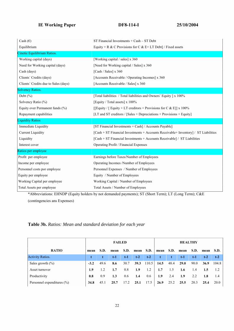
other hand, 11 new ratios were added which referred to time trend for 11 of the 36 ratios previously selected: three time trend were calculated for each ratio - trend between year t and t-1, between t-1 and t-2, and between t and t-2. Therefore, the total data for each company was 141 (108 plus 33). Including time variations for the ratios is not a common practice in insolvency analysis, with the exception of some few papers as the conducted by Becchetti et al. (2003). However, this can be of great interest as it is well known that the ratio distribution in healthy companies tends to be constant over time, whereas it va ries greatly in insolve nt companies due to ratio deterioration, [ e.g. see B eaver (1966)]. Bearing in mind this factor, time variations in some ratios could have a g reater predictive power than the own ratio value. On the other hand, it seems a priori that such variations mig ht have g reater independence from the activity sector and company size than the own ratio. Tables 3a and 3b show the definition of the financial ratios set and their main descriptors, respectively

<Table 3 about here> The relationship between the mean values of the ratios in both g roups generally is the expected one, with some exceptions (financial costs %, liquidity ratios, etc.). However, when such exceptions are ex amined in detail, we see t hat they are due to extreme values in the ratios of some of the companies. 4.- APPLYING GRASP AS RATIO PRESELECTION PROCEDURE

4.1.- PREVIOUS COMPUTATIONAL EXPERIMENTS

In order to compare the efficiency of our GRASP algorithm and its components, we carried out some tests as a previous step. W e used the table of 141 financial ratios for a total of 198 companies. From this table we obtained smaller tables with an m number of financial ratios for the 198 companies. Thus, we consider the following values of m, m = 40 (corresponding to the first 40 financial ratios), 65, 90, 105, and 120. The number of cases (companies) under consideration is 198, divided into classes (healthy and failed), with 131 and 67 items, respectively . We consider a partition, randomly obtained, A = A1 ∪ A2, where A1 has 100 items (66 solvent and 34 insolvent) and A 2 has 98 (65 and 33). Table 4 shows the results obtained, ex pressed as percentag e of hits, for the constructive deterministic algorithm (the one used by software packages like BMDP and SPSS), for 20 executions of the g reedy-random method4 (α = 0.85), and for our GRASP procedure 5 (α =

4 Which consist of the introduction of same randomness in the constructive algorithm. 5 Which introduces a local search procedure over the preceding.


10

0.85 and max_iter = 20), for different values of p (number of ratios selected) and different values of m (number of ratios under consideration).

<Table 4 about here> Table 4 shows that the repetition of the g reedy-random method gives better results than the constructive deterministic method: in 17 cases it is better (in bold), in seven the same and only in one case is it worse. The GRASP method (which includes the g reedy-random method and local search) strong ly improves the results of the g reedy-random method on its own. Therefore, local search is very efficient for improving the quality of the solutions obtained by the different constructive algorithms.

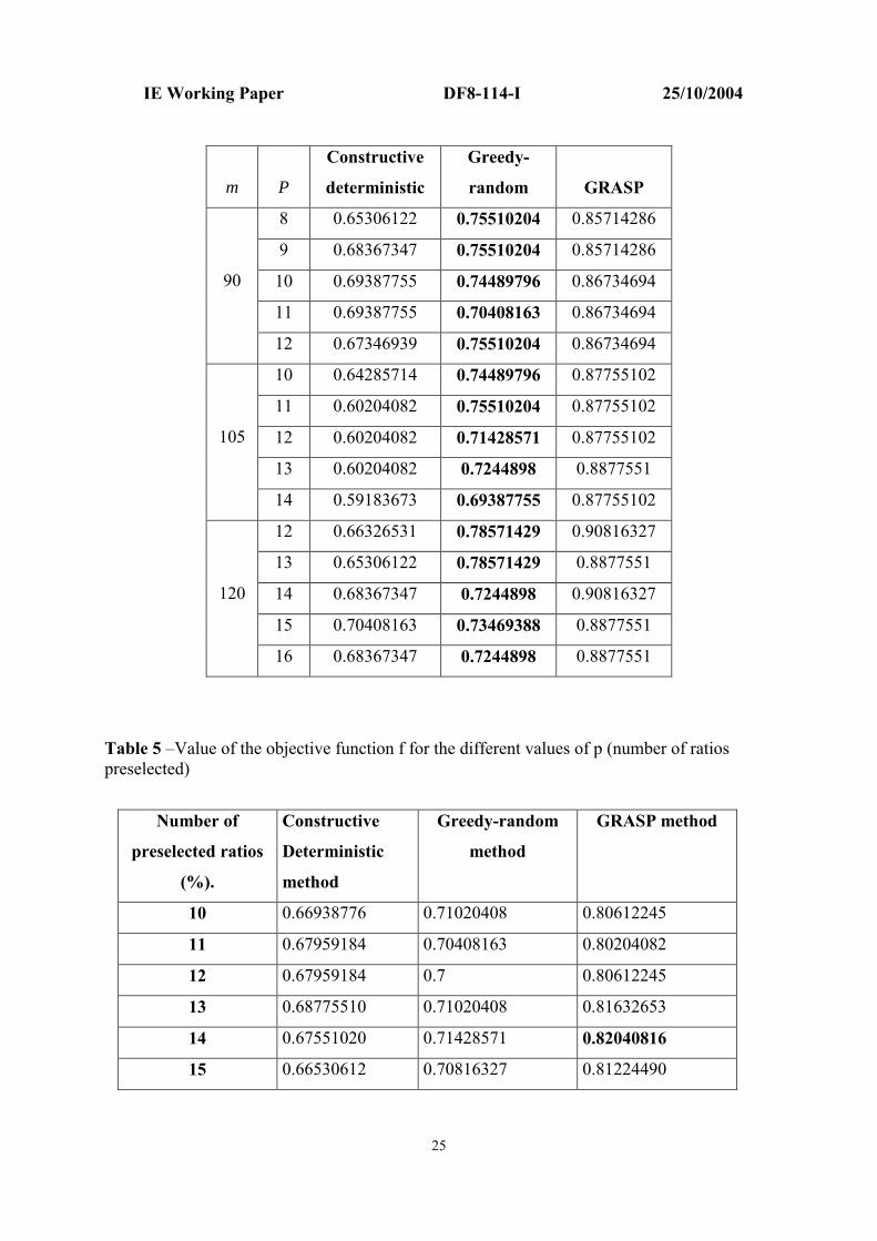
4.2.- PRESELECTION OF RATIOS BY GRASP In this section, we solve the problem of variable selection for our sample now that the efficiency of t he GRASP algorithm has been dem onstrated. As previ ously stated, we deal with 198 cases (firms), divided into two classes (healthy and failed), with 131 and 67 items, respectively. We consider the same partition as in previous tests, A = A1 ∪ A2, where A1 has 100 items (66 healthy and 34 failed) and A 2 has 98 (65 and 33). I n this case we use the total number of variables or ratios (m=141). Table 5 shows the values of the objective function obtained for the different values of p (p=10,..., 15). In each column the result for one of the three strateg ies used is shown: constructive deterministic, constructive greedy random (executed 20 times and α = 0.85), and GRASP methods (α = 0.85 and max_iter = 20).

<Table 5 about here> For each value of p the value of the objective function (the percentage of hits), is better when the GRASP procedure is applied (third column in the table). This make sense because in the GRASP procedure the solution obtained is improved by applying local search. Therefore, this metaheuristic strategy provides us with the best solutions. On the other hand, the g reedy random constructive method (2nd column) g enerates better results than the constructive deterministic strategy which coincides with the selection method used by statistics software like SPSS and BMDP. This means that the results obtained by these statistical packages can be improved simply by adding randomness to the constructive deterministic method or by a more complex metaheuristic strategy, such as GRASP; this will improve the solutions obtained with the random constructive method by applying a local search procedure. The number of financial ratios allowed for selection (p), rang es between 10 and 15. Note that if this number increases, the value of the objective function does not necessarily increase. In any case, the best values for the objective function are obtained when p=13, p=14, and p=15 with the GRASP proc edure. It is a lso interesting to se e that the value of f for p=10 is 0.71020408 when using the greedy random constructive method, but when p=11, f =


11

0.70408163 which means that the percentag e of hits is lower in spite of having increased the value of p. Finally, Table 6 shows the frecuency of selection for the ratios. Columns 2, 3 and 4 show the number of times each financial ratio is selected by the different strategies used: constructive deterministic, greedy random constructive and GRASP. The first column shows the total number of t imes such a rat io has been sel ected by the set of st rategies and t he last column shows the kind of ratio it is: A (a ctivity), R (re turns), E (e quilibrium), S (solve ncy), L (liquidity), E_C (equilibrium_cinetic), and PE (per employee).

<Table 6 about here> If we focus on the financial ratios selected, that is, those ratios that can better predict corporate failure we can conclude the following:

- Normally, the ratios more often selected are those referring to activity, solvency, and to a lesser deg ree, return. In more specific terms, the most relevant ratios are: Added Value Growth, Solvency ratio, Productivity , ROA before taxes, and Equity over Permanent Funds. As a whole, these financial ratios enable us to obtain good knowledge regarding the solvency of the company. However, it is interesting to point out that the “leading” ratios are not always the same in each selection procedure, as shown in Table 6.

- On the other hand, ratios referring to trends (time variations) are the most prominent

type within the selected ratios, either between year t and t-1 or t and t-2 and t-1, t-26. Eighteen models have been tested: 6 models (with values of p rang ing from 10 to 15) for each of the three strateg ies under consideration (constructive deterministic, g reedy random constructive, and GRASP). I n 16 out of the 18 models at least one trend ratio is always selected. Therefore, although trend ratios are not usually included in this kind of a nalysis, they are important. The relevance of time variability in financial ratios dealing with solvency and debts, which are the ones with the highest frecuency in all the models tested, makes sense because t he worsening of these ratios over time might suggest that the company is c lose to a n insolvency situation. From its beginning, the literature on financial distress [ see Beaver (1966)], suggests that the ratio distribution of healthy companies is steady over t ime whereas i t changes in a significant way for unsound companies.

5.- A “GRASP-LOGIT” MODEL Finally, in order to perform a whole analysis, besides solving the problem of variable selection, we have made use of logistic regression to fine tune the ratios that best predict the insolvency situation of a company. To this end, we took the selected ratios with the best value for the objective function (shown in bold in Table 5), which corresponds to the GRASP 6 For reasons of space this information has not been included in Table 6. It is available upon request.


12

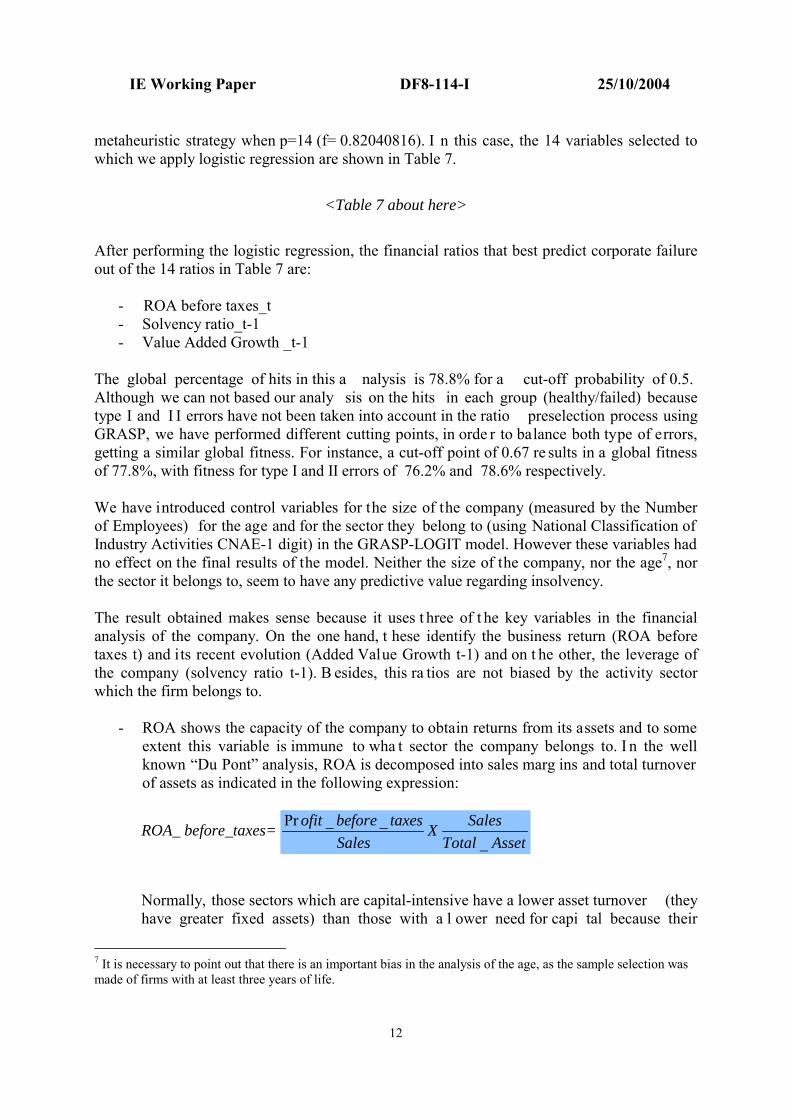
metaheuristic strategy when p=14 (f= 0.82040816). I n this case, the 14 variables selected to which we apply logistic regression are shown in Table 7.


After performing the logistic regression, the financial ratios that best predict corporate failure out of the 14 ratios in Table 7 are: - ROA before taxes_t

- Solvency ratio_t-1 - Value Added Growth _t-1

The global percentage of hits in this a nalysis is 78.8% for a cut-off probability of 0.5. Although we can not based our analy sis on the hits in each group (healthy/failed) because type I and I I errors have not been taken into account in the ratio preselection process using GRASP, we have performed different cutting points, in orde r to balance both type of errors, getting a similar global fitness. For instance, a cut-off point of 0.67 re sults in a global fitness of 77.8%, with fitness for type I and II errors of 76.2% and 78.6% respectively. We have introduced control variables for the size of the company (measured by the Number of Employees) for the age and for the sector they belong to (using National Classification of Industry Activities CNAE-1 digit) in the GRASP-LOGIT model. However these variables had no effect on the final results of the model. Neither the size of the company, nor the age7, nor the sector it belongs to, seem to have any predictive value regarding insolvency. The result obtained makes sense because it uses t hree of t he key variables in the financial analysis of the company. On the one hand, t hese identify the business return (ROA before taxes t) and its recent evolution (Added Value Growth t-1) and on t he other, the leverage of the company (solvency ratio t-1). B esides, this ra tios are not biased by the activity sector which the firm belongs to.

- ROA shows the capacity of the company to obtain returns from its assets and to some extent this variable is immune to wha t sector the company belongs to. I n the well known “Du Pont” analysis, ROA is decomposed into sales marg ins and total turnover of assets as indicated in the following expression:

ROA_ before_taxes= Pr _ __

ofit before taxes SalesXSales Total Asset

Normally, those sectors which are capital-intensive have a lower asset turnover (they have greater fixed assets) than those with a l ower need for capi tal because their

7 It is necessary to point out that there is an important bias in the analysis of the age, as the sample selection was made of firms with at least three years of life.


13

investment needs in assets are lower. However, capital-intensive sectors have a greater sales margin than those which are less capital-intensive. Therefore, given that ROA takes both variables together, this palliates, to a great extent, the effect of belonging to one sector or another.

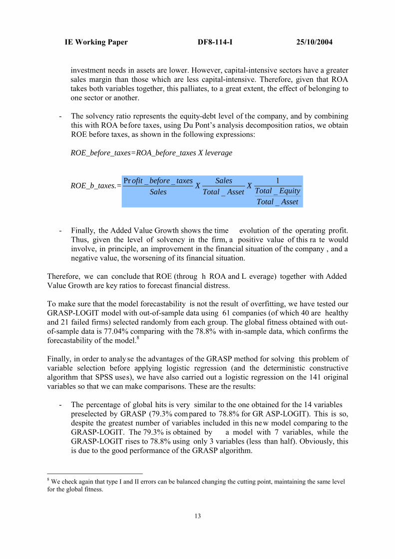
- The solvency ratio represents the equity-debt level of the company, and by combining this with ROA before taxes, using Du Pont’s analysis decomposition ratios, we obtain ROE before taxes, as shown in the following expressions:

ROE_before_taxes=ROA_before_taxes X leverage

ROE_b_taxes.= Pr _ _ 1___

ofit before taxes SalesX X Total EquitySales Total AssetTotal Asset

- Finally, the Added Value Growth shows the time evolution of the operating profit. Thus, given the level of solvency in the firm, a positive value of this ra te would involve, in principle, an improvement in the financial situation of the company , and a negative value, the worsening of its financial situation.

Therefore, we can conclude that ROE (throug h ROA and L everage) together with Added Value Growth are key ratios to forecast financial distress. To make sure that the model forecastability is not the result of overfitting, we have tested our GRASP-LOGIT model with out-of-sample data using 61 companies (of which 40 are healthy and 21 failed firms) selected randomly from each group. The global fitness obtained with out-of-sample data is 77.04% comparing with the 78.8% with in-sample data, which confirms the forecastability of the model.8 Finally, in order to analyse the advantages of the GRASP method for solving this problem of variable selection before applying logistic regression (and the deterministic constructive algorithm that SPSS uses), we have also carried out a logistic regression on the 141 original variables so that we can make comparisons. These are the results:

- The percentage of global hits is very similar to the one obtained for the 14 variables

preselected by GRASP (79.3% com pared to 78.8% for GR ASP-LOGIT). This is so, despite the greatest number of variables included in this new model comparing to the GRASP-LOGIT. The 79.3% is obtained by a model with 7 variables, while the GRASP-LOGIT rises to 78.8% using only 3 variables (less than half). Obviously, this is due to the good performance of the GRASP algorithm.

8 We check again that type I and II errors can be balanced changing the cutting point, maintaining the same level for the global fitness.


14

- The selected variables in the logit with 141 variables are the following: Value Added Growth _t (%) Value Added Growth _t-1 (%) Productivity_t-2 Equity over permanent funds _t(%) Debts _t-2 (%) ROA before taxes_t (%) Personnel expenditures_t-1 (%) Within the seven variables selected in this case — or six if we do not take into account the time factor — we fi nd the three variables which were previ ously selected by the GRASP-LOGIT model (ROA before taxes_t, Added Value Growth_t-1, and Debts_t-2). Debt is a variable equivalent to the variable solvency ratio that appeared in the GRASP-LOGIT (although it reading is the opposite) because:

Solvency ratio = 100 - Debts

This latter variable now appears in the t-2 period, while in the first GRASP- L OGIT model, the solvency ratio appeared in the t-1 period. The remaining selected variables for this model are personnel expenditures (%), productivity (gross operating margins per monetary unit used in labour), and equity over permanent funds. The meaning of these variables as predictors of failure is not as clear as for the three variables obtained with the GRASP-LOGIT model. Personnel ex penditures (measured as a percentag e of the firm income) show g reat dependency on sect or, because t he more labor-intensive sectors show higher values for this variable. The opposite happens with productivity ; i.e., the sector which is most la bor intensive has lower figures for this indicator. Finally, the variable equity over permanent funds or long -term funds does not seem to be a good predictor of insolvency, because it does not take into account short-term debts, which in many cases can be decisive for assessing the payment capacities of the company. Therefore, it seems that the interpretation that can be derived for the results obtained by the GRASP-LOGIT model is better than the ones from the log it with 141 ratios, whereas the predictive capacity of both models is the same. 7.- CONCLUSIONS This work has focused on the resolution of the problem of financial ratio preselection to model business insolvency -we use 141 financial ratios over a sample of 198 Spanish firms. To this end we used the metaheuristic strategy GRASP (Greedy Randomized Adaptive Search Procedure) which build solutions by controlled randomness over a g reedy function which guides the entry of variables into the solution. The n, the variable selection is improve d by local search. This strategy can be used for sol ving the feature subset selection problem when


15

all the variables are quantitative. There aren’t any references in the literature about algorithms designed “ad hoc” for this type of variables. The results obtained with GRASP and its elements were compared to those obtained by applying the deterministic constructive algorithm used in statistical software, such as BMDP and SPSS. The systematic superiority of GRASP means that the quality of the solutions found can be improved by introducing randomness in the selection procedure or by using local search. In addition, we modelled business insolvency by applying a logistic regression model to the results from the GRASP procedure. GRASP was used to preselect 14 financial ratios from which the logit was built. We called this model GRASP-LOGIT, and the results obtained with it were compared to those obtained by applying a logit directly to the orig inal 141 financial ratios. Although the classificatory capacity of the GRASP-L OGIT is the same as the log it model with 141 ratios, the explanatory capacity and the simplicity of the former is g reater than the latter. Therefore, we can assert that incorporating the GRASP metaheuristic into the preselection of financial ratios adds an improvement to the understanding of business insolvency model. I ts advantage is also apparent concerning reducing the cost of data acquisition. The GRASP-LOGIT model shows that the best combination of ratios to explain corporate failure are: ROA before taxes, Solvency ratio, and Added Value Growth. The first two ratios are the components of ROE identified by Du Pont’s analysis. Besides, our results reveal that neither the size of the company (measured by the number of employees), nor the age, nor the sector it belongs to seem to have any predictive value regarding modelling insolvency.


16

REFERENCES Altman, E. (1968). Financial Ratios, Discriminant analy sis and the prediction of corporate bankruptcy. Journal of Finance, September, pp. 189-209. Altman, E., Marco, G., and Varetto, F . (1994). Corporate distress diagnosis: comparisons using linear discriminant analysis and neural networks. J ournal of Banking and Finance, v.18, pp. 505-529. Bala J., Dejong K., Huang J., Vafaie H. and Wechsler H. (1996). Using Learning to Facilitate the Evolution of Features for Recognizing Visual Concepts. Ev olutionary Computation, 4, 3, 297-311. Baranauskas J.A. and Monard, M.C. (1998). Experimental Feature Selection Using the Wrapper Approach. International Conference on Data Mining, Sep 02-04, Data Mining, 161-170, 1998. Beaver, W., (1966): Financial ratios as predictors of failures, in Empirical Research. Accounting, selected studies, pp. 71-111. Becchetti, L. and Sierra, J. (2003). Bankruptcy risk and productive efficiency in manufacturing firms. Journal of Banking & Finance, 27, pp. 2099-2120. Cotta C., Sloper C. and Moscato P. (2004). Evolutionary Search of Thresholds for Robust Feature Set Selection: Application to the A nalysis of Microarray Data . Lecture Notes In Computer Science 3005: 21-30. Curran, S. and Ming ers, J., (1994). Neural networks, decision tree induction and discriminant analysis: an empirical comparison. Operational Research Society, v. 45 (4), pp. 440-450. Feo T.A. and Resende M.G.C. (1989). A Probabilistic heuristic for a computationally difficult Set Covering Problem. Oper Res Lett, 8, 67-71. Feo T.A. and Resende M.G.C. (1995). Greedy Randomized Adaptive Search Procedures. Journal of Global Optimization, vol. 2, pp 1-27. Ferri F., Pudil M., Hatef M. and Kittler J.(1994).Comparative study of techniques for large scale feature selection. In E. Gelsema and L. Kanal, editors, Patter Recognition in Practice IV, pages 403-413. Elsevier Science B.V. Gallego, A.M. and Gómez, M.A. (2002). Análisis integrado de la absorción y quiebra empresarial mediante la estimación de un modelo M ultilogit. Revista Española de F inanciación y Contabilidad, V. XXXI, nº111, pp. 111-144. Ganster H., P inz A., Rohrer R., W ildling E., Binder M . and Kittler H.(2001). Automated Melanoma Recognition . IEEE Transactions On Medical Imaging 20 (3): 233-239.


17

Huang, S.H. (2003). Dimens ionality reduction in automatic knowledg e acquisition: a simple greedy search approach. I EEE Transactions on know ledge and data engineering, 15(6), 1364-1373. Inza, I., Larrañaga, P., Etxeberria, R. and Sierra, B. (2000). F eature Subset Selection by Bayesian networks based optimization. Artificial Intelligence, 123, 157-184. Inza, I., Merino, M., Larranaga, P., Quiroga, J., Sierra, B. and Girala, M.(2001a). Feature Subset Selection by Genetic Algorithms and Estimation of Distribution Algorithms - A Case Study in the Survival of Cirrhotic Patients Treated with TIPS. Artificial Intelligence In Medicine 23 (2): 187-205. Inza I., Larranaga, P. and SIERRA, B. (2001b). Feature Subset Selection by Bayesian Networks: A Comparison with Genetic and Sequential Alg orithms. International Journal of Approximate Reasoning 27 (2): 143-164. Inza, I., Sierra, B. and Blanco, R. (2002). Gene Selection by Sequential Search W rapper Approaches in Microarray Cancer Class Prediction. Journal of Intelligent & Fuzzy Systems 12 (1): 25-33. Jain, A. and Zongker, D.(1997). Feature Selection: Evaluation, Application, and Small Sample Performance. IEEE Trans. Pattern Analysis and Machine Intelligence, vol. 19, no. 2, pp. 153-158. Jaroszewicz, S., Simovici, D.A., Kuo W.P. and Ohno-Machado L. (2004). The Goodman-Kruskal Coefficient and its Applications in G enetic Diagnosis of Cancer. IEEE Transactions on Biomedical Engineering 51 (7): 1095-1102. Jelonek, J. and Stefanowski, J. (1997). Feature Subset Selection f or Classification of Historical Images. Artificial Intelligence in Medicine 9(3):227-239. Jourdan, L., Dhaenens, C. and Talbi, E. (2001). A Genetic Algorithm for Feature Subset Selection in Data-Mining for Genetics. MIC 2001 Proceedings, 4th Metaheuristics Internationl Conference, 29-34. Kohavi, R. (1995). W rappers for Performance Enhancement and Oblivious Decision Graphs. Stanford University, Computer Science Department. Kohavi, R. and John, G.H. (1997). W rappers for Feature Subset Selection. Artificial Intelligence 97(1-2): 273-324. Laffarga, J., Martín, J .L., Vázquez, M.J. (1990). L a predicción de la quiebra bancaria: el caso español. Revista Española de Financiación y Contabilidad, V. XX, nº 66, pp.151-166. Lee, S., Yang, J. and Oh, K.W . (2003). Prediction of Molecular Bioactiv ity for Drug Design Using a Decision Tree Algorithm. Lecture Notes In Artificial Intelligence 2843: 344-351. Lennox, C. (1999). I dentifying failing companies: a reev aluation of the loog it, probit and da approaches. Journal of Economics and Business, v 51, pp. 347-364.


18

Lewis, P. M.(1962). The Characteristic Selection Problem in Recognition Systems. IEEE Trans. Information Theory, vol. 8: 171-178. Liu, H. and Motoda, H.(1998). F eature Selection f or Knowledge Discovery and Data Mining. Boston: Kluwer Academic. Narendra, P.M. and F ukunaga, K. (1977). A Branch and Bound Algorithm for Feature Subset Selection. IEEE Trans. Computers, vol. 26, no. 9: 917-922. Neophytou, E. and Molinero, C.M. (2004). Predicting corporate f ailure in the UK: a multidimensional scaling approach. Journal of Business Finance & Accounting, 31, (5&6).

Ohlson, J.A. (1980). F inancial ratios and the probabilis tic prediction of bankruptcy. Journal of Accounting Research, 18 (1): 109-111.

Oliveira, L.S., Sabourin, R., Bortolozzi, F., et al.(2003). A Methodolog y for Feature Selection Using Multiobjective Genetic Algorithms for Handwritten Digit String Recognition. International Journal of Pattern Recognition And Artificial Intelligence 17 (6): 903-929. Ooghe, , H. and Balcaen, S . (2002). Are failure prediction models transferable from one country to another?. An empirical study using Belgian financial statements. Vlerick Leuven Gent Management School. Vlerick Working Paper 2002/5.

Pitsoulis, L.S. and Resende, M.G.C. (2002). Greedy Randomized Adaptive Search Procedures in: P. M. Pardalos and M. G. C. Resende (Eds.), Handbook of Applied Optimiz ation, Oxford University Press, pp. 168-182.

Sanchís, A.; Gil, J.A. and Heras, A. (2003). El análisis discriminante en la prev isión de la insolvencia en las empresas de seg uros de no v ida. Revista Española de Financiación y Contabilidad, V. XXXII, nº 116: 183-233. Sebban, M. and Nock, R.(1999). Contribution of Boosting in Wrapper Models. Lecture Notes in Artificial Intelligence 1704:214-222. Sebestyen, G. (1962). Decision-Making Processes in Pattern Recognition. New York: MacMillan. Shy, S. and Suganthan, P.N. (2003). F eature Analysis and Clasif ication of Protein Secondary Structure Data. Lecture Notes in Computer Science 2714: 1151-1158. Siedlecki, W. and Sklansky , J.(1988). On Automatic F eature Selection. Int’l J. Pattern Recognition and Artificial Intelligence, vol. 2: 197-220. Sierra, B., Lazkano, E., Inza, I., Merino, M., L arrañaga, P. and Quirog a, J. (2001). Prototy pe Selection and Feature Subset Selection by Estimation of Distribution Algorithms. A Case Study in


19

the Survival of Cirrhotic Patients Treated w ith TIPS. Lecture Notes in A rtificial Intelligence 2101:20-29. Tamoto, E., Tada, M., Murakawa, K., Takada, M., Shindo, G., Teramoto, K., Matsunaga, A., Komuro, K., Kanai, M., Kawakami, A., Fujiwara, Y., Kobayashi, N., Shirata, K., Nishimura, N., Okushiba, S.I., Kondo, S., Hamada, J ., Yoshiki, T., Moriuchi, T. and Katoh, H.(2004). Gene.expression Profile Changes Correlated with Tumor Prog ression and Lymph Node Metastasis in Esophageal Cancer. Clinical Cancer Research 10(11):3629-3638. Varetto, F. (1998). Genetic Algorithms applications in the analysis of insolvency risk. Journal of Banking & Finance v. 22: 1421-39. Wong, M.L.D. and Nandi, A.K. (2004). Automatic Digital Modulation Recognition Using Artificial Neural Network and Genetic Algorithm. Signal Processing 84 (2): 351-365. Zmijewski, M.E. (1984). Methodological Issues Related to the Estimation of financial Distress Prediction Models. Journal of Accounting Research, V 22 (Supplement): 59-82


20

TABLES

Table 1 Breakdown of failed / healthy firms by CNAE classification.

CNAE Failed Healthy 01 Farming 0 3 02 Forestry 0 1 15 Food and beverage sector 5 6 17 Textile industry 3 1 18 Clothes industry 1 1 19 Shoemaking 0 1 20 Wood and cork industry 1 2 21 Paper industry 0 1 22 Publishing and graphic arts 2 3 24 Chemical industry 0 4 25 Manufacturing of plastic and rubber products 1 2 26 Manufacturing of other mineral products 0 1 27 Metalwork 2 1 28 Manufacturing of metal products 4 3 29 Building machinery 5 3 31 Manufacturing of electric equipment 2 0 33 Manufacturing of medical equipment 0 1 34 Manufacturing of motorised vehicles 0 1 35 Manufacturing of other transport material 1 0 36 Manufacturing of furniture; other industries 4 3 41 Water collecting, purifying and distribution 0 1 45 Building 10 16 50 Sales and repair of. motorised vehicles 0 5 51 Wholesale sales 12 16 52 Retail sales 7 11 55 Hospitality sector 0 4 60 Land transport 0 2 61 Sea transport 0 1 63 Transport-related activites 1 1 65 Finance trading (except insurance) 0 1 70 Estate agents 2 16 74 Other business activities 2 12 80 Education 2 0 85 Hospital and veterinary activities 0 2 92 Cultural, recreational and sport activities 0 4 93 Personal services activities 0 1 Total 67 131


21

Table 2 Mean size, Legal format and Years in buniness

Insolvent (67) Solvent (131) Size* Mean number of employees 22 (22) 36 ( 65) Mean number of employees (<100 employees)**

22 (22) 20 (23)

Legal format*** Corporation 27 (40%) 52 (40%) Limited Liability Company 40 (60%) 79 (60%) Years in business* Mean number of years in business 18 (15) 18 (13)

* Standard deviation in brackets

** After eliminating from the sample those solvent companies with more than 100 employees (a total of 10)

*** Number of companies (percentage in each sample in parenthesis)

Table 3a Ratios definitions

Activity Ratios.

Sales growth (%) [[Sales_t – Sales_t-1]/Sales_t-1] x 100%

Asset turnover Sales/Total Assets

Productivity [Operating revenues – Consumption and Operating expenditures] / Personnel expenditures

Personnel expenditures (%) [Personnel expenditures/ Operating revenues] x 100%

Value added growth (%) [[Value Added_t – Value Added_t-1]/Value Added_t-1] x 100%

Operating margin (%) [Earnings before Taxes / Operating revenues] x 100%

Net Asset Turnover Operating revenues/Permanent funds

Return Ratios.

ROCE [Earnings before Taxes + Financial expenses]/Permanent funds] x 100%

ROA [Earnings /Total assetsl] x 100%

ROA before taxes [Earnings before Taxes /Total assetsl] x 100%

ROE [Earnings /Equity] x 100%

ROE before taxes [Earnings before Taxes /Equity] x 100%

Financing costs (%) [Financing costs/Sales] x 100%

Equilibrium Ratios.

Working capital (€) Equity + Provisions for C & E+ LT Creditors – Fixed assets

Need for Working capital (€)

[EHNDP + Acrrued Expenses + (Inventory + Accounts Receivable)] –

[Accrued Incomes + Accounts Payable]


22

Cash (€) ST Financial Investments + Cash – ST Debt

Equilibrium Equity + R & C Provisions for C & E+ LT Debt] / Fixed assets

Cinetic Equilibrium Ratios.

Working capital (days) [Working capital / sales] x 360

Need for Working capital (days) [Need for Working capital / Sales] x 360

Cash (days) [Cash / Sales] x 360

Clients´ Credits (days) [Accounts Receivable / Operating Incomes] x 360

Clients´ Credits due to Sales (days) [Accounts Receivable / Sales] x 360

Solvency Ratios.

Debt (%) [Total liabilities / Total liabilities and Owners` Equity ] x 100%

Solvency Ratio (%) [Equity / Total assets] x 100%

Equity over Permanent funds (%) [[Equity / [ Equity + LT creditors + Provisions for C & E]] x 100%

Repayment capabilities [LT and ST creditors / [Sales + Depreciations + Provisions + Equity]

Liquidity Ratios

Immediate Liquidity [ST Financial Investments + Cash] / Accounts Payable]

Current Liquidity [Cash + ST Financial Investments + Accounts Receivable+ Inventory] / ST Liabilities

Liquidity [Cash + ST Financial Investments + Accounts Receivable] / ST Liabilities

Interest cover Operating Profit / Financial Expenses

Ratios per employee

Profit per employee Earnings before Taxes/Number of Employees

Income per employee Operating Incomes /Number of Employees

Personnel costs por employee Personnel Expenses / Number of Employees

Equity per employee Equity / Number of Employees

Working Capital per employee Working Capital / Number of Employees

Total Assets per employee Total Assets / Number of Employees

*Abbreviations: EHNDP (Equity holders by not demanded payments); ST (Short Term); LT (Long Term); C&E

(contingencies ans Expenses)

Table 3b. Ratios: Mean and standard deviation for each year

FAILED HEALTHY

RATIO mean S.D. mean S.D. mean S.D. mean S.D. mean S.D. mean S.D.

Activity Ratios. t t t-1 t-1 t-2 t-2 t t t-1 t-1 t-2 t-2

Sales growth (%) -3.2 49.6 8.6 30.7 39.3 110.5 14.5 48.4 29.0 90.0 36.9 104.8

Asset turnover 1.9 1.2 1.7 0.8 1.9 1.2 1.7 1.5 1.6 1.4 1.5 1.2

Productivity 0.8 0.9 1.3 0.6 1.4 0.6 1.9 2.4 1.9 2.2 1.8 1.4

Personnel expenditures (%) 34.8 45.1 25.7 17.2 25.1 17.5 26.9 25.2 25.5 20.3 25.4 20.0


23

Value Added Growth (%) -12.0 37.9 11.2 28.5 33.4 91.2 38.9 121.0 51.2 140.3 40.4 110.8

Operating Margin (%) -11.6 20.4 -1.4 7.1 0.0 5.3 -1.8 79.4 8.2 48.4 8.4 54.6

Net Asset Turnover 9.9 42.0 8.3 11.2 8.7 21.7 4.8 9.7 5.9 37.6 5.9 10.1

Return Ratios.

ROCE -4.7 199.2 17.3 95.4 32.7 91.5 21.9 37.2 19.5 36.5 20.5 34.8

ROA -25.8 59.7 -1.7 10.9 1.0 6.3 2.8 15.5 3.1 11.4 3.7 7.8

ROA before taxes -24.7 57.0 -1.2 10.8 1.3 7.9 4.6 15.6 4.1 16.2 4.9 10.7

ROE 15.4 167.9 15.2 134.6 12.6 57.4 12.9 85.2 11.5 56.2 5.7 65.2

ROE before taxes 7.8 182.3 8.5 87.2 14.1 70.0 19.2 93.2 19.7 70.0 14.6 44.4

Financial costs (%) 4.8 12.2 2.9 2.2 2.7 2.4 15.0 88.3 13.0 56.1 9.2 53.1

Equilibrium Ratios.

Working Capital (Mil) -163 1418 -76 1194 58 498 2049 15018 2669 11733 3159 17870

Need of Working capital (Mil) -19 1447 206 1154 252 1066 -182 14217 1078 7024 186 13888

Cash (Mil) -144 912 -282 1258 -194 1004 2231 21583 1591 13070 2973 29669

Equilibrium -2 27 3 5 3 9 11 72 7 39 5 26

Cinetic Equilibrium Ratios

Working Capital (days) -49 243 -9 172 -6 164 361 5608 1139 6770 525 5793

Need of Working capital (days) -61 266 -14 173 -13 173 -130 1659 298 3437 -65 888

Cash (days) 12 49 6 42 7 45 491 5286 841 6115 590 5993

Clients´ Credits (days) 179 753 86 61 89 65 281 1002 215 769 149 234

Clients´ Credits due to Sales (days) 178 753 86 61 88 65 234 800 109 128 127 191

Solvency Ratios.

Debts (%) 107.0 76.5 83.8 22.0 81.4 23.0 68.8 45.4 68.0 43.1 67.9 39.0

Solvency Ratio (%). -7.0 76.5 16.2 22.0 18.6 23.0 31.2 45.4 32.0 43.1 32.1 39.0

Equity over Permanent funds (%) 64.5 61.0 57.5 48.6 65.5 31.3 75.8 38.4 74.6 34.1 75.7 31.8

Repayment capabilities 2.1 11.0 0.6 0.6 0.6 0.6 5.7 46.5 2.2 10.7 1.8 8.1

Liquidity Ratios.

Immediate Liquidity 1.6 11.8 0.2 0.9 0.2 0.8 5.5 54.7 4.7 43.6 0.7 2.1

Current Liquidity 8.2 58.4 1.3 1.0 1.3 0.9 7.9 56.1 6.1 43.8 2.2 3.2

Liquidity 2.6 15.7 0.8 0.9 0.8 0.9 7.4 56.1 5.5 43.8 1.5 2.5

Interest cover -24.6 170.1 -18.5 170.7 -5.9 75.7 30.7 518.6 173.0 1325.0 207.9 1347.2

Ratios per employee.

Profit per employee (Mil) -21 60 -4 32 0 13 76 694 34 173 26 146

Income per employee (Mil) 183 234 196 290 199 303 471 1854 302 639 247 457

Personnel expenditures per employee

(Mil) 35 81 33 89 44 136 32 51 27 16 25 14

Equity per employee (Mil) 3 49 19 48 22 68 459 2060 390 1962 318 1812

Working Capital per employee (Mil) 79 139 78 130 76 137 255 1001 167 436 136 323

Total Assets per employee (Mil) 140 220 133 214 124 209 930 3928 597 2097 499 1920


24

mean S.D. mean S.D. mean S.D. mean S.D. mean S.D. mean S.D.

Ratio Trends (%). t_t-1 t_t-1 t-1_t-2 t-1_t-2 t_t-2 t_t-2 t_t-1 t_t-1 t-1_t-2 t-1_t-2 t_t-2 t_t-2

Activity Ratios Trend.

Operating Margin (%) -10.2 18.8 -1.4 6.4 -11.6 20.7 -13 96.4 -0.2 26.4 -13.2 98.1

Equilibrium Ratio Trend.

Working capital (Mil) -87 377 -134 1076 -221 1306 -620 7173 -491 8554 -1110 9858

Need for Working capital (Mil) -224 960 -46 920 -271 1733 -1259 9573 891 9911 -368 7909

Cash (Mil) 137 774 -88 460 49 538 640 10116 -1382 17489 -743 9376

Solvency Ratio Trend.

Debts (%) 23.3 67.6 2.3 12.9 25.6 71.5 0.9 16.6 0.1 12.8 1.0 19.4

Solvency Ratio (%). -23.3 67.6 -2.3 12.9 -25.6 71.5 -0.9 16.6 -0.1 12.8 -1.0 19.4

Equity over Permanent funds (%) 7.0 63.2 -8.1 39.6 1.1 68.3 1.2 32.6 -1.1 23.7 0.1 38.0

Repayment capabilities 1.4 10.9 0.0 0.3 1.5 11.0 3.5 44.3 0.3 11.2 3.8 45.8

Liquidity Ratio Trend.

Immediate Liquidity 1.4 11.8 0.0 0.2 1.4 11.8 0.9 11.3 3.9 41.8 4.8 52.9

Current Liquidity 7.0 58.5 0.0 0.4 6.9 58.5 1.9 16.2 3.9 42.1 5.8 54.5

Liquidity 1.8 15.8 0.0 0.2 1.8 15.8 1.9 16.1 4.0 42.0 5.9 54.4

Table 4.- Results from computational tests

m P

Constructive

deterministic

Greedy-

random GRASP

4 0.67346939 0.70408163 0.7755102

5 0.69387755 0.69387755 0.7755102

6 0.68367347 0.68367347 0.7755102

7 0.68367347 0.68367347 0.79591837

40

8 0.71428571 0.71428571 0.80612245

6 0.67346939 0.71428571 0.80612245

7 0.69387755 0.69387755 0.81632653

8 0.70408163 0.70408163 0.82653061

9 0.70408163 0.70408163 0.84693878

65

10 0.73469388 0.68367347 0.85714286


25

m P

Constructive

deterministic

Greedy-

random GRASP

8 0.65306122 0.75510204 0.85714286

9 0.68367347 0.75510204 0.85714286

10 0.69387755 0.74489796 0.86734694

11 0.69387755 0.70408163 0.86734694

90

12 0.67346939 0.75510204 0.86734694

10 0.64285714 0.74489796 0.87755102

11 0.60204082 0.75510204 0.87755102

12 0.60204082 0.71428571 0.87755102

13 0.60204082 0.7244898 0.8877551

105

14 0.59183673 0.69387755 0.87755102

12 0.66326531 0.78571429 0.90816327

13 0.65306122 0.78571429 0.8877551

14 0.68367347 0.7244898 0.90816327

15 0.70408163 0.73469388 0.8877551

120

16 0.68367347 0.7244898 0.8877551

Table 5 –Value of the objective function f for the different values of p (number of ratios preselected)

Number of

preselected ratios

(%).

Constructive

Deterministic

method

Greedy-random

method

GRASP method

10 0.66938776 0.71020408 0.80612245

11 0.67959184 0.70408163 0.80204082

12 0.67959184 0.7 0.80612245

13 0.68775510 0.71020408 0.81632653

14 0.67551020 0.71428571 0.82040816

15 0.66530612 0.70816327 0.81224490


26

Table 6 Number of times each financial ratio is selected by the different algorithmss

TOTAL Deterministic constructive

Random constructive GRASP Selected Ratios

31 12 12 7 Value Added Growth A 1 1 0 0 Sales growth A 26 12 12 2 Productivity A 15 6 6 3 Personnel expenditures (%) A 4 0 1 3 Operating Margin (%) A 7 2 2 3 Asset turnover A 10 3 3 4 Net Asset Turnover A 3 0 0 3 ROA R 23 12 6 5 ROA before taxes R 1 0 1 0 ROE R 6 0 3 3 ROE before taxes R 10 2 3 5 ROCE R 31 9 7 15 Solvency ratio S 22 12 7 3 Equity over Permanent Funds S 17 4 6 7 Debt ratio S 4 0 0 4 Equilibrium E 1 0 0 1 Working capital (€) E 2 0 0 2 Need of working capital (€) E 2 0 2 0 Clients’ Credits due to Sales (days) E_C 3 0 2 1 Income per employee PE 3 0 2 1 Personnel expenditures per employee PE 2 0 0 2 Immediate Liquidity L 1 0 0 1 Cash E

Deterministic constructive

Random constructive GRASP No Selected Ratios

0 0 0 Financial costs % R 0 0 0 Working capital (days) E_C 0 0 0 Need of Qorking capital (days) E_C 0 0 0 Cash (days) E_C 0 0 0 Clients´credit (days) E_C 0 0 0 Repayment capability S 0 0 0 Current liquidity L 0 0 0 Liquidity L 0 0 0 Interest cover L 0 0 0 Profit per employee PE 0 0 0 Equity per employee PE 0 0 0 Working capital per employee PE 0 0 0 Total Assets per employee PE

225 75 75 75


27

Table 7 Preselected variables using GRASP

ROA before taxes_t

ROA_t

Equity over Permanent funds _t-1

Solvency ratio_t-1

Value Added Growth _t-1

Equilibrium_t-1

Debts_t-1_vs_t-2

Working capital_t_vs_t-1

Need for working capital_t_vs_t-1

Debts_t_vs_t-1

Net Asset Turnover_t-1

Solvency ratio_t_vs _t-1

ROCE_t-2

Operating ratio_t

Dep

ósito

Leg

al: M

-200

73

I.S.S

.N.:

1579

-487

3

NOTAS

THE PROBLEM OF VARIABLE SELECTION FOR FINANCIAL DISTRESS: APPLYING GRASP METAHEURISTICS

Documents

Transcript of THE PROBLEM OF VARIABLE SELECTION FOR FINANCIAL DISTRESS: APPLYING GRASP METAHEURISTICS