Heuristics for a vehicle routing problem with information ...

HAL Id: hal-02338334https://hal.archives-ouvertes.fr/hal-02338334

Submitted on 29 Oct 2019

HAL is a multi-disciplinary open accessarchive for the deposit and dissemination of sci-entific research documents, whether they are pub-lished or not. The documents may come fromteaching and research institutions in France orabroad, or from public or private research centers.

L’archive ouverte pluridisciplinaire HAL, estdestinée au dépôt et à la diffusion de documentsscientifiques de niveau recherche, publiés ou non,émanant des établissements d’enseignement et derecherche français ou étrangers, des laboratoirespublics ou privés.

Heuristics for a vehicle routing problem withinformation collection in wireless networks

Luis Flores-Luyo, Agostinho Agra, Rosa Figueiredo, Eladio Ocana

To cite this version:Luis Flores-Luyo, Agostinho Agra, Rosa Figueiredo, Eladio Ocana. Heuristics for a vehicle routingproblem with information collection in wireless networks. Journal of Heuristics, Springer Verlag, Inpress, �10.1007/s10732-019-09429-6�. �hal-02338334�

https://hal.archives-ouvertes.fr/hal-02338334

https://hal.archives-ouvertes.fr

Noname manuscript No.(will be inserted by the editor)

Heuristics for a vehicle routing problem with informationcollection in wireless networks

Luis Flores-Luyo1,3 · Agostinho Agra2 ·Rosa Figueiredo3 · Eladio Ocana1

the date of receipt and acceptance should be inserted later

Abstract We consider a wireless network where a given set of stations iscontinuously generating information. A single vehicle, located at a base station,is available to collect the information via wireless transfer. The wireless transfervehicle routing problem (WTVRP) is to decide which stations should be visitedin the vehicle route, how long shall the vehicle stay in each station, and howmuch information shall be transferred from the nearby stations to the vehicleduring each stay. The goal is to collect the maximum amount of informationduring a time period after which the vehicle returns to the base station. TheWTVRP is NP-hard. Although it can be solved to optimality for small sizeinstances, one needs to rely on good heuristic schemes to obtain good solutionsfor large size instances. In this work, we consider a mathematical formulationbased on the vehicle visits. Several heuristics strategies are proposed, most ofthem based on the mathematical model. These strategies include constructiveand improvement heuristics. Computational experiments show that a strategythat combines a combinatorial greedy heuristic to design a initial vehicle route,improved by a fix-and-optimize heuristic to provide a local optimum, followedby an exchange heuristic, affords good solutions within reasonable amount ofrunning time.

Keywords Vehicle Routing Problem · Wireless Networks · Matheuristic

1Instituto de Matematica y Ciencias Afines, Lima, PeruE-mail: {lflores,eocana}@imca.edu.pe

2CIDMA, Universidade de Aveiro, Aveiro, PortugalE-mail: [email protected]

3Laboratoire Informatique d’Avignon, Avignon Universite, Avignon, FranceE-mail: {rosa.figueiredo}@univ-avignon.fr

2 Flores-Luyo et al.

1 Introduction

The vehicle routing problem (VRP) is one of the most studied problems in op-erations research (OR) with different variants defined and treated in the pastfive decades (see [16, 24]). The emergence of new computer network architec-tures add new features to well studied combinatorial optimization problems(e.g. scheduling problems [23], resource allocation problems [29, 22]) and, aswe could expect, also to VRPs [7, 20, 26]. The present work studies a VRPappearing in wireless networks applications.

Wireless Networks (WN) have recently received great attention from theOR community; as an example, we refer to the edition of a special issue in 2015dedicated to reliable deployment techniques in Wireless Sensor Networks [13].Many applications defined on WN need to provide vehicle routing strategieswith wireless information transmission to the vehicles involved (see [11]). Inthese applications, innovation and research appears most in the developmentof routing protocols [5, 6, 19, 26], while a smaller set of works addressesthe development of vehicle routing strategies, essentially in a two-phase man-ner [12, 14, 17, 21]. To the better of our knowledge, the works presented in[4, 10, 15, 9] are the only ones to focus on the simultaneous design of a vehi-cle route and a wireless transmission planning. Notice that the authors in [15]assume a fixed architecture for the vehicle routing (cycle path or zig-zag path).

In the context considered in this work, a base station is connected with theoutside while a vehicle is in charge of collecting information from the other sta-tions. The stations are supplied with technology capable of sending informationvia wireless connection to the vehicle whenever it is located in a sufficientlyclose station. Time of transmission depends on the distance between stations,the amount of information transmitted, and other physical factors (e.g. ob-stacles along the way, installed equipment). Simultaneous transmissions areallowed. Information to be sent outside the network is continuously generated,at a constant rate, in each station. The Wireless Transmission VRP (WTVRP)treated in this work looks for the vehicle route as well as for an efficient plan-ning on how to gather information from stations, in order to minimize thetotal amount of remaining information in the network. Applications for theWTVRP appear in situations where there is a need for providing connectionfor difficult environments [4, 18, 20, 27].

The authors in [4] were the first ones to propose a solution method for aVRP appearing in underwater wireless sensor networks. The authors consid-ered a scenario with a set of surfacing and underwater nodes where they lookfor a routing to an autonomous underwater vehicle (AUV) during a given timeperiod. The AUV must leave and return to a surface node while informationgenerated by the set of underwater nodes is collected along a path that physi-cally visits each station where information is collected. Information generatedin a given underwater node at a time point t1 which arrives to a surface nodeat a time point t2 has a value proportional to t2 − t1. The strategy adoptedin [4] is the maximization of the total value of the information collected. Theauthors proposed two solution approaches: an Integer Linear Programming

Heuristics for a VRP with information collection in wireless networks 3

(ILP) formulation able to solve the problem with up to 12 underwater nodesin a time that varies from a few hours to a few days; a greedy adaptive heuristicable to provide solutions to the problem with up to 35 underwater nodes.

A very close variant of the problem studied in the present work is treatedin [9], which differs from the WTVRP in only one additional imposition: if atransfer starts in a station, then all the information available at that station atthe beginning of the transmission needs to be extracted. In [9], three differentobjective functions are discussed and experiments are used to investigate howone strategy, i.e., the optimization of one objective function, affects the othersand impacts the periodicity of the remaining information. In [10], the exactsolution of the WTVRP defined here is investigated. The adoption of thestrategy that maximizes the amount of information collected at the end oftime horizon allowed the introduction of three different Mixed ILP (MILP)models: one discrete time model and two event based models. The discrete timemodel, that discretizes the routing and transfer times, provides the best resultsfor small size instances. However, when the size of the instances increases avehicle event model, in which the size of the model depends on a parameterestablishing a maximum number of visits, provided the best results. As wecould expect, all the models fail to solve the problem to optimality for largesize instances.

The development of commercial solvers and the increasing processing ca-pacity of computers are making possible to optimally solve larger size MILPmodels. But sooner or later, the instances of interest became too large or toohard to be optimally solved and new approaches based on matheuristics haveto come into play in order to treat the problem. For surveys on matheuristicswe refer the reader to [2, 3, 8]. For works on matheuristics applied to com-plex routing problems see for instance [1, 28]. In the present work, we use thevehicle event model presented in [10] and propose several matheuristic basedapproaches with the aim of solving large instances of the WTVRP.

Our contributions are summarized next. We introduce three heuristicsfor the construction of an initial solution to the WTVRP. Two of them arematheuristics based on the computational efficient mathematical model intro-duced in [10], and one is a greedy heuristic. As the size of the MILP modeldepends on the possible number of visits, the two matheuristics use the MILPmodel by setting a small number of visits. Taking into account the specificitiesof these constructive heuristics, two improvement heuristics are discussed. Afirst improvement heuristic, called best insertion, tests the insertion of newvisits in the vehicle route obtained with the matheuristic. In order to improvethe solution obtained from the greedy heuristic, a fix-and-optimize heuristicis provided. This heuristic fixes the vehicle route in the MILP model andsolve the resulting restricted model. Finally, a general exchange heuristic thatexchanges a number of consecutive visits is presented. The combination ofconstructive and improvement heuristics will lead to different heuristic strat-egy approaches. Computational results are conducted to test each heuristicstrategy approach proposed.


The paper is organized as follows. Section 2 states formally the WTVRPwhile notations and assumptions are presented. In Section 3, we describe thevehicle event model presented in [10] for the WTVRP. Then, in Section 4 theconstructive, the improvement heuristics and the strategies combining differ-ent types of heuristics are presented. In Section 5, we describe the computa-tional experiments carried out to compare the heuristic strategies while finalconclusions are given in Section 6.

2 Problem description and notation

The WN is modeled by a directed graph D = (V,A) with the node setV = {1, . . . , n} representing the n stations of the network and the arc setA representing the directed paths connecting pairs of stations in V . The basestation is regarded as node 1. Weights tij and dij are associated to each arc(path) (i, j) ∈ A representing, respectively, the time it takes to travel fromnode (station) i to node (station) j and the distance among these nodes (sta-tions). The terms node and station will be used indistinguishably throughoutthe text. Let T = {1, 2, . . . ,m} be the time horizon considered. At the begin-ning of the time horizon, each station j ∈ V \ {1} contains an amount Qj ofdata. For each station i ∈ V \ {1}, data is generated at a rate of rj units pertime point in T . Thus, the amount of information at station j at each timepoint k ∈ T , denoted by qjk, is proportional to the elapsed time from the lastextraction (either physically or by radio),

qjk ≥ (k − tlast)rj ,

where tlast is the time of the last extraction. If node j has not been visitedbefore time period k, then qjk = Qj + krj .

For an illustration of the WTVRP described in this section, see Figure 1from [10]. Only the base station is properly equipped to send informationoutside the network. An unique vehicle is in charge of collecting data from allthe stations in V \ {1} and of transporting it to the base station. There is nocapacity limit associated to the vehicle. At the beginning of the time horizon,the vehicle is located at the base station and at the end of the time horizonit must return to the base station. Multiple visits are allowed to each nodein V . Data can only be transmitted when the vehicle is located in one of thestations in V , i.e., no transmission is allowed while the vehicle is moving onan arc (i, j) ∈ A. Wireless transmission can be used to transfer data from astation j ∈ V to the vehicle located in a station i ∈ V \ {j}.

Wireless transmission is only possible for close enough stations. Let rcov bea maximum distance allowing wireless transmission. A station j can wirelesstransfer its data to (the vehicle in) station i whenever dij ≤ rcov. We define theset of nodes that can send information to node i as range(i) = {j ∈ V : dji ≤rcov}. In Figure 1, the vehicle is located at station 5 receiving information fromall stations in range(5) = {4, 5, 7}.


Base Station

rcov

1

2

3

4

5

6

7

Fig. 1 The wireless transfer vehicle routing problem with 7 stations [10].

Following the same assumptions made in [10, 9], the transmission speedis inversely proportional to the square of the distance between the stationsinvolved and it depends on two additional factors. First, on the amount of in-formation transmitted; second, on physical factors as the equipments used andobstacles among stations. The transmission occurs with a fixed transmissionpower of Pt and the received power Pr is given by

Pr = αPtD−η

where D is the distance between the receiver and transmitter and η is thepathloss parameter which we shall take in this paper to be equal to two. Weassume that the vehicle has an antenna with an elevation of one unit. Thecoordinates of a sensor are given by (xs, ys, 0) and those of the vehicle are(xb, yb, 1), e.g., the antenna on the vehicle is elevated by one unit with respectto the sensors. Thus, if d =

√(xs − xb)2 + (ys − yb)2 then D =

√1 + d2.

We use a linear approximation of the Shannon capacity (as a function of thepower) for the data transmission rate [25] and write it as

Thp(d) = log

(1 +

αPrσ

)∼ βPr

2σ=βPt2σ

(1 + d2)−1.

Let β be the antenna’s gain and σ be the noise at the receiver (assuming inde-pendent channels and as a consequence no interferences of other transmissionson the received signal from a sensor).

With these assumptions, the time necessary for a wireless transmission ofq units of data between stations j and i is

αji(1 + d2ij)q, (1)


implying the maximum amount of information per time unit that can be sentfrom node j to node i is at most

1

αji(1 + d2ji),

with parameter αji = βPt

2σ representing the physical limitations of sendinginformation between stations i and j.

Any station is free to transfer only part of its information to the vehicle andsimultaneous transmissions are possible. Parameter M denotes the maximumnumber of nodes that can transfer information simultaneously to the vehiclein each time period while R denotes the maximum amount of information thatcan be transferred in each time period.

The Wireless Transmission Vehicle Routing Problem (WTVRP) [10], con-sists of finding a feasible routing for the vehicle (i.e., a routing leaving atthe beginning and returning at the end to the base station) together with anefficient planning for collecting information from stations V \ {1}. The crite-ria for measuring the efficiency of a collect planning is the total amount ofinformation collected.

3 The vehicle event model

The authors in [10] introduced and compared three different MILP mod-els for the exact solution of the WTVRP: a discrete time model and twoevent based models. Computational experiments on small and medium-sizedinstances showed, typically, an optimal vehicle route includes only a small num-ber of nodes. In this section, we describe the vehicle event model introducedin [10] in which an event is defined as a vehicle stop.

Let N = {1, . . . , N} denote the set of possible events where N is an upperbound on the number of events. The routing variables indicate the node visitedat the kth vehicle stop, indexed by the event k ∈ N .

For each i ∈ V , k ∈ N , a binary variable is defined as follows.

xik =

{1 if the kth vehicle event occurs at node i,

0 otherwise.

The following continuous and integer variables are also defined. For each k ∈N ,

tk : time period at which the kth event occurs,

γk : time (in time periods) spent at the kth event.


For each j ∈ V , k ∈ N ,

qjk : amount of information in node j at the beginning of event k.

Finally, for each i, j ∈ V , k ∈ N ,

ξjik : duration (in time periods) of the information transfer from node j to node i at event k,

fjik : amount of information transmitted from node j to node i during event k.

The Vehicle Event Model introduced in [10] is as follows.

Minimize

∑i∈V

(Qi +mri)−∑

i∈V,j∈range(i),k∈N

fjik

(2)

∑j:(1,j)∈A

xj1 = 1, (3)

∑k∈N

x1k = 1, (4)∑j∈V

xjk ≤ 1, ∀k ∈ N \ {1}, (5)

xjk ≤∑

i:(i,j)∈A

xi,k−1, ∀j ∈ V, k ∈ N, (6)

xjk ≤ 1−k−1∑`=1

x1`, ∀j ∈ V \ {1}, k ∈ N, (7)

tk ≥ tk−1 + γk−1 + tij(xi,k−1 + xjk − 1), ∀(i, j) ∈ A, k ∈ N, (8)

t1 ≥∑

j:(1,j)∈A

t1jx1j , (9)

tk ≤ m, ∀k ∈ N, (10)


qjk = Qj + rjtk −k−1∑`=1

∑i∈range(j)

fji`, ∀j ∈ V, k ∈ N, (11)

fjik ≤ qjk + rjξjik, ∀j ∈ V, i ∈ range(j), k ∈ N,(12)

fjik ≤ξjik

αji(1 + d2ji), ∀j ∈ V, i ∈ range(j), k ∈ N,

(13)∑j∈range(i)

fjik ≤ Rγk, ∀i ∈ V, k ∈ N, (14)

∑i∈range(j)

ξjik ≤ γk, ∀j ∈ V, k ∈ N, (15)

∑j∈V,i∈range(j)

ξjik ≤Mγk, ∀k ∈ N, (16)

ξjik ≤ mxik, ∀i ∈ V, j ∈ range(i), k ∈ N,(17)

fjik ≥ 0, ∀i ∈ V, j ∈ range(i), k ∈ N,(18)

qjk ≥ 0, ∀j ∈ V, k ∈ N, (19)

tk ∈ Z+ ∀k ∈ N, (20)

γk ∈ Z+, ∀k ∈ N, (21)

ξjik ∈ Z+, ∀i ∈ V, j ∈ range(i), k ∈ N,(22)

xik ∈ {0, 1}, ∀i ∈ V, k ∈ N. (23)

Constraints (3)–(7) are the Routing Constraints. Equations (3) (respec-tively (4)) ensure the vehicle leaves (respectively, ends) its route at the basenode. Inequalities (5) ensure at most one visit labeled k is made. Inequalities(6) state that, if the kth visit is made to node j, then the k−1th visit occurredin a predecessors of node j. Constraints (7) ensure that each routing variableis equal to zero once the vehicle has returned to the base node.

Time Constraints are Constrains (8)–(10). Inequalities (8) ensure the starttime of the kth visit takes into account the start time of the previous visit,the time spent on the last visit as well as the traveling time between the twostations visited. Constraints (9) restrict the start time of the first visit whileconstraints (10) impose all the visits to start during the time horizon.

Constraints (11)–(17) are the Information Transfer Constraints. Constraints(11) set the amount of information at each node at the beginning of each visit.Constraints (12) ensure that the amount that can be transferred cannot ex-ceed the information available at the station. Constraints (13) (respectively


(14)) limit the transfer amount taking into account the transfer rate (respec-tively, the maximum transfer quantity per period). Constraints (15) ensurethat, when visiting a node i, the time used to transfer information from eachnode j to node i cannot exceed the total time of the visit. Constraints (16)ensure that during each visit, the total transfer time to node i cannot exceedthe maximum number of transfers per period, M , times the duration of thevisit. Transfer variables are linked to routing variables by Constraints (17),ensuring that a node j can transfer information to a node i during the kth

visit if the kth visit occurred at node i. Constraints (18)–(23) define the vari-ables domain. Finally, the objective function (2) is in charge of minimizing theamount of information kept in the nodes at the end of the time horizon.

Clearly, the size of the vehicle event model depends on the size of N , i.e., onthe value of N . LetN∗ be the maximum vehicle visits. The valueN∗, is difficultto estimate. From one hand, overestimating N∗, i.e., choosing a value N > N∗,ensures us to obtain the optimal solution, but the model becomes large andit may not be solved within reasonable running times. On the other hand,by underestimating N∗, i.e., choosing a value N < N∗, the model becomessmaller, thus easier to solve, and by solving it a feasible solution is obtained.However, this feasible solution may not be optimal and the solution cost mayincrease as N decreases.

As we have already mentioned, two other MILP formulations were pre-sented in [10] to the WTVRP: a discrete time model and another event model.The authors showed that the presented vehicle model outperforms the othertwo models for longer time horizons. The three MILP formulations model thetimes related to the node visits and transfer operations differently. From theexperiments described in [10], the authors concluded that depending on themodeling strategy adopted, we can obtain different optimal solutions w.r.t. totransfer operations. Although, the impact of this choice in the optimal solu-tions obtained for random instances was small. For a deep analysis of the threemodels and a discussion on problem assumptions, we refer the reader to [10].

4 Heuristics

When the number of stations is large, overestimating N∗ leads to huge sizeMILP models that, in general, cannot be solved within reasonable runningtime. In this section, we discuss several heuristic strategies combining dif-ferent types of heuristics that we will classify into constructive (Section 4.1)and improvement heuristics (Section 4.2). As we will see, most of them arematheuristics based on the MILP vehicle event model described in Section 3.

4.1 Constructive heuristics

Here we describe three constructive heuristics designed to derive good initialfeasible solutions: a simple combinatorial relaxation heuristic (Section 4.1.1),a fix-and-relax heuristic (Section 4.1.2); and a greedy heuristic (Section 4.1.3).


4.1.1 N-MILP heuristic

As discussed above, the size of the vehicle event model depends on the param-eter N indicating the maximum number of vehicle stops. For small values ofN , the MILP model can be quickly solved using a commercial solver (see [10]).However, imposing a small value for this parameter forces the solution proce-dure to act as a heuristic. The N-MILP heuristic consists in using the vehicleevent model considering a relatively small value of N . This will give the opti-mal solution, i.e., a vehicle route, with a maximum of N vehicle visits.

4.1.2 Fix-and-relax heuristic

This heuristic also uses the vehicle event model in order to define an initialroute. In contrast with the N-MILP heuristic, a large value for N will beassumed. In each iteration k, all variables are relaxed except the path variablesxjk for j ∈ V, which remain binary. The resulting relaxed MILP is solved.Constraints (5) ensure there must exist at most a jk such that xjkk is equalto 1. We fix xjkk = 1 and xjk = 0 for j 6= jk, and the process is repeated untiljk = 1 (i.e. until the vehicle returns to the base station). With this procedurea path R = (xj11, xj22, . . . , x1s) is obtained for s ≤ N . Finally, the routevariables are fixed and the resulting restricted vehicle event model is solved(with the time variables restricted to be integer). The process is detailed inAlgorithm 1.

Algorithm 1 Fix-and-relax1: Set k ← 1.2: repeat3: Relax all integer variables except xjk, for j ∈ V .4: Solve the relaxed model, and let x denote the resulting vector solution.5: Let jk be the node index such that xjkk = 1.6: Set xjk,k ← 1 and xjk ← 0 for all j 6= jk.7: Set k ← k + 1.8: until jk = 19: Solve the restricted model with all xjk variables fixed.

4.1.3 Greedy heuristic

In the following, we present a greedy algorithm that constructs a vehicle route.Starting at the base station, in each iteration, the next visit is chosen in orderto maximize the amount of information that can be extracted. Each iterationinvolves several choices: (i) which neighbor node to visit next; (ii) how longthe vehicle shall stay in that node; (iii) which nodes will be selected to transferinformation; (iv) how much information shall be collect from each node.

First, we consider a criterion to calculate the time of permanence at a givenstation j. This criterion depends upon the information that will be collected


from each node. Let (β(j)) denotes the vector (β(j)) ordered in decreasingorder. Let coll(j) denote the maximum amount of information that can becollected by a vehicle positioned in node j, assuming that station j and thestations in range(j) (stations in the transfer range of j) have sufficient quantityof information to transfer at the maximum rate. That is, the maximum amountof information that can be collected from node j depends only on the transferconstraints (13) and multi-transfer constraints (14) and not of the quantityavailable at the nodes:

coll(j) = min{R,min{M,|range(j)|}∑

l=1

(β(j))`}.

Let collk(j, t) denote the maximum amount of information collected in timeperiod t if the vehicle arrives at the end of time period k − 1 and collects themaximum information during periods k to t− 1. If the amount of informationat the stations in range(j) is large enough, collk(j, k) will be equal to coll(j).During the stop at station j, the amount of information collected at each con-secutive period will decrease over time. If the vehicle arrives at the beginningof time period k at station j, the time spent at j will be denoted by tj(k), andit is obtained as follow:

tj(k) = min{argmaxt≥k{collk(j, t) > l ∗ coll(j)}, (m− tj1 − k)+}

where l is a parameter satisfying 0 < l < 1 and (z)+ = max{0, z}. In thenumerical results we consider l = 0.8. That is, the first argument in the minfunction ensures that the vehicle stays in node j while it can extract at least80% of the maximum information that can be extracted from that node. Asone of the problem restrictions enforces the vehicle to be at the base stationat the end of the time horizon T, one needs to ensure (second argument of themin function) that a node can be visited at time k only if the minimum timeneeded to return to the base station, tj1, is less than or equal to m − k. Thetraveling times tj1 are computed by solving the shortest path problem from jto 1.

Now we consider the decision of which node to visit next. Assume thatat the beginning of period k the vehicle is leaving station i, as shown in theFigure 2. The next station is chosen accordingly to the following average speedinformation transfer parameter:

transf(i, j, k) =

∑k+tij+tj(k+tij)−1t=k+tij

collk+tij (j, t)

tij + tj(k + tij).

The station with largest value of transf(i, j, k) is selected.The algorithm stops when there is no candidate station to visit due to

time limitations, since the vehicle needs to return to the base station. Thissituation can be identified when the vehicle is leaving node i, by verifying thattj(k+tij) = 0 for all j ∈ range(i). The full description of the greedy algorithmis given in Algorithm 2.


Fig. 2 Choice of the neighbor station according to criterion of the greatest transfer.

Algorithm 2 Greedy algorithm1: Set i← 12: Set k ← 13: Set STOP ← false4: repeat5: Let j∗ ← argmax{transf(i, j, k)|j ∈ range(i)};6: if tj∗ (k + tij∗ ) > 0 then7: i← j∗

8: k ← k + tij∗ + tj∗ (k + tij∗ )9: else

10: STOP ← true11: end if12: until STOP = true

4.2 Improvement heuristics

In this section, we present heuristics that aim to improve an initial solutionof the WTVRP; each heuristic developed to upgrade a given criteria. In thatway, each heuristic will be suitable for a particular type of initial solution,for example, solutions based on short routes (with a small number of vehiclevisits), or solutions obtained with a specific constructive algorithm. Hence,the improvement heuristics will be combined with the different constructivemethods described in the previous section. Three improvement heuristics willbe presented: a Fix-and-optimize heuristic (Section 4.2.1); a best insertionheuristic (Section 4.2.2); and an exchange heuristic (Section 4.2.3).

4.2.1 Fix-and-optimize

This heuristic finds the optimal transmission planning for a given (fixed) route;thus it finds a local optima of the WTVRP.

Let x denote a vector with the value of the routing variables in the givensolution. The improvement is done by fixing the routing variables xik = xik,for each pair i ∈ V and k ∈ N , in the vehicle event model. Then the resulting


restricted model is solved. The restricted model allows to adjust the time spentduring each stay, at each of the visited nodes, as well as the quantities totransfer from each node during the stay at each node. Although the restrictedmodel is a mixed integer program, it can be solved to optimality quickly (seeresults on Section 5).

This heuristic is suitable when the routing decisions were taken withoutconsidering the mathematical model. In our case, it will be more suitable tobe combined with the greedy heuristic.

4.2.2 Best insertion heuristic

Consider a feasible route R with nodes i1 = 1, i2, . . . , i, k, . . . , ir = 1 where ris the route length and il represents the node visited in position l. The processof inserting a node j into position l consists of adding a node to the path atposition l, as shown the Figure 3.

Fig. 3 Insertion of the node j in the lth position of the route.

After the insertion, a new route that includes one more node (with lengthr + 1) is obtained. To obtain the best insertion in position l of a given route,the MILP vehicle event model is used by setting N = r + 1 and fixing all thepositions of the route except the lth visit. The routing variables are fixed asfollows: xik,k = 1, k < l and xik,k+1 = 1 for k > l. To find the best possibleinsertion, all the possible positions from 1 to r are examined and the best oneis chosen.

The insertion process is repeated until no improvement on the objectivefunction is observed. This algorithm is detailed in Algorithm 3.

This heuristic is suitable to improve initial solutions considering a shortroute (with small number of visits). Thus it may be combined with constructiveheuristics whose computational effort depends on the number of visits, whichis, for instance, the case of the N-MILP heuristic.

4.2.3 Exchange heuristic

Consider an initial route R. In the exchange heuristic, at each iteration, aposition k of the current route solution and a number l of nodes are selected.


Algorithm 3 Best insertion heuristic1: Consider an initial feasible solution obtained with r visits2: Let R← (i1 = 1, i2, . . . , ir−1, ir = 1) denote the route of the solution3: Let z denote the value of the objective function of the solution4: repeat5: N ← r + 16: z∗ ← z7: R∗ ← R8: z ←∞9: for all l from 2 to r − 1 do

10: Using R∗, set xik,k = 1, k < l and xik,k+1 = 1 for k > l11: Solve the restricted MILP model12: if the optimal value, z′, of the restricted model is lower than z then13: z ← z′

14: Set R as the vehicle route of the solution obtained15: end if16: end for17: r ← r + 118: until No improvement in the objective function is observed (z ≥ z∗)

Then the nodes of route R visited in positions k, k + 1, . . . , k + l − 1 areexchanged, using the following exchange procedure.

Exchange(k, l): Given a route R with nodes i1 = 1, i2, . . . , ir = 1, theprocedure exchanges l nodes starting from the position k (nodes visited in theposition k, k+1, . . . , k+ l−1) with a new set of nodes. In order to perform thenodes exchange, the routing variables xit,t are fixed to one, for t = 1, . . . , k−1and t = k + l, . . . , r, and the restricted vehicle event model is solved.

The optimal solution for this MILP will give a new route R with objectivefunction value z, (see Figure 4 for an example with l = 2). As the initial routeR is a feasible route for the restricted MILP model, then z ≤ z.

Fig. 4 Heuristic Exchange(l,2), i.e., the exchange of two neighboring nodes by nodes j andj′ starting at position l.

In each iteration of the exchange heuristic a route R is considered. Theinteger k is randomly generated between 1 and r− l+1 and the exchange pro-cedure Exchange(k, l) is used to obtain a new route. This process is repeated


a certain number of iterations. The value of k is selected so that the samenode is not repeated in two consecutive iterations. This algorithm is detailedin Algorithm 4.

Algorithm 4 Exchange heuristic1: Consider an initial route R← (i1 = 1, i2, . . . , ir = 1)2: k1← r3: for all i from 1 to iter do4: k ← Random(1, r − 1) with k 6= k15: k1← k6: Let R′ be the routing solution obtained when applying Exchange(k, l) to the route

R7: Update R← R′

8: end for

On one hand, when l is large, the restricted MILP model becomes largeand the solution approach becomes slow. On the other hand, with l = 1 thereis the possibility of the Exchange(k, l) procedure obtain the initial route Rbecause the graph may not be complete. Thus, there may be few nodes thatare simultaneously neighbors from the nodes visited in the k− 1th and k+ 1th

positions. In the computational results, we consider l equal to 2 and iter equalto 20.

4.3 Heuristic strategies

By combining different constructive and improvement heuristics, we face thepossibility of deriving different heuristic strategies. However, as explainedabove, some improvement heuristics were designed to improve solutions withparticular characteristics, thus obtained through particular constructive heuris-tics.

The N-MILP and fix-and-relax heuristics use the vehicle event model. Thus,they provide solutions which are optimal for the considered route (local opti-mum solutions). Conversely, the greedy heuristic is a combinatorial algorithmthat doesn’t use the MILP model and provides solutions that may not be opti-mal for the route obtained. Hence, the fix-and-optimize heuristic will be usedonly to improve the greedy algorithm, since it cannot be effective in improvingrouting solutions from the two other constructive heuristics.

The best insertion heuristic is useful to improve solutions using a smallnumber of visits. It may have a greater impact when combined with the heuris-tics based on the MILP vehicle event model, since the running times of thoseheuristics will depend on the number of visits N , and for small values of Nthey are in general fast. Hence, we will apply the best insertion heuristic toimprove solutions obtained with the N-MILP and fix-and-relax heuristics.

The exchange heuristic is suitable to be applied to solutions obtained fromany heuristic procedure. Here, we will use this heuristic to improve solutionsalready improved with the other improvement heuristics.


A general overview of the heuristics and their relations in order to derivefull heuristic strategies is given in Figure 5.

Constructive heuristics Improvement heuristics

N-MILPBest insertion

ExchangeFix-and-relax

Greedy Fix-and-optimize

Fig. 5 Combination of the heuristics procedures in order to derive different heuristic strate-gies.

From this discussion, we can derive several heuristic strategies that combineconstructive with improvement heuristics:

– N-MILP followed by Best insertion,– Fix-and-relax followed by Best insertion,– Greedy followed by Fix-and-optimize,– N-MILP followed by Best insertion followed by Exchange,– Fix-and-relax followed by Best insertion followed by Exchange,– Greedy followed by Fix-and-optimize followed by Exchange.

In the next section, we provide a computacional comparison of these strate-gies in order to identify the best approach for an instance of a given size.

5 Computational experiments

In this section, we report the computational tests conducted to evaluate theheuristics and compare the several strategies introduced in Section 4, whichcombine constructive and improvement heuristics. First, Subsection 5.1 presentscomputational results obtained on a set of random instances, indicating whichheuristic strategy is appropriate for an instance of a given size. Then, Subsec-tion 5.2 presents computational results obtained on a set of realist instancesdescribed in [4].

All the experiments presented here were performed using a server with 15CPU’s Intel R©Xeon (R) E5540@ 2.53Ghz X4, with 16 GB of RAM. To solvethe MILP models, the IBM CPLEX Optimizer 12.6.1.0 solver was used.

5.1 Random instances

The set of random instances was generated as described in [10, 9]. The verticesin V are located on a square grid of length ` = 8. The base station is locatedon the bottom left vertex and the remaining stations are placed randomly ona square of length `′ = 6, in the upper right of the grid. The distance matrix


is given by the euclidean distance between the stations. The graph edges areselected randomly. In order to obtain a certain graph density d, starting froma complete graph, edges are removed randomly, while ensuring connectivity,until the desired graph density is obtained. In this work, we generate instancesvarying |V | in {20, 50, 100} to cover different size instances and with d = 0.4.We considered the values ofm ∈ {72, 120, 240} and the data generation rates rjare randomly generated in the interval [1, 5]. The values of αij were randomlygenerated in {1/12, 1/13, 1/14} if i = j and in {1/5, 1/6, 1/7} otherwise. Thefollowing values parameters were set: rcov = 4, R = 20 and M = 3.

5.1.1 Basic computational results for the heuristic approaches

In each table presented in this section, column (MILP) provides information onthe solution obtained by solving the vehicle event model with CPLEX solverin a time limit of one hour.

Table 1 reports the results obtained with N-MILP heuristic. The first col-umn gives the parameters used in the instance generation. The next threecolumns present the results obtained by solving the MILP vehicle event model.The second column (z) gives the objective function value of the best solutionfound, the third column (Cpu) gives the running time in seconds (the asterisksmean the running time limit was attained) and the fourth column (DGap) givesthe duality gap at the end of the execution (DGap= z−z

z × 100, where z is thebest lower bound known). The last four columns report the results obtainedwith the N-MILP heuristic, where for 20 and 50 nodes we consider N = 5 andfor 100 nodes we consider N = 4. The fifth column gives the objective functionvalue of the best solution, the sixth column gives the corresponding vehicleroute, column (Gap) shows the gap, in percentage, between the values obtainedwith the MILP model and the N-MILP heuristic (Gap =

zmip−zNzmip

∗100, where

zmip is the value presented in the second column and zN is the value presentedin the fifth column). A negative value means that the solution obtained withthe N-MILP heuristic is better than the solution obtained with the MILPmodel. The last column gives the running time (in seconds).

We can see that only for two instances the value of the best solution ob-tained with the N-MILP heuristic was more than 2% higher than the bestsolution obtained with the MILP model. In four instances (all with 50 nodes)the N-MILP heuristic provided the best solution. As we exepcted, the N-MILPheuristic runs fast: always below 8 seconds for 20 nodes, 6 minutes for 50 nodes,and 12 minutes for 100 nodes.

Table 2 reports the results obtained with the greedy heuristic. The firsttwo columns repeat information given in the corresponding column of Table 1.The following three columns give the objective function value, the gap andthe route of the best solution obtained with the greedy algorithm. Again, thegap measures the relative difference, in percentage, between the value of thegreedy solution and the value given in column MILP. The last two columnsgive the objective function value and the corresponding gap of the solutionobtained with the greedy heuristic followed by the fix-and-optimize heuristic.


Table 1 Computational results for the MILP model with a run time limit of one hour andthe N-MILP heuristic.

MILP N-MILP heuristicParameter z Cpu DGap z Route Gap Cpu|V | =20 4880,91 173,24 0 4944,66 5-18-8-12-1 1,31 6,62m = 120 5538,05 69,80 0 5596,26 18-14-2-6-1 1,05 4,58M = 8 7722,55 61,77 0 7787,96 20-13-16-6-1 0,84 3,32R = 30 6103,32 204,44 0 6170,30 19-10-16-5-1 1,10 7,69

6002,21 131,28 0 6068,65 11-16-12-7-1 1,11 4,715190,95 301,47 0 5253,14 8-20-17-13-1 1,20 7,134880,42 96,17 0 4928,08 9-6-13-19-1 0,98 4,564750,10 101,54 0 4889,72 3-4-17-7-1 2,94 3,694459,60 41,69 0 4691,88 9-6-19-2-1 5,21 3,926548,51 175,71 0 6661,82 12-2-17-14-1 1,73 6,25

|V | =50 17776,60 *** 12,23 17722,30 17-41-44-18-1 -0,30 96,49m = 120 16140,40 *** 14,36 16128,70 30-5-11-16-1 -0,07 237,55M = 8 16757,80 *** 13,45 16737,60 31-46-19-7-1 -0,12 246,64R = 30 15009,50 *** 14,30 15068,40 42-17-6-25-1 0,39 258,63

15985,20 *** 14,12 16016,00 5-34-45-12-1 0,19 214,9216578,10 *** 14,14 16565,40 30-25-44-39-1 -0,07 291,9816174,60 *** 15,06 16285,10 6-14-22-31-1 0,68 242,9917997,70 *** 13,66 18012,00 4-16-47-2-1 0,08 335,7917554,00 *** 12,69 17611,30 28-49-48-46-1 0,32 329,3917557,00 *** 13,76 17588,60 33-4-11-37-1 0,18 244,82

|V |=100 55740,40 *** 9,45 56406,79 11-60-26-1 1,19 180,65m = 200 56446,00 *** 9,26 57207,39 37-35-54-1 1,35 135,81M = 12 52327,00 *** 9,94 53202,40 83-65-7-1 1,67 170,38R = 50 56939,80 *** 9,85 57675,49 32-99-43-1 1,29 972,52

55578,00 *** 9,24 56094,60 39-17-70-1 0,93 154,8957665,20 *** 9,40 58206,40 21-53-48-1 0,94 149,7151226,00 *** 9,97 51860,80 67-31-42-1 1,24 227,0753887,20 *** 9,40 54514,99 19-100-52-1 1,16 94,7556568,20 *** 9,71 57131,80 27-90-3-1 0,99 104,9956449,40 *** 9,45 57122,60 48-80-24-1 1,19 673,39

We can see that the fix-and-optimize heuristic always improve the greedysolution. The combination of the two heuristics provide solutions whose objec-tive function values are very close to the one given in column MILP, speciallyfor large size instances with 50 and 100 nodes. For 100 nodes, the relative dif-ference is always below 1% except for one instance. We can also observe thatfor 100 nodes the greedy solution tends to add more visits than the N-MILPheuristic.

In Table 3, we report the results obtained with the fix-and-relax heuristic.For 20, 50 and 100 nodes, parameter N was set to 6, 7 and 8, respectively.The last four columns give the values of the best solution, the correspondingvehicle route, the gap between the objective function value and the value ofthe best solution (presented in the second column), and the running time (inseconds), respectively, obtained with the fix-and-relax heuristic.

From the Gap column, we can see that for the easiest instances (with 20nodes), the performance of the fix-and-relax heuristic is clearly worst thansolving the MILP model with a time limit of one hour. However for 50 and100 nodes, the heuristic provides solutions with a gap below 1% in all butone instance, and for five instances it provides a better solution than the one


Table 2 Computational results obtained with the greedy heuristic and with the greedyheuristic followed by the fix-and-optimize improvement.

MILP Greedy heuristic Greedy+FO|V | z z Gap Route z Gap20 4880,91 4897,49 0,34 5-18-8-17-8-1 4881,07 0,01

5538,05 5713,06 3,16 6-17-2-16-1 5598,44 1,097722,55 7818,96 1,25 20-7-13-18-1 7776,75 0,706103,32 6294,46 3,13 16-10-6-5-11-1 6241,89 2,276002,21 6278,63 4,60 7-10-3-14-7-1 6258,21 4,275190,95 5358,59 3,23 8-15-20-13-20-1 5276,09 1,644880,42 5080,04 4,09 9-13-19-12-1 4980,57 2,054750,10 4872,56 2,58 7-17-4-3-5-19-1 4868,97 2,504459,60 4655,10 4,38 10-15-18-4-16-2-1 4636,90 3,986548,51 6772,08 3,41 2-17-9-10-6-1 6684,60 2,08

50 17776,60 17779,20 0,01 18-44-41-17-1 17737,40 -0,2216140,40 16260,20 0,74 14-50-49-30-24-19-1 16185,40 0,2816757,80 16951,04 1,15 7-11-16-31-1 16924,64 1,0015009,50 15225,90 1,44 7-10-6-10-1 15185,40 1,1715985,20 16250,20 1,66 12-9-31-36-1 16177,30 1,2016578,10 16673,00 0,57 39-22-25-44-39-1 16574,30 -0,0216174,60 16502,20 2,03 6-4-18-31-1 16483,20 1,9117997,70 18311,70 1,74 40-35-18-23-14-1 18255,90 1,4317554,00 17672,60 0,68 28-48-27-22-1 17629,20 0,4317557,00 17676,60 0,68 32-5-11-37-1 17655,10 0,56

100 55740,40 56027,20 0,51 34-64-60-11-40-65-78-19-1 55969,60 0,4156446,00 56713,40 0,47 37-21-19-12-95-5-35-97-1 56601,00 0,2752327,00 53073,40 1,43 7-83-51-37-22-16-8-91-7-1 52818,20 0,9456939,80 57395,60 0,80 40-38-84-99-43-47-25-99-32-1 57318,70 0,6755578,00 56274,40 1,25 59-20-40-17-29-89-91-92-26-1 56095,40 0,9357665,20 58063,40 0,69 48-41-67-53-94-60-40-4-85-1 57868,40 0,3551226,00 51750,40 1,02 15-45-58-65-55-54-29-4-1 51674,20 0,8753887,20 54245,80 0,67 52-17-31-63-72-32-100-67-75-1 54017,40 0,2456568,20 56849,00 0,50 31-32-74-24-67-78-9-31-1 56615,10 0,0856449,40 57315,40 1,53 42-25-73-24-78-54-8-38-1 57180,80 1,30

obtained with the MILP model. The running times increase with the increaseof the number of nodes. However, even for the 100 nodes case, the runningtimes are always below the 2000 seconds.

In Table 4, we report the results obtained with the two constructive heuris-tics based on the event vehicle model combined with the best insertion heuris-tic. From the third to sixth column, we report the results obtained with theconstructive N-MILP heuristic. Column (N-MILP) gives the value of the so-lution obtained with the N-MILP heuristic, and the following three columnsgive the information (objective function value, gap, and running time) corre-sponding to the solution obtained with the heuristic approach combining theN-MILP heuristic (used to obtain the initial solution) with the best insertionheuristic (used to improve the initial solution). The last four columns reportsimilar information obtained with the fix-and-relax heuristic combined withthe best insertion heuristic. In this case, the initial solution is obtained withfix-and-relax heuristic and its objective function value is reported in column(fix&relax).

Again, the gaps show that for the easiest instances (with 20 nodes), theperformance of the two heuristic strategies tested (N-MILP combined with


Table 3 Computational results obtained with the fix-and-relax heuristic.

MILP fix-and-relax|V | z z route Gap cpu20 4880,91 4953,04 12-8-18-11-12-1 1,48 7,27

5538,05 5636,80 6-12-11-18-4-1 1,78 6,597722,55 7875,96 19-7-13-3-19-1 1,99 6,296103,22 6180,02 16-10-6-5-14-1 1,26 9,686002,21 6097,97 7-12-16-2-7-1 1,60 8,145190,95 5247,81 8-15-17-20-13-1 1,10 11,004880,42 5059,50 9-14-12-19-12-1 3,67 7,724750,10 4993,72 4-5-3-4-3-1 5,10 7,844459,60 5154,30 11-9-2-9-11-10-1 15,58 6,366548,51 6664,75 2-17-12-14-8-1 1,77 8,36

50 17776,60 17761,60 18-41-44-41-17-4-1 -0,08 173,1816140,40 16119,10 16-5-11-43-30-40-1 -0,13 49,8416757,80 16796,10 7-15-31-7-10-7-1 0,22 73,1815009,50 15152,00 10-27-15-7-43-30-1 0,95 44,3915985,20 15990,60 12-45-40-11-12-1 0,03 45,7216578,10 16556,20 39-25-44-39-13-1 -0,13 52,5716174,60 16378,50 6-4-24-36-2-1 1,26 51,4317997,70 18022,60 40-16-47-30-2-1 0,14 49,0417554,00 17618,90 28-48-3-27-3-1 0,37 48,6317557,00 17663,70 32-34-11-4-35-43-1 0,61 103,81

100 55740,40 55974,60 34-28-68-40-11-10-26-1 0,42 1774,3756446,00 56600,11 22-95-37-35-54-20-95-1 0,27 1988,0652327,00 52827,40 7-61-65-83-58-92-1 0,96 1446,4356939,80 57010,90 40-43-99-32-25-47-69-1 0,12 1404,8755578,00 55395,40 39-17-62-59-70-39-83-1 -0,33 1929,5357665,20 57853,00 53-67-41-7-10-89-1 0,33 1210,0151226,00 51244,90 42-45-58-4-35-15-38-1 0,04 1786,2953887,20 54163,80 2-48-100-19-36-74-37-1 0,51 1620,9756568,20 56513,30 31-53-32-93-39-3-27-1 -0,10 1604,1356449,40 56843,60 46-13-94-24-80-78-12-1 0,70 1447,75

best insertion and fix-and-relax combined with best insertion) provide worstsolutions than solving the MILP model with a time limit of one hour. Howeverfor 50 and 100 nodes, both heuristic strategies are very competitive in termsof quality of the solution when compared against solving the MILP model.Both approaches are better in ten instances and worst in the remaining ten.However, the running times are much lower than the one hour spent in solvingthe MILP model. Between the two approaches it is not clear which one providesthe best solutions. However, considering the running times for 100 nodes, thestrategy based on the fix-and-relax is clearly slower than the one using theN-MILP heuristic.

Table 5 compares the greedy solution improved with the exchange heuristicagainst the greedy solution improved with the best insertion heuristic and theexchange heuristic.

Again, when the number of nodes increases, the greedy heuristic combinedwith the improvement heuristics becomes more competitive than solving thevehicle event MILP model with a time limit of one hour. The running timesare always lower (always below 1500 seconds) and, for 100 nodes, the objectivefunction values are in general better than the ones obtained with the MILP


Table 4 Computational results with the N-MILP heuristic and the fix-and-relax heuristiccombined with the best insertion heuristic.

MILP N-MILP + best insertion fix-and-relax + best insertion|V | z N-MILP z Gap Cpu fix&relax z Gap Cpu20 4880,91 5145,95 4918,15 0,76 26,77 5165,59 5021,14 2,87 14,66

5538,05 5718,10 5622,62 1,53 12,13 5674,89 5622,62 1,53 11,937722,55 7927,39 7768,47 0,59 10,35 8019,82 7789,89 0,87 12,296103,32 6283,85 6103,32 0,00 9,65 6295,59 6226,46 2,02 14,116002,21 6189,77 6050,54 0,8 9,78 6326,21 6192,29 3,17 9,745190,95 5374,00 5190,97 0,00 12,50 5295,01 5253,89 1,21 11,434880,42 5002,92 4906,61 0,54 10,55 5049,03 4986,19 2,17 12,744750,10 5001,32 4809,34 1,25 11,75 5143,65 4932,49 3,84 12,864459,60 4560,40 4560,40 2,26 11,94 5165,28 4578,02 2,66 21,026548,51 6737,40 6657,30 1,66 10,13 6785,39 6637,74 1,36 12,96

50 17776,60 17829,20 17736,10 -0,23 43,65 17763,00 17724,9 -0,29 43,8816140,40 16252,40 16119,80 -0,13 30,89 16282,10 16198,40 0,36 47,2216757,80 16852,90 16750,40 -0,04 36,64 16771,30 16757,60 0,00 65,6315009,59 15170,70 15038,70 0,19 46,78 15109,90 15076,50 0,45 48,7915985,20 16115,70 15970,20 -0,09 48,93 15989,70 15940,30 -0,28 61,7316578,10 16697,40 16540,00 -0,23 35,45 16615,99 16610,20 0,19 58,7116174,60 16448,20 16305,80 0,81 34,62 16380,13 16361,60 1,16 55,1717997,70 18127,30 18049,30 0,29 37,19 18102,40 18093,60 0,53 52,1817554,00 17690,50 17611,80 0,33 36,94 17612,70 17612,70 0,33 35,0817557,00 17737,90 17640,50 0,48 32,82 17680,70 17654,70 0,56 71,66

100 55740,40 56985,20 55639,80 -0,18 267,91 56087,20 55538,00 -0,36 1580,4156446,00 57729,40 56326,00 -0,21 446,72 56682,70 56343,30 -0,18 1267,0452327,00 53827,60 52333,80 0,01 155,84 52467,40 52158,50 -0,32 918,2556939,80 58219,40 56947,40 0,01 285,15 57185,80 56941,60 0,00 1252,3855578,00 56568,60 55255,40 -0,58 331,53 55454,20 55319,39 -0,47 1091,6957665,20 58592,60 57582,40 -0,14 221,79 57789,40 57255,20 -0,71 1029,9351226,00 52186,20 50988,10 -0,46 1150.93 51393,40 51013,40 -0,42 1954,0653887,20 55275,80 53896,00 0,02 391,52 54426,70 53824,00 -0,12 1033,6256568,20 57680,60 56383,00 -0,33 362,81 56774,70 56375,50 -0,34 873,6556449,40 57611,80 56511,20 0,11 235,50 56850,00 56421,30 -0,05 1027,11

model. Between the two tested approaches, none of the approaches is clearbetter than the other.

5.1.2 Graphical comparison of the best heuristic approaches

In this section, we compare the constructive heuristics as well as the construc-tive heuristics combined with the improvement heuristics. The comparison isdone with respect to two parameters: the quantity of information remaining inthe stations at time m (corresponding to figures (a)) and the running time (cor-responding to figures (b)). The comparison is performed for m ∈ {20, 50, 100}The results report average values obtained over all the tested instances.

Figures 6-8 compare the constructive heuristics with the exception that thegreedy heuristic includes the fix-and-optimize procedure that allows to obtainan initial local optimum solution (since, as explained in Section 4.2.1, thesolution is optimal for the given route). From these figures we can see that for| V |= 20 and | V |= 50 the N-MILP heuristic gives the best results. Even for| V |= 50 the N-MILP heuristic generates solutions with average running timeof 50 seconds, whose value is close to the best solution with time limit of one


Table 5 Computational results with the greedy heuristic combined with the best insertionand the exchange heuristic

MILP Greedy + Exchange N-MILP+B.Ins+Exchange|V | z z Cpu Gap z Cpu Gap20 4880,91 4880,91 12,37 0,00 4918,15 21,02 0,76

5538,05 5538,06 12,08 0,00 5557,67 14,01 0,357722,55 7729,48 15,07 0,09 7774,60 15,16 0,676103,32 6103,32 13,38 0,00 6103,32 22,04 0,006002,21 6029,38 12,12 0,45 6050,53 23,40 0,815190,95 5190,97 16,53 0,00 5190,97 29,22 0,004880,42 4980,55 8,93 2,05 4900,00 19,51 0,404750,10 4756,01 13,99 0,12 4750,15 23,98 0,004459,60 4515,21 13,40 1,25 4442,00 33,83 -0,396548,51 6572,84 15,82 0,37 6555,12 22,59 0,10

50 17776,60 17737,40 43,96 -0,22 17736,10 63,72 -0,2316140,40 16093,90 51,85 -0,29 16114,90 65,12 -0,1616757,80 16737,60 49,84 -0,12 16750,40 45,00 -0,0415009,50 15089,40 41,23 0,53 15009,00 118,43 0,0015985,20 16037,00 55,30 0,32 15964,70 101,91 -0,1316578,10 16516,90 55,61 -0,37 16496,30 139,28 -0,4916174,60 16289,30 40,56 0,71 16196,10 87,83 0,1317997,70 17937,50 57,51 -0,33 18012,00 93,27 0,0817554,00 17611,30 45,42 0,33 17599,60 112,63 0,2617557,00 17588,60 51,82 0,18 17555,70 87,50 -0,01

100 55740,40 55516,80 557,92 -0,40 55500,60 846,60 -0,4356446,00 56305,40 660,80 -0,25 56256,20 993,86 -0,3452327,00 52021,60 1011,37 -0,58 52192,00 605,40 -0,2656939,80 56693,80 918,44 -0,43 56727,60 911,75 -0,3755578,00 55238,40 1145,41 -0,61 55255,60 1268,06 -0,5857665,20 57383,40 502,63 -0,49 57450,80 626,73 -0,3751226,00 51075,20 730,26 -0,29 50954,40 1420,84 -0,5353887,20 53647,00 582,47 -0,45 53885,80 376,26 0,0056568,20 56253,00 448,97 -0,56 56256,50 979,76 -0,5556449,40 56362,60 429,55 -0,15 56278,90 729,45 -0,30

hour. However, for | V |= 100 the greedy heuristic provides better solutionsthan the N-MILP heuristic and spends less computational time. The fix-and-relax heuristic provides poor results for | V |= 20. However, for | V |= 100 itgenerates the best solutions among the constructive heuristics but the runningtimes are very hight.

Next, based on the previous results, we compare the best heuristic ap-proaches combining the constructive and improvement heuristics. This in-cludes the following heuristic strategies: N-MILP followed by Best insertion;fix-and-relax followed by Best insertion; N-MILP followed by Best insertionfollowed by Exchange; and Greedy followed by fix-and-optimize followed byExchange. The strategy S5, i.e., the fix-and-relax followed by Best insertionfollowed by Exchange, is not presented since the running times without theExchange heuristic are already too hight. Figures 9-11 present this comparison.

In these graphics, we denote the N-MILP heuristic combined with the bestinsertion heuristic as (N+best); the fix-and-relax combined with the best in-sertion as (fix+best), the greedy heuristic combined with the fix-and-optimizeand the exchange heuristic as (Gr+Exch) and the N-MILP heuristic followed


(a) remaining (b) cpu

Fig. 6 Comparison of constructive heuristic approaches on instances with | V |= 20,m =120.





by the best insertion heuristic and combined with the exchange heuristic as(N+Ins+Exch).

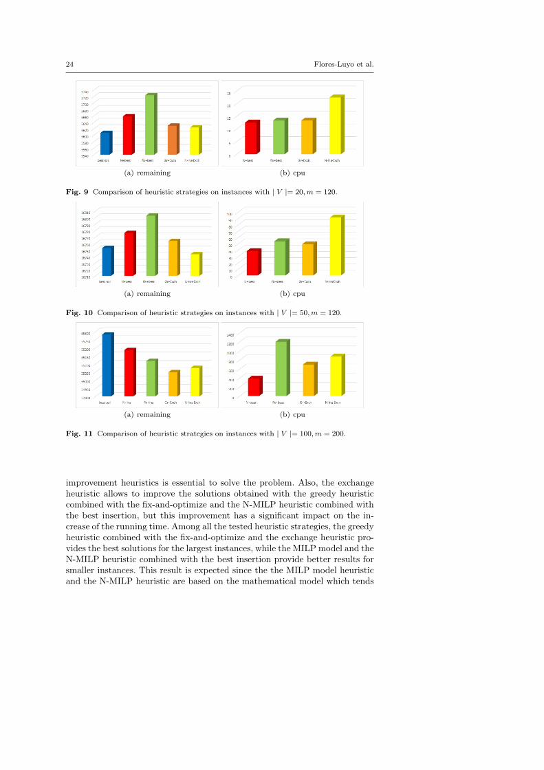
We can observe that, for the easiest instances, with | V |= 20, the MILPmodel provides the best solutions although all the heuristic approaches arequite fast. However, when | V | increases, the quality of the MILP solution de-creases and the heuristic strategies become more competitive. For | V |= 100,all the heuristic strategies provide better solutions than the MILP modelwithin a time limit of one hour. This contrasts with the case where only con-structive heuristics are considered, showing that combining constructive with



Fig. 9 Comparison of heuristic strategies on instances with | V |= 20,m = 120.





improvement heuristics is essential to solve the problem. Also, the exchangeheuristic allows to improve the solutions obtained with the greedy heuristiccombined with the fix-and-optimize and the N-MILP heuristic combined withthe best insertion, but this improvement has a significant impact on the in-crease of the running time. Among all the tested heuristic strategies, the greedyheuristic combined with the fix-and-optimize and the exchange heuristic pro-vides the best solutions for the largest instances, while the MILP model and theN-MILP heuristic combined with the best insertion provide better results forsmaller instances. This result is expected since the the MILP model heuristicand the N-MILP heuristic are based on the mathematical model which tends


h

h

h

h

0 1 ∗ l 2 ∗ l 3 ∗ l 4 ∗ l0

1 ∗ l2 ∗ l

3 ∗ l4 ∗ l

5 ∗ l6 ∗ l

h

h

h

h

0 1 ∗ l 2 ∗ l 3 ∗ l 4 ∗ l0

1 ∗ l2 ∗ l

3 ∗ l4 ∗ l

5 ∗ l6 ∗ l

Fig. 12 A grid topology inspired from [4] with 35 underwater stations and a unique surfacestation located either (rigth) in a extreme grid node or (left) in the central grid node.

to provide good quality solutions for the easiest instances and perform poorlyon hard instances.

5.2 Realistic instances

As we have mentioned in the introduction, Basagni et al. in [4] described aVRP appearing in underwater wireless sensor networks for submarine surveil-lance. This problem is related to the WTVRP considered in this work withthree major differences. First, the authors in [4] assume that stations must bephysically visited for information transmission. Second, multiple stations onthe surface connect the network with the outside. Third, the objective functionis the maximization of the value of the information transmitted. Although thetwo problems are not the same, the solution of the WTVRP can contribute inthe context described in [4] whenever equipments allow wireless transmission.The grid topology and technological assumptions described in [4] are used hereto generate a set of realistic instances for the WTVRP.

The largest topology described in [4] is depicted in Figure 12. We consider5 × 7 = 35 nodes uniformly deployed on a rectangle of 4l × 6l meters takingl = 500 (gray nodes in Figure 12). The Cartesian coordinates (x, y) of eachstation are done by the position of each gray node in the grid while the zcoordinates are randomly generated from 100 to 300 meters. The vehicle speedis set as 1.8 meters per second. Assuming a video encoded using the standardH.264 codec, each five minutes recording produces 9MB of information to betransfered. The transfer speed is assumed to be equal to 10Mbps which impliesαii = 375 for each station i. Acoustic channel data rate is set to 10Kbps whichimplies αij = 0.375 for each pair of stations i 6= j. We assume a time period of12 hours with the time unit defined as 5 minutes, which implies m = 144. Sincethe transfer equipments have a maximum speed of 100Mbps, i.e. 3750MB every10 minutes, we define R = 3750. Also, we assume M = 5, i.e., the existenceof 5 channels for simultaneous transmissions. Finally, we define the maximumrange for a wireless transfer rcov = 800 meters.


Table 6 Computational results with the N-MILP heuristic combined with the best insertionand the MILP model on the set of realistic instances.

MILP (N = 20) MILP (N = 25) Greedy N-MIP+best insertionInstances d z DGap z DGap z Length Cpu z Length Cpu

A.1 0,81 32343 33,10 32496 99,99 30221 31 0,40 27339 26 886,85A.2 33960 100,24 39363 100,20 31206 29 0,13 26325 27 1015,76A.3 31198 30,95 32571 100,25 29295 32 0,10 26160 28 1188,49A.4 32835 34,83 31342 100,25 29878 31 0,13 25803 28 1058,74A.5 32957 34,33 35772 100,23 29386 32 0,16 25995 28 1012,29B.1 0,81 32632 33,54 31846 99,91 30327 31 0,16 27064 27 782,43B.2 33778 100,08 31332 100,00 30082 31 0,11 27318 26 797,08B.3 33209 34,93 31883 100,23 30430 31 0,10 26813 27 973,58B.4 34034 36,49 36689 100,22 29045 32 0,15 26165 28 1409,04B.5 32111 32,69 32792 100,25 29325 32 0,10 25284 29 1420,10A.1 0,49 30591 99,99 30110 100,00 30638 30 3,59 17552 35 3560,00A.2 31354 97,23 28140 100,00 31198 30 0,13 17585 35 3105,80A.3 31363 100,22 28304 100,00 31818 30 0,12 17437 35 2751,83A.4 31524 100,00 28163 100,05 30083 32 0,12 17536 35 2709,26A.5 30011 100,14 28045 100,16 30320 31 0,12 17510 35 3117,12B.1 0,49 30390 28,62 29044 99,99 30197 31 0,12 17402 35 2770,80B.2 30436 28,89 27229 100,11 31325 30 0,11 18349 34 2461,94B.3 29272 57,84 30223 100,00 31075 30 0,11 18088 34 2420,64B.4 30202 28,64 28601 96,91 31530 28 0,11 18899 33 2561,15B.5 30695 93,92 27727 94,47 30816 30 0,11 17661 35 3018,83

*** time limit: 3600 sec.

Using these assumptions, five different complete graphs were generatedwith 35 underwater nodes. In order to simulate the existence of physical un-derwater obstacles, a random set of edges was deleted from each completegraph generating two sets of graphs: one set with densities equal to 0.81 andanother with densities equal to 0.49.

For each different graph obtained, we consider two scenarios for the positionof the unique base station located at the surface (black points in Figure 12)connected to each underwater station. The Cartesian coordinates (x, y) of thesurface station is defined as (0, 0) (right grid in Figure 12; instances A.i inTable 6) or (2l, 3l) (left grid in Figure 12; instances B.i in Table 6). Thatimplies a total of 20 realistic instances.

From the conclusions presented in the previous section, the N-MILP heuris-tic combined with the best insertion is the most appropriate strategy to solvethe set of realistic instances. In order to obtain an estimative for the value of Nto be used in the MILP model, we also run the greedy heuristic on this set ofinstances. Since, the value obtained for N was prohibitive for the execution ofthe MILP model, we run the MILP model with N = {20, 25}. Table 6 presentsthe results obtained by the heuristic strategies as well as by the event MILPmodel. Notations on this table are the same used in the previous ones. Addi-tionally, column “d” informs the density of the graphs while column “Length”the number of events (vehicle visits) in the heuristic solutions obtained.

From Table 6, we conclude there is no significant difference between in-stances in set A and B which is explained by the fact that the vehicle visitsthe surface station only at the beginning and at end of its route. The only dif-


ference was for the MILP model with N ≥ 20, for which a better performancewas obtained by this method. We can also observe that a value N ≥ 25 seemsnecessary but it is prohibitive for the MILP model on the realistic instances.For realistic instances with density d = 0.81, the quality of the solutions ob-tained by the Greedy heuristic were better than the ones obtained by theMILP model (N ∈ {20, 25}). Finally, as we expected, the heuristic strategyN-MILP followed by best insertion achieved lower cost solutions for all the re-alistic instances. Interestingly, compared with the greedy heuristic, the bettersolutions obtained by “N-MILP+best insertion“ considered longer paths whend = 0.49 but shorter when d = 0.81.

6 Conclusions

In this work, we considered a wireless transfer vehicle routing problem. Sincemost of the practical instances cannot be solved to optimality within a reason-able amount of computational time (see [9, 10]), we proposed several heuris-tic approaches that combine both constructive and improvement heuristics.In order to derive initial feasible solutions, three constructive heuristics wereproposed. Two of them use the MILP model and the other is a greedy heuris-tic. Three improvement heuristics were also proposed. These heuristics werederived to improve the initial solutions and take into account the particu-larities of the constructive algorithm used to obtain the initial solution. Afix-and-optimize heuristic fixes the routing decisions of the initial solutionand solves the resulting restricted MILP model. This heuristic was used toimprove the initial solution obtained with the greedy algorithm since this al-gorithm does not take into account the MILP model. As the size of the MILPmodel depends on the maximum possible number of visits, N , the constructiveheuristics based on the MILP model were fast for small values of N . Thus animprovement heuristic that starts from an initial route with a small number ofvehicle visits and iteratively tests the inclusion of another visit was proposed.Finally, an exchange heuristic that exchanges a consecutive set of nodes by newones was also presented. This heuristic was combined with all the constructiveheuristics introduced in the present work.

Computational tests showed that for the easiest instances, with a smallnumber of nodes and time periods, good quality solutions can, in general, beobtained by solving the MILP model using a solver with a running time limitof one hour. However, when the instances are larger, this approach tends tobe poor and to be outperformed by the heuristic strategies that combine theconstructive heuristics with the improvement heuristics. In particular, for thelargest instances with |V | = 100 nodes and m = 200 periods, the greedy heuris-tic combined with a fix-and-optimize and an exchange heuristics provided thebest solutions with average running times close to 10 minutes. Moreover, fora set of realistic instances occurring in submarine surveillance, a combinedheuristic strategy based on a restricted MILP model followed by a best inser-tion procedure provided the best computational results.


Acknowledgements

This research was supported by the Fundacao para a Ciencia e a Tecnologia(FCT), through the research program PESSOA 2018 - project FCT/5141/13/4/2018/Sand through project UID/MAT/04106/2019 (A. Agra). It was also supportedby Campus France through the research program PESSOA 2018 - project N40821YH (R. Figueiredo) and by the Fondo Nacional de Desarrollo Cientıfico,Tecnologico y de Innovacion Tecnologica (FONDECYT), with a PhD grant(L. Flores-Luyo).

References

1. A. Agra, M. Christiansen, A. Delgado, and L. Simonetti. Hybrid heuristicsfor a short sea inventory routing problem. European Journal of OperationalResearch, 236(3):924–935, 2014.

2. C. Archetti and M. G. Speranza. A survey on matheuristics for routingproblems. EURO Journal on Computational Optimization, 2(4):223–246,2014.

3. M. O. Ball. Heuristics based on mathematical programming. Surveys inOperations Research and Management Science, 16(1):21 – 38, 2011.

4. S. Basagni, L. Boloni, P. Gjanci, C. Petrioli, C.A. Phillips, and D. Turgut.Maximizing the value of sensed information in underwater wireless sensornetworks via an autonomous underwater vehicle. In Proceedings of IEEEINFOCOM’14, pages 988–996, April-May 2014.

5. Sourav Kumar Bhoi, Pabitra Mohan Khilar, and Munesh Singh. A pathselection based routing protocol for urban vehicular ad hoc network (uvan)environment. Wireless Networks, 23(2):311–322, Feb 2017.

6. G.D. Celik and E. Modiano. Dynamic vehicle routing for data gatheringin wireless networks. In 49th IEEE Conference on Decision and Control(CDC), pages 2372–2377. IEEE, 2010.

7. K. Collins and G. M. Muntean. An adaptive vehicle route managementsolution enabled by wireless vehicular networks. In 2008 IEEE 68th Ve-hicular Technology Conference, pages 1–5, Sept 2008.

8. K. F. Doerner and V. Schmid. Survey: Matheuristics for Rich VehicleRouting Problems, volume 6373 of Lecture Notes in Computer Science,chapter Hybrid Metaheuristics, pages 206–221. Springer, Berlin, Heidel-berg, 2010.

9. L. Flores-Luyo, A. Agra, R. Figueiredo, E. Altman, and E. Ocana Anaya.Vehicle routing problem for information collection in wireless networks. InProceedings of the 8th International Conference on Operations Researchand Enterprise Systems, ICORES 2019, Prague, Czech Republic, February19-21, 2019., pages 157–168, 2019.

10. L. Flores-Luyo, A. Agra, R. Figueiredo, and E. Ocana. Mixed integerformulations for a routing problem with information collection in wire-


less networks. European Journal of Operational Research, 280(2):621–638,2020.

11. M. Di Francesco, S.K. Das, and G. Anastasi. Data collection in wirelesssensor networks with mobile elements: A survey. ACM Transactions onSensor Networks, 8(1):1–31, 2011.

12. S. R. Gandham, M. Dawande, R. Prakash, and S. Venkatesan. Energyefficient schemes for wireless sensor networks with multiple mobile basestations. In GLOBECOM ’03. IEEE Global Telecommunications Confer-ence, volume 1, pages 377–381, 2003.

13. J. A. Gomez-Pulido and J. M. Lanza-Gutierrez, editors. Journal of Heuris-tics, chapter Heuristics for Reliable and Efficient Wireless Sensor NetworksDeployments. 2015.

14. L. Gu and A.J. Stankovic. Radio-triggered wake-up for wireless sensornetworks. Real-Time Systems, 29(2-3):157–182, 2005.

15. V. Kavitha and E. Altman. Queuing in space: Design of message ferryroutes in static ad hoc networks. In 2009 21st International TeletrafficCongress, pages 1–8, 2009.

16. G. Laporte. Fifty years of vehicle routing. Transportation Science,43(4):408–416, 2009.

17. J. Luo and J.-P. Hubaux. Joint mobility and routing for lifetime elongationin wireless sensor networks. In Proceedings IEEE 24th Annual Joint Con-ference of the IEEE Computer and Communications Societies., volume 3,pages 1735–1746, 2005.

18. M. Malowidzki, T. Dalecki, P. Berezinski, M. Mazur, and P. Skarzynski.Adapting standard tactical applications for a military disruption-tolerantnetwork. In 2016 International Conference on Military Communicationsand Information Systems (ICMCIS), pages 1–5, May 2016.

19. K.R. Moghadam, G.H. Badawy, T.D. Todd, D. Zhao, and J.A.P. Dıaz.Opportunistic vehicular ferrying for energy efficient wireless mesh net-works. In 2011 IEEE Wireless Communications and Networking Confer-ence, pages 458–463. IEEE, 2011.

20. A. Pentland, R. Fletcher, and A. Hasson. Daknet: Rethinking connectivityin developing nations. Computer, 37(1):78–83, 2004.

21. J. Rao, T. Wu, and S. Biswas. Network-assisted sink navigation protocolsfor data harvesting in sensor networks. In 2008 IEEE Wireless Commu-nications and Networking Conference, pages 2887–2892, 2008.

22. S. R. Shishira, A. Kandasamy, and K. Chandrasekaran. Survey on metaheuristic optimization techniques in cloud computing. In 2016 Interna-tional Conference on Advances in Computing, Communications and In-formatics (ICACCI), pages 1434–1440, Sept 2016.

23. L. Teylo, U. de Paula Junior, Y. Frota, D. de Oliveira, and L. Drummond.A hybrid evolutionary algorithm for task scheduling and data assignmentof data-intensive scientific workflows on clouds. Future Generation Comp.Syst., 76:1–17, 2017.

24. P. Toth and D. Vigo. Vehicle Routing: Problems, Methods, and Applica-tions, Second Edition. Society for Industrial and Applied Mathematics,


Philadelphia, PA, USA, 2014.25. D. Tse and P. Viswanath. Fundamentals of Wireless Communication.

Cambridge University Press, New York, NY, USA, 2005.26. C. Velasquez-Villada, F. Solano, and Y. Donoso. Routing optimization

for delay tolerant networks in rural applications using a distributed algo-rithm. International Journal of Computers Communications & Control,10(1):100–111, 2014.

27. R.G. Vieira, A.M. da Cunha, and A.P. de Camargo. An energy manage-ment method of sensor nodes for environmental monitoring in amazonianbasin. Wireless Networks, 21(3):793–807, Apr 2015.

28. K. Wang, Y. Shao, and W. Zhou. Matheuristic for a two-echelon capac-itated vehicle routing problem with environmental considerations in citylogistics service. Transportation Research Part D: Transport and Environ-ment, 57:262 – 276, 2017.

29. Z.-H. Zhan, X.-F. Liu, Y.-J. Gong, J. Zhang, H. S.-H Chung, and Y. Li.Cloud computing resource scheduling and a survey of its evolutionaryapproaches. ACM Comput. Surv., 47(4):63:1–63:33, July 2015.

Heuristics for a vehicle routing problem with information ...

Documents

Transcript of Heuristics for a vehicle routing problem with information ...