CanterburyBusinessSchool Working Paper Series

Working Paper No. 42November 2003

Heuristic Algorithms forSingle and Multiple DepotVehicle Routing Problemswith Pickups andDeliveries

Gábor NagyCanterbury Business School

Saïd SalhiUniversity of Birmingham

1

HEURISTIC ALGORITHMS FOR SINGLE AND MULTIPLE DEPOT

VEHICLE ROUTING PROBLEMS WITH PICKUPS AND DELIVERIES

GÁBOR NAGY a *, SAÏD SALHI b

a Canterbury Business School, University of Kent b School of Mathematics and Statistics, The University of Birmingham

Abstract: The Vehicle Routing Problem with Pickups and Deliveries (VRPPD) is an

extension to the classical Vehicle Routing Problem (VRP), where customers may both

receive and send goods. We do not make the assumption common in the VRPPD literature,

that goods may only be picked up after all deliveries have been completed. We also eschew

the concept of insertion and propose a method that treats pickups and deliveries in an

integrated manner. This method finds a solution to the corresponding VRP problem and

modifies this solution to make it feasible for the VRPPD. Such modification is achieved

mainly by heuristic routines taken from VRP methodology but modified such that their aim

becomes the reduction of infeasibilities, although a number of problem–specific routines are

also constructed. To render our procedures efficient when checking feasibility, we built

appropriate mathematical relationships to describe changes in the maximum load of routes.

Furthermore, several enhancements are introduced. Our methodology is also capable of

solving multi–depot problems, which has not been done before for this challenging general

version of the VRPPD. The methods are tested for single and multiple depot problems with

encouraging results.

Keywords: Vehicle routing; Heuristics; Pickups and deliveries; Multiple depots.

* This paper is to appear in the European Journal of Operational Research.

2

1. INTRODUCTION

The Vehicle Routing Problem with Pickups and Deliveries (VRPPD) is an extension to the

vehicle routing problem (VRP) where the vehicles are not only required to deliver goods to

customers but also to pick some goods up at customer locations. It is normally assumed that goods

stored at some customer location cannot directly be transported to another customer. In other

words, all goods have to either originate from, or end up, at a depot. Thus, problems such as the

dial-a-ride problem are excluded from our consideration, although some authors do refer even to

these as pickup-and-delivery problems. It is also usually assumed that the number of vehicles is

not fixed in advance. The objective function of the VRPPD is to minimise the total distance

travelled by the vehicles, subject to maximum distance and maximum capacity constraints on the

vehicles. We also mention that the VRPPD is NP–hard, being a generalisation of the classical

VRP. It can be formulated as a mixed ILP (see Appendix for a possible formulation), and solved

by exact methods for small problems. Our focus, however, will exclusively be on heuristics.

Within the above assumptions, three important VRPPD models may be distinguished. In the

following, we briefly describe these models, and then present and explain our choice of model.

Delivery–first, pickup–second VRPPD. Most researchers make the assumption that

customers can be divided into linehauls (customers receiving goods) and backhauls (customers

sending goods); furthermore vehicles can only pick up goods after they have finished delivering all

their load. One reason for this is that it may be difficult to re-arrange delivery and pickup goods on

the vehicles. We note that such an assumption makes the implementation issue easier, since

accepting pickups before finishing all deliveries results in a fluctuating load. This may cause the

vehicle to be overloaded during its trip (even if the total delivery and the total pickup loads are not

above the vehicle capacity), resulting in an infeasible vehicle tour.

Mixed pickups and deliveries. A VRPPD where linehauls and backhauls can occur in any

sequence on a vehicle route is referred to as a mixed VRPPD. Delivery-first pickup-second and

mixed VRPPD problems are jointly referred to as the vehicle routing problem with backhauling

(VRPB).

Simultaneous pickups and deliveries. In this model, customers may simultaneously receive

and send goods. We note that mixed and simultaneous VRPPD problems can be modelled in the

same framework. Mixed problems can be thought of as simultaneous ones with either the pickup

3

or the delivery load being nil; while the customers of simultaneous problems can be divided into

pickup and delivery entities to give a mixed formulation. (In the simultaneous problem, there may

be a further restriction on serving the pickup and delivery of a customer at the same time.)

The aims of this study are to produce an efficient composite heuristic approach for both the

simultaneous and the mixed VRPPD and to extend the methodology to the multiple depot VRPPD

problem. We do not address the delivery-first pickup-second problem. This is because we believe

that this assumption is unnecessarily restrictive, and results in poor quality solutions.

Consider the following example. A depot d is located at coordinates (0,0) and customers a,

b and c are located at coordinates (1,0), (1,1) and (0,1) respectively. (See Figure 1.) Customer a

and c need 9 tons and 1 ton, customer b sends 2 tons. The capacity of the vehicle is 10 tons. The

optimal mixed VRPPD solution is dabcd, with a length of 4 units. The optimal delivery-first

pickup-second solutions are dacbd and dcabd, with a length of 4.828 units. Thus, this restriction

resulted in an increase of over 20%.

Figure 1. An example of the drawback of the delivery-first pickup-second assumption.

We agree that serving pickups and deliveries in a mixed order or simultaneously causes difficulties,

due to the rearrangements of goods on board. However, it is not an impossible task, especially if

the vehicle is nearly empty. Some vehicles also have a better design (e.g. both rear and side

loading), making rearrangement of goods a more practical option. From a managerial viewpoint, it

is useful to find the solutions to both problems, as this can help in evaluating the cost benefit

4

against the inconvenience caused by the need to rearrange. Such inconvenience could be looked at

and examined whether it is worthwhile pursuing.

It is not possible to directly compare our methods with delivery-first pickup-second

algorithms, as our solutions may violate the delivery-first pickup-second restriction. If such a

restriction must be imposed, then a different methodology is likely to be more suitable. The special

structure of the routes in this case makes them more suitable to be solved as matching problems,

since routes consist of two distinct parts (a delivery and a pickup segment). In any case, our aim is

not to find small increases in solution quality, but to develop a solution methodology that is capable

of solving a wider class of problems than previously solved in the literature.

In the next section, we present a review of the literature. The overall structure of the new

heuristic is given in section 3 and its details are presented in section 4. Some enhancements of this

method are introduced in section 5 and an adaptation to the case of multiple depots is presented in

section 6. We provide the computational results in section 7. Finally, we present our conclusions

and outline some suggestions for future work.

2. LITERATURE REVIEW

The literature on the VRPPD is very scant compared to that of the classical VRP. VRPPD

literature can be classified into three main categories:

(i) simultaneous pickups and deliveries,

(ii) mixed pickups and deliveries, and

(iii) problems where pickups are only allowed to occur after deliveries.

Summary descriptions of the various papers are presented in Table 1. The reader is also referred to

the paper of Savelsbergh and Sol (1995), which presents a review of papers on a wider class of

pickup-and-delivery problems and gives a different classification.

5

AUTHOR (YEAR) TYPE SOLUTION METHOD SIZE

Deif and Bodin (1984) D1P2 extension to savings method, penalty term to push backhauls to ends of routes

d = 1, r = # 100 = c = 300

Golden, Baker, Alfaro and Schaffer (1985)

mixed VRP for linehaul customers, then backhauls inserted using stop-based criterion

d = 1, r = 6 c = 50

Yano et al. (1987) D1P2 list processing heuristic, set covering heuristic using Lagrangian relaxation

d = 1, r = 11 c = 40

Casco, Golden and Wasil (1988)

mixed VRP for linehaul customers, then backhauls inserted using load-based criterion

d = 1, r = 6 c = 61

Goetschalckx and Jacobs-Blecha (1989)

D1P2 spacefilling curves for clustering and routing, then improvement procedures

d = 1, r = 2 25 = c = 200

Min (1989) simul- taneous

clustering, solving TSPs, then infeasible arcs penalised and TSPs re-solved

d = 1, r = 2 c = 22

Min, Current and Schilling (1992)

D1P2 separate clustering for pickups and deliveries, then assignment, finally TSPs

d = 3, r = # c = 161

Halse (1992) simul- taneous

assignment first, routing second, then improvement procedures

d =1, r = # 22 = c = 150

Jacobs-Blecha and Goetschalckx (1993)

D1P2 joint clustering for pickup and delivery customers, then solving assignment problem

d = 1, r = # 25 = c = 200

Mosheiov (1994) mixed solving TSPs, then re-inserting depot d = 1, r = 1 17 = c = 200

Anily and Mosheiov (1994)

mixed create a minimum spanning tree, then transform it into a TSP

d = 1, r = 1 10 = c = 100

Thangiah, Sun and Potvin (1994)

D1P2 insert both pickups and deliveries one by one, then use improvement procedures

d = 1, r = # 25 = c = 100

Anily (1996) D1P2 separate clustering and TSPs, then assignment, finally constructing routes

d = 1, r = # c = #

Toth and Vigo (1996) D1P2 separate clustering, then matching clusters, solving TSPs, improvement procedures

d = 1, r = # 21 = c = 150

Gendreau, Laporte and Hertz (1997)

D1P2 create a spanning tree, minimal over linehauls and backhauls, transform into TSP

d = 1, r = 1 c = #

Toth and Vigo (1997) D1P2 exact method (Lagrangian branch-and-bound procedure)

d = 1, r = # 21 = c = 100

Toth and Vigo (1999) D1P2 separate clustering, then matching clusters, solving TSPs, improvement procedures

d = 1, r = 12 21 = c = 150

Salhi and Nagy (1999) mixed VRP for linehaul customers, backhauls inserted in clusters or one by one

d = 5, r = # 50 = c = 249

Gendreau, Laporte and Vigo (1999)

simul- taneous

solve TSP, then find pickup and delivery order on TSP-tour

d =1, r = 1 6 = c = 261

Osman and Wassan (2002)

D1P2 initial solution based on saving-insertion or saving-assignment, plus reactive tabu search

d =1, r = 12 21 = c = 150

Table 1. A comparison of the different papers on the VRPPD.

d denotes the number of depots, r the number of routes (if unknown or varying, “#” is used), and c the number of customers. “D1P2” stands for “delivery-first, pickup-second”.

6

Simultaneous VRPPD. Min (1989) was the first to tackle this version, solving a practical

problem faced by a public library, with one depot, two vehicles and 22 customers. The customers

were first clustered into groups and then in each group the travelling salesman problems were

solved. The infeasible arcs were penalised (their lengths set to infinity), and the TSPs solved again.

Halse (1992) studied a number of VRP versions, including the VRPB and the VRPPD. He solves

the latter problems using a cluster-first routing-second approach. In the first stage the assignment

of customers to vehicles is performed, then a routing procedure based on 3-opt is used. Solutions

to problems with up to 100 customers for the VRPPD and 150 customers for the VRPB are

reported. The recent paper of Gendreau, Laporte and Vigo (1999) investigates the travelling

salesman problem with pickups and deliveries (TSPPD). First, the TSP is solved without regard to

pickups and deliveries. Then, the order of pickups and deliveries on the TSP-tour is determined.

Mixed VRPPD. There are also very few papers which deal with (ii). The approach

described in Golden, Baker, Alfaro and Schaffer (1985) is based on inserting backhaul (pickup)

customers into the routes formed by linehaul (delivery) customers. Their insertion formula uses a

penalty factor which takes into account the number of delivery customers left on the route after the

insertion point. Casco, Golden and Wasil (1988) develop a “load-based insertion procedure” where

the insertion cost for backhaul customers takes into account the load still to be delivered on the

delivery route (rather than the number of stops). This latter approach was found to be superior.

Mosheiov (1994) investigated the TSPPD. It has been shown that if the solution is infeasible

because some arcs are overloaded, feasibility can be achieved by re-inserting the depot into the arc

with the highest load. Anily and Mosheiov (1994) present a solution method for the TSPPD, by

creating a minimum spanning tree. While its worst-case bound and computational complexity are

better than that of Mosheiov (1994), its average performance is found to be slightly inferior to it.

The recent paper of Salhi and Nagy (1999) extends the insertion method of Casco, Golden and

Wasil (1988) by allowing backhauls to be inserted in clusters, not just one by one. This approach

yields some modest improvements and requires negligible additional computational effort. This

procedure is also capable of solving simultaneous problems.

Delivery-first, pickup-second VRPPD. There is a much larger body of literature on the

VRPB covering (iii). As we do not make this assumption in our study, we refer the reader to Table

1 for a brief summary of the main papers treating this version.

7

3. THE BASIC INTEGRATED HEURISTIC

3.1. Introduction and rationale

As we have seen in the previous section, many of the solution methods for mixed VRPPD

problems are based on the concept of insertion. While these methods work very well for a small

number of backhauls as soon as the number of backhauls starts to rise their computational

complexity increases rapidly. The same problem would arise if an insertion method was applied to

a simultaneous VRPPD. (See Nagy (1996), p.134.) Thus, we have decided to construct a method

which treats both linehaul and backhaul customers the same way, in an integrated heuristic. While

this method was primarily designed with the simultaneous VRPPD in mind, it works equally well

for the mixed case. However, our methodology is not designed for the case of the assumption of

deliveries before pickups, as this assumption is contrary to an integrated treatment of linehauls and

backhauls.

We begin by presenting our notation and introducing a number of concepts. Vehicle routes

are characterised by a sequence of customers or of arcs. Routes are denoted by the letters x, y, z

and customers by a, b, etc. The supply and the demand of a customer a is denoted by p(a) and

q(a) respectively. The maximum capacity of the vehicle is denoted by C while the total pickup

and the total demand of route x are denoted by P(x) and Q(x) respectively. Functions are

distinguished by italic phrases such as load, maxload, minload: their meanings will be explained

below.

Let us now define the load function for a vehicle route: this is simply the load the vehicle

carries along the arcs of a tour. The load on arc ab is denoted by load(ab). We note that if the

“pickups after deliveries” assumption applies then this function is monotonously decreasing until

some point and then becomes monotonously increasing. Thus, provided that the load function is

not above the maximum capacity C for both the first and the last arcs it is never above it and the

route is feasible. On the other hand, if our problem falls into the categories of mixed or

simultaneous pickups and deliveries then it is possible that the load function “peaks” somewhere in

the middle. In particular, it is possible that the load function is below the maximum capacity for

the first and the last arc but not for some arcs in between. We now define the maximum load of a

route x, maxload(x), as the largest total load on the vehicle during the route. We can similarly

define the maximum load of a section of a route, maxload(a,b), as the maximum of the loads

8

between customers a and b of route x. A variable for the least load on a vehicle route or route

section is also introduced and referred to as minload(x) and minload(a,b) respectively. If

maxload(x) = C and minload(x) = 0, the route is feasible. (In our solution algorithm, the second

condition will always be fulfilled automatically.)

We note that for a route with n customers all the above functions can be stored in an n by n

matrix. The load for each arc can be stored in the leading diagonal of the matrix, the minimum and

maximum loads for route sections in the upper and lower triangles respectively, finally maxload

and minload will be in the lower left and upper right corners. The load function is updated together

with the route, at no additional computational effort. To create or update the table requires an O(n)

effort. This will need to be done each time a route is changed. However, as we shall see later, the

maxload of a planned route change can be calculated in constant time, making our procedure

computationally inexpensive.

Mosheiov (1994) proved that any travelling salesman tour can be made feasible, provided

that neither P(x) nor Q(x) exceeds the vehicle capacity. In his model there was no restriction on

maximum tour length. This theorem is useful since an infeasible vehicle tour for which the above

conditions hold can be made feasible by performing certain operations on it. In addition, if either

the total delivery load or the total pickup load exceeds the vehicle capacity for any route then that

route cannot be made feasible by modifying the order of customers on it. Thus, the conditions laid

down in Mosheiov (1994) are necessary and in most cases (i.e. if the distance constraint is not too

tight) sufficient to make a route feasible. In this study, we used this theorem indirectly and we refer

to a route for which neither the total pickup nor the total delivery load exceeds the vehicle capacity

and its length is below the maximum distance as a weakly feasible route. If the length of a tour

does not exceed the maximum distance and for each of its arcs the load function is below the

capacity constraint we call the tour strongly feasible.

In the following we aim to explain how certain transformations of routes change their

feasibility, where feasibility is measured in terms of the function maxload, thus providing the

foundation for the modification of the VRP algorithm into a VRPPD method and also for the

operations to eliminate infeasibilities.

9

3.2. How route changes influence feasibility

The improvement procedures used in the literature (such as the ones of Salhi and Rand,

1993) change the structure of the routes, often by inserting or removing customers, and sometimes

resulting in a reversal of the direction of parts of a vehicle route.

While in the VRP route direction is irrelevant, for the VRPPD it is an essential part of the

route design. If we have too many customers with large pickups and small deliveries at the

beginning of the route it may easily become infeasible. Reversing such a route may make it

feasible as we would serve the large deliveries first and the large pickups later on. It is very easy to

check the feasibility of the reversed route, as the following relationship holds:

maxload(x') = Q(x) + P(x) – minload(x) (1)

where x' refers to the reverse of route x. The above relation can easily be verified algebraically,

see Nagy (1996), p.143. We compare maxload(x') with C to check feasibility.

It is also possible that only a part of the route is reversed, for example when executing a

2-opt operation (Lin, 1965). Let the old route be 0…ab…cd…0 and the new one 0…ac…bd…0,

with 0 denoting the depot. (Note that the 2-opt procedure applied to customers a, b, c and d results

in the reversal of the route section between b and c.) The maximum load of the affected section can

be related to its former minimum load, as follows:

maxload(c,b) = load(ab) + load(cd) – minload(b,c) (2)

(see Nagy (1996), p.144.). This is sufficient to check the feasibility of the new route.

Another operation which occurs frequently is the removal of a customer (or less usually of a

depot) from a vehicle route, and its insertion to somewhere else on the same route, or into a

different route. The deletion of a customer a improves route feasibility, since the load on the arcs

before a will decrease by q(a), and on the arcs after a by p(a). It is possible that by re-assigning a

customer from an infeasible route to a strongly feasible one the former becomes strongly feasible

while the latter maintains its strong feasibility. Checking the feasibility changes of insertion-based

procedures can also be done computationally inexpensively, using the function maxload, see Nagy

(1996), p.146.

10

3.3. The structure of the basic integrated heuristic

Since weak feasibility of a VRPPD route is very similar to the feasibility of a VRP route we

surmise that a weakly feasible solution can be constructed using standard VRP techniques. This

can then be turned into a strongly feasible one, using route modification routines. As we have

noted in the previous subsection, checking of these changes in feasibility can be carried out with

little computational effort.

The underlying routing method used is that of Salhi and Sari (1997). This algorithm relies

on a route construction heuristic to provide an initial solution and then uses a variety of routines to

improve on the routes. Thus, we separate the method which creates the initial solution and the set

of improvement routines also here. We also notice that improvement routines can be modified to

improve on the feasibility of the routes. Finally, once strong feasibility is reached we can still

improve on the routes as long as we maintain strong feasibility.

Our integrated heuristic, referred to as IH for short, consists of the following four phases:

Phase 1. Find a weakly feasible initial solution

Phase 2. Improve on this solution while maintaining weak feasibility

Phase 3. Make the solution strongly feasible

Phase 4. Improve on this solution while maintaining strong feasibility

These phases are explained in the next section.

4. EXPLANATION OF THE MAIN PHASES

4.1. The route construction heuristic (phase 1)

This algorithm is based on the concept of multiple giant tours as extended by Salhi, Sari,

Saidi and Touati (1992). We shall look at both the original vehicle routing algorithm and how it

was modified to cater for the case of pickups and deliveries.

In the VRP version, a giant tour, including the depot, is first created. This is a tour that

starts from the depot, passes through all customer sites and returns to the depot. Second, a directed

11

cost network is constructed. This is a directed graph with customers as its nodes and edges defined

as follows. Let us define the tour Tab as a tour beginning with an arc from the depot to customer a,

then following the giant tour between customers a and b, then finishing with an arc from customer

b to the depot. Then, there is a directed edge in the cost network from a to b if and only if the tour

Tab is feasible in terms of vehicle capacity and distance restriction. The length of the edge ab in

the cost network is the length of Tab. Third, the shortest path problem is solved using Dijkstra’s

(1959) algorithm, giving us a partitioning of the giant tour. This procedure is repeated starting

from different giant tours and the overall least cost solution is chosen. In our experiments we

constructed 5 giant tours; one using the nearest neighbour, the other the least insertion cost rule and

the remaining three tours are generated randomly. A detailed description on how to generate these

giant tours and how to construct the associated cost networks can be found in Salhi et al. (1992).

It is the above partitioning of the giant tour, in particular the creation of the cost network,

which needs to be modified for the case of pickups and deliveries, since feasibility must be checked

in terms of a fluctuating load function. For the VRP, route feasibility is checked by comparing the

total demand of the route Q(x) against the maximum capacity C. For the VRPPD, we have to

introduce the total supply P(x) into this routine and accept a route as weakly feasible if the

inequality

max(Q(x),P(x)) = C (3)

is satisfied. We note that this extension to the original algorithm does not increase its

computational complexity. Other parts of this method need also be modified accordingly: these

changes are minor and do not increase the computational complexity either. The overall

complexity of this phase is O(n2), where n is the total number of customers (Salhi et al., 1992).

While the changes are sufficient for achieving weak feasibility they do not guarantee strong

feasibility. We will present a version of the method which can produce strongly feasible initial

solutions in subsection (5.1.). Finally, we note that, at the end of this phase, the routes are given

the direction which yields a smaller amount of infeasibility.

4.2. Explanations of the improvement/feasibility routines

We have taken the improvement routines for VRP from Salhi and Rand (1993) and

transformed them for the case of the VRPPD. A number of new routines were also added where

12

necessary. Most of them can be used both to improve optimality (reduce total distance) and to

decrease the amount of infeasibility (defined as maxload–C for each route): the next subsection will

show the different ways these algorithms are put to use. Some of these routines are explained in

more detail than others, depending on their importance. We refer the reader to Salhi and Rand

(1993) for more detailed explanation of the VRP versions of some of the routines, including

graphical illustrations. The subsection is rounded off by a brief discussion on the computational

complexity of the routines.

Routine REVERSE. This is a new routine, which is based on the observation that reversing

the direction of a route may improve its feasibility, without increasing its length. The procedure

simply chooses the route direction with the smaller maxload.

Routine 2-OPT. This method, first described by Lin (1965), is based on interchanging arcs,

say ab and cd with ac and bd. The direction of the route will be reversed between customers b and

c. We surmise that infeasibilities in VRPPD occur due to the fact that the customers are ‘in the

wrong order’ on the vehicle route. Thus, it is reasonable to re-arrange the ordering of the

customers on the route by reversing the direction of those parts of the vehicle route, where

infeasibilities occur. We note that applying this transformation twice returns the route to its

original state, thus 2-OPT can be thought of as its own dual. It may be used either to decrease route

length or to reduce the occurrence of infeasibilities. This observation is true for most of the

subsequent routines.

Routine 3-OPT. This is a slight modification of the original routine of Lin (1965), which is

based on the exchange of any three arcs with three other arcs. The modified method considers

only three consecutive arcs and hence is much faster.

Routine SHIFT. This routine involves two routes, but is otherwise very similar to our

version of 3-OPT. It involves the deletion of a customer from a route and its insertion into an arc

on another route.

Routine EXCHANGE. This routine is an extension to SHIFT in that two customers are

inserted simultaneously into each others’ former routes, but not necessarily into the former

locations of each other.

13

Routine PERTURB. This is another modification to SHIFT in that it considers three routes

at a time. A customer a is removed from a route x and inserted into a route y, at the same time a

customer b is removed from route y and inserted into a third route z. We note that this operation is

different to applying SHIFT twice as after the first SHIFT operation we may be in an infeasible (i.e.

not even weakly feasible) situation. Also, the complexity of this procedure is larger as there are

more possibilities to consider within the same move.

Routine REINSERT. This method originates from a theorem by Mosheiov (1994). The

author proved that a weakly feasible travelling salesman tour with pickups and deliveries can

always be made strongly feasible by re-inserting the depot. Thus routine REINSERT considers all

arcs on a tour for possible depot re-insertion, see Figure 2. Mosheiov (1994) showed just how

useful this routine can be in eliminating infeasibilities; however we note that it is also possible that

re-inserting the depot would decrease the route length.

Figure 2. An illustration of the routine REINSERT

Routines NECK and UNNECK. This is a new set of routines devised specially for the

VRPPD. In fact, they are only applicable for the simultaneous pickup and delivery problem and

only if customers are allowed to be visited twice. It is possible that we have some customers near

the depot which have large demand or supply levels. While REVERSE tries to ensure that

customers with large supplies are put to the end, and those with large demands at the beginning of

14

the vehicle route, we may still have some customers of the above type causing infeasibilities,

especially if both their demand and supply is high. However, we may serve these customers twice:

first for delivery and then for pickup. Thus, NECK splits a customer a into two entities: a pickup

customer ap and a delivery customer ad. The delivery entity is left where it currently is and the

pickup is considered for insertion into all the arcs of the route following the delivery, or vice versa,

see Figure 3. We observe that maxload(adap) is reduced by either p(a) or q(a). We also note that

unlike the previous routines NECK is not its own dual, thus we also introduce a routine called

UNNECK, which is the dual of NECK and tries to join separate entities a and a together if it is

feasible. Thus, NECK is a feasibility routine while UNNECK is an improvement routine.

Figure 3. An illustration of the routines NECK and UNNECK

Routines IDLE and CREATE. Routine IDLE is simply a service routine designed to remove

any routes which contain no customers and represent no physical movement of vehicles. It is

included in the cluster of improvement routines given in Salhi and Rand (1993). We constructed a

dual to IDLE called CREATE which creates an empty route. This, in itself, affects neither

optimality nor feasibility but can be useful as some later routine may move a customer into this

‘dummy’ route and thus make another route feasible.

Routines COMBINE and SPLIT. Routine COMBINE tries to combine two routes if it is

feasible to do so. We note that there are many ways of joining the two routes, especially if route

direction is important (it was not in the original VRP version but it is for the VRPPD). We observe

that the maxload of a combined route is simply the sum of the maxload values of the two original

15

routes. We created a dual to COMBINE called SPLIT which can improve on feasibility. It takes a

route and finds the best arc (say ab) where it may be split, see Figure 4.

Figure 4. An illustration of the routines COMBINE and SPLIT

Computational complexity. The computational complexity of the above routines is as

follows. REVERSE: O(n), 2-OPT: O(n2), 3-OPT(modified): O(n2), SHIFT: O(n2), EXCHANGE:

O(n4), PERTURB: O(n3), REINSERT: O(n), NECK/UNNECK: O(n2), IDLE/CREATE: O(n),

COMBINE/SPLIT: O(n), where n is the total number of customers. (See Nagy (1996), p.157. and

Salhi and Rand (1993).)

4.3. The composite improvement/feasibility phases (phases 2, 3 and 4)

The route improvement/feasibility routines presented in the previous subsection can be used

in three different contexts. They can either be used to improve optimality while maintaining weak

or strong feasibility or to improve feasibility. The structures of the three phases are described

below. The subsection is rounded off by a brief discussion on computational complexity.

Description of phase 2. This is used to improve on solution quality, while maintaining

weak feasibility. The modules are called in the following sequence:

16

1. 2-OPT, 3-OPT, REINSERT, REVERSE

2. COMBINE, 2-OPT, 3-OPT, REINSERT, REVERSE

3. EXCHANGE, IDLE, REVERSE, 2-OPT, 3-OPT, REINSERT, REVERSE

4. SHIFT, IDLE, REVERSE, 2-OPT, 3-OPT, REINSERT, REVERSE

5. PERTURB, IDLE, REVERSE, 2-OPT, 3-OPT, REINSERT, REVERSE

6. EXCHANGE, IDLE, REVERSE, 2-OPT, 3-OPT, REINSERT, REVERSE

7. COMBINE, IDLE, REVERSE, 2-OPT, 3-OPT, REINSERT, REVERSE

The ordering of the modules reflects their computational effort. Fast modules (2-OPT, 3-OPT,

REINSERT and IDLE) are called more often, alternating with the slower ones. These slower

modules are called first in an increasing, then in a decreasing order of complexity. We would like

to note that this ordering is somewhat arbitrary and any suitable schedule can be worthwhile

exploring. While REVERSE is not an improvement routine, it does not affect route length and

reduces the amount of infeasibility already at this stage.

Description of phase 3. The aim of this phase is to reduce the amount of infeasibility. The

input to this procedure is a weakly feasible solution while its output is a strongly feasible one. The

sequence of modules is given below.

1. 2-OPT, 3-OPT, REINSERT, REVERSE, NECK, REVERSE,

2. EXCHANGE, REVERSE, 2-OPT, 3-OPT, REINSERT, REVERSE, SHIFT, REVERSE

3. 2-OPT, 3-OPT, REINSERT, REVERSE, PERTURB, REVERSE

4. 2-OPT, 3-OPT, REINSERT, REVERSE, NECK, REVERSE

5. SPLIT, REVERSE, CREATE, REVERSE

As SPLIT and CREATE both generate additional routes we use them at the end of the composite

heuristic to eliminate any remaining infeasibilities. If they need to execute a move as the previous

stages failed to make the solution strongly feasible, then the procedure is repeated once more to

allow for re-arrangement of routes. We note that if the problem is mixed, or customers can only be

visited once, then module NECK is not applicable. In these cases, NECK and REVERSE are

deleted from the end of steps 1 and 4 above.

Description of phase 4. Phase 3 may necessitate an increase in routing cost and that is why

we employ another improvement phase. Phase 4 aims to improve on solution quality, while

17

maintaining strong feasibility. Its structure is almost identical to that of phase 2, except that a call

to UNNECK and REVERSE is added to the beginning of steps 2 and 7, if the module NECK was

used in phase 3. However, it is slower than phase 2, as checking strong feasibility is more

time-consuming than checking only weak feasibility.

Computational complexity. The above routines need to update the values of maxload and

minload. The updating process has complexity O(n2), see Nagy (1996), p.157. Thus, the overall

complexity of phases 2, 3 and 4 - and hence of the whole algorithm - is O(n4).

5. ENHANCEMENTS TO THE INTEGRATED HEURISTIC

In this section we present two modifications to the basic integrated heuristic. The first one

attempts to improve the feasibility of the solution provided by the route construction heuristic

(phase 1 of IH). The second one uses feasibility and improvement routines in turn, reducing the

amount of infeasibility in each iteration.

5.1. A version using a penalty factor

The route construction heuristic presented in subsection (4.1.) produces a weakly feasible

initial solution. It is possible to modify this method to produce a strongly feasible initial solution.

However, in practice this often yields a poor solution quality which even the improvement

procedures may not correct sufficiently. Because of this, a penalty factor is introduced into the

method to reduce the amount of infeasibility in the initial solution.

In the route construction heuristic, a tour is feasible in the cost network, if (2) holds. To

achieve strong rather then mere weak feasibility maxload(x) must be less than or equal to C. (With

a slight variation to account for the possible reversal of the route.) As we may not wish to achieve

strong feasibility, we introduce a penalty factor ? and use the criterion below.

? · maxload(x) + (1-?) · max(P(x),Q(x)) = C (0=?=l) (4)

The larger the value of ? becomes, the more the initial solution is pushed towards strong feasibility.

18

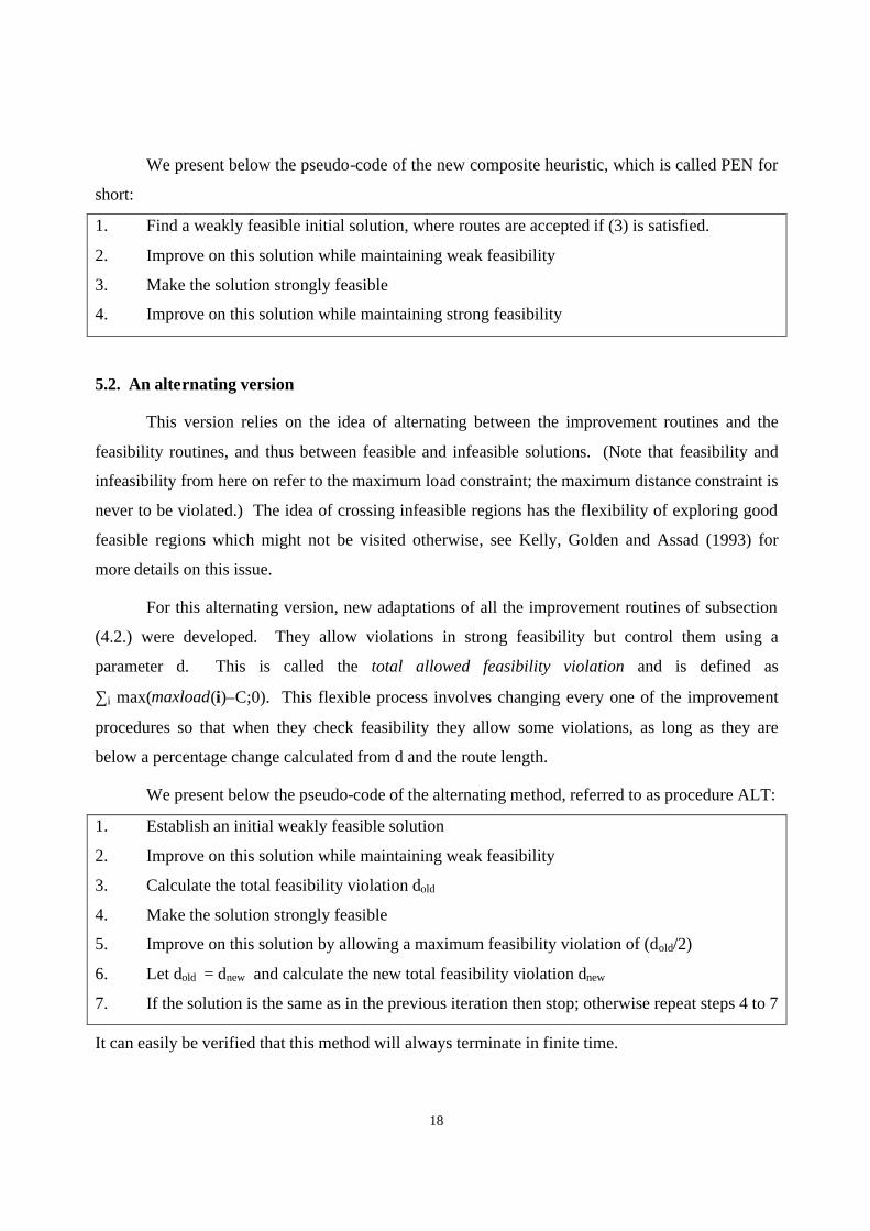
We present below the pseudo-code of the new composite heuristic, which is called PEN for

short:

1. Find a weakly feasible initial solution, where routes are accepted if (3) is satisfied.

2. Improve on this solution while maintaining weak feasibility

3. Make the solution strongly feasible

4. Improve on this solution while maintaining strong feasibility

5.2. An alternating version

This version relies on the idea of alternating between the improvement routines and the

feasibility routines, and thus between feasible and infeasible solutions. (Note that feasibility and

infeasibility from here on refer to the maximum load constraint; the maximum distance constraint is

never to be violated.) The idea of crossing infeasible regions has the flexibility of exploring good

feasible regions which might not be visited otherwise, see Kelly, Golden and Assad (1993) for

more details on this issue.

For this alternating version, new adaptations of all the improvement routines of subsection

(4.2.) were developed. They allow violations in strong feasibility but control them using a

parameter d. This is called the total allowed feasibility violation and is defined as

∑i max(maxload(i)–C;0). This flexible process involves changing every one of the improvement

procedures so that when they check feasibility they allow some violations, as long as they are

below a percentage change calculated from d and the route length.

We present below the pseudo-code of the alternating method, referred to as procedure ALT:

1. Establish an initial weakly feasible solution

2. Improve on this solution while maintaining weak feasibility

3. Calculate the total feasibility violation dold

4. Make the solution strongly feasible

5. Improve on this solution by allowing a maximum feasibility violation of (dold/2)

6. Let dold = dnew and calculate the new total feasibility violation dnew

7. If the solution is the same as in the previous iteration then stop; otherwise repeat steps 4 to 7

It can easily be verified that this method will always terminate in finite time.

19

A version similar to the above, which uses strategic oscillation, was also developed. It uses

an oscillation schedule as proposed by Kelly, Golden and Assad (1993). It extends the approach of

ALT by merging the improvement and feasibility routines into composite routines which attempt to

minimise a weighted combination of route length and amount of infeasibility. We do not provide a

description of this version, as the results obtained were not found to be sufficiently different from

those of ALT. We refer the reader to Nagy (1996), pp.161–163. for details.

6. ADAPTATION TO THE MULTI-DEPOT PROBLEM

In this section we present appropriate modifications to our proposed heuristics to address

the problem of multiple depots. To our knowledge, the only paper which attempts to treat the

simultaneous and the mixed pickup-and-delivery problems for the case of multiple depots is that of

Salhi and Nagy (1999). The multi-depot extension is based on the idea of borderline customers as

used by Salhi and Sari (1997) for the multi-depot vehicle fleet mix problem. Roughly speaking,

borderline customers are those customers situated approximately half-way between two depots.

More precisely, customer a is considered a borderline customer if dap/daq = ?, where ? is a

parameter between 0.5 and 1.0 (set to 0.9 in our heuristics) and p and q are the nearest and the

second-nearest depots to customer a.

The initial solution for the multi-depot VRPPD is found using the following four steps:

1. Divide the customer set into borderline and non-borderline customers

2. Assign the non-borderline customers to their nearest depot

3. For each depot, find a weakly feasible solution to the resulting single-depot VRPPD

4. Insert the borderline customers into the vehicle routes one at a time

As this procedure for the VRPPD is very similar to the original VRP version, the details are not

given here but the reader is referred to Salhi and Sari (1997) for a description. We note that step 3

is equivalent to the route construction heuristic described in subsection (4.1.). Furthermore, when

checking feasibility for insertion in step 4, both the total demand and the total supply must be

compared against the maximum capacity (this was not required in the original VRP version).

20

The improvement/feasibility routines of subsection (4.2.) are easily extended for the case of

multiple depots. Those routines which involve one route only are unchanged, although we note

that CREATE constructs one new (empty) route for every depot and REINSERT considers all the

depots for insertion into the vehicle route not just the one to which the route previously belonged.

More care is needed in the routines involving two or three routes (SHIFT, EXCHANGE,

PERTURB, COMBINE/SPLIT). For example, the new version of COMBINE tries to merge routes

which may not belong to the same depot. This necessitates determining which depot the combined

route should belong to.

Finally, we note that the modifications described in section 5 can also be extended with ease

for the case of multiple depots.

7. COMPUTATIONAL COMPARISON

The heuristics described in this study were written in VAX Fortran and executed on a VAX

4000-500 computer. They were evaluated using empirical testing, but we would also like to refer

the reader to the discussion on their computational complexities in subsection (4.3.).

7.1. Data generation

We used the problems given by Christofides, Mingozzi and Toth (1979) to generate our

single-depot data (50 to 199 customers) and the ones given by Gillett and Johnson (1976) for

multi-depot data (2 to 5 depots, 50 to 249 customers). There are 14 problems in the first case and

11 in the second.

For the case of mixed pickups and deliveries we have generated three VRPPD problems for

each VRP instance, declaring every second, fourth or tenth customer on the list a backhaul and

assigning to it a supply figure equal to the original demand figure, in other words for backhaul

customers let p(a) = t(a), and for others let q(a) = t(a), where t(a) is the original demand figure

given in the above papers. For each of the three sets, the average results are computed. This is

done for the single- and multi-depot problems.

21

For the case of simultaneous pickup-and-delivery, the same coordinate sets and demand

matrices were used again. For each customer a we calculated a ratio ra as min((xa/ya),(ya/xa)),

where xa and ya are the coordinates of customer a. Then, the new demand level of customer a is

q(a) = ra·t(a) and its supply level is p(a) = (1–ra)·t(a). This way the original demand is split up

between delivery and pickup loads. Another set of supply and demand levels was created by

exchanging the demand and supply figures of every other customer. Thus, we get two more

VRPPD problems for each VRP instance. Average results for this two sets are computed and

referred to as “A” and “B”.

Altogether, we have 70 single-depot problems, 42 of them mixed and 28 of them

simultaneous. Each set has 14 instances. There are 55 multi-depot problems, 33 of them mixed

and 22 of them simultaneous. Each set has 11 instances.

7.2. Benchmark methods

To compare our methods against those described in the literature, we chose three

procedures, namely the insertion-based algorithm (denoted by INS) of Casco, Golden and Wasil

(1988), the cluster insertion method (denoted by CI) of Salhi and Nagy (1999), and the

penalty-based algorithm (denoted by MIN) of Min (1989). These are the methods most

appropriate, see Table 1. We note that INS and MIN have originally been designed for

single-depot problems. For the multi-depot case we adapted these two procedures as follows. For

MIN, we find a weakly feasible solution using procedure MD (see Section 6). Then, the arcs are

penalised the same way as in the single-depot case. For INS, we follow procedure MD for linehaul

customers only. Note that in step 3 of MD the VRPPD is thus reduced to the VRP. Backhauls are

inserted the same way as in the single-depot case.

7.3. Analysis of results

The two comparison criteria we use are the quality of the solutions and computing speed.

In Tables 2 and 3, we summarise the results in terms of average routing cost and computational time

respectively. These are grouped by the percentage of backhauls for the categories of single-depot

22

and multi-depot data. Overall average values for these two categories are also given. We refer the

reader to Nagy (1996), pp.209-218, for detailed results.

In the penalty-based procedure, penalty values of 0.25, 0.5, 0.75 and 1.0 were tested and

very similar results were obtained. Thus we present only the case of 0.75 in Table 2.

INS CI MIN IH PEN ALT

10% mixed 25%

single-depot 50%

simultaneous AB X

single-depot average

percentage of best solutions

average number of vehicles

1015 1040 1061

1101 1105

1064

9

11.8

1011 1035 1047

1097 1093

1056

12

11.7

995 1019 1016

1064 1056

1030

41

11.1

995 998 995

996 994

995

71

10.7

997 998 994

997 992

995

77

10.7

995 998 991

991 989

992

97

10.6

10% mixed 25%

multi-depot 50%

simultaneous AB X

multi-depot average

percentage of best solutions

average number of vehicles

2008 2052 2136

2237 2173

2121

16

18.5

2008 2050 2099

2230 2160

2109

26

18.3

1999 2078 2007

2034 2149

2053

51

17.5

1996 2010 2004

2009 2004

2004

75

16.8

1996 2007 1999

1997 1997

1999

89

16.8

1996 2007 1993

1993 1993

1996

100

16.8

Table 2. Average solution quality (total routing cost)

The values 10, 25 and 50% refer to the percentage of backhauls used. A and B are the two sets of simultaneous pickup-and-delivery problems.

bold refers to the best average solutions.

We note that in some cases Min’s algorithm breaks down due to penalising too many arcs.

In several other cases, its speed is very slow as it has to re-solve VRPs a number of times. In our

experiments MIN failed to find feasible solutions for 7% of the test instances. Thus, the average

values for MIN are calculated as follows. For each set S of instances (corresponding to a row in

Table 2), we denote the subset of instances for which MIN found a feasible solution by E. Let

23

M(E) be the average solution found by MIN over E and let A(E) and A(S) be the average solutions

found by all the other methods over E and S, respectively. Let M(S) = M(E)*A(S)/A(E). In Table

2, we present M(S) as the average result found by MIN.

INS CI MIN IH PEN ALT

10% mixed 25%

single-depot 50%

simultaneous AB X

single-depot average

single-depot worst-case

2.5 2.8 3.1

3.9 3.9

3.2

12.3

2.8 3.1 3.6

4.9 4.8

3.8

17.2

7.3 8.9

19.0

14.9 13.2

12.6

79.8

2.6 2.6 2.6

2.5 2.5

2.5

9.1

2.7 2.6 2.6

2.5 2.5

2.5

9.1

3.1 3.6 3.9

3.9 3.3

3.5

18.1

10% mixed 25%

multi-depot 50%

simultaneous AB X

multi-depot average

multi-depot worst case

9.0 7.6

10.7

18.5 11.9

11.5

78.3

10.9 8.7

13.4

39.4 14.9

17.5

43.6

11.5 17.4 55.5

40.8 72.0

39.4

351

7.0 7.2 7.6

6.6 6.6

7.0

26.1

7.1 7.1 7.7

6.6 6.9

7.1

29.0

8.1 8.6

14.8

13.9 10.9

11.3

89.9

Table 3. Average solution speed

Rows and columns are as in Table 2. Entries are total computing times in seconds (averaged over the appropriate data sets).

“Worst-case” represents the largest computing time taken out of all the instances.

Within our versions, the alternating version ALT gives the best results. We note that the

small differences in the average costs produced by the different versions are not statistically

significant. However, ALT almost always finds the best solutions (for 97% of the single-depot and

100% of the multi-depot instances), while IH and PEN fail to do so for about a quarter of the

instances.

The results clearly show the superiority of the proposed heuristics over the insertion-based

methods of Casco, Golden and Wasil (1988) and Salhi and Nagy (1999). For single-depot

24

problems, the improvement in average solution quality of ALT over methods INS and CI is 7% and

6%, respectively. For multi-depot problems these figures are 6% and 5%. Our basic integrated

heuristic and its different versions also surpass the quality of Min’s (1989) results. The

improvement in average solution quality of ALT over MIN is 4% and 3% for single and multiple

depot problems, respectively.

The integrated methods require approximately one and two vehicles fewer than the

insertion-based procedures for the single- and multi-depot cases respectively, however this

difference can be as high as five vehicles for some larger instances.

Finally, we note that ALT is slower than other versions of the integrated heuristic, but its

running times are still comparable to the other methods and are usually below that of the procedure

MIN.

8. CONCLUSIONS AND SUGGESTIONS

In this paper we presented a number of heuristics for the vehicle routing problem with

pickups and deliveries (VRPPD). The proposed heuristics are capable of solving simultaneous

pickup and delivery problems (only Halse (1992) has done this for more than two routes). In

addition our methods can also solve problems with multiple depots (only Min, Current and

Schilling (1992) has explored this issue).

In this study, we introduced the concepts of weak and strong feasibility which were found to

be helpful in tackling the VRPPD. In our proposed heuristic we allowed infeasibilities to occur

while we guided the search towards strong feasibility (feasibility elimination is also used by Toth

and Vigo, 1996). A number of enhancements of this integrated heuristic were also developed. One

added advantage of these heuristics is that their computational complexity is comparable to, and

only slightly larger than, the complexity of the original VRP algorithm of Salhi and Rand (1993).

In summary, the proposed heuristics were able to provide good quality solutions to VRPPD

problems with one to five depots and 50 to 249 customers usually within a few seconds. Our

25

integrated heuristics generally give better results than the benchmark procedures of Min (1989),

Casco, Golden and Wasil (1988) and Salhi and Nagy (1999).

For future research the following issues may be worthwhile considering.

It may be possible to merge the ideas of Min (1989) and of Mosheiov (1994). One

approach could be to cluster the customers using the procedure given in Min (1989) and then solve

a number of TSPPDs using the method suggested in Mosheiov (1994). This composite procedure

can be complemented by multi-depot improvement routines. Another approach would be to adopt

some of the metaheuristics such as tabu search or genetic algorithms for the VRPPD. This issue is

currently being investigated.

In some circumstances the number of vehicles may be fixed in advance. To cater for this

case, a number of modifications would need to be done. In the partitioning of the giant tour

(phase 1), constrained shortest path problems need to be solved, which cannot be done using

Dijkstra’s (1959) method. There are two modules used in phases 2 to 4, which increase the number

of routes, namely SPLIT and CREATE. One way forward is to remove them from the algorithm,

another is to introduce a penalty function in combination with the module COMBINE.

Most of the literature, such as Goetschalckx and Jacobs-Blecha (1989), Jacobs-Blecha and

Goetschalckx (1993), Thangiah, Sun and Potvin (1996) and Toth and Vigo (1996, 1999), rely on

the assumption that pickups can only occur after all the deliveries on the route have been made.

We note that this assumption stems from the problem of load re-arrangement: if re-arrangement of

goods is always possible then our assumption is valid, if it is never possible, then the assumption

made in the above papers is valid. An interesting generalisation of both cases is when re-arranging

is only possible if k% of the vehicle is free, which is more likely to correspond to situations

occurring in practice. The two alternative assumptions correspond to the special cases of k = 0 and

k = 100. The generalised VRPPD may be tackled by using artificially lowered capacity constraints

or by addressing the combined packing-and-routing problem, which to our knowledge has not yet

received any attention. The authors consider this research avenue to be most promising.

26

APPENDIX. AN ILP FORMULATION FOR THE VRPPD

A.1. Notation L the set of depots, L = {1, 2, ... , t} H the set of customers, H = {1, 2, ... , n} K the set of vehicles, K = {1, 2, ... , m} dij the distance between customers i and j qi the demand of customer i pi the supply of customer i D the maximum distance which the vehicles may cover in a tour C the maximum capacity of the vehicles

1, if arc ij is part of route k xijk = { 0, otherwise

tijk the load on arc ij of vehicle route k A.2. Formulation Minimise ∑k∈K ∑i∈H∪L ∑j∈H∪L dij ⋅ xijk subject to ∑i∈H∪L ∑j∈H∪L dij ⋅ xijk ≤ D (k∈K) (A.1.)

tijk = C (i,j∈Η∪L, k∈K) (A.2.)

∑k∈K ∑i∈H∪L xijk = 1 (j∈H) (A.3.)

∑k∈K ∑i∈H∪L xijk ≥ 1 (j∈L) (A.4.)

∑k∈K ∑i∈S ∑j∈(H∪L)\S xijk ≥ 1 (2≤S) (A.5.)

∑i∈H∪L xijk = ∑i∈H∪L xjik (j∈H∪L, k∈K) (A.6.)

∑i∈H∪L ∑j∈H∪L xijk ≤ 1 (k∈K) (A.7.)

tijk ≤ xijk ⋅ ∑h(qh+ph) (i,j∈H∪L, k∈K) (A.8.)

∑k∈K ∑i∈H∪L tijk – qj = ∑k∈K ∑i∈H∪L tjik – rj (j∈H) (A.9.)

xijk = 0, 1 (i,j∈H∪L, k∈K) (A.10.)

tijk ≥ 0 (i,j∈H∪L, k∈K) (A.11.)

27

A.3. Discussion

In the above formulation, the objective function consists of the sum of variable routing costs for all vehicles. Constraints (A.1.) and (A.2.) are the maximum distance and maximum capacity constraints respectively. Constraints (A.3.) and (A.4.) stipulate that every customer belongs to one and only one route, but depots may belong to more than one route. Constraints (A.5.) ensure that every customer is on a route connected to the set of depots. Constraints (A.6.) stipulate that every customer is entered and left by the same vehicle. Constraints (A.7.) guarantee that a vehicle can depart only once from a customer. Constraints (A.8.) stipulate that flow is only present between customers and depots which are connected. Constraints (A.9.) are flow conservation equations. Finally, constraints (A.10.) and (A.11.) represent integrality and non-negativity conditions.

Other formulations can be found in Min (1989) and Nagy (1996), pp.51-57.

REFERENCES Sh. Anily (1996), “The Vehicle-Routing Problem with Delivery and Back-Haul Options,” Naval Research Logistics 43, 415-434. Sh. Anily and G. Mosheiov (1994), “The Traveling Salesman Problem with Delivery and Backhauls,” Operations Research Letters 16, 11-18. D. O. Casco, B. L. Golden and E. A. Wasil (1988), “Vehicle Routing with Backhauls: Models, Algorithms, and Case Studies,” in Vehicle Routing: Methods and Studies, pp. 127-147, B. L. Golden and A. A. Assad (eds.), Elsevier, Amsterdam. N. Christofides, A. Mingozzi and P. Toth (1979), “The Vehicle Routing Problem”, in Combinatorial Optimization, pp. 315-338, N. Christofides, A. Mingozzi, P. Toth and C. Sandi (eds.), Wiley, Chichester. I. Deif and L. Bodin (1984), “Extension of the Clarke and Wright Algorithm for Solving the Vehicle Routing Problem with Backhauling,” in Proceedings of the Babson Conference on Software Uses in Transportation and Logistic Management, pp. 75-96, A. Kidder (ed.), Babson Park. E. W. Dijkstra (1959), “A Note on Two Problems in Connexion with Graphs,” Numerische Mathematik 1, 269-271. M. Gendreau, G. Laporte and D. Vigo (1999), “Heuristics for the Travelling Salesman Problem with Pickup and Delivery,” Computers & Operations Research 26, 699-714. M. Gendreau, G. Laporte and A. Hertz (1997), “An Approximation Algorithm for the Traveling Salesman Problem with Backhauls”, Operations Research 45, 639-641. B. E. Gillett and J. G. Johnson (1976), “Multi-Terminal Vehicle-Dispatch Algorithm,” Omega 4, 711-718. M. Goetschalckx and Ch. Jacobs-Blecha (1989), “The Vehicle Routing Problem with Backhauls,” European Journal of Operational Research 42, 39-51.

28

B. L. Golden, E. K. Baker, J. L. Alfaro and J. R. Schaffer (1985), “The Vehicle Routing Problem with Backhauling: Two Approaches,” working paper MS/S 85-017, University of Maryland, College Park. K. Halse (1992), Modeling and Solving Complex Vehicle Routing Problems, PhD thesis, Institute of Mathematical Statistics and Operations Research, Technical University of Denmark, Lyngby. Ch. Jacobs-Blecha and M. Goetschalckx (1993), “The Vehicle Routing Problem with Backhauls: Properties and Solution Algorithms,” Materials Handling Research Centre Technical Report MHRC-TR-88-13, Georgia Institute of Technology, Atlanta. J. P. Kelly, B. L. Golden and A. A. Assad (1993), “Large-Scale Controlled Rounding Using Tabu Search with Strategic Oscillation,” Annals of Operations Research 41, 69-84. Sh. Lin (1965), “Computer Solutions of the Traveling Salesman Problem,” Bell Systems Technical Journal 44, 2245-2269. H. Min (1989), “The Multiple Vehicle Routing Problem with Simultaneous Delivery and Pick-up Points,” Transportation Research A 23A, 377-386. H. Min, J. Current and D. Schilling (1992), “The Multiple Depot Vehicle Routing Problem with Backhauling,” Journal of Business Logistics 13, 259-288. G. Mosheiov (1994), “The Travelling Salesman Problem with Pick-up and Delivery,” European Journal of Operational Research 79, 299-310. G. Nagy (1996), Heuristic Methods for the Many-to-Many Location-Routing Problem, PhD thesis, School of Mathematics and Statistics, The University of Birmingham, Birmingham. I. H. Osman and N. A. Wassan (2002), “A Reactive Tabu Search Meta-heuristic for the Vehicle Routing Problem with Backhauls,” Journal of Scheduling 5, 263-285. S. Salhi and G. Nagy (1999), “A cluster insertion heuristic for single and multiple depot vehicle routing problems with backhauling,” Journal of the Operational Research Society 50, 1034-1042. S. Salhi and G. K. Rand (1993), “Incorporating Vehicle Routing into the Vehicle Fleet Composition Problem,” European Journal of Operational Research 66, 313-330. S. Salhi and M. Sari (1997), “Models for the Multi-Depot Vehicle Fleet Mix Problem,” European Journal of Operational Research 103, 95-112. S. Salhi, M. Sari, D. Saidi and N. Touati (1992), “Adaptation of Some Vehicle Fleet Mix Heuristics,” Omega 20, 653-660. M. W. P. Savelsbergh and M. Sol (1995), “The General Pickup and Delivery Problem”, Transportation Science 29, 17-29. S. R. Thangiah, T. Sun and J-Y. Potvin (1996), “Heuristic Approaches to Vehicle Routing with Backhauls and Time Windows,” Computers & Operations Research 23, 1043-1057. P. Toth and D. Vigo (1996), “A Heuristic Algorithm for the Vehicle Routing Problem with Backhauls,” in Advanced Methods in Transportation Analysis, pp.585-608, L. Bianco and P. Toth (eds.), Springer, Berlin. P. Toth and D. Vigo (1997), “An Exact Algorithm for the Vehicle Routing Problem with Backhauls”, Transportation Science 31, 372-385. P. Toth and D. Vigo (1999), “A Heuristic Algorithm for the Symmetric and Asymmetric Vehicle Routing Problems with Backhauls,” European Journal of Operational Research 113, 528-543. C. Yano, T. Chan, L. Richter, T. Cutler, K. Murty and G. McGettigan (1987), “Vehicle Routing at Quality Stores”, Interfaces 17, 52-63.

http://www.kent.ac.uk/cbs/research-information/index.htm