c© 2008 Shravan Gaonkar

EXPLORING DESIGN CONFIGURATIONS OF SYSTEM MODELS:FROM SIMULTANEOUS SIMULATION TO SEARCH HEURISTICS

BY

SHRAVAN GAONKAR

B.E., Mangalore University, 2001M.S., University of Illinois at Urbana-Champaign, 2003

DISSERTATION

Submitted in partial fulfillment of the requirementsfor the degree of Doctor of Philosophy in Computer Science

in the Graduate College of theUniversity of Illinois at Urbana-Champaign, 2008

Urbana, Illinois

Doctoral Committee:

Professor William H. Sanders, ChairProfessor Sheldon JacobsonProfessor Klara NahrstedtProfessor David M. NicolDr. Kimberly Keeton, HP Labs

ABSTRACT

Simulation is applied in numerous and diverse fields, such as manufacturing sys-

tems, communications and protocol design, financial and economic engineering,

operations research, design of transportation networks and systems, and so forth.

The real utility of simulation lies in the ability to compare and evaluate alterna-

tive designs before actual implementation or deployment of a system. To perform

a thorough analysis of a large number of configurations with varying system de-

sign parameter values, it is important to develop efficient simulation and design

space exploration methods that can evaluate a large number of alternative system

configurations quickly and accurately.

In situations where it is practical to exhaustively explore design parameter

space, we proposed a new approach, called Simultaneous Simulation of Alternative

System Configurations (SSASC), to evaluate dependability models that combines

adaptive uniformization in simulation with the SCMS technique. SSASC showed

that a significant speed-up can be achieved compared to traditional discrete-event

simulation to evaluate all alternative configurations. The event set management

using adaptive clock algorithm and efficient data structures to manage system

model’s state access and update enables efficient simulation. Using SSASC, design

engineers can benefit from quicker evaluation of their system designs with bet-

ter accuracy (due to variance reduction) than traditional simulation approaches

provide.

In situations where complete design exploration is not practical, this disserta-

ii

tion provides an intelligent search space exploration technique to efficiently deter-

mine near optimal solutions. This dissertation provides a technique, called design

solver (DS), to determine near-optimal designs using meta-search heuristics. DS

achieves efficiency in exploring the design parameter space by first determining

the parameter values that have major impact on the quality of the design solution,

and then determining parameter values that further fine-tunes the quality of the

design solution. That decomposition reduces the size of the search space, allow-

ing DS algorithm to focus on the most relevant regions to achieve a near-optimal

solution.

In essence, this dissertation “develops algorithms and techniques that would

enable an efficient methodology to compare large numbers of alternative configu-

rations in order to speed-up the design evaluation and validation process”.

iii

To my family and friends.

iv

ACKNOWLEDGMENTS

First and foremost, I would like to my family (my fiancee Xiang, my sister Shweta,

and my dad) for the love, affection, and not asking how soon I will graduate over

my tenure as a graduate student. Next, I would like to thank my advisor, Professor

William H. Sanders, for his technical and financial support during my time as a

Mobius and PERFORM group member. I am greatly indebted to him for the

academic freedom he provided to pursue a research path of my choice irrespective

of the funding stipulated constraints.

I would like to thank Kim Keeton and Arif Merchant, from HP Labs at Palo

Alto, for partially funding my research through a Summer Internship and gift

grants to my research group. I personally owe a lot to Arif, and especially to

Kim, for teaching me the skills involved in being a good researcher during my

summer internship at HP. It was at that internship, that I learnt how to define

a research problem, develop and evaluate solutions to the problem, and finally

present results with detail and precision.

The financial support from the Department of Computer Science and Depart-

ment of Business Administration at the University of Illinois, the National Science

Foundation 1, Pioneer Hybrid, Motorola, and Hewlett Packard are gratefully ac-

knowledged.

1This material is based upon work supported by the National Science Foundation underGrant No. 0086096. Any opinions, findings, and conclusions or recommendations expressed inthis material are those of the author and do not necessarily reflect the views of the NationalScience Foundation.

v

I thank Professors Sheldon Jacobson, Klara Nahrstedt, and David M. Nicol

for serving on my Ph.D. committee. The technical feedback provided by them

during my preliminary examination was immensely helpful in redirecting the focus

of my Ph.D. dissertation towards simulations and algorithms, and away from

frameworks.

I am indebted to Jenny Applequist for her editorial comments throughout my

tenure in the PERFORM group. I have learned a lot about technical writing

and improved my writing skills due to her patience and her immaculate ability to

catch the smallest error.

I thank Tod Courtney and Eric William Davis Rozier for collaborating with

me on some of the papers I wrote in the Mobius group. The substantially de-

tailed technical feedback and long brainstorming sessions refined my thoughts

and assumptions about the problems we solved.

I thank Romit Roy Choudhury, a friend, philosopher, and guide, who helped

me immensely during my last year as a Ph.D. candidate. Without him, I would not

have published my Master’s thesis, or attempted to be an entrepreneur. Further-

more, I would not have had the fifteen minutes of fame of being in the mainstream

news with him. I also thank Professor Rajshree Agarwal, who helped me through-

out my Ph.D. career. Her insights, uncanny ability to practice what she preaches,

and management skills have been very helpful to my overall Ph.D. progress and

its completion.

I would like to thank my friends (Arshad Ahmed, Balaji Krishnan, Chris-

tine Lasco, Qing Zhang, Lee Baugh, Jennifer Morrison, Pradeep Kyasanur, Tessa

Oberg, and others) for their friendship and company.

Finally, I would like to thank the members of the PERFORM group for their

friendship that helped me get through the ups and downs of the roller coaster

ride that is graduate school. For this, and a lot more, I would like to thank

vi

Adnan Agbaria, Shuyi Chen, David Daly, Mark Griffith, Michael Ihde, Vinh Lam,

Ryan Lefever, James Lyons, Salem Derisavi, Michael McQuinn, Hari Ramasamy,

Elizabeth Van Ruitenbeek, Sankalp Singh, and Saman Aliari Zonouz.

vii

TABLE OF CONTENTS

LIST OF TABLES . . . . . . . . . . . . . . . . . . . . . . . . . . . . . . . xii

LIST OF FIGURES . . . . . . . . . . . . . . . . . . . . . . . . . . . . . . xiv

LIST OF ALGORITHMS . . . . . . . . . . . . . . . . . . . . . . . . . . . xvi

LIST OF ABBREVIATIONS . . . . . . . . . . . . . . . . . . . . . . . . . xvii

LIST OF SYMBOLS . . . . . . . . . . . . . . . . . . . . . . . . . . . . . . xix

CHAPTER 1 INTRODUCTION . . . . . . . . . . . . . . . . . . . . . . 11.1 Contributions . . . . . . . . . . . . . . . . . . . . . . . . . . . . . 41.2 Limitation of Scope . . . . . . . . . . . . . . . . . . . . . . . . . . 61.3 Thesis Organization . . . . . . . . . . . . . . . . . . . . . . . . . . 7

CHAPTER 2 EVALUATING ALTERNATIVE DESIGN CONFIGU-RATIONS USING SIMULTANEOUS SIMULATION . . . . . . . . . . 92.1 Background and Related Work . . . . . . . . . . . . . . . . . . . . 10

2.1.1 Discrete-event Simulation . . . . . . . . . . . . . . . . . . 102.1.2 Uniformization . . . . . . . . . . . . . . . . . . . . . . . . 112.1.3 Adaptive Uniformization . . . . . . . . . . . . . . . . . . . 122.1.4 Simultaneous Simulation of Alternative System Config-

urations . . . . . . . . . . . . . . . . . . . . . . . . . . . . 132.1.5 Single-Clock Multiple Simulations . . . . . . . . . . . . . . 132.1.6 Simultaneous Simulation of Non-Markovian Systems . . . 15

2.2 Generalized Semi-Markov Processes . . . . . . . . . . . . . . . . 162.3 SSASC: Markovian Models . . . . . . . . . . . . . . . . . . . . . . 17

2.3.1 Creating Alternative Configurations of the Simulation Model 182.3.2 Construction of Equivalent GSMP′s for Each Alternative

Configuration . . . . . . . . . . . . . . . . . . . . . . . . . 192.4 Adaptive Uniformization Algorithm of SSASC . . . . . . . . . . . 23

2.4.1 Common Adaptive Clock for SSASC . . . . . . . . . . . . 252.4.2 Efficient State Management System (ESMS) for SSASC . . 262.4.3 Reward Redefinition to Determine the Best Alternative

Configuration . . . . . . . . . . . . . . . . . . . . . . . . . 31

viii

2.5 G-SSASC: Non-Markovian System Models . . . . . . . . . . . . . 322.6 Generalizing SSASC . . . . . . . . . . . . . . . . . . . . . . . . . 33

2.6.1 Inter-configuration Thinning (ICT) of Poisson Processes . 362.7 Adaptive Uniformization Algorithm of G-SSASC . . . . . . . . . . 37

2.7.1 Common Adaptive Clock for G-SSASC . . . . . . . . . . 37

CHAPTER 3 ANALYSIS OF SSASC/G-SSASC USING CASE STUDIES 393.1 Evaluation Environment . . . . . . . . . . . . . . . . . . . . . . . 40

3.1.1 Integration of SSASC and G-SSASC into Mobius . . . . . 403.2 SAN Model of Distributed Information Service System (DISS) . . 41

3.2.1 Fault Model . . . . . . . . . . . . . . . . . . . . . . . . . . 453.3 SAN Model of Fault-tolerant Computer System with Repair (FTCSR) 46

3.3.1 Fault/Repair Model . . . . . . . . . . . . . . . . . . . . . . 473.4 SAN Model of Storage Area Network (StAN) Used in Abe’s

Cluster File-System (DDNCFS) . . . . . . . . . . . . . . . . . . . 493.4.1 Fault/Repair Model . . . . . . . . . . . . . . . . . . . . . . 49

3.5 Evaluation of Correctness and Efficiency of SSASC Algorithmusing DISS . . . . . . . . . . . . . . . . . . . . . . . . . . . . . . . 51

3.6 Scalability Evaluation of SSASC: Evaluating DISS using Termi-nating Simulation . . . . . . . . . . . . . . . . . . . . . . . . . . 523.6.1 Time/Speed-up Characteristics . . . . . . . . . . . . . . . 523.6.2 Memory Overhead Characteristics . . . . . . . . . . . . . . 553.6.3 2-stage Selection of Best Alternative Configuration . . . . 56

3.7 Scalability Evaluation of SSASC: Evaluating FTCSR using Steady-State Simulation . . . . . . . . . . . . . . . . . . . . . . . . . . . 58

3.8 Scalability Evaluation of G-SSASC: Evaluating DDNCFS usingSteady-State Simulation . . . . . . . . . . . . . . . . . . . . . . . 59

3.9 Comparative Evaluation of Cost of Event-Generation and StateUpdate: SSASC/G-SSASC versus TDES . . . . . . . . . . . . . . 603.9.1 Analysis of ESMS . . . . . . . . . . . . . . . . . . . . . . . 60

3.10 Comparative Evaluation of Event-Generation of Conditional Weibull:G-SSASC versus TDES . . . . . . . . . . . . . . . . . . . . . . . . 62

CHAPTER 4 EXPLORING ALTERNATIVE DESIGN CONFIGURA-TIONS USING SEARCH HEURISTICS . . . . . . . . . . . . . . . . . 654.1 Background and Related Work . . . . . . . . . . . . . . . . . . . . 66

4.1.1 Exploring Alternative Design Configurations Using SearchHeuristics . . . . . . . . . . . . . . . . . . . . . . . . . . . 66

4.1.2 Simulation Optimization . . . . . . . . . . . . . . . . . . . 674.1.3 Storage Systems Design: Backup and Recovery . . . . . . 684.1.4 Stochastic Simulation Optimization . . . . . . . . . . . . . 694.1.5 Hybrid Search Heuristics . . . . . . . . . . . . . . . . . . . 71

4.2 Designing Dependable Storage Systems . . . . . . . . . . . . . . . 734.2.1 Data Protection and Recovery Techniques . . . . . . . . . 754.2.2 Application Workload Characteristics . . . . . . . . . . . . 76

ix

4.2.3 Device Infrastructure . . . . . . . . . . . . . . . . . . . . . 774.2.4 Failure Model . . . . . . . . . . . . . . . . . . . . . . . . . 784.2.5 Solution Cost . . . . . . . . . . . . . . . . . . . . . . . . . 794.2.6 Putting It All Together: Problem Statement . . . . . . . . 79

4.3 Solution Techniques . . . . . . . . . . . . . . . . . . . . . . . . . . 804.3.1 Design Solver . . . . . . . . . . . . . . . . . . . . . . . . . 814.3.2 Configuration Solver (CS) . . . . . . . . . . . . . . . . . . 88

4.4 Experimental Results . . . . . . . . . . . . . . . . . . . . . . . . . 914.4.1 Human Heuristic . . . . . . . . . . . . . . . . . . . . . . . 924.4.2 Random Search . . . . . . . . . . . . . . . . . . . . . . . . 934.4.3 Genetic Algorithm . . . . . . . . . . . . . . . . . . . . . . 934.4.4 Environment . . . . . . . . . . . . . . . . . . . . . . . . . 1024.4.5 Simple Case Study: Peer Sites . . . . . . . . . . . . . . . . 1024.4.6 Scalability of Design Solver . . . . . . . . . . . . . . . . . 1054.4.7 Sensitivity to Execution Time . . . . . . . . . . . . . . . . 1084.4.8 Sensitivity to Failure Likelihood . . . . . . . . . . . . . . . 1094.4.9 Sensitivity to Application Workload Characteristics . . . . 110

CHAPTER 5 CONCLUSION . . . . . . . . . . . . . . . . . . . . . . . . 1155.1 Evaluating Alternative Configurations . . . . . . . . . . . . . . . . 1155.2 Exploring Alternative Configurations . . . . . . . . . . . . . . . . 1175.3 Improving Design Evaluation as a System Designer . . . . . . . . 1185.4 Final Comments . . . . . . . . . . . . . . . . . . . . . . . . . . . 119

APPENDIX A 2-STAGE SELECTION OF THE BEST ALTERNA-TIVE CONFIGURATION . . . . . . . . . . . . . . . . . . . . . . . . . 120

APPENDIX B ABE: CLUSTER FILE SYSTEM . . . . . . . . . . . . . 122B.1 Motivation . . . . . . . . . . . . . . . . . . . . . . . . . . . . . . . 123B.2 Related Work: Cluster File-systems . . . . . . . . . . . . . . . . . 125

B.2.1 Log/Trace-based Analysis . . . . . . . . . . . . . . . . . . 126B.2.2 Model-based Analysis . . . . . . . . . . . . . . . . . . . . . 126

B.3 Abe Cluster: System Configuration and Log File Analysis . . . . 127B.3.1 General Cluster File System (CFS) Architecture . . . . . . 128B.3.2 Abe CFS Server Hardware . . . . . . . . . . . . . . . . . . 130B.3.3 Abe CFS Storage Hardware . . . . . . . . . . . . . . . . . 130

B.4 Abe Log Failure Analysis . . . . . . . . . . . . . . . . . . . . . . . 131B.5 SAN Model of Abe’s Cluster File System . . . . . . . . . . . . . . 134

B.5.1 Overall Model . . . . . . . . . . . . . . . . . . . . . . . . . 134B.5.2 Reward Measures . . . . . . . . . . . . . . . . . . . . . . . 137B.5.3 Failure Model for Abe’s CFS . . . . . . . . . . . . . . . . . 138

B.6 Experimental Results and Analysis . . . . . . . . . . . . . . . . . 140B.6.1 Impact of Disk Failures on CFS . . . . . . . . . . . . . . . 141B.6.2 CFS Availability and CU . . . . . . . . . . . . . . . . . . . 143

B.7 Conclusion . . . . . . . . . . . . . . . . . . . . . . . . . . . . . . . 145

x

APPENDIX C MOBIUS GATE CODE OF THE CASE STUDY MODELS146C.1 Distributed Information Server . . . . . . . . . . . . . . . . . . . 146C.2 Fault Tolerant Computer with Repair . . . . . . . . . . . . . . . . 147C.3 StAN of Abe’s CFS . . . . . . . . . . . . . . . . . . . . . . . . . . 150

C.3.1 Atomic Model: RAID6Tiers . . . . . . . . . . . . . . . . . 150C.3.2 Atomic Model: RAID CONTROLLER . . . . . . . . . . . 151

REFERENCES . . . . . . . . . . . . . . . . . . . . . . . . . . . . . . . . . 153

AUTHOR’S BIOGRAPHY . . . . . . . . . . . . . . . . . . . . . . . . . . 162

xi

LIST OF TABLES

2.1 GSMP representation of M/M/2/B queue . . . . . . . . . . . . . 172.2 Parameter values of the alternative design configurations for the

M/M/2/B queuing model . . . . . . . . . . . . . . . . . . . . . . 182.3 Simulation state of the alternative design configurations for the

M/M/2/B queuing model . . . . . . . . . . . . . . . . . . . . . . 272.4 Trace of SSASC simulation of the M/M/2/B queuing network . . 272.5 Trace of SSASC simulation with ESMS of a M/M/2/B queuing

network . . . . . . . . . . . . . . . . . . . . . . . . . . . . . . . . 302.6 Indirect reference list for the M/M/2/B queuing model . . . . . . 312.7 Uniformization rates for distributions with bounded hazard rate

functions . . . . . . . . . . . . . . . . . . . . . . . . . . . . . . . . 35

3.1 Failure, corruption, and repair rates of submodels of DISS . . . . 433.2 Error propagation rates in the DISS model . . . . . . . . . . . . . 433.3 Failure and repair rates of FTCSR . . . . . . . . . . . . . . . . . 463.4 Parameters values of the DDNCFS . . . . . . . . . . . . . . . . . 493.5 Comparison of correctness/accuracy of SSASC and TDES using

DISS . . . . . . . . . . . . . . . . . . . . . . . . . . . . . . . . . . 513.6 Scalability experiments of SSASC and TDES algorithm: Eval-

uating DISS using terminating simulation . . . . . . . . . . . . . . 533.7 Comparison of computational overhead to evaluate reward mea-

sure defined on DISS: Row-access versus column-access of statevariables representing sub-components in DISS . . . . . . . . . . 54

3.8 Worst-case memory overhead of SSASC for the DISS model . . . 563.9 Scalability experiments of SSASC and TDES algorithm: Evalu-

ating DISS using terminating simulation with 2-stage selectionof best alternative configuration . . . . . . . . . . . . . . . . . . 57

3.10 Scalability experiments of SSASC and TDES algorithm: Eval-uating FTCSR using steady-state simulation . . . . . . . . . . . . 58

3.11 Scalability experiments of G-SSASC and TDES algorithm: Eval-uating DDNCFS using steady-state simulation . . . . . . . . . . . 59

3.12 Comparison of SSASC/G-SSASC against TDES using total num-ber of events generated and state updates for evaluating alter-native configurations . . . . . . . . . . . . . . . . . . . . . . . . . 61

xii

3.13 Average number of uniformization points generated for condi-tional Weibull normalized per alternative configuration of TDES . 64

4.1 Likelihood-correlation matrix . . . . . . . . . . . . . . . . . . . . 854.2 Possible genome encoding of a design solution to deploy three

applications. Values refer to the indexes of information pre-sented in Table 4.4 and Table 4.5. . . . . . . . . . . . . . . . . . . 95

4.3 Application business requirements and workload characteristics . . 984.4 Data protection techniques . . . . . . . . . . . . . . . . . . . . . . 994.5 Resource description (unamortized purchase price) . . . . . . . . . 1004.6 Data protection solutions chosen by design tool for peer sites . . . 101

B.1 Lustre mount failure notification by compute nodes from 07/01/07to 10/02/07; column with “#” represents the number of com-pute nodes that experienced mount failure . . . . . . . . . . . . . 130

B.2 User notification of outage of the Lustre-FS . . . . . . . . . . . . 131B.3 Job execution statistics for the Abe cluster . . . . . . . . . . . . . 132B.4 Disk failure log from 09/05/2007 to 11/28/2007 for disks sup-

porting Abe’s scratch partition . . . . . . . . . . . . . . . . . . . 133B.5 Abe cluster’s simulation model parameters . . . . . . . . . . . . . 139

xiii

LIST OF FIGURES

2.1 M/M/2/B queuing network. . . . . . . . . . . . . . . . . . . . . . 112.2 Compact state representation of nfast using linked lists . . . . . . 29

3.1 SAN model of the DISS . . . . . . . . . . . . . . . . . . . . . . . 443.2 Architecture of the FTCSR . . . . . . . . . . . . . . . . . . . . . 483.3 SAN model of the FTCSR . . . . . . . . . . . . . . . . . . . . . . 483.4 Compositional Rep/Join model of the DDNCFS . . . . . . . . . . 49

4.1 Basic simulation optimization framework. . . . . . . . . . . . . . . 684.2 Automated design tool for dependable storage solutions . . . . . . 814.3 Distribution of data protection solution costs of peer sites. Note

that the Y axis is in log scale. . . . . . . . . . . . . . . . . . . . . 1034.4 Comparison among costs of search heuristic solutions and opti-

mal solution for peer sites running eight applications . . . . . . . 1044.5 Comparison among search heuristic algorithms as applications

are scaled for a scenario with fully connected sites . . . . . . . . . 1064.6 Comparison of different heuristics’ execution time sensitivity for

a scenario with fully connected sites that have 40 applications . . 1064.7 Design solver’s solution sensitivity to likelihood of data object

failure . . . . . . . . . . . . . . . . . . . . . . . . . . . . . . . . . 1074.8 Design solver’s solution sensitivity to likelihood of disk failure . . 1074.9 Design solver’s solution sensitivity to likelihood of site failure . . 1074.10 Design solver’s solution sensitivity to application bandwidth re-

quirements without resource constraints . . . . . . . . . . . . . . 1114.11 Design solver’s sensitivity to application bandwidth require-

ments with resource constraints . . . . . . . . . . . . . . . . . . . 1114.12 Cost ratio with respect to solution cost for base bandwidth re-

quirements (scale factor = 1) without resource constraints . . . . 1114.13 Cost ratio with respect to solution cost for base capacity re-

quirements (scale factor = 1) with resource constraints . . . . . . 1114.14 Cost ratio with respect to solution cost for base bandwidth re-

quirements (scale factor = 1) with resource constraints . . . . . . 1124.15 Design solver’s solution sensitivity to application capacity re-

quirements with resource constraints . . . . . . . . . . . . . . . . 112

xiv

B.1 Architecture of Abe’s CFS. . . . . . . . . . . . . . . . . . . . . . . 128B.2 Compositional Rep/Join model of Abe’s CFS. . . . . . . . . . . . 135B.3 Atomic SAN model of CLIENT . . . . . . . . . . . . . . . . . . . 135B.4 Atomic SAN model of OST SAN NW . . . . . . . . . . . . . . . . 136B.5 Atomic SAN model of RAID CONTROLLER . . . . . . . . . . . 136B.6 Atomic SAN model of RAID6TIERS . . . . . . . . . . . . . . . . 136B.7 Atomic SAN model of OSS . . . . . . . . . . . . . . . . . . . . . . 137B.8 Atomic SAN model of Storage Area Network . . . . . . . . . . . . 137B.9 Availability of storage with respect to disk failures; label with

values (0.7, 2.92, 8+2, 4) represents a tuple as follows: (Weibullshape parameter β, AFR in %, RAID configuration, averagedisk replacement time in hours) . . . . . . . . . . . . . . . . . . . 141

B.10 Average number of disks that need to be replaced per week tosustain availability . . . . . . . . . . . . . . . . . . . . . . . . . . 142

B.11 Availability and utility of the Abe cluster when scaled to petaflop-petabyte system . . . . . . . . . . . . . . . . . . . . . . . . . . . . 143

xv

LIST OF ALGORITHMS

1 SSASC using adaptive uniformization: Exponential distributions . 24

2 Dynamic uniformization of a general random variable in alter-

native configurations . . . . . . . . . . . . . . . . . . . . . . . . . 36

3 G-SSASC using adaptive uniformization: General distribution

with bounded and decreasing hazard rate . . . . . . . . . . . . . . 38

4 Design solver . . . . . . . . . . . . . . . . . . . . . . . . . . . . . 84

5 Recovery time simulation using discrete event simulation . . . . . 90

6 Genetic algorithm to design dependable storage . . . . . . . . . . 96

xvi

LIST OF ABBREVIATIONS

AFR Annualized Failure Rate

CTMC Continuous Time Markov Chain

CFS Cluster File System

CRN Common Random Numbers

CSR Compact State Representation

CU Cluster Availability

CDF Cumulative Distribution Function

COTS Commercial Off The Shelf System

DNA Deoxyribonucleic Acid

DDN DataDirect Networks

DISS Distributed Information Service System

DDNCFS DataDirect Networks Cluster File-System

EES Enabled Event Set

ESMS Efficient State Management System

FCFS First Come First Serve

FTCSR Fault-tolerant Computer System with Repair

GA Genetic Algorithms

GSMP Generalized Semi-Markov Process

GPFS General Parallel File System

ICT Inter Configuration Thinning

xvii

IBM International Business Machines Corp.

LLNL Lawrence Livermore National Laboratory

MCB Multiple Comparison Procedure

MTBF Mean Time Before Failure

MTTF Mean Time To Failure

NCSA National Center for Super-computing Applications

OO Ordinal Optimization

PB Peta Bytes

PDF Probability Density Function

RAID Redundant Arrays of Inexpensive Disks

RVG Random Variate Generation

R&S Ranking and Selection

SA Simulated Annealing

SAN Stochastic Activity Network

SC Standard Clock

SD Standard Deviation

SCMS Single Clock Multiple Simulations

SDSC San Diego Supercomputer Center

SSASC Simultaneous Simulation of Alternative System Configurations

G-SSASC Generalized SSASC

StAN Storage Area Network

TB TeraBytes

TDES Traditional Discrete-Event Simulator

TS Tabu Search

xviii

LIST OF SYMBOLS

α Customer arrival rate

β Weibull shape parameter

µslow Service rate of the slow M/M/2/B server

µfast Service rate of the fast M/M/2/B server

λ Event firing rate

Λ Uniformization rate

xix

CHAPTER 1

INTRODUCTION

Deployment of large-scale systems is often expensive and sometimes catastrophic,

as these systems generally have large numbers of interacting components. Failure

of those components adds uncertainty to the normal operation of the system. To

manage that uncertainty, to understand the systems in depth before deployment,

and to protect them from unexpected repairs and costs, engineers rely heavily on

detailed evaluation and assessment of system design before implementation and

deployment.

Of the various approaches, such as drafting, prototyping, simulation, and re-

using and modification of existing designs, that exist for validating and artic-

ulating the efficacy of a design. Of the available approaches, prototyping and

simulation are the most favored and commonly used. While prototyping and sim-

ulation are similar in their utility to a design engineer, the distinction has often

been made to distinguish physical prototypes from computer simulation. With

recent advances in computer technology, this distinction is often blurred, as the

computer simulation methodology has been refined to such an extent that it has

almost eliminated the need for physical prototyping. Lower costs and flexibility

to alter designs have allowed simulation to emerge as the leading standard to

evaluate system designs.

Simulation is applied in numerous and diverse fields, such as manufacturing

systems, communications and protocol design, financial and economic engineering,

operations research, and design of transportation networks and systems, among

1

others. One of the most valuable benefits of system simulation is the ability to

validate system designs in the form of models to gather estimates of measures of

interest (reward or performance measures) for each proposed design. In addition

to the ability to articulate the best design in order to evaluate alternative design

solutions, simulation also provides designers with rigorous and practical feedback

on system designs with simplicity and flexibility. Another benefit of simulators is

that they permit system designers to study a problem at several different levels of

abstraction. By approaching a system at a higher level of abstraction, the designer

is better able to understand the behaviors and interactions of all the high-level

components within the system and is therefore better equipped to counteract the

complexity of the overall system.

While simulation is a powerful engineering tool for analyzing systems, several

hurdles must be crossed before it can be accepted widely as a standard design

approach. First, the correctness of the simulation-based evaluation depends heav-

ily upon the accuracy of the system representation and modeling. Second, the

reward measures computed for many of the real or practical system models are

often stochastic. That makes comparison of alternative configurations harder, as

reward measures cannot simply be compared using arithmetic inequalities. Third,

the reward measures computed by simulation of a system are always an estimate

of the metric with confidence level intervals. That makes comparison of alterna-

tive configuration a lot more challenging, as one needs to run a large number of

replications of a simulation to obtain statistically acceptable measures to compare

alternative configurations. In addition, since the reward measures computed for

alternative configurations are estimates of measures of interest, we cannot pro-

vide mathematically provable gradients to systematically explore the design space

generated by the alternative configurations. Fourth, simulation-based evaluation

of large systems takes a significant amount of computational resources and time.

2

Even though the clock speed of sequential processors improves every year, the

complexity of the systems being modeled also increases every year. Furthermore,

the real utility of simulation lies in comparing alternatives before actual imple-

mentation, suggesting that the system model has to be simulated and evaluated

multiple times for a large number of design configurations and parameter values

to allow determination of a good design configuration choice [53]. To perform a

thorough analysis of a large number of configurations by varying system design

parameter values, it is important to develop efficient simulation algorithms and

design space exploration techniques that can evaluate a large number of alterna-

tive system configurations quickly and accurately.

Simulation optimization is a process of finding the best design decision parame-

ter values when a system model is being evaluated using discrete-event simulation.

While there is an abundant literature on simulation optimization [41, 8, 91], re-

searchers have noted that there are significant differences between the techniques

studied in the literature and those implemented in practice [67]. Simulation opti-

mization techniques can be classified by the number of alternative configurations,

N , that are being compared. If N is small enough that all alternative configu-

rations can be compared to one another, statistical selection techniques such as,

ranking and selection, the multiple comparison procedure, and other approaches,

for obtaining statistically optimal solutions exist [32, 89, 13]. On the other hand,

when it is infeasible to compare all the alternative configurations to one another,

techniques such as random search or meta-heuristics (genetic algorithm, tabu

search, or simulated annealing, among others) are used to obtain potentially op-

timal solutions.

The key challenge addressed by this dissertation is the need to im-

prove the speed of the design process. That challenge inherently leads to

the evaluation alternative configurations of the design space. In this disserta-

3

tion, the speed-up in evaluating alternative configurations of a system’s model

is obtained using a multi-pronged approach. When evaluation of all alternative

configurations is feasible, this dissertation provides a new simulation technique,

called Generalized Simultaneous Simulation of Alternative System Configurations

(G-SSASC), that simultaneously evaluates the configurations. On the other hand,

when evaluation of all alternative configurations is not practical, this dissertation

provides a new search heuristic to intelligently explore the design space gener-

ated by the combination of alternative configurations. These contributions are

precisely elaborated in the next section.

1.1 Contributions

The specific contributions in this dissertation are listed as follows.

• A new simulation technique, called Simultaneous Simulation of Alterna-

tive System Configurations (SSASC) (first described in [27]), that is devel-

oped based on an idea from single-clock simulation (Vakili [92] and Chen

et al. [15]) along with a methodology that exploits the structural similarity

among the alternative configurations with exponential distributions, while

eliminating pseudo transitions. The result is an efficient simulation algo-

rithm that evaluates all the alternative configurations of a system design

simultaneously, eliminating the limitations of the single-clock technique for

models with event rates that vary greatly among alternative configurations1.

• An efficient data structure, called ESM, that exploits the unique state up-

date pattern and structural similarity among all the alternative configu-

rations to enhance the speed-up of the SSASC algorithm [24]. The data

1Schruben also used the Simultaneous Simulation terminology to evaluate alternative con-figurations [77]. However, their approach is different from our. More details are provided inSection 2.1.6.

4

structure encodes all of the individual states of all the alternative config-

urations to make them compact to represent, and efficient to access and

update.

• A new simulation algorithm, called G-SSASC, that composes the SSASC al-

gorithm with the general random variate generation for general distributions

to evaluate alternative configurations of system models. This algorithm ex-

tends the ability of SSASC to evaluate models with general distributions,

with the constraint that the distributions must have bounded hazard rates.

• Experimental results based on exhaustive evaluation of SSASC and G-

SSASC simulation algorithms to show that the algorithms are practical and

useful in evaluating alternative configurations of system designs.

• A software implementation of SSASC and G-SSASC that integrates seam-

lessly into the Mobius framework.

• Search heuristics for intelligent exploration of the large number of alternative

configurations of a system model, when it is not feasible to evaluate alter-

native configurations exhaustively. In addition, a quantitative evaluation of

the search heuristic approach, using a realistic case study of a storage system

environment is provided. The solutions generated by the search heuristic

are compared to those produced by a simple heuristic that emulates human

design choices and to those produced by a random search heuristic and a

genetic algorithm meta-heuristic.

• A practical case study that provides insight into a new design process that

will enable system designers to integrate the trace-based analysis of pa-

rameter values from real system data into their stochastic models. That

approach enables designers to constrain the range of the parameter values

5

in the system models that are being evaluated. Furthermore, it allows de-

signers to validate their system models against real systems. Using this new

design process, system designers can substantially explore large numbers of

alternative configurations to choose the best design configuration.

1.2 Limitation of Scope

Design in engineering is a subject that is as broad as engineering itself. This

dissertation focuses on developing an algorithm, tools, and techniques to evaluate

and refine designs efficiently. Since simulation is a widely used methodology, it is

the focus in this dissertation. Simulation is tightly coupled to three components:

(1) Representation, (2) Evaluation, and (3) Analysis.

In this dissertation, models are formal specification of real systems, often rep-

resented using formalisms like SANs [73] and we make no attempt to develop

any new formalisms to represent systems. Instead, we focus on evaluation and

analysis of models. Evaluation of models using simulation can be achieved using

serial, parallel, or distributed algorithms. In this dissertation, we concentrate on

developing an efficient serial simulation algorithm called simultaneous simulation.

Note that simultaneous simulation is itself parallelizable, but parallelization is out

of the scope of this dissertation. Analysis of models to refine designs is a well-

explored research problem. This dissertation addresses the problem of simulation

optimization. Several approaches exist to solve the optimization problem, such

as gradient-based search ( which includes the finite difference method, pertur-

bation analysis, frequency domain analysis, among other approaches), stochastic

approximation methods, the response surface methodology, the multiple compari-

son method, ranking and selection, and search heuristics (which includes simulated

annealing, tabu search, and genetic algorithms, among others). These approaches

6

are surveyed in [9]. This dissertation explores the genre of search heuristics to

develop a design solver that is well-suited for a specific class of design problems:

those represented with quantitative and qualitative parameter values.

1.3 Thesis Organization

The remainder of this dissertation is organized as follows.

Chapter 2 covers the evaluation of alternative configurations of system mod-

els when it is practical to examine all of them exhaustively. It examines two

discrete-event simultaneous simulation algorithms, SSASC and G-SSASC, that

can be used to evaluate and compare alternative design configurations that are

represented as stochastic models of systems. In addition, this chapter presents

a data structure, called ESM, that provides an efficient platform to speed up

the SSASC and G-SSASC algorithms. In addition, Section 2.1 reviews some of

the required background, including competing and complimentary approaches to

explore and evaluate alternative design configurations of system models. In addi-

tion, this chapter provides insight into the novelty of the techniques developed in

this dissertation when compared to existing research.

Chapter 3 presents the experimental evaluation of the SSASC and G-SSASC

algorithms developed in Chapter 2. Here, the algorithms are studied using three

representative models, where different aspects of the discrete-event simultane-

ous simulation algorithm of SSASC/G-SSASC are evaluated against the tradi-

tional discrete-event simulator. The terminating and steady-state simulations of

SSASC are compared using the models of Distributed Information Server and

Fault-tolerant Computer with Repair, respectively. The G-SSASC algorithm is

evaluated using a model that represents the cluster file-system of Abe (Super

computer cluster at NCSA).

7

Chapter 4 describes a search heuristic, called the design solver, to explore a

very large set of alternative configurations (design space) of system models, when

it is not practical to exhaustively evaluate all possible configurations. While

the search heuristic is applicable to a general class of design problems (those

with quantitative and qualitative design parameter choices), the design solver is

described and evaluated using a case study that explores design choices of building

and deploying a storage system in a large data-center, with a goal of minimizing

downtime and data loss.

Appendix B describes a design process, using a case study analysis of the avail-

ability of Cluster File System (CFS) in Abe’s cluster located at NCSA, where we

show how system designers do not have to depend on their past system expertise

to determine the potential drawbacks in their system design.

Finally, Chapter 5 presents concluding remarks and discusses some possibilities

for future expansion of the work described in this dissertation.

8

CHAPTER 2

EVALUATING ALTERNATIVE DESIGNCONFIGURATIONS USING SIMULTANEOUS

SIMULATION

Researchers have focused on evaluating large discrete-event systems using parallel

and distributed simulation methods [38, 64, 58, 71]. The novelty and appeal of

parallel and distributed simulation methods have not resulted in the widespread

use of these techniques in the real world. Some of this can be attributed to the

economic viability of the solution for companies, as it is difficult for them to

justify the purchase of large clusters of computer nodes needed to run parallel

simulation [58].

To encourage the widespread use of simulation, it is necessary to make sim-

ulation more efficient in evaluating large numbers of alternative design choices

and configurations. If the system under evaluation is scrutinized carefully, one

will notice that changing the system configuration or parameter values does not

dramatically alter the structure or behavior. Rather, much of the system be-

havior is similar for most of the possible alternative configurations. That fact

suggests the possibility of an efficient way to simulate multiple alternative system

configurations simultaneously on a uni-processor system.

The this chapter concerns itself with the topic of developing an efficient tech-

nique to simulate alternative system configuration and is organized as follows.

Section 2.1 provides the necessary background and related work required to un-

derstand the contribution in this chapter. Section 2.3 describes the approach,

development, and correctness of SSASC to evaluate Markovian system models.

Section 2.4 describes the algorithmic implementation of SSASC along with the

9

data-structure used to efficiently represent and update the state of the simulation

model. Section 2.5 describes generalized SSASC to support system models with

general distributions with certain restrictions.

2.1 Background and Related Work

In this section, we explore the background and other related work relevant to this

chapter. In each sub-section, we review general concepts with additional pointers

to references that provide greater in-depth detail. Furthermore, we provide insight

into the novelty of our approach which has been built to address the shortcomings

of other existing research and techniques.

When the number of alternative configurations is in the thousands, discrete

event simulation is often the best way to evaluate the system. Therefore, we first

provide, in Section 2.1.1, a brief overview of discrete event simulation of Markovian

stochastic models. Next, in Section 2.1.4, we cover the topic of simultaneous

simulation of a large number of alternative configurations and we compare existing

techniques with our approach. We finally discuss, in Section 2.1.6, approaches

that could be used to extend the uniformization in simulation to non-Markovian

system models.

2.1.1 Discrete-event Simulation

In this section, we provide a literature review on adaptive uniformization as ap-

plied to simulation, using an example M/M/2/B queuing system as shown in

Figure 2.1. This example is used throughout this section and in Chapter 2 to

build the reader’s understanding of SSASC. Readers are referred to [34] and [65]

for more detailed descriptions of uniformization and adaptive uniformization in

simulation.

10

In the example model, a Poisson stream of jobs arrives at rate α and is routed

to two exponential servers with service rates µslow and µfast with probabilities p

and (1− p), respectively. Each server has a finite buffer whose size is denoted by

Bslow and Bfast. Both servers provide service using the First Come First Serve

(FCFS) policy. When a job completes, it departs from the system. The state of

the system is represented by the queue length of jobs waiting to be served at the

slow and fast servers.

2.1.2 Uniformization

In order to simulate the queuing system using uniformization, it is necessary to

generate events as Poisson processes with parameter λ, where λ = α+µslow+µfast.

Each transition event is designated as

(a) an arrival event, AE, with probability αλ,

(b) a potential departure from the slow server, PDSS, with probability µslowλ

, or

(c) a potential departure from the fast server, PDFS, with probabilityµfastλ

.

Execution or firing of the events changes the state of the system. The efficiency

of simulation depends upon the fact that firing of the event changes the state of

the system. For example, whenever an event is designated as PDFS while the fast

0.999

0.001p=

α

µfast

µ

B

B

fast

slowslow

Figure 2.1: M/M/2/B queuing network.

11

server has no pending jobs, the firing of the event does not update the state of the

system. In such a situation, the firing of the event is called a pseudo transition.

Since the state of the system does not change, the pseudo transition adds to

simulation inefficiency.

2.1.3 Adaptive Uniformization

Since it is possible to have models whose simulations might lead to a large number

of pseudo transitions, adaptive uniformization provides a methodology to alleviate

these pseudo transitions to improve simulation efficiency [94]. In particular, for

the given M/M/2/B queuing system, if the routing probability p is set very close

to 1, i.e., p ' 1, and µslow � µfast, most of the incoming jobs would be routed

to the slow server, but most of the events generated would be designated as de-

partures from the fast server (PDFS). However, the fast server is idle most of the

time, causing the simulator to label most of those events as pseudo transitions.

Such conditions in the model add inefficiency in the discrete-event simulator. To

alleviate the problem, it is possible to adaptively uniformize the firing rate based

on the state the system, as described in [65]. The adaptive uniformization rate

for the M/M/2/B model, depending on the state of the system, is as shown below:

λ ≡ α When both servers are idle

λ ≡ α + µfast When the slow server is idle

λ ≡ α + µslow When the fast server is idle

λ ≡ α + µfast + µslow When both servers are busy

This technique of changing uniformization parameter values depending on the

state of the system guarantees that the simulator never fires a pseudo transition.

Thus, it enables continuous computational progress during the execution of the

12

simulation model. However, one must note that this efficiency is obtained only

while simulating individual simulation configurations. In this chapter, we extend

adaptive uniformization for simultaneous simulation of multiple alternative con-

figurations.

2.1.4 Simultaneous Simulation of Alternative SystemConfigurations

In this section, we describe the existing approaches taken to simulate alterna-

tive design configurations simultaneously, and provide insight into their potential

drawback that is overcome by our SSASC algorithm [27, 24]. We conclude this

section with a literature review on related work on generalizing uniformization of

simultaneous simulation to general distributions.

2.1.5 Single-Clock Multiple Simulations

Single-Clock Multiple Simulations (SCMS) [92] are a class of simulation tech-

niques that exploit the commonality that exists during evaluation of the alterna-

tive configurations of a discrete-event system. In the SCMS approach, clock ticks

are generated based upon a dominant process in the system, and the events are

chosen by appropriate thinning of the process for each alternative configuration

of the system. In that way, the clock update mechanism and the state update

mechanism are decoupled. The state update mechanism provides no feedback to

the clock update mechanism regarding generation of the next events. If a sin-

gle configuration of the discrete-event model is being evaluated (as in traditional

discrete-event simulation), SCMS would be equivalent to uniformization-based

simulation as described in the previous subsection (refer to Section 2.1.2). Note

that the single-clock multiple simulation approach does not maintain an enabled

13

event set, which means that it cannot take advantage of the adaptive uniformiza-

tion.

To illustrate the simultaneous evaluation of multiple configurations using the

SCMS technique, reconsider the example of the M/M/2/B queuing system from

Figure 2.1. Let the service rate of the slow server be the design parameter that

needs to be determined. For simplicity, suppose that we have n possible choices

for the service rate of the slow server. The SCMS would define the dominant

Poisson process as λ ≡ α + µfast + µslow, which would be used to generate the

main clock tick where µslow = max(µislow); 1 ≤ i ≤ n and i represents the ith

configuration. As in the uniformization approach described earlier, each clock

tick is designated as an arrival, as a potential departure from the slow server,

or as a potential departure from the fast server, and this information is sent

to each alternative configuration of the model. Consider a scenario where the

event is designated as a potential departure service from the slow server. Each

alternative configuration i with a nonempty buffer would update its state with the

probabilityµislowµslow

. This probability effectively thins the Poisson process as needed

for each configuration for the departure event from the slow server. Using this

technique, all the alternative configurations of the M/M/2/B queuing system can

be evaluated together with a single dominant clock.

The salient feature of the technique is that it uses a single clock to update all

the alternative configurations and eliminates the need to maintain any event list.

However, as mentioned by Vakili [92], this technique gives rise to the possibility of

generation of excessive pseudo transitions, creating the potential for inefficiency.

In Chapter 2, we propose the SSASC technique for simulating a family of alter-

native configurations of a system by using certain aspects from the single-clock

technique and adaptive uniformization to achieve better efficiency in simulation

compared to either of the techniques used independently.

14

2.1.6 Simultaneous Simulation of Non-Markovian Systems

The SSASC technique is quite efficient for simulating a large number of alternative

configurations. However, its applicability is limited to a class of system models

with exponential distributions. While this dissertation extends the SSASC tech-

nique to a larger subset of non-exponential distributions with specific properties

(bounded and decreasing hazard rate) as elaborated in Section 2.5, we focus on

other related work that attempts to extend uniformization from exponential to

non-exponential distribution.

Several approximation techniques exist that try to match the first, second,

and higher-order moments of the general distribution using phase type distribu-

tions, such as hyper-exponential and hypo-exponential distributions [15, 4, 3, 83].

Quasi birth-death processes with exponential distributions have also been used

to approximate general distributions to evaluate systems, particularly queuing

systems with general distributions [56, 45]. Several others have developed hy-

brid simulation approach where the simulation technique of uniformization for

exponential distributions is combined with traditional event list management for

non-exponential distributions [14,66,82].

Schruben first introduced the concept of event-time dilation as a vehicle to

choose best alternative configuration, where they also referred to their approach

as Simultaneous Simulation [77]. Here, each event is assigned a set of parameter

values that correspond to each alternative configurations. Running such a simul-

taneous experiment might result in enormous list of future events for simulation

to process. However, the event-dilation technique tries to minimize the impact

of large future event list by trying to concentrate on execution of those simula-

tion runs that might have interesting results [40,39]. Compared to our approach,

even-time dilation is applicable to all distributions. However, their technique is

15

not scalable due to linear scaling in the size of the simulation’s future-event list

with respect to the number of alternative configurations.

Sonderman originally developed the technique of constructing two new ran-

dom processes on the same probability space so that these two new processes have

the same distribution as the original process [84,85,86,87]. Shantikumar used the

construction developed by Sonderman to demonstrate the use of uniformization

to generate samples of random variate of renewal processes, those with a bounded

hazard rate function [81,79,80]. Our approach extends this technique to alterna-

tive configurations that have distributions that are renewable with bounded and

decreasing hazard rate functions (See Section 2.5).

2.2 Generalized Semi-Markov Processes

A discrete-event simulation can be represented using a generalized semi-Markov

process (GSMP) [30]. A GSMP is characterized by a triple, GSMP = (S,E(s), p(., s, e)),

with a set of input distributions, ψ =⋃F (.; s, e), e ∈ E, defined as follows:

S = a set of physical states of a system,

E = {e1, e2, ...., ek} is a set of finite events for the system,

E(s) = the set of possible events when the system is in state s,

p(s′, s, e) = the probability of transition from s to s′ when event e occurs,

ψ = the set of all clock distributions F (.; s, e) for the model, where

F (.; s, e) is the probability distribution of the “clock time” of

event e when the system is in state s.

The M/M/2/B discrete-event model from Figure 2.1 can be represented using

a GSMP as shown in Table 2.1.

In the above example, the parameters of interest that one could vary include

the number of jobs that the servers can queue (i.e., Bslow and Bfast), the service

16

Table 2.1: GSMP representation of M/M/2/B queue

S = {n = [nslow, nfast]: ni is the number of jobson server i, i = {slow, fast}},

E = {a, dslow, dfast} (a = arrival, di = departurefrom server i, i = {slow, fast}),

P = p([nslow+1, nfast], [nslow, nfast], a) = pif nslow ≤ Bslow,p([nslow, nfast+1], [nslow, nfast], a)=1− pif nfast ≤ Bfast,p([nslow-1, nfast], [nslow, nfast], dslow)=1if nslow > 0,p([nslow, nfast-1], [nslow, nfast], dfast)=1if nfast > 0, and

ψ = {1-e(−αx), 1-e(−µslowx), 1-e(−µfastx)}.

rate of the servers (i.e., µslow and µfast), the inter-arrival rates of jobs (i.e., α),

and the routing probability, p. All these parameter value variations result in

alternative design configurations of the M/M/2/B model, and can be evaluated

for the reward measures of interest using simulations.

2.3 SSASC: Markovian Models

We now describe an approach based on adaptive uniformization for simulation

of a discrete-event system with multiple parameter value settings. We first de-

scribe the general formal model, generalized semi-Markov processes (GSMPs),

that we use to represent the discrete-event model. We adapt this formal repre-

sentation from [92] and [93] for consistency and clarity to show how our approach

is a significant improvement over the SCMS technique. We then describe how the

general GSMP, when restricted to exponentially distributed clock times, that can

be modified to represent configurations with different parameter values such that

all the configurations of the system can be simulated simultaneously with adap-

17

Table 2.2: Parameter values of the alternative design configurations for theM/M/2/B queuing model

Config # 0 1 2 3 4 5 6 7 8 9 10 11Bslow 5 5 5 5 5 5 5 5 5 5 5 5Bfast 7 9 7 9 7 9 7 9 7 9 7 9µslow 1 1 2 2 1 1 2 2 1 1 2 2µfast 3 3 3 3 4 4 4 4 5 5 5 5

tive uniformization. Finally, we provide the necessary intuition into the workings

of the SSASC algorithm by describing how this technique can be used to simu-

late alternative configurations simultaneously and efficiently compared to previous

approaches.

2.3.1 Creating Alternative Configurations of the SimulationModel

In general, the behavior of a discrete-event system is governed by two components:

(a) the state space of the system, and (b) the events and rate that cause the state

changes. From the example in Figure 2.1, we see that alternative configurations of

a discrete-event system can be created by varying parameter values, such as Bslow

or Bfast, that change the system’s state space, or by varying parameter values,

such as p, α, µslow, or µfast, that change the rate of state transitions governed by

the event rate.

In particular, for a system represented as a GSMP, alternative configurations

can be generated by varying the following parameter values:

• The probability transition function that captures the behavior of the param-

eters controls the state space of the system. By varying either the values

of the probability that governs the probability transition function or the

conditions that control the probability transition function, one can create

18

discrete-event models that have different state spaces.

• The input distribution function ψ and the probability transition function

capture the behavior of the parameters that control the event rate of the

system. Changing parameter values of the rate parameters of events or

values of the probability that governs the probability transition function

varies the rate of change of system behavior of a discrete-event model.

Using a combination of both types of parameters, it is possible to generate a

large family of different configurations of the system that can be studied simul-

taneously. Table 2.2 describes a set of alternative configurations for M/M/2/B

queuing model.

2.3.2 Construction of Equivalent GSMP′s for Each AlternativeConfiguration

To construct an alternative configuration of a model that can be simulated si-

multaneously and correctly, we construct a GSMP′ that augments the GSMP of

each independent alternative configuration so that the behavior of GSMP′ is sta-

tistically identical to that of the GSMP. The goal is to have a common input

distribution function ψ for all the models. That would allow us to maintain a

common enabled event set (EES) while simulating all the alternative configura-

tions, thus amortizing the cost of event selection and firing. That necessitates

modifications to the probability transition functions for each of the alternative

configurations, to compensate for the existence of a common input distribution

function. In this section, we describe the construction of GSMP′ necessary to

modify each alternative configuration so as to enable the simultaneous evaluation

of all the alternative configurations.

Consider a discrete-event model represented by a GSMP = (S,E(s), p(., s, e)).

19

Let k be the number of parameters we wish to vary. Each parameter ki is evaluated

for nj combinations, which results in n =∏nj alternative configurations of the

discrete-event model. It is fairly simple to generate the GSMP for each of the

alternative configurations, as seen in the previous section. Let each alternative

configuration be denoted by GSMP v = (Sv, Ev(s), pv(., s, e)). Let i denote the

ith alternative configuration, where 0 ≤ i < n.

Each new augmented GSMP′v that supports simultaneous simulation, is con-

structed from GSMPv as follows.

1. The states S for the equivalent GSMP′v are be the same as the states Sv of

the particular configuration, i.e., S ′v = Sv.

2. The new set of actions for GSMP′v is the union of the actions of all the

configurations (E ′v =⋃ni=1 E

i). Note that an action ei ∈ Ei is said to be

equivalent to ej ∈ Ej, i.e., ei ≡ ej, if it has the same label, ignoring the

timing aspect of the action.

3. The set of possible events that are enabled is the union of the possible events

of all the configurations, i.e., E ′v(s) = Ev(s).

4. The probability distribution F (.; s, e) of each event e ∈ E and state s ∈ S

is modified to correspond to the shortest holding time of the individual

configurations. When the event is fired, the process is thinned to reflect its

true behavior. The thinning of the Poisson process is done using the state

transition probability p described later. In terms of the rate parameter for

the input distribution function, λ′e is now defined as λ′e = MAXni=1λ

ie. The

holding time in a state sv, given that the event e is enabled, is given by

F (.; sv, e) = F i(.; sv, e′′), provided that e′′ ∈ Ei(sv), e ≡ e′′, and λe′′ = λ′e,

where i is the index of variant that has the event e′′.

20

5. The transition probability for the new GSMP ’v is the modified transition

probability of the individual configuration. For each configuration that does

not have the event e defined, i.e., e ∈ (E ′v(s)− Ev(s)), a pseudo transition

with probability one is added. Additionally, the transition probability is

appropriately thinned to account for the timing aspect associated with event

e for the variant v for all e ∈ Ev(s), i.e., p′(s′, s, e) = λeλ′e

(p(s′, s, e)).

Note that the main difference between the construction of Vakili’s GSMP,

denoted by GSMP′′, and our construction of GSMP′ is that every event is active in

every state in GSMP′′ while GSMP′ maintains the original active events E(s) from

the original GSMP. Furthermore, in our construction of GSMP′, we modify the

probability distribution, F (.; s, e), and probability transition function, p(s′, s, e),

to accomplish the equivalent alternative GSMP′. That particular modification

allows us to use adaptive uniformization.

We now show that the behavior of an alternative configuration GSMP and the

behavior of its augmented version, GSMP′, are statistically equivalent for certain

class of stochastic models. In this chapter, the GSMPs are assumed to have

exponential distributed clock times. Therefore, it suffices to show that the Markov

chains of the processes represented by the original GSMP and the augmented

GSMP′ are equivalent. We do so by showing that the generator matrices Q for

both GSMP models are equal. Formally,

Proposition 2.3.1 Let S = {S(t); t ≥ 0} and S ′ = {S ′(t); t ≥ 0} be the process

representing the original GSMP and augmented GSMP′, respectively. Then S is

stochastically equivalent to S ′.

Proof : Since we consider GSMPs for which all the clock times are exponentially

distributed, their behavior can be represented as continuous time Markov chains,

CTMCs. By the definition of GSMP, the rate of going from state si to state sj is

21

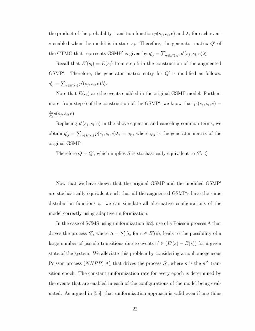
the product of the probability transition function p(sj, si, e) and λe for each event

e enabled when the model is in state si. Therefore, the generator matrix Q′ of

the CTMC that represents GSMP′ is given by q′ij =∑

e∈E′(si) p′(sj, si, e)λ

′e.

Recall that E ′(si) = E(si) from step 5 in the construction of the augmented

GSMP′. Therefore, the generator matrix entry for Q′ is modified as follows:

q′ij =∑

e∈E(si)p′(sj, si, e)λ

′e.

Note that E(si) are the events enabled in the original GSMP model. Further-

more, from step 6 of the construction of the GSMP′, we know that p′(sj, si, e) =

λeλ′ep(sj, si, e).

Replacing p′(sj, si, e) in the above equation and canceling common terms, we

obtain q′ij =∑

e∈E(si)p(sj, si, e)λe = qij, where qij is the generator matrix of the

original GSMP.

Therefore Q = Q′, which implies S is stochastically equivalent to S ′. ♦

Now that we have shown that the original GSMP and the modified GSMP′

are stochastically equivalent such that all the augmented GSMP′s have the same

distribution functions ψ, we can simulate all alternative configurations of the

model correctly using adaptive uniformization.

In the case of SCMS using uniformization [92], use of a Poisson process Λ that

drives the process S ′, where Λ =∑λe for e ∈ E ′(s), leads to the possibility of a

large number of pseudo transitions due to events e′ ∈ (E ′(s) − E(s)) for a given

state of the system. We alleviate this problem by considering a nonhomogeneous

Poisson process (NHPP ) Λ′n that drives the process S ′, where n is the nth tran-

sition epoch. The constant uniformization rate for every epoch is determined by

the events that are enabled in each of the configurations of the model being eval-

uated. As argued in [55], that uniformization approach is valid even if one thins

22

a nonhomogeneous Poisson process. In effect, in our technique, an NHPP with a

piecewise constant epoch is used to uniformize after the firing of each event. To

be conservative and prevent incorrect uniformization, care is taken to ensure that

the adaptive rate is always greater than or equal to the actual possible transition

rates of all the enabled events. In that way, the updating of the Λn is done as

follows after each epoch: Λi =∑λe, where e ∈ ∪ni=1E(si).

Note that E(si) is the set of events from the original representation of the

discrete-event model. It is always true that ∪ni=1(E(si)) ⊂ E ′(sv) for any variant

v. There is always the possibility that ∪ni=1(E(si)) = E ′(s), i.e., the system could

have all the events of all the variants enabled at all times. That could cause

the adaptive uniformization to behave just like uniformization, except that the

construction of the adaptive uniformization parameter will always ensure that

there is useful computation from at least one of the configurations, i.e., the firing

of an event in adaptive uniformization will change the state of at least one of the

configurations, which might not be the case with the traditional uniformization

technique. Hence, our technique will always guarantee progress in simulation

for at least one of the configurations. The next section describes a practical

implementation of the simulation algorithm that uses our new approach.

2.4 Adaptive Uniformization Algorithm of SSASC

Continuing with the notations from the previous section, consider a scenario where

we want to simulate N alternative configurations of a system parameterized by

its design parameter values. As we have discussed earlier, we obtain the new

configurations from the original model by modifying their probability transition

functions p(s′, s, e), input distribution functions ψ, and the conditions that enable

the state transition.

23

Algorithm 1 SSASC using adaptive uniformization: Exponential distributions1: Let

EES = ∅, enabled event set initialized to empty set,N = number of alternative configurations,E = number of exponential events in the system model,v = index of the vth alternative configuration,n = index to the nth event epoch,τn = nth event epoch,ne = event fired in the nth event epoch,ej = exponential event j in discrete-event system model,λvej

= exponential rate of event j in configuration v,λej = max(λvej

),sv0 = initial state of each configuration,D(e) = dependency list that maintains the set of

enabled events enabled due to firing of event e,u = U(0, 1), uniform random variable,Rvk = kth reward measure defined on variant v,erv = exponential random variable with rate 1,Λn = adaptive uniformization rate.

2: ∀e ∈⋃Nv=0E(sv0), EES = EES + {e}.

3: Λ0 =∑λej

where ej ∈ EES.4: n = 0, τ0 = 0.5: repeat6: Generate next event.

(a) τn+1 = τn + ervΛn

.(b) P [0] = 0.(c) for(j = 1; j≤ |EES|; j + +)

P [j] = P [j − 1] +λej

Λn.

(d) ne = ej where ej ∈ EESiff (P [j − 1] ≤ u < P [j]).

7: Update state (refer to Section 2.4.2).(a) ∀v with ne ∈ E(svn) enabled, set svn to

the next state s′vn+1 if u > p(s′vn+1, svn, ne).

8: Update EES(a) ∀e ∈ EES, EES = EES − {e},

if e /∈⋃E(svn+1).

(b) ∀e′ ∈ D(ne), e′ ∈⋃E(svn+1),

EES = EES + {e}.(c) Λn+1 =

∑λej

where ej ∈ EES.9: ∀v,∀k, compute Rvk.

10: n = n+ 1.11: until a defined terminating condition. {Refer to Section 2.4.3 for terminating condition.}

24

The simulation algorithm (See Algorithm 1) has three basic components: (1)

a Common Adaptive Clock to generate the next event and to update the enabled

event set, EES, based on the new state of the alternative configurations, (2)

an Efficient State Management System, ESMS, to efficiently update the state of

all the configurations simultaneously for the occurred event, and (3) a reward

redefinition process and an evaluation criterion that enables selection of the best

alternative configuration using a statistical procedure based on a common random

number generator. The algorithm is executed until a desired confidence interval

is achieved through execution of multiple batches (in the case of steady-state

simulation) or replication (in the case of terminating or transient simulation).

2.4.1 Common Adaptive Clock for SSASC

The SSASC algorithm begins with an empty EES (Line 1 in Algorithm 1). The

simulation algorithm initially iterates through all the events in the model, adding

them to the EES if they are enabled by any of the configurations (Line 2). Once

the initial EES is built, the simulator executes the basic components in a loop

(Line 5–11) until a terminating condition is satisfied.

In each iteration of the loop, the algorithm generates the next event epoch

using an exponential random variable using the adaptive uniformization rate, ∆n.

An event, e, is picked randomly from the EES (Line 6(d)) and is weighted by the

events firing rate, λe, that is in the EES. SSASC updates the state of the alterna-

tive configurations based on the firing of this event e (Line 7) provided that their

probability transition function p is greater than u, where u is a value from an uni-

form random variable between 0 and 1. Only those alternative configurations that

are enabled for the particular fired event, e, have their state updated. Note that p

has been modified to accommodate simultaneous simulation (See Section 2.3.2).

25

SSASC updates EES to remove disabled events and add new enabled events

(Line 8). Events that are disabled in all of the alternative configurations are

removed from the EES. Events that are enabled in any of the alternative con-

figurations are added to the EES. The algorithm computes the new adaptive

uniformization rate for the updated EES (Line 8(c)). To improve the efficiency

of the state update procedure, SSASC implements an ESMS that is described in

the next subsection (See Section 2.4.2).

The reward measures, R, are computed for each alternative configuration

based on the current state of the configuration. This loop is iterated until a

defined terminating condition occurs. Often the terminating condition is either

a fixed number of iterations or until a certain confidence level obtained for the

reward measures. To further improve simulation efficiency, SSASC redefines the

reward measures to incorporate a variance reduction technique as described in

Section 2.4.3.

2.4.2 Efficient State Management System (ESMS) for SSASC

SSASC has been shown to produce substantial execution speed-up because of a

common adaptive clock (refer to experimental results in Section 3.5). However,

there are significant overheads due to the state-saving/updating operation in the

simultaneous simulation algorithm (Line 7 in Algorithm 1). The loss of the ex-

pected speed-up of the SSASC algorithm is caused by the large memory footprint

used to represent the states of the alternative configurations and the operations

used to update the state of the model. In particular, each time an event is fired,

the simulation algorithm needs to check and update the state variable of all al-

ternative configurations. If the number of alternative configurations is large, a

substantial overhead is caused by the need to iterate through the state variables

26

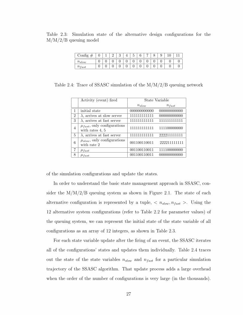
Table 2.3: Simulation state of the alternative design configurations for theM/M/2/B queuing model

Config # 0 1 2 3 4 5 6 7 8 9 10 11nslow 0 0 0 0 0 0 0 0 0 0 0 0nfast 0 0 0 0 0 0 0 0 0 0 0 0

Table 2.4: Trace of SSASC simulation of the M/M/2/B queuing network

Activity (event) fired State Variablenslow nfast

1 initial state 000000000000 0000000000002 λ, arrives at slow server 111111111111 0000000000003 λ, arrives at fast server 111111111111 111111111111

µfast, only configurations4 with rates 4, 5 111111111111 111100000000

5 λ, arrives at fast server 111111111111 222211111111µslow, only configurations

6 with rate 2 001100110011 222211111111

7 µfast 001100110011 1111000000008 µfast 001100110011 000000000000

of the simulation configurations and update the states.

In order to understand the basic state management approach in SSASC, con-

sider the M/M/2/B queuing system as shown in Figure 2.1. The state of each

alternative configuration is represented by a tuple, < nslow, nfast >. Using the

12 alternative system configurations (refer to Table 2.2 for parameter values) of

the queuing system, we can represent the initial state of the state variable of all

configurations as an array of 12 integers, as shown in Table 2.3.

For each state variable update after the firing of an event, the SSASC iterates

all of the configurations’ states and updates them individually. Table 2.4 traces

out the state of the state variables nslow and nfast for a particular simulation

trajectory of the SSASC algorithm. That update process adds a large overhead

when the order of the number of configurations is very large (in the thousands).

27

However, in Table 2.4, it’s evident that the change of state of the different config-

urations follows structured patterns. The reason is that the configurations share

similar simulation model structures and have very similar stochastic behavioral

properties. For example, configuration 0 and 1 differ only in the buffer capacity

of the fast server (refer Table 2.2). For the given parameter values, the simulation

trajectories of both of the configuration will be almost identical for most of the

simulation time. This creates the opportunity to design an efficient state repre-

sentation that would reduce cost overhead, in terms of both execution time and

memory, to update the state variable of the configurations.

Furthermore, for each event fired, only a regular subset of the alternative con-

figurations’ states are updated, due to the thinning of the poisson process. From

the traces of simulation, we see that when µfast fired only for rates 4 and 5 (see

line 4 in Table 2.4), only configurations 4 through 11 were updated. Similarly, for

µslow (see line 6 in Table 2.4), configurations 1, 3, 5, 7, 9, and 11 were updated.

All of these patterns can be predetermined before the running of the simulation

algorithm to provide a regular structure to update the state of the affected alter-

native configurations. That would significantly reduce the overhead of updating

states in the SSASC algorithm.

Finally, it is important to note that the most common operations on the state

variable are always accesses and updates to all the alternative configurations.

Therefore, the data structure can be designed in a manner that is most efficient

for the group access. Using the properties discussed above, we present the data

structure and operations supported by it to enable the speed-up in updating the

state as the simulation progresses.

28

state variable

n_fast

state

2

index

0

next

state

1

index

4

next

Figure 2.2: Compact state representation of nfast using linked lists

Data-structure for ESMS

The ESMS necessary to perform efficient state management has two components.

The first component is a data structure that encodes all of the individual states of

all the alternative configurations to make them compact to represent, and efficient

to access and update. Thus, the complete state of all the alternative configurations

with M individual states is encapsulated by M compact data structure represen-

tations. For the ease of referencing, we call an individual state the state variable

in the remainder of this chapter. For the M/M/2/B queuing system, nslow and

nfast are represented using the compact state representation.

The second component is an additional support data structure, called the Indi-

rect Reference List, IRL, that provides regularity to the access pattern to SSASC

when it updates the states of the model. This data structure is defined for each

state variable for each event defined in the simulation model. This list is ordered

based on the firing rates of events in each individual alternative configuration.

Compact State Representation (CSR)

Any access or update operation on the state variable is exactly N operations,

where N is the number of alternative configurations. Table 2.4 shows that the

state of the system is updated N = 12 times for each fired event. If we were to

represent each state variable in a more compact form, we could reduce the average

number of operations to be less than N operations.

CSR is achieved with a simple data structure that encodes the state of the

alternative configuration. This encoding can be represented using linked lists.

29

Table 2.5: Trace of SSASC simulation with ESMS of a M/M/2/B queuing network

Activity (event) fired State Variablenslow nfast

1 initial state [0,0,11] [0,0,11]2 λ, arrives at slow server [1,0,11] [0,0,11]3 λ, arrives at fast server [1,0,11] [1,0,11]

µfast, only configurations4with rates 4, 5

[1,0,11] [1,0,3],[0,4,11]

5 λ, arrives at fast server [1,0,11] [2,0,3],[1,4,11]µslow, only configurations6with rate 2

[0,0,5],[1,6,11] [2,0,3],[1,4,11]

7 µfast [0,0,5],[1,6,11] [1,0,3],[0,4,11]8 µfast [0,0,5],[1,6,11] [0,0,11]

Each cell in the list has three elements: the state of the model, the index of the

current cell, and a pointer to the next cell. The linked list of tuples, [state, index,

next ], represents the state variable of the simulation model. Figure 2.2 represents

the CSR data structure for the simulation trace when a customer arrives to the

fast server (Line 5) as depicted in Table 2.4. Table 2.5 traces the same simulation

trajectory with the CSR data-structure enabled for the state variables.

Since the size of the CSR is bounded by the number of alternative configura-

tions, N , an array implementation of the linked list is very efficient. Furthermore,

accesses and updates are executed on a single contiguous block of memory, which

makes them efficient on processors that provide pre-fetching and caching of blocks.

Indirect Reference List

From our example M/M/2/B queuing model, event rate parameter µfast is in the

sorted order that matches the ordering of the alternative configurations. Thus,

all state variables affected by µfast, such as nfast, will benefit from the CSR data-

structure. However, state variable nslow, affected by µslow, will be fragmented if

represented by CSR (as seen in line 6) as a series of “01” strings (as shown in

30

Table 2.6: Indirect reference list for the M/M/2/B queuing model

Config # 0 1 2 3 4 5 6 7 8 9 10 11nslow 0 2 4 6 8 10 1 3 5 7 9 11nfast 0 1 2 3 4 5 6 7 8 9 10 11

Table 2.4). It is possible to mitigate this fragmentation by building an Indirect

Referencing List (IRL) for each state that has a different sorted order of event

rates when compared to the actual configuration order. IRL is only built once,

during the initialization of the simulation model. The SSASC algorithm uses IRL

to access and update the state variable based on this indirect referencing of the

states. Table 2.6 presents the IRL for the M/M/2/B queuing model. With those

additions, the simulation trace seen in Table 2.4 will be modified as shown in

Table 2.5.

2.4.3 Reward Redefinition to Determine the Best AlternativeConfiguration

In Appendix A, we present a statistical procedure, 2-stage selection, developed

by [21], to choose the best alternative configuration automatically. SSASC inher-

ently implements common random numbers, (CRN), which has been considered as

the one of the best and popular approach to reduce variance [53]. We exploit this

inherent advantage provided by SSASC to reduce the number of batches(steady

state simulation) or replications(in terminating simulation) to show the real ad-

vantage of SSASC over tradition simulation approach. SSASC incorporates the

2-stage selection as its terminating condition in the Algorithm 1 (in line 11) by

automating the process as follows.

Given that Ri and Rj are the reward measures defined on alternative configu-

ration Ei and Ej respectively, define Dij as Ri − Rj, where 0 ≤ i < j < N . This

31

enables the SSASC to incorporate the cross correlation due to the use of common

random number generator in the simulation algorithm. Suppose choice of best

configuration is based on the largest rew Ri, i.e, Ei is the best configuration iff

Ri ≥ Rj for all j, j 6= i. Then, it is equivalent to choosing the largest Dij, and

picking the configuration Ej, where j is the column subscript. If choice of best

configuration was based on the smallest Rj, then it is equivalent to choosing the

smallest Dij, and picking the configuration Ej, where j is the column subscript.

With the reward redefinition in place, the SSASC algorithm terminates based on

2-stage algorithm.

2.5 G-SSASC: Non-Markovian System Models

In the previous sections of this chapter, we described the SSASC technique to

evaluate alternative configurations of system models with exponential distribution

of wait times. While the SSASC algorithm is efficient in evaluating Markovian

models, the ability to evaluate systems with general distributions using SSASC

is necessary in order to bridge the gap between practical use and theoretical con-

tributions from the SSASC algorithm. There are many approaches to developing

techniques to uniformize general distributions. Chapter 2.1.6 provides a general

overview of past research contributions to the uniformization of general distribu-

tions.

Sonderman [87] initially presented a technique to perform path-wise compar-

ison of semi-Markov processes by constructing a common underlying probability

space. Shantikumar [81] used Sonderman’s technique to generate samples for a

certain class of general distributions (with constraints that the distribution must

have bounded hazard rates) by constructing an equivalent Poisson process using

uniformization. In our approach, we extend Sonderman’s technique to the same

32

class of general distributions, but for general distributions with varying parameter

values. The parameters of general distributions are varied to obtain alternative

configurations of system models. For these alternative configurations, we develop

a simulation algorithm that composes an SSASC algorithm with the random vari-

ate generation for general distributions for evaluating alternative configurations

of system models simultaneously. In the next few sections, we extend the existing

theory and the algorithm necessary to generalize SSASC to support distributions

with bounded hazard rates. Readers are referred to Chapter 2 in [49] for additional

details on uniformization of distributions with bounded hazard rates.

2.6 Generalizing SSASC

Consider a stochastic process Y ≡ {Y (t), t ∈ R+}. Uniformization represents the

stochastic process Y as a discrete-time stochastic process Yn, where Y ≡ {Yn, n ∈

N+} and N is a Poisson process. Lewis [54], Sonderman [87], and others used

this underlying Poisson process to uniformize distributions. Shantikumar noted

that if 0 = S0 < S1 < S2 < ... are consecutive points of N on real line R+, then

Z| (Sn)∞0 is a Markov chain [79]. Using both the properties of Poisson process N

and the Markov property of Z| (Sn)∞0 , Shantikumar proposed a general approach

to simulate a uniformizable point process. Readers are referred to Theorems 2.1

and 2.2 in [79] for proof of correctness.

Vakili [93] and Ho et al. [14] incorrectly assumed that the SCMS algorithm

can be seamlessly extended to incorporate the uniformization of general renewable

processes. However, Shantikumar [81] correctly concluded that thinning of non-

homogenous Poisson process, initially proposed by Lewis and Shedler [55], can-

not be extended to general renewable processes to simulate systems even though

uniformization can be used to obtain the first passage time. Since the SSASC

33

algorithm evaluates independent alternative configurations of system models, it

is possible to use the concept of thinning of a Poisson process across alternative

configurations for each general renewable process, as described in Section 2.3.2.

Consider a general renewable random variable, G, that has a bounded and

non-increasing hazard rate. Table 2.7 enumerates standard distributions with

bounded hazard rates. For simplicity, let event g be the event that represents

G in the alternative configuration’s GSMP. Suppose that the parameters of g

are varied across alternative configurations obtaining v random variables denoted

by Gv. The uniformization constant is λ ≡ max∀v

(rv(x)) , x > 0. Algorithm 2

describes the modification to Shantikumar’s dynamic uniformization to support

simultaneous simulation of v random variables with general distribution.

34

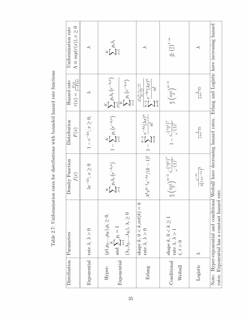
Tab

le2.

7:U

nif

orm

izat

ion

rate

sfo

rdis

trib

uti

ons

wit

hb

ounded

haz

ard

rate

funct

ions

Dis

trib

uti

onP

aram

eter

sD

ensi

tyF

unct

ion

Dis

trib

uti

onH

azar

dra

teU

nif

orm

izat

ion

rate

f(x

)F

(x)

r(x

)=

f(x

)1−F

(x)

Λ≡sup(r(x

)),x≥

0

Exp

onen

tial

rateλ

,λ>

0λe−

λx;x≥

01−e−

λx;x≥

0,λ

λ

Hyp

er-

(p1,p 2

,...,pK

),p i≥

0,K ∑ i=

1

p iλi

( e−λix)

1−

K ∑ i=1

p i( e−λ

ix)

K ∑ i=1

p iλi

( e−λix)

K ∑ i=1

p i( e−λ

ix)

K ∑ i=1

p iλi

Exp

onen

tial

and

K ∑ i=1

p i=

1

(λ1,λ

2,...,λK

),λi≥

0

Erl

ang

shap

ek,

0<k,int(k)

=k

λkxk−

1e−

λx/(k−

1)!

1−

k−

1 ∑ n=

0

e−λx(λx

)n

n!

λkxk−

1e−λx

(k−

1)!

k−

1 ∑ n=

0

e−λx(λx

)n

n!

λra

teλ

,λ>

0

Con

dit

ional

shap

ek,

0<k≥

1α β

( x+t β

) α−1e−

(x+t

β)α

e−(t β)α

1−

e−(x

+t

β)α

e−(t β)α

α β

( x+t β

) α−1α βα

( 1 t

) 1−αra

teλ

,λ>

1W

eibull

t,t>

0

Log

isti

cλ

e−λx

λ(1

+e−λx)2

11+e−λx

λ1+e−λx

λ

Not

e:H

yp

er-e

xp

onen

tial

and

condit

ional

Wei

bull

hav

edec

reas

ing

haz

ard

rate

s.E

rlan

gan

dL

ogis

tic

hav

ein

crea

sing

haz

ard

rate

s.E

xp

onen

tial

has

aco

nst

ant

haz

ard

rate

.

35

2.6.1 Inter-configuration Thinning (ICT) of Poisson Processes

Since general renewable processes does not support thinning, one could envi-

sion using traditional discrete-event simulation through event scheduling for non-

exponential distribution and SSASC for exponential distributions. However, there

are several advantages to using ICT instead of the traditional approach.

1. The number of events that need to be managed by an event-list manager in

a traditional simulator (extended to support alternative configurations) is of

the order of the number of alternative configurations. However, the number

of events that need to be managed in a ICT based simulation is independent

of the number of alternative configurations and depends only on the model.

Furthermore, the ICT algorithm does not require an event-list manager.

2. ICT with SSASC provides a framework for using a common random number

generator to simulate alternative configurations (See lines 4 and 5 in Algo-

rithm 2). Thus, the estimators that compare alternative configurations will

have lower variance than estimators used in traditional simulation.

Algorithm 2 Dynamic uniformization of a general random variable in alternativeconfigurations

1: Letλ = max∀v (rv(0)), an uniformization constantτ = Time epocherv(r) = Exponential random variable at rate rv = Number of alternative configurationsxv = Sample value of general distribution Gv

2: ∀v, xv = 03: repeat4: Generate sample t = erv(λ) and set τ = τ + t5: Generate a uniform random sample u between 0 and 1

(a) for any v, if u < rv(τ)λ

, set xv = t.(b) λ = max

∀v(rv(τ))

6: until for any v, xv 6= 0

36

2.7 Adaptive Uniformization Algorithm of G-SSASC

The G-SSASC algorithm (See Algorithm 3) is a composition of the SSASC algo-

rithm (See Algorithm 1) and dynamic uniformization of general renewable pro-

cesses (See Algorithm 2). The ESMS (refer to Section 2.4.2) and reward redef-

inition and evaluation criterion (refer to Section 2.4.3) in G-SSASC algorithm

remain unchanged from what they are in the SSASC algorithm. However, the

common adaptive clock component is modified to incorporate support for general

distributions in the G-SSASC algorithm. Four new variable, G, gv, hvgk

(x), and

ET vgk , are defined to implement the ICT of the general distribution using dynamic

uniformization.

2.7.1 Common Adaptive Clock for G-SSASC

The clock for G-SSASC algorithm needs to track the activation of the general

distribution. Therefore, a variable ET vgk , whose size is N ∗ sizeof(G), is defined

to store the last epoch when the general event was enabled (see line 8(c) in Al-

gorithm 3). The adaptive uniformization rate Λ is modified so that the rate is

greater than the hazard rate, hvgk(x), of any enabled general event, g or sum of

rates of enabled exponential events (see line 3 and 8(d)). After generating the

next event (see line 6(a)), the G-SSASC algorithm first iterates through the gen-

eral events (see line 6(e)). If none of the g’s are fired, then G-SSASC algorithm

proceeds to thin the exponential events, e, as in the SSASC algorithm. The state

update and computation of reward measures are similar to those in the SSASC

algorithm as described in Sections 2.4.2 and 2.4.3 respectively.

37

Algorithm 3 G-SSASC using adaptive uniformization: General distribution withbounded and decreasing hazard rate1: Let

EES = ∅, enabled event set initialized to empty set,N = number of alternative configurations,E = set of exponential events in the system model,G = set of generally distributed (bounded and decreasing hazard rate) events

in the system model,v = index of the vth alternative configuration,n = index to the nth event epoch,τn = nth event epoch,ne = event fired in the nth event epoch,ej = exponential event j in discrete-event system model, 0 ≤ j < size(E),λvej

= exponential rate of event j in configuration v,λej

= max(λvej),

gk = general event k in discrete-event system model, 0 ≤ k < size(G),hv

gk(x) = hazard rate of event k in configuration v, x ≥ 0 and h(x) ≤ h(0) <∞,

ET vgk

= event epoch, τ when event gvk was last enabled,hgk

(x) = max(hvgk(τn − ET vgk

)),sv0 = initial state of each configuration,D(e) = dependency list that maintains the set of enabled events enabled due to

firing of event e or g,u = U(0, 1), uniform random variable,Rvl = lth reward measure defined on variant v,erv = exponential random variable with rate 1,Λn = adaptive uniformization rate.

2: ∀e|g ∈⋃Nv=0E(sv0), EES = EES + {e|g}.

3: Λ0 = max(∑

λej,max(hgk

(0)))

where ej |gk ∈ EES.4: n = 0, τ0 = 0.5: repeat6: Generate next event

(a) τn+1 = τn + ervΛn

.(b) P [0] = 0.(c) for(m = 1; m≤ |EES|; m+ +) P [m] = P [m− 1] + λem

Λn, where em ∈ E.

(d) ne = 0.(e) ∀gm ∈ (EES ∪G) and ne == 0,

i. Generate u.ii. Set ne = gm iff u ≤ hvgm

(τn − Evgm

), for any v.

(f) ne = em where em ∈ EES iff [(P [m− 1] ≤ u < P [m]) and ne = 0].7: Update state (refer to Section 2.4.2)

(a) ∀v with ne ∈ E(svn) enabled, set svn to the next state s′vn+1 if u > p(s′vn+1, svn, ne).

8: Update EES(a) ∀e ∈ EES, EES = EES − {e}, if e /∈

⋃E(svn+1) or e /∈

⋃G(svn+1).

(b) ∀e′ ∈ D(ne), e′ ∈⋃E(svn+1) or e ∈

⋃G(svn+1), EES = EES + {e}.

(c) ET vgk= τn+1 iff gvk ∈

⋃G(svn+1).

(d) Λn+1 = max(∑

λej ,max (hgk(τn+1 − ETgk

)))

where ej |gk ∈ EES.9: ∀v,∀l, compute Rvl .

10: n = n+ 1.11: until a defined terminating condition. {Refer to Section 2.4.3 for terminating condition.}

38

CHAPTER 3

ANALYSIS OF SSASC/G-SSASC USING CASESTUDIES

This chapter presents 3 Stochastic Activity Network (SAN) models of depend-

able systems as case-studies to evaluate SSASC and G-SSASC algorithms. The

transient availability of a distributed information service system (DISS) adapted

from [52] and [62] is used to analyze SSASC. The model represents different com-

ponents of an information service and the interaction and propagation of faults

across the components. The steady state availability of a fault-tolerant computer

system that is adapted from [19, 73] is evaluated to compare SSASC with tradi-

tional discrete-event simulation (TDES) algorithm. The steady-state availability

of the storage area network in Abe’s cluster (DDNCFS) (see Appendix B for

complete case study) is used to evaluate G-SSASC. We evaluate all the models by

varying parameter values to generate alternative configurations. We show that the

SSASC/G-SSASC algorithm is efficient and scalable for evaluating large numbers

of alternative configurations.

The content of this chapter is organized as follows. Section 3.1 describes the

evaluation environment setup to compare SSASC/G-SSASC against the TDES.

Section 3.2, 3.3, and 3.4 presents the SAN model of DISS, FTCSR, and DDNCFS.

The gate code of those SAN models are listed in Appendix C. Finally, Section 3.5

concludes with evaluation and analysis of SSASC/G-SSASC’s performance.

39

3.1 Evaluation Environment

The SSASC, G-SSASC, and the TDES simulators are run on an AMD Athlon

XP 2700+ processor running at 2.2 GHz with 4Gb RAM in a Unix environment.

The implementation was compiled using g + + 3.4 with optimization level -03.

SSASC/G-SSASC is integrated into the Mobius simulator. This integration gives

us a fair way to compare the TDES built into Mobius against our simultaneous

simulator.

The Mobius tool was built on the observations that no formalism is best for

building and solving models, that no single solution method is appropriate for

solving all models, and that new formalisms and solution techniques are often

hindered by the need to build a complete tool to handle them. Mobius addressed

these issues by providing a broad framework in which new modeling formalisms

and model solution methods can be easily integrated. In Mobius, a model is a

collection of state variables, events, and reward variables expressed in some for-

malism. Briefly, state variables hold the state information of the model. Events

change the state of the model over time. Reward variables are quantitative mea-

sures of interest defined by the Mobius user to evaluate his or her models. In

the next section, we present the details on how SSASC/G-SSASC implements the

state variable representation, event management, and reward measure computa-

tion as the algorithms were integrated into Mobius framework.

3.1.1 Integration of SSASC and G-SSASC into Mobius

The SSASC and G-SSASC algorithms, described in Sections 2.4 and 2.7, are

implemented as a C++ module extending the simulation features in the Mobius

tool [17]. The implementation first separates the state of the model and the

clock event generation mechanism in the Mobius simulator. The state of the

40

model for each alternative configuration is replicated and represented using an

ESMS data structure. The event generations and management module for all

the alternative configurations are merged to obtain a single set of events, while

maintaining the information on parameter values of distributions used for each

event in the individual configurations. During the running of the simulation, when

any event is fired from the event list management module, the event is checked to

determine whether it is an actual state transition or a pseudo state transition. The

state of the configuration is updated based on the outcome of the classification of

the event. To further optimize the algorithm, the event list manager keeps track

of only those configurations that are active for a particular event, thus eliminating

the need to test all of the configurations when an event is fired.

The computational savings from the amortization of the cost of event list

management in a simultaneous simulation of all the configurations are quite sub-

stantial. These savings are illustrated in the next sections using a model of a

distributed information service system for transient analysis, a model of a fault-

tolerant computer with repair for steady-state analysis, and a model of StAN

in Abe’s CFS with general distributions. Moreover, the integration allows us to

perform a fair comparison between SSASC/G-SSASC against traditional discrete-

event simulator, as all these algorithms are built on the same Mobius framework.

3.2 SAN Model of Distributed Information Service System

(DISS)

The distributed information service system has a single front-end module that

interacts with four processing units [52, 62] . Each processing unit has two pro-

cessor units, one unit of memory, a switch, and a back-end database. Each of the

units can be in any of the following four states: Working, Corrupted, Failed, and

41

Repaired. The units cycle through those states, as shown in Figure 3.1, repre-

sented using a Stochastic Activity Network (SAN) model [61]. The gate code is

described in Appendix C.1.

42

Table 3.1: Failure, corruption, and repair rates of submodels of DISS

Submodel Corruption Failure RepairRate Rate Rate

Front-end 1/3000 * FFactor 10/1000 10/10Processor A1 4/5000 * P1Factor 4/1000 9/10

B1 3/5000 * P1Factor 4/1000 9/10C1 2/5000 * P1Factor 4/1000 9/10D1 1/5000 * P1Factor 4/1000 9/10A2 4/7000 * P1Factor 4/1000 9/10B2 3/7000 * P2Factor 4/1000 9/10C2 2/7000 * P2Factor 4/1000 9/10D2 1/7000 * P2Factor 4/1000 9/10

Switch A 4/11000 * SFactor 3/1000 8/10B 3/11000 * SFactor 3/1000 8/10C 2/11000 * SFactor 3/1000 8/10D 1/11000 * SFactor 3/1000 8/10

Memory A 4/13000 * MFactor 2/1000 7/10B 3/13000 * MFactor 2/1000 7/10C 2/13000 * MFactor 2/1000 7/10D 1/13000 * MFactor 2/1000 7/10

Database A 4/17000 * DFactor 1/1000 6/10B 3/17000 * DFactor 1/1000 6/10C 2/17000 * DFactor 1/1000 6/10D 1/17000 * DFactor 1/1000 6/10

Note: FFactor, P1Factor, P2Factor, SFactor, MFactor, andDFactor are global variables whose values are variedfrom 1 to 1000 by a multiplicative factor of 10.

Table 3.2: Error propagation rates in the DISS model

Error Propagation Rate

Error Rate Error Rate Error RateSynchFEPA 4·5/3000 SynchPASM 4·5/5000 SynchSMDA 4·5/7000SynchFEPB 3·5/3000 SynchPBSM 3·5/5000 SynchSMDB 3·5/7000SynchFEPC 2·5/3000 SynchPCSM 2·5/5000 SynchSMDC 2·5/7000SynchFEPD 1·5/3000 SynchPDSM 1·5/5000 SynchSMDD 1·5/7000

43

Fig

ure

3.1:

SA

Nm

odel

ofth

eD

ISS

44

3.2.1 Fault Model

The SAN model describes how the fault propagates through the various com-

ponents as each of them is corrupted. Each component can become corrupted

internally. While corrupted, some of the components can corrupt other units. Er-

rors are propagated from a corrupted component onto other working components

based on the following rules.

The corrupted front end may propagate an error to either of the two working

processors in any of the four processing units. The propagation occurs through

the common event between the front end and processors. After the failure is

propagated, the front end might still remain in the corrupted state and could

possibly corrupt the processors on the other Working processing units. When

both of the processors of a processing unit are in the Corrupted state, they may

corrupt the Working switch or the memory unit. Like the front end, the processor

might remain in the Corrupted state until it fails. Both the memory unit and the

switch unit in their Corrupted state can corrupt the back-end database unit by

propagating their error to it. Both the memory unit and switch unit can remain

in the Corrupted state independently before they move to the Failed state.

The distributed information server is said to be available if the front end is

able to communicate with the back-end database. The model parameters used in

the experiments are presented in Table 3.1 and Table 3.2. The availability of the

system is measured at the transient time point of 0.1 given that all the components

were in Working state at time point 0. We use the traditional Mobius simulator

to evaluate the configurations to compare the accuracy and scalability with our

technique. In order to have an accurate comparison between our technique and

standard discrete-event simulation, we ran a simulation of each configuration for

one million batches. We show that our approach evaluates the measures of interest

45

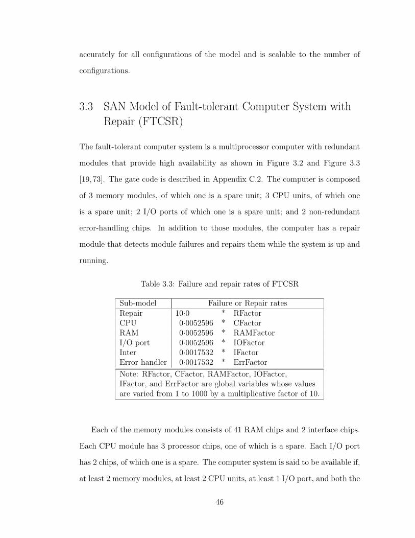
accurately for all configurations of the model and is scalable to the number of

configurations.

3.3 SAN Model of Fault-tolerant Computer System with

Repair (FTCSR)

The fault-tolerant computer system is a multiprocessor computer with redundant

modules that provide high availability as shown in Figure 3.2 and Figure 3.3

[19,73]. The gate code is described in Appendix C.2. The computer is composed

of 3 memory modules, of which one is a spare unit; 3 CPU units, of which one

is a spare unit; 2 I/O ports of which one is a spare unit; and 2 non-redundant

error-handling chips. In addition to those modules, the computer has a repair

module that detects module failures and repairs them while the system is up and

running.

Table 3.3: Failure and repair rates of FTCSR

Sub-model Failure or Repair ratesRepair 10·0 * RFactorCPU 0·0052596 * CFactorRAM 0·0052596 * RAMFactorI/O port 0·0052596 * IOFactorInter 0·0017532 * IFactorError handler 0·0017532 * ErrFactor

Note: RFactor, CFactor, RAMFactor, IOFactor,IFactor, and ErrFactor are global variables whose valuesare varied from 1 to 1000 by a multiplicative factor of 10.

Each of the memory modules consists of 41 RAM chips and 2 interface chips.

Each CPU module has 3 processor chips, one of which is a spare. Each I/O port

has 2 chips, of which one is a spare. The computer system is said to be available if,

at least 2 memory modules, at least 2 CPU units, at least 1 I/O port, and both the

46

error-handling chips are functioning. A memory module is said to be available

if at least 39 of its 41 RAM chips and 2 of its interface chips are functioning.

In addition, the fault-tolerant computer system has a failure detection/repair

module that detects failed chips and modules and automatically replaces them.

We assume that this module is a black box and suffers no failures. Since our goal

is to obtain the availability of the computer system, we are only interested in the

relative failure rates and repair rates of the components. Table 3.3 provides the

relative failure rate for the computer system for each component.

3.3.1 Fault/Repair Model

Each module (CPU, RAM, I/O port, Inter, and Error handler) can become cor-

rupted internally. In this SAN model, failures do not propagate from failed mod-

ules to working modules.

47

41 R

AM

s

2 in

terf

ace

chan

nels

mem

ory

mod

ule

41 R

AM

s

2 in

terf

ace

chan

nels

mem

ory

mod

ule

41 R

AM

s

2 in

terf

ace

chan

nels

mem

ory

mod

ule

2 ch

anne

l

erro

rhan

dler

s

2 I/

O c

hips

I/O

por

t mod

ule

2 I/

O c

hips

I/O

por

t mod

ule

CPU

mod

ule

3 cp

u ch

ips

CPU

mod

ule

3 cp

u ch

ips

CPU

mod

ule

3 cp

u ch

ips

Rep

air

mod

ule

Fig

ure

3.2:

Arc

hit

ectu

reof

the

FT

CSR

Fig

ure

3.3:

SA

Nm

odel

ofth

eF

TC

SR

48

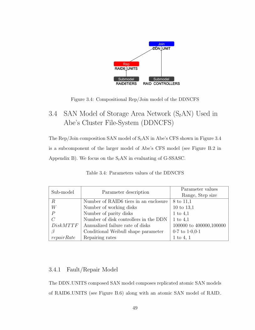
Figure 3.4: Compositional Rep/Join model of the DDNCFS

3.4 SAN Model of Storage Area Network (StAN) Used in

Abe’s Cluster File-System (DDNCFS)

The Rep/Join composition SAN model of StAN in Abe’s CFS shown in Figure 3.4

is a subcomponent of the larger model of Abe’s CFS model (see Figure B.2 in

Appendix B). We focus on the StAN in evaluating of G-SSASC.

Table 3.4: Parameters values of the DDNCFS

Sub-model Parameter descriptionParameter valuesRange, Step size

R Number of RAID6 tiers in an enclosure 8 to 11,1W Number of working disks 10 to 13,1P Number of parity disks 1 to 4,1C Number of disk controllers in the DDN 1 to 4,1DiskMTTF Annualized failure rate of disks 100000 to 400000,100000β Conditional Weibull shape parameter 0·7 to 1·0,0·1repairRate Repairing rates 1 to 4, 1

3.4.1 Fault/Repair Model

The DDN UNITS composed SAN model composes replicated atomic SAN models

of RAID6 UNITS (see Figure B.6) along with an atomic SAN model of RAID

49

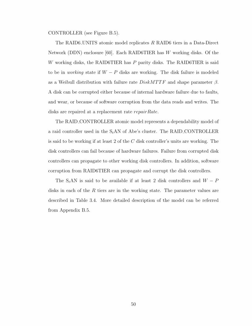
CONTROLLER (see Figure B.5).

The RAID6 UNITS atomic model replicates R RAID6 tiers in a Data-Direct

Network (DDN) enclosure [60]. Each RAID6TIER has W working disks. Of the

W working disks, the RAID6TIER has P parity disks. The RAID6TIER is said

to be in working state if W − P disks are working. The disk failure is modeled

as a Weibull distribution with failure rate DiskMTTF and shape parameter β.

A disk can be corrupted either because of internal hardware failure due to faults,

and wear, or because of software corruption from the data reads and writes. The

disks are repaired at a replacement rate repairRate.

The RAID CONTROLLER atomic model represents a dependability model of

a raid controller used in the StAN of Abe’s cluster. The RAID CONTROLLER

is said to be working if at least 2 of the C disk controller’s units are working. The

disk controllers can fail because of hardware failures. Failure from corrupted disk

controllers can propagate to other working disk controllers. In addition, software

corruption from RAID6TIER can propagate and corrupt the disk controllers.

The StAN is said to be available if at least 2 disk controllers and W − P

disks in each of the R tiers are in the working state. The parameter values are

described in Table 3.4. More detailed description of the model can be referred

from Appendix B.5.

50

3.5 Evaluation of Correctness and Efficiency of SSASC

Algorithm using DISS

Table 3.5: Comparison of correctness/accuracy of SSASC and TDES using DISS

Component TDES SSASCfailure rate

P1Factor P2Factor Availability SD Time Availability SD Time×10−02 ×10−05 (seconds) ×10−02 ×10−05 (seconds)

5 7 8·464 5·600 10·40 8·461 5·1265 70 8·999 4·716 10·40 8·995 4·7255 700 9·055 4·601 10·40 9·050 4·3275 7000 9·056 4·557 10·40 9·060 4·589

50 7 9·227 4·214 10·61 9·229 3·68650 70 9·829 2·068 10·21 9·831 2·43850 700 9·892 1·656 10·21 9·893 1·965 23·9050 7000 9·899 1·597 10·21 9·899 1·702

500 7 9·306 4·017 10·40 9·309 2·969500 70 9·917 1·447 10·21 9·919 1·328500 700 9·982 6·820 10·40 9·982 5·320500 7000 9·988 5·588 10·21 9·988 5·306

5000 7 9·316 3·989 10·21 9·318 2·7955000 70 9·926 4·601 10·21 9·927 1·1895000 700 9·991 4·922 10·21 9·991 4·7775000 7000 9·997 2·823 10·21 9·997 2·115Total Time 164·90 23·90

To illustrate the correctness and efficiency of SSASC from an implementa-

tion and practical perspective, we compare the simulation results obtained using

SSASC with TDES. We varied the individual corruption rate of processor 1 and

processor 2 by a multiplicative factor of 10 to obtain 16 alternative configurations

of the DISS model. The corruption rate of other components, such as the mem-

ory, the switch, the front end, and the database, were fixed. Table 3.5 shows the

expected instant-of-time availability measures for these configurations. The table

compares the traditional serial simulation to the SSASC algorithm. The results

were obtained at a 95% confidence level. As one can see from the table, the avail-

ability measures obtained from our technique and the traditional method fall in

51

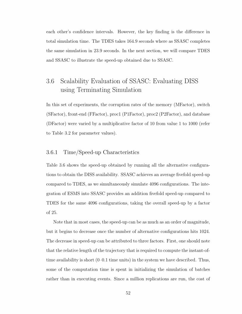
each other’s confidence intervals. However, the key finding is the difference in

total simulation time. The TDES takes 164.9 seconds where as SSASC completes

the same simulation in 23.9 seconds. In the next section, we will compare TDES

and SSASC to illustrate the speed-up obtained due to SSASC.

3.6 Scalability Evaluation of SSASC: Evaluating DISS

using Terminating Simulation

In this set of experiments, the corruption rates of the memory (MFactor), switch

(SFactor), front-end (FFactor), proc1 (P1Factor), proc2 (P2Factor), and database

(DFactor) were varied by a multiplicative factor of 10 from value 1 to 1000 (refer

to Table 3.2 for parameter values).

3.6.1 Time/Speed-up Characteristics

Table 3.6 shows the speed-up obtained by running all the alternative configura-

tions to obtain the DISS availability. SSASC achieves an average fivefold speed-up

compared to TDES, as we simultaneously simulate 4096 configurations. The inte-

gration of ESMS into SSASC provides an addition fivefold speed-up compared to

TDES for the same 4096 configurations, taking the overall speed-up by a factor

of 25.

Note that in most cases, the speed-up can be as much as an order of magnitude,

but it begins to decrease once the number of alternative configurations hits 1024.

The decrease in speed-up can be attributed to three factors. First, one should note

that the relative length of the trajectory that is required to compute the instant-of-

time availability is short (0–0.1 time units) in the system we have described. Thus,

some of the computation time is spent in initializing the simulation of batches

rather than in executing events. Since a million replications are run, the cost of

52

Table 3.6: Scalability experiments of SSASC and TDES algorithm: EvaluatingDISS using terminating simulation

Number of Simulation time (seconds) Speed-upalternative

TDES SSASCSSASC

SSASCSSASC

configurations with ESMS with ESMS1 10·21 10·59 11·16 0·96 0·914 41·40 13·17 11·13 3·14 3·72

16 164·90 23·90 12·71 6·90 12·9764 665·60 68·46 19·17 9·72 34·72

256 2, 648·00 165·91 47·31 15·96 55·971024 10, 559·00 1, 617·00 183·10 6·53 57·674096 41, 978·00 8, 088·00 1, 688·90 5·19 24·86

initializing the simulation was the largest overhead for this particular example.

We measured this initialization overhead to be around 10%–30%. Second, as the

number of configurations are increased, the dissimilarity amongst configurations

increases. That dissimilarity has a direct impact on speed-up. Third, we noted

that when the number of configurations increases beyond a certain threshold,

the advantage obtained by the locality of reference for memory access by the

processor to update the state of the model or to compute the reward measures is

lost. Due to the use of large arrays to represent the state of the system for each

configuration, the overhead of updating the state of the system and computing

the reward measures decreased the speed-up of the simulation. Thus, the speed-

up becomes comparatively moderate for the DISS model when the number of

alternative configurations is greater than 1024.

Evaluation of the Impact of Compiler Optimization and ProcessorCache on Speed-up

We performed a controlled experiment to evaluate the impact of compiler opti-

mization and processor cache on speed-up. The reward measure of the DISS model

53

states that DISS is only available if all of its sub-components are in the working

state. The DISS model has 21 subcomponents as shown in Figure 3.1. Therefore,

the function that computes reward measure of DISS in TDES has to only check

the status of 21 memory locations to determine the availability of DISS. This

operation is very efficient in TDES simulation. However, when SSASC with N

configurations represents the state variables using an array, the memory block, M ,

allocated have the size of 21xN memory locations. Computing reward measures

on this block, M , might be expensive. In order to compute the availability of

DISS for all alternative configurations, SSASC, the evaluation can proceed in two

ways. In the first approach, the implementation evaluates the reward measure for

each alternative configuration before proceeding to the next alternative configura-

tion. This is equivalent to performing column-access on M , and SSASC currently

implements the first approach. In the second approach, the implementation eval-

uates the reward measures for all alternative configurations by accessing the state

of sub-components in a consecutive order. This is equivalent to performing row

access on M .

Table 3.7: Comparison of computational overhead to evaluate reward measuredefined on DISS: Row-access versus column-access of state variables representingsub-components in DISS

Number ofRow-access Column-accessalternative

configurations1 1·0899 1·04 0·7857 1·0

16 0·8571 1·064 0·6896 1·0

256 0·7272 1·01024 0·8088 1·04096 0·5622 1·0

Note: The overhead is normalized with respect to column-access.

54

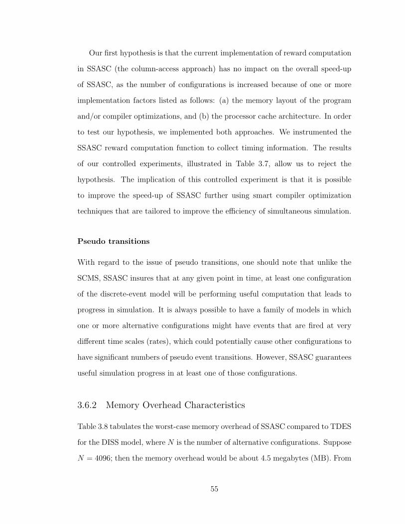
Our first hypothesis is that the current implementation of reward computation

in SSASC (the column-access approach) has no impact on the overall speed-up

of SSASC, as the number of configurations is increased because of one or more

implementation factors listed as follows: (a) the memory layout of the program

and/or compiler optimizations, and (b) the processor cache architecture. In order

to test our hypothesis, we implemented both approaches. We instrumented the

SSASC reward computation function to collect timing information. The results

of our controlled experiments, illustrated in Table 3.7, allow us to reject the

hypothesis. The implication of this controlled experiment is that it is possible

to improve the speed-up of SSASC further using smart compiler optimization

techniques that are tailored to improve the efficiency of simultaneous simulation.

Pseudo transitions

With regard to the issue of pseudo transitions, one should note that unlike the

SCMS, SSASC insures that at any given point in time, at least one configuration

of the discrete-event model will be performing useful computation that leads to

progress in simulation. It is always possible to have a family of models in which

one or more alternative configurations might have events that are fired at very

different time scales (rates), which could potentially cause other configurations to

have significant numbers of pseudo event transitions. However, SSASC guarantees

useful simulation progress in at least one of those configurations.

3.6.2 Memory Overhead Characteristics

Table 3.8 tabulates the worst-case memory overhead of SSASC compared to TDES

for the DISS model, where N is the number of alternative configurations. Suppose

N = 4096; then the memory overhead would be about 4.5 megabytes (MB). From

55

Table 3.8: Worst-case memory overhead of SSASC for the DISS model

Multiplicative factor Count Worst-case memory footprintPlaces 2 63 126NActivities1 2 67 134NGlobal variables1 4 6 24NIRL 1 6 6NTotal 290N

experimental evaluation, we see that the memory footprint of TDES averages

at 8MB. The memory footprint for SSASC averages at 8MB for 1 configuration

and 16MB for 4096 configurations. We can conclude that the memory requirement

grows linearly as the number of configurations is increased. However, the speed-up

achieved is far more significant, which improves the overall utility of simultaneous

simulation.

3.6.3 2-stage Selection of Best Alternative Configuration

In this subsection, we show how SSASC can be augmented with smart statis-

tical techniques, such as R&S or the MCB procedures described in [41]. Here,

we illustrate how a 2-stage selection approach of choosing the best alternative

configurations can further speed-up the SSASC algorithm.

Procedure of performing 2-stage selection

Refer to Appendix A for details on how to setup 2-stage selection process to choose

the best alternative configuration. Here, for this experiment, we set n0 = 10000.

We then compute nftrad = 1000000 for the traditional approach (so that Table 3.6

is comparable with Table 3.9). We estimate the variance for the traditional ap-

1Activity firing rates and global variables are floating point numbers.

56

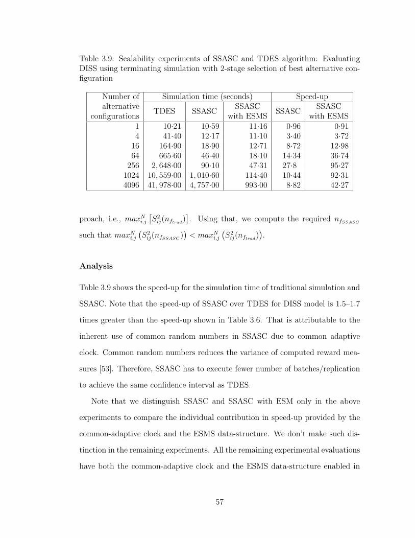
Table 3.9: Scalability experiments of SSASC and TDES algorithm: EvaluatingDISS using terminating simulation with 2-stage selection of best alternative con-figuration

Number of Simulation time (seconds) Speed-upalternative

TDES SSASCSSASC

SSASCSSASC

configurations with ESMS with ESMS1 10·21 10·59 11·16 0·96 0·914 41·40 12·17 11·10 3·40 3·72

16 164·90 18·90 12·71 8·72 12·9864 665·60 46·40 18·10 14·34 36·74

256 2, 648·00 90·10 47·31 27·8 95·271024 10, 559·00 1, 010·60 114·40 10·44 92·314096 41, 978·00 4, 757·00 993·00 8·82 42·27

proach, i.e., maxNi,j[S2ij(nftrad)

]. Using that, we compute the required nfSSASC

such that maxNi,j(S2ij(nfSSASC )

)< maxNi,j

(S2ij(nftrad)

).

Analysis

Table 3.9 shows the speed-up for the simulation time of traditional simulation and

SSASC. Note that the speed-up of SSASC over TDES for DISS model is 1.5–1.7

times greater than the speed-up shown in Table 3.6. That is attributable to the

inherent use of common random numbers in SSASC due to common adaptive

clock. Common random numbers reduces the variance of computed reward mea-

sures [53]. Therefore, SSASC has to execute fewer number of batches/replication

to achieve the same confidence interval as TDES.

Note that we distinguish SSASC and SSASC with ESM only in the above

experiments to compare the individual contribution in speed-up provided by the

common-adaptive clock and the ESMS data-structure. We don’t make such dis-

tinction in the remaining experiments. All the remaining experimental evaluations

have both the common-adaptive clock and the ESMS data-structure enabled in

57

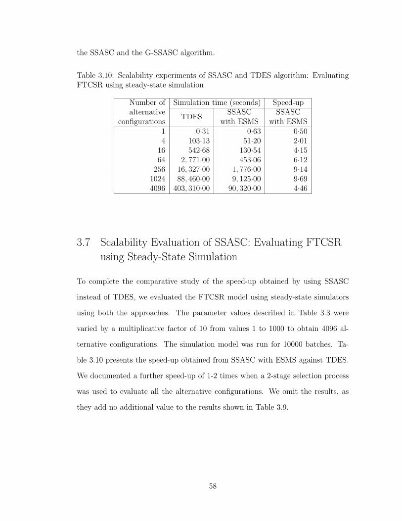
the SSASC and the G-SSASC algorithm.

Table 3.10: Scalability experiments of SSASC and TDES algorithm: EvaluatingFTCSR using steady-state simulation

Number of Simulation time (seconds) Speed-upalternative

TDESSSASC SSASC

configurations with ESMS with ESMS1 0·31 0·63 0·504 103·13 51·20 2·01

16 542·68 130·54 4·1564 2, 771·00 453·06 6·12

256 16, 327·00 1, 776·00 9·141024 88, 460·00 9, 125·00 9·694096 403, 310·00 90, 320·00 4·46

3.7 Scalability Evaluation of SSASC: Evaluating FTCSR

using Steady-State Simulation

To complete the comparative study of the speed-up obtained by using SSASC

instead of TDES, we evaluated the FTCSR model using steady-state simulators

using both the approaches. The parameter values described in Table 3.3 were

varied by a multiplicative factor of 10 from values 1 to 1000 to obtain 4096 al-

ternative configurations. The simulation model was run for 10000 batches. Ta-

ble 3.10 presents the speed-up obtained from SSASC with ESMS against TDES.

We documented a further speed-up of 1-2 times when a 2-stage selection process

was used to evaluate all the alternative configurations. We omit the results, as

they add no additional value to the results shown in Table 3.9.

58

3.8 Scalability Evaluation of G-SSASC: Evaluating

DDNCFS using Steady-State Simulation

The main difference between G-SSASC and SSASC is the ability of G-SSASC

to uniformize a certain class of non-exponential distributions (refer to Table 2.7

for the list of distributions). In this section, we focus our analysis on comparing

G-SSASC’s non-uniform RVG against TDES’s inversion approach of non-uniform

RVG.

To complete the scalability experiments, we compare the scalability of G-

SSASC against TDES as we scale the number of alternative configuration experi-

ments from 1 to 4096. G-SSASC achieves speed-up of up to 1 order of magnitude

for steady-state evaluation of DDNCFS.

Table 3.11: Scalability experiments of G-SSASC and TDES algorithm: EvaluatingDDNCFS using steady-state simulation

Number of Simulation time (seconds) Speed-upalternative

TDESG-SSASC G-SSASC

configurations with ESMS with ESMS1 29·14 42·44 0·684 118·26 47·23 2·50

16 473·97 112·54 4·2164 1, 897·40 158·53 11·96

256 7, 587·60 706·50 10·741024 30, 368·00 10, 002·00 3·034096 119, 980·00 53, 894·00 2·22

59

3.9 Comparative Evaluation of Cost of Event-Generation

and State Update: SSASC/G-SSASC versus TDES

As discussed in Chapter 2, SSASC/G-SSASC achieves speed-up because of two

components in its simulation algorithm: (a) the common adaptive clock, and (b)

ESMS. Table 3.12 illustrates the comparison of SSASC/G-SSASC and TDES with

respect to each of these components for each of the case-study models. 1,000,000

replications of alternative configurations of DISS were executed for terminating

simulation. 10,000 batches of alternative configurations were executed for steady-

state simulation. The table reiterates the fact that combining alternative config-

urations into one large simulation model has significant advantages.

3.9.1 Analysis of ESMS

As with any data-structure, the efficiency of the execution of ESMS depends

upon the data access/update patterns from the simulation algorithm. In Chap-

ter 2.4.2, we looked at some of the state update characteristics and built an ESMS

data structure to be optimized for those operations. We will now look into some

strategies that would make the best use of the ESM data structure to improve

the SSASC/G-SSASC algorithm.

Any operation that causes two or more state updates to directly interact re-

duces the simulation efficiency. Consider the M/M/2/B queuing system from

Figure 2.1. Suppose that there is an event, called transfer, that transfers cus-

tomers from the slow server to the fast server. Whenever transfer is fired, in

SSASC/G-SSASC without ESMS, it would take exactly N operations to access

and/or update the state of the simulation model, where N is the number of alter-

native configurations. Use of SSASC with ESMS would add an additional m ∗N

operations, due to the use of IRL, where m is the number of interacting state

60

Table 3.12: Comparison of SSASC/G-SSASC against TDES using total numberof events generated and state updates for evaluating alternative configurations

Number of DISSalternative Generated events State updates

configurations TDES SSASC TDES SSASC1 5.6109×1005 5.7037×1005 2.4936×1007 3.1508×1007

4 2.1049×1006 5.9200×1005 9.9590×1007 8.2953×1007

16 5.6845×1006 6.6062×1005 3.8059×1008 9.9101×1007

64 1.4833×1007 9.8219×1005 1.4607×1009 5.0861×1008

256 4.0003×1007 1.3229×1006 5.6717×1009 2.3451×1009

1024 1.3851×1008 1.3311×1007 2.2492×1010 6.33981×1009

4096 5.4912×1008 6.5311×1007 8.9870×1010 3.33284×1010

Number of FTPCSalternative Generated events State updates

configurations TDES SSASC TDES SSASC1 2.4765×1005 2.4657×1005 1.4340×1006 2.7320×1006

4 6.7939×1007 2.6983×1007 5.5780×1008 6.8780×1008

16 3.5932×1008 9.4765×1007 2.8662×1009 1.7386×1009

64 1.8717×1009 3.7657×1008 1.3593×1010 8.2765×1009

256 1.1186×1010 2.3456×1009 8.1333×1010 5.8345×1010

1024 6.3356×1010 4.4512×1009 4.1348×1011 1.5434×1011

4096 2.8790×1011 6.2545×1010 1.8948×1012 1.0645×1011

Number of DDNCFSalternative Generated events State updates

configurations TDES G-SSASC TDES G-SSASC1 2.0967×1007 2.0453×1007 7.2956×1007 7.0393×1007

4 8.4058×1007 2.4902×1007 2.9235×1008 9.1345×1007

16 3.3622×1008 8.4292×1007 1.1694×1009 5.1234×1008

64 1.3448×1009 2.4825×1008 4.6773×1009 1.0237×1009

256 5.3794×1009 6.2748×1008 1.8709×1010 5.8684×1009

1024 2.1517×1010 7.3648×1009 7.4837×1010 2.9371×1010

4096 8.6070×1010 3.6736×1010 2.9935×1011 1.6249×1011

61

variables (here, m = 2).

In general, the order in which the IRL is built for each state variable in the

model has some impact on the speed-up. Since faster-rate events are fired more

often, we achieve better speed-up if the IRL list is built based on the order of the

dominant event rate that affects each state variable. In situations in which the

state variable of a model is affected by more than one event, it is better to build

the IRL based on the fastest event affecting the state variable.

In the discussion about state update characteristics in Section 2.4.2, we noted

that minimizing the size of the linear list improves efficiency. The reason is that

one could pre-compute the sorted order of firing of a particular activity for all

the alternative configurations. However, note that the state-dependent activity

does not guarantee this property of sorted order of firing. Therefore, it might be

efficient to avoid using IRL lists and stick to the linear array representation when

an event’s rate depends on the state of the simulation model.

Finally, it is possible to significantly improve efficiency of the simulation by

viewing this simulation programming paradigm as N independent alternative sim-

ulations that depend on each other for computational efficiency, rather than taking

the traditional approach of viewing it as a simulation of N independent replication

of the model with different parameter values. In simplistic terms, the simulation

tool user should view the process of developing models in SSASC/G-SSASC as

similar to vector, set or matrix manipulation.

3.10 Comparative Evaluation of Event-Generation of

Conditional Weibull: G-SSASC versus TDES

The activity failDisk (refer to Figure B.6) has conditional Weibull as its failure

distribution. The value of the shape parameter, α, is varied over values from

62

0.7 to 1.0 in steps of 0.1. The parameter β is varied over values from 100,000

to 400,000 in steps of 100,000 as one evaluates 4096 alternative configurations of

the DDNCFS model. Table 3.13 presents a comparison of the average numbers

of events that are necessary to generate a sample for the conditional Weibull

distribution in the DDNCFN model. We normalize the results per alternative

configuration of TDES. Therefore, column 4 in Table 3.13 is the same as the

number of alternative configurations (column 2 in Table 3.13). Each alternative

configuration is run for 10000 batches. The results in Table 3.13 are collected

when failDisk is the lone entry in EES.

We notice that the number of events generated to uniformize the conditional

Weibull in G-SSASC is clearly independent of the number of alternative configu-

rations. However, note that the number of events generated in G-SSASC depends

on the ratio between the firing of the fastest rate of alternative configurations and

the slowest rate of alternative configurations. G-SSASC’s approach of extending

Shantikumar’s technique of non-uniform RVG using ICT and a common adap-

tive clock definitely makes non-uniform RVG practical. The TDES’s approach

of non-uniform RVG using inversion always performs better than Shantikumar’s

technique (Compare column 4 to column 5). However, G-SSASC takes advantage

of the common adaptive clock to mitigate the number of events generated as one

scales the number of alternative configurations.

63

Table 3.13: Average number of uniformization points generated for conditionalWeibull normalized per alternative configuration of TDES

1 2 3 4 5 6 7 8

Line #Parameter

TDESShantikumar’s RVG G-SSASC’s RVG

valuesα Mean SD Mean SD

01 4 0.7 4 8·9352 1·4822 8·9342 1·477502 4 0.8 4 8·7106 1·8110 8·6942 1·825203 4 0.9 4 7·8520 2·2481 7·8557 2·246104 4 1.0 4 5·4896 1·1201 5·4899 1·1281

total 16 ∗ 16 30·9874 3·4395 30·9740 3·424805 16 0.7 16 35·8692 5·8822 8·9462 1·477706 16 0.8 16 34·8136 7·3355 8·6983 1·831407 16 0.9 16 31·4852 9·0470 7·8270 2·265408 16 1.0 16 21·9220 4·4757 5·4918 1·1103

total 64 ∗ 64 124·0900 13·7882 30·9633 3·464309 64 0.7 64 142·9184 24·0699 8·9544 1·464910 64 0.8 64 139·2928 29·4515 8·6900 1·834211 64 0.9 64 124·6816 35·9597 7·8544 2·254912 64 1.0 64 87·9696 17·9692 5·4730 1·1245

total 256 ∗ 256 494·8624 55·6852 30·9718 3·463213 256 0.7 256 573·1776 94·9479 8·9526 1·509514 256 0.8 256 555·0656 117·7062 8·6769 1·823215 256 0.9 256 503·6224 143·8245 7·8364 2·249316 256 1.0 256 351·4816 71·5122 5·4959 1·1173

total 1024 ∗ 1024 1983·3472 220·3915 30·9618 3·442717 1024 0.7 1024 2294·7072 379·1811 8·9667 1·498218 1024 0.8 1024 2228·0192 465·9980 8·7170 1·813719 1024 0.9 1024 2006·1184 581·4884 7·8233 2·270220 1024 1.0 1024 1407·1296 287·4720 5·5058 1·1218

total 4096 ∗ 4096 7935·9744 878·5687 31·0128 3·4573

64

CHAPTER 4

EXPLORING ALTERNATIVE DESIGNCONFIGURATIONS USING SEARCH

HEURISTICS

In situations where it is practical to exhaustively explore design parameter space,

we proposed SSASC and G-SSASC (see in Chapter 2) as an alternative approach

to simulate models efficiently. In this chapter, we address the issue on how to

explore design spaces when a complete and exhaustive design exploration is not

practical. System designers have to resort to exploratory search heuristics when it

is impractical to explore the alternative configurations exhaustively with efficient

techniques such as SSASC/G-SSASC algorithms. In particular, we propose a

search heuristic technique that performs a principled and automated exploration

of the design space with a large number of alternative configuration choices to

minimize the cost of an objective function.

We present our search heuristics methodology using a case study that involves

design of dependable data storage systems for multi-application environments,

which minimizes the overall cost of the system while meeting business require-

ments. Previous work on this case study considered methods to automatically

design a dependable storage system that uses a single technique to protect a sin-

gle application workload [48], and algorithms to evaluate the recovery behavior of

a single application workload protected by a combination of techniques [47].

Our contributions include search heuristics for intelligent exploration that can

be easily generalized to a class of design problems (optimal resource allocation

with dependability constraints), as well as modeling techniques for capturing in-

teractions between multiple components in the design. We quantitatively evaluate

65

our heuristic approach using realistic storage system environments and compare

its solutions to those produced by a simple heuristic that emulates human design

choices and to those produced by a random search heuristic and a genetic algo-

rithm meta-heuristic. For the scenarios we study, we find that our approach’s

solutions reduce overall system costs due to equipment and software outlays and

data outage and loss penalties by at least a factor of two when compared to the

human design choices. Furthermore, our approach consistently produces better

solutions than the random heuristic and genetic algorithm. Finally, we study the

sensitivity of our approach’s solutions to several parameters, including the num-

ber of applications to be protected, the bandwidth and capacity characteristics of

those applications, the likelihood of failures, and algorithm execution time.

The remainder of this chapter is organized as follows. Section 4.2 formu-

lates the problem of designing storage systems to protect application data. In

Section 4.3, we describe our design methods. In Section 4.4, we evaluate our

approach quantitatively by comparing it to other meta-search heuristics, such as

random search and GA.

4.1 Background and Related Work

4.1.1 Exploring Alternative Design Configurations Using SearchHeuristics

To deal with extremely large number of alternative configurations, researchers

have often explored the possibility of design space exploration through simula-

tion optimization and search heuristics. We first provide a brief overview and

explore alternative approaches to simulation optimization in Sections 4.1.2 and

4.1.4. Next, we discuss hybrid search heuristics to explore and evaluate extremely

large number of alternative configurations in Section 4.1.5. We conclude with a

66

brief overview of the storage design problem used as the case study to evaluate

the search heuristics developed in Chapter 4.

4.1.2 Simulation Optimization

Simulation optimization is one approach by which a system designer can deter-

mine the best input parameter values from all the possible values without explic-

itly enumerating all possibilities. In the worst case, when the number of input

parameters becomes very large, the cost to simulate all experiments becomes com-

putationally prohibitive. The goal of simulation optimization is to minimize the

computational resources that are spent while maximizing the information that is

obtained through simulation. In a simulation optimization framework as shown

in Figure 4.1, the output of the simulation model is provided as input to an opti-

mization strategy to provide feedback for fine-tuning of the input parameters for

the next run of simulations. Although simulation optimization is a well-researched

topic, with several surveys available on the progress of research over the past fifty

years [9, 13], the characteristics of the certain design problem make it difficult to

apply simulation optimization. For example,

• The objective function (total cost) for the design problem could be non-

differentiable; it cannot be expressed as an analytical function of the inputs

and the constraints to the model.

• The decision variables that are being optimized can be either quantitative or

qualitative. Very little literature exists to optimize systems with qualitative

decision variables [9].

• The model being optimized can be fairly complicated.

67

Often, it is challenging or even impossible to develop a general optimization

strategy and evaluation algorithms to evaluate all classes of design problems.

Therefore, the solution technique to evaluate a very large design must be tai-

lored for a particular class of design problem. The algorithm is optimized for the

characteristics and traits of the design problem that is being solved.

AnalysisAlgorithmOptimization Simulation

Evaluation/

Figure 4.1: Basic simulation optimization framework.

4.1.3 Storage Systems Design: Backup and Recovery

In exploring very large design spaces, we picked the storage design problem as the

case study. Administration and deployment of storage systems are often complex.

Challenges include planning the infrastructure, laying out data on the storage

systems such that application performance goals are met, and planning efficient

data and application failure recovery strategies such that the penalties due to a

failure are minimized. Storage architects often use adhoc approaches, which might

not provide the best solutions.

Recent work addresses some of those problems by showing how to automate

the design of storage systems to meet various performance goals at the lowest

cost [5,7,6]. Minerva automates the storage design and configuration problem by

decomposing it into two subproblems, which are solved separately: storage array

configuration and data layout based on application workload characteristics [5].

68

The disk array designer handles the two issues simultaneously, using a generalized

best-fit bin-packing heuristic with randomization and backtracking [6]. RAID-

level selection [7] applies heuristics to choose a RAID array configuration, RAID

levels, and data layout to minimize the cost while assuring that the performance

requirements are met. [48, 47, 46] consider questions in the broader area of de-

pendable storage system evaluation and design, including online and off-line data

protection techniques. Keeton et al. explore methods for dependable storage de-

sign in the context of a single application and a single dependability technique [48];

this dissertation considers multiple applications and combinations of techniques,

which present a much more complex problem. In the area of modeling dependable

storage system behavior, Keeton and Merchant presented a framework for evalu-

ating the recovery time and recent data loss for a single application protected by

a combination of techniques [47]; more recent work by their group examines how

to schedule recovery operations for multiple workloads [46]. [47] considers only

the dependability evaluation of an existing storage system, and does not consider

how to design the system in the first place, when a very large number of design

choices exist.

4.1.4 Stochastic Simulation Optimization

Azadivar [9] has several descriptions of a general formulation of the simulation

optimization problem. According to one way of formulating the problem, one can

define

Maximize(minimize) f(X) = E[z(X)]

Subject to : g(X) = E[r(X)] < 0

and h(X) < 0

69

Where r and z are the response of the simulation model for given input parameter

X, f , and g are the expected values of the vectors that are estimated by observa-

tions of r and z. h(X) is a vector of deterministic constraints. We can tailor this

general formulation of simulation optimization to fit into the formulation of our

interest. However, in the current setting, we are interested only in the elements

of the input vector X. The elements of input vector X are a combination of para-

metric (continuous variables, discrete variables) and non-parametric (qualitative)

decision variables. From the dependable storage system modeling perspective,

the choice of recovery and backup technique is non-parametric input decision

variable. Furthermore, the frequency to tape-backup is a parametric input de-

cision variable. Optimization problems with these kinds of input variables are

labeled as non-parametric optimization problems. Traditional stochastic search

(for pure continuous variables) or integer programming (for discrete variables)

lack the ability to handle the qualitative decision variables. Furthermore, there

is a need to automatically generate a new simulation model based on the choice

of values of the qualitative decision variables. The most common approach to

solve non-parametric optimization problems has been by complete enumeration

or random sampling. Complete enumeration is an unlikely solution for the de-

pendability model. Again, in the case of a dependable storage system model, with

only 5 applications and 7 types of backup and recovery technique, we have 57 con-

figuration, without even considering the combinatorial of the resource choices that

can be used to deploy these applications and the parametric parameters of the

recovery techniques. Random sampling is the best available option when the num-

ber of alternative designs is very large. Azadivar [9] concludes that the traditional

“wait and see” random technique cannot be used with non-parametric decision

variables. A “wait and see” random technique is a method by which the next

point in the design space is selected based on the information obtained by past

70

evaluation of the space. Azadivar reasons that non-parametric decision variables

cannot be defined geometrically, and therefore we cannot decide on the direction

for the value of a decision variable. However, we have shown in [25] that it is not

necessary to have a sense of direction with non-parametric variables. Instead it is

sufficient to have an estimate of quality of the objective function based upon the

values of non-parametric decision variables.

In optimization problems, if the designer has enough knowledge of the rela-

tionship among the available alternatives, ranking and selection (R&S) methods

are frequently applied to select the best system or a subset that contains the best

system [89]. Multiple comparisons (MC) allow a certain pair-wise comparison to

make inference in the form of a confidence interval among all the designs.

4.1.5 Hybrid Search Heuristics

Direct search methods are some of the best-known techniques for unconstrained

optimization [13, 50]; they specifically address optimization problems in which

the derivatives of the objective functions are not available or are not reliable.

They do not make any assumptions about the underlying parameter space, but

rather optimize depending upon the value of the objective function [50]. In the

realm of discrete input parameters, pure combinatorial optimization problems

are concerned with the efficient allocation of limited resources to meet the de-

sired objectives [33]. Techniques for solving such problems, including linear and

integer programming, expect prior knowledge of the bounds on the available re-

sources to optimize. The number of different alternatives in the discretized space

of available resources makes it computationally expensive to compute all possible

combinations of allocations to solve the storage design problem using combina-

torial optimization techniques. In addition, the storage design problem for data

71

protection requires the optimization of both continuous and discrete parameters,

making it significantly harder to simply use combinatorial optimization or direct

search methods.

While it is interesting to determine an exact solution for a design problem, in

practice it is often unnecessary, since the computer models and specifications are

simplifications of reality. Often, designers are interested in good solutions that are

better than those generated by very simplistic methods (such as system architects’

past design experience). For the above reasons, researchers have developed meta-

heuristics to efficiently and effectively explore the problem to obtain near-optimal

solutions. Some well-known meta-heuristics are general hill-climbing [44], simu-

lated annealing [63], ant colony optimization [20], tabu search [29], and genetic

algorithms [31]. Hill-climbing is a greedy approach that attempts to maximize (or

minimize) the goal function by exploring the nodes neighboring the current solu-

tion. Simulated annealing (SA) is analogous to the physical process of annealing

in metallurgy. At each step, the SA algorithm replaces the current solution with

a neighboring solution, chosen with a probability that depends on the difference

between function values and the global parameter T (for temperature), which is

gradually reduced during the SA process. The solution efficiency and effectiveness

depend heavily on the parameter T . Tabu search (TS) is a generalized approach

that is similar to simulated annealing, in that it keeps track of multiple generated

solutions to determine the next possible potential solution.

Meta-heuristics searches are efficient in scenarios where the underlying struc-

ture of the parameter space is known [69]. Genetic algorithms (GAs) have emerged

as the most popular approach to solving problems with a mix of qualitative and

quantitative decision variables [9]. Dicke et al. have applied GAs to determine

efficient data placement in a storage area network based on workload character-

istics [18]. However, without sufficient information about the underlying problem

72

structure or sensitivity of the decision variables, such general meta-heuristics often

underperform, as shown by our comparison to the generic GA.

4.2 Designing Dependable Storage Systems

Businesses today rely on their IT infrastructures, and events that cause data un-

availability or loss can have expensive, or even catastrophic, consequences. Such

events can include natural disasters, hardware failures, software failures, user and

administrator errors, and malicious attacks. Given these threats, most businesses

protect their data using techniques such as remote mirroring, point-in-time copies

(e.g., snapshots), and periodic backups to tape or disk. These techniques have

different properties, advantages, and costs. For example, using synchronous re-

mote mirroring permits applications to be quickly failed over and resumed at the

remote location. Snapshots internal to a disk array are space-efficient and permit

fast recovery of a consistent recent version of the data. Backups to tape or disk

allow an older version of the data to be recovered. These techniques have limita-

tions. Remote mirroring usually has high resource requirements; local snapshots

do not protect against failure of the disk array; and recovering from backups can

result in significant loss of recent updates.

To achieve adequate levels of data protection, it may be necessary to use a

combination of techniques. The storage architect must select one or more data

protection techniques to apply to each application workload. Resources, such as

disk arrays, servers, tape libraries, and network links, must also be assigned to the

application to support these techniques. The resources and data protection tech-

niques have many configuration parameters; for example, a backup policy needs

to specify the frequency of the backups and whether the backups will be full or in-

cremental. The architect must verify that the design will meet normal operational

73

performance requirements (for example, the backups will complete overnight), and

also that the recovery behavior will be adequate under various expected failure

scenarios. These decisions must be made in a cost-effective manner. Faced with

such complexity, architects usually resort to simple ad hoc heuristics: categorize

applications by importance (gold, silver, or bronze) and assign a standard data

protection design depending upon the category. This approach frequently results

in either an over-engineered system that is more expensive than necessary, or an

under-provisioned one that does not meet requirements.

Our goal is to find the best storage solution, which is the one that minimizes

overall costs, including infrastructure outlays as well as penalties for application

downtime and data loss. The solution to this problem specifies 1) a combination

of data protection and recovery techniques for each application workload (e.g.,

remote synchronous mirroring, local snapshots, and local backup); 2) how those

data protection techniques should be configured (e.g., how frequently snapshots

and backups are taken); and 3) how physical resources like disk arrays, tape

libraries, and network links should be provisioned to support normal and recovery

operation.

To understand how the design tool makes choices among design alternatives,

this section describes the design space and all the parameters used to prescribe

a particular design. We begin by describing how we model the design space, in-

cluding the data protection and recovery techniques, application workload char-

acteristics, device infrastructure, and failure scenarios. We then describe how the

cost of a particular solution is computed and provide a precise description of the

problem we solve, in terms of this design space.

74

4.2.1 Data Protection and Recovery Techniques

In order to protect applications against data loss and unavailability, it is neces-

sary to make one or more secondary copies of the data that can be isolated from

failures of the primary data copy. Although standard redundant hardware tech-

niques such as RAID [70] are used to protect data from internal hardware failures,

they are not sufficient to protect data from other kinds of failures, such as human

errors, software failures, or site failure due to disasters. Geographic distribution

of secondary copies (e.g., through inter-array mirroring [42, 78] or remote vault-

ing) provides resilience against site and regional disasters. Point-in-time [10] and

backup [16, 35, 97] copies address application data object errors, like accidental

deletion and software failures due to buggy software or virus infection, by permit-

ting restoration of a previously consistent copy. Those data protection techniques

can be combined to provide more complete coverage for a broader set of threats.

After a failure, application data can be recovered either by restoring one of

the secondary copies at the primary site or a secondary site, or by failing over

to a secondary mirror. For the restoration case, data is copied from the sec-

ondary copy to the target site. For failover, the computation is simply transferred

to the secondary mirror, without any data copy operations. Failover requires a

later fail-back operation (performed in the background) to copy data and transfer

computation back to the target site.

We leverage the framework described in [47] to model data protection and

recovery technique behavior, including creation, retention, and propagation of

secondary copies. Primary and secondary copies are modeled as a hierarchy,

where each level in the hierarchy corresponds to either the primary copy or one

of the techniques used to maintain a secondary copy. For example, a hierarchy

might include the primary copy, intra-array snapshot, tape backup, and remote

75

vaulting. Secondary copies made at one level of the hierarchy are periodically

transferred to the next level of the hierarchy. For example, tape backups are

periodically shipped offsite to the remote vault. For each level of the hierarchy,

data protection technique parameters specify how frequently secondary copies are

made (the accumulation window), how long they take to propagate to a given

level of the hierarchy (the propagation window), and how long they are retained

at that level (the retention window), thus determining how much data loss might

be experienced after a disaster. (Table 4.4 provides examples of these parameters

for our experimental environment.) Evaluation of the models also determines

how the techniques consume resources, such as storage device and network link

bandwidth. Section 4.3.2 describes how this framework is extended to model

resource contention in multi-application environments.

4.2.2 Application Workload Characteristics

To estimate the bandwidth and capacity requirements for creating secondary

copies, we must understand the application’s data access patterns. Applications

share common resources to perform backup of data. Techniques that retain a

full copy of the data require the solver to understand the capacity of the dataset.

Techniques that immediately propagate updates, such as synchronous mirroring,

require an understanding of the application’s peak (non-unique) update rate to

determine the required network bandwidth. Asynchronous mirroring techniques

require network bandwidth to support the application’s average (non-unique) up-

date rate. Techniques that periodically create secondary copies require the solver

to understand the unique update rate. For a given period of time, the unique

update rate measures the last update to a given location, omitting overwrites; it

tells how much new data is generated between the creations of subsequent sec-

76

ondary copies. Finally, recovery techniques that redirect application computation,

such as failover, also require the solver to understand the application’s average

access (read + write) rate. Table 4.3 provides examples of these parameters for

the workloads considered in our experiments.

4.2.3 Device Infrastructure

Data protection and recovery techniques employ storage devices, such as disk ar-

rays, tape libraries, and network interconnects, to store and propagate copies. Re-

covery techniques like failover also employ computational resources. As in [47], we

model several aspects of device resource configuration. Each device has capacity

and bandwidth constraints that limit the number of applications and data protec-

tion techniques that can simultaneously use that device. Capacity and bandwidth

are allocated in discrete units, and we assume a linear additive model for resource

consumption. In addition, we model the outlay costs necessary to use the device

infrastructure. Each device has a fixed cost associated with acquiring an instance

of that device type (e.g., the cost of a disk array enclosure). A device may also

have a per-capacity cost and a per-bandwidth cost (e.g., the costs of tape cartridges

and tape drives for a tape library). The resource costs cover the direct and indi-

rect costs of using the resources, including the hardware (e.g., purchase or lease

price), software licenses, service contracts, management costs, and facility costs.

The solution must completely describe the employed resources, including each of

the available sites, the different storage and computational devices employed at

each site, the interconnects between the sites, and their parameters.

77

4.2.4 Failure Model

The primary copy of an application’s dataset faces a variety of failures after de-

ployment, including hardware failures, software failures, human errors, and site

and regional disasters. A failure scenario is described by its failure scope, or the

set of failed storage and interconnect devices. Examples include primary data

object failure, primary disk array failure, and primary site disaster. A primary

data object failure indicates the loss or corruption of the data due to human or

software error without a corresponding hardware failure. Each failure scenario

also has a likelihood of occurrence, which describes the expected annual likelihood

of experiencing that failure.

We assume that primary disk array failures and primary site disasters are

detected immediately, and that the desired point of recovery is the most recent

point in time. For primary data object failures, we assume that there is a delay

between the failure and the discovery of the failure(e.g., due to user error). The

desired point of recovery is the time (in the past) of the failure. For any failure,

we assume that the recent data loss is the failure detection delay (i.e., the updates

made after the failure), plus any additional updates lost due to recovery from a

point-in-time copy that is out of date, relative to the desired recovery point. For

instance, the failure may have occurred just before a backup, resulting in the loss

of all updates since the previous backup.

Failed applications incur penalty costs due to the unavailability and loss of

data. We model these penalties as described in [48]. In particular, a data outage

penalty rate describes the cost (e.g., in US$ per hour) of data unavailability. After

a failure, data is recovered from a secondary copy, which may be out of date

relative to the time of the failure, thus implying the loss of recent updates. The

recent data loss penalty rate describes the cost (e.g., in US$ per hour) of recent

78

data loss.

4.2.5 Solution Cost

In order to choose among alternative designs, the design tool must assign a cost

to each potential solution. The overall cost of the storage solution includes the

outlays for the employed resources and the penalties for recovering the application

data. Outlay costs are calculated for the entire resource infrastructure, including

the fixed and incremental costs of the devices and the facilities costs of the data

center sites.

The design tool evaluates the models (as described in Section 4.3.2) to de-

termine the recovery time (data outage time) and recent data loss time for each

failure scenario. It weights the computed data outage penalty and recent data loss

penalty from each scenario by the likelihood of that failure. The overall penalty

cost is the sum of the weighted data outage and recent data loss penalties over

all failure scenarios and all application workloads. To provide a meaningful sum

of the outlays and penalties, both cost categories must be calculated over a com-

mon time frame. Since most businesses look at annual costs, our models amortize

the purchase price of devices over their expected lifetime (which is chosen to be

three years). Similarly, the likelihood of failure is converted to an annual expected

failure likelihood.

4.2.6 Putting It All Together: Problem Statement

Given a description of application penalty rates, access characteristics, topology

of data center sites, maximum number of permitted devices among all sites, and

failure scenarios, our goal is to determine 1) the combination of data protection

and recovery techniques for each application; 2) the quantitative configuration

79

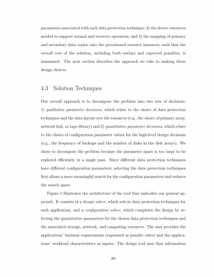
parameters associated with each data protection technique; 3) the device resources

needed to support normal and recovery operation; and 4) the mapping of primary

and secondary data copies onto the provisioned resource instances, such that the

overall cost of the solution, including both outlays and expected penalties, is

minimized. The next section describes the approach we take to making those

design choices.

4.3 Solution Techniques

Our overall approach is to decompose the problem into two sets of decisions:

1) qualitative parameter decisions, which relate to the choice of data protection

techniques and the data layout over the resources (e.g., the choice of primary array,

network link, or tape library) and 2) quantitative parameter decisions, which relate

to the choice of configuration parameter values for the high-level design decisions

(e.g., the frequency of backups and the number of disks in the disk arrays). We

chose to decompose the problem because the parameter space is too large to be

explored efficiently in a single pass. Since different data protection techniques

have different configuration parameters, selecting the data protection techniques

first allows a more meaningful search for the configuration parameters and reduces

the search space.

Figure 1 illustrates the architecture of the tool that embodies our general ap-

proach. It consists of a design solver, which selects data protection techniques for

each application, and a configuration solver, which completes the design by se-

lecting the quantitative parameters for the chosen data protection techniques and

the associated storage, network, and computing resources. The user provides the

applications’ business requirements (expressed as penalty rates) and the applica-

tions’ workload characteristics as inputs. The design tool uses that information

80

Data Protection Technique and Resource Library Minimal Cost Storage Solution

ExhaustiveSearch

EvaluatorAnalytic

SolverConfiguration

Resource Layout

Penalty Rates ($/hour)

Update Characteristics

Data Outage/Loss

Workload Access/

AlgorithmGreedy best−fit

Reconfiguration

AlgorithmRefit

Output

Algorithm

Parameters

Input Design Solver

TechniqueResource Parameters

TechniquesProtection

Figure 4.2: Automated design tool for dependable storage solutions

to evaluate candidate storage designs and to produce a solution that attempts to

minimize the overall cost. Many such complete designs are generated, and the

design with the lowest cost is selected. The output of the design tool is a depend-

able storage design with near-optimal (minimal) cost. The next sections describe

the operation of the design solver and configuration solver in more detail.

4.3.1 Design Solver

The process of assigning data protection techniques and resources to application

workloads can be thought of as a search on a graph of candidate partial designs.

Each node in the graph is a design with some fraction (possibly all) of the applica-

tion workloads to which data protection techniques and corresponding resources

have been assigned. If there is an edge from node A to node B, then the de-

sign in node B can be obtained from the design in node A, either by adding

an application workload (with the corresponding data protection technique and

resource assignments) or by changing the data protection technique or resource

assignments for one application workload.

The search consists of two stages. First, the greedy stage starts with an empty

81

node with no application workloads assigned and adds one application workload

at a time until a feasible solution is found with all application workloads assigned.

In the second, refit stage, the search explores the graph starting from the feasible

initial node until it finds a local optimum. In both stages, the design solver

evaluates each node by running the configuration solver to complete the design

and compute the corresponding overall cost for the node’s design. The search

is repeated multiple times until a required computation time or until a specific

criterion is satisfied. Since the steps in the search are randomized, all iterations

of the search are expected to be different, thus enabling the search heuristic to

escape local minima. The best solution found over all the searches is returned.

We describe the two stages of the search in more detail below.

Stage 1: Greedy Best-fit Algorithm

The greedy best-fit algorithm, shown in lines 3 through 8 of Algorithm 4, builds

an initial storage solution by successively adding application workloads and their

data protection techniques to the solution, assuming that the solution for the pre-

viously added application workloads remains constant. To add a new application,

the algorithm exhaustively tries all possible data protection techniques for the

chosen application and picks the one that minimizes the cost. The order in which

the applications are added determines the quality of the solution. The algorithm

chooses each application randomly, where the likelihood of choosing a particular

application is based on a factor that weights the sum of its penalty rates and the

prior overall cost of the solution for this particular application. More specifically,

application a is chosen with probability pp ∗ 0.5 + pc ∗ 0.5. Here, pp is∑Pa∑

u∈U Puand

pc is∑Ca∑

u∈U Cu, where U is the set of unassigned applications, Px is the penalty

rates defined on application x, and Cx is the cost of the solution for application

x. We use a probabilistic variant because the greedy best-fit algorithm may be

82

executed multiple times, and we want variation in the result in order to provide

different starting points for the stage 2 algorithm. The approach of probabilisti-

cally selecting applications with high penalty rates earlier favors applications with

stringent requirements, and the probabilistic selection provides slightly different

answers on successive iterations, allowing the algorithm to escape local minima.

The greedy best-fit algorithm terminates when all application workloads are as-

signed data protection techniques. The algorithm restarts if it determines that it

is infeasible to add the remaining application workloads into the current solution.

The function reconfiguration is described in Section 4.3.1. The greedily chosen

feasible design is passed on to the refit stage for further refinement.

Stage 2: Refit Algorithm

Starting from the greedily chosen design, the refit stage iteratively searches its

neighborhood in the design graph until a local optimum is found. In each it-

eration (lines 14 through 42 in Algorithm 4), the algorithm randomly selects b

(typically, 3) neighbors of the initial node and does a depth-first search up to a

level d (typically, 5) from each neighbor (lines 21 through 35 in Algorithm 4). At

each level, b randomly selected neighbors are evaluated, and the best (minimal-

cost) node is selected. At the end of the search, the best node found in that

iteration is selected as the initial node for the next iteration. A local optimum is

detected when the iteration completes without any improvement. Traversing an

edge in the design graph in the refit stage requires a reconfiguration, in which the

data protection techniques and resources assigned to an application workload are

changed.

83

Algorithm 4 Design solver1: Let

N = number of applicationsAi = ith application with its parameters, 1 ≤ i ≤ NunC = unassigned set of applications, i.e.,

⋃Ni=0 Ai

curC = ∅, current partial candidate solutionnewC = new partial candidate solutionbestC = minimum candidate solution seen so fard = level of depth of the search of a sibling treeb = breadth of search of sub-treestack[b ∗ d] = stacktos = top of stackrfgCnt = reconfiguration iteration count

2: rfgCnt = 0{STAGE 1: greedy best-fit algorithm}

3: repeat4: choose Ai such that sum of recovery time and data loss penalty rate is maximum from the set of appli-

cations in unC.5: reconfiguration(curC,Ai)6: newC =configuration solver(curC)7: curC+ = Ai, unC− = Ai8: until (unC = ∅){STAGE 2: refit algorithm}

9: tos = 010: bestC = curC11: if rfgCnt > threshold then12: terminate solver, return bestC to User.13: end if14: repeat15: stack[tos+ +] = curC16: for i = 1 to b do17: curC = reconfiguration(curC)18: curC = configuration solver(curC)19: stack[tos+ +] = curC20: j = 021: while (j <= d) do22: popCnt = 023: for k = 1 to b do24: newC = reconfiguration(curC)25: newC =configuration solver(newC)26: if (cost(newC) < cost(curC)) then27: stack[tos+ +] = curC28: popCnt = popCnt+ 129: end if30: end for31: curC = find min(stack,popCnt)

{find minimum-cost solution for the current level}32: tos = tos− popCnt33: stack[tos+ +] = curC34: j = j + 135: end while36: curC = stack[0]

{restart search for the next sibling of the initial node}37: end for38: bestC = find min(stack,tos)39: tos = 040: curC = stack[tos+ +] = bestC41: rfgCnt = rfgCnt + 1

{if sufficient progress check fails, go back to best-fit}42: until (rfgCnt > max) || (user-defined termination condition)43: return bestC

84

Table 4.1: Likelihood-correlation matrix

ApplicationDPT

Tape Asynchronous Synchronousbackup mirroring mirroring

Student accounts 0.3 0.5 0.2Consumer banking 0.5 0.3 0.2

Company Web service 0.3 0.1 0.6Central banking 0.7 0.3 0.1

Reconfiguration Algorithm

Reconfiguring an application is done by first removing the application from the

design, and then providing it with a new data protection design and data layout.

Although the choice of the application to reconfigure is probabilistic, the selection

is biased towards applications that contribute the most towards the overall cost

of the design, so that the reconfiguration has a higher chance of reducing the

cost significantly. The algorithm first chooses the data protection technique(s) to

protect the application, based on the application’s requirements. The algorithm

next determines the data layout (choices of devices and their layout on the sites)

for the application. The resources that can be used are limited to those that can

support the chosen data protection technique.

The reconfiguration algorithm keeps track of the quality of designs. It tracks

the design choices made for the qualitative parameters and correlates these choices

with the cost of the design solution. Using the collected information on design

decisions, the algorithm dynamically builds a matrix that correlates the qual-

ity of the design solution to qualitative parameter values. We call this matrix

the likelihood-correlation matrix (LCM). Each time the reconfiguration algorithm

changes the value of one of the input design decision variables, it uses the LCM

to choose the new value. For example, consider a scenario with four applications

and three data protection technique choices, as shown in Table 4.1. Each row in

Table 4.1 represents the likelihood of choosing a particular data protection tech-

85

nique for the application that would minimize the overall cost of the design. For

instance, if application “Central banking” is being reconfigured, the algorithm

is more likely to find a minimum-cost design solution if it chooses synchronous

mirroring to protect the application. The reconfiguration algorithm maintains

separate LCMs for each qualitative input decision variable, including the choice

of data protection technique and the choice of data layout.

The entries in these LCMs are generated by observing the past history of design

configurations that have already been explored. The reconfiguration algorithm

maintains a history of the past N designs. Each time a design configuration is

evaluated, it is added into this list, provided that its cost is less than twice the

cost of the overall minimum-cost design solution explored by the search heuristics.

If the design configuration’s cost does not satisfy that condition, it is added into

the list with a very low probability (p < 0.01). Both policies prevent the solver

from getting stuck at the local minima. Once the list grows to size N , the oldest

configuration is removed, provided that it is not the minimum cost design solution.

Each entry in the LCM is computed as the ratio of the number of times a particular

value was chosen to generate the design solutions maintained in the list to the total

number of design solutions in the list. Looking back at the application “Central

banking,” if tape backup was used X1 times, asynchronous mirror was used X2

times, and synchronous mirror was used X3 times, and these choices resulted in

good designs, then entries in the “Central banking” row would be X1N

, X2N

, and

X3N

, respectively.

To further restrict the space of possible data protection configurations to ex-

plore, we divide both the applications and the data protection techniques into a

small number of classes (e.g., three). Applications are categorized based on fixed

threshold values of the sum of their penalty rates. Data protection techniques are

categorized according to the level of protection they provide against downtime

86

and data loss. In descending order of protection, categories include techniques

using mirroring with failover recovery, techniques using mirroring with data re-

construction, and techniques using backup alone. For a given application class,

the algorithm considers only data protection configurations from the correspond-

ing class or better. It evaluates all such eligible configurations to determine their

incremental costs in the context of the full candidate solution. The algorithm

chooses one of the eligible techniques randomly, with a bias towards picking in-

expensive techniques. More precisely, technique dpt is chosen with probability

proportional to 1− cost dpt/∑all eligible dpt cost dpt.

A new, unused resource is picked from the pool of resources only if all the

currently used resources cannot accommodate the applications and their data

protection techniques. This policy prevents the algorithm from having a large

amount of underutilized resources in the final design solution. The resources

are selected randomly; the selection is biased towards underutilized resources (to

encourage load balancing) and against resources that have been used for this

application workload in previously explored configurations (to encourage diversity

of choices). More precisely, the selection probability of each eligible resource A is

proportional to αutil∗(1−util(A))+(1−αutil)∗(1−LCM(A)), where util(A) is the

current utilization of A, LCM(A) is the fraction of times that A has previously

been used for this application workload and resulted in a low-cost design solution,

and αutil is a weight between zero and one. We generally set αutil greater than 0.5,

favoring load balance over historical diversity. The new choices of data protection

technique(s) and resource layout are added to the design solution and returned to

the design solver (lines 5, 17, and 24 in Algorithm 4).

87

4.3.2 Configuration Solver (CS)

Given the partial candidate solution provided by the design solver, the configu-

ration solver optimizes the quantitative parameter values to obtain a complete

candidate solution (lines 6, 18, and 25 in Algorithm 4). It performs an exhaustive

search over a discretized range of values for each of the parameters. The valid

ranges of values are based on policies (e.g., the period between successive backups

must be in 12-hour increments) and infrastructure deployment (e.g., a physical

limit on the number of network links between two sites).

The configuration solver determines the recent data loss times and recovery

times for each failed application under all failure scenarios. The times are used

to compute the penalty costs for recovering the failed applications.

Recent Data-loss Time

Upon failure of the primary copy, a secondary copy must be used to recover the

data. The recent data loss time is the difference in time between the failure oc-

currence and the point in time represented by the secondary copy used for the

recovery. The configuration solver applies the methodology described in [47] to

determine how out-of-date each secondary copy is, and to choose which copy

should be used for recovery. The solver determines which secondary copies are

still accessible after the failure scenario, and chooses the copy that provides the

minimum recent data loss. Recent data loss is determined based on how fre-

quently the secondary copies were made and propagated through the levels of

the data protection hierarchy. More specifically, the recent data loss at level j

is∑j

i=1 propWini + accWini, where propWini is the propagation window and

accWini is the accumulation window at level i.

88

Recovery Time

Recovering an application from failure involves specific recovery tasks at each level

of the recovery hierarchy, including repairing failed resources, copying consistent

data back onto the primary disk arrays, and reconfiguring the application. The

CS simulates the recovery process to determine the recovery time for each failed

application. The CS builds a resource usage and scheduling chart (RC) for each

available resource. Each row in this chart is a resource such as a disk array,

tape backup, or network. The RC also stores information about the maximum

capacity of the resource. Each entry in the row is a linked list that represents

the utilization of the resource over time. Each entry has three records: the cur-

rent time, the availability as a percentage, and the pointer to the next entry for

the same resource. The CS reads this information entry by entry to determine

the availability of a resource over time. The CS tries to minimize recovery time

by maximizing the usage of available resources. Furthermore, the recovering ap-

plications are provided with exclusive access to available resources to eliminate

contention. Algorithm 5 describes the process of determining the recovery time

of the failed application.

Application and data protection workloads that are unaffected by the failure

continue to run uninterrupted, using their assigned resources. The remaining

bandwidth and capacity are made available for recovery operations, as indicated

in line 9 of the algorithm. Scheduling recovery of failed applications is itself a

complex problem; for simplicity, we assume the following policies. If multiple

recovery operations compete for the same resource, their execution is serialized

according to a priority (the sum of each application’s penalty rates). Recovery

tasks for applications with higher penalty rates get higher priority, thus delaying

the execution of lower-priority recovery tasks. If the sum of penalty rates cannot

89

Algorithm 5 Recovery time simulation using discrete event simulation1: Let

r represent a resourcea represent an applicationM represent the total number of resourcesRC is a data structure that manages the resource utilization as

applications are scheduled for recovery

2: Trigger failure based on the failure model (application failure, disk array fail-ure, or site failure)

3: Mark failed resources in RC as unavailable4: Initialize non-failed resources as 100% available

5: for each r ∈ failed-resource-list do6: Determine time tr required to repair resource and bring it online7: Add an entry {tr, 100, null} into the RC at location r

{This entry states that resource r is 100% availabletr seconds after thefailure}

8: end for

9: Add entries into RC to account for resources used for uninterrupted operationof applications and workloads that are unaffected by failure

10: for each a ∈ failed-application-list do11: Determine resources r on which a depends12: Determine order in which resources are required to restart application a13: Update entry of r in RC to reflect resource usage by application a14: Compute the time, ta, when application a resumes operation based on avail-

able resources and application characteristics15: Remove a from the failed-application-list16: end for{The order in which the application is chosen determines the cost}

17: Return values of ta for all failed-applications

90

break the tie, the data loss penalty rates are used to prioritize the order of recovery.

The configuration solver optimizes the resource-related parameters by first

evaluating the recovery times for configurations containing the minimum resources

required to support the applications and their data protection techniques. How-

ever, it is possible to shorten these initial computed recovery times by adding

resources to the system (e.g., additional network links or tape drives to provide

more bandwidth). Adding resources may decrease the overall cost (because the

decrease in recovery time penalties outweighs the increase in outlay costs), or

increase the overall cost (because the increase in outlay costs for the additional

resources does not provide sufficient recovery time savings). The algorithm con-

tinues to add resources until it no longer produces any cost savings. The config-

uration solver determines which set of configuration parameter values minimizes

the overall cost and returns the fully specified candidate solution and its cost to

the outer design solver.

4.4 Experimental Results

We present experimental results to evaluate the design tool. In doing so, we

compare the design produced by our design tool with those of a hypothetical hu-

man storage solution architect (approximated by a “human heuristic”), a random

design-selection algorithm, and a genetic algorithm (a general meta-heuristic). Af-

ter we describe the heuristics, we compare our method with three types of results.

We first describe a simple case study for a small environment, in order to build

our intuition about the design tool’s operation. We then study the scalability

of our algorithms using a larger number of applications. Finally, we analyze the

algorithm’s sensitivity to algorithm execution time, failure likelihood, application

bandwidth, and capacity requirements.

91

4.4.1 Human Heuristic

To understand the effectiveness of our design tool, we need a comparison point that

approximates the behavior of a human storage solution architect. Our discussions

with storage system architects revealed that they typically categorize applications,

data protection techniques, and resources into different classes (e.g., gold, silver,

and bronze) based on their business requirements, features, and capabilities. The

architect applies the data protection techniques and resources from a given class

to the applications in the corresponding class. Depending upon the availability

of resources, the architect spreads the applications uniformly over the resource

topology and sites to minimize the penalties due to failure.

The “human heuristic” emulates this process by classifying the applications,

data protection techniques, and resources into three categories. The heuristic

provides each application with data protection from the same or a better category

of data protection technique. Each category might have multiple applications,

so applications are assigned data protection techniques in a randomized-priority

order, based on the sum of each application’s penalty rates. Similarly, there may

be multiple data protection techniques in each class; the heuristic selects one of

these techniques, where all of the eligible techniques have the same probability of

being selected. Any technique whose class is the same or better than that of the

application’s class is an eligible technique for the application. The set of required

resources and sites is chosen such that applications are well-distributed over all

the sites. Once all the applications have been assigned a data protection design,

the heuristic uses the configuration solver to optimize the remaining configuration

parameters.

The heuristic determines if the assignments make the storage protection so-

lution infeasible; if they do, it restarts the algorithm. After a fixed number of

92

iterations, if no feasible solutions are found, it returns without a solution. Oth-

erwise, since the choices are random in nature, the human heuristic is run for a

bounded execution time, and the minimum-cost solution is selected.

4.4.2 Random Search

One question that often arises is the density of the optimal solution in the design

space. If a design problem has a large number of nearly optimal solutions, then

a simple strategy of random exploration should suffice. Since it is usually not

possible to explore the entire design space, we implement a random search to

compare the quality of the solution obtained using our design solver to a random

strategy that uses the same amount of computational resources. In the random

strategy, each application is provided with a data protection technique and a

layout on the resources using a uniform distribution. The random search strategy

uses the configuration solver to optimize the quantitative parameters.

4.4.3 Genetic Algorithm

Past research has explored Storage Area Network (SAN) design using genetic

algorithms (GAs) to produce good designs [18]. We develop a similar generic

genetic algorithm formulation to serve as a comparison point for the design solver.

Background

A GA is a computer simulation of biological evolution. The values of all the

decision variables are represented as a DNA string (also called an individual),

where each position in the string has a finite set of values. The GA keeps track

of the fitness of the DNA string (individual) using a function (e.g., a simulation

or analytical evaluation) that takes the string as input and returns a scalar value.

93

A group of individuals together forms a population. The transition from one

generation to the next is performed by crossover (mating) between two individuals,

genetic mutation within a single individual, and selection of the fittest individuals

for the next generation. This process is repeated over successive generations of

the population.

Genome Encoding

To have a fair comparison with other algorithms, our GA encodes and expresses

only the qualitative decision variables. To optimize the quantitative decision

variables, the GA uses an exhaustive search to determine the optimal values. The

genome string of a design configuration contains information about the choice of

data protection technique and resources used by each application deployed. All

the information on qualitative parameter values is encoded into a single sequence

ordered on the basis of the application to which it belongs, as shown in Figure 4.2.

94

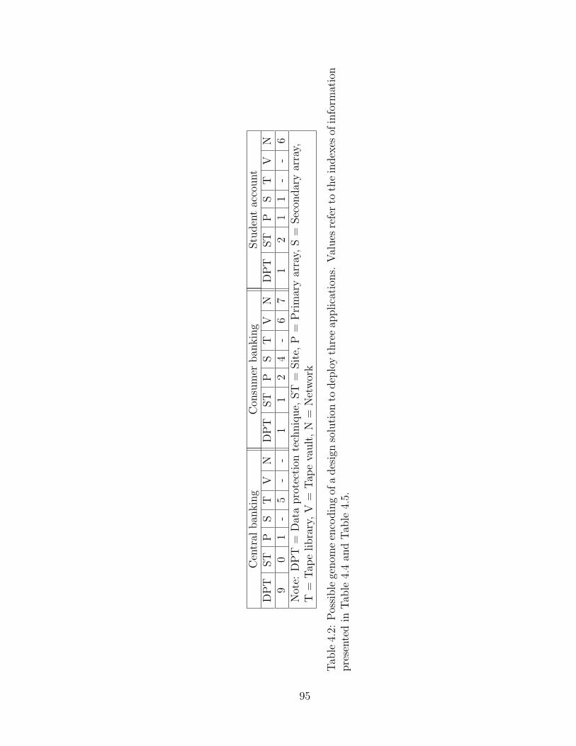
Cen

tral

ban

kin

gC

onsu

mer

ban

kin

gStu

den

tac

count

DP

TST

PS

TV

ND

PT

ST

PS

TV

ND

PT

ST

PS

TV

N9

01

-5

--

11

24

-6

71

21

1-

-6

Not

e:D

PT

=D

ata

pro

tect

ion

tech

niq

ue,

ST

=Sit

e,P

=P

rim

ary

arra

y,S

=Sec

ondar

yar

ray,

T=

Tap

elibra

ry,

V=

Tap

eva

ult

,N

=N

etw

ork

Tab

le4.

2:P

ossi

ble

genom

een

codin

gof

ades

ign

solu

tion

todep

loy

thre

eap

plica

tion

s.V

alues

refe

rto

the

index

esof

info

rmat

ion

pre

sente

din

Tab

le4.

4an

dT

able

4.5.

95

Genetic Algorithm

Algorithm 6 describes the details of our implementation of GA. The initial in-

dividuals are generated randomly to form the initial population. The maximum

population size is a user-tunable parameter currently set to a value of 10,000. The

algorithm is run for several generations until a terminating criterion is reached.

This criterion could be a limit on execution time or a limit on the number of

successive generations, or a situation in which the solution has not improved for a

defined amount of time. At each successive generation, the fitness of each individ-

ual is computed. Here the fitness function is the total cost of the design solution.

A lower cost means a more fit individual. The unfit individuals are discarded

stochastically (Line 5 in Algorithm 6) to keep diversity in the population and

prevent the algorithm from getting stuck at local minima.

Algorithm 6 Genetic algorithm to design dependable storage1: Let

N be total number of individuals in the populationfi Fitness of an individual i, where fi is the total cost of the design

2: while (timerunning < timeallotted) do3: Compute fitness fi for each i ∈ N4: Sort the individuals in a nondecreasing order based on fi {fmin is the fittest

individual}5: For each i, N − n ≤ i < N , delete i with probability p, where (M < n

2)

6: Generate n2

new individuals using mutation7: Generate n

2new individuals using crossover

8: end while

9: Sort the individuals in a nondecreasing order based on fi10: Return the individual(s) with value equal to fmin

The next two steps in the algorithm are used to generate the individuals for

the next generation of the population (Lines 6 and 7 in Algorithm 6). Mutation

is a process by which the algorithm creates a new individual from a parent by

choosing a random number of applications in the genome string and modifying all

96

the genes of these chosen applications. We pick a random number (user-defined

probability) of applications and replace all the genes (qualitative and associated

quantitative parameter values) during the mutation process. Crossover is a pro-

cess by which the algorithm creates a new individual (offspring) by recombining

substrings of the encoded genome strings from each individual parent. We pick

a random number (user-defined probability) of applications and cross-over (ex-

change parameter values for) all the genes for those applications. That enables

the algorithm to modify the characteristics of an individual (the qualitative pa-

rameters) on a per-application basis.

97

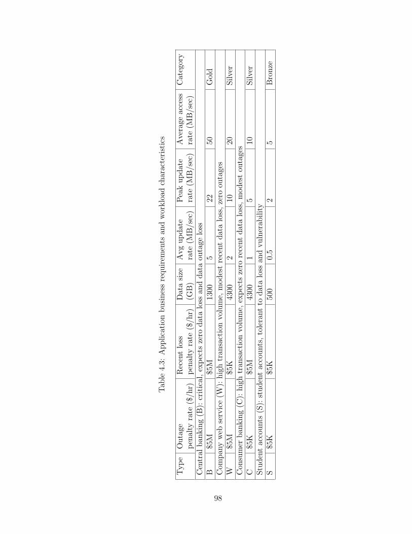
Tab

le4.

3:A

pplica

tion

busi

nes

sre

quir

emen

tsan

dw

orklo

adch

arac

teri

stic

s

Typ

eO

uta

geR

ecen

tlo

ssD

ata

size

Avg

up

dat

eP

eak

up

dat

eA

vera

geac

cess

Cat

egor

yp

enal

tyra

te($

/hr)

pen

alty

rate

($/h

r)(G

B)

rate

(MB

/sec

)ra

te(M

B/s

ec)

rate

(MB

/sec

)C

entr

alban

kin

g(B

):cr

itic

al,

exp

ects

zero

dat

alo

ssan

ddat

aou

tage

loss

B$5

M$5

M13

005

2250

Gol

dC

ompan

yw

ebse

rvic

e(W

):hig

htr

ansa

ctio

nvo

lum

e,m

odes

tre

cent

dat

alo

ss,

zero

outa

ges

W$5

M$5

K43

002

1020

Silve

rC

onsu

mer

ban

kin

g(C

):hig

htr

ansa

ctio

nvo

lum

e,ex

pec

tsze

rore

cent

dat

alo

ss,

modes

tou

tage

sC

$5K

$5M

4300

15

10Silve

rStu

den

tac

counts

(S):

studen

tac

counts

,to

lera

nt

todat

alo

ssan

dvuln

erab

ilit

yS

$5K

$5K

500

0.5

25

Bro

nze

98

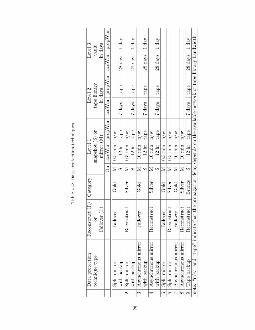
Tab

le4.

4:D

ata

pro

tect

ion

tech

niq

ues

Dat

apro

tect

ion

Rec

onst

ruct

(R)

Cat

egor

yL

evel

1L

evel

2L

evel

3te

chniq

ue

typ

eor

snap

shot

(S)

orta

pe

libra

ryva

ult

Fai

love

r(F

)m

irro

r(M

)in

day

sin

day

sO

nac

cWin

pro

pW

inac

cWin

pro

pW

inac

cWin

pro

pW

in

1Split

mir

ror

Fai

love

rG

old

M0.

5m

inn/w

wit

hbac

kup

S12

hr

tap

e7

day

sta

pe

28day

s1

day

2Split

mir

ror

Rec

onst

ruct

Silve

rM

0.5

min

n/w

wit

hbac

kup

S12

hr

tap

e7

day

sta

pe

28day

s1

day

3A

synch

ronou

sm

irro

rF

ailo

ver

Gol

dM

10m

inn/w

wit

hbac

kup

S12

hr

tap

e7

day

sta

pe

28day

s1

day

4A

synch

ronou

sm

irro

rR

econ

stru

ctSilve

rM

10m

inn/w

wit

hbac

kup

S12

hr

tap

e7

day

sta

pe

28day

s1

day

5Split

mir

ror

Fai

love

rG

old

M0.

5m

inn/w

6Split

mir

ror

Rec

onst

ruct

Silve

rM

0.5

min

n/w

7A

synch

ronou

sm

irro

rF

ailo

ver

Gol

dM

10m

inn/w

8A

synch

ronou

sm

irro

rR

econ

stru

ctSilve

rM

10m

inn/w

9T

ape

bac

kup

Rec

onst

ruct

Bro

nze

S12

hr

tap

e7

day

sta

pe

28day

s1

day

not

e:“n

/w”

and

“tap

e”in

dic

ate

that

the

pro

pag

atio

ndel

aydep

ends

onth

eav

aila

ble

net

wor

kor

tap

elibra

ryban

dw

idth

.

99

Tab

le4.

5:R

esou

rce

des

crip

tion

(unam

orti

zed

purc

has

epri

ce)

Res

ourc

eC

lass

Fix

edIn

crem

enta

lco

st($

)T

otal

amou

nt

ofC

apac

ity

BW

typ

eco

stB

Wp

erunit

per

unit

capac

ity

BW

per

unit

per

unit

($)

(MB

/s)

capac

ity

BW

(unit

s)(u

nit

s)(G

B)

(MB

/s)

1D

isk

arra

y(X

P10

24)

Hig

h37

5,00

051

287

2310

2414

325

2D

isk

arra

y(E

VA

8000

)M

ed12

3,00

025

637

2051

214

310

3D

isk

arra

y(M

SA

1500

)L

ow12

3,00

012

837

2012

814

38

4T

ape

Lib

rary

Hig

h14

1,00

024

0018

,400

720

2460

120

5T

ape

Lib

rary

Med

76,0

0040

010

,400

120

460

120

6N

etw

ork

Hig

h64

050

0,00

032

207

Net

wor

kM

ed16

020

0,00

016

108

Com

pute

Hig

h12

5,00

09

Sit

e1,

000,

000

100

Tab

le4.

6:D

ata

pro

tect

ion

solu

tion

sch

osen

by

des

ign

tool

for

pee

rsi

tes

App

Typ

eD

ata

pro

tect

ion

tech

niq

ue

Pri

mar

ysi

teSit

eP

1Sit

eP

2net

wor

kar

ray

tap

elib

arra

yta

pel

ib1

BA

sync

mir

ror

(F)

wit

hbac

kup

P2

√√

√√

2C

Sync

mir

ror

(R)

wit

hbac

kup

P1

√√

√√

3W

Asy

nc

mir

ror

(F)

wit

hbac

kup

P1

√√

√√

4S

Tap

ebac

kup

P1

√√

5B

Asy

nc

mir

ror

(F)

wit

hbac

kup

P1

√√

√√

6C

Sync

mir

ror

(R)

wit

hbac

kup

P1

√√

√√

7W

Sync

mir

ror

(F)

wit

hbac

kup

P1

√√

√√

8S

Tap

ebac

kup

P2

√√

101

4.4.4 Environment

Our experiments use a common set of input parameters for application business re-

quirements and workload characteristics, data protection technique alternatives,

and resource capabilities and costs. Table 4.3 describes the application classes

used in our experiments. The penalty rate magnitudes are based on market re-

search [22]. Table 4.4 summarizes the data protection alternatives considered by

our algorithms. Table 4.5 enumerates resource characteristics for disk arrays, tape

libraries, network links and data center sites.

The likelihoods of an application data object failure (e.g., due to user error

or software malfunction), a disk array failure, and a data center site disaster are

set to once in three years, once in five years, and once in ten years, respectively.

For an application data object failure, we model the delay from when the failure

occurs to when the failure is discovered as ten hours.

All our experiments were carried out on a 256-node Linux cluster running on

the 2.6.9 kernel. Each node on the cluster is an AMD dual-processor machine

with 1 to 8GB of RAM connected through an InfiniBand network to the cluster.

The experiments were submitted as jobs to the cluster, where each job used a

single processor core. All experiments were executed for thirty minutes, and the

experiments were repeated thirty times. Each experimental result is the average

of the thirty runs, and the error bar represents a 95% confidence interval.

4.4.5 Simple Case Study: Peer Sites

To build our intuition about the solution space and the algorithms’ behavior, we

modeled a simple peer environment in which a pair of sites serves as the primary

site for a fraction of the applications and as a secondary site for the remaining

fraction of the applications. This scenario models a multi-site corporation or

102

1000

10000

100000

1000000

10000000

100000000

1000000000

0 250 500 750 1000 1250 1500 1750 2000 2250 2500 2750 3000 3250 3500 3750 4000 4250 4500 4750

Overall solution costs (millions $)

Fre

qu

ency

dis

trib

uti

on

Figure 4.3: Distribution of data protection solution costs of peer sites. Note thatthe Y axis is in log scale.

service provider.

We want to deploy eight applications on two peer sites, P1 and P2. Each

site can accommodate a maximum of two disk arrays (e.g., one high-end and one

low-end), a single tape library, and compute resources for eight applications. A

network with a capacity of up to 32 links connects the two sites.

Solution Space Insight

The parameter space of the dependable storage solution problem is extremely

large. Even the partial qualitative parameter space is about da ∗at, where d is the

number of primary disk arrays, a is the number of applications deployed, and t is

the number of data protection techniques. Figure 4.3 illustrates the distribution

of the peer sites’ solution space, which is determined by exhaustive exploration

of the design space. The size of the design space, considering only the qualitative

variables, is about 43.1 billion alternative configurations (d = 2, a = 8, t = 9).

Exploring the entire space takes about 280 computer hours. We observe that

solution costs vary by more than an order of magnitude across the distribution.

103

The goal of any heuristic is to quickly identify solutions on the left side of the

graph.

The distribution of solution costs is multimodal, where each mode corresponds

to a different set of choices being made for the design trade-offs. Low-cost solutions

protect applications with stringent requirements by increasing resource outlay

expenditures to decrease penalties. Protection for applications with more relaxed

requirements may be able to leverage the resources already in place for the more

stringent applications. Higher-cost solutions provide inadequate protection for

workloads with stringent requirements, and thus incur high penalties.

Solution to Case Study

0

50

100

150

200

Humanheuristic

Randomsearch

Geneticalgorithm

Design solver Optimalsolution

Ove

rall

solu

tio

n c

ost

s (m

illio

ns

$)

Data loss penalty costs Data outage penalty costs Outlay costs

Figure 4.4: Comparison among costs of search heuristic solutions and optimalsolution for peer sites running eight applications

Table 4.6 describes the data protection solution chosen for each application

by the automated design tool. As expected, applications with high data outage

penalty rates always employ failover for recovery. It is cheaper to provide ad-

ditional network links and compute resources to support failover than to incur

penalties for recovery techniques that take longer. All applications employ some

104

form of tape backup to support recovery from user errors and software malfunc-

tions.

Counter to intuition, we note that the central banking applications (1 and

5) use asynchronous mirroring instead of synchronous mirroring. The increased

recent data loss penalty for asynchronous mirroring is small, relative to the outlay

for the additional resources to support synchronous mirroring. Therefore, the de-

sign tool chooses asynchronous mirroring over synchronous mirroring. Figure 4.4

compares the outlay, data loss penalty, and data outage penalty costs of the four

different heuristics against the cost of the optimal solution.

For our case study, the design tool’s solution costs roughly 1.5 times less than

either the human heuristic’s solution or the random heuristic’s solution. Here,

the design tool’s search heuristic found one of the optimal solutions for the case

study. Due to the simplicity of the case study, the solutions identified by the

design solver and the genetic algorithm have similar costs. In the next section, we

will see the impact of increasing the number of decision variables on the quality

of the design solution.

4.4.6 Scalability of Design Solver

Having developed an intuitive understanding of the solution space, in this sec-

tion we now examine the quality of solutions found by each of the algorithms as

we scale the number of applications in a larger environment. The environment

contains four sites, each with the potential to support two types of disk arrays,

one tape library, compute resources, and six network links that connect all the

sites together. We assume that we are working with the classes of applications

described in Table 4.3 and the failure model used in Section 4.4.4. We scale the

environment by adding four applications at a time, one from each class.

105

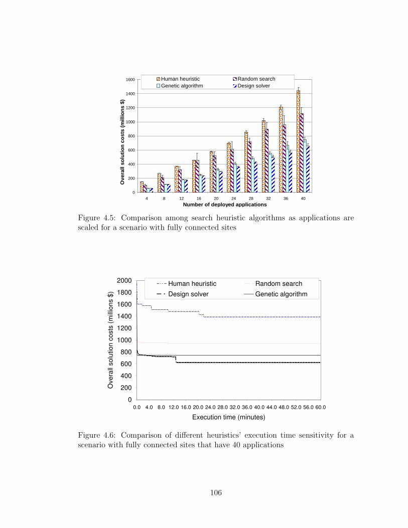
0

200

400

600

800

1000

1200

1400

1600

4 8 12 16 20 24 28 32 36 40

Number of deployed applications

Ove

rall

solu

tio

n c

ost

s (m

illio

ns

$)

Human heuristic Random searchGenetic algorithm Design solver

Figure 4.5: Comparison among search heuristic algorithms as applications arescaled for a scenario with fully connected sites

0

200

400

600

800

1000

1200

1400

1600

1800

2000

0.0 4.0 8.0 12.0 16.0 20.0 24.0 28.0 32.0 36.0 40.0 44.0 48.0 52.0 56.0 60.0

Execution time (minutes)

Ove

rall

so

lutio

n c

osts

(m

illio

ns $

)

Human heuristic Random search

Design solver Genetic algorithm

Figure 4.6: Comparison of different heuristics’ execution time sensitivity for ascenario with fully connected sites that have 40 applications

106

0.0

0.5

1.0

1.5

2.0

2.5

3.0

3.5

4.0

4.5

5.0

0.05 0.1 0.2 0.33 0.66 1

Data object failure likelihood

Co

st ra

tio

Data loss penalty costs Data outage penalty costs Outlay costs

Figure 4.7: Design solver’s solution sensitivity to likelihood of data object failure

0.0

0.5

1.0

1.5

2.0

2.5

3.0

3.5

4.0

4.5

5.0

0.05 0.2 0.5 0.33 0.66 1

Disk failure likelihood

Co

st ra

tio

Data loss penalty costs Data outage penalty costsOutlay costs

Figure 4.8: Design solver’s solution sensitivity to likelihood of disk failure

0.0

0.5

1.0

1.5

2.0

2.5

3.0

3.5

4.0

4.5

5.0

0.05 0.1 0.2 0.33 0.66 1

Site failure likelihood

Co

st ra

tio

Data loss penalty costs Data outage penalty costsOutlay costs

Figure 4.9: Design solver’s solution sensitivity to likelihood of site failure

107

Figure 4.5 compares the scalability of the four algorithms for the described

environment. The design tool consistently provides better solutions than the

other heuristics. More specifically, the design solver’s solutions are 1.9 times to

2.6 times cheaper than those chosen by the human heuristic, 1.7 times to 1.9 times

cheaper than those chosen by the random search heuristic, and up to 1.2 times

cheaper than those chosen by the genetic algorithm. While the human heuristic

fares poorly due to its inefficient layout strategy, the solutions provided by the

random search heuristic and the genetic algorithm deteriorate as the solution space

becomes larger. The key difference between the design solver search strategy and

other approaches is its ability to determine the sensitivity of the final solution to

the decision variable values, and to make decisions for the variables that have a

larger impact on the design solution. In particular, the GA chooses the decision

variables by looking at the overall cost of the system. As the number of design

decision variables increases, this single overall cost metric masks the intricate

relationships among the values of the variables. The design solver tracks these

relationships, thus enabling it to determine good decision variable values to obtain

near-optimal designs more quickly. Thus, the cost gap between the solution chosen

by the design solver and the solutions chosen by the other heuristics tends to

increase as the number of decision variables increases.

4.4.7 Sensitivity to Execution Time

Figure 4.6 illustrates the sensitivity of the four heuristics’ solution quality to exe-

cution time. In our experiment, 40 applications were deployed on 4 fully connected

data center sites. The cost of the initial solution obtained by each heuristic ranged

from 800 million dollars to 1.9 billion dollars. The figure traces the cost of the

minimal overall cost design solution for each of the heuristics by sampling the

108

cost every 4 seconds until the terminating time of twelve hours. As we observe

no further improvements after 30 minutes, we focus on the improvement gained

in the first hour.

Although we traced the improvement in solution quality as a function of al-

gorithm execution time for a large number of experiments (e.g., 30 replications

for each algorithm for three different combinations of applications, or a total of

360 experiments), we present detailed results only for a single experiment for each

heuristic algorithm as other experiments showed similar trends. The random

search heuristic is very simple in nature, and the solutions it determines depend

largely on chance. Given sufficient time, the random search will determine the

optimal solution, while the human heuristic might never find the optimal solution

because of the limited rules of thumb it employs in decision-making to explore

large design spaces. The genetic algorithm and design solver are able to quickly

reduce the costs in a few seconds using their specific strategies. As the design

problem is scaled to larger sizes, the GA takes significantly longer to converge

than the design solver does because the GA does not capture relationships among

input decision variables. Its evolutionary strategy is completely independent of

the decision variables and depends only on the objective function value. Unlike

the GA, the design solver attempts to build a distribution of the decision vari-

ables that result in good solutions, which allows our approach to converge to

better solutions.

4.4.8 Sensitivity to Failure Likelihood

In this section, we explore the sensitivity of the design solver’s solutions to fail-

ure likelihood. These experiments were conducted using the environment from

the simple case study in Section 4.4.5 and the base application characteristics

109

described in Table 4.3. We varied the likelihood of all failure scopes from once in

twenty years to once per year. When they were not being varied, the frequencies

of data object, disk, and site failures were fixed at once in three years, once in

five years, and once in ten years, respectively, as described in Section 4.4.4.

Figures 4.7, 4.8, and 4.9 plot the design tool’s solution cost ratio as a function

of the likelihood of data object failures, disk array failures, and site disasters,

respectively. For all figures, the cost ratio is calculated relative to the default

failure likelihood (0.33 for data objects, 0.2 for disk failures, and 0.1 for site

failures). The columns are stacked to make it easy to view the relative change

in overall costs. We observe that increasing the failure likelihood of disk or site

failures increases the data outage penalty. The disk or site failures increase the

recovery time because of the resource contention among the multiple recovering

applications.

That failure sensitivity analysis lets a human storage architect determine the

range of failure likelihoods for which the design solver’s solution would adequately

protect the applications. In this case study, the threshold is between 0.65–0.75

for data object, disk, and site failures. Using that information, a storage architect

can design solutions suitable for the observed likelihood of failure.

4.4.9 Sensitivity to Application Workload Characteristics

Our final experiments examined the sensitivity of the design solver’s choices to

variations in the applications’ bandwidth and capacity characteristics. These

experiments were conducted using the environment from the simple case study in

Section 4.4.5 and the base application characteristics described in Table 4.3. In the

capacity experiments, the capacities of all applications’ datasets were scaled by a

constant factor. In the bandwidth experiments, all of the bandwidth parameters

110

$0

$20

$40

$60

$80

$100

$120

$140

$160

1 5 10 15 20 25 30 35 40 45 50

Bandwidth scale factor

Ove

rall

solu

tio

n c

ost

s (m

illio

ns

$)Outlay costs Data outage penalty costsData loss penalty costs

Figure 4.10: Design solver’s solutionsensitivity to application bandwidthrequirements without resource con-straints

$0

$20

$40

$60

$80

$100

$120

$140

$160

$180

$200

1 5 10 15 20 25 30 35 40 45 50

Bandwidth scale factor

Ove

rall

solu

tio

n c

ost

s (m

illio

ns

$)

Outlay costs Data outage penalty costsData loss penalty costs

Figure 4.11: Design solver’s sensitiv-ity to application bandwidth require-ments with resource constraints

0.0

0.5

1.0

1.5

2.0

2.5

3.0

1 5 10 15 20 25 30 35 40 45 50

Bandwidth scale factor

Co

st r

atio

Data outage penalty cost ratio Outlay cost ratioData loss penalty cost ratio

Figure 4.12: Cost ratio with respectto solution cost for base bandwidthrequirements (scale factor = 1) with-out resource constraints

0

20

40

60

80

100

120

140

1 5 10 15 20 25 30 35 40 45 50

Capacity scale factor

Co

st r

atio

Data outage penalty cost ratio Outlay cost ratioData loss penalty cost ratio

Figure 4.13: Cost ratio with respectto solution cost for base capacity re-quirements (scale factor = 1) with re-source constraints

111

0.0

0.5

1.0

1.5

2.0

2.5

3.0

3.5

4.0

1 5 10 15 20 25 30 35 40 45 50

Bandwidth scale factor

Co

st r

atio

Data outage penalty cost ratio Outlay cost ratioData loss penalty cost ratio

Figure 4.14: Cost ratio with respectto solution cost for base bandwidthrequirements (scale factor = 1) withresource constraints

$0

$200

$400

$600

$800

$1,000

$1,200

$1,400

1 5 10 15 20 25 30 35 40 45 50

Capacity scaling factor

Ove

rall

solu

tio

n c

ost

s (m

illio

ns

$)

Outlay costs Data outage penalty costsData loss penalty costs

Figure 4.15: Design solver’s solutionsensitivity to application capacity re-quirements with resource constraints

in Table 4.3 were scaled by a constant factor. We run the design solver thirty times

for each scale factor, and present the results as an average plus a 95% confidence

interval.

The results from the first set of experiments, shown in Figures 4.10 and 4.12,

show the behavior of the solution as application bandwidth requirements are

scaled, with no constraints on the resources. As expected, we see that outlay costs

increase as the peak bandwidth requirements of all applications are scaled. Data

outage penalty costs increase slightly with increasing bandwidth requirements,

because less network bandwidth is available. A separate set of experiments (not

shown) in which capacity requirements were scaled, resulted in similar trends.

In the next set of experiments, we constrained the maximum amount of re-

sources that could be deployed at each site. In the bandwidth scaling experiments,

we constrained the amount of available network bandwidth to 64 links, totaling

1280MB/sec. In the capacity scaling experiments, we restricted the number of

tape libraries to twelve; when fully populated with 24 tape drives, a tape library

is capable of backing up 200 TB of data in two hours.

Figures 4.15 and 4.13 explore the sensitivity of solution cost to increasing

112

application dataset capacity. As expected, the overall solution cost increases with

increasing capacity requirements, driven by increases in data outage and data loss

penalty costs. For small increases in capacity, it is more cost-effective to use the

same (or similar) resources and suffer a slight increase in the outage duration (due

to the need to reconstruct additional data). For slightly larger capacity increases,

it is more cost-effective to add resources than to incur additional data outage

penalties. We observe this behavior in Figure 4.15 as a piecewise linear overall

cost function, with regions of scale factors 1 to 10, 15 to 20, and 25 to 50. As

seen in Figure 4.13, outlay costs increase as a step function, while the data outage

penalty costs increase for the scale factors at a single level of the step function.

As resource limits are approached for the larger-capacity scale factors (e.g., 25 to

50), it may no longer be possible to maintain the same data protection choices

as for lower-capacity scale factors. For example, backup windows may need to be

increased from two hours to four hours, due to tape library bandwidth limitations.

Those decisions result in increased recent data loss and associated penalty costs for

the highest-capacity scale factors. We note that the increase in data outage and

data loss penalty costs isn’t a smooth linear function, because different qualitative

data protection techniques (e.g., remote mirroring with failover vs. backup) are

chosen for the different workloads.

Figures 4.11 and 4.14 show the sensitivity of overall solution cost to increas-

ing application bandwidth requirements, under resource constraints. We observe

three regions of behavior: scale factors 1 to 5, scale factors 10 to 45, and scale

factor 50. In each region, the design solver increases network bandwidth (thus

increasing outlay costs) to accommodate the increasing application bandwidth re-

quirements, until a network bandwidth resource limit is reached. Between regions,

the solver must change its data protection technique choices to ease network band-

width requirements, in the face of increasing application bandwidth requirements.

113

In particular, the solver must shift some of the applications from synchronous

mirroring, which requires peak application update bandwidth, to asynchronous

mirroring, which requires only average application update bandwidth, thus re-

ducing network demand. That shift in storage design results in a slight increase

in data loss penalty, because an asynchronous mirror is slightly out-of-date rela-

tive to a synchronous mirror. We also note that as the outlay costs increase, the

outage penalties decrease (from scale factor 1 to 5 and again from scale factor 10

to 45). With the shift from synchronous mirroring to asynchronous mirroring as

the bandwidth scale factor increases, the recovery techniques have more available

bandwidth to recover the failed application data, which reduces the recovery time.

Although the exact costs and piecewise linear regions in the graphs are depen-

dent on the business requirements, workload parameters, and device parameters

used in the experiments, we believe that the described trends generalize to a

broader range of environments. A more comprehensive sensitivity analysis is an

area for future work.

114

CHAPTER 5

CONCLUSION

This dissertation makes the following two fundamental contributions to explore

alternative design configurations. In situations where it is practical to exhaus-

tively explore design parameter space, this dissertation provides a new approach,

called Simultaneous Simulation of Alternative System Configurations (SSASC),

to evaluate dependability models that combines adaptive uniformization in simu-

lation with the SCMS technique. SSASC showed that a significant speed-up can

be achieved (up to 2 orders of magnitude for the case-study models discussed in

this dissertation) compared to traditional discrete-event simulation to evaluate all

alternative configurations. In situations where complete design exploration is not

practical, this dissertation provides an intelligent search space exploration tech-

nique, called Design Solver, to efficiently determine near optimal solutions. The

design solver is able to design configurations and set parameter values of the case-

study model of designing data-protection techniques for data-center such that the

solution reduces the overall cost of the system by a factor of 2, when compared

to existing solutions.

5.1 Evaluating Alternative Configurations

In order to provide efficient simulation algorithm compared to TDES, SSASC

manages the enabled event set using an unified adaptive clock algorithm for all

alternative configurations. In addition, efficient data structures are used to man-

115

age system model’s state access and update operations to further enables efficient

simulation. Furthermore, correlation of reward measures among the trajectories

for the alternative configurations due to inherent use of common random num-

bers further improves the efficiency of SSASC. Even though there is a coupling

between the state update and the clock-event generation, the structural and be-

havioral similarity that all configurations display provides an opportunity to re-

duce the computational cost of updating and maintaining the enabled event set.

The state-updating mechanisms of the configurations are independent, allowing

comparison of the configurations and enabling the possibility of making decisions

at the run time of the simulations. We thus have provided a fast, efficient way to

evaluate a large number of alternative design choices. Furthermore, we presented

a technique to extend SSASC beyond models with exponential distributions to

models with general distribution with bounded hazard rates.

One of the goals of the simultaneous simulation algorithm is to aid the use

of simulation as an objective and/or constraint function in the optimization of

stochastic systems. Stochastic optimizations are often nonlinear, and it is not

possible to quantify them analytically. That eliminates the possibility of exact

calculations of local gradients upon which traditional optimization solvers rely.

Our approach provides a way to explore a large number of parameter values,

which could potentially allow us to use alternative approaches, such as compass

search, direct search, or other unconstrained optimization, more efficiently [51].

Furthermore, as the configurations are simulated, our approach provides a seam-

less framework that enables us to prune out designs that would not meet the

required objectives. The pruning criteria can be defined to eliminate uninterest-

ing designs to improve the efficiency of the simulations.

116

5.2 Exploring Alternative Configurations

Design Solver is a technique to determine near-optimal designs using search heuris-

tics for the class of design problems where parameter values can be both qualitative

and quantitative. We decompose the problem into two stages, first determining

the qualitative parameter values (such as what data protection techniques should

be applied to each application), and then determining quantitative parameter val-

ues (such as how to set the configuration parameters for these techniques and the

resources used by the storage configuration). That decomposition reduces the size

of the search space, allowing our algorithm to focus on the most relevant regions

to achieve a near-optimal solution.

We compare the operation of our design tool’s search heuristic with the ad

hoc approaches used by human architects today, and with a randomized search

heuristic and a genetic algorithm meta-heuristic. For the examples we consider,

our automated design framework consistently generates solutions that are better

than the solutions provided by the other competing approaches. In the case of

the human heuristic, our design tool’s solutions decrease overall costs by a factor

of 2.

In a holistic view of the search heuristic presented in Chapter 4, the algorithm

has strong parallels with general search strategies, such as genetic algorithms

especially with tabu search. The optimizer starts with no information about

the objective function or the underlying structure of the design parameter space.

The algorithm picks designs that need to be evaluated by selecting the values

for decision variables using a uniform distribution. As the optimizer continues

to evaluate the system, the relative quality of the final design is determined with

respect to the decision parameter values. Using that information, the search

algorithm changes the distribution for design selection from uniform distribution

117

to one more concentrated around input values that results in successful designs.

Unlike tabu search, it does not maintain a forbidden list, but rather lowers the

likelihood of choosing a particular value that has been shown to result in bad

overall design, thereby providing a positive probability to determine the optimal

design.

5.3 Improving Design Evaluation as a System Designer

While this dissertation has focused on improving the efficiency of evaluating the

system during its design phase, it has emphasized the engineering aspect of speed-

ing up the design process. However, the design process and methodology used to

evaluate system design does in fact play an important role to obtain optimal de-

sign quickly. The system design team’s past experience on designing systems,

smart management of the design constraints, and ability to conceptualize, spec-

ify, document, and present design solutions plays an important role in developing

optimal solutions to design problems.

In Appendix B, we provide one such design process using a case study analysis

of the CFS in Abe’s cluster at NCSA, for which we show how system designers

do not have to depend on their past system expertise to determine the potential

drawbacks in their system design. We show that system modeling, combined with

data analysis from real systems with similar design and requirement specifications,

can provide better insight in designing future systems. Here, the log/data analysis

allows system designers to extract certain parameter values for the system mod-

els of the design, which otherwise would have to be estimated using sensitivity

analysis. Therefore, in addition to providing better insight, such a design process

enables faster evaluation of system models by reducing the potential design space

or the numbers of alternative configurations. Such a process methodology could

118

be an added boon to engineering techniques discussed in this dissertation, as the

growth of the size of the design space is outpacing the development of techniques

to evaluate the design space.

5.4 Final Comments

We expect that our technique will open up new research issues and ideas in opti-

mization of simulations, sensitivity analysis, and parameter optimization of sys-

tems. SSASC also introduces an incentive to look at a new programming paradigm

for describing simulation models. The current programmer’s view of a simulation

execution sees it as a single model and its behavior. The speed-up of this approach

is greatly enhanced if the programmer understands programmatic dependencies

and interactions between alternative configurations, even though they’re stochas-

tically independent. Development of a programming paradigm to maximize the

utility of the speed-up achieved by the algorithm would be an interesting research

area to explore in future.

While the design solvers modeling and solution techniques to explore a large

number of alternative configurations focused on reliable storage system design,

the search heuristic is equally applicable to other design problems with optimal

resource allocation under dependability and performance constraints. One could

also envision a tool that is similar to Mobius in its design philosophy: a framework

that would enable multiple modeling formalisms, solution techniques, and design

space exploration techniques, to be synergistically combined to provide a powerful

automated design evaluation tool.

119

APPENDIX A

2-STAGE SELECTION OF THE BESTALTERNATIVE CONFIGURATION

Let Ri be the reward variable of interest of alternative configuration Ei. Let

µi be its mean. Let Dij be defined as the difference between reward measures.

In particular, Dij = Ri − Rj, for alternative configurations, Ei and Ej, where

0 ≤ i < j < N . Let µij be the mean of the difference.

Due to inherent randomness of the observation, the user cannot expect to pick

the best configuration with probability 1. Instead, the user can pre-specify the

probability of choosing the best alternative configuration (BAC) = p∗. Further-

more, to prevent the method from computing a large number of replications that

differentiate two configurations, the user needs to specify indifference amount d∗.

d∗ allows the method to be indifferent to configurations that satisfy the criterion

µi − µj ≤ d∗.

In the first stage, the SSASC executes a fixed number of replications or batches

of simulations, n0, of all N alternative configurations. Let Dk represent the reward

measure obtained from the kth replication or batch. The means and variances of

the first stage are computed as follows

µij(n0) =

∑k=n0

k=1 Dkij

n0(A.1)

S2ij(n

0) =

∑k=n0

k=1

[Dkij − µij(n0)

]2n0 − 1

(A.2)

In the second stage, we compute the total number of batches, nfi , that are

120

necessary for each alternative configuration i to make sure that the measures

computed on these system models are within the specified confidence level in-

tervals. We use nf which is the maximum of all nfi to perform the next set of

simulations

nf = maxm=0..

N(N−1)2

m

{n0 + 1,

(h2 ∗ S2

ij(n0)

(d∗)2

)}(A.3)

Here, h can be numerically computed, since F and f are CDF and PDF of a

t-distribution, which can be assumed to be Normally distributed,

p∗ =

∫ ∞−∞

[F (t+ h)](N−1)N

2 f(t)dt (A.4)

Now, the means for reward measures for the remaining batches are defined as

µij(nf − n0) =

∑k=nfik=n0+1D

kij

nf − n0(A.5)

where the weights are

W1ij =n0

nf

[1 +

√1− nf

n0

(1− (nf − n0)(d∗)2

h2S2ij(n

0)

)](A.6)

and W2ij = 1−W1ij for 0 ≤ j ≤ i ≤ N . The weighted sample means are

µij(nf ) = W1ij ∗ µij(nf − n0) +W2ij ∗ µij(n0) (A.7)

More details on 2-stage selection can be referred from [53].

121

APPENDIX B

ABE: CLUSTER FILE SYSTEM

In this Appendix1, we present the details on how the SAN model (See Section B.5)

of Abe’s cluster file system (CFS) was developed to evaluate/predict the reliabil-

ity/availability of the BlueWaters CFS, which was in its design phase at the time

of the study. The parameter values for the SAN model were extracted from data-

logs of the Abe cluster system. Using those parameter values, we developed the

SAN models to predict the behavior of the BlueWaters CFS. In this chapter, we

focus on the remaining details of modeling Abe’s CFS architecture, which makes

this case study realistic [26]. Specifically, the rest of this chapter is organized as

follows.

Section B.1 presents the compelling reasons and motivation for using our ap-

proach in modeling, evaluation, and prediction of measures of interest of large

systems. Section B.2 outlines other related research that has attempted to pre-

dict metrics of future designs using existing designs. Section B.3 provides a brief

overview of the CFS with the detailed system architecture of the Abe cluster at

NCSA. Section B.4 presents Abe’s failure log data with details on the analysis

and extraction of parameter values for the Mobius models covered in Section B.5.

Section B.6 covers results and analysis, and Section B.7 concludes.

1This research was conducted in collaboration with Eric W. D. Rozier, Anthony Tong, andWilliam H. Sanders, and presented at Anchorage in June 2008 at the 38th Annual IEEE/IFIPInternational Conference on Dependable Systems and Networks.

122

B.1 Motivation

Historically, scientific computing has driven large-scale computing resources to

their limits. Towards the end of the current decade, we are likely to achieve

petascale computing. While supercomputer performance has improved by over

two orders of magnitude every decade, the performance gap between the indi-

vidual nodes and the overall processing ability of an entire system has widened

drastically [88]. This has led to a shift in the paradigm of supercomputer design,

from a centralized approach to a distributed one that supports heterogeneity.

While most high-performance computing environments require parallel file sys-

tems, there have been several file systems, such as GPFS [74], PVFS2 [96], and

Lustre [11], that have been specifically proposed to support very large-scale sci-

entific computing environments.

As the number of individual computing resources and components becomes

very large, the frequency of failure of components within these clusters and the

propagation of these failures to other resources are important concerns to high-

performance computing applications. Failures can be caused by many factors:

(a) transient hardware faults due to increased chip density, (b) software error

propagation due to a large buggy legacy code base, or (c) manufacturing defects

and environmental factors such as temperature or humidity.

Recent literature on failure analysis of BlueGene/L discusses various causes

of increased downtime of supercomputers [57]. It has been well-established that

elimination of failures is impossible; it is only feasible to circumvent failures and

to mitigate their effects on a system’s performance. The standard approach to the

mitigation of a failure is to checkpoint the application at regular intervals. Long

et al., however, showed that checkpointing has a large impact on the performance

of very large computer clusters with large numbers of nodes [95].

123

Increasing the number of compute servers in a cluster almost always increases

the size of the desired storage subsystem. Depending on the type of parallel

file system, that means an increase in the number of file servers that could accept

requests from the compute servers to keep up with I/O requests. Compute servers

and file servers have very different characteristics. First, a failure in a file server

needs more attention than a failure in a compute node. A compute server might

just be marked as unavailable until it is repaired, but a failed file server might

have to be reconstructed, or its state might need to be transferred to another file

server, depending on the replication strategy. Second, file servers are inherently

slower than compute servers, due to their I/O characteristics. This generally

makes file servers the bottleneck for the reliability and performance of a cluster.

Unfortunately, there has been a trend towards increasing failure rates for I/O

subsystems that is similar to that for overall petascale clusters. This increase in

failures can be attributed to the increase in the number of individual components

that are used to build the whole I/O subsystem. Recent studies have shown

that workload intensity is highly correlated to the failure rates [75, 90]. That

emphasizes the need for thorough analysis to understand the impact of the I/O

subsystems and their failures on petascale computers.

To address the research challenge of providing realistic prediction of petascale

file system availability, we took a two-pronged approach. First, we have obtained

the failure event log of the Abe cluster from the National Center for Supercom-

puting Applications (NCSA). The log contains the failures of individual nodes, file

server nodes, and the storage area network (StAN). We preprocessed the event

logs to determine various reward measures of interest corresponding to the file

system, such as the availability of the file system over the lifetime of the log and

the failure rate of jobs due to I/O failures and other transient failures. Then, we

built and refined stochastic models of the file system used by these clusters that

124

abstract much of the operations, while generating reward measures that are com-

parable to the real log events. We then scaled the models to reflect the scale and

magnitude of a future petascale computer and estimated the impact of current

I/O and file system designs on a petascale computer. Furthermore, we evaluated

strategies that could be used to mitigate the bottlenecks due to scaling of I/O file

system and cluster designs from current supercomputers to petascale computers.

Our analysis will give storage architects support to make informed design choices

as they build larger cluster file systems.

B.2 Related Work: Cluster File-systems

Cluster file-system performance has been studied by various organizations in col-

laboration with the vendors of cluster file-systems. Lawrence Livermore National

Laboratory (LLNL) worked with the Cluster File System Inc. to develop Lus-

tre [11]. The Google file system, Google-FS, is a scalable distributed file system for

large, distributed, data-intensive applications customized to Google’s needs [28].

The novelty is in the innovative fault-tolerance and high-aggregate performance

it shows while running on inexpensive commodity hardware. On the other hand,

International Business Machines Corp. (IBM) has developed the General Parallel

File System (GPFS), which provides a general-purpose file system with very high

scalability that satisfies the throughput, capacity, and reliability needs of very

large cluster computers with shared disk architectures, using Gigaplane switches

to connect disks with I/O nodes [74]. Margo et al. from the San Diego Super-

computer Center (SDSC) evaluated PVFS [12], Lustre and GPFS on their IA-64

cluster [59]. Their main conclusion was that file-system selection is strongly influ-

enced by site requirements. The effect is greatly magnified as clusters are scaled

to large sizes.

125

The estimation and prediction of the failure of file systems are crucial to under-

standing the overall performance of petascale computers. Past literature describes

several attempts to model and analyze different aspects of large-scale supercom-

puting systems.

B.2.1 Log/Trace-based Analysis

Recent literature using trace-based system analysis has shown that storage sub-

systems are prone to higher failure rates than their makers estimate because of

underrepresented disk infant mortality rates [76]. In addition to disk failures,

the analysis by Jiang et al. shows that interconnects and protocol stacks play

a significant role in storage subsystem failure [43]. It could be speculated that

storage subsystems show such trends due to the presence of mechanical moving

parts. Schroeder and Gibson studied the failure characteristics of large computing

systems to find that failure rates are proportional to the size of the system and are

highly correlated with the type and intensity of the workload running on it [75].

Our survivability analysis concurred with the finding from [76, 75]. Furthermore,

Liang et alinvestigated the failure events from the event logs from BlueGene/L

to develop failure prediction models to anticipate future fatal failures [57]. In

general, trace-based analysis of logs provides good metrics for evaluating and un-

derstanding working systems, but is limited to the scope of events represented by

the traces, making it difficult to study trends or behaviors not witnessed in the

traces.

B.2.2 Model-based Analysis

Wang et al˙ looked at the impact on system performance in the presence of corre-

lated failures as the systems are scaled to several hundred thousand processors [95].

126

Rosti et al. presented a formal model to capture CPU and I/O interactions in

scientific applications, to characterize system performance [72]. Oliner et al. in-

vestigated the impact of checkpointing overhead using a distribution obtained

from a real BlueGene/L log [68]. Some literature has discussed the importance of

distributing data across multiple disks to improve performance and reliability of

a file system [37]. While [68, 72, 95] and others have evaluated the cluster from a

system model perspective, it is often challenging to justify the insights from these

abstract models due to the unavailability for real systems and measures that can

be use to verify the validity of the results. Gafsi and Biersack studied the trade-off

between high reliability and low cost in streaming media files. They determined

that the mirroring scheme outperforms a parity-based scheme in reliability [23].

The use of simulation for evaluating a model provides the ability to predict

behavior and bottlenecks of future designs, but the accuracy of predictions may

often be compromised by assumptions of parameter values. Our approach focuses

on integrating trace based analysis with model-based evaluation to form a com-

bined approach, providing guidance to make informed choices for system design.

Using failure data from the logs of the cluster as parameter values, we verify our

models against the real system. We then analyze the impact of current design

choices when the system is scaled. Our approach reduces the burden of sensi-

tivity analysis, reducing the design space to a moderate size that gives us the

opportunity to perform a robust analysis of the system.

B.3 Abe Cluster: System Configuration and Log File

Analysis

The Abe cluster architecture is the current state-of-the-art. Abe consists of 1200

blade compute nodes, i.e., 9600 core CPU Intel 64 (2.33 GHz dual-socket quad-

127

core) processors, 8/16 GB shared RAM per node, and an InfiniBand (IB) interface.

The cluster runs Red Hat Enterprise Linux 4 (Linux 2.6.9) as its operating sys-

tem. The cluster can provide a peak compute performance of 89.47 PFLOPS.

The Lustre file system supports a 100TB parallel cluster file system for the Abe

cluster’s compute nodes [2].

B.3.1 General Cluster File System (CFS) Architecture

Metadata

server

File server

Storage(commodity storage)

Storage(enterprise storage

unit)

Failover

Clients

Ethernet

10/100Mbps

Gigabit

Ethernet

1-100 nodes

1-1000 nodes1-100,000 nodes

Figure B.1: Architecture of Abe’s CFS.

128

Abe’s storage architecture (See Figure B.1) for a CFS consists of a metadata

server, multiple file servers, and clients [11]. The metadata server maintains

the file system’s metadata, which includes the access control information, map-

ping of files and directory names to their locations, and mapping of allocated

and free space. The metadata server serves the metadata to the clients. The

file servers maintain the actual data and information about the file blocks stored

on the connected I/O disks and serve these file blocks to the clients. For relia-

bility/performance, the file blocks can be replicated/striped over multiple disks.

The client communicates first with the metadata server and then with the appro-

priate file server to perform the required read and write operation. The reader is

referred to [11] for further details.

129

Date # Date # Date #07/03/07 102 07/19/07 258 08/16/07 37508/20/07 591 09/05/07 005 09/17/07 00209/18/07 004 09/19/07 003 09/28/07 46309/29/07 477 10/01/07 051 10/02/07 035

Table B.1: Lustre mount failure notification by compute nodes from 07/01/07to 10/02/07; column with “#” represents the number of compute nodes thatexperienced mount failure

B.3.2 Abe CFS Server Hardware

The Abe Lustre-FS is currently supported by 24 Dell dual Xeon servers that pro-

vide 12 fail-over pairs2. One OSS serves the metadata of the Lustre-FS, 8 OSSes

serve the /cfs/scratch OSS, and the remaining 6 servers handle the remaining

partitions of the shared file systems (home, local, usr, etc.) of the cluster. Each

server self-monitors its file system’s health. The 2 metadata OSSes are connected

to the storage I/O through a dual 2Gb fiber channel (FC).

B.3.3 Abe CFS Storage Hardware

Scratch partition: 2 S2A9550 storage units from DataDirect Networks Systems

provide the storage hardware for the CFS’s scratch partition. Each S2A9550

supports 8 4Gb FC ports. Each port connects to 3 tiers of SATA disks. Each tier

has (8+2) disks in a RAID6 configuration. Therefore, there are 480 disks, each

with a 250GB capacity, that form the scratch partition providing 96TB of usable

space.

Metadata: DDN EF2800 provides the I/O hardware to support the metadata

of the Lustre-FS. It is connected to the 2 metadata OSSes through a dual 2Gb

fiber channel. The EF2800 has one tier of 10 disks in RAID10 configuration.

Other partitions: 10 IBM DS4500s serve an approximate total of 40TB of

2We refer to a fail-over pair as an OSS in the remainder of the Chapter.

130

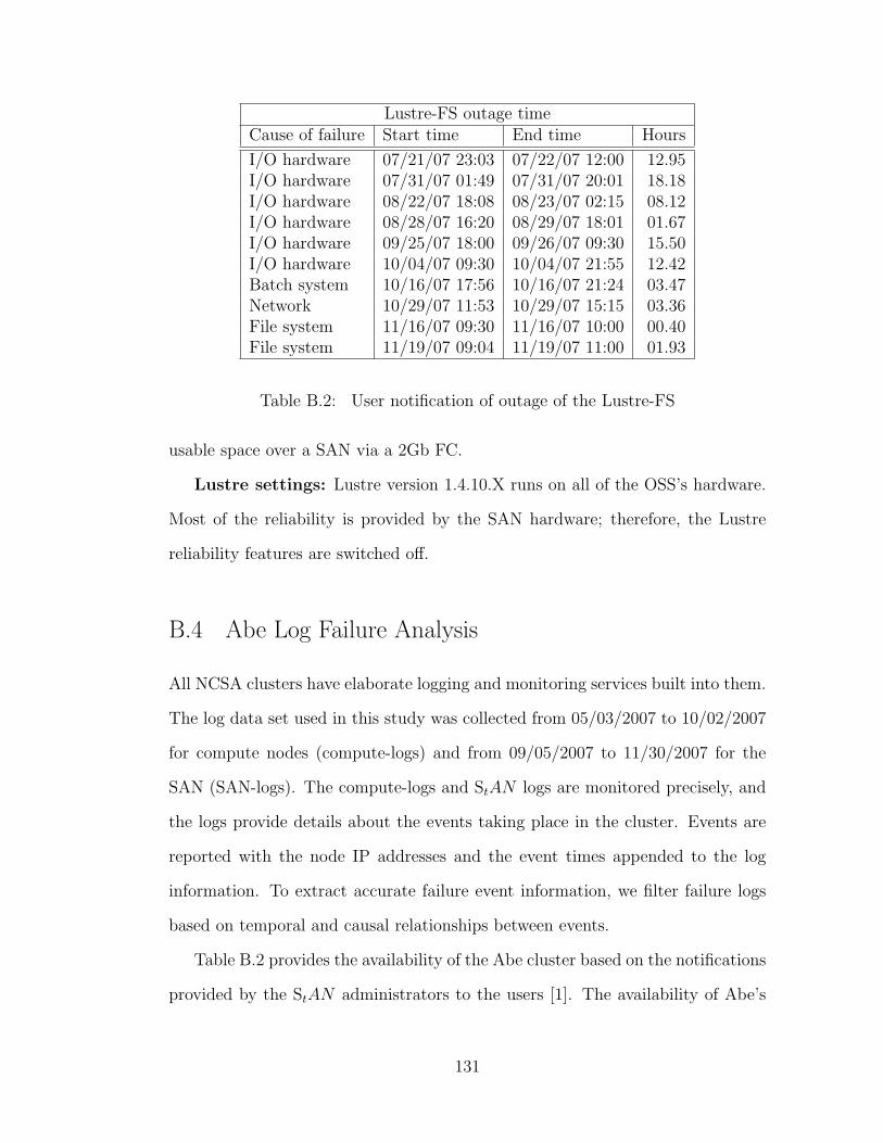
Lustre-FS outage timeCause of failure Start time End time Hours

I/O hardware 07/21/07 23:03 07/22/07 12:00 12.95I/O hardware 07/31/07 01:49 07/31/07 20:01 18.18I/O hardware 08/22/07 18:08 08/23/07 02:15 08.12I/O hardware 08/28/07 16:20 08/29/07 18:01 01.67I/O hardware 09/25/07 18:00 09/26/07 09:30 15.50I/O hardware 10/04/07 09:30 10/04/07 21:55 12.42Batch system 10/16/07 17:56 10/16/07 21:24 03.47Network 10/29/07 11:53 10/29/07 15:15 03.36File system 11/16/07 09:30 11/16/07 10:00 00.40File system 11/19/07 09:04 11/19/07 11:00 01.93

Table B.2: User notification of outage of the Lustre-FS

usable space over a SAN via a 2Gb FC.

Lustre settings: Lustre version 1.4.10.X runs on all of the OSS’s hardware.

Most of the reliability is provided by the SAN hardware; therefore, the Lustre

reliability features are switched off.

B.4 Abe Log Failure Analysis

All NCSA clusters have elaborate logging and monitoring services built into them.

The log data set used in this study was collected from 05/03/2007 to 10/02/2007

for compute nodes (compute-logs) and from 09/05/2007 to 11/30/2007 for the

SAN (SAN-logs). The compute-logs and StAN logs are monitored precisely, and

the logs provide details about the events taking place in the cluster. Events are

reported with the node IP addresses and the event times appended to the log

information. To extract accurate failure event information, we filter failure logs

based on temporal and causal relationships between events.

Table B.2 provides the availability of the Abe cluster based on the notifications

provided by the StAN administrators to the users [1]. The availability of Abe’s

131

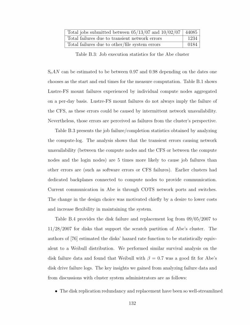
Total jobs submitted between 05/13/07 and 10/02/07 44085Total failures due to transient network errors 1234Total failures due to other/file system errors 0184

Table B.3: Job execution statistics for the Abe cluster

StAN can be estimated to be between 0.97 and 0.98 depending on the dates one

chooses as the start and end times for the measure computation. Table B.1 shows

Lustre-FS mount failures experienced by individual compute nodes aggregated

on a per-day basis. Lustre-FS mount failures do not always imply the failure of

the CFS, as these errors could be caused by intermittent network unavailability.

Nevertheless, those errors are perceived as failures from the cluster’s perspective.

Table B.3 presents the job failure/completion statistics obtained by analyzing

the compute-log. The analysis shows that the transient errors causing network

unavailability (between the compute nodes and the CFS or between the compute

nodes and the login nodes) are 5 times more likely to cause job failures than

other errors are (such as software errors or CFS failures). Earlier clusters had

dedicated backplanes connected to compute nodes to provide communication.

Current communication in Abe is through COTS network ports and switches.

The change in the design choice was motivated chiefly by a desire to lower costs

and increase flexibility in maintaining the system.

Table B.4 provides the disk failure and replacement log from 09/05/2007 to

11/28/2007 for disks that support the scratch partition of Abe’s cluster. The

authors of [76] estimated the disks’ hazard rate function to be statistically equiv-

alent to a Weibull distribution. We performed similar survival analysis on the

disk failure data and found that Weibull with β = 0.7 was a good fit for Abe’s

disk drive failure logs. The key insights we gained from analyzing failure data and

from discussions with cluster system administrators are as follows:

• The disk replication redundancy and replacement have been so well-streamlined

132

Dates in September 2007 05 06 09 13 23Number of failed disks 2 1 1 1 1Dates in October 2007 08 17 24Number of failed disks 2 1 1Dates in November 2007 08 17Number of failed disks 1 1

Survival analysis of the disk failures (n = 480) using Weibullregression (in log relative-hazard form) gives the shape parameter as0.6963571 with a standard deviation of 0.1923109 (95% confidence interval) [36]

Table B.4: Disk failure log from 09/05/2007 to 11/28/2007 for disks supportingAbe’s scratch partition

that they almost never cause catastrophic failure of the CFS. On average,

0-2 disks are replaced on the Abe cluster per week.

• The Abe cluster’s S2A9550 RAID6 (8+2) technology combines the virtues of

RAID3, RAID5, and RAID0 to provide both reliability and performance [60].

RAID6 prevents a second drive failure from occurring during disk re-mirroring.

The Blue Waters petascale computer, which will be built at the University

of Illinois, will likely have an (8+3) RAID configuration. That would make

the failure of the file system due to multiple individual disk failures highly

unlikely.

• Most file system failures are due to software errors, configuration errors, and

other transient errors. The software errors take, on average, 2-4 hours to

resolve. Most often, the fix is to bring the disks to a consistent state using a

file system check (fsck). A hardware failure due to a network component or

a RAID controller might take up to 24 hours to resolve, as these components

need to be procured from a vendor.

133

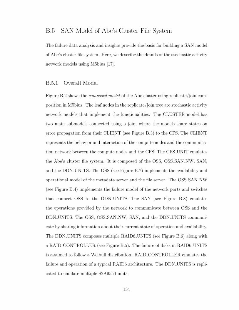
B.5 SAN Model of Abe’s Cluster File System

The failure data analysis and insights provide the basis for building a SAN model

of Abe’s cluster file system. Here, we describe the details of the stochastic activity

network models using Mobius [17].

B.5.1 Overall Model

Figure B.2 shows the composed model of the Abe cluster using replicate/join com-

position in Mobius. The leaf nodes in the replicate/join tree are stochastic activity

network models that implement the functionalities. The CLUSTER model has

two main submodels connected using a join, where the models share states on

error propagation from their CLIENT (see Figure B.3) to the CFS. The CLIENT

represents the behavior and interaction of the compute nodes and the communica-

tion network between the compute nodes and the CFS. The CFS UNIT emulates

the Abe’s cluster file system. It is composed of the OSS, OSS SAN NW, SAN,

and the DDN UNITS. The OSS (see Figure B.7) implements the availability and

operational model of the metadata server and the file server. The OSS SAN NW

(see Figure B.4) implements the failure model of the network ports and switches

that connect OSS to the DDN UNITS. The SAN (see Figure B.8) emulates

the operations provided by the network to communicate between OSS and the

DDN UNITS. The OSS, OSS SAN NW, SAN, and the DDN UNITS communi-

cate by sharing information about their current state of operation and availability.

The DDN UNITS composes multiple RAID6 UNITS (see Figure B.6) along with

a RAID CONTROLLER (see Figure B.5). The failure of disks in RAID6 UNITS

is assumed to follow a Weibull distribution. RAID CONTROLLER emulates the

failure and operation of a typical RAID6 architecture. The DDN UNITS is repli-

cated to emulate multiple S2A9550 units.

134

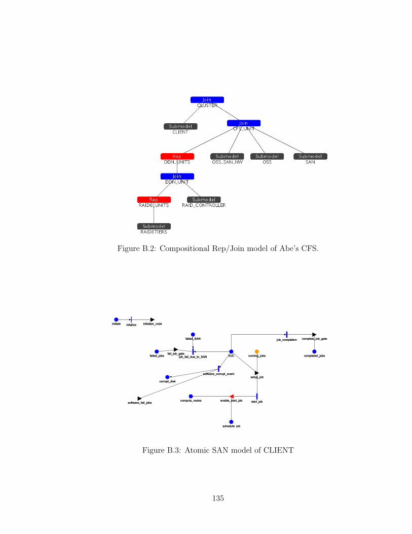
Figure B.2: Compositional Rep/Join model of Abe’s CFS.

Figure B.3: Atomic SAN model of CLIENT

135

Figure B.4: Atomic SAN model of OST SAN NW

Figure B.5: Atomic SAN model of RAID CONTROLLER

Figure B.6: Atomic SAN model of RAID6TIERS

136

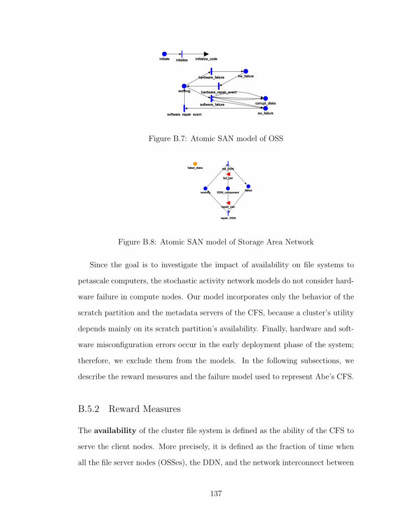
Figure B.7: Atomic SAN model of OSS

Figure B.8: Atomic SAN model of Storage Area Network

Since the goal is to investigate the impact of availability on file systems to

petascale computers, the stochastic activity network models do not consider hard-

ware failure in compute nodes. Our model incorporates only the behavior of the

scratch partition and the metadata servers of the CFS, because a cluster’s utility

depends mainly on its scratch partition’s availability. Finally, hardware and soft-

ware misconfiguration errors occur in the early deployment phase of the system;

therefore, we exclude them from the models. In the following subsections, we

describe the reward measures and the failure model used to represent Abe’s CFS.

B.5.2 Reward Measures

The availability of the cluster file system is defined as the ability of the CFS to

serve the client nodes. More precisely, it is defined as the fraction of time when

all the file server nodes (OSSes), the DDN, and the network interconnect between

137

the OSSes and the DDN are in the working state.

The disk replacement rate is defined as the number of disks that need to

be replaced per unit of time to sustain the maximum availability of the CFS.

The cluster utility, CU, is an availability metric from the cluster’s perspec-

tive. To be precise, it is defined as

CU =

(1− Compute cycles lost due to unavailable file system

Total available compute cycles

), (B.1)

where CU is a metric that is different from the availability metric of the CFS. Note

that CU does not distinguish between compute cycles used to perform checkpoint-

ing and those used for actual computation. The cluster users and SAN admin-

istrators tend to notice different levels of availability. The reasons are failures

in network communication between the compute nodes and the CFS as well as

failures due to intermittent transient errors that make CFS appear unavailable

even though it has not failed.

B.5.3 Failure Model for Abe’s CFS

Abe’s cluster suffers from failures mainly because of 3 types of errors: hardware

errors, software errors, and transient errors. Each kind of error affects all of the

CFS’s components.

The hardware errors in the metadata/file servers (OSSes) occur in the hard-

ware components that are built to operate the system. These errors include pro-

cessor, memory, and network errors. Hardware errors are assumed to be less

frequent than disk failures, occurring at the rate of 1–2 per month. The RAID

controllers in the DDN or network ports/switches that connect DDN to OSS show

similar failure rates. The repairs of these components take 12–36 hours depending

upon the severity of the failure (as reported by SAN administrators), as the needed

138

Model parameter Values (range)

Disk MTBF2 100000-3000000Annualized Failure Rate (AFR) 0.40%–8.6%Weibull distribution’s shape parameter1 0.6–1.0Number of DDNs1 2–20Number of compute nodes1 1200–32000Average time to replace disks3 1–12 hoursAverage time to replace hardware3 12–36 hoursAverage time to fix software3 2–6 hoursJob requests per hour1 12–15 per hourHardware failure rate1 1–2 per 720 hoursSoftware failure rate 1–2 per 720 hoursAnnual growth rate of disk capacity2 33%DDN Units1 2–20OSS Units1 8–80Parameter values obtained from log file analysis1, dataspecification from literature and hardware white papers2,discussions with NCSA cluster administrators3

Table B.5: Abe cluster’s simulation model parameters

replacement parts have to be shipped from the vendors. Most of the hardware

is replicated with fail-over mechanisms. Failure of both members of the fail-over

pair causes the unavailability of the CFS system. The replacement of failed disks

is modeled as a deterministic event. The repair time is varied from 1 to 12 hours

across simulation experiments.

The software errors that cause failure of the cluster file systems are mainly

due to the corrupted supercomputing applications running on the compute nodes

(implemented in the CLIENT submodel) or the Lustre-FS (implemented in the

OSS submodel). Since we do not have accurate estimates on software corruption

errors, we assume that the rates are similar in the orders of magnitude to hardware

error rates. The repair times for software errors are modeled as deterministic

events. The repair time is varied from 2 to 6 hours across simulation experiments.

Transient errors occur in most components of the cluster model, but mainly

139

in the network components. The error rates are obtained from the failure-log

analysis as shown in Table B.3. Transient errors are temporary, but hard to

diagnose. Our model assumes that one of these errors causes a few minutes of

unavailability of components under transient failure. The jobs that depend on

those components fail due to the temporary unavailability.

Past literature has emphasized the importance of modeling correlated fail-

ures [90]. Most correlated errors occur because of shared resources. Correlated

errors propagate to components that have causal or spatial proximity. In the CFS

model, hardware errors propagate because other hardware components are con-

nected to each other. Software errors propagate from compute nodes to OSS or

from OSS to disk, leading to data corruption. Transient errors propagate errors

into software. All failures except disk failures are modeled as exponential distri-

butions. To model correlated failures, we model jobs and requests submitted to

the CFS, and estimate the probability p that the job will require a resource that

is inaccessible due to failure, causing errors to propagate through the system.

B.6 Experimental Results and Analysis

We evaluate the design of the Abe cluster’s availability using simulation in the

Mobius tool. Table B.5 summarizes the parameters collected through failure

log analysis, hardware reliability specifications, and discussions with cluster ad-

ministrators. In order to reflect the size and scale of a petascale computer and

to determine the factors that impede the high availability of the CFS, we scale

the number of individual components in the composed model. By implementing

scaling through the addition of components (each of which has its own individ-

ual failure models) rather than by changing failure parameter values themselves,

we ensure that the failure rates observed in the overall system model accurately

140

0.9980

0.9985

0.9990

0.9995

1.0000

96(ABE)

828 1428 2190 3148 4344 5828 7660 9911 12664

Abe cluster scaled by storage size in terabytes

Ava

ilabi

lity

of s

tora

ge

0.6,8.76,8+2,4 0.6,8.76,8+3,12 0.6,4.38,8+2,4

0.7,2.92,8+2,4 0.7,8.76,8+3,12

Figure B.9: Availability of storage with respect to disk failures; label with values(0.7, 2.92, 8+2, 4) represents a tuple as follows: (Weibull shape parameter β,AFR in %, RAID configuration, average disk replacement time in hours)

reflect the new system size. All the simulation results are reported at a 95%

confidence level.

B.6.1 Impact of Disk Failures on CFS

To evaluate the baseline effect of failures of disks on availability of the CFS, we

evaluate the DDN UNITS models associated with the RAID6 tiers and the RAID

controllers in isolation from failures of other components of the SAN. Figure B.9

shows the availability of the storage hardware as one scales the file system from

the current 96TB (Abe’s file system) to 12PB (the BlueWaters file system). The

key observation is that the RAID6 architecture provides sufficient redundancy and

recovery mechanisms to mitigate the impact of high disk failure rates to a very

large extent. First, note that all configurations of failure and recovery rates for an

Abe-sized cluster file system have nearly 100% availability (refer to the first data

point in Figure B.9). However, as the experiments are scaled from Abe’s system

141

0

10

20

30

40

50

60

70

480

(A b e )

960 1440 1920 2400 2880 3360 3840 4320 4800

Abe computer scaled by number of disks

Num

ber

of

faile

d/r

epla

ced d

isks p

er

week

0.7,8.76,8+2,4 0.7,4.38,8+2,4 0.7,2.92,8+2,4 0.7,0.88.8+2,4

Figure B.10: Average number of disks that need to be replaced per week to sustainavailability

to a petascale system, our simulation results show that the RAID6 architecture

cannot provide the same level of storage availability for some of the failure model

configurations. The SAN architect’s plan to use (8+3) RAID in Blue Waters

is important; it provides better reliability than the (8+2) RAID on petascale

systems. While RAID6 provides a larger margin for disk failure rates, i.e., up to

8.6% AFR, it is very important that these rates be contained to lower thresholds

by disk manufacturers and vendors to provide an adequate level of availability.

If one makes a pessimistic assumption of a higher infant mortality rate in disks

(Weibull shape parameter = 0.6), the availability falls below 99.9% for petascale

storage.

To better understand the cost of disk replacement, we compute the expected

number of disks that need to be replaced per week for the RAID6 tiers. Fig-

ure B.10 depicts the average number of disks that need to be replaced per week to

sustain the availability so that the CFS does not suffer failure due to RAID6 fail-

ure. The configuration (0.7, 2.92, 8+2, 4) corresponds to the Abe cluster with 0 to

2 disk replacements per week. Each time a disk fails, there is an operational cost

142

(in dollars) that is borne by the SAN vendors as they provide extended support

to their SANs. As the CFS system is scaled to support petascale computers, the

number of disks that need to be replaced increases, increasing the labor cost and

the replacement cost. Therefore, the SAN vendors have an incentive to increase

the disk MTBF to reduce their overall support cost.

Survival analysis of the disk failure data provided a good estimate of the

Weibull distribution’s shape parameter β, but the estimate for the scale param-

eter (MTBF) was insignificant [36]. Using simulations, we estimated an MTBF

that matched the average disk failures per week for the scratch partition and de-

termined that an MTTF = 300,000 hours or an annualized failure rate (AFR) =

2.92% to be a good fit.

B.6.2 CFS Availability and CU

0.80

0.85

0.90

0.95

1.00

1.05

96

(Abe)

828 1428 2190 3148 4344 5828 7660 9911 12664

Abe cluster scaled by storage size in terabytes

Availa

bili

ty

Storage-availability CFS-availability-spare-OSS CFS-availability CU

Figure B.11: Availability and utility of the Abe cluster when scaled to petaflop-petabyte system

To analyze the impact of all components that determine the availability of the

CFS, we evaluated the availability and CU of the Abe system. The experiments

143

were scaled to the size of a petascale computer to allow understanding of the im-

pact of failures on those measures. Figure B.11 shows that the CFS availability

decreases as one scales the system to support a petascale computer. Since most

of the parameter values were obtained through the log data analysis and times

reported by SAN administrators, our measures for CFS availability matched with

Abe’s availability as shown in Table B.2. Therefore, we have higher confidence

in the measures of availability and CU as we scaled the models to represent a

petascale computer with a petabyte storage system. The storage availability in

Figure B.11 refers to configuration (0.7, 2.92, 8+2, 4), which models the Abe

cluster’s current environment. We find that the RAID6 subsystem in this con-

figuration continues to provide an availability of 1, but the CFS availability is

reduced from 0.972 to 0.909 as one scales the design to support the petascale sys-

tem. The reduction is mainly due to correlated failures in OSS and hardware. To

improve upon the Abe cluster’s design, an architect could provide an additional

standby or spare OSS to replace the failed OSS quickly. Our evaluation shows

that this approach can improve the availability by 3%. To improve the availability

further, architects will have to develop solutions to mitigate correlated errors. For

example, improving the robustness of the Lustre-FS software can reduce the num-

ber of software-correlated errors affecting the availability. The CU in Figure B.11

shows that the cluster’s network architecture between the compute nodes and the

CFS has a profound impact on the cluster utility available to the users. The trend

to move away from customized backplanes to COTS network hardware (with its

complicated software stacks) has decreased the CU. The transient errors seen in

the network can be mitigated by providing multiple network paths between the

compute nodes and the CFS.

144

B.7 Conclusion

Many researchers have focused on developing and understanding dependability

of clusters for supercomputing applications. We have taken steps to understand

the dependability and availability of the Abe cluster through failure data analysis

and discussions with administrators at multiple levels of the cluster operation,

from the lowest level of the StAN’s availability, to the cluster’s availability, and

to user perception of cluster utility at the top level. Our key findings through

analysis and simulation showed that the RAID6 design for a disk’s dependability

has limited the impact of disk failures on the CFS, even when the model is scaled

to evaluate the support for petascale systems. On the other hand, transient errors,

hardware errors, and software errors contribute significantly to failures, and these

components are the limiting factors for the high availability of the CFS. We believe

that petascale architects will have to focus on those issues to develop solutions to

improve the overall availability of the CFS.

Our work has mainly focused on evaluating the availability of the Abe’s CFS

through data collection, analysis, and system modeling. We showed that system

modeling, combined with data analysis from real systems, provides better insight

to design future systems.

145

APPENDIX C

MOBIUS GATE CODE OF THE CASE STUDYMODELS

Here, we present the gate code of the Mobius models represented in Chapter 3.

The Mobius tool can be obtained from

www.mobius.uiuc.edu.

C.1 Distributed Information Server

The SAN model of Distributed Information Server is presented in Figure 3.1.

Here, we outline the state updating code used in the output gates of the SAN

model. We outline the code of the first three output gates. The remaining gates

have similar code with appropriate changes to the place names.

Output gate function: OG SynchFEPA

// Corrupt PA1 and PA2

PA1_Corrupted->Mark()=1;

PA2_Corrupted->Mark()=1;

// FE remains corrupted until it fails

FE1_Corrupted->Mark()=1;

146

Output gate function: OG SynchPASM

// Corrupt SA and MA

SA_Corrupted->Mark()=1;

MA_Corrupted->Mark()=1;

// PA1 and PA2

// remains corrupted

PA1_Corrupted->Mark()=1;

PA2_Corrupted->Mark()=1;

Output gate function: OG SynchSMDA

// Corrupt DA

DA_Corrupted->Mark()=1;

// SA and MA

// remains corrupted

SA_Corrupted->Mark()=1;

MA_Corrupted->Mark()=1;

C.2 Fault Tolerant Computer with Repair

The SAN model of the Fault Tolerant Computer with repair is presented in Fig-

ure 3.3.

The model has one input gate that determines the firing of the activity repair

based on the following predicate function.

Input gate predicate: IG repair

(repair_flag->Mark() &&

!errorhandlers->Mark() &&

(comp_failed->Mark()< 2))

147

The remaining 7 output gate functions are described below.

Output gate function: OG repair

ram->Mark() = 40;

inter->Mark() = 2;

ioports->Mark() = 3;

mems->Mark() = 3;

cpus->Mark() = 4;

errorhandlers->Mark() = 3;

comp_failed->Mark() --;

if(!comp_failed->Mark())

repair_flag->Mark() = 1;

Output gate function: OG IO

if(!ioports->Mark()){

ram->Mark() = 0;

inter->Mark() = 0;

ioports->Mark() = 0;

mems->Mark() = 0;

cpus->Mark() = 0;

errorhandlers->Mark() = 0;

comp_failed->Mark() ++;

repair_flag->Mark() = 1;

}

Output gate function: OG MEM

if(mems->Mark() < 2){

ram->Mark() = 0;

inter->Mark() = 0;

ioports->Mark() = 0;

mems->Mark() = 0;

cpus->Mark() = 0;

errorhandlers->Mark() = 0;

comp_failed->Mark() ++;

repair_flag->Mark() = 1;

}

148

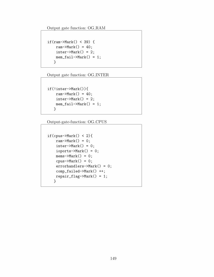
Output gate function: OG RAM

if(ram->Mark() < 39) {

ram->Mark() = 40;

inter->Mark() = 2;

mem_fail->Mark() = 1;

}

Output gate function: OG INTER

if(!inter->Mark()){

ram->Mark() = 40;

inter->Mark() = 2;

mem_fail->Mark() = 1;

}

Output-gate-function: OG CPUS

if(cpus->Mark() < 2){

ram->Mark() = 0;

inter->Mark() = 0;

ioports->Mark() = 0;

mems->Mark() = 0;

cpus->Mark() = 0;

errorhandlers->Mark() = 0;

comp_failed->Mark() ++;

repair_flag->Mark() = 1;

}

149

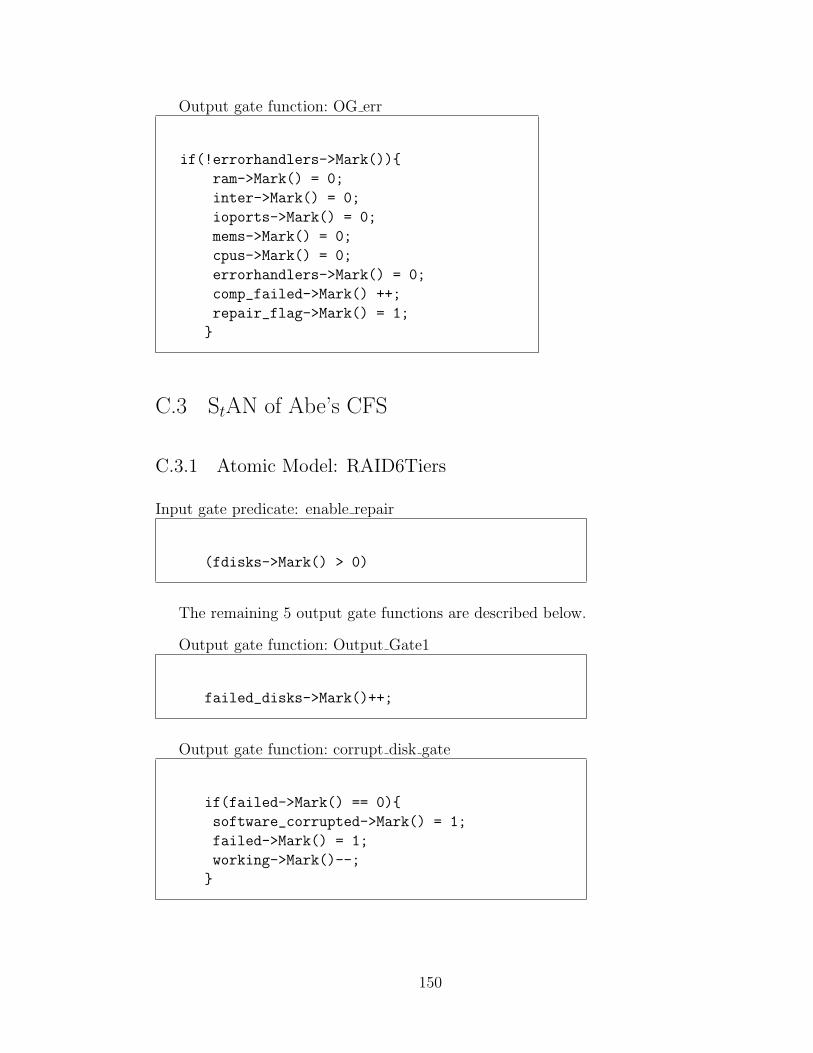
Output gate function: OG err

if(!errorhandlers->Mark()){

ram->Mark() = 0;

inter->Mark() = 0;

ioports->Mark() = 0;

mems->Mark() = 0;

cpus->Mark() = 0;

errorhandlers->Mark() = 0;

comp_failed->Mark() ++;

repair_flag->Mark() = 1;

}

C.3 StAN of Abe’s CFS

C.3.1 Atomic Model: RAID6Tiers

Input gate predicate: enable repair

(fdisks->Mark() > 0)

The remaining 5 output gate functions are described below.

Output gate function: Output Gate1

failed_disks->Mark()++;

Output gate function: corrupt disk gate

if(failed->Mark() == 0){

software_corrupted->Mark() = 1;

failed->Mark() = 1;

working->Mark()--;

}

150

Output gate function: fail raid

fdisks->Mark()++;

if(fdisks->Mark() > parity_disks_per_configuration

&& failed->Mark() ==0) {

working->Mark() --;

failed->Mark() ++;

}

Output gate function: fix raid

if(fdisks->Mark() < parity_disks_per_configuration

&& failed->Mark() ==1){

failed->Mark() = 0;

working->Mark() ++;

}

Output gate function: repair raid

wdisks->Mark() = disks_per_configuration;

fdisks->Mark() = 0;

if(failed->Mark() > 0 &&

software_corrupted->Mark() ==0){

working->Mark() ++;

failed->Mark() --;

}

C.3.2 Atomic Model: RAID CONTROLLER

Input gate predicate: fail ddn

(raid_component->Mark() < RAID6_units)

Input gate predicate: repair ddn

(raid_component->Mark() >= RAID6_units)

151

Output gate function: controller paired repair gate

if(pairedFailure->Mark() > 0 &&

failed->Mark() == 1){

failed->Mark() == 0;

working->Mark() ++;

}

pairedFailure->Mark() = 0;

FDiskControllers->Mark() = 0;

WDiskControllers->Mark() = 2* RAID6_units;

Output gate function: initialize code

WDiskControllers->Mark() = 2* RAID6_units;

Output gate function: paired failure gate

double unPairedFNodes = FDiskControllers->Mark()

- pairedFailure->Mark();

Distributions dist;

double uniform = dist.Uniform(0,1);

FDiskControllers->Mark()++;

if((unPairedFNodes/FDiskControllers->Mark()) > uniform){

pairedFailure->Mark() +=2;

if(failed->Mark() == 0){

failed->Mark() ++;

working->Mark() --;

}

}

152

REFERENCES

[1] “Notifications to Teragrid users about CFS unavailability of Abe cluster,”Nov 2007. [Online]. Available: http://news.teragrid.org/news controller.php

[2] “NCSA Intel 64 Linux Cluster Abe Technical Summary,” Jul 2007. [On-line]. Available: http://www.ncsa.uiuc.edu/UserInfo/Resources/Hardware/Intel64Cluster/TechSummary/

[3] T. Altiok, “Approximate analysis of queues in series with phase-type servicetimes and blocking,” Operations Research, vol. 37, no. 4, pp. 601–610, 1989.[Online]. Available: http://www.jstor.org/stable/171260

[4] T. Altiok, “On the phase-type approximations of general distributions,” IIETransactions, vol. 17, pp. 110–116, June, 1985.

[5] G. A. Alvarez, “Minerva: An automated resource provisioning tool for large-scale storage systems,” ACM Transactions on Computer Systems, vol. 19,no. 4, pp. 483–518, Nov. 2001.

[6] E. Anderson, S. Spence, R. Swaminathan, M. Kallahalla, and Q. Wang,“Quickly finding near-optimal storage designs,” ACM Transactions on Com-puter Systems, vol. 23, no. 4, pp. 337–374, 2005.

[7] E. Anderson, R. Swaminathan, A. Veitch, G. A. Alvarez, and J. Wilkes,“Selecting RAID levels for disk arrays,” in Proceedings of the 1st USENIXConference on File and Storage Technologies, 2002, pp. 189–201.

[8] F. Azadivar, “Simulation optimization methodologies,” in Proceedings of the31st conference on Winter simulation, 1999, pp. 93–100.

[9] F. Azadivar, “Simulation optimization methodologies,” in WSC ’99: Pro-ceedings of the 31st Winter Simulation Conference, 1999, pp. 93–100.

[10] A. Azagury, M. E. Factor, and J. Satran, “Point-in-Time copy: Yesterday,today and tomorrow,” in Proc. the 10th NASA Conference on Mass StorageSystems and Technologies/ 19th IEEE Symposium on Mass Storage Systems,Apr. 2002, pp. 259–270.

153

[11] R. L. Braby, J. E. Garlick, and R. J. Goldstone, “Achieving order throughCHAOS: The LLNL HPC Linux Cluster Experience,” in Proceedings of the4th International Conference on Linux Clusters: The HPC Revolution 2003,San Jose, CA, USA, 2003.

[12] P. H. Carns, W. B. Ligon III, R. B. Ross, and R. Thakur, “PVFS: A ParallelFile System for Linux Clusters,” in Proceedings of the 4th Annual LinuxShowcase and Conference, Atlanta, GA, 2000, pp. 317–327.

[13] Y. Carson and A. Maria, “Simulation Optimization: Methods And Applica-tions,” in WSC ’97: Proceedings of the 29th Winter Simulation Conference,1997, pp. 118–126.

[14] C.-H. Chen, “A hybrid approach of the standard clock method and eventscheduling approach for general discrete event simulation,” in WSC ’95: Pro-ceedings of the 27th Winter Simulation Conference, 1995, pp. 786–790.

[15] C.-H. Chen and Y.-C. Ho, “An approximation approach of the standard-clockmethod for general discrete-event simulation,” Control Systems Technology,vol. 3, no. 4, pp. 309–318, 1995.

[16] A. Chervenak, V. Vellanki, and Z. Kurmas, “Protecting file systems: A surveyof backup techniques,” in Proc. IEEE/NASA Conf. MSS, Mar. 1998, pp. 17–31.

[17] G. Clark, T. Courtney, D. Daly, D. Deavours, S. Derisavi, J. M. Doyle,W. H. Sanders, and P. Webster, “The Mobius modeling tool,” in Proceedingsof the 9th International Workshop on Petri Nets and Performance Models,September 11–14, 2001, pp. 241–250.

[18] E. Dicke, A. Byde, P. J. Layzell, and D. Cliff, “Using a genetic algorithmto design and improve storage area network architectures,” in Proceedings ofGenetic and Evolutionary Computation (GECCO), 2004, pp. 1066–1077.

[19] J. D. Diener, “Empirical Comparison of Uniformization Methods forContinuous-time Markov Chains,” M.S. thesis, University of Arizona, 1994.

[20] M. Dorigo and T. Stutzle, Ant Colony Optimization. MIT Press, 2004.

[21] E. J. Dudewicz and S. R. Dalal, “Allocation of observations in ranking andselection with unequal variances,” Sankhya: The Indian Journal of Statistics,vol. 37, pp. 28–78, 1975.

[22] Eagle Rock Alliance Ltd., “Online survey results: 2001 cost ofdowntime,” Aug. 2001, white Paper. [Online]. Available: http://www.contingencyplanningresearch.com/2001%20Survey.pdf

154

[23] J. Gafsi and E. W. Biersack, “Performance and reliability study for dis-tributed video servers: Mirroring or parity?” in Proceedings in the Interna-tional Conference on Mathematics and Computer Science, vol. 2, 1999, pp.628–634.

[24] S. Gaonkar, T. Courtney, and W. H. Sanders, “Efficient state managementto speed up simultaneous simulation of alternate system configurations,” inProceedings of the International Mediterranean Modelling Multiconference,Barcelona, Spain, 2006, pp. 31–36.

[25] S. Gaonkar, K. Keeton, A. Merchant, and W. H. Sanders, “Designing depend-able storage solutions for shared application environments,” in Proceedingsof the International Conference on Dependable Systems and Networks, DSN,Philadelphia, PA, USA, 2006, pp. 371–382.

[26] S. Gaonkar, E. Rozier, A. Tong, and W. H. Sanders, “Scaling file systemsto support petascale clusters: A dependability analysis to support informeddesign choices,” in Proceedings of the International Conference on DependableSystems and Networks, DSN, to appear, 2008.

[27] S. Gaonkar and W. H. Sanders, “Simultaneous simulation of alternative sys-tem configurations,” in Proceedings of the 11th Pacific Rim InternationalSymposium on Dependable Computing, Changsha, Hunan, China, 2005, pp.41–48.

[28] S. Ghemawat, H. Gobioff, and S.-T. Leung, “The Google file system,” inProceedings of the 19th ACM Symposium on Operating Systems Principles,,Bolton Landing, NY, USA, 2003, pp. 29–43.

[29] F. Glover and M. Lagun, Tabu Search. Kluwer Academic Publishers, 1997.

[30] P. W. Glynn, “On the role of generalized semi-Markov processes in simulationoutput analysis,” in WSC ’83: Proceedings of the 15th Winter simulationConference, 1983, pp. 39–44.

[31] D. E. Goldberg, Genetic Algorithms in Search, Optimization, and MachineLearning. Addison-Wesley Professional, Jan. 1989.

[32] L. Goldsman and B. L. Nelson, “Batch-size effects on simulation optimizationusing multiple comparisons with the best,” in WSC’ 90: Proceedings of the22nd Winter Conference on Simulation, 1990, pp. 288–293.

[33] M. Groetschel, “Theoretical and practical aspects of combinatorial problemsolving,” in Proceedings of the 3rd ACM-SIAM Symposium on Discrete Al-gorithms (SODA), 1992, p. 195.

[34] P. Heidelberger and D. M. Nicol, “Conservative parallel simulation of CTMCusing uniformization,” IEEE Transactions Parallel and Distributed Systems,vol. 4, no. 8, pp. 906–921, 1993.

155

[35] HP OpenView Storage Data Protector Administrator’s Guide, Hewlett-Packard Development Co., Oct. 2004, mfg. Part Number B6960-90106, Re-lease A.05.50.

[36] D. W. Hosmer and S. Lemeshow, Applied Survival Analysis: Regression Mod-eling of Time to Event Data. New York, NY, USA: John Wiley & Sons,Inc., 1999.

[37] K. Hwang, H. Jin, and R. S. Ho, “Orthogonal Striping and Mirroring inDistributed RAID for I/O-centric Cluster Computing,” IEEE Transactionin Parallel and Distributed Systems, vol. 13, no. 1, pp. 26–44, 2002.

[38] M. Hybinette and R. Fujimoto, “Cloning: A novel method for interactiveparallel simulation,” in WSC ’97: Proceedings of the 29th Winter Conferenceon Simulation. ACM Press, 1997, pp. 444–451.

[39] P. Hyden and L. Schruben, “Designing simultaneous simulation experi-ments,” in WSC ’99: Proceedings of the 31st conference on Winter simu-lation, 1999, pp. 389–394.

[40] P. Hyden and L. Schruben, “Improved decision processes through simulta-neous simulation and time dilation,” in WSC ’00: Proceedings of the 32ndconference on Winter simulation, 2000, pp. 743–748.

[41] S. H. Jacobson and L. W. Schruben, “Techniques for simulationresponse optimization,” Operations Research Letters, vol. 8, pp. 1–9, Feb1989. [Online]. Available: http://www.sciencedirect.com/science/article/B6V8M-48MPRV7-2/2/117ae1af164ea61dc96b78d9578915eb

[42] M. Ji, A. Veitch, and J. Wilkes, “Seneca: Remote mirroring done write,” inProc. USENIX Technical Conf. (USENIX’03), 2003, pp. 253–268.

[43] W. Jiang, C. Hu, Y. Zhou, and A. Kanevsky, “Are disks the dominant con-tributor for storage failures? a comprehensive study of storage subsystemfailure characteristics,” in Proceedings of 6th USENIX Conference on FileAnd Storage Technologies, FAST, 2008, pp. 111–125.

[44] A. W. Johnson and S. H. Jacobson, “A class of convergent generalized hillclimbing algorithms,” Appl. Math. Comput., vol. 125, no. 2-3, pp. 359–373,2002.

[45] K. Kawanishi, “QBD approximations of a call center queueing model withgeneral patience distribution,” Queues in Practice, Computers and Opera-tions Research, vol. 35, pp. 2463–2481, August, 2008.

[46] K. Keeton, D. Beyer, E. Brau, A. Merchant, C. Santos, and A. Zhang, “Onthe road to recovery: restoring data after disasters,” in Proceedings of Euro-pean Systems Conference (EuroSys), Apr. 2006, pp. 235–248.

156

[47] K. Keeton and A. Merchant, “A framework for evaluating storage systemdependability,” in Proceedings of International Conference on DependableSystems and Networks (DSN), Jun. 2004, pp. 877–886.

[48] K. Keeton, C. Santos, D. Beyer, J. Chase, and J. Wilkes, “Designing fordisasters,” in Proceedings of the 3rd USENIX Conference on File and StorageTechnologies (FAST), Mar. 2004, pp. 59–72.

[49] J. Keilson, Markov Chain Models–Rarity and Exponentiality. Springer-Verlag, 1979.

[50] T. G. Kolda, R. M. Lewis, and V. Torczon, “Optimization by direct search:New perspectives on some classical and modern methods,” in Society forIndustrial and Applied Mathematics (SIAM) Review, vol. 45, no. 3, Jul. 2003,pp. 385–482.

[51] T. G. Kolda, R. M. Lewis, and V. Torczon, “Optimization by direct search:New perspectives on some classical and modern methods,” Society for Indus-trial and Applied Mathematics (SIAM) Review, vol. 45, no. 3, pp. 385–482,Jul. 2003.

[52] V. Lam, P. Buchholz, and W. Sanders, “A structured path-based approachfor computing transient rewards of large CTMCs,” Proceedings of First In-ternational Conference on the Quantitative Evaluation of Systems (QEST),pp. 136–145, Sept. 2004.

[53] A. M. Law and W. D. Kelton, Simulation Modeling and Analysis. McGrawHill, 2000.

[54] P. A. Lewis and G. S. Shedler, “Simulation methods for poisson processes innonstationary systems,” in WSC ’78: Proceedings of the 10th Winter Simu-lation Conference, 1978, pp. 155–163.

[55] P. A. W. Lewis and G. S. Shedler, “Simulation of nonhomogeneous Poissonprocesses by thinning,” Naval Research Logistics Quarterly, vol. 26, no. 3,pp. 403–413, 1979.

[56] S.-Q. Li and J. Mark, “Performance of voice/data integration on a tdm sys-tem,” IEEE Transactions on Communications, vol. 33, no. 12, pp. 1265–1273,Dec 1985.

[57] Y. Liang, Y. Zhang, A. Sivasubramaniam, M. Jette, and R. Sahoo, “Blue-Gene/L Failure Analysis and Prediction Models,” in Proceedings of the Inter-national Conference on Dependable Systems and Networks, DSN, 2006, pp.425–434.

[58] Y. Low, C. Lim, W. Cai, S. Huang, W. Hsu, S. Jain, and S. Turner, “Surveyof languages and runtime libraries for parallel discrete-event simulation,”Simulation, vol. 72, pp. 170–186, Mar. 1999.

157

[59] M. W. Margo, P. A. Kovatch, P. Andews, and B. Banister, “An Analysis ofstate-of-the-art parallel file system for linux,” in Proceeding of the 5th Inter-national Confernce on Linux Clusters: The HPC Revolution 2004, Austin,TX, USA, 2004. [Online]. Available: http://www.linuxclustersinstitute.org/conferences/archive/2004/PDF/20-Margo M.pdf pp. 1–28.

[60] L. McBryde, G. Manning, D. Illar, R. Williams, and M. Piszczek, “DataManagement Architecture,” US Patent number 7127668, Oct. 2006.

[61] J. F. Meyer, A. Movaghar, and W. H. Sanders, “Stochastic activity networks:Structure, behavior, and application,” in Proceedings of the InternationalWorkshop on Timed Petri Nets, July 1985, pp. 106–115.

[62] R. R. Muntz and J. Lui, “Computing bounds on steady-state availabilityof repairable computer systems,” Journal of the ACM, vol. 41, no. 4, pp.676–707, 1994.

[63] S. Nahar, S. Sahni, and E. Shragowitz, “Simulated annealing and combina-torial optimization,” in Proceedings of the 23rd ACM/IEEE Conference onDesign Automation, 1986, pp. 293–299.

[64] D. M. Nicol and P. Heidelberger, “Optimistic parallel simulation of continu-ous time Markov chains using uniformization,” J. Parallel Distrib. Comput.,vol. 18, no. 4, pp. 395–410, 1993.

[65] D. M. Nicol and P. Heidelberger, “Parallel simulation of Markovian queueingnetworks using adaptive uniformization,” SIGMETRICS, vol. 21, no. 1, pp.135–145, 1993.

[66] V. Nicola, P. Heidelberger, and P. Shahabuddin, “Uniformization and expo-nential transformation: Techniques for fast simulation of highly dependablenon-markovian systems,” FTCS-22, Digest of Papers, Twenty-Second Inter-national Symposium on Fault-Tolerant Computing, pp. 130–139, Jul 1992.

[67] S. Olafsson and J. Kim, “Simulation optimization,” in Proceedings of the 34thconference on Winter simulation, 2002, pp. 79–84.

[68] A. J. Oliner, R. K. Sahoo, J. E. Moreira, and M. Gupta, “Performance im-plications of periodic checkpointing on large-scale cluster systems,” in Pro-ceedings of the 19th IEEE International Parallel and Distributed ProcessingSymposium (IPDPS’05), Washington, DC, USA, 2005, pp. 299–307.

[69] C. H. Papadimitriou and K. Steiglitz, Combinatorial Optimization: Algo-rithms and Complexity. Dover Publications, 1998.

[70] D. A. Patterson, G. Gibson, and R. H. Katz, “A case for redundant arraysof inexpensive disks (RAID),” in Proc. ACM SIGMOD Conf., Jun. 1988, pp.109–116.

158

[71] S. Prasad and Z. Cao, “Parallel distributed simulation and modeling meth-ods: Syncsim: a synchronous simple optimistic simulation technique basedon a global parallel heap event queue,” in Proceedings of the 35th Winterconference on Simulation, 2003, pp. 872–880.

[72] E. Rosti, G. Serazzi, E. Smirni, and M. S. Squillante, “Models of parallelapplications with large computation and I/O requirements,” IEEE Transac-tions on Software Engineering, vol. 28, no. 3, pp. 286–307, 2002.

[73] W. H. Sanders and L. M. Malhis, “Dependability evaluation using composedSAN-based reward models,” Journal of Parallel and Distributed Computing,vol. 15, no. 3, pp. 238–254, 1992.

[74] F. Schmuck and R. Haskin, “GPFS: A shared-disk file system for large com-puting clusters,” in Proceedings of 1st USENIX Conference on File And Stor-age Technologies, FAST, 2002, pp. 231–244.

[75] B. Schroeder and G. A. Gibson, “A large-scale study of failures in high-performance computing systems,” in Proceedings of the International Con-ference on Dependable Systems and Networks, DSN, 2006, pp. 249–258.

[76] B. Schroeder and G. A. Gibson, “Disk failures in the real world: What does anMTTF of 1,000,000 hours mean to you?” in Proceedings of the 5th USENIXConference on File And Storage Technologies, FAST, 2007, pp. 1–16.

[77] L. W. Schruben, “Simulation optimization using simultaneous replicationsand event time dilation,” in WSC ’97: Proceedings of the 29th conference onWinter simulation, 1997, pp. 177–180.

[78] R. R. Schulman, Disaster Recovery Issues and Solutions, HitachiData Systems white paper, Sep. 2004. [Online]. Available: http://www.hds.com/pdf/wp 117 02 disaster recovery.pdf

[79] J. G. Shanthikumar, “A random variate generation method useful in hybridsimulation/analytical modelling,” in WSC ’84: Proceedings of the 16th Win-ter Simulation Conference, 1984, pp. 160–167.

[80] J. G. Shanthikumar, “Discrete random variate generation us-ing uniformization,” European Journal of Operational Research,vol. 21, no. 3, pp. 387–398, Sep. 1985. [Online]. Available:http://ideas.repec.org/a/eee/ejores/v21y1985i3p387-398.html

[81] J. G. Shanthikumar, “Uniformization and hybrid simulation/analytic modelsof renewal processes,” Oper. Res., vol. 34, no. 4, pp. 573–580, 1986.

[82] J. G. Shanthikumar and R. G. Sargent, “A unifying view of hybridsimulation/analytic models and modeling,” Operations Research, vol. 31,no. 6, pp. 1030–1052, 1983. [Online]. Available: http://www.jstor.org/stable/170837

159

[83] E. Smeitink and R. Dekker, “A simple approximation to the renewal function[reliability theory],” IEEE Transactions on Reliability, vol. 39, no. 1, pp. 71–75, Apr 1990.

[84] D. Sonderman, “Comparision results for stochastic processes aris-ing in queuing system,” Dissertation, Yale University, 1978. [On-line]. Available: http://proquest.umi.com/pqdweb?did=761469881&sid=3&Fmt=1&clientId=36305&RQT=309&VName=PQD

[85] D. Sonderman, “Comparing multi-server queues with finite waiting rooms, i:Same number of servers,” Advances in Applied Probability, vol. 11, no. 2, pp.439–447, 1979. [Online]. Available: http://www.jstor.org/stable/1426848

[86] D. Sonderman, “Comparing multi-server queues with finite waiting rooms, ii:Different numbers of servers,” Advances in Applied Probability, vol. 11, no. 2,pp. 448–455, 1979. [Online]. Available: http://www.jstor.org/stable/1426849

[87] D. Sonderman, “Comparing semi-Markov processes,” Mathematics ofOperations Research, vol. 5, no. 1, pp. 110–119, 1980. [Online]. Available:http://www.jstor.org/stable/3689399

[88] E. Strohmaier, J. J. Dongarra, H. W. Meuer, and H. D. Simon, “The mar-ketplace of high performance computing,” Parallel Computing, vol. 25, no.13–14, pp. 1517–1544, 1999.

[89] J. R. Swisher, S. H. Jacobson, and E. Yucesan, “Discrete-event simulationoptimization using ranking, selection, and multiple comparison procedures: Asurvey,” ACM Transactions on Modeling and Computer Simulation, vol. 13,no. 2, pp. 134–154, 2003.

[90] D. Tang and R. K. Iyer, “Dependability measurement and modeling of amulticomputer system,” IEEE Transactions on Computers, vol. 42, no. 1,pp. 62–75, 1993.

[91] T. H. Truong and F. Azadivar, “Simulation based optimization for supplychain configuration design,” in Proceedings of the 35th conference on Wintersimulation, 2003, pp. 1268–1275.

[92] P. Vakili, “Massively parallel and distributed simulation of a class of discreteevent systems: A different perspective,” ACM Transactions on Modeling andComputer Simulation, vol. 2, no. 3, pp. 214–238, 1992.

[93] P. Vakili, “Massively parallel and distributed simulation of a class of discreteevent systems: a different perspective,” ACM Transactions on Modeling andComputer Simulation, vol. 2, no. 3, pp. 214–238, 1992.

[94] A. van Moorsel and W. H. Sanders, “Transient solution of markov modelsby combining adaptive and standard uniformization,” IEEE Transactions onReliability, vol. 46, no. 3, pp. 430–440, Sep 1997.

160

[95] L. Wang, K. Pattabiraman, Z. Kalbarczyk, R. K. Iyer, L. Votta, C. Vick, andA. Wood, “Modeling coordinated checkpointing for large-scale supercomput-ers,” in Proceedings of the International Conference on Dependable Systemsand Networks, DSN, 2005, pp. 812–821.

[96] W. Yu, S. Liang, and D. K. Panda, “High performance support of parallelvirtual file system (pvfs2) over quadrics,” in International Conference onSupercomputing, ICS, 2005, pp. 323–331.

[97] W. D. Zhu, J. Cerruti, A. A. Genta, H. Koenig, H. Schiavi, and T. Talone,IBM Content Manager Backup/Recovery and High Availability: Strategies,Options and Procedures, IBM Redbook, Mar. 2004.

161

AUTHOR’S BIOGRAPHY

Shravan Gaonkar was born in India in 1979. He graduated from the Karnataka

Regional Engineering College, Surathkal, affiliated to Mangalore University in

2000. His college is also known as the National Institute of Technology (http://

www.nitk.ac.in/). He worked for Aditi Technologies Pvt Limited (www.aditi.

com) for a year before he moved to Urbana-Champaign, Illinois, to pursue graduate

work in Computer Science. He obtained a Master of Science degree in Computer

Science from the University of Illinois in 2003. Following the completion of his

Ph.D., Shravan will begin work for NetApp (www.netapp.com) as a Software

Engineer in its Advanced Technology Group division.

162