Frequency Assignment i GSM Networks: odels, Heuristics, and Lower Bounds

vorgelegt von Diplom-Mathematiker

ANDREAS EISENBLÄTTER

Von der Fakultät II - Institut für Mathematik der Technische Unversität Berlin

r Erlangng des akademschen Grades enes

D O K R DER NATURWISSENSCHAFTEN

genehmgte Dissertaton

romotonsasschuß:

Vorstzender rof. r. Michael Schetzow Berchter rof. r. Martin Grötschel Berchter rof. r. Günter M. Zegler

Tag der wssenschaftlchen A s s r a c h e : 5. J i 2001

Berlin 2001 D 83

bstract

Mobile cellular communcication is a key technology in today's informa­tion age. Despite the continuing improvements in equipment design, interference is and will remain a limiting factor for the use of radio com­munication. This Ph. D. thesis investigates how to prevent interference to the largest possible extent when assigning the available frequencies to the base stations of a GSM cellular network. The topic is addressed from two directions: first, new algorithms are presented to compute "good" frequency assignments fast; second, a novel approach, based on semidef inite programming, is employed to provide lower bounds for the amount of unavoidable interference.

The new methods proposed for automatic frequency planning are compared in terms of running times and effectiveness in computational experiments, where the planning instances are taken from practice. For most of the heuristics the running time behavior is adequate for inter active planning; at the same time, they provide reasonable assignments from a practical point of view (compared to the currently best known, but substantially slower planning methods). In fact, several of these methods are successfully applied by the German GSM network operator E-Plus.

The currently best lower bounds on the amount of unavoidable (co-channel) interference are obtained from solving semidefinite programs These programs arise as nonpolyhedral relaxation of a minimum /c-parti tion problem on complete graphs. The success of this approach is made plausible by revealing structural relations between the feasible set of the semidefinite program and a polytope associated with an integer linear programming formulation of the minimum ^-partition problem. Compa­rable relations are not known to hold for any polynomial time solvable polyhedral relaxation of the minimum ^-partition problem. The appli cation described is one of the first of semidefinite programming for large industrial problems in combinatorial optimization.

K e y w o r d s : GSM, frequency planning, mimimum graph ^-partition, heuristics, semidefinite programming, integer programming, polytopes. Mathemat ics Subject Classification ( M S C 2000): 90C27 90C35 90B18 90C22 90C57

reface

A rucial and difficult task in operating a GSM network is to estab­lish a good frequency plan. When the project described in this thesis started in 1995, the commercially available software tools to assist a ra­dio engineer in this task were insufficient. Hence, many engineers kept on planning the frequency (re)use essentially by hand. Facing a stunning growth of the GSM network installations, this habit soon hit its limits. In search for new planning algorithms the German operator E-Plus Mobil funk GmbH & Co. KG approached Professor Dr. Martin Grötschel, head of the optimization department at the Konrad-ZuseZentrum für Infor mationstechnik Berlin (ZIB). A cooperation between E-Plus and ZlB on the frequency planning problem was set up.

At that time, I applied at ZlB for a Ph. D. position, and it became my task and my challenge to develop automatic frequency planning software for the use at E-Plus. The software that was developed and several sub­sequent extensions are nowadays in successful use at E-Plus, integrated into the regular network planning system.

This thesis describes in detail the planning methods developed, the underlying mathematical model, its connection to the problem of finding a minimum ft-partition in a graph, and how a quality guarantee for a fre quency assignment can be computed by solving a largescale semidefinite program. All of this is documented in a form accessible and informative to a mathematician as well as to a radio engineer, I hope.

I am greatly indebted to my family, my friends, and my colleagues for their continuing support in many ways. This thesis would not have been possible without them. To all of them go my sincere thanks.

In particular, I would like to mention three persons. My advisor Pro­fessor Dr. Martin Grötschel has provided a most fertile and stimulating environment at the Konrad-ZuseZentrum für Informationstechnik Ber lin. Dr. Thomas Kürner from the E-Plus Mobilfunk GmbH & Co. KG has been my link to the radio engineering world, and he introduced me to the European Cooperative Research in Science and Technology action 259 or COST 259, for short. My understanding of the GSM radio interface, in general, and the technical aspect of frequency planning, in particular has benefitted substantially from the numerous discussions with him and

other participants of COST259. My colleague Dr. Christoph Helmberg has seen me by-pass his advertisements for semidefinite programming for a long time, and yet he supported me right on from the minute I decided to give it a finally successful try.

February 1 , 2001 ndras Eisnblät

o n n t s

Preface

ntroduction

Frequency Planning in GSM 2.1 A Brief History of GSM 2. The General System for Mobile Communications

2.2.1 Mobile Stations 9 2.2. Subsystems 10 2.2.3 Network Dimensioning 12 2.2.4 Along the Radio Interface 14

2.3 Automatic Frequency Planning 18 2.3.1 Objective and Constraints 20 2.3. Precise Data 25 2.3.3 Practical Aspects 30

Mathematical Models 33 3.1 The Model FAP 33

3.1.1 Variants 37 3.1.2 Alternative Models

3. Computational Complexity 3.2.1 Preliminaries 3.2. Classical Problems related to FAP 46 3.2.3 Complexity of FAP 48

3.3 Alternative Formulations 49 3.3.1 Stable Set Model 50 3.3. Orientation Model 51

Fast Heuristic Methods 55 1 Preprocessing 57

.1.1 Eliminating Channels and Carriers 57 4.1.2 Tightening the separation 59 Greedy Methods

2.1 T-Coloring

vii

vi C O T E

2. Dsatur With Costs 4.2.3 Dual Greedy

3 Improvement Methods 3.1 Iterated 1OPT 3. Variable Depth Search 68 3.3 k-Opt 70 3. Min-Cost Flow 72

Computational Studies 77 5.1 Benchmarks 78

5.1.1 Test Instances 79 5.1.2 Threshold Accepting 87

5. Analysis of Greedy Heuristics 90 5.2.1 T-Coloring 90 5.2.2 DSATUR with Costs 92

5.3 Analysis of Improvement Heuristics 95 5.3.1 Iterated 1Opt 96 5.3. Variable Depth Search 98 5.3.3 k-Opt 102 5.3. Min-Cost Flow 10 5.3.5 Comparisons 104

5. Combinations of Heuristics 105 5. Selected Results for all Benchmark Scenarios 107 5. Conclusions and Challenges 112

Quality of Frequency Plans 117 1 Relaxed Frequency Planning 118

Minimum fe-Partition 120 2.1 Interference is not essentially metric 122

6.2.2 An ILP formulation and a SDP relaxation 124 3 Numerical Bounds and Quality Assessments 128

Relaxed and Ordinary Frequency Planning 131 1 Feasible Permutations 131

Tours without shortcuts 13 6.4.3 Computational Results 136 Conclusions 138

Partition Polytopes 14 7.1 Binary Linear Programs 1 7. The Polytope V(Kn) 1

7.2.1 2-chorded Inequalities 146

C O T E

7.2. Cliqueweb Inequalities and Speial Cases 148 7.2.3 Partition and Claw Inequalities 151

7.3 The Polytope V<k{Kn) 152 7.3.1 Inequalities with right-hand side independent of k . 154 7.3. Hypermetric Inequalities and Special Cases 155 7.3.3 Cycle Inequalities 1

7. Separating Violated Valid Inequalities 1

Semidefinite Relaxation of Minimum /^-Partition 169 8.1 Preliminaries 16 8. Semidefinite Programming 176 8.3 The Minimum fe-Partition Relaxation 182 8. The semidefinite relaxation Ofen and V<k{Kn) 187 8. Summary and Outlook 199

otation 20

Bibliography 20

ndex 19

Summary in German/Zusammenfassung 225

Curriculum Vitae/Lebenslau 22

List f Figures

1.1 GSM in principle

2.1 Architecture of GSM 12 2. Frequency/time slot diagram 15 2.3 DTX and SFH 18 2. Frequency planning process 20 2. Network TINY 21 2. Cell Models 27 2. rea-based interference prediction 28

5.1 GUI for automatic frequency planning 78 5. Unions of large cliques: K 85 5.3 Unions of large cliques: B[l] 8 5. Unions of large cliques: S l 86 5. T - C O L O R N G on instance K 91 5. T - C O L O R N G on instance B[l] 91 5. T - C O L O R N G on instance SlEl 92 5.8 SATUR W T H COST on instance K 93 5.9 SATUR W T H COST on instance B[l] 9 5.10 DSATUR W T H COSTS on instance SlEl 94 5.11 ITERATED 1-OP on instance K 99 5.12 ITERATED 1-OP on instance B[l] 99 5.13 ITERATED 1 O P on instance S IEI 100 5.14 VDS on instance K 100 5.15 DS on instance B[l] 101 5.16 VDS on instance SlEl 101 5.17 Interference plots 108 5.18 Line plots 109

1 Mapping separation to interference fails 123 Separation graph with shortcuts 133

7.1 2-chorded cycle inequality 1 7. 2-chorded path inequality 1

xi

xi LIST OF F U R

7.3 2-chorded even wheel inequality 1 7. 5-wheel inequality 149 7. 5-bicycle inequality 150 7. Web and antiweb 150 7. Clique-web inequality 151 7.8 2-partition inequalities 152

8.1 £3 and ^3 ; 3 184 8. Hypermetric inequalities for QU and V<k{Kn) 189

List Tables

2.1 GSM radio frequency bands 2. Growth of GSM 7 2.3 Number of TRXs installed per cell 20 2. Hand-over relation for T N Y 22 2. Hand-over separation for T N Y 22 2. Interference between cells in T N Y 23 2. Feasible assignment for TINY 24 2.8 Assignment respecting a band split 32

3.1 Separation and interference for TINY 35 3. Local blockings for NY 35 3.3 ssignments for NY 3

5.1 Scenario characteristics 81 5. Properties of B[d] 81 5.3 Characteristics of carrier networks 83 5. Effects of preprocessing 87 5. Running times of DSATUR WITH COSTS 92 5. DSATUR WITH COSTS including threshold search 95 5. Random assignments 95 5.8 Local improvement heuristics on instance K 96 5.9 Local improvement heuristics on instance B[l] 97 5.10 Local improvement heuristics on instance SlEl 97 5.11 Passes and times for TERATED 1-OPT 98 5.12 Passes and times for VDS 102 5.13 K - O P T versus ITERATED 1-OPT and VDS 10 5.14 Computational results for combinations of heuristics . . . .106 5.15 Assignments for all benchmark scenarios I l l

1 Violation of the A inequality by interference predictions . 124 Lower bounds on unavoidable interference 129

3 Quality guarantees for selected frequency assignments . . . 130 nalysis of assignments for simplified carrier networks . . . 137 nalysis of separation graphs 137

xi L I T OF

nalysis of permuted assignments for carrier networks . . . 138

7.1 Number of facetdefining inequalities for V<kKn) 1

List f A h m

T-COLORNG DSATUR WITH COSTS

DUAL GREED

TERATED 1 O P T

DS 6 M C 76 T H R H O L D A C C N G 88

xvi LIST F A L O R T H

HAPTER 1

ntrodcton

Frequency planning for GSM cellular radio networks is the topic of this thesis. We present results which were obtained in the context of a coop­eration between the Konrad-ZuseZentrum für Informationstechnik Ber lin ( Z I B ) and the German GSM 1800 network operator E-Plus Mobil funk GmbH & Co. KG. This cooperation started in September 1995, and has since then been extended several times.

Our focus was primarily on fast frequency planning heuristics for the use in the regular radio planning process at E-Plus. New planning meth­ods were developed at Z I B and integrated into E-Plus' software environ­ment. In 1997, our software was first used successfully in practice, and, in the meantime, it has been extended to better meet practical needs. We also studied approaches to provide quality guarantees for heuristically generated frequency plans.

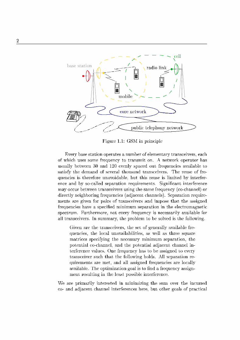
GSM is a second generation digital cellular radio system. Among others, GSM provides telephony service: a mobile phone may establish a communication link with any other party reachable through a public telephone network. This is achieved by means of a radio link to some stationary antenna which is part of a large infrastructure, see Figure 1.1. Since the introduction of GSM, radio telephony has grown from a costly service used by few professionals to a mass market with penetration rates as high as 70 % in Finland and Iceland, for example. In more and more countries, the mobile cellular phone subscribers outnumber the fixed-line telephone subscriptions

Frequency planning is a key issues in fully exploiting the radio spec trum available to GSM. It has a significant impact on the quantity as well as on the quality of the radio communication services. Roughly speak­ing, radio communication requires a radio signal of sufficient strength which is not suffering too severely from interference by other signals. In a cellular system like GSM, these two properties, strong signals and little interference, are in conflict. The problem of finding a "good" frequency plan is sketched in the following and described in full detail later

y ~ ~- ce

Figure 1.1: GSM in principle

Every base station operates a number of elementary transceivers, each of which uses some frequency to transmit on. A network operator has usually between 30 and 120 evenly spaced out frequencies available to satisfy the demand of several thousand transceivers. The reuse of fre­quencies is therefore unavoidable, but this reuse is limited by interfer ence and by so-called separation requirements. Significant interference may occur between transceivers using the same frequency (co-channel) or directly neighboring frequencies (adjacent channels). Separation require ments are given for pairs of transceivers and impose that the assigned frequencies have a specified minimum separation in the electromagnetic spectrum. Furthermore, not every frequency is necessarily available for all transceivers. In summary, the problem to be solved is the following.

Given are the transceivers, the set of generally available fre quencies, the local unavailabilities, as well as three square matrices specifying the necessary minimum separation, the potential co-channel, and the potential adjacent channel in­terference values. One frequency has to be assigned to every transceiver such that the following holds. All separation re quirements are met, and all assigned frequencies are locally available. The optimization goal is to find a frequency assign­ment resulting in the least possible interference.

We are primarily interested in minimizing the sum over the incurred co- and adjacent channel interferences here, but other goals of practical

T R O D U

interest exist as well. Striving for "minimum interference" asignments is in a sense a luxury to be paid for with frequencies. If only few frequencies are available to a GSM operator, then the emphasis is likely on providing some acceptable frequency plan at all. But the optimization aspect gains importance when feasible assignments can be obtained "easily." E-Plus is currently in the latter position. The network contains roughly 8000 base stations, and 115 frequencies are available.

New assignments have to be computed on several occasions. Some examples are: the network is modified or expanded, the characteristics of a transceiver are changed, or significant unpredicted interference is reported and has to be resolved.

Several commercial software packages exist which allow to document the network configuration, to plan radio coverage, and to predict interfer­ence in addition to frequency planning. GSM infrastructure manufactur ers develop such tools, but also independent companies such as AIRCOM International (Asset), COSIRO GmbH (Fun), Lociga Pic. (Odyssey) L&S Hochfrequenztechnik GmbH (CHIRplus), or Metapath Software In­ternational Limited (PlaNet). At the time when the cooperation with E-Plus started, however, the optimization of frequency assignments with respect to interference was often only poorly supported. This has cer tainly improved since then.

In the following, we deal with a broad spectrum of topics ranging from the technical background of the GSM frequency planning problem over alternative mathematical models and heuristic planning methods to quality assessments for the generated frequency plans. In addition to this introduction, the thesis comprises seven chapters and an appendix containing a compilation of mathematical notation used in the following. The content of each chapter is now briefly stated.

In Chapter 2, we give a survey of GSM and explain the technical conditions to be taken into account during frequency planning. We also describe how the input data is generated and stress the importance of reliable interference predictions for the success of automatic frequency planning.

In Chapter 3, the frequency planning problem (as sketched above) is formalized as a combinatorial minimization problem. We investigate the computational complexity of the model beyond stating its A/'P-hardness and we discuss extensions of the model as well as alternative models.

In Chapter 4, seven heuristic frequency planning methods are de scribed. Depending on the point of view, five or six of them can be used (in combination) for generating frequency assignments in practice. In

accordance with the objective of the cooperation with E-Plus, our focus is on fast methods rather than on more elaborate, but slower methods.

In Chapter 5, the previously described planning methods are com­pared on the basis of realistic frequency planning problems. In this com­parison, we include the currently best performing method we know of as a reference. An analysis of the realistic planning scenarios is provided, and we explain how to use the described heuristics in order to obtain time savings and quality improvements in practice.

In Chapter 6, a lower bound on the amount of unavoidable co-channel interference is computed for each planning scenario. These bounds are obtained by solving large semidefinite programs (which are challenges to the currently existing solvers). Based on these bounds, quality guarantees are provided for the frequency assignments from the preceding chapter Moreover, we introduce a relaxed version of our frequency planning prob­lem. The solutions for the relaxed problem can sometimes be turned into feasible assignments for the original problem. Exploiting this connection, we point out room for further development of heuristics

The relaxed version of frequency planning leads us to the study of the mathematical M I N I M U M K - P A R T I T I O N problem and its semidefinite relaxation (which we considered so far mostly as a "black box" providing lower bounds)

In Chapter 7, we mostly review results on a polytope, which is ob­tained as the convex hull of the feasible solutions to an integer linear programming formulation of the MINIMUM K-PART problem. Par ticular emphasis is on the hypermetric inequalities.

In Chapter 8, we first give an introduction to semidefinite program­ming and then study the semidefinite relaxation for the M I N I M U M K-

P A R T I T I O N problem. In particular, we describe a large class of valid inequalities for the solution set of the semidefinite relaxation (a shifted version of hypermetric inequalities), and we prove that neither the linear programming relaxation of the integer linear programming formulation nor the semidefinite programming relaxation is always stronger than the other

HAPTER

F r e q c y la SM

The General System for Mobile Communicaons or GSM,1 for short, is a GSM multi-service cellular communication system providing speech and data services. The most important service is radio telephony, but data services like short message service (SMS) and mobile Internet access building on the Wireless Application Protocol (WAP) are also rapidly gaining popularity.

In this chapter, the ground is laid for understanding the constraints and the objectives of frequency planning for a GSM network. Moreover the frequency planning problem is informally stated. A brief sketch of GSM's history is given in Section 2.1. The four major subsystems are explained in Section 2.2, and those parts of the radio interface which are relevant to frequency planning are discussed in detail. In Section 2.3, we show how to phrase frequency planning as an optimization problem, explain the constraints to be met, discuss how the input data is generated, and report on practical aspects of frequency planning. The reader who is familiar with GSM and is primarily interested in frequency planning may skip straight to Section 2.3.

2.1 Brief History of GSM

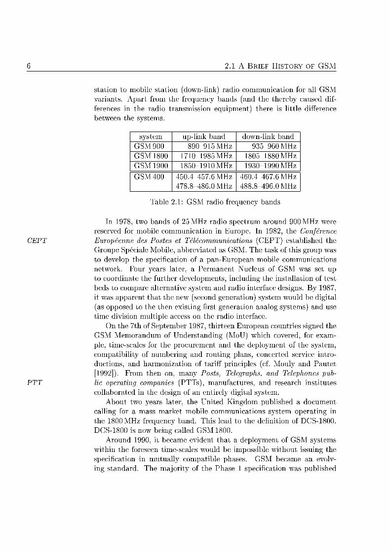
GSM has been designed as a pan-European cellular communications sys­tem to be operated in the 900 MHz radio frequency band. It has subse quently been extended to the 1800 MHz band in Europe. Today, there are also variants operated in the 1900 MHz band in other parts of the world. The respective systems are nowadays called GSM 900, GSM 1800, and GSM 1900. A fourth variant, called GSM 400, is under specification and will operate between 400 and 500 MHz. Table 2.1 lists the precise frequency bands for mobile station to base station (up-link) and base

1GSM and "General System for Mobile Communications" are trademarks of the GSM Association, Geneva Switzerland.

2. F H S T O R O F

station to mobile station (down-link) radio communication for all GSM variants. Apart from the frequency bands (and the thereby caused dif ferences in the radio transmission equipment) there is little difference between the systems

system up-link band down-link band GSM 900 890-915 MHz 935-90 MHz GSM 1800 1710-1985 MHz 1805-1880 MHz GSM 1900 850-1910 MHz 1930-1990 MHz

GSM 00 50 .457 .6 MHz 7 8 . 8 - 0 MHz

460.4467.6 MHz 4 8 8 . 8 - 4 0 MHz

Table 2.1: GSM radio f q u e n c y bands

In 1978, two bands of 25 MHz radio spectrum around 900 MHz we reserved for mobile communication in Europe. In 1982, the Conferenc

CEPT Europeenne des Postes et Telecommunications (CEPT) established the Groupe Speciale Mobile, abbreviated as GSM. The task of this group was to develop the specification of a pan-European mobile communications network. Four years later, a Permanent Nucleus of GSM was set up to coordinate the further developments, including the installation of test beds to compare alternative system and radio interface designs. By 1987, it was apparent that the new (second generation) system would be digital (as opposed to the then existing first generation analog systems) and use time division multiple access on the radio interface.

On the 7th of September 1987, thirteen European countries signed the GSM Memorandum of Understanding (MoU) which covered, for exam­ple, t imescales for the procurement and the deployment of the system, compatibility of numbering and routing plans, concerted service intro­ductions, and harmonization of tariff principles (cf. Mouly and Pautet [1992]). From then on, many Posts, Telegraphs, and Telephones pub-

PTT lie operating companies (PTTs), manufactures, and research institutes collaborated in the design of an entirely digital system.

About two years later, the United Kingdom published a document calling for a mass market mobile communications system operating in the 1800 MHz frequency band. This lead to the definition of DCS-1800. DCS-1800 is now being called GSM 1800.

Around 1990, it became evident that a deployment of GSM systems within the foreseen timescales would be impossible without issuing the specification in mutually compatible phases. GSM became an evolv­ing standard. The majority of the Phase 1 specification was published

RE NG

in 1990. At that time, the Technical Specification of GSM 900 contained 130 recommendations on more than 5000 pages. These recommenda­tions comprised the full specification of the radio interface as well as a detailed specification of infrastructure, architecture, and many intra-and intersystem interfaces. The first GSM pilot network was successfully demonstrated at the Telecom '91 fair, organized by the International Telecommunication Union (ITU). Later in the same year, several net TU works were fully operational, but type approved GSM terminals were not available, and GSM was made fun of as the acronym for the prayer "God Send Mobiles." The reason was simply that the procedures for type ap­proval were not settled. In April 1992, an Iterim Te Approval (ITA) ITA was agreed on.

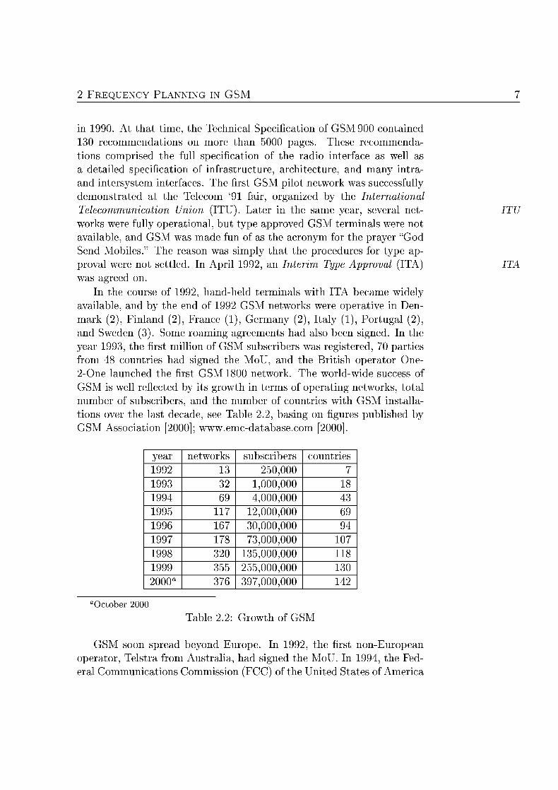
In the course of 1992, hand-held terminals with ITA became widely available, and by the end of 1992 GSM networks were operative in Den­mark (2), Finland (2), France (1), Germany (2), Italy (1), Portugal (2) and Sweden (3). Some roaming agreements had also been signed. In the year 1993, the first million of GSM subscribers was registered, 70 parties from 48 countries had signed the MoU, and the British operator One 2One launched the first GSM 1800 network. The world-wide success of GSM is well reflected by its growth in terms of operating networks, total number of subscribers, and the number of countries with GSM installa­tions over the last decade, see Table 2.2, basing on figures published by GSM Association [2000]; www.emcdatabase.com [2000]

year networks subscribers countries

1992 250,000

1993 32 1,000,000 18 199 000,000

1995 117 2,000,000

199 30,000,000

1997 178 73,000,000 07 1998 320 135,000,000 118 1999 355 255,000,000 30 2000a 37 397,000,000

a O r 2000

Table 2.2: Growth of GSM

GSM soon spread beyond Europe. In 1992, the first non-European operator, Telstra from Australia, had signed the MoU. In 1994, the Fed­eral Communications Commission (FCC) of the United States of America

2. F H S T O R O F

auctioned several licenses to operate mobile networks around 1900 MHz. No particular network type was imposed, and the first GSM 1900 net work (then still called PCS 1900) was launched by American Personal Communications in November 1995.

By the end of the third quarter of the year 2000, there were 376 operating GSM networks world-wide with a total of 396.6 million sub­scribers. In Europe alone (including Russia), there were 141 GSM900 and GSM 1800 networks with a total of 255.1 million subscribers.

In the meantime, the specification of GSM had been continued. GSM Phase 2 was issued in 1993. Numerous extensions were made such as an option for half-rate speech telephony, improved short message services calling/connected line identity presentation, call waiting and call hold features, mul t ipar ty calls, and advice of charge. But data transmission kept essentially restricted to at most 9.6 kbps. Opening up this bottleneck has become a central theme in the still ongoing specifications of Phase 2+ Three major new technologies are introduced. (The transmission rates are taken from GSM Association [2000, Glossary])

CSD High Speed Circuit Switched Data (HSCSD) allows the transmis sion of circuitswitched data with a speed of up to 57. kbps. The data rate per time slot is increased to 14.4 kbps and up to four consecutive time slots may be concatenated.

PR General Packet Radio Service (GPRS) introduces the option for packetswitched services into GSM. GPRS will provide data trans mission speeds of up to 115 kbps to mobile users

Enhanced Data for GSM Evolution (EDGE) uses a new modulation scheme to allow data transmission with rates of up to 38 kbps on the basis of the GSM infrastructure.

These technologies, however, require a higher signal to noise ratio at the receiver (i.e., they can cope with less interference) than regular data transmissions in order to guarantee proper reception. This has an impact on the planning of the radio interface in general and frequency planning in particular.

Finally, over the past years the standards for third generation cellular mobile systems (IMT-2000) have been under development. The Uni versal Mobile Telecommunications System (UMTS) is one of them, for which a first standard was issued in the beginning of the year 2000. The radio interface of UMTS is different from that of GSM. The Code Di vision Multiple Access (CDMA) scheme is used, and no frequency plan­ning problem comparable to that of GSM has to be solved. UMTS is

RE NG

expected to be commercially available in Europe around the year 2002. It allows for true global roaming, and it is supposed to support a wide range of voice and data services. Depending on the user mobility and the propagation environment, different maximal data transmission rates are foreseen: 144 kbps for vehicular, 384 kbps for pedestrian, and 2 Mbps for indoor users. UMTS will be deployed parallel to GSM, and more than ten years of coexistence of GSM and UMTS are expected. In Germany, for example, the first GSM license expires at the end of the year 2009.

2.2 The G e n r a l System for obile Communication

GSM is a multiservice cellular radio system, capable of transmitting speech as well as data and with numerous supplementary features. The area covered by a GSM network consists of (overlapping) cells, which are served by stationary antennas. The kind of service provided depends on the conten of he subscription, the apabilities of h e t k , and the

apabilities of userel equien

2.2. Mobile Stat ions

radio link connects a mobile station to the GSM network infrastructure. A switched-on mobile station is either in idle mode or in dedicated mode. In idle mode, the mobile station listens to control channels, but does not idle mode have a channel of its own. In dedicated mode, a bidirectional channel dedicated mode is allocated to the mobile terminal allowing it to exchange information with and through the GSM network. A mobile terminal switches from idle into dedicated mode, for example, if the user wants to place a call The mobile sends a corresponding request to the cell of which it monitors the control channel. Another example is the arrival of a call. In that case, however, the network is generally not aware of the cell a mobile terminal is listening to (if any) so that the mobile is "paged.

To limit the amount of paging messages, location areas are defined. A location area is a group of cells, and every cell belongs to exactly one location area location area. The identity of the location area is broadcast by each cell so that a mobile station can always find out what location area it is in. In case the mobile is moved and the location area changes, a message is sent out, and the network registers the change. This process is called location updating. When a call for a mobile station arrives, a paging message for location updating that mobile station is broadcast in all cells of the location area the mobile station has last registered in. (Sometimes, this is preceded by paging the

2 E G E R A S T E O R C O A T

mobile station only in the cell of last active contact with the network.) If this paging fails, a paging message is broadcast in all cells of the network.

A mobile terminal may, of course, also be moved while in dedicated mode. Depending on the distance to the serving base station and the propagation conditions, the radio link can degrade below the required quality. The bidirectional channel has then to be dropped or to be main­tained by another cell. Changing the serving cell in dedicated mode is

and-over called hand-over. During a hand-over, the network has to reroute the communication channel without the user noticing. The decisions, when to perform a hand-over and to which cell, are taken in the network in­frastructure, but with the support of the mobiles. Each mobile terminal routinely monitors a list of neighboring cells, records the reception qual ity, and sends measurement reports the network.

Despite the option of international roaming, a GSM telephone call usually comes to an end at national borders due to a call drop. The rea­sons are primarily billing issues. But (presuming frequency band com­patibility) the mobile station may then log on into a foreign network in order to place and to receive calls, if the user's subscription allows inter national roaming and appropriate roaming agreements are made between the operators

2.2.2 S u b s y s t e m s

Next to the mobile sttions, the three further major parts of GSM are the base station subsystem, the network and switching subsystem, and the operation and maintenance subsystem. A detailed description of these subsystems and their interfaces is given in the relevant standards issued

ET by the European Telecommunications Standards Institute (ETSI), Sophia Antipolis, France. A more accessible source of information, however, is the book of Mouly and Pautet [1992].

MS A Mobile Station (MS) usually consists of some mobile equipment, SIM like a hand-held mobile, and a Subscriber Identification Module (SIM)

which is inserted into the mobile equipment. Depending on the frequency band of the network, see Table 2.1, different mobile equipment is typically required, but the same SIM can be used. Modern dual- or t r ip leband mo­bile terminals allow to communicate in two or three of those bands. The

IMS SIM carries an International Mobile Subscriber Identify (IMSI), personal izing the mobile equipment, and can be protected by a Personal Identity

PIN Number (PIN), similar to the PINs of credit cards. The SIM is the peer of the network during authentication, and it is involved in ciphering and

RE NG 11

d e i p h e i n g t a n s m i t e d mesages (when encryption is applied). The Base Station Subsystem (BSS) comprises base transceiver sta- BSS

tions and base station controllers. A Base Transceiver Station (BTS) is the peer of a mobile terminal in radio communications, both having radio transmission and reception devices, including antennas and all nec essary signal processing capabilities. The site at which a BTS is installed is organized in sectors; one or three sectors are typical. An antenna is sector operated for each sector. If three sectors exist, then antennas with an opening angle of 120 degree are usually employed. If only one sector ex­ists at a site, then an omnidirectional antenna can be used. (The details of how many sectors to choose, which antenna types, etc., depend on the practical needs, and are more complex than indicated here.) Each sector defines a cell. The capacity of a cell is determined by the number cell of elementary transmitter/receiver units, called TRXs, installed for the TRX sector. As a rule of thumb, the first TRX of a sector provides capacity for 6 parallel calls, and each additional TRX for seven to eight more calls The reduced capacity of the first and some of the additional TRXs is due to the need to transmit cell organization and protocol information. A maximum of 12 TRXs can be installed for one sector of a BTS. Every BTS is connected to one Base Station Controller (BSC), whereas one BS BSC typically handles several BTSs in parallel. A BSC is in charge of the allocation and release of radio channels as well as the management of hand-overs. All cells in a location area have to be controlled by the same BSC, but one BSC may serve more than one location area.

The Network and Switching Subsystem (NSS) manages the commu- NSS nication to and from GSM users. Every BSC is connected to one Mobil service Switching Center (MSC), and the core network interconnects the MS MSCs. Specially equipped Gateway MSCs (GMSCs) interface with other core network telephony and data networks. The Home Location Registers (HLRs) and GMS Visitors Location Registers (VLRs) are data base systems, which contain HL subscriber data and facilitate mobility management. Each Gateway MSC VL consults its home location register if an incoming call has to be routed to a mobile terminal. The HLR is also used in the authentication of the subscribers together with the Authentication Center (AuC). The VLRs are associated to one or more MSCs and temporarily store information on all subscribers that were last traced in one of the BSCs attached to any of its associated MSC(s). The interworking of all components of the NSS is organized via a SS7 signaling network.

The Operation and maintenance SubSystem (OSS) is specified to a OSS smaller extent than the rest of GSM. The network is run and maintained through the OSS: calls have to be billed and charged; SIMs have to

12 2 E G E R A STE OR C O A T

OM

be initialized; stolen or misbehaving mobile equipment is registered and possibly excluded from network service on the basis of the Equipmen Identity Register (EIR). The network and switching subsystem, the base station subsystem, and, to some extent, also the mobile stations (via the BSS) are administered from Operation and Management Centers (OMC)

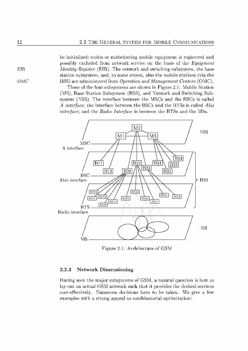
Three of the four subsystems are shown in Figure 2.1: Mobile Station (MS), Base Station Subsystem (BSS), and Network and Switching Sub­system (NSS). The interface between the MSCs and the BSCs is called A interface; the interface between the BSCs and the BTSs is called Abi interfac] and the dio terfac is between the BTSs and the MSs

NSS

MSC A interface

BSC Abis interface

BTS Radio interface

BSS

Figure 2.1: rchiteture of GSM

2.2. etwork Dimensioning

Having seen the major subsystems of GSM, a natural question is how to lay out an actual GSM network such that it provides the desired services costeffectively. Numerous decisions have to be taken. We give a few examples with a strong appeal to combinatorial optimization:

RE NG 13

Where to insa l l the BTSs? How to adjust the antennas and what frequencies to use? How to connect the BTSs to the BSCs, and where to put the MSCs? How to connect the MSCs among each other and to the BSCs?

These important questions have to be answered prior to network de ployment or expansion. All of them have an impact on generating rev­enues, because these decisions affect the cost of deploying and operating the network as well as the quality of service that can be offered.

Before focusing on frequency assignment in the chapters to come, we pick out some of these questions and explain the underlying optimization problem briefly. We give references, whenever we are aware of them.

At the core of planning a network deployment or extension is cus tomers' demand. This demand may be observed or forecasted. In one way or another, the customers' demand for mobile telecommunications has to be made precise in a geographical distribution in terms of Erlang, a unit for measuring telecommunication demand. This distribution essentially states how large the need for mobile telecommunications is depending on the location.

Base Transceiver Stat ion Location is the step in which radio engi neers decide how many and where to erect BTSs in order to provide service for the (prospective) demand. This is a mixture of deter mining sites, which are preferable from an "electromagnetic" point of view (providing good coverage), and searching for sites, which are actually available. Research in this direction has been carried out, for example, in ACTS/STORMS project (supported the Eu­ropean Union), see Menolascino and Pizarroso [1999], as well as by Eidenbenz, Stamm, and idmayer [1999] and Tutschku, Mathar and Niessen [1999]

Base Transceiver Stat ion Clustering denotes here the problem of where to place the BSCs and which BTSs to connect to them. Examples for the issues to be taken into account are the costs for renting or building spaces for operating BSCs and the running cost of attaching BTSs to BSCs by cables or pointto-point radio links The mobility profile of customers also plays a role here, because hand-overs between cells handled by the same BSC are treated lo­cally for the most part, whereas an inter-BSC hand-over requires a rerouting of connections in the core network also. Similar comments apply with respect to location-updating. Ferracioli and Verdone [2000] report on results in this area.

2 E G E R A S T E O R C O A T

Core Network Des ign denotes here the planning necessary to decide where to operate MSCs, which BSCs to connect to them, and how to interconnect the MSCs among each other. The locations of MSCs are usually more dependent on "political" rather than "technical" considerations. The core network may comprise leased lines, the operator's own cable infrastructure, and pointto-point radio links Usually, not every pair of MSCs is connected directly in the core network. Instead, routing tables are used to describe how to route traffic from one MSC to another along one or more links. The network has to be laid out (selection of connections, capacities, and routings) in such a way that a failure of a single link or a failure of a single MSCs has only a "manageable" impact on the traffic volume, which can be handled by the remaining part of the network. Such a network is called "survivable" in the literature, see, for example, Wessäly [2000] and the references therein.

Frequency Ass ignment or Channel Assignment or Frequency Plan­ning are synonyms for the following problem. Once the sites for the BTSs are selected and the sector layout is decided, the number of TRXs to be operated per sector has to be fixed. This is done by means of the Erlang-B formula, taking the demand to support and the maximally tolerable blocking probability (of 2% or the like) as input. The result is a listing of the demand in TRXs per cell Now, every TRX has to receive a channel. This demand has to be satisfied by a frequency plan.

The last problem is going to be the central topic from now on, and further details of the radio interface are discussed next

FDM TDM

annel

2.2. long the Radio nterface

In order to understand the various restrictions and the possible alterna­tive objectives in frequency planning, we take a closer look at the tech­nicalities of the GSM radio interface. Even more details can be found in the books by Mouly and Pautet [1992] and Redl Weber, and Oliphant 1995] as well as in the relevant ETSI standards.

GSM uses a Frequency Division Multiple Access (FDMA) and Time Division Multiple Access (TDMA) scheme to maintain several communi cation links within one cell "in parallel." The available frequency band is slotted into channels of 200 kHz width. The time axis is organized in 8 cyclicly recurring time slots, numbered TN0, TNI , . , TN7.

RE NG 15

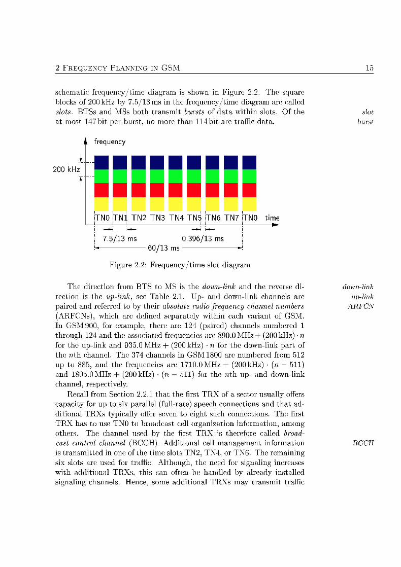
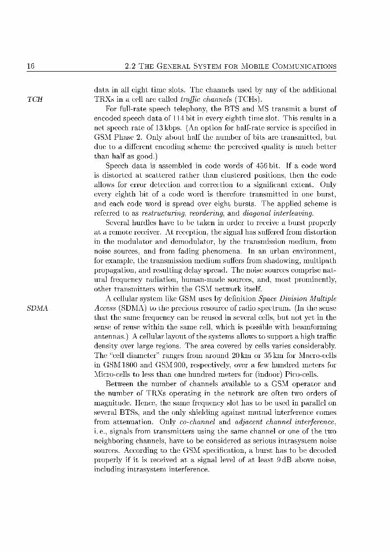
schematic frequency/time diagram is shown in Figure 2.2. The square blocks of 200 kHz by 7.5/13 ms in the frequency/time diagram are called slots. BTSs and MSs both transmit bursts of data within slots Of the at most 1 7 b i t per burst, no more than 11 bit are traffic data.

A frequency

i k

T K . . . . . . .

• • • • • • • UN TN TN TN TN4 TN TN TN TN time

75/13 ms 39 /13 ms /13 ms

Figure 2.2: Frquency/time slot diagram

ot rst

The direction from BTS to MS is the downlink and the reverse di rection is the up-link, see Table 2.1. Up- and down-link channels are paired and referred to by their absolute radio frequency channel numbers (ARFCNs), which are defined separately within each variant of GSM. In GSM 900, for example, there are 124 (paired) channels numbered through 124 and the associated frequencies are 890.0 MHz + (200 kHz) • n for the up-link and 9350 MHz + (200 kHz) • n for the down-link part of the nth channel. The 374 channels in GSM 1800 are numbered from 512 up to 885, and the frequencies are 1710.0 MHz + (200 kHz) • (n - 511 and 1805.0 MHz + (200 kHz) • (n - 511) for the nth up- and down-link channel, respectively.

Recall from Section 2.2.1 that the first TRX of a sector usually offers capacity for up to six parallel (full-rate) speech connections and that ad­ditional TRXs typically offer seven to eight such connections. The first TRX has to use TNO to broadcast cell organization information, among others. The channel used by the first TRX is therefore called broad cast control channel (BCCH). Additional cell management information is transmitted in one of the time slots TN2, TN4, or TN6. The remaining six slots are used for traffic. Although, the need for signaling increases with additional TRXs, this can often be handled by already installed signaling channels Hence, some additional TRXs may transmit traffic

down upli

CC

2 E G E R A S T E O R C O A T

data in all eight time s lo t . The channels u s d by any of he additional TC TRXs in a cell are called traffic channels (TCHs).

For full-rate speech telephony, the BTS and MS transmit a burst of encoded speech data of 114 bit in every eighth time slot. This results in a net speech rate of 13 kbps. (An option for halfrate service is specified in GSM Phase 2. Only about half the number of bits are transmitted, but due to a different encoding scheme the perceived quality is much better than half as good.)

Speech data is assembled in code words of 456 bit. If a code word is distorted at scattered rather than clustered positions, then the code allows for error detection and correction to a significant extent. Only every eighth bit of a code word is therefore transmitted in one burst and each code word is spread over eight bursts. The applied scheme is referred to as restructuring, reordering, and diagonal interleaving.

Several hurdles have to be taken in order to receive a burst properly at a remote receiver. At reception, the signal has suffered from distortion in the modulator and demodulator, by the transmission medium, from noise sources, and from fading phenomena. In an urban environment for example, the transmission medium suffers from shadowing, multipath propagation, and resulting delay spread. The noise sources comprise nat ural frequency radiation, human-made sources, and, most prominently, other transmitters within the GSM network itself

A cellular system like GSM uses by definition Space Division Multipl SDM Access (SDMA) to the precious resource of radio spectrum. (In the sense

that the same frequency can be reused in several cells, but not yet in the sense of reuse within the same cell, which is possible with beamforming antennas.) A cellular layout of the systems allows to support a high traffic density over large regions. The area covered by cells varies considerably. The "cell diameter" ranges from around 20 km or 35 km for Macro-cells in GSM 1800 and GSM 900, respectively, over a few hundred meters for Micro-cells to less than one hundred meters for (indoor) Pico-cells.

Between the number of channels available to a GSM operator and the number of TRXs operating in the network are often two orders of magnitude. Hence, the same frequency slot has to be used in parallel on several BTSs, and the only shielding against mutual interference comes from attenuation. Only co-channel and adjacent channel interference i.e., signals from transmitters using the same channel or one of the two neighboring channels, have to be considered as serious intrasystem noise sources. According to the GSM specification, a burst has to be decoded properly if it is received at a signal level of at least 9 dB above noise, including intrasystem interference.

RE NG 17

A number of measures is foreseen in GSM to counteract the generation of and the sensitivity to interference. We mention only those with significant impact on the frequency planning problem.

Power Control is a feature of GSM that allows to dynamically ad­just the transmission power to an appropriate level. A maximum emission power is specified for GSM transmitters. For hand-held mobiles this is 1 W or 2 W, depending on the GSM variant. In case less transmission power is sufficient to guarantee proper reception, the power can be reduced. Any power excess would only cause un­necessary interference and power consumption. A trade off between power control and hand-over has to be made: without the emission power being at the maximum level, a hand-over may be favorable to enter another cell, where a yet smaller power level suffices

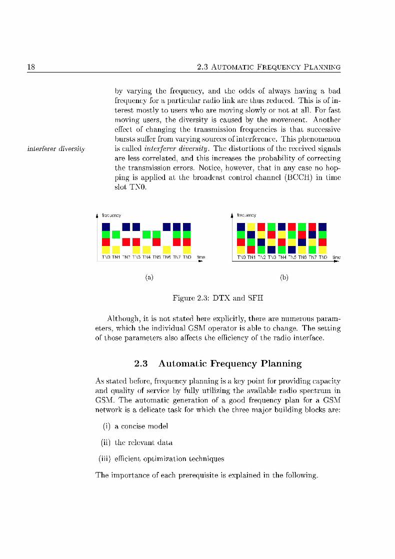
Discontinuous Transmission (DTX) is a feature of GSM that sup­presses transmission if no data has to be transmitted. There is, for example, no need to transmit the (short) phases of silence within a conversation. The transmission is suspended and the receiving mobile generates a so-called comfort noise to make the suppression (almost) imperceptible. Triggered by a mechanism called voice ac­tivity detection, the transmission resumes as soon as the need arises Figure 2.3(a) gives an illustration, where the pattern indicates the bursts. In case a channel is used as BCCH, a burst has to be trans mitted in every time slot and DTX cannot be applied. (Hence, none of channels in Figure 2.3(a) is used as BCCH in the corresponding cell)

Slow Frequency Hopping (SFH) allows the transmission of consec utive bursts on different frequencies. Two variants exist. With synthesized frequency hopping, each TRX of a sector transmits suc cessive bursts on different channels. The sequence, in which the available channels are switched, is determined by two parameters One is the Hopping Sequence Number (HSN), selecting one out of hopping sequences, and the other is the Mobile Allocation Index Offset (MAIO), which determines the starting point within the sequence. If more than one TRX is used for a sector, baseband frequency hopping can be applied alternatively. Each TRX uses a fixed channel, and the code words constituting a flow of communi cation are dispatched to changing TRXs, see Figure 2.3(b)

Frequency hopping addresses two problems. The quality of a ra­dio path is frequency dependent requency diersity is obtained

frequency divert

2.3 AT NG

ierferer diversi

by varying the frequency, and the odds of always having a bad frequency for a particular radio link are thus reduced. This is of in­terest mostly to users who are moving slowly or not at all. For fast moving users, the diversity is caused by the movement. Another effect of changing the transmission frequencies is that successive bursts suffer from varying sources of interference. This phenomenon is called interferer diversity. The distortions of the received signals are less correlated, and this increases the probability of correcting the transmission errors. Notice, however, that in any case no hop­ping is applied at the broadcast control channel (BCCH) in time slot TNO.

1 frequency k frequency

TN0 TN1 TN2 TN3 TN4 TN5 TN6 TN7 TN0 time TN0 TN1 TN2 TN3 TN4 TN5 TN6 TN7 TN0 time

a) b)

Figure 2.3: DTX and SFH

Although, it is not stated here explicitly, there are numerous param­eters, which the individual GSM operator is able to change. The setting of those parameters also affects the efficiency of the radio interface.

2.3 tomatic Frequency Planning

As stated before, frequency planning is a key point for providing capacity and quality of service by fully utilizing the available radio spectrum in GSM. The automatic generation of a good frequency plan for a GSM network is a delicate task for which the three major building blocks are:

(i) a concise model

(ii) the relevant data

(iii) efficient optimization techniques

The imporance of each p r q u i s i t e is explained in the following.

RE NG 19

First, the automatic generation of a frequency assignment by a com­puter relies on the representation of all relevant aspects. Hence, a concise (mathematical) model of the frequency planning problem is necessary. On one hand, this model should be simple for the sake of easy handling. On the other hand, all information has to be captured which is necessary to accurately estimate a frequency plan's quality (without testing it in the real network). This is, for example, a point where the traditional model with hexagonal cell shapes fails, compare with Section 2.3.2. (The model still receives attention in the literature, however, because all relevant data is easily generated and planning based on this model is more easily accessible.) The spectrum of models currently in use is wide. It ranges from simplistic graph coloring models over graph-based models dealing with the maximization of satisfied demand or the minimization of inter ference to models building directly on signal predictions and looking at the probability of failed code word reception (frame erasure rate), see, for example, Koster [1999], Murphey, Pardalos, and Resende [1999], and Correia [2001, Section 4.2]. After preparing the ground in Section 2.3.1, we come back to models in Chapter 3.

Second, the concise model is futile unless the corresponding data is provided. The main difficulties here are related to data on radio signal levels. This data is needed in ample ways, for example, in order to estimate how much interference can occur between transmitters or to determine between which cells a hand-over can be supported. Details are discussed in Section 2.3.2.

Third, with a concise model and reliable data in hands, the task of producing a good frequency plan can be reduced to the problem of finding a solution to a mathematical optimization problem. Special software for this purpose is in demand. Operations Research has picked up this problem in the late 1 9 0 s and dealt with it steadily, compare Metzger [1970], Hale [1980], and Roberts [1991a]. The most progress has been made within recent years, accompanying the deployment and extension of GSM networks and often stimulated by close cooperations between research facilities and network operators or equipment manufacturers We come back to planning algorithms in Chapter 4.

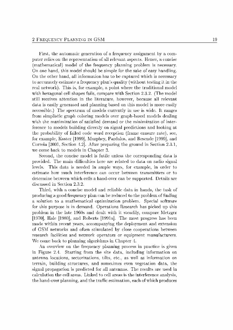
An overview on the frequency planning process in practice is given in Figure 2.4. Starting from the site data, including information on antenna locations, sectorizations, tilts, etc., as well as information on terrain, building structures, and sometimes even vegetation data, the signal propagation is predicted for all antennas. The results are used in calculation the cell areas. Linked to cell areas is the interference analysis the hand-over planning, and the traffic estimation, each of which produces

20 2.3 AT NG

mandatory input data for the actual frequency assignment. Details on most of these items are given in the remainder of this chapter

e dat

path loss p r d i o n

l c a l u l a t o n

i n t n c e analysis hand-over planning

n t n c e mat

neighborhood lis

affic calculation

pa ra ton mat channel r q u i m e n t

frequency assignment

Figure 2 . : Frquency planning proc

ste sector cell

2. b j e c t v e and C o n s r a i n t s

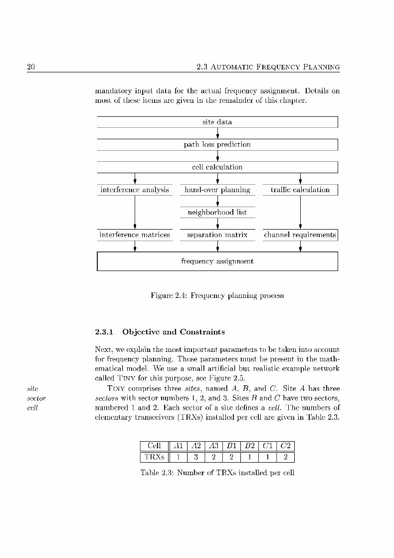
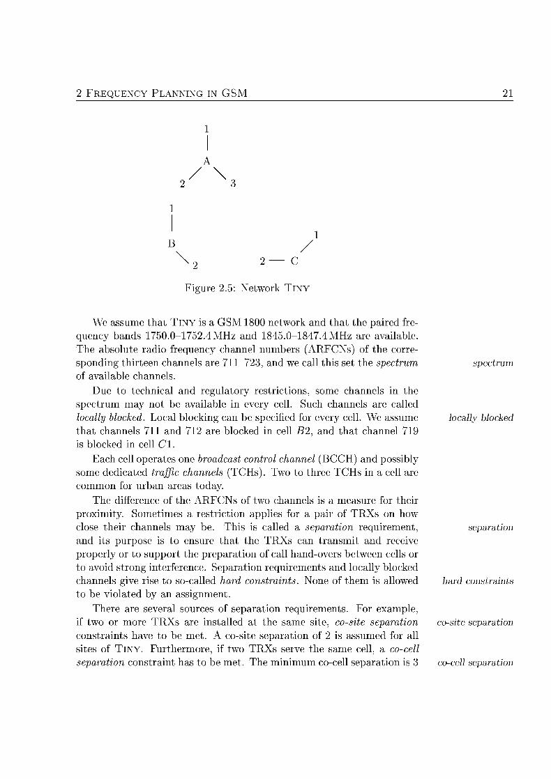
Next, we explain the most important parameters to be taken into account for frequency planning. Those parameters must be present in the math­ematical model. We use a small artificial but realistic example network called T N Y for this purpose, see Figure 2.5.

NY comprises three sites, named A, B, and C. Site A has three sectors with sector numbers 1, 2, and 3. Sites B and C have two sectors numbered 1 and 2. Each sector of a site defines a cell. The numbers of elementary transceivers (TRXs) installed per cell are given in Table 2.3.

Cell A3 Bl

Xs

Table 2.3: Number of TRXs installed per c l l

RE NG 21

Figure 2.5: Network T N Y

We assume that TINY is a GSM 1800 network and that the paired fre quency bands 1750.0-1752.4 MHz and 1845.0-187.4 MHz are available. The absolute radio frequency channel numbers (ARFCNs) of the corre sponding thirteen channels are 711-723, and we call this set the spectrum of available channels

Due to technical and regulatory restrictions, some channels in the spectrum may not be available in every cell. Such channels are called locally blocked. Local blocking can be specified for every cell. We assume that channels 711 and 712 are blocked in cell 2, and that channel 719 is blocked in cell CI.

Each cell operates one broadcast control channel (BCCH) and possibly some dedicated traffic channels (TCHs). Two to three TCHs in a cell are common for urban areas today.

The difference of the ARFCNs of two channels is a measure for their proximity. Sometimes a restriction applies for a pair of TRXs on how close their channels may be. This is called a separation requirement and its purpose is to ensure that the TRXs can transmit and receive properly or to support the preparation of call hand-overs between cells or to avoid strong interference. Separation requirements and locally blocked channels give rise to so-called had constraints None of them is allowed to be violated by an assignment

There are several sources of separation requirements. For example, if two or more TRXs are installed at the same site, cosite separation constraints have to be met. A co-site separation of 2 is assumed for all sites of T N Y . Furthermore, if two TRXs serve the same cell, a cocell epation constraint has to be met. The minimum co-cell separation is

specru

locall blocked

ard conrai

co searaton

cocell searation

22 2.3 AT NG

in each cell for TINY. In practice, this value may vary from cell to cell due to different technologies in use, but the values given here are typical

AI

A2

Bl

Table 2. Hand-over rlation for NY

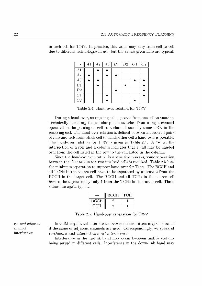
During a hand-over, an ongoing call is passed from one cell to another Technically speaking, the cellular phone switches from using a channel operated in the passing-on cell to a channel used by some TRX in the receiving cell. The hand-over relation is defined between all ordered pairs of cells and tells from which cell to which other cell a hand-over is possible. The hand-over relation for TINY is given in Table 2.4. A "•" at the intersection of a row and a column indicates that a call may be handed over from the cell listed in the row to the cell listed in the column.

Since the hand-over operation is a sensitive process, some separation between the channels in the two involved cells is required. Table 2.5 lists the minimum separation to support hand-over for TINY. The BCCH and all TCHs in the source cell have to be separated by at least 2 from the BCCH in the target cell. The BCCH and all TCHs in the source cell have to be separated by only 1 from the TCHs in the target cell. These values are again typical

BCCH TCH BCCH TCH

Table 2.5: Hand-over sparation for NY

In GSM, significant interference between transmitters may only occur if the same or adjacent channels are used. Correspondingly, we speak of cochannel and adjacent channel interference.

Interference in the up-link band may occur between mobile stations being served in different cells. Interference in the down-link band may

co and adjacen channel iterference

RE NG 23

occur between TRXs operated at different sites. Although the up-link is usually more critical in GSM than the down-link, the interference is specified for the down-link. The reason for this is the lack of appropriate ways to predict up-link interference. Already the prediction of down-link interference is intricate, see Section 2.3.2.

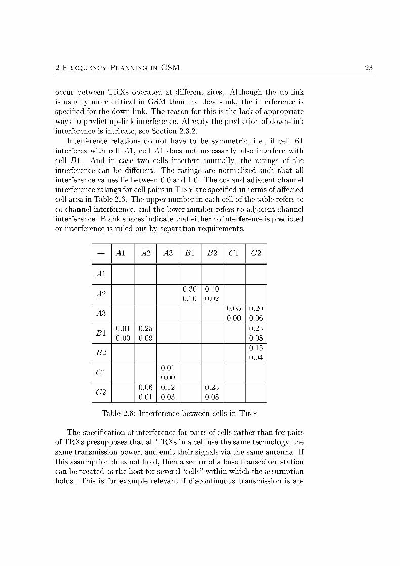
Interference relations do not have to be symmetric, i.e., if cell Bl interferes with cell Al, cell Al does not necessarily also interfere with cell Bl. And in case two cells interfere mutually, the ratings of the interference can be different. The ratings are normalized such that all interference values lie between 0.0 and 1.0. The co- and adjacent channel interference ratings for cell pairs in TINY are specified in terms of affected cell area in Table 2.6. The upper number in each cell of the table refers to co-channel interference, and the lower number refers to adjacent channel interference. Blank spaces indicate that either no interference is predicted or interference is ruled out by separation requirements

Bl

0.30 010

0.10 002

A3 0.05 000

0. 00

Bl 0.0 000

0.25 009

0.25 008 0. 004

0.0 000

0.06 001

0.12 003

0.25 008

Table 2 . : I n t n c e b e w e n cl ls in NY

The specification of interfence for pairs of cells rather than for pair of TRXs presupposes that all TRXs in a cell use the same technology, the same transmission power, and emit their signals via the same antenna. If this assumption does not hold, then a sector of a base transceiver station can be treated as the host for several "cells" within which the assumption holds. This is for example relevant if discontinuous transmission is ap-

2.3 AT NG

plied, because the average interference caused by a TCH applying DTX is less than that of the BCCH, which is not allowed to apply DTX.

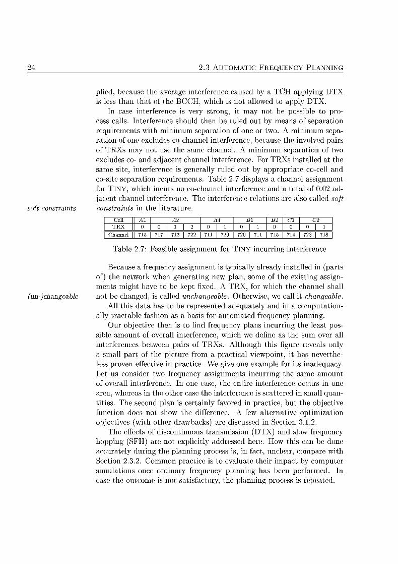
In case interference is very strong, it may not be possible to pro­cess calls. Interference should then be ruled out by means of separation requirements with minimum separation of one or two. A minimum sepa­ration of one excludes co-channel interference, because the involved pairs of TRXs may not use the same channel. A minimum separation of two excludes co- and adjacent channel interference. For TRXs installed at the same site, interference is generally ruled out by appropriate co-cell and co-site separation requirements. Table 2.7 displays a channel assignment for T I N Y , which incurs no co-channel interference and a total of 0.02 ad­jacent channel interference. The interference relations are also called sof

so constrai constraints in the literature.

Cell Al A2 CI C2 TRX | | | | |

Channel 15 | 13 | 22 | | 15 14 23 | 18

Table 2.7: Feasible as ignment for NY incur ing i n t n c

Because a frequency assignment is typically already installed in (parts of) the network when generating new plan, some of the existing assign­ments might have to be kept fixed. A TRX, for which the channel shall

-)cangeable not be changed, is called unchangeable. Otherwise, we call it changeable All this data has to be represented adequately and in a computation­

ally tractable fashion as a basis for automated frequency planning. Our objective then is to find frequency plans incurring the least pos

sible amount of overall interference, which we define as the sum over all interferences between pairs of TRXs. Although this figure reveals only a small part of the picture from a practical viewpoint, it has neverthe less proven effective in practice. We give one example for its inadequacy. Let us consider two frequency assignments incurring the same amount of overall interference. In one case, the entire interference occurs in one area, whereas in the other case the interference is scattered in small quan­tities. The second plan is certainly favored in practice, but the objective function does not show the difference. A few alternative optimization objectives (with other drawbacks) are discussed in Section 3.1.2.

The effects of discontinuous transmission (DTX) and slow frequency hopping (SFH) are not explicitly addressed here. How this can be done accurately during the planning process is, in fact, unclear, compare with Section 2.3.2. Common practice is to evaluate their impact by computer simulations once ordinary frequency planning has been performed. In case the outcome is not satisfactory, the planning process is repeated.

RE NG 25

Our v e i o n of the req asgnmt prob is, thus, as follows

Gen e a list of TRXs, rang of channels, a list of locally blocked channel for ach TR as well as mini mum sepation, the cohannel interferene, and djacen hannel interference trices

Assign to every TRX one channel rom te spectrum whic t locally block such tha all separtion requirements ar

et and suc tha e sum over all interferenes occurring beten pai of TRX minimizd

We give a mathematical statement of this problem in Chapter 3. Next we explain how the input data is generated with sufficient accuracy and in which way solving the above problem is embedded in practice.

2 . 2 Precise Data

The main difficulties concerning reliable data arise with respect to radio signal levels. Signal levels are provided through measurements in few cases only. In the other cases, the signal strength is predicted using wave propagation models. We sketch the most prominent tasks and the related problems to be tackled in preparation for algorithmic frequency planning.

Cells and eighbors

The area, where a mobile station may get service from a particular sector of a BTS, is called cell area. Cell areas may overlap. The cell areas have cell area to be estimated for at least two purposes.

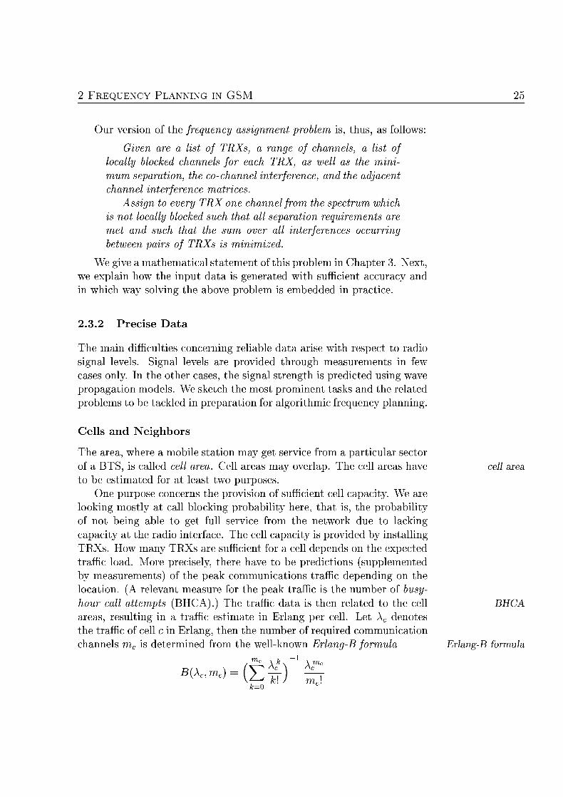
One purpose concerns the provision of sufficient cell capacity. We are looking mostly at call blocking probability here, that is, the probability of not being able to get full service from the network due to lacking capacity at the radio interface. The cell capacity is provided by installing TRXs. How many TRXs are sufficient for a cell depends on the expected traffic load. More precisely, there have to be predictions (supplemented by measurements) of the peak communications traffic depending on the location. (A relevant measure for the peak traffic is the number of busy hour all attempts (BHCA).) The traffic data is then related to the cell areas, resulting in a traffic estimate in Erlang per cell. Let Ac denotes the traffic of cell c in Erlang, then the number of required communication channels mc is determined from the wellknown Erlang formul ang- for

c

26 2.3 AUTOMATIC FREQUENCY PLANNING

by setting mc to the least possible value such that a blocking probability B(XC, mc) of 2%, say is not exceeded. Then the smallest number of TRXs is chosen for cell c, which allows to support mc simultaneous calls.

The other purpose of calculating the cell areas is to decide on the hand-over relations, that is, from which cell to which other cell a hand­over should be possible. This has to be settled in advance, because every cell broadcasts on the BCCH to which neighboring cells a hand-over is supported, and, correspondingly, hand-over separation requirements have to be observed during frequency planning. In order to hand an established communication link from one cell over to another the mobile station has to be located in the overlap of the two cell areas.

Notice that the cell area does not only depend on the installation and configuration of the BTS and its sectors (including antenna height tilt, transmission power, etc.) but also on the noise and interference from other BTSs. In addition to having a sufficiently strong radio signal at the receiver, this signal must also be sufficiently undistorted to be decoded correctly. This issue, however is neglected in the folloing discussion of cell area prediction models.

The simplest model assigns each point to the cell with the strongest signal. The BTSs are assumed to be spaced out regularly on a grid and to have identical antenna configurations as well as identical transmission powers. The propagation conditions are taken to be isotropic. The result

hexagonal cell is a hexagonal cell pattern. In case the antennas radiate omnidirection­ally, the BTS would be in the middle of a cell. In case a sectorization with 120 degree is used, the BTSs are located on the intersection of three cells each of the sectors serving one of the cells, see Figure 2.6(a).

More precise cell models rely on realistic signal propagation predic­tions. For each sector, an attenuation diagram for the emitted radio signal is computed. For the following discussion, we assume that for each grid point of a regular mesh the signal strength of the surrounding base stations is known. Each of the grid points is a representative of its surrounding. Typical mesh sizes are 5 x 5m (metropolitan), 50 x 50m (urban), and 200 x 200m (suburban & rural). Up to which distance base stations have to be considered is a matter of experience. In a GS 1800 network, this distance can be in the order of up to 50 km.

best server The best server model is commonly used today. Each grid point is assigned to the cell with the antenna providing the strongest signal. This results in a partition of the service region into cell areas ithout overlap see Figure 2.6(b).

assignment In the assignment probability model, the probability is estimated that probabilit a mobile station located at a given grid point is served by a given cell

2 FREQUENCY PLANNING IN GSM 27

(a) (b) (c

Images (b) and (c) are kindly provided by E-Plus Mobilfunk GmbH & Co. KG.

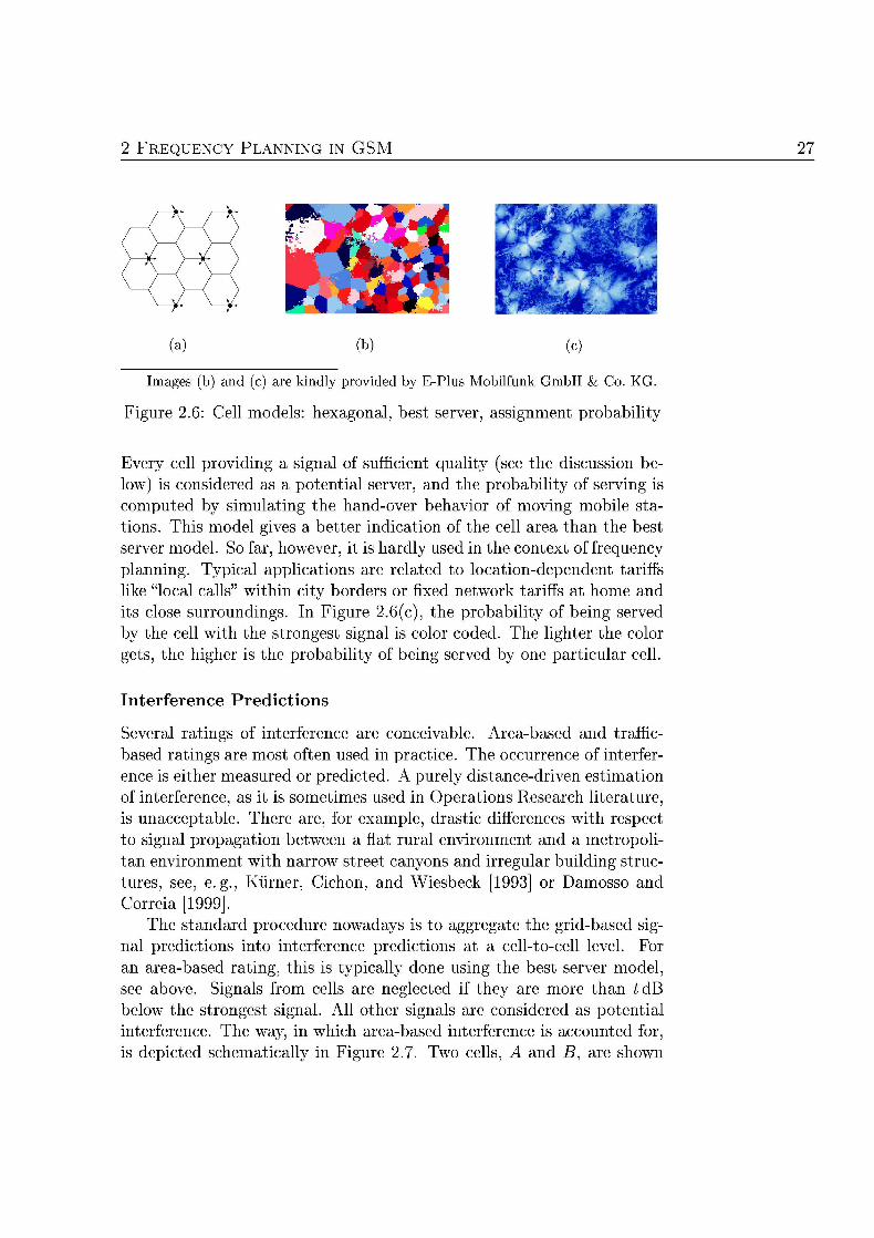
Figure 2.6: Cell models: hexagonal, best server, assignment probability

Every cell providing a signal of sufficient quality (see the discussion be low) is considered as a potential server, and the probability of serving is computed by simulating the hand-over behavior of moving mobile sta­tions. This model gives a better indication of the cell area than the best server model. So far, however, it is hardly used in the context of frequency planning. Typical applications are related to location-dependent tariffs like "local calls" within city borders or fixed network tariffs at home and its close surroundings. In Figure 2.6(c), the probability of being served by the cell with the strongest signal is color coded. The lighter the color gets the higher is the probability of being served by one particular cell

Interference Predictions

Several ratings of interference are conceivable. Area-based and traffic-based ratings are most often used in practice. The occurrence of interfer ence is either measured or predicted. A purely distance-driven estimation of interference, as it is sometimes used in Operations Research literature is unacceptable. There are, for example, drastic differences with respect to signal propagation between a flat rural environment and a metropoli tan environment ith narrow street canyons and irregular building struc tures, see, e.g., Kürner Cichon and Wiesbeck [1993] or Damosso and Correia [1999].

The standard procedure nowadays is to aggregate the grid-based sig­nal predictions into interference predictions at a cellto-cell level. For an area-based rating, this is typically done using the best server model see above. Signals from cells are neglected if they are more than tdB below the strongest signal. All other signals are considered as potential interference. The way, in which area-based interference is accounted for is depicted schematically in Figure . Two cells, A and are sho

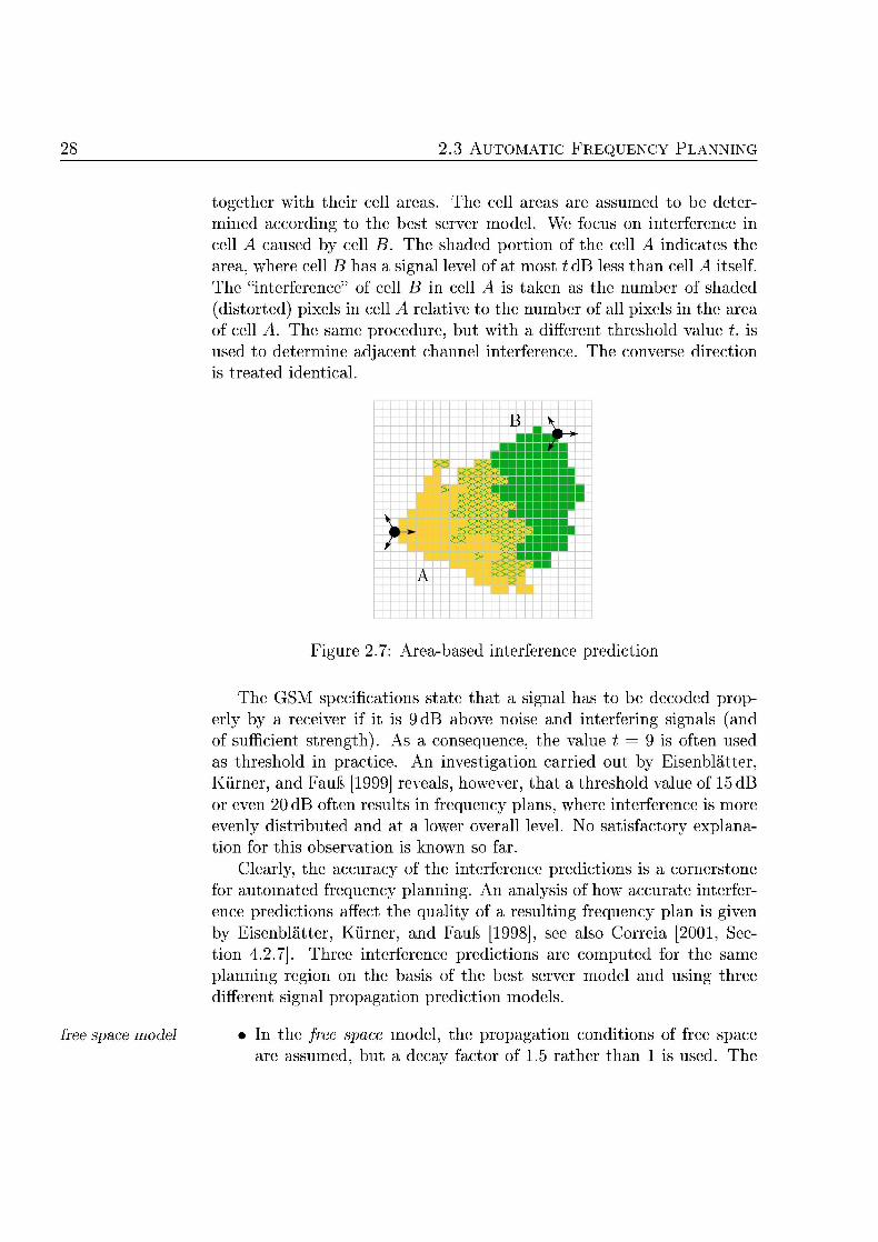
2.3 AUTOMATIC FREQUENCY PLANNING

together with their cell areas. The cell areas are assumed to be deter mined according to the best server model. We focus on interference in cell A caused by cell B. The shaded portion of the cell A indicates the area, where cell B has a signal level of at most t dB less than cell A itself The "interference" of cell B in cell A is taken as the number of shaded (distorted) pixels in cell A relative to the number of all pixels in the area of cell A. The same procedure, but with a different threshold value t, is used to determine adacent channel interference. The converse direction is treated identical

Figur 7: Area-based interference prediction

The GSM specifications state that a signal has to be decoded prop­erly by a receiver if it is 9 dB above noise and interfering signals (and of sufficient strength). As a consequence, the value t = 9 is often used as threshold in practice. An investigation carried out by Eisenblätter Kürner and Fauß [1999] reveals, however, that a threshold value of 15 dB or even 20 dB often results in frequency plans, where interference is more evenly distributed and at a lower overall level o satisfactory explana­tion for this observation is known so far.

Clearly, the accuracy of the interference predictions is a cornerstone for automated frequency planning. An analysis of how accurate interfer ence predictions affect the quality of a resulting frequency plan is given by Eisenblätter, Kürner, and Fauß [1998], see also Correia [2001, Sec tion 4.2.7]. Three interference predictions are computed for the same planning region on the basis of the best server model and using three different signal propagation prediction models.

free sace model In the free space model, the propagation conditions of free space are assumed but a decay factor of 1.5 rather than 1 is used. The

2 FREQUENCY PLANNING IN GSM

increase of the factor from 1 to 1.5 (or the like) is taken as an empirical value between the decay factor when only the direct ray is taken into account (resulting in a decay factor of 1) and the decay factor observed in a two ray model, see, e.g., Kürner and Fauß [1994]. In the two-ray model, the interaction between the direct ray and a reflected ray results in a decay factor of 2 for distances larger than a specific threshold.

The Modified Okumura-Hata race predictor bases on an 1800 MH race model extension of the basic path loss equation as described in Damosso and Correia [1999]. Land use information is used by means of em­pirical correction factors for each land use class. Terrain variations are taken into account by using an effective antenna height. To­pographical obstacles are treated as knifeedges, that is, infinitely long, straight "razor blades" for hich a closed simple formula for the diffraction is k n o n .

The eplus propagation prediction model, see Kürner, Fauß, and plus model Wasch [1996], is the most sophisticated approach used in the com­parison. The model consists of a combination of several propaga­tion models like COST 231-Walfisch-Ikegami MacielXia-Bertoni and Okumura-Hata. It is developed for GSM 1800 and calibrated

ith numerous measurements in the network of E-Plus.

Ranking these wave propagation prediction models has its difficulties. The crucial question is how to compare assignments computed on the basis of different predictions without implementing the assignments into the live network and performing measurements. In the approach taken by Eisenblätter et al. [1998], each assignment's interference is determined according to all three interference predictions. The findings are as follos.

The assignments computed on the basis of the predictions from the eplus model have relatively little interference according to all three predictions.

The assignments computed on the basis of the predictions from the free space model have decent interference ratings according to the race predictions but are mediocre according to the eplus predic tions.

For the assignments computed on the basis of the race predictions the worst picture is obtained. They are mediocre to bad according to the two other predictions.

2.3 AUTOMATIC FREQUENCY PLANNING

n v i w of t h i , the eplus model is ranked above the free space model which, in turn, is ranked above the race model (in this particular context) In total, varying the signal propagation predictor shows a larger impact on the frequency assignment quality than choosing among the different frequency planning heuristics considered by Eisenblätter et al. [1998]

hich are similar to those described in Chapter 4 and Section 5.1.

Effects of DTX and SFH

The GSM features of discontinuous transmission (DTX) and slow fre­quency hopping (SFH) both address the problem of interference either by reducing interference itself (DTX) or by reducing the impact of inter ference (SFH).

Neither of these features is explicitly addressed within our frequency assignment model, but it is possible to incorporate their effects into the interference ratings. Nielsen and Wigard [2000] and Majewski, Hallmann and Volke [2000] propose different ways to do so, both being validated using GSM simulators. Nielsen and Wigard [2000] introduce two param-

hopping gain eters called hopping gain and load gain by whose product the interference load gai rating is scaled. The setting of the parameters depends on the load of

each cell, a voice activity factor, and the number of channels to hop pre factors on, among others. Majewski et al. [2000] introduce pre factors and post

ost factors factors in order to scale interference, but do not provide the full details. Björklund, Värbrand, and Yuan [2000] optimize the hopping sequence

for each cell. This sequence is determined by the hopping sequence num­ber ( ) and sequence starting point ( A I O ) .

2.3.3 Pract ical Aspects

Since the introduction of GSM, operators have steadily increased their networks coverage and capacity. This typically involves installing addi tional TRXs and providing them with channels. Hence, the frequency plan has to be adjusted. The same holds if the transmission characteris tics of a BTS change.

Installing a new frequency plan is not as simple as it may sound at first. In Germany, for example, the operator has to submit the frequency plan to a governmental regulation office and ask for approval. This ap­proval is given if the frequency plan adheres to the bilateral agreements on channel use along national borders and if no interference with other radio systems operating in the same frequency band is expected. The restrictions from both sources are recorded as locally blocked channels.

2 FREQUENCY PLANNING IN GSM 31

The former are known in advance, but the latter are often only revealed through rejection. The turn around time for such an approval is in the order of a few weeks.

Changes in the frequency plan take effect at the BTSs. In "old times the channels had to be adjusted manually at the combiners. Nowadays remotely tunable combiners may be used. These allow to change the channels through the OSS, but this convenience comes at the expense of less effective combiners. In principle, a TCH can be changed while the cell is in operation as long as the corresponding TRX is not in use. Changing a BCCH, however, requires to shut down the cell completely for a couple of minutes. Therefore changes in the frequency usage are mostly performed at night times.

Another problem is that the effects of the changes are not easily assessed. Extensive, timeconsuming quality measurements campaigns could be performed, but much rather a "sit and wait" strategy is adopted measurements by the Operation and Maintenance Center (OMC) of the rate of quality-driven hand-overs and an increase in customer complaints substitute the explicit quality assessment. Common to both alternatives is that they require users which are getting service or unsuccessfully try to get service. This happens to a sufficient extent only at the next day.

The way in which frequency planning is done differs from operator to operator. Some operators divide their service area among regional offices which act more or less independently. For example, E-Plus operates five regional offices. Between the regional offices, the channel use along the regional border is settled through agreements similar to bilateral agree ments for national borders. Obviously, regional borders (these are the ones an operator may choose) should be in areas with little telecommuni cations traffic, where planning is simple even with additional restrictions.

Even if operators are confident in the overall reliability of the fre quency planning process, they try to change the BCCH assignment rather seldom. Recall in this context that solving the combinatorial optimiza­tion problem of finding a good frequency plan is merely one important step in this process. Other, equally important ones, are maintaining up to date and sufficiently detailed data about terrain and buildings as well as generating accurate interference predictions.

Some GSM operators split their available spectrum into two separate parts, one for BCCHs, the other for TCHs. This is called band split. The band split reasoning behind performing a band split is to be able to plan the TCHs (almost) independently from the BCCHs. Table 2.8 shows an assignment for TINY, which is compatible with splitting the spectrum of 11-723 into a B C C b a n d of 11- and a T C b a n d of 723.

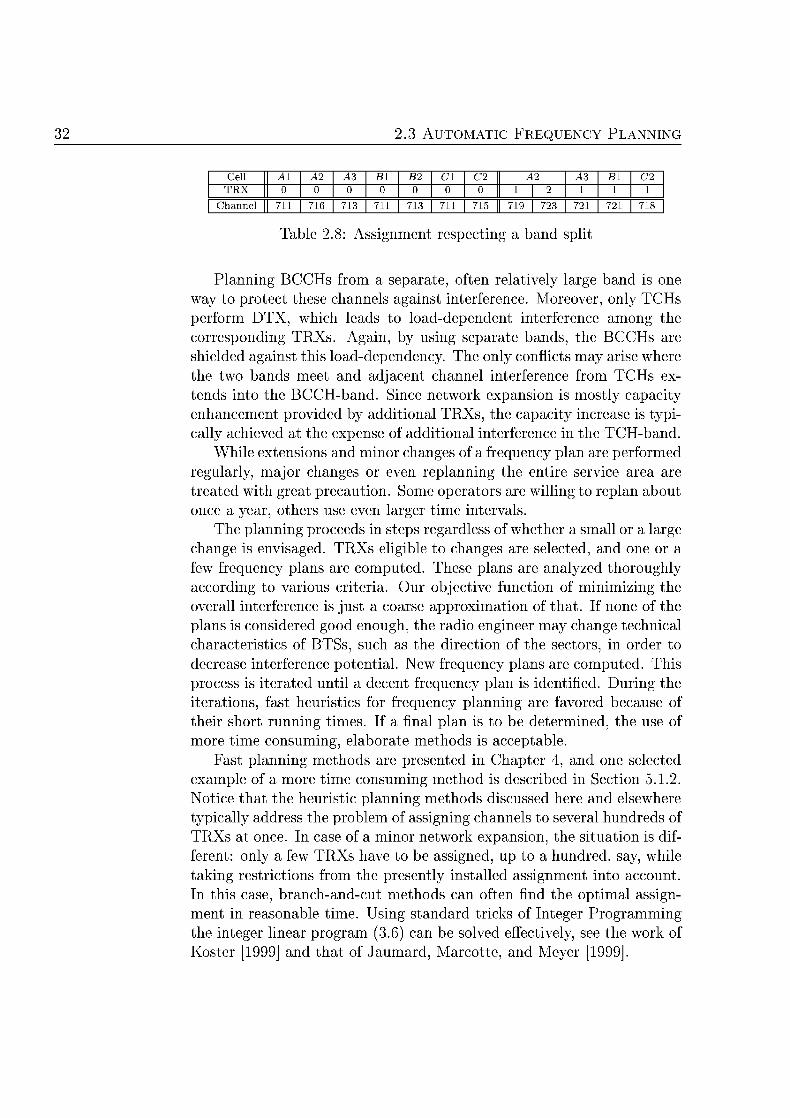
2.3 AUTOMATIC FREQUENCY PLANNING

Cell A2 A3 B2 C2 A2 A3 C2 TRX |

Channel 11 16 13 11 13 11 15 19 | 23 21 21 18

Table Asignment respecting a band split

Planning BCCHs from a separate, often relatvely large band is one way to protect these channels against interference. Moreover, only TCH perform DTX, which leads to load-dependent interference among the corresponding TRXs. Again, by using separate bands, the B C C s are shielded against this load-dependency. The only conflicts may arise where the two bands meet and adjacent channel interference from TCHs ex­tends into the BCCHband. Since network expansion is mostly capacity enhancement provided by additional TRXs, the capacity increase is typi cally achieved at the expense of additional interference in the TCHband.

While extensions and minor changes of a frequency plan are performed regularl major changes or even replanning the entire service area are treated with great precaution. Some operators are illing to replan about once a year, others use even larger time intervals.

The planning proceeds in steps regardless of whether a small or a large change is envisaged. TRXs eligible to changes are selected, and one or a few frequency plans are computed. These plans are analyzed thoroughly according to various criteria. Our objective function of minimizing the overall interference is just a coarse approximation of that. If none of the plans is considered good enough, the radio engineer may change technical characteristics of BTSs, such as the direction of the sectors, in order to decrease interference potential. New frequency plans are computed. This process is iterated until a decent frequency plan is identified. During the iterations, fast heuristics for frequency planning are favored because of their short running times. If a final plan is to be determined the use of more time consuming, elaborate methods is acceptable.

Fast planning methods are presented in Chapter 4, and one selected example of a more time consuming method is described in Section 5.1.2 Notice that the heuristic planning methods discussed here and elsewhere typically address the problem of assigning channels to several hundreds of TRXs at once. In case of a minor network expansion, the situation is dif ferent: only a few TRXs have to be assigned, up to a hundred, say, while taking restrictions from the presently installed assignment into account. In this case, branch-and-cut methods can often find the optimal assign­ment in reasonable time. Using standard tricks of Integer Programming the integer linear program (3.6) can be solved effectively, see the work of

oster [1999] and that of Jaumard arcotte and eyer [1999]

C H A P T E R 3

athematical Models

In the following, we translate the informal statement of the GSM fre quency planning problem from Section 3.1 into a mathematical model For convenience, we restate the problem

Given are a list of TRXs, a range of channels, a list of locally blocked channels for each TRX, as well as the mini mum separation, the co-channel interference, an the adjacent channel interference matrices.

Assign to every TRX one channel from the spectrum which is not locally blocked such that all separation requirements are met and such that the sum over all interferences occurring between pairs of TRXs is minimize

Our mathematical model is presented in Section 3.1. In the context of GSM frequency planning, similar models are used by Duque-Antön and Kunz [1990]; DuqueAnton, Kunz, and Rüber [1993]; Carlsson and Grindal [1993]; Plehn [1994]. During the late nineties, this model became popular among researchers as well as practitioners, see Koster [1999, Sec tion 2.6] and Correia [2001, Section 4. .5], for example. A few competing models are addressed in Section 3.1.2. The computational complexity of solving our model of the frequency assignment problem is studied in Section 3.2. It turns out that finding a feasible solution is A/"'P-complete and even if that were simple finding (close to) optimal solutions would remain AfV-havd. Finally, two reformulations of the frequency assign­ment problem as integer linear programs are given in Section 3.3. The mathematical notions used in the folloing are explained in Appendi A.

3.1 The Model FAP

The objective of minimizing the overall interference is blind to the "direc­tion" of interference that is, whether the use of a channel in a cell causes

33

34 3.1 T H ODEL FAP

rner pectrum

blocked channel available

separation co-channel djacent channel

carrier netwo assignment feasible

interference somewhere or whether the channel itself suffers from interfer ence. The mathematical formulation of our frequency planning problem is therefore undirected, and we simply add the interference ratings given for the two directions into a single value.

Let (V, E) be an undirected graph. The vertices of the graph are also called carriers and represent the TRXs. The spectrum C is a finite interval in Z+ , the set of nonnegative integers representing the range of channels. For every carrier v G V a set Bv C C of blocked channels is specified. The channels in C \ Bv are called available at carrier v. Bv

may be empty. Three functions, d: E -> Z+, c: E -> [0, 2] and cad: E -> [0, 2]Q

are specified on the edge set. For an edge vw G E, d(vw) gives the separation necessary between channels assigned to v and w. c(vw and cad(vw) denote the co-channel and adjacent channel interference respectively, which may occur between v and w. (Both functions map into the interval [0, 2]Q rather than into [0, 1]Q because of the symmetrization mentioned above. This may be remedied by scaling if desired.)

We refer to the tuple iV (V, E, C\ {Bv}veV, d, c , cad) as carrier network or network, for short. A frequency assignment or simply an assignment for A is a function y: V —> C. An assignment is feasible if every carrier v G V is assigned an available channel and all separation requirements are met that is if

eC\Bv VveV,

) — \ > vw Mvw G

(3.1)

(3.

list coloring

Tcoloring

list Tcoloring

Feasible assignments are a generalization of list colorings and are re­lated to T-colorings of graphs in the following way. For a list coloring problem, a graph and lists of colors for every vertex are given. The task is to find a vertex coloring for the graph such that every vertex receives a color from its list and such that no two adacent vertices receive the same color, compare Erdös, Rubin, and Taylor [1979]. Since an available channel has to be picked for every carrier feasible assignments are list colorings.

T-colorings are introduced by Hale [1980]. Given an undirected graph G (V, E) and nonempty finite sets T(vw) of positive integers for all edges vw G E, a T-coloring of is a labeling / of the vertices of ith nonnegative integers such that \f(v) — f(w)\ G- T(vw) for all vw G E.

A frequency assignment has to meet list coloring as well as T-coloring constraints in order to be feasible. Such list T-coloring are first studied by Tesman [1993]

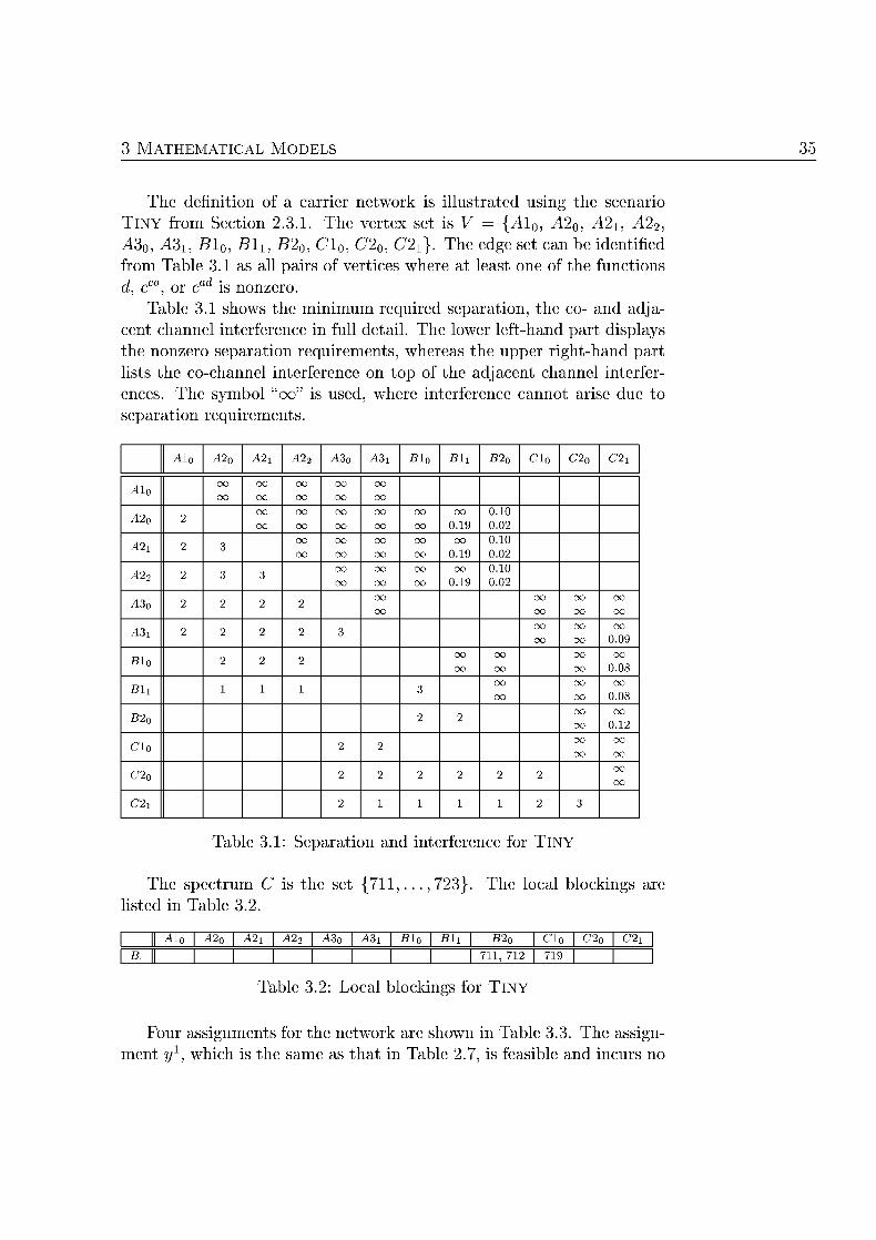
A T E M A T I C A L ODEL 35

The definition of a carrier network is i l u s a t e d usng the scenar INY from Section 3.1. The vertex set is V {Al0, A20, A2U A22

A3, A3U Bio, Bli, B20, Cl0 , C20, C2i}. The edge set can be identified from Table 3.1 as all pairs of vertices here at least one of the functions d, c , or cad is nonzero.

Table 3.1 shows the minimum required separation, the co- and adja­cent channel interference in full detail. The lower lefthand part displays the nonzero separation requirements, whereas the upper righthand part lists the co-channel interference on top of the adjacent channel interfer ences. The symbol "oo" is used, where interference cannot arise due to separation requirements.

A2i 22 A3 A3i C2 C2i

A2

A2i

A22

A3

A3

B2

C2

C2i

Tabl 3. Separaton and interference for NY

The spectum is the set { 7 1 1 , 7 . The local blockings ar listed in Table 3.

| || | I A2i | A22 | A3 | A 3 I | | | B2 | | C2 | C2i~ |

\ B. || | | | | | | | | 11, 12 | 19 | | ~ |

Table 3.2: Local blockings for INY

Four assignments for the network are s h o n in Table 3.3. The assign­ment y, which is the same as that in Table 7, is feasible and incurs no

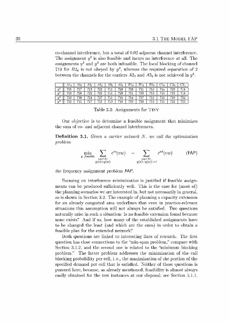
3.1 T H ODEL FAP

co-channel interference, but a total of 0.02 adjacent channel interference. The assignment y is also feasible and incurs no interference at all. The assignments y and y are both infeasible. The local blocking of channel 719 for B2Q is not obeyed by y, whereas the required separation of between the channels for the carriers and A3 is not achieved in

A2i 22 A3 3i B2 C2 C2i 15 13 22 11 20 20 11 15 14 23 18

1 13 28 22 25 11 20 11 20 13 13 15 18 yA 13 30 24 11 15 14 12 13 19 22 y4 12 11 15 13 16 19 20 13 11 22 23

Table 3.3 Asignments for INY

Our objective is to determine a feasible assignment that minimizes the sum of co- and adacent channel interferences.

Definition 3.1 iven carrier network N, we call the optimization problem

min V vw V cadvw (FAP) y feasibl ^—' - — '

vw£E: vwdE: y(v)y{w) y(v)y(w)

the frequency assignment problem FAP

Focusing on interference minimization is justified if feasible assign­ments can be produced sufficiently well. This is the case for (most of) the planning scenarios we are interested in, but not necessarily in general as is shown in Section 3.2. The example of planning a capacity extension for an already congested area underlines that even in practice-relevant situations this assumption will not always be satisfied. Two questions naturally arise in such a situation: Is no feasible extension found because none exists? And if so, how many of the established assignments have to be changed the least (and which are the ones) in order to obtain a feasible plan for the extended network?

Both questions are linked to interesting lines of research. The first question has close connections to the "min-span problem," compare with Section 3.1.2, and the second one is related to the "minimum blocking problem. The latter problem addresses the minimization of the call blocking probability per cell, i. e., the maximization of the portion of the specified demand per cell that is satisfied. either of those questions is pursued here, because, as already mentioned, feasibility is almost always easily obtained for the test instances at our disposal see Section 5.1.1.

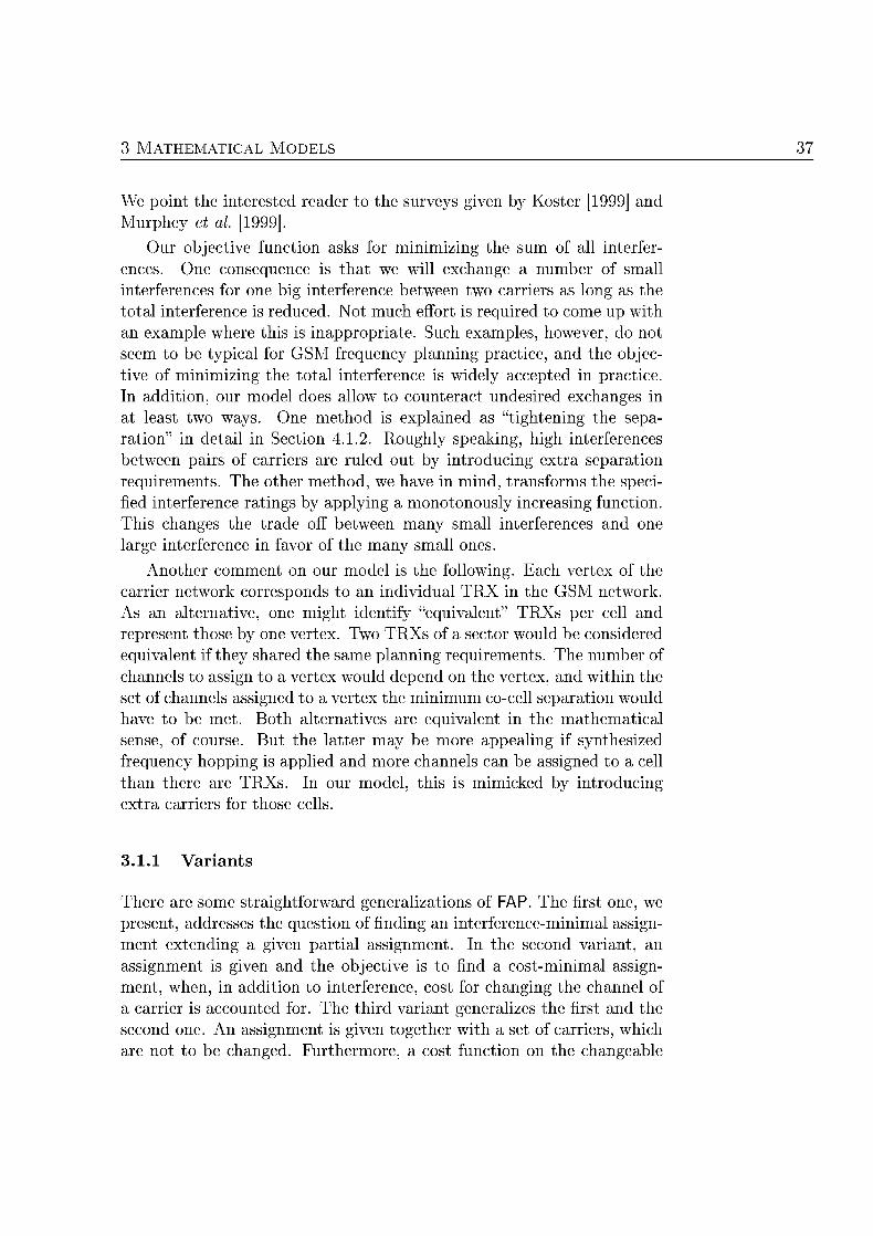
A T E M A T I C A L ODEL

We point the interested reader to the surveys given by oser [1999] and urphey et al. [1999]

Our objective function asks for minimizing the sum of all interfer ences. One consequence is that we will exchange a number of small interferences for one big interference between two carriers as long as the total interference is reduced. Not much effort is required to come up with an example where this is inappropriate. Such examples, however, do not seem to be typical for GSM frequency planning practice, and the objec tive of minimizing the total interference is widely accepted in practice. In addition our model does allo to counteract undesired exchanges in at least two ways. One method is explained as "tightening the sepa­ration" in detail in Section 4.1.2. Roughly speaking, high interferences between pairs of carriers are ruled out by introducing extra separation requirements. The other method, we have in mind, transforms the speci fied interference ratings by applying a monotonously increasing function. This changes the trade off between many small interferences and one large interference in favor of the many small ones.

Another comment on our model is the following. Each vertex of the carrier network corresponds to an individual TRX in the GSM network. As an alternative, one might identify "equivalent" TRXs per cell and represent those by one vertex. Two TRXs of a sector would be considered equivalent if they shared the same planning requirements. The number of channels to assign to a vertex would depend on the vertex, and within the set of channels assigned to a vertex the minimum co-cell separation would have to be met. Both alternatives are equivalent in the mathematical sense, of course. But the latter may be more appealing if synthesized frequency hopping is applied and more channels can be assigned to a cell than there are TRXs. In our model this is mimicked by introducing extra carriers for those cells.

3.1.1 r i n t s

There are some straightforward generalizations of FAP. The first one, we present, addresses the question of finding an interference-minimal assign­ment extending a given partial assignment. In the second variant, an assignment is given and the objective is to find a costminimal assign­ment, when, in addition to interference, cost for changing the channel of a carrier is accounted for. The third variant generalizes the first and the second one. An assignment is given together with a set of carriers, which are not to be changed. Furthermore a cost function on the changeable

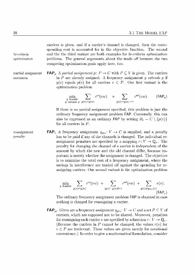
38 3.1 T H ODEL FAP

carriers is given, and if a carriers channel is changed, then the corre­sponding cost is accounted for in the objective function. The second

bicriteria and the the third variant are both examples for bicriteria optimization timiation problems. The general arguments about the trade off between the t

competing optimization goals apply here too.

partial assignment FAPp partial assignment p: P C with P CV is given. The carriers extension in are already assigned. A frequency assignment y extends p if

y(v) equals p(v) for all carriers v Our first variant is the optimization problem

vw cadvw (FAPP) mm y feasible extends y(y( y(y(

If there is no partial assignment specified, this problem is just the ordinary frequency assignment problem FAP. Conversely, this can also be expressed as an ordinary FAP by setting Bv C \ )} for all carriers in

reassignment FAPr A frequency assignment ypre: V) C is supplied, and a penalty enalty has to be paid if any of the channels is changed. The individual re­

assignment penalties are specified by a mapping r: V> Q+. The penalty for changing the channel of a carrier is independent of the amount by which the new and the old channel differ, because im­portant is merely whether the assignment is changed. The objective is to minimize the total cost of a frequency assignment, where the savings in interference are traded off against the spending for re­assigning carriers. Our second variant is the optimization problem

min Y vw advw V y feasible * ^ — *-^

y(v)y{w) y(V)y( y(v)yprev)

(FAPr) The ordinary frequency assignment problem FAP is obtained in case nothing is charged for reassigning a carrier.

FAPpr Given are a frequency assignment ypre: V —v C and a set P C V of carriers, which are supposed not to be altered. Moreover penalties for reassigning each carrier v are specified by a function r: V —>• Q+ . (Because the carriers in P cannot be changed, the values r{v) for j ) £ P are irrelevant. These values are given merely for notational convenience.) In order to give a mathematical formulation consider

A T E M A T I C A L ODEL 39

the partial assignment p: P —>• C obtained from ypre by letting Upre\p, i. e., p maps every carrier v contained in P to the channel

p{v) and is undefined on all carriers not in Our third variant is the optimization problem

min vw advw y feasible —' ' — ' — ' exends y(y( y(v)y(w) y(ypr(v)

{ r A rpr ) A similar effect can be achieved by using the model FAPr and setting r(v) for all v G P to an arbitrarily high value (exceeding all other penalties by far)

By specializing FAPpr, the two first variants and FAP itself can be obtained: in case r(v) 0 for all penalties, FAPpr reduces to FAPP; in case P = 0, FAPpr simplifies to FAPr; and in case both previous restrictions hold, then FAPpr turns into FAP.

Conversely, an equivalent instance of FAP exists for every instance of FAPpr for which the maximum penalty for reassigning is bounded by 2 The penalties for reassigning in FAPpr are accounted for as co-channel interference with additional carriers in FAP. The bound of 2 comes from the definition of a carrier network, in particular from the maximum admissible amount of co-channel interference.

Let A (V,£,C,{B„} v G V ,d ,c ,c o d ) , P C V, : V ) [0, 2]Q, and Upre V —• C be an instance of FAPpr. We define a FAP instance iV as follows. An extra carrier is introduced for every / e C . The edges in N are all edges from A plus all vf for v G V, f 6 C with r{v) ^ 0 and Vpre{v) 7 /• The spectrum is unchanged and so are the locally blocked channels for all v G V. We set Bf = C \ {/} for the new carriers / G C. The edge labelings d, , and cad are extended to the new edges with zeros for d and cad and ith f) r(v). (The transformation can be generalized to the case where r(v) > 2 for some v G V. More than \C additional carriers become necessary, which may lead to carrier networks of significantly increased size.)

Notice that if changing the channel allocation of a TRX is penalized too heavily in comparison to the interference it would incur without a change, then the character of the optimization problem may change. In this context, optimal solutions for problem with up to one thousand TRXs are reported by Aardal, Hurkens, Lenstra, and Tiourine [1996] on test instances which do not arise from GSM frequency assignment.

evertheless these findings are likely to hold for GS instances too.

3.1 T H ODEL FAP

3.1.2 ternat ive M d e

The scientific study of frequency planning started in the late sixties. The presentation of etzger [1970] is often seen as the starting point. Ten years later, Hale [1980] published a classification of frequency planning problems and their applications. To our best knowledge, these early works do not address problems that are equivalent to frequency planning for GSM. This changed with the deployment of GSM networks.

Several different problem types are subsumed under the general terms frequency planning, frequency assignment, and channel allocation. In our following discussion of alternative models, we focus solely on models which we consider relevant for GSM frequency planning. More compre­hensive treatments of frequency planning in general are given by Koster [1999] and by urphey et al. [1999]. Notice also that we only address

FCA Fixed Channel Allocation (FC A), where the channel demand per cell is fixed. Two other types of problems ith varying demands are briefly explained and references are given.

DCA Dynamic Channel Allocation (DCA) considers varying traffic profiles and, consequently, also varying channel demands per cell. Channels have to be assigned on request. GSM does not support dynamic channel allo­cation. The planning is done statically for the busy hour, i.e., with the peak traffic in view although the traffic load is clearly changing over time. Studies on the potential impact of using DCA for GSM networks are de­scribed by Kennedy, Vries, and Koorevaar [1998], for example. More general studies of DCA are performed by alesihska [199 Grace Burr and Tozer [1998], and Grace [1999]

HCA A mixture of FCA and DCA is called Hybrid Channel Allocation (HCA). Some basic demand is covered by solving an FCA problem, and additional demand is handled dynamically in the sense of DCA. Hybrid channel allocation is studied by alesihska [199 for example. CA is also not supported by GSM

We now turn back to FCA and alternative models for FAP. The ac­tual quality of a frequency plan is at best predictable with very time-consuming simulations using a GSM link-level simulator. In practice the quality will typically be only observed once a frequency plan is in­stalled. The model underlying the planning process should express the anticipated quality reasonably well and be pessimistic in doing so. It would be unrealistic to expect that the model is completely accurate. Consequently, there is a range of different and yet reasonable models focusing on different quality aspects of a frequency plan.

min-san model In the minspan model frequency planning is handled as a generalized

A T E M A T I C A L ODEL 41

graph coloring problem (see Tesman [1993]). Each vertex has a set of available "colors" and the edges are labeled with minimum separation requirements. The result is a mixture of list and T-coloring as explained in Section 3.1. The objective is to find a coloring of the vertices, which satisfies the list as well as the T-coloring constraints and which uses "colors" from an as narrow range as possible. The span is the difference an between the largest and the smallest "color" used.

Interference information is not directly taken into account within this model. Instead, when setting up the underlying graph and fixing the min­imum required separation along each edge, a distinction is made between "acceptable" and "unacceptable" interference. This is typically done by means of a threshold value. For example, co-channel interference above the threshold is ruled out by introducing a separation requirement of at least 1. Interference below the threshold value is neglected altogether. The min-span model is not directly applied in GSM frequency planning, but occurs as the core problem in minimizing the maximal interference. This is the next approach described below.

A detailed discussion of the min-span model and an extensive survey of related mathematical results and algorithmic developments is given by Murphey et al. [1999], see also Koster [1999, Section 24] and FAP web [2000]. Numerous authors have addressed the problem of computing lower bounds on the required span. We mention only a few important contributions: Gamst [1986] provides a bound basing on cliques in the un­derlying graph; Raychaudhuri [1994] Roberts [1991b], Smith and Hurley [1997] obtain bounds from solving the TRAVELING ALESMAN PROBLEM

(see Section 6 4 . ) on subgraphs; and Janssen and Kilakos [1996] as well as Janssen and Kilakos [1999] derive bounds from polyhedral studies.

In GSM frequency planning practice the min max interference ap- min max proach has been popular until recently. At first, similar input data is interference generated as required for the specification of our carrier network. In a second step, the interference predictions are the basis for increasing sep­aration requirements in order to prevent the occurrence of severe inter ference. As indicated in the context of the min-span model, a tentative threshold value is chosen to separate "acceptable" from "unacceptable" interference. "Unacceptable" interference is transformed into additional separation requirements, and "acceptable" interference is simply ignored.

The result is a min-span problem with local blockings recorded at the vertices and with minimum required separation recorded at the edges. An attempt is made to solve this min-span problem. Two outcomes are possible. In one case, a feasible solution is generated. This corresponds to a frequency assignment obeying all imposed conditions. In the other

3.2 OMUTATIONAL O M L E X I T Y

case, no solution is found. The tentative threshold value is increased which results in less "unacceptable" interference and, correspondingly, in fewer additional separation requirements. The planning process is started over with the new input.

The final threshold value is the result of repeatedly increasing or de­creasing the value with the goal of finding an assignment that barely fits into the available spectrum. In practice, the threshold value is driven up beyond desirable limits by capacity-related interference problems in metropolitan areas. As a consequence, interference not exceeding this threshold becomes generally invisible to the planning process. Although avoidable outside of the critical areas by careful planning, many inter ference situations are not resolved because they have become impercep­tible. Alternatively, the planning radio engineer may choose (potentially many) location-dependent threshold values. Either way this planning style proved unattractive in practice.

min max local Minimizing the maximal interference experienced by a TRX can be interference done on the basis of our carrier network representation as well, but the

use of a directed version is also conceivable. The difference to our fre­quency planning problem is primarily in the definition of the objective function. The goal here is to keep the maximal interference experienced by a TRX as low as possible. To that end, the impact of the interfering TRXs is recorded for every TRX and the maximum is determined. This maximum is to be minimized. Most prominently, this approach is pur sued by Fischetti, Lepschy, Minerva, Jacur, and Toto [2000], who also give satisfactory computational results for realistic planning problems

ith several hundreds of TRXs.

3.2 Computational Complexity

The results presented in this section are the justification for our focus in Chapter 4. Resorting to heuristic methods for solving FAP would not be (easily) ustified if reasonable approximations of optimal frequency assignments were computable in polynomial time. We sho in Proposi tion 3.11 that this is not the case.

3.2. Preliminaries

Throughout the following discussion, we assume basic familiarity with the concepts of computational complexity. Several textbooks contain introductions see for example Garey and Johnson [199] Bovet and

A T E M A T I C A L ODEL

Crescenzi [1994], Papadimitriou [1994] as well as Cormen, Leiserson, and Rivest [1990, Chapters 36, 37]. With respect to the complexity of ap­proximation, we recommend the book of Ausiello, Crescenzi, Gambosi Kann, MarchettiSpaccamela, and Protasi [1999], which is also our pri mary reference here. Nevertheless, we recall the basic definitions, which are required in the following, from the literature.

We start with the complexity of an algorithm. (See any of the above mentioned books for a discussion of the subtleties of defining "algorithm.") For an algorithm A, let IA{X) denote the number of steps executed by

on input . The worst case running time of A is defined as tAiji) max{£^(:r) | x : \\ < n} . The size \x\ of an instance x depends on the encoding scheme. We assume here that a "reasonable" compact binary encoding of the instances is used, see the discussion in Garey and Johnson [1979, Chapter 2] or Grtschel, Loväsz, and Schrijver [1988, Section 1.3] for example. Algorithm A has a running time complexity ö(g(n)) if i^(n) is in ö(g(nj), see Appendix A for the meaning of the (9()notation. In accordance ith this definition, we say that A runs in polynomial time if tA{n) is in öp(n)) for some polynomial^. Likewise, A runs in exponential time if £A(^) is in 0(2^) for some polynomial p. Similar definitions for the space complexity of an algorithm exist.

Next, we deal with decision and optimization problems. We address decision problems first. Formally, we define a decision problem as a tuple (/, SOL), where / is the set of instances and SOL: I —> {0,1} as sociates with every instance x either zero or one. The problem P is identified with the language L {x G / | SOL(x)}. Answer ing the question whether x G Lp for any given x is called to recognize the language Lp or to solve the problem P. The two most prominent complexity classes concerning decision problems are defined as follos.

Definition 3.2. A decision problem P is solved by a deterministic al gorithm A if the algorithms halts for every instance x G lp and returns YES if and only if x G Lp. The class V consists of all problems solvable in polynomial time by some deterministic algorithm

worst case unning time

unning time complexity

olynomial time

exponential time ace complexity

decision problem

language recognize

solve

In addition to deterministic algorithms, nondeterministic algorithms are considered. One way of thinking about a nondeterministic algorithm is that the algorithm nondeterministically chooses one out of at most t possible instructions for execution at each step.

nondeerministi algorithm

Definition 3.3. A decision problem is solved by a nondeterministic algorithm A if for any instance x G LP, A halts and x G LP if at least one possible sequence of instructions causes the algorithm to return

MV

44 3.2 OMUTATIONAL O M L E X I T Y

ucible

complete

minimiat problem feasible solutions measure function value

timal solution

underlying language

FAP

The class MV consists of all problems solvable in polynomial time by some nondeterministic algorithm

Clearly, V C J\fV. One of the challenging open problems in com­putational complexity theory is to settle the question whether V \TV. Despite continuous and serious efforts over the past three decades this problem is still open. It is, however commonly believed that V HV.

Given two decision problems Pi and P2, Pi is said to be (poly­nomial time m-)reducible to if a polynomial time algorithm A ex­ists hich maps instances x G Ip1 into instances A(x) G p2 satisfying x G Lpx < => A(x) G Lp2. On the basis of this reducibility the notions of A^P-completeness and A/'P-hardness are defined.

Definition 3.4. A decision problem P is called J\fV-hard if every problem in NV is reducible to . The problem is AP-complete if aditionally

itself is in MV

If V C AfV, then no A^P-complete problem can in general be solved deterministically in polynomial time; in Section 3.2.3, we show that de­ciding whether there is a feasible assignment for a carrier network is

TP-complete. We now turn to the complexity of optimization problems and approx­

imation. Our focus is on minimization problems, and all our definitions are specialized to this case. Definitions applying simultaneously for min­imization and maximization problems can be found in Ausiello et al [1999, Chapters 1, 3, and 8].

Formally, a minimization problem P is characterized by a triple (IP

SOLp, mp), where Ip is the set of instances of SOLP is a function that assigns to every instance G Ip a set SOLP(x) of feasible solutions for ; and mp is the measure function that assigns to every pair (x,y with x G Ip and y SOL a positive integer called the value of the feasible solution y.

Given some x G the obective is to find an optimal solution y* G SOLp(x), satisfying mp(x,y*) yeSoLp(x)mp{xiy)- We denote the value of an optimal solution by m*P(x). A decision problem is associated to every optimization problem in a natural manner: let PD (I Z+JSOL), where SOL(x,K) 1 if mPx) < K and SOL(x,K) otherwise. The language LpD is called the underlying language of P .

According to the above definition, FAP itself does not qualify as a minimization problem, because the objective function may take every value in Q+ . By adding the following measure function, this is remedied. Given an instance x, let digits(x) denote the number of decimal digits in the smallest interference value (other than zero) in PFAP is defined by

A T E M A T I C A L ODEL 45

^FAP, whih is the set of all c a r e r networks

S'OLFAP, which associates ith each carrier network its set of feasi ble assignments

mpAP, which computes digits(x) and the total interference of an assignment, scales the result by the factor of I0dlglts(a) (in order to make it integral) and adds one (in order make it strictly positive).

With respect to optimization problems plays a role similar to that of among decision problems.

Definition 3.5 minimization problem P = (IP, SOL m belongs MVÖ to the class MVÖ if the following three conditions hold:

(i) the set of instances is recognizable in polynomial time;

(ii) a polynomial q exists such that \y\ < q(\x\) for all y G SOL( an such that it is decidable in polynomial time whether y G SOL for every y with

(iii) the measure function is computable in polynomial time

The problem PFAP is in MVÖ. First, it is recognizable in polynomial time whether a string encodes a carrier network. Second, the encoding of a feasible assignment does not take more space than the encoding of a carrier network (assuming that all carriers are listed individually and that all channels in the spectrum are listed as well); and it is recognizable in polynomial time whether an assignment is feasible. Third, digits(x) and the total interference of an assignment are computable in polynomial time and so is the above measure function.

An optimization problem P 6 MVÖ is NT-hard if the language un- MVhar derlying P is A/"P-complete. (The precise definition of .AAp-hardness for optimization problems is more involved, compare e.g., Ausiello et al [1999, Definition 1.19]. Our definition is merely an immediate conse­quence of the more general definition.) Sometimes, the .AAp-hardness of a minimization problem P is only due to instances involving large numbers. If this is not the case, the problem is said to be strongly

fP-hard. PFAP is strongly AfP-hard as we sho in Section 3 . 3 .

3.2 O M U T A T I O N A L O M L E X I T Y

stronglhar Definition 3.6. Consider a problem P G MVÖ, and let max( i ) denote the value of the largest number occurring in the instance x. For a polyno­mial p pmax' is the restriction of P containing only the instances with max(a;) j5(|x|). The problem is called strongly MV-hoxd i _pmax> is Mhar for some polynomial

Finally, we address the complexity of approximating optimal solu­tions for minimization problems. Given a minimization problem P, the

erformance ratio performance ratio of a solution y SOL ith respect to instance is defined as

R(

Recall in this context that the measure function takes values in the pos itive integers even though it often seems convenient to allow zero or negative values too. But this would clash ith the previous definition.

rapproximate Definition 3.7. Given an optimization problem , an algorithm A for solving P, and a function r: Z + > ] l , then A is an rapproximate algorithm for P if for every instance x G Ip with SOL) ^ 0 the performance ratio of the approximate (feasible) solution A is bounded by , i. e R ( ) )

In case the function r maps all arguments to some constant c G Q+, we also speak of a capproximate algorithm. The class ÄPX contains of all minimization problems in HVÖ that are approximable with a constant performance guarantee in polynomial time. We sho in Section 3 . 3 that PF A P is not in AVX.

ÄPX Definition 3.8. minimization problem P G MVÖ is in AVX if, for some constant c , a capproximate polynomial time algorithm for exists

3.2.2 ass ica r o b l e m s r e a t e d t o FAP

The variant PFAP of FAP is in MVÖ. PFAP is closely related to several optimization problems studied in the literature. We quote some examples from the list of A/W-prob lems of Ausiello et al. [1999 Appendix B]. The labels correspond to those given in the reference.

G T 5 INIMUM RA OLORING

GT22 XIMUM LIQUE

A T E M A T I C A L ODEL

GT27 INIMUM DGE-DELETION B G R A H WIT P R O E R T Y n

GT INIMUM DGE DELETION K-PARTITION

GT33 XIMUM K - O L O R A B L E BGRA

D1 XIMUM UT

D1 XIMUM K - U T

D55 INIMUM K - L U S T E R I N G UM

S 1 XIMUM FREQUENCY ALLOCATION

We pick out the MINIMUM EDGE DELETION K-PARTITION problem and show in which way PFAP generalizes this problem. We then quote results on the complexity of MINIMUM EDGE DELETION K-PARTITION

from the literature and derive lower bounds on the complexity of PFAP

Definition 3.9. An instance of the MINIMUM DGE DELETION K-PAR­

TITION problem consists of an undirected graph (V, E), a weighting w: E> Z + of the edges, and a positive integer k < . The objective is to find a partition o into at most k disoint sets Vp such that

Y v ijE-.eV

is minimized. The associated measure function evaluates the obective function and ads 1

Proposition 3.10. The following statements hold with respect to the computational complexity o MINIMUM DGE DELETION K-PARTITION

(i) The problem is strongly Nhar

(ii) Unless V = M, the problem is not in VX (Sahni an onzalez [1976]

(Hi) For k > 3 an approximation within Ö( is AfV-hard, even when restricting the instances to graphs with \E\ = £2(\V\) for a fixed , 0 < (Kann, Khanna, Lagergren, and Panconesi [1997]

(iv) Unless V = MV, no polynomial time algorithm can achieve a better performance ratio than 1.058 in the case of k (Hästa [1997]

48 3.2 OMUTATIONAL O M L E X I T Y

In case of k , a polynomial time algorithm with a performance guarantee of lo is known arg, Vazirani, and Yannakakis [1996]

(vi) In case of , a polynomial time algorithm with a performance uarantee o for any 0 is known (Kann et al [1997]

Although the first fact listed in Proposition 3.10 is certainly known we are not aware of a reference. The folloing simple proof is given for the sake of completeness.

Proof of Proposition 3.10 (i). Let P denote the minimization problem MINIMUM DGE DELETION K-PARTITION. We show that the restricted version ™ 1 is AA'P-hard by reducing the A^P-complete decision prob­lem GRAPH K-COLORABILITY, see Garey and Johnson [19 GT4] to the language underlying Fm a x '1 .

We associate to every instance G, k) of GRAPH K-COLORABILITY

an instance xGjk of MINIMUM EDGE DELETION K-PARTITION by simply labeling every edge in G with a weight of 1. Clearly, G is A;-colorable if and only if the optimal solution to the associated instance XG n a s a

value of 0. ence the language underlying ™3*' is A"P-hard. D

3.2.3 mplexity of FAP

We now transfer the negative results concerning MINIMUM EDGE DELE­

TION K-PARTITION to PFAP- TO every instance of the former problem we associate an instance of PFAP as follo

(V, E) (V,E,{ } , (vev, ),

where c(ij) 10dlgl^ (ij) and digits(iu) denotes the number of digits of max{w(ij) | ij -E1} (in a representation to the basis 10). The corresponding carrier network can be computed in polynomial time and in particular, its encoding length is polynomially bounded in the encod­ing length of the MINIMUM EDGE DELETION K-PARTITION instance. The /c-partitions of the graph (V, E) and the frequency assignments for the carrier network are in one-to-one correspondence. By definition the measure functions produce identical values for all partitions of V with respect to both problems. ence, the hardness results from Proposi tion 3.10 translate directly to PFAP- Together with the already established ATP-hardness of finding any feasible assignment for a carrier network, w obtain the folloing list of results.

A T E M A T I C A L ODEL

roposition 3.11.

(i) Deciding whether a feasible assignment exists for a carrier network is MV-complete

(ii) P e MVÖ

(iii) P is strongly Nhar

(iv) Unless V NV, PFAP is not in VX

v) Unless V MV, an approximation o PFAP within 0 is impos sible in polynomial time for

Unlike in the case of MINIMUM EDGE DELETION K-PARTITION, pos itive results on the approximation of PFAP cannot be proven due to Propo­sition 3.11 (i) unless V J\fV. We read the above negative results on the approximation of PFAP in the following way: even if feasible solutions were producable in polynomial time ( h i l e still assuming V ^ •A/*73) finding approximately optimal solutions would be hard nevertheless.

As a final remark concerning the approximation complexity, we add that the result stated in Proposition 3.11 (v) does not depend on the par ticular measure function associated ith PFAP- The result of Kann et al [1997] also transfers directly to FAP because their proof only involves instances ith edge weights of 1.

3. Alternative Formulations

In the remainder of this chapter, two integer linear programming formula­tions of FAP are presented. Solving either of the associated integer linear programs (ILPs) for a given carrier network to optimality is equivalent to solving FAP.

The modeling of the nonlinear separation constraints v) — y(w)\ > (vw) poses a problem in linear formulations. The two models cope

with them differently. Our first formulation, called "stable set model," is classical. The variables are only allowed to take the values zero or one. The second formulation, called "orientation model," uses binary as well as integer variables. For the ease of notation let us define

E vw e vw }, (3.3)

vw e vw vw }, (3.4) ad vw e vw cadvw 0}, (3.5)

for a given carrier network A (V, E, , {Bv}veV, ad

3.3 A L T E R N A T I E FORMULATION

3.3. St Se od

Binary variables yl are used to select a channel per carrier. The co-and adjacent channel interference indicator variables zw and z^, re­spectively, are needed for accounting the total amount of interference in the obective function. The folloing I is equivalent to FAP

Y cco zco Y cad zad

/ - v w v w / J ^VWVW

we vweEad

s.t.

(3.a) c\Bv

yw vw e d (3.b)

zco vw e e C {Bv U Bw) (3.c)

za vweadeCBvjieC (3.d)

l v,feBv (3.e)

zco vw e (3.f) a vw e ad (3-g)

We first explain the constraints and then the objective function. The constraints (3.6a) model that precisely one available channel has to be assigned to every carrier. In case channel / is assigned to carrier v, then yl takes the value 1. Otherwise, the value is 0. The inequalities (3.6b) enforce that the selection of the available channels also satisfies all sep­aration constraints. Every 0/1-assignment of the variables yl satisfying the constraints (3.6a) and (3.6b) corresponds to a feasible frequency as signment for N, see constraints (3.1) and (3.2) on page 34.

We now turn to the interference accounting. A binary variable z™w

is used for every edge vw co to indicate co-channel interference, i.e., z™w 1 has to hold if vw G E and v and w receive the same channel This implication is implemented by the constraints (3.6c). Likewise, a binary variable z^ is used for every potential adjacent channel interfer ence. In case vw 6 Ead and v and w have adjacent channels, z^ = 1 has to hold. This is achieved by the corresponding constraints (3.6d). Ex­changing v and w and replacing / by 1 in (3.d) yields the constraint

y-w ^vw — •*-•

Notice that the interference accounting variables are not fully con­trolled by the given constraints in the sense that ^ for example may

A T E M A T I C A L ODEL 51

take the value 1 where a value of 0 would be sufficient. This never hap­pens in an optimal solution because we are minimizing and all obective function coefficients are assumed to be strictly positive.

We call the formulation (3 . ) a stable set model for the following rea­son: if no interference were allowed, then the set of carriers receiving the same channel in a feasible assignment would be stable sets in the under lying graph G (V, E). (A subset of the vertices in G is called stable or stable independent if no two vertices are adjacent.) Hence, a feasible assignment indeendent not incurring any interference partitions the vertices of G (V, E) into stable sets. The Ph. D. thesis of Borndörfer [1998] contains an in-depth treatment of set partition problems and the related problems of set cov­ering and set packing. We also refer to the Ph. D. thesis of Schulz [1996, Chapter 4], where an extension of the set packing problem is described. This so-called transitive packing puts our interference accounting con- transitive acking straints (3.c) and (3.6d) into a general framework.

We come back to the stable set model in Section

3.3.2 rientation de

The orientation model, as presented here, is only correct if the input data satisfies additional restrictions. The first type of restrictions is that cvw > cvt n a s t° be met for every edge vw G E with dvw 0. This is uncritical from a practical point of view and can be seen as a merely technical restriction. The second type of restrictions concerns locally blocked channels. Those are not handled in the model, and we assume that none exist. This restriction is drastic, but we explain how to by­pass it later on. The model is introduced and discussed thoroughly by Borndörfer, Eisenblätter, Grötschel, and artin [1998b]

As the main difference to the stable set model no binary variables y with v G V and / G C are used. Instead an integral variable yv with domain C is introduced for every carrier v E V. The value of y indicates the channel to assign. As before binary variables z™ and z0^ are used for accounting interference.

The intuition behind the model is to consider FAP as two nested problems. An acyclic orientation A of the edges E in the graph underlying the carrier network is determined in the outer part. Such an orientation uter art

of the edges induces a partial order <A on the carrier set: we declare v <A w if a directed path starting at v and ending at w exists in (V, A) (Checking that <A is indeed a partial order is straight forward.) The inner part of the nested problem is to find a feasible frequency assignment inner art

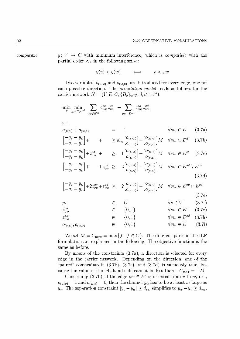
3.3 A L T E R N A T I E FORMULATION

atible y: V> C ith minimum interference, which is compatible ith the partial order in the folloing sense

< y

Two variables, 0(„)U)) and 0(WjV), are introduced for every edge, one for each possible direction. The orientation model reads as follos for the carrier network (V, E, , {Bv}veV, cad

min y,zco

V cco

we

CO

£E

ad a

s.t.

w ) v ) vw G (3.a)

Vv + Vw

Vv - Vw

w)

v) M vw G (3.b)

Vv + Vw

Vv - Vw

w)

v) M vw G (3.c)

Vv + Vw

Vv - Vw

ad vw

w)

v)

v) M vw G ad

(3.d)

Vv + Vw

Vv - Vw z°° a w)

v)

v) vw G ad

(3.e)

v ve (3.7f)

vw G (3-g) ad vw G ad (3.h)

w) v) vw G (3.i)

We set M = Cmax max{/ | / G C} . The different parts in the ILP formulation are explained in the folloing. The obective function is the same as before.

By means of the constraints (3.7a), a direction is selected for every edge in the carrier network. Depending on the direction, one of the "paired" constraints in (3.7b), (3.7c), and (3.7d) is vacuously true be­cause the value of the left-hand side cannot be less than Cmax M

Concerning (3.7b) if the edge vw G E is oriented from v to w, i.e. v,w) 1 a n d 0(WjV) 0, then the channel yw has to be at least as large as . The separation constraint yv — \ > dvw simplifies to dvw

A T E M A T I C A L ODEL 53

This is expressed in the first constraint of (3.7b). Conversely, if the edge vw is oriented the other way around, the separation constraint reduces to yv yw dvw, as imposed in the second part of (3.7b).

Concerning (3.7c), if the edge vw 6 Ed is oriented from v to w, then Vw > Vv has to hold. This is enforced by the first constraint of (3.7c). Co-channel interference arises in the case of yw = yv, and the same constraint drives the variable z^w to 1. The reverse case is analogous.

Accounting adjacent channel interference is more subtle. The cases vw 6 Ead \ E and vw G Ead n are distinguished. First, we consider two carriers v,w £ V with dvw 1 and c"^ > i e . vw £ ad \ E Examining the two cases of either 0(VjW) 1 and 0(WjV) = 0 or (VjW) = 0 and 0,jt)) 1, we observe that the pair of constraints of (3.d) drive z%w to 1 if yv — y = 1. Second, we consider two carriers v,w e V with dvw = 0 and C cad i.e., vw e Ead n E . We pick the orientation expressed by 0(VjW) 1 in order to discuss the effects of the paired constraints (3.e) . Assuming 0(„jW) 1 and the second part is vacuously true and the first part reduces to

zvw

zvw

Consequently z™w 1 has to hold in case of yv = yw. If yw yv = 1 however, both z™w 1 and z%w 1 would satisfy the constraint. At this point the additional assumption of c ^ steps in to guarantee that z% 1 holds in an optimal solution.

The integrality constraints need no further explanation but recall that Bv 0 is assumed for all carriers.

Although we do not give all the details here, it should be clear that solving the orientation model to optimality is equivalent to solving FAP if the additional restrictions mentioned above hold.

Finally, we indicate how the restriction of Bv 0 for all carriers v E V can be by-passed. We do not formalize how to include locally blocked channels in the orientation model, because it is simpler to express in words. The problem with the local blockings is that they may "puncture" the otherwise contiguous domain C of the y-variables. Let B veV Bv

denote the union of all locally blocked channels. (By definition, B C C. We introduce an artificial carrier b for each b G B and restrict its available set of channels to the singleton {b}. Additionally, for each carrier v with b £ Bv, &n edge vb is inserted and the edge labelings d, c , and cad are extended by setting d(vb) = 1, c(vb) = 0, cad(vb) 0. The orientation model for this extended carrier network fixes the values of the variables yb to b G C. A closer inspection of the extended model reveals that some

3.3 A L T E R N A T I E FORMULATION

new constraints may be superfluous but the detais are technical and skip the corresponding discussion.

The "inner part" of the orientation model, which deals with finding an assignment of minimal interference among all feasible assignments compatible ith a given orientation, forms the basis of the improvement heuristic . This is discussed in Section 4.3.4.

CHAPTER

st euristic ethod

Before we proceed, let us recapitulate our points up to now. The problem of generating "good" frequency plans for GSM networks was explained in detail, see Section 2.3, and the notion of a carrier network, see Section 3.1 was introduced to represent the essential characteristics of a GSM fre quency planning problem: N = (V, E7 C, {Bv}veV, d, c , cad) denotes a generic carrier network, the carriers in the set V represent the TRXs the edges in the set E the relation between carriers the channels in the set C the available spectrum and the sets {Bv}veV the locally blocked channels; furthermore, d, c , and cad represent the required minimum separation, the expected co- and the expected adacent channel interfer ence between pairs of carriers, respectively.

We argued that the sum over all co- and adjacent channel interferences between carriers is an adequate measure for the quality of a frequency assignment. This quantity is minimized in the mathematical optimization problem FAP, see Section 3.1. Furthermore, we pointed out that the generation of reliable input data for setting up the carrier network is intricate. This holds in particular for interference data. But we also stated that the generation of input data can be mastered ith a sufficient accuracy today see Section 3.

We are now at the point to address the optimization problem FAP computationally. Recall from Section 3.2.3 that solving FAP is jVP-hard and that finding solutions which are guaranteed to be close to optimal is also jVP-hard. Hence, according to present understanding, both tasks are unlikely to be algorithmically solvable in a running time which is polynomially bounded in the size of the input. This is our justification for the development of fast methods which neither necessarily produce close to optimal nor even feasible assignments (provided some exist)

Our focus is on frequency planning heuristics, capable of dealing with carrier networks of around 2000 carriers in a quarter of an hour on a mod­ern PC or workstation. Such methods are wellsuited for GSM frequency planning in practice ith particular emphasis on the intermediate steps

55

in the planning cycle, see Section 23.3. Several of these methods are no in use at the GSM operator E-Plus Mobilfunk GmbH & Co. KG.

More elaborate but also more time-consuming methods are capable of producing better results than our fast heuristics. This type of meth­ods targets primarily the generation of the final frequency plan, where running times in the order of one or two days are acceptable. We come back to this issue in Section 5.6.

The algorithmic solution of frequency planning problems is not a new topic, of course. Well over a hundred articles and reports propose and discuss algorithmic techniques for frequency planning in general or in the

urveys specialization to GSM. Recent surveys are given by Jaumard et al. [1999] oster [1999], and Murphey et al. [1999].

The published algorithms can be distinguished according to whether they guarantee to produce optimal solutions or approximately optimal solutions or neither of both. None of the enumeration or cutting-plane algorithms, however, which may produce provably optimal solutions in the general case are suited for frequency planning in practice, because their running times grow exponentially with the size of the carrier net work. And for the algorithms proven to produce (approximately) optimal assignments for special cases in polynomial running time the relevant cases are not known to appear in practice. ence, these two types are not of interest to us. Among the algorithms without quality guarantee there are proposals for procedures building on the meta-heuristics Sim­ulated Annealing, Tabu Search, Genetic Algorithms, Neural Networks etc. Such procedures typically have much higher running times than the ones we are aiming at. But also fast methods are proposed, which mostly build on ideas published in connection with computing graph colorings.

Despite our focus on fast methods, we also performed extensive exper iments with Simulated Annealing and Tabu Search, see Schneider [1997] for an early report on these experiments. A general introduction to local search methods as well as to Genetic Algorithms and Neural Networks is given in Aarts and Lenstra [1997]. The implementations of those meth­ods typically have running times in the order of several hours up to one or two days on large carrier networks. Our own results are in the range of what is published by Beckmann and Killat [1999]. Further imple­mentations of Simulated Annealing or Tabu Search for GSM frequency planning are discussed by Duque-Anton et al. [1993] Castelino, Hurley and Stephens [1996], urley Smith, and Thiel [1997], Hao Dorne, and Galinier [1998], Smith, Allen, Hurley, and Watkins [1998], and Correia [2001, Section 4.2.5]. This list is incomplete but provides starting points for a further exploration of the literature.

FAST HEURISTI E T O D

The chapter is organized as follows. In Section 4.1, we describe tech­niques for preprocessing the carrier network prior to running frequency planning procedures. Then, we turn to two types of algorithms, which are generally known for efficiently "solving" combinatorial optimization prob­lems: greedy construction heuristics and simple improvement heuristics. We describe methods of these kinds in Sections 4.2 and 4.3, respectively. Computational results for our methods are reported in Chapter 5.

For the most part, this chapter describes joint work with Ralf Born­dörfer, Martin Grötschel, and Alexander Martin as well as ith the stu­dents Daniel Haberland and Margherita Hebermehl. The M C F method is described together with the orientation model (presented in Section 3.3. by Borndrfer et al. [1998b]. The other heuristics of Sections 4.2 and 4.3 except for K - O P T and VDS, are also contained in Borndrfer Eisenblät ter Grtschel and artin [1998a]

r e r o c s i n g

Prior to calling some planning method, a carrier network may be prepro-cessed in order to simplify the frequency planning problem. Techniques to identify possible simplifications are, for example, studied in the field of constraint satisfaction programming (CSP). We are not aware, however of any specific study for our version of the frequency planning problem.

We consider two types of modifications here. In the case which we call structurepreserving, the modified carrier network allows feasible assign- structure ments if and only if the original carrier network a l l o s them. Moreover preserving for each optimal assignment for the modified network, an optimal assign­ment for the original network can be generated in polynomial time. In the other case, we call it heuristic, the modifications may change the feasibil heuristic ity status, and optimal assignments to both networks are not necessarily related. We are interested in this type of modifications, nevertheless, be cause the frequency assignments produced by some of our methods are often better when such a preprocessing is applied.

We present structurepreserving modifications in Section 4.1.1 and heuristic modifications in Section 4.1.

1.1 liminating C h a n l s an arriers

We specify a few situations in which the carrier network may be reduced structure-preservingly by either dropping available channels for a carrier or by dropping a carrier altogether.

58 1 PREROCESING

r o p i Chan

As a motivating example, we look at a carrier network, where some of the carriers are effectively fixed by having only one channel available. Let v0

denote such a carrier with C \ BVo {/o oreover let w be a carrier with d(v0w) > 0. Then the channels f0 — (d(vow) — 1 ) , . . . , fo + (d(v0w) — may be added to Bw without changing the set of feasible solutions.

This can be generalized to situations, where v has a fe channels available and for a fixed g C \ Bw the relation f g\ < d(v0w) holds for all channels / G C \ Bvo. Then the channel g may be added to Bw

The idea can be pursued further and extended to larger sets of carriers than merely two carriers. The computational burden of recognizing such a situation, however becomes significantly harder ith each additional carrier considered.

None of the above cases turns out to be relevant for our test instances introduced in Section 5.1.1. In planning practice, however, the first case is relevant and therefore part of our preprocessing. The other cases are not addressed.

r o p i n arriers

Clearly, we may drop every carrier for which only one available channel is left. This is preferably done after dropping channels. Another situation in which carriers may be dropped without harm, is described next. We

generali degree call the generalized degree of a carrier v the quantity

2_] maxvw), h(vw)} l) £E

ith

if cad(vw

if cvw) cadvw

otherise.

For a fixed carrier w, the summand "2 m.ax{d(vw), h(vw)} 1" equals the maximal number of channels which may become burdened with sep­aration constraints or interference for carrier vifw gets assigned. Hence the above sum gives an upper bound on the effect of assigning channels to all adacent carriers of v. The actual effect however may be much smaller.

If the generalized degree of a carrier is less than the number of avail able channels then the carrier may be dropped for the folloing reason.

FAST HEURISTI E T O D 59

Whatever the assignments to the adjacent carriers a r , there is always at least one channel available which can be assigned ithout causing a separation constraint violation or interference.

As reported in Section 5.1.1, this form of preprocessing often allows to drop a few carriers. If one carrier is dropped, the generalized degree of its adjacent carriers reduces. Consequently, the technique can be applied repeatedly until no more carrier is dropped. A feasible assignment for the reduced carrier network is extended in the reverse dropping order to a feasible assignment of the original network and without introducing extra interference. Carriers may also be dropped if the generalized degree exceeds the number of available channels by some small factor. In that case, however, the modification is heuristic.

We also look for possibilities to reduce the size of a carrier network by amalgamating carriers, i e . , by treating them exactly the same way. Let v and w be two nonadjacent carriers. We say that v dominates dominates

if Bv and if the edge vx is in E for all wx 6 E satisfying d(vx) > max{d(wx),h(wx)}. The function h is the same as defined above. Then, a feasible assignment for a carrier network without w can be extended to include w by simply assigning the channel of v to w as well. Although appealing in principle domination plays no role for any of our planning instances.

1.2 Tihtening t e seration

The following modification is a heuristic in the sense defined above. Let v and w be adjacent carriers, then d(vw) is the minimum necessary sep­aration between the channels assigned to v and w. In case d(vw) > 1 the same channel must not be given to both carriers. This rules out co-channel interference between v and w. Similarly in case d(vw) > 2 no adjacent channel interference between v and w occurs in a feasible assignment.

One approach to control interference beyond minimizing its overall sum is to exclude assignments causing large interference between individ­ual carrier pairs. To this end, we introduce a threshold t. The threshold threshol is used to impose a sufficiently large separation between carriers hich may other ise cause interference exceeding

max vw)}, if cvw t and cadvw

max{ vw)}, if cadvw

d(vw), otherise

60 2 REEDY E T O D

The carrier network iV = (V, E, C, {Bv}veV, d, c , cad) is obtained tightening from N by tightening the separation with t. A feasible assignment for JV

may still incur interference, but none exceeding the threshold t between a carrier pair. Because an assignment causing high interference between one pair may save considerably between others, no optimal assignment for the original problem may be feasible for the modified one.

Despite this fact, tightening the separation works well in conjunction with some of our heuristics. By applying heuristics to N for different threshold values, solutions of varying quality are usually obtained. A suitable threshold value t may be determined by some search routine. One example for such a search routine is described in Section 5.

.2 eedy Method

Greedy methods compute a frequency assignment from scratch, step-wise extending an initially empty assignment to a complete assignment. In the course of the construction, partial frequency assignments occur. A partial

artial assignment frequency assignment is a mapping : A> C that is defined on a subset A of the carrier set V. In case a partial assignment is ust an ordinary frequency assignment.

We have performed experiments with several greedy methods and describe three prototypical ones in the following. Among them is the adaption DSATUR WITH COSTS of the well-known graph coloring heuris tic DSATUR. This is our most successful greedy method and it is used in frequency planning practice at E-Plus obilfunk Gmb Co. G.

2 T - l o r i n

We recall the definition of a T-coloring. Given an undirected graph G (V, E) and nonempty finite sets T(vw) of nonnegative integers for all vw G E. A T-coloring of is a labeling / of the vertices of G with nonnegative integers such that \f) f(w $_ T(vw) for all edges vw G E. Since their introduction by Hale [1980], T-colorings of graphs and methods to produce them have been studied by several authors. A survey is given by Murphey et al. [1999]. Here, we are interested in the blend of T-coloring and list coloring introduced by Tesman [1993], where each vertex has a list of colors available.

Our OLORING heuristic, designed and implemented by Haber land [1996], is a modification of a T-coloring procedure proposed by Costa [1993]. The underlying idea is however already used in the graph

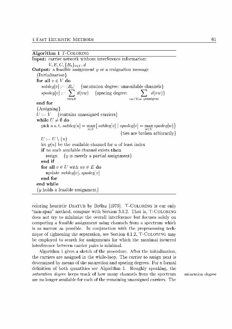
FAST HEURISTI E T O D

gorit OLORING

I n t : carrier network w h o u t interference informaton V, E, C, {Bv}veV, d

tput: a feasible assignment y or a resignation message {Initialization} for all v o

sadeg[ BV {saturation degree unavailable channels} deg[ YJ vw spacing degree YJ vw

&E vwdE-.w unassigned

end for Assigning}

V contains unassigned carriers} ile U ^ 0 do ick u s.t. sadeg[ maxsadeg[ deg[ maxdeg[w]

v£U wdU es are broken a r b i a r y }

UU\{u} let y(u) be the available channel for u of least index if no such available channel exists then

resign y is merely a artial assignment} en if for all v U with u G E do

update sadeg[] deg[ end for

end while y holds a feasible assignment}

coloring heuristic DSATUR by Brelaz [1979]. T C O L O R I N G is our only "min-span" method, compare with Section 3.1.2. That is, T-COLORING

does not try to minimize the overall interference but focuses solely on computing a feasible assignment using channels from a spectrum which is as narrow as possible. In conjunction with the reprocessing tech­nique of tightening the separation, see Section 4.1.2, T-COLORING may be employed to search for assignments for which the maximal incurred interference between carrier pairs is minimal.

Algorithm 1 gives a sketch of the procedure. After the initialization, the carriers are assigned in the while-loop. The carrier to assign next is determined by means of the saturation and sacing degrees. For a formal definition of both quantities see Algorithm 1. Roughly speaking, the saturation degree keeps track of how many channels from the spectrum saturation degree are no longer available for each of the remaining unassigned carriers. The

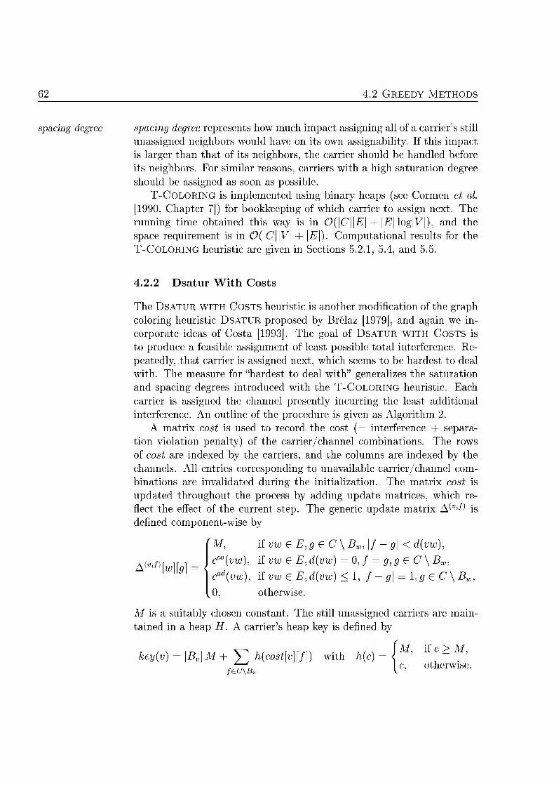
2 ET

spaing degree spacing degree represents how much impact assigning all of a carriers still unassigned neighbors would have on its own assignability. If this impact is larger than that of its neighbors, the carrier should be handled before its neighbors. For similar reasons, carriers ith a high saturation degree should be assigned as soon as possible.

T-COLORING is implemented using binary heaps (see Cormen et al [1990, Chapter 7]) for bookkeeping of hich carrier to assign next. The running time obtained this way is in (9(|C||i?| + \E\ log|V|), and the space requirement is in 0( |C| |V + |£"|). Computational results for the T - O L O R I N G heuristic are given in Sections 5.2.1, 5.4, and 5.5.

4.2.2 Dsatur W i h Costs

The DSATUR WITH COSTS heuristic is another modification of the graph coloring heuristic DSATUR proposed by Brelaz [1979], and again we in­corporate ideas of Costa [1993]. The goal of DSATUR WITH COSTS is to produce a feasible assignment of least possible total interference. Re­

eatedly, that carrier is assigned next, which seems to be hardest to deal with. The measure for "hardest to deal ith" generalizes the saturation and spacing degrees introduced with the T-COLORING heuristic. Each carrier is assigned the channel presently incurring the least additional interference. An outline of the procedure is given as Algorithm 2.

A matrix cost is used to record the cost ( interference + separa­tion violation penalty) of the carrier/channel combinations. The row of cost are indexed by the carriers, and the columns are indexed by the channels. All entries corresponding to unavailable carrier/channel com­binations are invalidated during the initialization. The matrix cost is

pdated throughout the process by adding update matrices, which re­flect the effect of the current s t e . The generic u d a t e matrix A^'^ is defined c o m o n e n t i s e by

^[w][g]

M, ifvweE,g\Bw,\f-g\<d(vw),

cco(v), if vw e E, d(v) = 0, / = g g G C \ Bw,

cad(v), if vw E E, d{v) < 1, | / - 1, g G C \ Bw,

otherise.

M is a suitably chosen constant. The still unassigned cariers are main­tained in a heap H carrier's hea key is defined by

key{v) + V h(cos][}) with h{) = \ f c - M

fiE\Bv c ' t h e r w i s e

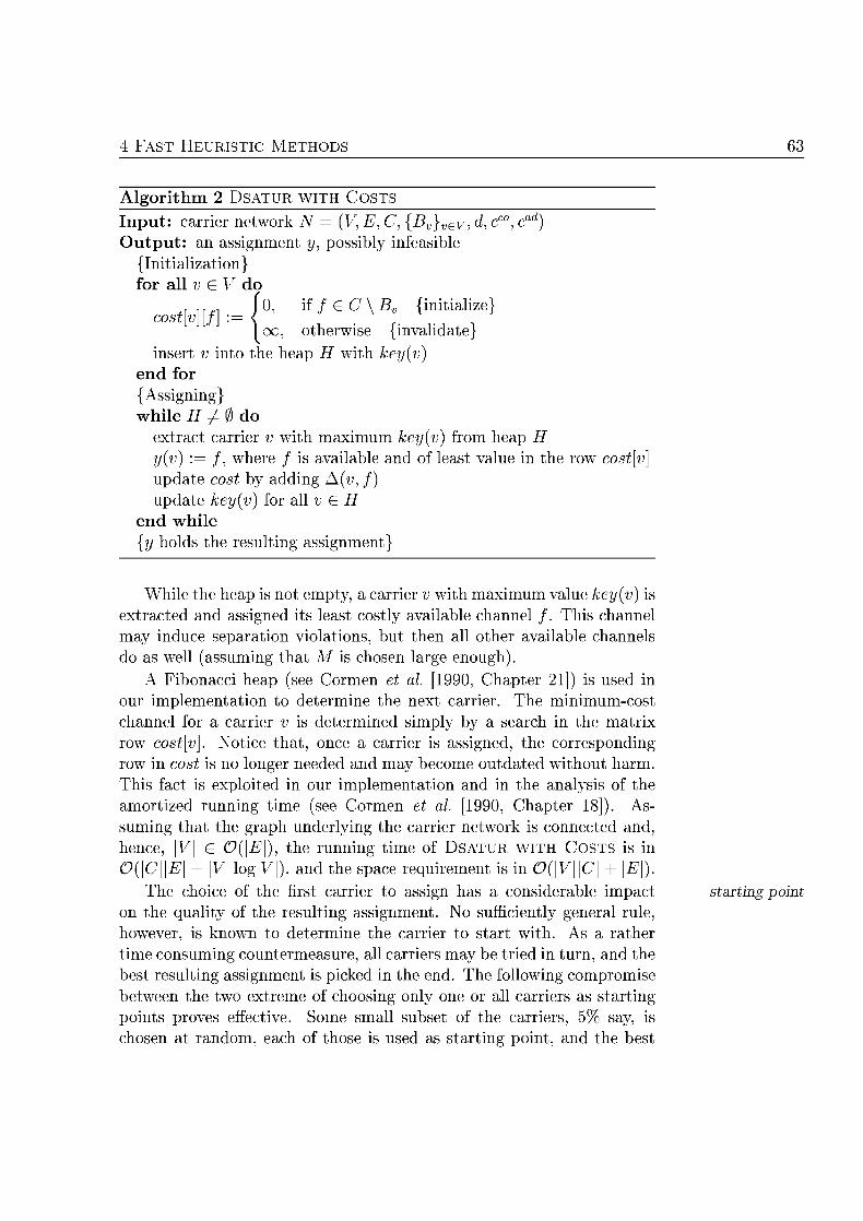
4 F S T HEURISTI E T O D

A l g r i h m 2 SATUR WITH C O S T

Input: carrier netwrk TV V, E, C, {Bv}veV d, cco c Output: an assignment y, possibly infs ib le

Initializtion} ll v V d

i r i / e C \ ^ i t i l i c o s J [ J :

loo, therwise { n v l i d t e sert the he with key

d f s s igng}

hile H ± 0 do extrac carrier i with aximum key(v) from he ? y ) := / , where / is ilable of l e s t the cos update cos by addin v, f u p t e key for ll H

nd whle lds the res l t i ssignm

While th eap is not empty a carrie with ximum vaue v) is extracted and ssigned its least cotly availble hannel / . This annel

indue s e p a t i o n violtion but then all other i lble nnels s well assumig that M is se l r ge enough).

A Fibonacci h e p (see C o e n et al. [1990, Chapter 21] is used in ou impleentation d e t e r m e the next carrier. The nimum-cost hannel for a carrier v is determined simply by a search the matrix ow c o s t [ . Notice t h t , onc a carrier is assigned the corresponding ow in cost is no onger eeded and ay becom outdated withou h r m .

This fact is e x i t e d our m p l e n t a t i o n and in the analysis of the amotized running t i e (see Cormen et al. [1990, Chpter 18]) s u m g that the graph underlyig the carrier network is connected a d hece , \V\ e Ö(\E\), the running time of DSATUR WITH COSTS is i

C | |£ | + \V\ log|V|) and the spac require is n C?(|V||C| + \E\

The co ic of the first carrier o ssign h a considerable impac starting point on the quality of the resulti assignment. No sufficiently general rule however is known to de t e r ine the carrier o start with s ather time c o n s u m g c o u n t e r m e r e , ll carriers may be tried i rn, nd the best reslting ssignmnt is ked the end. The following ompomise betwee the tw extre of oosing only one or all carriers as s t i n g ponts roves effective Som m l l subset of the carriers, 5% say, is

se t r o m , ac of t h s e is sed s s t r t i po the best

2 E T O D

resuting ssignm s reurne in end. T computatonl behavio of DSATUR WITH STS is d u m n t e d i tions 5.2. nd 5.4, see

lso S t i o n 5.5.

4.2.3 l G e e d y

he UAL G E E D Y heristic constrcts an ssignment by me of elim­ating alternatives. Reeatedly, a option fo assigning some nnel

to a carrier is elimiated until only a single annel remans for very carrier. Our interest in this type of m e t h d is d e to the results o b t e d by Jünger, M r t i , Reielt , and Weismantel [1994] in VLSI design.

The DUAL GREEDY is greedy i the following sense: the exclusion of carrier/hannel combintion is based on oca perception of wh s e e s to be n unfavoble combintion. We use a set A C V x keep track of the r e m n i n g eligible combiat ion. Initially, A contain

ll carriers paired with ll their availble nnels A si version of the cedure is shown Algorithm 3. Hebereh l [199 investigates this b s i c version and several vriants

The principal distintion among the studied variants lies in the defini tion of "unfavorble." The following example, where is the already estblished rtial assignment nd A is the set of r e g eligible om biations is ken fom Hebereh l [199

unfavorable A; g)) = 2_, co y , adw) (v,g)eA: v,g±l)eA:

£E,(vw)=0 aE,dw)<l

+ Y^ Mi coväic{g))\W (vj)eA-.eE

f-g\<

The set conflict g)) contains the alredy assigned carriers in y whic re adjacent t which stisfy on of the three condition g =

y(vcco) > 0 or y(v) l c ) > — y w) Mj nd W are two p m e t e r s .

This definition of unfavorable(-, • is not the best e r f o n g amon those investigted, but it is easily e x p l e d . On assigning chnnel / carrier , the parameter is used to pnalize ll still eligible ombia­tion that would r e s l t in nterferece or a separation violation if one of them were cked for ssignment. Among the still unassigned carriers, potentia co an djace channel terfere is diretly accounted for

potentil s e p t i o n constraint vilation are p a l i z e d with the pa eter Mj High es fo should l e d t little nterfere few

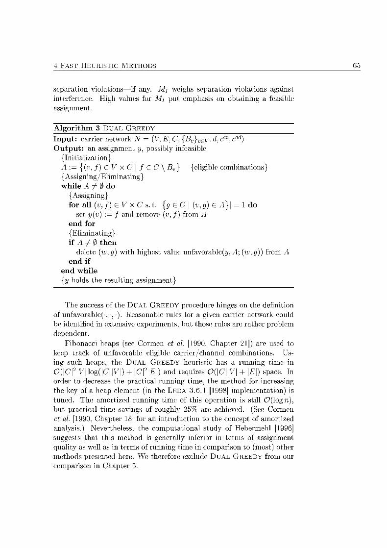
4 F T HEU ETHO

paation o l a t i o n i f an Mj weighs p a a t o n v o n ains nterfere High es fo Mj put e m p s i s on bt sible ssignm

A l g r i h m 3 UAL G Input: carrier netwrk T V, E, C, {Bv}veV d, cco c Output: an assignment possibly infs ib le

Initialization} = {v, f) G C | / C \ Bv] eligible ombiation s s i g i n / E l i a t i

e A s s i g n g

r all v,f x C s.t. \{g G C \ v,g) 1 d set v) : d remov v, f om d l iminti A ^ 0 then delete g) with highest unfavorable A; g)) om

w h l e lds the res l t i ssignm

he s u e s he UAL GREEDY p r d u nges on the definiton of unfavorale(-, -, . Reasonable rules for a giv carrier e twrk could be identified n extesive e x e r i m t s b t t h s e les re ther ble d e d e t .

Fibonacci heaps see Cormen t al. [199 Cha te r 21 are sed to keep track of unfavorable eligible carrier/channel ombinations. Us

g such heaps, the DUAL G E E Y heuristi has a runni time in ö ( | C | 2 | F | l o g C | | V | + |Cf |£|) an requires 0{\C\\V\ + \E\) a c . In order t d e r e s e the practical r u n n g time, the method for icreasing the key of a hea element ( the DA 3.6.1 [1998] i m p l e m e t i o n ) is uned The amortized runn ig time of this operation is till ö(logn

t actica t i e savings of oughly 25% re achieved (See Cormen t al. [199 hapter 18] for n introduction to the concept of amortized nalysis.) Nevertheless, the computational s t d y of Hebermehl [199 ggests that this method is generlly inferior i term of assignment

uality as well as in t e r s of runnng time n comparison to (most) other methds presented here. We therefore e x d e DUAL EE om ou omprison n C t e r 5.

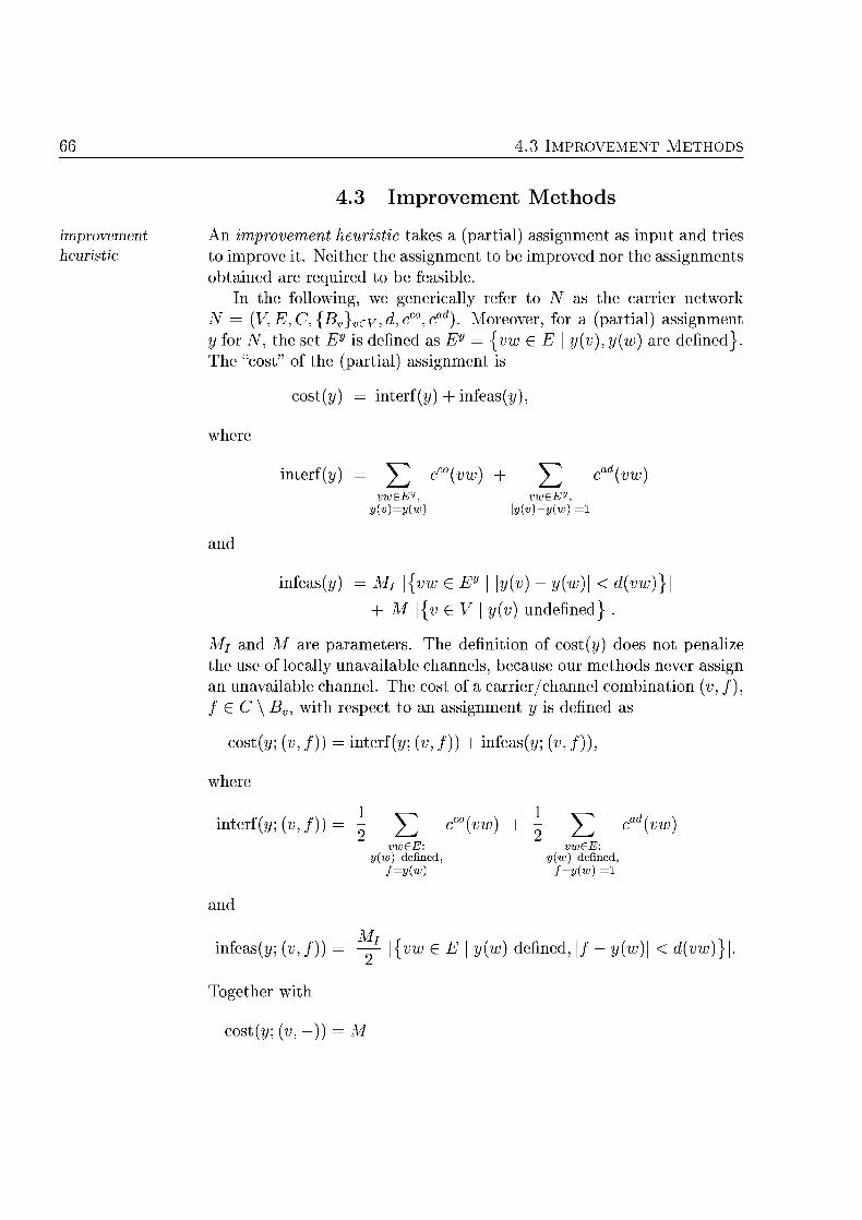
I M P O V E N T ETHO

4.3 Improvement Methods

improveent n improvement heuristi takes (partial) assignmnt as input and tries euristic o mprove it. Neither the assignmet t be impoved nor the assignmnts

btained re required to be feasible In the followig, we generically refer to N s the carrier netwrk

iV (V E, C, {Bv}vey, d, cC0 c)- reover for (p r t i assignm y fo TV, the set Ey is defined as Ey = {vw G | y y re defined The " " of the (parti ssignmnt is

cos iner inf

where

iner Y^ cow) Y^ vweEV, vweEV, v)=y{ (v)-{w=l

inf Mj Ey \ \ yw)\ <

V | y u n d e f e d |

Mj and M are a r e t e r s . he definition of c o s t ) d e s no pnalize the use of ocally unav i lb le hannels, becase our methds ever assig

n unavailable channel The st of a carriercannel c o m b i t i o n v, / / 6 C \B, with r e s t t ssignm is d e f e d

cost y, / )) i n e r v, / ) ) inf / ) )

where

iner «, /)) \ ^ cow) \ ^ vwdE: vwdE: ) defined, (w) defined

}=w /-2/(w)|=l

inf v, / )) -— w £ | yw) d e f e d | / — \ < d\

gether with

costv,-))

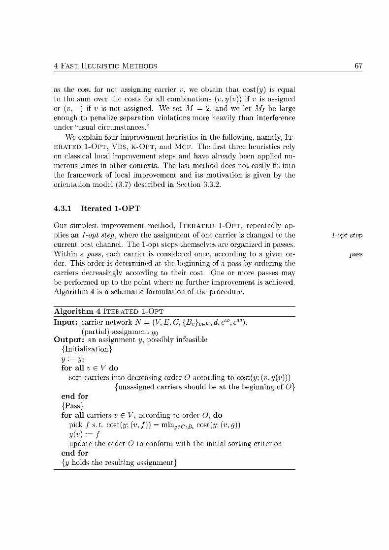
4 F T H E U C METHO 67

the cost for not ignn carrier v, we o n at o s y is e u a the sum over the costs fo all combintion y(v)) if v is assigned

or (ft, —) if v is not ssigned We set M a d we let Mj be l rge enough o pnalize s e a t i o n tion more h e i l y th nterfere under "usua ircumstaces"

W exp fou mprov heuristi in the following, namely, IT E A T E D 1-OPT, V S , K-O an M C F he first three heristics rely on classical l c a l impovement teps and ave alredy been applied nu merou times n other ontexts The l s t method d e s not easily fit into the mework of loca improvement d its m o t i t i o n is gi by the

r i e a t i o n model (3. desribed i tion 3.3.

4.3.1 at 1-OPT

Our simples mprovement method, TERATE - O P T , r e a t e d l y ap lies n 1-opt step, where the assignment of one carrier is changed to the 1-opt ep rren best channel The 1-opt steps themselves are organized in psses

Within a pass, each carrier is considered one , accrding t a giv or pass der. This rder is determined at the beginn of ss by rderin the carriers decreasigly according to their cost. On o more passes ma be er fored up o the pont where no further mprovem is achieved

lgri thm 4 is a c h e t i fomuation of the r o e d r e

A l g r i h m 4 TERATE - O T

Input: carrier etwork T V, E, C, {Bv}veV d, cco c (prtial) a s s i g n m t y0

tput: an assignmen possibly infs ib le Initializtion}

Vo all v 6 V d rt carriers to decreasing order O accordi to cost(y; v,y(v)))

u n s s i g e d carriers should be the beginnin of e d {Pss}

ll carriers v V, accordig o order O k / . cost v, / )) = minseC\B„ cos g))

y ) ••= f update the rder O onfo with the i t i l s t i riterion

nd for lds the res l t i ssignm

I M P O V E N T METHO

T E A T E 1-OP is a c l a c a l loca earch mthod. The sates in h search pac are the ssignments, the neighborhood relation is defned through the 1-opt ste nd the merit of movng to a neighbor is the differece of the sts omprehesiv suvey on cal se e t h d s is g i n by A t s a enstra [199], for example

miim Unless the current assignment ontitutes local nimm with re ect to the neighbrhood relation an the cost structure, conse t ive

passes result i reeated improvemnts e iterate while impovements re bta ied, a computationl e x e r i n t s idicate no need for som iling-off contro n practi

Fibonacci hea (see C o n et al [1990 h a t e r 21]) are sed to determ which carrier to consider next and what hnne l to as sign t that carrier. We observe th the running time of a single

ss is in 0( |C| | i? | log|C| + \V\ log|V|) and t h t the required space is in C(C||V^| -h I-£71). In theory, the number of impovng psses is not poly-nomally bounded the size of a carrier graph, because that umber may depend exponentilly on the values of cco c . Compuationa res l t s fo the I T E A T E - O re reported i tion 5.3.1 5.4.

4.3.2 ariab th S a r c

The VDS herist i is an mpleentation of the onep of variable depth eighbrhoo s e a h as i n t r c e d by n nd Kerigh [193] see als

Aarts an enstra [199 h a t e r 1]. The carriers are sorted to om rder 0 , a d the ssignme of each carrier is c g e d one by on accrd

ing to this order The bes alterative channel the resently assigned one is tentatively selected. O n e all carriers bee onsidered, the sequene of t e n a t i e changes is canned om art to nd d the t of very intermediate ssignment is recorded Finlly, the t e a t i v e ges

are committed up to the pont where the first assignm of le is btained. All further t e a t i ges re rejected

Like n the case of TERATED - O P call the oessing of on pass rder pass. Psses are erformed s lon a i m p r o v n t s re achieved

f o l desription of DS is g i n lgri thm 5 VDS is local seach me tho . G n n assignment another assig nt is its neighbor if this assignme can be o b t a e d by the mprove

ment rocess desribed bov for some order of the vertices Hence, the neighbrhoo of a g ien assignm consists of ll ssignmnts that ca be r o c e d by executing the tentati ssignng an the committi

rt of lgr i th 5 for som rder In t h t r e s t our meth

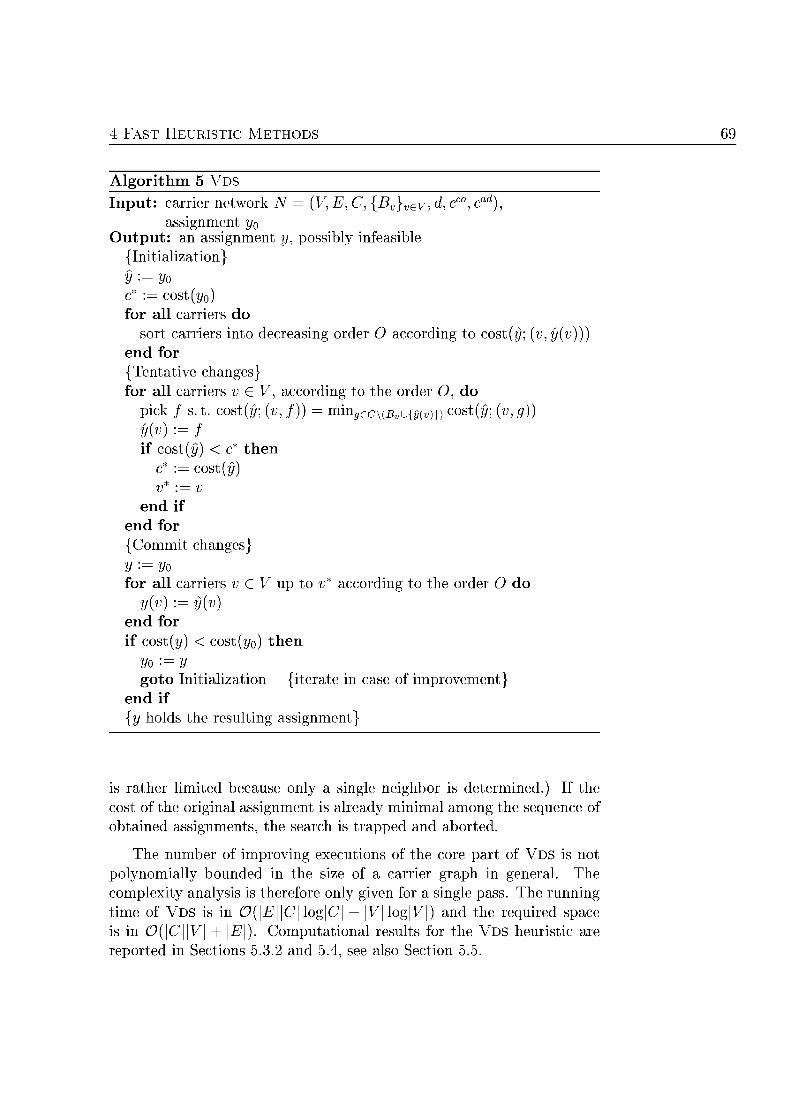
4 F T H E U C METHO

A l g r i h m 5 DS Input: carrier e twrk T V, E, C, {Bv}veV d, cco c

assignment tput: an assignm possibly infs ib le Initializtion}

yo c* cost(y0)

all carriers rt carriers d e r e s i rder O accrdi cost v,)))

or tative chages ll carriers v V, a c c r d i g the rder O, d

. cost v, / ) ) = mmgeC\{BvU{yv)}) cos g)) v) c o s y ) < c* th c* cost

nd for Commit ges

=yo ll carriers up o v accrdi the rder O ) :

nd for cost cost th o y ot Ini t i l iz t ion i t e r t e i case of mpov

if lds the res l t i ssignm

is rather limite cause only a s inle ig is determine the ost of the origi assignme is already m among the se of b t n e d ssignmnts the search is t rpped an ted

The number of improving execution of the core part of V is no polynomially bounded in the size of a carrier graph in general. he complexity nalysis is therefore only given for a s igle pass. he runnin time of VDS is in C(|£711C| log|C| + |V|log|V|) and the required ace is in 0( |C| |V| + \E\). Computational results for the V heris t i re reported i tion 5.3. and 5. see lso S t i o n 5.5.

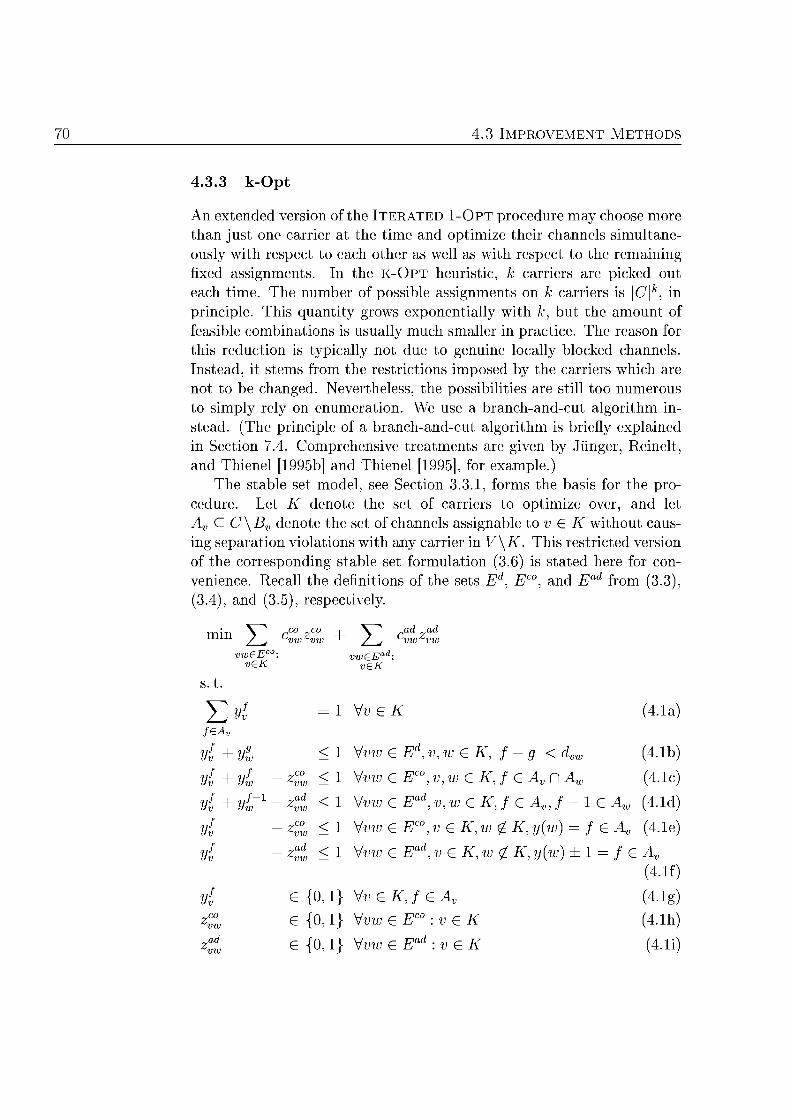
I M P O V E N T METHO

33

A extended version of the T E A T E 1 - O T procedre may choose more than just one carrier t the tim nd optimize their nnels s i m u l t e ously with resec o ach ther well as with respect the remanin fixed assignments. In the K - O P T heuristi k carriers are piked ou eac tim The umber of possible assignmnts on carriers is \C\ in

rinciple. This quantity grws exponentially with k, t the amount of feasible ombinations is uually m u h smaller in practice The r e o n fo this reduction is typcally not due genuine locally blocked channels Insted, it stems om the restriction imposed by the carriers which are not to be chaged Nevertheless the possibilities re still too numerou o simply rely on numertion. W use b r n c h - d - c u t lgorith in t e d (The principle of b r c h - d - u t lgorith is briefly explaned

Setion 7.4. Comprehensiv treatments are given by Jüger , Reiel t d Thienel [1995b] nd Thieel [1995], for example.) The stable set model see Setion 3.3.1, forms the basis for the ro

ed re . et K denote the set of carriers to optimize over d let v C C\BV denote the set of nnels a s s i g b l e v K without caus

ing s e a t i o n volation with any carrier in \K This restricted version of the rresponding stable set fomuation (3.6) is sated here fo con venie Recall the definition of the sets Ed Eco Ea om 3. (3. (3.5) respetively

rco co ad ad

7 W^ / W^ weEco weEad

veK vex

1 VD (4. feA

< 1 V v w £ v , \ f \ < (4.1b

Z < 1 Vvw G co v , f vn (4.

w - lv i < 1 V v w e a d , v , f J - (4.1d

Z < 1 V v w e C 0 , v , y w ) = (4.1e

< 1 Mvw e ad\ v yw) ± Av

(4.f)

,1 Vvef (4.1g

,1 Vvw eC0 (4.1h

1 Vvw e a d (4.1i

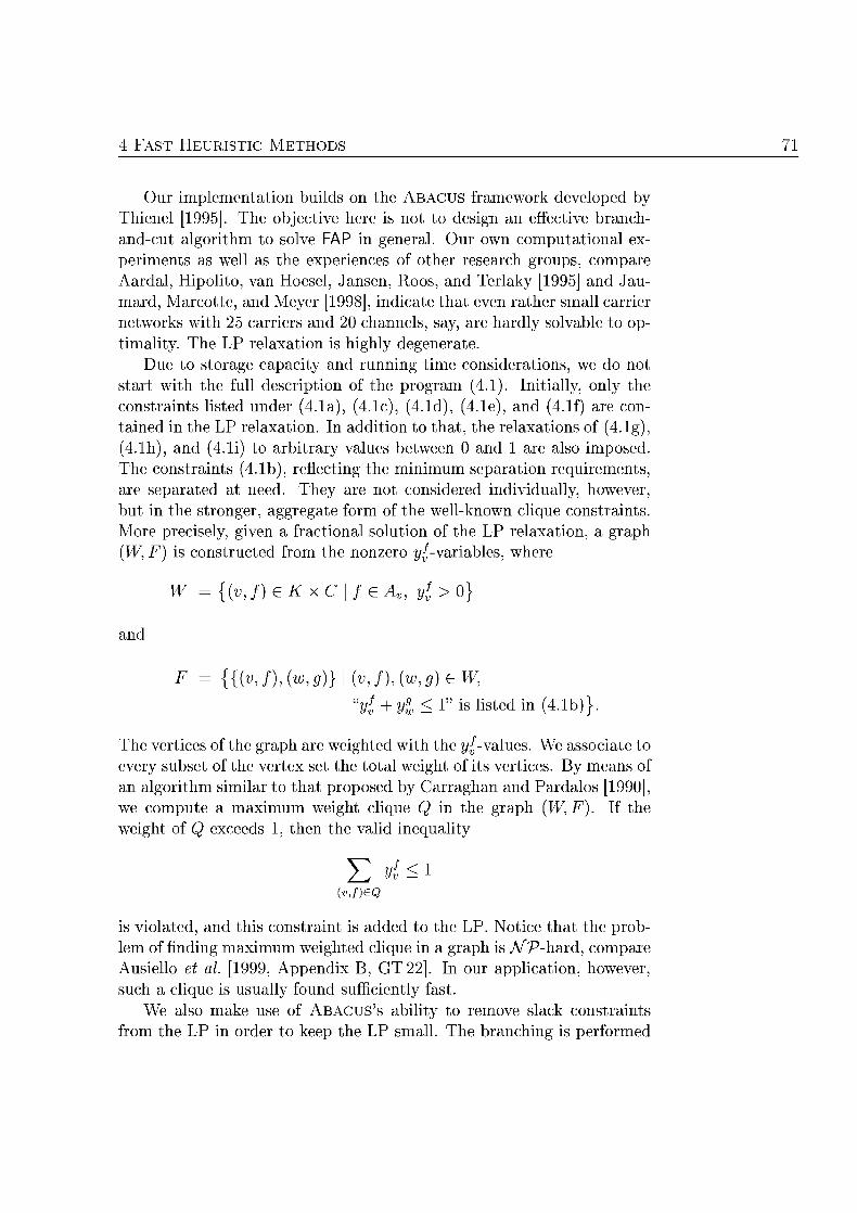
4 F T H E U C METHO

Our m p l e t a o n uilds on h ABACUS f r k deelop by hieel [1995]. he jet ive here is not t desig effective b r c h -nd- algorithm solve FAP i general. Our o computational ex­e r i n t s as well the experiences of other research groups ompre

rda, Hipolito Hoesel, Janse , Roos, a d Terlaky [1995] and Jau-mard, Marcotte, and Meyer [1998] indicate that eve rather s a l l carrier networks with 2 carriers a d 20 channels say, are h rd ly ble o op t i l i t y The P relxation is highly degenerte.

Due to stoage capacity a d r u n n g ti onsiderations, we do no t a t with the full description of the rogrm (4 . ) Initially, only the o n s t r n t s listed under (4.1a (4.1c), 4.Id (4.1e), a (4.If) are con ained the LP r e l a t i o n . In ddition to that the relxation of (4.1g 4.lh), nd (4.1i to rbi t r ry alues betwee an are als imposed.

The contraints 4.1b reflectig the inmum sepration requiremnts, re separated t need. They are not considered i d i v i d l l y , howver

t i the stronger ggregate form of the well-knon c l i e contrants re reisely, given fractional solution of the LP relaxtion gr

W, F is o n s t r t e d om the nonzer y v a r i b l e s where

v , f ) e C \ f , y > 0

v , f g ) ( v , f ) , , g ) e

uy( + Vi< 1" is listed in (4.1b

he vertices of the graph are weighted with the ^ - v l u e s W s s a t e to very ubset of the vertex set the otal weight of its verties. B mean of

an lgorithm s i i l a r to that proposed by r raghn r d s [1990] we compute a maximum weigh clique Q n the gr W,F f the weight of exeeds 1 the the lid i n e q l i t y

v,f)eQ

is ol ted, d this constraint is dded t the Notie that the p b ­lem of ding maximum weighted cli n a grap is A/'Phard, ompare

siello et al. [1999, Appendix B G T 2 . In ou pplication hwever a clique is u a l l y found suf ient ly f s t

We lso make use of ABACUS' bility o remove slack o n s t r n t s om the LP n order kee the ll he b r c h i g is e r f o e d

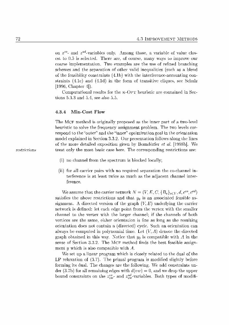
I M P O V E N T METHO

on d z va rb les only Among thoe, vaab le f v u e lo est to 0.5 is seleted. here are, of course, m n y ways impove ou oarse implemenation. Two examples are the se of r e f e d brnchi

schemes and the separtion of other valid equalities (such as blen of the fasibility o n s t r a t s (4.1b with the nterfereceaccountig con strants (4.1c) and 4.Id the fo of t r s i t i l i e s see lz [1996, C h t e r 4]).

Computional res l ts fo the - O heristic are o n e d i tion 53.3 5. see lso 55.

4.3.4 n-Cost F

The M C F ethod is o r i g i l l y roposed s the inner art of a twolevel heuristi o solve the frequen assignmen poble he tw levels cor respond the "outer and the nner" optimization goa in the orientation model explaned in Sction 3 .3 . . O present ion follows ong the l i e s of the more detailed exposition gi by Borndörfer et al. [1998 W

retric tre only the most bs ic case here he rrespondi restrition re:

) no nnel om the trum is blcked cally;

ii) for all carrier pairs with no required sepaation the channel in­t e r f e r ee is t l e t twi mu s the djac nnel i t e r fere

We ssum that the carrier etwork N (V E, C, {Bv}veV, d, cco c) satisfies the above restrictions nd tha is an associated feasible as signment. A directed version of the g r h V, E underlying the carrier

etwork is de fed : let each edge poin om the vertex with the s l l e r hannel o the vertex with the rger cannel; f the nnels of both

verties are the s a e , either rientation is fine s long as the resultin rienttion does no ontain a directed ycle. Such an orientation can

always be omputed i polynomil tim et (V, denote the direted g r p o b t n e d n this ay. Noti th is ompatible with A in the sese of Setion 3.3. The M C F meth ds the best fesible ssig

y which is ls ompatible with We set up a l i e a progrm whih is clsely related to the dual of the

L r e l a t i o n of 3.7) he rimal rogram is modified slightly before f o r i n its d a l . The nges are the followi add constraints un der 3 .b) for ll remining edges with w = 0 and we drop the upper

ound o n s t r n t s on the ™ an ribles. Both t y e s of modifi-

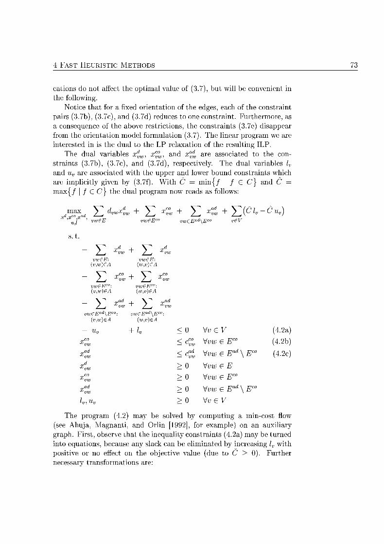
4 F T H E U C METHO

catons do no 3. t will b o n i e the followin

Notie that fo xed rientation of the edges, eac of the constra pairs (3. 3.7), a (3.7d) reduces to on cons t rn t Furthermore, a consequen of the above restritions the o n s t r a t s 3.e) disappa from the orienation model formuation 3.7). The linea progra we re

terested i is the dual t the L r e l t i o n of the resulting ILP. he du riables %w x° and 0^ are ssociated t the con

traints (3.7b 3.7c, and (3.7d, respectively The d u l riables l nd uv are assoc ted with the upper d lwer ound c o n t r n t s whic re impliitly given by 3 . ) . With C = min{/ | / ax{ / | / C the d l gr no r e d s follows:

^lf^ad J / / v) eE eEc° £Ead v£V

Vve (4.

Vvw e co 4.

yvw G ad \ Eco 4.

yvw €

yvw e CO

yvw e ad \ ECO

yv

og 4.2) m be lve y computing a st fow (see huja, Magnnti and Orlin [ 1 9 9 , for example) on an auxiliary g r h First observe t h t the inequlity con t r i n t s ( 4 . ) may be t r n e d into e q t i o n s becase ny slack ca be e l i t e d by ncresing l with positie or no e on the objeti e t F t h e r

essry t r f o t i o n re:

E vweE

(v,)eA

/ vwdE wdE

{v,)eA v)eA

2.^ l^ vw£Eco: eEc

{v,w)eA v)eA

E ad

eEad\E eEad\E

(v,w)eA v)eA

v co

< o < CC°

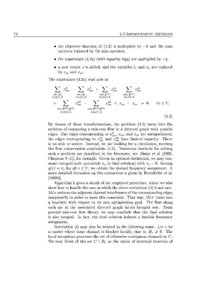
I M P O V E N T METHO

the ject ie function of 4.2) is multilied b th ax oper r e a c e d by the min operato

the o n s t r n t s 4 . ) with e q l i t y sign) re multilied by

a ew vertex is dded, d the ribles re r e a c e d by vs sv

he o n s t r t s 4. re no

E co co

vweE weE vweEco: eEco

{v,)eA v)eA (v,w)eA v)eA

eEad\Ec eEad\Ecc: (v,w)eA w,v)eA

4.3)

m n s f those t r f o a t i o n s th roblem (4. urns the poble of computing a m n - o s t direted g r a h with paallel edges. The edges corresponding t vs d xsv re uncapacitated, the edges rrespondin t xc°w d x^ h e l i i t e d capacity There is no si or source. Instead, we re lookin for ircuation eeti the onse r t ion constraints (43). Numerous e t h d s for olving

a proble are described the li teratre, see Ahuja et al [1992, Chpters 9-11, for example n o p t i a l cirulation we y con t r t integr node potentils n a dual solution) with is = 0. etti

y(v) = T for all G V, w o b t n the desired f r e e n y ssignm A more detiled d i s s s ion on this onnection is gi by Bodörfer et al [199b

lgorith gives a sket of the e m o y e d procedure, where we ls sho how to handle the case n whih the a o v e restrition (ii) is not met M C F reduces the adjacen channel interfere of the orrespondig edges temporarily in order o meet this cons t rn t . Th ay, M C F s in a heris t i with resect to its wn optimization goal. The flo alon each the s s i a t e d direted g r p h incurs integral st. From gee r m i n - s t f w theory, may c o n d e that the d u l s t i o n is also ntegr In fact the tion es asible fre

ssignmet. Restriction (i) lso be relaxed i the followig sese . Let v be

carrier where some hnne l is blocked locally, that is ^ 0. The cal exception puncture the set of otherwise ontiguou nnels in C

ay thi of the set the unon of axi n t e r l s of

4 F T H E U C METHO

oniguou channls call e inter ndow, and, ven indow sible ssignment the window I%° with yo(v) I%° is called the

active window fo v. If ocal blockigs re resent, the jet ive function ve window of 4 . ) ca be nged by replac C an by I%° min{/ / i^0}

a d 1%° max{ | / I%, respectively The effet of this ge is t h t eac node receives a channel from the active window.

he xil iry directed graph is easily o n t r u t e d in Od-E"! time The mincost flo problem is solved by mean of a e twrk implex Method implemeation, see Löbel [1997. The s a c e requirement of this lgorithm is in Od-El), but its wrst-case r u n n g t i e is exponnti n the input size lthough there re strongly polynomia m i n - c t fow lgrithms (see huj et al. [199 Capte r 10]), we hoose this imple

m e n t i o n of the etwork Simplex lgorithm for its typically ompetitiv unning time a c t i . Compuation res l ts fo the M C F herist i re repoted i tion 5.4.

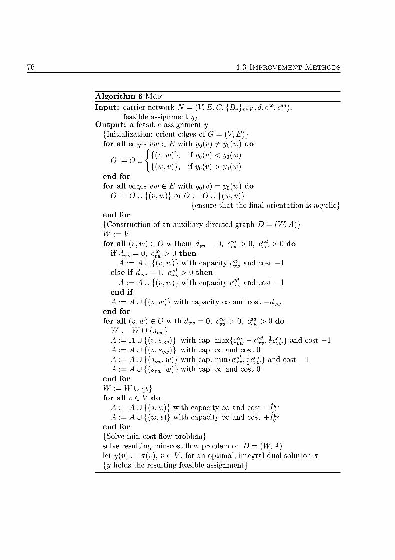
76 I M P O V E N T METHO

A l g r i h m 6 M C F Input: carrier etwork V, E, C, {Bv}veV d7 cco c

feasible assignmen tput: a feasible assignmet Initialization: orient edges of G V E

ll edges w G with y ^ w

O u ^ ^ ty < yw) {(w f y w)

for ll edges vw G with ) = (w

Ouv7 r O O U {( u)} re th the f r i e a t i o n is a c l i

nd or C o n t r t i o n of xil iry direted graph D (W

ll v, w) G withou = 0, c™ > 0, c > 0 w = 0, cc° > 0 then

J 4 u w , w ) with caacity cc° —1 i 1, c" > 0 t h n

J 4 u w , w ) with caacity c^ —1

A U with capacity o an t — d fo ll ) e with = 0, cc° > 0, c ^ > 0

{sv

AU , s with cap. ax{c™ - cad \cc° st - 1 A U s„ with cap. an A U ^ , with cap. in{c \ ^ st A U ^ , with cap.

W{s} ll v V d

AU {(sw with caacity st %° A U s with caacity st %°

n S o e mn- prblem}

so resulti m i s t flow proble on D = let v) = T(V) v for an optim i tegr tion

lds the res l t i sible ssignm

CHAPTER 5

omputational Studies

In this ter we report on computtional experimets erfomed with the frequen p l n n i g heuristics desribed in the p r e o u ter Re

lts are gi for eleven relistic b e h m a r k s r i o s We introdue these senarios i tion 5.1. The indiidu erfor

m a e of the herist i nd their parameter interdeendenc is nlyzed n S t i o n s 5. and 5.3. he conerted acting of the heristics is studied

Section 5.4, where we ls select our favorite o m b i t i o n of me thds together with the r e l e n t parameter sett igs. e f o s on three ou of the eleve s n a r i for these extensive studies In S t i o n 5.5 our vorite combintions of heuristics are pplied t ll benchmark scenrios

detiled lysis of the resulting frequncy s is given. Fially, Section 5 , ompre our swiftly geerated p l n s with t h s e om

puted by the e l a t e lannng heuristi rocedure of Hellebrandt an Heller 2000] exp l aed n Setion 5.12. We give r e o m m a t i o n fo the use of the riou heuristis in p a c t i e .

he followin t e n i c a l information on the omputer system environ ent should a l lw o estimate how the running times of the herist i

provided here t r s l a t e to other system environmnts. The computation are erfomed on BM h i a d 00X with a Intel Pentium II p o ­cessor operatin t 6 0 M z lock speed, and equpped with 576 MB of system memory The operatig syste is GNU/Lnu the uSE distribtion, kerel version 14.

The herist i are impleented the p g r m m n g langage C++, u s i g d t ruct res for g r h s and riority quues from the Library of Efcie Data structures lgrithms ( L A ) , version 3.6.1, see Mehl-ho and Näher [1999 DA 6.1 [1998]. The compilations are per formed by m n s of GN ++ version 295.2, with -mcpu=i686 -06 optimization ags The m c o s t fl problem arising withi the M C F heuristic is ved usi the etwrk Simplex Method i m p l e m e t i o n of Löbel [197], version 0 A B C U version 2.2, is used to implement the K-O herist i ll re ved s i g C E X version 5.

PHI, 650 MHz GNU/Linux

C++

LEDA 3.6.

ABACUS 2.2 CPLEX 6.5

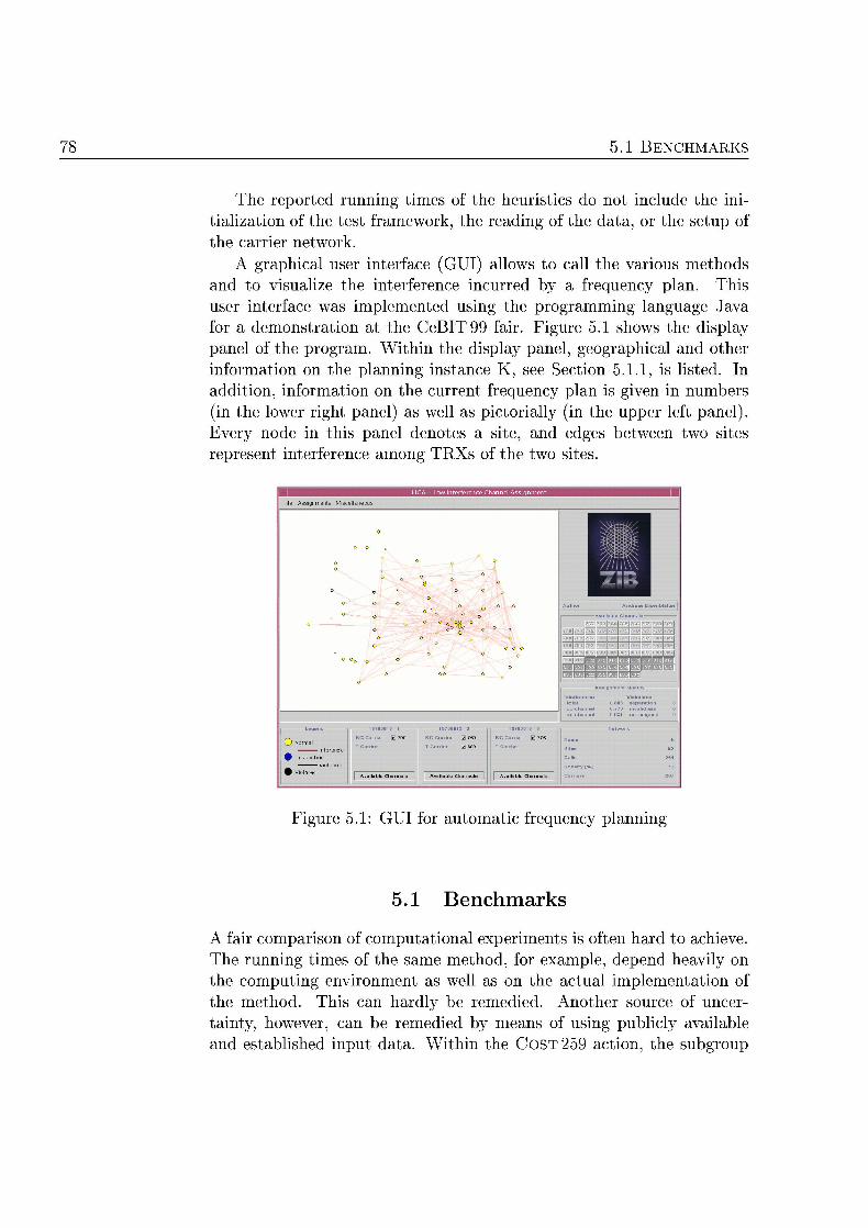
1 BENC

The reported runn t i e s of the e u t i s do no lude the ini­tialization of the test ewrk, the r e d i of the the setup of the carrier netwrk.

A graphical ser nterface GU llows t call the riou methods nd to visualize the interferene i n r r e d by a freq n. his

user interface was implemnted usi the p rg r ammn laguage fo a demonstration a the CeBIT 99 ir Figure 5.1 shows the display panel of the p o g r m . Within the display pae l , geogrhica l and ther nformation on the planning i s t a n e K, see ection 5.11, is listed. In

addition informtion on the curre f r e u n c y p n is given in numbers (in the lower right el) as well ictorilly (in the upper left pnel) Every node in this nel denotes a site a d edges betwee tw sites r e r e s e t interfere mon RXs of the tw sites

5.1: nn

.1 enchmarks

A f i r comprison of omput iona l experiments is often rd to achieve The running times of the s e methd , for example, deped hevily on the omput ig environmnt as well on the actual i m p l e n t a t i o n of the method This can hardly be r eed i ed Another soure of uncer

inty, however can be remedied by m of sing publicly available d estblished nput d ithi the action the bgroup

M P U T A T N A TU

on " t a n d r d nari fo Frequncy nnng establishd a cllection of relistic GSM f r e y p n n n g s e n a r i s in order to allow oun omparison of diferen anning e thds . Sveral of these tes s c a r i o s re used here, p l s one addition n r io . ll our nr ios re avail ble via the Internet rom the P web [2000] hey are i n t r e d i

Section 5.11, tgether with an analysis of their racteristis. In S t i o n 5 . 2 , we describe the f r e q e n y a n n g heuristic pro

posed by Hellebrandt and Heller [2000 This heuristic is presently the most competitive one fo ou a r i s and w se its res l t s s refere

the omprison of ou ter ethods

5.1.1 st Insta

Our b e n m a r k i n snces re i n t r o e d i the following noationa o n v i e e , we use other abels t h n the riginal ones but povide the rigina mes in the descrition The brief des r i t ions of the nnin

r i s are mostly taken from E i seb l t t e r ü r e r [2000 ac ri gives rise a carrier e twrk

for a GSM 1 0 0 network with 92 active sites 4 cells an verage of 1.01 TRXs per cell Fifty contiguous chnnels fo the trum (Povided by bilfun GmbH & o.

at fo GS 800 etwork with active sites and 88 cells B[d] The paameter t scales the traffic d e a d . The a v i l b l e trum consists of 75 contiguou chnnels. (Povided by P bil fun GmbH & Co. " b r f o r d _ i e

he basic trffic load is d r w n at random accordi a distri bution observed empirically by Gotzner, a m t nd Rathgeber [199 his t r a c is then scaled with the fact r d e q l to 0, 1, 2, 4 nd 10 rior to pplying the r lag-B formula n rder t btain the required number of TRXs per ell. he res l t i ver

age numbers of TRXs per cell re 00, 1 , 1.17, 1 nd 220, respectively The different t r c demands ay be seen a the evo lution of a etwork over time The interference preditions base on signal opaation predition accrding to the p lu" model, see

tion 3.2. The two alterative rediction models "free pace and race, also mentioned i ection 3.2, re no considered here, because in most of the cases frequency without any interfer

e is asily b t b l e , see iseblätter Küre r [2000

1 BENC

SIEI at fo a GS 900 ntwork with 1 active site 506 lls and an averge of 1.84 TRXs per cell The i lble pe t rum consists of two contiguou b l k s o n i n g 20 an 23 nnels r e s t i v e l y (Povided by iem s i e s l

SIE2 at for a GS 900 netwrk with 8 active sites 254 ells and an averge of 3.85 TRXs er ell he i lble pectrum consists of two ontiguous blcks o n i n 2 nnels, r e s t i v e l y (Povided by Siem sie

SIE3 for a GS 1800 network with 366 active sites, 89 cells and an average of 2 TRXs per cell. he vailble trum omprises 55 ontiguou hnnels (Povided by i e e n s "siemen3.

SIE4 at fo a GS 900 network with 276 active sites 760 ells and an verage of 3. TRXs er cell. The ailble trum consists of

ontiguou nnels (Povided by ieme as s i e 4 .

Sw ta fo GS 900 network n a ity with many locally blcked hnnels On averge, 09 TRXs are istalled per cell. here

are 148 ells with 1 to TRXs an 70 neighbor reltion In general, 52 nnels in tw ontiguous blocks of sizes 49 are v i l b l e , but 36 cells h v e l c a l restrictions. Only 15 nnels re available i the worst case the edian of vailable nnels

per ell is 29 (Other figres c o n e r n i g the availability of chnnels are provided with the scenario. We give the results of our computations.) Together with the senario, a rtia assignme is supplied which is supposed to be extended The restriction mposed by the uncangeable TRXs are l redy ken nto accoun n the abov figres (Povided by wissom td "Swissom.

Fr the r details c o n e r g the underlying GSM etwork are listed i ble 5.1; amely: the number of site in the p l n n rea; the numbe

of cell no site hosts more t h n three cells); the spectrum size or, in the rese of gloally blcked nnels, the sizes of the ontiguou portion

the trum; the average number of TRX per cell; an the maximum nmber of TRXs per cell. Notie that i ach of the s n r i o s with glbally bloked channels, the reslting g p n the s t r u m exceeds the maximal required sepration. Thus there is no dire ouplig betwee distinct contiguous portions of the spectrum

Three further figures are given for each s n a r i o in Table 5 . hese re esies e x n e d i term of the carrier e twrk which is b t e d

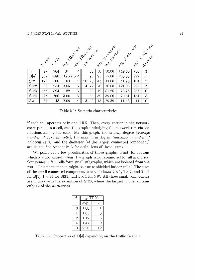
M P U T A T N A TU

& ^ J 4 %

$ j $

ft

01 50 50 5000

d] ble 00 25 77 50 84 20, 3.00 76 10 25 3. 76 7600 21

51 76 67 10 76 3. 00 84

09 29 11 10

ble 1: is

each cell operates only one TRX Then, every carrier n the etwork corresponds to a cell and the graph underlyin this network r e t s the relation mong the ells For this g r h , the verge degree (averag number of adjcent cells) the ximum degree (maximu number of adjacent cells) an the meter of the largest c o n n t e d o m p o n t ) re listed. See ppndix fo definitions of these terms

W poin out a few peculiarities of those g rahs . First for reson which re no entirely c le r the g r p h is not c o n n t e d fo all s e n r i o s Sometimes a few ells form small s b g r p h s , whi are isolated rom the rest. (This henomenon might be due shielded doo cells he sizes of the s a l l c o n n t e d components are follows: x 1 1 x 2 , and x 3 for B[l 1 x 34 for SI and 1 x 1 for Sw. All t h s e sml l omponents are l iues with the excetion of S I E , where the lrgest l i e con only of the 34 verties

RX

00 05

10 20

ble 2: operties of d] d e d i on the tr fac

1 BENC

cond, ookng the olumn s w i n aveag n u m r of dja ce cells, we see that cells are djacent to urprisigly man other cells on average. In enr io K, for examle, eac ell is adjacent to more than

f of ll ells. (We belie t h t the comparatively high numbers for the cenari provided by E s Mobilfunk GmbH & Co. KG are e t the se of 20 dB threshold distiguishing between interferen ted

d unaffected pixels see Sction 2.3. for further e x l a t i o n . ) Finlly, the l s t umn shows that the cells re all r t h e r " n r b y

in most all sceari Recall tha the dimeter in a connected graph is the maximum length mong ll shortest paths between pairs of verties

hus, diameter of , fo example, mplies th for every nonadjacen p i r of ells, there is on cell bein adjacet to both of them If the graph ha more t h n on conneted componnt, we give the diameter of the lrges o m p o n . The d i a e t e r of the mall connected compon of S E 3 is The diameter of ll ther small omponents is either 0 r 1

After ha ing looked the c e r i o s , we turn to the carrier networks derived fom the s r i o s he f o s is on the undirected graphs under lying the s a r i s a d on a few aracteristi of the edge lbelings d cco nd cad he results of our a l y s i s are gi in Table 5 , whih is r g i z e d i ve blocks of c u m n s . In the first umn, the label of the

assciated scenario is given. The next block contans information on the graph, namely, its number of verties, its edge density tha is, number of edges relative o the maximum possible number of '), the aver­

ge degree of its vertices as well the maximum degree, and the size of a aximum li The third block addresses the imum separation requirements a ecified by the lbeling d. he tota number of edges with nonzer separation requirements as well the breakdown of the to ta accrding the required s e p a t i o n is displayed he forth and fth block provide formation on the c and adjacent channel interference labelings cco and cad, respectively. In each b l k , we list the to umber of interference reltions, their verge and mximal iterfere v e s

s well a the um over ll interferen vales. There are again some noteworthy facts First, the average degree of

a carrier is sigificantly higher th the number of available chnnels in all the carrier networks excep fo Sw. This dicates that the nnel ssignme for difere ells h s t be carefully uned n order t ood frequency p l a s .

Second, the size of the aximum liques in most carrier networks is rger than the number of avilable channels. Fo those carrier networks

every sible assignm mu i n r interfere We investigte this futher C h t e r 6

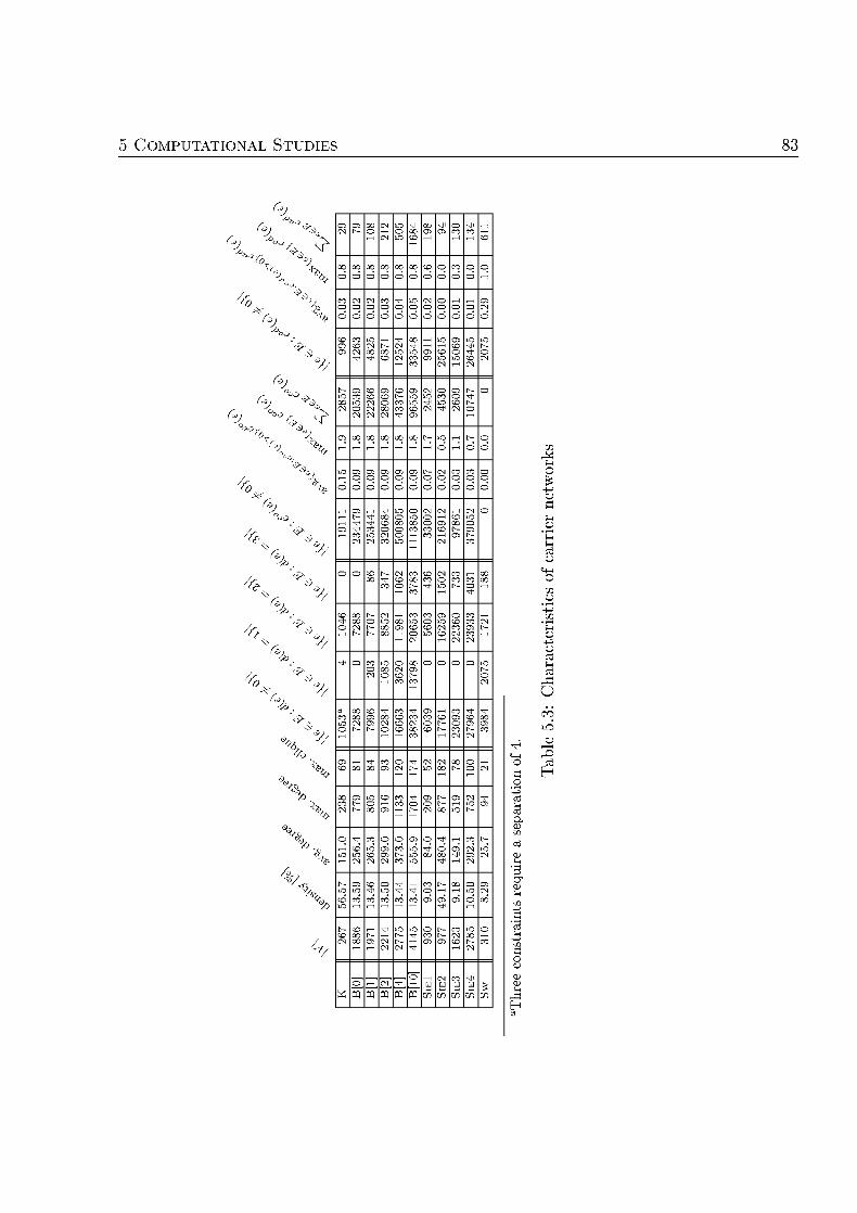
M P U T A T N A TU 83

56.4

373.

0

56.5

13

.5

13.4

13

.5

13.4

13

.4

S

CO

L6

^

84 1 BENC

Third, reca om Section 3.1 ha he n t e c e labelings are ob ed by summing up the two direted nterference tings between pairs

of TRXs Those directed ra t igs are normalized a d take vaues be twee nd 1 The sum is thus bounded by 2 In several cases the maxim co- or adjacnt channel i te r ferece is, i fact, close to 2. he

c c r r e e of ch hevy interference is cnsidered cmpletely unaccep able in ractie. In Setion , we see t h t such heavy interfere can typically be avoided by good frequency assignments. his happens ei ther by coi idence, indirectly due to the optimization g o , or is imposed by "tighten the s e t i o n " s explained in S t i o n 4 . 2 .

Fourth, we see th o co-channel interferene is reported for Sw hen generati the s c e r i o , the radio laner apprently decided to rule t this t y e o n te r fe ree etirely by d d i g the essry s e a t i o straints Fifth, o e might hav guessed t h t the g rphs underlyig carrier net

anar gra works re ot mu deser t h n r g r h s . A lanar graph ca be drawn the Euclidean p l n e in ch a manner t h t edges are rep resented by iece-wise str ight lines d o edges cross P l n a r g r h s are of interest becase m n y generally A/'Phard roblems on graphs are solvable in p o l y o m l time if restricted to anar graphs he following relation betwee the number o vertices a edges i gr is wel lkow follows fro ler formu

P r o o s i t i o 5.1. A anar graph G = {V,E) satisfs \E\ < 3 \V\ — 6.

For the carrier network K, for example, the expression yields 3 267 — 6 = 795 as opposed to 27388 edges. Even the number of edges with separation costraints is roughly 1.3 times this valu. Consequently, the graph underlyig the carrier network cannot be planar. The large max imum cliques in the carrier networks as well as the small diameters of the connected components also idicate substantially tighter c o p l i g s among large sets of carriers than one might have suspected.

The degree of interdepedencies clearly affects the possibilities for de composing the optimization problem. Ideally, we wold like to be able to independentl solve small subproblems to optimality a d assemble an optimal solution for the whole problem from the solutions to the sub-problems. The stronger the depedencies between the subproblems we choose, the harder is the assemblig. In the thesis of Koster [1999],

tree such an approach is described using a ree decomposition of a graph, see, dempo for example, Bodlaender [1993] for an introduction to tree decomposi

tion. We do not give details here, but merely state that this approach is ccessfll applied to graphs with a treewidth of p to 11, say, a d that

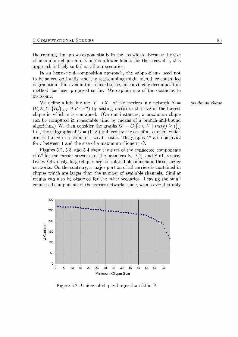
M P U T A T A L TUD

the r u n n g time grows exponentially in the treewidth. Because the size of maximum cl iue minus one is a lower boun for the treewidth, this approach is likely to fail o all o r scenarios

In an heuristic decomposition approach, the subproblems need not to be solved optimally, and the reassembling might introduce controlled degradation. But even in this relaxed sense, no convincing decomposition method has bee proposed so far We explai e of the obstacles to overcome

We define a labeling mc: V —>• Z + of the carriers in a network N = (V, E, C, {Bv}vV, d, cco cad) by se t t ig mc{v) to the size of the largest clique in which v is contained. (On o r instances, a maximm cliq can be compted i reasonable time by m e a s of a brach-and-bound algorithm.) We then consider the graphs Gl = G[{v G V \ mc(v) > z}] i. e., the sbgraphs of G = (V, E) induced by the set of all carriers which are contained a clique of size at least i. The graphs Gl are ntrivial for between 1 d the size of a maximm cl iqe i

Figures 5.2, 5.3, and 5.4 show the sizes of the connected components of G for the carrier networks of the instances K, B[l], and SlEl, respec tively. Obviosly, large cliques are no isolated phenomena in these carrier networks. O the contrary, a major portion of all carriers is contained in cliques which are larger than the number of available channels. Similar results can also be observed for the other scenarios. Leaving the small connected c o m p o n t s of the carrier etworks aside, we also see that o

xim lique

300

• • • • . ' ' • • • ,

•

•

100

50

0

5 10 15 20 25 30 35 40 45 50 55 60 65

Minimum Clique Size

Fig 5.2: U i o s of cliqes larger tha 50 i

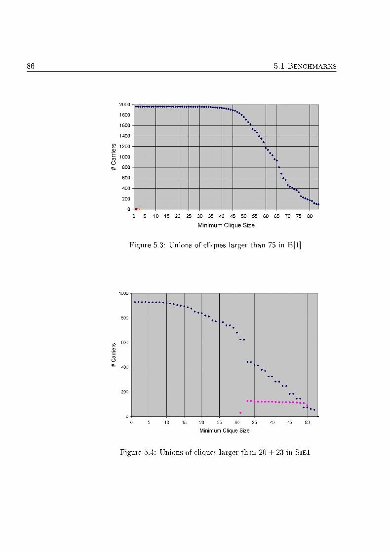
5. BENCHMARKS

2000

1800

1600

1400

1200

1000

800

600

400

200

0

* * * * < * • • • < ' • • • • 4 <XX*H

'S ,

\ • " •

•

• •

• . .

•

• • < .

• • • .

- « V —

0 5 10 15 20 25 30 35 40 45 50 55 60 65 70 75 80

Minimum Clique Size

Figre 5.3: U i o s of cliqes larger than 75 i l]

000 • • • • • • • • •

' • • • . .

•

• •

• • < 1 • • •

•

•

• •

600

• • 4 > •

•

• •

4 ' •

• •

0

•

0 5 10 15 20 25 30 35 40 45 50

Minimum Clique Size

Fig re 5.4: U i o s of cliqes larger than 20 + 23 Sl

M P U T A T A L TUD

in case of SlEl the subgraphs G decompose. (For i = 32, the cliqes observed for 31 disappear, and from i = 33 up to 50 a new componen splits off from the major chunk.) Good frequncy plans thus have to resolve separation conflicts a d interferece a m o g large sets of s t rogl

terdependent carriers n this context, we also report on the effects of the preprocessing preprocessi

techniques proposed in Section 4.1. Table 5.4 docments that these tech­niques have only a rather limited impact. A few carriers can often be safel excluded from frequency planning due to a small generalized de gree. Most dominated carriers, however, are in fact isolated nd th trivially dominated by ever other carrier. The sceario Sw may be con sidered as a minor exception, because the reduced 85 carriers constitute a significant portion of all carriers. Nonetheless Sw is the scenario for which almost no feasible assigment can be prodced s i g o r heristics from Chapter 4, compare with Sectio 5.5.

B[0] B[l B[ B[4] B[10] SlEl SIE2 S I E 3 S I E 4 Sw

reductio 15 27 26 22 19 21 60 96 10 83 domination

Table 5.4: Effects of preproces

With a number of benchmark cenarios i stock, we n o a "bechmark" heristic to compare o r o heristics with.

5.1.2 T h r e s o l d Accepting

We use the heristic proposed by Hellebrandt an Heller [2000 to com­pare o r computational results with. The implementation of H n s Heller Siemens AG, Germany, shows presently the best performance in compar ison with several methods o the COST 259 scenarios, see the study of Eisenblätter and Küre r [2000. The refereced frequenc plans are also available via the Internet from the FAP web [2000. Because the method is not yet published in open li teratre, we give a tline of this method, drawing freely on ur presentatio n Correia 2001, Section 4.2.5].

The method of Hellebrandt and Heller [2000] makes use of the Thresh­old Acceptig paradigm. Threshold Accepting is proposed by Dueck and Scheuer [1990] as a variant of Simulated Annealing with a deterministic acceptance criterion: a proposed change of the solution, also called a move, is accepted if an improvement is achieved or the deterioration is move below a threshold. The value of this threshold declines with the progress of the algorithm. The basic scheme is agmented here b a l t e r a t i g be

5.1 BENCHMARKS

tween andom changes a d local optimizatio ke th of the algorithm is give as Algorithm

lgorithm 7 T H R S H L D A C C P T I N G

nput: carrier network N = (V, E, C {Bv}V, d co cad

assignmet yo, time bound Ttt Output: an assigment y, possibl ifeasible

nitialization} itialize threshold hile stopping criterion not met do for time T do

select random move M cost of M threshold en xec te M

end if select r a d o m cell a d optimize it

end for decrease threshold

ile

The cost of a move is the difference between the cost of the assig ments after a d before the move. For the most part, Threshold Accepting inherits from Simulated Annealing the variety of popular implementa­t i o s for each geeral step. The followig choices are made b elle b r a d t a eller 2000

Start Solution: The random moves described below are not specially suited for findig a feasible assigment if many hard constraints have to be taken into account. I uch feasible assignment shold be provided at the start therwise, any assigment is f e

nitial Threshold: The threshold value controls how much deviatio is allowed from the cost of the current s o l t i o . A binary search is performed to identify a threshold, where 0-90% of the proposed r a d o m moves are accepted.

S t p i n g Criterion: The terminatio is triggered whe the acceptace rate for r a d o m moves s i k s belo 5%

er Loop/Threso ld Reduction: The r u n n g time of the proce dure depends on the initial threshold, the factor b which the threshold is reduced, the length of the inner loop, and the stop­pi criterio The l eg th of the inner loop is limited b a time

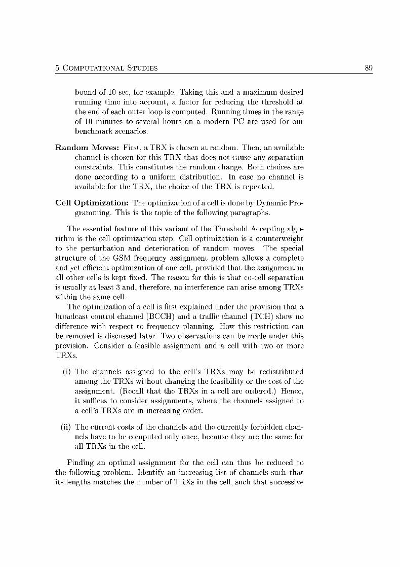
M P U T A T A L TUD

bound of 10 sec, for example. Taking this a d a maximum desired r u n n g time into account, a factor for redcing the threshold at the e d of each outer loop is compted. R u n n g times in the r a g e of 10 minutes to several h o r s moder PC are sed for bechmark scearios

dom Moves: First, a TRX is chosen at r adom. Then, an available channel is chosen for this TRX that does not cause any separation

straints. This c s t i t u t e s the random chage. Both choices are done according to a uniform distributio. In case no channel is available for the TRX, the choice of the TRX is repeated.

ll Optimization: The optimization of a cell is done by Dynamic Pro­grammig. This is the topic of the followig paragraphs

The essential feature of this variant of the Threshold Accepting algo­rithm is the cell optimization step. Cell optimizatio is a counterweight to the perturbatio nd deterioratio of random moves. The special s t rc ture of the GSM frequncy assignment problem allows a complete and yet efficient optimization of one cell, provided that the assignment i all other cells is kept fixed. The reaso for this is that co-cell separation is usually at least 3 a d , therefore o i ter ferece ca arise am TRXs within the same cell

The optimization of a cell is first explained under the provision that a broadcast control channel ( B C H ) nd a traffic channel (TCH) show n differece with respect to f r e q u e y planning. How this restriction can be removed is discussed later. Two observatios can be made under this provisio sider a feasible a s s i g m e t a a cell with tw or more TRXs

The channels assigned to the cell's TRXs ma be redistributed a m o g the TRXs without chaging the feasibilit or the cost of the assignment. (Recall that the TRXs in a cell are ordered.) Hence it suffices to consider assignments, where the channels assiged to a cell's TRXs are i creasi order

(ii The current costs of the channels and the currentl forbidden chan nels have to be compted o ce, becase the are the same for all TRXs i the cell

Finding an optimal assignment for the cell can thus be reduced to the following problem. Identif an creasing list of channels such that its legths matches the number of TRXs i the cell, s c h that sccessive

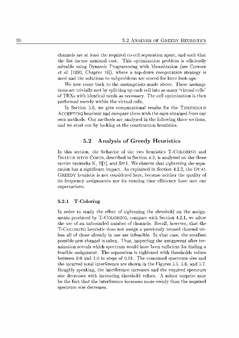
90 5.2 LYS OF G D Y H U R S T

channels are at least the r equed cocell s e p a r a t n apart, and such that the list i nc r s mi imal cost. This optimization problem is efficientl olvable sing Dynamic Programmig with Memoization see Cormen

et al. 1990, Chapter 16]), where a top-down computation strateg is sed a d the solutions to subproblems are stored for later lookups

We now come back to the assmptions made above. These assump­t i o s are trivially met b splittin up each cell into as many v i r t a l cells" of TRXs with identical eeds as ecessary The cell optimizatio is the performed merel within the v i r t a l cells

Section 5.6, we give computational results for the THRESLD E P T N G heristic and compare them with the ones obtained from our

wn methods Our methods are analzed in the following three sectios d we start o t b lookig at the c s t r c t i o heristics

5.2 Analysis of Greedy Heuristics

n this sectio, the behavior of the two heuristics T - C O R I N G and DSATUR WITH COSTS, described i Section 4.2, is analyzed n the three carrier networks K, [l], and SlEl. We observe that tightening the sepa­ration has a significant impact. As explained i Section 4.2.3, the DUAL

GREEDY heristic is not cnsidered here, because neither the quality of its frequecy assigments or its runn time efficie have met xpectatios

5.2.1 T-Colorin

In order to study the effect of tightening the threshold on the assig ments prodced by T-COLORING, compare with Section 4.2.1, we allow the se of a unounded number of channels. Recall, however, that the T-COLORING heuristic does not assign a previosly unused channel un­less all of those already in use are infeasible In that case, the smallest possible new channel is taken T h s , inspecting the assigment after ter mination reveals which spectrum wuld have been sufficient for finding a feasible assigment. The separation is t ighteed with thresholds vales betwee 0.0 and 1.0 in steps of 0.01 The conumed spectrum size an the incrred total interference are shown in the Figures 5.5, 5.6, and 5. Roughly speaking, the interference increases an the required spectru size decreases with i c r e a s i g threshold values. A minor surprise may be the fact that the interferece icreases more eve tha the reqired spectr size decreases

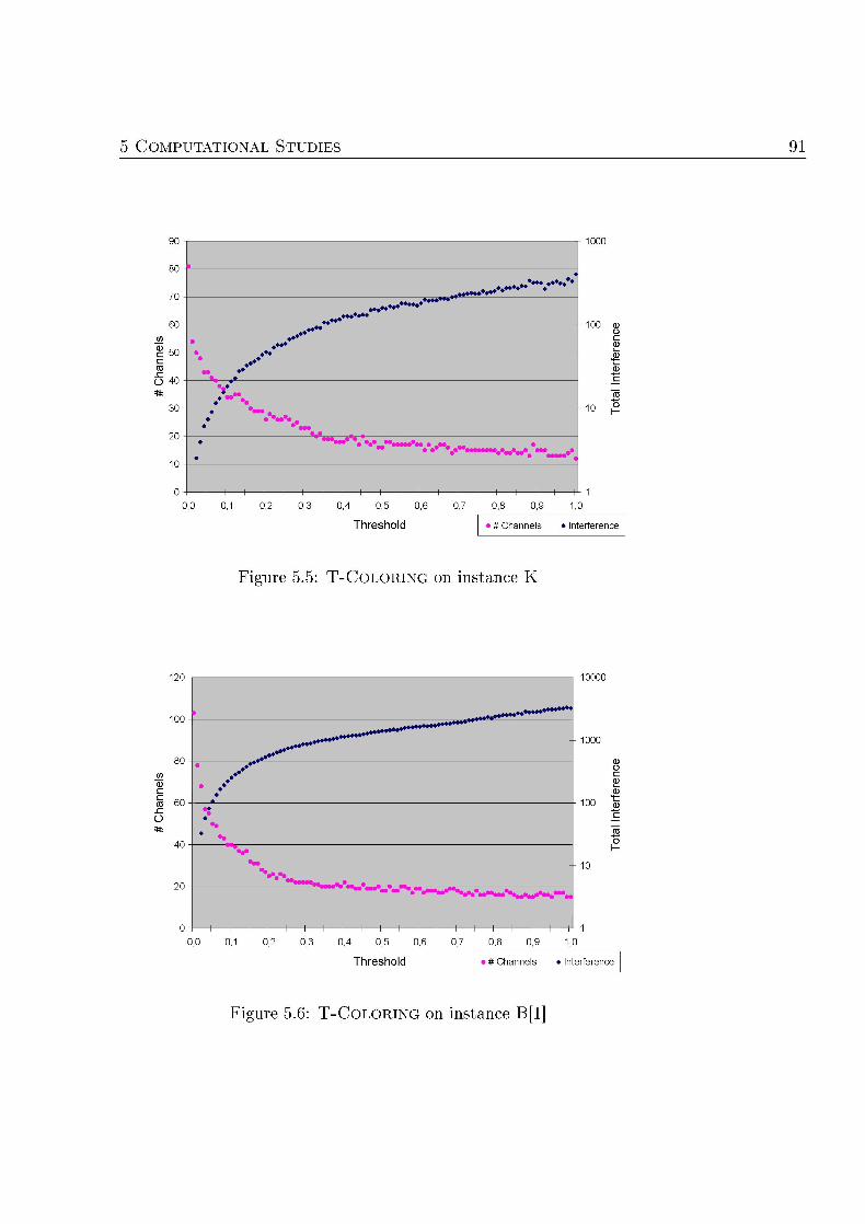
M P U T A T A L TUD

90

80

70

60

50

40

30

20

10

I

•

• • - • . • • • • • m

• • • • • • • . • • • • •

• • • " • • • # ' « '^II I I I 'M • #«»# , , •

1000

100

10

0 1 0,0 0,1 0,2 0,3 0,4 0,5 0,6 0,7 0,8 0,9 1,0

Threshold > # Channels • Interference

Fig re 5.5: T - N G s t ace

120 10000

1000

100

0,0 0,1 0,2 0,3 0,4 0,5 0,6 0,7 0,8 0,9 1,0

Threshold • # Channels »Interference

F i g e 5. NG ce

92 5.2 LYS OF G D Y H U R S T

90

80

70

60

40

30

20

10

0

, — • — • • '

. • * , • « « • • • • • . « « * • * • • • •

. l l > i M i t i

1000

100

10

0,0 0,1 0,2 0,3 0,4 0,5 0,6

Threshold

1 0,7 0,8 0,9 1,0

> # Channels • Interference

Fig re 5. T - N G s t a c e Si

5.2.2 SATU Co

For the DSATUR WTH COSTS heuristic two parameters are relevant compare with Section 4.2.2. These parameters are the threshold value for tightenig the separatio and the amount of carriers selected randomly as starting points We consider the threshold values t = 0.01, 0.025, 0 .5 , 0.075, 0.10, 0.15, 0.20, 0.25, 0.50, 0.75, and 1.00. Moreover 1, 2, 3, 5,

0, 25, 50, and 100% of the carriers are sed as starting points i tu For all possible combinatios of these two parameters freq pla are compted for the carrier networks K, B[l], an SiE

The runnng times of this algorithm do not depend significantly on the threshold v a l e and scale linearly with the percetage value Table 5.5 shows the running times i s e c d s of DSATUR WITH STS for 1% of the carriers as s t a r t ig points a s i g a threshold v a l e t = 0 . 5 .

Si

time 0. 04

Table 5.5: u n n g times i s e c d s of DSATUR STS

The total inerference i u r e d y the resulting frequenc p l s ar give Figres 5. 5.9, a d 5 .0 . We make three observatios:

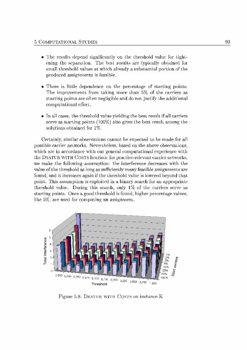
M P U T A T A L TUD

The results depend ignificantly on the threshold value for tight ening the separation. The best results are typically obtaied for small threshold vales at which alread a sbstantial portio of the prodced assigments is feasible

There is little dependece o the percentage of starting points The improvements from taking more than 5% of the carriers as s t a r t ig points are often negligible a d do ot j s t i f the additioal o m p t a t i o a l effort

In all cases, the threshold val yielding the best result if all carriers serve as starting points 00% also gives the best r e s l t a m o g the sol t io obtaied for

Certainly, similar observations cannot be expected to be made for all possible carrier networks. Nevertheless, based n the above observations which are i accordace with our general computatioal experience with the DSATUR WITH COSTS heuristic for practicerelevant carrier networks we make the following assumption: the interference decreases with the v a l e of the threshold as long as sufficiently many feasible assignments are found, and it increases again if the threshold value is lowered beyond that point. This assumption is exploited in a b i a r search for an appropriate threshold value During this search, only 1% of the carriers serve as s t a r t ig po i t s . Once a good threshold is found, higher percentage vales like 5%, are sed for c o m p t i g a assigment

F i g e 5. SATUR W STS ce

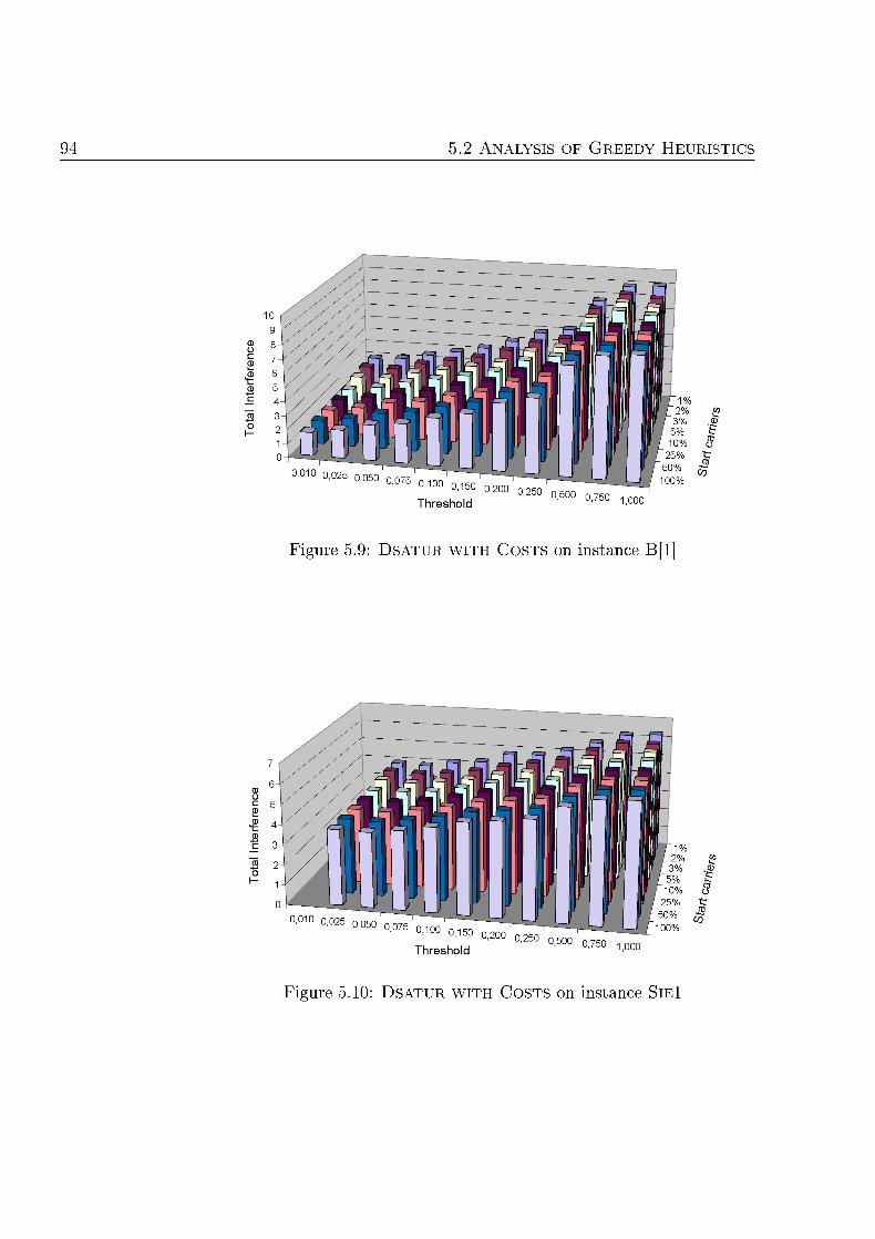
94 5.2 LYS OF G D Y H U R S T

Threshold 0,250

0,500 0,750 1,000

Fig re 5.9: SATUR STS s t ace l]

0,010 0,025 n ncn ' ~ U ' U ^ D 0,050 0075 0 1 0,150

Threshold 0,200

t r 1 % 1 f 2% f 3%

£ 5 % r10% ' 25% 50%

100% 0,250

0,500 0,750 1,000

F i g e 5 .0: SATU STS ce Si

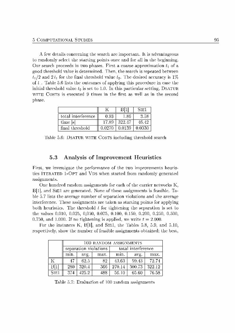
M P U T A T A L TUD 95

A few details concerning the search are important. It is advantageus to randomly select the starting points once and for all in the beginning.

ur search proceeds in two phases. First a coarse approximation t\ of a good threshold value is determined. T h e , the search is repeated betwee t\/ nd 2 for the final threshold value t2 The desired accuracy is 1% of ti. Table 5.6 lists the outcomes of applying this procedure in case the

itial threshold valu t0 is set to 1.0. In this particular se t t ig , DSATUR

WITH STS is exected 9 times i the first as well as i the seco phase

Sl

total interferece 0.93 3. ime 322. 4

al threshold 0.02 0 . 3 9 0 . 3 0

Table 5. SATUR STS c l d i g threshold sear

5.3 Analysis of Improvemen euristics

First, we investigate the performance of the two improvements heuris tics ITERATE O P T and VDS whe started from randomly generate assigments

One hundred random a s s i g m e t s for each of the arrier networks K, B[l], and SlEl are generated. None of these assignments is feasible. Ta­ble 5.7 lists the average umber of separation violations and the average interference. These assignments are taken as starting points for applying both heuristics. The threshold t for tightening the separation is set to the values 0 . 0 , 0.025, 0,050, 0.075, 0.100, 0.150, 0.200, 0.250, 0.500, 0.750, and 1000. If o tightening is applied, we write t = 2.000.

For the instances K, B[l], and SlEl, the Tables 5.8, 5.9, and 5.10, respectively, show the number of feasible assignments obtained; the best

0 0 R A M A S E N

p a i o n violaio t o l i f e n c mi g. max. mi g. max.

2. 82 43. 59.43 2. 80 320. 0. 300. 322.

Sl 25. 5. 5

Table 5 . : E l u a i o 00 r n d m a i g m e

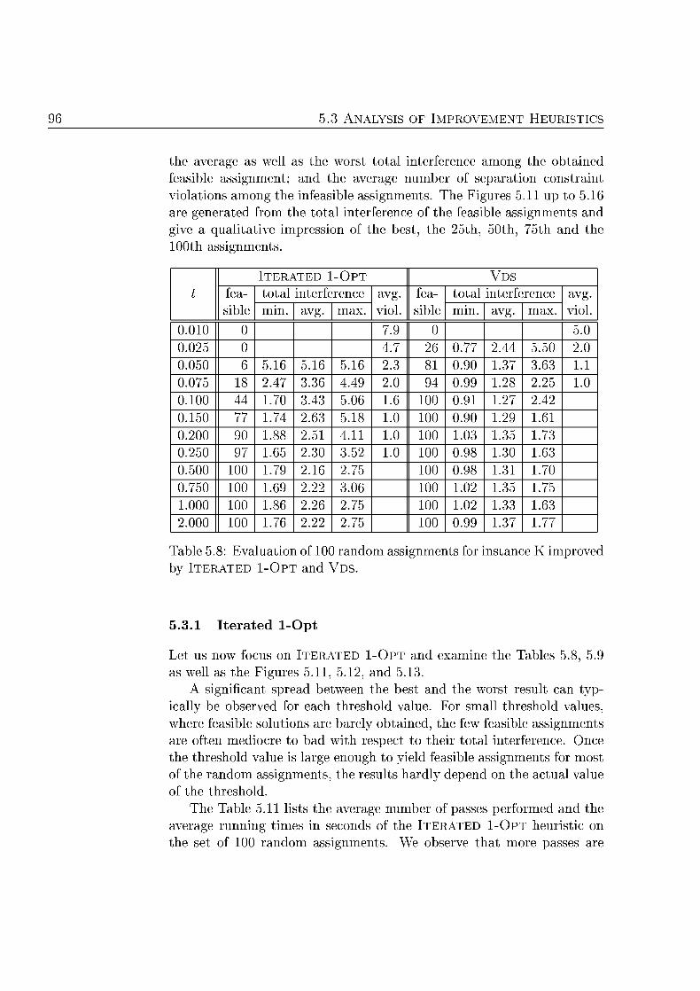
5.3 ALY M P R O V E N EU

the average as well as the w t total interfernce among he btain feasible assignment; and the average number of separation constrai violations among the infeasible assignments. The Figures 5.1 up to 5.1 are generated from the total interference of the feasible assignments and give a qualitative impression of the best, the 25th, 50th, 5th nd the

00th assigments

I T - O V D

fea sible

t o l i f e n c avg. iol

fea sible

t o l i f e n c avg. iol

fea sible mi g. max.

avg. iol

fea sible mi g. max.

avg. iol

0. 9 5. 0.025 4. 0. 2. 5.50 2. 0.050 5. 5. 5. 2.3 0.90 3 3. 0. 2. 3.3 4.49 2.0 94 0.99 2.25 0.00 3.43 5. 00 0. 2. 0.50 2. 5. 0 00 0.90 29 0.200 90 2.5 4. 0 00 35 0.250 2.30 3.5 0 00 0. 30 0.500 00 2. 2. 00 0. 3 0.50 00 2.2 3. 00 02 35

000 00 2.2 2. 00 02 3 2.000 00 2.2 2. 00 0.99 3

Tb le 5.8: E l u a i o n of 100 r n d i g m e s f r i n c impro by ITERAT 1 - O T and VDS

5.3.1 rated 1-

Let us now fous on ITERATED 1-OPT and examie the Tables 5.8, 5. as well as the Figures 5.11, 5.12, and 5.13.

A significant spread between the best and the worst result n typ­ically be observed for each threshold value. For small threshold values where feasible solutions are barely obtained, the few feasible assignments are often mediocre to bad with respect to their total interference. Once the threshold value is large enough to yield feasible assignments for most of the random assignments the results h a r l y epend the actual value of the threshold

The Table 5.11 lists the average number of passes performed and the average runnng times in seond of the I T E R A T D 1 - O T heuristic on the set of 00 random assigments. We obser that more passes are

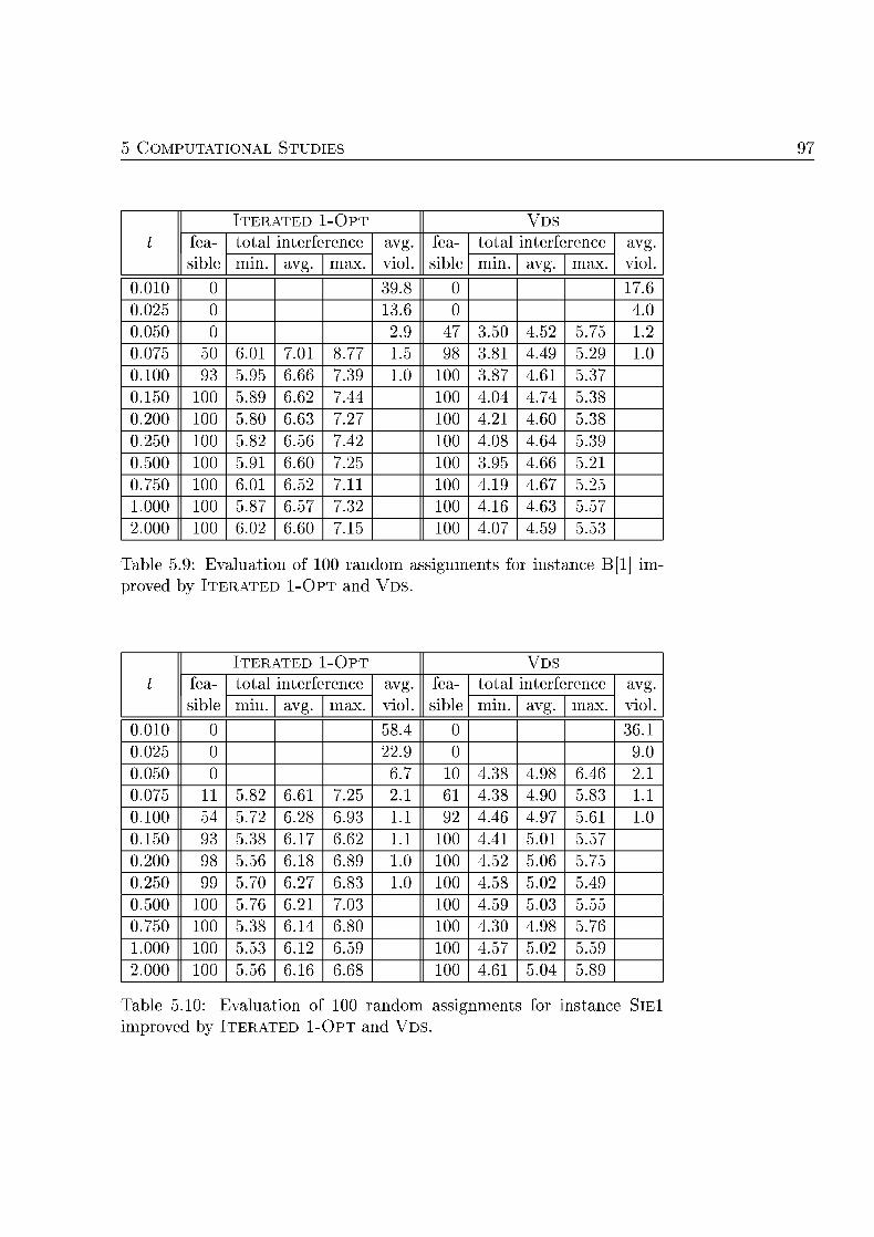
MP

I T R A - O VD fea sible

t o l i f e n c avg. iol

fea sible

t o l i f e n c avg. iol

fea sible mi g. max.

avg. iol

fea sible mi g. max.

avg. iol

0.0 39. 0.025 3. 4. 0.050 2.9 3.50 4.5 5. 2 0.0 50 0 8. 3.8 4.49 5.29 0.00 5.95 39 0 00 3.8 4. 5.3 0.50 00 5.89 4 00 4.04 4. 5.3 0.200 00 5.80 2 00 4.2 4. 5.3 0.250 00 5.82 5 4 00 4. 4. 5.39 0.500 00 5.9 25 00 3.95 4. 5. 0 .50 00 0 5 00 4. 4. 5.25

000 00 5. 5 32 00 4. 4. 5. 2.000 00 02 00 4. 4.59 5.

Table 5.9: E l u a t i o of 00 random ssigments for i s t anc im p r o d by I T R A T O T and V D

I T R A - O V D

fea sible

t o l i f e n c avg. iol

fea sible

t o l i f e n c avg. iol

fea sible mi g. max.

avg. iol

fea sible mi g. max.

avg. iol

0.0 58. 0.025 2.9 9. 0.050 4.3 4. 2. 0.0 5.82 25 2. 4.3 4.90 5. 0 .00 54 5. 2 4.4 4. 5. 0 .50 5.3 00 4.4 5. 5. 0.200 5. 89 0 00 4.5 5. 5. 0.250 99 5. 2 8 0 00 4.5 5.02 5.49 0.500 00 5. 2 00 4.59 5. 5.55 0.50 00 5.3 80 00 4.30 4. 5.

000 00 5. 59 00 4.5 5.02 5.59 2.000 00 5. 00 4. 5.04 5.89

Table 5 .0: E l u a i o of 00 random i g m e r i n c Sl improed by I T R A - O nd V D

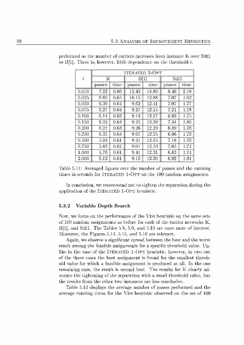
5.3 ALY M P R O V E N EU

p e r m e d as the number of cariers inceass from instance K o Sl to l] There is, however, little ependnce o the threshol t

I T R A - O

Sl pa ime pa ime pa ime

0. 2 0. 2.43 4. 8.4 2. 0.025 0. 0. 2. 92 0.050 39 0. 9. 2. 0. 2 0. 9. 2. 2 0.00 0. 9. 2. 0.50 32 0. 9.25 2.39 34 80 0.200 24 0. 9. 2.29 89 0.250 35 0. 9.0 2.25 0.500 5.92 0. 9. 2.35 0.50 5.8 0. 9.0 2. 05

000 5. 0. 9. 2.3 8 2.000 0. 9. 2.30 92 8

Table 5.11: Averaged figur r the umber f passes and the running times in s e n d s for ITERA 1-OP on the 00 random assignments

In conclusion, we reommend not to tighte the separation duri the applicatio of the ITERATED 1 - O T heuristi

5.3.2 Variable ept arc

Now, we focus on the performance of the V D heuristic on the same sets of 100 random assignments as before for each of the carrier networks K,

[l], and SlE The Tables 5.8, 5.9, and 5.10 are once more of nterest oreover, the Figures 5.14, 5.15, and 5 .6 are relevant.

Aga i , we observe a significant spread between the best and the worst result among the feasible assigments for a specifc threshold value. Un like in the case of the ITERATED 1-OPT heuristic, however, in two out of the three cases the best assignment is found for the smallest thresh­old value for which a feasible assignment is produced at all n the o remaining case, the result is second best The results for K clearly ad vocate the tightening of the separation with a small threshold value, but the results from the other two instances are less conclusive.

Table 5. displays the average number of passes performed nd the verage r u n n g times for the V D heuristi observed the set of 00

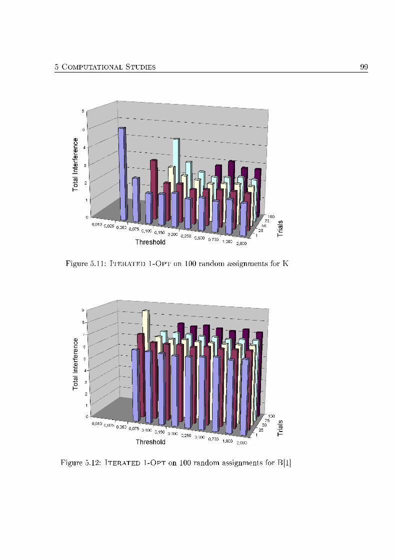
MP 99

0,010 0025 0,050 0075

0,100 0,150 0,200 0250

Threshold 0,500 0750

Figure 5 . : I T R A O 00 r a n d m assigments for K

0,010 0025 0,050 0075

Threshold 2,000

igur 5 .2 : I R A O 00 r n d i g m e s fo

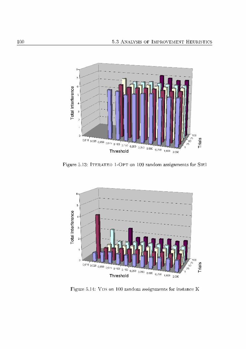
00 5.3 ALY M P R O V E N EU

0,010 0,025 U ' U 2 b 0,050 0,075 0100

0,150 0,200

Threshold 0,250 0,500

2,000

igure 5 .3 : I T R A O 00 rand s s i g m e t s fo Si

Threshold 1,000 2,000

Figur 5 .4: V D 00 r n d i g m e s f r i n c

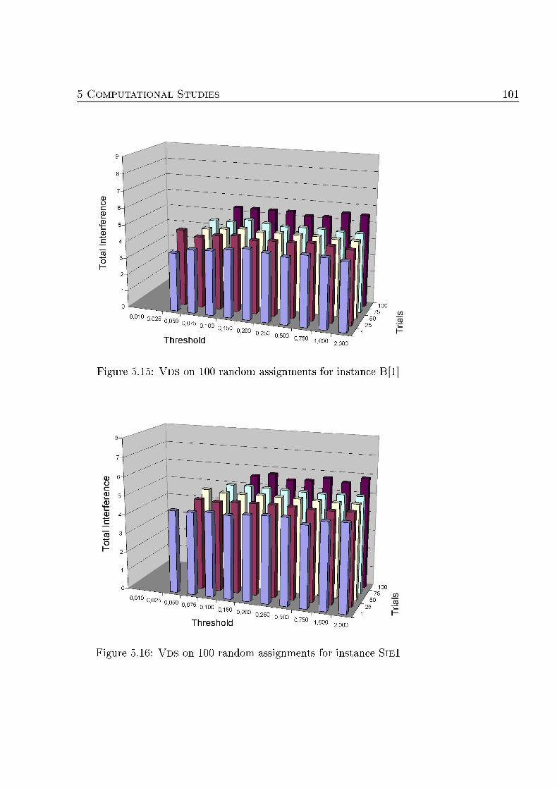
MP

0,025 0,050 0,075 0100 0,150 0,200

Threshold 0,250 0,500

1,000 2,0

igure 5 .5 : V D 00 random assigments for i s t anc l]

0,010 0025 0,050 0075

Threshold 0,750 1,000

igur 5. V D 00 r n d m a i g m e s f r i n c Sl

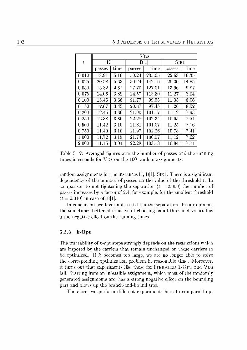
02 5.3 ALY M P R O V E N EU

V D

Sl pa ime pa ime pa ime

0.0 8. 5. 50. 235.05 2. 35 0.025 20.5 5. 30. 2. 20.30 4.85 0.050 5.82 4.32 0 3. 9. 0.0 4. 3.89 4. 3.50 2 8.04 0.00 3.45 3. 77 99.55 35 8.0 0.50 2. 3.45 20. 45 2 8.0 0.200 2.45 3.3 90 93 0.250 2.3 3.3 2. 02.34 0. 0.500 4 3. 0 25 0.50 40 3. 9 02. 0.

000 3. 00.0 2.000 4 3.04 2. 3. 0.84

Table 5.12: Averaged figur ovr the number of passes and he r n n times in s e n d s for VDS the 100 random assignments

random assignments for the instances K, B[l] S lE . There is a sigific dependenc of the number of passes on the value of the threshold t. In comparison to not tightenng the separation (t = 2.000) the number of passes increases by a fator of 2.4, for example for the smallest threshol (t = 0.010 n case of B[l]

In conclusion, we favor not to tighten the separation. In our opinion the sometimes better alternative of choosing small threshol values has a too negative effet on the r u n n g times

5.3. k - p t

The tractability of f op t steps strongly epends on the restrictions whi are imposed by the carriers that remain unchage on those carriers to be optimized. If k becomes too large, we are o longer able to solve the corresponding optimization problem in r e a s a b l e time Moreover it turns out that experiments like those for ITERATED 1-OPT and V D

fail. Starting from n infeasible assigment, which most of the randomly generated assignments are, has a strong egative effe n the boundin part and blows up the branch-andbound tree

Therefore, we perform different experiments here to ompare opt

MP

and VDStype ps o o e hand, and A;opt seps he other hand Starting with 100 random assignments, we run ITERATED 1 O P T and V D on e c h of them and appl K - O P T to the best assignments obtained

Instead of selecting carriers completely at random, we select the carri ers by sites. This is reasonable because the co-site and, in particular, the co-cell separation constraints impose strong mutual restrictions on their assignment The optimization is again organized in passes. All sites are arranged a random order in the beginning, and the course of a pass the first unprocesse sites are iteratively selected until either at least k many arriers or the arriers from many sites are selected.

cosider three ases First, one site is optimize at a time for 1 and no bound k. In the two remaining cases s is unbounded

nd as many sites as ecessary are selected to obtai k carriers i total We let k either be the number of available hannels in the sceario or o

nd a half times that quantity. I case s = 1, we stop after completin one pass without improvement. In the other two cases, the optimizatio is halted once two passes without improvement are completed

W t h the abve parameter choices the optimization gets sometimes "stuck" for some selection of carriers and either runs for hours or ex hausts the available memory. We avoid such "deadends" by restricting the permitte branch-and-bound tree to at most 8 levels. This number is determind experimentally as a ompromise between completing most omputations and abor t ig when continuing a computation seems futile

The results are sho in Table 5.13. The interference incurred by the best plans from I T E R A E D 1-OPT and VDS is contrasted with the resul obtain from K - O P T . For the ifferent runs of the - O P T heuristic we list the number of passes, the verage umber k of carriers optimized over, the average number s of consiered sites, and the number of times the growth of the branch-and-bound tree triggered termination. No run ning times are listed, beause these omputatios are performed o different computer system. Translated into runnin times n the P used otherwise, they range from some minutes to o or two ays.

O ious ly , the local optimization performed by K - O P T is apable of improing n the results from ITERAT 1-0 PT and V D in all cases except for one namely V D applied to B[l]. Notice that in three cases two for K nd one for [l] K O P T omputes a better result when started from the inferior assignment produced by ITERATED 1-OPT. TO some extent unexpected, however, are the merely modest improvements if we onsider the large amoun of carriers optimize ver simultanously W ome back to this issue i Setio 5.5.

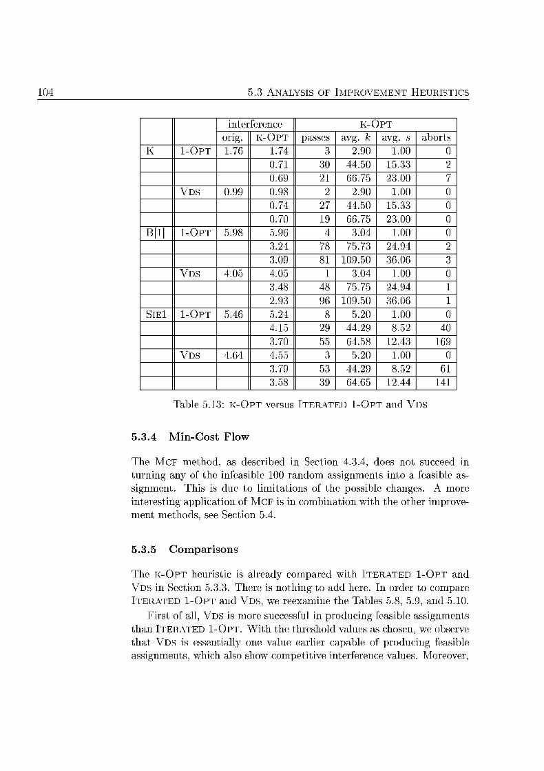
04 5.3 ALY M P R O V E N EU

nterferenc - O

ig. pa g. g. - O 2.90 00

0.71 30 4.50 5.3 0. 3.00

V D 0.99 0.9 2.90 00 0. 4.50 5.3 0. 3.00

- O 5. 5.9 3.04 00 3. 5. 24.94 3.09 09.50 0

V D 4.05 4.05 3.04 00 3. 5. 24.94 2.9 09.50 0

Sl - O 5.4 5. 5.20 00 4. 29 4.29 8. 40 3. 55 4.5 2.43

V D 4. 4.55 5.20 00 3. 4.29 8. 3. 39 4. 2.

Table 5 . 3 : us I R A nd V D

5.3.4 i n C o t F

The M C method, as described in Section 4.3.4, does not succeed i turning a y of the infeasible 100 random assignments into a feasible as signment. This is due to limitations of the possible changes A more interesting application of M C F is n combinatio with the other improve ment methods, see Setio 5.4.

5.3.5 Coparison

The - O T heuristic is alrea compared with I T R A T D 1-OPT and V D Setion 5.3.3. There is nothing to add here. In order to compare I T R A T E D 1-OPT and VDS, we reexamine the Tables 5.8, 5.9, and 5 .0 .

First of all V D is more successful in producing feasible assignments than I T R A T E D 1-OPT. With the threshold values as chose, we observe that VDS is essentially one value earlier capable of producing feasible assignments, whih also show ompetitive interference values. Morever

MP 05

if the results of the two h e u r i s s a compared per threshold value, then the worst result of VDS is in most cases better than the best result of ITERATED 1 - O T . The average of the VDS results is always better tha the best of ITERATED 1-OPT, see also Figures 5.11 up to 5.16.

On verage VDS performs between 2 and 3 times as many passes as ITERATED 1 O P T , and each pass takes about three times as long. The resulting effet on the total running time for the sets of 100 assignments is not uniform Taking averages again V D is about 5 to 0 times slower than ITERATED 1-OPT.

In conclusion, VDS is our method of choice in practice, because O is p r a t i a l l y not an alternative and VDS always outperforms ITERAT

1 O P T in our experiments. n addition, we consier the increase in ru ning time to be tolerable. Reiewing our previous discussion about which threshold value to use for V D , we tend not to tighten the separation for ts potential negative effect o the r u n n g time

5. ombinations of euristic

n this sectio, we study the ncerted ting of our heuristics Numerous combinations of the greedy cns t ru t ion and the improvement heuristics are possible. We idntify favorable combination of these methods to­gether with the relevant parameter settings.

Given two frequency plans of different quality, the application of (the same) improvement heuristis ca possibly lead to plans for which the quality rankig is reversed. As we observe in extensive comparisons, this is selom the case for the heuristics cnsidered here. Therefore, we use for each heuristic the parameters se t t ig w h h is favored in Section 5.3, that is, the se t t ig we o b t a i d from looking at ea of the heuristic separate from the others.

compare combinatio of heuristics on the istances K, B[l], and SlEl in Table 5.14. For each instance, three assigments are p r o d c d u s i g a greedy s ta r t ig heuristi

Plain T-COLORING is alled without t i g h t e n g the separation T-COLORING

This usually results i assignmet, where o l y few of the avail able channels are use

The acronym Ts C L O R I N G stands for calling T-COLORING Ts T-COLORING

with the separatio being tightened with the least possible thresh­old value yielding an assignment that still fits into the vailable spectrum This threshol is computed the same fashio as for

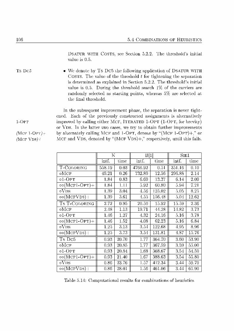
5. MB EU

DSATUR W , s e S e i o 5.2.2. The t h r h o s i i t value is 0.5.

s Dc5 We ote by Ts Dc5 the followig applicatio of DSATUR WIT COSTS. The value of the threshold t for tightening the separation is determine as explained in Section 5.2.2. The threshold's initial value is 0.5. During the threshold search 1% of the carriers are randomly selected as startin p o i t s whereas 5% are seleted at the fnal threshol

the subsequent improvemet phase, the separation is never tight ened Each of the previously construted assignments is alternatively

-OPT improed by calling either M C F , I T E R A D 1 - O T ( 1 - O P T , for brevity) or VDS. In the latter tw ases, we try to obtain further improvements

('MCF - O P T J + by alternately calling M C F nd 1-OPT, note by " ( M C F 1 - O P T ) + , " or ('MCF VDSJ+ nd V D ote by (M V D S ) + " respetively, until this fails

B[l] Sl ime ime ime

T - N G 558. 0.03 92 0. 35 0. 49.2 0.2 32.89 2. 2 9 8 2.

O 84 0.83 3.3 2.09 O O O ) + 84 11 5.92 0.80 5.94 2

V D 39 3.04 4. 25.02 5.05 8.25 O O V D ) + 39 3.61 4.55 4 5.04 2.

NG 2. 0.95 20.50 5.92 5.59 2.3 2.4 9. 4.2 4.82 3.

O 4 2 4.32 24. 5. 3. O O - O ) + 4 52 4.0 2.23 5. 84

V D 25 3. 3.54 22. 4.95 8.9 O O V D ) + 25 3. 3.54 8 4.8 5.

0.93 20. 4. 3. 53.90 0.93 20.85 59 3.59 55.00

O 0.93 20.84 8. 3.54 4.50 O O O ) + 0.93 40 8. 3.54 55.80

V D 0.8 23. 2.34 3.4 59. O O V D ) + 0.8 8.0 61 3.4 6190

ble 5 .4: C m p u t i o l r u l s f m b i i o heuris

MP

Table 5. isplays the incurr t oa l i n t e r n c e of the reul frequency plans nd the required running times in seconds. A "o" in fro of the name of an improvement heuristic i n d a t e s that the assigme obtaine from the last preceeding construction heuristic is improved. "oo" indcates that the result of the iretly preceedg heuristi is use as starting point The running times in econds a totals in all cases. A few observatios ca be m a e :

The start heuristics show a lear r a k i g with respect to their re­sults: Ts Dc5 is best, Ts T C R I N G second, and T - C O L O N G

thir The order reverses whe s i e r i g running times

The r a k i of the assigments produced by different start heuris­tics is in no case change when the same ombination of improve­ment heuristics is applied. Leaving M C F aside, this is also true without reuiring the use of the same ombiation of heuristics

The heuristi has no arguable use its own. E the simple I T E R A D 1 O heuristis beats M all ases

The M C F heuristic is of some use in ombiatio with I T R A

1 O T , but h a r l y ever in combinatio with V D

VDS alone is the preferable imprvement heuristi to be applie after a start heuristi

The total runn ig times required by T - O L R I N G V D nd C O L N G VDS are about the same i all ases

COLORING or Ts T - C O N G n combination with VDS pro­uce worse assignments than 5 alone, but spend nly about

a fifth of the time required by c5.

n summary, our ombination of choice is s D O V D That this selection is not best in all cases, however, is documented Table 5.15. If a feasible assignment is ot easily obtained, then T - N G O V D S

and T C O I N G O V D are attrative alternatives

5. Selected Results for all Benchmrk Scenarios

The total amoun of iterference incurred by a frequency assigment is used as cost function during the optimization. As mentioned in Sec tio 2 .3 . , this figure reveals only a small part of the pi ture from

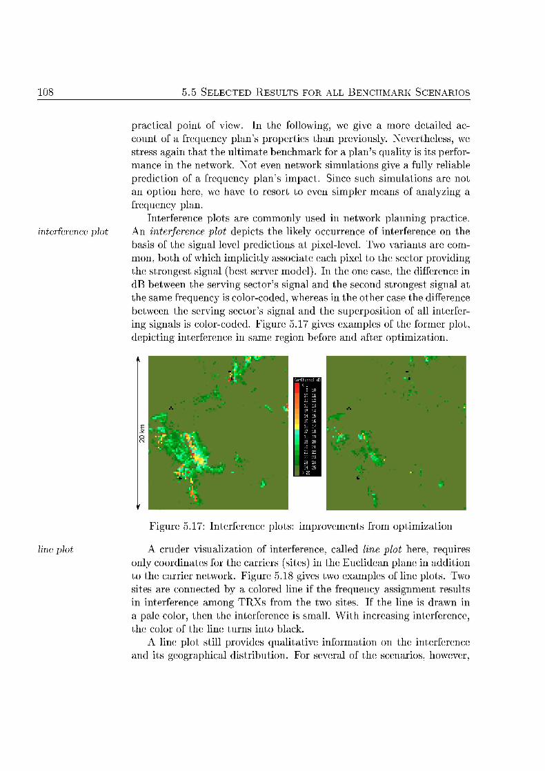
5 FO AL N C M A R K AR

p r a c a l point of ew. In the following, we ive a mor detailed a count of a frequency plan's properties than previously. Nevertheless, w stress again that the ultimate benchmark for a plan' quality is its perfor­mance in the network. Not e e n network simulatio give a fully reliable predictio of a frequency plan's i m p a t ince such simulations are not an option here, we have to resort to e simpler m e a s of a a l y z i g a f reuency plan.

Interference plots are commonly used in network planning p r a t i c e interference plot An interference plot depicts the likely occurrenc of interference the

basis of the signal level p red ic t ios at pixellevel. Two v a r i n t s are om­mon, both of which implicitly a s sc ia t e e a h pixel to the sector providin the s t roges t s i g a l (best server m o e l ) . I the o e case the difference i dB b th i h t l th be i

ur 5 . 7 : nce pl m p r o m e s fro p t m i

line plot ru v i s u a l z a t n of i n e r f e r n c , calle l e plo h e r , requi only coordinates for the carriers (sites) in the Euclidean p l a e in additio to the carrier etwork. igure 5.18 gives two examples of l i e plots. Two sites are connecte by a olored line if the frequency assignment results in interference among TRXs from the two sites. If the line is drawn in a pale color, then the interference is small th increas ig interference the color of the lin t u r s into black.

A line plot still provides qualitative information the interference nd its geographial distribution For s e e r a l of the s a r i o s , however

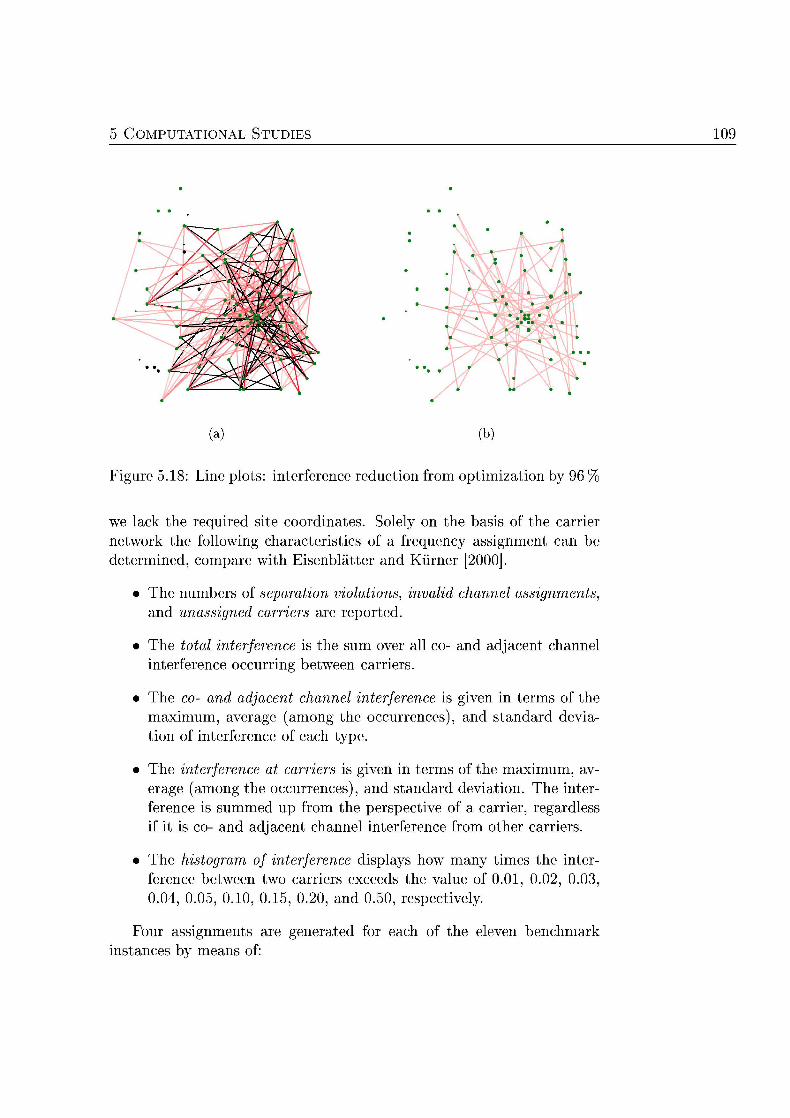
MP 09

a) b)

Figure 5 . : L e plots nterference r e t i o from optimizatio by 9

we lack the require site coordinates Solely on the basis of the arrier network the following characteristics of a frequenc assigment be

etermied compare with Eiseblätter and Kürner 2000

The umbers of eparaton violation inal channel assme and unassi rri are reporte

The total interference is the sum over all - and dj hannel interferenc ccurrig between carriers

The co- and adjacet channel interference is give in terms of the maximum, average ( a m g the occurrences), and standard evia tion of interference of e h type

The interfence at carrier is give in terms of the maximum, av erage (among the occurrences), and standard deviation. The inter­ference is summe up from the perspective of a arrier, regardless if it is co- and adjcent hannel interference from other carriers

The histogram f interference isplays how many times the inter­ference between two carriers exceeds the value of 0.01 0.02, 0.03, 0.04, 0.05, 0 .0 , 0 . 5 , 0.20, and 0.50, respetively

Four assignments are geerate for e of the ele benchmark stances by mean of

11 5 FO AL N C M A R K AR

T-COL VDS a. NG followe VD

T-COL VDS b. T C O N G with automati tighte of the separatio followe by VD

s Dc5 VDS DSATUR W T H COSTS with 5 % of the carriers randomly selecte as s t a r t ig points, automati tightenin of the separatio, and fol lowe by VD

THRESHOL a. HOLD A C C N G (the a s s i g m e t s are kindy pro by CCEPTING eller ieme Germa

These fortyfour assignments n total are analyzed according to our abo criteria, and the results are displayed in Table 5.15. The fields whic would otherwise contain a zero are left blank for the sake of better leg ibility. We first observe a few points concerng the feasibility of the assigments

C O L O R N G fails to generate a (feasible assigment for SI

SIE4, and w, e v n without the separation bei t ighteed In this case, no assignment is generated by T-COLORING, and we take the situation with all carriers uassig as s t a r t ig point for VDS. Hence the assigments obtained for T C O L O R I N G o VDS and Ts T-COLORING VDS are the same. For these three s n a r i o s the resultig assigment is ifeasible

Ts Dc V D also fails to geerate a feasible a s s i g m e t for i stances SIE3, S I 4 , and Sw

Next, we fous ur attention to the results o V D and THRESHOLD ACCEPTING o the istances, where V D pro­

es a feasible a s s i g m e t

In all cases, the assignmet from the combination V D ncurs more interference in total than that from THSHOLD A

CEPTING. The dfference rages between 29% and 90%. The a erage ifference is 60 %.

The values for the maximum co and d j a n t channel interferenc nd the maximum interference affectig a arrier are about equal n the case of instance 4], the THRESHO C C P T N G result is

n o t i a b l y worse i that respet

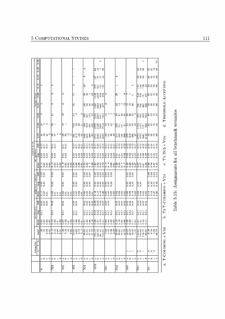
MP 111

Ö

H

11 .6 S A A L N G

The second point c be explaned as a sde effect of automatically tightening the separatio in Ts Dc5. It is, nevertheless, fair to say that the T H E S H O L D A C C E P I N G heuristic is the clear winner among the methods compared here in terms of the verall incurred nterference and it is ompetitive with respect to the loa l distributio of interference No of our improvement heuristics (except for K - O P T improves the T H R E L D A C C T I N G results. We also apply the K O P T heuristic to the T H R E S H D ACCEPTING assignments for the instances K, B l ] , and SlE without any success. The parameter k is set to .5 times the number of available hannels, the parameter s is left unbounded We stop the optimizatio after two unsuccessful passes, ompare with Setio 5.3.3.

We should keep i mind, however, that one of our primary design goals has been to devce methods with a small verall r u n n g time Although the precise runnng times of THRESHO ACCEPTING are not known to us, it takes about one order of magnitu loger tha Ts Dc5 o VDS Heller [2000]) Taking this into account, s Dc5 o VDS presents tself as a fast plannng method which oes not ompromise too mu

the optimization goal. In ase Ts Dc5 V D is still too slow, the T - C O L O R N G V D or, even faster, s T C O L O R I N G O I T E R A T E D 1

O P T are alteratives gain, some egraatio of the solutio has to be ccepted.

We come ba to the issue of ho goo frequency pla is i the ext hapter

5.6 onclusions and hallenges

A stead expansion of GSM networks an still today be observed i terms of overage as well as apacity. Every hange of the network in this respect calls for a h a g e of the frequency assignment. Up to this point, we focused on how to use mathematical optimization techniques in order to provide frequenc plans for GS ellular networks ncurrin little interference between r a i o signals

Plnning the use of freuencies is o ntral tasks in engieering the radio nterface of a GSM network and corerstone for p r o d i n g the desired grade of service as well as the desired quality of s e r e . One of the limiting fators is interference; and it has bee our o b j t i v e to design algorithmic methods for quickly geerating freuency pl that ncur as little interference as possible

Typically, a etwork operator tries to keep the assignment essetially fixed for a onsierable time, performing o l y m i o r hanges, whi are

M P N A 11

rced by m o i f i c t i o n s f the n e t w r k . But e e r y now and hen, once year, say, a new assignment is generated for (maor portions of) the

network. Then, all previous changes are fully taken into account and the foreseen future c h a g e s are prepared for. This is a highly complex task with literally tens or even hundreds of thousands constraints to consider. Clearly there is a nee for algorithmic optimization p r o d u r e s to support the radio planner in this task. From our poi of iew three distinct p l n n i n g tasks be i n t i f i e d i p r a t i c e

In what we call the relaxed planning situation, the p l n n e r wants to relaxed planning produce a new frequency ass igment for a large region in a network and is in the fortunate position to have ample frequencies available The objective is then to minimize interference and thus to eliver the r a i o s e r i ce at high quality

In what we call the congested planning s i t u a t i o , again a new plan for large portions of a etwork is to be produced, but this time the number of available frequencies hardly allows to provide the desired grade of s e r e (at the least accepted level of quality)

I the adaptin planning ase, the planner is terested n adapti adapon planning l oa l ly the frequenc ass igment to h a g e s i the etwork.

Accordng to our experience each of these situation alls for differe algorithmic planning methods. Our focus here is clearly o the relaxed p lannn situation. Nevertheless, we nsider the K - O T heuristic dis­cussed ection 4.3.3 as a prime choic for adapting loa l ly to changes Surveys o research directed more towards the "congeste case are given by Koster [1999], Murphey et al [1999], and Jaumar et al. [1999, for example. The book of Nielsen and Wigard 2000] is also of interest in that respect because deals with the use of GSM features like slo f reuenc hopping ( F H ) i order to tune the radio interface

In the course of the previous chapters, we ga a thorough intro­duction to the G M frequency planning problem and disussed several algorithmi m e t h o s solving this problem heuristically more detail we explained the t echn ia l background of frequency planning and p i k e an adequate m a t h e m a t i a l m o e l of the p l n n i n g task. The resulting op­timization problem is j V P - h a r , and s o l g this optimization problem to optimality is ot p r a t i a b l e (from today's point of view).

We therefore designed number of planning algorithms with small theoretical and practical running times The latter property, in partic­ular, renders them a t t r a t i v e for use i n in tera t ive p lannng p r o e s s

congested planning

11 N C S A AL

whee fequency plans a e geneated for a l rna t ive t e n v e hanges i the network. We analyzed their omputational behaior on eleve realis tic p l n n n g scnarios These scenarios have been made publily available at the FAP web 2000] through the COST 259 a t ion see Eiseblätter and Kürner 2000] or orreia [2001, S t i o n 4.2.7]

Our ndings an be summarized as follows. The selfset goal of swiftly generating lowinterference frequency plans is achievd reasonably well on all senarios except for one, where no feasible assigment is obtained This exeption, however, represents a har "congested" planning situa­tion. Among our methods, we identified a combiation of two heuristi namely, UR WIT COSTS and V D , as a reasonable compromise be­tween planning effectiveness and running time efficiency In comparison to the best alternative method we are aware of our assignment incur at most twice the amount of interference on the studied scenarios

Notice however, that this alternative planning heuristic THRESHOL

A C C E P T N G proposed by Hellebrandt and Heller [2000] is a randomize local search p r o u r e similar to Simulated A n n a l i g , and it often re­quires at least one order of magitude higher runnng times tha our heuristics espite the superiority of that metho i terms of the over­all incurred interference our favorite combination produces assignments which are competitive in terms of local interference Such local properties are of e u a l practical interest. Therefore we consier our methods a rea soable choice uring the interactive p l n n g process. More elaborate plannin methods, like T H R E S D A C C E T I N G , may be used prefer­ably for computing the final p r o t i o n pla in a batch process.

We mention two more points concerning the heuristics before turn ng to their practical merits First, although we applied kopt steps for

values of k as large as 1.5 times the number of available frequencies the assignments p r o i d by Heller Siemen AG, were not improed in our experiments (see tion 5.5 for details). This is surprising because THRESHOLD A C C E P I N G relies on a mix of a comparatively weak local optimization step and small random perturbatios of de l inng deteriora­tion. It is not obvious to us why a much more powerful loa l optimizatio fails to improve the three resulting assignments for the scenarios K, B[l] and SiEl—i particular, since we show in the ext chapter that at least the assignment for K is far from optimal

The second point concerns the question whether some sort of ecom position might be applied to a planning problem The goal would be to olve the resulting parts separately and to combine the partial solution

to an assigment for the whole problem i the end Our experiments i

M P N A 11

this i r t i o n faile The discusion c n c e r n g the high c o n n e i t y ob­served in the planning instances (see Section 5.1.1) is certainly e item

explaining this failure, but we lack a better understandng. After having dwelt on the mathematial optimizatio problem and

discussing the pros and cons of trading o running time versus solutio quality it is time to turn b a k to p r a t i e To ut a long story short ur oftwa is ued successfully in practce at E-Plus, nd better freqcy

assmets have ee taind more much quickly han t pre viou lnning process. n e example, a region containing 2118 cells with -3 TRXs per ell and 75 available frequencies was planne usi DSATUR W H COSTS followed by ITERATED 1-OPT. The assignment was istalled into the network. After performing fewer changes of cells in reaction to unforesee hea interference than usual (a regular on line optimization p r e s s , the down-li quality hand-over request rate had dropped around 20 % n ompariso to the preiousl operatioal freuency pla

Finally, G M networks will certainly remain n operation throughout this e c a e Most European networks face major capacity extension in o r e r to support the foreseen ncrease in data services. Hence, the presently satisfying planning methods may reah their limits at some fu­ture point in time W lose by l i s t ig four directions for further resear n that respe

Imprvements in the planning methos are still possible. We giv reasons for our point of view in the next chapter, where we ob­tain a muc better assigment for the benchmark scenario K tha those presented up to now. Among others, however, the unsuc­essful attempts to improve the assignments p r o v i d by Heller

Siemens AG, using the loa l optimiation K - O P T indicate that th loa l optimization steps sidered so far are not powerful enough to eal with the omplex nterependencies among large amounts of TRXs

A more practical point is the design and tun of software whi automatically handles all three types of the above mentioed plan ning situations. Suh a software should also suggest whe to per­form a maor replannng.

Instead of aggregatig all pixel-based signal predictions into inter­ference relations at cell-level, all the available data should be fed nto a more omplex optimization m o e l This woul allow for a

116 NC AL

m e acurate nalysis of a frequency plan during the op t imi t ion process. Morever, the effects of GSM features like iscontinuous transmissio DTX) or slow frequency hopping (SFH) ould better be taken into ccout . (We are aware that some work in this di­rectio is already done within companies and at the versity of C a r f , but further studies are er tai ly of use)

Among the several ways to enlarge the scope of the freuency plan optimization, we want to highlight the following. Given a network nd the istalled frequency plan, find an optimized assignment and

migron pth migration path from the given assignment to the ultimate new one Here, we understand a migration path as a sequence of changes to be performed, one after the other, such that all the intermediate stages constitute feasible frequency plans and the changes comply with restritions related to the available maintenance persnnel for example

CHAPTER 6

uality of Frequency Plans

In the preious two chapters we explaine nd alyzed seeral heuris methods to generate frequency plans for GSM etworks. A significa spread is o b s e r d in how well (combinations of) these methods achieve the goal of finding feasible assigments incurring minimum interference So far, however, it remains open whether the best results are actually good or merely the relative bests among mediocre ones. In order to rem edy this uncertainty we would like to prove statements like the following this assignment, for the given plnning scenario, incurs at most twice the amou t of interference which is unvoidable. Such a s tatemet is called a quality guarntee Our aim in this chapter is to p r e suc guarantees qualit guarantee for the assigments of Sectio 5.5.

Let us put our uest for lower bounds and uality guarantees into perspective. We show in Section 3.2 that unless V = J\fV no polynomial time algorithm is capable of computing frequency assigments that are close to optimal (or merely feasible in all cases. As a consequence, we do not analyze algorithms here We analyze the algorithms' input namely, the carrier networks. We want to prove that a ertain amount of interference is unavoiable due to the network layout. Hence, the bound have to be computed on perinstanc basis For reasons to become clear, our bounds take o-channel but o adj channel interferenc

to accoun We p r d e the first s i g n i f n t lower bounds for the o b j t i v e of

minimizing overall interferenc n realistic frequency plnning scenarios Large gaps between the amount of nterference incurred by the heuristi cally generated frequency plans and the lower bounds still exist. We give reasons that these gaps are not to be blamed entirely on the weakness of the lower bounds. Instead, the gaps also indcate room for improveme on the side of the frequency planning methods

Up to ow, our bounds have no direct practical impact. The situation may improve if information from the lower bound computation were to be exploited the frequency p l n n n g process With the approach pursued

11

11 L A X D F E Q N C Y PLA

hee, however, it is not yet lear how this be e effeciv The chapter is organzed as follows. In Section 6.1, we introduce the

relaxed frequency planning problem." Optimal solutions to this problem yield lower bounds on the unavoiable interference in the original prob­lem. In Section 6.2, the tight nnectio between the relaxed plann problem and the wellknown MINIMUM K-PARTITION problem is sho Morever, two possible approaches for (approximately) solving a MIN MUM P A T I I O N problem are described. In Sction 6.3, lower bound are proided by means of one of the approaches, namely, by solving large semidinite programs We use these bounds to estimate the quality of the freuency assignments from Section 5.5. In ection 6.4, we revisit fre­quency plannig heuristis. Our goal is to tur feasible frequency plan for the relaxe frequency plnning problem into feasible plans for the ordinary planning problem. some cases it is possible to produce sig nificantly better frequency plans than before. This supports our opinio that, from the point of view of mathematical optimization the frequency planning problem is not yet fully mastered; this also sheds a ew light

n the lower bounds, which now appear stronger tha before. Including this chapter, our focus is primarily on frequency assignment

We change our point of view for the last two chapters, where we deal with the mathematics behind our computations of unavoidable interference that is, the M N I M U M K P A T I O N nd ts s e m i e f i t e relaxatio

.1 elaxed Frequency Plannin

We consider a relaxed version of our frequency p n n i g problem where the feasibility constraints are weakened and the objective function is sim­plified. Although the complexity status of both problems is formally the same the resulting problem is more accessible than the original freuency assigment problem The simplifcatios are the followig.

ropping adjacent channel interference The major portion of the total interference incurre by a frequency plan is often co-channel interference, see Table 5.15 in Chapter 5. Good lower bounds for our enarios are, thus, hardly obtain without fully exploiting co-channel interference, whereas a d j c n t channel interference ofte plays a minor role (An exeption is the scenario Sw, where nly adjacent channel i terferene is specified Our approach does not allow to erive a nontrivial lower bound for the scenario Sw, but as explai n S t i o 5 . , this s n a r i o is atypial

AL E Q C Y LA 11

r o p i n g local blockings: Only few local blockings are present in ur cearios Thus, assumig Bv = 0 for all v E V leads to minor

changes the scenarios We pointed out, however, that in a real life planning numerous local blockings may be present. One sour of blockings are the agreements between GSM network operators on the use of available spectrum border regions, e. g., along national borders. Another source is the essity to seamlessly integrate the frequency plan for a rearranged ortion of the network with the assignment for the remaining part of the network. The frequency pl for an entire network is h a r l y ever haged at once

ting down required separation: A ertain debatable step is to relax the separation requirements by bounding the maximal re­quired separatio n d by But this is essential for arri ing at a simpler" problem

All three s impl i fa t ios toether yiel a problem, whi is almost MINIMUM EDGE ETIO K P A R T I T I O N problem, see Setion 3.2. omputational methods may ow be applied that are not suited for sol g the original frequency plannng problem, see S t i o n s 62 and 6.3.

Formally we write the relaxed problem as o r a r y frequency plan problem on a simplified carrier graph. Gi a carrier network (V,E,C,{Bv}veV,d,cc°,cad), the associated simplif carrir net

work is defined as the 5-tuple Ns = (V, E, C, d cco) where E — {0,1} with vw i> mm{d(vw),l}. The sets Bv of locally blocke channels as well as the adjacent channel interference cad disappear, and the reuire minimum separatios in d are ut ff at 1

As before, a frequency assignment or just an assignme for Ns is a function: V —> C that assigs a channel to every carrier A assignmen is feasible if \v) — y(w)\ > (vw) for all vw E E.

efinition 6 1 . A instce relaxe frequency p l n n g problem coists of rri etw Ns, and the objectve i to lve the optiizat lem

min \ y feasibl ' J

vweE: y{v)=y{w)

vw) (RFAP

Solving the relaxed frequency ssignmet prblem clerly yields a lower bound n the optimal solution for the ordinary assignment prob­lem, but not e versa. nding a optimal solutio for the relaxe

implißed carrie network

gnment

easib

relaxed FAP

P A I O

frequency planning problem is not k n to be simpler than for the original problem. Both problems are A / h a r d . (The considerations of Section 3.2 for the ordinary frequency planning problem transfer irectly to the relaxed problem.) The following observation, however, points out one maor dfference between the origial problem nd its relaxed version

Osevation 6.2. Fo imifie rrie netw nd an assat freuecy assnment y ing ds. Lt f\ and f2 be tw cha nels fro spectrum, and t t assnmet y be btaine fr y b changing al rrie wh channel f\ nd al carrie h channe f2 fi. T , y is feasibl nd nly feasib Furrmre, y

nd inur me un inrfere

onsequently, all assigments dffering ony the permutation of channels may be considered equivalent If all channels are in use, the there are \C\\ many assigments whi are e u i v a l e t in that sense

2 inimum fc-Partition

Relaxed frequency plnning is o a simplified carrier etwork Ns = (V, E, C, d, cco), where o adjaent channel interference or loally blocked channels are specifie and minimum separatio is at most 1. Basically a partition Vi,.. Vp of V into at most k \ disjoint sets of arriers (using distinct freuencies has to be determine such that no tw vertices v w with d(vw) = 1 are i the same set and such that the sum over the edge weights in the induced subgraphs G[V ], 1 < I < k, is miimized This problem is almost the same as findng a minimum ^-partition of the vertex set of the graph G = (V,E), which underlies the simplified carrier

etwork. The edge weights for G are d e r i d from d nd cc° Let Eco = {vw E E : c™w > 0} and Ed = {vw e E : dvw > 0}. We

may assume that the intersection of Eco nd E is empty and that their union is E. Furthermore, we set M = J2weE cc

v°w + 1. The edge weight function c: E —> K_|_ is define as c(vw) = c° in ase of vw G Eco an

vw) = M in case of vw E E Any solution to this MINIMUM KPARTITION problem induces a fre­

quency assignment for Ns The same channel is assigned to all vertices in one block, and dist int channels are given to distinct blocks. If an optimal solution to the fc-partition problem has a value less than M then the indued assignment is feasible for iVs. The solution value is the interferen incurred by a corresponding assignment—no matter how we choose to istribute the freuenies among the bloks If, on the other

AL E Q C Y LA

hand, the optimal s l u t i o n lue is t l e t M, the h e e is no f i b l e assignment for iVs.

Another way of looking at the problem is to find a weightminimum set of edges whose removal results in a A;-partite graph. A graph is k-partite k-arte rap if its vertex set can be partitioned into at most k independent sets, i e all edges have their endpoints in distinct sets. A graph is obviously k-colorable if and only if it is partite. A graph without edges is fc-partite and a graph containing a clique of size k 1 is not. A natural question to ask is: what is the maximum number of edges that a partite graph on n vertices may have? The wellknown answer is ( ) |_|J +r( 1) |_|J + Q where r denotes the remainder of the integer division of n/k. Hence, k-partite graphs can be fairly ense. The complete graph K2$7 for example has (^7) = 3 5 5 1 edges, a 0par t i t e graph on 267 vertices an have as many as 34926 edges, which is onl (ln/

2k]) + (k - ([n/

2ki) = 585 less

than in the complete graph. Formally, the minimum graph ^par t i t ion problem or K-

P A T I O problem an be state s follows

efinition 6. An insta M N I M K - P A R T I O problem M I M U M

nists f undirect gra V, E), a hting c E o f P A I T I O N edges, and a ive ineger objective is t find a pa in at st in t s . , Vp ch that te value

weE(G[V

inimiz

The M N I M U M K - P A T I T I O N problem is a generalization of the M I N

IMUM E D G E D E L E T I O N K - P A R T I T I O N problem, see Definition 3.9, to general rational edge weights. Therefore, the computational comlex i ty of the former is at least as hard as that of the latter.

The M I N I M U M K - P A R T I T I O N problem is explicitly studied by Chopra and Rao [1993], b t more is known from related problems, e. g., by means of the following equivalence: for every partition, an edge has either its both endpoints within the same block or within distinct blocks; hence the problem of finding a minimum ^par t i t ion is equivalent to finding a k-cut, where the sum over the weight of all edges with their endpoints in distinct sets is maximized. The M A X I M U M K - C T problem has received more attention in the literature than the MINMUM K-PARTITION prob­lem, see, e g , Deza, Grötschel, and aurent [199 992 and C h o r a

22 U M I O

and Rao [1995]. Results on the approximation the MAXIMUM K-CUT

problem are obtained by Karger, Motwani, and Sudan [1994] as well as by Frieze and Jerrum [1997]. Those results are, however, of little help here The optimal c t value is underestimated so that the value of the MINIMUM K-PARTITION is overestimated, and no lower bound is supplied that way. Assming that all edge weights are nonnegative, Goldschmidt and Hochbau [1994] show how a maximum partition of the g r a h into k nonemty components can be computed in ö(nk _ 3 / / + 4 T(n, m)) time where T(n, m) is the time required to compute a minimum (s, i ) c t . Du to the sign-constraint, their result does not apply here either

AXIMUM CUT Notice also the connection to the MAXIMUM C U T problem: an edge-

weighted graph is given, and the task is to find a partition of the vertex set into two sets (one possibly empty) such that the sum over the weights of all edges with their endpoints in different sets is maximized. The literature on the MAXIMUM C U T problem is extensive, see the survey article by Poljak and Tuza [1995], the book by D e a and Laurent [1997] and the references contained therein. The MAXIMU roblem is equivalent to the MINIMU 2 - P A O N problem.

6. nterference is not e s s n t i a l y metri

The MINIMUM K - P A T I T I O N problem gets simpler if the edge weights are nonnegative and fulfill the triangle inequalities, i.e., cvx + cxw cv

for all triangles in the g r a h . The roblem is then also called MINIMUM

K-CLUSTERING SUM, see Ausiello et al. [1999, Appendix B, ND55], and is proven to be approximable within a factor of two in polynomial time by Buttmann-Beck and Hassin [1998]. We show, however, that the triangle inequalities are far from being fulfilled by our data sets

A systematic reason is d e to the mapping of separation constraints to large weights. Consider the placement of transmitters and their pairwise interference as depicted in Figure 6.1. The rectangle in the center repre sents an obstacle. Assume the availability of only two adjacent channels and that the channels for transmitters a and b need to be at least one apart. If all triangle inequalities are to be met, then the triangle between a, b, and c bounds the value of M to at most 0.2. Setting M to 0.2 or less, however, implies that the minimum-weight solution assigns a, b, and d the same channel. The resulting assignment is infeasible. Hence separation conditions can, in general not be represented adequately by an appropriately chosen weight without violating the triangle inequality This first obstacle stems solely from reresenting separation constraints

INIMUM

K-CLUSTERING

SUM

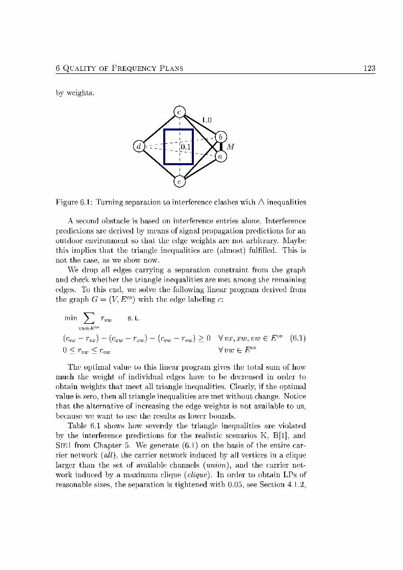
U A T Y OF F R E Q N C ANS 123

by w

ig 1: T i n g s i o n to in la with A i n l i t i e

A second obstacle is based on interference entries alone. Interference redictions are derived by means of signal propagation predictions for an

outdoor environment so that the edge weights are not arbitrary Maybe this implies that the triangle ineqalities are (almost) flfilled This is not the case, as we show now.

We drop all edges carrying a separation constraint from the graph and check whether the triangle inequalities are met among the remaining edges. To this end, we solve the following linear rogram derived from the g r a h G = (V, Eco) with the edge labeling c:

s t

c Vvx,xw,vw e Eco (61)

Vvwe Eco

The optimal value to this linear program gives the total sum of how much the weight of individual edges have to be decreased in order to obtain weights that meet all triangle inequalities. Clearly, if the ptimal value is zero, then all triangle inequalities are met without change. Notice that the alternative of increasing the edge weights is not available to s because we want to use the results as lower bounds

Table 6.1 shows how severely the triangle inequalities are violated by the interference predictions for the realistic scenarios K, B[l], and SlEl from hapter 5. We generate (6.1) on the basis of the entire car rier network (all), the carrier network indced by all vertices in a clique larger than the set of available channels (union), and the carrier net­work induced by a maximum clique (clique). In order to obtain LPs of reasonable sizes, the searation is tightened with 0 . , see Section 4 1 2

w£E

Cx p

r

12 INIMUM

and all dges with co-chann interference less than 0.001 are dropped This reduces the number of potentially violated triangle inequalities in the carrier networks. The first two columns of Table 61 indicate the in­stance and the type of the (sub-)network. Then, the number of violated triangle inequalities, the maximum violation, and the average violation are shown. Next, the number of variables and constraints in the gen­erated LPs are reported. Finally, the optimal value of the LP is given. The optimal solution could not be computed for B[l]/all due to a lack of computer memory (CPLE reqests more than 4 GB of memory).

iol ma L P 1 ) iol iolaion on

all 3229 47 32 477 3739 89 ion 17 47 32 6744 12000 82

li 447 33 00 33 B[l] ll 4338 31 437 8265 B[l]

ion 5495 47 31 982 44 3865 B[l]

li 811 43 11 5112 18 ll 81683 66 217 3236 72

ion 8686 66 827 118833 8886 li 111 47 3153

le 6 1 : Violaion i n e q l i t y by in icion

The r u c t i o n s of the edge weights that a e necessary to fulfll all tri angle inequalities are in fact, orders of magnitude larger than the total in­terference incurred by the feasible frequency plans analyzed in Table 5.15 Hence, is seems futile to consider the (olynomial time) 2-approximation algorithm for the MINIMUM K - C L U S T E I N G SUM problem by Buttmann-Beck and Hassin [1998] as a reasonable option for computing strong lower bounds on the navoidable interference. We therefore t r n back to the general MINIMUM K P A T I T N problem.

6. ILP formulation d a S relaxation

Two formulations of the MINIMUM K - P A R T I O N problem on a complete graph Kn with n > k > 2 are given next. (The graph G = (V, E) with edge weights c is completed to K\V\, and the edge weighting is extended to all new edges by assigning a weight of ero) These two formlations have relaxations of quite different kind.

The first formlation is a lain integer linear rogram LP) see 62)

U A T Y OF F R E Q N C ANS 12

with an LP r e l a x o n obtained by dropping all grl i ty con t r i n t s A binary variable w is associated to every edge vw of the graph. The valu of zvw equals 1 if and only if both endpoints are in the same partite set. The constraints (6.2a) require the setting of the variables to be consistent, that is, transitive. For example, if zvx and zxw indicate that v, x, and w are in the same partite set (by transitivity), then the setting of zvw has to reflect that as well. The constraints (6.2b) impose that at least two from a set of k + 1 vertices have to be in the same partite set Together with the constraints 6.2a) this implies that there are at most k

artite sets. We deal with the LP 62) extensively in the next cha ter

Vv,x,weV (62a)

V Q c y with Q\ (62b)

The second formulaton can be seen as a semidefinite program wi "integrality" constraints. This formlation builds on the following two facts: there are k unit vectors in 1 with m u a l scalar products of rjy and this value of the scalar prodcts is least possible. Consider, for xample, a simplex with k vertices in R centered at the origin and scaled

such that all vertices have a Euclidean distance of 1 to the origin The vectors pointing at the vertices of this simlex have the desired roer ty Formally the following can be roved

emma 6.4. Fo all egers n nd k satisfyng 2 th llowng ds:

(i) There exist uni vers ü % uch that (üj üf) j ^ fo all i ^ j

i) ny k uni vers .. atisfy:

(ui Uj) < S all i ^ j , th j ^

in J2 W(V

S t

w£Q

e [0,1] integer

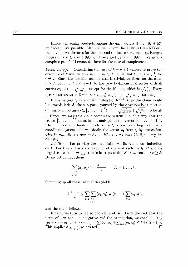
12 INIMUM

Hence, the scalar proucts among the unit vectors üi,..., ük E Mn

are indeed least possible. Although we believe that Lemma 6.4 is folklore, we only know references for the first and the last claim, see, e. g., Karger Motwani, and Sudan [1998] or Frieze and Jerrum [1997]. We give a complete proof of Lemma 64 here for the sake of comleteness.

Proof. Ad (i): Considering the case of k n + 1 sufces to rove the existence of k unit vectors üi,... ,ük E K such that (üi,üj) = ^ y for

7 j . Since the onedimensional case is trivial, we focus on the cases n > 2 Let U, n + 1, be the (n + ldimensional vector with all

entries e q a l to —.n(^ except for the ith one, which is ^J^h- Every

is a unit vector in R , and (ij.t,-) = ?\^ 77 — for i ^ j ' " JI n ) n+1 n ' J

If the vectors ij were in R instead of R"+1, then the claim would be proved; indeed, the subsace spanned by those vectors is at most n-dimensional, becase (U, [l .. l] } — n Jn,^+1 + \l^i = 0 for all i. Hence, we may rotate the coordinate system in such a way that the vector [l . . . l] turns into a multiple of the vector [0 . . . O l ] Then the last coordinate of each vector £j is ero according to the new coordinate system, and we obtain the vector üi from ti by truncation Clearly, each is a nit vector in W1, and we have ü i ü j ) ^ for all ^

Ad (ii): For proving the first claim, we fix n and se induction on k. For k 2, the scalar product of any unit vector u E W and its negative — u is 1 = ^ - this is least ossible We now consider k > 3 By indction hyothesis

22i,Uj}—— k. i<j

mming up all these ineqalities yields

i<j i<j

and the claim follows. Finally, we turn to the second claim of (ii). From the fact that the

norm of a vector is nonnegative and the a s s t i o n , we conclude 0 (uH \-,ui-\ Vuk) = J2(uhui)+^i,uj) < (k This imlies ^ - as desired D

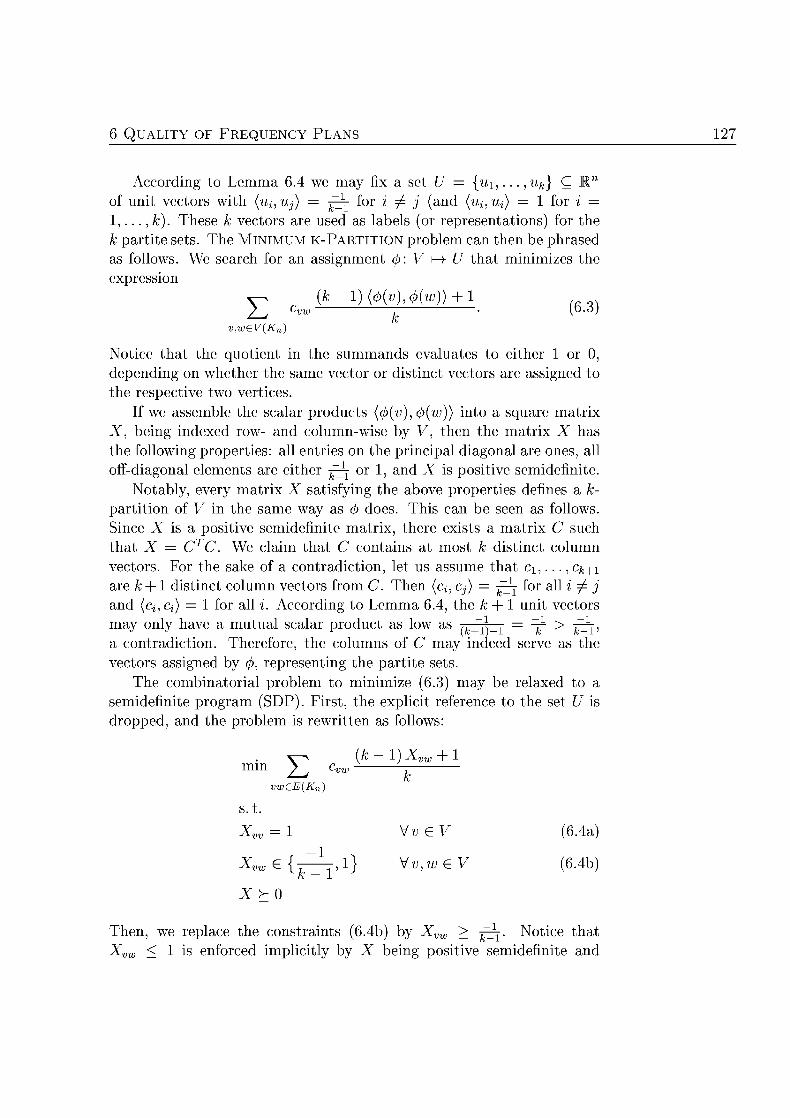
U A T Y OF F N C Y PLANS 127

According to Lemma 6.4 we may fix a set U = { . . , uk} C of nit vectors with (ui,Uj) = j ^ - for i ^ (and (ui,Ui) = 1 for i =

. . , k). These k vectors are sed as labels (or reresentations) for the k partite sets. The MINIMUM K-PARTITION problem can then be phrased as follows We search for an assignment (f>: V ^ U that minimies the expression

£ (Kn)

3)

Ntice that the quotient in the summands evaluates to either 1 or 0 depending on whether the same vector or distinct vectors are assigned to the respective two vertices.

If we assemble the scalar products {<ß(v), 4>{w)) into a square matrix X, being indexed row- and column-wise by V, then the matrix X has the following properties: all entries on the principal diagonal are ones, all

ff-diagonal elements are either -^ or 1, and X is positive semidefinite Notably, every matrix X satisfying the above properties defines a k-

partition of V in the same way as 4> does. This can be seen as follows Since X is a positive semidefinite matrix, there exists a matrix C uch that X = CC. We claim that C contains at most k distinct co lmn vectors For the sake of a contradiction, let us assume that Ci,.. Ck+

are k distinct column vectors from C. Then (Q, Cj) = -j^j for all i ^ j and (CJ, Ci) = 1 for all i. According to Lemma 64, the k + nit vectors may only have a mutual scalar product as low as k^_1 = -jjr > f~[ a contradiction. Therefore, the columns of C may indeed serve as the vectors assigned by (/>, representing the partite sets.

The combinatorial problem to minimize (6.3) may be relaxed to a semidefinite program (SDP). First, the explicit reference to the set U is dropped, and the roblem is rewritten as follows:

p weE(K

s t

vv Vv

E { l } Vv

64a)

(64b)

x y

Then, we replace the constraints (64b) by Xvw > ^ - . Notice that Xw < 1 is enforced imlicitly by X being ositive semidefinite and

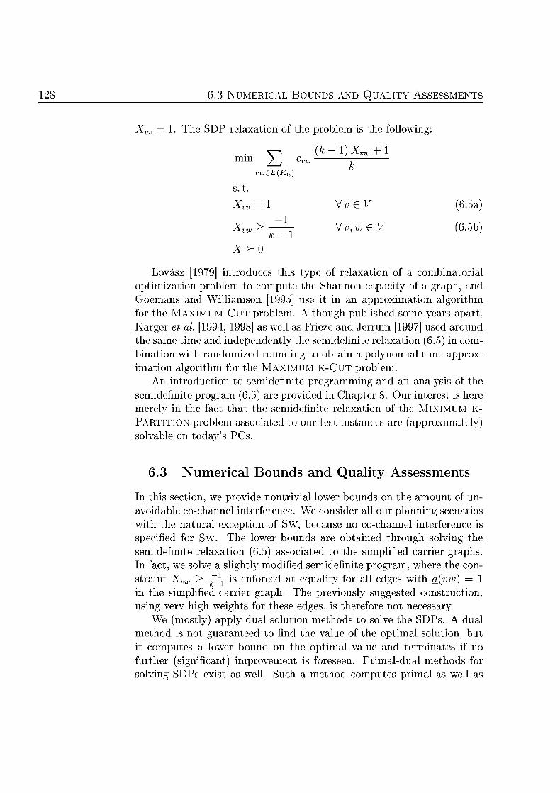
12 3 N U M C A UNDS AND U A T Y A S S S S M

Xvv Th DP ion o lem is e fllowin

^ (A 1) X + 1 mm ^ 7

w£Kn)

s t

Xvv 65a)

YZ\ 65b)

Loväsz [1979] introduces this type of relaxation of a combinatorial ptimization roblem to compute the Shannon capacity of a graph, and

Goemans and illiamson [1995] use it in an approximation algorithm for the MAXIMUM C U T problem. Although published some years a a r t Karger et al. [1994, 1998] as well as Frieze and Jerrum [1997] used around the same time and independently the semidefinite relaxation (6.5) in com­bination with randomized ronding to obtain a polynomial time approx­imation algorithm for the MAXIMUM K-CUT problem.

An introduction to semidefinite programming and an analysis of the semidefinite program (6.5) are provided in Chapter 8. Our interest is here merely in the fact that the semidefinite relaxation of the MINIMUM K

P A R T I T O N problem associated to o r test instances are (approximately) solvable on today's P s

6.3 Numerical Bounds and Quality Assessments

In this section, we provide nontrivial lower bounds on the amount of un­avoidable cochannel interference We consider all our planning scenarios with the natural exception of Sw, because no co-channel interference is specified for Sw. The lower bounds are obtained through solving the semidefinite relaxation (6.5) associated to the simplified carrier graphs In fact we solve a slightly modified semidefinite program, where the con­straint Xvw > -j y is enforced at equality for all edges with d(vw) = 1 in the simplified carrier graph. The previously suggested construction,

sing very high weights for these edges, is therefore not necessary We (mostly) apply dual solution methods to solve the SDPs. A d a l

method is not guaranteed to find the value of the optimal solution, bu it computes a lower bound on the optimal value and terminates if no further (significant) improvement is foreseen. Primaldual methods for solving SDPs exist as well ch a method comptes primal as well as

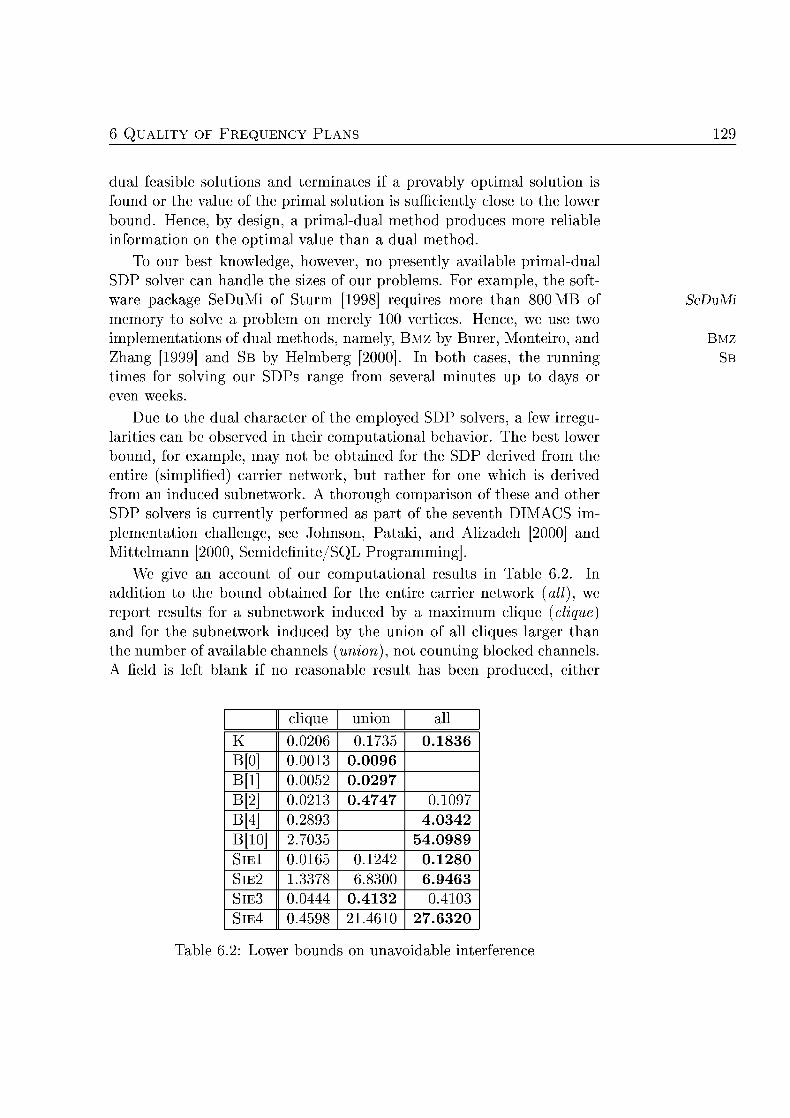
ALITY O F F N C Y P L A N S 12

d a l feasible s o l i o n s and terminates if a provably optimal solution is f o n d or the value of the primal solution is sufficiently close to the lower bound. Hence, by design, a pr imaldual method produces more reliable information on the optimal v a l e than a dual method.

To our best knowledge, however, no presently available primal-dual SDP solver can handle the s i e s of our problems. For example, the soft ware package SeDuMi of Sturm [1998] requires more than 800 MB of SeDuMi memory to solve a problem on merely 100 vertices. Hence, we use two implementations of dual methods, namely, B M Z by Burer, Monteiro, and BMZ Zhang [1999] and SB by Helmberg [2000]. In both cases, the running SB times for solving our SDPs range from several minutes up to days or even weeks.

Due to the dual character of the employed SDP solvers, a few irregu­larities can be observed in their computational behavior. The best lower bound, for example, may not be obtained for the SDP derived from the entire (simplified) carrier network, but rather for one which is derived from an induced subnetwork. A thorough comparison of these and other SDP solvers is currently performed as part of the seventh D M ACS im­plementation challenge, see Johnson, Pataki, and Al i adeh 2000] and

ittelman [2000, Semidefinite/SQL Programming].

We give an account of our computational results in Table 6.2. In addition to the bound obtained for the entire carrier network (all), we report results for a subnetwork induced by a maximum clique (clique) and for the subnetwork induced by the union of all cliques larger than the number of available channels (union), not counting blocked channels.

field is left blank if no reasonable result has been produced, either

clique nio all

0.0206 0.1735 0.1836 B[ 0 .01 0.0096 B[l 0.052 0.0297 B[2] 0.021 0. 0.1097 B[ 0.2893 03 B[1 2.7035 0989

0.0165 0.1 0.1280 1.337 6.83 6 . 9 6 3 0. 0 . 1 3 2 0.4103 0.4598 21.461 27.6320

Table 6. ower bounds n unavoidable i n t e r n c

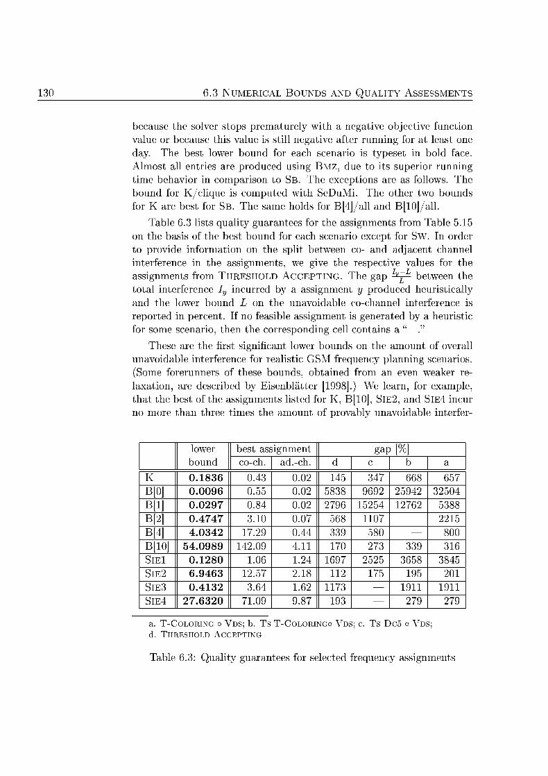
3 N U M A L UND ND ITY A S S S S M N T

because the solver stops prematurely with a negative objective function value or because this value is still negative after running for at least one day. The best lower bound for each scenario is typeset in bold face. Almost all entries are produced using BMZ, due to its superior running time behavior in comparison to SB. The exceptions are as follows. The bound for K/clique is computed with SeDuMi. The other two bounds for are best for SB The same holds for B[]/all and B[10]/all

Table 6.3 lists quality guarantees for the assignments from Table 5.15 on the basis of the best bound for each scenario except for Sw. In order to provide information on the split between co- and adjacent channel interference in the assignments, we give the respective values for the assignments from T H R E S H O D ACCEPTING. The gap IjL^- between the total interference Iy incurred by a assignment y produced heuristically and the lower bound L on the unavoidable cochannel interference is reported in percent. If no feasible assignment is generated by a heuristic for some scenario, then the corresponding cell contains a " "

These are the first significant lower bounds on the amount of overall unavoidable interference for realistic GSM frequency planning scenarios. (Some forerunners of these bounds, obtained from an even weaker re laxation, are described by Eisenblätter [1998].) We learn, for example, that the best of the assignments listed for K, B[10], SIE2, and SIE4 incur no more than three times the amount of provably unavoidable interfer

lower bound

best assignment gap [% lower bound ch. a d . h .

1836 0.43 0.02 145 47 668 657 B[ 0096 0.55 0.02 838 692 259 325 B[l] 0297 0.8 0.02 2796 525 12762 538 B[2] 3.1 0.07 68 07 221 B[4 03 7.29 0.4 339 B[10] 0989 42.09 4.11 273 339 316 Sl 128 1. 1. 1697 2525 365 3845 SI 6 . 9 6 3 2.57 2.18 12 175 195 01 SI 132 3.6 1.62 1173 1911 191 SI 27.632 71.09 9.87 193 279 279

a. T-COLORING o VDS; b. Ts T-COLORINGO VDS; C. T S D C 5 O VDS;

d. THRESHOLD ACCEPTING

Table 6. Quality g u a r n t e s for seleced quency asignment

A L Y OF F N C Y PLANS 31

ence. Yet, it is fair to say that our quality guarantees are not particularly strong. The gap between the upper and the lower bound is considerable in all cases. Nevertheless, the gaps are small enough so that the differ ences in quality between simple (and fast) methods like D R WITH COSTS and the more intricate method T H NG are not diminished.

One might conjecture that the large gaps between upper and lower bounds are to be blamed primarily on the lower bounds. After all, we are merely approximately solving a relaxation of a relaxation of the original problem. n the next section, however, we present a frequency plan for the scenario K that is much better than the best one reported in Table 5.15. This shows that the heuristically generated plans are ot generally as good as one might have hoped.

6.4 Relaxed and Ordinary Frequency Planning

We would like to turn a feasible frequency assignment for a simplified carrier network into a feasible one for the associated ordinary carrier network. The only change we allow is to relabel the channels in the assignments. Thus, among the \C\\ many equivalent assignments for the simplified carrier network we look for one which is feasible for the original problem (and incurs as little adjacent channel interference as possible). How to find such a permutation is the topic of this section.

The absence of locally blocked channels, of separation constraints larger than one, and of adjacent channel interference simplifies the tasks of a planning heuristic. Running the same heuristic methods as before, we often obtain frequency plans with less co-channel interference than in the original setting, and we try to take advantage of this as follows. First, we heuristically produce a frequency plan for the relaxed problem; then, provided the plan is feasible, we try to turn this plan into a feasible one for the original problem by relabeling the channels. If we succeed, the new plan will have the same amount of cochannel interference as the one for the relaxed case. The amount of additional adjacent channel interference should be as small as possible. Although this procedure is certainly of limited applicability, we obtain the best known frequency plan for scenario K in this way. This assignment incurs 18% less interference than the previously best one.

6 . 1 Feasibl rmutations

We start out by formally introducing the notion of a feasible permutation.

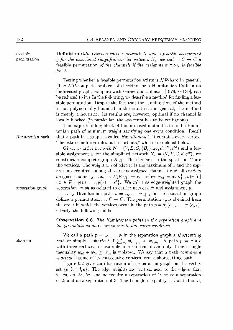
32 4 R L A ND O R Y F L A N N N G

easble D e f i n t i o n 6.5. Given a carrier nework N and a feasible asgnment ermutation y for the associated simplifie carrier netork Ns, we call 7 : C> C a

feasible permutation of t annel if t assignment TT O is feasible forN.

Testing whether a feasible permutation exists is A/'P-hard in general (The jVP-complete problem of checking for a Hamiltonian Path in an undirected graph, compare with Garey and Johnson [1979, GT39], can be reduced to it.) In the following, we describe a method for finding a fea­sible permutation. Despite the fact that the running time of the method is not polynomially bounded in the input size in general, the method is merely a heuristic. Its results are, however, optimal if no channel is locally blocked (in particular, the spectrum has to be contiguous).

The major building block of the proposed method is to find a Hamil tonian path of minimum weight satisfying one extra condition. Recall

Hamiltonian ath that a path in a graph is called Hamiltonian if it contains every vertex. The extra condition rules out "shortcuts," which are defined below.

Given a carrier network JV = (V, E, C, {Bv}v€V, d, co, ad) and a fea­sible assignment y for the simplified network Ns = (V,E,C,d,cC0) we construct a complete graph K\C\. The channels in the spectrum C are the vertices. The weight Wij of edge ij is the maximum of 1 and the sep­arations required among all carriers assigned channel and all carriers assigned channel , i.e., w: K\V\)> Z+,cc > WCC> = m a x j l , d(vx) vx E E : y(v) c,y(x) = c } . We call this edge-weighted graph the

searation gra eparation graph associated to carrier network iV and assignment y. Every Hamiltonian path p VQ,...,V\C\-I in the separation graph

defines a permutation np: C> C'. The permutation 7rp is obtained from the order in which the vertices occur in the path p irpci,..., 7rp

learly, the following holds.

Observation 6.6. Te Hamiltonian paths in the separation grap and e permutations on C are in one-to-one correspondence.

We call a path p = VQ, ... ,vi in the separation graph a shortcutting shortcut path or simply a shortcut if ^2i=i wVi_lVi < wvm. A path p = a,b,c

with three vertices, for example, is a shortcut if and only if the triangle inequality wab + w^ > wac is violated. We say that a path contains a shortcut if some of its consecutive vertices form a shortcutting path.

Figure 6.2 gives an illustration of a separation graph on the vertex set , 6, , e . The edge weights are written next to the edges; tha is, ab, a e, bd, and de require a separation of 1; ae,ce a separation of 2; and a separation of 3. The triangle inequality is violated once,

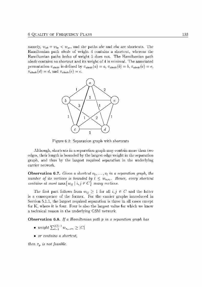
A L T Y OF F R E E N C LANS 13

namely, % + wbc ac, and the pahs abc and cba are shortcuts. The Hamiltonian path of weight 4 contains a shortcut, whereas the Hamiltonian paths bcdea of weight 5 does not. The Hamiltonian path abedc contains no shortcut and its weight of 4 is minimal The associated permutation >Kabedc is defined by nabedc(a) = a, 7abedc , Trabedc

nabedc , and 7abedc

Figur 6.2: Separation graph with sor tcut

Although, shortcuts in a separation graph may contain more than two edges, their length is bounded by the largest edge weight in the separation graph, and thus by the largest required separation in the underlying carrier network.

Observation 6.7. Given a shortcut VQ, ..., vi in a separation graph, the number of its vertices is bounded by I < wvm. Hence, every shortcut contains at most maxjwj \i,j } many vertices.

The first part follows from Wij > 1 for all i,j 6 C and the latter is a consequence of the former. For the carrier graphs introduced in Section 5.1.1, the largest required separation is three in all cases except for K, where it is four. Four is also the largest value for which we a technical reason in the underlying SM network.

Obervati 6.8. If a Hamiltonian path p in a separation graph has

• weight Y}S Vi_lVi C\

or contains shortcut

then 7TP is not feasible.

13 6.4 R L A D O F R E E N LANN

Hence, only Hamiltonian paths with all edges having weight 1 may give rise to feasible permutations. The converse, hwever, holds only if no channel is locally unavailable.

In addition to finding some feasible permutation, we also want to keep the adjacent channel interference under control. This issue is addressed as follows. We set /^ Wi | maxj'a^ eC^ for every edge in the separation graph, where

d: ->• K % cad

v: {w)j

Then Wij < Uj < w^ + \C\ , and every Hamiltonian path of least weight with respect to I is of least weight with respect to w. With our preceding discussion in mind, the following is easy to see.

Propositio 6.9. Given are a carrier network N without blocked chan­nels, that is, Bv = 0 for all v £ V, and a feasible assignment y for the cor responding simplified carrier network. Moreover, let p be a Hamiltonian path of least weight with respect to I in the eparation graph associated t

and y. Then the folloing holds. If p has weight \C\ 1 with respect to w and does not contain a

shortcut, then npoy is a feasible solution for the carrier network N. Fur thermore, iipoy incurs the least amount of adjacent channel interference among all feasible assignments n o y.

Next, we explain how such a Hamiltonian path can be computed heuristically by solving a modified A V G S E S M P R E M

6.42 T o u s without s h t c u t s

Finding a Hamiltonian path of minimum weight in a graph is traditionally done by solving a T R A V L I N G SALESMAN PROBLEM. An instance of the

TSP TRAVELING SALESMAN PROBLEM (TSP) consists of a complete graph tour together with edge weights. The task is to find a minimum weight tour

(or cycle) containing every vertex. The weight of an edge is usually called its length in the context of a TSP, and a tour of minimum weight

shortest tour is called a shortest tour. We stick to this tradition. The TSP and many of its variations receive considerable attention in the literature. Jünger, Reinelt, and Rinaldi [1995a], for example, give a survey on the TSP, and

pplegate, Bixby, Chvatal, and Cook [1998] report on recent progress. Our restricted Hamiltonian path problem is transformed into a re­

stricted SP as follows. First, we add one additional vertex a to the

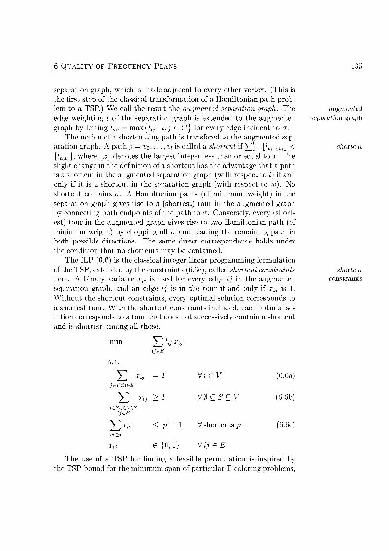
A L T Y O F F R E E N C LANS 135

separation graph, which is made adjacent to every other vertex. (This is the first step of the classical transformation of a Hamiltonian path prob­lem to a TSP.) We call the result the augmented separation graph. The augmente edge weighting / of the separation graph is extended to the augmented searation gra graph by letting luv maxj/j,, \ i,j E C } for every edge incident to o.

The notion of a shortcutting path is transfered to the augmented sep­aration graph. A path p = i>0 , . . . , vi is called a shortcut if Yli=i lAi-n>d < shortcut lAwJ) where [x\ denotes the largest integer less than or equal to x. The slight change in the definition of a shortcut has the advantage that a path is a shortcut in the augmented separation graph (with respect to I) if and only if it is a shortcut in the separation graph (with respect to w). No shortcut contains a. A Hamiltonian paths (of minimum weight) in the separation graph gives rise to a (shortest) tour in the augmented graph by connecting both endpoints of the path to a. Conversely, every (short est) tour in the augmented graph gives rise to two Hamiltonian path (of minimum weight) by chopping off a and reading the remaining path in both possible directions. The same direct correspondence holds under the condition that no shortcuts may be contained.

The ILP (6.6) is the classical integer linear programming formulation of the TSP, extended by the constraints (6.6c), called shortcut constraints shortcut here. A binary variable x^ is used for every edge ij in the augmented constraints separation graph, and an edge ij is in the tour if and only if xij is 1. Without the shortcut constraints, every optimal solution corresponds to a shortest tour. With the shortcut constraints included, each optimal so­lution corresponds to a tour that does not successively contain a shortcut and is shortest among all those.

min y xi ijE

s.t.

^ x^ =2 (6.6a) evE

^2 Xi ßCSC (6.6b) s,jev\

E

x^ p \ s h o r t c u t s p (6.6c) j

x^ {0 EE

The use of a TSP for finding a feasible permutation is inspired by the SP bound for the minimum span of particular T-coloring problems,

E

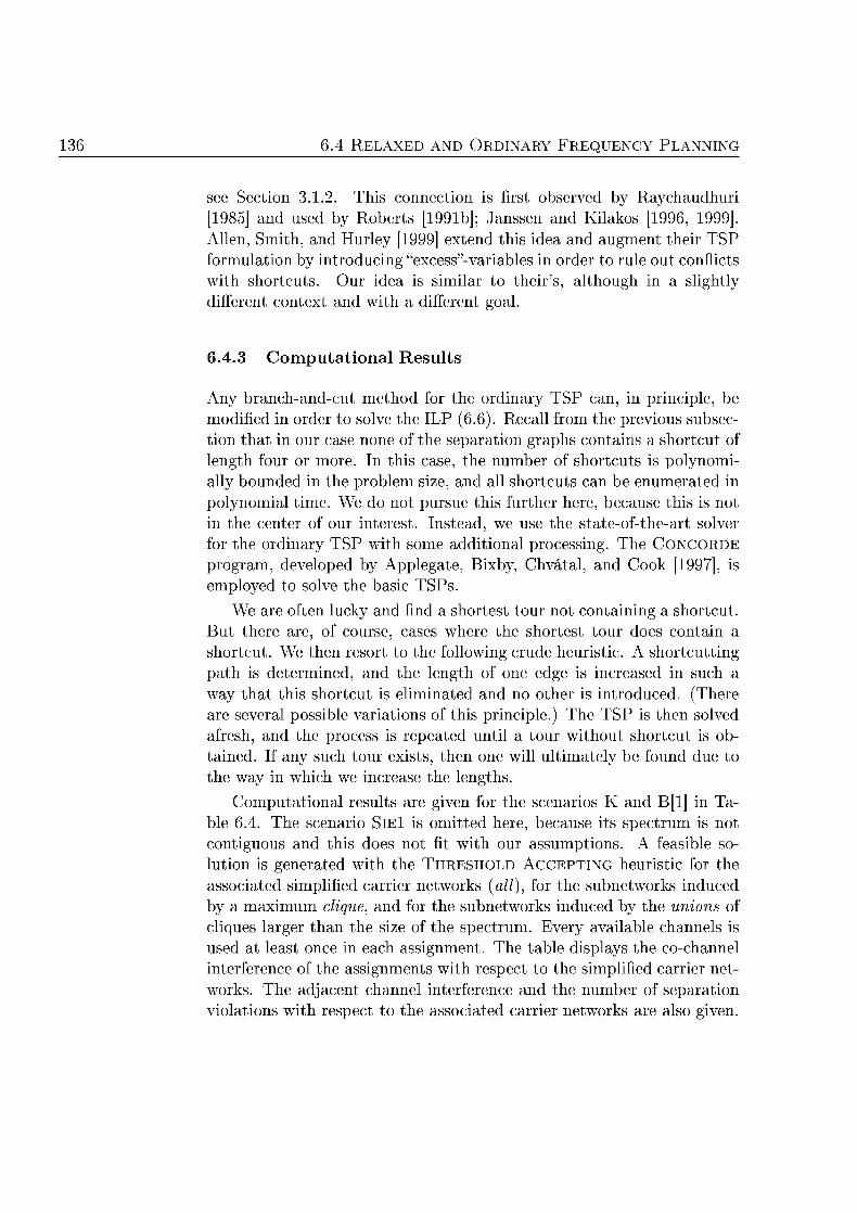
13 6.4 R L A D O F R E E N LANN

see Section 3.1.2. This connection is first observed by Raychaudhuri [1985] and used by Roberts [1991b]; Janssen and Kilakos [1996, 1999] Allen, Smith, and Hurley [1999] extend this idea and augment their TSP formulation by introducing "excess"variables in order to rule out conflicts with shortcuts. Our idea is similar to their's, although in a slightly different context and with different goal

6 . 4 3 o m u t a t i o l R s u l t s

Any branch-and-cut method for the ordinary TSP can, in principle, be modified in order to solve the ILP (6.6). Recall from the previous subsec­tion that in our case one of the separation graphs contains a shortcut of length four or more. In this case, the number of shortcuts is polynomi ally bounded in the problem size, and all shortcuts can be enumerated in polynomial time. We do not pursue this further here, because this is not in the center of our interest. Instead, we use the s t a t e o f t h e a r t solver for the ordinary TSP with some additional processing. The C O N C O R D E

program, developed by Applegate, Bixby, hvätal, and ok [1997], is employed to solve the basic TSPs.

We are often lucky and find a shortest tour not containing a shortcut. But there are, of course, cases where the shortest tour oes contain a shortcut. We then resort to the following crude heuristic. A shortcutting path is determined, and the length of one edge is increased in such a way that this shortcut is eliminated and no other is introduced. (There are several possible variations of this principle.) The TSP is then solved afresh, and the process is repeated until a tour without shortcut is ob­tained. If any such tour exists, then one will ultimately be found due to the way in which we increase the lengths.

Computational results are given for the scenarios K and B[l] in Ta­ble 6.4. The scenario SlEl is omitted here, because its spectrum is not contiguous and this does not fit with our assumptions. A feasible so­lution is generated with the T H R E S H O L D A C C E P T I N G heuristic for the associated simplified carrier networks (all), for the subnetworks induced by a maximum clique, and for the subnetworks induced by the unions of cliques larger than the size of the spectrum. Every available channels is used at least once in each assignment. The table displays the co-channel interference of the assignments with respect to the simplified carrier net works. The adjacent channel interference and the number of separation violations with respect to the associated carrier networks are also given.

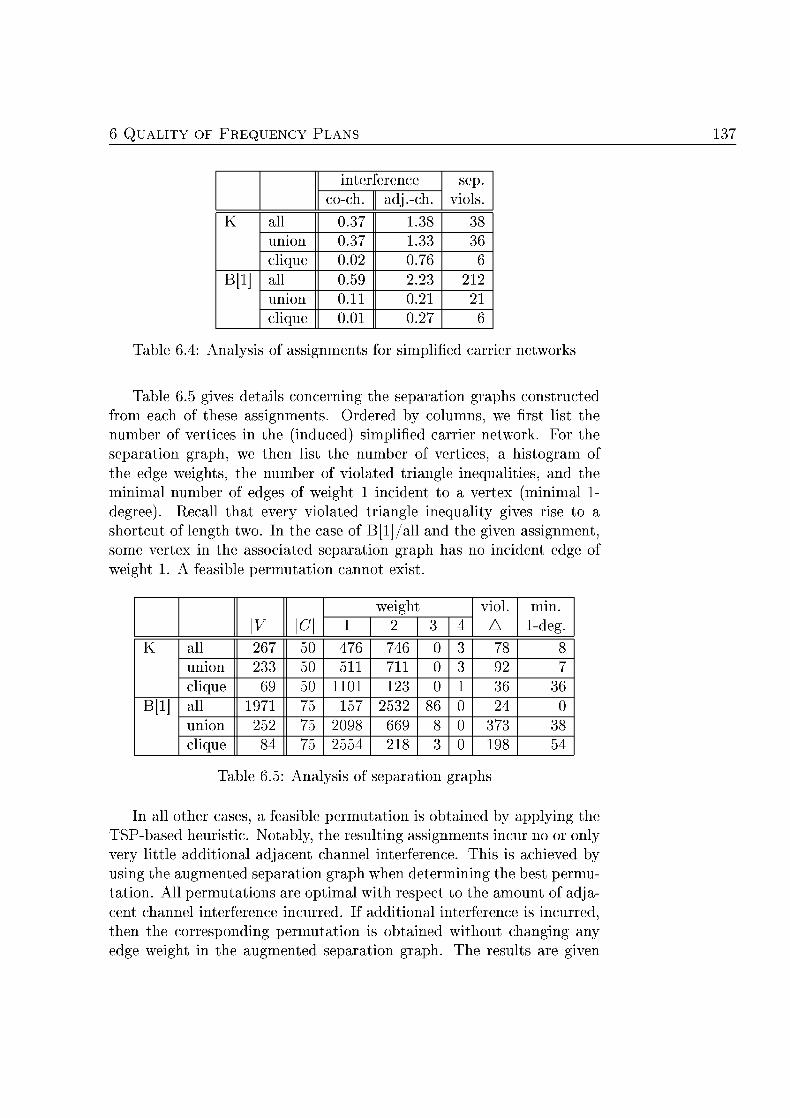
A L T Y OF F R E E N C LANS 137

interference sep. viols. o-h. adj.ch.

sep. viols.

all 0.37 1.38 38 nio 0.37 1.

clique 0.02 0.76 [l] all 0.59 2.23 212 [l]

nio 0.1 0.21 21 [l]

clique 0.01 0.2

Table 6. nalysis of asignments for simplified carier neworks

Table 6.5 gives details concerning the separation graphs constructed from each of these assignments. Ordered by columns, we first list the number of vertices in the (induced) simplified carrier network. For the separation graph, we then list the number of vertices, a histogram of the edge weights, the number of violated triangle inequalities, and the minimal number of edges of weight 1 incident to a vertex (minimal 1-degree). Recall that every violated triangle inequality gives rise to a shortcut of length two. In the case of B[l]/all and the given assignment, some vertex in the associated separation graph has no incident edge of weight 1. feasible permutation cannot exist.

C\ weight viol min.

1-deg. C\ viol min.

1-deg.

all 267 50 76 78 nio 23 51 71 92

clique 69 01 123 B[l] all 1971 75 2532 B[l]

nio 25 75 098 69 373 38 B[l]

clique 75 255 218 198

Table 6.5: nalysis of sparation graphs

n all other feasible permutation is obtained by applying the TSPbased heuristic. Notably, the resulting assignments incur no or only very little additional adjacent channel interference. This is achieved by using the augmented separation graph when determining the best permu­tation. All permutations are optimal with respect to the amount of adja­cent channel interference incurred. If additional interference is incurred, then the corresponding permutation is obtained without changing any edge weight in the augmented separation graph. The results are given

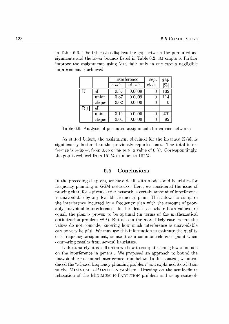
138 6.5 C O O N S

in Table 6.6. The table also displays the gap b e t w e n the permuted as signments and the lower bounds listed in Table 6.2. Attempts to further improve the assignments using V fail: only in one case a negligible improvement is achieved.

interference sep. viols.

gap o-ch. adj.ch.

sep. viols.

gap

all 0.37 0.0009 102 nio 0.37 0 . 0 9 11

clique 0.02 0. B[l] all B[l]

nio 0.1 0. B[l]

clique 0.01 0. 92

Table 6. nalysis of permuted asignments for ca r ie r neworks

As stated before, the assignment obtained for the instance K/all is significantly better than the previously reported ones. The total inter ference is reduced from 46 or more to a value of 37. orrespondingly, the gap is reduced from 51 % or more to 102 %.

6.5 onclusions

In the preceding chapters, we have dealt with models and heuristics for frequency planning in SM networks. Here, we considered the issue of proving that , for a given carrier network, a certain amount of interference is unavoidable by any feasible frequency plan. This allows to compare the interference incurred by a frequency plan with the amount of prov-ably unavoidable interference. In the ideal case, where both values are equal, the plan is proven to be optimal (in terms of the mathematical optimization problem FAP). But also in the more likely case, where the values do not coincide, knowing how much interference is unavoidable can be very helpful. We may use this information to estimate the quality of a frequency assignment, or use it as a common reference point when comparing results from several heuristics.

Unfortunately, it is still unknown how to compute strong lower bounds on the interference in general. We proposed an approach to bound the unavoidable co-channel interference from below. In this context, we intro­duced the "relaxed frequency planning problem" and explained its relation to the M N I M U M K - P N problem. Drawing on the semidefmite relaxation of the M M K - P O N problem and using s ta teof

A L T Y OF F R E E N C LANS 139

the-art SDP olver, we computed the first significant lower bounds for the frequency planning problem FAP. In the best case, we show that a frequency assignment incurs merely twice the amount of provably un­avoidable interference. In the worst case, however, the factor is almost 60. This situation is not satisfactory and deserves further investigations

A drawback of our approach is that solving the large semidefinite programs is presently quite challenging and may take days or even weeks of running time. Moreover, it is not yet clear ho information acquired through the solution of the semidefinite program can be effectively ex­ploited to generate better frequency plans. This also deserves additional ttention.

We pointed out that for our scenarios many triangles in the carrier graph violate the triangle inequality significantly. Alternative approaches to compute strong lower bounds on the unavoidable interference may fail if they rely on the triangle inequalities being (almost) fulfilled.

Finally, frequency planning methods for GSM networks have been developed for almost a decade now, and several of the recent methods show good performance in practice. One might conclude that frequency planning, at least from a practical point of view, can be considered as "solved," see also our comments in Section 5.6. In this respect, however, it is irritating that we were able to provide a significantly better solution to a realistic planning problem than known before. The employed method, i.e., first solving the relaxed frequency planning problem heuristically and then trying to fix all separation violations by relabeling the chan­nels, is certainly of limited applicability. Its success, however, documents that improvements on the presently used techniques are possible. This will be of interest for GSM network planners if, at some future point in time, frequency planning again becomes a limiting factor. From the com­binatorial optimization point of view, the frequency assignment problem FAP, even on the rather restricted set of realistic planning data, is clearly ot yet fully mastered.

CHAPTER 7

Partition Polytopes

The focus of the remaining two chapters is no longer directly on frequency assignment. Instead, we pursue the problem of finding a ^-partition of the vertex set in a complete graph such that the edge weights in the induced subgraphs are minimal ( M N I M U M KPARTITION) . We are led to this problem by its close relation to the relaxed frequency planning problem, see Section 6.2.

In this chapter, we mostly survey results from the literature concern­ing the polytope V<k{Kn), which is defined by the convex combination of all feasible solutions to the ILP formulation (6.2) of the MINIMUM

K-PARTTION problem. This polytope is full-dimensional in the space spanned by the edge variables. A particular emphasis is on the hyper-metric inequalities. Moreover, we address the complexity of solving the separation problem for several classes of (facetdefining) inequalities.

n the next chapter, we turn to the semidefinite relaxation (6.5) of the MINIMUM K P R T I I O N problem. The set of the relaxation's feasible solutions is studied and related to the polytope V<Kn This is done mostly on the basis of the hypermetric inequalities.

The chapter is organized as follows. Section 7.1, two binary lin­ear programming formulations of the MINIMU K-PARTITION problem are compared. We explain why the formulation (6.2) is favored. In Sec tion 7.2, the polytope obtained for k = n is studied. Several classes of facet-defining inequalities from the literature are reviewed. In Section 7.3, we consider the polytope V<Kn) for k < n with a strong emphasis on the hypermetric inequalities. In Section 7.4, we briefly discuss the issue of developing a branch-and-cut algorithm for the MINIMUM K-PARTITION

problem on the basis of the classes of valid inequalities presented in the preceding two sections.

Appendix A contains a compilation of mathematical notions, which are used but not introduced here.

Usually, we assume k > 3 or even k > 4 in the following. Clearly, if , then only one "partition" exists; in the case of k the M

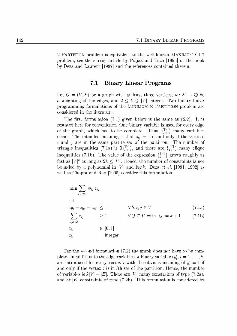
R P R M S

2-PARTITION problem is equivalent to the wellknown MAXIMUM C U T

problem, see the survey article by Poljak and Tuza [1995] or the book by Deza and Laurent [1997] and the references contained therein.

1 Binary Linear Programs

Let G = (V, E) be a graph with at least three vertices, w: E —) Q be a weighting of the edges, and 2 < k \ integer. Two binary linear programming formulations of the M K - P I O problem are considered in the literature.

The first formulation (7.1) given below is the same as (6.2). It is restated here for convenience. One binary variable is used for every edge of the graph, which has to be complete. Thus, (2 ' ) many variables occur. The intended meaning is that Zij — 1 if and only if the vertices i and j are in the same partite set of the partition. The number of triangle inequalities (7.1a) is 3( ' 3 ' ) , and there are L\) many clique

inequalities (7.1b). The value of the expression {L\) grows roughly as fast as \V\k as long as 2k < V\. Hence, the number of constraints is not bounded by a polynomial in \V\ and \ogk. Deza et al. [1991, 1992] as well as Chopra and Rao [1995] consider this formulation.

Vhje 7.1a)

VQC V with k + 7.1b

For the second formulation (7.2) the graph does not have t be com plete. In addition to the edge variables, k binary variables y\, I . . . k, are introduced for every vertex i with the obvious meaning of y\ 1 if and only if the vertex i is in /th set of the partition. Hence, the number of variables is k\V\ + \E\. There are |V| many constraints of type (7.2a), and 3k \ constraints of type (7.2b). This formulation is considered by

inz2 i j v

s.t.

Y^ za > jeQ

Zi E [0,1] z^ integer

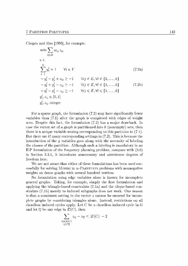
P E S

Chopra and Rao [1993], for example.

min ij zi

s.t.

7 - 2 a )

+ ^ > ij e E e { . . . k }

Zij > ij e £ e { . . . k} 7.2b)

+ y Zij > ij e E e { . . . k )

zijE [ 1 ]

Zij integer

For a sparse graph, the formulation 7.2) may have significantly fewer variables than (7.1) after the graph is completed with edges of weight zero. Despite this fact, the formulation (7.2) has a major drawback. In case the vertex set of a graph is partitioned into k (nonempty) sets, then there is a unique variable setting corresponding to this partition in (7.1). But there are A;! many corresponding settings in (7.2). This is because the introduction of the y variables goes along with the necessity of labeling the classes of the partition. Although such a labeling is mandatory in an ILP formulation of the frequency planning problem, compare with (3.6) in Section 3.3.1, it introduces unnecessary and nwelcome degrees of freedom here.

We are not aware that either of these formulations has been used suc­cessfully for solving MINIMUM K-PARTITION problems with nonnegative weights on dense graphs with several hundred vertices.

No formulation using edge variables alone is known for incomplete general graphs. Taking, for example, simply the first formulation and applying the trianglebased constraints (7.1a) and the clique-based con­straints 7.1b) merely to induced subgraphs does not work. One reason is that a consistent setting in the vector z cannot be ensured for incom plete graphs by considering triangles alone. Instead, restrictions on all chordless induced cycles apply. Let C be a chordless induced cycle in G and let rj be any edge in , then

X) %-% ijeE(c)

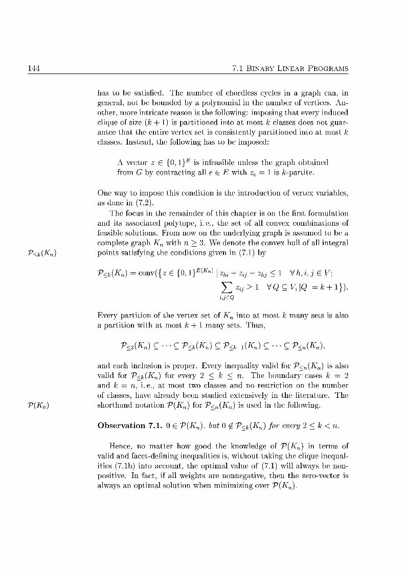
44 R P R M S

has to be satisfied. The number of chordless cycles in a graph can, in general, not be bounded by a polynomial in the number of vertices. An­other, more intricate reason is the following: imposing that every induced clique of size (k + 1) is partitioned into at most k classes does not guar antee that the entire vertex set is consistently partitioned into at most k classes. Instead, the following has to be imposed

A vector E {0,1} is infeasible unless the graph obtained from by contracting all with z is A;-partite.

One way to impose this condition is the introduction of vertex variables, as done in (7.2).

The focus in the remainder of this chapter is on the first formulation and its associated polytope, i.e., the set of all convex combinations of feasible solutions. From now on the underlying graph is assumed to be a complete graph Kn with n > 3. We denote the convex hull of all integral

k{K) points satisfying the conditions given in (7.1) by

V< = c n v ( { E { K ^ zhi + zi:j - zhj < VhjeV;

^ % > ! VQcy, =A; + 1} Q

Every partition of the vertex set of Kn into at most k many sets is also a partition with at most k + many sets. Thus,

V<Kn C • • • V<Kn V<k+1Kn C • • • V<Kn

and each inclusion is proper. very inequality valid for V<n(Kn is also valid for V<k{Kn) for every < k < n. The boundary cases k 2 and k = n, i.e., at most two classes and no restriction on the number of classes, have already been studied extensively in the literature. The

(Kn) shorthand notation Kn for V< is used in the following.

Observ 7.1 Kn, but 0 0 V< for every

Hence, no matter how good the knowledge of V{Kn) in terms of valid and facet-defining inequalities is, without taking the clique inequal ities (7.1b) into account, the optimal value of (7.1) will always be non-positive. In fact, if all weights are nonnegative, then the zero-vector is always an optimal solution when minimizing over VKn

P E S

The Polytope T(Kn)

Our survey on properties of V{Kn) does not aim at completeness. The Ph. D. thesis of Rutten [1998] contains a more comprehensive compilation (which, however omits the results of Deza et al [1991])

Propos i t ion 7.2 (Grötsch nd Wakabayashi [1990]) The poly-ope V(Kn has dimension 2 )

The clique inequalities (7.1b) are void for V(Kn). The remaining constraints in the binary linear programming formulation are the trian­gle inequalities (7.1a), the bounds on the variables, and the integrality conditions. The bound constraints are called trivial inequalities trivial inequalities

Propos i t ion 7.3 (Grötschel a d Wakabayashi [1990]). Wth respec the poltope V(Kn > 3

every nonnegaivi consrain Zij > defnes a face

every riangle inequaliy (7.1a) defnes a face

no upper bound consrain z^ < 1 defnes a facet

Some properties are shared by all nontrivial facet-defining inequalities for V(Kn). One of the three properties listed next concerns the support graph of an inequality. Given some inequality aTz > ao, the suppor graph of aT > ao or just , is the subgraph of Kn induced by all edges support graph ij with

Propos i t ion 7.4 ( G r ö t s h e l and Wakabayashi [1990]). L aTz < ÜQ e a nontrivial inequali defining a facet ofV{Kn) then

ao >

has posiive and negaive enries

he suppor graph of Tz < ao is 2-conneced

Corollary 7.5. Under the same assumpions as in Proposiion 74 the subgraph H+ of Kn induced by E = [i e E(Kn) \ 0} is a connected, spannig subgraph of the suppor graph

Proof Let [S, T] be any cut in the 2-connected support graph H i n u c e d by Ea. There exists a vector ~ E 0 l}E(K> satisfying aT~z ao > 0 for which restriction to the cut S, T] is not identical to zero. (Otherwise, the facet efined by aT~z > ÜQ woul be contained in all the trivial facets

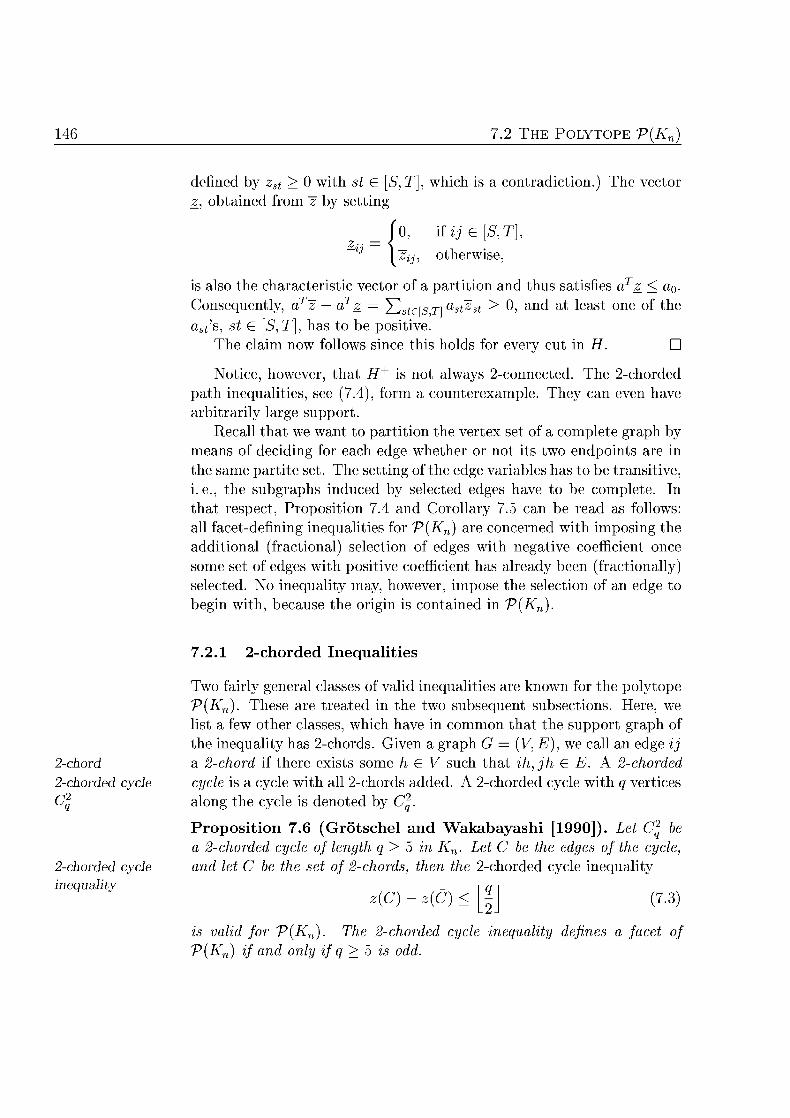
2 L Y T P E V{Kn)

efined by zst > 0 with st E [ T , which is a contraiction.) The vector _ obtained from ~z by setting

\Hje[ST

otherwise,

is also the characteristic vector of a partition and thus satisfies a1\ < CLQ Consequently, aT aF_ — astersT] ~Zt > , and at least one of the aS 's, st E [S,T\, has to be positive.

The claim now follows since this h o l s for every cut in H D

Notice, however, that H is not always 2-connected. The 2-chorded path inequalities, see (7.4), form a counterexample. They can even have arbitrarily large support.

Recall that we want to partition the vertex set of a complete graph by means of deciding for each edge whether or not its two endpoints are in the same partite set. The setting of the edge variables has to be transitive, i.e., the subgraphs induced by selected edges have to be complete. In that respect, Proposition 7.4 and Corollary 7.5 can be read as follows: all facetdfining inequalities for V(Kn) are concerned with imposing the additional (fractional) selection of edges with negative coefficient once some set of edges with positive coefficient has already been (fractionally) selected. No inequality may, however, impose the selection of an edge to begin with, because the origin is contained in V(Kn)

2-cho 2-cho cycl

2-chorde cyl inequalit

7.2.1 c h d e d I u a l i t i e

Two fairly general classes of valid inequalities are known for the polytope V(Kn). These are treated in the two subsequent subsections. Here, we list a few other classes, which have in common that the support graph of the inequality has 2-chords. Given a graph G (V, E), we call an edge ij a 2-chord if there exists some h E V such that h jh E E. A 2-chorded cycle is a cycle with all 2-chors add A 2-chor cycle with q vertices along the cycle is denote by C2

Proposition 7.6 (Grötschel and Wakabayashi [1990]). Let C2q he

a 2-chorded cycle of length q > 5 in Kn. Let C b the edges of the cycle and let C b he set of 2-chords, then he 2-chor cycle inequality

z(C) z(C) < 7.3)

is valid for V{Kn). The 2-chor cycle equal efines a face V(Kn) and only if q 5 s odd

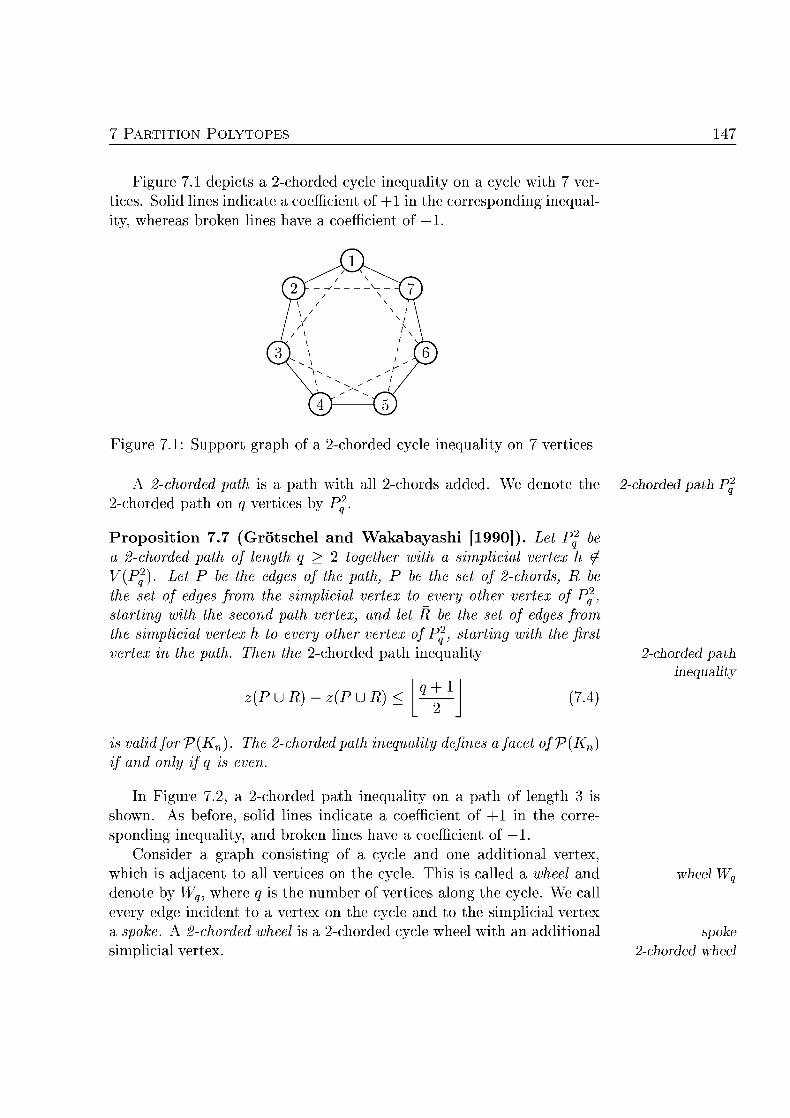
Figure 7.1 depicts a 2chorded cycle inequality on a cycle with 7 ver tices. Solid lines indicate a coefficient of +1 in the corresponding inequal ity, whereas broken lines have a coefficient of —1

Figur 7.1 Support graph of a or ycle inequality o 7 v e i c

A 2-chorded path is a path with all 2-chors a d d . W enote the 2-chorded path P 2 c h o r d path on q vertices by P£

Proposition 7.7 (Gröschel and Waka a 2-chord path of length q > 2 together V(Pg). L P b the edges of the path P the set of dges from the impliial verex starng wh the second path vertex, an let the simplcial verex h to every other vertex verex i the pa Then the 2-chordd path

z(P UR)- z(P U R) <

s valid for V(Kn) The 2-chor pa nequal efins a V(Kn) f and onl if i even

In Figure 7.2, a 2-chorded path inequality on a path of length 3 is shown. As before, soli lines indicate a coefficient of +1 in the corre sponding inequality, and broken lines have a coefficient of —1.

Consider a graph consisting of a cycle and one additional vertex, which is adjacent to all vertices on the cycle. This is called a wheel and denote by Wg, where q is the number of vertices along the cycle. We call every edge incident to a vertex on the cycle and to the simplicial vertex a spoke. A 2-chordd wheel is a 2-chordd cycle wheel with an additional simplicial vertex.

ayashi [1990]). Lt th a simplicial vetex

ie the set of 2-chords, R o every other vertex o Pg

R e the set o dges from of Pg, starng w the fir inequality

q + 7.4)

2-corded pat inequalit

spoke 2-corded ee

7.2 E P O V{Kn)

Figur 7. Support graph of a chor path inequalit

Proposition 7.8 (Grötschel and Wakabayashi [1990]). L C\ 2-chorded cycle of even length q > 8 n Kn and let h $ V(C^ We deno by C he edges f the cycle, by the set of 2-chords, by he set o dges from he simplicial vertex h to the every other vertex of C^, an by

2-chorded even the se remaiing spokes The 2 - c h o r d even wheel inequality eel inequalit

C UR)CuR)<j- 7.5)

s valid for V(Kn) and defines a face V{Kn)

A 2-chordd even wheel inequality for a wheel with 8 vertices on the rim is depicted in Figure 7.2. Again, solid lines indicate a coefficient of +1 in the corresponing inequality and broken lines a coefficient of —1

Figur 7. Support graph of a hor ven whel inequalit

Generalizations of the previous three types of inequalities are given by Rutten [1998]

7.2.2 Clique-web Iequal i t ies and S c i a l Cases

The next two types of inequalities are specializations of the rather general cliqueweb inequalities (except for bounary cases), which are described at the end of this section.

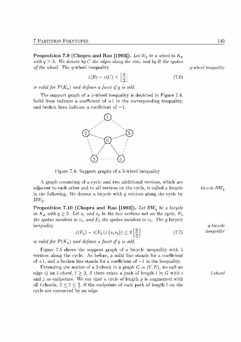
RTITI P O 49

roposition 7.9 ( C h o p a and Rao [1993]). Let W e a heel in Kn

th q > 3. W denote by C the edges along the rm, an by the spokes the wheel The gwheel inequality

R) - C) < 7.

s valid for V(Kn) an defins a f f s odd

The support graph of a 5-wheel inequality is depicte in Figure 7.4. Solid lines indicate a coefficient of +1 in the corresponing inequality, and brken lines indicate a coefficient of —1

el inequli

Figure 7.4 Support graphs of a 5 w h e l inequality

A graph consisting of a cycle and two additional vertices, which are adjacent to each other and to all vertices on the cycle, is called a bicycl in the following. We denote a bicycle with q vertices along the cycle by BWq

Proposit ion 7.10 C h o p a and R [1993]). Let BW a bcycl n Kn wh q > 3 s± and be he two v t s no on cycle, E^

the spoke cidet t s\, an spok iidet t ^-bicycle inequality

{Ei) - (E U {Sls2}) < 2 [J 7.7)

s valid for V(Kn) an defins a fac s odd

Figure 7.5 shows the support graph of a bicycle inequality with 5 vertices along the cycle. As before, a solid line stands for a coefficient of +1, and a broken line stands for a coefficient of — in the inequality.

Extening the notion of a 2-chord in a graph G (V, E), we call an edge ij an lchord, I 2, if there exists a path of length / in G with i and j as endpoints We say that a cycle of length p is augmented with all lchords, 2 < / < | , if the endpoints of each path of length / on the cycle are connected by an edge.

cye BW

q-bicyc inequalit

ch

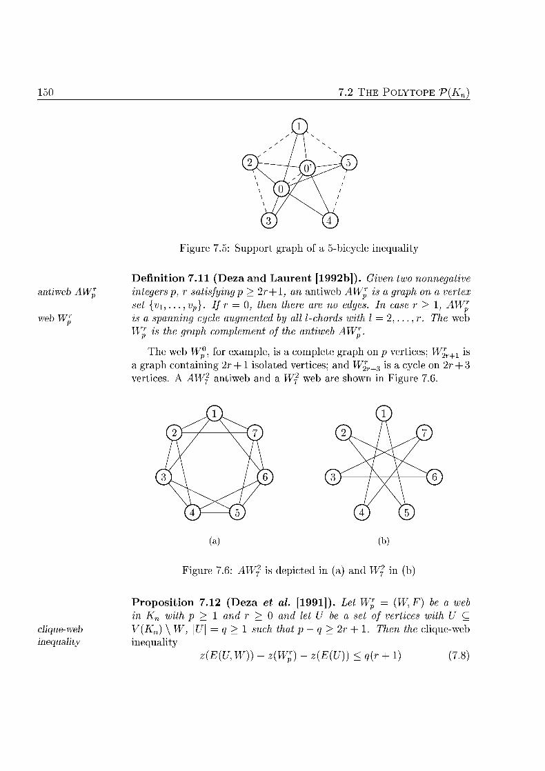
7.2 E P O V{Kn)

Figur 7. Support graph of a 5bicycle inequalit

e f i t i o n 7.11 (Deza and Laurent [1992b]). Given two nonnega antib A eg , r satifng p > 2r , an antiweb AW* s a graph on a v

set {vi,..., v}. I = 0 then there are no e d . I case > 1, AW is a spanning cycle augmed by all lchords with I ,... , . T web W* th graph compl th anib AW*

The web W, for example, is a complete graph on p vertices; WJr+1 is a graph containing 2r + 1 isolated vertices; and VFJr+3 is a cycle on 2r + 3 vertices A AWf antiweb and a W web are shown in Figure 7.6

a) b)

Figure 7 . : A is epicte in a) an in b)

Proposition 7.12 ( e z a et al. [1991]). L Wrv W, F) b

n Kn wth p > 1 an > and lt U be s with U C clique-w V(Kn) \ W, \ such tha 2r cliqueweb inequalit inequality

(E{ W)) - ) - (E()) < q{r + 7.

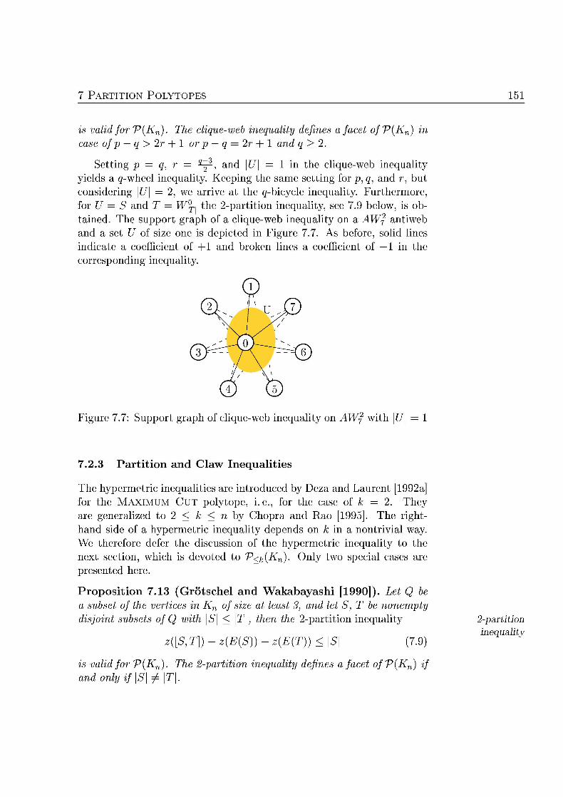
RTITI P O 51

is valid r V(Kn) e b uali defins a V{Kn) cas 2r or p 2r + 1 an q>2

Setting p = q, r ^ , and \U\ 1 in the cliqueweb inequality yields a (/-wheel inequality Keeping the same setting for p q, and r, but considering \U 2, we arrive at the ^bicycle inequality. Furthermore, for U = S and T = W?T> the 2-partition inequality, see 7.9 below, is ob­tained. The support graph of a cliqueweb inequality on a AW% antiweb and a set U of size one is depicted in Figure 7.7. As before, solid lines indicate a coefficient of an broken lines a coefficient of 1 in the corresponding inequality

Figure 7.7 Support graph of cliqueweb inequality on with \

7.2. on Cl qual

The hypermetric inequalities are introduced by Deza and Laurent [1992a for the MAXIMUM CU polytope, i.e., for the case of k 2. They are generalized to 2 < k < n by Chopra and Rao [1995]. The right hand side of a hypermetric inequality depends on k in a nontrivial way. We therefore defer the discussion of the hypermetric inequality to the next section, which is evote o V<k{Kn). Only two special cases are presente here.

Proposition 7.13 (Grötschel and Wakabayashi [1990]). Let Q subs of t ve n Kn of iz t last 3, and let S, T be nonmp

disjo subss o th \S\ 2-partition inequality 2-partitio inequalit

([T])-(E())-(E()) (7.9)

is valid for V(Kn) 2-paron qual defins a fac V(Kn) and only if \S\ ^

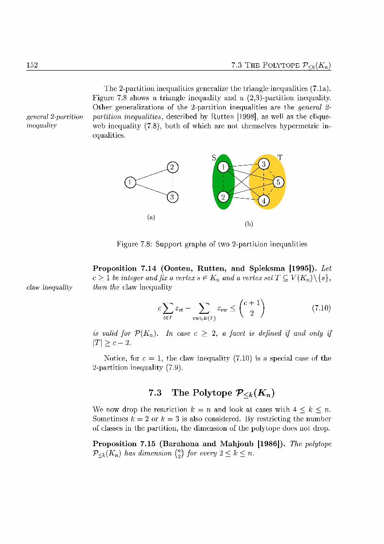
7.3 E P O V<k(Kn)

The 2par t i t ion inequalities generalize the t i ang le inequalities (7.1a). Figure 7.8 shows a triangle inequality and a (2,3)-partition inequality. Other generalizations of the 2-partition inequalities are the general 2-

general 2-partiti partition inequalites, described by Rutten [1998], as well as the clique inequalit web inequality ( 7 ) , both of which are not themselves hypermetric in­

equalities

ig p o t g wo ition i n l i t i e

Propos i t ion 7.14 (Oosten, R u t t e n , nd ieksma [1995]). L 1 e integer and fix a v e x s G Kn an a v C V {Kn)\{s

l inequalit he claw inequality

c 5> E *™ 71

vwE(T)

s valid for V{Kn) case c , a fac defined i an onl T\ > + 2

Notice, for c = 1, the claw inequality 7 1 ) is a special case of the 2-partition inequality 79)

7.3 The Polytope T<k{Kn)

We now drop the restriction k = n and look at cases with 4 < k < n. Sometimes k = 2 or k = 3 is also considered. By restricting the number of classes in the partition the dimension of the polytope does not drop.

Propos i t ion 7 1 5 ( B a r o n nd M h j u b [1986]) polop V<k(Kn) has dinsion (™) for ry 2 k <

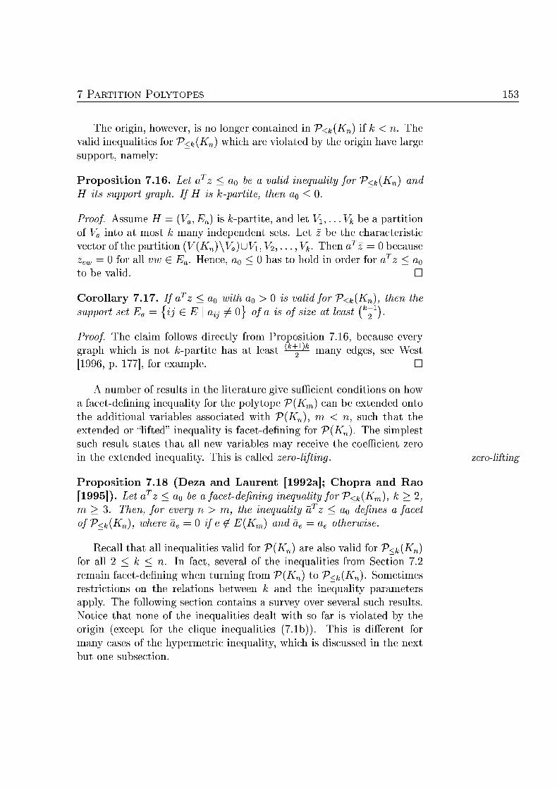
RTITI P O

The origin, h o w e v , is no longe contained in V<k{Kn) if k < n. The valid inequalities for V<k(Kn) which are violated by the origin have large support namely:

Propos i t ion 7.16. Lt a ÜQ a valid iqual for V<k(Kn) an s support graph f H s kpar t n a0

Proo. Assume H — (Va, Ea) is ^-partite, and let , . . . 14 be a partition of Va into at most k many independent sets et z be the characteristic vector of the partition (V(Kn)\V)U V2, • • • 14- Then aTz = because zvw — 0 for all vw £ E. Hence has t hold in order for o be valid. D

Corolla 1 az < a0 0 > is valid for V<k{Kn), suppor et E = \ £ E \ a^ ^ 0} f s of iz t last ^"1)

Proof. The claim follows directly from Proposition 7.16, because every graph which is not fc-partite has at least * + many edges, see West 199 p. 1 for example D

A number of results in the literature give sufficient conditions on how a facet-defining inequality for the polytope V(Km) can be extended onto the additional variables associated with V(Kn), m < n, such that the extended or "lifted" inequality is facet-defining for V(Kn). The simplest such result states that all new variables ay receive the coefficient zer in the extended inequality. This is called ro-lng. zerolifti

Propos i t ion 7 1 eza and a u e n t [1992a]; Chopra and R a [1995]). Let z a facetdefinng inequalit for V<k{Km), > 2,

> 3. Then, fo evry n m, the inequality z < defins a facet V<k(Kn), wh ae if e £ E{Km) and ae ae otrwi

Recall that all inequalities valid for V(Kn) are also valid for V<k(Kn) for all 2 < k < n. In fact, several of the inequalities from Section 7.2 remain facetdefining when turning from V{Kn) to V<k(Kn) Sometimes restrictions on the relations between k and the inequality parameters apply. The following section contains a survey over several such results Notice that none of the inequalities dealt with so far is violated by the origin (except for the clique inequalities (7.1b)). This is different for many cases of the hypermetric inequality which is discussed in the next but one subsection.

7.3 E P O V<k(Kn)

nequal wi h t a n i n e n e n t of k

Several of the facetdefning inequalities for T(Kn) are als facetdefning iovV<k{Kn)

P r o s i t i o n 7.19 ( C h o a an ao [199] ) . For 3 < k < n, f o i n inqualiti defin facet V<k{Kn):

trigle inqualiti 71a)

q-wh inqualiti 7 nd onl 3 i odd

q-bcycle wh inqualiti 77) i nd only f 3 i odd

The cliqueweb inequalities quite often als remain facetdefning

Prpos i t i on 20 ( e z a et al. [1992]; C h o p a and Rao [1995]) For k > 2 and integers p , > 0 wit n = p + q and p — q > 2r +

folling assertions it spt to V<k(Kn):

(i) For k andp — q = + 1 cliqu qual 7 defin facet > 2kr and 1 < — 2.

(ii) Forp q = 2r + l clqu qual 7 defins a facet q > 2.

(iii) For r > 1 and q > 2r + 2, the clqub inequali 7.8) defin a facet in case \(p — q)/( + 1)] + 2 < k < n, but do ot defin facet cas 2 < k < (p — q)/(r + 1)] — 1.

(iv) p — q = (r + 1) w > 1 en t clqu qual 7 ot facetnducg.

(v) For r = nd p q > 2 the clque- qualit 7 ) defines a facet if > p — q + 2, bu t do ot defin facet < p — q — 1.

The above results are cited from (i) Chopra and Rao [1995], Thm. 5.1 dealing with the special case of hypermetric inequality (712) called

antiwe iequalit antiweb iquality) (ii) Deza and Laurent 1992b; (iii) Deza et al. [1992] Thm. 1.1 (ii, iv) (iv) Deza et al [1992 Thm. 117 (v); and v) Deza et al 199 Thm 120

RTITI P O

y p m e t i c nequalit ie an S p i a l

The hypermetric inequalities are introduced for the case k = 2 by Deza and Laurent [1992a] and generalized to k > 2 by Chopra and Rao [1995] Their right-hand sides involve a peculiar function, depending on two in­tegral parameters r\ and k r > 1: fhm(ilk)

k —

k) A;)

711

As usual, (^) = 0 in case < b If rj < k for example then straightfor ward calculations show

(vk) L (» fc)

Equivalents, fm(r],k) = ^^{YJi<i<j<kxix3 I E j U ^ = ^xi e Z + } can be defined. This definition makes the connection to ^-partitioning more explicit, but is inconvenient in several of our computations The following facts are, however, obvious from this characterization.

Observation 21 . Th ncton fhiV ncras nd trongly ncreases wit

The function /ftm(-,-) appears as some kind of "correction term" in the r igh thand side of the hypermetric inequality defned next

Propos i t ion 7.22 (Chopra an Rao [1995]) Gien k > nd complete graph Kn and vertex b G Z r\ = eViK

Th hypermetric inequality hypermi

yZ zvw ^2 {rk) 712 vweE(K vwE(K

valid for V<k(Kn)

The condition " { f e V | bv > 0} | > k" given by Chopra and Rao [1995] in their Lemma 2.1 concerning the validity of the hypermetric in equality is not necessary, and it is in fact, not used in their proof. The hypermetric inequality generalizes a number of previously known inequal ities. The claw inequality (7.10) is one example. (The claw inequality was introduced later than the hypermetric inequality, but the previously known cases in which the hypermetric inequality defines a facet do not include that of the claw inequality.) Other examples are the clique in­equality 71b) and the following general clique inequality

iqual

7.3 T H E P O V<k(Kn)

r o s i t i o 3 ( h o r a and R [1993]). Consider a cliqu general cque th q Q\ ert Kn. Then general clique inequality iequalit

Yl Z ( mod k) r ^ mod k) 713)

al for V<kKn) nd et defin nd onl ot ulipl

The general clique inequality (7.13) is obtained from the hypermetric inequality 712) by setting the weights of all vertices in Q to 1, and to 0 otherwise. A straightforward calculation shows that the right-hand sides of both inequalities are indeed the same. Moreover the right-hand side of (7.13) is positive if and only if q > k. Hence, each of the general clique inequalities 7.13) separates the origin from V<k(Kn)

There are other cases in which the r igh thand side of the hypermetric inequality 712) is positive

roposit ion 7 2 4 ien n ger k > 2 and a complet rap Kn

k <n, wh ertex ei = ± for al v G Kn) su V(Kn) = } nd T = {v e V{Kn) v = 1} satisf Then yperet inqual 712) ds as fows:

(E())(E())([,T ^ ^ ^ * )

714) acet o V<k(Kn) is defined if (\T\ ) mod The nequal (714) i alid for origi if — 2 k. I

vilaed by the org if T\ — 2 k + 1. Th nd ht for 1 < \ k and can e rlaed for k.

Theorem 2 of Chopra and Rao [199 states that in case S| > 2 \T > k, \T\ > \S\, and (|T| — \S\) mod k ^ 0 the inequality (7.14) defines a facet. Proposition 724 relaxes the first two conditions so that the 2-partition inequality for V{Kn) and the triangle inequality for V<k(Kn) are now covered, too. In the part of the proof concerned with facets we apply the same technique as Chopra and Rao [1995], but a weaker version of their Lemma 2.2 suffices. Their full Lemma 2.2 is stated next but only the case with the third set M being empty is used later

e m m 25 Chopra and Rao [1995]) Let aT a0 valid qual it spct to V<k(Kn). Moreover, let (Kn)

RTITI P O

e tree pai sj et Let fi , . . . , V), r partition ofV(Kn) such l5 C i and C V and su ncdenc vector z(jji) safi a 1 ) qualy. Th on of t parttion Hi a defined

, ...,V , \M , ...,V

Mx U M : U , . . . , V

ncdenc ctor ) , i = 2,3 al sa aT en

M!eM2 £M2eM3

as = 0 en

M!veM2

We now turn t the proof of Proposition 724.

Poof positon 7.24- Consider any valid and facetdefning inequal ity aT

0 for V<k{Kn) such that

V<k(Kn) satisfies ( 7 4 ) at equality} C e R | a z a

An incidence vector z of a partition attains equality in (7.14) if and only if corresponds t a partition Vi, . . . 4 of (/fn) with 6(V ) G { [ T | - \\)/k\, \(T\ S\)/k]} for alH = 1 , . . . k (see e.g., the proof of Lemma 21 given by hopra and Rao [1995]) Since we presuppose that ( S\) mod ^ 0, we may assume that i) = )/k~ and b{V2) = L(|T| - |5|)/fcJ holds.

We first show that all entries in a corresponding to edges with both endpoints in T have the same value 7 and that the entries corresponding to edges in the cut [S, T] are —7. In order to prove this, we may also assume without loss of generality that Vi contains at least one vertex s G

and at least two vertices t±,t2 G T. Let M = {s,}, M2 = {t2}, and M3 = 0. It is straightforward but technical o check that the incidence vectors of all three partitions as constructed in Lemma 7.25 satisfy (7.14) at equality and therefore oF z do as well. We omit the details Applying Lemma 7.25, we obtain — astl = at The roles of ti and t2 can be played by any pair of distinct vertices in T. This allows to derive atlt2 = 7 for all t ikewise as —7 can be obtained for all s G and t G

7.3 T H E P O V<k(Kn)

case S contain re than one element, it remains to show that aSlS2 = 7 for all Si 2 G S. We consider the same partition as bove but exchange V\ and V% so that now (Vi) = [(l^l — \S\)/k\ and biVz) = \(\T — \S\)/k~\. This time, we may assume without loss of generality that V\ contains two vertices S\, and one vertex t G T. With M± = {si,t, M2 = {s2}, and = 0 the incidence vectors of the partitions as constructed in Lemma 7.25 satisf 714) at equality. As before emma 7.25 allows us to conclude that and, further on aslS2 = 7 for all Si 2 G S.

Together with {z G V<k{Kn) \ satisfies (7.14) at equality} 0, this shows that aTz > a0 is a multiple of the hypermetric inequality 7.14) The scaling factor has to be positive, because both inequalities are valid for V<kKn). Therefore, the hypermetric inequality 714) does indeed defne a facet under the specified conditions.

Finally, the claims concerning the right-hand side of the inequality are immediate consequences of Proposition 7. below. D

Our next result addresses the righthand side of the hypermetric in­equality (7.12). We want to identify conditions under which the right hand side is strictly positive. Instead of bounding the right-hand side from below, we only manage to bound it from above. For those cases, in which we show that the upper bound is attained, we can draw conclu­sions

P r o o s i t i o n 7 2 6 ien e n inter k > nd complet rap Kn, n > k toeter w ral ertex Kn) sa

ev(K) etr JV:v> v nd a V:

(i) The fo qual i al

£ < ( ™ vwE(K

Equality n t inquality f nd onl all poi g ffer by mot on nd al egai fer by mot on

(ii) Th t-and de f ypermetrc inequaly (712) orrspond­o th ien vertex s bnded from ab

y^ fh k) vwE(

Ly od

RTITI P O

Equal nder sae condon as (i)

(Hi) Morer

k + 1, for — 2

k for

en

y od k —

e condon — 2 k + 1 sary

of We prove the three parts separately

(i) et v e {Kn) bv > 0} (Kn) 0} then

<fhm( </tm

y^ Y2 ^2 ^ vwE(K vwE( vwE( vwT]

^

The inequality is fulflled at equality if and only if th boun on th two first terms are tight This happens precisely if max{|6 — bw v, E

< 1 and max \ \ 1, see the defnition (711 of )

(%): We define q = [Ij^-\ and r = (r — a) mod k Recall that by hypothesis) Two cases are distinguished

If r = then

k) = k) 2 ^ qq

60 7.3 T H P O V<k(Kn)

sin this eqation an eriv th esired result:

k) vwE(

:

k) k)

fc) ^

- (

- 2{ ) - )]

- - 2

If r > 0, the derivation is more involved but does not require addi tional insight We therefore omit the details

(Hi) et h,a) = L ^ ^ ) mod then

(k + , a

^ 1 +U • <

k +

1 +

k + ) mod

od k) —

{ la H

2 - , ii + (1 + )r - (qk + r) if a > kq = |f mod

The result is zero in the first two cases n the case of k we further deduce

, a k k I r + r) k I

using the identity (q^1) + (I) The last strict inequality holds because either q = 1 and r > 0 or q > 2. Finally, we observe that, for fixed , h(ra is strictly increasing with (> a). Let q = \J-Y-\ and r = (r—a) mod k, then /i(r, a) = kfy+r—a. For fixed c/, this expression increases with r Hence the only problem may arise when p increases and

PARTITION P O E S

T — a becomes divisible by k Due to A;(<?^) = k(f)+kq > k(£+q(k — l) this is not the case. The sufficiency and the necessity of the conditions now follow as claimed D

By Proposition ii) the righthand side of 14) is equivalent

(7

Hence, the inequality (714) is equivalent the 2partition inequal ity (7.9) whenever \T\ — \S\ < k

The hypermetric inequality (7.12) is also known to be facet-defning is several other cases where the vertex weights are not restricted t 1

roposition 2 (Chopra and Rao [1995]). T yermet equaly 71 defins a fet ofV<k(Kn) k> on of foowng ondon ds:

(i) 2 < d Z, R {v e = , R { V \ v

S+ = = d v e V | = -d = R+U R + U S- \, > d, R+ ) mod

(ii) < d e Z, R v e | 1} S { V v = d), = RU S\ >k, k- od k)d +1, od k < k-2,

+ d modfc^O

(iii) < d E Z, R v e V | S v e bv = d = RUS,\R\ h-\)d+l, S\ < k, (\ + d \S\) mod k £

Another example for the case f k n is the claw nequality (7.10) Under the conditions give in Proposition 7. (ii) the rigi is not feasi ble whereas it is feasible u d e r the condition give iii) This f l l w s

P r s i t i o n

ycle Inequalities

For the sake of completeness we also address the cycle iequalities here The cycle inequalities are introduced the case k = by Deza a Laurent [1992a] and generalized 2 by Chopra Ra [1995] Their left and righthand sides also involve the function fhm(-, •) defned in (7.11). This type of iequalities is even more complicated than the hypermetric iequalities (712), and it is not addressed in Chapter 8. The reason for mentioning them nevertheless is that u d e r certai ondition the cycle iequalities als separate the rigi V<k{Kn)

T H TO T<k(Kn)

iqualt

rops i t ion 7.28 (Chopra and Rao [1995]). Gien complete graph Kn, 3 k < n, and T C V(Kn) wit \T\ > k, let v G VKn), be

egral vertx wets satisfyng r\ = £V(K ^, T {v E {Kn)

> 0}? lYV£V(Kn) /k\ > 2, and v( m o d k = l. Let C be spannng cycle n te sbgrap ndu y T e cycle iequality

/ w Zvw yV "0 — hiV ~ 1) / j zvw vwE( vwE(

^ 2 ( r k ) - ( r k ) - ( r - l ) vw

ald for V<k{Kn) A ycle quali efines a t of V<k{Kn) e following condi

ons ae mt: \T\ > k + 1, p for ome p G Z nd all v E , and = for a l l v { e Kn) 0}

ssume that k + 1 with 0 < 2 the the l l w i g h l d s

fhm(v) - f 1)

fhk + 1 k) - -l) l)

+ l +l

-l)- + l ) ( l ) l)

(Some ntermediate steps are omitted) Furthermore, assume that all positive vertex weights differ by at most one and that all negative ver­tex weights als differ by at m s t one, the by Proposition 7 6 (ii) Y.vweE{Kn)

bvK ~ fhm(v k) = k(l) + l s . The r i g h t h a d side f the cycle iequality 1 ) reduces

k(t Y-(((t s

We now consider tw sets f conditions u d e r which the rigi is no valid for the iequality (7.16), but a facet V<k(Kn) is defied

irst, fix tw d i s j t subsets S a d T of V(Kn) such that \S\ k — = 2 et 1 f r all ve l f r all G

PARTITI ES 63

v 0 otherwise. Th correspon le lit 'P<k{Kn). The r i g h t h a d side is

2\ 2 - k + 1 + k){2) -2k)

k + 2 - + 1 + | ) ( 1)

(fc + l) 2 ( l )

Second, fix an integer p with 1 p < | 1 a two disj subsets S, Kn) such that 2k 1 and \S p - 1 Let p f v € bv 1 fo v E , and 6„ = otherwise We have r\ = p\T\ — \S = p(2k + 1) (p — 1) = 2pk + 1. The cr respondig cycle inequality defnes a facet o V<k(Kn). The right-han side of (7.16) simplifies as f l l w s

der the give assumption with s m e derivation mitted):

^ 2p- (p-l) - k + { ^ -2

k^y-((^y2 1 + k + 1) p)

Further details oncern the cycle iequality ( 1 ) are described by Chpra a o [1995]

7.4 Separating Violated Valid Inequalities

Several classes f valid and sometimes facet-defining inequalities for the plytope V<k{Kn) are presented n the previus sections. We are now at the p o i t where a cu t t i g p laes algrithm r a branch-and-cut al gorithm on the basis f the known valid or eve face t -def ig iequali ties f r V<k(Kn) cu ld be developed in order to solve the M N I M U M K-

RTITION problem computationally. Cutting planes as well as branch-nd-cut algrithms have been successfully applied to solve nstances of

numerous A/'Phard c m b i a t r i a l optimization problems. r example the already metioned C N C R D prgram, by Applegate et al. [1997] for the TRAVELING SALESMAN PROB is certaily among the m s t advanced branch-and-cut algorithms

The reader not familiar with cutting p laes and branch-and-cut alg rithms may f example, consult J ü g e r al 1995b], Nemhauser a

4 ATING V D I E Q U I T I E S

ti

ti

cuting alorith

banch-and-alrith

Wolsey [1988], or Schrijver [1986] fo t h o u g h introductions Roughly speaking, the notion of a "cutting plane" can be explained as fl lows. We use the example of ptimizin a linear objective fuc t ion over V<k{Kn) nstead optimizin over the mplete description of V<k(Kn) in terms

of linear equalities (which is unknown r general n and k y h w ) the linear fnc t ion is optimized over [0, l ]v ) subject t me set l i e a r

equalities which are all valid for V<k{Kn). Assume the r e s u l t i g optimal solution is a fractional vecto z , then

there exists another linear inequality which is valid for V<k{Kn)1 but violated by z°. Since an inequality (usually) defines a half-space delimited by an hyperplane, such an nequality is often called a utting plane. If a cutting plane can be identified, it may be added to the present set

f iequal i t ies in order o "cut off" the vecto z . This is also called eparate z om the p l y t o p e V<k{Kn). Geeral ly , given a class C o

inequalities and a vector z, the sepation proble is to check whether all inequalities in C are satisfied by if no p r d u c e at least on v i l a t e d inequality out f C.

The optimization process is iterated d possibly ther cutting planes are added. If some h a p p e s t be an ntegral v e c t r , then this might be a vertex of V<k{Kn). If so, z is optimal in V<k{Kn) with respect the given linear objective function. Otherwise, there gain exists an in equality which is valid fo V<k{Kn) nd is violated by z% We iterate with an appropriate equality added A a l g r i t h m e m p l y i g this paradigm is called a uting planes algorhm.

A branch-and-cut algorm may also use "branching:" assume some z% is fractional and / is one the fractional coordinates, the two sub-problems can be gee ra t ed . In one of the subproblems, the /th coordinate is fixed to 0, in the ther to 1 The vector z is infeasible i each of the two subproblems Both subproblems have to be processed in order to determine which of the "branches" contains the better solution inside V<k(Kn). Of course, more complex b r a n c h i g rules tha just b r a c h i on a fractional variable can also be used.

We pursue neither of these appraches here. Our initial computational experiments were not ecouraging. Among thers we exper imeted with the p r g r a m developed by Ferreira, Marti de S u z a Weismantel, and Wolsey 1996] for the N O D E C I T T E D G H P A R T I T I O N problem. This is an extension of the M N I M U M K-PARTITION problem, where each

tex is assigned a weight and t h e e are upper limits on the weight a partite set may have. Their program, howeve did not provide nont ial lower unds for the i n s t a c e s we tested. ( J h n s o n , Mehro ta , and Nemhause 199 ] descibe a ch -ad-cu t a l g i t h m which, i addi

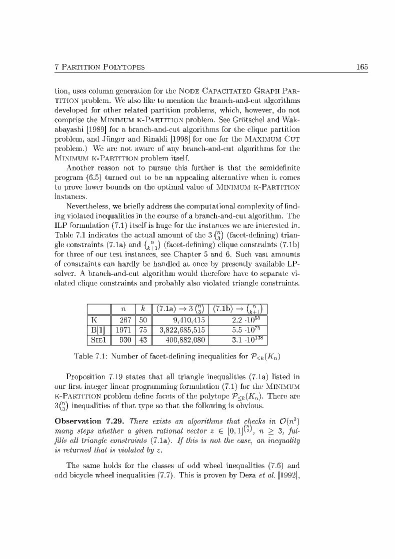
PARTITI ES

on, uses column g e e r a o n fo the NODE C C I T A E D GRA PAR

TITIO prblem. We also like to mention the branch-and-cut a l i t h m s developed for ther related p t i t i o n prblems, which, howeve o not omprise the M I M U M K-PARTITION prblem. See Grötschel a Wak-

abayashi [1989] or a bnch-and-cut a l g i t h m s the clique p t i t i o n prblem, a d J ü g e r and Rialdi 1998 or on for the MAXIMUM C U T

prblem. We a not awae of ny b c h - d - c u t a l i t h m s the NIMUM K-PARTITION prblem itsel Another reason not t rsue this further is that the semidefmite

progam 6.5) t u e d out to e an appealig a l t e t i v e whe it mes o p rve lowe ds on the timal value of IMUM K-PARTITI

stances. Nevertheless, we briefly addess the c u t a t i o n a l complexity of find­

in lated inequalities in the couse of a branch-and-cut algrithm. The ILP fmulat ion (7.1) itself is huge the instaces we are inteested i Table 7.1 indicates the actual amount of the 3 (") (facetdefning) t i a n gle constraints 7.1a) and (^"-J ( facetdefng) clique constraints 1b) fo three of our test instaces, see Cha te r 5 and 6. uch vast amounts of onstaints can hardly be handled at once by presently available L olver. A brch-and-cut algorithm would therefore have to separate vi lated clique onstaints a prbably als lated t i a g l e constaints.

1a) - Q l b ) - ^ 50 9,10, 055

19 2,85, 075

00,882,080 1

Table 1: Num of f a c e t d e g iqua l i t i es V<kKn)

oposition 719 states that all iangle inequalities 7.1a) listed i ur st integer linear p r o a m m i n frmulation 7.1) for the MINIMUM

K - P R T I T I O N problem defne facets of the polytpe T<k(Kn). Thee a 3Q) equalities of that t y e s that the llowig is us.

Observation 7.29 e s an algor hat eck n ö many teps whhe ivn rational ctor z £ [0, l ] w , n 3, f lls all trngle onsr (71a). I not ase, a qual

urnd th s vila

The same holds for the classes of odd wheel inequalities (76) a d dd bicycle wheel equalities ). This is pr by Deza al 1992]

4 ATING V D I E Q U I T I E S

basin on an agument of Gerads 1985]. Both types of qualities dein facets oiV<k{Kn) u d e faily g e a l onditions, see P s i t i o n 9.

roposition 7 0 (Deza et al [1992]) followng as be omhd b lynomial ti algor

ckng all q qualit q > nd od

y i n onal vector G [0, l ] , n 3, ee all ngle qual 1a) ot, a vila qual

ckng all q l e quali ( ) q > 5 nd od

y i n onal vector z G 0, l ] , n 3, wh ee all ngle qual 1a) ot vila le qual

Separating the class of clique iequalities ( 1 b ) , h o w e , is fV-ha k is consided as of the i u t :

roposition 7 . Gi omle grap Kn, n 3, nd onal

ctor [0,1] d qual

Y j

for all Q C V(Kn) it k + 1. role s H

Proof. The proof is a simple reduction of the I N D E N D E N SET prob­lem, see Garey and hnson 199 , 20], to the searation problem.

We a e gi a g p h G = V, E) for which we want t kno whethe it contais an deendent set of size k + 1. Let n \V\ define ze [0,1]© by zlj = lii ij nd ^ 0 othewise. The z lates the clique inequality ^ g„ 1 i only i Q* is a d e d e set of size k + 1 i G. D

One may think of several heuristic ways to sepaate violated clique inequalities. O e simpleminded examle is the following. Gi a ra­tional vect [0,1] , let Gz (V, Ez) denote the s u b g p of Kn

with ij G Ez if and only if z^ < (fe^1) Fo very clique in Gz of size k + 1, a corresponding clique constraints is vilated by z. Testi whether such a clique exists is, of course, also A/'P-coplete. But a sim ple greedy heuistic may often d such a clique as lon as not very many clique cons t a i t s have bee s e a t e d . Anothe examle is the heuistic

PARTITI ES

descibed by Krumke [1996, Section 5.5]. This heurisic is a olynomial time 2-approximation algorithm as long as the metic t i a g l e iequalities

ij + Zjk > zik) are all satisfied by z Recall that the clique inequalities 7.1b) are a secial case of the hy-

permetric inequalities (7.12). The complexity status of separatig hy metic inequalities is not yet fully settled i g e a l . Deza and Lau [1997, Section 28.4] discuss this issue and gi refeences to related w e. g. on heuristic appraches to separate hyermetric inequalities. To our best knowledge, the complexity of separating cycle inequalities 16) is no fully settled as well. The llowig h d s i g e a l

roposition 3 . Suppo er ts a las of poop Vc, 2 n, suc

(i) V<k{K) C V C 1 ] all2 n;

(ii) t iqualit m Cn^ efni Vc arable i poomal t all 2 n;

(Hi) ter a S f mm-pk(Kn) c mm-p

all G {0, 1} all 2 n;

V = HV.

Proof Let G = E) be a grap on n tices. We def cG by cfj = 1 if ij £ E and cfj 0 therwise. The MINIMUM K - P R T I T I O N prblem assciated with cG has timal value mhizlzV<^ (cG)z 0 i only

G is ft-patite (or A;-coloable), a d at least otherwise. By assumption (ii) the result of rötschel et al 988, Theorem 4.9]

oncerning the use of strong separation oracle solving the s ton timization prblem in aclepolynomial time implies that any linea

function can be timize Vc lynomial time. tice that Vr u is "welldescried.")

Exploiting assumtion (i) a (iii)7 we can the fo re check in p l y ­nomial time whethe the graph G is A;-cloable. ce this problem is known t be A / 'P -co l e t e , c m r e Gaey an on 9, 4] the assumtions take gethe i m l y V = MV. D

Recall in this context from ollary 7. that every valid inequality az ÜQ with ositie righthand side has to have a suppr t of size at least (fe+1) or k = 50,7543, this is 127 2850, and 946, respectively. In addition the prblems of identifying violated iequalities with such a lage supp the is another ptential prblem ce. I many such

4 ATING V O L LID I E Q U I T I E S

inequalities are separated in the c o u e of b d - c u t procedue, this may lead to numerical problems i the LPsolver. With this in m i d we proceed o the next chapte. Thee, we ague that the s e m i d e i t e elaxation (6.5) of the MINIMUM K - A R T I T I O N prblem can be solve

^pproximately i polynomial time and that its set of feasible solution ca e see as a easonble appr ima t ion of the l y t e V<k{K).

CHAPTER 8

Semidefinite elaxation of the inimum fc-Partition Problem

Lower bounds on the optimal solution of several MINIMUM K-PARTITION

instances are r e t e d in Section 6.3. We use these results to bound the unavoidable interfrence in a frequency assignment problem from below. The bounds are obtained from (approximately) solving the semidefinite relaxations (6.5) from Section 6.2.2. Semidefinite programming is the task of minimizing (or maximizing) a linear objective function o e r the c o n x cone o positive semidefinite matrices subject to linear constaints.

Here, we discuss the strength of the semidefinite relaxation. We elate the solution set of the semidefinite relaxation to the polytope V<k(Kn

as defined in Section 7.1. This is done by considering a projection of an affine image of the solution set into The image of the projection is called 9 ^ n and contains V<kKn). We bound the extent to which the valid and often facetdefining hyprmetric inequality (7.2) for V<k(Kn) may be violated by points in Qk,n- We prove that this bound is tight in seveal cases. We also show that for the MINIMUM K-PARTITION

problem, neither the LP relaxation of the ILP formulation (6.2)/(7 no the SDP relaxation (65) is geneally stonger than the other.

The chapter is organized as follows. We fix notation in Section 8.1. A short introduction to semidefinite programming is given in Section 8.2. We treat the semidefinite relaxation (6.5) of the MINIMUM K-PARTITION

problem and its connection to the elliptope in Section 8.3. The relation between the polytope V<k{Kn) and the set Qk,n is studied in Section 8.4. Finally, we state ossible diections of f t h e r reseach in Section 8.5

8.1 Preliminaries

We ecall here basic proerties o symmetric and positive (semi)definite matices, which a e used in the following sections. See Appendix A geneal notation.

69

8. P R E A R E S

symmetric and

skew-symmetric matrices

A square matrix A is symmetric f the matrix is identical to its trans pose, e., A = AT. The set of n x ndimensional symmetric matrices is denoted by Sn. The matrix A is skew-symmetric if A = —AT. The two sets of ndimensional symmetic and of skewsymmetric matices orm

thogonal subspaces of Rnx of dimension (^"1) and ( ) respectively. Every square matrix can be witten uniquely as the sum o a symmetic and a skewsymmetic m a t x :

A + AT A-AT

The inner product o two matrices A, B £ RT is defined here as A,B) = YllLi S j = i AijBij. For the inner product of a square matrix

A £ Rnx and a symmetric matrix X Sn, the skewsymmetric part of A is irrelevant because

A,X) -^—X) A *> ^ U

orthonormal

orthonormal diagonalization

A matrix P £ W is orthonormal if its column vectors Pi, • • • ,p satisfy ||pj|| = 1 (they are unit vectors) and (jPj) = 0 for i ^ (they are pairwise orthogonal). A diagonal matrix D £ Sn is an orthonormal diagonalizati of a matrix A £ Wix if D = PTAP for some orthonor mal matrix P £ R n x . The following result from linear algebra states that every symmetric matrix has an orthonormal diagonalization.

Proposition 8.1 (orthonormal diagonalization). Le A £ Sn. All egenvalues of A are real. There exts a rthnormal maix P £ Mnx

such that PAP = AA, were A^ s a diagal matrix for whic the nties are the egenvalues of . T lumn v r s of P are eigenvrs

of

An immediate consequence of the orthonormal diagonalization is that every symmetric matrix can be written as the sum of rank-one matrices

Proposition 8.2. Le A £ Sn, thn A = 5Z"=1 X(A)piPiT, were(^4) 1,. are the egenvalues of A a the pi 's are assci igen rs

positive (semi-)deRnite

A symmetric matrix A £ Sn is posite semidefine or A y. 0, for short if xT Ax > 0 for all x £ n . If in addition, xTAx > 0 for all x T 0 then the matrix is po efe or A >- 0 for short.The

E M E F N I T E R E A X A O N F M N I M U M / E - P A R O N

subsets of Sn consisting of all positive midefinite and positive definit matrices are denote here by S+ and S*++, respectively. The following two £+, + propositions give known characterizations of positive semidefinite and positive definite matrices

Proposit ion 8.3. Let A be a symmetic n x nmatix. T foll ropertes are equalet:

(i) p o e semefte

(ii) All egenvalues of A are egate

(Hi) A be wrtten as t of a matrix C of rank(A) a ts raspose, A = CCT

(i (A, B) > for all matices B G S+ (Fejer's Trae Trem

v) det(A7") > for eery cial submatrix Au of

reer for ea p o e semefte matrix A ds:

(i) IBeS+ A, B) = 07 t AB

(ii) A agoal element omiating all entes, 3i : Aü = max{\Aki\ 1 < 1 < n } ; and if diagnal element is zero, so are all entres in the crrespding r an lumn, i , Aü = 0 mples A^ = for all j

(Hi) B e Rnx s a regular matrix, ten i e S + < ^ BTAB e S+

Proposit ion 8.4. Let A be a symmetrc n x nmatr follng propertes are equalent:

(i) s p efinte

(ii) All egenalues of A are p

(in) s te pr of a regular matrix C and its transpse, A = CCT

d e t ( A ^ ) > 0, j = 1 , . . . , and Ix C • • • C for a neste se quence of prcipal submatres

reer for ea efinte matrix A ds:

(i) B G S*++ s aner p efinte matrix, ten A, B) >

(ii) B G Rnx s regular, ten A G S++ ^ BTAB G S++

8. P R E L A R E S

(strictly) A matrix A G R is diagonally dominant if \AÜ\ > YTj=i j^il^-i diagonall holds for all i = 1 , . . . n. In case the inequalities are all strictly fulfilled dominant then the matrix is strictly diagonally dominant. The following sufficient

criteria for being positive (semi)definite are direct consequences of Gers gorin's disc theorem.

Propos i t ion 8.5. Let A G Sn be diagonally inant with onnegative entries n the prcipal diagnal, then A is p o e semidefinte n case he prcipal diagnal s p e an s strl diagnally nant

en A s p efinite

The trace of a square matrix is the sum of its eigenvalues. Bounds on the inner product of two positive semidefinite matrices are easily obtain­able from this fact.

P r o o s i t i o n 8.6. Let A,B 5*+ en A, B) an be bel an frm a e :

{A)maxB) A) -B)

(A,B)

\nax(A)B) max(A)maxB)

Given a symmetric matrix for which it is known that some principal submatrix is positive definite, the following theorem states the neces sary and sufficient condition under which the entire matrix is positive semidefinite.

heore 8.7 (Schu o m p l e n t ) . Let A S++, B G Rmx, C , ten

^ A~B.

A partial characterization of the cone S*+ of positive semidefinite ma­trices is the following.

Propos i t ion 8.8. The set of ptive semidefinte matries S^ is a full dimensinal clsed, and ponted cone in the vector space S of symmetri matres e pos efinite matres S++ are t nter of ne

Proof olklore). Obviously, S+ is a nonempty cone. In order to see that S is pointed, pick any A G S^ other than the matrix containing only zeros. There exists a vector x G W1 such that xTAx > 0. Thus xT (—A) x < and —A ^ S+- Now consider the set of symmetric

A B BT C

E M E F N I T E R E A X A T O N F M N I M U M / E - P A R T O N

matrices that have ones at positions (ii), (j,j), {i,j) and (j,i) and zeros elsewhere for possibly equal i and j . There are ("J1) such matrices, all of which are positive semidefinite and mutually linearly independent Thus, 5*+ is full-dimensional. Finally, a symmetric matrix is positive semidefinite if and only if all principal subdeterminants are nonnegative and it follows from continuity that S+ is a closed set. D

The plar cone C* of a cone C C R is the set C* = {y G R n

Vx G C (y,x) > 0} . Hence, another way of stating Fejers Trace Theorem, see Proposition 8.3, is to say that the polar cone of positive semidefinite matrices coincides with itself, that is, S+ is selfpolar. This fact is important in the duality theory of semidefinite programming.

P r i t o n 8.9. $n

We state the simple proof

Proof (Folklore). S+ C S+: Consider A e S+ and let AA = PAPT

be its eigenvalue decomposition with PPT = In, see Proposition 8. Then for every positive semidefinite B G S*+

A, B) = PAAP B) = PAA, BP) = AA, PBP)

\(A)(PiPi.>0,

olar cone

self-olar

since i(A) > 0 and (P f) BP{. > 0. Thus, A e S+. $n — ^n: The square matrix xxT of rank one is positive semidef

inite all x G R . If A G S*+* then x1Ax (A,xxT) > 0 and hence A G S+ D

Given two convex sets F and C with FCC the set F is called a face of C if x, y G C, a G ]0,1[, ctx + ( — o;)y G F x, G F . The cone 5+ has the following faces

heor 8.10. E fae F of S+ ne of the sets 0, {0} PWPT

G S for some 1 < n an me P G Rnxk P =

Every positive semidefinite matrix can be expressed as ^ixixi with j > 0 according to Proposition 8.2. For each x G R the set {\xxT | A > 0} is a face of S+- None of these faces can be expressed as the convex combination of smaller faces of S^. Hence, {X = <]C*XJ I 11 *jC 11 l,x G Rn} is a minimal generating system of S+ (strictly speaking, a restriction like "the first nonzero coordinate of each x is positive" has to be

face

8. P R E L A R E S

added). This implies that the cone S+ is not polyhedral, i.e., S+ cannot be described as the intersection of finitely many hyperplanes for n > 1 Since the faces of S+ have dimension ( ^x) for some k, there are gaps of more than one between the dimensions of nested faces.

Let A4 i = , . . . , m, be symmetric matrices from Sn, then a lnear operatr A: Sn — Rm is defined via

X ^AX

AiX)

_(X)

The a pera AT: W of A is give by VM n (

X,A) = AX,) = MiX) = y^X)

The following three simple results are used in Section 8.4.

O b s r v a t i o n 8 .11 . Let X G S+, m > , and J C { l m \ here exsts a matrix l e S su at X XJJ

Proof Let be the identity matrix with the submatrix IJJ replaced b y X . D

Notice that if X is positive definite then the constructed matrix is also positive definite.

In the course of our further calculations, matrices of a particular struc ß() ture are of importance. Let Da@n) denote the symmetric square matrix

of order n > 1 with all entries on the principal diagonal equal to a and ) all other entries equal to ß. Let E(m,n)E Wx be the matrix with all

entries equal to . The following properties of D{n) are easily observed.

P r o s i t i o n 8.12. , the etermnant of Da s gen by

det(D)) = (a - ß a + )ß

r ß ^TJ; c\ te matrix Da s regular and its erse

. Da+(2)ß Y (g a - ß a + )ß

D a n is ptive semidefinite if an nly if a > ß > - ^ is p definte if and only strict inequalty hlds n bth ases. (In ase n 1, Da'ß) = [a] an is assumed be 0 n the a formulas reer

dition UB > -^SL" bemes id

E M E F N I T E R E A X A T O N F M N I M U M / E - P A R T O N

We are intereste under which cnditions o , 5, nd e the matrix

DaP(s) fE(s,t E(t, s) Ds{t

A = (8.2)

is positive semidefinite. They be derive by m e n s of the Schur Complement see Theorem 8.7.

P r i t o n 8.13. Gi ntegers s,t>, te matr

A = Dß(s) fE(s,tj #( t , s) Ds(t)

is poitive semidefinite if and nly if D(s), D(t) are semidefinte an [a + (s — )ß ( + (t — )e > st

Proof. Clearly, the composite matrix cannot be positive semidefinite un­less Daß(s) and Ds(t) are both positive semidefinite.

We first deal with the case of Da(s) being positive definite. By the Schur Complement Theorem 8.7, A is positive semidefinite if and only if Ds'£(t) y 7E(t, s) DaP(s) jE(s,t). We compute the expression on the righthand side of this inequality:

E(t s)Da+(sV(s)E(s t E{t,s)D{s)E{s,t ^ s > u W ^ W l ' ' K ' K ' (a-ß)(a+(s-)ß)

a-ß)E(t,s)E(s,t

a -ßa+(s- )ß

E(t,t a + (s-

_ ?+(s_ Ds-^-(t) = D^( t ) - 7 E(t , s ) D^{s) ^E{t,s) By Proposition 8 . , this matrix is positive semidefinite if and only if > \

~w After resubstituting for L the latter condition reads

For a; =

nd e — u as (a + (s- l)ß) +(t- )e) > st/

Finally, let Da(s) be positive semidefinite. Then Da+®ß(s) is pos itive definite for all 9 > 0. Let A{9) denote the matrix A with a being replaced by a + 9. From what is proven so far A{9) is positive semidefi­nite if and only if ( + 9 (s - )ß) S (t - l)e > st for all 9 > 0. The cai now folows fom the fact that ST+ s c o s d . D

8.2 E M E F N I T E P R R A M M

8.2 emidefinite Programming

primal semidefinite program

In a semidefinite program a linear objective function is minimized (or maximized) over the cone of positive semidefinite matrices subject to linear constraints. This cone is closed and convex but not polyhedral The duality theory for semidefinite programming is not as smooth as that of linear programming. A gap between the optimal primal and dual objective function value is possible. This gap vanishes under a simple condition, which holds for the M I N I M U M K - P A R T I T I O N relaxation.

We give a brief introduction to semidefinite programming here. More comprehensive treatments of this topic are, for example, given by Al izadeh [1995] Helmberg [2000], and can be found in the book edited by Wolkowicz, Saigal, and Vandenberghe [2000].

The generic 'prmal semidefinte 'program reads as follows

i n C , X ) s t AX-beK,Xy ( P S D P

K is one of the following convex cones: {0} m , R™, or {0} m i x This formulation is not entirely standard but has been used before. The appearance of the cone K may seem awkward at first. In the cases K = {0} m , K = R™, and K = {0} m x R™ the corresponding semidefi­nite programs have equality constraints, inequality constraints, or a mix ture of both. Hence all cases of linear constraints can be represented adequately. Moreover we will also have a nice formulation when turning to the dual program.

If the inner product in the objective function is spelled out and the effect of the operator A of X is written explicitly, then it is obvious that the objective and all restrictions are indeed linear The only nonlinear ingredient is the condition "X y 0.

What constraints does X y 0 impose on the entries of XI We give some examples. Straight from the definition of positive semidefiniteness follows that all diagonal elements have to be nonnegative. Moreover, the absolute value of each offdiagonal element is bounded from above by the maximum of the diagonal elements in its row and column. A strength­ening of this constraint is obtained by considering the determinant of

principal submatrices. Let {i j} with 1 < i j then the

submatrix XJJ

computation yields X-Ü

is itself positive semidefinite nd a short

et Y

Y ) > Xjj > and XXjj.

E M E F N I T E R E A X A T O N F M N I M U M / E - P A R T O N

Hence, \Xy\ y/XaXjj has to hold for all i and j . In order for a real, symmetric, 3 x 3ma t r ix to be positive semidefinite

it is necessary but not sufficient that all principal 2 x 2 submatrices are positive semidefinite, recall Proposition 8.3. We give an example for the insufficiency. The parameterized matrix

has the determinant 1 + 2ac — b . Hence this matrix is positive semidefinite if and only if — 1 < a, b, c < 1 and 2abc — a2 — b2 c2 > 0. If we set a = b = 1 and = 0, then all three 2 x principal submatrices are positive semidefinite, but the determinant is —1 and the matrix itself is thus not in S%. Similarly, the positive semidefiniteness of a matrix in S+ can generally not be solely guaranteed by the fact that all its (n 1) x (n — ) principal submatrices are in S^_v We do not pursue this further and turn to the duality theory of semidefinite programming instead.

The dual semidefinite program is obtained by a standard Lagrangian approach:

i n f C , X ) s t AXbE inf sup C,X) b - AX, xto xes+eK*

sup inf C, X) b- AX, eK* xes sup inf b ) + C- A X) eK* XES

sup b, s t C — A E S eK

Using that 5+ is self-dual, i.e., (S+) S+ we may define the generic dual semidefinte program as follows: dual semideßnite

program b, s.t. C - A 0, E K (D-SDP

The dual cones of K = {0}, K = R , and K {0} x R^2 are W R+, and R i x R™, respectively. In other words, a dual variable asso ciated to an equality constraint is unrestricted, whereas a dual variable associated to an inequality constraint has to be nonnegative. This is in perfect accordance with what we know from linear programming.

Notice that in the same fashion as above, a more general optimization problem can be "dualized. ne may replace the condition "X y " (or

8.2 E M E F N I T E P R R A M M

equivalently, "X 6 S+") by the condition X 6 L for any convex cone L, see Ben-Israel, Charnes, and Kortanek [191], for example. Instead of the self-dual cone of semidefinite matrices, the polar cone L then appears in the constraint section of the dual program. Take L = K." and K = { 0 } , for example, then the primal program is a linear program with equality constraints and nonnegative variables. The corresponding dual program has inequality constraints and its variables are unrestricted. Thus, classical weak LP-duality appears as special case.

Although (D-SDP) does not look like a semidefinite program at first it is one nevertheless. The feasible sets of the primal and of the dual program are both intersections of an affine subspace with the semidefinite cone, see Nesterov and Nemirovskii [1994].

Weak duality holds as explained above.

P r o s i t i o n 8.1 (Weak d u l i t y ) . r a semidefinte 'program and its ual follwing ds:

s u p 6 , C - A y O , i n f C , X ) AX beK,Xy

inf0 = + o an sup 0 = — o

Strong duality does not always hold. Here is an example with duality gap taken from Vandenberghe and Boyd [ 9 9 ]

Example 8. ( M i s s i g s t o n g d u l i t y ) . Cnsider

\ X) AX , X y

Ai f

A A M =

rrespng ual seidefinte prram

. Z C ~ V A i = o.

ce t agnal element Z22 z e , te elements Zu = ^Y~ an Z32 = —1/4 n rresponding row and column ve to be er as well

nsequently, , an the maxmum of I is aie by y

O O ] The optimal value of e prmal semidefinte program . Hene, tere s a duality gap of 1

E M E F N I T E R E A X A T O N F M N I M U M / E - P A R T O N

Conditions are nown under which a duality gap does not occur

Definition 8.1 (strictly f s i b l e ) . (PSDP s strictly feasible if there s a solutin which is positiv efinite, i. ., he inter of the set of

soluns nonempty. Analusly, (D-SDP) s strly feasble nter of e set of ual s l n s s nnempty

Recall that is one of the convex cones {0 or {0} n thee cass s g d u a l y holds if the dual prgram

is strictly feasible, see, e.g., Helmberg [2000]. Stoer and Witgall for example describe more general results on strong duality.

heor 8 . 7 (Strong d u l i t y ) . Assume (D-SDP s strl feasble en

MC,X) XyO,AX-be snpb, C

is value is finte, that is in case the prmal problem s feasble en optmal alue s attane for sme X y th AX b E

The strict feasibility in the theorem is indeed necessary. Here is a folklore example to illustrate this

ample 8.18. nsid

i n X X I n X22

strictl feasible

ts dual

o.

e primal problem s strly feasble, e , X y 0 for Xu = X22 The dual optimal s l n 0 s attaned fo y± = 0, which is t, the onl feasible slutio. Due to din X y 0, Xu an X22 must satfy Xu,X22 > 0 an XUX22 > nsequently, Xu > -^—. F X22 —> o, te r a n ide tends t e primal optmum alue

t attaned

Asume that we want to solve

in C, X) s.t. AX b E K,X h 0, (8.3

8.2 E M E F N I T E P R R A M M

where a, ß are real number hen we may as well solve

minC,X) s t AX-beK,X>O, (8.4

multiply the optimal value by a and add ß. The optimal solutions them selves are the same in both cases. A minor technical difference concerns the dual programs. In the former case the dual is

6, ) + s t . aC - A 0,

whereas scaling and shifting the objective function of the dual to (8.4 yields

6, s.t. C - / 0 j

Those programs are equivalent This can be seen by substituting ay for y in the first dual and canceling a in the constraints. Recall that a > 0 and that S+ is a cone.)

Hence, in order to obtain a lower bound on the optimal value of the primal program (8.3) we may try to find a feasible solution to

6, s.t. C - A 0,

If y is such a feasible solution, then a(b,y) + ß is a lower bound. This procedure is applied a number of times in Section 8. and we summarize it for reference.

Obsrvation 8.19. Let be a feasble s l n t

b, C - 0,

en b, s a lwer b fo

mmC7X) + AX - b G K, X y 0.

Finally, we turn to the computational complexity of solving semidefi­nite programs. Such programs can in general not be solved in polynomial time. One reason is that the feasible set is not generally contained in a sufficiently bounded area around the origin. In fact, it is not even known whether testing the solution set for nonemptiness is in MV in the Turing model of computation, see Ramana [1997] and the references contained therein. If, however, the feasible set of the semidefinite program is known to be contained in the hypercube [1 ,1 ]^ >, for example, then an opti mal solution can be approximated with arbitrary precision in polynomial

E M E F N I T E R E A X A T O N F M N I M U M / E - P A R T O N

time. This is a consquence of the general theory on optimization ove circumscribed convex bodies developed by Grötschel et al. [1988].

In order to make this more precise, let us recall what the weak opti­mization problem is The definition relies on the following two notions Given a convex set C W and a real number e > the e-ball ar K is defined by

K,e x E R \\x - e for some

where \\x — y\\ = ^{x — yx — ) is the Euclidean norm in R and the nter e-ball is defined as

K,-e) xEK {x},e }

Definition 8.20 (Grötschel et al. [1988]). An nstance of the weak optimization problem onssts of a mpact and coex set K, a weak otimization

E Q, and a ratnal number e > 0 Te tas s t er

find a vecto y E Q su at E BK, e an x) ) + for all x E BK, —

assert tat BK, —) s empty

A simple adaptation of the proof of Theorem 9.3.30 by Grötschel et al [1988] shows that for every fixed e > 0 the weak optimization problem for a semidefinite program is solvable in a running time which is polynomially bounded in the two parameters n and R. Here, n is the dimension of the space, and R is the radius of a ball around the origin which is known to contain an optimal solution.

The hypercube [—1, l] is contained in £?({0},n), and the Corol­lary 4.2.7 of Grötschel et al. [1988], concerning the use of a weak separa­tion oracle for efficiently solving the weak optimization problem imme diately yields the following.

Propos i t ion 8.21. Let F 1, l l be the feasble set of a semid inite program wth m linear onstraints. Then, for eery fixed e > 0, th weak o p t a t n prblem er an be s d in plynoal tme in m an

If e is considered part of the input, then the running time of the ellipsoid method, used for the proof of Corollary 4.2.7 by Gr t sche l et al

88], depends exponentially on the coding length of e. In the above mentioned counterexample for the general solvability of

semidefinite programs in polynomial time the radius R grows exponen­tially in the size of the problem formulation.

ball around K

interior ball

82 8.3 T H E M N I M U M A P A R T O N RELAXATON

8.3 The Minimum fc-Parition Relaxatio

In Section 6.2.2, the program (6.4) is stated as an alternative formula­tion of the MINIMUM K-PARTITION problem and the program (6.5) is its semidefinite relaxation. After having elaborated on the basics of semidef inite programming, we now come back to this relaxation. We study the semidefinite program (6.5) from a particular point of view. Namely, we relate the set of feasible solutions to the semidefinite program to the k partition polytope V<k() as defined through (6.4) in Section 6.2.2 see also (7.1) in Section 7.1.

We briefly recall how the semidefinite program (6.5) is obtained. Given are a complete graph Kn on n vertices together with an edge weighting w: E{Kn) —> R and an integer A;, 2 < k < n. We assume for notational convenience that the vertex set of Kn is { 1 , . . . , n} and that the edge set is [ij | 1 < i < j < n} . According to Lemma 6.4 we may pick a set U of k unit vectors v,\,..., u^ G R such that (ui, Uj) = -^ for all pairs of distinct vectors. Let Tk : R K be the affine transformation x i->- ^Y~ x | , mapping 1 onto 1 and ^ - onto 0. With the vectors as labels the INIMUM K - P A R T I O N problem can be stated as follows

J^}nr WijTkd&^j)) (8.5) i<-Ht>i eE(

The weight of an edge is accounted for if and only if its endpoints have the same label Every such labeling of the vertex set defines a matrix X [((ßi,ßj)]1< •< G Mn xwith the following properties: (i) X is positive semidefinite; (ii) all entries on the principal diagonal of X are equal to 1; (iii) all off-diagonal entries of X are equal to ^ y or ; and (iv) X has rank at most k.

In case the last property is not enforced and the second last is relaxed to the request that all off-diagonal entries are between -0^ and an optimal matrix X can be found by solving the semidefinite program

mh^Fw'x) + iw'E)

s.t.

X) = , . . . (8.6)

X ) > _ Z L i j G } , i < j

x t This is the same semidefinite program as (6.5) in Section 6.2.2, only stated in different way. Here denotes the symmetric matrix obtained

E M E F N I T E R E A X A T O N F M N I M U M / E - P A R T O N 83

Wij for al from the vector w E by letting Wü = 0 and Wt

1 < i < j < n- Moreover, Ei{n) denotes the symmetric n x nmatrix with an 1entry at positions (i, j) and (j, i) and zeros elsewhere. If the dimension is clear from the context we simply write E Let

X E 5 Xü = Xi:i > -j—^ij

6 then this semidefinite program

# * (8.7)

denote the set of feasble solutions of can be rewritten as

mm±W,Tk{X)) s.t. l e t Since all the diagonal elements of elements X E \&fcj„ are equal to all off diagonal elements are confined to take values between ^ y and 1. Thus \tfc is contained in the hypercube in Sn with vertex coordinates from {—1,1}, and Proposition 8.21 implies that the semidefinite program (8.6) is approximately solvable in polynomial time.

n the case of ^k is the elliptope

{XeSXu = i e , . . . }

For k > 2, ^k,n is obtained by intersecting the elliptope £n with the halfspaces defined by X^ > ^ - for all i,j E { , . . . , n } . Projections of the elliptope £ and the truncated elliptope ^ 3 ^ on the set of upper triangular matrix entries are depicted in Figure 8.1. The elliptope is studied extensively in the literature in terms of the following notions

A boundary point A0 of the nonpolyhedral but convex £n is an ex­treme point if {A0} is a face of £n; it is called a vertex if the cone of nor mal vectors to the hyperplanes supporting £n at A0 is fulldimensional Moreover, we denote the smallest face of £n containing A by F£ (A). The following characterizations are taken from Deza and Laurent 1997 but most of them are originally due to Laurent and Poljak [ 9 9 , 996b

heor 8 . 2 . e elliptope has t follng propertes

(i) vertices of £n are te matres xxT for x E {± ere are many of em

(ii) Let A be a bondary nt of rank(^4) = r an let I = (F£(A)), ten

0, ( ^ Q Furtermore for all ntegers r, I > 0 satng the aboe inequality, a bary pnt A of rank r an = dim(F£(Aj) exsts

olynomial time

ellito

extreme point vertex

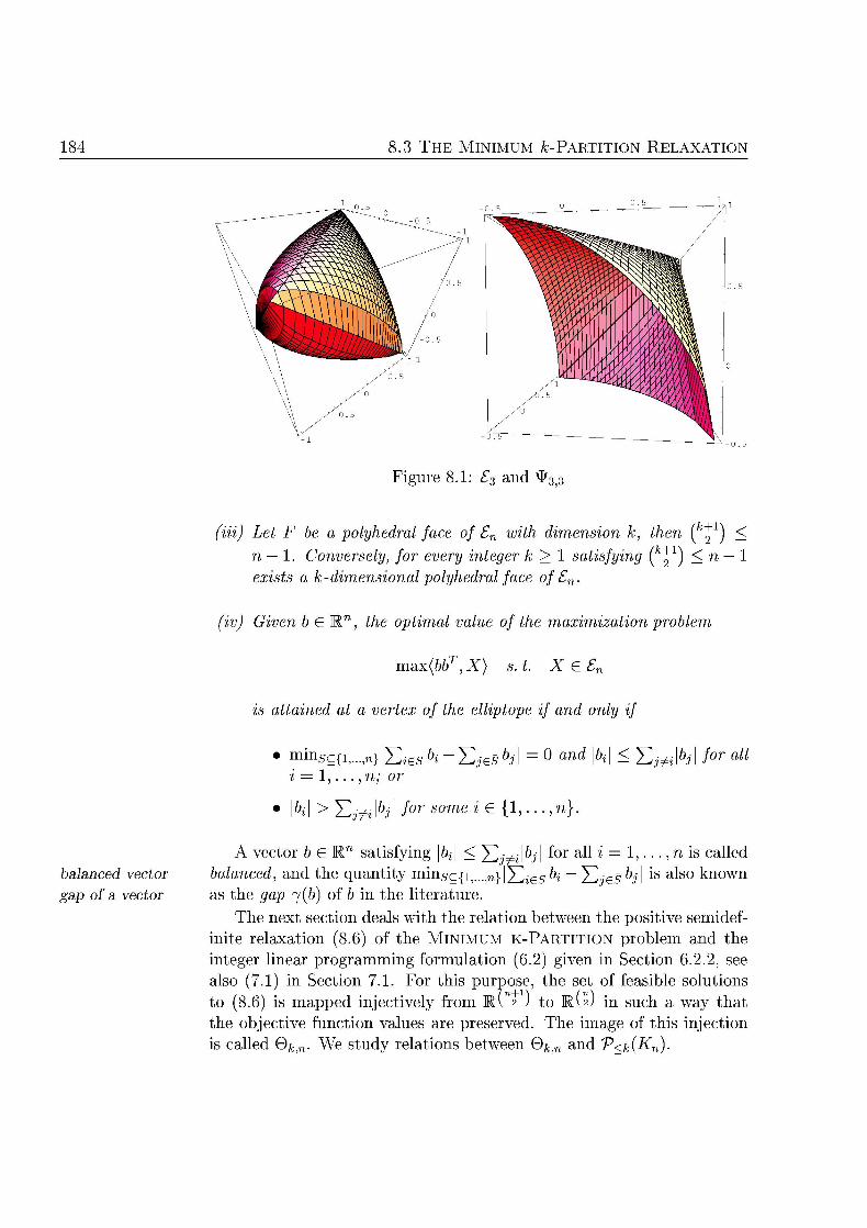
8.3 T H E M I N I M U M A;-PARTITION R E L A X A T I O N

Figure 8. and 3]

(iii) Let be a polyhdral fce of En w dimens , ten

n — 1. nversely, for eery nteger 1 satng C exsts adimensnal lydral of Sn

Gien b G K 7 t optmal alue of e maxat prblem

X ) XeSn

s attane at a ertex of e elliptope an nl

m i n S c { i , . . n } e s ^ _ e s ö ° an b b\ for al1

i = 1

N b\ for some « e ,...

A vector b 6 R satisfying öj X ^ ^ for a lH 1 , . . . , n is called

balanced vector balanced, and the quantity m i n , g c { i , . . n } e , bi ~ ^ b\ i s a^so known ga of a vector as the gap 7(6) of b in the literature.

The next section deals with the relation between the positive semidef inite relaxation (8.6) of the M I N I M U M K - P A R T I T I O N problem and the integer linear programming formulation (6.2) given in Section 6.2.2, see also (7.1) in Section 7.1. For this purpose the set of feasible solutions to (8.6) is mapped injectively from to KU) in such a way that the objective function values are preserved. The image of this injection is called Qk- We study relations between O f and V<{)

M I F I N I LAXATION F MINIMUM /^-PARTITION

The afne transformation Tk is extended from R to S (which is iso-

orphic to by letting

k — Tk: S S —-— - E(n)

(Recall that E(n, n) is the n x n matrix with all entries being equal to one.) hich dimension applies will be clear from the context. Let

: S P O = z w i t h % = TkiX) for i < j

and consider 6

©* Ä ) = PO X e ** 8-8)

The restriction of Ck,n onto ^ n is onetoone and vkn : ^k,n> ©*;,

is an afne bijection. Moreover for any given X ^ and any given w G ) the identity

±{Tk(X)) = (X))

holds,where W is again the symmetric matrix obtained from by letting Wa = 0 and W^ = Wij for all 1 < i < j n.

A direct consequence of our definitions is as follows

b s r v a t i o n 8 . 3 . e optat prblem

min - Tk(X)) s X G \t f an min z) s z G 6^

ar qualnt

The afne image 0^> of the truncated elliptope \tfj contains the

polytope V < ) and is itself contained in the hypercube

P r o s i t i o 8.24. ry an n > 3 w n, t t Qk

ex, an

v < c e k

We call Qk)U emidefin laxatn ofV<k(Kn). A related connec emießnite tion between the MAXIMUM C U T polytope and the elliptope is observed relaxation by Laurent and Poljak [1995, Lemma 4.1] See also their eorem 25

ic aracerizes the verices of the ellipope

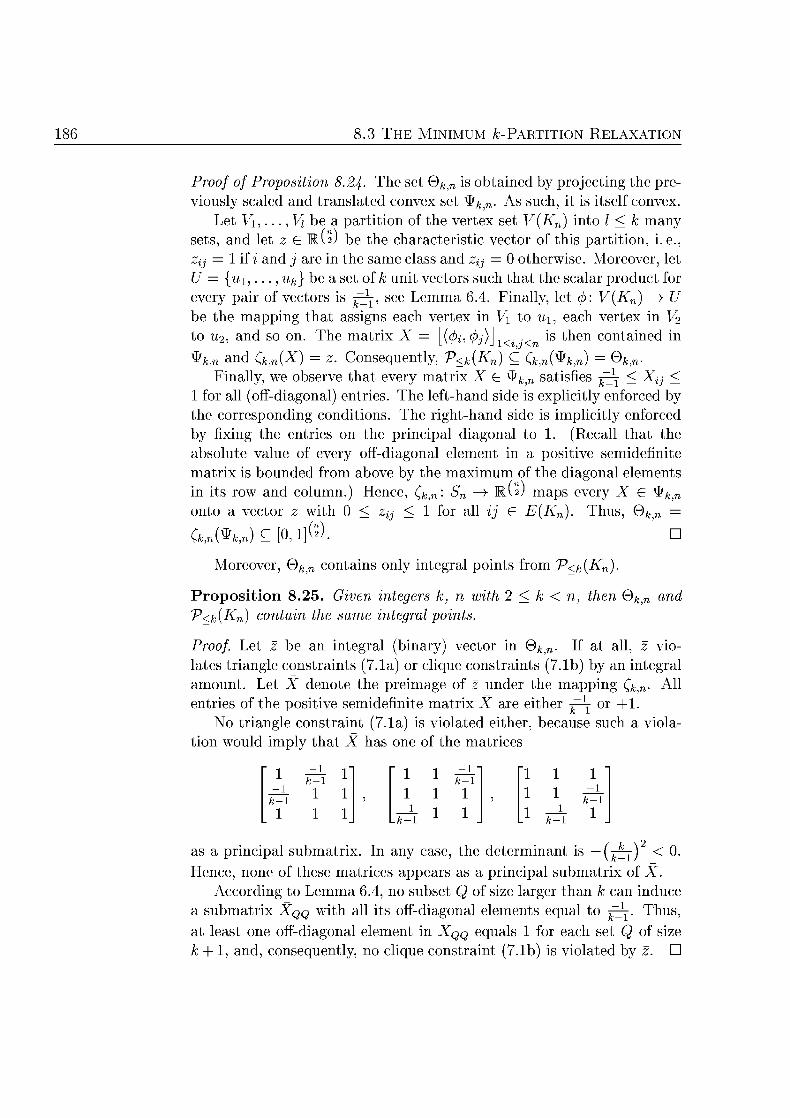
86 3 T H MINIMUM A;-PARTITION LAXATION

Proof of Propositn 8.24- The s t Qk, is o i n e d by p o j i n g the pre­viously scaled and translaed convex se ^k,n As such, t is self convex

Let Vi , . . . , Vi be a partition of the vertex set V(Kn into k many sets and let z E KU) be the characteristic vector of this partition, i e Zij = if i and j are in the same class and Zij = 0 otherwise. Moreover let U = {ui,... Uk} be a se of k unit vecors suc that the scalar produc for every pair of vectors is -^y, see Lemma 6.4 inally, let 4 V(Kn) be the mapping th assigns eac verex in Vi ui eac verex in V o u2, and so on h atrix X (P,<Pj)]l< .< is then conained in

^ and (X) = z Consequently, V<k{Kn) C ,«**,«) = ©f Finally we observe that every marix X E ^k,n satisfies -^ < X <

1 for all (ofdiagonal) entries. e lef-hand side is explicitly enforced by th corresponding condiions The right-hand side is implicitly enforced by fixing the entries on the principal diagonal to 1. (Recall that th absolute value of every fdiagonal element in a positive semidefini marix is bounded from above by th maximum of the diagonal elemen in its row and c o l u m ) Hence : Sn> maps very X E ^k ono a vecor z w th z^ for all i E() us Of

oreover Ofe>n conains only inegral poin from )

Proposition 8.25 Giv integers k, n th thn Qkn and V<k{Kn) contn th same ntegral nts

Proof Let z be an integral (binary) vector in 0^>n. If a all, vio laes triangle constrains (71a) or clique constraints (7.b) by an inegral amount. Let X denote the preimage of z under the mapping (k ll enries of the positive semidefinite matrix X are either -r y or

N triangle consraint (7.1a) is violated either because suc iola­ion would imply th as one of the m r i c e s

a fh

A A

fh as a principal submatrix. In any case the determinant is (jpj) < 0

ence, none of these matrices appears as a principal submarix of X. According to Lemma 6 no subset Q of size larger than an induce

submarix XQQ with all its off-diagonal elemens equal o -^j. Thus least one off-diagonal element in XQQ equals 1 for ach set Q of size

and consequenly no clique constrain ( 7 b ) is iolaed by z D

EMIDEFINI LAXATION MINI /E-PARTITION

e following o s e i o n is used in some o the followin roofs

rvation 8.26 ry trix C 6 S th emefin prog

min Ci

X) = )>-ZL je{,...n}i< 8

XeS+

nd

10 j J ^ y t

Y, ^ K ^ - € 1 j<

dual to ot nd oth s

Th dual variable associaed to the primal consraint X) = is and th associated th primal constrain X) > -j^ is y^

Proof. he two programs are simply (P-SDP) and (D-SDP) see Sec tion 82 specialized wth paricular constraints.

The identity matrix is ositive defini and fulfills all inequali constraints of (8.9) w th strict inequality Hence i is in the relati inerior of the solution space, and the firs program is strictly feasible.

e vector y e RU) with yü — 'YTj=\\^ij\~n f° r a ^ * a n d Uij = 1 f° r

all i < j is a feasible dual soluion All sign restricions on y are strictly met, and the matrix C — J2i<i<nyij ^ ^s positive definite, because it is strictly diagonally dominant \see roposiion 85) erefore th program 81 is ricly feasible, too D

8.4 The semidefinite relaxation &k,n and V<k(Kn)

As reported in Secion 63 , a nontriial lower bound on the optimal value of MINIMUM K-PARTITION problem can often be obtained from solving the positive semidefinite relaxation (65)/(86). In search of an explana­tion of this, our approach is to bound the maximal possible violaion of facet-defining inequalities for V<k(K) by points in Qk, T results pre sened ere are obained in this conex also how th neither th

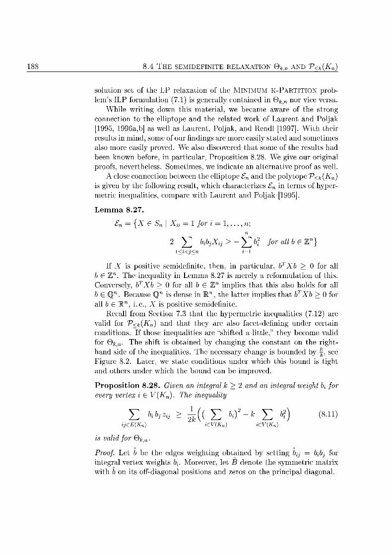
188 IDEFINI LAXATION 9 f AN V<

solution et of th L r e x a i o n of the MINIMUM K-PARTITION prob­lems ILP formulation (7.1 is generally contained in 9fcjn nor vice versa

While wriing down this material, we became aware of th strong connecion the elliptope and the related work of Lauren and Poljak [199 1996a,b as well as Laurent, Poljak, and Rendl [1997]. With their resul in mind, some of our findings are more easily s taed and someimes also more easily proved. We also discovered that some of the results had been known before, in particular roposiion 8.28. We give our original proofs, nevertheless. Sometimes we indicae an alernativ proof as well

A close connection between th ellipope £n and the polytope V<k(Kn) is given by the following result, wich characterizes £n in terms of hyper metric inequaliies compare th auren and Poljak [1995].

emma 8.2

£n = { eSn\ Xu = l for = l,...n;

Y^ bXij > for all b e Z } <j<

I X is positive semidefinite, then in particular, bTXb 0 for all b e Z . T inequality in Lemma 827 is merely a reformulation of this Conversely, bTX 0 for all !) G Z implies that this also olds for all b £ Q . Because Q is dense in Rn , the latter implies th T b > for all b G R , i.e X is positve semidefinite.

Recall from Section 73 that the ypermetric inequalities (712) are valid for V<kKn) and that they are also facet-defining under certain conditions. If those inequalities are "shifted a little," they become valid for Qk,n- The shift is obtained by changing the constant on the right-

and side of the inequaliies. The necessary change is bounded by | , see Figure 8.2. Later we tate condiions under w i c this bound is ight and others under whic the bound an be improved

Proposition 8. Given ntegral egral bi for i 6 K). T neqalit

w* ^ ( ( k) 0 (8n) e E )

ald for &k,n

Proof. Let b be the edges weighting obained by setting = bfij for integral vertex weights 6j. Moreover, let B denoe the symmetric matrix

th on s ofdiagonal posiions and zeros on the principal diagonal

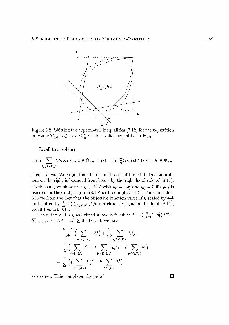
EMIDEFINITE R E L X A T I O N INIMUM -PARTITION 189

Figure 8.2: S i f i n g the h m e t r i c inequalities (712) f r th ion polyope V<k(K) by S < | yields valid inequaliy for Qk

all th sol in

mm ^ s z E Qk and mm-T s . X E ^k

jeE(Kn)

is equivalent. We argue that the optimal value of the minimization prob lem on th right is bounded from below by th right-hand side of (811) To this end, we show that y E RV2 ith yü —bf and yij 0 if i ^ j is feasible for the dual program (8.10) th B in place of C. The claim then follows from th fac tha the objec function value of scaled by ^-and shifted by ^ ^ijeE( es th r i g h t a n d side of (811 recall Remark 819

irst, the vecor y as defined abo is f e a s i b l e : ) E <j< 0 ' bbT h 0 Second

E *) + — y eV{Kn

E K„)

i E * + E E s E

Kn) £ ?)

ev(Kn)

s d i r e d is comple th oo D

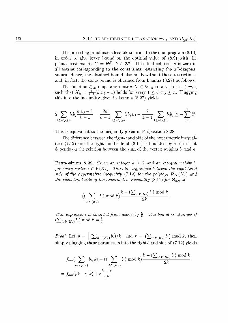
19 T H M I E F I N E R I O 9 f „ A V<{K

The preceding proof uses a feasible soluion t the dual program (8.1 in order t give lower bound on th opimal value of (8 ith th primal cost matrix C = bbT, b G Z . This dual soluion y is zero in all entries corresponding t the constraints restricting the offdiagonal values Hence, the obained bound also olds withou those resrictions and in fact, the same ound is obained from Lemm 8.27) as follows

he funcion maps any matrix G ^ to a vecor z G &k,n suc that Xij = ^ - / c % 1) holds for every < i < . Plugging this in the inequaliy given in Lemm 827) ields

Y -f~r v~i £ h: £ A-> <j <j <j

is is equivalen to the inequaliy given in Proposiion 828. he difference between the righthand side of the hypermetric inequal

ities (7.12) and the right-hand side of (811) is bounded by a erm th depends on the relation beween th sum of th verex weight and

Proposition 8.29. Given nege 2 inegral ig for rte G V(K) Then the derene beween the right-

e th yprmeri neqalit (712) for the polytope V<k{K) r i t d hyprmeri neqality (811 for Qk

Y mod ev(

ev(Kn) m o d

k

ssn i e b | e b ttne

e y ( K n ) m o d |

roof Let p = (£ev(*„) &0/ f c and r {2iev(Kn)i) mod A then simply plugging these parameers into the right-and side f (712) ields

fU Y Y mod eV{^ ev( ev(

= fh -^-

E M E F E REL MUM 19

We e n d this ressi l l s :

f -^-

2)

— A;3

—

e right-and side f (811) is:

k E E *) £V(K eV(K

U E E E ev(

evi E ijeE(K

ijeE(K eV(K

E ^ " ' l2 f " o d

The first part of the claim fllows rom this. As far as he second par is concerned we observe ha ^r is a quadratic plynomial in r maximum of f is attained \ This c m p l e e s he proof D

Other than the nsrain on th variables o be binary, the ineger linear prgramming formulaon (7.1) linked t V<k{Kn contains only

n s r a in s on riangles and on cliques of size k + Both classes of consrains are facet-defining hypermetric inequalities for V<k(Kn). Re call from Section 7.4 that the class of triangle inequaliies (7.1a) can be separated in running time ö(n and that separating iolated clique inequalities (7.1b) is jVP-hard if is considered as part of the input Recall also f m S e c t n 73 that every inequality separating he origin and the polytope V<k{Kn) has a s u p p t of size a leas • Wi his in mind we obser he llwing

19 T H M I I N IO V<{Kn

Propositio 8.30. Given coete aph Kn te it n for every z k

j

ds for every ri

V2

^ ij£E(

12)

(813)

ver que iz k Kn. B bo are ht.

In other words, all riangle inequalities (71a) and all clique c n traints (71b) are "more han half satisfied" by every p i n t in Qk>n in

the sense hat the v i l a o n is bounded by \ rather tha by , whic is wr s t possible oth ounds are special cases of result to follow. A direct proof can be given by considering a principal 3 x 3-submarix of X G k,n in the first case and by applying Lemma 6.4 in he second case

Before we continue investigating he relaion betwee the p o l y p e 'P<k{Kn and its semidefinie relaxaon ©kn, we l°° at the rela betwee Qk<n and the l u t i n se of the LP relaxation of he ILP fo mulat in (71) t which V<k{Kn) is associated. From P p o s i t n 8.3

llows hat Qk,n contains poins whic are infeasible fo he LP relax a t n of ( 7 1 . Hence, 9 ^ n is not contained in he soluon set of the LP r e l a x a t i . In general, he reverse inclusion does ot ld either. I rder to see his, we fix integers k and n such tha < \f. Let

z G R e the vector wi all coordinates equal to ^ The z is feasible for the LP relaxation of (7.1) because 0 < z^ < 1 for all ij and z satisfies all triangle inequaliies (71a) as well as all clique inequali ties (7.1b). The vector z is hwever not contained in O ^ , because he valid inequaliy (811) wi = 1 r every verex i is v i l a e d by

jeE(

(n - (n

This foll (n — 1) < (k + l) k) <^=^ 0 < and ur assump / . In summary he llwing h lds .

Propoti 1. two nt and n w 4 < k /n, then either Qk, s cntai the ol et of the L relaxat of (71) or the cvere t

M / 19

This is interesting, since the wea p i m z a t i o n problem over Qktn can be solved in polynomial time see P r o p o s i n 8 2 1 , whereas s l v i n g he LP r e l a x a n of (7.1) is j P - h a r d , see P roos i t ion 7.31.

We now turn back to sudy ing relations between V<k{Kn and k,n The left-hand side of the inequality dealt w i h in the next p r p o s i tion maches that of the general clique inequality (713), which is facet defining for V<k {Kn) the size of he clique is larger han k bu ot an integer multiple of k

Propos i t ion 8.32. Given the comlee graph Kn and n integer wi k < Le e a clique i Kn of ize larger tha . The

E * ; ^ (814) ijeE(Q

valid for ©&„ nd there i oint z G u sfyi the iqual (8.14) t qualy.

A proof using Lemma 6 4 is possible bu we give a m r e c n s r u c i v e argument using SDP dua l iy h e r y

Proof The inequality (8.14) is obtained f r m (811) by setting ftj = 1 alH Q nd bj = 0 otherwise. Hence, it is valid or 6jt,n-

Let q = \Q. We sh hat there exis asible s l u to the i m i z a n p r b l e m

m i n ^ D 0 1 ^ ) ) s.t. X * k

with bjective n c o n value ^q . (See P o s i t i o n 812 for he definition of Dq).) The claim then follows from Observaton 811

The matrix D '«Iri (q) is primal feasible because all i s entries he principal diagonal are equal to and it is osiive semidefinite, see P r o o ­s i n 812. The c r r e s p n d i n g objecive f u n c n value is as desired:

\ { D ^ { ^ ) ) )

^ { D ^ ) ) j - ( D ) )

l ) ^

-^

D

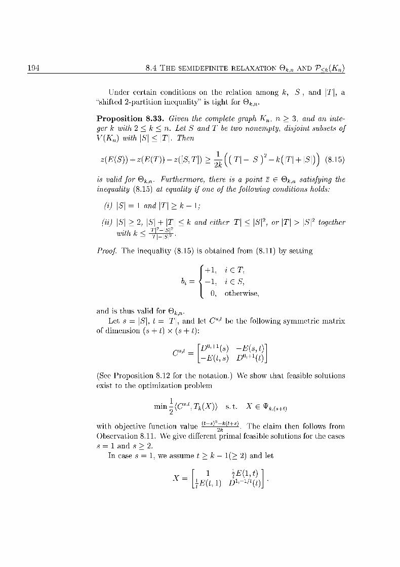
19 T H I D I N IO V<Kn

n c e i n condition n he r e l a n g k \S "shied p a r n inequali is ght for k

Proposition 8.33. Given the comlee gra Kn, n > 3, and a nte ger k with 2 < n Let S nd em disjoint ub of

Kn wi \S The

)) T))-([T]±-((\-\S \S (815)

valid for ©&,„. Furthermore here is a point z G &kn isfying the qual (815) qualty of the followig condio holds:

(i) \S\ = 1 nd 1;

(H) \S > 2, \S \T nd either \S or \S ogeher I SI

wi k < ' .I — \ S \ Z

roof The inequaliy (815) is ained 811) by setting

+1, i

- l , i e S,

otherwise

is th lid ^. Let s = \S t and let Cs he llowing symmeric marix

of dimensi

D - E t ) -E )

(See P r o p o s i n 81 or th n o t ) sh feasile lu exist to the i m i n prblem

m i n ^ C T f O ) s V

with objective functin value 2fc ^ n e c l a i m hen l lws from bse rva tn 811 We give diferen primal asible l u n s he cases

1 and n case we assume t and le

\{l 1'

F M M U M / 19

The matrix X h only entries o prinipal diagonal nd all of its o diagonal elements are no less than ^ y . Moreover, X is posiive semide inie. This is verified by checking he c n d i n s of P r s i n 813

^ii — nd

nsequenly, X laer reference, w ha \ + 2g)f - 1) = -(t + 1) = - + w, he case is nsidered. We assume tha + t and ha

lds t a %%[^ eiher t togeher wih k t ^

' T ^ V a n d s e

)

W ceck con i tons given in Proposi 12 and 8.13 in order to prove ha is p s i i v e semidefinie Firs is p s i i v e semidef

—^r is:

) -

fc>

Both of e latter inequalities hold due to the conditions th re laons a m n g s, t, and k. (This can be verified by case d i s t i n c n . ) Secnd D1,(t) is psitive semidefnite if 1 > ß j z i e ^ j j ^ which h l d s ecause k Finally

+ )/ i) -

- ( k 1

als olds due to t > 2. Thus, X is psitive semidefinite. Next, we sho tha ^k,n by checking ha he diagonal enries of X are n less han ^Py This is bviusly rue nd 7. F we disinguish

19 T H E S I D I N IO V<Kn

-^j n

i) -; —TT- TT (

<=^ ) -

^ t> -<= k >

is holds by asum Again evaluaing yields:

) -

tk tk ~^

~(s t)

Thus in both cases the corresponding solution X yields nd he resuling bjecive f u n c n values are:

^ jj- + )) ) -

^ ~ kt

This cncludes he proof. D

The reatment of the case \S\ = in Props i ion 8.33 is not fully satisfactory, because the most prominent representative of the 2-partiton inequality, namely he riangle inequaliy, is not covered The ase of

and is h e r e r e cnsidered separaely

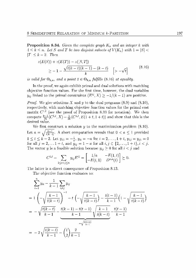
F M M U M / 19

ition 3 . ivn t complet gra Kn nd integ Let S nd be sjoint ub ofKn wi

The

)) )) ([T\)

-vi (816)

vald for kn, and point z G Qk,n flfills (816) equalty.

In the proof we again exhibit primal and dual s o l u t n s with matching bjective function values F r the first time hwever he dual variables

H linked to the primal nsraints (E^,X) /(k — ) are p s i i v e

Proof We give s o l u t n s X and y to the dual programs (8.9) and (8.10) respecively with matching objecive function values fo he primal cos matrix C (see he proof of s i n 833 for n o t o n ) . W hen compute ^ ( + ^ ( C { )) and show hat this is he desired value

We firs onsruc a slution y to the m a x i m i n prblem 8.10)

t a = V t-t} sh m p u n reveals ha 0 < provided

t . L /n = J yu a i . . , 1 t = yn

for all j = . . . + t, and y^ — a for alii, 6 {2,.. t} The vecto is a feasible s l u because y r all nd

-E J2 V

<j<n

The latter is a direct nsequence of P s i n 813 The bjecive f u n c n evaluaes to

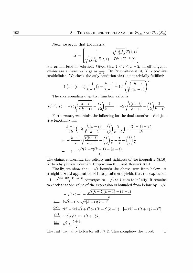
19 T H E S I D I N IO V<Kn

ix

h ^ 1 ^ ^

is a primal feasible solution. Given tha < k — 2, all ff-diagna entries are at least as large as -^j. By o p s i o n 8.13, X is positive s e m i d e n i e . We chec he nly ndi ha is ot trivially fulfilled:

\l in iv lu is

r t e r m o r e , w in l l i n r a r m e d jec ive n c n value:

^ ^ ) + 1) t\

2 ~ ~

t) t)

6) T e claims c n c e r n n g the v y d tightnes of the inequal is hereby proven c m p a r e P o p s i t i o n 8.11 and Remark 819.

Finally, we show ha —y/i bounds the above term from below. A raightfrward a p p l i c o n of l 'Höspial 's rule yields hat the expression

J t ) { k l ) - t ) r- . „ T+

— j converges to /t as goes to infinity It remains hec hat the value of he express in is b u n d e d m below by /i:

/- t ) t )

/i t) k>t tk/i t) tk )k

t> /i )k

m v~^ The las inequaliy h l d s r a lH This c m p l e e s he proof D

F M M U M / 199

8.5 Summary and Outlook

The semidefinie prgram (8.6) is a r e l a x a n of he combinatorial MIN IMUM K-PARTITION problem. It is known f r more than a decade that such a semidefinite prgram is in principle solvable in lynomial time Merely within the last one or two years however, SDP solvers have ma tured to the p i n t , where the semidefinite programs associated to graphs of sizes in the order of a few hundred vertices becme cmpuationally tractable in practice We are now in he position to solve our large semidenite r e l a x a n s w ih a sufficien degree of accuracy in tolerable running imes

The wer unds obtained in Section 6 on the o i m a l value of minimal c - p a r n are higher than we had expected. The previously

own computatinal sudies n related problems like the M I M U M

C U T prblem (wi k = 2) or the graph partitio problem wih given sizes fo the partite sets and with values k up to 4, see Wolkowicz nd Zhao [1999] can hardly give an indicaton of what to expect for he

INIMUM K - R T I T I O N problem r values of k btween 39 and 76 We attribute the strength of the bound to a large extent to the "shifted

hypermetric inequalities" (8.11), which are implicit in he semidefini relaxaon. Cnsequently, the solutions to the semidefnite relaxation always fulfill at least partially every single valid (and oft facet-defining) hypermetric inequality (7.12) the plytope V<k{Kn). paricular with respect to the ILP formulation (7.1) of the MINIMUM K P A R I O N

problem, all triangle constraints (7.1a) are violaed by at most y/2 1 and all clique cns t r a ins (71b) are violated less han \. Hence, in the LP relaxatin o a i n e d from the ILP (71) by dropping the integrality consrains, this corresponds to the s i m u l n e u s parial fulfillment of all (exponentially many) consraints.

The semidefinite relaxaion (8.6) of the MINIMUM K-PARTITION prob lem thus appears as an intriguing alernaive to the classical LP relax ation. Due to the enormus a m u n t of constraints he latter seems to be hardly olvable in practice. f his ottleneck is t be bypassed by adding the triangle and clique constraints as m d e l cuts, then he sepa r a t i n problem he clique inequaliies in paricular has to e slved effectively.

As an alternaive to develping a radiional branchand-cut algo rithm for slving MINIMUM K - P A R T I I O N prblems wit guaranteed quality, we may as well cnsider a brancand-cu algorithm on the basis of he semidefinite relaxation and an SDP solver. Successful applications of his kind are r e p e d by Helmberg 1995]; Helmberg Rendl, Vander

5 RY D O

bei, and Wlkowicz [1996]; H e l m b g d Re [1998]; Helmberg an Weismantel [1998]; Karisch Rendl, and lause [1998], for example. I heir conclusion, Karisch et al 1998] s t e : " u r results compare fa

rably to previously published nes [for graph bisection], which were obtained with cutting plane m e t h d s based on linear p r g r a m m i n g re l a x a t n s . " As po ined ou before t is not even clear h w mpetitive

wer unds an LP-based branch-and-cut algorithm for the M I N I M U M

K - P A R T I T I O N problem uld p r v i d e he insances we are i n e r e s e d in, see Sect 6 3

In the c e x of an SDP-based branch-andcu algorithm for the

I N I M U I O N p r b l e m , he llowing p i n s deserve cns ide r

F u r h e r invesigations concerning the re la ion tween the polytope

^<k{Kn) and its semidefinite relaxation 0fc]Jl in rder to give a

tter t h e r e i c a l underpinning of our empirically bserved l w e r

nds

A computational udy of the reng of the semidefinite re laxaio n a larger se of INIMU ION insances wi own

imal s o l u n

For which classes of valid inequalities for V<kKn) is the s e p a r a o n problem (heuristically) well solvable in practice and wha is he

fec he s r e n g of he c r r e s p n d i n g r e l a x a n ?

Another interesing issue is the generation of goo ^ - p a r n s on he basis of the s l u t i n for the semidefinite relaxation 8.6). How well fo example, does r andmized r n d i n g p e r r m ? Whic other heurisics are of pracical use?

APPENDIX A

otation

The follwing survey on basic o t t ion and facts f r m linear algebra linear programming, and graph t h e r y is primarily intended to serve as a glossary. For cmprehensive inroductions see, for example, hvätal [1983] or Padberg 1995] linear programming; Schrijver [1986] o Nem hauser and Wolsey 1988] or integer linear programming; Schrijver [1986] or iegler [1994] f olyhedral heory; Wolkowicz al. [2000] for semidefi nite programming; West [1996] or Diesel 1997] for graph theory; Cormen et al. 1990] for algorithm and data ture; and Garey and J h n s 1979] as well as Ausiell t al 1999] comutional comlexi

Basics

The cardinality of he set A is deoted by \A\. The Cartesian produc \A\ of ses A and B is written as A x B. The se difference of A and B A x B, A\B is A \ The intersection and union of A and B are denoted by An B Af]B, Au B and Au B, respectively. The symbls C and C denote se inclusin and AC B, AC B prpe r se inclusion, respectively.

The sets of real, rational, and ineger numbers are denoted by K, Q, M, Q, Z and Z, respectively. Their restrictions to the nonnegative numbers are denoted by K+, Q+ , and The symbol K. is used to represent Q and R Q Z in cases where the defini r p r p e r y applies to bot fields The se of all column vectors with n c m p o n e s , and enries me se is denoted by Bn, in particular, Rn , Q Z Q Z

Let k, n be a nnegative integers. Then k\ is equal to k\ nd equal to 1 • . . . • k otherwise. Moreover, (™) is equal to _^y_ (£)

0 < k < n and equal t 0 otherwise The expression mod k s n d s n mod k he remainder of the integer divisi of n divided by k.

F r x £ K, he ceiling \x\ of x is the smallest integer larger than \x equal t x, and he foor [x\ of x is he largest integer less or equal to x [x\

For , | / e [x,y] and ]y[ denot the clsed and open inerval of [x,y],]x,y real numbers ween x and , respecively n a l u s l y ] and x,y]]x.

incide v

support

V

]X,;?/[Q denot in bers x and y

For a finie set E, the f u n c n x £"—) K is identified w i h an \E dimensional olumn vector x £ K ^ L Given a finie set E and a subse F he incidence vector of in E is t h e d i m e n s i o n a l vecto XF £ 0, wit x F ( e F and x F ( e otherwise. The support of a function / : X —> Y is the set { 0} The expression f is used as an alernat ive to f(x)

The s y m l s 3 and V s n d he niveral and exienal qanifier

inear Algebra

AJJ

det(A) tx(A) singula regula

< >

{AB,C) = (A,C (AxxT) = x

cala prodct

ositive emi-)deRnite

+ c

eigenvalu

The set K m x n c n s i s s of all (m x n)-matrices with enr ies om K. Th n d i m e n s i n a l c l u m n vectors are identified w i h K"x r a m a r i x

Wnx he e r y in row i nd column j is referenced by ^, he ith row by Ai the th lumn by A.j, and the submatrix cns is t ing of the elements in the rows cn t a ined in set / and he columns ained in se

is referenced by u If I = J, then u is rincipal ubmtri of A The determinant of a square m a r i x A £ K n is denoted by det)

and its race, i e , the sum of s diagonal elements is denoted by tr(A). A square m t r i x A is singular if i s deerminant is z e r , and it is nns ingula r or regular otherwise The m u l t i p l i c i ve inverse of a regular m r i x is d e o t e d by A- and denotes he enty m in

ix rix AT

th th lumn of A o r i n he r w s of AT. In p a r t i c l a th tr se of a lumn vec is a vector. The inner produ n KmX

(• ) Kmxn x Kmx wi , B) ^ , B) = YT=i i AiJBiJ ti(BTA). The ident ty AB, C) = A,CBT h l d s all m r i c e s wi

mpa ib le dimensions. F u r h e r m r e , the identity TA holds or every vector x £ Kn and every atrix A £ K n . The in ner produc of w (column) v e c r s is als alled scalar produ The

uclidean norm of a vector x £ K is \x\ /(,x A m a r i x A £ K is symmeric if A = AT. A symmeric matrix

is positive semidefini (A y 0) i xTAx > 0 for all vectors x Kn . I furthermore, xT Ax = 0 implies x = 0, then A is positive definite (Ay 0) The sets of n x ndimensional posiive semidefinite and positive defini matrices are denoed by 5+ and respecively

A scalar A £ K is an eigenvalue of a matrix £ WlXn if Ax for some x £ K n x ^ 0. If A is an eigenvalue of ^4, hen all vectors x £ K saisfying x are eigenvecors o A associaed he eigenvalue A

A N O T A T I O N

Th determinant of a matrix A is the pro ll i g e l u he race is the sum of all its eigenvalues

A vecor x Kn is a linear combination of vectors in X if f inie number vecors x1,..., x G X and scalars A i , . . , A K. exis such that x = Y x % The vector a; is a conic combinaion he x if, in addition, Aj > 0 for all is an affine combinaion X^i=i = 1 and a convex combination if X^=i Aj = 1 as well as Aj > 0 for all i The linear, affine and convex hull as well as the cone of A , denoted by lin(X) aff(A), c o n v X ) , and cone(A) are the s e s of all linear a f n e , convex and conic combinations respecively. A set X is convex if X conv A set X saisfying X = cone(X) is a cone. A cone is poin implies for every nonzero vector x

A se I C P of vecors is linearly independent only one linear combination of vecors in X is equal to he zero-vector in K . The dimension dim A of A is maximal number of linearly independent vecors from A, ha is the dimension f the linear hull o as a subspace o

affine, conic convex, linea

combintion

convex ointed) cone

linearly indeendent

dim A

olyhedral Theory

Given a vector a G W1 \ } and a scalar K, hen he se {x IK™ aTx = a } is a hyperplane, and {x G K | ax < is the half-space delimied by he hyperplane The finie inersection half-spaces, given by { Kn | Ax < b} with A G K m , b G K m , is polyhedron. A set S C W is bounded if it is contained in a set { | | x | | < r } for some r G K. A bounded polyhedron is a poltope

The inequali a ra; < a0 for a G K \ { } K is wa/ for a polyhedron P if is contained in the half-space {x aTx < and it is tight for P i it is valid for P and he hyperplane aT

contains a leas one point in P. T h e s e t P n j j : G Kn | aTx = a } is the face of induced by aTx < a

A zerodimensional face is a vertex. A face F C P o f a polyhedron P is face of if it is a maximal face w i h respect o inclusion An inequali

x < is facet-defining for P if it is valid for P and F G aT is a facet f P . An equivalen c h a r a c e r i z i o n face ha im im P

yperplane alf-space

olyedron

olytop valid

tig for P

face of vertex

facet of P cetdeRning

inear rogramming

A polyhedron P { i I " x < 6} C Kn , a vector c G K" and an bjecive define a linear rogram or LP for shor The minimizaion and lin prog

P} and i n { a ; x G P}. A.l)

A vector x G P attaining the maximum minimum) in (A.l), provided timal solution this exists, is an optimal oltion. In case P is a nonempty polytope, at al prog least one ve rex o P is an optimal soluion The dual program to a linear

program { T x < b x > 0} is vamTy Ty > c, 0}

T h e o e m l (Dual i ty of l i n a r programming) Le x n

a n . In ca

x < b, 0} ^ an > c, 0} ^ 0

t/ie opimal olion val of

x < 6, x > 0} an min > c, 0} (A.

are fini an

x < 6 x > an > c,

exi uc ha

binry/integer A linear program turns into an integer linear program (ILP) if all liner prog variables are required to take integer values. In the special case of a

binary linear program the values of the variables are restricted to 0 and 1. LP relation The LP relaxation of an integer linear program is obtained by dropping

the integrality constraints

aph Theory

ur graph theoretic nomenclature is mostly taken from West [1996] (simple) graph A simple graph G with n vertices and edges consists of a vertex set vertex/edge et V(G) = {vi,..., vn} and an edge set E(G) = { i , . , em}. Each edge is

an unordered pair of distinct vertices. The edge {v, w} is also written as incident adjcent vw. If e = vw G E(G), then is incident to and w, the vertices v and neighborood w are the endpoints of e, and v and w are adjcent. The neighborhood of degree a vertex are its adjacent vertices. The degree of a vertex is the number

olated vertex of incident edges. A vertex in a graph is olated if its degree is zero. graph complement The graph omplement G of a graph G is a graph on the same vertex subgrap set as G with t w G -E(ö) if and only if G E(). A subgraph of a

graph is a graph if such that ) ) and ( ) ) The

A N O T A T I O N

subgraph H of is an inded subgraph if every edge in E(G with both endpoints in V(H) is in (H). If H is an induced subgraph of ith vertex set S, then this is written as H = G]

A nonempty subset Q of the vertices of V is a clique in G if every pair of vertices in Q is an edge in E(G). A set S C V(G) is an independent set if G^S] contains no edge. A clique (independent set) is maximal if no larger clique (independent set) contains it, and it is maximum if no clique (independent set) of larger size exists. The size of a maximum clique in a graph G is its clique number, denoted by u(G), and the size of a maximum independent set is its independen or stability nmber denote by a(G).

A graph is complete if its vertex set is a clique. Kn is complete graph on n vertices. A vertex is simpliial if its neighborhood is a clique.

A vertex labeling of a graph G (with elements from a set Y) is a function / : V . Analogously, an edge labeling is a function

G ) ^ r A graph is bipartite if its vertex set can be partitioned into at most

two independent sets; it is k-partite if its vertex set may be partitioned into k or fewer independent sets. A fc-partite graph is kolorable, and a fccoloring of a graph is a vertex labeling / : V(G) —> { 1 , . . . , k}. The coloring is proper if f(v) ^ f{w) for every pair of adjacent vertices. The minimum number k such that a graph is properly /colorable is its

romatic number, denoted by x ( ) . A walk of length A; in a graph is a sequence vQ, Vi €2, • • •, e^

vk of vertices and edges such that e* f - iU for a lH = 1 , . . . , k. The endpoints of the walk are v0 and Vk- A pa£/i is a walk containing no vertex more than once. A Hamiltonian path contains every vertex of the graph. A cycle or tour is a walk with both endpoints being the same vertex and no repeated vertex otherwise. A cycle of length 3 is also called a triangle The graph Cn contains n vertices and its edge set is a cycle. An edge v is a (I)chord with respect to a walk if v = Vi and w = V+i for some i.

A graph is connected if a path exists between any two vertices. A tree is a connected graph which does not contain a cycle. A component of a graph is a maximal induced subgraph that is connected. A horte path between two vertices v and w is a path with endpoints v and w of shortest length. In a connected graph, the diameter is the maximal length of a shortest path; otherwise, the diameter is infinite. An (edge) cut in a graph is a subset of the edges for which its removal disconnects the graph. For a partition of the vertex set into two nonempty, disjoint sets S and T, the cut [S, T] contains all edges ith one endpoint in S and the other endpoint in T. A graph is 2(edge) onneed if every cut has

in surap

G liq

indeendent et

liqu number indeendence

ber

complete graph,K simplicial vertex

vertex labeling edge labeling

bipartite k-partite coor

tic nber walk

amitoni pa

cle, to triang

Cn

(l-)cord connected, tree

comonent

ortet path ameter

(edge) c

2 c t e

06

(simple) digrap vertex/arc et

d, t acyclic orienttion

size at least 2. A subgraph H of a graph is spanning if (H and H is connected.

A simple direted graph with n vertices and m arcs consists of a ertex set V(D) = {vi7... ,vn} and an arc set A(D) { a i , . m } ,

where each arc is an ordered pair of distinct vertices. We write vw for the arc (v,w). The vertex v is the head and the vertex w the tail of the arc vw. A digraph not containing any directed cycle is cycli. A digraph D is an orientation of a graph if V(G) (D and u> G ^ O if and only if either M G E(D) or w (D)

(M

Asymtotic Function rowhs

Given a function / : Z + Z+ , let

: Z + Z + I c, a, n Z + \/n > (n < c(n) + a

and

: ^+ ^+ I c, a, n Z + Vn > (n) + a > / («)}

Every funcion g G ö ( / ) grows asymptotically no more tha / , h e a s every / ) g r o s asymptotically at least as much as / .

bliography

ardal, K., Hipolito, A., van Hoesel, C , Jansen, B., Roos, C , and Terlaky, T. EUCLID CALMA Radio Link Frequency Assignment Project: A branchandcut algorithm for the frequency assignment problem. Technical Annex T 1 A, T.

indhoven R F A P Group and T. Delft R F A P Group, 1995.

ardal, K., Hurkens, C., Lenstra, J., and Tiourine, S. Algorithms for frequency assignment problems. CWI Qaterly, 9(1 & ):l-8, 1996.

arts, E H. and Lenstra, J. K. (eds). Lal Sear in Combinatorial Optimization John Wiley & Sons Ltd., 1997.

Ahuja, R. K., Magnanti T., and rlin, J. B. Netork Flos. Prentice Hall 199

Alizadeh, F. Interior point methods in semidefinite programming with applications to combinatorial optimization. SI AM Jornal on Optimization 5(1):1 51, 1995.

Allen, S., Smith, D., and Hurley, S. Lower bounding techniques for frequency as signment. Drete Mathematis, 197/198:41-5 1999.

Applegate, D., Bixby, R., Chvätal, V., and Cook, W. Concorde: A computer cod for the traveling salesman problem. 1997. RL http://www.caam.rice.edu/ ~kec/concorde.html.

Applegate, D., Bixby, R., Chvätal, V., and Cook, W. On the solution of traveling salesman problems. In Proceeding of the International Congress of Mathemati cians Berlin 1998 vol. Ill of Dmenta Mathemati. Deutsche Mathematiker Vereinigung, 1998.

Ausiello, G., Crescenzi, P., Gambosi, G., Kann, V., Marchetti-Spaccamela, A., and Protasi, M. Complexity and Approximation: combinatorial optimization problem and their approximability properties. SpringerVerlag, 1999.

Barahona, F. and Mahjoub, A. the cut polytope. Mathematial Programming 6:157-17 1986.

Beckmann, D. and Killat, U Frequency planning with respect to interference min­imization in cellular radio networks. Tech. Rep. T D ( 9 9 ) 0 , C S T 59, Vienna,

ustria, 1999.

B L O G R A P H Y

Ben-Israel, A., Charnes, A., and Kortanek, K. O. Asymptotic duality over closed convex sets Jornal of Mathematial Anal and Appliations 5:677-691, 1971.

Björklund, P., Värbrand, P., and Yuan, D. Optimal GSM network planning with frequency hopping. Tech. rep., Linköping Institute of Technology, Norrköpping, Sweden, 000. Presented at the INFORMS Telecommuncitations Conference, Boca Ration, SA.

Bodlaender H. L. A tourist guide through t r e e i d t h . ta Cyberneti 1 1 ( 1 - ) : 1 -1, 199

Borndörfer, R. Aspects of Set Packing, Partitioning, and Covering. Ph.D. thesis Technische niversität Berlin, Fachbereich Mathematik, Berlin, Germany, 1998.

Borndörfer, R., Eisenblätter, A., Grötschel, M., and Martin, A. Frequency assign­ment in cellular phone networks. Annal of Operations R e a r , 7 6 : - 9 1998a.

Borndörfer, R., Eisenblätter, A., Grötschel, M., and Martin, A. The orientation model for frequency assignment problems. Tech. Rep. TR 98-1, Konrad-Zuse Zentrum für Informationstechnik Berlin (ZIB) 1998b. URL h t t p : / / w w w . z i b . d e /

ape rWeb/abs t rac t s /TR-98-1 .

Bovet, D. P. and Crescenzi, P. Introduction to the Theory of Complexity. Series in Computer Science. Prentice Hall 1994.

Brelaz, D. New methods to color the vertices of a graph. Commniation of the AM 22():169-174, 1979.

Burer, S., Monteiro, R. D., and Zhang, Y. Interiorpoint algorithms for semidefinite programming based on a nonlinear programming formulation. Tech. Rep. TR 99-27, Department of Computational and pplied Mathematics, Rice nviversity, 1999.

Buttmann-Beck, N. and Hassin, R. Approximation algorithms for minimum sum p-clustering. Drete Applied Mathematis 8 9 : 1 5 - 1 1998.

Carlsson, M. and Grindal, M. Automatic frequency assignment for cellular telephones using constraint satisfaction techniques. In Proceeding of the Tenth International Conferene on ogi Programming, pp. 648-665. 199

Carraghan, R. and Pardalos P. An exact algorithms for the maximum clique prob­lem. Operations Rear etters, 9 : 7 5 - 1990.

Castelino, D., Hurley, S., and Stephens, N. A tabu search algorithm for frequency assignment Annal of Operations Rear, 6 0 1 - 1 9 , 1996.

LIOGRAPH 09

Chopra, S. and Rao, M. R. The parition prblem. Mathematal Prramming 59:87-115, 199

Chopra, S. and Rao, M. R. Facets of the ^-partition polytope. rete Applied Mathematis, 61:7-48, 1995.

Chvätal V. Linear Programming W. H. Freeman and Company, 198

Cormen, T. H., Leiserson, C , and Rivest R. L. Introdtion to Algorithms. The MI Press, 1990.

Correia, L. M. (ed.). COST259: Wireless Flexible Peronalized ommniations John Wiley & Sons Ltd. 001.

Costa, D. On the use of some known methods for T-colorings of graphs Annal of Operation earh 4 1 : 5 8 , 199

amosso, E. and Correia, L. M. (eds.). COST231: Digital mobile radio toard re generation ems European Commission, 1999.

Deza, M. M., Grötschel, M, and Laurent, M. Complete descriptions of small mul-ticut polytopes Applied Geometry and Drete Mathematis—The Vitor Klee Fehrift 4:221-2 1991.

Deza, M. M., Grötschel, M., and Laurent, M. Clique-web facets for multicut poly-topes Mathemati of Operations Rearh 17:981-1000, 199

Deza, M. M. and Laurent M. Facets for the cut cone I Mathematial Programming 56:11-160, 199a.

Deza, M. M. and Laurent, M. Facets for the cut cone II: cliqueweb facets Mathe matial Programming 56:161-188, 199b.

Deza, M. M. and Laurent, M. Geometry of C and Metris, vol. 15 of lgorithm and Combinatoris. SpringerVerlag, 1997.

Diestel R. Graph Theory. SpringerVerlag, 1997.

Dueck, G. and Scheuer, T. Threshold accepting: a general purpose optimization algorithm appearing superior to simulated annealing. Jornal of Comptational Phys, pp. 161-175, 1990.

DuqueAnton, M. and Kunz, D. Channel assignment based on neural network algo­rithms. In Proc. IV, pp. 5.4.1-5.4.9. slo, Norway, 1990.

BLOGRAPHY

uqueAntön, M., Kunz, D., and Rübe, B. Channel asignment for cellular radio using simulated annealing. IEEE Trantion on Vehilar Tehnology 4 (1 ) : 14-

1, 199

Eidenbenz, S., Stamm, C , and Widmayer, P. R A D I - Wellenausbreitung in D. Comperorld eiz 7 : 6 - 9 , 1999.

Eisenblätter, A. Combinatorial lower bounds for co-channel interference in GSM-networks (preliminary report) Tech. Rep. TD(98) 104, COST 59, Duisburg, Ger many, 1998.

Eisenblätter, A. and Kürner T. Benchmarking frequency allocation strategies Tech. Rep. TD(00)044, COST 59, Bergen, Noray, 000.

Eisenblätter, A., Kürner, T., and Fauß, R. Radio planning algorithms for inter ference reduction in cellular networks. In Communication for the Millennium. COST252/29 Joint Worho, Unierity of radford, 1- pr 1998, pp. 8 7 - 9 . 1998.

Eisenblätter, A., Kürner, T., and Fauß, R. Analysis of C/I-ratio thresholds for fre quency planning. Tech. Rep. TD(99) 01 C S T 259, Thessaloniki Greece, 1999.

Erdös P. Rubin, A. L., and Taylor H. Choosability in graphs. Congressus Numer-anti 6:15-157, 1979.

FAP web. FAP web—A website abot Frequency Assignment Problems Andreas Eisenblätter and Arie Koster 000. URL h t t p : / / f a p . z i b . d e / .

Ferracioli M. and Verdone, R. A general methodology based on the handover rate for network planning of cellular radio networks based on ATM. IEEE Jornal on Seleted Area in Commniations 18() 000.

Ferreira, C. E., Martin, A., de Souza, C. C , Weismantel, R., and Wolsey, L. A. The node capacitated graph partitioning problem: a computational study. Mathemat

al Programming 7 4 A ( ) : 4 7 - 6 6 , 1996.

ischetti, M., Lepschy, C , Minerva, G., Jacur, G. R., and Toto, E. Frequency assignment in mobil radio systems using branch-and-cut techniques. European Jornal of Operational ear 1 4 1 - 2 5 5 , 000.

Frieze, A. and Jerrum, M. Improved approximation algorithms for max k-cut and max bisection. Algorithmi 18:67-81, 1997.

Gamst, A. Some lower bounds for a class of frequency assignment problems. IEEE Trantion on Vehilar Tehnology VT-5(1):8-14, 1986.

LIOGRAPH

Garey, M. R. and Johnson, D. S. Computes and Intractability - A de to the Theory ofCompleteness. W. H. Freeman and Company, 1979.

Garg, N., Vazirani, V. V., and Yannakakis M. Approximate max-ow min-(multi)cut theorems and their applications. SI AM Jornal on ompting, 2 5 : 2 - 2 5 1 , 1996.

Gerards, A. Testing the odd bicycle wheel inequalites for the bipartite subgraph olytope. Mathemati of Operations Rear 10 :59-60 , 1985.

oemans, M. X. and Williamson, D. P. Improved approximation algorithms for maximum cut and satisfiability problems using semidenite programming. Jornal of the AM 42():1115-1145, 1995.

oldschmidt . and Hochbaum, D. S. A polynomial algorithm for the k-cui problem for ixed k. Mathemati of Operation earh, 19(l):24-7, 1994.

otzner, U., Gamst A., and Rathgeber, R. Statial traffic distribution in cellular networks. I Proc. IEEE VTC'97 Otta Canada, pp. 1994-1998. I E E , 1997.

Grace, D. Distributed Dynamic Channel Assignment for the Wireless ironment Ph.D. thesis niversity of York, York, K, 1999.

Grace, D., Burr, A. G., and Tozer, T. C. Performance of a distributed dynamic chan­nel assignment algorithm incorporating power control in a ireless environment

Globeom 98 Sydney, Australia, 1998.

Grötschel, M, Loväsz, L., and Schrijver, A. Geometri lgorithm and Combinato­rial Optimization. SpringerVerlag, 1988.

Grötschel, M. and Wakabayashi, Y. A cutting plane algorithm for a clustering problem. Mathematial Programming 45:59-96, 1989.

Grötschel, M. and Wakabayashi, Y. Facets of the clique partitioning polytope. Math­ematial Programming 47 :67 -87 , 1990.

GSM ssociation. 2000. RL http://www.gmworld.com.

Haberland, D. Azyklische Subdigraphenprobleme und Frequenzzuweisung im Mobil funk. Master's thesis, Technische niversität Berlin, Fachbereich Mathematik, Berlin, Germany, 1996.

Hale, W. K. Frequency assignment: Theory and applications. I Proeeding of the IEEE, vol. 68, pp. 1497-1514. IEEE, 1980.

Hao, J.K., Dorne, R., and Galinier, P. Tabu search for the frequency assignment in cellular radio networks. Jornal of Hritis 4:47-62, 1998.

BLIOGRAPHY

Häsad, J. Some optimal inapproximability results. In Proceedings of the 9th Anal AC Sympom on Theory of Compting, pp. 1-10. ACM, 1997.

Hebermehl, M. Hristische Algorithmen zur Lösung von Färbungsproblemen im Mo­bilfunk. Masters thesis Technische Universität Berlin, Fachbereich Mathematik, Berlin, Germany, 1996.

Hellebrandt, M. and Heller, H. A new heuristic method for frequency assignment Tech. Rep. TD(00) 00 COST 259, Valencia, Spain, 2000.

Heller H. private communication, 2000.

Helmberg, C. An interior point method for semidefinite programming and ma bonds. Ph.D. thesis, Technische niversität Graz, Graz, Austria, 1995.

Helmberg, C. Semidenite programming for combinatorial optimization. Habilita­tionsschrift 2000.

Helmberg, C. and Rendl, F. Solving quadratic (0,l)-problems by semidefinite pro­grams and cutting planes Mathematial Programming 82() :291-15, 1998.

Helmberg, C , Rendl F., Vanderbei, R. J., and Wolkowicz, H. An interior point method for semidefnite programming. SI AM Jornal on Optimization, 6 ( ) 1996.

Helmberg, C and Weismantel, R. Cutting plane algorithms for semidefinite relax­ations. In P. M. Pardalos and H. Wolkowic (eds) Topis in Semidefinite and InteriorPoint Methods, vol. 18 of Fields Institte Commniation Series, pp. 197-21. American Mathematical Society, 1998.

Hurley, S., Smith, D., and Thiel, S. FASoft A system for discrete channel frequency assignment. Radio Sien 2(5):1921-19, 1997.

Janssen, J. and Kilakos, K. Polyhedral analysis of channel assignment problems: (i tours. Tech. Rep. LSE-CDAM96-17, London School of Economics, 1996.

Janssen, J. and Kilakos, K. An optimal solution t the "Philadelphia" channel assignmetn problem. IEEE Trantion on Vehilar Tehnology, 48():1012-1014, 1999.

Jaumard, B., Marcotte, O , and Meyer, C. Estimation of the quality of cellular networks using column generation techniques. Tech. Rep. G-98-02, GERAD, ni versity of Montreal Montreal Canada, 1998.

IOGRAPH

Jaumard, B., Marcotte, O., and Meye, C. Mathematical models and exact methods for channel assignment in cellular networks. In B. Sansö and P. Soriano (eds.) Telecommunications Netork Planning, chap. 1 , pp. 9-255. Kluwer Academic Publishers 1999.

ünger, M. and Rinaldi, G. Relaxations of the max cut problem and computation of spin glass ground states. In P. Kischka, H.W. Lorenz, . Derigs, W. Domschke, P. Kleinschmidt, and R. Möhring (eds), Operation Reearch Proeedings 1997 Selected Papers of the Sympo on Operation ear (SOR'97, pp. 74-8 SpringerVerlag, 1998.

Johnson, D., Pataki, G., and Alizadeh, F. Seventh DIMACS implementation chal lenge: Semidefinite and related optimization problems. DIMACS, 2000. RL ht tp: / /dimacs.rutgers .edu/Chal lenges/Seventh/ .

Johnson, E. L., Mehrotra, A., and Nemhauser G. L. Min-cut clustering. Mathemat­al Programming, 62:133-151, 199

ünger, M., Martin, A., Reinelt, G., and Weismantel, R. Quadratic 0/1 optimization and a decomposition approach for the placement of electronic circuits Mathemat­

al Programming, 6257-279, 1994.

ünger, M., Reinelt, G., and Rinaldi, G. Network Models, vol. 7 of Handboo in Operation Rsearch and Management Science, chap. The traveling salesman problem, pp. 25330. Elsevier Science B V., 1995a.

ünger, M., Reinelt, G., and Thienel, S. Practical problem olving with cutting plane algorithms in combinatorial optimization. In W. Cook, L. Loväsz, and P. D. Seymour (eds.), Combinatorial Optimization, vol. 20, pp. 111-152. American Mathematical Society, 1995b.

Kann, V., Khanna, S., Lagergren, J., and Panconesi, A. Hardness of approximating max k-cut and its dual. Chicago Journal of Theoretical Compter Sien 2, 1997.

RL h t t p : //www. cs . uchicago. edu/publ icat ions/c j t c s .

Karger, D., Motwani, R., and Sudan, M. Approximate graph coloring by semidenite programming. I FOCS 94, pp. 2-1 1994.

Karger, D., Motwani R., and Sudan, M. Approximate graph coloring by semidenite programming. Jornal of the ACM 45():246-265, 1998.

Karisch, S. E., Rendl, F., and Clausen, J. Solving graph bisection problems with semidefnite programming. NFOMS Jornal on Compting 1998. To appear.

B L I O G R A P H Y

Kennedy, K., Vries, E. D., and Koorevaar, P. Performanc of a distributed DCA algorithm under inhomogeneous traffic modelled from an operational GSM net work. In Proc. of VTC'98-48th IEEE Vehilar Tehnology Conferen Phoenix, Arizona, USA, 1998.

Koster, A. M. C. A. Frequency Assignment - Models and Algorithms. Ph.D. thesis niversiteit Maastricht Maastricht The Netherlands, 1999.

Krumke, S. O On the Approximability of Location and Networ Design Prob lems. Ph.D. thesis, Ju l iusMaximi l i ansn ive r s i t ä t Würzburg, Würzburg, Ger many, 1996.

ürner, T., Cichon, D. J., and Wiesbeck, W. Concepts and results for 3D digital terrain-based wave propagation models: An overvie EEE Jornal on Seleted Area in Commniations 11(7):1002-1012, 199

ürner, T. and Fauß, R. Investigation of path loss algorithms at 1900 MHz. Tech. Rep. TD(94)109, COST 1, Darmstadt Germany, 1994.

ürner, T., Fauß, R., and Wasch, A. A hybrid propagation odelling approach for DCS 1800 macro cells. In Proc. IEEE C , pp. 1 6 2 8 - 1 2 . Atlanta, Georgia,

SA, April 28-May 1, 1996.

Laurent, M. and Poljak, S. On a positive semiden i te relaxation of the cut polytope. inear Algebra and it Apliations / 2 4 : 4 9 - 4 6 1 , 1995.

Laurent, M. and oljak, S. Gap inequalities for the cut polytope. European Jornal of Combinatoris 17(2-3):33-254, 1996a.

Laurent M. and Poljak, S. On the facial structure of the set of correlation matrices SIAM Jornal on Matri Anal and Appliations 1 7 ( ) : 0 - 5 4 7 , 1996b.

Laurent, M., Poljak, S., and Rendl, F. Connection between semidefinite relaxations of the max-cut and stable set problems Mathematial Programming 77B( ) :225 -246, 1997.

Lin, S. and Kernighan, B. An effective heuristic algorithm for the traveling salesman problem. Operations Rearh 21:498-516, 197

öbel, A. MCF Version 1.0 - A network simplex implementation 1997. RL h t tp : / /www.zib .de/Opt imizat ion/Sof tware/Mcf .

oväsz, L. On the Shannon capacity of a graph. IEEE Trantion on Information Theory IT-25:l-7, 1979.

IOGRAPH

EDA 3.6.1. The LED A User Manual Version 3.6.1. LEDA Software GmbH, D-661 Saarbrücken, Germany, 1998. RL http://www.mpi-sb.mpg.de/LEDA.

Majewski, K., Hallmann, E., and Volke, A. From propagation predictions to fre quency planning: An approach capturing radio link control options. In AP2000 Millenni Conferene on Antenna and Propagation Davos Sitzerland, 2000.

Malesihska, E. Graph-Theoretical Models for Frequency Assignment Problems. Ph.D. thesis Technische niversität Berlin, Fachbereich Mathematik, Berlin, Germany, 1997.

Mehlhorn, K. and Näher, S. LEDA: a platform for ombinatorial and geometri ompting. Cambridge University Press, 1999.

Menolascino, R. and Pizarroso, M. STORMS Project Final Report ACTS Pro­gramm AC016, European Union, 1999. URL http:/ /www.fowin.org/ACTS/ RUS/0JECTS/FINAL-RE0RTS/fr-016.pdf.

Metzger, B. H. Spectrum management technique. Presentation at 8th ational RSA meeting (Detroit MI), 1970.

Mittelmann, H. Benchmarks for optimiation softare. 2000. RL h t t p : / / p l a t o . la.asu.edu/bench.html.

Mouly, M. and Pautet, M The GSM Sytem for Mobile ommniations. Cell & Sys, France, 1992.

Murphey, R. A., Pardalos, P. M., and Resende, M. G. C. Frequency assignment problems. In D.-Z. Du and P. M. Pardalos (eds.), Handboo of Combinatorial Optimization, vol. A. Kluwer Academic Publishers, 1999.

Nemhauser G. L. and Wolsey, L. A. Integer and Combinatorial Optimization. John iley ons Ltd., 1988.

Nesterov, Y. and Nemirovskii, A. Interior-point polynomial algorithms in convex pro­gramming. No. 13 in SIAM Studies in Applied Mathematics Society for Industrial and Applied Mathematics, 1994.

Nielsen, T. T. and Wigard, J. Performance Enhancement in a Freqen ping GSM Netork. Kluwer Academic Publishers 2000.

osten, M., Rutten, J., and Spieksma, F. The facial structure of the clique parti tioning polytope. Tech. Rep. Rep. 95-09, Universiteit Maastricht, Maastricht, The Netherlands, 1995. RL f tp: / / f tp .unimaas.nl /pub/grey_fi les / fdaw/1995/ rep95-09.ps.

16 BLIOGRAPHY

adbeg, M. Lner Optmizatn and E x t . Spr ingeVeag , 995.

apadimitriou, C H. Comptational Complexity Addison-Wesley, 1994.

Plehn, J. Applied frequency assignment. Proceeding of the IEEE Vehiclar Technology Conference IEEE, 1994.

Poljak, S. and Tuza, Z. Maximum cuts and large bipartite subgraphs. In W. C o k , L. Loväsz, and P. Seymour (eds.), Combinatorial Optimization, vol. 20 of DIMACS Series in Discrete Mathematics and Theoretical Compter Science pp. 188-244.

merican Matematical Society, 1995.

Ramana, M. V. An exact duality theory for semidefinite programming and its com­lexity imlications. Mathematical Programming 77():129-162, 1997.

Raychauduri, A. Interection Assignment, TColoring and Poer of Graphs. D. t es i s Rutgers niversity, 1985.

Raychaudhuri, A Fur te r results on T-coloring and frequency assignment oblems. IAM Jornal on crete Mathematics, 7(4):605-61 1994.

Redl, S. M., Weber, M. K., and liphant, M. W. An Introdction GSM. Mobile ommunications Series. rtec ouse Publisers, 1995.

oberts, F. S. From garbage to rainbws: generalizations of graph coloring and their applications. In Y. Alavi, G. Chartrand, 0 . Oellermann, and A. Schwenk (eds.), Graph Theory, Combinatoric, and Applications, vol 2, pp. 1031-1052. J o n Wiley & Sons Ltd., 1991a.

oberts, F. S. T-colorings of graph: recent results and en roblems. Dcrete Mathematics, 9229-245, 1991b.

Rutten, J. Polyhedral Clustering. P D . t e s i s niversität Maastrict Maastric Neterlands, 1998.

Sahni, S. K. and Gonzalez, T. F. P-comlete appximat ion roblems. Jornal of the ACM 555-565, 1976.

Schneider, K. Frequenzzuweisung im Mobilfk mittels lokaler Suche Master's t e s i s Tecnisc Universität Berlin, Facbereic Matematik, 1997.

Schrijver Theory of inear and Integer Programming J o n Wiley & ons Ltd. 1986.

Schulz, A. S. Polytopes and Scheduling. Ph.D. thesis, Tecnisc niversität Berlin, Fachbereic Matematik, Berlin, Germany, 1996.

IOGRAPH

Smith, D., Allen, S. M., Hurley, S., and Watkins, W. J. Frequency assignment Methods and algorithms. In N A O (ed.), RTO 1ST Symposium on "Freqency Assignment, Sharing and Conseration in Systems (Aerospace)", Aalborg, Den­mark -7 Oct 1998, vol. MP- of RTO pp. K-l-K-18. alborg, Denmark, 1998.

Smith, D. and Hurley, S. Bounds for t e frequency assignment roblem. Dcrete Mathematics 167-168:571-582, 1997.

Stoer, J. and Witzgall, C Conexity and Optimization in Finite imenion I. ringerVerlag, 1970.

Sturm, J. F. Sedumi 1998. RL http://www2.unimaas.nl/sturm/software/ sedumi.html.

Tesman, B. List T-colorings of graphs. Dcrete Aplied Mathematics 45:277-289, 199

hienel, S. ABACUS - A Branch-And-Ut Sytem D. esis niversität zu Köln, Köln, Germany, 1995.

Tutschku, K., Mathar, R., and Niessen, T. Interference minimization in wireless communciation systems by optimal cell site selection. I 3rd European Peronal Mobile Commnication Conference Paris France, 1999.

Vandenberge, L. and Boyd, S. Semidenite ogramming. I AM iew, (1):49-95, 1996.

Wessäly, R. Dimensioning Surivable Capacitated NETworks. Ph.D. thesis, Tec nisc Universität Berlin, Facbereic Matematik, Berlin, Germany, 2000.

West D. B Introdction to graph theory. Prentice Hall 1996.

Wolkowicz, H., Saigal, R., and Vandenberghe, L. (eds.). Handbook on Semidefinite Programming, vol. 27. Kluwer cademic Publisers, 2000.

Wolkowicz, H. and Zhao, Q. Semidefinite programming relaxations for the graph artitioning roblem. Dcrete Applied Mathematics, 96-97:461-479, 1999.

wwwemcdatabase.com. 2000. RL http://www.emc-database .com.

Ziegler G. M. Lectre on Polytopes. SringerVerlag, 1994.

BLIOGRAPHY

Index

B(K,±e), 181 Da>P{n) 17

E(mri), 17 fhm(vk) ÄfV 43 ** 18 V,43 PFAP, 4

V<{Kn) 14 V n ) , 144

Tk 182, 18

A B A C U S 71, 77

adaption planning situation, 113 RFC (absolute radio frequency

channel number), 15, 20, 21

assignment, see frequency assign­ment

band s l i t 31 BCCH (broadcast control c a n ­

nel) 15, 21, 31 BHC (busy hour call a t t e m t s )

25 B M Z , 129, 1 0 branc-and-bound, 85, 10 branch-and-cut, 32, 70, 163, 199 broadcast control channel, see BCCH BSC base station controller) 11

13 BTS base transceiver station)

11, 1 25,

burst, 1

carrier, 34 carrier network, 3

simplified, 119 t i g t e n i n g the sea ra t ion , 59

CDM (code division m u l t i l e ac cess) 8

cell 11, 20 area, 25

odel

assignment probability, 26 best server 26 hexagonal 26

annel, 14 available blocked, 34

broadcast control, see BCCH changeable, 24 locally blocked, 21 traffic, see TCH uncangeable 24

coloring

list coloring, 34, 60 list T-coloring, 34, 60 span, 40 T-coloring, 34, 60, 1

O N C O R E , 136, 163

congested planning situation, 11 O S T 259, 78, 87, 11

C P L E X 77, 124

cutting lane, 164 cutting lanes a lgo r i tm , 164

DC (dynamic annel allocation) 40

EX

DCS1800, 6 discontinuous transmission, see DT down-link, 15

A T R , 60, 62 A T R W I T H C O S T S , 62, 92,

106, 111, 114, 115, 130 DT (discontinuous transmission)

17, 24, 30, 32, 115 duality gap, see s emiden i te ro­

gram

EDG (enhanced data for GS evolution), 8

elliptope (£•„), 1 8 - 1 8 5 , 188 truncated ( ^ ) , 18

eplus model, 29 Erlang-B formula, 25 ETSI (European Telecommunica­

tions Standards Institute) 10, 14

FC (fixed annel allocation) 40

FDM (frequency division mul t i l e access), 1

free space model, 28 frequency assignment, 34, 119

compatible orientation, 51 7 extension, 38 feasible 34, 119 feasible ermutation, 1 partial, 38 reassigning, 38

frequency assignment problem alternative odels 9-42

, 24, PP , 38, P r , 38, 3

FAPpu), 38, 39 ILP formulation, 49-54 min max interference 41

min max local interference 42 min-span, 36, 40, 60 minimum blocking, 36 orientation model 51, 72 PFAP, 44

relaxed, 119 stable set model 50 variants 3 7 3

frequency hopping baseband, 17 frequency diversity, 17 hopping gain, 30 interferer diversity, 18 load gain, 30 yntes ized, 17

GPRS (general acket radio ser vice) 8

graph antiweb, 150 bicycle, 149 Hamiltonian a t , 1 c a r t i t e 121 -chord, 149 lanar, 84

spoke, 148 tree decomposition, 84 2-chord, 146 2-corded cycle, 14 2-corded ath, 147 2-chorded eel, 148 web, 150 wheel, 148

G R A P H K - C R A B 48

GSM, 5-32 broadcast control c a n n e l see

BCCH BSC, see BSC BSS, see BSS BTS, see BTS core network, 11, 1

EX

dedicated mode, 9 discontinuous transmission, see

DTX frequency bands, 6 frequency h p p i n g , see frequency

h p p i n g growth, 7 hand-over, 10 HLR ome location register)

11 idle mode, 9 location area, 9 location updating, 9 MS, see MS network planning, 19 NSS, see NSS OMC, see OMC OSS, see OSS power control, 16 slow frequency pping, see

SFH traffic channel, see TCH transceiver, see TRX VLR (visitors location regis

ter), 11

Hamiltonian p a t , 1 hard constraints, 21 HC ybric annel allocation)

40 HSCSD (high s e e d circuit swi t ced

data), 8 HS opping sequence number)

17, 30

I N D E P E N D E N T S , 166

interference adjacent channel, 16, co-channel, 16, 34

rediction model lus 29

free pace race, 29

interference lot, 108 RATED 1 - O P T 67, 96, 104,

106, 115 (International Telecommuni

cation nion) 7

kpt step, 70 K - O P T , 70, 102, 105, 112, 11

115

L E A , 65, 77 line lot 108

(mobile allocation index ffset), 17,

matrix (strictly) diagonally dominant

172 ositive (semi defnite, 170

IQUE, 46

UM C U T 47,122,128,142, 85, 199 M F R E Q U E N C Y LL

ATION 47

UM K - C O L R A B L

G R A P H 47

XIMUM K - C U T , 47, 121, 128

M C F , 72, 77, 104, 106, 107 migration planning, 116 min-cost network flow 7

I N M E D E L E T I O N K-

P A R T I O N 47, 119, 121

I N U M E D E D L E I O N S U B

G R A P H O P R T

n , 47 I N U M G R A P H C I N 46

I N U M K - L U S T I N G S M

47, 1 2 I N U M K - P A R T I T I O N , 1 2 0 , 1 8 ,

142, 1 6 , 182, 187, 199

EX

MS (mobile station) 10, 15 MSC (mobile w i t c i n g center)

11, 1

network, see carrier network D E C A P A C T A T E D R A P H P A R

T T I O N , 164

NSS network and swi tc ing sub­system), 11

MC operation and management center), 12,

1 o p t step, 67 orientation model, 51

SS (operation and maintenance subsystem), 11

artition p o l y t e s inequalities

antiweb, 154 claw, 152 clique-web, 150 cycle, 162, 167 general clique, 156, 193

ypermetric 155, 167, 188, 190 bicycle, 149, 166

gwheel, 149, 166 trivial, 145 2-corded cycle, 146 2-corded even wheel, 148 2-chorded path, 147 2part i t ion, 151, 156, 194,

196, 197 V(Kn), 144 V<k(Kn), 144

PCS 1900, 8 olynomial time 4 ower control, 16 rerocessing, 57-60, 87

heuristic, 57, 59 s t ruc turereserv ing , 57-58

qual guarantee, 1 7 ,

race model, 29 relaxed planning situation, 11 running time 42

SB, 129, 1 scenarios

B[] , 79, 83, 111 24, 129, 130, 137, 138

K, 79, 83 111 124, 129, 1 0 , 137, 13 , 80, 8 , 111, 124, 129,

130 E 2 , 80, 8 , 111, 129, 1

, 80, 8 , 111, 129, 1 E 4 , 80, 83, 111, 129, 1

80, 8 , 111 INY, 20, 4

SDM (space division m u l t i l e access), 16

sector, 11, 20 SeDuMi, 129, 130 semidefinite ogram

dual, 177 duality gap, 178 primal, 176 strictly feasible, 179

semideinite relaxation (of mini­mum / c a r t i t i o n ) 128, 185

sea ra t ing , 164

cycle inequalities, 167 ypermetric inequalities, 167 bicycle inequalities, 166

gwheel inequalities 166 sea ra t ion , 21,

co-cell, 21 co-site 21

s e a r a t i o n graph, 132

augmented, 134, 13 s e a r a t i o n oblem, 164

EX

FH (slow frequency hopping) 7, 24, 30, 113, 115

ortcut, 132, 135, 1 constraints, 135

simplified carrier network, 119 sit, 20 slot 14 slow frequency hopping, see SFH oft constraints 24

spectrum, 20, 34 stable set model, 50, 70 starting oint, see D A T U R

C O S T S

support graph 145

IN 60, 90, 106, 111 130

TCH (traffic channel), 15, 21, 30 TDM (time division m u l t i l e ac

cess), 14 HOLD A C C P T I N 87, 111,

114, 130, 136 tightening t s ea ra t ion , 61 tour, 134 traffic channel, see TCH transitive packing, 51 T R , 11, 14, 15, 20, 30, 4 TSP (traveling salesman roblem)

4, 1

MTS (universal mobile telecom­munications system) 8

-link, 15

68, 98, 104, 106, 111, 114, 130

Zusamnfassung

Eine Schüsseltecnologie im Informationszeitalter ist die mobile Telekommunikation. Diese kann durch Interferenz empndlich gestört werden. Für GSMMobilfunknetze untersucht die Dissertation wie sich Interferenz möglichst weitgehend vermeiden läßt indem die verfügbaren Frequenzen geeignet an die Basisstationen zugewiesen werden. Mathematisch wird dieses Ziel als Minimierung der Gesamtinterferenz aufgefaßt.

Heuristisce Methoden zur Lösung des Frequenzzuweisungsproblems werden ent wickelt und anhand der Laufzeiten und Ergebnisse für Planungsfälle, die der Praxis entstammen, verglichen. Der Großteil der Methoden eignet sich aufgrund des guten Laufzeitverhaltens für den interaktiven Einsatz bei der Netzplanung. Die Resultate sind im Vergleich mit denen des besten derzeit bekannten (aber deutlich langsame ren) Verfahrens durchaus akzeptabel. Eine Auswal der Metoden ist eute bei der E-Plus Mobilfunk GmbH & Co. KG erfolgreich im Einsatz.

Weiterhin wird in der Dissertation der Frage nachgegangen, wieviel Interferenz in einem gegebenen Netz bei der Frequenzzuweisung unvermeidbar ist. Die Ergebnisse entsprechender Berechnungen werden verwendet, um (im mathematischen Sinne) Qualitätsgarantien für Frequenzzuweisungen hinsichtlich der Interferenzvermeidung zu geben. Im besten betrachteten Fall verursacht eine Frequenzzuweisung nur doppelt oviel Interferenz wie nachweislich unvermeidbar.

Das Frequenzzuweisungsproblem läßt sic zu einem fcPartitionierungsproblem eines vollständigen Graphen relaxieren. Dem fcPartitionierungsproblem ist (ausge hend von einer Formulierung als ganzzahliges lineares Programm) eine Polyederklasse zugeordnet, wobei die Ecken der Polyeder jeweils die Partitionierungen des zuge hörigen Graphen darstellen. Anstelle der sonst üblichen polyedrischen Relaxierungen wird eine nichtpolyedrisce Umschreibung des Polyeders analysiert, die sich als Lö­sungsmenge eines semidefiniten Programmes ergibt. Dieses Programm läßt sich für festes e > 0 in Polynomialzeit eoptimal lösen (im Gegensatz zur linearen Relaxie rung des ganzzahligen Programmes - ? ^ J\fV vorausgesetzt).

Die Lösung der semideniten Programme f ü r t zu den derzeit mit Abstand be sten unteren Abschätzungen der unvermeidbaren (Gleichkanal)Interferenz. Zudem handelt es sich um eine der ersten Anwendungen von semidefiniter Programmierung bei großen industriellen Problemen mit kombinatoriscem Hintergrund.

Schlüsselwörter: GSM, Frequenzzuweisung, Minimale Ä;Partitionierung, Heuristi ken, Semidefinite Pogrammierung, Ganzzahlige Programmierung, Polyeder. Mathematics Subject Clssification ( S C 2000): 90C27 90C35 90B18 90C

ebnslauf

LÄTT

geboren am 27. ugust 1967 in Hilden/Rld.

1974-1978: Grundscule

1978-1980: ntegrierte Gesamtscule NiederRoden

1980-1987: Gymnasium in Haan, bitur im Mai 1987

1987-1990: Studium der Tecniscen nformatik an der Berufsakademie Stuttgart

S e t . 1990: Dilom-ngenieur ( B ) Vertiefungsrichtung „Prozeßdatenverarbeitung"

1990-1991: Zivildienst beim Studentenwerk üsseldorf ö.

1988-1992: Teilzeitstudium der Matematik an der Fernuniversität Hagen

1992-199: Matematikstudium an der Universität Heidelberg

1992-1994: Studiengangzweitörer in Informatik an der Fernuniversität Hagen

1992-1994: Freier Mitarbeiter am Euroean Networking Center der I B , Heidelber

1994-199 ustauscstudent an der Univ. of Illinois at Urbana-Camaign, US

S e t . 199: Di lom in Matematik an der Universität Heidelberg, Szialgebiet „Komlexitätstheorie", Betreuer: Prof. Dr. mbosSies

seit 199 Wissenschaftlicher Mitarbeiter am onrad-Zuse-Zentrum für Informa­tionstecnik Berlin (Z

Juni 2000: Mitgründer der riston Consulting mbH (jetzt Atesio GmbH

27