Performance of critical path type algorithms for scheduling on parallel processors

Operations Research Letters 29 (2001) 17–30www.elsevier.com/locate/dsw

Performance of critical path type algorithms for schedulingon parallel processors

Gaurav Singh ∗

Department of Mathematical Sciences, University of Technology, Sydney, NSW 2007, Australia

Received 6 September 2000; received in revised form 15 May 2001; accepted 17 May 2001

Abstract

In this paper, two well-known NP-hard problems with parallel processors, precedence constraints, unit execution timetask systems, and the criterion of maximum lateness, are considered. The 2rst problem has an additional restriction thata task may occupy more than one processor simultaneously, and the second considered problem is a unit communicationdelay problem. For both problems the worst-case performance of critical path type algorithms is analyzed. All performanceguarantees presented are tight for arbitrary large instances of the respective problems. c© 2001 Elsevier Science B.V. Allrights reserved.

Keywords: Scheduling; Unit execution times; Maximum lateness; Precedence constraints; Concurrency; Unitcommunication delays

1. Introduction

Suppose that a set N = {1; 2; : : : ; n} of n tasks (jobs, operations) is to be processed on m¿ 1 identicalprocessors (machines) subject to precedence constraints in the form of an anti-re=exive, anti-symmetric andtransitive relation on N . If task i precedes task j, denoted i → j, then the processing of task i must becompleted before the processing of task j begins. The processing of the tasks commences at time t = 0.Each processor can process at most one task at a time, and each task can be processed by any processor.Once a processor begins executing a task it continues until completion (i.e. no preemptions are allowed). Allprocessing times are equal, and therefore, without loss of generality, can be taken as one unit of time. It isconvenient to represent a partially ordered set of tasks by an acyclic directed graph where nodes correspondto the tasks and arcs re=ect the precedence constraints.

Since no preemptions are allowed and all processors are identical, to specify a schedule s it su?ces tode2ne for each task j∈N its completion time Cj(s) in such a way that not more than m tasks are assignedthe same completion time, and the precedence constraints are satis2ed. Each task j∈N has a due date dj,the desired point in time by which the processing should be completed. The goal is to 2nd a schedule which

∗ Corresponding author. Tel.: +61-2-9514-2303; fax: +61-2-9514-2248.E-mail address: [email protected] (G. Singh).

0167-6377/01/$ - see front matter c© 2001 Elsevier Science B.V. All rights reserved.PII: S 0167 -6377(01)00077 -3

18 G. Singh /Operations Research Letters 29 (2001) 17–30

minimizes the criterion of maximum lateness

Lmax(s) = maxi∈N

(Ci(s) − di):

Without loss of generality, in this paper we will consider only schedules in which all completion times arepositive integers.

Using the popular three 2eld notation � | � | �, where � speci2es the processor environment, � speci-2es the task characteristics, and � denotes the optimality criterion, the above problem can be denoted byP | prec; pj = 1 |Lmax. Here P speci2es that there are several parallel identical processors, prec indicates thepresence of precedence constraints, and the term pj = 1 indicates that each task has a unit processing time.

If all due dates are equal to zero the problem stated above converts to the so-called makespan problem,with the criterion

Cmax(s) = maxi∈N

Ci(s);

which is known to be NP-hard [10]. There are several approximation algorithms which yield an optimalsolution for some particular cases [1–4]. The 2rst theoretical justi2cation of the critical path method was givenby Hu [4], who showed that the well known critical path method yields an optimal schedule for the makespanproblem if the graph representing the partially ordered set of tasks is a tree. Brucker et al. [1] proved thata straightforward extension of Hu’s algorithm yields an optimal schedule for the maximum lateness problemif the graph representing the partially ordered set of tasks is an in-tree. For arbitrary precedence constraintsthe worst-case performance of the Brucker–Garey–Johnson algorithm has been characterized in [8] with thefollowing performance guarantee:

Lmax(sBGJ)6(

2 − 1m

)Lmax(s∗) +

(1 − 1

m

)maxa∈N

da −(m− 1m

); (1)

where sBGJ is a schedule obtained by the Brucker–Garey–Johnson algorithm, and s∗ is an optimal schedulefor the maximum lateness problem.

In Section 2, the restriction that each task requires exactly one processor is relaxed. Using the three 2eldnotation, this problem can be denoted by P | sizej; prec; pj = 1 |Lmax. Here, the term sizej indicates that a task jmay occupy k processors simultaneously, where 16 k6m. In this paper, the case where a task requires eitherone or all m processors for processing will be considered. Using the three 2eld notation, this problem can bedenoted by P | sizej = {1; m}; prec; pj = 1 |Lmax. A performance guarantee for the Brucker–Garey–Johnson [1]algorithm is presented. This result gives a performance guarantee for the critical path method (Hu’s algorithm)for the makespan problem. Lloyd [6] shows that a straightforward extension of CoLman–Graham [2] algorithmsolves the P2 | sizej; prec; pj = 1 |Cmax problem polynomially. In this paper, we will show that an extensionof the Brucker–Garey–Johnson algorithm, in the sense of Lloyd [6], does not improve the performance of thealgorithm.

In Section 3, we consider another generalization of the P | prec; pj = 1 |Lmax problem—the problem with aunit communication delay. This problem, denoted by P | prec; pj = 1; cij = 1 |Lmax, has an additional constraintthat if in a schedule s any two tasks i and j such that i → j are processed on diLerent processors, thenCj(s)¿Ci(s)+2. The presence of a unit communication delay is indicated by the term cij = 1. Rayward-Smith[7] showed that the corresponding makespan problem which is obtained by setting all due dates equal to zerois NP-hard. Moreover, this makespan problem remains NP-hard even if the partially ordered set of tasks isrepresented by an in-tree [5]. For the case of a unit communication delay, we present a performance guaranteefor the generalization of the Brucker–Garey–Johnson algorithm [1]. This result leads also to a performanceguarantee for the critical path method (Hu’s algorithm) for the makespan problem. These results complementprevious results on the characterization of the critical path method presented in [8,9].

G. Singh /Operations Research Letters 29 (2001) 17–30 19

A distinctive feature of all presented performance guarantees is their tightness for arbitrary large instancesof the respective problems. In both subsequent sections, we will use the following notation. For an arbitrarytask j the set of its immediate successors will be denoted by K(j). A task i is an immediate successor oftask j if j → i and there is no task i′ satisfying j → i′ → i.

2. The worst-case performance of a critical path type algorithm for the P | sizej = {1; m}; prec; pj = 1 |Lmax

problem

In this section, we analyze the worst-case performance of the Brucker–Garey–Johnson [1] algorithmfor the P | sizej = {1; m}; prec; pj = 1 |Lmax problem. Consider an arbitrary task j∈N such that K(j) �= ∅. Sincethe processing of any successor of task j can commence only after the completion of this task, for anyschedule s

Lmax(s)¿max{

maxi∈K( j)

[Cj(s) + 1 − di]; Cj(s) − dj

}:

Therefore, the replacement of the original due dates dj with the due dates d′j, which will be called modi2ed

due dates and calculated in accordance with the algorithm below, does not aLect the criterion of maximumlateness. In [1], the algorithm computing the modi2ed due dates was given only for in-trees. The algorithmbelow is a straightforward extension of this algorithm to the case of an arbitrary partially ordered set.

Due date modi�cation algorithm

1. For each task j that does not have successors, set d′j =dj.

2. Select a task j which has not been assigned its modi2ed due date d′j and all of whose immediate successors

have been assigned their modi2ed due dates. If no such task exists, halt with all modi2ed due dates assigned.3. Set d′

j = min{dj; mini∈K( j)

(d′i − 1)} and return to step 2.

To construct the desired schedule, arrange the tasks in a list in nondecreasing order of their modi2ed duedates and apply the following algorithm.

2.1. List scheduling

Consider sequentially the time points t = 0; 1; 2, and so on. For each such time point, starting from t = 0,the list is scanned from left to right and the 2rst encountered task available for processing is assigned toan idle processor. At each time point the algorithm continues to scan the list and allocate available tasksfor processing until at least one of the following events occurs: (a) the end of the list has been reached; or(b) all processors have had tasks assigned to them. Then the allocation of the remaining tasks is made forsubsequent time points untill all tasks have been assigned.

Let sDM be a schedule constructed by the above algorithm. From the set of all tasks v such that

Cv(sDM) − d′v =Lmax(sDM);

select a task p with the smallest completion time. If Cp(sDM) = 1, then sDM is optimal. If Cp(sDM)¿ 1,then denote task p by a1. Starting with this task, we will construct a sequence of tasks al; : : : ; a1 and asequence of sets of tasks Ml; : : : ; M1 using the following procedure. Suppose that tasks ak ; : : : ; a1 and setsMk−1; : : : ; M1 have been de2ned. Select the smallest integer t such that on the time interval [t; Cak (s

DM) − 1]


all processors are busy and all the tasks processed on this time interval have modi2ed due dates less thanor equal to d′

ak . If t = 0, then ak is the last task in the sequence, and Mk is the set comprising ak and alltasks a satisfying Ca(sDM)¡Cak (s

DM). Otherwise, since during the time slot [t − 1; t] at least one processoris either idle or processes a task with modi2ed due date greater than d′

ak , there exists a task b such thatCb(sDM)¿ t and b → ak . If Cb(sDM) = t then denote b by ak+1, otherwise let ak+1 be the task which the2rst processor completes at the time point t. Let Mk be the set comprising ak and all tasks a such thatCak+1(s

DM)¡Ca(sDM)¡Cak (sDM). Note that sizeai = 1 for all i= 2; : : : ; l. From the selection of ai’s, either

ai+1 → ai or there is a task b, with sizeb =m, such that Cai+1(sDM)¡Cb(sDM)¡Cai(s

DM) and b → ai. In theformer case, the due date modi2cation algorithm implies that

d′ai+16d′

ai − 1: (2)

In the latter case, from the same property, d′b6d′

ai −1. Since sDM is based on a list where tasks are arrangedin nondecreasing order of modi2ed due dates, d′

ai+16d′

b, and therefore (2) holds in this case as well.It is easy to see that if |Mi | = 1 for all i= 1; : : : ; l, or if l= 1, then the schedule sDM is optimal. Suppose

that l¿ 1 and |Mi | ¿ 1 for at least one value of i. Note that, if |Mi | ¿ 1, then⌈∑v∈Mi

sizevm

⌉¿ 2:

Let s∗ be an optimal schedule. Then

Lmax(s∗)¿ maxv∈∪l

i=1 Mi

[Cv(s∗) − d′v]¿ max

v∈∪li=1 Mi

[Cv(s∗) − d′a1

]¿

∑v∈∪l

i=1 Misizev

m− d′

a1: (3)

The following lemma establishes another lower bound on Lmax(s∗).

Lemma 2.1. If s∗ is an optimal schedule for the P | sizej = {1; m}; prec; pj = 1 |Lmax problem, then

Lmax(s∗)¿ l− d′a2: (4)

Proof. We 2rst observe that for all i¿ 2, (2) implies that d′ai 6d′

a2− (i − 2). If |Ml | ¿ 1, then

Lmax(s∗) = maxv∈N

[Cv(s∗) − d′v]¿max

v∈Ml

[Cv(s∗) − d′v]¿max

v∈Ml

[Cv(s∗) − d′al ]

¿maxv∈Ml

Cv(s∗) − d′a2

+ (l− 2)¿⌈∑

v∈Mlsizev

m

⌉− d′

a2+ (l− 2)¿ l− d′

a2:

Suppose that |Mi | = 1 for all i¿ k, and |Mk−1 | ¿ 1. Then ai+1 → ai for all l¿ i¿ k, and thereforeCak (s

∗)¿ l− k + 1. If for each a∈Mk−1 the inequality Cak (s∗)¡Ca(s∗) holds, then

Lmax(s∗)¿ maxv∈Mk−1

[Cv(s∗) − d′v]¿ max

v∈Mk−1

[Cv(s∗) − d′ak−1

]

¿ l− k + 1 +

⌈∑v∈Mk−1

sizevm

⌉− d′

ak−1¿ l− k + 3 − d′

ak−1

¿ l− k + 3 − (d′a2− k + 3) = l− d′

a2:


Suppose that for some a∈Mk−1 the inequality Cak (s∗)¿Ca(s∗) holds. Then either sizea =m or there exists

b∈Mk−1 such that sizeb =m and b → a. In both cases Cak (s∗)¿ l− k + 2 and

Lmax(s∗)¿Cak (s∗) − d′

ak ¿ l− k + 2 − d′ak ¿ l− k + 2 − (d′

a2− k + 2) = l− d′

a2:

This completes the proof of the lemma.

Theorem 2.2. Let s∗ be a schedule optimal for the P | sizej = {1; m}; prec; pj = 1 |Lmax problem. Then

Lmax(sDM)6(

2 − 1m

)Lmax(s∗) +

(1 − 1

m

)(maxv∈N

dv − 1): (5)

For any positive integer n̂ there is an instance of the maximum lateness problem with n¿ n̂ such that (5)is an equality.

Proof. Let q be the number of tasks j with sizej = 1 in the set {a1; : : : ; al}. If sizea1 =m, then q= l− 1, andfrom (4) we have

Lmax(s∗)¿ q + 1 − d′a2¿ q + 1 − d′

a1:

Suppose the sizea1 = 1. Then q= l. Since sizea1 = 1, either a2 → a1 or there is a task b with sizeb =m suchthat Ca2 (s

DM)¡Cb(sDM)¡Ca1 (sDM) and b → a1. In both cases d′

a26d′

a1− 1, and again, from (4)

Lmax(s∗)¿ q− d′a2¿ q + 1 − d′

a1:

This bound together with (3) leads to the following:

Lmax(sDM) =Ca1 (sDM) − d′

a1=

∑v∈∪l

i=1Misizev + (m− 1)q

m− d′

a1=

∑v∈∪l

i=1Misizev

m− d′

a1

+(m− 1m

)(q + 1 − d′

a1) +

(m− 1m

)(d′

a1− 1)6

(2 − 1

m

)Lmax(s∗)

+(

1 − 1m

)(maxv∈N

dv − 1):

In order to show that this bound is tight, consider the graph depicted in Fig. 1. This graph is comprised of kidentical sections and one terminal section, each containing m rows. The last (bottom) row of each identicalsection contains only one node, and the last (bottom) row of the terminal section contains two nodes. Allother rows in the graph contain m+1 nodes each. All shaded nodes precede all nodes in the next row, whereaseach non-shaded node has no successors. The task j corresponding to the hatched node has sizej =m, andall other tasks i corresponding to a shaded or non-shaded node have sizei = 1. Each task corresponding to anode in the 2rst (top) row has a due date of one unit of time. Each task from any other row has the duedate of the previous row plus one. The corresponding optimal schedule and the schedule sDM constructedby the Brucker–Garey–Johnson algorithm are presented in Figs. 2 and 3, respectively. It is easy to see thatmaxv∈N dv =m(k + 1), Lmax(sDM) =mk − k + m, Lmax(s∗) = 1, and (5) is an equality for any k and m.

Remarks. 1. The above presented example also shows that an extension of the Brucker–Garey–Johnson al-gorithm, in the sense of [6], does not improve the worst-case performance of the algorithm.

2. Let lj be the length of the longest path emanating from the node associated with task j in the acyclicdirected graph corresponding to the partially ordered set of tasks. If K(j) = ∅, then lj = 0, and if K(j) �= ∅,then lj = maxi∈K( j) li + 1. According to Hu’s algorithm the tasks are arranged in a list in nonincreasing order


Fig. 1. The partially ordered set of tasks which shows the tightness of (5).

Fig. 2. An optimal schedule for the P | sizej = {1; m}; prec; pj = 1 | Lmax problem.

of lj values, and then are scheduled in accordance with the list algorithm. On the other hand, if all due datesare equal to zero, the maximum lateness problem converts into the makespan problem. Moreover, in this case,−d′

j = lj for all tasks j, and therefore the Brucker–Garey–Johnson algorithm is equivalent to Hu’s algorithm.In what follows, we assume that all due dates are equal to zero and replace Lmax(s) by Cmax(s) and sDM bysCP, emphasizing that this schedule is based on the idea of the critical path method. Certainly, in the case of


Fig. 3. A non-optimal schedule constructed by the Brucker–Garey–Johnson algorithm.


Fig. 5. (a) An optimal schedule for the makespan problem; (b) A non-optimal schedule constructed by Hu’s algorithm.

zero due dates, the selection of task p and the corresponding results presented in the previous section hold.In particular,

Cp(sCP) + lp = maxa∈N

(Ca(sCP) + la) =Cmax(sCP)

and (5) gives

Cmax(sCP)6(

2 − 1m

)Cmax(s∗) −

(m− 1m

); (6)

where s∗ is an optimal schedule for the makespan problem. It is not di?cult to see, from Figs. 5a and b, thatfor the partially ordered set of tasks presented in Fig. 4,

Cmax(sCP) = (2m− 1)k + 1 and Cmax(s∗) =mk + 1

and therefore, for any k and m, (6) is an equality.


3. The worst-case performance of a critical path type algorithm for the problems with a unit communicationdelay

In this section, we consider the P | prec; pj = 1; cij = 1 |Lmax problem and analyze the worst-case performanceof a generalization of the algorithm presented in [1].

Let j be an arbitrary task such that K(j) �= ∅, and let j1 ∈K(j) satisfy dj1 = mini∈K( j) di. For an arbitraryschedule s, let

Lj(s) =

{Cj(s) + 1 − dj1 if |K(j) | = 1;

max[Cj(s) + 1 − dj1 ; Cj(s) + 2 − mini∈[K( j)−{j1}] di] if |K(j) | ¿ 1:

Since task j1 can be processed only after the completion of task j, and at most one task from the set K(j)can be scheduled immediately after task j, we have

Lmax(s)¿max[Lj(s); Cj(s) − dj]:

Therefore, the replacement of the original due dates by due dates d′j, calculated according to the following

algorithm, does not change the value Lmax(s) for all feasible schedules s.

Due date modi�cation algorithm for the model with a unit communication delay

1. For each task j such that K(j) = ∅, set d′j =dj.

2. Select a task j which has not been assigned its modi2ed due date d′j and all of whose immediate successors

have been assigned their modi2ed due dates. Select j1 ∈K(j) such that d′j1 = mini∈K( j) d′

i and set

d′j =

{min[dj; d′

j1 − 1] if |K(j) | = 1;

min[dj; d′j1 − 1;mini∈[K( j)−{j1}]{d′

i − 2}] if |K(j) | ¿ 1:

Repeat step 2 until all tasks have been assigned their modi2ed due dates.

To construct the desired schedule we arrange the tasks in a list in nondecreasing order of their modi2eddue dates and apply the following algorithm.

3.1. List scheduling with communication delay

1. Set t = 0 and A= ∅.2. Scan the list from left to right and select the 2rst task available for processing in time slot t. A task

is available for processing in time slot t if this task has no unscheduled predecessors and at most onepredecessor of this task is processed in the time slot t − 1. Let it be task j. If task j can be processed inthe time slot t on only one speci2c processor, then assign j to that processor. Otherwise set A=A ∪ {j}.Delete task j from the list and repeat this step until either the number of tasks in the set A becomes equalto the number of processors which remain idle, or the end of the list is reached.

3. Allocate the tasks from the set A to the idle processors.4. Set t = t + 1, A= ∅, and go to step 2.

Let sD be a schedule constructed by the above algorithm. From the set of all tasks v such that

Cv(sD) − d′v =Lmax(sD);

choose a task p with the smallest completion time. Let M (p) be the set of all tasks j∈N such that d′j6d′

p.The selection of task p is similar to that in Section 2, which we emphasize by using the same notation. It iseasy to see that, for any task i∈M (p), the inequality Ci(sD)6Cp(sD) holds, and that any predecessor of a


task from M (p) also belongs to M (p). If Cp(sD) = 1, then sD is optimal, so let us assume that Cp(sD)¿ 1.For any positive integer t ¡Cp(sD), we say that the time slot t is complete if exactly m tasks from M (p)are processed on the time interval [t − 1; t]. We say that the time slot t is incomplete, if the number of tasksfrom M (p) which are processed on the time interval [t − 1; t] is greater than or equal to one, but less thanm. Because of communication delay a time slot t may contain no tasks from M (p) at all. In this case, wewill call this time slot empty. Corresponding to this classi2cation of time slots, we introduce the followingnotation. Let lc(t), li(t), and l0(t) be the number of complete, incomplete, and empty time slots before timeslot t. Because we consider a model with a unit communication delay, in a list schedule for any empty timeslot t the time slot t− 1 is either complete or incomplete. The number of empty time slots t′ such that t′ ¡tand the time slot t′ − 1 is complete will be denoted by l0c(t). Correspondingly, the numbers of empty timeslots t′ such that t′ ¡t and the time slot t′ − 1 is incomplete will be denoted by l0i(t). Hence, for any t,l0(t) = l0c(t) + l0i(t). It is also convenient to introduce the following notation. Consider an arbitrary task jand all paths which terminate at the node corresponding to j in the graph representing the partially orderedset of tasks. Let ‘(j) be the length of the longest of these paths.

Lemma 3.1. For any task j;

‘(j)¿ 1 + l0(Cj(sD)) +li(Cj(sD)) − l0i(Cj(sD))

2: (7)

Proof. We will prove (7) by induction on l0(Cj(sD)) + li(Cj(sD)). Since any path which terminates at somenode includes this node, ‘(j)¿ 1. Therefore, if l0(Cj(sD)) + li(Cj(sD)) = 0, then (7) holds. Suppose thatl0(Cj(sD)) + li(Cj(sD)) = 1. The existence of time slot t such that t ¡Cj(sD), and is either incomplete orempty, indicates that task j has a predecessor, because, otherwise, according to the list algorithm, task j canbe processed on the time interval [t − 1; t]. Therefore, ‘(j)¿ 2 and (7) holds.

Suppose that for each task j′ such that l0(Cj′(sD)) + li(Cj′(sD))6 k

‘(j′)¿ 1 + l0(Cj′(sD)) +li(Cj′(sD)) − l0i(Cj′(sD))

2: (8)

Let j be a task satisfying l0(Cj(sD)) + li(Cj(sD)) = k + 1. Among all non-negative integers t such thatt ¡Cj(sD) and the time slot t is either incomplete or empty, select the largest one. Let it be t′. If the timeslot t′ is empty, then the time slot t′ − 1 contains a predecessor of task j. Denote this predecessor by j′.We have li(Cj′(sD))− l0i(Cj′(sD)) = li(Cj(sD))− l0i(Cj(sD)) and l0(Cj′(sD))+1 = l0(Cj(sD)), which, togetherwith ‘(j)¿ ‘(j′) + 1 and (8), leads to (7).

If the time slot t′ is incomplete, then either time slot t′ or t′ − 1 contains a predecessor of task j. Againdenote this predecessor by j′. We have li(Cj′(sD)) − l0i(Cj′(sD)) + 2¿ li(Cj(sD)) − l0i(Cj(sD)), and, using(8), we get

‘(j)¿ ‘(j′) + 1¿ 1 + l0(Cj′(sD)) +li(Cj′(sD)) − l0i(Cj′(sD))

2+ 1 = 1 + l0(Cj′(sD))

+li(Cj′(sD)) − l0i(Cj′(sD)) + 2

2¿ 1 + l0(Cj(sD)) +

li(Cj(sD)) − l0i(Cj(sD))2

;

which completes the proof.

Theorem 3.2. If s∗ is an optimal schedule for the maximum lateness problem then

Lmax(sD) − Lmax(s∗)6 2(m− 1m

)‘ − w(m); (9)


where ‘ is the length of the longest path in the corresponding graph and

w(m) =

m− 1m

for m odd;

1 for m even:

For any positive integer n̂ there is an instance of the maximum lateness problem with n¿ n̂ such that (9)is an equality.

Proof. If Cp(sD) = 1, then sD is optimal and therefore (9) holds. If Cp(sD)¿ 1 and l0(Cp(sD))+li(Cp(sD)) = 0,then the tasks from M (p) cannot be processed more quickly by any other schedule. Therefore

Cp(sD)6 maxi∈M (p)

Ci(s∗);

and since d′i6d′

p for all i∈M (p),

Lmax(sD) = Cp(sD) − d′p6 max

i∈M (p)Ci(s∗) − d′

p = maxi∈M (p)

{Ci(s∗) − d′p}

6 maxi∈M (p)

{Ci(s∗) − d′i}6max

i∈N{Ci(s∗) − d′

i}=Lmax(s∗):

Hence, sD is optimal and therefore again (9) holds.Suppose that Cp(sD)¿ 1 and l0(Cp(sD)) + li(Cp(sD))¿ 1. In order to estimate |M (p) | , note that if t is

an incomplete time slot such that t+1 is empty, then any task j∈M (p) such that t+1¡Cj(sD) has at leasttwo predecessors in the time slot t. Since a predecessor of a task from M (p) also belongs to M (p), thereare at least two tasks from M (p) in each such incomplete time slot t. Also there is at least one task fromM (p) in every other incomplete time slot and in the time slot Cp(sD). Hence

|M (p) | ¿mlc(Cp(sD)) + 2l0i(Cp(sD)) + (li(Cp(sD)) − l0i(Cp(sD))) + 1

= mlc(Cp(sD)) + li(Cp(sD)) + l0i(Cp(sD)) + 1

and therefore

maxi∈M (p)

Ci(s∗)¿|M (p) |

m¿ lc(Cp(sD)) +

li(Cp(sD)) + l0i(Cp(sD)) + 1m

: (10)

Also, since d′i6d′

p for all i∈M (p), we have

Lmax(s∗) = maxi∈N

{Ci(s∗) − d′i}¿ max

i∈M (p){Ci(s∗) − d′

i}¿ maxi∈M (p)

Ci(s∗) − d′p: (11)

From (10) and (11) together with Lemma 3.1, we have

Lmax(sD) − Lmax(s∗)6Cp(sD) − d′p − ( max

i∈M (p)Ci(s∗) − d′

p) =Cp(sD) − maxi∈M (p)

Ci(s∗)

6 lc(Cp(sD)) + li(Cp(sD)) + l0(Cp(sD)) + 1

−(lc(Cp(sD)) +

li(Cp(sD)) + l0i(Cp(sD)) + 1m

)

= l0c(Cp(sD)) + 2(m− 1m

)(li(Cp(sD)) + l0i(Cp(sD))

2

)+(m− 1m

)


6 2(m− 1m

)(1 + l0c(Cp(sD)) +

li(Cp(sD)) + l0i(Cp(sD))2

)−(m− 1m

)

= 2(m− 1m

)(1 + l0(Cp(sD)) +

li(Cp(sD)) − l0i(Cp(sD))2

)−(m− 1m

)

6 2(m− 1m

)l(p) −

(m− 1m

)6 2

(m− 1m

)‘ −

(m− 1m

):

If m is even the term

2(m− 1m

)‘ −

(m− 1m

)

can never be an integer, and therefore can be replaced by

2(m− 1m

)‘ − 1:

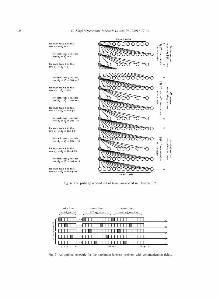
In order to show that (9) is tight, we consider the partially ordered set of tasks corresponding to a graphwhich is comprised of an initial section followed by k identical sections and one terminal section. The initialsection is comprised of m=2� rows, whereas each of k identical sections, and the terminal section, is comprisedof m rows. The 2rst row of the initial section contains 2m+1 nodes, and the last row of each identical sectioncontains m+2 nodes. The m=2�th row of each section contains m+2 nodes, and all other remaining rows ofeach section contain 2m + 2 nodes. Fig. 6 gives an example of such a graph when m= 5. In this graph, theshaded nodes precede all nodes in the next row, whereas each non-shaded node has no successors. Each taskcorresponding to a node in the 2rst (top) row has a due date of two units of time. Each task from any otherrow has the due date of the previous row plus two. The corresponding optimal schedule and the schedule sD,constructed by the due date modi2cation algorithm, are presented in Figs. 7 and 8, respectively. It is easy tosee that ‘= m=2� + m(k + 1); Lmax(sD) = 2m=2� + 2mk − 2k + 2m− 3; Lmax(s∗) = 1 and (9) is an equalityfor any k and m.

When all due dates are zero the maximum lateness problem converts to the makespan problem. In thiscase, the algorithm of due date modi2cation with communication delay, presented above, can be viewed as ageneralization of the well known Hu’s algorithm (critical path) [4] for the model with a unit communicationdelay and with −d′

j as the priority associated with each task j. Hence, (9) gives the following performanceguarantee for the makespan problem,

Cmax(sCP) − Cmax(s∗)6 2(m− 1m

)‘ − w(m); (12)

where sCP is a schedule constructed by the critical path method and s∗ is an optimal schedule for a unitcommunication delay makespan problem.

In order to show that (12) is tight, consider the partially ordered set of tasks corresponding to the graphin Fig. 9. This graph is comprised of an initial section followed by k identical sections. The initial sectionis comprised of m=2� rows, whereas each of k identical sections are comprised of m rows. The 2rst row ofthe initial section contains 2m + 1 nodes, and all other rows in the graph contain 2m + 2 nodes each. Theshaded node in any row precedes all nodes in the next row. All non-shaded nodes in the same row (exceptthe last row) have two common successors, which are the last two nodes in the next row. The correspondingoptimal schedule and the schedule sCP, constructed by the critical path method, are presented in Figs. 10and 11, respectively. It is easy to see that ‘= m=2�+mk; Cmax(sCP) = 4m=2�+ 4mk − 1; Cmax(s∗) = 2(m+1)=mm=2� + 2(m + 1)k + w(m) − 1, and (12) is an equality for any k and m.


Fig. 6. The partially ordered set of tasks considered in Theorem 3.2.

Fig. 7. An optimal schedule for the maximum lateness problem with communication delay.


Fig. 8. A non-optimal schedule constructed by the due date modi2cation algorithm for the UET-UCT model.


Fig. 10. An optimal schedule for the makespan problem with communication delay.


Fig. 11. A non-optimal schedule constructed by the generalized critical path method.

References

[1] P. Brucker, M.R. Garey, D.S. Johnson, Scheduling equal-length tasks under tree-like precedence constraints to minimise maximumlateness, Math. Oper. Res. 2 (3) (1977) 275–284.

[2] E.G.Jr. CoLman, R.L. Graham, Optimal scheduling for two-processor systems, Acta Inform. 1 (1972) 200–213.[3] M.R. Garey, D.S. Johnson, Scheduling tasks with nonuniform deadlines on two processors, J. Assoc. Comput. Mach. 23 (3) (1976)

461–467.[4] T.C. Hu, Parallel sequencing and assembly line problems, Oper. Res. 9 (1961) 841–848.[5] J.K. Lenstra, M. Veldhorst, B. Veltman, The complexity of scheduling trees with communication delays, J. Algorithms 20 (1) (1996)

157–173.[6] E.L. Lloyd, Concurrent task systems, Oper. Res. 29 (1981) 189–201.[7] V.J. Rayward-Smith, UET scheduling with unit interprocessor communication delays, Discrete Appl. Math. 18 (1987) 55–71.[8] G. Singh, Y. Zinder, Worst-case performance of two critical path type algorithms, Asia Paci2c J. Oper. Res. 17 (1) (2000) 101–122.[9] G. Singh, Y. Zinder, Worst-case performance of critical path type algorithms, Int. Trans. Oper. Res. 7 (2000) 383–399.

[10] J.D. Ullman, NP-Complete scheduling problems, J. Comput. Systems Sci. 10 (1975) 384–393.

Performance of critical path type algorithms for scheduling on parallel processors

Documents

Transcript of Performance of critical path type algorithms for scheduling on parallel processors