Modeling Superscalar Processors via Statistical Simulation

Sbbastien Nussbaum James E. Smith Department of Electrical and Computer Engineering

University of Wisconsin -Madison Madison, WI 53706

{nussbaum, jes] @ece. wisc.edu

Abstract

Statistical simulation is a technique for fast per- formance evaluation of superscalar processors. First, intrinsic statistical information is collected from a single detailed simulation of a program. This information is then used to generate a synthetic instruction trace that is fed to a simple processor model, along with cache and branch prediction statistics. Because of the probabilistic nature of the simulation, it quickly converges to a per- formance rate. The simplicit;v and simulation speed make it useful f o r fast design space exploration; as such, it is a good complement to conventional detailed simulation.

The accuracy of this technique is evaluated for different levels of modeling complexity. Both errors and convergence properties are studied in detail. A simple instruction model yields an average error of 8% compared with detailed simulation. A more detailed instruction model reduces the error to 5% but requires about three times as long to converge.

1. Introduction

Simulation is a widely used and effective tool for evaluating computer performance. For superscalar proc- essors very detailed simulation models [ 1 , 2,3] are typi- cally developed to support design decisions and to per- mit accurate performance estimates prior to chip fabrica- tion. They are also used in the research environment to quantify performance improvements provided by mi- croarchitecture innovations. For these detailed processor models, simulation times are relatively long, often re- quiring many hours for a single run. Furthermore, simu- lations are based on specific benchmark programs and consequently only provide performance information for programs similar to the benchmarks. Although long run- times and benchmark constraints limit the amount of design space exploration, detailed simulation is critical for evaluating specific design points and is widely used in both industry and academia.

Reducing the input size of benchmark programs can shorten simulation times. In [4] some practical input reductions to Spec2000 are shown, for either validating research simulators, obtaining quick performance esti- mates, or accurate performance estimates. Although it is possible to obtain quick (1 minute) performance esti- mates, some benchmarks also have very high errors (up to 80%) compared to the full input.

Trace sampling [5 , 6, 71 can be used to reduce run- times and can be made to work reasonably well for uni- processor performance simulation. However it requires detailed understanding of the program, is restricted to specific benchmarks, and has cold-start problems at the beginning of each sample segment.

An alternative to detailed simulation is the use of ana- lytical models [8, 9, 101. However, existing analytical models of superscalar processors are hard to modify and adapt to other microarchitecture. Consequently, analyti- cal models must be kept simple (compared with the de- tailed simulation models) or are restricted to processors much simpler than today’s superscalar processors.

We and others have proposed and have been studying an approach where certain processor and program statis- tics are collected or otherwise generated, and a processor model is then probabilistically simulated with these sta- tistics as inputs [ I ] , 12, 131. The simulation quickly converges to a solution (performance estimate). Super- scalar processors, and eventually large systems built of superscalar processors, can be rapidly simulated with this technique referred to as statistical simulation.

Although it has been previously used (in a limited way), we do not believe that either the overall accuracy of statistical simulation or several alternatives for model- ing have been properly studied or evaluated. In this pa- per, we first focus on the general process flow of statisti- cal simulation. We then study its use for superscalar processors by developing several models of synthetic trace generation, with different degrees of detail. We validate the model’s accuracy against a detailed simula- tion model and study its convergence properties. Then, we discuss the applicability of the model for processor design by modifying some processor parameters and

15 0-7695-1363-8101 $10.00 0 2001 IEEE

Fast Simulation for ultiple architectures 6 I

Instruction Trace Generator

-

’:: branch ’,.. . predictor ’.:-

’..-. ..._._____.. ...-..‘. 4- FRONTEND -b d-, BACKEND --+

(Statistics collection) Figure 1 : Statistical simulation process flow

evaluating how well projected performance changes “track” the results of detailed simulations.

1.1. Statistical simulation methodology

The simulation process is illustrated in Figure 1. First, a benchmark program is simulated with a detailed execution driven simulator to produce a dynamic instruc- tion trace. The program instruction trace is then ana- lyzed to generate statistical tables of intrinsic program characteristics and statistics about locality events. In- trinsic characteristics should be as independent as pos- sible of the underlying microarchitecture (no speculation or cache information) but do depend on the compiler and the ISA. Locality events, such as branch miss-prediction rate, or cache misses, which depend on the specifics of the microarchitecture are also collected for specific cache and branch prediction configurations. We refer to this part of the process flow as the “front-end”. It needs to be done only once for each benchmark program to be studied.

Then, to carry out a statistical simulation, the pro- gram statistics are used to drive the random generation of a synthetic instruction trace. This synthetic instruction trace, including branch and cache hidmiss information, is fed into a superscalar processor simulator. The processor model itself is simplified, modeling the major pipeline resources without ever having to compute values, store results, or model the memory hierarchy in detail.

The statistical simulator “back-end” processes the randomly generated synthetic trace, and assumes con- vergence when the standard deviation of the instruction throughput is less than 1 percent for a sequence of 2000 cycle samples (Section 3 discusses convergence in more

Cache & bpred event generator

000 processor core

(Synthetic simulator)

detail). This convergence usually happens after a few tens of thousands of clock cycles of simulation.

1.2. Applications

The statistical simulation model is simple, and after the initial trace-driven characterization, a simulation run can be performed very quickly, literally orders of magni- tude faster than with conventional detailed simulation of a full benchmark program. Assuming for the moment that the results are reasonably accurate (as will be shown later in this paper Section 3.2) there are a number of po- tential applications.

Processor evaluation -- This is perhaps the most ob- vious application because it is the common application for conventional detailed simulation. Although statistical simulation is probably not accurate enough to replace detailed simulation for making final design decisions, it can be quite useful as a complementary tool for rapid design space evaluation. Due to the simple processor model, microarchitecture modifications are straightfor- ward relative to modifications of a conventional execu- tion driven simulator. New benchmarks can easily be created to stress various aspects of a processor that are not stressed by a set of existing benchmarks. A design space can be covered very quickly by repeatedly running a set of pre-parameterized benchmarks over a set of mi- croarchitecture variations [13], or an application program space can be covered by varying the parameters that drive the synthetic benchmark generator.

System evaluation - In some respects, we consider this to be an even better application than uniprocessor evaluation. Large-scale systems containing many proc- essors, large memory systems, and running large applica-

16

tions simply cannot be simulated over realistic time scales if detailed clock-cycle simulation is done system- wide. For system design, the processor microarchitec- ture is typically fixed and the system structure is being evaluated. In this application, it is easy to simulate sys- tems as they scale in numbers of processors and memory systems. Furthermore, by adjusting workload parameters based on forecasts of application characteristics it is pos- sible to extrapolate and predict system performance for future applications.

Program characterization -- In the process of gen- erating synthetic versions of real benchmarks and vali- dating the accuracy of statistical simulation, we are ef- fectively isolating those program features that affect per- formance from those that do not. And, these key pro- gram parameters may provide a way of concisely charac- terizing benchmarks. These parameters can be used to extrapolate the performance of an application program from the performance for a benchmark with similar characteristics or to test the “coverage” of a benchmark suite.

Physical design - A fast statistical simulation model can be incorporated into sophisticated physical design tools. For example, for a given floorplan, estimated de- lays can be fed into a parameterized processor perform- ance model and performance can be quickly evaluated via statistical simulation. An automatic floorplanner can then incorporate such a performance model as it system- atically searches for performance-optimal floorplans.

High-level power modeling -- Another physical characteristic of growing importance is power consump- tion. Statistical simulation can be incorporated into a power estimation tool [ 141 to allow fast evaluation of the average power consumption of a program. This would be particularly useful for embedded systems where a small set of programs are typically used in a given appli- cation.

2. Minimal statistical model

In this section we develop a basic statistical simula- tion model. First, we describe the modeling of program characteristics, then the processor and the locality- capturing structures such as caches and branch predic- tors.

2.1. Base program characteristics model

Two types of statistical tables are used to construct the synthetic instruction stream, one is used to generate an instruction type, and the second is used to determine register dependences among the instructions.

2.1.1. Basic instruction mix An important first step in reduction of the real dy-

namic instruction stream to a synthetic stream is the re- duction of the full instruction set (typically containing 100+ opcodes) to a much smaller set of generic types. We settled on 14 instruction types; the instruction types can be found in the left hand column of Table 2 (further described in section 3.1). A simple instruction mix is then formed by analyzing the dynamic trace of the benchmark program and determining the percentage of each of the basic instruction types. In later sections we consider more sophisticated methods of characterizing the instruction stream, but the basic instruction mix is an important method to consider because of its simplicity.

2.1.2. Instruction dependences Besides the mix of instructions, another important

characteristic is their interdependences; for this simple model we consider register dependences. Dependences should be characterized according to the distance be- tween two dependent instructions [ I ] and, we have found, as a function of the instruction types. A depend- ence matrix is used to model the dependences between the individual instructions. One method for building a dependence matrix is to collect distributions that give the probability that an instruction of a particular type is de- pendent on the one immediately before it, two instruc- tions before it, etc.; i.e. “upstream” dependences. A variation is to collect probability distributions for each of an instruction’s register operands [I21 [13]. A problem with this approach occurs during the trace construction process when the instruction at the selected dependence distance does not produce a register value, e.g. it is a store or branch instruction. In this case, some fix-up is required, for example by going back to the distribution and trying again. Oskin et al. in [ 131 prevent instructions being dependent on stores only within the same basic block; but nothing is enforced beyond the basic block boundary. Eeckhout et al. in [12] generate multiple de- pendences until no store or branch appears to produce an output. If this fails to happen, the instruction is marked dependent on previous instruction, at a fixed distance.

We use another approach, “downstream” depend- ences, where the dependence table contains probabilities that an instruction at distance d in the future will be de- pendent on the instruction currently being generated. Then constructing dependences consists of generating a dependence condition for all instructions up to N in the future, where N is the maximum expected size of instruc- tion windows that will be simulated (for instructions farther than N , the dependence will not affect perform- ance). This approach implies that some instruction may depend on more (or fewer) preceding instructions than it has operands. Hence, the branchktore dependence prob- lem is fixed, but a problem with mismatches in numbers

17

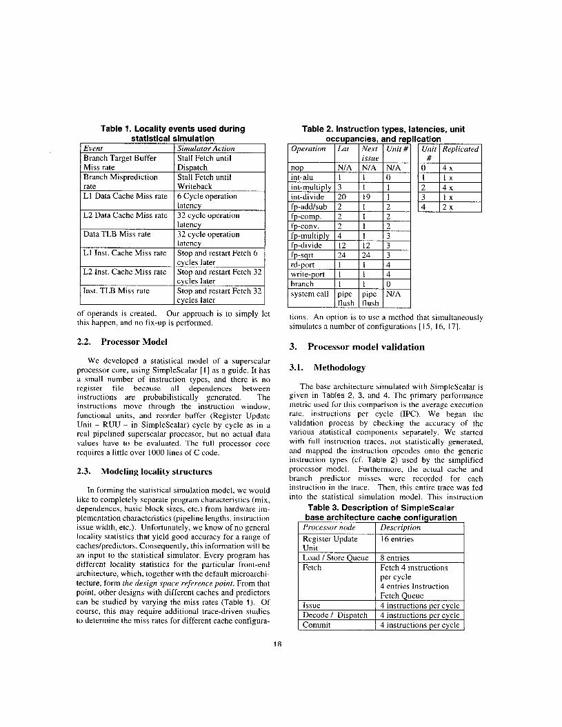
Table 1. Locality events used during statistical simulation

rate L1 Data Cache Miss rate

L2 Data Cache Miss rate

Data TLB Miss rate

L1 Inst. Cache Miss rate

L2 Inst. Cache Miss rate

Inst. TLB Miss rate

Event I Simulator Action Branch Target Buffer I Stall Fetch until

Writeback 6 Cycle operation latency 32 cycle operation latency 32 cycle operation latency Stop and restart Fetch 6 cycles later Stop and restart Fetch 32 cycles later Stop and restart Fetch 32 cycles later

Miss rate I Dispatch Branch Misprediction I Stall Fetch until

system call pipe flush

pipe N/A flush

of operands is created. this happen, and no fix-up is performed.

Our approach is to simply let

Register Update Unit Load / Store Queue Fetch

Issue Decode / Dispatch Commit

2.2. Processor Model

16 entries

8 entries Fetch 4 instructions per cycle 4 entries Instruction Fetch Queue 4 instructions per cycle 4 instructions per cycle 4 instructions per cycle

We developed a statistical model of a superscalar processor core, using SimpleScalar [ I ] as a guide. It has a small number of instruction types, and there is no register file because all dependences between instructions are probabilistically generated. The instructions move through the instruction window, functional units, and reorder buffer (Register Update Unit - RUU - in SimpleScalar) cycle by cycle as in a real pipelined superscalar processor, but no actual data values have to be evaluated. The full processor core requires a little over 1000 lines of C code.

2.3. Modeling locality structures

In forming the statistical simulation model, we would like to completely separate program characteristics (mix, dependences, basic block sizes, etc.) from hardware im- plementation characteristics (pipeline lengths, instruction issue width, etc.). Unfortunately, we know of no general locality statistics that yield good accuracy for a range of caches/predictors. Consequently, this information will be an input to the statistical simulator. Every program has different locality statistics for the particular front-end architecture, which, together with the default microarchi- tecture, form the design space reference point. From that point, other designs with different caches and predictors can be studied by varying the miss rates (Table 1). Of course, this may require additional trace-driven studies to determine the miss rates for different cache configura-

Table 2. Instruction types, latencies, unit occupancies, and replication

Operution I Lut I Next I Unit # I I Unit I Replicated I

int-alu

branch

l l Y l - I Fl 4 x

3. Processor model validation

3.1. Methodology

The base architecture simulated with SimpleScalar is given in Tables 2, 3, and 4. The primary performance metric used for this comparison is the average execution rate, instructions per cycle (IPC). We began the validation process by checking the accuracy of the various statistical components separately. We started with full instruction traces, not statistically generated, and mapped the instruction opcodes onto the generic instruction types (cf. Table 2) used by the simplified processor model. Furthermore, the actual cache and branch predictor misses were recorded for each instruction in the trace. Then, this entire trace was fed into the statistical simulation model. This instruction

Table 3. Description of SimpleScalar base architecture cache configuration

I Processor node I Description

18

Structure

L1 cache

L2 cache

Branch Predictor Memory

.- c 0 Detailed Statistical

v) 0 Statistical Branch Misspredictions L 0 Statistical Instruction Dependencies 2 ti Statistical Cache+Branch+Dependencies

&? El Statistical Using Mix

Statistical Cache Misses .U, -15 a K

c c

.-

Description

Instruction : 8K, direct mapped, 1 cycle hit Data : 8K, 4 way associative Unified 256K, 4-way associative, 7 cycles hit 2K two-bit counter entries

32 cycles latency to transfer 1 cache line; no early restart

Figure 2. Error introduced by different levels of approximation of the trace, simulated on base architecture (1 00 million instructions)

Statistical Branch Prediction Statistical Dependences Full Statistical Simulation

Approximation level

Table 5. Statistical Model Validation Levels I Approximation I Description

cache events. Detailed trace, with statistical branch prediction events. Detailed trace, with statistical instruction dependences Instructions, Cache, Branch prediction events and instruction dependences all statistically generated Description

level Detailed Synthetic I Real trace, with orxodes Simulation Statistical Cache

I mapped to synthekc ISA I Detailed trace, with statistical

1.32

1.3

Simulaioncydes( inlms)

Figure 3. Convergence time for compress, using the simple mix, for the base architecture and different random seeds

19

15

; 10

._ c ffl .- c

C ._ L

; 5

s? 0

-5

Figure 4. Error in statistical (mix) IPC compared to SimpleScalar IPC, for the base architecture (1 billion instructions)

standard deviation over multiple runs using different random seeds is about 2% of the IPC -- informally, the "noise" level (convergence values for compress, for dif- ferent seeds, are shown in Figure 3). This is not the error with respect to SimpleScalar, only differences in esti- mated performance among multiple runs.

Figure 4 shows the error of Statistical Simulation us- ing Mix for all Spec95 benchmarks run for 1 billion in- structions on the Spec Reference Input. We can see the results are relatively accurate (within 5% of SimpleSca- lar for half of the benchmarks, 15% error for tomcatv and 20% error for compress and 12% error for gcc), even though the synthetic instruction stream is formed in a simple manner using a basic instruction mix. The reason behind the high error in compress is that it spends all of the first 1 billion instructions of the Spec Reference In- put initializing the data structures. This code is a very tight loop spanning over 6 branches. Two of these share 85% of the branch mispredictions, and a third branch has the remaining 15%. This imbalance of mispredictions together with the very repetitive code pattern, make sim- ple statistical simulation difficult. In the next section, we refine the synthetic instruction model in an attempt to reduce modeling errors, with special attention given to the kind of behavior exhibited by compress.

We note that statistical simulation using mix overestimates the performance of most benchmark programs. This can be attributed to simplified modeling of several second-order effects, for example dependences among memory references are not modeled. Also, for programs not having a long, dominant critical path, averaging dependences is an accurate model. However, if there is a long, dominant critical path, average dependences will generate multiple small dependence

chains instead of one long dependence chain, leading to a performance overestimation.

3.2. Enhanced Instruction Models

Now, we look at various refinements of the basic model for synthetic trace generation in order to increase accuracy (possibly increasing convergence time). Each workload model must describe the control flow, the distribution of instruction types, the distribution of locality events, and instruction or memory dependences. The simple mix described earlier defines control flow and the instruction distribution in a unified way. More complex models describe them separately, first by using a distribution of basic block sizes then by using an instruction distribution (excluding branches). A more detailed model may have a different instruction distribution for each basic block size. We studied a number of combinations and will describe three that seem to be most useful.

3.2.1. Basic block generation The length of basic blocks is an important aspect of

program behavior because when combined with branch mispredictions it affects the number of valid instructions in the superscalar instruction window. We first collect the complete distribution of basic block sizes over a benchmark trace. Then, the synthetic instruction genera- tor begins by randomly generating a basic block length based on this distribution, (called BBlock Distribution) which is subsequently filled with instructions (BBlock Distribution + Mix).

30

25

20

15 U .- - 2 10

: o

%

.E 5

e L

-5

-10

-15 1

Figure 5. Error in statistical IPC for each level of accuracy of the model, base architecture, 1 billion instructions

20

Another approach for representing the basic block distribution is to keep the mean and standard deviation of the basic block lengths (Normal BBlock), but common basic block distributions are often multi-modal and do not map well to a normal distribution. Improvements include keeping a different distribution based on the his- tory of recent branch outcomes- (Branch Histon BBlock Distribution). This enables the sequence of basic blocks to match more closely ones of loops, and improve con- vergence times. Creating basic blocks apart from the regular flow of instructions, that is, going from Mix to BBlock Distribiition + Mix. decreased the average error by more than a full percentage point for large configura-

16 ,, , , . , , , ,........ . . , ,,,...... .... _. . . . .. .. -.. .. li ~

14

12

_ - 2 l o

._ , a

- $?

v

L

g 6 w

4

2

0 16RUU. 16RUU. 32RUU. 32RUU. 64RUU. 128RUU. 4 ~ 7 , 4uw.16 4 ~ , 1 6 8 q . 3 2 8 w . 3 2 8vq.32

4fetdg fetchQ fetchQ fetchQ fetchQ fetchQ

0 mix

n o r m B Hock + m x

B Mock ds triMion +mix

0 8 Hock ds triMion +ba7b, ds t- pofile

.B Mock ds trimion +Bock pofile

OB Mock ds triMion +Hock s izepofile

bcnch his toryB Mock ds trimion +Bock pofile

Obcnch historyB Mock dstriMion+tlock pofile+Wock events

.bench historyB Mock dstrib+t;lock pofile+Wock locdity&

RE3 Mock dstriMion+Mock pofile+Wock events &-

ObcnchhistoryB Mock dstriMion+tlock pofile+mock locdity&

- - Figure 6. Statistical simulation results for various microarchitectures, and trace models, averaged over all Speclnt95 benchmarks

tions (8 way superscalar), but slightly increased the error (within the noise) for small configurations, including the base architecture (Figures 5 above and Figure 6). Overall, the average error increases with the size of the processor configuration. Indeed, a larger issue window offers more combinations of issuing sequences, and it is less likely that our dependence model statistically regenerates the same sequence. This may lead to a higher average error.

3.2.2. Basic block instruction profile Thus far we have considered generating instructions

from a single trace-wide mix. In real programs, espe- cially within loops, the type of instruction tends to be a function of its location with respect to branches; for ex- ample, load instructions tend to follow a branch, and store instructions tend to immediately precede branches. Consequently, instead of having a single global program Mix, we consider a method of generating a synthetic in- struction stream where the probability of an instruction of each type is a function of its distance from the imme- diately preceding branch. We call this instruction distri- bution the Branch Distance Profile.

Another way to refine synthetic instruction generation is to keep a different instruction mix for each basic block size. The reasoning is that long basic blocks tend to be computation bound with relatively higher numbers of ALU operations. This leads us to the Block Size Profile that maintains a different instruction distribution for each member of the basic block distribution.

As a further refinement, one can combine the features of the Block Size Profile and the Branch Distance Profile

100000

90000

80000

ar 70000 F

60000

I E 50000

40000

=x 30000

20000

10000

0

0

v)

0

Block T '0

" compress convergence time

D per1 convergence time *overall method error (in %)

Figure 7. Convergence time and error for Compress and Perl, on the base architecture, 1 billion instructions

21

by adding a third dimension to the instruction distribution matrix. That is, we maintain a distribution of instruction types over different basic block sizes and distances from the previous branch. We call this the Block Profile. Figure 6 shows validation results for the four instruction distributions just described, on different processor configurations.

For small configurations (4-way superscalar) simple mix achieves comparable or better accuracy than com- plex distributions. For example, the base architecture statistically simulated with mix has 7.6% error, and 8.2% error with block profile, but converges 8 times faster (Figure 7). More complex models, however, have a 20% smaller coefficient of variation (ratio of the standard deviation to the mean, and that we simply call “varia- tion” later in this paper), when running simulations with different seeds (Figure 8), than Mix and normal BBlock + Mix.

Consistently over all configurations, BBlock Distribu- tion + Block Size Profile achieves the highest accuracy of all refined models presented here (Figure 6), though it is not the most detailed. Large 8-way superscalar (64 RUU and 128 RUU) configurations have 0.5% less error with Block Size Profile than simple Mix. As one might expect, the more detailed instruction models require longer convergence times, as shown in Figure 7 but show less variation between runs (Figure 8). However, when the distribution of basic blocks depends on the recent branch history, the convergence time is cut down by 30% without reducing accuracy or variation between runs (Figure 8). This makes Brunch Histon BBlock Dis- tribution + Block Size Profile the most attractive model for large configurations; Mix is most attractive for small configurations where it is accurate and fast.

3.2.3. Improving dependence modeling As mentioned earlier, compress code contains a few

tight loops. Because of the recurrent code pattern, i t is important to get the correct dependence information to achieve accurate simulation.

We observe that one could also make the dependence distribution a function of the basic block size. The results for this model are shown in Figure 7, under Bblock De- pendences. The accuracy for per1 is improved by 5%, and for compress by 4% for the same the convergence time.

3.2.4. Locality statistics Just as dependence modeling is improved by using

statistics dependent on basic block size, we can keep different cache and branch prediction statistics for each basic block size. The source of error in compress was a large imbalance between branch mispredictions for dif- ferent static branches. Making branch prediction statis- tics a function of the basic block size took the error in

0.008T I ?a 1% Standard +Mean1 1.4

0.007

‘0 0.006 .- w

.: 0.005

0.004 E 0.003

m 0.002

a,

0.001

0

1.39

1.38

1.37

1.36

1.35

1.34

1.33

1.32

1.31

1.3

Figure 8. IPC mean and standard deviation on Compress, base architecture

conipress error down to 5%, as shown in Figure 7. It is important to note that the average absolute error on Spe- cInt went down to 5% for the base architecture (Figure 6)

3.2.5. Summary: three main models We observe that all models should generate basic

blocks based on a distribution indexed by the recent brunch his ton (Branch Histor? BBlock Distribution) as it enables better accuracy and fast convergence. Simple models for which speed is critical should fill basic blocks with a global Mix . Intermediate models seeking good performance, yet reasonable complexity should use a Block Size Profile instruction distribution within basic blocks, and instruction dependences should be a function of the basic block size. Finally, for applications to proc- essor design, where accuracy is critical, and the perform- ance of locality structures can be studied in other ways, Block Profiling with Basic Block Dependences, and Ba- sic Block Locality events work well.

4. Uniprocessor performance evaluation

A potential application of the statistical simulation model is design space exploration where the full range of program characteristics and a broad range of microarchi- tecture parameters can be studied. The study in [ 131 is a very good example where data value prediction was studied for a wide range of prediction characteristics.

For studying the performance improvements (or losses) of a specific feature for a set of benchmarks, the value of statistical simulation is less clear. Many pro- posed microarchitecture features provide improvements of five percent or less - in the “noise” for statistical simulation. However, for this application, the absolute

22

0 . 0 3

0.025

c g 0 .02 E ~

0 'E 0.015 H 0.01 0

0 . 0 0 5 .-

-0 .005

-0 .o 1

0.6

0.5

0.4

0 . 3

0.2

C .- O m m

-0.12

-0.2

- 0 . 3

U U

Figure 9. An evaluation of microarchitecture changes. Statistical simulation is compared with detailed SimpleScalar simulation

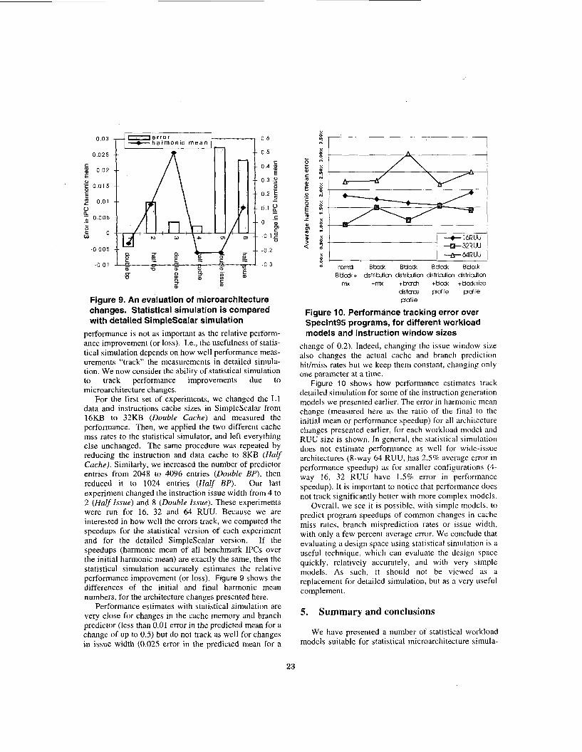
performance is not as important as the relative perform- ance improvement (or loss). I.e., the usefulness of statis- tical simulation depends on how well performance meas- urements "track the measurements in detailed simula- tion. We now consider the ability of statistical simulation to track performance improvements due to microarchitecture changes.

For the first set of experiments, we changed the L1 data and instructions cache sizes in SimpleScalar from 16KB to 32KB (Double Cache) and measured the performance. Then, we applied the two different cache mss rates to the statistical simulator, and left everything else unchanged. The same procedure was repeated by reducing the instruction and data cache to 8KB (Half Cache). Similarly, we increased the number of predictor entries from 2048 to 4096 entries (Double BP), then reduced it to 1024 entries (Half BP) . Our last experiment changed the instruction issue width from 4 to 2 (Half Issue) and 8 (Double Issue). These experiments were run for 16, 32 and 64 RUU. Because we are interested in how well the errors track, we computed the speedups for the statistical version of each experiment and for the detailed SimpleScalar version. If the speedups (harmonic mean of all benchmark IPCs over the initial harmonic mean) are exactly the same, then the statistical simulation accurately estimates the relative performance improvement (or loss). Figure 9 shows the differences of the initial and final harmonic mean numbers, for the architecture changes presented here.

Performance estimates with statistical simulation are very close for changes in the cache memory and branch predictor (less than 0.01 error in the predicted mean for a change of up to 0.5) but do not track as well for changes in issue width (0.025 error in the predicted mean for a

Y 0

K Y 0

N

Y 0 z Y U!

S 0

0

c

". . 2 - c z 2 2

Y 0

B u d + dstriuicn dstriwicn dstriWicr dstriuicn mix +mix +bmh +kid +Udsize

d s t m pdi le pdi le pofile

Figure 10. Performance tracking error over Speclnt95 programs, for different workload models and instruction window sizes

change of 0.2). Indeed, changing the issue window size also changes the actual cache and branch prediction hidmiss rates but we keep them constant, changing only one parameter at a time.

Figure 10 shows how performance estimates track detailed simulation for some of the instruction generation models we presented earlier. The error in harmonic mean change (measured here as the ratio of the final to the initial mean or performance speedup) for all architecture changes presented earlier, for each workload model and RUU size is shown. In general, the statistical simulation does not estimate performance as well for wide-issue architectures (8-way 64 RUU, .has 2.5% average error in performance speedup) as for smaller configurations (4- way 16, 32 RUU have 1.5% error in performance speedup). It is important to notice that performance does not track significantly better with more complex models.

Overall, we see it is possible, with simple models, to predict program speedups of common changes in cache miss rates, branch misprediction rates or issue width, with only a few percent average error. We conclude that evaluating a design space using statistical simulation is a useful technique, which can evaluate the design space quickly, relatively accurately, and with very simple models. As such, it should not be viewed as a replacement for detailed simulation, but as a very useful complement.

5. Summary and conclusions

We have presented a number of statistical workload models suitable for statistical microarchitecture simula-

23

tion. After an initial phase collecting statistics, instruc- tions are randomly generated based on the data gathered. The instruction throughput converges within seconds to a statistical performance estimate. This approach leads to a number of potential applications involving design space exploration.

We started our study by examining the tradeoffs be- tween convergence speed, accuracy, and variance over multiple runs using several workload models. The more interesting models first generate a basic block size from a distribution, then populate it from a separate instruction mix. The simplest such model, Bblock Mix, achieves the fastest convergence time with less than 8% average error on our base architecture for the SpecInt95 benchmark programs. The most detailed model, Block Profile with Bblock locality events, correlates the instruction mix, cache and branch prediction miss rates, and depend- ences, with the basic block size. This leads to a little more than 5% average error with a convergence time three times that of the simple model.

Our initial study of each workload model used the same locality characteristics (e.g. cache and branch pre- dictor) as those captured during the statistical collection phase. However, design space exploration requires itera- tions over a range of microarchitecture characteristics (cache and branch prediction performance, issue width, window size, etc.). We studied the accuracy of each model in predicting the performance effect of simple microarchitecture configuration changes by extrapolating locality statistics from an initial design point to new con- figuration s.

A complex correlation between basic block sizes and locality events makes it non-intuitive to extrapolate lo- cality event rates on a basic block basis. This means the most accurate model is probably less appropriate for design space exploration, though it accurately represents the workload and precisely evaluates the performance for single design points.

We showed, however, that the simple model (Mix with separately generated basic blocks) performs as well as more complex instruction distributions for measuring relative speedups when designs are modified. Within seconds, this method can evaluate the relative performance of various microarchitecture changes (in caches, branch predictors, and issue widths) with less than four percent average error in the performance speedup. Thus, statistical simulation appears to be a good to complement to detailed timing simulation for fast design space exploration.

Acknowledgements This work was supported in part by a National Sci-

ence Foundation grant CCR-99006 10, by IBM Corpora- tion, Sun Microsystems, and Intel Corporation. We also

thank Rick Carl, Dan Sorin, and David Wood for initial contributions to this work.

[ 1 ] Doug Burger and Todd Austin, ‘The Simplescalar Tool Set, Version 2.0, Computer Architecture News, pp. 13-25, June 1997. [2] P. Bose and T. M. Conte, “Performance Analysis and Its Impact on Design,” IEEE Computer, pp. 41-49, May 1998. [3] P. Bose, “Performance Evaluation and Validation of Mi- croprocessors,’’ 1999 Sigmetrics, pp. 226-227, May 1999. [4] AJ KleinOsowski, John Flynn, Nancy Meares, and David J. Lilja, “Adapting the SPEC 2000 Benchmark Suite for Simulation-Based Computer Architecture Research”, Workshop on Workload Characterization, International Conference on Computer Design, Austin, TX, Sept 18-20, 2000. [5 ] T. M. Conte, M. A. Hirsch, and K. N. Menezes, “Reducing State Loss for Effective Trace Sampling of Superscalar Processors, Proc. I996 Int. Conk on Comp. Design, Oct. 1996 [6] V. S. Iyengar and L. H. Trevillyan, “Evaluation and Generation of Reduced Traces for Benchmarks,” Tech. Report RC20610, IBM T. J . Watson Rsch. Center, Oct. 1996. [7] T. Lafage, A. Seznec, E. Rohou, F. Bodin. “Code Cloning Tracing: A “Pay per Trace” Approach“, EuroPar’99 Parallel Processing, Toulouse, France, August 1999. Lecture Notes in Computer Science, No. 1685, Springer-Verlag, pp. 1265-1268. [8] Pradeep K. Dubey, George B. Adams 111, and Michael J. Flynn, “Instruction Window Size Trade-offs and Characteriza- tion of Program Parallelism“. IEEE Transactions on Com- puters,43(4):431-442, April 1994 [9] D. B. Noonburg and J. P. Shen, “A Framework for Statisti- cal Modeling of Superscalar Processor Performance,” Proc.

[ IO] D. Sorin et al.,”A Customized MVA Model for ILP Mul- tiprocessors.”, Technical Report #1369, Computer Sciences Dept., Univ. of Wisconsin - Madison, Mar. 1998. [ 11 ] R. Carl and J . E. Smith, “Modeling Superscalar Processors via Statistical Simulation,” Workshop on Perjormance Analysis and Its Impact on Design,’’ June 1998. [12] L. Eeckhout, K. DeBousschere, and H. Neefs, “Perform- ance Analysis Through Synthetic Trace Generation,” Int. Symp. on PerIformance Analysis of Systems and Software, April 2000, http://www.elis.rug.ac.be/-leeckhoul [13] M. Oskin, F. T. Chong, and M. Farrens, “HLS: Combining Statistical and Symbolic Simulation to Guide Microprocessor Design,” Proc. 21* Int. Symp. on Computer Arch., June 2000. [14] C. Hsieh and M. Pedram, “Microprocessor Power Estima- tion Using Profile-Driven Program Synthesis, ” IEEE Trans. on Computer-Aided Design of Integrated Circuits and Systems,

[15] Raphaael H. Saavedra, Alan J. Smith, “Analysis of Benchmark Characteristics and Benchmark Performance Pre- diction” Transactions on Computer Systems, Vol 14, No 4, pp.

[ 161 M.Holliday, “Techniques for cache and memory simula- tion using address reference traces”, International journal in computer simulation pp 129- 15 1, 1991 [17] D. Albonesi et al, An automated and flexible framework for integrated processor and system-level design space explora- tion’’, Workshop on performance analysis and its impact on design, June 1997, pp 24-34

References

Third In. Symp. On High Pet$ Computer Architecture, 1997.

pp. 1080-1089, NOV. 1998.

344-384, NOV 1996.

24