
Increasing the performance of superscalar processors through ...
171
HAL Id: tel-01235370 https://tel.archives-ouvertes.fr/tel-01235370v2 Submitted on 3 Mar 2016 HAL is a multi-disciplinary open access archive for the deposit and dissemination of sci- entific research documents, whether they are pub- lished or not. The documents may come from teaching and research institutions in France or abroad, or from public or private research centers. L’archive ouverte pluridisciplinaire HAL, est destinée au dépôt et à la diffusion de documents scientifiques de niveau recherche, publiés ou non, émanant des établissements d’enseignement et de recherche français ou étrangers, des laboratoires publics ou privés. Increasing the performance of superscalar processors through value prediction Arthur Perais To cite this version: Arthur Perais. Increasing the performance of superscalar processors through value prediction. Hard- ware Architecture [cs.AR]. Université Rennes 1, 2015. English. NNT : 2015REN1S070. tel- 01235370v2
-
Upload
khangminh22 -
Category
Documents
-
view
0 -
download
0
Transcript of Increasing the performance of superscalar processors through ...

HAL Id: tel-01235370https://tel.archives-ouvertes.fr/tel-01235370v2
Submitted on 3 Mar 2016
HAL is a multi-disciplinary open accessarchive for the deposit and dissemination of sci-entific research documents, whether they are pub-lished or not. The documents may come fromteaching and research institutions in France orabroad, or from public or private research centers.
L’archive ouverte pluridisciplinaire HAL, estdestinée au dépôt et à la diffusion de documentsscientifiques de niveau recherche, publiés ou non,émanant des établissements d’enseignement et derecherche français ou étrangers, des laboratoirespublics ou privés.
Increasing the performance of superscalar processorsthrough value prediction
Arthur Perais
To cite this version:Arthur Perais. Increasing the performance of superscalar processors through value prediction. Hard-ware Architecture [cs.AR]. Université Rennes 1, 2015. English. �NNT : 2015REN1S070�. �tel-01235370v2�

ANNÉE 2015
THÈSE / UNIVERSITÉ DE RENNES 1sous le sceau de l’Université Européenne de Bretagne
pour le grade deDOCTEUR DE L’UNIVERSITÉ DE RENNES 1
Mention : InformatiqueÉcole doctorale Matisse
présentée par
Arthur PERAIS
préparée à l’unité de recherche INRIAInstitut National de Recherche en Informatique et
Automatique – Université de Rennes 1
Increasing the Per-formance of Super-scalar Processorsthrough Value Pre-diction
Thèse soutenue à Rennesle 24 septembre 2015devant le jury composé de :
Christophe WOLINSKIProfesseur à l’Université de Rennes 1 / PrésidentFrédéric PÉTROTProfesseur à l’ENSIMAG, Institut Polytechnique deGrenoble / Rapporteur
Pierre BOULETProfesseur à l’Université de Lille 1 / RapporteurChristine ROCHANGEProfesseur à l’Université de Toulouse / ExaminatricePierre MICHAUDChargé de Recherche à l’INRIA Rennes – BretagneAtlantique / Examinateur
André SEZNECDirecteur de recherche à l’INRIA Rennes – BretagneAtlantique / Directeur de thèse


Je sers la science et c’est ma joie.Basile, disciple

Remerciements
Je tiens à remercier les membres de mon jury pour avoir jugé les travaux réalisésdurant cette thèse, ainsi que pour leurs remarques et questions.
En particulier, je remercie Christophe Wolinski, Professeur à l’Université deRennes 1, qui m’a fait l’honneur de présider ledit jury. Je remercie aussi FrédéricPétrot, Professeur à l’ENSIMAG, et Pierre Boulet, Professeur à l’Université deLille 1, d’avoir bien voulu accepter la charge de rapporteur. Je remercie finalementChristine Rochange, Professeur à l’Université de Toulouse et Pierre Michaud,Chargé de Recherche à l’INRIA Bretagne Atlantique, d’avoir accepté de juger cetravail.
Je souhaite aussi remercier tout particulièrement Yannakis Sazeides, Pro-fesseur à l’Université de Chypre. Tout d’abord pour avoir accepté de siéger dans lejury en tant que membre invité, mais aussi pour avoir participé à l’établissementdes fondements du domaine sur lequel mes travaux de thèse se penchent.
Je tiens à remercier André Seznec pour avoir assuré la direction et le bondéroulement de cette thèse. Je lui suis particulièrement reconnaissant d’avoirtransmis sa vision de la recherche ainsi que son savoir avec moi. J’ose espérer quetoutes ces heures passées à tolérer mon ignorance auront au moins été divertis-santes pour lui.
Je veux remercier les membres de l’équipe ALF pour toutes les discussionssérieuses et moins sérieuses qui auront sûrement influencées la rédaction de cedocument.
Mes remerciements s’adressent aussi aux membres de ma famille, auxquelsj’espère avoir pû fournir une idée plus ou moins claire de la teneur de mes travauxde thèse au cours des années. Ce document n’aurait jamais pû voir le jour sansleur participation active à un moment ou à un autre.
Je suis reconnaissant à mes amis, que ce soit ceux avec lesquels j’ai pû quo-tidiennement partager les joies du doctorat, ou ceux qui ont eu le bonheur dechoisir une autre activité.1
Finalement, un merci tout particulier à ma relectrice attitrée, sans laquelle denombreuses fôtes subsisteraient dans ce manuscrit. Grâce à elle, la rédaction de
1"Un vrai travail"

2 Table of Contents
ce manuscrit fut bien plus plaisante qu’elle n’aurait dû l’être.
Contents
Table of Contents 2
Résumé en français 9
Introduction 15
1 The Architecture of a Modern General Purpose Processor 231.1 Instruction Set – Software Interface . . . . . . . . . . . . . . . . . 23
1.1.1 Instruction Format . . . . . . . . . . . . . . . . . . . . . . 241.1.2 Architectural State . . . . . . . . . . . . . . . . . . . . . . 24
1.2 Simple Pipelining . . . . . . . . . . . . . . . . . . . . . . . . . . . 251.2.1 Different Stages for Different Tasks . . . . . . . . . . . . . 27
1.2.1.1 Instruction Fetch – IF . . . . . . . . . . . . . . . 271.2.1.2 Instruction Decode – ID . . . . . . . . . . . . . . 271.2.1.3 Execute – EX . . . . . . . . . . . . . . . . . . . . 271.2.1.4 Memory – MEM . . . . . . . . . . . . . . . . . . 281.2.1.5 Writeback – WB . . . . . . . . . . . . . . . . . . 30
1.2.2 Limitations . . . . . . . . . . . . . . . . . . . . . . . . . . 301.3 Advanced Pipelining . . . . . . . . . . . . . . . . . . . . . . . . . 32
1.3.1 Branch Prediction . . . . . . . . . . . . . . . . . . . . . . . 321.3.2 Superscalar Execution . . . . . . . . . . . . . . . . . . . . 331.3.3 Out-of-Order Execution . . . . . . . . . . . . . . . . . . . 34
1.3.3.1 Key Idea . . . . . . . . . . . . . . . . . . . . . . 341.3.3.2 Register Renaming . . . . . . . . . . . . . . . . . 351.3.3.3 In-order Dispatch and Commit . . . . . . . . . . 371.3.3.4 Out-of-Order Issue, Execute and Writeback . . . 391.3.3.5 The Particular Case of Memory Instructions . . . 421.3.3.6 Summary and Limitations . . . . . . . . . . . . . 46
2 Value Prediction as a Way to Improve Sequential Performance 492.1 Hardware Prediction Algorithms . . . . . . . . . . . . . . . . . . . 50
2.1.1 Computational Prediction . . . . . . . . . . . . . . . . . . 50
3

4 Contents
2.1.1.1 Stride-based Predictors . . . . . . . . . . . . . . 512.1.2 Context-based Prediction . . . . . . . . . . . . . . . . . . . 55
2.1.2.1 Finite Context-Method (FCM) Prediction . . . . 552.1.2.2 Last-n values Prediction . . . . . . . . . . . . . . 572.1.2.3 Dynamic Dataflow-inherited Speculative Context
Predictor . . . . . . . . . . . . . . . . . . . . . . 592.1.3 Hybrid Predictors . . . . . . . . . . . . . . . . . . . . . . . 602.1.4 Register-based Value Prediction . . . . . . . . . . . . . . . 61
2.2 Speculative Window . . . . . . . . . . . . . . . . . . . . . . . . . 612.3 Confidence Estimation . . . . . . . . . . . . . . . . . . . . . . . . 632.4 Validation . . . . . . . . . . . . . . . . . . . . . . . . . . . . . . . 642.5 Recovery . . . . . . . . . . . . . . . . . . . . . . . . . . . . . . . . 64
2.5.1 Refetch . . . . . . . . . . . . . . . . . . . . . . . . . . . . 652.5.2 Replay . . . . . . . . . . . . . . . . . . . . . . . . . . . . . 662.5.3 Summary . . . . . . . . . . . . . . . . . . . . . . . . . . . 67
2.6 Revisiting Value Prediction . . . . . . . . . . . . . . . . . . . . . 67
3 Revisiting Value Prediction in a Contemporary Context 693.1 Introduction . . . . . . . . . . . . . . . . . . . . . . . . . . . . . . 693.2 Motivations . . . . . . . . . . . . . . . . . . . . . . . . . . . . . . 70
3.2.1 Misprediction Recovery . . . . . . . . . . . . . . . . . . . . 703.2.1.1 Value Misprediction Scenarios . . . . . . . . . . . 713.2.1.2 Balancing Accuracy and Coverage . . . . . . . . 72
3.2.2 Back-to-back Prediction . . . . . . . . . . . . . . . . . . . 733.2.2.1 LVP . . . . . . . . . . . . . . . . . . . . . . . . . 743.2.2.2 Stride . . . . . . . . . . . . . . . . . . . . . . . . 743.2.2.3 Finite Context Method . . . . . . . . . . . . . . . 743.2.2.4 Summary . . . . . . . . . . . . . . . . . . . . . . 75
3.3 Commit Time Validation and Hardware Implications on the Out-of-Order Engine . . . . . . . . . . . . . . . . . . . . . . . . . . . . 76
3.4 Maximizing Value Predictor Accuracy Through Confidence . . . . 773.5 Using TAgged GEometric Predictors to Predict Values . . . . . . 78
3.5.1 The Value TAgged GEometric Predictor . . . . . . . . . . 783.5.2 The Differential VTAGE Predictor . . . . . . . . . . . . . 80
3.6 Evaluation Methodology . . . . . . . . . . . . . . . . . . . . . . . 813.6.1 Value Predictors . . . . . . . . . . . . . . . . . . . . . . . 81
3.6.1.1 Single Scheme Predictors . . . . . . . . . . . . . 813.6.1.2 Hybrid Predictors . . . . . . . . . . . . . . . . . 83
3.6.2 Simulator . . . . . . . . . . . . . . . . . . . . . . . . . . . 833.6.2.1 Value Predictor Operation . . . . . . . . . . . . . 843.6.2.2 Misprediction Recovery . . . . . . . . . . . . . . 85

Contents 5
3.6.3 Benchmark Suite . . . . . . . . . . . . . . . . . . . . . . . 863.7 Simulation Results . . . . . . . . . . . . . . . . . . . . . . . . . . 86
3.7.1 General Trends . . . . . . . . . . . . . . . . . . . . . . . . 863.7.1.1 Forward Probabilistic Counters . . . . . . . . . . 863.7.1.2 Pipeline Squashing vs. selective replay . . . . . . 883.7.1.3 Prediction Coverage and Performance . . . . . . 89
3.7.2 Hybrid predictors . . . . . . . . . . . . . . . . . . . . . . . 903.8 Conclusion . . . . . . . . . . . . . . . . . . . . . . . . . . . . . . . 92
4 A New Execution Model Leveraging Value Prediction: EOLE 954.1 Introduction & Motivations . . . . . . . . . . . . . . . . . . . . . 954.2 Related Work on Complexity-Effective Architectures . . . . . . . 97
4.2.1 Alternative Pipeline Design . . . . . . . . . . . . . . . . . 974.2.2 Optimizing Existing Structures . . . . . . . . . . . . . . . 98
4.3 {Early | Out-of-order | Late} Execution: EOLE . . . . . . . . . . 994.3.1 Enabling EOLE Using Value Prediction . . . . . . . . . . . 994.3.2 Early Execution Hardware . . . . . . . . . . . . . . . . . . 1014.3.3 Late Execution Hardware . . . . . . . . . . . . . . . . . . 1024.3.4 Potential OoO Engine Offload . . . . . . . . . . . . . . . . 105
4.4 Evaluation Methodology . . . . . . . . . . . . . . . . . . . . . . . 1064.4.1 Simulator . . . . . . . . . . . . . . . . . . . . . . . . . . . 106
4.4.1.1 Value Predictor Operation . . . . . . . . . . . . . 1074.4.2 Benchmark Suite . . . . . . . . . . . . . . . . . . . . . . . 108
4.5 Experimental Results . . . . . . . . . . . . . . . . . . . . . . . . . 1084.5.1 Performance of Value Prediction . . . . . . . . . . . . . . . 1084.5.2 Impact of Reducing the Issue Width . . . . . . . . . . . . 1094.5.3 Impact of Shrinking the Instruction Queue . . . . . . . . . 1104.5.4 Summary . . . . . . . . . . . . . . . . . . . . . . . . . . . 110
4.6 Hardware Complexity . . . . . . . . . . . . . . . . . . . . . . . . . 1114.6.1 Shrinking the Out-of-Order Engine . . . . . . . . . . . . . 111
4.6.1.1 Out-of-Order Scheduler . . . . . . . . . . . . . . 1114.6.1.2 Functional Units & Bypass Network . . . . . . . 1124.6.1.3 A Limited Number of Register File Ports dedi-
cated to the OoO Engine . . . . . . . . . . . . . 1124.6.2 Extra Hardware Complexity Associated with EOLE . . . . 112
4.6.2.1 Cost of the Late Execution Block . . . . . . . . . 1124.6.2.2 Cost of the Early Execution Block . . . . . . . . 1134.6.2.3 The Physical Register File . . . . . . . . . . . . . 113
4.6.3 Mitigating the Hardware Cost of Early/Late Execution . . 1134.6.3.1 Mitigating Early-Execution Hardware Cost . . . 1134.6.3.2 Narrow Late Execution and Port Sharing . . . . 115

6 Contents
4.6.3.3 The Overall Complexity of the Register File . . . 1164.6.3.4 Further Possible Hardware Optimizations . . . . 117
4.6.4 Summary . . . . . . . . . . . . . . . . . . . . . . . . . . . 1174.6.5 A Note on the Modularity of EOLE: Introducing OLE and
EOE . . . . . . . . . . . . . . . . . . . . . . . . . . . . . . 1194.7 Conclusion . . . . . . . . . . . . . . . . . . . . . . . . . . . . . . . 120
5 A Realistic, Block-Based Prediction Infrastructure 1235.1 Introduction & Motivations . . . . . . . . . . . . . . . . . . . . . 1235.2 Block-Based Value Prediction . . . . . . . . . . . . . . . . . . . . 124
5.2.1 Issues on Concurrent Multiple Value Predictions . . . . . . 1245.2.2 Block-based Value-Predictor accesses . . . . . . . . . . . . 126
5.2.2.1 False sharing issues . . . . . . . . . . . . . . . . . 1265.2.2.2 On the Number of Predictions in Each Entry . . 1275.2.2.3 Multiple Blocks per Cycle . . . . . . . . . . . . . 127
5.3 Implementing a Block-based D-VTAGE Predictor . . . . . . . . . 1285.3.1 Complexity Intrinsic to D-VTAGE . . . . . . . . . . . . . 129
5.3.1.1 Prediction Critical Path . . . . . . . . . . . . . . 1295.3.1.2 Associative Read . . . . . . . . . . . . . . . . . . 1295.3.1.3 Speculative History . . . . . . . . . . . . . . . . . 129
5.3.2 Impact of Block-Based Prediction . . . . . . . . . . . . . . 1305.3.2.1 Predictor Entry Allocation . . . . . . . . . . . . . 1305.3.2.2 Prediction Validation . . . . . . . . . . . . . . . . 130
5.4 Block-Based Speculative Window . . . . . . . . . . . . . . . . . . 1315.4.1 Leveraging BeBoP to Implement a Fully Associative Struc-
ture . . . . . . . . . . . . . . . . . . . . . . . . . . . . . . 1315.4.2 Consistency of the Speculative History . . . . . . . . . . . 132
5.5 Evaluation Methodology . . . . . . . . . . . . . . . . . . . . . . . 1345.5.1 Simulator . . . . . . . . . . . . . . . . . . . . . . . . . . . 134
5.5.1.1 Value Predictor Operation . . . . . . . . . . . . . 1345.5.2 Benchmark Suite . . . . . . . . . . . . . . . . . . . . . . . 135
5.6 Experimental Results . . . . . . . . . . . . . . . . . . . . . . . . . 1355.6.1 Baseline Value Prediction . . . . . . . . . . . . . . . . . . 1355.6.2 Block-Based Value Prediction . . . . . . . . . . . . . . . . 137
5.6.2.1 Varying the Number of Entries and the Numberof Predictions per Entry . . . . . . . . . . . . . . 137
5.6.2.2 Partial Strides . . . . . . . . . . . . . . . . . . . 1375.6.2.3 Recovery Policy . . . . . . . . . . . . . . . . . . . 1385.6.2.4 Speculative Window Size . . . . . . . . . . . . . . 138
5.6.3 Putting it All Together . . . . . . . . . . . . . . . . . . . . 1395.7 Related Work on Predictor Storage & Complexity Reduction . . . 141

Contents 7
5.8 Conclusion . . . . . . . . . . . . . . . . . . . . . . . . . . . . . . . 141
Conclusion 143
Author’s Publications 147
Bibliography 157
List of Figures 159

8 Contents
Résumé en français
Le début des années 2000 aura marqué la fin de l’ère de l’uni-processeur, etle début de l’ère des multi-cœurs. Précédemment, chaque génération de pro-cesseur garantissait une amélioration super-linéaire de la performance grâce àl’augmentation de la fréquence de fonctionnement du processeur ainsi que lamise en œuvre de micro-architectures (algorithme matériel avec lequel le pro-cesseur exécute les instructions) intrinsèquement plus efficaces. Dans les deuxcas, l’amélioration était généralement permise par les avancées technologiquesen matière de gravure des transistors. En particulier, il était possible de graverdeux fois plus de transistors sur la même surface tous les deux ans, permettantd’améliorer significativement la micro-architecture. L’utilisation de transistorsplus fins a aussi généralement permis d’augmenter la fréquence de fonctionnement.
Cependant, il est vite apparu que continuer à augmenter la fréquence n’étaitpas viable dans la mesure où la puissance dissipée augmente de façon super-linéaire avec la fréquence. Ainsi, les 3,8GHz du Pentium 4 Prescott (2004) sem-blent être la limite haute de la fréquence atteignable par un processeur destinéau grand public. De plus, complexifier la micro-architecture d’un uni-processeuren ajoutant toujours plus de transistors souffre d’un rendement décroissant. Ilest donc rapidement apparu plus profitable d’implanter plusieurs processeurs –cœurs – sur une même puce et d’adapter les programmes afin qu’ils puissent tirerparti de plusieurs coeurs, plutôt que de continuer à améliorer la performance d’unseul cœur. En effet, pour un programme purement parallèle, l’augmentation dela performance globale approche 2 si l’on a deux cœurs au lieu d’un seul (tousles cœurs étant identiques). Au contraire, si l’on dépense les transistors utiliséspour mettre en œuvre le second cœur à l’amélioration du cœur restant, alorsl’expérience dicte que l’augmentation de la performance sera inférieure à 2.
Nous avons donc pu constater au cours des dernières années une augmentationdu nombre de coeurs par puce pour arriver à environ 16 aujourd’hui. Par con-séquent, la performance des programmes parallèles a pu augmenter de manièresignificative, et en particulier, bien plus rapidement que la performance des pro-grammes purement séquentiels, c’est à dire dont la performance globale dépend dela performance d’un unique cœur. Ce constat est problématique dans la mesureoù il existe de nombreux programmes étant intrinsèquement séquentiels, c’est à
9

10 Résumé
Figure 1: Impact de la prédiction de valeurs (VP) sur la chaîne de dépendancesséquentielles exprimée par un programme.
dire ne pouvant pas bénéficier de la présence de plusieurs coeurs. De plus, lesprogrammes parallèles possèdent en général une portion purement séquentielle.Cela implique que même avec une infinité de coeurs pour exécuter la partie par-allèle, la performance sera limitée par la partie séquentielle, c’est la loi d’Amdahl.Par conséquent, même à l’ère des multi-coeurs, il reste nécessaire de continuer àaméliorer la performance séquentielle.
Hélas, la façon la plus naturelle d’augmenter la performance séquentielle (aug-menter le nombre d’instructions traitées chaque cycle ainsi que la taille de lafenêtre spéculative d’instructions) est connue pour être très couteuse en tran-sistors et pour augmenter la consommation énergétique ainsi que la puissancedissipée. Il est donc nécessaire de trouver d’autres moyens d’améliorer la perfor-mance sans augmenter la complexité du processeur de façon déraisonnable.
Dans ces travaux, nous revisitions un tel moyen. La prédiction de valeurs(VP) permet d’augmenter le parallélisme d’instructions (le nombre d’instructionspouvant s’exécuter de façon concurrente, ou ILP) disponible en spéculant surle résultat des instructions. De ce fait, les instructions dépendantes de résultatsspéculés peuvent être exécutées plus tôt, augmentant la performance séquentielle.La prédiction de valeurs permet donc une meilleure utilisation des ressourcesmatérielles déjà présentes et ne requiert pas d’augmenter le nombre d’instructionsque le processeur peut traiter en parallèle. La Figure 1 illustre comment laprédiction du résultat d’une instruction permet d’extraire plus de parallélismed’instructions que la sémantique séquentielle du programme n’exprime.
Cependant, la prédiction de valeurs requiert un mécanisme validant les pré-dictions et s’assurant que l’exécution reste correcte même si un résultat est

Résumé en français 11
mal prédit. En général, ce mécanisme est implanté directement dans le cœurd’exécution dans le désordre, qui est déjà très complexe en lui-même. Mettreen œuvre la prédiction de valeurs avec ce mécanisme de validation serait donccontraire à l’objectif de ne pas complexifier le processeur.
De plus, la prédiction de valeurs requiert un accès au fichier de registres, quiest la structure contenant les valeurs des opérandes des instructions à exécuter,ainsi que leurs résultats. En effet, une fois un résultat prédit, il doit être insérédans le fichier de registres afin de pouvoir être utilisé par les instructions qui endépendent. De même, afin de valider une prédiction, elle doit être lue depuis lefichier de registres et comparée avec le résultat non spéculatif. Ces accès sont enconcurrence avec les accès effectués par le moteur d’exécution dans le désordre,et des ports de lectures/écritures additionnels sont donc requis afin d’éviter lesconflits. Cependant, la surface et la consommation du fichier de registres croissentde façon super-linéaire avec le nombre de ports d’accès. Il est donc nécessaire detrouver un moyen de mettre en œuvre la prédiction de valeurs sans augmenter lacomplexité du fichier de registres.
Enfin, la structure fournissant les prédictions au processeur, le prédicteur, doitêtre aussi simple que possible, que ce soit dans son fonctionnement ou dans le bud-get de stockage qu’il requiert. Cependant, il doit être capable de fournir plusieursprédictions par cycle, puisque le processeur peut traiter plusieurs instructionspar cycle. Cela sous-entend que comme pour le fichier de registres, plusieursports d’accès sont nécessaires afin d’accéder à plusieurs prédictions chaque cycle.L’ajout d’un prédicteur de plusieurs kilo-octets possédant plusieurs ports d’accèsaurait un impact non négligeable sur la consommation du processeur, et devraitdonc être évité.
Ces trois exigences sont les principales raisons pour lesquelles la prédiction devaleurs n’a jusqu’ici pas été implantée dans un processeur. Dans ces travaux dethèse, nous revisitons la prédiction de valeurs dans le contexte actuel. En par-ticulier, nous proposons des solutions aux trois problèmes mentionnés ci-dessus,permettant à la prédiction de valeurs de ne pas augmenter significativement lacomplexité du processeur, déjà très élevée. Ainsi, la prédiction de valeurs devientune façon réaliste d’augmenter la performance séquentielle.
Dans un premier temps, nous proposons un nouveau prédicteur tirant partides avancées récentes dans le domaine de la prédiction de branchement. Ce pré-dicteur est plus performant que les prédicteurs existants se basant sur le contextepour prédire. De plus, il ne souffre pas de difficultés intrinsèques de mise enœuvre telle que le besoin de gérer des historiques locaux de façon spéculative. Ils’agit là d’un premier pas vers un prédicteur efficace mais néanmoins réalisable.Nous montrons aussi que si la précision du prédicteur est très haute, i.e., les mau-vaises prédictions sont très rares, alors la validation des prédictions peut se fairelorsque les instructions sont retirées du processeurs, dans l’ordre. Il n’est donc

12 Résumé
pas nécessaire d’ajouter un mécanisme complexe dans le cœur d’exécution pourvalider les prédictions et récupérer d’une mauvaise prédiction. Afin de s’assurerque la précision est élevée, nous utilisons un mécanisme d’estimation de confianceprobabiliste afin d’émuler des compteurs de 8-10 bits en utilisant seulement 3 bitspar compteur.
Dans un second temps, nous remarquons que grâce à la prédiction de valeurs,de nombreuses instructions sont prêtes à être exécutées bien avant qu’elle n’entrentdans le moteur d’exécution dans le désordre. De même, les instructions préditesn’ont pas besoin d’être exécutées avant le moment ou elles sont retirées du pro-cesseur, puisque les instructions qui en dépendent peuvent utiliser la prédic-tion comme opérande source. De ce fait, nous proposons un nouveau mod-èle d’exécution, EOLE, dans lequel de nombreuses instructions sont exécutéesdans l’ordre, hors du moteur d’exécution dans le désordre. Ainsi, le nombred’instructions que le moteur d’exécution dans le désordre peut traiter à chaquecycle peut être réduit, et donc le nombre de ports d’accès qu’il requiert sur lefichier de registre. Nous obtenons donc un processeur avec des performancessimilaires à un processeur utilisant la prédiction de valeurs, mais dont le mo-teur d’exécution dans le désordre est plus simple, et dont le fichier de registresnécessite autant de ports d’accès qu’un processeur sans prédiction de valeurs.
Finalement, nous proposons une infrastructure de prédiction capable de prédireplusieurs instructions à chaque cycle, tout en ne possédant que des structures avecun seul port d’accès. Pour ce faire, nous tirons parti du fait que le processeurexécute les instructions de façon séquentielle, et qu’il est donc possible de grouperles prédictions qui correspondent à des instructions contiguës en mémoire dansune seule entrée du prédicteur. Il devient donc possible de récupérer toutes lesprédictions correspondant à un bloc d’instructions en un seul accès au prédicteur.Nous discutons aussi de la gestion spéculative du contexte requis par certains pré-dicteurs pour prédire les résultats, et proposons une solution réaliste tirant aussiparti de l’agencement en bloc des instructions. Nous considérons aussi des façonsde réduire le budget de stockage nécessaire au prédicteur et montrons qu’il estpossible de n’utiliser que 16-32 kilo-octets, soit un budget similaire à celui ducache de premier niveau ou du prédicteur de branchement.
Au final, nous obtenons une amélioration moyenne des performances de l’ordrede 11.2%, allant jusqu’à 62.2%. Les performances obtenues ne sont jamais in-férieures à celles du processeur de référence (i.e., sans prédiction de valeurs) surles programmes considérés. Nous obtenons ces chiffres avec un processeur dontle moteur d’exécution dans le désordre est significativement moins complexe quedans le processeur de référence, tandis que le fichier de registres est équivalent aufichier de registres du processeur de référence. Le principal coût vient donc duprédicteur de valeur, cependant ce coût reste raisonnable dans la mesure où il estpossible de mettre en œuvre des tables ne possédant qu’un seul port d’accès.

Résumé en français 13
Ces trois contributions forment donc une mise en œuvre possible de la prédic-tion de valeurs au sein d’un processeur généraliste haute performance moderne,et proposent donc une alternative sérieuse à l’augmentation de la taille de lafenêtre spéculative d’instructions du processeur afin d’augmenter la performanceséquentielle.

14 Résumé

Introduction
Processors – in their broader sense, i.e., general purpose or not – are effectivelythe cornerstone of modern computer science. To convince ourselves, let us try toimagine for a minute what computer science would consist of without such chips.Most likely, it would be relegated to a field of mathematics as there would not beenough processing power for graphics processing, bioinformatics (including DNAsequencing and protein folding) and machine learning to simply exist. Languagesand compilers would also be of much less interest in the absence of machines torun the compiled code on. Evidently, processor usage is not limited to computerscience: Processors are everywhere, from phones to cars, to houses, and manymore.
Yet, processors are horrendously complex to design, validate, and manufac-ture. This complexity is often not well understood by their users. To give anidea of the implications of processor design, let us consider the atomic unit ofa modern processor: the transistor. Most current generation general purposemicroprocessor feature hundreds of millions to billions of transistors. By con-necting those transistors in a certain fashion, binary functions such as OR andAND can be implemented. Then, by combining these elementary functions, weobtain a device able to carry out higher-level operations such as additions andmultiplications. Although all the connections between transistors are not explic-itly designed by hand, many high-performance processors feature custom logicwhere circuit designers act at the transistor level. Consequently, it follows thatdesigning and validating a processor is extremely time and resource consuming.
Moreover, even if modern general purpose processors possess the ability toperform billions of arithmetic operations per second, it appears that to keep asteady pace in both computer science research and quality of life improvement,processors should keep getting faster and more energy efficient. Those representthe two main challenges of processor architecture.
To achieve these goals, the architect acts at a level higher than the transistorbut not much higher than the logic gate (e.g., OR, AND, etc.). In particular, heor she can alter the way the different components of the processor are connected,the way they operate, and simply add or remove components. This is in contrastwith the circuit designer that would improve performance by rearranging tran-
15

16 Introduction
sistors inside a component without modifying the function carried out by thiscomponent, in order to reduce power consumption or shorten the electric criticalpath. As a result, the computer architect is really like a regular architect: he orshe draws the blueprints of the processor (respectively house), while the builders(resp. circuit designers) are in charge of actually building the processor with tran-sistors and wires (resp. any house material). It should be noted, however, that theprocessor architect should be aware of what is actually doable with the currentcircuit technology, and what is not. Therefore, not unlike a regular architect, heor she should keep the laws of physics in mind when drawing his or her plans.
In general, processor architecture is about tradeoffs. For instance, tradeoffsbetween simplicity ("My processor can just do additions in hardware, but it waseasy to build") and performance ("The issue is that divisions are very slow be-cause I have to emulate them using additions"), or tradeoffs between raw computepower ("My processor can do 4 additions at the same time") and power efficiency("It dissipates more power than a vacuum cleaner to do it"). Therefore, in anutshell, architecture consists in designing a computer processor from a reason-ably high level, by taking into account those tradeoffs and experimenting withnew organizations. In particular, processor architecture has lived through severalparadigm shifts in just a few decades, going from 1-cycle architectures to moderndeeply pipelined superscalar processors, from single core to multi-core, from veryhigh frequency to very high power and energy efficiency. Nonetheless, the goalsremain similar: increase the amount of work that can be done in a given amountof time, while minimizing the energy spent doing this work.
Overall, there are two main directions to improve processor performance. Thefirst one leverages the fact that processors are clocked objects, meaning that whenthe associated clock ticks, then some computation step has finished. For instance,a processor may execute one instruction per clock tick. Therefore, if the clockspeed of the processor is increased, then more work can be done in a given unitof time, as there are now more clock ticks in said unit of time. However, asthe clock frequency is increased, the power consumption of the processor growssuper-linearly,2 and quickly becomes too high to handle. Moreover, transistorspossess an intrinsic maximum switching frequency and a signal can only travelso far in a wire in a given clock period. Exceeding these two limits would lead tounpredictable results. For these reasons, clock frequency has generally remainedcomprised between 2GHz and 5GHz in the last decade, and this should remainthe case for the same reasons.
Second, thanks to improvements in transistor implantation processes, moreand more transistors can be crammed in a given surface of silicon. This phe-
2Since the supply voltage must generally grow as the frequency is increased, power con-sumption increases super-linearly with frequency. If the supply voltage can be kept constantsomehow, then the increase should be linear.

Introduction 17
nomenon is embodied by Moore’s Law, that states that the number of transistorsthan can be implanted on a chip doubles every 24 months [Moo98]. Although itis an empirical law, it has proven exactly right between 1971 and 2001. However,increase has slowed down during the past decade. Nonetheless, consider that theIntel 8086 released in 1978 had between 20,000 and 30,000 transistors while somemodern Intel processors have more than 2 billions, that is 100,000 times more.3However, if a tremendous number of transistors are available to the architect, it isbecoming extremely hard to translate these additional transistors into additionalperformance.
In the past, substantial performance improvements due to an increased num-ber of transistors came from the improvement of uni-processors through pipelin-ing, superscalar execution and out-of-order execution. All those features targetsequential performance, i.e., the performance of a single processor. However,it has become very hard to keep on targeting sequential performance with theadditional transistors we get, because of diminishing returns. Therefore, as nonew paradigm was found to replace the current one (superscalar out-of-orderexecution), the trend regarding high performance processors has shifted fromuni-processor chips to multi-processor chips. This allows to obtain a performanceincrease on par with the additional transistors provided by transistor technology,keeping Moore’s Law alive in the process.
More specifically, an intuitive way to increase the performance of a programis to cut it down into several smaller programs that can be executed concur-rently. Given the availability of many transistors, multiple processors can beimplemented on a single chip, with each processor able to execute one piece ofthe initial program. As a result, the execution time of the initial program isdecreased. This not-so-new paradigm targets parallel performance (i.e., through-put: how much work is done in a given unit of time), as opposed to sequentialperformance (i.e., latency or response time: how fast can a task finish).
However, this approach has two limits. First, some programs may not beparallel at all due to the nature of the algorithm they are implementing. Thatis, it will not be possible to break them down into smaller programs executedconcurrently, and they will therefore not benefit from the additional processors ofthe chip. Second, Amdahl’s Law [Amd67] limits the performance gain that can beobtained by parallelizing a program. Specifically, this law represents a programas a sequential part and a parallel part, with the sum of those parts adding up to1. Among those two parts, only the parallel one can be sped up by using severalprocessors. For instance, for a program whose sequential part is equivalent tothe parallel part, execution time can be reduced by a factor of 2 at most, that isif there is an infinity of processors to execute the parallel part. Therefore, even
3Moore’s Law would predict around 5 billions.

18 Introduction
with many processors at our disposal, the performance of a single processor (theone executing the sequential part) quickly becomes the limiting factor. Given theexistence of intrinsically sequential programs and the fact that even for parallelprograms, the sequential part is often non-negligible, it is paramount to keep onincreasing single processor performance.
This thesis provides realistic means to substantially improve the sequentialperformance of high performance general purpose processors. These means arecompletely orthogonal to the coarse grain parallelism leveraged by Chip Multi-Processors (CMP, several processors on a single chip a.k.a. multi-cores). Theycan therefore be added on-top of existing hardware. Furthermore, if this thesis fo-cuses on the design step of processor conception, technology constraints are keptin mind. In other words, specific care is taken to allow the proposed mechanismsto be realistically implementable using current technology.
Contributions
We revisit a mechanism aiming to increase sequential performance: Value Pre-diction (VP). The key idea behind VP is to predict instruction results in orderto break dependency chains and execute instructions earlier than previously pos-sible. In particular, for out-of-order processors, this leads to a better utilizationof the execution engine: Instead of being able to uncover more Instruction LevelParallelism (ILP) from the program by being able to look further ahead (e.g., byhaving a larger instruction window), the processor creates more ILP by breakingsome true dependencies in the existing instruction window.
VP relies on the fact that there exist common instructions (e.g., load, readdata from memory) that can take up to a few hundreds of processor cycles toexecute. During this time, no instruction requiring the data retrieved by the loadinstruction can be executed, most likely stalling the whole processor. Fortunately,many of these instructions often produce the same result, or results that followa pattern, which could therefore be predicted. Consequently, by predicting theresult of a load instruction, dependents can execute while the memory hierarchyis processing the load. If the prediction is correct, execution time decreases,otherwise, dependent instructions must be re-executed with the correct input toenforce correctness.
Our first contribution [PS14b] makes the case that contrarily to previous im-plementations described in the 90’s, it is possible to add Value Prediction on topof a modern general purpose processor without adding tremendous complexity inits pipeline. In particular, it is possible for VP to intervene only in the front-endof the pipeline, at Fetch (to predict), and in the last stage of the back-end, Com-mit (to validate predictions and recover if necessary). Validation at Commit is

Introduction 19
rendered possible because squashing the whole pipeline can be used to recoverfrom a misprediction, as long as value mispredictions are rare. This is in con-trast with previous schemes where instructions were replayed directly inside theout-of-order window. In this fashion, all the – horrendously complex – logic re-sponsible for out-of-order execution need not be modified to support VP. This isa substantial improvement over previously proposed implementations of VP thatcoupled VP with the out-of-order execution engine tightly. In addition, we intro-duce a new hybrid value predictor, D-VTAGE, inspired from recent advances inthe field of branch prediction. This predictor has several advantages over exist-ing value predictors, both from a performance standpoint and from a complexitystandpoint.
Our second contribution [PS14a, PS15b] focuses on reducing the additionalPhysical Register File (PRF) ports required by Value Prediction. Interestingly,we achieve this reduction because VP actually enables a reduction in the com-plexity of the out-of-order execution engine. Indeed, an instruction whose resultis predicted does not need to be executed as soon as possible, since its dependentscan use the prediction to execute. Therefore, we introduce some logic in charge ofexecuting predicted instructions as late as possible, just before they are removedfrom the pipeline. These instructions never enter the out-of-order window. Wealso notice that thanks to VP, many instructions are ready to be executed veryearly in the pipeline. Consequently, we also introduce some logic in charge of exe-cuting such instructions in the front-end of the pipeline. As a result, instructionsthat are executed early are not even dispatched to the out-of-order window. Withthis {Early | Out-of-Order | Late} (EOLE) architecture, a substantial portion ofthe dynamic instructions is not executed inside the out-of-order execution engine,and said engine can be simplified by reducing its issue-width, for instance. Thismechanically reduces the number of ports on the register file, and is a strong ar-gument in favor of Value Prediction since the complexity and power consumptionof the out-of-order execution engine are already substantial.
Our third and last contribution [PS15a] relates to the design of a realistic pre-dictor infrastructure allowing the prediction of several instructions per cycle withsingle-ported structures. Indeed, modern processors are able to retrieve severalinstructions per cycle from memory, and the predictor should be able to providea prediction for each of them. Unfortunately, accessing several predictor entriesin a single cycle usually requires several access ports, which should be avoidedwhen considering such a big structure (16-32KB). To that extent, we propose ablock-based prediction infrastructure that provides predictions for the whole in-struction fetch block with a single read in the predictor. We achieve superscalarprediction even when a variable-length instruction set such as x86 is used. Weshow that combined to a reasonably sized D-VTAGE predictor, performance im-provements are close to those obtained by using an ideal infrastructure combined

20 Introduction
to a much bigger value predictor. Moreover, even with these modifications, VPstill enables a reduction in the complexity of the out-of-order execution enginethanks to EOLE.
Combined, these three contributions provide a possible implementation ofValue Prediction on top of a modern superscalar processor. Contrarily to previoussolutions, this one does not increase the complexity of already complex processorcomponents such as the out-of-order execution engine. In particular, predictionand prediction validation can both take place outside said engine, limiting theinteractions between VP and the engine to the register file only. Moreover, weprovide two structures that execute instructions either early or late in the pipeline,offloading the execution of many instructions from the out-of-order engine. Asa result, it can be made less aggressive, and VP viewed as a means to reducecomplexity rather than increase it. Finally, by devising a better predictor inspiredfrom recent branch predictors and providing a mechanism to make it single-ported, we are able to outperform previous schemes and address complexity inthe predictor infrastructure.
Organization
This document is divided in five chapters and architected around three publishedcontributions: two in the International Symposium on High Performance Com-puter Architecture (HPCA 2014/15) [PS14b, PS15a] and one in the InternationalSymposium on Computer Architecture (ISCA 2014) [PS14a].
Chapter 1 provides a description of the inner workings of modern generalpurpose processors. We begin with the simple pipelined architecture and thenimprove on it by following the different processor design paradigms in a chrono-logical fashion. This will allow the reader to grasp why sequential performancebottlenecks remain in deeply pipelined superscalar processors and understandhow Value Prediction can help mitigate at least one of such bottlenecks.
Chapter 2 introduces Value Prediction in more details and presents previouswork. Existing hardware prediction algorithms are detailed and their advantagesand shortcomings discussed. In particular, we present computational predictorsthat compute a prediction from a previous result and context-based predictor thatprovide a prediction when some current information history matches a previouslyseen pattern [SS97a]. Then, we focus on how VP – and especially prediction val-idation – has usually been integrated with the pipeline. Specifically, we illustratehow existing implementations fall short of mitigating the complexity introducedby VP in the out-of-order execution engine.
Chapter 3 focuses on our first [PS14b] and part of our third [PS15a] contri-butions. We describe a new predictor, VTAGE, that does not suffer from the

Introduction 21
shortcomings of existing context-based predictors. We then improve on it by hy-bridizing it with a computational predictor in an efficient manner and presentDifferential VTAGE (D-VTAGE). In parallel, we show that Value Prediction canbe plugged into an existing pipeline without increasing complexity in parts of thepipeline that are already tremendously complex. We do so by delaying predictionvalidation and prediction recovery until in-order retirement.
Chapter 4 goes further by showing that Value Prediction can be leveraged toactually reduce complexity in the out-of-order window of a modern processor. Byenabling a reduction in the out-of-order issue-width through executing instructionearly or late in the pipeline, the EOLE architecture [PS14a] outperforms a widerprocessor while having 33% less out-of-order issue capacity and the same numberof register file ports.
Finally, Chapter 5 comes back to the predictor infrastructure and addressesthe need to provide several predictions per cycle in superscalar processors. Wedetail our block-based scheme enabling superscalar value prediction. We alsopropose an implementation of the speculative window tracking inflight predictionsthat is needed to compute predictions in many predictors [PS15a]. Lastly, westudy the behavior of the D-VTAGE predictor presented in Chapter 2 when itsstorage budget is reduced to a more realistic 16-32KB.

22 Introduction

Chapter 1
The Architecture of a ModernGeneral Purpose Processor
General purpose processors are programmable devices, hence, they present aninterface to the programmer known as the Instruction Set Architecture or ISA.Among the few widely used ISA, the x86 instruction set of Intel stands out fromthe rest as it remained retro-compatible across processor generations. That is,a processor bought in 2015 will be able to execute a program written for the8086 (1978). Fortunately, this modern processor will be much faster than a 8086.As a result, it is important to note that the interface exposed to the softwareis not necessarily representative of the underlying organization of the processorand therefore its computation capabilities. It is required to distinguish betweenthe architecture or ISA (e.g., x86, ARMv7, ARMv8, Alpha) from the micro-architecture implementing the architecture on actual silicon (e.g. Intel Haswell orAMD Bulldozer for x86, ARM Cortex A9 or Qualcomm Krait for ARMv7). Inthis thesis, we focus on the micro-architecture of a processor and aim to remainagnostic of the actual ISA.
1.1 Instruction Set – Software InterfaceEach ISA defines a set of instructions and a set of registers. Registers can beseen as scratchpads from which instructions read their operands and to whichinstructions write their results. They also define an address space used to accessglobal memory, which can be seen as a backing store for registers. These threecomponents are visible to the software, and they form the interface with whichthe processor can be programmed to execute a specific task.
The distinction is often made between Reduced Instruction Set Computer ISAs(RISC) and Complex Instruction Set Computer ISAs (CISC). The former indi-cates that instructions visible to the programmer are usually limited to simple
23
24 The Architecture of a Modern Processor
operations (e.g., arithmetic, logic and branches). The latter provides the pro-grammer with more complex instructions (e.g., string processing, loop instruc-tion). Therefore, RISC usually has less instructions available to the programmerbut its functionalities are easier to implement. As a result, more instructions aregenerally required than in CISC to do the same amount of work. However, CISCis usually considered as harder to implement because of the complex processingcarried out by some of its instructions.
The main representatives of RISC ISAs are ARMv7 (32-bit) and ARMv8 (64-bit) while the most widely used CISC ISA is x86 in its 64-bit version (x86_64).32- and 64-bit refer to the width of the – virtual – addresses used to access globalmemory. That is, ARMv7 can only address 232 memory locations (4 GB), whileARMv8 and x86_64 can address 264 memory locations (amounting to 16 EB).
1.1.1 Instruction Format
The instructions of a program are stored in global memory using a binary repre-sentation. Each particular ISA defines how instructions are encoded. Nonetheless,there exists two main paradigms for instruction encoding.
First, a fixed-length can be used, for instance 4 bytes (32 bits) in ARMv7.These 4 bytes contain – among other information – an opcode (the nature ofthe operation to carry out), two source registers and one destination register. Inthat case, decoding the binary representation of the instruction to generate thecontrol signals for the rest of the processor is generally straightforward. Indeed,each field is always stored at the same offset in the 4-byte word. Unfortunately,memory capacity is wasted for instructions that do not need two sources (e.g.,incrementing a single register) or that do not produce any output (e.g., branches).
Conversely, a variable-length can be used to encode different instructions. Forinstance, in x86, instructions can occupy 1 to 15 bytes (120 bits!) in memory.As a result, instruction decoding is much more complex as the location of afield in the instruction word (e.g., the first source register) depends on the valueof previous fields. Moreover, since an instruction has variable-length, it is notstraightforward to identify where the next instruction is. Nonetheless, variable-length representation is generally more storage-efficient.
1.1.2 Architectural State
Each ISA defines an architectural state. It is the state of the processor that isvisible by the programmer. It consists of all registers1 defined by the ISA as wellas the state of global memory, and it is agnostic of which program is currently
1Including the Program Counter (PC) pointing to the memory location containing the in-struction to execute next.

Simple Pipelining 25
being executed on the processor. The instructions defined by the ISA operateon this architectural state. For instance, an addition will take the architecturalstate as its input (or rather, a subset of the architectural state) and output avalue that will be put in a register, hence modify the architectural state. Fromthe software point of view, this modification is atomic: there is no architecturalstate between the state before the addition and the state after the addition.
Consequently, a program is a sequence of instructions (as defined by the ISA)that keeps on modifying the architectural state to compute a result. It followsthat programs running on the processor have sequential semantics. That is, fromthe point of view of the software, the architectural state is modified atomically byinstructions following the order in which they appear in the program. In practice,the micro-architecture may work on its own internal version of the architecturalstate as it pleases, as long as updates to the software-visible architectural staterespect atomicity and the sequential semantics of the program. In the remainderof this document, we differentiate between the software-visible state and anyspeculative (i.e., not software-visible yet) state living inside the processor.
1.2 Simple Pipelining
Processors are clocked devices, meaning that they are driven by a clock that ticksa certain number of times per second. Each tick triggers the execution of somework in the processor. Arguably, the most intuitive micro-architecture is thereforethe 1-cycle micro-architecture where the operation triggered by the clock tick isthe entire execution of an instruction. To guarantee that this is possible, theclock has to tick slow enough to allow the slowest (the one requiring the mostprocessing) instruction to execute in a single clock cycle.
Regardless, the execution of an instruction involves several very different stepsrequiring very different hardware structures. In a 1-cycle micro-architecture, asingle instruction flows through all these hardware structures during the clockcycle. Assuming there are five steps to carry out to actually execute the instruc-tion and make its effects visible to the software, this – roughly – means that eachof the five distinct hardware structures is idle during four-fifth of the clock cycle.As a result, this micro-architecture is highly inefficient.
Pipelined micro-architectures were introduced to remedy this issue. The high-level idea is that since an instruction flows sequentially through several stagesto be processed, there is potential to process instruction I0 in stage S1 whileinstruction I1 is concurrently processed in stage S0. Therefore, resources aremuch better utilized thanks to this pipeline parallelism. Moreover, instead ofconsidering the slowest instruction when choosing cycle time, only the delay ofthe slowest pipeline stage has to be considered. Therefore, cycle time can be
26 The Architecture of a Modern Processor
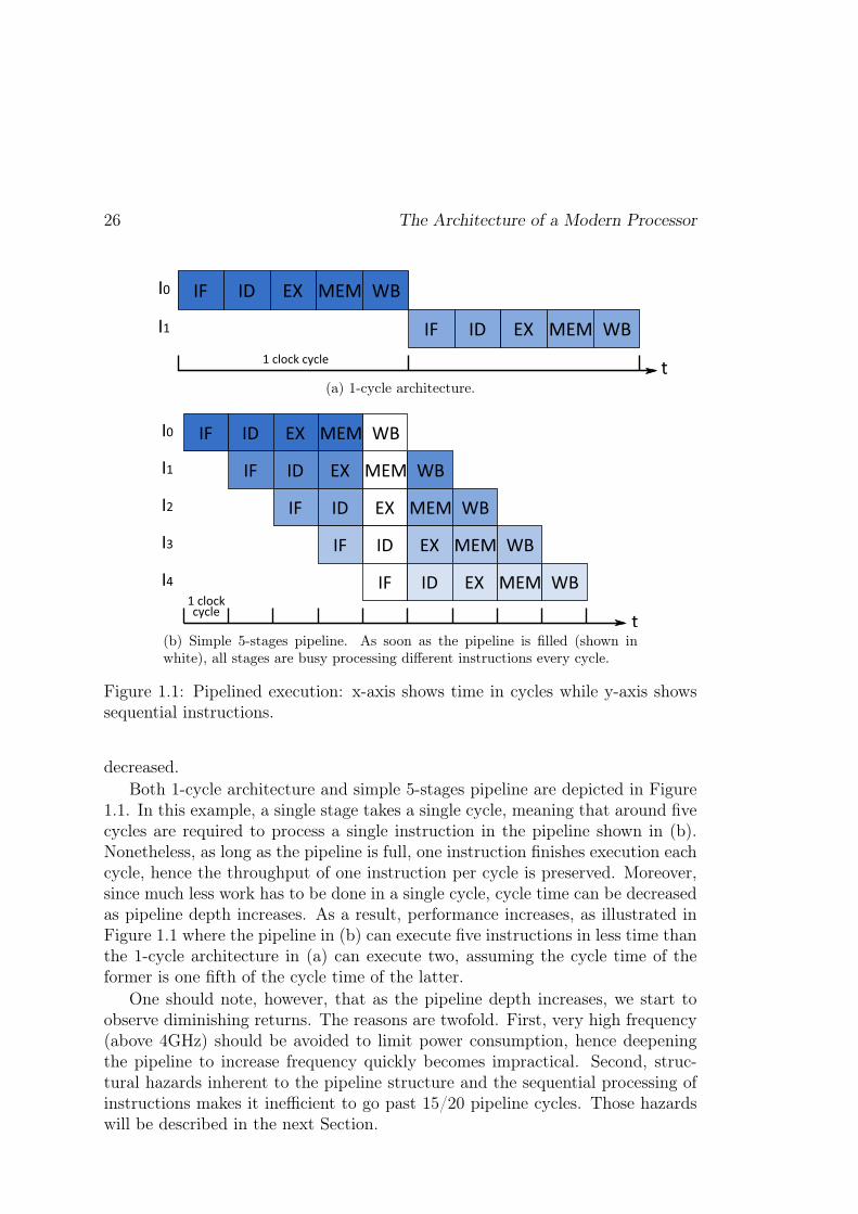
(a) 1-cycle architecture.
(b) Simple 5-stages pipeline. As soon as the pipeline is filled (shown inwhite), all stages are busy processing different instructions every cycle.
Figure 1.1: Pipelined execution: x-axis shows time in cycles while y-axis showssequential instructions.
decreased.Both 1-cycle architecture and simple 5-stages pipeline are depicted in Figure
1.1. In this example, a single stage takes a single cycle, meaning that around fivecycles are required to process a single instruction in the pipeline shown in (b).Nonetheless, as long as the pipeline is full, one instruction finishes execution eachcycle, hence the throughput of one instruction per cycle is preserved. Moreover,since much less work has to be done in a single cycle, cycle time can be decreasedas pipeline depth increases. As a result, performance increases, as illustrated inFigure 1.1 where the pipeline in (b) can execute five instructions in less time thanthe 1-cycle architecture in (a) can execute two, assuming the cycle time of theformer is one fifth of the cycle time of the latter.
One should note, however, that as the pipeline depth increases, we start toobserve diminishing returns. The reasons are twofold. First, very high frequency(above 4GHz) should be avoided to limit power consumption, hence deepeningthe pipeline to increase frequency quickly becomes impractical. Second, struc-tural hazards inherent to the pipeline structure and the sequential processing ofinstructions makes it inefficient to go past 15/20 pipeline cycles. Those hazardswill be described in the next Section.

Simple Pipelining 27
1.2.1 Different Stages for Different Tasks
In the following paragraphs, we describe how the execution of an instruction canbe broken down into several steps. Note that it is possible to break down thesesteps even further, or to add more steps depending on how the micro-architectureactually processes instructions. In particular, we will see in 1.3.3 that additionalsteps are required for out-of-sequence execution.
1.2.1.1 Instruction Fetch – IF
As previously mentioned, the instructions of the program to execute reside inglobal memory. Therefore, the current instruction to execute has to be broughtinto the processor to be processed. This requires accessing the memory hierarchywith the address contained in the Program Counter (PC) and updating the PCfor the next cycle.
1.2.1.2 Instruction Decode – ID
The instruction retrieved by the Fetch stage is encoded in a binary format tooccupy less space in memory. This binary word has to be expanded – decoded –into the control word that will drive the rest of the pipeline (e.g., register indexesto access the register file, control word of the functional unit, control word of thedatapath multiplexers, etc.). In the pipeline we consider, Decode includes readingsources from the Physical Register File (PRF), although a later stage could bededicated to it, or it could be done at Execute.
For now, we only consider the case of a RISC pipeline, but in the case ofCISC, the semantics of many instructions are too complex to be handled by thestages following Decode as is. Therefore, the Decode stage is in charge of crackingsuch instructions into several micro-operations (µ-ops) that are more suited tothe hardware. For instance, a load instruction may be cracked into a µ-op thatcomputes the address from which to load the data from, and a µ-op that actuallyaccesses the memory hierarchy.
1.2.1.3 Execute – EX
This stage actually computes the result of the instruction. In the case of loadinstructions, address calculation is done in this stage, while the access to thememory hierarchy will be done in the next stage, Memory.
To allow the execution of two dependent instructions back-to-back, the resultof the first instruction is made available to the second instruction on the bypassnetwork. In this particular processor, the bypass network spans from Execute toWriteback, at which point results are written to the PRF. For instance, let us

28 The Architecture of a Modern Processor
Figure 1.2: Origin of the operands of four sequential instructions dependent on asingle instruction. Some stage labels are omitted for clarity.
consider Figure 1.2 where I1, I2, I3 and I4 all require the result of I0. I1 will catchits source r0 on the bypass network since I0 is in the Memory stage when I1 is inExecute. I2 will also catch r0 on the network because I0 is writing back its resultto the PRF when I2 is in Execute. Interestingly, I3 will also catch its source onthe network since when I3 read its source registers in the Decode stage, I0 waswriting its result to the PRF, therefore, I3 read the old value of the register. Asa result, only I4 will read r0 from the PRF.
Without the bypass network, a dependent instruction would have to wait untilthe producer of its source left Writeback2 before entering the Decode stage andreading it in the PRF. In our pipeline model, this would amount to a minimumdelay of 3 cycles between any two dependent instructions. Therefore, the bypassnetwork is a key component of pipelined processor performance.
1.2.1.4 Memory – MEM
In this stage, all instructions requiring access to the memory hierarchy proceedwith said access. In modern processors, the memory hierarchy consists of sev-eral levels of cache memory intercalated between the pipeline and main memory.Cache memories contain a subset of main memory, that is, a datum that is in thecache also resides in main memory3.
We would like to stress that contrarily to scratchpads, caches are not managedby the software and are therefore transparent to the programmer. Any memory
2Results are written to the PRF in Writeback.3Note that a more recent version of the datum may reside in the cache and be waiting to be
written back to main memory.

Simple Pipelining 29
Figure 1.3: 3-level memory hierarchy. As the color goes from strong green to red,access latency increases. WB stands for writeback.
30 The Architecture of a Modern Processor
instruction accessing data that is not in the Level 1 (L1) cache (miss) will bringthe required data from Level 2 (L2) cache. If said data is not in the L2, it will bebrought from lower levels of the hierarchy. Since the L1 is generally small, cachespace may have to be reclaimed to insert the new data. In this case, another pieceof data is selected using a dedicated algorithm e.g., Least Recently Used (LRU)and written back to the L2 cache. Then it is overwritten by the new data in theL1 cache. Note that since we are putting the data evicted from the L1 in theL2, L2 space may also need to be reclaimed. In that case, the data evicted inthe L2 is written back to the next lower level of the hierarchy (potentially mainmemory), and so on.
An organization with two levels4 of cache is shown in Figure 1.3. The firstlevel of cache is the smallest but also the fastest, and as we go down the hierarchy,size increases but so does latency. In particular, an access to the first cache levelonly requires a few processor cycles while going to main memory can takes upto several hundreds of processor cycles and stall the processor in the process. Asa result, thanks to temporal5 and spatial6 locality, caches allow memory accessesto be very fast on average, while still providing the full storage capacity of mainmemory to the processor.
1.2.1.5 Writeback – WB
This stage is responsible for committing the computed result (or loaded value) tothe PRF. As previously mentioned, results in flight between Execute and Write-back are made available to younger instructions on the bypass network. In thissimple pipeline, once an instruction leaves the Writeback stage, its execution hascompleted and from the point of view of the software, the effect of the instructionon the architectural state is now visible.
1.2.2 Limitations
Control Hazards In general, branches are resolved at Execute. Therefore,an issue related to control flow dependencies begins to emerge when pipelining isused. Indeed, when a conditional branch leaves the Fetch stage, the processor doesnot know which instruction to fetch next because it does not know what directionthe branch will take. As a result, the processor should wait for the branch tobe resolved until it can continue fetching instructions. Therefore, bubbles (nooperation) must be inserted in the pipeline until the branch outcome is known.
4Modern Chip Multi-Processors (CMP, a.k.a. multi-cores) usually possess a L3 cache sharedbetween all cores. Its size ranges from a few MB to a few tens of MB.
5Recently used data is likely to be re-used soon.6Data located close in memory to recently used data is likely to be used soon.

Simple Pipelining 31
Figure 1.4: Control hazard in the pipeline: new instructions cannot enter thepipeline before the branch outcome is known.
In this example, this would mean stalling the pipeline for two cycles on eachbranch instruction, as illustrated in Figure 1.4. In general, a given pipeline wouldbe stalled for Fetch-to-Execute cycles, which may amount to a few tens of cyclesin some pipelines (e.g., Intel Pentium 4 has a 20/30-stages pipeline depending onthe generation). Therefore, if deepening the pipeline allows to increase processorspeed by decreasing the cycle time, the impact of control dependencies quicklybecomes prevalent and should be addressed [SC02].
Data Hazards Although the bypass network increases efficiency by forwardingvalues to instructions as soon as they are produced, the baseline pipeline alsosuffers from data hazards. Data hazards are embodied by three types of registerdependencies.
On the one hand, true data dependencies, also called Read-After-Write (RAW )dependencies cannot generally be circumvented as they are intrinsic to the algo-rithm that the program implements. For instance, in the expression (1 + 2 ∗ 3),the result of 2 ∗ 3 is always required before the addition can be done. Unfortu-nately, in the case of long latency operations such as a load missing in all cachelevels, a RAW dependency between the load and its dependents entails that saiddependents will be stalled for potentially hundreds of cycles.
On the other hand, there are two kind of false data dependencies. Theyboth exist because of the limited number of architectural registers defined by theISA (only 16 in x86_64). That is, if there were an infinite number of registers,they would not exist. First, Write-after-Write (WAW ) hazards take place whentwo instructions plan to write to the same architectural register. In that case,writes must happen in program order. This is already enforced by the in-order

32 The Architecture of a Modern Processor
nature of execution in the simple pipeline model we consider. Second, Write-after-Read (WAR) hazards take place when a younger instruction plans to write to anarchitectural register than must be read by an older instruction. Once again, theread must take place before the write, and this is once again enforced in our caseby executing instructions in-order. As a result, WAW and WAR hazards are anon-issue in processors executing instructions in program order.
Nonetheless, we will see in the next section that to mitigate the impact ofRAW hazards, it is possible to execute instructions out-of-sequence (out-of-orderexecution). However, in this case, WAW and WAR hazards become a substantialhindrance to the efficient processing of instructions. Indeed, they forbid two inde-pendent instructions to be executed out-of-order simply because both instructionswrite to the same architectural register (case of WAW dependencies). The reasonbehind this name collision is that ISAs only define a few number of architecturalregisters. As a result, the compiler often does not have enough architecturalregisters (i.e., names) to attribute a different one to each instruction destination.
1.3 Advanced Pipelining
1.3.1 Branch Prediction
As mentioned in the previous section, the pipeline must introduce bubbles insteadof fetching instructions when an unresolved branch is in flight. This is becauseneither the direction of the branch nor the address from which to fetch nextshould the branch be taken are known. To address this issue, Branch Predictionwas introduced [Smi81]. The key idea is that when a branch is fetched, a predictoris accessed, and a predicted direction and branch target are retrieved.
Naturally, because of the speculative nature of branch prediction, it will benecessary to throw some instructions away when the prediction is found out tobe wrong. In our 5-cycle pipeline where branches are resolved at Execute, thiswould translate in two instructions being thrown away on a branch misprediction.Fortunately, since execution is in-order, no rollback has to take place, i.e., theinstructions on the wrong path did not incorrectly modify the architectural state.Moreover, in this particular pipeline, the cost of never predicting is similar to thecost of always mispredicting. Therefore, it follows that adding branch predictionwould have a great impact on performance even if one branch out of two wasmispredicted. This is actually true in general although mispredicting has a mod-erately higher cost than not predicting. Nonetheless, branch predictors are gener-ally able to attain an accuracy in the range of 0.9 to 0.99 [SM06, Sez11b, cbp14],which makes branch prediction a key component of processor performance.
Although part of this thesis work makes use of recent advances in branchprediction, we do not detail the inner workings of existing branch predictors in
Advanced Pipelining 33
this Section. We will only describe the TAGE [SM06] branch predictor in Chapter3 as it is required for our VTAGE value predictor. Regardless, the key idea isthat given the address of a given branch instruction and some additional processorstate (e.g., outcome of recent branches), the predictor is able to predict the branchdirection. The target of the branch is predicted by a different – though equivalentin the input it takes – structure and can in some cases be computed at Decodeinstead of Execute.
1.3.2 Superscalar Execution
In a sequence of instructions, it is often the case that two or more neighbor-ing instructions are independent. As a result, one can increase performance byprocessing those instructions in parallel. For instance, pipeline resources can beduplicated, allowing several instructions to flow in the pipeline in parallel, al-though still following program order. That is, by being able to fetch, decode,execute and writeback several instructions per cycle, throughput can be greatlyincreased, as long as instructions are independent. If not, only a single instructioncan proceed while subsequent ones are stalled.
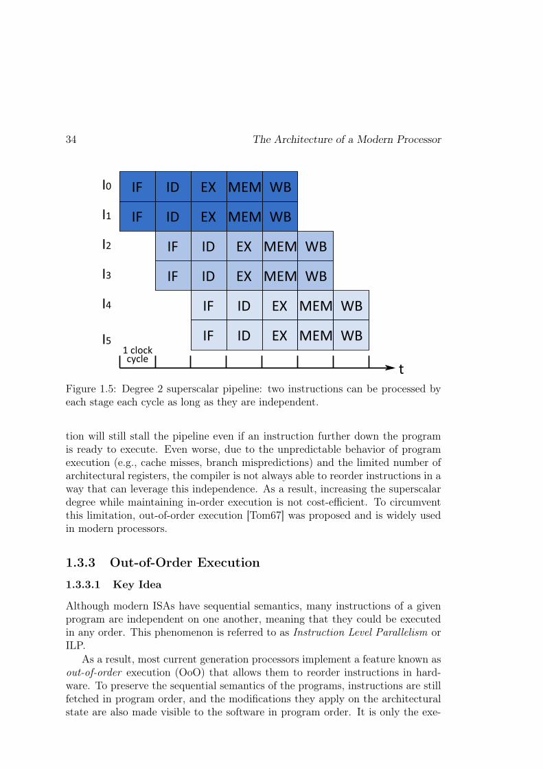
For instance, in Figure 1.5, six instructions can be executed by pairs in apipeline having a superscalar degree of 2 (i.e., able to process two instructionsconcurrently). One should note that only 7 cycles are required to execute thoseinstructions while the scalar pipeline of Figure 1.1 (b) would have required 10cycles.
Unfortunately, superscalar execution has great hardware cost. Indeed, if in-creasing the width of the Fetch stage is fairly straightforward up to a few in-structions (get more bytes from the instruction cache), the Decode stage is nowin charge of decoding several instructions and resolving any dependencies be-tween them to determine if they can proceed further together or if one must stall.Moreover, if functional units can simply be duplicated, the complexity of thebypass network in charge of providing operands on-the-fly grows quadraticallywith the superscalar degree. Similarly, the PRF must now handle 4 reads and 2writes per cycle instead of 2 reads and 1 write in a scalar pipeline, assuming twosources and one destination per instruction. Therefore, ports must be added onthe PRF, leading to a much higher area and power consumption since both growsuper-linearly with the port count [ZK98]. The same stands for the L1 cache ifone wants to enable several load instructions to proceed each cycle.
In addition, this implementation of a superscalar pipeline is very limited inhow much it can exploit the independence between instructions. Indeed, it isnot able to process concurrently two independent instructions that are a few in-structions apart in the program. It can only process concurrently two neighboringinstructions, because it executes in-order. This means that a long latency instruc-
34 The Architecture of a Modern Processor
Figure 1.5: Degree 2 superscalar pipeline: two instructions can be processed byeach stage each cycle as long as they are independent.
tion will still stall the pipeline even if an instruction further down the programis ready to execute. Even worse, due to the unpredictable behavior of programexecution (e.g., cache misses, branch mispredictions) and the limited number ofarchitectural registers, the compiler is not always able to reorder instructions in away that can leverage this independence. As a result, increasing the superscalardegree while maintaining in-order execution is not cost-efficient. To circumventthis limitation, out-of-order execution [Tom67] was proposed and is widely usedin modern processors.
1.3.3 Out-of-Order Execution
1.3.3.1 Key Idea
Although modern ISAs have sequential semantics, many instructions of a givenprogram are independent on one another, meaning that they could be executedin any order. This phenomenon is referred to as Instruction Level Parallelism orILP.
As a result, most current generation processors implement a feature known asout-of-order execution (OoO) that allows them to reorder instructions in hard-ware. To preserve the sequential semantics of the programs, instructions are stillfetched in program order, and the modifications they apply on the architecturalstate are also made visible to the software in program order. It is only the exe-

Advanced Pipelining 35
cution that happens out-of-order, driven by true data dependencies (RAW) andresource availability.
To ensure that out-of-order provides both high performance and sequentialsemantics, numerous modifications must be made to our existing 5-stage pipeline.
1.3.3.2 Register Renaming
We previously presented the three types of data dependencies: RAW, WAW andWAR. We mentioned that WAW and WAR are false dependencies, and that in anin-order processor, they are a non-issue since in-order execution prohibits themby construction. However, in the context of out-of-order execution, these twotypes of data dependencies become a major hurdle to performance.
Indeed, consider two independent instructions I0 and I7 that belong to differ-ent dependency chains, but both write to register r0 simply because the compilerwas not able to provide them with distinct architectural registers. As a result,the hardware should ensure that any instruction dependent on I0 can get thecorrect value for that register before I7 overwrites it. In general, this means thata substantial portion of the existing ILP will be inaccessible because the desti-nation names of independent instructions collide. However, if the compiler hadhad more architectural registers to allocate, the previous dependency would havedisappeared. Unfortunately, this would entail modifying the ISA.
A solution to solve this issue is to provide more registers in hardware but keepthe number of registers visible to the compiler the same. This way, the ISA doesnot change. Then, the hardware can dynamically rename architectural registersto physical registers residing in the PRF. In the previous example, I0 could seeits architectural destination register, ar0 (arch. reg 0), renamed to pr0 (physicalregister 0). Conversely, I7 could see its architectural destination register, also ar0,renamed to pr1. As a result, both instructions could be executed in any orderwithout overwriting each other’s destination register. The reasoning is exactlythe same for WAR dependencies.
To track register mappings, a possibility is to use a Rename Map and a FreeList. The Rename Map gives the current mapping of a given architectural registerto a physical register. The Free List keeps track of physical registers that are notmapped to any architectural register, and is therefore in charge of providingphysical registers to new instructions entering the pipeline. These two steps,source renaming and destination renaming are depicted in Figure 1.6.
Note however that the mappings in the Rename Map are speculative by naturesince renamed instructions may not actually be retained if, for instance, an olderbranch has been mispredicted. Therefore, a logical view of the renaming processincludes a Commit Rename Map that contains the non-speculative mappings,i.e., the current software-visible architectural state of the processor. When an

36 The Architecture of a Modern Processor
Figure 1.6: Register renaming. Left: Both instruction sources are renamed bylooking up the Rename Table. Right: The instruction destination is renamed bymapping a free physical register to it.
Figure 1.7: Introduction of register renaming in the pipeline. The new stage,Rename, is shown in dark blue.
instruction finishes its execution and is removed from the pipeline, the mapping ofits architectural destination register is now logically part of the Commit RenameMap.
A physical register is put back in the Free List once a younger instructionmapped to the same architectural register (i.e., that has a more recent mapping)leaves the pipeline.
Rename requires its own pipeline stage(s), and is usually intercalated betweenDecode and the rest of the pipeline, as shown in Figure 1.7. Thus, it is not possibleto read the sources of an instruction in the Decode stage anymore. Moreover,to enforce the sequential semantics of the program, Rename must happen inprogram order, as Fetch and Decode. Lastly, note that as the superscalar degreeincreases, the hardware required to rename registers becomes slower as well asmore complex [PJS97], since among a group of instruction being renamed in the
Advanced Pipelining 37
same cycle, some may depend on others. In that case, the younger instructionsrequire the destination mappings of the older instructions to rename their sources,but those mappings are being generated. An increased superscalar degree alsoputs pressure on the Rename Table since it must support that many more readsand writes each cycle.
1.3.3.3 In-order Dispatch and Commit
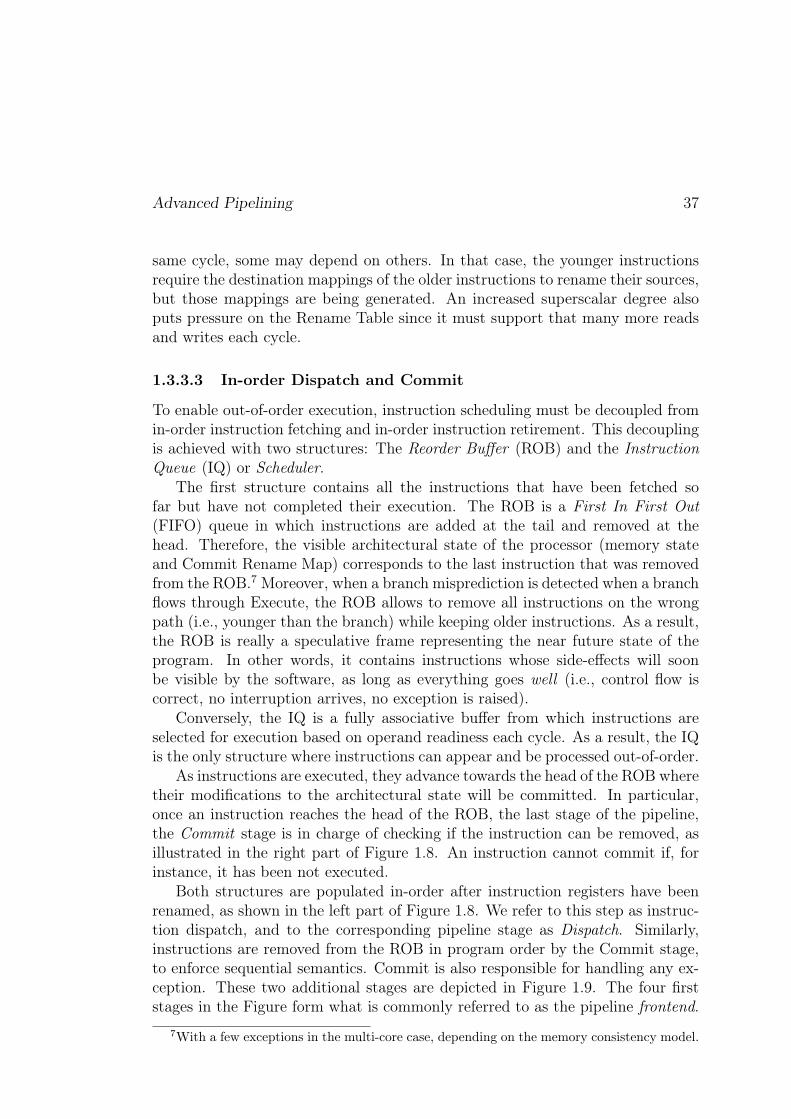
To enable out-of-order execution, instruction scheduling must be decoupled fromin-order instruction fetching and in-order instruction retirement. This decouplingis achieved with two structures: The Reorder Buffer (ROB) and the InstructionQueue (IQ) or Scheduler.
The first structure contains all the instructions that have been fetched sofar but have not completed their execution. The ROB is a First In First Out(FIFO) queue in which instructions are added at the tail and removed at thehead. Therefore, the visible architectural state of the processor (memory stateand Commit Rename Map) corresponds to the last instruction that was removedfrom the ROB.7 Moreover, when a branch misprediction is detected when a branchflows through Execute, the ROB allows to remove all instructions on the wrongpath (i.e., younger than the branch) while keeping older instructions. As a result,the ROB is really a speculative frame representing the near future state of theprogram. In other words, it contains instructions whose side-effects will soonbe visible by the software, as long as everything goes well (i.e., control flow iscorrect, no interruption arrives, no exception is raised).
Conversely, the IQ is a fully associative buffer from which instructions areselected for execution based on operand readiness each cycle. As a result, the IQis the only structure where instructions can appear and be processed out-of-order.
As instructions are executed, they advance towards the head of the ROB wheretheir modifications to the architectural state will be committed. In particular,once an instruction reaches the head of the ROB, the last stage of the pipeline,the Commit stage is in charge of checking if the instruction can be removed, asillustrated in the right part of Figure 1.8. An instruction cannot commit if, forinstance, it has been not executed.
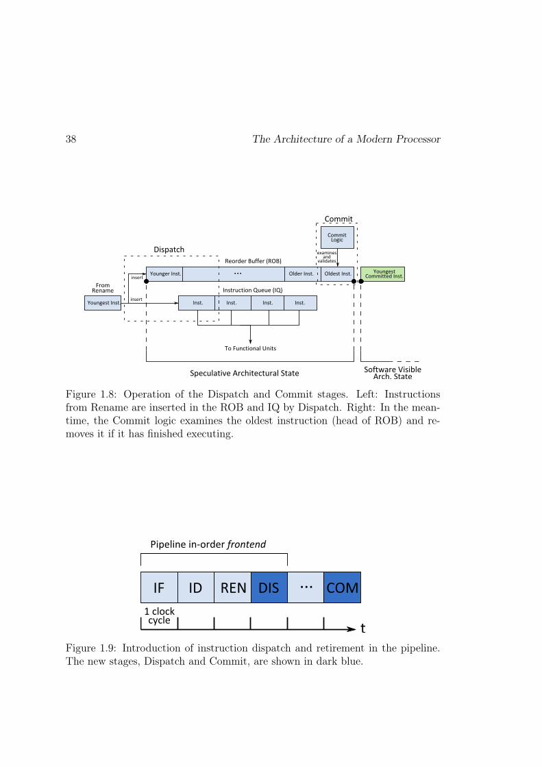
Both structures are populated in-order after instruction registers have beenrenamed, as shown in the left part of Figure 1.8. We refer to this step as instruc-tion dispatch, and to the corresponding pipeline stage as Dispatch. Similarly,instructions are removed from the ROB in program order by the Commit stage,to enforce sequential semantics. Commit is also responsible for handling any ex-ception. These two additional stages are depicted in Figure 1.9. The four firststages in the Figure form what is commonly referred to as the pipeline frontend.
7With a few exceptions in the multi-core case, depending on the memory consistency model.
38 The Architecture of a Modern Processor
Figure 1.8: Operation of the Dispatch and Commit stages. Left: Instructionsfrom Rename are inserted in the ROB and IQ by Dispatch. Right: In the mean-time, the Commit logic examines the oldest instruction (head of ROB) and re-moves it if it has finished executing.
Figure 1.9: Introduction of instruction dispatch and retirement in the pipeline.The new stages, Dispatch and Commit, are shown in dark blue.

Advanced Pipelining 39
1.3.3.4 Out-of-Order Issue, Execute and Writeback
Operation The IQ is responsible for instruction scheduling or issuing. Eachcycle, logic scans the IQ for n instructions8 whose sources are ready i.e., in thePRF or the bypass network. These selected instructions are then issued to thefunctional units for execution, with no concern for their ordering. To carry outscheduling, a pipeline stage, Issue, is required.
Before being executed on the functional units (FUs), issued instructions willread their sources from either the PRF or the bypass network in a dedicatedstage we refer to as Register/Bypass Read (RBR). In the two subsequent stages,Execute and Writeback, selected instructions will respectively execute and writetheir result to the PRF. Instruction processing by this four stages is depicted inFigure 1.10.
Note that if two dependent instructions I0 and I1 execute back-to-back, thenthe destination of I0 (respectively source of I1) is not available on the multiplexerof the RBR stage when I1 is in RBR. Consequently, in this case, the bypass net-work is able to forward the result of I0 from the output of the FU used by I0during the previous cycle to the input of the FU used by I1 when I1 enters Exe-cute. The bypass network is therefore multi-level. Also consider that a hardwareimplementation may not implement several levels of multiplexers as in Figure1.10, but a single one where results are buffered for a few cycles and taggedwith the physical register they correspond to. In that case, an instruction maycheck the network with its source operands identifiers to get their data from thenetwork.
These four stages form the out-of-order engine of the processor, and are de-coupled from the in-order frontend and in-order commit by the IQ itself. Theresulting 9-stage pipeline is shown in Figure 1.11.
Complexity It should be mentioned that the logic used in the out-of-orderengine is complex and power hungry. For instance, assuming an issue width ofn, then up to 2n registers may have to be read from the PRF and up to n mayhave to be written, in the same cycle. Moreover, an increased issue-width usuallyimplies a larger instruction window, hence more registers. As a result, PRF areaand power consumption grow quadratically with the issue width [ZK98].
Similarly, to determine operand readiness (Wakeup phase), each entry in theIQ has to monitor the name of the registers whose value recently became avail-able. That is, each source of each IQ entry must be compared against n physicalregister identifiers each cycle. Assuming n = 8, 8-bit identifiers (i.e., 256 physicalregisters), 2 sources per IQ entry, and a 60-entry IQ, this amounts to 960 8-bitcomparisons per cycle. Only when this comparisons have taken place can the
8n is the issue-width, which does not necessarily correspond to the superscalar degree.

40 The Architecture of a Modern Processor
Figure 1.10: Operation of the out-of-order execution engine. The Scheduler is incharge of selecting 2 ready instructions to issue each cycle. Selected instructionscollect their sources in the next stage (RBR) or in Execute in some cases, thenexecute on the functional units (FUs). Finally, instructions write their results tothe PRF.
Figure 1.11: Introduction of the out-of-order execution engine in the pipeline.New stages are shown in dark blue. IS: Issue, RBR: Register/Bypass Read, EX:Execute, WB: Writeback.
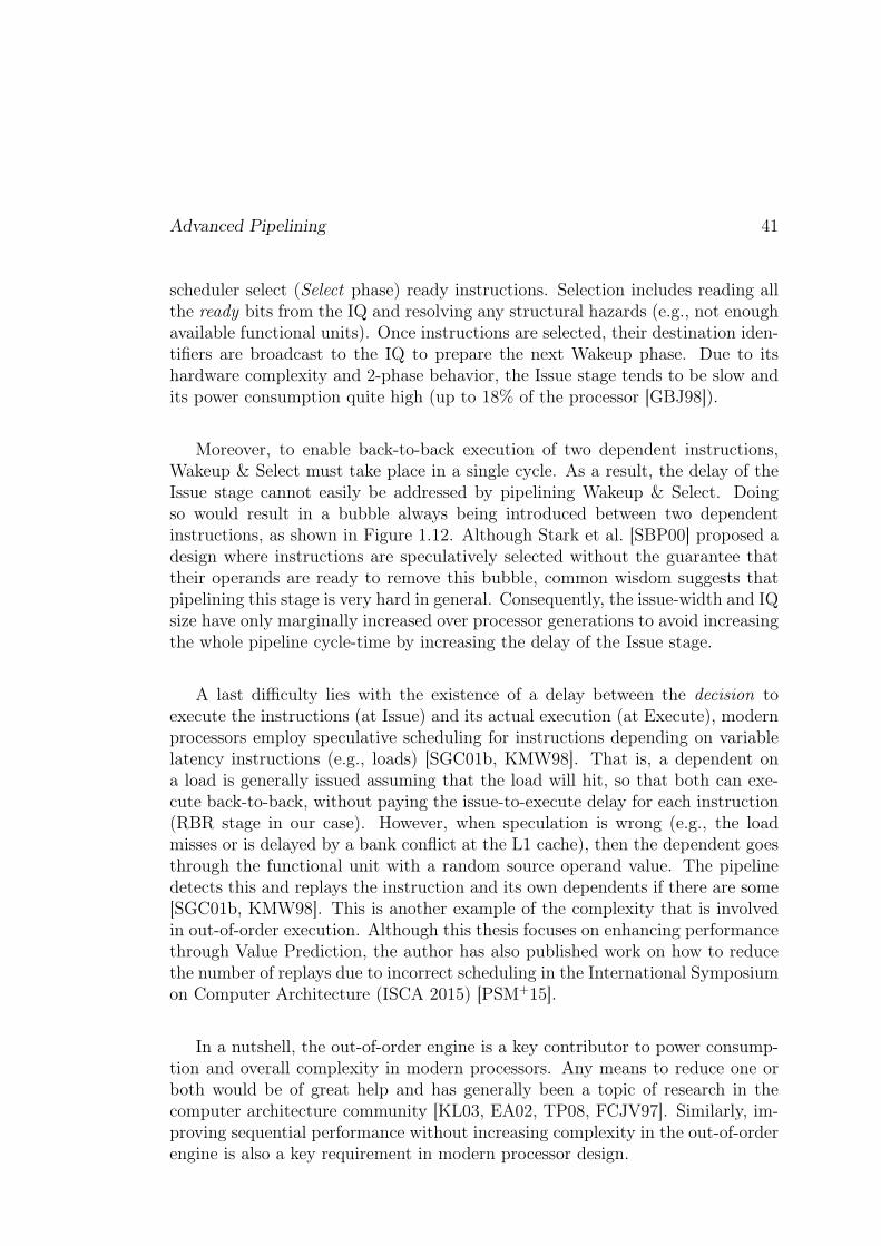
Advanced Pipelining 41
scheduler select (Select phase) ready instructions. Selection includes reading allthe ready bits from the IQ and resolving any structural hazards (e.g., not enoughavailable functional units). Once instructions are selected, their destination iden-tifiers are broadcast to the IQ to prepare the next Wakeup phase. Due to itshardware complexity and 2-phase behavior, the Issue stage tends to be slow andits power consumption quite high (up to 18% of the processor [GBJ98]).
Moreover, to enable back-to-back execution of two dependent instructions,Wakeup & Select must take place in a single cycle. As a result, the delay of theIssue stage cannot easily be addressed by pipelining Wakeup & Select. Doingso would result in a bubble always being introduced between two dependentinstructions, as shown in Figure 1.12. Although Stark et al. [SBP00] proposed adesign where instructions are speculatively selected without the guarantee thattheir operands are ready to remove this bubble, common wisdom suggests thatpipelining this stage is very hard in general. Consequently, the issue-width and IQsize have only marginally increased over processor generations to avoid increasingthe whole pipeline cycle-time by increasing the delay of the Issue stage.
A last difficulty lies with the existence of a delay between the decision toexecute the instructions (at Issue) and its actual execution (at Execute), modernprocessors employ speculative scheduling for instructions depending on variablelatency instructions (e.g., loads) [SGC01b, KMW98]. That is, a dependent ona load is generally issued assuming that the load will hit, so that both can exe-cute back-to-back, without paying the issue-to-execute delay for each instruction(RBR stage in our case). However, when speculation is wrong (e.g., the loadmisses or is delayed by a bank conflict at the L1 cache), then the dependent goesthrough the functional unit with a random source operand value. The pipelinedetects this and replays the instruction and its own dependents if there are some[SGC01b, KMW98]. This is another example of the complexity that is involvedin out-of-order execution. Although this thesis focuses on enhancing performancethrough Value Prediction, the author has also published work on how to reducethe number of replays due to incorrect scheduling in the International Symposiumon Computer Architecture (ISCA 2015) [PSM+15].
In a nutshell, the out-of-order engine is a key contributor to power consump-tion and overall complexity in modern processors. Any means to reduce one orboth would be of great help and has generally been a topic of research in thecomputer architecture community [KL03, EA02, TP08, FCJV97]. Similarly, im-proving sequential performance without increasing complexity in the out-of-orderengine is also a key requirement in modern processor design.

42 The Architecture of a Modern Processor
Figure 1.12: Pipelining Issue (Wakeup & Select) over two cycles introduces abubble between any two dependent instructions.
1.3.3.5 The Particular Case of Memory Instructions
Readers may have noticed that the Memory stage has been removed from Figure1.11. The reason is that because instruction sequencing and instruction schedul-ing/execution are decoupled, the Execute stage can take up as many cycles asnecessary without stalling subsequent instructions, thanks to out-of-order execu-tion. As a result, we embed the Memory stage inside the Execute stage.
Regardless, in its current state, our out-of-order model is incorrect, for tworeasons. First, if loads can generally be executed speculatively (i.e., on the wrongcontrol path) without threatening correctness, the same is not true for storeinstructions. Indeed, if a value is committed to memory only to find out that thestore instruction must be thrown away because an older branch was mispredicted,then execution is incorrect.
Second, if RAW dependencies between registers can easily be enforced, RAWmemory dependencies cannot. The reason is that the addresses accessed by mem-ory instructions are generally not known until Execute. That is, an older storemay write to a location that is accessed by a younger load, but there is no wayto know it before both instructions have computed their respective addresses. Ifthe load is selected for execution before the store, then it will obtain a stale valueand break the sequential semantics of the program.
Therefore, it follows that the hardware should provide two guarantees:
1. Store instructions may only write their data to memory once they are guar-anteed to be on the correct control path, i.e., after they have been commit-ted.
2. Sequential ordering between dependent memory operations must be en-forced9.
9With regard to the memory consistency model provided by the ISA.

Advanced Pipelining 43
Figure 1.13: Store Queue operation. Left: New store instructions are put at thetail in Dispatch. Bottom: During Execute, the address is computed and put inthe SQ with the corresponding data. Right: After Commit, the store is writtenback to the data cache when it arrives at the head of the SQ.
Post-Commit Writeback Since stores may only access the data cache afterhaving committed, another structure is required to keep track of pending stores.Thus, current processors provide a third structure, the Store Queue (SQ), thattracks both inflight stores (i.e., speculative) and pending stores (i.e., committedbut waiting to write their data to the data cache). The operation of the SQ isillustrated in Figure 1.13.
The left part of the Figure shows that the SQ is populated at Dispatch, as theROB and IQ. As the ROB, it keeps track of stores in a FIFO fashion, to enforcesequential ordering of memory writes. An entry in the SQ has two main fields:address and data. Keeping data in the SQ is required as once a store commits,there is no guarantee that the data to be written will remain in the PRF until thecache is actually accessed. Keeping the computed address is required to enablea feature known as Store-to-Load Forwarding (STLF), which plays a key role inenforcing sequential semantics for memory instructions. It will be described inthe next paragraph.
Regardless, with this mechanism, a store instruction is issued in the out-of-order engine, as soon as its sources (partial address and data) are ready. DuringExecute, the data cache is not accessed. Rather, the address is computed andboth computed address and data are copied to the SQ entry, as depicted in the

44 The Architecture of a Modern Processor
bottom of Figure 1.13.Once a store has committed, it becomes eligible to be written back to the data
cache. In particular, each cycle, the processor writes back stores at the head ofthe SQ to the data cache, if a cache port is available. Then, it clears their SQentry. This is shown in the right corner of Figure 1.13.
Astute readers may have noticed that some stores may not have written backtheir data to the cache, yet have committed. This committed memory writeshould be part of the software-visible architectural state of the processor. How-ever, in this particular pipeline instance, software visibility of the write is notguaranteed since the data may still be in the SQ when a subsequent load to thesame address executes. This is addressed by Store-To-Load Forwarding (STLF).
Store-to-Load Forwarding STLF consists in probing all SQ entries contain-ing an older store with the load address every time a load executes. If a match isfound, then the data in the SQ can be forwarded to the load destination register.Such a mechanism is illustrated in Figure 1.14.
With STLF, any committed store waiting for its turn to write its data inthe cache can still supply its data to younger load instructions. In effect, anypending memory write becomes visible to younger instructions, guaranteeing thatcommitted stores are part of the software-visible architectural state. Note thatSTLF must not be limited to committed stores: any store is allowed match a givenload address as long as it is older. In particular, in Figure 1.14, an uncommittedstore provides the data.
Yet, correctness is still not guaranteed. Indeed, consider the case where theload in Figure 1.14 should actually match the younger older store (2nd entry),but the address collision remains undetected since that store has not executedyet. In that case, execution is incorrect because the hardware was not able toenforce and even detect the Read-after-Write dependency existing between thetwo memory instructions.
Out-of-Order Execution of Memory Operations To remedy the memoryordering violation example described in the last paragraph and provide the secondguarantee discussed in 1.3.3.5, the hardware can simply forbid memory instruc-tions to issue out-of-order. However, this would defeat the purpose of out-of-orderexecution and greatly hinder performance in the process.
Thus, a more efficient solution would be to allow stores being executed tocheck that all younger loads either access a different address or have not executedyet. To do so, another structure is required to track the addresses of inflightloads. Specifically, current processors implement a Load Queue (LQ), which isvery similar to the Store Queue, except for the instructions it tracks and the fact
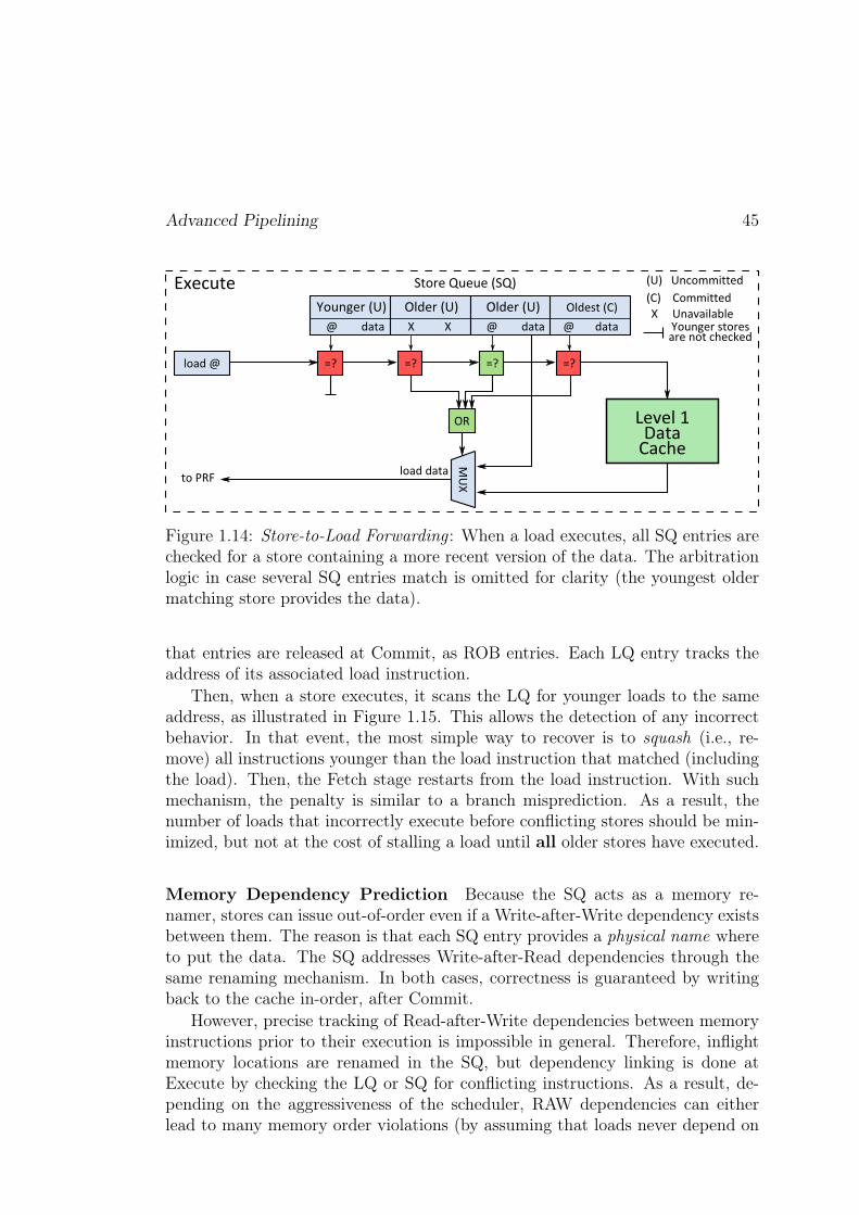
Advanced Pipelining 45
Figure 1.14: Store-to-Load Forwarding : When a load executes, all SQ entries arechecked for a store containing a more recent version of the data. The arbitrationlogic in case several SQ entries match is omitted for clarity (the youngest oldermatching store provides the data).
that entries are released at Commit, as ROB entries. Each LQ entry tracks theaddress of its associated load instruction.
Then, when a store executes, it scans the LQ for younger loads to the sameaddress, as illustrated in Figure 1.15. This allows the detection of any incorrectbehavior. In that event, the most simple way to recover is to squash (i.e., re-move) all instructions younger than the load instruction that matched (includingthe load). Then, the Fetch stage restarts from the load instruction. With suchmechanism, the penalty is similar to a branch misprediction. As a result, thenumber of loads that incorrectly execute before conflicting stores should be min-imized, but not at the cost of stalling a load until all older stores have executed.
Memory Dependency Prediction Because the SQ acts as a memory re-namer, stores can issue out-of-order even if a Write-after-Write dependency existsbetween them. The reason is that each SQ entry provides a physical name whereto put the data. The SQ addresses Write-after-Read dependencies through thesame renaming mechanism. In both cases, correctness is guaranteed by writingback to the cache in-order, after Commit.
However, precise tracking of Read-after-Write dependencies between memoryinstructions prior to their execution is impossible in general. Therefore, inflightmemory locations are renamed in the SQ, but dependency linking is done atExecute by checking the LQ or SQ for conflicting instructions. As a result, de-pending on the aggressiveness of the scheduler, RAW dependencies can eitherlead to many memory order violations (by assuming that loads never depend on

46 The Architecture of a Modern Processor
Figure 1.15: Memory ordering check: When a store executes, all younger inflightloads addresses are compared against the store address. Here, a younger loadmatches, meaning that the instruction has loaded stale data. All instructionsyounger than the load (including the load) will be removed from the pipeline andre-fetched. The arbitration logic in case several LQ entries match is omitted forclarity (squashing starts from the oldest matching load).
stores) or to a loss in potential performance (by assuming that a load dependson all older un-executed stores). Therefore, to enable efficient out-of-order ex-ecution of memory operations, current processors usually implement a MemoryDependency Predictor. Indeed, instances of a given static load instruction oftendepend on instances of a single static store instruction [CE98]. As a result, astructure can be used to remember the past behavior of memory instructions andpredict that a given dynamic load will repeat the behavior of past instances ofthe same static instruction.
We do not detail any specific algorithm of memory dependency prediction,but we note that with the Store Sets predictor [CE98], most of the potentialof executing memory instructions out-of-order is retained while minimizing thenumber of ordering violations.
1.3.3.6 Summary and Limitations
Figure 1.16 gives a higher-level view of a modern out-of-order pipeline, startingfrom the in-order frontend on the left, then going to the out-of-order engine inthe middle, to finish with in-order instruction removal on the right. Althoughsome links between structures are omitted for clarity (e.g., Commit updates thebranch predictor and the memory dependency predictor, Execute can squash thepipeline on branch mispredictions and memory order violations), the Figure gives
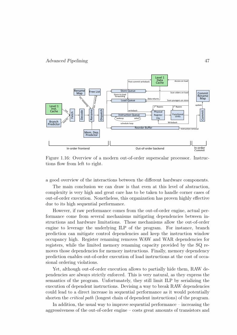
Advanced Pipelining 47
Figure 1.16: Overview of a modern out-of-order superscalar processor. Instruc-tions flow from left to right.
a good overview of the interactions between the different hardware components.The main conclusion we can draw is that even at this level of abstraction,
complexity is very high and great care has to be taken to handle corner cases ofout-of-order execution. Nonetheless, this organization has proven highly effectivedue to its high sequential performance.
However, if raw performance comes from the out-of-order engine, actual per-formance come from several mechanisms mitigating dependencies between in-structions and hardware limitations. Those mechanisms allow the out-of-orderengine to leverage the underlying ILP of the program. For instance, branchprediction can mitigate control dependencies and keep the instruction windowoccupancy high. Register renaming removes WAW and WAR dependencies forregisters, while the limited memory renaming capacity provided by the SQ re-moves those dependencies for memory instructions. Finally, memory dependencyprediction enables out-of-order execution of load instructions at the cost of occa-sional ordering violations.
Yet, although out-of-order execution allows to partially hide them, RAW de-pendencies are always strictly enforced. This is very natural, as they express thesemantics of the program. Unfortunately, they still limit ILP by serializing theexecution of dependent instructions. Devising a way to break RAW dependenciescould lead to a direct increase in sequential performance as it would potentiallyshorten the critical path (longest chain of dependent instructions) of the program.
In addition, the usual way to improve sequential performance – increasing theaggressiveness of the out-of-order engine – costs great amounts of transistors and
48 The Architecture of a Modern Processor
increases power consumption substantially. As a result, sequential performancehas only increased marginally with processor generations. Breaking RAW depen-dencies would increase sequential performance by uncovering more ILP withoutpaying the cost of a more aggressive out-of-order engine, rendering it even moreattractive a solution.
This thesis work revisits Value Prediction (VP), which goal is to predict theresult of dynamic instructions. That is, it allows a dependent on a predictedinstruction to execute with its producer concurrently by using the prediction asa source operand. Hence, the RAW dependency is effectively broken. To enforcecorrectness, wrong predictions must be detected and the pipeline state must berolled-back, much like in the case of a branch misprediction. Therefore, in addi-tion to a realistic but efficient prediction algorithm, a practical implementationof VP should provide a complexity-effective way to detect mispredictions andrecover from them. It should also increase sequential performance enough to beworth its cost, and said cost should be made as small as possible.

Chapter 2
Value Prediction as a Way toImprove Sequential Performance
As mentioned in the previous Chapter, Value Prediction (VP) speculates on theresult of instructions to break RAW dependencies and artificially increase ILP.This is illustrated in Figure 2.1, where the sequential execution of a chain ofdependency comprising four instructions is depicted, with and without VP. VPwas introduced independently by Lipasti et al. [LWS96, LS96] and Gabbay andMendelson [GM96]. It leverages the low dynamic range exhibited by the resultstream of some instructions, also known as value locality. In other words, in-stances of the same static instruction often produce the same result, or resultsthat fall within an easily recognizable pattern (e.g., strided).
Value Prediction has been an active topic of research in the 90’s. As a re-sult, many prediction algorithms have been devised, as well as other mechanismsleveraging VP. For instance, Aragon et al. [AGGG01] and Gonzalez and Gonzalez[GG99] use it to improve branch prediction, while other works use it to predictmemory addresses and trigger prefetches [EV93, GG97]. Burtscher et al. evenconsider the use of value prediction to compress execution traces more efficiently[BJ03, Bur04]. However, due to an ambient skepticism regarding the feasibilityof an actual implementation, the focus of the community shifted away from VPin the late 90’s. The main reason being the assumption that VP introduces com-plexity in critical stages of the pipeline: prediction in the frontend, and validationand recovery in the backend. In particular, we already mentioned the high com-plexity of the out-of-order engine, therefore, complexifying it further with VP isnot an attractive proposition.
In the common approach, a predictor is added to the frontend and accessedon a per-instruction basis. This predictor provides a prediction that acts as atemporary result for the instruction and can therefore be sourced by dependentsbefore the actual result is computed. When the predicted instructions leaves the
49

50 Value Prediction as a Way to Improve Sequential Performance
Figure 2.1: Impact of Value Prediction on the ILP that the processor can extractfrom a given program.
functional units, its prediction is validated against the actual result, and recoverytakes place if necessary. Finally, when the instruction leaves the pipeline, itsresult is sent to the predictor to update it according to the prediction algorithm.
Arguably, the key component of a value prediction micro-architecture is thevalue predictor. Sazeides and Smith define two main types of predictors: compu-tational and context-based [SS97a]. We detail the main representatives of bothcategories in the following paragraphs as well as the way they are updated.
2.1 Hardware Prediction Algorithms
2.1.1 Computational Prediction
Computational predictors compute a prediction by applying a function to theresult of the previous instance, or previous instances. Therefore, they are able togenerate values that have not yet been seen in the value stream, depending onthe applied function.
Last Value Prediction The Last Value Predictor (LVP), as its name suggests,predicts that the result of an instruction is the result produced by the previousinstance of the same static instruction. In other words, it applies the identityfunction to the last result. It was introduced by Lipasti and Shen [LS96] andmay be the most simple prediction generation mechanism. Nonetheless, it is ableto improve performance by 4.5% on average in the framework used in [LS96].
This predictor is shown in Figure 2.2. It is a direct-mapped table addressed by
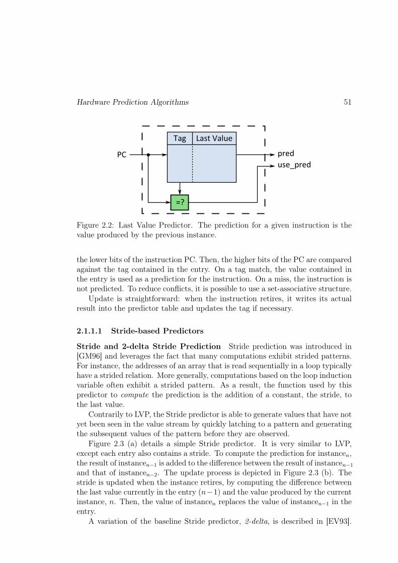
Hardware Prediction Algorithms 51
Figure 2.2: Last Value Predictor. The prediction for a given instruction is thevalue produced by the previous instance.
the lower bits of the instruction PC. Then, the higher bits of the PC are comparedagainst the tag contained in the entry. On a tag match, the value contained inthe entry is used as a prediction for the instruction. On a miss, the instruction isnot predicted. To reduce conflicts, it is possible to use a set-associative structure.
Update is straightforward: when the instruction retires, it writes its actualresult into the predictor table and updates the tag if necessary.
2.1.1.1 Stride-based Predictors
Stride and 2-delta Stride Prediction Stride prediction was introduced in[GM96] and leverages the fact that many computations exhibit strided patterns.For instance, the addresses of an array that is read sequentially in a loop typicallyhave a strided relation. More generally, computations based on the loop inductionvariable often exhibit a strided pattern. As a result, the function used by thispredictor to compute the prediction is the addition of a constant, the stride, tothe last value.
Contrarily to LVP, the Stride predictor is able to generate values that have notyet been seen in the value stream by quickly latching to a pattern and generatingthe subsequent values of the pattern before they are observed.
Figure 2.3 (a) details a simple Stride predictor. It is very similar to LVP,except each entry also contains a stride. To compute the prediction for instancen,the result of instancen−1 is added to the difference between the result of instancen−1and that of instancen−2. The update process is depicted in Figure 2.3 (b). Thestride is updated when the instance retires, by computing the difference betweenthe last value currently in the entry (n−1) and the value produced by the currentinstance, n. Then, the value of instancen replaces the value of instancen−1 in theentry.
A variation of the baseline Stride predictor, 2-delta, is described in [EV93].

52 Value Prediction as a Way to Improve Sequential Performance
(a) Prediction. (b) Predictor entry update.
Figure 2.3: (a) Simple Stride Predictor. The prediction for a given instancenis the value produced by instancen−1 plus the given stride. (b) Entry update:the new stride is computed by subtracting resultn and resultn−1. Then, resultnreplaces resultn−1 in the Last Value field of the entry.
(a) Prediction. (b) Predictor entry update.
Figure 2.4: (a) 2-delta Stride Predictor. The prediction for a given instancenis the value produced by instancen−1 plus stride2. (b) Entry update: the newstride is computed by subtracting resultn and resultn−1. If the new stride equalsStride1, then it replaces Stride1 and Stride2, otherwise, it replaces only Stride1.Then, resultn replaces resultn−1 in the Last Value field of the entry.

Hardware Prediction Algorithms 53
Instead of storing a single stride in each predictor entry, this predictor keeps two.The first stride is always updated, but the second stride is updated only if thefirst stride has not changed after the update. Only the second stride is used togenerate the prediction.
The key insight behind 2-delta is that if the stride is always updated, thenthere will be at least two mispredictions per instance of a loop: one when the loopstarts again, and one for the second iteration of the loop. By storing two stridesto provide hysteresis, only one misprediction takes place in that case: when theloop starts again.
Per-Path Stride Prediction Another predictor using a stride-based algo-rithm is the Per-Path Stride (PS) predictor of Nakra et al. [NGS99]. The ideais to use the global branch history to select the stride to use for this particularinstance of a static instruction, by hashing it with the PC to index the tablecontaining the strides. The PS predictor is depicted in Figure 2.5.
Selecting the last value depending on the global branch history is also a pos-sibility, but is less space efficient as instead of having a single last value for eachstatic instruction, we might have several values relating to different dynamicstreams of a single static instruction. However, depending on the number ofglobal branch history bits that are used, selecting the last value with the globalbranch history may be the only way to capture certain patterns [NGS99]. Asa result, the authors also propose a predictor where both stride and last valueare selected using a hash of the branch history and the PC of the instruction topredict.
Regardless, in both cases, only a few bits of the global history are used in[NGS99] (2 bits), hence correlation is limited.
gDiff Prediction The gDiff predictor of Zhou et al. takes the approach ofglobal correlation [ZFC03]. That is, instead of trying to detect a strided patternwithin the stream of values produced by a given static instruction, it tries tocorrelate the result of different neighbouring dynamic instructions. This predictoris depicted in Figure 2.6. On the left, a PC-indexed prediction table tracks, foreach static instruction, the recently observed differences between the result of thelast instance of this static instruction, and the results of dynamic instructionsimmediately preceding this instance. Another field, distance, indicates how manydynamic instructions were observed between the instruction to predict and theone it correlates with. That is, the distance field indicates what difference to useto generate the prediction.
On the right, the Global Value Queue (GVQ) is a window of in-flight results.When a result becomes available, the hardware computes the differences betweenthis result and all the other values present in the GVQ. If one of these differences

54 Value Prediction as a Way to Improve Sequential Performance
Figure 2.5: Per-path Stride (PS) predictor. The prediction for a given instructionis the value produced by the previous instance plus a stride chosen depending onthe current control flow. Updating PS is similar to updating the 2-delta Stridepredictor.
Figure 2.6: Order n gDiff Predictor. The prediction is generated by adding thedistanceth stride to the distanceth youngest value in the Global Value Queue.

Hardware Prediction Algorithms 55
matches a difference that is already stored in the prediction table at the sameposition, then correlation has been identified.
However, in the baseline gDiff predictor, the GVQ is filled at retirement,meaning that a result required to generate a prediction may not be in the GVQat prediction time. Therefore, the authors propose to use results produced atExecute to fill the GVQ earlier. Unfortunately, in most modern high-performanceprocessors, results become available out-of-order. Therefore, the order in whichresults are put in the GVQ may vary depending on processor events impactingdynamic scheduling (e.g., cache misses). Consequently, the authors propose toback gDiff with another predictor (e.g., stride-based) to fill the gaps and enforceprogram order within the GVQ. This implies that the performance of gDiff willbe contingent on the performance of this backing predictor, especially as theinstruction window grows in size.
It follows that gDiff is a complex predictor. For an order n predictor (8 in[ZFC03]), a prediction involves reading and multiplexing n differences from theprediction table. The base value is read from the GVQ according to the distancefield, and then added to the difference. If gDiff does not have a prediction forthe instruction, the backing predictor produces a prediction and inserts it in theGVQ.
Updating involves computing n full-width differences in parallel, then com-paring them to the n differences stored in the prediction table, for each dynamicinstruction eligible for prediction. In addition, at Writeback, the result producedby the instruction overwrites the prediction in the GVQ. Consequently, the GVQappears as a complex structure that must support several random accesses percycle as several instructions may complete each cycle.
Lastly, space efficiency is questionable as results in the GVQ also live in thePRF. Similarly, among the n differences stored for each static instructions, onlyone will be used to predict.
2.1.2 Context-based Prediction
Context-based predictors are really pattern-matching predictors. If a given con-text of the processor matches the context recorded in the predictor, then thepredictor simply has to look at the value that was produced following that con-text and provide it to the instruction.
As a result, and contrarily to computational predictors, context-based predic-tors cannot generally predict a value that has never been seen during execution.
2.1.2.1 Finite Context-Method (FCM) Prediction

56 Value Prediction as a Way to Improve Sequential Performance
Figure 2.7: Order x Finite Context Method Predictor. The prediction is retrievedfrom the second level table using a hash of the x last values as an index.
FCM Framework Sazeides and Smith define a framework for building FiniteContext Method (FCM) predictors in [SS98a]. FCM predictors are two-level pre-dictors. The first level, the Value History Table (VHT), contains the local valuehistory of an instruction and is accessed with the instruction PC. The secondlevel, the Value Prediction Table (VPT), is accessed with a hash of the localvalue history of the VHT and contains the actual prediction.
In effect, a given hash corresponds to a given pattern of recent values. There-fore, FCM provides the value that comes after said pattern in the local valuestream. Sazeides and Smith define an nth order FCM predictor as a predictortracking the last n values produced by a given static instruction in the first leveltable. An order x FCM predictor is depicted in Figure 2.7.
To capture most of the patterns, an order of 4 is sufficient [SS98a]. This hashcan be computed at update time, but depending on the hash function, the n lastvalues may have to kept in the predictor entry, although they can be pre-hashedthemselves (e.g., folded [SS98a]). Update also includes writing the retired valueto the VPT entry that was accessed at prediction time.
Differential FCM Goeman et al. [GVDB01] build on FCM by tracking dif-ferences between values in the VHT and the VPT instead of values themselves.As such, the Differential FCM (D-FCM) predictor is much more space efficientbecause partial strides can be stored in the tables. An order x D-FCM predictoris depicted in Figure 2.8, where an additional table can be seen on the bottom.This table contains the last values to which the strides will be added.
Updating the D-FCM predictor is similar to updating FCM, albeit slightlymore complex: First, the new stride has to be computed by subtracting the lastvalue in the predictor table with the produced value. Second, this new stride is

Hardware Prediction Algorithms 57
Figure 2.8: Order x Differential Finite Context Method Predictor. The strideis retrieved from the second level table using a hash of the x last strides as anindex. Then, it is added to the value produced by the last dynamic instance ofinstruction.
pushed in the local history and the new hash is computed. In parallel, the strideis written in the VPT entry that was accessed at prediction time.
2.1.2.2 Last-n values Prediction
Perfect Selector In their pioneering paper, Lipasti and Shen [LS96] also in-troduced the Last-n predictor. Instead of storing the last value produced by themost recent instance of an instruction, they propose to store the n most recentvalues. Then, a selector is responsible for choosing a prediction among those nvalues. Therefore, an intuitive representation of a last-n predictor is to considern Last Value predictors that are accessed in parallel and drive their respectivepredictions to a multiplexer that is controlled by the selector. In their study,Lipasti and Shen only consider a perfect selector, as a result, the first version ofthe Last-n predictor was unrealistic.
2-level Local Outcome History-based Burtscher and Zorn [BZ99] devise arealistic selector that leverages the outcome history of each recent value. Thatis, a bit-vector is added to each of the n values contained in a given entry. Inthis vector, a 1 at position k means that the (k + 1)th-old instance was correctlypredicted, and a 0 means that it was incorrectly predicted.
This vector is used to index an array of saturating counters. That is, the pre-diction table is accessed using the lower bits of the PC to retrieve the n outcomehistories that will be used to index n counter arrays. Finally, the counter values
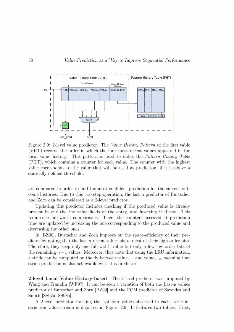
58 Value Prediction as a Way to Improve Sequential Performance
Figure 2.9: 2-level value predictor. The Value History Pattern of the first table(VHT) records the order in which the four most recent values appeared in thelocal value history. This pattern is used to index the Pattern History Table(PHT), which contains a counter for each value. The counter with the highestvalue corresponds to the value that will be used as prediction, if it is above astatically defined threshold.
are compared in order to find the most confident prediction for the current out-come histories. Due to this two-step operation, the last-n predictor of Burtscherand Zorn can be considered as a 2-level predictor.
Updating this predictor includes checking if the produced value is alreadypresent in one the the value fields of the entry, and inserting it if not. Thisrequires n full-width comparisons. Then, the counters accessed at predictiontime are updated by increasing the one corresponding to the produced value anddecreasing the other ones.
In [BZ00], Burtscher and Zorn improve on the space-efficiency of their pre-dictor by noting that the last n recent values share most of their high order bits.Therefore, they keep only one full-width value but only a few low order bits ofthe remaining n−1 values. Moreover, they note that using the LRU information,a stride can be computed on the fly between valuen−1 and valuen−2, meaning thatstride prediction is also achievable with this predictor.
2-level Local Value History-based The 2-level predictor was proposed byWang and Franklin [WF97]. It can be seen a variation of both the Last-n valuespredictor of Burtscher and Zorn [BZ99] and the FCM predictor of Sazeides andSmith [SS97a, SS98a].
A 2-level predictor tracking the last four values observed in each static in-struction value stream is depicted in Figure 2.9. It features two tables. First,

Hardware Prediction Algorithms 59
the Value History Table (VHT) contains the last four values observed in the localvalue history of each static instruction, as well as the order in which they ap-peared in the Value History Pattern (VHP). Each item of the VHP encodes oneof the four values in the VHT. For instance, if the last four values are respectively[0 1 2 3]hex, and the VHP is [00 01 00 01 11]b this means that the local valuehistory is [0 1 0 1 3]hex (from oldest to youngest).
The VHP is used to index the Pattern History Table (PHT). An entry ofthe PHT contains one counter for each value in the VHT. The counter havingthe highest value corresponds to the value in the VHT that will be used as theprediction, as long as the counter value is above a statically defined threshold.
Similarly to FCM, the 2-level predictor gives a prediction corresponding toa given local value history. However, it can only choose among the four morerecent values, as the Last-4 values predictor imagined by Lipasti and Shen [LS96].Moreover, the history is not perfectly represented as a new value may overwritean older one in the VHT. As a result, all elements of the VHP pointing to theVHT entry that contained the old value now point to the value that was justinserted. In FCM, the values stored in the first level table perfectly match thelocal value history.
Regardless, the 2-level predictor presented in [WF97] is not evaluated againstan equivalent FCM predictor. Thus, it is not clear which performs best. However,both leverage the local value history to predict, which is impractical as we willillustrate in Chapter 3.
Updating the 2-level predictor involves checking if the new value is alreadypresent in the VHT. This involves four 64-bit comparisons in [WF97]. If not,then a value is evicted using a regular replacement algorithm such as LRU. Then,the VHP is left-shifted (by two bits in [WF97]) and the new outcome is inserted.In the meantime, the counter corresponding to the new value in the PHT entryselected at prediction time is incremented by 3, and all remaining counters aredecremented by 1. Finally, note that contrarily to FCM, the values in the localhistory cannot be kept pre-hashed as they will be used as predictions. Therefore,each entry is quite big as n full-width values must be kept uncompressed.
2.1.2.3 Dynamic Dataflow-inherited Speculative Context Predictor
Finally, Thomas et al. introduce a predictor that uses predicted dataflow infor-mation to predict values: the Dynamic Dataflow-inherited Speculative Contextpredictor or DDISC [TF01]. As gDiff, DDISC relies on a backing predictor togenerate predictions for easy-to-predict instructions. This is required since forhard-to-predict instructions, DDISC makes use of an improved context consist-ing not only of the instruction PC, but of the value of its operands. Since theseoperands may become available very late in the pipeline, using their predicted
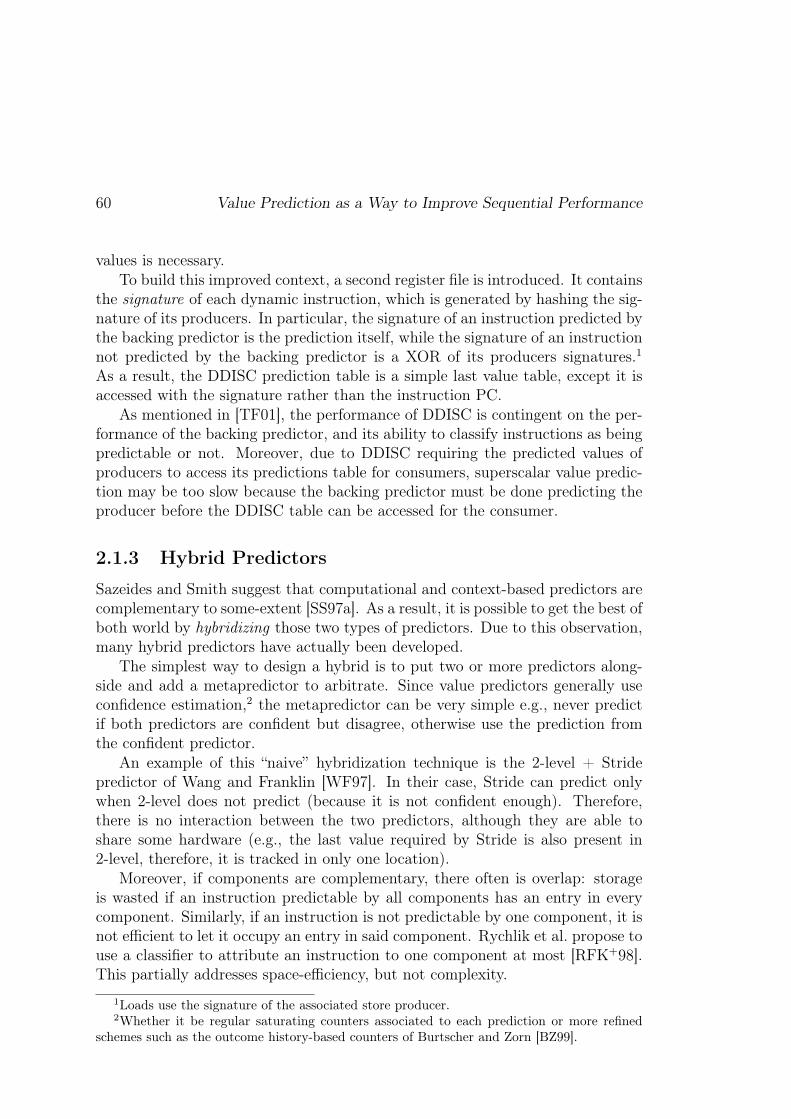
60 Value Prediction as a Way to Improve Sequential Performance
values is necessary.To build this improved context, a second register file is introduced. It contains
the signature of each dynamic instruction, which is generated by hashing the sig-nature of its producers. In particular, the signature of an instruction predicted bythe backing predictor is the prediction itself, while the signature of an instructionnot predicted by the backing predictor is a XOR of its producers signatures.1As a result, the DDISC prediction table is a simple last value table, except it isaccessed with the signature rather than the instruction PC.
As mentioned in [TF01], the performance of DDISC is contingent on the per-formance of the backing predictor, and its ability to classify instructions as beingpredictable or not. Moreover, due to DDISC requiring the predicted values ofproducers to access its predictions table for consumers, superscalar value predic-tion may be too slow because the backing predictor must be done predicting theproducer before the DDISC table can be accessed for the consumer.
2.1.3 Hybrid Predictors
Sazeides and Smith suggest that computational and context-based predictors arecomplementary to some-extent [SS97a]. As a result, it is possible to get the best ofboth world by hybridizing those two types of predictors. Due to this observation,many hybrid predictors have actually been developed.
The simplest way to design a hybrid is to put two or more predictors along-side and add a metapredictor to arbitrate. Since value predictors generally useconfidence estimation,2 the metapredictor can be very simple e.g., never predictif both predictors are confident but disagree, otherwise use the prediction fromthe confident predictor.
An example of this “naive” hybridization technique is the 2-level + Stridepredictor of Wang and Franklin [WF97]. In their case, Stride can predict onlywhen 2-level does not predict (because it is not confident enough). Therefore,there is no interaction between the two predictors, although they are able toshare some hardware (e.g., the last value required by Stride is also present in2-level, therefore, it is tracked in only one location).
Moreover, if components are complementary, there often is overlap: storageis wasted if an instruction predictable by all components has an entry in everycomponent. Similarly, if an instruction is not predictable by one component, it isnot efficient to let it occupy an entry in said component. Rychlik et al. propose touse a classifier to attribute an instruction to one component at most [RFK+98].This partially addresses space-efficiency, but not complexity.
1Loads use the signature of the associated store producer.2Whether it be regular saturating counters associated to each prediction or more refined
schemes such as the outcome history-based counters of Burtscher and Zorn [BZ99].

Speculative Window 61
As a result, more tightly-coupled predictors were proposed. In fact, many ofthe predictors that we previously mentioned can be seen as tightly-coupled hybridpredictors. For instance, D-FCM [GVDB01] is a hybrid of Stride and FCM.However, contrarily to a “naive” hybrid, it is able to predict the stride based onthe local value history, when the former can only predict a single stride for a givenstatic instruction (Stride), or a pattern of values for a given static instruction(FCM). Similarly, the Per-Path Stride (PS) predictor of Nakra et al. [NGS99]can also be seen a tightly-coupled hybrid, since it uses a computational predictor(2-delta Stride), but indexes it based on context (global branch history).
2.1.4 Register-based Value Prediction
Instead of relying on a predictor, Tullsen and Seng propose to reuse values thatare already present in registers [TS99]. They present both static and dynamicmechanisms. In the former case, the ISA has to be modified so that the pro-grammer or compiler can explicitly state that an instruction should use the valuealready present in a specific register as a prediction. In the latter case, no ISAmodifications is required as all instructions (or a subset, e.g., loads) are predictedusing this technique, depending on per-PC confidence counters. In both cases,the compiler has opportunities to alter register allocation so that register reuseis more frequent.
This form of speculation is able to capture local correlation (e.g., last-valuereuse) as well as global correlation (e.g., reuse of a register produced by a differ-ent instruction). Nonetheless, only reuse can be captured, while more advancedrelations between values (e.g., strided patterns) cannot.
Register-based value prediction is particularly interesting as no additionalstorage is required, which alleviates concerns regarding storage requirement andpower consumption in the value predictor. However, additional logic is still re-quired to handle mispredictions as well as identify instructions eligible for predic-tion in the dynamic case (e.g., comparing the produced result with the previousvalue of the architectural destination register).
2.2 Speculative Window
In most of the predictors we described, a strong requirement is that the resultof the previous instance(s) is required to generate the prediction for the currentinstance. For example, in stride-based predictors, the last value is required topredict for the next instance, and in FCM, the last n values are required.
Unfortunately, the previous instance may not have retired at prediction time,meaning that a stale value is present in the predictor entry. In fact, Lee and Yew

62 Value Prediction as a Way to Improve Sequential Performance
Figure 2.10: Prediction of two close instances of a given static instruction withFCM. In the absence of a speculative window, the local value history is not upto date for the second instance, and the prediction is most likely wrong.
found that for SPECint95 benchmarks, as much as 36% of instructions access thesame prediction table within 5 cycles, and 22% within 2 cycles [LY00]. Therefore,the predictor should be updated speculatively at prediction time, under penaltyof losing potential in workloads having many short loops. Any wrong speculativeupdate should be undone at Commit.
To better illustrate how potential can be lost, consider Figure 2.10 that showshow FCM would handle close instances of the same static instruction. In par-ticular, in the absence of a speculative window, the result of I1,iteration0 would beput in the local value history at retirement, well after I1,iteration1 would have beenfetched. To allow speculative updates, a speculative window tracking predictionsof instructions that have not retired yet must be implemented.
Unfortunately, in most studies,3 this requirement is not addressed while theabsence of a speculative window has substantial impact on performance in specificbenchmarks, as we will demonstrate in Chapter 5. In this Chapter, we will alsoprovide a realistic implementation of the speculative window. Indeed, an intuitiveway of implementing it would be to build a fully associate ROB-sized4 structurethat would be queried and updated on each prediction. However, such a structure
3The exception is gDiff where the GVQ is essentially a speculative window filled by thebacking predictor.
4192 entries in recent Intel Haswell processors.

Confidence Estimation 63
would be slow and power hungry [EA02, KL03, PJS97], especially since severalpredictions (i.e., associative search of the window, then inserting the predictionin it) can be made each cycle in superscalar processors. Therefore, a differentway to implement the speculative window is required.
Lastly, it should be noted that for stride-based predictors, only one result hasto be tracked per instruction in the speculative window. However, for predic-tors using local value histories (e.g., FCM [SS98a] and 2-level [WF97]) or localoutcome histories (e.g., Last-n with SAg confidence estimation [BZ99]), up to nvalues (respectively outcome histories) have to be tracked for each instruction,and merging the information contained in the predictor entry and the specula-tive window may be required to generate the index of the second level. As aresult, managing the speculative window should be much more complex for thosepredictors.
2.3 Confidence Estimation
As a value misprediction entails a certain cost (depending on the recovery mecha-nism), predictors are usually accompanied by a confidence estimation mechanism,to filter out uncertain predictions. As for branch predictors, 2- or 3-bit saturat-ing counters [Smi81, JRS96] can be used, with a potentially asymmetric updatepolicy. In particular, a counter is associated with each prediction, and the latteris used by the pipeline only if the counter value is saturated or above a cer-tain threshold. Said counter is updated at retire time, by incrementing it if theprediction was correct, and decrementing – or resetting – it if not.
A more refined scheme proposed independently by Burtscher and Zorn [BZ99,Bur00] and Calder et al. [CRT99] leverages the per-instruction recent outcomes(i.e., prediction success or failure) to index a table containing saturating counters.This SAg confidence estimation scheme (inspired by Yeh and Patt [YP93]) ismore accurate than a regular array of PC-indexed counters, leading to additionalspeedup in [Bur00] (from 0.1% to 2% on average). Nonetheless, it is slower dueto its 2-level nature and requires much more storage, as each predictor entry nowstores n outcome history bits to index the counter arrays, with n being 10 in[Bur00].
In Chapter 3, we will argue that regular saturating counters can be made veryefficient by having them saturate probabilistically, after many correct predictions.Therefore, very high accuracy can be achieved with very simple hardware and lowstorage overhead.
64 Value Prediction as a Way to Improve Sequential Performance
2.4 ValidationAs Value Prediction is speculative in nature, a prediction must be validatedagainst the actual result once it is known. To our knowledge, validation takesplace as soon as possible in virtually all previous studies [GM98a, GVDB01,ZFC03, RFK+98, ZYFRC00, SS98a, GM96, LS96, WF97, RFKS98, BZ99, Bur00,GM98b, GG98b, CRT99, SS97a, TS99, NGS99, LWS96, TF01, LY02, LWY00,LY01]. That is, predictions are validated as results are produced, at the out-put of the functional units. In that case, the prediction has to be read fromthe Physical Register File (PRF) along the source operands and propagated tothe functional unit (FU) when the predicted instruction is selected for execution.Lastly, a comparator must be implemented after each FU to do the validation.This comparison step may require an additional pipeline stage or be done duringWriteback.
As a result, validation at Execute also has some implications on the PRF.Indeed, it is commonly assumed that predictions and actual results co-exist in thePRF to ease the management of predictions. In particular, this removes the needto multiplex from the PRF and a buffer dedicated to predictions. However, thisimplies that predictions are written to the PRF, hence that additional write portsare available at Dispatch. Moreover, in addition to reading two operands from thePRF when it is issued, an instruction will also need to read the prediction in orderto propagate it to the FU and validate it. As a result, in the worst case, up to66% more ports are required on the PRF, assuming 1 write port and 2 read portsfor each potentially issued instruction. This is already impractical for moderate-issue processors given the increase in area and power consumption of the PRFas the number of ports increases [ZK98]. Fortunately, we will show in Chapter3 that validation can actually be delayed until Commit, greatly decreasing theadditional port pressure put by VP on the PRF.
In the case of a correct prediction, the instruction continues towards Write-back and Commit. In the case of an incorrect prediction, however, dependentinstructions may have executed with an incorrect source operand. As a result,they should be re-executed.
2.5 RecoveryContrarily to a branch misprediction, a value misprediction does not necessarilyimply that execution is on the wrong control path. As a result, recovery is moreflexible and does not require a pipeline squash. In theory, only the instructionsthat depend directly or indirectly on the value misprediction must be re-executed.The computations made by independent instructions are correct regardless of themisprediction.

Recovery 65
2.5.1 Refetch
Although not necessary, squashing the pipeline starting from the mispredictedinstruction or the oldest dependent remains the simplest way to recover. Thismechanism, known as Refetch [TS99] is similar to the mechanism used to handlebranch mispredictions.
Refetch has several drawbacks. First, it is slow: the cost of a value mispre-diction becomes similar to the cost of a branch misprediction. As a result, it canonly be used if the value predictor is very accurate. Indeed, if all instructionsproducing a register are predicted (i.e., not only loads), then the average gainof a correct prediction may be very low (e.g., one cycle if a simple addition ispredicted), while the cost of a misprediction would be very high.
Second, it may require more hardware than expected. Indeed, consider thaton a branch prediction, a checkpoint of the architectural state (e.g., register map-pings, pipeline state, etc.) must be taken to correctly restart execution should thebranch be mispredicted. Indeed, since branch resolution is done at Execute, thestate to restore on a misprediction is not the software-visible state provided bythe Commit stage. Rather, the architectural state corresponding to the branchinstruction itself should be restored, hence a checkpoint is required because thisstate might still be speculative at branch resolution time since older instructionsmight still be in flight. However, since branches may represent one out of eightor ten instructions, the number of hardware checkpoints to implement is man-ageable. Moreover, checkpoints may only be taken on low confidence branches,which are even less frequent.
Consequently, and since common wisdom suggests that resolving branches atCommit doubles the average penalty of a branch misprediction, checkpointing isworth the benefit of resolving branches at Execute instead than Commit.
We already mentioned that value predictions are validated at Execute. There-fore, recovery with pipeline squashing implies that the speculative state to restorehas been checkpointed. However, contrarily to branches, instructions eligible forVP represent the majority of the dynamic instructions. Moreover, the dynamicrange of values is much higher than that of branch outcomes, meaning that theaccuracy of the value predictor may be much lower. Consequently, an ideal imple-mentation of Refetch should provision checkpoint space for every in-flight instruc-tion, or around two hundred checkpoints if we consider a recent microarchitecturesuch as Intel Haswell.5 As a result, despite its apparent simplicity, an optimalimplementation of Refetch may not be possible for Value Prediction. In partic-ular, the number of checkpoints may be limited, leading to an increase in themisprediction penalty as instructions older than the misprediction but youngerthan the youngest correct checkpoint will be also squashed.
5There may be 192 in-flight µ-ops in Haswell.

66 Value Prediction as a Way to Improve Sequential Performance
2.5.2 Replay
An alternative to Refetch is to simply re-execute instructions, since they arealready in the pipeline because the control path is correct. This mechanism,known as Replay, can be either selective or not. As both mechanisms do notimply a pipeline squash, they are much less expensive than Refetch (in cycles).Nonetheless, their operation is not trivial and still likely to cost several cycles.
Selective Replay This first version of Replay re-executes only the instructionsthat have executed with the wrong source(s). Instructions independent on themisprediction are not replayed.
Selective replay requires the identification of all instructions directly or indi-rectly dependent on the misprediction through both register and memory depen-dencies. Since the concerned instructions necessarily have executed before theinstruction that was wrongly predicted, selective replay for VP cannot be donein the same fashion as selective replay for schedule mispredictions [KL04].
In the latter case, instructions dependent on a variable-latency instructionmay execute with wrong sources when the producer latency is higher than ex-pected. Nonetheless, since the RAW dependency is enforced in the scheduler[PSM+15, MBS07, MS01, MSBU00, MLO01], the dependents are still issued af-ter the long-latency instruction. As a result, by dedicating a pipeline stage to thevalidation of all instructions after Execute, the wrong execution of a dependentcan be identified because the unexpected longer latency of the producer is knownbefore the dependent actually executes.
In the case of Value Prediction, a dependent may have executed well beforethe producer executes. As a result, it has left the execution pipeline and onlysits in the ROB and potentially a dedicated buffer holding instructions that mayhave to be replayed. Therefore, the only way to identify that it needs to be re-played is to scan the ROB or buffer and re-dispatch instructions to the scheduleraccordingly6. Consequently, selective replay for VP is likely to take several cy-cles as an arbitrarily long dependency chain has to be identified and replayed.Moreover, it does not integrate seamlessly with the mechanism used for sched-ule mispredictions because the producer triggers the re-execution of dependents,while in the case of schedule mispeculations, each dependent determines if it cor-rectly executed or not (at least in some implementations such as Intel Pentium 4[SGC01b]).
Nonetheless, an implementation adapted to Value Prediction is provided byKim and Lipasti in [KL04]. In a nutshell, each instruction possesses a moderatelysmall bit-vector (8-16 bits) indicating if the instruction depends on a given token.
6Alternatively, instructions may retain their entry in the scheduler as long as they remaindependent on an un-resolved value prediction

Revisiting Value Prediction 67
A token belongs to an instruction that may execute incorrectly, be it a value pre-dicted instruction, or a load that woke up its dependents speculatively assuminga hit. The last key component is that instructions retain their scheduler entry aslong as they may have to be replayed. As a result, even if a dependent has issuedbefore a producer because the producer is value predicted, the producer-consumerrelation is preserved in the scheduler thanks to the bit-vector. Hence, replay isnot dependent on the issue order. If an instruction that does not have a token(all have been allocated to other instructions) is mispredicted, the scheduler isflushed and instructions are re-inserted from the ROB, guaranteeing correctness.
Non-selective Replay Conversely to the previous scheme, non-selective re-play simply has to re-dispatch all in-flight instructions that are younger than themispredicted instruction from the ROB. In particular, it is not necessary to scanthe ROB and LQ/SQ in a sequential fashion to precisely identify dependencies,only the faulting instruction has to be found. As a result, recovery latency may beon par with selective replay, although more instructions will have to be replayed,increasing contention.
2.5.3 Summary
Of the three mechanisms described in the literature, none can be implemented ina straightforward fashion. Refetch requires substantial checkpointing hardwaresince most instructions are eligible for Value Prediction. Selective replay hashigh complexity yet will still require several cycles to process the arbitrarily longdependency chain to replay. Non-selective replay has lower complexity but apotentially higher latency. Note that both flavors of replay will still be muchfaster than Refetch.
2.6 Revisiting Value PredictionGiven the salient issues existing with previous propositions (e.g., complex pre-dictors, execute-time validation, complex recovery, PRF port requirement, etc.),the reader may question the choice to reconsider Value Prediction as a means toincrease sequential performance. Nonetheless, let us consider the following:
1. Value Prediction intrinsically targets sequential performance. It does nottry to leverage multi-cores to improve sequential performance, contrarilyto certain schemes such as Helper Threading [CSK+99], Speculative Multi-threading (such as Multiscalar [Fra93]) and Slipstream [SPR00], to cite afew. Therefore, it is the author’s intuition that Value Prediction is a morenatural candidate to improve sequential performance.

68 Value Prediction as a Way to Improve Sequential Performance
2. Value Prediction is orthogonal to mechanisms usually considered to increasesequential performance, such as improved branch prediction and prefetch-ing. Moreover, we argue that it can generally be leveraged to improvesaid mechanisms as knowing the output of instructions can be of great helpe.g., address prediction for better disambiguation and cache bank prediction[YERJ], branch prediction [AGGG01, GG99], or prefetching [EV93, GG97].
3. Value Prediction has high potential: a perfect predictor can yield tremen-dous improvements up to 5X in [PS14b], especially if the cache hit ratio islow.
As a result, if one could address the implementation challenges posed byValue Prediction, additional sequential performance could be directly harvestedfrom the increased ILP. In a context where parallel performance is limited byAmdahl’s Law and many intrinsically sequential workloads remain, this additionalperformance would be more than welcome. Moreover, still assuming that a lowcost implementation can be provided, VP would improve performance withoutincreasing the size of the out-of-order window or the issue width, which contributeto sequential performance but also to overall complexity and power consumption.Better yet, it would actually allow for a better utilization of the out-of-orderengine by increasing average ILP. As a result, it may even be possible to reducethe out-of-order aggressiveness through Value Prediction. Therefore, despite theremaining challenges, there are strong arguments in favor of VP.
This thesis revisits Value Prediction in a contemporary context and tackles themain issues preventing VP from being added to a modern superscalar pipeline.More specifically, it provides an end-to-end (predictor in the frontend to validationand recovery in the backend) implementation of VP. This implementation actuallypossesses a less aggressive out-of-order engine, greatly diminishing the overallcomplexity of the pipeline.

Chapter 3
Revisiting Value Prediction in aContemporary Context
This Chapter covers a publication in the International Symposium on High Per-formance Computer Architecture (HPCA 2014) [PS14b] as well as part of a secondpublication in the same conference (HPCA 2015) [PS15a].
3.1 Introduction
Initial studies have led to moderately to highly accurate value predictors [NGS99,SS97a, WF97] while predictor accuracy has been shown to be critical due to themisprediction penalty [CRT99, ZYFRC00]. Said penalty can be as high as thecost of a branch misprediction, yet the benefit of an individual correct predictionis often very limited. As a consequence, high coverage1 is mostly irrelevant in thepresence of low accuracy.2
To that extent, we first present a simple yet efficient confidence estimationmechanism for value predictors. The Forward Probabilistic Counters (FPC)scheme yields value misprediction rates well under 1%, at the cost of reason-ably decreasing predictor coverage. All classical predictors are amenable to thislevel of accuracy. FPC is very simple to implement and does not require sub-stantial change in the confidence counters update automaton. Our experimentsshow that when FPC is used, no complex repair mechanism such as selectivereplay [KL04, TS99] is needed. Prediction validation can even be delayed untilcommit time and be done in-order: Complex and power hungry logic needed forexecution time validation is not required anymore. As a result, prediction is per-formed in the in-order pipeline front-end, validation is performed in the in-order
1Correct predictions over total number of dynamic instructions eligible for VP.2Correct predictions over total number of predictions that were used by the pipeline.
69

70 Revisiting Value Prediction in a Contemporary Context
pipeline back-end while the out-of-order execution engine is only marginally mod-ified. This is in contrast with all previous propositions relying on execution timevalidation.
Second, we introduce the Value TAGE predictor (VTAGE) and a direct im-provement, the Differential VTAGE predictor (D-VTAGE). VTAGE is derivedfrom research propositions on branch predictors [SM06] and more precisely fromthe indirect branch predictor ITTAGE. VTAGE is the first hardware value pre-dictor to leverage a long global branch history and the path history. Like all othervalue predictors, VTAGE is amenable to very high accuracy thanks to ForwardProbabilistic Counters. D-VTAGE is a tightly-coupled hybrid that resembles theDifferential Finite Context Method (D-FCM) predictor. In particular, it tracksthe difference between successive results of instances on a given path, rather thaneach distinct values. It is shown to outperform previously proposed context-basedpredictors such as Finite Context Method (FCM) [SS97a] and a naive hybrid be-tween VTAGE and a 2-delta Stride predictor [EV93].
Moreover, we point out that unlike two-level predictors (in particular, predic-tors based on local value histories such as FCM), VTAGE and D-VTAGE canseamlessly predict back-to-back occurrences of instructions, that is, instructionsinside tight loops. Practical implementations are then feasible.
3.2 Motivations
We identify two factors that will complicate the adaptation and implementationof value predictors in future processor cores. First, the misprediction recoverypenalty and/or hardware complexity. Second the need to handle back-to-backpredictions for two occurrences of the same instruction which can be very complexto implement while being required to predict instructions within tight loops.
3.2.1 Misprediction Recovery
Most of the initial studies on Value Prediction were assuming that the recov-ery on a value misprediction is immediate and induces – almost – no penalty[GM98b, LWS96, LS96, ZFC03] or simply focused on accuracy and coveragerather than actual speedup [GVDB01, NGS99, RFK+98, SS97a, TF01, WF97].The latter studies were essentially ignoring the performance loss associated withmisprediction recovery. Moreover, despite quite high coverage and reasonableaccuracy, one observation that can be made from these early studies is that theaverage performance gain per correct prediction is rather small.
Furthermore, Zhou et al. observed that to maximize the interest of VP, thetotal cost of recoveries should be as low as possible [ZYFRC00]. To limit this

Motivations 71
total cost, one can leverage two factors: The average misprediction penalty Pvalue
and the absolute number of mispredictions Nmisp. A very simple modelization ofthe total misprediction penalty is Trecov = Pvalue ∗Nmisp.
3.2.1.1 Value Misprediction Scenarios
Two mechanisms already implemented in processors can be adapted to managevalue misprediction recovery: Pipeline squashing and selective replay. They in-duce very different average misprediction penalties, but are also very differentfrom a hardware complexity standpoint, as we illustrated in 2.5.
Pipeline squashing is already implemented to recover from branch mispredic-tions. On a branch misprediction, all the subsequent instructions in the pipelineare flushed and instruction fetch is resumed at the branch target. This mechanismis also generally used on load/store dependency mispredictions [BBB+11, CE98].Using pipeline squashing on a value misprediction is straightforward, but costly asthe minimum misprediction penalty is the same as the minimum branch mispre-diction penalty. However, to limit the number of squashes due to VP, squashingcan be avoided if the predicted result has not been used yet, that is, if no depen-dent instruction has been issued.
Selective replay is implemented in processors to recover in case where instruc-tions have been executed with incorrect operands, in particular this is used to re-cover from L1 cache hit/miss mispredictions [PSM+15, MBS07, MS01, MSBU00,SGC01b, MLO01, KL04] (i.e., load-dependent instructions are issued after pre-dicting a L1 hit, but finally the load results in a L1 miss). When the executionof an instruction with an incorrect operand is detected, the instruction as well asall its dependent chain of instructions are canceled then replayed.
Validation at Execution Time vs. Validation at Commit Time On theone hand, selective replay must be implemented at execution time in order tolimit the misprediction penalty. On the other hand, pipeline squashing can beimplemented either at execution time or at commit time. Pipeline squashingat execution time results in a minimum misprediction penalty similar to thebranch misprediction penalty. However, validating predictions at execution timenecessitates to redesign the complete out-of-order engine: The predicted valuesmust be propagated through all the out-of-order execution engine stages and thepredicted results must be validated as soon as they are produced in this out-of-order execution engine. Moreover, the repair mechanism must be able to restoreprocessor state for any predicted instruction. Lastly, prediction checking mustalso be implemented in the commit stage(s) since predictors have to be trainedeven when predictions were not used due to low confidence.
On the contrary, pipeline squashing at Commit results in a quite high average
72 Revisiting Value Prediction in a Contemporary Context
misprediction penalty since it can delay prediction validation by a substantialnumber of cycles. Yet, it is much easier to implement for Value Prediction sinceit does not induce complex mechanisms in the out-of-order execution engine. Itessentially restrains the Value Prediction related hardware to the in-order pipelinefront-end (prediction) and the in-order pipeline back-end (validation and train-ing). Moreover, it allows not to checkpoint the rename table since the committedrename map contains all the necessary mappings to restart execution in a correctfashion.
A Simple Synthetic Example Realistic estimations of the average mispre-diction penalty Pvalue could be 5-7 cycles for selective replay,3 20-30 cycles forpipeline squashing at execution time and 40-50 cycles for pipeline squashing atCommit.
For the sake of simplicity, we will respectively use 5, 20 and 40 cycles in thesmall example that follows. We assume an average benefit of 0.3 cycles per cor-rectly predicted value (taking into account the number of unused predictions).With predictors achieving around 40% coverage and around 95% accuracy asoften reported in the literature, 50% of predictions used before execution, theperformance benefit when using selective replay would be around 64 cycles perKinstructions, a loss of around 86 cycles when using pipeline squashing at ex-ecution time and a loss of around 286 cycles when using pipeline squashing atcommit time.
Our experiments in Section 3.7 confirm that when a value predictor exhibits afew percent misprediction rate on an application, it can induce significant perfor-mance loss when using pipeline squashing at Commit. Therefore, such a predictorshould rather be used in conjunction with selective replay.
3.2.1.2 Balancing Accuracy and Coverage
The total misprediction penalty Trecov is roughly proportional to the number ofmispredictions. Thus, if one drastically improves the accuracy at the cost of somecoverage then, as long as the coverage of the predictor remains quite high, theremight be a performance benefit brought by Value Prediction, even though theaverage value misprediction penalty is very high.
Using the same example as above, but sacrificing 25% of the coverage (nowonly 30%), and assuming 99.75% accuracy, the performance benefit would bearound 88 cycles per Kinstructions cycles when using selective replay, 83 cycles
3Including tracking and canceling the complete chain of dependent instructions as well as theindirect sources of performance loss encountered such as resource contention due to reexecution,higher misprediction rate (e.g. a value predicted using wrong speculative value history) andlower prediction coverage

Motivations 73
when using pipeline squashing at execution time and 76 cycles when using pipelinesquashing at commit time.
In Section 3.7, we will show that the ranges of accuracy and coverage allowedby our FPC proposition are in the range of those used in this small example. Asa consequence, it is not surprising that our experiments confirm that, using FPC,pipeline squashing at commit time achieves performance in the same range as anidealistic 0-cycle selective replay implementation.
3.2.2 Back-to-back Prediction
Figure 3.1: Prediction flow and critical paths for different value predictors whentwo occurrences of an instruction are fetched in two consecutive cycles.
Unlike a branch prediction, a value prediction is needed rather late in thepipeline (at dispatch time). Thus, at first glance, prediction latency does notseem to be a concern and long lookups in large tables and/or fairly complex com-putations could be tolerated. However, for most predictors, the outcomes of afew previous occurrences of the instruction are needed to perform a predictionfor the current occurrence. Consequently, for those predictors, either the crit-ical operation must be made short enough to allow for the prediction of close(possibly back-to-back) occurrences (e.g. by using small tables) or the predictionof tight loops must be given up. Unfortunately, tight loops with candidates forVP are quite abundant in existing programs. Experiments conducted with the

74 Revisiting Value Prediction in a Contemporary Context
methodology we will introduce in Section 3.6 suggest that for a subset of theSPEC’00/’06 benchmark suites, fetched instructions eligible for VP for which theprevious occurrence was fetched in the previous cycle (8-wide Fetch) represent upto 38.8% (4.4% a-mean) of the fetched instructions. We highlight such criticaloperations for each predictor in the subsequent paragraphs.
3.2.2.1 LVP
Despite its name, LVP does not require the previous prediction to predict thecurrent instance as long as the table is trained. Consequently, LVP uses onlythe program counter to generate a prediction. Thus, successive table lookupsare independent and can last until Dispatch, meaning that large tables can beimplemented. The top part of Fig. 3.1 describes such behavior. Similarly, thepredictor we introduce in Section 3.5, VTAGE, only uses control-flow informa-tion to predict, allowing it to seamlessly predict back-to-back occurrences. Thesame goes for the gDiff predictor itself [ZFC03] although a critical path may beintroduced by the predictor providing speculative values for the global history.
3.2.2.2 Stride
Prediction involves using the result of the previous occurrence of the instruction.Thus, tracking the result of only the last speculative occurrence of the instructionis sufficient.
The Stride value predictor acts in two pipeline steps: 1) retrieval of the strideand the last value 2) computation of the sum. The first step induces a difficultywhen the last occurrence of the instruction has not committed or is not evenexecuted. One has to track the last occurrence in the pipeline and use the spec-ulative value predicted for this occurrence. This tracking can span over severalcycles. The critical operation is introduced by the need to bypass the result of thesecond step directly to the adder in case of fetching the same instruction in twoconsecutive cycles (e.g. in a very tight loop), as illustrated by the central part ofFigure 3.1. The D-VTAGE predictor that we introduce in Section 3.5 possessesthe same critical path. Regardless, a stride-based value predictor supporting theprediction of two consecutive occurrences of the same instruction one cycle apartcould reasonably be implemented since the second pipeline step is quite simple.In other words, since back-to-back additions can be done in the execution units,stride-based predictors should be able to handle back-to-back occurrences.
3.2.2.3 Finite Context Method
The local value history predictor (nth-order FCM) is a two-level structure. Thefirst-level consists of a value history table accessed using the instruction address.

Motivations 75
This history is then hashed and used to index the second level table.As for the Stride value predictor, a difficulty arises when several occurrences
of the same instruction are fetched in a very short interval since the predictor isindexed through a hash of the last n values produced by the instruction. In manycases, the previous occurrences of the instruction have not been committed, oreven executed. The logic will be more complex than for the Stride predictor sinceone has to track the last n values instead of a single one.
However, the critical delay is on the second step. To predict consecutiveoccurrences of an instruction, the delay between the accesses to the second leveltable for the two occurrences is likely to be much shorter than the delay forcomputing the hash, reading the value table and then forward the predicted valueto the second index hash/computation, as illustrated by the bottom part of Figure3.1. This implies that FCMmust either use very small tables to reduce access timeor give up predicting tight loops altogether. Note that D-FCM [GVDB01], Last-n[BZ99] with SAg confidence estimation,4 2-level [WF97] and DDISC [TF01] alsorequire two successive lookups. Consequently, these observations also stand forthose predictors.
In summary, a hardware implementation of a local history value predictorwould be very complex since 1) it involves tracking the n last speculative occur-rences of each fetched instruction 2) the predictor cannot predict instructions insuccessive iterations of a loop body if the body is fetched in a delay shorter thanthe delay for retrieving the prediction and forwarding it to the second level indexcomputation step.
3.2.2.4 Summary
Table lookup time is not an issue as long as the prediction arrives before Dis-patch for LVP and Stride. Therefore, large predictor tables can be considered forimplementation. For stride-based value predictor, the main difficulty is that onehas to track the last (possibly speculative) occurrence of each instruction.
For local value history-based predictors the same difficulty arises with theaddition of tracking the n last occurrences. Moreover the critical operations (hashand the 2nd level table read) lead to either using small tables or not being able totimely predict back-to-back occurrences of the same instruction. Implementingsuch predictors can only be justified if they bring significant performance benefitover alternative predictors.
The VTAGE predictor we introduce in this work is able to seamlessly pre-dict back-to-back occurrences of the same instruction, thus its access can spanover several cycles. VTAGE does not require any complex tracking of the last
4Due to the need to update the outcome history speculatively for the next access, dependingon the values of the n counters.

76 Revisiting Value Prediction in a Contemporary Context
occurrences of the instruction. Conversely, D-VTAGE requires to track the lastinstance due to its stride-based nature. We provide an actual mechanism to do soin Chapter 5, where we focus on a practical implementation of the value predictoritself.
3.3 Commit Time Validation and Hardware Im-plications on the Out-of-Order Engine
In the previous Section, we have pointed out that the hardware modificationsinduced by pipeline squashing at commit time on the Out-of-Order engine arelimited. In practice, the only major modification compared to a processor withoutValue Prediction is that the predicted values must be written in physical registersat Dispatch.
At first glance, if every destination register has to be predicted for each fetchgroup, one would conclude that the number of write ports should double. Inthat case the overhead on the register file would be quite high. The area cost ofa register file is approximately proportional to (R +W ) ∗ (R + 2W ), R and Wrespectively being the number of read ports and the number of write ports [ZK98].Assuming R = 2W , the area cost without VP would be proportional to 12W 2
and the one with VP would be proportional to 24W 2, i.e. the double. Energyconsumed in the register file would also be increased by around 50% (using verysimple Cacti 5.3 [TMJHJ08] approximations).
For practical implementations, there exist several opportunities to limit thisoverhead. For instance one can limit the number of extra ports needed to writepredictions. Each cycle, only a few predictions are used and the predictions canbe known several cycles before Dispatch: One could limit the number of writeson each cycle to a certain limit, and buffer the extra writes, if there are any. As-suming only W
2write ports for writing predicted values leads to a register file area
of 35W 2
2, saving half of the overhead of the naive solution. The same savings are
observed for energy consumption (Cacti 5.3 estimations). Another opportunity isto allocate physical registers for consecutive instructions in different register filebanks, limiting the number of write ports on the individual banks. One can alsoprioritize the predictions according to the criticality of the instruction and onlyuse the most critical one, leveraging the work on criticality estimation of Fieldset al. [FRB01], Tune et al. [TTC02] as well as Calder et al. [CRT99].
Exploring the complete optimization set available to reduce the overhead onthe register file design is out of the scope of this Chapter. It would depend on theprecise micro-architecture of the processor, but we have clearly shown that thisoverhead in terms of energy and silicon area can be reduced to less than 25% and50% respectively. Moreover, this overhead is restricted to the register file and does

Maximizing Value Predictor Accuracy Through Confidence 77
not impact the other components of the out-of-order engine. Similarly, thanks tocommit time validation, the power overhead introduced by Value Prediction willessentially reside in the predictor table.
3.4 Maximizing Value Predictor Accuracy ThroughConfidence
As we already pointed out, the total misprediction recovery cost can be minimizedthrough two vehicles: Minimizing the individual misprediction penalty and/orminimizing the total number of mispredictions.
When using the prediction is not mandatory (i.e., contrarily to branch pre-diction), an efficient way to minimize the number of mispredictions is to usesaturating counters to estimate confidence and use the prediction only when theassociated confidence is very high. For instance, for the value predictors consid-ered in this study, a saturating 3-bit confidence counter per entry that is reseton each misprediction leads to an accuracy in the 95-99% range if the predic-tion is used only when the counter is saturated. However this level of accuracyis still not sufficient to avoid performance loss in several cases unless idealisticselective replay is used. To increase accuracy, Burtscher et al. proposed the SAgconfidence estimation scheme to assign confidence to a history of outcomes ratherthan to a particular instruction [BZ99]. However, this entails a second lookupin the counter table using the outcome history retrieved in the predictor tablewith the PC of the instruction. A way to maximize accuracy without increasingcomplexity and latency would be preferable.
We actually found that simply using wider counters (e.g., 6 or 7 bits) leadsto much more accurate predictors while the prediction coverage is only reducedslightly. Prediction is only used on saturated confidence counters and countersare reset on each misprediction. Interestingly, probabilistic 3-bit counters such asdefined by Riley et al. [RZ06] augmented with reset on misprediction achieve thesame accuracy for substantially less storage and a marginal increase in complexity.
We refer to these probabilistic counters as Forward Probabilistic Counters(FPC). In particular, each forward transition is only triggered with a certainprobability. In this work, we will consider 3-bit confidence counters using aprobability vector v = {1, 1
16, 116, 116, 116, 132, 132} for pipeline squashing at Commit
and v = {1, 18, 18, 18, 18, 116, 116} for selective replay, respectively mimicking 7-bit and
6-bit counters. This generally prevents all the considered VP schemes to slowdown execution while minimizing the loss of coverage (as opposed to using lowerprobabilities). The used pseudo-random generator is a simple Linear FeedbackShift Register.
Using FPC counters instead of full counters limits the overhead of confidence

78 Revisiting Value Prediction in a Contemporary Context
estimation. It also opens the opportunity to adapt the probabilities at run-timeas suggested in [Sez11c] and/or to individualize these probabilities depending onthe criticality of the instructions.
Figure 3.2: (1+N)-component VTAGE predictor. Val is the prediction, c is thehysteresis counter acting as confidence counter, u is the useful bit used by thereplacement policy.
3.5 Using TAgged GEometric Predictors to Pre-dict Values
3.5.1 The Value TAgged GEometric Predictor
Branch predictors exploiting correlations inside the global branch history havebeen shown to be efficient. Among these global history branch predictors, TAGE[SM06] is generally considered state-of-the-art. An indirect branch predictor IT-TAGE [SM06] has been directly derived from TAGE. Since targets of indirectbranches are register values, we have explored the possibility of adapting ITTAGEto Value Prediction. We refer to this modified ITTAGE as the Value TAgged GE-ometric history length predictor, VTAGE. To our knowledge, VTAGE is the firsthardware value predictor to make extensive use of recent and less recent control-flow history. In particular, PS [NGS99] only uses a few bits of the global branch
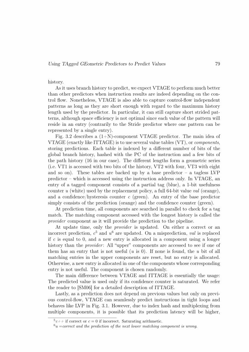
Using TAgged GEometric Predictors to Predict Values 79
history.As it uses branch history to predict, we expect VTAGE to perform much better
than other predictors when instruction results are indeed depending on the con-trol flow. Nonetheless, VTAGE is also able to capture control-flow independentpatterns as long as they are short enough with regard to the maximum historylength used by the predictor. In particular, it can still capture short strided pat-terns, although space efficiency is not optimal since each value of the pattern willreside in an entry (contrarily to the Stride predictor where one pattern can berepresented by a single entry).
Fig. 3.2 describes a (1+N)-component VTAGE predictor. The main idea ofVTAGE (exactly like ITTAGE) is to use several value tables (VT), or components,storing predictions. Each table is indexed by a different number of bits of theglobal branch history, hashed with the PC of the instruction and a few bits ofthe path history (16 in our case). The different lengths form a geometric series(i.e. VT1 is accessed with two bits of the history, VT2 with four, VT3 with eightand so on). These tables are backed up by a base predictor – a tagless LVPpredictor – which is accessed using the instruction address only. In VTAGE, anentry of a tagged component consists of a partial tag (blue), a 1-bit usefulnesscounter u (white) used by the replacement policy, a full 64-bit value val (orange),and a confidence/hysteresis counter c (green). An entry of the base predictorsimply consists of the prediction (orange) and the confidence counter (green).
At prediction time, all components are searched in parallel to check for a tagmatch. The matching component accessed with the longest history is called theprovider component as it will provide the prediction to the pipeline.
At update time, only the provider is updated. On either a correct or anincorrect prediction, c5 and u6 are updated. On a misprediction, val is replacedif c is equal to 0, and a new entry is allocated in a component using a longerhistory than the provider : All “upper” components are accessed to see if one ofthem has an entry that is not useful (u is 0). If none is found, the u bit of allmatching entries in the upper components are reset, but no entry is allocated.Otherwise, a new entry is allocated in one of the components whose correspondingentry is not useful. The component is chosen randomly.
The main difference between VTAGE and ITTAGE is essentially the usage:The predicted value is used only if its confidence counter is saturated. We referthe reader to [SM06] for a detailed description of ITTAGE.
Lastly, as a prediction does not depend on previous values but only on previ-ous control-flow, VTAGE can seamlessly predict instructions in tight loops andbehaves like LVP in Fig. 3.1. However, due to index hash and multiplexing frommultiple components, it is possible that its prediction latency will be higher,
5c++ if correct or c = 0 if incorrect. Saturating arithmetic.6u =correct and the prediction of the next lower matching component is wrong.
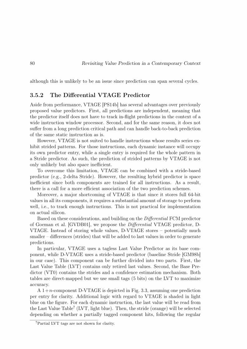
80 Revisiting Value Prediction in a Contemporary Context
although this is unlikely to be an issue since prediction can span several cycles.
3.5.2 The Differential VTAGE Predictor
Aside from performance, VTAGE [PS14b] has several advantages over previouslyproposed value predictors. First, all predictions are independent, meaning thatthe predictor itself does not have to track in-flight predictions in the context of awide instruction window processor. Second, and for the same reason, it does notsuffer from a long prediction critical path and can handle back-to-back predictionof the same static instruction as is.
However, VTAGE is not suited to handle instructions whose results series ex-hibit strided patterns. For those instructions, each dynamic instance will occupyits own predictor entry, while a single entry is required for the whole pattern ina Stride predictor. As such, the prediction of strided patterns by VTAGE is notonly unlikely but also space inefficient.
To overcome this limitation, VTAGE can be combined with a stride-basedpredictor (e.g., 2-delta Stride). However, the resulting hybrid predictor is spaceinefficient since both components are trained for all instructions. As a result,there is a call for a more efficient association of the two prediction schemes.
Moreover, a major shortcoming of VTAGE is that since it stores full 64-bitvalues in all its components, it requires a substantial amount of storage to performwell, i.e., to track enough instructions. This is not practical for implementationon actual silicon.
Based on these considerations, and building on the Differential FCM predictorof Goeman et al. [GVDB01], we propose the Differential VTAGE predictor, D-VTAGE. Instead of storing whole values, D-VTAGE stores – potentially muchsmaller – differences (strides) that will be added to last values in order to generatepredictions.
In particular, VTAGE uses a tagless Last Value Predictor as its base com-ponent, while D-VTAGE uses a stride-based predictor (baseline Stride [GM98b]in our case). This component can be further divided into two parts. First, theLast Value Table (LVT) contains only retired last values. Second, the Base Pre-dictor (VT0) contains the strides and a confidence estimation mechanism. Bothtables are direct-mapped but we use small tags (5 bits) on the LVT to maximizeaccuracy.
A 1+n-component D-VTAGE is depicted in Fig. 3.3, assuming one predictionper entry for clarity. Additional logic with regard to VTAGE is shaded in lightblue on the figure. For each dynamic instruction, the last value will be read fromthe Last Value Table7 (LVT, light blue). Then, the stride (orange) will be selecteddepending on whether a partially tagged component hits, following the regular
7Partial LVT tags are not shown for clarity.

Evaluation Methodology 81
Figure 3.3: 1 + n-component Differential Value TAGE predictor.
VTAGE operation [PS14b, SM06]. If the same instruction is fetched twice in twoconsecutive cycles, the prediction for the first one is bypassed to the input of theadders to be used as the last values for the second instance.
If the same instruction block is fetched twice in a single cycle, both instancescan be predicted by using 3-input adders (not shown in Fig. 3.3).
The advantages of D-VTAGE are twofold. First, it is able to predict control-flow dependent patterns, strided patterns and control-flow dependent strided pat-terns. Second, it has been shown that short strides could capture most of thecoverage of full strides in a stride-based value predictor [GVDB01]. As such usingD-VTAGE instead of VTAGE would allow to greatly reduce storage requirements.
3.6 Evaluation Methodology
3.6.1 Value Predictors
3.6.1.1 Single Scheme Predictors
We study the behavior of several distinct value predictors in addition to VTAGEand D-VTAGE. Namely, LVP [LS96], the 2-delta Stride predictor (2D-Stride)
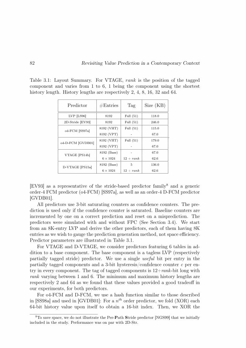
82 Revisiting Value Prediction in a Contemporary Context
Table 3.1: Layout Summary. For VTAGE, rank is the position of the taggedcomponent and varies from 1 to 6, 1 being the component using the shortesthistory length. History lengths are respectively 2, 4, 8, 16, 32 and 64.
Predictor #Entries Tag Size (KB)
LVP [LS96] 8192 Full (51) 118.0
2D-Stride [EV93] 8192 Full (51) 246.0
o4-FCM [SS97a]8192 (VHT) Full (51) 115.0
8192 (VPT) - 67.0
o4-D-FCM [GVDB01]8192 (VHT) Full (51) 179.0
8192 (VPT) - 67.0
VTAGE [PS14b]8192 (Base) - 67.0
6× 1024 12 + rank 62.6
D-VTAGE [PS15a]8192 (Base) 5 136.0
6× 1024 12 + rank 62.6
.
[EV93] as a representative of the stride-based predictor family8 and a genericorder-4 FCM predictor (o4-FCM) [SS97a], as well as an order-4 D-FCM predictor[GVDB01].
All predictors use 3-bit saturating counters as confidence counters. The pre-diction is used only if the confidence counter is saturated. Baseline counters areincremented by one on a correct prediction and reset on a misprediction. Thepredictors were simulated with and without FPC (See Section 3.4). We startfrom an 8K-entry LVP and derive the other predictors, each of them having 8Kentries as we wish to gauge the prediction generation method, not space efficiency.Predictor parameters are illustrated in Table 3.1.
For VTAGE and D-VTAGE, we consider predictors featuring 6 tables in ad-dition to a base component. The base component is a tagless LVP (respectivelypartially tagged stride) predictor. We use a single useful bit per entry in thepartially tagged components and a 3-bit hysteresis/confidence counter c per en-try in every component. The tag of tagged components is 12+rank -bit long withrank varying between 1 and 6. The minimum and maximum history lengths arerespectively 2 and 64 as we found that these values provided a good tradeoff inour experiments, for both predictors.
For o4-FCM and D-FCM, we use a hash function similar to those describedin [SS98a] and used in [GVDB01]: For a nth order predictor, we fold (XOR) each64-bit history value upon itself to obtain a 16-bit index. Then, we XOR the
8To save space, we do not illustrate the Per-Path Stride predictor [NGS99] that we initiallyincluded in the study. Performance was on par with 2D-Str.
Evaluation Methodology 83
most recent one with the second most recent one left-shifted by one bit, and soon. Even if it goes against the spirit of FCM, we XOR the resulting index withthe PC in order to break conflicts as we found that too many instructions wereinterfering with each other in the VPT.
We consider that all predictors are able to predict instantaneously. As aconsequence, they can seamlessly deliver their prediction before Dispatch. Thisalso implies that o4-FCM and o4-D-FCM are – unrealistically – able to deliverpredictions for two occurrences of the same instruction fetched in two consecutivecycles. Hence, their performance is most likely to be overestimated.
3.6.1.2 Hybrid Predictors
We also report numbers for a simple combination of VTAGE/2D-Str and o4-FCM/2D-Str, using the predictors described in Table 3.1. To select the prediction,we use a very simple mechanism: If only one component predicts (i.e., has highconfidence), its prediction is naturally selected. When both predictors predictand if they do not agree, no prediction is made. If they agree, the predictionproceeds. Our hybrids also use the prediction of a component as the speculativelast occurrence used by the other component to issue a prediction (i.e., use thelast prediction of VTAGE as the next last value for 2D-Stride if VTAGE is moreconfident). When a given instruction retires, all components are updated withthe committed value. To obtain better space efficiency, one can use a dynamicselection scheme such as the one Rychlik et al. propose. They assign a predictionto one component at most [RFK+98].
For the sake of clarity, we do not study gDiff [ZFC03] and DDISC [TF01] butwe point out that they can be added on top of any other predictor. In particular,D-VTAGE, which, contrarily to FCM or any hybrid featuring FCM, would befeasible.
3.6.2 Simulator
In our experiments, we use a modified9 version of the gem5 cycle-accurate simu-lator [BBB+11]. Unfortunately, contrarily to modern x86 implementations, gem5does not support move elimination [FRPL05, JRB+98, PSR05], µ-op fusion[GRA+03a] and does not implement a stack-engine [GRA+03a]. Hence, its base-line IPC may be lower than what can commonly be observed on modern proces-sors.
9Our modifications mostly lie with the ISA implementation. In particular, we implementedbranches with a single µ-op instead of three and we removed some false dependencies existingbetween instructions due to the way flags are renamed/written.
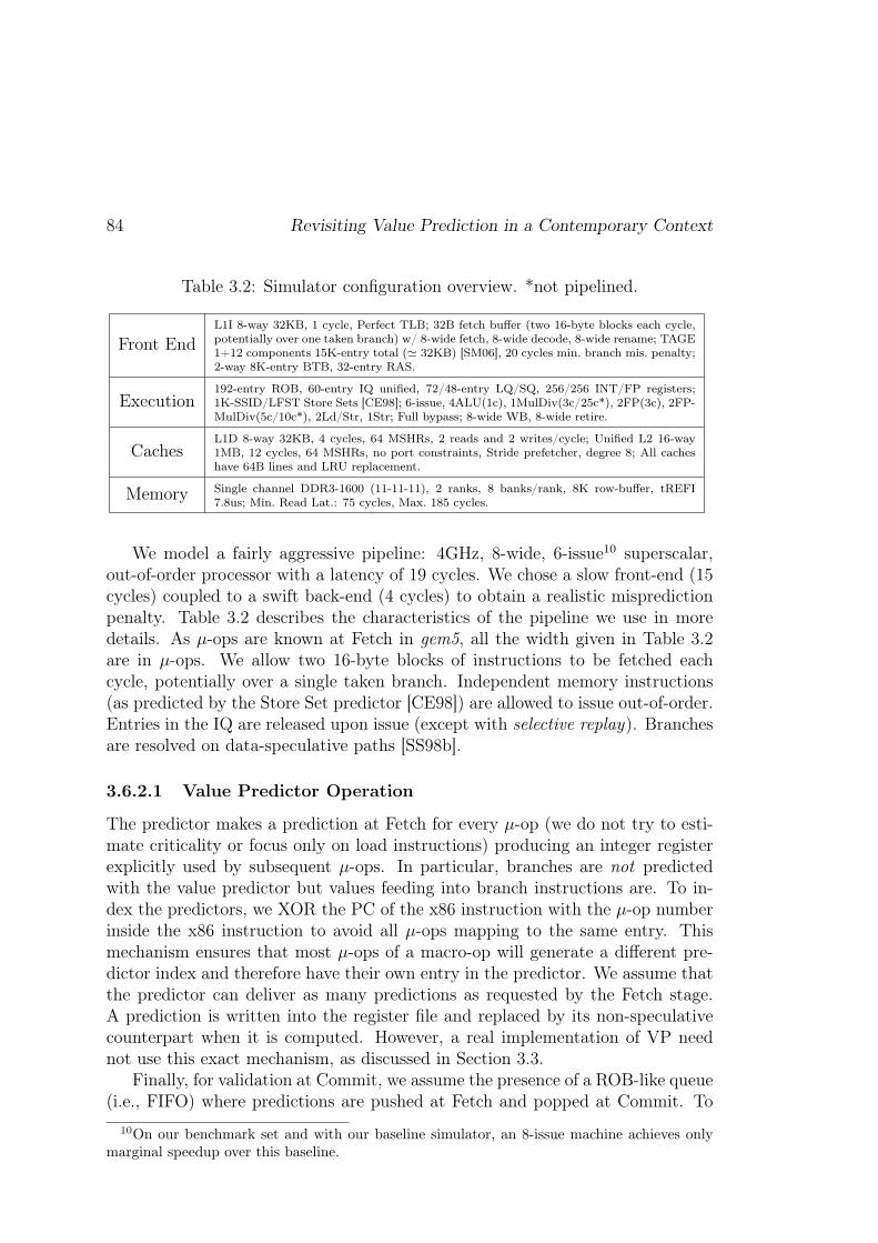
84 Revisiting Value Prediction in a Contemporary Context
Table 3.2: Simulator configuration overview. *not pipelined.
Front EndL1I 8-way 32KB, 1 cycle, Perfect TLB; 32B fetch buffer (two 16-byte blocks each cycle,potentially over one taken branch) w/ 8-wide fetch, 8-wide decode, 8-wide rename; TAGE1+12 components 15K-entry total (' 32KB) [SM06], 20 cycles min. branch mis. penalty;2-way 8K-entry BTB, 32-entry RAS.
Execution192-entry ROB, 60-entry IQ unified, 72/48-entry LQ/SQ, 256/256 INT/FP registers;1K-SSID/LFST Store Sets [CE98]; 6-issue, 4ALU(1c), 1MulDiv(3c/25c*), 2FP(3c), 2FP-MulDiv(5c/10c*), 2Ld/Str, 1Str; Full bypass; 8-wide WB, 8-wide retire.
CachesL1D 8-way 32KB, 4 cycles, 64 MSHRs, 2 reads and 2 writes/cycle; Unified L2 16-way1MB, 12 cycles, 64 MSHRs, no port constraints, Stride prefetcher, degree 8; All cacheshave 64B lines and LRU replacement.
Memory Single channel DDR3-1600 (11-11-11), 2 ranks, 8 banks/rank, 8K row-buffer, tREFI7.8us; Min. Read Lat.: 75 cycles, Max. 185 cycles.
We model a fairly aggressive pipeline: 4GHz, 8-wide, 6-issue10 superscalar,out-of-order processor with a latency of 19 cycles. We chose a slow front-end (15cycles) coupled to a swift back-end (4 cycles) to obtain a realistic mispredictionpenalty. Table 3.2 describes the characteristics of the pipeline we use in moredetails. As µ-ops are known at Fetch in gem5, all the width given in Table 3.2are in µ-ops. We allow two 16-byte blocks of instructions to be fetched eachcycle, potentially over a single taken branch. Independent memory instructions(as predicted by the Store Set predictor [CE98]) are allowed to issue out-of-order.Entries in the IQ are released upon issue (except with selective replay). Branchesare resolved on data-speculative paths [SS98b].
3.6.2.1 Value Predictor Operation
The predictor makes a prediction at Fetch for every µ-op (we do not try to esti-mate criticality or focus only on load instructions) producing an integer registerexplicitly used by subsequent µ-ops. In particular, branches are not predictedwith the value predictor but values feeding into branch instructions are. To in-dex the predictors, we XOR the PC of the x86 instruction with the µ-op numberinside the x86 instruction to avoid all µ-ops mapping to the same entry. Thismechanism ensures that most µ-ops of a macro-op will generate a different pre-dictor index and therefore have their own entry in the predictor. We assume thatthe predictor can deliver as many predictions as requested by the Fetch stage.A prediction is written into the register file and replaced by its non-speculativecounterpart when it is computed. However, a real implementation of VP neednot use this exact mechanism, as discussed in Section 3.3.
Finally, for validation at Commit, we assume the presence of a ROB-like queue(i.e., FIFO) where predictions are pushed at Fetch and popped at Commit. To
10On our benchmark set and with our baseline simulator, an 8-issue machine achieves onlymarginal speedup over this baseline.

Evaluation Methodology 85
validate, the actual result is read from the PRF and the prediction from the headof the queue. Note that all predictions are pushed in the queue, even if theyare not used by the execution engine. This is required to train the predictorby determining if the prediction was correct at validation time, and update theassociated confidence counter accordingly.
x86 Flags In the x86_64 ISA, some instructions write flags based on theirresults while some need them to execute (e.g., branches) [Int12]. Therefore, theflags should generally be predicted along the values to avoid stalling dependents.This is particularly true for the Late Execution hardware that we will present inthe next Chapter. Therefore, we assume that flags are computed as the last step ofValue Prediction, based on the predicted value. In particular, the Zero Flag (ZF),Sign Flag (SF) and Parity Flag (PF) can easily be inferred from the predictedresult. Remaining flags – Carry Flag (CF), Adjust Flag (AF) and Overflow Flag(OF) – depend on the operands and cannot be inferred from the predicted resultonly. We found that always setting the Overflow Flag to 0 did not cause manymispredictions and that setting CF if SF was set was a reasonable approximation.The Adjust Flag, however, cannot be set to 0 or 1 in the general case. This is amajor impediment to the value predictor coverage since we consider a predictionas incorrect if a single one of the derived flags – thus the flag register – is wrong.Fortunately, x86_64 forbids the use of decimal arithmetic instructions. As such,AF is not used and we can simply ignore its correctness when checking for amisprediction [Int12].
Free Load Immediate Prediction Our implementation of Value Predictionfeatures write ports available at dispatch time to write predictions to the PRF.Thus, it is not necessary to predict load immediate instructions11 since their actualresult is available in the front-end. The predictor need not be trained for theseinstructions, and they need not be validated or even dispatched to the IQ. Theirresult simply has to be written to the PRF as if it were a value prediction. Dueto this optimization, the addition of a specific table that would only predict smallconstants [SA02] may become much less interesting.
3.6.2.2 Misprediction Recovery
We illustrate two possible recovery scenarios, squashing at commit time and veryidealistic selective replay. In both scenarios, recovery is unnecessary if the pre-diction of instruction I was wrong but no dependent instruction has been issuedbefore the execution of I, since the prediction is replaced by the effective result atexecution time. This removes useless squashes and is part of our implementation.
11With the exception of load immediate instructions that write to a partial register [Int12].

86 Revisiting Value Prediction in a Contemporary Context
For selective replay, we assume an idealistic mechanism where recovery isimmediate. All value-speculatively issued instructions stay in the IQ until theybecome non speculative (causing more pressure on the IQ). When a value mispre-diction is found, the IQ and LSQ are searched for dependents to reissue. Readyinstructions can be rescheduled in the same cycle with respect to the issue width.
Yet, even such an idealistic implementation of selective replay does not onlyoffer performance advantages. In particular, it can only inhibit an entry respon-sible for a wrong prediction at update time. Consequently, in the case of tightloops, several occurrences of the same instruction can be in-flight, and a mispre-diction for the first occurrence will often result in mispredictions for subsequentoccurrences, causing multiple replays until the first misprediction retires.
In any case, the 0-cycle replay mechanism is overly optimistic because of thenumerous and complex steps selective replay implies. Our experiments should beconsidered as the illustration that even a perfect mechanism would not signifi-cantly improve performance compared to squashing at commit time as long asthe predictor is very accurate.
3.6.3 Benchmark Suite
We use a subset of the the SPEC’00 [Staa] and SPEC’06 [Stab] suites to evaluateour contributions as we focus on single-thread performance. Specifically, we use18 integer benchmarks and 18 floating-point programs.12 Table 3.3 summarizesthe benchmarks we use as well as their input, which are part of the referenceinputs provided in the SPEC software packages. To get relevant numbers, weidentify a region of interest in the benchmark using Simpoint 3.2 [PHC03]. Wesimulate the resulting slice in two steps: 1) Warm up all structures (caches,branch predictor and value predictor) for 50M instructions, then collect statistics(speedup, coverage, accuracy) for 100M instructions.
3.7 Simulation Results
3.7.1 General Trends
3.7.1.1 Forward Probabilistic Counters
Fig. 3.4 illustrates speedup over baseline using squashing at Commit to repaira misprediction. First, Fig. 3.4 (a) suggests that the simple 3-bit counter confi-dence estimation is not sufficient. Accuracy is generally comprised between 0.94and almost 1.0, yet fairly important slowdowns can be observed. Much better
12We do not use the whole suites due to some currently missing system calls and x87 instruc-tions in gem5-x86.

Simulation Results 87
Table 3.3: Benchmarks used for evaluation. Top: CPU2000, Bottom: CPU2006.INT: 18, FP: 18, Total: 36.
Program Input IPC (6-issue)164.gzip (INT) input.source 60 0.841
168.wupwise (FP) wupwise.in 1.303171.swim (FP) swim.in 1.745172.mgrid (FP) mgrid.in 2.364173.applu (FP) applu.in 1.481
175.vpr (INT)
net.in arch.in place.out dum.out-nodisp -place_only -init_t 5 -exit_t 0.005 -alpha_t 0.9412 -inner_num 2
0.663
177.mesa (FP)-frames 1000 -meshfile mesa.in -ppmfile mesa.ppm 0.951
179.art (FP)
-scanfile c756hel.in -trainfile1a10.img -trainfile2 hc.img -stride 2-startx 110 -starty 200 -endx 160-endy 240 -objects 10
0.442
183.equake (FP) inp.in 0.656186.crafty (INT) crafty.in 1.562188.ammp (FP) ammp.in 1.260197.parser (INT) ref.in 2.1.dict -batch 0.455255.vortex (INT) lendian1.raw 1.481300.twolf (INT) ref 0.259
400.perlbench (INT)-I./lib checkspam.pl 2500 5 25 11150 1 1 1 1 1.395
401.bzip2 (INT) input.source 280 0.700403.gcc (INT) 166.i 0.998
416.gamess (FP) cytosine.2.config 1.697429.mcf (INT) inp.in 0.111433.milc (FP) su3imp.in 0.503
435.gromacs (FP) -silent -deffnm gromacs -nice 0 0.770437.leslie3d (FP) leslie3d.in 2.157444.namd (FP) namd.input 1.760445.gobmk (INT) 13x13.tst 0.716450.soplex (FP) -s1 -e -m45000 pds-50.mps 0.273453.povray (FP) SPEC-benchmark-ref.ini 1.468456.hmmer (INT) nph3.hmm 2.039458.sjeng (INT) ref.txt 1.145
459.GemsFDTD (FP) / 2.148462.libquantum (INT) 1397 8 0.459464.h264ref (INT) foreman_ref_encoder_baseline.cfg 0.977
470.lbm (FP) reference.dat 0.381471.omnetpp (INT) omnetpp.ini 0.301473.astar (INT) BigLakes2048.cfg 1.165482.sphinx3 (FP) ctlfile . args.an4 0.802
483.xalancbmk (INT) -v t5.xml xalanc.xsl 1.831

88 Revisiting Value Prediction in a Contemporary Context
0.6
0.7
0.8
0.9
1
1.1
1.2
1.3
1.4
1.5
LVP 2d-Stride o4-FCM VTAGE
(a) Baseline counters
0.9
1
1.1
1.2
1.3
1.4
1.5
(b) FPC
Figure 3.4: Speedup over baseline for different predictors using validation atCommit and refetch to recover from a value misprediction.
accuracy is attained in (b) using FPC (above 0.997 in all cases), and translates toperformance gain when using VP. This demonstrates that by pushing accuracyup, VP yields performance increase even with a pessimistic – but much simpler– recovery mechanism.
Fig. 3.4 (b) also shows that from a performance standpoint, no single-schemepredictor plainly outperforms the others. In bzip and astar, 2D-Stride achieveshigher performance than VTAGE, and in others, VTAGE performs better (wup-wise, applu, perlbench, gcc, gamess, namd and h264 ). This advocates for hy-bridization.
Nonetheless, if VTAGE is outperformed by a computational predictor in somecases, it generally appears as a simpler and better context-based predictor thanour implementation of o4-FCM. In our specific case, o4-FCM suffers mostly froma lack of coverage stemming from the use of a stricter confidence mechanism(FPC) and from needing more time to learn patterns.
3.7.1.2 Pipeline Squashing vs. selective replay
Fig. 3.5 illustrates experiments similar to those of Fig. 3.4 except selective replay isused to repair value mispredictions. On the one hand, selective replay significantlydecreases the misprediction penalty, therefore, performance gains are generallyobtained even without FPC because less coverage is lost due to the confidence
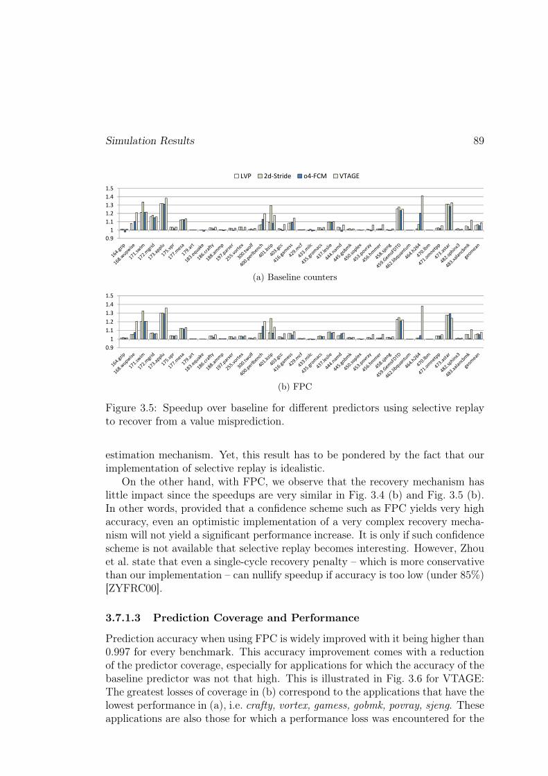
Simulation Results 89
0.9
1
1.1
1.2
1.3
1.4
1.5
LVP 2d-Stride o4-FCM VTAGE
(a) Baseline counters
0.9
1
1.1
1.2
1.3
1.4
1.5
(b) FPC
Figure 3.5: Speedup over baseline for different predictors using selective replayto recover from a value misprediction.
estimation mechanism. Yet, this result has to be pondered by the fact that ourimplementation of selective replay is idealistic.
On the other hand, with FPC, we observe that the recovery mechanism haslittle impact since the speedups are very similar in Fig. 3.4 (b) and Fig. 3.5 (b).In other words, provided that a confidence scheme such as FPC yields very highaccuracy, even an optimistic implementation of a very complex recovery mecha-nism will not yield a significant performance increase. It is only if such confidencescheme is not available that selective replay becomes interesting. However, Zhouet al. state that even a single-cycle recovery penalty – which is more conservativethan our implementation – can nullify speedup if accuracy is too low (under 85%)[ZYFRC00].
3.7.1.3 Prediction Coverage and Performance
Prediction accuracy when using FPC is widely improved with it being higher than0.997 for every benchmark. This accuracy improvement comes with a reductionof the predictor coverage, especially for applications for which the accuracy of thebaseline predictor was not that high. This is illustrated in Fig. 3.6 for VTAGE:The greatest losses of coverage in (b) correspond to the applications that have thelowest performance in (a), i.e. crafty, vortex, gamess, gobmk, povray, sjeng. Theseapplications are also those for which a performance loss was encountered for the

90 Revisiting Value Prediction in a Contemporary Context
0.8
0.9
1
1.1
1.2
1.3
1.4
1.5
Baseline FPC
(a) Speedup
0
0.2
0.4
0.6
0.8
1
(b) Coverage
Figure 3.6: Speedup and coverage of VTAGE with and without FPC. The recov-ery mechanism is squashing at Commit.
baseline while no performance is lost with FPC. For applications already havinghigh accuracy and showing performance increase with the baseline, coverage isalso slightly decreased, but in a more moderate fashion. Similar behaviors areobserved for the other predictors.
Note that high coverage does not always correlate with high performance,e.g. leslie exhibits 70-80% coverage but marginal speedup. Conversely, a smallercoverage may lead to significant speed-up e.g., h264.
3.7.2 Hybrid predictors
For the sake of readability, we only report results for the squashing recoverymechanism, but trends are similar for selective replay.
Fig. 3.7 (a) illustrates speedups for a combination of VTAGE and 2D-Strideas well as o4-FCM and 2D-Stride, and more tightly-coupled hybrid: D-FCM andD-VTAGE. As expected, simple hybrids yield slightly higher performance thansingle predictor schemes, generally achieving performance at least on par withthe best of the two predictors on a given benchmark. Yet, improvement over thislevel is generally marginal.
Interestingly, we can observe that D-VTAGE is able to provide better perfor-mance than its naive hybrid equivalent. As a result, a more tightly-coupled hybrid

Simulation Results 91
0.9
1
1.1
1.2
1.3
1.4
1.5
1.6
1.7
1.8
2dS-FCM 2dS-VTAGE o4-D-FCM D-VTAGE
(a) Speedup
0
0.2
0.4
0.6
0.8
1
(b) Coverage
Figure 3.7: Speedup over baseline and coverage of a 2-component symmetrichybrid made of 2D-Stride and VTAGE/FCM, as well as D-FCM and D-VTAGE.All predictors feature FPC for confidence estimation. Recovery is done via squashat Commit.
92 Revisiting Value Prediction in a Contemporary Context
of VTAGE and Stride seems more interesting from a performance standpoint.Therefore, since D-FCM suffers from the same shortcomings as FCM (predic-
tion critical loop and complex management of the speculative history), D-VTAGEappears as a better choice overall.
3.8 Conclusion
In this Chapter, we have first shown that the use of Value Prediction can be effec-tive, even if prediction validation is performed at commit time. Using probabilis-tic saturating confidence counters with a low increment probability can greatlybenefit any value predictor: A very high accuracy (> 99.7%) can be ensured forall existing value predictors at some cost in coverage, using very simple hardware.Very high accuracy is especially interesting because it allows to tolerate the highindividual average misprediction cost associated with validation at commit time.In this context, complex recovery mechanisms such as selective replay have verymarginal performance interest. In other words, we claim that, granted a properconfidence estimation mechanism such as the FPC scheme, state-of-the-art valuepredictors can improve performance on a fairly wide and deep pipeline while theprediction validation is performed at commit time. In this case, the Value Pre-diction hardware is essentially restricted to the in-order front-end (prediction)and the in-order back-end (validation and training) and the modifications to theout-of-order engine are very limited.
Second, we have introduced a new context-based value predictor, the ValueTAGE predictor, and an improved version able to capture strided patterns, D-VTAGE. We derived VTAGE from the ITTAGE predictor by leveraging similar-ities between Indirect Branch Target Prediction and Value Prediction. VTAGEuses the global branch history as well as the path history to predict values.We have shown that it outperforms previous generic context-based value pre-dictors leveraging per-instruction value history (e.g., FCM). A major advantageof VTAGE is its tolerance to high latency which has to be contrasted with localvalue history based predictors as they suffer from long critical operation whenpredicting consecutive instances of the same instruction. They are highly sensi-tive to the prediction latency and cannot afford long lookup times, hence largetables.
On the contrary, the access to VTAGE tables can span over several cycles(from Fetch to Dispatch) and VTAGE can be implemented using very large ta-bles. D-VTAGE follows VTAGE operation except only the stride is selectedusing the TAGE scheme. As a result, D-VTAGE possesses the same predictioncritical path and requirement for a speculative window as any stride-based pre-dictors. Fortunately, contrarily to FCM predictors, the critical path is only a

Conclusion 93
64-bit adder. Moreover, we propose a realistic implementation of the speculativewindow in Chapter 5. As a result, we claim that D-VTAGE is suited for actualimplementations.
Through combining our two propositions, a practical value predictor improvesperformance while only requiring limited hardware modifications to the out-of-order execution engine. Our experiments show that while improvement mightbe limited in many applications – less than 5% on 21 out of 38 benchmarks –,encouraging performance gains are encountered in remaining applications: From6.6% up to 64.8% on 17 benchmarks. Yet, this contribution does not addressthe requirements on the Physical Register File. Indeed, we have considered thatup to 8 predictions were written to the PRF at Dispatch, and although bankingthe PRF can limit the number of write ports required per bank, those ports arestill required in addition to those required by the execution engine. Moreover,validating predictions at Commit still implies that the actual result should beread from the PRF and compared against the associated prediction, that can sitin a FIFO queue similar to the ROB. Yet, this also entails additional read ports.As a result, and given the poor scalability of the PRF as the port count grows[ZK98], VP cannot be envisioned if the port requirements on the PRF is notkept reasonable. In the next Chapter, we will show that it is actually possible toimplement VP with as many ports on the PRF as a regular out-of-order processor,paving the way for an actual implementation of VP on real silicon.

94 Revisiting Value Prediction in a Contemporary Context

Chapter 4
A New Execution Model LeveragingValue Prediction: EOLE
This Chapter covers a publication in the International Symposium on ComputerArchitecture (ISCA 2014) [PS14a] that was also selected to appear in IEEE Microas a Top Pick from Computer Architecture conferences of 2014 [PS15b].
4.1 Introduction & Motivations
Even in the multicore era, the need for higher single thread performance is driv-ing the definition of new high-performance cores. Although the usual superscalardesign does not scale, increasing the ability of the processor to extract Instruc-tion Level Parallelism (ILP) by increasing the window size as well as the issuewidth1 has generally been the favored way to enhance sequential performance.For instance, consider the recently introduced Intel Haswell micro-architecturethat has 33% more issue capacity than Intel Nehalem.2 To accommodate thisincrease, both the Reorder Buffer (ROB) and Scheduler size were substantiallyincreased.3 On top of this, modern schedulers must support complex mechanismssuch as speculative scheduling to enable back-to-back execution of variable latencyinstructions and their dependents, and thus a form of replay to efficiently re-cover from schedule mispredictions [PSM+15, MBS07, MS01, MSBU00, SGC01b,MLO01, KL04].
In addition, the issue width impacts other structures: The Physical RegisterFile (PRF) must provision more read/write ports as the width grows, while thenumber of physical registers must also increase to accommodate the ROB size.
1How many instructions can be sent to the functional units to be executed each cycle.2State-of-the-art in 20093From respectively 128 and 36 entries to 192 and 60 entries.
95

96 A New Execution Model Leveraging Value Prediction: EOLE
Because of this, both latency and power consumption increase and using a mono-lithic register file rapidly becomes complexity-ineffective. Similarly, a wide-issueprocessor should provide enough functional units to limit resource contention.Yet, the complexity of the bypass network grows quadratically with the numberof functional units and quickly becomes critical regarding cycle time [PJS97]. Inother words, the out-of-order engine impact on power consumption and cycle timeis ever increasing [EA02].
We previously mentioned that in the context of Value Prediction, validationand recovery from a misprediction can be done at commit time, but predictionsmust still be written to the PRF at Dispatch. As a result, additional ports arerequired on the register file, which may lead to an unbearably large and power-hungry structure, especially as the issue width is already high (e.g., 8 in Haswell).
To that extent, we propose a modified superscalar design, the {Early | Out-of-Order | Late} Execution microarchitecture, EOLE. EOLE builds on a pipelineimplementing Value prediction and aims to further reduce both the complexityof the out-of-order (OoO) execution engine and the number of ports requiredon the PRF when VP is implemented. We achieve this reduction without sig-nificantly impacting overall performance. The contribution is therefore twofold:First, EOLE paves the way to truly practical implementations of VP. Second, itreduces complexity in the most complicated and power-hungry part of a modernOoO core.
To do so, we rely on two observations. First, when using VP, a significantamount of single-cycle instructions have their operands ready in the front-endthanks to the value predictor. As such, we introduce Early Execution to executesingle-cycle ALU instructions in-order in parallel with Rename by using predictedand/or immediate operands. Early-executed instructions are not sent to the OoOScheduler. Validation at Commit [PS14b] guarantees that the operands of com-mitted early-executed instructions were the correct operands. Early Executionrequires simple hardware and reduces pressure on the OoO instruction window.
Second, and also thanks to the fact that predicted results can be validatedoutside the OoO engine at commit time, we can offload the execution of predictedsingle-cycle ALU instructions to some dedicated in-order Late Execution pre-commit stage, where no dynamic scheduling has to take place. This does not hurtperformance since instructions dependent on predicted instructions will simplyuse the predicted results rather than wait in the OoO Scheduler. Similarly, theresolution of high confidence branches can be offloaded to the Late Executionstage since they are very rarely mispredicted [Sez11c].
Overall, a total of 7% to 75% (37% on average) of the retired instructionscan be offloaded from the OoO core, on our benchmark suite. As a result, EOLEshould benefit from both the aggressiveness of modern OoO designs and the higherenergy-efficiency of more conservative in-order designs.

Related Work on Complexity-Effective Architectures 97
We evaluate EOLE against a baseline OoO model featuring VP and show thatit achieves similar levels of performance having only 66% of the baseline issuecapacity and a significantly less complex physical register file. This is especiallyinteresting since it provides architects extra design headroom in the OoO engineto implement new architectural features.
4.2 Related Work on Complexity-Effective Archi-tectures
Many propositions aim to reduce complexity in modern superscalar designs. Inparticular, it has been shown that most of the complexity and power consump-tion reside in the OoO engine, including the PRF [WB96], Scheduler and bypassnetwork [PJS97]. As such, previous studies focused on either reducing the com-plexity of existing structures, or in devising new pipeline organizations.
4.2.1 Alternative Pipeline Design
Farkas et al. propose the Multicluster architecture in which execution is dis-tributed among several execution clusters, each of them having its own registerfile [FCJV97]. Since each cluster is simpler, cycle time can be decreased eventhough some inefficiencies are introduced due to the inter-cluster dependencies.In particular, inter-cluster data dependencies are handled by dispatching the sameinstruction to several clusters and having all instances but one serve as inter-cluster data-transfer instructions while a single instance actually computes theresult. To enforce correctness, this instance is data-dependent on all others.
The Alpha 21264 [KMW98] is an example of real-world clustered architectureand shares many traits with the Multicluster architecture. It features two sym-metric clusters sharing the frontend (i.e., Fetch to Rename) and the store queue.Instructions are then steered to one of them depending on a given heuristic.
Palacharla et al. introduce a dependence-based microarchitecture where thecentralized instruction window is replaced by several parallel FIFOs [PJS97].FIFOs are filled with independent instructions (i.e., all instructions in a singleFIFO are dependent) to allow ILP to be extracted: since instructions at the headof the FIFOs are generally independent, they can issue in parallel.
This greatly reduces complexity since only the head of each FIFO has to beselected by the Select logic. They also study a clustered dependence-based ar-chitecture to reduce the amount of bypass and window logic by using clustering.That is, a few FIFOs are grouped together and assigned their own copy of theregister file and bypass network, mimicking a wide issue window by having sev-eral smaller ones. Inter-cluster bypassing is naturally slower than intra-cluster

98 A New Execution Model Leveraging Value Prediction: EOLE
bypassing.Tseng and Patt propose the Braid architecture [TP08], which shares many
similarities with the clustered dependence-based architecture with three majordifferences: 1) Instruction partitioning – steering – is done at compile time viadataflow-graph coloring 2) Each FIFO is a narrow-issue (dual issue in [TP08])in-order cluster called a Braid Execution Unit with its own local register file,execution units, and bypass network 3) A global register file handles inter-unitdependencies instead of an inter-cluster bypass network. As such, they obtainperformance on-par with an accordingly sized OoO machine without using com-plicated scheduling logic, register file and bypass logic.
Austin proposes Dynamic Implementation VAlidation (DIVA) to check in-struction results just before commit time, allowing the core to be faulty [Aus99].DIVA can greatly reduce the complexity of functionally validating the core sinceonly the checker has to be functionally correct. The core complexity itself canremain very high, however. An interesting observation is that the latency of thechecker has very limited impact on performance. This hints that adding pipelinestages between Writeback and Commit does not actually impact performancemuch, as long as the instruction window is large enough.
Fahs et al. study Continuous Optimization where common compile-time op-timizations are applied dynamically in the Rename stage [FRPL05]. This allowsto early-execute some instructions in the front-end instead of the OoO core. Sim-ilarly, Petric et al. propose RENO which also dynamically applies optimizationsat rename-time [PSR05].
4.2.2 Optimizing Existing Structures
Instead of studying new organizations of the pipeline, Kim and Lipasti presentthe Half-Price Architecture [KL03] in which regular structures are made operand-centric rather than instruction-centric. For instance, they argue that many in-structions are single operand and that both operands of dual-operand instructionsrarely become ready at the same time. Thus, the load capacitance on the tagbroadcast bus can be greatly reduced by sequentially waking-up operands. Inparticular, the left operand is woken-up as usual, while the right one is woken-upone cycle later by inserting a latch on the broadcast bus. They use a criticalitypredictor to place the critical tag in the left operand field.
Similarly, Ernst and Austin propose Tag Elimination to limit the number ofcomparators used for Wakeup [EA02]. Only the tag of the – predicted – lastarriving operand is put in the scheduler. This allows to only use one comparatorper entry instead of one per operand (e.g., 4 per instruction in AMD Bulldozer[GAV11]). However, this also implies that the instruction must be replayed on awrong last operand prediction.

{Early | Out-of-order | Late} Execution: EOLE 99
Regarding the register file, Kim and Lipasti also observe in their Half-Price Ar-chitecture that many issuing instructions do not need to read both their operandsin the register file since one or both will be available on the bypass network [KL03].Thus, provisioning two read ports per issue slot is generally over-provisioning. Inparticular, for the small proportion of instructions that effectively need to readtwo operands in the RF, they propose to use a single port but use it for two con-secutive cycles. Reducing the number of ports drastically reduces the complexityof the register file as ports are much more expensive than registers [ZK98].
Lastly, many studies on heterogeneous architectures have been done in therecent past, although most of them focus on heterogeneous multicores, which areout of the scope of this work. Nonetheless, Lukefahr et al. propose to implementtwo back-ends – in-order and OoO – in a single core [LPD+12] and to dynamicallydispatch instructions to the most adapted one. In most cases, this saves power ata slight cost in performance. In a sense, EOLE has similarities with such a designsince instructions can be executed in different locations. However, no decisionhas to be made as the location where an instruction will be executed dependsonly on its type and status (e.g., predicted or not).
4.3 {Early | Out-of-order | Late} Execution: EOLE
4.3.1 Enabling EOLE Using Value Prediction
As previously described, EOLE consists of a set of simple ALUs in the in-orderfront-end to early-execute instructions in parallel with Rename, and a second setin the in-order back-end to late-execute instructions just before they are validatedand committed. With EOLE, instructions are either executed early, as usual inthe out-of-order engine, or late, but at most once (there is no re-execution).
While EOLE is heavily dependent on Value Prediction, they are in factcomplementary features. Indeed, the former needs a value predictor to predictoperands for Early Execution and provide temporal slack for Late Execution,while Value Prediction needs EOLE to reduce PRF complexity and thus becometruly practical. Yet, to be implemented, EOLE requires prediction validation tobe done at Commit since validating at Execute mechanically forbids Late Exe-cution. Furthermore, using selective replay to recover from a value misprediction[MBS07, MS01, MSBU00, SGC01b, MLO01, KL04] nullifies the interest of bothEarly and Late Execution as all instructions must flow through the OoO Sched-uler in case they need to be replayed. Hence, squashing must be used to recoverfrom a misprediction so that early/late-executed instructions can safely bypassthe Scheduler.
Fortunately, we previously described a confidence estimation mechanism greatlylimiting the number of value mispredictions, Forward Probabilistic Counters (FPC)

100 A New Execution Model Leveraging Value Prediction: EOLE
(a) Block diagram.
(b) Pipeline diagram.
Figure 4.1: The EOLE µ-architecture.
{Early | Out-of-order | Late} Execution: EOLE 101
[PS14b]. With FPC, the cost of a single misprediction can be high since mispre-dicting is very rare. Thus, validation can be done late – at commit time – andsquashing can be used as the recovery mechanism. This enables the implementa-tion of both Early and Late Execution, hence EOLE.
By eliminating the need to dispatch and execute many instructions in the OoOengine, EOLE substantially reduces the pressure on complex and power-hungrystructures. Thus, those structures can be scaled down, yielding a less complexarchitecture whose performance is on par with a more aggressive design. More-over, doing so is orthogonal to previously proposed mechanisms such as clustering[FCJV97, KMW98, PJS97, STR02] and does not require a centralized instructionwindow, even though this is the model we use in this work. Figure 4.1 depicts theEOLE architecture, implementing both Early Execution (green), Late Execution(red) and Value Prediction (blue). In the following paragraphs, we detail the twoadditional blocks required to implement EOLE and their interactions with therest of the pipeline.
4.3.2 Early Execution Hardware
The core idea of Early Execution (EE) is to position one or more ALU stagesin the front-end in which instructions with available operands will be executed.For complexity concerns, however, it seems necessary to limit Early Executionto single-cycle ALU instructions. Indeed, implementing complex functional unitsin the front-end to execute multi-cycle instructions does not appear as a wor-thy tradeoff. In particular, memory instructions are not early-executed (i.e., nomemory accesses). Early Execution is done in-order, hence, it does not requirerenamed registers and can take place in parallel with Rename. For instance,Figure 4.2 depicts the Early Execution Block adapted to a 2-wide Rename stage.
Renaming can be pipelined over several cycles [SMV11]. Consequently, we canuse several ALU stages and simply insert pipeline registers between each stage.The actual execution of an instruction can then happen in any of the ALU stages,depending on the readiness of its operands coming from Decode (i.e., immediate),the local4 bypass network (i.e., from instructions early-executed in the previouscycle) or the value predictor. Operands are never read from the PRF.
In a nutshell, all eligible instructions flow through the ALU stages, propa-gating their results in each bypass network accordingly once they have executed.Finally, after the last stage, results as well as predictions are written into thePRF.
4For complexity concerns, we consider that bypass does not span several stages. Conse-quently, if an instruction depends on a result computed by an instruction located two rename-groups ahead, it will not be early-executed.

102 A New Execution Model Leveraging Value Prediction: EOLE
Figure 4.2: Early Execution Block. The logic controlling the ALUs and muxes isnot shown for clarity.
An interesting design concern lies with the number of stages required to cap-ture a reasonable proportion of instructions. We actually found that using morethan a single stage was highly inefficient, as illustrated in Figure 4.3. This figureshows the proportion of committed instructions eligible for Early Execution fora baseline 8-wide rename, 6-issue model (see Table 3.2), using the D-VTAGEpredictor described in Table 3.1. As a result, in further experiments, we considera 1-deep Early Execution Block only.
To summarize, Early Execution only requires a single new computing block,which is shown in green in Figure 4.1. The mechanism we propose does not requireany storage area for temporaries as all values are living inside the pipeline registersor the local bypass network. Finally, since we execute in-order, each instructionis mapped to a single ALU and scheduling is straightforward.
4.3.3 Late Execution Hardware
Late Execution (LE) targets instructions whose result has been predicted.5 It isdone in-order just before validation time, that is, outside of the execution engine.As for Early Execution, we limit ourselves to single-cycle ALU instructions tominimize complexity. That is, predicted loads are executed in the OoO engine,but validated at commit.
Interestingly, Seznec showed in [Sez11c] that conditional branch predictionsflowing from the TAGE [SM06, Sez11b] branch predictor can be categorized such
5Instructions eligible for prediction are µ-ops producing a 64-bit or less result that can beread by a subsequent µ-op, as defined by the ISA implementation.

{Early | Out-of-order | Late} Execution: EOLE 103
0
0.05
0.1
0.15
0.2
0.25
0.3
0.35
0.4
0.45
1-stage 2-stage 3-stage
Figure 4.3: Proportion of committed instructions that can be early-executed,using one, two and three ALU stages and a D-VTAGE predictor.
0
0.1
0.2
0.3
0.4
0.5
High-Confidence Branches Value predicted
Figure 4.4: Proportion of committed instructions that can be late-executed us-ing a D-VTAGE predictor. Late-executable instructions that can also be early-executed are not counted since instructions are executed once at most.

104 A New Execution Model Leveraging Value Prediction: EOLE
that very high confidence predictions are known. Since high confidence branchesexhibit a misprediction rate generally lower than 0.5%, resolving them in theLate Execution block has a marginal impact on overall performance. Thus, weconsider both single-cycle predicted ALU instructions and very high confidencebranches6 for Late Execution. In this study, we did not try to set confidence onthe other types of branches (indirect jumps, returns). Yet, provided a similarhigh confidence estimator for these categories of branches, one could postponethe resolution of high confidence ones until the LE stage.
Furthermore, note that predicted instructions can also be early-executed. Inthat event, they only need to be validated in case another early-executed instruc-tion from the same rename-group used the prediction as an operand.
In any case, Late Execution further reduces pressure on the OoO engine interms of instructions dispatched to the Scheduler. As such, it also removes theneed for predicting only critical instructions [FRB01, RFK+98, TTC02] sinceminimizing the number of instructions flowing through the OoO engine requiresmaximizing the number of predicted instructions. Hence, usually useless predic-tions from a performance standpoint become useful in EOLE. Figure 4.4 showsthe proportion of committed instructions that can be late-executed using a base-line 6-issue processor with a D-VTAGE predictor (respectively described in Tables3.2 and 3.1 in Section 3.6).
Late Execution needs to implement commit width ALUs and the associatedread ports in the PRF. If an instruction I1 to be late-executed depends on the re-sult of instruction I0 of the same commit group, and I0 will also be late-executed,it does not need to wait as it can use the predicted result of I0. In other words,all non-executed instructions reaching the Late Execution stage have all theiroperands ready by construction, as in DIVA [Aus99]. Due to the need to late-execute some instructions as well as validate predictions (including reading resultsto train the value predictor), at least one extra pipeline stage after Writeback islikely to be required in EOLE. In the remainder of this Chapter, we refer to thisstage as the Late Execution/Validation and Training (LE/VT) stage.
As a result, the hardware needed for LE is fairly simple, as suggested bythe high-level view of a 2-wide LE/VT Block shown in Figure 4.5. It does noteven require a bypass network. In further experiments, we consider that LEand prediction validation can be done in the same cycle, before the Commitstage. EOLE is therefore only one cycle longer than the baseline superscalar itis compared to. While this may be optimistic due to the need to read from thePRF, this only impacts the value misprediction penalty and the pipeline fill delay.In particular, since low confidence branches are resolved in the same cycle as forthe baseline, the average branch misprediction penalty will remain very similar.
6Predictions whose confidence counter is saturated [Sez11c].

{Early | Out-of-order | Late} Execution: EOLE 105
Figure 4.5: Late Execution Block for a 2-wide processor. The top part can late-execute two instructions while the bottom part validates two results against theirrespective predictions. Buses are register-width-bit wide.
Lastly, as a first step, we also consider that enough ALUs are implemented (i.e.,as many as the commit width). As a second step, we shall consider reduced-widthLate Execution.
4.3.4 Potential OoO Engine Offload
We obtain the ratio of retired instructions that can be offloaded from the OoOengine for each benchmark by summing the columns in Figure 4.3 and 4.4 (bothsets are disjoint as we only count late executable instructions that cannot alsobe early-executed). We also add the load immediate instructions that were notconsidered in Figure 4.3 but that will be early-executed by construction. Thosenumbers are reported in Figure 4.6. We distinguish four types of instructions:
1. Early-executed because it is a load immediate, i.e., its operand is necessarilyready at Rename. In a regular Value Prediction pipeline, these instructionscan also bypass the out-of-order engine, as mentioned in 3.6.2.1.
2. Early-executed because it is a ready single-cycle instruction.
3. Late-executed because it is a high-confidence branch, as predicted by theTAGE branch predictor described in 3.6.

106 A New Execution Model Leveraging Value Prediction: EOLE
Figure 4.6: Overall portion of committed instructions that can be bypassed fromthe out-of-order engine, including early-executed, late-executed instructions andLoad Immediate instructions that can be done for free thanks to the PRF writeports provisioned for VP.
4. Late-executed because it is a value prediction single-cycle instruction.
The ratio of instructions bypassing the OoO engine is very dependent on theapplication, ranging from around 10% for equake, milc, gromacs, hmmer and lbmto more than 60% for mgrid, applu, art, perlbench, leslie and namd and up to75% for libquantum. Nonetheless, it generally represents a significant portion ofthe retired instructions.
4.4 Evaluation Methodology
4.4.1 Simulator
We reuse the simulator configuration presented in the previous Chapter (Table3.2). That is, we consider a relatively aggressive 4GHz, 6-issue superscalar base-line with a fetch-to-commit latency of 19 cycles. Since we focus on the OoO enginecomplexity, both in-order front-end and in-order back-end are overdimensionedto treat up to 8 µ-ops per cycle. We model a deep front-end (15 cycles) coupledto a shallow back-end (4 cycles) to obtain realistic branch/value mispredictionpenalties. The OoO scheduler features a unified centralized 60-entry IQ and a192-entry ROB on par with Haswell’s, the latest commercially available Intel mi-croarchitecture. We refer to this baseline as the Baseline_6_60 configuration(6-issue, 60-entry IQ).
The only difference with the simulator configuration presented in Table 3.2is that in the case where Value Prediction is used, we add a pre-commit stageresponsible for validation/training and Late Execution when relevant: the LE/VTstage. This accounts for an additional pipeline cycle (20 cycles) and an increasedvalue misprediction penalty (21 cycles min.). Minimum branch misprediction

Evaluation Methodology 107
latency remains unchanged except for mispredicted very high confidence brancheswhen Late Execution is used. Note that the value predictor is effectively trainedafter commit, but the value is read from the PRF in the LE/VT stage.
4.4.1.1 Value Predictor Operation
As in the previous Chapter, the predictor makes a prediction at fetch time forevery eligible µ-op (i.e. producing a 64-bit or less register that can be read by asubsequent µ-op, as defined by the ISA implementation). To index the predictor,we XOR the PC of the x86_64 instruction left-shifted by two with the µ-opnumber inside the x86_64 instruction. This avoids all µ-ops mapping to thesame entry. We assume that the predictor can deliver as many predictions asrequested by the Fetch stage.
In the previous Chapter, we assumed that a prediction is written into thePRF and replaced by its non-speculative counterpart when it is computed in theOoO engine [PS14b]. In parallel, predictions are put in a FIFO queue to be ableto validate them – in-order – at commit time. In EOLE, we also use a queue forvalidation. However, instead of directly writing predictions to the PRF, we placepredictions in the Early Execution units, which will in turn write the predictionsto the PRF at Dispatch. By doing so, we can use predictions as operands in theEE units.
Finally, since we focus on single core, the impact of VP on memory consistency[MSC+01] in EOLE is left for future work. However, VP should not alter thebehavior of processors implementing Sequential Consistency [Lam79] or TotalStore Ordering [SSO+10] (which is used in x86).
Predictor Considered in this Study In this study, we focus on the tightly-coupled hybrid of VTAGE and a simple stride-based Stride predictor, D-VTAGE[PS15a]. For confidence estimation, we use Forward Probabilistic Counters [PS14b],that were described in the previous Chapter. In particular, we use 3-bit con-fidence counters whose forward transitions are controlled by the vector v ={1, 1
16, 116, 116, 116, 132, 132} as we found it to perform best with D-VTAGE. We use
the same configuration as in the previous Chapter (see Table 3.1): a 8K-entrybase predictor and 6 1K-entry partially tagged components. We do not try tooptimize the size of the predictor (by using partial strides, for instance), but wewill see in Chapter 5 that even 16 to 32KB of storage are sufficient to get goodperformance with D-VTAGE.

108 A New Execution Model Leveraging Value Prediction: EOLE
Figure 4.7: Speedup over Baseline_6_60 brought by Value Prediction using D-VTAGE.
4.4.2 Benchmark Suite
We reuse the benchmarks used to evaluate the contribution of Chapter 3. Specif-ically, we use 18 integer benchmarks and 18 floating-point programs. Table 3.3summarizes the benchmarks we use as well as their input, which are part ofthe reference inputs provided in the SPEC software packages. To get relevantnumbers, we identify a region of interest in the benchmark using Simpoint 3.2[PHC03]. We simulate the resulting slice in two steps: First, warm up all struc-tures (caches, branch predictor and value predictor) for 50M instructions, thencollect statistics for 100M instructions.
4.5 Experimental Results
In our experiments, we first use Baseline_6_60 as the baseline to gauge theimpact of adding a value predictor only. Then, in all subsequent experiments,we use said baseline augmented with the D-VTAGE predictor detailed in Table3.1. We refer to it as the Baseline_VP_6_60 configuration. Our objective isto characterize the potential of EOLE at decreasing the complexity of the OoOengine. We assume that Early and Late Execution stages are able to treat anygroup of up to 8 consecutive µ-ops every cycle. In Section 4.6, we will considertradeoffs to enable realistic implementations.
4.5.1 Performance of Value Prediction
Figure 4.7 illustrates the performance benefit of augmenting the baseline proces-sor with the D-VTAGE predictor. A few benchmarks present interesting potentiale.g., wupwise, swim, mgrid, applu, perlbench, bzip, gemsFDTD, h264 and astar,some a more moderate potential e.g., mesa, gamess, leslie, namd, hmmer andxalancbmk, and a few others low potential. No slowdown is observed.

Experimental Results 109
Figure 4.8: Performance of EOLE and the baseline with regard to issue width,normalized to Baseline_VP_6_60.
In further experiments, figures will depict speedups over the baseline featuringD-VTAGE (Baseline_VP_6_60 ).
4.5.2 Impact of Reducing the Issue Width
Applying EOLE without modifying the OoO core (EOLE_6_60 ) is illustratedin Figure 4.8. In this figure, we also illustrate the baseline, but with a 4-issue OoO engine (Baseline_VP_4_60 ) and EOLE using a 4-issue OoO engine(EOLE_4_60 ).
By itself, EOLE slightly increases performance over the baseline, with a fewbenchmarks achieving 5% speedup or higher (20% in xalancmbk). These improve-ments come from the fact that we actually increase the number of instructionsthat can be executed each cycle through EOLE.
Shrinking the issue width to 4 reduces the performance of the baseline by a sig-nificant factor in many applications e.g., applu, perlbench, namd and gemsFDTDfor which slowdown is worse than 5%. For EOLE, such a shrink only reduces per-formance slightly compared with EOLE_6_60. Furthermore, EOLE_4_60 stillperforms slightly higher than Baseline_VP_6_60 in several benchmarks e.g.,swim, mgrid, applu, crafty, vortex, perlbench, gcc, leslie, namd, gemsFDTD, as-tar and xalancbmk. Only a few slight slowdowns can be observed (e.g., vpr, milc,gromacs) and povray. Fortunately, even the worst slowdown (2.7% in povray) isacceptable.
As a result, EOLE can be considered as a means to reduce issue width withoutsignificantly impacting performance on a processor featuring VP.
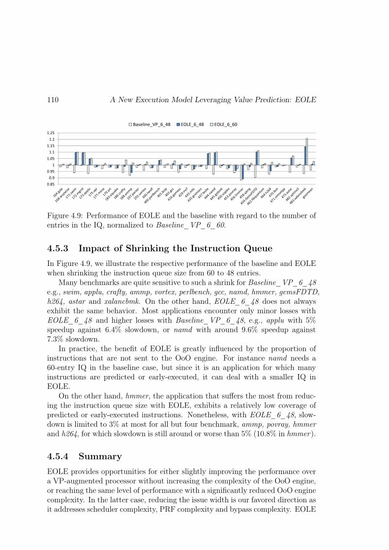
110 A New Execution Model Leveraging Value Prediction: EOLE
Figure 4.9: Performance of EOLE and the baseline with regard to the number ofentries in the IQ, normalized to Baseline_VP_6_60.
4.5.3 Impact of Shrinking the Instruction Queue
In Figure 4.9, we illustrate the respective performance of the baseline and EOLEwhen shrinking the instruction queue size from 60 to 48 entries.
Many benchmarks are quite sensitive to such a shrink for Baseline_VP_6_48e.g., swim, applu, crafty, ammp, vortex, perlbench, gcc, namd, hmmer, gemsFDTD,h264, astar and xalancbmk. On the other hand, EOLE_6_48 does not alwaysexhibit the same behavior. Most applications encounter only minor losses withEOLE_6_48 and higher losses with Baseline_VP_6_48, e.g., applu with 5%speedup against 6.4% slowdown, or namd with around 9.6% speedup against7.3% slowdown.
In practice, the benefit of EOLE is greatly influenced by the proportion ofinstructions that are not sent to the OoO engine. For instance namd needs a60-entry IQ in the baseline case, but since it is an application for which manyinstructions are predicted or early-executed, it can deal with a smaller IQ inEOLE.
On the other hand, hmmer, the application that suffers the most from reduc-ing the instruction queue size with EOLE, exhibits a relatively low coverage ofpredicted or early-executed instructions. Nonetheless, with EOLE_6_48, slow-down is limited to 3% at most for all but four benchmark, ammp, povray, hmmerand h264, for which slowdown is still around or worse than 5% (10.8% in hmmer).
4.5.4 Summary
EOLE provides opportunities for either slightly improving the performance overa VP-augmented processor without increasing the complexity of the OoO engine,or reaching the same level of performance with a significantly reduced OoO enginecomplexity. In the latter case, reducing the issue width is our favored direction asit addresses scheduler complexity, PRF complexity and bypass complexity. EOLE
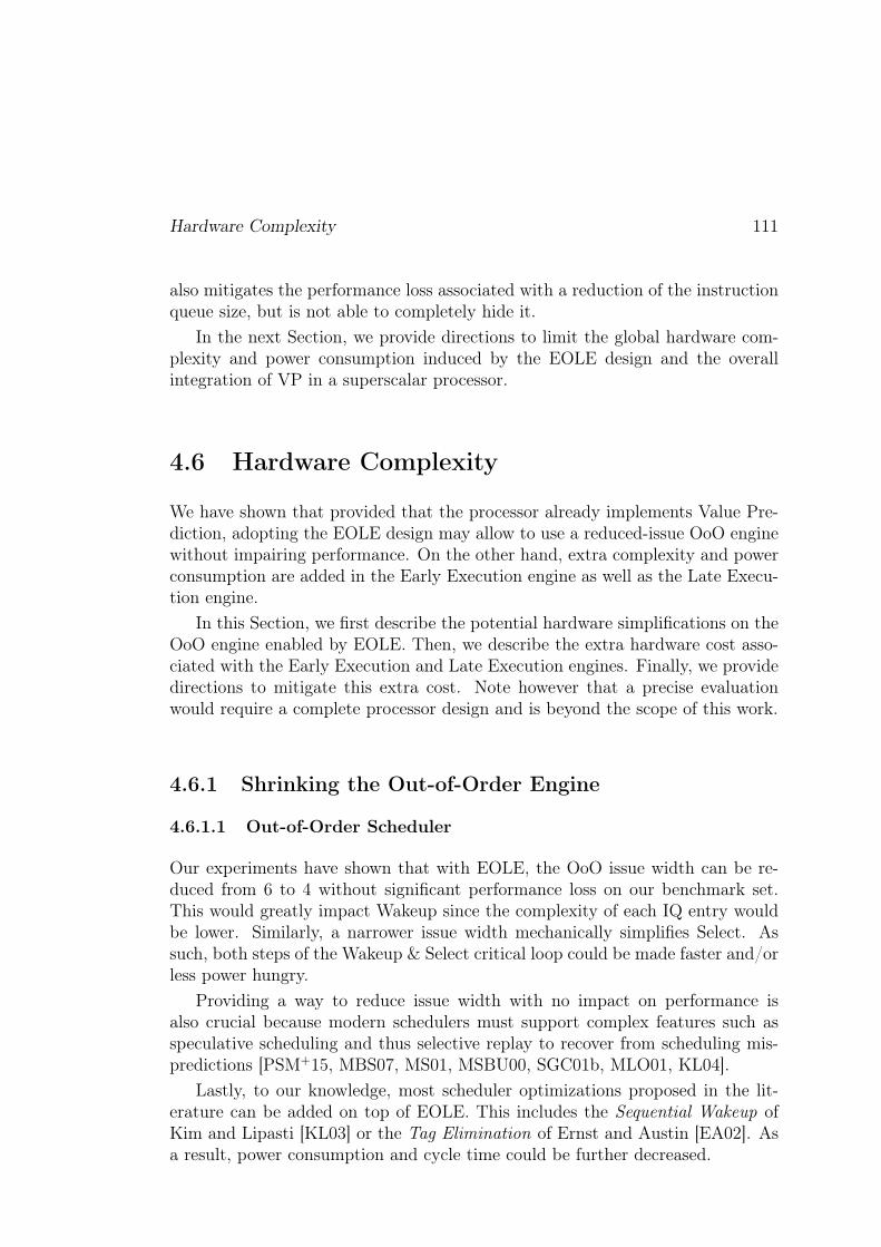
Hardware Complexity 111
also mitigates the performance loss associated with a reduction of the instructionqueue size, but is not able to completely hide it.
In the next Section, we provide directions to limit the global hardware com-plexity and power consumption induced by the EOLE design and the overallintegration of VP in a superscalar processor.
4.6 Hardware Complexity
We have shown that provided that the processor already implements Value Pre-diction, adopting the EOLE design may allow to use a reduced-issue OoO enginewithout impairing performance. On the other hand, extra complexity and powerconsumption are added in the Early Execution engine as well as the Late Execu-tion engine.
In this Section, we first describe the potential hardware simplifications on theOoO engine enabled by EOLE. Then, we describe the extra hardware cost asso-ciated with the Early Execution and Late Execution engines. Finally, we providedirections to mitigate this extra cost. Note however that a precise evaluationwould require a complete processor design and is beyond the scope of this work.
4.6.1 Shrinking the Out-of-Order Engine
4.6.1.1 Out-of-Order Scheduler
Our experiments have shown that with EOLE, the OoO issue width can be re-duced from 6 to 4 without significant performance loss on our benchmark set.This would greatly impact Wakeup since the complexity of each IQ entry wouldbe lower. Similarly, a narrower issue width mechanically simplifies Select. Assuch, both steps of the Wakeup & Select critical loop could be made faster and/orless power hungry.
Providing a way to reduce issue width with no impact on performance isalso crucial because modern schedulers must support complex features such asspeculative scheduling and thus selective replay to recover from scheduling mis-predictions [PSM+15, MBS07, MS01, MSBU00, SGC01b, MLO01, KL04].
Lastly, to our knowledge, most scheduler optimizations proposed in the lit-erature can be added on top of EOLE. This includes the Sequential Wakeup ofKim and Lipasti [KL03] or the Tag Elimination of Ernst and Austin [EA02]. Asa result, power consumption and cycle time could be further decreased.

112 A New Execution Model Leveraging Value Prediction: EOLE
4.6.1.2 Functional Units & Bypass Network
As the number of cycles required to read a register from the PRF increases,the bypass network becomes more crucial. It allows instructions to “catch” theiroperands as they are produced and thus execute back-to-back. However, a fullbypass network is very expensive, especially as the issue width – hence the num-ber of functional units – increases. Ahuja et al. showed that partial bypassingcould greatly impede performance, even for a simple in-order single-issue pipeline[ACR95]. Consequently, in the context of a wide-issue OoO superscalar witha multi-cycle register read, missing bypass paths may cripple performance evenmore.
EOLE allows to reduce the issue width in the OoO engine. Therefore, itreduces the design complexity of a full bypass by reducing the number of ALUsand thus the number of simultaneous writers on the network.
4.6.1.3 A Limited Number of Register File Ports dedicated to theOoO Engine
Through reducing the issue width of the OoO engine, EOLE mechanically re-duces the number of read and write ports required on the PRF for regular OoOexecution. Indeed, assuming 2 read ports and 1 write port per potentially issuedinstruction each cycle, reducing the issue width from 6 to 4 saves 4 read portsand 2 write ports.
4.6.2 Extra Hardware Complexity Associated with EOLE
4.6.2.1 Cost of the Late Execution Block
The extra hardware complexity associated with Late Execution consists of threemain components. First, for validation at commit time, a prediction queue(FIFO) is required to store predicted results. This component is needed anywayas soon as VP associated with validation at commit time is implemented. Second,ALUs are needed for Late Execution. Last, the operands for the late-executedinstructions must be read from the PRF. Similarly, the result of VP-eligible in-structions must be read from the PRF for validation (predicted instructions only)and predictor training (all VP-eligible instructions).
In the simulations presented in Section 4.5, we have assumed that up to 8 µ-ops(i.e., commit width) could be late-executed per cycle. This would necessitate 8ALUs and up to 16 read ports on the PRF (including ports required for validationand predictor training).
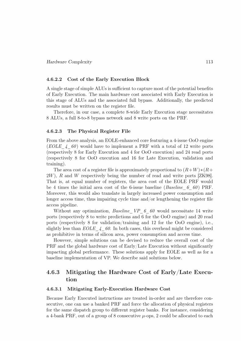
Hardware Complexity 113
4.6.2.2 Cost of the Early Execution Block
A single stage of simple ALUs is sufficient to capture most of the potential benefitsof Early Execution. The main hardware cost associated with Early Execution isthis stage of ALUs and the associated full bypass. Additionally, the predictedresults must be written on the register file.
Therefore, in our case, a complete 8-wide Early Execution stage necessitates8 ALUs, a full 8-to-8 bypass network and 8 write ports on the PRF.
4.6.2.3 The Physical Register File
From the above analysis, an EOLE-enhanced core featuring a 4-issue OoO engine(EOLE_4_60 ) would have to implement a PRF with a total of 12 write ports(respectively 8 for Early Execution and 4 for OoO execution) and 24 read ports(respectively 8 for OoO execution and 16 for Late Execution, validation andtraining).
The area cost of a register file is approximately proportional to (R+W )∗(R+2W ), R and W respectively being the number of read and write ports [ZK98].That is, at equal number of registers, the area cost of the EOLE PRF wouldbe 4 times the initial area cost of the 6-issue baseline (Baseline_6_60 ) PRF.Moreover, this would also translate in largely increased power consumption andlonger access time, thus impairing cycle time and/or lengthening the register fileaccess pipeline.
Without any optimization, Baseline_VP_6_60 would necessitate 14 writeports (respectively 8 to write predictions and 6 for the OoO engine) and 20 readports (respectively 8 for validation/training and 12 for the OoO engine), i.e.,slightly less than EOLE_4_60. In both cases, this overhead might be consideredas prohibitive in terms of silicon area, power consumption and access time.
However, simple solutions can be devised to reduce the overall cost of thePRF and the global hardware cost of Early/Late Execution without significantlyimpacting global performance. These solutions apply for EOLE as well as for abaseline implementation of VP. We describe said solutions below.
4.6.3 Mitigating the Hardware Cost of Early/Late Execu-tion
4.6.3.1 Mitigating Early-Execution Hardware Cost
Because Early Executed instructions are treated in-order and are therefore con-secutive, one can use a banked PRF and force the allocation of physical registersfor the same dispatch group to different register banks. For instance, consideringa 4-bank PRF, out of a group of 8 consecutive µ-ops, 2 could be allocated to each
114 A New Execution Model Leveraging Value Prediction: EOLE
Figure 4.10: Organization of a 4-bank PRF supporting 8-wide VP/Early Execu-tion and 4-wide OoO issue. The additional read ports per-bank required for LateExecution are not shown for clarity.
Figure 4.11: Performance of EOLE_4_60 using a different number of banks inthe PRF, normalized to EOLE_4_60 with a single bank.
Hardware Complexity 115
bank. A dispatch group of 8 consecutive µ-ops would at most write 2 registersin a single bank after Early Execution. Thus, Early Execution would necessitateonly two extra write ports on each PRF bank, as illustrated in Figure 4.10 foran 8-wide Rename/Early Execute, 4-issue OoO core. Interestingly, this wouldadd-up to the number of write ports required by a baseline 6-issue OoO Core.
In Figure 4.11, we illustrate simulation results with a banked PRF. In partic-ular, registers from distinct banks are allocated to consecutive µ-ops and Renameis stalled if the current bank does not have any free register. We consider respec-tively 2 banks of 128 registers, 4 banks of 64 registers and 8 banks of 32 registers.7We observe that the performance loss associated with the unbalanced PRF loadis quite limited for our benchmark set, and using 4 banks of 64 registers insteadof a single bank of 256 registers appears as a reasonable tradeoff.
Note that register file banking is also a solution for a practical implementationof a core featuring Value Prediction without EOLE, although in that latter caseports are required in addition to those required by the baseline pipeline, whilewe will see that EOLE allows to implement VP with the same amount of PRFports as the baseline OoO pipeline.
4.6.3.2 Narrow Late Execution and Port Sharing
Not all instructions are predicted or late-executable (i.e., predicted and simpleALU or high confidence branches). Moreover, entire groups of 8 µ-ops are rarelyready to commit. Therefore, one can limit the number of potentially late-executedinstructions and/or predicted instructions per cycle. For instance, the maximumcommit width can be kept to 8 with the extra constraint of using only 6 or 8 PRFread ports for Late Execution and validation/training.
Moreover, one can also leverage the register file banking proposed above tolimit the number of read ports on each individual register file bank at Late Exe-cution/Validation and Training. To only validate the prediction for 8 µ-ops andtrain the predictor, and assuming a 4-bank PRF, 2 read ports per bank would besufficient. However, not all instructions need validation/training (e.g., branchesand stores). Hence, some read ports may be available for LE, although extra readports might be necessary to ensure smooth LE.
Our experiments showed that limiting the number of LE/VT read ports oneach register file bank to 4 results in a marginal performance loss. Figure 4.12illustrates the performance of EOLE_4_60 with a 4-bank PRF and respectively2, 3 and 4 ports provisioned for the LE/VT stage (per bank). As expected,having only two additional read ports per bank is not always sufficient. Having4 additional read ports per bank, however, yields an IPC very similar to that of
78 banks were simulated. However, there could be rare situations where the whole set ofarchitectural registers would be allocated to a single bank, leading to major functionality issues.

116 A New Execution Model Leveraging Value Prediction: EOLE
Figure 4.12: Performance of EOLE_4_60 (4-bank PRF) when the numberof read ports dedicated to Late Execution and validation/training is limited,normalized to EOLE_4_60 (1-bank PRF) with enough ports for full widthLE/validation.
EOLE_4_60. Interestingly, adding 4 read ports adds up to a total of 12 readports per bank (8 for OoO execution and 4 for LE/VT), that is, the same amountof read ports as the baseline 6-issue configuration. Note that provisioning only3 read ports per bank is also a possibility in that case, but a slightly higherslowdown was observed in [PS14a] when using 3 ports instead of 4. Since thispast study used VTAGE and not D-VTAGE, this suggests that the exact amountof ports required may be contingent on the performance of the value predictor.
Regardless, it should be emphasized that the logic needed to select the group ofµ-ops to be Late Executed/Validated on each cycle does not not require complexcontrol and is not on the critical path of the processor. This could be implementedeither by an extra pipeline cycle or speculatively after dispatch.
4.6.3.3 The Overall Complexity of the Register File
On EOLE_4_60, the register file banking proposed above leads to equivalentperformance as a non-constrained register file. However, the 4-bank file has only2 extra write ports per bank for Early Execution and prediction writing and 4extra read ports for Late Execution/Validation/Training. That is a total of 12read ports (8 for the OoO engine and 4 for LE/VT) and 6 write ports (4 for theOoO engine and 2 for EE/Prediction), just as the baseline 6-issue configurationwithout VP.
As a result, if the additional complexity induced on the PRF by VP is no-ticeable (as issue-width must remain 6), EOLE allows to virtually nullify thiscomplexity by diminishing the number of ports required by the OoO engine. Theonly remaining difficulty comes from banking the PRF. Nonetheless, accordingto the previously mentioned area cost formula [ZK98], the total area and power

Hardware Complexity 117
consumption of the PRF of a 4-issue EOLE core is similar to that of a baseline6-issue core.
It should also be mentioned that the EOLE structure naturally leads to adistributed register file organization with one file servicing reads from the OoOengine and the other servicing reads from the LE/VT stage. The PRF could benaturally built with a 4-bank, 6 write/8 read ports file (or two copies of a 6 write/4read ports) and a 4-bank, 6 write/4 read ports one. As a result, the register filein the OoO engine would be less likely to become a temperature hotspot than ina conventional design.
4.6.3.4 Further Possible Hardware Optimizations
It might be possible to further limit the number of effective write ports on thePRF required by Early-Execution and Value Prediction as many µ-ops are notpredicted or early-executed. Hence, they do not generate any writes on the PRFand one could therefore limit the number of µ-ops that write to the PRF at theexit of the EE stage. The number of ALUs in said EE stage could also be limited.Specifically, µ-ops and their predicted/computed results could be buffered afterthe Early Execution/Rename stage. Dispatch groups of up to 8 µ-ops would bebuilt, with the extra constraint of a limited number of at most 4 early-executionsor prediction writes on the PRF per dispatch group.
As already mentioned, it is also possible to limit the number of read ports ded-icated to LE/VT on each register file bank to 3 with only marginal performanceloss, on our benchmark set.
4.6.4 Summary
Apart from the prediction tables and the update logic, the major hardware over-head associated with implementing VP and validation at commit time comes fromthe extra read and write ports on the register file [PS14b]. We have shown abovethat EOLE allows to get rid of this overhead on the PRF as long as enough bankscan be implemented.
Specifically, EOLE allows to use a 4-issue OoO engine instead of a 6-issueengine. This implies a much smaller instruction scheduler, a much simpler bypassnetwork and a reduced number of PRF read and write ports in the OoO engine.As a result, one can expect many advantages in the design of the OoO executioncore: Significant silicon area savings, significant power savings in the schedulerand the register file and savings on the access time of the register file. Powerconsumption savings are crucial since the scheduler has been shown to consumealmost 20% of the power of a modern superscalar core [EA02], and is often atemperature hotspot in modern designs. As such, even if global power savings

118 A New Execution Model Leveraging Value Prediction: EOLE
Figure 4.13: Performance of EOLE_4_60 using 4 ports for Late Execution andvalidation/training and having 4 64-register banks, EOLE_4_60 with 16 portsfor LE/validation and a single bank and Baseline_6_60, normalized to Base-line_VP_6_60.
were not to be achieved due to the extra hardware required in EOLE, the powerconsumption is likely to be more distributed across the core.
On the other hand, EOLE requires some extra but relatively simple hardwarefor Early/Late Execution. Apart from some relatively simple control logic, thisextra hardware consists of a set of ALUs and a bypass network in the EarlyExecution stage and a set of ALUs in the Late Execution stage. A full rank ofALUs is actually unlikely to be needed. From Figure 4.3, we presume that a rankof 4 ALUs would be sufficient.
Furthermore, implementing EOLE will not impair cycle time. Indeed, EarlyExecution requires only one stage of simple ALUs and can be done in parallel withRename. Late Execution and validation may require more than one additionalpipeline stage compared to a conventional superscalar processor, but this shouldhave a fairly small impact since low-confidence branch resolution is not delayed.In fact, since EOLE simplifies the OoO engine, it is possible that the core couldactually be clocked higher, yielding even more sequential performance.
Therefore, our claim is that EOLE makes a clear case for implementing VP onwide-issue superscalar processors. Higher performance is enabled thanks to VP(see Figure 4.13) while EOLE enables a much simpler and far less power hungryOoO engine. The extra hardware blocks required for EOLE are relatively simple:Sets of ALUs in Early Execution and Late Execution stages, and storage tablesand update logic for the value predictor itself.
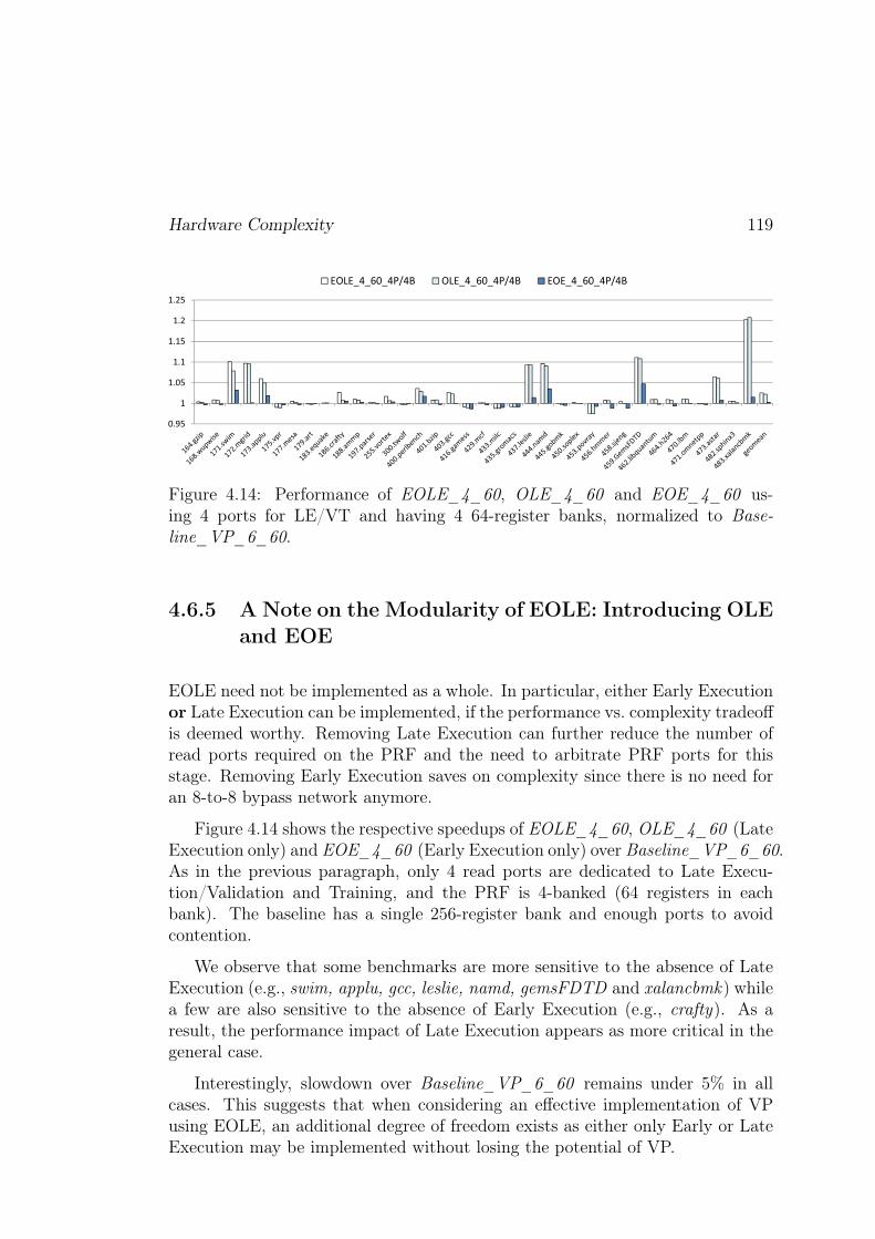
Hardware Complexity 119
Figure 4.14: Performance of EOLE_4_60, OLE_4_60 and EOE_4_60 us-ing 4 ports for LE/VT and having 4 64-register banks, normalized to Base-line_VP_6_60.
4.6.5 A Note on the Modularity of EOLE: Introducing OLEand EOE
EOLE need not be implemented as a whole. In particular, either Early Executionor Late Execution can be implemented, if the performance vs. complexity tradeoffis deemed worthy. Removing Late Execution can further reduce the number ofread ports required on the PRF and the need to arbitrate PRF ports for thisstage. Removing Early Execution saves on complexity since there is no need foran 8-to-8 bypass network anymore.
Figure 4.14 shows the respective speedups of EOLE_4_60, OLE_4_60 (LateExecution only) and EOE_4_60 (Early Execution only) over Baseline_VP_6_60.As in the previous paragraph, only 4 read ports are dedicated to Late Execu-tion/Validation and Training, and the PRF is 4-banked (64 registers in eachbank). The baseline has a single 256-register bank and enough ports to avoidcontention.
We observe that some benchmarks are more sensitive to the absence of LateExecution (e.g., swim, applu, gcc, leslie, namd, gemsFDTD and xalancbmk) whilea few are also sensitive to the absence of Early Execution (e.g., crafty). As aresult, the performance impact of Late Execution appears as more critical in thegeneral case.
Interestingly, slowdown over Baseline_VP_6_60 remains under 5% in allcases. This suggests that when considering an effective implementation of VPusing EOLE, an additional degree of freedom exists as either only Early or LateExecution may be implemented without losing the potential of VP.

120 A New Execution Model Leveraging Value Prediction: EOLE
4.7 Conclusion
Single thread performance remains the driving force for high-performance design.However, hardware complexity and power consumption remain major obstaclesto the implementation of new architectural features.
Value Prediction (VP) is one of such features that has still not been imple-mented in real-world products due to those obstacles. Fortunately, the mecha-nisms we have presented in Chapter 3 partially addresses these issues [PS14b]. Inparticular, prediction validation can be performed at commit time without sac-rificing performance. This greatly simplifies design, as the burdens of validationat execution-time and selective replay for VP in the OoO engine are eliminated.
Building on this work, we have proposed EOLE, an {Early | Out-of-Order| Late} Execution microarchitecture aiming at further reducing the hardwarecomplexity and the power consumption of a VP-augmented superscalar processor.
With Early Execution, single-cycle instructions whose operands are immediateor predicted are computed in-order in the front-end and do not have to flowthrough the OoO engine. With Late Execution, predicted single-cycle instructionsas well as very high confidence branches are computed in-order in a pre-commitstage. They also do not flow through the OoO engine. As a result, EOLEsignificantly reduces the number of instructions dispatched to the OoO engine.
Considering a 6-wide, 60-entry IQ processor augmented with VP and valida-tion at commit time as the baseline, EOLE allows to drastically reduce the overallcomplexity and power consumption of both the OoO engine and the PRF. EOLEachieves performance very close to the baseline using a 6-issue, 48-entry IQ OoOengine. It achieves similar or higher performance when using a 4-issue, 60-entryIQ engine, with the exception of four benchmarks, vpr, milc, gromacs and povray(2.7% slowdown at worst).
With EOLE, the overhead over a 6-wide, 60-entry IQ processor (without VP)essentially consists of relatively simple hardware components, the two set of ALUsin the Early and Late Execution, a bypass network and the value predictor tablesand update logic. The need for additional ports on the PRF is also substantiallylowered by the reduction in issue width and some PRF optimizations (e.g., bank-ing). Lastly, the PRF could be distributed into a copy in the OoO engine anda copy only read by the Late Execution/Validation and Training stage. Conse-quently, EOLE results in a much less complex and power hungry OoO engine,while generally benefiting from higher performance thanks to Value Prediction.Moreover, we hinted that Late Execution and Early Execution can be imple-mented separately, with Late Execution appearing as more cost-effective.
Further studies to evaluate the possible variations of EOLE designs may in-clude the full range of hardware complexity mitigation techniques that were dis-cussed in Section 4.6.3 for both Early and Late execution, and the exploration

Conclusion 121
of other possible sources of Late Execution e.g., indirect jumps, returns, but alsostore address computations. One can also explore the interactions between EOLEand previous propositions aiming at reducing the complexity of the OoO enginesuch as the Multicluster architecture [FCJV97] or register file-oriented optimiza-tions [WB96]. Finally, there is still a need to look for practical and storage-effective value prediction schemes as well as even more accurate predictors. Inthe next Chapter, we propose such an infrastructure by relying on D-VTAGEand block-based instruction fetch mechanisms.

122 A New Execution Model Leveraging Value Prediction: EOLE

Chapter 5
A Realistic, Block-Based PredictionInfrastructure
This Chapter covers a publication1 in the International Symposium on High Per-formance Computer Architecture (HPCA 2015) [PS15a].
5.1 Introduction & Motivations
Taking a step back, only two distinct components are responsible for the majorityof the additional complexity brought by Value Prediction: 1) the out-of-orderexecution engine and 2) the intrinsic complexity of the Value Prediction datapath.
The first source of complexity was studied in Chapter 3 [PS14b] and Chapter4 [PS14a]. We showed that the out-of-order engine does not need to beoverhauled to support VP. First, very high accuracy can be enforced at rea-sonable cost in coverage and minimal complexity [PS14b]. Thus, both predictionvalidation and recovery by squashing can be done outside the out-of-order (OoO)engine, at commit time instead of execution time. Moreover, we devised a newpipeline organization, EOLE (depicted in Figure 5.1), that leverages VP withvalidation at Commit to execute many instructions outside the OoO core, in-order [PS14a]. Those instructions are processed either as-soon-as-possible (EarlyExecution in parallel with Rename) using predicted/immediate operands or as-late-as-possible (Late Execution just before Commit) if they are predicted. WithEOLE, the issue width can be reduced without sacrificing performance, mechan-ically decreasing the number of ports on the Physical Register File (PRF). Val-idation at commit time also allows to leverage PRF banking for prediction andvalidation, leading to an overall number of ports similar in EOLE with VP and in
1D-VTAGE was also introduced in this publication but was covered in Chapter 3.
123

124 A Realistic, Block-Based Prediction Infrastructure
Figure 5.1: Pipeline diagram of EOLE.
the baseline case without VP. That is, EOLE achieves VP-enabled performancewhile the overall hardware cost of the execution engine is actually lower than ina baseline processor without VP.
In this Chapter, we address the remaining source of hardware complexity,which is associated with the value predictor infrastructure itself.
First, to handle the multiple value predictions needed each cycle in a wideissue processor, we proposeBlock-Based value Prediction (BBP or BeBoP). Withthis scheme, all predictions associated with an instruction fetch block are put ina single predictor entry. The predictor is therefore accessed with the PC ofthe instruction fetch block and the whole group of predictions is retrieved ina single read. BeBoP accommodates currently implemented instruction fetchmechanisms. However, it only addresses complexity of operation, but not storagerequirement.
As a result, in a second step, we propose ways to reduce the storage footprintof the tightly-coupled hybrid predictor presented in Chapter 3, D-VTAGE. Thispredictor can be made very space-efficient as it can use partial strides (e.g., 8-and 16-bit). As a result, its storage cost is amenable to that of the I-Cache orthe branch predictor.
Third, we devise a cost-effective checkpoint-based implementation of the spec-ulative last-value window that was previously discussed in 2.2. Such a window isrequired due to the presence of a stride-based prediction scheme in D-VTAGE.Without it, instructions in loops of which there can be several instances in thepipeline are unlikely to be correctly predicted.
5.2 Block-Based Value Prediction
5.2.1 Issues on Concurrent Multiple Value Predictions
Modern superscalar processors are able to fetch/decode several instructions percycle. Ideally, the value predictor should be able to predict a value for all instruc-tions fetched during that cycle.
For predictors that do not use any local value history to read tables (e.g., the

Block-Based Value Prediction 125
Figure 5.2: Prediction attribution with BeBoP and 8-byte fetch blocks. Thepredictor is accessed with the currently fetched PC and predictions are attributedusing byte indexes as tags.
Last Value Predictor, the Stride predictor or VTAGE), and when using a RISCISA producing at most one result per instruction (e.g., Alpha), a straightforwardimplementation of the value predictor consists in mimicking the organization ofthe instruction fetch hardware in the different components of predictor. Predic-tions for contiguous instructions are stored in contiguous locations in the predic-tor components and the same interleaving structures are used in the instructioncache, the branch predictor and the value predictor. However, for predictors us-ing local value history (e.g., FCM [SS97a]), even in this very favorable scenario,some predictor components must be bank-interleaved at the instruction level andthe banks individually accessed with different indexes.
Moreover, the most popular ISAs do not have the regularity property of Alpha.For x86 – that we consider in this study – some instructions may produce severalresults, and information such as the effective PC of instructions in the fetchblock2 and the number of produced values are known after several cycles (afterpre-decoding at Fetch and after decoding, respectively). That is, there is nonatural way to associate a value predictor entry with a precise PC:Smooth multiple-value prediction on a variable-length ISA remains a challengein itself.
2Storing boundary bits in the I-cache can remedy this, but at high storage cost [AMD98].
126 A Realistic, Block-Based Prediction Infrastructure
5.2.2 Block-based Value-Predictor accesses
We remedy this fundamental issue by proposing Block-Based Value Prediction(BeBoP). To introduce this new access scheme and layout, we consider a VTAGE-like predictor, but note that block-based prediction can be generalized to mostpredictors.
The idea is to access the predictor using the fetch-block PC (i.e., the currentPC right-shifted by log2(fetchBlockSize)), as well as some extra global infor-mation as defined in VTAGE [PS14b]. Instead of containing a single value, theentry that is accessed now consists in Npred values (Npred > 0). The mth value inthe predictor entry is associated with the mth result in the fetch block, and notwith its precise PC.
The coupling of the Fetch/Decode pipeline and the value predictor is illus-trated in more details in Figure 5.2, assuming an x86-like ISA and a VTAGE-likevalue predictor. Fetch first retrieves a chunk of n bytes from the I-cache, thenpre-decodes it to determine instruction boundaries, to finally put it in a decodequeue. This queue feeds the x86 decoders in charge of generating µ-ops. Atthe same time, the value predictor is read using the fetch-block PC and globalinformation to retrieve Npred predictions. After Decode, the predictions are at-tributed to the µ-ops in the fetch block by matching instruction boundaries withsmall per-prediction tags. The rationale behind this tagging scheme is highlightedin the next paragraph. Finally, predictions proceeds to the PRF depending onthe saturation of the confidence counter associated with each of them.
5.2.2.1 False sharing issues
Grouping predictions introduces the issue of false prediction sharing if one usesthe most significant bits of the PC to index the value predictor (e.g., removing the4 last bits of the address when fetching 16-byte instruction blocks). False sharingarises when an instruction block is fetched with two distinct entry points e.g.,instructions I1 and I2. In that case, the traces of µ-ops generated for this blockat Decode are different, leading to complete confusion in the predicted values.
We avoid this issue by tagging each prediction in the block with the lastlog2(fetchBlockSize) bits of the instruction PC to which the prediction wasattributed the last time the block was fetched.
That is, to access the predictor, we use the block address, and once Npred
predictions have flowed out of the predictor, they are attributed to each µ-op bymatching the indexes given by the boundary bits against the per-prediction tags,as described in Figure 5.2. In this particular case, the first instruction of theblock is I2, while predictions correspond to the case where the block was enteredthrough instruction I1. If no specific action were taken, prediction P1 would beattributed to UOP1 of I2. However, thanks to the use of tags to mask predictions,

Block-Based Value Prediction 127
prediction P2 (with tag T2 equals 3) is attributed to UOP1 of I2 (with boundary3 since I2 starts at byte 3). That is, P1 is not shared between I1 and I2.
Tags are modified when the predictor is updated with the following constraint:a greater tag never replaces a lesser tag, so that the entry can learn the “real”location of instructions/µ-ops in the block. For instance, if the block was enteredthrough I2 but has already been entered through I1 before, then the tag associatedwith P1 is the address of the first byte of I1 (i.e., 0). The address of the firstbyte of I2 is greater than that of I1, so it will not replace the tag associated withP1 in the predictor, even though dynamically, for that instance of the block, I2is the first instruction of the block. As a result, the pairing P1/I1 is preservedthroughout execution. This constraint does not apply when the entry is allocated.
5.2.2.2 On the Number of Predictions in Each Entry
The number of µ-ops producing a register depends on the instructions in the block,but only the size of the instruction fetch block is known at design-time. Thus,Npred should be chosen as a tradeoff between coverage (i.e., provision enoughpredictions in an entry for the whole fetch block) and wasted area (i.e., havingtoo many predictions provisioned in the entry). For instance, in Figure 5.2,since I1 and I2 both consume a prediction, only UOP2 of instruction I3 can bepredicted.
In Section 5.6.2, we will study the impact of varying Npred while keeping thesize of the predictor constant. Specifically, a too small Npred means that potentialis lost while a too big Npred means that space is wasted as not all prediction slotsin the predictor entry are used. Additionally, at constant predictor size, a smallerNpred means more entries, hence less aliasing.
5.2.2.3 Multiple Blocks per Cycle
In order to provide high instruction fetch bandwidth, several instruction blocksare fetched in parallel on wide-issue processors. For instance, on the EV8 [SFKS02],two instruction fetch blocks are retrieved each cycle. To support this parallelfetch, the instruction cache has to be either fully dual-ported or bank-interleaved.In the latter case, a single block is fetched on a conflict unless the same blockappears twice. Since fully dual-porting is much more area- and power-consuming,bank interleaving is generally preferred.
In BeBoP, the (potential) number of accesses per cycle to the predictor tablesis similar to the number of accesses made to the branch predictor tables, i.e., upto 3 accesses per fetch block: Read at fetch time, second read at commit time andwrite to update. This adds up to 6 accesses per cycle if two instruction blocksare fetched each cycle.
128 A Realistic, Block-Based Prediction Infrastructure
However, for value predictor or branch predictor components that are indexedusing only the block PC (e.g., Last Value component of VTAGE and Stridepredictors), one can replicate the same bank interleaving as the instruction cachein the general case. If the same block is accessed twice in a single cycle, stride-based predictors must provision specific hardware to compute predictions for bothblocks. This can be handled through computing both (Last Value + stride) and(Last Value + stride1 + stride2) using 3-input adders.
For value or branch predictor components that are indexed using the globalbranch history or the path history, such as VTAGE tagged components, one canrely on the interleaving scheme that was proposed to implement the branch pre-dictor in the EV8 [SFKS02]. By forcing consecutive accesses to map to differentbanks, the 4-way banked predictor components are able to provide predictions forany two consecutively fetched blocks with a single read port per bank. Moreover,Seznec states that for the TAGE predictor [Sez11b], one can avoid the secondread at update. The same can be envisioned for VTAGE. Lastly, since they aremore infrequent than predictions, updates can be performed through cycle steal-ing. Therefore, tagged components for VTAGE and TAGE can be designed withsingle ported RAM arrays.
That is, in practice, the global history components of a hybrid predictor usingBeBoP such as VTAGE-Stride or D-VTAGE – that was presented in Chapter 3 –can be built with the same bank-interleaving and/or multi-ported structure as amultiple table global history branch predictor such as the EV8 branch predictoror the TAGE predictor. Only the Last Value Table (LVT) of (D-)VTAGE mustreplicate the I-Cache organization.
5.3 Implementing a Block-based D-VTAGE Pre-dictor
In 3.5.2, we presented D-VTAGE, an efficient, tightly-coupled hybrid value predic-tor. Its advantages are twofold. First, it is able to predict control-flow dependentpatterns, strided patterns and control-flow dependent strided patterns. Second, ithas been shown that short strides could capture most of the coverage of full stridesin a stride-based value predictor [GVDB01]. As such, using D-VTAGE instead ofVTAGE, for instance, would allow to greatly reduce storage requirements. Par-tial strides should be sign-extended when they flow out of the predictor to beadded to the base value. This is required to enable the use of negative strides.
Nonetheless, a concrete implementation of D-VTAGE is not straightforwardas it should be practical enough but still worth the transistors spent from a perfor-mance standpoint. This is true for an instruction-based D-VTAGE predictor, butalso for a block-based implementation, as BeBoP uncovers some new challenges
Implementing a Block-based D-VTAGE Predictor 129
for the architect. In this section, we describe the main implementation-relatedissues that must be addressed.
5.3.1 Complexity Intrinsic to D-VTAGE
5.3.1.1 Prediction Critical Path
Because of its stride-based prediction mechanism, D-VTAGE possesses a predic-tion critical path. Specifically, the prediction for a given instance must be madeavailable fast enough so that a subsequent instance can use it as its last value.In other words, bypassing the output of the adder to its input in a single cycleis required to predict back-to-back3 occurrences [PS14b], as previously shown inFigure 3.1.
While this might prove challenging, it actually appears feasible as 64-bit ad-dition and bypassing are already performed in a single cycle in the out-of-orderengine.
In the case where two instances of the same instruction are fetched in thesame cycle, a 3-input adder can provide the prediction for the second instance.
5.3.1.2 Associative Read
D-VTAGE features several tagged components that are accessed in parallel tofind the relevant stride. In nature, this is an associative read, a usually costlyoperation. However, since the value predictor is not on the critical path becausethe prediction is only needed at Dispatch,4 the data does not need to flow outof the components in an associative fashion. Rather, only the tags need to beread at the same time, while the stride can be fetched directly from the correctcomponent, once identified. Moreover, the components are partially tagged, e.g.,tags are in the range of 10-15 bits instead of full width, hence comparison energyand latency are lower than for D-Cache tag matching, for instance.
5.3.1.3 Speculative History
Because of its stride-based nature, D-VTAGE relies on the value produced by themost recent instance of an instruction to compute the prediction for the newlyfetched instance. As many instances of the same instruction can coexist in theinstruction window at the same time, the hardware should provide some supportto grab the predicted value for the most recent speculative instance. Such ahardware structure could be envisioned as a chronologically ordered associativebuffer whose size is roughly that of the ROB. For instruction-based VP, such a
3Fetched in two consecutive cycles, e.g., in tight loops4Rename if Early Execution is implemented [PS14a].

130 A Realistic, Block-Based Prediction Infrastructure
design should prove slow and power hungry, e.g., more than ROB-size entries atworst and 8 parallel associative searches each cycle for the simulation frameworkwe are considering (8-wide, 6-issue superscalar).
Fortunately, BeBoP allows to greatly reduce the number of required entriesas well as the number of parallel accesses each cycle. We develop such a designof the speculative window in Section 5.4.
5.3.2 Impact of Block-Based Prediction
5.3.2.1 Predictor Entry Allocation
As for VTAGE and TAGE, the allocation policy in the tagged components ofD-VTAGE is driven by the usefulness of a prediction [SM06]. The allocation of anew entry also depends on whether the prediction was correct or not. However,we consider a block-based predictor. Therefore, the allocation policy needs to bemodified since there can be correct and incorrect predictions in a single entry,and some can be useful or not.
In our implementation, a new entry is allocated if at least one prediction in theblock is wrong. However, the confidence counter of predictions from the providingentry are propagated to the newly allocated entry. This allows the predictor tobe efficiently trained (allocate on a wrong prediction) while preserving coveragesince high confidence predictions are duplicated. The usefulness bit is kept perblock and set if a single prediction of the block is useful as defined in [PS14b],that is if it is correct and the prediction in the alternate5 component is not.
5.3.2.2 Prediction Validation
The EOLE processor model assumes that predictions are used only if they arevery high confidence. Therefore, unused predictions must be stored to wait forvalidation in order to train the predictor. To that extent, we assume a FIFOUpdate Queue where prediction blocks are pushed at prediction time and poppedat validation time. This structure can be read and written in the same cycle, butreads and writes are guaranteed not to conflict by construction. Specifically, thisqueue should be able to contain all the predictions potentially in flight after thecycle in which predictions become available. It would also be responsible forpropagating any information visible at prediction time that might be needed atupdate time (e.g., predictor entry, confidence, etc.).
In essence, this structure is very similar to the speculative window that shouldbe implemented for D-VTAGE. Indeed, it contains all the inflight predictions foreach block, and it should be able to rollback to a correct state on a pipeline flush
5Next lower matching component.

Block-Based Speculative Window 131
(we describe recovery in the context of BeBoP in the next Section). However,to maximize coverage, the FIFO update queue must be large enough so thatprediction information is never lost due to a shortage of free entries. On thecontrary, we will see that we can implement the speculative window with muchless entries than the theoretical number of blocks that can be in flight at any giventime. Moreover, the speculative window must be associatively searched every timea prediction block is generated while the FIFO does not need associative lookup(except potentially for rollback). As a result, if both structures essentially storethe same data, it is still interesting to implement them as two separate items.
5.4 Block-Based Speculative Window
5.4.1 Leveraging BeBoP to Implement a Fully AssociativeStructure
In the context of superscalar processors where many instructions can be in flight,computational predictors such as D-VTAGE cannot only rely on their Last ValueTable. Indeed, in the case where several instances of a loop body are live in thepipeline, the last value required by the predictor may not have been retired, oreven computed. As a result, a speculative LVT is required so that the predictorcan keep up with the processor. Given the fact that an instruction is allowed touse its prediction only after several tens of previous instances have been correctlypredicted (because of confidence estimation), keeping the predictor synchronizedwith the pipeline is even more critical. As a result, the third and last contributionof this Chapter deals with the specific design of the Speculative Window.
An intuitive solution would consist in using an associative buffer that canstore all the in-flight predictions. On each lookup, this buffer would be probedand provide the most recent prediction to be used as the last value, if any. Un-fortunately, its size would be that of the ROB plus all instructions potentially inflight between prediction availability (Rename) and Dispatch. Associative struc-tures of this size – such as the Instruction Queue – are known to be slower thantheir RAM counterparts as well as power hungry [EA02, KL03, PJS97].
Nonetheless, thanks to BeBoP, the number of required entries is actually muchsmaller than with instruction-based VP, and the number of accesses is at mostthe number of fetch blocks accessed in a given cycle. Furthermore, althoughthis buffer behaves as a fully associative structure for reads, it acts as a simplecircular buffer for writes because it is chronologically ordered. That is, whenthe predictor provides a new prediction block, it simply adds it at the head ofthe buffer, without having to match any tag. If the head overlaps with the tail(i.e., if the buffer was dimensioned with too few entries), both head and tail are

132 A Realistic, Block-Based Prediction Infrastructure
Figure 5.3: N-way speculative window. The priority encoder controls the mul-tiplexer by prioritizing the matching entry corresponding to the most recent se-quence number.
advanced. Lastly, partial tags (e.g., 15 bits) can be used to match the blocks, asVP is speculative by nature (false positive is allowed).
To order the buffer and thus ensure that the most recent entry is providing thelast values if multiple entries hit, we can simply use internal sequence numbers.In our experiments, we use the sequence number of the first instruction of theblock. A block-diagram of our speculative window is shown in Figure 5.3.
5.4.2 Consistency of the Speculative History
Block-based VP entails intrinsic inconsistencies in the speculative window. Forinstance, if a branch is predicted as taken, some predictions are computed whilethe instructions corresponding to them have been discarded (the ones in the sameblock as the branch but located after the branch). Therefore the speculativehistory becomes inconsistent even if the branch is correctly predicted.
Moreover, pipeline squashing events may also cause inconsistencies in thespeculative window. The same stands for the FIFO update queue, as it is orga-nized in a similar fashion as the speculative window6. To illustrate why, let usdenote the first instruction to be fetched after the pipeline flush as Inew and theinstruction that triggered the flush as Iflush. Let us also denote the fetch blockaddress of Inew as Bnew and that of Iflush as Bflush.
On a pipeline flush, all the entries whose associated sequence number is strictlygreater than that of Iflush are discarded in both the speculative window and
6In our implementation, each entry of the FIFO update queue is also tagged with the internalsequence number of the first instruction in the fetch-block to enable rollback.

Block-Based Speculative Window 133
the FIFO update queue. The block at the head of both structures thereforecorresponds to Bflush. We must then consider if whether Inew belongs to thesame fetch block as Iflush or not. If not, the predictor should operate as usualand provide a prediction block for the new block, Bnew. If it does belong to thesame block (i.e. Bflush equals Bnew), several policies are available to us.
Do not Repredict and Reuse (DnRR) This policy assumes that all thepredictions referring to Bflush/Bnew are still valid after the pipeline flush. Thatis, Inew and all subsequent instructions belonging to Bflush will be attributedpredictions from the prediction block that was generated when Bflush/Bnew wasfirst fetched. Those predictions are available at the head of the FIFO updatequeue. With this policy, the heads of the speculative history and FIFO updatequeue are not discarded.
Do not Repredict and do not Reuse (DnRDnR) This policy is similar toDnRR except that all newly fetched instruction belonging to Bflush/Bnew will beforbidden to use their respective predictions. The reasoning behind this policy isthat the case where Bnew equals Bflush typically happens on a value misprediction,and if a prediction was wrong in the block, chances are that the subsequent oneswill be wrong too.
Repredict (Repred) This policy squashes the heads of the speculative historyand FIFO update queue (the blocks containing Iflush). Then, once Inew is fetched,a new prediction block for Bflush/Bnew is generated. In general, this provides thesame predictions for the block, however, more up-to-date predictions may begenerated if the entry has been updated since it was accessed the first time bythis block.
Keep Older, Predict Newer (Ideal) This idealistic policy is able to keepthe predictions pertaining to instructions of block Bflush older than Iflush whilegenerating new predictions for Inew and subsequent instructions belonging toBnew. In essence, this policy assumes a speculative window (resp. FIFO updatequeue) that tracks predictions at the instruction level, rather than the blocklevel. As a result, the speculative window (resp. FIFO update queue) is alwaysconsistent.

134 A Realistic, Block-Based Prediction Infrastructure
5.5 Evaluation Methodology
5.5.1 Simulator
We use the framework described in 3.6 with the modifications made to evaluateEOLE detailed in 4.4. Table 3.2 describes our model: A relatively aggressive4GHz, 6-issue superscalar pipeline. The fetch-to-commit latency is 20 cycles aswe are dedicating one stage to validation and late-execution, as in the previousChapters. The in-order front-end and in-order back-end are overdimensioned totreat up to 8 µ-ops per cycle. We model a deep front-end (15 cycles) coupledto a shallow back-end (5 cycles) to obtain a realistic branch/value mispredictionpenalty: 20/21 cycles minimum. We allow two 16-byte blocks of instructions tobe fetched each cycle, potentially over a single taken branch. The OoO scheduleris dimensioned with a unified centralized 60-entry IQ and a 192-entry ROB onpar with the latest commercially available Intel microarchitecture.
In the first experiment, we consider as a baseline a pipeline with Value Pre-diction without EOLE. The processor is therefore similar to the one described inTable 3.2, except the pipeline latency is 20 cycles instead of 19 cycles, as we stilldedicate a stage to validation. Moreover, the register file is 4-banked to model arealistic pipeline with VP without EOLE (only 2 additional write ports and 2 ad-ditional read ports per bank). We refer to this model as the Baseline_VP_6_60configuration (6-issue, 60-entry IQ).
In the last experiment, we go back to a baseline without Value Prediction atall. In that case, the processor is exactly the one depicted in Table 3.2: the Val-idation and Late Execution stage is removed, yielding a fetch-to-commit latencyof 19 cycles. We refer to this model as the Baseline_6_60 configuration.
In the remaining experiments, our baseline uses EOLE: we consider a 1-deep,8-wide Early Execution stage and an 8-wide Late Execution/Validation stagelimited to 4 read ports per bank, with a 4-bank register file and a 4-issue out-of-order engine, as described in 4.6.3. We refer to this model as the EOLE_4_60configuration.
5.5.1.1 Value Predictor Operation
In its baseline version, the predictor makes a prediction at Fetch for every eligibleµ-op (i.e., producing a 64-bit or less register that can be read by a subsequent µ-op, as defined by the ISA implementation). To index the predictor, we XOR thePC of the x86_64 instruction with the µ-op index inside that x86_64 instruction[PS14a]. This avoids all µ-ops mapping to the same entry, but may create aliasing.We assume that the predictor can deliver fetch-width predictions each cycle. Thepredictor is updated in the cycle following retirement.

Experimental Results 135
When using block-based prediction, the predictor is simply accessed with thePC of each fetch block and provides several predictions at once for those blocks.Similarly, update blocks are built after retirement and an entry is updated assoon as an instruction belonging to a block different than the one being built isretired. Update can thus be delayed for several cycles.
We use the D-VTAGE configuration depicted in Table 3.1: 8K-entry basecomponent with 6 1K-entry partially tagged components. The partial tags are 13bits for the first component, 14 for the second, and so on. Histories range from 2to 64 bits in a geometric fashion. We also use 3-bit Forward Probabilistic Counterswith probabilities v = {1, 1
16, 116, 116, 116, 132, 132}. Unless specified otherwise, we use
64-bit strides in the predictor. Finally, to maximize accuracy, we tag the LVTwith the 5 higher bits of the fetch block PC.
5.5.2 Benchmark Suite
We reuse the benchmarks used to evaluate the contribution of Chapter 3. Specif-ically, we use 18 integer benchmarks and 18 floating-point programs. Table 3.3summarizes the benchmarks we use as well as their input, which are part ofthe reference inputs provided in the SPEC software packages. To get relevantnumbers, we identify a region of interest in the benchmark using Simpoint 3.2[PHC03]. We simulate the resulting slice in two steps: First, warm up all struc-tures (caches, branch predictor and value predictor) for 50M instructions, thencollect statistics for 100M instructions.
5.6 Experimental Results
In further experiments, when we do not give speedup for each individual bench-mark, we represent results using the geometric mean of the speedups on top ofthe [Min,Max] box plot of the speedups.
5.6.1 Baseline Value Prediction
Figure 5.4 depicts the speedup of a 4-issue, 60-entry IQ, 4-bank PRF, 12-readports per bank EOLE architecture featuring D-VTAGE over Baseline_VP_6_60.As expected, very little slowdown is observed by scaling down the issue width from6 to 4 (at worst 0.982 in povray). We refer to this configuration as EOLE_4_60and use it as our baseline in further experiments.

136 A Realistic, Block-Based Prediction Infrastructure
0.95
1
1.05
1.1
1.15
1.2
1.25
EOLE_4_60 (w/ D-VTAGE)
Figure 5.4: Speedup of bank/port constrained EOLE_4_60 w/ D-VTAGE overBaseline_VP_6_60.
0.8
0.85
0.9
0.95
1
1.05
4p 1K +
6x128
6p 1K +
6x128
8p 1K +
6x128
4p 2K +
6x256
6p 2K +
6x256
8p 2K +
6x256
[Q1,Med] [Med,Q3] gmean
(a) Impact of the number of predictions per entry in D-VTAGE.
0.8
0.85
0.9
0.95
1
1.05
512 +
6x128
1K +
6x128
2K +
6x128
512 +
6x256
1K +
6x256
2K +
6x256
(b) Impact of the key structures sizes for a 6 predictions per entryD-VTAGE.
Figure 5.5: Performance of D-VTAGE with BeBoP normalized to the perfor-mance of EOLE_4_60.

Experimental Results 137
5.6.2 Block-Based Value Prediction
5.6.2.1 Varying the Number of Entries and the Number of Predictionsper Entry
Figure 5.5 (a) shows the impact of using BeBoP on top of EOLE_4_60. Werespectively use 4, 6 and 8 predictions per entry in the predictor, while keepingthe size of the predictor roughly constant. For each configuration, we study apredictor with either a 2K-entry base predictor and six 256-entry tagged compo-nents or a 1K-entry base predictor and six 128-entry tagged components. TheIdeal policy is used to handle recovery in the infinite speculative window.
We first make the observation that 6 predictions per 16-byte fetch block appearsufficient. Second, we note that reducing the size of the structures plays a keyrole in performance. For instance, maximum slowdown is 0.876 for {6p 1K +6x128}, but only 0.957 for {6p 2K + 2x256}.
To gain further insight, in Figure 5.5 (b), we focus on a D-VTAGE predictorwith 6 predictions per entry and we vary the number of entries in the base compo-nent while keeping the number of entries in the tagged components constant, andvice-versa. The results hint that decreasing the sizes of the tagged componentsfrom 256 entries to 128 has more impact than reducing the number of entries ofthe base predictor.
In further experiments, we consider an optimistic predictor configuration witha 2K-entry base predictor and six 256-entry tagged components. Each entrycontains six predictions. Such an infrastructure has an average slowdown overEOLE_4_60 of 0.991, a maximum slowdown of 0.957, and its size is around290KB assuming 64-bit strides are stored in the predictor.
5.6.2.2 Partial Strides
To predict, D-VTAGE adds a constant, the stride to the last value produced bya given instruction. In general, said constant is not very large. As most of theentries of D-VTAGE only contain strides and not last values, reducing the size ofstrides from 64 bits to 16 or 8 bits would provide tremendous savings in storage.
Using the baseline D-VTAGE configuration, but varying the size of the stridesused to predict, we found that average speedup (gmean) ranges from 0.991 (64-bitstrides) to 0.985 (8-bit strides), while maximum slowdown increases from 0.957(64-bit) to 0.927 (8-bit). However, results for 16-, 32- and 64-bit strides are verysimilar. In other words, performance is almost entirely conserved even though thesize of the predictor has been reduced from around 290KB (64-bit) to respectively203KB (32-bit), 160KB (16-bit) and 138KB (8-bit). That is, it makes little doubtthat by combining partial strides and a reduction in the number of entries of thebase predictor, good performance can be attained with a storage budget that is

138 A Realistic, Block-Based Prediction Infrastructure
0.9
0.95
1
1.05
Ideal Repred DnRDnR DnRR
[Q1,Med] [Med,Q3] gmean
(a) Impact of the recovery policy of the speculative window andFIFO update queue on speedup over EOLE_4_60.
0.8
0.85
0.9
0.95
1
1.05
∞ 64 56 48 32 16 None
(b) Impact of the size of the speculative window on speedup overEOLE_4_60. The recovery policy is DnRDnR.
Figure 5.6: Impact of the speculative window on performance for D-VTAGE withBeBoP. Speedup over EOLE_4_60.
comparable to that of the L1 D/I-Cache or the branch predictor.
5.6.2.3 Recovery Policy
Figure 5.6 (a) gives some insight on the impact of the speculative window recoverypolicy used for D-VTAGE with BeBoP, assuming an infinite window. In generalthe differences between the realistic policies are marginal, and on average, theybehave equivalently. As a result, we only consider DnRDnR as it reduces thenumber of predictor accesses versus Repred and it marginally outperforms DnRR.
5.6.2.4 Speculative Window Size
Figure 5.6 (b) illustrates the impact of the speculative window size on D-VTAGE.When last values are not speculatively made available, some benchmarks are notaccelerated as much as in the infinite window case e.g., wupwise (0.914 vs. 0.984),

Experimental Results 139
Figure 5.7: Speedup brought by different D-VTAGE configurations on top of anEOLE_4_60 pipeline over Baseline_6_60.
applu (0.866 vs. 0.996), bzip (0.820 vs. 0.998) and xalancbmk (0.923 vs. 0.973).Having 56 entries in the window, however, provides roughly the same level ofperformance as an infinite number of entries, while using only 32 entries appearsas a good tradeoff (average performance is a slowdown of 0.980 for 32-entry and0.988 for ∞).
5.6.3 Putting it All Together
In previous experiments, we used a baseline EOLE_4_60 model having a D-VTAGE predictor with 6 predictions per entry, a 2K-entry base component andsix 256-entry tagged components. Because it also uses 64-bit strides, it requiresroughly 290KB, not even counting the speculative window. Fortunately, we sawthat the size of the base predictor could be reduced without too much impacton performance. Moreover, a speculative window with only a small number ofentries performs well enough. Therefore, in this Section, we devise three pre-dictor configurations based on the results of previous experiments as well as theobservation that partial strides can be used in D-VTAGE [GVDB01]. To obtaina storage budget we consider as reasonable, we use 6 predictions per entry and six128/256-entry tagged components. We then vary the size of the base predictor,the speculative window, and the stride length. Table 5.1 reports the resultingconfigurations.
In particular, for Small (' 16KB), we also consider a version with 4 pre-dictions per entry but a base predictor twice as big (Small_4p). For Medium(' 32KB), we found that both tradeoffs have similar performance on average;for Large (' 64KB), 4 prediction per entry perform worse than 6 on average,even with a 1K-entry base predictor. Thus, we do not report results for thehypothetical Medium_4p and Large_4p for the sake of clarity.
To summarize, the implementation cost – i.e., storage budget, but also RAMstructure (see Section 5.2.2.3) – is in the same range as that of the TAGE branch

140 A Realistic, Block-Based Prediction Infrastructure
Table 5.1: Final predictor configurations.
Predictor #Base ent. #Tagged ent. #Spec. win. ent. Str. len. Size (KB)Small_4p 256 (5b tag) 6× 128 32 (15b tag) 8 bits 17.26KBSmall_6p 128 (5b tag) 6× 128 32 (15b tag) 8 bits 17.18KBMedium 256 (5b tag) 6× 256 32 (15b tag) 8 bits 32.76KBLarge 512 (5b tag) 6× 256 56 (15b tag) 16 bits 61.65KB
.
predictor considered in the study. In particular, even if we omit the – marginal –cost of sequence numbers and that of the FIFO update queue (around 5.6KB atworst7), the sizes reported in Table 5.1 have to be contrasted with the 44KB ofthe EV8 branch predictor [SFKS02] that was planned to be implanted on actualsilicon.
Figure 5.7 reports the speedups obtained with these four predictor configura-tions on top of EOLE_4_60, over Baseline_6_60. We also show performancefor Baseline_VP_6_60 (first bar, white) and EOLE_4_60 with an instruction-based D-VTAGE (second bar, green). We observe that even with around 32KBof storage and practical mechanisms, we manage to preserve most of the speedupassociated with an idealistic implementation of VP. Maximum speedup decreasesfrom 1.726 (applu) for EOLE_4_60 to 1.622 (swim) for Medium and 1.710 (ap-plu) for Large. Average speedup goes from 1.154 for EOLE_4_60 down to 1.112for Medium and 1.130 for Large. A noteworthy data point is GemsFDTD, whereMedium and Large perform slightly better than EOLE_4_60. This is due toaccuracy being slightly higher in Medium and Large, even if coverage is lower.
Allocating around 17KB of storage to the predictor, however, hurts per-formance noticeably: Average speedup over Baseline_6_60 is only 1.088 forSmall_6p (although max. is 1.622 in swim). Yet, it still represents a noticeableimprovement. Interestingly, for this storage budget, using only 4 predictions perentry but a bigger base predictor (Small_4p) provides better performance onaverage: 1.095. This is because a smaller base predictor suffers from aliasing inwupwise, applu, namd and GemsFDTD.
As a result, we claim that BeBoP combined to D-VTAGE is an appealingpossibility for an actual implementation of VP, even at reasonable storage budget(e.g., 16/32KB).
7116 blocks in flight at worst in our simulation framework, if a block is an instruction anda branch.

Related Work on Predictor Storage & Complexity Reduction 141
5.7 Related Work on Predictor Storage & Com-plexity Reduction
To further improve space-efficiency, Sato et al. propose to use two tables for theLast Value Predictor (2-mode scheme) [SA00]. One contains full-width valuesand the other 8- or 16-bit values. At prediction time, both tables are accessedand the one with a tag match provides the prediction. Using 0/1-bit values isalso a very space-efficient alternative [SA02].
Loh extends the 2-mode scheme by implementing several tables of differingwidth [Loh03]. The width of the result is predicted by a simple classifier at pre-diction time. By serializing width-prediction and table access, a single predictiontable has to be accessed in order to predict.
Executing load immediate instructions for free in the front-end as suggestedin 3.6.2.1 overlaps with the two propositions mentioned above, at lower cost.
Burtscher et al. reduce the size of a Last n value predictor by noting thatmost of the high-order bits are shared between recent values [BZ00]. Hence, theyonly keep one full-width value and the low-order bits of the n− 1 previous ones.Moreover, they remark that if n > 1, then a stride can be computed on the fly,meaning that stride prediction can be done for nearly free.
Finally, Lee et al. leverage trace processors to reduce complexity [LWY00].They decouple the predictor from the Fetch stage: Predictions are attributed totraces by the fill unit. Thus, they solve the access latency and port arbitrationproblems on the predictor. They also propose some form of block-based predictionby storing predictions in the I-cache [LY01]. However, a highly ported centralizedstructure is still required to build predictions at retire-time. To address this,Bhargava et al. replace the value predictor by a Prediction Trace Queue thatrequires a single read port and a single write port [BJ02]. Lastly, Gabbay andMendelson also devise a hardware structure to handle multiple prediction percycle by using highly interleaved tables accessed with addresses of instructionsin the trace cache [GM98a]. Unfortunately, the scope of all these studies except[LY01] is limited to trace processors.
5.8 Conclusion
Value Prediction is a very attractive technique to enhance sequential performancein a context where power efficiency and cycle time entail that the instructionwindow cannot scale easily. However, many implementation details make VPhard to imagine on real silicon.
In this Chapter, we first described BeBoP, a block-based prediction schemeadapted to complex variable-length ISAs such as x86 as well as usually imple-
142 A Realistic, Block-Based Prediction Infrastructure
mented fetch mechanism. BeBoP contributes to reducing the number of portsrequired on the predictor by allowing several instructions to be predicted in asingle access. Then, to reduce the footprint of the value predictor, we providedsolutions for an actual implementation of D-VTAGE, a space-efficient tightly-coupled hybrid of VTAGE and a Stride predictor. In particular, a small spec-ulative window to handle in-flight instructions that only requires an associativesearch on read operations, and a reduction in size thanks to partial strides andsmaller tables. In a nutshell, the hardware complexity of D-VTAGE is similar tothat of an aggressive TAGE branch predictor.
As a result, by combining the work presented in Chapters 3 and 4 with BeBoP,we provide one possible implementation of VP that requires around 32KB toaround 64KB of additional storage. The issue width is reduced when comparedto the baseline 6-issue model. Nonetheless, this implementation of VP is able tospeed up execution by up to 62.2% with an average speedup of 11.2% (for the32KB predictor version).
Conclusion
Over the past decade, computer architects have especially focused on efficientmulti-core architectures and the challenges they offer, whether it be the memorymodel, coherency, the interconnect, shared caches management, and so on. Cur-rently, the community appears to have reached a consensus in the fact that futuremulti- and many-cores will be heterogeneous. The rationale behind this choiceis that even for parallel programs, the sequential portion caps the speedup thatcan be obtained by having more cores, as expressed by Amdahl’s Law. There-fore, a processor should feature a sea of small cores to provide throughput (i.e.,parallel performance) to parallel programs, and a few big cores to provide goodperformance on sequential code.
As a result, continuing to improve the performance of big cores is paramount asit will dictate the performance of sequential programs as well as parallel programsthat are able to saturate the small cores. In the uni-processor era, increasing se-quential performance could be done by increasing clock speed and implementingmore complex micro-architectures. However, due to the increase in power con-sumption, scaling the frequency is no longer considered an option. Moreover,scaling the processor structures able to leverage ILP increases cycle time, powerconsumption and complexity. Therefore, alternative ways of improving sequentialperformance must be considered.
In this thesis work, we have revisited Value Prediction (VP), a less intuitivemeans to increase performance. Indeed, instead of being able to uncover moreILP from the program by being able to look further ahead (i.e., by having abigger instruction window), the processor creates more ILP by breaking sometrue dependencies in the existing instruction window. As a result, performanceincreases without lengthening the processor electric critical path, usually locatedin the out-of-order scheduling logic.
In particular, we have addressed the main remaining concerns that were pre-venting Value Prediction from being implemented on actual silicon. We havefirst shown that prediction validation can be done at Commit, meaning that theVP hardware is conscripted to the in-order frontend and the in-order backend,with few interactions with the out-of-order engine. This is of particular impor-tance since validating predictions in the out-of-order engine adds some strong
143

144 Conclusion
constraints on an already very complex piece of hardware. In the meantime, wehave proposed a new, more practical value predictor leveraging the global branchhistory to generate predictions, VTAGE. We showed that it could be cleverlyhybridized with a pre-existing Stride predictor to form D-VTAGE in order to im-prove prediction coverage even more. Although this hybrid requires a speculativewindow as it needs the result of the previous instance to predict for the currentone, it does not suffer from shortcomings of other context-based predictors, suchas a long prediction critical path and the need to manage local value histories.
Second, we have shown that Value Prediction can in fact be leveraged to re-duce the aggressiveness of the out-of-order engine, by executing many instructionsin-order either in the frontend or at Commit. As a direct result, the number ofphysical register file (PRF) ports required by the out-of-order engine is reduced.Moreover, since prediction and validation are done in-order, banking the registerfile can greatly decrease the number of PRF ports required by the VP hard-ware. Consequently, we can obtain performance on-par with a wide processorimplementing VP but using a smaller out-of-order engine and a PRF of similarcomplexity as a processor without VP. This is especially interesting as it shouldreduce the impact of the out-of-order engine on cycle time and the overall pro-cessor power consumption.
Third, and last, we have devised a prediction scheme able to provide severalpredictions each cycle using only single-ported arrays. Block-based predictionleverages the block-based fetch mechanism of modern processors by associatinga block of predictions to a block of instructions. Then, for a given block ofinstructions, a single read has to be performed to retrieve predictions for thatblock. Furthermore, by banking the D-VTAGE predictor in an efficient manner,it is even possible to support two instruction blocks each cycle with only the LastValue Table being dual-ported (only if the I-Cache is also dual ported). Finally,we take advantage of block-based prediction to implement the speculative windowrequired for stride-based predictors. We propose to use a small fully-associativespeculative window containing inflight predictions that is managed at the blocklevel rather than the instruction level.
Although we do not claim to have addressed every implementation issuesassociated with Value Prediction, we are confident that our solutions tackle majorflaws that can be observed in pre-existing Value Prediction design. We also makethe case that Value Prediction need not be seen as a mechanism that wouldincrease complexity in every stage of the pipeline. Rather, it allows to increaseperformance while re-distributing execution to different stages of the pipeline,reducing the out-of-order engine complexity in the process. As a result, we hopethat Value Prediction will be re-considered by the industry in the near future,since some programs do not benefit from throwing more cores at them or puttinga GPU on the die.

Conclusion 145
PerspectivesAs previously mentioned, the ability to know the result of an instruction beforeit is executed opens the door to many optimizations. In the future, we aim toleverage the Value Prediction infrastructure to improve on two mechanisms.
First, even in the absence of a value predictor (but in the presence of a val-idation mechanism), we aim to improve on memory dependency prediction byrevisiting memory renaming. In particular, by identifying producer/consumerpairs of stores and loads, the produced value can be forwarded to the destina-tion register of the load speculatively, before usual store-to-load forwarding. Thiscan be leveraged to increase the store-to-load forwarding capacity of the processorwithout increasing the size of the store queue. In particular, a simple FIFO buffercan hold older (i.e., written-back) store instructions and the memory renamingscheme pinpoint which entry to access for a given load.
Using this specific flavor of value prediction, we also aim to improve the ac-curacy of the branch predictor for some hard-to-predict branches. For instance,by looking at the sign of a forwarded value that is close to a branch, we mightbe able to cancel a wrongly predicted branch quicker than it is usually done (atExecute). This has already been generalized to all value predictions produced bya regular value predictor, but since both TAGE and (D-)VTAGE use the globalbranch history to predict, we do not expect that the value predictor can help thebranch predictor when state-of-the art hardware is considered.
Second, we will study using value prediction to skip the execution of wholefunctions, as long as they are pure. In particular, by predicting the parametersof a function, a small memoization table can be accessed, and the result fetchedbefore the parameters are actually available. In that case, the instruction streamcan be redirected to the call site using the address present on the stack. The mainchallenge will be the identification of pure functions, since only these functionscan be skipped. On the one hand, software can identify pure functions moreeasily but requires ISA changes to convey the information to the hardware. Onthe other hand, the hardware may have to be too conservative when identifyingpure functions because of the various calling conventions used by the software.

146 Conclusion

Author’s Publications
[PS14a] A. Perais and A. Seznec. EOLE: Paving the way for an effectiveimplementation of value prediction. In Proceedings of the InternationalSymposium on Computer Architecture, 2014.
[PS14b] A. Perais and A. Seznec. Practical data value speculation for futurehigh-end processors. In Proceedings of the International Symposiumon High Performance Computer Architecture, 2014.
[PS15a] A. Perais and A. Seznec. BeBoP: A cost effective predictor infras-tructure for superscalar value prediction. In Proceedings of the In-ternational Symposium on High Performance Computer Architecture,2015.
[PS15b] A. Perais and A. Seznec. EOLE: Toward a practical implementation ofvalue prediction. IEEE Micro’s Top Picks from Computer ArchitectureConferences, 2015.
[PSM+15] A. Perais, A. Seznec, P. Michaud, A. Sembrant, and E. Hagersten.Cost-effective speculative scheduling in high performance processors.In Proceedings of the International Symposium on Computer Architec-ture, 2015.
147

148 Bibliography

Bibliography
[ACR95] P.S. Ahuja, D.W. Clark, and A. Rogers. The performance impactof incomplete bypassing in processor pipelines. In Proceedings of theInternational Symposium on Microarchitecture, pages 36–45, 1995.
[AGGG01] J. L. Aragón, J. González, J. M. García, and A. González. Selectivebranch prediction reversal by correlating with data values and controlflow. In Proceedings of the International Conference on ComputerDesign, pages 228–233, 2001.
[Amd67] G.M. Amdahl. Validity of the single processor approach to achievinglarge scale computing capabilities. In Proceedings of the Spring JointComputer Conference, pages 483–485, 1967.
[AMD98] Advanced Micro Devices. AMD K6-III Processor Data Sheet. pages11–12, 1998.
[Aus99] T. M. Austin. DIVA: a reliable substrate for deep submicron microar-chitecture design. In Proceedings of the International Symposium onMicroarchitecture, pages 196–207, 1999.
[BBB+11] N. Binkert, B. Beckmann, G. Black, S. K. Reinhardt, A. Saidi,A. Basu, J. Hestness, D. R. Hower, T. Krishna, S. Sardashti, R. Sen,K. Sewell, M. Shoaib, N. Vaish, M. D. Hill, and D. A. Wood. Thegem5 simulator. SIGARCH Computer Architecture News, 39(2):1–7,Aug. 2011.
[BJ02] R. Bhargava and L. K. John. Latency and energy aware value pre-diction for high-frequency processors. In Proceedings of the Interna-tional Conference on Supercomputing, pages 45–56, 2002.
[BJ03] M. Burtscher and M. Jeeradit. Compressing extended program tracesusing value predictors. In Proceedings of the International Confer-ence on Parallel Architectures and Compilation Techniques, pages159–169, 2003.
149

150 Bibliography
[Bur00] M. Burtscher. Improving Context-Based Load Value Prediction. PhDthesis, University of Colorado, 2000.
[Bur04] M. Burtscher. VPC3: A fast and effective trace-compression al-gorithm. In Proceedings of the Joint International Conference onMeasurement and Modeling of Computer Systems, pages 167–176,2004.
[BZ99] M. Burtscher and B. G. Zorn. Exploring last-n value prediction. InProceedings of the International Conference on Parallel Architecturesand Compilation Techniques, pages 66–76, 1999.
[BZ00] M. Burtscher and B. G. Zorn. Hybridizing and coalescing load valuepredictors. In Proceedings of the International Conference on Com-puter Design, pages 81–92, 2000.
[cbp14] Championship Branch Prediction. Held in conjunction withthe International Symposium on Computer Architecture,http://www.jilp.org/cbp2014/program.html, 2014.
[CE98] G. Z. Chrysos and J. S. Emer. Memory dependence prediction us-ing store sets. In Proceedings of the International Symposium onComputer Architecture, pages 142–153, 1998.
[CRT99] B. Calder, G. Reinman, and D. M. Tullsen. Selective value predic-tion. In Proceedings of the International Symposium on ComputerArchitecture, pages 64–74, 1999.
[CSK+99] R. S. Chappell, J. Stark, S. P. Kim, S. K. Reinhardt, and Y. N. Patt.Simultaneous subordinate microthreading (ssmt). In Proceedings ofthe International Symposium on Computer Architecture, pages 186–195, 1999.
[EA02] D. Ernst and T. Austin. Efficient dynamic scheduling through tagelimination. In Proceedings of the International Symposium on Com-puter Architecture, pages 37–46, 2002.
[EV93] R. J. Eickemeyer and S. Vassiliadis. A load-instruction unit forpipelined processors. IBM Journal of Research and Development,37(4):547–564, Jul. 1993.
[FCJV97] K. I. Farkas, P. Chow, N. P. Jouppi, and Z. Vranesic. The Multi-cluster architecture: reducing cycle time through partitioning. InProceedings of the International Symposium on Microarchitecture,pages 149–159, 1997.
Bibliography 151
[Fra93] M. Franklin. The Multiscalar Architecture. PhD thesis, Universityof Wisconsin at Madison, 1993.
[FRB01] B. Fields, S. Rubin, and R. Bodík. Focusing processor policies viacritical-path prediction. In Proceedings of the International Sympo-sium on Computer Architecture, pages 74–85, 2001.
[FRPL05] B. Fahs, T. Rafacz, S. J. Patel, and S. S. Lumetta. Continuous op-timization. In Proceedings of the International Symposium on Com-puter Architecture, pages 86–97, 2005.
[GAV11] M. Golden, S. Arekapudi, and J. Vinh. 40-entry unified out-of-orderscheduler and integer execution unit for the AMD Bulldozer x86_64core. In Proceedings of the International Conference on Solid-StateCircuits Conference, Digest of Technical Papers, pages 80–82, 2011.
[GBJ98] M. K. Gowan, L. L. Biro, and D. B. Jackson. Power considerationsin the design of the alpha 21264 microprocessor. In Proceedings ofthe Design Automation Conference, pages 726–731, 1998.
[GG97] J. González and A. González. Speculative execution via addressprediction and data prefetching. In Proceedings of the InternationalConference on Supercomputing, pages 196–203, 1997.
[GG98b] J. González and A. González. The potential of data value speculationto boost ILP. In Proceedings of the International Conference onSupercomputing, pages 21–28, 1998.
[GG99] J. González and A. González. Control-flow speculation through valueprediction for superscalar processors. In Proceedings of the Interna-tional Conference on Parallel Architectures and Compilation Tech-niques, pages 57–65, 1999.
[GM96] F. Gabbay and A. Mendelson. Speculative execution based on valueprediction. Technical Report TR-1080, Technion-Israel Institute ofTechnology, 1996.
[GM98a] F. Gabbay and A. Mendelson. The effect of instruction fetch band-width on value prediction. In Proceedings of the International Sym-posium on Computer Architecture, pages 272 –281, 1998.
[GM98b] F. Gabbay and A. Mendelson. Using value prediction to increasethe power of speculative execution hardware. ACM Transactions onComputer Systems, pages 234–270, Aug. 1998.

152 Bibliography
[GRA+03a] S. Gochman, R. Ronen, I. Anati, A. Berkovits, T. Kurts, A. Naveh,A. Saeed, Z. Sperber, and R. C. Valentine. The Intel Pentium M pro-cessor: Microarchitecture and performance. Intel Technology Jour-nal, 7, May 2003.
[GVDB01] B. Goeman, H. Vandierendonck, and K. De Bosschere. DifferentialFCM: Increasing value prediction accuracy by improving table usageefficiency. In Proceedings of the International Symposium on HighPerformance Computer Architecture, pages 207–216, 2001.
[Int12] Intel. Intel 64 and IA-32 Architectures Software Developer’s Manual,May 2012.
[JRB+98] S. Jourdan, R. Ronen, M. Bekerman, B. Shomar, and A. Yoaz. Anovel renaming scheme to exploit value temporal locality throughphysical register reuse and unification. In Proceedings of the Inter-national Symposium on Microarchitecture, pages 216–225, 1998.
[JRS96] E. Jacobsen, E. Rotenberg, and J. E. Smith. Assigning confidence toconditional branch predictions. In Proceedings of the InternationalSymposium on Microarchitecture, pages 142–152, 1996.
[KL03] I. Kim and M. H. Lipasti. Half-price architecture. In Proceedings ofthe International Symposium on Computer Architecture, pages 28–38, 2003.
[KL04] I. Kim and M. H. Lipasti. Understanding scheduling replay schemes.In Proceedings of the International Symposium on High PerformanceComputer Architecture, pages 198–209, 2004.
[KMW98] R. E. Kessler, E. J. Mclellan, and D. A. Webb. The Alpha 21264microprocessor architecture. In Proceedings of the International Con-ference on Computer Design, pages 90–95, 1998.
[Lam79] L. Lamport. How to make a multiprocessor computer that correctlyexecutes multiprocess programs. IEEE Transactions on Computers,C-28(9):690–691, Sep. 1979.
[Loh03] G. H. Loh. Width prediction for reducing value predictor size andpower. First Value Prediction Workshop, held in conjunction withthe International Symposium on Computer Architecture, 2003.
Bibliography 153
[LPD+12] A. Lukefahr, S. Padmanabha, R. Das, F.M. Sleiman, R. Dreslinski,T.F. Wenisch, and S. Mahlke. Composite cores: Pushing heterogene-ity into a core. In Proceedings of the International Symposium onMicroarchitecture, pages 317–328, 2012.
[LS96] M. H. Lipasti and J. P. Shen. Exceeding the dataflow limit viavalue prediction. In Proceedings of the International Symposium onMicroarchitecture, pages 226–237. IEEE Computer Society, 1996.
[LWS96] M. H. Lipasti, C. B. Wilkerson, and J. P. Shen. Value locality andload value prediction. In Proceedings of the International Conferenceon Architectural Support for Programming Languages and OperatingSystems, pages 138–147, 1996.
[LWY00] S-J. Lee, Y. Wang, and P-C. Yew. Decoupled value prediction ontrace processors. In Proceedings of the International Symposium onHigh Performance Computer Architecture, pages 231–240, 2000.
[LY00] S-J. Lee and P-C. Yew. On some implementation issues for valueprediction on wide-issue ILP processors. In Proceedings of the In-ternational Conference on Parallel Architectures and CompilationTechniques, pages 145–156, 2000.
[LY01] S-J. Lee and P-C. Yew. On table bandwidth and its update delay forvalue prediction on wide-issue ILP processors. IEEE Transactionson Computers, 50(8):847–852, Aug. 2001.
[LY02] S-J. Lee and P-C. Yew. On augmenting trace cache for high-bandwidth value prediction. IEEE Transactions on Computers,51(9):1074–1088, Sep. 2002.
[MBS07] A. A. Merchant, D. D. Boggs, and D. J. Sager. Processor with areplay system that includes a replay queue for improved throughput,2007. US Patent 7,200,737.
[MLO01] E. Morancho, J. M. Llabería, and À. Olivé. Recovery mechanism forlatency misprediction. In Proceedings of the International Conferenceon Parallel Architectures and Compilation Techniques, pages 118–128, 2001.
[Moo98] G. E. Moore. Cramming more components onto integrated circuits.Proceedings of the IEEE, 86:82–85, Jan. 1998.
[MS01] A. A. Merchant and D. J. Sager. Computer processor having achecker, 2001. US Patent 6,212,626.
154 Bibliography
[MSBU00] A. A. Merchant, D. J. Sager, D. D. Boggs, and M. D. Upton. Com-puter processor with a replay system having a plurality of checkers,2000. US Patent 6,094,717.
[MSC+01] M. M. K. Martin, D. J. Sorin, H. W. Cain, M. D. Hill, and M. H.Lipasti. Correctly implementing value prediction in microprocessorsthat support multithreading or multiprocessing. In the InternationalSymposium on Microarchitecture, pages 328–337, 2001.
[NGS99] T. Nakra, R. Gupta, and M. L. Soffa. Global context-based valueprediction. In Proceedings of the International Symposium on HighPerformance Computer Architecture, pages 4–12, 1999.
[PHC03] E. Perelman, G. Hamerly, and B. Calder. Picking statistically validand early simulation points. In Proceedings of the International Con-ference on Parallel Architectures and Compilation Techniques, pages244–, 2003.
[PJS97] S. Palacharla, N. P. Jouppi, and J. E. Smith. Complexity-effectivesuperscalar processors. In Proceedings of the International Sympo-sium on Computer Architecture, pages 206–218, 1997.
[PSR05] V. Petric, T. Sha, and A. Roth. RENO: a rename-based instruc-tion optimizer. In Proceedings of the International Symposium onComputer Architecture, pages 98–109, 2005.
[RFK+98] B. Rychlik, J. W. Faistl, B.P. Krug, A. Y. Kurland, J. J. Sung, M. N.Velev, and J. P. Shen. Efficient and accurate value prediction usingdynamic classification. Technical report, Carnegie Mellon University,1998.
[RFKS98] B. Rychlik, J. W. Faistl, B. Krug, and J. P. Shen. Efficacy andperformance impact of value prediction. In Proceedings of the In-ternational Conference on Parallel Architectures and CompilationTechniques, pages 148–154, 1998.
[RZ06] N. Riley and C. B. Zilles. Probabilistic counter updates for predictorhysteresis and stratification. In Proceedings of the International Sym-posium on High Performance Computer Architecture, pages 110–120,2006.
[SA00] T. Sato and I. Arita. Table size reduction for data value predictors byexploiting narrow width values. In Proceedings of the InternationalConference on Supercomputing, pages 196–205, 2000.

Bibliography 155
[SA02] T. Sato and I. Arita. Low-cost value predictors using frequent valuelocality. In Proceedings of the International Symposium on High Per-formance Computing, pages 106–119, 2002.
[SBP00] J. Stark, M. D. Brown, and Y. N. Patt. On pipelining dynamic in-struction scheduling logic. In Proceedings of the International Sym-posium on Microarchitecture, pages 57–66, 2000.
[SC02] E. Sprangle and D. Carmean. Increasing processor performance byimplementing deeper pipelines. In Proceedings of the Annual Inter-national Symposium on Computer Architecture, pages 25–34, 2002.
[Sez11b] A. Seznec. A new case for the TAGE branch predictor. In Proceedingsof the International Symposium on Microarchitecture, pages 117–127,2011.
[Sez11c] A. Seznec. Storage free confidence estimation for the TAGE branchpredictor. In Proceedings of the International Symposium on HighPerformance Computer Architecture, pages 443–454, 2011.
[SFKS02] A. Seznec, S. Felix, V. Krishnan, and Y. Sazeides. Design tradeoffsfor the alpha EV8 conditional branch predictor. In Proceedings of theInternational Symposium on Computer Architecture, pages 295–306,2002.
[SGC01b] Dave Sager, Desktop Platforms Group, and Intel Corporation. Themicroarchitecture of the pentium 4 processor. Intel Technology Jour-nal, 1:2001, 2001.
[SM06] A. Seznec and P. Michaud. A case for (partially) TAgged GEomet-ric history length branch prediction. Journal of Instruction LevelParallelism, 8:1–23, Feb. 2006.
[Smi81] J. E. Smith. A study of branch prediction strategies. In Proceedingsof the International Symposium on Computer Architecture, pages135–148, 1981.
[SMV11] E. Safi, A. Moshovos, and A. Veneris. Two-stage, pipelined regis-ter renaming. IEEE Transactions on Very Large Scale Integration(VLSI) Systems, 19(10):1926–1931, Oct. 2011.
[SPR00] K. Sundaramoorthy, Z. Purser, and E. Rotenberg. Slipstream pro-cessors: Improving both performance and fault tolerance. In Pro-ceedings of the International Conference on Architectural Support

156 Bibliography
for Programming Languages and Operating Systems, pages 257–268,2000.
[SS97a] Y. Sazeides and J. E. Smith. The predictability of data values. InProceedings of the International Symposium on Microarchitecture,pages 248–258, 1997.
[SS98a] Y. Sazeides and J. E. Smith. Implementations of context based valuepredictors. Technical report, University of Wisconsin at Madison,1998.
[SS98b] A. Sodani and G. S. Sohi. Understanding the differences betweenvalue prediction and instruction reuse. In Proceedings of the Inter-national Symposium on Microarchitecture, pages 205–215, 1998.
[SSO+10] P. Sewell, S. Sarkar, S. Owens, F. Z. Nardelli, and M. O. Myreen.X86-TSO: A rigorous and usable programmer’s model for x86 mul-tiprocessors. Communications of the ACM, 53(7):89–97, Jul. 2010.
[Staa] Standard Performance Evaluation Corporation. CPU2000.
[Stab] Standard Performance Evaluation Corporation. CPU2006.
[STR02] A. Seznec, E. Toullec, and O. Rochecouste. Register write special-ization, register read specialization: a path to complexity-effectivewide-issue superscalar processors. In Proceedings of the InternationalSymposium on Microarchitecture, pages 383–394, 2002.
[TF01] R. Thomas and M. Franklin. Using dataflow based context for accu-rate value prediction. In Proceedings of the International Conferenceon Parallel Architectures and Compilation Techniques, pages 107–117, 2001.
[TMJHJ08] S. Thoziyoor, N. Muralimanohar, A. Jung Ho, and N. P. Jouppi.CACTI 5.1. Technical Report HPL-2008-20, HP Laboratories, 2008.
[Tom67] R. M. Tomasulo. An efficient algorithm for exploiting multiple arith-metic units. IBM Journal of Research and Development, pages 25–33,Jan. 1967.
[TP08] F. Tseng and Y. N. Patt. Achieving out-of-order performance withalmost in-order complexity. In Proceedgins of the International Sym-posium on Computer Architecture, pages 3–12, 2008.
Bibliography 157
[TS99] D. M. Tullsen and J. S. Seng. Storageless value prediction usingprior register values. In Proceedings of the International Symposiumon Computer Architecture, pages 270–279, 1999.
[TTC02] E. S. Tune, D. M. Tullsen, and B. Calder. Quantifying instructioncriticality. In Proceedings of the International Conference on ParallelArchitectures and Compilation Techniques, pages 104–113, 2002.
[WB96] S. Wallace and N. Bagherzadeh. A scalable register file architec-ture for dynamically scheduled processors. In Proceedings of theInternational Conference on Parallel Architectures and CompilationTechniques, pages 179–184, 1996.
[WF97] K. Wang and M. Franklin. Highly accurate data value prediction us-ing hybrid predictors. In Proceedings of the International Symposiumon Microarchitecture, pages 281–290, 1997.
[YERJ] A. Yoaz, M. Erez, R. Ronen, and S. Jourdan. Speculation techniquesfor improving load related instruction scheduling. In Proceedings ofthe International Symposium on Computer Architecture.
[YP93] T-Y. Yeh and Y. N. Patt. A comparison of dynamic branch pre-dictors that use two levels of branch history. In Proceedings of theInternational Symposium on Computer Architecture, pages 257–266,1993.
[ZFC03] H. Zhou, J. Flanagan, and T. M. Conte. Detecting global stride lo-cality value streams. In Proceedings of the International Symposiumon Computer Architecture, pages 324–335, 2003.
[ZK98] V. Zyuban and P. Kogge. The energy complexity of register files. InProceedings of the International Symposium on Low Power Electron-ics and Design, pages 305–310, 1998.
[ZYFRC00] H. Zhou, C. Ying Fu, E. Rotenberg, and T. Conte. A study ofvalue speculative execution and misspeculation recovery superscalarmicroprocessors. Technical report, North Carolina State University,2000.

158 Bibliography

List of Figures
1 Impact de la prédiction de valeurs (VP) sur la chaîne de dépen-dances séquentielles exprimée par un programme. . . . . . . . . . 10
1.1 Pipelined execution: x-axis shows time in cycles while y-axis showssequential instructions. . . . . . . . . . . . . . . . . . . . . . . . . 26
1.2 Origin of the operands of four sequential instructions dependenton a single instruction. Some stage labels are omitted for clarity. . 28
1.3 3-level memory hierarchy. As the color goes from strong green tored, access latency increases. WB stands for writeback. . . . . . . 29
1.4 Control hazard in the pipeline: new instructions cannot enter thepipeline before the branch outcome is known. . . . . . . . . . . . 31
1.5 Degree 2 superscalar pipeline: two instructions can be processedby each stage each cycle as long as they are independent. . . . . . 34
1.6 Register renaming. Left: Both instruction sources are renamed bylooking up the Rename Table. Right: The instruction destinationis renamed by mapping a free physical register to it. . . . . . . . . 36
1.7 Introduction of register renaming in the pipeline. The new stage,Rename, is shown in dark blue. . . . . . . . . . . . . . . . . . . . 36
1.8 Operation of the Dispatch and Commit stages. Left: Instructionsfrom Rename are inserted in the ROB and IQ by Dispatch. Right:In the meantime, the Commit logic examines the oldest instruction(head of ROB) and removes it if it has finished executing. . . . . 38
1.9 Introduction of instruction dispatch and retirement in the pipeline.The new stages, Dispatch and Commit, are shown in dark blue. . 38
1.10 Operation of the out-of-order execution engine. The Scheduleris in charge of selecting 2 ready instructions to issue each cycle.Selected instructions collect their sources in the next stage (RBR)or in Execute in some cases, then execute on the functional units(FUs). Finally, instructions write their results to the PRF. . . . . 40
1.11 Introduction of the out-of-order execution engine in the pipeline.New stages are shown in dark blue. IS: Issue, RBR: Register/BypassRead, EX: Execute, WB: Writeback. . . . . . . . . . . . . . . . . 40
159

160 List of Figures
1.12 Pipelining Issue (Wakeup & Select) over two cycles introduces abubble between any two dependent instructions. . . . . . . . . . . 42
1.13 Store Queue operation. Left: New store instructions are put at thetail in Dispatch. Bottom: During Execute, the address is computedand put in the SQ with the corresponding data. Right: AfterCommit, the store is written back to the data cache when it arrivesat the head of the SQ. . . . . . . . . . . . . . . . . . . . . . . . . 43
1.14 Store-to-Load Forwarding : When a load executes, all SQ entries arechecked for a store containing a more recent version of the data.The arbitration logic in case several SQ entries match is omittedfor clarity (the youngest older matching store provides the data). . 45
1.15 Memory ordering check: When a store executes, all younger inflightloads addresses are compared against the store address. Here, ayounger load matches, meaning that the instruction has loadedstale data. All instructions younger than the load (including theload) will be removed from the pipeline and re-fetched. The arbi-tration logic in case several LQ entries match is omitted for clarity(squashing starts from the oldest matching load). . . . . . . . . . 46
1.16 Overview of a modern out-of-order superscalar processor. Instruc-tions flow from left to right. . . . . . . . . . . . . . . . . . . . . . 47
2.1 Impact of Value Prediction on the ILP that the processor can ex-tract from a given program. . . . . . . . . . . . . . . . . . . . . . 50
2.2 Last Value Predictor. The prediction for a given instruction is thevalue produced by the previous instance. . . . . . . . . . . . . . . 51
2.3 (a) Simple Stride Predictor. The prediction for a given instancenis the value produced by instancen−1 plus the given stride. (b)Entry update: the new stride is computed by subtracting resultnand resultn−1. Then, resultn replaces resultn−1 in the Last Valuefield of the entry. . . . . . . . . . . . . . . . . . . . . . . . . . . . 52
2.4 (a) 2-delta Stride Predictor. The prediction for a given instancen isthe value produced by instancen−1 plus stride2. (b) Entry update:the new stride is computed by subtracting resultn and resultn−1. Ifthe new stride equals Stride1, then it replaces Stride1 and Stride2,otherwise, it replaces only Stride1. Then, resultn replaces resultn−1in the Last Value field of the entry. . . . . . . . . . . . . . . . . . 52
2.5 Per-path Stride (PS) predictor. The prediction for a given instruc-tion is the value produced by the previous instance plus a stridechosen depending on the current control flow. Updating PS issimilar to updating the 2-delta Stride predictor. . . . . . . . . . . 54
List of Figures 161
2.6 Order n gDiff Predictor. The prediction is generated by addingthe distanceth stride to the distanceth youngest value in the GlobalValue Queue. . . . . . . . . . . . . . . . . . . . . . . . . . . . . . 54
2.7 Order x Finite Context Method Predictor. The prediction is re-trieved from the second level table using a hash of the x last valuesas an index. . . . . . . . . . . . . . . . . . . . . . . . . . . . . . . 56
2.8 Order x Differential Finite Context Method Predictor. The strideis retrieved from the second level table using a hash of the x laststrides as an index. Then, it is added to the value produced by thelast dynamic instance of instruction. . . . . . . . . . . . . . . . . 57
2.9 2-level value predictor. The Value History Pattern of the firsttable (VHT) records the order in which the four most recent valuesappeared in the local value history. This pattern is used to indexthe Pattern History Table (PHT), which contains a counter foreach value. The counter with the highest value corresponds tothe value that will be used as prediction, if it is above a staticallydefined threshold. . . . . . . . . . . . . . . . . . . . . . . . . . . . 58
2.10 Prediction of two close instances of a given static instruction withFCM. In the absence of a speculative window, the local value his-tory is not up to date for the second instance, and the predictionis most likely wrong. . . . . . . . . . . . . . . . . . . . . . . . . . 62
3.1 Prediction flow and critical paths for different value predictorswhen two occurrences of an instruction are fetched in two con-secutive cycles. . . . . . . . . . . . . . . . . . . . . . . . . . . . . 73
3.2 (1+N)-component VTAGE predictor. Val is the prediction, c isthe hysteresis counter acting as confidence counter, u is the usefulbit used by the replacement policy. . . . . . . . . . . . . . . . . . 78
3.3 1 + n-component Differential Value TAGE predictor. . . . . . . . 813.4 Speedup over baseline for different predictors using validation at
Commit and refetch to recover from a value misprediction. . . . . 883.5 Speedup over baseline for different predictors using selective replay
to recover from a value misprediction. . . . . . . . . . . . . . . . . 893.6 Speedup and coverage of VTAGE with and without FPC. The
recovery mechanism is squashing at Commit. . . . . . . . . . . . . 903.7 Speedup over baseline and coverage of a 2-component symmetric
hybrid made of 2D-Stride and VTAGE/FCM, as well as D-FCMand D-VTAGE. All predictors feature FPC for confidence estima-tion. Recovery is done via squash at Commit. . . . . . . . . . . . 91
4.1 The EOLE µ-architecture. . . . . . . . . . . . . . . . . . . . . . . 100

162 List of Figures
4.2 Early Execution Block. The logic controlling the ALUs and muxesis not shown for clarity. . . . . . . . . . . . . . . . . . . . . . . . . 102
4.3 Proportion of committed instructions that can be early-executed,using one, two and three ALU stages and a D-VTAGE predictor. 103
4.4 Proportion of committed instructions that can be late-executedusing a D-VTAGE predictor. Late-executable instructions thatcan also be early-executed are not counted since instructions areexecuted once at most. . . . . . . . . . . . . . . . . . . . . . . . . 103
4.5 Late Execution Block for a 2-wide processor. The top part can late-execute two instructions while the bottom part validates two re-sults against their respective predictions. Buses are register-width-bit wide. . . . . . . . . . . . . . . . . . . . . . . . . . . . . . . . . 105
4.6 Overall portion of committed instructions that can be bypassedfrom the out-of-order engine, including early-executed, late-executedinstructions and Load Immediate instructions that can be done forfree thanks to the PRF write ports provisioned for VP. . . . . . . 106
4.7 Speedup over Baseline_6_60 brought by Value Prediction usingD-VTAGE. . . . . . . . . . . . . . . . . . . . . . . . . . . . . . . 108
4.8 Performance of EOLE and the baseline with regard to issue width,normalized to Baseline_VP_6_60. . . . . . . . . . . . . . . . . . 109
4.9 Performance of EOLE and the baseline with regard to the numberof entries in the IQ, normalized to Baseline_VP_6_60. . . . . . . 110
4.10 Organization of a 4-bank PRF supporting 8-wide VP/Early Exe-cution and 4-wide OoO issue. The additional read ports per-bankrequired for Late Execution are not shown for clarity. . . . . . . . 114
4.11 Performance of EOLE_4_60 using a different number of banks inthe PRF, normalized to EOLE_4_60 with a single bank. . . . . . 114
4.12 Performance of EOLE_4_60 (4-bank PRF) when the number ofread ports dedicated to Late Execution and validation/training islimited, normalized to EOLE_4_60 (1-bank PRF) with enoughports for full width LE/validation. . . . . . . . . . . . . . . . . . . 116
4.13 Performance of EOLE_4_60 using 4 ports for Late Execution andvalidation/training and having 4 64-register banks, EOLE_4_60with 16 ports for LE/validation and a single bank and Baseline_6_60,normalized to Baseline_VP_6_60. . . . . . . . . . . . . . . . . . 118
4.14 Performance of EOLE_4_60, OLE_4_60 and EOE_4_60 using4 ports for LE/VT and having 4 64-register banks, normalized toBaseline_VP_6_60. . . . . . . . . . . . . . . . . . . . . . . . . . 119
5.1 Pipeline diagram of EOLE. . . . . . . . . . . . . . . . . . . . . . . 124

List of Figures 163
5.2 Prediction attribution with BeBoP and 8-byte fetch blocks. Thepredictor is accessed with the currently fetched PC and predictionsare attributed using byte indexes as tags. . . . . . . . . . . . . . . 125
5.3 N-way speculative window. The priority encoder controls the mul-tiplexer by prioritizing the matching entry corresponding to themost recent sequence number. . . . . . . . . . . . . . . . . . . . . 132
5.4 Speedup of bank/port constrained EOLE_4_60 w/ D-VTAGEover Baseline_VP_6_60. . . . . . . . . . . . . . . . . . . . . . . 136
5.5 Performance of D-VTAGE with BeBoP normalized to the perfor-mance of EOLE_4_60. . . . . . . . . . . . . . . . . . . . . . . . . 136
5.6 Impact of the speculative window on performance for D-VTAGEwith BeBoP. Speedup over EOLE_4_60. . . . . . . . . . . . . . . 138
5.7 Speedup brought by different D-VTAGE configurations on top ofan EOLE_4_60 pipeline over Baseline_6_60. . . . . . . . . . . . 139

164 List of Figures

AbstractAlthough currently available general purpose microprocessors feature more than10 cores, many programs remain mostly sequential. This can either be due to aninherent property of the algorithm used by the program, to the program being oldand written during the uni-processor era, or simply to time to market constraints,as writing and validating parallel code is known to be hard. Moreover, even forparallel programs, the performance of the sequential part quickly becomes thelimiting improvement factor as more cores are made available to the application,as expressed by Amdahl’s Law. Consequently, increasing sequential performanceremains a valid approach in the multi-core era.
Unfortunately, conventional means to do so – increasing the out-of-order win-dow size and issue width – are major contributors to the complexity and powerconsumption of the chip. In this thesis, we revisit a previously proposed techniquethat aimed to improve performance in an orthogonal fashion: Value Prediction(VP). Instead of increasing the execution engine aggressiveness, VP improvesthe utilization of existing resources by increasing the available Instruction LevelParallelism.
In particular, we address the three main issues preventing VP from beingimplemented. First, we propose to remove validation and recovery from theexecution engine, and do it in-order at Commit. Second, we propose a new exe-cution model that executes some instructions in-order either before or after theout-of-order engine. This reduces pressure on said engine and allows to reduceits aggressiveness. As a result, port requirement on the Physical Register Fileand overall complexity decrease. Third, we propose a prediction scheme thatmimics the instruction fetch scheme: Block Based Prediction. This allows pre-dicting several instructions per cycle with a single read, hence a single port onthe predictor array. This three propositions form a possible implementation ofValue Prediction that is both realistic and efficient.

RésuméBien que les processeurs actuels possèdent plus de 10 cœurs, de nombreux pro-grammes restent purement séquentiels. Cela peut être dû à l’algorithme que leprogramme met en œuvre, au programme étant vieux et ayant été écrit durantl’ère des uni-processeurs, ou simplement à des contraintes temporelles, car écriredu code parallèle est notoirement long et difficile. De plus, même pour les pro-grammes parallèles, la performance de la partie séquentielle de ces programmesdevient rapidement le facteur limitant l’augmentation de la performance apportéepar l’augmentation du nombre de cœurs disponibles, ce qui est exprimé par laloi d’Amdahl. Conséquemment, augmenter la performance séquentielle reste uneapproche valide même à l’ère des multi-cœurs.
Malheureusement, la façon conventionnelle d’améliorer la performance (aug-menter la taille de la fenêtre d’instructions) contribue à l’augmentation de lacomplexité et de la consommation du processeur. Dans ces travaux, nous revisi-tons une technique visant à améliorer la performance de façon orthogonale: Laprédiction de valeurs. Au lieu d’augmenter les capacités du moteur d’exécution,la prédiction de valeurs améliore l’utilisation des ressources existantes en aug-mentant le parallélisme d’instructions disponible.
En particulier, nous nous attaquons aux trois problèmes majeurs empêchantla prédiction de valeurs d’être mise en œuvre dans les processeurs modernes.Premièrement, nous proposons de déplacer la validation des prédictions depuis lemoteur d’exécution vers l’étage de retirement des instructions. Deuxièmement,nous proposons un nouveau modèle d’exécution qui exécute certaines instructionsdans l’ordre soit avant soit après le moteur d’exécution dans le désordre. Celaréduit la pression exercée sur ledit moteur et permet de réduire ses capacités. Decette manière, le nombre de ports requis sur le fichier de registre et la complexitégénérale diminuent. Troisièmement, nous présentons un mécanisme de prédic-tion imitant le mécanisme de récupération des instructions: La prédiction parblocs. Cela permet de prédire plusieurs instructions par cycle tout en effectuantune unique lecture dans le prédicteur. Ces trois propositions forment une miseen œuvre possible de la prédiction de valeurs qui est réaliste mais néanmoinsperformante.