STATS 100A: RANDOM VARIABLES - UCLA Statistics
111
100A Ying Nian Wu Discrete Continuous Movie 1/111 STATS 100A: RANDOM VARIABLES Ying Nian Wu Department of Statistics University of California, Los Angeles Some pictures are taken from the internet. Credits belong to original authors.
-
Upload
khangminh22 -
Category
Documents
-
view
0 -
download
0
Transcript of STATS 100A: RANDOM VARIABLES - UCLA Statistics
100A
Ying Nian Wu
Discrete
Continuous
Movie
1/111
STATS 100A: RANDOM VARIABLES
Ying Nian Wu
Department of StatisticsUniversity of California, Los Angeles
Some pictures are taken from the internet.Credits belong to original authors.
100A
Ying Nian Wu
Discrete
Continuous
Movie
2/111
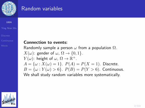
Random variables
Connection to events:Randomly sample a person ω from a population Ω.X(ω): gender of ω, Ω→ 0, 1.Y (ω): height of ω, Ω→ R+.A = ω : X(ω) = 1. P (A) = P (X = 1). Discrete.B = ω : Y (ω) > 6. P (B) = P (Y > 6). Continuous.We shall study random variables more systematically.
100A
Ying Nian Wu
Discrete
Continuous
Movie
3/111
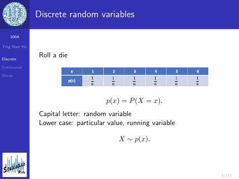
Discrete random variables
Roll a die
p(x) = P (X = x).
Capital letter: random variableLower case: particular value, running variable
X ∼ p(x).
100A
Ying Nian Wu
Discrete
Continuous
Movie
4/111
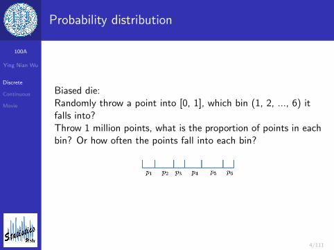
Probability distribution
Biased die:Randomly throw a point into [0, 1], which bin (1, 2, ..., 6) itfalls into?Throw 1 million points, what is the proportion of points in eachbin? Or how often the points fall into each bin?
100A
Ying Nian Wu
Discrete
Continuous
Movie
5/111
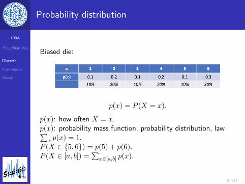
Probability distribution
Biased die:
p(x) = P (X = x).
p(x): how often X = x.p(x): probability mass function, probability distribution, law∑
x p(x) = 1.P (X ∈ 5, 6) = p(5) + p(6).P (X ∈ [a, b]) =
∑x∈[a,b] p(x).
100A
Ying Nian Wu
Discrete
Continuous
Movie
6/111
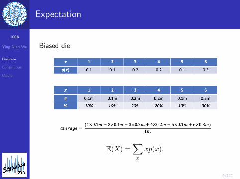
Expectation
Biased die
E(X) =∑x
xp(x).
100A
Ying Nian Wu
Discrete
Continuous
Movie
7/111
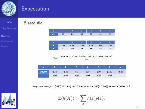
Expectation
Biased die
E(h(X)) =∑x
h(x)p(x).
100A
Ying Nian Wu
Discrete
Continuous
Movie
8/111
Utility
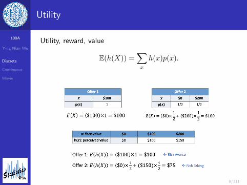
Utility, reward, value
E(h(X)) =∑x
h(x)p(x).
100A
Ying Nian Wu
Discrete
Continuous
Movie
9/111
Variance
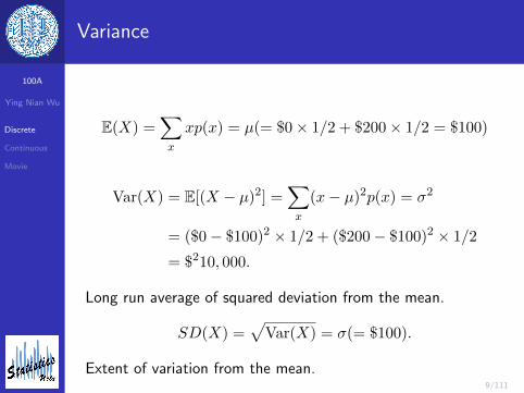
E(X) =∑x
xp(x) = µ(= $0× 1/2 + $200× 1/2 = $100)
Var(X) = E[(X − µ)2] =∑x
(x− µ)2p(x) = σ2
= ($0− $100)2 × 1/2 + ($200− $100)2 × 1/2
= $210, 000.
Long run average of squared deviation from the mean.
SD(X) =√
Var(X) = σ(= $100).
Extent of variation from the mean.
100A
Ying Nian Wu
Discrete
Continuous
Movie
10/111
Variance
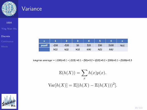
E(h(X)) =∑x
h(x)p(x).
Var[h(X)] = E[(h(X)− E(h(X)))2].
100A
Ying Nian Wu
Discrete
Continuous
Movie
11/111
Variance
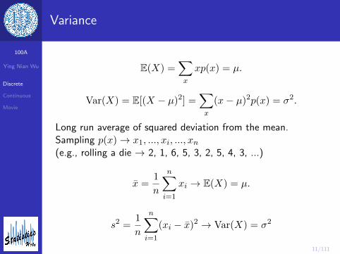
E(X) =∑x
xp(x) = µ.
Var(X) = E[(X − µ)2] =∑x
(x− µ)2p(x) = σ2.
Long run average of squared deviation from the mean.Sampling p(x)→ x1, ..., xi, ..., xn(e.g., rolling a die → 2, 1, 6, 5, 3, 2, 5, 4, 3, ...)
x =1
n
n∑i=1
xi → E(X) = µ.
s2 =1
n
n∑i=1
(xi − x)2 → Var(X) = σ2
100A
Ying Nian Wu
Discrete
Continuous
Movie
12/111
Linear transformation
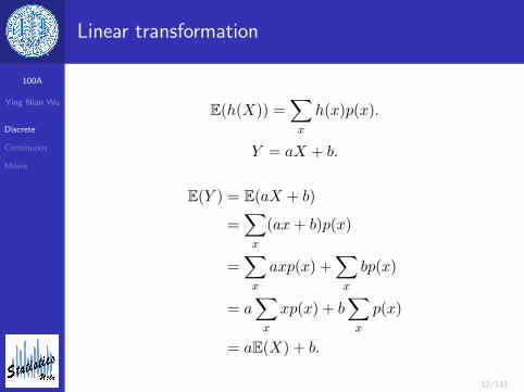
E(h(X)) =∑x
h(x)p(x).
Y = aX + b.
E(Y ) = E(aX + b)
=∑x
(ax+ b)p(x)
=∑x
axp(x) +∑x
bp(x)
= a∑x
xp(x) + b∑x
p(x)
= aE(X) + b.
100A
Ying Nian Wu
Discrete
Continuous
Movie
13/111
Linear transformation
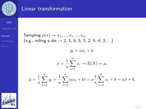
Sampling p(x)→ x1, ..., xi, ..., xn(e.g., rolling a die → 2, 1, 6, 5, 3, 2, 5, 4, 3, ...)
yi = axi + b.
x =1
n
n∑i=1
xi → E(X) = µ.
y =1
n
n∑i=1
yi =1
n
n∑i=1
(axi + b) = a1
n
n∑i=1
xi + b = ax+ b.
100A
Ying Nian Wu
Discrete
Continuous
Movie
14/111
Linear transformation
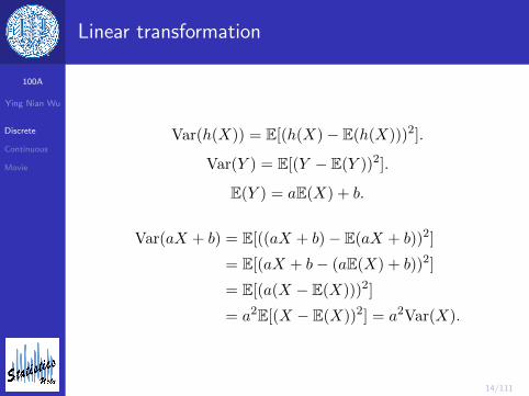
Var(h(X)) = E[(h(X)− E(h(X)))2].
Var(Y ) = E[(Y − E(Y ))2].
E(Y ) = aE(X) + b.
Var(aX + b) = E[((aX + b)− E(aX + b))2]
= E[(aX + b− (aE(X) + b))2]
= E[(a(X − E(X)))2]
= a2E[(X − E(X))2] = a2Var(X).
100A
Ying Nian Wu
Discrete
Continuous
Movie
15/111
Linear transformation
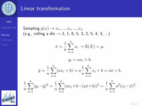
Sampling p(x)→ x1, ..., xi, ..., xn(e.g., rolling a die → 2, 1, 6, 5, 3, 2, 5, 4, 3, ...)
x =1
n
n∑i=1
xi → E(X) = µ.
yi = axi + b.
y =1
n
n∑i=1
(axi + b) = a1
n
n∑i=1
xi + b = ax+ b.
1
n
n∑i=1
(yi− y)2 =1
n
n∑i=1
(axi+b−(ax+b))2 =1
n
n∑i=1
a2(xi−x)2.

100A
Ying Nian Wu
Discrete
Continuous
Movie
16/111
Variance
µ = E(X).
Var(X) = E[(X − µ)2]
= E[X2 − 2µX + µ2]
= E(X2)− 2µE(X) + µ2
= E(X2)− µ2 = E(X2)− [E(X)]2.
E[h(X) + g(X)] =∑x
[h(x) + g(x)]p(x)
=∑x
h(x)p(x) +∑x
g(x)p(x)
= E[h(X)] + E[g(X)].
100A
Ying Nian Wu
Discrete
Continuous
Movie
17/111
Transformation
h(x) = ax+ b.
E[h(X)] = E(aX + b) = aE(X) + b = h(E(X)).
Var(X) = E(X2)− [E(X)]2.
h(x) = x2.
E[h(X)] = E(X2);
h(E(X)) = [E(X)]2.
100A
Ying Nian Wu
Discrete
Continuous
Movie
18/111
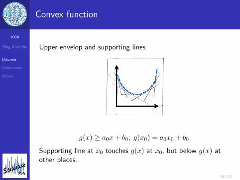
Convex function
Upper envelop and supporting lines
g(x) ≥ a0x+ b0; g(x0) = a0x0 + b0.
Supporting line at x0 touches g(x) at x0, but below g(x) atother places.
100A
Ying Nian Wu
Discrete
Continuous
Movie
19/111
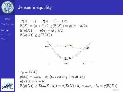
Jensen inequality
P (X = a) = P (X = b) = 1/2.E(X) = (a+ b)/2, g(E(X)) = g((a+ b/2).E(g(X)) = (g(a) + g(b))/2.E(g(X)) ≥ g(E(X)).
x0 = E(X).g(x0) = a0x0 + b0 (supporting line at x0)g(x) ≥ a0x+ b0.E(g(X)) ≥ E(a0X+b0) = a0E(X)+b0 = a0x0+b0 = g(E(X)).
100A
Ying Nian Wu
Discrete
Continuous
Movie
20/111
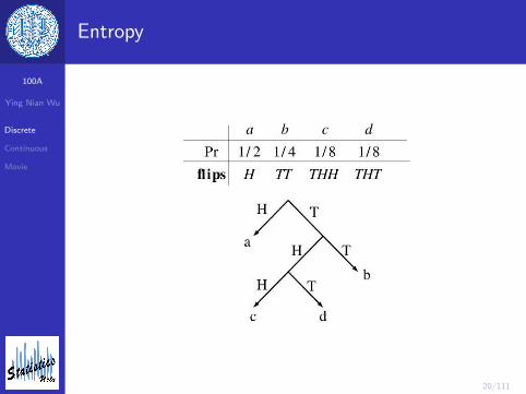
Entropy
100A
Ying Nian Wu
Discrete
Continuous
Movie
21/111
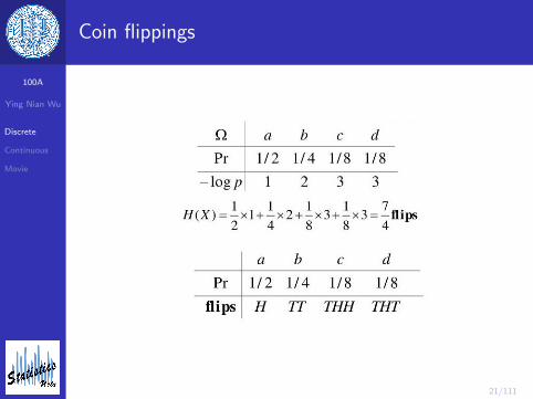
Coin flippings
100A
Ying Nian Wu
Discrete
Continuous
Movie
22/111
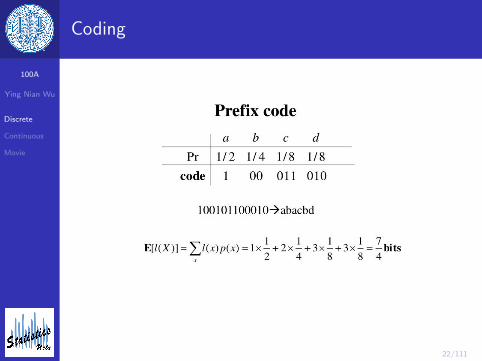
Coding

100A
Ying Nian Wu
Discrete
Continuous
Movie
23/111
Coding
100A
Ying Nian Wu
Discrete
Continuous
Movie
24/111
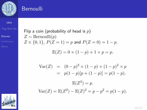
Bernoulli
Flip a coin (probability of head is p)Z ∼ Bernoulli(p)Z ∈ 0, 1, P (Z = 1) = p and P (Z = 0) = 1− p.
E(Z) = 0× (1− p) + 1× p = p.
Var(Z) = (0− p)2 × (1− p) + (1− p)2 × p= p(1− p)[p+ (1− p)] = p(1− p).
E(Z2) = p.
Var(Z) = E(Z2)− E(Z)2 = p− p2 = p(1− p).
100A
Ying Nian Wu
Discrete
Continuous
Movie
25/111
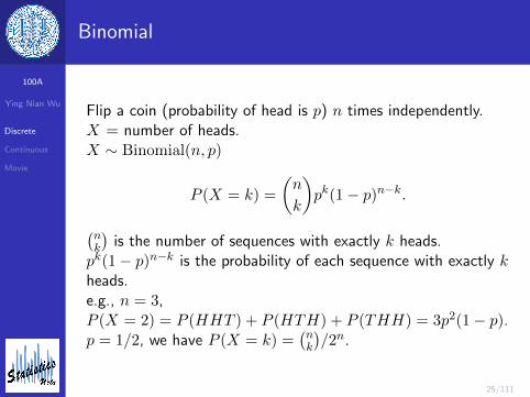
Binomial
Flip a coin (probability of head is p) n times independently.X = number of heads.X ∼ Binomial(n, p)
P (X = k) =
(n
k
)pk(1− p)n−k.
(nk
)is the number of sequences with exactly k heads.
pk(1− p)n−k is the probability of each sequence with exactly kheads.e.g., n = 3,P (X = 2) = P (HHT ) + P (HTH) + P (THH) = 3p2(1− p).p = 1/2, we have P (X = k) =
(nk
)/2n.
100A
Ying Nian Wu
Discrete
Continuous
Movie
26/111
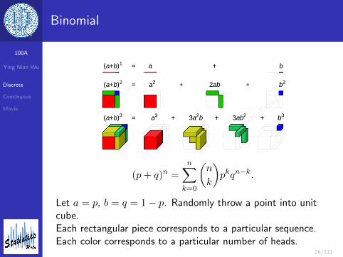
Binomial
(p+ q)n =
n∑k=0
(n
k
)pkqn−k.
Let a = p, b = q = 1− p. Randomly throw a point into unitcube.Each rectangular piece corresponds to a particular sequence.Each color corresponds to a particular number of heads.
100A
Ying Nian Wu
Discrete
Continuous
Movie
27/111
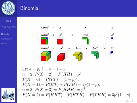
Binomial
Let a = p, b = q = 1− p.n = 2, P (X = 2) = P (HH) = p2.P (X = 0) = P (TT ) = (1− p)2.P (X = 1) = P (HT ) + P (TH) = 2p(1− p).n = 3, P (X = 3) = P (HHH) = p3.P (X = 2) = P (HHT ) + P (HTH) + P (THH) = 3p2(1− p).
100A
Ying Nian Wu
Discrete
Continuous
Movie
28/111
Binomial
X = Z1 + Z2 + ...+ Zn,
where Zi ∼ Bernoulli(p) independently.
E(X) =
n∑i=1
E(Zi) = np.
Due to independence of Zi, i = 1, ..., n,
Var(X) =
n∑i=1
Var(Zi) = np(1− p).
100A
Ying Nian Wu
Discrete
Continuous
Movie
29/111
Binomial
X/n is the frequency of heads.
E(X/n) = E(X)/n = p.
Var(X/n) = Var(X)/n2 = p(1− p)/n.Var(X/n)→ 0 as n→∞.
X/n→ p, in probability
Law of large numberProbability = long run frequency
100A
Ying Nian Wu
Discrete
Continuous
Movie
30/111
Law of large number
Probability = long run frequencyFlip a fair coin independently → 2n sequences, Ω.
Aε = ω : X(ω)/n ∈ (1/2− ε, 1/2 + ε),
the set of sequences whose frequencies of heads are close to1/2.
P (X/n ∈ (1/2− ε, 1/2 + ε)) =|Aε||Ω| → 1.
Almost all the sequences have frequencies of heads close to1/2.
e.g., n = 1 million. Almost all the 21 million sequences havefrequencies of heads to be within [.49, .51].
100A
Ying Nian Wu
Discrete
Continuous
Movie
31/111
Law of large number
e.g., n = 1 million. Almost all the 21 million sequences havefrequencies of heads to be within [.49, .51].
P (X/1m ∈ [.49, .51]) = P (X ∈ [.49m, .51m])
=
.51m∑k=.49m
(1m
k
)/21m.
100A
Ying Nian Wu
Discrete
Continuous
Movie
32/111
Binomial
E(X) =
n∑k=0
kP (X = k)
=
n∑k=0
kn!
k!(n− k)!pk(1− p)n−k
=
n∑k=1
np(n− 1)!
(k − 1)!(n− k)!pk−1(1− p)n−k
=
n′∑k′=0
np
(n′
k′
)pk
′(1− p)n′−k′ = np.
k′ = k − 1; n′ = n− 1.
100A
Ying Nian Wu
Discrete
Continuous
Movie
33/111
Binomial
E(X(X − 1)) =
n∑k=0
k(k − 1)P (X = k)
=
n∑k=0
k(k − 1)n!
k!(n− k)!pk(1− p)n−k
=
n∑k=2
n(n− 1)p2 (n− 2)!
(k − 2)!(n− k)!pk−2(1− p)n−k
=
n′∑k′=0
n(n− 1)p2
(n′
k′
)pk
′(1− p)n′−k′
= n(n− 1)p2.
k′ = k − 2; n′ = n− 2.
100A
Ying Nian Wu
Discrete
Continuous
Movie
34/111
Binomial
E(X) = np.
E(X(X − 1)) = E(X2)− E(X) = n(n− 1)p2.
Var(X) = E(X2)− E(X)2
= n(n− 1)p2 + np− (np)2
= np− np2 = np(1− p).
100A
Ying Nian Wu
Discrete
Continuous
Movie
35/111
Binomial
A box with R red balls and B blue balls. N = R+B balls intotal.Randomly pick a ball. P (red) = R/N = p.Randomly pick n balls sequentially (with replacement, put thepicked ball back). Let X = number of red balls.The distribution of X:X ∼ Binomial(n, p = R/N).
100A
Ying Nian Wu
Discrete
Continuous
Movie
36/111
Binomial
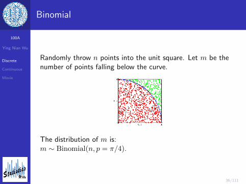
Randomly throw n points into the unit square. Let m be thenumber of points falling below the curve.
The distribution of m is:m ∼ Binomial(n, p = π/4).
100A
Ying Nian Wu
Discrete
Continuous
Movie
37/111
Geometric
T ∼ Geometric(p)T is the number of flips to get the first head, if we flip a coinindependently and the probability of getting a head in each flipis p.
P (T = k) = (1− p)k−1p.
e.g., T = 1, HT = 2, TH.T = 3, TTH.T = 4, TTTH.Waiting time.
100A
Ying Nian Wu
Discrete
Continuous
Movie
38/111
Geometric
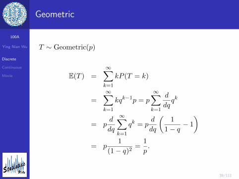
T ∼ Geometric(p)
E(T ) =
∞∑k=1
kP (T = k)
=
∞∑k=1
kqk−1p = p
∞∑k=1
d
dqqk
= pd
dq
∞∑k=1
qk = pd
dq
(1
1− q − 1
)= p
1
(1− q)2=
1
p.
100A
Ying Nian Wu
Discrete
Continuous
Movie
39/111
Geometric
(1− a)(1 + a+ ...+ am) = 1 + a+ ...+ am
−(a+ a2 + ...+ am + am+1)
= 1− am+1.
1 + a+ ...+ am =1− am+1
1− a .
If |a| < 1,am+1 → 0, as m→∞.
100A
Ying Nian Wu
Discrete
Continuous
Movie
40/111
Continuous random variable
Recall discrete (e.g., gender)
P (X = x) = p(x).
Continuous (e.g., height)
P (X ∈ (x, x+ ∆x)).= f(x)∆x,
e.g., (6 ft, 6 ft 1 inch).
f(x) = lim∆x→0
P (X ∈ (x, x+ ∆x))
∆x.
f(x): probability density functionX ∼ f(x).
100A
Ying Nian Wu
Discrete
Continuous
Movie
41/111
Probability density function
100A
Ying Nian Wu
Discrete
Continuous
Movie
42/111
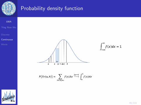
Probability density function
Recall discreteP (X = x) = p(x).
P (X ∈ [a, b]) =∑x∈[a,b]
p(x).
Continuous
P (X ∈ (x, x+ ∆x)).= f(x)∆x,
P (X ∈ [a, b]) =∑x∈[a,b]
P (X ∈ (x, x+ ∆x))
.=
b∑a
f(x)∆x.=
∫ b
af(x)dx.
100A
Ying Nian Wu
Discrete
Continuous
Movie
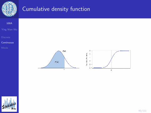
43/111
Cumulative density function
100A
Ying Nian Wu
Discrete
Continuous
Movie
44/111
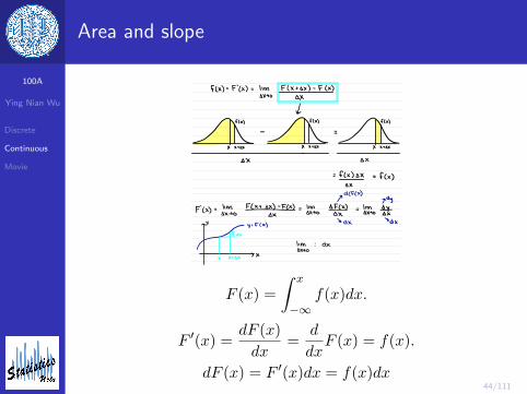
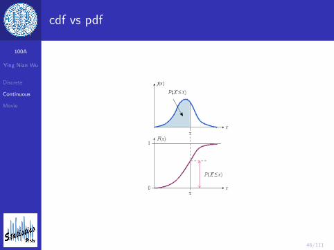
Area and slope
Cumulative Density Function :
F C x ) = Pf II Ex ) = fax fix )dx
¥,,^ I
raw score percentile
IFFX FCX )
O
f ( x ) = F' ( x ) = Iim Flxtsx ) - F C x )sx→o
d
iii. iii. .
X xtsx
SX sx
= f ( x ) DX = fcx )sx
11119119
WEEK 8- LECTURE Immmm
Calculus : derivative
y=FCx )
F'
C x )
II,
dI,
¥ Fix )
dye F' L x )dx
DFCX )= F' L x ) dx
ydlflx ) gdyF C × ) =
11 m FCxtsx)-t# =Ilm bF# =
Iimsysx→osx SHO Sx SHO sx
NY tax DX" " "
Ilm : DXSHO
X Xtsx> X
Integral
£ bftxsdx-s.info?fa.ngflx)sx"bins "
F (x) =
∫ x
−∞f(x)dx.
F ′(x) =dF (x)
dx=
d
dxF (x) = f(x).
dF (x) = F ′(x)dx = f(x)dx
100A
Ying Nian Wu
Discrete
Continuous
Movie
45/111
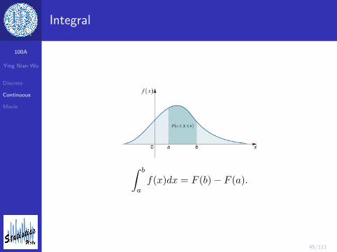
Integral
∫ b
af(x)dx = F (b)− F (a).
100A
Ying Nian Wu
Discrete
Continuous
Movie
46/111
cdf vs pdf
100A
Ying Nian Wu
Discrete
Continuous
Movie
47/111
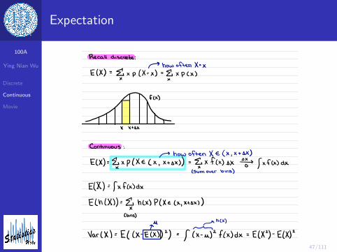
Expectation
Recall discrete :
A how often X -- X
E c X ) = § xp ( X -- x ) = § xp Cx )
thX Xtsx
Continuous :
p how often X E ( X,
Xt DX )E ( X ) = § xp ( XE ( x
,xtsx ) ) = § xfcx ) SX ⇒ fxfcxsdx
( Sum over bins )
ECI ) = fxfcx )dx
Echl # D= § hlx ) PCXE C x,
xtsx ) )
( bins )
~hcx )
-
Varix ) =E( C x - Effi) ) =/ C x -
u)2fCx)dx=E(X
'
) - ECX)'
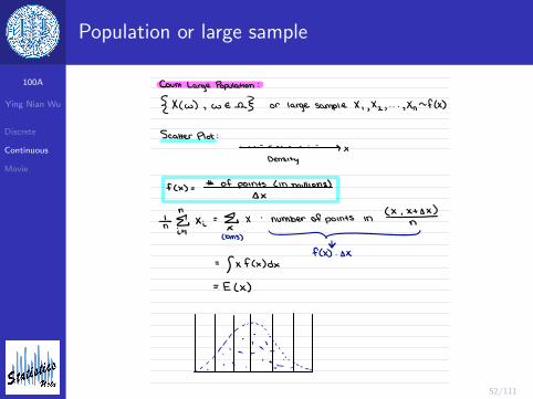
Count Large Population :
X ( w ),
we r or large sample X, ,Xz ,
- . . ,Xn~fCx )
Scatter Plot :
. . -.
- -- . - - - -
9 ×
Density
100A
Ying Nian Wu
Discrete
Continuous
Movie
48/111
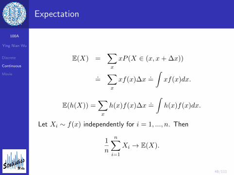
Expectation
E(X) =∑x
xP (X ∈ (x, x+ ∆x))
.=
∑x
xf(x)∆x.=
∫xf(x)dx.
E(h(X)) =∑x
h(x)f(x)∆x.=
∫h(x)f(x)dx.
Let Xi ∼ f(x) independently for i = 1, ..., n. Then
1
n
n∑i=1
Xi → E(X).
100A
Ying Nian Wu
Discrete
Continuous
Movie
49/111
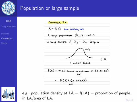
Population or large sample11114119
WEEK 7- LECTURE 2mmmm
Continuous R.V
.
II - fcx ) prob . density fxn
A large population XL w ) WES
A large sample X, Xz . . - Xn large n
t×I I I L - - l I - n \ I \ -
I million points
f ( x ) = # of points in millions In ( X,
Xt DX )Sx
= PCXECX , xtsx ) )
÷-
,
.
"-
-
.
"" -
. -
, .
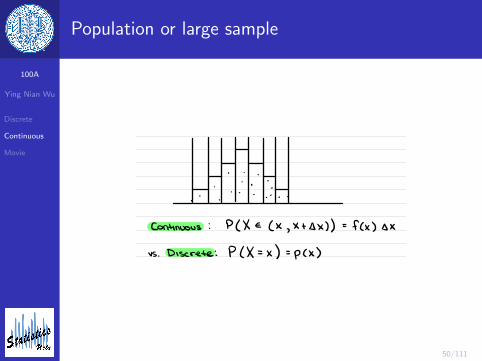
Continuous : P ( X E ( X,
Xtsx ) ) = fcx ) sx
vs .Discrete : P(X=x ) =p C x )
e.g., population density at LA = f(LA) = proportion of peoplein LA/area of LA.
100A
Ying Nian Wu
Discrete
Continuous
Movie
50/111
Population or large sample
11114119
WEEK 7- LECTURE 2mmmm
Continuous R.V
.
II - fcx ) prob . density fxn
A large population XL w ) WES
A large sample X, Xz . . - Xn large n
t×I I I L - - l I - n \ I \ -
I million points
f ( x ) = # of points in millions In ( X,
Xt DX )Sx
= PCXECX , xtsx ) )
÷-
,
.
"-
-
.
"" -
. -
, .
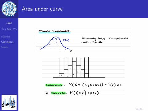
Continuous : P ( X E ( X,
Xtsx ) ) = fcx ) sx
vs .Discrete : P(X=x ) =p C x )
100A
Ying Nian Wu
Discrete
Continuous
Movie
51/111
Area under curve
f ( × ) =
# Of points C in millions )Sx
T if Xi =p,§,
X . number of points in (×iXn)-
f C x ) . DX
= fxfcx )dx
= E ( x )
--
-n
,
/ I
/,
- '
.
/ r I'
,
/ i
- ,
I- .
'
:
,
'-
s'
.
..
in.
.
-
'÷.
..
Thought Experiment :
! p ?.IE?nYItaheex-coordinate
Probability Model :
Un Uniform [ 0,17 fTn Exp ( T )
11114119
WEEK 7- LECTURE 2mmmm
Continuous R.V
.
II - fcx ) prob . density fxn
A large population XL w ) WES
A large sample X, Xz . . - Xn large n
t×I I I L - - l I - n \ I \ -
I million points
f ( x ) = # of points in millions In ( X,
Xt DX )Sx
= PCXECX , xtsx ) )
÷-
,
.
"-
-
.
"" -
. -
, .
Continuous : P ( X E ( X,
Xtsx ) ) = fcx ) sx
vs .Discrete : P(X=x ) =p C x )
100A
Ying Nian Wu
Discrete
Continuous
Movie
52/111
Population or large sample
Recall discrete :
A how often X -- X
E c X ) = § xp ( X -- x ) = § xp Cx )
thX Xtsx
Continuous :
p how often X E ( X,
Xt DX )E ( X ) = § xp ( XE ( x
,xtsx ) ) = § xfcx ) SX ⇒ fxfcxsdx
( Sum over bins )
ECI ) = fxfcx )dx
Echl # D= § hlx ) PCXE C x,
xtsx ) )
( bins )
~hcx )
-
Varix ) =E( C x - Effi) ) =/ C x -
u)2fCx)dx=E(X
'
) - ECX)'
Count Large Population :
X ( w ),
we r or large sample X, ,Xz ,
- . . ,Xn~fCx )
Scatter Plot :
. . -.
- -- . - - - -
9 ×
Density
f ( × ) =
# Of points C in millions )Sx
T if Xi =p,§,
X . number of points in (×iXn)-
f C x ) . DX
= fxfcx )dx
= E ( x )
--
-n
,
/ I
/,
- '
.
/ r I'
,
/ i
- ,
I- .
'
:
,
'-
s'
.
..
in.
.
-
'÷.
..
Thought Experiment :
! p ?.IE?nYItaheex-coordinate
Probability Model :
Un Uniform [ 0,17 fTn Exp ( T )
100A
Ying Nian Wu
Discrete
Continuous
Movie
53/111
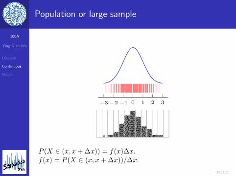
Population or large sample
P (X ∈ (x, x+ ∆x)) = f(x)∆x.f(x) = P (X ∈ (x, x+ ∆x))/∆x.
100A
Ying Nian Wu
Discrete
Continuous
Movie
54/111
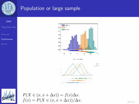
Population or large sample
P (X ∈ (x, x+ ∆x)) = f(x)∆x.f(x) = P (X ∈ (x, x+ ∆x))/∆x.
100A
Ying Nian Wu
Discrete
Continuous
Movie
55/111
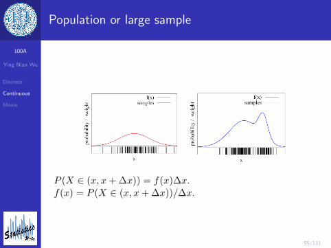
Population or large sample
P (X ∈ (x, x+ ∆x)) = f(x)∆x.f(x) = P (X ∈ (x, x+ ∆x))/∆x.
100A
Ying Nian Wu
Discrete
Continuous
Movie
56/111
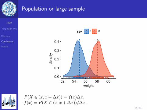
Population or large sample
P (X ∈ (x, x+ ∆x)) = f(x)∆x.f(x) = P (X ∈ (x, x+ ∆x))/∆x.
100A
Ying Nian Wu
Discrete
Continuous
Movie
57/111
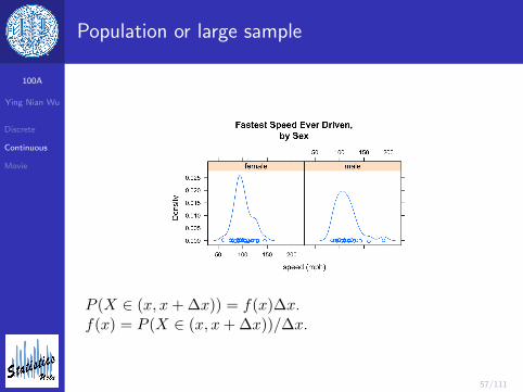
Population or large sample
P (X ∈ (x, x+ ∆x)) = f(x)∆x.f(x) = P (X ∈ (x, x+ ∆x))/∆x.
100A
Ying Nian Wu
Discrete
Continuous
Movie
58/111
Uniform
§ xpcx ) discrete
F- ( X ) =§×p(Xecx,
xtsx ) ) continuous
( bins ) I DX → O
× xtsxfxfcx )dx
Elhlx ) ) Varix ) Varchlx ) )
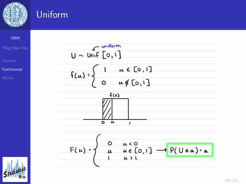
Uniform
U - Unf [ 0,1 ]
I u E CO ,I ]
flu )=o µ #Co ,
' ]
f L x )
%O M I
Fcu )=I1190,1
] → Pcusa ) -- n
I U > I
100A
Ying Nian Wu
Discrete
Continuous
Movie
59/111
Uniform
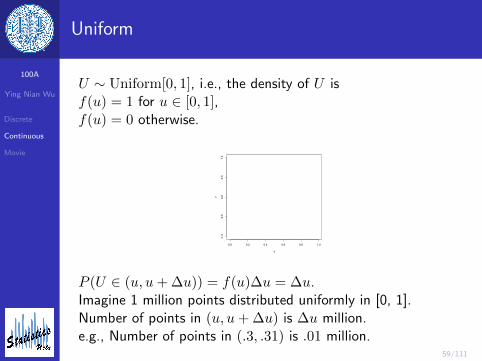
U ∼ Uniform[0, 1], i.e., the density of U isf(u) = 1 for u ∈ [0, 1],f(u) = 0 otherwise.
0.0 0.2 0.4 0.6 0.8 1.0
-1.0
-0.5
0.0
0.5
1.0
u
y
P (U ∈ (u, u+ ∆u)) = f(u)∆u = ∆u.Imagine 1 million points distributed uniformly in [0, 1].Number of points in (u, u+ ∆u) is ∆u million.e.g., Number of points in (.3, .31) is .01 million.
100A
Ying Nian Wu
Discrete
Continuous
Movie
60/111
Uniform
F (u) = P (U ≤ u) =
0 0 < uu 0 ≤ u ≤ 11 u > 1
F (u): proportion of points below u.
E(U) =
∫ 1
0uf(u)du =
1
2.
E(U2) =
∫ 1
0u2f(u)du =
1
3.
Var(U) = E(U2)− (E(U))2 =1
3− 1
4=
1
12.
100A
Ying Nian Wu
Discrete
Continuous
Movie
61/111
Pseudo-random number generator
Start from an integer X0, and iterate
Xt+1 = aXt + b mod M.
Output Ut = Xt/M . e.g., a = 75, b = 0, and M = 231 − 1.mod: divide and take the remainder, e.g., 7 = 2 mod 5.e.g., a = 7, b = 1, M = 5, X0 = 1, thenX1 = 1× 7 + 1 mod 5 = 3.X2 = 3× 7 + 1 mod 5 = 2.
100A
Ying Nian Wu
Discrete
Continuous
Movie
62/111
Exponential
0 1 2 3 4 5
-1.0
-0.5
0.0
0.5
1.0
t
y
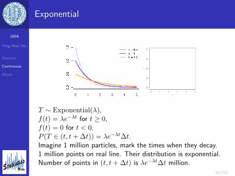
T ∼ Exponential(λ),f(t) = λe−λt for t ≥ 0,f(t) = 0 for t < 0.P (T ∈ (t, t+ ∆t)) = λe−λt∆t.Imagine 1 million particles, mark the times when they decay.1 million points on real line. Their distribution is exponential.Number of points in (t, t+ ∆t) is λe−λt∆t million.
100A
Ying Nian Wu
Discrete
Continuous
Movie
63/111
Exponential
0 1 2 3 4 5
-1.0
-0.5
0.0
0.5
1.0
t
y
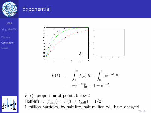
F (t) =
∫ t
0f(t)dt =
∫ t
0λe−λtdt
= −e−λt|t0 = 1− e−λt.
F (t): proportion of points below tHalf-life: F (thalf) = P (T ≤ thalf) = 1/2.1 million particles, by half life, half million will have decayed.
100A
Ying Nian Wu
Discrete
Continuous
Movie
64/111
Exponential
E(T ) =
∫ ∞0
tλe−λtdt
= −∫ ∞
0tde−λt
= −(te−λt|∞0 −∫ ∞
0e−λtdt)
= −(0− 0 +1
λe−λt|∞0 ) =
1
λ.
100A
Ying Nian Wu
Discrete
Continuous
Movie
65/111
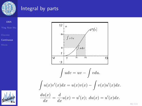
Integral by parts
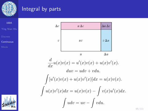
d
dxu(x)v(x) = u′(x)v(x) + u(x)v′(x).
duv = udv + vdu.∫[u′(x)v(x) + u(x)v′(x)]dx = u(x)v(x).∫
u(x)v′(x)dx = u(x)v(x)−∫v(x)u′(x)dx.∫
udv = uv −∫vdu.
100A
Ying Nian Wu
Discrete
Continuous
Movie
66/111
Integral by parts
∫udv = uv −
∫vdu.∫
u(x)v′(x)dx = u(x)v(x)−∫v(x)u′(x)dx.
du(x)
dx=
d
dxu(x) = u′(x); du(x) = u′(x)dx.
100A
Ying Nian Wu
Discrete
Continuous
Movie
67/111
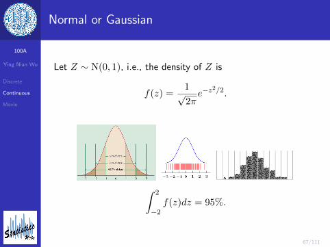
Normal or Gaussian
Let Z ∼ N(0, 1), i.e., the density of Z is
f(z) =1√2πe−z
2/2.
∫ 2
−2f(z)dz = 95%.
100A
Ying Nian Wu
Discrete
Continuous
Movie
68/111
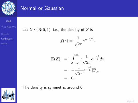
Normal or Gaussian
Let Z ∼ N(0, 1), i.e., the density of Z is
f(z) =1√2πe−z
2/2.
E(Z) =
∫ ∞−∞
z1√2πe−
z2
2 dz
= − 1√2πe−
z2
2 |∞−∞= 0.
The density is symmetric around 0.
100A
Ying Nian Wu
Discrete
Continuous
Movie
69/111
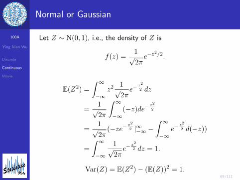
Normal or Gaussian
Let Z ∼ N(0, 1), i.e., the density of Z is
f(z) =1√2πe−z
2/2.
E(Z2) =
∫ ∞−∞
z2 1√2πe−
z2
2 dz
=1√2π
∫ ∞−∞
(−z)de− z2
2
=1√2π
(−ze− z2
2 |∞−∞ −∫ ∞−∞
e−z2
2 d(−z))
=
∫ ∞−∞
1√2πe−
z2
2 dz = 1.
Var(Z) = E(Z2)− (E(Z))2 = 1.
100A
Ying Nian Wu
Discrete
Continuous
Movie
70/111
Variance
For X ∼ f(x), let µ = E(X).
Var(X) = E[(X − µ)2]
= E[X2 − 2µX + µ2]
= E(X2)− 2µE(X) + µ2
= E(X2)− (E(X))2.
E[r(X) + s(X)] =
∫[r(x) + s(x)]f(x)dx
=
∫r(x)f(x)dx+
∫s(x)f(x)dx
= E[r(X)] + E[s(X)].
100A
Ying Nian Wu
Discrete
Continuous
Movie
71/111
Linear transformation
For X ∼ f(x). Let Y = aX + b.
E(Y ) = E(aX + b) =
∫(ax+ b)f(x)dx
= a
∫xf(x)dx+ b
∫f(x)dx
= aE(X) + b.
Var(Y ) = Var(aX + b) = E[((aX + b)− E(aX + b))2]
= E[(aX + b− (aE(X) + b))2]
= E[a2(X − E(X))2]
= a2E[(X − E(X))2] = a2Var(X).
100A
Ying Nian Wu
Discrete
Continuous
Movie
72/111
Large sample
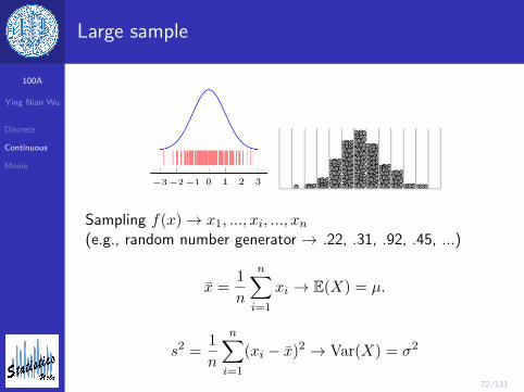
Sampling f(x)→ x1, ..., xi, ..., xn(e.g., random number generator → .22, .31, .92, .45, ...)
x =1
n
n∑i=1
xi → E(X) = µ.
s2 =1
n
n∑i=1
(xi − x)2 → Var(X) = σ2
100A
Ying Nian Wu
Discrete
Continuous
Movie
73/111
Linear transformation
Sampling f(x)→ x1, ..., xi, ..., xn(e.g., random number generator → .22, .31, .92, .45, ...)
yi = axi + b.
x =1
n
n∑i=1
xi → E(X) = µ.
y =1
n
n∑i=1
yi =1
n
n∑i=1
(axi + b) = a1
n
n∑i=1
xi + b = ax+ b.
1
n
n∑i=1
(yi− y)2 =1
n
n∑i=1
(axi+b−(ax+b))2 =1
n
n∑i=1
a2(xi−x)2.
100A
Ying Nian Wu
Discrete
Continuous
Movie
74/111
Linear transformation
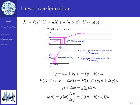
X ∼ f(x), Y = aX + b (a > 0). Y ∼ g(y).
y= f Cx ) 7¥ fi l × ) ⇒
safe = If ¥#x = gcz ) sjxz = g
' L Z )
y-
- f ( g Cz ) ) ftx ) g'Cz 's
IIT = f'
( g Cz ) ) g' C z )
d¥f(g Cz) ) = f'
( g Cz , ) g' Cz )
II ~
f¥¥tensityof X
y = h ( It ) -¥9!ensue , of Y
Y = a X t b,
a > O
y -
y = ax t b
i Itsy
y← greater density
× sx xtsx 2X
I
y.bay = axtb
* small slope → squeezing pts together⇒ t density
Tby e- smaller density * large slope → stretching out ptsI ⇒ tr density
+ sx - I
y = ax+ b, x = (y − b)/a.P (X ∈ (x, x+ ∆x)) = P (Y ∈ (y, y + ∆y)).
f(x)∆x = g(y)∆y.
g(y) = f(x)∆x
∆y= f((y − b)/a))/a.
100A
Ying Nian Wu
Discrete
Continuous
Movie
75/111
Normal or Gaussian
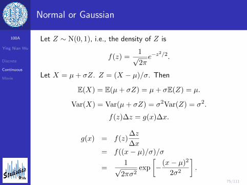
Let Z ∼ N(0, 1), i.e., the density of Z is
f(z) =1√2πe−z
2/2.
Let X = µ+ σZ. Z = (X − µ)/σ. Then
E(X) = E(µ+ σZ) = µ+ σE(Z) = µ.
Var(X) = Var(µ+ σZ) = σ2Var(Z) = σ2.
f(z)∆z = g(x)∆x.
g(x) = f(z)∆z
∆x= f((x− µ)/σ)/σ
=1√
2πσ2exp
[−(x− µ)2
2σ2
].
100A
Ying Nian Wu
Discrete
Continuous
Movie
76/111
Normal or Gaussian
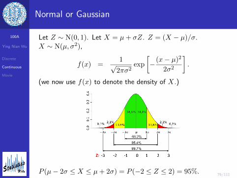
Let Z ∼ N(0, 1). Let X = µ+ σZ. Z = (X − µ)/σ.X ∼ N(µ, σ2),
f(x) =1√
2πσ2exp
[−(x− µ)2
2σ2
].
(we now use f(x) to denote the density of X.)
P (µ− 2σ ≤ X ≤ µ+ 2σ) = P (−2 ≤ Z ≤ 2) = 95%.
100A
Ying Nian Wu
Discrete
Continuous
Movie
77/111
Uniform and Exponential
Let U ∼ Unif(0, 1). LetX = a+ (b− a)U ∈ [a, b] ∼ Unif[a, b]. U = (X − a)/(b− a).
f(u)∆u = g(x)∆x.
∆u = g(x)∆x,
g(x) = ∆u/∆x = 1/(b− a), x ∈ [a, b].
Let T ∼ Exp(1). Let X = T/λ. T = λX.
f(t)∆t = g(x)∆x.
exp(−t)∆t = g(x)∆x.
g(x) = λ exp(−λx), x ≥ 0.
100A
Ying Nian Wu
Discrete
Continuous
Movie
78/111
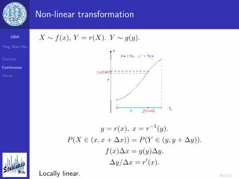
Non-linear transformation
X ∼ f(x), Y = r(X). Y ∼ g(y).
y = r(x), x = r−1(y).
P (X ∈ (x, x+ ∆x)) = P (Y ∈ (y, y + ∆y)).
f(x)∆x = g(y)∆y.
∆y/∆x = r′(x).
Locally linear.
100A
Ying Nian Wu
Discrete
Continuous
Movie
79/111
Inversion method
100A
Ying Nian Wu
Discrete
Continuous
Movie
80/111
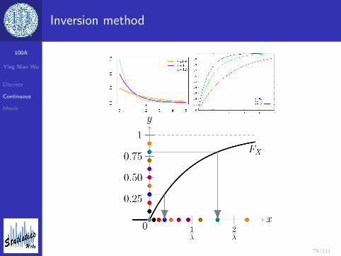
Inversion method
F (x) is a cdf. x = F−1(u) means that x is the solution to theequation F (x) = u.U ∼ Unif[0, 1]. X = F−1(U). Then F (x) is the cdf of X.
P (U ∈ (u, u+ ∆u)) = P (X ∈ (x, x+ ∆x)).
∆u = f(x)∆x.
f(x) =∆u
∆x= F ′(x).
100A
Ying Nian Wu
Discrete
Continuous
Movie
81/111
Inversion method
Suppose we want to generate X ∼ Exponential(1).F (x) = 1− e−x.F (x) = u, i.e., 1− e−x = u, e−x = 1− u. x = − log(1− u).Generate U ∼ Unif[0, 1]. Return X = − log(1− U).
100A
Ying Nian Wu
Discrete
Continuous
Movie
82/111
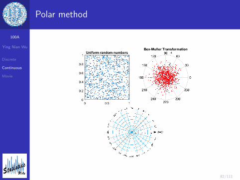
Polar method
100A
Ying Nian Wu
Discrete
Continuous
Movie
83/111
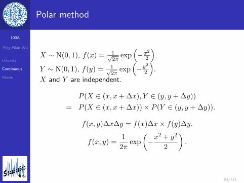
Polar method
X ∼ N(0, 1), f(x) = 1√2π
exp(−x2
2
).
Y ∼ N(0, 1), f(y) = 1√2π
exp(−y2
2
).
X and Y are independent.
P (X ∈ (x, x+ ∆x), Y ∈ (y, y + ∆y))
= P (X ∈ (x, x+ ∆x))× P (Y ∈ (y, y + ∆y)).
f(x, y)∆x∆y = f(x)∆x× f(y)∆y.
f(x, y) =1
2πexp
(−x
2 + y2
2
).
100A
Ying Nian Wu
Discrete
Continuous
Movie
84/111
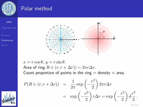
Polar method
x = r cos θ, y = r sin θ.Area of ring R ∈ (r, r + ∆r)) = 2πr∆r.Count proportion of points in the ring = density × area.
P (R ∈ (r, r + ∆r)) =1
2πexp
(−r
2
2
)2πr∆r
= exp
(−r
2
2
)r∆r = exp
(−r
2
2
)dr2
2.
100A
Ying Nian Wu
Discrete
Continuous
Movie
85/111
Polar method
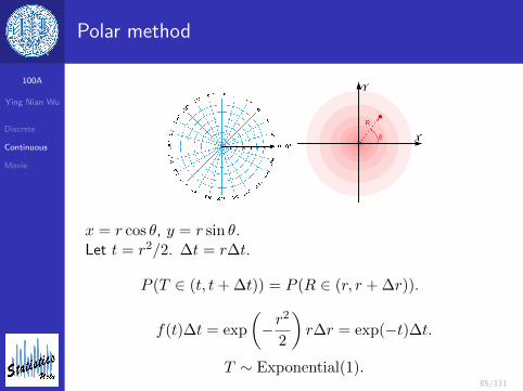
x = r cos θ, y = r sin θ.Let t = r2/2. ∆t = r∆t.
P (T ∈ (t, t+ ∆t)) = P (R ∈ (r, r + ∆r)).
f(t)∆t = exp
(−r
2
2
)r∆r = exp(−t)∆t.
T ∼ Exponential(1).

100A
Ying Nian Wu
Discrete
Continuous
Movie
86/111
Polar method
T = − log(1− U1).R =
√2T .
θ = 2πU2.X = R cos θ, Y = R sin θ.(U1, U2)→ (X,Y ).
100A
Ying Nian Wu
Discrete
Continuous
Movie
87/111
Non-linear transformation
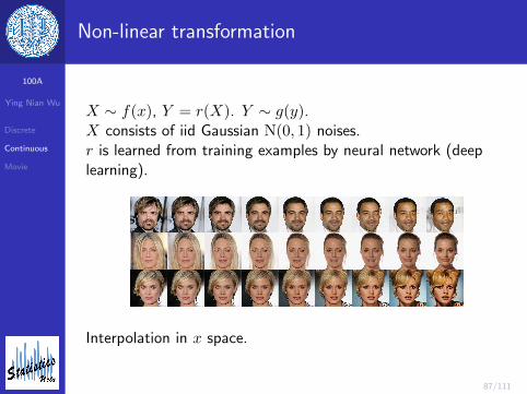
X ∼ f(x), Y = r(X). Y ∼ g(y).X consists of iid Gaussian N(0, 1) noises.r is learned from training examples by neural network (deeplearning).
Figure 5: Linear interpolation in latent space between real images
(a) Smiling (b) Pale Skin
(c) Blond Hair (d) Narrow Eyes
(e) Young (f) Male
Figure 6: Manipulation of attributes of a face. Each row is made by interpolating the latent code of animage along a vector corresponding to the attribute, with the middle image being the original image
6 Qualitative Experiments
We now study the qualitative aspects of the model on high-resolution datasets. We choose theCelebA-HQ dataset (Karras et al., 2017), which consists of 30000 high resolution images from theCelebA dataset, and train the same architecture as above but now for images at a resolution of 2562,K = 32 and L = 6. To improve visual quality at the cost of slight decrease in color fidelity, we trainour models on 5-bit images. We aim to study if our model can scale to high resolutions, producerealistic samples, and produce a meaningful latent space. Due to device memory constraints, at theseresolutions we work with minibatch size 1 per PU, and use gradient checkpointing (Salimans andBulatov, 2017). In the future, we could use a constant amount of memory independent of depth byutilizing the reversibility of the model (Gomez et al., 2017).
Consistent with earlier work on likelihood-based generative models (Parmar et al., 2018), we foundthat sampling from a reduced-temperature model often results in higher-quality samples. Whensampling with temperature T , we sample from the distribution p,T (x) / (p(x))T 2
. In case ofadditive coupling layers, this can be achieved simply by multiplying the standard deviation of p(z)by a factor of T .
Synthesis and Interpolation. Figure 4 shows the random samples obtained from our model. Theimages are extremely high quality for a non-autoregressive likelihood based model. To see howwell we can interpolate, we take a pair of real images, encode them with the encoder, and linearlyinterpolate between the latents to obtain samples. The results in Figure 5 show that the imagemanifold of the generator distribution is extremely smooth and almost all intermediate samples looklike realistic faces.
Semantic Manipulation. We now consider modifying attributes of an image. To do so, we use thelabels in the CelebA dataset. Each image has a binary label corresponding to presence or absence ofattributes like smiling, blond hair, young, etc. This gives us 30000 binary labels for each attribute.
8
Interpolation in x space.
100A
Ying Nian Wu
Discrete
Continuous
Movie
88/111
Non-linear transformation
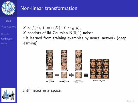
X ∼ f(x), Y = r(X). Y ∼ g(y).X consists of iid Gaussian N(0, 1) noises.r is learned from training examples by neural network (deeplearning).
arithmetics in x space.
100A
Ying Nian Wu
Discrete
Continuous
Movie
89/111
Quantum mechanics
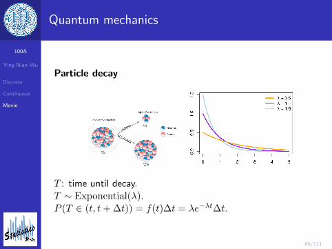
Particle decay
T : time until decay.T ∼ Exponential(λ).P (T ∈ (t, t+ ∆t)) = f(t)∆t = λe−λt∆t.
100A
Ying Nian Wu
Discrete
Continuous
Movie
90/111
Continuous time process
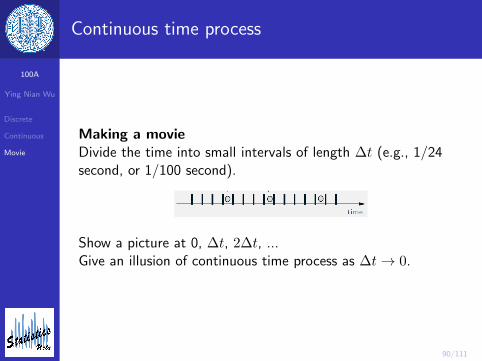
Making a movieDivide the time into small intervals of length ∆t (e.g., 1/24second, or 1/100 second).
Merging of Independent Bernoulli Processes
yields a Bernoulli process (collisions are counted as one arrival)
14
Show a picture at 0, ∆t, 2∆t, ...Give an illusion of continuous time process as ∆t→ 0.
100A
Ying Nian Wu
Discrete
Continuous
Movie
91/111
Continuous time process
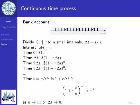
Bank account
Merging of Independent Bernoulli Processes
yields a Bernoulli process (collisions are counted as one arrival)
14
Divide [0, t] into n small intervals, ∆t = t/n.Interest rate = r.Time 0: $1.Time ∆t: $(1 + r∆t).Time 2∆t: $(1 + r∆t)2.Time 3∆t: $(1 + r∆t)3....Time t = n∆t: $(1 + r∆t)n.(
1 + rt
n
)n→ ert,
as n→∞ or ∆t→ 0.

100A
Ying Nian Wu
Discrete
Continuous
Movie
92/111
Continuous time process
Bank account
Merging of Independent Bernoulli Processes
yields a Bernoulli process (collisions are counted as one arrival)
14
Divide [0, t] into n small intervals, ∆t = t/n.Interest rate = r. (
1 +1
n
)n→ e.
1 +1
n
.= e1/n.
1 + ∆x.= e∆x.(
1 + rt
n
)n→ ert.
(1 + r∆t)t/∆t.=(er∆t
)t/∆t= ert.
100A
Ying Nian Wu
Discrete
Continuous
Movie
93/111
Poisson process
Merging of Independent Bernoulli Processes
yields a Bernoulli process (collisions are counted as one arrival)
14
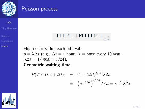
Flip a coin within each interval.p = λ∆t (e.g., ∆t = 1 hour. λ = once every 10 year.λ∆t = 1/3650× 1/24).Geometric waiting time
P (T ∈ (t, t+ ∆t)) = (1− λ∆t)t/∆tλ∆t
.=
(e−λ∆t
)t/∆tλ∆t = e−λtλ∆t.
100A
Ying Nian Wu
Discrete
Continuous
Movie
94/111
Exponential distribution
Merging of Independent Bernoulli Processes
yields a Bernoulli process (collisions are counted as one arrival)
14
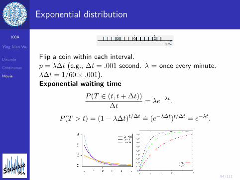
Flip a coin within each interval.p = λ∆t (e.g., ∆t = .001 second. λ = once every minute.λ∆t = 1/60× .001).Exponential waiting time
P (T ∈ (t, t+ ∆t))
∆t= λe−λt.
P (T > t) = (1− λ∆t)t/∆t.= (e−λ∆t)t/∆t = e−λt.
100A
Ying Nian Wu
Discrete
Continuous
Movie
95/111
Exponential = geometric
Merging of Independent Bernoulli Processes
yields a Bernoulli process (collisions are counted as one arrival)
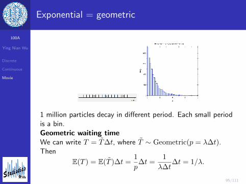
14 1 million particles decay in different period. Each small periodis a bin.Geometric waiting timeWe can write T = T∆t, where T ∼ Geometric(p = λ∆t).Then
E(T ) = E(T )∆t =1
p∆t =
1
λ∆t∆t = 1/λ.
100A
Ying Nian Wu
Discrete
Continuous
Movie
96/111
Poisson distribution
Merging of Independent Bernoulli Processes
yields a Bernoulli process (collisions are counted as one arrival)
14
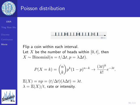
Flip a coin within each interval.Let X be the number of heads within [0, t], thenX ∼ Binomial(n = t/∆t, p = λ∆t).
P (X = k) =
(n
k
)pk(1− p)n−k → (λt)k
k!e−λt.
E(X) = np = (t/∆t)(λ∆t) = λt.λ = E(X)/t, rate or intensity.
100A
Ying Nian Wu
Discrete
Continuous
Movie
97/111
Poisson distribution
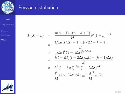
P (X = k) =n(n− 1)...(n− k + 1)
k!pk(1− p)n−k
=t/∆t(t/∆t− 1)...(t/∆t− k + 1)
k!
× (λ∆t)k(1− λ∆t)t/∆t−k
=t(t−∆t)(t− 2∆t)...(t− (k − 1)∆t)
k!
× λk(1− λ∆t)t/∆t(1− λ∆t)−k
→ tk
k!λk(e−λ∆t)t/∆t =
(λt)k
k!e−λt.
100A
Ying Nian Wu
Discrete
Continuous
Movie
98/111
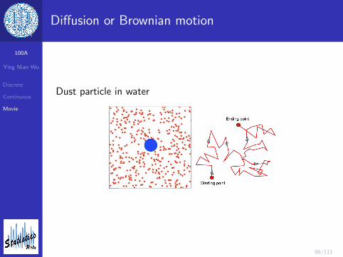
Diffusion or Brownian motion
Dust particle in water
100A
Ying Nian Wu
Discrete
Continuous
Movie
99/111
Diffusion or Brownian motion
Merging of Independent Bernoulli Processes
yields a Bernoulli process (collisions are counted as one arrival)
14
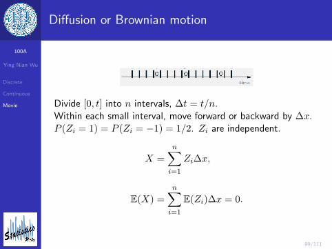
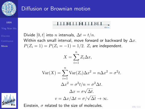
Divide [0, t] into n intervals, ∆t = t/n.Within each small interval, move forward or backward by ∆x.P (Zi = 1) = P (Zi = −1) = 1/2. Zi are independent.
X =
n∑i=1
Zi∆x,
E(X) =
n∑i=1
E(Zi)∆x = 0.
100A
Ying Nian Wu
Discrete
Continuous
Movie
100/111
Diffusion or Brownian motion
Merging of Independent Bernoulli Processes
yields a Bernoulli process (collisions are counted as one arrival)
14
Divide [0, t] into n intervals, ∆t = t/n.Within each small interval, move forward or backward by ∆x.P (Zi = 1) = P (Zi = −1) = 1/2. Zi are independent.
X =
n∑i=1
Zi∆x,
Var(X) =
n∑i=1
Var(Zi)∆x2 = n∆x2 = σ2t.
∆x2 = σ2t/n = σ2∆t.
∆x = σ√
∆t.
v = ∆x/∆t = σ/√
∆t→∞.Einstein, σ related to the size of molecules.
100A
Ying Nian Wu
Discrete
Continuous
Movie
101/111
Diffusion or Brownian motion
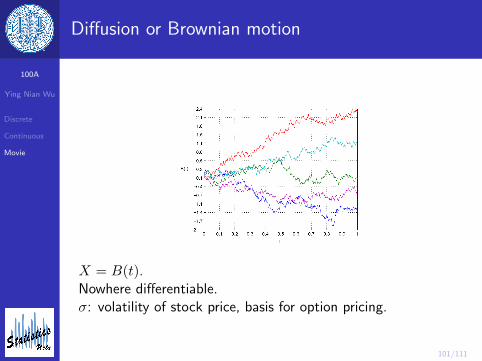
X = B(t).Nowhere differentiable.σ: volatility of stock price, basis for option pricing.
100A
Ying Nian Wu
Discrete
Continuous
Movie
102/111
Normal approximation
Central limit theoremP (Zi = 1) = P (Zi = −1) = 1/2. Zi are independent.
X =
n∑i=1
Zi∆x ∼ N(0, σ2t),
as n→ 0.Sum of independent random variables ∼ Normaldistribution.A drop of milk (millions of particles) diffuses in coffee.
100A
Ying Nian Wu
Discrete
Continuous
Movie
103/111
Normal approximation
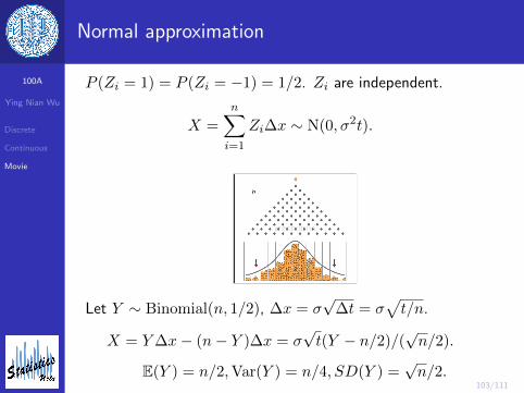
P (Zi = 1) = P (Zi = −1) = 1/2. Zi are independent.
X =
n∑i=1
Zi∆x ∼ N(0, σ2t).
Let Y ∼ Binomial(n, 1/2), ∆x = σ√
∆t = σ√t/n.
X = Y∆x− (n− Y )∆x = σ√t(Y − n/2)/(
√n/2).
E(Y ) = n/2,Var(Y ) = n/4, SD(Y ) =√n/2.
100A
Ying Nian Wu
Discrete
Continuous
Movie
104/111
Normal approximation
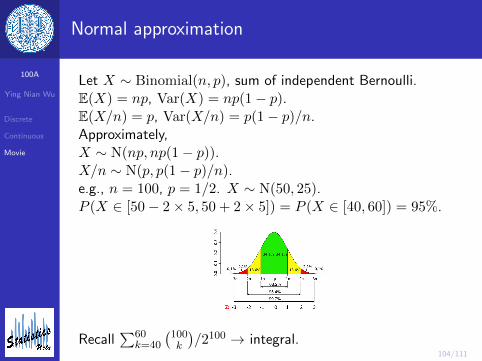
Let X ∼ Binomial(n, p), sum of independent Bernoulli.E(X) = np, Var(X) = np(1− p).E(X/n) = p, Var(X/n) = p(1− p)/n.Approximately,X ∼ N(np, np(1− p)).X/n ∼ N(p, p(1− p)/n).e.g., n = 100, p = 1/2. X ∼ N(50, 25).P (X ∈ [50− 2× 5, 50 + 2× 5]) = P (X ∈ [40, 60]) = 95%.
Recall∑60
k=40
(100k
)/2100 → integral.

100A
Ying Nian Wu
Discrete
Continuous
Movie
105/111
Normal approximation
Let X ∼ Binomial(n, p), sum of independent Bernoulli.E(X) = np, Var(X) = np(1− p).E(X/n) = p, Var(X/n) = p(1− p)/n.Approximately,X ∼ N(np, np(1− p)).X/n ∼ N(p, p(1− p)/n).e.g., Polling n = 100, p = .2. X/n ∼ N(.2, .042).P (X/n ∈ [.2− 2× .04, .2 + 2× .04]) = P (X/n ∈ [.12, .28]) =95%.
100A
Ying Nian Wu
Discrete
Continuous
Movie
106/111
Normal approximation
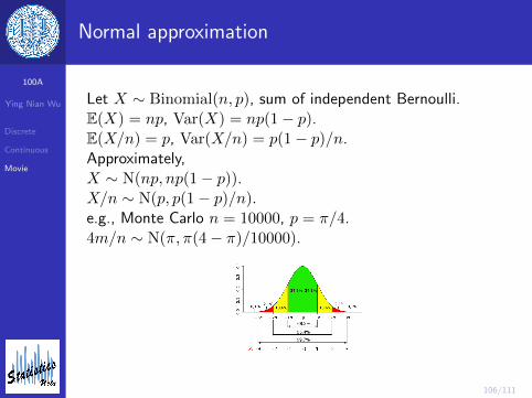
Let X ∼ Binomial(n, p), sum of independent Bernoulli.E(X) = np, Var(X) = np(1− p).E(X/n) = p, Var(X/n) = p(1− p)/n.Approximately,X ∼ N(np, np(1− p)).X/n ∼ N(p, p(1− p)/n).e.g., Monte Carlo n = 10000, p = π/4.4m/n ∼ N(π, π(4− π)/10000).
100A
Ying Nian Wu
Discrete
Continuous
Movie
107/111
Normal approximation
X ∼ Binomial(n, 1/2). µ = E(X) = n/2,σ2 = Var(X) = n/4, σ = SD(X) =
√n/2.
Let Z = (X − µ)/σ, then E(Z) = 0, Var(Z) = 1, no matterwhat n is.X = µ+ Zσ = n/2 + Z
√n/2.
P (X = k) =
(nk
)2n
=n!
k!(n− k)!2n,
100A
Ying Nian Wu
Discrete
Continuous
Movie
108/111
Normal approximation
For big n,n! ∼
√2πnnne−n,
P (X = n/2) ∼ n!
(n/2)!22n
∼√
2πnnne−n
(√
2π(n/2)(n/2)n/2)22n
∼ 1√2π
2√n.
100A
Ying Nian Wu
Discrete
Continuous
Movie
109/111
Normal approximation
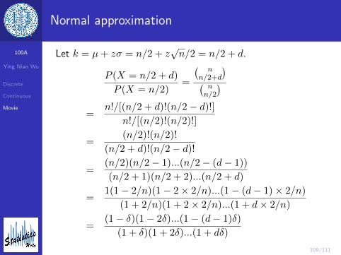
Let k = µ+ zσ = n/2 + z√n/2 = n/2 + d.
P (X = n/2 + d)
P (X = n/2)=
(n
n/2+d
)(nn/2
)=
n!/[(n/2 + d)!(n/2− d)!]
n!/[(n/2)!(n/2)!]
=(n/2)!(n/2)!
(n/2 + d)!(n/2− d)!
=(n/2)(n/2− 1)...(n/2− (d− 1))
(n/2 + 1)(n/2 + 2)...(n/2 + d)
=1(1− 2/n)(1− 2× 2/n)...(1− (d− 1)× 2/n)
(1 + 2/n)(1 + 2× 2/n)...(1 + d× 2/n)
=(1− δ)(1− 2δ)...(1− (d− 1)δ)
(1 + δ)(1 + 2δ)...(1 + dδ)
100A
Ying Nian Wu
Discrete
Continuous
Movie
110/111
Normal approximation
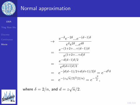
→ e−δe−2δ...e−(d−1)δ
eδe2δ...edδ
=e−(1+2+...+(d−1))δ
e(1+2+...+d)δ
=e−d(d−1)δ/2
ed(d+1)δ/2
= e−[d(d−1)/2+d(d+1)/2]δ = e−d2δ
= e−(z√n/2)2(2/n) = e−
z2
2 ,
where δ = 2/n, and d = z√n/2.
100A
Ying Nian Wu
Discrete
Continuous
Movie
111/111
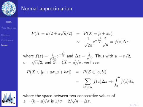
Normal approximation
P (X = n/2 + z√n/2) = P (X = µ+ zσ)
∼ 1√2πe−
z2
22√n
= f(z)∆z,
where f(z) = 1√2πe−
z2
2 and ∆z = 2√n
. Thus with µ = n/2,
σ =√n/2, and Z = (X − µ)/σ, we have
P (X ∈ [µ+ aσ, µ+ bσ]) = P (Z ∈ [a, b])
=∑z∈[a,b]
f(z)∆z →∫ b
af(z)dz,
where the space between two consecutive values ofz = (k − µ)/σ is 1/σ = 2/
√n = ∆z.