water

Article

The Effects of Hydraulic Jumps Instabilityon a Natural River Confluence: The Case Studyof the Chiaravagna River (Italy)

Annalisa De Leo 1,* , Alessia Ruffini 1,2 , Matteo Postacchini 2 , Marco Colombini 1

and Alessandro Stocchino 1

1 DICCA, Università degli Studi di Genova, via Montallegro 1, 16145 Genova, Italy;alessia.ruffini@outlook.it (A.R.); col@dicca.unige.it (M.C.); alessandro.stocchino@unige.it (A.S.)

2 DICEA, Università Politecnica delle Marche, via Brecce Bianche 12, 60131 Ancona, Italy;m.postacchini@staff.univpm.it

* Correspondence: annalisa.deleo@edu.unige.it

Received: 29 May 2020; Accepted: 13 July 2020; Published: 16 July 2020�����������������

Abstract: The occurrence and the effects of hydraulic jump instabilities on a natural river confluencein a small river basin in Liguria (Italy) is here investigated. Hydraulic jump instability has beenextensively studied in controlled and simplified laboratory rectangular flumes. In the present study,a scaled physical model of the Chiaravagna River and Ruscarolo Creek confluence has been used,retaining the realistic geometry of the reaches. This reach has been subject to frequent floods in thelast twenty years and the entire area of the confluence has been redesigned to decrease the floodrisk. A series of experiments has been performed varying the discharge on the two reaches andthe geometrical configurations. Free surface levels and two dimensional horizontal velocities havebeen measured in several positions along the physical model. The analysis of the water levels andvelocities reveals that oscillations characterised by large amplitude and low frequency occur underparticular hydraulic conditions. These oscillations have been found to be triggered by the hydraulicjump toe instability of the smallest reach of the confluence. Aiming at reducing the amplitude ofthe oscillations, which can be of the order of the flow depth, possible constructive solutions havebeen tested to control or damp the oscillations. Indeed, the insertion of a longitudinal dyke at theconfluence has proven to be an effective solution to limit the amplitude of the transversal oscillations.

Keywords: river confluence; hydraulic toe jump instability; flood risk

1. Introduction

Hydraulic jumps are common phenomena in free surface flows in natural rivers, artificial canalsand industrial applications. They occur whenever a supercritical high velocity flow impacts asubcritical low-velocity flow and the abrupt transition leads to a strong energy dissipation. The role ofthe jumps in hydraulics [1] and environmental engineering [2–4] is well known and this motivateda great number of scientific contributions. Starting from the seminal studies of Bakhmeteff [5] andRouse and Siao [6], a considerable effort has been devoted to understand the complex turbulent flowinvolved, the prediction of the free surface profile and its stability. Applying the integral form of theconservation of momentum, it is found that the momentum of the supercritical flow balances themomentum of the subcritical one downstream in correspondence of the hydraulic jump. In the caseof a prismatic rectangular channel, neglecting the flow resistance and velocity distribution effects,the balance provides the classical Bélanger relationship between the flow depth upstream (d1) and

Water 2020, 12, 2027; doi:10.3390/w12072027 www.mdpi.com/journal/water

Water 2020, 12, 2027 2 of 18

downstream (d2) of the hydraulic jump itself as a function of the inflow Froude number (Fr1), definedas Fr1 = V1/

√gd1, which reads [7–9]:

d2

d1=

12(√

1 + 8F21 − 1) (1)

Chanson (2012) [10] extended the Bélanger equation to a generic cross-section with the inclusionof flow resistance. Starting from this analytical description, many studies have concentrated on theturbulent characteristics of the hydraulic jumps that are very often complicated by a strong aeration ofthe flow [11–18]. Most of the cited works were based on experimental analysis. However, the numericalcomputation of river flow, including a detailed representation of the hydraulic jumps, has been subjectto an analogous large number of studies, see among others [19–22] and references herein.

As seen in Mossa (1999) and Wang and Chanson (2015), different kinds of hydraulic jumps mightoccur. The present work is mostly interested in investigating the hydraulic jump toe instability (hereand after indicated as jump instability). Indeed, the high intensity turbulent flow that characterisesthese phenomena and the air–water interactions often lead to free-surface instabilities and/or thehydraulic jump toe oscillations, see among others [12,15–17,23–25]. In particular, Murzyn and Chanson(2009) and Wang and Chanson (2015) focused on how the Strouhal number St = Ftoed1/V1 varies withrespect to the Reynolds number Re = V1d1/ν, where the former characterises the oscillating nature ofa physical system and the latter the ratio between inertial and viscous stresses. Moreover, Ftoe is thehydraulic jump toe frequency of oscillation deduced from a spectral analysis of the displacement ofthe toe itself, d1 and V1 are the flow depth and velocity upstream the toe and ν the water kinematicviscosity. Both the aforementioned contributions remark out that for relatively low Reynolds numbers,the Strouhal number remains nearly constant, whereas Wang and Chanson (2015) also explored therange of high Reynolds numbers showing that the Strouhal number increases and that the rapidjump toe oscillations are owed to air entrapment at the impact point (see also Long et al. (1991)).Other studies, e.g., conducted by Zhang et al. (2013), performed a comparison between St and Re,and established a relation between them. Mossa and Tolve (1998), instead, highlighted that it ispossible to recognise the oscillating nature of the jump toe position through the use of the Fast FourierTransform (FFT) technique, whereby a quasi-periodic oscillation of both the jump toe and the freesurface implies the presence of a neat peak in the spectrum. The same technique has been used byKramer and Valero (2020). They performed a spectral analysis on velocity signals collected by opticalflow measurements, with the aim to incorporate the aerated nature of the hydraulic jump.

All the above contributions were based on experimental studies performed in laboratoryrectangular flumes. A theoretical model explaining the onset of the instability is still lacking. It isreasonable to assume that the inflection point in the mean velocity profile at the hydraulic jump toerepresents a sufficient condition for an inviscid instability [26]. However, to our knowledge no specificstudies are available in the literature. Following the experimental approach used in the cited works,the present study focuses on the possibility that this kind of instabilities could arise also in morecomplex geometries and tries to asses their implications on the flood risk in natural rivers. In particular,the area of interest is the confluence between the Chiaravagna River and the Ruscarolo Creek, a naturalriver confluence on which several floods occurred in the past twenty years.

Rivers with small catchment areas, less than 50 km2, are subject to the occurrence of the so calledflash floods: short and intense events owed to extreme rainfalls that causes a quick response of theriver reach.

In this context, the confluence between the Chiaravagna River and the Ruscarolo Creek has beensubject to recent river-works in order to reduce the flooding risks. The design solution has beeninvestigated using a scaled laboratory model and tested for the design flow discharge, which ischosen as the event with 200 years return period. The experiments showed the occurrence ofintense free surface oscillations just downstream of the river confluence. The amplitude of theoscillations was almost comparable with the mean depth, thus, reducing the positive effect of the

Water 2020, 12, 2027 3 of 18

design configuration in terms of flood risk. The main cause of the free surface oscillations is rooted inan instability mechanism similar to the hydraulic jump toe instability discussed in the above mentionedcontributions. The high flow coming from the Ruscarolo Creek generated an oblique hydraulic jump,which was found to be unstable under certain flow discharge conditions and the resulting toe oscillationfrequency was close to the transversal free mode of oscillation of the free surface downstream theconfluence. The understanding of this mechanism suggested some modification of the originallydesigned configuration in order to limit the effect of the hydraulic jump instability.

The paper proceeds with Section 2.1, regarding the description of the study area, then the physicalmodel, measuring techniques and data analysis are described in the rest of Section 2. Section 3 describesthe results of the experiments performed on the different geometrical and hydrological conditions,followed by a discussion. Eventually, the conclusions are drawn in Section 5.

2. Materials and Methods

2.1. Study Area

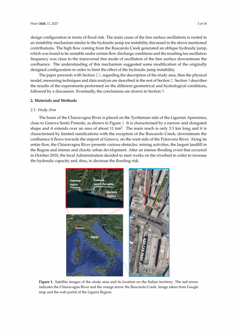
The basin of the Chiaravagna River is placed on the Tyrrhenian side of the Ligurian Apennines,close to Genova Sestri Ponente, as shown in Figure 1. It is characterised by a narrow and elongatedshape and it extends over an area of about 11 km2. The main reach is only 3.3 km long and it ischaracterised by limited ramifications with the exception of the Ruscarolo Creek; downstream theconfluence it flows towards the airport of Genova, on the west side of the Polcevera River. Along itsentire flow, the Chiaravagna River presents various obstacles: mining activities, the largest landfill inthe Region and intense and chaotic urban development. After an intense flooding event that occurredin October 2010, the local Administration decided to start works on the riverbed in order to increasethe hydraulic capacity and, thus, to decrease the flooding risk.

Figure 1. Satellite images of the study area and its location on the Italian territory. The red arrowindicates the Chiaravagna River and the orange arrow the Ruscarolo Creek. Image taken from Googlemap and the web portal of the Liguria Region.

Water 2020, 12, 2027 4 of 18

2.2. Physical Model Description

In order to test the designed configuration, a physical scaled model of the confluence of theChiaravagna River and the Ruscarolo Creek has been prepared in the hydraulic Laboratory ofthe Department of Civil, Chemical and Environmental Engineering of the University of Genova.The geometric reduction scale, defined as the ratio of the lengths on the prototype (indicated with theP subscript) compared to the lengths on the model (indicated with the M subscript), has been chosenas λ = LP/LM = 35. Scale reproduction of free surface flows is typically achieved through a partialsimilarity of Froude, defined as Fr = V/

√gd where V and d are the average velocity and depth of

the current, g the acceleration of gravity, thus accepting that the Reynolds number is not preserved inthe model [27]. Once the geometrical reduction scale λ has been set, Froude’s similarity determinesthe scales for other quantities. In particular, fluid velocity, time and volumetric flow rate assume thefollowing reduction scales:

UPUM

= λ1/2 = 5.92TPTM

= λ1/2 = 5.92QPQM

= λ5/2 = 7247 (2)

In this case, the correct representation of the flow resistance requires special attention, owingto the reduced value of the Reynolds number on the model. In fact, the model Reynolds number isreduced by about two hundred times compared to the one in the prototype. This implies, for example,that the flow in the physical model might be in the hydrodynamically rough regime, as it typicallyoccurs in real river flows. On the contrary, a smooth flow regime is observed on the model, leading toa conductance coefficient C that depends on the Reynolds number alone and not on the dimensionalroughness. In the present case, owing to the geometrical scale adopted and the dimensional roughnessof the material used for the model construction, the flow falls in the smooth case and, using theBlasius resistance law valid in this condition, it turns out that the mean non dimensional smoothconductance coefficient of the model CM = 17 corresponds on the prototype (in the rough regime) to aGauckler–Strickler coefficient of 55 m

13 /s, which is adequate for a concrete pavement.

Moreover, when dealing with free surface flows, Chanson and Gualtieri (2008) noted that possibleair entrapment in hydraulic jumps could not be correctly reproduced under a Froude similarity, owingto the different processes that regulate aeration, i.e., surface tension. Even though this is probably notthe main mechanism driving the hydraulic jump instability.

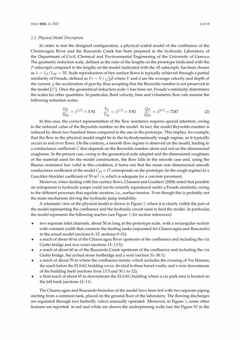
A schematic view of the physical model is shown in Figure 2, where it is clearly visible the part ofthe model representing the confluence and the hydraulic circuit used to feed the model. In particular,the model represents the following reaches (see Figure 3, for section references):

• two separate inlet channels, about 50 m long at the prototype scale, with a rectangular sectionwith constant width that connects the feeding tanks (separated for Chiaravagna and Ruscarolo)to the actual model (sections 0–15, sections 0–33);

• a reach of about 60 m of the Chiaravagna River upstream of the confluence and including the viaGiotto bridge and two weirs (sections 15–13.5);

• a reach of about 60 m of the Ruscarolo Creek upstream of the confluence and including the viaGiotto bridge, the arched stone footbridge and a weir (section 31–30.1);

• a reach of about 70 m where the confluence insists, which includes the crossing of Via Manara,the reach below the ELSAG building cover, divided in three barrel-vaults, and a weir downstreamof the building itself (sections from 13.5 and 30.1 to 12);

• a final reach of about 65 m downstream the ELSAG building where a car park area is located onthe left bank (sections 12–11).

The Chiaravagna and Ruscarolo branches of the model have been fed with two separate pipingstarting from a common tank, placed on the ground floor of the laboratory. The flowing dischargesare regulated through two butterfly valves manually operated. Moreover, in Figure 3, some otherfeatures are reported: in red and white are shown the underpinning walls (see the Figure S1 in the

Water 2020, 12, 2027 5 of 18

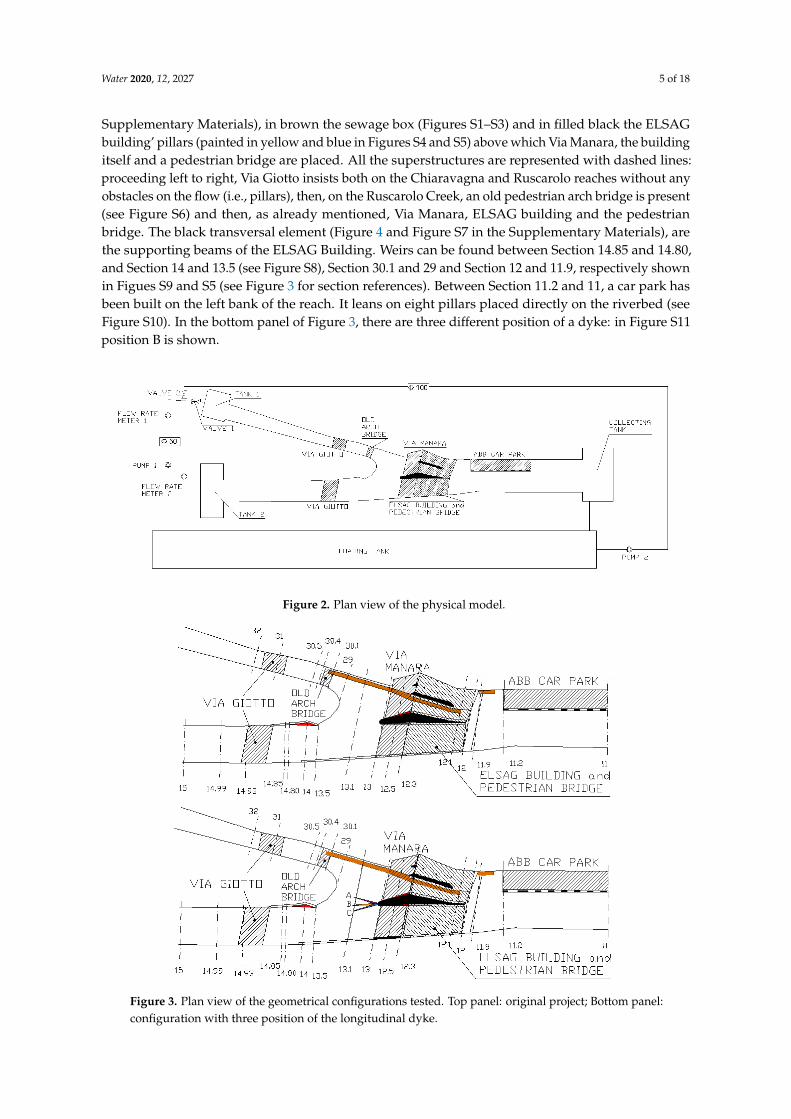
Supplementary Materials), in brown the sewage box (Figures S1–S3) and in filled black the ELSAGbuilding’ pillars (painted in yellow and blue in Figures S4 and S5) above which Via Manara, the buildingitself and a pedestrian bridge are placed. All the superstructures are represented with dashed lines:proceeding left to right, Via Giotto insists both on the Chiaravagna and Ruscarolo reaches without anyobstacles on the flow (i.e., pillars), then, on the Ruscarolo Creek, an old pedestrian arch bridge is present(see Figure S6) and then, as already mentioned, Via Manara, ELSAG building and the pedestrianbridge. The black transversal element (Figure 4 and Figure S7 in the Supplementary Materials), arethe supporting beams of the ELSAG Building. Weirs can be found between Section 14.85 and 14.80,and Section 14 and 13.5 (see Figure S8), Section 30.1 and 29 and Section 12 and 11.9, respectively shownin Figues S9 and S5 (see Figure 3 for section references). Between Section 11.2 and 11, a car park hasbeen built on the left bank of the reach. It leans on eight pillars placed directly on the riverbed (seeFigure S10). In the bottom panel of Figure 3, there are three different position of a dyke: in Figure S11position B is shown.

Figure 2. Plan view of the physical model.

Figure 3. Plan view of the geometrical configurations tested. Top panel: original project; Bottom panel:configuration with three position of the longitudinal dyke.

Water 2020, 12, 2027 6 of 18

2.2.1. Measuring Techniques and Data Analysis

The physical model has been equipped with several measuring instruments. In particular, the flowdischarge has been monitored using two electromagnetic flowmeters PROMAG P, one on each feedingpipeline. During each experiment, the water level and the velocities in different position of the modelwere recorded. In order to perform the water level measurements, an ultrasound gauge (Honeywellmodel 946-A4V-2D-2C0-380E, with 30 cm range and an accuracy of 0.2% of the full scale) has beenused. The velocities have been recorded through a micropropeller (velocity range 0–1.2 m/s) and anacoustic velocimeter (Nortek Vectrino ADV probe with a velocity range ±0.01–4 m/s and an accuracy±0.5% of measured value ±1 mm/s). All the instruments have been installed on a movable carrier:this allowed to place the instruments on several and repeatable positions. In Figure 4 the measuringpoint of the water level (panel c) and the velocity (panel a) are shown. Note that in the latter, all thevelocity measuring points are represented. Indeed, a complete map of the velocity has been obtainedonly in few runs, owed to the complexity of these measurements in an unsteady situation, as the onehere examined. In the following, most of the discussion of the velocity spectra is focused on signalsmeasured in few stations along a single cross section located in the confluence area. Moreover, not allfeatures of the model are here illustrated, e.g., just few ELSAG Building’s pillars are shown in black.The water level measuring points have been used to produce longitudinal free surface profiles alongseveral paths indicated in Figure 4b. All instruments have been connected to a DAQ unit (NationalInstrument model 6250). The ultrasound gauge and the micropropeller have been used with anacquisition frequency of 100 Hz, whereas the acquisition frequency of the acoustic velocimeter was setat 200 Hz. The acquired signals have been analysed in both time and frequency domains. In particular,probability density function and its moments have been calculated for each signal, providing estimatesof its mean and standard deviation values. In the frequency domain, a spectral analysis has beenperformed, by computing the power spectral density (PSD) estimate of the longitudinal velocity vx

(Svx ( f )) and, when appropriate, of the transversal velocity vy (Svy( f )), using Welch’s overlappedsegment averaging estimator. The signals are divided into the longest possible segments to obtain asclose to but not exceeding 8 segments with 50% overlap. Each segment is windowed with a Hammingwindow. The modified periodograms are averaged to obtain the PSD estimate.

2.2.2. Experimental Conditions

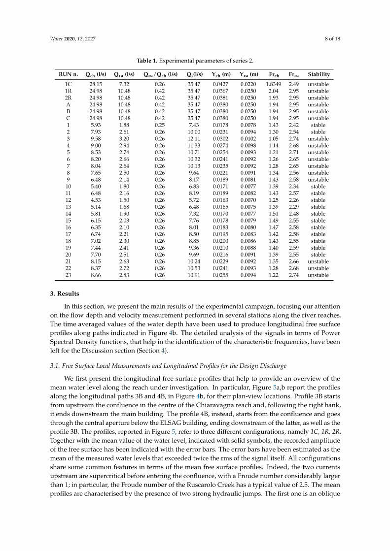
In the present study, a total of 28 runs have been performed, varying the volumetric discharge andthe geometrical configuration of the model. In Table 1, the controlling parameters, i.e., the flow rates,the water depth of the Chiaravagna and Ruscarolo Creek and the corresponding Froude numbers arereported. In the final column, it is indicated whether free surface oscillations were observed duringthe runs.

To investigate the response of the model in its original design (see Figure 3 top panel), a first set ofexperiments were performed in different hydraulic scenarios, labelled 1C and 1R. In fact, the dischargedownstream the confluence was set to the value corresponding to a return period of 200 years.Two combinations of discharges on the upstream reaches producing the same output discharge weretested, one assuming a 200 return time event on the Chiaravagna river and setting the discharge on theRuscarolo by difference(1C), the other assuming a bicentennial event on the Ruscarolo and setting thedischarge on the Chiaravagna by difference (1R). The experiment 2R has been performed with the samehydraulic condition of experiment 1R, but with the insertion of a longitudinal dyke. The experimentslabelled A, B and C have been performed with the hydraulic condition of experiment 2R with theaim to test the dyke orientation that better damp the free surface oscillations associated with the toejump instability. In particular, the longitudinal dyke, tested in the physical model, consists of wall ofheight equal to 6 cm, with a rounded tip triangular base of 2 cm width and 32.5 cm length, positionedupstream of the main beam of the ELSAG building (see Figure 3 bottom panel).

The series of experimental runs, labelled from 1 to 23, has been performed with the specific aimto find the critical conditions for the onset of instability. The procedure required to progressively

Water 2020, 12, 2027 7 of 18

increase the flow discharges starting from very low values. The experiments have been performedkeeping the discharge ratio Qru/Qch constant and equal to 26%, i.e., the same hydraulic conditionof experiment 1C, in which the maximum discharge is set on the Chiaravagna River. For each runthe following quantities have been measured: the discharges in the two branches, the water levelsupstream the confluence, both in the Ruscarolo Creek and in the Chiaravagna River, and the relativeFroude numbers. Moreover, the velocity at three different locations has been recorded. The locationshave been selected along the cross section of the river confluence, namely positions 19, 22 and 25 inFigure 4a, respectively in front of the Chiaravagna River, in the middle of the confluence and in frontof the Ruscarolo Creek.

Figure 4. Schematic map of the measurement positions: (a) velocity measurements; (b) longitudinalprofiles; (c) free surface level measurements.

Water 2020, 12, 2027 8 of 18

Table 1. Experimental parameters of series 2.

RUN n. Qch (l/s) Qru (l/s) Qru/Qch (l/s) Qt(l/s) Ych (m) Yru (m) Frch Frru Stability

1C 28.15 7.32 0.26 35.47 0.0427 0.0220 1.8349 2.49 unstable1R 24.98 10.48 0.42 35.47 0.0367 0.0250 2.04 2.95 unstable2R 24.98 10.48 0.42 35.47 0.0381 0.0250 1.93 2.95 unstableA 24.98 10.48 0.42 35.47 0.0380 0.0250 1.94 2.95 unstableB 24.98 10.48 0.42 35.47 0.0380 0.0250 1.94 2.95 unstableC 24.98 10.48 0.42 35.47 0.0380 0.0250 1.94 2.95 unstable1 5.93 1.88 0.25 7.43 0.0178 0.0078 1.43 2.42 stable2 7.93 2.61 0.26 10.00 0.0231 0.0094 1.30 2.54 stable3 9.58 3.20 0.26 12.11 0.0302 0.0102 1.05 2.74 unstable4 9.00 2.94 0.26 11.33 0.0274 0.0098 1.14 2.68 unstable5 8.53 2.74 0.26 10.71 0.0254 0.0093 1.21 2.71 unstable6 8.20 2.66 0.26 10.32 0.0241 0.0092 1.26 2.65 unstable7 8.04 2.64 0.26 10.13 0.0235 0.0092 1.28 2.65 unstable8 7.65 2.50 0.26 9.64 0.0221 0.0091 1.34 2.56 unstable9 6.48 2.14 0.26 8.17 0.0189 0.0081 1.43 2.58 unstable

10 5.40 1.80 0.26 6.83 0.0171 0.0077 1.39 2.34 stable11 6.48 2.16 0.26 8.19 0.0189 0.0082 1.43 2.57 stable12 4.53 1.50 0.26 5.72 0.0163 0.0070 1.25 2.26 stable13 5.14 1.68 0.26 6.48 0.0165 0.0075 1.39 2.29 stable14 5.81 1.90 0.26 7.32 0.0170 0.0077 1.51 2.48 stable15 6.15 2.03 0.26 7.76 0.0178 0.0079 1.49 2.55 stable16 6.35 2.10 0.26 8.01 0.0183 0.0080 1.47 2.58 stable17 6.74 2.21 0.26 8.50 0.0195 0.0083 1.42 2.58 stable18 7.02 2.30 0.26 8.85 0.0200 0.0086 1.43 2.55 stable19 7.44 2.41 0.26 9.36 0.0210 0.0088 1.40 2.59 stable20 7.70 2.51 0.26 9.69 0.0216 0.0091 1.39 2.55 stable21 8.15 2.63 0.26 10.24 0.0229 0.0092 1.35 2.66 unstable22 8.37 2.72 0.26 10.53 0.0241 0.0093 1.28 2.68 unstable23 8.66 2.83 0.26 10.91 0.0255 0.0094 1.22 2.74 unstable

3. Results

In this section, we present the main results of the experimental campaign, focusing our attentionon the flow depth and velocity measurement performed in several stations along the river reaches.The time averaged values of the water depth have been used to produce longitudinal free surfaceprofiles along paths indicated in Figure 4b. The detailed analysis of the signals in terms of PowerSpectral Density functions, that help in the identification of the characteristic frequencies, have beenleft for the Discussion section (Section 4).

3.1. Free Surface Local Measurements and Longitudinal Profiles for the Design Discharge

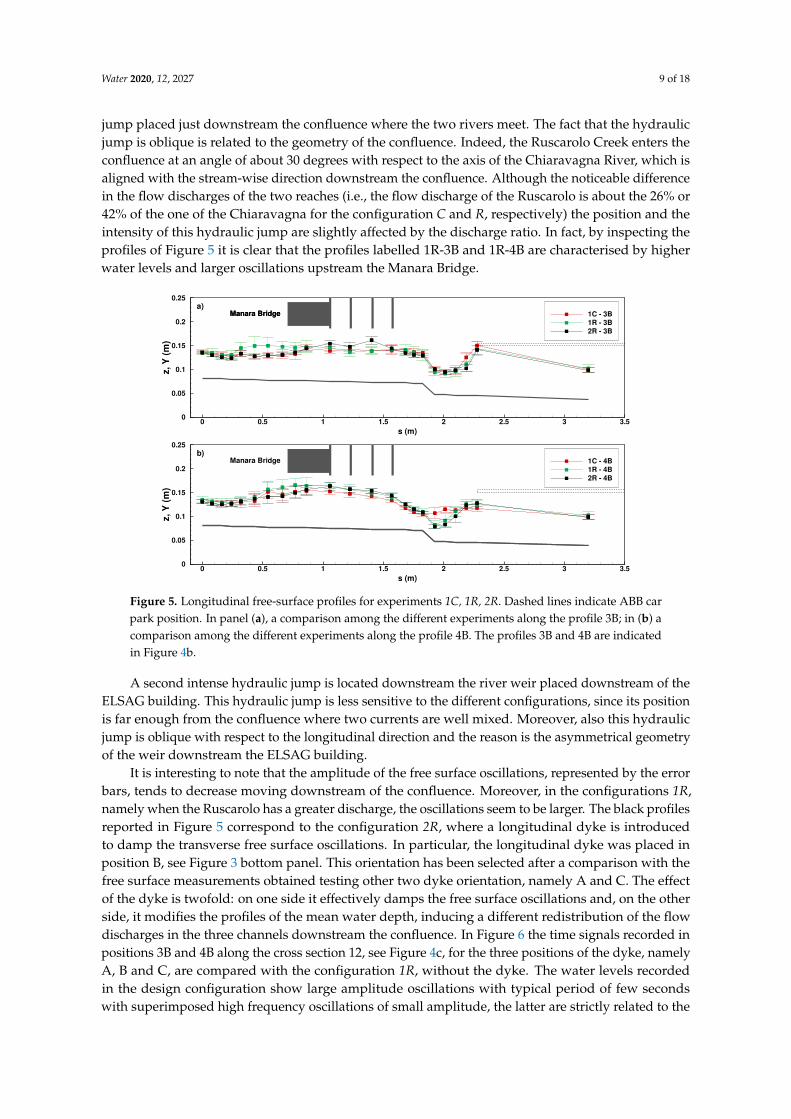
We first present the longitudinal free surface profiles that help to provide an overview of themean water level along the reach under investigation. In particular, Figure 5a,b report the profilesalong the longitudinal paths 3B and 4B, in Figure 4b, for their plan-view locations. Profile 3B startsfrom upstream the confluence in the centre of the Chiaravagna reach and, following the right bank,it ends downstream the main building. The profile 4B, instead, starts from the confluence and goesthrough the central aperture below the ELSAG building, ending downstream of the latter, as well as theprofile 3B. The profiles, reported in Figure 5, refer to three different configurations, namely 1C, 1R, 2R.Together with the mean value of the water level, indicated with solid symbols, the recorded amplitudeof the free surface has been indicated with the error bars. The error bars have been estimated as themean of the measured water levels that exceeded twice the rms of the signal itself. All configurationsshare some common features in terms of the mean free surface profiles. Indeed, the two currentsupstream are supercritical before entering the confluence, with a Froude number considerably largerthan 1; in particular, the Froude number of the Ruscarolo Creek has a typical value of 2.5. The meanprofiles are characterised by the presence of two strong hydraulic jumps. The first one is an oblique

Water 2020, 12, 2027 9 of 18

jump placed just downstream the confluence where the two rivers meet. The fact that the hydraulicjump is oblique is related to the geometry of the confluence. Indeed, the Ruscarolo Creek enters theconfluence at an angle of about 30 degrees with respect to the axis of the Chiaravagna River, which isaligned with the stream-wise direction downstream the confluence. Although the noticeable differencein the flow discharges of the two reaches (i.e., the flow discharge of the Ruscarolo is about the 26% or42% of the one of the Chiaravagna for the configuration C and R, respectively) the position and theintensity of this hydraulic jump are slightly affected by the discharge ratio. In fact, by inspecting theprofiles of Figure 5 it is clear that the profiles labelled 1R-3B and 1R-4B are characterised by higherwater levels and larger oscillations upstream the Manara Bridge.

s (m)

z, Y

(m

)

0 0.5 1 1.5 2 2.5 3 3.50

0.05

0.1

0.15

0.2

0.25

1C ­ 4B

1R ­ 4B

2R ­ 4B

Manara Bridgeb)

s (m)

z, Y

(m

)

0 0.5 1 1.5 2 2.5 3 3.50

0.05

0.1

0.15

0.2

0.25

1C ­ 3B1R ­ 3B

2R ­ 3B

Manara BridgeManara Bridgea)

Figure 5. Longitudinal free-surface profiles for experiments 1C, 1R, 2R. Dashed lines indicate ABB carpark position. In panel (a), a comparison among the different experiments along the profile 3B; in (b) acomparison among the different experiments along the profile 4B. The profiles 3B and 4B are indicatedin Figure 4b.

A second intense hydraulic jump is located downstream the river weir placed downstream of theELSAG building. This hydraulic jump is less sensitive to the different configurations, since its positionis far enough from the confluence where two currents are well mixed. Moreover, also this hydraulicjump is oblique with respect to the longitudinal direction and the reason is the asymmetrical geometryof the weir downstream the ELSAG building.

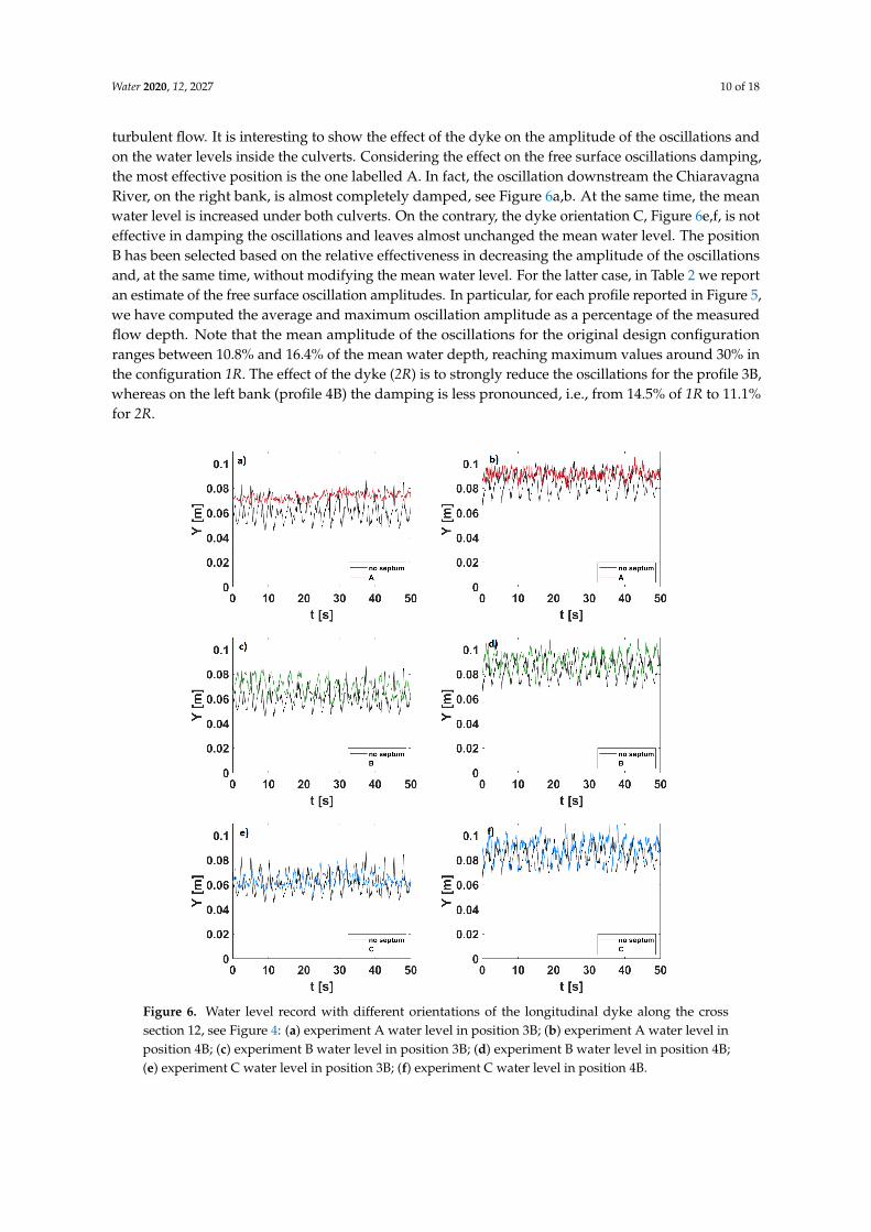
It is interesting to note that the amplitude of the free surface oscillations, represented by the errorbars, tends to decrease moving downstream of the confluence. Moreover, in the configurations 1R,namely when the Ruscarolo has a greater discharge, the oscillations seem to be larger. The black profilesreported in Figure 5 correspond to the configuration 2R, where a longitudinal dyke is introducedto damp the transverse free surface oscillations. In particular, the longitudinal dyke was placed inposition B, see Figure 3 bottom panel. This orientation has been selected after a comparison with thefree surface measurements obtained testing other two dyke orientation, namely A and C. The effectof the dyke is twofold: on one side it effectively damps the free surface oscillations and, on the otherside, it modifies the profiles of the mean water depth, inducing a different redistribution of the flowdischarges in the three channels downstream the confluence. In Figure 6 the time signals recorded inpositions 3B and 4B along the cross section 12, see Figure 4c, for the three positions of the dyke, namelyA, B and C, are compared with the configuration 1R, without the dyke. The water levels recordedin the design configuration show large amplitude oscillations with typical period of few secondswith superimposed high frequency oscillations of small amplitude, the latter are strictly related to the

Water 2020, 12, 2027 10 of 18

turbulent flow. It is interesting to show the effect of the dyke on the amplitude of the oscillations andon the water levels inside the culverts. Considering the effect on the free surface oscillations damping,the most effective position is the one labelled A. In fact, the oscillation downstream the ChiaravagnaRiver, on the right bank, is almost completely damped, see Figure 6a,b. At the same time, the meanwater level is increased under both culverts. On the contrary, the dyke orientation C, Figure 6e,f, is noteffective in damping the oscillations and leaves almost unchanged the mean water level. The positionB has been selected based on the relative effectiveness in decreasing the amplitude of the oscillationsand, at the same time, without modifying the mean water level. For the latter case, in Table 2 we reportan estimate of the free surface oscillation amplitudes. In particular, for each profile reported in Figure 5,we have computed the average and maximum oscillation amplitude as a percentage of the measuredflow depth. Note that the mean amplitude of the oscillations for the original design configurationranges between 10.8% and 16.4% of the mean water depth, reaching maximum values around 30% inthe configuration 1R. The effect of the dyke (2R) is to strongly reduce the oscillations for the profile 3B,whereas on the left bank (profile 4B) the damping is less pronounced, i.e., from 14.5% of 1R to 11.1%for 2R.

Figure 6. Water level record with different orientations of the longitudinal dyke along the crosssection 12, see Figure 4: (a) experiment A water level in position 3B; (b) experiment A water level inposition 4B; (c) experiment B water level in position 3B; (d) experiment B water level in position 4B;(e) experiment C water level in position 3B; (f) experiment C water level in position 4B.

Water 2020, 12, 2027 11 of 18

Table 2. Comparison among the free surface oscillations amplitude evaluated as a percentage of thewater depth for the different configurations.

Configuration Longitudinal Profile Maximum Oscillation Amplitude Mean Oscillation Amplitude

1C 3B 22.6% 10.8%1R 3B 33.2% 16.4%2R 3B 13.9% 8.2%

1C 4B 24.1% 11.9%1R 4B 30.3% 14.5%2R 4B 24.5% 11.1%

3.2. Time Velocity Distributions

The velocity measurements performed in terms of time signals of the longitudinal (vx(x, y, t)) andtransversal component (vy(x, y, t)) are presented in this section. The velocity measurements have beenperformed in several points along the river reach, see Figure 4a. However, in the present section weshow only few typical examples of the velocity records for the sake of brevity.

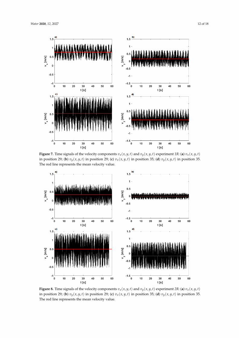
In Figures 7 and 8, we show the time signals of vx(x, y, t) and vy(x, y, t) recorded in two points:one in front of the Chiaravagna River, position 29, and one in front of the Ruscarolo Creek, position 35of Figure 4a, for the experiments 1R and 2R, respectively. In the same plots the time averaged value ofthe velocity is represented with a red line.

Figure 7 represents the experiment 1R, with the maximum flow discharge in the Ruscarolo Creek.It can be noticed that the time signals of both components of the velocity show a low frequencyoscillation with large amplitude, especially in front of the Ruscarolo Creek. In both positions, the maincomponent of the velocity is the longitudinal one, see Figure 7a,c. Indeed, the mean longitudinalcomponent has values around 0.53–0.75 m/s compared to values around 0.1–0.15 m/s of the meantransversal velocity. The above considerations apply in most of the measuring points in the confluenceregion for all the experiments performed with the design discharge.

The presence of a circulation zone, which occupies most of the river width, is highlighted by anon negligible transversal velocity component vy(x, y, t), recorded not only in the position shown butalso in several points downstream the confluence between Sections 3 and 8 (see Figure 4b). Movies,recorded during the experiments and attached as Supplementary Materials, help in the visualisationof this recirculating flow region that extends from the left bank to the centre of the confluence. Seemovies 1 and 2 for the experiments 1C and 1R, respectively.

The positive effect of the presence of the dyke clearly appears also in the velocity signals. Figure 8shows the velocity signals recorded during experiment 2R, in the same position of the previous run.It is worth noting how the Ruscarolo Creek is not particularly influenced by the presence of the dyke,panel c and d, whereas the flow in front of the Chiaravagna River is remarkably different. Firstly,the peak in the low frequency range disappears and only the high frequency turbulent oscillationsare detected. Secondly, the transversal component of the velocity is almost vanished. A transversalvelocity is still visible in front of the Ruscarolo Creek where, indeed, a recirculating zone is still present,which is however confined between the left bank and the dyke (see movie 3).

Water 2020, 12, 2027 12 of 18

Figure 7. Time signals of the velocity components vx(x, y, t) and vy(x, y, t) experiment 1R: (a) vx(x, y, t)in position 29; (b) vy(x, y, t) in position 29; (c) vx(x, y, t) in position 35; (d) vy(x, y, t) in position 35.The red line represents the mean velocity value.

Figure 8. Time signals of the velocity components vx(x, y, t) and vy(x, y, t) experiment 2R: (a) vx(x, y, t)in position 29; (b) vy(x, y, t) in position 29; (c) vx(x, y, t) in position 35; (d) vy(x, y, t) in position 35.The red line represents the mean velocity value.

Water 2020, 12, 2027 13 of 18

4. Discussion

The velocity signals show an oscillating character with a clear wide spectrum of frequency.The velocity for the flow under investigation is fully turbulent and, for this reason, the time recordsof the velocity have been decomposed in a time averaged components plus a fluctuating residual.The velocity residuals have been used to perform a spectral analysis with the aim to describe thecharacteristic frequency of oscillation of either the free surface instability and the jump toe instability.This approach is very common when the stability of an hydraulic jump is investigated [15–17,25,26].

The spectral analysis is presented on stations 19, 22 and 25, in Figure 4a, which lie along a crosssection located in the confluence area.

This helps to identify the variations of the dominant frequencies along the cross section itself.In the following discussion, we intend to show how the free surface fluctuations observed duringthe experiments, performed with the design discharge, can be rooted to the occurrence of a specificinstability of the hydraulic jump, namely the hydraulic jump toe instability. Moreover, we discuss therole of the longitudinal dyke in decreasing the effect of the jump toe instability.

4.1. The Onset of the Free Surface Instability

A dedicated set of experiments on the design configuration, experimental runs from 1 to 23reported in Table 1, have been performed with the aim of investigating the process that leads to theflow instability already introduced in the previous section.

The critical condition for the onset of the oscillations can be defined based on the spectral analysisof the velocity signals. In fact, the spectral signature of the oscillations should appear quite clearly as astrong peak in the low frequency range, whereas conditions where the flow is undisturbed show aclassical scaling of energy spectra for fully three dimensional turbulence.

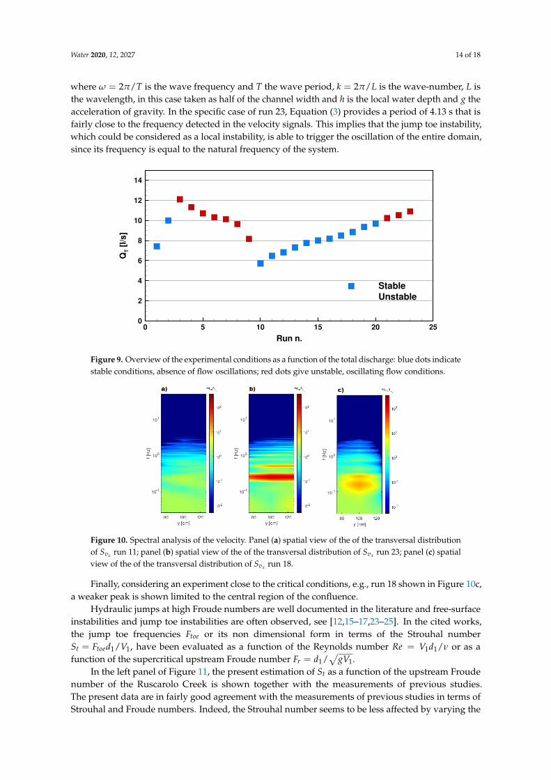
Figure 9 summarises the stability condition of the whole set of experiments performed, using thetotal discharge as the main parameter. The different colours of the symbols indicate the experimentshowing stable and unstable conditions, in blue and red, respectively. Starting from run 1, the onset ofthe instability has been observed between flow rates equal to 10.00 and 12.11 L/s. The falling branchhas been investigated with differential steps much finer with respect to the rising one, looking forthe conditions under which the oscillations naturally were damped. Note that the flow disturbancesrequire a much lower discharge to offset with respect to the critical value for their onset. In fact,the flow returns stable for a discharge equal to 5.83 L/s. This behaviour indicates a possible hysteresisin the response of the system to the flow disturbances. Moreover, this aspect has motivated the restof the experiments, performed with the aim to detect the critical conditions in more details on a newand finer rising branch. Following the runs from number 10 to 23, the instability has been detectedmore precisely for the total flow rate between 9.69 and 10.24 L/s, confirming the observations ofthe first experiments. Note that in previous works only unstable conditions have been investigated,as in [12,15–17,23–25], without looking specifically at the onset of the instability.

In Figure 10, the spatial spectral analysis of the velocity signals are shown for the runs 11, 23and 18. The velocities have been recorded along a cross section in the confluence area. The y-axis isoriented from Chiaravagna River towards the Ruscarolo Creek.

The three experiments selected correspond to flow conditions at which no oscillations occur(run 11), strong velocity fluctuations are clearly detectable (run 23) and, finally, at the onset of the mainhydraulic jump toe instability (run 18).

Starting from the stable condition (panel a), the spectrum of the velocity signals displays noparticular peaks. In panel b, a fully unstable solution is presented, whereby a clear peak is found for afrequency of about 0.24 HZ, which corresponds to a period of about 4.17 s, and spans the entire crosssection. It is worth computing the natural frequency of the system using the dispersion relationship inthe limit of shallow water [28], which reads:

ω =√

gk2h (3)

Water 2020, 12, 2027 14 of 18

where ω = 2π/T is the wave frequency and T the wave period, k = 2π/L is the wave-number, L isthe wavelength, in this case taken as half of the channel width and h is the local water depth and g theacceleration of gravity. In the specific case of run 23, Equation (3) provides a period of 4.13 s that isfairly close to the frequency detected in the velocity signals. This implies that the jump toe instability,which could be considered as a local instability, is able to trigger the oscillation of the entire domain,since its frequency is equal to the natural frequency of the system.

Run n.

QT [

l/s

]

0 5 10 15 20 250

2

4

6

8

10

12

14

Stable

Unstable

Figure 9. Overview of the experimental conditions as a function of the total discharge: blue dots indicatestable conditions, absence of flow oscillations; red dots give unstable, oscillating flow conditions.

Figure 10. Spectral analysis of the velocity. Panel (a) spatial view of the of the transversal distributionof Svx run 11; panel (b) spatial view of the of the transversal distribution of Svx run 23; panel (c) spatialview of the of the transversal distribution of Svx run 18.

Finally, considering an experiment close to the critical conditions, e.g., run 18 shown in Figure 10c,a weaker peak is shown limited to the central region of the confluence.

Hydraulic jumps at high Froude numbers are well documented in the literature and free-surfaceinstabilities and jump toe instabilities are often observed, see [12,15–17,23–25]. In the cited works,the jump toe frequencies Ftoe or its non dimensional form in terms of the Strouhal numberSt = Ftoed1/V1, have been evaluated as a function of the Reynolds number Re = V1d1/ν or as afunction of the supercritical upstream Froude number Fr = d1/

√gV1.

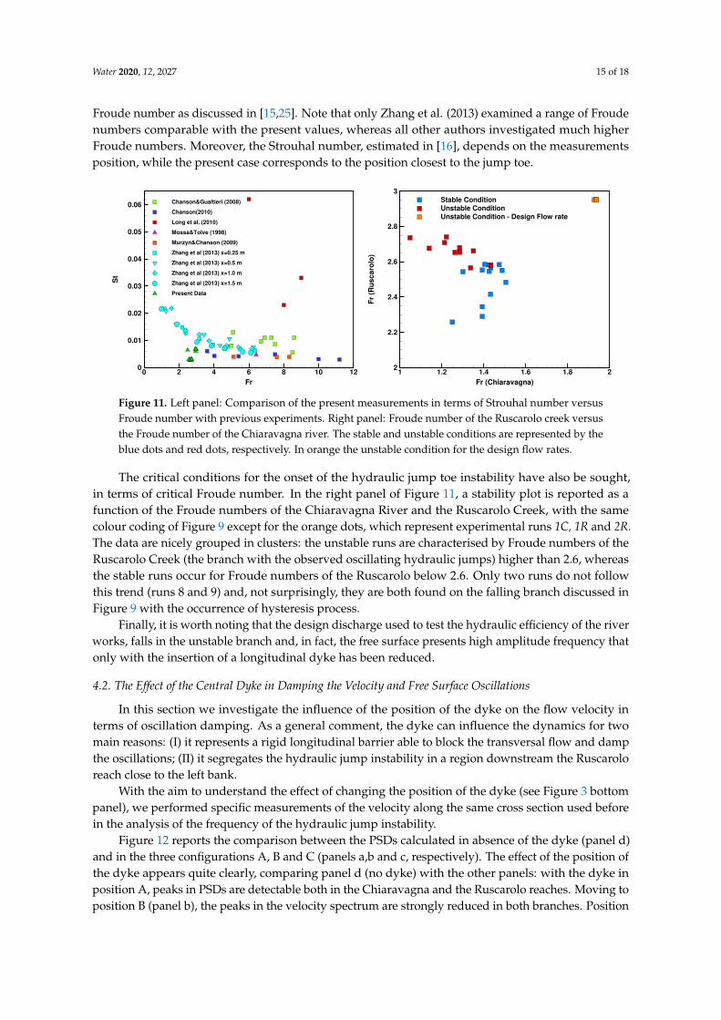
In the left panel of Figure 11, the present estimation of St as a function of the upstream Froudenumber of the Ruscarolo Creek is shown together with the measurements of previous studies.The present data are in fairly good agreement with the measurements of previous studies in terms ofStrouhal and Froude numbers. Indeed, the Strouhal number seems to be less affected by varying the

Water 2020, 12, 2027 15 of 18

Froude number as discussed in [15,25]. Note that only Zhang et al. (2013) examined a range of Froudenumbers comparable with the present values, whereas all other authors investigated much higherFroude numbers. Moreover, the Strouhal number, estimated in [16], depends on the measurementsposition, while the present case corresponds to the position closest to the jump toe.

Fr

St

0 2 4 6 8 10 120

0.01

0.02

0.03

0.04

0.05

0.06 Chanson&Gualtieri (2008)

Chanson(2010)

Long et al. (2010)

Mossa&Tolve (1998)

Murzyn&Chanson (2009)

Zhang et al (2013) x=0.25 m

Zhang et al (2013) x=0.5 m

Zhang et al (2013) x=1.0 m

Zhang et al (2013) x=1.5 m

Present Data

Fr (Chiaravagna)

Fr

(Ru

sc

aro

lo)

1 1.2 1.4 1.6 1.8 22

2.2

2.4

2.6

2.8

3

Stable Condition

Unstable Condition

Unstable Condition ­ Design Flow rate

Figure 11. Left panel: Comparison of the present measurements in terms of Strouhal number versusFroude number with previous experiments. Right panel: Froude number of the Ruscarolo creek versusthe Froude number of the Chiaravagna river. The stable and unstable conditions are represented by theblue dots and red dots, respectively. In orange the unstable condition for the design flow rates.

The critical conditions for the onset of the hydraulic jump toe instability have also be sought,in terms of critical Froude number. In the right panel of Figure 11, a stability plot is reported as afunction of the Froude numbers of the Chiaravagna River and the Ruscarolo Creek, with the samecolour coding of Figure 9 except for the orange dots, which represent experimental runs 1C, 1R and 2R.The data are nicely grouped in clusters: the unstable runs are characterised by Froude numbers of theRuscarolo Creek (the branch with the observed oscillating hydraulic jumps) higher than 2.6, whereasthe stable runs occur for Froude numbers of the Ruscarolo below 2.6. Only two runs do not followthis trend (runs 8 and 9) and, not surprisingly, they are both found on the falling branch discussed inFigure 9 with the occurrence of hysteresis process.

Finally, it is worth noting that the design discharge used to test the hydraulic efficiency of the riverworks, falls in the unstable branch and, in fact, the free surface presents high amplitude frequency thatonly with the insertion of a longitudinal dyke has been reduced.

4.2. The Effect of the Central Dyke in Damping the Velocity and Free Surface Oscillations

In this section we investigate the influence of the position of the dyke on the flow velocity interms of oscillation damping. As a general comment, the dyke can influence the dynamics for twomain reasons: (I) it represents a rigid longitudinal barrier able to block the transversal flow and dampthe oscillations; (II) it segregates the hydraulic jump instability in a region downstream the Ruscaroloreach close to the left bank.

With the aim to understand the effect of changing the position of the dyke (see Figure 3 bottompanel), we performed specific measurements of the velocity along the same cross section used beforein the analysis of the frequency of the hydraulic jump instability.

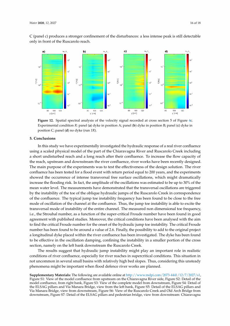
Figure 12 reports the comparison between the PSDs calculated in absence of the dyke (panel d)and in the three configurations A, B and C (panels a,b and c, respectively). The effect of the position ofthe dyke appears quite clearly, comparing panel d (no dyke) with the other panels: with the dyke inposition A, peaks in PSDs are detectable both in the Chiaravagna and the Ruscarolo reaches. Moving toposition B (panel b), the peaks in the velocity spectrum are strongly reduced in both branches. Position

Water 2020, 12, 2027 16 of 18

C (panel c) produces a stronger confinement of the disturbances: a less intense peak is still detectableonly in front of the Ruscarolo reach.

Figure 12. Spatial spectral analysis of the velocity signal recorded at cross section 5 of Figure 4c.Experimental condition R: panel (a) dyke in position A; panel (b) dyke in position B; panel (c) dyke inposition C; panel (d) no dyke (run 1R).

5. Conclusions

In this study we have experimentally investigated the hydraulic response of a real river confluenceusing a scaled physical model of the part of the Chiaravagna River and Ruscarolo Creek includinga short undisturbed reach and a long reach after their confluence. To increase the flow capacity ofthe reach, upstream and downstream the river confluence, river works have been recently designed.The main purpose of the experiments was to test the effectiveness of the design solution. The riverconfluence has been tested for a flood event with return period equal to 200 years, and the experimentsshowed the occurrence of intense transversal free surface oscillations, which might dramaticallyincrease the flooding risk. In fact, the amplitude of the oscillations was estimated to be up to 30% of themean water level. The measurements have demonstrated that the transversal oscillations are triggeredby the instability of the toe of the oblique hydraulic jumps of the Ruscarolo Creek in correspondenceof the confluence. The typical jump toe instability frequency has been found to be close to the freemode of oscillation of the channel at the confluence. Thus, the jump toe instability is able to excite thetransversal mode of instability of the entire channel. The measured non dimensional toe frequency,i.e., the Strouhal number, as a function of the super-critical Froude number have been found in goodagreement with published studies. Moreover, the critical conditions have been analysed with the aimto find the critical Froude number for the onset of the hydraulic jump toe instability. The critical Froudenumber has been found to be around a value of 2.6. Finally, the possibility to add to the original projecta longitudinal dyke placed within the river confluence has been investigated. The dyke has been foundto be effective in the oscillation damping, confining the instability in a smaller portion of the crosssection, namely on the left bank downstream the Ruscarolo Creek.

The results suggest that hydraulic jump instability might play an important role in realisticconditions of river confluence, especially for river reaches in supercritical conditions. This situation innot uncommon in several small basins with relatively high bed slopes. Thus, considering this unsteadyphenomena might be important when flood defence river works are planned.

Supplementary Materials: The following are available online at http://www.mdpi.com/2073-4441/12/7/2027/s1,Figure S1: View of the model confluence from upstream on the Chiaravagna River side, Figure S2: Detail of themodel confluence, from right bank, Figure S3: View of the complete model from downstream, Figure S4: Detail ofthe ELSAG pillars and Via Manara Bridge, view from the left bank, Figure S5: Detail of the ELSAG pillars andVia Manara Bridge, view from downstream, Figure S6: View of the Ruscarolo Creek and Old Arch Bridge fromdownstream, Figure S7: Detail of the ELSAG pillars and pedestrian bridge, view from downstream: Chiaravagna

Water 2020, 12, 2027 17 of 18

River is on the left side of the figure, whereas Ruscarolo Creek is on the right, Figure S8: View of the ChiaravagnaRiver from downstream, Figure S9: Detail of the dyke in position B and Ruscarolo weir, Figure S10: View fromdownstream of the ABB car park, Figure S11: Detail of the model confluence with dyke in position B, view fromright bank.

Author Contributions: All authors contributed to the building of this paper in its different aspects.Conceptualisation: M.C.: and A.S.; experiments: A.D.L., A.R. and A.S.; data analysis; A.D.L., A.R., M.P., M.C. andA.S. writing—original draft preparation: A.D.L., M.P., M.C. and A.S.; writing—review and editing: A.D.L., A.R.,M.P., M.C. and A.S. All authors have read and agreed to the published version of the manuscript.

Acknowledgments: The study has been financially supported by ITEC Engineering, responsible for the riverworks design. We thank Ing. Pinasco of the Comune di Genova, public Authority in charge of the flood riskmanagement of the City of Genova (Italy) and Maurizio Brocchini for the fruitful discussion on the experimentalmeasurements.

Conflicts of Interest: The authors declare no conflict of interest.

Abbreviations

The following abbreviations are used in this manuscript:

PSD Power Spectral DensityFr Foude numberSt Strouhal number

References

1. Hager, W.H. Energy Dissipators and Hydraulic Jump; Springer Science & Business Media: Berlin, Germany,2013; Volume 8.

2. Endreny, T.; Lautz, L.; Siegel, D. Hyporheic flow path response to hydraulic jumps at river steps: Flume andhydrodynamic models. Water Resour. Res. 2011, 47. [CrossRef]

3. Wildhaber, Y.S.; Michel, C.; Epting, J.; Wildhaber, R.; Huber, E.; Huggenberger, P.; Burkhardt-Holm, P.;Alewell, C. Effects of river morphology, hydraulic gradients, and sediment deposition on water exchangeand oxygen dynamics in salmonid redds. Sci. Total Environ. 2014, 470, 488–500. [CrossRef]

4. Grant, S.B.; Gomez-Velez, J.D.; Ghisalberti, M. Modeling the effects of turbulence on hyporheic exchangeand local-to-global nutrient processing in streams. Water Resour. Res. 2018, 54, 5883–5889. [CrossRef]

5. Bakhmeteff, B.A. The hydraulic jump in terms of dynamic similarity. Trans. Am. Soc. Civ. Eng. ASCE 1936,61, 145–162.

6. Rouse, H.; Siao, T.T.; Nagaratnam, S. Turbulence characteristics of the hydraulic jump. J. Hydraul. Div. 1958,84, 1–30.

7. Bélanger, J. Notes sur l’Hydraulique; Ecole Royale des Ponts et Chaussées: Paris, France, 1841; Volume 1842, p. 223.8. Henderson, F.M. Open Channel Flow; Macmillan Co., Inc.: New York, NY, USA, 1966.9. Chanson, H. Development of the Bélanger equation and backwater equation by Jean-Baptiste Bélanger

(1828). J. Hydraul. Eng. 2009, 135, 159–163. [CrossRef]10. Chanson, H. Momentum considerations in hydraulic jumps and bores. J. Irrig. Drain. Eng. 2012, 138, 382–385.

[CrossRef]11. Lennon, J.; Hill, D. Particle image velocity measurements of undular and hydraulic jumps. J. Hydraul. Eng.

2006, 132, 1283–1294. [CrossRef]12. Long, D.; Rajaratnam, N.; Steffler, P.M.; Smy, P.R. Structure of flow in hydraulic jumps. J. Hydraul. Res. 1991,

29, 207–218. [CrossRef]13. Hager, W.H.; Bretz, N.V. Hydraulic jumps at positive and negative steps. J. Hydraul. Res. 1986, 24, 237–253.

[CrossRef]14. Chanson, H.; Brattberg, T. Experimental study of the air–water shear flow in a hydraulic jump. Int. J.

Multiph. Flow 2000, 26, 583–607. [CrossRef]15. Chanson, H. Convective transport of air bubbles in strong hydraulic jumps. Int. J. Multiph. Flow 2010,

36, 798–814. [CrossRef]16. Zhang, G.; Wang, H.; Chanson, H. Turbulence and aeration in hydraulic jumps: Free-surface fluctuation and

integral turbulent scale measurements. Environ. Fluid Mech. 2013, 13, 189–204. [CrossRef]

Water 2020, 12, 2027 18 of 18

17. Wang, H.; Chanson, H. Experimental study of turbulent fluctuations in hydraulic jumps. J. Hydraul. Eng.2015, 141, 04015010. [CrossRef]

18. Montano, L.; Felder, S. An experimental study of air–water flows in hydraulic jumps on flat slopes. J. Hydraul.Res. 2019, 1–11. [CrossRef]

19. Valero, D.; Viti, N.; Gualtieri, C. Numerical Simulation of Hydraulic Jumps. Part 1: Experimental Data forModelling Performance Assessment. Water 2019, 11, 36. [CrossRef]

20. Viti, N.; Valero, D.; Gualtieri, C. Numerical simulation of hydraulic jumps. Part 2: Recent results and futureoutlook. Water 2019, 11, 28. [CrossRef]

21. Jesudhas, V.; Balachandar, R.; Bolisetti, T. Numerical study of a symmetric submerged spatial hydraulicjump. J. Hydraul. Res. 2019, 1–15. [CrossRef]

22. Jesudhas, V.; Balachandar, R.; Wang, H.; Murzyn, F. Modelling hydraulic jumps: IDDES versus experiments.Environ. Fluid Mech. 2020, 1–21. [CrossRef]

23. Mossa, M. On the oscillating characteristics of hydraulic jumps. J. Hydraul. Res. 1999, 37, 541–558. [CrossRef]24. Mossa, M.; Tolve, U. Flow Visualization in Bubbly Two-Phase Hydraulic Jump. Trans. ASME 1998. [CrossRef]25. Murzyn, F.; Chanson, H. Free-surface fluctuations in hydraulic jumps: Experimental observations.

Exp. Therm. Fluid Sci. 2009, 33, 1055–1064. [CrossRef]26. Kramer, M.; Valero, D. Turbulence and self-similarity in highly aerated shear flows: The stable hydraulic

jump. Int. J. Multip. Flow 2020, 103316. [CrossRef]27. Chanson, H.; Gualtieri, C. Similitude and scale effects of air entrainment in hydraulic jumps. J. Hydraul. Res.

2008, 46, 35–44. [CrossRef]28. Pedlosky, J. Geophysical Fluid Dynamics; Springer Science & Business Media: Berlin, Germany, 2013.

c© 2020 by the authors. Licensee MDPI, Basel, Switzerland. This article is an open accessarticle distributed under the terms and conditions of the Creative Commons Attribution(CC BY) license (http://creativecommons.org/licenses/by/4.0/).