water

Review

Numerical Simulation of Hydraulic Jumps. Part 2:Recent Results and Future Outlook

Nicolò Viti 1, Daniel Valero 2,3 and Carlo Gualtieri 1,*1 Department of Civil, Architectural and Environmental Engineering, University of Naples Federico II,

80125 Napoli, Italy; nicolo.viti@gmail.com2 Hydraulic Engineering Section, Aachen University of Applied Sciences, Bayernallee 9,

52066 Aachen, Germany; valero@fh-aachen.de3 Hydraulics in Environmental and Civil Engineering, University of Liège, Chemin des Chevreuils, 1, B52/3,

4000 Liège, Belgium* Correspondence: carlo.gualtieri@unina.it; Tel.: +39-081-768-3433

Received: 31 October 2018; Accepted: 17 November 2018; Published: 24 December 2018�����������������

Abstract: During the past two decades, hydraulic jumps have been investigated using ComputationalFluid Dynamics (CFD). The second part of this two-part study is devoted to the state-of-the-art of thenumerical simulation of the hydraulic jump. First, the most widely-used CFD approaches, namely theReynolds-Averaged Navier–Stokes (RANS), the Large Eddy Simulation (LES), the Direct NumericalSimulation (DNS), the hybrid RANS-LES method Detached Eddy Simulation (DES), as well as theSmoothed Particle Hydrodynamics (SPH), are introduced pointing out their main characteristics alsoin the context of the best practices for CFD modeling of environmental flows. Second, the literatureon numerical simulations of the hydraulic jump is presented and discussed. It was observed thatthe RANS modeling approach is able to provide accurate results for the mean flow variables, whilehigh-fidelity methods, such as LES and DES, can properly reproduce turbulence quantities of thehydraulic jump. Although computationally very expensive, the first DNS on the hydraulic jumpled to important findings about the structure of the hydraulic jump and scale effects. Similarly,application of the Lagrangian meshless SPH method provided interesting results, notwithstandingthe lower research activity. At the end, despite the promising results still available, it is expectedthat with the increase in the computational capabilities, the RANS-based numerical studies of thehydraulic jump will approach the prototype scale problems, which are of great relevance for hydraulicengineers, while the application at this scale of the most advanced tools, such as LES and DNS, is stillbeyond expectations for the foreseeable future. Knowledge of the uncertainty associated with RANSmodeling may allow the careful design of new hydraulic structures through the available CFD tools.

Keywords: hydraulic jump; two-phase flow; computational fluid dynamics; turbulent free surfaceflows; numerical simulation accuracy

1. Introduction

Numerical modeling has been a revolution in most civil engineering disciplines. With the boomof available computer power and the continuous algorithm improvement, classic Partial DifferentialEquations (PDE) have been numerically addressed, allowing accurate case-dependent solutions for awide range of problems. However, fluid dynamics equations remain obscure to both researchers andpractitioners, and highly accurate numerical solutions have been obtained uniquely for very simplegeometries. Computational Fluid Dynamics (CFD) has benefited from simplifications, which mainlycame in the form of turbulence models, hence allowing the study of large, complex problems.Nonetheless, the focus is on the accuracy for complex hydraulic engineering challenges. For such

Water 2019, 11, 28; doi:10.3390/w11010028 www.mdpi.com/journal/water

Water 2019, 11, 28 2 of 18

problems, modeler needs to be aware of the associated uncertainties and take them into considerationin the design stage. The accuracy of CFD for such specific problems can deviate from typical valuesobtained in simpler flows, reported in the classic literature (e.g., [1,2]).

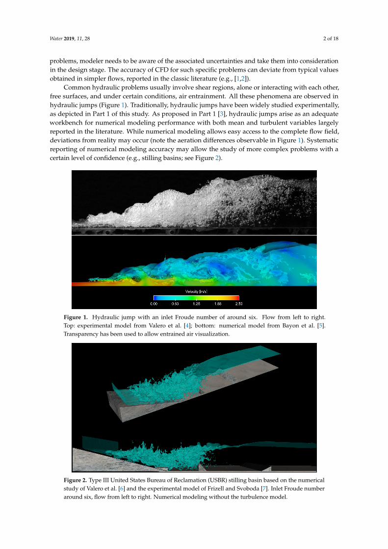
Common hydraulic problems usually involve shear regions, alone or interacting with each other,free surfaces, and under certain conditions, air entrainment. All these phenomena are observed inhydraulic jumps (Figure 1). Traditionally, hydraulic jumps have been widely studied experimentally,as depicted in Part 1 of this study. As proposed in Part 1 [3], hydraulic jumps arise as an adequateworkbench for numerical modeling performance with both mean and turbulent variables largelyreported in the literature. While numerical modeling allows easy access to the complete flow field,deviations from reality may occur (note the aeration differences observable in Figure 1). Systematicreporting of numerical modeling accuracy may allow the study of more complex problems with acertain level of confidence (e.g., stilling basins; see Figure 2).

Figure 1. Hydraulic jump with an inlet Froude number of around six. Flow from left to right.Top: experimental model from Valero et al. [4]; bottom: numerical model from Bayon et al. [5].Transparency has been used to allow entrained air visualization.

Figure 2. Type III United States Bureau of Reclamation (USBR) stilling basin based on the numericalstudy of Valero et al. [6] and the experimental model of Frizell and Svoboda [7]. Inlet Froude numberaround six, flow from left to right. Numerical modeling without the turbulence model.

Water 2019, 11, 28 3 of 18

Part 2 of this study presents several three-dimensional numerical modeling techniques and theirachievements to date. In Section 2, focus is put on giving the basic concepts, while the adventurousreader is addressed to the relevant experts’ reviews and books for each of the techniques [8–13]. Somecomments on best practices are presented, as well. Section 3 brings to light a large variety of studiesconducted during the past twenty years, disclosing aspects related to the expected accuracy of theemployed numerical modeling methods. Conclusions are presented in Section 4, followed by Section 5,which includes a brief future outlook.

2. Numerical Methods for Hydraulic Jump Research

2.1. Overview

Incompressible two-phase flows are governed by the equations of conservation of mass andmomentum, defined for both air and water phases. These laws are represented through theNavier–Stokes (N-S) equations, which, in their original form, encompass all known internal andexternal effects of the motion of a fluid. Further details can be found in general fluid mechanics bookssuch as Pope [8], among others. Any form of numerical modeling of hydraulic jumps was achievedby means of the N-S equations or any of their simplifications. N-S equations are inherently nonlinear,time-dependent, and three-dimensional PDE. Three-dimensionality is essential in these equations,because vortex stretching is not possible in a two-dimensional space.

The numerical modeling of turbulent flows involves considerable difficulties, related to theaccurate computation of the vortex dynamics, the determination of the instantaneous position andconfiguration of the free surface, turbulence effects, and air entrainment [13,14]. The hydraulic jumphas been studied using mathematical models based on the N-S equations, free surface tracking methodssuch as the Volume Of Fluid (VOF) method [15], or the level-set method and different turbulencemodels (see, e.g., [16–18]).

The VOF method uses a function f (x, y, z, t) to assign the free surface. The function f , representinga fraction of fluid, is obtained from the following equation:

∂ f∂t

+ Uj∂ f∂xj

= 0 (1)

U being the convection velocity.A unit value of f corresponds to a cell full of fluid, while a zero value indicates that the cell

contains no fluid. Cells with f values between zero and one contain a free surface. The function fcan be solved with different methods, and different schemes have been implemented to improve theaccuracy of the free surface reconstruction. More complicated free surface tracking schemes are alsopossible; see for instance the methods used in the study of Mortazavi et al. [19], Fuster et al. [20], or theextensive review of Scardovelli and Zaleski [21]. It must be noted that the free surface is a movableinterface where both density and viscosity change abruptly, being prone to significant numericaldiffusion. Accurate estimation of surface tension effects directly depends on proper representation offree surface curvature.

2.2. One- and Two-Dimensional Modeling

One- and two-dimensional modeling was attempted for hydraulic jumps, obtaining greatinsight into the flow structure. Non-hydrostatic approaches are noteworthy, providing considerableunderstanding of the free surface profile, velocity fields, and even characteristic frequencies. Some one-and two-dimensional modeling includes Madsen and Svendsen [22], Valiani [23], Madsen et al. [24],Castro-Orgaz and Hager [25], and Richard and Gavrilyuk [26]. For the sake of briefness, the interestedreader is addressed to the extensive book of Castro-Orgaz and Hager [27] for a thorough descriptionon non-hydrostatic methods.

Water 2019, 11, 28 4 of 18

2.3. Three-Dimensional Modeling

2.3.1. RANS Approach

The most commonly-applied approach to simulate a turbulent flow is that based on the timeaveraging, herein Reynolds-averaging, of the N-S equations, leading to the Reynolds Averaged N-S(RANS) equations. In this statistical approach, the instantaneous values of velocity and pressure aredepicted as the sum of a mean and fluctuating component [28]. Any instantaneous velocity ui at agiven coordinate x and time t can be written as:

ui(x, t) = ui(x, t) + u′i(x, t) (2)

ui and u′i being the mean and fluctuating velocity, respectively.Note that the mean velocity is still meant to depend on the time t, which is possible when the

time averaging is defined as [2]:

ui(x, t) =1T

∫ t+T

tui(x, t)dt , T1 � T � T2 (3)

T1 is a characteristic time-scale of the turbulent fluctuations and T2 a characteristic time-scale of theunsteadiness. While T � T2, some flow unsteadiness can be reproduced (e.g., jump toe fluctuations,as shown by Bayon et al. [5]). Hence, we are assuming that a difference between both time-scales existsand is of several orders of magnitude. Consequently, the time derivative of the RANS equations doesnot necessarily vanish, and transient flows can be also modeled through a time-averaged procedure:

ρ

(∂ui∂t

+ uj∂ui∂xj

)= − ∂p

∂xi+

∂

∂xi

(µ

∂ui∂xi

+ Rij

)(4)

µ is the dynamic viscosity, ρ the density, and p the mean pressure. Due to the non-linearity ofthe N-S equations, averaging leads to unknown correlations between scalar quantities known asReynolds stresses, which are represented in the previous formula with the Reynolds stress tensorRij = −ρ u′iu

′j [28]. The Reynolds stresses are six additional unknowns introduced by the averaging

procedure, which, nonetheless, do not introduce any new equation. This is the well-known closureproblem of the RANS equations [2,8]. How the Reynolds stresses are modeled has led to a wide,eclectic range of turbulence models.

The simplest RANS models are the eddy viscosity models (based on the Boussinesq hypothesis).Following the Boussinesq hypothesis, Reynolds stresses are modeled using an eddy (or turbulent)viscosity νt (equivalently, µt), which, ultimately, means that the effect of turbulence is to act on the meanflow as an increased viscosity [29]. Hence, apparent stresses Rij are nulled, and an increased viscosity iscontemplated instead. Based on dimensional analysis, νt can be determined from a turbulent time-scale(or velocity scale) and a turbulent length-scale. Note that two parameters are needed to close thesystem properly through an eddy viscosity model. The most commonly-used variables are listed inTable 1.

Table 1. Variables used in the most common turbulence models to calculate µt.

Dimensional Scale Unit Equation

Turbulent kinetic energy L2/T2 k = u′iu′i/2

Turbulence dissipation rate L2/T3 ε = ν∂u′i∂xj

∂u′i∂xj

Specific dissipation rate 1/T ω = ε/k

Water 2019, 11, 28 5 of 18

Different turbulence models estimate νt based on different turbulent variables. Some examples areas follows:

• The Spalart–Allmaras model [30] solves a transport equation for an auxiliary turbulent viscosityνt ∼ ν̃.

• The standard k− ε [31,32] and the RNG k− ε [33,34] solve transport equations for k and anotherfor ε → νt ∼ k2/ε. The former is the most widely-used engineering turbulence model forindustrial applications because of its robustness and reasonable accuracy for a wide range offlows. It is a two-equation transport model for k and ε, their coefficients being empirically derived.The RNG version adds a term for the ε equation, which is known to be responsible for differencesin its performance [8]. It is oftentimes mentioned that accuracy for rapidly-swirling flows isimproved, despite fewer validations having been conducted [1].

• Standard k − ω (2008) and SST k − ω [35] solve transport equations for k and ω → νt ∼ k/ω.The k − ω model is a two-equation transport model based on solving equations for k and ω.The original version was known to be excessively sensitive to free stream quantities, which isan undesired feature [36], while the revised version of Wilcox [37] attempts to solve this issue.The SST k − ω is a variant of the former. The SST k − ω model uses a blending function totransition gradually from the standard k− ω model near the wall to a high Reynolds numberversion of the k− ε model in the outer portion of the boundary layer [35].

In addition to the eddy viscosity models, the Reynolds stress tensor can be modeled (based onsome assumptions) by formulating an equation for each of the terms. The large dimension of theresulting equations and the small gain in accuracy has led to a reduced use in comparison to eddyviscosity models [38].

2.3.2. LES and DES Approach

Large Eddy Simulation (LES) has been developed considering that the large scale is stronglyenergetic, whereas the small scale, which is more dissipative, is universal and represents only a smallpart of the turbulent spectrum. Hence, the large scale of turbulence is resolved, while the small scaleis modeled [39]. The main difference between RANS and LES approaches is that the N-S equationsare, in the former, time-averaged and, in the latter, space filtered. Notwithstanding that, both sets ofequations take a similar form because a stress tensor is created by the time-averaging and filteringprocesses. In the LES approach, the stress tensor resulting from low-pass filtering is:

RSGSij = ρ

(uiuj − ui uj

)(5)

These sub-grid scale stresses, differently than in RANS models, attempt to approximate onlythe part of the turbulence that is unresolved, i.e., below the size of the low-pass filter window. It isnoteworthy that while some unsteadiness can be reproduced by RANS models, their computationdoes not change (in theory) with the cell size, while in LES, RSGS

ij → 0 and, consequently, convergesto a DNS. In a similar manner to RANS models, the stresses appearing in the flow equations can bemodeled in different ways [39].

Some hybrid LES-RANS approaches were also proposed in the literature. They have the generalgoal of combining the advantages of LES and RANS, minimizing their shortcomings. For the DetachedEddy Simulation (DES) approach [40], the near-wall region is simulated using the RANS method,while away from the wall, LES is used [39].

2.3.3. DNS Approach

DNS numerically addresses the N-S and continuity equations with physically consistent accuracyin space and time, in such a way as to resolve all the essential turbulent scales. If the mesh is fineenough, the time step is short enough, and the numerical scheme is designed to minimize the dispersion

Water 2019, 11, 28 6 of 18

and dissipation errors, one obtains an accurate three-dimensional time-dependent solution of thegoverning equations, in which the only errors are those introduced by the residual approximationsincorporated in the numerical scheme and in the number-representation technology of the computingmachine [41]. The contributions of DNS to turbulence research in the last few decades have beenimpressive [42]. As one can see, the biggest problem regarding DNS is their overwhelming requirementfor computer power in a sense of both the processor’s performance and the size of the memory forstoring intermediate results.

2.4. Best Practices for CFD Modeling of Environmental Flows

The application of CFD methods to the environmental fluid mechanics area generally involvesmany different issues related to the existing uncertainty of geometry and boundary conditions,drag coefficients, driving forces, and the interactions among different processes and inputs [43].This is particularly important in the numerical simulation of the hydraulic jump, which involvesfluctuating boundaries, as well as a multiphase flow. These uncertainties involve almost every aspectof the modeling process, and it may therefore be very difficult to assess model performance, as theseuncertainties also apply to the experimental model (see Part 1). This implies that CFD applicationto environmental flows may have research priorities very different from other CFD applications,bearing in mind that the closer they are to the left side of Table 2, the more necessary proper validationwill be.

Table 2. Turbulence modeling, indicator for resolved/modeled turbulence (R: Resolved; M: Modeled),accuracy, and computational cost of RANS, LES, Detached Eddy Simulation (DES), and DNS.

RANS DES LES DNS

Modeling approach Reynolds-averaged RANS-LES coupling Sub-grid scale Not necessary

Large scales/inertial M/M/M R/M/M R/R/M R/R/RSubrange/dissipation scale

Expected accuracy Mean variables Allow inertial Allow inertial Up to thescales’ modeling scales’ modeling Kolmogorov scale

Computational cost Low High High Extremely high

Roache [44] discussed the quantification of uncertainty in CFD methods, pointing out thedifference between verification, which means solving the equations right, and validation, whichis solving the right equations, concluding that a code cannot be validated, but only a calculation or arange of calculations with a code can be validated. Later, Roache [45] noted that calibration, which isthe adjustment or tuning of free parameters in a model to fit the model output with experimental data,which is a sometimes necessary component of model development, cannot be considered as validation,unless when the previously-calibrated model predictions are evaluated using a dataset not used inthe tuning.

Some criteria for the application of CFD codes to open channel flows were proposed byKnight et al. [46], while Lane et al. [47] expanded the guidelines specified by ASME [48] for the specificcase of open channel flows. They demonstrated that the ASME criteria may not be sufficient for manypractical fluvial applications, but can provide a minimum framework. In particular, Lane et al. [47]argued that the ASME criterion on model validation should be replaced by a more comprehensiveframework based on sensitivity analysis, including mesh sensitivity study, benchmarking, and flowvisualization. For mesh sensitivity analysis, methods such as that of Celik et al. [49], recommended bythe ASME, should be preferred. Celik et al.’s work [49] was based on the Richardson extrapolation andallows computation of the numerical uncertainty of a given variable. A common error in numericalstudies is the misjudgment in detecting the relevant variable to be subject to the numerical uncertaintyanalysis. Preferably, the numerical uncertainty analysis should be performed on all the resultspresented or on variables with an expected similar level of uncertainty. A study should not assess

Water 2019, 11, 28 7 of 18

the numerical uncertainty of the water depth and claim that turbulence fluctuations would present asimilar level of mesh dependence. If the aim of the study is to reproduce aeration, air concentrationsor turbulence quantities should be the main variables of the sensitivity analysis.

Finally, as suggested by Blocken and Gualtieri [43], it is advisable that future best practiceguidelines for CFD applications to environmental flows include a larger application of benchmarkingbecause this provides relevant information for reliable comparison among different CFD techniquesand approaches. Therefore, specific benchmarks should be developed in the different contexts andpractical applications of CFD methods for environmental flows.

3. Hydraulic Jump Numerical Modeling Studies

3.1. General Comments

The study of aerated flows in hydraulic engineering is still challenging in terms of eitherexperimental investigation or numerical modeling considering the large number of relevant equations,parameters, and their complexity (see Part 1). Thus, the hydraulics of two-phase flows can greatlybenefit from the insights provided by numerical simulations, and the last few decades have seen thedevelopment of powerful numerical capabilities with direct applications into gas-liquid flows [11].

Depending on the flow field description, two approaches can be distinguished: Lagrangianmethods and Eulerian methods. The first approach follows a fluid particle at each point. The lattertreats the fluid properties as a function of time and space. Both approaches have been used in fluidmechanics to describe hydraulic jump flows. Among the meshless Lagrangian techniques, one of themost versatile techniques is Smoothed Particle Hydrodynamics (SPH), which solves flow equations fora set of moving particles (with a certain mass). Use of a kernel function to interpolate flow variablesbecomes critical, but the determination of the free surface is natural, unlike grid-based techniques(Eulerian methods), which need an additional method to track the free surface (i.e., VOF by Hirt andNichols [15]).

Within Eulerian methods, the RANS approach is the most widely used, followed by LES.Hybrid RANS-LES methods, such as DES, are growing in popularity. For the sake of briefness,the aforementioned methods are not extensively described in this study, but the reader is addressed toprevious works, as referenced in Tables 3 and 4.

Table 3. Milestone references on different numerical modeling approaches.

Flow Field Description Approach References

Lagrangian Smoothed ParticleGingold and Monhagan [50]

HydrodynamicsMonaghan [51]

Violeau [52]Violeau and Rogers [53]

Eulerian

Reynolds-Averaged Navier–Stokes

Reynolds [54]Rodi [28]

Spalart [36]Wilcox [2]

Detached Eddy Simulation Spalart [55]

Large Eddy Simulation Labourasse et al. [56]Rodi et al. [39]

Direct Numerical SimulationMoin and Mahesh [42]

Prosperetti and Tryggvason [11]Alfonsi [41]

Water 2019, 11, 28 8 of 18

Table 4. Most widely-used turbulence models in RANS applications and original contributions.

Turbulence Model References

Standard k− εJones and Launder [31]

Launder and Sharma [32]

RNG k− εYakhot and Orszag [33]

Yakhot et al. [34]

k−ωWilcox [2]Wilcox [37]

SST k−ω Menter [35]

Table 5 lists several numerical CFD studies dealing with hydraulic jumps. They are presentedchronologically and are classified according to the flow field description and the type of numericalapproach used. RANS-based methods prevail due to their lower computational cost, but, in turn,turbulence model dependence is stronger (we mention: standard k− ε, termed in Table 5 as STD k− ε,RNG k− ε, and SST k−ω).

Table 5. Numerical simulation studies of hydraulic jumps and inlet Froude number (F1).

Flow Field Description References Year Numerical Turbulence Resolution F1Approach Model Dependence Study

Lagrangian Methods

Lopez et al. [57] 2010 SPH k− ε Meshless method

3.25, 3.41, 3.58,3.61, 3.64, 4.12,4.45, 4.88, 5.13,

5.24, 6.62, 7.06, 7.16

De Padova et al. [58] 2013 XSPH mixing length Meshless method 3.90, 8.30and k− ε

De Padova et al. [59] 2018 XSPH mixing length Meshless method 2.58, 2.66, 2.70,and k− ε 3.89, 4.99, 5.11

Eulerian Methods

Chippada et al. [60] 1994 RANS STD k− ε − 2.00, 4.00

Zhao et al. [61] 2004 RANS STD k− ε, k− l − 1.46

Gonzalez and 2005 RANS STD k− ε√

2.00, 2.50, 3.32Bombardelli [62]

Carvalho et al. [14] 2008 RANS RNG k− ε − 6.00

Abbaspour et al. [63] 2009 RANS STD k− ε −4.00, 4.70, 5.00,

RNG k− ε5.70, 5.80, 6.107.00, 7.20, 8.00

Ma et al. [64] 2011 RANS SST k−ω − 1.98

Ebrahimi et al. [65] 2013 RANS STD k− ε −3.00, 3.30, 3.603.60, 5.00, 5.70

6.70, 8.00

Bayon-Barrachina 2015 RANS STD k− ε √6.10and Jiménez [66] RANS RNG k− ε

SST k−ω

Witt et al. [67] 2015 RANS realizable k− ε√

2.43, 3.65, 4.82

Bayon et al. [5] 2016 RANS RNG k− ε√

6.50

Witt et al. [68] 2018 RANS realizable k− ε√

2.43, 3.65, 4.82

Harada and Li [69] 2018 RANS k− ε, k−ω√

5.80

Valero et al. [6] 2018 RANS RNG k− ε, k− ε√ 3.12, 3.88, 4.20,

6.17, 6.37, 6.47,8.27, 9.52

Ma et al. [64] 2011 DES√

1.98

Jesudhas et al. [70] 2018 DES√

8.5

Gonzalez and 2005 LES√

2.00, 2.50, 3.32Bombardelli [62]

Lubin et al. [71] 2009 LES − 5.09

Mortazavi et al. [19] 2016 DNS Full solution √2.00of all the scales

Water 2019, 11, 28 9 of 18

3.2. Reynolds-Averaged Navier–Stokes Approach

The early study of Chippada et al. [60] studied two Froude numbers (F1 = 2, 4) using the standardstandard k − ε model and 2D simulations, together with a Eulerian-Lagrangian flow descriptionhelping the determination of the moving free surface.

Zhao and Misra [61] focused on the mean flow motions of a hydraulic jump using the numericalmodel RIPPLE [72]. Two turbulence models were used: the standard k− ε model and the k− l modelof Zhao et al. [61]. Zhao and Misra focused on weak hydraulic jumps, their main interest beingon bores. Model results were compared to the LDV laboratory measurements of Bakunin [73] andSvendsen et al. [74] with an overall adequate agreement, despite underestimation of downstreamstreamwise velocities.

Gonzalez and Bombardelli [62] simulated the entire two-phase flow of low Froude numberhydraulic jumps (mean flow, turbulence, and air entrainment). Air features were incorporated throughthe free surface. Gonzalez and Bombardelli [62] compared 2D and 3D RANS and LES models to theexperimental observations of Liu et al. [75], including both mean flow and turbulence, and somequalitative analysis of the air fractions.

Carvalho et al. [14] carried out a 2D RANS simulation of a hydraulic jump with a higher Froude(F1 = 6). The jump was contained in a stilling basin downstream of a spillway, and the comparisonwas conducted against their own experimental data and Hager [76] empirical relations. The numericalmodel combined high-order schemes [77] for the advection terms, a refined VOF algorithm [78]for free surface tracking, the Fractional Area-Volume Obstacle Representation (FAVOR) method forrepresenting internal obstacles (as defined by Hirt and Sicilian [79]), and the RNG k− ε turbulencemodel. The numerical models of Carvalho et al. [14] were not able to properly represent either the freesurface or the pressures. Additionally, shear stresses were underestimated. Nevertheless, the meanvelocities were satisfactorily predicted, except in the zone where vortices develop. The maximumvalues of the velocity and pressure in the flow domain remained below those measured in theexperimental installation, but their locations were well predicted.

Abbaspour et al. [63] used 2D numerical models to study the hydraulic jump over a rough bedusing both standard and RNG k− ε models, together with a VOF method to determine the free surfacelocation. Characteristics of the jump, such as water surface profile, length of the jump, velocity profilein different sections, and bed shear stress were evaluated for a range of Froude numbers 4 < F1 < 8through a total of 12 simulations. The authors found a close agreement with both the experimentalvalues obtained by Ead and Rajaratnam [80] in terms of mean relative error: about 1%–8.6% for freesurface profiles and about 1%–12% for the length of the jump. The bed shear stresses were computedusing the measured depths up- and down-stream of the jump. Differences between total shear stressin experimental and numerical models remained small. Abbaspour et al. [63] concluded that the bestagreement was obtained using the RNG model.

Void fraction predictions in a hydraulic jump were the main goal of Ma et al. [64], who used asub-grid air entrainment model coupled with RANS and DES models to study an F1 = 1.98 hydraulicjump. Sub-grid models arise from the hypothesis that the numerical model alone will not be able toreproduce aeration. Thus, some additional “physics” are input; likewise, a turbulence model aimsto represent the small scale fluctuations. Free surface was modeled using a level-set method andturbulent viscosity evaluated using the SST model. Results were compared to the experimental modelof Murzyn et al. [81], concluding that air transported in the shear layer was better reproduced than inthe upper region due to RANS modeling limitations to capture free surface fluctuations.

Water 2019, 11, 28 10 of 18

Ebrahimi et al. [65] carried out 2D simulations (together with the standard k− ε and VOF) ofhydraulic jumps on a rough bed for a wide range of Froude numbers (3 < F1 < 7) across a total of 16simulations. The authors found a close agreement with the experimental measurements from Elsebaieand Shabayek [82], with mean relative errors around 0–4.4% for water surface profiles and 0–6.7% forthe length of the jump. The model also provided good estimates of the total shear force.

Bayon-Barrachina and Jimenéz [66] used the open source OpenFOAM code with standard k− ε,RNG k− ε, and SST k− ω models to study a 3D classic hydraulic jump with F1 = 6.1. Results werecompared to the experimental relations of Hager [76] and Wu and Rajaratnam [83], among others,obtaining high accuracies. The authors found that the RNG k − ε model was performing better,followed by the SST k−ω and the k− ε; although in all cases, errors were lower than 4%.

Witt et al. [67] simulated the air entrainment characteristics of three Froude number hydraulicjumps using the realizable k − ε model, with VOF treatment for the free surface through 2D and3D simulations. Velocity profiles, void fraction profiles, and Sauter mean diameter were comparedto the experimental data from Murzyn et al. [81], Liu et al. [75], and Lin et al. [84], among others.Velocity profiles showed good agreement with the experimental observations for jumps. Void fractionswere well predicted with differences rarely over 10%. Witt et al. [67] observed that at least eight cellsper bubble diameter are necessary to reproduce the associated aeration. Furthermore, 3D simulationimproved void fraction predictions in the shear layer, and consequently, the average free surfaceelevation.

A systematic performance analysis of the OpenFOAM and FLOW-3D R© codes was presented byBayon et al. [5], investigating a steady hydraulic jump of a Froude number of 6.5. The RNG k− ε

model and the VOF method were used. Performance assessment was conducted by comparing severalhydraulic jump variables with the literature and their own experimental data [76,85–90]. Numericaluncertainty was assessed following Celik et al. [49], finding that FLOW-3D R© presented a fasterconvergence with coarser meshes, whereas OpenFOAM had a more stable solution with refinement.All mean variables studied (not including aeration) obtained accuracies above 90%, except for theroller length, which remained at around 80%, and the negative velocities at the upper jump region.An autocorrelation analysis was conducted, finding good computation of jump toe frequencies, thusshowing that RANS models can also reproduce the unsteadiness typical of hydraulic jumps.

Witt et al. [68] extended the analysis of the work of Witt et al. [67], studying some air-water meanand turbulent flow features, showing that satisfactory prediction of turbulence quantities can also beachieved through RANS modeling.

Harada and Li [69] modeled a 2D hydraulic jump of F1 = 5.8 using the standard k − ε modeland the VOF method. Air concentrations were compared to the experimental model of Kucukali andChanson [91], obtaining errors below 10% roller length against Hager [76].

Valero et al. [6] studied the flow field (RNG k − ε model and the VOF method) inside aUnited States Bureau of Reclamation (USBR) Type III stilling basin and compared numerical results,contemplating eight Froude numbers (in the range of 3.12–9.52), to the data of Frizell and Svoboda [7].Good agreement was obtained for sequent depth relations and sweep-off point. The numerical modelallowed insight into the distribution of forces on the different elements of the basin, thus explainingthe experimental observation of Frizell and Svoboda [7] on the capacity of the Type III to hold insidejumps even for very low tailwater levels.

Figure 3 shows the accuracy of previous RANS models with standard k− ε, RNG k− ε, and theSST k−ω turbulence models. In Figure 3, the results are also classified by Froude number; followingthe jump typology of Bradley and Peterka [92] (see Part 1). The RNG k − ε model comparativelyprovided the best performances for all four jump parameters, despite is also showing the largestscatter. The standard k− ε model provided more accurate results in terms of the roller length and thefree surface.

Water 2019, 11, 28 11 of 18

Figure 3. Accuracy obtained in some of the past RANS studies for different turbulence models andflow variables: (a) sequent depths relation; (b) roller length; (c) efficiency; and (d) mean free surface.Inlet Froude numbers clustered by jump typology, as presented in Part 1 of this study.

3.3. Detached Eddy Simulation and Large Eddy Simulation

Ma et al. [64], besides RANS simulations, used also the DES approach to predict air entrainmentin a hydraulic jump of F1 = 1.98. By comparing the numerical results with the experimental dataof Murzyn et al. [81], Ma et al. [64] found that the averaged DES results predicted the observedvoid fraction profiles in both the lower shear layer and the upper roller region, while the RANSapproach missed the latter. This is due to the better capabilities of DES to capture strong fluctuations.Nonetheless, Bayon et al. [5] showed that the RANS model can reproduce satisfactorily big-scalefluctuations inside hydraulic jumps.

Recently, Jesudhas et al. [70] studied an F1 = 8.5 hydraulic jump using a DES approach togetherwith a VOF and a high-resolution capturing scheme. Not only were the numerical results compared topast experimental literature (among others, [84,89,93,94])—with excellent agreement—but also newinsights into the turbulence structure were presented, as for instance how the developing shear layerleads to intense free surface deformations. The study of Jesudhas et al. [70] proved that DES maysuffice to study turbulent features.

Concerning the LES part of the study of Gonzalez and Bombardelli [62], satisfactory agreementwas found in terms of mean flow, turbulence, and air entrainment. However, LES outcomes showedsimilar patterns in the time-averaged flow field as those obtained with the k− ε model.

Large eddy simulation of the hydraulic jump was also executed by Lubin et al. [71]. The numericalresults were then compared with experimental data collected on a physical model. Important handicapswere noticed as a result of the strong interface deformations, break-ups, and high shear levels. The flowdid not tend to a stationary state because of some numerical diffusion at the free surface.

3.4. Direct Numerical Simulation

Mortazavi et al. [19] recently presented the first Direct Numerical Simulation (DNS) of a stationaryturbulent hydraulic jump with F1 = 2 and a low Reynolds number (11,000) with no boundarylayer development at the inlet. A non-dissipative geometric VOF method was used to track thestrongly-distorted interface, while level-set equations were also solved in order to calculate the

Water 2019, 11, 28 12 of 18

interface curvature for the surface tension forces’ computation. They compared the numerical resultswith the experimental data by Murzyn et al. [95]. It was shown that the Reynolds number did notinfluence the DNS statistics. The error of the mean velocity, fluctuations, and Reynolds stressescomputed was within±10% accuracy. Reasonably good agreement was observed with experiments forvoid fraction measurements and interface length-scale measurements. Mortazavi et al. [19] found thatbubble entrainment presented a periodic nature, bubbles being generated in patches with a specificfrequency associated with the roll-up frequency of the roller at the toe of the jump. This highlightsthe relevance of experimental studies focused on hydraulic jump frequencies to better understandthe air entrainment process. The study of Mortazavi et al. [19] also shed light on the energy transferprocesses, yielding better understanding of the energy dissipating properties of the jump. Additionally,Mortazavi et al. [19] analyzed how the effects of scale affect the entrainment of air by modeling thesame hydraulic jump with the same flow parameters, except the Reynolds number (5000 and 11,000).Despite the limited Reynolds number range, this type of information can be priceless for the study ofscale effects.

3.5. Smoothed Particle Hydrodynamics

Lopez et al. [57] investigated the capabilities of Smoothed Particle Hydrodynamics (SPH) toreproduce a mobile hydraulic jump for different Froude numbers. Numerical simulations werecompared to their own physical model. Results showed good agreement for F1 < 5. Applying thestandard k− ε model, a considerable improvement in the model simulating hydraulic jumps withF1 > 5 was also obtained. The main disadvantage of this approach is the doubling of the computationaltime. Finally, it was found that SPH provides correct estimates of the average pressures at theboundaries, but exhibits large dispersion for instantaneous water depths.

De Padova et al. [58,59] carried out different studies on the numerical modeling of the hydraulicjump using the SPH method and a weakly-compressible XSPHscheme, which includes a mixing-lengthturbulence model and a two-equation turbulence model to represent turbulent stresses. First,they reproduced the formation of different undular jumps [58]. Instantaneous and time-averaged flowvariables were compared with acoustic Doppler velocity measurements for F1 equal to 3.9 and 8.3. TheSPH model slightly overestimated the measurements of the velocity, in the zone of the lateral shockwave and in the vortex zone near the lateral wall. The predicted free surface elevations and velocityprofiles showed a satisfactory agreement with measurements and most of the particular features of theflow, such as the trapezoidal shape of the wave front and the flow separations at the toe of the obliqueshock wave along the side walls. The numerical results were compared with their own experimentalinvestigations. The comparison proved that, when simulating hydraulic jumps without a surface roller,a simple turbulence model based on the mixing-length hypothesis suffices to yield results that, interms of water depths and average velocity predictions, were like those obtained using the standardk− ε turbulence model.

De Padova et al. [59] investigated the oscillating characteristics and cyclic mechanisms in hydraulicjumps. Both the mixing-length turbulence model and the standard k− ε model were able to predictsome features of the flow, but comparison with experimental results showed that the mixing-lengthresults were closer to the experimental data [96] than those from the k− ε in, for instance, predictingthe spectra of the surface elevations upstream and downstream of the jump.

4. Conclusions

Hydraulic jumps have been traditionally studied mainly by means of experimental modeling,with some limited contributions from analytical studies (see Part 1 of this study [3]). In the past twentyyears, numerical research activity has experienced a large burst in terms of quantity and quality. Twodifferent types of studies can be found: those that aim to validate the numerical tool for a set of flowconditions (mainly RANS modeling techniques) and those that aim to shed light on some unresolvedflow features (DES, LES, and DNS).

Water 2019, 11, 28 13 of 18

Surprisingly, RANS modeling approaches have yielded accurate results, with accuracies over90% for mean flow variables, including air concentrations in some cases. Besides, some fluctuationshave been observed, contrary to the early RANS studies’ conclusions. It must be noted, however,that aeration has been studied mainly in terms of air concentrations. Two different solutions canpresent the same air concentration profile with a completely different distribution of bubble sizes.Future validations in terms of air entrainment should address this key issue. Nonetheless, the numberof available validations is limited (Figure 3) with very sparse approaches used, and hence, it cannot bestated that a single model has stood out over the rest. From an engineering point of view, any of thetwo-equation transport models presented could be used for design purposes as long as the uncertaintyreported by previous studies is kept in mind on the final results. In this regard, it must be noted thatthe recirculation length should hold a larger uncertainty than the variables reported in Figure 3.

High-fidelity approaches, such as DES and LES, have shown that turbulence quantities can beproperly reproduced with these models. It is noteworthy that the first DNS study on hydraulic jumpshas been released [19], leading to important conclusions in terms of hydraulic jump structure and scaleeffects, despite the low Froude and Reynolds numbers.

5. Future Outlook

With recent years, numerical studies have become more physically sound and follow more strictanalysis procedures. Upcoming model validations should include turbulent variables, and larger,community-based benchmarking may help to cover the gaps of Figure 3. Once having properlyestablished the deficiencies of low fidelity models, they should be compensated with improvedturbulence and sub-grid air entrainment models.

Results of the high fidelity models can compensate handicaps of multiphase flow instrumentation.Yet, it is still to be exploited how the information of higher accuracy models (and morecomputationally expensive, in turn comparable to experimental modeling) is used to formulatemore accurate—physically-based—sub-grid and turbulence models to be used in more affordabletechniques (e.g., within RANS models or improved DES models).

Solving the shortcomings of less demanding models could anticipate a new era of massive3D numerical modeling of prototype-scale problems (with scales reaching hundreds of meters andvelocities a few dozens of meters per second); which is of great relevance for practitioners, for whichLES (and obviously DNS) could remain out of their hardware capabilities for some decades.

Author Contributions: Writing-Original Draft Preparation, D.V. and N.V.; Writing-Review and Editing, D.V. andC.G.; Supervision, C.G.; Funding Acquisition, C.G.

Acknowledgments: Nicolò Viti acknowledges the support from the Project “Sistemi avanzati di dissipazione arisalto nelle opere idrauliche: aspetti teorici e progettuali” funded by the Regione Campania under the “L.R. n. 5del 28/03/1992”.

Funding: The APC was funded by the University of Napoli Federico II.

Conflicts of Interest: The authors declare no conflict of interest.

Nomenclature

The following symbols are used in this manuscript:

F1 inlet Froude numberf fraction of fluidk turbulence kinetic energyp mean pressureRij Reynolds stress tensorRSGS

ij sub-grid scale stresses

T time intervalt time

Water 2019, 11, 28 14 of 18

T1 characteristic time-scale of the velocity fluctuationsT2 characteristic time-scale of the unsteadinessT time intervalU convection velocityu instantaneous velocityu mean velocityu′ velocity fluctuationu′iu′j velocity fluctuation covariance

xj coordinates (x, y, z)ε turbulence dissipation rateµ dynamic viscosityµt turbulent viscosityνt turbulent viscosity (µt/ρ)ρ fluid densityω specific dissipation rate

Abbreviations

The following abbreviations are used in this manuscript:

ASME American Society of Mechanical EngineersCFD Computational Fluid DynamicsDES Detached Eddy SimulationDNS Direct Numerical SimulationFAVOR Fractional Area-Volume Obstacle RepresentationLES Large Eddy SimulationN-S Navier StokesPDE Partial Differential EquationsRANS Reynolds-Averaged Navier StokesSPH Smoothed Particles HydrodynamicsUSBR United States Bureau of ReclamationVOF Volume of Fluid

References

1. Bradshaw, P.; Launder, B.E.; Lumley, J.L. Collaborative testing of turbulence models. J. Fluids Eng. 1996, 118,243–247. [CrossRef]

2. Wilcox, D.C. Turbulence Modeling for CFD; DCW Industries: La Canada Flintridge, CA, USA, 2006.3. Valero, D.; Viti, N.; Gualtieri, C. Numerical Simulation of Hydraulic Jumps. Part 1: Experimental Data for

Modelling Performance Assessment. Water 2018, in press.4. Valero, D.; Fullana, O.; Gacía-Bartual, R.; Andrés-Domenech, I.; Valles, F. Analytical formulation for the

aerated hydraulic jump and physical modeling comparison. In Proceedings of the 3rd IAHR EuropeCongress, Porto, Portugal, 14–16 April 2014.

5. Bayon, A.; Valero, D.; García-Bartual, R.; Vallés-Morán, F.J.; López-Jiménez, P.A. Performance assessment ofOpenFOAM and FLOW-3D in the numerical modeling of a low Reynolds number hydraulic jump. Environ.Model. Softw. 2016, 80, 322–335. [CrossRef]

6. Valero, D.; Bung, D.B.; Crookston, B.M. Energy dissipation of a Type III basin under design and adverseconditions for stepped and smooth spillways. J. Hydraul. Eng. 2018, 144, 04018036. [CrossRef]

7. Frizell, K.W.; Svoboda, C.D. Performance of Type III Stilling Basins-Stepped Spillway Studies: Do SteppedSpillways Affect Traditional Design Parameters? US Department of the Interior, Bureau of Reclamation:Denver, CO, USA, 2012.

8. Pope, S.B. Turbulent Flows; Cambridge University Press: Cambridge, UK, 2000.9. Hirsch, C. Numerical Computation of Internal and External Flows: The Fundamentals of Computational Fluid

Dynamics, 2nd ed.; Butterworth-Heinemann, Elsevier: Oxford, UK, 2007.10. Versteeg, H.K.; Malalasekera, W. An Introduction to Computational Fluid Dynamics: The Finite Volume Method,

2nd ed.; Pearson Prentice Hall: Englewood Cliffs, NJ, USA, 2007.

Water 2019, 11, 28 15 of 18

11. Prosperetti, A.; Tryggvason, G. Computational Methods for Multiphase Flow; Cambridge University Press:Cambridge, UK, 2000.

12. Ishii, M.; Hibiki, T. Thermo-Fluid Dynamics of Two-Phase Flow, 2nd ed.; Springer: New York, NY, USA, 2010.13. Bombardelli, F. Computational multi-phase fluid dynamics to address flows past hydraulic structures.

In Proceedings of the 4th IAHR International Symposium on Hydraulic Structures, Porto, Portugal,9–11 February 2012.

14. Carvalho, R.; Lemos, C.; Ramos, C. Numerical computation of the flow in hydraulic jump stilling basins.J. Hydraul. Res. 2008, 46, 739–752. [CrossRef]

15. Hirt, C.W.; Nichols, B.D. Volume of fluid (VOF) method for the dynamics of free boundaries. J. Comput. Phys.2008, 39, 201–225. [CrossRef]

16. Lemos, C.M. Wave Breaking: A Numerical Study; Brebbia, C.A., Orszag, S.A., Eds.; Lecture Notes inEngineering; Springer: New York, NY, USA, 1992.

17. Qingchao, L.; Drewes, U. Turbulence characteristics in free and forced hydraulic jumps. J. Hydraul. Res. 1994,32, 877–898. [CrossRef]

18. Ubbink, O. Numerical Prediction of Two Fluid Systems with Sharp Interfaces. Ph.D. Thesis, Department ofMechanical Engineering, Imperial College of Science, Technology and Medicine, London, UK, 1997.

19. Mortazavi, M.; Le Chenadec, V.; Moin, P.; Mani, A. Direct numerical simulation of a turbulent hydraulicjump: Turbulence statistics and air entrainment. J. Fluid Mech. 2016, 797, 60–94. [CrossRef]

20. Fuster, D.; Bagué, A.; Boeck, T.; Le Moyne, L.; Leboissetier, A.; Popinet, S.; Ray, P.; Scardovelli, R.; Zaleski, S.Simulation of primary atomization with an octree adaptive mesh refinement and VOF method. Int. J.Multiph. Flow 2000, 35, 550–565. [CrossRef]

21. Scardovelli, R.; Zaleski, S. Direct numerical simulation of free-surface and interfacial flow. Annu. Rev.Fluid Mech. 1999, 31, 567–603. [CrossRef]

22. Madsen, P.A.; Svendsen, I.A. Turbulent bores and hydraulic jumps. J. Fluid Mech. 1983, 129, 1–25. [CrossRef]23. Valiani, A. Linear and angular momentum conservation in hydraulic jump. J. Hydraul. Res. 1997, 35, 323–354.

[CrossRef]24. Madsen, P.A.; Simonsen, H.J.; Pan, C.H. Numerical simulation of tidal bores and hydraulic jumps. Coast. Eng.

2005, 52, 409–433. [CrossRef]25. Castro-Orgaz, O.; Hager, W.H. Classical hydraulic jump: Basic flow features. J. Hydraul. Res. 2009, 47,

744–754. [CrossRef]26. Richard, G.L.; Gavrilyuk, S.L. The classical hydraulic jump in a model of shear shallow-water flows.

J. Fluid Mech. 2013, 725, 492–521. [CrossRef]27. Castro-Orgaz, O.; Hager, W.H. Non-Hydrostatic Free Surface Flows; Advances in Geophysical and

Environmental Mechanics and Mathematics Book Series (AGEM); Springer: New York, NY, USA, 2017.28. Rodi, W. Turbulence Models and Their Application in Hydraulics, 3rd ed.; IAHR Monograph; Taylor & Francis:

New York, NY, USA, 1993.29. Davidson, P. Turbulence: An Introduction for Scientists and Engineers; Oxford University Press: Oxford, UK, 2015.30. Spalart, P.R.; Allmaras, S.R. A One-Equation Turbulence Model for Aerodynamic Flows. Rech. Aerosp. 1994,

1, 5–21.31. Jones, W.P.; Launder, B.E. The Prediction of Laminarization with a Two-Equation Model of Turbulence. Int. J.

Heat Mass Transf. 1972, 15, 301–314. [CrossRef]32. Launder, B.E.; Sharma, B.I. Application of the Energy Dissipation Model of Turbulence to the Calculation of

Flow Near a Spinning Disc. Lett. Heat Mass Transf. 1974, 1, 131–138. [CrossRef]33. Yakhot, V.; Orszag, S.A. Renormalization group analysis of turbulence. I. Basic theory. J. Sci. Comput. 1986, 1,

3–51. [CrossRef]34. Yakhot, V.; Orszag, S.A.; Thangam, S.; Gatski, T.B.; Speziale, C.G. Development of turbulence models for

shear flows by a double expansion technique. Phys. Fluids A Fluid Dyn. 1992, 4, 1510–1520. [CrossRef]35. Menter, F.R. Two-equation eddy-viscosity turbulence models for engineering applications. AIAA J. 1994, 32,

1598–1605. [CrossRef]36. Spalart, P.R. Strategies for turbulence modeling and simulations. Int. J. Heat Fluid Flow 2000, 21, 252–263.

[CrossRef]37. Wilcox, D.C. Formulation of the kw turbulence model revisited. AIAA J. 2008, 46, 2823–2838. [CrossRef]

Water 2019, 11, 28 16 of 18

38. Slotnick, J.; Khodadoust, A.; Alonso, J.; Darmofal, D.; Gropp, W.; Lurie, E.; Mavriplis, D. CFD Vision 2030Study: A Path to Revolutionary Computational Aerosciences; NASA/CR-2014–218178, NF1676L-18332; NASA:Pasadena, CA, USA, 2014.

39. Rodi, W.; Constantinescu, G.; Stoesser, T. Large-Eddy Simulation in Hydraulics; CRC Press: Boca Raton,FL, USA, 2013.

40. Spalart, P.R.; Jou, W.-H.; Strelets, M.; Allmaras, S.R. Comments on the Feasibility of LES for Wings, and on aHybrid RANS/LES Approach. In Proceedings of the 1st AFOSR International Conference on Advances inDNS/LES, DNS/LES, Ruston, LA, USA, 4–8 August 1997.

41. Alfonsi, G. On direct numerical simulation of turbulent flows. Appl. Mech. Rev. 2011, 64, 020802. [CrossRef]42. Moin, P.; Mahesh, K. Direct numerical simulation: A tool in turbulence research. Annu. Rev. Fluid Mech.

1998, 30, 539–578. [CrossRef]43. Blocken, B.; Gualtieri, C. Ten iterative steps for model development and evaluation applied to Computational

Fluid Dynamics for Environmental Fluid Mechanics. Environ. Model. Softw. 2012, 33, 1–22. [CrossRef]44. Roache, P.J. Quantification of uncertainty in computational fluid dynamics. Annu. Rev. Fluid Mech. 1998, 29,

123–160. [CrossRef]45. Roache, P.J. Perspective: Validation—What does it mean? J. Fluids Eng. 2009, 131, 034503. [CrossRef]46. Knight, D.W.; Wright, N.G.; Morvan, H.P. Guidelines for Applying Commercial CFD Software to Open Channel

Flow; Report Based on Research Work Conducted under EPSRC Grants GR/R43716/01 and GR/R43723/01;EPSRC: Swindon, UK, 2005.

47. Lane, S.N.; Hardy, R.J.; Ferguson, R.I.; Parsons, D.R. A framework for model verification and validation ofCFD schemes in natural open channel flows. In Computational Fluid Dynamics: Applications in EnvironmentalHydraulics; Bates, P.D., Lane, S.N., Ferguson, R.I., Eds.; John Wiley & Sons: Chichester, UK, 2005.

48. ASME. Perspective: Journal of Fluids Engineering Editorial Policy Statement on the Control of NumericalAccuracy. J. Fluids Eng. 2009, 115, 339–340.

49. Celik, I.B.; Ghia, U.; Roache, P.J. Procedure for estimation and reporting of uncertainty due to discretizationin CFD applications. J. Fluids Eng. 2008, 130, 078001. [CrossRef]

50. Gingold, R.A.; Monaghan, J.J. Smoothed particle hydrodynamics: Theory and application to non-sphericalstars. Mon. Not. R. Astron. Soc. 1977, 181, 375–389. [CrossRef]

51. Monaghan, J.J. Simulating free surface flows with SPH. J. Comput. Phys. 1994, 110, 399–406. [CrossRef]52. Violeau, D. Fluid Mechanics and the SPH Method: Theory and Applications; Oxford University Press:

Oxford, UK, 2015.53. Violeau, D.; Rogers, B.D. Smoothed particle hydrodynamics (SPH) for free-surface flows: Past, present and

future. J. Hydraul. Res. 2016, 54, 1–26. [CrossRef]54. Reynolds, O. On the dynamical theory of incompressible viscous fluids and the determination of the criterion.

Philos. Trans. R. Soc. Lond. A 1895, 186, 123–164. [CrossRef]55. Spalart, P.R. Detached-Eddy Simulation. Annu. Rev. Fluid Mech. 1999, 41, 181–202. [CrossRef]56. Labourasse, E.; Lacanette, D.; Toutant, A.; Lubin, P.; Vincent, S.; Lebaigue, O.; Caltagirone, J.-P.; Sagaut, P.

Towards large eddy simulation of isothermal two-phase flows: Governing equations and a priori tests. Int. J.Multiph. Flow 2007, 33, 1–39. [CrossRef]

57. López, D.; Marivela, R.; Garrote, L. Smoothed particle hydrodynamics model applied to hydraulic structures:A hydraulic jump test case. J. Hydraul. Res. 2010, 48, 142–158. [CrossRef]

58. De Padova, D.; Mossa, M.; Sibilla, S.; Torti, E. 3D SPH modeling of hydraulic jump in a very large channel.J. Hydraul. Res. 2010, 51, 158–173. [CrossRef]

59. De Padova, D.; Mossa, M.; Sibilla, S. SPH numerical investigation of characteristics of hydraulic jumps.Environ. Fluid Mech. 2018, 18, 849–870. [CrossRef]

60. Chippada, S.; Ramaswamy, B.; Wheeler, M.F. Numerical simulation of hydraulic jump. Int. J. Numer.Meth. Eng. 1994, 37, 1381–1397. [CrossRef]

61. Zhao, Q.; Misra, S.K.; Svendsen, I.A.; Kirby, J.T. Numerical study of a turbulent hydraulic jump.In Proceedings of the 17th Engineering Mechanics Division Conference, Newark, DE, USA, 13–16 June 2004.

62. Gonzalez, A; Bombardelli, F. Two-phase-flow theoretical and numerical models for hydraulic jumps,including air entrainment. In Proceedings of the 31st IAHR Congress, Beijing, China, 16–21 September 2005.

63. Abbaspour, A.; Farsadizadeh, D.; Hosseinadeh, A.D.; Sadraddini, A.A. Numerical study of hydraulic jumpson corrugated beds using turbulence models. Turk. J. Eng. Environ. Sci. 2009, 33, 61–72. [CrossRef]

Water 2019, 11, 28 17 of 18

64. Ma, J.; Oberai, A.A.; Lahey, R.T.; Drew, D.A. Modeling air entrainment and transport in a hydraulic jumpusing two-fluid RANS and DES turbulence models. Heat Mass Transf. 2011, 47, 911. [CrossRef]

65. Ebrahimi, S.; Salmasi, F.; Abbaspour, A. Numerical Study of Hydraulic Jump on Rough Beds Stilling Basins.J. Civ. Eng. Urban. 2013, 3, 19–24.

66. Bayon-Barrachina, A.; Lopez-Jimenez, P.A. Numerical analysis of hydraulic jumps using OpenFOAM.J. Hydroinform. 2015, 17, 662–678. [CrossRef]

67. Witt, A.; Gulliver, J.; Shen, L. Simulating air entrainment and vortex dynamics in a hydraulic jump. Int. J.Multiph. Flow 2015, 72, 165–180. [CrossRef]

68. Witt, A.; Gulliver, J.; Shen, L. Numerical investigation of vorticity and bubble clustering in an air entraininghydraulic jump. Comput. Fluids 2018, 172, 162–180. [CrossRef]

69. Harada, S.; Li, S.S. Modeling hydraulic jump using the bubbly two-phase flow method. Environ. Fluid Mech.2018, 18, 335–356. [CrossRef]

70. Jesudhas, V.; Balachandar, R.; Roussinova, V.; Barron, R. Turbulence Characteristics of Classical HydraulicJump Using DES. J. Hydraul. Eng. 2018, 144, 04018022. [CrossRef]

71. Lubin, P.; Glockner, S.; Chanson, H. Numerical Simulation of Air Entrainment and Turbulence in a HydraulicJump. In Proceedings of the Colloque SHF Modèles Modèles Physiques Hydrauliques, Lyon, France,24–25 November 2009.

72. Kothe, D.B.; Mjolsness, R.C.; Torrey, M.D. RIPPLE: A Computer Program for Incompressible Flows with FreeSurfaces; Los Alamos Report, LA-72007-MS; Los Alamos National Laboratory: Los Alamos, NM, USA, 1994.

73. Bakunin, J. Experimental Study of Hydraulic Jumps in Low Froude Number Range. Ph.D. Thesis,Department of Civil and Environmental Engineering, University of Delaware, Newark, DE, USA, 1995.

74. Svendsen, I.A.; Veeramony, J.; Bakunin, J.; Kirby, J. T. The flow in weak turbulent hydraulic jumps.J. Fluid Mech. 2000, 418, 25–57. [CrossRef]

75. Liu, M.; Rajaratnam, N.; Zhu, D.Z. Turbulence structure of hydraulic jumps of low Froude numbers.J. Hydraul. Eng. 2004, 130, 511–520.:6. [CrossRef]

76. Hager, W.H. Energy Dissipators and Hydraulic Jump; Water Science and Technology Library; Springer:New York, NY, USA, 1992; Volumn 8, ISBN 978-90-481-4106-7.

77. Darwish, M.S.; Moukalled, F. The Normalized Weighting Factor Method: A Novel Technique for Acceleratingthe Convergence of High-Resolution Convective Schemes. Numer. Heat Transf. Fundam. 1996, 30, 217–237.[CrossRef]

78. Rider, W.J.; Kothe, D.B. Reconstructing Volume Tracking. J. Comput. Phys. 1998, 141, 112–152. [CrossRef]79. Hirt, C.W.; Sicilian, J.M. A porosity technique for the definition of obstacles in rectangular cell meshes.

In Proceedings of the 4th International Conference on Ship Hydrodynamics, National Academy of Science,Washington, DC, USA, 24–27 September 1985.

80. Ead, S.A.; Rajaratnam, N. Hydraulic jumps on corrugated beds. J. Hydraul. Eng. 2002, 128, 656–663.:7.[CrossRef]

81. Murzyn, F.; Mouaze, D.; Chaplin, J.R. Optical fibre probe measurements of bubbly flow in hydraulic jumps.Int. J. Multiph. Flow 2005, 31, 141–154. [CrossRef]

82. Elsebaie, I.H.; Shabayek, S. Formation of Hydraulic Jumps on Corrugated Beds. Int. J. Civ. Environ. Eng.2005, 10, 37–47.

83. Wu, S.; Rajaratnam, N. Transition from Hydraulic Jump to Open Channel Flow. J. Hydraul. Eng. 1996, 122,158–173.:9. [CrossRef]

84. Lin, C.; Hsieh, S.C.; Lin, I.J.; Chang, K.A.; Raikar, R.V. Flow property and self-similarity in steady hydraulicjumps. Exp. Fluids 2012, 53, 1591–1616. [CrossRef]

85. Bakhmeteff, B.A.; Matzke, A.E. The hydraulic jump in terms of dynamic similarity. ASCE Trans. 1936, 101,630–680.

86. Hager, W.H.; Sinniger, R. Flow characteristics of the hydraulic jump in a stilling basin with an abrupt bottomrise. J. Hydraul. Res. 1985, 23, 101–113. [CrossRef]

87. Hager, W.H.; Bremen, R. Classical hydraulic jump: Sequent depths. J. Hydraul. Res. 1989, 27, 565–585.[CrossRef]

88. Chanson, H.; Carvalho, R. Hydraulic jumps and stilling basins. In Energy Dissipation in Hydraulic Structures;Chanson, H., Ed.; CRC Press: Leiden, The Netherlands, 2015; pp. 65–104, ISBN 978-1-138-02755-8.

Water 2019, 11, 28 18 of 18

89. Wang, H.; Chanson, H. Experimental study of turbulent fluctuations in hydraulic jumps. J. Hydraul. Eng.2015, 141, 04015010. [CrossRef]

90. Bombardelli, F. Integral turbulent length and time scales in hydraulic jumps: An experimental investigationat large Reynolds numbers. In Proceedings of the 36th IAHR World Congress, The Hague, The Netherlands,28 June–3 July 2015.

91. Kucukali, S.; Chanson, H. Turbulence in Hydraulic Jumps: Experimental Measurements; CH62/07; Departmentof Civil Engineering, The University of Queensland: Brisbane, Australia, 2007.

92. Bradley, J.N.; Peterka, A.J. Hydraulic Design of Stilling Basins. ASCE J. Hydraul. Div. 1957, 83, 1401–1406.93. Chanson, H.; Brattberg, T. Experimental study of the air-water shear flow in a hydraulic jump. Int. J.

Multiph. Flow 2000, 26, 583–607. [CrossRef]94. Murzyn, F.; Chanson, H. Free-surface fluctuations in hydraulic jumps: Experimental observations.

Exp. Therm. Fluid Sci. 2018, 33, 1055–1064. [CrossRef]95. Murzyn, F.; Chanson, H. Free Surface, Bubbly Flow and Turbulence Measurements in Hydraulic Jumps; CH63/07;

Department of Civil Engineering, The University of Queensland: Brisbane, Australia, 2007.96. Mossa, M. On the oscillating characteristics of hydraulic jumps. J. Hydraul. Res. 1999, 34, 541–558. [CrossRef]

c© 2018 by the authors. Licensee MDPI, Basel, Switzerland. This article is an open accessarticle distributed under the terms and conditions of the Creative Commons Attribution(CC BY) license (http://creativecommons.org/licenses/by/4.0/).