A coupled numerical model for simulation of wave breaking and hydraulic performances of a composite...

A coupled numerical model for simulation

of wave breaking and hydraulic performances

of a composite seawall

Mohammed Fazlul Karim*, Tawatchai Tingsanchali1

Water Engineering and Management, School of Civil Engineering, Asian Institute of Technology, P.O. Box 4,

Klong Luang, Pathumthani 12120, Thailand

Received 5 June 2004; accepted 6 October 2004

Available online 15 August 2005

Abstract

A numerical model is developed by combining a porous flow model and a two-phase flow model

to simulate wave transformation in porous structure and hydraulic performances of a composite type

low-crest seawall. The structure consists of a wide submerged reef, a porous terrace at the top and an

impermeable rear wall. The porous flow model is based on the extended Navier-Stokes equations for

wave motion in porous media and kK3 turbulence equations. The two-phase flow model combines

the water domain with the air zone of finite thickness above water surface. A unique solution domain

is established by satisfying kinematic boundary condition at the interface of air and water. The free

surface advection of water wave is modeled by the volume of fluid method with newly developed

fluid advection algorithm. Comparison of computed and measured wave properties shows

reasonably good agreement. The influence of terrace width and structure porosity is investigated

based on numerical results. It is concluded that there exist optimum value of terrace width and

porosity that can maximize hydraulic performances. The velocity distributions inside and in front of

the structure are also investigated.

q 2005 Elsevier Ltd. All rights reserved.

Keywords: Seawall; Two-phase model; VOF method; Wave breaking; Reflection

Ocean Engineering 33 (2006) 773–787

www.elsevier.com/locate/oceaneng

0029-8018/$ - see front matter q 2005 Elsevier Ltd. All rights reserved.

doi:10.1016/j.oceaneng.2004.10.026

* Corresponding author. Address: Ibaraki University, Center for Water Env. Studies, 4-12-1 Nakanarusawa,

Hitachi, 316-8511, Ibaraki, Japan. Tel.: C66 2 524 5572; fax: C66 2 524 6425.

E-mail addresses: [email protected] (M.F. Karim), [email protected] (T. Tingsanchali).1 Tel.: C66 2 524 5557; fax: C66 2 516 2126.

http://www.elsevier.com/locate/oceaneng

M.F. Karim, T. Tingsanchali / Ocean Engineering 33 (2006) 773–787774

1. Introduction

Conventionally, ‘vertical wall’ and ‘sloping mound’ seawalls are used for the

protection of coastal water front against storm waves. One of the major disadvantages of

those structures is the large crest height which prevents people to see natural beauty of the

sea. As an alternative of traditional seawalls, porous structures of composite type are being

increasingly used for the purpose of harbor securing and shore protection all over the

world. Karim et al. (2002) investigated the overtopping characteristics of a seawall having

a submerged artificial reef and a porous terrace with impermeable rear wall. In that study,

overtopping rate of proposed seawall was evaluated with respect to the Goda, et al. (1975)

model for the conventional seawalls. It was concluded that the crest height of traditional

seawalls could be reduced significantly using porous terrace. Later on, Tanimoto et al.

(2002) investigated the hydraulic performances of similar type of structure based on

experimental studies. They also applied the numerical software package CADMAS-SURF

of Coastal Development Institute of Technology (CDIT, 2001) to simulate the wave

transformation in the structure of seawall with porous terrace. The comparison of

measured wave heights in the experiments, however, shows some discrepancy with the

results of CADMAS-SURF.

Due to the complexities of both porous flow and nonlinear wave behavior, the problems

related to it are extremely difficult to solve and are being investigated for many years.

However, the mechanism of wave energy dissipation and reflection due to porous structure

is not understood clearly yet. The first systematic study on wave transmission through

porous structure was performed by Sollit and Cross (1972) based on linear wave theory

and linearised friction equation for flows in porous media. Following Sollit and Cross

(1972), several analytical and experimental studies were carried out on wave and porous

structure interactions (Karim, 2003). However, all these studies are based on a set of

assumptions, which limits the applicability of the model.

The drawbacks in the above-mentioned models for simulating interactions between

water waves and porous structures can be overcome by Navier-Stokes type model.

Sakakiyama and Kajima (1992) and Van Gent (1995) are the pioneer of Navier-Stokes

type numerical modeling of wave and porous structure interactions. Later on, the

governing equations and the solution techniques are modified and improved by several

other researchers (Mizutani et al., 1996; Liu et al., 1999; Hsu et al., 2002; Hur and

Mizutani, 2003). The studies above are the one-phase models in which the effect of air

movement above the free surface is ignored. The water splash in the air or entrapped air in

the water during wave breaking is not fully treated in those models. In addition to this

problem, one-phase model requires extrapolation or interpolation for physical variables

such as pressure and velocity at the interface boundary between air and water.

Occasionally, this approximation leads to the source of error in the solution domain.

One of the methods of improvement is to introduce the two-phase model considering finite

air zone above the free surface.

Karim (2003) developed a volume of fluid (VOF) based two-phase model to simulate

wave transformation in vertical porous structure. The vertical porous structure with an

impermeable rear wall is considered as an extremely simplified model of a porous seawall.

The wave breaking phenomenon which is more crucial for wave energy dissipation was

M.F. Karim, T. Tingsanchali / Ocean Engineering 33 (2006) 773–787 775

not included in that model. In the present study the model is further improved by

incorporating kK3 turbulence model so as to applicable for composite porous seawall. The

VOF method originally proposed by Hirt and Nichols (1981) was used in Navier-Stokes

type models for the fluid advection in past studies. However, outgoing fluid regions with in

a cell may overlap in their scheme and hence conservation of fluid volume is not assured.

Harvie and Fletcher (2001) proposed a new algorithm called ‘Defined Donating Region’ to

identify the true donating regions before calculating volume of outgoing fluid within a

time step. This new advection algorithm is implemented in the present study.

2. Numerical wave model

2.1. Governing equations

With consideration to the porosity of the structure, the extended Navier-Stokes

equations for two-dimensional wave field in porous media are used (Sakakiyama and

Kajima, 1992). The same set of equations is used for the flow outside the structure with the

null value of porous parameters. Assuming incompressible viscous fluid, the wave motion

is governed by the following set of equations.

vðgxuÞ

vxC

vðgzwÞ

vzZ 0 (1)

lv

vu

vtC

vðlxu2Þ

vxC

vðlzuwÞ

vz

ZKgv

vj

vxC

v

vxgxne 2

vu

vx

� �� C

v

vzgzne

vu

vzC

vw

vx

� �� KRx (2)

lv

vw

vtC

vðlxuwÞ

vxC

vðlzw2Þ

vz

ZKgv

vj

vzC

v

vxgxne

vw

vxC

vu

vz

� �� C

v

vzgzne 2

vw

vz

� �� KRz (3)

where t: time; x, z: horizontal and vertical coordinates; u, w: horizontal and vertical velocity

components; jZp=rCgz, r: density of fluid, p: pressure, g: gravitational acceleration; gv:

volume porosity; gx, gz: surface porosity components in the x and z projections. The

parameters lv, lx and lz are defined from the relationship lZgC ð1KgÞCM where CM is the

added mass coefficient. (Rx, Rz) is the resistance force due to porous media and is defined in

terms of drag coefficient CD, velocity components and porosity, ne: kinematic viscosity

(summation of molecular kinematic viscosity n and eddy kinematic viscosity nt. Based on

the kK3 model, ntZCmk2/3 where k and 3 are the turbulence energy and energy dissipation


function determined by the following equations.

lv

vk

vtC

vlxuk

vxC

vlzwk

vzZ

v

vxgxnk

vk

vx

� �� C

v

vzgznk

vk

vz

� �� KgvGsKgv3 (4)

lv

v3

vtC

vlxu3

vxC

vlzw3

vz

Zv

vxgxn3

v3

vx

� �� C

v

vzgzn3

v3

vz

� �� KgvC1GsKgvC2

32

k(5)

where

nk Z ne=sk (6)

n3 Z ne=s3 (7)

Gs Z ne 2vu

vx

� �2

C2vw

vz

� �2

Cvw

vxC

vu

vz

� �2� �(8)

and CmZ0.09, skZ1.00, s3Z1.30, C1Z1.44, C2Z1.92 (CDIT, 2001).

The VOF method is used to represent the interface boundary between water and air

which is commonly known as free surface (Hirt and Nichols, 1981). It introduces a volume

of fluid function F(x,z,t) to define the fluid region. The physical meaning of F is the

fractional volume of a cell occupied by water. A unit value of F corresponds to a cell full

of water, while a zero value indicates that the cell contains no water. Cells with F value

between zero and one must then contain a free surface. The advection of free surface is

represented by the convective equation of F extended for porous media as follows:

vðgvFÞ

vtC

vðgxuFÞ

vxC

vðgzwFÞ

vzZ 0 (9)

A two-phase flow model is incorporated considering air zone of finite thickness above

free surface. The continuity of flow in the entire solution domain is represented by the

advection equations of fluid density and viscosity.

vðgvrÞ

vtC

vðgxurÞ

vxC

vðgzwrÞ

vzZ 0 (10)

vðgvneÞ

vtC

vðgxuneÞ

vxC

vðgzwneÞ

vzZ 0 (11)

The governing equations of porous flow are solved by standard finite difference

technique. However, it is difficult to solve Eqs. (10) and (11) using existing finite

difference scheme as the density and viscosity change sharply at the air water interface.

Consequently, numerical oscillation appears near the interface. To avoid this problem, a

level set method by using a level set function which defines the interface of water and air is

used (Sussman et al., 1994). The essential idea is that the density of fully air cell is equal to

air density while for fully water cell is equal to water density. At the interface it is


determined by averaging the water and air density. This idea can be represented by the

VOF function F. According to the definition, F represents the fractional volume of water

in a cell and consequently volume of air can be calculated. Therefore, advection equations

of density and viscosity are replaced as follows:

r Z ð1KFÞrair CFrwater (12)

ne Z ð1KFÞ½ne�air CF½ne�water (13)

2.2. Boundary conditions

The numerical wave channel is considered impermeable at the left and right wall

and at the bottom while it is considered open at the top. At the top boundary where the

computational domain is connected to the open air above, tangential boundary

condition is imposed by assuming the same velocities outside the solution domain (zero

gradient boundary condition). The gradient of pressure is set equal to the hydrostatic

pressure gradient. At the impermeable boundary the following velocity conditions are

adopted.

un Z 0 (14)

vus

vnZ 0 (15)

where n is the coordinate in the normal direction to the impermeable surface, un the

normal velocity component and us the velocity component along the surface. The

pressure gradient for the left and right boundaries is set zero while for the top and

bottom boundaries it is the product of density and gravitational acceleration.

On the interface of air and water, kinematic boundary condition is satisfied by the

advective equation of VOF function. As the same governing equations are used for

both air and water zones, it is not essential to apply the dynamic boundary condition at

the free surface, rather it is automatically satisfied from the concept of zero divergence

of the continuity equation. At the still water condition, zero pressure is considered at

the top of the solution domain instead of free surface. It is worthy to mention that no

boundary condition is needed at the surface boundary of porous structure as the flow is

continuous.

At the inflow section, a piston type non-reflective wave source is adopted. The

wave paddle is driven by the second order Stokes wave theory (Zhao and Tanimoto, 1998).

A gradual increase of wave amplitude is set for one wave period to avoid suddenly

accelerated flow.

2.3. Stability condition

In the computation of time domain, the stability of the calculation which is related with

the convergence of the numerical solution is assured by applying the Courant-Friedrichs-


Levy (CFL) condition and a diffusive limit condition. They are respectively as follows:

Dt%minDx

juj;

Dz

jwj

� �Z Dtc (16)

Dt%1

2

1

ne1

Dx

� �2C 1

Dz

2� � Z Dtv (17)

Based on the above conditions, time increment Dt is defined by DtZkmin(Dtc,Dtv), where

k is a weighting parameter needed to ensure numerical stability. The proper choice for k is:

1RkOmaxuDt

Dx

��; wDt

Dz

��

� �(18)

As a rule of thumb, k is chosen approximately 1.2–1.5 times larger than the right side term

of the above inequality (CDIT, 2001). In the present study kZ0.3 is used throughout.

2.4. Solution algorithm

The staggered grid system is used for the discretization of governing equations using

finite difference technique. The pressure, density and viscosity are located at cell center,

while velocity components are defined at the cell faces. The locations of variables are

shown in Fig. 1(a). Setting position of control volume is different for different physical

variables in staggered grid system as shown in Fig. 1(b) and (c). The simplified marker and

cell (SMAC) method (Fletcher, 1991) is followed to solve the continuity and momentum

equations. In the solution algorithm of SMAC method, there are three steps: (a) explicit

approximation of transient velocity components using initial conditions or previous time

level values, (b) solution of Poisson equation for pressure difference by iterative

technique, and (c) modification of transient velocity by adopting pressure differences.

For a given/known time step m, the transient velocity u�i;k for the next time step mC1 is

obtained from the momentum equation by explicit Euler method where (i,k) represents

grid coordinates. The finite difference approximation of the momentum equation in the x

direction for a typical cell is given here in details while the momentum equation in z

direction and also the governing equations for kK3 model are discretized using same

method.

u�i;k Zum

i;kKDt

ðlvÞDxi;k

ðgvÞDxi;k

ri;k

pi;kKpiK1;k

Dxi

CFUXi;k CFUZi;kKVISXi;k CðRxÞi;k

� �(19)

FUXi;k Zv

vxðlxu2ÞZ

ðlxuÞdxi;kjui;k;uiC1;k

� K ðlxuÞdx

iK1;kjuiK1;k;ui;k

� dxi

(20)

FUZi;k Zv

vzðlzuwÞZ

ðlzÞDxi;kC1ðwÞ

Dxi;kC1jui;k;ui;kC1

� K ðlzÞ

Dxi;k ðwÞ

Dxi;k jui;kK1;ui;k

� Dzk

(21)

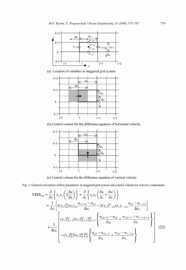
Fig. 1. General convention of flow parameters in staggered grid system and control volume for velocity components.


VISXi;k Zv

vxgxne 2

vu

vx

� �� C

v

vzgzne

vu

vzC

vw

vx

� ��

Z1

dxi

2ðgxÞdxi;kðneÞi;k

uiC1;kKui;k

Dxi

K2ðgxÞdxiK1;kðneÞiK1;k

ui;kKuiK1;k

Dxi

� �

C1

Dzk

ðgzÞDxi;kC1fðneÞ

Dxi;kC1g

Dzi;kC1

ui;kC1Kui;k

dzk

Cwi;kC1KwiK1;kC1

dxi

8<:

9=;

KðgzÞDxi;k fðneÞ

Dxi;k g

Dzi;k

ui;kKui;kK1

dzk

Cwi;kKwiK1;k

dxi

8<:

9=;

266666664

377777775

ð22Þ


ðRxÞi;k Z1

2

CD

Dxð1KgxÞu

ffiffiffiffiffiffiffiffiffiffiffiffiffiffiffiffiu2 Cw2

pZ

1

2

½CD�Dxi;k

Dxi

f1KðgxÞi;kgui;k

ffiffiffiffiffiffiffiffiffiffiffiffiffiffiffiffiffiffiffiffiffiffiffiffiffiffiffiffiffiffiffiffiffiffiffiffiu2

i;k C fðwÞdzi;kg

Dxi;k

h i2r

(23)

The transient velocity field does not satisfy the continuity equation. The deviation from

the equation of mass conservation is found as the source term Di,k of the predicted velocity

field. The difference between the new time level velocity and the predicted velocity field is

due to the effect of the change of the pressure Dp at the new time step. The corrected

velocity is computed as:

umC1i;k Zu�

i;kKðgvÞi;k

ðlvÞi;k

1

ri;k

vDpi;k

vxi

� �Dt (24)

where DpZpmC1Kpm. The corrected velocity field must satisfy the equation of mass

conservation and thus substituting Eq. (24) in continuity equation one can obtain the

Poisson equation for the pressure correction with the source term Di,k as follows:

v

vxgx

gv

lv

1

r

vðDpÞ

vx

� �C

v

vzgz

gv

lv

1

r

vðDpÞ

vz

� �Z

Di;k

Dt(25)

which is called the Poisson pressure equation. The second order five points scheme is used

for the discretization of Eq. (25) and simultaneous equations are solved by Bi-conjugate

gradient stabilize method for Dp (Van der Vorst, 1992). The Dp is substitute into Eq. (24)

to obtain the actual velocity at new time step. Then the advection equation of VOF

function F is solved explicitly using the new velocity field. Once the F value at the new

time step is obtained for all cells, the free surface position is reconstructed and the

distribution of density and viscosity are calculated.

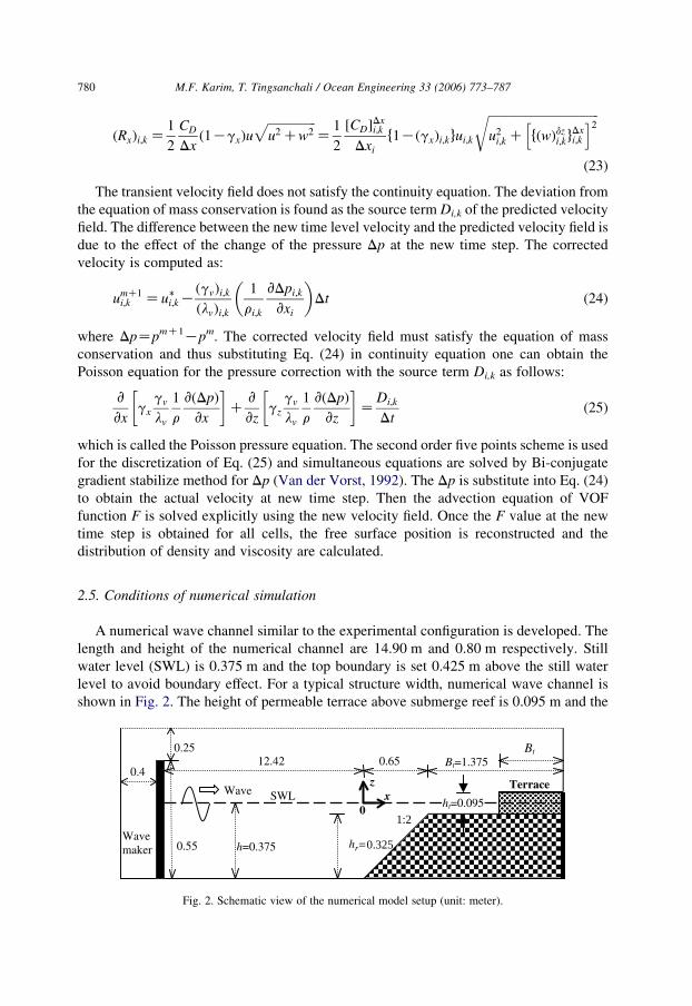
2.5. Conditions of numerical simulation

A numerical wave channel similar to the experimental configuration is developed. The

length and height of the numerical channel are 14.90 m and 0.80 m respectively. Still

water level (SWL) is 0.375 m and the top boundary is set 0.425 m above the still water

level to avoid boundary effect. For a typical structure width, numerical wave channel is

shown in Fig. 2. The height of permeable terrace above submerge reef is 0.095 m and the

1:2

0.325

Fig. 2. Schematic view of the numerical model setup (unit: meter).


thickness Bt varies from 0 to 0.625 m. The computations are carried out for several terrace

width and porosity but same structure height. The origin of x-axis is considered at the front

face of the sloping reef and the positive distance is in the propagating direction of incident

wave.

Simulations of wave propagation have been carried out with appropriate inflow and

mesh boundaries. Three wave periods TZ1.2, 1.6 and 2.0 s, and several incident wave

height HI ranging from 0.03 to 0.12 m are considered for the model calibration. The

influence of different structural parameters are investigated for a typical wave condition

TZ1.6 s and HIZ0.076 m for which HI/hZ0.20, HI/LZ0.028 and h/LZ0.136.

Computational grid size is 0.02 m in the horizontal direction (x-axis) and 0.01 m in the

vertical direction (z-axis). Time increment is set by satisfying CFL and viscous stability

conditions. The computation starts from still water condition and the surface displacement

h at tZ0 is null for whole computational region as well as uZwZ0. The pressure at tZ0

is given by the hydrostatic pressure. Total computational time is set for approximately 16

incident wave cycles. However, in the analysis of numerical results, the last 8 wave cycles

are considered to avoid initial disturbances.

3. Results and discussions

3.1. Verification of numerical results

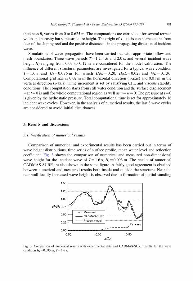
Comparison of numerical and experimental results has been carried out in terms of

wave height distributions, time series of surface profile, mean water level and reflection

coefficient. Fig. 3 shows the comparison of numerical and measured non-dimensional

wave height for the incident wave of TZ1.6 s, HIZ0.093 m. The results of numerical

CADMAS-SURF are also shown in the same figure. A fairly good agreement is obtained

between numerical and measured results both inside and outside the structure. Near the

rear wall locally increased wave height is observed due to formation of partial standing

Fig. 3. Comparison of numerical results with experimental data and CADMAS-SURF results for the wave

condition HIZ0.093 m, TZ1.6 s.

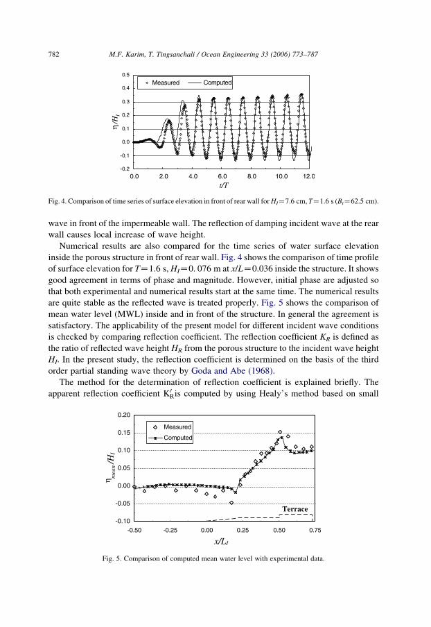
Fig. 4. Comparison of time series of surface elevation in front of rear wall for HIZ7.6 cm, TZ1.6 s (BtZ62.5 cm).


wave in front of the impermeable wall. The reflection of damping incident wave at the rear

wall causes local increase of wave height.

Numerical results are also compared for the time series of water surface elevation

inside the porous structure in front of rear wall. Fig. 4 shows the comparison of time profile

of surface elevation for TZ1.6 s, HIZ0. 076 m at x/LZ0.036 inside the structure. It shows

good agreement in terms of phase and magnitude. However, initial phase are adjusted so

that both experimental and numerical results start at the same time. The numerical results

are quite stable as the reflected wave is treated properly. Fig. 5 shows the comparison of

mean water level (MWL) inside and in front of the structure. In general the agreement is

satisfactory. The applicability of the present model for different incident wave conditions

is checked by comparing reflection coefficient. The reflection coefficient KR is defined as

the ratio of reflected wave height HR from the porous structure to the incident wave height

HI. In the present study, the reflection coefficient is determined on the basis of the third

order partial standing wave theory by Goda and Abe (1968).

The method for the determination of reflection coefficient is explained briefly. The

apparent reflection coefficient K0Ris computed by using Healy’s method based on small

Fig. 5. Comparison of computed mean water level with experimental data.

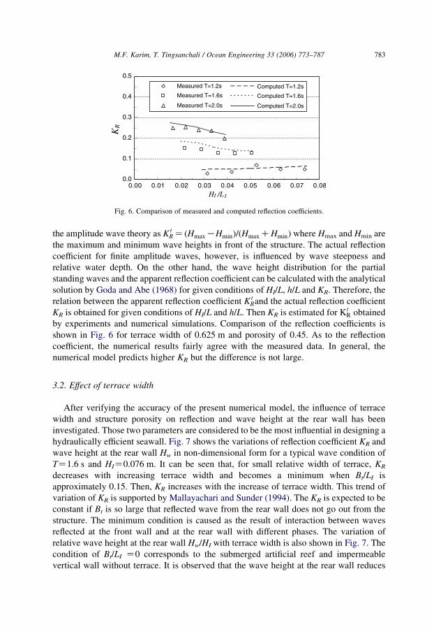
Fig. 6. Comparison of measured and computed reflection coefficients.


the amplitude wave theory as K 0R Z ðHmax KHminÞ=ðHmax CHminÞ where Hmax and Hmin are

the maximum and minimum wave heights in front of the structure. The actual reflection

coefficient for finite amplitude waves, however, is influenced by wave steepness and

relative water depth. On the other hand, the wave height distribution for the partial

standing waves and the apparent reflection coefficient can be calculated with the analytical

solution by Goda and Abe (1968) for given conditions of HI/L, h/L and KR. Therefore, the

relation between the apparent reflection coefficient K 0Rand the actual reflection coefficient

KR is obtained for given conditions of HI/L and h/L. Then KR is estimated for K0R obtained

by experiments and numerical simulations. Comparison of the reflection coefficients is

shown in Fig. 6 for terrace width of 0.625 m and porosity of 0.45. As to the reflection

coefficient, the numerical results fairly agree with the measured data. In general, the

numerical model predicts higher KR but the difference is not large.

3.2. Effect of terrace width

After verifying the accuracy of the present numerical model, the influence of terrace

width and structure porosity on reflection and wave height at the rear wall has been

investigated. Those two parameters are considered to be the most influential in designing a

hydraulically efficient seawall. Fig. 7 shows the variations of reflection coefficient KR and

wave height at the rear wall Hw in non-dimensional form for a typical wave condition of

TZ1.6 s and HIZ0.076 m. It can be seen that, for small relative width of terrace, KR

decreases with increasing terrace width and becomes a minimum when Bt/LI is

approximately 0.15. Then, KR increases with the increase of terrace width. This trend of

variation of KR is supported by Mallayachari and Sunder (1994). The KR is expected to be

constant if Bt is so large that reflected wave from the rear wall does not go out from the

structure. The minimum condition is caused as the result of interaction between waves

reflected at the front wall and at the rear wall with different phases. The variation of

relative wave height at the rear wall Hw/HI with terrace width is also shown in Fig. 7. The

condition of Bt/LI Z0 corresponds to the submerged artificial reef and impermeable

vertical wall without terrace. It is observed that the wave height at the rear wall reduces

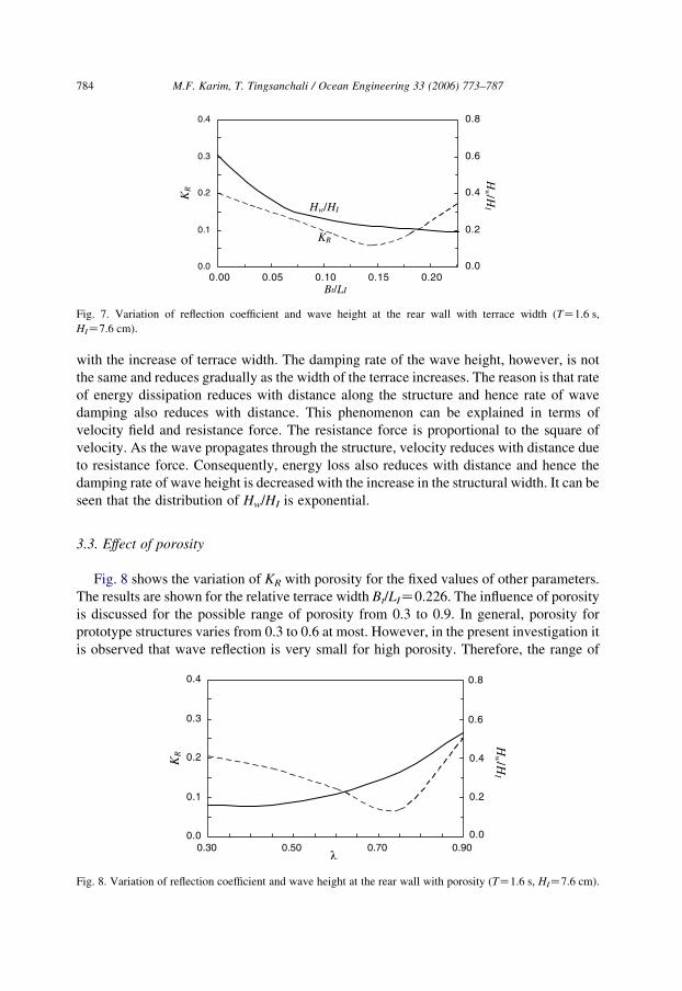
Fig. 7. Variation of reflection coefficient and wave height at the rear wall with terrace width (TZ1.6 s,

HIZ7.6 cm).


with the increase of terrace width. The damping rate of the wave height, however, is not

the same and reduces gradually as the width of the terrace increases. The reason is that rate

of energy dissipation reduces with distance along the structure and hence rate of wave

damping also reduces with distance. This phenomenon can be explained in terms of

velocity field and resistance force. The resistance force is proportional to the square of

velocity. As the wave propagates through the structure, velocity reduces with distance due

to resistance force. Consequently, energy loss also reduces with distance and hence the

damping rate of wave height is decreased with the increase in the structural width. It can be

seen that the distribution of Hw/HI is exponential.

3.3. Effect of porosity

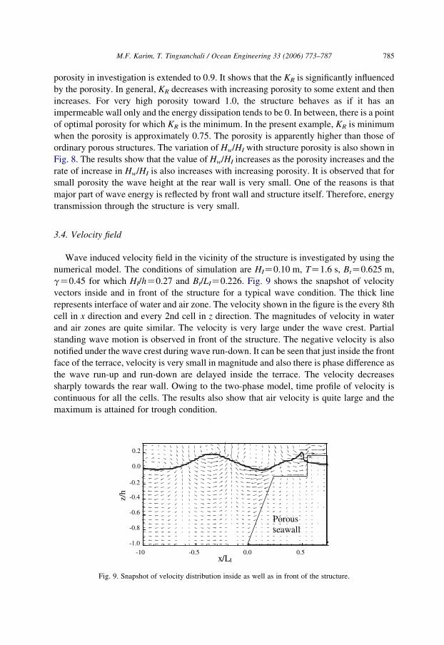
Fig. 8 shows the variation of KR with porosity for the fixed values of other parameters.

The results are shown for the relative terrace width Bt/LIZ0.226. The influence of porosity

is discussed for the possible range of porosity from 0.3 to 0.9. In general, porosity for

prototype structures varies from 0.3 to 0.6 at most. However, in the present investigation it

is observed that wave reflection is very small for high porosity. Therefore, the range of

Fig. 8. Variation of reflection coefficient and wave height at the rear wall with porosity (TZ1.6 s, HIZ7.6 cm).


porosity in investigation is extended to 0.9. It shows that the KR is significantly influenced

by the porosity. In general, KR decreases with increasing porosity to some extent and then

increases. For very high porosity toward 1.0, the structure behaves as if it has an

impermeable wall only and the energy dissipation tends to be 0. In between, there is a point

of optimal porosity for which KR is the minimum. In the present example, KR is minimum

when the porosity is approximately 0.75. The porosity is apparently higher than those of

ordinary porous structures. The variation of Hw/HI with structure porosity is also shown in

Fig. 8. The results show that the value of Hw/HI increases as the porosity increases and the

rate of increase in Hw/HI is also increases with increasing porosity. It is observed that for

small porosity the wave height at the rear wall is very small. One of the reasons is that

major part of wave energy is reflected by front wall and structure itself. Therefore, energy

transmission through the structure is very small.

3.4. Velocity field

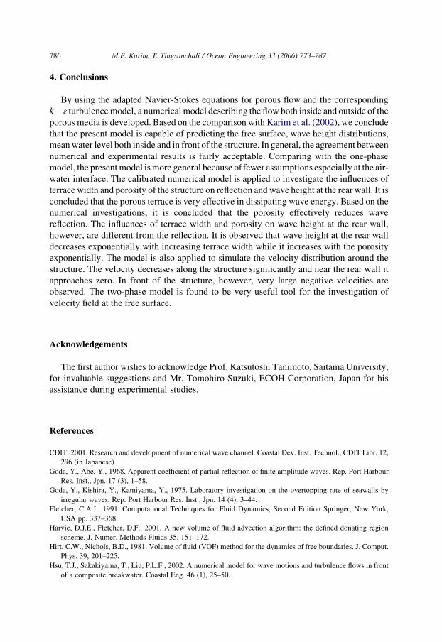
Wave induced velocity field in the vicinity of the structure is investigated by using the

numerical model. The conditions of simulation are HIZ0.10 m, TZ1.6 s, BtZ0.625 m,

gZ0.45 for which HI/hZ0.27 and Bt/LIZ0.226. Fig. 9 shows the snapshot of velocity

vectors inside and in front of the structure for a typical wave condition. The thick line

represents interface of water and air zone. The velocity shown in the figure is the every 8th

cell in x direction and every 2nd cell in z direction. The magnitudes of velocity in water

and air zones are quite similar. The velocity is very large under the wave crest. Partial

standing wave motion is observed in front of the structure. The negative velocity is also

notified under the wave crest during wave run-down. It can be seen that just inside the front

face of the terrace, velocity is very small in magnitude and also there is phase difference as

the wave run-up and run-down are delayed inside the terrace. The velocity decreases

sharply towards the rear wall. Owing to the two-phase model, time profile of velocity is

continuous for all the cells. The results also show that air velocity is quite large and the

maximum is attained for trough condition.

Fig. 9. Snapshot of velocity distribution inside as well as in front of the structure.


4. Conclusions

By using the adapted Navier-Stokes equations for porous flow and the corresponding

kK3 turbulence model, a numerical model describing the flow both inside and outside of the

porous media is developed. Based on the comparison with Karim et al. (2002), we conclude

that the present model is capable of predicting the free surface, wave height distributions,

mean water level both inside and in front of the structure. In general, the agreement between

numerical and experimental results is fairly acceptable. Comparing with the one-phase

model, the present model is more general because of fewer assumptions especially at the air-

water interface. The calibrated numerical model is applied to investigate the influences of

terrace width and porosity of the structure on reflection and wave height at the rear wall. It is

concluded that the porous terrace is very effective in dissipating wave energy. Based on the

numerical investigations, it is concluded that the porosity effectively reduces wave

reflection. The influences of terrace width and porosity on wave height at the rear wall,

however, are different from the reflection. It is observed that wave height at the rear wall

decreases exponentially with increasing terrace width while it increases with the porosity

exponentially. The model is also applied to simulate the velocity distribution around the

structure. The velocity decreases along the structure significantly and near the rear wall it

approaches zero. In front of the structure, however, very large negative velocities are

observed. The two-phase model is found to be very useful tool for the investigation of

velocity field at the free surface.

Acknowledgements

The first author wishes to acknowledge Prof. Katsutoshi Tanimoto, Saitama University,

for invaluable suggestions and Mr. Tomohiro Suzuki, ECOH Corporation, Japan for his

assistance during experimental studies.

References

CDIT, 2001. Research and development of numerical wave channel. Coastal Dev. Inst. Technol., CDIT Libr. 12,

296 (in Japanese).

Goda, Y., Abe, Y., 1968. Apparent coefficient of partial reflection of finite amplitude waves. Rep. Port Harbour

Res. Inst., Jpn. 17 (3), 1–58.

Goda, Y., Kishira, Y., Kamiyama, Y., 1975. Laboratory investigation on the overtopping rate of seawalls by

irregular waves. Rep. Port Harbour Res. Inst., Jpn. 14 (4), 3–44.

Fletcher, C.A.J., 1991. Computational Techniques for Fluid Dynamics, Second Edition Springer, New York,

USA pp. 337–368.

Harvie, D.J.E., Fletcher, D.F., 2001. A new volume of fluid advection algorithm: the defined donating region

scheme. J. Numer. Methods Fluids 35, 151–172.

Hirt, C.W., Nichols, B.D., 1981. Volume of fluid (VOF) method for the dynamics of free boundaries. J. Comput.

Phys. 39, 201–225.

Hsu, T.J., Sakakiyama, T., Liu, P.L.F., 2002. A numerical model for wave motions and turbulence flows in front

of a composite breakwater. Coastal Eng. 46 (1), 25–50.


Hur, D.S., Mizutani, M., 2003. Numerical estimation of the wave forces acting on a three-dimensional body on

submerged breakwater. Coastal Eng. 47 (3), 329–345.

Karim, M.F., 2003. Study on interaction between waves and porous structure by numerical simulation. Ph. D

dissertation, Saitama University, Japan.

Karim, M.F., Tanimoto, K., Suzuki, T., Hieu, P.D., 2002. Wave overtopping on seawall with permeable terrace

Proceedings of 4th international summer symposium. JSCE, Kyoto, Japan pp. 175–178.

Liu, P.L.F., Lin, P., Chang, K., Sakakiyama, T., 1999. Numerical modeling of wave interaction with porous

structures. J. Waterway, Port, Coastal Ocean Eng 125 (6), 322–330.

Mallayachari, V., Sundar, V., 1994. Reflection characteristics of permeable seawalls. Coastal Eng. 23, 135–150.

Mizutani, N., McDougal, D.G., Mostafa, A.M., 1996. BEM-FEM combined analysis of non-linear interaction

between wave and submerged breakwater. Proc. 25th Int. Conf. Coastal Eng, ASCE, 2377–2390.

Sakakiyama, T., Kajima, R., 1992. Numerical simulation of nonlinear wave interacting with permeable

breakwaters. Proc. 23rd Int. Conf. Coastal Eng., ASCE, 1517–1530.

Sollit, C.K., Cross, R.H., 1972. Wave transmission through permeable breakwaters. Proc. 13th Int. Conf. Coastal

Eng.,ASCE, 1827–1846.

Sussman, M., Smereka, P., Osher, S., 1994. A level set approach for computing solutions to incompressible two-

phase flow. J. Comput Phys. 114, 146–159.

Tanimoto, K., Suzuki, T., Karim, M.F., Hieu, P.D., 2002. Hydraulic Characteristics of Seawall with

Permeable Terrace Proc. 28th International Conference on Coastal Engineering, vol. 3. ASCE, Cardiff, UK

pp. 2019–2030.

Van Gent, M.R.A., 1995. Wave Interaction with Permeable Coastal Structures, Ph.D thesis, Delft University of

Technology, The Netherlands.

Van der Vorst, H.A., 1992. BI-CGSTAB: a fast and smoothly converging variant of BI-CG for the solution of

nonsymmetric linear systems. J. Sci. Stat. Comput., SIAM 13, 631–644.

Zhao, Q., Tanimoto, K., 1998. Numerical simulation of breaking waves by large eddy simulation and VOF

method. Proc. Int. Conf. Coastal Eng., ASCE, 892–905.

A coupled numerical model for simulation of wave breaking and hydraulic performances of a composite...

Documents

Transcript of A coupled numerical model for simulation of wave breaking and hydraulic performances of a composite...