Evolving two-dimensional fuzzy systems

Fuzzy Sets and Systems 138 (2003) 381–398www.elsevier.com/locate/fss

Evolving two-dimensional fuzzy systems

V$%ctor M. Rivasa ;∗;1, J.J. Merelob;1, I. Rojasb, G. Romerob;1,P.A. Castillob;1, J. Carpiob;1

aDpto. de Inform atica, Universidad de Ja en, E.P.S., Avda. de Madrid 35, E.23071, Ja en, SpainbDpto. de Arquitectura y Tecnolog 'a de Computadores, Universidad de Granada, Spain

Received 15 September 1999; received in revised form 9 September 2002; accepted 24 September 2002

Abstract

The design of fuzzy logic systems (FLS) generally involves determining the structure of the rules andthe parameters of the membership functions. In this paper we present a methodology based on evolutionarycomputation for simultaneously designing membership functions and appropriate rule sets. This property makesit di9erent from many techniques that address these goals separately with the result of suboptimal solutionsbecause the design elements are mutually dependent. We also apply a new approach in which the evolutionaryalgorithm is applied directly to a FLS data structure instead of a binary or other codi<cation. Results onfunction approximation show improvements over other incremental and analytical methods.c© 2002 Elsevier B.V. All rights reserved.

Keywords: Fuzzy systems; Genetic algorithms; Evolutionary algorithms; Hybrid methods; Function approximation

1. Introduction

Since the introduction of the basic methods of fuzzy reasoning by Zadeh [23], and the success oftheir original application to fuzzy control, fuzzy logic and its application to fuzzy control have beenwidely studied. However, certain important questions still remain open, including: (1) the selection ofthe fuzzy rule base; (2) the subjective de<nitions of the membership functions; and (3) the structureof the fuzzy system (number of rules and membership functions).The transfer function of a fuzzy system is not based on a mathematical model; it is given by the

de<nition of fuzzy rules and fuzzy sets of linguistic variables (for each membership function). Thefuzzy rules and the fuzzy sets are designed on the basis of the human operator’s experience, decisions

∗ Corresponding author. Tel.: +34-953-012344; fax: +34-953-002420.E-mail addresses: [email protected] (V.M. Rivas).URLs: http://pagina.de/vrivas, http://geneura.ugr.es1 GeNeura Team.

0165-0114/03/$ - see front matter c© 2002 Elsevier B.V. All rights reserved.PII: S0165-0114(02)00483-9

mailto:[email protected]

http://pagina.de/vrivas

http://geneura.ugr.es

382 V.M. Rivas et al. / Fuzzy Sets and Systems 138 (2003) 381–398

and control actions. In conventional expert systems the operator cannot often clearly explain whyhe=she acts in a certain way. Furthermore, there is no reason to believe that an operator’s controlis optimal. Then an automatic design method based on a set of examples for the input=outputrelationship becomes important. Such a set of examples is commonly called the referential data set.In general, creating a fuzzy logic system (FLS) involves designing the structure of the rules of the

system and the parameters of the membership functions. Most techniques deal with these separately,which may result in a suboptimal solution because the design elements are mutually dependent. Forexample, Genetic Algorithms (GAs) can <rstly be used to determine the rules of the system and then,in a second stage, to tune the parameters of the linguistic values, as in [10]. We propose optimizingthese parts simultaneously using Evolutionary Computation techniques with a new method slightlydi9erent from those presented in [18–20]. This will be discussed later.The rest of the paper is organized as follows: the next section deals with the current state of the

art, including an introduction to Evolutionary Algorithms (EA); Section 3 describes the EA used inthis work, including genetic operators, the algorithm itself and the evolutionary computation library,Evolutionary Objects [13]. After this, Section 4 describes some experiments and their results; and<nally, Section 5 presents some conclusions and future lines of work.

2. State of the art

2.1. Evolutionary algorithms

Evolutionary algorithms (EAs) represent a set of strategies to eJciently search for near optimalsolutions in hard to search spaces imitating natural genetics. Depending on the problem, the optimalsolution may be one that either maximizes or minimizes a given function. Nevertheless, as mini-mization problems can be easily changed into maximization ones, EA terminology tends to referonly to the latter.EAs can be characterized by the following features ([14]):

• A genetic representation for potential solutions to the problem. Solutions are called individuals.However, in this work we apply a new approach in which individuals are not encoded into achromosome (as they usually are), but in which the EA can directly deal with the solutions asthey are, i.e. as FLSs.

• A way to create an initial population of potential solutions. The most common method is bymeans of a random generator.

• An evaluation function that plays the role of the environment rating solutions in terms of their<tness. In general, the best individuals are those which have the highest <tness.

• Genetic operators are used to manipulate the population’s genetic composition. New individualsare created by applying these operators to the previously existing ones. The best individuals shouldgenerate more o9spring than the rest.

• A set of parameters that provide the initial settings for the algorithm: population size, probabilitiesemployed by the genetic operators, termination conditions, and probably, a set of constraints forindividuals.

EAs usually implement three basic operators to manipulate the population’s genetic composition:selection, recombination and mutation.

V.M. Rivas et al. / Fuzzy Sets and Systems 138 (2003) 381–398 383

Selection. Selection is the process by which individuals with higher <tness values have a higherprobability of being chosen to reproduce, generating and o9spring, than individuals with smaller<tness values. Because of this, it is considered a diversity-destruction operator. The most commonmethod used is the weighted roulette selection.

Recombination. Recombination is the process by which one or more new individuals are createdusing parts from two or more parents. The underlying idea is that the optimal solution is composedof several optimal parts (or building blocks [7]), so the massive interchange of information betweenindividuals may lead to better and better new ones. Like selection, recombination operator alsodecreases diversity.

Mutation. Mutation operators alter, in a random way, the structure or the stored information ofthe individual to which they are applied. They increase the diversity of population, providing amechanism to escape from local optima and premature convergence. High rates of these operatorsallow better exploration of the search space, but make convergence slower and can result in randomsearch.

2.2. Applications of EA to FLS design

The properties of EAs make them a powerful technique for selecting high performance parametersfor FLSs. Previous work focused basically on optimizing the FLS parameters and on reducing thenumber of the rules. In this paper EAs are used to search for an optimized subset of rules (both thenumber of rules and the rule values) from a given knowledge base to achieve the goal of minimizingthe number of rules used while maintaining the FLS performance. EAs will eliminate all unnecessaryrules, i.e., those which have no signi<cant contribution to improving system performance.Recently, EAs have been combined with fuzzy logic and neural networks in the process of de-

signing fuzzy systems. For a good review see [7]. Ishibuchi et al. [9], for instance, propose a hybridapproach where a set of fuzzy rules is <rst extracted from a trained neural network, and an EA isthen used to select a small subset of rules from the extracted rule set. The <tness function of theEA is designed to minimize the number of selected rules and maximize the number of correctlyclassi<ed examples. For example, Karr and Gentry [11] control the pH of an acid–base system withthe fuzzy system’s input membership functions manipulated by an EA.Some other methods [21] combine EA and FLS in order to tune the parameters of the membership

functions and outputs of a Takagi–Sugeno fuzzy rule base, and have been used for the approximationof one-input analytical functions.On the other hand, the codi<cation of rules and membership functions is typically done using

vectors (1-D matrices) [2,16,12,8,11]; this is not the most natural way to do it because it keeps“natural” building blocks (for instance, four contiguous cells in the matrix) apart from each other.In this work FLSs are not coded that way, but implemented by 2-D matrices; this device allowsus to represent rules with close antecedents together (after all these rules are generally activated atthe same time, interfering with each other). This way they can be more easily transmitted to theo9spring.It should also be noted that several researchers have concentrated on using real number coding

for chromosomal representation of individuals instead of traditional bit string based coding; and it isreported that for some problems, these techniques outperform the conventional bit string based EAs[3,5,22]. This partly supports our work, since we use real numbers for evolution.


A special mention has to be made to some papers in which EAs are used to model and=or tunecomplete fuzzy systems. By chronological order, the two <rst are due to Lian et al. [18,19]. Inthese works the authors developed a method to tune a neuro-fuzzy controller using genetic algo-rithms, applied to a set of problems like coupled-tank liquid-level control, unstable plants controland automatic car parking. The main di9erence in their method and the one presented in this paperis that the size of the controller and the number of parameters is <xed and <tted to the problembeing solved at every moment. So this method implies a previous study of the problem to be solvedand cannot be applied directly to any kind of problem with two inputs and one output. A seconddi9erence is that parameters, that are real values, are represented using bit strings, which is not thenatural and logical way it should be done, as was discussed before. A more recent paper is theone by Setnes and Roubos [20], showing how GA can be used to create fuzzy systems applied tomodeling and classi<cation problems. Once more, the problem of how to represent the solutions hasbeen solved in an unnatural way, since rule antecedents and consequents are stored sequentially inthe chromosome. This adds a new problem, given that the genetic operators can produce solutionsthat violate the di9erent constraints imposed to both the input space and the output space.

3. The evolutionary algorithm

To program this algorithm we used the EO [19] library (evolutionary objects) because of thefacilities it o9ers to evolve any object (in the sense of object oriented programming) that can beassigned a cost or <tness function. EO is a library that de<nes the interfaces of several types ofevolutionary algorithms, and includes several examples of their use. It is currently programmed inC++ but easily portable to any other object oriented language. It is open-source, and available fromhttp://eodev.sourceforge.net.The EO library directly evolves classes of objects, so there is no need to code them in a binary

chromosome. In this work evolved objects are fuzzy logic systems (FLS) which are implemented as2-D arrays; thus, some speci<c operators are needed to mutate and combine them in order to createnew FLSs.The following subsection explain the architectures of both the FLS and the EA that optimizes it.

3.1. The 2-D fuzzy logic system

In this work each FLS is implemented as a two-dimensional matrix storing two di9erent things:(a) the centres of the triangular partition membership functions of two input variables, X and Y ,and (b) the values of the output variable, Z . Thus, any 2-D matrix stores both the precedents andthe consequents of the FLS rules.A little more formally, a m by n FLS is implemented by a two-dimensional matrix:

M (m+ 1; n+ 1) =

∣∣∣∣∣∣∣∣∣∣

− Y1 Y2 · · · YnX1 Z1;1 Z1;2 · · · Z1;nX2 Z2;1 Z2;2 · · · Z2;n· · · · · · · · · · · · · · ·Xm Zm;1 Zm;2 · · · Zm;n

∣∣∣∣∣∣∣∣∣∣

http://eodev.sourceforge.net


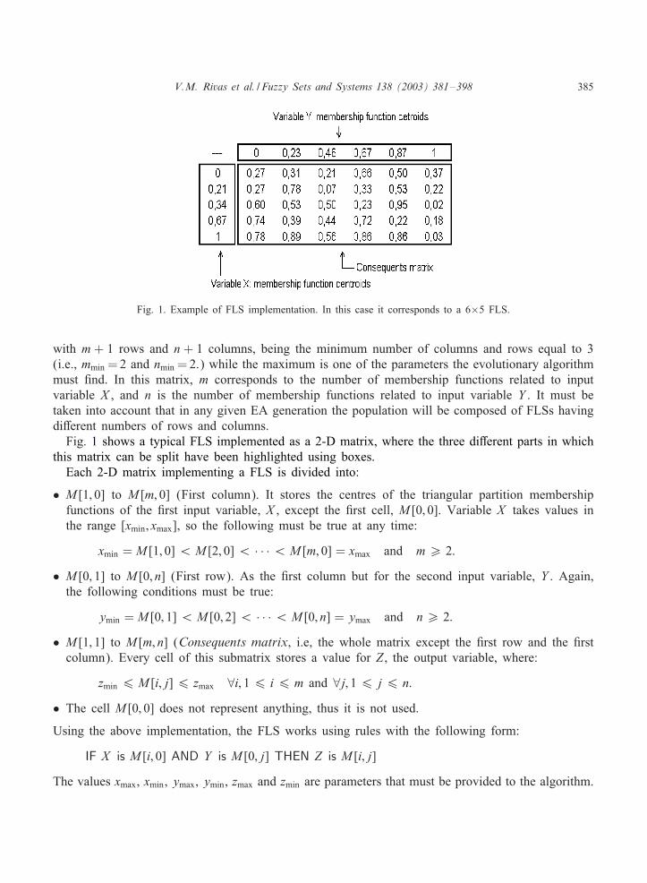
Fig. 1. Example of FLS implementation. In this case it corresponds to a 6×5 FLS.

with m + 1 rows and n + 1 columns, being the minimum number of columns and rows equal to 3(i.e., mmin = 2 and nmin = 2.) while the maximum is one of the parameters the evolutionary algorithmmust <nd. In this matrix, m corresponds to the number of membership functions related to inputvariable X , and n is the number of membership functions related to input variable Y . It must betaken into account that in any given EA generation the population will be composed of FLSs havingdi9erent numbers of rows and columns.Fig. 1 shows a typical FLS implemented as a 2-D matrix, where the three di9erent parts in which

this matrix can be split have been highlighted using boxes.Each 2-D matrix implementing a FLS is divided into:

• M [1; 0] to M [m; 0] (First column). It stores the centres of the triangular partition membershipfunctions of the <rst input variable, X , except the <rst cell, M [0; 0]. Variable X takes values inthe range [xmin; xmax], so the following must be true at any time:

xmin = M [1; 0]¡ M [2; 0]¡ · · ·¡ M [m; 0] = xmax and m¿ 2:

• M [0; 1] to M [0; n] (First row). As the <rst column but for the second input variable, Y . Again,the following conditions must be true:

ymin = M [0; 1]¡ M [0; 2]¡ · · ·¡ M [0; n] = ymax and n¿ 2:

• M [1; 1] to M [m; n] (Consequents matrix, i.e, the whole matrix except the <rst row and the <rstcolumn). Every cell of this submatrix stores a value for Z , the output variable, where:

zmin 6 M [i; j]6 zmax ∀i; 16 i 6 m and ∀j; 16 j 6 n:

• The cell M [0; 0] does not represent anything, thus it is not used.

Using the above implementation, the FLS works using rules with the following form:

IF X is M [i; 0] AND Y is M [0; j] THEN Z is M [i; j]

The values xmax, xmin, ymax, ymin, zmax and zmin are parameters that must be provided to the algorithm.


3.2. Genetic operators

Using EO library to develop the EA allows us to directly evolve a FLS instead of its bitstringrepresentation. For this reason we are not constrained to use traditional genetic operators. Thus,diversity-generation (mutators) and diversity-destruction (crossover-like or recombination) operatorshave been designed making use of speci<c problem knowledge. Moreover, since EO is implementedusing C++, an Object Oriented language, operators act over the evolvable objects via their inter-faces, and they never modify the objects directly. This property makes unnecessary the use of penaltyfunctions or repair methods to deal with invalid objects generated by the operators: the FLSs them-selves control that changes ordered by the operator are carried out in such a way that the resultingobjects are always valid.

3.2.1. RecombinationThis operator splices values from one matrix into another. Taking into account that these two FLSs

do not necessarily have the same dimensions, the recombination cannot be performed in a trivial way.The operator works as follows:

(1) It randomly chooses a FLS to be modi<ed (we will call it Mr , or receiver FLS), and anotherthat will provide the genes to be recombined (the Md, or donor FLS). Only the <rst one, Mr ,will be changed.

(2) It chooses a random block of cells from the consequent matrix of Mr . To specify this block weonly need to randomly select two cells corresponding to the top left corner and bottom rightcorner of the block, respectively. Call these two cells Mr[r1; c1] and Mr[r2; c2]. The values ofthe cells included in this block will be changed by values coming from Md.

(3) For each cell Mr[ri; cj], where ri goes from r1 to r2, and cj goes from c1 to c2, the operatordoes the following:

(4) From the <rst column of the donor, Md, it selects the cell whose value is closer to Mr[ri; 0].Design that cell as Md[rd; 0].

(5) From the <rst row of the donor, Md, it selects the cell whose value is closest to Mr[0; cj]. Designthat cell Md[0; cd].

(6) Finally, it changes the value stored in Mr[ri; cj] by the one stored in Md[rd; cd]. As can be seen,the donor FLS, Md, remains unchanged.

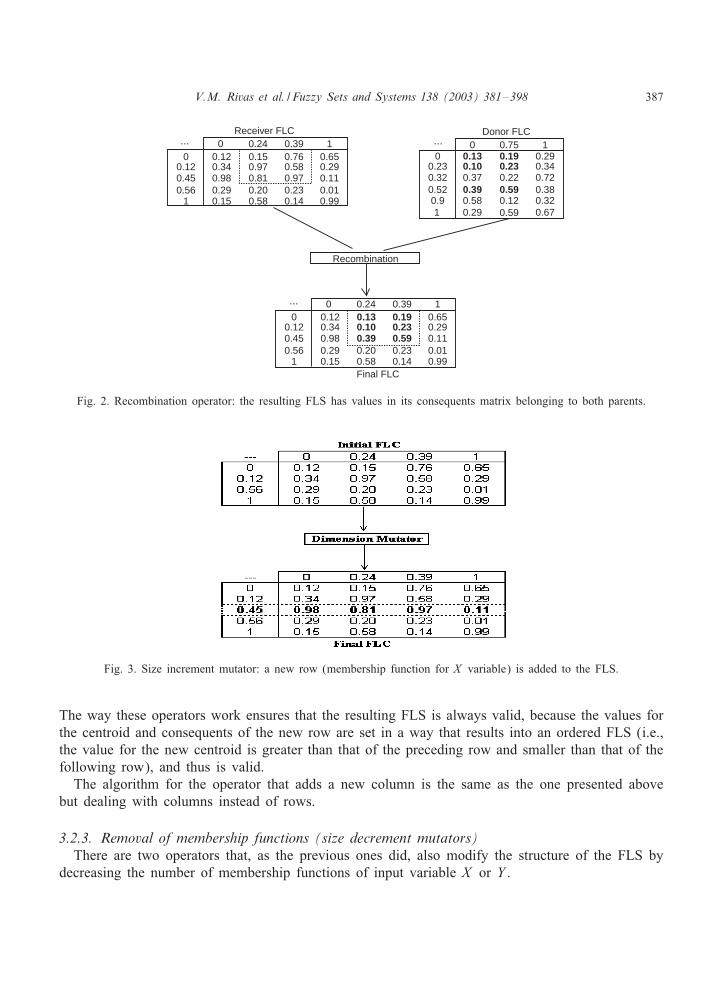
An example of the action of this operator is shown in Fig. 2.

3.2.2. Addition of membership functions (size increment mutators)There are two independent operators that modify the structure of the FLS they are applied to by

adding a membership function to input variables. One of these operators a9ects he input variable Xwhile the other operates with the input variable Y .Fig. 3 graphically shows the e9ect of incrementing the number of rows. In order to do that, once

the FLS to be changed has been randomly chosen the operator works as follows:

(1) It inserts an empty row in a random position, di9erent from the <rst and last ones.(2) It <lls the cells of the new row with random values generated by a Gaussian function centered

on the middle point between the corresponding to the preceding row and that corresponding tothe following one.


00

1

1

0.24

0.120.450.56

0.120.340.980.290.15

0.130.100.390.200.58 0.14

0.230.590.230.19 0.65

0.290.110.010.99

0.39

00

1

1

0.24

0.120.450.56

0.120.340.980.290.15

0.150.970.810.200.58 0.14

0.230.970.580.76 0.65

0.290.110.010.99

0.39 00

10.9

0.75

0.230.320.52

0.130.100.370.390.580.29 0.59 0.67

0.190.230.220.590.12 0.32

0.380.720.340.29

1

Recombination

Receiver FLC Donor FLC

Final FLC

... ...

...

Fig. 2. Recombination operator: the resulting FLS has values in its consequents matrix belonging to both parents.

Fig. 3. Size increment mutator: a new row (membership function for X variable) is added to the FLS.

The way these operators work ensures that the resulting FLS is always valid, because the values forthe centroid and consequents of the new row are set in a way that results into an ordered FLS (i.e.,the value for the new centroid is greater than that of the preceding row and smaller than that of thefollowing row), and thus is valid.The algorithm for the operator that adds a new column is the same as the one presented above

but dealing with columns instead of rows.

3.2.3. Removal of membership functions (size decrement mutators)There are two operators that, as the previous ones did, also modify the structure of the FLS by

decreasing the number of membership functions of input variable X or Y .


Fig. 4. Size decrement mutator: a row (membership function for the X variable) is deleted from the FLS.

Fig. 5. Precedent mutator: the value for the centroid of the third membership function of input Y has been changed bythe operator.

These operators work by choosing a row=column to delete (di9erent from the <rst and last ones)and removing it (see Fig. 4).Once again, they ensure that the resulting FLS is valid, given that (a) they cannot delete a

row=column of a FLS that has the minimum number allowed (i.e., 3 column by 3 rows); (b) the<rst and last rows=columns cannot be chosen to be deleted; and (c) obviously, the FLS remainssorted once the row or column has been removed.

3.2.4. Modi@cation of a centroid value (precedent mutators)These two operators, one for input X and the other for input Y , modify one of the values stored

in the FLS <rst row or <rst column, respectively.Once an FLS has been selected, the operator that modi<es centroids of variable Y carries out the

following operations (see Fig. 5):

(1) It randomly selects a cell in the <rst row (because we are going to change a centroid of Y ).This cell can be neither the <rst nor the last one.


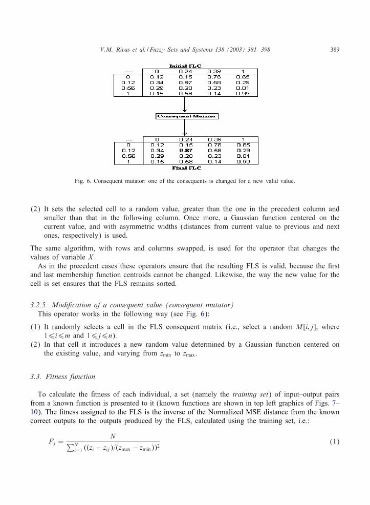
Fig. 6. Consequent mutator: one of the consequents is changed for a new valid value.

(2) It sets the selected cell to a random value, greater than the one in the precedent column andsmaller than that in the following column. Once more, a Gaussian function centered on thecurrent value, and with asymmetric widths (distances from current value to previous and nextones, respectively) is used.

The same algorithm, with rows and columns swapped, is used for the operator that changes thevalues of variable X .As in the precedent cases these operators ensure that the resulting FLS is valid, because the <rst

and last membership function centroids cannot be changed. Likewise, the way the new value for thecell is set ensures that the FLS remains sorted.

3.2.5. Modi@cation of a consequent value (consequent mutator)This operator works in the following way (see Fig. 6):

(1) It randomly selects a cell in the FLS consequent matrix (i.e., select a random M [i; j], where16i6m and 16j6n).

(2) In that cell it introduces a new random value determined by a Gaussian function centered onthe existing value, and varying from zmin to zmax.

3.3. Fitness function

To calculate the <tness of each individual, a set (namely the training set) of input–output pairsfrom a known function is presented to it (known functions are shown in top left graphics of Figs. 7–10). The <tness assigned to the FLS is the inverse of the Normalized MSE distance from the knowncorrect outputs to the outputs produced by the FLS, calculated using the training set, i.e.:

Fj =N

∑Ni=1 ((zi − zij)=(zmax − zmin))2

(1)


FUNCTION TO BE APROXIMATED #1

-2-1.5

-1-0.5

00.5

11.5

2Input X

-2-1.5

-1-0.5

00.5

11.5

2

Input Y

-1-0.8-0.6-0.4-0.2

00.20.40.60.8

1

Output Z

RESULTS PRODUCED BY THE BEST FOUND FUZZY LOGIC CONTROLLER

-2-1.5

-1-0.5

00.5

11.5

2Input X

-2-1.5

-1-0.5

00.5

11.5

2

Input Y

-1-0.8-0.6-0.4-0.2

00.20.40.60.8

1

Output Z

0

10

20

30

40

50

60

70

0 50 100 150 200 250 300

Fitn

ess

(=1/

NM

SE

)

Generation

WORST, AVERAGE AND BEST FITNESS ALONG GENERATIONS

WorstAverage

Best

0

200

400

600

800

1000

1200

1400

1600

0 50 100 150 200 250 300

Siz

e (r

ows

by c

olum

ns)

Generation

MINIMUM, AVERAGE, AND MAXIMUM SIZE ALONG GENERATIONS

MinimumAverage

Maximum

f (x,y) = sin (xy)

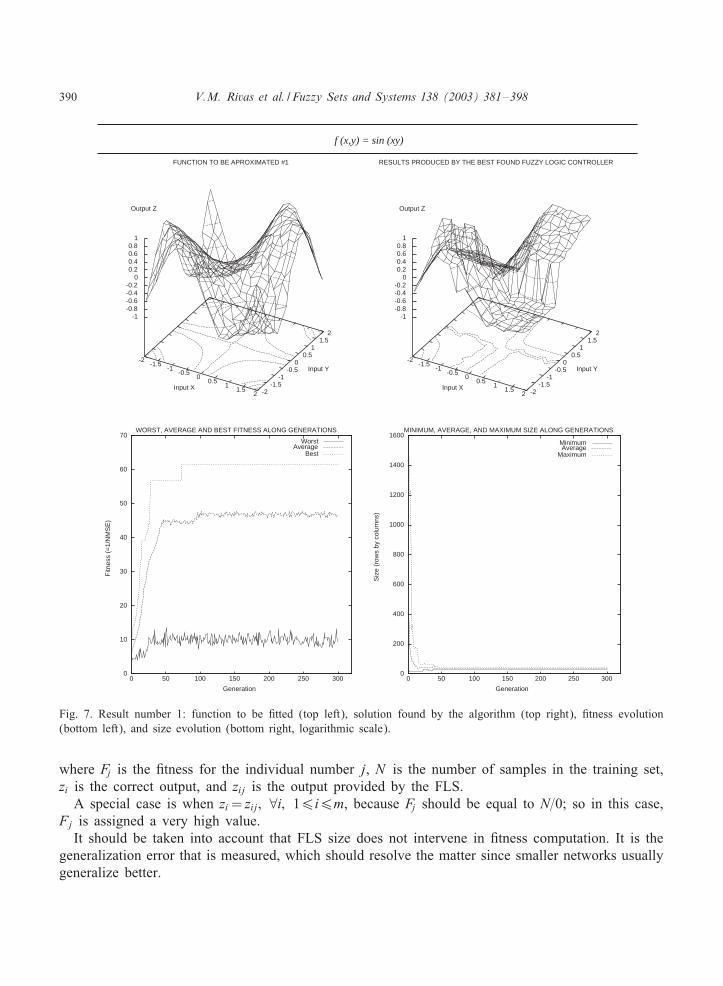
Fig. 7. Result number 1: function to be <tted (top left), solution found by the algorithm (top right), <tness evolution(bottom left), and size evolution (bottom right, logarithmic scale).

where Fj is the <tness for the individual number j, N is the number of samples in the training set,zi is the correct output, and zij is the output provided by the FLS.A special case is when zi= zij; ∀i; 16i6m, because Fj should be equal to N=0; so in this case,

Fj is assigned a very high value.It should be taken into account that FLS size does not intervene in <tness computation. It is the

generalization error that is measured, which should resolve the matter since smaller networks usuallygeneralize better.



-1-0.5

00.5

1Input X

-1

-0.5

0

0.5

1

Input Y

0

0.5

1

1.5

2

2.5

3

Output Z


-1-0.5

00.5

1Input X

-1

-0.5

0

0.5

1

Input Y

0.4

0.6

0.8

1

1.2

1.4

1.6

1.8

2

Output Z

0

50

100

150

200

250

0 50 100 150 200 250 300

Fitn

ess

(=1/

NM

SE

)

Generation


WorstAverage

Best

0

200

400

600

800

1000

1200

1400

1600

0 50 100 150 200 250 300

Siz

e (r

ows

by c

olum

ns)

Generation


MinimumAverage

Maximum

f (x,y) = exsin (�y)

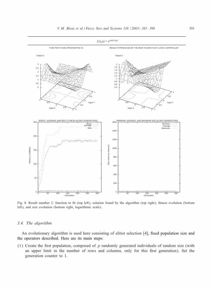
Fig. 8. Result number 2: function to <t (top left), solution found by the algorithm (top right), <tness evolution (bottomleft), and size evolution (bottom right, logarithmic scale).

3.4. The algorithm

An evolutionary algorithm is used here consisting of elitist selection [4], <xed population size andthe operators described. Here are its main steps:

(1) Create the <rst population, composed of p randomly generated individuals of random size (withan upper limit in the number of rows and columns, only for this <rst generation). Set thegeneration counter to 1.



00.2

0.40.6

0.81

Input X 0

0.2

0.4

0.6

0.8

1

Input Y

0

2

4

6

8

10

12

14

16

Output Z


00.2

0.40.6

0.81

Input X0

0.2

0.4

0.6

0.8

1

Input Y

123456789

1011

Output Z

0

20

40

60

80

100

120

140

0 50 100 150 200 250 300

Fitn

ess

(=1/

NM

SE

)

Generation


WorstAverage

Best

0

200

400

600

800

1000

1200

1400

1600

0 50 100 150 200 250 300

Siz

e (r

ows

by c

olum

ns)

Generation


MinimumAverage

Maximum

f (x,y) = 40e8((x-0.5)2+(y-0.5)2

e8((x-0.2)2+(y-0.7)2

+e8((x-0.7)2+(y-0.2)2


(2) Compute the <tness value of every individual.(3) Sort the individuals from highest to lowest <tness values.(4) Select the q best individuals (population elite subset). Delete the remaining p− q individuals.(5) Generate p− q new FLSs, increasing population size up to p. Every new individual is created

by (1) duplicating one individual in the elite subset, and after that, (2) applying one of theoperators to the copy. The probability of one individual in the elite subset being selected forreproduction is related to its <tness value.



-1-0.5

00.5

1Input X

-1

-0.5

0

0.5

1

Input Y

-1-0.8-0.6-0.4-0.2

00.20.40.60.8

1

Output Z


-1-0.5

00.5

1Input X

-1

-0.5

0

0.5

1

Input Y

-1.5

-1

-0.5

0

0.5

1

1.5

Output Z

0

5

10

15

20

25

30

35

40

45

50

0 50 100 150 200 250 300

Fitn

ess

(=1/

NM

SE

)

Generation


WorstAverage

Best

0

200

400

600

800

1000

1200

1400

1600

0 50 100 150 200 250 300

Siz

e (r

ows

by c

olum

ns)

Generation


MinimumAverage

Maximum

f (x,y) = sin (2� x2+y2)


(6) Evaluate the new individuals.(7) Increment the generation counter, and go back to step 3, unless a speci<ed number of generations

has been reached.(8) Finally, the best FLS found is the <rst individual of the current (last) population (because they

are sorted form highest to lowest <tness).

This algorithm is run with the following free parameters:

• Population size.


• Rate of individuals to be removed in every new generation (the non-elite rate).• Application rates of every operator (henceforth, these are normalized to become probabilities).• Maximum number of rows and columns for the <rst generation.• Maximum number of generations.

Every operator has an associated probability of being applied that does not change during the ap-plication of the algorithm (although EO allows adaptive operator rates). Furthermore, every newindividual is created by applying one, and only one, operator to the copy or duplicate of its parent,be it the recombination operator or any of the mutators.As usual, the recombination operator is applied with a higher rate to allow mixing of building

blocks, while mutation-like operators are applied with smaller rates in order to escape from randomsearch. On the other hand, all the mutation-like operators share the same rate in order to balance theincrease and decrease of FLS size. Additionally, a termination condition is <xed at a given numberof generations to speci<cally limit the algorithm running time.

4. Experiments and results

The goal of these experiments was to validate the behavior of the operators created. Parameters ofthe algorithm were <xed to default values, although further study is necessary in order to establishwhich values are the best. Table 1 the values used for the parameters in the following examples.In every experiment we attempted to obtain a FLS that estimates a known function. Several

functions were used, although only four of them are shown here. For every function the algorithm wasrun three times with di9erent random seeds in order to get average values and standard deviations.Functions have been taken from [15], chosen for being used in other works to compare results.One <le per function with 400 points was generated to carry out the experiments. Inputs X and

Y were given equally spaced values. The resultant values for output Z were modi<ed adding smallquantity of random noise. Every time the algorithm was executed 320 randomly chosen points (80%of 400) were used as the training set, while the remaining 80 points were used as validation setused to test the generalizing capabilities of the FLS.Taking into account that the algorithm deals with large matrices storing Toating point numbers, it

is obviously a very time consuming task. For this reason the number of individuals, generations andinitial maximum rows=columns was set to small values allowing us to carry out several experiments

Table 1Values for parameters

Parameter Value

Population size 500Non-elite rate 0.7Recombination rate 0.1Dimension mutator rates 0.01Precedent mutator rates 0.01Consequent mutator rate 0.01Number of generations 300Max. init. number of rows=columns 40


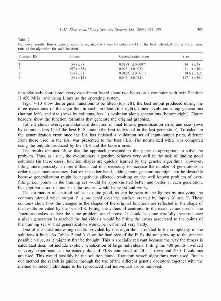
Table 2Numerical results: <tness, generalization error, and size (rows by columns−1) of the best individual during the di9erentruns of the algorithm for each function

Function ID Fitness Generalization error Size

1 54 (±8) 0.0288 (±0:0007) 34 (±3)2 197 (±35) 0.006 (±0:003) 41 (±40)3 114 (±8) 0.0122 (±0:0011) 18.6 (±1:2)4 34 (±12) 0.046 (±0:012) 117 (±36)

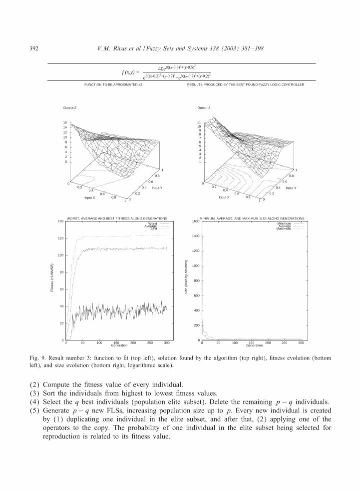
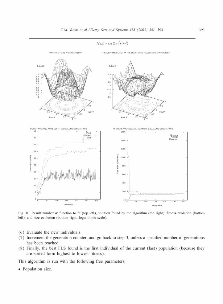
in a relatively short time: every experiment lasted about two hours on a computer with twin PentiumII 450 MHz, and using Linux as the operating system.Figs. 7–10 show the original functions to be <tted (top left), the best output produced during the

three executions of the algorithm in each problem (top right), <tness evolution along generations(bottom left), and size (rows by columns, less 1) evolution along generations (bottom right). Figureheaders show the function formulas that generate the original graphics.Table 2 shows average and standard deviation of <nal <tness, generalization error, and size (rows

by columns, less 1) of the best FLS found (the best individual in the last generation). To calculatethe generalization error once the EA has <nished a validation set of input–output pairs, di9erentfrom those used in the EA, was presented to the best FLS. The normalized MSE was computedusing the outputs produced by the FLS and the known ones.The results obtained show that the approach presented in this paper is appropriate to solve the

problem. Thus, as usual, the evolutionary algorithm behaves very well in the task of <nding goodsolutions (in these cases, function shapes are quickly learned by the genetic algorithm). However,<tting more precisely is more diJcult and it is necessary to increase the number of generations inorder to get more accuracy. But on the other hand, adding more generations might not be desirablebecause generalization might be negatively a9ected, resulting on the well known problem of over-<tting, i.e., points in the training set would be approximated better and better at each generation,but approximation of points in the test set would be worst and worst.The estimation of centroid values is quite good, as can be seen in the <gures by analyzing the

contours plotted when output Z is projected over the surface created by inputs X and Y . Thesecontours show how the changes in the shapes of the original functions are reTected in the shape ofthe results provided by the best FLS. Fitting the values of centroids to the exact values used in thefunctions makes us face the same problem stated above. It should be done carefully, because oncea given generation is reached the individuals would be <tting the errors associated to the points ofthe training set so that generalization would be performed very badly.One of the most interesting results provided by this algorithm is related to the complexity of the

solutions it <nds. As Tables 2 and 3 show the <nal size of the FLSs did not grow up to the greatestpossible value, as it might at <rst be thought. This is specially relevant because the way the <tness iscalculated does not include explicit penalization of large individuals. Fitting the 400 points involvedin every experiment can be exactly done if FLSs composed of 20 + 1 rows and 20 + 1 columnsare used. This would possibly be the solution found if random search algorithms were used. But inour method the search is guided through the use of the di9erent genetic operators together with themethod to select individuals to be reproduced and individuals to be removed.


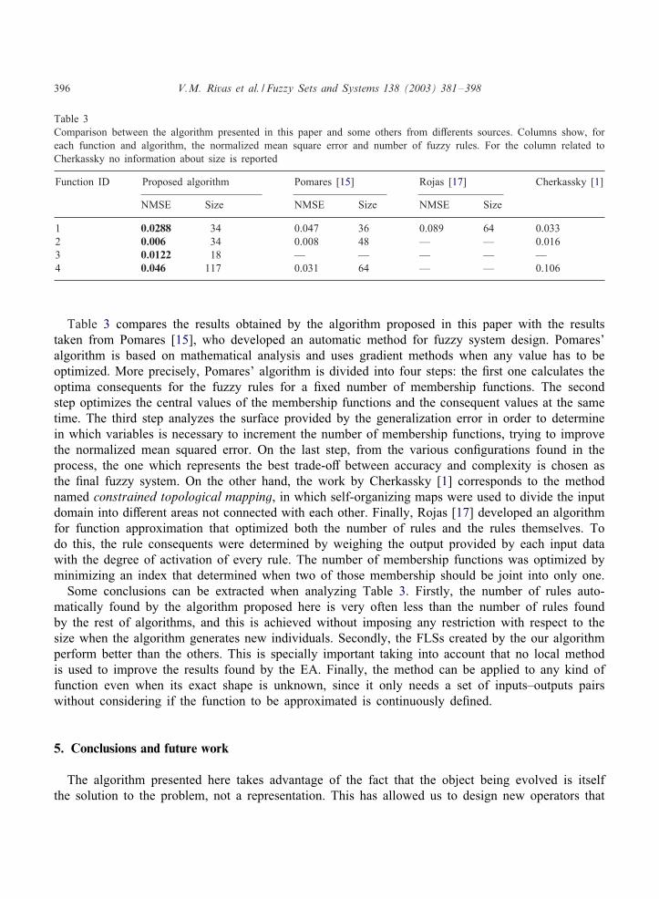
Table 3Comparison between the algorithm presented in this paper and some others from di9erents sources. Columns show, foreach function and algorithm, the normalized mean square error and number of fuzzy rules. For the column related toCherkassky no information about size is reported

Function ID Proposed algorithm Pomares [15] Rojas [17] Cherkassky [1]

NMSE Size NMSE Size NMSE Size

1 0.0288 34 0.047 36 0.089 64 0.0332 0.006 34 0.008 48 — — 0.0163 0.0122 18 — — — — —4 0.046 117 0.031 64 — — 0.106

Table 3 compares the results obtained by the algorithm proposed in this paper with the resultstaken from Pomares [15], who developed an automatic method for fuzzy system design. Pomares’algorithm is based on mathematical analysis and uses gradient methods when any value has to beoptimized. More precisely, Pomares’ algorithm is divided into four steps: the <rst one calculates theoptima consequents for the fuzzy rules for a <xed number of membership functions. The secondstep optimizes the central values of the membership functions and the consequent values at the sametime. The third step analyzes the surface provided by the generalization error in order to determinein which variables is necessary to increment the number of membership functions, trying to improvethe normalized mean squared error. On the last step, from the various con<gurations found in theprocess, the one which represents the best trade-o9 between accuracy and complexity is chosen asthe <nal fuzzy system. On the other hand, the work by Cherkassky [1] corresponds to the methodnamed constrained topological mapping, in which self-organizing maps were used to divide the inputdomain into di9erent areas not connected with each other. Finally, Rojas [17] developed an algorithmfor function approximation that optimized both the number of rules and the rules themselves. Todo this, the rule consequents were determined by weighing the output provided by each input datawith the degree of activation of every rule. The number of membership functions was optimized byminimizing an index that determined when two of those membership should be joint into only one.Some conclusions can be extracted when analyzing Table 3. Firstly, the number of rules auto-

matically found by the algorithm proposed here is very often less than the number of rules foundby the rest of algorithms, and this is achieved without imposing any restriction with respect to thesize when the algorithm generates new individuals. Secondly, the FLSs created by the our algorithmperform better than the others. This is specially important taking into account that no local methodis used to improve the results found by the EA. Finally, the method can be applied to any kind offunction even when its exact shape is unknown, since it only needs a set of inputs–outputs pairswithout considering if the function to be approximated is continuously de<ned.

5. Conclusions and future work

The algorithm presented here takes advantage of the fact that the object being evolved is itselfthe solution to the problem, not a representation. This has allowed us to design new operators that


include speci<c problem knowledge; for this very fact, every time an operator is applied the newindividual it produces is always valid, and penalty functions and repair methods need not to be used.The evolutionary algorithm performs well in the task of learning the shape of the function to be

<tted (this is, the task of approximating the solution to the optimum one). This means that mem-bership function centroids are well estimated and even trends in the rule consequents are detected,although exact values are more diJcult to <nd. All this is done while keeping a small number ofmembership functions; thus, the <tness function used is easy to calculate, and good enough to ensurethat good results are found without requiring any method that penalizes big FLSs.The research presented in this paper will continue along the following lines:

• To use some kind of local searching in order to tune up the solutions found by the EA, gettingmore accurate values for consequents.

• To <nd some other way to compute the <tness in order to signi<cantly reduce the time needed torun the algorithm.

• To test variations on current operators, especially in recombination, to allow the interchange offull rows=columns, and, in general, the interchange of cells from the <rst row and <rst column.This is diJcult since every individual has a di9erent size.

• To generalize the method so that any number of input variables can be used. This represents aserious challenge because a new representation and a di9erent way to handle the individuals aswell as new operators would be needed.

Acknowledgements

This work has been partially supported by the FEDER I+D project 1FD97-0439-TEL1, and bythe CICYT projects TIC97-1149 and CICYT, TIC99-0550 (PUFO).We would also thank the anonymous referees who reviewed this work. Their comments have

helped to signi<cantly improve the paper.

References

[1] V. Cherkassky, D. Gehring, F. Mulier, Comparison of adaptative methods for non-parametric regression analysis,IEEE Trans. Neural Networks 7 (4) (1996) 969–984.

[2] O. Cord$on, M.J. del Jes$us, F. Herrera, E. L$opez, Selecting fuzzy rule-based classi<cation systems with speci<creasoning methods using genetic algorithms, in: Proc. Internat. Fuzzy Systems Assoc. (IFSA), Prague, CzechRepublic, June 1997, pp. 424–429.

[3] L. Davis, The Handbook of Genetic Algorithms, Van Nostrand Reinhold, New York, 1991.[4] K.A. De Jong, An analysis of the behavior of a class of genetic adaptative systems, Dissertation Abstract International,

1975.[5] L.J. Eshelman, J.D. Sha9er, Real-coded genetic algorithms and interval-schema, in: Foundation of Genetic Algorithms,

Vol. 2, Morgan Kaufmann Publishers, Los, Atlos, CA, 1993, pp. 187–202.[6] D.E. Goldberg, Genetic Algorithms in Search, Optimization and Machine Learning, Addison-Wesley, Reading, MA,

USA, 1989.[7] F. Herrera, M. Lozano, J.L. Verdegay, Genetic Algorithms and Soft Computing, Physica-Verlag, Heidelberg, 1996.[8] A. Homaifar, E. McCormick, Simultaneous design of membership functions and rule sets for fuzzy controllers using

genetic algorithms, IEEE Trans. Fuzzy Systems 3 (2) (1995) 129–139.


[9] H. Ishibuchi, T. Murata, I.B. TWurksen, A genetic-algorithm-based approach to the selection of linguistic classi<cationrules, in: Proc. EUFIT’95, Aachen, Germany, 1995, pp. 1414–1419.

[10] C. Karr, Applying genetics to fuzzy logic, AI Expert 6 (1991) 26–33.[11] C. Karr, E. Gentry, Fuzzy control of ph using genetic algorithms, IEEE Trans. Fuzzy Systems 1 (1993) 46–53.[12] D. Kim, C. Kim, Forecasting time series with genetic fuzzy predictor ensemble, IEEE Trans. Fuzzy Systems 5 (4)

(1997) 523–535.[13] J.J. Merelo, J. Carpio, P.A. Castillo, V. Rivas, G. Romero, Evolving Objects, in: Proc. Internat. Workshop on

Evolutionary Computation (IWEC’2000), State Key Laboratory of Software Engineering, Wuhan University, 2000,pp. 202–208.

[14] Z. Michalewicz, Genetic Algorithms+Data Structures=Evolution programs, 3rd Edition, Springer, New York, USA,1999.

[15] H. Pomares, Nueva metodolog$%a para el diseno autom$atico de sistemas difusos, Ph.D. Thesis, University of Granada,Spain, 1999.

[16] I. Rojas, J.J. Merelo, J.L. Bernier, A. Prieto, A new approach to fuzzy controller designing and coding via geneticalgorithms, in: Proc. 6th IEEE Internat. Conf. on Fuzzy Systems, Vol. II, Barcelona, Spain, 1997, IEEE ServiceCenter, NJ, USA, pp. 1505–1510.

[17] I. Rojas, H. Pomares, J. Ortega, A. Prieto, Self-organized fuzzy system generation from training examples, IEEETrans. Fuzzy Systems 8 (1) (2000) 23–36.

[18] T.L. Seng, M. Bin Khalid, R. Yusof, Tuning of a neuro-fuzzy controller by genetic algorithms with and applicationto a coupled-tank liquid-level control system, Eng. Appl. Artif. Intell. 11 (1998) 517–529.

[19] T.L. Seng, M. Bin Khalid, R. Yusof, Tuning of a neuro-fuzzy controller by genetic algorithm, IEEE Trans. Systems,Man, Cybernet. 29 (2) (1999) 226–236.

[20] M. Setnes, H. Roubos, Ga-fuzzy modeling and classi<cation: complexity and performance, IEEE Trans. FuzzySystems 8 (2000) 509–522.

[21] P. Siarry, F. Guely, A genetic algorithm for optimizing Takagi-Sugeno fuzzy rule bases, Fuzzy Sets and Systems99 (1998) 37–47.

[22] A. Wright, Genetic algorithms for real parameter optimization, in: Foundation of Genetic Algorithms, MorganKaufmann Publishers, Los Altos, CA, 1991, pp. 205–218.

[23] L.A. Zadeh, Fuzzy sets, Inform. Control 8 (1965) 338–353.

Evolving two-dimensional fuzzy systems

Documents

Transcript of Evolving two-dimensional fuzzy systems