
Neuro-fuzzy synthesis of flight control electrohydraulic servo
Upload
independentCategory
view
1download
0
Fuzzy Control
Kevin M. PassinoDepartment of Electrical Engineering
The Ohio State University
Stephen YurkovichDepartment of Electrical Engineering
The Ohio State University
An Imprint of Addison-Wesley Longman, Inc.
Menlo Park, California • Reading, Massachusetts • Harlow, England • Berkeley, CaliforniaDon Mills, Ontaria • Sydney • Bonn • Amsterdam • Mexico City

ii
Assistant Editor: Laura CheuEditorial Assistant: Royden TonomuraSenior Production Editor: Teri HydeMarketing Manager: Rob MerinoManufacturing Supervisor: Janet WeaverArt and Design Manager: Kevin BerryCover Design: Yvo Riezebos (technical drawing by K. Passino)Text Design: Peter VacekDesign Macro Writer: William Erik BaxterCopyeditor: Brian JonesProofreader: Holly McLean-Aldis
Copyright c© 1998 Addison Wesley Longman, Inc.
All rights reserved. No part of this publication may be reproduced, or stored in a databaseor retrieval system, or transmitted, in any form or by any means, electronic, mechanical,photocopying, recording, or otherwise, without the prior written permission of the pub-lisher. Printed in the United States of America. Printed simultaneously in Canada.
Many of the designations used by manufacturers and sellers to distinguish their productsare claimed as trademarks. Where those designations appear in this book, and Addison-Wesley was aware of a trademark claim, the designations have been printed in initial capsor in all caps.
MATLAB is a registered trademark of The MathWorks, Inc.
Library of Congress Cataloging-in-Publication Data
Passino, Kevin M.
Fuzzy control / Kevin M. Passino and Stephen Yurkovich.
p. cm.
Includes bibliographical references and index.
ISBN 0-201-18074-X
1. Automatic control. 2. Control theory. 3. Fuzzy systems.
I. Yurkovich, Stephen. II. Title.
TJ213.P317 1997 97-14003
629.8’9--DC21 CIP
Instructional Material Disclaimer: The programs presented in this book have beenincluded for their instructional value. They have been tested with care but are not guaran-teed for any particular purpose. Neither the publisher or the authors offer any warrantiesor representations, nor do they accept any liabilities with respect to the programs.
About the Cover: An explanation of the technical drawing is given in Chapter 2 onpage 50.
ISBN 0–201–18074–X1 2 3 4 5 6 7 8 9 10—CRW—01 00 99 98 97

iii
Addison Wesley Longman, Inc., 2725 Sand Hill Road, Menlo Park, California 94025

iv
To Annie and Juliana (K.M.P)
To Tricia, B.J., and James (S.Y.)

v

vi

PrefaceFuzzy control is a practical alternative for a variety of challenging control applica-tions since it provides a convenient method for constructing nonlinear controllersvia the use of heuristic information. Such heuristic information may come froman operator who has acted as a “human-in-the-loop” controller for a process. Inthe fuzzy control design methodology, we ask this operator to write down a set ofrules on how to control the process, then we incorporate these into a fuzzy con-troller that emulates the decision-making process of the human. In other cases, theheuristic information may come from a control engineer who has performed exten-sive mathematical modeling, analysis, and development of control algorithms for aparticular process. Again, such expertise is loaded into the fuzzy controller to au-tomate the reasoning processes and actions of the expert. Regardless of where theheuristic control knowledge comes from, fuzzy control provides a user-friendly for-malism for representing and implementing the ideas we have about how to achievehigh-performance control.
In this book we provide a control-engineering perspective on fuzzy control.We are concerned with both the construction of nonlinear controllers for challeng-ing real-world applications and with gaining a fundamental understanding of thedynamics of fuzzy control systems so that we can mathematically verify their prop-erties (e.g., stability) before implementation. We emphasize engineering evaluationsof performance and comparative analysis with conventional control methods. Weintroduce adaptive methods for identification, estimation, and control. We exam-ine numerous examples, applications, and design and implementation case studiesthroughout the text. Moreover, we provide introductions to neural networks, ge-netic algorithms, expert and planning systems, and intelligent autonomous control,and explain how these topics relate to fuzzy control.
Overall, we take a pragmatic engineering approach to the design, analysis,performance evaluation, and implementation of fuzzy control systems. We are notconcerned with whether the fuzzy controller is “artificially intelligent” or with in-vestigating the mathematics of fuzzy sets (although some of the exercises do), but
vii

viii
rather with whether the fuzzy control methodology can help solve challenging real-world problems.
Overview of the Book
The book is basically broken into three parts. In Chapters 1–4 we cover the basics of“direct” fuzzy control (i.e., the nonadaptive case). In Chapters 5–7 we cover adap-tive fuzzy systems for estimation, identification, and control. Finally, in Chapter 8we briefly cover the main areas of intelligent control and highlight how the topicscovered in this book relate to these areas. Overall, we largely focus on what onecould call the “heuristic approach to fuzzy control” as opposed to the more recentmathematical focus on fuzzy control where stability analysis is a major theme.
In Chapter 1 we provide an overview of the general methodology for conven-tional control system design. Then we summarize the fuzzy control system designprocess and contrast the two. Next, we explain what this book is about via a simplemotivating example. In Chapter 2 we first provide a tutorial introduction to fuzzycontrol via a two-input, one-output fuzzy control design example. Following thiswe introduce a general mathematical characterization of fuzzy systems and studytheir fundamental properties. We use a simple inverted pendulum example to illus-trate some of the most widely used approaches to fuzzy control system design. Weexplain how to write a computer program to simulate a fuzzy control system, usingeither a high-level language or Matlab1. In the web and ftp pages for the book weprovide such code in C and Matlab. In Chapter 3 we use several case studies toshow how to design, simulate, and implement a variety of fuzzy control systems.In these case studies we pay particular attention to comparative analysis with con-ventional approaches. In Chapter 4 we show how to perform stability analysis offuzzy control systems using Lyapunov methods and frequency domain–based sta-bility criteria. We introduce nonlinear analysis methods that can be used to predictand eliminate steady-state tracking error and limit cycles. We then show how touse the analysis approaches in fuzzy control system design. The overall focus forthese nonlinear analysis methods is on understanding fundamental problems thatcan be encountered in the design of fuzzy control systems and how to avoid them.
In Chapter 5 we introduce the basic “function approximation problem” andshow how identification, estimation, prediction, and some control design problemsare a special case of it. We show how to incorporate heuristic information into thefunction approximator. We show how to form rules for fuzzy systems from data pairsand show how to train fuzzy systems from input-output data with least squares,gradient, and clustering methods. And we show how one clustering method fromfuzzy pattern recognition can be used in conjunction with least squares methods toconstruct a fuzzy model from input-output data. Moreover, we discuss hybrid ap-proaches that involve a combination of two or more of these methods. In Chapter 6we introduce adaptive fuzzy control. First, we introduce several methods for auto-matically synthesizing and tuning a fuzzy controller, and then we illustrate theirapplication via several design and implementation case studies. We also show how
1. MATLAB is a registered trademark of The MathWorks, Inc.

ix
to tune a fuzzy model of the plant and use the parameters of such a model in theon-line design of a controller. In Chapter 7 we introduce fuzzy supervisory control.We explain how fuzzy systems can be used to automatically tune proportional-integral-derivative (PID) controllers, how fuzzy systems provide a methodologyfor constructing and implementing gain schedulers, and how fuzzy systems can beused to coordinate the application and tuning of conventional controllers. Follow-ing this, we show how fuzzy systems can be used to tune direct and adaptive fuzzycontrollers. We provide case studies in the design and implementation of fuzzysupervisory control.
In Chapter 8 we summarize our control engineering perspective on fuzzy control,provide an overview of the other areas of the field of “intelligent control,” andexplain how these other areas relate to fuzzy control. In particular, we briefly coverneural networks, genetic algorithms, knowledge-based control (expert systems andplanning systems), and hierarchical intelligent autonomous control.
Examples, Applications, and Design and Implementation Case Studies
We provide several design and implementation case studies for a variety of appli-cations, and many examples are used throughout the text. The basic goals of thesecase studies and examples are as follows:
• To help illustrate the theory.
• To show how to apply the techniques.
• To help illustrate design procedures in a concrete way.
• To show what practical issues are encountered in the development and implemen-tation of a fuzzy control system.
Some of the more detailed applications that are studied in the chapters and theiraccompanying homework problems are the following:
• Direct fuzzy control: Translational inverted pendulum, fuzzy decision-making sys-tems, two-link flexible robot, rotational inverted pendulum, and machine schedul-ing (Chapters 2 and 3 homework problems: translational inverted pendulum, au-tomobile cruise control, magnetic ball suspension system, automated highway sys-tem, single-link flexible robot, rotational inverted pendulum, machine scheduling,motor control, cargo ship steering, base braking control system, rocket velocitycontrol, acrobot, and fuzzy decision-making systems).
• Nonlinear analysis: Inverted pendulum, temperature control, hydrofoil controller,underwater vehicle control, and tape drive servo (Chapter 4 homework problems:inverted pendulum, magnetic ball suspension system, temperature control, andhydrofoil controller design).

x
• Fuzzy identification and estimation: Engine intake manifold failure estimation,and failure detection and identification for internal combustion engine calibra-tion faults (Chapter 5 homework problems: tank identification, engine frictionestimation, and cargo ship failures estimation).
• Adaptive fuzzy control: Two-link flexible robot, cargo ship steering, fault toler-ant aircraft control, magnetically levitated ball, rotational inverted pendulum,machine scheduling, and level control in a tank (Chapter 6 homework problems:tanker and cargo ship steering, liquid level control in a tank, rocket velocity con-trol, base braking control system, magnetic ball suspension system, rotationalinverted pendulum, and machine scheduling).
• Supervisory fuzzy control: Two-link flexible robot, and fault-tolerant aircraft con-trol (Chapter 7 homework problems: liquid level control, and cargo and tankership steering).
Some of the applications and examples are dedicated to illustrating one idea fromthe theory or one technique. Others are used in several places throughout the textto show how techniques build on one another and compare to each other. Many ofthe applications show how fuzzy control techniques compare to conventional controlmethodologies.
World Wide Web Site and FTP Site: Computer Code Available
The following information is available electronically:
• Various versions of C and Matlab code for simulation of fuzzy controllers, fuzzycontrol systems, adaptive fuzzy identification and estimation methods, and adap-tive fuzzy control systems (e.g., for some examples and homework problems inthe text).
• Other special notes of interest, including an errata sheet if necessary.
You can access this information via the web site:
http://www.awl.com/cseng/titles/0-201-18074-X
or you can access the information directly via anonymous ftp to
ftp://ftp.aw.com/cseng/authors/passino/fc
For anonymous ftp, log into the above machine with a username “anonymous” anduse your e-mail address as a password.
Organization, Prerequisites, and Usage
Each chapter includes an overview, a summary, and a section “For Further Study”that explains how the reader can continue study in the topical area of the chapter.At the end of each chapter overview, we explain how the chapter is related to the

xi
others. This includes an outline of what must be covered to be able to understandthe later chapters and what may be skipped on a first reading. The summaries atthe end of each chapter provide a list of all major topics covered in that chapter sothat it is clear what should be learned in each chapter.
Each chapter also includes a set of exercises or design problems and often both.Exercises or design problems that are particularly challenging (considering how faralong you are in the text) or that require you to help define part of the problem aredesignated with a star (“”) after the title of the problem. In addition to helpingto solidify the concepts discussed in the chapters, the problems at the ends ofthe chapters are sometimes used to introduce new topics. We require the use ofcomputer-aided design (CAD) for fuzzy controllers in many of the design problemsat the ends of the chapters (e.g., via the use of Matlab or some high-level language).
The necessary background for the book includes courses on differential equa-tions and classical control (root locus, Bode plots, Nyquist theory, lead-lag com-pensation, and state feedback concepts including linear quadratic regulator design).Courses on nonlinear stability theory and adaptive control would be helpful butare not necessary. Hence, much of the material can be covered in an undergraduatecourse. For instance, one could easily cover Chapters 1–3 in an undergraduate courseas they require very little background besides a basic understanding of signals andsystems including Laplace and z-transform theory (one application in Chapter 3does, however, require a cursory knowledge of the linear quadratic regulator). Also,many parts of Chapters 5–7 can be covered once a student has taken a first coursein control (a course in nonlinear control would be helpful for Chapter 4 but is notnecessary). One could cover the basics of fuzzy control by adding parts of Chapter 2to the end of a standard undergraduate or graduate course on control. Basically,however, we view the book as appropriate for a first-level graduate course in fuzzycontrol.
We have used the book for a portion (six weeks) of a graduate-level course onintelligent control and for undergraduate independent studies and design projects.In addition, portions of the text have been used for short courses and workshops onfuzzy control where the focus has been directed at practicing engineers in industry.
Alternatively, the text could be used for a course on intelligent control. In thiscase, the instructor could cover the material in Chapter 8 on neural networks andgenetic algorithms after Chapter 2 or 3, then explain their role in the topics coveredin Chapters 5, 6, and 7 while these chapters are covered. For instance, in Chapter 5the instructor would explain how gradient and least squares methods can be usedto train neural networks. In Chapter 6 the instructor could draw analogies betweenneural control via the radial basis function neural network and the fuzzy modelreference learning controller. Also, for indirect adaptive control, the instructor couldexplain how, for instance, the multilayer perceptron or radial basis function neuralnetworks can be used as the nonlinearity that is trained to act like the plant. InChapter 7 the instructor could explain how neural networks can be trained to serveas gain schedulers. After Chapter 7 the instructor could then cover the material onexpert control, planning systems, and intelligent autonomous control in Chapter 8.Many more details on strategies for teaching the material in a fuzzy or intelligent

xii
control course are given in the instructor’s manual, which is described below.Engineers and scientists working in industry will find that the book will serve
nicely as a “handbook” for the development of fuzzy control systems, and that thedesign, simulation, and implementation case studies will provide very good insightsinto how to construct fuzzy controllers for specific applications. Researchers inacademia and elsewhere will find that this book will provide an up-to-date viewof the field, show the major approaches, provide good references for further study,and provide a nice outlook for thinking about future research directions.
Instructor’s Manual
An Instructor’s Manual to accompany this textbook is available (to instructors only)from Addison Wesley Longman. The Instructor’s Manual contains the following:
• Strategies for teaching the material.
• Solutions to end-of-chapter exercises and design problems.
• A description of a laboratory course that has been taught several times at TheOhio State University which can be run in parallel with a lecture course that istaught out of this book.
• An electronic appendix containing the computer code (e.g., C and Matlab code)for solving many exercises and design problems.
Sales Specialists at Addison Wesley Longman will make the instructor’s manualavailable to qualified instructors. To find out who your Addison Wesley LongmanSales Specialist is please see the web site:
http://www.aw.com/cseng/
or send an email to:
Feedback on the Book
It is our hope that we will get the opportunity to correct any errors in this book;hence, we encourage you to provide a precise description of any errors you mayfind. We are also open to your suggestions on how to improve the textbook. Forthis, please use either e-mail ([email protected]) or regular mail to thefirst author: Kevin M. Passino, Dept. of Electrical Engineering, The Ohio StateUniversity, 2015 Neil Ave., Columbus, OH 43210-1272.
Acknowledgments
No book is written in a vacuum, and this is especially true for this one. We mustemphasize that portions of the book appeared in earlier forms as conference pa-pers, journal papers, theses, or project reports with our students here at Ohio

xiii
State. Due to this fact, these parts of the text are sometimes a combination of ourwords and those of our students (which are very difficult to separate at times).In every case where we use such material, the individuals have given us permis-sion to use it, and we provide the reader with a reference to the original sourcesince this will typically provide more details than what are covered here. Whilewe always make it clear where the material is taken from, it is our pleasure tohighlight these students’ contributions here as well. In particular, we drew heavilyfrom work with the following students and papers written with them (in alpha-betical order): Anthony Angsana [4], Scott C. Brown [27], David L. Jenkins [83],Waihon Andrew Kwong [103, 104, 144], Eric G. Laukonen [107, 104], Jeffrey R.Layne [110, 113, 112, 114, 111], William K. Lennon [118], Sashonda R. Morris[143], Vivek G. Moudgal [145, 144], Jeffrey T. Spooner [200, 196], and MoeljonoWidjaja [235, 244]. These students, and Mehmet Akar, Mustafa K. Guven, Min-Hsiung Hung, Brian Klinehoffer, Duane Marhefka, Matt Moore, Hazem Nounou,Jeff Palte, and Jerry Troyer helped by providing solutions to several of the exer-cises and design problems and these are contained in the instructor’s manual for thisbook. Manfredi Maggiore helped by proofreading the manuscript. Scott C. Brownand Raul Ordonez assisted in the development of the associated laboratory courseat OSU.
We would like to gratefully acknowledge the following publishers for giving uspermission to use figures that appeared in some of our past publications: The In-stitute of Electrical and Electronic Engineers (IEEE), John Wiley and Sons, Hemi-sphere Publishing Corp., and Kluwer Academic Publishers. In each case where weuse a figure from a past publication, we give the full reference to the original pa-per, and indicate in the caption of the figure that the copyright belongs to theappropriate publisher (via, e.g., “ c© IEEE”).
We have benefited from many technical discussions with many colleagues whowork in conventional and intelligent control (too many to list here); most of thesepersons are mentioned by referencing their work in the bibliography at the end ofthe book. We would, however, especially like to thank Zhiqiang Gao and Oscar R.Gonzalez for class-testing this book. Moreover, thanks go to the following personswho reviewed various earlier versions of the manuscript: D. Aaronson, M.A. Abidi,S.P. Colombano, Z. Gao, O. Gonzalez, A.S. Hodel, R. Langari, M.S. Stachowicz,and G. Vachtsevanos.
We would like to acknowledge the financial support of National Science Foun-dation grants IRI-9210332 and EEC-9315257, the second of which was for the de-velopment of a course and laboratory for intelligent control. Moreover, we hadadditional financial support from a variety of other sponsors during the course ofthe development of this textbook, some of whom gave us the opportunity to applysome of the methods in this text to challenging real-world applications, and otherswhere one or both of us gave a course on the topics covered in this book. Thesesponsors include Air Products and Chemicals Inc., Amoco Research Center, Bat-telle Memorial Institute, Delphi Chassis Division of General Motors, Ford MotorCompany, General Electric Aircraft Engines, The Center for Automotive Research(CAR) at The Ohio State University, The Center for Intelligent Transportation

xiv
Research (CITR) at The Ohio State University, and The Ohio Aerospace Institute(in a teamed arrangement with Rockwell International Science Center and WrightLaboratories).
We would like to thank Tim Cox, Laura Cheu, Royden Tonomura, Teri Hyde,Rob Merino, Janet Weaver, Kevin Berry, Yvo Riezebos, Peter Vacek, William ErikBaxter, Brian Jones, and Holly McLean-Aldis for all their help in the productionand editing of this book. Finally, we would most like to thank our wives, who havehelped set up wonderful supportive home environments that we value immensely.
Kevin PassinoSteve YurkovichColumbus, OhioJuly 1997

ContentsPREFACE vii
CHAPTER 1 / Introduction 1
1.1 Overview 1
1.2 Conventional Control System Design 3
1.2.1 Mathematical Modeling 31.2.2 Performance Objectives and Design Constraints 51.2.3 Controller Design 71.2.4 Performance Evaluation 8
1.3 Fuzzy Control System Design 10
1.3.1 Modeling Issues and Performance Objectives 121.3.2 Fuzzy Controller Design 121.3.3 Performance Evaluation 131.3.4 Application Areas 14
1.4 What This Book Is About 14
1.4.1 What the Techniques Are Good For: An Example 151.4.2 Objectives of This Book 17
1.5 Summary 18
1.6 For Further Study 19
1.7 Exercises 19
CHAPTER 2 / Fuzzy Control: The Basics 23
2.1 Overview 23
2.2 Fuzzy Control: A Tutorial Introduction 24
2.2.1 Choosing Fuzzy Controller Inputs and Outputs 262.2.2 Putting Control Knowledge into Rule-Bases 27
xv

xvi CONTENTS
2.2.3 Fuzzy Quantification of Knowledge 322.2.4 Matching: Determining Which Rules to Use 372.2.5 Inference Step: Determining Conclusions 422.2.6 Converting Decisions into Actions 442.2.7 Graphical Depiction of Fuzzy Decision Making 492.2.8 Visualizing the Fuzzy Controller’s Dynamical Operation 50
2.3 General Fuzzy Systems 51
2.3.1 Linguistic Variables, Values, and Rules 522.3.2 Fuzzy Sets, Fuzzy Logic, and the Rule-Base 552.3.3 Fuzzification 612.3.4 The Inference Mechanism 622.3.5 Defuzzification 652.3.6 Mathematical Representations of Fuzzy Systems 692.3.7 Takagi-Sugeno Fuzzy Systems 732.3.8 Fuzzy Systems Are Universal Approximators 77
2.4 Simple Design Example: The Inverted Pendulum 77
2.4.1 Tuning via Scaling Universes of Discourse 782.4.2 Tuning Membership Functions 832.4.3 The Nonlinear Surface for the Fuzzy Controller 872.4.4 Summary: Basic Design Guidelines 89
2.5 Simulation of Fuzzy Control Systems 91
2.5.1 Simulation of Nonlinear Systems 912.5.2 Fuzzy Controller Arrays and Subroutines 942.5.3 Fuzzy Controller Pseudocode 95
2.6 Real-Time Implementation Issues 97
2.6.1 Computation Time 972.6.2 Memory Requirements 98
2.7 Summary 99
2.8 For Further Study 101
2.9 Exercises 101
2.10 Design Problems 110
CHAPTER 3 / Case Studies in Design and Implementation 119
3.1 Overview 119
3.2 Design Methodology 122
3.3 Vibration Damping for a Flexible Robot 124
3.3.1 The Two-Link Flexible Robot 1253.3.2 Uncoupled Direct Fuzzy Control 1293.3.3 Coupled Direct Fuzzy Control 134
3.4 Balancing a Rotational Inverted Pendulum 142
3.4.1 The Rotational Inverted Pendulum 142

CONTENTS xvii
3.4.2 A Conventional Approach to Balancing Control 1443.4.3 Fuzzy Control for Balancing 145
3.5 Machine Scheduling 152
3.5.1 Conventional Scheduling Policies 1533.5.2 Fuzzy Scheduler for a Single Machine 1563.5.3 Fuzzy Versus Conventional Schedulers 158
3.6 Fuzzy Decision-Making Systems 161
3.6.1 Infectious Disease Warning System 1623.6.2 Failure Warning System for an Aircraft 166
3.7 Summary 168
3.8 For Further Study 169
3.9 Exercises 170
3.10 Design Problems 172
CHAPTER 4 / Nonlinear Analysis 187
4.1 Overview 187
4.2 Parameterized Fuzzy Controllers 189
4.2.1 Proportional Fuzzy Controller 1904.2.2 Proportional-Derivative Fuzzy Controller 191
4.3 Lyapunov Stability Analysis 193
4.3.1 Mathematical Preliminaries 1934.3.2 Lyapunov’s Direct Method 1954.3.3 Lyapunov’s Indirect Method 1964.3.4 Example: Inverted Pendulum 1974.3.5 Example: The Parallel Distributed Compensator 200
4.4 Absolute Stability and the Circle Criterion 204
4.4.1 Analysis of Absolute Stability 2044.4.2 Example: Temperature Control 208
4.5 Analysis of Steady-State Tracking Error 210
4.5.1 Theory of Tracking Error for Nonlinear Systems 2114.5.2 Example: Hydrofoil Controller Design 213
4.6 Describing Function Analysis 214
4.6.1 Predicting the Existence and Stability of Limit Cycles 2144.6.2 SISO Example: Underwater Vehicle Control System 2184.6.3 MISO Example: Tape Drive Servo 219
4.7 Limitations of the Theory 220
4.8 Summary 222
4.9 For Further Study 223
4.10 Exercises 225

xviii CONTENTS
4.11 Design Problems 228
CHAPTER 5 / Fuzzy Identification and Estimation 233
5.1 Overview 233
5.2 Fitting Functions to Data 235
5.2.1 The Function Approximation Problem 2355.2.2 Relation to Identification, Estimation, and Prediction 2385.2.3 Choosing the Data Set 2405.2.4 Incorporating Linguistic Information 2415.2.5 Case Study: Engine Failure Data Sets 243
5.3 Least Squares Methods 248
5.3.1 Batch Least Squares 2485.3.2 Recursive Least Squares 2525.3.3 Tuning Fuzzy Systems 2555.3.4 Example: Batch Least Squares Training of Fuzzy Systems 2575.3.5 Example: Recursive Least Squares Training of Fuzzy Systems 259
5.4 Gradient Methods 260
5.4.1 Training Standard Fuzzy Systems 2605.4.2 Implementation Issues and Example 2645.4.3 Training Takagi-Sugeno Fuzzy Systems 2665.4.4 Momentum Term and Step Size 2695.4.5 Newton and Gauss-Newton Methods 270
5.5 Clustering Methods 273
5.5.1 Clustering with Optimal Output Predefuzzification 2745.5.2 Nearest Neighborhood Clustering 279
5.6 Extracting Rules from Data 282
5.6.1 Learning from Examples (LFE) 2825.6.2 Modified Learning from Examples (MLFE) 285
5.7 Hybrid Methods 291
5.8 Case Study: FDI for an Engine 292
5.8.1 Experimental Engine and Testing Conditions 2935.8.2 Fuzzy Estimator Construction and Results 2945.8.3 Failure Detection and Identification (FDI) Strategy 297
5.9 Summary 301
5.10 For Further Study 302
5.11 Exercises 303
5.12 Design Problems 311

CONTENTS xix
CHAPTER 6 / Adaptive Fuzzy Control 317
6.1 Overview 317
6.2 Fuzzy Model Reference Learning Control (FMRLC) 319
6.2.1 The Fuzzy Controller 3206.2.2 The Reference Model 3246.2.3 The Learning Mechanism 3256.2.4 Alternative Knowledge-Base Modifiers 3296.2.5 Design Guidelines for the Fuzzy Inverse Model 330
6.3 FMRLC: Design and Implementation Case Studies 333
6.3.1 Cargo Ship Steering 3336.3.2 Fault-Tolerant Aircraft Control 3476.3.3 Vibration Damping for a Flexible Robot 357
6.4 Dynamically Focused Learning (DFL) 364
6.4.1 Magnetic Ball Suspension System: Motivation for DFL 3656.4.2 Auto-Tuning Mechanism 3776.4.3 Auto-Attentive Mechanism 3796.4.4 Auto-Attentive Mechanism with Memory 384
6.5 DFL: Design and Implementation Case Studies 388
6.5.1 Rotational Inverted Pendulum 3886.5.2 Adaptive Machine Scheduling 390
6.6 Indirect Adaptive Fuzzy Control 394
6.6.1 On-Line Identification Methods 3946.6.2 Adaptive Control for Feedback Linearizable Systems 3956.6.3 Adaptive Parallel Distributed Compensation 3976.6.4 Example: Level Control in a Surge Tank 398
6.7 Summary 402
6.8 For Further Study 405
6.9 Exercises 406
6.10 Design Problems 407
CHAPTER 7 / Fuzzy Supervisory Control 413
7.1 Overview 413
7.2 Supervision of Conventional Controllers 415
7.2.1 Fuzzy Tuning of PID Controllers 4157.2.2 Fuzzy Gain Scheduling 4177.2.3 Fuzzy Supervision of Conventional Controllers 421
7.3 Supervision of Fuzzy Controllers 422
7.3.1 Rule-Base Supervision 4227.3.2 Case Study: Vibration Damping for a Flexible Robot 4237.3.3 Supervised Fuzzy Learning Control 427

xx CONTENTS
7.3.4 Case Study: Fault-Tolerant Aircraft Control 429
7.4 Summary 435
7.5 For Further Study 436
7.6 Design Problems 437
CHAPTER 8 / Perspectives on Fuzzy Control 439
8.1 Overview 439
8.2 Fuzzy Versus Conventional Control 440
8.2.1 Modeling Issues and Design Methodology 4408.2.2 Stability and Performance Analysis 4428.2.3 Implementation and General Issues 443
8.3 Neural Networks 444
8.3.1 Multilayer Perceptrons 4448.3.2 Radial Basis Function Neural Networks 4478.3.3 Relationships Between Fuzzy Systems and Neural Networks 449
8.4 Genetic Algorithms 451
8.4.1 Genetic Algorithms: A Tutorial 4518.4.2 Genetic Algorithms for Fuzzy System Design and Tuning 458
8.5 Knowledge-Based Systems 461
8.5.1 Expert Control 4618.5.2 Planning Systems for Control 462
8.6 Intelligent and Autonomous Control 463
8.6.1 What Is “Intelligent Control”? 4648.6.2 Architecture and Characteristics 4658.6.3 Autonomy 4678.6.4 Example: Intelligent Vehicle and Highway Systems 468
8.7 Summary 471
8.8 For Further Study 472
8.9 Exercises 472
BIBLIOGRAPHY 477
INDEX 495

C H A P T E R 1
IntroductionIt is not only old and early impressions
that deceive us; the charms of novelty
have the same power.
–Blaise Pascal
1.1 OverviewWhen confronted with a control problem for a complicated physical process, acontrol engineer generally follows a relatively systematic design procedure. A simpleexample of a control problem is an automobile “cruise control” that provides theautomobile with the capability of regulating its own speed at a driver-specifiedset-point (e.g., 55 mph). One solution to the automotive cruise control probleminvolves adding an electronic controller that can sense the speed of the vehicle viathe speedometer and actuate the throttle position so as to regulate the vehicle speedas close as possible to the driver-specified value (the design objective). Such speedregulation must be accurate even if there are road grade changes, head winds, orvariations in the number of passengers or amount of cargo in the automobile.
After gaining an intuitive understanding of the plant’s dynamics and establish-ing the design objectives, the control engineer typically solves the cruise controlproblem by doing the following:
1. Developing a model of the automobile dynamics (which may model vehicle andpower train dynamics, tire and suspension dynamics, the effect of road gradevariations, etc.).
2. Using the mathematical model, or a simplified version of it, to design a con-troller (e.g., via a linear model, develop a linear controller with techniques fromclassical control).
1

2 Chapter 1 / Introduction
3. Using the mathematical model of the closed-loop system and mathematicalor simulation-based analysis to study its performance (possibly leading to re-design).
4. Implementing the controller via, for example, a microprocessor, and evaluatingthe performance of the closed-loop system (again, possibly leading to redesign).
This procedure is concluded when the engineer has demonstrated that the con-trol objectives have been met, and the controller (the “product”) is approved formanufacturing and distribution.
In this book we show how the fuzzy control design methodology can be usedto construct fuzzy controllers for challenging real-world applications. As opposedto “conventional” control approaches (e.g., proportional-integral-derivative (PID),lead-lag, and state feedback control) where the focus is on modeling and the use ofthis model to construct a controller that is described by differential equations, infuzzy control we focus on gaining an intuitive understanding of how to best controlthe process, then we load this information directly into the fuzzy controller.
For instance, in the cruise control example we may gather rules about how toregulate the vehicle’s speed from a human driver. One simple rule that a humandriver may provide is “If speed is lower than the set-point, then press down fur-ther on the accelerator pedal.” Other rules may depend on the rate of the speederror increase or decrease, or may provide ways to adapt the rules when there aresignificant plant parameter variations (e.g., if there is a significant increase in themass of the vehicle, tune the rules to press harder on the accelerator pedal). Formore challenging applications, control engineers typically have to gain a very goodunderstanding of the plant to specify complex rules that dictate how the controllershould react to the plant outputs and reference inputs.
Basically, while differential equations are the language of conventional control,heuristics and “rules” about how to control the plant are the language of fuzzycontrol. This is not to say that differential equations are not needed in the fuzzycontrol methodology. Indeed, one of the main focuses of this book will be on how“conventional” the fuzzy control methodology really is and how many ideas fromconventional control can be quite useful in the analysis of this new class of controlsystems.
In this chapter we first provide an overview of the standard approach to con-structing a control system and identify a wide variety of relevant conventional con-trol ideas and techniques (see Section 1.2). We assume that the reader has at leastsome familiarity with conventional control. Our focus in this book is not only onintroducing a variety of approaches to fuzzy control but also on comparing these toconventional control approaches to determine when fuzzy control offers advantagesover conventional methods. Hence, to fully understand this book you need to un-derstand several ideas from conventional control (e.g., classical control, state-spacebased design, the linear quadratic regulator, stability analysis, feedback lineariza-tion, adaptive control, etc.). The reader not familiar with conventional control tothis extent will still find the book quite useful. In fact, we expect to whet the

1.2 Conventional Control System Design 3
appetite of such readers so that they become interested in learning more aboutconventional control. At the end of this chapter we will provide a list of books thatcan serve to teach such readers about these areas.
Following our overview of conventional control, in Section 1.3 we outline a“philosophy” of fuzzy control where we explain the design methodology for fuzzycontrollers, relate this to the conventional control design methodology, and highlightthe importance of analysis and verification of the behavior of closed-loop fuzzycontrol systems.
We highly recommend that you take the time to study this chapter (even if youalready understand conventional control or even the basics of fuzzy control) as itwill set the tone for the remainder of the book and provide a sound methodologyfor approaching the sometimes “overhyped” field of fuzzy control. Moreover, inSection 1.4 we provide a more detailed overview of this book than we provided inthe Preface, and you will find this useful in deciding what topics to study closelyand which ones you may want to skip over on a first reading.
1.2 Conventional Control System DesignA basic control system is shown in Figure 1.1. The process (or “plant”) is theobject to be controlled. Its inputs are u(t), its outputs are y(t), and the referenceinput is r(t). In the cruise control problem, u(t) is the throttle input, y(t) is thespeed of the vehicle, and r(t) is the desired speed that is specified by the driver.The plant is the vehicle itself. The controller is the computer in the vehicle thatactuates the throttle based on the speed of the vehicle and the desired speed thatwas specified. In this section we provide an overview of the steps taken to designthe controller shown in Figure 1.1. Basically, these are modeling, controller design,and performance evaluation.
T
C P
FIGURE 1.1 Control system.
1.2.1 Mathematical ModelingWhen a control engineer is given a control problem, often one of the first tasks thatshe or he undertakes is the development of a mathematical model of the process tobe controlled, in order to gain a clear understanding of the problem. Basically, thereare only a few ways to actually generate the model. We can use first principles of

4 Chapter 1 / Introduction
physics (e.g., F = ma) to write down a model. Another way is to perform “systemidentification” via the use of real plant data to produce a model of the system.Sometimes a combined approach is used where we use physics to write down ageneral differential equation that we believe represents the plant behavior, andthen we perform experiments on the plant to determine certain model parametersor functions.
Often, more than one mathematical model is produced. A “truth model” is onethat is developed to be as accurate as possible so that it can be used in simulation-based evaluations of control systems. It must be understood, however, that thereis never a perfect mathematical model for the plant. The mathematical model isan abstraction and hence cannot perfectly represent all possible dynamics of anyphysical process (e.g., certain noise characteristics or failure conditions). This isnot to say that we cannot produce models that are “accurate enough” to closelyrepresent the behavior of a physical system. Usually, control engineers keep in mindthat for control design they only need to use a model that is accurate enough tobe able to design a controller that will work. Then, they often also need a veryaccurate model to test the controller in simulation (e.g., the truth model) beforeit is tested in an experimental setting. Hence, lower-order “design models” arealso often developed that may satisfy certain assumptions (e.g., linearity or theinclusion of only certain forms of nonlinearities) yet still capture the essential plantbehavior. Indeed, it is quite an art (and science) to produce good low-order modelsthat satisfy these constraints. We emphasize that the reason we often need simplermodels is that the synthesis techniques for controllers often require that the modelof the plant satisfy certain assumptions (e.g., linearity) or these methods generallycannot be used.
Linear models such as the one in Equation (1.1) have been used extensively inthe past and the control theory for linear systems is quite mature.
x = Ax + Bu (1.1)y = Cx + Du
In this case u is the m-dimensional input; x is the n-dimensional state (x = dx(t)dt
);y is the p dimensional output; and A, B, C, and D are matrices of appropriatedimension. Such models, or transfer functions (G(s) = C(sI − A)−1B + D wheres is the Laplace variable), are appropriate for use with frequency domain designtechniques (e.g., Bode plots and Nyquist plots), the root-locus method, state-spacemethods, and so on. Sometimes it is assumed that the parameters of the linearmodel are constant but unknown, or can be perturbed from their nominal values(then techniques for “robust control” or adaptive control are developed).
Much of the current focus in control is on the development of controllers usingnonlinear models of the plant of the form
x = f(x, u) (1.2)y = g(x, u)

1.2 Conventional Control System Design 5
where the variables are defined as for the linear model and f and g are nonlinearfunctions of their arguments. One form of the nonlinear model that has receivedsignificant attention is
x = f(x) + g(x)u (1.3)
since it is possible to exploit the structure of this model to construct nonlinear con-trollers (e.g., in feedback linearization or nonlinear adaptive control). Of particularinterest with both of the above nonlinear models is the case where f and g are notcompletely known and subsequent research focuses on robust control of nonlinearsystems.
Discrete time versions of the above models are also used, and stochastic effectsare often taken into account via the addition of a random input or other stochasticeffects. Under certain assumptions you can linearize the nonlinear model in Equa-tion (1.2) to obtain a linear one. In this case we sometimes think of the nonlinearmodel as the truth model, and the linear models that are generated from it as con-trol design models. We will have occasion to work with all of the above models inthis book.
There are certain properties of the plant that the control engineer often seeksto identify early in the design process. For instance, the stability of the plant maybe analyzed (e.g., to see if certain variables remain bounded). The effects of certainnonlinearities are also studied. The engineer may want to determine if the plantis “controllable” to see, for example, if the control inputs will be able to properlyaffect the plant; and “observable” to see, for example, if the chosen sensors will allowthe controller to observe the critical plant behavior so that it can be compensatedfor, or if it is “nonminimum phase.” These properties will have a fundamentalimpact on our ability to design effective controllers for the system. In addition,the engineer will try to make a general assessment of how the plant behaves undervarious conditions, how the plant dynamics may change over time, and what randomeffects are present. Overall, this analysis of the plant’s behavior gives the controlengineer a fundamental understanding of the plant dynamics. This will be veryvaluable when it comes time to synthesize a controller.
1.2.2 Performance Objectives and Design ConstraintsController design entails constructing a controller to meet the specifications. Oftenthe first issue to address is whether to use open- or closed-loop control. If youcan achieve your objectives with open-loop control, why turn to feedback control?Often, you need to pay for a sensor for the feedback information and there needsto be justification for this cost. Moreover, feedback can destabilize the system. Donot develop a feedback controller just because you are used to developing feedbackcontrollers; you may want to consider an open-loop controller since it may provideadequate performance.
Assuming you use feedback control, the closed-loop specifications (or “perfor-mance objectives”) can involve the following factors:

6 Chapter 1 / Introduction
• Disturbance rejection properties (e.g., for the cruise control problem, that thecontrol system will be able to dampen out the effects of winds or road grade vari-ations). Basically, the need for disturbance rejection creates the need for feedbackcontrol over open-loop control; for many systems it is simply impossible to achievethe specifications without feedback (e.g., for the cruise control problem, if youhad no measurement of vehicle velocity, how well could you regulate the velocityto the driver’s set-point?).
• Insensitivity to plant parameter variations (e.g., for the cruise control problem,that the control system will be able to compensate for changes in the total massof the vehicle that may result from varying the numbers of passengers or theamount of cargo).
• Stability (e.g., in the cruise control problem, to guarantee that on a level road theactual speed will converge to the desired set-point).
• Rise-time (e.g., in the cruise control problem, a measure of how long it takes forthe actual speed to get close to the desired speed when there is a step change inthe set-point speed).
• Overshoot (e.g., in the cruise control problem, when there is a step change in theset-point, how much the speed will increase above the set-point).
• Settling time (e.g., in the cruise control problem, how much time it takes for thespeed to reach to within 1% of the set-point).
• Steady-state error (e.g., in the cruise control problem, if you have a level road,can the error between the set-point and actual speed actually go to zero; or ifthere is a long positive road grade, can the cruise controller eventually achievethe set-point).
While these factors are used to characterize the technical conditions that indi-cate whether or not a control system is performing properly, there are other issuesthat must be considered that are often of equal or greater importance. These includethe following:
• Cost: How much money will it take to implement the controller, or how muchtime will it take to develop the controller?
• Computational complexity: How much processor power and memory will it taketo implement the controller?
• Manufacturability: Does your controller have any extraordinary requirements withregard to manufacturing the hardware that is to implement it?
• Reliability: Will the controller always perform properly? What is its “mean timebetween failures?”

1.2 Conventional Control System Design 7
• Maintainability: Will it be easy to perform maintenance and routine adjustmentsto the controller?
• Adaptability: Can the same design be adapted to other similar applications sothat the cost of later designs can be reduced? In other words, will it be easy tomodify the cruise controller to fit on different vehicles so that the developmentcan be done just once?
• Understandability: Will the right people be able to understand the approach tocontrol? For example, will the people that implement it or test it be able to fullyunderstand it?
• Politics: Is your boss biased against your approach? Can you sell your approachto your colleagues? Is your approach too novel and does it thereby depart toomuch from standard company practice?
Most often not only must a particular approach to control satisfy the basictechnical conditions for meeting the performance objectives, but the above issuesmust also be taken into consideration — and these can often force the controlengineer to make some very practical decisions that can significantly affect how, forexample, the ultimate cruise controller is designed. It is important then that theengineer has these issues in mind early in the design process.
1.2.3 Controller DesignConventional control has provided numerous methods for constructing controllersfor dynamic systems. Some of these are listed below, and we provide a list of ref-erences at the end of this chapter for the reader who is interested in learning moreabout any one of these topics.
• Proportional-integral-derivative (PID) control: Over 90% of the controllers in op-eration today are PID controllers (or at least some form of PID controller like a Por PI controller). This approach is often viewed as simple, reliable, and easy to un-derstand. Often, like fuzzy controllers, heuristics are used to tune PID controllers(e.g., the Zeigler-Nichols tuning rules).
• Classical control: Lead-lag compensation, Bode and Nyquist methods, root-locusdesign, and so on.
• State-space methods: State feedback, observers, and so on.
• Optimal control: Linear quadratic regulator, use of Pontryagin’s minimum prin-ciple or dynamic programming, and so on.
• Robust control: H2 or H∞ methods, quantitative feedback theory, loop shaping,and so on.

8 Chapter 1 / Introduction
• Nonlinear methods: Feedback linearization, Lyapunov redesign, sliding mode con-trol, backstepping, and so on.
• Adaptive control: Model reference adaptive control, self-tuning regulators, non-linear adaptive control, and so on.
• Stochastic control: Minimum variance control, linear quadratic gaussian (LQG)control, stochastic adaptive control, and so on.
• Discrete event systems: Petri nets, supervisory control, infinitesimal perturbationanalysis, and so on.
Basically, these conventional approaches to control system design offer a varietyof ways to utilize information from mathematical models on how to do good control.Sometimes they do not take into account certain heuristic information early in thedesign process, but use heuristics when the controller is implemented to tune it(tuning is invariably needed since the model used for the controller development isnot perfectly accurate). Unfortunately, when using some approaches to conventionalcontrol, some engineers become somewhat removed from the control problem (e.g.,when they do not fully understand the plant and just take the mathematical modelas given), and sometimes this leads to the development of unrealistic control laws.Sometimes in conventional control, useful heuristics are ignored because they donot fit into the proper mathematical framework, and this can cause problems.
1.2.4 Performance EvaluationThe next step in the design process is to perform analysis and performance evalua-tion. Basically, we need performance evaluation to test that the control system thatwe design does in fact meet the closed-loop specifications (e.g., for “commissioning”the control system). This can be particularly important in safety-critical applica-tions such as a nuclear power plant control or in aircraft control. However, in someconsumer applications such as the control of a washing machine or an electric shaver,it may not be as important in the sense that failures will not imply the loss of life(just the possible embarrassment of the company and cost of warranty expenses),so some of the rigorous evaluation methods can sometimes be ignored. Basically,there are three general ways to verify that a control system is operating properly:(1) mathematical analysis based on the use of formal models, (2) simulation-basedanalysis that most often uses formal models, and (3) experimental investigationson the real system.
Mathematical Analysis
In mathematical analysis you may seek to prove that the system is stable (e.g.,stable in the sense of Lyapunov, asymptotically stable, or bounded-input bounded-output (BIBO) stable), that it is controllable, or that other closed-loop specifica-tions such as disturbance rejection, rise-time, overshoot, settling time, and steady-state errors have been met. Clearly, however, there are several limitations to mathe-

1.2 Conventional Control System Design 9
matical analysis. First, it always relies on the accuracy of the mathematical model,which is never a perfect representation of the plant, so the conclusions that arereached from the analysis are in a sense only as accurate as the model that theywere developed from (the reader should never forget that mathematical analysisproves that properties hold for the mathematical model, not for the real physicalsystem). And, second, there is a need for the development of analysis techniques foreven more sophisticated nonlinear systems since existing theory is somewhat lack-ing for the analysis of complex nonlinear (e.g., fuzzy) control systems, particularlywhen there are significant nonlinearities, a large number of inputs and outputs, andstochastic effects. These limitations do not make mathematical analysis useless forall applications, however. Often it can be viewed as one more method to enhanceour confidence that the closed-loop system will behave properly, and sometimes ithelps to uncover fundamental problems with a control design.
Simulation-Based Analysis
In simulation-based analysis we seek to develop a simulation model of the physicalsystem. This can entail using physics to develop a mathematical model and perhapsreal data can be used to specify some of the parameters of the model (e.g., via systemidentification or direct parameter measurement). The simulation model can oftenbe made quite accurate, and you can even include the effects of implementationconsiderations such as finite word length restrictions. As discussed above, oftenthe simulation model (“truth model”) will be more complex than the model thatis used for control design because this “design model” needs to satisfy certainassumptions for the control design methodology to apply (e.g., linearity or linearityin the controls). Often, simulations are developed on digital computers, but thereare occasions where an analog computer is still quite useful (particularly for real-time simulation of complex systems or in certain laboratory settings).
Regardless of the approach used to develop the simulation, there are alwayslimitations on what can be achieved in simulation-based analysis. First, as with themathematical analysis, the model that is developed will never be perfectly accurate.Also, some properties simply cannot be fully verified via simulation studies. Forinstance, it is impossible to verify the asymptotic stability of an ordinary differentialequation via simulations since a simulation can only run for a finite amount oftime and only a finite number of initial conditions can be tested for these finite-length trajectories. Basically, however, simulation-based studies can enhance ourconfidence that properties of the closed-loop system hold, and can offer valuableinsights into how to redesign the control system before you spend time implementingthe control system.
Experimental Investigations
To conduct an experimental investigation of the performance of a control system,you implement the control system for the plant and test it under various condi-tions. Clearly, implementation can require significant resources (e.g., time, hard-ware), and for some plants you would not even consider doing an implementation

10 Chapter 1 / Introduction
until extensive mathematical and simulation-based investigations have been per-formed. However, the experimental evaluation does shed some light on some otherissues involved in control system design such as cost of implementation, reliability,and perhaps maintainability. The limitations of experimental evaluations are, first,problems with the repeatability of experiments, and second, variations in physicalcomponents, which make the verification only approximate for other plants thatare manufactured at other times. On the other hand, experimental studies can go along way toward enhancing our confidence that the system will actually work sinceif you can get the control system to operate, you will see one real example of howit can perform.
Regardless of whether you choose to use one or all three of the above approachesto performance evaluation, it is important to keep in mind that there are two basicreasons we do such analysis. First, we seek to verify that the designed control systemwill perform properly. Second, if it does not perform properly, then we hope thatthe analysis will suggest a way to improve the performance so that the controllercan be redesigned and the closed-loop specifications met.
1.3 Fuzzy Control System DesignWhat, then, is the motivation for turning to fuzzy control? Basically, the difficulttask of modeling and simulating complex real-world systems for control systemsdevelopment, especially when implementation issues are considered, is well docu-mented. Even if a relatively accurate model of a dynamic system can be developed,it is often too complex to use in controller development, especially for many conven-tional control design procedures that require restrictive assumptions for the plant(e.g., linearity). It is for this reason that in practice conventional controllers areoften developed via simple models of the plant behavior that satisfy the necessaryassumptions, and via the ad hoc tuning of relatively simple linear or nonlinearcontrollers. Regardless, it is well understood (although sometimes forgotten) thatheuristics enter the conventional control design process as long as you are concernedwith the actual implementation of the control system. It must be acknowledged,moreover, that conventional control engineering approaches that use appropriateheuristics to tune the design have been relatively successful. You may ask the fol-lowing questions: How much of the success can be attributed to the use of the math-ematical model and conventional control design approach, and how much shouldbe attributed to the clever heuristic tuning that the control engineer uses uponimplementation? And if we exploit the use of heuristic information throughout theentire design process, can we obtain higher performance control systems?
Fuzzy control provides a formal methodology for representing, manipulating,and implementing a human’s heuristic knowledge about how to control a system.In this section we seek to provide a philosophy of how to approach the design offuzzy controllers. This will lead us to provide a motivation for, and overview of, theentire book.
The fuzzy controller block diagram is given in Figure 1.2, where we show afuzzy controller embedded in a closed-loop control system. The plant outputs are

1.3 Fuzzy Control System Design 11
denoted by y(t), its inputs are denoted by u(t), and the reference input to the fuzzycontroller is denoted by r(t).
Fuzz
ific
atio
n
Def
uzzi
fica
tion
FuzzyInferenceMechanis
m
Rule-Base
Fuzz
ific
atio
n
Def
uzzi
fica
tionInference
mechanism
Rule-base
Process
Inputs OutputsReference input
Fuzzy controller
r(t)u(t) y(t)
FIGURE 1.2 Fuzzy controller architecture.
The fuzzy controller has four main components: (1) The “rule-base” holds theknowledge, in the form of a set of rules, of how best to control the system. (2)The inference mechanism evaluates which control rules are relevant at the currenttime and then decides what the input to the plant should be. (3) The fuzzificationinterface simply modifies the inputs so that they can be interpreted and comparedto the rules in the rule-base. And (4) the defuzzification interface converts theconclusions reached by the inference mechanism into the inputs to the plant.
Basically, you should view the fuzzy controller as an artificial decision makerthat operates in a closed-loop system in real time. It gathers plant output data y(t),compares it to the reference input r(t), and then decides what the plant input u(t)should be to ensure that the performance objectives will be met.
To design the fuzzy controller, the control engineer must gather information onhow the artificial decision maker should act in the closed-loop system. Sometimesthis information can come from a human decision maker who performs the controltask, while at other times the control engineer can come to understand the plantdynamics and write down a set of rules about how to control the system withoutoutside help. These “rules” basically say, “If the plant output and reference inputare behaving in a certain manner, then the plant input should be some value.”A whole set of such “If-Then” rules is loaded into the rule-base, and an inferencestrategy is chosen, then the system is ready to be tested to see if the closed-loopspecifications are met.
This brief description provides a very high-level overview of how to design afuzzy control system. Below we will expand on these basic ideas and provide moredetails on this procedure and its relationship to the conventional control designprocedure.

12 Chapter 1 / Introduction
1.3.1 Modeling Issues and Performance ObjectivesPeople working in fuzzy control often say that “a model is not needed to developa fuzzy controller, and this is the main advantage of the approach.” However, willa proper understanding of the plant dynamics be obtained without trying to usefirst principles of physics to develop a mathematical model? And will a properunderstanding of how to control the plant be obtained without simulation-basedevaluations that also need a model? We always know roughly what process weare controlling (e.g., we know whether it is a vehicle or a nuclear reactor), and itis often possible to produce at least an approximate model, so why not do this?For a safety-critical application, if you do not use a formal model, then it is notpossible to perform mathematical analysis or simulation-based evaluations. Is itwise to ignore these analytical approaches for such applications? Clearly, there willbe some applications where you can simply “hack” together a controller (fuzzy orconventional) and go directly to implementation. In such a situation there is no needfor a formal model of the process; however, is this type of control problem really sochallenging that fuzzy control is even needed? Could a conventional approach (suchas PID control) or a “table look-up” scheme work just as well or better, especiallyconsidering implementation complexity?
Overall, when you carefully consider the possibility of ignoring the informationthat is frequently available in a mathematical model, it is clear that it will often beunwise to do so. Basically, then, the role of modeling in fuzzy control design is quitesimilar to its role in conventional control system design. In fuzzy control there is amore significant emphasis on the use of heuristics, but in many control approaches(e.g., PID control for process control) there is a similar emphasis. Basically, in fuzzycontrol there is a focus on the use of rules to represent how to control the plantrather than ordinary differential equations (ODE). This approach can offer someadvantages in that the representation of knowledge in rules seems more lucid andnatural to some people. For others, though, the use of differential equations is moreclear and natural. Basically, there is simply a “language difference” between fuzzyand conventional control: ODEs are the language of conventional control, and rulesare the language of fuzzy control.
The performance objectives and design constraints are the same as the onesfor conventional control that we summarized above, since we still want to meetthe same types of closed-loop specifications. The fundamental limitations that theplant provides affect our ability to achieve high-performance control, and these arestill present just as they were for conventional control (e.g., nonminimum phase orunstable behavior still presents challenges for fuzzy control).
1.3.2 Fuzzy Controller DesignFuzzy control system design essentially amounts to (1) choosing the fuzzy controllerinputs and outputs, (2) choosing the preprocessing that is needed for the controllerinputs and possibly postprocessing that is needed for the outputs, and (3) designingeach of the four components of the fuzzy controller shown in Figure 1.2. As youwill see in the next chapter, there are standard choices for the fuzzification and

1.3 Fuzzy Control System Design 13
defuzzification interfaces. Moreover, most often the designer settles on an inferencemechanism and may use this for many different processes. Hence, the main part ofthe fuzzy controller that we focus on for design is the rule-base.
The rule-base is constructed so that it represents a human expert “in-the-loop.”Hence, the information that we load into the rules in the rule-base may come froman actual human expert who has spent a long time learning how best to control theprocess. In other situations there is no such human expert, and the control engineerwill simply study the plant dynamics (perhaps using modeling and simulation) andwrite down a set of control rules that makes sense. As an example, in the cruisecontrol problem discussed above it is clear that anyone who has experience drivinga car can practice regulating the speed about a desired set-point and load thisinformation into a rule-base. For instance, one rule that a human driver may use is“If the speed is lower than the set-point, then press down further on the acceleratorpedal.” A rule that would represent even more detailed information about how toregulate the speed would be “If the speed is lower than the set-point AND thespeed is approaching the set-point very fast, then release the accelerator pedal bya small amount.” This second rule characterizes our knowledge about how to makesure that we do not overshoot our desired goal (the set-point speed). Generallyspeaking, if we load very detailed expertise into the rule-base, we enhance ourchances of obtaining better performance.
1.3.3 Performance EvaluationEach and every idea presented in Section 1.2.4 on performance evaluation for con-ventional controllers applies here as well. The basic reason for this is that a fuzzycontroller is a nonlinear controller — so many conventional modeling, analysis (viamathematics, simulation, or experimentation), and design ideas apply directly.
Since fuzzy control is a relatively new technology, it is often quite important todetermine what value it has relative to conventional methods. Unfortunately, fewhave performed detailed comparative analyses between conventional and intelligentcontrol that have taken into account a wide array of available conventional methods(linear, nonlinear, adaptive, etc.); fuzzy control methods (direct, adaptive, super-visory); theoretical, simulation, and experimental analyses; computational issues;and so on.
Moreover, most work in fuzzy control to date has focused only on its advantagesand has not taken a critical look at what possible disadvantages there could beto using it (hence the reader should be cautioned about this when reading theliterature). For example, the following questions are cause for concern when youemploy a strategy of gathering heuristic control knowledge:
• Will the behaviors that are observed by a human expert and used to construct thefuzzy controller include all situations that can occur due to disturbances, noise,or plant parameter variations?
• Can the human expert realistically and reliably foresee problems that could arisefrom closed-loop system instabilities or limit cycles?

14 Chapter 1 / Introduction
• Will the human expert be able to effectively incorporate stability criteria andperformance objectives (e.g., rise-time, overshoot, and tracking specifications)into a rule-base to ensure that reliable operation can be obtained?
These questions may seem even more troublesome (1) if the control problem in-volves a safety-critical environment where the failure of the control system to meetperformance objectives could lead to loss of human life or an environmental dis-aster, or (2) if the human expert’s knowledge implemented in the fuzzy controlleris somewhat inferior to that of the very experienced specialist we would expect todesign the control system (different designers have different levels of expertise).
Clearly, then, for some applications there is a need for a methodology to develop,implement, and evaluate fuzzy controllers to ensure that they are reliable in meetingtheir performance specifications. This is the basic theme and focus of this book.
1.3.4 Application AreasFuzzy systems have been used in a wide variety of applications in engineering,science, business, medicine, psychology, and other fields. For instance, in engineeringsome potential application areas include the following:
• Aircraft/spacecraft: Flight control, engine control, avionic systems, failure diag-nosis, navigation, and satellite attitude control.
• Automated highway systems: Automatic steering, braking, and throttle controlfor vehicles.
• Automobiles: Brakes, transmission, suspension, and engine control.
• Autonomous vehicles: Ground and underwater.
• Manufacturing systems: Scheduling and deposition process control.
• Power industry: Motor control, power control/distribution, and load estimation.
• Process control: Temperature, pressure, and level control, failure diagnosis, dis-tillation column control, and desalination processes.
• Robotics: Position control and path planning.
This list is only representative of the range of possible applications for the methodsof this book. Others have already been studied, while still others are yet to beidentified.
1.4 What This Book Is AboutIn this section we will provide an overview of the techniques of this book by usingan automotive cruise control problem as a motivational example. Moreover, we willstate the basic objectives of the book.

1.4 What This Book Is About 15
1.4.1 What the Techniques Are Good For: An ExampleIn Chapter 2 we will introduce the basics of fuzzy control by explaining how thefuzzy controller processes its inputs to produce its outputs. In doing this, we explainall the details of rule-base construction, inference mechanism design, fuzzification,and defuzzification methods. This will show, for example, how for the cruise controlapplication you can implement a set of rules about how to regulate vehicle speed.In Chapter 2 we also discuss the basics of fuzzy control system design and provideseveral design guidelines that have been found to be useful for practical applicationssuch as cruise controller development. Moreover, we will show, by providing psue-docode, how to simulate a fuzzy control system, and will discuss issues that youencounter when seeking to implement a fuzzy control system. This will help youbridge the gap between theory and application so that you can quickly implementa fuzzy controller for your own application.
In Chapter 3 we perform several “case studies” in how to design fuzzy controlsystems. We pay particular attention to how these perform relative to conventionalcontrollers and provide actual implementation results for several applications. Itis via Chapter 3 that we solidify the reader’s knowledge about how to design,simulate, and implement a fuzzy control system. In addition, we show examples ofhow fuzzy systems can be used as more general decision-making systems, not justin closed-loop feedback control.
In Chapter 4 we will show how conventional nonlinear analysis can be used tostudy, for example, the stability of a fuzzy control system. This sort of analysis isuseful, for instance, to show that the cruise control system will always achieve thedesired speed. For example, we will show how to verify that no matter what theactual vehicle speed is when the driver sets a desired speed, and no matter whatterrain the vehicle is traveling over, the actual vehicle speed will stay close to thedesired speed. We will also show that the actual speed will converge to the desiredspeed and not oscillate around it. While this analysis is important to help verifythat the cruise controller is operating properly, it also helps to show the problemsthat can be encountered if you are not careful in the design of the fuzzy controller’srule-base.
Building on the basic fuzzy control approach that is covered in Chapters 2–4, inthe remaining chapters of the book we show how fuzzy systems can be used for moreadvanced control and signal processing methods, sometimes via the implementationof more sophisticated intelligent reasoning strategies.
First, in Chapter 5 we show how to construct a fuzzy system from plant dataso that it can serve as a model of the plant. Using the same techniques, we showhow to construct fuzzy systems that are parameter estimators. In the cruise controlproblem such a “fuzzy estimator” could estimate the current combined mass ofthe vehicle and its occupants so that this parameter could be used by a controlalgorithm to achieve high-performance control even if there are significant masschanges (if the mass is increased, rules may be tuned to provide increased throttlelevels). Other times, we can use these “fuzzy identification” techniques to construct(or design) a fuzzy controller from data we have gathered about how a human

16 Chapter 1 / Introduction
expert (or some other system) performs a control problem. Chapter 5 also includesseveral case studies to show how to construct fuzzy systems from system data.
In Chapter 6 we further build on these ideas by showing how to construct“adaptive fuzzy controllers” that can automatically synthesize and, if necessary,tune a fuzzy controller using data from the plant. Such an adaptive fuzzy controllercan be quite useful for plants where it is difficult to generate detailed a prioriknowledge on how to control a plant, or for plants where there will be significantchanges in its dynamics that result in inadequate performance if only a fixed fuzzycontroller were used. For the cruise control example, an adaptive fuzzy controllermay be particularly useful if there are failures in the engine that result in somewhatdegraded engine performance. In this case, the adaptation mechanism would try totune the rules of the fuzzy controller so that if, for example, the speed was lowerthan the set-point, the controller would open the throttle even more than it wouldwith a nondegraded engine. If the engine failure is intermittent, however, and theengine stops performing poorly, then the adaptation mechanism would tune therules so that the controller would react in the same way as normal. In Chapter 6we introduce several approaches for adaptive fuzzy control and provide several casestudies that help explain how to design, simulate, and implement adaptive fuzzycontrol systems.
In Chapter 7 we study another approach to specifying adaptive fuzzy controllersfor the case where there is a priori heuristic knowledge available about how a fuzzyor conventional controller should be tuned. We will load such knowledge abouthow to supervise the fuzzy controller into what we will call a “fuzzy supervisorycontroller.” For the cruise control example, suppose that we have an additionalinput to the system that allows the driver to specify how the vehicle is to respondto speed set-point changes. This input will allow the driver to specify if he or shewants the cruise controller to be very aggressive (i.e., act like a sports car) or veryconservative (i.e., more like a family car). This information could be an input toa fuzzy supervisor that would tune the rules used for regulating the speed so thatthey would result in either fast or slow responses (or anything in between) to set-point changes. In Chapter 7 we will show several approaches to fuzzy supervisorycontrol where we supervise either conventional or fuzzy controllers. Moreover, weprovide several case studies to help show how to design, simulate, and implementfuzzy supervisory controllers.
In the final chapter of this book we highlight the issues involved in choosingfuzzy versus conventional controllers that were brought up throughout the bookand provide a brief overview of other “intelligent control” methods that offer dif-ferent perspectives on fuzzy control. These other methods include neural networks,genetic algorithms, expert systems, planning systems, and hierarchical intelligentautonomous controllers. We will introduce the multilayer perceptron and radialbasis function neural network, explain their relationships to fuzzy systems, and ex-plain how techniques from neural networks and fuzzy systems can cross-fertilize thetwo fields. We explain the basics of genetic algorithms, with a special focus on howthese can be used in the design and tuning of fuzzy systems. We will explain how“expert controllers” can be viewed as a general type of fuzzy controller. We high-

1.4 What This Book Is About 17
light the additional functionalities often used in planning systems to reason aboutcontrol, and discuss the possibility of using these in fuzzy control. Finally, we offera broad view of the whole area of intelligent control by providing a functional ar-chitecture for an intelligent autonomous controller. We provide a brief descriptionof the operation of the autonomous controller and explain how fuzzy control can fitinto this architecture.
1.4.2 Objectives of This BookOverall, the goals of this book are the following:
1. To introduce a variety of fuzzy control methods (fixed, adaptive, and super-visory) and show how they can utilize a wide diversity of heuristic knowledgeabout how to achieve good control.
2. To compare fuzzy control methods with conventional ones to try to determinethe advantages and disadvantages of each.
3. To show how techniques and ideas from conventional control are quite useful infuzzy control (e.g., methods for verifying that the closed-loop system performsaccording to the specifications and provides for stable operation).
4. To show how a fuzzy system is a tunable nonlinearity, various methods fortuning fuzzy systems, and how such approaches can be used in system identi-fication, estimation, prediction, and adaptive and supervisory control.
5. To illustrate each of the fuzzy control approaches on a variety of challengingapplications, to draw clear connections between the theory and application offuzzy control (in this way we hope that you will be able to quickly apply thetechniques described in this book to your own control problems).
6. To illustrate how to construct general fuzzy decision-making systems that canbe used in a variety of applications.
7. To show clear connections between the field of fuzzy control and the otherareas in intelligent control, including neural networks, genetic algorithms, ex-pert systems, planning systems, and general hierarchical intelligent autonomouscontrol.
The book includes many examples, applications, and case studies; and it is ourhope that these will serve to show both how to develop fuzzy control systems andhow they perform relative to conventional approaches. The problems at the endsof the chapters provide exercises and a variety of interesting (and sometimes chal-lenging) design problems, and are sometimes used to introduce additional topics.

18 Chapter 1 / Introduction
1.5 SummaryIn this chapter we have provided an overview of the approaches to conventionaland fuzzy control system design and have showed how they are quite similar inmany respects. In this book our focus will be not only on introducing the basicsof fuzzy control, but also on performance evaluation of the resulting closed-loopsystems. Moreover, we will pay particular attention to the problem of assessing whatadvantages fuzzy control methods have over conventional methods. Generally, thismust be done by careful comparative analyses involving modeling, mathematicalanalysis, simulation, implementation, and a full engineering cost-benefit analysis(which involves issues of cost, reliability, maintainability, flexibility, lead-time toproduction, etc.). Some of our comparisons will involve many of these dimensionswhile others will necessarily be more cursory.
Although it is not covered in this book, we would expect the reader to have asprerequisite knowledge a good understanding of the basic ideas in conventional con-trol (at least, those typically covered in a first course on control). Upon completingthis chapter, the reader should then understand the following:
• The distinction between a “truth model” and a “design model.”
• The basic definitions of performance objectives (e.g., stability and overshoot).
• The general procedure used for the design of conventional and fuzzy control sys-tems, which often involves modeling, analysis, and performance evaluation.
• The importance of using modeling information in the design of fuzzy controllersand when such information can be ignored.
• The idea that mathematical analysis provides proofs about the properties of themathematical model and not the physical control system.
• The importance, roles, and limitations of mathematical analysis, simulation-basedanalysis, and experimental evaluations of performance for conventional and fuzzycontrol systems.
• The basic components of the fuzzy controller and fuzzy control system.
• The need to incorporate more sophisticated reasoning strategies in controllersand the subsequent motivation for adaptive and supervisory fuzzy control.
Essentially, this is a checklist for the major topics of this chapter. The readershould be sure to understand each of the above concepts before proceeding to laterchapters, where the techniques of fuzzy control are introduced. We find that if youhave a solid high-level view of the design process and philosophical issues involved,you will be more effective in developing control systems.

1.6 For Further Study 19
1.6 For Further StudyThe more that you understand about conventional control, the more you will beable to appreciate some of the finer details of the operation of fuzzy control systems.We realize that all readers may not be familiar with all areas of control, so nextwe provide a list of books from which the major topics can be learned. There aremany good texts on classical control [54, 102, 55, 45, 41, 10]. State-space methodsand optimal and multivariable control can be studied in several of these texts andalso in [56, 31, 3, 12, 132]. Robust control is treated in [46, 249]. Nonlinear controlis covered in [90, 223, 13, 189, 217, 80]; stability analysis in [141, 140]; and adaptivecontrol in [77, 99, 180, 11, 60, 149]. System identification is treated in [127] (andin the adaptive control texts), and optimal estimation and stochastic control arecovered in [101, 123, 122, 63]. A relatively complete treatment of the field of controlis in [121].
For more recent work in all these areas, see the proceedings of the IEEEConference on Decision and Control, the American Control Conference, the Eu-ropean Control Conference, the International Federation on Automatic ControlWorld Congress, and certain conferences in chemical, aeronautical, and mechani-cal engineering. Major journals to keep an eye on include the IEEE Transactionson Automatic Control, IEEE Transactions on Control Systems Technology, IEEEControl Systems Magazine, Systems and Control Letters, Automatica, Control En-gineering Practice, International Journal of Control, and many others. Extensivelists of references for fuzzy and intelligent control are provided at the ends of Chap-ters 2–8.
1.7 ExercisesExercise 1.1 (Modeling): This problem focuses on issues in modeling dynamicsystems.
(a) What do we mean by model complexity and representation accuracy? Listmodel features that affect the complexity of a model.
(b) What issues are of concern when determining how complex of a model todevelop for a plant that is to be controlled?
(c) Are stochastic effects always present in physical systems? Explain.
(d) Why do we use discrete-time models?
(e) What are the advantages and disadvantages of representing a system witha linear model?
(f) Is a linear model of a physical system perfectly accurate? A nonlinear model?Explain.
Exercise 1.2 (Control System Properties): In this problem you will definethe basic properties of systems that are used to quantify plant and closed-loopsystem dynamics and hence some performance specifications.

20 Chapter 1 / Introduction
(a) Define, in words, bounded-input bounded-output (BIBO) stability, stabilityin the sense of Lyapunov, asymptotic stability, controllability, observabil-ity, rise-time, overshoot, and steady-state error (see [54, 31, 90] if you areunfamiliar with some of these concepts).
(b) Give examples of the properties in (a) for the following systems: cruise con-trol for an automobile, aircraft altitude control, and temperature control ina house.
(c) Explain what disturbance rejection and sensitivity to plant parameter varia-tions are, and identify disturbances and plant parameter variations for eachof the systems in (b) (to do this you should describe the process, draw thecontrol system for the process, show where the disturbance or plant param-eter variation enters the system, and describe its effects on the closed-loopsystem). (See, for example, [45] if you are unfamiliar with these concepts.)
Exercise 1.3 (Fuzzy Control Design Philosophy): In this problem we willfocus on the fuzzy control system design methodology.
(a) Is a model used in fuzzy control system design? If it is, when is it used, andwhat type of model is it? Should a model be used? Why? Why not?
(b) Explain the roles of knowledge acquisition, modeling, analysis, and pastcontrol designs in the construction of fuzzy control systems.
(c) What role does nonlinear analysis of stability play in fuzzy control systemdesign?
Exercise 1.4 (Analysis): In this problem we will focus on performance analysisof control systems.
(a) Why are control engineers concerned with verifying that a control systemwill meet its performance specifications?
(b) How do they make sure that they are met? Is there any way to be 100%certain that the performance specifications can be met?
(c) What are the limitations of mathematical analysis, simulation-based analy-sis, and experimental analysis? What are the advantages of each of these?
Exercise 1.5 (Control Engineering Cost-Benefit Analysis): In this prob-lem we will focus on engineering cost-benefit analysis for control systems.
(a) List all of the issues that must be considered in deciding what is the bestapproach to use for the control of a system (include in your list such issuesas cost, marketing, etc.).
(b) Which of these issues is most important and why? In what situations? Rankthe issues that must be considered in the order of priority for consideration,and justify your order.

1.7 Exercises 21
Exercise 1.6 (Relations to Biological Intelligent Systems):1 In this prob-lem you will be asked to relate systems and control concepts to intelligent bio-logical systems.
(a) The fuzzy controller represents, very crudely, the human deductive process.What features of the human deductive process seem to be ignored? Are theseimportant for controller emulation? How could they be incorporated?
(b) Define the human brain as a dynamic system with inputs and outputs (whatare they?). Define controllability, observability, and stability for both neu-rological (bioelectrical) activity and cognitive activities (i.e., the hardwareand software of our brain).
(c) Do you think that it is possible to implement artificial intelligence in a cur-rent microcomputer and hence achieve intelligent control? On any computeror at any time in the future?
1. Reminder: Exercises or design problems that are particularly challenging (sometimes simplyconsidering how far along you are in the text) or that require you to help define part of the
problem are designated with a star (“”).

22 Chapter 1 / Introduction

C H A P T E R 2
Fuzzy Control:The Basics
A few strong instincts and a few plain rules suffice
us.
–Ralph Waldo Emerson
2.1 OverviewThe primary goal of control engineering is to distill and apply knowledge abouthow to control a process so that the resulting control system will reliably andsafely achieve high-performance operation. In this chapter we show how fuzzy logicprovides a methodology for representing and implementing our knowledge abouthow best to control a process.
We begin in Section 2.2 with a “gentle” (tutorial) introduction, where we focuson the construction and basic mechanics of operation of a two-input one-outputfuzzy controller with the most commonly used fuzzy operations. Building on ourunderstanding of the two-input one-output fuzzy controller, in Section 2.3 we pro-vide a mathematical characterization of general fuzzy systems with many inputsand outputs, and general fuzzification, inference, and defuzzification strategies. InSection 2.4 we illustrate some typical steps in the fuzzy control design process viaa simple inverted pendulum control problem. We explain how to write a computerprogram that will simulate the actions of a fuzzy controller in Section 2.5. More-over, we discuss various issues encountered in implementing fuzzy controllers inSection 2.6.
Then, in Chapter 3, after providing an overview of some design methodologiesfor fuzzy controllers and computer-aided design (CAD) packages for fuzzy systemconstruction, we present several design case studies for fuzzy control systems. Itis these case studies that the reader will find most useful in learning the finer
23

24 Chapter 2 / Fuzzy Control: The Basics
points about the fuzzy controller’s operation and design. Indeed, the best way toreally learn fuzzy control is to design your own fuzzy controller for one of theplants studied in this or the next chapter, and simulate the fuzzy control system toevaluate its performance. Initially, we recommend coding this fuzzy controller in ahigh-level language such as C, Matlab, or Fortran. Later, after you have acquireda firm understanding of the fuzzy controller’s operation, you can take shortcuts byusing a (or designing your own) CAD package for fuzzy control systems.
After completing this chapter, the reader should be able to design and simulatea fuzzy control system. This will move the reader a long way toward implementationof fuzzy controllers since we provide pointers on how to overcome certain practicalproblems encountered in fuzzy control system design and implementation (e.g.,coding the fuzzy controller to operate in real-time, even with large rule-bases).
This chapter provides a foundation on which the remainder of the book rests.After our case studies in direct fuzzy controller design in Chapter 3, we will usethe basic definition of the fuzzy control system and study its fundamental dynamicproperties, including stability, in Chapter 4. We will use the same plants, andothers, to illustrate the techniques for fuzzy identification, fuzzy adaptive control,and fuzzy supervisory control in Chapters 5, 6, and 7, respectively. It is thereforeimportant for the reader to have a firm grasp of the concepts in this and the nextchapter before moving on to these more advanced chapters.
Before skipping any sections or chapters of this book, we recommend that thereader study the chapter summaries at the end of each chapter. In these summarieswe will highlight all the major concepts, approaches, and techniques that are coveredin the chapter. These summaries also serve to remind the reader what should belearned in each chapter.
2.2 Fuzzy Control: A Tutorial IntroductionA block diagram of a fuzzy control system is shown in Figure 2.1. The fuzzy con-troller1 is composed of the following four elements:
1. A rule-base (a set of If-Then rules), which contains a fuzzy logic quantificationof the expert’s linguistic description of how to achieve good control.
2. An inference mechanism (also called an “inference engine” or “fuzzy inference”module), which emulates the expert’s decision making in interpreting and ap-plying knowledge about how best to control the plant.
3. A fuzzification interface, which converts controller inputs into information thatthe inference mechanism can easily use to activate and apply rules.
4. A defuzzification interface, which converts the conclusions of the inferencemechanism into actual inputs for the process.
1. Sometimes a fuzzy controller is called a “fuzzy logic controller” (FLC) or even a “fuzzylinguistic controller” since, as we will see, it uses fuzzy logic in the quantification of linguistic
descriptions. In this book we will avoid these phrases and simply use “fuzzy controller.”

2.2 Fuzzy Control: A Tutorial Introduction 25
Fuzz
ific
atio
n
Def
uzzi
fica
tion
FuzzyInferenceMechanis
m
Rule-Base
Fuzz
ific
atio
n
Def
uzzi
fica
tionInference
mechanism
Rule-base
Process
Inputs OutputsReference input
Fuzzy controller
r(t)u(t) y(t)
FIGURE 2.1 Fuzzy controller.
We introduce each of the components of the fuzzy controller for a simple prob-lem of balancing an inverted pendulum on a cart, as shown in Figure 2.2. Here, ydenotes the angle that the pendulum makes with the vertical (in radians), l is thehalf-pendulum length (in meters), and u is the force input that moves the cart (inNewtons). We will use r to denote the desired angular position of the pendulum.The goal is to balance the pendulum in the upright position (i.e., r = 0) whenit initially starts with some nonzero angle off the vertical (i.e., y = 0). This is avery simple and academic nonlinear control problem, and many good techniquesalready exist for its solution. Indeed, for this standard configuration, a simple PIDcontroller works well even in implementation.
In the remainder of this section, we will use the inverted pendulum as a con-venient problem to illustrate the design and basic mechanics of the operation of afuzzy control system. We will also use this problem in Section 2.4 to discuss muchmore general issues in fuzzy control system design that the reader will find usefulfor more challenging applications (e.g., the ones in the next chapter).
y
2l
u
FIGURE 2.2 Inverted pendulumon a cart.

26 Chapter 2 / Fuzzy Control: The Basics
2.2.1 Choosing Fuzzy Controller Inputs and OutputsConsider a human-in-the-loop whose responsibility is to control the pendulum, asshown in Figure 2.3. The fuzzy controller is to be designed to automate how ahuman expert who is successful at this task would control the system. First, theexpert tells us (the designers of the fuzzy controller) what information she or hewill use as inputs to the decision-making process. Suppose that for the invertedpendulum, the expert (this could be you!) says that she or he will use
e(t) = r(t) − y(t)
and
d
dte(t)
as the variables on which to base decisions. Certainly, there are many other choices(e.g., the integral of the error e could also be used) but this choice makes goodintuitive sense. Next, we must identify the controlled variable. For the invertedpendulum, we are allowed to control only the force that moves the cart, so thechoice here is simple.
u yInverted
pendulum
r
FIGURE 2.3 Human controlling aninverted pendulum on a cart.
For more complex applications, the choice of the inputs to the controller andoutputs of the controller (inputs to the plant) can be more difficult. Essentially, youwant to make sure that the controller will have the proper information availableto be able to make good decisions and have proper control inputs to be able tosteer the system in the directions needed to be able to achieve high-performanceoperation. Practically speaking, access to information and the ability to effectivelycontrol the system often cost money. If the designer believes that proper informationis not available for making control decisions, he or she may have to invest in anothersensor that can provide a measurement of another system variable. Alternatively,the designer may implement some filtering or other processing of the plant outputs.In addition, if the designer determines that the current actuators will not allowfor the precise control of the process, he or she may need to invest in designingand implementing an actuator that can properly affect the process. Hence, while insome academic problems you may be given the plant inputs and outputs, in manypractical situations you may have some flexibility in their choice. These choices

2.2 Fuzzy Control: A Tutorial Introduction 27
affect what information is available for making on-line decisions about the controlof a process and hence affect how we design a fuzzy controller.
Once the fuzzy controller inputs and outputs are chosen, you must determinewhat the reference inputs are. For the inverted pendulum, the choice of the referenceinput r = 0 is clear. In some situations, however, you may want to choose r assome nonzero constant to balance the pendulum in the off-vertical position. To dothis, the controller must maintain the cart at a constant acceleration so that thependulum will not fall.
After all the inputs and outputs are defined for the fuzzy controller, we canspecify the fuzzy control system. The fuzzy control system for the inverted pendu-lum, with our choice of inputs and outputs, is shown in Figure 2.4. Now, within thisframework we seek to obtain a description of how to control the process. We see thenthat the choice of the inputs and outputs of the controller places certain constraintson the remainder of the fuzzy control design process. If the proper information isnot provided to the fuzzy controller, there will be little hope for being able to designa good rule-base or inference mechanism. Moreover, even if the proper informationis available to make control decisions, this will be of little use if the controller isnot able to properly affect the process variables via the process inputs. It must beunderstood that the choice of the controller inputs and outputs is a fundamentallyimportant part of the control design process. We will revisit this issue several timesthroughout the remainder of this chapter (and book).
Invertedpendulumd
dt
Σr e
u yFuzzy
controller
+
FIGURE 2.4 Fuzzy controller for an inverted pendulum on a cart.
2.2.2 Putting Control Knowledge into Rule-BasesSuppose that the human expert shown in Figure 2.3 provides a description of howbest to control the plant in some natural language (e.g., English). We seek to takethis “linguistic” description and load it into the fuzzy controller, as indicated bythe arrow in Figure 2.4.

28 Chapter 2 / Fuzzy Control: The Basics
Linguistic Descriptions
The linguistic description provided by the expert can generally be broken intoseveral parts. There will be “linguistic variables” that describe each of the time-varying fuzzy controller inputs and outputs. For the inverted pendulum,
“error” describes e(t)“change-in-error” describes d
dte(t)“force” describes u(t)
Note that we use quotes to emphasize that certain words or phrases are linguisticdescriptions, and that we have added the time index to, for example, e(t), to em-phasize that generally e varies with time. There are many possible choices for thelinguistic descriptions for variables. Some designers like to choose them so that theyare quite descriptive for documentation purposes. However, this can sometimes leadto long descriptions. Others seek to keep the linguistic descriptions as short as pos-sible (e.g., using “e(t)” as the linguistic variable for e(t)), yet accurate enough sothat they adequately represent the variables. Regardless, the choice of the linguisticvariable has no impact on the way that the fuzzy controller operates; it is simplya notation that helps to facilitate the construction of the fuzzy controller via fuzzylogic.
Just as e(t) takes on a value of, for example, 0.1 at t = 2 (e(2) = 0.1), linguisticvariables assume “linguistic values.” That is, the values that linguistic variablestake on over time change dynamically. Suppose for the pendulum example that“error,” “change-in-error,” and “force” take on the following values:
“neglarge”“negsmall”
“zero”“possmall”“poslarge”
Note that we are using “negsmall” as an abbreviation for “negative small in size”and so on for the other variables. Such abbreviations help keep the linguistic de-scriptions short yet precise. For an even shorter description we could use integers:
“−2” to represent “neglarge”“−1” to represent “negsmall”
“0” to represent “zero”“1” to represent “possmall”“2” to represent “poslarge”
This is a particularly appealing choice for the linguistic values since the descriptionsare short and nicely represent that the variable we are concerned with has a numericquality. We are not, for example, associating “−1” with any particular number ofradians of error; the use of the numbers for linguistic descriptions simply quantifiesthe sign of the error (in the usual way) and indicates the size in relation to the
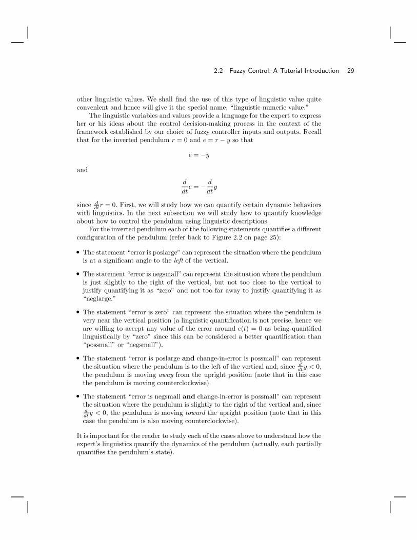
2.2 Fuzzy Control: A Tutorial Introduction 29
other linguistic values. We shall find the use of this type of linguistic value quiteconvenient and hence will give it the special name, “linguistic-numeric value.”
The linguistic variables and values provide a language for the expert to expressher or his ideas about the control decision-making process in the context of theframework established by our choice of fuzzy controller inputs and outputs. Recallthat for the inverted pendulum r = 0 and e = r − y so that
e = −y
and
d
dte = − d
dty
since ddtr = 0. First, we will study how we can quantify certain dynamic behaviors
with linguistics. In the next subsection we will study how to quantify knowledgeabout how to control the pendulum using linguistic descriptions.
For the inverted pendulum each of the following statements quantifies a differentconfiguration of the pendulum (refer back to Figure 2.2 on page 25):
• The statement “error is poslarge” can represent the situation where the pendulumis at a significant angle to the left of the vertical.
• The statement “error is negsmall” can represent the situation where the pendulumis just slightly to the right of the vertical, but not too close to the vertical tojustify quantifying it as “zero” and not too far away to justify quantifying it as“neglarge.”
• The statement “error is zero” can represent the situation where the pendulum isvery near the vertical position (a linguistic quantification is not precise, hence weare willing to accept any value of the error around e(t) = 0 as being quantifiedlinguistically by “zero” since this can be considered a better quantification than“possmall” or “negsmall”).
• The statement “error is poslarge and change-in-error is possmall” can representthe situation where the pendulum is to the left of the vertical and, since d
dty < 0,the pendulum is moving away from the upright position (note that in this casethe pendulum is moving counterclockwise).
• The statement “error is negsmall and change-in-error is possmall” can representthe situation where the pendulum is slightly to the right of the vertical and, sinceddt
y < 0, the pendulum is moving toward the upright position (note that in thiscase the pendulum is also moving counterclockwise).
It is important for the reader to study each of the cases above to understand how theexpert’s linguistics quantify the dynamics of the pendulum (actually, each partiallyquantifies the pendulum’s state).

30 Chapter 2 / Fuzzy Control: The Basics
Overall, we see that to quantify the dynamics of the process we need to have agood understanding of the physics of the underlying process we are trying to control.While for the pendulum problem, the task of coming to a good understanding ofthe dynamics is relatively easy, this is not the case for many physical processes.Quantifying the process dynamics with linguistics is not always easy, and certainlya better understanding of the process dynamics generally leads to a better linguisticquantification. Often, this will naturally lead to a better fuzzy controller providedthat you can adequately measure the system dynamics so that the fuzzy controllercan make the right decisions at the proper time.
Rules
Next, we will use the above linguistic quantification to specify a set of rules (arule-base) that captures the expert’s knowledge about how to control the plant. Inparticular, for the inverted pendulum in the three positions shown in Figure 2.5,we have the following rules (notice that we drop the quotes since the whole rule islinguistic):
1. If error is neglarge and change-in-error is neglarge Then force is poslarge
This rule quantifies the situation in Figure 2.5(a) where the pendulum has alarge positive angle and is moving clockwise; hence it is clear that we shouldapply a strong positive force (to the right) so that we can try to start thependulum moving in the proper direction.
2. If error is zero and change-in-error is possmall Then force is negsmall
This rule quantifies the situation in Figure 2.5(b) where the pendulum hasnearly a zero angle with the vertical (a linguistic quantification of zero does notimply that e(t) = 0 exactly) and is moving counterclockwise; hence we shouldapply a small negative force (to the left) to counteract the movement so that itmoves toward zero (a positive force could result in the pendulum overshootingthe desired position).
3. If error is poslarge and change-in-error is negsmall Then force is negsmall
This rule quantifies the situation in Figure 2.5(c) where the pendulum is far tothe left of the vertical and is moving clockwise; hence we should apply a smallnegative force (to the left) to assist the movement, but not a big one since thependulum is already moving in the proper direction.
Each of the three rules listed above is a “linguistic rule” since it is formedsolely from linguistic variables and values. Since linguistic values are not preciserepresentations of the underlying quantities that they describe, linguistic rules arenot precise either. They are simply abstract ideas about how to achieve good controlthat could mean somewhat different things to different people. They are, however, at

2.2 Fuzzy Control: A Tutorial Introduction 31
u
(a)
u
(b)
u
(c)
FIGURE 2.5 Inverted pendulum in various positions.
a level of abstraction that humans are often comfortable with in terms of specifyinghow to control a process.
The general form of the linguistic rules listed above is
If premise Then consequent
As you can see from the three rules listed above, the premises (which are sometimescalled “antecedents”) are associated with the fuzzy controller inputs and are onthe left-hand-side of the rules. The consequents (sometimes called “actions”) areassociated with the fuzzy controller outputs and are on the right-hand-side of therules. Notice that each premise (or consequent) can be composed of the conjunctionof several “terms” (e.g., in rule 3 above “error is poslarge and change-in-error isnegsmall” is a premise that is the conjunction of two terms). The number of fuzzycontroller inputs and outputs places an upper limit on the number of elementsin the premises and consequents. Note that there does not need to be a premise(consequent) term for each input (output) in each rule, although often there is.
Rule-Bases
Using the above approach, we could continue to write down rules for the pendulumproblem for all possible cases (the reader should do this for practice, at least fora few more rules). Note that since we only specify a finite number of linguisticvariables and linguistic values, there is only a finite number of possible rules. Forthe pendulum problem, with two inputs and five linguistic values for each of these,there are at most 52 = 25 possible rules (all possible combinations of premiselinguistic values for two inputs).
A convenient way to list all possible rules for the case where there are not toomany inputs to the fuzzy controller (less than or equal to two or three) is to use atabular representation. A tabular representation of one possible set of rules for theinverted pendulum is shown in Table 2.1. Notice that the body of the table lists thelinguistic-numeric consequents of the rules, and the left column and top row of thetable contain the linguistic-numeric premise terms. Then, for instance, the (2,−1)position (where the “2” represents the row having “2” for a numeric-linguistic valueand the “−1” represents the column having “−1” for a numeric-linguistic value)has a −1 (“negsmall”) in the body of the table and represents the rule
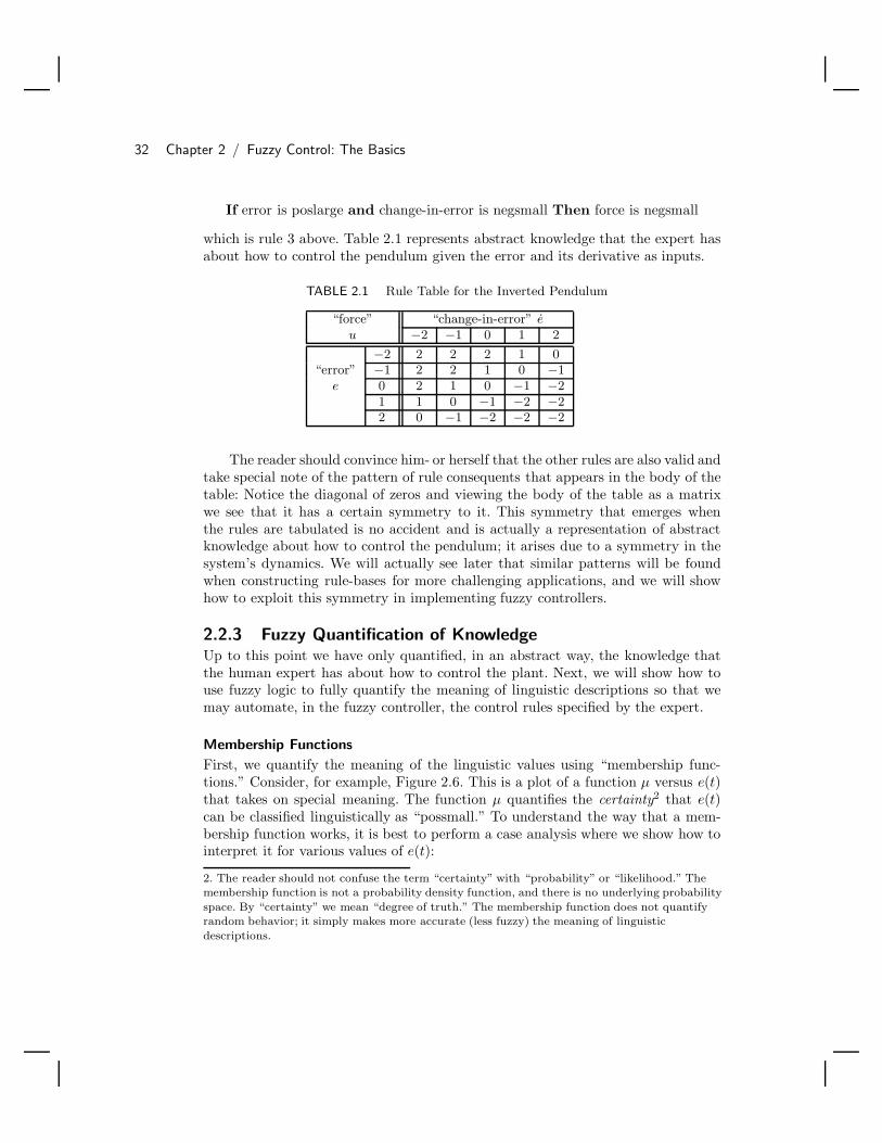
32 Chapter 2 / Fuzzy Control: The Basics
If error is poslarge and change-in-error is negsmall Then force is negsmall
which is rule 3 above. Table 2.1 represents abstract knowledge that the expert hasabout how to control the pendulum given the error and its derivative as inputs.
TABLE 2.1 Rule Table for the Inverted Pendulum
“force” “change-in-error” eu −2 −1 0 1 2
−2 2 2 2 1 0“error” −1 2 2 1 0 −1
e 0 2 1 0 −1 −21 1 0 −1 −2 −22 0 −1 −2 −2 −2
The reader should convince him- or herself that the other rules are also valid andtake special note of the pattern of rule consequents that appears in the body of thetable: Notice the diagonal of zeros and viewing the body of the table as a matrixwe see that it has a certain symmetry to it. This symmetry that emerges whenthe rules are tabulated is no accident and is actually a representation of abstractknowledge about how to control the pendulum; it arises due to a symmetry in thesystem’s dynamics. We will actually see later that similar patterns will be foundwhen constructing rule-bases for more challenging applications, and we will showhow to exploit this symmetry in implementing fuzzy controllers.
2.2.3 Fuzzy Quantification of KnowledgeUp to this point we have only quantified, in an abstract way, the knowledge thatthe human expert has about how to control the plant. Next, we will show how touse fuzzy logic to fully quantify the meaning of linguistic descriptions so that wemay automate, in the fuzzy controller, the control rules specified by the expert.
Membership Functions
First, we quantify the meaning of the linguistic values using “membership func-tions.” Consider, for example, Figure 2.6. This is a plot of a function µ versus e(t)that takes on special meaning. The function µ quantifies the certainty2 that e(t)can be classified linguistically as “possmall.” To understand the way that a mem-bership function works, it is best to perform a case analysis where we show how tointerpret it for various values of e(t):
2. The reader should not confuse the term “certainty” with “probability” or “likelihood.” Themembership function is not a probability density function, and there is no underlying probability
space. By “certainty” we mean “degree of truth.” The membership function does not quantifyrandom behavior; it simply makes more accurate (less fuzzy) the meaning of linguistic
descriptions.
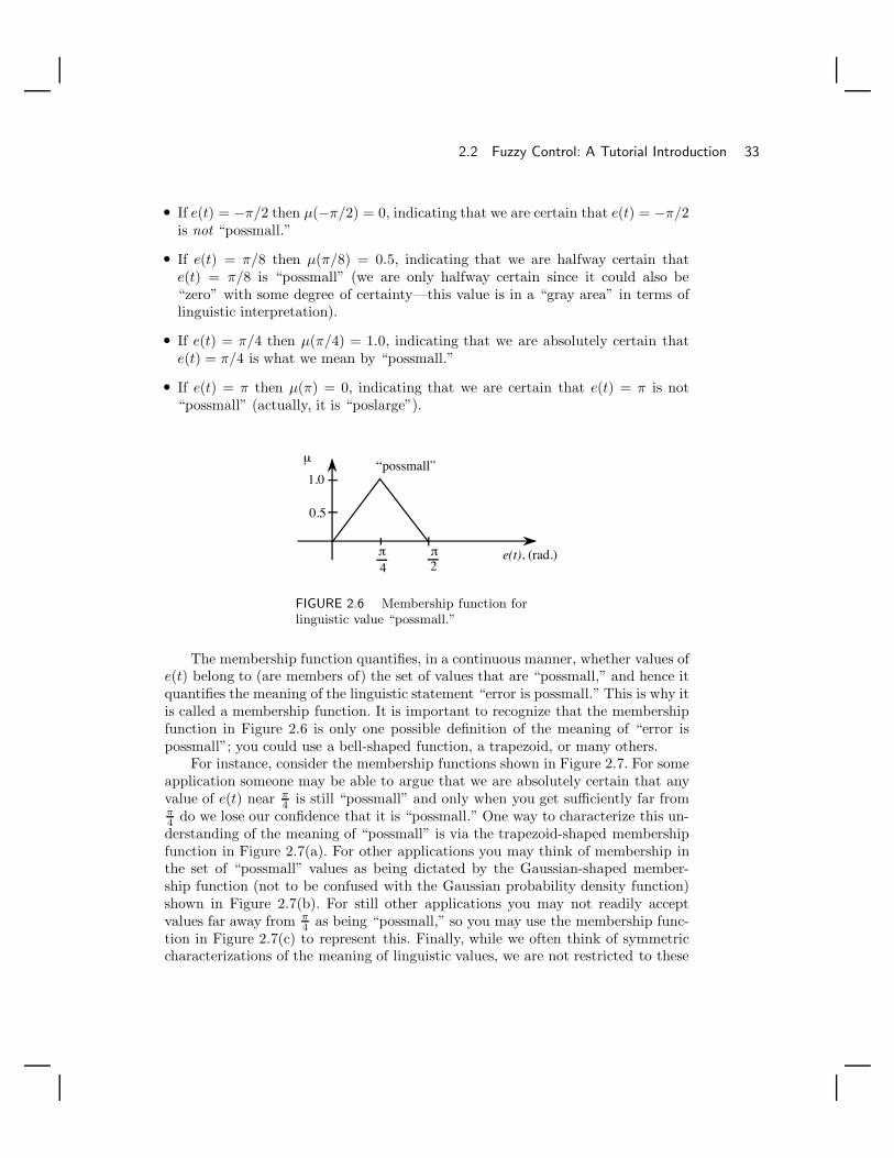
2.2 Fuzzy Control: A Tutorial Introduction 33
• If e(t) = −π/2 then µ(−π/2) = 0, indicating that we are certain that e(t) = −π/2is not “possmall.”
• If e(t) = π/8 then µ(π/8) = 0.5, indicating that we are halfway certain thate(t) = π/8 is “possmall” (we are only halfway certain since it could also be“zero” with some degree of certainty—this value is in a “gray area” in terms oflinguistic interpretation).
• If e(t) = π/4 then µ(π/4) = 1.0, indicating that we are absolutely certain thate(t) = π/4 is what we mean by “possmall.”
• If e(t) = π then µ(π) = 0, indicating that we are certain that e(t) = π is not“possmall” (actually, it is “poslarge”).
1.0
0.5
µ
e(t), (rad.)
“possmall”
π4
π2
FIGURE 2.6 Membership function forlinguistic value “possmall.”
The membership function quantifies, in a continuous manner, whether values ofe(t) belong to (are members of) the set of values that are “possmall,” and hence itquantifies the meaning of the linguistic statement “error is possmall.” This is why itis called a membership function. It is important to recognize that the membershipfunction in Figure 2.6 is only one possible definition of the meaning of “error ispossmall”; you could use a bell-shaped function, a trapezoid, or many others.
For instance, consider the membership functions shown in Figure 2.7. For someapplication someone may be able to argue that we are absolutely certain that anyvalue of e(t) near π
4 is still “possmall” and only when you get sufficiently far fromπ4 do we lose our confidence that it is “possmall.” One way to characterize this un-derstanding of the meaning of “possmall” is via the trapezoid-shaped membershipfunction in Figure 2.7(a). For other applications you may think of membership inthe set of “possmall” values as being dictated by the Gaussian-shaped member-ship function (not to be confused with the Gaussian probability density function)shown in Figure 2.7(b). For still other applications you may not readily acceptvalues far away from π
4 as being “possmall,” so you may use the membership func-tion in Figure 2.7(c) to represent this. Finally, while we often think of symmetriccharacterizations of the meaning of linguistic values, we are not restricted to these
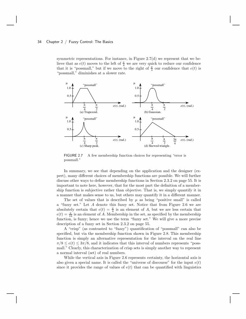
34 Chapter 2 / Fuzzy Control: The Basics
symmetric representations. For instance, in Figure 2.7(d) we represent that we be-lieve that as e(t) moves to the left of π
4 we are very quick to reduce our confidencethat it is “possmall,” but if we move to the right of π
4 our confidence that e(t) is“possmall,” diminishes at a slower rate.
1.0
0.5
µ
e(t), (rad.)
“possmall”
π4
π2
1.0
0.5
µ
e(t), (rad.)
“possmall”
π4
π
2
1.0
0.5
µ
e(t), (rad.)
“possmall”
π4
π2
1.0
0.5
µ
e(t), (rad.)
“possmall”
π4
π2
(a) Trapezoid. (b) Gaussian.
(c) Sharp peak. (d) Skewed triangle.
π4
3
FIGURE 2.7 A few membership function choices for representing “error ispossmall.”
In summary, we see that depending on the application and the designer (ex-pert), many different choices of membership functions are possible. We will furtherdiscuss other ways to define membership functions in Section 2.3.2 on page 55. It isimportant to note here, however, that for the most part the definition of a member-ship function is subjective rather than objective. That is, we simply quantify it ina manner that makes sense to us, but others may quantify it in a different manner.
The set of values that is described by µ as being “positive small” is calleda “fuzzy set.” Let A denote this fuzzy set. Notice that from Figure 2.6 we areabsolutely certain that e(t) = π
4 is an element of A, but we are less certain thate(t) = π
16is an element of A. Membership in the set, as specified by the membership
function, is fuzzy; hence we use the term “fuzzy set.” We will give a more precisedescription of a fuzzy set in Section 2.3.2 on page 55.
A “crisp” (as contrasted to “fuzzy”) quantification of “possmall” can also bespecified, but via the membership function shown in Figure 2.8. This membershipfunction is simply an alternative representation for the interval on the real lineπ/8 ≤ e(t) ≤ 3π/8, and it indicates that this interval of numbers represents “poss-mall.” Clearly, this characterization of crisp sets is simply another way to representa normal interval (set) of real numbers.
While the vertical axis in Figure 2.6 represents certainty, the horizontal axis isalso given a special name. It is called the “universe of discourse” for the input e(t)since it provides the range of values of e(t) that can be quantified with linguistics

2.2 Fuzzy Control: A Tutorial Introduction 35
1.0
0.5
µ
e(t), (rad.)π4
π2
FIGURE 2.8 Membership function for acrisp set.
and fuzzy sets. In conventional terminology, a universe of discourse for an input oroutput of a fuzzy system is simply the range of values the inputs and outputs cantake on.
Now that we know how to specify the meaning of a linguistic value via a mem-bership function (and hence a fuzzy set), we can easily specify the membershipfunctions for all 15 linguistic values (five for each input and five for the output)of our inverted pendulum example. See Figure 2.9 for one choice of membershipfunctions.
Notice that (for our later convenience) we list both the linguistic values andthe linguistic-numeric values associated with each membership function. Hence,we see that the membership function in Figure 2.6 for “possmall” is embeddedamong several others that describe other sizes of values (so that, for instance, themembership function to the right of the one for “possmall” is the one that represents“error is poslarge”). Note that other similarly shaped membership functions makesense (e.g., bell-shaped membership functions). We will discuss the multitude ofchoices that are possible for membership functions in Section 2.3.2 on page 55.
The membership functions at the outer edges in Figure 2.9 deserve specialattention. For the inputs e(t) and d
dte(t) we see that the outermost membershipfunctions “saturate” at a value of one. This makes intuitive sense as at some pointthe human expert would just group all large values together in a linguistic de-scription such as “poslarge.” The membership functions at the outermost edgesappropriately characterize this phenomenon since they characterize “greater than”(for the right side) and “less than” (for the left side). Study Figure 2.9 and convinceyourself of this.
For the output u, the membership functions at the outermost edges cannot besaturated for the fuzzy system to be properly defined (more details on this pointwill be provided in Section 2.2.6 on page 44 and Section 2.3.5 on page 65). The basicreason for this is that in decision-making processes of the type we study, we seek totake actions that specify an exact value for the process input. We do not generallyindicate to a process actuator, “any value bigger than, say, 10, is acceptable.”
It is important to have a clear picture in your mind of how the values of themembership functions change as, for example, e(t) changes its value over time.For instance, as e(t) changes from −π/2 to π/2 we see that various membership

36 Chapter 2 / Fuzzy Control: The Basics
e(t), (rad.)
“possmall”
π4
π2
π2
π4
“zero”“negsmall”“neglarge”-1-2 0 1 2
“poslarge”
e(t), (rad/sec)
“possmall”
4ππ π
4
“zero”“negsmall”“neglarge”-1-2 0 1 2
“poslarge”
8π8 dt
dπ16
u(t), (N)
“possmall”
30-20
“zero”“negsmall”“neglarge”
-1-2 0 1 2“poslarge”
-10 2010-30
FIGURE 2.9 Membership functions for an inverted pendulum ona cart.
functions will take on zero and nonzero values indicating the degree to which thelinguistic value appropriately describes the current value of e(t). For example, ate(t) = −π/2 we are certain that the error is “neglarge,” and as the value of e(t)moves toward −π/4 we become less certain that it is “neglarge” and more certainthat it is “negsmall.” We see that the membership functions quantify the meaningof linguistic statements that describe time-varying signals.
Finally, note that often we will draw all the membership functions for one inputor output variable on one graph; hence, we often omit the label for the verticalaxis with the understanding that the plotted functions are membership functionsdescribing the meaning of their associated linguistic values. Also, we will use thenotation µzero to represent the membership function associated with the linguisticvalue “zero” and a similar notation for the others.
The rule-base of the fuzzy controller holds the linguistic variables, linguisticvalues, their associated membership functions, and the set of all linguistic rules(shown in Table 2.1 on page 32), so we have completed the description of thesimple inverted pendulum. Next we describe the fuzzification process.

2.2 Fuzzy Control: A Tutorial Introduction 37
Fuzzification
It is actually the case that for most fuzzy controllers the fuzzification block inFigure 2.1 on page 25 can be ignored since this process is so simple. In Section 2.3.3on page 61 we will explain the exact operations of the fuzzification process and alsoexplain why it can be simplified and under certain conditions virtually ignored.For now, the reader should simply think of the fuzzification process as the act ofobtaining a value of an input variable (e.g., e(t)) and finding the numeric valuesof the membership function(s) that are defined for that variable. For example, ife(t) = π/4 and d
dte(t) = π/16, the fuzzification process amounts to finding thevalues of the input membership functions for these. In this case
µpossmall(e(t)) = 1
(with all others zero) and
µzero
(d
dte(t)
)= µpossmall
(d
dte(t)
)= 0.5.
Some think of the membership function values as an “encoding” of the fuzzy con-troller numeric input values. The encoded information is then used in the fuzzyinference process that starts with “matching.”
2.2.4 Matching: Determining Which Rules to UseNext, we seek to explain how the inference mechanism in Figure 2.1 on page 25operates. The inference process generally involves two steps:
1. The premises of all the rules are compared to the controller inputs to determinewhich rules apply to the current situation. This “matching” process involvesdetermining the certainty that each rule applies, and typically we will morestrongly take into account the recommendations of rules that we are morecertain apply to the current situation.
2. The conclusions (what control actions to take) are determined using the rulesthat have been determined to apply at the current time. The conclusions arecharacterized with a fuzzy set (or sets) that represents the certainty that theinput to the plant should take on various values.
We will cover step 1 in this subsection and step 2 in the next.
Premise Quantification via Fuzzy Logic
To perform inference we must first quantify each of the rules with fuzzy logic. To dothis we first quantify the meaning of the premises of the rules that are composed ofseveral terms, each of which involves a fuzzy controller input. Consider Figure 2.10,where we list two terms from the premise of the rule
If error is zero and change-in-error is possmall Then force is negsmall

38 Chapter 2 / Fuzzy Control: The Basics
Above, we had quantified the meaning of the linguistic terms “error is zero” and“change-in-error is possmall” via the membership functions shown in Figure 2.9.Now we seek to quantify the linguistic premise “error is zero and change-in-erroris possmall.” Hence, the main item to focus on is how to quantify the logical “and”operation that combines the meaning of two linguistic terms. While we could usestandard Boolean logic to combine these linguistic terms, since we have quantifiedthem more precisely with fuzzy sets (i.e., the membership functions), we can usethese.
e(t), (rad.)π4
π4
“zero”0
zeroµ
e(t), (rad/sec)
“possmall”
4π
1
π8 dt
d
possmallµ
quantified with quantified with
and“error is zero change-in-error is possmall”
1
0.5
π16
FIGURE 2.10 Membership functions of premise terms.
To see how to quantify the “and” operation, begin by supposing that e(t) = π/8and d
dte(t) = π/32, so that using Figure 2.9 (or Figure 2.10) we see that
µzero(e(t)) = 0.5
and
µpossmall
(d
dte(t)
)= 0.25
What, for these values of e(t) and ddte(t), is the certainty of the statement
“error is zero and change-in-error is possmall”
that is the premise from the above rule? We will denote this certainty by µpremise.There are actually several ways to define it:
• Minimum: Define µpremise = min0.5, 0.25 = 0.25, that is, using the minimumof the two membership values.
• Product: Define µpremise = (0.5)(0.25) = 0.125, that is, using the product of thetwo membership values.
Do these quantifications make sense? Notice that both ways of quantifying the“and” operation in the premise indicate that you can be no more certain about

2.2 Fuzzy Control: A Tutorial Introduction 39
the conjunction of two statements than you are about the individual terms thatmake them up (note that 0 ≤ µpremise ≤ 1 for either case). If we are not very cer-tain about the truth of one statement, how can we be any more certain about thetruth of that statement “and” the other statement? It is important that you con-vince yourself that the above quantifications make sense. To do so, we recommendthat you consider other examples of “anding” linguistic terms that have associatedmembership functions.
While we have simply shown how to quantify the “and” operation for one valueof e(t) and d
dte(t), if we consider all possible e(t) and ddte(t) values, we will obtain a
multidimensional membership function µpremise
(e(t), d
dte(t))
that is a function ofe(t) and d
dte(t) for each rule. For our example, if we choose the minimum operationto represent the “and” in the premise, then we get the multidimensional membershipfunction µpremise
(e(t), d
dte(t)
)shown in Figure 2.11. Notice that if we pick values for
e(t) and ddte(t), the value of the premise certainty µpremise
(e(t), d
dte(t))
representshow certain we are that the rule
If error is zero and change-in-error is possmall Then force is negsmall
is applicable for specifying the force input to the plant. As e(t) and ddt
e(t) change,the value of µpremise
(e(t), d
dte(t)
)changes according to Figure 2.11, and we become
less or more certain of the applicability of this rule.
e(t), (rad)4π
e(t), (rad/sec)dtd
4π
π4
π4
premiseµ
8π 16
π
FIGURE 2.11 Membership function of the premise for asingle rule.
In general we will have a different premise membership function for each of therules in the rule-base, and each of these will be a function of e(t) and d
dte(t) so that
given specific values of e(t) and ddt
e(t) we obtain a quantification of the certainty

40 Chapter 2 / Fuzzy Control: The Basics
that each rule in the rule-base applies to the current situation. It is important youpicture in your mind the situation where e(t) and d
dte(t) change dynamically overtime. When this occurs the values of µpremise
(e(t), d
dte(t))
for each rule change,and hence the applicability of each rule in the rule-base for specifying the forceinput to the pendulum, changes with time.
Determining Which Rules Are On
Determining the applicability of each rule is called “matching.” We say that a ruleis “on at time t” if its premise membership function µpremise(e(t), d
dte(t)) > 0.
Hence, the inference mechanism seeks to determine which rules are on to find outwhich rules are relevant to the current situation. In the next step, the inferencemechanism will seek to combine the recommendations of all the rules to come upwith a single conclusion.
Consider, for the inverted pendulum example, how we compute the rules thatare on. Suppose that
e(t) = 0
and
d
dte(t) = π/8 − π/32 (= 0.294)
Figure 2.12 shows the membership functions for the inputs and indicates with thickblack vertical lines the values above for e(t) and d
dte(t). Notice that µzero(e(t)) =
1 but that the other membership functions for the e(t) input are all “off” (i.e.,their values are zero). For the d
dte(t) input we see that µzero
(ddte(t)
)= 0.25 and
µpossmall
(ddte(t)
)= 0.75 and that all the other membership functions are off. This
implies that rules that have the premise terms
“error is zero”“change-in-error is zero”
“change-in-error is possmall”
are on (all other rules have µpremise
(e(t), d
dte(t)
)= 0. So, which rules are these?
Using Table 2.1 on page 32, we find that the rules that are on are the following:
1. If error is zero and change-in-error is zero Then force is zero
2. If error is zero and change-in-error is possmall Then force is negsmall
Note that since for the pendulum example we have at most two membership func-tions overlapping, we will never have more than four rules on at one time (thisconcept generalizes to many inputs and will be discussed in more detail in Sec-tions 2.3 and 2.6). Actually, for this system we will either have one, two, or fourrules on at any one time. To get only one rule on choose, for example, e(t) = 0and d
dte(t) = π8 so that only rule 2 above is on. What values would you choose for
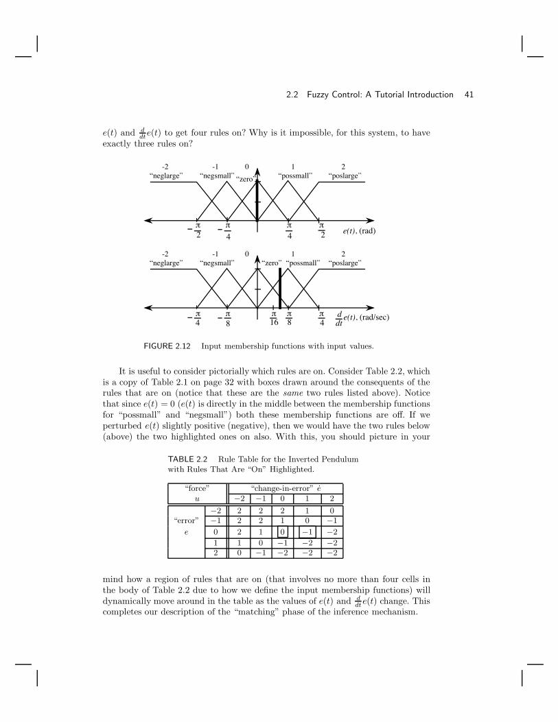
2.2 Fuzzy Control: A Tutorial Introduction 41
e(t) and ddte(t) to get four rules on? Why is it impossible, for this system, to have
exactly three rules on?
e(t), (rad)
“possmall”
π4
π2
π2
π4
“zero”“negsmall”“neglarge”-1-2 0 1 2
“poslarge”
e(t), (rad/sec)
“possmall”“zero”“negsmall”“neglarge”-1-2 0 1 2
“poslarge”
dtd
4ππ π
4 8π8
π16
FIGURE 2.12 Input membership functions with input values.
It is useful to consider pictorially which rules are on. Consider Table 2.2, whichis a copy of Table 2.1 on page 32 with boxes drawn around the consequents of therules that are on (notice that these are the same two rules listed above). Noticethat since e(t) = 0 (e(t) is directly in the middle between the membership functionsfor “possmall” and “negsmall”) both these membership functions are off. If weperturbed e(t) slightly positive (negative), then we would have the two rules below(above) the two highlighted ones on also. With this, you should picture in your
TABLE 2.2 Rule Table for the Inverted Pendulumwith Rules That Are “On” Highlighted.
“force” “change-in-error” eu −2 −1 0 1 2
−2 2 2 2 1 0“error” −1 2 2 1 0 −1
e 0 2 1 0 −1 −2
1 1 0 −1 −2 −22 0 −1 −2 −2 −2
mind how a region of rules that are on (that involves no more than four cells inthe body of Table 2.2 due to how we define the input membership functions) willdynamically move around in the table as the values of e(t) and d
dte(t) change. Thiscompletes our description of the “matching” phase of the inference mechanism.

42 Chapter 2 / Fuzzy Control: The Basics
2.2.5 Inference Step: Determining ConclusionsNext, we consider how to determine which conclusions should be reached whenthe rules that are on are applied to deciding what the force input to the cartcarrying the inverted pendulum should be. To do this, we will first consider therecommendations of each rule independently. Then later we will combine all therecommendations from all the rules to determine the force input to the cart.
Recommendation from One Rule
Consider the conclusion reached by the rule
If error is zero and change-in-error is zero Then force is zero
which for convenience we will refer to as “rule (1).” Using the minimum to representthe premise, we have
µpremise(1) = min0.25, 1 = 0.25
(the notation µpremise(1) represents µpremise for rule (1)) so that we are 0.25 certainthat this rule applies to the current situation. The rule indicates that if its premiseis true then the action indicated by its consequent should be taken. For rule (1) theconsequent is “force is zero” (this makes sense, for here the pendulum is balanced,so we should not apply any force since this would tend to move the pendulumaway from the vertical). The membership function for this consequent is shown inFigure 2.13(a). The membership function for the conclusion reached by rule (1),which we denote by µ(1), is shown in Figure 2.13(b) and is given by
µ(1)(u) = min0.25, µzero(u)
This membership function defines the “implied fuzzy set”3 for rule (1) (i.e., it is theconclusion that is implied by rule (1)). The justification for the use of the minimumoperator to represent the implication is that we can be no more certain about ourconsequent than our premise. You should convince yourself that we could use theproduct operation to represent the implication also (in Section 2.2.6 we will do anexample where we use the product).
Notice that the membership function µ(1)(u) is a function of u and that theminimum operation will generally “chop off the top” of the µzero(u) membershipfunction to produce µ(1)(u). For different values of e(t) and d
dte(t) there will bedifferent values of the premise certainty µpremise(1)
(e(t), d
dte(t)
)for rule (1) and
hence different functions µ(1)(u) obtained (i.e., it will chop off the top at differentpoints).
3. This term has been used in the literature for a long time; however, there is no standard
terminology for this fuzzy set. Others have called it, for example, a “consequent fuzzy set” or an“output fuzzy set” (which can be confused with the fuzzy sets that quantify the consequents of
the rules). We use “implied fuzzy set” so that there is no ambiguity and to help to distinguish itfrom the “overall implied fuzzy set” that is introduced in Section 2.3.

2.2 Fuzzy Control: A Tutorial Introduction 43
We see that µ(1)(u) is in general a time-varying function that quantifies howcertain rule (1) is that the force input u should take on certain values. It is mostcertain that the force input should lie in a region around zero (see Figure 2.13(b)),and it indicates that it is certain that the force input should not be too large in eitherthe positive or negative direction—this makes sense if you consider the linguisticmeaning of the rule. The membership function µ(1)(u) quantifies the conclusionreached by only rule (1) and only for the current e(t) and d
dte(t). It is importantthat the reader be able to picture how the shape of the implied fuzzy set changesas the rule’s premise certainty changes over time.
u(t), (N)
“zero”0
-10 10
(a)
u(t), (N)
“zero”0
-10 10
(b)
0.25
FIGURE 2.13 (a) Consequent membership function and (b)implied fuzzy set with membership function µ(1)(u) for rule (1).Recall that the units for u(t) are Newtons (N).
Recommendation from Another Rule
Next, consider the conclusion reached by the other rule that is on,
If error is zero and change-in-error is possmall Then force is negsmall
which for convenience we will refer to as “rule (2).” Using the minimum to representthe premise, we have
µpremise(2) = min0.75, 1 = 0.75
so that we are 0.75 certain that this rule applies to the current situation. Noticethat we are much more certain that rule (2) applies to the current situation thanrule (1). For rule (2) the consequent is “force is negsmall” (this makes sense, for herethe pendulum is perfectly balanced but is moving in the counterclockwise directionwith a small velocity). The membership function for this consequent is shown inFigure 2.14(a). The membership function for the conclusion reached by rule (2),which we denote by µ(2), is shown in Figure 2.14(b) (the shaded region) and isgiven by
µ(2)(u) = min0.75, µnegsmall(u)
This membership function defines the implied fuzzy set for rule (2) (i.e., it is theconclusion that is reached by rule (2)). Once again, for different values of e(t)

44 Chapter 2 / Fuzzy Control: The Basics
and ddte(t) there will be different values of µpremise(2)
(e(t), d
dte(t))
for rule (2) andhence different functions µ(2)(u) obtained. The reader should carefully consider themeaning of the implied fuzzy set µ(2)(u). Rule (2) is quite certain that the controloutput (process input) should be a small negative value. This makes sense since ifthe pendulum has some counterclockwise velocity then we would want to apply anegative force (i.e., one to the left). As rule (2) has a premise membership functionthat has higher certainty than for rule (1), we see that we are more certain of theconclusion reached by rule (2).
u(t), (N)-20
“negsmall”-1
-10
(a)
u(t), (N)
-20
“negsmall”-1
-10
(b)
0.75
FIGURE 2.14 (a) Consequent membership function and (b)implied fuzzy set with membership function µ(2)(u) for rule (2).
This completes the operations of the inference mechanism in Figure 2.1 onpage 25. While the input to the inference process is the set of rules that are on, itsoutput is the set of implied fuzzy sets that represent the conclusions reached by allthe rules that are on. For our example, there are at most four conclusions reachedsince there are at most four rules on at any one time. (In fact, you could say thatthere are always four conclusions reached for our example, but that the impliedfuzzy sets for some of the rules may have implied membership functions that arezero for all values.)
2.2.6 Converting Decisions into ActionsNext, we consider the defuzzification operation, which is the final component ofthe fuzzy controller shown in Figure 2.1 on page 25. Defuzzification operates onthe implied fuzzy sets produced by the inference mechanism and combines theireffects to provide the “most certain” controller output (plant input). Some think ofdefuzzification as “decoding” the fuzzy set information produced by the inferenceprocess (i.e., the implied fuzzy sets) into numeric fuzzy controller outputs.
To understand defuzzification, it is best to first draw all the implied fuzzy setson one axis as shown in Figure 2.15. We want to find the one output, which wedenote by “ucrisp,” that best represents the conclusions of the fuzzy controller thatare represented with the implied fuzzy sets. There are actually many approachesto defuzzification. We will consider two here and several others in Section 2.3.5 onpage 65.

2.2 Fuzzy Control: A Tutorial Introduction 45
u(t), (N)30
-20
“zero”“negsmall”-1
0
-10 2010
-30
FIGURE 2.15 Implied fuzzy sets.
Combining Recommendations
Due to its popularity, we will first consider the “center of gravity” (COG) defuzzi-fication method for combining the recommendations represented by the impliedfuzzy sets from all the rules. Let bi denote the center of the membership function(i.e., where it reaches its peak for our example) of the consequent of rule (i). Forour example we have
b1 = 0.0
and
b2 = −10
as shown in Figure 2.15. Let ∫µ(i)
denote the area under the membership function µ(i). The COG method computesucrisp to be
ucrisp =∑
i bi
∫µ(i)∑
i
∫µ(i)
(2.1)
This is the classical formula for computing the center of gravity. In this case it isfor computing the center of gravity of the implied fuzzy sets. Three items aboutEquation (2.1) are important to note:
1. Practically, we cannot have output membership functions that have infinitearea since even though they may be “chopped off” in the minimum operationfor the implication (or scaled for the product operation) they can still end upwith infinite area. This is the reason we do not allow infinite area membershipfunctions for the linguistic values for the controller output (e.g., we did notallow the saturated membership functions at the outermost edges as we hadfor the inputs shown in Figure 2.9 on page 36).

46 Chapter 2 / Fuzzy Control: The Basics
2. You must be careful to define the input and output membership functions sothat the sum in the denominator of Equation (2.1) is not equal to zero nomatter what the inputs to the fuzzy controller are. Essentially, this means thatwe must have some sort of conclusion for all possible control situations we mayencounter.
3. While at first glance it may not appear so,∫
µ(i) is easy to compute for ourexample. For the case where we have symmetric triangular output membershipfunctions that peak at one and have a base width of w, simple geometry canbe used to show that the area under a triangle “chopped off” at a height of h(such as the ones in Figures 2.13 and 2.14) is equal to
w
(h − h2
2
)
Given this, the computations needed to compute ucrisp are not too significant.
We see that the property of membership functions being symmetric for theoutput is important since in this case no matter whether the minimum or productis used to represent the implication, it will be the case that the center of the impliedfuzzy set will be the same as the center of the consequent fuzzy set from which itis computed. If the output membership functions are not symmetric, then theircenters, which are needed in the computation of the COG, will change dependingon the membership value of the premise. This will result in the need to recomputethe center at each time instant.
Using Equation (2.1) with Figure 2.15 we have
ucrisp =(0)(4.375) + (−10)(9.375)
4.375 + 9.375= −6.81
as the input to the pendulum for the given e(t) and ddte(t).
Does this value for a force input (i.e., 6.81 Newtons to the left) make sense?Consider Figure 2.16, where we have taken the implied fuzzy sets from Figure 2.15and simply added an indication of what number COG defuzzification says is thebest representation of the conclusions reached by the rules that are on. Notice thatthe value of ucrisp is roughly in the middle of where the implied fuzzy sets say theyare most certain about the value for the force input. In fact, recall that we had
e(t) = 0
and
d
dte(t) = π/8 − π/32 (= 0.294)
so the pendulum is in the inverted position but is moving counterclockwise with asmall velocity; hence it makes sense to pull on the cart, and the fuzzy controller

2.2 Fuzzy Control: A Tutorial Introduction 47
does this.
u(t), (N)30
-20
“zero”“negsmall”
-10
-10 2010-30
ucrisp = -6.81
FIGURE 2.16 Implied fuzzy sets.
It is interesting to note that for our example it will be the case that
−20 ≤ ucrisp ≤ 20
To see this, consider Figure 2.17, where we have drawn the output membershipfunctions. Notice that even though we have extended the membership functions atthe outermost edges past −20 and +20 (see the shaded regions), the COG methodwill never compute a value outside this range.
u(t), (N)
“possmall”
30-20
“zero”“negsmall”“neglarge”-1-2 0 1 2
“poslarge”
-10 2010-30
FIGURE 2.17 Output membership functions.
The reason for this comes directly from the definition of the COG method inEquation (2.1). The center of gravity for these shapes simply cannot extend beyond−20 and +20. Practically speaking, this ability to limit the range of inputs to theplant is useful; it may be the case that applying a force of greater than 20 Newtonsis impossible for this plant. Thus we see that in defining the membership functionsfor the fuzzy controller, we must take into account what method is going to be usedfor defuzzification.

48 Chapter 2 / Fuzzy Control: The Basics
Other Ways to Compute and Combine Recommendations
As another example, it is interesting to consider how to compute, by hand, theoperations that the fuzzy controller takes when we use the product to represent theimplication or the “center-average” defuzzification method.
First, consider the use of the product. Consider Figure 2.18, where we havedrawn the output membership functions for “negsmall” and “zero” as dotted lines.The implied fuzzy set from rule (1) is given by the membership function
µ(1)(u) = 0.25µzero(u)
shown in Figure 2.18 as the shaded triangle; and the implied fuzzy set for rule (2)is given by the membership function
µ(2)(u) = 0.75µnegsmall(u)
shown in Figure 2.18 as the dark triangle. Notice that computation of the COG iseasy since we can use 1
2wh as the area for a triangle with base width w and heighth. When we use product to represent the implication, we obtain
ucrisp =(0)(2.5) + (−10)(7.5)
2.5 + 7.5= −7.5
which also makes sense.
u(t), (N)30
-20
“zero”“negsmall”-1 0
-10 2010-30
0.25
0.75
FIGURE 2.18 Implied fuzzy sets when the product is used torepresent the implication.
Next, as another example of how to combine recommendations, we will intro-duce the “center-average” method for defuzzification. For this method we let
ucrisp =
∑i biµpremise(i)∑i µpremise(i)
(2.2)
where to compute µpremise(i) we use, for example, minimum. We call it the “center-average” method since Equation (2.2) is a weighted average of the center valuesof the output membership function centers. Basically, the center-average methodreplaces the areas of the implied fuzzy sets that are used in COG with the valuesof µpremise(i) . This is a valid replacement since the area of the implied fuzzy set

2.2 Fuzzy Control: A Tutorial Introduction 49
is generally proportional to µpremise(i) since µpremise(i) is used to chop the top off(minimum) or scale (product) the triangular output membership function whenCOG is used for our example. For the above example, we have
ucrisp =(0)(0.25) + (−10)(0.75)
0.25 + 0.75= −7.5
which just happens to be the same value as above. Some like the center-averagedefuzzification method because the computations needed are simpler than for COGand because the output membership functions are easy to store since the onlyrelevant information they provide is their center values (bi) (i.e., their shape doesnot matter, just their center value).
Notice that while both values computed for the different inference and defuzzi-fication methods provide reasonable command inputs to the plant, it is difficult tosay which is best without further investigations (e.g., simulations or implementa-tion). This ambiguity about how to define the fuzzy controller actually extends tothe general case and also arises in the specification of all the other fuzzy controllercomponents, as we discuss below. Some would call this “ambiguity” a design flexibil-ity, but unfortunately there are not too many guidelines on how best to choose theinference strategy and defuzzification method, so such flexibility is of questionablevalue.
2.2.7 Graphical Depiction of Fuzzy Decision MakingFor convenience, we summarize the procedure that the fuzzy controller uses to com-pute its outputs given its inputs in Figure 2.19. Here, we use the minimum operatorto represent the “and” in the premise and the implication and COG defuzzification.The reader is advised to study each step in this diagram to gain a fuller understand-ing of the operation of the fuzzy controller. To do this, develop a similar diagram forthe case where the product operator is used to represent the “and” in the premiseand the implication, and choose values of e(t) and d
dte(t) that will result in four rulesbeing on. Then, repeat the process when center-average defuzzification is used witheither minimum or product used for the premise. Also, learn how to picture in yourmind how the parameters of this graphical representation of the fuzzy controlleroperations change as the fuzzy controller inputs change.
This completes the description of the operation of a simple fuzzy controller.You will find that while we will treat the fully general fuzzy controller in the nextsection, there will be little that is conceptually different from this simple example.We simply show how to handle the case where there are more inputs and outputsand show a fuller range of choices that you can make for the various componentsof the fuzzy controller.
As evidenced by the different values obtained by using the minimum, product,and defuzzification operations, there are many ways to choose the parameters ofthe fuzzy controller that make sense. This presents a problem since it is almostalways difficult to know how to first design a fuzzy controller. Basically, the choiceof all the components for the fuzzy controller is somewhat ad hoc. What are the

50 Chapter 2 / Fuzzy Control: The Basics
u(t), (N)
“zero”
-10 10
0.25
u(t), (N)
-20
“negsmall”
-10
0.75
u(t), (N)
-20
“zero”“negsmall”
-10 10
ucrisp = - 6.81
If error is zero and change-in-error is zero Then force is zero
e(t)π4
π4
“zero”
e(t)π4
π4
“zero”
π
“zero”
8π8 e(t)dt
dπ16
“possmall”
π8
e(t)dtdπ
16π4
If error is zero and change-in-error is possmall Then force is negsmall
FIGURE 2.19 Graphical representation of fuzzy controller operations.
best membership functions? How many linguistic values and rules should there be?Should the minimum or product be used to represent the “and” in the premise—andwhich should be used to represent the implication? What defuzzification methodshould be chosen? These are all questions that must be addressed if you want todesign a fuzzy controller.
We will show how to answer some of these questions by going through a designprocedure for the inverted pendulum in Section 2.4 on page 77. After this, we willdiscuss how to write a computer program to simulate a fuzzy control system andhow to do a real-time implementation of the fuzzy controller. Ultimately, however,the answers to the above questions are best found by studying how to design fuzzycontrollers for a wide range of applications that present more challenging charac-teristics than the inverted pendulum. This is what we do in the case studies inChapter 3.
2.2.8 Visualizing the Fuzzy Controller’s Dynamical OperationThe figure on the cover of the book can serve as a nice visual depiction of how a fuzzysystem operates dynamically over time. The figure represents a fuzzy system withtwo inputs, for example, e, and e, and one output. There are triangular membership

2.3 General Fuzzy Systems 51
functions on the two input universes of discourse, and minimum is used to representthe conjunction in the premise. The blue pyramids represent the premise certaintiesof the rules in a rule-base with 49 rules. Note that for simplicity of the graphic,the outermost membership functions do not saturate in this fuzzy controller; henceif e or e goes outside the range it appears that there will be no rules on, so thedefuzzification will fail. Actually, the pyramids should be viewed as part of a rule-base with many more rules, and only the central ones for the rule-base are shownfor simplicity.
The shading from blue, to red, to yellow, on the pyramids indicates progressionin time of rules that were (are) on (i.e., the pyramids describing their premises hadnonzero certainties) and the two in the middle that are fully shaded in yellow arethe two rules that are on now. The pyramids with some blue on them, and somered, are ones that were on some time ago. The ones with red, and some yellow, wereon more recently, while the ones that have a little less red shading and more yellowwere on even more recently. The pyramids that are entirely blue, either were neverturned on, or they were on a long time ago. Hence, the path of color (blue to redto yellow) could have traveled all over a large landscape of blue pyramids. At thistime the path has come very near the e = 0, e = 0 location in the rule-base andthis is normally where you want it to be (for a tracking problem where e = r − ywhere r is the reference input and y is the plant output we want e = 0 if y is totrack r).
The colored vertical beam holds the four numbers that are the premise cer-tainties for the four rules that are on now. Note that two of the rules that are on,are on with a certainty of zero, so really they are off and this is why they go tothe output universe of discourse (top horizontal axis) at the zero level of certainty(see the top figure with the tan-colored output membership functions). The coloredvertical beam contains only green and orange since these represent the values ofthe premise certainties from the two rules that are on. The beam does not haveany purple or pink in it as these colors represent the zero values of the premises ofthe two rules that are off (we have constructed the rule-base so that there are atmost four rules on at any time). The green and orange values chop the tops off twotriangular output membership functions that then become the implied fuzzy sets(i.e., we use minimum to represent the implication). The defuzzified value is shownas the arrow at the top (it looks like a COG defuzzification).
2.3 General Fuzzy SystemsIn the previous section we provided an intuitive overview of fuzzy control via asimple example. In this section we will take a step back and examine the moregeneral fuzzy system to show the range of possibilities that can be used in defininga fuzzy system and to solidify your understanding of fuzzy systems.4 In particular,
4. Note that we limit our range of definition of the general fuzzy system (controller) to those
that have found some degree of use in practical control applications. The reader interested instudying the more general mathematics of fuzzy sets, fuzzy logic, and fuzzy systems should
consult [95, 250].

52 Chapter 2 / Fuzzy Control: The Basics
we will consider the case where there are many fuzzy controller inputs and outputsand where there are more general membership functions, fuzzification procedures,inference strategies, and defuzzification methods. Moreover, we introduce a classof “functional fuzzy systems” that have been found to be useful in some applica-tions and characterize the general capabilities of fuzzy systems via the “universalapproximation property.”
This section is written to build on the previous one in the sense that we relyon our intuitive explanations for many of the concepts and provide a more mathe-matical and complete exposition on the details of the operation of fuzzy systems.The astute reader will actually see intuitively how to extend the basic fuzzy con-troller to the case where there are more than two inputs. While an understandingof how to define other types of membership functions (Section 2.3.2) is importantsince they are often used in practical applications, the remainder of the materialin Sections 2.3.2– 2.3.5 and 2.3.8 can simply be viewed as a precise mathematicalcharacterization and generalization of what you have already learned in Section 2.2.Section 2.3.6, and hence much of this section, is needed if you want to understandChapter 5. Section 2.3.7 on page 73 is important to cover if you wish to understandall of Section 4.3 in Chapter 4, Chapter 5 (except Section 5.6), all of Section 7.2.2in Chapter 7, and other ideas in the literature. In fact, Section 2.3.7, particularlythe “Takagi-Sugeno fuzzy system,” is one of the most important new concepts inthis section.
Hence, if you are only concerned with gaining a basic understanding of fuzzycontrol you can skim the part in Section 2.3.2 on membership functions, teachyourself Section 2.3.7, and skip the remainder of this section on a first reading andcome back to it later to deepen your understanding of fuzzy systems and the widevariety of ways that their basic components can be defined.
2.3.1 Linguistic Variables, Values, and RulesA fuzzy system is a static nonlinear mapping between its inputs and outputs (i.e.,it is not a dynamic system).5 It is assumed that the fuzzy system has inputs ui ∈ Ui
where i = 1, 2, . . . , n and outputs yi ∈ Yi where i = 1, 2, . . . , m, as shown in Fig-ure 2.20. The inputs and outputs are “crisp”—that is, they are real numbers, notfuzzy sets. The fuzzification block converts the crisp inputs to fuzzy sets, the infer-ence mechanism uses the fuzzy rules in the rule-base to produce fuzzy conclusions(e.g., the implied fuzzy sets), and the defuzzification block converts these fuzzyconclusions into the crisp outputs.
Universes of Discourse
The ordinary (“crisp”) sets Ui and Yi are called the “universes of discourse” forui and yi, respectively (in other words, they are their domains). In practical ap-
5. Some people include the preprocessing of the inputs to the fuzzy system (e.g., differentiators
or integrators) in the definition of the fuzzy system and thereby obtain a “fuzzy system” that isdynamic. Here, we adopt the convention that such preprocessing is not part of the fuzzy system,
and hence the fuzzy system will always be a memoryless nonlinear map.
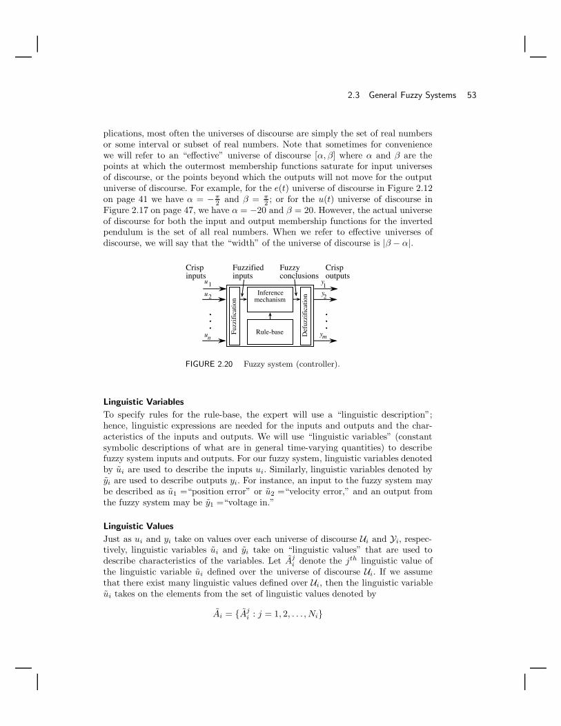
2.3 General Fuzzy Systems 53
plications, most often the universes of discourse are simply the set of real numbersor some interval or subset of real numbers. Note that sometimes for conveniencewe will refer to an “effective” universe of discourse [α, β] where α and β are thepoints at which the outermost membership functions saturate for input universesof discourse, or the points beyond which the outputs will not move for the outputuniverse of discourse. For example, for the e(t) universe of discourse in Figure 2.12on page 41 we have α = −π
2 and β = π2 ; or for the u(t) universe of discourse in
Figure 2.17 on page 47, we have α = −20 and β = 20. However, the actual universeof discourse for both the input and output membership functions for the invertedpendulum is the set of all real numbers. When we refer to effective universes ofdiscourse, we will say that the “width” of the universe of discourse is |β − α|.
Inferencemechanism
Rule-baseFuzz
ific
atio
n
Def
uzzi
fica
tion
u1
u2
un
y1y2
ym
Crispinputs
Crispoutputs
Fuzzifiedinputs
Fuzzyconclusions
FIGURE 2.20 Fuzzy system (controller).
Linguistic Variables
To specify rules for the rule-base, the expert will use a “linguistic description”;hence, linguistic expressions are needed for the inputs and outputs and the char-acteristics of the inputs and outputs. We will use “linguistic variables” (constantsymbolic descriptions of what are in general time-varying quantities) to describefuzzy system inputs and outputs. For our fuzzy system, linguistic variables denotedby ui are used to describe the inputs ui. Similarly, linguistic variables denoted byyi are used to describe outputs yi. For instance, an input to the fuzzy system maybe described as u1 =“position error” or u2 =“velocity error,” and an output fromthe fuzzy system may be y1 =“voltage in.”
Linguistic Values
Just as ui and yi take on values over each universe of discourse Ui and Yi, respec-tively, linguistic variables ui and yi take on “linguistic values” that are used todescribe characteristics of the variables. Let Aj
i denote the jth linguistic value ofthe linguistic variable ui defined over the universe of discourse Ui. If we assumethat there exist many linguistic values defined over Ui, then the linguistic variableui takes on the elements from the set of linguistic values denoted by
Ai = Aji : j = 1, 2, . . . , Ni

54 Chapter 2 / Fuzzy Control: The Basics
(sometimes for convenience we will let the j indices take on negative integer values,as in the inverted pendulum example where we used the linguistic-numeric values).Similarly, let Bj
i denote the jth linguistic value of the linguistic variable yi definedover the universe of discourse Yi. The linguistic variable yi takes on elements fromthe set of linguistic values denoted by
Bi = Bpi : p = 1, 2, . . . , Mi
(sometimes for convenience we will let the p indices take on negative integer values).Linguistic values are generally descriptive terms such as “positive large,” “zero,”and “negative big” (i.e., adjectives). For example, if we assume that u1 denotes thelinguistic variable “speed,” then we may assign A1
1 = “slow,” A21 = “medium,” and
A31 = “fast” so that u1 has a value from A1 = A1
1, A21, A
31.
Linguistic Rules
The mapping of the inputs to the outputs for a fuzzy system is in part characterizedby a set of condition → action rules, or in modus ponens (If-Then) form,
If premise Then consequent. (2.3)
Usually, the inputs of the fuzzy system are associated with the premise, and theoutputs are associated with the consequent. These If-Then rules can be representedin many forms. Two standard forms, multi-input multi-output (MIMO) and multi-input single-output (MISO), are considered here. The MISO form of a linguisticrule is
If u1 is Aj1 and u2 is Ak
2 and, . . . , and un is Aln Then yq is Bp
q (2.4)
It is an entire set of linguistic rules of this form that the expert specifies on howto control the system. Note that if u1 =“velocity error” and Aj
1 =“positive large,”then “u1 is Aj
1,” a single term in the premise of the rule, means “velocity error ispositive large.” It can be easily shown that the MIMO form for a rule (i.e., one withconsequents that have terms associated with each of the fuzzy controller outputs)can be decomposed into a number of MISO rules using simple rules from logic. Forinstance, the MIMO rule with n inputs and m = 2 outputs
If u1 is Aj1 and u2 is Ak
2 and, . . . , and un is Aln Then y1 is Br
1 and y2 is Bs2
is linguistically (logically) equivalent to the two rules
If u1 is Aj1 and u2 is Ak
2 and, . . . , and un is Aln Then y1 is Br
1
If u1 is Aj1 and u2 is Ak
2 and, . . . , and un is Aln Then y2 is Bs
2
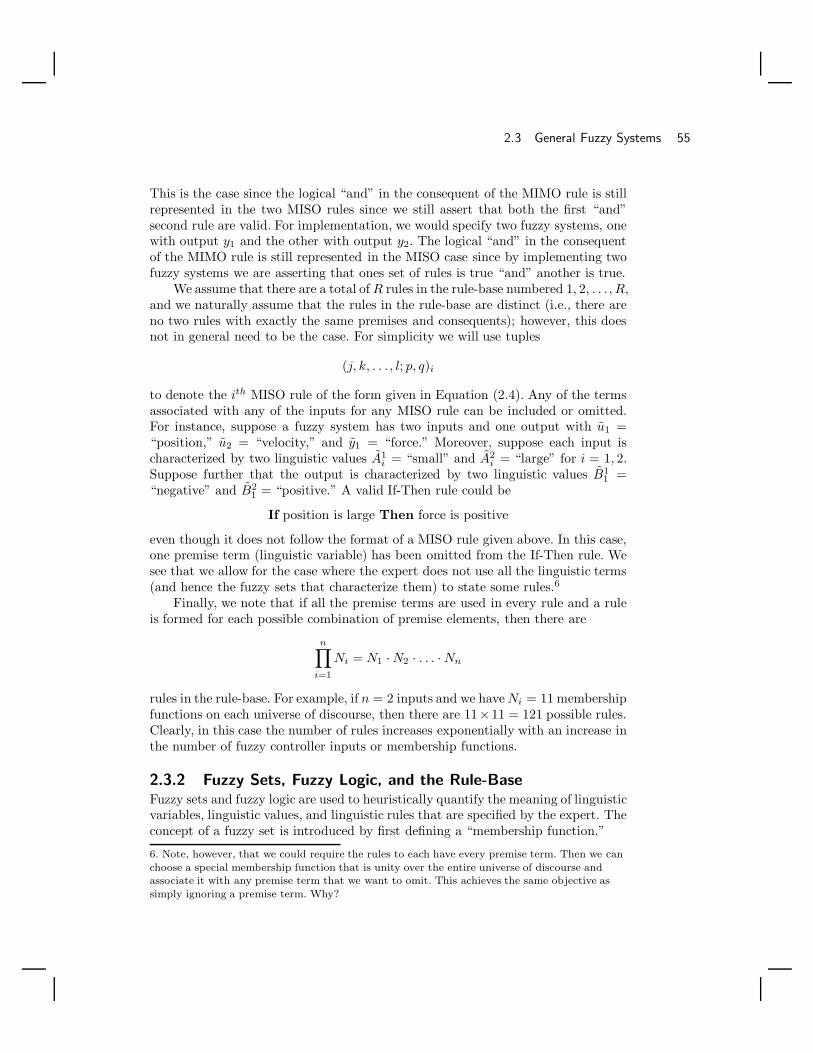
2.3 General Fuzzy Systems 55
This is the case since the logical “and” in the consequent of the MIMO rule is stillrepresented in the two MISO rules since we still assert that both the first “and”second rule are valid. For implementation, we would specify two fuzzy systems, onewith output y1 and the other with output y2. The logical “and” in the consequentof the MIMO rule is still represented in the MISO case since by implementing twofuzzy systems we are asserting that ones set of rules is true “and” another is true.
We assume that there are a total of R rules in the rule-base numbered 1, 2, . . . , R,and we naturally assume that the rules in the rule-base are distinct (i.e., there areno two rules with exactly the same premises and consequents); however, this doesnot in general need to be the case. For simplicity we will use tuples
(j, k, . . . , l; p, q)i
to denote the ith MISO rule of the form given in Equation (2.4). Any of the termsassociated with any of the inputs for any MISO rule can be included or omitted.For instance, suppose a fuzzy system has two inputs and one output with u1 =“position,” u2 = “velocity,” and y1 = “force.” Moreover, suppose each input ischaracterized by two linguistic values A1
i = “small” and A2i = “large” for i = 1, 2.
Suppose further that the output is characterized by two linguistic values B11 =
“negative” and B21 = “positive.” A valid If-Then rule could be
If position is large Then force is positive
even though it does not follow the format of a MISO rule given above. In this case,one premise term (linguistic variable) has been omitted from the If-Then rule. Wesee that we allow for the case where the expert does not use all the linguistic terms(and hence the fuzzy sets that characterize them) to state some rules.6
Finally, we note that if all the premise terms are used in every rule and a ruleis formed for each possible combination of premise elements, then there are
n∏i=1
Ni = N1 ·N2 · . . . · Nn
rules in the rule-base. For example, if n = 2 inputs and we have Ni = 11 membershipfunctions on each universe of discourse, then there are 11×11 = 121 possible rules.Clearly, in this case the number of rules increases exponentially with an increase inthe number of fuzzy controller inputs or membership functions.
2.3.2 Fuzzy Sets, Fuzzy Logic, and the Rule-BaseFuzzy sets and fuzzy logic are used to heuristically quantify the meaning of linguisticvariables, linguistic values, and linguistic rules that are specified by the expert. Theconcept of a fuzzy set is introduced by first defining a “membership function.”
6. Note, however, that we could require the rules to each have every premise term. Then we can
choose a special membership function that is unity over the entire universe of discourse andassociate it with any premise term that we want to omit. This achieves the same objective as
simply ignoring a premise term. Why?

56 Chapter 2 / Fuzzy Control: The Basics
Membership Functions
Let Ui denote a universe of discourse and Aji ∈ Ai denote a specific linguistic value
for the linguistic variable ui. The function µ(ui) associated with Aji that maps Ui
to [0, 1] is called a “membership function.” This membership function describes the“certainty” that an element of Ui, denoted ui, with a linguistic description ui, maybe classified linguistically as Aj
i . Membership functions are subjectively specified inan ad hoc (heuristic) manner from experience or intuition.
For instance, if Ui = [−150, 150], ui =“velocity error,” and Aji =“positive
large,” then µ(ui) may be a bell-shaped curve that peaks at one at ui = 75 andis near zero when ui < 50 or ui > 100. Then if ui = 75, µ(75) = 1, so we areabsolutely certain that ui is “positive large.” If ui = −25 then µ(−25) is very nearzero, which represents that we are very certain that ui is not “positive large.”
Clearly, many other choices for the shape of the membership function are possi-ble (e.g., triangular and trapezoidal shapes), and these will each provide a differentmeaning for the linguistic values that they quantify. See Figure 2.21 for a graph-ical illustration of a variety of membership functions and Tables 2.3 and 2.4 fora mathematical characterization of the triangular and Gaussian membership func-tions (other membership functions can be characterized with mathematics usinga similar approach).7 For practice, you should sketch the membership functionsthat are described in Tables 2.3 and 2.4. Notice that for Table 2.3 cL specifies the“saturation point” and wL specifies the slope of the nonunity and nonzero part ofµL. Similarly, for µR. For µC notice that c is the center of the triangle and w isthe base-width. Analogous definitions are used for the parameters in Table 2.4. InTable 2.4, for the “centers” case note that this is the traditional definition for theGaussian membership function. This definition is clearly different from a standardGaussian probability density function, in both the meaning of c and σ, and in thescaling of the exponential function. Recall that it is possible that a Gaussian prob-ability density function has a maximum value achieved at a value other than one;the standard Gaussian membership function always has its peak value at one.
µ
ui
FIGURE 2.21 Some typical membership functions.
7. The reader should not fall into the trap of calling a membership function a “probability
density function.” There is nothing stochastic about the fuzzy system, and membershipfunctions are not restricted to obey the laws of probability (consider, for example, the
membership functions in Figure 2.21).

2.3 General Fuzzy Systems 57
TABLE 2.3 Mathematical Characterization ofTriangular Membership Functions
Triangular membership functions
Left µL(u) =
1 if u ≤ cL
max
0, 1 + cL−u0.5wL
otherwise
Centers µC(u) =
max
0, 1 + u−c
0.5w
if u ≤ c
max0, 1 + c−u
0.5w
otherwise
Right µR(u) =
max
0, 1 + u−cR
0.5wR
if u ≤ cR
1 otherwise
TABLE 2.4 Mathematical Characterization ofGaussian Membership Functions
Gaussian membership functions
Left µL(u) =
1 if u ≤ cL
exp
(− 1
2
(u−cL
σL
)2)
otherwise
Centers µ(u) = exp(− 1
2
(u−c
σ
)2)
Right µR(u) =
exp
(− 1
2
(u−cR
σR
)2)
if u ≤ cR
1 otherwise
Fuzzy Sets
Given a linguistic variable ui with a linguistic value Aji defined on the universe of
discourse Ui, and membership function µAji(ui) (membership function associated
with the fuzzy set Aji ) that maps Ui to [0, 1], a “fuzzy set” denoted with Aj
i isdefined as
Aji = (ui, µAj
i(ui)) : ui ∈ Ui (2.5)
(notice that a fuzzy set is simply a crisp set of pairings of elements of the universe ofdiscourse coupled with their associated membership values). For example, supposewe assign a linguistic variable u1 = “temperature” and the linguistic value A1
1 =“hot,” then A1
1 is a fuzzy set whose membership function describes the degree ofcertainty that the numeric value of the temperature, u1 ∈ U1, possesses the propertycharacterized by A1
1 (see the pendulum example in the previous section for otherexamples of fuzzy sets).
Additional concepts related to membership functions and fuzzy sets are cov-ered in Exercise 2.5 on page 104 and Exercise 2.6 on page 105. These include thefollowing:

58 Chapter 2 / Fuzzy Control: The Basics
• “Support of a fuzzy set”: The set of points on the universe of discourse where themembership function value is greater than zero.
• “α-cut”: The set of points on the universe of discourse where the membershipfunction value is greater than α.
• “Height” of a fuzzy set or membership function: The peak value reached by themembership function.
• “Normal” fuzzy sets: Ones with membership functions that reach one for at leastone point on the universe of discourse.
• “Convex fuzzy sets”: Ones that satisfy a certain type of convexity condition thatis given in Equation (2.29) on page 104,
• “Linguistic hedges”: Mathematical operations on membership functions of fuzzysets that can be used to change the meaning of the underlying linguistics.
• “Extension principle”: If you are given a function that maps some domain intosome range and you have membership functions defined on the domain, the ex-tension principle shows how to map the membership functions on the domain tothe range.
Fuzzy Logic
Next, we specify some set-theoretic and logical operations on fuzzy sets. The readershould first understand the conventional counterparts to each of these; the fuzzyversions will then be easier to grasp as they are but extensions of the correspondingconventional notions. Also, we recommend that the reader sketch the fuzzy setsthat result from the following operations.
Fuzzy Subset: Given fuzzy sets A1i and A2
i associated with the universe of dis-course Ui (Ni = 2), with membership functions denoted µA1
i(ui) and µA2
i(ui), re-
spectively, A1i is defined to be a “fuzzy subset” of A2
i , denoted by A1i ⊂ A2
i , ifµA1
i(ui) ≤ µA2
i(ui) for all ui ∈ Ui.
Fuzzy Complement: The complement (“not”) of a fuzzy set A1i with a mem-
bership function µA1i(ui) has a membership function given by 1 − µA1
i(ui).
Fuzzy Intersection (AND): The intersection of fuzzy sets A1i and A2
i , whichare defined on the universe of discourse Ui, is a fuzzy set denoted by A1
i ∩A2i , with
a membership function defined by either of the following two methods:
1. Minimum: Here, we find the minimum of the membership values as in
µA1i∩A2
i= minµA1
i(ui), µA2
i(ui) : ui ∈ Ui (2.6)
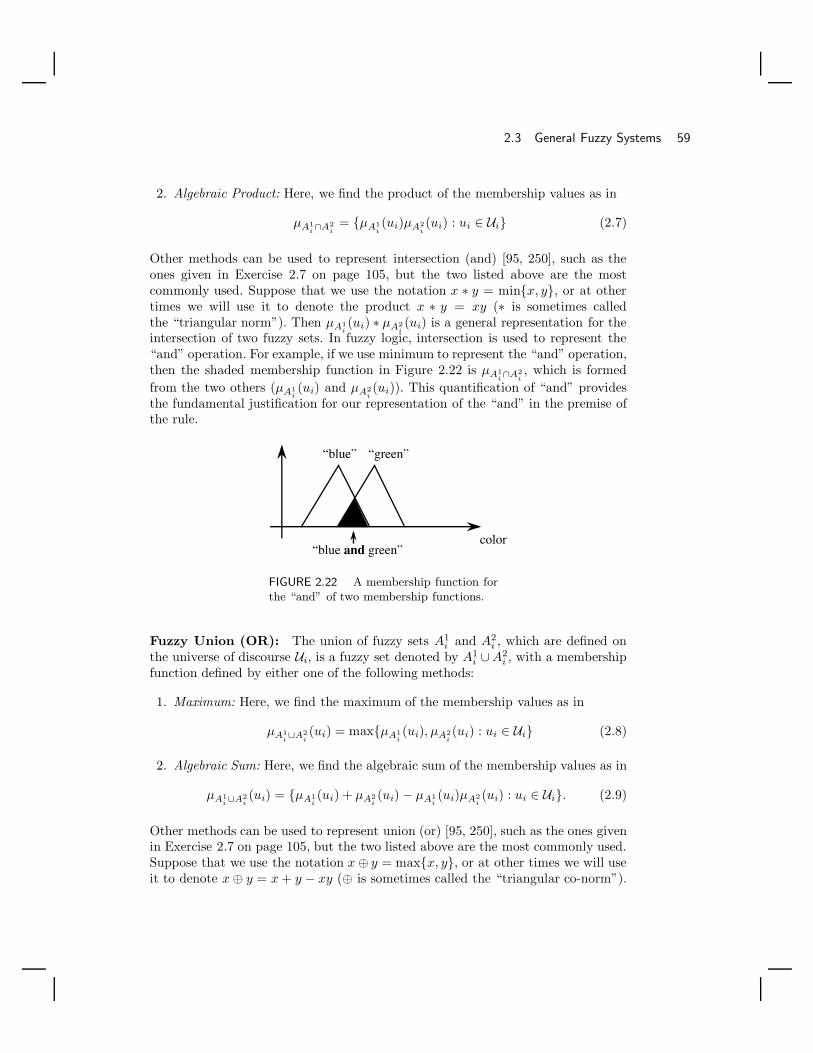
2.3 General Fuzzy Systems 59
2. Algebraic Product: Here, we find the product of the membership values as in
µA1i∩A2
i= µA1
i(ui)µA2
i(ui) : ui ∈ Ui (2.7)
Other methods can be used to represent intersection (and) [95, 250], such as theones given in Exercise 2.7 on page 105, but the two listed above are the mostcommonly used. Suppose that we use the notation x ∗ y = minx, y, or at othertimes we will use it to denote the product x ∗ y = xy (∗ is sometimes calledthe “triangular norm”). Then µA1
i(ui) ∗ µA2
i(ui) is a general representation for the
intersection of two fuzzy sets. In fuzzy logic, intersection is used to represent the“and” operation. For example, if we use minimum to represent the “and” operation,then the shaded membership function in Figure 2.22 is µA1
i∩A2
i, which is formed
from the two others (µA1i(ui) and µA2
i(ui)). This quantification of “and” provides
the fundamental justification for our representation of the “and” in the premise ofthe rule.
color
“blue” “green”
“blue and green”
FIGURE 2.22 A membership function forthe “and” of two membership functions.
Fuzzy Union (OR): The union of fuzzy sets A1i and A2
i , which are defined onthe universe of discourse Ui, is a fuzzy set denoted by A1
i ∪A2i , with a membership
function defined by either one of the following methods:
1. Maximum: Here, we find the maximum of the membership values as in
µA1i∪A2
i(ui) = maxµA1
i(ui), µA2
i(ui) : ui ∈ Ui (2.8)
2. Algebraic Sum: Here, we find the algebraic sum of the membership values as in
µA1i∪A2
i(ui) = µA1
i(ui) + µA2
i(ui) − µA1
i(ui)µA2
i(ui) : ui ∈ Ui. (2.9)
Other methods can be used to represent union (or) [95, 250], such as the ones givenin Exercise 2.7 on page 105, but the two listed above are the most commonly used.Suppose that we use the notation x ⊕ y = maxx, y, or at other times we will useit to denote x ⊕ y = x + y − xy (⊕ is sometimes called the “triangular co-norm”).

60 Chapter 2 / Fuzzy Control: The Basics
Then µA1i(ui)⊕ µA2
i(ui) is a general representation for the union of two fuzzy sets.
In fuzzy logic, union is used to represent the “or” operation. For example, if we usemaximum to represent the “or” operation, then the shaded membership function inFigure 2.23, is µA1
i∪A2i, which is formed from the two others (µA1
i(ui) and µA2
i(ui)).
This quantification of “or” provides the fundamental justification for the “or” thatinherently lies between the rules in the rule-base (note that we interpret the listof rules in the rule-base as “If premise-1 Then consequent-1” or “If premise-2Then consequent-2,” or so on). Note that in the case where we form the “overallimplied fuzzy set” (to be defined more carefully below) this “or” between the rulesis quantified directly with “⊕” as it is described above. If we use only the impliedfuzzy sets (as we did for the inverted pendulum problem in the last section), thenthe “or” between the rules is actually quantified with the way the defuzzificationoperation works (consider the way that the COG defuzzification method combinesthe effects of all the individual implied fuzzy sets).
color
“blue” “green”
“blue or green”
FIGURE 2.23 A membership function forthe “or” of two membership functions.
Fuzzy Cartesian Product: The intersection and union above are both definedfor fuzzy sets that lie on the same universe of discourse. The fuzzy Cartesian productis used to quantify operations on many universes of discourse. If Aj
1, Ak2 , . . . , A
ln are
fuzzy sets defined on the universes of discourse U1,U2, . . . ,Un, respectively, theirCartesian product is a fuzzy set (sometimes called a “fuzzy relation”), denoted byAj
1 × Ak2 × · · · × Al
n, with a membership function defined by
µAj1×Ak
2×···×Aln(u1, u2, . . . , un) = µAj
1(u1) ∗ µAk
2(u2) ∗ · · · ∗ µAl
n(un)
The reader may wonder why the “∗” operation is used here. Basically, it arisesfrom our interpretation of a standard Cartesian product, which is formed by takingan element from the first element of the product “and” the second element of theproduct “and” so on. Clearly, in light of this interpretation, the use of “∗” and hence“and” makes sense. Note that the “ands” used in the Cartesian product actuallyrepresent the “ands” used in the rule premises since normally each of the terms ina premise comes from a different universe of discourse.

2.3 General Fuzzy Systems 61
Fuzzy Quantification of Rules: Fuzzy Implications
Next, we show how to quantify the linguistic elements in the premise and consequentof the linguistic If-Then rule with fuzzy sets. For example, suppose we are giventhe If-Then rule in MISO form in Equation (2.4). We can define the fuzzy sets asfollows:
Aj1 = (u1, µA
j1(u1)) : u1 ∈ U1
Ak2 = (u2, µAk
2(u2)) : u2 ∈ U2
... (2.10)Al
n = (un, µAln(un)) : un ∈ Un
Bpq = (yq, µBp
q(yq)) : yq ∈ Yq
These fuzzy sets quantify the terms in the premise and the consequent of the givenIf-Then rule, to make a “fuzzy implication” (which is a fuzzy relation)
If Aj1 and Ak
2 and, . . . , and Aln Then Bp
q (2.11)
where the fuzzy sets Aj1, A
k2 , . . . , A
ln, and Bp
q are defined in Equation (2.10). There-fore, the fuzzy set Aj
1 is associated with, and quantifies the meaning of the linguisticstatement “u1 is Aj
1,” and Bpq quantifies the meaning of “yq is Bp
q .” Each rule inthe rule-base, which we denote by (j, k, . . . , l; p, q)i, i = 1, 2, . . . , R, is representedwith such a fuzzy implication (a fuzzy quantification of the linguistic rule).
There are two general properties of fuzzy logic rule-bases that are sometimesstudied. These are “completeness” (i.e., whether there are conclusions for everypossible fuzzy controller input) and “consistency” (i.e., whether the conclusionsthat rules make conflict with other rules’ conclusions). These two properties arecovered in Exercise 2.8 on page 106.
2.3.3 FuzzificationFuzzy sets are used to quantify the information in the rule-base, and the inferencemechanism operates on fuzzy sets to produce fuzzy sets; hence, we must specifyhow the fuzzy system will convert its numeric inputs ui ∈ Ui into fuzzy sets (aprocess called “fuzzification”) so that they can be used by the fuzzy system.
Let U∗i denote the set of all possible fuzzy sets that can be defined on Ui. Given
ui ∈ Ui, fuzzification transforms ui to a fuzzy set denoted by8 Afuzi defined on
the universe of discourse Ui. This transformation is produced by the fuzzificationoperator F defined by
F : Ui → U∗i
8. In this section, as we introduce various fuzzy sets we will always use a hat over any fuzzy set
whose membership function changes dynamically over time as the ui change.
62 Chapter 2 / Fuzzy Control: The Basics
where
F(ui) = Afuzi
Quite often “singleton fuzzification” is used, which produces a fuzzy set Afuzi ∈ U∗
i
with a membership function defined by
µAfuz
i
(x) =
1 x = ui
0 otherwise
Any fuzzy set with this form for its membership function is called a “singleton.”For a picture of a singleton membership function, see the single vertical line shownin Figure 2.21 on page 56. Note that the discrete impulse function can be used torepresent the singleton membership function.
Basically, the reader should simply think of the singleton fuzzy set as a dif-ferent representation for the number ui. Singleton fuzzification is generally usedin implementations since, without the presence of noise, we are absolutely certainthat ui takes on its measured value (and no other value), and since it providescertain savings in the computations needed to implement a fuzzy system (relativeto, for example, “Gaussian fuzzification,” which would involve forming bell-shapedmembership functions about input points, or triangular fuzzification, which woulduse triangles).
Since most practical work in fuzzy control uses singleton fuzzification, we willalso use it throughout the remainder of this book. The reasons other fuzzificationmethods have not been used very much are (1) they add computational complexityto the inference process and (2) the need for them has not been that well justified.This is partly due to the fact that very good functional capabilities can be achievedwith the fuzzy system when only singleton fuzzification is used.
2.3.4 The Inference MechanismThe inference mechanism has two basic tasks: (1) determining the extent to whicheach rule is relevant to the current situation as characterized by the inputs ui,i = 1, 2, . . . , n (we call this task “matching”); and (2) drawing conclusions usingthe current inputs ui and the information in the rule-base (we call this task an“inference step”). For matching note that Aj
1 × Ak2 × · · · × Al
n is the fuzzy setrepresenting the premise of the ith rule (j, k, . . . , l; p, q)i (there may be more thanone such rule with this premise).
Matching
Suppose that at some time we get inputs ui, i = 1, 2, . . . , n, and fuzzification pro-duces
Afuz1 , Afuz
2 , . . . , Afuzn
the fuzzy sets representing the inputs. There are then two basic steps to matching.

2.3 General Fuzzy Systems 63
Step 1: Combine Inputs with Rule Premises: The first step in matchinginvolves finding fuzzy sets Aj
1, Ak2 , . . . , A
ln with membership functions
µAj1(u1) = µAj
1(u1) ∗ µ
Afuz1
(u1)
µAk2(u2) = µAk
2(u2) ∗ µ
Afuz2
(u2)
...µAl
n(un) = µAl
n(un) ∗ µ
Afuzn
(un)
(for all j, k, . . . , l) that combine the fuzzy sets from fuzzification with the fuzzysets used in each of the terms in the premises of the rules. If singleton fuzzificationis used, then each of these fuzzy sets is a singleton that is scaled by the premisemembership function (e.g., µAj
1(u1) = µAj
1(u1) for u1 = u1 and µAj
1(u1) = 0 for
u1 = u1). That is, with singleton fuzzification we have µAfuz
i
(ui) = 1 for all i =
1, 2, . . . , n for the given ui inputs so that
µAj1(u1) = µAj
1(u1)
µAk2(u2) = µAk
2(u2)
...µAl
n(un) = µAl
n(un)
We see that when singleton fuzzification is used, combining the fuzzy sets that werecreated by the fuzzification process to represent the inputs with the premise mem-bership functions for the rules is particularly simple. It simply reduces to computingthe membership values of the input fuzzy sets for the given inputs u1, u2, . . . , un
(as we had indicated at the end of Section 2.2.3 for the inverted pendulum).
Step 2: Determine Which Rules Are On: In the second step, we form mem-bership values µi(u1, u2, . . . , un) for the ith rule’s premise (what we called µpremise
in the last section on the inverted pendulum) that represent the certainty that eachrule premise holds for the given inputs. Define
µi(u1, u2, . . . , un) = µAj1(u1) ∗ µAk
2(u2) ∗ · · · ∗ µAl
n(un) (2.12)
which is simply a function of the inputs ui. When singleton fuzzification is used (asit is throughout this entire book), we have
µi(u1, u2, . . . , un) = µAj1(u1) ∗ µAk
2(u2) ∗ · · · ∗ µAl
n(un) (2.13)
We use µi(u1, u2, . . . , un) to represent the certainty that the premise of rule imatches the input information when we use singleton fuzzification. This µi(u1, u2, . . . , un)is simply a multidimensional certainty surface, a generalization of the surface shown

64 Chapter 2 / Fuzzy Control: The Basics
in Figure 2.11 on page 39 for the inverted pendulum example. It represents the cer-tainty of a premise of a rule and thereby represents the degree to which a particularrule holds for a given set of inputs.
Finally, we would remark that sometimes an additional “rule certainty” is mul-tiplied by µi. Such a certainty could represent our a priori confidence in each rule’sapplicability and would normally be a number between zero and one. If for rule iits certainty is 0.1, we are not very confident in the knowledge that it represents;while if for some rule j we let its certainty be 0.99, we are quite certain that theknowledge it represents is true. In this book we will not use such rule certaintyfactors.
This concludes the process of matching input information with the premises ofthe rules.
Inference Step
There are two standard alternatives to performing the inference step, one thatinvolves the use of implied fuzzy sets (as we did for the pendulum earlier) and theother that uses the overall implied fuzzy set.
Alternative 1: Determine Implied Fuzzy Sets: Next, the inference step istaken by computing, for the ith rule (j, k, . . . , l; p, q)i, the “implied fuzzy set” Bi
q
with membership function
µBiq(yq) = µi(u1, u2, . . . , un) ∗ µBp
q(yq) (2.14)
The implied fuzzy set Biq specifies the certainty level that the output should be a
specific crisp output yq within the universe of discourse Yq, taking into considerationonly rule i. Note that since µi(u1, u2, . . . , un) will vary with time, so will the shapeof the membership functions µBi
q(yq) for each rule. An example of an implied fuzzy
set can be seen in Figure 2.13(b) on page 43 for the inverted pendulum example.
Alternative 2: Determine the Overall Implied Fuzzy Set: Alternatively,the inference mechanism could, in addition, compute the “overall implied fuzzy set”Bq with membership function
µBq(yq) = µB1
q(yq) ⊕ µB2
q(yq) ⊕ · · · ⊕ µBR
q(yq) (2.15)
that represents the conclusion reached considering all the rules in the rule-baseat the same time (notice that determining Bq can, in general, require significantcomputational resources). Notice that we did not consider this possibility for theinverted pendulum example for reasons that will become clearer in the next sub-section. Instead, our COG or center-average defuzzification method performed theaggregation of the conclusions of all the rules that are represented by the impliedfuzzy sets.

2.3 General Fuzzy Systems 65
Discussion: Compositional Rule of Inference Using the mathematical ter-minology of fuzzy sets, the computation of µBq
(yq) is said to be produced by a “sup-star compositional rule of inference.” The “sup” in this terminology correspondsto the ⊕ operation, and the “star” corresponds to ∗. “Zadeh’s compositional ruleof inference” [245, 246, 95] is the special case of the sup-star compositional ruleof inference when maximum is used for ⊕ and minimum is used for ∗. The overalljustification for using the above operations to represent the inference step lies inthe fact that we can be no more certain about our conclusions than we are aboutour premises. The operations performed in taking an inference step adhere to thisprinciple. To see this, you should study Equation (2.14) and note that the scalingfrom µi(u1, u2, . . . , un) that is produced by the premise matching process will al-ways ensure that supyq
µBiq(yq) ≤ µi(u1, u2, . . . , un). The fact that we are no more
certain of our consequents than our premises is shown graphically in Figure 2.19on page 50 where the heights of the implied fuzzy sets are always less than thecertainty values for all the premise terms.
Up to this point, we have used fuzzy logic to quantify the rules in the rule-base, fuzzification to produce fuzzy sets characterizing the inputs, and the inferencemechanism to produce fuzzy sets representing the conclusions that it reaches afterconsidering the current inputs and the information in the rule-base. Next, we lookat how to convert this fuzzy set quantification of the conclusions to a numeric valuethat can be input to the plant.
2.3.5 DefuzzificationA number of defuzzification strategies exist, and it is not hard to invent more. Eachprovides a means to choose a single output (which we denote with y
crispq ) based
on either the implied fuzzy sets or the overall implied fuzzy set (depending on thetype of inference strategy chosen, “Alternative 1 or 2,” respectively, in the previoussection).
Defuzzification: Implied Fuzzy Sets
As they are more common, we first specify typical defuzzification techniques for theimplied fuzzy sets Bi
q :
• Center of gravity (COG): A crisp output ycrispq is chosen using the center of area
and area of each implied fuzzy set, and is given by
ycrispq =
∑Ri=1 bq
i
∫Yq
µBiq(yq)dyq∑R
i=1
∫Yq
µBiq(yq)dyq
where R is the number of rules, bqi is the center of area of the membership function
of Bpq associated with the implied fuzzy set Bi
q for the ith rule (j, k, . . . , l; p, q)i,
66 Chapter 2 / Fuzzy Control: The Basics
and ∫Yq
µBiq(yq)dyq
denotes the area under µBiq(yq). Notice that COG can be easy to compute since
it is often easy to find closed-form expressions for∫Yq
µBiq(yq)dyq , which is the
area under a membership function (see the pendulum example in Section 2.2.6on page 44 where this amounts to finding the area of a triangle or a triangle withits top chopped off). Notice that the area under each implied fuzzy set must becomputable, so the area under each of the output membership functions (thatare used in the consequent of a rule) must be finite (this is why we cannot “sat-urate” the membership functions at the outermost edges of the output universeof discourse). Also, notice that the fuzzy system must be defined so that
R∑i=1
∫Yq
µBiq(yq)dyq = 0
for all ui or ycrispq will not be properly defined. This value will be nonzero if there
is a rule that is on for every possible combination of the fuzzy system inputs andthe consequent fuzzy sets all have nonzero area.
• Center-average: A crisp output ycrispq is chosen using the centers of each of the
output membership functions and the maximum certainty of each of the conclu-sions represented with the implied fuzzy sets, and is given by
ycrispq =
∑Ri=1 bq
i supyqµBi
q(yq)∑R
i=1 supyqµBi
q(yq)
where “sup” denotes the “supremum” (i.e., the least upper bound which can oftenbe thought of as the maximum value). Hence, supxµ(x) can simply be thoughtof as the highest value of µ(x) (e.g., supuµ(1)(u) = 0.25 for µ(1) when productis used to represent the implication, as shown in Figure 2.18 on page 48). Also, bq
i
is the center of area of the membership function of Bpq associated with the implied
fuzzy set Biq for the ith rule (j, k, . . . , l; p, q)i. Notice that the fuzzy system must
be defined so that
R∑i=1
supyq
µBiq(yq) = 0
for all ui. Also, note that supyqµBi
q(yq) is often very easy to compute since if
µBpq(yq) = 1 for at least one yq (which is the normal way to define consequent

2.3 General Fuzzy Systems 67
membership functions), then for many inference strategies, using Equation (2.14),we have
supyq
µBiq(yq) = µi(u1, u2, . . . , un)
which has already been computed in the matching process. Moreover, the formulafor defuzzification is then given by
ycrispq =
∑Ri=1 bq
i µi(u1, u2, . . . , un)∑Ri=1 µi(u1, u2, . . . , un)
(2.16)
where we must ensure that∑R
i=1 µi(u1, u2, . . . , un) = 0 for all ui. Also note thatthis implies that the shape of the membership functions for the output fuzzy setsdoes not matter; hence, you can simply use singletons centered at the appropriatepositions. Convince yourself of this.
Defuzzification: The Overall Implied Fuzzy Set
Next, we present typical defuzzification techniques for the overall implied fuzzy setBq :
• Max criterion: A crisp output ycrispq is chosen as the point on the output universe
of discourse Yq for which the overall implied fuzzy set Bq achieves a maximum—that is,
ycrispq ∈
arg sup
Yq
µBq
(yq)
Here, “arg supxµ(x)” returns the value of x that results in the supremum of thefunction µ(x) being achieved. For example, suppose that µoverall(u) denotes themembership function for the overall implied fuzzy set that is obtained by takingthe maximum of the certainty values of µ(1) and µ(2) over all u in Figure 2.18on page 48 (i.e., µoverall(u) = maxuµ(1)(u), µ(2)(u) per Equation (2.15)). Inthis case, arg supuµoverall(u) = −10, which is the defuzzified value via the maxcriterion.
Sometimes the supremum can occur at more than one point in Yq (e.g.,consider the use of the max criterion for the case where minimum is used torepresent the implication, and triangular membership functions are used on theoutput universe of discourse, such as in Figure 2.19 on page 50). In this case you
also need to specify a strategy on how to pick only one point for ycrispq (e.g.,
choosing the smallest value). Often this defuzzification strategy is avoided due tothis ambiguity; however, the next defuzzification method does offer a way aroundit.

68 Chapter 2 / Fuzzy Control: The Basics
• Mean of maximum: A crisp output ycrispq is chosen to represent the mean value
of all elements whose membership in Bq is a maximum. We define bmaxq as the
supremum of the membership function of Bq over the universe of discourse Yq.Moreover, we define a fuzzy set B∗
q ∈ Yq with a membership function defined as
µB∗q(yq) =
1 µBq
(yq) = bmaxq
0 otherwise
then a crisp output, using the mean of maximum method, is defined as
ycrispq =
∫Yq
yqµB∗q(yq)dyq∫
YqµB∗
q(yq)dyq
(2.17)
where the fuzzy system must be defined so that∫Yq
µB∗q(yq)dyq = 0 for all ui.
As an example, suppose that for Figure 2.19 on page 50 the two implied fuzzysets are used to form an overall implied fuzzy set by taking the maximum of thetwo certainty values over all of u (i.e., µoverall(u) = maxuµ(1)(u), µ(2)(u) perEquation (2.15)). In this case there is an interval of u values around −10 wherethe overall implied fuzzy set is at its maximum value, and hence there is anambiguity about which is the best defuzzified value. The mean of the maximummethod would pick the value in the middle of the interval as the defuzzified value,so it would choose −10.
Note that the integrals in Equation (2.17) must be computed at each timeinstant since they depend on Bq , which changes with time. This can require exces-sive computational resources for continuous universes of discourse. For some typesof membership functions, simple ideas from geometry can be used to simplify thecalculations; however, for some choices of membership functions, there may bemany subintervals spread across the universe of discourse where the maximum isachieved. In these cases it can be quite difficult to compute the defuzzified valueunless the membership functions are discretized. Complications such as theseoften cause designers to choose other defuzzification methods.
• Center of area (COA): A crisp output ycrispq is chosen as the center of area for
the membership function of the overall implied fuzzy set Bq . For a continuousoutput universe of discourse Yq , the center of area output is denoted by
ycrispq =
∫Yq
yqµBq(yq)dyq∫
YqµBq
(yq)dyq
The fuzzy system must be defined so that∫Yq
µBq(yq)dyq = 0 for all ui. Note that,
similar to the mean of the maximum method, this defuzzification approach canbe computationally expensive. For instance, we leave it to the reader to computethe area of the overall implied fuzzy set µoverall(u) = maxuµ(1)(u), µ(2)(u) for
2.3 General Fuzzy Systems 69
Figure 2.19 on page 50. Notice that in this case the computation is not as easy asjust adding the areas of the two chopped-off triangles that represent the impliedfuzzy sets. Computation of the area of the overall implied fuzzy set does not countthe area that the implied fuzzy sets overlap twice; hence, the area of the overallimplied fuzzy set can in general be much more difficult to compute in real time.
It is important to note that each of the above equations for defuzzification actuallyprovides a mathematical quantification of the operation of the entire fuzzy systemprovided that each of the terms in the descriptions are fully defined. We discussthis in more detail in the next section.
Overall, we see that using the overall implied fuzzy set in defuzzification is oftenundesirable for two reasons: (1) the overall implied fuzzy set Bq is itself difficultto compute in general, and (2) the defuzzification techniques based on an inferencemechanism that provides Bq are also difficult to compute. It is for this reason thatmost existing fuzzy controllers (including the ones in this book) use defuzzificationtechniques based on the implied fuzzy sets, such as center-average or COG.
2.3.6 Mathematical Representations of Fuzzy SystemsNotice that each formula for defuzzification in the previous section provides a math-ematical description of a fuzzy system. There are many ways to represent the oper-ations of a fuzzy system with mathematical formulas. Next, we clarify how to con-struct and interpret such mathematical formulas for the case where center-averagedefuzzification is used for MISO fuzzy systems. Similar ideas apply for some of theother defuzzification strategies, MIMO fuzzy systems, and the Takagi-Sugeno fuzzysystems that we discuss in the next section.
Assume that we use center-average defuzzification so that the formula describ-ing how to compute the output is
y =∑R
i=1 biµi∑Ri=1 µi
(2.18)
Notice that we removed the “crisp” superscript and “q” subscript from y (compareto Equation (2.16)). Also, we removed the “q” superscript from bi. The q indexis no longer needed in both cases since we are considering MISO systems, so thatwhile there can be many inputs, there is only one output.
To be more explicit in Equation (2.18), we need to first define the premise mem-bership functions µi in terms of the individual membership functions that describeeach of the premise terms. Suppose that we use product to represent the conjunc-tions in the premise of each rule. Suppose that we use the triangular membershipfunctions in Table 2.3 on page 57 where we suppose that µL
j (uj) (µRj (uj)) is the
“left-” (“right-”) most membership function on the jth input universe of discourse.In addition, let µCi
j (uj) be the ith “center” membership function for the jth inputuniverse of discourse. In this case, to define µL
j (uj) we simply add a “j” subscriptto the parameters of the “left” membership function from Table 2.3. In particular,

70 Chapter 2 / Fuzzy Control: The Basics
we use cLj and wL
j to denote the jth values of these parameters. We take a similarapproach for the µR
j (uj), j = 1, 2, . . . , n. For µCi
j (uj) we use cij (wi
j) to denote theith triangle center (triangle base width) on the jth input universe of discourse.
Suppose that we use all possible combinations of input membership functionsto form the rules, and that each premise has a term associated with each and everyinput universe of discourse. A more detailed description of the fuzzy system inEquation (2.18) is given by
y =b1
∏nj=1 µL
j (uj) + b2µC11 (u1)
∏nj=2 µL
j (uj) + · · ·∏nj=1 µL
j (uj) + µC11 (u1)
∏nj=2 µL
j (uj) + · · ·
The first term in the numerator is b1µ1 in Equation (2.18). Here, we have calledthe “first rule” the one that has premise terms all described by the membershipfunctions µL
j (uj), j = 1, 2, . . . , n. The second term in the numerator is b2µ2 and ituses µC1
1 (u1) on the first universe of discourse and the leftmost ones on the otheruniverses of discourse (i.e., j = 2, 3, . . . , n). Continuing in a similar manner, the sumin the numerator (and denominator) extends to include all possible combinationsof products of the input membership functions, and this fully defines the µi inEquation (2.18).
Overall, we see that because we need to define rules resulting from all possiblecombinations of given input membership functions, of which there are three kinds(left, center, right), the explicit mathematical representation of the fuzzy system issomewhat complicated. To avoid some of the complications, we first specify a singlefunction that represents all three types of input membership functions. Suppose thaton the jth input universe of discourse we number the input membership functionsfrom left to right as 1, 2, . . . , Nj, where Nj is the number of input membershipfunctions on the jth input universe of discourse. A single membership function thatrepresents all three in Table 2.3 is
µij(uj) =
1 if uj ≤ c1j or uj ≥ c
Nj
j
max0, 1 + uj−ci
j
0.5wij
if uj ≤ ci
j and (uj > c1j and uj < c
Nj
j )
max0, 1 + ci
j−uj
0.5wij
if uj > ci
j and (uj > c1j and uj < c
Nj
j )
A similar approach can be used for the Gaussian membership functions in Table 2.4.Recall that we had used
(j, k, . . . , l; p, q)i
to denote the ith rule. In this notation the indices in (the “tuple”) (j, k, . . . , l)range over 1 ≤ j ≤ N1, 1 ≤ k ≤ N2, . . ., 1 ≤ l ≤ Nn, and specify which linguisticvalue is used on each input universe of discourse. Correspondingly, each index in thetuple (j, k, . . . , l) also specifies the linguistic-numeric value of the input membershipfunction used on each input universe of discourse.
2.3 General Fuzzy Systems 71
Let
b(j,k,...,l;p,q)i
denote the output membership function (a singleton) center for the ith rule (ofcourse, q = 1 in our MISO case). Note that we use “i” in the notation (j, k, . . . , l; p, q)i
simply as a label for each rule (i.e., we number the rules in the rule-base, and i isthis number). Hence, when we are given i, we know the values of j, k, . . ., l, p, andq. Because of this, an explicit description of the fuzzy system in Equation (2.18) isgiven by
y =∑R
i=1 b(j,k,...,l;p,q)iµj1µ
k2 · · ·µl
n∑Ri=1 µj
1µk2 · · ·µl
n
(2.19)
This formula clearly shows the use of the product to represent the premise. Noticethat since we use all possible combinations of input membership functions to formthe rules there are
R =n∏
j=1
Nj
rules, and hence it takes
n∑j=1
2Nj +n∏
j=1
Nj (2.20)
parameters to describe the fuzzy system since there are two parameters for eachinput membership function and R output membership function centers. For someapplications, however, all the output membership functions are not distinct. Forexample, consider the pendulum example where five output membership functioncenters are defined, and there are R = 25 rules. To define the center positionsb(j,k,...,l;p,q)i so that they take on only a fixed number of given values, that is lessthan R, one approach is to specify them as a function of the indices of the inputmembership functions. What is this function for the pendulum example?
A different approach to avoiding some of the complications encountered inspecifying a fuzzy system mathematically is to use a different notation, and hencea different definition for the fuzzy system. For this alternative approach, for thesake of variety, we will use Gaussian input membership functions. In particular, forsimplicity, suppose that for the input universes of discourse we only use membershipfunctions of the “center” Gaussian form shown in Table 2.4. For the ith rule, supposethat the input membership function is
exp
−1
2
(uj − ci
j
σij
)2

72 Chapter 2 / Fuzzy Control: The Basics
for the jth input universe of discourse. Hence, even though we use the same notationfor the membership function, these centers ci
j are different from those used above,both because we are using Gaussian membership functions here, and because the “i”in ci
j is the index for the rules, not the membership function on the jth input universeof discourse. Similar comments can be made about the σi
j, i = 1, 2, . . . , R, j =1, 2, . . . , n. If we let bi, i = 1, 2, . . . , R, denote the center of the output membershipfunction for the ith rule, use center-average defuzzification, and product to representthe conjunctions in the premise, then
y =
∑Ri=1 bi
∏nj=1 exp
(−1
2
(uj−ci
j
σij
)2)
∑Ri=1
∏nj=1 exp
(−1
2
(uj−ci
j
σij
)2) (2.21)
is an explicit representation of a fuzzy system. Note that we do not use the “left”and “right” versions of the Gaussian membership functions in Table 2.4 as thiscomplicates the notation (how?). There are nR input membership function centers,nR input membership function spreads, and R output membership function centers.Hence, we need a total of
R(2n + 1)
parameters to describe this fuzzy system.Now, while the fuzzy systems in Equations (2.19) and (2.21) are in general
different, it is interesting to compare the number of parameters needed to describea fuzzy system using each approach. In practical situations, we often have Nj ≥ 3for each j = 1, 2, . . . , n, and sometimes the number of membership functions oneach input universe of discourse can be quite large. From Equation (2.20) we canclearly see that large values of n will result in a fuzzy system with many parameters(there is an exponential increase in the number of rules). On the other hand, usingthe fuzzy system in Equation (2.21) the user specifies the number of rules and this,coupled with the number of inputs n, specifies the total number of parameters.There is not an exponential growth in the number of parameters in Equation (2.21)in the same way as there is in the fuzzy system in Equation (2.19) so you may betempted to view the definition in Equation (2.21) as a better one. Such a conclusion,can, however be erroneous for several reasons.
First, the type of fuzzy system defined by Equation (2.19) is sometimes morenatural in control design when you use triangular membership functions since youoften need to make sure that there will be no point on any input universe of discoursewhere there is no membership function with a nonzero value (why?). Of course, ifyou are careful, you can avoid this problem with the fuzzy system represented byEquation (2.21) also. Second, suppose that the number of rules for Equation (2.21)is the same as that for Equation (2.19). In this case, the number of parameters

2.3 General Fuzzy Systems 73
needed to describe the fuzzy system in Equation (2.21) is n∏
j=1
Nj
(2n + 1)
Now, comparing this to Equation (2.20) you see that for many values of Nj ,j = 1, 2, . . . , n, and number of inputs n, it is possible that the fuzzy system inEquation (2.21) will require many more parameters to specify it than the fuzzysystem in Equation (2.19). Hence, the inefficiency in the representation in Equa-tion (2.19) lies in having all possible combinations of output membership functioncenters, which results in exponential growth in the number of parameters needed tospecify the fuzzy system. The inefficiency in the representation in Equation (2.21)lies in the fact that, in a sense, membership functions on the input universes ofdiscourse are not re-used by each rule. There are new input membership functionsfor every rule.
Generally, it is difficult to know which is the best fuzzy system for a particularproblem. In this book, we will sometimes (e.g., in Chapter 5) use the mathematicalrepresentation in Equation (2.21) because it is somewhat simpler, and possessessome properties that we will exploit. At other times we will be implicitly using therepresentation in Equation (2.19) because it will lend to the development of certaintechniques (e.g., in Chapter 6). In every case, however, that we use Equation (2.21)(Equation (2.19)) you may want to consider how the concepts, approaches, andresults change (or do not change) if the form of the fuzzy system in Equation (2.19)(Equation (2.21)) is used.
Finally, we would like to recommend that you practice creating mathematicalrepresentations of fuzzy systems. For instance, it is good practice to create a math-ematical representation of the fuzzy controller for the inverted pendulum of theform of Equation (2.19), then also use Equation (2.21) to specify the same fuzzysystem. Comparing these two approaches, and resolving the issues in specifying theoutput centers for the Equation (2.19) case, will help clarify the issues discussed inthis section.
2.3.7 Takagi-Sugeno Fuzzy SystemsThe fuzzy system defined in the previous sections will be referred to as a “standardfuzzy system.” In this section we will define a “functional fuzzy system,” of whichthe Takagi-Sugeno fuzzy system [207] is a special case.
For the functional fuzzy system, we use singleton fuzzification, and the ith
MISO rule has the form
If u1 is Aj1 and u2 is Ak
2 and, . . . , and un is Aln Then bi = gi(·)
where “·” simply represents the argument of the function gi and the bi are notoutput membership function centers. The premise of this rule is defined the same asit is for the MISO rule for the standard fuzzy system in Equation (2.4) on page 54.
74 Chapter 2 / Fuzzy Control: The Basics
The consequents of the rules are different, however. Instead of a linguistic termwith an associated membership function, in the consequent we use a function bi =gi(·) (hence the name “functional fuzzy system”) that does not have an associatedmembership function. Notice that often the argument of gi contains the termsui, i = 1, 2, . . . , n, but other variables may also be used. The choice of the functiondepends on the application being considered. Below, we will discuss linear and affinefunctions but many others are possible. For instance, you may want to choose
bi = gi(·) = ai,0 + ai,1(u1)2 + · · ·+ ai,n(un)2
or
bi = gi(·) = exp [ai,1sin(u1) + · · ·+ ai,nsin(un)]
Virtually any function can be used (e.g., a neural network mapping or another fuzzysystem), which makes the functional fuzzy system very general.
For the functional fuzzy system we can use an appropriate operation for rep-resenting the premise (e.g., minimum or product), and defuzzification may be ob-tained using
y =∑R
i=1 biµi∑Ri=1 µi
(2.22)
where µi is defined in Equation (2.13). It is assumed that the functional fuzzysystem is defined so that no matter what its inputs are, we have
∑Ri=1 µi = 0. One
way to view the functional fuzzy system is as a nonlinear interpolator between themappings that are defined by the functions in the consequents of the rules.
An Interpolator Between Linear Mappings
In the case where
bi = gi(·) = ai,0 + ai,1u1 + · · ·+ ai,nun
(where the ai,j are real numbers) the functional fuzzy system is referred to asa “Takagi-Sugeno fuzzy system.” If ai,0 = 0, then the gi(·) mapping is a linearmapping and if ai,0 = 0, then the mapping is called “affine.” Often, however, as isstandard, we will refer to the affine mapping as a linear mapping for convenience.Overall, we see that the Takagi-Sugeno fuzzy system essentially performs a nonlinearinterpolation between linear mappings.
As an example, suppose that n = 1, R = 2, and that we have rules
If u1 is A11 Then b1 = 2 + u1
If u1 is A21 Then b2 = 1 + u1
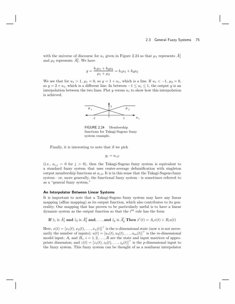
2.3 General Fuzzy Systems 75
with the universe of discourse for u1 given in Figure 2.24 so that µ1 represents A11
and µ2 represents A21. We have
y =b1µ1 + b2µ2
µ1 + µ2= b1µ1 + b2µ2
We see that for u1 > 1, µ1 = 0, so y = 1 + u1, which is a line. If u1 < −1, µ2 = 0,so y = 2 + u1, which is a different line. In between −1 ≤ u1 ≤ 1, the output y is aninterpolation between the two lines. Plot y versus u1 to show how this interpolationis achieved.
-1 1 u 1
µ µ1 21
FIGURE 2.24 Membershipfunctions for Takagi-Sugeno fuzzysystem example.
Finally, it is interesting to note that if we pick
gi = ai,0
(i.e., ai,j = 0 for j > 0), then the Takagi-Sugeno fuzzy system is equivalent toa standard fuzzy system that uses center-average defuzzification with singletonoutput membership functions at ai,0. It is in this sense that the Takagi-Sugeno fuzzysystem—or, more generally, the functional fuzzy system—is sometimes referred toas a “general fuzzy system.”
An Interpolator Between Linear Systems
It is important to note that a Takagi-Sugeno fuzzy system may have any linearmapping (affine mapping) as its output function, which also contributes to its gen-erality. One mapping that has proven to be particularly useful is to have a lineardynamic system as the output function so that the ith rule has the form
If z1 is Aj1 and z2 is Ak
2 and, . . . , and zp is Alp Then xi(t) = Aix(t) + Biu(t)
Here, x(t) = [x1(t), x2(t), . . . , xn(t)] is the n-dimensional state (now n is not neces-sarily the number of inputs); u(t) = [u1(t), u2(t), . . . , um(t)] is the m-dimensionalmodel input; Ai and Bi, i = 1, 2, . . . , R are the state and input matrices of appro-priate dimension; and z(t) = [z1(t), z2(t), . . . , zp(t)] is the p-dimensional input tothe fuzzy system. This fuzzy system can be thought of as a nonlinear interpolator

76 Chapter 2 / Fuzzy Control: The Basics
between R linear systems. It takes the input z(t) and has an output
x(t) =∑R
i=1(Aix(t) + Biu(t))µi(z(t))∑Ri=1 µi(z(t))
or
x(t) =
(R∑
i=1
Aiξi(z(t))
)x(t) +
(R∑
i=1
Biξi(z(t))
)u(t) (2.23)
where
ξ = [ξ1, . . . , ξR] =
[1∑R
i=1 µi
][µ1, . . . , µR]
If R = 1, we get a standard linear system. Generally, for R > 1 and a givenvalue of z(t), only certain rules will turn on and contribute to the output. Manychoices are possible for z(t). For instance, we often choose z(t) = x(t), or sometimesz(t) = [x(t), u(t)].
As an example, suppose that z(t) = x(t), p = n = m = 1, and R = 2 with rules
If x1 is A11 Then x1 = −x1 + 2u1
If x1 is A21 Then x2 = −2x1 + u1.
Suppose that we use µ1 and µ2 from Figure 2.24 as the membership functions forA1
1 and A21, respectively (i.e., we relabel the horizontal axis of Figure 2.24 with x1).
In this case Equation (2.23) becomes
x1(t) = (−µ1 − 2µ2)x1(t) + (2µ1 + µ2)u1(t)
If x1(t) > 1, then µ1 = 0 and µ2 = 1, so the behavior of the nonlinear systemis governed by
x1(t) = −2x1(t) + u1(t)
which is the linear system specified by the second rule above. However, if x1(t) <−1, then µ1 = 1 and µ2 = 0, so the behavior of the nonlinear system is governedby
x1(t) = −x1(t) + 2u1(t)
which is the linear system specified by the first rule above. For −1 ≤ x1(t) ≤ 1, theTakagi-Sugeno fuzzy system interpolates between the two linear systems. We seethat for changing values of x1(t), the two linear systems that are in the consequentsof the rules contribute different amounts.

2.4 Simple Design Example: The Inverted Pendulum 77
We think of one linear system being valid on a region of the state space thatis quantified via µ1 and another on the region quantified by µ2 (with a “fuzzyboundary” in between). For the higher-dimensional case, we have premise member-ship functions for each rule quantify whether the linear system in the consequent isvalid for a specific region on the state space. As the state evolves, different rules turnon, indicating that other combinations of linear models should be used. Overall, wefind that the Takagi-Sugeno fuzzy system provides a very intuitive representationof a nonlinear system as a nonlinear interpolation between R linear models.
2.3.8 Fuzzy Systems Are Universal ApproximatorsFuzzy systems have very strong functional capabilities. That is, if properly con-structed, they can perform very complex operations (e.g., much more complex thanthose performed by a linear mapping). Actually, many fuzzy systems are known tosatisfy the “universal approximation property” [227].
For example, suppose that we use center-average defuzzification, product forthe premise and implication, and Gaussian membership functions. Name this fuzzysystem f(u). Then, for any real continuous function ψ(u) defined on a closed andbounded set and an arbitrary ε > 0, there exists a fuzzy system f(u) such that
supu
|f(u) − ψ(u)| < ε .
Note, however, that all this “universal approximation property” does is guar-antee that there exists a way to define the fuzzy system f(u) (e.g., by picking themembership function parameters). It does not say how to find the fuzzy system,which can, in general, be very difficult. Furthermore, for arbitrary accuracy youmay need an arbitrarily large number of rules.
The value of the universal approximation property for fuzzy systems is simplythat it shows that if you work hard enough at tuning, you should be able to make thefuzzy system do what you are trying to get done. For control, practically speaking,it means that there is great flexibility in tuning the nonlinear function implementedby the fuzzy controller. Generally, however, there are no guarantees that you willbe able to meet your stability and performance specifications by properly tuninga given fuzzy controller. You also have to choose the appropriate controller inputsand outputs, and there will be fundamental limitations imposed by the plant thatmay prohibit achieving certain control objectives no matter how you tune the fuzzycontroller (e.g., a nonminimum phase system may provide certain limits on thequality of the performance that can be achieved).
2.4 Simple Design Example: The InvertedPendulum
As there is no general systematic procedure for the design of fuzzy controllers thatwill definitely produce a high-performance fuzzy control system for a wide varietyof applications, it is necessary to learn about fuzzy controller design via examples.

78 Chapter 2 / Fuzzy Control: The Basics
Here, we continue with the inverted pendulum example to provide an introductionto the typical procedures used in the design (and redesign) of a fuzzy controller.After reading the next section, on simulation of fuzzy control systems, the readercan follow this section more carefully by fully reproducing our design steps. For afirst reading, however, we recommend that you not worry about how the simulationswere produced; rather, focus on their general characteristics as they are related todesign.
To simulate the fuzzy control system shown in Figure 2.4 on page 27 it is nec-essary to specify a mathematical model of the inverted pendulum. Note that wedid not need the model for the initial design of the fuzzy controller in Section 2.2.1;but to accurately assess the quality of a design, we need either a model for mathe-matical analysis or simulation-based studies, or an experimental test bed in whichto evaluate the design. Here, we will study simulation-based evaluations for design,while in Chapter 4 we will study the use of mathematical analysis to verify thequality of a design (and to assist in redesign). Throughout the book we will alsoshow actual implementation results that are used to assess the performance of fuzzycontrollers.
One model for the inverted pendulum shown in Figure 2.2 on page 25 is givenby
y =9.8 sin(y) + cos(y)
[−u−0.25y2 sin(y)
1.5
]0.5
[43 − 1
3 cos2(y)] (2.24)
˙u = −100u + 100u.
The first order filter on u to produce u represents an actuator. Given this andthe fuzzy controller developed in Section 2.2.1 (the one that uses the minimumoperator to represent both the “and” in the premise and the implication and COGdefuzzification), we can simulate the fuzzy control system shown in Figure 2.4 onpage 27. We let the initial condition be y(0) = 0.1 radians (= 5.73 deg.), y(0) = 0,and the initial condition for the actuator state is zero. The results are shown inFigure 2.25, where we see in the upper plot that the output appropriately movestoward the inverted position, and the force input in the lower plot that moves backand forth to achieve this.9
2.4.1 Tuning via Scaling Universes of DiscourseSuppose that the rate at which the pendulum balances in Figure 2.25 is consid-ered to be unacceptably slow and that there is too much control action. To solvethese problems, we use standard ideas from control engineering to conclude thatwe ought to try to tune the “derivative gain.” To do this we introduce gains on the
9. If you attempt to reproduce these results, you should be cautioned that, as always, inaccurateresults can be obtained if a small enough integration step size is not chosen for numerical
simulation. For all the simulation results of this section, we use the fourth-order Runge-Kuttamethod and an integration step size of 0.001. The plots of this subsection were produced by
Scott C. Brown.
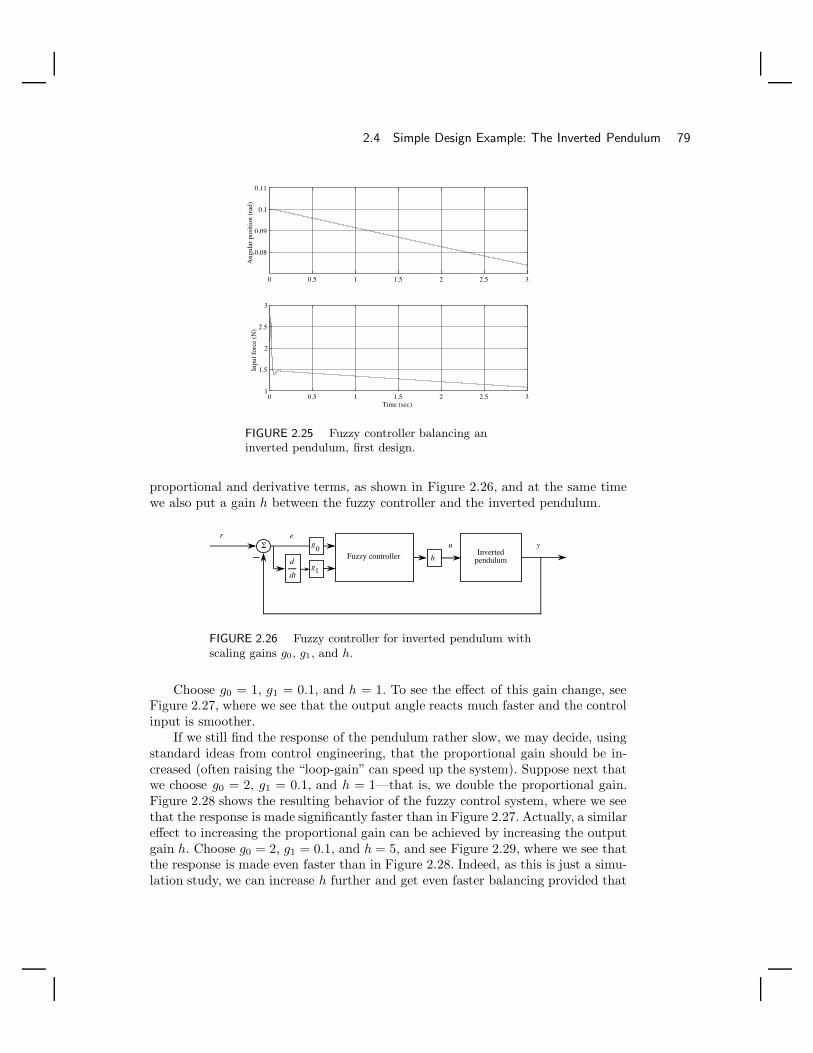
2.4 Simple Design Example: The Inverted Pendulum 79
0 0.5 1 1.5 2 2.5 3
0.08
0.09
0.1
0.11
Ang
ular
pos
ition
(ra
d)
0 0.5 1 1.5 2 2.5 31
1.5
2
2.5
3
Inpu
t for
ce (
N)
Time (sec)
FIGURE 2.25 Fuzzy controller balancing aninverted pendulum, first design.
proportional and derivative terms, as shown in Figure 2.26, and at the same timewe also put a gain h between the fuzzy controller and the inverted pendulum.
Invertedpendulumd
dt
Σr e
u y
Fuzzy controller
g0
g1
h
FIGURE 2.26 Fuzzy controller for inverted pendulum withscaling gains g0, g1, and h.
Choose g0 = 1, g1 = 0.1, and h = 1. To see the effect of this gain change, seeFigure 2.27, where we see that the output angle reacts much faster and the controlinput is smoother.
If we still find the response of the pendulum rather slow, we may decide, usingstandard ideas from control engineering, that the proportional gain should be in-creased (often raising the “loop-gain” can speed up the system). Suppose next thatwe choose g0 = 2, g1 = 0.1, and h = 1—that is, we double the proportional gain.Figure 2.28 shows the resulting behavior of the fuzzy control system, where we seethat the response is made significantly faster than in Figure 2.27. Actually, a similareffect to increasing the proportional gain can be achieved by increasing the outputgain h. Choose g0 = 2, g1 = 0.1, and h = 5, and see Figure 2.29, where we see thatthe response is made even faster than in Figure 2.28. Indeed, as this is just a simu-lation study, we can increase h further and get even faster balancing provided that

80 Chapter 2 / Fuzzy Control: The Basics
0 0.5 1 1.5 2 2.5 3-0.05
0
0.05
0.1
0.15
Ang
ular
pos
ition
(ra
d)
0 0.5 1 1.5 2 2.5 3-1
0
1
2
3In
put f
orce
(N
)
Time (sec)
FIGURE 2.27 Fuzzy controller balancing aninverted pendulum with g0 = 1, g1 = 0.1, and h = 1.
we simulate the system properly by having a small enough integration step size.However, the reader must be cautioned that this may stretch the simulation modelbeyond its range of validity. For instance, further increases in h will generally resultin faster balancing at the expense of a large control input, and for a big enoughh the input may be larger than what is allowed in the physical system. At thatpoint the simulation would not reflect reality since if the controller were actuallyimplemented, the plant input would saturate and the proper balancing behaviormay not be achieved.
0 0.5 1 1.5 2 2.5 3-0.05
0
0.05
0.1
0.15
Ang
ular
pos
ition
(ra
d)
0 0.5 1 1.5 2 2.5 3-2
-1
0
1
2
3
4
Inpu
t for
ce (
N)
Time (sec)
FIGURE 2.28 Fuzzy controller balancing aninverted pendulum with g0 = 2, g1 = 0.1, and h = 1.

2.4 Simple Design Example: The Inverted Pendulum 81
0 0.5 1 1.5 2 2.5 3-0.05
0
0.05
0.1
0.15
Ang
ular
pos
ition
(ra
d)
0 0.5 1 1.5 2 2.5 3-10
-5
0
5
10
15
20
Inpu
t for
ce (
N)
Time (sec)
FIGURE 2.29 Fuzzy controller balancing aninverted pendulum with g0 = 2, g1 = 0.1, and h = 5.
We see that the change in the scaling gains at the input and output of thefuzzy controller can have a significant impact on the performance of the resultingfuzzy control system, and hence they are often a convenient parameter for tuning.Because they are frequently used for tuning fuzzy controllers, it is important tostudy exactly what happens when these scaling gains are tuned.
Input Scaling Gains
First, consider the effect of the input scaling gains g0 and g1. Notice that we canactually achieve the same effect as scaling via g1 by simply changing the labelingof the d
dte(t) axis for the membership functions of that input. The case where
g0 = g1 = h = 1.0 corresponds to our original choice for the membership functionsin Figure 2.9 on page 36. The choice of g1 = 0.1 as a scaling gain for the fuzzycontroller with these membership functions is equivalent to having the membershipfunctions shown in Figure 2.30 with a scaling gain of g1 = 1.
e(t), (rad/sec)
“possmall”
4ππ π
4
“zero”“negsmall”“neglarge”-1-2 0 1 2
“poslarge”
8π8 dt
d10 10-10-10
FIGURE 2.30 Scaled membership functions for ddt
e(t).
We see that the choice of a scaling gain g1 results in scaling the horizontal axis
82 Chapter 2 / Fuzzy Control: The Basics
of the membership functions by 1g1
. Generally, the scaling gain g1 has the followingeffects:
• If g1 = 1, there is no effect on the membership functions.
• If g1 < 1, the membership functions are uniformly “spread out” by a factor of 1g1
(notice that multiplication of each number on the horizontal axis of Figure 2.9on page 36 by 10 produces Figure 2.30).
• If g1 > 1, the membership functions are uniformly “contracted” (to see this,choose g1 = 10 and notice that the numbers on the horizontal axis of the newmembership functions that we would obtain by collapsing the gain into the choiceof the membership functions, would be scaled by 0.1).
The expansion and contraction of the horizontal axes by the input scaling gains issometimes described as similar to how an accordion operates, especially for trian-gular membership functions. Notice that the membership functions for the otherinput to the fuzzy controller will be affected in a similar way by the gain g0.
Now that we see how we can either use input scaling gains or simply redefinethe horizontal axis of the membership functions, it is interesting to consider howthe scaling gains actually affect the meaning of the linguistics that form the basisfor the definition of the fuzzy controller. Notice that
• If g1 = 1, there is no effect on the meaning of the linguistic values.
• If g1 < 1, since the membership functions are uniformly “spread out,” this changesthe meaning of the linguistics so that, for example, “poslarge” is now characterizedby a membership function that represents larger numbers.
• If g1 > 1, since the membership functions are uniformly “contracted,” thischanges the meaning of the linguistics so that, for example, “poslarge” is nowcharacterized by a membership function that represents smaller numbers.
Similar statements can be made about all the other membership functions and theirassociated linguistic values. Overall, we see that the input scaling factors have aninverse relationship in terms of their ultimate effect on scaling (larger g1 that isgreater than 1 corresponds to changing the meaning of the linguistics so that theyquantify smaller numbers). While such an inverse relationship exists for the inputscaling gains, just the opposite effect is seen for the output scaling gains, as we shallsee next.
Output Scaling Gain
Similar to what you can do to the input gains, you can collapse the output scalinggain into the definition of the membership functions on the output. In particular,
• If h = 1, there is no effect on the output membership functions.

2.4 Simple Design Example: The Inverted Pendulum 83
• If h < 1, there is the effect of contracting the output membership functionsand hence making the meaning of their associated linguistics quantify smallernumbers.
• If h > 1, there is the effect of spreading out the output membership functions andhence making the meaning of their associated linguistics quantify larger numbers.
There is a proportional effect between the scaling gain h and the output member-ship functions. As an example, for the inverted pendulum the output membershipfunctions are scaled by h as shown in Figure 2.31. The reader should verify theeffect of h by considering how the membership functions shown in Figure 2.31 willmove for varying values of h.
u(t), (N)
“possmall”
30h-20h
“zero”“negsmall”“neglarge”
-1-2 0 1 2“poslarge”
-10h 20h10h-30h
FIGURE 2.31 The effect of scaling gain h on the spacing ofthe output membership functions.
Overall, the tuning of scaling gains for fuzzy systems is often referred to as“scaling a fuzzy system.” Notice that if for the pendulum example the effectiveuniverses of discourse for all inputs and outputs are [−1, +1] (i.e., the input (output)left-most membership function saturates (peaks) at −1 and the right-most input(output) membership function saturates (peaks) at +1), then we say that the fuzzycontroller is “normalized.” Clearly, scaling gains can be used to normalize the givenfuzzy controllers for the pendulum. What gains g0, g1, and h will do this?
2.4.2 Tuning Membership FunctionsIt is important to realize that the scaling gains are not the only parameters thatcan be tuned to improve the performance of the fuzzy control system. Indeed,sometimes it is the case that for a given rule-base and membership functions youcannot achieve the desired performance by tuning only the scaling gains. Often,what is needed is a more careful consideration of how to specify additional rules orbetter membership functions.
The problem with this is that there are often too many parameters to tune (e.g.,membership function shapes, positioning, and number and type of rules) and oftenthere is not a clear connection between the design objectives (e.g., better rise-time)and a rationale and method that should be used to tune these parameters. Thereare, however, certain methods to overcome this problem, and here we will examine

84 Chapter 2 / Fuzzy Control: The Basics
one of these that has been found to be very useful for real implementations of fuzzycontrol systems for challenging applications.
Output Membership Function Tuning
In this method we will tune the positioning of the output membership functions(assume that they are all symmetric and equal to one only at one point) by char-acterizing their centers by a function. Suppose that we use ci, i = −2,−1, 0, 1, 2, todenote the centers of the output membership functions for the fuzzy controller forthe inverted pendulum, where the indices i for the ci are the linguistic-numeric val-ues used for the output membership functions (see Figure 2.9 on page 36). (This is adifferent notation from that used for the centers in our discussion on defuzzificationin Section 2.3.5 since there the index referred to the rule.) If h = 1 then
ci = 10i
describes the positioning of the centers of the output membership functions shownin Figure 2.9 on page 36 and if we scale by h then
ci = 10hi
describes the position centers as shown in Figure 2.31. We see that a linear rela-tionship in the ci equation produces a linear (uniform) spacing of the membershipfunctions. Suppose that we instead choose
ci = 5hsign(i)i2 (2.25)
(sign(x) returns the sign of the number x and sign(0) = 1), then this will havethe effect of making the output membership function centers near the origin bemore closely spaced than the membership functions farther out on the horizontalaxis. The effect of this is to make the “gain” of the fuzzy controller smaller whenthe signals are small and larger as the signals grow larger (up to the point wherethere is a saturation, as usual). Hence, the use of Equation (2.25) for the centersindicates that if the error and change-in-error for the pendulum are near wherethey should be, then do not make the force input to the plant too big, but if theerror and change-in-error are large, then the force input should be much biggerso that it quickly returns the pendulum to near the balanced position (note thata cubic function ci = 5hi3 will provide a similar effect as the sign(i)i2 term inEquation (2.25)).
Effect on Performance
At this point the reader should wonder why we would even bother with more com-plex tuning of the fuzzy controller for the inverted pendulum since the performanceseen in our last design iteration, in Figure 2.29 on page 81, was quite successful.
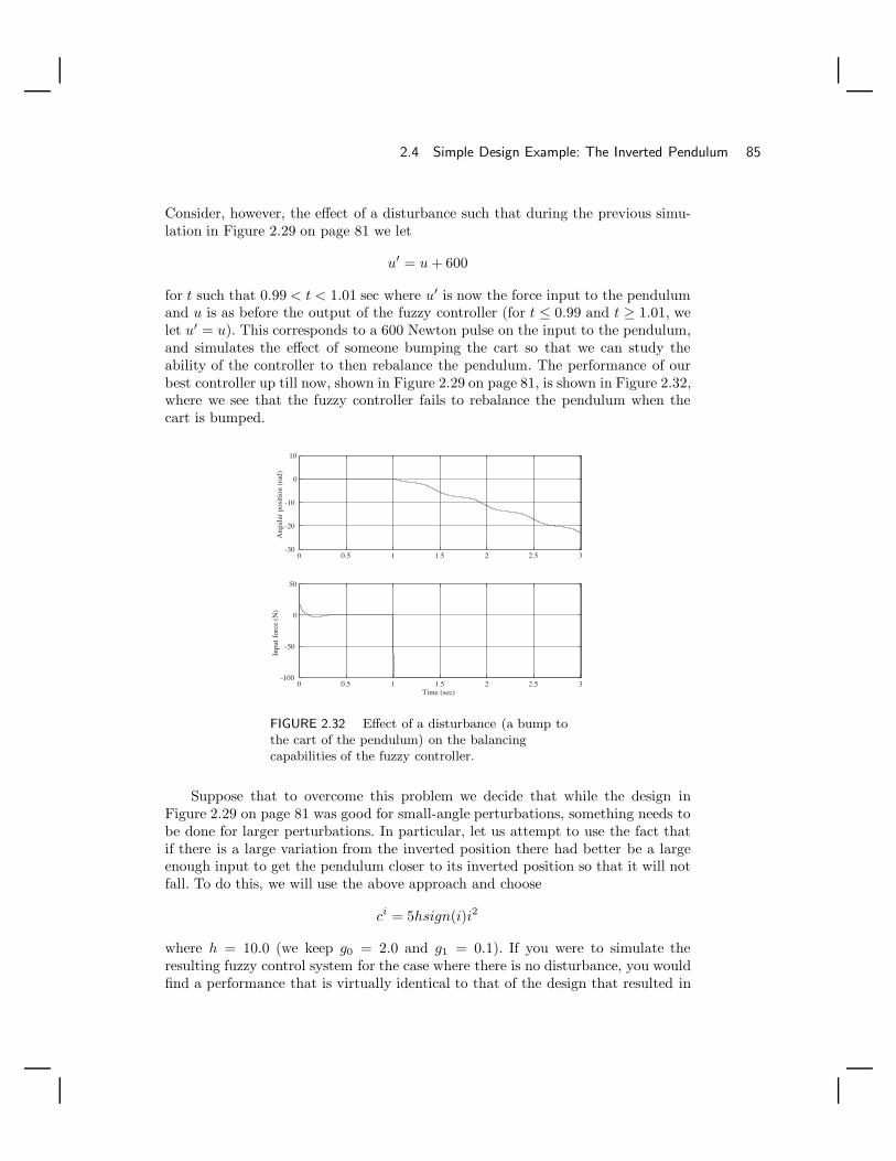
2.4 Simple Design Example: The Inverted Pendulum 85
Consider, however, the effect of a disturbance such that during the previous simu-lation in Figure 2.29 on page 81 we let
u′ = u + 600
for t such that 0.99 < t < 1.01 sec where u′ is now the force input to the pendulumand u is as before the output of the fuzzy controller (for t ≤ 0.99 and t ≥ 1.01, welet u′ = u). This corresponds to a 600 Newton pulse on the input to the pendulum,and simulates the effect of someone bumping the cart so that we can study theability of the controller to then rebalance the pendulum. The performance of ourbest controller up till now, shown in Figure 2.29 on page 81, is shown in Figure 2.32,where we see that the fuzzy controller fails to rebalance the pendulum when thecart is bumped.
0 0.5 1 1.5 2 2.5 3-30
-20
-10
0
10
Ang
ular
pos
ition
(ra
d)
0 0.5 1 1.5 2 2.5 3-100
-50
0
50
Inpu
t for
ce (
N)
Time (sec)
FIGURE 2.32 Effect of a disturbance (a bump tothe cart of the pendulum) on the balancingcapabilities of the fuzzy controller.
Suppose that to overcome this problem we decide that while the design inFigure 2.29 on page 81 was good for small-angle perturbations, something needs tobe done for larger perturbations. In particular, let us attempt to use the fact thatif there is a large variation from the inverted position there had better be a largeenough input to get the pendulum closer to its inverted position so that it will notfall. To do this, we will use the above approach and choose
ci = 5hsign(i)i2
where h = 10.0 (we keep g0 = 2.0 and g1 = 0.1). If you were to simulate theresulting fuzzy control system for the case where there is no disturbance, you wouldfind a performance that is virtually identical to that of the design that resulted in

86 Chapter 2 / Fuzzy Control: The Basics
Figure 2.29 on page 81. The reason for this can be explained as follows: Notice thatfor Figure 2.29 on page 81 the gains were g0 = 2.0 and g1 = 0.1 and that we havethe output membership function centers given by
ci = 5hi
where h = 10. Notice that for both controllers, if i = 0 or i = 1 we get the samepositions of the output membership functions. Hence, if the signals are small, wewill get nearly the same effect from both fuzzy controllers. However, if, for example,i = 2 then the center resulting from the controller with ci = 5hsign(i)i2 will havea membership function that is much farther out, which says that the input to theplant should be larger. The effect of this will be to have the fuzzy controller providevery large force inputs when the pendulum is not near its inverted position. To seethis, consider Figure 2.33, where we see that the newly redesigned fuzzy controllercan in fact rebalance the pendulum in the presence of the disturbance (and itperforms similarly to the best previous one, shown in Figure 2.29 on page 81, inresponse to smaller perturbations from the inverted position, as is illustrated byhow it recovers from the initial condition). Notice, however, that it used a largeinput force to counteract the bump to the pendulum.
0 0.5 1 1.5 2 2.5 3-0.6
-0.4
-0.2
0
0.2
Ang
ular
pos
ition
(ra
d)
0 0.5 1 1.5 2 2.5 3-200
-150
-100
-50
0
50
100
Inpu
t for
ce (
N)
Time (sec)
FIGURE 2.33 Effect of a disturbance (a bump tothe cart of the pendulum) on the balancingcapabilities of the fuzzy controller.
You may wonder why we did not just increase the gain on the fuzzy controllerdepicted in Figure 2.29 on page 81 to the point where it would be able to recoversimilarly to this new control system. However, if we did this, we would also raisethe gain of the controller when its input signals are small, which can have adverseeffects of amplifying noise in a real implementation. Besides, our redesign above

2.4 Simple Design Example: The Inverted Pendulum 87
was used simply to illustrate the design approach. In the applications studied inChapter 3, we will use a similar design approach where the need for the nonlinearspacing of the output membership functions is better motivated due to the factthat a more challenging application dictates this.
2.4.3 The Nonlinear Surface for the Fuzzy ControllerUltimately, the goal of tuning is to shape the nonlinearity that is implemented bythe fuzzy controller. This nonlinearity, sometimes called the “control surface,” isaffected by all the main fuzzy controller parameters. Consider, for example, thecontrol surface for the fuzzy controller that resulted in the response shown in Fig-ure 2.29 on page 81 (i.e., g0 = 2.0, g1 = 0.1, and h = 5), which is shown inFigure 2.34, where the output of the fuzzy controller is now plotted against its twoinputs. Notice that the surface represents in a compact way all the information inthe fuzzy controller (but of course this representation is limited in that if thereare more than two inputs it becomes difficult to visualize the surface). To convinceyourself of this, you should pick a value for e and d
dte(t), read the correspondingfuzzy controller output value off the surface, and determine if the rule-base wouldindicate that the controller should behave in this way. Figure 2.34 simply representsthe range of possible defuzzified values for all possible inputs e and d
dte(t).
-1-0.5
00.5
1
-10
-5
0
5
10
-100
-50
0
50
100
e (rad)e (rad/sec)
Out
put,
u (
N)
ddt
FIGURE 2.34 Control surface of the fuzzycontroller for g0 = 2.0, g1 = 0.1, and h = 5.
Note that the control surface for a simple proportional-derivative (PD) con-troller is a plane in three dimensions. With the proper choice of the PD gains, thelinear PD controller can easily be made to have the same shape as the fuzzy con-troller near the origin. Hence, in this case the fuzzy controller will behave similarlyto the PD controller provided its inputs are small. However, notice that there isno way that the linear PD controller can achieve a nonlinear control surface of

88 Chapter 2 / Fuzzy Control: The Basics
the shape shown in Figure 2.34 (this is not surprising considering the complexitydifference of the two controllers).
Next, notice changing the gains g0 and g1 will rescale the axis, which will changethe slope of the surface. Increasing g0 is analogous to increasing the proportionalgain in a PD controller (i.e., it will often make the system respond faster). Increasingthe gain g1 is analogous to increasing the derivative gain in a PD controller. Notice,also, that changing h will scale the vertical axis of the controller surface plot. Hence,for instance, increasing h will make the entire surface have a higher slope and makethe output saturate at higher values.
It is useful to notice that there is a type of interpolation that is performedby the fuzzy controller that is nicely illustrated in Figure 2.34. If you study theplot carefully, you will notice that the rippled surface is created by the rules andmembership functions. For instance, if we kept a similar uniform distribution ofmembership functions for the input and outputs of the fuzzy system, but increasedthe number of membership functions, the ripples would correspondingly increasein number and the amplitude of the ripple would decrease (indeed, in the limit,as more and more membership functions are added in this way, the controller canbe made to approximate a plane in a larger and larger region—but this may notoccur for other membership function distributions and rule-base choices). What ishappening is that there is an interpolation between the rules. The output is aninterpolation of the effects of the four rules that are on for the inverted pendulumfuzzy controller. For more general fuzzy controllers, it is important to keep in mindthat this sort of interpolation is often occurring (but not always—it depends onyour choice of the membership functions).
When we tune the fuzzy controller, it changes the shape of the control surface,which in turn affects the behavior of the closed-loop control system. Changing thescaling gains changes the slope of the surface and hence the “gain” of the fuzzycontroller as we discussed above and as we will discuss in Chapter 4 in more detail.The output membership function centers will also affect the shape of the surface.For instance, the control surface for the fuzzy controller that had
ci = 5hsign(i)i2
where h = 10.0, g0 = 2.0, and g1 = 0.1 is shown in Figure 2.35. You must carefullycompare this surface to the one in Figure 2.34 to assess the effects of using thenonlinear spacing of the output membership function centers. Notice that near thecenter of the plot (i.e., where the inputs are zero) the shape of the two plots isnearly the same (i.e., as explained above, the two controllers will behave similarlyfor small input signals). Notice, however, that the slope of the surface is greater forlarger signals in Figure 2.35 than in Figure 2.34. This further illustrates the effectof the choice of the nonlinear spacing for the output membership function centers.
This concludes the design process for the fuzzy controller for the pendulum.Certainly, if you were concerned with the design of a fuzzy controller for an indus-trial control problem, many other issues besides the ones addressed above wouldhave to be considered. Here, we simply use the inverted pendulum as a convenient
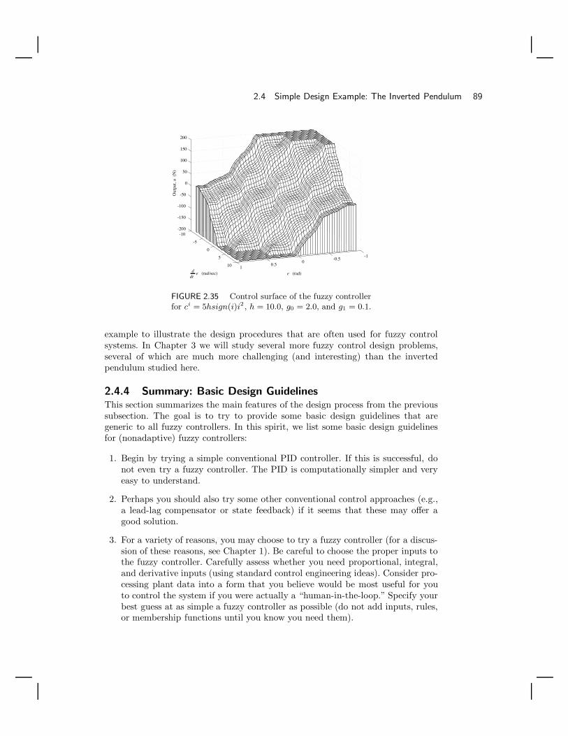
2.4 Simple Design Example: The Inverted Pendulum 89
-1-0.5
00.5
1
-10
-5
0
5
10
-200
-150
-100
-50
0
50
100
150
200
e (rad)e (rad/sec)
Out
put,
u (
N)
ddt
FIGURE 2.35 Control surface of the fuzzy controllerfor ci = 5hsign(i)i2 , h = 10.0, g0 = 2.0, and g1 = 0.1.
example to illustrate the design procedures that are often used for fuzzy controlsystems. In Chapter 3 we will study several more fuzzy control design problems,several of which are much more challenging (and interesting) than the invertedpendulum studied here.
2.4.4 Summary: Basic Design GuidelinesThis section summarizes the main features of the design process from the previoussubsection. The goal is to try to provide some basic design guidelines that aregeneric to all fuzzy controllers. In this spirit, we list some basic design guidelinesfor (nonadaptive) fuzzy controllers:
1. Begin by trying a simple conventional PID controller. If this is successful, donot even try a fuzzy controller. The PID is computationally simpler and veryeasy to understand.
2. Perhaps you should also try some other conventional control approaches (e.g.,a lead-lag compensator or state feedback) if it seems that these may offer agood solution.
3. For a variety of reasons, you may choose to try a fuzzy controller (for a discus-sion of these reasons, see Chapter 1). Be careful to choose the proper inputs tothe fuzzy controller. Carefully assess whether you need proportional, integral,and derivative inputs (using standard control engineering ideas). Consider pro-cessing plant data into a form that you believe would be most useful for youto control the system if you were actually a “human-in-the-loop.” Specify yourbest guess at as simple a fuzzy controller as possible (do not add inputs, rules,or membership functions until you know you need them).

90 Chapter 2 / Fuzzy Control: The Basics
4. Try tuning the fuzzy controller using the scaling gains, as we discussed in theprevious section.
5. Try adding or modifying rules and membership functions so that you moreaccurately characterize the best way to control the plant (this can sometimesrequire significant insight into the physics of the plant).
6. Try to incorporate higher-level ideas about how best to control the plant. Forinstance, try to shape the nonlinear control surface using a nonlinear functionof the linguistic-numeric values, as explained in the previous section.
7. If there is unsmooth or chattering behavior, you may have a gain set too highon an input to the fuzzy controller (or perhaps the output gain is too high).Setting the input gain too high makes it so that the membership functionssaturate for very low values, which can result in oscillations (i.e., limit cycles).
8. Sometimes the addition of more membership functions and rules can help. Thesecan provide for a “finer” (or “higher-granularity”) control, which can sometimesreduce chattering or oscillations.
9. Sometimes it is best to first design a linear controller, then choose the scalinggains, membership functions, and rule-base so that near the origin (i.e., forsmall controller inputs) the slope of the control surface will match the slope ofthe linear controller. In this way we can incorporate all of the good ideas thathave gone into the design of the linear controller (about an operating point)into the design of the fuzzy controller. After this, the designer should seek toshape the nonlinearity for the case where the input signals are not near theorigin using insights about the plant. This design approach will be illustratedin Chapter 3 when we investigate case studies in fuzzy control system design.
Generally, you do not tune the fuzzy controller by evaluating all possibilitiesfor representing the “and” in the premise or for the implication (e.g., minimum orproduct operations) or by studying different defuzzification strategies. While thereare some methods for tuning fuzzy controllers this way, these methods most oftendo not provide insights into how these parameters ultimately affect the performancethat we are trying to achieve (hence it is difficult to know how to tune them toget the desired performance). We must emphasize that the above guidelines do notconstitute a systematic design procedure. As with conventional control design, aprocess of trial and error is generally needed.
Generally, we have found that if you are having trouble coming up with a goodfuzzy controller, you probably need to gain a better understanding of the physicsof the process you are trying to control, and you then need to get the knowledge ofhow to properly affect the plant dynamics into the fuzzy controller.

2.5 Simulation of Fuzzy Control Systems 91
2.5 Simulation of Fuzzy Control SystemsOften, before you implement a fuzzy controller, there is a need to perform asimulation-based evaluation of its performance. As we saw in Section 2.4, wherewe studied the inverted pendulum, these simulation-based investigations can helpto provide insight into how to improve the design of the fuzzy controller and verifythat it will operate properly when it is implemented. To perform a simulation, wewill need a model of the plant and a computer program that will simulate the fuzzycontrol system (i.e., a program to simulate a nonlinear dynamic system).
2.5.1 Simulation of Nonlinear SystemsIn the next subsection we will explain how to write a subroutine that will simulate afuzzy controller. First, however, we will briefly explain how to simulate a nonlinearsystem since every fuzzy control system is a nonlinear system (even if the plant islinear, the fuzzy controller and hence fuzzy control system is nonlinear). Supposethat we denote the fuzzy controller in Figure 2.4 on page 27 by f(e, e). Supposethat the fuzzy control system in Figure 2.4 can be represented by the ordinarydifferential equation
x(t) = F (x(t), r(t)) (2.26)y = G(x(t), r(t))
where x = [x1, x2, . . . , xn] is a state vector, F = [F1, F2, . . . , Fn] is a vector ofnonlinear functions, G is a nonlinear function that maps the states and referenceinput to the output of the system, and x(0) is the initial state. To simulate anonlinear system, we will assume that the nonlinear ordinary differential equationsare put into the form in Equation (2.26).
To see how to put a given ordinary differential equation into the form givenin Equation (2.26), consider the inverted pendulum example. For our pendulumexample, define the state
x = [x1, x2, x3] = [y, y, u]
Then, using Equation (2.25) on page 78 we have
x1 = x2 = F1(x, r)
x2 =9.8 sin(x1) + cos(x1)
[−x3−0.25x2
2 sin(x1)1.5
]0.5
[43 − 1
3 cos2(x1)] = F2(x, r)
x3 = −100x3 + 100f(−x1,−x2) = F3(x, r)
since u = f(e, e), e = r−y, r = 0, and e = −y. Also, we have y = G(x, r) = x1. Thisputs the fuzzy control system for the nonlinear inverted pendulum in the properform for simulation.

92 Chapter 2 / Fuzzy Control: The Basics
Now, to simulate Equation (2.26), we could simply use Euler’s method toapproximate the derivative x in Equation (2.26) as
x(kh + h) − x(kh)h
= F (x(kh), r(kh), kh) (2.27)
y = G(x(kh), r(kh), kh)
Here, h is a parameter that is referred to as the “integration step size” (not to beconfused with the scaling gain h used earlier). Notice that any element of the vector
x(kh + h) − x(kh)h
is simply an approximation of the slope of the corresponding element in the timevarying vector x(t) at t = kh (i.e., an approximation of the derivative). For smallvalues of h, the approximation will be accurate provided that all the functions andvariables are continuous. Equation (2.27) can be rewritten as
x(kh + h) = x(kh) + hF (x(kh), r(kh), kh)y = G(x(kh), r(kh), kh)
for k = 0, 1, 2, . . . . The value of the vector x(0) is the initial condition and isassumed to be given. Simulation of the nonlinear system proceeds recursively bycomputing x(h), x(2h), x(3h), and so on, to generate the response of the systemfor the input r(kh). For practice the reader should place the pendulum differentialequations developed above into the form for simulation via the Euler method givenin Equation (2.27). Using this, and provided that you pick your integration stepsize h small enough, the Euler method can be used to reproduce all the simulationresults of the previous section.
Note that by choosing h small, we are trying to simulate the continuous-timenonlinear system. If we want to simulate the way that a digital control system wouldbe implemented on a computer in the laboratory, we can simulate a controllerthat only samples its inputs every T seconds (T is not the same as h; it is the“sampling interval” for the computer in the laboratory) and only updates its controloutputs every T seconds (and it would hold them constant in between). Normally,you would choose T = αh where α > 0 is some positive integer. In this way wesimulate the plant as a continuous-time system that interacts with a controller thatis implemented on a digital computer.
While Euler’s method is easy to understand and implement in code, sometimesto get good accuracy the value of h must be chosen to be very small. Most often,to get good simulation accuracy, more sophisticated methods are used, such as theRunge-Kutta method with adaptive step size or predictor-corrector methods. Inthe fourth-order Runge-Kutta method, we begin with Equation (2.26) and a given
2.5 Simulation of Fuzzy Control Systems 93
x(0) and let
x(kh + h) = x(kh) +16
(k1 + 2k2 + 2k3 + k4) (2.28)
where the four vectors
k1 = hF (x(kh), r(kh), kh)
k2 = hF
(x(kh) +
k1
2, r
(kh +
h
2
), kh +
h
2
)
k3 = hF
(x(kh) +
k2
2, r
(kh +
h
2
), kh +
h
2
)k4 = hF (x(kh) + k3, r(kh + h), kh + h)
These extra calculations are used to achieve a better accuracy than the Eulermethod. We see that the Runge-Kutta method is very easy to use; it simply in-volves computing the four vectors k1 to k4, and plugging them into Equation (2.28).Suppose that you write a computer subroutine to compute the output of a fuzzycontroller given its inputs (in some cases these inputs could include a state of theclosed-loop system). In this case, to calculate the four vectors, k1 to k4, you willneed to use the subroutine four times, once for the calculation of each of the vectors,and this can increase the computational complexity of the simulation. To simplifythe complexity of the simulation you can simulate the fuzzy controller as if it wereimplemented on a digital computer in the laboratory with a sampling interval ofT = h (i.e., α = 1 in our discussion above). Now, you may not be concerned withimplementation of the fuzzy controller on a digital computer in the laboratory, oryour choice of h may not actually correspond to a reasonable choice of a samplingperiod in the laboratory; however, using this approach you typically can simplifycomputations. The savings come from assuming that over the length of time cor-responding to an integration step size, you hold the value of the fuzzy controlleroutput constant. Hence, this approach to simplifying computations is really simplybased on making an approximation to the fuzzy controller output over the amountof time corresponding to an integration step size.
Generally, if the Runge-Kutta method has a small enough value of h, it issufficiently accurate for the simulation of most fuzzy control systems (and if anadaptive step size method [59, 215] is used, then even more accuracy can be obtainedif it is needed). We invite the reader to code the Runge-Kutta method on theproblems at the end of the chapter.10
Clearly, the above approaches are complete only if we can compute the fuzzycontroller outputs given its inputs. That is, we need a subroutine to compute u =f(e, e). This is what we study next.
10. The reader can, however, download the code for a Runge-Kutta algorithm for simulating an
nth order nonlinear ordinary differential equation from the web site or ftp site listed in thePreface.

94 Chapter 2 / Fuzzy Control: The Basics
2.5.2 Fuzzy Controller Arrays and SubroutinesThe fuzzy controller can be programmed in C, Fortran, Matlab, or virtually anyother programming language. There may be some advantage to programming it inC since it is then sometimes easier to transfer the code directly to an experimen-tal setting for use in real-time control. At other times it may be advantageous toprogram it in Matlab since plotting capabilities and other control computationsmay be easier to perform there. Here, rather than discussing the syntax and char-acteristics of the multitude of languages that we could use to simulate the fuzzycontroller, we will develop a computer program “pseudocode” that will be useful indeveloping the computer program in virtually any language. For readers who arenot interested in learning how to write a program to simulate the fuzzy controller,this section will provide a nice overview of the steps used by the fuzzy controller tocompute its outputs given some inputs.
We will use the inverted pendulum example of the last section to illustratethe basic concepts on how to program the fuzzy controller, and for that examplewe will use the minimum operation to represent both the “and” in the premiseand the implication (it will be obvious how to switch to using, for example, theproduct). At first we will make no attempt to code the fuzzy controller so thatit will minimize execution time or minimize the use of memory. However, afterintroducing the pseudocode, we will address these issues.
First, suppose that for convenience we use a different set of linguistic-numericdescriptions for the input and output membership functions than we used up tillnow. Rather than numbering them
−2,−1, 0, 1, 2
we will renumber them as
0, 1, 2, 3, 4
so that we can use these as indices for arrays in the program (if your languagedoes not allow for the use of “0” as an index, simply renumber them as 1, 2, 3, 4, 5).Suppose that we let the computer variable x1 denote (notice that a different typefaceis used for all computer variables) e(t), which we will call the first input, and x2denote d
dte(t), which we will call the second input. Next, we define the followingarrays and functions:
• Let mf1[i] (mf2[j]) denote the value of the membership function associatedwith input 1 (2) and linguistic-numeric value i (j). In the computer programmf1[i] could be a subroutine that computes the membership value for the ith
membership function given a numeric value for the first input x1 (note thatin the subroutine we can use simple equations for lines to represent triangularmembership functions). Similarly for mf2[j].
• Let rule[i,j] denote the index of the consequent of the rule that has linguistic-numeric value “i” as the first term in its premise and “j” as the second term in

2.5 Simulation of Fuzzy Control Systems 95
its premise. Hence rule[i,j] is essentially a matrix that holds the body of therule-base table shown in Table 2.1 with the appropriate changes to the linguistic-numeric values (i.e., switching from the use of −2,−1, 0, 1, 2 to 0, 1, 2, 3, 4). Inparticular, for the inverted pendulum we have
rule[i, j] =
4 4 4 3 24 4 3 2 14 3 2 1 03 2 1 0 02 1 0 0 0
• Let prem[i,j] denote the certainty of the premise of the rule that has linguistic-numeric value “i” as the first term in its premise and “j” as the second term inits premise given the inputs x1 and x2.
• Let center[k] denote the center of the kth output membership function. For theinverted pendulum k = 0, 1, 2, 3, 4 and the centers are at the points where thetriangles reach their peak.
• Let areaimp[k,h] denote the area under the kth output membership function(where for the inverted pendulum k = 0, 1, 2, 3, 4) that has been chopped off at aheight of h by the minimum operator. Hence, we can think of areaimp[k,h] asa subroutine that is used to compute areas under the membership functions forthe implied fuzzy sets.
• Let imps[i,j] denote the areas under the membership functions for the impliedfuzzy sets for the rule that has linguistic-numeric value “i” as the first term inits premise, and “j” as the second term in its premise given the inputs x1 andx2.
2.5.3 Fuzzy Controller PseudocodeUsing these definitions, consider the pseudocode for a simple fuzzy controller thatis used to compute the fuzzy controller output given its two inputs:
1. Obtain x1 and x2 values(Get inputs to fuzzy controller)
2. Compute mf1[i] and mf2[j] for all i, j(Find the values of all membership functions given the values forx1 and x2)
3. Compute prem[i,j]=min[mf1[i],mf2[j]] for all i, j(Find the values for the premise membership functions for a givenx1 and x2 using the minimum operation)

96 Chapter 2 / Fuzzy Control: The Basics
4. Compute imps[i,j]=areaimp[rule[i,j],prem[i,j]] for all i, j(Find the areas under the membership functions for allpossible implied fuzzy sets)
5. Let num=0, den=0(Initialize the COG numerator and denominator values)
6. For i=0 to 4, For j=0 to 4,(Cycle through all areas to determine COG)
num=num+imps[i,j]*center[rule[i,j]](Compute numerator for COG)
den=den+imps[i,j](Compute denominator for COG)
7. Next i, Next j
8. Output ucrisp=num/den(Output the value computed by the fuzzy controller)
9. Go to Step 1.
To learn how this code operates, the reader should define each of the functionsand arrays for the inverted pendulum example and show how to compute the fuzzycontroller output for the same (and some different) inputs used in Section 2.4.Following this, the reader should develop the computer code to simulate the fuzzycontroller for the inverted pendulum and verify that the computations made by thecomputer match the ones made by hand.11
We do not normally recommend that initially you use only the computer-aideddesign (CAD) packages for fuzzy systems since these tend to remove you fromunderstanding the real details behind the operation of the fuzzy controller. However,after you have developed your own code and fully understand the details of fuzzycontrol, we do advise that you use (or develop) the tools you believe are necessaryto automate the process of constructing fuzzy controllers.
Aside from the effort that you must put into writing the code for the fuzzycontroller, there are the additional efforts that you must take to initially type in therule-base and membership functions and possibly modify them later (which mightbe necessary if you need to perform redesigns of the fuzzy controller). For largerule-bases, this effort could be considerable, especially for initially typing the rule-base into the computer. While some CAD packages may help solve this problem, itis not hard to write a computer program to generate the rule-base, because thereare often certain regular patterns in the rule-base. For example, a very commonpattern found in rule-bases is the “diagonal” one shown in Table 2.1 on page 32.Here, the linguistic-numeric indices in the row at the top and the column on the
11. One way to start with the coding of the fuzzy controller is to start with the code that isavailable for downloading at the web site or ftp site described in the Preface.
2.6 Real-Time Implementation Issues 97
left are simply added, and the sum is multiplied by minus one and saturated sothat it does not grow beyond the available indices for the consequent membershipfunctions (i.e., below −2 or above 2).
Also notice that since there is a proportional correspondence between the inputlinguistic-numeric values and the values of the inputs, you will often find it easy toexpress the input membership functions as a nonlinear function of their linguistic-numeric values. Another trick that is used to make the adjustment of rule-baseseasier is to make the centers of the output membership functions a function of theirlinguistic-numeric indices, as we discussed in Section 2.4.2.
2.6 Real-Time Implementation IssuesWhen it comes to implementing a fuzzy controller, you often want to try to mini-mize the amount of memory used and the time that it takes to compute the fuzzycontroller outputs given some inputs. The pseudocode in the last section was notwritten to exploit certain characteristics of the fuzzy controller that we had devel-oped for the inverted pendulum; hence, if we were to actually implement this fuzzycontroller and we had severe implementation constraints, we could try to optimizethe code with respect to memory and computation time.
2.6.1 Computation TimeFirst, we will focus on reducing the amount of time it takes to compute the outputsfor some given inputs. Notice the following about the pseudocode:
• We compute prem[i,j] for all values of i and j (25 values) when for our fuzzycontroller for the inverted pendulum, since there are never more than two mem-bership functions overlapping, there will be at most four values of prem[i,j]needed (the rest will have zero values and hence will have no impact on theultimate computation of the output).
• In a similar manner, while we compute imps[i,j] for all i and j, we only needfour of these values.
• If we compute only four values for imps[i,j], we will have at most four valuesto sum up in the numerator and denominator of the COG computation (and not25 for each).
At this point, from the view of computational complexity, the reader may wonderwhy we even bothered with the pseudocode of the last section since it appears tobe so inefficient. However, the code is only inefficient for the chosen form for thefuzzy controller. If we had chosen Gaussian-shaped (i.e., bell-shaped) membershipfunctions for the input membership functions, then no matter what the input wasto the fuzzy controller, all the rules would be on so all the computations shown inthe pseudocode were necessary and not too much could be done to improve on thecomputation time needed. Hence, we see that if you are concerned with real-time
98 Chapter 2 / Fuzzy Control: The Basics
implementation of your fuzzy controller, you may want to put constraints on thetype of fuzzy controller (e.g., membership functions) you construct.
It is important to note that the problems with the efficiency of the pseudocodehighlighted above become particularly acute when there are many inputs to thefuzzy controller and many membership functions for each input, since the numberof rules increases exponentially with an increase in the number of inputs (assumingall possible rules are used, which is often the case). For example, if you have atwo-input fuzzy controller with 11 membership functions for each input, you willhave 112 = 121 rules, and you can see that if you increase the number of inputs,this number will quickly increase.
How do we overcome this problem? Assume that you have defined your fuzzycontroller so that at most two input membership functions overlap at any one point,as we had for the inverted pendulum example. The trick is to modify your code sothat it will compute only four values for the premise membership functions, onlyfour values for areas of implied fuzzy sets, and hence have only four additions in thenumerator and denominator of the COG computation. There are many ways to dothis. For instance, you can have the program scan mf1[i] beginning at position zerountil a nonzero membership value is obtained. Call the index of the first nonzeromembership value “istar.” Repeat this process for mf2[j] to find a corresponding“jstar.” The rules that are on are the following:
rule[istar,jstar]rule[istar,jstar+1]rule[istar+1,jstar]
rule[istar+1,jstar+1]
provided that the indicated indices are not out of range. If only the rules identifiedby the indices of the premises of these rules are used in the computations, thenwe will reduce the number of required computations significantly, because we willnot be computing values that will be zero anyway (notice that for the invertedpendulum example, there will be one, two, or four rules on at any one time, sothere could still be a few wasted computations). Notice that even in the case wherethere are many inputs to the fuzzy controller the problem of how to code efficientlyreduces to a problem of how to determine the set of indices for the rules that are on.So that you may fully understand the issues in coding the controller in an efficientmanner, we challenge you to develop the code for an n-input fuzzy controller thatwill exploit the fact that only a hypercubical block of 2n rules will be on at any onetime (provided that at most two input membership functions overlap at any onepoint).
2.6.2 Memory RequirementsNext, we consider methods for reducing memory requirements. Basically, this canbe done by recognizing that it may be possible to compute the rule-base at eachtime instant rather than using a stored one. Notice that there is a regular patternto the rule-base for the inverted pendulum; since there are at most four rules on

2.7 Summary 99
at any one time, it would not be hard to write the code so that it would actuallygenerate the rules while it computes the controller outputs. It may also be possibleto use a memory-saving scheme for the output membership functions. Rather thanstoring their positions, there may be a way to specify their spacing with a functionso that it can be computed in real-time. For large rule-bases, these approaches canbring a huge savings in memory (however, if you are working with adaptive fuzzysystems where you automatically tune membership functions, then it may not bepossible to use this memory-saving scheme). We are, however, gaining this savingsin memory at the expense of possibly increasing computation time.
Finally, note that while we focus here on the real-time implementation issuesby discussing the optimization of software, you could consider redesigning the hard-ware to make real-time implementation possible. Implementation prospects couldimprove by using a better microprocessor or signal processing chip. An alternativewould be to investigate the advantages and disadvantages of using a “fuzzy pro-cessor” (i.e., a processor designed specifically for implementing fuzzy controllers).Of course, many additional issues must be taken into consideration when trying todecide if a switch in computing technology is needed. Not the least among theseare cost, durability, and reliability.
2.7 SummaryIn this chapter we have provided a “tutorial introduction” to direct fuzzy control. Inour tutorial introduction we provided a step-by-step overview of the operations ofthe fuzzy controller. We provided an inverted pendulum problem for which we dis-cussed several basic issues in the design of fuzzy controllers. Moreover, we discussedsimulation and implementation via the use of a pseudocode for a fuzzy controller.Our introduction is designed to provide the reader with an intuitive understandingof the mechanics of the operation of the fuzzy controller.
Our mathematical characterization served to show how the fuzzy controller canhandle more inputs and outputs, the range of possibilities for the definition of uni-verses of discourse, the membership functions, the rules, the inference mechanism,and defuzzification methods. The reader who studies the mathematical characteri-zation of fuzzy systems will gain a deeper understanding of fuzzy systems.
The design example for the inverted pendulum problem is meant to be anintroduction to basic design methods for fuzzy controllers. The section on codingis meant to help the reader bridge the gap between theory and application so thatyou can quickly get a fuzzy controller implemented.
Upon completing this chapter, the reader should understand the following top-ics:
• Issues in the choice of the inputs and outputs of the fuzzy controller.
• Linguistic variables.
• Linguistic values (and linguistic-numeric values).

100 Chapter 2 / Fuzzy Control: The Basics
• Linguistic rules (MISO, MIMO, and ones that do not use all their premise orconsequent terms).
• Membership functions (in terms of how they quantify linguistics and their math-ematical definition).
• Fuzzy sets (mathematical definition and relation to crisp sets).
• Operations on fuzzy sets (subset, complement, union, intersection, and relationsto representation of the logical “and” and “or”).
• Fuzzy Cartesian product and its use in representation of the premise.
• The multidimensional premise membership function that represents the conjunc-tion of terms in the premise.
• Fuzzification (singleton and more general forms).
• Inference mechanism (three stages: matching, selection of rules that are on, andtaking the actions specified by the applicable rules).
• Implied fuzzy sets.
• Overall implied fuzzy sets (and the differences from the implied fuzzy sets).
• Sup-star and Zadeh’s compositional rule of inference.
• Defuzzification methods (including those for the implied fuzzy sets and overallimplied fuzzy set).
• The method of providing a graphical explanation of the inference process thatwas given at the end of Section 2.2.1.
• Mathematical representations of fuzzy systems, including issues related to thenumber of parameters needed to represent a fuzzy system.
• Functional fuzzy systems (and Takagi-Sugeno fuzzy systems).
• The universal approximation property and its implications.
• Basic approaches to the design of the fuzzy controller, including the use of pro-portional, integral, and derivative terms.
• The value of getting the best knowledge about how to achieve good control intothe rule-base and methods for doing this (e.g., the use of functions mapping thelinguistic-numeric indices to the centers of the output membership functions).
• The manner in which a fuzzy controller implements a nonlinearity and connec-tions between the choice of controller parameters (e.g., scaling gains) and theshape of this nonlinearity.

2.8 For Further Study 101
• How to simulate a nonlinear system.
• How to simulate a fuzzy system and a fuzzy control system.
• Methods to optimize the code that implements a fuzzy controller (with respectto both time and memory).
Essentially, this is a checklist for the major topics of this chapter. The readershould be sure to understand each of the above concepts or approaches beforemoving on to later chapters.
2.8 For Further StudyThere are many conferences and journals that cover issues in fuzzy systems andcontrol. Some journals to consider include the following: (1) IEEE Transactionson Fuzzy Systems, (2) IEEE Control Systems Magazine, (3) IEEE Transactions onSystems, Man, and Cybernetics, and (4) Fuzzy Sets and Systems. The field of fuzzysets and logic was first introduced by Lotfi Zadeh [245, 246], and fuzzy controlwas first introduced by E. Mamdani [135, 134]. There are many books on themathematics of fuzzy sets, fuzzy logic, and fuzzy systems; a few that the reader maywant to study include [95, 94, 250, 48, 87] or the article [138]. There are also severalbooks that provide introductions to the area of fuzzy control [47, 230, 238, 229, 167].Other sources for introductory material on fuzzy control are in [165, 115].
An early version of the mathematical introduction to fuzzy control given in thischapter is given in [107, 110] and a more developed one, that was the precursor toSection 2.3 is in [165]. While in most applications singleton fuzzification is used,there have been some successful uses of nonsingleton fuzzification [146]. For moredetails on how to simulate nonlinear systems, see [59, 215]. The ball-suspensionsystem problem at the end of the chapter was taken from [103]. The automatedhighway system problem was taken from [200].
2.9 ExercisesExercise 2.1 (Defining Membership Functions: Single Universe of Dis-course): In this problem you will study how to represent various concepts andquantify various relations with membership functions. For each part below, thereis more than one correct answer. Provide one of these and justify your choice ineach case.
(a) Draw a membership function (and hence define a fuzzy set) that quantifiesthe set of all people of medium height.
(b) Draw a membership function that quantifies the set of all short people.
(c) Draw a membership function that quantifies the set of all tall people.
(d) Draw a membership function that quantifies the statement “the number xis near 10.”

102 Chapter 2 / Fuzzy Control: The Basics
(e) Draw a membership function that quantifies the statement “the number xis less than 10.”
(f) Draw a membership function that quantifies the statement “the number xis greater than 10.”
(g) Repeat (d)–(f) for −5 rather than 10.
Exercise 2.2 (Defining Membership Functions: Multiple Universes ofDiscourse): In this problem you will study how to represent various conceptsand quantify various relations with membership functions when there is morethan one universe of discourse. Use minimum to quantify the “and.” For eachpart below, there is more than one correct answer. Provide one of these andjustify your choice in each case. Also, in each case draw the three-dimensionalplot of the membership function.
(a) Draw a membership function (and hence define a fuzzy set) that quantifiesthe set of all people of medium height who are “tan” in color (i.e., tan andmedium-height people). Think of peoples’ colors being on a spectrum fromwhite to black.
(b) Draw a membership function (and hence define a fuzzy set) that quantifiesthe set of all short people who are “white” in color (i.e., short and whitepeople).
(c) Draw a membership function (and hence define a fuzzy set) that quantifiesthe set of all tall people who are “black” in color (i.e., tall and black people).
(d) Draw a membership function that quantifies the statement “the number xis near 10 and the number y is near 2.”
(e) Draw a membership function that quantifies the statement “the number xis less than 10 and the number y is near 2.”
(f) Draw a membership function that quantifies the statement “the number xis greater than 10 and the number y is near 2.”
(g) Repeat (d)–(f) for −5 rather than 10 and −1 rather than 2.
(h) Repeat (d)–(f) using product rather than minimum to represent the “and.”
Exercise 2.3 (Inverted Pendulum: Gaussian Membership Functions):Suppose that for the inverted pendulum example, we use Gaussian membershipfunctions as defined in Table 2.4 on page 57 rather than the triangular member-ship functions. To do this, use the same center values as we had for the triangularmembership functions, use the “left” and “right” membership functions shownin Table 2.4 for the outer edges of the input universes of discourse, and choosethe widths of all the membership functions to get a uniform distribution of themembership functions and to get adjacent membership functions to cross overwith their neighboring membership functions at a certainty of 0.5.

2.9 Exercises 103
(a) Draw the membership functions for the input and output universes of dis-course. Be sure to label all the axes and include both the linguistic valuesand the linguistic-numeric values. Explain why this choice of membershipfunctions also properly represents the linguistic values.
(b) Assuming that we use the same rules as earlier, use a computer program toplot the membership function for the premise of a rule when you use theminimum operation to represent the “and” between the two elements in thepremise. For this plot you will have e and d
dte on the x and y axes and the
value of the premise membership function on the z axis. Use the rule
If error is zero and change-in-error is possmall Then force is negsmall
as was done when we used triangular membership functions (see its premisemembership function in Figure 2.11 on page 39).
(c) Repeat (b) for the case where the product operation is used. Compare theresults of (b) and (c).
(d) Suppose that e(t) = 0 and ddte(t) = π/8 − π/32 (= 0.294). Which rules are
on? Assume that minimum is used to represent the premise and implication.Provide a plot of the implied fuzzy sets for the two rules that result in thehighest peak on their implied fuzzy sets (i.e., the two rules that are “on”the most).
(e) Repeat (d) for the case where e(t) = π/4 and ddte(t) = π/8. Assume that
the product is used to represent the implication and minimum is used forthe premise. However, plot only the one implied fuzzy set that reaches thehighest value.
(f) For (d) use COG defuzzification and find the output of the fuzzy controller.First, compute the output assuming that only the two rules found in (d) areon. Next, use the implied fuzzy sets from all the rules that are on (note thatmore than two rules are on). Note that for computation of the area under aGaussian curve, you will need to write a simple numerical integration routine(e.g., based on a trapezoidal approximation) since there is no closed-formsolution for the area under a Gaussian curve.
(g) Repeat (f) for the case in (e).
(h) Assume that the minimum operation is used to represent the premise andimplication. Plot the control surface for the fuzzy controller.
(i) Repeat (h) for the case where the product operation is used for the premiseand implication. Compare (h) and (i).
Exercise 2.4 (Inverted Pendulum:Rule-Base Modifications): In this prob-lem we will study the effects of adding rules to the rule-base. Suppose that we useseven triangular membership functions on each universe of discourse and makethem uniformly distributed in the same manner as how we did in Exercise 2.3. Inparticular, make the points at which the outermost input membership functions
104 Chapter 2 / Fuzzy Control: The Basics
for e saturate at ±π2 and for e at ±π
4 . For u make the outermost ones have theirpeaks at ±20.
(a) Define a rule-base (i.e., membership functions and rules) that uses all pos-sible rules, and provide a rule-base table to list all of the rules (make anappropriate choice of the linguistic-numeric values for the premise termsand consequents). There should be 49 rules.
(b) Use triangular membership functions and repeat Exercise 2.3 (a), (b), (c),(d), (e) (but provide the implied fuzzy sets for the four rules that are on),(f), (g) (but use all four implied fuzzy sets in the COG computation), (h),and (i).
Exercise 2.5 (Fuzzy Sets): There are many concepts that are used in fuzzysets that sometimes become useful when studying fuzzy control. The followingproblems introduce some of the more popular fuzzy set concepts that were nottreated earlier in the chapter.
(a) The “support” of a fuzzy set with membership function µ(x) is the (crisp)set of all points x on the universe of discourse such that µ(x) > 0 andthe “α-cut” is the (crisp) set of all points on the universe of discourse suchthat µ(x) > α. What is the support and 0.5-cut for the fuzzy set shown inFigure 2.6 on page 33?
(b) The “height” of a fuzzy set with membership function µ(x) is the highestvalue that µ(x) reaches on the universe of discourse on which it is defined.A fuzzy set is said to be “normal” if its height is equal to one. What is theheight of the fuzzy set shown in Figure 2.6 on page 33? Is it normal? Givean example of a fuzzy set that is not normal.
(c) A fuzzy set with membership function µ(x) where the universe of discourseis the set of real numbers is said to be “convex” if and only if
µ(λx1 + (1 − λ)x2) ≥ minµ(x1), µ(x2) (2.29)
for all x1 and x2 and all λ ∈ [0, 1]. Note that just because a fuzzy set issaid to be convex does not mean that its membership function is a convexfunction in the usual sense. Prove that the fuzzy set shown in Figure 2.6on page 33 is convex. Prove that the Gaussian membership function is notconvex. Give an example (besides the fuzzy set with a Gaussian membershipfunction) of a fuzzy set that is not convex.
(d) A linguistic “hedge” is a modifier to a linguistic value such as “very” or“more or less.” When we use linguistic hedges for linguistic values that al-ready have membership functions, we can simply modify these membershipfunctions so that they represent the modified linguistic values. Considerthe membership function in Figure 2.6 on page 33. Suppose that we obtainthe membership function for “error is very possmall” from the one for “poss-mall” by squaring the membership values (i.e., µverypossmall = (µpossmall)2).

2.9 Exercises 105
Sketch the membership function for “error is very possmall.” For “error ismore or less possmall” we could use µmoreorlesspossmall = √
µpossmall . Sketchthe membership function for “error is more or less possmall.”
Exercise 2.6 (The Extension Principle): A method for fuzzifying crisp func-tions is called an “extension principle.” If X is a universe of discourse, let X∗
denote the “fuzzy power set” of X, which is the set of all fuzzy sets that canbe defined on X (since there are many ways to define membership functions,X∗ is normally a large set—e.g., if X is the set of real numbers, then there is acontinuum number of elements in X∗). Suppose that X and Y are two sets. The“extension principle” states that any function
f : X → Y
induces two functions,
f : X∗ → Y ∗
and
f−1 : Y ∗ → X∗
which are defined by
[f(A)](y) = supx:y=f(x)
µA(x)
for all fuzzy sets A defined on X∗ that have membership functions denoted byµA(x) (we use [f(A)](y) to denote the membership function produced by themapping f and defined on the range of f) and
[f−1(B)](x) = µB(f(x))
for all fuzzy sets B defined on Y ∗ that have membership functions denoted byµB(x) (we use [f−1(B)](x) to denote the membership function produced by themapping f−1 and defined on the domain of f).
(a) Suppose that X = [0,∞), Y = [0,∞) and y = f(x) = x3. Find [f(A)](y).
(b) Repeat (a) for y = f(x) = x2.
Exercise 2.7 (Fuzzy Logic): There are many concepts that are used in fuzzylogic that sometimes become useful when studying fuzzy control. The followingproblems introduce some of the more popular fuzzy logic concepts that were nottreated earlier in the chapter or were treated only briefly.

106 Chapter 2 / Fuzzy Control: The Basics
(a) The complement (“not”) of a fuzzy set with a membership function µ has amembership function given by µ(x) = 1 − µ(x). Sketch the complement ofthe fuzzy set shown in Figure 2.6 on page 33.
(b) There are other ways to define the “triangular norm” for representing theintersection operation (“and”) on fuzzy sets, different from the ones intro-duced in the chapter. Two more are given by defining “∗” as a “boundeddifference” (i.e., x∗y = max0, x+y−1) and “drastic intersection” (wherex∗y is x when y = 1, y when x = 1, and zero otherwise). Consider the mem-bership functions shown in Figure 2.9 on page 36. Sketch the membershipfunction for the premise “error is zero and change-in-error is possmall” whenthe bounded difference is used to represent this conjunction (premise). Dothe same for the case when we use the drastic intersection. Compare theseto the case where the minimum operation and the product were used (i.e.,plot these also and compare all four).
(c) There are other ways to define the “triangular co-norm” for representing theunion operation (“or”) on fuzzy sets, different from the ones introduced inthe chapter. Two more are given by defining “⊕” as a “bounded sum” (i.e.,x⊕ y = min1, x+ y) and “drastic union” (where x⊕ y is x when y = 0, ywhen x = 0, and one otherwise). Consider the membership functions shownin Figure 2.9 on page 36. Sketch the membership function for “error is zeroor change-in-error is possmall” when the bounded sum is used. Do the samefor the case when we use the drastic union. Compare these to the case wherethe maximum operation and the algebraic sum were used (i.e., plot thesealso and compare all four).
Exercise 2.8 (Rule-Base Completeness and Consistency): A system oflogic is “complete” if everything that is true that can be derived can in fact bederived. It is “consistent” if only true things can be derived according to thesystem of logic. We consider a rule-base to be “complete” if for every possiblecombination of inputs to the fuzzy system, the fuzzy system can infer a responseand generate an output. We consider it to be consistent if there are no rules thathave the same premise and different consequents.
(a) Is the rule-base for the inverted pendulum example shown in Table 2.1 onpage 32 with membership functions shown in Figure 2.9 on page 36 com-plete? Consistent?
(b) Suppose that any one rule is removed from the rule-base shown in Table 2.1on page 32. Is it still complete and consistent? If it is complete and con-sistent, explain why. If it is not, explain this also. In particular, if it is notcomplete, provide the values of the fuzzy controller inputs that will result inthe fuzzy controller failing to provide an output for the rule that you chooseto omit. Also, provide the rule that you choose to omit.
(c) Suppose that you replace the triangular membership functions in the in-verted pendulum problem with Gaussian ones, as explained in Exercise 2.3.Repeat parts (a) and (b).

2.9 Exercises 107
(d) Suppose that for the inverted pendulum problem (with triangular member-ship functions) we remove the membership functions associated with “zero”and “possmall” on the e universe of discourse, which are shown in Figure 2.9on page 36, and all rules that use these two membership functions in theirpremises. Show the resulting rule-base table. Is the resulting rule-base com-plete and consistent? Explain why.
(e) Suppose you designed a slightly different pattern of consequent linguistic-numeric values than those shown in Table 2.1 on page 32 (but with the sametriangular membership functions and the same number of rules). Further-more, suppose that we used your rules and the rules shown in Table 2.1in the new fuzzy controller (i.e., a rule-base that has twice as many rules,with many of the rules you created inconsistent with the ones in Table 2.1).Essentially, this scheme will provide an interpolation between your fuzzycontroller design and the one in Table 2.1. Why? Will the fuzzy systemstill provide a plant input for every possible combination of fuzzy controllerinputs?
Exercise 2.9 (Normalized Fuzzy Systems): Sometimes when we use the scal-ing gains for the inputs and outputs of the fuzzy controller, we refer to the re-sulting fuzzy system, with the gains, as a “scaled fuzzy system.” When a fuzzysystem is scaled so that the left-most membership function saturates (peaks) at−1 and the right-most one at +1 for both the input and output universes ofdiscourse, we call this a “normalized fuzzy system.” Often in computer imple-mentations you will work with a subroutine for a fuzzy system that makes itscomputations for a normalized fuzzy system, and scaling factors are then usedoutside the subroutine to obtain appropriately scaled universes of discourse (inthis way a single subroutine can be used for many choices of the scaling gains).
(a) For the inverted pendulum problem, what are the scaling factors for theinput and output universes of discourse that will achieve normalization ofthe fuzzy controller? (Use the fuzzy controller that is defined via Table 2.1on page 32 with membership functions in Figure 2.9 on page 36.)
(b) Given that the fuzzy controller for the inverted pendulum was normalized,what are the scaling gains that should be used to get the universes of dis-course shown in Figure 2.9 on page 36?
(c) Suppose that you are given the fuzzy controller that is defined via Table 2.1on page 32 with membership functions in Figure 2.9 on page 36, but that youwould like the universes of discourse to be on a different scale. In particular,you would like the effective universes of discourse to be [−10, 10] for e, [−5, 5]for e, and [−2, 2] for u. What are the scaling gains that will achieve this?
Exercise 2.10 (Defuzzification): Suppose that for the inverted pendulum we

108 Chapter 2 / Fuzzy Control: The Basics
have
e(t) =π
8
and
d
dte(t) = −π
8+
π
32
at some time t. Assume that we use the rule-base shown in Table 2.1 on page 32and minimum to represent both the premise and implication.
(a) Draw all the implied fuzzy sets on the output universe of discourse.(b) Draw the overall implied fuzzy set assuming that maximum is used.(c) Find the output of the fuzzy controller using center-average defuzzification.
(d) Find the output of the fuzzy controller using COG defuzzification.(e) For the overall implied fuzzy set, find the output of the fuzzy controller
using the maximum criterion, the mean of the maximum, and the COAdefuzzification techniques.
(f) Assume that we use the product to represent both the premise and implica-tion. Repeat (a)–(e).
(g) Assume that we use the product to represent the premise and minimum torepresent the implication. Repeat (a)–(e).
(h) Assume that we use the minimum to represent the premise and product torepresent the implication. Repeat (a)–(e).
(i) Suppose that rather than using the membership functions shown in Fig-ure 2.9 on page 36, we make a small change to one membership functionon the output universe of discourse. In particular, we take the right-mostmembership function (i.e., the one for “poslarge”) on the output universe ofdiscourse and make it the same shape as the right-most one on the e universeof discourse (i.e., to saturate at 20 and remain at a value of one for all valuesgreater than 20). Suppose that the inputs to the fuzzy controller are
e(t) =d
dte(t) = −π
2
at some time t. Repeat (a)–(e) (use minimum to represent both the premiseand implication). Explain any problems that you encounter.
Exercise 2.11 (Graphical Depiction of Fuzzy Decision Making): Developa graphical depiction of the operation of the fuzzy controller for the invertedpendulum similar to the one given in Figure 2.19 on page 50. For this, choosee(t) = 3π
8and d
dte(t) = π
16, which will result in four rules being on. Be sure to
show all parts of the graphical depiction, including an indication of your choicesfor e(t) and d
dte(t), the implied fuzzy sets, and the final defuzzified value.

2.9 Exercises 109
(a) Use minimum for the premise and implication and COG defuzzification.(b) Use product for the premise and implication and center-average defuzzifica-
tion.
Exercise 2.12 (Fuzzy Controllers as Interpolators): Fuzzy controllers actas interpolators in the sense that they interpolate between the conclusions thateach individual rule of the rule-base reaches. It is possible to derive formulas thatshow exactly how this interpolation takes place; this is the focus of this problem.
Suppose that you are given a single-input, single-output fuzzy system withinput x and output y. Suppose that the input universe of discourse has only twomembership functions. The first one is zero from minus infinity to x = −1. Thenit increases linearly to reach a value of unity when x = 1. From x = 1 out toplus infinity, the value of the membership function is one. Hence, at x = 0 themembership function’s value is 0.5. The second membership function is a mirrorimage of this one about the vertical axis. That is, at minus infinity it starts atone and stays there up till x = −1. Then it starts decreasing linearly so that ithas a value of zero by x = 1. There are only two output membership functions,each of which is a singleton, with one of these centered at y = −1 and the othercentered at y = 1. There are two rules, one that has as a premise the first inputmembership function and a consequent of the singleton that is centered at y = −1,and the other that has as a premise the other input membership function and asa consequent the output membership function centered at y = 1. Notice that thisfuzzy system is so simple that the input membership functions are the same asthe premise membership functions. Use center-average defuzzification.
(a) Sketch the membership functions. Are the computations used to computethe output y for an input x any different if we use symmetric triangularoutput membership functions centered at ±1? Why?
(b) Show that for x ∈ [−1, 1], y = x. Show that for x ∈ (−∞,−1], y = −1.Show that for x ∈ [1, +∞), y = 1.
This demonstrates that for this case center-average defuzzification performs alinear interpolation between the output centers. Other types of fuzzy systems,such as ones with Gaussian membership functions or COG defuzzification, achievedifferent types of interpolations that result in different-shaped functions (e.g., seethe nonlinear control surface in Figure 2.35 on page 89).
Exercise 2.13 (Takagi-Sugeno Fuzzy Systems): In this problem you willstudy the way that a Takagi-Sugeno fuzzy system interpolates between linearmappings. Consider in particular the example from Section 2.3.7 where n = 1,R = 2, and that we had rules
If u1 is A11 Then b1 = 2 + u1
If u1 is A21 Then b2 = 1 + u1

110 Chapter 2 / Fuzzy Control: The Basics
with the universe of discourse for u1 given in Figure 2.24 on page 75 so that µ1
represents A11 and µ2 represents A2
1. We have y = b1µ1 + b2µ2.
(a) Show that the nonlinear mapping induced by this Takagi-Sugeno fuzzy sys-tem is given by
y =
1 + u1 if u1 > 10.5u1 + 1.5 if − 1 ≤ u1 ≤ 12 + u1 u1 < −1
(Hint: The Takagi-Sugeno fuzzy system represents three lines, two in theconsequents of the rules and one that interpolates between these two.)
(b) Plot y versus u1 over a sufficient range of u1 to illustrate the nonlinearmapping implemented by the Takagi-Sugeno fuzzy system.
Exercise 2.14 (Fuzzy Controller Simulation): In this problem you will de-velop a computer program that can simulate a fuzzy controller. You may use thecode available at the web site or ftp site listed in the Preface but you must recodeit (and add comments to the code) to be able to meet the specifications given inpart (a).
(a) Using the approach developed in this chapter, develop a subroutine thatwill simulate a two-input, one-output fuzzy controller that uses triangularmembership functions (except at the outermost edges), either the minimumor the product to represent the “and” in the premise or the implication, andCOG or center-average defuzzification.
(b) Use the rule-base from Table 2.1 on page 32 for the inverted pendulum, lete(t) = 3π
8 and ddte(t) = π
16 , and find the output of the fuzzy controller.
2.10 Design ProblemsDesign Problem 2.1 (Inverted Pendulum: Design and Simulation): Inthis problem you will study the simulation of the fuzzy control system for theinverted pendulum studied in the tutorial introduction to fuzzy control. Use themodel defined in Equation (2.25) on page 78 for the model for the pendulum.Be sure to use an appropriate numerical simulation technique for the nonlinearsystem and a small enough integration step size.
(a) Verify all the simulation results of Section 2.4.1 (i.e., use all the same pa-rameters as used there and reproduce all the simulation results shown).
(b) Repeat (a) for the case where we use Gaussian membership functions, asin Exercise 2.3. Use product to represent the premise and implication andCOG defuzzification. This problem demonstrates that changing membershipfunction shapes and the inference strategy can have a significant impact onperformance. Once you have completed (a) for all its parts, tune the scaling
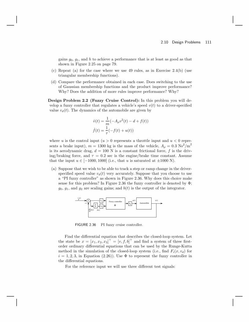
2.10 Design Problems 111
gains g0, g1, and h to achieve a performance that is at least as good as thatshown in Figure 2.25 on page 79.
(c) Repeat (a) for the case where we use 49 rules, as in Exercise 2.4(b) (usetriangular membership functions).
(d) Compare the performance obtained in each case. Does switching to the useof Gaussian membership functions and the product improve performance?Why? Does the addition of more rules improve performance? Why?
Design Problem 2.2 (Fuzzy Cruise Control): In this problem you will de-velop a fuzzy controller that regulates a vehicle’s speed v(t) to a driver-specifiedvalue vd(t). The dynamics of the automobile are given by
v(t) =1m
(−Aρv2(t) − d + f(t))
f(t) =1τ
(−f(t) + u(t))
where u is the control input (u > 0 represents a throttle input and u < 0 repre-sents a brake input), m = 1300 kg is the mass of the vehicle, Aρ = 0.3 Ns2/m2
is its aerodynamic drag, d = 100 N is a constant frictional force, f is the driv-ing/braking force, and τ = 0.2 sec is the engine/brake time constant. Assumethat the input u ∈ [−1000, 1000] (i.e., that u is saturated at ±1000 N).
(a) Suppose that we wish to be able to track a step or ramp change in the driver-specified speed value vd(t) very accurately. Suppose that you choose to usea “PI fuzzy controller” as shown in Figure 2.36. Why does this choice makesense for this problem? In Figure 2.36 the fuzzy controller is denoted by Φ;g0, g1, and g2 are scaling gains; and b(t) is the output of the integrator.
AutomobileΣ
v (t)u(t) v(t)
Fuzzy controllerg0
g1
g2
d
b(t)b(t)ddt
Φ
FIGURE 2.36 PI fuzzy cruise controller.
Find the differential equation that describes the closed-loop system. Letthe state be x = [x1, x2, x3] = [v, f, b] and find a system of three first-order ordinary differential equations that can be used by the Runge-Kuttamethod in the simulation of the closed-loop system (i.e., find Fi(x, vd) fori = 1, 2, 3, in Equation (2.26)). Use Φ to represent the fuzzy controller inthe differential equations.
For the reference input we will use three different test signals:

112 Chapter 2 / Fuzzy Control: The Basics
1. Test input 1 makes vd(t) = 18 m/sec (40.3 mph) for 0 ≤ t ≤ 10 andvd(t) = 22 m/sec (49.2 mph) for 10 ≤ t ≤ 30.
2. Test input 2 makes vd(t) = 18 m/sec (40.3 mph) for 0 ≤ t ≤ 10 andvd(t) increases linearly (a ramp) from 18 to 22 m/sec by t = 25 sec, andthen vd(t) = 22 for 25 ≤ t ≤ 30.
3. Test input 3 makes vd(t) = 22 for t ≥ 0 and we use x(0) = 0 as theinitial condition (this represents starting the vehicle at rest and suddenlycommanding a large increase in speed).
Use x(0) = [18, 197.2, 20] for test inputs 1 and 2. Why is x(0) = [18, 197.2, 20]
a reasonable choice for the initial conditions?Design the fuzzy controller Φ to get less than 2% overshoot, a rise-time
between 5 and 7 sec, and a settling time of less than 8 sec (i.e., reach towithin 2% of the final value within 8 sec) for the jump from 18 to 22 m/secin “test input 1” that is defined above. Also, for the ramp input (“test input2” above) it must have less than 1 mph (0.447 m/sec) steady-state error(i.e., at the end of the ramp part of the input have less than 1 mph error).Fully specify your controller (e.g., the membership functions, rule-base de-fuzzification, etc.) and simulate the closed-loop system to demonstrate thatit performs properly. Provide plots of v(t) and vd(t) on the same axis andu(t) on a different plot. For test input 3 find the rise-time, overshoot, 2%settling time, and steady-state error for the closed-loop system for the con-troller that you designed to meet the specifications for test input 1 and 2. Inyour simulations use the Runge-Kutta method and an integration step sizeof 0.01.
(b) Next, suppose that you are concerned with tracking a step change in vd(t)accurately and that you use the PD fuzzy controller shown in Figure 2.37.To represent the derivative, simply use a backward difference
c(t) =e(t) − e(t − h)
h
where h is the integration step size in your simulation (or it could be yoursampling period in an implementation).
ddt
AutomobileΣ
v (t)u(t) v(t)
Fuzzy controllerg
0
g1
g2
d
c(t)
Φ
FIGURE 2.37 PD fuzzy cruise controller.
Design a PD fuzzy controller to get less than 2% overshoot, a rise-timebetween 7 and 10 sec, and a settling time of less than 10 sec for test input 1

2.10 Design Problems 113
defined in (a). Also, for the ramp input (test input 2 in (a)) it must have lessthan 1 mph steady-state error to the ramp (i.e., at the end of the ramp partof the input, have less than 1mph error). Fully specify your controller andsimulate the closed-loop system to demonstrate that it performs properly.Provide plots of v(t) and vd(t) on the same axis and u(t) on a different plot.In your simulations use the Runge-Kutta method and an integration stepsize of 0.01.
Assume that x(0) = [18, 197.2] for test inputs 1 and 2 (hence we ignorethe derivative input in coming up with the state equations for the closed-loop system and simply use the approximation for c(t) that is shown aboveso that we have a two-state system). As a final test let x(0) = 0 and use testinput 3 defined in (a). For this, what is the rise-time, overshoot, 2% settlingtime, and steady state error for your controller?
(c) Explain the effect of the aerodynamic drag term and how you would redesigna rule-base to take this effect into account if you used vehicle velocity directlyas an input to the fuzzy controller.
An expanded version of this problem is given in Design Problem 2.4. There, PDcontrollers are used, and we show how to turn the cruise control problem into anautomated highway system control problem where the speeds of many vehiclesare regulated so that they can move together as a “platoon.”
Design Problem 2.3 (Fuzzy Control for a Thermal Process): This prob-lem is used to show how you can get into trouble in fuzzy control design if youdo not understand basic ideas from conventional control or if you do not tunethe controller properly. Suppose that you are given the thermal process shown inFigure 4.8 on page 209 described in Chapter 4 except that you use the plant
τ (s)q(s)
=1
s + 1
(this is a thermal process with slower dynamics than the one in Chapter 4).Note that q(t) > 0 corresponds to adding heat while q(t) < 0 corresponds tocooling. Suppose that we wish to track a unit-step input of desired temperaturedifference τd with zero steady-state tracking error. Using ideas from conventionalcontrol for linear systems, you would normally first choose to put a pole of thecompensator at zero since this would give you zero steady-state tracking error toa step input (why?). Next, for a linear control system design you might proceedwith the design of a cascaded lead controller (why?).
Now, rather than designing a linear controller, suppose that you decide to trya fuzzy controller that has as an output q(t) and inputs g0e(t) and g1e(t) wheree(t) = τd(t) − τ (t) and g0 and g1 are scaling gains (i.e., a PD fuzzy controller).That is, you are ignoring that you may need an integrator in the loop to effec-tively eliminate steady-state tracking error. For the PD fuzzy controller, use thesame membership functions as we did in Figure 2.9 on page 36 for the inverted
114 Chapter 2 / Fuzzy Control: The Basics
pendulum. Here, however, make the effective universes of discourse for e(t) ande(t), [−1, 1] and [−0.5, 0.5], respectively, and the effective universe of discoursefor q(t), [−20, 20] (i.e., the exact same output membership functions as for theinverted pendulum in Figure 2.9 on page 36). Use minimum for the premise andimplication and COG defuzzification. For the rule-base we simply modify the oneused in Table 2.1 on page 32 for the inverted pendulum: Specifically, simply mul-tiply each element of the body of Table 2.1 by −1 and use the resulting rule-basetable as a rule-base for the PD fuzzy controller (this shows one case where youcan reuse rule-bases in a convenient manner). Why is this a reasonable choice fora rule-base? To explain this, compare it to the pendulum’s rule-base and explainthe meaning of a few of the new rules for the thermal process.
(a) Design a linear controller that will result in zero steady-state tracking errorfor the step input, minimize the rise time, achieve less than 5% overshoot,and try to minimize the settling time (treat the tracking error and rise-timespecifications as your primary objectives, and the overshoot and settlingtime as your secondary objectives). Simulate the control system you design,and provide plots of τ versus t to verify that you meet the desired objectives.
(b) Simulate the fuzzy control system using the PD fuzzy controller describedabove. Plot q(t) and τ (t) and discuss the results. Use the Runge-Kuttamethod for simulation with an integration step size of 0.0005 and zero initialconditions.
(c) Even though it may be more appropriate to use a PI fuzzy controller, youcan tune the PD fuzzy controller to try to meet the above specifications.Tune the PD fuzzy controller by changing the scaling gains g0 and g1 tomeet the same objectives as stated in (a). Compare the results from (a) and(b).
(d) Is it fair to compare the linear and fuzzy controllers? Which uses morecomputations? Is nonlinear control (fuzzy control) really needed for thislinear plant?
Design Problem 2.4 (Fuzzy Control for an Automated Highway System):12
Due to increasing traffic congestion, there has been a renewed interest in the de-velopment of an automated highway system (AHS) in which high traffic flow ratesmay be safely achieved. Since many of today’s automobile accidents are causedby human error, automating the driving process may actually increase safetyon the highway. Vehicles will be driven automatically with on-board lateral andlongitudinal controllers. The lateral controllers will be used to steer the vehiclesaround corners, make lane changes, and perform additional steering tasks. Thelongitudinal controllers will be used to maintain a steady velocity if a vehicleis traveling alone (conventional cruise control), follow a lead vehicle at a safe
12. Reminder: Exercises or design problems that are particularly challenging (considering howfar along you are in the text) or that require you to help define part of the problem are
designated with a star (“”).
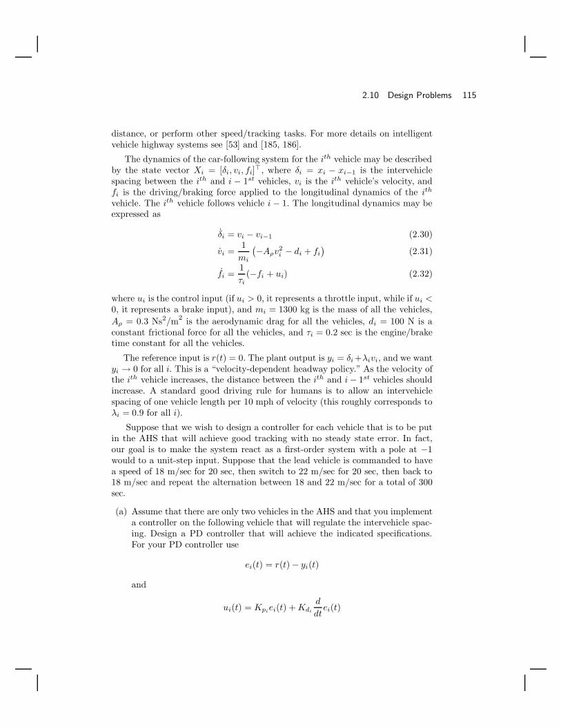
2.10 Design Problems 115
distance, or perform other speed/tracking tasks. For more details on intelligentvehicle highway systems see [53] and [185, 186].
The dynamics of the car-following system for the ith vehicle may be describedby the state vector Xi = [δi, vi, fi], where δi = xi − xi−1 is the intervehiclespacing between the ith and i − 1st vehicles, vi is the ith vehicle’s velocity, andfi is the driving/braking force applied to the longitudinal dynamics of the ith
vehicle. The ith vehicle follows vehicle i − 1. The longitudinal dynamics may beexpressed as
δi = vi − vi−1 (2.30)
vi =1
mi
(−Aρv2
i − di + fi
)(2.31)
fi =1τi
(−fi + ui) (2.32)
where ui is the control input (if ui > 0, it represents a throttle input, while if ui <0, it represents a brake input), and mi = 1300 kg is the mass of all the vehicles,Aρ = 0.3 Ns2/m2 is the aerodynamic drag for all the vehicles, di = 100 N is aconstant frictional force for all the vehicles, and τi = 0.2 sec is the engine/braketime constant for all the vehicles.
The reference input is r(t) = 0. The plant output is yi = δi +λivi, and we wantyi → 0 for all i. This is a “velocity-dependent headway policy.” As the velocity ofthe ith vehicle increases, the distance between the ith and i − 1st vehicles shouldincrease. A standard good driving rule for humans is to allow an intervehiclespacing of one vehicle length per 10 mph of velocity (this roughly corresponds toλi = 0.9 for all i).
Suppose that we wish to design a controller for each vehicle that is to be putin the AHS that will achieve good tracking with no steady state error. In fact,our goal is to make the system react as a first-order system with a pole at −1would to a unit-step input. Suppose that the lead vehicle is commanded to havea speed of 18 m/sec for 20 sec, then switch to 22 m/sec for 20 sec, then back to18 m/sec and repeat the alternation between 18 and 22 m/sec for a total of 300sec.
(a) Assume that there are only two vehicles in the AHS and that you implementa controller on the following vehicle that will regulate the intervehicle spac-ing. Design a PD controller that will achieve the indicated specifications.For your PD controller use
ei(t) = r(t) − yi(t)
and
ui(t) = Kpiei(t) + Kdi
d
dtei(t)

116 Chapter 2 / Fuzzy Control: The Basics
(b) Repeat (a) except use a fuzzy controller.
(c) Repeat (a) except use a sliding-mode controller.
(d) Compare the performance of the controllers and make recommendations onwhich one should be used. Be careful to tune each of the controllers as wellas you can so that you will feel confident about your recommendation ofwhich approach to use.
(e) Repeat (a)–(d) for five vehicles all with different masses, aerodynamic drags,and engine/brake time constants.
Design Problem 2.5 (Fuzzy Control for a Magnetic Ball SuspensionSystem): See the model of the magnetic ball suspension system shown inFigure 6.19 on page 366 in Chapter 6.
(a) Use the linear model given in Chapter 6 to design a linear controller thatachieves zero steady-state tracking error and a fast rise-time with as littleovershoot as possible. Demonstrate that the controller works properly for thelinear plant model. Next, investigate how it performs for the nonlinear plantmodel (you may need to pick a reference input that is small in magnitudewhen you test your system in simulation with the nonlinear plant model).
(b) Repeat (a) but design a conventional nonlinear controller for the nonlinearmodel of the system.
(c) Repeat (b) except use a fuzzy controller.
(d) Compare the performance of the fuzzy and conventional linear and nonlinearcontrollers. Be careful to tune each of the controllers as well as you can sothat you will feel confident about your recommendation of which approachto use.
Design Problem 2.6 (Fuzzy System Design for Basic Math Operations):In a PD controller, the plant input is generated by scaling the error and deriva-tive of the error and summing these two values. A fuzzy controller that uses theerror and derivative of the error as inputs can be designed to perform a similarscaling and summing operation (a linear operation), at least locally. For example,in the inverted pendulum problem we actually achieve such a scaling and sum-ming operation with the fuzzy controllers that we designed (provided that thefuzzy controller input signals are small). The scaling is actually achieved by thescaling gains, and the summing operation is achieved by the rule-base (recall thatthe pattern of the consequent linguistic-numeric values in Table 2.1 on page 32is achieved by adding the linguistic-numeric values associated with each of theinputs, taking the negative of the result, and saturating their values at +2 or−2). We see that fuzzy systems are capable of performing basic mathematicaloperations, at least on a region of their input space.

2.10 Design Problems 117
(a) Suppose that there are two inputs to the fuzzy system, x and y, and oneoutput, z. Define a fuzzy system that can add two numbers that lie withinthe regions x ∈ [−2, 2] and y ∈ [−1, 1]. Plot the three-dimensional nonlinearsurface induced by the fuzzy system.
(b) Repeat (a) for subtraction.
(c) Repeat (a) for multiplication.
(d) Repeat (a) for division.
(e) Repeat (a) for taking the maximum of two numbers.
(f) Repeat (a) for taking the minimum of two numbers.

118 Chapter 2 / Fuzzy Control: The Basics

C H A P T E R 3
Case Studiesin Design
and ImplementationExample is the school of mankind.
–Edmund Burke
3.1 OverviewAs indicated in Chapters 1 and 2, there is no generally applicable systematicmethodology for the construction of fuzzy controllers for challenging control ap-plications that is guaranteed to result in a high-performance closed-loop controlsystem. Hence, the best way to learn the basics of how to design fuzzy controllersis to do so yourself—and for a variety of applications. In this chapter we show howto design fuzzy controllers for a variety of applications in a series of case studies.We then include at the end of the chapter a variety of design problems that thereader can use to gain experience in fuzzy control system design.
Despite the lack of a general systematic design procedure, by reading this chap-ter you will become convinced that the fuzzy control design methodology doesprovide a way to design controllers for a wide variety of applications. Once themethodology is understood, it tends to provide a “way to get started,” a “way toat least get a solution,” and often a “way to quickly get a solution” for many typesof control problems. Indeed, we have found that if you focus on one application, a(somewhat) systematic design methodology for that application seems to emergefrom the fuzzy control approach. While the procedure is typically closely linkedto application-specific concepts and parameters and is therefore not generally ap-plicable to other plants, it does often provide a very nice framework in which thedesigner can think about how to achieve high-performance control.
119

120 Chapter 3 / Case Studies in Design and Implementation
You must keep in mind that the fuzzy controller has significant functional ca-pabilities (recall the universal approximation property described in Section 2.3.8 onpage 77) and therefore with enough work the designer should be able to achieve justabout anything that is possible in terms of performance (up to the computationallimits of the computer on which the controller is implemented). The problem is thatjust because the controller can be tuned does not mean that it is easy to tune, orthat the current framework in which you are tuning will work (e.g., you may notbe using the proper preprocessing of the fuzzy controller inputs or enough rules).We have found that while for some applications fuzzy control makes it easy to “dowhat makes sense” in terms of control, in others high performance is achieved onlyafter a significant amount of work on the part of the control designer, who must getthe best knowledge on how to control the system into the rule-base, which oftencan only occur by understanding the physics of the process very well.
Ultimately, the reader should always remember that the fuzzy control designprocess is nothing more than a heuristic technique for the synthesis of nonlinearcontrollers (there is nothing mystical about a fuzzy controller). For each of the casestudies and design problems, the reader should keep in mind that an underlyingnonlinearity is being shaped in the design of a fuzzy controller (recall that we showedthe nonlinear surface that results from a fuzzy controller in Figure 2.35 on page 89).The shape of this nonlinearity is what determines the behavior of the closed-loopsystem, and it is the task of the designer to get the proper control knowledge intothe rule-base so that this nonlinearity is properly shaped.
Conventional control provides a different approach to the construction of non-linear controllers (e.g., via feedback-linearization or sliding-mode control). Whenyou have a reasonably good model of the plant, which satisfies the necessaryassumptions—and even sometimes when it does not (e.g., for some PID controllersthat we design with no model or a very poor one)—then conventional control canoffer quite a viable solution to a control problem. Indeed, conventional control ismore widely used than fuzzy control (it is said that more than 90% of all controllersin operation are PID controllers), and for a variety of reasons may be a more viableapproach (see Chapters 1 and 8 for more discussion on the relative merits of fuzzyversus conventional control). Due to the success of conventional control, we placea particular emphasis in this book on comparative analysis of fuzzy versus conven-tional control; the reader will see this emphasis winding its way through the casestudies and design problems in this chapter. We believe that it is unwise to ignorepast successes in control in the excitement over trying fuzzy control.
In this chapter we begin, in Section 3.2, by providing an overview of a gen-eral methodology for fuzzy controller design (including issues in computer-aideddesign) and then show how to design fuzzy controllers for a variety of challengingapplications: a two-link flexible robot, a rotational inverted pendulum, a machinescheduling problem, and fuzzy decision-making systems. In each case study we havea specific objective in mind:
1. Vibration damping for a flexible-link robot (Section 3.3): Here, we illustratethe basic strength of the fuzzy control methodology, which is to use heuristic

3.1 Overview 121
information about how to achieve high-performance control. We explain in aseries of steps how to quantify control knowledge in a fuzzy controller andshow how performance can be subsequently improved. Moreover, we provideexperimental results in each case and especially highlight the importance ofunderstanding the physics of the underlying control problem so that appropriatecontrol rules can be designed. In Chapters 6 and 7 we will study adaptive andsupervisory fuzzy control techniques for this problem, and achieve even betterperformance than in this chapter, even for the case where a mass is added tothe second link’s endpoint.
2. Rotational inverted pendulum (Section 3.4): In this case study we first designa conventional linear controller for balancing the pendulum. Then we intro-duce a general procedure for incorporating these conventional control laws intoa fuzzy controller. In this way, for small signals the fuzzy controller will actlike a well-designed linear controller, and for larger signals the fuzzy controllernonlinearity can be shaped appropriately. Experimental results are provided tocompare the conventional and fuzzy control approaches. In Chapter 6 we showhow an adaptive fuzzy controller can be used to achieve very good balancingperformance even if a sealed bottle half-filled with water is attached to thependulum endpoint to create a disturbance.
3. Machine Scheduling (Section 3.5): Here, we show how a fuzzy controller canbe used to schedule part processing in a simple manufacturing system. Thiscase study is included to show how a fuzzy system has wide applicability sinceit can be used as a very general decision maker. Comparisons are made toconventional scheduling methods to try to uncover the advantages of fuzzycontrol. In Chapter 6 we extend the basic approach to provide an adaptivescheduler that can reconfigure itself to maintain throughput performance evenif there are unpredictable changes in the machine.
4. Fuzzy decision-making systems (Section 3.6): In this case study we explainthe various roles that fuzzy systems can serve in the implementation of generaldecision-making systems. Then we show how to construct fuzzy decision-makingsystems for providing warnings of the spread of an infectious disease and failurewarnings for an aircraft. This case study is used to show that fuzzy systemshave broad applicability outside the area of traditional feedback control.
When you complete this chapter, you will have solidified your understanding ofthe general fuzzy control system design methodology over that which was presentedin Chapter 2 for the academic inverted pendulum design problem. Also, you willhave gained an understanding of how to design fuzzy controllers for three specificapplications and fuzzy decision-making systems for several applications.
As indicated above, the case studies in this chapter will actually be usedthroughout the remainder of the book. In particular, they will be used in Chapter 6on adaptive fuzzy control and Chapter 7 on fuzzy supervisory control. Moreover,they will be used as design problems in this and these later chapters. Hence, you

122 Chapter 3 / Case Studies in Design and Implementation
will want to at least skim the case studies if you are concerned with understandingthe corresponding later case studies where we will use adaptive and supervisorycontrol for the same plants. However, the reader who wants to learn techniquesalone and is not as concerned with applications and implementations can skip thischapter.
3.2 Design MethodologyIn Chapter 2 we provided an introduction to how to design fuzzy controllers, andseveral basic guidelines for their design were provided in Section 2.4.4 on page 89.Here, we provide an overview of the design procedure that we have in mind whenwe construct the fuzzy controllers for the first two case studies in this chapter. Ourmethodology is as follows:
1. Try to understand the behavior of the plant, how it reacts to inputs, whatare the effects of disturbances, and what fundamental limitations it presents(e.g., nonminimum phase or unstable behavior). A clear understanding comesfrom studying the physics of the process, developing mathematical models, us-ing system identification methods, doing analysis, performing simulations, andusing heuristic knowledge about the plant dynamics. The analysis could in-volve studying stability, controllability, or observability of the plant; how fastthe plant can react to various inputs; or how noise propagates in the dynam-ics of the process (e.g., via stochastic analysis). The heuristic knowledge maycome from, for example, a human operator of the process or a control engi-neer. Sometimes, knowledge of the plant’s behavior comes from actually tryingout a controller on the system (e.g., a PID, lead-lag, state-feedback, or fuzzycontroller).
2. Gain a clear understanding of the closed-loop specifications (i.e., the perfor-mance objectives). These may be stated in terms of specifications on stability,rise-time, overshoot, settling time, steady-state error, disturbance rejection, ro-bustness, and so on. You should make sure that the performance objectives arereasonable and achievable, and that they properly characterize exactly what isdesired in terms of closed-loop behavior.
3. Establish the basic structure of the control system (here we assume that a“direct” (nonadaptive) controller is used). This will establish what the plantand controller inputs and outputs should be.
4. Perform an initial control design. This may be with a simple PID controller,some other linear technique (e.g., lead-lag compensation or state feedback), ora simple fuzzy controller (often you should first try a fuzzy PD, PI, or PIDcontroller). For some basic ideas on how to design fuzzy controllers, see Chap-ter 2, Section 2.4.4 on page 89. The basic approaches include (a) inclusion ofgood control knowledge, (b) tuning the scaling gains, (c) tuning the member-ship functions, and (d) adding more rules or membership functions. Work hard

3.2 Design Methodology 123
to tune the chosen method. Evaluate if the performance objectives are met viasimulations or mathematical analysis (such as that found in Chapter 4) if youhave a model.
5. If your simple initial approach to control is successful, begin working on animplementation. If it is not successful, first make sure that you are using solidcontrol engineering ideas to pick the “nonfuzzy” part of the controller (e.g.,the preprocessing of fuzzy controller inputs by choosing to use an integrator totry to remove steady-state error). If this does not work, consider the followingoptions:
• A more sophisticated conventional control method (e.g., feedback-linearizationor sliding-mode control).
• A more sophisticated fuzzy controller. You may need more inputs to thefuzzy controller or more rules in the rule-base. You should carefully con-sider if you have loaded the best knowledge about how to control theprocess into the rule-base (often, the problem with tuning a fuzzy con-troller boils down to a basic lack of understanding of how best to controlthe plant and the corresponding lack of knowledge in the rule-base).
• Try designing the fuzzy controller by using a well-designed linear controltechnique to specify the general shape of the control surface (especiallyaround zero) and then tune the surface starting from there (this approachis illustrated in this chapter for the rotational inverted pendulum).
• Conventional or fuzzy adaptive or supervisory control approaches (seeChapters 6 and 7).
Work hard to tune the chosen method. Evaluate if the performance objectivesare met.
6. Repeat the above process as often as necessary, evaluating the designs in sim-ulation and, if possible, implementation. When you have met the performanceobjectives for the implementation, you will likely have additional work including“burn-in” tests, marketing analyses, cost analyses, and other issues (of course,several of these will have to be considered much earlier in the design process).
Computer-aided design (CAD) packages are designed to try to help automatethe above process. While we recommend that you strongly consider their use, wemust reemphasize that it is best to first know how to program the fuzzy controllerin a high-level language before moving on to the use of CAD packages where theuser can be removed from understanding the low-level details of the operation offuzzy systems. Once fuzzy systems are well understood, you can use one of theexisting packages (e.g., the one currently in Matlab) or design a package on yourown. However, you should not dismiss the importance of knowing how to code afuzzy controller on your own. Often this is necessary for implementation anyway(e.g., in C or assembly language).
124 Chapter 3 / Case Studies in Design and Implementation
3.3 Vibration Damping for a Flexible RobotFor nearly a decade, control engineers and roboticists alike have been investigatingthe problem of controlling robotic mechanisms that have very flexible links. Suchmechanisms are important in space structure applications, where large, lightweightrobots are to be utilized in a variety of tasks, including deployment, spacecraftservicing, space-station maintenance, and so on. Flexibility is not designed into themechanism; it is usually an undesirable characteristic that results from trading offmass and length requirements in optimizing effectiveness and “deployability” of therobot. These requirements and limitations of mass and rigidity give rise to manyinteresting issues from a control perspective.
In this section we present a design case study that makes use of previous expe-rience in the modeling and control of a two-link planar flexible robot. First, though,we provide some motivation for why you would want to consider using fuzzy controlfor the robot.
The modeling complexity of multilink flexible robots is well documented, andnumerous researchers have investigated a variety of techniques for representing flex-ible and rigid dynamics of such mechanisms. Equally numerous are the works ad-dressing the control problem in simulation studies based on mathematical models,under assumptions of perfect modeling. Even in simulation, however, a challengingcontrol problem exists; it is well known that vibration suppression in slewing me-chanical structures whose parameters depend on the configuration (i.e., are timevarying) can be extremely difficult to achieve. Compounding the problem, numer-ous experimental studies have shown that when implementation issues are takeninto consideration, modeling uncertainties either render the simulation-based con-trol designs useless, or demand extensive tuning of controller parameters (often inan ad hoc manner).
Hence, even if a relatively accurate model of the flexible robot can be developed,it is often too complex to use in controller development, especially for many controldesign procedures that require restrictive assumptions for the plant (e.g., linearity).It is for this reason that conventional controllers for flexible robots are developedeither (1) via simple crude models of the plant behavior that satisfy the necessaryassumptions (e.g., the model we develop below), or (2) via the ad hoc tuning oflinear or nonlinear controllers. Regardless, heuristics enter the design process whenthe conventional control design process is used.
It is important to emphasize, however, that such conventional control-engineeringapproaches that use appropriate heuristics to tune the design have been relativelysuccessful. For a process such as a flexible robot, you are left with the followingquestion: How much of the success can be attributed to the use of the mathe-matical model and conventional control design approach, and how much should beattributed to the clever heuristic tuning that the control engineer uses upon im-plementation? While control engineers have a relatively good understanding of thecapabilities of conventional mathematical approaches to control, much less is un-derstood about whether or not control techniques that are designed to exploit theuse of heuristic information (such as fuzzy control approaches) can perform better

3.3 Vibration Damping for a Flexible Robot 125
than conventional techniques.In this section we show that fuzzy control can, in fact, perform quite well for
a particular two-link flexible robot. In Chapters 6 and 7 we will show how to useadaptive and supervisory fuzzy control for this same mechanism. These methodsbuild on the direct fuzzy control methods studied in this chapter and provide thebest controllers developed for this experiment to date (including many conventionalmethods).
3.3.1 The Two-Link Flexible RobotIn this section we describe the laboratory test bed, the control objectives, and howthe robot reacts to open-loop control.
Laboratory Test Bed
The two-link flexible robot shown in Figure 3.1 consists of three main parts: (1)the robot with its sensors, (2) the computer and the interface to the robot, and(3) the camera with its computer and interface. The robot is made up of two veryflexible links constrained to operate in the horizontal plane. The “shoulder link” is acounterbalanced aluminum strip that is driven by a DC direct-drive motor with aninput voltage v1. The “elbow link,” which is mounted on the shoulder link endpoint,is a smaller aluminum strip. The actuator for the elbow link is a geared DC motorwith an input voltage v2. The sensors on the robot are two optical encoders forthe motor shaft positions Θ1 and Θ2, and two accelerometers mounted on the linkendpoints to measure the accelerations a1 and a2.
Camera
a 1
a 2 Θ2
Θ1
v1
v 2
Camera dataacquisitioncomputer
Control computer
Motor voltageAmplifier Cards
EncoderInterface
Camerainterface
Lightsource Elbow link
Shoulder link Counterbalance
FIGURE 3.1 Two-link flexible robot setup (figure taken from[145], c© IEEE).
A line scan camera is used to monitor the endpoint position of the robot forplotting; this data is not used for feedback. The sampling period used for all sensorsand control updates is 15 milliseconds (ms). For comparative purposes, we use the

126 Chapter 3 / Case Studies in Design and Implementation
camera data for robot movements that begin in some position and end in a fullyextended position, to approximate equal movements in each joint. When responsesare plotted, the final endpoint position is nominally indicated (on the plot) to reflect(approximately) the total movement, in degrees, of the shoulder joint.
Objectives and Open-Loop Control
The primary objective of this case study is to develop a controller that makesthe robot move to its desired position as quickly as possible, with little or noendpoint oscillation. To appreciate the improvement in the plant behavior due tothe application of the various control strategies, we will first study how the robotoperates under the “no control” situation; that is, when no external digital controlalgorithm is applied for vibration compensation. To implement the no control case,we simply apply v1 = v2 = 0.3615 volts at t = 0 seconds and return v1 and v2 to zerovoltages as soon as the links reach their set-points. Note that for this experimentwe monitor the movement of the links but do not use this information as feedbackfor control.
The results of the “no control” experiment are plotted in Figure 3.2, where theendpoint position shows a significant amount of endpoint oscillation. As is typicalin mechanisms of this sort, inherent modal damping is present. It is well knownthat the effect of mass-loading a slewing flexible beam is to reduce the modalfrequencies and this is indeed the case for this experiment. Indeed, when a 30-grampayload is attached to the robot endpoint, the first modal frequency of the secondlink (endpoint) reduces significantly. This effect causes performance degradation infixed, linear controllers. In Figure 3.2, as in all plots to follow, endpoint positionrefers to the position of the elbow link endpoint. Note that the inset shown inFigure 3.2 depicts the robot slew employed. The two dashed lines describe theinitial position of the links. The arrows show the direction of movement, and thesolid line shows the final position of the links. Hence, for this open-loop experiment,we wanted 90 degrees of movement in each link. In the ideal case the shaft shouldstop moving the instant the voltage signal to the motor amplifier is cut off. Butthe arm had been moving at a constant velocity before the signal was cut off, andthus had a momentum that dragged the shaft past the angle at which it was tostop. This movement depends on the speed at which the arm was moving, which inturn depends on the voltage signal applied. Clearly, there is a significant need forvibration damping in endpoint positioning.
Quantitatively speaking, in terms of step-type responses (for motions throughlarge angles in each joint), the control objectives are as follows: system settling(elimination of residual vibrations in endpoint position) within 2 seconds of mo-tion initiation, and overshoot minimized to less than 5% deviation from the finaldesired position. In addition, we wish to achieve certain qualitative aspects such aseliminating jerky movements and having smooth transitions between commandedmotions.

3.3 Vibration Damping for a Flexible Robot 127
50
60
70
80
90
100
110
120
130
140
0 1 2 3 4 5 6 7
. . . . . . . . . . . . . . . . . . . . . . . . . . . . .
Time (sec)
End
poin
t pos
ition
(de
g)
FIGURE 3.2 Endpoint position: “No control” response(figure taken from [145], c© IEEE).
Model
While it is difficult to produce an accurate model of the two-link robot using mod-eling based on first principles, it is possible to perform system identification studiesfor this system to produce approximate linear models. Working along these lines,the authors in [243] developed linear models for the two-link flexible robot. In par-ticular, random inputs were injected via the voltage inputs, data was gathered atthe outputs, and a least squares method was used to compute the parameters oflinear models. Several experiments had to be performed since there are two inputsand four outputs. To identify transfer functions from the inputs to the shaft ve-locity and endpoint acceleration for the shoulder link, the elbow link was initiallyfixed at a 180-degree angle (directly in line) with the shoulder link. While voltagewas applied to one link it was set to zero for the other link so that it would not becommanded to move from its initial position. The sampling period for these sys-tem identification experiments is 20 ms (note that this is different from the 15-mssampling period used in our control implementation studies to follow). Note thatthe joint angles Θ1 and Θ2 must lie in a ±250-degree range, and v1 and v2 must liein a range of ±5 volts (the values are saturated beyond this point). The saturationconstraints should be considered part of the model (so that the resulting model isnonlinear).
Let ω1 and ω2 denote the shaft velocity of the shoulder and elbow joints, re-spectively. The models produced by the system identification experiments in [243]

128 Chapter 3 / Case Studies in Design and Implementation
are given by
ω1
v1=
−0.0166(z − 0.6427± j1.2174)(z − 1.4092)(z − 0.7385± j0.6288)(z − 0.8165± j0.2839)
(3.1)
ω2
v2=
−0.1(z − 1.8062± j1.7386)(z + 0.9825)(z − 0.7158± j0.615)(z − 0.8377± j0.2553)
These equations provide models for relating voltages to velocities, but we actuallyneed the models for relating voltages to positions. To get these, you can simplyuse a discrete approximation to an integrator (using a sampling period of 20 ms)concatenated with the models for velocities to obtain the positions Θ1 and Θ2.
The transfer functions that describe how the motor voltages affect the endpointaccelerations a1 and a2 were determined in a similar way in [243] and are given by
a1
v1=
0.1425(z − 0.9589± j0.9083)(z − 1.7945)(z − 0.7521± j0.573)(z − 0.9365± j0.139)
a2
v2=
−0.228(z − 1.5751)(z − 1.2402)(z − 0.9126)(z − 0.8387± j0.4752)
Experiments showed that lower-order models resulted in less accurate models andhigher-order ones did not seem to make any of the above models more accurate.Simple inspection of the root locations in the z-plane shows that parts of the dy-namics are especially lightly damped, which characterizes the vibration dampingchallenge for this problem.
Notice that we are ignoring certain cross-coupling effects in the model (e.g.,how v1 combined with v2 will affect a2); the effect of the movement of the modes,and hence plant parameters, due to mass-loading (these models are for a robot thatis not mass-loaded); the effects of the position of one link on the model used forthe other link; dead-zone nonlinearities due to the gearbox on the elbow motor;and many other characteristics. It is for these reasons that this model cannot beexpected to be a perfectly accurate representation of the two-link robot. It is correctonly under the experimental conditions outlined above. We present the model heremainly to give the reader an idea of the type of dynamics involved in this experimentand to use these models in a design problem at the end of the chapter.
We would like to emphasize that models that accurately characterize the cou-pling effects between the two links are particularly difficult to develop. This hassignificant effects on what is possible to illustrate in simulation, relative to whatcan be illustrated in implementation. For instance, in the two following subsectionswe will show that while an “uncoupled controller” (i.e., one where there are separatecontrollers for the shoulder and elbow links) performs adequately in implementa-tion, significant performance improvements can be obtained by using some heuristicideas about how to compensate for some of the coupling effects between the links

3.3 Vibration Damping for a Flexible Robot 129
(e.g., how v2 for the elbow link should be changed based on the acceleration a1 ofthe shoulder link so that the effects of the movement of the shoulder link on theelbow link can be tailored so that the endpoint vibrations can be reduced).
We have used least squares methods to identify linear models that attempt tocharacterize the coupling between the two links; however, we were not able to makethese accurate enough so that a coupled controller developed from these modelswould perform better than those developed as uncoupled controllers without thisinformation. Hence, the case study that follows is a good example of the case whereheuristic ideas about how to control a system proved to be more valuable than themodels we were able to produce for the system (and significantly less work wasneeded to specify the heuristic ideas about compensating for coupling effects thanwhat it took to try to construct models and develop controllers based on these).
3.3.2 Uncoupled Direct Fuzzy ControlIn this section and the next we investigate the use of two types of direct fuzzycontrollers for the flexible robot, one that uses information about the couplingeffects of the two links (coupled direct fuzzy control) and one that does not usesuch information (uncoupled direct fuzzy control). The design scenario we present,although specific to the flexible robot test bed under study, may be viewed asfollowing a general philosophy for fuzzy controller design where we are concernedwith loading good control knowledge into the rule-base.
For uncoupled direct fuzzy control, two separate controllers are implemented,one for each of the two links. Each controller has two inputs and one output, asshown in Figure 3.3. The term uncoupled is used since the controllers operate in-dependent of each other. No information is transferred between the shoulder andelbow motor controllers. We thus consider the robot to be made up of two separatesingle-link systems. In Figure 3.3, Θ1d and Θ2d denote the desired positions of theshoulder and elbow links, respectively, and Θ1(t) and Θ2(t) denote their positionat time t, as measured from the optical encoders. The inputs to the shoulder linkcontroller are the position error of the shoulder motor shaft e1(t) = Θ1d − Θ1(t),and the acceleration information a1(t) from the shoulder link endpoint. The out-put of this controller is multiplied by the output gain gv1 to generate the voltagesignal v1(t) that drives the shoulder motor amplifier. The inputs to the elbow linkcontroller are the elbow motor shaft position error e2(t) = Θ2d − Θ2(t) and theacceleration information from the elbow link endpoint a2(t). The output of thiscontroller is multiplied by the output gain gv2 to generate the voltage signal v2(t)that drives the elbow motor amplifier. We did experiment with using the changein position error of each link as an input to each of the link controllers but foundthat it significantly increased the complexity of the controllers with very little, ifany, improvement in overall performance; hence we did not pursue the use of thiscontroller input. Typically, we use filtered signals from the accelerometers, prior toprocessing, to enhance their effectiveness.
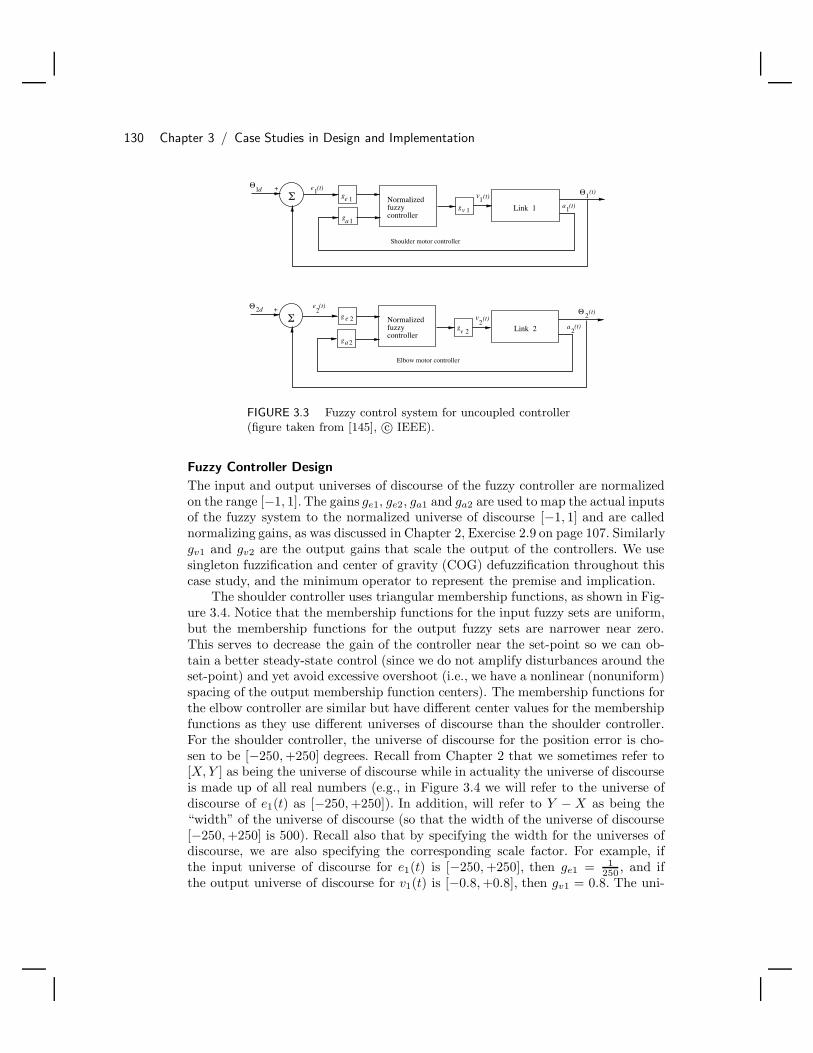
130 Chapter 3 / Case Studies in Design and Implementation
Normalized fuzzy controller
+
Link 2
ΘΘd
a2
Link 1Normalized fuzzy controller
+
Θd1
22Σ
Σ gegv
ga
Θ1(t)
a (t)1
e (t)1
e (t)2 (t)
(t)
Shoulder motor controller
Elbow motor controller
gv
g e
ga
(t)2
v
(t)1v1
1
1
2
2
2
FIGURE 3.3 Fuzzy control system for uncoupled controller(figure taken from [145], c© IEEE).
Fuzzy Controller Design
The input and output universes of discourse of the fuzzy controller are normalizedon the range [−1, 1]. The gains ge1, ge2, ga1 and ga2 are used to map the actual inputsof the fuzzy system to the normalized universe of discourse [−1, 1] and are callednormalizing gains, as was discussed in Chapter 2, Exercise 2.9 on page 107. Similarlygv1 and gv2 are the output gains that scale the output of the controllers. We usesingleton fuzzification and center of gravity (COG) defuzzification throughout thiscase study, and the minimum operator to represent the premise and implication.
The shoulder controller uses triangular membership functions, as shown in Fig-ure 3.4. Notice that the membership functions for the input fuzzy sets are uniform,but the membership functions for the output fuzzy sets are narrower near zero.This serves to decrease the gain of the controller near the set-point so we can ob-tain a better steady-state control (since we do not amplify disturbances around theset-point) and yet avoid excessive overshoot (i.e., we have a nonlinear (nonuniform)spacing of the output membership function centers). The membership functions forthe elbow controller are similar but have different center values for the membershipfunctions as they use different universes of discourse than the shoulder controller.For the shoulder controller, the universe of discourse for the position error is cho-sen to be [−250, +250] degrees. Recall from Chapter 2 that we sometimes refer to[X, Y ] as being the universe of discourse while in actuality the universe of discourseis made up of all real numbers (e.g., in Figure 3.4 we will refer to the universe ofdiscourse of e1(t) as [−250, +250]). In addition, will refer to Y − X as being the“width” of the universe of discourse (so that the width of the universe of discourse[−250, +250] is 500). Recall also that by specifying the width for the universes ofdiscourse, we are also specifying the corresponding scale factor. For example, ifthe input universe of discourse for e1(t) is [−250, +250], then ge1 = 1
250, and if
the output universe of discourse for v1(t) is [−0.8, +0.8], then gv1 = 0.8. The uni-

3.3 Vibration Damping for a Flexible Robot 131
verse of discourse for the endpoint acceleration of the shoulder link is [−4, +4] g.This width of 8 g was picked after experimentation with different slews at differentspeeds, upon observing the output of the acceleration sensor. The output universeof discourse of [−0.8, +0.8] volts was chosen so as to keep the shaft speed withinreasonable limits.
-50 -100-150-250 50 100 150 200-200 250 0
µ
(deg)e
0-1-2-3-4-5 54321
µ
(g)a
0-1-2-3-4-5 54321
0 -0.8-1.6-2.4-3.2 4.0-4.0 3.22.41.60.8
µ
(volts)
0-5 -4 -3 -2 -1 1 2 3 4 5
-0.1 0.1-0.2 0.20-0.4 0.4-0.6 0.6 0.8-0.8
11111111111
1 1111111 111
11111111 111
v
1
1
1
AAAA AAA AAAA
E E E E EE E E E EE
VVVVV V VVVVV
FIGURE 3.4 Membership functions for the shoulder controller(figure taken from [145], c© IEEE).
For the elbow motor controller, the universe of discourse for the error input is setto [−250, +250] degrees. This motor is mounted on the shoulder link endpoint andthe link movement is limited by the shoulder link. The universe of discourse for theacceleration input is set to [−8, +8] g, which was picked after several experiments.The universe of discourse for the output of the elbow controller is [−5, +5] volts.This universe of discourse is large compared to the shoulder link as this motor is ageared-head motor with a 30:1 reduction in the motor to the output shaft speed.
The rule-base array that we use for the shoulder controller is shown in Table 3.1,and for the elbow link, in Table 3.2. Each rule-base is an 11×11 array, as we have 11fuzzy sets on the input universes of discourse. The topmost row shows the indices forthe eleven fuzzy sets for the acceleration input a1, and the column at the extremeleft shows the indices for the eleven fuzzy sets for the position error input e1. Thebodies of the tables in Tables 3.1 and 3.2 show the indices m for V m
1 in fuzzyimplications of the form
If Ej1 and Ak
1 Then V m1
where Eji , Aj
i , and V ji denote the jth fuzzy sets associated with ei, ai, and vi,
respectively (i = 1, 2;−5 ≤ j ≤ +5). The number of rules used for the uncoupled

132 Chapter 3 / Case Studies in Design and Implementation
direct fuzzy controller is 121 for the shoulder controller, plus another 121 for theelbow controller, giving a total of 242 rules.
What is the rationale for these choices for the rule-bases? First, notice theuniformity of the indices in Tables 3.1 and 3.2. For example, for Table 3.1 if there isa positive error e1(t) > 0 and a positive acceleration a1(t) > 0, then the controllerwill input a positive voltage v1(t) > 0, since in this case the link is not properlyaligned but is moving in the proper direction. As the error (e1(t) > 0) decreases,and the acceleration (a1(t) > 0) decreases the controller applies smaller voltagesto try to avoid overshoot. The other part of Table 3.1 and all of Table 3.2 can beexplained in a similar way. Next, notice that for row j = 0 there are three zeros inthe center of both Tables 3.1 and 3.2. These zeros have been placed so as to reducethe sensitivity of the controller to the noisy measurements from the accelerometer.Via the interpolation performed by the fuzzy controller, these zeros simply lowerthe gain near zero to make the controller less sensitive so that it will not amplifydisturbances.
TABLE 3.1 Rule-Base for Shoulder Link
Ak1
V m1 −5 −4 −3 −2 −1 0 1 2 3 4 5
−5 −5 −5 −5 −4 −4 −3 −3 −2 −2 −1 0−4 −5 −5 −4 −4 −3 −3 −2 −2 −1 0 1−3 −5 −4 −4 −3 −3 −2 −2 −1 0 1 2−2 −4 −4 −3 −3 −2 −2 −1 0 1 2 2−1 −4 −3 −3 −2 −2 −1 0 1 2 2 3
Ej1 0 −4 −3 −2 −1 0 0 0 1 2 3 4
1 −3 −2 −2 −1 0 1 2 2 3 3 42 −2 −2 −1 0 1 2 2 3 3 4 43 −2 −1 0 1 2 2 3 3 4 4 54 −1 0 1 2 2 3 3 4 4 5 55 0 1 2 2 3 3 4 4 5 5 5
Experimental Results
The endpoint position response for the uncoupled fuzzy controller is shown in Fig-ure 3.5. The robot was commanded to slew 90 degrees for each link from the initialposition (shown by the dashed lines in the inset) to its fully extended position(shown by the solid lines). Other “counterrelative” and small-angle movementsproduced similar results in terms of the quality of the responses. From the plotin Figure 3.5, we see that the magnitude of the endpoint oscillations is reducedas compared to the “no control” case, and the settling time is also improved (seeFigure 3.2 on page 127). In the initial portion of the response (between 0.8 and 2.0sec), we see large oscillations due to the fact that the controllers are uncoupled.That is, the shoulder link comes close to its set-point at around 0.9 seconds butis still traveling at a high speed. When the controller detects this, it tries to cut

3.3 Vibration Damping for a Flexible Robot 133
TABLE 3.2 Rule-Base for Elbow Link
Ak2
V m2 −5 −4 −3 −2 −1 0 1 2 3 4 5
−5 −5 −5 −4 −4 −3 −3 −3 −2 −2 −1 0−4 −5 −4 −4 −3 −3 −3 −2 −2 −1 0 1−3 −4 −4 −3 −3 −3 −2 −2 −1 0 1 2−2 −4 −3 −3 −3 −2 −2 −1 0 1 2 2−1 −4 −3 −3 −2 −2 −1 0 1 2 2 3
Ej2 0 −4 −3 −2 −1 0 0 0 1 2 3 4
1 −3 −2 −2 −1 0 1 2 2 3 3 42 −2 −2 −1 0 1 2 2 3 3 3 43 −2 −1 0 1 2 2 3 3 3 4 44 −1 0 1 2 2 3 3 3 4 4 55 0 1 2 2 3 3 3 4 4 5 5
the speed of the link by applying an opposite voltage at around 0.9 seconds. Thiscauses the endpoint of the elbow link to accelerate due to its inertia, causing it tooscillate with a larger magnitude. When the controller for the elbow link detectsthis sudden change, it outputs a large control signal in order to move the shaft inthe direction of acceleration so as to damp these oscillations. Once the oscillationsare damped out, the controller continues to output signals until the set-point isreached.
30
40
50
60
70
80
90
100
110
0 1 2 3 4 5 6 7
Time (sec)
End
poin
t pos
ition
(de
g)
FIGURE 3.5 Endpoint position for uncoupled controller design(figure taken from [145], c© IEEE).

134 Chapter 3 / Case Studies in Design and Implementation
Note that a portion of the oscillation is caused by the dead-zone nonlinearityin the gearbox of the elbow motor. The sudden braking of the shoulder link causesthe elbow link to jerk, and the link oscillates in the dead-zone, creating what issimilar to a limit-cycle effect. One way of preventing these oscillations in the linkis to slow down the speed of the elbow link until the shoulder link is moving fastand speed it up as the shoulder link slows down. This would ensure that the elbowlink is not allowed to oscillate as the motor is moving fast, and that the driven geardoes not operate in the dead-zone. This control technique will be examined in thenext section when we couple the acceleration feedback signals from the robot.
Figure 3.6 shows the response of the plant with a payload. The payload usedwas a 30-gram block of aluminum attached to the elbow link endpoint. A slew of 90degrees for each link was commanded, as shown in the inset. The payload at the endof the elbow link increases the inertia of the link and reduces the modal frequenciesof oscillation. In this case this reduction in the frequency positively affected thecontroller’s ability to dampen the oscillation caused by the dead-zone, as comparedto the unloaded case shown in Figure 3.5.
30
40
50
60
70
80
90
100
110
0 1 2 3 4 5 6 7
Time (sec)
End
poin
t pos
ition
(de
g)
FIGURE 3.6 Endpoint position for uncoupled controller designwith payload (figure taken from [145], c© IEEE).
3.3.3 Coupled Direct Fuzzy ControlWhile the two uncoupled controllers provide reasonably good results, they are notable to take control actions that are directly based on the movements in both links.In this section we investigate the possibility of improving the performance by cou-

3.3 Vibration Damping for a Flexible Robot 135
pling the two controllers; this can be done by using either the position information,the acceleration information, or both. From the tests on the independent controllers,it was observed that the acceleration at the endpoint of the shoulder link signifi-cantly affected the oscillations of the elbow link endpoint, whereas the accelerationat the endpoint of the elbow link did not significantly affect the shoulder link. Theposition of one link does not have a significant effect on the vibrations in the other.As the primary objective here is to reduce the vibration at the endpoint as muchas possible while still achieving adequate slew rates, it was decided to couple thecontroller for the elbow link to the shoulder link using the acceleration feedbackfrom the endpoint of the shoulder link; this is shown schematically in Figure 3.7.Note that in addition to the six normalizing gains ge1, ge2, ga1, ga2, gv1, and gv2, aseventh gain ga12 is added to the system. This gain can also be varied to tune thecontroller and need not be the same as ga1.
Normalized fuzzy controller
+
Link 2
Θ Θd
a 2
Link 1Normalized fuzzy controller
+
Θ Θd
a 1
1 1
22Σ
Σ g e
g a
g v
(t)
(t)
(t)
ga
g e
a
e (t)1
e (t)2
(t)
g
g v
1(t)
2(t)
Shoulder motor controller
Elbow motor controller
v
v1
1
1
2
2
2
21
FIGURE 3.7 Coupled fuzzy controller (figure taken from [145],c© IEEE).
Fuzzy Controller Design
Essentially, in coupling the controllers we are using our experience and intuitionto redesign the fuzzy controller. The rule-base and the membership functions forthe shoulder link are kept the same as in Figure 3.4 and Table 3.1, and the rule-base for the elbow link is modified to include the acceleration information from theshoulder link endpoint. Adding a third premise term to the premises of the rulesin the rule-base in this manner will, of course, increase the total number of rules.The number of fuzzy sets for the elbow controller was therefore reduced to sevenin order to keep the number of rules at a reasonable level. The number of rulesfor the second link with seven fuzzy sets increased to 343 (7 × 7 × 7). Hence, the
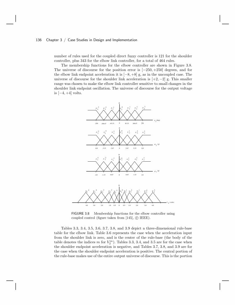
136 Chapter 3 / Case Studies in Design and Implementation
number of rules used for the coupled direct fuzzy controller is 121 for the shouldercontroller, plus 343 for the elbow link controller, for a total of 464 rules.
The membership functions for the elbow controller are shown in Figure 3.8.The universe of discourse for the position error is [−250, +250] degrees, and forthe elbow link endpoint acceleration it is [−8, +8] g, as in the uncoupled case. Theuniverse of discourse for the shoulder link acceleration is [+2,−2] g. This smallerrange was chosen to make the elbow link controller sensitive to small changes in theshoulder link endpoint oscillation. The universe of discourse for the output voltageis [−4, +4] volts.
250-250
0
µ
µ
(deg)
(g)a
0-1-2-3 321
e
0-1-2-3 321
|| | | |||
| | | | | | | 1
µ
a
2
(g)
|| | | |||
1 1 1 1 1 1 10-1-2-3 321
2 2 2 2 2 2 2
8.02.67-5.33 5.33-2.67-8.0
-0.67 0-1.33 1.330.67 2.0-2.0
83.33-166.67 -83.33 166.67 0
µ
(volts)
0-5
-4 -3 -2-1
1 2 3 4 5
0 0.50.5 1.01.0 2.02.0 3.03.0 4.04.0
| | | | | | | | | | | | |
E 2 E 2E 2 E 2
E 2E 2E 2
AAA
AAAAAAA
AAAA
VVVV VV V VV V V2 2 2 2 2 2 2 2 2 22
v 2
2
FIGURE 3.8 Membership functions for the elbow controller usingcoupled control (figure taken from [145], c© IEEE).
Tables 3.3, 3.4, 3.5, 3.6, 3.7, 3.8, and 3.9 depict a three-dimensional rule-basetable for the elbow link. Table 3.6 represents the case when the acceleration inputfrom the shoulder link is zero, and is the center of the rule-base (the body of thetable denotes the indices m for V m
2 ). Tables 3.3, 3.4, and 3.5 are for the case whenthe shoulder endpoint acceleration is negative, and Tables 3.7, 3.8, and 3.9 are forthe case when the shoulder endpoint acceleration is positive. The central portion ofthe rule-base makes use of the entire output universe of discourse. This is the portion

3.3 Vibration Damping for a Flexible Robot 137
of the rule-base where the acceleration input from the shoulder link endpoint is zeroor small. As we move away from the center of the rule-base (to the region wherethe shoulder link endpoint acceleration is large), only a small portion of the outputuniverse of discourse is used to keep the output of the controller small. Thus thespeed of the elbow link is dependent on the acceleration input from the shoulderlink endpoint. The speed of the elbow link is decreased if the acceleration is largeand is increased as the acceleration input decreases.
TABLE 3.3 A−31 portion of Rule-Base Array for the
Elbow Link
A−31 Ak
2
V m2 −3 −2 −1 0 1 2 3
−3 −3 −3 −2 −2 −1 −1 0−2 −3 −2 −2 −1 −1 0 1−1 −2 −2 −1 −1 0 1 1
Ej2 0 −2 −1 −1 0 1 1 2
1 −1 −1 0 1 1 2 22 −1 0 1 1 1 2 23 0 1 1 1 2 2 2
TABLE 3.4 A−21 portion of Rule-Base Array for the
Elbow Link
A−21 Ak
2
V m2 −3 −2 −1 0 1 2 3
−3 −3 −3 −3 −2 −2 −1 0−2 −3 −3 −2 −1 −1 0 1−1 −3 −2 −2 −1 0 1 1
Ej2 0 −2 −2 −1 0 1 2 2
1 −2 −1 0 1 1 2 22 −1 0 1 1 2 2 23 0 1 1 2 2 2 3
Also note that in Tables 3.5, 3.6, and 3.7 there are three zeros in the middlerows to reduce the sensitivity of the controller to the noisy accelerometer signal.This noise is not a significant problem when the endpoint is oscillating, and sothe rule-base does not have the zeros in the outer region. Taking the rule-base asa three-dimensional array, we get a central cubical core made up of zeros. Alsonotice that some parts of the rule-base, especially toward the extremes of the thirddimension, are not fully uniform. This has been done to slow down the elbow linkwhen the acceleration input from the shoulder link is very large. Overall, we seethat we are incorporating our understanding of the physics of the plant into the

138 Chapter 3 / Case Studies in Design and Implementation
TABLE 3.5 A−11 portion of Rule-Base Array for the
Elbow Link
A−11 Ak
2
V m2 −3 −2 −1 0 1 2 3
−3 −4 −4 −3 −3 −2 −1 0−2 −4 −3 −3 −2 −1 0 1−1 −3 −3 −2 −1 0 1 1
Ej2 0 −2 −2 0 0 0 1 2
1 −2 −1 0 1 2 2 32 −1 0 1 2 2 3 33 0 1 2 2 3 3 3
TABLE 3.6 A01 portion of Rule-Base Array for the
Elbow Link
A01 Ak
2
V m2 −3 −2 −1 0 1 2 3
−3 −5 −4 −4 −3 −3 −2 0−2 −4 −4 −3 −2 −1 0 1−1 −4 −3 −2 −1 0 1 2
Ej2 0 −2 −1 0 0 0 1 2
1 −2 −1 0 1 2 3 42 −1 0 2 2 3 4 43 0 1 2 3 4 4 5
rule-base. We are shaping the nonlinearity of the fuzzy controller to try to improveperformance.
The coupled direct fuzzy controller seeks to vary the speed of the elbow linkdepending on the amplitude of oscillations in the shoulder link. If the shoulder linkis oscillating too much, the speed of the elbow link is reduced so as to allow theoscillations in the shoulder link to be damped; and if there are no oscillations inthe shoulder link, then the second link speed is increased. We do this to eliminatethe oscillation of the elbow link close to the set-point, where the control voltagefrom the elbow controller is small. This scheme works well as will be shown bythe results, but the drawback is that it slows down the overall plant response ascompared to the uncoupled case (i.e., it slows the slew rate).
Experimental Results
The experimental results obtained using coupled direct fuzzy control are shown inFigure 3.9. The slew requested here is the same as in the case of the uncoupled directfuzzy control experiment (Figure 3.5) as shown by the inset—that is, 90 degrees foreach link. We also ran experiments for “counterrelative” and small-angle slews andobtained results of a similar nature. Note that there is no overshoot in the response,

3.3 Vibration Damping for a Flexible Robot 139
TABLE 3.7 A11 portion of Rule-Base Array for the
Elbow Link
A11 Ak
2
V m2 −3 −2 −1 0 1 2 3
−3 −4 −3 −3 −2 −2 −1 0−2 −3 −3 −2 −2 −1 0 1−1 −3 −2 −2 −1 0 1 2
Ej2 0 −2 −1 0 0 0 1 2
1 −2 −1 0 1 2 3 32 −1 0 1 2 3 3 43 0 1 2 3 3 4 4
TABLE 3.8 A21 portion of Rule-Base Array for the
Elbow Link
A21 Ak
2
V m2 −3 −2 −1 0 1 2 3
−3 −3 −2 −2 −1 −1 −1 0−2 −3 −2 −2 −1 −1 0 1−1 −2 −2 −1 −1 0 1 2
Ej2 0 −2 −1 −1 0 1 1 2
1 −1 −1 0 1 1 2 32 −1 0 1 1 2 3 33 0 1 2 2 3 3 4
with negligible residual vibrations. The dip in the curve in the initial part of thegraph is due to the first link “braking” as it reaches the set-point and is primarilydue to the dead-zone nonlinearity in the gears. As the shoulder link brakes, theelbow link is accelerated due to its inertia. The elbow link, which was at one end ofits dead-zone while the shoulder was moving, shoots to the other end of the dead-zone, causing the local maxima seen in Figure 3.9 at around 0.9 seconds. The linkrecoils due to its flexibility and starts moving to the lower end of the dead-zone. Bythis time the elbow motor speed increases and prevents further oscillation of theelbow link in the dead-zone.
Notice that the multiple oscillations in the elbow link have been eliminated ascompared to Figure 3.5 on page 133. This is due to the fact that when the shoulderlink reaches its set-point, the elbow link is still away from its set-point, and as theshoulder link slows down, the elbow link motor speeds up and keeps the elbow linkat one end of the dead-zone, preventing oscillation. Also notice that the rise time hasincreased in this case compared to that of the uncoupled case due to the decreasein speed of the second link while the first link is moving. This fact (increase inrise-time) and, especially, the schema embodied in the coupled-controller rule-basecontribute to the reduction in endpoint residual vibration.
Experimentally, we have determined that the dip in the curve can be decreased,

140 Chapter 3 / Case Studies in Design and Implementation
TABLE 3.9 A31 portion of Rule-Base Array for the
Elbow Link
A31 Ak
2
V m2 −3 −2 −1 0 1 2 3
−3 −2 −2 −2 −1 −1 −1 0−2 −2 −2 −1 −1 −1 0 1−1 −2 −2 −1 −1 0 1 2
Ej2 0 −2 −1 −1 0 1 1 2
1 −1 −1 0 1 1 2 22 −1 0 1 1 2 2 33 0 1 1 2 2 3 3
but not completely eliminated as the rule-base does not have enough “granularity”near zero (i.e., enough membership functions and rules). To alleviate this problem,a “supervisor” can be used to change the granularity of the rule-base as the shoulderlink comes close to its desired set-point by changing the universes of discourse andthe appropriate normalizing gains. This would produce finer control close to the set-point, resulting in a smoother transition in the speed of the shoulder link (this effectcould also be achieved via the addition of more membership functions and hencerules, but this will adversely affect computational complexity). We will investigatethe use of such a supervisor in Chapter 7.
40
50
60
70
80
90
100
110
0 1 2 3 4 5 6 7
Time (sec)
End
poin
t pos
ition
(de
g)
FIGURE 3.9 Endpoint position for coupled controller design(figure taken from [145], c© IEEE).

3.3 Vibration Damping for a Flexible Robot 141
Figure 3.10 shows the endpoint response of the robot with a 30-gram payloadattached to its endpoint. The commanded slew is 90 degrees for each link, as shownin the inset. Notice that the dip in the curve (between 1.0 and 1.5 sec) is reduced ascompared to the case without a payload (Figure 3.9). This is due to the increasedinertia of the elbow link, which reduces the frequency of oscillation of the link,as the elbow link motor speeds up at this point, preventing further oscillations.Obviously, there is performance degradation relative to Figure 3.9 due to the factthat the modal frequencies of the flexible links (particularly the elbow link) havechanged with the additional payload attached to the endpoint.
30
40
50
60
70
80
90
100
110
0 1 2 3 4 5 6 7
Time (sec)
End
poin
t pos
ition
(de
g)
FIGURE 3.10 Endpoint position for coupled controller designwith payload (figure taken from [145], c© IEEE).
This completes our case study for direct fuzzy control of the flexible robot.The reader should note that while the performance obtained here compares fa-vorably with all previous conventional control approaches studied to date for thisexperimental apparatus, it is not the best possible. In particular, we will show inChapter 6 how to use adaptive fuzzy control to synthesize and later tune the fuzzycontroller when there are payload variations. Moreover, we will show in Chapter 7how a supervisory fuzzy control approach can be used to incorporate abstract ideasabout how to achieve high-performance control and in fact improve performanceover the direct and adaptive fuzzy control approaches (and all past conventionalmethods).
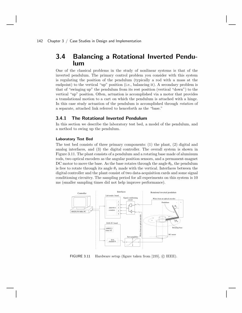
142 Chapter 3 / Case Studies in Design and Implementation
3.4 Balancing a Rotational Inverted Pendu-lum
One of the classical problems in the study of nonlinear systems is that of theinverted pendulum. The primary control problem you consider with this systemis regulating the position of the pendulum (typically a rod with a mass at theendpoint) to the vertical “up” position (i.e., balancing it). A secondary problem isthat of “swinging up” the pendulum from its rest position (vertical “down”) to thevertical “up” position. Often, actuation is accomplished via a motor that providesa translational motion to a cart on which the pendulum is attached with a hinge.In this case study actuation of the pendulum is accomplished through rotation ofa separate, attached link referred to henceforth as the “base.”
3.4.1 The Rotational Inverted PendulumIn this section we describe the laboratory test bed, a model of the pendulum, anda method to swing up the pendulum.
Laboratory Test Bed
The test bed consists of three primary components: (1) the plant, (2) digital andanalog interfaces, and (3) the digital controller. The overall system is shown inFigure 3.11. The plant consists of a pendulum and a rotating base made of aluminumrods, two optical encoders as the angular position sensors, and a permanent-magnetDC motor to move the base. As the base rotates through the angle θ0 , the pendulumis free to rotate through its angle θ1 made with the vertical. Interfaces between thedigital controller and the plant consist of two data-acquisition cards and some signalconditioning circuitry. The sampling period for all experiments on this system is 10ms (smaller sampling times did not help improve performance).
V
AM9513timer #2
D/Achannel 0
DAS-20 board
1
2
3
4
5
AM 9513counters
Lab tender board
circuit
Servoamplifier
θ1
θ0
486DX/50 MHz PC
-
+
Wires from an optical encoderSignal conditioning
Wir
es f
rom
an
optic
al e
ncod
er
DC motor
Rotating base
Pendulum
Interfaces Rotational inverted pendulumController
+-
FIGURE 3.11 Hardware setup (figure taken from [235], c© IEEE).

3.4 Balancing a Rotational Inverted Pendulum 143
Model
The differential equations that approximately describe the dynamics of the plantare given by
θ0 = −apθ0 + Kp va
θ1 = −C1
J1θ1 +
m1 g l1J1
sin(θ1) + K1θ0
where, again, θ0 is the angular displacement of the rotating base, θ0 is the angularspeed of the rotating base, θ1 is the angular displacement of the pendulum, θ1 is theangular speed of the pendulum, va is the motor armature voltage, Kp = 74.8903rad-s−2-v−1 and ap = 33.0408 s−2 are parameters of the DC motor with torqueconstant K1 = 1.9412× 10⁻³ kg-m/rad, g = 9.8066 m/sec2 is the acceleration dueto gravity, m1 = 0.086184 kg is the pendulum mass, l1 = 0.113 m is the pendulumlength, J1 = 1.3011×10⁻³ N-m-s2 is the pendulum inertia, and C1 = 2.9794×10⁻³
N-m-s/rad is a constant associated with friction. Note that the sign of K1 dependson whether the pendulum is in the inverted or noninverted position. In particular,for π
2 < θ1 < 3π2 (pendulum hanging down) we have K1 = 1.9412 × 10⁻³, and
K1 = −1.9412×10⁻³ otherwise. Hence, to properly simulate the system you changethe sign of K1 depending on the value of θ1.
For controller synthesis we will require a state-variable description of the pen-dulum system. This is easily done by defining state variables x1 = θ0, x2 = θ0,x3 = θ1 , and x4 = θ1, and control signal u = va to get
x1 = x2 (3.2)x2 = −ap x2 + Kp u
x3 = x4
x4 = −K1 ap
J1x2 +
m1 g l1J1
sin(x3) −C1
J1x4 +
K1 Kp
J1u
Linearization of these equations about the vertical position (i.e., θ1 = 0), resultsin the linear, time-invariant state variable model
x1
x2
x3
x4
=
0 1 0 00 −33.04 0 00 0 0 10 49.30 73.41 −2.29
x1
x2
x3
x4
+
074.89
0−111.74
u
Clearly, we cannot expect the above models to perfectly represent the physicalsystem. We are ignoring saturation effects, motor dynamics, friction and dead-zonenonlinearities for movement of the links, and other characteristics. We present themodel here to give the reader an idea of how the physical system behaves and tomake it possible for the reader to study fuzzy controller design and simulation inthe design problems at the end of the chapter.

144 Chapter 3 / Case Studies in Design and Implementation
Swing-Up Control
Because we intend to develop control laws that will be valid in regions about thevertical up position, it is necessary to swing the pendulum up so that it is nearvertical at near zero angular velocity. Elaborate schemes can be used for this task,but for the purposes of this case study, we choose to use a simple heuristic procedurecalled an “energy-pumping strategy.”
The goal of this simple swing-up strategy is to “pump” energy into the pendu-lum link in such a way that the energy or magnitude of each swing increases untilthe pendulum approaches its inverted position. To apply such an approach, considerhow you would (intuitively) swing the pendulum from its vertical down position toits vertical up position. If the rotating base is repeatedly swung to the left and thenright at an appropriate magnitude and frequency, the magnitude of the pendulumangle θ1 relative to the down position will increase with each swing. Swinging thependulum in this fashion is continued until θ1 is close to zero (vertical up), and wetry to design the swing up strategy so that θ1 is also near zero at this point (so thatit is nearly balanced for an instant). Then, the swing up controller is turned off anda “balancing controller” is used to catch and balance the pendulum (we switch theswing-up controller off and the balancing controller on when |θ1| < 0.3 rad). Next,we explain the details of how such a swing-up strategy can be implemented.
Suppose that initially θ1(0) = π and θ0(0) = 0. We use a swing-up strategythat has u = Kp(θref
0 −θ0) where θref0 is switched between +Γ and −Γ where Γ > 0
is a parameter that specifies the amplitude of the rotating base movement duringswing-up. The criterion for switching between ±Γ is that if the pendulum base ismoving toward +Γ then we use u = Kp(Γ − θ0) until θ1 is close to zero (indicatingthat the pendulum has swung up as far as it can for the given movement from thebase). Then we switch the control to u = Kp(−Γ − θ0) to drive the base in theother direction until θ1 is close to zero again. Then the process repeats until thependulum position is brought close to the vertical up position, where the swing-up control is turned off and the balancing control is switched on. In addition tomanual tuning of Γ, it is necessary for the operator of the experiment to performsome initial tuning for the positioning control gain Kp. Basically, the gain Kp ischosen just large enough so that the actuator drives the base fast enough withoutsaturating the control output.
Finally, we note that if the dynamics of the pendulum are changed (e.g., addingextra weight to the endpoint of the pendulum), then the parameter Γ must beretuned by the operator of the experiment. Moreover, retuning is sometimes evenneeded if the temperature in the room changes.
3.4.2 A Conventional Approach to Balancing ControlAlthough numerous linear control design techniques have been applied to this par-ticular system, here we consider the performance of only the linear quadratic reg-ulator (LQR) [3, 12]. Our purpose is twofold: First, we wish to form a baseline forcomparison to fuzzy control designs to follow, and second, we wish to provide astarting point for synthesis of the fuzzy controller.
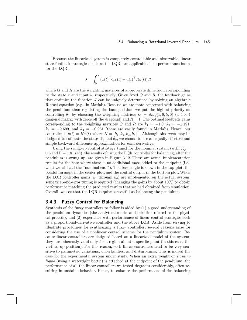
3.4 Balancing a Rotational Inverted Pendulum 145
Because the linearized system is completely controllable and observable, linearstate-feedback strategies, such as the LQR, are applicable. The performance indexfor the LQR is
J =∫ ∞
0
(x(t)Qx(t) + u(t)Ru(t))dt
where Q and R are the weighting matrices of appropriate dimension correspondingto the state x and input u, respectively. Given fixed Q and R, the feedback gainsthat optimize the function J can be uniquely determined by solving an algebraicRiccati equation (e.g., in Matlab). Because we are more concerned with balancingthe pendulum than regulating the base position, we put the highest priority oncontrolling θ1 by choosing the weighting matrices Q = diag(1, 0, 5, 0) (a 4 × 4diagonal matrix with zeros off the diagonal) and R = 1. The optimal feedback gainscorresponding to the weighting matrices Q and R are k1 = −1.0, k2 = −1.191,k3 = −9.699, and k4 = −0.961 (these are easily found in Matlab). Hence, ourcontroller is u(t) = Kx(t) where K = [k1, k2, k3, k4]. Although observers may bedesigned to estimate the states θ1 and θ0, we choose to use an equally effective andsimple backward difference approximation for each derivative.
Using the swing-up control strategy tuned for the nominal system (with Kp =0.5 and Γ = 1.81 rad), the results of using the LQR controller for balancing, after thependulum is swung up, are given in Figure 3.12. These are actual implementationresults for the case where there is no additional mass added to the endpoint (i.e.,what we will call the “nominal case”). The base angle is shown in the top plot, thependulum angle in the center plot, and the control output in the bottom plot. Whenthe LQR controller gains (k1 through k4) are implemented on the actual system,some trial-and-error tuning is required (changing the gains by about 10%) to obtainperformance matching the predicted results that we had obtained from simulation.Overall, we see that the LQR is quite successful at balancing the pendulum.
3.4.3 Fuzzy Control for BalancingSynthesis of the fuzzy controllers to follow is aided by (1) a good understanding ofthe pendulum dynamics (the analytical model and intuition related to the physi-cal process), and (2) experience with performance of linear control strategies suchas a proportional-derivative controller and the above LQR. Aside from serving toillustrate procedures for synthesizing a fuzzy controller, several reasons arise forconsidering the use of a nonlinear control scheme for the pendulum system. Be-cause linear controllers are designed based on a linearized model of the system,they are inherently valid only for a region about a specific point (in this case, thevertical up position). For this reason, such linear controllers tend to be very sen-sitive to parametric variations, uncertainties, and disturbances. This is indeed thecase for the experimental system under study. When an extra weight or sloshingliquid (using a watertight bottle) is attached at the endpoint of the pendulum, theperformance of all the linear controllers we tested degrades considerably, often re-sulting in unstable behavior. Hence, to enhance the performance of the balancing
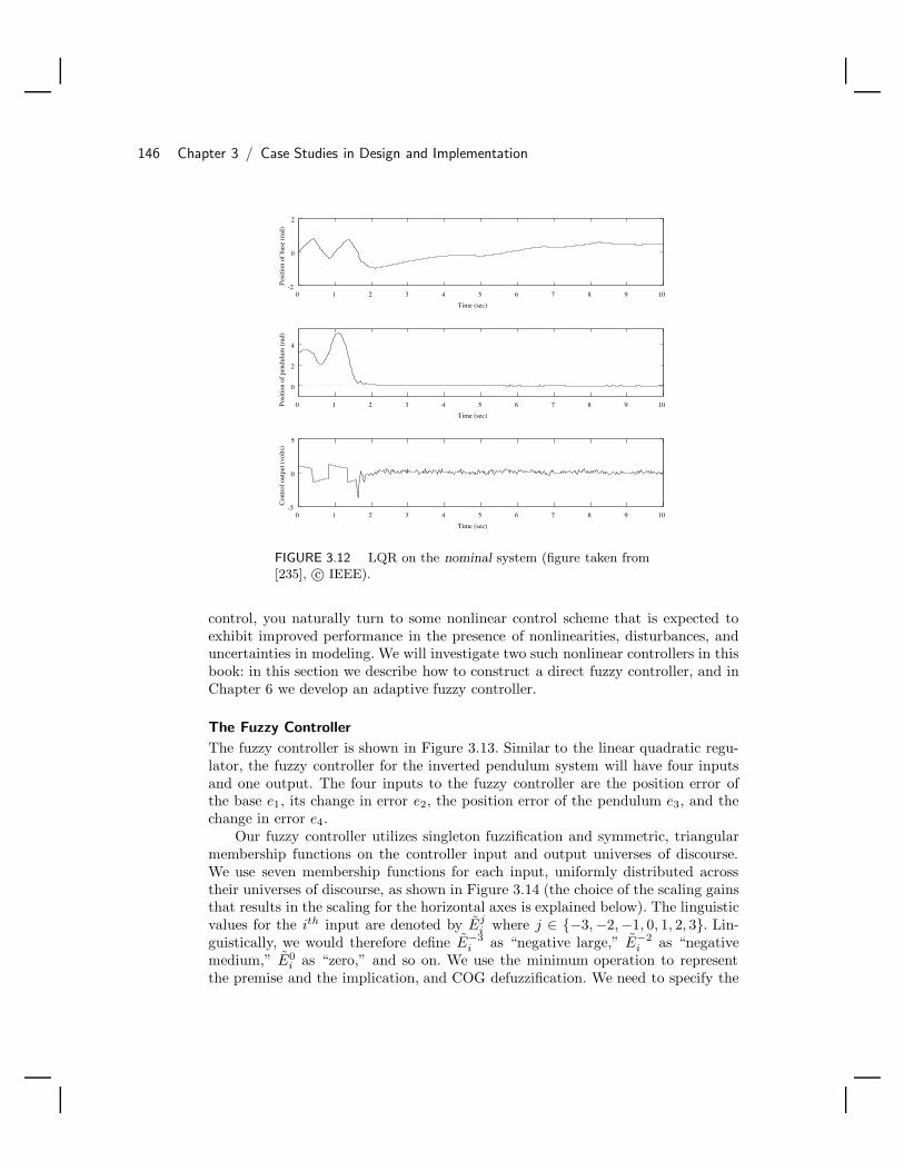
146 Chapter 3 / Case Studies in Design and Implementation
0 1 2 3 4 5 6 7 8 9 10-2
0
2
Time (sec)
Posi
tion
of b
ase
(rad
)
0 1 2 3 4 5 6 7 8 9 10
0
2
4
Time (sec)
Posi
tion
of p
endu
lum
(ra
d)
0 1 2 3 4 5 6 7 8 9 10-5
0
5
Time (sec)
Con
trol
out
put (
volts
)
FIGURE 3.12 LQR on the nominal system (figure taken from[235], c© IEEE).
control, you naturally turn to some nonlinear control scheme that is expected toexhibit improved performance in the presence of nonlinearities, disturbances, anduncertainties in modeling. We will investigate two such nonlinear controllers in thisbook: in this section we describe how to construct a direct fuzzy controller, and inChapter 6 we develop an adaptive fuzzy controller.
The Fuzzy Controller
The fuzzy controller is shown in Figure 3.13. Similar to the linear quadratic regu-lator, the fuzzy controller for the inverted pendulum system will have four inputsand one output. The four inputs to the fuzzy controller are the position error ofthe base e1, its change in error e2, the position error of the pendulum e3, and thechange in error e4.
Our fuzzy controller utilizes singleton fuzzification and symmetric, triangularmembership functions on the controller input and output universes of discourse.We use seven membership functions for each input, uniformly distributed acrosstheir universes of discourse, as shown in Figure 3.14 (the choice of the scaling gainsthat results in the scaling for the horizontal axes is explained below). The linguisticvalues for the ith input are denoted by Ej
i where j ∈ −3,−2,−1, 0, 1, 2, 3. Lin-guistically, we would therefore define E−3
i as “negative large,” E−2i as “negative
medium,” E0i as “zero,” and so on. We use the minimum operation to represent
the premise and the implication, and COG defuzzification. We need to specify the
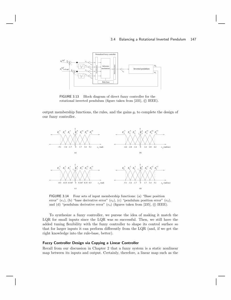
3.4 Balancing a Rotational Inverted Pendulum 147
Σ
Σθ0
ref
θ1ref
= 0 rad
1 - z-1
T
θ1
θ0
Fuzz
ific
atio
n
Def
uzzi
fica
tion
Inferencemechanism
g4
g 3
g2
g1
g0
e 1
e 2
e 3
e 4
+
-
-
+
Inverted pendulum
Rule-base
Normalized fuzzy controller
1 - z-1
T
FIGURE 3.13 Block diagram of direct fuzzy controller for therotational inverted pendulum (figure taken from [235], c© IEEE).
output membership functions, the rules, and the gains gi to complete the design ofour fuzzy controller.
e1
3e
e2
e4
(b)(a)
(c) (d)
E1
+3E1
0
1
0
E+3
E 0
1
-0.5 -0.167-0.33 0 0.50.330.167
E+3
E 0
1
0
E+3
E 0
1
0
E-3
1 E1
-2E1
-1E1
+1E1
+2
E-3
E-2
E-1
E+1
E+2
E-3
E-2
E-1
E+1
E+2
E-3
E-2
E-1
E+1
E+2
2 2 2 2 2 2 2
3 3 3 3 3 3 3 4 4 4 4 4 4 4
-5.1 5.1
3.4 5.1
-1.7-3.4 1.7 3.4 -1.4-2.8-4.2 1.4 2.8 4.2
-1.7-3.4-5.1 1.7
(rad)
(rad)
(rad/sec)
(rad/sec)
FIGURE 3.14 Four sets of input membership functions: (a) “Base positionerror” (e1), (b) “base derivative error” (e2), (c) “pendulum position error” (e3),and (d) “pendulum derivative error” (e4) (figures taken from [235], c© IEEE).
To synthesize a fuzzy controller, we pursue the idea of making it match theLQR for small inputs since the LQR was so successful. Then, we still have theadded tuning flexibility with the fuzzy controller to shape its control surface sothat for larger inputs it can perform differently from the LQR (and, if we get theright knowledge into the rule-base, better).
Fuzzy Controller Design via Copying a Linear Controller
Recall from our discussion in Chapter 2 that a fuzzy system is a static nonlinearmap between its inputs and output. Certainly, therefore, a linear map such as the

148 Chapter 3 / Case Studies in Design and Implementation
LQR can be easily approximated by a fuzzy system (at least for small values ofthe inputs to the fuzzy system). Two components of the LQR are the optimalgains and the summation operation; the optimal gains can be replaced with thescaling gains of a fuzzy system, and the summation can essentially be incorporatedinto the rule-base of a fuzzy system. By doing this, we can effectively utilize afuzzy system to expand the region of operation of the controller beyond the “linearregion” afforded by the design process that relied on linearization. Intuitively, this isdone by making the “gain” of the fuzzy controller match that of the LQR when thefuzzy controller inputs are small, while shaping the nonlinear mapping representingthe fuzzy controller for larger inputs (in regions further from zero).
Implementing the summation operation in the rule-base is straightforward.First, we assume that all the input universes of discourse have uniformly distributedtriangular membership functions, such as those shown in Figure 3.14, but with ef-fective universes of discourse all given by [−1, +1] (i.e., so that the left-most mem-bership function and the right-most membership function saturate at −1 and +1,respectively). Then we arrange the If-Then rules so that the output membershipfunction centers are equal to a scaled sum of the premise linguistic-numeric indices.
Assume that we label the membership functions with linguistic-numeric indicesthat are integers with zero at the middle (as in our example below). In general, fora fuzzy controller with n inputs and one output, the center of the controller outputfuzzy set Y s membership function would be located at
(j + k + ... + l) × 2(N − 1)n
(3.3)
where s = j + k + ... + l is the index of the output fuzzy set Y s, j, k, ...l are thelinguistic-numeric indices of the input fuzzy sets, N is the number of membershipfunctions on each input universe of discourse (we assume that there is the samenumber on each universe of discourse), and n is the number of inputs. This willresult in the positioning of a certain number of distinct output membership functioncenters (the actual number depends on n and N). We choose triangular membershipfunctions for these, with centers given by Equation (3.3), and base widths equal to1
2.5.As a simple example of how to make a rule-base implement a summation op-
eration, assume that we have input membership functions of the form shown inFigure 3.14 but with N = 5 and n = 2 and effective universes of discourse [−1, +1].In this case Equation (3.3) is given by
(j + k)14
and will result in the rule-base shown in Table 3.10, where the body of the tablerepresents the centers of nine distinct output membership function centers (weassume that their base widths are equal to 0.5 so that they are uniformly distributedon the output universe of discourse).

3.4 Balancing a Rotational Inverted Pendulum 149
TABLE 3.10 Rule Table Created forCopying a Linear Controller
Output center “Input 2” j index−2 −1 0 1 2
−2 −1 −0.75 −0.5 −0.25 0“Input 1” −1 −0.75 −0.5 −0.25 0 0.25k index 0 −0.5 −0.25 0 0.25 0.5
1 −0.25 0 0.25 0.5 0.752 0 0.25 0.5 0.75 1
In this case we know that our fuzzy system is normalized (i.e., its effectiveuniverse of discourse for the inputs and output are [−1, +1]). Also, the fuzzy systemwill act like a summation operation. All that remains is to explain how to pick thescaling gains so that the fuzzy system implements a weighted sum.
The basic idea in specifying the scaling gains g0, . . . , g4 is that for “small”controller inputs (ei) the local slope (about zero) of the input-output mappingrepresenting the controller should be similar to the LQR gains (i.e., the ki). Weknow that by changing the gi we change the slope of the nonlinearity. Increasing gi,i = 1, 2, . . . , n causes the “gain” of the fuzzy controller to increase for small signals(recall the discussions from Chapter 2, Section 2.4.1 on page 78). Increasing g0, weproportionally increase the “gain” of the fuzzy system. Hence, the approximate gainon the ith input-output pair is gig0, so to copy the ki gains of the state-feedbackcontroller choose
gig0 = ki
We can select all the scaling gains via this formula. Recall that the LQR gains arek1 = −0.9, k2 = −1.1, k3 = −9.2, and k4 = −0.9. Transformation of the LQR gainsinto the scaling gains of the fuzzy system is achieved according to the followingsimple scheme:
• Choose the controller input that most greatly influences plant behavior and over-all control objectives; in our case, we choose the pendulum position θ1. Next, wespecify the operating range of this input (e.g., the interval [−0.5, +0.5] radians,for which the corresponding normalizing input gain g3 = 2).
• Given g3, the output gain of the fuzzy controller is calculated according to g0 =k3g3
= −4.6.
• Given the output gain g0, the remaining input gains can be calculated accordingto gj = kj
g0, where j ∈ 1, 2, 3, 4, j = i (note that i = 3). For g0 = −4.6, the
input gains g1, g2, g3, and g4 are 0.1957, 0.2391, 2, and 0.1957, respectively.
The resulting (nonnormalized) input universes of discourse are shown in Figure 3.14.

150 Chapter 3 / Case Studies in Design and Implementation
Experimental Results
If the resulting fuzzy controller that was designed based on the LQR is implemented,we get similar results to the LQR, so we do not include them here. Instead, we willpursue the idea of shaping the nonlinearity induced by the fuzzy controller so thatit will be able to perform better than the LQR for the case where a sloshing liquidis added to the endpoint of the pendulum.
The fuzzy controller is a parameterized nonlinearity that can be tuned in avariety of ways. For instance, in Chapter 2 we explained how the output centerscan be specified according to a nonlinear function to shape the nonlinearity. Suchshaping of the fuzzy controller nonlinearity represents yet another area where intu-ition (i.e., knowledge about how best to control the process) may be incorporatedinto the design process. In order to preserve behavior in the “linear” region (i.e.,the region near the origin) of the fuzzy controller that we designed using the LQRgains, but at the same time provide a smooth transition from the linear region toits extensions (e.g., regions of saturation), we choose an arctangent-type mappingof the output membership function centers to achieve this rearrangement. Becauseof the slope of such a mapping near the origin, we expect the fuzzy controller tobehave somewhat like the LQR when the states are near the process equilibrium;however, for our particular chosen arctan-type function, we do not expect it to beexactly the same since this warping of the fuzzy controller nonlinearity with thefunction on the output centers actually changes the slope on the nonlinearity com-pared to the LQR near the origin. The rationale for this choice of raising the gainnear zero will become clear below when we test the fuzzy controller for a variety ofconditions on the experimental test bed.
For comparative purposes, we first consider the nominal system—that is, thependulum alone with no added weight or disturbances. With the pendulum ini-tialized at its hanging position, the swing-up control was tuned to give the bestswing-up response (we left Kp the same as for the LQR case but set Γ = 1.71). Theonly tuning required for the fuzzy control scheme in transferring it from simulationto implementation was in adjusting the value for g3 upward to improve performance(recall that the gain g3 is critical in that it essentially determines the other scalinggains).
Figure 3.15 shows the results for the fuzzy controller on the laboratory appara-tus. The response is comparable to that of the LQR controller (compare Figure 3.15to Figure 3.12 on page 146) in terms of the ability of the controller to balance thependulum in the vertical up position. Although some oscillation is noticed in thecontroller output, any difference in the ability to balance the pendulum is onlyslightly discernible in viewing the operation of the system. (This oscillation on thecontroller input arises from our use of the arctan-type function since it raises thegain of the controller near zero.)
As a final evaluation of the performance of the fuzzy controller, and to showwhy we employ the arctan-type function, we illustrate how it performs when a con-tainer half-filled with water is attached to the pendulum endpoint. This essentiallygives a “sloshing-liquid” effect when the pendulum reaches the balanced position. In

3.4 Balancing a Rotational Inverted Pendulum 151
0 1 2 3 4 5 6 7 8 9 10-2
0
2
Time (sec)
Posi
tion
of b
ase
(rad
)
0 1 2 3 4 5 6 7 8 9 10
0
2
4
Time (sec)
Posi
tion
of p
endu
lum
(ra
d)
0 1 2 3 4 5 6 7 8 9 10-5
0
5
Time (sec)
Con
trol
out
put (
volts
)
FIGURE 3.15 Direct fuzzy control on the nominal rotationalinverted pendulum system (figure taken from [235], c© IEEE).
addition, the added weight shifts the pendulum center of mass away from the pivotpoint; as a result, the natural frequency of the pendulum decreases. Furthermore,the effect of friction becomes less dominant because the inertia of the pendulumincreases. These effects obviously come to bear on the balancing controller perfor-mance, but also significantly affect the swing-up controller as well.
With the sloshing liquid added to the pendulum endpoint, the LQR controller(and, in fact, other linear control schemes we implemented on this system) producedan unstable response and was unable to balance the pendulum, so we do not showtheir responses here. Of course, the linear control schemes can be tuned to improveperformance for the perturbed system, at the expense of degraded performance forthe nominal system. Moreover, it is important to note that tuning of the LQR typecontroller is difficult and ad hoc without additional modeling to account for theadded dynamics. Such an attempt on this system produced a controller with stablebut poor performance.
It is interesting to note, however, that the fuzzy controller was able to maintainstability in the presence of the additional dynamics and disturbances caused bythe sloshing liquid, without tuning. These results are shown in Figure 3.16, wheresome degradation of controller performance is apparent. Basically, due to the addedflexibility in tuning the fuzzy controller nonlinearity, we are able to make it behavesimilarly to the LQR for the nominal case, but also make it perform reasonablywell for the case where the sloshing-liquid disturbance is added. Moreover, thereis nothing mystical about the apparent “robustness” of the fuzzy controller: The

152 Chapter 3 / Case Studies in Design and Implementation
shaping of the nonlinearity near zero with the arctan-type function provides a highergain that counteracts the effects of the sloshing liquid.
0 1 2 3 4 5 6 7 8 9 10-2
0
2
Time (sec)
Posi
tion
of b
ase
(rad
)
0 1 2 3 4 5 6 7 8 9 10
0
2
4
Time (sec)
Posi
tion
of p
endu
lum
(ra
d)
0 1 2 3 4 5 6 7 8 9 10-5
0
5
Time (sec)
Con
trol
out
put (
volts
)
FIGURE 3.16 Direct fuzzy control on the rotational invertedpendulum with sloshing liquid at its endpoint (figure taken from[235], c© IEEE).
In Chapter 6 we will show how to design an adaptive fuzzy controller that canautomatically reshape its control surface to compensate for endpoint disturbances.This controller will try to optimize its own performance for both the nominal andadded-weight cases; we will demonstrate how it will improve the performance ofthe direct fuzzy controller.
3.5 Machine SchedulingThe flexible manufacturing system (FMS) that we consider in this case study isa system composed of several machines, such as the one shown in Figure 3.17.The system processes several different part-types (indicated by Pi, i= 1, 2, 3 inFigure 3.17). Each part-type enters the system at a prespecified rate and is routedin the system through a sequence of machines (indicated by Mi, i= 1, 2, ..., 6 inFigure 3.17) over the transportation tracks (the arrows in Figure 3.17). A part-type may enter the same machine more than once for processing (i.e., the FMS is“nonacyclic”). The length of processing time for each part-type at each machine isalso prespecified. The same part-type may have different processing times for thesame machine at different visits—that is, a machine may process a part-type longer
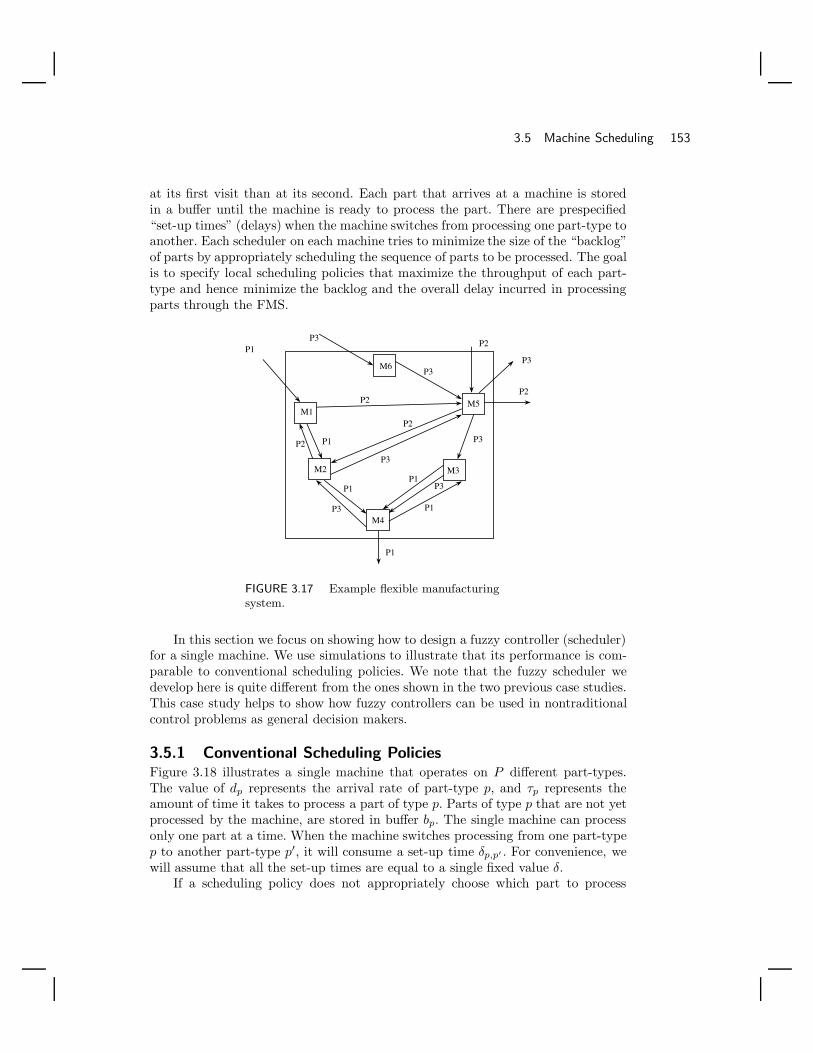
3.5 Machine Scheduling 153
at its first visit than at its second. Each part that arrives at a machine is storedin a buffer until the machine is ready to process the part. There are prespecified“set-up times” (delays) when the machine switches from processing one part-type toanother. Each scheduler on each machine tries to minimize the size of the “backlog”of parts by appropriately scheduling the sequence of parts to be processed. The goalis to specify local scheduling policies that maximize the throughput of each part-type and hence minimize the backlog and the overall delay incurred in processingparts through the FMS.
M6
M1
M2 M3
M4
M5
P3
P3
P2
P3
P2
P1
P2
P1
P1
P1
P1
P1
P2
P2 P3
P3
P3
P3
FIGURE 3.17 Example flexible manufacturingsystem.
In this section we focus on showing how to design a fuzzy controller (scheduler)for a single machine. We use simulations to illustrate that its performance is com-parable to conventional scheduling policies. We note that the fuzzy scheduler wedevelop here is quite different from the ones shown in the two previous case studies.This case study helps to show how fuzzy controllers can be used in nontraditionalcontrol problems as general decision makers.
3.5.1 Conventional Scheduling PoliciesFigure 3.18 illustrates a single machine that operates on P different part-types.The value of dp represents the arrival rate of part-type p, and τp represents theamount of time it takes to process a part of type p. Parts of type p that are not yetprocessed by the machine, are stored in buffer bp. The single machine can processonly one part at a time. When the machine switches processing from one part-typep to another part-type p′, it will consume a set-up time δp,p′ . For convenience, wewill assume that all the set-up times are equal to a single fixed value δ.
If a scheduling policy does not appropriately choose which part to process
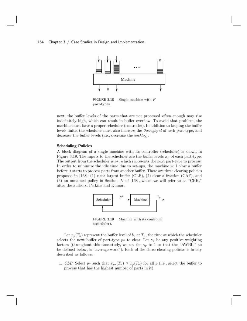
154 Chapter 3 / Case Studies in Design and Implementation
...
Machine
FIGURE 3.18 Single machine with Ppart-types.
next, the buffer levels of the parts that are not processed often enough may riseindefinitely high, which can result in buffer overflow. To avoid that problem, themachine must have a proper scheduler (controller). In addition to keeping the bufferlevels finite, the scheduler must also increase the throughput of each part-type, anddecrease the buffer levels (i.e., decrease the backlog).
Scheduling Policies
A block diagram of a single machine with its controller (scheduler) is shown inFigure 3.19. The inputs to the scheduler are the buffer levels xp of each part-type.The output from the scheduler is p∗, which represents the next part-type to process.In order to minimize the idle time due to set-ups, the machine will clear a bufferbefore it starts to process parts from another buffer. There are three clearing policiesproposed in [168]: (1) clear largest buffer (CLB), (2) clear a fraction (CAF), and(3) an unnamed policy in Section IV of [168], which we will refer to as “CPK,”after the authors, Perkins and Kumar.
MachineSchedulerxpp*
FIGURE 3.19 Machine with its controller(scheduler).
Let xp(Tn) represent the buffer level of bp at Tn, the time at which the schedulerselects the next buffer of part-type p∗ to clear. Let γp be any positive weightingfactors (throughout this case study, we set the γp to 1 so that the “AWBL,” tobe defined below, is “average work”). Each of the three clearing policies is brieflydescribed as follows:
1. CLB: Select p∗ such that xp∗(Tn) ≥ xp(Tn) for all p (i.e., select the buffer toprocess that has the highest number of parts in it).

3.5 Machine Scheduling 155
2. CAF: Select p∗ such that
xp∗(Tn) ≥ ε
P∑p=1
xp(Tn)
where ε is a small number, often set to 1P (i.e., when ε = 1
P , select any bufferto process that has greater than the average number of parts in the buffers).
3. CPK: Select p∗ such that
p∗ = arg maxp
xp(Tn) + δdp
dp
√γpρ
−1p (1 − ρp)
where ρp = dpτp.
In addition to these clearing policies, there exist many other policies that are usedin FMS (e.g., first-come first-served (FCFS)).
Machine Properties
A single machine is “stable” if the buffer level for each part-type is bounded. Inthis case there exists mp > 0, p = 1, 2, . . . , P , such that
supt
xp(t) ≤ mp < +∞ for p = 1, 2, . . . , P
A necessary condition for stability is that the machine load ρ =∑P
p=1 ρp < 1where ρp = dpτp. For the single-machine case, the authors in [168] prove that allthree policies described above cause the machine to be stable.
There are various ways to measure the performance of a scheduling policy. Wecan measure the average delays incurred when a part is processed in the machine.We can also measure the maximum value of each buffer level. The performancecriterion proposed in [168] is a quantity called the average weighted buffer level(AWBL), defined as follows:
AWBL = lim inft→∞
1t
∫ t
0
[∑p
γpτpxp(s)
]ds
For any stable scheduling policy, the average weighted buffer level has a lowerbound (LB), defined in [168] as follows:
LB =δ[∑
p
√γpρp (1 − ρp)
]2
2(1 − ρ).

156 Chapter 3 / Case Studies in Design and Implementation
Let η = AWBLLB be a measure of how close a scheduling policy is to optimal.
An optimal scheduling policy has η equal to 1; any scheduling policy has η ≥ 1. Tocompute the value of AWBL, we will of course have to choose some finite value oft to terminate our simulations.
Stabilizing Mechanism
The universally stabilizing supervisory mechanism (USSM) introduced in [100] isa mechanism that is used to govern any scheduling policy. There are two sets ofparameters employed by the mechanism for the single machine—namely, γ and zp,where it must be the case that
γ >
∑bmaxb′ δb′,b1−ρ
and zp can be chosen arbitrarily. The single machine will process parts of typep for exactly γdpτp units of time unless it is cleared first (if a part is currentlybeing processed when this amount of time is up, the processing on this part isfinished). Once the machine takes γdpτp units of time to process parts of type por the parts of type p are cleared before γdpτp elapses, the machine will scheduleanother part to be processed next. In addition, the USSM has a first-in-first-outqueue Q. When a buffer level xp exceeds zp, and the buffer is not being processedor set up, that buffer will be placed into Q. When there is some buffer in the queueoverruling the scheduling policy, the next buffer scheduled to be processed is thefirst buffer in the queue. Once that first buffer is processed, it leaves the queue,then any remaining buffers in the queue are processed. Hence, the USSM stabilizesany scheduling policy by truncating long production runs and by giving priority tobuffers that become excessively high. Note that xp is not exactly bounded by zp
since xp can still increase while it is listed in the queue. However, xp is affected byzp. The larger zp is, the larger the maximum of xp tends to be. Also, note that ifthe system is already stable (i.e., without the USSM) and the values of γ and zp
are large enough, the mechanism will not be invoked.
3.5.2 Fuzzy Scheduler for a Single MachineIn this section we will show how to perform scheduling via a fuzzy scheduler. Thefuzzy scheduler is designed to be a clearing policy just as CLB, CAF, and CPKare. There is no guarantee of stability when operating by itself; therefore, the fuzzyscheduler is always augmented with the USSM.
As for the conventional scheduling policies CLB, CAF, and CPK, the inputs tothe fuzzy scheduler policy are the buffer levels xp. The output of the fuzzy scheduleris simply an index p∗ indicating which one of the buffers will be processed next. Theuniverse of discourse for each xp is [0,∞). The universe of discourse of each xp hasseveral fuzzy sets. The membership function for each fuzzy set is triangular exceptat the extreme right, as shown in Figure 3.20. Figure 3.20 shows the membershipfunctions µ for the case where the universe of discourse for xp has three fuzzy sets.These fuzzy sets, indexed as 1, 2, and 3, indicate how “small,” “medium,” and“large,” respectively, the value of xp is. If the buffer level xp exceeds Mp, the value

3.5 Machine Scheduling 157
of xp is assumed to be Mp by the fuzzy scheduler, where Mp must be predetermined.We will call this parameter Mp the saturation value of the fuzzy scheduler for xp
and will use Mp as a tuning parameter.
1
0 Mp
1 2 3
xp
µ low medium high
FIGURE 3.20 Threemembership functions for xp.
Table 3.11 shows a rule-base of a fuzzy scheduler for a single machine that has3 part-types using the fuzzy sets shown in Figure 3.20. In each rule, Ixp representsthe index of the fuzzy set and J represents the part-type that is selected by therule. Then, for instance, rule number 2 takes on the form
If x1 is small and x2 is small and x3 is medium Then p∗ = 3
In other words, if the buffer levels of b1 and b2 are small and the buffer level ofb3 is medium then process part-type 3. The part of type J that is selected in eachrule has buffer level xJ that falls into a fuzzy set that has index IxJ the largestcompared to the other indices. In some rules, there are indices of fuzzy sets of severalpart-types that have equal largest value. In these cases, one of these part-types isselected arbitrarily in our rule-base. For example, the first rule in Table 3.11 is fixedto select part-type 1 even though the fuzzy set indices of all part-types in the ruleare equal to 1. Therefore, this rule is biased toward part-type 1. We note that ourfuzzy scheduler essentially “fuzzifies” the operation of the CLB policy; however,due to the interpolation inherent in the implementation of the fuzzy scheduler itwill behave quite differently from the conventional CLB (as the simulation resultsbelow indicate).
Throughout the simulation studies in the next subsection, if we use more fuzzysets on the universe of discourse we will utilize a similar structure for the rule-base (i.e., uniformly distributed and symmetric membership functions). The outputuniverse of discourse (the positive integers) has P membership functions denotedby µp where for each p ∈ 1, 2, ..., P, µp(i) = 1 for i = p and µp(i) = 0 fori = p (i.e., singletons). We use singleton fuzzification, minimum for the premise andimplication, and max-defuzzification to pick p∗, given the rule-base and particularvalues of xp.
For P buffers and m fuzzy sets, the size of memory needed to store the rulesis on the order of P m; hence, the CLB, CPK, and CAF policies are simpler thanthe fuzzy scheduler. We will, however, show that with the use of this more complexscheduler we can get enhanced performance in some cases.

158 Chapter 3 / Case Studies in Design and Implementation
TABLE 3.11 Rule-Base of aFuzzy Scheduler with 3 Inputs and3 Fuzzy Sets on Each Universe ofDiscourse
Rule No. Ix1 Ix2 Ix3 J
1 1 1 1 12 1 1 2 33 1 1 3 34 1 2 1 25 1 2 2 26 1 2 3 37 1 3 1 28 1 3 2 29 1 3 3 210 2 1 1 111 2 1 2 112 2 1 3 313 2 2 1 114 2 2 2 115 2 2 3 316 2 3 1 217 2 3 2 218 2 3 3 319 3 1 1 120 3 1 2 121 3 1 3 322 3 2 1 123 3 2 2 124 3 2 3 125 3 3 1 126 3 3 2 127 3 3 3 3
It is possible to expand the fuzzy scheduler to use the information about ar-rival rates, processing times, and set up times also. There may be significant im-provements in performance if this information is represented with the control rules;however, the memory size can significantly increase too. In the interest of ensuringthat the fuzzy scheduler will be implementable in real time we did not present thisvariation in this case study.
3.5.3 Fuzzy Versus Conventional SchedulersNext, we simulate a single machine that uses CLB, CAF, CPK, and the fuzzyscheduler so that we can compare their performance. The machine parameters areas follows: d1 = 7, d2 = 9, d3 = 3, τ1 = 1/100, τ2 = 1/51, τ3 = 1/27, and δ = 1.Figures 3.21 and 3.22 show the plots of the buffer levels of a single machine withthree part-types for the first 10 production runs (a production run is defined as
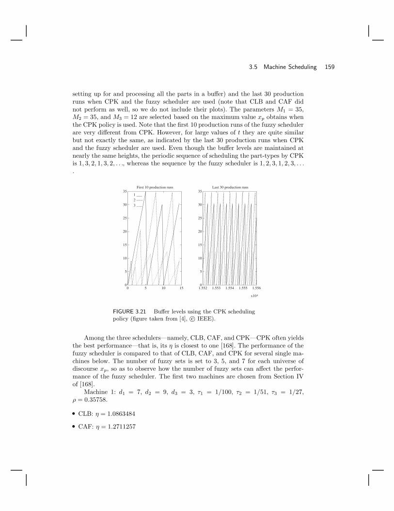
3.5 Machine Scheduling 159
setting up for and processing all the parts in a buffer) and the last 30 productionruns when CPK and the fuzzy scheduler are used (note that CLB and CAF didnot perform as well, so we do not include their plots). The parameters M1 = 35,M2 = 35, and M3 = 12 are selected based on the maximum value xp obtains whenthe CPK policy is used. Note that the first 10 production runs of the fuzzy schedulerare very different from CPK. However, for large values of t they are quite similarbut not exactly the same, as indicated by the last 30 production runs when CPKand the fuzzy scheduler are used. Even though the buffer levels are maintained atnearly the same heights, the periodic sequence of scheduling the part-types by CPKis 1, 3, 2, 1, 3, 2, . . ., whereas the sequence by the fuzzy scheduler is 1, 2, 3, 1, 2, 3, . . ..
0
5
10
15
20
25
30
35
0 5 10 15
First 10 production runs
1 ___
2 -----
3 ......
0
5
10
15
20
25
30
35
1.552 1.553 1.554 1.555 1.556
x104
Last 30 production runs
FIGURE 3.21 Buffer levels using the CPK schedulingpolicy (figure taken from [4], c© IEEE).
Among the three schedulers—namely, CLB, CAF, and CPK—CPK often yieldsthe best performance—that is, its η is closest to one [168]. The performance of thefuzzy scheduler is compared to that of CLB, CAF, and CPK for several single ma-chines below. The number of fuzzy sets is set to 3, 5, and 7 for each universe ofdiscourse xp, so as to observe how the number of fuzzy sets can affect the perfor-mance of the fuzzy scheduler. The first two machines are chosen from Section IVof [168].
Machine 1: d1 = 7, d2 = 9, d3 = 3, τ1 = 1/100, τ2 = 1/51, τ3 = 1/27,ρ = 0.35758.
• CLB: η = 1.0863484
• CAF: η = 1.2711257

160 Chapter 3 / Case Studies in Design and Implementation
0
5
10
15
20
25
30
35
0 5 10 15
First 10 production runs
1 ___
2 -----
3 ......
0
5
10
15
20
25
30
35
1.552 1.553 1.554 1.555 1.556
x104
Last 30 production runs
FIGURE 3.22 Buffer levels using the fuzzy scheduler(figure taken from [4], c© IEEE).
• CPK: η = 1.0262847
• Fuzzy scheduler: M1 = 35, M2 = 35, M3 = 12; γ = 34.0, z1 = 30, z2 = 30,z3 = 30For 3 fuzzy subsets, η = 1.0263256For 5 fuzzy subsets, η = 1.0262928For 7 fuzzy subsets, η = 1.0262928
These simulations show that a fuzzy scheduler can perform nearly as well ascan CPK. Note also that we cannot significantly improve η by simply increasingthe number of fuzzy subsets for the same Mp (for this machine).
Machine 2: d1 = 18, d2 = 3, d3 = 1, τ1 = 1/35, τ2 = 1/7, τ3 = 1/20, ρ =0.99286.
• CLB: η = 1.1738507
• CAF: η = 1.179065
• CPK: η = 1.0017406
• Fuzzy scheduler: M1 = 3375, M2 = 626, M3 = 665; γ = 1000.0, z1 = 5000,z2 = 5000, z3 = 5000.For 3 fuzzy subsets, η = 1.0027945For 5 fuzzy subsets, η = 1.0027945For 7 fuzzy subsets, η = 1.0013173
These simulations show that with the machine load closer to one, the fuzzy

3.6 Fuzzy Decision-Making Systems 161
scheduler can work even better than CPK provided that there are enough fuzzysets on the input space. Next, we create a new machine that has a lower machineload, and compare the performance of the scheduling policies.
Machine 3: d1 = 3.5, d2 = 4.5, d3 = 1.5, τ1 = 1/100, τ2 = 1/51, τ3 = 1/27,ρ = 0.17879.
• CLB: η = 1.0841100
• CAF: η = 1.3456014
• CPK: η = 1.0306833
• Fuzzy scheduler: M1 = 23.6, M2 = 25.1, M3 = 5.6; γ = 100.0, z1 = 5000,z2 = 5000, z3 = 5000.For 3 fuzzy subsets, η = 1.0307992For 5 fuzzy subsets, η = 1.0319630For 7 fuzzy subsets, η = 1.0306972
• Fuzzy scheduler with 3 fuzzy subsets; M1 = 50, M2 = 50, M3 = 20; γ = 100.0,z1 = 5000, z2 = 5000, z3 = 5000: η = 1.2273009
These simulations show that the fuzzy scheduler cannot perform any betterthan CPK when the machine load is small for this machine. Also note that if theparameters Mp are not set properly, the performance of the fuzzy scheduler candegrade.
Our experience in simulation above shows that it is possible to tune the fuzzyscheduler by choosing the values of Mp and the fuzzy sets to minimize η. We haveused the following procedure to tune the fuzzy scheduler to get smaller η: (1) usei fuzzy sets and set the Mp all to unity, (2) run a simulation, (3) replace Mp withthe maximum buffer levels obtained in xp and rerun the simulation, and (4) repeatas necessary with i + 1 fuzzy sets, i + 2 fuzzy sets, and so on. Using this tuningapproach for the above machine we find that for 3-buffer machines the results are asgood as those of CPK, and for some 5-buffer machines the tuning method convergesto a good result, even though the result is not quite as good as that of CPK. Notethat our experiences in tuning allowed us to develop the on-line adaptive fuzzyscheduler technique that is studied in Chapter 6.
3.6 Fuzzy Decision-Making SystemsA fuzzy controller is constructed to make decisions about what the control inputto the plant should be given processed versions of the plant outputs and referenceinput. It is a form of artificial (i.e., nonbiological) decision-making system. Decision-making systems find wide application in many areas, not only the ones that havebeen traditionally studied in control systems. For instance, the machine schedulingcase study of the previous section shows a nontraditional application of feedbackcontrol where a fuzzy system can play a useful role as a decision-making system.

162 Chapter 3 / Case Studies in Design and Implementation
There are many other areas in which fuzzy decision-making systems can be usedincluding the following:
• Manufacturing: Scheduling and planning materials flow, resource allocation, rout-ing, and machine and equipment design.
• Traffic systems: Routing and signal switching.
• Robotics: Path planning, task scheduling, navigation, and mission planning.
• Computers: Memory allocation, task scheduling, and hardware design.
• Process industries: Monitoring, performance assessment, and failure diagnosis.
• Science and medicine: Medical diagnostic systems, health monitoring, and auto-mated interpretation of experimental data.
• Business: Finance, credit evaluation, and stock market analysis.
This list is by no means exhaustive. Virtually any computer decision-making systemhas the potential to benefit from the application of fuzzy logic to provide for “soft”decisions when there is the need for decision making under uncertainty.
In this section we focus on the design of fuzzy decision-making systems forproblems other than feedback control. We begin by showing how to construct fuzzysystems that provide warnings for the spread of an infectious disease. Then we showhow to construct a fuzzy decision making system that will act as a failure warningsystem in an aircraft.
3.6.1 Infectious Disease Warning SystemIn this section we study a biological system where a fuzzy decision-making systemis used as a warning system to produce alarm information. To model a form ofbiological growth, one of Volterra’s population equations is used. A simple modelrepresenting the spread of a disease in a given population is given by
dx1(t)dt
= −ax1(t) + bx1(t)x2(t) (3.4)
dx2(t)dt
= −bx1(t)x2(t) (3.5)
where x1(t) is the density of the infected individuals, x2(t) is the density of thenoninfected individuals, a > 0, and b > 0. These equations are only valid forx1(t) ≥ 0 and x2(t) ≥ 0. The initial conditions x1(0) ≥ 0 and x2(0) ≥ 0 must alsobe specified.
Equation (3.5) intuitively means that the noninfected individuals become in-fected at a rate proportional to x1(t)x2(t). This term is a measure of the interactionbetween the two groups. The term −ax1(t) in Equation (3.4) represents the rate atwhich individuals die from disease or survive and become forever immune. The term

3.6 Fuzzy Decision-Making Systems 163
bx1(t)x2(t) in Equation (3.4) represents the rate at which previously noninfectedindividuals become infected.
Here, we design a fuzzy system to produce alarms if certain conditions occurin the diseased population—that is, a simple warning system. The fuzzy systemuses x1(t) and x2(t) as inputs, and its output is an indication of what type ofwarning condition occurred along with the certainty that this warning condition hasoccurred. To specify the types of alarms we would like the fuzzy system to output,we first begin by using conventional (nonfuzzy) logic and “decision regions” tospecify the alarms. In particular, we would like indications of the following alarms:
1. “Warning: The density of infected individuals is unsafe”; this occurs if x1(t) >α1 where α1 is some positive real number (here x1(t) > α1 specifies a “decisionregion” for where we could like the warning to be given).
2. “Caution: The density of infected individuals is unsafe, and the number ofinfected individuals is greater than the number of noninfected individuals”;this occurs if x1(t) > α1 and x1(t) ≥ x2(t) + α2 but x1(t) < x2(t) + α3, whereα2 and α3 are positive real numbers such that α2 < α3.
3. “Critical: The density of infected individuals is unsafe, and the number of in-fected individuals is much greater than the number of noninfected individuals”;this occurs if x1(t) > α1 and x1(t) ≥ x2(t) + α3.
The three alarms represent certain warnings characterized by the decision re-gions shown in Figure 3.23. The darkest region plus the other lighter shaded regionsrepresent the first warning’s decision region, the slightly lighter one represents thesecond warning, and the lightest shaded represents the third warning.
x2(t)
x1(t)
α2
α3
α1
α2 α3
-
-
FIGURE 3.23 Decision regions for thebiological system (figure taken from [164],c© IEEE).
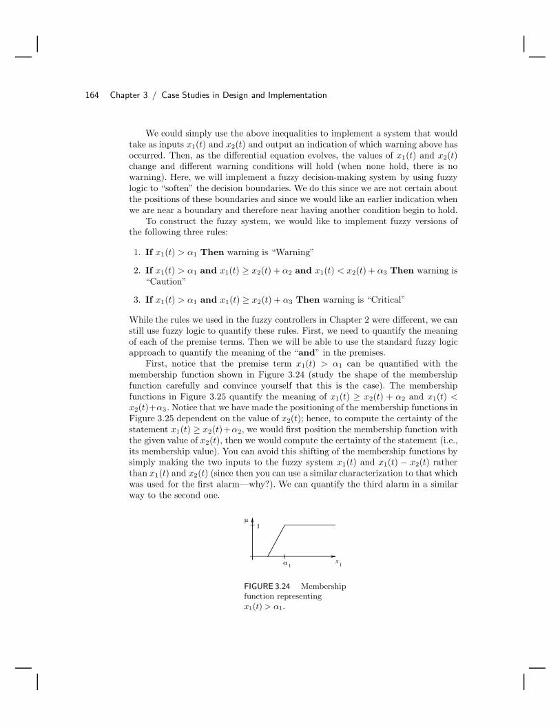
164 Chapter 3 / Case Studies in Design and Implementation
We could simply use the above inequalities to implement a system that wouldtake as inputs x1(t) and x2(t) and output an indication of which warning above hasoccurred. Then, as the differential equation evolves, the values of x1(t) and x2(t)change and different warning conditions will hold (when none hold, there is nowarning). Here, we will implement a fuzzy decision-making system by using fuzzylogic to “soften” the decision boundaries. We do this since we are not certain aboutthe positions of these boundaries and since we would like an earlier indication whenwe are near a boundary and therefore near having another condition begin to hold.
To construct the fuzzy system, we would like to implement fuzzy versions ofthe following three rules:
1. If x1(t) > α1 Then warning is “Warning”
2. If x1(t) > α1 and x1(t) ≥ x2(t) + α2 and x1(t) < x2(t) + α3 Then warning is“Caution”
3. If x1(t) > α1 and x1(t) ≥ x2(t) + α3 Then warning is “Critical”
While the rules we used in the fuzzy controllers in Chapter 2 were different, we canstill use fuzzy logic to quantify these rules. First, we need to quantify the meaningof each of the premise terms. Then we will be able to use the standard fuzzy logicapproach to quantify the meaning of the “and” in the premises.
First, notice that the premise term x1(t) > α1 can be quantified with themembership function shown in Figure 3.24 (study the shape of the membershipfunction carefully and convince yourself that this is the case). The membershipfunctions in Figure 3.25 quantify the meaning of x1(t) ≥ x2(t) + α2 and x1(t) <x2(t)+α3 . Notice that we have made the positioning of the membership functions inFigure 3.25 dependent on the value of x2(t); hence, to compute the certainty of thestatement x1(t) ≥ x2(t)+α2, we would first position the membership function withthe given value of x2(t), then we would compute the certainty of the statement (i.e.,its membership value). You can avoid this shifting of the membership functions bysimply making the two inputs to the fuzzy system x1(t) and x1(t) − x2(t) ratherthan x1(t) and x2(t) (since then you can use a similar characterization to that whichwas used for the first alarm—why?). We can quantify the third alarm in a similarway to the second one.
1µ
x1α 1
FIGURE 3.24 Membershipfunction representingx1(t) > α1.
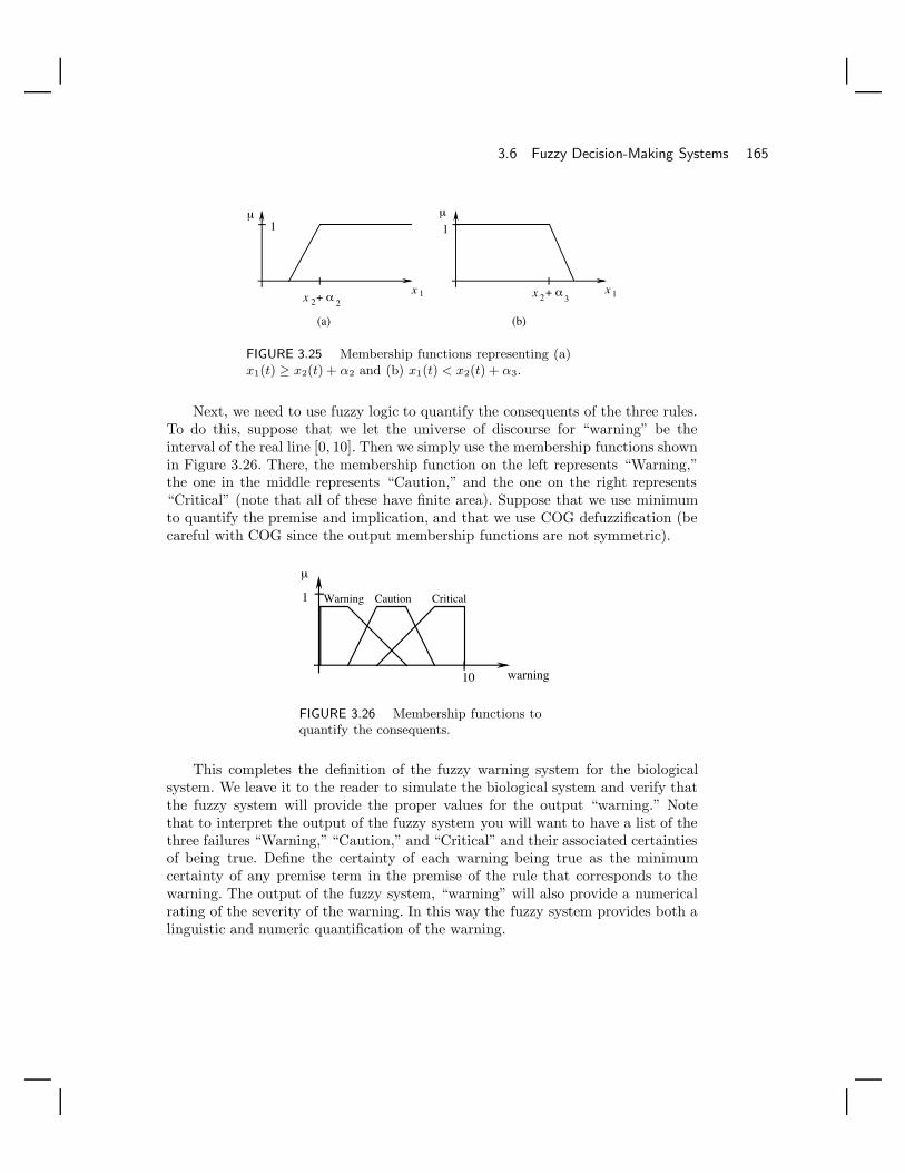
3.6 Fuzzy Decision-Making Systems 165
1
µ
x 1
1µ
x 1 + α2x 2
+ α3
x 2
(a) (b)
FIGURE 3.25 Membership functions representing (a)x1(t) ≥ x2(t) + α2 and (b) x1(t) < x2(t) + α3.
Next, we need to use fuzzy logic to quantify the consequents of the three rules.To do this, suppose that we let the universe of discourse for “warning” be theinterval of the real line [0, 10]. Then we simply use the membership functions shownin Figure 3.26. There, the membership function on the left represents “Warning,”the one in the middle represents “Caution,” and the one on the right represents“Critical” (note that all of these have finite area). Suppose that we use minimumto quantify the premise and implication, and that we use COG defuzzification (becareful with COG since the output membership functions are not symmetric).
warning
1
µ
10
Warning Caution Critical
FIGURE 3.26 Membership functions toquantify the consequents.
This completes the definition of the fuzzy warning system for the biologicalsystem. We leave it to the reader to simulate the biological system and verify thatthe fuzzy system will provide the proper values for the output “warning.” Notethat to interpret the output of the fuzzy system you will want to have a list of thethree failures “Warning,” “Caution,” and “Critical” and their associated certaintiesof being true. Define the certainty of each warning being true as the minimumcertainty of any premise term in the premise of the rule that corresponds to thewarning. The output of the fuzzy system, “warning” will also provide a numericalrating of the severity of the warning. In this way the fuzzy system provides both alinguistic and numeric quantification of the warning.
166 Chapter 3 / Case Studies in Design and Implementation
3.6.2 Failure Warning System for an AircraftConsumer and governmental demands have provided the impetus for an extraor-dinary increase in the complexity of the systems that we use. For instance, inautomotive and aircraft systems, governmental demands have called for (1) highlyaccurate air-to-fuel-ratio control in automobiles to meet pollution standards, and(2) highly technological aircraft capable of achieving frequent flights with very littlemaintenance downtime. Similarly, consumer demands have driven (1) the develop-ment of antiskid braking systems for increased stopability, steerability, and stabilityin driving and (2) the need for increased frequency of commercial flights such thattravel must occur under all weather conditions in a timely manner.
While engineers have, in general, been able to meet these demands by enhancingthe functionality of high-technology systems, this has been done at the risk ofsignificant failures (it is generally agreed that “the more complex a system is themore likely it is to fail in some way”). For automotive and aircraft systems, someof the failures that are of growing concern include the following:
• Failures and/or degradation of performance of the emissions control systems (fail-ures or degradation leads to a significant increase in the level of pollutants).
• “Cannot duplicate” failures where a failure is detected while the aircraft is in flightthat cannot be duplicated during maintenance, which lengthens the downtime.
• Actuator, sensor, and other failures in aircraft systems that cause commercialaircraft crashes in adverse weather conditions.
• A system failure in an integrated vehicle handling, braking and traction controlsystem, which can lead to a loss of control by the driver.
Automotive and aircraft systems provide excellent examples of how failures inhigh-technology systems can result in catastrophic failures. In addition, the effectof undetected system faults can lead to costly downtime or catastrophic failuresin manufacturing systems, nuclear power plants, and process control problems. Ashistory indicates, the probability of some of the system failures listed above issometimes high. There is then the need for detecting, identifying, and providingappropriate warnings about failures that occur on automobiles, aircraft, and othersystems so that corrective actions can be taken before there is a loss of life or otherundesirable consequences.
Experience in developing on-line failure warning systems has indicated thatthere is no uniform approach to solving all problems; solutions are “problem-dependent.” This makes the fuzzy system particularly well suited for this applica-tion. You simply have to load different knowledge into a fuzzy system for differentapplications. Next, we look at a simple example of how to construct a fuzzy warningsystem for an aircraft.
The simple warning system for an aircraft uses the aircraft’s measurable inputsand outputs. Suppose the aircraft’s input vector u has two components, the elevatorδe (deg), and thrust δt (deg). The output vector y has three components, pitch rate q

3.6 Fuzzy Decision-Making Systems 167
(deg/sec), pitch angle θ (deg), and load factor ηz (g). Four aircraft failure modes areconsidered here. To define the modes, we take the same approach as in the previoussection and define decision regions using conventional logic and inequalities. Later,we will soften the decision boundaries and define the fuzzy decision-making system.
To define the decision boundaries, each input and output is discretized into fiveregions with four boundaries associated with the real number line. For example,the elevator δe is discretized as follows:
• Region R1: δe ≤ δR1
• Region Y1: δR1 < δe ≤ δY1
• Region G: δY1 < δe ≤ δY2
• Region Y2: δY2 < δe ≤ δR2
• Region R2: δe ≥ δR2
where δR1 and δY1 are negative constants with δR1 larger in magnitude than δY1 ,and δY2 and δR2 are positive constants with δY2 ≤ δR2 . The G (for Green) regiondenotes an area of safe operation, the Y1 and Y2 (for Yellow) regions denote areasof warning, and the R1 and R2 (for Red) regions denote areas of unsafe operation.Suppose that using a similar notation we define such regions for all the other aircraftinput and output variables. For simplicity we will then sometimes say that othervariables lie in the regions R1, Y1, G, Y2, and R2 with the understanding that therecan be different values of the constants used to define the intervals on the real line.
Using the defined regions for the aircraft inputs and outputs, four failure modesfor the aircraft are identified as follows:
1. Load factor is in region R2.
2. Load factor is in region Y2.
3. Load factor is in region Y2 and elevator is in region Y1
4. (Pitch rate is in Y1 and Pitch angle is in Y1) or (Pitch rate is in Y2 and Pitchangle is in Y2).
The decision regions for the fourth failure mode are shown as the shaded areasin Figure 3.27 (notice that we use an appropriate notation for the constants thatdefine the boundaries).
The fuzzy system’s inputs are the aircraft inputs and outputs, and its outputsare the four failure warnings. Suppose that the output of the fuzzy system is either1, 2, 3, or 4, representing the failure warning mode, i = 1, 2, 3, 4. Now, we want todefine a fuzzy system that will give a proper indication of the above failure warningmodes. To define the fuzzy system, we use the same approach as in the previoussection. We can define rules representing each of the four failure warning modes.

168 Chapter 3 / Case Studies in Design and Implementation
θ
q
θR
θY
θ θR
qR
qY
qY
qR 2
2
1 1Y 2 2
1
1
FIGURE 3.27 Decision regions for aircraftfailure mode four (figure taken from [164],c© IEEE).
These will have the proper logical combinations of the inequalities in the premises,and the consequents will be, for example, “failure warning = 1.”
For the first mode (load factor is in region R2), you can use the same approachas in the last section to specify a membership function to represent the singlepremise term; the same for the second and third failure warning modes. For thefourth failure warning mode, we can use fuzzy logic in the characterization of the“and” in the premise as we did in the last section. Also, we can use the fuzzylogic characterization of “or” to represent the combination of the two terms in thepremise of the rule for the fourth failure warning mode. You can use singletonspositioned at i = 1, 2, 3, 4 for the ith failure warning mode rule. Then use center-average defuzzification to complete the specification of the fuzzy warning system.We leave the details of constructing this fuzzy decision-making system to the reader.
3.7 SummaryIn this chapter we provided an overview of the design methodology for fuzzy controlsystems and showed how to design fuzzy controllers in the two-link flexible robot andthe rotational inverted pendulum case studies. We used the machine control problemand fuzzy decision-making systems to illustrate how the fuzzy system can alsobe useful in nontraditional control applications. Each problem provided differentchallenges, and in two of the case studies we showed actual implementation results.In two of the cases we compared the fuzzy controller to conventional approaches,which highlights the advantages and disadvantages of fuzzy control.
Upon completing this chapter, the reader should understand the following:

3.8 For Further Study 169
• The general design methodology for fuzzy controllers.
• How to design a fuzzy controller for a flexible-link robot and how the use of ad-ditional, more-detailed knowledge can improve performance (e.g., the uncoupledversus coupled cases) but increases the complexity of the controller (e.g., thenumber of rules increased).
• How to design a swing-up controller and LQR for balancing for the rotationalinverted pendulum, how to use the LQR design to provide the first guess at thefuzzy controller (that may later be tuned), and how to use a nonlinear mappingto set the positions of the output membership function centers.
• How to specify a fuzzy controller that can schedule the processing of parts at amachine and perform at comparable levels to good conventional schedulers.
• How to design fuzzy decision-making systems, particularly for failure warningsystems.
Essentially, this is a checklist for the major topics covered in this chapter. Thereader should be sure to understand each of the above concepts or approachesbefore proceeding on to more-advanced chapters, especially the ones on adaptiveand supervisory fuzzy control, where the first three case studies examined here arefurther investigated.
3.8 For Further StudyThere are many conference and journal papers that focus on the application of directfuzzy control—indeed, too many to mention here. Here, we simply highlight a fewcase studies that are particularly interesting or instructive [125, 91, 21, 35, 25]and refer the interested reader to several books that have focused on industrialapplications of fuzzy control, including [240, 137, 175, 206] (these also have extensivelists of references that the interested reader may want to follow up on). Also, thereare some recent books [47, 154] and papers (e.g., [218]) that focus on some newdesign methodologies for fuzzy controllers that the reader may be interested in.One of these is based on sliding-mode control [217], and the other is related togain-scheduling-type control.
The case study in this chapter on the two-link flexible robot was taken directlyfrom [145, 144]; the interested reader should see those papers (and the referenceswithin them) to obtain a more complete treatment of work related to the case study.Since the literature abounds with work on the modeling and control of flexiblerobots, both from a theoretical (simulation-based) and an experimental point ofview, we refer the interested reader to Chapter 8 of [193] for an overview of theliterature on conventional approaches. Some studies that are particularly relevantto our case study are in [69, 242, 243].
The case study for the rotational inverted pendulum was taken from [235, 244].The literature abounds in research and implementations of the linear-translational

170 Chapter 3 / Case Studies in Design and Implementation
inverted pendulum. The approach of using the linear controller to initialize the fuzzycontroller that is used for the rotational inverted pendulum was first introducedin [104], where it was used for an aircraft application. It is interesting to note thatin [235] it is shown how a fuzzy system can be used to automate the swing-upcontrol so that the manual tuning of the above parameters is not needed even ifadditional mass is added to the endpoint of the pendulum.
The machine control case study was taken directly from [6]. The work wasinspired by the earlier work of P.R. Kumar and his colleagues (see, for example,[168, 100]) on the development of distributed scheduling policies for flexible man-ufacturing systems. The failure warning systems are fuzzy versions of the ones de-veloped in [164]; for a more detailed study of aircraft failure diagnostic systems, see[161]. Fuzzy decision-making systems are discussed in some more detail in [206, 175].
The motor control design problem in the problems at the end of the chapteris part of a control laboratory at Ohio State University (developed over the yearsby many people, including U. Ozguner, L. Lenning, and S. Brown). The ship steer-ing problem comes from [11] and [112]. The rocket velocity control problem wastaken directly from [113]. The design problem on the acrobot was taken directlyfrom [27] and builds directly on earlier work performed by M. Spong and his col-leagues, who have focused on the development of conventional controllers for theacrobot. Their work in [190] and [191] serves as an excellent introduction to theacrobot and its dynamics. The dynamics of a simple acrobot are also describedin both works; however, a more complete development of the acrobot dynamicsmay be found in [192]. The base-braking control problem is taken from [75, 66]and was based on years of contracted research with Delphi Chassis Division ofGeneral Motors. Previous research on the brake system has been conducted usingproportional-integral-derivative (PID), lead-lag, autotuning, and model referenceadaptive control (MRAC) techniques [66]. The particular problem description weuse for the brakes was taken from [118].
3.9 ExercisesExercise 3.1 (Simulation of General Fuzzy Systems): Write a program inhigh-level language that will simulate a general fuzzy controller with the followingcharacteristics:
(a) n inputs and one output (i.e., so that the user can input n).
(b) Triangular membership functions (with appropriately saturated ones at theendpoints of the input universes of discourse).
(c) Gaussian membership functions (with appropriately saturated ones at theendpoints of the input universes of discourse).
(d) Trapezoidal membership functions (with appropriately saturated ones at theendpoints of the input universes of discourse).
(e) The use of product or minimum for representing the premise and implication.
(f) The use of center-average or COG defuzzification.

3.9 Exercises 171
Exercise 3.2 (Efficient Simulation of Fuzzy Systems): Write a program inhigh-level language that will simulate a general fuzzy controller with the followingcharacteristics:
• n inputs and one output.• Triangular membership functions (with appropriately saturated ones at the
outermost regions of the input universes of discourse) that are uniformlydistributed across the universes of discourse so that there are at most twoof them overlapping at any one point.
• The use of minimum for representing the premise and implication.• The use of COG defuzzification.
Exploit the fact that no more than two membership functions overlap at any onepoint to make the code as efficient as possible. Use ideas from Chapter 2 wherewe discuss simulation of fuzzy systems and real-time implementation issues.
Exercise 3.3 (Fuzzy Systems: Computational Complexity): Fuzzy con-trollers can at times require significant computational resources to compute op-erations in real-time. Define a “computing step” as the act of performing a basicmathematical operation (e.g., addition, subtraction, multiplication, division, orfinding the maximum or minimum of a set of numbers). For the first invertedpendulum controller that we designed in Chapter 2 (i.e., the one using triangu-lar membership functions with R = 25 rules), using this measure, determine thenumber of computing steps that it takes to perform the following operations (as-sume that you code it efficiently, exploiting the fact that only two membershipfunctions overlap at any point so at most four rules are on):
(a) COG defuzzification—assuming that you are already given the values of thepremise membership function certainties.
(b) Center-average defuzzification—assuming that you are already given the val-ues of the premise membership function certainties.
(c) Assume that we switch to using Gaussian membership functions as in Exer-cise 2.3 on page 102. Does this increase or decrease computational complex-ity? Why?
Exercise 3.4 (Fuzzy Controller Design Using Linear Controllers): Sup-pose that you have a PD controller that generates the plant input u = Kpe +Kd
ddte (e = r − y where r is the reference input and y is the plant output) and
that it performs well for small values of its inputs, but that for larger values youhappen to know some additional heuristics that can be used to improve perfor-mance. To capture this information, suppose that you decide to use a two-input,one-output fuzzy controller. Rather than throwing out all the work you have doneto tune the PD gains Kp and Kd, you would like to make the fuzzy controllerbehave similarly to the PD controller. Suppose that Kp = 2 and Kd = 5. Designa fuzzy controller that will approximate these same gains for small values of e

172 Chapter 3 / Case Studies in Design and Implementation
and ddte. Demonstrate that the two are close by providing a three-dimensional
plot of the control surfaces for both the PD and the fuzzy controller (note thatthe PD controller surface looks like a plane in three dimensions).
Exercise 3.5 (Fuzzy Control Design Trade-Offs): List all the trade-offsinvolved in choosing fuzzy versus conventional control and, for the applicationof your choice, provide a written analysis of whether you think fuzzy control isa viable approach for your problem. Fully support your conclusions. You maychoose your own application, but if you do you must fully describe the controlproblem that you study and provide at least simulation studies to back up yourconclusions. Alternatively, you may choose one of the case study examples in thischapter (or one of the design problems) for your analysis.
3.10 Design ProblemsDesign Problem 3.1 (Inverted Pendulum: Use of a CAD Package): Inthis problem you will learn to use a CAD package (such as the one available inMatlab) for the development and analysis of fuzzy control systems.
(a) Use a CAD package to solve Exercise 2.3 on page 102.
(b) Use a CAD package to solve Exercise 2.4 on page 103.
(c) Use a CAD package to solve Design Problem 2.1 on page 110.
Design Problem 3.2 (Single-Link Flexible Robot): This problem focuseson the design of a fuzzy controller for a single-link flexible robot. To performthe designs, use the model provided in Section 3.3.1 on page 127 (in particular,Equation (3.1)); hence, the plant input is v1 and the plant output is θ1. Com-mand a 90-degree step change in the position to test your closed-loop system.Use the saturation nonlinearities that were provided for the voltage input andlink position. The goals are fast slewing with minimal endpoint vibrations andno steady-state tracking error. Use a 20-ms sampling period and discrete timecontrollers.
(a) Design a fuzzy controller for the single-link flexible robot and evaluate itsperformance.
(b) Design the best linear controller that you can for the flexible robot andcompare its performance to that of the fuzzy controller.
(c) Compare the performance that was obtained in (a) to that obtained in (b).Identify which characteristics of your simulation responses are different fromthe implementation responses for the two-link robot, and try to providereasons for these differences.

3.10 Design Problems 173
Design Problem 3.3 (Rotational Inverted Pendulum): This problem fo-cuses on the design of fuzzy controllers for the rotational inverted pendulum thatwas studied in this chapter. To perform the designs, use the model provided inSection 3.4.1 on page 143. You should seek to obtain performance comparable tothat seen in the implementation results for the rotational inverted pendulum.
(a) Design an “energy-pumping” swing-up strategy for the rotational invertedpendulum, and develop a LQR controller for balancing the pendulum. Demon-strate its performance in simulation.
(b) Design a fuzzy controller for balancing the pendulum, and, using the sameswing-up strategy as in (a), demonstrate its performance in simulation.
(c) For both (a) and (b), compare the performance that was obtained to thatwhich was found in implementation. Identify characteristics of your simu-lation responses that are different from the implementation responses, andprovide a reason for these differences.
Design Problem 3.4 (Machine Scheduling): Here, we focus on the designof fuzzy schedulers for the machine scheduling problem that was studied in thischapter. To perform the designs, use the model provided in Section 3.5.1 onpage 153. Suppose that we define “Machine 4” to have the following characteris-tics: d1 = 1, d2 = 1, d3 = 1/0.9, d4 = 1, d5 = 1, τ1 = 0.15, τ2 = 0.2, τ3 = 0.05,τ4 = 0.1, τ5 = 0.2, ρ = 0.7055556 (i.e., it has five buffers).
(a) Develop CLB, CAF, and CPK schedulers, simulate them, and determine thevalue for η for each of these.
(b) Develop a fuzzy scheduler using the same approach as in the case study.Find the value of η for the cases where 3, 5, and 7 fuzzy sets are used oneach input universe of discourse. Be careful to properly tune the values ofthe Mi and use γ = 100.0, and zi = 30, i = 1, 2, 3, 4, 5. You should tunethe Mi so that the fuzzy scheduler performs better than the ones in (a) asmeasured by η.
Design Problem 3.5 (Motor Control): In this problem we study control ofthe Pittman GM9413H529 DC motor with a simulated inertial load (aluminumdisk). The simulated moment of inertia is small, and is considerably less thanthe actual motor moment of inertia. The effective gear ratio is 7860:18 (from themotor armature shaft to the actual load); therefore, the reflected load inertiaseen by the motor is very small. The equivalent circuit diagram of the DC motorsystem is shown in Figure 3.28.
The DC motor has a single measurable signal: the motor’s rotational ve-locity. This velocity is sensed using an optical encoder mounted on the shaftof the motor. An optical encoder outputs square wave pulses with a frequencyproportional to rotational velocity. The pulses from the encoder are counted by

174 Chapter 3 / Case Studies in Design and Implementation
+
V eq
aI aR aL
aJaVL
JN
+
ω ωa L
LoadGearbox
FIGURE 3.28 Equivalent circuit diagram of the DC motorsystem (figure drawn by Scott C. Brown).
a data-acquisition card’s counter/timer, and translated to a rotational velocityof the inertial plate. Pulse width modulation (PWM) is used to vary the inputvoltage to the motor. PWM varies the duty cycle of a constant magnitude squarewave to achieve an approximation of a continuous control input. A diagram ofthe motor experimental setup is shown in Figure 3.29.
Motor
BreadboardInterface
box
PWMamplifier 12 V.
powersupply
Tocomputer
FIGURE 3.29 Motor experimental setup(figure drawn by Scott C. Brown).
The transfer function of the motor can be derived from the following data(taken from the Pittman motor spec sheets for winding 114T32):
Ra = armature resistance = 8.33 ΩLa = armature inductance = 6.17 mHKe = back emf constant = 4.14 V/krpm = 3.953× 10⁻² V/(rad/s)Kt = torque constant = 5.60 oz · in/A = 0.03954 N ·m/AJa = armature inertia = 3.9× 10⁻⁴ oz · in · s2 = 2.75× 10⁻⁶ Kg · m2
JL = load inertia = 0.0137 Kg · m2
J = total inertia = motor + load = Ja +JL
N2= 2.82× 10⁻⁶ Kg · m2
N = Gear ratio = 7860 : 18

3.10 Design Problems 175
The aluminum disk has a radius of 15.24 cm, a thickness of 0.6 cm and a densityof 2699 Kg/m3.
Using these parameters, the following system time constants can be deter-mined:
1/Te = Ra/La = 1350 (rad/sec)1/Tm = KeKt
RaJ= 66.43 (rad/sec)
Since La R2aJ
KeKt,
G1(s) =ωa(s)Veq(s)
=1/Ke
(1 + Tes)(1 + Tms)
=25.3
(1 + s1350)(1 + s
66.4)
=2.27× 10⁶
(s + 1350)(s + 66.4)
(rad/sec
V
)
G2(s) =ωL(s)Veq(s)
=1N
G(s) =ωL(s)Veq(s)
=5194
(s + 1350)(s + 66.4)
(rad/sec
V
)
G3(s) =ωL(s)Veq(s)
=5194 · ( 60
2π)
(s + 1350)(s + 66.4)
=49.60× 10³
(s + 1350)(s + 66.4)
( rpmV
)
G1(s) specifies the transfer function from voltage input to motor speed, whileG2(s) and G3(s) specify the transfer function from voltage input to load speed(in different units). G3(s) is the transfer function of interest for this system, asthe reference input to track is specified in rpm. Note that the maximum systeminput is ±12 volts.
We will study the development of controllers with a focus on implementation;hence, we will develop a discrete model for the simulations. To simulate thesystem G3(s), it is converted to a state-space realization, and then a discretestate-space realization (we use the zero order hold (ZOH) method for continuousto discrete-time conversion). Use a sampling period of 0.01 sec. The discrete-timemodel
x(k + 1) = Ax(k) + B u(k)y(k) = C x(k) + D u(k)
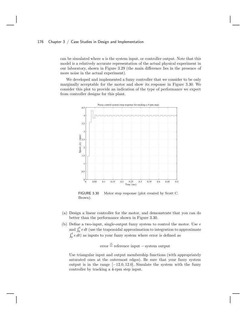
176 Chapter 3 / Case Studies in Design and Implementation
can be simulated where u is the system input, or controller output. Note that thismodel is a relatively accurate representation of the actual physical experiment inour laboratory, shown in Figure 3.29 (the main difference lies in the presence ofmore noise in the actual experiment).
We developed and implemented a fuzzy controller that we consider to be onlymarginally acceptable for the motor and show its response in Figure 3.30. Weconsider this plot to provide an indication of the type of performance we expectfrom controller designs for this plant.
0 0.05 0.1 0.15 0.2 0.25 0.3 0.35 0.4 0.45 0.50
0.5
1
1.5
2
2.5
3
3.5
4
4.5Fuzzy control system (step response for tracking a 4 rpm step)
Spee
d, y
(t)
(rp
m)
Time (sec)
FIGURE 3.30 Motor step response (plot created by Scott C.Brown).
(a) Design a linear controller for the motor, and demonstrate that you can dobetter than the performance shown in Figure 3.30.
(b) Define a two-input, single-output fuzzy system to control the motor. Use e
and∫ t
0e dt (use the trapezoidal approximation to integration to approximate∫ t
0e dt) as inputs to your fuzzy system where error is defined as
error= reference input − system output
Use triangular input and output membership functions (with appropriatelysaturated ones at the outermost edges). Be sure that your fuzzy systemoutput is in the range [−12.0, 12.0]. Simulate the system with the fuzzycontroller by tracking a 4-rpm step input.

3.10 Design Problems 177
(c) Tune your fuzzy system to obtain a better step response. Try changing thenumber of input and output membership functions, as well as the gains mul-tiplying the fuzzy controller inputs and outputs. (Remember, your outputshould saturate at ±12 volts.) Can you do better than the response shownin Figure 3.30? Obtain plots of the input and output membership functions,and simulated step response for your best response.
(d) Using your best fuzzy controller in (c), simulate the system tracking a 1-rpmstep input.
Design Problem 3.6 (Cargo Ship Steering): In this problem we study thedevelopment of fuzzy controllers for a ship steering problem. The model for theship is given in Chapter 6, Section 6.3.1 on page 333. Use the nonlinear modelof the ship provided in Equation (6.5) in all the simulation evaluations for thecontrol systems that you develop. Note that we would like to make the closed-loopsystem for the ship steering system behave like the reference model provided inChapter 6 for the ship. Note that to simulate the system given in Equation (6.5) onpage 334, you will have to convert the third-order nonlinear ordinary differentialequation to three first-order ordinary differential equations, as is explained inChapter 6.
(a) Develop a fuzzy controller for the ship steering problem that will resultin achieving the performance specified by the reference model (it may beoff slightly during transients). That is, you should achieve nearly the sameperformance as that shown in Figure 6.6 on page 342.
(b) Design a linear controller for the ship steering problem that will result inachieving the performance specified by the reference model (it may be offslightly during transients).
(c) Compare the results in (a) and (b).
Design Problem 3.7 (Base Braking Control): Antilock braking systems(ABS) are designed to stop vehicles as safely and quickly as possible. Safetyis achieved by maintaining lateral stability (and hence steering effectiveness) andreducing braking distances over the case where the brakes are controlled by thedriver. Current ABS designs typically use wheel speed compared to the velocityof the vehicle to measure when wheels lock (i.e., when there is “slip” between thetire and the road) and use this information to adjust the duration of brake signalpulses (i.e., to “pump” the brakes). Essentially, as the wheel slip increases pasta critical point where it is possible that lateral stability (and hence our abilityto steer the vehicle) could be lost, the controller releases the brakes. Then, oncewheel slip has decreased to a point where lateral stability is increased and brakingeffectiveness is decreased, the brakes are reapplied. In this way the ABS cycles thebrakes to achieve an optimum trade-off between braking effectiveness and lateral

178 Chapter 3 / Case Studies in Design and Implementation
stability. Inherent process nonlinearities, limitations on our abilities to sense cer-tain variables, and uncertainties associated with process and environment (e.g.,road conditions changing from wet asphalt to ice) make the ABS control problemchallenging. Many successful proprietary algorithms exist for the control logic forABS. In addition, several conventional nonlinear control approaches have beenreported in the literature.
In this problem, we do not consider brake control for a “panic stop,” and hencefor this problem the brakes are in a non-ABS mode. Instead, we consider whatis referred to as the “base-braking” control problem, where we seek to have thebrakes perform consistently as the driver (or an ABS) commands, even thoughthere may be aging of components or environmental effects (e.g., temperatureor humidity changes) that can cause “brake grab” or “brake fade.” We seek todesign a controller that will ensure that the braking torque commanded by thedriver (related to how hard we hit the brakes) is achieved by the brake system.Clearly, solving the base-braking problem is of significant importance since thereis a direct correlation between safety and the reliability of the brakes in providingthe commanded stopping force. Moreover, base-braking algorithms would run inparallel with ABS controllers so that they could also enhance braking effectivenesswhile the brakes are in an ABS mode.
Figure 3.31 shows the diagram of the base-braking system, as developedin [66, 118]. The input to the system, denoted by r(kT ), is the braking torque(in ft-lbs) requested by the driver. The output, y(kT ) (in ft-lbs), is the output ofa torque sensor, which directly measures the torque applied to the brakes. Notethat while torque sensors are not available on current production vehicles, thereis significant interest in determining the advantages of using such a sensor. Thesignal e(kT ) represents the error between the reference input and output torques,which is used by the controller to create the input to the brake system, u(kT ). Asampling interval of T = 0.005 seconds is used.
1/2560
Brake system
0.5187
z 2-1.94z+0.9409
27000
5v
0 F(y) x
Torque sensor
0.28
z-0.72
Brakecontroller
2560
2560
Specific torqueS
Σ
e(kT)y(kT)
Outputtorque
+
u(kT)
r(kT)
Desiredtorque
t
FIGURE 3.31 Brake control system (figure taken from [118], c© IEEE).
The General Motors braking system used in this problem is physically limitedto processing signals between [0, +1] volts, while the braking torque can rangefrom 0 to 2700 ft-lbs. For this reason and other hardware specific reasons [66],the input torque is attenuated by a factor of 2560 and the output is amplifiedby the same factor. After u(kT ) is multiplied by 2560, it is passed through asaturation nonlinearity where if 2560u(kT ) ≤ 0, the brake system receives a zero

3.10 Design Problems 179
input and if 2560u(kT ) ≥ 5, the input is 5. The output of the brake system passesthrough a similar nonlinearity that saturates at zero and 2700. The output of thisnonlinearity passes through F (y), which is defined as
F (y) =y
2502.4419+ 0.0139878
The function F (y) was experimentally determined and represents the relation-ship between brake fluid pressure and the stopping force on the car. Next, F (y)is multiplied by the “specific torque” St. This signal is passed through an exper-imentally determined model of the torque sensor, the signal is scaled, and y(kT )is output.
The specific torque St in the braking process reflects the variations in thestopping force of the brakes as the brake pads increase in temperature. Thestopping force applied to the wheels is a function of the pressure applied to thebrake pads and the coefficient of friction between the brake pads and the wheelrotors. As the brake pads and rotors increase in temperature, the coefficient offriction between the brake pads and the rotors increases. The result is that lesspressure on the brake pads is required for the same amount of braking force. Thespecific torque St of this braking system has been found experimentally to liebetween two limiting values so that
0.85 ≤ St ≤ 1.70
To conduct simulations for this problem, you should use the specific methodologythat we present next to represent the fact that as you repeatedly apply yourbrakes, they heat up—which is represented by increasing the value of St. Inparticular, a repeating 4-second input reference signal should be used where eachperiod of this signal corresponds to one application of the brakes. The inputreference begins at 0 ft-lbs, increases linearly to 1000 ft-lbs by 2 seconds, andremains constant at 1000 ft-lbs until 4 seconds. After 4 seconds the states ofthe brake system and controller should be cleared, and the simulation can berun again. For part (d) below the first two 4-second simulations are run withSt = 0.85, corresponding to “cold brakes” (a temperature of 125 F for the brakepads). The next two 4-second simulations are run with St increasing linearly from0.85 at 8 seconds to 1.70 after 12 seconds. Finally, two more 4-second simulationsare run with St = 1.7, corresponding to “hot brakes” (a temperature of 250 Ffor the brake pads).
(a) Develop a fuzzy controller for the base-braking control problem assumingthat the brakes always stay cold (i.e., St = 0.85).
(b) Develop a fuzzy controller for the base-braking control problem assumingthat the brakes always stay hot (i.e., St = 1.7).
(c) Test the fuzzy controller developed for the cold brakes on the hot ones, andvice-versa.

180 Chapter 3 / Case Studies in Design and Implementation
(d) Next, test the performance of the controller developed for the cold brakeson brakes that heat up over time. Use the simulation methodology outlinedabove.
(e) Repeat (a)–(d) using a conventional control approach and compare its per-formance to that of the fuzzy controllers.
Design Problem 3.8 (Rocket Velocity Control): A mathematical modelthat is useful in the study of the control of the velocity of a single-stage rocket isgiven by (see [16] and [136])
d v(t)dt
= c(t)(
m
M − m t
)− g
(R
R + y(t)
)− 0.5 v2(t)
(ρa A Cd
M − m t
)(3.6)
where v(t) is the rocket velocity at time t (the plant output), y(t) is the altitudeof the rocket (above sea level), and c(t) (the plant input) is the velocity of theexhaust gases (in general, the exhaust gas velocity is proportional to the cross-sectional area of the nozzle, so we take it as the input). Also,
• M = 15000.0 kg = the initial mass of the rocket and fuel.
• m = 100.0 kgs = the exhaust gases mass flow rate (approximately constant
for some solid propellant rockets).• A = 1.0 meter2 = the maximum cross-sectional area of the rocket.• g = 9.8 meters
s2 = the the acceleration due to gravity at sea level.• R = 6.37× 10⁶ meters = the radius of the earth.
• ρa = 1.21 kgm3 = the density of air.
• Cd = 0.3 = the drag coefficient for the rocket.
Due to the loss of fuel resulting from combustion and exhaust, the rocket has atime-varying mass.
To specify the performance objectives, we use a “reference model.” That is, wedesire to have the closed-loop system from r to v behave the same as a referencemodel does from r to vm. In our case, we choose the reference model to be
dvm(t)dt
= −0.2vm(t) + 0.2r(t)
where vm(t) specifies the desired rocket velocity. This shows that we would likea first-order-type response due to a step input.
(a) Pick an altitude trajectory y(t) that you would like to follow.
(b) Develop a fuzzy controller for the rocket velocity control problem and demon-strate that it meets the performance specifications via simulation.

3.10 Design Problems 181
(b) Develop a controller using conventional methods and demonstrate that itmeets the performance objectives. Compare its performance to that of thefuzzy controller.
Design Problem 3.9 (An Acrobot): An acrobot is an underactuated, un-stable two-link planar robot that mimics the human acrobat who hangs froma bar and tries to swing up to a perfectly balanced upside-down position withhis or her hands still on the bar (see Figure 3.32). In this problem we apply di-rect fuzzy control to two challenging robotics control problems associated withthe acrobot, swing-up and balancing, and use different controllers for each case.Typically, a heuristic strategy is used for swing-up, where the goal is to force theacrobot to reach its vertical upright position with near-zero velocity on both links.Then, when the links are close to the inverted position, a balancing controller isswitched on and used to maintain the acrobot in the inverted position (again, seeFigure 3.32). Such a strategy was advocated in earlier work in [191] and [190].
Hangingposition(stable)
Movementto helpswing-up
Movingtowardinvertedposition
Nearinvertedposition
Invertedposition(unstable)
Use swing-up controller Switch to balancing controller
Motor fixedto link 1, usedto drivelink 2
Sensors forangularposition
"Link 1"
"Link 2"
FIGURE 3.32 The acrobot (figure takenfrom [27], c© Kluwer Academic Pub.).
The acrobot has a single actuator at the elbow and no actuator at theshoulder; the system is “underactuated” because we desire to control two links ofthe acrobot (each with a degree of freedom) with only a single system input. Theconfiguration of a simple acrobot, from which the system dynamics are obtained,is shown in Figure 3.33. The joint angles q1 and q2 serve as the generalized systemcoordinates; m1 and m2 specify the mass of the links; l1 and l2 specify the linklengths; lc1 and lc2 specify the distance from the axis of rotation of each link to

182 Chapter 3 / Case Studies in Design and Implementation
its center of mass; and I1 and I2 specify the moment of inertia of each link takenabout an axis coming out of the page and passing through its center of mass. Thesingle system input τ is defined such that a positive torque causes q2 to increase(move in the counterclockwise direction).
2m 2 I,
q1
q2
l
l
l
c
c
l1
2
, I1m1
2
1
FIGURE 3.33 Simple acrobot notation(figure taken from [27], c© Kluwer AcademicPub.).
The dynamics of the simple acrobot may be obtained by determining the Euler-Lagrange equations of motion for the system. This is accomplished by findingthe Lagrangian of the system, or the difference between the system’s kineticand potential energies. Indeed, determining the kinetic and potential energiesof each link is the most difficult task in obtaining the system dynamics andrequires forming the manipulator Jacobian (see Chapters 5 and 6 of [192] for moredetails). In [192], Spong has developed the equations of motion of a planar elbowmanipulator; this manipulator is identical to the acrobot shown in Figure 3.33,except that it is actuated at joints one and two. The dynamics of the acrobotare simply those of the planar manipulator, with the term corresponding to theinput torque at the first joint set equal to zero. The acrobot dynamics may bedescribed by the two second-order differential equations
d11q1 + d12q2 + h1 + φ1 = 0 (3.7)d12q1 + d22q2 + h2 + φ2 = τ (3.8)
where the coefficients in Equations (3.7) and (3.8) are defined as
d11 = m1l2c1 + m2(l21 + l2c2 + 2l1lc2 cos(q2)) + I1 + I2

3.10 Design Problems 183
d22 = m2l2c2 + I2
d12 = m2(l2c2 + l1lc2 cos(q2)) + I2
h1 = −m2l1lc2 sin(q2)q22 − 2m2l1lc2 sin(q2)q2q1
h2 = m2l1lc2 sin(q2)q21
φ1 = (m1lc1 + m2l1)g cos(q1) + m2lc2g cos(q1 + q2)φ2 = m2lc2g cos(q1 + q2)
In our acrobot model, we have also limited the range for joint angle q2 to[−π, π] (i.e., the second link is not free to rotate in a complete revolution—itcannot cross over the first link). We have also cascaded a saturation nonlinearitybetween the controller output and plant input to limit the input torque magnitudeto 4.5 N-m. The model parameter values are given in Table 3.12.
TABLE 3.12 Acrobot ModelParameters Used in Simulations
Parameter Value
m1 1.9008 kg
m2 0.7175 kg
l1 0.2 m
l2 0.2 m
lc1 1.8522 × 10⁻¹ m
lc2 6.2052 × 10⁻² m
I1 4.3399 × 10⁻³ kg·m2
I2 5.2285 × 10⁻³ kg·m2
When you simulate the acrobot, be sure to use a good numerical simulationalgorithm with a small enough integration step size. For instance, use a fourth-order Runge-Kutta technique with an integration step size of 0.0025 seconds. Tosimulate the effects of implementing the controllers on a digital computer, samplethe output signals with a period T = 0.01 seconds, and only update the controlinput every T seconds (holding the value constant in between updates).
(a) Find a linear model about the equilibrium inverted position (q1 = π/2,q2 = 0, q1 = 0, q2 = 0) with τ = 0 (note that there is actually a continuumof equilibrium positions). Define the state vector x = [q1 − π/2, q2, q1, q2]
to transform the balancing control problem to a regulation problem. Theacrobot dynamics linearized about x = [0, 0, 0, 0] may be described by
x = Ax + Bτ
y = Cx + Dτ
Find the numerical values for the A, B, C, and D matrices and verify that thesystem is unstable. Design a linear quadratic regulator (LQR), and illustrate

184 Chapter 3 / Case Studies in Design and Implementation
its performance in simulation for an initial condition q1(0) = π/2 + 0.04,q2(0) = −0.0500, q1(0) = −0.2000, and q2(0) = 0.0400. This initial conditionis such that the first link is approximately 2.29 beyond the inverted position,while the second link is displaced approximately −2.86 from the first link.The initial velocities are such that the first link is moving away from theinverted position, while the second link is moving into line with the firstlink.
(b) Next we study the development of a fuzzy controller for the acrobot. Supposethat your fuzzy controller has four inputs: g0(q1−π/2), g1q2, g2q1, and g3q2;and a single output. Here, g0–g3 are scaling gains, and the output of thefuzzy controller is scaled by a gain h. Test your controller in simulationusing the same initial conditions as in part (a). Hint: Use the approach ofcopying the LQR gains as we did for the rotational inverted pendulum. Also,consider specifying the output membership function centers via a nonlinearfunction.
Design Problem 3.10 (Fuzzy Warning Systems): In this problem you willfully develop the fuzzy decision-making systems that are used as warning systemsfor an infectious disease and an aircraft.
(a) Fully develop the fuzzy system that will serve as a warning system for theinfectious disease warning system described in Section 3.6.1 on page 162.Test the performance of the system by showing that it can provide properwarnings for each of the warning conditions.
(b) Repeat (a) but for the aircraft failure warning system described in Sec-tion 3.6.2 on page 166.
Design Problem 3.11 (Automobile Speed Warning System): In thisproblem you will study the development of a fuzzy decision-making system for“intelligent vehicle and highway systems” where there is a focus on the devel-opment of “automated highway systems” (AHS). In AHS it is envisioned thatvehicles will be automatically driven by an on-board computer that interactswith a specially designed roadway. Such AHS offer significant improvements insafety and overall roadway efficiency (i.e., they increase vehicle throughput). Itis evident that the AHS will evolve by the sequential introduction of increasinglyadvanced automotive and roadway subsystems. One such system that may beused is a speed advisory system to be placed on the vehicle to enhance safety,as shown in Figure 3.34. There is a vehicle and a changeable electronic sign thatdisplays the speed limit for the current weather and traffic conditions, and inaddition transmits the current speed limit to passing vehicles. There is a receiverin the vehicle that can collect this speed limit information. The problem is todesign a speed advisory system that can display warnings to the driver about thedangers of exceeding the speed limit. We will use this problem to illustrate the

3.10 Design Problems 185
development of a fuzzy decision-making system that can emulate the manner inwhich a human safety expert would warn the driver about traveling at dangerousspeeds if such a person could be available on each and every vehicle.
55
FIGURE 3.34 Scenario for an automobile speed advisorysystem.
The first step in the design of the speed advisory system is to specify the typesof advice that the safety expert should provide. Then the expert should indicatewhat variables need to be known to in order to provide such advice. This will helpdefine the inputs and outputs of the fuzzy system. Suppose specifications dictatethat the advisory system is to provide (1) an indication of the likelihood (on ascale of zero to one, with one being very likely) that the vehicle will exceed thecurrent speed limit (which we assume is fixed at 55 mph for our example), and (2)a numeric rating between one and ten (ten being the highest) of how dangerousthe current operating speed is. Suppose that to provide such information thesafety expert indicates that the error between the current vehicle speed and thespeed limit and the derivative of the error between the current vehicle speed andthe speed limit will be needed. Clearly, the fuzzy system will then have two inputsand two outputs.
To develop a fuzzy speed warning system, we need to have the engineerinterview the safety expert to determine how to decide what warnings should beprovided to the driver. The safety expert will provide a linguistic description ofher or his approach. First, define the universe of discourse for the speed errorinput to the fuzzy system to be [−100, 100] mph (where 100 mph is the highestspeed that the vehicle can attain) and universe of discourse for the change in speedinput to be [−10, 10] mph/sec (so that the vehicle can accelerate or decelerateat most 10 mph in one second). The universe of discourse for the output thatindicates the likelihood to exceed the speed limit is [0, 1], and the universe ofdiscourse for the danger rating output is [0, 10], with 10 representing the mostdangerous situation. We use e to denote the speed error, e for the derivative ofthe error, s for the likelihood that the speed limit will be exceeded, and d forthe danger rating for the current speed. The linguistic variables for the inputscould be = “error” and = “error-deriv,” and for the outputs they could be =“likely-to-exceed-limit” and = “danger-rating.”
Examples of linguistic rules for the fuzzy system could be the following: (1)If error is “possmall” and error-deriv is “neglarge” Then likely-to-exceed-limit is“medium” (i.e., if the speed is below the limit, but it is approaching the limitquickly, then there is some concern that the speed limit will be exceeded), (2) If

186 Chapter 3 / Case Studies in Design and Implementation
error is “zero” and error-deriv is “neglarge” Then likely-to-exceed-limit is “large”(i.e., if the speed is currently at the speed limit and it is increasing rapidly, thenthere is a significant concern that the speed limit will be exceeded), and (3) Iferror is “possmall” and error-deriv is “neglarge” Then danger-rating is “small”(i.e., if the speed is below the limit, but it is approaching the limit quickly, Thenthere is some danger because the limit is likely to at least slightly exceed whatexperts judge to be a safe driving speed).
(a) Develop a fuzzy decision-making system that can serve as a speed advisorysystem for automobiles.
(b) Develop a test scenario for the fuzzy system. Clearly explain how you willtest the system.
(c) Test the system according to your plan in (b), and show your results (theseshould include showing that the system can provide warnings under theproper conditions).
Design Problem 3.12 (Design of Fuzzy Decision-Making Systems): Inthis problem you will assist in both defining the problem and the solution. Theproblem focuses on the development of fuzzy decision-making systems that arenot necessarily used in the control of a system.
(a) Suppose that you wish to buy a used car. You have various priorities withregard to price, color, safety features, the year the car was made, and themake of the car. Quantify each of these characteristics with fuzzy sets andload appropriate rules into a fuzzy decision-making system that representsyour own priorities in purchasing a used car. For instance, when presentedwith N cars in a row, the fuzzy system should be able to provide a valuethat represents your ranking of the desirability of purchasing each of thecars. Demonstrate in simulation the performance of the system (i.e., thatit properly represents your decision-making strategy for purchasing a usedcar).
(b) Suppose that you wish to design a computer program that will guess whichteam wins in a football game (that has already been played) when it is givenonly total passing yards, total rushing yards, and total time of possessionfor each team. Design a fuzzy decision-making system that will guess at theoutcome (score) of a game based on these inputs. Test the performance ofthe system by using data from actual games played by your favorite team.
(c) An alternative, perhaps more interesting system to develop than the onedescribed in (b), would be one that would predict who would win the gamebefore it was played. How would you design such a system?

C H A P T E R 4
Nonlinear AnalysisSo far as the laws of mathematics refer to reality,
they are not certain. And so far as they are certain,
they do not refer to reality.
–Albert Einstein
4.1 OverviewAs we described it in Chapters 1–3, the standard control engineering methodologyinvolves repeatedly coordinating the use of modeling, controller design, simulation,mathematical analysis, implementations, and evaluations to develop control sys-tems. In Chapters 2 and 3 we showed via examples how modeling is used, and weprovided guidelines for controller design. Moreover, we discussed how to simulatefuzzy controllers, highlighted some issues that are encountered in implementation,and showed case studies that illustrated the design, simulation, and implementa-tion of fuzzy control systems. In this chapter we show how to perform mathematicalanalysis of various properties of fuzzy control systems so that the designer will haveaccess to all steps of the basic control design methodology.
Basically, we use the mathematical model of the plant and nonlinear analysis toenhance our confidence in the reliability of a fuzzy control system by verifying sta-bility and performance specifications and possibly redesigning the fuzzy controller.We emphasize, however, that mathematical analysis alone cannot provide defini-tive answers about the reliability of the fuzzy control system since such analysisproves properties about the model of the process, not the actual physical process.Indeed, it can be argued that a mathematical model is never a perfect representa-tion of a physical process; hence, while nonlinear analysis may appear to providedefinitive statements about control system reliability, you must understand thatsuch statements are only accurate to the extent that the mathematical model isaccurate. Nonlinear analysis does not replace the use of common sense and evalua-
187

188 Chapter 4 / Nonlinear Analysis
tion via simulations and experimentation. It simply assists in providing a rigorousengineering evaluation of a fuzzy control system before it is implemented.
It is important to note that the advantages of fuzzy control often become mostapparent for very complex problems where we have an intuitive idea about howto achieve high-performance control (e.g., the two-link flexible robot case studyin Chapter 3). In such control applications, an accurate mathematical model is socomplex (i.e., high order, nonlinear, stochastic, with many inputs and outputs) thatit is sometimes not very useful for the analysis and design of conventional controlsystems since assumptions needed to utilize conventional control design approachesare often violated. The conventional control engineering approach to this problem isto use an approximate mathematical model that is accurate enough to characterizethe essential plant behavior in a certain region of operation, yet simple enough sothat the necessary assumptions needed to apply the analysis and design techniquesare satisfied. However, due to the inaccuracy of the model, upon implementationthe developed controllers often need to be tuned via the “expertise” of the controlengineer.
The fuzzy control approach, where explicit characterization and utilization ofcontrol expertise is used earlier in the design process, largely avoids the problemswith model complexity that are related to design. That is, for the most part, fuzzycontrol system design does not depend on a mathematical model unless it is neededto perform simulations to gain insight into how to choose the rule-base and mem-bership functions. However, the problems with model complexity that are relatedto analysis have not been solved (i.e., analysis of fuzzy control systems criticallydepends on the form of the mathematical model); hence, it is often difficult orimpossible to apply nonlinear analysis techniques to the applications where theadvantages of fuzzy control are most apparent!
For instance, existing results for stability analysis of fuzzy control systems typ-ically require that the plant model be deterministic and satisfy some continuityconstraints, and sometimes require the plant to be linear or have a very specificmathematical form. The most general approaches to the nonlinear analysis of fuzzycontrol systems are those due to Lyapunov (his direct and indirect methods). Onthe other hand, for some stability analysis approaches (e.g., for absolute stability),the only results for analysis of steady-state tracking error of fuzzy control systems,and the existing results on the use of describing functions for analysis of limit cycles,essentially require a linear time-invariant plant (or one that has a special form sothat the nonlinearities can be bundled into one nonlinear component in the loop).
These limitations in the theory help to show that fuzzy control technology is ina sense leading the theory; the practitioner will go ahead with the design and im-plementation of many fuzzy control systems without the aid of nonlinear analysis.In the meantime, theorists will continue to develop a mathematical theory for theverification and certification of fuzzy control systems. This theory will have a syn-ergistic effect by driving the development of fuzzy control systems for applicationswhere there is a need for highly reliable implementations.
Overall, the objectives of this chapter are as follows:

4.2 Parameterized Fuzzy Controllers 189
• To help teach sound techniques for the construction of fuzzy controllers by alertingthe designer to some of the pitfalls that can occur if a rule-base is improperlyconstructed (e.g., instabilities, limit cycles, and steady-state errors).
• To provide insights into how to modify the fuzzy controller rule-base to guar-antee that performance specifications are met (thereby helping make the fuzzycontroller design process more systematic).
• To provide examples of how to apply the theory to some simple fuzzy controlsystem analysis and design problems.
We provide an introduction to the use of Lyapunov stability analysis in Sec-tion 4.3. In particular, we introduce Lyapunov’s direct and indirect methods andillustrate the use of these via several examples and an inverted pendulum applica-tion. Moreover, we show how to use Lyapunov’s direct method for the analysis ofstability of plants represented with Takagi-Sugeno fuzzy systems that are controlledwith a Takagi-Sugeno form of a fuzzy controller.
We introduce analysis of absolute stability in Section 4.4, steady-state erroranalysis in Section 4.5, and describing function analysis in Section 4.6. In eachof these sections we show how the methods can aid in picking the membershipfunctions in a fuzzy controller to avoid limit cycles, and instabilities, and ultimatelyto meet a variety of closed-loop specifications. Since most fuzzy control systems are“hybrid” in that the controller contains a linear portion (e.g., an integrator ordifferentiator) as well as a nonlinear portion (a fuzzy system), we will show how touse nonlinear analysis to design both of these portions of the fuzzy control system.
Overall, while we highly recommend that you study this chapter carefully, if youare not concerned with the verification of the behavior of a fuzzy control system,you can skip to the next chapter. Indeed, there is no direct dependence of any topicin the remaining chapters of this book on the material in this chapter. This chaptersimply tends to deepen your understanding of the material studied in Chapters 1–3.
4.2 Parameterized Fuzzy ControllersIn this section we will introduce the fuzzy control system to be investigated andbriefly examine the nonlinear characteristics of the fuzzy controller. Except in Sec-tion 4.3, the closed-loop systems in this chapter will be as shown in Figure 4.1(where we assume that G(s) is a single-input single-output (SISO) linear system)or they will be modified slightly so that the fuzzy controller is in the feedback path.1
We will be using both SISO and MISO (multi-input single-output) fuzzy controllersas they are defined in the next subsections.
1. We assume throughout this chapter that the fuzzy controller is designed so that the existence
and uniqueness of the solution of the differential equation describing the closed-loop system isguaranteed.

190 Chapter 4 / Nonlinear Analysis
PlantΣ
r e u yFuzzycontroller+
Φ
FIGURE 4.1 Fuzzy control system.
4.2.1 Proportional Fuzzy ControllerFor the “proportional fuzzy controller,” as the SISO fuzzy controller in Figure 4.1is sometimes called, the rule-base can be constructed in a symmetric fashion withrules of the following form:
1. If e is NB Then u is NB
2. If e is NM Then u is NM
3. If e is NS Then u is NS
4. If e is ZE Then u is ZE
5. If e is PS Then u is PS
6. If e is PM Then u is PM
7. If e is PB Then u is PB
where NB, NM, NS, ZE, PS, PM, and PB are linguistic values representing “nega-tive big,” “negative medium,” and so on.
The membership functions for the premises and consequents of the rules areshown in Figure 4.2. Notice in Figure 4.2 that the widths of the membership func-tions are parameterized by A and B. Throughout this chapter, unless it is indicatedotherwise, the same rule-base and similar uniformly distributed membership func-tions will be used for all applications (where if the number of input and outputmembership functions and rules increase, our analysis approaches work in a similarmanner). The fuzzy controller will be adjusted by changing the values of A andB. The manner in which these values affect the nonlinear map that the fuzzy con-troller implements will be discussed below. The fuzzy inference mechanism operatesby using the product to combine the conjunctions in the premise of the rules andin the representation of the fuzzy implication. Singleton fuzzification is used, anddefuzzification is performed using the center-average method.
The SISO fuzzy controller described above implements a static nonlinear input-output map between its input e(t) and output u(t). As we discussed in Chapter 2,the particular shape of the nonlinear map depends on the rule-base, inference strat-egy, fuzzification, and defuzzification strategy utilized by the fuzzy controller. Con-sider the input-output map for the above fuzzy controller shown in Figure 4.3 withA = B = 1. Modifications to the fuzzy controller can provide an infinite variety

4.2 Parameterized Fuzzy Controllers 191
µ
e(t)
µ
u(t)
NB NM NS ZE PS PM PB
NB NM NS ZE PS PB
-B B
-A A0
0
A3
-A3
A3
2A3
-2
3B
32B
3-B
3-2 B
PM
FIGURE 4.2 Membership functions for e(t) and u(t) (figuretaken from [83], c© John Wiley and Sons).
of such input-output maps (e.g., by changing the consequents of the rules). Notice,however, that there is a marked similarity between the input-output map in Fig-ure 4.3 and the standard saturation nonlinearity. In fact, the parameters A and Bfrom the fuzzy controller are similar to the saturation parameters of the standardsaturation nonlinearity—that is, B is the level at which the output saturates, andA is the value of e(t) at which the saturation of u(t) occurs. Because the input-output map of the fuzzy controller is odd, −B is the saturation level for e(t) ≤ −A,and −A is the value of e(t) where the saturation occurs. By modifying A and B(and hence moving the input and output membership functions), we can change theinput-output map nonlinearity and its effects on the system. Throughout this chap-ter, except in Section 4.3, we will always use rules in the form described above. Weemphasize, however, that the nonlinear analysis techniques used in this chapter willwork in the same manner for other types of rule-bases (and different fuzzification,inference, and defuzzification techniques).
4.2.2 Proportional-Derivative Fuzzy ControllerThere are many different types of fuzzy controllers we could examine for the MISOcase. Here, aside from Section 4.3, we will constrain ourselves to the two input“proportional-derivative fuzzy controller” (as it is sometimes called). This controlleris similar to our SISO fuzzy controller with the addition of the second input, e. Infact, the membership functions on the universes of discourses and linguistic valuesNB, NM, NS, ZE, PS, PM, and PB for e and u are the same as they are shown inFigure 4.2 and will still be adjusted using the parameters A and B, respectively.The membership functions on the universe of discourse and the linguistic values forthe second input, e, are the same as for e with the exception that the adjustment
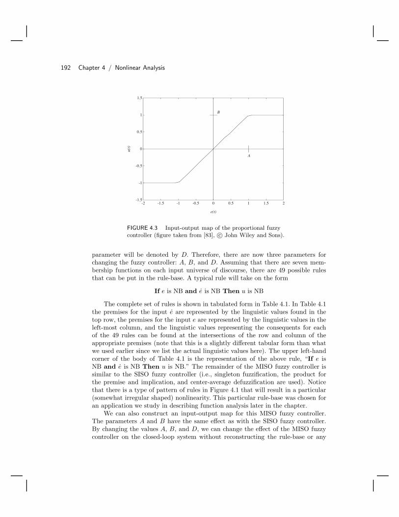
192 Chapter 4 / Nonlinear Analysis
-1.5
-1
-0.5
0
0.5
1
1.5
-2 -1.5 -1 -0.5 0 0.5 1 1.5 2
A
B
e(t)
u(t)
FIGURE 4.3 Input-output map of the proportional fuzzycontroller (figure taken from [83], c© John Wiley and Sons).
parameter will be denoted by D. Therefore, there are now three parameters forchanging the fuzzy controller: A, B, and D. Assuming that there are seven mem-bership functions on each input universe of discourse, there are 49 possible rulesthat can be put in the rule-base. A typical rule will take on the form
If e is NB and e is NB Then u is NB
The complete set of rules is shown in tabulated form in Table 4.1. In Table 4.1the premises for the input e are represented by the linguistic values found in thetop row, the premises for the input e are represented by the linguistic values in theleft-most column, and the linguistic values representing the consequents for eachof the 49 rules can be found at the intersections of the row and column of theappropriate premises (note that this is a slightly different tabular form than whatwe used earlier since we list the actual linguistic values here). The upper left-handcorner of the body of Table 4.1 is the representation of the above rule, “If e isNB and e is NB Then u is NB.” The remainder of the MISO fuzzy controller issimilar to the SISO fuzzy controller (i.e., singleton fuzzification, the product forthe premise and implication, and center-average defuzzification are used). Noticethat there is a type of pattern of rules in Figure 4.1 that will result in a particular(somewhat irregular shaped) nonlinearity. This particular rule-base was chosen foran application we study in describing function analysis later in the chapter.
We can also construct an input-output map for this MISO fuzzy controller.The parameters A and B have the same effect as with the SISO fuzzy controller.By changing the values A, B, and D, we can change the effect of the MISO fuzzycontroller on the closed-loop system without reconstructing the rule-base or any

4.3 Lyapunov Stability Analysis 193
TABLE 4.1 Rule Table for PD Fuzzy Controller
“output” “change-in-error” eu NB NM NS ZE PS PM PB
NB NB NS PS PB PB PB PBNM NB NM ZE PM PM PB PB
“error” NS NB NM NS PS PM PB PBe ZE NB NM NS ZE PS PM PB
PS NB NB NM NS PS PM PBPM NB NB NM NM ZE PM PBPB NB NB NB NB NS PS PB
other portion of the fuzzy controller. Again, we emphasize that while we use thisparticular fuzzy controller, which is conveniently parameterized by A, B, and D, theapproaches to nonlinear analysis in this chapter work in a similar manner for fuzzycontrollers that use other membership functions, rule-bases, inference mechanisms,and fuzzification and defuzzification strategies.
4.3 Lyapunov Stability AnalysisOften the designer is first concerned about investigating the stability properties ofa fuzzy control system, since it is often the case that if the system is unstable thereis no chance that any other performance specifications will hold. For example, ifthe fuzzy control system for an automobile cruise control is unstable, you wouldbe more concerned with the possibility of unsafe operation than with how well itregulates the speed at the set-point. In this section we provide an overview of twoapproaches to stability analysis of fuzzy control systems: Lyapunov’s direct andindirect methods. We provide several examples for each of the methods, includingthe application of Lyapunov’s direct method to the stability analysis of Takagi-Sugeno fuzzy systems. In the next section we show how to use the circle criterionin the analysis of absolute stability of fuzzy control systems.
4.3.1 Mathematical PreliminariesSuppose that a dynamic system is represented with
x(t) = f(x(t)) (4.1)
where x ∈ n is an n vector and f : D → n with D = n or D = B(h) for someh > 0 where
B(h) = x ∈ n : |x| < h
is a ball centered at the origin with a radius of h and | · | is a norm on n (e.g.,|x| =
√(xx)). If D = n then we say that the dynamics of the system are defined
globally, while if D = B(h) they are only defined locally. Assume that for every x0

194 Chapter 4 / Nonlinear Analysis
the initial value problem
x(t) = f(x(0)), x(0) = x0 (4.2)
possesses a unique solution φ(t, x0) that depends continuously on x0. A point xe ∈n is called an “equilibrium point” of Equation (4.1) if f(xe) = 0 for all t ≥ 0. Anequilibrium point xe is an “isolated equilibrium point” if there is an h′ > 0 suchthat the ball around xe,
B(xe, h′) = x ∈ n : |x − xe| < h′
contains no other equilibrium points besides xe. As is standard, we will assume thatthe equilibrium of interest is an isolated equilibrium located at the origin of n.This assumption results in no loss of generality since if xe = 0 is an equilibriumof Equation (4.1) and we let x(t) = x(t) − xe, then x = 0 is an equilibrium of thetransformed system
˙x(t) = f(x(t)) = f(x(t) + xe)
(for an example of this idea, see Section 4.3.4).The equilibrium xe = 0 of (4.1) is “stable” (in the sense of Lyapunov) if for
every ε > 0 there exists a δ(ε) > 0 such that |φ(t, x0)| < ε for all t ≥ 0 whenever|x0| < δ(ε) (i.e., it is stable if when it starts close to the equilibrium it will stayclose to it). The notation δ(ε) means that δ depends on ε. A system that is notstable is called “unstable.”
The equilibrium xe = 0 of Equation (4.1) is said to be “asymptotically stable” ifit is stable and there exists η > 0 such that limt→∞ φ(t, x0) = 0 whenever |x0| < η(i.e., it is asymptotically stable if when it starts close to the equilibrium it willconverge to it).
The set Xd ⊂ n of all x0 ∈ n such that φ(t, x0) → 0 as t → ∞ is called the“domain of attraction” of the equilibrium xe = 0 of Equation (4.1). The equilibriumxe = 0 is said to be “globally asymptotically stable” if Xd = n (i.e., if no matterwhere the system starts, its state converges to the equilibrium asymptotically).
As an example, consider the scalar differential equation
x(t) = −2x(t)
which is in the form of Equation (4.2). For this system, D = 1 (i.e., the dynamicsare defined on the entire real line, not just some region around zero). We havexe = 0 as an equilibrium point of this system since 0 = −2xe. Notice that for anyx0, we have the solution
φ(t, x0) = x0e−2t → 0
as t → ∞ so that the equilibrium xe = 0 is stable since if you are given anyε > 0 there exists a δ > 0 such that if |x0| < δ, φ(t, x0) ≤ ε. To see this, simply

4.3 Lyapunov Stability Analysis 195
choose δ = ε for any ε > 0 that you choose. Also note that since for any x0 ∈ n,φ(t, x0) → 0, the system is globally asymptotically stable. While determining if thissystem possesses certain stability properties is very simple since the system is sosimple, for complex nonlinear systems it is not so easy. One reason for this is thatfor complex nonlinear systems, it is difficult to even solve the ordinary differentialequations (i.e., to find φ(t, x0) for all t and x0). However, Lyapunov’s methodsprovide two techniques that allow you to determine the stability properties withoutsolving the ordinary differential equations.
4.3.2 Lyapunov’s Direct MethodThe stability results for an equilibrium xe = 0 of Equation (4.1) that we providenext depend on the existence of an appropriate “Lyapunov function” V : D → where D = n for global results (e.g., global asymptotic stability) and D = B(h) forsome h > 0, for local results (e.g., stability in the sense of Lyapunov or asymptoticstability). If V is continuously differentiable with respect to its arguments, then thederivative of V with respect to t along the solutions of Equation (4.1) is
V(4.1)(x(t)) = ∇V (x(t))f(x(t))
where
∇V (x(t)) =[
∂V
∂x1,∂V
∂x2, . . . ,
∂V
∂xn
]
is the gradient of V with respect to x. Using the subscript on V is sometimescumbersome, so we will at times omit it with the understanding that the derivativeof V is taken along the solutions of the differential equation that we are studyingthe stability of.
Lyapunov’s direct method is given by the following:
1. Let xe = 0 be an equilibrium for Equation (4.1). Let V : B(h) → be acontinuously differentiable function on B(h) such that V (0) = 0 and V (x) > 0in B(h)−0, and V(4.1)(x) ≤ 0 in B(h). Then xe = 0 is stable. If, in addition,V(4.1)(x) < 0 in B(h) − 0, then xe = 0 is asymptotically stable.
2. Let xe = 0 be an equilibrium for Equation (4.1). Let V : n → be a contin-uously differentiable function such that V (0) = 0 and V (x) > 0 for all x = 0,|x| → ∞ implies that V (x) → ∞, and V(4.1)(x) < 0 for all x = 0. Then xe = 0is globally asymptotically stable.
As an example, consider the system
x(t) = −2x3

196 Chapter 4 / Nonlinear Analysis
that has an equilibrium xe = 0. Choose
V (x) =12x2
With this choice we have
V =∂V
∂x
dx
dt= xx = −2x4
so that clearly if x = 0 then −2x4 < 0, so that by Lyapunov’s direct method xe = 0is asymptotically stable. Notice that xe = 0 is in fact globally asymptotically stable.
While Lyapunov’s direct method has found wide application in conventionalcontrol, it is important to note that it is not always easy to find the “Lyapunovfunction” V that will have the above properties so that we can guarantee that thesystem is stable. Next, we introduce Lyapunov’s indirect method.
4.3.3 Lyapunov’s Indirect Method
Let ∂f∂x =
[∂fi
∂xj
]denote the n×n “Jacobian matrix.” For the next result, assume that
f : D → n where D ⊂ n, that xe ∈ D, and that f is continuously differentiable.Lyapunov’s indirect method is given by the following: Let xe = 0 be an equi-
librium point for the nonlinear system Equation (4.1). Let the n × n matrix
A =∂f
∂x(x)
∣∣∣∣x=xe=0
then
1. The origin xe = 0 is asymptotically stable if Re[λi] < 0 (the real part of λi) forall eigenvalues λi of A.
2. The origin xe = 0 is unstable if Re[λi] > 0 for one or more eigenvalues of A.
3. If Re[λi] ≤ 0 for all i with Re[λi] = 0 for some i where the λi are the eigenvaluesof A, then we cannot conclude anything about the stability of xe = 0 fromLyapunov’s indirect method.
Lyapunov’s indirect method has also found wide application in conventionalcontrol. Note that the term “indirect” is used since we arrive at our conclusionsabout stability indirectly by first linearizing the system about an operating point.The indirect method is sometimes called Lyapunov’s “first method,” while the directmethod is referred to as his “second method.”
As an example, consider the system
x = −x2
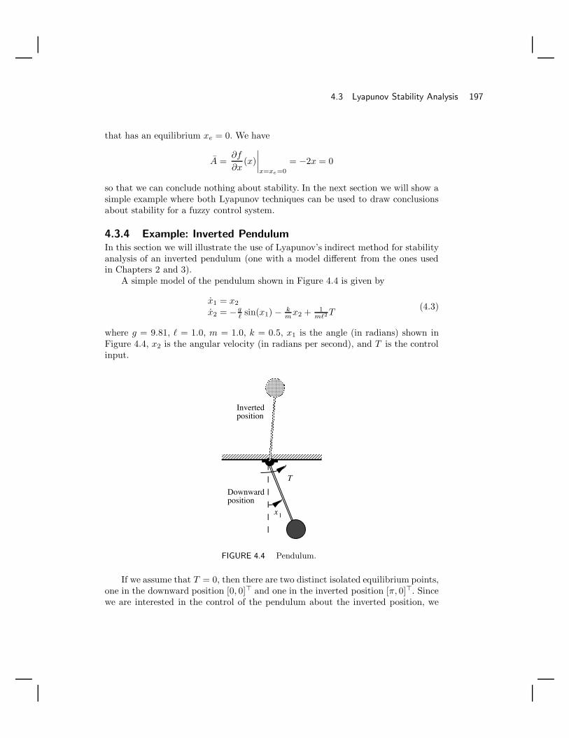
4.3 Lyapunov Stability Analysis 197
that has an equilibrium xe = 0. We have
A =∂f
∂x(x)
∣∣∣∣x=xe=0
= −2x = 0
so that we can conclude nothing about stability. In the next section we will show asimple example where both Lyapunov techniques can be used to draw conclusionsabout stability for a fuzzy control system.
4.3.4 Example: Inverted PendulumIn this section we will illustrate the use of Lyapunov’s indirect method for stabilityanalysis of an inverted pendulum (one with a model different from the ones usedin Chapters 2 and 3).
A simple model of the pendulum shown in Figure 4.4 is given by
x1 = x2
x2 = −gsin(x1) − k
mx2 + 1
m2T
(4.3)
where g = 9.81, = 1.0, m = 1.0, k = 0.5, x1 is the angle (in radians) shown inFigure 4.4, x2 is the angular velocity (in radians per second), and T is the controlinput.
x1
Invertedposition
Downwardposition
T
FIGURE 4.4 Pendulum.
If we assume that T = 0, then there are two distinct isolated equilibrium points,one in the downward position [0, 0] and one in the inverted position [π, 0]. Sincewe are interested in the control of the pendulum about the inverted position, we
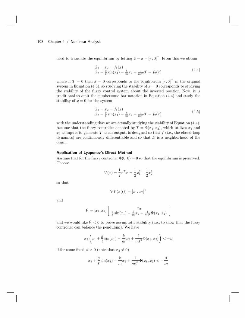
198 Chapter 4 / Nonlinear Analysis
need to translate the equilibrium by letting x = x − [π, 0]. From this we obtain
˙x1 = x2 = f1(x)˙x2 = g
sin(x1) − k
mx2 + 1
m2T = f2(x) (4.4)
where if T = 0 then x = 0 corresponds to the equilibrium [π, 0] in the originalsystem in Equation (4.3), so studying the stability of x = 0 corresponds to studyingthe stability of the fuzzy control system about the inverted position. Now, it istraditional to omit the cumbersome bar notation in Equation (4.4) and study thestability of x = 0 for the system
x1 = x2 = f1(x)x2 = g
sin(x1) − kmx2 + 1
m2 T = f2(x)(4.5)
with the understanding that we are actually studying the stability of Equation (4.4).Assume that the fuzzy controller denoted by T = Φ(x1, x2), which utilizes x1 andx2 as inputs to generate T as an output, is designed so that f (i.e., the closed-loopdynamics) are continuously differentiable and so that D is a neighborhood of theorigin.
Application of Lyapunov’s Direct Method
Assume that for the fuzzy controller Φ(0, 0) = 0 so that the equilibrium is preserved.Choose
V (x) =12xx =
12x2
1 +12x2
2
so that
∇V (x(t)) = [x1, x2]
and
V = [x1, x2][
x2g sin(x1) − k
mx2 + 1m2 Φ(x1, x2)
]
and we would like V < 0 to prove asymptotic stability (i.e., to show that the fuzzycontroller can balance the pendulum). We have
x2
(x1 +
g
sin(x1) −
k
mx2 +
1m2
Φ(x1, x2))
< −β
if for some fixed β > 0 (note that x2 = 0)
x1 +g
sin(x1) −
k
mx2 +
1m2
Φ(x1, x2) < − β
x2

4.3 Lyapunov Stability Analysis 199
Rearranging this equation, we see that we need
Φ(x1, x2) ≤ m2(− β
x2+
k
mx2 − x1 −
g
sin(x1)
)
on x ∈ B(h) for some h > 0 and β > 0. As a graphical approach, we can plotthe right-hand side of this equation, design the fuzzy controller Φ(x1, x2), and findh > 0 and β > 0 so that the given inequality holds and hence asymptotic stabilityholds.
We must emphasize that this is a local result. This means that we have shownthat there exists an h and hence a ball B(h) such that if we start our initialconditions in this ball (i.e., x(0) ∈ B(h)), then the fuzzy controller will balance thependulum. The theory does not say how large h is; hence, it can be very small sothat you may have to start the initial condition very close to the vertical equilibriumpoint for it to balance.
Application of Lyapunov’s Indirect Method
For Equation (4.5)
A =
[∂f1∂x1
∂f1∂x2
∂f2∂x1
∂f2∂x2
]∣∣∣∣∣x=0
=[
0 1g + 1
m2∂T∂x1
− km + 1
m2∂T∂x2
]∣∣∣∣x=0
(4.6)
The eigenvalues of A are given by the determinant of λI − A. To ensure that theeigenvalues λi, i = 1, 2, of A are in the left half of the complex plane, it is sufficientthat
λ2 +(
k
m− 1
m2∂T
∂x2
)λ +
(−g
− 1
m2∂T
∂x1
)= 0 (4.7)
where x = 0, has its roots in the left half-plane. Equation (4.7) will have its rootsin the left half-plane if each of its coefficients are positive. (Why?) Hence, if wesubstitute the values of the model parameters, we need
∂T∂x2
∣∣∣x=0
< k2 = 0.5,
∂T∂x1
∣∣∣x=0
< gm = −9.81(4.8)
to ensure asymptotic stability.Using simple intuitive knowledge about the dynamics of the inverted pendu-
lum, we can design a fuzzy controller that uses triangular membership functionsand 25 rules that meets these constraints. Rather than provide the details of thedevelopment of the fuzzy controller, which differs slightly from the one introducedin Section 4.2.1 on page 190, we would simply like to emphasize that any fuzzycontroller that satisfies the above conditions in Equation (4.8) will result in a sta-ble closed-loop system (we have designed and tested one). One easy way to design

200 Chapter 4 / Nonlinear Analysis
such a fuzzy controller is to construct one in the usual way (i.e., heuristically) thenplot the controller surface and check that the above conditions in Equation (4.8)are met (by simply inspecting the plot to make sure that its slope near zero (i.e.,x = 0) satisfies the above constraints).
Finally, it is important that the reader not overgeneralize the stability resultthat is obtained via Lyapunov’s indirect method. For the pendulum, Lyapunov’sindirect method simply says that if the pendulum position begins close enoughto the inverted position, the fuzzy controller will be guaranteed to balance it inthe upright position; whereas if the pendulum starts too far from the balancedcondition, the fuzzy controller may not balance it.
4.3.5 Example: The Parallel Distributed CompensatorWhile in the remainder of this chapter we consider nonlinear analysis of fuzzy con-trol systems where the fuzzy controller is the “standard” one, in this one subsectionwe consider the case where the plant and controller are Takagi-Sugeno fuzzy sys-tems. While here we will study the continuous-time case, in Exercise 4.6 on page 227we will focus on the discrete-time case.
Plant, Controller, and Closed-Loop System
In particular, consider the plant introduced in Chapter 2, Section 2.3.7, in Equa-tion (2.23) on page 76, where if we let z(t) = x(t) we have
x(t) =
(R∑
i=1
Aiξi(x(t))
)x(t) +
(R∑
i=1
Biξi(x(t))
)u(t) (4.9)
which is a Takagi-Sugeno fuzzy system. We could let u(t) = 0, t ≥ 0 and studythe stability of Equation (4.9). Instead, we will consider the case where we use acontroller to generate u(t).
Assume that we can measure x(t) and that the controller is another Takagi-Sugeno fuzzy system with R rules (the same number of rules as was used to describethe plant) of the form
If x1 is Aj1 and x2 is Ak
2 and, . . . , and xn is Aln Then ui = Kix(t)
where Ki, i = 1, 2, . . . , R, are 1 × n vectors of control gains and the premises ofthe rules are identical to the premises of the plant rules that were used to specifyEquation (4.9). In this case
u(t) =R∑
j=1
Kjξj(x(t))x(t) (4.10)
This controller is sometimes referred to as a “parallel distributed compensator”since some think of the ith rule in the controller as controlling the ith rule ofthe plant, as this may be how you think of the design methodology for the Ki
4.3 Lyapunov Stability Analysis 201
gains. In this context some people think of the compensator as being “parallel”and “distributed” since the rules can be viewed as parallel and since some viewthe construction of the gain Ki as separate from the construction of the gain Kj
where i = j. We will, however, see below that the construction of each Ki gain isnot necessarily independent of the construction of other Kj gains, i = j.
If we connect the controller to the plant in Equation (4.9), we get a closed-loopsystem
x(t) =
R∑
i=1
Aiξi(x(t)) +
(R∑
i=1
Biξi(x(t))
) R∑
j=1
Kjξj(x(t))
x(t) (4.11)
which is in the form of Equation (4.1). We assume that µi and hence ξi are definedso that Equation (4.11) possesses a unique solution that is continuously dependenton x(0).
Stability Analysis
For stability analysis we use the direct method of Lyapunov. Choose a (quadratic)Lyapunov function
V (x) = xPx
where P is a “positive definite matrix” (denoted by P > 0) that is symmetric (i.e.,P = P). Given a symmetric matrix P we can easily test if it is positive definite.You simply find the eigenvalues of P , and if they are all strictly positive, then P ispositive definite. If P is positive definite, then for all x = 0, xPx > 0. Hence, wehave V (x) > 0 and V (x) = 0 only if x = 0. Also, if |x| → ∞, then V (x) → ∞.
To show that the equilibrium x = 0 of the closed-loop system in Equation (4.11)is globally asymptotically stable, we need to show that V (x) < 0 for all x. Noticethat
V (x) = xP x + xPx
so that since
ξi(x(t)) =µi(x(t))∑Ri=1 µi(x(t))
we have
V (x) = xP
[∑Ri=1 Aiµi(x(t))∑R
i=1 µi(x(t))+
(∑Ri=1 Biµi(x(t))∑R
i=1 µi(x(t))
)(∑Rj=1 Kjµj(x(t))∑R
j=1 µj(x(t))
)]x
+x[∑R
i=1 Aiµi(x(t))∑Ri=1 µi(x(t))
+
(∑Ri=1 Biµi(x(t))∑R
i=1 µi(x(t))
)(∑Rj=1 Kjµj(x(t))∑R
j=1 µj(x(t))
)]
Px

202 Chapter 4 / Nonlinear Analysis
= xP
[∑Ri=1 Aiµi(x(t))
∑Rj=1 µj(x(t))∑R
i=1 µi(x(t))∑R
j=1 µj(x(t))+
(∑Ri=1 Biµi(x(t))∑R
i=1 µi(x(t))
)(∑Rj=1 Kjµj(x(t))∑R
j=1 µj(x(t))
)]x
+x[∑R
i=1 Aiµi(x(t))∑R
j=1 µj(x(t))∑Ri=1 µi(x(t))
∑Rj=1 µj(x(t))
+
(∑Ri=1 Biµi(x(t))∑R
i=1 µi(x(t))
)(∑Rj=1 Kjµj(x(t))∑R
j=1 µj(x(t))
)]
Px
Now, if we let∑
i,j denote the sum over all possible combinations of i and j,i = 1, 2, . . . , R, j = 1, 2, . . . , R, we get
V (x) = xP
[∑i,j Aiµi(x(t))µj(x(t))∑
i,j µi(x(t))µj(x(t))+
∑i,j BiKjµi(x(t))µj(x(t))∑
i,j µi(x(t))µj(x(t))
]x
+x[∑
i,j Aiµi(x(t))µj(x(t))∑i,j µi(x(t))µj(x(t))
+
∑i,j BiKjµi(x(t))µj(x(t))∑
i,j µi(x(t))µj(x(t))
]
Px
= xP
[∑i,j(Ai + BiKj)µi(x(t))µj(x(t))∑
i,j µi(x(t))µj(x(t))
]x
+x[∑
i,j(Ai + BiKj)µi(x(t))µj(x(t))∑i,j µi(x(t))µj(x(t))
]
Px
= x[P
[∑i,j(Ai + BiKj)µi(x(t))µj(x(t))∑
i,j µi(x(t))µj(x(t))
]
+
[∑i,j(Ai + BiKj)µi(x(t))µj(x(t))∑
i,j µi(x(t))µj(x(t))
]
P
x
= x[∑
i,j µi(x(t))µj(x(t))[P (Ai + BiKj) + (Ai + BiKj)P
]∑
i,j µi(x(t))µj(x(t))
]x
Now, since
0 ≤ µi(x(t))µj(x(t))∑i,j µi(x(t))µj(x(t))
≤ 1
we have
V (x) ≤∑i,j
x (P (Ai + BiKj) + (Ai + BiKj)P
)x
Hence, if
x (P (Ai + BiKj) + (Ai + BiKj)P
)x < 0 (4.12)

4.3 Lyapunov Stability Analysis 203
then V (x) < 0.Let
Z = P (Ai + BiKj) + (Ai + BiKj)P
Notice that since P is symmetric Z is symmetric so that Z = Z. Equation (4.12)holds if Z is a “negative definite matrix.” For a symmetric matrix Z, we say thatit is negative definite (denoted Z < 0) if xZx < 0 for all x = 0. If Z is symmetric,then it is negative definite if the eigenvalues of Z are all strictly negative. Hence,to show that the equilibrium x = 0 of Equation (4.11) is globally asymptoticallystable, we must find a single n × n positive definite matrix P such that
P (Ai + BiKj) + (Ai + BiKj)P < 0 (4.13)
for all i = 1, 2, . . . , R and j = 1, 2, . . . , R.Notice that in Equation (4.13) finding the common P matrix such that the
R2 matrices are negative definite is not trivial to compute by hand if n and R arelarge. Fortunately, “linear matrix inequality” (LMI) methods can be used to find Pif it exists, and there are functions in a Matlab toolbox for solving LMI problems.If, however, via these methods there does not exist a P , this does not mean thatthere does not exist a Takagi-Sugeno fuzzy controller that can stabilize the plant;it simply means that the quadratic Lyapunov function approach (i.e., our choice ofV (x) above) did not lead us to find one. If you pick a different Lyapunov function,you may be able to find a Takagi-Sugeno controller that will stabilize the plant. Itis in this sense that Lyapunov techniques often are called “conservative” in thatconditions can often be relaxed beyond what the Lyapunov method would say for agiven Lyapunov function and stability is still maintained. This does not, however,give us the license to ignore the conditions set up by the Lyapunov method; it simplyis something that the designer must keep in mind in designing stable controllerswith a Lyapunov method.
In our use of the Lyapunov method for constructing a Takagi-Sugeno fuzzycontroller, it is evident that the overall approach must be conservative due partiallyto the use of the quadratic Lyapunov function and also since the stability test inEquation (4.13) depends in no way on the membership functions that are chosen forthe plant representation that are used in the controller. In other words the resultsindicate that no matter what membership functions are used to represent the plant,and these are what allow for the modeling of nonlinear behavior, the stability testis the same. In this sense the test is for all possible membership functions that canbe used. Clearly, then, we are not exploiting all of the known nonlinear structureof the plant and hence we are opening the possibility that the resulting stabilityanalysis is conservative.
Regardless of the conservativeness, the above approach to controller construc-tion and stability analysis can be quite useful for practical applications where youmay ignore the stability analysis and simply use the type of controller that themethod suggests (i.e., the controller in Equation (4.10) that is a nonlinear inter-

204 Chapter 4 / Nonlinear Analysis
polation between R linear controllers). We will discuss the use of this controller inmore detail in Chapter 7, Section 7.2.2, when we discuss gain scheduling since youcan view the Takagi-Sugeno fuzzy controller as a nonlinear interpolator between Rlinear controllers for R linear plants represented by the Takagi-Sugeno model of theplant.
Simple Stability Analysis Example
As a simple example of how to use the stability test in Equation (4.13), assumethat n = 1, R = 2, A1 = −1, B1 = 2, A2 = −2, and B2 = 1. These providethe parameters describing the plant. We do not provide the membership functionsas any that you choose (provided that they result in a differential equation witha unique solution that depends continuously on x(0)) will work for the stabilityanalysis that we provide.
Equation (4.13) says that to stabilize the plant with the Takagi-Sugeno fuzzycontroller in Equation (4.10), we need to find a scalar P > 0 and gains K1 and K2
such that
P (−1 + 2K1) + (−1 + 2K1)P < 0P (−1 + 2K2) + (−1 + 2K2)P < 0P (−2 + K1) + (−2 + K1)P < 0P (−2 + K2) + (−2 + K2)P < 0
Choose any P > 0 such as P = 0.5. The stability test indicates that we need K1
and K2 such that K1 < 0.5 and K2 < 2 to get a globally asymptotically stableequilibrium x = 0. If you simulated the closed-loop system for some x(0) = 0, youwould find that x → 0 as t → ∞.
4.4 Absolute Stability and the Circle Crite-rion
In this section we will examine the use of the Circle Criterion for testing anddesigning to ensure the stability of a fuzzy control system. The methods of thissection provide an alternative (to the ones described in the previous section) forwhen the closed-loop system is in a special form to be defined next.
4.4.1 Analysis of Absolute StabilityFigure 4.5 shows a basic regulator system. In this system G(s) is the transferfunction of the plant and is equal to C(sI − A)−1B where (A, B, C) is the statevariable description of the plant (x is the n-dimensional state vector). Furthermore,(A, B) is controllable and (A, C) is observable [54]. The function Φ(t, y), representsa memoryless, possibly time-varying nonlinearity—in our case, the fuzzy controller.Here, the fuzzy controller does not change with time, so we denote it by Φ(y). Eventhough the fuzzy controller is in the feedback path rather than the feed-forward

4.4 Absolute Stability and the Circle Criterion 205
path in this system, we will be able to use the same SISO fuzzy controller describedin Section 4.2.1 since it represents an odd function (i.e., for our illustrative examplewith the SISO fuzzy controller Φ(−y) = −Φ(y) so we can transform Figure 4.5into Figure 4.2). It is assumed that Φ(y) is piecewise continuous in t and locallyLipschitz [141].
G(s)
Φ(t,y)
Σyr=0 u
FIGURE 4.5 Regulatorsystem.
If Φ is bounded within a certain region as shown in Figure 4.6 so that thereexist α, β, a, b, (β > α, a < 0 < b) for which
αy ≤ Φ(y) ≤ βy (4.14)
for all t ≥ 0 and all y ∈ [a, b] (i.e., it fits between two lines that pass throughzero) then Φ is said to be a “sector nonlinearity” or it is said to “lie on a sector.” IfEquation (4.14) is true for all y ∈ (−∞,∞), then the sector condition holds globally;and if certain conditions hold (to be listed below), the system is “absolutely stable”(i.e., x = 0 is (uniformly) globally asymptotically stable). For the case where Φ onlysatisfies Equation (4.14) locally (i.e., for some a and b), if certain conditions (tobe listed below) are met, then the system is “absolutely stable on a finite domain”(i.e., x = 0 is asymptotically stable).
y
β y
α y
Φ
a
b
FIGURE 4.6 Sector-boundednonlinearity.

206 Chapter 4 / Nonlinear Analysis
Recall that in Section 4.2.1 we explained how the fuzzy controller is often similarto a saturation nonlinearity. Clearly, the fuzzy controller can be sector-bounded inthe same manner as the saturation nonlinearity with either α = 0 for the globalcase, or for local stability, with some α > 0. To see this, consider how you wouldbound the plot of the fuzzy controller input-output map in Figure 4.3 on page 192with two lines as shown in Figure 4.6.
Last, we define D(α, β) to be a closed disk in the complex plane whose diameteris the line segment connecting the points − 1
α + j0 and − 1β + j0. A picture of this
disk is shown in Figure 4.7.
-1α
-1β
Im[s]
Re[s]
FIGURE 4.7 Disk.
Circle Criterion: With Φ satisfying the sector condition in Equation (4.14), theregulator system in Figure 4.5 is absolutely stable if one of the following threeconditions is met:
1. If 0 < α < β, the Nyquist plot of G(jω) is bounded away from the diskD(α, β) and encircles it m times in the counterclockwise direction where m isthe number of poles of G(s) in the open right half-plane.
2. If 0 = α < β, G(s) is Hurwitz (i.e., has its poles in the open left half plane)and the Nyquist plot of G(jω) lies to the right of the line s = − 1
β .
3. If α < 0 < β, G(s) is Hurwitz and the Nyquist plot of G(jω) lies in the interiorof the disk D(α, β) and is bounded away from the circumference of D(α, β).
If Φ satisfies Equation (4.6) only on the interval y ∈ [a, b] (i.e., it only lies betweenthe two lines in a region around zero), then the above conditions ensure absolutestability on a finite domain. It is important to note that the above conditions areonly sufficient conditions for stability and hence there is the concern that they areconservative. In [223] it is shown how the circle criterion can be adjusted such thatthe conditions are sufficient and necessary in a certain way. We introduce thesenext.
It is necessary to begin by providing some mathematical preliminaries. For eachreal p ∈ [1,∞), the set Lp consists of functions f(·) : [0,∞) → such that∫∞
0|f(t)|p dt < ∞ (4.15)
For instance, if f(t) = e−t, then we can say that f(t) ∈ L1. The set L∞ denotesthe set of all functions f(t) such that suptf(t) < ∞ (i.e., the set of all bounded

4.4 Absolute Stability and the Circle Criterion 207
functions). Clearly, e−t ∈ L∞ also.Let
fT (t) =
f(t), 0 ≤ t ≤ T0, T < t
(4.16)
be a truncated version of f(t). Let the set Lpe, the extension of Lp, consist of allfunctions fT : [0,∞) → , such that fT ∈ Lp for all finite T . Finally, let
‖ f(·) ‖p =[∫ ∞
0
|f(t)|p dt
]1/p
‖ f(·) ‖Tp = ‖ f(·)T ‖p
If R is a binary relation on Lpe, then R is said to be Lp-stable if
(x, y) ∈ R, x ∈ Lp ⇒ y ∈ Lp (4.17)
For example, if x is the input to a system and y is the output, this quantifies a typeof input-output stability. R is “Lp-stable with finite gain” if it is Lp-stable, and inaddition there exist finite constants γp and bp such that
(x, y) ∈ R, x ∈ Lp ⇒ ‖y‖p ≤ γp‖x‖p + bp (4.18)
R is “Lp-stable with finite gain and zero bias” if it is Lp-stable, and in additionthere exists a finite constant γp such that
(x, y) ∈ R, x ∈ Lp ⇒ ‖y‖p ≤ γp‖x‖p (4.19)
Assume that we are given the regulator system shown in Figure 4.5 (with Gdefined as above) except that now Φ is in general defined by Φ : L2e → L2e (moregeneral than above so it can still represent a fuzzy controller). Φ belongs to theopen sector (α, β) if it belongs to the sector [α + ε, β − ε] for some ε > 0 with thesector bound defined as
‖Φx − [(β + α)/2]x‖T2 ≤ (β−α)2
‖x‖T2, for all T ≥ 0, for all x ∈ L2e (4.20)
In actuality, this definition of the sector [α, β] is the same as our previous definitionin Equation (4.14) if Φ is memoryless (i.e., it has no dynamics, and it does not usepast values of its inputs, only its current input). Hence, since we have a memorylessfuzzy controller, we can use the sector condition from Equation (4.14). Next, westate a slightly different version of the circle criterion that we will call the circlecriterion with sufficient and necessary conditions (SNC).
Circle Criterion with Sufficient and Necessary Conditions (SNC): Forthe system of Figure 4.5 with Φ defined as Φ : L2e → L2e, which satisfies Equa-tion (4.20), and α, β two given real numbers with α < β, the following two state-ments are equivalent [223]:

208 Chapter 4 / Nonlinear Analysis
1. The feedback system is L2-stable with finite gain and zero bias for every Φbelonging to the sector (α, β).
2. The transfer function G satisfies one of the following conditions as appropriate:
(a) If αβ > 0, then the Nyquist plot of G(jω) does not intersect the interiorof the disk D(α, β) and encircles the interior of the disk D(α, β) exactlym times in the counterclockwise direction, where m is the number of polesof G with positive real part.
(b) If α = 0, then G has no real poles with positive real part, and Re[G(jω)] ≥− 1
β for all ω.
(c) If αβ < 0, then G is a stable transfer function and the Nyquist plot ofG(jω) lies inside the disk D(α, β) for all ω.
If the conditions in statement 2 are satisfied, the system is L2-stable and theresult is similar to the circle criterion with sufficient conditions only. Negation ofstatement 2 infers negation of statement 1, and we can state that the system willnot be L2-stable for every nonlinearity in the sector (it may not be apparent whichof the nonlinearities in a sector will cause the instability). Hence, if a given fuzzycontrol system does not satisfy any of the conditions of statement 2, then we donot know that it will result in an unstable system. All we know is that there is away to define the fuzzy controller (perhaps one you would not pick) that will resultin an unstable closed-loop system.
4.4.2 Example: Temperature ControlSuppose that we are given the thermal process shown in Figure 4.8, where τe is thetemperature of a liquid entering the insulated chamber, τo is the temperature ofthe liquid leaving the chamber, and τ = τo − τe is the temperature difference dueto the thermal process. The heater/cooling element input is denoted with q. Thedesired temperature is τd. Suppose that the plant model is
τ (s)q(s)
=1
s + 2
(note that we are slightly abusing the notation by showing τ as a function of theLaplace variable). Suppose that we wish to track a unit step input τd. We wish todesign a stable fuzzy control system and would like to try to make the steady-stateerror go to zero.
Suppose that the control system that we use is shown in Figure 4.9. The con-troller Gc(s) is a post compensator for the fuzzy controller. Suppose that we beginby choosing Gc(s) = K = 2 and that we simply consider this gain to be part of theplant. Furthermore, for the SISO fuzzy controller we use input membership func-tions shown in Figure 4.10 and output membership functions shown in Figure 4.11.Note that we denote the variable that is output from the fuzzy controller (and inputto Gc(s)) as q′. We use 11 rules in the rule-base. For instance,

4.4 Absolute Stability and the Circle Criterion 209
Heater/cooling element
Fluid in
Fluid out
FIGURE 4.8 Thermal process.
• If e is positive small Then q is positive small
• If e is zero Then q is zero
• If e is negative big Then q is negative big
are rules in the rule-base (the others are similar in that they associate one fuzzy seton the input universe of discourse with one on the output universe of discourse).We use minimum to represent the premise and implication, singleton fuzzification,and COG defuzzification (different from our parameterized fuzzy controller in Sec-tion 4.2.1).
Fuzzy controller G
c GΣ
τd e q τ
Controller Thermal heatingprocess
FIGURE 4.9 Thermal process control system.
e, temperature difference0
18 36 54 72 90-18-36-54-72-90
µ (e)"zero" "positive small"
FIGURE 4.10 Input fuzzy sets.
A plot of the nonlinear surface for the fuzzy controller, which looks similar to asaturation nonlinearity, can be used to show that α = 0 (it must be since the fuzzycontroller output is saturated and the only line that will fit under the saturation
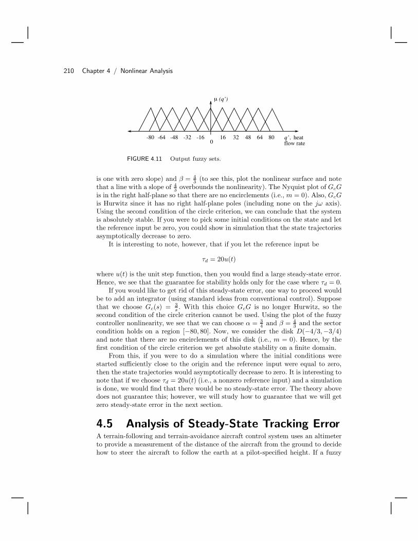
210 Chapter 4 / Nonlinear Analysis
016 32 48 64 80-16-32-48-64-80
µ (q’)
q’, heat flow rate
FIGURE 4.11 Output fuzzy sets.
is one with zero slope) and β = 43 (to see this, plot the nonlinear surface and note
that a line with a slope of 43 overbounds the nonlinearity). The Nyquist plot of GcG
is in the right half-plane so that there are no encirclements (i.e., m = 0). Also, GcGis Hurwitz since it has no right half-plane poles (including none on the jω axis).Using the second condition of the circle criterion, we can conclude that the systemis absolutely stable. If you were to pick some initial conditions on the state and letthe reference input be zero, you could show in simulation that the state trajectoriesasymptotically decrease to zero.
It is interesting to note, however, that if you let the reference input be
τd = 20u(t)
where u(t) is the unit step function, then you would find a large steady-state error.Hence, we see that the guarantee for stability holds only for the case where τd = 0.
If you would like to get rid of this steady-state error, one way to proceed wouldbe to add an integrator (using standard ideas from conventional control). Supposethat we choose Gc(s) = 3
s . With this choice GcG is no longer Hurwitz, so thesecond condition of the circle criterion cannot be used. Using the plot of the fuzzycontroller nonlinearity, we see that we can choose α = 3
4 and β = 43 and the sector
condition holds on a region [−80, 80]. Now, we consider the disk D(−4/3,−3/4)and note that there are no encirclements of this disk (i.e., m = 0). Hence, by thefirst condition of the circle criterion we get absolute stability on a finite domain.
From this, if you were to do a simulation where the initial conditions werestarted sufficiently close to the origin and the reference input were equal to zero,then the state trajectories would asymptotically decrease to zero. It is interesting tonote that if we choose τd = 20u(t) (i.e., a nonzero reference input) and a simulationis done, we would find that there would be no steady-state error. The theory abovedoes not guarantee this; however, we will study how to guarantee that we will getzero steady-state error in the next section.
4.5 Analysis of Steady-State Tracking ErrorA terrain-following and terrain-avoidance aircraft control system uses an altimeterto provide a measurement of the distance of the aircraft from the ground to decidehow to steer the aircraft to follow the earth at a pilot-specified height. If a fuzzy

4.5 Analysis of Steady-State Tracking Error 211
controller is employed for such an application, and it consistently seeks to controlthe height of the plane to be lower than what the pilot specifies, there will be asteady-state tracking error (an error between the desired and actual heights) thatcould result in a crash. In this section we will show how to use the results in [178]for predicting and eliminating steady-state tracking errors for fuzzy control systemsso that problems of this sort can be avoided.
4.5.1 Theory of Tracking Error for Nonlinear SystemsThe system is assumed to be of the configuration shown in Figure 4.1 on page 190where r, e, u, and y belong to L∞e and Φ(e) is the SISO fuzzy controller describedin Section 4.2.1. We will call ess = limt→∞ e(t) the steady-state tracking error. G(s)has the form
G(s) =p(s)
sρq(s)(4.21)
where ρ, a nonnegative integer, is the number of poles of G(s) at s = 0, and p(s)and sρq(s) are relatively prime polynomials (i.e., they have no common factors)such that deg(p(s)) < deg(sρq(s)). For example, if
G(s) =s + 1
s(s + 2)
then ρ = 1. Furthermore, we assume that Φ(0) = 0, and Φ is bounded by α and βaccording to
α ≤ Φ(a) − Φ(b)a − b
≤ β (4.22)
for all a = b. Notice that this sector bound is different from the sector boundin Equation (4.14). This new sector bound is determined by the maximum andminimum slopes of Φ at any point and is sometimes not as easy to determine asthe graphical sector bound described in the last section. Finally, we assume thatone of the three circle criterion conditions listed on page 207 is satisfied.
To predict the value of ess, we must make several definitions. First, we definean “average gain” for Φ, c0, as
c0 =12(α + β)
and we assume that c0 = 0. In [178] the authors show that for this c0, 1+c0G(s) = 0for Re(s) ≥ 0. Therefore, the rational function
H(s) =G(s)
1 + c0G(s)

212 Chapter 4 / Nonlinear Analysis
is strictly proper, and has no poles in the closed right half-plane. Defined in thismanner, H(s) is the closed-loop equation for the system shown in Figure 4.1 withc0 as an average gain of Φ. Finally, we define
Φ(e) = Φ(e) − c0e
for all e. That is, Φ is the difference between the actual value of Φ at some point eand a predicted value found by using the average gain c0.
Suppose that the above assumptions are met. It is proven in [178] that for eachgiven real number γ, there exists a unique real number ξ such that
γ = ξ + H(0)Φ(ξ) (4.23)
where to find the value of ξ we use
ξ = limk→∞
ξk (4.24)
where
ξk+1 = γ − H(0)Φ(ξk) (4.25)
and ξ0 is an arbitrary real number and γ is given (Equation (4.25) is an iterativealgorithm that will be used to find ess). Furthermore, if we define c as
c =12(β − α)|H(0)| (4.26)
and assume that c < 1, then the equation
|ξ − ξk| ≤ck
1 − c|ξ0 − γ + H(0)η(ξ0)|, k ≥ 1 (4.27)
must be true for the iterative algorithm, Equation (4.25), to converge.Finally, suppose that we define Θ(γ) = ξ to represent the algorithm in Equa-
tion (4.25). Hence, Θ is given a γ, an arbitrary ξ0 is chosen, c0 and H(0) arespecified, then with the given fuzzy controller Φ, we let Φ(e) = Φ(e) − c0e, andEquation (4.25) is computed until k is large enough that ξk+1 − ξk is very small.The resulting converged value of ξ is the value of Θ(γ).
Tracking Error Theorem: Assuming that all the described assumptions aresatisfied, then
1. If r(t) approaches a limit l as t → ∞, then ess ≡ limt→∞ e(t) exists. Moreover,ess = 0 if and only if l = 0 and ρ = 0, and then ess = Θ(γ) where γ = l
1+c0G(0) .
4.5 Analysis of Steady-State Tracking Error 213
2. Assuming that
r(t) =ν∑
j=0
ajtj , t ≥ 0 (4.28)
in which the aj are real, ν is a positive integer, and aν = 0, the following holds:
(a) e is unbounded if ν > ρ.
(b) if ν ≤ ρ, then e approaches a limit as t → ∞. If ν = ρ, this limit isess = Θ(γ) where
γ =aνν !q(0)c0p(0)
(4.29)
If ν < ρ, then the limit is zero.
Notice that for Equation (4.28) if we want r(t) to be a unit step, then ν = 0 sor(t) = a0, t ≥ 0 and we choose a0 = 1. If we want r(t) to be a ramp of unit slope,then we choose ν = 1 so that r(t) = a0 + a1t and we choose a0 = 0 and a1 = 1.
An examination of the above theorem reveals that in actuality the proposedmethod for finding the steady-state error for fuzzy control systems is similar to theequations used in conventional linear control systems. The theorem performs thefunction of identifying an appropriate equation for ess based on the type of inputand the “system type.” Notice that the two equations for γ in the theorem areanalogous to the equations for the “error constants” [54], 1/(1 + Kp), 1/Kv, and1/Ka, and provide an initial estimate for ess.
4.5.2 Example: Hydrofoil Controller DesignThe HS Denison is an 80-ton hydrofoil stabilized via flaps on the main foils and theincidence of the aft foil. The transfer function for a linearized model of the plantthat includes the foil and vehicle is
θ(s)D(s)
=104
s2 + 60s + 104
where θ(s) is the pitch angle and D(s) is the command input. We wish to designa fuzzy controller that will maintain a constant deflection of the pitch angle withless than 1% steady-state error from the desired angle.
We first determine that if α = 0, then β must be less than 1.56 for the circlecriterion conditions to be satisfied. Therefore, our preliminary design for the SISOparameterized fuzzy controller will have A = B = 1. For this controller β = 1,α = 0, and c0 = 0.5. The other relevant values are H(0) = 0.6667 and G(0) = 1. Ifour input r(t) is a step with magnitude 5.0, then we will use the first condition ofthe theorem and γ = 3.3333. Using these values in the iterative equation, we findthat our steady-state error will be 4.0. This is a very large error and is obviously

214 Chapter 4 / Nonlinear Analysis
much larger than 1%. Even with β = 1.559 we cannot meet the error requirement.Therefore, the system requirements cannot be met with a simple fuzzy controller.However, if we combine a simple fuzzy controller with an integrator, the circlecriterion is satisfied as long as B/A < 50. Furthermore, ρ = 1 for this systemand part 1 of the theorem predicts that ess = 0. Simulations for this system withA = B = 1 show that in fact ess = 0 and we have met the design criteria.
4.6 Describing Function AnalysisAutopilots used for cargo ship steering seek to achieve a smooth response by ap-propriately actuating the rudder to steer the ship. The presence of unwanted oscil-lations in the ship heading results in loss of fuel efficiency and a less comfortableride. While such oscillations, which are closed periodic orbits in the state plane,sometimes called “limit cycles,” result from certain inherent nonlinearities in thecontrol loop, it is sometimes possible to carefully construct a controller so that suchundesirable behavior is avoided.
In this section we will investigate the use of the describing function method forthe prediction of the existence, frequency, amplitude, and stability of limit cycles.We will first present describing function theory following the format in [189]. Next,we will use several examples to show how describing function analysis can be used inthe design of SISO and MISO fuzzy controllers of the form described in Section 4.2.Finally, we will use describing function analysis to design fuzzy controllers for anunderwater vehicle and a tape drive servo.
4.6.1 Predicting the Existence and Stability of Limit CyclesBefore explaining the describing function method, we will discuss several assump-tions that we will use in applying the techniques of this section.
Basic Assumptions
There are several assumptions that need to be satisfied for our purposes for thedescribing function method. These assumptions are as follows:
1. There is only a single nonlinear component and the system can be rearrangedinto the form shown in Figure 4.1 on page 190.
2. The nonlinear component is time-invariant.
3. Corresponding to a sinusoidal input e(t) = sin(ωt), only the fundamental com-ponent u1(t) in the output u(t) must be considered.
4. The nonlinearity Φ (which will represent the fuzzy controller) is an odd function.
The first assumption requires that nonlinearities associated with the plant or outputsensors be rearranged to appear in Φ as shown in Figure 4.1. The second assumptionoriginates from the use in this method of the Nyquist criterion, which can only be

4.6 Describing Function Analysis 215
applied to linear time-invariant systems. The third assumption implies that thelinear component following the nonlinearity has characteristics of a low-pass filterso that
|G(jω)| |G(njω)| for n = 2, 3, ... (4.30)
and therefore the higher-frequency harmonics, as compared to the fundamentalcomponent, can be neglected in the analysis. This is the fundamental assumptionof describing function analysis and represents an approximation as there normallywill be higher-frequency components in the signal. The fourth assumption simplifiesthe analysis of the system by allowing us to neglect the static term of the Fourierexpansion of the output.
We emphasize that due to the lack of perfect satisfaction of the above assump-tions the resulting analysis is only approximate. Next, we introduce the tools andmethods of describing function analysis.
Defining and Computing the Describing Function
For an input e(t) = C sin(ωt) to the nonlinearity, Φ(e), there will be an output u(t).This output will often be periodic though generally nonsinusoidal. Expanding thisu(t) into a Fourier series results in
u(t) =a0
2+
∞∑n=1
[an cos(nωt) + bn sin(nωt)] (4.31)
The Fourier coefficients (ai’s and bi’s) are generally functions of C and ω and aredetermined by
a0 =1π
∫ π
−π
u(t)d(ωt) (4.32)
an =1π
∫ π
−π
u(t) cos(nωt)d(ωt) (4.33)
bn =1π
∫ π
−π
u(t) sin(nωt)d(ωt) (4.34)
Because of our assumptions a0 = 0, n = 1, and
u(t) ≈ u1(t) = a1 cos(ωt) + b1 sin(ωt) = M(C, ω) sin(ωt + φ(C, ω)) (4.35)
where
M(C, ω) =√
a21 + b2
1 (4.36)
216 Chapter 4 / Nonlinear Analysis
and where
φ(C, ω) = arctan(
a1
b1
)(4.37)
From the above equations we can see that the fundamental component of the out-put, corresponding to a sinusoidal input, is a sinusoid of the same frequency thatcan be written in complex representation as
u1 = M(C, ω)ej(ωt+φ(C,ω)) = (b1 + ja1)ejωt (4.38)
We will now define the describing function of the nonlinear element to be thecomplex ratio of the fundamental component of the nonlinear element by the inputsinusoid
N(C, ω) =u1
C sin(ωt)=
M(C, ω)ej(ωt+φ(C,ω))
Cejωt=
1C
(b1 + ja1) (4.39)
By replacing the nonlinear element Φ(e) with its describing function N(C, ω), thenonlinear element can be treated as if it were a linear element with a parameterizedfrequency response function.
Generally, the describing function depends on the frequency and amplitude ofthe input signal. However, for some special cases it does not depend on frequency.For example, if the nonlinearity is time-invariant and memoryless, N(C, ω) is realand frequency-independent. For this case, N(C, ω) is real because evaluating Equa-tion (4.33) gives a1 = 0. Furthermore, in the same equations, the integration of thesingle-valued function u(t) sin(ωt) = [C sin(ωt)] sin(ωt) is done for the variable ωt,implying that ω does not explicitly appear in the integration and that the functionN(C, ω) is frequency-independent.
There are several ways to compute describing functions. The describing functioncan be computed analytically if u = Φ(e) is known and the integrations to find a1
and b1 can be easily carried out. If the input-output relationship of Φ(e) is givenby graphs or tables, then numerical integration can be used. The third method,and the one that we will use, is “experimental evaluation.” We will excite the inputof the fuzzy controller with sinusoidal inputs, save the related outputs, and thenuse the input and output waveforms to determine the gain and phase shift at thefrequency of the input sinusoid. By varying the amplitude and frequency (or justthe amplitude if the fuzzy controller is SISO, time-invariant, and memoryless) ofthe input sinusoid, we can find u1 at several points and plot the correspondingdescribing function.
Predicting Limit Cycles
In Figure 4.1 on page 190, if we replace Φ(e) with N(C, ω) and assume that a self-sustained oscillation of amplitude C and frequency ω exists in the system, then for

4.6 Describing Function Analysis 217
r = 0, y = 0, and
G(jω)N(C, ω) + 1 = 0 (4.40)
This equation, sometimes called the “harmonic balance equation,” can be rewrittenas
G(jω) = − 1N(C, ω)
(4.41)
If any limit cycles exist in our system, and the four basic assumptions outlinedabove are satisfied, then the amplitude and frequency of the limit cycles can bepredicted by solving the harmonic balance equation. If there are no solutions to theharmonic balance equation, then the system will have no limit cycles (under theabove assumptions).
However, solving the harmonic balance equation is not trivial; for higher-ordersystems, the analytical solution is very complex. The usual method, therefore, is toplot G(jω) and −1/N(C, ω) on the same graph and find the intersection points. Foreach intersection point, there will be a corresponding limit cycle. The amplitudeand frequency of each limit cycle can then be determined by finding the particularC and ω that give the value of −1/N(C, ω) and G(jω) at the intersection point.
Along with the amplitude and frequency of the limit cycles, we also wouldlike to determine whether the limit cycles are stable or unstable. A limit cycle isconsidered stable if system trajectories move to the limit cycle when they startwithin a certain neighborhood of it. Therefore, once the system is in a limit cycle,the system will return to the limit cycle when perturbations move the system off ofthe limit cycle. For an unstable limit cycle, there is no neighborhood within whichthe system trajectory moves to the limit cycle when the system trajectory startsnear it. Instead, the trajectory will move away from the limit cycle. Therefore, ifa system is perturbed from an unstable limit cycle, the oscillations will either dieout, increase until the system goes unstable, or move to a stable limit cycle. Thestability of limit cycles can be determined from the same plot used to predict theexistence of the limit cycles. A summary of the above conclusions is given by thefollowing criterion from [189].
Limit Cycle Criterion: Each intersection point of the G(jω) and −1/N(C, ω)curves corresponds to a limit cycle. In particular, if the curves intersect, we predictthat there will be a limit cycle in the closed-loop system with amplitude C andfrequency ω. If points near the intersection and along the increasing-C side of thecurve −1/N(C, ω) are not encircled by the curve G(jω), then the correspondinglimit cycle is stable. Otherwise, the limit cycle is unstable.
In the next two subsections we will show how to use this criterion to test forthe existence, amplitude, frequency, and stability of limit cycles. Also, we will showhow it can be used in the redesign of the fuzzy controller to eliminate limit cycles.

218 Chapter 4 / Nonlinear Analysis
4.6.2 SISO Example: Underwater Vehicle Control SystemWe wish to design a fuzzy controller for the direction control system of an under-water vehicle described in [45]. The electrically controlled rudder and an addedcompensator have transfer function
C(s)R(s)
=s + 0.1
s(s + 5)2(s + 0.001)
We must design the fuzzy controller such that there are no limit cycles possiblewithin the closed-loop system.
Our fuzzy controller will be SISO, odd, time-invariant, and memoryless. There-fore, we know that the describing function will be real-valued and can only intersectthe Nyquist plot of G(jω) along the real axis. Examining a Nyquist plot of G(jω) forthis system, we find that it intersects the real axis at one point only, −0.0042 + j0(an enlargement of this plot is shown in Figure 4.12, where −1/N(C, ω) is ontop of the horizontal axis) and hence a limit cycle exists (you can simulate theclosed-loop system to illustrate this). To avoid intersecting this point, we must con-struct the fuzzy controller so that −1/N(C, ω) < −0.0042 or N(C, ω) < 240.0528for all values of C. For the type of fuzzy controller we are using, this criterioncan be achieved if B/A < 240.0528. We will choose A = 2 and B = 200. Theresulting describing function is shown in Figure 4.13. Since the largest value of−1/N(C, ω) = −2/200 = −0.01 is less than −0.0042, there is no solution to theharmonic balance equation, and the approximate analysis indicates that the exis-tence of a limit cycle is unlikely. A simulation of this system for r = 5 is shown inFigure 4.14. No limit cycles exist, and our design was successful.
-0.02
-0.015
-0.01
-0.005
0
0.005
0.01
0.015
0.02
-0.02 -0.015 -0.01 -0.005 0 0.005 0.01 0.015 0.02
Real axis
Imag
inar
y ax
is
FIGURE 4.12 Plot of G(jω) for the underwater vehicle(figure taken from [83], c© John Wiley and Sons).

4.6 Describing Function Analysis 219
0
20
40
60
80
100
0 1 2 3 4 5 6 7 8 9 10
Amplitude, C
N(C
)
FIGURE 4.13 Describing function for fuzzy controllerwith A = 2 and B = 200 (figure taken from [83], c© JohnWiley and Sons).
0
1
2
3
4
5
6
7
0 10 20 30 40 50 60 70 80 90 100
Time (sec)
y(t)
FIGURE 4.14 Simulation of the underwater vehicle(figure taken from [83], c© John Wiley and Sons).
4.6.3 MISO Example: Tape Drive ServoThe describing function analysis of the previous design example was for SISO fuzzycontrollers whose describing functions are not dependent on ω. However, it is impor-

220 Chapter 4 / Nonlinear Analysis
tant that we also examine how this type of analysis can be applied to MISO fuzzycontrollers. While for a MISO fuzzy controller the basic theory is still the same,there are several differences in determining and using the describing function. First,the describing function will be dependent on both C and ω. Because of this, whenwe experimentally determine N(C, ω), we have to find not only the amplitude ofthe fundamental frequency of the output waveform but also the phase of the fun-damental frequency for inputs of different amplitude and frequency. Methods fordoing this can be found in [13]. This also means that there will be more lines to plotas we will have to plot −1/N(C, ω) as C changes for each value of ω so that therewill be a curve for each value of ω for which N(C, ω) is calculated. Second, not allintersections of G(jω) and −1/N(C, ω) will be limit cycles. For an intersection topredict a limit cycle, the values of ω for G(jω) and −1/N(C, ω) at the intersectionmust be the same. We can see that, as would be expected, the limit cycle predictionprocedure using describing functions is slightly more complex for MISO systems.However, with the adjustments mentioned above, the procedure follows the sameformat as before. This will be shown in the following design example.
We will design a fuzzy controller for a tape drive servo described in [54] withtransfer function
G(s) =15s2 + 13.5s + 12
(s + 1)(s2 + 1.1s + 1)
Also included in the system is a precompensator of the form C(s) = (s + 20)/s. Itis desired that a step input of current to the drive mechanism will cause the tapeto have a stable velocity. To analyze the system for limit cycles, we will choose afuzzy controller, empirically find the describing function, search for solutions to theharmonic balance equation, and then redesign the fuzzy controller if necessary.
We will begin by choosing A = 100, B = 600, and D = 50. Next, we willfind N(C, ω) for 0 ≤ C ≤ 100 and ω = 0.5, 1, 10, 50, 100, and 500. The resultingplot of G(jω) and −1/N(C, ω) is shown in Figure 4.15. There are no intersectionpoints and therefore no predicted limit cycles. By simulating the system with thechosen values of A, B, and D and r = 12, we verify that no limit cycles exist. Thissimulation is shown in Figure 4.16.
4.7 Limitations of the TheoryIt is important to note that there are limitations to the approaches that we coveredin this chapter in addition to the general ones outlined in Section 4.1 on page 187,which included the following:
• The model of a physical process is never perfectly accurate, and since the mathe-matical analysis is based on the model, the analysis is of limited accuracy for thephysical system. The more accurate the model, the more accurate the conclusionsfrom the mathematical analysis as they pertain to the real physical system.
• Fuzzy control tends to show its greatest advantages for processes that are very
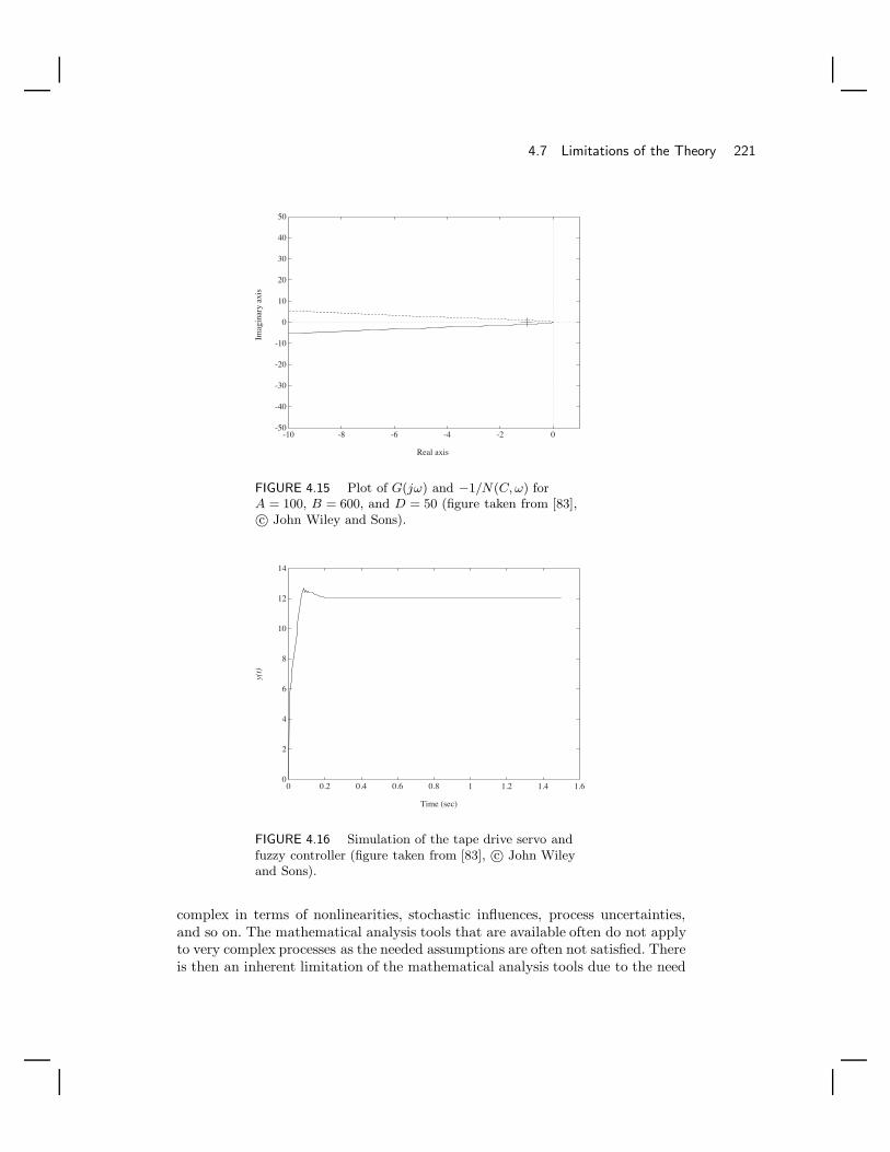
4.7 Limitations of the Theory 221
-50
-40
-30
-20
-10
0
10
20
30
40
50
-10 -8 -6 -4 -2 0
Real axis
Imag
inar
y ax
is
FIGURE 4.15 Plot of G(jω) and −1/N(C, ω) forA = 100, B = 600, and D = 50 (figure taken from [83],c© John Wiley and Sons).
0
2
4
6
8
10
12
14
0 0.2 0.4 0.6 0.8 1 1.2 1.4 1.6
Time (sec)
y(t)
FIGURE 4.16 Simulation of the tape drive servo andfuzzy controller (figure taken from [83], c© John Wileyand Sons).
complex in terms of nonlinearities, stochastic influences, process uncertainties,and so on. The mathematical analysis tools that are available often do not applyto very complex processes as the needed assumptions are often not satisfied. Thereis then an inherent limitation of the mathematical analysis tools due to the need

222 Chapter 4 / Nonlinear Analysis
for such tools for any nonlinear control systems, let alone fuzzy control systems.
Next, we provide a more detailed overview of some additional limitations tothe approaches covered in this chapter. In general, except for Lyapunov’s methods,discussed in Section 4.3, we have examined only linear plant models or nonlinearplants that can be manipulated to be in the form of Figure 4.5. In Section 4.3 someof the stability conditions are often conservative, which means that if the conditionsfor stability are not met, the system could still be stable. Indeed, the results for thecircle criterion have often been found to be too conservative. While the results forabsolute stability, steady-state tracking error, and describing functions can certainlybe applied to models linearized about operating points in a nonlinear system, suchresults are only local in nature. Furthermore, we have limited ourselves throughoutthe entire chapter (except Section 4.3) to SISO and MISO fuzzy controllers. Inaddition to these general limitations, there are also limitations specific to eachsection. In the section on absolute stability, we have only examined the SISO fuzzycontroller and not the MISO case (of course, extension to the multivariable case isnot difficult using, for example, the development in [90]). Furthermore, althoughthe circle criterion conditions are sufficient and necessary, the necessary conditionsare for a class of nonlinearities and do not identify which of the nonlinearities (i.e.,which fuzzy controller) within the class will cause the system to become unstable.There is currently no theory for the tracking error analysis of multivariable nonlinearsystems. Our describing function technique, even though it can be applied to SISOand MISO fuzzy controllers and certain nonlinear plant models, is limited by thefact that the use of the approach for more than three inputs to the fuzzy controllerbecomes prohibitive. There has been some work on the expansion of the theoryof nonlinear analysis to a wider class of nonlinear plants where a mathematicalcharacterization of the fuzzy controller is used (see, for example, [106, 105, 47, 154]).
In this chapter we often utilize a graphical approach to nonlinear analysis where,for example, we plot the input-output map of the fuzzy controller and read off per-tinent information such as the sector bounds, or use a graphical technique for de-scribing function analysis. We believe that the incorporation of graphical techniquesfor the nonlinear analysis of fuzzy control systems offers (1) an intuitive approachthat ties in better with the fuzzy control design procedure, and (2) some of thesame advantages as have been realized in classical control via the use of graphicaltechniques (such as the Nyquist plot). On the other hand, our approach has itsown limitations (listed above). We emphasize that there are many approaches toanalyzing fuzzy control systems, and we highly recommend that the reader studySection 4.9, For Further Study, and the references provided there.
4.8 SummaryIn this chapter we have provided an introduction to nonlinear analysis of (non-adaptive) fuzzy control systems. We showed how to perform Lyapunov stabilityanalysis of fuzzy control systems and showed how the circle criterion could beused to analyze and redesign a fuzzy control system. We introduced the theory of

4.9 For Further Study 223
steady-state tracking error for fuzzy control systems and showed how to predictand eliminate tracking error. We outlined the theory of describing functions andshowed how to predict the amplitude, frequency, and stability of limit cycles. Weperformed analysis and design examples for an inverted pendulum, a temperaturecontrol problem, a hydrofoil, an underwater vehicle, and a tape drive servo.
Upon completing this chapter, the reader should understand the following:
• Lyapunov’s direct and indirect methods.
• How to use the direct and indirect methods, coupled with a plot of the nonlinearsurface of the fuzzy controller, to establish conditions for stability.
• How to use Lyapunov’s direct method to provide sufficient conditions for stabilityfor Takagi-Sugeno fuzzy systems.
• The concept of absolute stability.
• The circle criterion in two forms.
• The procedure for the application of the circle criterion to fuzzy control systems,both to predict instability and its use in design to avoid instability.
• The concepts and theory of steady-state tracking error for nonlinear systems.
• The procedure for applying the theory of analysis of tracking error to fuzzy controlsystems.
• The assumptions and theory of describing functions.
• How to construct a describing function for a fuzzy controller that has one or twoinputs.
• The conditions for the existence of limit cycles and how to determine their am-plitude and frequency, and whether or not they are stable.
• The procedure to use describing function analysis for both SISO and MISO fuzzycontrol systems, both for limit cycle prediction and in redesigning for limit cycleelimination.
Essentially, this is a checklist of the major topics of this chapter. With thecompletion of Chapters 1–4 you have now finished the first part of this book, whereour primary focus has been on direct fuzzy controllers. The second part of the book,Chapters 5–7, focuses on adaptive fuzzy systems in estimation and control.
4.9 For Further StudyAn earlier version of this chapter appears in [83]. Several of the design problems atthe end of the chapter also came from [83]. For a detailed comparative analysis of

224 Chapter 4 / Nonlinear Analysis
fuzzy controllers and linear controllers and for more details on the nonlinear char-acteristics of fuzzy controllers, see [29, 28, 241] and the more recent work in [124].The work in [30] and [34] presents Lyapunov methods for analyzing the stability offuzzy control systems. The authors in [106, 105] also use Lyapunov’s direct methodand the generalized theorem of Popov [148, 90] to provide sufficient conditions forfuzzy control system stability.
An area that is receiving an increasing amount of attention is stability analysisof fuzzy control systems where the fuzzy control system is developed using ideasfrom sliding-mode control or where Takagi-Sugeno fuzzy systems are used in again-scheduling type of control [153, 47, 154]. Here, our treatment of the stabilityof Takagi-Sugeno fuzzy systems is based on the work in [213, 209]. Extensions tothis work that focus on robustness can be found in [212, 210, 84], and work focusingon the use of linear matrix inequality (LMI) methods for analysis and controllerconstruction is provided in [210, 226, 225, 248, 247].
In [7], stability indices for fuzzy control systems are established using phaseportraits (of course, standard phase plane analysis [90] can be useful in character-izing and understanding the dynamic behavior of low-order fuzzy control systems[65]). Related work is given in [49]. The circle criterion [148] is used in [171] and[172] to provide sufficient conditions for fuzzy control system stability. Related workon stability analysis of fuzzy control systems is provided in [211]. While we use thecircle criterion theory found in [90] and [223], there are other frequency domain–based criteria for stability that can be utilized for fuzzy control system analysis(e.g., Popov’s criterion and the multivariable circle criterion [148, 90]). Describingfunction analysis has already been examined in [92] and [14]. Our coverage herediffers from that in [92] in that we use experimentally determined describing func-tions, whereas in [92] the describing function is determined for a “multilevel relay”model of a specific class of fuzzy controllers. A collection of papers on theoreticalaspects of fuzzy control is in [151].
The characterization and analysis of the stability of fuzzy dynamic systems isstudied in [93]. Furthermore, approximate analysis of fuzzy systems is studied bythe authors in [33, 32, 52] using the “cell-to-cell mapping approach” from [71, 72].
One graphical technique that we have found to be useful on occasion, which wedid not cover here, is called the “method of equivalent gains” (see [55, 54]), wherewe view the fuzzy controller as an input-dependent time-varying gain and then useconventional root-locus methods to design fuzzy control systems (the gain movesthe poles along the root-locus). This method is, however, limited to the case oflinear plants. For an idea of how this approach is used, see Exercise 4.3 at the endof the chapter. Another topic that we did not cover is that of phase plane analysisfor differential equations and what has been called “fuzzy phase plane analysis.” Toget an idea of how such analysis is done, see Exercise 4.2 at the end of this chapteror [47].
For a more detailed discussion on the general relationships between conventionaland intelligent control and mathematical modeling and nonlinear analysis of moregeneral intelligent control systems (including expert control systems), see [6, 160,156, 157, 163].

4.10 Exercises 225
4.10 ExercisesExercise 4.1 (The Nonlinear Fuzzy Control Surface): In this problem youwill study the nonlinear control surface that is induced by the fuzzy controller.
(a) Plot u versus e for the parameterized SISO fuzzy controller of Section 4.2.1for the case where A = 5 and B = 2.
(b) Plot u versus e for the parameterized SISO fuzzy controller of Section 4.2.1for the case where A = 3 and B = 6. Compare the result to that obtainedin (a).
(c) Plot the three-dimensional plot of the PD fuzzy controller surface for thecase where there is a proportional and derivative input, as described inSection 4.2. Choose A = B = D = 1.
(d) Choose A = 5, B = 2, and D = 1 and repeat (c). Compare the result tothat obtained in (c).
Exercise 4.2 (Phase Plane Analysis: Conventional and Fuzzy): The phaseplane is a graph used for the analysis of low-order (typically second-order) non-linear differential equations (i.e., n = 2 for Equation (4.1)). The phase plane issimply a plot of x1(t) versus x2(t), where x = [x1, x2] is the state of Equa-tion (4.1), for a number of initial conditions x(0).
(a) Write down second-order differential equations that are unstable, marginallystable, and asymptotically stable, and use a computer program to generatetheir phase planes (the choice of the initial conditions should be done sothat they are within a ball of size h where h = 10 and there are at least 50initial conditions spread out uniformly in the ball).
(b) Learn at least one technique for the construction of phase planes (by hand)and apply it to the differential equations you developed for (a). Refer to [90]to learn a method for constructing the phase plane.
(c) When the inputs to a fuzzy controller are e(t) = r(t) − y(t) (where r(t) isthe reference input and y(t) is the plant output) and d
dte(t), sometimes theplot of e(t) versus d
dte(t) is thought of as a type of phase plane if r(t) = 0.Moreover, some have introduced the notion of a “fuzzy phase plane” thatis best thought of as a rule-base table for the two-input fuzzy controller.Motion in the fuzzy phase plane is given by which membership functions havevalues greater than zero and as the control system operates, different cellsin the rule-base table become “active” (i.e., the rules associated with themare on). Following Design Problem 2.1(a) on page 110, begin the pendulumout of the balanced position but with zero initial velocity and show on thecorresponding rule-base table the trajectory of active regions as the fuzzycontroller balances the pendulum.

226 Chapter 4 / Nonlinear Analysis
Exercise 4.3 (Method of Equivalent Gains): In the “method of equivalentgains” (see [55, 54]), we view the fuzzy controller as an input-dependent time-varying gain and use conventional root-locus methods to design fuzzy controlsystems (the gain moves the poles along the root-locus).
(a) To understand why the fuzzy controller is an input-dependent gain, chooseA = B = 1 for the parameterized SISO fuzzy controller of Section 4.2.1, andplot the output of the fuzzy controller u divided by its input e (i.e., the “gainof the fuzzy controller”—notice that it is closely related to the describingfunction of the fuzzy controller) versus its input e for both positive andnegative values of e.
(b) Suppose that you are given a plant
G(s) =1
s(s + 1)
that is in a unity feedback configuration with a fuzzy controller. Suppose thatyou know that the reference input will never be larger, in magnitude, thanone. View the fuzzy controller as implementing a gain in the control loopwhere the value of the gain is given at any one time by the plot you producedin (a). Use this gain, coupled with the conventional root-locus approach [54],to design a fuzzy controller so that you get as short a rise-time due to a unit-step input as possible but with no more than 5% overshoot. This approachto design is called the method of equivalent gains. Note that this approachis heuristic and that there are no guarantees of achieving the performancesought or that the resulting closed-loop system will be stable.
Exercise 4.4 (Lyapunov’s Direct Method): Suppose that you are given theplant
x = ax + bu
where b > 0 and a < 0 (so the system is stable). Suppose that you design a fuzzycontroller Φ that generates the input to the plant given the state of the plant(i.e., u = Φ(x)). Assume that you design the fuzzy controller so that Φ(0) = 0and so that Φ(x) is continuous. Choose the Lyapunov function V (x) = 1
2x2.
(a) Show that if x and Φ(x) always have opposite signs, then x = 0 is stable.
(b) What types of stability does x = 0 of the fuzzy control system possess forpart (a)?
(c) Why do we assume that Φ(0) = 0 for (a)?
(d) Design a fuzzy controller that satisfies the condition stated in (a) and simu-late the closed-loop system to help illustrate the stability of the fuzzy controlsystem (of course, the simulation does not prove that the closed-loop system

4.10 Exercises 227
is stable—it only shows that for one initial condition the state appears toconverge but cannot prove that it converges since the simulation is only fora finite amount of time). Choose the initial condition x(0) = 1, a = −2, andb = 2.
Exercise 4.5 (Stability of Takagi-Sugeno Fuzzy Systems): Suppose thatyou have the same plant as described in the Section 4.3.5 example but withA1 = −3, B1 = 6, A2 = −5, and B2 = 2. Construct the Takagi-Sugeno fuzzycontroller gains K1 and K2 so that x(0) = 0 of the closed-loop system is globallyasymptotically stable.
Exercise 4.6 (Stability of Discrete-Time Takagi-Sugeno Fuzzy Systems):Suppose that you are given a discrete-time Takagi-Sugeno fuzzy system model
of a nonlinear system that arises from R Takagi-Sugeno rules and results in
x(k + 1) =R∑
i=1
Φiξi(x(k))x(k) +R∑
i=1
Γiξi(x(k))u(k) (4.42)
where
ξi(x(k)) =µi(x(k))∑R
i=1 µi(x(k))
In Equation (4.42), Φi is an n × n matrix, and Γi is the n input matrix.
Stability conditions for the discrete-time direct method of Lyapunov areslightly different from the continuous-time case so we discuss these first. Theequilibrium x(0) = 0 of the system in Equation (4.42) is globally asymptoticallystable if there exists a function V (x) such that V (x) ≥ 0 except at x = 0 whereV (x) = 0, V (x) → ∞ if |x| → ∞, and
V (x(k + 1)) − V (x(k)) < 0
(a) Let u(k) = 0 for k ≥ 0. Choose V (x) = xPx where P is a positive definitesymmetric matrix. Show that if there exists a single n × n matrix, P > 0such that for all i = 1, 2, . . . , R and j = 1, 2, . . . , R
Φi PΦj − P < 0 (4.43)
then the equilibrium x = 0 of Equation (4.42) is globally asymptoticallystable.
(b) Suppose that you use a Takagi-Sugeno fuzzy controller to choose the inputu(k) so that
u(k) =R∑
i=1
Kiξi(x(k))x(k)

228 Chapter 4 / Nonlinear Analysis
Using the result from (a), find a stability condition similar to Equation (4.43)for the closed-loop system.
This problem is based on the work in [213] where the authors also show how tofurther simplify the condition in Equation (4.43).
4.11 Design ProblemsDesign Problem 4.1 (Stable Fuzzy Controller for an Inverted Pendu-lum): In this problem you will verify the stability analysis for the design of thefuzzy controller for the inverted pendulum described in Section 4.3.
(a) Design a fuzzy controller that will result in the inverted pendulum of Sec-tion 4.3 being locally stable, and demonstrate this via Lyapunov’s indirectmethod.
(b) Repeat (a) except use minimum to represent the premise and implicationand COG for defuzzification.
(c) Using Lyapunov’s direct method, design a fuzzy controller for the invertedpendulum that you can guarantee is stable in the inverted position. Providea simulation to help verify the stability of the closed-loop system.
Design Problem 4.2 (Stable Fuzzy Controller for the Magnetic Ball Sus-pension System): In this problem you study the stability properties of a fuzzycontroller for the magnetic ball suspension system.
(a) Design a fuzzy controller for the ball suspension system studied in Exer-cise 2.5 on page 116, and demonstrate in simulation that it appears to bestable (at least locally—i.e., for initial conditions very near the operatingpoint at which you perform the linearization to test stability). Seek to bal-ance the ball half way between the coil and the “ground.”
(b) Prove, using the methods of Section 4.3, that the fuzzy control system islocally stable at the operating point studied in (a).
Design Problem 4.3 (Designing Stable Fuzzy Control Systems): Sup-pose that you are given a plant with transfer function
G(s) =1
s3 + 7s2 + 7s + 15
This plant is chosen because it illustrates the problems with stability that canarise when designing fuzzy controllers.
4.11 Design Problems 229
(a) A controller that some expert could construct is one with A = 0.5 andB = 16.6667 (using the parameterized fuzzy controller of Section 4.2.1).Simulate this system with initial conditions x(0) = [0, 0, 2] to show thatthe system has sustained oscillations.
(b) If we consider the fuzzy controller as a nonlinearity Φ, we can find a sector(α, β) in which Φ lies and use the circle criterion to determine why the insta-bility is occurring and perhaps determine how to tune the fuzzy controllerso that it does not cause sustained oscillations. Plot the nonlinearity of thefuzzy controller from (a). Plot the Nyquist plot of G. Show that the circlecriterion/SNC predicts that not all of the nonlinearities within this sectorwill be stable. Hence, the fuzzy controller in (a) verifies this statement byproducing sustained oscillations in the closed-loop system.
(c) Next we use condition (b) of the circle criterion/SNC to provide ideas onhow to tune the fuzzy controller. To do this, we will have to adjust β so that− 1
β < −0.0733, (i.e., so that β < 13.64). Why? As there are many differentchoices for A and B so that the fuzzy controller will fit inside the sector, moreabout the system would have to be known (e.g., what the saturation limitsat the input of the plant are) to know whether to tune A or B. Suppose youchoose B = 16.6667 and make A > 1.222 so that B
A < 13.64. As an example,choose A = 1.3. Produce a simulation of the resulting fuzzy control systemwith x(0) = [0, 0, 2] to show that there are no sustained oscillations so thatthe fuzzy controller has been successfully redesigned to avoid the instability.
(d) Repeat (c) but choose A = 0.5 and find a value of B that will result ina stable closed-loop system. Justify your choice of B theoretically and byproviding a simulation that shows the choice was good.
Design Problem 4.4 (Stable Temperature Control): In this problem youwill verify the results of Section 4.4.2 on page 208 where the problem of designinga stable fuzzy control system for a temperature control problem was addressed.Suppose that the control system that we use is shown in Figure 4.9. The controllerGc(s) is a post compensator for the fuzzy controller.
(a) Suppose that we begin by choosing Gc(s) = K = 2. Provide a plot of q′
versus e for the 11-rule fuzzy controller that is specified in Section 4.4.2.(b) Show that α = 0 and β = 4
3 . Plot the Nyquist plot of GcG and determine thenumber of encirclements. What conclusion can be reached from the circlecriterion?
(c) Choose a value for the initial state of the system, let the reference input bezero, and show that the state trajectories converge asymptotically to zero.
(d) Let τd = 20u(t) where u(t) is a unit step, and determine the value of thesteady-state error using a simulation of the closed-loop system.
(e) Suppose that we choose Gc(s) = 3s (chosen to try to eliminate the steady-
state error). Using the plot of the fuzzy controller nonlinearity, show that

230 Chapter 4 / Nonlinear Analysis
we can choose α = 34 and β = 4
3 and the sector condition holds on a region[−80, 80].
(f) Show that the Nyquist plot of GcG does not encircle the disk D(−4/3,−3/4).What is concluded from the circle criterion?
(g) Do a simulation where the initial conditions are started sufficiently close tothe origin (and the reference input is equal to zero) to show that the statetrajectories asymptotically decrease to zero.
(h) Next, choose τd = 20u(t) where u(t) is a unit step, and do a simulation toshow that there is no steady-state error.
Design Problem 4.5 (Designing for Zero Steady State Tracking Error):Consider a plant of the form
G(s) =1
s2 + 4s + 3
(a) Choose a SISO proportional fuzzy controller and determine the α and βdescribing the sector in which it lies where the type of sector is the one usedfor the theory of steady-state tracking error. Note that you can find α andβ numerically by inserting values of a and b into the equation
α ≤ Φ(a) − Φ(b)a − b
≤ β
and determining the maximum and minimum values. An alternative ap-proach is to plot the fuzzy controller nonlinearity and read the values off theplot by inspection.
(b) Which condition of the circle criterion holds? Show a Nyquist plot to supportyour conclusion.
(c) For your choice of α and β, find c0 and H(0). Find γ, and then solve therecursive equation from Equation (4.25). Suppose that we choose a stepinput of magnitude 3. What is the value of ess?
(d) Suppose that we consider the steady-state error to be excessive, and thatwe would like to redesign our fuzzy controller using the steady-state errorprediction procedure as part of the design process. Intuitively, we wouldexpect that if we increased the “gain of the fuzzy controller,” the steady-state error would decrease. In terms of the ess prediction procedure, thiswould mean changing α and β. Because of the inherent saturation of thefuzzy controller, α will always equal 0. Therefore, we will have to adjust bychanging β only. Find a value of β so that ess < 0.4.
(e) Consider the response of the system from (d) to a ramp input. What is thevalue of e(t) as t goes to infinity? Will changing the scaling gains of yourfuzzy controller improve tracking error?

4.11 Design Problems 231
Design Problem 4.6 (Design of Hydrofoil Controller to Get Zero Track-ing Error): In this problem you will verify the results of Section 4.5.2 onpage 213. Suppose that we use a proportional fuzzy controller of the form de-scribed in Section 4.2.1.
(a) Show that β must be less than 1.56 for the circle criterion conditions to besatisfied.
(b) Choose A = B = 1. Show that c0 = 0.5, H(0) = 0.6667, and G(0) = 1. Letthe input be a step with magnitude 5.0, and show that γ = 3.3333. Find thevalue of the steady-state error.
(c) Add an integrator and show that if B/A < 50 we can meet the conditionsto get ess = 0. Perform a simulation for this system with A = B = 1 andshow that ess = 0.
Design Problem 4.7 (Prediction and Elimination of Limit Cycles: SISOCase): Suppose that a fuzzy controller of the form described in Section 4.2.1has A = 0.2 and B = 0.1 and a plant with transfer function
G(s) =1
s(s2 + 0.2s + 1)
configured in the form used in Section 4.6.1.
(a) Plot the describing function for the fuzzy controller.(b) Plot G(jω) and − 1
N(C,ω) on the same plot and find the intersection point(s).What are the magnitude and frequency of the predicted limit cycle? Is thelimit cycle stable? Why?
(c) The last step of this process is to verify by simulation that the limit cycledoes exist. Choose r(t) = 1 and simulate the closed-loop system. What arethe frequency and amplitude of the limit cycle in the simulation? Compareyour results to the predicted values in (b).
(d) Now that we have predicted the existence of a limit cycle for our system, wedesire to redesign the fuzzy controller so that there are no limit cycles. Whatvalue must −1/N(C, ω) be less than so that there would be no intersectionpoint and no limit cycle? What values of A and B should you choose so thatthere will be no limit cycles? Why? Choose r(t) = 1 and simulate the closed-loop system to verify that there are now no limit cycles for your choice of Aand B.
Design Problem 4.8 (Prediction and Elimination of Limit Cycles: SISOCase, Unstable Limit Cycle): Consider a plant with transfer function
G(s) =s2 + 0.4s + 2.29
s(s2 + 0.4s + 1.04)

232 Chapter 4 / Nonlinear Analysis
(a) Our first design for the fuzzy controller will have A = 0.1 and B = 0.3. Topredict the limit cycles of this system, find N(C, ω) then plot −1/N(C, ω)and G(jω) on the same plot and identify the intersection points. Whatamplitudes and frequencies will the limit cycles have? Are they stable?
(b) To confirm that these limit cycles exist, simulate the system with r = 0.761(this value was chosen to best show the existence of both limit cycles). Whatare the values of the amplitudes and frequencies of the limit cycles? Howdo these compare with the predicted values? What happens if r < 0.761?Simulate the system for this case to illustrate the behavior.
(c) Redesign the fuzzy controller so that no limit cycles exist. To demonstratethat no limit cycles exist for your design, use the theory and a simulationwith r = 0.761.
Design Problem 4.9 (Prediction and Elimination of Limit Cycles: MISOCase): Suppose that the plant has the transfer function
G(s) =(s + 1)2
s3
Our fuzzy controller is the two-input fuzzy controller with inputs e and e describedin Section 4.2 on page 189, and with parameters A, B, and D.
(a) Show that choosing A = B = D = 1 is not a good choice.
(b) Use describing function analysis to choose the parameters A, B, and D forthe fuzzy controller so that no limit cycles occur, and demonstrate in simu-lation that they do not occur. Note that when you experimentally determinethe describing function you must consider a range of values of both C andω to find different −1/N(C, ω) curves to find the intersection points. Youcan assume that the reference input is a positive step with a magnitude nolarger than five. What happens if the amplitude of the step input is greaterthan 30? Simulate the system for this case to illustrate the behavior.

C H A P T E R 5
Fuzzy Identificationand Estimation
For the things we have to learn before we can do
them,
we learn by doing them.
–Aristotle
5.1 OverviewWhile up to this point we have focused on control, in this chapter we will examinehow to use fuzzy systems for estimation and identification. The basic problem tobe studied here is how to construct a fuzzy system from numerical data. This isin contrast to our discussion in Chapters 2 and 3, where we used linguistics asthe starting point to specify a fuzzy system. If the numerical data is plant input-output data obtained from an experiment, we may identify a fuzzy system modelof the plant. This may be useful for simulation purposes and sometimes for use in acontroller. On the other hand, the data may come from other sources, and a fuzzysystem may be used to provide for a parameterized nonlinear function that fits thedata by using its basic interpolation capabilities. For instance, suppose that we havea human expert who controls some process and we observe how she or he does thisby observing what numerical plant input the expert picks for the given numericaldata that she or he observes. Suppose further that we have many such associationsbetween “decision-making data.” The methods in this chapter will show how toconstruct rules for a fuzzy controller from this data (i.e., identify a controller fromthe human-generated decision-making data), and in this sense they provide anothermethod to design controllers.
Yet another problem that can be solved with the methods in this chapter isthat of how to construct a fuzzy system that will serve as a parameter estimator.
233

234 Chapter 5 / Fuzzy Identification and Estimation
To do this, we need data that shows roughly how the input-output mapping of theestimator should behave (i.e., how it should estimate). One way to generate this datais to begin by establishing a simulation test bed for the plant for which parameterestimation must be performed. Then a set of simulations can be conducted, eachwith a different value for the parameter to be estimated. By coupling the testconditions and simulation-generated data with the parameter values, you can gatherappropriate data pairs that allow for the construction of a fuzzy estimator. For someplants it may be possible to perform this procedure with actual experimental data(by physically adjusting the parameter to be estimated). In a similar way, you couldconstruct fuzzy predictors using the approaches developed in this chapter.
We begin this chapter by setting up the basic function approximation problemin Section 5.2, where we provide an overview of some of the fundamental issues inhow to fit a function to input-output data, including how to incorporate linguisticinformation into the function that we are trying to force to match the data. Weexplain how to measure how well a function fits data and provide an example of howto choose a data set for an engine failure estimation problem (a type of parameterestimation problem in which when estimates of the parameters take on certainvalues, we say that a failure has occurred).
In Section 5.3 we introduce conventional least squares methods for identifica-tion, explain how they can be used to tune fuzzy systems, provide a simple exam-ple, and offer examples of how they can be used to train fuzzy systems. Next, inSection 5.4 we show how gradient methods can be used to train a standard andTakagi-Sugeno fuzzy system. These methods are quite similar to the ones used totrain neural networks (e.g., the “back-propagation technique”). We provide exam-ples for standard and Takagi-Sugeno fuzzy systems. We highlight the fact that viaeither the recursive least squares method for fuzzy systems or the gradient methodwe can perform on-line parameter estimation. We will see in Chapter 6 that thesemethods can be combined with a controller construction procedure to provide amethod for adaptive fuzzy control.
In Section 5.5 we introduce two techniques for training fuzzy systems basedon clustering. The first uses “c-means clustering” and least squares to train thepremises and consequents, respectively, of the Takagi-Sugeno fuzzy system; whilethe second uses a nearest neighborhood technique to train standard fuzzy systems.In Section 5.6 we present two “learning from examples” (LFE) methods for con-structing rules for fuzzy systems from input-output data. Compared to the previousmethods, these do not use optimization to construct the fuzzy system parameters.Instead, the LFE methods are based on simple procedures to extract rules directlyfrom the data.
In Section 5.7 we show how hybrid methods for training fuzzy systems canbe developed by combining the methods described in this chapter. Finally, in Sec-tion 5.8, we provide a design and implementation case study for parameter estima-tion in an internal combustion engine.
Overall, the objective of this chapter is to show how to construct fuzzy systemsfrom numerical data. This will provide the reader with another general approachfor fuzzy system design that may augment or extend the approach described in
5.2 Fitting Functions to Data 235
Chapters 2 and 3, where we start from linguistic information. With a good under-standing of Chapter 2, the reader can complete this chapter without having readChapters 3 and 4. The section on indirect adaptive control in Chapter 6 relies onthe gradient and least squares methods discussed in this chapter, and a portion ofthe section on gain schedule construction in Chapter 7 relies on the reader knowingat least one method from this chapter. In other words, this chapter is importantsince many adaptive control techniques depend on the use of an estimator. More-over, the sections on neural networks and genetic algorithms in Chapter 8 dependon this chapter in the sense that if you understand this chapter and those sections,you will see how those techniques relate to the ones discussed here. Otherwise, theremainder of the book can be completed without this chapter; however, this chapterwill provide for a deeper understanding of many of the concepts to be presentedin Chapters 6 and 7. For example, the learning mechanism for the fuzzy modelreference learning controller (FMRLC) described in Chapter 6 can be viewed as anidentification algorithm that is used to tune a fuzzy controller.
5.2 Fitting Functions to DataWe begin this section by precisely defining the function approximation problem, inwhich you seek to synthesize a function to approximate another function that isinherently represented via a finite number of input-output associations (i.e., we onlyknow how the function maps a finite number of points in its domain to its range).Next, we show how the problem of how to construct nonlinear system identifiersand nonlinear estimators is a special case of the problem of how to perform functionapproximation. Finally, we discuss issues in the choice of the data that we use toconstruct the approximators, discuss the incorporation of linguistic information,and provide an example of how to construct a data set for a parameter estimationproblem.
5.2.1 The Function Approximation ProblemGiven some function
g : X → Y
where X ⊂ n and Y ⊂ , we wish to construct a fuzzy system
f : X → Y
where X ⊂ X and Y ⊂ Y are some domain and range of interest, by choosing aparameter vector θ (which may include membership function centers, widths, etc.)so that
g(x) = f(x|θ) + e(x) (5.1)

236 Chapter 5 / Fuzzy Identification and Estimation
for all x = [x1, x2, . . . , xn] ∈ X where the approximation error e(x) is as small aspossible. If we want to refer to the input at time k, we will use x(k) for the vectorand xj(k) for its jth component.
Assume that all that is available to choose the parameters θ of the fuzzy systemf(x|θ) is some part of the function g in the form of a finite set of input-output datapairs (i.e., the functional mapping implemented by g is largely unknown). The ith
input-output data pair from the system g is denoted by (xi, yi) where xi ∈ X,yi ∈ Y , and yi = g(xi). We let xi = [xi
1, xi2, ..., x
in] represent the input vector
for the ith data pair. Hence, xij is the jth element of the ith data vector (it has a
specific value and is not a variable). We call the set of input-output data pairs thetraining data set and denote it by
G = (x1, y1), . . . , (xM , yM ) ⊂ X × Y (5.2)
where M denotes the number of input-output data pairs contained in G. For con-venience, we will sometimes use the notation d(i) for data pair (xi, yi).
To get a graphical picture of the function approximation problem, see Fig-ure 5.1. This clearly shows the challenge; it can certainly be hard to come up witha good function f to match the mapping g when we know only a little bit aboutthe association between X and Y in the form of data pairs G. Moreover, it may behard to know when we have a good approximation—that is, when f approximatesg over the whole space of inputs X.
g
X
Y
x
x
1
2
x3
y
y
y
1
2
3
G
FIGURE 5.1 Function mapping with threeknown input-output data pairs.
To make the function approximation problem even more concrete, consider asimple example. Suppose that n = 2, X ⊂ 2, Y = [0, 10], and g : X → Y . LetM = 3 and the training data set
G =([
02
], 1
),
([24
], 5
),
([36
], 6
)(5.3)
which partially specifies g as shown in Figure 5.2. The function approximationproblem amounts to finding a function f(x|θ) by manipulating θ so that f(x|θ)

5.2 Fitting Functions to Data 237
approximates g as closely as possible. We will use this simple data set to illustrateseveral of the methods we develop in this chapter.
1
2
3
4
5
67
0 1 2 3 4 5 6 7 0 1 2 3 4 5 6 7 yx
x
1
2
FIGURE 5.2 The training data G generated from thefunction g.
How do we evaluate how closely a fuzzy system f(x|θ) approximates the func-tion g(x) for all x ∈ X for a given θ? Notice that
supx∈X
|g(x) − f(x|θ)| (5.4)
is a bound on the approximation error (if it exists). However, specification of such abound requires that the function g be completely known; however, as stated above,we know only a part of g given by the finite set G. Therefore, we are only able toevaluate the accuracy of approximation by evaluating the error between g(x) andf(x|θ) at certain points x ∈ X given by available input-output data. We call thisset of input-output data the test set and denote it as Γ, where
Γ = (x1, y1), . . . , (xMΓ , yMΓ) ⊂ X × Y (5.5)
Here, MΓ denotes the number of known input-output data pairs contained withinthe test set. It is important to note that the input-output data pairs (xi, yi) con-tained in Γ may not be contained in G, or vice versa. It also might be the case thatthe test set is equal to the training set (G = Γ); however, this choice is not alwaysa good one. Most often you will want to test the system with at least some datathat were not used to construct f(x|θ) since this will often provide a more realisticassessment of the quality of the approximation.
We see that evaluation of the error in approximation between g and a fuzzysystem f(x|θ) based on a test set Γ may or may not be a true measure of the errorbetween g and f for every x ∈ X, but it is the only evaluation we can make based

238 Chapter 5 / Fuzzy Identification and Estimation
on known information. Hence, you can use measures like∑(xi,yi)∈Γ
(g(xi) − f(xiθ))2 (5.6)
or
sup(xi,yi)∈Γ
|g(xi) − f(xi|θ)| (5.7)
to measure the approximation error. Accurate function approximation requires thatsome expression of this nature be small; however, this clearly does not guaranteeperfect representation of g with f since most often we cannot test that f matchesg over all possible input points.
We would like to emphasize that the type of function that you choose to ad-just (i.e., f(x|θ)) can have a significant impact on the ultimate accuracy of theapproximator. For instance, it may be that a Takagi-Sugeno (or functional) fuzzysystem will provide a better approximator than a standard fuzzy system for a par-ticular application. We think of f(x|θ) as a structure for an approximator that isparameterized by θ. In this chapter we will study the use of fuzzy systems as ap-proximators, and use a fuzzy system as the structure for the approximator. Thechoice of the parameter vector θ depends on, for example, how many membershipfunctions and rules you use. Generally, you want enough membership functions andrules to be able to get good accuracy, but not too many since if your function is“overparameterized” this can actually degrade approximation accuracy. Often, it isbest if the structure of the approximator is based on some physical knowledge ofthe system, as we explain how to do in Section 5.2.4 on page 241.
Finally, while in this book we focus primarily on fuzzy systems (or, if you un-derstand neural networks you will see that several of the methods of this chapterdirectly apply to those also), at times it may be beneficial to use other approxi-mation structures such as neural networks, polynomials, wavelets, or splines (seeSection 5.10 “For Further Study,” on page 302).
5.2.2 Relation to Identification, Estimation, and PredictionMany applications exist in the control and signal processing areas that may utilizenonlinear function approximation. One such application is system identification,which is the process of constructing a mathematical model of a dynamic systemusing experimental data from that system. Let g denote the physical system thatwe wish to identify. The training set G is defined by the experimental input-outputdata.
In linear system identification, a model is often used where
y(k) =q∑
i=1
θaiy(k − i) +p∑
i=0
θbiu(k − i) (5.8)

5.2 Fitting Functions to Data 239
and u(k) and y(k) are the system input and output at time k ≥ 0. Notice that youwill need to specify appropriate initial conditions. In this case f(x|θ), which is nota fuzzy system, is defined by
f(x|θ) = θx
where
x(k) = [y(k − 1), · · · , y(k − q), u(k), · · · , u(k − p)] (5.9)θ = [θa1 , · · · , θaq , θb0 , · · · , θbp ] (5.10)
Let N = q + p+1 so that x(k) and θ are N ×1 vectors. Linear system identificationamounts to adjusting θ using information from G so that g(x) = f(x|θ) + e(x)where e(x) is small for all x ∈ X.
Similar to conventional linear system identification, for fuzzy identification wewill utilize an appropriately defined “regression vector” x as specified in Equa-tion (5.9), and we will tune a fuzzy system f(x|θ) so that e(x) is small. Our hope isthat since the fuzzy system f(x|θ) has more functional capabilities (as characterizedby the universal approximation property described in Section 2.3.8 on page 77) thanthe linear map defined in Equation (5.8), we will be able to achieve more accurateidentification for nonlinear systems by appropriate adjustment of its parameters θof the fuzzy system.
Next, consider how to view the construction of a parameter (or state) estimatoras a function approximation problem. To do this, suppose for the sake of illustrationthat we seek to construct an estimator for a single parameter in a system g. Supposefurther that we conduct a set of experiments with the system g in which we vary aparameter in the system—say, α. For instance, suppose we know that the parameterα lies in the range [αmin, αmax] but we do not know where it lies and hence we wouldlike to estimate it. Generate a data set G with data pairs (xi, αi) ∈ G where the αi
are a range of values over the interval [αmin, αmax] and the xi corresponding to eachαi is a set of input-output data from the system g in the form of Equation (5.9)that results from using αi as the parameter value in g. Let α denote the fuzzysystem estimate of α. Now, if we construct a function α = f(x|θ) from the datain G, it will serve as an estimator for the parameter α. Each time a new x vectoris encountered, the estimator f will interpolate between the known associations(xi, αi) ∈ G to produce the estimate α. Clearly, if the data set G is “rich” enough,it will have enough (xi, αi) pairs so that when the estimator is presented with anx = xi, it will have a good idea of what α to specify because it will have many xi
that are close to x that it does know how to specify α for. We will study severalapplications of parameter estimation in this chapter and in the problems at the endof the chapter.
To apply function approximation to the problem of how to construct a predictorfor a parameter (or state variable) in a system, we can proceed in a similar manner tohow we did for the parameter estimation case above. The only significant differencelies in how to specify the data set G. In the case of prediction, suppose that we

240 Chapter 5 / Fuzzy Identification and Estimation
wish to estimate a parameter α(k + D), D time steps into the future. In this casewe will need to have available training data pairs (xi, αi(k+D)) ∈ G that associateknown future values of α with available data xi. A fuzzy system constructed fromsuch data will provide a predicted value α(k + D) = f(x|θ) for given values of x.
Overall, notice that in each case—identification, estimation, and prediction—we rely on the existence of the data set G from which to construct the fuzzy system.Next, we discuss issues in how to choose the data set G.
5.2.3 Choosing the Data SetWhile the method for adjusting the parameters θ of f(x|θ) is critical to the overallsuccess of the approximation method, there is virtually no way that you can succeedat having f approximate g if there is not appropriate information present in thetraining data set G. Basically, we would like G to contain as much informationas possible about g. Unfortunately, most often the number of training data pairsis relatively small, or it is difficult to use too much data since this affects thecomputational complexity of the algorithms that are used to adjust θ. The keyquestion is then, How would we like the limited amount of data in G structured sothat we can adjust θ so that f matches g very closely?
There are several issues involved in answering this question. Intuitively, if wecan manage to spread the data over the input space uniformly (i.e., so that thereis a regular spacing between points and not too many more points in one regionthan another) and so that we get coverage of the whole input space, we would oftenexpect that we may be able to adjust θ properly, provided that the space betweenthe points is not too large [108]. This is because we would then expect to haveinformation about how the mapping g is shaped in all regions so we should be ableto approximate it well in all regions. The accuracy will generally depend on theslope of g in various regions. In regions where the slope is high, we may need moredata points to get more information so that we can do good approximation. Inregions with lower slopes, we may not need as many points. This intuition, though,may not hold for all methods of adjusting θ. For some methods, you may need justas many points in “flat” regions as for those with ones that have high slopes. It isfor this reason that we seek data sets that have uniform coverage of the X space.If you feel that more data points are needed, you may want to simply add themmore uniformly over the entire space to try to improve accuracy.
While the above intuitive ideas do help give directions on how to choose G formany applications, they cannot always be put directly into use. The reason for thisis that for many applications (e.g., system identification) we cannot directly pick thedata pairs in G. Notice that since our input portion of the input-output trainingdata pairs (i.e., x) is typically of the form shown in Equation (5.9), x actuallycontains both the inputs and the outputs of the system. It is for this reason that itis not easy to pick an input to the system u that will ensure that the outputs y willhave appropriate values so that we get x values that uniformly cover the space X.Similar problems may exist for other applications (e.g., parameter estimation), butfor some applications this may not be a problem. For instance, in constructing a

5.2 Fitting Functions to Data 241
fuzzy controller from human decision-making data, we may be able to ensure thatwe have the human provide data on how to respond to a whole range of input data(i.e., we may have full control over what the input portion of the training data inG is).
It is interesting to note that there are fundamental relationships between a dataset that has uniform coverage of X and the idea of “sufficiently rich” signals in sys-tem identification (i.e., “persistency of excitation” in adaptive systems). Intuitively,for system identification we must choose a signal u to “excite” the dynamics of thesystem so that we can “see,” via the plant input-output data, what the dynamicsare that generated the output data. Normally, constraints from conventional linearsystem identification will require that, for example, a certain number of sinusoidsbe present in the signal u to be able to estimate a certain number of parameters.The idea is that if we excite more modes of the system, we will be able to identifythese modes. Following this line of reasoning, if we use white noise for the inputu, then we should excite all frequencies of the system—and therefore we should beable to better identify the dynamics of the plant.
Excitation with a noise signal will have a tendency to place points in X overa whole range of locations; however, there is no guarantee that uniform coveragewill be achieved for nonlinear identification problems with standard ideas fromconventional linear identification. Hence, it is a difficult problem to know how topick u so that G is a good data set for solving a function approximation problem.Sometimes we will be able to make a choice for u that makes sense for a particularapplication. For other applications, excitation with noise may be the best choicethat you can make since it can be difficult to pick the input u that results in abetter data set G; however, sometimes putting noise into the system is not really aviable option due to practical considerations.
5.2.4 Incorporating Linguistic InformationWhile we have focused above on how best to construct the numerical data set G sothat it provides us with good information on how to construct f , it is importantnot to ignore the basic idea from the earlier chapters that linguistic informationhas a valuable role to play in the construction of a fuzzy system. In this sectionwe explain how all the methods treated in this chapter can be easily modified sothat linguistic information can be used together with the numerical data in G toconstruct the fuzzy system.
Suppose that we call f the fuzzy system that is constructed with one of thetechniques described in this chapter—that is, from numerical data. Now, supposethat we have some linguistic information and with it we construct another fuzzysystem that we denote with fL. If we are studying a system identification problem,then fL may contain heuristic knowledge about how the plant outputs will respondto its inputs. For specific applications, it is often easy to specify such information,especially if it just characterizes the gross behavior of the plant. If we are studyinghow to construct a controller, then just as we did in Chapters 2 and 3, we mayknow something about how to construct the controller in addition to the numerical
242 Chapter 5 / Fuzzy Identification and Estimation
data about the decision-making process. If so, then this can be loaded into fL. Ifwe are studying an estimation or prediction problem, then we can provide similarheuristic information about guesses at what the estimate or prediction should begiven certain system input-output data.
Suppose that the fuzzy system fL is in the same basic form (in terms of itsinference strategy, fuzzification, and defuzzification techniques) as f , the one con-structed with numerical data. Then to combine the linguistic information in fL
with the fuzzy system f that we constructed from numerical data, we simply needto combine the two fuzzy systems. There are many ways to do this. You couldmerge the two rule-bases then treat the combined rule-base as a single rule-base.Alternatively, you could interpolate between the outputs of the two fuzzy systems,perhaps with another fuzzy system. Here, we will explain how to merge the twofuzzy systems using one rule-base merging method. It will then be apparent howto incorporate linguistic information by combining fuzzy systems for the variety ofother possible cases (e.g., merging information from two different types of fuzzysystems such as the standard fuzzy system and the Takagi-Sugeno fuzzy system).
Suppose that the fuzzy system we constructed from numerical data is given by
f(x) =∑R
i=1 biµi(x)∑Ri=1 µi(x)
where
µi(x) =n∏
j=1
exp
−1
2
(xj − ci
j
σij
)2
It uses singleton fuzzification, Gaussian membership functions, product for thepremise and implication, and center-average defuzzification. It has R rules, out-put membership function centers at bi, input membership function centers at ci
j ,and input membership function spreads σi
j . Suppose that the additional linguisticinformation is described with a fuzzy system
fL(x) =∑RL
i=1 bLi µL
i (x)∑RL
i=1 µLi (x)
where
µLi (x) =
n∏j=1
exp
−1
2
(xj − ci
j
σij
)2
This fuzzy system has RL rules, output membership function centers at bLi , input
membership function centers at cij , and input membership function widths σi
j.

5.2 Fitting Functions to Data 243
The combined fuzzy system fC can be defined by
fC(x) =∑R
i=1 biµi(x) +∑RL
i=1 bLi µL
i (x)∑Ri=1 µi(x) +
∑RL
i=1 µLi (x)
This fuzzy system is obtained by concatenating the rule-bases for the two fuzzysystems, and this equation provides a mathematical description of how this is done.This combination approach results in a fuzzy system that has the same basic formas the fuzzy systems that it is made of.
Overall, we would like to emphasize that at times it can be very beneficial toinclude heuristic information via the judicious choice of fL. Indeed, at times it canmake the difference between the success or failure of the methods of this chapter.Also, some would say that our ability to easily incorporate heuristic knowledge viafL is one of the advantages of fuzzy over neural or conventional identification andestimation methods.
5.2.5 Case Study: Engine Failure Data SetsIn this section we will show how to choose the training data for a case study that wewill use in the homework problems of this chapter. In particular, we will establishan engine failure simulator for the generation of data to train a failure estimator (atype of parameter estimator) for an internal combustion engine.
Engine Failure Simulator
An engine failure simulator takes engine inputs and and uses an engine model withspecified parameters to produce engine outputs. When the engine parameters arevaried, the failure simulator produces an output corresponding to the varied pa-rameters. In this case study we use the engine model shown in Figure 5.3, with pa-rameters defined in Table 5.1, which was developed in [174]. This particular modelis a crude representation of a fuel-injected internal combustion engine. It describesthe throttle to engine speed dynamics, taking into account some of the dynamicsfrom other engine subsystems. The engine model includes a throttle position sensorfor Θ, manifold absolute pressure (MAP) sensor for Pm, and a sensor for the en-gine speed N . The model describes the intake manifold dynamics, the pressure totorque map, the rotating dynamics of the engine, including the inherent frictionallosses, and the load torque due to outside disturbances, TL. Under normal vehicleoperation, the system contains nonlinearities that make modeling the engine quitecomplex. Some of these nonlinearities are determined by the speed and throttle andcan be linearized about an idle speed operating point, as was done with this model.While such a simple model does not represent the complete engine dynamics, itproves adequate for our failure estimation example, as it has the ability to roughlymodel the failure modes that we are interested in.
There are several inputs to the failure simulator: the throttle position Θ; theparameters k1–k7, whose variations represent failures; and the load torque distur-bance TL. Recall that we will use different conditions for training and testing the

244 Chapter 5 / Fuzzy Identification and Estimation
Time delaytD =0.0549
1s
1s
k
k
k
k k
TL
k1
2
3
4
5
6
7
k
1J
N
Enginespeed
-
-
+
--
Σ+
Θ
Σ
PmMAP sensor
Throttleposition
FIGURE 5.3 Linearized engine model (figure drawn by Sashonda Morris).
TABLE 5.1 Parameter Values for an Operating Condition
Engine speed N 1092.6 rpm
Throttle position Θ 10.22% of full throttle
Change in input throttle angle k1 949.23 kPa/second-volts
Change in intake manifold k2 6.9490 kPa/second-kPa
Change in engine pumping k3 0.3787 kPa/second-rpm
Change in combustion characteristic k4 0.8045 (Nt-m)/kPa
Change in the engine friction k5 0.0246 (Nt-m)/rpm
Change in air pressure intake manifold k6 1.0000 kPa/second-kPa
Change in speedometer sensor k7 1.0000 (Nt-m)/rpm
Time delay tD 0.0549 second
Inertia J 0.00332 (Nt-m second)/rpm
accuracy of our estimator. For training, the input Θ is a “staircase step,” withamplitude ranging from 0.1 to 0.025, as shown in Figure 5.4. For testing, the in-put Θ is a constant step of 0.1. For training, we set TL = 0. For testing, the loadtorque disturbance TL is shown in Figure 5.4 where we use a height of 5 Nm, a starttime of 0.1 sec, a period of 3 sec, and a width of 0.2 sec. This type of disturbancecorresponds to the load placed on the engine due to the on/off cycling of the airconditioner compressor. Since we are using a linearized model, the values of thestep correspond to the change in the input throttle angle and load torque aroundthe idle speed. Note that we use TL = 0 for training since this represents that wedo not know how the load torque will influence the system a priori. Then, in testingwe can evaluate the ability of our estimator to perform under conditions that itwas not originally designed for.
To modify the gains k1–k7 in the engine model in Figure 5.3 to represent fail-ures, we use
ki(failure) = ki(nominal) + ∆ki × ki(nominal) (5.11)

5.2 Fitting Functions to Data 245
0 2 4 6 80.02
0.04
0.06
0.08
0.1
Time (sec)
Thr
ottle
pos
ition
Training input
0 2 4 6 80
1
2
3
4
5
T
(Nm
)
Disturbance input
Time (sec)
L
FIGURE 5.4 Throttle position Θ and load torque TL (plotscreated by Sashonda Morris).
where
∆ki =% of failure
100(5.12)
∆ki ∈ [−1.0, +1.0 ], i ∈ 1, 2, . . . , 7, and the ki(nominal), are the values of theparameters ki given in Table 5.1. The percentage of failure can be any value between±100%. If ∆ki = 0, then ki(failure) = ki(nominal), and no failure occurred for thatparticular parameter. If ∆ki = 0, then the value of the nominal gain is increasedfor ∆ki > 0 and decreased for ∆ki < 0.
Engine Failure Scenarios
The failure simulator is capable of simulating throttle position, manifold absolutepressure, and vehicle speed sensor failures. It also has the ability to simulate variousplant and actuator failures, such as the change in engine pumping and change incombustion characteristics. In this case study, the intake manifold coefficient, k2,and the frictional coefficient, k5, were varied for failure estimation purposes. Adecrease in k2 represents a vacuum or gasket leak, which results from a cracked orloose gasket. Under these conditions, the engine may idle rough, stall, or yield poorfuel economy. An increase in k5 indicates excessive engine friction resulting from anexcessive loss in torque. This condition may result in engine knocking, backfiring,surging at steady speed, or a lack of engine power. Our objective is to develop aparameter estimator for these parameters so that we can provide an indication ifthere has been a failure in the engine.
The two failure scenarios are shown in Table 5.2. The scenarios represent singleparameter engine faults. Figure 5.5 shows the output responses for the specifiedfailure scenarios. These will be used to test the fuzzy parameter estimators for k2
and k5 after they are constructed. The first plot in the figure indicates normaloperation of the engine when Θ is a step input of amplitude 0.1. The last two plotsillustrate the output responses for the failure scenarios specified in Table 5.2. Thefailures were induced at the beginning of the simulation. Notice that a k2 failure

246 Chapter 5 / Fuzzy Identification and Estimation
results in an increase in overshoot and some steady-state error, while a k5 failureresults in a significant steady-state error.
TABLE 5.2 Failure Scenarios for Automotive Engine
Failure Gain Original FailureScenarios Value Setting
Leakage in gasket k2 6.9490 kPa/second-kPa −50%
Excessive engine friction k5 0.0246 (Nt-m)/rpm +100%
0 1 2 3 4 5 6 7 80
100
200
300
Time (sec)
Eng
ine
spee
d (r
pm)
-50% k failure
0 1 2 3 4 5 6 7 80
50
100
150
Time (sec)
Eng
ine
spee
d (r
pm)
+100% k failure
0 1 2 3 4 5 6 7 80
100
200
300
Time (sec)
Eng
ine
spee
d (r
pm)
No failures
2
5
FIGURE 5.5 Output responses for the automotive engine failurescenarios (plots created by Sashonda Morris).
The Training Data Set
To train the fuzzy parameter estimator, the training input for the throttle posi-tion Θ shown in Figure 5.4 is used as the input to the engine. Using this input,the engine failure simulator produces output responses corresponding to the sys-tem parameters. Varying a single parameter over a range of values yields differentresponses, with each one corresponding to the value of the parameter. For our pur-poses, the parameters k2 and k5 were varied individually over a specified rangeof values to account for the possible failure scenarios the system might encounter.The parameter k2 was varied between −50% and +50% of its nominal value (i.e.,

5.2 Fitting Functions to Data 247
∆k2 ∈ [−0.5, +0.5]), and k5 was varied between +100% and +200% of its nominalvalue (i.e., ∆k5 ∈ [+1, +2]). The parameters k2 and k5 were varied at 5% and 10%increments, yielding Mk2 = 21 and Mk5 = 11 responses, which are shown in Fig-ures 5.6 and 5.7. These plots represent how the engine will behave over a variety offailure conditions.
0 1 2 3 4 5 6 7 80
50
100
150
200
250
300
Time (sec)
Eng
ine
spee
d (r
pm)
FIGURE 5.6 Automotive engine rpm for∆k2 ∈ [−0.5,0.5] (plots created by Sashonda Morris).
0 1 2 3 4 5 6 7 80
50
100
150
200
250
Time (sec)
Eng
ine
spee
d (r
pm)
FIGURE 5.7 Automotive engine rpm for∆k5 ∈ [+1, +2] (plots created by Sashonda Morris).

248 Chapter 5 / Fuzzy Identification and Estimation
The output responses were sampled with a sampling period of T = 0.25 sec toform the engine failure data sets. In particular, the full set of engine failure data isgiven by
Gki = ([Θji (kT ), N j
i (kT ), N ji (kT − T )], kj
i ) : k ∈ 1, 2, . . . , 30,if i = 2, 1 ≤ j ≤ Mk2 , and if i = 5, 1 ≤ j ≤ Mk5 (5.13)
where kji denotes the jth value (1 ≤ j ≤ Mki) of ki and Θj
i (kT ), N ji (kT ), and
N ji (kT − T ) represent the corresponding values of Θ(kT ), N(kT ), and N(kT − T )
that were generated using this kji (note that “k” denotes a time index while ki and
kji denote parameter values). Hence, Gk2 (Gk5) is the set of data that we will use
in the problems at the end of the chapter to train fuzzy systems to estimate thevalue of k2 (k5). Notice that the number of training data points in Gki is 30Mki ,i = 2, 5.
We choose x = [Θji (kT ), N j
i (kT ), N ji (kT − T )] since the value of ki depends
on the size of Θ, the size of N(kT ), and the rate of change of N(kT ). Also, wechose to have more training points in the k2 data set since we found it somewhatmore difficult to estimate. Notice also that we choose the Gki to represent a range offailures, and for illustration purposes we will test the performance of our estimatorsnear the end of these ranges (i.e., a −50% failure on k2 and a +100% failure on k5).Generally, it is often better to train for a whole range of failures around where youexpect the failed parameter values to be. For this reason, estimators developed basedon these training data will tend to be worse than what is possible to obtain (wemade this choice for testing our fuzzy parameter estimation systems for illustrativepurposes to show that even at the limits of the training data it is possible for youget reasonably good estimation results).
5.3 Least Squares MethodsIn this section we will introduce batch and recursive least squares methods forconstructing a linear system to match some input-output data. Following this, weexplain how these methods can be directly used for training fuzzy systems. Webegin by discussing least squares methods as they are simple to understand andhave clear connections to conventional estimation methods. We also present themfirst since they provide for the training of only certain parameters of a fuzzy system(e.g., the output membership function centers). Later, we will provide methods thatcan be used to tune all the fuzzy system’s parameters.
5.3.1 Batch Least SquaresWe will introduce the batch least squares method to train fuzzy systems by firstdiscussing the solution of the linear system identification problem. Let g denotethe physical system that we wish to identify. The training set G is defined by theexperimental input-output data that is generated from this system. In linear system

5.3 Least Squares Methods 249
identification, we can use a model
y(k) =q∑
i=1
θaiy(k − i) +p∑
i=0
θbiu(k − i)
where u(k) and y(k) are the system input and output at time k. In this case f(x|θ),which is not a fuzzy system, is defined by
f(x|θ) = θx(k) (5.14)
where we recall that
x(k) = [y(k − 1), · · · , y(k − q), u(k), · · · , u(k − p)]
and
θ = [θa1 , · · · , θaq , θb0 , · · · , θbp ]
We have N = q + p + 1 so that x(k) and θ are N × 1 vectors, and often x(k) iscalled the “regression vector.”
Recall that system identification amounts to adjusting θ using information fromG so that f(x|θ) ≈ g(x) for all x ∈ X. Often, to form G for linear system identifi-cation we choose xi = x(i), yi = y(i), and let G = (xi, yi) : i = 1, 2, . . . , M. Todo this you will need appropriate initial conditions.
Batch Least Squares Derivation
In the batch least squares method we define
Y (M) =[y1, y2, . . . , yM
]to be an M × 1 vector of output data where the yi, i = 1, 2, . . . , M come from G(i.e., yi such that (xi, yi) ∈ G). We let
Φ(M) =
(x1)
(x2)...
(xM)
be an M ×N matrix that consists of the xi data vectors stacked into a matrix (i.e.,the xi such that (xi, yi) ∈ G). Let
εi = yi − (xi)θ

250 Chapter 5 / Fuzzy Identification and Estimation
be the error in approximating the data pair (xi, yi) ∈ G using θ. Define
E(M) = [ε1, ε2, . . . , εM ]
so that
E = Y − Φθ
Choose
V (θ) =12EE
to be a measure of how good the approximation is for all the data for a given θ. Wewant to pick θ to minimize V (θ). Notice that V (θ) is convex in θ so that a localminimum is a global minimum.
Now, using basic ideas from calculus, if we take the partial of V with respect toθ and set it equal to zero, we get an equation for θ, the best estimate (in the leastsquares sense) of the unknown θ. Another approach to deriving this is to noticethat
2V = EE = Y Y − Y Φθ − θΦY + θΦΦθ
Then, we “complete the square” by assuming that ΦΦ is invertible and letting
2V = Y Y − Y Φθ − θΦY + θΦΦθ
+ Y Φ(ΦΦ)−1ΦY − Y Φ(ΦΦ)−1ΦY
(where we are simply adding and subtracting the same terms at the end of theequation). Hence,
2V = Y (I − Φ(ΦΦ)−1Φ)Y + (θ − (ΦΦ)−1ΦY )ΦΦ(θ − (ΦΦ)−1ΦY )
The first term in this equation is independent of θ, so we cannot reduce V viathis term, so it can be ignored. Hence, to get the smallest value of V , we chooseθ so that the second term is zero. We will denote the value of θ that achieves theminimization of V by θ, and we notice that
θ = (ΦΦ)−1ΦY (5.15)
since the smallest we can make the last term in the above equation is zero. This isthe equation for batch least squares that shows we can directly compute the leastsquares estimate θ from the “batch” of data that is loaded into Φ and Y . If we pickthe inputs to the system so that it is “sufficiently excited” [127], then we will beguaranteed that ΦΦ is invertible; if the data come from a linear plant with knownq and p, then for sufficiently large M we will achieve perfect estimation of the plantparameters.

5.3 Least Squares Methods 251
In “weighted” batch least squares we use
V (θ) =12EWE (5.16)
where, for example, W is an M × M diagonal matrix with its diagonal elementswi > 0 for i = 1, 2, . . . , M and its off-diagonal elements equal to zero. These wi
can be used to weight the importance of certain elements of G more than others.For example, we may choose to have it put less emphasis on older data by choosingw1 < w2 < · · · < wM when x2 is collected after x1, x3 is collected after x2, and soon. The resulting parameter estimates can be shown to be given by
θwbls = (ΦWΦ)−1ΦWY (5.17)
To show this, simply use Equation (5.16) and proceed with the derivation in thesame manner as above.
Example: Fitting a Line to Data
As an example of how batch least squares can be used, suppose that we would liketo use this method to fit a line to a set of data. In this case our parameterizedmodel is
y = x1θ1 + x2θ2 (5.18)
Notice that if we choose x2 = 1, y represents the equation for a line. Suppose thatthe data that we would like to fit the line to is given by([
11
], 1
),
([21
], 1
),
([31
], 3
)
Notice that to train the parameterized model in Equation (5.18) we have chosenxi
2 = 1 for i = 1, 2, 3 = M . We will use Equation (5.15) to compute the parametersfor the line that best fits the data (in the sense that it will minimize the sum of thesquared distances between the line and the data). To do this we let
Φ =
1 1
2 13 1
and
Y =
1
13

252 Chapter 5 / Fuzzy Identification and Estimation
Hence,
θ = (ΦΦ)−1ΦY =([
14 66 3
])−1 [ 125
]=
[1−1
3
]
Hence, the line
y = x1 −13
best fits the data in the least squares sense. We leave it to the reader to plot thedata points and this line on the same graph to see pictorially that it is indeed agood fit to the data.
The same general approach works for larger data sets. The reader may want toexperiment with weighted batch least squares to see how the weights wi affect theway that the line will fit the data (making it more or less important that the datafit at certain points).
5.3.2 Recursive Least SquaresWhile the batch least squares approach has proven to be very successful for a varietyof applications, it is by its very nature a “batch” approach (i.e., all the data aregathered, then processing is done). For small M we could clearly repeat the batchcalculation for increasingly more data as they are gathered, but the computationsbecome prohibitive due to the computation of the inverse of ΦΦ and due to the factthat the dimensions of Φ and Y depend on M . Next, we derive a recursive versionof the batch least squares method that will allow us to update our θ estimate eachtime we get a new data pair, without using all the old data in the computation andwithout having to compute the inverse of ΦΦ.
Since we will be considering successively increasing the size of G, and we willassume that we increase the size by one each time step, we let a time index k = Mand i be such that 0 ≤ i ≤ k. Let the N × N matrix
P (k) = (ΦΦ)−1 =
(k∑
i=1
xi(xi))−1
(5.19)
and let θ(k−1) denote the least squares estimate based on k−1 data pairs (P (k) iscalled the “covariance matrix”). Assume that ΦΦ is nonsingular for all k. We haveP−1(k) = ΦΦ =
∑ki=1 xi(xi) so we can pull the last term from the summation
to get
P−1(k) =k−1∑i=1
xi(xi) + xk(xk)

5.3 Least Squares Methods 253
and hence
P−1(k) = P−1(k − 1) + xk(xk) (5.20)
Now, using Equation (5.15) we have
θ(k) = (ΦΦ)−1ΦY
=
(k∑
i=1
xi(xi))−1 ( k∑
i=1
xiyi
)
= P (k)
(k∑
i=1
xiyi
)
= P (k)
(k−1∑i=1
xiyi + xkyk
)(5.21)
Hence,
θ(k − 1) = P (k − 1)k−1∑i=1
xiyi
and so
P−1(k − 1)θ(k − 1) =k−1∑i=1
xiyi
Now, replacing P−1(k − 1) in this equation with the result in Equation (5.20), weget
(P−1(k) − xk(xk))θ(k − 1) =k−1∑i=1
xiyi
Using the result from Equation (5.21), this gives us
θ(k) = P (k)(P−1(k) − xk(xk))θ(k − 1) + P (k)xkyk
= θ(k − 1) − P (k)xk(xk)θ(k − 1) + P (k)xkyk
= θ(k − 1) + P (k)xk(yk − (xk)θ(k − 1)). (5.22)
This provides a method to compute an estimate of the parameters θ(k) at each timestep k from the past estimate θ(k − 1) and the latest data pair that we received,(xk, yk). Notice that (yk −(xk)θ(k−1)) is the error in predicting yk using θ(k−1).
To update θ in Equation (5.22) we need P (k), so we could use
P−1(k) = P−1(k − 1) + xk(xk) (5.23)
254 Chapter 5 / Fuzzy Identification and Estimation
But then we will have to compute an inverse of a matrix at each time step (i.e.,each time we get another set of data). Clearly, this is not desirable for real-timeimplementation, so we would like to avoid this. To do so, recall that the “matrixinversion lemma” indicates that if A, C, and (C−1+DA−1B) are nonsingular squarematrices, then A + BCD is invertible and
(A + BCD)−1 = A−1 − A−1B(C−1 + DA−1B)−1DA−1
We will use this fact to remove the need to compute the inverse of P−1(k) thatcomes from Equation (5.23) so that it can be used in Equation (5.22) to update θ.Notice that
P (k) = (Φ(k)Φ(k))−1
= (Φ(k − 1)Φ(k − 1) + xk(xk))−1
= (P−1(k − 1) + xk(xk))−1
and that if we use the matrix inversion lemma with A = P−1(k − 1), B = xk,C = I, and D = (xk), we get
P (k) = P (k − 1) − P (k − 1)xk(I + (xk)P (k − 1)xk)−1(xk)P (k − 1) (5.24)
which together with
θ(k) = θ(k − 1) + P (k)xk(yk − (xk) θ(k − 1)) (5.25)
(that was derived in Equation (5.22)) is called the “recursive least squares (RLS)algorithm.” Basically, the matrix inversion lemma turns a matrix inversion into theinversion of a scalar (i.e., the term (I + (xk)P (k − 1)xk)−1 is a scalar).
We need to initialize the RLS algorithm (i.e., choose θ(0) and P (0)). Oneapproach to do this is to use θ(0) = 0 and P (0) = P0 where P0 = αI for somelarge α > 0. This is the choice that is often used in practice. Other times, you maypick P (0) = P0 but choose θ(0) to be the best guess that you have at what theparameter values are.
There is a “weighted recursive least squares” (WRLS) algorithm also. Supposethat the parameters of the physical system θ vary slowly. In this case it may beadvantageous to choose
V (θ, k) =12
k∑i=1
λk−i(yi − (xi)θ)2
where 0 < λ ≤ 1 is called a “forgetting factor” since it gives the more recent datahigher weight in the optimization (note that this performance index V could alsobe used to derive weighted batch least squares). Using a similar approach to the

5.3 Least Squares Methods 255
above, you can show that the equations for WRLS are given by
P (k) =1λ
(I − P (k − 1)xk(λI + (xk)P (k − 1)xk)−1(xk)
)P (k − 1) (5.26)
θ(k) = θ(k − 1) + P (k)xk(yk − (xk)θ(k − 1))
(where when λ = 1 we get standard RLS). This completes our description of theleast squares methods. Next, we will discuss how they can be used to train fuzzysystems.
5.3.3 Tuning Fuzzy SystemsIt is possible to use the least squares methods described in the past two sectionsto tune fuzzy systems either in a batch or real-time mode. In this section we willexplain how to tune both standard and Takagi-Sugeno fuzzy systems that havemany inputs and only one output. To train fuzzy systems with many outputs,simply repeat the procedure described below for each output.
Standard Fuzzy Systems
First, we consider a fuzzy system
y = f(x|θ) =∑R
i=1 biµi(x)∑Ri=1 µi(x)
(5.27)
where x = [x1, x2, . . . , xn] and µi(x) is defined in Chapter 2 as the certainty of thepremise of the ith rule (it is specified via the membership functions on the inputuniverse of discourse together with the choice of the method to use in the triangularnorm for representing the conjunction in the premise). The bi, i = 1, 2, . . . , R, valuesare the centers of the output membership functions. Notice that
f(x|θ) =b1µ1(x)∑Ri=1 µi(x)
+b2µ2(x)∑Ri=1 µi(x)
+ · · ·+ bRµR(x)∑Ri=1 µi(x)
and that if we define
ξi(x) =µi(x)∑Ri=1 µi(x)
(5.28)
then
f(x|θ) = b1ξ1(x) + b2ξ2(x) + · · ·+ bRξR(x)
Hence, if we define
ξ(x) = [ξ1, ξ2, . . . , ξR]

256 Chapter 5 / Fuzzy Identification and Estimation
and
θ = [b1, b2, . . . , bR]
then
y = f(x|θ) = θξ(x) (5.29)
We see that the form of the model to be tuned is in only a slightly different formfrom the standard least squares case in Equation (5.14). In fact, if the µi are given,then ξ(x) is given so that it is in exactly the right form for use by the standard leastsquares methods since we can view ξ(x) as a known regression vector. Basically, thetraining data xi are mapped into ξ(xi) and the least squares algorithms producean estimate of the best centers for the output membership function centers bi.
This means that either batch or recursive least squares can be used to traincertain types of fuzzy systems (ones that can be parameterized so that they are“linear in the parameters,” as in Equation (5.29)). All you have to do is replace xi
with ξ(xi) in forming the Φ vector for batch least squares, and in Equation (5.26)for recursive least squares. Hence, we can achieve either on- or off-line training ofcertain fuzzy systems with least squares methods. If you have some heuristic ideasfor the choice of the input membership functions and hence ξ(x), then this methodcan, at times, be quite effective (of course any known function can be used to replaceany of the ξi in the ξ(x) vector). We have found that some of the standard choicesfor input membership functions (e.g., uniformly distributed ones) work very wellfor some applications.
Takagi-Sugeno Fuzzy Systems
It is interesting to note that Takagi-Sugeno fuzzy systems, as described in Sec-tion 2.3.7 on page 73, can also be parameterized so that they are linear in theparameters, so that they can also be trained with either batch or recursive leastsquares methods. In this case, if we can pick the membership functions appro-priately (e.g., using uniformly distributed ones), then we can achieve a nonlinearinterpolation between the linear output functions that are constructed with leastsquares.
In particular, as explained in Chapter 2, a Takagi-Sugeno fuzzy system is givenby
y =∑R
i=1 gi(x)µi(x)∑Ri=1 µi(x)
where
gi(x) = ai,0 + ai,1x1 + · · ·+ ai,nxn
5.3 Least Squares Methods 257
Hence, using the same approach as for standard fuzzy systems, we note that
y =∑R
i=1 ai,0µi(x)∑Ri=1 µi(x)
+∑R
i=1 ai,1x1µi(x)∑Ri=1 µi(x)
+ · · ·+∑R
i=1 ai,nxnµi(x)∑Ri=1 µi(x)
We see that the first term is the standard fuzzy system. Hence, use the ξi(x) definedin Equation (5.28) and redefine ξ(x) and θ to be
ξ(x) = [ξ1(x), ξ2(x), . . . , ξR(x), x1ξ1(x), x1ξ2(x), . . . , x1ξR(x), . . . ,
xnξ1(x), xnξ2(x), . . . , xnξR(x)]
and
θ = [a1,0, a2,0, . . . , aR,0, a1,1, a2,1, . . . , aR,1, . . . , a1,n, a2,n, . . . , aR,n]
so that
f(x|θ) = θξ(x)
represents the Takagi-Sugeno fuzzy system, and we see that it too is linear in theparameters. Just as for a standard fuzzy system, we can use batch or recursiveleast squares for training f(x|θ). To do this, simply pick (a priori) the µi(x) andhence the ξi(x) vector, process the training data xi where (xi, yi) ∈ G throughξ(x), and replace xi with ξ(xi) in forming the Φ vector for batch least squares, orin Equation (5.26) for recursive least squares.
Finally, note that the above approach to training will work for any nonlinearitythat is linear in the parameters. For instance, if there are known nonlinearitiesin the system of the quadratic form, you can use the same basic approach as theone described above to specify the parameters of consequent functions that arequadratic (what is ξ(x) in this case?).
5.3.4 Example: Batch Least Squares Training of Fuzzy SystemsAs an example of how to train fuzzy systems with batch least squares, we willconsider how to tune the fuzzy system
f(x|θ) =
∑Ri=1 bi
∏nj=1 exp
(−1
2
(xj−ci
j
σij
)2)
∑Ri=1
∏nj=1 exp
(−1
2
(xj−ci
j
σij
)2)
(however, other forms may be used equally effectively). Here, bi is the point in theoutput space at which the output membership function for the ith rule achieves amaximum, ci
j is the point in the jth input universe of discourse where the member-ship function for the ith rule achieves a maximum, and σi
j > 0 is the relative widthof the membership function for the jth input and the ith rule. Clearly, we are using
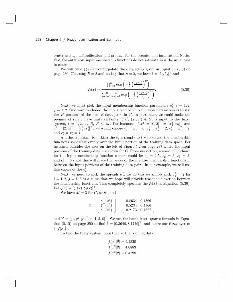
258 Chapter 5 / Fuzzy Identification and Estimation
center-average defuzzification and product for the premise and implication. Noticethat the outermost input membership functions do not saturate as is the usual casein control.
We will tune f(x|θ) to interpolate the data set G given in Equation (5.3) onpage 236. Choosing R = 2 and noting that n = 2, we have θ = [b1, b2] and
ξi(x) =
∏nj=1 exp
(−1
2
(xj−ci
j
σij
)2)
∑Ri=1
∏nj=1 exp
(−1
2
(xj−ci
j
σij
)2) . (5.30)
Next, we must pick the input membership function parameters cij, i = 1, 2,
j = 1, 2. One way to choose the input membership function parameters is to usethe xi portions of the first R data pairs in G. In particular, we could make thepremise of rule i have unity certainty if xi, (xi, yi) ∈ G, is input to the fuzzysystem, i = 1, 2, . . . , R, R ≤ M . For instance, if x1 = [0, 2] = [x1
1, x12]
andx2 = [2, 4] = [x2
1, x22], we would choose c1
1 = x11 = 0, c1
2 = x12 = 2, c2
1 = x21 = 2,
and c22 = x2
2 = 4.Another approach to picking the ci
j is simply to try to spread the membershipfunctions somewhat evenly over the input portion of the training data space. Forinstance, consider the axes on the left of Figure 5.2 on page 237 where the inputportions of the training data are shown for G. From inspection, a reasonable choicefor the input membership function centers could be c1
1 = 1.5, c12 = 3, c2
1 = 3,and c2
2 = 5 since this will place the peaks of the premise membership functions inbetween the input portions of the training data pairs. In our example, we will usethis choice of the ci
j.Next, we need to pick the spreads σi
j. To do this we simply pick σij = 2 for
i = 1, 2, j = 1, 2 as a guess that we hope will provide reasonable overlap betweenthe membership functions. This completely specifies the ξi(x) in Equation (5.30).Let ξ(x) = [ξ1(x), ξ2(x)].
We have M = 3 for G, so we find
Φ =
ξ(x1)
ξ(x2)ξ(x3)
=
0.8634 0.1366
0.5234 0.47660.2173 0.7827
and Y = [y1, y2, y3] = [1, 5, 6]. We use the batch least squares formula in Equa-tion (5.15) on page 250 to find θ = [0.3646, 8.1779], and hence our fuzzy systemis f(x|θ).
To test the fuzzy system, note that at the training data
f(x1|θ) = 1.4320f(x2|θ) = 4.0883f(x3|θ) = 6.4798

5.3 Least Squares Methods 259
so that the trained fuzzy system maps the training data reasonably accurately(x3 = [3, 6]). Next, we test the fuzzy system at some points not in the trainingdata set to see how it interpolates. In particular, we find
f([1, 2]|θ) = 1.8267f([2.5, 5]|θ) = 5.3981
f([4, 7]|θ) = 7.3673
These values seem like good interpolated values considering Figure 5.2 on page 237,which illustrates the data set G for this example.
5.3.5 Example: Recursive Least Squares Training ofFuzzy Systems
Here, we illustrate the use of the RLS algorithm in Equation (5.26) on page 255 fortraining a fuzzy system to map the training data given in G in Equation (5.3) onpage 236. First, we replace xk with ξ(xk) in Equation (5.26) to obtain
P (k) =1λ
(I − P (k − 1)ξ(xk)(λI + (ξ(xk))P (k − 1)ξ(xk))−1(ξ(xk)))P (k − 1)
θ(k) = θ(k − 1) + P (k)ξ(xk)(yk − (ξ(xk)) θ(k − 1)) (5.31)
and we use this to compute the parameter vector of the fuzzy system. We will trainthe same fuzzy system that we considered in the batch least squares example ofthe previous section, and we pick the same ci
j and σij, i = 1, 2, j = 1, 2 as we chose
there so that we have the same ξ(x) = [ξ1, ξ2].For initialization of Equation (5.31), we choose
θ(0) = [2, 5.5]
as a guess of where the output membership function centers should be. Anotherguess would be to choose θ(0) = [0, 0]. Next, using the guidelines for RLS initial-ization, we choose
P (0) = αI
where α = 2000. We choose λ = 1 since we do not want to discount old data, andhence we use the standard (nonweighted) RLS.
Before using Equation (5.31) to find an estimate of the output membershipfunction centers, we need to decide in what order to have RLS process the trainingdata pairs (xi, yi) ∈ G. For example, you could just take three steps with Equa-tion (5.31), one for each training data pair. Another approach would be to use each(xi, yi) ∈ G Ni times (in some order) in Equation (5.31) then stop the algorithm.Still another approach would be to cycle through all the data (i.e., (x1, y1) first,(x2, y2) second, up until (xM , yM ) then go back to (x1, y1) and repeat), say, NRLS
times. It is this last approach that we will use and we will choose NRLS = 20.
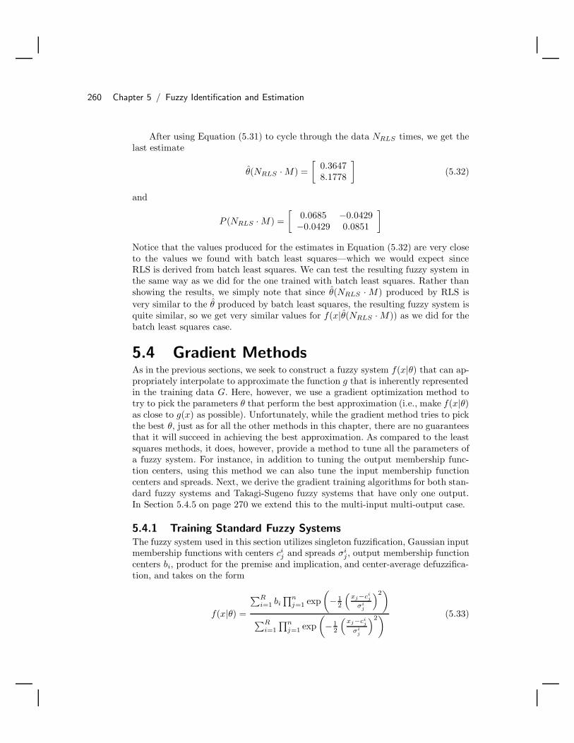
260 Chapter 5 / Fuzzy Identification and Estimation
After using Equation (5.31) to cycle through the data NRLS times, we get thelast estimate
θ(NRLS · M) =[
0.36478.1778
](5.32)
and
P (NRLS · M) =[
0.0685 −0.0429−0.0429 0.0851
]
Notice that the values produced for the estimates in Equation (5.32) are very closeto the values we found with batch least squares—which we would expect sinceRLS is derived from batch least squares. We can test the resulting fuzzy system inthe same way as we did for the one trained with batch least squares. Rather thanshowing the results, we simply note that since θ(NRLS · M) produced by RLS isvery similar to the θ produced by batch least squares, the resulting fuzzy system isquite similar, so we get very similar values for f(x|θ(NRLS · M)) as we did for thebatch least squares case.
5.4 Gradient MethodsAs in the previous sections, we seek to construct a fuzzy system f(x|θ) that can ap-propriately interpolate to approximate the function g that is inherently representedin the training data G. Here, however, we use a gradient optimization method totry to pick the parameters θ that perform the best approximation (i.e., make f(x|θ)as close to g(x) as possible). Unfortunately, while the gradient method tries to pickthe best θ, just as for all the other methods in this chapter, there are no guaranteesthat it will succeed in achieving the best approximation. As compared to the leastsquares methods, it does, however, provide a method to tune all the parameters ofa fuzzy system. For instance, in addition to tuning the output membership func-tion centers, using this method we can also tune the input membership functioncenters and spreads. Next, we derive the gradient training algorithms for both stan-dard fuzzy systems and Takagi-Sugeno fuzzy systems that have only one output.In Section 5.4.5 on page 270 we extend this to the multi-input multi-output case.
5.4.1 Training Standard Fuzzy SystemsThe fuzzy system used in this section utilizes singleton fuzzification, Gaussian inputmembership functions with centers ci
j and spreads σij, output membership function
centers bi, product for the premise and implication, and center-average defuzzifica-tion, and takes on the form
f(x|θ) =
∑Ri=1 bi
∏nj=1 exp
(−1
2
(xj−ci
j
σij
)2)
∑Ri=1
∏nj=1 exp
(−1
2
(xj−ci
j
σij
)2) (5.33)

5.4 Gradient Methods 261
Note that we use Gaussian-shaped input membership functions for the entire inputuniverse of discourse for all inputs and do not use ones that saturate at the outer-most endpoints as we often do in control. The procedure developed below works ina similar fashion for other types of fuzzy systems. Recall that ci
j denotes the centerfor the ith rule on the jth universe of discourse, bi denotes the center of the outputmembership function for the ith rule, and σi
j denotes the spread for the ith rule onthe jth universe of discourse.
Suppose that you are given the mth training data pair (xm, ym) ∈ G. Let
em =12
[f(xm|θ) − ym ]2
In gradient methods, we seek to minimize em by choosing the parameters θ, whichfor our fuzzy system are bi, ci
j , and σij , i = 1, 2, . . . , R, j = 1, 2, . . . , n (we will use
θ(k) to denote these parameters’ values at time k). Another approach would be tominimize a sum of such error values for a subset of the data in G or all the data inG; however, with this approach computational requirements increase and algorithmperformance may not.
Output Membership Function Centers Update Law
First, we consider how to adjust the bi to minimize em. We use an “update law”(update formula)
bi(k + 1) = bi(k) − λ1∂em
∂bi
∣∣∣∣k
where i = 1, 2, . . . , R and k ≥ 0 is the index of the parameter update step. This is a“gradient descent” approach to choosing the bi to minimize the quadratic functionem that quantifies the error between the current data pair (xm, ym) and the fuzzysystem. If em were quadratic in θ (which it is not; why?), then this update methodwould move bi along the negative gradient of the em error surface—that is, downthe (we hope) bowl-shaped error surface (think of the path you take skiing downa valley—the gradient descent approach takes a route toward the bottom of thevalley). The parameter λ1 > 0 characterizes the “step size.” It indicates how biga step to take down the em error surface. If λ1 is chosen too small, then bi isadjusted very slowly. If λ1 is chosen too big, convergence may come faster but yourisk it stepping over the minimum value of em (and possibly never converging toa minimum). Some work has been done on adaptively picking the step size. Forexample, if errors are decreasing rapidly, take big steps, but if errors are decreasingslowly, take small steps. This approach attempts to speed convergence yet avoidmissing a minimum.
Now, to simplify the bi update formula, notice that using the chain rule fromcalculus
∂em
∂bi= (f(xm |θ) − ym)
∂f(xm |θ)∂bi

262 Chapter 5 / Fuzzy Identification and Estimation
so
∂em
∂bi= (f(xm|θ) − ym)
∏nj=1 exp
(−1
2
(xm
j −cij
σij
)2)
∑Ri=1
∏nj=1 exp
(−1
2
(xm
j −cij
σij
)2)
For notational convenience let
µi(xm, k) =n∏
j=1
exp
−1
2
(xm
j − cij(k)
σij(k)
)2 (5.34)
and let
εm(k) = f(xm|θ(k)) − ym
Then we get
bi(k + 1) = bi(k) − λ1εm(k)µi(xm, k)∑Ri=1 µi(xm, k)
(5.35)
as the update equation for the bi, i = 1, 2, . . . , R, k ≥ 0.The other parameters in θ, ci
j(k) and σij(k), will also be updated with a gradient
algorithm to try to minimize em, as we explain next.
Input Membership Function Centers Update Law
To train the cij , we use
cij(k + 1) = ci
j(k) − λ2∂em
∂cij
∣∣∣∣∣k
where λ2 > 0 is the step size (see the comments above on how to choose this stepsize), i = 1, 2, . . . , R, j = 1, 2, . . . , n, and k ≥ 0. At time k using the chain rule,
∂em
∂cij
= εm(k)∂f(xm |θ(k))∂µi(xm, k)
∂µi(xm, k)∂ci
j
for i = 1, 2, . . . , R, j = 1, 2, . . . , n, and k ≥ 0. Now,
∂f(xm|θ(k))∂µi(xm, k)
=
(∑Ri=1 µi(xm, k)
)bi(k) −
(∑Ri=1 bi(k)µi(xm, k)
)(1)(∑R
i=1 µi(xm, k))2

5.4 Gradient Methods 263
so that
∂f(xm|θ(k))∂µi(xm, k)
=bi(k) − f(xm|θ(k))∑R
i=1 µi(xm, k)
Also,
∂µi(xm, k)∂ci
j
= µi(xm, k)
(xm
j − cij(k)(
σij(k)
)2
)
so we have an update method for the cij(k) for all i = 1, 2, . . . , R, j = 1, 2, . . . , n,
and k ≥ 0. In particular, we have
cij(k+1) = ci
j(k)−λ2εm(k)
(bi(k) − f(xm|θ(k))∑R
i=1 µi(xm, k)
)µi(xm, k)
(xm
j − cij(k)(
σij(k)
)2
)(5.36)
for i = 1, 2, . . . , R, j = 1, 2, . . . , n, and k ≥ 0.
Input Membership Function Spreads Update Law
To update the σij(k) (spreads of the membership functions), we follow the same
procedure as above and use
σij(k + 1) = σi
j(k) − λ3∂em
∂σij
∣∣∣∣∣k
where λ3 > 0 is the step size, i = 1, 2, . . . , R, j = 1, 2, . . . , n, and k ≥ 0. Using thechain rule, we obtain
∂em
∂σij
= εm(k)∂f(xm|θ(k))∂µi(xm, k)
∂µi(xm, k)∂σi
j
We have
∂µi(xm, k)∂σi
j
= µi(xm, k)
(xm
j − cij(k)
)2
(σi
j(k))3
so that
σij(k + 1) = σi
j(k) − λ3εm(k)bi(k) − f(xm|θ(k))∑R
i=1 µi(xm, k)µi(xm, k)
(xmj − ci
j(k))2
(σij(k))3
(5.37)
for i = 1, 2, . . . , R, j = 1, 2, . . . , n, and k ≥ 0. This completes the definition ofthe gradient training method for the standard fuzzy system. To summarize, theequations for updating the parameters θ of the fuzzy system are Equations (5.35),(5.36), and (5.37).

264 Chapter 5 / Fuzzy Identification and Estimation
Next, note that the gradient training method described above is for the casewhere we have Gaussian-shaped input membership functions. The update formulaswould, of course, change if you were to choose other membership functions. Forinstance, if you use triangular membership functions, the update formulas can bedeveloped, but in this case you will have to pay special attention to how to definethe derivative at the peak of the membership function.
Finally, we would like to note that the gradient method can be used in eitheran off- or on-line manner. In other words, it can be used off-line to train a fuzzysystem for system identification, or it can be used on-line to train a fuzzy system toperform real-time parameter estimation. We will see in Chapter 6 how to use suchan adaptive parameter identifier in an adaptive control setting.
5.4.2 Implementation Issues and ExampleIn this section we discuss several issues that you will encounter if you implement agradient approach to training fuzzy systems. Also, we provide an example of howto train a standard fuzzy system.
Algorithm Design
There are several issues to address in the design of the gradient algorithm fortraining a fuzzy system. As always, the choice of the training data G is critical.Issues in the choice of the training data, which we discussed in Section 5.2 onpage 235, are relevant here. Next, note that you must pick the number of inputs nto the fuzzy system to be trained and the number of rules R; the method does notadd rules, it just tunes existing ones.
The choice of the initial estimates bi(0), cij(0), and σi
j(0) can be important.Sometimes picking them close to where they should be can help convergence. Noticethat you should not pick bi = 0 for all i = 1, 2, . . . , R or the algorithm for the bi
will stay at zero for all k ≥ 0. Your computer probably will not allow you to pickσi
j(0) = 0 since you divide by this number in the algorithm. Also, you may need tomake sure that in the algorithm σi
j(k) ≥ σ > 0 for some fixed scalar σ so that thealgorithm does not tune the parameters of the fuzzy system so that the computerhas to divide by zero (to do this, just monitor the σi
j(k), and if there exists some k′
where σij(k
′) < σ, let σij(k
′) = σ). Notice that for our choice of input membershipfunctions
R∑i=1
µi(xm, k) = 0
so that we normally do not have to worry about dividing by it in the algorithm.Note that the above gradient algorithm is for only one training data pair. That
is, we could run the gradient algorithm for a long time (i.e., many values of k) foronly one data pair to try to train the fuzzy system to match that data pair verywell. Then we could go to the next data pair in G, begin with the final computedvalues of bi, ci
j, and σij from the last data pair we considered as the initial values for

5.4 Gradient Methods 265
this data pair, and run the gradient algorithm for as many steps as we would likefor that data pair—and so on. Alternatively, we could cycle through the trainingdata many times, taking one step with the gradient algorithm for each data pair.It is difficult to know how many parameter update steps should be made for eachdata pair and how to cycle through the data. It is generally the case, however, thatif you use some of the data much more frequently than other data in G, then thetrained fuzzy system will tend to be more accurate for that data rather than thedata that was not used as many times in training. Some like to cycle through thedata so that each data pair is visited the same number of times and use small stepsizes so that the updates will not be too large in any direction.
Clearly, you must be careful with the choices for the λi, i = 1, 2, 3 step sizesas values for these that are too big can result in an unstable algorithm (i.e., θvalues can oscillate or become unbounded), while values for these that are toosmall can result in very slow convergence. The main problem, however, is that inthe general case there are no guarantees that the gradient algorithm will convergeat all! Moreover, it can take a significant amount of training data and long trainingtimes to achieve good results. Generally, you can conduct some tests to see howwell the fuzzy system is constructed by comparing how it maps the data pairs totheir actual values; however, even if this comparison appears to indicate that thefuzzy system is mapping the data properly, there are no guarantees that it will“generalize” (i.e., interpolate) for data not in the training data set that it wastrained with.
To terminate the gradient algorithm, you could wait until all the parametersstop moving or change very little over a series of update steps. This would indicatethat the parameters are not being updated so the gradients must be small so wemust be at a minimum of the em surface. Alternatively, we could wait until theem or
∑Mm=1 em does not change over a fixed number of steps. This would indicate
that even if the parameter values are changing, the value of em is not decreasing,so the algorithm has found a minimum and it can be terminated.
Example
As an example, consider the data set G in Equation (5.3) on page 236: we will trainthe parameters of the fuzzy system with R = 2 and n = 2. Choose λ1 = λ2 = λ3 =1. Choose [
c11(0)
c12(0)
]=
[02
],
[σ1
1(0)σ1
2(0)
]=
[11
], b1(0) = 1
and [c21(0)
c22(0)
]=
[24
],
[σ2
1(0)σ2
2(0)
]=
[11
], b2(0) = 5
In this way the two rules will begin by perfectly mapping the first two data pairsin G (why?). The gradient algorithm has to tune the fuzzy system so that it will

266 Chapter 5 / Fuzzy Identification and Estimation
provide an approximation to the third data pair in G, and in doing this it will tendto somewhat degrade how well it represented the first two data pairs.
To train the fuzzy system, we could repeatedly cycle through the data in G sothat the fuzzy system learns how to map the third data pair but does not forgethow to map the first two. Here, for illustrative purposes, we will simply performone iteration of the algorithm for the bi parameters for the third data pair. Thatis, we use
xm = x3 =[
36
], ym = y3 = 6
In this case we have
µ1(x3, 0) = 0.000003724
and
µ2(x3, 0) = 0.08208
so that f(x3|θ(0)) = 4.99977 and εm(0) = −1.000226. With this and Equation (5.35),we find that b1(1) = 1.000045379 and b2(1) = 6.0022145. The calculations for thecij(1) and σi
j(1) parameters, i = 1, 2, j = 1, 2, are made in a similar way, but usingEquations (5.36) and (5.37), respectively.
Even with only one computation step, we see that the output centers bi, i = 1, 2,are moving to perform an interpolation that is more appropriate for the third datapoint. To see this, notice that b2(1) = 6.0022145 where b2(0) = 5.0 so that theoutput center moved much closer to y3 = 6.
To further study how the gradient algorithm works, we recommend that youwrite a computer program to implement the update formulas for this example. Youmay need to tune the λi and approach to cycling through the data. Then, using anappropriate termination condition (see the discussion above), stop the algorithmand test the quality of the interpolation by placing inputs into the fuzzy system andseeing if the outputs are good interpolated values (e.g., compare them to Figure 5.2on page 237). In the next section we will provide a more detailed example, but forthe training of Takagi-Sugeno fuzzy systems.
5.4.3 Training Takagi-Sugeno Fuzzy SystemsThe Takagi-Sugeno fuzzy system that we train in this section takes on the form
f(x|θ(k)) =∑R
i=1 gi(x, k)µi(x, k)∑Ri=1 µi(x, k)
where µi(x, k) is defined in Equation (5.34) on page 262 (of course, other definitionsare possible), x = [x1, x2, . . . , xn], and
gi(x, k) = ai,0(k) + ai,1(k)x1 + ai,2(k)x2 + · · ·+ ai,n(k)xn

5.4 Gradient Methods 267
(note that we add the index k since we will update the ai,j parameters). For moredetails on how to define Takagi-Sugeno fuzzy systems, see Section 2.3.7 on page 73.
Parameter Update Formulas
Following the same approach as in the previous section, we need to update theai,j parameters of the gi(x, k) functions and ci
j and σij. Notice, however, that most
of the work is done since if in Equations (5.36) and (5.37) we replace bi(k) withgi(xm, k), we get the update formulas for the ci
j and σij for the Takagi-Sugeno fuzzy
system.To update the ai,j we use
ai,j(k + 1) = ai,j(k) − λ4∂em
∂ai,j
∣∣∣∣k
(5.38)
when λ4 > 0 is the step size. Notice that
∂em
∂ai,j= εm(k)
∂f(xm |θ(k))∂gi(xm, k)
∂gi(xm, k)∂ai,j(k)
for all i = 1, 2, . . . , R, j = 1, 2, . . . , n (plus j = 0) and
∂f(xm |θ(k))∂gi(xm, k)
=µi(xm, k)∑R
i=1 µi(xm, k)
for all i = 1, 2, . . . , R. Also,
∂gi(xm, k)∂ai,0(k)
= 1
and
∂gi(x, k)∂ai,j(k)
= xj
for all j = 1, 2, . . . , n and i = 1, 2, . . . , R.This gives the update formulas for all the parameters of the Takagi-Sugeno
fuzzy system. In the previous section we discussed issues in the choice of the stepsizes and initial parameter values, how to cycle through the training data in G,and some convergence issues. All of this discussion is relevant to the training ofTakagi-Sugeno models also. The training of more general functional fuzzy systemswhere the gi take on more general forms proceeds in a similar manner. In fact, itis easy to develop the update formulas for any functional fuzzy system such that
∂gi(xm, k)∂ai,j(k)

268 Chapter 5 / Fuzzy Identification and Estimation
can be determined analytically. Finally, we would note that Takagi-Sugeno or gen-eral functional fuzzy systems can be trained either off- or on-line. Chapter 6 dis-cusses how such on-line training can be used in adaptive control.
Example
As an example, consider once again the data set G in Equation (5.3) on page 236.We will train the Takagi-Sugeno fuzzy system with two rules (R = 2) and n = 2considered in Equation (5.33). We will cycle through the data set G 40 times (similarto how we did in the RLS example) to get the error between the fuzzy system outputand the output portions of the training data to decrease to some small value.
We use Equations (5.38), (5.36), and (5.37) to update the ai,j(k), cij(k), and
σij(k) values, respectively, for all i = 1, 2, . . . , R, j = 1, 2, . . . , n, and we choose σ
from the previous section to be 0.01. For initialization we pick λ4 = 0.01, λ2 =λ3 = 1, ai,j(0) = 1, and σi
j = 2 for all i and j, and c11(0) = 1.5, c1
2(0) = 3,c21(0) = 3, and c2
2(0) = 5. The step sizes were tuned a bit to improve convergence,but could probably be further tuned to improve it more. The ai,j(0) values aresimply somewhat arbitrary guesses. The σi
j(0) values seem like reasonable spreadsconsidering the training data. The ci
j(0) values are the same ones used in the leastsquares example and seem like reasonable guesses since they try to spread thepremise membership function peaks somewhat uniformly over the input portions ofthe training data. It is possible that a better initial guess for the ai,j(0) could beobtained by using the least squares method to pick these for the initial guesses forthe ci
j(0) and σij(0); in some ways this would make the guess for the ai,j(0) more
consistent with the other initial parameters.By the time the algorithm terminates, the error between the fuzzy system
output and the output portions of the training data has reduced to less than 0.125but is still showing a decreasing oscillatory behavior. At algorithm termination(k = 119), the consequent parameters are
a1,0(119) = 0.8740, a1,1(119) = 0.9998, a1,2(119) = 0.7309
a2,0(119) = 0.7642, a2,1(119) = 0.3426, a2,2(119) = 0.7642
the input membership function centers are
c11(119) = 2.1982, c2
1(119) = 2.6379
c12(119) = 4.2833, c2
2(119) = 4.7439
and their spreads are
σ11(119) = 0.7654, σ2
1(119) = 2.6423
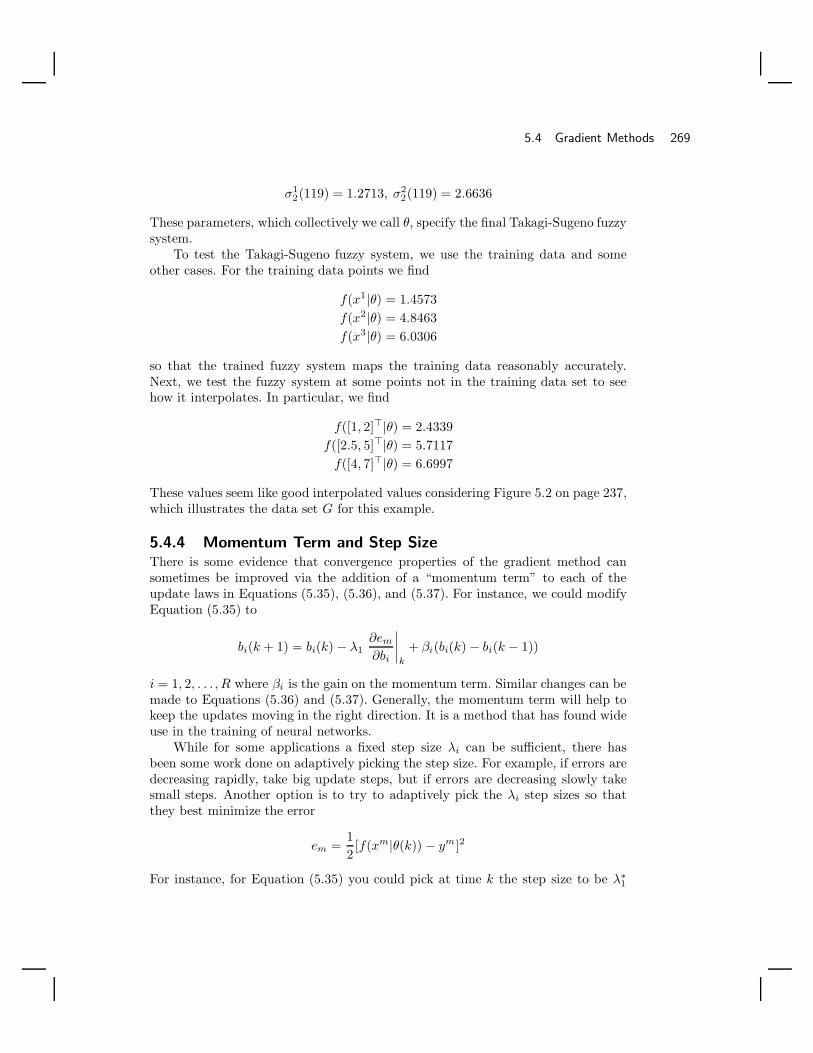
5.4 Gradient Methods 269
σ12(119) = 1.2713, σ2
2(119) = 2.6636
These parameters, which collectively we call θ, specify the final Takagi-Sugeno fuzzysystem.
To test the Takagi-Sugeno fuzzy system, we use the training data and someother cases. For the training data points we find
f(x1|θ) = 1.4573f(x2|θ) = 4.8463f(x3|θ) = 6.0306
so that the trained fuzzy system maps the training data reasonably accurately.Next, we test the fuzzy system at some points not in the training data set to seehow it interpolates. In particular, we find
f([1, 2]|θ) = 2.4339f([2.5, 5]|θ) = 5.7117
f([4, 7]|θ) = 6.6997
These values seem like good interpolated values considering Figure 5.2 on page 237,which illustrates the data set G for this example.
5.4.4 Momentum Term and Step SizeThere is some evidence that convergence properties of the gradient method cansometimes be improved via the addition of a “momentum term” to each of theupdate laws in Equations (5.35), (5.36), and (5.37). For instance, we could modifyEquation (5.35) to
bi(k + 1) = bi(k) − λ1∂em
∂bi
∣∣∣∣k
+ βi(bi(k) − bi(k − 1))
i = 1, 2, . . . , R where βi is the gain on the momentum term. Similar changes can bemade to Equations (5.36) and (5.37). Generally, the momentum term will help tokeep the updates moving in the right direction. It is a method that has found wideuse in the training of neural networks.
While for some applications a fixed step size λi can be sufficient, there hasbeen some work done on adaptively picking the step size. For example, if errors aredecreasing rapidly, take big update steps, but if errors are decreasing slowly takesmall steps. Another option is to try to adaptively pick the λi step sizes so thatthey best minimize the error
em =12[f(xm|θ(k)) − ym]2
For instance, for Equation (5.35) you could pick at time k the step size to be λ∗1
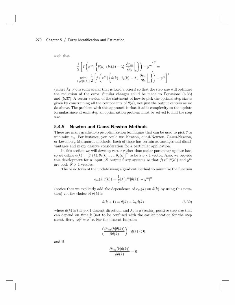
270 Chapter 5 / Fuzzy Identification and Estimation
such that
12
[f
(xm|
θ(k) : bi(k) − λ∗
1
∂em
∂bi
∣∣∣∣k
)− ym
]2
=
minλ1∈[0,λ1]
12
[f
(xm|
θ(k) : bi(k) − λ1
∂em
∂bi
∣∣∣∣k
)− ym
]2
(where λ1 > 0 is some scalar that is fixed a priori) so that the step size will optimizethe reduction of the error. Similar changes could be made to Equations (5.36)and (5.37). A vector version of the statement of how to pick the optimal step size isgiven by constraining all the components of θ(k), not just the output centers as wedo above. The problem with this approach is that it adds complexity to the updateformulas since at each step an optimization problem must be solved to find the stepsize.
5.4.5 Newton and Gauss-Newton MethodsThere are many gradient-type optimization techniques that can be used to pick θ tominimize em. For instance, you could use Newton, quasi-Newton, Gauss-Newton,or Levenberg-Marquardt methods. Each of these has certain advantages and disad-vantages and many deserve consideration for a particular application.
In this section we will develop vector rather than scalar parameter update lawsso we define θ(k) = [θ1(k), θ2(k), . . . , θp(k)] to be a p× 1 vector. Also, we providethis development for n input, N output fuzzy systems so that f(xm|θ(k)) and ym
are both N × 1 vectors.The basic form of the update using a gradient method to minimize the function
em(k|θ(k)) =12|f(xm|θ(k)) − ym|2
(notice that we explicitly add the dependence of em(k) on θ(k) by using this nota-tion) via the choice of θ(k) is
θ(k + 1) = θ(k) + λkd(k) (5.39)
where d(k) is the p×1 descent direction, and λk is a (scalar) positive step size thatcan depend on time k (not to be confused with the earlier notation for the stepsizes). Here, |x|2 = xx. For the descent function
(∂em(k|θ(k))
∂θ(k)
)d(k) < 0
and if
∂em(k|θ(k))∂θ(k)
= 0

5.4 Gradient Methods 271
where “0” is a p× 1 vector of zeros, the method does not update θ(k). Our updateformulas for the fuzzy system in Equations (5.35), (5.36), and (5.37) use
d(k) = −∂em(k|θ(k))∂θ(k)
= −∇em(k|θ(k))
(which is the gradient of em with respect to θ(k)) so they actually provide for a“steepest descent” approach (of course, Equations (5.35), (5.36), and (5.37) arescalar update laws each with its own step size, while Equation (5.39) is a vectorupdate law with a single step size). Unfortunately, this method can sometimesconverge slowly, especially if it gets on a long, low slope surface.
Next, let
∇2em(k|θ(k)) =[∂2em(k|θ(k))∂θi(k)θj(k)
]
be the p × p “Hessian matrix,” the elements of which are the second partials ofem(k|θ(k)) at θ(k). In “Newton’s method” we choose
d(k) = −(∇2em(k|θ(k))
)−1 ∇em(k|θ(k)) (5.40)
provided that ∇2em(k|θ(k)) is positive definite so that it is invertible (see Sec-tion 4.3.5 for a definition of “positive definite”). For a function em(k|θ(k)) thatis quadratic in θ(k), Newton’s method provides convergence in one step; for someother functions, it can converge very fast. The price you pay for this convergencespeed is computation of Equation (5.40) and the need to verify the existence of theinverse in that equation.
In “quasi-Newton methods” you try to avoid problems with existence and com-putation of the inverse in Equation (5.40) by choosing
d(k) = −Λ(k)∇em(k|θ(k))
where Λ(k) is a positive definite p× p matrix for all k ≥ 0 and is sometimes chosento approximate
(∇2em(k|θ(k))
)−1 (e.g., in some cases by using only the diagonalelements of
(∇2em(k|θ(k))
)−1). If Λ(k) is chosen properly, for some applicationsmuch of the convergence speed of Newton’s method can be achieved.
Next, consider the Gauss-Newton method that is used to solve a least squaresproblem such as finding θ(k) to minimize
em(k|θ(k)) =12|f(xm|θ(k)) − ym|2 =
12|εm(k|θ(k))|2
where
εm(k|θ(k)) = f(xm|θ(k)) − ym = [εm1 , εm2 , . . . , εmN]

272 Chapter 5 / Fuzzy Identification and Estimation
First, linearize εm(k|θ(k)) around θ(k) (i.e., use a truncated Taylor series expansion)to get
εm(θ|θ(k)) = εm(k|θ(k)) + ∇εm(k|θ(k))(θ − θ(k))
Here,
∇εm(k|θ(k)) =[∇εm1(k|θ(k)),∇εm2 (k|θ(k)), . . . ,∇εmN
(k|θ(k))]
is a p × N matrix whose columns are gradient vectors
∇εmi(k|θ(k)) =∂∇εmi(k|θ(k))
∂θ(k)
i = 1, 2, . . . , N . Notice that
∇εm(k|θ(k))
is the “Jacobian.” Also note that the notation εm(θ|θ(k)) is used to emphasize thedependence on both θ(k) and θ.
Next, minimize the norm of the linearized function εm(θ|θ(k)) by letting
θ(k + 1) = arg minθ
12|εm(θ|θ(k))|2
Hence, in the Gauss-Newton approach we update θ(k) to a value that will bestminimize a linear approximation to εm(k|θ(k)). Notice that
θ(k + 1) = arg minθ
12[|εm(k|θ(k))|2 + 2(θ − θ(k)) (∇εm(k|θ(k))) εm(k|θ(k))
+ (θ − θ(k))∇εm(k|θ(k))∇εm(k|θ(k))(θ − θ(k))]
= arg minθ
12[|εm(k|θ(k))|2 + 2(θ − θ(k)) (∇εm(k|θ(k))) εm(k|θ(k))
+ θ∇εm(k|θ(k))∇εm(k|θ(k))θ − 2θ(k)∇εm(k|θ(k))∇εm(k|θ(k))θ
+ θ(k)∇εm(k|θ(k))∇εm(k|θ(k))θ(k)]
(5.41)
To perform this minimization, notice that we have a quadratic function so we find
∂[·]∂θ
= ∇εm(k|θ(k))εm(k|θ(k)) + ∇εm(k|θ(k))∇εm(k|θ(k))θ
− ∇εm(k|θ(k))∇εm(k|θ(k))θ(k) (5.42)
where [·] denotes the expression in Equation (5.41) in brackets multiplied by onehalf. Setting this equal to zero, we get the minimum achieved at θ∗ where
∇εm(k|θ(k))∇εm(k|θ(k))(θ∗ − θ(k)) = −∇εm(k|θ(k))εm(k|θ(k))

5.5 Clustering Methods 273
or, if ∇εm(k|θ(k))∇εm(k|θ(k)) is invertible,
θ∗ − θ(k) = −(∇εm(k|θ(k))∇εm(k|θ(k))
)−1 ∇εm(k|θ(k))εm(k|θ(k))
Hence, the Gauss-Newton update formula is
θ(k + 1) = θ(k) −(∇εm(k|θ(k))∇εm(k|θ(k))
)−1 ∇εm(k|θ(k))εm(k|θ(k))
To avoid problems with computing the inverse, the method is often implementedas
θ(k + 1) = θ(k) − λk
(∇εm(k|θ(k))∇εm(k|θ(k)) + Γ(k)
)−1 ∇εm(k|θ(k))εm(k|θ(k))
where λk is a positive step size that can change at each time k, and Γ(k) is a p× pdiagonal matrix such that
∇εm(k|θ(k))∇εm(k|θ(k)) + Γ(k)
is positive definite so that it is invertible. In the Levenberg-Marquardt method youchoose Γ(k) = αI where α > 0 and I is the p × p identity matrix. Essentially,a Gauss-Newton iteration is an approximation to a Newton iteration so it canprovide for faster convergence than, for instance, steepest descent, but not as fastas a pure Newton method; however, computations are simplified. Note, however,that for each iteration of the Gauss-Newton method (as it is stated above) we mustfind the inverse of a p× p matrix; there are, however, methods in the optimizationliterature for coping with this issue.
Using each of the above methods to train a fuzzy system is relatively straight-forward. For instance, notice that many of the appropriate partial derivatives havealready been found when we developed the steepest descent approach to training.
5.5 Clustering Methods“Clustering” is the partitioning of data into subsets or groups based on similaritiesbetween the data. Here, we will introduce two methods to perform fuzzy clusteringwhere we seek to use fuzzy sets to define soft boundaries to separate data intogroups. The methods here are related to conventional ones that have been developedin the field of pattern recognition. We begin with a fuzzy “c-means” techniquecoupled with least squares to train Takagi-Sugeno fuzzy systems, then we brieflystudy a nearest neighborhood method for training standard fuzzy systems. In thec-means approach, we continue in the spirit of the previous methods in that weuse optimization to pick the clusters and, hence, the premise membership functionparameters. The consequent parameters are chosen using the weighted least squaresapproach developed earlier. The nearest neighborhood approach also uses a type ofoptimization in the construction of cluster centers and, hence, the fuzzy system. Inthe next section we break away from the optimization approaches to fuzzy system

274 Chapter 5 / Fuzzy Identification and Estimation
construction and study simple constructive methods that are called “learning byexamples.”
5.5.1 Clustering with Optimal Output PredefuzzificationIn this section we will introduce the clustering with optimal output predefuzzifi-cation approach to train Takagi-Sugeno fuzzy systems. We do this via the simpleexample we have used in previous sections.
Clustering for Specifying Rule Premises
Fuzzy clustering is the partitioning of a collection of data into fuzzy subsets or“clusters” based on similarities between the data and can be implemented usingan algorithm called fuzzy c-means. Fuzzy c-means is an iterative algorithm used tofind grades of membership µij (scalars) and cluster centers vj (vectors of dimensionn × 1) to minimize the objective function
J =M∑
i=1
R∑j=1
(µij)m|xi − vj|2 (5.43)
where m > 1 is a design parameter. Here, M is the number of input-output datapairs in the training data set G, R is the number of clusters (number of rules)we wish to calculate, xi for i = 1, ..., M is the input portion of the input-outputtraining data pairs, vj = [vj
1, vj2, . . . , v
jn] for j = 1, ..., R are the cluster centers,
and µij for i = 1, ..., M and j = 1, ..., R is the grade of membership of xi in the jth
cluster. Also, |x| =√
xx where x is a vector. Intuitively, minimization of J resultsin cluster centers being placed to represent groups (clusters) of data.
Fuzzy clustering will be used to form the premise portion of the If-Then rules inthe fuzzy system we wish to construct. The process of “optimal output predefuzzifi-cation” (least squares training for consequent parameters) is used to form the con-sequent portion of the rules. We will combine fuzzy clustering and optimal outputpredefuzzification to construct multi-input single-output fuzzy systems. Extensionof our discussion to multi-input multi-output systems can be done by repeating theprocess for each of the outputs.
In this section we utilize a Takagi-Sugeno fuzzy system in which the consequentportion of the rule-base is a function of the crisp inputs such that
If Hj Then gj(x) = aj,0 + aj,1x1 + · · ·+ aj,nxn (5.44)
where n is the number of inputs and Hj is an input fuzzy set given by
Hj = (x, µHj(x)) : x ∈ X1 × · · · × Xn (5.45)
where Xi is the ith universe of discourse, and µHj (x) is the membership functionassociated with Hj that represents the premise certainty for rule j; and gj(x) = a
j x
where aj = [aj,0, aj,1 . . . , aj,n] and x = [1, x] where j = 1, . . . , R. The resulting
5.5 Clustering Methods 275
fuzzy system is a weighted average of the output gj(x) for j = 1, ..., R and is givenby
f(x|θ) =
∑Rj=1 gj(x)µHj (x)∑R
j=1 µHj (x)(5.46)
where R is the number of rules in the rule-base. Next, we will use the Takagi-Sugenofuzzy model, fuzzy clustering, and optimal output defuzzification to determine theparameters aj and µHj (x), which define the fuzzy system. We will do this via asimple example.
Suppose we use the example data set in Equation (5.3) on page 236 that hasbeen used in the previous sections. We first specify a “fuzziness factor” m > 1, whichis a parameter that determines the amount of overlap of the clusters. If m > 1 islarge, then points with less membership in the jth cluster have less influence on thedetermination of the new cluster centers. Next, we specify the number of clustersR we wish to calculate. The number of clusters R equals the number of rules in therule-base and must be less than or equal to the number of data pairs in the trainingdata set G (i.e., R ≤ M). We also specify the error tolerance εc > 0, which is theamount of error allowed in calculating the cluster centers. We initialize the clustercenters vj
0 via a random number generator so that each component of vj0 is no larger
(smaller) than the largest (smallest) corresponding component of the input portionof the training data. The selection of vj
0, although somewhat arbitrary, may affectthe final solution.
For our simple example, we choose m = 2 and R = 2, and let εc = 0.001. Ourinitial cluster centers were randomly chosen to be
v10 =
[1.893.76
]
and
v20 =
[2.474.76
]
so that each component lies in between xi1 and xi
2 for i = 1, 2, 3 (see the definitionof G in Equation (5.3)).
Next, we compute the new cluster centers vj based on the previous clustercenters so that the objective function in Equation (5.43) is minimized. The necessaryconditions for minimizing J are given by
vjnew =
∑Mi=1 xi(µnew
ij )m∑Mi=1(µ
newij )m
(5.47)

276 Chapter 5 / Fuzzy Identification and Estimation
where
µnewij =
R∑
k=1
(|xi − vj
old|2
|xi − vkold|
2
) 1m−1
−1
(5.48)
for each i = 1, . . . , M and for each j = 1, 2, . . . , R such that∑R
j=1 µnewij = 1 (and
|x|2 = xx). In Equation (5.48) we see that it is possible that there exists ani = 1, 2, . . . , M such that |xi − vj
old|2 = 0 for some j = 1, 2, . . . , R. In this case the
µnewij is undefined. To fix this problem, let µij for all i be any nonnegative numbers
such that∑R
j=1 µij = 1 and µij = 0, if |xi − vj
old|2 = 0.
Using Equation (5.48) for our example with vj
old = vj0, j = 1, 2, we find that
µnew11 = 0.6729, µnew
12 = 0.3271, µnew21 = 0.9197, µnew
22 = 0.0803, µnew31 = 0.2254,
and µnew32 = 0.7746. We use these µnew
ij from Equation (5.48) to calculate the newcluster centers
v1new =
[1.3663.4043
]
and
v2new =
[2.54105.3820
]
using Equation (5.47).Next, we compare the distances between the current cluster centers vj
new andthe previous cluster centers vj
old (which for the first step is vj0). If |vj
new−vj
old| < εc
for all j = 1, 2, . . . , R then the cluster centers vjnew accurately represent the input
data, the fuzzy clustering algorithm is terminated, and we proceed on to the optimaloutput defuzzification algorithm (see below). Otherwise, we continue to iterativelyuse Equations (5.47) and (5.48) until we find cluster centers vj
new that satisfy|vj
new − vj
old| < εc for all j = 1, 2, . . . , R. For our example, vj
old = vj0, and we see
that |vjnew − vj
old| = 0.6328 for j = 1 and 0.6260 for j = 2. Both of these valuesare greater than εc, so we continue to update the cluster centers.
Proceeding to the next iteration, let vj
old = vjnew, j = 1, 2, . . . , R from the last
iteration, and apply Equations (5.47) and (5.48) to find µnew11 = 0.8233, µnew
12 =0.1767, µnew
21 = 0.7445, µnew22 = 0.2555, µnew
31 = 0.0593, and µnew32 = 0.9407 using
the cluster centers calculated above, yielding the new cluster centers
v1new =
[0.90562.9084
]

5.5 Clustering Methods 277
and
v2new =
[2.83815.7397
]
Computing the distances between these cluster centers and the previous ones, wefind that |vj
new−vj
old| > εc, so the algorithm continues. It takes 14 iterations before
the algorithm terminates (i.e., before we have |vjnew − vj
old| ≤ εc = 0.001 for allj = 1, 2, . . . , R). When it does terminate, name the final membership grade valuesµij and cluster centers vj , i = 1, 2, . . . , M , j = 1, 2, . . . , R.
For our example, after 14 iterations the algorithm finds µ11 = 0.9994, µ12 =0.0006, µ21 = 0.1875, µ22 = 0.8125, µ31 = 0.0345, µ32 = 0.9655,
v1 =[
0.07142.0725
]
and
v2 =[
2.58545.1707
]
Notice that the clusters have converged so that v1 is near x1 = [0, 2] and v2 liesin between x2 = [2, 4] and x3 = [3, 6].
The final values of vj , j = 1, 2, . . . , R, are used to specify the premise mem-bership functions for the ith rule. In particular, we specify the premise membershipfunctions as
µHj (x) =
[R∑
k=1
( |x − vj|2|x− vk|2
) 1m−1
]−1
(5.49)
j = 1, 2, . . . , R where vj, j = 1, 2, . . . , R are the cluster centers from the lastiteration that uses Equations (5.47) and (5.48). It is interesting to note that forlarge values of m we get smoother (less distinctive) membership functions. Thisis the primary guideline to use in selecting the value of m; however, often a goodfirst choice is m = 2. Next, note that µHj (x) is a premise membership functionthat is different from any that we have considered. It is used to ensure certainconvergence properties of the iterative fuzzy c-means algorithm described above.With the premises of the rules defined, we next specify the consequent portion.
Least Squares for Specifying Rule Consequents
We apply “optimal output predefuzzification” to the training data to calculate thefunction gj(x) = a
j x, j = 1, 2, . . . , R for each rule (i.e., each cluster center), bydetermining the parameters aj. There are two methods you can use to find the aj .

278 Chapter 5 / Fuzzy Identification and Estimation
Approach 1: For each cluster center vj , we wish to minimize the squared errorbetween the function gj(x) and the output portion of the training data pairs. Letxi = [1, (xi)] where (xi, yi) ∈ G. We wish to minimize the cost function Jj givenby
Jj =M∑i=1
(µij)2(yi − (xi)aj
)2(5.50)
for each j = 1, 2, . . . , R where µij is the grade of membership of the input portionof the ith data pair for the jth cluster that resulted from the clustering algorithmafter it converged, yi is the output portion of the ith data pair d(i) = (xi, yi), andthe multiplication of (xi) and aj defines the output associated with the jth rulefor the ith training data point.
Looking at Equation (5.50), we see that the minimization of Jj via the choice ofthe aj is a weighted least squares problem. From Section 5.3 and Equation (5.15) onpage 250, the solution aj for j = 1, 2, . . . , R to the weighted least squares problemis given by
aj = (XD2j X)−1XD2
j Y (5.51)
where
X =[
1 ... 1x1 ... xM
]Y = [y1, . . . , yM ],
D2j = (diag([µ1j, . . . , µMj]))
2
For our example the parameters that satisfy the linear function gj(x) = aj xi for
j = 1, 2 such that Jj in Equation (5.50) is minimized were found to be a1 =[3, 2.999,−1] and a2 = [3, 3,−1], which are very close to each other.
Approach 2: As an alternative approach, rather than solving R least squaresproblems, one for each rule, we can use the least squares methods discussed in Sec-tion 5.3 to specify the consequent parameters of the Takagi-Sugeno fuzzy system. Todo this, we simply parameterize the Takagi-Sugeno fuzzy system in Equation (5.46)in a form so that it is linear in the consequent parameters and of the form
f(x|θ) = θξ(x)
where θ holds all the ai,j parameters and ξ is specified in a similar manner to howwe did in Section 5.3.3. Now, just as we did in Section 5.3.3, we can use batchor recursive least squares methods to find θ. Unless we indicate otherwise, we willalways use approach 1 in this book.

5.5 Clustering Methods 279
Testing the Approximator
Suppose that we use approach 1 to specify the rule consequents. To test how accu-rately the constructed fuzzy system represents the training data set G in Figure 5.2on page 237, suppose that we choose the test point x′ such that (x′, y′) ∈ G. Specif-ically, we choose
x′ =[
12
]
We would expect from Figure 5.2 on page 237 that the output of the fuzzy systemwould lie somewhere between 1 and 5. The output is 3.9999, so we see that thetrained Takagi-Sugeno fuzzy system seems to interpolate adequately. Notice alsothat if we let x = xi, i = 1, 2, 3 where (xi, yi) ∈ G, we get values very close tothe yi, i = 1, 2, 3, respectively. That is, for this example the fuzzy system nearlyperfectly maps the training data pairs. We also note that if the input to the fuzzysystem is x = [2.5, 5], the output is 5.5, so the fuzzy system seems to performgood interpolation near the training data points.
Finally, we note that the aj will clearly not always be as close to each otheras for this example. For instance, if we add the data pair ([4, 5], 5.5) to G (i.e.,make M = 4), then the cluster centers converge after 13 iterations (using the sameparameters m and εc as we did earlier). Using approach 1 to find the consequentparameters, we get
a1 = [−1.458, 0.7307, 1.2307]
and
a2 = [2.999, 0.00004, 0.5]
For the resulting fuzzy system, if we let x = [1, 2] in Equation (5.46), we getan output value of 1.8378, so we see that it performs differently than the case forM = 3, but that it does provide a reasonable interpolated value.
5.5.2 Nearest Neighborhood ClusteringAs with the other approaches, we want to construct a fuzzy estimation systemthat approximates the function g that is inherently represented in the trainingdata set G. We use singleton fuzzification, Gaussian membership functions, productinference, and center-average defuzzification, and the fuzzy system that we train isgiven by
f(x|θ) =
∑Ri=1 Ai
∏nj=1 exp
(−(
xj−vij
2σ
)2)
∑Ri=1 Bi
∏nj=1 exp
(−(
xj−vij
2σ
)2) (5.52)
280 Chapter 5 / Fuzzy Identification and Estimation
where R is the number of clusters (rules), n is the number of inputs,
vj = [vj1, v
j2, . . . , v
jn]
are the cluster centers, σ is a constant and is the width of the membership functions,and Ai and Bi are the parameters whose values will be specified below (to traina multi-output fuzzy system, simply apply the procedure to the fuzzy system thatgenerates each output). From Equation (5.52), we see that the parameter vector θis given by
θ = [A1, . . . , AR, B1, . . . , BR, v11, . . . , v
1n, ..., vR
1 , . . . , vRn , σ]
and is characterized by the number of clusters (rules) R and the number of inputsn. Next, we will explain, via a simple example, how to use the nearest neighborhoodclustering technique to construct a fuzzy system by choosing the parameter vectorθ.
Suppose that n = 2, X ⊂ 2, and Y ⊂ , and that we use the training data setG in Equation (5.3) on page 236. We first specify the parameter σ, which definesthe width of the membership functions. A small σ provides narrow membershipfunctions that may yield a less smooth fuzzy system mapping, which may causefuzzy system mapping not to generalize well for the data points not in the trainingset. Increasing the parameter σ will result in a smoother fuzzy system mapping.Next, we specify the quantity εf , which characterizes the maximum distance allowedbetween each of the cluster centers. The smaller εf , the more accurate are theclusters that represent the function g. For our example, we chose σ = 0.3 andεf = 3.0. We must also define an initial fuzzy system by initializing the parametersA1, B1, and v1. Specifically, we set A1 = y1 , B1 = 1, and v1
j = x1j for j = 1, 2, . . . , n.
If we take our first data pair,
(x1, y1) =([
02
], 1
)
we get A1 = 1, B1 = 1, and
v1 =[
02
]
which forms our first cluster (rule) for f(x|θ). Next, we take the second data pair,
(x2, y2) =([
24
], 5
)
and compute the distance between the input portion of the data pair and each ofthe R existing cluster centers, and let the smallest distance be |xi − vl| (i.e., thenearest cluster to xi is vl) where |x| =
√xx. If |xi − vl| < εf , then we do not add
any clusters (rules) to the existing system, but we update the existing parameters
5.5 Clustering Methods 281
Al and Bl for the nearest cluster vl to account for the output portion yi of thecurrent input-output data pair (xi, yi) in the training data set G. Specifically, welet
Al := Aoldl + yi
and
Bl := Boldl + 1
These values are incremented to represent adding the effects of another data pairto the existing cluster. For instance, Al is incremented so that the sum in thenumerator of Equation (5.52) is modified to include the effects of the additionaldata pair without adding another rule. The value of Bl is then incremented torepresent that we have added the effects of another data pair (it normalizes thesum in Equation (5.52)). Note that we do not modify the cluster centers in thiscase, just the Al and Bl values; hence we do not modify the premises (that areparameterized via the cluster centers and σ), just the consequents of the existingrule that the new data pair is closest to.
Suppose that |xi−vl| > εf . Then we add an additional cluster (rule) to representthe (x2, y2) information about the function g by modifying the parameter vectorθ and letting R = 2 (i.e., we increase the number of clusters (rules)), vR
j = x2j for
j = 1, 2, . . . , n, AR = y2, and BR = 1. These assignments of variables represent theexplicit addition of a rule to the fuzzy system. Hence, for our example
v2 =[
24
], A2 = 5, B2 = 1
The nearest neighbor clustering technique is implemented by repeating the abovealgorithm until all of the M data pairs in G are used.
Consider the third data pair,
(x3, y3) =([
36
], 6
)
We would compute the distance between the input portion of the current data pairx3 and each of the R = 2 cluster centers and find the smallest distance |x3 − vl|.For our example, what is the value of |x3 − vl| and which cluster center is closest?Explain how to update the fuzzy system (specifically, provide values for A2 andB2). To test how accurately the fuzzy system f represents the training data set G,suppose that we choose a test point x′ such that (x′, y′) ∈ G. Specifically, we choose
x′ =[
12
]

282 Chapter 5 / Fuzzy Identification and Estimation
We would expect the output value of the fuzzy system for this input to lie somewherebetween 1 and 5 (why?).
5.6 Extracting Rules from DataIn this section we discuss two very intuitive approaches to the construction of afuzzy system f so that it approximates the function g. These approaches involveshowing how to directly specify rules that represent the data pairs (“examples”).Our two “learning from examples” approaches depart significantly from the ap-proaches used up to this point that relied on optimization to specify fuzzy systemparameters. In our first approach, the training procedure relies on the completespecification of the membership functions and only constructs the rules. The sec-ond approach constructs all the membership functions and rules, and for this reasoncan be considered a bit more general.
5.6.1 Learning from Examples (LFE)In this section we show how to construct fuzzy systems using the “learning fromexamples” (LFE) technique. The LFE technique generates a rule-base for a fuzzysystem by using numerical data from a physical system and possibly linguisticinformation from a human expert. We will describe the technique for multi-inputsingle-output (MISO) systems. The technique can easily be extended to apply toMIMO systems by repeating the procedure for each of the outputs. We will usesingleton fuzzification, minimum to represent the premise and implication, andCOG defuzzification; however, the LFE method does not explicitly depend on thesechoices. Other choices outlined in Chapter 2 can be used as well.
Membership Function Construction
The membership functions are chosen a priori for each of the input universes ofdiscourse and the output universe of discourse. For a two-input one-output fuzzysystem, one typical choice for membership functions is shown in Figure 5.8, where
1. Xi = [x−i , x+
i ], i = 1,2, and Y = [y−, y+] are chosen according to the expectedrange of variation in the input and output variables.
2. The number of membership functions on each universe of discourse affects theaccuracy of the function approximation (with fewer generally resulting in loweraccuracy).
3. Xji and Y j denote the fuzzy sets with associated membership functions µXj
i(xi)
and µY j (y), respectively.
In other cases you may want to choose Gaussian or trapezoidal-shaped membershipfunctions. The choice of these membership functions is somewhat ad hoc for theLFE technique.

5.6 Extracting Rules from Data 283
X
X
X X X X
X X X X X X X X
1 1 1 1 11 2 3 4 5
2 2 2 2 22 2 2 221 63 4 5 7 8 9
Y2
Y1
Y3
Y4
Y5
xxx +-1 1 1
xxx +-2 2 2
yyy - +y m
x2m
x 1m
FIGURE 5.8 Example membership functions forinput and output universes of discourse for learningfrom examples technique.
Rule Construction
We finish the construction of the fuzzy system by using the training data in G toform the rules. Generally, the input portions of the training data pairs xj, where(xj, yj) ∈ G, are used to form the premises of rules, while the output portions ofthe data pairs yj are used to form the consequents. For our two-input one-outputexample above, the rule-base to be constructed contains rules of the form
Ri = If x1 is Xj1 and x2 is Xk
2 Then y is Y l
where associated with the ith rule is a “degree” defined by
degree(Ri) = µXj1(x1) ∗ µXk
2(x2) ∗ µY l(y) (5.53)
where “∗” represents the triangular norm defined in Chapter 2. We will use thestandard algebraic product for the definition of the degree of a rule throughoutthis section so that “∗” represents the product (of course, you could use, e.g., theminimum operator also). With this, degree(Ri) quantifies how certain we are thatrule Ri represents some input-output data pair ([xj
1, xj2]
, yj) ∈ G (why?). As anexample, suppose that degree(Ri) = 1 for ([xj
1, xj2]
, yj) ∈ G. Using the abovemembership functions, if the input to the fuzzy system is x = [xj
1, xj2]
then yj willbe the output of the fuzzy system (i.e., the rule perfectly represents this data pair).If, on the other hand, x = [xj
1, xj2]
, then degree(Ri) < 1 and the mapping inducedby rule Ri does not perfectly match the data pair ([xj
1, xj2]
, yj) ∈ G.

284 Chapter 5 / Fuzzy Identification and Estimation
The LFE technique is a procedure where we form rules directly from data pairsin G. Assume that several rules have already been constructed from the data pairsin G and that we want to next consider the mth piece of training data d(m). Forour example, suppose
d(m) = ([xm1 , xm
2 ], ym)
where example values of xm1 , xm
2 , and ym are shown in Figure 5.8. In this caseµX3
1(xm
1 ) = 0.3, µX41(xm
1 ) = 0.7, µX32(xm
2 ) = 0.8, µX42(xm
2 ) = 0.2, µY 3(ym) = 0.9,and µY 4(ym) = 0.1. In the learning from examples approach, you choose input andoutput membership functions for the rule to be synthesized from d(m) by choosingthe ones with the highest degree of membership (resolve ties arbitrarily). For ourexample, from Figure 5.8 we would consider adding the rule
Rm = If x1 is X41 and x2 is X3
2 Then y is Y 3
to the rule-base since µX41(xm
1 ) > µX31(xm
1 ), µX32(xm
2 ) > µX42(xm
2 ), and µY 3(ym) >
µY 4(ym) (i.e., it has a form that appears to best fit the data pair d(m)).Notice that we have degree(Rm) = (0.7)(0.8)(0.9) = 0.504 if x1 = xm
1 , x2 =xm
2 , and y = ym . We use the following guidelines for adding new rules:
• If degree(Rm) > degree(Ri), for all i = m such that rules Ri are already in therule-base (and degree(Ri) is evaluated for d(m)) and the premises for Ri and Rm
are the same, then the rule Rm (the rule with the highest degree) would replacerule Ri in the existing rule-base.
• If degree(Rm) ≤ degree(Ri) for some i, i = m, and the premises for Ri and Rm
are the same, then rule Rm is not added to the rule-base since the data pair d(m)
is already adequately represented with rules in the fuzzy system.
• If rule Rm does not have the same premise as any other rule already in therule-base, then it is added to the rule-base to represent d(m).
This process repeats by considering each data pair i = 1, 2, 3, . . . , M . Once youhave considered each data pair in G, the process is completed.
Hence, we add rules to represent data pairs. We associate the left-hand side ofthe rules with the xi portion of the training data pairs and the consequents with theyi, (xi, yi) ∈ G. We only add rules to represent a data pair if there is not alreadya rule in the rule-base that represents the data pair better than the one we areconsidering adding. We are assured that there will be a bounded number of rulesadded since for a fixed number of inputs and membership functions we know thatthere are a limited number of possible rules that can be formed (and there is onlya finite amount of data). Notice that the LFE procedure constructs rules but doesnot modify membership functions to help fit the data. The membership functionsmust be specified a priori by the designer.
5.6 Extracting Rules from Data 285
Example
As an example, consider the formation of a fuzzy system to approximate the dataset G in Equation (5.3) on page 236, which is shown in Figure 5.2. Suppose that weuse the membership functions pictured in Figure 5.8 with x−
1 = 0, x+1 = 4, x−
2 = 0,x+
2 = 8, y− = 0, and y+ = 8 as a choice for known regions within which all thedata points lie (see Figure 5.2). Suppose that
d(1) = (x1, y1) =([
02
], 1
)
is considered first. With this we would consider adding the rule
R1 = If x1 is X11 and x2 is X3
2 Then y is Y 1
(notice that we resolved the tie between choosing Y 1 or Y 2 for the consequent fuzzyset arbitrarily). Since there are no other rules in the rule-base, we will put R1 inthe rule-base and go to the next data pair. Next, consider
d(2) =([
24
], 5
)
With d(2) from Figure 5.8, we would consider adding rule
R2 = If x1 is X31 and x2 is X5
2 Then y is Y 3
(where once again we arbitrarily chose Y 3 rather than Y 4). Should we add rule R2
to the rule-base? Notice that degree(R2) = 0.5 for d(2) and that degree(R1) = 0for d(2) so that R2 represents the data pair d(2) better than any other rule in therule-base; hence, we will add it to the rule-base. Proceeding in a similar manner,we will also add a third rule to represent the third data pair in G (show this) sothat our final fuzzy system will have three rules, one for each data pair.
If you were to train a fuzzy system with a much larger data set G, you wouldfind that there will not be a rule for each of the M data pairs in G since somerules will adequately represent more than one data pair. Generally, if some x suchthat (x, y) /∈ G is put into the fuzzy system, it will try to interpolate to produce areasonable output y. You can test the quality of the estimator by putting inputs xinto the fuzzy system and checking that the outputs y are such that (x, y) ∈ G, orthat they are close to these.
5.6.2 Modified Learning from Examples (MLFE)We will introduce the “modified learning from examples” (MLFE) technique inthis section. In addition to synthesizing a rule-base, in MLFE we also modify themembership functions to try to more effectively tailor the rules to represent thedata.

286 Chapter 5 / Fuzzy Identification and Estimation
Fuzzy System and Its Initialization
The fuzzy system used in this section utilizes singleton fuzzification, Gaussian mem-bership functions, product for the premise and implication, and center-average de-fuzzification, and takes on the form
f(x|θ) =
∑Ri=1 bi
∏nj=1 exp
(−1
2
(xj−ci
j
σij
)2)
∑Ri=1
∏nj=1 exp
(−1
2
(xj−ci
j
σij
)2) (5.54)
(however, other forms may be used equally effectively). In Equation (5.54), theparameter vector θ to be chosen is
θ = [b1, . . . , bR, c11, . . . , c
1n, . . . , cR
1 , . . . , cRn , σ1
1, . . . , σ1n, . . . , σR
1 , . . . , σRn ] (5.55)
where bi is the point in the output space at which the output membership functionfor the ith rule achieves a maximum, ci
j is the point in the jth input universe ofdiscourse where the membership function for the ith rule achieves a maximum, andσi
j > 0 is the width (spread) of the membership function for the jth input and theith rule. Notice that the dimensions of θ are determined by the number of inputs nand the number of rules R in the rule-base. Next, we will explain how to constructthe rule-base for the fuzzy estimator by choosing R, n, and θ. We will do this viathe simple example data set G where n = 2 that is given in Equation (5.3) onpage 236.
We let the quantity εf characterize the accuracy with which we want the fuzzysystem f to approximate the function g at the training data points in G. Wealso define an “initial fuzzy system” that the MLFE procedure will begin with byinitializing the parameters θ. Specifically, we set R = 1, b1 = y1 , c1
j = x1j , and
σ1j = σ0 for j = 1, 2, . . . , n where the parameter σ0 > 0 is a design parameter. If we
take σ0 = 0.5 and
(x1, y1) =([
02
], 1
)
we get b1 = 1, c11 = 0, c1
2 = 2, σ11 = 0.5, and σ1
2 = 0.5, which forms our first rule forf .
Next, we describe how to add rules to the fuzzy system and modify the member-ship functions so that the fuzzy system matches the data and properly interpolates.In the first approach that we describe, we will assume that for the training data(xi, yi) ∈ G, xj
i = xj′
i′ for any i′ = i, for each j′ = j (i.e., the data values are alldistinct element-wise). Later, we will show several ways to remove this restriction.Notice, however, that for practical situations where, for example, you use a noiseinput for training, this assumption will likely be satisfied.

5.6 Extracting Rules from Data 287
Adding Rules, Modifying Membership Functions
Following the initialization procedure, for our example we take the second data pair
(x2, y2) =([
24
], 5
)
and compare the data pair output portion y2 with the existing fuzzy system f(x2|θ)(i.e., the one with only one rule). If∣∣f(x2|θ) − y2
∣∣ ≤ εf
then the fuzzy system f already adequately represents the mapping information in(x2, y2) and hence no rule is added to f and we consider the next training data pairby performing the same type of εf test.
Suppose that ∣∣f(x2|θ) − y2∣∣ > εf
Then we add a rule to represent the (x2, y2) information about g by modifying thecurrent parameters θ by letting R = 2 (i.e., increasing the number of rules by one),b2 = y2, and c2
j = x2j for all j = 1, 2, . . . , n (hence, b2 = 5, c2
1 = 2, and c22 = 4).
Moreover, we modify the widths σij for rule i = R (i = 2 for this example) to
adjust the spacing between membership functions so that
1. The new rule does not distort what has already been learned.
2. There is smooth interpolation between training points.
Modification of the σij for i = R is done by determining the “nearest neighbor”
n∗j in terms of the membership function centers that is given by
n∗j = arg min|ci′
j − cij| : i′ = 1, 2, . . . , R, i′ = i (5.56)
where j = 1, 2, . . . , n and cij is fixed. Here, n∗
j denotes the i′ index of the ci′j that
minimizes the expression (hence, the use of the term “argmin”). For our examplewhere we have just added a second rule, n∗
1 = 1 and n∗2 = 1 (the only possible
nearest neighbor for each universe of discourse is found from the initial rule in thesystem).
Next, we update the σij for i = R by letting
σij =
1W
|cij − c
n∗j
j | (5.57)
for j = 1, 2, . . . , n, where W is a weighting factor that determines the amount ofoverlap of the membership functions. Notice that since we assumed that for thetraining data (xi, yi) ∈ G, xj
i = xj′
i′ for any i′ = i, for each j′ = j we will never

288 Chapter 5 / Fuzzy Identification and Estimation
have σij = 0, which would imply a zero width input membership function that could
cause implementation problems. From Equation (5.57), we see that the weightingfactor W and the widths σi
j have an inverse relationship. That is, a larger W impliesless overlap. For our example, we choose W = 2 so σ2
1 = 12| c2
1− c11 |= 1
2| 2−0 |= 1
and σ22 = 1
2 | c22 − c1
2 |= 12 | 4 − 2 |= 1. The MLFE algorithm is implemented by
repeating the above procedure until all the M data pairs are exhausted.For instance, for our third training data pair,
(x3, y3) =([
36
], 6
)
we would test if∣∣f(x3 |θ) − y3
∣∣ ≤ εf . If it is, then no new rule is added. If∣∣f(x3 |θ) − y3
∣∣ >εf , then we let R = 3 and add a new rule letting bR = yR and cR
j = xRj for all
j = 1, 2, . . . , n. Then we set the σRj , j = 1, 2, . . . , n by finding the nearest neighbor
n∗j (nearest in terms of the closest premise membership function centers) and using
σRj = 1
W | cRj − c
n∗j
j |, j = 1, 2, . . . , n.For example, for (x3, y3) suppose that εf is chosen so that
∣∣f(x3 |θ) − y3∣∣ > εf
so that we add a new rule letting R = 3, b3 = 6, c31 = 3, and c3
2 = 6. It is easy tosee from Figure 5.2 on page 237 that with i = 3, for j = 1, n∗
1 = arg min|ci′j − c3
j | :i′ = 1, 2 = arg min3, 1 = 2 and, for j = 2, n∗
2 = arg min|ci′j − c3
j | : i′ =1, 2 = arg min4, 2 = 2. In other words, [2, 4] is the closest to [3, 6]. Hence, viaEquation (5.57) with W = 2, σ3
1 = 12(3 − 2) = 1
2and σ3
2 = 12(6 − 4) = 1.
Testing the Approximator
To test how accurately the fuzzy system represents the training data set G, notethat since we added a new rule for each of the three training data points it will bethe case that the fuzzy system f(x|θ) = y for all (x, y) ∈ G (why?). If (x′, y′) ∈ Gfor some x′, the fuzzy system f will attempt to interpolate. For instance, for ourexample above if
x′ =[
13
]
we would expect from Figure 5.2 on page 237 that f(x′|θ) would lie somewherebetween 1 and 5. In fact, for the three-rule fuzzy system we constructed above,f(x′|θ) = 4.81 for this x′. Notice that this value of f(x′|θ) is quite reasonable as aninterpolated value for the given data in G (see Figure 5.2).
Alternative Methods to Modify the Membership Functions
Here, we first remove the restriction that for the training data (xi, yi) ∈ G, xji = xj′
i′
for any i′ = i, for each j′ = j and consider any set of training data G. Followingthis we will briefly discuss other ways to tune membership functions.

5.6 Extracting Rules from Data 289
Recall that the only reason that we placed the restriction on G was to avoidhaving a value of σi
j = 0 in Equation (5.57). One way to avoid having a value ofσi
j = 0 is simply to make the computation in Equation (5.57) and if
σij < σ
for some small σ > 0, let σij = σ. This ensures that the algorithm will never pick
σij smaller than some preset value. We have found this method to work quite well
in some applications.Another way to avoid having a value of σi
j = 0 from Equation (5.57) is simplyto set
σij = σ
n∗j
j
This says that we find the closest membership function center cn∗
j
j , and if it is thesame as ci
j then let the width of the membership function associated with cij be
the same as that of the membership function associated with cn∗
j
j (i.e., σn∗
j
j ). Yet
another approach would be to compute the width of the cij based not on c
n∗j
j but onthe other nearest neighbors that do not have identical centers, provided that thereare such centers currently loaded into the rule-base.
There are many other approaches that can be used to train membership func-tions. For instance, rather than using Equation (5.56), we could let ci = [ci
1, ci2, . . . , c
in]
and compute
n∗ = arg min|ci′ − ci| : i′ = 1, 2, . . . , R, i′ = i
and then let
σij =
1W
| ci − cn∗ |
for j = 1, 2, . . . , n. This approach will, however, need similar fixes to the one abovein case the assumption that the input portions of the training data are distinctelement-wise is not satisfied.
As yet another approach, suppose that we use triangular membership functions.For initialization we use some fixed base width for the first rule and choose its centerc1j = x1
j as before. Use the same εf -test to decide whether to add rules. If you adda rule, let ci
j = xij, i = R, j = 1, 2, . . . , n as before. Next, to fully specify the
membership functions, compute
n−j = arg min|ci
j − ci′j | : i′ = 1, 2, . . . , M, ci′
j < cij
n+j = arg min|ci
j − ci′j | : i′ = 1, 2, . . . , M, ci′
j > cij.
These are the indices of the nearest neighbor membership functions both above
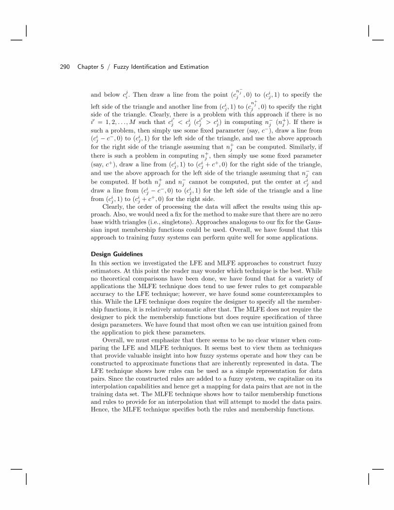
290 Chapter 5 / Fuzzy Identification and Estimation
and below cji . Then draw a line from the point (c
n−j
j , 0) to (cij, 1) to specify the
left side of the triangle and another line from (cij, 1) to (c
n+j
j , 0) to specify the rightside of the triangle. Clearly, there is a problem with this approach if there is noi′ = 1, 2, . . . , M such that ci′
j < cij (ci′
j > cij) in computing n−
j (n+j ). If there is
such a problem, then simply use some fixed parameter (say, c−), draw a line from(ci
j − c−, 0) to (cij, 1) for the left side of the triangle, and use the above approach
for the right side of the triangle assuming that n+j can be computed. Similarly, if
there is such a problem in computing n+j , then simply use some fixed parameter
(say, c+), draw a line from (cij, 1) to (ci
j + c+, 0) for the right side of the triangle,and use the above approach for the left side of the triangle assuming that n−
j canbe computed. If both n+
j and n−j cannot be computed, put the center at ci
j anddraw a line from (ci
j − c−, 0) to (cij , 1) for the left side of the triangle and a line
from (cij , 1) to (ci
j + c+, 0) for the right side.Clearly, the order of processing the data will affect the results using this ap-
proach. Also, we would need a fix for the method to make sure that there are no zerobase width triangles (i.e., singletons). Approaches analogous to our fix for the Gaus-sian input membership functions could be used. Overall, we have found that thisapproach to training fuzzy systems can perform quite well for some applications.
Design Guidelines
In this section we investigated the LFE and MLFE approaches to construct fuzzyestimators. At this point the reader may wonder which technique is the best. Whileno theoretical comparisons have been done, we have found that for a variety ofapplications the MLFE technique does tend to use fewer rules to get comparableaccuracy to the LFE technique; however, we have found some counterexamples tothis. While the LFE technique does require the designer to specify all the member-ship functions, it is relatively automatic after that. The MLFE does not require thedesigner to pick the membership functions but does require specification of threedesign parameters. We have found that most often we can use intuition gained fromthe application to pick these parameters.
Overall, we must emphasize that there seems to be no clear winner when com-paring the LFE and MLFE techniques. It seems best to view them as techniquesthat provide valuable insight into how fuzzy systems operate and how they can beconstructed to approximate functions that are inherently represented in data. TheLFE technique shows how rules can be used as a simple representation for datapairs. Since the constructed rules are added to a fuzzy system, we capitalize on itsinterpolation capabilities and hence get a mapping for data pairs that are not in thetraining data set. The MLFE technique shows how to tailor membership functionsand rules to provide for an interpolation that will attempt to model the data pairs.Hence, the MLFE technique specifies both the rules and membership functions.

5.7 Hybrid Methods 291
5.7 Hybrid MethodsIn this chapter we have discussed least squares (batch and recursive), gradient(steepest descent, Newton, and Gauss-Newton), clustering (with optimal outputpredefuzzification and nearest neighbor), learning from examples, and modifiedlearning from examples methods for training standard and Takagi-Sugeno fuzzysystems. In this section we will discuss hybrid approaches where we combine twoor more of the above methods to train a fuzzy system.
Basically, the hybrid methods can be classified three ways:
• Hybrid initialization/training: You could initialize the parameters of the fuzzysystem with one method and then use a different method for the training. Forinstance, you could use the learning by examples methods to create a fuzzy systemthat you could later tune with a gradient or least squares method. Alternatively,you could use a least squares method to initialize the output centers of a standardfuzzy system and then use a gradient method to tune the premise parameters andto fine-tune the output centers.
• Hybrid premise/consequent training: You could train the premises of the ruleswith one method and the consequents with another. This is exactly what is donein clustering with optimal output predefuzzification in Section 5.5.1 on page 274:A clustering method is used to specify the premise parameters, and least squaresis used to train the consequent functions since they are linear in the parameters.Other examples of hybrid training of this type include the use of least squares fortraining the consequent functions of a Takagi-Sugeno fuzzy system (since theyenter linearly) and a gradient method for training the premise parameters (sincethey enter in a nonlinear fashion). Alternatively, you could train the premises witha clustering method and the consequents with a gradient method (especially fora functional fuzzy system that has consequent functions that are not linear in theparameters). Still another option would be to use ideas from the learning fromexamples techniques to train the premises and use the least squares or gradientmethods for the consequents.
• Hybrid interleaved training: You could train with one method then another, fol-lowed by another, and so on. For instance, you could use a learning by examplesmethod to initialize the fuzzy system parameters, then train the fuzzy systemwith a gradient method, with periodic updates to the output membership func-tion centers coming from a least squares method.
Basically, all these methods provide the advantage of design flexibility for the tuningof fuzzy systems. While some would view this flexibility in a positive light, it doeshave its drawbacks, primarily in trying to determine which approach to use, or thebest combination of approaches.
Indeed, it is very difficult to know which of the methods in this chapter to useas the choice ultimately depends on the application. Moreover, it is important tohave in mind what you mean by “best.” This would likely involve accuracy of esti-

292 Chapter 5 / Fuzzy Identification and Estimation
mation or identification, but it could also focus on the computational complexity ofimplementing the resulting fuzzy system. We have found that for some applicationsthe LFE and MLFE approaches can take many rules to get good identificationaccuracy (as can the nearest neighborhood clustering approach). Sometimes thecomputations for large data sets are prohibitive for batch least squares, but re-cursive least squares can then be used. Sometimes gradient training takes a largeamount of training data and extremely long training times. On the other hand,the clustering with optimal output predefuzzification method needs relatively fewrules (partially because one Takagi-Sugeno rule carries more information than onestandard fuzzy rule) and hence often results in low computational complexity whileat the same time providing better accuracy; it seems to exploit the advantages ofthe least squares approach and ideas in clustering that result in well-tuned inputmembership functions. We do not, however, consider this finding universal. Forother applications, one of the other methods (e.g., gradient and least squares), ora combination of the above methods, may provide a better approach.
In the next section we provide a design and implementation case study wherewe use the clustering with optimal output predefuzzification approach.
5.8 Case Study: FDI for an EngineIn recent years more attention has been given to reducing exhaust gas emissions pro-duced by internal combustion engines. In addition to overall engine and emissionsystem design, correct or fault-free engine operation is a major factor determin-ing the amount of exhaust gas emissions produced in internal combustion engines.Hence, there has been a recent focus on the development of on-board diagnosticsystems that monitor relative engine health. Although on-board vehicle diagnosticscan often detect and isolate some major engine faults, due to widely varying drivingenvironments they may be unable to detect minor faults, which may nonethelessaffect engine performance. Minor engine faults warrant special attention becausethey do not noticeably hinder engine performance but may increase exhaust gasemissions for a long period of time without the problem being corrected.
The minor faults we consider in this case study include “calibration faults” (forour study, the occurrence of a calibration fault means that a sensed or commandedsignal is multiplied by a gain factor not equal to one, while in the no-fault casethe sensed or commanded signal is multiplied by one) in the throttle and mass fuelactuators, and in the engine speed and mass air sensors (we could also consider“bias”-type faults even though we do not do so in this case study). The reliabilityof these actuators and sensors is particularly important to the engine controllersince their failure can affect the performance of the emissions control system.
Our particular focus in this design and implementation case study is to showhow to construct fuzzy estimators to perform failure detection and identification(FDI) for certain actuator and sensor calibration faults. We compare the resultsfrom the fuzzy estimators to a nonlinear autoregressive moving average with ex-ogenous inputs (ARMAX) technique and provide experimental results showing theeffectiveness of the technique. Next, we provide an overview of the experimental

5.8 Case Study: FDI for an Engine 293
engine test bed and testing conditions that we use.
5.8.1 Experimental Engine and Testing ConditionsAll investigations in this case study were performed using the experimental enginetest cell shown in Figure 5.9. The experimental setup in the engine test cell consistsof a Ford 3.0 L V-6 engine coupled to an electric dynamometer through an automatictransmission. An air charge temperature sensor (ACT), a throttle position sensor(TPS), and a mass airflow sensor (MAF) are installed in the engine to measurethe air charge temperature, throttle position, and air mass flow rate. Two heatedexhaust gas oxygen sensors (HEGO) are located in the exhaust pipes upstream ofthe catalytic converter. The resultant airflow information and input from the variousengine sensors are used to compute the required fuel flow rate necessary to maintaina prescribed air-to-fuel ratio for the given engine operation. The central processingunit (EEC-IV) determines the needed injector pulse width and spark timing, andoutputs a command to the injector to meter the exact quantity of fuel. An ECM(electronic control module) breakout box is used to provide external connections tothe EEC-IV controller and the data acquisition system. The angular velocity sensorsystem consists of a digital magnetic zero-speed sensor and a specially designedfrequency-to-voltage converter, which converts frequency signals proportional to therotational speed into an analog voltage. Data is sampled every engine revolution. Avariable load is produced through the dynamometer, which is controlled by a DYN-LOC IV speed/torque controller in conjunction with a DTC-1 throttle controllerinstalled by DyneSystems Company. The load torque and dynamometer speed areobtained through a load cell and a tachometer, respectively. The throttle and thedynamometer load reference inputs are generated through a computer programand sent through an RS-232 serial communication line to the controller. Physicalquantities of interest are digitized and acquired utilizing a National InstrumentsAT-MIO-16F-5 A/D timing board for a personal computer.
Computer
Dyno
ECM A/D
Tach
V6 engine
DDSTC
DTC
EEC-IV
Transmission
Dyno speed
Load torque
Throttle command
Reference input
Engine speed
Dyno speed
Load torque
Throttleactuator
FIGURE 5.9 The experimental engine test cell(figure taken from [109], c© IEEE).
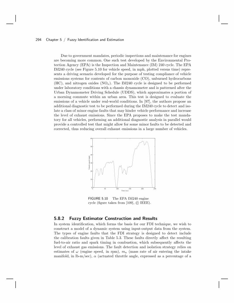
294 Chapter 5 / Fuzzy Identification and Estimation
Due to government mandates, periodic inspections and maintenance for enginesare becoming more common. One such test developed by the Environmental Pro-tection Agency (EPA) is the Inspection and Maintenance (IM) 240 cycle. The EPAIM240 cycle (see Figure 5.10 for vehicle speed, in mph, plotted versus time) repre-sents a driving scenario developed for the purpose of testing compliance of vehicleemissions systems for contents of carbon monoxide (CO), unburned hydrocarbons(HC), and nitrogen oxides (NOx). The IM240 cycle is designed to be performedunder laboratory conditions with a chassis dynamometer and is patterned after theUrban Dynamometer Driving Schedule (UDDS), which approximates a portion ofa morning commute within an urban area. This test is designed to evaluate theemissions of a vehicle under real-world conditions. In [97], the authors propose anadditional diagnostic test to be performed during the IM240 cycle to detect and iso-late a class of minor engine faults that may hinder vehicle performance and increasethe level of exhaust emissions. Since the EPA proposes to make the test manda-tory for all vehicles, performing an additional diagnostic analysis in parallel wouldprovide a controlled test that might allow for some minor faults to be detected andcorrected, thus reducing overall exhaust emissions in a large number of vehicles.
0 50 100 150 200 2500
10
20
30
40
50
60
Time (sec)
Veh
icle
spe
ed (
mph
)
FIGURE 5.10 The EPA IM240 enginecycle (figure taken from [109], c© IEEE).
5.8.2 Fuzzy Estimator Construction and ResultsIn system identification, which forms the basis for our FDI technique, we wish toconstruct a model of a dynamic system using input-output data from the system.The types of engine faults that the FDI strategy is designed to detect includethe calibration faults given in Table 5.3. These faults directly affect the resultingfuel-to-air ratio and spark timing in combustion, which subsequently affects thelevel of exhaust gas emissions. The fault detection and isolation strategy relies onestimates of ω (engine speed, in rpm), ma (mass rate of air entering the intakemanifold, in lb-m/sec), α (actuated throttle angle, expressed as a percentage of a

5.8 Case Study: FDI for an Engine 295
TABLE 5.3 Types of Faults Detectable with FDI Strategy
Fault Type Description
ma sensor calibration Measures amount of air intake for combustion
ω sensor calibration Measures engine speed
α actuator calibration Actuates throttle angle
mf actuator calibration Actuates amount of fuel for combustion
full-scale opening), mf (mass of fuel entering the combustion chamber, in lb-m),and TL (the load torque on the engine, in ft-lb) (which we denote by ω, ma, α, mf ,and TL, respectively) that are provided by identifying models fω, fma , fα, fmf ,and fTL of how the engine operates. In particular, we have
ω = fω(xω) (5.58)ma = fma (xma ) (5.59)
α = fα(xα) (5.60)mf = fmf (xmf ) (5.61)
TL = fTL(xTL). (5.62)
where the inputs are given in Equations (5.63)–(5.67) (k is a discrete time in thecrankshaft domain where physical quantities are sampled every turn of the enginecrankshaft)
xω = [ω(k − 1), ω(k − 2), ω(k − 3), α(k − 1), α(k − 2),α(k − 3), mf(k − 1), mf (k − 2), mf (k − 3), TL(k − 2)] (5.63)
xma = [ma(k − 1), ma(k − 2), ma(k − 3), α(k − 1), α(k − 2),mf (k − 1), mf (k − 2), mf (k − 3), TL(k − 1), TL(k − 3)] (5.64)
xα = [α(k − 1), α(k − 2), α(k − 3), ma(k − 1),ma(k − 2), ma(k − 3), ωdy(k − 1), ωdy(k − 2)] (5.65)
xmf = [mf(k − 1), mf(k − 2), mf(k − 3), ma(k − 1),
ma(k − 2), ma(k − 3), ω(k − 1), ω(k − 2), ω(k − 3)] (5.66)xTL = [TL(k − 1), TL(k − 2), TL(k − 3), α(k − 1), α(k − 2),
mf (k − 1), ma(k − 1), ma(k − 3), ωdy(k − 1), ωdy(k − 3)] (5.67)
where ωdy is an output of the dynamometer. These regression vectors were chosenusing simulation and experimental studies to determine which variables are usefulin estimating others and how many delayed values must be used to get accurateestimation.
One approach to nonlinear system identification that has been found to be par-ticularly useful for this application [119, 120] and that we will employ in the currentstudy in addition to the fuzzy estimation approach is the NARMAX (nonlinearARMAX) method, which is an extension of the linear ARMAX system identifica-tion technique. The general model structure for NARMAX uses scaled polynomial

296 Chapter 5 / Fuzzy Identification and Estimation
combinations of the arguments contained in the regression vector; here we use theNARMAX model structure given by
y(k) =n∑
i=1
βixi +n∑
i=1
n∑j=1
βijxixj (5.68)
where βi, βij are parameters to be adjusted so that y(k) is as close as possible toy(k) for all x ∈ n (i.e., we use only one second-order polynomial term in ourmodel structure). As is usual, in this case study we will use the standard batchleast squares approach to adjust the βi, βij since they enter linearly.
For training purposes, data were collected to calculate the necessary models fω ,fma , fα, fmf , and fTL . Due to mechanical constraints on the electric dynamometer,we reduced the IM240 cycle to only 7000 engine revolutions for the tests that weran. In addition, a uniformly distributed random signal was added to the throttleand torque inputs in order to excite the system. The data generated were utilizedto construct five multi-input single-output fuzzy systems, one for each of the Equa-tions (5.58)–(5.62). In fuzzy clustering we choose 10 clusters (R = 10), a fuzzinessfactor m = 2, and tolerance εc = 0.01 for each of the constructed fuzzy systems.These were derived via experimentation until desired accuracy was achieved (e.g.,increasing R to more than 10 did not provide improved estimation accuracy). Forcomparison purposes, we also calculated models utilizing the nonlinear ARMAXtechnique based on the same experimental data. Then the experimental test cellwas run, and the models derived through fuzzy clustering and the nonlinear AR-MAX technique were validated by collecting data for similar tests run on differentdays.
The results in identification with the validation data (not the training data)for both techniques are given in Figures 5.11, 5.12, 5.13, 5.14, and 5.15 (plots in(a) show the results for the fuzzy identification approach and in (b) for the NAR-MAX approach). We measure approximation error by evaluating the squared errorbetween the real and estimated value (which we denote by
∑k e2 where k ranges
over the entire simulation time). As the results show, both techniques approximatethe real system fairly well; however, for the mass air and engine speed estimates,the NARMAX technique performed slightly better than the clustering technique.For the throttle, load torque, and the mass fuel estimates, the clustering techniqueestimated slightly better than the NARMAX technique.
Overall, we see that there is no clear overall advantage to using NARMAX orthe fuzzy estimator even though the fuzzy estimator performs better for estimatingseveral variables. We would comment, however, that it took a significant amountof experimental work to determine where to truncate the polynomial expansion inEquation (5.68) for the NARMAX model structure. The parameters R, m, and εc
for the fuzzy estimator construction were, however, quite easy to select. Moreover,the fuzzy estimation approach provides the additional useful piece of informationthat the underlying system seems to be adequately represented by interpolatingbetween 10 linear systems each of which is represented by the output of the ten
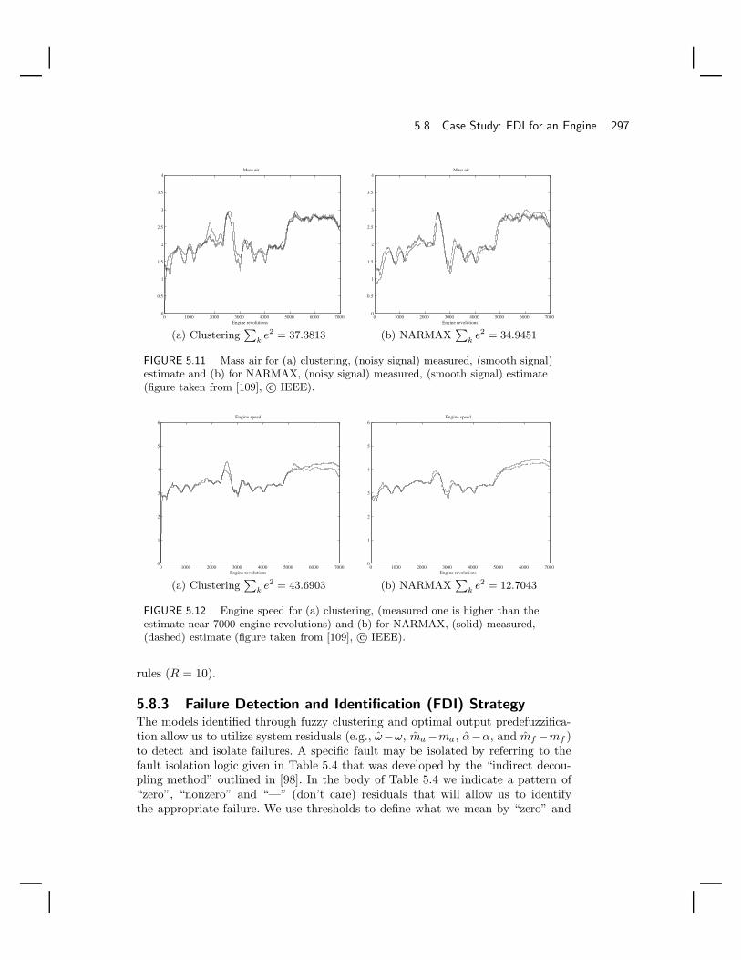
5.8 Case Study: FDI for an Engine 297
0 1000 2000 3000 4000 5000 6000 70000
0.5
1
1.5
2
2.5
3
3.5
4
Engine revolutions
Mass air
0 1000 2000 3000 4000 5000 6000 70000
0.5
1
1.5
2
2.5
3
3.5
4
Engine revolutions
Mass air
(a) Clustering∑
ke2 = 37.3813 (b) NARMAX
∑k
e2 = 34.9451
FIGURE 5.11 Mass air for (a) clustering, (noisy signal) measured, (smooth signal)estimate and (b) for NARMAX, (noisy signal) measured, (smooth signal) estimate(figure taken from [109], c© IEEE).
0 1000 2000 3000 4000 5000 6000 70000
1
2
3
4
5
6
Engine revolutions
Engine speed
0 1000 2000 3000 4000 5000 6000 70000
1
2
3
4
5
6
Engine revolutions
Engine speed
(a) Clustering∑
ke2 = 43.6903 (b) NARMAX
∑k
e2 = 12.7043
FIGURE 5.12 Engine speed for (a) clustering, (measured one is higher than theestimate near 7000 engine revolutions) and (b) for NARMAX, (solid) measured,(dashed) estimate (figure taken from [109], c© IEEE).
rules (R = 10).
5.8.3 Failure Detection and Identification (FDI) StrategyThe models identified through fuzzy clustering and optimal output predefuzzifica-tion allow us to utilize system residuals (e.g., ω−ω, ma −ma, α−α, and mf −mf )to detect and isolate failures. A specific fault may be isolated by referring to thefault isolation logic given in Table 5.4 that was developed by the “indirect decou-pling method” outlined in [98]. In the body of Table 5.4 we indicate a pattern of“zero”, “nonzero” and “—” (don’t care) residuals that will allow us to identifythe appropriate failure. We use thresholds to define what we mean by “zero” and
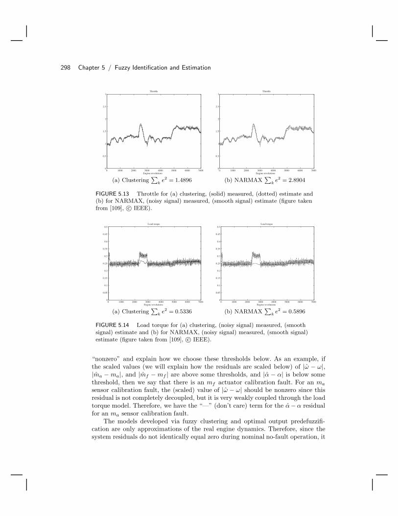
298 Chapter 5 / Fuzzy Identification and Estimation
0 1000 2000 3000 4000 5000 6000 70000
0.5
1
1.5
2
2.5
3
Engine revolutions
Throttle
0 1000 2000 3000 4000 5000 6000 70000
0.5
1
1.5
2
2.5
3
Engine revolutions
Throttle
(a) Clustering∑
ke2 = 1.4896 (b) NARMAX
∑k
e2 = 2.8904
FIGURE 5.13 Throttle for (a) clustering, (solid) measured, (dotted) estimate and(b) for NARMAX, (noisy signal) measured, (smooth signal) estimate (figure takenfrom [109], c© IEEE).
0 1000 2000 3000 4000 5000 6000 70000
0.05
0.1
0.15
0.2
0.25
0.3
0.35
0.4
0.45
0.5
Engine revolutions
Load torque
0 1000 2000 3000 4000 5000 6000 70000
0.05
0.1
0.15
0.2
0.25
0.3
0.35
0.4
0.45
0.5
Engine revolutions
Load torque
(a) Clustering∑
ke2 = 0.5336 (b) NARMAX
∑k
e2 = 0.5896
FIGURE 5.14 Load torque for (a) clustering, (noisy signal) measured, (smoothsignal) estimate and (b) for NARMAX, (noisy signal) measured, (smooth signal)estimate (figure taken from [109], c© IEEE).
“nonzero” and explain how we choose these thresholds below. As an example, ifthe scaled values (we will explain how the residuals are scaled below) of |ω − ω|,|ma − ma|, and |mf − mf | are above some thresholds, and |α − α| is below somethreshold, then we say that there is an mf actuator calibration fault. For an ma
sensor calibration fault, the (scaled) value of |ω − ω| should be nonzero since thisresidual is not completely decoupled, but it is very weakly coupled through the loadtorque model. Therefore, we have the “—” (don’t care) term for the α−α residualfor an ma sensor calibration fault.
The models developed via fuzzy clustering and optimal output predefuzzifi-cation are only approximations of the real engine dynamics. Therefore, since thesystem residuals do not identically equal zero during nominal no-fault operation, it
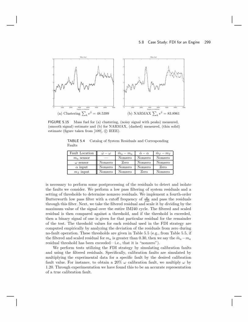
5.8 Case Study: FDI for an Engine 299
0 1000 2000 3000 4000 5000 6000 70000
1
2
3
4
5
6
Engine revolutions
Mass fuel
0 1000 2000 3000 4000 5000 6000 70000
1
2
3
4
5
6
Engine revolutions
Mass fuel
(a) Clustering∑
ke2 = 48.5399 (b) NARMAX
∑k
e2 = 83.8961
FIGURE 5.15 Mass fuel for (a) clustering, (noisy signal with peaks) measured,(smooth signal) estimate and (b) for NARMAX, (dashed) measured, (thin solid)estimate (figure taken from [109], c© IEEE).
TABLE 5.4 Catalog of System Residuals and CorrespondingFaults
Fault Location ω − ω ma − ma α − α mf − mf
ma sensor — Nonzero Nonzero Nonzero
ω sensor Nonzero Zero Nonzero Nonzero
α input Nonzero Nonzero Nonzero Zero
mf input Nonzero Nonzero Zero Nonzero
is necessary to perform some postprocessing of the residuals to detect and isolatethe faults we consider. We perform a low pass filtering of system residuals and asetting of thresholds to determine nonzero residuals. We implement a fourth-orderButterworth low pass filter with a cutoff frequency of π
100 and pass the residualsthrough this filter. Next, we take the filtered residual and scale it by dividing by themaximum value of the signal over the entire IM240 cycle. The filtered and scaledresidual is then compared against a threshold, and if the threshold is exceeded,then a binary signal of one is given for that particular residual for the remainderof the test. The threshold values for each residual used in the FDI strategy arecomputed empirically by analyzing the deviation of the residuals from zero duringno-fault operation. These thresholds are given in Table 5.5 (e.g., from Table 5.5, ifthe filtered and scaled residual for ma is greater than 0.30, then we say the ma−ma
residual threshold has been exceeded—i.e., that it is “nonzero”).We perform tests utilizing the FDI strategy by simulating calibration faults
and using the filtered residuals. Specifically, calibration faults are simulated bymultiplying the experimental data for a specific fault by the desired calibrationfault value. For instance, to obtain a 20% ω calibration fault, we multiply ω by1.20. Through experimentation we have found this to be an accurate representationof a true calibration fault.
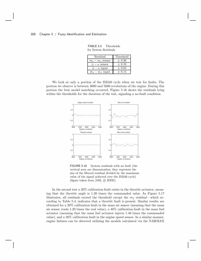
300 Chapter 5 / Fuzzy Identification and Estimation
TABLE 5.5 Thresholdsfor System Residuals
Residual Threshold
ma − ma sensor ± 0.30
ω − ω sensor ± 0.10
α − α input ± 0.04
mf − mf input ± 0.15
We look at only a portion of the IM240 cycle when we test for faults. Theportion we observe is between 3000 and 5000 revolutions of the engine. During thisportion the best model matching occurred. Figure 5.16 shows the residuals lyingwithin the thresholds for the duration of the test, signaling a no-fault condition.
3000 3500 4000 4500 5000-1
-0.5
0
0.5
1
Engine revolutions
Engine speed residual
3000 3500 4000 4500 5000-1
-0.5
0
0.5
1
Engine revolutions
Mass air residual
3000 3500 4000 4500 5000-1
-0.5
0
0.5
1
Engine revolutions
Throttle residual
3000 3500 4000 4500 5000-1
-0.5
0
0.5
1
Engine revolutions
Mass fuel residual
FIGURE 5.16 System residuals with no fault (thevertical axes are dimensionless; they represent thesize of the filtered residual divided by the maximumvalue of the signal achieved over the IM240 cycle)(figure taken from [109], c© IEEE).
In the second test a 20% calibration fault exists in the throttle actuator, mean-ing that the throttle angle is 1.20 times the commanded value. As Figure 5.17illustrates, all residuals exceed the threshold except the mf residual—which ac-cording to Table 5.4, indicates that a throttle fault is present. Similar results areobtained for a 20% calibration fault in the mass air sensor (meaning that the massair sensor reads 1.20 times the real value), a 40% calibration fault in the mass fuelactuator (meaning that the mass fuel actuator injects 1.40 times the commandedvalue), and a 20% calibration fault in the engine speed sensor. In a similar manner,engine failures can be detected utilizing the models calculated via the NARMAX

5.9 Summary 301
technique; however, the resulting residuals are not shown here as they were verysimilar. Overall, we see that by combining the estimates from the fuzzy estimatorswith the FDI logic, we were able to provide an effective FDI strategy for a class ofminor engine failures.
3000 3500 4000 4500 5000-1
-0.5
0
0.5
1
Engine revolutions
Engine speed residual
3000 3500 4000 4500 5000-1
-0.5
0
0.5
1
Engine revolutions
Mass air residual
3000 3500 4000 4500 5000-1
-0.5
0
0.5
1
Engine revolutions
Throttle residual
3000 3500 4000 4500 5000-1
-0.5
0
0.5
1
Engine revolutions
Mass fuel residual
FIGURE 5.17 System residuals with 20% throttlecalibration fault (the vertical axes are dimensionless;they represent the size of the filtered residual dividedby the maximum value of the signal achieved overthe IM240 cycle) (figure taken from [109], c© IEEE).
5.9 SummaryIn this chapter we have provided an introduction to several techniques on howto construct fuzzy systems using numerical data. We used a simple example toillustrate how several of the methods operate. The least squares method can be usedto train linear systems and should be considered as a conventional alternative to theother methods (since it can sometimes be easier to implement). Gradient methodsare especially useful for training parameters that enter in a nonlinear fashion. Theclustering and optimal output predefuzzification method combined the conventionalleast squares method with the c-means clustering technique that provided for thespecification of the input membership functions and served to interpolate betweenthe linear models that were specified via least squares. Clustering based on nearestneighborhood methods helps to provide insight into fuzzy system construction. TheLFE and MLFE techniques provide unique insights into how to associate rules withdata pairs to train the fuzzy system to map the input-output data. The chapterclosed with a discussion on how to combine the methods of this chapter into hybrid

302 Chapter 5 / Fuzzy Identification and Estimation
training techniques and a design and implementation case study.Upon completing this chapter, you should understand the following:
• The function approximation problem.
• How construction of models, estimators, predictors, and controllers can be viewedas a special case of the function approximation problem.
• The issues involved in choosing a training data set.
• How to incorporate linguistic information into a fuzzy system that you train withdata.
• The batch and recursive least squares methods.
• How to train standard or Takagi-Sugeno fuzzy systems with least squares meth-ods.
• The gradient algorithm method for training a standard or Takagi-Sugeno fuzzysystem.
• The clustering with optimal output predefuzzification method for constructing aTakagi-Sugeno fuzzy system.
• The nearest neighborhood clustering method for training standard fuzzy systems.
• The learning from examples (LFE) method for constructing a fuzzy system.
• The modified learning from examples (MLFE) method for constructing a fuzzysystem.
• How different methods can be combined into hybrid training techniques for fuzzysystems.
• How the clustering with optimal output predefuzzification method can be usedfor failure detection and identification in an internal combustion engine.
Essentially, this is a checklist of the major topics of this chapter. The gradient orrecursive least squares methods are essential for understanding the indirect adaptivefuzzy control method treated in Chapter 6, and some of the supervisory controlideas in Chapter 7 rely on the reader’s knowledge of at least one method from thischapter.
5.10 For Further StudyAn earlier version of the problem formulation for the function approximation prob-lem appeared in [108]. The idea of combining linguistic information with the fuzzysystem constructed from numerical training data has been used by several re-searchers and is exploited in a particularly coherent way in [229].

5.11 Exercises 303
The idea of using least squares to train fuzzy systems was first introducedin [207] and was later studied in [232] and other places. For more details on leastsquares methods, see [127]. The gradient method for training fuzzy systems wasoriginally developed as the “back-propagation” approach for training neural net-works, and many people recognized that such gradient methods could also be usedfor training fuzzy systems (e.g., see [231] for a treatment of the steepest descentapproach). For more details on gradient methods, see [128, 22]. The clustering withoptimal output predefuzzification approach was introduced in [187] but is mod-ified somewhat from its original form in our presentation. The nearest neighborclustering approach was introduced in [228]. For more details on fuzzy clustering,see [24, 23, 89, 187, 236, 177]. The learning from examples technique was first in-troduced in [233], and the modified learning from examples approach [108] wasdeveloped using ideas from the approaches in [133, 233]. A slightly different ap-proach to the computation in Equation (5.56) on page 287 is taken in [108], wherethe MLFE was first introduced. The hybrid methods have been used by a varietyof researchers; a particularly nice set of applications were studied in [81, 82].
The case study in implementation of the fuzzy estimators for an internal com-bustion engine was taken from [109]. All investigations in this case study wereperformed using the experimental engine test cell in [129, 130]. We take the samebasic approach to FDI for minor engine faults as in [97] except that we utilize afuzzy estimation approach rather than the nonlinear ARMAX approach used in [97].Related work on the use of nonlinear ARMAX is given in [130].
The case study in engine failure estimation used in the chapter and in theproblems at the end of the chapter, and the cargo ship failure estimation problemused in the problems at the end of the chapter were developed in [143]. For a generaloverview of the field of FDI, see [166].
Some other methods related to the topics in this chapter are given in [73, 18,237, 117, 1, 76]. There is related work in the area of neural networks also. See,for example, [150, 26]. A good introduction to the topical area of this chapter isgiven in [188, 86], where the authors also cover wavelets, neural networks, and otherapproximators and properties in some detail.
5.11 ExercisesExercise 5.1 (Training Fuzzy Systems to Approximate a Simple DataSet): In this problem you will study the training of standard and Takagi-Sugenofuzzy systems to represent the data in G in Equation (5.3) on page 236. Thisis the data set that was used as an example throughout the chapter. You canprogram the methods on the computer yourself or use the Matlab code providedat the web and ftp sites listed in the Preface.
(a) Batch least squares: For the example in Section 5.3.3 on page 255, find thevalue of θ and compare it with the value found there. Also, test the fuzzysystem with the same six test inputs and verify that the outputs are as givenin Section 5.3.3. Next, let c1
1 = 0, c12 = 2, c2
1 = 2, and c22 = 4; find θ; and

304 Chapter 5 / Fuzzy Identification and Estimation
repeat the testing process for the six test inputs. Does the fuzzy system seemto interpolate well?
(b) Weighted batch least squares: Choose W = diag([10, 1, 1]) so that we weightthe first data pair in G (i.e., ([0, 2], 1)) as being the most important one.Does this make f([0, 2]|θ) closer to one (y1) than for the fuzzy systemtrained in (a)?
(c) Recursive least squares: Repeat (a) but use RLS with λ = 1.(d) Weighted recursive least squares: Repeat (a) but use weighted RLS with
λ = 0.9.(e) Gradient method: Verify all computed values for the gradient training of
the Takagi-Sugeno fuzzy system in Section 5.4.3 (this includes finding thefuzzy system parameter values and the fuzzy system outputs for the six testinputs).
(f) Clustering with optimal output predefuzzification: Verify all computed val-ues for all cases in the example of Section 5.5.1. Be sure to include the casewhere we use one more training data pair (i.e., when M = 4).
Exercise 5.2 (Training a Fuzzy System to Approximate a Simple Func-tion): In this problem you will study methods for constructing fuzzy systems toapproximate the mapping defined by a quadratic function
y = 2x21 + x2
2 (5.69)
over the range x1 ∈ [−12, 12], x2 ∈ [−12, 12] (note that here x21 is x1 squared).
To train and test the fuzzy system, use the training data set G and the testdata set Γ, defined as
G = ([x1, x2], y) | x1, x2 ∈ −12,−10.5,−9, . . . , 9, 10.5, 12, y = 2x21 + x2
2(5.70)
Γ = ([x1, x2], y) | x1, x2 ∈ −12,−11,−10, . . . , 10, 11, 12, y = 2x21 + x2
2(5.71)
The training data set G and the test data set Γ are used for each technique inthis problem. Plot the function over the range of values provided in the inputportions of the data in Γ.
For each constructed fuzzy system for each part below, calculate the maximumerror, emax, defined as
emax = max|f(x) − y| : (x, y) ∈ Γ
where f is the fuzzy system output and y is the output of the quadratic functionand the “percentage maximum error,” which is defined as
epmax = 100emax
y∗

5.11 Exercises 305
where y∗ is the y value of the quadratic function that makes the error maximum—that is,
y∗ ∈ y′ : (x′, y′) ∈ Γ and |f(x′) − y′| ≥ |f(x) − y| for all (x, y) ∈ Γ
Clearly, we would like to construct the fuzzy system so that emax and epmax areminimized.
(a) Batch least squares: Consider the fuzzy system
y = f(x|θ) =∑R
i=1 biµi(x)∑Ri=1 µi(x)
(5.72)
where x = [x1, x2] and µi(x) is the certainty of the premise of the ith
rule that is specified by Gaussian membership functions. We use singletonfuzzification and product for premise and implication, and bi is the center ofthe output membership function for the ith rule. The Gaussian membershipfunctions have the form
µ(x) = exp
(−1
2
(x − c
σ
)2)
so that
µi(x) =2∏
j=1
exp
−1
2
(xj − ci
j
σij
)2
is defined where cij is the center of the membership function of the ith rule for
the jth universe of discourse and σij is the relative width of the membership
function of the ith rule of the jth universe of discourse.We use nine membership functions for each input universe of discourse
with centers given by the elements of the set
−12,−9,−6,−3, 0, 3, 6, 9, 12
from which we can see that the membership functions are distributed uni-formly. From these centers we will form R = 9 × 9 = 81 rules—that is, arule for every possible combination. We must specify the input membershipfunction centers ci
j. Let the columns of the matrix
[−12 −12 · · · −12 −9 −9 · · · −9 · · · 12−12 −9 · · · 12 −12 −9 · · · 12 · · · 12
]
be denoted by ci, and let ci = [ci1, c
i2], i = 1, 2, . . . , 81. The relative widths
of the membership functions, σij for all j = 1, 2 and i = 1, 2, . . . , R, are

306 Chapter 5 / Fuzzy Identification and Estimation
chosen as 4 to get a reasonable coverage of each universe of discourse.Write a computer program to implement batch least squares to find the
output centers. Compute epmax, plot the input-output map of the resultingfuzzy system, and compare it to the plot of the quadratic function.
(b) Gradient method: Use the “standard” fuzzy system defined in Section 5.4 forwhich the update formulas are already derived in Equations (5.35), (5.36),and (5.37). You have n = 2. The centers of the membership functions shouldbe initialized to the values that we used in part (a), and their relative widthsshould be initialized as σi
j = 1. Also, let
bi = 2(ci1)
2 + (ci2)
2
for all i = 1, 2, . . . , 81 and j = 1, 2. Why is this a reasonable choice for theinitial values? As can be seen from the definition above, you use 9 mem-bership functions for each input universe of discourse, which means 81 rules(i.e., R = 81). Choose λ1, λ2, and λ3 as 0.0001. In your algorithm, cyclethrough the entire training data set G many times, processing one data pairin every step of the the gradient algorithm, until the error em is less than orequal to 1.6.
Write a computer program to implement the gradient method to train thefuzzy system. Compute epmax, plot the input-output map of the resultingfuzzy system, and compare it to the plot of the quadratic function.
(c) Clustering with optimal output predefuzzification: Here, you train the fuzzysystem defined in the chapter. Choose R = 49, m = 2, and εc = 0.0001. Inthis problem, two definitions of gj are used. The first one is given by
gj = aj,0 + aj,1x1 + aj,2x2
and the second one is defined as
gj = aj,0 + aj,1(x1)2 + aj,2(x2)2
where xi is the ith input value, j = 1, 2, . . . , R, and the (xi)2 terms repre-sent that we assume in this case that we have special knowledge about thefunction we want to approximate (i.e., in this case we assume that we knowit is a quadratic function). Initialize the cluster centers as
vji = (vj
i )′ + εp(r − 0.5)
where (vji )
′ ∈ −12,−8, . . . , 8, 12, j = 1, 2, . . . , R, i = 1, 2, εp = 0.001, and“r” is a random number between 0 and 1.
Write a computer program to implement the clustering with optimaloutput predefuzzification method to train the fuzzy system. Compute epmax,plot the input-output map of the resulting fuzzy system, and compare it tothe plot of the quadratic function.

5.11 Exercises 307
(d) Nearest neighborhood clustering: The fuzzy system used in this part is theone that the nearest neighborhood clustering method was developed for inthe chapter. Initialize the parameters A1 = y1 = 432, B1 = 1, and v1
j = x1j
for j = 1, 2 (i.e., v11 = −12 and v1
2 = −12). Let εf = 0.5 and the relativewidth of the membership functions σ = 5, which affects the accuracy of theapproximation.
Write a computer program to implement the nearest neighborhood clus-tering method to train the fuzzy system. What is the number of clusters thatare produced? Compute epmax, plot the input-output map of the resultingfuzzy system, and compare it to the plot of the quadratic function.
(e) Learning from examples: For our fuzzy system we use singleton fuzzification,minimum to represent the premise and implication, and “center of gravity”(COG) defuzzification. Choose the effective universes of discourse for thetwo inputs and the output as
X1 = [x−1 , x+
1 ] = [−12, 12]
X2 = [x−2 , x+
2 ] = [−12, 12]
Y = [y−, y+] = [0, 432]
This choice is made since we seek to approximate our unknown functionover x1 ∈ [−12, 12], x2 ∈ [−12, 12] and we know that for these valuesy ∈ [0, 432]. You should use triangular-shaped membership functions forµXj
1(x1), µXj
2(x2), µY j (y), associated with the fuzzy sets Xj
1 , Xj2 , and Y j ,
respectively. In particular, use 9 membership functions for inputs x1 and x2
and 45 membership functions for the output y; these membership functionsare shown in Figures 5.18, 5.19, and 5.20.
0
1(µ x )
-3-6 3 6-9-12 9 12
X 1
1
XX X X1 1 X 1X3
1X2
1X1
1 1 1
4 5 6 7 8 9
x
FIGURE 5.18 Membership functions for the x1 universe of discourse(figure created by Mustafa K. Guven).
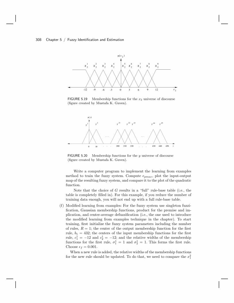
308 Chapter 5 / Fuzzy Identification and Estimation
0
µ(x 2 )
-6 -3 3 6
2 X 2 X 2 X 2
-9
X 2X 2XX 22
32X
1
2
4X
5 6 7 8 9
9 12 x 2-12
FIGURE 5.19 Membership functions for the x2 universe of discourse(figure created by Mustafa K. Guven).
0 1
µ(
y0
YYYYYYY21
.. . .. .
. . ... .
4544232221
y)
200 210 220 430 440 450
FIGURE 5.20 Membership functions for the y universe of discourse(figure created by Mustafa K. Guven).
Write a computer program to implement the learning from examplesmethod to train the fuzzy system. Compute epmax, plot the input-outputmap of the resulting fuzzy system, and compare it to the plot of the quadraticfunction.
Note that the choice of G results in a “full” rule-base table (i.e., thetable is completely filled in). For this example, if you reduce the number oftraining data enough, you will not end up with a full rule-base table.
(f) Modified learning from examples: For the fuzzy system use singleton fuzzi-fication, Gaussian membership functions, product for the premise and im-plication, and center-average defuzzification (i.e., the one used to introducethe modified learning from examples technique in the chapter). To starttraining, first initialize the fuzzy system parameters including the numberof rules, R = 1; the center of the output membership function for the firstrule, b1 = 432; the centers of the input membership functions for the firstrule, c1
1 = −12 and c12 = −12; and the relative widths of the membership
functions for the first rule, σ11 = 1 and σ1
2 = 1. This forms the first rule.Choose εf = 0.001.
When a new rule is added, the relative widths of the membership functionsfor the new rule should be updated. To do that, we need to compare the x2
1

5.11 Exercises 309
with the centers of the membership functions that are in the first universeof discourse, ci
1 for all i = 1, 2, . . . , R and x22 with ci
2 for all i = 1, 2, . . . , R, tofind the nearest membership functions for each universe of discourse. Usingthe distance between the input portion of the training data and the nearestmembership function, we determine the σi
j for all i = 1, 2, . . . , R and j = 1, 2.Specifically, let
σij =
|cij − c
n∗j
j |W
for all i = 1, 2, . . . , R and j = 1, 2 and where W is the weighting factor,which we choose as 2.
Since we have repeated numbers in our data set (i.e., there exist i′ andj′ such that xi
j = xi′j′ , for i = i′, j = j′), we will have a problem for some
σij for i = 1, 2, . . . , R and j = 1, 2. For instance, assume that we have R = 1
(i.e., we have one rule in our rule-base) and let
[c11, c
12]
= [−12,−12]
and the next training data is
([x1, x2], y) = ([−12,−10.5], 398.25)
For the x1 universe of discourse, the nearest membership function is the onethat has −12 as its center. Therefore, the distance and the σ2
1 will be zero.Because of this, during testing of the fuzzy system, we will have
x1 − c21
σ21
=x1 − c2
1
0
which is not well-defined.To avoid this situation, the following procedure can be used. If for
[x1, x2], cij = xj, then let
σR+1j = σR
j
for j = 1, 2. For our example,
σ21 = σ1
1
With this procedure, instead of updating the relative width of the new rule,we will keep one of the old relative widths for the new rule. Other ways tosolve the problem of updating the relative widths are given in the chapter.
Write a computer program to implement the modified learning fromexamples method to train the fuzzy system. Compute epmax, plot the input-

310 Chapter 5 / Fuzzy Identification and Estimation
output map of the resulting fuzzy system, and compare it to the plot of thequadratic function.
Exercise 5.3 (Estimation of ζ for a Second-Order System): In this problemsuppose that you are given a plant that is perfectly represented by a second-ordertransfer function
G(s) =ω2
n
s2 + 2ζωns + ω2n
Suppose that ωn = 1 and that you know 0.1 ≤ ζ ≤ 1, but that you do not knowits value and you would like to estimate it using input-output data from the plant.Assume that you know that the input to G(s) and in each case below choose theinput trajectory and provide a rationale for your choice. Assume that you do notknow that the system is perfectly linear and second order (so that you cannotsimply use, e.g., standard least squares for estimating ζ).
(a) Generate the set G of training data. Provide a rationale for your choice.(b) Use the batch least squares method to construct a fuzzy estimator for ζ.
Provide all the details on how you construct your estimator (including alldesign parameters).
(c) Use the gradient method to construct a fuzzy estimator for ζ. Provide allthe details on how you construct your estimator (including all design pa-rameters).
(d) Use the clustering with optimal output predefuzzification method to con-struct a fuzzy estimator for ζ. Provide all the details on how you constructyour estimator (including all design parameters).
(e) Use the LFE method to construct a fuzzy estimator for ζ. Provide all thedetails on how you construct your estimator (including all design parame-ters).
(f) Use the MLFE method to construct a fuzzy estimator for ζ. Provide all thedetails on how you construct your estimator (including all design parame-ters).
(g) Test the ζ estimators that you constructed in (b)–(f). Be sure to test themfor data that you trained them with, and with data that you did not use intraining. Provide plots that show both the estimated and actual values of ζon the same plot.
Exercise 5.4 (Least Squares Derivation): Recall that for batch least squareswe had
V (θ, M) =12EE
as a measure of the approximation error. In this problem you will derive severalof the least squares methods that were developed in this chapter.

5.12 Design Problems 311
(a) Using basic ideas from calculus, take the partial of V with respect to θ andset it equal to zero. From this derive an equation for how to pick θ. Compareit to Equation (5.15). Hint: If m and b are two n × 1 vectors and A is ann × n symmetric matrix (i.e., A = A), then d
dm bm = b, ddmmb = b, and
ddmmAm = 2Am.
(b) Repeat (a) for the weighted batch least squares approach, where V is chosenas in Equation (5.16), and compare it to Equation (5.17).
(c) Derive the update Equations (5.26) for the weighted recursive least squaresapproach.
Exercise 5.5 (Gradient Training of Fuzzy Systems): In this problem youwill derive gradient update formulas for fuzzy systems by directly building on thediscussion in the chapter.
(a) Derive the update equations for bi(k), cij(k), and σi
j(k) for the gradienttraining method described in Section 5.4 on page 260. Show the full detailsof the derivations for all three cases.
(b) Repeat (a) but for the Takagi-Sugeno fuzzy system so that you will find theupdate formula for ai,j(k) rather than for bi(k).
(c) Repeat (a) but for a generalization of the Takagi-Sugeno fuzzy system (i.e., afunctional fuzzy system) with the same parameters as in the chapter except
gi(x) = ai,0 + ai,1(x1)2 + · · ·+ ai,n(xn)2
i = 1, 2, . . . , R. In this case our gradient method will try to train the ai,j, cij ,
and σij to find a fuzzy system that provides nonlinear interpolation between
R quadratic functions.
(d) Repeat (c) but for
gi(x) = ai,0 + exp[ai,1(x1)2
]+ · · ·+ exp
[ai,n(xn)2
]
5.12 Design ProblemsDesign Problem 5.1 (Identification of a Fuzzy System Model of a Tank):
Suppose that you are given the “surge tank” system that is shown in Figure 6.44on page 399. Suppose that the differential equation representing this system is
dh(t)dt
=−c
√2gh(t)
A(h(t))+
1A(h(t))
u(t)
where u(t) is the input flow (control input) that can be positive or negative (itcan pull liquid out of the tank), h(t) is the liquid level (the output y(t) = h(t)),A(h(t)) is the cross-sectional area of the tank, g = 9.8 m/sec2 is acceleration dueto gravity, and c = 1 is the known cross-sectional area of the output pipe. Assume

312 Chapter 5 / Fuzzy Identification and Estimation
that a = 1 and that A(h) = ah2 + b where a = 1 and b = 2 (i.e., that we knowthe tank characteristics exactly). Assume, however, that you have only an ideaabout what the order of the system is. That is, assume that you do not know thatthe system is governed exactly by the above differential equation. Hence, you willtreat this system as your physical system (“truth model”) when you gather datato perform identification of the model. When you then want to test the validityof the model that you construct with your identification approaches, you test itagainst the truth model.
(a) Use the fuzzy clustering with optimal output predefuzzification approach toconstruct a fuzzy system whose input-output behavior is similar to that ofthe surge tank. Clearly explain your approach, any assumptions that youmake, and the design parameters you choose. Also, be careful in your choiceof the training data set. Make sure that the input u(t) properly excites thesystem dynamics.
(b) Develop a second identification approach to producing a fuzzy system model,different from the one in (a).
(c) Perform a comparative analysis between the approaches in (a) and (b) focus-ing on how well the fuzzy system models you produced via the identificationapproaches model the physical system represented by the truth model. Todo this, be sure to test the system with inputs different from those you usedto train the models.
Design Problem 5.2 (Gasket Leak Estimation for an Engine): Govern-ment regulations that attempt to minimize environmental impact and safety haz-ards for automobiles have motivated the need for estimation of engine parametersthat will allow us to determine if an engine has failed. In this problem you will de-velop a fuzzy estimator for estimating the parameter k2 for the engine describedin Section 5.2.5 on page 243 (i.e., use the data in Gk2).
(a) Establish an engine failure simulator as it is described in Section 5.2.5 onpage 243. Demonstrate that your engine failure simulator produces the sameresults as in Section 5.2.5. Develop the training data set Gk2 for the engineas it is described in Section 5.2.5.
(b) Choose a method from the chapter and develop a fuzzy estimator for k2.You can either use the data Gk2 or compute your own training data set.
(c) Next, test the failure estimator using the engine simulator for the failurescenario for k2 in Table 5.2. The testing process is implemented using theengine failure simulator and a constant step of Θ = 0.1 for both an idealno-disturbance condition and a disturbance input TL of the form shown inFigure 5.4 on page 245. Plot the estimates and actual values on the samegraph, and evaluate the accuracy of the estimator.

5.12 Design Problems 313
Design Problem 5.3 (Engine Friction Estimation): In this problem youwill use the data set Gk5 in Section 5.2.5 on page 243 to design parameter estima-tors for the parameter k5, which can indicate whether there is excessive frictionin the engine.
(a) Establish an engine failure simulator as it is described in Section 5.2.5 onpage 243. Demonstrate that your engine failure simulator produces the sameresults as in Section 5.2.5. Develop the training data set Gk5 for the engineas it is described in Section 5.2.5.
(b) Choose a method from the chapter and develop a fuzzy estimator for k5.You can either use the data Gk5 or compute your own training data set.
(c) Test the quality of the estimators that you developed in (b). The testingprocess should be implemented using the engine failure simulator from (a)and a constant step of Θ = 0.1 for both an ideal no-disturbance conditionand a disturbance input TL of the form shown in Figure 5.4 on page 245.Plot the estimates and actual values on the same graph, and evaluate theaccuracy of the estimator.
Design Problem 5.4 (Cargo Ship Failure Estimator): In this problem weintroduce the cargo ship models and the failure modes to be considered, and youwill first develop a failure simulator test bed for the cargo ship. We use the cargoship model given in Chapter 6, Section 6.3.1 on page 333, where the rudder angleδ is used to steer the ship along a heading ψ (see Figure 6.5). The referenceinput is ψd and e = ψd − ψ. A simple control law, such as proportional-integral-derivative (PID) control, is typically used in autopilot regulation of the ship. Inthis problem we will use a proportional derivative (PD) controller of the form
δ = kpe + kde (5.73)
where we choose kp = −3.1 and kd = 105. Closed-loop control of this form willbe used in both training and testing of failure estimators for the ship.
The inputs to the failure simulator should be the desired ship heading ψd andthe possible parameter changes representing failures. Again, there are trainingand testing inputs; these are shown in Figure 5.21. Unlike the engine failuresimulator developed in Section 5.2.5, there exist two cargo ship models where themodel to be used depends whether we are constructing the failure identifier ortesting it. If the simulator is being used to train the fuzzy failure estimator, thenwe select the training input and use the third-order linear model in Equation (6.6)on page 334. We use the nonlinear model, in Equation (6.7) on page 335, whentesting the failure estimator methods.
There are two parameters that are varied to represent failures in the cargo ship.They are the velocity parameter u (which represents an inaccurate speed sensorreading), and a bias in the control variable δ. The value of the failed parameter for

314 Chapter 5 / Fuzzy Identification and Estimation
0 2000 4000 60000
10
20
30
40
50
Time (sec)
Ship
hea
ding
(de
g)
Training input
0 2000 4000 60000
10
20
30
Time (sec)
Ship
hea
ding
(de
g)
Testing input
FIGURE 5.21 Failure simulator inputs (plots created bySashonda Morris).
the velocity u is determined by equations similar to Equations (5.11) and (5.12)that were used for the engine failure simulator. The value of the rudder anglefailure δ(failure) is determined by adding a constant bias, ± δ, to the nominalrudder angle value.
Table 5.6 shows the failure scenarios that we would like to be able to predict(so we would like to estimate u and δ).
TABLE 5.6 Failure Scenarios for CargoShip
Parameter Nominal FailureValue Setting
u 5 m/s −80%
δ δ ∈ [−45, +45] δ = ±5
(a) Do four simulations, all for the “testing” input for the ship when the nonlin-ear ship model is used. The first should show the response of the closed-loopcontrol system for the nominal no-failure case. The second should show howthe closed-loop control system will respond to a speed sensor failure of −80%induced at t = 0. The third (fourth) should show how the closed-loop controlsystem will respond to a rudder angle bias error of +5 degrees (−5 degrees)that is induced at t = 0. Each of the four simulations should be run for 6000seconds. What effect does the speed sensor failure have on rise-time, settlingtime, and overshoot? What effect does the rudder angle bias have on thesteady-state error?
(b) Using the cargo ship failure simulator from (a) with the linear ship model andthe training input ψd shown in Figure 5.21, data sets should be generatedfor training fuzzy estimators. The parameters u and δ should be varied overa specified range of values to account for the possible failure scenarios thecargo ship steering system might encounter. The parameter u should bevaried between 0% and 90% of its nominal value (i.e., ∆u ∈ [0, 0.9]) at 10%

5.12 Design Problems 315
increments yielding Mu = 10 output responses. The constant bias value δshould be varied between ± 10 at an increment of 2, yielding Mδ = 11output responses. Plot the output responses when the parameters u and δare varied in this way.
Explain why a good way to estimate a failure in the velocity parameter u isbased on the rise-time and percent overshoot of the output responses, whilea failure in the control parameter δ is best characterized by the steady-stateerror e = ψd − ψ. The percent overshoot can be best characterized by theerror e = ψd−ψ responses for the given parameter u. Plot the error responsesfor variations in the velocity parameter u and the control parameter δ.
The error responses of the cargo ship when the parameter u is variedshould be used to form the data d(m) for training the estimators for thevelocity parameter. A moving window of length = 200 seconds should beused to sample the response at an interval of T = 50 seconds. Notice thatmost information about a particular failure is contained between 100 and1200 seconds for a step input of ψd = 45, and between 3100 and 4200seconds for a step input of ψd = 0. The error responses should be sampledover these ranges. The full set of cargo ship failure data for the speed sensoris then given by
Gu = ([ej(kT ), ej(kT − T ), ej(kT − 2T ), ej(kT − 3T ),ej(kT − 4T )cej(kT )], uj) :k ∈ 1, 2, . . . , 23, 1 ≤ j ≤ Mu (5.74)
where uj denotes the jth value (1 ≤ j ≤ Mu) of u and ej(kT ), ej(kT −T ), ej(kT − 2T ), ej(kT − 3T ), ej(kT − 4T ), and cej(kT ) represent the cor-responding values of e(kT ), e(kT − T ), e(kT − 2T ), e(kT − 3T ), e(kT − 4T ),and ce(kT ) that were generated using this uj. The value of cej(kT ) is thecurrent change in error given by
cej(kT ) =ej(kt) − ej(kT − T )
T(5.75)
and uj represents the size of the failure and the parameter we want toestimate. Generate the data set Gu.
(c) The failure data sets for the control parameter δ should be formed usingthe error responses generated when the parameter δ was varied. Because theresponses for this parameter settle within 500 seconds, the fuzzy estimatoris trained between 50 and 500 seconds at a sampling period T = 50 seconds.The full set of cargo ship failure data for the control variable δ is given by
Gδ = ([ej(kT ), ej(kT − T ), ej(kT − 2T )], δj) :k ∈ 1, 2, . . . , 8, 1 ≤ j ≤ Mδ (5.76)
where ej(kT ), . . . , ej(kT − 2T ) are the sampled values of the error e = ψd −

316 Chapter 5 / Fuzzy Identification and Estimation
ψ, and δj represents the failure and the parameter we want to estimate.Generate the data set Gδ.
(d) Using a method of your choice, train the estimators for both failures. Testthe quality of the estimators and provide plots of estimated and actual valueson the same graph.

C H A P T E R 6
Adaptive FuzzyControl
They know enough who know how to learn.
–Henry Brooks Adams
6.1 OverviewThe design process for fuzzy controllers that is based on the use of heuristic in-formation from human experts has found success in many industrial applications.Moreover, the approach to constructing fuzzy controllers via numerical input-outputdata, which we described in Chapter 5, is increasingly finding use. Regardless ofwhich approach is used, however, there are certain problems that are encounteredfor practical control problems, including the following: (1) The design of fuzzy con-trollers is performed in an ad hoc manner so it is often difficult to choose at leastsome of the controller parameters. For example, it is sometimes difficult to knowhow to pick the membership functions and rule-base to meet a specific desiredlevel of performance. (2) The fuzzy controller constructed for the nominal plantmay later perform inadequately if significant and unpredictable plant parametervariations occur, or if there is noise or some type of disturbance or some other en-vironmental effect. Hence, it may be difficult to perform the initial synthesis of thefuzzy controller, and if the plant changes while the closed-loop system is operatingwe may not be able to maintain adequate performance levels.
As an example, in Chapter 3 we showed how our heuristic knowledge can beused to design a fuzzy controller for the rotational inverted pendulum. However,we also showed that if a bottle half-filled with water is attached to the endpoint,the performance of the fuzzy controller degraded. While we certainly could havetuned the controller for this new situation, it would not then perform as well with-out a bottle of liquid at the endpoint. It is for this reason that we need a wayto automatically tune the fuzzy controller so that it can adapt to different plant
317
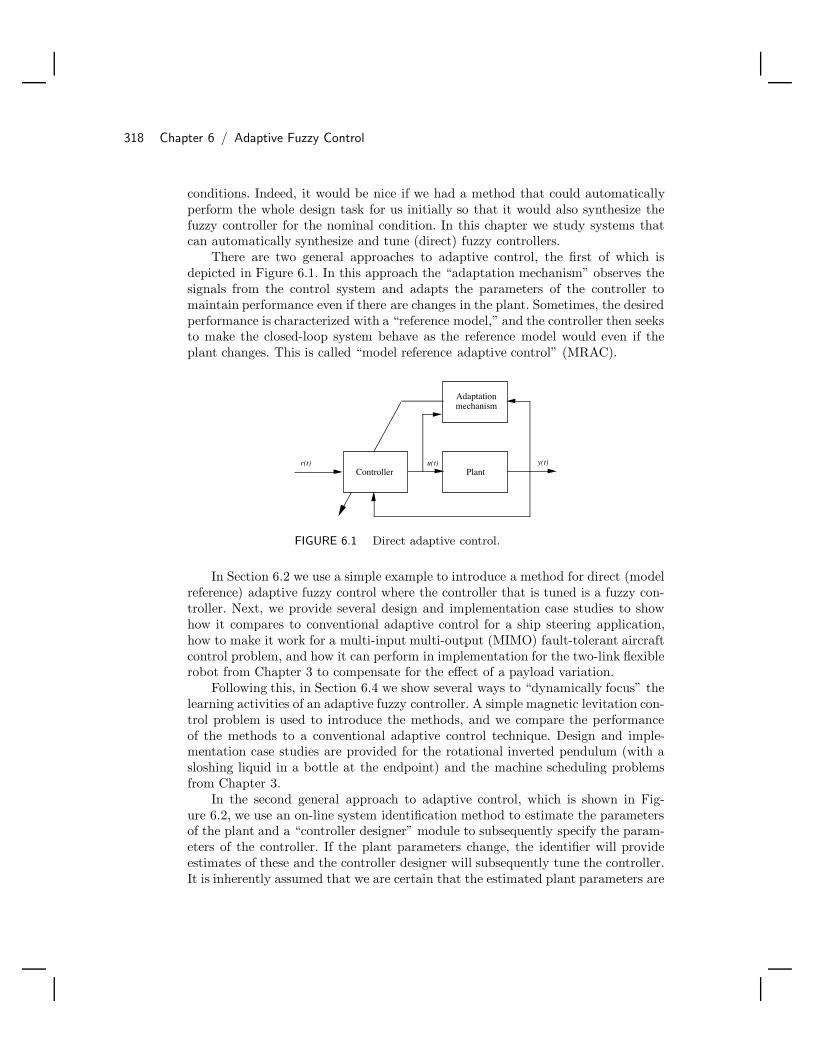
318 Chapter 6 / Adaptive Fuzzy Control
conditions. Indeed, it would be nice if we had a method that could automaticallyperform the whole design task for us initially so that it would also synthesize thefuzzy controller for the nominal condition. In this chapter we study systems thatcan automatically synthesize and tune (direct) fuzzy controllers.
There are two general approaches to adaptive control, the first of which isdepicted in Figure 6.1. In this approach the “adaptation mechanism” observes thesignals from the control system and adapts the parameters of the controller tomaintain performance even if there are changes in the plant. Sometimes, the desiredperformance is characterized with a “reference model,” and the controller then seeksto make the closed-loop system behave as the reference model would even if theplant changes. This is called “model reference adaptive control” (MRAC).
PlantController
Adaptationmechanism
r(t) u(t) y(t)
FIGURE 6.1 Direct adaptive control.
In Section 6.2 we use a simple example to introduce a method for direct (modelreference) adaptive fuzzy control where the controller that is tuned is a fuzzy con-troller. Next, we provide several design and implementation case studies to showhow it compares to conventional adaptive control for a ship steering application,how to make it work for a multi-input multi-output (MIMO) fault-tolerant aircraftcontrol problem, and how it can perform in implementation for the two-link flexiblerobot from Chapter 3 to compensate for the effect of a payload variation.
Following this, in Section 6.4 we show several ways to “dynamically focus” thelearning activities of an adaptive fuzzy controller. A simple magnetic levitation con-trol problem is used to introduce the methods, and we compare the performanceof the methods to a conventional adaptive control technique. Design and imple-mentation case studies are provided for the rotational inverted pendulum (with asloshing liquid in a bottle at the endpoint) and the machine scheduling problemsfrom Chapter 3.
In the second general approach to adaptive control, which is shown in Fig-ure 6.2, we use an on-line system identification method to estimate the parametersof the plant and a “controller designer” module to subsequently specify the param-eters of the controller. If the plant parameters change, the identifier will provideestimates of these and the controller designer will subsequently tune the controller.It is inherently assumed that we are certain that the estimated plant parameters are

6.2 Fuzzy Model Reference Learning Control (FMRLC) 319
equivalent to the actual ones at all times (this is called the “certainty equivalenceprinciple”). Then if the controller designer can specify a controller for each set ofplant parameter estimates, it will succeed in controlling the plant. The overall ap-proach is called “indirect adaptive control” since we tune the controller indirectlyby first estimating the plant parameters (as opposed to direct adaptive control,where the controller parameters are estimated directly without first identifying theplant parameters). In Section 6.6 we explain how to use the on-line estimationtechniques described in Chapter 5 (recursive least squares and gradient methods),coupled with a controller designer, to achieve indirect adaptive fuzzy control fornonlinear systems. We discuss two approaches, one based on feedback linearizationand the other we name “adaptive parallel distributed compensation” since it buildson the parallel distributed compensator discussed in Chapter 4.
PlantController
Systemidentification
Controllerdesigner
r(t) u(t) y(t)
Plantparameters
Controllerparameters
FIGURE 6.2 Indirect adaptive control.
Upon completing this chapter, the reader will be able to design a variety ofadaptive fuzzy controllers for practical applications. The reader should consider thischapter fundamental to the study of fuzzy control systems as adaptation techniquessuch as the ones presented in this chapter have proven to be some of the mosteffective fuzzy control methods. Given a firm understanding of Chapter 2 (andparts of Chapter 3), it is possible to cover the material in this chapter on directadaptive fuzzy control in Sections 6.2–6.5 without having read anything else inthe book. The reader wanting to cover this entire chapter will, however, need afirm understanding of all the previous chapters except Chapter 4. The reader doesnot need to cover this chapter to understand the basic concepts in the next one;however, a deeper understanding of the concepts in this chapter will certainly bebeneficial for the next chapter since fuzzy supervisory control provides yet anotherapproach to adaptive control.
6.2 Fuzzy Model Reference Learning Control(FMRLC)
A “learning system” possesses the capability to improve its performance over timeby interacting with its environment. A learning control system is designed so that

320 Chapter 6 / Adaptive Fuzzy Control
its “learning controller” has the ability to improve the performance of the closed-loop system by generating command inputs to the plant and utilizing feedbackinformation from the plant.
In this section we introduce the “fuzzy model reference learning controller”(FMRLC), which is a (direct) model reference adaptive controller. The term “learn-ing” is used as opposed to “adaptive” to distinguish it from the approach to theconventional model reference adaptive controller for linear systems with unknownplant parameters. In particular, the distinction is drawn since the FMRLC will tuneand to some extent remember the values that it had tuned in the past, while theconventional approaches for linear systems simply continue to tune the controllerparameters. Hence, for some applications when a properly designed FMRLC re-turns to a familiar operating condition, it will already know how to control for thatcondition. Many past conventional adaptive control techniques for linear systemswould have to retune each time a new operating condition is encountered.
The functional block diagram for the FMRLC is shown in Figure 6.3. It has fourmain parts: the plant, the fuzzy controller to be tuned, the reference model, andthe learning mechanism (an adaptation mechanism). We use discrete time signalssince it is easier to explain the operation of the FMRLC for discrete time systems.The FMRLC uses the learning mechanism to observe numerical data from a fuzzycontrol system (i.e., r(kT ) and y(kT ) where T is the sampling period). Using thisnumerical data, it characterizes the fuzzy control system’s current performanceand automatically synthesizes or adjusts the fuzzy controller so that some givenperformance objectives are met. These performance objectives (closed-loop specifi-cations) are characterized via the reference model shown in Figure 6.3. In a manneranalogous to conventional MRAC where conventional controllers are adjusted, thelearning mechanism seeks to adjust the fuzzy controller so that the closed-loop sys-tem (the map from r(kT ) to y(kT )) acts like the given reference model (the mapfrom r(kT ) to ym(kT )). Basically, the fuzzy control system loop (the lower part ofFigure 6.3) operates to make y(kT ) track r(kT ) by manipulating u(kT ), while theupper-level adaptation control loop (the upper part of Figure 6.3) seeks to makethe output of the plant y(kT ) track the output of the reference model ym(kT ) bymanipulating the fuzzy controller parameters.
Next, we describe each component of the FMRLC in more detail for the casewhere there is one input and one output from the plant (we will use the design andimplementation case studies in Section 6.3 to show how to apply the approach toMIMO systems).
6.2.1 The Fuzzy ControllerThe plant in Figure 6.3 has an input u(kT ) and output y(kT ). Most often theinputs to the fuzzy controller are generated via some function of the plant outputy(kT ) and reference input r(kT ). Figure 6.3 shows a simple example of such a mapthat has been found to be useful in some applications. For this, the inputs to the
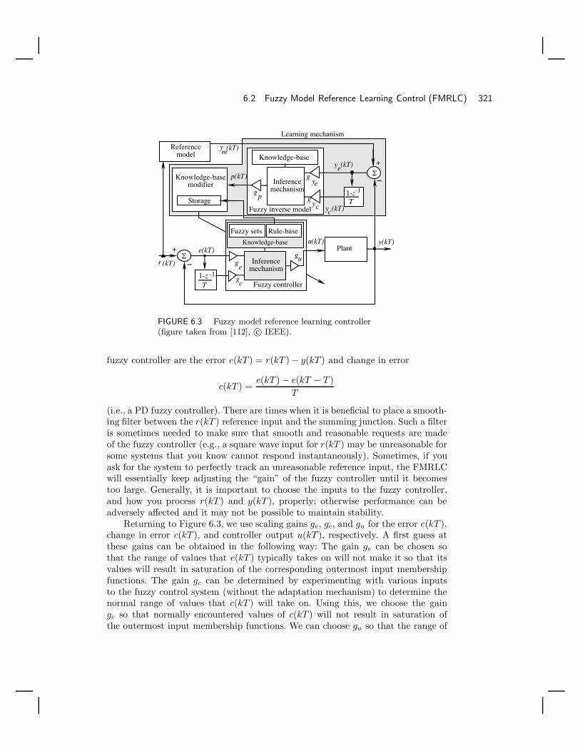
6.2 Fuzzy Model Reference Learning Control (FMRLC) 321
Planty(kT)
1-z -1
T
1-z-1
T
Knowledge-base
gc
ge
Inferencemechanism
Fuzzy sets Rule-base
Σ
Σ
Fuzzy controller
gue(kT)
u(kT)
r (kT)
ye(kT)
+
yc(kT)
+
gyc
gye
gp
Inferencemechanism
Knowledge-base
Referencemodel
p(kT)
Storage
Knowledge-basemodifier
Fuzzy inverse model
my (kT)
Learning mechanism
FIGURE 6.3 Fuzzy model reference learning controller(figure taken from [112], c© IEEE).
fuzzy controller are the error e(kT ) = r(kT ) − y(kT ) and change in error
c(kT ) =e(kT ) − e(kT − T )
T
(i.e., a PD fuzzy controller). There are times when it is beneficial to place a smooth-ing filter between the r(kT ) reference input and the summing junction. Such a filteris sometimes needed to make sure that smooth and reasonable requests are madeof the fuzzy controller (e.g., a square wave input for r(kT ) may be unreasonable forsome systems that you know cannot respond instantaneously). Sometimes, if youask for the system to perfectly track an unreasonable reference input, the FMRLCwill essentially keep adjusting the “gain” of the fuzzy controller until it becomestoo large. Generally, it is important to choose the inputs to the fuzzy controller,and how you process r(kT ) and y(kT ), properly; otherwise performance can beadversely affected and it may not be possible to maintain stability.
Returning to Figure 6.3, we use scaling gains ge, gc, and gu for the error e(kT ),change in error c(kT ), and controller output u(kT ), respectively. A first guess atthese gains can be obtained in the following way: The gain ge can be chosen sothat the range of values that e(kT ) typically takes on will not make it so that itsvalues will result in saturation of the corresponding outermost input membershipfunctions. The gain gc can be determined by experimenting with various inputsto the fuzzy control system (without the adaptation mechanism) to determine thenormal range of values that c(kT ) will take on. Using this, we choose the gaingc so that normally encountered values of c(kT ) will not result in saturation ofthe outermost input membership functions. We can choose gu so that the range of

322 Chapter 6 / Adaptive Fuzzy Control
outputs that are possible is the maximum one possible yet still so that the inputto the plant will not saturate (for practical problems the inputs to the plant willalways saturate at some value). Clearly, this is a very heuristic choice for the gainsand hence may not always work. Sometimes, tuning of these gains will need to beperformed when we tune the overall FMRLC.
Rule-Base
The rule-base for the fuzzy controller has rules of the form
If e is Ej and c is C l Then u is Um
where e and c denote the linguistic variables associated with controller inputs e(kT )and c(kT ), respectively, u denotes the linguistic variable associated with the con-troller output u, Ej and C l denote the jth (lth) linguistic value associated with e(c), respectively, and Um denotes the consequent linguistic value associated with u.Hence, as an example, one fuzzy control rule could be
If error is positive-large and change-in-error is negative-smallThen plant-input is positive-big
(in this case e = “error”, E4 = “positive-large”, etc.). We use a standard choice forall the membership functions on all the input universes of discourse, such as theones shown in Figure 6.4. Hence, we would simply use some membership functionssimilar to those in Figure 6.4, but with a scaled horizontal axis, for the c(kT ) input.
-1 -0.8 -0.6 -0.4 -0.2 0.2 0.4 0.6 0.8 1 e(kT)
EEEEEEEEEEE-5 -4 -3 -2 -1 0 1 2 3 4 5
1
FIGURE 6.4 Membership functions for input universe ofdiscourse (figure taken from [112], c© IEEE).
We will use all possible combinations of rules for the rule-base. For example, wecould choose to have 11 membership functions on each of the two input universesof discourse, in which case we would have 112 = 121 rules in the rule-base. At firstglance it would appear that the complexity of the controller could make implemen-tation prohibitive for applications where it is necessary to have many inputs to thefuzzy controller. However, we must remind the reader of the results in Section 2.6on page 97 where we explain how implementation tricks can be used to significantlyreduce computation time when there are input membership functions of the formshown in Figure 6.4.

6.2 Fuzzy Model Reference Learning Control (FMRLC) 323
Rule-Base Initialization
The input membership functions are defined to characterize the premises of therules that define the various situations in which rules should be applied. The inputmembership functions are left constant and are not tuned by the FMRLC. Themembership functions on the output universe of discourse are assumed to be un-known. They are what the FMRLC will automatically synthesize or tune. Hence,the FMRLC tries to fill in what actions ought to be taken for the various situationsthat are characterized by the premises.
We must choose initial values for each of the output membership functions.For example, for an output universe of discourse [−1, 1] we could choose triangular-shaped membership functions with base widths of 0.4 and centers at zero. Thischoice represents that the fuzzy controller initially knows nothing about how tocontrol the plant so it inputs u = 0 to the plant initially (well, really it does knowsomething since we specify the remainder of the fuzzy controller a priori). Of course,one can often make a reasonable best guess at how to specify a fuzzy controllerthat is “more knowledgeable” than simply placing the output membership functioncenters at zero. For example, we could pick the initial fuzzy controller to be thebest one that we can design for the nominal plant. Notice, however, that this choiceis not always the best one. Really, what you often want to choose is the fuzzycontroller that is best for the operating condition that the plant will begin in (thismay not be the nominal condition). Unfortunately, it is not always possible to picksuch a controller since you may not be able to measure the operating conditionof the plant, so making a best guess or simply placing the membership functioncenters at zero are common choices.
To complete the specification of the fuzzy controller, we use minimum or prod-uct to represent the conjunction in the premise and the implication (in this bookwe will use minimum unless otherwise stated) and the standard center-of-gravitydefuzzification technique. As an alternative, we could use appropriately initializedsingleton output membership functions and center-average defuzzification.
Learning, Memorization, and Controller Input Choice
For some applications you may want to use an integral of the error or other prepro-cessing of the inputs to the fuzzy controller. Sometimes the same guidelines thatare used for the choice of the inputs for a nonadaptive fuzzy controller are useful forthe FMRLC. We have found, however, times where it is advantageous to replacepart of a conventional controller with a fuzzy controller and use the FMRLC totune it (see the fault-tolerant control application in Section 6.3). In these cases thecomplex preprocessing of inputs to the fuzzy controller is achieved via a conven-tional controller. Sometimes there is also the need for postprocessing of the fuzzycontroller outputs.
Generally, however, choice of the inputs also involves issues related to the learn-ing dynamics of the FMRLC. As the FMRLC operates, the learning mechanism willtune the fuzzy controller’s output membership functions. In particular, in our ex-ample, for each different combination of e(kT ) and c(kT ) inputs, it will try to learn
324 Chapter 6 / Adaptive Fuzzy Control
what the best control actions are. In general, there is a close connection betweenwhat inputs are provided to the controller and the controller’s ability to learn tocontrol the plant for different reference inputs and plant operating conditions. Wewould like to be able to design the FMRLC so that it will learn and remember dif-ferent fuzzy controllers for all the different plant operating conditions and referenceinputs; hence, the fuzzy controller needs information about these. Often, however,we cannot measure the operating condition of the plant, so the FMRLC does notknow exactly what operating condition it is learning the controller for. Moreover, itthen does not know exactly when it has returned to an operating condition. Clearly,then, if the fuzzy controller has better information about the plant’s operating con-ditions, the FMRLC will be able to learn and apply better control actions. If itdoes not have good information, it will continually adapt, but it will not properlyremember.
For instance, for some plants e(kT ) and c(kT ) may only grossly characterizethe operating conditions of the plant. In this situation the FMRLC is not able tolearn different controllers for different operating conditions; it will use its limitedinformation about the operating condition and continually adapt to search for thebest controller. It degrades from a learning system to an adaptive system that willnot properly remember the control actions (this is not to imply, however, that therewill automatically be a corresponding degradation in performance).
Generally, we think of the inputs to the fuzzy controller as specifying whatconditions we need to learn different controllers for. This should be one guidelineused for the choice of the fuzzy controller inputs for practical applications. A com-peting objective is, however, to keep the number of fuzzy controller inputs low dueto concerns about computational complexity. In fact, to help with computationalcomplexity, we will sometimes use multiple fuzzy controllers with fewer inputs toeach of them rather than one fuzzy controller with many inputs; then we may, forinstance, sum the outputs of the individual controllers.
6.2.2 The Reference ModelNext, you must decide what to choose for the reference model that quantifies thedesired performance. Basically, you want to specify a desirable performance, butalso a reasonable one. If you ask for too much, the controller will not be able todeliver it; certain characteristics of real-world plants place practical constraints onwhat performance can be achieved. It is not always easy to pick a good referencemodel since it is sometimes hard to know what level of performance we can expect,or because we have no idea how to characterize the performance for some of theplant output variables (see the flexible robot application in Section 6.3 where it isdifficult to know a priori how the acceleration profiles of the links should behave).
In general, the reference model may be discrete or continuous time, linear ornonlinear, time-invariant or time-varying, and so on. For example, suppose that wewould like to have the response track the continuous time model
G(s) =1
s + 1

6.2 Fuzzy Model Reference Learning Control (FMRLC) 325
Suppose that for your discrete-time implementation you use T = 0.1 sec. Using abilinear (Tustin) transformation to find the discrete equivalent to the continuous-time transfer function G(s), we replace s with 2
Tz−1z+1 to obtain
Ym(z)R(z)
= H(z) =121
(z + 1)z − 19
21
where Ym(z) and R(z) are the z-transform of ym(kT ) and r(kT ), respectively. Now,for a discrete-time implementation we would choose
ym(kT + T ) =1921
ym(kT ) +121
r(kT + T ) +121
r(kT )
This choice would then represent that we would like our output y(kT ) to track asmooth, stable, first-order type response of ym(kT ). A similar approach can be usedto, for example, track a second-order system with a specified damping ratio ζ andundamped natural frequency ωn.
The performance of the overall system is computed with respect to the referencemodel by the learning mechanism by generating an error signal
ye(kT ) = ym(kT ) − y(kT )
Given that the reference model characterizes design criteria such as rise-time andovershoot and the input to the reference model is the reference input r(kT ), thedesired performance of the controlled process is met if the learning mechanismforces ye(kT ) to remain very small for all time no matter what the reference inputis or what plant parameter variations occur. Hence, the error ye(kT ) provides acharacterization of the extent to which the desired performance is met at time kT .If the performance is met (i.e., ye(kT ) is small), then the learning mechanism willnot make significant modifications to the fuzzy controller. On the other hand ifye(kT ) is big, the desired performance is not achieved and the learning mechanismmust adjust the fuzzy controller. Next, we describe the operation of the learningmechanism.
6.2.3 The Learning MechanismThe learning mechanism tunes the rule-base of the direct fuzzy controller so thatthe closed-loop system behaves like the reference model. These rule-base modifica-tions are made by observing data from the controlled process, the reference model,and the fuzzy controller. The learning mechanism consists of two parts: a “fuzzyinverse model” and a “knowledge-base modifier.” The fuzzy inverse model performsthe function of mapping ye(kT ) (representing the deviation from the desired be-havior), to changes in the process inputs p(kT ) that are necessary to force ye(kT )to zero. The knowledge-base modifier performs the function of modifying the fuzzycontroller’s rule-base to affect the needed changes in the process inputs. We explaineach of these components in detail next.

326 Chapter 6 / Adaptive Fuzzy Control
Fuzzy Inverse Model
Using the fact that most often a control engineer will know how to roughly char-acterize the inverse model of the plant (examples of how to do this will be given inseveral examples in this chapter), we use a fuzzy system to map ye(kT ), and pos-sibly functions of ye(kT ) such as yc(kT ) = 1
T (ye(kT ) − ye(kT − T )) (or any otherclosed-loop system data), to the necessary changes in the process inputs p(kT ).This fuzzy system is sometimes called the “fuzzy inverse model” since informationabout the plant inverse dynamics is used in its specification. Some, however, avoidthis terminology and simply view the fuzzy system in the adaptation loop in Fig-ure 6.3 to be a controller that tries to pick p(kT ) to reduce the error ye(kT ). This isthe view taken for some of the design and implementation case studies in the nextsection.
Note that similar to the fuzzy controller, the fuzzy inverse model shown inFigure 6.3 contains scaling gains, but now we denote them with gye, gyc , and gp.We will explain how to choose these scaling gains below. Given that gyeye andgycyc are inputs to the fuzzy inverse model, the rule-base for the fuzzy inversemodel contains rules of the form
If ye is Y je and yc is Y l
c Then p is P m
where Y je and Y l
c denote linguistic values and P m denotes the linguistic value as-sociated with the mth output fuzzy set. In this book we often utilize membershipfunctions for the input universes of discourse as shown in Figure 6.4, symmetrictriangular-shaped membership functions for the output universes of discourse, min-imum to represent the premise and implication, and COG defuzzification. Otherchoices can work equally well. For instance, we could make the same choices, exceptuse singleton output membership functions and center-average defuzzification.
Knowledge-Base Modifier
Given the information about the necessary changes in the input, which are repre-sented by p(kT ), to force the error ye to zero, the knowledge-base modifier changesthe rule-base of the fuzzy controller so that the previously applied control actionwill be modified by the amount p(kT ). Consider the previously computed controlaction u(kT − T ), and assume that it contributed to the present good or bad sys-tem performance (i.e., it resulted in the value of y(kT ) such that it did not matchym(kT )). Hence, for illustration purposes we are assuming that in one step the plantinput can affect the plant output; in Section 6.2.4 we will explain what to do if ittakes d steps for the plant input to affect the plant output. Note that e(kT − T )and c(kT −T ) would have been the error and change in error that were input to thefuzzy controller at that time. By modifying the fuzzy controller’s knowledge-base,we may force the fuzzy controller to produce a desired output u(kT − T ) + p(kT ),which we should have put in at time kT − T to make ye(kT ) smaller. Then, thenext time we get similar values for the error and change in error, the input to theplant will be one that will reduce the error between the reference model and plantoutput.

6.2 Fuzzy Model Reference Learning Control (FMRLC) 327
Assume that we use symmetric output membership functions for the fuzzycontroller, and let bm denote the center of the membership function associatedwith Um. Knowledge-base modification is performed by shifting centers bm of themembership functions of the output linguistic value Um that are associated withthe fuzzy controller rules that contributed to the previous control action u(kT −T ).This is a two-step process:
1. Find all the rules in the fuzzy controller whose premise certainty
µi(e(kT − T ), c(kT − T )) > 0 (6.1)
and call this the “active set” of rules at time kT − T . We can characterize theactive set by the indices of the input membership functions of each rule thatis on (since we use all possible combinations of rules, there will be one outputmembership function for each possible rule that is on).
2. Let bm(kT ) denote the center of the mth output membership function at timekT . For all rules in the active set, use
bm(kT ) = bm(kT − T ) + p(kT ) (6.2)
to modify the output membership function centers. Rules that are not in theactive set do not have their output membership functions modified.
Notice that for our development, when COG is used, this update will guaranteethat the previous input would have been u(kT −T )+p(kT ) for the same e(kT −T )and c(kT −T ) (to see this, simply analyze the formula for COG to see that addingthe amount p(kT ) to the centers of the rules that were on will make the output shiftby p(kT )). For the case where the fuzzy controller has input membership functionsof the form shown in Figure 6.4, there will only be at most four rules in the activeset at any one time instant (i.e., four rules with µi(e(kT − T ), c(kT − T )) > 0 attime kT ). Then we only need to update at most four output membership functioncenters via Equation (6.2).
Example
As an example of the knowledge-base modification procedure, assume that all thescaling gains for both the fuzzy controller and the fuzzy inverse model are one.Suppose that the fuzzy inverse model produces an output p(kT ) = 0.5, indicatingthat the value of the output to the plant at time kT−T should have been u(kT−T )+0.5 to improve performance (i.e., to force ye ≈ 0). Next, suppose that e(kT − T ) =0.75 and c(kT − T ) = −0.2 and that the membership functions for the inputs tothe fuzzy controller are given in Figure 6.4. Then rules
R1: If E3 and C−1 Then U1
and
328 Chapter 6 / Adaptive Fuzzy Control
R2: If E4 and C−1 Then U2
are the only rules that are in the active set (notice that we chose to use the indicesfor the rule “1” and “2” simply for convenience). In particular, from Figure 6.4 wehave µ1 = 0.25 and µ2 = 0.75, so rules R1 and R2 are the only ones that havetheir consequent fuzzy sets (U1, U2) modified. Suppose that at time kT −T we hadb1(kT − T ) = 1 and b2(kT − T ) = 3. To modify these fuzzy sets we simply shifttheir centers according to Equation (6.2) to get
b1(kT ) = b1(kT − T ) + p(kT ) = 1 + 0.5 = 1.5
and
b2(kT ) = b2(kT − T ) + p(kT ) = 3 + 0.5 = 3.5
Learning, Memorization, and Inverse Model Input Choice
Notice that the changes made to the rule-base are only local ones. That is, theentire rule-base is not updated at every time step, just the rules that needed tobe updated to force ye(kT ) to zero. Notice that this local learning is importantsince it allows the changes that were made in the past to be remembered by thefuzzy controller. Recall that the type and amount of memory depends criticallyon the inputs to the fuzzy controller. Different parts of the rule-base are “filled in”based on different operating conditions for the system (as characterized by the fuzzycontroller inputs), and when one area of the rule-base is updated, other rules arenot affected. Hence, if the appropriate inputs are provided to the fuzzy controller sothat it can distinguish between the situations in which it should behave differently,the controller adapts to new situations and also remembers how it has adapted topast situations.
Just as the choice of inputs to the fuzzy controller has a fundamental impacton learning and memorization, so does the choice of inputs to the inverse model.For instance, you may want to choose the inputs to the inverse model so that itwill adapt differently in different operating conditions. In one operating conditionwe may want to adapt more slowly than in another. In some operating conditionthe direction of adjustment of the output membership function centers may bethe opposite of that in another. If there are multiple fuzzy controllers, you maywant multiple inverse models to adjust them. This can sometimes help with com-putational complexity since we could then be using fewer inputs per fuzzy inversemodel.
The choice of inputs to the fuzzy inverse model shown in Figure 6.3 indicatesthat we want to adapt differently for different errors and error rates between thereference model and plant output. The inverse model may be designed so that, forexample, if the error is small, then the adjustments to the fuzzy controller shouldbe small, and if the error is small but the rate of error increase is high, then theadjustments should be larger. It is rules such as these that are loaded into the fuzzyinverse model.
6.2 Fuzzy Model Reference Learning Control (FMRLC) 329
6.2.4 Alternative Knowledge-Base ModifiersRecall that we had assumed that the plant input u(kT ) would affect the plantoutput in one time step so that y(kT + T ) would be affected by u(kT ). To removethis assumption and hence generalize the approach, let d denote the number of timesteps that it takes for an input to the plant u(kT ) to first affect its output. Thatis, y(kT + dT ) is affected by u(kT ). To handle this case, we use the same approachbut we go back d steps to modify the rules. Hence, we use
µi(e(kT − dT ), c(kT − dT )) > 0 (6.3)
to form the “active set” of rules at time kT − dT . To update the rules in the activeset, we let
bm(kT ) = bm(kT − dT ) + p(kT ) (6.4)
(when d = 1, we get the case in Equations (6.1) and (6.2)). This ensures that wemodify the rules that actually contributed to the current output y(kT ) that resultedin the performance characterization ye(kT ). For applications we have found thatwe can most often perform a simple experiment with the plant to find d (e.g., puta short-duration pulse into the plant and determine how long it takes for the inputto affect the output), and with this choice we can often design a very effectiveFMRLC. However, this has not always been the case. Sometimes we need to treatd as a tuning parameter for the knowledge-base modifier.
There are several alternatives to how the basic knowledge-base modificationprocedure can work that can be used in conjunction with the d-step back approach.For instance, note that an alternative to Equation (6.1) would be to include rulesin the active set that have
µi(e(kT − dT ), c(kT − dT )) > α
where 0 ≤ α < 1. In this case we will not modify rules whose premise certainty isbelow some given threshold α. This makes some intuitive sense since we will thennot modify rules if the fuzzy system is not too sure that they should be on. However,one could argue that any rule that contributed to the computation of u(kT − dT )should be modified. This approach may be needed if you choose to use Gaussianmembership functions for the input universes of discourse since it will ensure thatyou will not have to modify all the output centers at each time step, and hence thelocal learning characteristic is maintained.
There are also alternatives to the center update procedure given in Equa-tion (6.2). For instance, we could choose
bm(kT ) = bm(kT − dT ) + µm(e(kT − dT ), c(kT − dT ))p(kT )
so that we scale the amount we shift the membership functions by the µm certaintyof their premises. Intuitively, this makes sense since we will then change the mem-bership functions from rules that were on more by larger amounts, and for rules

330 Chapter 6 / Adaptive Fuzzy Control
that are not on as much we will not modify them as much. This approach hasproven to be more effective than the one in Equation (6.2) for some applications;however, it is difficult to determine a priori which approach to use. We usually trythe scaled approach if the one in Equation (6.2) does not seem to work well, par-ticularly if there are some unwanted oscillations in the system that seem to resultfrom excessive modification of output membership function center positions.
Another modification to the center update law is also necessary in some prac-tical applications to ensure that the centers stay in some prespecified range. Forinstance, you may want the centers to always be positive so that the controller willnever provide a negative output. Other times you may want the centers no largerthan some prespecified value to ensure that the control output will become no largerthan this value. In general, suppose that we know a priori that the centers shouldbe in the range [bmin, bmax] where bmin and bmax are given scalars. We can modifythe output center update rule to ensure that if the centers start in this range theywill stay in the range by adding the following two rules after the update formula:
If bm(kT ) < bmin Then bm(kT ) = bmin
If bm(kT ) > bmax Then bm(kT ) = bmax.
In other words, if the centers jump over the boundaries, they are set equal to theboundary values.
Notice that you could combine the above alternatives to knowledge-base mod-ification so that we set a threshold for including rules in the active set, scale theupdates to the centers, bound the updates to the centers, and use any number oftime steps back to form the active set. There are yet other alternatives that can beused for knowledge-base modification procedures. For instance, parts of the rule-base could be left intact (i.e., we would not let them be modified). This can beuseful when we know part of the fuzzy controller that is to be learned, we embedthis part into the fuzzy controller that is tuned, and do not let the learning mech-anism change it. Such an approach is used for the vibration damping problem forthe two-link flexible robot in Section 6.3. As another alternative, when a center isupdated, you could always wait d or more steps before updating the center again.This can be useful as a more “cautious” update procedure. It updates, then waitsto see if the update was sufficient to correct the error ye before it updates again. Wehave successfully used this approach to avoid inducing oscillations when operatingat a set-point.
6.2.5 Design Guidelines for the Fuzzy Inverse ModelIn this section we provide some design guidelines for the fuzzy inverse model andits scaling gains. The choice of a particular fuzzy inverse model is application-dependent, so we will use the case studies in Section 6.3 to show how it is chosen.There are, however, some general guidelines for the the choice of the fuzzy inversemodel that we will outline here.

6.2 Fuzzy Model Reference Learning Control (FMRLC) 331
First, we note that for a variety of applications we find that the specification ofthe fuzzy inverse model is not much more difficult than the specification of a directfuzzy controller. In fact, the fuzzy inverse model often takes on a form that is quitesimilar to a direct fuzzy controller. For instance, as you will see in the case studiesin Section 6.3, the rule-base often has some typical symmetry properties.
Second, for some practical applications it is necessary to define the inversemodel so that when the response of the plant is following the output of the refer-ence model very closely, the fuzzy inverse model turns off the adaptation (such anapproach is used in the aircraft application in Section 6.3). In this way once theinputs to the fuzzy inverse model get close to zero, the output of the fuzzy inversemodel becomes zero. We think of this as forcing the fuzzy inverse model to be satis-fied with the response as long as it is quite close to the reference model; there is noneed to make it exact in many applications. Designing this characteristic into thefuzzy inverse model can sometimes help ensure stability of the overall closed-loopsystem. Another way to implement such a strategy is to directly modify the outputof the fuzzy inverse model by using the rule:
If |p(kT )| < εp Then p(kT ) = 0
where εp > 0 is a small number that is specified a priori. For typical fuzzy inversemodel designs (i.e., ones where the size of the output of the fuzzy inverse modelis directly proportional to the size of the inputs to the fuzzy inverse model), thisrule will make sure that when the inputs to the fuzzy inverse model are in a regionof zero, its output will be modified to zero. Hence, for small fuzzy inverse modelinputs the learning mechanism will turn off. If, however, the error between the plantoutput and the reference input grows, then the learning mechanism will turn backon and it will try to reduce the error. Such approaches to modifying the adaptationon-line are related to “robustification” methods in conventional adaptive control.
Next, we provide general tuning procedures for the scaling gains of a given fuzzyinverse model. For the sake of discussion, assume that both the fuzzy controller andfuzzy inverse model are normalized so that their input and output effective universesof discourse are all [−1, 1].
Fuzzy Inverse Model Design Procedure 1
Generally, we have found the following procedure to be useful for tuning the scalinggains of the inverse model:
1. Select the gain gye so that ye(kT ) will not saturate the input membershipfunction certainty (near the endpoints). This is a heuristic choice since wecannot know a priori how big ye(kT ) will get; however, we have found that formany applications intuition about the process can be quite useful in determiningthe maximum value.
2. Choose the gain gp to be the same as for the fuzzy controller output gain gu.Let gyc = 0.

332 Chapter 6 / Adaptive Fuzzy Control
3. Apply a step reference input r(kT ) that is of a magnitude that may be typicalduring normal operation.
4. Observe the plant and reference model responses. There are three cases:
(a) If there exist unacceptable oscillations in the plant output response aboutthe reference model response, then increase gyc (we need additional deriva-tive action in the learning mechanism to reduce the oscillations). Go tostep 3.
(b) If the plant output is unable to “keep up” with the reference model re-sponse, then decrease gyc . Go to step 3.
(c) If the plant response is acceptable with respect to the reference modelresponse, then the controller design is completed.
We will use this gain selection procedure for the ship steering application in Sec-tion 6.3.
Fuzzy Inverse Model Design Procedure 2
For a variety of applications, the above gain selection procedure has proven tobe very successful. For other applications, however, it has been better to use analternative procedure. In this procedure you pick the fuzzy controller and inversemodel using intuition, then focus on tuning the scaling gain gp, which we will callthe “adaptation gain” using an analogy with conventional adaptive controllers. Theprocedure is as follows:
1. Begin with gp = 0 (i.e., with the adaptation mechanism turned off) and simu-late the system. With a well-designed direct fuzzy controller you should get areasonable response, but if there is good reason to have adaptive control youwill find that the performance is not what you specified in the reference model(at least for some plant conditions).
2. Choose the gains of the inverse model so that there is no saturation on its inputuniverses of discourse.
3. Increase gp slightly so that you just turn on the learning mechanism and itmakes only small changes to the rule-base at each step. For small gp you willallow only very small updates to the fuzzy controller so that the learning rate(adaptation rate) will be very slow. Perform any necessary tuning for the inversemodel.
4. Continue to increase gp and subsequently tune the inverse model as needed.With gp large, you increase the adaptation rate, and hence if you increase ittoo much, you can get undesirable oscillations and sometimes instability. Youshould experiment and then choose an adaptation rate that is large enough tomake it so that the FMRLC can quickly adapt to changes in the plant, yet slowenough so that it does not cause oscillations and instability.

6.3 FMRLC: Design and Implementation Case Studies 333
This design approach is what we will use for the fault-tolerant aircraft controlproblem in Section 6.3, and it is one that we have successfully used for severalother FMRLC applications.
6.3 FMRLC: Design and Implementation CaseStudies
The FMRLC has been used in simulation studies for a variety of applications,including an inverted pendulum (translational for swing-up and balancing, and ro-tational for balancing); rocket velocity control; a rigid two-link robot; fault-tolerantcontrol for aircraft; ship steering; longitudinal and lateral control for automatedhighway systems; antilock brake systems; base braking control; temperature, pres-sure, and level control in a glass furnace; and others. It has been implemented forbalancing the rotational inverted pendulum, a ball-on-a-beam experiment, a liquidlevel control problem, a single-link flexible robot, the two-link flexible robot, andan induction machine. See the references at the end of the chapter for more details.
In this section we will study the cargo ship and fault-tolerant aircraft controlproblems in simulation and provide implementation results for the two-link flexiblerobot that was studied in Chapter 3. The cargo ship application helps to illustrateall the steps in how to design an FMRLC. Moreover, we design two conventionaladaptive controllers and compare their performance to that of the FMRLC. Thefault-tolerant aircraft control problem helps to illustrate issues in fuzzy controllerinitialization and how to design a more complex fuzzy inverse model by viewingit as a controller in the adaptation loop. The two-link flexible link robot applica-tion is used to show how the FMRLC can automatically synthesize a direct fuzzycontroller; you will want to compare its performance with the one that we manu-ally constructed in Chapter 3. It also illustrates how to develop and implement anFMRLC that can tune the fuzzy controller to compensate for changes in a MIMOplant—in this case, payload variations.
6.3.1 Cargo Ship SteeringTo improve fuel efficiency and reduce wear on ship components, autopilot systemshave been developed and implemented for controlling the directional heading ofships. Often, the autopilots utilize simple control schemes such as PID control.However, the capability for manual adjustments of the parameters of the controlleris added to compensate for disturbances acting upon the ship such as wind andcurrents. Once suitable controller parameters are found manually, the controllerwill generally work well for small variations in the operating conditions. For largevariations, however, the parameters of the autopilot must be continually modified.Such continual adjustments are necessary because the dynamics of a ship vary with,for example, speed, trim, and loading. Also, it is useful to change the autopilotcontrol law parameters when the ship is exposed to large disturbances resultingfrom changes in the wind, waves, current, and water depth. Manual adjustment ofthe controller parameters is often a burden on the crew. Moreover, poor adjustment

334 Chapter 6 / Adaptive Fuzzy Control
may result from human error. As a result, it is of great interest to have a methodfor automatically adjusting or modifying the underlying controller.
Ship Model
Generally, ship dynamics are obtained by applying Newton’s laws of motion to theship. For very large ships, the motion in the vertical plane may be neglected sincethe “bobbing” or “bouncing” effects of the ship are small for large vessels. Themotion of the ship is generally described by a coordinate system that is fixed to theship [11, 149]. See Figure 6.5.
δ
ψ
xuV
vy
FIGURE 6.5 Cargo ship.
A simple model of the ship’s motion is given by
...
ψ (t) +(
1τ1
+1τ2
)ψ(t) +
(1
τ1 τ2
)ψ(t) =
K
τ1 τ2
(τ3 δ(t) + δ(t)
)(6.5)
where ψ is the heading of the ship and δ is the rudder angle. Assuming zero initialconditions, we can write Equation (6.5) as
ψ(s)δ(s)
=K(sτ3 + 1)
s(sτ1 + 1)(sτ2 + 1)(6.6)
where K, τ1, τ2, and τ3 are parameters that are a function of the ship’s constantforward velocity u and its length l. In particular,
K = K0
(u
l
)τi = τi0
(l
u
)i = 1, 2, 3
where we assume that for a cargo ship K0 = −3.86, τ10 = 5.66, τ20 = 0.38, τ30 =0.89, and l = 161 meters [11]. Also, we will assume that the ship is traveling in thex direction at a velocity of 5 m/s.

6.3 FMRLC: Design and Implementation Case Studies 335
In normal steering, a ship often makes only small deviations from a straight-linepath. Therefore, the model in Equation (6.5) is obtained by linearizing the equationsof motion around the zero rudder angle (δ = 0). As a result, the rudder angle shouldnot exceed approximately 5 degrees, otherwise the model will be inaccurate. For ourpurposes, we need a model suited for rudder angles that are larger than 5 degrees;hence, we use the model proposed in [20]. This extended model is given by
...
ψ (t) +(
1τ1
+1τ2
)ψ(t) +
(1
τ1 τ2
)H(ψ(t)) =
K
τ1 τ2
(τ3 δ(t) + δ(t)
)(6.7)
where H(ψ) is a nonlinear function of ψ(t). The function H(ψ) can be found fromthe relationship between δ and ψ in steady state such that
...
ψ= ψ = δ = 0. Anexperiment known as the “spiral test” has shown that H(ψ) can be approximatedby
H(ψ) = aψ3 + bψ
where a and b are real-valued constants such that a is always positive. For oursimulations, we choose the values of both a and b to be one.
Simulating the Ship
When we evaluate our controllers, we will use the nonlinear model in simulation.Note that to do this we need to convert the nth-order nonlinear ordinary differentialequations representing the ship to n first-order ordinary differential equations; forconvenience, let
a =(
1τ1
+1τ2
)
b =(
1τ1τ2
)
c =Kτ3
τ1τ2
and
d =K
τ1τ2
(this notation is not to be confused with the d-step delay of Section 6.2.4). Wewould like the model in the form
x(t) = F (x(t), δ(t))

336 Chapter 6 / Adaptive Fuzzy Control
y(t) = G(x(t), δ(t))
where x(t) = [x1(t), x2(t), x3(t)] and F = [F1, F2, F3] for use in a nonlinearsimulation program. We need to choose xi so that Fi depends only on xi and δ fori = 1, 2, 3. We have
...
ψ (t) = −aψ(t) − bH(ψ(t)) + cδ(t) + dδ(t) (6.8)
Choose
x3(t) =...
ψ (t) − cδ(t)
so that F3 will not depend on cδ(t) and
x3(t) = ψ(t) − cδ(t)
Choose x2(t) = ψ(t) so that x2(t) = ψ(t). Finally, choose x1(t) = ψ. This gives us
x1(t) = x2(t) = F1(x(t), δ(t))x2(t) = x3(t) + cδ(t) = F2(x(t), δ(t))x3(t) = −aψ(t) − bH(ψ(t)) + dδ(t)
But, ψ(t) = x3(t) + cδ(t), ψ(t) = x2(t), and H(x2) = x32(t) + x2(t) so
x3(t) = −a (x3(t) + cδ(t)) − b(x3
2(t) + x2(t))
+ dδ(t) = F3(x(t), δ(t))
This provides the proper equations for the simulation. Next, suppose that the initialconditions are ψ(0) = ψ(0) = ψ(0) = 0. This implies that x1(0) = x2(0) = 0 andx3(0) = ψ(0) − cδ(0) or x3(0) = −cδ(0). For a discrete-time implementation, wesimply discretize the differential equations.
FMRLC Design
In this section we explain how to design an FMRLC for controlling the directionalheading of the cargo ship. The inputs to the fuzzy controller are the heading errorand change in heading error expressed as
e(kT ) = ψr(kT ) − ψ(kT )
and
c(kT ) =e(kT ) − e(kT − T )
T
respectively, where ψr(kT ) is the desired ship heading (T = 50 milliseconds). Thecontroller output is the rudder angle δ(kT ) of the ship. For our fuzzy controllerdesign, 11 uniformly spaced triangular membership functions are defined for eachcontroller input, as shown in Figure 6.4 on page 322.
6.3 FMRLC: Design and Implementation Case Studies 337
The scaling controller gains for the error, change in error, and the controlleroutput are chosen via the design procedure to be ge = 1
π (since the error e(kT )can never be over 180), gc = 100 (since we have found via simulations that theship does not move much faster than 0.01 rad/sec), and gu = 8π
18(since we want
to limit δ between ±80, we have gu = 80π180
= 8π18
). The fuzzy sets for the fuzzycontroller output are assumed to be symmetric and triangular-shaped with a basewidth of 0.4, and all centered at zero on the normalized universe of discourse (i.e.,121 output membership functions all centered at zero).
The reference model was chosen so as to represent somewhat realistic perfor-mance requirements as
ψm(t) + 0.1 ψm(t) + 0.0025 ψm(t) = 0.0025 ψr(t)
where ψm(t) specifies the desired system performance for the ship heading ψ(t).The input to the fuzzy inverse model includes the error and change in error
between the reference model and the ship heading expressed as
ψe(kT ) = ψm(kT ) − ψ(kT )
and
ψc(kT ) =ψe(kT ) − ψe(kT − T )
T
respectively. For each of these inputs, 11 symmetric and triangular-shaped member-ship functions are defined that are evenly distributed on the appropriate universesof discourse (the same as shown in Figure 6.4 on page 322). The normalizing con-troller gains associated with ψe(kT ), ψc(kT ), and p(kT ) are chosen to be gψe = 1
π ,gψc = 5, and gp = 8π
18, respectively, according to design procedure 1 in Section 6.2.5.
For a cargo ship, an increase in the rudder angle δ(kT ) will generally result ina decrease in the ship heading angle (see Figure 6.5). This is the information aboutthe inverse dynamics of the plant that we use in the fuzzy inverse model rules.Specifically, we will use rules of the form
If ψe is Ψie and ψc is Ψj
c Then p is P m
Suppose that we name the center of the output membership function for this rule ci,j
to emphasize that it is the center associated with the output membership functionthat has the ith membership function for the ψe universe of discourse and the jth
membership function for the ψc universe of discourse. The rule-base array shown inTable 6.1 is employed for the fuzzy inverse model for the cargo ship. In Table 6.1,Ψi
e denotes the ith fuzzy set associated with the error signal ψe, and Ψjc denotes the
jth fuzzy set associated with the change in error signal ψc. The entries of the tablerepresent the center values of symmetric triangular-shaped membership functionsci,j with base widths 0.4 for output fuzzy sets P m on the normalized universe ofdiscourse.
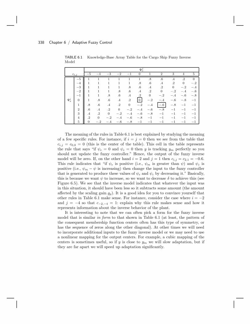
338 Chapter 6 / Adaptive Fuzzy Control
TABLE 6.1 Knowledge-Base Array Table for the Cargo Ship Fuzzy InverseModel
Ψjc
ci,j −5 −4 −3 −2 −1 0 1 2 3 4 5
−5 1 1 1 1 1 1 .8 .6 .4 .2 0−4 1 1 1 1 1 .8 .6 .4 .2 0 −.2
−3 1 1 1 1 .8 .6 .4 .2 0 −.2 −.4−2 1 1 1 .8 .6 .4 .2 0 −.2 −.4 −.6
−1 1 1 .8 .6 .4 .2 0 −.2 −.4 −.6 −.8
Ψie 0 1 .8 .6 .4 .2 0 −.2 −.4 −.6 −.8 −1
1 .8 .6 .4 .2 0 −.2 −.4 −.6 −.8 −1 −1
2 .6 .4 .2 0 −.2 −.4 −.6 −.8 −1 −1 −1
3 .4 .2 0 −.2 −.4 −.6 −.8 −1 −1 −1 −14 .2 0 −.2 −.4 −.6 −.8 −1 −1 −1 −1 −1
5 0 −.2 −.4 −.6 −.8 −1 −1 −1 −1 −1 −1
The meaning of the rules in Table 6.1 is best explained by studying the meaningof a few specific rules. For instance, if i = j = 0 then we see from the table thatci,j = c0,0 = 0 (this is the center of the table). This cell in the table representsthe rule that says “if ψe = 0 and ψc = 0 then y is tracking ym perfectly so youshould not update the fuzzy controller.” Hence, the output of the fuzzy inversemodel will be zero. If, on the other hand i = 2 and j = 1 then ci,j = c2,1 = −0.6.This rule indicates that “if ψe is positive (i.e., ψm is greater than ψ) and ψc ispositive (i.e., ψm − ψ is increasing) then change the input to the fuzzy controllerthat is generated to produce these values of ψe and ψc by decreasing it.” Basically,this is because we want ψ to increase, so we want to decrease δ to achieve this (seeFigure 6.5). We see that the inverse model indicates that whatever the input wasin this situation, it should have been less so it subtracts some amount (the amountaffected by the scaling gain gp). It is a good idea for you to convince yourself thatother rules in Table 6.1 make sense. For instance, consider the case where i = −2and j = −4 so that c−2,−4 = 1: explain why this rule makes sense and how itrepresents information about the inverse behavior of the plant.
It is interesting to note that we can often pick a form for the fuzzy inversemodel that is similar in form to that shown in Table 6.1 (at least, the pattern ofthe consequent membership function centers often has this type of symmetry, orhas the sequence of zeros along the other diagonal). At other times we will needto incorporate additional inputs to the fuzzy inverse model or we may need to usea nonlinear mapping for the output centers. For example, a cubic mapping of thecenters is sometimes useful, so if y is close to ym we will slow adaptation, but ifthey are far apart we will speed up adaptation significantly.
6.3 FMRLC: Design and Implementation Case Studies 339
Gradient-Based Model Reference Adaptive Control
The controller parameter adjustment mechanism for the gradient approach to MRACcan be implemented via the “MIT rule.” For this, the cost function
J(θ) =12ψ2
e(t)
where θ holds the parameters of the controller that will be tuned, ψe(t) = ψm(t)−ψ(t), and
dθ
dt= −γ
∂J
∂θ
so that
dθ
dt= −γ ψe(t)
∂ψe(t)∂θ
For developing the MIT rule for the ship we assume that the ship may bemodeled by a second-order linear differential equation. This model is obtained byeliminating the process pole resulting from τ2 in Equation (6.5) since its associ-ated dynamics are significantly faster than those resulting from τ1. Also, for smallheading variations the rudder angle derivative δ is likely to be small and may beneglected. Therefore, we obtain the following reduced-order model for the ship:
ψ(t) +(
1τ1
)ψ(t) =
(K
τ1
)δ(t) (6.9)
The PD-type control law that will be employed for this process may be expressedby
δ(t) = kp (ψr(t) − ψ(t)) − kd ψ(t) (6.10)
where kp and kd are the proportional and derivative gains, respectively, and ψr(t)is the desired process output. Substituting Equation (6.10) into Equation (6.9), weobtain
ψ(t) +(
1 + K kd
τ1
)ψ(t) +
(K kp
τ1
)ψ(t) =
(K kp
τ1
)ψr(t) (6.11)
It follows from Equation (6.11) that
ψ(t) =K kp
τ1
p2 +(
1+K kd
τ1
)p +
(K kp
τ1
)ψr(t) (6.12)
where p is the differential operator.

340 Chapter 6 / Adaptive Fuzzy Control
The reference model for this process is chosen to be
ψm(t) =ω2
n
p2 + 2ζωn p + ω2n
ψr(t) (6.13)
where to be consistent with the FMRLC design we choose ζ = 1 and ωn = 0.05.Combining Equations (6.13) and (6.12) and finding the partial derivatives withrespect to the proportional gain kp and the derivative gain kd, we find that
∂ ψe
∂kp=
K
τ1
p2 +(
1+K kd
τ1
)p +
(K kp
τ1
) (ψ − ψr) (6.14)
and
∂ ψe
∂kd=
K
τ1p
p2 +(
1+K kd
τ1
)p +
(K kp
τ1
)ψ (6.15)
In general, Equations (6.14) and (6.15) cannot be used because the controllerparameters kp and kd are not known. Observe that for the “optimal values” of kp
and kd, we have
p2 +(
1 + K kd
τ1
)p +
(K kp
τ1
)= p2 + 2ζωn p + ω2
n
Furthermore, the term Kτ1
may be absorbed into the adaptation gain γ. However, thisrequires that the sign of K
τ1be known since, in general, γ should be positive to ensure
that the controller updates are made in the direction of the negative gradient. For aforward-moving cargo ship the sign of K
τ1happens to be negative, which implies that
the term γ with Kτ1
absorbed into it must be negative to achieve the appropriatenegative gradient. After making the above approximations, we obtain the followingdifferential equations for updating the PD controller gains:
d kp
dt= −γ1
(1
p2 + 2ζωnp + ω2n
(ψ − ψr))
ψe
d kd
dt= −γ2
(p
p2 + 2ζωnp + ω2n
ψ
)ψe
where γ1 and γ2 are negative real numbers. After many simulations, the best valuesthat we could find for the γi are γ1 = −0.005 and γ2 = −0.1.
Lyapunov-Based Model Reference Adaptive Control
In this section we present a Lyapunov-based approach to MRAC that tunes aproportional derivative (PD) control law. Recall that the ship dynamics may be
6.3 FMRLC: Design and Implementation Case Studies 341
approximated by a second-order linear time-invariant differential equation given byEquation (6.9). We use a PD control law
δ(t) = kp (ψr(t) − ψ(t)) − kd ψ(t)
where kp and kd are the proportional and derivative gains, respectively, and ψr(t) isthe desired process output. The dynamic equation that describes the compensatedsystem is ψ = Acψ + Bcψr where ψ = [ψ, ψ] and
Ac =[
0 1−Kkp
τ1− (1+Kkd)
τ1
]
Bc =[
0Kkp
τ1
]
The reference model is given by
ψm
= Amψm
+ Bmψr
(6.16)
where ψm
= [ψm, ψm]T and
Am =[
0 1−ω2
n −2ζωn
]
Bm =[
0ω2
n
]
and where to be consistent with the FMRLC design we choose ζ = 1 and ωn = 0.05.The differential equation that describes the error ψ
e(t) = ψ
m(t)−ψ(t) may be
expressed by
ψe
= Am(t)ψe+ (Am(t) − Ac(t))ψ + (Bm(t) − Bc(t))ψr
(6.17)
The equilibrium point ψe
= 0 in Equation (6.17) is asymptotically stable if wechoose the adaptation laws to be
Ac(t) = γPψeψ (6.18)
Bc(t) = γPψeψ
r(6.19)
where P ∈ n×n is a symmetric, positive definite matrix that is a solution of theLyapunov equation
AmP + PAm = −Q < 0
Assuming that Q is a 2 × 2 identity matrix and solving for P , we find that
P =[
p11 p12
p21 p22
]=
[25.0125 200.000200.000 2005.00
]

342 Chapter 6 / Adaptive Fuzzy Control
Solving for kp and kd in Equations (6.18) and (6.19), respectively, the adaptationlaw in Equations (6.18) and (6.19) may be implemented as
kp = −γ1(p21ψe + p22ψe)(ψ − ψr), (6.20)kd = −γ2(p21ψe + p22ψe)ψ. (6.21)
Equations (6.20) and (6.21) assume that the plant parameters and disturbanceare varying slowly. In obtaining Equations (6.20) and (6.21), we absorbed the termKτ1
into the adaptation gains γ1 and γ2. Recall that for the cargo ship, Kτ1
happensto be a negative quantity. Therefore, both γ1 and γ2 must be negative. We foundthat γ1 = −0.005 and γ2 = −0.1 were suitable adaptation gains.
Comparative Analysis of FMRLC and MRAC
For the simulations for both the FMRLC and the MRACs, we use the nonlinearprocess model given in Equation (6.7) to emulate the ship’s dynamics. Figure 6.6shows the results for the FMRLC, and we see that it was quite successful in gener-ating the appropriate control rules for a good response since the ship heading tracksthe reference model almost perfectly. In fact, the maximum deviation between thetwo signals was observed to be less than 1 over the entire simulation. This is thecase even though initially the right-hand sides of the control rules have membershipfunctions with centers all at zero (i.e., initially, the controller knows little about howto control the plant), so we see that the FMRLC learns very fast.
-80
-60
-40
-20
0
20
40
60
80
0 1000 2000 3000 4000 5000 6000
Time (sec)
Hea
ding
(de
g)
Cargo ship response: FMRLC
Reference inputReference model responseCargo ship response
FIGURE 6.6 FMRLC simulation results (figure taken from [112],c© IEEE).

6.3 FMRLC: Design and Implementation Case Studies 343
Compare the results for the FMRLC with those obtained for the gradient-basedand Lyapunov-based approaches to MRAC, which are shown in Figures 6.7 and6.8. For the gradient-based and Lyapunov-based approaches, both system responsesconverged to track the reference model. However, the convergence rate of both algo-rithms was significantly slower than that of the FMRLC method (and comparablecontrol energy was used by the FMRLC and the MRACs). The controller gains kp
and kd for both MRACs were initially chosen to be 5. This choice of initial controllergains happens to be an unstable case for the second-order linear process model (inthe case where the adaptation mechanism is disconnected). However, we felt thisto be a fair comparison since the fuzzy controller is initially chosen so that it wouldput in zero degrees of rudder no matter what the controller input values were. Wewould have chosen both controller gains to be zero, but this choice resulted in avery slow convergence rate for the MRACs.
-80
-60
-40
-20
0
20
40
60
80
0 1000 2000 3000 4000 5000 6000
Time (sec)
Hea
ding
(de
g)
Cargo ship response: Gradient-based approach to MRAC
Reference inputReference model responseCargo ship response
FIGURE 6.7 Gradient-based MRAC simulation results (figuretaken from [112], c© IEEE).
The final set of simulations for the ship was designed to illustrate the ability ofthe learning and adaptive controllers to compensate for disturbances at the processinput. A disturbance is injected by adding it to the rudder command δ then puttingthis signal into the plant as the control signal. Specifically, the disturbance waschosen to be be a sinusoid with a frequency of one cycle per minute and a magnitudeof 2 with a bias of 1 (see the bottom plot in Figure 6.9). The effect of thisdisturbance is similar to that of a gusting wind acting upon the ship.
Figure 6.9 illustrates the results obtained for this simulation. To provide an

344 Chapter 6 / Adaptive Fuzzy Control
-80
-60
-40
-20
0
20
40
60
80
0 1000 2000 3000 4000 5000 6000
Time (sec)
Hea
ding
(de
g)
Cargo ship response: Lyapunov-based approach to MRAC
Reference inputReference model responseCargo ship response
FIGURE 6.8 Lyapunov-based MRAC simulation results (figuretaken from [112], c© IEEE).
especially fair comparison with the FMRLC algorithm, we initially loaded the PDcontrollers in both MRAC algorithms with the controller gains that resulted at theend of their 6000-second simulations in Figures 6.7 and 6.8. However, the centers ofthe right-hand sides of the membership functions for the knowledge-base of the fuzzycontroller in the FMRLC algorithm were initialized with all zeros as before (hence,we are giving the MRACs an advantage). Notice that the FMRLC algorithm wasnearly able to completely cancel the effects of the disturbance input (there is stilla very small magnitude oscillation). However, the gradient- and Lyapunov-basedapproaches to MRAC were not nearly as successful.
Discussion: A Control-Engineering Perspective
In this section we summarize and more carefully discuss the conclusions from oursimulation studies. The results in the previous section seem to indicate that theFMRLC has the following advantages:
• It achieves fast convergence compared to the MRACs.
• No additional control energy is needed to achieve this faster convergence.
• It has good disturbance rejection properties compared to the MRACs.
• Its design is independent of the particular form of the mathematical model of theunderlying process (whereas in the MRAC designs, we need an explicit mathe-matical model of a particular form)

6.3 FMRLC: Design and Implementation Case Studies 345
-0.5
0
0.5
0 200 400 600 800 1000 1200 1400 1600 1800 2000
Time (sec)
Hea
ding
(de
g)
Cargo ship response: FMRLC
-0.5
0
0.5
0 200 400 600 800 1000 1200 1400 1600 1800 2000
Time (sec)
Hea
ding
(de
g)
Cargo ship response: Gradient-based approach to MRAC
-0.5
0
0.5
0 200 400 600 800 1000 1200 1400 1600 1800 2000
Time (sec)
Hea
ding
(de
g)
Cargo ship response: Lyapunov-based approach to MRAC
-5
0
5
0 200 400 600 800 1000 1200 1400 1600 1800 2000
Time (sec)
Dis
turb
ance
at r
udde
r (d
eg) Wind disturbance as seen at the rudder
FIGURE 6.9 Simulation results comparingdisturbance rejection for the FMRLC, thegradient-based approach to MRAC, and theLyapunov-based approach to MRAC (figure takenfrom [112], c© IEEE).
Overall, the FMRLC provides a method to synthesize (i.e., automatically design)and tune the knowledge-base for a direct fuzzy controller. As the direct fuzzy con-troller is a nonlinear controller, some of the above advantages may be attributed tothe fact that the underlying controller that is tuned inherently has more significantfunctional capabilities than the PD controllers used in the MRAC designs.
While our application may indicate that FMRLC is a promising alternative toconventional MRAC, we must also emphasize the following:
• We have compared the FMRLC to only two types of MRACs, for only one appli-

346 Chapter 6 / Adaptive Fuzzy Control
cation, for a limited class of reference inputs, and only in simulation. There is awide variety of other adaptive control approaches that also deserve consideration.
• There are no guarantees of stability or convergence; hence, we can simply pick adifferent reference input, and the system may then be unstable (indeed, for someapplications, we have been able to destabilize the FMRLC, especially if we pickthe adaptation gain gp large).
• “Persistency of excitation”[77] is related to the learning controller’s ability toalways generate an appropriate plant input and to generalize the results of whatit has learned earlier and apply this to new situations. In this context, for theship we ask the following questions: (1) What if we need to turn the ship in adifferent direction? Will the rule-base be “filled in” for this direction? (2) Or willit have to learn for each new direction? (3) If it learns for the new directions, willit forget how to control for the old ones?
• In terms of control energy, we may have just gotten lucky for this applicationand for the chosen reference input (although with additional tests, this does notseem to be the case). There seem to be no analytical results that guarantee thatthe FMRLC or any other fuzzy learning control technique minimizes the use ofcontrol energy for a wide class of plants.
• This is a very limited investigation of the disturbance rejection properties (i.e.,only one type of wind disturbance is considered).
• The design approach for the FMRLC, although it did not depend on a mathemat-ical model, is somewhat ad hoc. What fundamental limitations will, for example,nonminimum phase systems present? Certainly there will be limitations for classesof nonlinear systems. What will these limitations be? It is important to note thatthe use of a mathematical model helps to show what these limitations will be(hence, it cannot always be considered an advantage that many fuzzy controltechniques do not depend on the specification of a mathematical model). Also,note that due to our avoidance of using a mathematical model of the plant, wehave also ignored the “model matching problem” in adaptive control [77].
• There may be gains in performance, but are these gains being made by paying ahigh price in computational complexity for the FMRLC? The FMRLC is some-what computationally intensive (as are many neural and fuzzy learning controlapproaches), but we have shown implementation tricks in Chapter 2 that can sig-nificantly reduce problems with computation time. The FMRLC can, however,require significant memory since we need to store each of the centers of the outputmembership functions of the rules, and with increased numbers of inputs to thefuzzy controller, there is an exponential increase in the numbers of these centers(assuming you use all possible combinations of rules). The FMRLC in this sectionrequired us to store and update 121 output membership function centers.

6.3 FMRLC: Design and Implementation Case Studies 347
6.3.2 Fault-Tolerant Aircraft ControlThere are virtually an unlimited number of possible failures that can occur ona sophisticated modern aircraft such as the F-16 that we consider in this casestudy. While preplanned pilot-executed response procedures have been developedfor certain anticipated failures, especially catastrophic and high-probability failures,certain unanticipated events can occur that complicate successful failure accommo-dation. Indeed, aircraft accident investigations sometimes find that even with someof the most severe unanticipated failures, there was a way in which the aircraftcould have been saved if the pilot had taken proper actions in a timely fashion. Be-cause the time frame during a catastrophic event is typically short, given the levelof stress and confusion during these incidents, it is understandable that a pilot maynot find the solution in time to save the aircraft.
With the recent advances in computing technology and control theory, it ap-pears that the potential exists to implement a computer control strategy that canassist (or replace) the pilot in helping to mitigate the consequences of severe fail-ures in aircraft. In this case study we will investigate the use of the FMRLC forfailure accommodation; however, we must emphasize that our study is somewhatacademic. The reader should be aware that there currently exists no completelysatisfactory solution to the fault-tolerant aircraft control problem. Indeed, it is animportant area of current research. For instance, in this case study we will onlystudy a certain class of actuator failures where in some aircraft sensor failures areof concern. We do not compare and contrast the fuzzy control approach to otherconventional approaches to fault tolerant control (e.g., conventional adaptive con-trol approaches). We do not study stability and robustness of the resulting controlsystem. These, and many other issues, are interesting areas for future research.
Aircraft Model
The F-16 aircraft model used in this case study is based on a set of five linear per-turbation models (that are extracted from a nonlinear model at the five operatingconditions1) (Ai, Bi, Ci, Di), i ∈ 1, 2, 3, 4, 5:
x = Aix + Biuy = Cix + Diu (6.22)
where the variables are defined as follows (see Figure 6.10):
• Inputs u = [δe, δde, δa, δr]:
1. δe = elevator deflection (in degrees)
2. δde = differential elevator deflection (in degrees)
3. δa = aileron deflection (in degrees)
4. δr = rudder deflection (in degrees)
1. All information about the F-16 aircraft models was provided by Wright Laboratories,
WPAFB, OH.

348 Chapter 6 / Adaptive Fuzzy Control
• System state x = [α, q, φ, β, p, r]:
1. α = angle of attack (in degrees)
2. q = body axis pitch rate (in degrees/second)
3. φ = Euler roll angle (in degrees)
4. β = sideslip angle (in degrees)
5. p = body axis roll rate (in degrees/second)
6. r = body axis yaw rate (in degrees/second)
The output is y = [x, Az] where Az is the normal acceleration (in g).
Sideslip = β
Y
Xφ
Y
Z
Horizontal β
Rudder δr
Aileron δa
Differential elevator δde
Y
Body axis
Mass Center
XZ
Velocity
Angle of attack = α
Horizontalθ
α
Velocit
y
Pitch angle = θ
Pitch rate = q = θ.
Roll angle = φ
Roll rate = p = φ.
Elevator δe
X
Z
Yaw rate = r
A
Velocity
z
FIGURE 6.10 The F-16 aircraft (figure taken from [103], c© IEEE).
Nominal Control Laws
The nominal control laws for the F-16 aircraft used in this study consist of twoparts, one for the lateral channel as shown in Figure 6.11, and the other for thelongitudinal channel. The inputs to the controller are the pilot commands and theF-16 system feedback signals. For the longitudinal channel, the pilot command isthe desired pitch Azd, and the system feedback signals are normal acceleration Az ,angle of attack α, and pitch rate q. For the lateral channel, the pilot commands arethe desired roll rate pd as well as the desired sideslip βd, and the system feedbacksignals are the roll rate p, yaw angle r, and sideslip β. The controller gains for thelongitudinal channel and K(q) for the lateral channel in Figure 6.11 are scheduledas a function of different dynamic pressures q. The dynamic pressure for all fiveperturbation models is fixed at 499.24 psf, which is based on an assumption that

6.3 FMRLC: Design and Implementation Case Studies 349
the F-16 aircraft will operate with constant speed and altitude. For the lateralchannel we have
K(499.24) =[
0.47 0.14 0.14 −0.56 −0.38−0.08 −0.056 0.78 −1.33 −4.46
](6.23)
K(q)
∫
∫
Σ_
+
u1COS(α)
Σu 2
COS(α)
SIN(α) SIN(α)
pd
p
+
+
Σu 3r
Σβd u 4
β u 5
_-
+
_
+
1/4
δa
δde
δr
Gainmatrix
FIGURE 6.11 Nominal lateral control system (figure taken from [103],c© IEEE).
The transfer function 20s+20 is used to represent the actuator dynamics for each
of the aircraft control surfaces, and the actuators have physical saturation limits sothat −21 ≤ δe ≤ 21, −21 ≤ δde ≤ 21, −23 ≤ δa ≤ 20, and −30 ≤ δr ≤ 30.The actuator rate saturation is ±60/sec for all the actuators.
To simulate the closed-loop system, we interpolate between the five perturba-tion models based on the value of α, which produces a nonlinear simulation of theF-16. For all the simulations, a special “loaded roll command sequence” is used.This command sequence is as follows: At time t = 0.0, a 60/sec roll rate command(pd) is held for 1 second. At time t = 1.0, a 3 g pitch command (Azd) is held for 9seconds. At time t = 4.5, a −60/sec roll rate command (pd) is held for 1.8 seconds.Finally, at time t = 11.5, a 60/sec roll rate command (pd) is held for 1 second.The sideslip command βd is held at zero throughout the sequence.
Failure Scenarios
Many different failures can occur on a high-performance aircraft such as the F-16.For instance, there are two major types of actuator failures:
1. Actuator malfunction: Two main types are possible:
(a) Actuator performance degradation (e.g., a bandwidth decrease).
(b) Actuator stuck at a certain angle (e.g., an arbitrary angle during a motion,or at the maximum deflection).
2. Actuator damage: Again, two main types are possible:

350 Chapter 6 / Adaptive Fuzzy Control
(a) Actuator damaged so that the control surface oscillates in an uncontrol-lable fashion.
(b) Control surface loss due to severe structural damage.
Here we focus on actuator malfunctions for the F-16.
FMRLC for the F-16
In this section we develop a MIMO FMRLC for the fault-tolerant aircraft controlproblem. We use the same basic structure for the FMRLC as in Figure 6.3 onpage 321 with a slightly different notation for the variables. In particular, we useunderlines for vector quantities so that y
r(kT ) is the vector of reference inputs,
yf(kT ) is the vector of outputs from the MIMO fuzzy inverse model, e(kT ) is the
vector of error inputs to the fuzzy controller, ye(kT ) is the vector of error inputs
to the inverse model, and c(kT ) and yc(kT ) are the change-in-error vectors to the
fuzzy controller and inverse model, respectively. The scaling gains are denoted as,for example, g
e= [ge1, . . . , ges] if there are s inputs to the fuzzy controller—
similarly for the other scaling gains (the gains on the inverse model output yf(kT )
will be denoted with gf) so that geiei(kT ) is an input to the fuzzy controller. The
gains ge
are chosen so that the range of values of geiei(kT ) lies on [−1, 1], and gu
is chosen by using the allowed range of inputs to the plant in a similar way. Thegains g
care determined by experimenting with various inputs to the system to
determine the normal range of values that c(kT ) will take on; then gc
is chosen sothat this range of values is scaled to [−1, 1]. We utilize r MISO fuzzy controllers,one for each process input un (equivalent to using one MIMO controller). Each ofthe fuzzy controllers and fuzzy inverse models has the form explained in Section 6.2.
To begin the design of the FMRLC, it is important to try to use some intuitionthat we have about how to achieve fault-tolerant control. For instance, generally itis not necessary to utilize all the control effectors to compensate for the effects of thefailure of a single actuator on the F-16. If the ailerons in the lateral channel fail, thedifferential elevators can often be used for compensation, or vice versa. However,the elevators may not aid in reconfiguration for an aileron failure unless they arespecially designed to induce moments in the lateral channel. Hence, it is sufficientto redesign only part of the nominal controller to facilitate control reconfiguration.Here, we will replace the K(q) portion of the lateral nominal control laws (seeFigure 6.11) with a fuzzy controller and let the learning mechanism of the FMRLCtune the fuzzy controller to perform control reconfiguration for an aileron failure(see Figure 6.12).
To apply the FMRLC in the F-16 reconfigurable control application, it is offundamental importance that for an unimpaired aircraft, the FMRLC must behaveat least as good as (indeed, the same as) the nominal control laws. In normal op-eration, the learning mechanism is inactive or used only to maintain the aircraftperformance at the level of specified reference models. In the presence of failures,where the performance becomes different from the specified reference model, the

6.3 FMRLC: Design and Implementation Case Studies 351
Lateral controller for the ailerons and differential elevators
Fuzzy controller(Replacement of gain matrix)
∫
∫
Σ_
+
CO
S(α
)
Σ
CO
S(α
)
SIN
(α)
SIN
(α)
pd +
+
Σ
Σβd
_+
+
1/4
Fuzzyinference
mechanism
g1
g 2
g0
Fuzz
ific
atio
n
Fuzzy inverse model
Fuzzyinference
mechanism
m 2m 0
g3
g4
g5
Reference model
Roll angle (φ )
Roll rate (p )
1 - z-1
T
m3 v 3
Σ
Σ
yep
(kT)
ye φ(kT)v 2
_
+ _
+
u 3
u 4
u5
Actuatordynamics,actuator
nonlinearity,and
F-16 lateralDynamics
u 1
yf
(kT)
m 1
Knowledge-base
Output(y)
Roll rate (p )
Yaw rate (r )
Sideslip angle ( β)
v 1
Knowledge-base
yep (kT).
_y_
δde
δaD
efuz
zifi
catio
nu2
Knowledge-base modifier
Storage (activated rules)
_
Fuzz
ific
atio
n
Def
uzzi
fica
tion
FIGURE 6.12 FMRLC for reconfigurable control in case of aileron or differentialelevator failures (figure taken from [103], c© IEEE).
learning mechanism can then tune the fuzzy controller to achieve controller recon-figuration. In the next section, we explain how to pick the initial fuzzy controllershown in Figure 6.12 so that it will perform the same as the nominal controllerwhen there is no failure (the procedure is different from the initialization approachwhere you simply choose all output membership functions to be centered at zero).Following this we introduce the reference model and learning mechanism.
The Fuzzy/Nominal Controller
Notice that the gain matrix block K(q) in Figure 6.11 is replaced by a fuzzy con-troller in Figure 6.12, which will be adjusted by the FMRLC to reconfigure part ofthe control laws in case there is a failure. Therefore, to copy the nominal controllaws, all that is necessary is for the fuzzy controller to simulate the effects of theportion of the gain matrix K(q) that affects the aileron and differential elevatoroutputs. In this way, the FMRLC is provided with the very good initial guess ofthe control strategies (i.e., nominal control laws resulting from years of experienceof the designer). We have shown how to make a fuzzy controller form a weightedsum of its inputs for the rotational inverted pendulum in Chapter 3. A similarapproach is used here to produce the fuzzy controller that approximates the gain

352 Chapter 6 / Adaptive Fuzzy Control
matrix K(q). If we name the gains g0−g5 for the five inputs to the fuzzy controller,then using the procedure from Chapter 3 we get
[g0, g1, g2, g3, g4, g5] =[14,
129.79
,1
100,
1100
,− 125
,− 136.84
](6.24)
With this choice the direct fuzzy controller (i.e., with the adaptation mechanismturned off) performs similarly to the nominal control laws.
F-16 Reference Model Design
As discussed in the previous subsection, the reference model is used to character-ize the closed-loop specifications such as rise-time, overshoot, and settling time.The performance of the overall system is computed with respect to the referencemodel by generating error signals between the reference model output and theplant outputs–that is, yeφ(kT ), yep(kT ), and yep(kT ) in Figure 6.12. (Note that weuse the notation yep to denote the signal that is the approximate derivative of thechange in error of the roll rate p. The use of “p” in the subscript does not denote theuse of a continuous-time signal.) To achieve the desired performance, the learningmechanism must force yeφ(kT ) ≈ 0, yep(kT ) ≈ 0, and yep(kT ) ≈ 0 for all k ≥ 0.For the aircraft, the reference model must be chosen so that the closed-loop systemwill behave similarly to the unimpaired aircraft when the nominal control laws areused, and so that unreasonable performance requirements are not requested. Withthese two constraints in mind, we choose a second-order transfer function
H(s) =ω2
n
s2 + 2ζωns + ω2n
where ωn =√
200 and ζ = 0.85 for the reference models for the roll rate and H(s)/sfor the reference model of the roll angle. An alternative choice for the referencemodel would be to use the actual nominal closed-loop system with a plant modelsince the objective of this control problem is to design an adaptive controller thatwill try to make a failed aircraft behave like the nominal unfailed aircraft.
Learning Mechanism Design Procedure
The learning mechanism consists of two parts: (1) a fuzzy inverse model, whichperforms the function of mapping the necessary changes in the process output er-ror yeφ(kT ), yep(kT ), and yep(kT ), to the relative changes in the process inputsyf (kT ), so that the process outputs will match the reference model outputs, and(2) a knowledge-base modifier that updates the fuzzy controller’s knowledge-base.As discussed earlier, from one perspective the fuzzy inverse model represents in-formation that the control engineer has about what changes in the plant inputsare needed so that the plant outputs track the reference model outputs. From an-other point of view that we use here, the fuzzy inverse model can be considered asanother fuzzy controller in the adaptation loop that is used to monitor the error
6.3 FMRLC: Design and Implementation Case Studies 353
signals yeφ(kT ), yep(kT ), and yep(kT ), and then choose the controller parametersin the main loop (i.e., the lower portion of Figure 6.12) in such a way that theseerrors go to zero. With this concept in mind, we introduce the following design pro-cedure for the FMRLC, which we have found to be very useful for the fault-tolerantcontrol application (it is based on the two procedures in Section 6.2.5):
1. Initialize the fuzzy controller by designing its rule-base to achieve the highestperformance possible when the learning mechanism is disconnected. (If you wishto initialize the fuzzy controller rule-base so that all the output membershipfunctions are located at zero (as in Section 6.2), then this design procedureshould be applied iteratively where for each pass through the design proce-dure the trained fuzzy controller from steps 5–6 is used to initialize the fuzzycontroller in step 1.)
2. Choose a reference model that represents the desired closed-loop system be-havior (you must be careful to avoid requesting unreasonable performance).
3. Choose the rule-base for the fuzzy inverse model in a manner similar to howyou would design a standard fuzzy controller (if there are many inputs to thefuzzy inverse model, then follow the approach taken in the application of thisprocedure below).
4. Find the range in which the ith input to the fuzzy inverse model lies for atypical reference input and denote this by [−Ri, Ri] (i = 1, 2, . . . , n where ndenotes the number of inputs).
5. Construct the FMRLC with the domain interval of the output universe ofdiscourse [−R0, R0] to be [0, 0], which is represented by the output gain m0 ofthe fuzzy inverse model set at zero. Then, excite the system with a referenceinput that would be used in normal operation (such as a series of step changes,but note that simulations must be run long enough so that possible instabilitiesare detected). Then, increase the gain m0 and observe the process responseuntil the desired overall performance is achieved (i.e., the errors between thereference models and system outputs are minimum).
6. If there are difficulties in finding a value of m0 that improves performance, thencheck the following three cases:
(a) If there exist unacceptable oscillations in a given process output responseabout the reference model response, then choose the domain intervalsof the input universes of discourse for the fuzzy inverse model to be[−aiRi, aiRi] where ai is a scaling factor that must be selected (typically,it lies in the range 0 < ai ≤ 10), and go back to step 5. Note that thevalue of ai should not be chosen too small, nor too large, such that theresulting domain interval [−aiRi, aiRi] is out of the operating range of thesystem output; often you would choose to enlarge the input universes ofdiscourse by decreasing ai.

354 Chapter 6 / Adaptive Fuzzy Control
(b) If a process response is acceptable but there exist unacceptable oscillationsin the command input to the plant, then adjust the rule-base of the fuzzyinverse model and go back to step 4.
(c) If the process output is unable to follow the reference model response,then choose a different reference model (typically at this point, you wouldwant to choose a “slower” (i.e., less demanding) reference model), and goback to step 3.
It is important to note that for step 5, investigations have shown that the choiceof m0 significantly affects the learning capabilities and stability of the system.Generally, the size of m0 is proportional to the learning rate, and with m0 = 0learning capabilities are turned off completely. Hence, for applications where a goodinitial guess for the controller is known and only minor variations occur in the plant,you may want to choose a relatively small value of m0 to ensure stability yet allowfor some learning capabilities. For other applications where significant variations inthe plant are expected (e.g., failures), you may want to choose a larger value form0 so that the system can quickly learn to accommodate for the variation. In sucha situation there is, however, a danger that the larger value of m0 could lead to aninstability. Hence, you generally want to pick m0 large enough so that the systemcan quickly adapt to variations, yet small enough to ensure a stable operation.Moreover, we would like to emphasize that if a single step response is used as anevaluation during the tuning procedure, there exists the danger that the resultingsystem may not be stable for other inputs. Thus, a long enough reference inputsequence must be used to show whether using a specific m0 will result in a stableoverall system. Next, we finish the design of the FMRLC by using the above designprocedure to choose the learning mechanism.
In the F-16 aircraft application, step 1 of the design procedure was presentedearlier where the fuzzy controller was picked so that it emulated the gain matrixof the nominal controller. After the equivalent fuzzy controller was constructed,the reference models were picked as described in step 2. Following step 3, the rule-base of the fuzzy inverse model is constructed. To ensure smooth performanceat all times, we would like the fuzzy inverse model (viewed as a controller) toprovide the capability to correct a big error quickly and adjust more slowly forminor errors; that is indicated in the input-output map for the fuzzy inverse modelin Figure 6.13. To realize the map in Figure 6.13 we use (1) a similar rule-baseinitialization procedure to the one discussed in the fuzzy controller design, wherewe picked a set of uniformly spaced input membership functions for each of thethree input universes of discourse, and (2) the centers of the output membershipfunctions given by a nonlinear function of the input membership function centers.
According to step 4, the difference between the reference model responses andthe system outputs are measured when m0 = 0. Based on this information, theranges of all the three inputs to the fuzzy inverse model yeφ(kT ), yep(kT ), andyep(kT ) are found to be [−4.4, 4.4] , [−8.4, 8.4], and [−97.6, 97.6]. For the firstiteration, we will choose ai = 1 (where i = 1, 2, 3).

6.3 FMRLC: Design and Implementation Case Studies 355
-1 -0.5 0 0.5 1
-1
-0.5
0
0.5
1
Input (ye φ , yep , yep ).
Out
put (
y f)
FIGURE 6.13 Input-output relationshipsfor yeφ, yep, and yep to yf maps (figuretaken from [103], c© IEEE).
In order to apply step 5, the loaded roll sequence is repeated several times.In this first iteration of the design procedure, the gain m0 is found to be 0.02,which is a relatively small value that will not give significant learning capabilities.Therefore, we will proceed to step 6, and apply condition (a) where the scalingfactors ai (i = 1, 2, 3) are selected to obtain a higher m0. After a few iterations, thescaling factors are found to be a1 = 2.273, a2 = 5.952, and a3 = 2.049 such thatthe domain intervals for the input universes of discourse for the fuzzy inverse modelare [−10, 10], [−50, 50], and [−200,−200], which correspond to yeφ(kT ), yep(kT ),and yep(kT ). Then, m0 is found to be 0.1, and the tuning procedure is completed.
Notice that the actual acceptable m0, where the difference between the referencemodels and the system outputs is deemed small enough, is found to be in the range[0.05, 0.11] (i.e., a range of m0 values worked equally well). Due to the fact thatwe would like the largest possible value of m0 (i.e., higher learning capabilities)to adapt to failures in the aircraft, and we would like to ensure stability of theoverall system, we picked the value of m0 = 0.1. Moreover, we will not considerconditions (b) and (c) under step 6 because we assumed that the rule-base of thefuzzy inverse model represents good knowledge about how to minimize the errorsbetween the reference model and the aircraft, and the reference models are indeedthe design specifications for the aircraft that must be met in all cases.
Simulation Results
In this section, the F-16 aircraft with the FMRLC is simulated using the samplingtime T of 0.02 seconds, and tested with an aileron failure at 1 second. We found thatthe FMRLC performed equally well when failures were induced at other times. Thet = 1 sec failure time was chosen as it represents the first time maximum ailerondeflection is achieved. Figure 6.14 compares the performance of the FMRLC to thenominal control laws for the case where there is no failure. All six plots show thatthe FMRLC performs as good as, if not better than, the nominal control laws. No-tice that the FMRLC achieves its goal of following the reference models of the rollangle and the roll rate, except for slight steady-state errors (see the portions of the

356 Chapter 6 / Adaptive Fuzzy Control
response indicated by the arrows in Figure 6.14) where the responses of the FMRLCdo not exactly match that of the nominal control laws. These errors are due to thefact that simple, second- or third-order, zero steady-state error reference models(roll rate/roll angle) are picked for the closed-loop multiple perturbation modelsof the aircraft. This discrepancy between the nominal controller and FMRLC re-sponses is due to the difficulties you encounter in defining the reference models thatcan accurately emulate the nominal behavior of a given closed-loop system.
Differential elevator ( δ )
Aileron ( δa )
Roll angle ( φ)
Roll rate (p )
Sideslip angle ( β )
Yaw rate (r )
0 10 20 30 40Time (sec)
-5
0
5
Deg
0 10 20 30 40Time (sec)
-50
0
50
Deg
/sec
0 10 20 30 40Time (sec)
-5
0
5
Deg
/Sec
0 10 20 30 40Time (sec)
-50
0
50
Deg
0 10 20 30 40Time (sec)
-1
0
1
Deg
Unimpaired F-16with FMRLC
Unimpaired F-16 withnominal controller
0 10 20 30 40Time (sec)
-2
0
2
Deg
de
FIGURE 6.14 Unimpaired F-16 system outputs with FMRLC (figure taken from [103],c© IEEE).
In case of failure, when the ailerons stick at 1 sec, the responses are shown inFigure 6.15. The FMRLC system responses are acceptable since all the responseseventually match that of the unimpaired aircraft. However, the performance in thefirst 9 seconds of the command sequence is obviously degraded as compared tothe unimpaired responses (the portions of the roll angle and roll rate responseshighlighted with arrows in Figure 6.15) but improves as time goes on. The perfor-mance degradation precipitates from the actuator failure. As shown in the actuatorresponses in Figure 6.15, the differential elevator (δde) swings between −1.30 and10.00 with a bias of about 4.5 degrees for the impaired aircraft with FMRLC. Theactuation of the differential elevator replaces the original function of the aileronwith the bias so that the effect of the failure is canceled. We see that via reconfig-urable control, the differential elevator can be made to have the same effectivenessas the ailerons as a roll effector for this particular failure. This application will berevisited in Chapter 7 when we study supervision of adaptive fuzzy controllers.

6.3 FMRLC: Design and Implementation Case Studies 357
Differential elevator (δde )
Aileron ( δa )
Roll angle ( φ)
Roll rate (p )
Sideslip angle ( β)
Yaw rate (r )
0 10 20 30 40Time (sec)
-5
0
5
10
Deg
0 10 20 30 40Time (sec)
-50
0
50
100
Deg
0 10 20 30 40Time (sec)
-5
0
5
Deg
0 10 20 30 40Time (sec)
-50
0
50
Deg
/Sec
0 10 20 30 40Time (sec)
-5
0
5
10
Deg
/Sec
0 10 20 30 40Time (sec)
-1
0
1
Deg
Impaired F-16 withFMRLC
Impaired F-16 withnominal controller
Unimpaired F-16 withnominal controller
FIGURE 6.15 Impaired F-16 with FMRLC (aileron stuck at 1 sec) (figure taken from[103], c© IEEE).
6.3.3 Vibration Damping for a Flexible RobotFor the two-link flexible robot considered here and in Chapter 3, our goal of achiev-ing fast slews over the entire workspace with a minimum amount of endpoint vi-bration is complicated by two factors:
1. The manner in which varying the inertial configuration of the links has an effecton structural parameters (e.g., its effects on the modes of vibration).
2. Unknown payload variations (i.e., what the robot picks up), which significantlyaffect the plant dynamics.
Using several years of experience in developing conventional controllers for the robotmechanism, coupled with our intuitive understanding of the dynamics of the robot,in Chapter 3 we developed a fuzzy controller that achieves adequate performance fora variety of slews. However, even though we were able to tune the fuzzy controllerto achieve such performance for varying configurations, its performance generallydegrades when there is a payload variation at the endpoint.
While some would argue that the solution to such a performance degradationproblem is to “load more expertise into the rule-base,” there are several limitationsto such a philosophy including the following:
1. The difficulties in developing (and characterizing in a rule-base) an accurateintuition about how to best compensate for the unpredictable and significantpayload variations that can occur while the robot is in any position in itsworkspace.

358 Chapter 6 / Adaptive Fuzzy Control
2. The complexities of constructing a fuzzy controller that potentially has a largenumber of membership functions and rules.
Moreover, our experience has shown that it is possible to tune fuzzy controllersto perform very well if the payload is known. Hence, the problem does not resultfrom a lack of basic expertise in the rule-base, but from the fact that there is nofacility for automatically redesigning (i.e., retuning) the fuzzy controller so that itcan appropriately react to unforeseen situations as they occur.
In this case study, we develop an FMRLC for automatically synthesizing andtuning a fuzzy controller for the flexible robot. We use the FMRLC structure shownin Figure 6.16, which tunes the coupled direct fuzzy controller from Chapter 3 andis simply a MIMO version of the one shown in Figure 6.3 on page 321. Next, wewill describe each component of the FMRLC for the two-link flexible robot.
Rule-base
Inferencemechanism
Fuzzy inverse model: shoulder link
Knowledge-base modifier
Knowledge-base modifier(Shoulder controller)
Knowledge-base modifier(Elbow controller)
Rule-base
Inferencemechanism
Fuzzy controller: elbow link
Fuzzy controller: shoulder link
Rule-base
Inferencemechanism
Shoulder link
Elbow link
1 - z -1
T
1 - z -1
T
Elbow accelerationShoulder accelerationElbow positionShoulder position
Reference model
Shoulder link
Elbow link
Learning Mechanism
Plant
Rule-base
Inferencemechanism
Fuzzy inverse model: elbow link
Shoulderllink set-point
Elbowlink set-point
+
+
+
+
ye
y
a
yryr
c
y (t)e
c
a (t)
(t)
(t)
(t)
gy
gye
c
g
gye
gyc
ge
ga
ge
ga
ga
ia
gia
y (t)
y (t)
v (t)
v (t)
a (t)
a (t)
e (t)
e (t)
gv
gv
a (t)
a (t)
gp
gp
y (t)
p (t)2
1p (t)
a (t)
Θd
Θ d
1
1
1
11
1
1
2
2
2
2
2
2
2
2
1
1
11
1
1
1
1
11
2 2
22
22
21
2
22
21
FIGURE 6.16 FMRLC for the flexible-link robot (figure taken from[144], c© IEEE).
6.3 FMRLC: Design and Implementation Case Studies 359
The Fuzzy Controller and Reference Model
We use the same basic structure for the fuzzy controller as was used in Chapter 3with the same input fuzzy sets as shown in Figure 3.4 on page 131 and Figure 3.8on page 136, but the difference here is that the output fuzzy sets for both con-trollers are all initially centered at zero, resulting in rule-bases filled with zeros (wetried to initialize the fuzzy controller with the one from Chapter 3 but it worksbest if it is initialized with zeros and constructs its own controller). This impliesthat the fuzzy controller by itself has little knowledge about how to control theplant. As the algorithm executes, the output membership functions are rearrangedby the learning mechanism, filling up the rule-base. For instance, once a slew iscommanded, the learning mechanism described below will move the centers of theoutput membership functions of the activated rules away from zero and begin tosynthesize the fuzzy controller.
The universe of discourse for the position error input e1 to the shoulder linkcontroller was chosen to be [−100, +100] degrees, and the universe of discoursefor the endpoint acceleration a1 is [−10, +10] g. For the elbow link controller, theuniverse of discourse for the position error e2 is [−80, +80] degrees, and the universeof discourse for the acceleration input a2 is [−10, +10] g. The universe of discoursefor the shoulder link acceleration input a12 to the elbow link controller is [−8, +8]g. We choose the output universe of discourse for v1 and v2 by letting gv1 = 0.125and gv2 = 1.0. We determined all these values from our experiences experimentingwith the fuzzy controller in Chapter 3 and from our experiments with the FMRLC.
The desired performance is achieved if the learning mechanism forces
ye1(kT ) ≈ 0, ye2(kT ) ≈ 0
for all k ≥ 0. It is important to make a proper choice for a reference model so thatthe desired response does not dictate unreasonable performance requirements forthe plant to be controlled. Through experimentation, we determined that
3s + 3
is a good choice for the reference models for both the shoulder and the elbow links.
The Fuzzy Inverse Models
There are several steps involved in specifying the fuzzy inverse models and theseare outlined next.
Choice of Inputs: For our robot there are two fuzzy inverse models, each withthree inputs yej(t), ycj(t), and aj(t) (j = 1 corresponding to the shoulder link andj = 2 corresponding to the elbow link, as shown in Figure 6.16). Several issuesdictated the choice of these inputs: (1) we found it easy to specify reference modelsfor the shoulder and elbow link position trajectories (as we discussed above) andhence the position error signal is readily available; (2) we found via experimentationthat the rates of change of position errors, ycj(t), j = 1, 2, and acceleration signals

360 Chapter 6 / Adaptive Fuzzy Control
aj(t), j = 1, 2, were very useful in deciding how to adjust the fuzzy controller;and (3) we sought to minimize the number of inputs to the fuzzy inverse modelsto ensure that we could implement the FMRLC with a short enough samplinginterval (in our case, 15 milliseconds). The direct use of the acceleration signalsaj(t), j = 1, 2, for the inverse models actually corresponds to choosing referencemodels for the acceleration signals that say “no matter what slew is commanded, thedesired accelerations of the links should be zero” (why?). While it is clear that thelinks cannot move without accelerating, with this choice the FMRLC will attemptto accelerate the links as little as possible to achieve the command slews, therebyminimizing the amount of energy injected into the modes of vibration. Next, wediscuss rule-base design for the fuzzy inverse models.
Choice of Rule-Base: For the rule-bases of the fuzzy inverse models, we userules similar to those described in Tables 3.3–3.9 beginning on page 137, for boththe shoulder and elbow links except that the cubical block of zeros is eliminatedby making the pattern of consequents uniform. These rules have premises thatquantify the position error, the rate of change of the position error, and the amountof acceleration in the link. The consequents of the rules represent the amount ofchange that should be made to the direct fuzzy controller by the knowledge-basemodifier. For example, fuzzy inverse model rules capture knowledge such as (1) ifthe position error is large and the acceleration is moderate, but the link is movingin the correct direction to reduce this error, then a smaller change (or no change)is made to the direct fuzzy controller than if the link were moving to increase theposition error; and (2) if the position error is small but there is a large change inposition error and a large acceleration, then the fuzzy controller must be adjustedto avoid overshoot. Similar interpretations can be made for the remaining portionsof the rule-bases used for both the shoulder and elbow link fuzzy inverse models.
Choice of Membership Functions: The membership functions for both theshoulder and elbow link fuzzy inverse models are similar to those used for the el-bow link controller shown in Figure 3.8 on page 136 except that the membershipfunctions on the output universe of discourse are uniformly distributed and thereare different widths for the universes of discourse, as we explain next (these widthsdefine the gains gyej , gycj , gaj, and gpj for j = 1, 2). We choose the universe ofdiscourse for yei to be [−80, +80] degrees for the shoulder link and [−50, +50] forthe elbow link. We have chosen a larger universe of discourse for the shoulder linkinverse model than for the elbow link inverse model because we need to keep thechange of speed of the shoulder link gradual so as not to induce oscillations in theelbow link (the elbow link is mounted on the shoulder link and is affected by theoscillations in the shoulder link). The universe of discourse for yc1 is chosen to be[−400, +400] degrees/second for the shoulder link and [−150, +150] degrees/secondfor yc2 of the elbow link. These universes of discourse were picked after experimentaldetermination of the angular velocities of the links. The output universe of discoursefor the fuzzy inverse model outputs (p1 and p2) is chosen to be relatively small tokeep the size of the changes to the fuzzy controller small, which helps ensure smoothmovement of the robot links. In particular, we choose the output universe of dis-

6.3 FMRLC: Design and Implementation Case Studies 361
course to be [−0.125, +0.125] for the shoulder link inverse model, and [−0.05, +0.05]for the elbow link inverse model. Choosing the output universe of discourse for theinverse models to be [−1, +1] causes the learning mechanism to continually makethe changes in the rule-base of the controller so that the actual output is exactlyequal to the reference model output, making the actual plant follow the referencemodel closely. This will cause significant amounts of speed variations in the motorsas they try to track the reference models exactly, resulting in chattering along areference model path. The choice of a smaller width for the universe of discoursekeeps the actual output below the output of the reference model until it reachesthe set-point. This increases the settling time slightly, but the response is much lessoscillatory. This completes the definition of two fuzzy inverse models in Figure 6.16.
The Knowledge-Base Modifier
Given the information (from the inverse models) about the necessary changes in theinput needed to make ye1 ≈ 0 and ye2 ≈ 0, the knowledge-base modifier changes theknowledge-base of the fuzzy controller so that the previously applied control actionwill be modified by the amount specified by the inverse model outputs pi, i = 1, 2.To modify the knowledge-base, the knowledge-base modifier shifts the centers ofthe output membership functions (initialized at zero) of the rules that were “on”during the previous control action by the amount p1(t) for the shoulder controllerand p2(t) for the elbow controller.
Note that to achieve good performance, we found via experimentation thatcertain enhancements to the FMRLC knowledge-base modification procedure wereneeded. In particular, based on the physics of the flexible robot, we know that ifthe errors e1 and e2 are near zero, the fuzzy controller should choose v1 = v2 = 0.0.Hence, using this knowledge about how to control the plant, we use the sameFMRLC knowledge-base modification procedure as in Section 6.2.3 except that wenever modify the rules at the center of the rule-base so the fuzzy controller willalways output zero when there is zero error. Essentially, we make this adjustmentto the knowledge-base modification procedure to overcome a high gain effect nearzero that we observed in previous experiments.
Experimental Results
The total number of rules used by the FMRLC is 121 for the shoulder controller,plus 343 for the elbow controller, plus 343 for the shoulder fuzzy inverse model,plus 343 for the elbow fuzzy inverse model, for a total of 1150 rules. Even withthis number of rules, we were able to keep the same sampling time of T = 15milliseconds that was used for the direct fuzzy controller in Chapter 3.
Experimental results obtained from the use of the FMRLC are shown in Figure6.17 for a slew of 90 for each link (see inset for inertial configuration). The rise-time for the response is about 1.0 sec and the settling time is approximately 1.8sec. Comparing this response to the direct fuzzy control response (Figure 3.9 onpage 140), we see an improvement in the endpoint oscillation and the settling time.Notice that the settling time for the robot is slightly larger than that of the reference
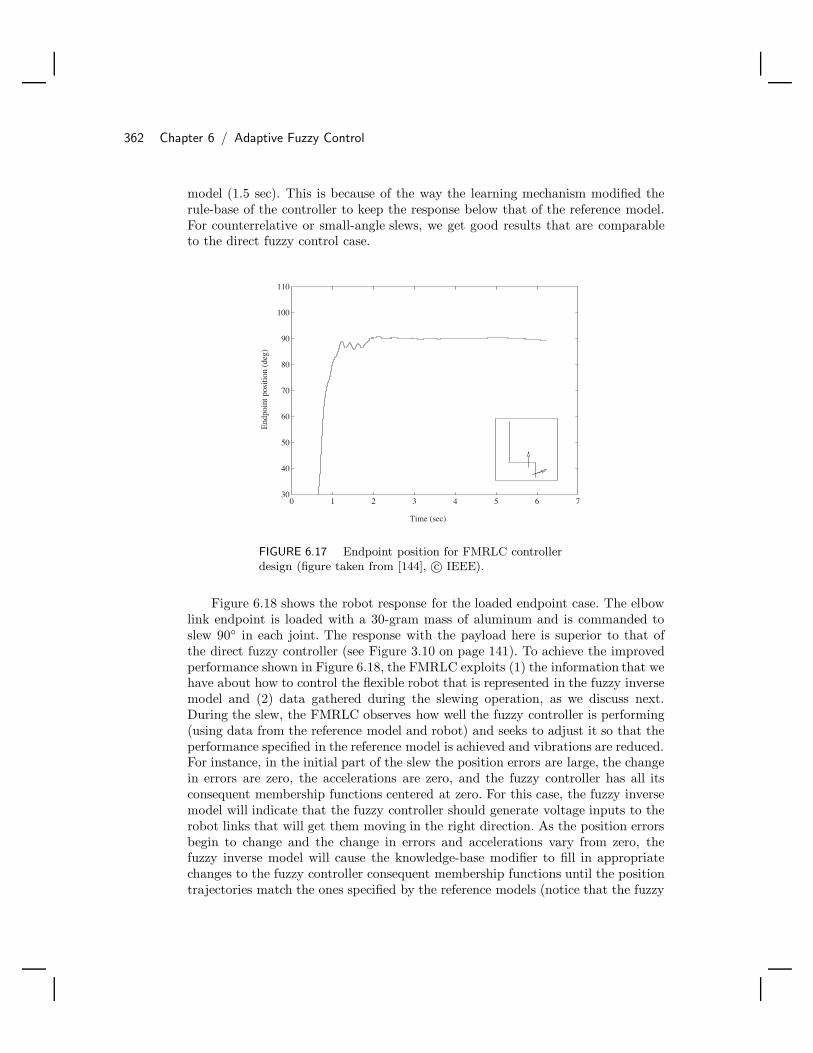
362 Chapter 6 / Adaptive Fuzzy Control
model (1.5 sec). This is because of the way the learning mechanism modified therule-base of the controller to keep the response below that of the reference model.For counterrelative or small-angle slews, we get good results that are comparableto the direct fuzzy control case.
30
40
50
60
70
80
90
100
110
0 1 2 3 4 5 6 7
Time (sec)
End
poin
t pos
ition
(de
g)
FIGURE 6.17 Endpoint position for FMRLC controllerdesign (figure taken from [144], c© IEEE).
Figure 6.18 shows the robot response for the loaded endpoint case. The elbowlink endpoint is loaded with a 30-gram mass of aluminum and is commanded toslew 90 in each joint. The response with the payload here is superior to that ofthe direct fuzzy controller (see Figure 3.10 on page 141). To achieve the improvedperformance shown in Figure 6.18, the FMRLC exploits (1) the information that wehave about how to control the flexible robot that is represented in the fuzzy inversemodel and (2) data gathered during the slewing operation, as we discuss next.During the slew, the FMRLC observes how well the fuzzy controller is performing(using data from the reference model and robot) and seeks to adjust it so that theperformance specified in the reference model is achieved and vibrations are reduced.For instance, in the initial part of the slew the position errors are large, the changein errors are zero, the accelerations are zero, and the fuzzy controller has all itsconsequent membership functions centered at zero. For this case, the fuzzy inversemodel will indicate that the fuzzy controller should generate voltage inputs to therobot links that will get them moving in the right direction. As the position errorsbegin to change and the change in errors and accelerations vary from zero, thefuzzy inverse model will cause the knowledge-base modifier to fill in appropriatechanges to the fuzzy controller consequent membership functions until the positiontrajectories match the ones specified by the reference models (notice that the fuzzy

6.3 FMRLC: Design and Implementation Case Studies 363
inverse model was designed so that it will continually adjust the fuzzy controlleruntil the reference model behavior is achieved). Near the end of the slew (i.e., whenthe links are near their commanded positions), the FMRLC is particularly good atvibration damping since in this case the plant behavior will repeatedly return thesystem to the portion of the fuzzy controller rule-base that was learned the last timea similar oscillation occurred (i.e., the learning capabilities of the FMRLC enableit to develop, remember, and reapply a learned response to plant behaviors).
30
40
50
60
70
80
90
100
110
0 1 2 3 4 5 6 7
Time (sec)
End
poin
t pos
ition
(de
g)
FIGURE 6.18 Endpoint position for loaded elbow link forFMRLC (figure taken from [144], c© IEEE).
Different payloads change the modal frequencies in the link/payload combi-nation (e.g., heavier loads tend to reduce the frequencies of the modes of oscilla-tion) and the shapes of the error and acceleration signals e1(t), e2(t), and a1(t)(e.g., heavier loads tend to slow the plant responses). Hence, changing the payloadsimply results in the FMRLC developing, remembering, and applying different re-sponses depending on the type of the payload variation that occurred. Essentially,the FMRLC uses data from the closed-loop system that is generated during on-lineoperation of the robot to specially tailor the manner in which it designs/tunes thefuzzy controller. This enables it to achieve better performance than the direct fuzzycontroller described in Chapter 3.
Finally, we note that if a series of slews is made we do not use the fuzzycontroller that is learned by the end of one slew to initialize the one that is tunedin the next slew. We found experimentally that it is a bit better to simply zero allthe elements of the rule-base for each slew and have it re-learn the rule-base eachtime. The reason for this is that the fuzzy controller that is learned for a slew is ina sense optimized for the vibration damping near the end of the slew and not the

364 Chapter 6 / Adaptive Fuzzy Control
large angle movements necessary in the initial part of the slew (note that most ofthe time, the rule-base modifications are being made during the vibration dampingphase). This shows that there is some room for improvement of this FMRLC whereadditional inputs to the fuzzy controller may allow it to learn and remember theappropriate controllers in different operating regions so they do not have to bere-learned.
6.4 Dynamically Focused Learning (DFL)As we pointed out at the beginning of Section 6.2, a learning system possesses thecapability to improve its performance over time by interacting with its environment.A learning control system is designed so that its learning controller has the ability toimprove the performance of the closed-loop system by generating command inputsto the plant and utilizing feedback information from the plant. Learning controllersare often designed to mimic the manner in which a human in the control loop wouldlearn how to control a system while it operates. Some characteristics of this humanlearning process may include the following:
1. A natural tendency for the human to focus her or his learning by paying par-ticular attention to the current operating conditions of the system since thesemay be most relevant to determining how to enhance performance.
2. After the human has learned how to control the plant for some operating con-dition, if the operating conditions change, then the best way to control thesystem may have to be relearned.
3. A human with a significant amount of experience at controlling the system inone operating region should not forget this experience if the operating conditionchanges.
To mimic these types of human learning behavior, in this section we introducethree strategies that can be used to dynamically focus a learning controller onto thecurrent operating region of the system. We show how the subsequent “dynamicallyfocused learning” (DFL) can be used to enhance the performance of the FMRLCthat was introduced and applied in the last two sections, and we also performcomparative analysis with a conventional adaptive control technique.
Ultimately, the same overall objectives exist as for the FMRLC. That is, weseek to provide a way to automatically synthesize or tune a direct fuzzy controllersince it may be hard to do so manually or it may become “detuned” while inoperation. With DFL, however, we will be tuning not only the centers of the outputmembership functions, but also the input membership functions of the rules. Amagnetic ball suspension system is used throughout this section to perform thecomparative analyses, and to illustrate the concept of dynamically focused fuzzylearning control.

6.4 Dynamically Focused Learning (DFL) 365
6.4.1 Magnetic Ball Suspension System: Motivation for DFLIn this section we develop a conventional adaptive controller and an FMRLC fora magnetic ball suspension system and perform a comparative analysis to assessthe advantages and disadvantages of each approach. At the end of this section,we highlight certain problems that can arise with the FMRLC and use these asmotivation for the dynamically focused learning enhancement to the FMRLC.
Magnetic Ball Suspension System
The model of the magnetic ball suspension system shown in Figure 6.19 is given by[102]
Md2y(t)dt2
= Mg − i2(t)y(t)
v(t) = Ri(t) + Ldi(t)dt
(6.25)
where y(t) is the ball position in meters, M = 0.1 kg is the ball mass, g = 9.8m/s2 is the gravitational acceleration, R = 50 Ω is the winding resistance, L = 0.5Henrys is the winding inductance, v(t) is the input voltage, and i(t) is the windingcurrent. The position of the ball is detected by a position sensor (e.g., an infrared,microwave, or photoresistive sensor) and is assumed to be fully detectable over theentire range between the magnetic coil and the ground level. We assume that theball will stay between the coil and the ground level (and simulate the system thisway). In state-space form, Equation (6.25) becomes
dx1(t)dt
= x2(t)
dx2(t)dt
= g − x23(t)
Mx1(t)dx3(t)
dt= −R
Lx3(t) +
1L
v(t) (6.26)
where [x1(t), x2(t), x3(t)] = [y(t), dy(t)dt , i(t)]. Notice that the nonlinearities are
induced by the x23(t) and 1
x1(t)terms in the dx2(t)
dt equation. By linearizing the plantmodel in Equation (6.26), assuming that the ball is initially located at x1(0) = y(0),we can find a linear system by calculating the Jacobian matrix at y(0). The linearstate-space form of the magnetic ball suspension system is given as
dx1(t)dt
= x2(t)
dx2(t)dt
=g
y(0)x1(t) − 2
√g
My(0)x3(t)
dx3(t)dt
= −R
Lx3(t) +
1L
v(t) (6.27)

366 Chapter 6 / Adaptive Fuzzy Control
0.3 m
Magnet coil (R, L )
Input current i(t)
y(t)
d = 0.03 m
+
−Input voltage v(t)
Ball (M )
Ground level
Infrared or microwave sensor
FIGURE 6.19 Magnetic ball suspensionsystem (figure taken from [103], c© IEEE).
Since the ball position y(t) is the only physical output of the plant, by assumingthat all initial conditions are zero for the linear perturbation model, we can rewritethe model as a transfer function
Y (s)V (s)
=− 2
L
√g
My(0)
(s2 − gy(0))(s + R
L )(6.28)
Note that there are three poles (two stable and one unstable) and no zeros in thetransfer function in Equation (6.28). Two poles (one stable and one unstable) andthe DC gain change based on the initial position of the ball so that the systemdynamics will vary significantly depending on the location of the ball. From Fig-ure 6.19, the total distance between the magnetic coil and the ground level is 0.3m, and the diameter of the ball is 0.03 m. Thus, the total allowable travel is 0.27 m,and the initial position of the ball y(0) can be anywhere between 0.015 m (touchingthe coil) and 0.285 m (touching the ground). For this range the numerator of thetransfer function
− 2L
√g
My(0)
varies from −323.3 (ball at 0.015 m) to −74.17 (ball at 0.285 m), while the twopoles move from ±25.56 to ±5.864.
Clearly, then, the position of the ball will affect our ability to control it. If it isclose to the coil it may be difficult to control since the unstable pole moves fartherout into the right-half plane, while if it is near the ground level it is easier to control.The effect of the ball position on the plant dynamics can cause problems with theapplication of fixed linear controllers (e.g., ones designed with root locus or Bodetechniques that assume the plant parameters are fixed). It is for this reason thatwe investigate the use of a conventional adaptive controller and the FMRLC forthis control problem. We emphasize, however, that our primary concern is not withthe determination of the best control approach for the magnetic ball suspensionsystem; we simply use this system as an example to compare control approaches
6.4 Dynamically Focused Learning (DFL) 367
and to illustrate the ideas in this section.
Conventional Adaptive Control
In this section a model reference adaptive controller (MRAC) is designed for themagnetic ball suspension system. The particular type of MRAC we use is describedin [180] (on p. 125); it uses the so-called “indirect” approach to adaptive controlwhere the updates to the controller are made by first identifying the plant param-eters. To design the MRAC, a linear model is required. To make the linear modelmost representative of the range of dynamics of the nonlinear plant, we assumethat the ball is initialized at the middle between the magnetic coil and the groundlevel where y(0) = 0.15 m to perform our linearization. In order to simplify theMRAC design, we will assume that the plant is second-order by neglecting the poleat −100 since its dynamics are much faster than the remaining roots in the plant.We found via simulation that the use of this second-order linear model has no sig-nificant effect on the low-frequency responses compared to the original third-orderlinear model. Hence, the transfer function of the system is rewritten as (note thatthe DC gain term kp is changed accordingly)
Y (s)V (s)
=−1.022
s2 − 65.33(6.29)
A reference model is used to specify the desired closed-loop system behavior. Here,the reference model is chosen to be
−25s2 + 10s + 25
(6.30)
This choice reflects our desire to have the closed-loop response with minimal over-shoot, zero steady-state error, and yet a stable, fast response to a reference input.Moreover, to ensure that the “matching equality” is achieved (i.e., that there willexist a set of controller parameters that can achieve the behavior specified in thereference model [180]) we choose the order of the reference model to be the sameas that of the plant.
We use a “normalized gradient algorithm with projection” [180] to update theparameters of a controller. Since the plant is assumed to be second-order, based onthe theory of persistency of excitation [180], the identifier parameters will convergeto their true values if an input that is “sufficiently rich” of an order that is atleast twice the order of the system is used. Therefore, an input composed of thesum of two sinusoids will be used to obtain richness of order four according to thetheory. In order to pick the two sinusoids as the input, it would be beneficial tostudy the frequency response of the plant model. The way to pick the inputs isthat the frequency selected should be able to excite most of the frequency rangewe are interested in. A Bode plot of the third-order linear system suggested thatthe cutoff frequency (3dB cutoff) of the plant is about 6 rad/sec. Hence, we pickedtwo sinusoids (1 rad/sec and 10 rad/sec) to cover the most critical frequency range.

368 Chapter 6 / Adaptive Fuzzy Control
The amplitude of the input is chosen to force the system, as well as the referencemodel, to swing approximately between ±0.05 m around the initial ball position(i.e., at 0.15 m, where the total length of the system is 0.3 m); hence, we chooser(t) = 0.05(sin(1t) + sin(10t)). Note that this input will drive the system intodifferent operating conditions where the plant behavior will change due to thenonlinearities.
Next, the adaptive controller will be simulated with two different plant modelsto demonstrate the closed-loop performance. The two plant models used are (1)the second-order linear model, and (2) the original nonlinear system (i.e, Equa-tion (6.26)).
Second-Order Linear Plant: With an appropriate choice for the adaptationgains, we get the responses shown in Figure 6.20, where the identifier error ei = yi−y(where yi is the output of the identifier model) is approaching zero in 0.5 sec, whilethe plant output error eo = ym − y is still slowly converging after 20 sec (i.e.,swinging between ±0.005 m) but y(t) is capable of matching the response specifiedby the reference model in about 15 sec. Notice that there is a fairly large transientperiod in the first 2 seconds when both the identifier and the controller parametersare varying widely. We see that the system response is approaching the one specifiedby the reference model, but the convergence rate is quite slow (even with relativelylarge adaptation gains). Note that the voltage input v in Figure 6.20 is of acceptablemagnitude compared with the implementation in [15]; in fact, all control strategiesstudied in this case study produced acceptable voltage control inputs to the plantcompared to [15].
0 5 10 15 20Time (sec)
-0.1
-0.05
0
Met
ers
Identifier errorOutput error
0 5 10 15 20Time (sec)
0
10
20
Vol
ts
0 5 10 15 20Time (sec)
0.1
0.15
0.2
Met
ers
PlantReference model
Ball position (y ) Voltage input (v ) Identifier and output error (e ,e )i o
FIGURE 6.20 Responses using MRAC design (reduced order linear model, sinusoidalinput sequence) (figure taken from [103], c© IEEE).
Nonlinear Plant: In this section, the adaptive controller will be simulated withthe nonlinear model of the ball suspension system with the same controller andinitial conditions so that the ball starts at 0.15 m. Figure 6.21 shows the responsesfor the nonlinear model. It is observed that the ball first drops to the ground levelsince the adaptation mechanism is slow and it cannot keep up with the fast-movingsystem. After about 2.5 sec, the system starts to recover and tries to keep up withthe plant. The identifier error ei dies down after about 5 sec to where it swingsbetween ±0.001 m; however, the plant output error swings between ±0.03 m and

6.4 Dynamically Focused Learning (DFL) 369
appears to maintain at the same level (i.e., the plant output never perfectly matchesthat of the reference model). The plant output is not capable of matching the onespecified by the reference model mainly because the indirect adaptive controller isnot designed for the nonlinear model. We also observe that the ball position reactsbetter in the range where the ball is close to the ground level (0.3 m), whereas theresponse gets worse in the range where the ball is close to the magnetic coil (0 m)(i.e., the nonzero identifier error is found and the control input is more oscillatoryin the instants when the ball position is closer to 0 m). This behavior is due tothe nature of the nonlinear plant, where the system dynamics vary significantlywith the ball position, and the adaptive mechanism is not fast enough to adapt thecontroller parameters with respect to the system dynamics.
0 5 10 15 20Time (sec)
0.1
0.2
Met
ers
PlantReference model
0 5 10 15 20Time (sec)
-0.1
0
Met
ers
Identifier errorOutput error
0 5 10 15 20Time (sec)
0
10
20
30
Vol
ts
Ball position (y ) Voltage input (v ) Identifier and output error (e ,e )i o
FIGURE 6.21 Responses for MRAC design (nonlinear model, sinusoidal inputsequence) (figure taken from [103], c© IEEE).
In order to keep the ball from falling to the ground level or lifting up to the coil,one approach is to apply the previously adapted controller parameters to initializethe adaptive controller. It is hoped that this initialization process would help theadaptation mechanism to keep up with the plant dynamics at the beginning of thesimulation. As shown in Figure 6.22, when this approach is employed, the ball doesnot fall to the ground level (compared to Figure 6.21). Despite the fact that thesystem appears to be stable, the identifier error does not approach zero and swingsbetween ±0.001 m and the plant output error swings between ±0.03 m (i.e., theclosed-loop response of the plant is still not matching that of the reference model).
0 5 10 15 20Time (sec)
-0.06
-0.04
-0.02
0
0.02
Met
ers
Identifier errorOutput error
0 5 10 15 20Time (sec)
0
10
20
30
Vol
ts
0 5 10 15 20Time (sec)
0.1
0.15
0.2
Met
ers
PlantReference model
Ball position (y ) Voltage input (v ) Identifier and output error (e ,e )i o
FIGURE 6.22 Responses for MRAC design after “training” (nonlinear model,sinusoidal input sequence) (figure taken from [103], c© IEEE).

370 Chapter 6 / Adaptive Fuzzy Control
Unfortunately, if a step input sequence is used as the reference input to thenonlinear plant, as shown in Figure 6.23, the MRAC does a very poor job of fol-lowing the reference model. However, the DFL strategies will significantly improveon this performance.
0 5 10 15 20Time (sec)
0.1
0.15
0.2
Met
ers
PlantReference model
0 5 10 15 20Time (sec)
-0.06
-0.04
-0.02
0
0.02
Met
ers
Identifier errorOutput error
0 5 10 15 20Time (sec)
0
10
20
30
Vol
ts
Ball position (y ) Voltage input (v ) Identifier and output error (e ,e )i o
FIGURE 6.23 Responses for MRAC (nonlinear model, step input sequence) (figuretaken from [103], c© IEEE).
Fuzzy Model Reference Learning Control
In this section, the FMRLC will be designed for the magnetic ball suspension sys-tem. Note that the design of the FMRLC does not require the use of a linear plantmodel, and thus from now on we will always use the nonlinear model of the mag-netic ball suspension system. The fuzzy controller uses the error signal e(kT ) =r(kT ) − y(kT ) and the change in error of the ball position c(kT ) = e(kT )−e(kT−T )
Tto decide what voltage to apply so that y(kT ) → r(kT ) as k → ∞. For our fuzzycontroller design, the gains ge, gc, and gv were employed to normalize the universeof discourse for the error e(kT ), change in error c(kT ), and controller output v(kT ),respectively. The gain ge is chosen so that the range of values of gee(kT ) lies on[−1, 1], and gv is chosen by using the allowed range of inputs to the plant in asimilar way. The gain gc is determined by experimenting with various inputs to thesystem to determine the normal range of values that c(kT ) will take on; then gc ischosen so that this range of values is scaled to [−1, 1]. According to this procedure,the universes of discourse of the inputs to the fuzzy controller e(t) and c(t) arechosen to be [−0.275, 0.275] and [−2.0, 2.0], respectively. This choice is made basedon the distance between the coil and ground level of the magnetic ball suspensionsystem and an estimate of the maximum attainable velocity of the ball that weobtain via simulations. Thus, the gains ge and gc are 1
0.275 and 12 , respectively. The
output gain gv is then chosen to be 30, which is the maximum voltage we typicallywould like to apply to the plant.
We utilize one MISO fuzzy controller, which has a rule-base of If-Then controlrules of the form
If e is Ea and c is Cb Then v is V a,b

6.4 Dynamically Focused Learning (DFL) 371
where e and c denote the linguistic variables associated with controller inputs e(kT )and c(kT ), respectively; v denotes the linguistic variable associated with the con-troller output v; Ea denotes the ath linguistic value associated with e; Cb denotesthe bth linguistic value associated with c; and V a,b denotes the consequent linguis-tic value associated with v. We use 11 fuzzy sets (triangular-shaped membershipfunction with base widths of 0.4) on the normalized universes of discourse for e(kT )and c(kT ), as shown in Figure 6.24(a).
V a,b
C b
-5-4-3-2-1012345
E a
-5 -4 -3 -2 -1 0 1 2 3 4 5
1
e(kT)
c(kT)
1
Degree of certainty
0.5
v(kT)
1
1-1
−1
-0.5 0
0
C 0
Degree of certainty
V a,b
(a)
Index b ofinput
membershipfunctions on
c(kT)
Index a ofinput
membershipfunctions on
e(kT)
0.5-0.5
E 0
C 4 C 5C -4C -5
E 4 E 5E -4E -5
-1.0-0.8-0.6-0.4-0.20.00.20.40.60.81.0
-1.0 -0.8 -0.6 -0.4 -0.2 0.0 0.2 0.4 0.6 0.8 1.00 0 0 0 0 0 0 0 0 0 0
0 0 0 0 0 0 0 0 0 0 0
0 0 0 0 0 0 0 0 0 0 0
0 0 0 0 0 0 0 0 0 0 0
0 0 0 0 0 0 0 0 0.5 0.5 0
0 0 0 0 0 0 0 0 0 0 0
0 0 0 0 0 0 0 0 0 0 0
0 0 0 0 0 0 0 0 0 0 0
0 0 0 0 0 0 0 0 0 0 0
0 0 0 0 0 0 0 0 0 0 0
0 0 0 0 0 0 0 0 0 0 0
(b)
Center ofoutput
membershipfunctions on
v(kT)
Center valuesafter update
Center ofinput
membershipfunctions on
c(kT)
Center ofinput
membershipfunctions on
e(kT)
FIGURE 6.24 Input-output universes of discourse and rule-base for the fuzzy controller(figure taken from [103], c© IEEE).
Assume that we use the same fuzzy sets on the c(kT ) normalized universesof discourse (i.e., Cb = Ea). As shown in Figure 6.24(a), we initialize the fuzzycontroller knowledge-base with 121 rules (using all possible combinations of rules)where all the right-hand-side membership functions are triangular with base widthsof 0.2 and centers at zero.
We use a discretized version of the same reference model as was used for theMRAC of the previous section for the conventional MRAC. The performance of theoverall system is computed with respect to the reference model by generating errorsignals
ye(kT ) = ym(kT ) − y(kT )
and
yc(kT ) =ye(kT ) − ye(kT − T )
T
The fuzzy inverse model is set up similar to the fuzzy controller with the sameinput membership functions as in Figure 6.24 for ye(kT ) and yc(kT ), but thereare 21 triangular output membership functions that are uniformly spaced across a

372 Chapter 6 / Adaptive Fuzzy Control
[−1, 1] effective universe of discourse. The rule-base is chosen so that it representsthe knowledge of how to update the controller when the error, the change of errorbetween the reference model, and the plant output are given. In particular, thecenters of the membership functions for Y a,b
f (the inverse model output membershipfunctions) are given by
−(a + b)10
so that the rule-base has a similar form to the one in Table 6.1 on page 338 but hasdifferent off-diagonal terms. The gains of the fuzzy inverse model are then initiallychosen to be gye = 1
0.275 , gyc = 0.5, and gf = 30. Note that all the gains arechosen based on the physical properties of the plant, so that gye = ge, gyc = gc,and gf = gv (more details on the rationale and justification for this choice for thegains is provided in Section 6.2).
According to the second design procedure in Section 6.2.3, a step input can beused to tune the gains gc and gyc of the FMRLC. Here, we chose a step responsesequence. Notice in the ball position plot in Figure 6.25 that the FMRLC design wasquite successful in generating the control rules such that the ball position tracks thereference model almost perfectly. It is important to note that the FMRLC designhere required no iteration on the design process. However, this is not necessarilytrue in general, and some tuning is most often needed for different applications.
0 5 10 15 20Time (sec)
-0.02
-0.01
0
Met
ers
0 5 10 15 20Time (sec)
0
10
20
30
Vol
ts
0 5 10 15 20Time (sec)
0.1
0.12
0.14
0.16
0.18
0.2
Met
ers
PlantReferencemodel
Ball position (y ) Voltage input (v ) Output error (y )e
FIGURE 6.25 Responses for FMRLC (step input sequence) (figure taken from [103],c© IEEE).
While the FMRLC seems quite successful, it is possible that there exists aninput sequence that will cause the FMRLC to fail since stability of the FMRLCdepends on the input (as it does for all nonlinear systems). For example, if thesinusoidal input sequence r(t) = 0.05(sin(1t)+sin(10t)) is used (as it was used in theadaptive controller design), the plant response is unstable, as shown in Figure 6.26,in the sense that the ball hits the coil and stays there. Notice that the ball hits thecoil and even with a small (or zero) voltage is held there; this is a characteristicof the somewhat academic plant model, the saturations due to restricting the ballmovements between the coil and ground level, and the way that the system issimulated. Although exhaustive tuning of the gains (except ge, gv, gye , and gf since

6.4 Dynamically Focused Learning (DFL) 373
we artificially consider these to be set by the physical system) are performed toimprove the FMRLC, Figure 6.26 indeed shows one of the best responses we canobtain.
0 5 10 15 20Time (sec)
0
20
40
60
80
Vol
ts
0 5 10 15 20Time (sec)
0
0.05
0.1
0.15
Met
ers
0 5 10 15 20Time (sec)
0.05
0.1
0.15
0.2
Met
ers
PlantReference model
Ball position (y ) Voltage input (v ) Output error (y )e
FIGURE 6.26 Responses for FMRLC (sinusoidal input sequence) (figure taken from[103], c© IEEE).
Motivation for Dynamically Focused Learning
To gain better insight into why the FMRLC fails, in Figure 6.27 we show the learnedrule-base of the fuzzy controller in the FMRLC (after the step input sequencein Figure 6.25 is applied to the system for 20 sec). This shows that the fuzzycontroller actually utilized only 9 of the 121 possible rules. In fact, the 9 rules thatare learned lie within the center section. With such a small number of rules, thelearning mechanism of the FMRLC performed inadequately because the resultingcontrol surface can capture only very approximate control actions. In other words,for more complicated control actions, such a rule-base may not be able to force theplant to follow the reference model closely.
To improve FMRLC performance, one possible solution is to redesign the con-troller so that the rule-base has enough membership functions at the center, wherethe most learning is needed. Yet, we will not consider this approach because theresulting controller will then be limited to a specific range of the inputs that hap-pen to have been generated for the particular reference input sequence. Anotherpossible solution is to increase the number of rules (by increasing the number ofmembership functions on each input universe of discourse) used by the fuzzy con-troller. Therefore, the total number of rules (for all combinations) is also increased,and we enhance the capability of the rule-base to memorize more distinct controlactions (i.e., to achieve “fine control”).
For instance, if we increase the number of membership functions on each inputuniverse of discourse from 11 to, say 101 (but keeping all other parameters, suchas the scaling gains, the same), the total number of rules will increase from 121to 10,201—that is, there is a two order of magnitude increase in the number ofrules (we chose this number of membership functions by trial and error and foundthat further increases in the number of membership functions had very little effecton performance), and we get the responses shown in Figure 6.28 for the FMRLC.

374 Chapter 6 / Adaptive Fuzzy Control
-1.0 -0.8 -0.6 -0.4 -0.2 0.0 0.2 0.4 0.6 0.8 1.0
-1.0
-0.8
-0.6
-0.4
-0.2
0.0
0.2
0.4
0.6
0.8
1.0
0.0
0.0
0.0
0.0
0.0
0.0
0.0
0.0
0.0
0.0
0.0
0.0
0.0
0.0
0.0
0.0
0.0
0.0
0.0
0.0
0.0
0.0
0.0
0.0
0.0
0.0
0.0
0.0
0.0
0.0
0.0
0.0
0.0
0.0
0.0
0.0
0.0
0.0
0.0
0.0
0.0
0.0
0.0
0.0
0.0
0.0
0.0
0.0
0.0
0.0
0.0
0.0
0.0
0.0
0.0
0.0
0.0
0.0
0.0
0.0
0.0
0.0
0.0
0.0
0.0
0.0
0.0
0.0
0.0
0.0
0.0
0.0
-0.32 -2.93 -2.60
0.54 0.64 0.10
0.87 3.57 2.70
0.0
0.0
0.0
0.0
0.0
0.0
0.0
0.0
0.0
0.0
0.0
0.0
0.0
0.0
0.0
0.0
0.0
0.0
0.0
0.0
0.0
0.0
0.0
0.0
0.0
0.0
0.0
0.0
0.0
0.0
0.0
0.0
0.0
0.0
0.0
0.0
0.0
0.0
0.0
0.0
Center ofinput
membershipfunctions on
c(kT)
Center ofinput
membershipfunctions on
e(kT)
Center ofoutput
membershipfunctions on
v(kT)
Center valuesafter update
FIGURE 6.27 Rule-base of the learned fuzzy controller (step inputsequence) (figure taken from [103], c© IEEE).
Clearly, as compared to Figure 6.26, we have drastically improved the performanceof the FMRLC to the extent that it performs similarly to the MRAC for the non-linear model (see Figure 6.22). Notice that in Figure 6.28 the output error swingsbetween ±0.027 m even after 15 sec of simulation, and the plant output is oscilla-tory. Longer simulations have shown that this FMRLC appears to be stable, butthe plant cannot perfectly follow the response of the reference model.
Even though we were able to significantly improve performance, enlarging therule-base has many disadvantages: (1) the number of rules increases exponentiallyfor an increase in membership functions and inputs to the fuzzy controller, (2) thecomputational efficiency decreases as the number of rules increases, and (3) a rule-base with a large number of rules will require a long time period for the learningmechanism to fill in the correct control laws since smaller portions of the rule-base map in Figure 6.27 will be updated by the FMRLC for a higher-granularityrule-base (unless, of course, you raise the adaptation gain). Hence, the advantagesof increasing the number of rules will soon be offset by practical implementationconsiderations and possible degradations in performance.
This motivates the need for special enhancements to the FMRLC so that wecan (1) minimize the number of membership functions and therefore rules used, and(2) at the same time, maximize the granularity of the rule-base near the point wherethe system is operating (e.g., the center region of the rule-base map in Figure 6.27)so that very effective learning can take place.
FMRLC Learning Dynamics
Before introducing the DFL strategies that will try to more effectively use the rules,we clarify several issues in FMRLC learning dynamics including the following: (1)the effects of gains on linguistic values, and (2) characteristics of the rule-base such
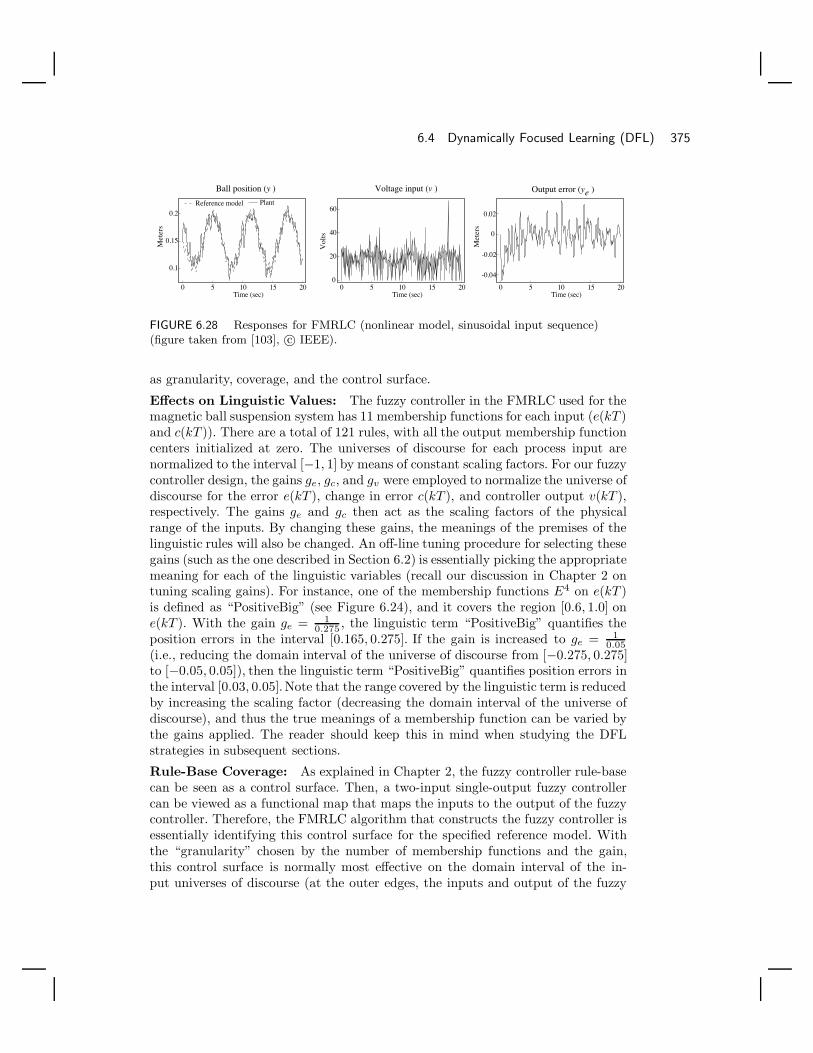
6.4 Dynamically Focused Learning (DFL) 375
0 5 10 15 20Time (sec)
0.1
0.15
0.2
Met
ers
PlantReference model
0 5 10 15 20Time (sec)
-0.04
-0.02
0
0.02
Met
ers
0 5 10 15 20Time (sec)
0
20
40
60
Vol
ts
Ball position (y ) Voltage input (v ) Output error (y )e
FIGURE 6.28 Responses for FMRLC (nonlinear model, sinusoidal input sequence)(figure taken from [103], c© IEEE).
as granularity, coverage, and the control surface.
Effects on Linguistic Values: The fuzzy controller in the FMRLC used for themagnetic ball suspension system has 11 membership functions for each input (e(kT )and c(kT )). There are a total of 121 rules, with all the output membership functioncenters initialized at zero. The universes of discourse for each process input arenormalized to the interval [−1, 1] by means of constant scaling factors. For our fuzzycontroller design, the gains ge, gc, and gv were employed to normalize the universe ofdiscourse for the error e(kT ), change in error c(kT ), and controller output v(kT ),respectively. The gains ge and gc then act as the scaling factors of the physicalrange of the inputs. By changing these gains, the meanings of the premises of thelinguistic rules will also be changed. An off-line tuning procedure for selecting thesegains (such as the one described in Section 6.2) is essentially picking the appropriatemeaning for each of the linguistic variables (recall our discussion in Chapter 2 ontuning scaling gains). For instance, one of the membership functions E4 on e(kT )is defined as “PositiveBig” (see Figure 6.24), and it covers the region [0.6, 1.0] one(kT ). With the gain ge = 1
0.275 , the linguistic term “PositiveBig” quantifies theposition errors in the interval [0.165, 0.275]. If the gain is increased to ge = 1
0.05(i.e., reducing the domain interval of the universe of discourse from [−0.275, 0.275]to [−0.05, 0.05]), then the linguistic term “PositiveBig” quantifies position errors inthe interval [0.03, 0.05].Note that the range covered by the linguistic term is reducedby increasing the scaling factor (decreasing the domain interval of the universe ofdiscourse), and thus the true meanings of a membership function can be varied bythe gains applied. The reader should keep this in mind when studying the DFLstrategies in subsequent sections.
Rule-Base Coverage: As explained in Chapter 2, the fuzzy controller rule-basecan be seen as a control surface. Then, a two-input single-output fuzzy controllercan be viewed as a functional map that maps the inputs to the output of the fuzzycontroller. Therefore, the FMRLC algorithm that constructs the fuzzy controller isessentially identifying this control surface for the specified reference model. Withthe “granularity” chosen by the number of membership functions and the gain,this control surface is normally most effective on the domain interval of the in-put universes of discourse (at the outer edges, the inputs and output of the fuzzy
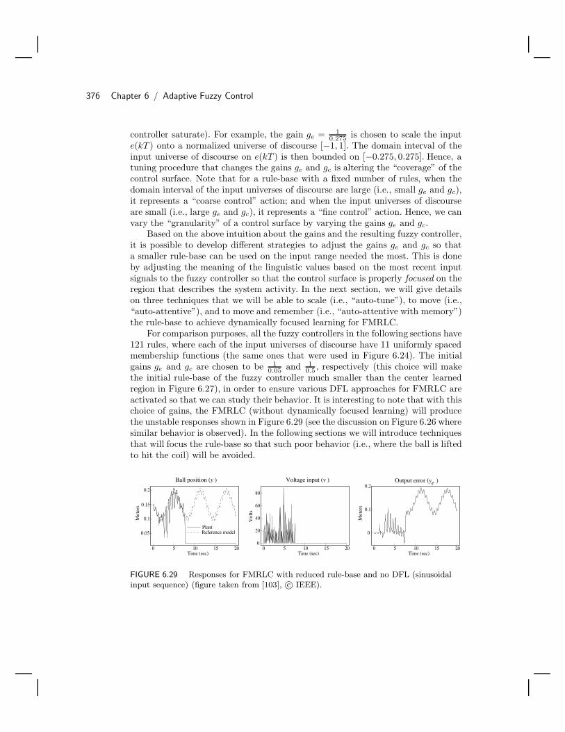
376 Chapter 6 / Adaptive Fuzzy Control
controller saturate). For example, the gain ge = 10.275 is chosen to scale the input
e(kT ) onto a normalized universe of discourse [−1, 1]. The domain interval of theinput universe of discourse on e(kT ) is then bounded on [−0.275, 0.275]. Hence, atuning procedure that changes the gains ge and gc is altering the “coverage” of thecontrol surface. Note that for a rule-base with a fixed number of rules, when thedomain interval of the input universes of discourse are large (i.e., small ge and gc),it represents a “coarse control” action; and when the input universes of discourseare small (i.e., large ge and gc), it represents a “fine control” action. Hence, we canvary the “granularity” of a control surface by varying the gains ge and gc.
Based on the above intuition about the gains and the resulting fuzzy controller,it is possible to develop different strategies to adjust the gains ge and gc so thata smaller rule-base can be used on the input range needed the most. This is doneby adjusting the meaning of the linguistic values based on the most recent inputsignals to the fuzzy controller so that the control surface is properly focused on theregion that describes the system activity. In the next section, we will give detailson three techniques that we will be able to scale (i.e., “auto-tune”), to move (i.e.,“auto-attentive”), and to move and remember (i.e., “auto-attentive with memory”)the rule-base to achieve dynamically focused learning for FMRLC.
For comparison purposes, all the fuzzy controllers in the following sections have121 rules, where each of the input universes of discourse have 11 uniformly spacedmembership functions (the same ones that were used in Figure 6.24). The initialgains ge and gc are chosen to be 1
0.05 and 10.5 , respectively (this choice will make
the initial rule-base of the fuzzy controller much smaller than the center learnedregion in Figure 6.27), in order to ensure various DFL approaches for FMRLC areactivated so that we can study their behavior. It is interesting to note that with thischoice of gains, the FMRLC (without dynamically focused learning) will producethe unstable responses shown in Figure 6.29 (see the discussion on Figure 6.26 wheresimilar behavior is observed). In the following sections we will introduce techniquesthat will focus the rule-base so that such poor behavior (i.e., where the ball is liftedto hit the coil) will be avoided.
0 5 10 15 20Time (sec)
0
20
40
60
80
Vol
ts
0 5 10 15 20Time (sec)
0
0.1
0.2
Met
ers
0 5 10 15 20Time (sec)
0.05
0.1
0.15
0.2
Met
ers
PlantReference model
Ball position (y ) Voltage input (v ) Output error (y )e
FIGURE 6.29 Responses for FMRLC with reduced rule-base and no DFL (sinusoidalinput sequence) (figure taken from [103], c© IEEE).

6.4 Dynamically Focused Learning (DFL) 377
6.4.2 Auto-Tuning MechanismIn the standard FMRLC design for the magnetic ball suspension system, the inputsequence does not excite the whole range of the designated input universes of dis-course (see Figure 6.27). Instead, the rule-base learned for the input sequence onlycovered the center part of the rule-base. Hence, to achieve an adequate numberof rules to enhance the granularity of the rule-base near the center, it would benecessary to design the rule-base so that it is located at exactly where most of therules are needed. However, we would like to ensure that we can adapt the fuzzyrule-base should a different input sequence drive the operation of the system out ofthis center region.
Auto-Tuning
Based on our experience in tuning the FMRLC, it is often observed that the gainsge and gc are chosen as bounds on the inputs to the controller so that the rule-baserepresents the active region of the control actions (e.g., see the cargo ship FMRLCdesign example in Section 6.3.1 on page 333). We base our on-line auto-tuningstrategy for the input scaling gains on this idea. Let the maximum of each fuzzycontroller input over a time interval (window) of the last TA seconds be denotedby maxTAe(kT ) and maxTAc(kT ). Then this maximum value is defined as thegain of each input e(kT ) and c(kT ) so that
ge =1
maxTAe(kT )
and
gc =1
maxTAc(kT )
For the magnetic ball suspension system, after some experimentation, we choseTA = 0.1 sec (it was found via simulations that any TA ∈ [0.05, 0.3] sec can beused equally effectively). Longer time windows tend to slow down the auto-tuningaction; while a shorter window often speeds up the auto-tuning, but the resultingcontrol is more oscillatory. Once the gains are changed, it is expected that thelearning mechanism of the FMRLC will adjust the rules accordingly when they arereactivated, because the scaling will alter all the rules in the rule-base.
Note that the learning process now involves two individual, distinct compo-nents: (1) the FMRLC learning mechanism that fills in the appropriate consequentsfor the rules, and (2) the auto-tuning mechanism (i.e., an adaptation mechanism)that scales the gains that actually redefine the premise membership functions. Nor-mally, we make the learning mechanism operate “at a higher rate” than the auto-tuning mechanism for the premise membership functions in order to try to assurestability. If the auto-tuning mechanism is designed to be “faster” than the FMRLClearning mechanism, the learning mechanism will not be able to keep up with thechanges made by the auto-tuning mechanism so it will never be able to learn the

378 Chapter 6 / Adaptive Fuzzy Control
rule-base correctly. The different rates in learning and adaptation can be achievedby adjusting the sampling period T of the FMRLC and the window length TA ofthe auto-tuning mechanism.
-1.0 -0.8 -0.6 -0.4 -0.2 0.0 0.2 0.4 0.6 0.8 1.0
-1.0
-0.8
-0.6
-0.4
-0.2
0.0
0.2
0.4
0.6
0.8
1.0
-1.0 -0.9 -0.8 -0.7 -0.6 -0.5 -0.4 -0.3 -0.2 -0.1 0.0
-0.9 -0.8 -0.7 -0.6 -0.5 -0.4 -0.3 -0.2 -0.1 0.0 0.1
-0.8 -0.7 -0.6 -0.5 -0.4 -0.3 -0.2 -0.1 0.0 0.1 0.2
-0.7 -0.6 -0.5 -0.4 -0.3 -0.2 -0.1 0.0 0.1 0.2 0.3
-0.6 -0.5 -0.4 -0.3 -0.2 -0.1 0.0 0.1 0.2 0.3 0.4
-0.5 -0.4 -0.3 -0.2 -0.1 0.0 0.1 0.2 0.3 0.4 0.5
-0.4 -0.3 -0.2 -0.1 0.0 0.1 0.2 0.3 0.4 0.5 0.6
-0.3 -0.2 -0.1 0.0 0.1 0.2 0.3 0.4 0.5 0.6 0.7
-0.2 -0.1 0.0 0.1 0.2 0.3 0.4 0.5 0.6 0.7 0.8
-0.1 0.0 0.1 0.2 0.3 0.4 0.5 0.6 0.7 0.8 0.9
0.0 0.1 0.2 0.3 0.4 0.5 0.6 0.7 0.8 0.9 1.0
-2.0
-1.6
-1.2
-0.8
-0.4
0.0
1.6
0.4
1.2
0.8
2.0
-2.0 -1.6 -1.2 -0.8 -0.4 0.0 1.60.4 1.20.8 2.0
Center of inputmembership
functions afterauto-tuning
Center of inputmembershipfunctions on
c(kT)Center of
inputmembershipfunctions on
e(kT)
Center ofoutput
membershipfunctions on
v(kT)
FIGURE 6.30 Dynamics of auto-tuning for FMRLC (figure taken from [103],c© IEEE).
Figure 6.30 illustrates how the gain scaling implemented by auto-tuning affectsthe input membership functions. Note that the center of the output membershipfunctions defined on the v(kT ) universe of discourse in Figure 6.30 are filled witha “standard” set of rules such that they represent a typical choice (for illustrationpurposes) from a control engineer’s experience for the fuzzy controller. For example,at the beginning, the centers of each of the input membership functions are shownin the rule-base in Figure 6.30. In the next time instant, if the values maxTAe(kT )and maxTAc(kT ) are halved, the gains
ge =1
maxTAe(kT )
and
gc =1
maxTAc(kT )
are now doubled. Then, the overall effect is that each of the membership functions

6.4 Dynamically Focused Learning (DFL) 379
on the input universes of discourse is given a new linguistic meaning, and thedomain of the control surface is expanded as shown by the centers of each inputmembership function after the auto-tuning action (see Figure 6.30).
Notice that we will require a maximum gain value; otherwise, each input uni-verse of discourse for the fuzzy system may be reduced to zero (where the gains ge
and gc go to infinity) so that controller stability is not maintained. For the magneticball suspension system, the maximum gain is chosen to be the same as the initialvalue (i.e., ge = 1
0.05 and gc = 10.5). Other gains gv, gye , gyc and gf (the gain on the
output of the model) are the same as those used in the standard FMRLC.
Auto-Tuning Results
For FMRLC with auto-tuning, Figure 6.31 shows that the ball position can followthe sinusoidal input sequence very closely, although perfect tracking of the refer-ence response is not achieved. However, this result is better than the case whereconventional adaptive control is used (see Figure 6.22), and definitely better thanthe standard FMRLC design (see Figure 6.26). Notice that the results shown inFigure 6.31 are similar to those shown in Figure 6.28, where 10,201 rules are used;however, the auto-tuning approach used only 121 rules. There are extra compu-tations needed to implement the auto-tuning strategy to take the maximum overa time interval in computing the gains. Figure 6.32 shows excellent responses forthe same auto-tuned FMRLC with the step input sequence where the ball positionfollows the reference model without noticeable difference (compare to Figures 6.23and 6.25 for the MRAC and FMRLC, respectively).
0 5 10 15 20Time (sec)
-0.02
0
0.02
Met
ers
0 5 10 15 20Time (sec)
0
20
40
60
80
Vol
ts
0 5 10 15 20Time (sec)
0.1
0.15
0.2
Met
er
PlantReference model
Ball position (y ) Voltage input (v ) Output error (y )e
FIGURE 6.31 Responses for FMRLC with auto-tuning (sinusoidal input sequence)(figure taken from [103], c© IEEE).
6.4.3 Auto-Attentive MechanismOne of the disadvantages of auto-tuning the FMRLC is that all the rules in therule-base are changed by the scaling of the gains, which may cause distortions inthe rule-base and require the learning mechanism to relearn the appropriate controllaws. Hence, instead of scaling, in this section we will consider moving the entirerule-base with respect to a fixed coordinate system so that the fuzzy controller canautomatically “pay attention” to the current inputs.

380 Chapter 6 / Adaptive Fuzzy Control
0 5 10 15 20Time (sec)
-0.001
0
0.001
Met
ers
0 5 10 15 20Time (sec)
0
10
20
Vol
ts
0 5 10 15 20Time (sec)
0.1
0.12
0.14
0.16
0.18
0.2M
eter
sPlantReference
model
Ball position (y ) Voltage input (v ) Output error (y )e
FIGURE 6.32 Responses for FMRLC with auto-tuning (step input sequence) (figuretaken from [103], c© IEEE).
Auto-Attentive Approach
To explain the auto-attentive mechanism, it is convenient to define some new termsthat are depicted in Figure 6.33. First of all, the rule-base of the fuzzy controlleris considered to be a single cell called the “auto-attentive active region,” and itrepresents a fixed-size rule-base that is chosen by the initial scaling gains (i.e.,ge and gc must be selected a priori). The outermost lightly shaded region of therule-base is defined as the “attention boundary.” The four lightly shaded rules(note that there are at most four rules “on” at one time due to our choice formembership functions shown in Figure 6.24) in the lower right portion of the rule-base are referred as the FMRLC “active learning region”; this is where the rulesare updated by the learning mechanism of the FMRLC. Finally, the white arrow inFigure 6.33 indicates the direction of movement of the active learning region.
-1.0 -0.8 -0.6 -0.4 -0.2 0.0 0.2 0.4 0.6 0.8 1.0
-1.0
-0.8
-0.6
-0.4
-0.2
0.0
0.2
0.4
0.6
0.8
1.0
-1.0 -0.9 -0.8 -0.7 -0.6 -0.5 -0.4 -0.3 -0.2 -0.1 0.0
-0.9 -0.8 -0.7 -0.6 -0.5 -0.4 -0.3 -0.2 -0.1 0.0 0.1
-0.8 -0.7 -0.6 -0.5 -0.4 -0.3 -0.2 -0.1 0.0 0.1 0.2
-0.7 -0.6 -0.5 -0.4 -0.3 -0.2 -0.1 0.0 0.1 0.2 0.3
-0.6 -0.5 -0.4 -0.3 -0.2 -0.1 0.0 0.1 0.2 0.3 0.4
-0.5 -0.4 -0.3 -0.2 -0.1 0.0 0.1 0.2 0.3 0.4 0.5
-0.4 -0.3 -0.2 -0.1 0.0 0.1 0.2 0.3 0.4 0.5 0.6
-0.3 -0.2 -0.1 0.0 0.1 0.2 0.3 0.4 0.5 0.6 0.7
-0.2 -0.1 0.0 0.1 0.2 0.3 0.4 0.5 0.6 0.7 0.8
-0.1 0.0 0.1 0.2 0.3 0.4 0.5 0.6 0.7 0.8 0.9
0.0 0.1 0.2 0.3 0.4 0.5 0.6 0.7 0.8 0.9 1.0
Active learningregion
Attention boundaryfor activating
rule-base movement
Center of inputmembershipfunctions on
e(kT)
Center of outputmembershipfunctions on
v(kT)
Center of inputmembershipfunctions on
c(kT)
Auto-attention activeregion before a
rule-base movement
Direction of themovement of the active
learning region
FIGURE 6.33 Auto-attentive mechanism for FMRLC (before shifting) (figure takenfrom [103], c© IEEE).
For the auto-attentive mechanism, if the FMRLC active learning region moves

6.4 Dynamically Focused Learning (DFL) 381
into the attention boundary, a “rule-base shift” is activated. For example, if theactive learning region hits the lower-right attention boundary, as shown in Fig-ure 6.34, the result is that the rule-base will be shifted down one unit and to theright one unit (i.e., the width of a membership function). We chose the conventionthat shifting the rule-base to the right and downward both correspond to positiveoffsets and shifting the rule-base to the left and upward both correspond to nega-tive offsets. This choice is made to be compatible with the convention used in theinput universes of discourse in the rule-base (as shown in Figures 6.33 and 6.34).Hence, the shift in the rule-base is represented by the “offset” of the rule-base fromits initial position, which is (Eoffset, Coffset) = (1, 1) as shown in Figure 6.34 forthis example. With the offset values, the shift of the rule-base is obtained simplyby adding the offset values to each of the premise membership functions. After therule-base is shifted, the active attention region is moved to the region in the largedashed box shown in Figure 6.34. In the new unexplored region (i.e., the darklyshaded row and column), the consequents of the rules will be filled with zeros sincethis represents that there is no knowledge of how to control in the new region.Another approach would be to extrapolate the values from the adjacent cells sincethis may provide a more accurate guess at the shape of the controller surface.
Conceptually, the rule-base is moving and following the FMRLC active learningregion. We emphasize, however, that if the active learning region never hits theattention boundary, there will never be a rule-base shift and the controller willbehave exactly the same as the standard FMRLC. Overall, we see that the auto-attentive mechanism seeks to keep the controller rule-base focused on the regionwhere the FMRLC is learning how to control the system (one could think of this aswe did with the auto-tuning mechanism as adapting the meaning of the linguisticvalues). If the rule-base shifts frequently, the system will “forget” how to controlin the regions where it used to be, yet learn how to control in the new regionswhere adaptation is needed most. Note that we can consider the width of theattention boundary to be a design parameter, but we found that it is best to set theattention boundary as shown in Figure 6.33 since this choice minimizes oscillationsand unnecessary shifting of the rule-base for this example.
Similar to the auto-tuning DFL strategy, there are two distinct processes here:(1) the FMRLC learning mechanism that fills in appropriate consequents for therules, and (2) the auto-attentive mechanism (another adaptation mechanism) thatmoves the entire rule-base. Moreover, we think of the FMRLC learning mechanismas running at a higher rate compared to the auto-attentive mechanism (in order totry to assure stability), since we only allow a shift of the entire rule-base by a singleunit in any direction in any time instant. The rate of adaptation can be controlledby using a different attention boundary to activate the rule-base movement. Forexample, if the attention boundary shown in Figure 6.33 is in the inner part ofthe rule-base (say, the second outermost region of the rule-base instead of theoutermost region), then the rule-base will be shifted more often and thus increasethe adaptation rate of the auto-attentive mechanism.

382 Chapter 6 / Adaptive Fuzzy Control
-1.0 -0.8 -0.6 -0.4 -0.2 0.0 0.2 0.4 0.6 0.8 1.0
-1.0
-0.8
-0.6
-0.4
-0.2
0.0
0.2
0.4
0.6
0.8
1.0
-1.0 -0.9 -0.8 -0.7 -0.6 -0.5 -0.4 -0.3 -0.2 -0.1 0.0
-0.9 -0.8 -0.7 -0.6 -0.5 -0.4 -0.3 -0.2 -0.1 0.0 0.1
-0.8 -0.7 -0.6 -0.5 -0.4 -0.3 -0.2 -0.1 0.0 0.1 0.2
-0.7 -0.6 -0.5 -0.4 -0.3 -0.2 -0.1 0.0 0.1 0.2 0.3
-0.6 -0.5 -0.4 -0.3 -0.2 -0.1 0.0 0.1 0.2 0.3 0.4
-0.5 -0.4 -0.3 -0.2 -0.1 0.0 0.1 0.2 0.3 0.4 0.5
-0.4 -0.3 -0.2 -0.1 0.0 0.1 0.2 0.3 0.4 0.5 0.6
-0.3 -0.2 -0.1 0.0 0.1 0.2 0.3 0.4 0.5 0.6 0.7
-0.2 -0.1 0.0 0.1 0.2 0.3 0.4 0.5 0.6 0.7 0.8
-0.1 0.0 0.1 0.2 0.3 0.4 0.5 0.6 0.7 0.8 0.9
0.0 0.1 0.2 0.3 0.4 0.5 0.6 0.7 0.8 0.9 1.0
0.0 0.0 0.0 0.0 0.0 0.0 0.0 0.0 0.0 0.0
1.2
0.0
0.0
0.0
0.0
0.0
0.0
0.0
0.0
0.0
0.0
0.01.2
An active learningregion
Offset of indices due torule-base shift:
(Eoffset , Coffset ) = (1, 1)
Center of inputmembershipfunctions on
e(kT)
Center of outputmembershipfunctions on
v(kT)
Center of inputmembershipfunctions on
c(kT)
Auto-attentionactive region aftera rule-base shift
FIGURE 6.34 Auto-attentive mechanism for FMRLC (after shifting) (figure taken from[103], c© IEEE).
Auto-Attentive Mechanism Results
For the magnetic ball suspension system, the input universes of discourse are chosenas [−0.05, 0.05] and [−0.5, 0.5] (i.e., the gains ge and gc are 1
0.05 and 10.5 , respec-
tively), while all the other gains are the same as the ones used in the standardFMRLC design in Section 6.4.1. Figure 6.35 illustrates the performance of the FM-RLC with the auto-attentive mechanism. We see that the ball position can follow theinput sequence very closely, although perfect tracking of the reference model cannotbe achieved (with maximum output error ye within ±0.0078 m), but this result isbetter than the case with the conventional adaptive controller (see Figure 6.22), thestandard FMRLC with 10201 rules (see Figure 6.28) and the auto-tuning FMRLC(see Figure 6.31); and definitely better than the case with the unstable standardFMRLC (see Figure 6.26, where the ball is lifted to the coil).
0 5 10 15 20Time (sec)
-0.006
-0.004
-0.002
0
Met
ers
0 5 10 15 20Time (sec)
0.1
0.15
0.2
Met
ers
PlantReference model
0 5 10 15 20Time (sec)
0
20
40
Vol
ts
Ball position (y ) Voltage input (v ) Output error (y )e
FIGURE 6.35 Responses for FMRLC with auto-attentive mechanism (sinusoidal inputsequence) (figure taken from [103], c© IEEE).

6.4 Dynamically Focused Learning (DFL) 383
To gain insight into the dynamics of the auto-attentive mechanism, Figures 6.36(a)and (b) show the Eoffset and Coffset values throughout the simulation, and Fig-ure 6.36(c) depicts the first five movements of the rule-base. The double arrowsin Figure 6.36(c) denote the movement of the rule-base from the initial position(shown as an empty box) to an outer region (shown as a shaded box), while thenumber next to the shaded box is the rule-base at the next time instant wherethe rule-base moved (the shades also change to deeper gray as time progresses).Hence, the rule-base is actually oscillating about to the (Eoffset, Coffset) origin astime progresses, and it also moves around the initial position in a counterclockwisecircular motion (this motion is induced by the sinusoids that the rule-base is tryingto track). Note that we have done simulation tests for different sizes of the activeattention region for improving the responses from the auto-attentive FMRLC. How-ever, we found that smaller active attention regions result in excessive motion forthe rule-base, while larger auto-attention active regions will have the same low rule-base “granularity” problem as the standard FMRLC. Figure 6.37 shows excellentresponses for the same auto-attentive FMRLC design with a step input sequence,which is basically the same as in the case of standard FMRLC (see Figure 6.25).
0 5 10 15 20Time (sec)
-2
-1
0
1
2
Eoffset Coffset
Eoffset
Coffset
1
2
34
5
Rule-base (initially)
(a) (b) (c)
0 5 10 15 20Time (sec)
-2
0
2
4
FIGURE 6.36 Movement of the rule-base for the auto-attentive mechanism (sinusoidalinput sequence) (figure taken from [103], c© IEEE).
0 5 10 15 20Time (sec)
0.1
0.12
0.14
0.16
0.18
0.2
Met
ers
PlantReferencemodel
0 5 10 15 20Time (sec)
-0.003
-0.002
-0.001
0
Met
ers
0 5 10 15 20Time (sec)
0
10
20
Vol
ts
Ball position (y ) Voltage input (v ) Output error (y )e
FIGURE 6.37 Responses for FMRLC with auto-attentive mechanism (step inputsequence) (figure taken from [103], c© IEEE).

384 Chapter 6 / Adaptive Fuzzy Control
6.4.4 Auto-Attentive Mechanism with MemoryNote that in the auto-attentive DFL strategy, every shift of the rule-base will createa new unexplored region (i.e., the darkly shaded row and column in Figure 6.34).This region will be filled with zeros since this represents that we have no knowledgeof how to control when we move into a new operating condition. Having to learnthe new regions from scratch after every movement of the rule-base can causedegradations in the performance of the auto-attentive FMRLC since it will requirethe learning mechanism to fill in the unknown rules (i.e., additional time for learningwill be needed). For example, if an auto-attentive FMRLC has been operating fora long time on an input sequence, then at some time instant a disturbance affectedthe controller inputs and forced the rule-base to leave its current position, some ofthe rules are lost and replaced by new rules that will accommodate the disturbance.When the temporary disturbance is stopped and the rule-base returns to its initialposition again, its previous experience is lost and it has to “relearn” everythingabout how to control in a region where it actually has gained a significant amountof experience.
Auto-Attentive Approach with Memory
There are two main components to add to the auto-attentive mechanism to obtainthe auto-attentive mechanism with memory. These are the fuzzy experience modeland its update mechanism.
Fuzzy Experience Model: To better reflect the “experience” that a controllergathers, we will introduce a third fuzzy system, which we call the “fuzzy experiencemodel” for the FMRLC, as the memory to record an abstraction of the control lawsthat are in the region previously reached through the auto-attentive mechanism.The rule-base of this fuzzy experience model (i.e., the “experience rule-base”) isused to represent the “global knowledge” of the fuzzy controller. In this case, nomatter how far off the auto-attentive mechanism has offset the rule-base, there is arough knowledge of how to control in any region the controller has visited before. Inother words, this fuzzy controller not only possesses learning capabilities from thelearning mechanism and adaptation abilities from the auto-attentive algorithm; italso maintains a representation of the “experience” it has gathered on how to controlin an additional fuzzy system (an added level of memory and hence learning—withsome imagination you can envision how to add successive nested learning/auto-attentive mechanisms and memory models for the FMRLC).
As shown in Figure 6.38, the fuzzy experience model has two inputs ecenter(kT )and ccenter(kT ), which represent the center of the auto-attentive active region thatis defined on e(kT ) and c(kT ). For our example, these inputs have five symmetric,uniformly spaced membership functions, and there are a total of 25 rules (i.e., 25output membership functions that are initialized at zero). The universes of discoursefor each of these inputs are normalized to the interval [−1, 1] by means of constant
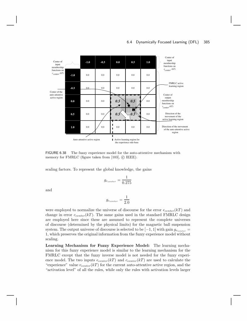
6.4 Dynamically Focused Learning (DFL) 385
-1.0
FMRLC activelearning region
Center ofinput
membershipfunctions onecenter (kT)
Center ofoutput
membershipfunctions onvcenter (kT)
Center ofinput
membershipfunctions onccenter (kT)
Active learning region forthe experience rule-base
Direction of themovement of the
active learning region
-0.5
0.0
0.5
1.0
-1.0 -0.5 0.0 0.5 1.0
0.0 0.0
0.0 0.0
0.0
0.0
0.0
0.0
0.0
0.0
0.0 0.0 0.0
0.0 0.0 0.0
0.5 0.5
0.5 0.5
0.0
0.0
0.0
0.0 0.0 Direction of the movementof the auto-attentive active
region
Auto-attentive active region
Center of theauto-attentiveactive region
FIGURE 6.38 The fuzzy experience model for the auto-attentive mechanism withmemory for FMRLC (figure taken from [103], c© IEEE).
scaling factors. To represent the global knowledge, the gains
gecenter =1
0.275
and
gccenter =1
2.0
were employed to normalize the universe of discourse for the error ecenter(kT ) andchange in error ccenter(kT ). The same gains used in the standard FMRLC designare employed here since these are assumed to represent the complete universesof discourse (determined by the physical limits) for the magnetic ball suspensionsystem. The output universe of discourse is selected to be [−1, 1] with gain gvcenter =1, which preserves the original information from the fuzzy experience model withoutscaling.
Learning Mechanism for Fuzzy Experience Model: The learning mecha-nism for this fuzzy experience model is similar to the learning mechanism for theFMRLC except that the fuzzy inverse model is not needed for the fuzzy experi-ence model. The two inputs ecenter(kT ) and ccenter(kT ) are used to calculate the“experience” value vcenter(kT ) for the current auto-attentive active region, and the“activation level” of all the rules, while only the rules with activation levels larger

386 Chapter 6 / Adaptive Fuzzy Control
than zero will be updated (i.e., the same as the method used in the FMRLC learningmechanism in Section 6.2.3). Each time after the fuzzy controller rule-base (i.e., theauto-attentive active region) is updated, the numerical average value of the auto-attentive rule-base consequent centers, denoted by vcenter(avg)(kT ), will be takenfor the corresponding fuzzy experience model. Hence, the change of the consequentfuzzy sets of the experience rule-base that have premises with nonzero activationlevels, can be computed as
vcenter(chg) = vcenter(avg)(kT ) − vcenter(kT )
and vcenter(chg) is used to update the fuzzy experience model exactly the same wayas the fuzzy controller is updated in Section 6.2.3.
For example, the shaded area in Figure 6.38 (the active learning region for theexperience rule-base) is activated by the inputs ecenter(kT ) and ccenter(kT ) (i.e.,these are the rules that have nonzero activation level). First, assume that the centersof all membership functions on vcenter(kT ) are zero at the beginning, and thus theoutput of the fuzzy experience model vcenter(kT ) is zero. Then, assume we foundvcenter(avg)(kT ) = 0.5 to be the average value of the control surface (i.e., averagevalue of the centers of the output membership functions) for the auto-attentiveactive region; hence, the update of the fuzzy experience model vcenter(chg) = 0.5can be found. Hence, the consequent membership functions of the fuzzy experiencemodel will be shifted to 0.5, as shown in the shaded region of Figure 6.38.
It is obvious that there are numerous other methods to obtain an abstractrepresentation of the rule-base in the auto-attentive active region besides using theaverage. In fact, more complicated methods, such as using least squares to find a lin-ear surface that best fits the control surface, could be used. However, we have foundthat such a method significantly increases the computational complexity withoutmajor performance improvements (at least, for the magnetic ball suspension sys-tem example). Our approach here uses a simple method to represent experienceand hence provides a rough estimate of the unknown control laws.
Using Information from the Fuzzy Experience Model: As the auto-attentiveactive region moves, the shaded region at the boundary of the auto-attentive activeregion in Figure 6.34 can be filled in using the information recorded in the fuzzyexperience model, instead of filling with zeros in the consequent of the rules. To dothis we will need to perform a type of interpolation that pulls information off theexperience model and puts it in the shaded region on the boundary. The interpo-lation is achieved by finding the consequent fuzzy sets for the unexplored region(see the shaded region in Figure 6.39) given the centers of each of the premisefuzzy sets. The enlarged active learning region for the experience rule-base shownin Figure 6.39 illustrates that there are 21 unexplored rules in the auto-attentiveactive region that needed to be estimated. We could simply compute the outputof the experience model for each of the 21 cells in the shaded region and putthese values in the shaded region. However, these computations are expensive forobtaining the guesses for the unexplored region, and thus we choose to computeonly the consequent fuzzy sets for the center of the column (i.e., with input at
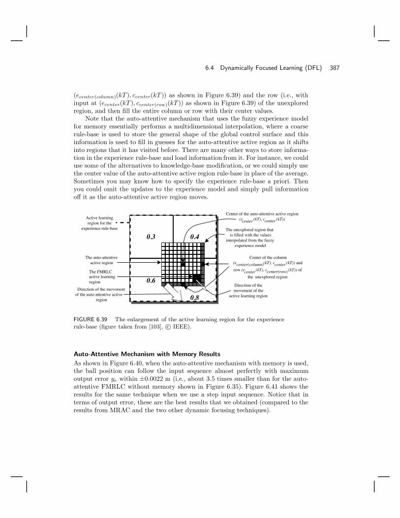
6.4 Dynamically Focused Learning (DFL) 387
(ecenter(column)(kT ), ccenter(kT )) as shown in Figure 6.39) and the row (i.e., withinput at (ecenter(kT ), ccenter(row)(kT )) as shown in Figure 6.39) of the unexploredregion, and then fill the entire column or row with their center values.
Note that the auto-attentive mechanism that uses the fuzzy experience modelfor memory essentially performs a multidimensional interpolation, where a coarserule-base is used to store the general shape of the global control surface and thisinformation is used to fill in guesses for the auto-attentive active region as it shiftsinto regions that it has visited before. There are many other ways to store informa-tion in the experience rule-base and load information from it. For instance, we coulduse some of the alternatives to knowledge-base modification, or we could simply usethe center value of the auto-attentive active region rule-base in place of the average.Sometimes you may know how to specify the experience rule-base a priori. Thenyou could omit the updates to the experience model and simply pull informationoff it as the auto-attentive active region moves.
0.3 0.4
0.6
0.8
The unexplored region thatis filled with the values
interpolated from the fuzzyexperience model
The auto-attentiveactive region
Active learningregion for the
experience rule-base
The FMRLCactive learningregion
Direction of themovement of the
active learning region
Direction of the movementof the auto-attentive active
region
Center of the auto-attentive active region(ecenter (kT), ccenter (kT))
Center of the column(ecenter(column)(kT), ccenter (kT)) and
row (ecenter(kT), ccenter(row) (kT)) of
the unexplored region
FIGURE 6.39 The enlargement of the active learning region for the experiencerule-base (figure taken from [103], c© IEEE).
Auto-Attentive Mechanism with Memory Results
As shown in Figure 6.40, when the auto-attentive mechanism with memory is used,the ball position can follow the input sequence almost perfectly with maximumoutput error ye within ±0.0022 m (i.e., about 3.5 times smaller than for the auto-attentive FMRLC without memory shown in Figure 6.35). Figure 6.41 shows theresults for the same technique when we use a step input sequence. Notice that interms of output error, these are the best results that we obtained (compared to theresults from MRAC and the two other dynamic focusing techniques).

388 Chapter 6 / Adaptive Fuzzy Control
0 5 10 15 20Time (sec)
-0.002
-0.001
0
0.001
Met
ers
0 5 10 15 20Time (sec)
0
10
20
30
40
Vol
ts
0 5 10 15 20Time (sec)
0.1
0.15
0.2
Met
ers
PlantReference model
Ball position (y ) Voltage input (v ) Output error (y )e
FIGURE 6.40 Responses for FMRLC with auto-attentive mechanism with memory(sinusoidal input sequence) (figure taken from [103], c© IEEE).
0 5 10 15 20Time (sec)
-4
-4
0
2x10⁻⁴
Met
ers
0 5 10 15 20Time (sec)
0
10
20
Vol
ts
0 5 10 15 20Time (sec)
0.1
0.12
0.14
0.16
0.18
0.2
Met
ers
PlantReferencemodel
Ball position (y ) Voltage input (v ) Output error (y )e
-2x10
-4x10
FIGURE 6.41 Responses for FMRLC with auto-attentive mechanism with memory(step input sequence) (figure taken from [103], c© IEEE).
6.5 DFL: Design and Implementation CaseStudies
In this section we provide two case studies in the design and implementation ofDFL strategies. In the first, we will simply use the auto-tuning strategy on a directfuzzy controller (not an FMRLC) for the rotational inverted pendulum case study ofChapter 3. Next, we will use similar auto-tuning strategy for the machine schedulingproblem in Chapter 3. We refer the reader to the appropriate sections in Chapter 3for background on the problem formulations and studies in direct fuzzy control forthese problems.
6.5.1 Rotational Inverted PendulumWhile the direct fuzzy controller synthesized in Chapter 3 using the LQR gainsperformed adequately for the nominal case, its performance degraded significantlywhen a bottle of sloshing liquid was added to the endpoint. It is the objective of thissection to use the auto-tuning method to try to achieve good performance for boththe nominal and perturbed conditions without any manual tuning in between thetwo experiments. We will not auto-tune the FMRLC as we did in the last section.Here, we simply tune a direct fuzzy controller. This helps show the versatility ofthe dynamically focused learning concepts.

6.5 DFL: Design and Implementation Case Studies 389
Auto-Tuning Strategy
The auto-tuning method for a direct fuzzy controller essentially expands on theidea of increasing the “resolution” of the fuzzy controller by dynamically increasingor decreasing the density of the input membership functions. For the rotationalinverted pendulum, if we increase the number of membership functions on eachinput to 25, improved performance (and smoother control action) can be obtained.To increase the resolution of the direct fuzzy controller with a limited number ofmembership functions (as before, we will impose a limit of seven), we propose touse auto-tuning to dynamically focus the membership functions to regions wherethey are most useful.
Ideally, the auto-tuning algorithm should not alter the nominal control algo-rithm near the center; we therefore do not adjust each input gain independently.We can, however, tune the most significant input gain, and then adjust the rest ofthe gains based on this gain as we did in Chapter 3. For the inverted pendulumsystem, the most significant controller input is the position error of the pendulum,e3 = θ1. The input-output gains are updated every ns samples in the followingmanner:
1. Find the maximum e3 over the most recent ns samples and denote it by emax3 .
2. Set the input gain g3 = 1|emax
3 | .
3. Recalculate the remaining gains using the technique discussed in Chapter 3 soas to preserve the nominal control action near the center.
We note that the larger ns is, the slower the updating rate is, and that too fast anupdating rate may cause instability.
Auto-Tuning Results
Simulation tests with ns = 50 and g3 = 2 reveal that when the fuzzy controlleris activated after swing-up, the input gains gradually increase while the outputgain decreases, as the pendulum moves closer to its inverted position. As a result,the input and output universes of discourses contract, and the resolution of thefuzzy system increases. In practice, it is important to constrain the maximum valuefor g3 (for our system, to a value of 10) because disturbances and inaccuracies inmeasurements could have adverse effects. As g3 reaches its maximum value, thecontrol action near θ1 = 0 is smoother than that of direct fuzzy control with 25membership functions, and very good balancing performance is achieved.
When turning to actual implementation on the laboratory apparatus describedin Chapter 3, some adjustments were done in order to optimize the performance ofthe auto-tuning controller. As with the direct fuzzy controller, the value of g3 wasadjusted upward, and the tuning (window) length was increased to ns = 75 samples.In the first experiment we applied the scheme to the nominal system. In this case,the auto-tuning mechanism improved the response of the direct fuzzy controller(see Figure 3.15 on page 151) by varying the controller resolution on-line. That

390 Chapter 6 / Adaptive Fuzzy Control
is, as the resolution of the fuzzy controller increased over time, the high-frequencyeffects diminished.
However, the key issue with the adaptive (auto-tuning) mechanism is whether itcan adapt its controller parameters as the process dynamics change. Once again weinvestigate the performance when the “sloshing liquid” dynamics (and additionalweight) are added to the endpoint of the pendulum. As expected from simulationexercises, the auto-tuning mechanism effectively suppressed the disturbances causedby the sloshing liquid, as clearly shown in Figure 6.42. Overall, we see that the auto-tuning method provides a very effective controller for this application.
0 1 2 3 4 5 6 7 8 9 10-2
0
2
Time (sec)
Posi
tion
of b
ase
(rad
)
0 1 2 3 4 5 6 7 8 9 10
0
2
4
Time (sec)
Posi
tion
of p
endu
lum
(ra
d)
0 1 2 3 4 5 6 7 8 9 10-5
0
5
Time (sec)
Con
trol
out
put (
volts
)
FIGURE 6.42 Experimental results: Auto-tuned fuzzy control on thependulum with sloshing liquid at its endpoint (figure taken from [244],c© IEEE).
6.5.2 Adaptive Machine SchedulingIn this section we develop an adaptive fuzzy scheduler (AFS) for scheduling the sin-gle machine by augmenting the fuzzy scheduler in Chapter 3 with an auto-tuningmechanism. In the AFS there is an adaptation mechanism that can automaticallysynthesize a fuzzy scheduler, independent of the machine parameters. Moreover, ifthere are machine parameter changes during operation that still satisfy the neces-sary conditions for stability (see Chapter 3), the AFS will tune the parameters of the

6.5 DFL: Design and Implementation Case Studies 391
fuzzy scheduler so that high-performance operation is maintained. The universallystabilizing supervisory mechanism (USSM) that is described in Chapter 3 governsthe AFS to ensure that it is stable. Therefore, the complete scheduler consists ofthree layers: The bottom layer is simply the fuzzy scheduler itself, the middle layeris the adaptation mechanism to be introduced here, and the top layer is the USSMthat supervises the lower two layers to ensure stable operation.
If the parameters of the machine change, the USSM may not guarantee sta-bility anymore since it assumes that the machine parameters stay constant. Theparameter γ of the USSM is dependent on the parameters of the machine, whereasthe parameters zi are not. If the parameter γ is chosen large enough, the USSMmay still provide stability over a large class of machine parameters. However, sincethe USSM assumes constant machine parameters, stability is not guaranteed whenthe machine parameters change even if γ is large enough for the new machine pa-rameters. It is for this reason that we split the adaptation problem into controllersynthesis (i.e., determining the positioning of a fixed number of fuzzy sets by au-tomatically picking Mp) and controller tuning (i.e., tuning the positioning of thefuzzy sets by changing Mp to react to machine parameter changes). In synthesis weare guaranteed stability, while in tuning we have no proof that the policy is stable.
Automatic Scheduler Synthesis
In this section, we introduce the AFS that has an adaptive mechanism that observesxp, p ∈ 1, 2, 3, . . . , P and automatically tunes the values of Mp (see Chapter 3).This adaptation mechanism, shown in Figure 6.43, adjusts the parameters Mp ofthe fuzzy scheduler by using a moving window. The size of the window is not fixedbut is equal to the length of time for a fixed number of production runs. In thissection we will use a window size of 10 production runs, while in the next sectionwe will use a larger window size. Throughout this window the buffer levels xp arerecorded. The window slides forward at the end of each production run, and thevalues of Mp are updated to the maximum values of xp over the last window frame.As Mp is updated, the fuzzy sets on the universe of discourse for xp are shiftedso that they remain symmetric and uniformly distributed. The fuzzification anddefuzzification strategies, the output fuzzy sets, and the rule-base remain constantso that the adaptation mechanism adjusts only the input membership functions toimprove machine performance. Basically, the AFS tunes the Mp values in search ofa lower η. It does this by automatically adjusting the premise membership functionsof the rules of the fuzzy scheduler so that they appropriately fit the machine.
Next, we show how the automatic tuning method can be used to synthesize thefuzzy scheduler for the single machine. In particular, we will show how without anyknowledge of the machine parameters, our adaptation mechanism can synthesize afuzzy scheduler that can perform as well as the CPK policy (see Chapter 3). Weshall first consider the same machines used in Chapter 3. For each of the followingmachines, the number of fuzzy sets is set to 5. The parameter Mp is initially set to1. The adaptation mechanism will adjust Mp at the end of each production run.
When simulating the AFS for machine 1 (see Chapter 3 for its description),

392 Chapter 6 / Adaptive Fuzzy Control
MachineFuzzyscheduler
Adaptationmechanism
Mp
pxp*
FIGURE 6.43 Adaptive fuzzy scheduler(AFS) for a single machine.
by the end of 15 production runs M1 = 30.993, M2 = 34.605, and M3 = 12.4519(and for later production runs, the Mp values stay near these values). After 10,000production runs, we find that η = 1.0263, which is the same as that producedby CPK after 10,000 production runs. But the AFS automatically constructed itsscheduler without knowledge of the machine parameters. The CPK policy usesmachine parameters to help specify the policy and is therefore tailored specificallyto the machine.
When simulating the AFS for machine 2 (see Chapter 3 for its description), wefind that the values of Mp converge slowly compared to the previous machine (ittook until about 700 production runs to get convergence). After 10,000 productionruns, η = 1.0993 which is worse than the η = 1.0017 produced by CPK after10,000 production runs. However, when Mp is initially 10,000 instead of 1 and theadaptation mechanism updates the Mp every other 10 production runs, η fromfuzzy scheduler improves to 1.0018. This highlights an inherent problem with theadaptation mechanism: the window size and Mp update strategy must be chosenin an ad hoc manner with no guarantees on performance levels.
Automatic Scheduler TuningIn this section we investigate whether the AFS and CPK can adjust themselvesto disturbances or failures that may occur during the operation of a machine. Thedisturbance or failure may be in the form of changes in arrival rates, processingtimes, or setup times. In order to observe how the fuzzy scheduler and CPK adjustto machine parameter changes, first we use the same machine parameters and part-types, and switch the part-types to arrive at different buffers. Following this, we willinvestigate the tuning capabilities of the adaptation mechanism by examining theeffects of changing the machine load. In the simulations, the machine parametersstay constant for the first 10,000 production runs, then the machine parametersare changed and remain constant at different values for the next 10,000 productionruns. When the parameters are changed, the parameters Mp of the fuzzy schedulerare continued from the last production run. For the last 10,000 production runs,the CPK schedules based on the former machine parameters, while the AFS adjustsitself to improve performance.

6.5 DFL: Design and Implementation Case Studies 393
1. Switching buffers:
(a) Case 1:Old machine: d1 = 7, d2 = 9, d3 = 3, τ1 = 1/100, τ2 = 1/51, τ3 = 1/27.New machine: d2 = 7, d3 = 9, d1 = 3, τ2 = 1/100, τ3 = 1/51, τ1 = 1/27.The AFS maintains the same η at 1.026, whereas η of CPK degrades from1.027 to 1.237.
(b) Case 2:Old Machine: d1 = 18, d2 = 3, d3 = 1, τ1 = 1/35, τ2 = 1/7, τ3 = 1/20.New Machine: d2 = 18, d3 = 3, d1 = 1, τ1 = 1/35, τ2 = 1/7, τ3 = 1/20.The value of η of the AFS improves from 1.0993 to 1.0018, whereas η ofCPK degrades from 1.0017 to 1.1965.
The AFS is expected to perform similarly since the parameters of the machinesare similar. However, as you can see from the rule-base for the fuzzy scheduler,there are some rules in the rule-base of the fuzzy scheduler that are biasedtoward some part-types. Therefore, when we switch the order of indexing thepart-types, the performance of the fuzzy scheduler can be different.
2. Machine load variations:
(a) Case 3:Old machine (ρ = 0.99286): d1 = 18, d2 = 3, d3 = 1, τ1 = 1/35, τ2 = 1/7,τ3 = 1/20.New machine (ρ = 0.35758): d1 = 7, d2 = 9, d3 = 3, τ1 = 1/100, τ2 =1/51, τ3 = 1/27.This is a transition from a high to a low machine load. The value of η ofthe AFS changes from 1.0993 to 1.0263, as expected. On the other hand,η of CPK changes from 1.0017 to 1.0477 instead of 1.0263. Note that CPKcan still perform reasonably well as the machine parameters change froma highly loaded to a lightly loaded machine.
(b) Case 4:Old machine (ρ = 0.35758): d1 = 7, d2 = 9, d3 = 3, τ1 = 1/100, τ2 = 1/51,τ3 = 1/27.New machine (ρ = 0.99286): d1 = 18, d2 = 3, d3 = 1, τ1 = 1/35, τ2 = 1/7,τ3 = 1/20.This is a transition from a low to a high machine load. The value of η ofthe AFS changes from 1.0263 to 1.0993, as expected. On the other hand,η of CPK changes from 1.0263 to 1.106 instead of 1.0017—that is, itsperformance degrades.
The results show that the AFS we have developed has the capability to main-tain good performance even if there were significant changes in the underlyingmachine parameters (representing, e.g., machine failures). CPK, on the other hand,is dependent on the exact specification of the machine parameters, and hence itsperformance can degrade if the parameters change. We found similar improvements

394 Chapter 6 / Adaptive Fuzzy Control
in performance as compared to the CLB and CAF policies that are described inChapter 3.
6.6 Indirect Adaptive Fuzzy ControlIn this section we take the “indirect” approach to adaptive fuzzy control where weuse an on-line identification method to estimate the parameters of a model of theplant. The estimated model of the plant is then used by a “controller designer”that specifies the controller parameters. See Figure 6.2 on page 319. There is aninherent assumption by the controller designer that the model parameter estimatesprovided at each time instant represent the plant perfectly. Then the controllerdesigner specifies a controller assuming that this is a perfect model. The resultingcontrol law is called a “certainty equivalence controller” since it was specified byassuming that we were certain that the plant model estimates were equivalent tothose of the actual plant.
One strength of the indirect approach is that it is modular in the sense thatthe design of the plant model identifier can be somewhat independent of the waythat we specify the controller designer. In this section we will first introduce twomethods from Chapter 5 that can be used for on-line plant model estimation; theseare the gradient and least squares methods. Following this we discuss an approachbased on feedback linearization, then we introduce the “adaptive parallel distributedcompensator” that builds on the parallel distributed compensator from Chapter 4.We close the section with a simple example of how to design an indirect adaptivefuzzy controller.
6.6.1 On-Line Identification MethodsSeveral of the methods for identification in Chapter 5 were inherently batch ap-proaches so they cannot be used in indirect adaptive control since an on-line ad-justment method is needed. For instance, in the learning from examples approaches,there are only methods for adding rules to the system so they do not provide theappropriate adjustment capabilities for achieving the on-line tracking of dynamicchanges in the plant. Similar comments can be made about the batch least squaresmethod and the clustering with optimal output predefuzzification methods.
Two methods from Chapter 5 do lend themselves to on-line implementation;these are the recursive least squares and gradient training methods. For each ofthese we can easily establish an “identifier structure” (i.e., the structure for themodel that has its parameters tuned). Then we use the RLS or gradient methodto tune the parameters of the model (e.g., the membership function centers). Weshould note that RLS only allows for tuning parameters that enter the model ina linear fashion (e.g., the output membership function centers), while the gradientmethod allows for tuning parameters that enter in a nonlinear fashion (e.g., theinput membership function widths). It is for this reason that the gradient methodmay have an enhanced ability to tune the fuzzy system to act like the plant. How-ever, we must emphasize that we will not be providing stability or convergence

6.6 Indirect Adaptive Fuzzy Control 395
results showing that either method will succeed in their tasks. Ours is simply aheuristic construction procedure for the adaptive fuzzy controllers; we cannot saya priori which tuning method to choose.
6.6.2 Adaptive Control for Feedback Linearizable SystemsIn the case of conventional indirect adaptive control for linear systems with constantbut unknown parameters, the certainty equivalence control law is used and thecontroller designer may use, for example, “model reference control” [77] or poleplacement methods (e.g., LQR or polynomial methods). As the adaptive controlproblem for linear systems is well studied and many methods exist for that case, webriefly focus here on the use of adaptive control for nonlinear (feedback linearizable)systems.
Following the approach in [189], we assume that our plant is in the form
x(t) = f(x(t)) + g(x(t))u(t)y(t) = h(x(t))
where x is the state, u is the input, and y is the output of the plant. Under certainassumptions by differentiating the plant output it is possible to transform the plantmodel into the form
y(r) = α(x(t)) + β(x(t))u(t) (6.31)
where y(d) denotes the dth derivative of y and d denotes the “relative degree” of thenonlinear plant. If d < n then there can be “zero dynamics” [223], and normally youmust assume that these are stable, as we do here. We assume that β(x(t)) ≥ β0 > 0for all x(t) for some given β0. Note that if at some x(t) we have β(x(t)) = 0, thenu is not able to affect the system at this state.
For the plant in Equation (6.31) we can use the controller
u(t) =1
β(x(t))(−α(x(t)) + ν(t)) (6.32)
where ν will be specified below. Now, if we substitute this control law into Equa-tion (6.31), the closed-loop system will become
y(d) = ν(t)
(which is a linear system with input ν(t)). We see that the control law uses feedbackto cancel the nonlinear dynamics of the plant and replaces them with ν(t). Hence,all we have to do is choose ν(t) so that it represents the kind of dynamics that wewould like to have in our closed-loop system. For example, suppose that the relativedegree is the same as the order of the plant and is equal to two (i.e., d = n = 2).In this case we could choose
ν(t) = ae(1)o (t) + beo(t)

396 Chapter 6 / Adaptive Fuzzy Control
where eo(t) = r(t) − y(t), e(i)o is the ith derivative of eo(t), r(t) is the reference
input, and a and b are design parameters. Notice that with this choice
y(2) = ae(1)o (t) + beo(t)
or
y(2) + ay(1) + by(t) = ar(1)(t) + br(t)
to make the closed-loop system linear. Hence,
Y (s)R(s)
=as + b
s2 + as + b
so that if we pick a > 0 and b > 0, we will have a stable closed-loop system(you can use the quadratic formula to show this). Also, we see that we can pick aand b to specify the type of closed-loop response we want (i.e., fast, slow, with aspecific amount of overshoot, etc.). The same general approach works for higher-order systems (show how by repeating the above analysis for an arbitrary value ofd = n).
Now, the above design procedure for nonlinear controllers for the nonlinearsystem in Equation (6.31) assumes that we have perfect knowledge of the plantdynamics (i.e., that we know α(x(t)) and β(x(t)) and the order of the plant). Here,we will assume that we do not know α(x(t)) or β(x(t)) but that we do know thatβ(x(t)) ≥ β0 > 0 for all x(t) for some given β0. Then, we will use on-line identifiersto estimate the plant dynamics α(x(t)) and β(x(t)) with α(x(t)) and β(x(t)), whichwill be fuzzy systems. With this we use the certainty equivalence control law forthe plant in Equation (6.31), which, based on Equation (6.32), would be
u(t) =1
β(x(t))(−α(x(t)) + ν(t)) (6.33)
We will choose ν(t) the same way as we did above. This control law specifies the“controller designer.” That is, it is the recipe for specifying the control law giventhe estimates of the plant dynamics. Intuitively, we know that if our identifier cando a good job at identifying the dynamics of the plant then it will be possible toachieve the closed-loop behavior (which we characterize above via a and b).
The complete indirect adaptive fuzzy controller consists of an on-line estimatorfor the fuzzy systems α(x(t)) and β(x(t)). If recursive least squares is used with astandard fuzzy system, then the output membership function centers of the fuzzysystems α(x(t)) and β(x(t)) are tuned. If recursive least squares is used with α(x(t))and β(x(t)) defined as Takagi-Sugeno fuzzy systems, then the parameters of theoutput functions are tuned. If a gradient method is used, then all the parametersof the fuzzy systems α(x(t)) and β(x(t)) (either standard or Takagi-Sugeno) can betuned to try to make α(x(t)) → α(x(t)) and β(x(t)) → β(x(t)) so that a feedbacklinearizing control law is found and the nonlinear dynamics are replaced by the

6.6 Indirect Adaptive Fuzzy Control 397
designed dynamics specified in ν(t) (note that even if we do not get this convergencewe can often still obtain a successful adaptive controller).
As a final note we must emphasize, however, that there are no guaranteesthat you will achieve good performance or stable operation with this approach.If you want guarantees, you should study the methods that are shown to achievestable operation (see For Further Study at the end of this chapter). There, work isdescribed that explains the full details on how to define the fuzzy system parameterupdate methods and the entire indirect adaptive fuzzy controller that will ensurestable operation.
6.6.3 Adaptive Parallel Distributed CompensationIn Chapter 4 we studied the parallel distributed compensator for Takagi-Sugenofuzzy systems. For that controller we assumed that either via system identificationor modeling we have a Takagi-Sugeno model of the nonlinear plant. From thismodel we constructed a parallel distributed compensator that could provide a globalasymptotically stable equilibrium for the closed-loop system.
Here, we do not assume that the Takagi-Sugeno model of the plant is knowna priori. Instead, we use an on-line identification method to adjust the parametersof a Takagi-Sugeno “identifier model” to try to make it match the behavior of theplant. Then, using the certainty equivalence principle, we employ the parametersof the Takagi-Sugeno identifier model in a standard control design method for thestandard parallel distributed compensator. In this way, as the identifier becomesmore accurate, the controller parameters of the parallel distributed compensatorwill be adjusted, and if the identifier succeeds in its task, the controller should too.
Suppose that the identifier model is specified by R rules
If y(k) is Aj1 and, . . . , and y(k − n + 1) is A
n
Thenyi(k + 1) = αi,1y(k) + · · ·+ αi,ny(k − n + 1) + βi,1u(k) + · · ·+ βi,mu(k − m + 1)
which have as consequents discrete-time linear systems (see Exercise 4.6 on page 227for stability results for the discrete-time case). Here, u(k) and y(k) are the plantinput and output, respectively; Aj
i is the linguistic value; αi,j, βi,p, i = 1, 2, . . . , R,j = 1, 2, . . . , n, and p = 1, 2, . . . , m are the parameters of the consequents; andyi(k + 1) is the identifier model output considering only rule i. Suppose that µi
denotes the premise certainty for rule i. Using center-average defuzzification, weget the identifier model output
y(k + 1) =∑R
i=1 yi(k + 1)µi∑Ri=1 µi
Let
ξi =µi∑Ri=1 µi
(6.34)

398 Chapter 6 / Adaptive Fuzzy Control
ξ =
y(k)ξ1
y(k)ξ2
...y(k)ξR
...u(k − m + 1)ξ1
u(k − m + 1)ξ2
...u(k − m + 1)ξR
, θ =
α1,1
α2,1
...αR,1
...β1,m
...βR,m
so that
y(k + 1) = θξ
is the identifier model output. An on-line method such as RLS could adjust theαi,j and βi,p parameters since they enter linearly. Gradient methods could be usedto adjust the αi,j and βi,p parameters and the parameters of the premises (e.g.,the input membership function centers and spreads if Gaussian input membershipfunctions are used).
For the controller, we can use Takagi-Sugeno rules of the form
If y(k) is Aj1 and, . . . , and y(k − n + 1) is A
n Then ui(k) = Li(·)
where Li(·) is a linear function of its arguments that can depend on past plantinputs and outputs and the reference input, and ui(k) is the controller outputconsidering only rule i. For example, for some applications it may be appropriateto choose
Li(r(k), y(k)) = ki,0r(k) − ki,1y(k)
which is simply a proportional controller with gains ki,0 and ki,1. For other applica-tions you may need a more complex linear mapping in the consequents of the rules.In any case, the identifier will adjust the gains of the Li functions using a certaintyequivalence approach. For example, the gains ki,0 and ki,1 could be chosen at eachtime step to try to meet some stability or performance specifications. In the nextsection we give an example of how to do this.
6.6.4 Example: Level Control in a Surge TankIn this section we use a level control problem for a surge tank to show how todesign an indirect adaptive fuzzy controller using the adaptive parallel distributedcompensation approach. In particular, suppose that you are given the “surge tank”that is shown in Figure 6.44.

6.6 Indirect Adaptive Fuzzy Control 399
h(t)
u(t)
FIGURE 6.44 Surge tank.
The differential equation representing this system is
dh(t)dt
=−c
√2gh(t)
A(h(t))+
1A(h(t))
u(t)
where u(t) is the input flow (control input), which can be positive or negative (itcan both pull liquid out of the tank and put it in); h(t) is the liquid level (theoutput of the plant); A(h(t)) is the cross-sectional area of the tank; g = 9.8m/sec2
is gravity; and c = 1 is the known cross-sectional area of the output pipe. Let r(t)be the desired level of the liquid in the tank (the reference input). Assume thath(0) = 1. Also assume that a is unknown but that a ∈ [a1, a2], a1 ≥ 0, for somefixed real numbers a1 and a2, and that A(h) = ah2 + b where a ∈ [a1, a2], a1 ≥ 0,and b ∈ [b1, b2], b1 > 0, where a1 = 0.5, a2 = 4, b1 = 1, b2 = 3 are all fixed.
First, we will choose a = 1 and b = 2 as the nominal plant parameters. Also,since we will be using a discrete-time identifier, we discretize the plant and use itin all our simulations. In particular, using an Euler approximation
h(k + 1) = h(k) + T
[−√
19.6h(k)h2(k) + 2
+1
h2(k) + 2u(k)
]
where T = 0.1. We have additional restrictions on the plant dynamics. In particular,we assume the plant input saturates at ±50 so that if the controller generates aninput u′(k)
u(k) =
50 if u′(k) > 50u′(k) if −50 ≤ u′(k) ≤ 50−50 if u′(k) < −50
Also, to ensure that the liquid level never goes negative (which is physically impos-

400 Chapter 6 / Adaptive Fuzzy Control
sible), we simulate our plant using
h(k + 1) = max
0.001, h(k) + T
[−√
19.6h(k)h2(k) + 2
+1
h2(k) + 2u(k)
]
We can use either gradient or RLS to tune the parameters of the Takagi-Sugenofuzzy system that we use as our identifier model. Here, we use the RLS method totune to the consequent parameters and specify a priori the parameters that definethe premise certainties. In particular, we use only five rules (R = 5), n = 1, andm = 1, in the last section. Hence, one rule of our identifier model would be
If h(k) is Aj1 Then hi(k + 1) = αi,1h(k) + βi,1u(k)
We use Gaussian input membership functions on the h(k) universe of discourse ofthe form
µ(h(k)) = exp
−1
2
(h(k) − cj
i
σ
)2
where c11 = 0, c2
1 = 2.5, c31 = 5, c4
1 = 7.5, c51 = 10, and σ = 0.5. Notice that since
there is only one input, µi(h(k)) = µ(h(k)); that is, the membership function cer-tainty is the premise membership function certainty for a rule. Also, if h(k) ≤ c1
1,then we let µ1(h(k)) = 1, and if h(k) ≥ c5
1, then we let µ5(h(k)) = 1. This causessaturation of the outermost input membership functions. With center-average de-fuzzification our fuzzy system is
h(k + 1) = θξ(h(k))
where ξi is defined in Equation (6.34) and
ξ(h(k)) =
h(k)ξ1
h(k)ξ2
...h(k)ξR
u(k)ξ1
u(k)ξ2
...u(k)ξR
, θ =
α1,1
α2,1
...α5,1
β1,1
β2,1
...β5,1
We use a nonweighted (i.e., λ = 1) RLS algorithm with update formulas givenby
P (k + 1) =1λ
(I − P (k)ξ(h(k))(λI + (ξ(h(k)))P (k)ξ(h(k)))−1(ξ(h(k))))P (k)

6.6 Indirect Adaptive Fuzzy Control 401
θ(k + 1) = θ(k) + P (k)ξ(h(k))(h(k + 1) − (ξ(h(k)))θ(k))
Notice that we have adjusted the time indices in these equations so that they solvethe identification problem of trying to estimate the output of the identifier model(i.e., h(k + 1)). We choose θ(0) = [0, 2, 4, 6, . . . , 18] and P (0) = Pβ(0) = 2000Iwhere I is the identity matrix. The choice of θ(0) is simply one that is not closeto the final tuned values (to see this consider the rules of the Takagi-Sugeno fuzzysystem for this case and how, based on our understanding of the dynamics of atank, how these could not properly represent it).
Our controller that is tuned is given by
u(k) =∑R
i=1 ui(k)µi∑Ri=1 µi
where we choose
ui(k) = Li(r(k), h(k)) = ki,0r(k) − ki,1h(k)
Using a certainty equivalence approach for the parallel distributed compensator, weview each rule of the controller as if it were controlling only one rule of the plant, andwe assume that the identifier is accurate. In particular, we assume that h(k) = h(k)and hi(k) = hi(k), where hi(k) represents the ith component of the plant model(assuming it can be split this way), so that the identifier is also perfectly estimatingthe dynamics represented by each rule in the plant. If the plant is operating nearits ith rule and there is little or no affect from its other rules, then h(k) = hi(k) so
hi(k + 1) = hi(k + 1) = αi,1hi(k) + βi,1 [ki,0r(k) − ki,1hi(k)] (6.35)
We pick ki,0 and ki,1 for each i = 1, 2, . . . , R so that the pole of the closed-loop sys-tem is at 0.1 and the steady-state error between h(k) and r(k) is zero. In particular,if Hi(z) and R(z) are the z-transforms of hi(k) and r(k), respectively, then
Hi(z)R(z)
=βi,1ki,0
z + βi,1ki,1 − αi,1
Choose
ki,1βi,1 − αi,1 = −0.1
to get the placement of the pole so that our controller designer in our indirectadaptive scheme will pick
ki,1 =αi,1 − 0.1
βi,1(6.36)
i = 1, 2, . . . , R, at each time step using the estimates of αi,1 and βi,1 from theidentifier. Notice that we must ensure that βi,1 > 0 and we can do this by specifying

402 Chapter 6 / Adaptive Fuzzy Control
a priori some β > 0 and adding a rule to the adaptation scheme that says that ifat some time the RLS updates any βi,1 so that it becomes less than β, we let itbe equal to β. In this way the lowest value that βi,1 will take is β. Another way tospecify the update method for the ki,1 (and ki,0 below) would be to use the stabilityconditions for the parallel distributed compensator from Chapter 4.
Next, we want a zero steady-state error, so we want hi(k + 1) = hi(k) = r(k)for large k and all i = 1, 2, . . . , R, so from Equation (6.35) we want
1 = αi,1 + βi,1ki,0 − βi,1ki,1
so our controller designer will choose
ki,0 =1 − αi,1 + βi,1ki,1
βi,1(6.37)
i = 1, 2, . . . , R. Equations (6.36) and (6.37) specify the controller designer for theindirect adaptive scheme, and the identifier will provide the values of αi,1 and βi,1
at each time step so that the ki,0 and ki,1 can be updated at each time step. Noticethat the modifications to Equation (6.36) with β above will also ensure that we willnot divide by zero in Equation (6.37).
The results of the RLS-based adaptive parallel distributed compensator areshown in Figure 6.45. Notice that the output of the plant h(k) tracks the referenceinput r(k) quite well. Next, we show values of h(k) and h(k) in Figure 6.46. Noticethat with only five rules in the identifier model we get a reasonably good estimateof h(k), and hence we can see why our closed-loop response tracks the referenceinput so well.
6.7 SummaryIn this chapter we have provided an overview of several adaptive fuzzy controlmethods. First, we introduced the fuzzy model reference learning controller andprovided several guidelines for how to design it. We showed three case studies indesign and implementation, including the ship steering problem where we comparedit against some conventional model reference adaptive control methods. We showedhow it could be used for fault-tolerant aircraft control, and provided implementationresults for the flexible-link robot.
Next, we showed how “dynamically focused learning” could be used for theFMRLC. We introduced the three DFL strategies (auto-tuning, auto-attentive,and auto-attentive with memory) via a simple academic magnetic levitation con-trol problem. We provided two case studies in DFL design and implementation. Inparticular, we showed how to design auto-tuning mechanisms for direct fuzzy con-trollers for the rotational inverted pendulum and the machine scheduling problemsstudied in Chapter 3.
Finally, we introduced indirect adaptive fuzzy control. There, we discussedindirect adaptive fuzzy control for feedback linearizable systems, introduced the

6.7 Summary 403
0 10 20 30 40 50 60 70 80 90 1000
2
4
6
8r(k) (solid), h(k) (dashed)
Time (sec)
0 10 20 30 40 50 60 70 80 90 100-50
0
50
Time (sec)
u(k)
FIGURE 6.45 Response of RLS-based adaptive paralleldistributed compensator for the tank (plot produced byMustafa K. Guven).
adaptive parallel distributed compensator, and studied a tank application.The overall approach that we take to adaptive control in this chapter is a
heuristic one as opposed to a mathematical one. We focused on the use of intuitionto motivate why adaptation is needed, and we provided natural extensions to thedirect fuzzy control methods described in Chapters 2 and 3.
Upon completing this chapter, the reader should understand the following top-ics:
• Basic schemes for adaptive control (e.g., model reference adaptive control anddirect versus indirect schemes).
• Fuzzy model reference learning control (FMRLC).
• Design methods for the FMRLC.
• Issues in adaptive versus learning control.
• The issues that must be considered in comparing or evaluating conventional versusadaptive fuzzy control.
• How failures can be viewed as a significant plant variation that can be accommo-dated for via adaptive control.

404 Chapter 6 / Adaptive Fuzzy Control
0 10 20 30 40 50 60 70 80 90 1000
2
4
6
8
10
12Estimate of liquid height (solid), h(k) (dashed)
Time (sec)
FIGURE 6.46 The values of h(k) and h(k) for the RLS-basedadaptive parallel distributed compensator for the tank (plotproduced by Mustafa K. Guven).
• Dynamically focused learning (DFL) strategies (auto-tuning, auto-attentive, andauto-attentive with memory).
• How to apply DFL strategies to both the FMRLC and a direct fuzzy controller.
• The concept of a certainty equivalence control law.
• How the RLS and gradient methods can be used for on-line identification of aplant model and hence used in indirect adaptive fuzzy control (and in directadaptive control for identification of a controller; see Design Problem 6.10).
• The feedback linearization and adaptive parallel distributed compensation ap-proaches to indirect adaptive fuzzy control.
• How to construct an indirect adaptive fuzzy controller for a surge tank.
Essentially, this is a checklist of the major topics of this chapter. We encouragethe reader to test the adaptive fuzzy control methods by doing some problems atthe end of the chapter or by trying them out on your own applications. Additionaladaptive methods are introduced in the next chapter.

6.8 For Further Study 405
6.8 For Further StudyThe reader wishing to strengthen her or his background in conventional adaptivecontrol should consult [77, 180, 149, 11]. The FMRLC algorithm was first introducedin [111, 112] and grew from research performed on the linguistic self-organizingcontroller (SOC) presented in [170] (with applications in [181, 214, 78, 40, 39,38, 239]) and ideas in conventional “model reference adaptive control” (MRAC)[149, 11]. The ship steering application is described in [11, 149] which are thesources for the problem formulation for this chapter. The ship steering section,where the FMRLC is used, is based on [112]. Examples of Lyapunov-based MRACdesigns are illustrated in [149, 220]; in the case study in this chapter we use theapproach in [149] to design our Lyapunov-based MRAC. The fault-tolerant aircraftcontrol section is based on [104], and the application to the two-link flexible robotis based on [144]. The FMRLC has also been used for a robotics problem and arocket velocity control problem [113], a cart-pendulum system [111], the control ofan experimental induction machine, an automated highway system, in automobilesuspension control, for liquid level control in a surge tank [251], for the rotationalinverted pendulum of Chapter 3, for a single-link flexible robot, and for a ball ona beam experiment; it has also been used to improve the performance of antiskidbrakes on adverse road conditions [114].
The section on dynamically focused fuzzy learning control is based on [103].For a discussion on how to program rule-base shifts and a detailed analysis of thecomputational complexity of the DFL strategies relative to conventional MRAC,see [103]. The section on the rotational inverted pendulum is based on [235], andthe adaptive machine scheduling work is based on [6]. While in this chapter wehave considered only the single machine case (and only for a limited number oftypes of machines in simulation), in [6] the authors show how to use the the AFSon each machine in a network of machines to improve overall scheduling perfor-mance of a flexible manufacturing system (FMS). Basically, this is done by usingthe fuzzy scheduler, adaptation mechanism, and USSM on each machine in thenetwork. Generally, we can find topologies of FMS for which the AFS can fine-tunethemselves so that they optimize certain performance measures (e.g., minimizingthe maximum backlog in the FMS). This often involves having the local schedulerson some machines sacrifice their local throughput performance to make it possibleto achieve higher performance for the entire FMS. See [6] for more details.
Other alternatives to FMRLC, DFL, and SOC are contained in [47, 87, 26, 229]and in [17, 208, 184]. Other work is also given in [173], where the authors present aknowledge-based fuzzy control system that is constructed off-line. Another exampleof indirect adaptive fuzzy control presented by Graham and Newell in [62, 61] uses afuzzy identification algorithm developed by Czogala and Pedrycz [36, 37] to identifya fuzzy process model that is then used to determine the control actions. Batur andKasparian [19] present a methodology to adapt the initial knowledge-base of a fuzzycontroller to changing operating conditions. The output membership functions oftheir fuzzy controller are adjusted in response to the future or past performance ofthe overall system, where the prediction is obtained through a linear process model

406 Chapter 6 / Adaptive Fuzzy Control
updated by on-line identification. Other indirect approaches to adaptive fuzzy con-trol are shown in [26, 224]. In addition to all these, there are many other adaptivefuzzy system applications that, to name a few, choose to use neural networks foridentification and reinforcement learning [26, 126] or genetic algorithms for naturalselection of controller parameters as the learning mechanism (for some references onthe genetic algorithm approach to tuning fuzzy systems see the For Further Studysection at the end of Chapter 8).
Recent work on adaptive fuzzy systems has focused on merging concepts andtechniques from conventional adaptive systems into a fuzzy systems framework andperforming stability analysis to guarantee properties of the operation of adaptivefuzzy control systems. For example, the reader could consider the work in [229] andthe references contained therein. More recent work on the development of stabledirect and indirect adaptive fuzzy controllers is contained in [85, 200, 195, 196, 198,197, 194, 199, 202, 201, 203] (for a more complete treatment of the literature see thereferences in [200]). The reader interested in the feedback linearization approach toindirect (and direct) adaptive fuzzy control in Section 6.6.2 starting on page 395should consult these references.
This is a fairly representative sampling of the literature in adaptive fuzzy con-trol; we emphasize, however, that it is not complete as the amount of literaturein this area is quite large, especially considering the many heuristic adaptive ap-proaches that are used for all types of applications.
6.9 ExercisesExercise 6.1 (FMRLC Programming and Operation): In this problem wewill consider an academic control problem for the purpose of focusing on how toprogram the operation of the FMRLC. In this way we focus only on the operationof the FMRLC and avoid application-specific details. Suppose that you are givena plant
G(s) =kp
s2 + 2ζpωps + w2p
where kp is the gain in the numerator, ζp is the damping ratio, and ωp is theundamped natural frequency (all unknown but constant). Nominally, we havekp = 1, ζp = 0.707, and ωp = 1. The reference model is a first-order system
M(s) =kr
s + ar
where kr = 1 and ar = 1. Use r(t) = sin(0.6t) as the reference input.
(a) Design a direct (nonadaptive) fuzzy controller for the plant that as nearlyas possible achieves the performance specified in the reference model. Usetwo inputs to the fuzzy controller, the error e = r − y where r is the refer-ence input and y is the plant output, and the change in this error (i.e., its

6.10 Design Problems 407
derivative approximated by a backward difference).
(b) Design an FMRLC for the plant to make it track the reference model asclosely as possible. Use the fuzzy controller designed in (a) to initialize thecontroller that the FMRLC tunes. Provide the tuned rule-base at the endof the simulation and compare it to the rule-base from (a). Is the FMRLCstill tuning the rule-base at the end of the simulation (i.e., are the outputcenters still moving)?
(c) Repeat (b) except initialize the direct fuzzy controller the same as in (a)except let all the output membership function centers be zero. Provide thetuned rule-base that results at the end of the simulation, and compare it tothe ones from (a) and (b).
Exercise 6.2 (Rule-Base Update Procedure for the FMRLC): Considerthe rule-base update procedure for the FMRLC given by Equations (6.1) and (6.2).Notice that for our development, when COG is used, this update will guaranteethat the previous input would have been u(kT − T ) + p(kT ). Prove this for boththe center-average and COG defuzzification methods.
Exercise 6.3 (Dynamically Focused Learning Methods): In this problemyou will explain various characteristics of the DFL methods used in the chapterand propose how to extend these methods.
(a) Explain in words the analogies between the auto-tuning, auto-attentive, andauto-attentive with memory strategies and the way that humans appear tolearn.
(b) We have used the auto-tuning method for both tuning a direct fuzzy con-troller for the rotational inverted pendulum and for adaptive machine schedul-ing. Suppose that you design an adaptive fuzzy controller by simply usingthe auto-tuning strategy for a direct fuzzy controller. Suppose that you nowwant to augment this learning strategy with an ability to remember thecontrol map in regions where it has operated in the past (so you use theauto-tuning method as the basic fuzzy learning controller and add a certaintype of fuzzy system experience model). Explain in words how to do this (userule-base diagrams in your explanation similar to those used in the chapter).
(c) Explain in words how you could add a successive hierarchy of auto-attentivewith memory strategies.
6.10 Design ProblemsDesign Problem 6.1 (FMRLC for Cargo and Tanker Ship Steering):In this problem we will study the use of the FMRLC for steering various ships.
(a) Verify the results in the chapter for the cargo ship by simulating the FM-RLC under the same conditions. In particular, generate the plots shown inFigure 6.6.

408 Chapter 6 / Adaptive Fuzzy Control
(b) In this part you will study the steering of a “tanker ship” defined in [11].The tanker (under “ballast” conditions) has the same differential equationsdescribing its behavior as the cargo ship, but it has K0 = 5.88, τ10 = −16.91,τ20 = 0.45, and τ30 = 1.43, and its length is l = 350 (assume that the shipvelocity is u = 5). Assume that the rudder input to the tanker saturates at±π/2, but also assume that this is the only way that the rudder movementis constrained (i.e., do not assume that there are extra actuator dynamics ora rate limiter on the rudder’s movement). Design an FMRLC for the tanker.Initialize it either with your best direct fuzzy controller or in the way wedid for the cargo ship in the chapter. It is your responsibility to choose areasonable reference model, and you must justify your choice. Is the one forthe cargo ship appropriate? If you believe so, then justify this choice. Next,design the learning mechanism similar to how we did for the cargo shipbut keep in mind that the tanker has somewhat different dynamics so thatyou may need to tune the fuzzy inverse model. Use the design proceduresprovided in the chapter to tune the FMRLC.
(c) Evaluate the performance of the tanker closed-loop system using a simula-tion. Does the system appear to be stable? Is the rise-time, overshoot, andsettling time adequate for your system? Use a reference input that com-mands +45 for 500 sec, then commands 0 for 500 sec, then commands−45 for 500 sec, then commands 0 for the next 500 sec. Then repeat this2000-sec sequence at least twice so that the FMRLC has adequate time toadapt.
(d) Study the effects of plant parameter variations and the ability of the tankercontrol system to adapt to these changes. In particular, for the tanker runa simulation for 2000 sec, and then suddenly at t = 2000 sec switch theparameters of the tanker to K0 = 0.83, τ10 = −2.88, τ20 = 0.38, τ30 = 1.07(this represents the tanker being “full” rather than “ballast,” i.e., a weightchange on the ship) and study how the FMRLC adapts to such a plantparameter variation.
(e) Study the effects of changing the speed of the ship during the simulations(note that increasing the speed will likely make it possible to improve theperformance, while decreasing the speed will make it more difficult to followthe reference trajectory). For example, increasing the speed to u = 7 m/sectypically makes the ship a bit easier to control, while changing it to u = 3m/sec makes it much harder to control. If under the speed changes the tankerdoes not perform too well, tune the controller until acceptable performanceis achieved (but make sure it works for the original parameters also—that is,that the values you tune the parameters to do not destroy the performancethat you were able to achieve for (c)).
(f) Study the effects of a wind disturbance on the rudder of the tanker as wedid in the chapter for the cargo ship.

6.10 Design Problems 409
Design Problem 6.2 (FMRLC for a Surge Tank): Suppose that you aregiven the surge tank system that is shown in Figure 6.44 on page 399. Recall thatthe differential equation representing this system is
dh(t)dt
=−c
√2gh(t)
A(h(t))+
1A(h(t))
u(t)
where u(t) is the input flow (control input), which can be positive or negative(i.e., it can also pull liquid out of the tank); h(t) is the liquid level (the outputy(t) = h(t)); A(h(t)) is the cross-sectional area of the tank; g = 9.8m/sec2 isgravity; and c = 1 is the known cross-sectional area of the output pipe. Let hd(t)be the desired level of the liquid in the tank. Assume that h(0) = 0. Also assumethat a is unknown but that a ∈ [a1, a2], a1 ≥ 0, for some fixed real numbers a1
and a2, and that A(h) = ah2 + b where a ∈ [a1, a2], a1 ≥ 0, and b ∈ [b1, b2],b1 > 0, where a1 = 0.5, a2 = 4, b1 = 1, b2 = 3 are all fixed. For this problemassume that the input to the plant is saturated at ±50.
(a) Choose a = 1 and b = 2 as the nominal plant parameters. Choose a referencemodel for the system and justify your choice (i.e., explain why it is a reason-able performance request yet one that would represent good performanceobjectives).
(b) Design an FMRLC for the tank. Use a PD fuzzy controller as the controllerthat is tuned, and provide the full details on the rationale for your choiceof the fuzzy inverse model. Fully explain all of the design choices that youmake for the FMRLC (including how you initialize it).
(c) Next, use the following reference input signals to test the performance of theFMRLC: (i) a step input of amplitude 4; (ii) a sinusoid 2 + 2 sin( π
20t); (iii)a sinusoid 2 + 2 sin(2π
5t); and (iv) a square wave with a period of T = 20
seconds, with a peak-to-peak amplitude of 4, but a constant term of twoadded to it. Provide simulations that illustrate the performance of yourFMRLC for each of these cases.
(d) In this part, you will study how the FMRLC performs when the plant param-eters change. In particular, from t = 30 seconds to t = 35 seconds parametera decreases from 1 to 0.5, and parameter b decreases linearly from 2 to 1.After that, from t = 35 seconds to t = 45 seconds a increases linearly from0.5 to 4 and b increases linearly from 1 to 3 and then they remain constantat these new values. Simulate the system using reference inputs (i), (ii),and (iii) from part (c) above to illustrate the performance of the FMRLC.Hint: It is possible to tune the FMRLC to overcome the effects of the plantparameter variations so that performance similar to that obtained in (c) isobtained. It is your objective to tune it so that this is the case.
(e) Let a = 4 and b = 3 be fixed. Let the reference input be a step of amplitude 7.Simulate the system to illustrate the performance of the FMRLC. Compareto (c) above. Discuss.

410 Chapter 6 / Adaptive Fuzzy Control
Design Problem 6.3 (FMRLC for Rocket Velocity Control): In this prob-lem you will develop an FMRLC that is used to control the velocity of the single-stage rocket that is described in Design Problem 3.8 on page 180.
(a) Design a discrete FMRLC (T = 100 milliseconds). Provide all your designvariables. Notice that for the design of the inverse model for the rocketprocess, an increase in the exhaust gas velocity will generally result in anincrease in the process output.
(b) Pick an altitude trajectory y(t) and simulate the closed-loop system to verifythe performance (i.e., that the output tracks the reference model output).
Design Problem 6.4 (FMRLC for the Base Braking Control Problem):This problem focuses on the development of an FMRLC for the base braking
control problem described in Design Problem 3.7 on page 177. You should designyour FMRLC so that it is able to track the reference torque trajectory withinless than 100 ft-lbs over the entire operation of the brakes with zero steady-stateerror, even when they heat up and cool down while the FMRLC is operating(use the reference input specified in Chapter 3). Provide a three-dimensionalplot of the fuzzy controller surface (the one being tuned) at t = 0, 8, 16, and 24seconds. Explain the connection between the changing shape of the surface andthe objectives the FMRLC is trying to achieve.
Design Problem 6.5 (FMRLC and Auto-Tuning for the Rotational In-verted Pendulum): In this problem you will develop an FMRLC and an auto-tuner for the rotational inverted pendulum.
(a) Design an FMRLC to be the balancing controller for the rotational invertedpendulum that is studied in Chapter 3. You should seek to obtain a perfor-mance comparable to that achieved in implementation.
(b) Design an auto-tuned direct fuzzy controller for the rotational inverted pen-dulum that is studied in Chapter 3. Use the same approach as we did inthe case study in this chapter (but simply study the control for the nominalcase).
Design Problem 6.6 (Adaptive Machine Scheduling via Auto-Tuning):In this problem you will take the same approach as in the chapter to design anadaptive scheduler for a machine.
(a) Simulate the AFS for machine 3 (see Chapter 3) and show how each Mp isadjusted for the first 14 production runs. In particular, show that for laterproduction runs, M1 remains around 12.338, M2 around 14.9886, and M3
around 5.1753. Use the same type of rule-base as the one in the chapter andfive membership functions on each input universe of discourse. Let Mp = 1for all p initially.

6.10 Design Problems 411
(b) Show that after 10,000 production runs, η = 1.031 (which is the same asthat produced by CPK after 10,000 production runs).
Design Problem 6.7 (DFL for the Magnetically Suspended Ball): In thisproblem you will study DFL for the magnetically suspended ball studied in thischapter.
(a) Design two FMRLCs for the magnetically levitated ball problem studied inSection 6.4—one that fails and one that succeeds, just as we did in Sec-tion 6.4. Use the exact same FMRLCs as we used in the chapter (i.e., repro-duce the results there).
(b) Augment the FMRLC with the auto-tuning mechanism and reproduce theresults in the chapter for this case.
(c) Repeat (b) but for the auto-attentive mechanism.
(d) Repeat (b) but for the auto-attentive mechanism with memory.
Design Problem 6.8 (Indirect Adaptive Fuzzy Control for a Tank: RLSIdentifier): Repeat the design of the indirect adaptive fuzzy controller (usingthe adaptive parallel distributed compensation approach) for the tank that waspresented in Section 6.6.4 on page 398, simulate the closed-loop system, andprovide plots like those shown.
Design Problem 6.9 (Indirect Adaptive Fuzzy Control: Gradient Identifier):Design an indirect adaptive fuzzy controller for the tank that was presented inSection 6.6.4 on page 398 using the gradient approach for tuning of the mem-bership functions and the consequent parameters. Use the adaptive parallel dis-tributed compensator approach. Simulate the system to show that you achievegood performance. Fully specify your algorithm and give values for all the designparameters.
Design Problem 6.10 (Alternatives for Direct Adaptive Fuzzy Control):Aside from their use in indirect adaptive control, on-line identification techniquescan be used for the direct tuning of a controller by using plant data.
(a) Design a direct adaptive control scheme for the surge tank in Design Prob-lem 6.2. To do this, use the gradient approach to identification and simplyspecify the adaptive control algorithm equations (you do not have to simu-late it).
(b) Repeat part (a) except use the RLS-based identifier.
Note that you may want to see the references in the For Further Study sectionof this chapter to complete this problem.

412 Chapter 6 / Adaptive Fuzzy Control

C H A P T E R 7
Fuzzy SupervisoryControl
If we could first know where we are,
and whither we are tending,
we could better judge what to do,
and how to do it.
–Abraham Lincoln
7.1 OverviewThis chapter focuses on yet another set of adaptive system and control methods;in this sense they can be grouped with those of Chapters 5 and 6 and in somecases can be viewed as extensions or augmentations of those methods. The generalapproach in this chapter is, however, distinctly different from that of past chaptersin that we study methods to supervise existing controllers, whether they be fuzzyor conventional ones, adaptive or nonadaptive.
In this chapter we study a multilayer (hierarchical) controller with the supervi-sor at the highest level, as shown in Figure 7.1. The supervisor can use any availabledata from the control system to characterize the system’s current behavior so thatit knows how to change the controller and ultimately achieve the desired specifica-tions. In addition, the supervisor can be used to integrate other information into thecontrol decision-making process. It can incorporate certain user inputs, or inputsfrom other subsystems. For example, in an automotive cruise control problem, in-puts from the driver (user) may indicate that she or he wants the cruise controllerto operate either like a sports car or more like a sluggish family car. The othersubsystem information that a supervisor could incorporate for supervisory controlfor an automotive cruise control application could include data from the enginethat would help integrate the controls on the vehicle (i.e., engine and cruise control
413

414 Chapter 7 / Fuzzy Supervisory Control
integration). Given information of this type, the supervisor can seek to tune thecontroller to achieve higher performance operation or a performance that is moreto the liking of the driver.
PlantController
Fuzzy supervisory controller
OutputReferenceinput
User inputsInformation from other systems
FIGURE 7.1 Supervisory controller.
Conceptually, the design of the supervisory controller can then proceed in thesame manner as it did for direct fuzzy controllers: either via the gathering of heuris-tic control knowledge or via training data that we gather from an experiment. Theform of the knowledge or data is, however, somewhat different than in the simplefuzzy control problem. For instance, the type of heuristic knowledge that is used ina supervisor may take one of the following two forms:
1. Information from a human control system operator who observes the behaviorof an existing control system (often a conventional control system) and knowshow this controller should be tuned under various operating conditions.
2. Information gathered by a control engineer who knows that under differentoperating conditions controller parameters should be tuned according to certainrules.
Some may view the distinction between a supervisory controller and a conven-tional direct fuzzy controller as quite subtle, but this is not the case. Basically, thedistinction in the past has been simply to call it a “supervisor” if its focus is onthe use of inputs that are not traditionally inputs to, for example, a PID controller.Furthermore, the outputs of the supervisor are most often not direct command in-puts to the plant. Rather, they dictate changes to a controller that generates thesecommand inputs. Supervisory control is a type of adaptive control since it seeksto observe the current behavior of the control system and modify the controllerto improve the performance. In supervisory control, however, we do not constrainourselves to the conventional structures and methods of adaptive control (e.g., di-rect or indirect). In fact, in some cases a supervisor is used to tune an adaptive

7.2 Supervision of Conventional Controllers 415
controller. Supervisory control seeks to integrate a whole variety of information andbring it to bear on a control problem.
This chapter is broken into two main parts: supervision of conventional con-trollers in Section 7.2, and supervision of fuzzy controllers in Section 7.3. For thesupervision of conventional controllers, we begin by discussing the supervision ofPID controllers and how the supervisor can act as a gain scheduler. For the super-vision of fuzzy controllers, we first study the supervision of direct fuzzy controllerswhere the supervisor simply chooses between different fixed rule-bases. We alsostudy how to supervise the operation of an adaptive fuzzy controller. Applicationsto the two-link flexible robot from Chapter 3 (which was also studied in Chapter 6),and the fault-tolerant aircraft control problem from Chapter 6 are used to illustratethese ideas.
The techniques discussed in this chapter are quite pragmatic, often useful inindustry, and help to show some more of the fundamental advantages of fuzzycontrol. This chapter augments the previous adaptive methods with a new set ofideas; hence, to fully understand this chapter, many of the topics in Chapters 5 and 6must be fully understood. In this sense, for a full understanding of this chapter,all the previous chapters, except Chapter 4, but including the parallel distributedcompensator, need to be studied before this one. At the same time, the high-levelconcepts (e.g., the controller block diagrams) can be understood quite easily oncethe reader understands the basics of fuzzy control as described in Chapter 2. Hence,we recommend that the reader at least skim this chapter after completing Chapter 2,focusing on the ideas characterized by the controller block diagrams.
7.2 Supervision of Conventional ControllersMost controllers in operation today have been developed using conventional con-trol methods. There are, however, many situations where these controllers are notproperly tuned and there is heuristic knowledge available on how to tune themwhile they are in operation. There is then the opportunity to utilize fuzzy controlmethods as the supervisor that tunes or coordinates the application of conventionalcontrollers.
7.2.1 Fuzzy Tuning of PID ControllersOver 90% of the controllers in operation today are PID controllers. This is becausePID controllers are easy to understand, easy to explain to others, and easy toimplement. Moreover, they are often available at little extra cost since they areoften incorporated into the programmable logic controllers (PLCs) that are usedto control many industrial processes. Unfortunately, many of the PID loops thatare in operation are in continual need of monitoring and adjustment since they caneasily become improperly tuned.
Suppose for the sake of discussion that a PID controller is placed in a unityfeedback control system where the input to the plant is u, the plant output is y,the reference input is r, and the error input to the PID controller is e = r − y. The
416 Chapter 7 / Fuzzy Supervisory Control
basic form for the PID controller is
u(t) = Kpe(t) + Ki
∫ t
0
e(τ )dτ + Kdde(t)dt
where Kp is the proportional gain, Ki is the integral gain, and Kd is the derivativegain.
Because PID controllers are often not properly tuned (e.g., due to plant param-eter variations or operating condition changes), there is a significant need to developmethods for the automatic tuning of PID controllers. While there exist many con-ventional methods for PID auto-tuning, here we will strictly focus on providingthe basic ideas on how you would construct a fuzzy PID auto-tuner. The basicapproach is summarized in Figure 7.1, where the supervisor is trying to recognizewhen the controller is not properly tuned and then seeks to adjust the PID gainsto obtain improved performance. The other user inputs or subsystem inputs maybe particularly useful in practical situations to, for example, provide the supervisorwith an indication that there will be different effects on the control system thatwill cause it to become out of tune.
A more detailed figure showing how a fuzzy PID auto-tuner may work is shownin Figure 7.2. There, the “behavior recognizer” seeks to characterize the currentbehavior of the plant in a way that will be useful to the PID designer. The whole(upper-level) supervisor may be implemented in a similar fashion to an indirectadaptive controller as described in Chapter 6. Alternatively, simple tuning rulesmay be used where the premises of the rules form part of the behavior recognizerand the consequents form the PID designer. In this way, a single fuzzy system isused to implement the entire supervisory control level. Some candidate rules forsuch a fuzzy system may include the following:
• If steady-state error is large Then increase the proportional gain.
• If the response is oscillatory Then increase the derivative gain.
• If the response is sluggish Then increase the proportional gain.
• If the steady-state error is too big Then adjust the integral gain.
• If the overshoot is too big Then decrease the proportional gain.
Alternatively, you could use the Zeigler-Nichols PID tuning rules [54] but representthem with a fuzzy system.
We would like to emphasize, however, that while such rules appear to offera very simple solution to the PID auto-tuning problem, it is not always easy tomeasure the quantities that are listed in the premises above. For example, whenis the system in steady-state operation? How do we precisely quantify “sluggish”behavior? How do we measure a degree of oscillatory behavior? How do we measurethe overshoot on-line when we cannot be guaranteed that the system will have a step

7.2 Supervision of Conventional Controllers 417
PlantPID
controller
Behaviorrecognition
PIDdesigner
r(t) u(t) y(t)
PIDparameters
Supervisory controller
User inputsInformation from other systems
FIGURE 7.2 Fuzzy PID auto-tuner.
for a reference input? The answers to these questions tend to be very application-dependent. Overall, we see that the behavior recognizer will also need to containsome algorithms for preprocessing data from the plant before it can be used in theabove rules.
For some applications, it is best to have a tuning phase and an on-line operationphase where tuning does not occur. In the tuning phase, the system takes over andgenerates a set of reference inputs (e.g., a step) and observes and analyzes the stepresponse to determine the values of the parameters of the premises of the aboverules. Then the rule-base is applied to these, the new PID gains are found, andthe closed-loop control system is put into operation with these new gains. Clearly,however, it may be unacceptable to expect the system to be taken off-line forsuch tests and retuning. On the other hand, for some applications (e.g., in processcontrol) it is possible to follow such a retuning scenario.
Overall, we would emphasize that fuzzy PID auto-tuners tend to be very appli-cation dependent and it is difficult to present a general approach to on-line fuzzyPID auto-tuning that will work for a wide variety of applications. At this point,however, the reader who understands how a fuzzy system operates and has a specificapplication in mind, can probably quickly write down a set of rules that quantifieshow to keep the PID controller properly tuned. This is often the primary advantageof the fuzzy systems approach to PID auto-tuning over conventional methods.
7.2.2 Fuzzy Gain SchedulingConventional gain scheduling involves using extra information from the plant, en-vironment, or users to tune (via “schedules”) the gains of a controller. The overallscheme is shown in Figure 7.3. There are many applications where gain schedulingis used. For instance, in aircraft control you often perform linear control designsabout a whole range of operating points (e.g., for certain machs and altitudes).These control designs provide a set of gains for the controller at each operatingcondition over the entire flight envelope. A gain schedule is simply an interpolator

418 Chapter 7 / Fuzzy Supervisory Control
that takes as inputs the operating condition and provides values of the gains asits outputs. One way to construct this interpolator is to view the data associationsbetween operating conditions and controller gains as forming a large table. Then,when we encounter an operating condition that is not in the table, we simply in-terpolate between the ones in the table to find an interpolated set of gains. In thisway, as the aircraft moves about its flight envelope, the gain scheduler will keepupdating the gains of the controller with the ones that we would have picked basedon a linear design about an operating point. This general gain scheduling approachis widely used in the aircraft industry (e.g., also for engine control).
PlantController
Gainschedules
r(t) u(t) y(t)
Extra information(e.g., from plant, environment, users)
FIGURE 7.3 Conventional gain scheduler.
Notice that Figure 7.1 could be viewed as a gain scheduling approach to controlwhere we come up with a fixed mapping between operating conditions, plant data,and external inputs (e.g., the user inputs) and the controller parameters. The fuzzysystem is a static nonlinearity just like many conventional gain schedules, andit simply offers another type of interpolator for gain scheduling. So, what doesthe fuzzy system methodology offer to conventional gain scheduling approaches?First, as we discuss next, it offers three different methodologies for gain scheduleconstruction.
Heuristic Gain Schedule Construction
It may be possible to use intuition to write down a rule-base that characterizeshow the gains should be tuned based on certain operating conditions. In this casethe design of a set of linear controllers for various operating conditions may not benecessary as it may be possible to simply specify, in a heuristic fashion, how thegains should change. The use of rules may be particularly useful here. For example,consider the tank level control application described in Section 6.6.4 on page 398.We could use a rule-base to schedule the gain of a linear proportional controllerbased on our knowledge that for higher liquid levels we will have bigger cross-sectional areas for the tank. In this case the rules may represent that we want tohave a lower proportional gain for lower liquid levels since for lower levels the tankwill fill faster with smaller amounts of liquid but for high levels the controller will

7.2 Supervision of Conventional Controllers 419
have to pump more liquid to achieve the same change in liquid level. We see thatsome practical knowledge of the tank’s shape, which is not normally used in thedesign of a linear controller, can possibly be effectively used to schedule the gain ofa linear controller for the tank. It is clear that the knowledge used to construct thegain schedule can be highly application-specific; hence, it is difficult to provide ageneral methodology for the heuristic construction of fuzzy gain schedulers beyondwhat has already been presented for techniques to design standard fuzzy controllers.
Identification for Gain Schedule Construction
In the case where we have a set of controller designs (based on linear or nonlineartheory) for each set of operating conditions that we can measure, we can use themethods for function approximation described in Chapter 5 to identify the func-tion that the data inherently represents. This function that interpolates betweenthe data is the gain schedule, and the methods of Chapter 5 can be used for itsconstruction. To use the methods of Chapter 5, consider how we would schedulejust one of the (possibly) many gains of the controller. To do this we view theoperating condition–gain associations produced by the design of the controllers asdata pairs
(xi, yi) ∈ G
where xi is the ith operating point and yi is the gain that the controller designprocedure produced at this operating point. The set G is the set of all such datapairs—that is, operating condition–controller associations. Now, the problem isformulated in exactly the same manner as the one for Chapter 5 and hence any ofthe methods there can apply. For instance, we can use the learning from examplesmethods, a least squares method, a gradient technique, or a clustering approach.
Parallel Distributed Compensation
Here we consider the case where the plant to be controlled is a nonlinear interpola-tion of R linear models as discussed in Chapter 2, Section 2.3.7 on page 73, and inChapter 4, Section 4.3.5 on page 200. Recall that we had rules of a Takagi-Sugenofuzzy system representing the plant that are of the form
If x1 is Aj1 and x2 is Ak
2 and, . . . , and xn is Aln Then xi(t) = Aix(t) + Biu(t)
Similar rules could be created with consequents that use a discrete-time state-space representation or transfer functions, either discrete or continuous. Here wewill simply use the continuous-time linear state-space models as consequents forconvenience, but the same basic concepts hold for other forms.
No matter what form the rules are in, there are basically two ways that therules can be constructed to represent the plant. First, for some nonlinear systemsthe mathematical differential equations describing the plant can be transformed

420 Chapter 7 / Fuzzy Supervisory Control
into
x(t) =
(R∑
i=1
Aiξi(x(t))
)x(t) +
(R∑
i=1
Biξi(x(t))
)u(t) (7.1)
which is the model resulting from the above rules. A second approach would be touse system identification to construct the rules (e.g., use the least squares, gradi-ent, or clustering with optimal output predefuzzification methods of Chapter 5).While it is possible to modify the identification methods so that they apply di-rectly to continuous-time systems, it may be easier to simply use a discrete-timerepresentation in the consequents and directly use the methods of Chapter 5.
Recall that in Chapter 4 our controller for the above plant used the rules
If x1 is Aj1 and x2 is Ak
2 and, . . . , and xn is Aln Then ui = Kix(t)
where Ki, i = 1, 2, . . . , R, are 1 × n vectors of control gains, and the premises ofthe rules are identical to the premises of the plant rules. In this case
u(t) =R∑
j=1
Kjξj(x(t))x(t) (7.2)
Under certain conditions this controller can be used to stabilize the plant (seeSection 4.3.5 on page 200).
Many view parallel distributed compensation as a form of gain scheduling sincewe have shown in Chapter 4 that we can achieve stability by designing the Kj ,j = 1, 2, . . . , R then using Equation (7.2) to interpolate between these gains. Someview this interpolation as a “smooth switching” between the gains so that thecontroller gains for each rule compensate for their corresponding local linear modelfor the plant.
The above approach may be particularly appealing since under the conditionsoutlined in Chapter 4 the gain schedule construction method guarantees globalasymptotic stability of the equilibrium point of the closed-loop system. However,it is important to note that the method can sometimes be effectively applied in amore heuristic manner when, for example, the plant cannot be transformed intoEquation (7.1) so that we may not be able to guarantee stability. For instance, youmay use the above approach to interpolate between different nonlinear controllerswhen a plant can be viewed as an interpolation of R nonlinear systems. Such anapproach can be very valuable in practical applications.
Gain Schedule Implementation
Regardless of which of the above methodologies is used to construct the gain sched-ule, these approaches also automatically provide for the fuzzy system implementa-tion of the gain scheduler (interpolator), which can at times be an advantage overconventional methods. That is, the fuzzy system approach provides methods to

7.2 Supervision of Conventional Controllers 421
construct gain schedules, and then as a by-product of the construction procedure,one obtains a method for implementing the fuzzy gain scheduler.
It is important to note that computational complexity is of concern in the im-plementation of a gain scheduler. Sometimes it is not computation time that isthe main problem (since the interpolator is usually relatively simple), but memorystorage since the tables of gains can be quite large for practical applications. Somemay think that the fuzzy system methodologies could offer an approach to reducethe memory storage requirements since the rules will tend to provide an interpola-tion that may make it possible to omit some data. However, we have found that forpractical applications this is sometimes simply wishful thinking. The conventionalmethods used for gain scheduling use interpolation techniques that are basicallyquite similar (sometimes identical) to what is implemented by a fuzzy system. Ifthe original designers found that the extra data were needed to make the map-ping that the gain scheduler implements more accurate, then these extra data areprobably needed for the fuzzy system also.
7.2.3 Fuzzy Supervision of Conventional ControllersIn the two previous subsections we have studied how to use a fuzzy system (super-visor) to tune the gains of a PID controller and schedule controller gains. Each ofthese subsections offers a method for fuzzy supervision of conventional controllers.In general, however, we view the supervisory control approach as offering more gen-eral functionalities than the simple tuning of gains: They also provide the capabilityto completely switch which controllers are operating at the lower level. That is, theycan switch between linear and nonlinear controllers, controllers of different order orstructure, or between controllers that regulate and actuate different signals. Next,we briefly consider an application where we have found it necessary to both tunethe gains of the lower-level controllers and switch between different controllers.
In particular, it has been shown [57] that for a two-link flexible robot (the onestudied in Chapters 3 and 6 and later in this chapter) we can design very goodconventional controllers for certain operating conditions and slews of the robot. Forinstance, after years of experience with this robot, we know that for small slews weneed a certain type of controller, whereas for large slews and counterrelative slewswe need a different kind of controller. Past work showed, however, that none of thecontrollers developed for one set of slew conditions would work perfectly for othersets of conditions. However, in [57] it was shown that since we know what slewis commanded by the user, this information can be incorporated into a supervisorthat simply tunes the lower-level controllers or selects the proper controller for theslew that is commanded. This supervisory control approach proved to be successful.However, it could not accommodate for unknown effects such as adding a payloadto the endpoint of the second link as we did in Chapter 6. The reason that thissort of condition could not be accommodated for in this supervisory method is thatit cannot be directly measured and used to tune the controllers. We emphasize,however, that if you were to add some preprocessing (e.g., on-line frequency domainanalysis), it is possible to guess what payload has been added by correlating the

422 Chapter 7 / Fuzzy Supervisory Control
movement of the modes of vibration with the known effects of mass loading. We didnot, however, pursue this as the adaptive methods in Chapter 6 and the rule-basesupervision approach presented in the next section proved to be quite effective.
7.3 Supervision of Fuzzy ControllersThe basic architecture for the operation of a supervisor for fuzzy controllers is thesame as the one shown in Figure 7.1 with the controller at the lower level being afuzzy controller or adaptive fuzzy controller that is tuned by the supervisor. Thesupervisor could be in the same form as a basic fuzzy controller or it could be ageneral rule-based expert system. We have not yet found, however, a clear need forthe general knowledge-base and inference strategies found in conventional expertsystems. It is for this reason that in this section we will consider the use of fuzzysystems or simple sets of rules for the tuning of fuzzy controllers (note that simplesets of crisp rules can actually be represented by fuzzy systems with an appropriatechoice of membership functions and inference strategy; in this sense we really onlyconsider fuzzy supervision of fuzzy controllers).
This section is broken into two parts, each of which has an associated design casestudy. First, we discuss the supervision of a direct fuzzy controller by supervisingits rule-base. Next, we discuss the supervision of an adaptive fuzzy controller bysupervision of its adaptation mechanism.
7.3.1 Rule-Base SupervisionWhen you consider the possibility of tuning direct fuzzy controllers, you may bestruck by the possibility of automatically adjusting each and every component of thefuzzy controller. This is, however, not usually a good idea. Since there are very fewheuristic ideas on why it is best to choose a certain fuzzification or defuzzificationmethod, it is very difficult to know when or how to tune these on-line. Moreover,it is difficult to gather on-line information that suggests how these components ofa fuzzy system should be tuned. It is possible to develop tuning methods for theparameters of the inference mechanism, but some parameterization of the inferencestrategy is needed and a rationale for tuning must be specified.
It is for these reasons that most often the focus is on tuning the rule-base(both membership functions and rules), which we often have good heuristic ideason how to tune, and on-line signals that tell us what tuning needs to be done.For instance, when we design a direct fuzzy controller we may initially have hada certain set of operating conditions in mind. We may also know that if differentoperating conditions are encountered, the controller’s performance will degrade anda different controller should be used. The higher-level knowledge of when differentcontrollers are needed for different operating conditions can be loaded into therule-based supervisor.
The supervisory tuning of rule-bases is, however, very application-specific; thisis not surprising as the very design of the rule-base for the direct fuzzy controllerthat we seek to tune is application-specific. It is for this reason that to further

7.3 Supervision of Fuzzy Controllers 423
explain how rule-bases can be supervised, we provide a design and implementationcase study for a rule-base supervisor.
7.3.2 Case Study: Vibration Damping for a Flexible RobotThe experiments using direct and adaptive fuzzy control for the two-link flexiblerobot described in Chapters 3 and 6 show a considerable improvement over the no-control case shown in Figure 3.2 on page 127, but are not quite the best possible.The uncoupled direct fuzzy controller described in Chapter 3 has a fast rise-timebut has the drawback of having a large overshoot and oscillations near its set-point. Coupling the two controllers via the endpoint acceleration signal reduces theovershoot and oscillation problems considerably but makes the overall response abit slower due to the reduction of speed of the elbow link while the shoulder linkis moving fast. This reduction of speed of the elbow link was necessary to preventthe oscillations of the elbow link endpoint near the set-point, caused by the inertiaof the links.
We can overcome this problem if we are able to make a smooth transition in thespeed of the shoulder link. This can be achieved by using a higher level of controlfor monitoring and adjusting the direct fuzzy controller. Here, we will use a simple“expert controller,” shown in Figure 7.4, which monitors the position error inpute1(t) to the shoulder motor controller and changes the fuzzy sets and the rule-baseof the shoulder motor controller. As we saw in the response for the coupled directfuzzy controller (see Figure 3.9 on page 140), the main cause for the hump appearingat about 0.9 seconds in the plot is the sudden change in speed of the shoulder link.The elbow link is coupled to the shoulder link using the endpoint acceleration fromthe shoulder link, and its speed is varied depending on the oscillation of the shoulderlink. To eliminate the hump, we use the expert controller to vary the speed of theshoulder link gradually so as to avoid exciting oscillatory modes, which result inexcessive endpoint vibrations.
The rule-base for the expert controller consists of two single-input multiple-output rules:
1. If |e1(t)| ≥ 20 Then use Rule-Base 1 (Table 7.1) and use expanded universesof discourse.
2. If |e1(t)| < 20 Then use Rule-Base 2 (Table 7.2) and use compressed universesof discourse.
The expert controller expands or compresses the universes of discourse by sim-ply changing the scaling gains (explained below). When the universe of discourseis expanded, a “coarse control” is achieved, and when it is compressed, a “fine con-trol” is achieved. You may think of this as being similar to the dynamically focusedlearning that we studied in Chapter 6; it is a type of auto-tuning strategy. The formof the premises of the rules of the supervisor guarantees that one (and only one) ofthe rules will be enabled and used at each time step. Since the control objectivescan be achieved using only these two rules and since only one rule will be enabled

424 Chapter 7 / Fuzzy Supervisory Control
Normalized fuzzy controller
+
Link 2
ΘΘd
a 2
Link 1Normalized fuzzy controller
+
ΘΘd
a1
1
2Σ
Σ ge
ga
(t)
(t)
(t)
ga
ge
a
e (t)
e (t)
(t)
g
gv
1(t)
2(t)
Expertcontroller( supervisor )
Shoulder motor controller
Elbow motor controller
gv
Supervisory control level
Lower level controllers
v
v1
2
2
1
1
1
1
12
2
2
2
FIGURE 7.4 Fuzzy control system with a supervisory level(figure taken from [145], c© IEEE).
at each time step, there is no need for the use of complex inference strategies in theexpert controller.
Clearly, it would be possible to view the premises of the above rules as linguisticstatements then define membership functions to quantify their meaning. We couldalso use membership functions to quantify the meaning of the consequents (how?).Then, our supervisor would be a fuzzy system that would gradually rather thanabruptly switch between the two conditions. Here, we did not pursue this approach.Instead, we made sure that the rule-bases were designed so that a smooth transitionwould occur as the supervisor switched between the rules.
Rule-Base Construction
The membership functions and the rule-base for the elbow link controller were keptthe same as in Figure 3.8 on page 136. In addition to the rule-base in Table 7.1, an-other rule-base was added for the shoulder motor controller. The expert controllertherefore switches between these two rule-bases for the shoulder link, for “coarsecontrol” and “fine control.” The membership functions for the coarse controller aresimilar to those used in the coupled direct fuzzy controller case (see Figure 3.4 onpage 131) where the universe of discourse is [−250, +250] degrees for the positionerror, [−2, +2] g for the endpoint acceleration, and [−1.5, +1.5] volts for the outputvoltage. The fine controller, with rule-base shown in Table 7.2, uses the same shapefor the membership functions as shown in Figure 3.4 except the universes of dis-

7.3 Supervision of Fuzzy Controllers 425
course for the inputs and the outputs are compressed. The universe of discourse forthe position error is [−25, +25] degrees, and the universe of discourse for the end-point acceleration is [−1, +1] g. The output universe of discourse is [−0.15, +0.15]volts.
TABLE 7.1 Rule-Base for Coarse Control
Ak1
V m1 −5 −4 −3 −2 −1 0 1 2 3 4 5
−5 −5 −5 −5 −4 −4 −3 −3 −2 −2 −1 0−4 −5 −5 −4 −4 −3 −3 −2 −2 −1 0 1−3 −5 −4 −4 −3 −3 −2 −2 −1 0 1 2−2 −4 −4 −3 −3 −2 −2 −1 0 1 2 2−1 −4 −3 −3 −2 −2 −1 0 1 2 2 3
Ej1 0 −3 −3 −2 −2 −1 0 1 2 2 3 3
1 −3 −2 −2 −1 0 1 2 2 3 3 42 −2 −2 −1 0 1 2 2 3 3 4 43 −2 −1 0 1 2 2 3 3 4 4 54 −1 0 1 2 2 3 3 4 4 5 55 0 1 2 2 3 3 4 4 5 5 5
Notice that while going from the coarse to the fine control, the widths of theuniverses of discourse for the position error and the output of the shoulder linkcontroller have been reduced by a factor of ten, while the width of the universe ofdiscourse for the endpoint acceleration is reduced by a factor of two. This choicewas made after several experiments where it was found that when the width ofthe universe of discourse for the acceleration was reduced by a large factor, thecontroller became too sensitive near the set-point.
Tables 7.1 and 7.2 show the rule-bases used for the coarse and fine control,respectively. Notice that in row j = 0 for the rule-base for fine control there areextra zeros as before to reduce the sensitivity of the controller to a noisy accelerationsignal. The rule-base for coarse control does not have these zeros as the offset voltagefrom the accelerometers is of no consequence as long as the controller is operatingin this region. Also notice that while the patterns in the bodies of the tables shownin Tables 7.1 and 7.2 are similar, there are differences included to reflect the bestway to control the robot. Notice that the center values in the fine control rule-basechange more rapidly as we move away from the center of the rule-base as comparedto the coarse control rule-base. This causes a bigger change in the output of thecontroller for smaller changes in the input, resulting in better control over the shaftspeed of the motor, preventing it from overshooting its set-point and at the sametime causing gradual braking of the motor speed. Finally, we note that the finecontrol rule-base was selected so that the output is not changed too much when therule-bases are switched, promoting a smooth transition between the rule-bases.
The number of rules used by the supervisory control algorithm is 121 for thecoarse controller, plus 121 for the fine controller, plus 343 for the elbow controller,

426 Chapter 7 / Fuzzy Supervisory Control
TABLE 7.2 Rule-Base for Fine Control
Ak1
V m1 −5 −4 −3 −2 −1 0 1 2 3 4 5
−5 −5 −5 −5 −5 −4 −4 −3 −3 −2 −1 0−4 −5 −5 −5 −4 −4 −3 −3 −2 −1 0 1−3 −5 −5 −4 −4 −3 −3 −2 −1 0 1 2−2 −5 −4 −4 −3 −3 −2 −1 0 1 2 3−1 −4 −4 −3 −3 −2 −1 0 1 2 3 3
Ej1 0 −4 −3 −2 −1 0 0 0 1 2 3 4
1 −3 −3 −2 −1 0 1 2 3 3 4 42 −3 −2 −1 0 1 2 3 3 4 4 43 −2 −1 0 1 2 3 3 4 4 5 54 −1 0 1 2 3 3 4 4 5 5 55 0 1 2 3 3 4 4 5 5 5 5
plus 2 for the expert controller, resulting in a total of 587 rules. As either the coarsecontroller or the fine controller is active at any time, effectively the number of rulesused is 587 − 121 = 466 rules (which is similar to what was used for the coupleddirect fuzzy controller in Chapter 3).
Experimental Results
Experimental results obtained using this supervisory scheme are shown in Fig-ure 7.5. The requested slew is 90 for both links as shown in the inset. The responseis relatively fast with very little overshoot. Comparing this response to the responseobtained for the coupled direct fuzzy controller (see Figure 3.9 on page 140), we cansee that the response from the supervisory controller has a much smaller settlingtime and that the hump in the initial portion of the graph is almost eliminated.Note that this is similar to what we obtained for the FMRLC (see Figure 6.17 onpage 362).
The response of the robot to a counterrelative slew is better than the responsewhen using the direct fuzzy controllers (coupled or uncoupled). The responses forsmall-angle slews are similar to those obtained for the direct fuzzy controller andthe FMRLC. Figure 7.6 shows the response of the robot with a 30-gram payload onthe endpoint. The commanded slew is 90 for both the links, as shown in the inset.The response is significantly improved as compared to the response from the directfuzzy control schemes (see Figures 3.6 and 3.10 on pages 134 and 141) and slightlybetter than that of the FMRLC (see Figure 6.18 on page 363). The oscillations inthe endpoint due to the added inertia, visible in the direct fuzzy control case (seeFigures 3.6 and 3.10), are eliminated here.
From the results obtained for the direct fuzzy control techniques (see Chap-ter 3), the FMRLC (see Chapter 6), and the supervisory control technique (here),we see that the results from the latter are superior in all the cases tested. Thesupervisor gave better results in the case of large, counterrelative, and loaded-tipslews, and was comparable to the results obtained from the direct fuzzy controller

7.3 Supervision of Fuzzy Controllers 427
30
40
50
60
70
80
90
100
110
0 1 2 3 4 5 6 7
Time (sec)
End
poin
t pos
ition
(de
g)
FIGURE 7.5 Endpoint position for supervisory control (figures takenfrom [145], c© IEEE).
in the case of small slews. Compared to the FMRLC, the supervisor did slightlybetter on the counterrelative slew and the case where there is a payload; not onlythat but the FMRLC needed 1150 rules compared to the 466 needed for the su-pervisory approach. The major difference in the implementation of the supervisorycontroller and the direct fuzzy controllers is the addition of the expert controller,and the additional rule-base for the shoulder link controller. This addition doesincrease the complexity of the control algorithm but not to a large extent (recallthat we used 464 rules for the coupled controller and only 466 for the supervisorycontroller with an extra 121 for the second shoulder controller). The loop executiontime increased very little, and the same sampling time (15 milliseconds) as in thedirect fuzzy control case was used. The supervisory control does use extra memoryas compared to the direct fuzzy algorithms since the second rule-base (with 121rules) for the shoulder controller had to be stored; however, in implementation, thesupervisor simply has to select one rule-base or the other.
Overall, we see that rule-base supervision can be used to significant benefit in apractical application. Next, we study how to supervise an adaptive fuzzy controller.
7.3.3 Supervised Fuzzy Learning ControlA supervisor for an adaptive fuzzy controller could serve to supervise the adaptationmechanism and fuzzy controller in the case of direct adaptive fuzzy control, or the

428 Chapter 7 / Fuzzy Supervisory Control
20
30
40
50
60
70
80
90
100
110
0 1 2 3 4 5 6 7
Time (sec)
End
poin
t pos
ition
(de
g)
FIGURE 7.6 Endpoint position for supervisory controller design withpayload (figure taken from [145], c© IEEE).
identifier and controller designer in the case of indirect adaptive control. If a modelreference approach is used then there may be a need to supervise the referencemodel. Basically, supervision allows for the incorporation of additional informationon how the adaptation process should proceed. In the indirect case, certain extrainformation may be useful in helping tune the model of the plant. Or it may be thecase that certain information can be used by the controller designer. The supervisionof the adaptation mechanism is useful to speed or slow the adaptation rate or totry to maintain stable operation. A supervisor for a reference model will update itso that it continually represents the desired specifications.
The number of possibilities for supervising adaptive fuzzy controllers is quiteextensive. At present there are no general guidelines on which approach to choose,so the designer is often left to use intuition to make a best guess at an approachto take (especially for complex applications). As with the previous supervisorycontrol approaches, the supervision method for adaptive fuzzy controllers is highlydependent on the application at hand.
To illustrate the ideas, we will provide a case study where we supervise thelearning mechanism and reference model of the FMRLC for a fault-tolerant controlapplication.

7.3 Supervision of Fuzzy Controllers 429
7.3.4 Case Study: Fault-Tolerant Aircraft ControlThe FMRLC designed for the fault-tolerant aircraft control case study in Chapter 6gives promising results; however, the learning process takes considerable time tocompletely reconfigure the control laws due to the actuator failure (approximately9 seconds, as shown in Figure 6.15 on page 357). This time requirement arisesfrom the fact that we are forced to use a “slower” learning mechanism to ensurestable operation for a wide variety of failures, and the FMRLC does not use specialinformation about the actuator failure (e.g., information about when the failureoccurs and where the actuator is stuck). Basically, no matter what kind of failureoccurs, the FMRLC of Chapter 6 will try to redistribute the remaining controlauthority to the healthy channels so that the aircraft will behave, if not exactlythe same, as close as possible to its unimpaired condition. It is, however, somewhatunreasonable to expect the FMRLC to achieve performance levels comparable to theunimpaired case if, for example, the aileron becomes stuck at near full deflection. Forsuch failures, we would find it acceptable to achieve somewhat lower performancelevels.
In this section, we will show that if failure detection and identification (FDI)information is exploited, a supervisory level can be added to the FMRLC to tunethe reference model characterization of the desired performance according to thetype of failure that occurred. We show that if the supervisory level uses FDI in-formation to tune the reference model, and if it appropriately adjusts the learningmechanism for different failures, then adequate performance levels can be achieved,even for more drastic failures. We begin by investigating two such supervised FM-RLC techniques, one that uses limited FDI information, and the other that usesperfect FDI knowledge. Moreover, utilizing the approach and results in [108], weexplain how a fuzzy system can be used for failure estimation and can be coupledwith the fuzzy supervisor so that we do not need to assume that we have perfectknowledge about failures.
FMRLC Supervision with Limited FDI Information
We will first consider the case where only limited failure information is available. Inparticular, we assume that we have an FDI system that can only indicate whetheror not an actuator has failed; hence, while it indicates when an actuator failureoccurs, it does not indicate the severity of the failure (we also assume it providesno false alarms). A supervised FMRLC that uses such failure information is shownin Figure 7.7. The FMRLC supervisor consists of an FDI system, which gives binaryinformation about an actuator failure, and a control supervisor, which will tune thereference model and learning mechanism when an actuator failure is detected.
Because only limited knowledge about the nature of the actuator failure isprovided by our FDI system, it is not possible to design very complex supervisionstrategies. In general, in this case there are two approaches to supervising theFMRLC. One possible supervision strategy is to increase the learning capabilitiesof the FMRLC (i.e., increase the output gain m0 of the fuzzy inverse model) so thatthe failure recovery can be accelerated. However, in order to obtain an adequate

430 Chapter 7 / Fuzzy Supervisory Control
Lateral Channel Feedback
Longitudinal F-16 dynamics
F-16multi-perturbation
dynamics
Actuatordynamics
Longitudinal control system
Lateral control system
Σ
Σ
Azd
pd
βd
Elevator
Rudder
Actuatorsaturation
nonlinearity
-
+
+
-
Longitudinal channel feedback
Lateral F-16 Dynamics
F-16multi-perturbation
dynamics
Actuatordynamics
Actuatorsaturationnonlinearity
Output (y )
Aileron anddifferential elevator
Fuzzy controller
Learning mechanism
roll angle and roll rateΣ
-+
Fuzzy inverse modelfor
roll angle and roll rate
Knowledge-base modifier
Supervisory Level
FMRLC
Supervisor
FDI system
FDI Inputs
Reference modelfor
roll angle and roll rate
FIGURE 7.7 Supervised FMRLC using FDI information (figure taken from [104],c© IEEE).
increased output gain for the fuzzy inverse model, the reference model needs tobe “slowed down” to help ensure stability. Therefore, the reference models mustbe designed much more carefully to represent achievable performance levels of theimpaired aircraft. Intuitively, the pilot will probably not push the performance ofan impaired aircraft to the same level as its unimpaired condition. In the case ofan aileron actuator malfunction, the pilot loses the primary roll control effector.Even though the differential elevator can be used to reconfigure for this failure, thepilot will never expect a full recovery of the original performance, realizing thatthe differential elevators alone do not have enough control authority to overcomethe failure and replace all the functions originally designed for the ailerons. In allcases, when an aircraft loses a control surface, it loses some performance. Hence,there is a general decrease in performance expectations from the pilot, which canbe mimicked by the change in the functionality provided by the reference model inthe FMRLC design.
Hence, as soon as a failure is detected, a different set of reference models shouldbe used. The second- and third-order reference models chosen for the FMRLC havetwo parameters available for modification; they are ζ and ωn (which are 0.85 and14.14, respectively, in Chapter 6, Section 6.3.2). In the case of actuator failures, apilot would expect the aircraft to react in a much slower fashion with overdampedresponses. Hence, this expectation is translated to a larger ζ (i.e., ζ > 0.85) and

7.3 Supervision of Fuzzy Controllers 431
a smaller ωn (i.e., ωn < 14.4). We find that the values ζ = 1.0 and ωn = 10.0 arereasonable choices—that is, they do not jeopardize performance too much.
With this set of slower reference models, the fuzzy inverse model is re-tuned(using the approach introduced in the Chapter 6 case study), and it is found thatthe output gain m0 is 0.6. Here, by reducing the performance requested by thereference model, the learning capabilities (i.e., its adaptation rate) are increasedby a factor of six. This greater learning capacity will then speed up the controlreconfiguration process.
As an alternative approach, the fuzzy controller can be modified directly in thedirection of how the learning mechanism will do the control reconfiguration. Refer-ring to the F-16 nominal controller of the lateral channel as shown in Figure 6.11 onpage 349, the effectiveness of the differential elevators as the roll effector is actuallydepressed by a factor of four compared to the ailerons (see the 0.25 factor betweenthe δa and δde controller outputs). Thus, in the control reconfiguration process,the learning mechanism of the standard FMRLC needs to bring the effectivenessof the differential elevators up to the level of the ailerons, and then further fine-tune the control laws (i.e., the rule-base of the fuzzy controller) to compensate forthe actuator failure. With this process in mind, another approach to accelerate thelearning process is to assist the learning mechanism in increasing the effectivenessof the differential elevators. This approach can be achieved simply by increasing theoutput gain of the fuzzy controller for the differential elevators by a factor of, forexample, four as soon as the stuck aileron is detected. Using this direct controllermodification, instead of using a slower learning mechanism to achieve the samegoal, the control reconfiguration process will definitely be accelerated.
Notice that in the first approach, the learning capabilities are increased by re-ducing the requirements posed by the reference model, whereas the second methodallows a direct change in the configuration of the controller itself. The results ofapplying these two supervision approaches are actually similar, and in both casesit is necessary to incorporate them in a fashion that helps ensure stability. Aftersome simulation studies, it was found that it is best to use a combination of thetwo methods. The output gain m0 = 0.3 is chosen with the slower reference modelgiven above in the first approach, and the controller output gain of the differentialelevators is increased by a factor of two to 0.5. This choice reflects a moderatecontribution from each approach, but detailed simulation studies show that virtu-ally any combination of the two approaches will also work with relatively minordifferences. Hence, as soon as the FDI system detects the aileron failure, the super-visor will switch the reference models, increase the output gain of the fuzzy inversemodel, and alter the fuzzy controller as described above.
FMRLC Supervision Results
Figure 7.8 shows the responses of the F-16 using the supervised FMRLC. By com-paring these to the responses in which no FDI information is used (see the dottedline in Figure 7.8), the results show improvements in that there are fewer oscilla-tions in the first 9 seconds (see, e.g., the arrows in the roll rate and the roll angle

432 Chapter 7 / Fuzzy Supervisory Control
plots) compared with the unsupervised case. The supervised FMRLC ensures thatthe system follows the “slower” reference models in case of failure, which preventsthe controller from pushing the aircraft beyond its capabilities. By allowing theFMRLC to learn the failure situation more rapidly, the actuator response of thedifferential elevators is more active than that of the response in the FMRLC with-out the supervisor (see the arrows in the differential elevator plots in Figure 7.8).However, the choice of a set of slower reference models results in a larger steadystate error in the roll angle after and during the maneuver (see the arrows in theroll angle plot in Figure 7.8). This is due to the fact that the slower roll rate modelcauses the final value of the roll angle to shift. This phenomenon is a characteristicof the new set of reference models. From the simulation results, this study showsthat a “slower” reference model for FMRLC will often give a less oscillatory overallresponse; clearly, there exists a trade-off between performance and stability for animpaired aircraft.
We have also shown that if there is a delay in the FDI system providing itsfailure information, there is little degradation in performance. Actually, a 0.5-seconddelay in obtaining FDI information does not further degrade the response of theaircraft; rather, the time delay only briefly suspends the enhancement made by thesupervised FMRLC.
Differential elevator (δde )
Aileron (δa )
Roll angle ( φ )
Roll rate (p )
Sideslip angle ( β )
Yaw rate (r )
0 10 20 30 40Time (sec)
-1
-0.5
0
0.5
Deg
0 10 20 30 40Time (sec)
-50
0
50
Deg
/sec
0 10 20 30 40Time (sec)
0
10
Deg
0 10 20 30 40Time (sec)
-5
0
5
Deg
/sec
0 10 20 30 40Time (sec)
-50
0
50
Deg
0 10 20 30 40Time (sec)
-6
-4
-2
0
Deg
Impaired F-16 withFMRLC and supervisor
Impaired F-16 withFMRLC
FIGURE 7.8 Impaired F-16 with supervised FMRLC (aileron stuck at 1 second) usinglimited FDI information (figure taken from [104], c© IEEE).

7.3 Supervision of Fuzzy Controllers 433
FMRLC Supervision: Failure Estimation and Other Scenarios
In more advanced FDI systems, estimation of the actual failure condition is pos-sible. For instance, the actuator position can be estimated from the input-outputmeasurements of the aircraft, which allows the supervisor to accelerate the con-trol reconfiguration. Actually, if either exact FDI information or estimated failureinformation is provided by a fuzzy estimator, then we can further improve theperformance of the fault-tolerant control strategy (even if there is some delay inobtaining the FDI information). Basically, the supervised FMRLC with perfect FDIinformation will accelerate the control reconfiguration so that there is no noticeableoscillation in the learning process and will outperform the supervised FMRLC thatuses only limited FDI information.
The supervised FMRLC with perfect information gives excellent results com-pared to the standard FMRLC of Chapter 6, Section 6.3.2, and when fuzzy failureestimation is used, we get essentially the same results. However, there is at least onemore problem that must be addressed. In the case where the failed aileron sticksat near maximum deflection, the differential elevator is saturated by the controlreconfiguration process since its roll capabilities are less than that of the ailerons.This causes an instability due to the fact that when the healthy channels are sat-urated under the standard FMRLC, the learning mechanism modifies the controllaws in the wrong direction with even more severe saturation. As an illustration,assume that the fuzzy controller gives a control output that saturates the actuator.If the plant responses are significantly slower than that of the reference models,this results in larger inputs to the fuzzy inverse model (i.e., the larger errors be-tween the plant and the reference models). Hence, the monotonic relationship givenby the fuzzy inverse model will try to update the fuzzy controller to increase itsoutput in the direction of further saturating the actuator. Finally, the system willgo unstable because the learning mechanism is not working in its designed fashionto “memorize” the past successful actions. Note that if there are extra redundantcontrol surfaces for control reconfiguration, this situation may not occur.
In order to accommodate for the actuator failures at high deflection angle,which will cause the healthy channel to saturate, an extra (crisp) rule is used inthe supervisor to correct the deficiency in the standard FMRLC:
If any actuator is saturated Then do not update the corresponding fuzzycontroller.
With this rule, the controller update is ceased by the saturation of any actuatorin the healthy channels. This action assumes that the controller output at whichthe saturation occurred is the best control signal the plant can handle, and furthermodification should not be made.
Since we have studied only aileron failures to this point, we now investigate abit more severe failure in the differential elevator. To simulate the failure in thedifferential elevator, at the time of failure instant t = 1 second, we will force thedifferential elevator to move at its highest rate until 85% of maximum deflection isreached (for the F-16 simulation, a failure at 100% maximum deflection in either the

434 Chapter 7 / Fuzzy Supervisory Control
aileron or the differential elevator results in severe performance degradation, to theextent that the loaded roll sequence cannot be followed in the manner specified bythe reference model, at least using the present control methods). The rule describedabove is used in the supervisor for the standard FMRLC (i.e., no other previoussupervision strategies are used), and the results are compared with the impairedand unimpaired F-16 with the nominal controller, as shown in Figure 7.9. The rulecan also be applied to the FMRLC with the FDI-based supervisors, but the resultsare similar to those in Figure 7.9 because any further improvements in performanceare hindered by actuator saturation. We note that the responses with the standardFMRLC are extremely oscillatory (as it cannot recover the performance requestedby the reference model), and are therefore not shown in Figure 7.9.
0 10 20 30 40Time (sec)
-50
0
50
Deg
/sec
0 10 20 30 40Time (sec)
-50
0
50
Deg
0 10 20 30 40Time (sec)
0
5
10
15
Deg
Differential elevator (δde )
Aileron (δa )
Roll angle ( φ)
Roll rate (p )
Sideslip angle ( β)
Yaw rate (r )
0 10 20 30 40Time (sec)
-10
-5
0
5
10
Deg
/sec
0 10 20 30 40Time (sec)
-20
-10
0
Deg
0 10 20 30 40Time (sec)
-2
0
2
Deg
Impaired F-16 withFMRLC and supervisor
Impaired F-16 withnominal controller
Unimpaired F-16 withnominal controller
FIGURE 7.9 Impaired F-16 with supervised FMRLC (differential elevator goes to 85%maximum deflection at 1 second) with no FDI information (figure taken from [104],c© IEEE).
As shown in the aileron actuator plot in Figure 7.9, the actuator output issaturated during certain parts of the loaded roll sequence. The resulting roll rateplot shows that the plant output is degraded in the positive side of the motion (asindicated by the arrows where the output is slower than the reference responses).Moreover, the overall roll rate responses are oscillatory, and the sideslip peakedat 2.6 at 1.8 seconds. The performance degradation is due to the momentarysuspension of learning by the supervisor rule given above, which hinders the normalreconfiguration process. However, the roll angle response is reasonably well behaved.

7.4 Summary 435
Discussion: Significant Further Investigations Needed
While in some respects the supervised FMRLC approach appears promising, thereis a significant need to investigate the following:
• The performance of the supervised FMRLC for a more complete nonlinear sim-ulation model, and for a wider range of failures over more aircraft operatingconditions.
• Stability and convergence issues.
• Robustness issues for the developed techniques, including determining if accept-able plant parameter variations can cause the failure estimation techniques toproduce false alarms, and determining if the reconfiguration strategies can ac-commodate for other types of failures (including simultaneous and intermittentfailures).
• Comparative analyses between some of the conventional approaches to recon-figurable control and FDI, and the fuzzy reconfigurable control and fuzzy FDIapproaches investigated in this case study, in order to determine the achievableperformance levels and computational complexity.
Moreover, issues related to proper interface between the pilot and the reconfigura-tion strategy are critical to the development of a reconfigurable control system.
The reader is cautioned to view the above application as being illustrative of anapproach to supervising an adaptive fuzzy controller. It is not to be interpreted as asolution to the general problem of fault-tolerant aircraft control. We must emphasizethat the solution studied in this case study falls significantly short of providing apractical solution to this very important problem (but many other “solutions” havethe same basic problems). Significant research needs to be done, including flighttests, before you could come to trust a control reconfiguration strategy.
7.4 SummaryIn this chapter we have provided an overview of the variety of methods that areavailable for fuzzy supervisory control. Basically, the techniques should be viewedas providing design methodologies for hierarchical controllers for nonlinear systems.We have found the methods to be very practical and useful for industrial applica-tions.
The chapter was basically divided into two parts. In the first part, we showedhow to supervise conventional controllers, including a PID controller, and explainedhow fuzzy systems are useful for gain scheduling. In the second part, we showedhow to supervise both direct fuzzy controllers (i.e., rule-base supervision) and anadaptive fuzzy controller. We used the two-link flexible robot implementation casestudy to illustrate one way to perform rule-base supervision, and we used the fault-tolerant aircraft control problem to illustrate how to supervise an adaptive fuzzycontroller.

436 Chapter 7 / Fuzzy Supervisory Control
Upon completing this chapter, the reader should understand the following:
• The basic approach to using fuzzy systems to tune PID controllers.
• How to use heuristic information to construct fuzzy gain schedulers.
• How to use the identification methods of Chapter 5 to construct fuzzy gain sched-ules when you are given as set of controllers designed at a set of measurableoperating conditions.
• How the “parallel distributed compensator” can be viewed as a gain schedulingmethodology.
• Basic ideas in the tuning and supervision of conventional controllers.
• Rule-base supervision via tuning of membership functions and switching betweenrule-bases.
• How rule-base supervision can be used for control of a two-link flexible robot.
• How both direct and indirect adaptive fuzzy controllers can be supervised (e.g.,via supervision of the reference model or learning mechanism).
• How supervised adaptive fuzzy control provides an approach to “performanceadaptive” control (in the sense that it seeks an appropriate performance levelbased on the failure conditions) and fault-tolerant control for an aircraft.
• The limitations of the methods for fault-tolerant aircraft control and the need forfuture research.
Essentially, this is a checklist of the major topics of this chapter. We must em-phasize that this chapter is different from the past ones in that realistic applicationsof these approaches are difficult to define in a short amount of space. Hence, whileit is easy to explain the ideas at a conceptual level, it is difficult to provide gen-eral design guidelines for supervisory control approaches. It is our hope, however,that with the foundation built by the first six chapters of this book, the conceptsdiscussed here can be readily used for your own applications.
7.5 For Further StudyA variety of conventional PID auto-tuning methods are presented in [9] (a summaryof several of the ideas in this book is contained in [121]). In addition to [57], theauthors in [221, 152, 42, 216, 147] study fuzzy supervisory controllers that tuneconventional controllers, especially ones that tune PID controllers. Conventionalgain scheduling has been studied extensively in the literature, especially for a widerange of practical applications. See [182, 176, 183] for some more theoretical studiesof gain scheduling. The connections between fuzzy supervision and gain schedulinghave been highlighted by several researchers. A more detailed mathematical study of

7.6 Design Problems 437
the connections is provided in [154]. The idea of using a supervisor for conventionaladaptive controllers was studied earlier in [8, 6]. The case study for supervisorycontrol of the two-link flexible robot was first presented in [145]. The approachto supervision there bears some similarity to the one in [125]. The case study forthe fault-tolerant aircraft control problem was taken from [104]. General issues inhierarchical fuzzy control are discussed in [43].
7.6 Design ProblemsDesign Problem 7.1 (Fuzzy Gain Scheduling for Liquid Level Control):
In this problem you will study how to heuristically construct a fuzzy gain sched-uler for the tank problem described in in Section 6.6.4. This problem is onlypartly specified. It is up to you to fully define the assumptions and approach.
(a) Design a conventional controller for the tank and use simulations to showhow it performs in regulating the liquid level.
(b) Design a fuzzy scheduler for the controller you designed in (a) based onyour knowledge that the tank has a larger cross-section at the top of thetank (but do not assume that you know A(h) perfectly). Use a simulation toshow how the gain scheduler performs. Compare it to the results in (a). Ifyou design the problem correctly, you should be able to show that by usingthe additional information on the cross-sectional area of the tank you canachieve better performance than in the case where this information is notused in (a).
Design Problem 7.2 (Gain Scheduling and PID Tuning for the CargoShip): Suppose that you consider the speed u of the cargo ship described inChapter 6 to dictate the ship’s operating conditions and allow it to be an inputto a gain scheduler. Note that if the ship is traveling very fast, a small change inthe rudder angle will result in a large change in the heading. On the other hand,if the ship is traveling very slowly, then the rudder loses its control authority andthe ship is harder to control. In this problem you will study the use of a gainscheduler for the control of the cargo ship. This problem is only partly specified.It is up to you to fully define the assumptions and approach. Overall, however,you should recognize that if a gain scheduler can properly tune the parameters ofa controller, it should be possible to make the performance of the ship (in termsof heading response) less sensitive to changes in the ship’s speed.
(a) Develop a PD controller for the cargo ship. Illustrate its performance insimulation. For a guideline for the type of performance that you should beable to achieve, use the plots shown in the cargo ship case study in Chapter 6and the reference models provided there.
(b) Design a fuzzy gain scheduler that tunes the PD gains based on the speedas which the ship operates. Use a heuristic approach to specify the rules fora fuzzy gain scheduler that uses the above knowledge.

438 Chapter 7 / Fuzzy Supervisory Control
(c) Develop several PD controllers for a variety of speeds, and then use themethods of Chapter 5 to construct a gain schedule from the operating point–controller design data pairs. Illustrate how this and the methods in (b) canbe used to improve performance over the case where no speed input is used(i.e., compare to (a)).
(d) Use the parallel distributed compensator approach to construct a gain sched-uled control law for the plant. Illustrate its performance in simulation.
Design Problem 7.3 (Gain Scheduling and PID Tuning for the TankerShip): This problem focuses on the construction of gain schedulers for the tankership.
(a) Repeat Design Problem 7.2 for the tanker ship defined in Design Problem 6.1on page 407 for the case where there are ballast conditions.
(b) Suppose that you can also obtain from the ship’s captain an indication ofthe weight of the ship (e.g., when it is “full”). Explain how to design a gainscheduler using this information. Do not fully design the gain scheduler;simply provide a block diagram explaining how it would operate.

C H A P T E R 8
Perspectives onFuzzy Control
He who knows only his own side of the case,
knows little of that.
–John Stuart Mill
8.1 OverviewFuzzy control does not exist as an isolated topic devoid of relationships to otherfields, and it is important to understand how it relates to these other fields in orderto strengthen your understanding of it. We have emphasized that fuzzy controlhas its foundations in conventional control and that there are many relationshipsto techniques, ideas, and methodologies there. Fuzzy control is also an “intelligentcontrol” technique, and hence there are certain relationships between it and otherintelligent control methods. In this chapter we will provide a brief overview of someof the basic relationships between fuzzy control and other control methods. Thiswill give the reader who has a good understanding of fuzzy control a glimpse ofrelated topics in other areas. Moreover, it will give the reader who has a goodunderstanding of other areas of control an idea of what the field of fuzzy control isconcerned with.
We begin the chapter in Section 8.2 by providing a conventional control engi-neering perspective on fuzzy control. This is essentially a summary of many of thepoints that we have made throughout the text, but here we bring them all together.Following this, in Section 8.3 we introduce two popular areas in neural networks,the multilayer perceptron and the radial basis function neural network. We explainthat a class of radial basis function neural networks is identical to a class of fuzzysystems. Moreover, we explain how techniques covered in this book (e.g., gradienttraining and adaptive control) can be used for neural networks. In Section 8.4 we
439

440 Chapter 8 / Perspectives on Fuzzy Control
explain genetic algorithms, their relationship to the field of control, and particularlytheir use with fuzzy systems. Next, in Section 8.5 we provide an overview of someof the relationships to knowledge-based systems, particularly expert systems (andhence expert control) and planning systems. Finally, in Section 8.6 we provide anoverview of the general area of (hierarchical) intelligent and autonomous controlwhere we offer some ideas on how to define the field of intelligent control and howsome of the most general intelligent controllers operate. We use an “intelligent ve-hicle highway system” problem to illustrate the use of the intelligent autonomouscontroller functional architecture.
This chapter is meant to provide a view of, and motivation for, the main areasin the field of intelligent control. The reader interested only in fuzzy control cancertainly ignore this chapter; we do not, however, advise this as the relationships toother fields often suggest ideas on how to expand the basic fuzzy control methodsand may provide key ideas on how to solve a control problem for a particularapplication.
8.2 Fuzzy Versus Conventional ControlWhat are the advantages and disadvantages of fuzzy control as compared to con-ventional control? What are the perspectives of conventional control engineers onfuzzy control? In this section we will attempt to give answers to these questionsby asking, and at least partially answering, a series of questions that we have ac-cumulated over the years from a variety of engineers in industry and universitiesconcerned about whether to use fuzzy or conventional control. We break the ques-tions into three categories and use the questions to summarize several points madein earlier chapters.
8.2.1 Modeling Issues and Design MethodologyFirst, we will discuss several issues related to modeling and the overall fuzzy con-troller design methodology.
1. Is the fuzzy controller design methodology viable? Success in a variety of appli-cations (e.g., the flexible-link robot application studied in this book) has provenfuzzy control to be a viable methodology and therefore worthy of consideration.
2. Do engineers like the methodology? Some do, and some do not. Engineers whohave found success with it tend to like it. Often, we find that if engineersinvest the time into learning it, they find it to be a tool with which they arecomfortable working (they feel like it is “one more tool in their toolbox”).This may be because fuzzy systems are interpolators and engineers are used tothinking about using interpolation as a solution to a wide variety of problems.
3. Will the methodology always work? No. The reason we can be so definite inthis answer is that it is not the methodology that ultimately leads to success;it is the clever ideas that the control engineer uses to achieve high-performance

8.2 Fuzzy Versus Conventional Control 441
control. Fuzzy control is a vehicle, and the engineer is the driver. Some findthat the vehicle is comfortable and that they can coax it into performing allkinds of functions for them. Others are not so comfortable with it.
4. Does the design methodology always shorten the “lead time” to design andimplementation? In talking with many people in industry, we have found thatmost often it does (and this is very important, especially in today’s competitiveclimate), but we have also heard of instances where people factor in the costof having their engineers learn the method and then found the membershipfunctions very hard to tune. In these cases the clear answer from the engineerswas that it did not make things easier. We have heard from some that fuzzylogic implements, in a similar way, the standard logic and interpolation methodsthey already use. Sometimes such engineers find that the fuzzy control jargonclouds the issues that are central to the control problem. Others like that ithelps to formalize what they have been doing and helps to suggest ideas forother approaches.
5. Is a model used in the fuzzy control design methodology? It is possible thata mathematical model is not used. However, often it is used in simulation toredesign a fuzzy controller. Others argue that a model is always used: even ifit is not written down, some type of model is used “in your head.”
6. Since most people claim that no formal model is used in the fuzzy control designmethodology, the following questions arise:
(a) Is it not true that there are few, if any, assumptions to be violated by fuzzycontrol and that the technique can be indiscriminately applied? Yes, andsometimes it is applied to systems where it is clear that a PID controlleror look-up table would be just as effective. So, if this is the case, then whynot use fuzzy control? Because it is more computationally complex thana PID controller and the PID controller is much more widely understood.
(b) Are heuristics all that are available to perform fuzzy controller design?No. Any good models that can be used, probably should be.
(c) By ignoring a formal model, if it is available, is it not the case that asignificant amount of information about how to control the plant is ig-nored? Yes. If, for example, you have a model of a complex process, weoften use simulations to gain an understanding of how best to control theplant—and this knowledge can be used to design a fuzzy controller.
(d) Can standard control theoretic analysis be used to verify the operationof the resulting control system? Sometimes, if the fuzzy control systemsatisfies the assumptions needed for the mathematical analysis. This willbe discussed in more detail in the next section.
(e) Will it be difficult to clearly characterize the limitations of various fuzzycontrol techniques (i.e., to classify which plants can be controlled best withdifferent fuzzy or conventional controllers)? Yes.

442 Chapter 8 / Perspectives on Fuzzy Control
(f) Will it be difficult to clearly relate the results of using the fuzzy con-troller to previous work in conventional control to definitively show thatcontributions are being made to the field of control? Yes.
7. Is there always a formal model available for control design? No, but for mostsystems there is at least an approximate model available. This information isoften valuable and should not be ignored.
8. Does the use of fuzzy controllers limit the design methodology as compared tothe use of more general expert controllers? Expert controllers use more generalknowledge-representation schemes and inference strategies (see more details inSection 8.5.1), so for some plants it may be advantageous to use the expertcontroller. It is, however, not clear at this point what class of plants call for theuse of expert control.
8.2.2 Stability and Performance AnalysisNext, we will discuss several issues related to the performance analysis of fuzzycontrol systems.
1. Is verification and certification of fuzzy control systems important? Yes, espe-cially for safety-critical systems (e.g., an aircraft). It may not be as importantfor certain applications (e.g., a washing machine with a fuzzy control system).
2. What are the roles of simulation and implementation in evaluating the per-formance of fuzzy control systems? They play exactly the same role as forconventional control systems.
3. What are the roles of the following nonlinear analysis approaches in fuzzy con-trol system design?
(a) Phase plane analysis (see the references at the end of Chapter 4, in Sec-tion 4.9 on page 223).
(b) Describing function analysis (see Chapter 4, Section 4.6 on page 214).
(c) Stability analysis: Lyapunov’s first and second methods (see Chapter 4,Section 4.3 on page 193); absolute stability (see Section 4.4 on page 204);and the small gain theorem (see Section 4.9 on page 223).
(d) Analysis of steady-state errors (see Chapter 4, Section 4.5 on page 210) .
(e) Method of equivalent gains (see Section 4.9 on page 223).
(f) Cell-to-cell mapping approaches (see the references at the end of Chapter 4in Section 4.9 on page 223).
Several of these approaches may apply to the analysis of the behavior of thefuzzy control system you design. As you can see, in Chapter 4 we discussedmany of these topics.

8.2 Fuzzy Versus Conventional Control 443
4. What are the problems with utilizing mathematical analysis for fuzzy controlsystem verification? The techniques take time to learn. The problems for whichfuzzy control are particularly well suited, and where there is often very goodmotivation to use fuzzy rather than conventional control, are the control prob-lems where the plant has complex nonlinear behavior, and where a model ishard to derive due to inherent uncertainties. Each of these characteristics oftenmakes the assumptions that are needed for the nonlinear analysis techniquesinvalid, so the theory often does not end up offering much when it is reallyneeded.
5. Does fuzzy control provide “robust control”? If so, can this be demonstratedmathematically or experimentally? There has been a recent focus in researchon stability analysis to show that fuzzy control does provide robust control. Itis very difficult, of course, to show robustness via experimentation since by itsvery definition robustness verification requires extensive experimentation (e.g.,you could not call the fuzzy controller for the rotational inverted pendulumcase study in Chapter 3 or Chapter 6 “robust” when it was only shown to besuccessful for one disturbance condition).
8.2.3 Implementation and General IssuesFinally, we will discuss several issues related to implementation and the overallfuzzy controller design methodology.
1. Are there computational advantages in using fuzzy control as compared toconventional control? Not always. PID control is simpler than fuzzy control;however, there are some types of conventional control that are very difficult toimplement where a fuzzy controller can be simpler. It depends on the applica-tion and the methods you choose.
2. Should I use a conventional or “fuzzy processor” for implementation? We havetypically found that our needs can be met if we use a conventional processorthat has a better track record with reliability; however, there may be someadvantages to fuzzy processors when large rule-bases are used and fast samplingtimes are needed.
3. Are there special “tricks of the trade” in the implementation of fuzzy controllersthat have many rules? Yes. Several of these are listed in Chapter 2, in Section 2.6beginning on page 97.
4. Does fuzzy control provide for a user-friendly way to tune the controller duringimplementation studies? Often it does. We have found in field studies that whenyou know generally what to do to get a controller to work, it is sometimes hardto get this information into the gains of a conventional controller and easier toexpress it in rules and load them into a fuzzy controller or fuzzy supervisor.

444 Chapter 8 / Perspectives on Fuzzy Control
Overall, in comparing fuzzy to conventional control, it is interesting to note thatthere are conventional control schemes that are analogous to fuzzy ones: (1) directfuzzy control is analogous to direct nonlinear control, (2) fuzzy adaptive control isanalogous to conventional adaptive control (e.g., model reference adaptive control),and (3) fuzzy supervisory control is analogous to hierarchical control. Does thereexist an analogous conventional approach to every fuzzy control scheme? If so,then in doing fuzzy control research it seems to be very important to compare andcontrast the performance of the fuzzy versus the conventional approaches.
8.3 Neural NetworksArtificial neural networks are circuits, computer algorithms, or mathematical rep-resentations of the massively connected set of neurons that form biological neuralnetworks. They have been shown to be useful as an alternative computing technol-ogy and have proven useful in a variety of pattern recognition, signal processing,estimation, and control problems. Their capabilities to learn from examples havebeen particularly useful.
In this section we will introduce two of the more popular neural networks anddiscuss how they relate to the areas of fuzzy systems and control. We must em-phasize that there are many topics in the area of neural networks that are notcovered here. For instance, we do not discuss associative memories and Hopfieldneural networks, recurrent networks, Boltzmann machines, or Hebbian or compet-itive learning. We refer the reader to Section 8.8, For Further Study, for referencesthat cover these topics in detail.
8.3.1 Multilayer PerceptronsThe multilayer perceptron is a feed-forward neural network (i.e., it does not use pastvalues of its outputs or other internal variables to compute its current output). Itis composed of an interconnection of basic neuron processing units.
The Neuron
For a single neuron, suppose that we use xi, i = 1, 2, . . . , n, to denote its inputs andsuppose that it has a single output y. Figure 8.1 shows the neuron. Such a neuronfirst forms a weighted sum of the inputs
z =
(n∑
i=1
wixi
)− θ
where wi are the interconnection “weights” and θ is the “bias” for the neuron (theseparameters model the interconnections between the cell bodies in the neurons of abiological neural network). The signal z represents a signal in the biological neuron,and the processing that the neuron performs on this signal is represented with an“activation function.” This activation function is represented with a function f ,

8.3 Neural Networks 445
and the output that it computes is
y = f(z) = f
((n∑
i=1
wixi
)− θ
)(8.1)
Basically, the neuron model represents the biological neuron that “fires” (turns on)when its inputs are significantly excited (i.e., z is big enough). The manner in whichthe neuron fires is defined by the activation function f . There are many ways todefine the activation function:
• Threshold function: For this type of activation function we have
f(z) =
1 if z ≥ 00 if z < 0
so that once the input signal z is above zero the neuron turns on.
• Sigmoid function: For this type of activation function we have
f(z) =1
1 + exp(−bz)(8.2)
so that the input signal z continuously turns on the neuron an increasing amountas it increases (plot the function values against z to convince yourself of this). Theparameter b affects the slope of the sigmoid function. There are many functionsthat take on a shape that is sigmoidal. For instance, one that is often used inneural networks is the hyperbolic tangent function
f(z) = tanh(z
2
)=
1 − exp(z)1 + exp(z)
Equation (8.1), with one of the above activation functions, represents the com-putations made by one neuron in the neural network. Next, we define how weinterconnect these neurons to form a neural network—in particular, the multilayerperceptron.
Network of Neurons
The basic structure for the multilayer perceptron is shown in Figure 8.2. There,the circles represent the neurons (weights, bias, and activation function) and thelines represent the connections between the inputs and neurons, and between theneurons in one layer and those in the next layer. This is a three-layer perceptronsince there are three stages of neural processing between the inputs and outputs.More layers can be added by concatenating additional “hidden” layers of neurons.
The multilayer perceptron has inputs xi, i = 1, 2, . . . , n, and outputs yj , j =1, 2, . . . , m. The number of neurons in the first hidden layer (see Figure 8.2) is n1.In the second hidden layer there are n2 neurons, and in the output layer there are

446 Chapter 8 / Perspectives on Fuzzy Control
f(z)yz
x
x
x
Activation function
w
w
w
1
1
2
n
2
n
θ
Weights
Bias
FIGURE 8.1 Single neuron model.
m neurons. Hence, in an N layer perceptron there are ni neurons in the ith hiddenlayer, i = 1, 2, . . . , N − 1.
(1)
x 1
x 2
xn
.
.
.
x 1
x 2
.
.
.
x 1
x 2
2xn
.
.
.
y
y
y
(1) (2)
m
1
2
(1)
(2)
xn 1(2)
First hiddenlayer
Secondhiddenlayer
Outputlayer
FIGURE 8.2 Multilayer perceptron model.
The neurons in the first layer of the multilayer perceptron perform computa-tions, and the outputs of these neurons are given by
x(1)j = f
(1)j
((n∑
i=1
w(1)ij xi
)− θ
(1)j
)

8.3 Neural Networks 447
with j = 1, 2, . . . , n1. The neurons in the second layer of the multilayer perceptronperform computations, and the outputs of these neurons are given by
x(2)j = f
(2)j
((n1∑i=1
w(2)ij x
(1)i
)− θ
(2)j
)
with j = 1, 2, . . . , n2. The neurons in the third layer of the multilayer perceptronperform computations, and the outputs of these neurons are given by
yj = fj
((n2∑i=1
wijx(2)i
)− θj
)
with j = 1, 2, . . . , m.The parameters (scalar real numbers) w
(1)ij are called the weights of the first
hidden layer. The w(2)ij are called the weights of the second hidden layer. The wij
are called the weights of the output layer. The parameters θ(1)j are called the biases
of the first hidden layer. The parameters θ(2)j are called the biases of the second
hidden layer, and the θj are the biases of the output layer. The functions fj (forthe output layer), f
(2)j (for the second hidden layer), and f
(1)j (for the first hidden
layer) represent the activation functions. The activation functions can be differentfor each neuron in the multilayer perceptron (e.g., the first layer could have onetype of sigmoid, while the next two layers could have different sigmoid functions orthreshold functions).
This completes the definition of the multilayer perceptron. Next, we will intro-duce the radial basis function neural network. After that we explain how both ofthese neural networks relate to the other topics covered in this book.
8.3.2 Radial Basis Function Neural NetworksA locally tuned, overlapping receptive field is found in parts of the cerebral cortex,in the visual cortex, and in other parts of the brain. The radial basis function neuralnetwork model is based on these biological systems.
A radial basis function neural network is shown in Figure 8.3. There, the inputsare xi, i = 1, 2, . . . , n, and the output is y = f(x) where f represents the processingby the entire radial basis function neural network. Let x = [x1, x2, . . . , xn]. Theinput to the ith receptive field unit is x, and its output is denoted with Ri(x). Ithas what is called a “strength” which we denote by yi. Assume that there are Mreceptive field units. Hence, from Figure 8.3,
y = f(x) =M∑i=1
yiRi(x) (8.3)
is the output of the radial basis function neural network.There are several possible choices for the “receptive field units” Ri(x):
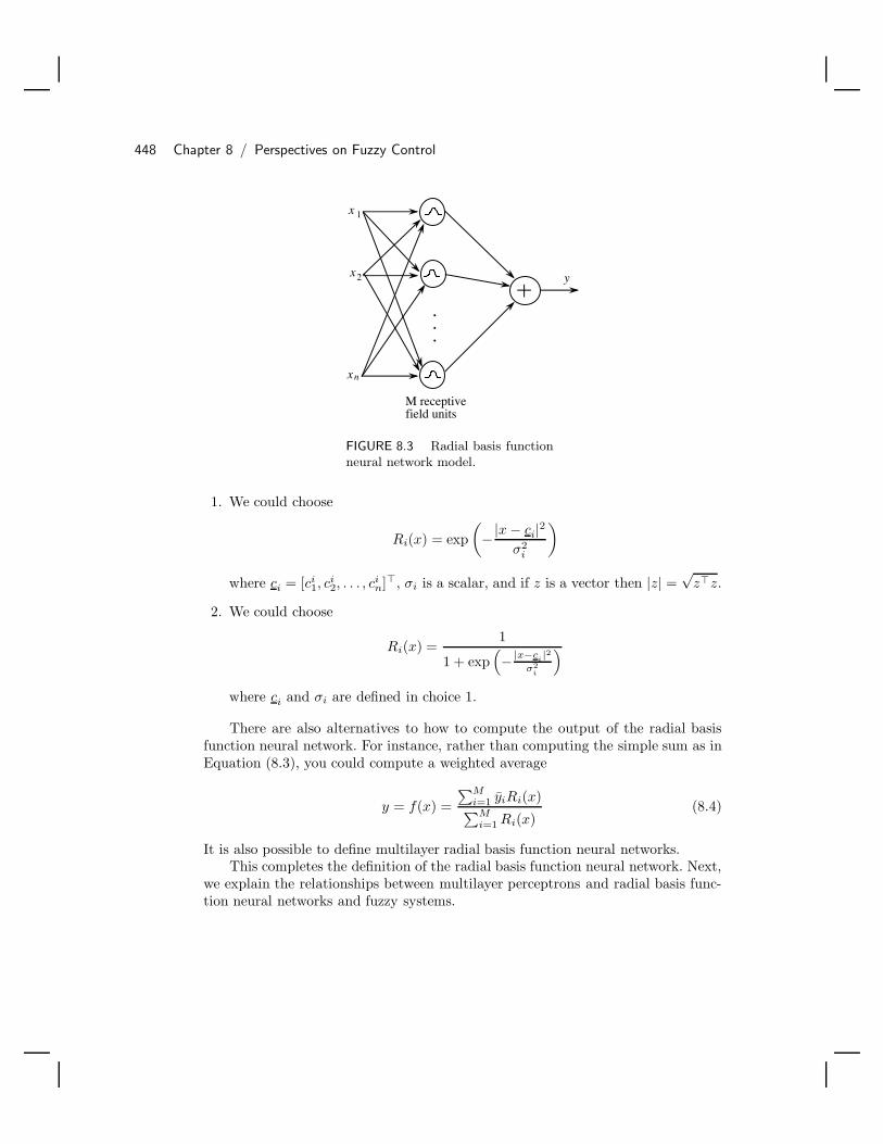
448 Chapter 8 / Perspectives on Fuzzy Control
x 1
x2
xn
.
.
.
M receptivefield units
y
FIGURE 8.3 Radial basis functionneural network model.
1. We could choose
Ri(x) = exp(−|x − ci|2
σ2i
)
where ci = [ci1, c
i2, . . . , c
in], σi is a scalar, and if z is a vector then |z| =
√zz.
2. We could choose
Ri(x) =1
1 + exp(− |x−c
i|2
σ2i
)where ci and σi are defined in choice 1.
There are also alternatives to how to compute the output of the radial basisfunction neural network. For instance, rather than computing the simple sum as inEquation (8.3), you could compute a weighted average
y = f(x) =∑M
i=1 yiRi(x)∑Mi=1 Ri(x)
(8.4)
It is also possible to define multilayer radial basis function neural networks.This completes the definition of the radial basis function neural network. Next,
we explain the relationships between multilayer perceptrons and radial basis func-tion neural networks and fuzzy systems.

8.3 Neural Networks 449
8.3.3 Relationships Between Fuzzy Systems and NeuralNetworks
There are two ways in which there are relationships between fuzzy systems andneural networks. First, techniques from one area can be used in the other. Second,in some cases the functionality (i.e., the nonlinear function that they implement) isidentical. Some label the intersection between fuzzy systems and neural networkswith the term “fuzzy-neural” or “neuro-fuzzy” to highlight that techniques fromboth fields are being used. Here, we avoid this terminology and simply highlightthe basic relationships between the two fields.
Multilayer Perceptrons
The multilayer perceptron should be viewed as a nonlinear network whose nonlin-earity can be tuned by changing the weights, biases, and parameters of the activa-tion functions. The fuzzy system is also a tunable nonlinearity whose shape can bechanged by tuning, for example, the membership functions. Since both are tunablenonlinearities, the following approaches are possible:
• Gradient methods can be used for training neural networks to perform systemidentification or to act as estimators or predictors in the same way as fuzzysystems were trained in Chapter 5, Section 5.4, beginning on page 260. Indeed,the gradient training of neural networks, called “back-propagation training,” wasintroduced well before the gradient training of fuzzy systems, and the idea fortraining fuzzy systems this way came from the field of neural networks.
• Hybrid methods for training, which were covered in Chapter 5, Section 5.7, onpage 291, can also be used for neural networks. For instance, gradient methodsmay be used in conjunction with clustering methods applied to neural networks.
• Indirect adaptive control, which was covered in Chapter 6, Section 6.6 on page 394,can also be achieved with a multilayer perceptron. To do this we use two multi-layer perceptrons as the tunable nonlinearities in the certainty equivalence controllaw and the gradient method for tuning.
• Gain scheduled control, covered in Chapter 7, Section 7.2.2, on page 417 maybe achieved by training a multilayer perceptron to map the associations betweenoperating conditions and controller parameters.
This list is by no means exhaustive. It simply shows that multilayer perceptronnetworks can take on a similar role to that of a fuzzy system in performing thefunction of being a tunable nonlinearity. An advantage that the fuzzy system mayhave, however, is that it often facilitates the incorporation of heuristic knowledgeinto the solution to the problem, which can, at times, have a significant impact onthe quality of the solution (see Section 5.2.4 on page 241).

450 Chapter 8 / Perspectives on Fuzzy Control
Radial Basis Function Neural Networks
Some radial basis function neural networks are equivalent to some standard fuzzysystems in the sense that they are functionally equivalent (i.e., given the sameinputs, they will produce the same outputs). To see this, suppose that in Equa-tion (8.4) we let M = R (i.e., the number of receptive field units equal to thenumber of rules), yi = bi (i.e., the receptive field unit strengths equal to the outputmembership function centers), and choose the receptive field units as
Ri(x) = µi(x)
(i.e., choose the receptive field units to be the same as the premise membershipfunctions). In this case we see that the radial basis function neural network isidentical to a certain fuzzy system that uses center-average defuzzification. Thisfuzzy system is then given by
y = f(x) =∑R
i=1 biµi(x)∑Ri=1 µi(x)
It is also interesting to note that the functional fuzzy system (the more generalversion of the Takagi-Sugeno fuzzy system), which was covered in Section 2.3.7 onpage 73, is equivalent to a class of two-layer neural networks [200].
The equivalence between this type of fuzzy system and a radial basis functionneural network shows that all the techniques in this book for the above type of fuzzysystem work in the same way for the above type of radial basis function neuralnetwork (or, using [200], the techniques for the Takagi-Sugeno fuzzy system can beused for a type of multilayer radial basis function neural network).
Due to the above relationships between fuzzy systems and neural networks,some would like to view fuzzy systems and neural networks as identical areas. Thisis, however, not the case for the following reasons:
• There are classes of neural networks (e.g., dynamic neural networks) that mayhave a fuzzy system analog, but if so it would have to include not only standardfuzzy components but some form of a differential equation component.
• There are certain fuzzy systems that have no clear neural analog. Consider, forexample, certain “fuzzy dynamic systems” [48, 167]. We can, however, envisionhow you could go about designing a neural analog to such fuzzy systems.
• The neural network has traditionally been a “black box” approach where theweights and biases are trained (e.g., using gradient methods like back-propagation)using data, often without using extra heuristic knowledge we often have. In fuzzysystems you can incorporate heuristic information and use data to train them(see Chapter 5, Section 5.2.4 on page 241). This last difference is often quoted asbeing one of the advantages of fuzzy systems over neural networks, at least forsome applications.
8.4 Genetic Algorithms 451
Regardless of the differences, it is important to note that many methods inneural control (i.e., when we use a neural network for the control of a system) arequite similar to those in adaptive fuzzy control. For instance, since the fuzzy systemand radial basis function neural network can be linearly parameterized (see [200]),we can use them as the identifier structures in direct or indirect adaptive controlschemes and use gradient or least squares methods to update the parameters (seeChapters 5 and 6 and [200, 229, 50]). Indeed, we could have used neural networksas the structure that we trained for all of the identification methods in Chapter 5.In this sense we can use neural networks in system identification, estimation, andprediction, and as a direct (fixed) controller that is trained with input-output data.Basically, to be fluent with the methods of adaptive fuzzy systems and control, youmust know the methods of neural control—and vice versa.
8.4 Genetic AlgorithmsA genetic algorithm (GA) uses the principles of evolution, natural selection, andgenetics from natural biological systems in a computer algorithm to simulate evolu-tion. Essentially, the genetic algorithm is an optimization technique that performsa parallel, stochastic, but directed search to evolve the most fit population. In thissection we will introduce the genetic algorithm and explain how it can be used fordesign and tuning of fuzzy systems.
8.4.1 Genetic Algorithms: A TutorialThe genetic algorithm borrows ideas from and attempts to simulate Darwin’s theoryon natural selection and Mendel’s work in genetics on inheritance. The geneticalgorithm is an optimization technique that evaluates more than one area of thesearch space and can discover more than one solution to a problem. In particular,it provides a stochastic optimization method where if it “gets stuck” at a localoptimum, it tries to simultaneously find other parts of the search space and “jumpout” of the local optimum to a global one.
Representation and the Population of Individuals
The “fitness function” measures the fitness of an individual to survive in a popula-tion of individuals. The genetic algorithm will seek to maximize the fitness functionJ(θ) by selecting the individuals that we represent with θ. To represent the geneticalgorithm in a computer, we make θ a string. In particular, we show such a string inFigure 8.4. A string is a chromosome in a biological system. It is a string of “genes”that can can take on different “alleles.” In a computer we use number systems toencode alleles. Hence, a gene is a “digit location” that can take on different valuesfrom a number system (i.e., different types of alleles).
For instance, in a base-2 number system, alleles come from the set 0, 1,while in a base-10 number system, alleles come from the set 0, 1, 2, 3, 4, 5, 6, 7, 8, 9.Hence, a binary chromosome has zeros or ones in its gene locations. As an example,
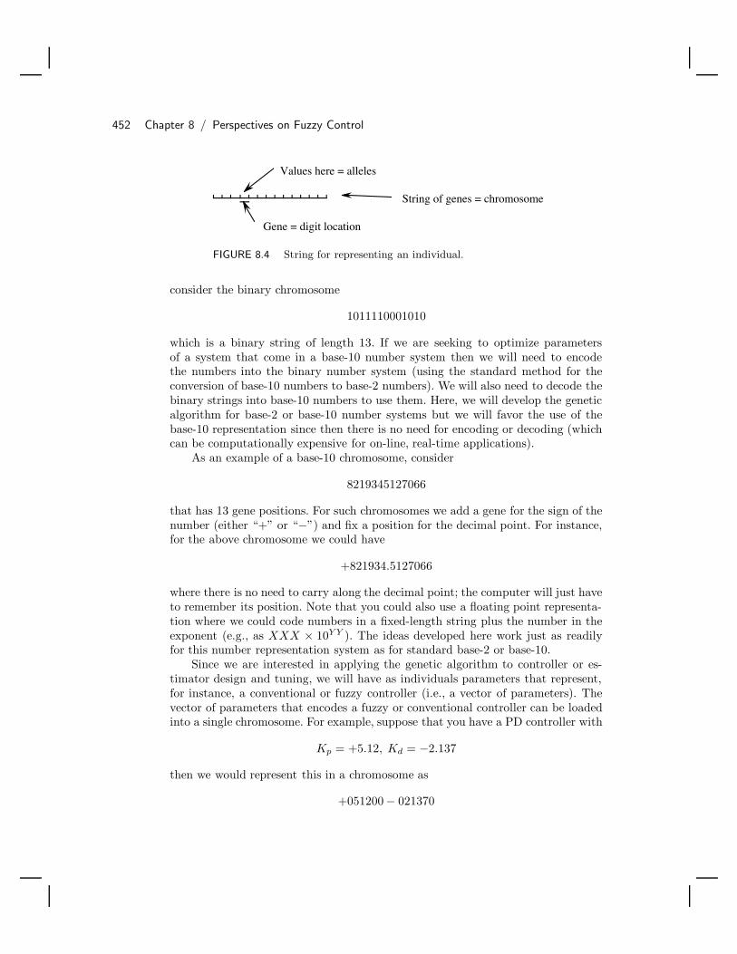
452 Chapter 8 / Perspectives on Fuzzy Control
Gene = digit location
Values here = alleles
String of genes = chromosome
FIGURE 8.4 String for representing an individual.
consider the binary chromosome
1011110001010
which is a binary string of length 13. If we are seeking to optimize parametersof a system that come in a base-10 number system then we will need to encodethe numbers into the binary number system (using the standard method for theconversion of base-10 numbers to base-2 numbers). We will also need to decode thebinary strings into base-10 numbers to use them. Here, we will develop the geneticalgorithm for base-2 or base-10 number systems but we will favor the use of thebase-10 representation since then there is no need for encoding or decoding (whichcan be computationally expensive for on-line, real-time applications).
As an example of a base-10 chromosome, consider
8219345127066
that has 13 gene positions. For such chromosomes we add a gene for the sign of thenumber (either “+” or “−”) and fix a position for the decimal point. For instance,for the above chromosome we could have
+821934.5127066
where there is no need to carry along the decimal point; the computer will just haveto remember its position. Note that you could also use a floating point representa-tion where we could code numbers in a fixed-length string plus the number in theexponent (e.g., as XXX × 10Y Y ). The ideas developed here work just as readilyfor this number representation system as for standard base-2 or base-10.
Since we are interested in applying the genetic algorithm to controller or es-timator design and tuning, we will have as individuals parameters that represent,for instance, a conventional or fuzzy controller (i.e., a vector of parameters). Thevector of parameters that encodes a fuzzy or conventional controller can be loadedinto a single chromosome. For example, suppose that you have a PD controller with
Kp = +5.12, Kd = −2.137
then we would represent this in a chromosome as
+051200− 021370

8.4 Genetic Algorithms 453
which is a concatenation of the digits, where we assume that there are six digitsfor the representation of each parameter plus the sign digit (this is why you see theextra padding of zeros). The computer will have to keep track of where the decimalpoint is. We see that each chromosome will have a certain structure (its “genotype”in biological terms), but here rather than a set of chromosomes for the structurewe just concatenate the parameters and use one one chromosome for convenience.Each chromosome represents a point in the search space of the genetic algorithm(i.e., a “phenotype” in biological terms).
Next, we develop a notation for representing a whole set of individuals (i.e., apopulation). Let θj
i (k) be a single parameter at time k (a fixed-length string withsign digit), and suppose that chromosome j is composed of N of these parameters,which are sometimes called “traits.” Let
θj(k) =[θj1(k), θj
2(k), . . . , θjN (k)
]be the jth chromosome. Note that earlier we had concatenated elements in a stringwhile here we simply take the concatenated elements and form a vector from them.We do this simply because this is probably the way that you will want to code thealgorithm in the computer. We will at times, however, still let θj be a concatenatedstring when it is convenient to do so.
The population of individuals at time k is given by
P (k) =θj(k)|j = 1, 2, . . . , S
(8.5)
and the number of individuals in the population is given by S. We want to pick S tobe big enough so that the population elements can cover the search space. However,we do not want S to be too big since this increases the number of computations wehave to perform.
Genetic Operations
The population P (k) at time k is often referred to as the “generation” of individualsat time k. Evolution occurs as we go from a generation at time k to the nextgeneration at time k + 1. Genetic operations of selection, crossover, and mutationare used to produce one generation from the next.
Selection: Basically, according to Darwin the most qualified individuals surviveto mate. We quantify “most qualified” via an individual’s fitness J(θj(k)) at timek. For selection we create a “mating pool” at time k, which we denote by
M(k) =mj(k)|j = 1, 2, . . . , S
(8.6)
The mating pool is the set of chromosomes that are selected for mating. We selectan individual for mating by letting each mj(k) be equal to θi(k) ∈ P (k) with
454 Chapter 8 / Perspectives on Fuzzy Control
probability
pi =J(θi(k))∑S
j=1 J(θj(k))(8.7)
To clarify the meaning of this formula and hence the selection strategy, Goldberg[58] uses the analogy of spinning a unit circumference roulette wheel where thewheel is cut like a pie into S regions where the ith region is associated with the ith
element of P (k). Each pie-shaped region has a portion of the circumference thatis given by pi in Equation (8.7). You spin the wheel, and if the pointer points atregion i when the wheel stops, then you place θi into the mating pool M(k). Youspin the wheel S times so that S elements end up in the mating pool. Clearly,individuals who are more fit will end up with more copies in the mating pool;hence, chromosomes with larger-than-average fitness will embody a greater portionof the next generation. At the same time, due to the probabilistic nature of theselection process, it is possible that some relatively unfit individuals may end up inthe mating pool.
Reproduction Phase, Crossover: We think of crossover as mating in biologicalterms, which at a fundamental biological level involves the process of combiningchromosomes. The crossover operation operates on the mating pool M(k). First,you specify the “crossover probability” pc (usually chosen to be near one sincewhen mating occurs in biological systems, genetic material is swapped between theparents). The procedure for crossover consists of the following steps:
1. Randomly pair off the individuals in the mating pool M(k) (i.e., form pairs tomate by the flip of a coin). If there are an odd number of individuals in M(k),then, for instance, simply take the last individual and pair it off with anotherindividual who has already been paired off.
2. Consider chromosome pair θj , θi that was formed in step 1. Generate a randomnumber r ∈ [0, 1].
(a) If r < pc then cross over θj and θi. To cross over these chromosomes selectat random a “cross site” and exchange all the digits to the right of thecross site of one string with those of the other. This process is picturedin Figure 8.5. In this example the cross site is position five on the string,and hence we swap the last eight digits between the two strings. Clearly,the cross site is a random number between one and the number of digitsin the string minus one.
(b) If r > pc then we will not cross over; hence, we do not modify the strings,and we go to the mutation operation below.
3. Repeat step 2 for each pair of strings that is in M(k).

8.4 Genetic Algorithms 455
θ i 1 2 3 4 5 6 7 8 9 10 11 12 13
θ j 1 2 3 4 5 6 7 8 9 10 11 12 13
Cross site
Switch these two parts of the strings
FIGURE 8.5 Crossover operation example.
As an example, suppose that S = 10 and that in step 1 above we randomly pair offthe chromosomes. Suppose that θ5 and θ9 (j = 5, i = 9) are paired off where
θ5 = +2.9845
and
θ9 = +1.9322
Suppose that pc = 0.9 and that when we randomly generate r we get r = 0.34.Hence, by step 2 we will cross over θ5 and θ9 . According to step 2 we randomlypick the cross site. Suppose that it is chosen to be position three on the string. Inthis case the strings that are produced by crossover are
θ5 = +2.9322
and
θ9 = +1.9845
Besides the fact that crossover helps to model the mating part of the evolution pro-cess, why should the genetic algorithm perform crossover? Basically, the crossoveroperation perturbs the parameters near good positions to try to find better solutionsto the optimization problem. It tends to help perform a localized search around themore fit individuals (since on average the individuals in the mating pool at time kare more fit than the ones in the population at time k).
Reproduction Phase, Mutation: Like crossover, mutation modifies the matingpool (i.e., after selection has taken place). The operation of mutation is normallyperformed on the elements in the mating pool after crossover has been performed.The biological analog of our mutation operation is the random mutation of geneticmaterial. To perform mutation in the computer, first choose a mutation probabilitypm. With probability pm, change (mutate) each gene location on each chromosomerandomly to a member of the number system being used. For instance, in a base-2genetic algorithm, we could mutate
1010111

456 Chapter 8 / Perspectives on Fuzzy Control
to
1011111
where the fourth bit was mutated to one. For a base-10 number system you wouldsimply pick a number at random to replace a digit with if you are going to mutatea digit location.
Besides the fact that this helps to model mutation in a biological system, whyshould the genetic algorithm perform mutation? Basically, it provides random ex-cursions into new parts of the search space. It is possible that we will get lucky andmutate to a good solution. It is the mechanism that tries to make sure that we donot get stuck at a local maxima and that we seek to explore other areas of the searchspace to help find a global maximum for J(θ). Usually, the mutation probability ischosen to be quite small (e.g., less than 0.01) since this will help guarantee that allthe individuals in the mating pool are not mutated so that any search progress thatwas made is lost (i.e., we keep it relatively low to avoid degradation to exhaustivesearch via a random walk in the search space).
After mutation we get a modified mating pool at time k, M(k). To form thenext generation for the population, we let
P (k + 1) = M(k)
where this M(k) is the one that was formed by selection and modified by crossoverand mutation. Then the above steps repeat, successive generations are produced,and we thereby model evolution (of course it is a very crude model).
Optional Features: There have been many different options used in the defini-tion of a genetic algorithm. These include the following:
• There is the possibility of using other genetic operators. For instance, there is anoperation called “elitism” where the most fit individual in P (k) is copied directlyto P (k + 1) without being changed by the other operations. This operator issometimes used to try to make sure that there will be a reasonably fit individualpresent in the population at every time step; it helps to avoid having all thestrings get modified by crossover and mutation in a way so that no good solutionexists at some time k.
• Some use a “population splitting” approach where the population of S membersis partitioned into subsets and the genetic operations are constrained to only mixwithin these partitions. This can produce different subpopulations that will seekdifferent solutions.
• There are many options for the crossover operation. For instance, some considercrossing over at every site in the chromosome. Others will perform crossover foreach separate parameter (trait) on the chromosome.
• Some will grow and shrink the population.

8.4 Genetic Algorithms 457
There are many other options besides the ones listed above. The interested readershould consult Section 8.8, For Further Study, for more details about genetic algo-rithms.
Termination Conditions, Initialization, and Implementation Issues
The above discussion showed how to produce successive generations and therebysimulate evolution. While the biological evolutionary process continues, perhapsindefinitely, there are many times when we would like to terminate our artificialone and find the following:
• The population individual—say, θ∗(k)—that best maximizes the fitness function.Notice that to determine this we also need to know the generation number k wherethe most fit individual existed (it is not necessarily in the last generation). Youmay want to design the computer code that implements the genetic algorithm toalways keep track of the highest J value and the generation number and individualthat achieved this value of J .
• The value of the fitness function J(θ∗(k)). While for some applications this valuemay not be important, for others it is critical (e.g., in many function optimizationproblems).
• Information about the way that the population has evolved, which areas of thesearch space were visited, and how the fitness function has evolved over time. Youmay want to design the code that implements the genetic algorithm to provideplots or printouts of all the relevant genetic algorithm data.
There is then the question of how to terminate the genetic algorithm. There aremany ways to terminate a genetic algorithm, many of them similar to terminationconditions used for conventional optimization algorithms. To introduce a few ofthese, let ε > 0 be a small number and M1 > 0 and M2 > 0 be integers. Considerthe following options for terminating the genetic algorithm:
• Stop the algorithm after generating generation P (M2)—that is, after M2 gener-ations.
• Stop the algorithm after at least M2 generations have occurred and at least M1
steps have occurred where the maximum (or average) value of J for all populationmembers has increased by no more than ε.
• Stop the algorithm once J takes on a value above some fixed value.
Of course, there are other possibilities for termination conditions. The above onesare easy to implement on a computer but sometimes you may want to watch theparameters evolve and decide yourself when to stop the algorithm.
Initialization of the genetic algorithm is done by first choosing the represen-tation to be used (including the structure of the chromosomes, the number base,

458 Chapter 8 / Perspectives on Fuzzy Control
and the number of digits to be used). Next, you need to specify the size of thepopulation, decide which genetic operations will be used, specify the crossover andmutation probabilities pc and pm, and pick a termination method (if it is needed).
Sometimes for problems that are solved by the genetic algorithm it is knownthat the parameters that are manipulated by the genetic algorithm will lie in acertain fixed range (e.g., you may know that you would never want to make theproportional gain of a PID controller negative). Suppose, for the sake of discussion,that θ is a scalar and we know a priori that it will stay in a certain interval—say, [θmin, θmax]. It is important to note that crossover and mutation can generatestrings that are out of a fixed range even if parameters all start within the properranges (provide an example of this). Due to this there is a problem when it comesto implementing the genetic algorithm of what to do when the algorithm generatesa chromosome that is out of range. There are several approaches to solving thisproblem. For instance, if a scalar parameter θ is to lie in [θmin, θmax], and at timek crossover or mutation makes θ(k) > θmax, then simply choose θ(k) = θmax. Ifat time k crossover or mutation makes θ(k) < θmin, then simply choose θ(k) =θmin. An alternative approach would be to simply repeat the crossover or mutationoperation again and hope that the newly generated parameters will be in range. Ofcourse, this may not solve the problem since the next time they are generated theymay also be out of range (and the number of tries that it takes to get in range israndom).
8.4.2 Genetic Algorithms for Fuzzy System Design and TuningThere are basically two ways that the genetic algorithm can be used in the areaof fuzzy systems: They can be used for the off-line design of fuzzy systems and intheir on-line tuning. Both of these options are considered next.
Computer-Aided Design of Fuzzy Systems
The genetic algorithm can be used in the (off-line) computer-aided design of controlsystems since it can artificially evolve an appropriate controller that meets theperformance specifications to the greatest extent possible. To do this, the geneticalgorithm maintains a population of strings that each represent a different controller(digits on the strings characterize parameters of the controller), and it uses a fitnessmeasure that characterizes the closed-loop specifications. Suppose, for instance, thatthe closed-loop specifications indicate that you want, for a step input, a (stable)response with a rise-time of t∗r , a percent overshoot of M∗
p , and a settling time of t∗s.We need to define the fitness function so that it measures how close each individualin the population at time k (i.e., each controller candidate) is to meeting thesespecifications. Suppose that we let tr , Mp, and ts denote the rise-time, overshoot,and settling time, respectively, for a given individual (we compute these for anindividual in the population by performing a simulation of the closed-loop systemwith the candidate controller and a model of the plant). Given these values, we let

8.4 Genetic Algorithms 459
(for each individual and every time step k)
J = w1(tr − t∗r)2 + w2(Mp − M∗
p )2 + w3(ts − t∗s)2
where wi > 0, i = 1, 2, 3, are positive weighting factors. The function J characterizeshow well the candidate controller meets the closed-loop specifications where if J = 0it meets the specifications perfectly. The weighting factors can be used to prioritizethe importance of meeting the various specifications (e.g., a high value of w2 relativeto the others indicates that the percent overshoot specification is more importantto meet than the others).
Now, we would like to minimize J , but the genetic algorithm is a maximiza-tion routine. To minimize J with the genetic algorithm, we can choose the fitnessfunction
J =1
J + ε
where ε > 0 is a small positive number. Maximization of J can only be achievedby minimization of J , so the desired effect is achieved. Another way to define thefitness function is to let
J(θ(k)) = −J(θ(k)) + maxθ(k)
J(θ(k))
The minus sign in front of the J(θ(k)) term turns the minimization problem intoa maximization problem (to see this, consider J(θ) = (θ)2 , where θ is a scalar, asan example). The maxθ(k)J(θ(k)) term is needed to shift the function up so thatJ(θ(k)) is always positive. We need it positive since in selection, Equation (8.7)defines a probability that must always be positive and between one and zero.
This completes the definition of how to use a genetic algorithm for computer-aided control system design. Note that the above approach depends in no wayon whether the controller that is evolved is a conventional controller (e.g., a PIDcontroller) or a fuzzy system or neural network. For instance, you could use aTakagi-Sugeno fuzzy system or a standard fuzzy system for the controller and letthe genetic algorithm tune the appropriate parameters. Moreover, we could takeany of the controllers described in Chapters 6 or 7 and parameterize them anduse the above approach to tune these adaptive or supervisory controllers. We haveused the genetic algorithm to tune direct, adaptive, and supervisory controllers forseveral applications, and while this approach is computationally intensive, and wedid have to make some application-dependent modifications to the above fitnessevaluation approach, it did produce successful results (see, e.g., [27]).
The above approach can also be used in system identification and for the con-struction of estimators and predictors, just as we used gradient optimization forthese in Chapter 5. The genetic algorithm can be used for the tuning of fuzzy sys-tem parameters that enter in a nonlinear fashion and can be used in conjunctionwith other methods from Chapter 5 to form hybrid approaches such as those de-

460 Chapter 8 / Perspectives on Fuzzy Control
scribed in Section 5.7 on page 291. To use the genetic algorithm for tuning fuzzysystems as estimators, we could choose J to be Equation (5.7) or (5.6) on page 238.Then we would choose the fitness function J similarly to how we did above. Wehave used such an approach to construct a Takagi-Sugeno fuzzy system that actedas a gain scheduler. One possible advantage that the GA approach could offer over,for example, a gradient method is that it may be able to better avoid local optimaand hence find the global optimum.
On-Line Tuning of Fuzzy Systems
Traditionally, genetic algorithms have been used for off-line design, search, and op-timization. There are ways, however, to evolve controllers (fuzzy or conventional)while the system is operating, rather than in off-line design. Progress in this direc-tion has been made by the introduction of the “genetic model reference adaptivecontroller” (GMRAC) shown in Figure 8.6. As in the FMRLC, the GMRAC uses areference model to characterize the desired performance. For the GMRAC there isa genetic algorithm that maintains a population of strings each of which representsa candidate controller. This genetic algorithm uses a process model (e.g., a linearmodel of the process) and data from the process to evaluate the fitness of eachcontroller in the population. It does this evaluation at each time step by simulatingout into the future with each candidate controller and forming a fitness functionbased on the error between the predicted output for each controller and that ofthe reference model. Using this fitness evaluation, the genetic algorithm propagatescontrollers into the next generation via the standard genetic operations. The con-troller that is the most fit one in the population at each time step is used to controlthe system.
Plantcontroller
r(t)y(t)u(t)
Referencemodel
y (t)m
Most fit
Genetic algorithm
Popu
latio
nof
cont
rolle
rs
Proc
ess
mod
el
Adaptationlevel
FIGURE 8.6 Genetic model reference adaptivecontroller (figure taken from [158], c© IEEE).
This allows the GMRAC to automatically evolve a controller from generationto generation (i.e., from one time step to the next, but of course multiple genera-tions could occur between time steps) and hence to tune a controller in response
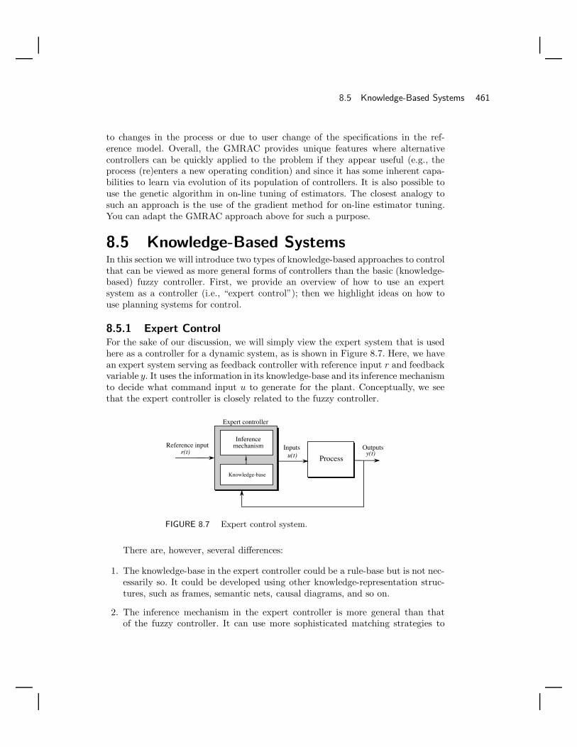
8.5 Knowledge-Based Systems 461
to changes in the process or due to user change of the specifications in the ref-erence model. Overall, the GMRAC provides unique features where alternativecontrollers can be quickly applied to the problem if they appear useful (e.g., theprocess (re)enters a new operating condition) and since it has some inherent capa-bilities to learn via evolution of its population of controllers. It is also possible touse the genetic algorithm in on-line tuning of estimators. The closest analogy tosuch an approach is the use of the gradient method for on-line estimator tuning.You can adapt the GMRAC approach above for such a purpose.
8.5 Knowledge-Based SystemsIn this section we will introduce two types of knowledge-based approaches to controlthat can be viewed as more general forms of controllers than the basic (knowledge-based) fuzzy controller. First, we provide an overview of how to use an expertsystem as a controller (i.e., “expert control”); then we highlight ideas on how touse planning systems for control.
8.5.1 Expert ControlFor the sake of our discussion, we will simply view the expert system that is usedhere as a controller for a dynamic system, as is shown in Figure 8.7. Here, we havean expert system serving as feedback controller with reference input r and feedbackvariable y. It uses the information in its knowledge-base and its inference mechanismto decide what command input u to generate for the plant. Conceptually, we seethat the expert controller is closely related to the fuzzy controller.
Fuzz
ific
atio
n
Def
uzzi
fica
tion
FuzzyInferenceMechanis
m
Rule-BaseKnowledge-base
Process
Inputs OutputsReference input
Expert controller
r(t) u(t) y(t)
Inferencemechanism
FIGURE 8.7 Expert control system.
There are, however, several differences:
1. The knowledge-base in the expert controller could be a rule-base but is not nec-essarily so. It could be developed using other knowledge-representation struc-tures, such as frames, semantic nets, causal diagrams, and so on.
2. The inference mechanism in the expert controller is more general than thatof the fuzzy controller. It can use more sophisticated matching strategies to

462 Chapter 8 / Perspectives on Fuzzy Control
determine which rules should be allowed to fire. It can use more elaborateinference strategies. For instance, some expert systems use (a) “refraction,”where if a rule has fired recently it may not be allowed back into the “conflictset” (i.e., the set of rules that are allowed to fire), (b) “recency,” where rulesthat were fired most recently are given priority in being fired again, and (c)various other priority schemes.
It is in fact the case that an expert system is in a sense more general than afuzzy system since it can be shown that a single rule in an expert controller canbe used to represent an entire fuzzy controller [163]. From another perspective, wecan “fuzzify” the expert controller components and make it a more general fuzzysystem. Regardless, it is largely a waste of time to concern ourselves with whichis more general. What is of concern is whether the traditional ideas from expertsystems offer anything on how to design fuzzy systems. The answer is certainly af-firmative. Clearly, certain theory and applications may dictate the need for differentknowledge-representation schemes and inference strategies.
Next, we should note that Figure 8.7 shows a direct expert controller. As wepointed out in Chapter 7, it is also possible to use an expert system in adaptiveor supervisory control systems. Expert systems can be used in a supervisory rolefor conventional controllers or for the supervision of fuzzy controllers (e.g., forsupervision of the learning mechanism and reference model in an adaptive fuzzycontroller). Expert systems themselves can also be used as the basis for generallearning controllers.
8.5.2 Planning Systems for ControlArtificially intelligent planning systems (computer programs that emulate the wayexperts plan) have been used in path planning and high-level decisions about controltasks for robots. A generic planning system can be configured in the architectureof a standard control system, as shown in Figure 8.8. Here, the “problem domain”(the plant) is the environment that the planner operates in. There are measuredoutputs yk at step k (variables of the problem domain that can be sensed in realtime), control actions uk (the ways in which we can affect the problem domain),disturbances dk (which represent random events that can affect the problem do-main and hence the measured variable yk), and goals gk (what we would like toachieve in the problem domain). There are closed-loop specifications that quantifyperformance specifications and stability requirements.
It is the task of the planner in Figure 8.8 to monitor the measured outputs andgoals and generate control actions that will counteract the effects of the disturbancesand result in the goals and the closed-loop specifications being achieved. To do this,the planner performs “plan generation,” where it projects into the future (usuallya finite number of steps, and often using a model of the problem domain) andtries to determine a set of candidate plans. Next, this set of plans is pruned toone plan that is the best one to apply at the current time (where “best” can bedetermined based on, e.g., consumption of resources). The plan is then executed,
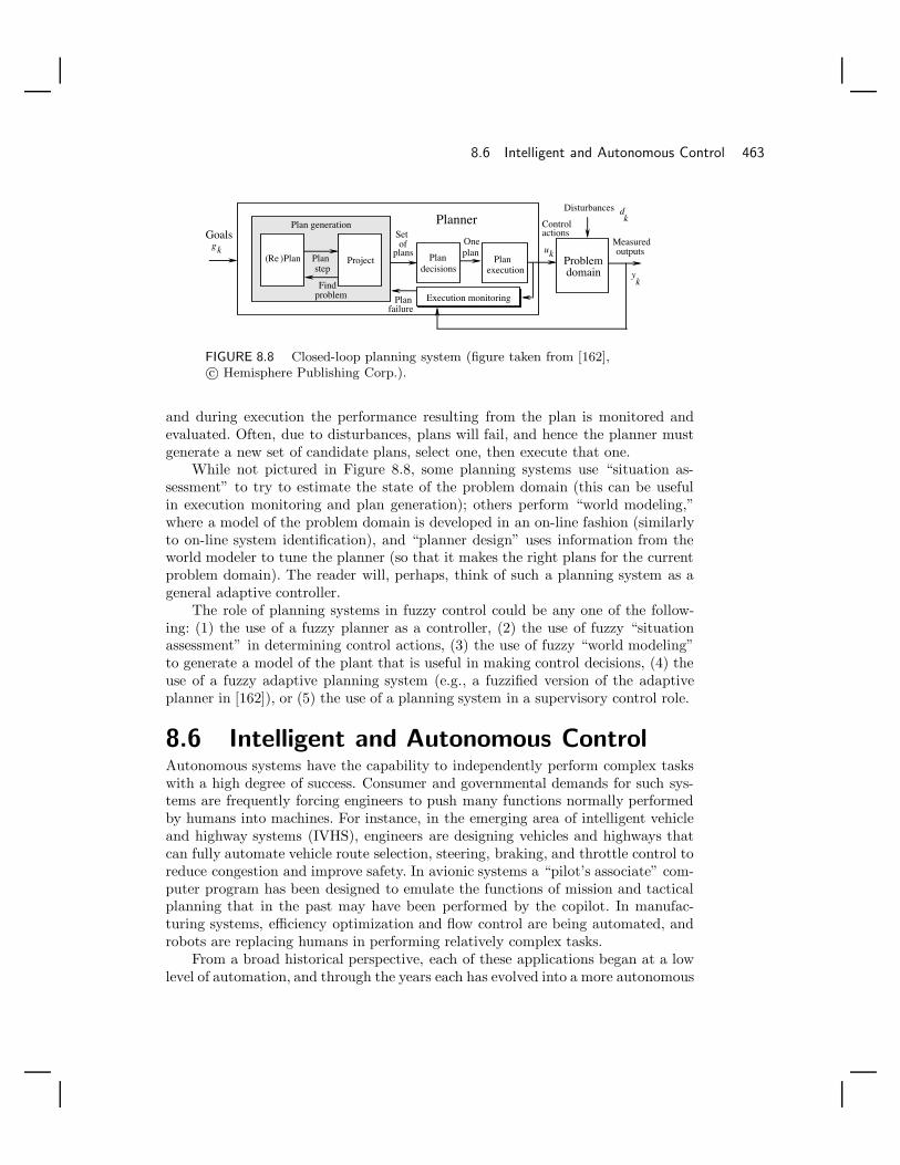
8.6 Intelligent and Autonomous Control 463
Planstep
Findproblem
Plan generation
Project(Re )Plan
Setof
plansOneplan
Planner
Plandecisions
Planexecution
Goals
Problemdomain
Controlactions
Measuredoutputs
Disturbances dk
uk
yk
gk
Execution monitoringPlanfailure
FIGURE 8.8 Closed-loop planning system (figure taken from [162],c© Hemisphere Publishing Corp.).
and during execution the performance resulting from the plan is monitored andevaluated. Often, due to disturbances, plans will fail, and hence the planner mustgenerate a new set of candidate plans, select one, then execute that one.
While not pictured in Figure 8.8, some planning systems use “situation as-sessment” to try to estimate the state of the problem domain (this can be usefulin execution monitoring and plan generation); others perform “world modeling,”where a model of the problem domain is developed in an on-line fashion (similarlyto on-line system identification), and “planner design” uses information from theworld modeler to tune the planner (so that it makes the right plans for the currentproblem domain). The reader will, perhaps, think of such a planning system as ageneral adaptive controller.
The role of planning systems in fuzzy control could be any one of the follow-ing: (1) the use of a fuzzy planner as a controller, (2) the use of fuzzy “situationassessment” in determining control actions, (3) the use of fuzzy “world modeling”to generate a model of the plant that is useful in making control decisions, (4) theuse of a fuzzy adaptive planning system (e.g., a fuzzified version of the adaptiveplanner in [162]), or (5) the use of a planning system in a supervisory control role.
8.6 Intelligent and Autonomous ControlAutonomous systems have the capability to independently perform complex taskswith a high degree of success. Consumer and governmental demands for such sys-tems are frequently forcing engineers to push many functions normally performedby humans into machines. For instance, in the emerging area of intelligent vehicleand highway systems (IVHS), engineers are designing vehicles and highways thatcan fully automate vehicle route selection, steering, braking, and throttle control toreduce congestion and improve safety. In avionic systems a “pilot’s associate” com-puter program has been designed to emulate the functions of mission and tacticalplanning that in the past may have been performed by the copilot. In manufac-turing systems, efficiency optimization and flow control are being automated, androbots are replacing humans in performing relatively complex tasks.
From a broad historical perspective, each of these applications began at a lowlevel of automation, and through the years each has evolved into a more autonomous

464 Chapter 8 / Perspectives on Fuzzy Control
system. For example, today’s automotive cruise controllers are the ancestors of thecontrollers that achieve coordinated control of steering, braking, and throttle forautonomous vehicle driving. And the terrain following, terrain avoidance controlsystems for low-altitude flight are ancestors of an artificial pilot’s associate thatcan integrate mission and tactical planning activities. The general trend has beenfor engineers to incrementally “add more intelligence” in response to consumer,industrial, and government demands and thereby create systems with increasedlevels of autonomy. In this process of enhancing autonomy by adding intelligence,engineers often study how humans solve problems, then try to directly automatetheir knowledge and techniques to achieve high levels of automation. Other times,engineers study how intelligent biological systems perform complex tasks, then seekto automate “nature’s approach” in a computer algorithm or circuit implementationto solve a practical technological problem (e.g., in certain vision systems). Suchapproaches where we seek to emulate the functionality of an intelligent biologicalsystem (e.g., the human) to solve a technological problem can be collectively named“intelligent systems and control techniques.” It is by using such techniques thatsome engineers are trying to create highly autonomous systems such as those listedabove.
In this section we will explain how “intelligent” control methods can be usedto create autonomous systems. First we will define “intelligent control.” Next, weprovide a framework for the operation of autonomous systems to clarify the ultimategoal of achieving autonomous behavior in complex technological systems.
8.6.1 What Is “Intelligent Control”?Since the answer to this question can get rather philosophical, let us focus on aworking definition that does not dwell on definitions of “intelligence” (since thereis no widely accepted one partly because biological intelligence seems to have manydimensions and appears to be very complex) and issues of whether we truly modelor emulate intelligence, but instead focuses on (1) the methodologies used in theconstruction of controllers and (2) the ability of an artificial system to performactivities normally performed by humans.
“Intelligent control” techniques offer alternatives to conventional approaches byborrowing ideas from intelligent biological systems. Such ideas can either come fromhumans who are, for example, experts at manually solving the control problem, orby observing how a biological system operates and using analogous techniques inthe solution of control problems. For instance, we may ask a human driver to pro-vide a detailed explanation of how she or he manually solves an automated highwaysystem intervehicle distance control problem, then use this knowledge directly in afuzzy controller. In another approach, we may train an artificial neural network toremember how to regulate the intervehicle spacing by repeatedly providing it withexamples of how to perform such a task. After the neural network has learned thetask, it can be implemented on the vehicle to regulate the intervehicle distance byrecalling the proper throttle input for each value of the intervehicle distance thatis sensed. In another approach, genetic algorithms may be used to automatically

8.6 Intelligent and Autonomous Control 465
synthesize and tune a control algorithm for the intervehicle spacing control problemby starting with a population of candidate controllers and then iteratively allowingthe most fit controller, which is determined according to the performance specifica-tions, to survive in an artificial evolution process implemented in a computer. In thisway the controller evolves over time, successively improving its performance andadapting to its environment, until it meets the prespecified performance objectives.
Such intelligent control techniques may exploit the information represented ina mathematical model or may heavily rely on heuristics on how best to controlthe process. The primary difference from conventional approaches, such as PIDcontrol, is that intelligent control techniques are motivated by the functionality ofintelligent biological systems, either in how they perform the control task or inhow they provide an innovative solution to another problem that can be adaptedto solve a control problem. This is not to say that systems that are not developedusing intelligent systems and control techniques such as those listed above cannotbe called “intelligent”; traditionally, we have often called any system intelligent ifit is designed to perform a task that has normally been performed by humans (e.g.,we use the term “intelligent” vehicle and highway systems).
A full discussion on defining intelligent control involves considering additionalissues in psychology, human cognition, artificial intelligence, and control. The in-terested reader is referred to the articles listed at the end of this chapter for a moredetailed exposition that considers these issues.
8.6.2 Architecture and CharacteristicsFigure 8.9 shows a functional architecture for an intelligent autonomous controllerwith an interface to the process involving sensing (e.g., via conventional sensingtechnology, vision, touch, smell, etc.), actuation (e.g., via hydraulics, robotics, mo-tors, etc.), and an interface to humans (e.g., a driver, pilot, crew, etc.) and othersystems.
The “execution level” has low-level numeric signal processing and control algo-rithms (e.g., PID, optimal, adaptive, or intelligent control; parameter estimators,failure detection and identification (FDI) algorithms). The “coordination level”provides for tuning, scheduling, supervision, and redesign of the execution-levelalgorithms, crisis management, planning and learning capabilities for the coordi-nation of execution-level tasks, and higher-level symbolic decision making for FDIand control algorithm management. The “management level” provides for the su-pervision of lower-level functions and for managing the interface to the human(s)and other systems. In particular, the management level will interact with the usersin generating goals for the controller and in assessing the capabilities of the sys-tem. The management level also monitors performance of the lower-level systems,plans activities at the highest level (and in cooperation with humans), and performshigh-level learning about the user and the lower-level algorithms.
Intelligent systems or intelligent controllers (e.g., fuzzy, neural, genetic, expert,and planning) can be employed as appropriate in the implementation of variousfunctions at the three levels of the intelligent autonomous controller. For example,

466 Chapter 8 / Perspectives on Fuzzy Control
Humans and other subsystems
Process
Management level
Coordinationlevel
Executionlevel
FIGURE 8.9 Intelligentautonomouscontroller.
adaptive fuzzy control may be used at the execution level for adaptation, geneticalgorithms may be used in the coordination level to pick an optimal coordinationstrategy, and planning systems may be used at the management level for sequencingoperations. Hierarchical controllers composed of a hybrid mix of intelligent and con-ventional systems are commonly used in the intelligent control of complex dynamicsystems. This is because to achieve high levels of autonomy, we often need highlevels of intelligence, which calls for incorporating a diversity of decision-makingapproaches for complex dynamic learning and reasoning.
There are several fundamental characteristics that have been identified for in-telligent autonomous control systems. For example, there is generally a successivedelegation of duties from the higher to lower levels, and the number of distincttasks typically increases as we go down the hierarchy. Higher levels are often con-cerned with slower aspects of the system’s behavior and with its larger portions, orbroader aspects. There is then a smaller contextual horizon at lower levels—thatis, the control decisions are made by considering less information. Higher levels aretypically concerned with longer time horizons than lower levels. It is said that thereis “increasing intelligence with decreasing precision as one moves from the lowerto the higher levels” (see [179]). At the higher levels there is typically a decreasein time-scale density, a decrease in bandwidth or system rate, and a decrease inthe decision (control action) rate. In addition, there is typically a decrease in thegranularity of models used—or, equivalently, an increase in model abstractness atthe higher levels.
Finally, we note that there is an ongoing evolution of the intelligent functions ofan autonomous controller so that by the time you implement its functions, they nolonger appear intelligent, just algorithmic. It is because of this evolution principle,doubts about our ability to implement “artificial intelligence,” and the fact that

8.6 Intelligent and Autonomous Control 467
implemented intelligent controllers are nonlinear controllers, that many researchersfeel more comfortable focusing on enhancing autonomy rather than achieving intel-ligent behavior.
8.6.3 AutonomyNext, we explain how to incorporate the notion of autonomy into the conventionalmanner of thinking about control problems. Consider the general control systemshown in Figure 8.10 where P is a model of the plant, C represents the controller,and T represents specifications on how we would like the closed-loop system tobehave (i.e., closed-loop specifications). For some classical control problems, thescope is limited so that C and P are linear and T simply represents, for example,stability, robustness, rise-time, and overshoot specifications. In this case intelligentcontrol techniques may not be needed. As engineers, we must remember that thesimplest solution that works is the best one. We tend to need more complex con-trollers for more complex plants (where, for example, there is a significant amountof uncertainty) and more demanding closed loop specifications T . Consider the casewhere the following statements hold:
• P is so complex that it is most convenient to represent it with ordinary differentialequations and discrete-event system (DES) models [70] (or some other hybrid mixof models), and for some parts of the plant the model is not known (or is tooexpensive to determine).
• T is used to characterize the desire to make the system perform well and actwith high degrees of autonomy (i.e., via [6] “so that the system performs wellunder significant uncertainties in the system and its environment for extendedperiods of time, and compensates for significant system failures without externalintervention”).
The general control problem is how to construct C, given P , so that T holds. Theintelligent autonomous controller described briefly in the previous section providesa general architecture for C to achieve highly autonomous behavior specified by Tfor very complex plants P .
T
C P
FIGURE 8.10 General control system.

468 Chapter 8 / Perspectives on Fuzzy Control
From a control engineer’s perspective, we are trying to solve the general controlproblem (i.e., we are trying to find C to enhance autonomy). Often, in practice,engineers in intelligent (and conventional) control are often examining portions ofthe above general control problem and trying to make incremental progress towarda solution. For example, a simple direct fuzzy controller could, perhaps, be called an“intelligent controller” (although some would never call a controller without adap-tation capabilities an intelligent controller) but not an “autonomous controller,”as most of them do not achieve high levels of autonomous operation but merelyhelp enhance performance as many conventional controllers do (adaptive and su-pervisory approaches slightly increase performance but typically do not achieve fullautonomy). It is important to note that researchers in intelligent control have beennaturally led to focus on the very demanding general control problem describedabove for two reasons: (1) in order to address pressing needs for practical applica-tions, and (2) since often there is a need to focus on representing more aspects ofthe process so that they can be used to reduce the uncertainty in making high-leveldecisions about how to perform control functions that are normally performed byhumans.
Have we achieved autonomous control via intelligent control or any other meth-ods? This is a difficult question to answer since certain levels of autonomy havecertainly been achieved but there are no rigorous definitions of “degrees of auton-omy.” For instance, relatively autonomous robots and autonomous vehicles havebeen implemented. It is clear that current intelligent systems only roughly modeltheir biological counterparts, and hence from one perspective they can achieve rel-atively little. What will we be able to do if we succeed in emulating the functions oftheir biological counterparts? Achieve full autonomy via the correct orchestrationof intelligent control?
8.6.4 Example: Intelligent Vehicle and Highway SystemsTo make the operation of autonomous systems and the notion of autonomy moreconcrete, let us examine an intelligent vehicle and highway systems (IVHS) problemof automating a highway system. One possible general functional architecture forautomated highway systems is shown in Figure 8.11. Here, suppose that we havemany vehicles operating on a large roadway system in the metropolitan area of alarge city.
Execution Level
Each vehicle is equipped with a (1) vehicle control system that can control thebrakes, throttle, and steering to automate the driving task (for normal operationor collision avoidance). In addition, suppose that there is a (2) vehicle informa-tion system in each vehicle that provides information to the driver (e.g., platoonlead vehicle information; vehicle health status; information on traffic congestion,road construction, accidents, weather, road conditions, lodging, and food; etc.) andinformation to the overall system about the vehicle (e.g., if the vehicle has hadan accident or if the vehicle’s brakes have failed). For the roadway there are (3)

8.6 Intelligent and Autonomous Control 469
the traffic signal controllers (e.g., for intersections and ramp metering) and (4)the roadway information systems that provide information to the driver and othersubsystems (e.g., automatic signing systems that provide rerouting information incase of congestion, road condition warning systems, accident information, etc.). It isthese four components that form the “execution level” in the intelligent autonomouscontroller, and clearly these components will be physically distributed across manyvehicles, roadways, and areas of the metropolitan area.
Vehicle 1controlsystem
Vehicle icontrolsystem
Vehicle 1informationsystem
Vehicle iinformationsystem
Traffic signal control system i
Execution level
Manager forVehicle Information
Manager forvehicle information
Manager forvehicle control
Manager forRoadway Information
Manager forroadway information
Manager fortraffic signal control
Coordination level
Traffic and vehicle management center
Traffic authorities and other automated highway systems
Management level
Vehicles and roadways
Roadwayinformation system 1
Roadwayinformationsystem i
Traffic signal control system 1
FIGURE 8.11 Intelligent autonomous controller for an intelligent vehicle and highwaysystem (figure taken from [158], c© IEEE).
Coordination Level
In the coordination level shown in Figure 8.11, there is a manager for vehicle controlthat (1) may coordinate the control of vehicles that are in close proximity to form“platoons,” maneuver platoons, and avoid collisions; and (2) provide information

470 Chapter 8 / Perspectives on Fuzzy Control
about such control activities to the rest of the system. In addition, there is a man-ager for vehicle information that (1) makes sure that appropriate vehicles get thecorrect information about road, travel, and traffic conditions; and (2) manages anddistributes the information that comes in from vehicles on accidents and vehiclefailures (e.g., so that the control manager can navigate platoons to avoid colli-sions). The manager for traffic signal control could (1) utilize information from theroadway information system (e.g., on accidents or congestion) to adaptively changethe traffic light sequences at several connected intersections to reduce congestion;and (2) provide information to the other subsystems about signal control changes(e.g., to the vehicle information systems). The manager for roadway information(1) provides information on road conditions, accidents, and congestion to the othersubsystems; and (2) provides information from the other subsystems to the road-way for changeable message signs (e.g., rerouting information from the traffic signalcontrol manager). As indicated in Figure 8.11, there are multiple copies of each ofthe managers and the entire coordination level as needed for different areas in themetropolitan region.
Management Level
The management level is the traffic and vehicle management center, which providesfor high-level management of traffic flow. It provides an interface to other automatedhighway systems (perhaps in rural areas or other nearby metropolitan areas) and totraffic authorities (e.g., to provide information to police and emergency services onaccidents and to input information on construction, weather predictions, and othermajor events that affect traffic flow). It can interact with traffic authorities toadvise them on the best way to avoid congestion given current weather conditions,construction, and expected traffic loads. It can monitor the performance of allthe lower-level subsystems in the coordination and execution levels, and suggestcorrective actions if there are problems.
Fundamental Characteristics
Notice that in terms of the fundamental characteristics of intelligent autonomouscontrol systems discussed in Section 8.6.2, we find a successive delegation of dutiesas we go down the hierarchy of the controller in Figure 8.11. For example, high-level tasks at the management level may involve reconfiguring traffic signaling due toconstruction and weather. The coordination-level manager for roadway informationand traffic signal control may develop a new signaling strategy. This strategy wouldbe implemented in the execution level on the changeable message signs (to informdrivers) and the traffic signal control strategy. The higher levels of the hierarchy areoften concerned with slower and broader aspects of the system behavior (of course,in an accident situation the traffic and vehicle management center would react asquickly as possible to alert emergency vehicles). The lower levels of the systemhave a smaller “contextual horizon” since they consider much less information inmaking decisions. Also, the decision rate tends to be higher at the lower levels(e.g., the rate at which control corrections are made as a vehicle automatically
8.7 Summary 471
steers around a curve may be on the order of milliseconds, while the decision rateat the management level may be on the order of minutes or hours).
Clearly, there is the need for a significant amount of interdisciplinary activity toimplement such a complex control system that involves a wide range of technologiesand falls beyond the traditional scope of control problems. There is no single controltechnique (conventional or intelligent) that can be used to solve the diversity ofproblems that is found in a complex automated highway system problem. Whileconventional systems and control technologies will certainly find wide use in IVHS,it seems likely that intelligent systems and control techniques will prove to be usefulfor at least some functions, especially considering the focus on automating whathas traditionally been largely a human control activity. Similar statements seem tohold for many complex autonomous systems.
8.7 SummaryIn this chapter we have provided an overview of the relationships between fuzzycontrol and intelligent control. Our overall objective is twofold. First, we wish toprovide the reader who understands the basics of fuzzy control with a view of theother areas of intelligent control, as this tends to strengthen one’s understandingof fuzzy control. Second, we wish to provide the reader who knows some otherarea of intelligent control with a view of fuzzy control. We provided an overviewof a conventional control-engineering perspective on fuzzy control. Next, we high-lighted some ideas from expert control, planning systems, neural networks, geneticalgorithms, and intelligent autonomous control.
Upon completing this chapter, the reader should understand the following:
• The general ideas in how conventional control compares to fuzzy control.
• The basics of the operation of the multilayer perceptron and the radial basisfunction neural network.
• The general ideas on how fuzzy systems and neural networks are related and howtechniques from each of the fields can be used in the other.
• The basic mechanics of the operation of the genetic algorithm.
• How genetic algorithms can be used for the design of fuzzy estimators or controlsystems, and some basic ideas on how a genetic algorithm can be used in anadaptive controller to tune a fuzzy or conventional controller.
• The connections to expert control, particularly in how expert systems use moregeneral knowledge representation and inference.
• The basics of how a planning system operates and how a planning system mightbe used in a fuzzy control system.
• A general definition of intelligent controllers.

472 Chapter 8 / Perspectives on Fuzzy Control
• The general hierarchical functional architecture for intelligent autonomous controlsystems.
• Some of the basic characteristics of intelligent autonomous control systems.
• How to view the autonomous control problem as a general control problem.
• Basic ideas in how to form an intelligent autonomous controller for an IVHSapplication.
Essentially, this is a checklist of the major topics of this chapter. This chapterserves as the concluding remarks for the entire book and tries to motivate the readerto branch out into the many other interesting areas in intelligent control.
8.8 For Further StudyThe section on fuzzy versus conventional control has developed over the years andhas been woven throughout many of the papers published by our Ohio State group.Section 8.2 appeared, however, in an earlier form in [157]. Other articles on therelationships between conventional and intelligent control can be found in [160,156, 159]. There are many books and articles on neural networks [68, 67, 96]. Forneural control, consider, for example, the books [142, 234, 64, 26] and the articles[150, 74]. Nice introductions to neural control and learning control are contained in[50, 51]. For more details on genetic algorithms, see the books [58, 139] or article[204]. Computer-aided design of fuzzy controllers via genetic algorithms has beenstudied in a variety of places including [88, 79, 155, 222, 116]. An example of how touse a genetic algorithm to design direct, adaptive, and supervisory fuzzy controllersfor a robot is given in [27]. The genetic model reference adaptive controller wasfirst introduced in [169]. For more details on (direct) expert control, see [163], or[131] for a control-engineering analysis of the feedback loop that is inherent inthe expert system inference process. The idea of using expert systems to superviseadaptive control systems was first introduced in [8] and is also reported on in[6]. The section on planning systems is based on [162], where the authors alsodiscuss situation assessment, world modeling, and adaptive planning systems. Foran artificial intelligence perspective on planning systems that attempts to relateplanning ideas to control theory, see [44]. For a general introduction to intelligentcontrol, see the books [6, 64, 219, 234] or articles [5, 2, 205]. For a particularlyeasy-to-read introduction that provides a brief overview of many of the areas ofintelligent control, see [158] (several parts of this chapter are based on that article,e.g., the IVHS example).
8.9 ExercisesExercise 8.1 (Conventional Versus Fuzzy Control): In this problem youwill compare and contrast conventional versus fuzzy control.

8.9 Exercises 473
(a) When and how is a mathematical model used in the fuzzy control designmethodology?
(b) What are the disadvantages of not using a mathematical model in the controldesign process?
(c) Why is the verification of the behavior of a fuzzy control system important?When is it unimportant?
(d) Can a fuzzy controller be implemented on a conventional microprocessor?
Exercise 8.2 (Back-Propagation Training of Multilayer Perceptrons):Suppose that you use a three-layer multilayer perceptron and the sigmoidal acti-vation function given in Equation (8.2) on page 445 for all neurons in the network.
(a) Use the gradient approach to training that is developed in Chapter 5, Sec-tion 5.4, on page 260, to develop training algorithms for the weights, biases,and b parameters of the activation functions (i.e., their slopes).
(b) Choose n = n1 = n2 = 2 and m = 1, and use the algorithm in (a) to trainthe network to map the data set G used in Chapter 5, Equation (5.3), onpage 236. Test the interpolation capabilities of the network by seeing how itwill map an input that is not in the data set G.
Exercise 8.3 (Gradient Training of Radial Basis Function Neural Net-works): Consider training the radial basis function shown in Figure 8.3 onpage 448.
(a) Use the gradient approach to develop update laws for ci = [ci1, c
i2, . . . , c
Mn ],
σi, and yi, i = 1, 2, . . . , M . Develop the parameter update laws for thefollowing four cases: (1) For the output, choose Equation (8.3) on page 447to compute its output and use “choice 1” for the receptive field unit; (2)For the output, choose Equation (8.3) on page 447 to compute its outputand use “choice 2” for the receptive field unit; (3) For the output, chooseEquation (8.4) on page 448 to compute its output and use “choice 1” forthe receptive field unit; and (4) For the output, choose Equation (8.4) onpage 448 to compute its output and use “choice 2” for the receptive fieldunit.
(b) Suppose our unknown function is
y = 2x2 = g(x)
where x and y are scalars. Suppose that we know that f(x|θ) = θx2, whichis not a fuzzy system (i.e., we know that our unknown system squares itsinput, but we do not know how it scales it). Develop a gradient algorithmthat will estimate θ given
G = (i, g(i)) : i = 5, 6, 7, . . . , 60
474 Chapter 8 / Perspectives on Fuzzy Control
Cycle through the data once and use only one gradient update step for eachdata pair. Hint: You will need a small step size.
(c) You will use the RBF training formulas obtained in part (a), case 1, to trainan RBF f(x|θ) where θ holds the parameters of the RBF neural network.Use the training data set G from (b). Use the same basic training approachas in (b) except cycle through the data repeatedly until the error betweenthe output of the RBF neural network and the output portion of the trainingdata is less than 10 for all the training data.
(d) Repeat (c) but for g(x) = (7/500)x2.
Exercise 8.4 (Genetic Algorithms for Optimization): In this problem youwill use the genetic algorithm to solve some simple optimization problems. Youwill need to write a computer program that simulates the genetic algorithm.
(a) Suppose that you are given the function
f(x) = x sin(10πx) + 1
which is taken from [139]. Design and implement on a computer a geneticalgorithm for finding the maximum of this function over the range x ∈[−0.5, 1]. Plot the best individual, best fitness, and average fitness againstthe generation. Plot the function to verify the results.
(b) Suppose that you are given the function
f(x) = sinc(x + 2) =sin(x + 2)
x + 2.
Design and implement on a computer a genetic algorithm for finding themaximum of this function over the range x ∈ [−10, 10]. Plot the best in-dividual, best fitness, and average fitness against the generation. Plot thefunction to verify the results.
(c) Suppose that you are given the function
z = 0.8x exp(−x2 − (y + 1.3)2
)+ x exp
(−x2 − (y − 1)2
)+ 1.15x exp
(−x2 − (y + 3.25)2
).
Design and implement on a computer a genetic algorithm for finding themaximum of this function over the range x ∈ [−5, 2], y ∈ [−2, 2]. Plot thebest individual, best fitness, and average fitness against the generation. Plotthe function to verify the results.
(d) Suppose that you are given the function
z = 1.5sinc(x) + 2sinc(y) + 3sinc(x + 8) + sinc(y + 8) + 2.

8.9 Exercises 475
Design and implement on a computer a genetic algorithm for finding themaximum of this function over the range x ∈ [−12, 12], y ∈ [−12, 12]. Plotthe best individual, best fitness, and average fitness against the generation.Plot the function to verify the results.
Overall, the objective of this exercise is for you to get a genetic algorithm oper-ating in the computer. From there you can apply the genetic algorithm to thedesign or tuning of fuzzy systems, as we discussed in the chapter.
Exercise 8.5 (Knowledge-Based Control): In this problem you will studysome general issues in knowledge-based control.
(a) Describe an inference strategy that is not used in a standard fuzzy systembut may be useful in expert control.
(b) Draw the block diagrams for a planning system–based controller that usesa “situation assessor.” Draw the block diagrams for a planning system–based controller that uses “world modeling” in conjunction with a “plannerdesigner.” In each case build on the planning system–based controller shownin Figure 8.8 on page 463.
Exercise 8.6 (Defining Intelligent Control): Based on your reading of thisbook, and particularly Section 8.6 of this chapter, provide a definition for thefield of “intelligent control.” Your definition should clearly reflect whether youbelieve that current computers can exhibit intelligent behavior. Moreover, youshould pay special attention to how the word “intelligent” is defined.
Exercise 8.7 (Intelligent Autonomous Controller Functional Architectures):In this problem you will design a functional hierarchy for an intelligent au-tonomous controller for two different applications.
(a) Draw the block diagram for the functional architecture for a multilayer hier-archical controller for solving a robot control problem (one where planning,learning, and low-level control is used).
(b) Repeat (a) but for an autonomous land or underwater vehicle problem.

476 Chapter 8 / Perspectives on Fuzzy Control

Bibliography[1] S. Abe and M.-S. Lan. Fuzzy rules extraction directly from numerical data
for function approximation. IEEE Trans. on Systems, Man, and Cybernetics,25(1):119–129, January 1995.
[2] J. S. Albus. Outline for a theory of intelligence. IEEE Trans. on Systems,Man, and Cybernetics, 21(3):473–509, May/Jun. 1991.
[3] B. D. O. Anderson and J. B. Moore. Optimal Control: Linear QuadraticMethods. Prentice-Hall, Englewood Cliffs, NJ, 1990.
[4] A. Angsana and K. M. Passino. Distributed fuzzy control of flexible manufac-turing systems. IEEE Trans. on Control Systems Technology, 2(4):423–435,December 1994.
[5] P. J. Antsaklis and K. M. Passino. Towards intelligent autonomous controlsystems: Architecture and fundamental issues. Journal of Intelligent andRobotic Systems, 1:315–342, 1989.
[6] P. J. Antsaklis and K. M. Passino, editors. An Introduction to Intelligent andAutonomous Control. Kluwer Academic Publishers, Norwell, MA, 1993.
[7] J. Aracil, A. Ollero, and A. Garcia-Cerezo. Stability indices for the globalanalysis of expert control systems. IEEE Trans. on Systems, Man, and Cy-bernetics, 19(5):998–1007, Sep./Oct. 1989.
[8] K. J. Astrom, J. J. Anton, and K. E. Arzen. Expert control. Automatica,22(3):277–286, March 1986.
[9] K. J. Astrom and T. Hagglund, editors. PID Control: Theory, Design, andTuning. Instrument Society of America Press, Research Triangle Park, NC,second edition, 1995.
477

478 BIBLIOGRAPHY
[10] K. J. Astrom and B. Wittenmark. Computer Controlled Systems: Theory andDesign. Prentice-Hall, Englewood Cliffs, NJ, 1984.
[11] K. J. Astrom and B. Wittenmark. Adaptive Control. Addison-Wesley, Read-ing, MA, 1995.
[12] M. Athans and P. L. Falb. Optimal Control. McGraw-Hill, New York, 1966.
[13] D. P. Atherton. Nonlinear Control Engineering: Describing Function Analysisand Design. Van Nostrand Reinhold, Berkshire, England, 1982.
[14] D. P. Atherton. A describing function approach for the evaluation of fuzzylogic control. In Proc. of the American Control Conf., pages 765–766, SanFrancisco, CA, June 1993.
[15] W. G. Barie. Design and implementation of a nonlinear state-space controllerfor a magnetic levitation system. Master’s thesis, University of Pittsburgh,1994.
[16] M. Barrere, A. Jaumotte, B. Veubeke, and J. Vandenkerckhove, editors.Rocket Propulsion. Elsevier, New York, 1960.
[17] G. Bartolini, G. Casalino, F. Davoli, R. Minciardi M. Mastretta, andE. Morten. Development of performance adaptive fuzzy controllers with appli-cations to continuous casting plants. In M. Sugeno, editor, Industrial Applica-tions of Fuzzy Control, pages 73–86. Elsevier, Amsterdam, The Netherlands,1985.
[18] C. Batur, A. Srinivasan, and C.-C. Chan. Automated rule-based model gen-eration for uncertain complex dynamic systems. Engineering Applications inArtificial Intelligence, 4(5):359–366, 1991.
[19] C. Batur, A. Srinivasan, and C. C. Chan. Fuzzy model based fuzzy predictivecontrol. In Proc. of the 1st Int. Conf. on Fuzzy Theory and Technology, pages176–180, 1992.
[20] M. Bech and L. Smitt. Analogue simulation of ship maneuvers. Technicalreport, Hydro-og Aerodynmisk Laboratorium, Lyngby, Denmark, 1969.
[21] J. Bernard. Use of a rule-based system for process control. IEEE ControlSystems Magazine, 8(5):3–13, October 1988.
[22] D. P. Bertsekas and J. N. Tsitsiklis. Neuro-Dynamic Programming. AthenaScientific Press, Belmont, MA, 1996.
[23] J. C. Bezdek. A convergence theorem for the fuzzy isodata clustering algo-rithms. In J. C. Bezdek and S. K. Pal, editors, Fuzzy Models for PatternRecognition, pages 130–137. IEEE Press, New York, 1992.

BIBLIOGRAPHY 479
[24] J. C. Bezdek, R. J. Hathaway, M. J. Sabin, and W. T. Tucker. Convergencetheory for fuzzy c-means: Counterexamples and repairs. In J. C. Bezdek andS. K. Pal, editors, Fuzzy Models for Pattern Recognition, pages 138–142. IEEEPress, New York, 1992.
[25] P. P. Bonissone, V. Badami, K. H. Chiang, P. S. Khedkar, K. W. Marcelle,and M. J. Schutten. Industrial applications of fuzzy logic at General Electric.Proc. of the IEEE, Special Issue on Fuzzy Logic in Engineering Applications,83(3):450–465, March 1995.
[26] M. Brown and C. Harris. Neurofuzzy Adaptive Modeling and Control.Prentice-Hall, Englewood Cliffs, NJ, 1994.
[27] S. C. Brown and K. M. Passino. Intelligent control for an acrobot. Journal ofIntelligent and Robotic Systems: Theory and Applications, 18:209–248, 1997.
[28] J .J. Buckley. Fuzzy controller: Further limit theorems for linear control rules.Fuzzy Sets and Systems, 36:225–233, 1990.
[29] J. J. Buckley and H. Ying. Fuzzy controller theory: Limit theorems for linearfuzzy control rules. Automatica, 25(3):469–472, March 1989.
[30] S. Chand and S. Hansen. Energy based stability analysis of a fuzzy rollcontroller design for a flexible aircraft wing. In Proc. of the IEEE Conf. onDecision and Control, pages 705–709, Tampa, FL, December 1989.
[31] C. T. Chen. Linear System Theory and Design. Saunders College Publishing,Fort Worth, TX, 1984.
[32] Y.-Y. Chen. The Global Analysis of Fuzzy Dynamical Systems. PhD thesis,University of California at Berkeley, 1989.
[33] Y. Y. Chen and T. C. Tsao. A description of the dynamical behavior of fuzzysystems. IEEE Trans. on Systems, Man, and Cybernetics, 19(4):745–755,Jul./Aug. 1989.
[34] S. Chiu and S. Chand. Fuzzy controller design and stability analysis foran aircraft model. In Proc. of the American Control Conf., pages 821–826,Boston, June 1991.
[35] S. Chiu, S. Chand, D. Moore, and A. Chaudhary. Fuzzy logic for control ofroll and moment for a flexible wing aircraft. IEEE Control Systems Magazine,11(4):42–48, June 1991.
[36] E. Czogala and W. Pedrycz. On identification in fuzzy systems and its appli-cations in control problems. Fuzzy Sets and Systems, 6:73–83, 1981.
[37] E. Czogala and W. Pedrycz. Control problems in fuzzy systems. Fuzzy Setsand Systems, 7:257–273, 1982.

480 BIBLIOGRAPHY
[38] S. Daley and K. F. Gill. A design study of a self-organizing fuzzy logiccontroller. Proc. Institute of Mechanical Engineers, 200(C1):59–69, 1986.
[39] S. Daley and K. F. Gill. Atitude control of a spacecraft using an extendedself-organizing fuzzy logic controller. Proc. Institute of Mechanical Engineers,201(C2):97–106, 1987.
[40] S. Daley and K. F. Gill. Comparison of a fuzzy logic controller with a P+Dcontrol law. Trans. ASME, Journal of Dynamical System, Measurement, andControl, 111:128–137, June 1989.
[41] J. H. D’Azzo and C. H. Houpis. Linear Control System Analysis and Design:Conventional and Modern. McGraw-Hill, New York, 1995.
[42] C. W. de Silva. An analytical framework for knowledge-based tuning of servocontrollers. Engineering Applications in Artificial Intelligence, 4(3):177–189,1991.
[43] C. W. de Silva. Considerations of hierarchical fuzzy control. In H. T. Nguyen,M. Sugeno, R. Tong, and R. R. Yager, editors, Theoretical Aspects of FuzzyControl, pages 183–234. Wiley, New York, 1995.
[44] T. Dean and M. P. Wellman. Planning and Control. Morgan Kaufman, SanMateo, CA, 1991.
[45] R. C. Dorf and R. H. Bishop. Modern Control Systems. Addison-Wesley,Reading, MA, 1995.
[46] J. C Doyle, B. A. Francis, and A. R. Tannenbaum. Feedback Control Theory.Macmillan, New York, 1992.
[47] D. Driankov, H. Hellendoorn, and M. Reinfrank. An Introduction to FuzzyControl. Springer-Verlag, New York, 1993.
[48] D. Dubois and H. Prade. Fuzzy Sets and Systems: Theory and Applications.Academic Press, Orlando, FL, 1980.
[49] S. S. Farinwata and G. Vachtsevanos. Stability analysis of the fuzzy controllerdesigned by the phase portrait assignment algorithm. In Proc. of the 2ndIEEE Int. Conf. on Fuzzy Systems, pages 1377–1382, San Francisco, CA,March 1993.
[50] J. Farrell. Neural control. In W. Levine, editor, The Control Handbook, pages1017–1030. CRC Press, Boca Raton, FL, 1996.
[51] J. A. Farrell and W. Baker. Learning control systems. In P. J. Antsaklisand K. M. Passino, editors, An Introduction to Intelligent and AutonomousControl Systems, pages 237–262. Kluwer Academic Publishers, Norwell, MA,1993.

BIBLIOGRAPHY 481
[52] J. Fei and C. Isik. The analysis of fuzzy knowledge-based systems using cell-to-cell mapping. In Proc. of the IEEE Int. Symp. on Intelligent Control, pages633–637, Philadelphia, September 1990.
[53] R. E. Fenton and R. J. Mayhan. Automated highway studies at TheOhio State University: An overview. IEEE Trans. on Vehicular Technology,40(1):100–113, February 1991.
[54] G. F. Franklin, J. D. Powell, and A. Emami-Naeini. Feedback Control ofDynamic Systems. Addison-Wesley, Reading, MA, 1994.
[55] G. F. Franklin, J. D. Powell, and M. L. Workman. Digital Control of DynamicSystems. Addison-Wesley, Reading, MA, 1990.
[56] B. Friedland. Control System Design. McGraw-Hill, New York, 1986.
[57] E. Garcia-Benitez, S. Yurkovich, and K. M. Passino. Rule-based supervisorycontrol of a two-link flexible manipulator. Journal of Intelligent and RoboticSystems, 7(2):195–213, 1993.
[58] D. Goldberg. Genetic Algorithms in Search, Optimization and MachineLearning. Addison-Wesley, Reading, MA, 1989.
[59] G. H. Golub and J. H. Ortega. Scientific Computing and Differential Equa-tions: An Introduction to Numerical Methods. Academic Press, Boston, 1992.
[60] G. C. Goodwin and K. S. Sin. Adaptive Filtering Prediction and Control.Prentice-Hall, Englewood Cliffs, NJ, 1984.
[61] P. Graham and R. Newell. Fuzzy identification and control of a liquid levelrig. Fuzzy Sets and Systems, 26:255–273, 1988.
[62] P. Graham and R. Newell. Fuzzy adaptive control of a first-order process.Fuzzy Sets and Systems, 31:47–65, 1989.
[63] M. J. Grimble and M. A. Johnson. Optimal Control and Stochastic Estima-tion. Wiley, New York, 1988.
[64] M. Gupta and N. Sinha, editors. Intelligent Control: Theory and Practice.IEEE Press, Piscataway, NJ, 1995.
[65] C. J. Harris and C. G. Moore. Phase plane analysis tools for a class of fuzzycontrol systems. In Proc. of the IEEE Int. Conf. on Fuzzy Systems, pages511–518, San Diego, CA, March 1992.
[66] J. K. Harvey. Implementation of fixed and self-tuning controllers for wheeltorque regulation. Master’s thesis, The Ohio State University, 1993.
[67] S. Haykin. Neural Networks: A Comprehensive Foundation. Macmillan, NewYork, 1994.

482 BIBLIOGRAPHY
[68] J. Hertz, A. Krogh, and R. G. Palmer. Introduction to the Theory of NeuralComputation. Addison-Wesley, Reading, MA, 1991.
[69] K. L. Hillsley and S. Yurkovich. Vibration control of a two-link flexible robotarm. Dynamics and Control, 3:261–280, 1993.
[70] L. Ho, editor. Discrete Event Dynamic Systems: Analyzing Complexity andPerformance in the Modern World. IEEE Press, New York, 1992.
[71] C. S. Hsu. A theory of cell-to-cell mapping dynamical systems. Trans. of theASME, Journal of Applied Mechanics, 47:931–939, December 1980.
[72] C. S. Hsu and R. S. Guttalu. An unraveling algorithm for global analysisof dynamical systems: An application of cell-to-cell mapping. Trans. of theASME, Journal of Applied Mechanics, 47:940–948, December 1980.
[73] K. J. Hunt. Induction of decision trees for rule based modelling and control. InProc. of the IEEE Int. Symp. on Intelligent Control, pages 306–311, Glasgow,Scotland, August 1992.
[74] K. J. Hunt, D. Sbarbaro, R. Zbikowski, and P. J. Gawthrop. Neural networksfor control systems: A survey. In M. M. Gupta and D. H. Rao, editors,Neuro-Control Systems: Theory and Applications, pages 171–200. IEEE Press,Piscataway, NJ, 1994.
[75] J. K. Hurtig, S. Yurkovich, K. M. Passino, and D. Littlejohn. Torque regula-tion with the General Motors ABS VI electric brake system. In Proc. of theAmerican Control Conf., pages 1210–1211, Baltimore, MD, June 1994.
[76] H. Ichihashi. Efficient algorithms for acquiring fuzzy rules from examples.In H. T. Nguyen, M. Sugeno, R. Tong, and R. R. Yager, editors, TheoreticalAspects of Fuzzy Control, pages 261–280. Wiley, New York, 1995.
[77] P. A. Ioannou and J. Sun. Robust Adaptive Control. Prentice-Hall, EnglewoodCliffs, NJ, 1996.
[78] S. Isaka, A. Sebald, A. Karimi, N. Smith, and M. Quinn. On the design andperformance evaluation of adaptive fuzzy controllers. In Proc. of the IEEEConf. on Decision and Control, pages 1068–1069,Austin, TX, December 1988.
[79] H. Ishibuchi, K. Nozaki, and N. Yamamoto. Selecting fuzzy rules by geneticalgorithm for classification problems. In Proc. of the 2nd IEEE Int. Conf. onFuzzy Systems, pages 1119–1124, San Francisco, CA., March 1993.
[80] A. Isidori. Nonlinear Control Systems. Springer-Verlag, New York, thirdedition, 1995.
[81] J.-S. R. Jang. ANFIS: Adaptive-Network-Based Fuzzy Inference System.

BIBLIOGRAPHY 483
IEEE Trans. on Systems, Man, and Cybernetics, 23(3):665–685, May/Jun.1993.
[82] J.-S. R. Jang and C.-T. Sun. Neuro-fuzzy modeling and control. Proc. of theIEEE, Special Issue on Fuzzy Logic in Engineering Applications, 83(3):378–406, March 1995.
[83] D. L. Jenkins and K. M. Passino. Introduction to nonlinear analysis of fuzzycontrol systems. Unpublished paper, 1996.
[84] T. A. Johansen. Stability, robustness, and performance of fuzzy model basedcontrol. In Proc. of the IEEE Conf. on Decision and Control, pages 604–609,Kobe, Japan, December 1996.
[85] Tor A. Johansen. Fuzzy model based control: Stability, robustness, and per-formance issues. IEEE Trans. on Fuzzy Systems, 2(3):221–234, August 1994.
[86] A. Juditsky, H. Hjalmarsson, A. Benveniste, B. Deylon, L. Ljung, J. Sjoberg,and Q. Zhang. Nonlinear black-box modeling in system identification: Math-ematical foundations. Automatica, 31(12):1691–1724, December 1995.
[87] A. Kandel and G. Langholz, editors. Fuzzy Control Systems. CRC Press,Boca Raton, FL, 1993.
[88] C. Karr and E. Gentry. Fuzzy control of pH using genetic algorithms. IEEETrans. on Fuzzy Systems, 1(1):46–53, 1993.
[89] J. M. Keller, M. R. Gray, and J. A. Givens. A fuzzy k-nearest neighboralgorithm. IEEE Trans. on Systems, Man, and Cybernetics, 15(4):580–585,July 1985.
[90] H. K. Khalil. Nonlinear Systems. Prentice-Hall, Englewood Cliffs, NJ, 2ndedition, 1996.
[91] W. Kickert and H. Van Nauta Lemke. Application of a fuzzy controller in awarm water plant. Automatica, 12(4):301–308, April 1976.
[92] W. J. M. Kickert and E. H. Mamdani. Analysis of a fuzzy logic controller.Fuzzy Sets and Systems, 1:29–44, 1978.
[93] J. B. Kiszka, M. M. Gupta, and P. N. Nikiforuk. Energetistic stability offuzzy dynamic systems. IEEE Trans. on Systems, Man, and Cybernetics,15(6):783–792, Nov./Dec. 1985.
[94] G. J. Klir and T. A. Folger. Fuzzy Sets, Uncertainty and Information.Prentice-Hall, Englewood Cliffs, NJ, 1988.
[95] G. J. Klir and B. Yuan. Fuzzy Sets and Fuzzy Logic: Theory and Applications.Prentice-Hall, Englewood Cliffs, NJ, 1995.

484 BIBLIOGRAPHY
[96] B. Kosko. Neural Networks and Fuzzy Systems. Prentice-Hall, EnglewoodCliffs, NJ, 1992.
[97] V. Krishnaswami, G. C. Luh, and G. Rizzoni. Fault detection in IC enginesusing nonlinear parity equations. In Proc. of the American Control Conf.,pages 2001–2005, Baltimore, MD, 1994.
[98] V. Krishnaswami and G. Rizzoni. Nonlinear parity equation residual gen-eration for fault detection and isolation. In Proc. of the IFAC/IMACSSymp. on Fault Detection, Supervision and Saftey for Technical Processes–SAFEPROCESS 1994, pages 317–322, Espoo, Finland, 1994.
[99] M. Krstic, I. Kanellakopoulos, and P. Kokotovic. Nonlinear and AdpativeControl Design. Wiley, New York, 1995.
[100] P. R. Kumar and T. I. Seidman. Dynamic instabilities and stabilizationmethods in distributed real-time scheduling of manufacturing systems. IEEETrans. Automatic Control, 35(3):289–298, March 1990.
[101] P. R. Kumar and P. P. Varaiya. Stochastic Systems: Estimation, Identifica-tion, and Adaptive Control. Prentice-Hall, Englewood Cliffs, NJ, 1986.
[102] B. C. Kuo. Automatic Control Systems. Prentice-Hall, Englewood Cliffs, NJ,1991.
[103] W. A. Kwong and K. M. Passino. Dynamically focused fuzzy learning control.IEEE Trans. on Systems, Man, and Cybernetics, 26(1):53–74, February 1996.
[104] W. A. Kwong, K. M. Passino, E. G. Laukonen, and S. Yurkovich. Ex-pert supervision of fuzzy learning systems for fault tolerant aircraft control.Proc. of the IEEE, Special Issue on Fuzzy Logic in Engineering Applications,83(3):466–483, March 1995.
[105] G. Langari. A Framework for Analysis and Synthesis of Fuzzy LinguisticControl Systems. PhD thesis, University of California at Berkeley, 1990.
[106] G. Langari and M. Tomizuka. Stability of fuzzy linguistic control systems. InProc. of the IEEE Conf. on Decision and Control, pages 2185–2190, Honolulu,HI, December 1990.
[107] E. Laukonen and K. M. Passino. Tools for computer simulation of fuzzy sys-tems. Control Research Laboratory Report CRL-1081-SP93-R, Departmentof Electrical Engineering, The Ohio State University, July 1993.
[108] E. G. Laukonen and K. M. Passino. Training fuzzy systems to perform esti-mation and identification. Engineering Applications of Artificial Intelligence,8(5):499–514, 1995.

BIBLIOGRAPHY 485
[109] E. G. Laukonen, K. M. Passino, V. Krishnaswami, G.-C. Luh, and G. Riz-zoni. Fault detection and isolation for an experimental internal combustionengine via fuzzy identification. IEEE Trans. on Control Systems Technology,3(3):347–355, September 1995.
[110] J. Layne. Fuzzy model reference learning control. Master’s thesis, Departmentof Electrical Engineering, The Ohio State University, 1992.
[111] J. R. Layne and K. M. Passino. Fuzzy model reference learning control. InIEEE Conf. on Control Applications, pages 686–691, Dayton, OH, September1992.
[112] J. R. Layne and K. M. Passino. Fuzzy model reference learning control forcargo ship steering. IEEE Control Systems Magazine, 13(6):23–34, December1993.
[113] J. R. Layne and K. M. Passino. Fuzzy model reference learning control.Journal of Intelligent and Fuzzy Systems, 4(1):33–47, 1996.
[114] J. R. Layne, K. M. Passino, and S. Yurkovich. Fuzzy learning control for anti-skid braking systems. IEEE Trans. on Control Systems Technology, 1(2):122–129, June 1993.
[115] C. Lee. Fuzzy logic in control systems: Fuzzy logic controller–Parts I–II. IEEETrans. on Systems, Man, and Cybernetics, 20(2):404–435, Mar./Apr. 1990.
[116] M. A. Lee and H. Takagi. Integrating design stages of fuzzy systems usinggenetic algorithms. In Proc. of the 2nd IEEE Int. Conf. on Fuzzy Systems,pages 612–617, San Francisco, CA, March 1993.
[117] Y.-C. Lee, C. Hwang, and Y.-P. Shih. A combined approach to fuzzy modelidentification. IEEE Trans. on Systems, Man, and Cybernetics, 24(5):736–744, May 1994.
[118] W. K. Lennon and K. M. Passino. Intelligent control for brake systems. InProc. IEEE Int. Symp. on Intelligent Control, pages 499–504, Monterey, CA,August 1995.
[119] I. J. Leontaritis and S. A. Billings. Input-output parametric models for non-linear systems, Part I: Deterministic nonlinear systems. International Journalof Control, 41(2):303–328, 1985.
[120] I. J. Leontaritis and S. A. Billings. Input-output parametric models for non-linear systems, Part II: Stochastic nonlinear systems. International Journalof Control, 41(2):329–344, 1985.
[121] W. Levine, editor. The Control Handbook. CRC Press, Boca Raton, FL, 1996.
[122] F. L. Lewis. Optimal Control. Wiley, New York, 1986.

486 BIBLIOGRAPHY
[123] F. L. Lewis. Optimal Estimation. Wiley, New York, 1986.
[124] F. L. Lewis and K. Liu. Towards a paradigm for fuzzy logic control. Auto-matica, 32(2):167–181, February 1995.
[125] Y. Li and C. Lau. Development of fuzzy algorithms for servo systems. IEEEControl Systems Magazine, 9(2):65–72, April 1989.
[126] C. T. Lin and C. S. G. Lee. Neural network-based fuzzy logic control anddecision system. IEEE Trans. on Computers, 40(12):1320–1336, December1991.
[127] L. Ljung. System Identification: Theory for the User. Prentice-Hall, Engle-wood Cliffs, NJ, 1987.
[128] D. G. Luenberger. Linear and Nonlinear Programming. Addison-Wesley,Reading, MA, 1984.
[129] G.-C. Luh. Multi-Input Multi-Output Modelling of Nonlinear Systems withApplication to Internal Combustion Engine Modelling. PhD thesis, The OhioState University, 1994.
[130] G.-C. Luh and G. Rizzoni. Identification of a nonlinear MIMO IC enginemodel during IM/240 driving cycle for on-board diagnosis. In Proc. of theAmerican Control Conf., pages 1581–1584, Baltimore, MD, June 1994.
[131] A. D. Lunardhi and K. M. Passino. Verification of qualitative propertiesof rule-based expert systems. Int. Journal of Applied Artificial Intelligence,9(6):587–621, Nov./Dec. 1995.
[132] J. M. Maciejowski. Multivariable Feedback Design. Addison-Wesley, Reading,MA, 1989.
[133] A. T. Magan. Fuzzy parameter estimation for failure identification. Master’sthesis, The Ohio State University, 1992.
[134] E. Mamdani. Advances in the linguistic synthesis of fuzzy controllers.Int. Journal of Man-Machine Studies, 8(6):669–678, 1976.
[135] E. Mamdani and S. Assilian. An experiment in linguistic synthesis with afuzzy logic controller. Int. Journal of Man-Machine Studies, 7(1):1–13, 1975.
[136] G. Mandell, G. Caporaso, and W. Bengen, editors. Topics in Advanced ModelRocketry. The MIT Press, Cambridge, MA, 1973.
[137] R. J. Marks, editor. Fuzzy Logic Technology and Applications. IEEE Press,New York, 1994.

BIBLIOGRAPHY 487
[138] J. M. Mendel. Fuzzy logic systems for engineering: A tutorial. Proc. of theIEEE, Special Issue on Fuzzy Logic in Engineering Applications, 83(3):345–377, March 1995.
[139] Z. Michalewicz. Genetic Algorithms + Data Structure = Evolution Programs.Springer-Verlag, Berlin, 1992.
[140] A. N. Michel and R. K. Miller. Qualitative Analysis of Large Scale DynamicalSystems. Academic Press, New York, 1977.
[141] R. K. Miller and A. N. Michel. Ordinary Differential Equations. AcademicPress, New York, 1982.
[142] W. T. Miller, R. S. Sutton, and P. J. Werbos, editors. Neural Networks forControl. The MIT Press, Cambridge, MA, 1991.
[143] S. R. Morris. Fuzzy estimation for failure detection and identification. Mas-ter’s thesis, The Ohio State University, 1994.
[144] V. G. Moudgal, W. A. Kwong, K. M. Passino, and S. Yurkovich. Fuzzylearning control for a flexible-link robot. IEEE Trans. on Fuzzy Systems,3(2):199–210, May 1995.
[145] V. G. Moudgal, K. M. Passino, and S. Yurkovich. Rule-based control for aflexible-link robot. IEEE Trans. on Control Systems Technology, 2(4):392–405, December 1994.
[146] G. C. Mouzouris and J. M. Mendel. Nonsingleton fuzzy logic systems: Theoryand application. IEEE Trans. on Fuzzy Systems, 5(1):56–71, February 1997.
[147] T. F. Murphy, S. Yurkovich, and S.-C. Chen. Intelligent control for paper ma-chine moisture control. In Proc. of the IEEE Conf. on Control Applications,pages 826–833, Dearborn, MI, September 1996.
[148] K. Narendra and J. Taylor. Frequency Domain Criteria for Absolute Stability.Academic Press, New York, 1973.
[149] K. S. Narendra and A. M. Annaswamy. Stable Adaptive Systems. Prentice-Hall, Englewood Cliffs, NJ, 1989.
[150] K. S. Narendra and K. Parthasarathy. Identification and control of dynamicalsystems using neural networks. IEEE Trans. on Neural Networks, 1(1):4–27,1990.
[151] H. T Nguyen, M. Sugeno, R. Tong, and R. R. Yager, editors. TheoreticalAspects of Fuzzy Control. Wiley, New York, 1995.
[152] A. Ollero and A. J. Garcia-Cerezo. Direct digital control, auto-tuning andsupervision using fuzzy logic. Fuzzy Sets and Systems, 12:135–153, 1989.

488 BIBLIOGRAPHY
[153] R. Palm. Sliding mode fuzzy control. In Proc. of the IEEE Int. Conf. onFuzzy Systems, pages 519–526, San Diego, CA, March 1992.
[154] R. Palm, D. Driankov, and H. Hellendoorn. Model Based Fuzzy Control.Springer-Verlag, New York, 1997.
[155] D. Park, A. Kandel, and G. Langholz. Genetic-based new fuzzy reasoningmodels with application to fuzzy control. IEEE Trans. on Systems, Man andCybernetics, 24(1):39–47, 1994.
[156] K. M. Passino. Bridging the gap between conventional and intelligent con-trol. IEEE Control Systems Magazine, Special Issue on Intelligent Control,13(3):12–18, June 1993.
[157] K. M. Passino. Fuzzy vs. conventional control. In Proc. of the IEEEInt. Symp. on Intelligent Control, pages 511–512, Chicago, August 1993.
[158] K. M. Passino. Intelligent control for autonomous systems. IEEE Spectrum,32(6):55–62, June 1995.
[159] K. M. Passino. Intelligent control. In W. Levine, editor, The Control Hand-book, pages 994–1101. CRC Press, Boca Raton, FL, 1996.
[160] K. M. Passino. Towards bridging the perceived gap between conventional andintelligent control. In M. Gupta and N. Sinha, editors, Intelligent Control:Theory and Practice, pages 1–27. IEEE Press, Piscataway, NJ, 1996.
[161] K. M. Passino and P. J. Antsaklis. Fault detection and identification inan intelligent restructurable controller. Journal of Intelligent and RoboticSystems, 1(1):145–161, June 1988.
[162] K. M. Passino and P. J. Antsaklis. A system and control theoretic perspectiveon artificial intelligence planning systems. Int. Journal of Applied ArtificialIntelligence, 3:1–32, 1989.
[163] K. M. Passino and A. D. Lunardhi. Qualitative analysis of expert controlsystems. In M. Gupta and N. Sinha, editors, Intelligent Control: Theory andPractice, pages 404–442. IEEE Press, Piscataway, NJ, 1996.
[164] K. M. Passino, M. Sartori, and P. J. Antsaklis. Neural computing for numericto symbolic conversion in control systems. IEEE Control Systems Magazine,9(3):44–52, April 1989.
[165] K. M. Passino and S. Yurkovich. Fuzzy control. In W. Levine, editor, TheControl Handbook, pages 1001–1017. CRC Press, Boca Raton, FL, 1996.
[166] R. Patton, P. Frank, and R. Clark. Fault Diagnosis in Dynamic Systems:Theory and Applications. Prentice-Hall, New York, 1989.

BIBLIOGRAPHY 489
[167] W. Pedrycz. Fuzzy Control and Fuzzy Systems. Wiley, New York, secondedition, 1993.
[168] J. R. Perkins and P. R. Kumar. Stable, distributed, real-time schedulingof flexible manufacturing/assembly/disassembly systems. IEEE Trans. onAutomatic Control, 34(2):139–148, February 1989.
[169] L. Porter and K. M. Passino. Genetic model reference adaptive control. InProc. of the IEEE Int. Symp. on Intelligent Control, pages 219–224, Chicago,August 1994.
[170] T. Procyk and E. Mamdani. A linguistic self-organizing process controller.Automatica, 15(1):15–30, January 1979.
[171] K. S. Ray, A. M. Ghosh, and D. D. Majumder. L2-stability and the relateddesign concept for SISO linear systems associated with fuzzy logic controllers.IEEE Trans. on Systems, Man, and Cybernetics, 14(6):932–939, Nov./Dec.1984.
[172] K. S. Ray and D. D. Majumder. Application of circle criteria for stabil-ity analysis of linear SISO and MIMO systems associated with fuzzy logiccontrollers. IEEE Trans. on Systems, Man, and Cybernetics, 14(2):345–349,Mar./Apr. 1984.
[173] F. Van Der Rhee, H. Van Nauta Lemke, and J. Dijkman. Knowledge basedfuzzy control of systems. IEEE Trans. on Automatic Control, 35(2):148–155,February 1990.
[174] G. Rizzoni and P. S. Min. Detection of sensor failures in automotive engines.IEEE Trans. on Vehicular Technology, 40(2):487–500, May 1991.
[175] T. Ross. Fuzzy Logic in Engineering Applications. McGraw-Hill, New York,1995.
[176] W. Rugh. Analytical framework for gain scheduling. IEEE Control SystemsMagazine, 11(1):79–84, January 1991.
[177] M. J. Sabin. Convergence and consistency of fuzzy c-means/isodata algo-rithms. In J. C. Bezdek and S. K. Pal, editors, Fuzzy Models for PatternRecognition, pages 143–150. IEEE Press, New York, 1992.
[178] I. W. Sandberg and K. K. Johnson. Steady state errors in nonlinear controlsystems. IEEE Trans. on Automatic Control, 37(12):1985–1989, December1992.
[179] G. N. Saridis. Analytical formulation of the principle of increasing precisionwith decreasing intelligence for intelligent machines. Automatica, 25(3):461–467, March 1989.
490 BIBLIOGRAPHY
[180] S. Sastry and M. Bodson. Adaptive Control: Stability, Convergence, and Ro-bustness. Prentice-Hall, Englewood Cliffs, NJ, 1989.
[181] E. Scharf and N. Mandic. The application of a fuzzy controller to the con-trol of a multi-degree-of-freedom robot arm. In M. Sugeno, editor, Indus-trial Applications of Fuzzy Control, pages 41–62. Elsevier, Amsterdam, TheNetherlands, 1985.
[182] J. S. Shamma and M. Athans. Analysis of nonlinear gain-scheduled controlsystems. IEEE Trans. on Automatic Control, 35(8):898–907, August 1990.
[183] J. S. Shamma and M. Athans. Gain scheduling: Potential hazards and possibleremedies. IEEE Control Systems Magazine, 12(2):101–107, April 1992.
[184] C. Y. Shieh and S. S. Nair. A new self tuning fuzzy controller design andexperiements. In Proc. of the 2nd IEEE Int. Conf. on Fuzzy Systems, pages309–314, San Francisco, CA, March 1993.
[185] S. E. Shladover. Longitudinal control of automotive vehicles in close-formation platoons. Trans. ASME, Journal of Dynamic Systems, Measure-ment and Control, 113:231–241, June 1991.
[186] S. E. Shladover, C. A. Desoer, J. K. Hedrick, M. Tomizuka, J. Walrand, W.-B.Zhang, D. H. McMahon, H. Peng, S. Sheikholeslam, and N. McKeown. Au-tomatic vehicle control developments in the PATH program. IEEE Trans. onVehicular Technology, 40(1):114–130, February 1991.
[187] S. K. Sin and R. J. P. Defigueiredo. Fuzzy system design through fuzzyclustering and optimal predefuzzification. In Proc. of the 2nd IEEE Conf. onFuzzy Systems, pages 190–195, San Francisco, CA, March 1993.
[188] J. Sjoberg, Q. Zhang, L. Ljung, A. Benveniste, B. Deylon, P. Glorennec,H. Hjalmarsson, and A. Juditsky. Nonlinear black-box modeling in systemidentification: A unified overview. Automatica, 31(12):1725–1750, December1995.
[189] J. E. Slotine and W. Li. Applied Nonlinear Control. Prentice-Hall, EnglewoodCliffs, NJ, 1991.
[190] M. Spong. Swing up control of the acrobot. In Proc. of the IEEE Conf. onRobotics and Automation, pages 2356–2361, San Diego, CA, May 1994.
[191] M. Spong. The swing up control problem for the acrobot. IEEE ControlSystems Magazine, 15(1):49–55, February 1995.
[192] M. Spong and M. Vidyasagar. Robot Dynamics and Control. Wiley, NewYork, 1989.

BIBLIOGRAPHY 491
[193] M. W. Spong, F. L. Lewis, and C. T. Abdallah, editors. Robot Control. IEEEPress, New York, 1992.
[194] J. T. Spooner, R. Ordonez, and K. M. Passino. Stable direct adaptive controlof a class of discrete time nonlinear systems. In Proc. of the IFAC WorldCongress, Vol. K, pages 343–348, San Francisco, CA, July 1996.
[195] J. T. Spooner and K. M. Passino. Stable adaptive control using fuzzy systemsand neural networks. IVHS-OSU Report 95-01, The Ohio State University,February 1995.
[196] J. T. Spooner and K. M. Passino. Stable adaptive fuzzy control for an au-tomated highway system. In Proc. of the IEEE Int. Symp. on IntelligentControl, pages 531–536, Monterey, CA, August 1995.
[197] J. T. Spooner and K. M. Passino. Stable direct adaptive control using fuzzysystems and neural networks. In Proc. of the IEEE Conf. on Decision andControl, pages 249–254, New Orleans, LA, December 1995.
[198] J. T. Spooner and K. M. Passino. Stable indirect adaptive control using fuzzysystems and neural networks. In Proc. of the IEEE Conf. on Decision andControl, pages 243–248, New Orleans, LA, December 1995.
[199] J. T. Spooner and K. M. Passino. Adaptive control of a class of decentral-ized nonlinear systems. IEEE Trans. on Automatic Control, 41(2):280–284,February 1996.
[200] J. T. Spooner and K. M. Passino. Stable adaptive control using fuzzy systemsand neural networks. IEEE Trans. on Fuzzy Systems, 4(3):339–359, August1996.
[201] Jeffrey T. Spooner, Raul Ordonez, and Kevin M. Passino. Direct adaptivefuzzy control for a class of discrete time systems. In Proceedings of the Amer-ican Control Conf., pages 1814–1818, Albuquerque, NM, June 4-6 1997.
[202] Jeffrey T. Spooner, Raul Ordonez, and Kevin M. Passino. Indirect adap-tive fuzzy control for a class of discrete time systems. In Proceedings of theAmerican Control Conf., pages 3311–3315, Albuquerque, NM, June 4-6 1997.
[203] Jeffrey T. Spooner and Kevin M. Passino. Adaptive prediction using fuzzysystems and neural networks. In Proceedings of the American Control Conf.,pages 1266–1270, Albuquerque, NM, June 4-6 1997.
[204] M. Srinivas and L. M. Patnaik. Genetic algorithms: A survey. IEEE ComputerMagazine, pages 17–26, June 1994.
[205] R. F. Stengel. Toward intelligent flight control. IEEE Trans. on Systems,Man, and Cybernetics, 23(6):1699–1717, Nov./Dec. 1993.
492 BIBLIOGRAPHY
[206] M. Sugeno, editor. Industrial Applications of Fuzzy Control. Elsevier, Ams-terdam, The Netherlands, 1985.
[207] T. Takagi and M. Sugeno. Fuzzy identification of systems and its applicationsto modeling and control. IEEE Trans. on Systems, Man, and Cybernetics,15(1):116–132, January 1985.
[208] H. Takahashi. Automatic speed control device using self-tuning fuzzy logic.In Proc. of the IEEE Workshop on Automotive Applications of Electronics,pages 65–71, Dearborn, MI, October 1988.
[209] K. Tanaka. Design of model-based fuzzy controller using Lyapunov’s stabilityapproach and its application to trajectory stabilization of a model car. InH. T. Nguyen, M. Sugeno, R. Tong, and R. R. Yager, editors, TheoreticalAspects of Fuzzy Control, pages 31–50. Wiley, New York, 1995.
[210] K. Tanaka, T. Ikeda, and H. O. Wang. Robust stabilization of a class ofuncertain nonlinear systems via fuzzy control: Quadratic stabilizability, h∞
control theory, and linear matrix inequalities. IEEE Trans. on Fuzzy Systems,4(1):1–13, 1996.
[211] K. Tanaka and M. Sano. Concept of stability margin for fuzzy systems anddesign of robust fuzzy controllers. In Proc. of the IEEE Int. Conf. on FuzzySystems, pages 29–34, San Francisco, CA, March 1993.
[212] K. Tanaka and M. Sano. A robust stabilization problem of fuzzy controlsystems and its application to backing up control of a truck-trailer. IEEETrans. on Fuzzy Systems, 2(2):119–134, 1994.
[213] K. Tanaka and M. Sugeno. Stability analysis and design of fuzzy controlsystems. Fuzzy Sets and Systems, 45:135–156, 1992.
[214] R. Tanscheit and E. Scharf. Experiments with the use of a rule-basedself-organising controller for robotics applications. Fuzzy Sets and Systems,26:195–214, 1988.
[215] S. A. Teukolsky, W. T. Vetterling, and B. P. Flannery. Numerical Recipes inC. Cambridge University Press, Cambridge, England, 1992.
[216] S. Tzafestas and N. Papanikolopoulos. Incremental fuzzy expert PID control.IEEE Trans. on Industrial Electronics, 37(5):365–371, October 1990.
[217] V. I. Utkin. Sliding Modes in Control Optimization. Springer-Verlag, Berlin,1992.
[218] G. Vachtsevanos, S. S. Farinwata, and D. K. Pirovolou. Fuzzy logic control ofan automotive engine. IEEE Control Systems Magazine, 13(3):62–68, June1993.

BIBLIOGRAPHY 493
[219] K. Valavanis and G. Saridis. Intelligent Robotic Systems: Theory, Design,and Applications. Kluwer Academic Publishers, Norwell, MA, 1992.
[220] J. Van-Amerongen and A. J. Udink ten Cate. Model reference adaptive au-topilots for ships. Automatica, 11:441–449, 1975.
[221] H. R. van Nauta Lemke and D.-Z. Wang. Fuzzy PID supervisor. In Proc. ofthe IEEE Conf. on Decision and Control, pages 602–608, Fort Lauderdale,FL, December 1985.
[222] A. Varsek, T. Ubancic, and B. Filipic. Genetic algorithms in controller designand tuning. IEEE Trans. on Systems, Man and Cybernetics, 23(5):1330–1339,Sept./Oct. 1993.
[223] M. Vidyasagar. Nonlinear Systems Analysis. Prentice-Hall, Englewood Cliffs,NJ, 1993.
[224] B. H. Wang and G. Vachtsevanos. Learning fuzzy logic control: An indirectcontrol approach. In Proc. 1st IEEE Int. Conf. on Fuzzy Systems, pages297–304, San Diego, CA, March 1992.
[225] H. O. Wang and K. Tanaka. An LMI-based stable fuzzy control of nonlinearsystems and its application to the control of chaos. In Proc. of the IEEEInt. Conf. on Fuzzy Systems, pages 1433–1439, New Orleans, LA, September1996.
[226] H. O. Wang, K. Tanaka, and M. F. Griffin. An approach to fuzzy control ofnonlinear systems: Stability and design issues. IEEE Trans. on Fuzzy Systems,4(1):14–23, 1996.
[227] L.-X. Wang. Fuzzy systems are universal approximators. In Proc. of the 1stIEEE Conf. on Fuzzy Systems, pages 1163–1170, San Deigo, CA, March 1992.
[228] L.-X. Wang. Training of fuzzy logic systems using nearest neighborhoodclustering. In Proc. of the 2nd IEEE Int. Conf. on Fuzzy Systems, pages13–17, San Francisco, CA, March 1993.
[229] L.-X. Wang. Adaptive Fuzzy Systems and Control: Design and Stability Anal-ysis. Prentice-Hall, Englewood Cliffs, NJ, 1994.
[230] L.-X. Wang. A Course in Fuzzy Systems and Control. Prentice-Hall, Engle-wood Cliffs, NJ, 1997.
[231] L.-X. Wang and J. M. Mendel. Back-propagation fuzzy system as nonlineardynamic system identifiers. In Proc. of the 1st IEEE Int. Conf. on FuzzySystems, pages 1409–1418, San Diego, CA, March 1992.
[232] L.-X. Wang and J. M. Mendel. Fuzzy basis functions, universal approximation

494 BIBLIOGRAPHY
and orthogonal least-squares learning. IEEE Trans. on Neural Networks,3(5):1–8, September 1992.
[233] L.-X. Wang and J. M. Mendel. Generating fuzzy rules by learning fromexamples. IEEE Trans. on Systems, Man, and Cybernetics, 22(6):1414–1427,November 1992.
[234] D. White and D. Sofge, editors. Handbook of Intelligent Control: Neural,Fuzzy and Adaptive Approaches. Van Nostrand Reinhold, New York, 1992.
[235] M. Widjaja and S. Yurkovich. Intelligent control for swing up and balancingof an inverted pendulum system. In Proc. of the IEEE Conf. on ControlApplications, pages 534–542, Albany, NY, September 1995.
[236] M. P. Windham. Geometrical fuzzy clustering algorithms. In J. C. Bezdekand S. K. Pal, editors, Fuzzy Models for Pattern Recognition, pages 123–129.IEEE Press, New York, 1992.
[237] Q. M. Wu and C. W. de Silva. Model identification for fuzzy dynamic systems.In Proc. of the American Control Conf., pages 2246–2247, San Francisco, CA,June 1993.
[238] R. R. Yager and L. A. Zadeh. An Introduction to Fuzzy Logic Applicationsin Intelligent Systems. Kluwer Academic Publishers, New York, 1992.
[239] T. Yamazaki. An Improved Algorithm for a Self-Organizing Controller andIts Experimental Analysis. PhD thesis, London University, 1982.
[240] J. Yen, R. Langari, and L. Zadeh, editors. Industrial Applications of FuzzyLogic and Intelligent Systems. IEEE Press, New York, 1995.
[241] H. Ying, W. Siler, and J. J. Buckley. Fuzzy control theory: A nonlinear case.Automatica, 26(3):513–520, March 1990.
[242] S. Yurkovich, A. Tzes, and K.Hillsley. Controlling coupled flexible links ro-tating in the horizontal plane. In Proc. of the American Control Conf., pages362–366, San Diego, CA, May 1990.
[243] S. Yurkovich, A. Tzes, I. Lee, and K. Hillsley. Control and system identi-fication of a two-link flexible manipulator. In Proc. of the IEEE Conf. onRobotics and Automation, pages 1626–1631, Cincinnati, OH, May 1990.
[244] S. Yurkovich and M. Widjaja. Fuzzy controller synthesis for an invertedpendulum system. IFAC Control Engineering Practice, 4(4):455–469, 1996.
[245] L. A. Zadeh. Fuzzy sets. Informat. Control, 8:338–353, 1965.
[246] L. A. Zadeh. Outline of a new approach to the analysis of complex systems

BIBLIOGRAPHY 495
and decision processes. IEEE Trans. on Systems, Man, and Cybernetics,3(1):28–44, 1973.
[247] J. Zhao, R. Gorez, and V. Wertz. Synthesis of fuzzy control systems based onlinear Takagi-Sugeno fuzzy models. In R. Murray-Smith and T. A. Johansen,editors, Multiple Model Approaches to Nonlinear Modeling and Control, pages311–340. Taylor and Francis, UK, 1996.
[248] J. Zhao, R. Gorez, and V. Wertz. Synthesis of fuzzy control systems withdesired performances. In Proc. of the IEEE Int. Symp. on Intelligent Control,pages 115–120, Dearborn, MI, September 1996.
[249] K. Zhou, J. C. Doyle, and K. Glover. Robust and Optimal Control. Prentice-Hall, Englewood Cliffs, NJ, 1996.
[250] H. J. Zimmerman. Fuzzy Set Theory–and Its Applications. Kluwer AcademicPress, Boston, 2nd edition, 1991.
[251] J. Zumberge and K. M. Passino. A case study in intelligent control for aprocess control experiment. In Proc. IEEE Int. Symp. on Intelligent Control,pages 37–42, Dearborn, MI, September 1996.

Indexabsolute stability, 205, 222absolute stability on a finite domain,
205acrobot, 181–184activation function, 444
sigmoid function, 445threshold function, 445
active learning region, 380active set, 327adaptation gain, 332adaptation mechanism, 318adaptation rate, 332adaptive parallel distributed compen-
sation, 397–402, 411affine mapping, 74aircraft failure warning system, 166–
168, 184alleles, 451α-cut, 58, 104AND, 58antecedent, 31application
acrobot, 181–184aircraft failure warning system,
166–168, 184automated highway system, 114–
116, 184–186, 468–471automobile speed warning system,
184–186braking control, 177–180, 410
cargo ship failure estimator, 313–316
cargo ship steering, 177, 333–346,407–408, 437–438
engine failure estimation, 243–248,312
engine friction estimation, 313failure detection and identifica-
tion for an engine, 292–301fault-tolerant aircraft control, 347–
356hydrofoil controller, 213–214, 231infectious disease warning system,
162–165, 184intelligent vehicle highway system,
468–471inverted pendulum, 25, 77, 172,
197–200, 228machine scheduling, 152–161, 173,
390–394, 410–411magnetic ball suspension, 116, 228,
365–376, 379, 382–383, 387,411
motor control, 173–177one-link flexible robot, 127–129,
172rocket velocity control, 180–181,
410rotational inverted pendulum, 142–
152, 173, 388–390, 410
496

INDEX 497
tank, 311–312, 398–402, 409–410,437
tanker ship steering, 407–408, 438tape drive servo, 219–220temperature control, 208–210, 229–
230thermal process, 113, 208–210, 229–
230two-link flexible robot, 124–141,
357–364, 423–427underwater vehicle controller, 218
architecture, 465–467, 475attention boundary, 380auto-attentive, 379–383auto-attentive active region, 380auto-attentive with memory, 384–387auto-tuning, 377–379, 389–394automated highway system, 114–116,
184–186, 468–471automobile speed warning system, 184–
186autonomous controller, 468autonomous system, 463autonomy, 467–468average gain, 211
back-propagation, 303, 449, 473–474balancing control, 144, 145batch least squares, 249–252, 311bias, 444biological intelligent systems, 21book cover
about the, 50braking control, 177–180, 410
c-means clustering, 274cargo ship failure estimator, 313–316cargo ship steering, 177, 333–346, 407–
408, 437–438model, 334–336
center of area, 68–69center of gravity, 45–49, 65–66center-average, 66–67certainty equivalence control law, 395–
398
certainty equivalence principle, 319chromosome, 451circle criterion, 206–208, 222, 228–229cluster, 274, 280cluster center, 274, 280clustering method, 273–301, 449
c-means clustering, 274clustering with optimal output pre-
defuzzification, 274–279nearest neighborhood clustering,
279–282clustering with optimal output prede-
fuzzification, 274–279coarse control, 376, 424compositional rule of inference, 65computational complexity, 97–99
memory, 98–99time, 97–98
conflict set, 462consequent, 31control surface, 87–89, 190, 225conventional control
design, 3–10methods, 7–8versus fuzzy control, 440–444
coupled direct fuzzy control, 134crisp, 52crisp set, 34cross site, 454crossover, 454–455crossover probability, 454
data set, 236data set choice, 240–241decision boundary, 164, 167decision-making system, 161–168, 184–
186aircraft failure warning system,
166–168, 184automobile speed warning system,
184–186infectious disease warning system,
162–165, 184decode, 452defuzzification, 24, 65–69

498 INDEX
center of area, 68–69center of gravity, 45–49, 65–66center-average, 66–67implied fuzzy set, 65–67max criteria, 67mean of maximum, 68overall implied fuzzy set, 67–69
degree of rule, 283describing function, 215–216describing function analysis, 214–220,
222, 231–232fundamental assumption, 215
designcomputer-aided, 123constraints, 5–7conventional, 7copying a linear controller, 147–
149methodology, 89–90, 122–123, 440–
442objectives, 5–7scaling, 78–83tuning membership functions, 83–
87design guidelines, 330–333, 352–355direct adaptive control, 318direct method, 195–196disk (in circle criterion), 206domain of attraction, 194dynamically focused learning, 364–394
auto-attentive, 379–383auto-attentive with memory, 384–
387auto-tuning, 377–379, 389–394fuzzy experience model, 384–385fuzzy experience model learning
mechanism, 385–387
effective universe of discourse, 53encode, 452engine failure, 243engine failure estimation, 243–248, 312engine friction estimation, 313equilibrium, 194estimation, 239
Euler’s method, 92expert control, 423, 461–462extension principle, 58, 105
failure detection and identification, 297–301, 429–434
failure detection and identification foran engine, 292–301
fault-tolerant aircraft control, 347–356feedback linearization, 395, 406file transfer protocol (ftp) site, xfine control, 376, 424fitness function, 451, 454, 459flexible robot
one-link, 127–129, 172two-link, 124–141, 357–364, 423–
427floating point representation, 452forgetting factor, 254ftp site, xfunction approximation problem, 235–
238functional architecture, 465–467, 475functional fuzzy system, 73–77, 268fuzzification, 24, 37, 61–62
Gaussian, 62singleton, 62triangular, 62
fuzzy cartesian product, 60fuzzy complement (not), 58, 106fuzzy decision-making system, 162fuzzy dynamic systems, 450fuzzy experience model, 384–385fuzzy experience model learning mech-
anism, 385–387fuzzy implication, 61fuzzy intersection (and), 38, 58–59fuzzy inverse model, 326, 328, 330–
333fuzzy linguistic controller, 24fuzzy logic controller, 24fuzzy model reference learning con-
trol, 319–387, 429–434supervision, 427–435

INDEX 499
fuzzy model reference learning con-troller
design guidelines, 330–333, 352–355
fuzzy controller, 320–324fuzzy inverse model, 326, 328, 330–
333knowledge-base modifier, 326–330learning mechanism, 325–328reference model, 324–325
fuzzy phase plane analysis, 224fuzzy relation, 61fuzzy set, 34, 57–58
α-cut, 58, 104convex, 58, 104height, 58, 104implied, 42normal, 58, 104singleton, 62support, 58, 104
fuzzy subset, 58fuzzy supervisory control, 413fuzzy union (or), 59–60fuzzy-neural, 449
gain scheduling, 417–421, 437–438, 449Gauss-Newton method, 270–273Gaussian fuzzification, 62generalize, 265generation, 453genes, 451genetic algorithm, 451–461, 474–475
fuzzy system design, 458–460fuzzy system tuning, 460–461initialization, 457–458termination condition, 457
genetic model reference adaptive con-troller, 460
genetic operations, 453–457crossover, 454–455elitism, 456mutation, 455–456reproduction, 454–456selection, 453–454
genotype, 453
global asymptotic stability, 194gradient descent, 261gradient method, 260–273, 311, 394–
395, 411, 449, 451, 461standard fuzzy system, 260–266Takagi-Sugeno fuzzy system, 266–
273granularity, 375
harmonic balance equation, 217Hessian matrix, 271hidden layer, 445hierarchical control, 466Hurwitz, 206hybrid method, 291–292, 449, 459hydrofoil controller, 213–214, 231
identification, 238–239implied fuzzy set, 42, 64
defuzzification, 65–67indirect adaptive control, 319indirect adaptive fuzzy control, 394–
402, 411, 449indirect method, 196–197infectious disease warning system, 162–
165, 184inference mechanism, 24, 42–44, 62–
65inference step, 62, 64–65integration step size, 92intelligent control, 464–465, 475intelligent vehicle highway system, 114–
116, 468–471interpolation, 74–77, 109, 265inverse model, 326, 328, 330–333inverted pendulum, 25, 77, 172, 197–
200, 228model, 78
isolated equilibrium, 194
Jacobian, 272
knowledge-base modifier, 326–330knowledge-based system, 461–463
learning controller, 320

500 INDEX
learning from examples, 282–285, 290learning mechanism, 325–328learning rate, 332learning system, 319least squares, 248–260Levenberg-Marquardt method, 273limit cycle, 217
existence, 216–217prediction, 231–232stability, 216–217
limit cycle criterion, 217linear in the parameters, 256, 257linear quadratic regulator, 145linguistic hedge, 58, 104linguistic information, 241–243, 449linguistic rule, 30, 54–55linguistic value, 28, 53–54linguistic variable, 28, 53linguistic-numeric value, 29Lyapunov function, 195Lyapunov stability, 193, 222
direct method, 195–196, 226–228first method, 196indirect method, 196–197second method, 196
machine scheduling, 152–161, 173, 390–394, 410–411
magnetic ball suspension, 116, 228, 365–376, 379, 382–383, 387, 411
model, 365matching, 40, 62–64mathematical representation of fuzzy
system, 69mating pool, 453max criteria, 67mean of maximum, 68membership function, 32–36, 56
α-cut, 58, 104convex, 58, 104crisp set, 34Gaussian, 56granularity, 90height, 58, 104linguistic hedge, 58, 104
normal, 58, 104singleton, 62triangular, 33, 56tuning, 83–87
method of equivalent gains, 224, 226model
nonlinear, 193, 395model reference adaptive control, 367–
370gradient, 339–340Lyapunov, 340–342
modelinggeneral issues, 3–5, 12, 440–442linear, 4nonlinear, 4–5
modified learning from examples, 285–290
modus ponens, 54momentum term, 269motor control, 173–177multi-inputmulti-output (MIMO) rule,
54multi-input single-output (MISO) rule,
54multilayer perceptron, 444–447, 449,
473mutation, 455–456
nearest neighbor, 287nearest neighborhood clustering, 279–
282negative definite, 203neural network, 444–451
multilayer perceptron, 444–447, 449,473
radial basis function, 447–448, 450–451
neuro-fuzzy, 449neuron, 444Newton method, 270–273nonlinear surface, 87–89, 190, 225normalize, 107
objective function, 145, 274optimal output predefuzzification, 277

INDEX 501
OR, 59output layer, 445overall implied fuzzy set, 64–65
defuzzification, 67–69
parallel distributed compensator, 200–204, 227–228, 419–420
adaptive, 397–402parameterized fuzzy controller, 189–
193performance evaluation
experimental, 9, 443–444fuzzy control systems, 13mathematical, 8, 442–443simulation, 9
performance index, 145phase plane analysis, 225phenotype, 453planner design, 463planning system, 462–463, 475population, 453population splitting, 456positive definite, 201prediction, 239–240premise, 31
membership function, 39representation with minimum, 38representation with product, 38
probability, 32problem domain, 462proportional fuzzy controller, 190–191proportional-derivative fuzzy controller,
191–193proportional-integral-derivative controller,
89, 122, 416auto-tuning, 416
pseudocode, 94–96
quasi-Newton method, 271
radial basis function neural network,447–448, 450–451, 473–474
real time, 97recency, 462receptive field unit, 447–448
recursive least squares, 252–255, 394–395, 411, 451
reference model, 318, 324–325refraction, 462regression vector, 239relative degree, 395reproduction, 454–456rocket velocity control, 180–181, 410rotational inverted pendulum, 142–152,
173, 388–390, 410model, 143
ruledegree of, 283linguistic, 30, 54multi-inputmulti-output (MIMO),
54multi-input single-output (MISO),
54rule certainty factors, 64rule-base, 24, 30
completeness, 106–107consistency, 106–107modification, 326–330shift, 381supervision, 422–427table, 31
Runge-Kutta method, 92
sampling interval, 92scaling, 78–83, 107sector, 205, 207, 211sector condition, 205, 207, 211sector nonlinearity, 205, 207, 211selection, 453–454sigmoid function, 445simulation, 91–93
Euler’s method, 92fuzzy controller, 94–97Runge-Kutta method, 92–93
singleton, 62singleton fuzzification, 62, 63situation assessment, 463stability
absolute, 205

502 INDEX
absolute stability on a finite do-main, 205
asymptotic stability, 194domain of attraction, 194global asymptotic stability, 194Lyapunov, 194
stability analysis, 193–210standard fuzzy system, 52–69steady-state tracking error, 210–214,
222, 230–231steepest descent, 271step size, 261, 265, 269string, 451sufficiently excited, 250supervised fuzzy learning control, 427–
435supervision of conventional controllers,
421–422supervision of fuzzy controllers, 422–
435support, 58, 104swing-up control, 144system type, 213
Takagi-Sugeno fuzzy system, 73–77,200–204, 227–228, 256, 266,311, 450, 460
stability, 200–204stability of discrete-time, 227–228
tank, 311–312, 398–402, 409–410, 437tanker ship steering, 407–408, 438tape drive servo, 219–220temperature control, 208–210, 229–230test set, 237thermal process, 113, 229–230
model, 208threshold function, 445training data, 236training data set choice, 240–241traits, 453triangular co-norm, 59, 106triangular fuzzification, 62triangular membership function, 56triangular norm, 59, 106tuning of PID controllers, 415–417
uncoupled direct fuzzy control, 129underwater vehicle controller, 218universal approximation property, 77universal approximator, 77universe of discourse, 34, 52–53
compressed, 423effective, 53expanded, 423width, 53
unstable, 194update formula, 261–263, 267update law, 261–263, 267
vector derivatives, 311
weighted batch least squares, 251, 278,311
weighted recursive least squares, 254,311
weights, 444world modeling, 463world wide web site, x
Zadeh’s compositional rule of infer-ence, 65
zero dynamics, 395
Copyright © 2022 FDOKUMEN