The 11th Iranian Conference on Fuzzy SystemsUniversity of Sistan and Baluchestan

Zahedan, Iran

Optimal control of fuzzy linear controlled system with

fuzzy initial conditions

Marzieh Najariyan1 , Mohamad Hadi Farahi2

1)Department of Applied Mathematics, School of Mathematical Sciences, Ferdowsi

University of Mashhad, Mashhad, Iran, marzieh.najariyan@gmail.com

2)Department of Applied Mathematics, School of Mathematical Sciences, Ferdowsi

University of Mashhad, Mashhad, Iran, farahi2001@yahoo.ie

Abstract

In this article we found the solution of fuzzy linear controlled systems with fuzzyinitial conditions by using α-cuts and presentation of numbers in a more compactform by moving to the field of complex numbers. Next, the solution of fuzzy optimalcontrolled system is considered. In the last section two numerical examples are givento illustrate the effectiveness of the method.

Keywords : Fuzzy linear controlled system, Optimal fuzzy controlled system, PMP

1 Introduction

Optimal control theory is developed to find optimal ways to control dynamic systems. Uncertaintyis inherent in most real-world systems. To deal with such systems, stochastic optimal control the-ories governed by Ito’s stochastic differential equations are investigated.Fuzziness is another kind of uncertainty is real-word. So, some dynamic control systems may de-scribe by fuzzy differential equations and fuzzy control. The decision makers must select an optimaldecision among all possible ones to reach the result. Such optimal control problems, called fuzzyoptimal control problems.Many authors have studied several concepts of fuzzy systems. Zhu [1] applied Bellman’s optimalprinciple to obtain the principle of optimality for fuzzy optimal control problems. Diamond andKloeden [2] showed the existence of the fuzzy optimal control for the system x(t) = a(t)x(t) +u(t),x(0) = x0 , where admissible pair p = [x(.), u(.)] are nonempty compact interval-valued functionson E1. Kwun and Park [3] by using Kuhn-Tucker theorem, proved the existence of fuzzy optimalcontrol for the nonlinear fuzzy differential system. Balasubramaniam and Muralisankar [4] provedthe existence and uniqueness of fuzzy solutions for the semilinear fuzzy integrodifferential equationwith nonlocal initial condition. J.H. Park and et.al [5] find the sufficient conditions of nonlocalcontrollability for the semilinear fuzzy integrodifferential equations.In [6] Filev and Angelov, formulated the problem of fuzzy optimal control of nonlinear system andsolved on the basis of fuzzy mathematical programming. They considered a particular case of fuzzyoptimal control with fuzzy objective function and crisp transversality conditions.Z. Qin [7] considers the time-homogeneous fuzzy optimal control problems, with discounted ob-jective function. Zhu [8] introduced a method to solve fuzzy optimal control problem by usingdynamic programming.

1

2

Applications of optimal control problems involve the control of dynamic systems, that evolve overtime either continuous-time systems or discrete time systems. The notion of continuous dynamicalsystem is a basic concept in system theory: it is the formalization of a natural phenomenon in aset of variables defined as the state and a set of deterministic differential equations, defined as themodel and a set of variables defined as the control.In [9] authors presented the new solution for fuzzy differential equation with fuzzy initial conditionby using α-cut, in this paper we extended this solution for fuzzy control system and in the end byusing PMP [10] solved tho optimal fuzzy controlled systems.

2 Fundamental theorem for the linear systems

In this section we will consider the problem of solving the linear controlled system with fuzzy initialconditions. We begin by describing the problem of the linear differential dynamical system:{

˙x(t) = Ax(t)

x(t0) = x0(1)

where x is a fuzzy function, and x0 is a fuzzy initial condition, A = [aij ]n×m, aij ∈ < and ˙x(t) =dxdt

= [ dx1dt, . . . , dxn

dt]T .

2.1 Time invariant system with fuzzy conditions

Definition 1. Denote E1 = {u| u satisfies (1)− (4)} where:

(1) u is normal, i.e. there exists x ∈ < , such that u(x) = 1.(2) u is fuzzy convex, i.e. ∀x, y ∈ < and λ ∈ [0, 1] , u(λx+ (1− λ)y) ≥ min{u(x), u(y)} .(3) u is upper semi continuous.(4) cl{s ∈ <|u(s) > 0}, is compact in <.

For 0 < α ≤ 1, denote uα = {s ∈ <|u(s) ≥ α}, uα is α-level set.If u ∈ E1, then u is fuzzy convex, so uα is closed and bounded in <, i.e. uα = [uα, uα], whereuα = inf{x ∈ < : u(x) ≥ α} > −∞ and uα = sup{x ∈ < : u(x) ≥ α} <∞. See [11], [12]

Lemma 1. ( [13], [14] ) Denote I = [0, 1]. Assumed that a : I → < and b : I → < satisfy thefollowing conditions:

(1) a : I → < is a bounded non-decreasing function,(2) b : I → < is a bounded non-increasing function,(3) a(1) ≤ b(1),(4) for 0 < k ≤ 1, limα→k− a(α) = a(k) and limα→k− b(α) = b(k),(5) limα→0+ a(α) = a(0) and limα→0+ b(α) = b(0),

then η : < → I defined by η(x) = sup{α|a(α) ≤ x ≤ b(α)} is a fuzzy number with parametrizationgiven by {(a(α), b(α), α)|0 ≤ α ≤ 1}. Moreover, if η : < → I is a fuzzy number with parametrizationgiven by {(a(α), b(α), α)|0 ≤ α ≤ 1} then functions a(α) and b(α) satisfy the conditions (1)− (5).

Lemma 2. (see [14], [15], [16]) Assume that each element of the vector x in (1) at the timeinstant t is a fuzzy number where

xkα(t) = [xkα(t), xkα(t)], k = 1, 2, . . . , n, (2)

then, the evaluation of the system (1) can be described by 2n differential equations for the endpointsof the intervals (2). The equations for the endpoints of the intervals are as follows:

xkα(t) = min{(Au)k : ui ∈ [xiα(t), xiα(t)]},¯xkα(t) = max{(Au)k : ui ∈ [xiα(t), xiα(t)]}xα(t0) = xα0xα(t0) = xα0

(3)

Optimal control of fuzzy linear controlled system... 3

where (Au)k :=∑kj=1 akju

j is the kth row of Au. Since the vector field in (1) is linear, thefollowing rule applies in (3):

xkα(t) =

k∑j=1

akjuj

where {uj = xjα(t)

uj = xjα(t)

akj ≥ 0

akj < 0

and

˙xkα(t) =

k∑j=1

akjvj ,

where {vj = xjα(t)

vj = xjα(t)

akj ≥ 0

akj < 0

Now we consider the following fuzzy controlled system with fuzzy end conditions:{˙x(t) = Ax(t) + Cu(t)

x(t0) = x0, x(tf ) = xf(4)

The task is to carry the controlled system from the initial point x(t0) = x0 to final target x(tf ) = xf ,by using suitable fuzzy control function u. As indicated in [15], it is possible to present number ina more compact form by moving to the field of complex numbers. Define new complex variables asfollows:

xkα = xkα(t) + ixkα(t), k = 1, . . . , n. (5)

where i :=√−1. then we have the following theorem:

Theorem 1. Let A and C be respectively n×n and n×m matrices. Then for a given x0, the fuzzycontrolled system {

˙x(t) = Ax(t) + Cu(t)

x(t0) = x0(6)

has the following solution:{xα(t) + i ˙xα(t) = B(xα(t) + ixα(t)) +D(uα(t) + iuα(t))

xα(t0) + ixα(t0) = xα0 + ixα0(7)

where the elements of matrices B and D are determined from those of A and C as follows:

bij =

{eaij ,

gaij

aij ≥ 0

aij < 0

and

dij =

{ecij ,

gcij

cij ≥ 0

cij < 0

where ∀a+ bi ∈ C

e : a+ bi→ a+ bi

g : a+ bi→ b+ ai(8)

Proof. By using (5) and the two operators in (8), system (6) can be written as (7). The solutionto (7) is given by:

xα(t) + ixα(t) = exp((t− t0)B)(xα0 + ixα0) +

∫ t

t0

exp((t− s)B)D(uα(s) + iuα(s))ds, (9)

4

because

xα(t) + i ˙xα(t) =d

dt(e(t−t0)B(xα0 + ixα0)) +

d

dt(

∫ t

t0

e(t−s)BD(uα(s) + iuα(s))ds)

= limh→0

e(t+h−t0)B − e(t−t0)B

h(xα0 + ixα0)

+ limh→0

∫ t+ht0

e(t+h−s)BD(uα(s) + iuα(s))ds−∫ tt0e(t−s)BD(uα(s) + iuα(s))ds

h

= e(t−t0)B limh→0

ehB − Ih

(xα0 + ixα0)

+ limh→0

∫ tt0e(t+h−s)BD(uα(s) + iuα(s))ds−

∫ tt0e(t−s)BD(uα(s) + iuα(s))ds

h

+ limh→0

∫ t+ht

e(t+h−s)BD(uα(s) + iuα(s))ds

h= e(t−t0)B lim

h→0

ehB − Ih

(xα0 + ixα0)

+ limh→0

∫ tt0e(t−s)B(ehB − I)D(uα(s) + iuα(s))ds

h+ limh→0

∫ t+ht

e(t+h−s)BD(uα(s) + iuα(s))ds

h

= e(t−t0)B limh→0

limk→+∞

(B +B2h

2!+ ...+

Bkhk−1

k!)(xα0 + ixα0)

+

∫ t

t0

e(t−s)B limh→0

limk→+∞

(B +B2h

2!+ ...+

Bkhk−1

k!)D(uα(s) + iuα(s))ds

+ limh→0

e(t+h−t)BD(uα(t) + iuα(t))h

h= e(t−t0)BB(xα0 + ixα0) +

∫ t

t0

e(t−s)BBD(uα(s) + iuα(s))ds

+D(uα(t) + iuα(t)).

Since B commutes exp((t− t0)B) then

xα(t) + i ˙xα(t) = B(xα(t) + ixα(t)) +D(uα(t) + iuα(t))

3 Optimal control of time invariant system with fuzzyconditions

Consider the fuzzy optimal controlled system:

Min

∫ tf

t0

u2(t)dt

s.t.

˙x(t) = Ax(t) + Cu(t)

x(t0) = x0, x(tf ) = xf

(10)

Similar the fuzzy controlled system (4), the optimal controlled system(10) changed to:

Min

∫ tf

t0

(u2α(t) + iu2

α(t))dt

s.t.

xα(t) + i ˙xα(t) = B(xα(t) + ixα(t)) +D(uα(t) + iuα(t))

xα(t0) + ixα(t0) = xα0 + ixα0

xα(tf ) + ixα(tf ) = xαf + ixαf

(11)

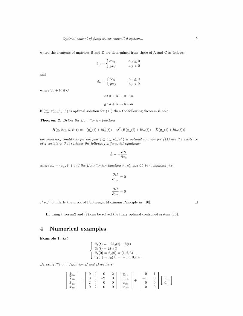
Optimal control of fuzzy linear controlled system... 5

where the elements of matrices B and D are determined from those of A and C as follows:

bij =

{eaij ,

gaij

aij ≥ 0

aij < 0

and

dij =

{ecij ,

gcij

cij ≥ 0

cij < 0

where ∀a+ bi ∈ Ce : a+ bi→ a+ bi

g : a+ bi→ b+ ai

If (x∗α, x∗α, u

∗α, u

∗α) is optimal solution for (11) then the following theorem is hold:

Theorem 2. Define the Hamiltonian function

H(x, x, u, u, ψ, t) = −(u2α(t) + iu2

α(t)) + ψT (B(xα(t) + ixα(t)) +D(uα(t) + iuα(t)))

the necessary conditions for the pair (x∗α, x∗α, u

∗α, u

∗α) is optimal solution for (11) are the existence

of a costate ψ that satisfies the following differential equations:

ψ = − ∂H∂xα

where xα = (xα, xα) and the Hamiltonian function in u∗α and u∗α be maximized ,i.e.

∂H

∂uα= 0

∂H

∂uα= 0

Proof. Similarly the proof of Pontryagin Maximum Principle in [10].

By using theorem2 and (7) can be solved the fuzzy optimal controlled system (10).

4 Numerical examples

Example 1. Let ˙x1(t) = −2x2(t)− u(t)˙x2(t) = 2x1(t)x1(0) = x2(0) = (1, 2, 3)x1(1) = x2(1) = (−0.5, 0, 0.5)

By using (7) and definition B and D we have:x1α˙x1αx2α˙x2α

=

0 0 0 −20 0 −2 02 0 0 00 2 0 0

x1αx1αx2αx2α

+

0 −1−1 0

0 00 0

[ uαuα

]

6

The solution of the above system is:x1αx1αx2αx2α

=

cos2t

2+ e2t+e−2t

4cos2t

2− e2t+e−2t

4−sin2t

2+ e2t−e−2t

4−sin2t

2− e2t−e−2t

4cos2t

2− e2t+e−2t

4cos2t

2+ e2t+e−2t

4−sin2t

2− e2t−e−2t

4−sin2t

2+ e2t−e−2t

4sin2t

2+ e2t−e−2t

4sin2t

2− e2t−e−2t

4cos2t

2+ e2t+e−2t

4cos2t

2− e2t+e−2t

4sin2t

2− e2t−e−2t

4sin2t

2+ e2t−e−2t

4cos2t

2− e2t+e−2t

4cos2t

2+ e2t+e−2t

4

2α+ (1− α)2α+ 3(1− α)2α+ (1− α)2α+ 3(1− α)

+

∫ t

0

cos2(t−s)

2+ e2(t−s)+e−2(t−s)

4cos2(t−s)

2− e2(t−s)+e−2(t−s)

4cos2(t−s)

2− e2(t−s)+e−2(t−s)

4cos2(t−s)

2+ e2(t−s)+e−2(t−s)

4sin2(t−s)

2+ e2(t−s)−e−2(t−s)

4sin2(t−s)

2− e2(t−s)−e−2(t−s)

4sin2(t−s)

2− e2(t−s)−e−2(t−s)

4sin2(t−s)

2+ e2(t−s)−e−2(t−s)

4

−sin2(t−s)2

+ e2(t−s)−e−2(t−s)

4−sin2(t−s)

2− e2(t−s)−e−2(t−s)

4−sin2(t−s)

2− e2(t−s)−e−2(t−s)

4−sin2(t−s)

2+ e2(t−s)−e−2(t−s)

4cos2(t−s)

2+ e2(t−s)+e−2(t−s)

4cos2(t−s)

2− e2(t−s)+e−2(t−s)

4cos2(t−s)

2− e2(t−s)+e−2(t−s)

4cos2(t−s)

2+ e2(t−s)+e−2(t−s)

4

0 −1−1 0

0 00 0

[ uα(s)uα(s)

]ds

the control function and x1(t) and x2(t) respectively are given in Figure 1 for α ∈ [0, 1] where thered lines are the centers and the blue lines are the lower bounds and the green lines are the upperbounds for fuzzy functions.

Example 2. Consider the following optimal fuzzy controlled system:

Min

∫ 1

0

u2(t)dt

s.t.

˙x1(t) = −2x2(t) + u(t)

˙x2(t) = 2x1(t)

x1(0) = x2(0) = (1, 2, 3)

x1(1) = x2(1) = (−0.5, 0, 0.5)

Similar the fuzzy controlled system (4), the above optimal controlled system is changed to the fol-lowing form:

Min

∫ 1

0

(u2α(t) + u2

α(t))dt

s.t. x1α˙x1αx2α˙x2α

=

0 0 0 −20 0 −2 02 0 0 00 2 0 0

x1αx1αx2αx2α

+

0 11 00 00 0

[ uαuα

]x1α(0)˙x1α(0)x2α(0)˙x2α(0)

=

2α+ (1− α)2α+ 3(1− α)2α+ (1− α)2α+ 3(1− α)

x1α(1)˙x1α(1)x2α(1)˙x2α(1)

=

−0.5(1− α)

0.5(1− α)−0.5(1− α)

0.5(1− α)

Optimal control of fuzzy linear controlled system... 7

The Hamiltonian function for the above optimal controlled system is:

H = −(u2α(t) + u2

α(t)) + ψ1(−2x2α + uα) + ψ2(−2x2α + uα) + ψ3(2x1α) + ψ4(2x1α)

By considering the theorem 2uα = 0.5ψ1

uα = 0.5ψ2

and ψ1

ψ2

ψ3

ψ4

=

0 0 −2 00 0 0 −20 2 0 02 0 0 0

ψ1

ψ2

ψ3

ψ4

Now by using [9] we will have:

uα(t) =1

8[(2cos2t+ (e−2t + e2t))c1 + (2cos2t− (e−2t + e2t))c2

+ (−2sin2t+ (e−2t − e2t))c3 + (−2sin2t− (e−2t − e2t))c4](12)

uα(t) =1

8[(2cos2t− (e−2t + e2t))c1 + (2cos2t+ (e−2t + e2t))c2

+ (−2sin2t− (e−2t − e2t))c3 + (−2sin2t+ (e−2t − e2t))c4](13)

Where ci for i = 1, ..., 4 are real numbers. The solution of optimal controlled system is:x1αx1αx2αx2α

=

cos2t

2+ e2t+e−2t

4cos2t

2− e2t+e−2t

4−sin2t

2+ e2t−e−2t

4−sin2t

2− e2t−e−2t

4cos2t

2− e2t+e−2t

4cos2t

2+ e2t+e−2t

4−sin2t

2− e2t−e−2t

4−sin2t

2+ e2t−e−2t

4sin2t

2+ e2t−e−2t

4sin2t

2− e2t−e−2t

4cos2t

2+ e2t+e−2t

4cos2t

2− e2t+e−2t

4sin2t

2− e2t−e−2t

4sin2t

2+ e2t−e−2t

4cos2t

2− e2t+e−2t

4cos2t

2+ e2t+e−2t

4

2α+ (1− α)2α+ 3(1− α)2α+ (1− α)2α+ 3(1− α)

+

∫ t

0

cos2(t−s)

2+ e2(t−s)+e−2(t−s)

4cos2(t−s)

2− e2(t−s)+e−2(t−s)

4cos2(t−s)

2− e2(t−s)+e−2(t−s)

4cos2(t−s)

2+ e2(t−s)+e−2(t−s)

4sin2(t−s)

2+ e2(t−s)−e−2(t−s)

4sin2(t−s)

2− e2(t−s)−e−2(t−s)

4sin2(t−s)

2− e2(t−s)−e−2(t−s)

4sin2(t−s)

2+ e2(t−s)−e−2(t−s)

4

−sin2(t−s)2

+ e2(t−s)−e−2(t−s)

4−sin2(t−s)

2− e2(t−s)−e−2(t−s)

4−sin2(t−s)

2− e2(t−s)−e−2(t−s)

4−sin2(t−s)

2+ e2(t−s)−e−2(t−s)

4cos2(t−s)

2+ e2(t−s)+e−2(t−s)

4cos2(t−s)

2− e2(t−s)+e−2(t−s)

4cos2(t−s)

2− e2(t−s)+e−2(t−s)

4cos2(t−s)

2+ e2(t−s)+e−2(t−s)

4

1 00 10 00 0

[ uα(s)uα(s)

]ds

Now by replacing (12) and (13) in the above equations and using the trapezoidal integration forapproximation the integral we can calculate the states of system. the control function and x1(t) andx2(t) respectively are given in Figure 2 for α ∈ [0, 1] where the red lines are the centers and the bluelines are the lower bounds and the green lines are the upper bounds for fuzzy functions.

5 Conclusion

We studied fuzzy linear time invariant controlled system and fuzzy optimal controlled system,where in the fuzzy optimal control system, the target is to minimize a functional subject to fuzzydifferential equation with fuzzy initial conditions. By applying α-cuts and presenting numbers inmore compact form by moving to the field of complex numbers, the fuzzy controlled system andfuzzy optimal controlled system, extended to a new form involve of lower and upper state andcontrol. Two numerical examples are given to show the effectiveness of the method.

8

Figure 1: The state functions and control function for example 1

Optimal control of fuzzy linear controlled system... 9

Figure 2: The state functions and control function for example 2

10

References

[1] Y. Zhu, Fuzzy optimal control with application to portfolio selection, (To appear).

[2] P. Diamond and P. E. Kloeden, Metric space of Fuzzy sets, Theory And Applications, Worldscientific publishing, (1994).

[3] Y. C. Kwun and D. G. Park, Optimal control problem for fuzzy differential equations, Pro-ceedings of the Korea-Vietnam Joint Seminar, (1998),103-114.

[4] P. Balasubramaniam and S. Muralisankar, Existence and uniqueness of fuzzy solution for semi-linear fuzzy integrodifferential equations with nonlocal conditions, An International Computer& Mathematics with applications, Volume 47, (2004), 1115-1122.

[5] J.H. Park, J.S. Park and Y.C. Kwun, Controllability for the semilinear fuzzy integrodifferentialequations with nonlocal conditions, Lecture Notes in Artificial Intelligence, LNAI 4223, (2006),221-230.

[6] Dimiter Filev and Plamen Angelove, Fuzzy optimal control, Fuzzy Sets and Systems, Volume47,(1992), 151-56.

[7] Z. Qin, Time-homogeneous fuzzy optimal control problems, (To appear)

[8] Y. Zhu, A fuzzy optimal control model, Journal of uncertain systems, Volume 3, No. 4, (2009),270-279

[9] J.Xu, Z.Liao, Z. Hu, A class of linear differential dynamical systems with fuzzy initial condition,Fuzzy Sets and Systems, 158 (2007) 2339-2358

[10] R. Bellman, Dynamic Programming, Princeton N.J.: Princeton University Press, (1957).

[11] J. J. Nieto, A. Khastan, and K. Ivaz, ”Numerical solution of fuzzy differential equations undergeneralized differentiability”, Nonlinear Analysis: Hybrid Systems 3, (2009) 700-707.

[12] B. Bede, I. J. Rudas, A. L. Bencsik, First order linear fuzzy differential equations undergeneralized differentiability, Information Sciences 177 (2007) 16481662.

[13] R. Goetschel, W.Voxman, Elementary fuzzy calculus, Fuzzy Sets and Systems 18 (1986), 31-43.

[14] J. Xu, Z. Liao, J. J. Nieto, Aclass of differential dynamical systems with fuzzy matrices, J.Math. Anal. Appl. 368 (2010) 54-68.

[15] D. W. Pearson, A property of linear fuzzy differential equations, Appl. Math. Lett. 10(3) (1997)99-103.

[16] S. Seikkala, On the fuzzy initial value problem, Fuzzy Sets and Systems 24 (1987) 319-330.