Stationary fuzzy Fokker–Planck learning and stochastic fuzzy filtering

IEEE TRANSACTIONS ON FUZZY SYSTEMS, VOL. 19, NO. 5, OCTOBER 2011 873

Stationary Fuzzy Fokker–Planck Learningand Stochastic Fuzzy Filtering

Mohit Kumar, Norbert Stoll, and Regina Stoll

Abstract—The application of nonlinear optimization to the esti-mation of fuzzy model parameters is well known. To do the reverseof this, the concept of stationary fuzzy Fokker–Planck learning(SFFPL) is introduced, i.e., SFFPL applies the fuzzy modelingtechnique in nonlinear optimization problems. SFFPL is basedon the fuzzy approximation of the stationary cumulative distri-bution function of a stochastic search process associated with thenonlinear optimization problem. A carefully designed algorithm issuggested for SFFPL to locate the optimum point. This paper alsoconsiders the variational Bayes (VB)-based inference of a stochasticfuzzy filter whose consequents, as well as antecedents, are randomvariables. The problem of VB inference of stochastic antecedents,because of the nonlinearity of the likelihood function, is analyticallyintractable. The SFFPL algorithm for high-dimensional nonlinearoptimization that does not require the derivative of the objectivefunction can be used to numerically solve the stochastic fuzzy fil-tering problem.

Index Terms—Bayesian inference, Fokker–Planck equation,fuzzy filtering, stochastic search.

I. INTRODUCTION

O PTIMIZATION problems are frequently encountered inscience and engineering. Stochastic search methods for

optimization problems have been studied at the interface be-tween artificial intelligence and operational research. Simulatedannealing is a popular stochastic method that is based on theconnection between statistical mechanics and optimization [1].The recursive stochastic algorithms [2], [3] to find the globalminimum of a smooth function U(x), x ∈ Rn are related to aLangevin-type Markov diffusion:

dx(t) = −∇U(x(t))dt + c(t)dw(t)

where w(·) is a standard n-dimensional Wiener process, andc(t) is a positive function with c(t) → 0 as t → ∞. The dif-fusion x(·) is called continuous simulated annealing, whereU(x) is the energy of the state x, and T (t) = c2(t)/2 is the

Manuscript received August 11, 2010; revised January 2, 2011; acceptedMarch 9, 2011. Date of publication May 2, 2011; date of current versionOctober 10, 2011. This work was supported by Center for Life ScienceAutomation, Rostock, Germany.

M. Kumar is with the Center for Life Science Automation, D-18119 Rostock,Germany (e-mail: [email protected]).

N. Stoll is with the Institute of Automation, College of Computer Science andElectrical Engineering, University of Rostock, D-18119 Rostock-Warnemunde,Germany (e-mail: [email protected]).

R. Stoll is with the Institute of Preventive Medicine, Faculty of Medicine,University of Rostock, D-18055 Rostock, Germany (e-mail: [email protected]).

Color versions of one or more of the figures in this paper are available onlineat http://ieeexplore.ieee.org.

Digital Object Identifier 10.1109/TFUZZ.2011.2148724

temperature at time t. This stochastic differential equation hasbeen extended to include linear/nonlinear constraints in the op-timization problem [4], [5]. In [6], the conditional transitiondensity p(x, t|x0 , t0) that satisfies the Fokker–Planck equationassociated with continuous simulated annealing is consideredas follows:

∂p

∂t=∑

i

∂U

∂xi

∂p

∂xi+∑

i

∂2U

∂x2i

p +12c2(t)

∑

i

∂2p

∂x2i

.

The goal of such stochastic search algorithms is the convergenceto global minima as the temperature T is decreased.

Unlike the simulated annealing algorithm, the method of [7]keeps temperature fixed at a level and approximates the station-ary probability density of the stochastic search process. The sta-tionary probability density of xi at temperature T , while keepingother variables {xj , j �= i} fixed, satisfies the one-dimensional(1-D) Fokker–Planck equation [7]:

T∂p(xi |{xj �=i = x∗

j})∂xi

+ p(xi |{xj �=i = x∗j})

×∂U(xi, {xj �=i = x∗

j})∂xi

= 0

whose solution is given by

p(xi |{xj �=i = x∗j}) =

exp(−U(xi, {xj �=i = x∗j})/T )∫

exp(−U(xi, {xj �=i = x∗j})/T )dxi

.

(1)It follows that the stationary cumulative distribution

y(xi |{xj �=i = x∗j}) =

∫ xi

−∞p(xi |{xj �=i = x∗

j})dxi

is governed by a linear second-order differential equation

T∂2y(xi |{xj �=i = x∗

j})∂x2

i

+∂U(xi, {xj �=i = x∗

j})∂xi

×∂y(xi |{xj �=i = x∗

j})∂xi

= 0. (2)

The distribution y(xi |{xj �=i = x∗j}) can be approximated by the

use of a model whose parameters are adjusted in such a way thatthe approximate distribution satisfies (2) at some finite valuesof xi . Taking the average of model parameters over {xj �=i} willprovide an approximation to the marginal

y(xi) = E{xj �= i }[y(xi |{xj �=i})].This is how y(xi) [thus, p(xi)] can be computed and how thehigher probability regions of the search space, which containglobal minima, can be identified. This method of global opti-mization was proposed in [7], where a linear combination of

1063-6706/$26.00 © 2011 IEEE

874 IEEE TRANSACTIONS ON FUZZY SYSTEMS, VOL. 19, NO. 5, OCTOBER 2011

Fourier basis was used for the approximation. The method wascalled stationary Fokker–Planck learning (SFPL) in [8].

Our idea is to introduce a procedure that we will call station-ary fuzzy Fokker–Planck learning (SFFPL) based on the fuzzyapproximation of stationary probability density of the stochas-tic search process. The differences between proposed SFFPLand the method of [7], as well as the motivations behind thesedifferences, are as follows.

1) A zero-order Takagi–Sugeno (T–S) fuzzy model that de-fines uniformly distributed triangular membership func-tions on the input range is identified to approximate thefunctional relation between xi and y(xi |{xj �=i = x∗

j}).The motivation to use the fuzzy model is derived fromfollowing fact

a) A necessary condition on the model-approximatedcumulative distribution is that it should be a mono-tonically increasing function. This requirement caneasily be met by putting constraints on the identi-fication of consequents of a zero-order T–S fuzzymodel. The method of [7], however, does not for-mulate this requirement mathematically while iden-tifying the parameters of model.

2) The parameters of the fuzzy model are identified by the useof a finite number of training data points under the iden-tification criterion that the fuzzy-model-generated distri-bution satisfies (1). However, SFPL identifies the modelparameters based on (2). The motivation to consider (1)instead of (2) is as follows.

a) Equation (2) involves the partial derivative ∂U/∂xi

whose numerical computation needs two evalua-tions of the cost function U . Equation (1), if usedfor model parameter identification, has the computa-tional advantage as the identification procedure doesnot need to compute the derivative ∂U/∂xi .

3) The author of SFPL suggests to assess global minimaby finding the point at which the estimated density ismaximum. That is, a point (xm

1 , . . . , xmn ) is computed

such that

xmi = arg max

xi

〈p(xi |{xj �=i})〉{xj �= i }

where 〈·〉{xj �= i } denotes the average over {xj �=i}, and p isthe model-generated density. Our approach to assess theglobal minima is to compute a point (xp

1 , . . . , xpn ) such

that

xpi = arg max

xi

〈p(xi |{xj �=i})〉{xj �= i ∈Ij }, (3)

Ij = [xpj − Δj , x

pj + Δj ]. (4)

That is, average is taken over the values of xj �=i lying inthe neighborhood of xp

j (i.e., in the range xpj ± Δj ), where

xpj is defined by (3). Here, Δi reflects an uncertainty in the

computation of xpi as a result of the modeling errors. Δi

is a measure of the mismatch between model-generateddensity p and true density p such that

limΔ i →0

p(xi |{xj �=i}) = p(xi |{xj �=i}). (5)

The motivation to compute (xp1 , . . . , x

pn ) as an assessment

of global minima (xo1 , . . . , x

on ) is as follows.

a) It implies from (1), (3), and (5) that

limΔ j →0, xp

j �= i →xoj

xpi = xo

i . (6)

That is, when Δj = 0, and xpj = xo

j , interval Ij

shrinks to a point xoj , and thus

xpi = arg max

xi

exp(−U(xi, {xj �=i = xoj })/T )∫

exp(−U(xi, {xj �=i = xoj })/T )dxi

= xoi .

We are now in the position to state that if the mod-eling error is small (i.e., Δj is small) and the fixedvariables are close to their optimal values (i.e., xp

j �=i

is close to xoj ), then xp

i should remain close to theoptimal value xo

i .4) For the fuzzy approximation of the stationary density

function, C different fuzzy models (m1 , . . . ,mC ) with(K1 , . . . ,KC ) number of fuzzy rules, respectively, areconsidered. Let ΔK i

j be the uncertainty interval [which isused to define Ij as per (4)] for the ith fuzzy model mi

that has Ki number of fuzzy rules. The number of fuzzyrules and uncertainty intervals are chosen in such a waythat

K1 < K2 < · · · < KC

Δ1j > Δ2

j > · · · > ΔCj .

Our approach is to estimate a minima by the use of m1

taking any random initial guess. The estimated minimaserves as the initial guess for m2-based evaluation. Thisprocess is continued till the estimation of global minimaby the use of mC . The motivation to consider the differentfuzzy models of increasing complexity is derived fromfollowing considerations.

a) For a small model (i.e., with a smaller number of pa-rameters), the uncertainty interval Δj will be larger.This is because of the reason that the model param-eters will be identified by the use of a finite numberof uniformly distributed points in the input rangesuch that the number of identification data pointsmust be equal to the number of unknown model pa-rameters for their unique estimation. For a modelwith a smaller number of parameters, the averagedistance between two successive identification datapoints will be larger, which might result in highermodeling errors as the model interpolation in thisrange (i.e., between two successive identificationdata points) might not be enough accurate. There-fore, Δj (which is a measure of modeling errorsand should be chosen proportional to the averagedistance between two successive identification datapoints) will be larger for small models. The effectof larger Δj [and, thus, larger volume of Ij as per(4)] will be that xp

i computed by (3) should not be

KUMAR et al.: STATIONARY FUZZY FOKKER–PLANCK LEARNING AND STOCHASTIC FUZZY FILTERING 875

very sensitive to the fixed variables values {xpj �=i}.

In summary, a small model should result in a robust-ness in the estimation of xp

i against the uncertaintiesin the values {xp

j �=i}.b) For a large model, Δj will be smaller, and it follows

from (6) that xpi should remain close to the optimal

value xoi , provided that the fixed variables values

{xpj �=i} are close to their optimal values.

c) Based on these two aforementioned facts, we statethat the use of different fuzzy models of increasingcomplexity in a series should lead to an increase inthe accuracy of estimated global minima.

This paper also considers an application of the SFFPL algo-rithm in statistical inference of fuzzy model parameters. Thedata-driven fuzzy modeling remains as one of the most activeareas of research on fuzzy systems [9]–[23]. The identifica-tion data are usually contaminated with noise, and thus, severalstudies address the issue of robustness toward noise [24]–[42].The authors believe that fuzzy-filtering algorithms have muchto offer in practical modeling applications [43]–[52], providedthat the fuzzy-filtering algorithms are studied in the frame-work of modern system theory for a proper mathematical han-dling of uncertainties. Our previous work presented in [21]and [23] demonstrates the applications of mathematical tools(used in control and system theory) in the study of fuzzy-filteringalgorithms.

The Bayesian inference of model parameters is a powerfultechnique to deal with the data uncertainties and many otherissues. A T–S fuzzy filter, with membership functions that arebased on the grid partitioning of input space, can be mathemat-ically represented as [53]

yf = GT (x, θ)α (7)

where antecedents (θ) are membership functions’ related param-eters, α is a vector of consequents, and G(·) is a nonlinear func-tion that is defined by the shape of membership functions andfuzzy rules. Recently, we have introduced in [53] a mixed T–Sfuzzy filter whose antecedents are deterministic while the conse-quents are random variables. The parameters of the mixed fuzzyfilter were inferred under the variational Bayes (VB) framework.The motivation of the work of [53] was to take advantages ofthe VB framework to design fuzzy-filtering algorithms. Theseadvantages include an automated regularization, incorporationof statistical noise models, and model comparison capability.

The VB algorithm of [53], by the maximization of a strictlower bound on the data evidence, makes the approximate pos-terior of consequents as close to the true posterior as possiblewhile the deterministic antecedents are identified in a way tofurther increase the lower bound on data evidence. This paperextends the mixed stochastic/deterministic fuzzy filter of [53] toa stochastic fuzzy filter whose antecedents are random variablestoo. The problem of VB inference of stochastic antecedents,because of the nonlinearity of the likelihood function, is an-alytically intractable. This problem of intractability is usuallysolved by the Laplace approximation. The Laplace approxima-tion further approximates the approximate posterior density bya Gaussian density whose sufficient statistics (i.e., mean and

covariance) is derived from a second-order truncation of theTaylor series to the variational energy [54]. Our approach to theBayesian inference of fuzzy filter parameters circumvents theLaplace approximation by

1) deriving an approximate analytical expression for varia-tion posterior distribution of antecedents,

2) computing numerically the mode of variation posteriordistribution of antecedents,

3) inferring the analytically tractable consequents and noiseparameters under the VB framework while keeping an-tecedents fixed at their mode values.

The method consists of following steps.1) Under the VB framework, it is possible to derive an an-

alytical expression for a lower bound on logarithmic evi-dence for the data (i.e., log p(data|θ)). This lower boundis essentially a function of θ and sufficient statistics ofconsequents (α) and noise present in data.

2) For a given prior probability of antecedents (p(θ)),log(p(θ|data)) can be expressed as

log(p(θ|data)) ∝ log(p(θ)) + log p(data|θ)≈ log(p(θ))

+ max [lower bound on log p(data|θ)] .

Here, the maximization of the lower bound is with respectto the sufficient statistics of consequents (α) and noise.

3) The SFFPL algorithm can be used to find the maxima (θ)of the expression:

log(p(θ)) + max [lower bound on log p(data|θ)] .

4) The VB algorithm can be used to update the sufficientstatistics of consequents (α) and noise by the maximiza-tion of the lower bound on log p(data|θ) at θ = θ.

5) The posterior density of θ is approximated by a distribution(q(θ)) such that

log (q(θ)) ∝ log(p(θ))

+ max [lower bound on log p(data|θ)] .

The mode of q(θ) is, obviously, given by θ.The Bayesian inference of fuzzy filter parameters with the

help of SFFPL machine enables us to develop a stochastic fuzzyfilter algorithm.

Remark 1: A potential application of stochastic fuzzy filter-ing is in the analysis of biomedical signals, where a stochasticfuzzy model is inferred from the biomedical data in such a waythat the stochastic fuzzy model should characterize the complexphysiological state of the patient. The identified stochastic fuzzyphysiological state model can be used to analyze the biomedicalsignals to predict the state of the patient. These details have beenprovided in [55].


II. STATIONARY FUZZY FOKKER–PLANCK LEARNING

A. Zero-Order T–S Fuzzy Model With Uniformly DistributedTriangular Membership Functions

Consider a fuzzy model that maps an input variable xi ∈[ai, bi ] to the output variable yi through K different fuzzy rules:

R1 : IF xi is A1 , THEN yi = S1...

...RK : IF xi is AK , THEN yi = SK

Here, (A1 , . . . , AK ) are fuzzy sets, and (S1 , . . . , SK ) are realscalars. To define the membership functions, consider K equallydistanced points on the considered range of xi :{t0 = ai, t1 = ai + δi, t2 = ai + 2δi, . . .

tK−2 = ai + (K − 2)δi, tK−1 = bi

}

where

δi =bi − ai

K − 1.

Now, K triangular membership functions (μA 1 , . . . , μAK) can

be defined as

μA 1 (xi) = max(

0,min(

1,t1 − xi

t1 − t0

))

μAj(xi) = max

(0,min

(xi − tj−2

tj−1 − tj−2 ,tj − xi

tj − tj−1

))

for all j = 2, . . . , K − 1, and

μAK(xi) = max

(0,min

(xi − tK−2

tK−1 − tK−2 , 1))

.

The output of the fuzzy model is computed by taking theweighted average of the output provided by each rule. Thatis

yi =S1μA 1 (xi) + S2μA 2 (xi) + · · · + SK μAK

(xi)μA 1 (xi) + μA 2 (xi) + · · · + μAK

(xi)

= S1μA 1 (xi) + S2μA 2 (xi) + · · · + SK μAK(xi).

For the defined triangular membership functions, it is easy toobserve that for any xi ∈ [ai, bi ]

dyi

dxi=

Sz (xi )+1 − Sz (xi )

tz (xi ) − tz (xi )−1

where z(xi) ∈ {1, 2, . . . ,K − 1} is an integer such that

tz (xi )−1 ≤ xi ≤ tz (xi ) .

Since tz (xi ) − tz (xi )−1 = δi , we have

dyi

dxi=

Sz (xi )+1 − Sz (xi )

δi.

B. Fuzzy Approximation of Stationary Cumulative Distribution

Since xi ∈ [ai, bi ], and given that the fuzzy model’s output toinput xi is a cumulative distribution [i.e., an approximation ofy(xi |{xj �=i = x∗

j})], we must have

S1 = 0, SK = 1, and S1 ≤ S2 ≤ . . . ≤ SK−1 ≤ SK .

Consider a set of K − 1 points (x1i , x

2i , . . . , x

K−1i ) used for

an identification of fuzzy model parameters (S2 , . . . , SK−1)in approximating the functional relation between xi andy(xi |{xj �=i = x∗

j}). An identification point xki could be cho-

sen randomly from a uniform distribution on (tk−1 , tk ), i.e.,

xki ∈ (tk−1 , tk ), where k ∈ {1, 2, . . . ,K − 1}.

This results in(

dyi

dxi

)

xi =xki

=Sk+1 − Sk

δi.

The fuzzy approximation problem is to estimate the parame-ters (S2 , . . . , SK−1), which satisfy 0 ≤ S2 ≤ · · · ≤ SK−1 ≤ 1,such that(

dyi

dxi

)

xi =xki

≈exp(−U(xk

i , {xj �=i = x∗j})/T )

∫ bi

aiexp(−U(xi, {xj �=i = x∗

j})/T )dxi

, i.e.,

Sk+1 − Sk ≈ δi

exp(−U(xki , {xj �=i = x∗

j})/T )∫ bi

aiexp(−U(xi, {xj �=i = x∗

j})/T )dxi

.

The least-squares estimation of fuzzy model parameters followsas

S = arg minS

[‖Y − BS‖2 , BS ≥ h

]

where

S =

⎡

⎢⎢⎣

S2S3...

SK−1

⎤

⎥⎥⎦ ∈ R(K−2)×1

B =

⎡

⎢⎢⎢⎢⎢⎢⎣

1−1 1

−1 1...

......

...−1 1

−1

⎤

⎥⎥⎥⎥⎥⎥⎦∈ R(K−1)×(K−2) (8)

Y =

⎡

⎢⎢⎢⎢⎢⎢⎢⎢⎢⎢⎢⎢⎢⎢⎢⎢⎢⎣

δiexp(−U(x1

i , {xj �=i = x∗j})/T )

∫ bi

ai


...

δiexp(−U(xK−2

i , {xj �=i = x∗j})/T )

∫ bi

ai


δiexp(−U(xK−1

i , {xj �=i = x∗j})/T )

∫ bi

ai


− 1

⎤

⎥⎥⎥⎥⎥⎥⎥⎥⎥⎥⎥⎥⎥⎥⎥⎥⎥⎦

(9)

h =

⎡

⎢⎢⎣

0...0−1

⎤

⎥⎥⎦ ∈ R(K−1)×1 . (10)


C. Issue of Modeling Errors

Observe that for any value of xi that lies in the interval(tk−1 , tk ), the model-generated density value will be the same(i.e., equal to (Sk+1 − Sk )/δi) and independent of the xi value.However, p(xi |{xj �=i = x∗

j}) may vary as xi varies within theinterval (tk−1 , tk ). These modeling errors arise because of thechosen triangular shape of membership functions. We are in-terested to locate the point of maximum density by the use ofthe identified fuzzy model. Since the model-generated densityvalue remains constant for the length δi (where δi = tk − tk−1),there exists an interval such that any value of xi that liesin this interval corresponds to the maximum density value.If S = [ S2 S3 . . . SK−1 ]T are the estimated parameters,then the problem to locate the point of maximum density can bemathematically expressed as

arg maxxi

Sz (xi )+1 − Sz (xi )

δi

where z(xi) ∈ {1, 2, . . . ,K − 1} is an integer such thattz (xi )−1 < xi < tz (xi ) . The solution of this problem is, obvi-ously, nonunique. However, we can consider the center of thesolution interval as follows:

xpi =

tz∗−1 + tz

∗

2, where z∗ = arg max

z

Sz+1 − Sz

δi.

Let Δi be a quantity that reflects an uncertainty in the maximumdensity point (xp

i ). One possible choice of Δi is as follows:

Δi = width of solution interval on either side of xpi︸︷︷︸

=0.5δi

+ uncertainty due to model prediction error︸︷︷︸=kΔ δi

where kΔ is a constant of proportionality. The term (kΔδi)reflects the uncertainty because of a difference between themodel-predicted density and the true density. Thus

Δi = (0.5 + kΔ)δi.

D. Stationary Fuzzy Fokker–Planck Learning Algorithm

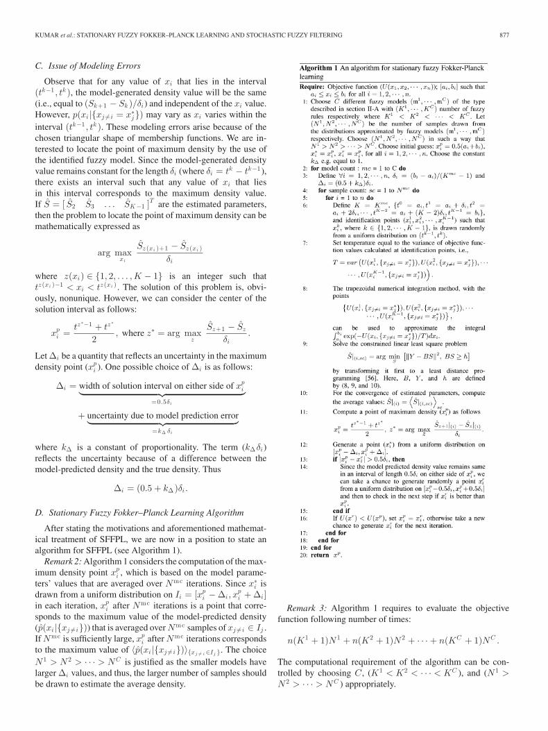
After stating the motivations and aforementioned mathemat-ical treatment of SFFPL, we are now in a position to state analgorithm for SFFPL (see Algorithm 1).

Remark 2: Algorithm 1 considers the computation of the max-imum density point xp

i , which is based on the model parame-ters’ values that are averaged over Nmc iterations. Since x∗

i isdrawn from a uniform distribution on Ii = [xp

i − Δi , xpi + Δi ]

in each iteration, xpi after Nmc iterations is a point that corre-

sponds to the maximum value of the model-predicted density(p(xi |{xj �=i})) that is averaged over Nmc samples of xj �=i ∈ Ij .If Nmc is sufficiently large, xp

i after Nmc iterations correspondsto the maximum value of 〈p(xi |{xj �=i})〉{xj �= i ∈Ij }. The choiceN 1 > N 2 > · · · > NC is justified as the smaller models havelarger Δi values, and thus, the larger number of samples shouldbe drawn to estimate the average density.

Remark 3: Algorithm 1 requires to evaluate the objectivefunction following number of times:

n(K1 + 1)N 1 + n(K2 + 1)N 2 + · · · + n(KC + 1)NC .

The computational requirement of the algorithm can be con-trolled by choosing C, (K1 < K2 < · · · < KC ), and (N 1 >N 2 > · · · > NC ) appropriately.


Remark 4: The global convergence of the proposed SFFPLalgorithm can be studied (i.e., proved under some conditions)with the similar mathematical theory as presented in [57]. Thisstudy, however, will be presented elsewhere. The aim of thispaper is to introduce to the fuzzy readers the idea that how fuzzymodeling can be used for derivative-free optimization purposes.

Remark 5: The value of T in Algorithm 1 decides the heightof the peaks of the density function. Setting T equal to varianceof objective function values ensures that density curves remainin a suitable range, even in the cases of ranges of objectivefunction values that are too wide or too small.

E. Benchmark Examples

The SFFPL algorithm is tested on the following benchmarkexamples [7].

1) Schwefel:

U(x1 , . . . , x6) = 418.9829 × 6 −6∑

i=1

xi sin(√

|xi |)

where −500 ≤ xi ≤ 500. The solution is xo =(420.9687, . . . , 420.9687).

2) Levy no. 5:

U(x1 , x2) =5∑

i=1

i cos((i − 1)x1 + i)

×5∑

j=1

j cos((j + 1)x2 + j)

+ (x1 + 1.42513)2 + (x2 + 0.80032)2

where −10 ≤ xi ≤ 10. The solution is xo =(−1.3068,−1.4248).

3) Booth:

U(x1 , x2) = (x1 + 2x2 − 7)2 + (2x1 + x2 − 5)2

where −10 ≤ xi ≤ 10. The solution is xo = (1, 3).4) Colville:

U(x1 , x2 , x3 , x4) = 100(x21 − x2)2 + (x1 − 1)2

+ (x3 − 1)2 + 90(x23 − x4)2 + 10.1((x2 − 1)2

+ (x4 − 1)2) + 19.8(x2 − 1)(x4 − 1)

where −10 ≤ xi ≤ 10. The solution is xo = (1, . . . , 1).5) Rosenbrock:

U(x1 , . . . , x20) =19∑

i=1

100(xi+1 − x2i )

2 + (xi − 1)2

where −10 ≤ xi ≤ 10. The solution is xo = (1, . . . , 1).Algorithm 1 needs a set of fuzzy models of increasing com-

plexity. The smallest possible model is with K1 = 3. One canincrease the complexity of the model by choosing, e.g., K2 = 6,K3 = 12, K4 = 24, and so on. However, our studies show thatmodels with number of rules equal to 3 or 6 are of little use forthe benchmark problems. Thus, our smallest model is with 12

rules, and we keep on doubling the number of rules for the nextfive models. That is

K1 = 12, K2 = 24, K3 = 48, K4 = 96

K5 = 192, K6 = 384.

Let the number of samples for the smallest model be equal to1000. As the model complexity increases, the sample numbercan be decreased as follows:

N 1 = 1000, N 2 = 500, N 3 = 250, N 4 = 125

N 5 = 63, N 6 = 32.

Fig. 1 shows, after a run of the SFFPL algorithm, plots of theestimated density and the objective function for variables x1 andx6 of the Schwefel function. Figs. 2–5 plot the estimated den-sity functions for Levy no. 5, Booth, Colville, and Rosenbrock,respectively. A performance measure that is equal to the dis-tance (normalized w.r.t. search space) between global optimumand the estimated maximum density point can be calculated asfollows:

distance =

√(xo

1 − xp1 )2 + · · · + (xo

n − xpn )2

(b1 − a1)2 + · · · + (bn − an )2 .

Tables III–VII in the appendix report the results of ten inde-pendent experiments made on each of the five examples. Theseresults clearly demonstrate the effectiveness of the SFFPL al-gorithm to locate the point of maximum probability, i.e., theglobal minima. Therefore, the SFFPL algorithm is potentially auseful tool for heuristical high-dimensional global optimizationmethods.

Now, we demonstrate that, unlike the method of [7], the com-putation of the maximum of 〈p(xi |{xj �=i})〉{xj �= i ∈Ij } (instead of〈p(xi |{xj �=i})〉{xj �= i }) and use of different fuzzy models of in-creasing complexity in a series (instead of a single large model)lead to an improved accuracy. For this purpose, the Rosenbrockproblem is again studied with an algorithm that is based onthe approach of [7]. An algorithm that is based on the approachof [7], which is comparable with the proposed SFFPL algorithm,has been derived by making following changes in Algorithm 1.

1) At Step 12 of Algorithm 1, x∗i is drawn from p(xi |{xj �=i =

x∗j}) by the use of the estimated fuzzy model parameters

S|(i,sc) . This is done via inverse transform sampling, i.e.,generating a random number from the uniform distribu-tion on [0, 1] and then linearly interpolating the generatednumber to the parameters S|(i,sc) in order to find the cor-responding value of xi .

2) A single large model is used, i.e., C = 1. For a fair compar-ison, the number of rules K1 and the number of samplesN 1 should be chosen in such a way that the objectivefunction is evaluated as many times as in the earlier case.We choose the largest model with K1 = 384, and N 1 , fora comparable number of function evaluations, is chosen


Fig. 1. Fuzzy approximation of the stationary probability density of a stochastic search process in the Schwefel problem. The minima and the maxima ofthe objective function correspond roughly to the maxima and the minima, respectively, of the estimated density function. (a) 〈p(x1 |{xj �=1})〉{xj �= 1 ∈Ij } andU (x1 , {xj �=1 = xo

j }). (b) 〈p(x6 |{xj �=6})〉{xj �= 6 ∈Ij } and U (x6 , {xj �=6 = xoj }).

Fig. 2. Fuzzy approximation of the stationary probability density of a stochastic search process in the Levy no. 5 problem. The minima and the maxima of theobjective function correspond roughly to the maxima and the minima, respectively, of the estimated density function. (a) 〈p(x1 |x2 )〉x 2 ∈I2 and U (x1 , x2 = xo

2 ).(b) 〈p(x2 |x1 )〉x 1 ∈I1 and U (x2 , x1 = xo

1 ).

as

N 1 = round

(1

385(13 ∗ 1000 + 25 ∗ 500 + 49 ∗ 250

+97 ∗ 125 + 193 ∗ 63 + 385 ∗ 32))

.

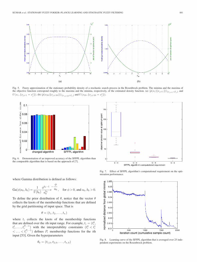
Fig. 6 demonstrates the better performance of the SFFPL al-gorithm than the changed one in term of the normalized distanceof the estimated minima from global minima during ten inde-pendent experiments. Therefore, the modifications that are madeto the method of [7] and incorporated in the SFFPL algorithmmake a sense.

It is interesting to see the effect of SFFPL algorithm’s compu-tational requirement (i.e., number of times the objective functionis evaluated) on the optimization performance. Thus, the Rosen-

brock problem is once more studied with the following differentconfigurations of the SFFPL algorithm.

1) C = 3 such that (K1 = 12,K2 = 24,K3 = 48) and(N 1 = 1000, N 2 = 500, N 3 = 250).

2) C = 4 such that (K1 = 12,K2 = 24,K3 = 48,K4 =96) and (N 1 = 1000, N 2 = 500, N 3 = 250, N 4 = 125).

3) C = 5 such that (K1 = 12,K2 = 24,K3 = 48,K4 =96,K5 = 192) and (N 1 = 1000, N 2 = 500, N 3 =250, N 4 = 125, N 5 = 63).

4) C = 6 such that (K1 = 12,K2 = 24,K3 = 48,K4 =96,K5 = 192,K6 = 384) and (N 1 = 1000, N 2 =500, N 3 = 250, N 4 = 125, N 5 = 63, N 6 = 32).

Fig. 7 shows the boxplots of the minimized objective func-tion values that are obtained in ten independent experiments.As expected, the optimization performance increases with anincrease in the computational requirement of the algorithm.


Fig. 3. Fuzzy approximation of the stationary probability density of a stochastic search process in the Booth problem. The minima and the maxima of theobjective function correspond roughly to the maxima and the minima, respectively, of the estimated density function. (a) 〈p(x1 |x2 )〉x 2 ∈I2 and U (x1 , x2 = xo

2 ).(b) 〈p(x2 |x1 )〉x 1 ∈I1 and U (x2 , x1 = xo

1 ).

Fig. 4. Fuzzy approximation of the stationary probability density of a stochastic search process in the Colville problem. The minima and the maxima ofthe objective function correspond roughly to the maxima and the minima, respectively, of the estimated density function. (a) 〈p(x1 |{xj �=1})〉{xj �= 1 ∈Ij } andU (x1 , {xj �=1 = xo

j }). (b) 〈p(x4 |{xj �=4})〉{xj �= 4 ∈Ij } and U (x4 , {xj �=4 = xoj }).

Finally, Fig. 8 plots the error (normalized distance from globalminima) curve of the SFFPL algorithm that is averaged over25 independent experiments on the Rosenbrock problem. Thejumps in the curve correspond to the switching to the next modelof higher complexity.

III. STOCHASTIC FUZZY FILTERING

The SFFPL algorithm for high-dimensional nonlinear opti-mization that does not require the derivative of the objectivefunction can be used to numerically solve the stochastic fuzzy-filtering problem.

A. Process Model and Prior Distributions

Consider a process model with n inputs (represented by thevector x ∈ Rn ) and a single output (represented by the scalary). It is assumed that input–output (I/O) data pairs {x(j), y(j)}(j = 1, 2, . . . is the time index) are generated as per the

equation

y(j) = GT (x(j), θ)α + nj (11)

where antecedents (θ) are membership functions’ related pa-rameters, α is a vector of consequents, and G(·) is a nonlinearfunction that is defined by the shape of membership functionsand fuzzy rules [53]. Here, nj is the Gaussian noise with mean0 and a variance of 1/φ:

p(nj ) ∼ N(0, φ−1).

The following distributions are chosen for the parameters priors:

p(α|m0 ,Λ0) = N(α|m0 , (Λ0)−1)

p(φ|a0 , b0) = Ga(φ|a0 , b0)


Fig. 5. Fuzzy approximation of the stationary probability density of a stochastic search process in the Rosenbrock problem. The minima and the maxima ofthe objective function correspond roughly to the maxima and the minima, respectively, of the estimated density function. (a) 〈p(x1 |{xj �=1})〉{xj �= 1 ∈Ij } andU (x1 , {xj �=1 = xo

j }). (b) 〈p(x20 |{xj �=20})〉{xj �= 2 0 ∈Ij } and U (x20 , {xj �=20 = xoj }).

Fig. 6. Demonstration of an improved accuracy of the SFFPL algorithm thanthe comparable algorithm that is based on the approach of [7].

where Gamma distribution is defined as follows:

Ga(φ|a0 , b0) =1

Γ(b0)φb0 −1

ab00

e− φ

a0 , for φ > 0, and a0 , b0 > 0.

To define the prior distribution of θ, notice that the vector θcollects the knots of the membership functions that are definedby the grid partitioning of input space. That is

θ = (t1 , t2 , . . . , tn )

where ti collects the knots of the membership functionsthat are defined over the ith input range. For example, ti = (t0i ,t1i , . . . , t

Pi −1i ) with the interpretability constraints (t0i < t1i

< . . . < tPi −1i ) defines Pi membership functions for the ith

input [53]. Given the hyperparameters

θ0 = (t1,0 , t2,0 , . . . , tn,0)

Fig. 7. Effect of SFFPL algorithm’s computational requirement on the opti-mization performance.

Fig. 8. Learning curve of the SFFPL algorithm that is averaged over 25 inde-pendent experiments on the Rosenbrock problem.


Fig. 9. Example of stochastic antecedents. (a) Membership functions. (b) Prior distribution functions.

where ti,0 = (t0i,0 , t1i,0 , . . . , t

P −1i,0 ) with (t0i,0 < t1i,0 < · · · <

tP −1i,0 ), the triangular distribution is defined for each element of

ti as follows:

p(t0i |θ0

)= T

(t0i |t0i,0 , t0i,0 ,

t0i,0 + t1i,02

)

p(t1i |θ0

)= T

(t1i |

t0i,0 + t1i,02

, t1i,0 ,t1i,0 + t2i,0

2

)

...

p(tPi −2i |θ0

)=T

(tPi −2i |

tPi −3i,0 +tPi −2

i,0

2, tPi −2

i,0 ,tPi −2i,0 +tPi −1

i,0

2

)

p(tPi −1i |θ0

)= T

(tPi −1i |

tPi −2i,0 + tPi −1

i,0

2, tPi −1

i,0 , tPi −1i,0

).

Here,

T (x|a, b, c) =

⎧⎪⎪⎪⎪⎨

⎪⎪⎪⎪⎩

2 (x − a)(c − a) (b − a) , for a ≤ x ≤ b

2 (c − x)(c − a) (c − b) , for b ≤ x ≤ c

0, otherwise.

Now, the prior distribution p(θ|θ0), assuming each element ofθ independent, is defined as

p(θ|θ0) =n∏

i=1

(p(t0i |θ0)p(t1i |θ0) · · · p(tPi −1

i |θ0))

. (12)

Example 1: Suppose that five different “1-D clustering-criterion-based membership functions” (see, e.g., [21] and [53]for the definition of such types of membership functions) aredefined over the ith input such that ti = (0, 1, 2, 3, 4). Fig. 9

plots the membership functions and prior distributions takingti,0 = (0, 1, 2, 3, 4).

B. Problem Formulation

The aim is to determine the posterior probability of the pa-rameters (α, θ, φ) given the data and the structure of the fuzzymodel. The analytical evaluation of posterior probability distri-butions is not possible in every case. Thus, these are approx-imated by the variational distributions (q(α), q(θ), q(φ)). Theproblem is particularly formulated as follows.

1) The posterior probability of θ is approximated by a varia-tional distribution:

q(θ) ≈ p (θ|y(j),m, x(j)) .

2) Let θ be the mode of q(θ), i.e.,

θ = arg maxθ

q(θ).

3) Now, variational distributions (q(α), q(φ)) are introducedto approximate the posterior distributions as follows:

q(α) ≈ p(α|θ, y(j),m, x(j))

q(φ) ≈ p(φ|θ, y(j),m, x(j)).

For the given fuzzy model structure m (i.e., membership type,number of membership functions, and rules) of a T–S filter oftype (7) such that the I/O data pair (x(j), y(j)) satisfies (11),the logarithmic evidence for y(j) is given as

log p (y(j)|θ,m, x(j)) = log∫

dαdφp(α|m0 ,Λ0)p(φ|a0 , b0)

× p (y(j)|α, φ, θ,m, x(j)) .

The introduction of an arbitrary joint probability density func-tion q(α, φ) would give rise to a lower bound on output evidence


as follows:

log p (y(j)|θ,m, x(j)) ≥∫ (

dαdφq(α, φ)

× logp(α|m0 ,Λ0)p(φ|a0 , b0)p (y(j)|α, φ, θ,m, x(j))

q(α, φ)

)

where we have made use of Jensen’s inequality. The method isrestricted to use the mean-field approximation:

q(α, φ) ≈ q(α)q(φ).

This results in

log p (y(j)|θ,m, x(j)) ≥∫

dαq(α) logp(α|m0 ,Λ0)

q(α)

+∫

dφq(φ) logp(φ|a0 , b0)

q(φ)+∫

dαdφq(α)q(φ)

× log p (y(j)|α, φ, θ,m, x(j)) .

The lower bound is defined as a functional of the variationaldistributions and other parameters as follows:

F(q(α), q(φ), θ) =∫

dαq(α) logp(α|m0 ,Λ0)

q(α)

+∫

dφq(φ) logp(φ|a0 , b0)

q(φ)+∫

dαdφq(α)q(φ)

× log p (y(j)|α, φ, θ,m, x(j)) .

That is

log p (y(j)|θ,m, x(j)) ≥ F(q(α), q(φ), θ).

By Bayes’ theorem

p (θ|y(j),m, x(j)) =p (y(j)|θ,m, x(j)) p (θ|m, x(j))

p (y(j)|m, x(j)).

That is

log p (θ|y(j),m, x(j)) ∝ (log p (y(j)|θ,m, x(j))

+ log p (θ|θ0)) .

We assume that θ is independent of x(j), and for a given fuzzyfilter structure m with an initial antecedents guess (θ0), the priordistribution is given by (12):

p (θ|m, x(j)) = p(θ|θ0) defined by (12)

The mode of the posterior distribution p (θ|y(j),m, x(j)) isgiven as

θ∗ = arg maxθ

[log p (θ|y(j),m, x(j))] (13)

= arg maxθ

[log p (y(j)|θ,m, x(j)) + log p (θ|θ0)] . (14)

The term log p (y(j)|θ,m, x(j)) in (14) may not be analyticallytractable; thus, an approximate solution can be derived by thereplacement of log p (y(j)|θ,m, x(j)) in (14) with the maximum

possible value of its lower bound F(q(α), q(φ), θ):

θ = arg maxθ

[max

q(α),q(φ)[F(q(α), q(φ), θ)] + log p (θ|θ0)

]

(15)

and an approximation to p (θ|y(j),m, x(j)) is given by q∗(θ) as

q∗(θ) ∝ exp(

maxq(α),q(φ)

[F(q(α), q(φ), θ)] + log p (θ|θ0)).

(16)

The variational Bayesian method minimizes the Kullback–Leibler divergence of the approximate posterior from the trueposterior density by the maximization of the lower bound onlogarithmic evidence for data [53]. Thus, p(α|θ, y(j),m, x(j))and p(φ|θ, y(j),m, x(j)) can be approximated with the opti-mal expressions for variational distributions (q(α), q(φ)), whereoptimality is in the sense to maximize F(q(α), q(φ), θ) over(q(α), q(φ)). That is

(q∗(α), q∗(φ)) = arg maxq(α),q(φ)

F(q(α), q(φ), θ) (17)

subject to the normalization constraints∫

dαq(α) = 1,∫

dφq(φ) = 1.

The fuzzy-filtering inference problem is formally stated asfollows.

Problem 1: Given a pair of I/O data (x(j), y(j)) and a struc-ture m (i.e., membership type, number of membership functions,and rules) of a T–S filter of type (7) such that data satisfy (11),estimate the distributions (q∗(α), q∗(φ), q∗(θ)) by solving (16)and (17).

C. Stochastic Fuzzy-Filtering Algorithm

The normalization constraints can be incorporated by the useof Lagrange multipliers (λ1 , λ2) to form the new functional:

F(q(α), q(φ), θ) = F(q(α), q(φ), θ) + λ1

[∫dαq(α) − 1

]

+ λ2

[∫dφq(φ) − 1

].

The derivative of F(q(α), q(φ), θ) w.r.t. q(α) and q(φ) shouldbe set equal to zero to derive expressions for q∗(α) and q∗(φ).F will be stationary w.r.t. distribution q(α), if

log(p(α|m0 ,Λ0)) − log(q(α)) − 1

+∫

dφq(φ) log(p(y(j)|α, φ, θ,m, x(j)

))+ λ1 = 0.

The substitutions

p(α|m0 ,Λ0) ∝exp(−1

2(α − m0)T Λ0(α − m0)

)

p(y(j)|α, φ, θ,m, x(j)

)∝exp

(−φ

2|y(j) − GT (x(j), θ)α|2

)


result in

− (α − m0)T Λ0(α − m0)2

− log(q(α))

−∫

dφq(φ)φ2

|y(j) − GT (x(j), θ)α|2 + λ1 + cons{α} = 0

where cons{α} represents all α-independent terms. That is

q(α) = exp(− (α − m0)T Λ0(α − m0)

2

−∫

dφq(φ)φ2

|y(j)−GT (x(j), θ)α|2 +λ1 +cons{α})

.

Thus, q(α) can be expressed as

q(α) = exp(− (α − m)T Λ(α − m)

2+ λ1 + cons{α}

)

where

Λ = Λ0 +(∫

dφq(φ)φ)

G(x(j), θ)GT (x(j), θ)

m = Λ−1[Λ0m0 +

(∫dφq(φ)φ

)G(x(j), θ)y(j)

].

The optimal value of λ1 will be obtained by setting the derivativeof F(q(α), q(φ), θ) w.r.t. λ1 equal to zero. That is, the optimalvalue of λ1 is obtained by solving

∫dαq(α) = 1. This implies

that optimal value of q(α) is given as

q∗(α) = N(α|m,Λ−1).

Now, F will be stationary w.r.t. q(φ), if

log(p(φ|a0 , b0)) − log(q(φ)) − 1

+∫

dαq(α) log(p(y(j)|α, φ, θ,m, x(j)

))+ λ2 = 0

log(p(φ|a0 , b0)) − log(q(φ)) + cons{φ}

+∫

dαq(α)[log(φ)

2− φ

2|y(j)−GT (x(j), θ)α|2

]+λ2 = 0.

By the use of the facts

log(p(φ|a0 , b0)) = (b0 − 1) log(φ) − φ

a0+ cons{φ}

∫dαq(α)|y(j) − GT (x(j), θ)α|2 = |y(j)

− GT (x(j), θ)m|2 + Tr(Λ−1G(x(j), θ)GT (x(j), θ)

)

we have

(b0 − 1) log(φ) − φ

a0− log(q(φ)) +

log(φ)2

− φ

2rj (m,Λ, θ)

+λ2 + cons{φ} = 0

where

rj (m,Λ, θ) = |y(j) − GT (x(j), θ)m|2

+ Tr(Λ−1G(x(j), θ)GT (x(j), θ)

).

Thus

q(φ) = exp(

(b0 − 1) log(φ) − φ

a0+

log(φ)2

−φ

2rj (m,Λ, θ) + λ2 + cons{φ}

)

= exp(

(b − 1) log(φ) − φ

a+ λ2 + cons{φ}

)

where

b = b0 +12

and1a

=1a0

+12rj (m,Λ, θ).

The optimal value of λ2 that is obtained by solving∫

dφq(φ) =1 leads to

q∗(φ) = Ga(φ|a, b).

In the expressions for Λ and m, the term∫

dφq(φ)φ can be nowsubstituted as ab. This results in

Λ = Λ0 + abG(x(j), θ)GT (x(j), θ)

m = Λ−1[Λ0m0 + abG(x(j), θ)y(j)

].

After obtaining the expressions for the distributions, we canderive an expression for the maximum value ofF(q(α), q(φ), θ)as follows:

maxq(α),q(φ)

[F(q(α), q(φ), θ)]

=12(Ψ(b) + log(a)) − 1

2log(2π) − ab

2rj (m,Λ, θ)

− 12

log(|Λ−1

0 ||Λ−1 |

)− 1

2(m − m0)T Λ0(m − m0)

− 12

Tr(Λ0Λ−1) +K

2− log(Γ(b0)) − b0 log(a0)

+ log(Γ(b)) + b0 log(a) − bΨ(b) + b0Ψ(b) − ba

a0+ b.

This allows reformulations of (15) and (16), respectively, as

θ = arg minθ

[ab

2rj (m,Λ, θ) − log p (θ|θ0)

]

and

q∗(θ) ∝ exp(

ab

2rj (m,Λ, θ) − log p (θ|θ0)

).

Algorithm 2 can be used to solve iteratively Problem 1.Algorithm 2 performs several iterations of update rules to in-crease F . The iterative optimization process is terminated if theincrease inF from an iteration to the next is less than a tolerancelimit. The stochastic fuzzy-filtering algorithm is formally statedin Algorithm 3.


Remark 6: A mathematical interpretation of priorsprovides regularization to the estimation of parameters.Algorithm 3 sets some of the priors at (j + 1)th time indexequal to the posteriors inferred with jth data pair. This is nec-essary for the convergence of parameters. However, θ0 is notupdated as the algorithm runs. This is because of the fact thatθ0 defines the membership functions’ related interpretabilityconstraints that should not be changed.

Fig. 10. Plots of membership functions when antecedents take their modevalues.

TABLE IINFERRED RULE-BASE OF THE FILTER WHEN CONSEQUENTS

TAKE THEIR MEAN VALUES

D. Simulation Studies

The authors would like to remark that the proposed stochas-tic fuzzy-filtering algorithm is not meant for function approx-imation problems but for the stochastic fuzzy approximationof the noisy processes, e.g., related to biomedical engineer-ing [55]. Several simulation studies were provided in our previ-ous work [53] to demonstrate the advantages of the VB inferenceof fuzzy filter parameters. The aim of this section is to providea numerical example that should demonstrate the following.

1) Assuming antecedents and consequents as random vari-ables and inferring them by the use of the proposed algo-rithm might result in a better filtering performance. For acomparison, we take the H∞-optimal-like fuzzy-filteringalgorithm of [21] as the reference because of its determin-istic robustness property.


TABLE IIFILTERING PERFORMANCE COMPARISON

2) The performance of the method is enough robust towardthe choice of free parameters (i.e. (K1 , . . . ,KC ) and(N 1 , . . . , NC )) of Algorithm 1.

3) The improvement in filtering performance is attributed notonly to the VB-based estimation of consequents but to theSFFPL-based estimation of antecedents as well.

The numerical example has been taken from [21], where thegoal was to filter noise δyj from the measured value y(j) that isgenerated as

y(j) = f(x1(j), x2(j))+δyj , f(x1 , x2) =sin(5x1) sin(5x2)

25x1x2.

Here, x1(j) and x2(j) take random values from a uniform dis-tribution on [−1, 1], and δyj is a random noise that is chosenfrom a uniform distribution on the interval [−0.2, 0.2]. A zero-order T–S fuzzy model that defines, e.g., four different triangularmembership functions on each of the two inputs is consideredfor filtering purpose. The filtering algorithms were run fromj = 1 to j = 500, and the filtering performance was measuredby the calculation of the energy of filtering errors defined as

FEE =500∑

j=1

|f(x1(j), x2(j)) − GT (x(j), θ)m|2

where (m, θ) are the model parameters that are returnedby the filtering algorithm at jth time instant. To illus-trate the result of the stochastic fuzzy-filtering algorithm,the plots of membership functions (for the case when an-tecedents take their mode values) are shown in Fig. 10, whilethe fuzzy rule base (for the case when consequents take theirmean values) is listed in Table I.

Table II lists the filtering performance of different algorithms.Following inferences could be made from the simulation resultsprovided in Table II.

1) The stochastic fuzzy filtering has provided better filteringperformance than the robust fuzzy-filtering algorithms of[21].

2) The stochastic fuzzy-filtering algorithm provided a robust-ness against the choice of free parameters.

3) The final row of Table II stated the filtering performanceof the proposed method when antecedents were kept fixedequal to their initial values, i.e., Step 3 of Algorithm 2was avoided. The comparison of the final row of Table IIwith second, third, fourth, and fifth rows indicated that theSFFPL-based statistical inference of antecedents, whichis the novelty of this work, resulted in a remarkable im-provement in filtering performance.

IV. CONCLUDING REMARKS

In this paper, a novel idea to use a fuzzy model to approx-imate the stationary behavior of a stochastic search process atoptimum point has been presented. The proposed SFFPL algo-rithm to find, approximately, the global minima has been testedon several benchmark examples. SFFPL may serve potentiallyas a useful tool for heuristical high-dimensional global opti-mization methods.

The analytically intractable problem of stochastic fuzzy-filtering can be numerically solved by the use of the SFFPLalgorithm under the VB framework. Our method of stochas-tic fuzzy filtering assigns probability distributions to the mem-bership function knots as well. This leads to an improvementin the filtering performance. The method can be easily ex-tended to the stochastic mixture of finite number of fuzzymodels.

The readers might have observed that our method is differentfrom classical VB in the sense that instead of integrating theθ-dependent terms of the likelihood function with respect to thevariation distribution q(θ), θ is kept fixed at its mode, where q(θ)is maximum. The future research is concerned with the modifi-cation of the SFFPL algorithm to generate random vectors fromq(θ). A large but finite number of samples from q(θ) can be usedto calculate approximately the integrals of θ-dependent termswith respect to q(θ), and thus, a complete Bayesian inferenceof fuzzy model parameters is possible.


APPENDIXEXPERIMENTAL RESULTS

TABLE IIIESTIMATED MAXIMUM DENSITY POINTS OF THE SCHWEFEL FUNCTION IN TEN INDEPENDENT EXPERIMENTS

TABLE IVESTIMATED MAXIMUM DENSITY POINTS OF THE LEVY NO. 5 FUNCTION IN TEN INDEPENDENT EXPERIMENTS

TABLE VESTIMATED MAXIMUM DENSITY POINTS OF THE BOOTH FUNCTION IN TEN INDEPENDENT EXPERIMENTS

TABLE VIESTIMATED MAXIMUM DENSITY POINTS OF THE COLVILLE FUNCTION IN TEN INDEPENDENT EXPERIMENTS


TABLE VIIESTIMATED MAXIMUM DENSITY POINTS OF THE ROSENBROCK FUNCTION IN TEN INDEPENDENT EXPERIMENTS

REFERENCES

[1] S. Kirkpatrick, C. D. Gelatt, and M. P. Vecchi, “Optimization by simulatedannealing,” Science, vol. 220, no. 4598, pp. 671–680, May 1983.

[2] S. B. Gelfand and S. K. Mitter, “Recursive stochastic algorithms for globaloptimization in Rd ,” SIAM J. Control Optim., vol. 29, no. 5, pp. 999–1018,Sep. 1991.

[3] S. B. Gelfand and S. K. Mitter, “Metropolis-type annealing algorithmsfor global optimization in Rd ,” SIAM J. Control Optim., vol. 31, no. 1,pp. 111–131, Jan. 1993.

[4] P. Parpas, B. Rustem, and E. N. Pistikopoulos, “Linearly constrainedglobal optimization and stochastic differential equations,” J. Global Op-tim., vol. 36, no. 2, pp. 191–217, 2006.

[5] P. Parpas and B. Rustem, “Convergence analysis of a global optimiza-tion algorithm using stochastic differential equations,” J. Global Optim.,vol. 45, no. 1, pp. 95–110, 2009.

[6] J. A. K. Suykens, H. Verrelst, and J. Vandewalle, “On-Line learningFokker–Planck machine,” Neural Process. Lett., vol. 7, no. 2, pp. 81–89, 1998.

[7] A. Berrones, “Stationary probability density of stochastic search processesin global optimization,” J. Stat. Mech.: Theory Exp., Jan. 2008, p. P01013.

[8] A. Berrones, “Characterization of the convergence of stationary Fokker–Planck learning,” Neurocomput., vol. 72, no. 16–18, pp. 3602–3608,2009.

[9] L. X. Wang and J. M. Mendel, “Generating fuzzy rules by learning fromexamples,” IEEE Trans. Syst., Man, Cybern., vol. 22, no. 6, pp. 1414–1427, Nov./Dec. 1992.

[10] K. Nozaki, H. Ishibuchi, and H. Tanaka, “A simple but powerful heuristicmethod for generating fuzzy rules from numerical data,” Fuzzy Sets Syst.,vol. 86, pp. 251–270, 1997.

[11] J. J. Shan and H. C. Fu, “A fuzzy neural network for rule acquiring onfuzzy control systems,” Fuzzy Sets Syst., vol. 71, pp. 345–357, 1995.

[12] J.-S. R. Jang, “ANFIS: Adaptive-network-based fuzzy inference systems,”IEEE Trans. Syst., Man, Cybern., vol. 23, no. 3, pp. 665–685, May 1993.

[13] A. Gonzalez and R. Perez, “Completeness and consistency conditions forlearning fuzzy rules,” Fuzzy Sets Syst., vol. 96, pp. 37–51, 1998.

[14] R. Babuska, Fuzzy Modeling for Control. Boston, MA: Kluwer, 1998.[15] J. Abonyi, R. Babska, and F. Szeifert, “Modified Gath–Geva fuzzy

clustering for identification of Takagi–Sugeno fuzzy models,” IEEETrans. Syst., Man Cybern. B, Cybern. vol. 32, no. 5, pp. 612–621, Oct.2002.

[16] D. Simon, “Design and rule base reduction of a fuzzy filter for the esti-mation of motor currents,” Int. J. Approx. Reason., vol. 25, pp. 145–167,Oct. 2000.

[17] D. Simon, “Training fuzzy systems with the extended Kalman filter,”Fuzzy Sets Syst., vol. 132, pp. 189–199, Dec. 2002.

[18] J. S. R. Jang, C. T. Sun, and E. Mizutani, Neuro-Fuzzy and Soft Comput-ing: A Computational Approach to Learning and Machine Intelligence.Upper Saddle River, NJ: Prentice-Hall, 1997.

[19] W. Wang and J. Vrbanek, “An evolving fuzzy predictor for industrialapplications,” IEEE Trans. Fuzzy Syst., vol. 16, no. 6, pp. 1439–1449,Dec. 2008.

[20] E. Lughofer, “FLEXFIS: A robust incremental learning approach forevolving TS fuzzy models,” IEEE Trans. Fuzzy Syst., vol. 16, no. 6,pp. 1393–1410, Dec. 2008.

[21] M. Kumar, N. Stoll, and R. Stoll, “On the estimation of parameters ofTakagi–Sugeno fuzzy filters,” IEEE Trans. Fuzzy Syst., vol. 17, no. 1,pp. 150–166, Feb. 2009.

[22] C.-J. Lin, C.-H. Chen, and C.-T. Lin, “Efficient self-evolving evolutionarylearning for neuro-fuzzy inference systems,” IEEE Trans. Fuzzy Syst.,vol. 16, no. 6, pp. 1476–1490, Dec. 2008.

[23] M. Kumar, N. Stoll, and R. Stoll, “Adaptive fuzzy filtering in a determin-istic setting,” IEEE Trans. Fuzzy Syst., vol. 17, no. 4, pp. 763–776, Aug.2009.

[24] W. Y. Wang, T. T. Lee, C. L. Liu, and C. H. Wang, “Function approxima-tion using fuzzy neural networks with robust learning algorithm,” IEEETrans. Syst., Man., Cybern. B, Cybern. vol. 27, no. 4, pp. 740–747, Sep.1997.

[25] M. Burger, H. Engl, J. Haslinger, and U. Bodenhofer, “Regularized data-driven construction of fuzzy controllers,” J. Inverse Ill-Posed Problems,vol. 10, pp. 319–344, 2002.

[26] W. Yu and X. Li, “Fuzzy identification using fuzzy neural networks withstable learning algorithms,” IEEE Trans. Fuzzy Syst., vol. 12, no. 3,pp. 411–420, Jun. 2004.

[27] T. Johansen, “Robust identification of Takagi–Sugeno–Kang fuzzy modelsusing regularization,” in Proc. IEEE Conf. Fuzzy Syst., New Orleans, LA,1996, pp. 180–186.

[28] X. Hong, C. J. Harris, and S. Chen, “Robust neurofuzzy rulebase knowledge extraction and estimation using subspace decompo-sition combined with regularization and D-optimality,” IEEE Trans.Syst., Man., Cybern. B, Cybern. vol. 34, no. 1, pp. 598–608, Feb.2004.


[29] J. Kim, Y. Suga, and S. Won, “A new approach to fuzzy modeling ofnonlinear dynamic systems with noise: Relevance vector learning mecha-nism,” IEEE Trans. Fuzzy Syst., vol. 14, no. 2, pp. 222–231, Apr. 2006.

[30] M. Kumar, R. Stoll, and N. Stoll, “Robust solution to fuzzy identificationproblem with uncertain data by regularization. Fuzzy approximation tophysical fitness with real world medical data: An application,” FuzzyOptim. Decision Making, vol. 3, no. 1, pp. 63–82, Mar. 2004.

[31] M. Kumar, R. Stoll, and N. Stoll, “Robust adaptive fuzzy identificationof time-varying processes with uncertain data. Handling uncertainties inthe physical fitness fuzzy approximation with real world medical data: Anapplication,” Fuzzy Optim. Decision Making, vol. 2, no. 3, pp. 243–259,Sep. 2003.

[32] M. Kumar, R. Stoll, and N. Stoll, “SDP and SOCP for outer and robustfuzzy approximation,” presented at the 7th IASTED Int. Conf. Art. Intell.Soft Comput., Banff, AB, Canada, Jul. 2003.

[33] M. Kumar, R. Stoll, and N. Stoll, “A robust design criterion for inter-pretable fuzzy models with uncertain data,” IEEE Trans. Fuzzy Syst.,vol. 14, no. 2, pp. 314–328, Apr. 2006.

[34] M. Kumar, R. Stoll, and N. Stoll, “A min-max approach to fuzzy clustering,estimation, and identification,” IEEE Trans. Fuzzy Syst., vol. 14, no. 2,pp. 248–262, Apr. 2006.

[35] M. Kumar, R. Stoll, and N. Stoll, “Robust adaptive identification of fuzzysystems with uncertain data,” Fuzzy Optim. Decision Making, vol. 3,no. 3, pp. 195–216, Sep. 2004.

[36] M. Kumar, N. Stoll, and R. Stoll, “An energy-gain bounding approachto robust fuzzy identification,” Automatica, vol. 42, no. 5, pp. 711–721,May 2006.

[37] M. Kumar, R. Stoll, and N. Stoll, “Deterministic approach to robust adap-tive learning of fuzzy models,” IEEE Trans. Syst., Man., Cybern. B,vol. 36, no. 4, pp. 767–780, Aug. 2006.

[38] C. C. Chuang, S. F. Su, and S. S. Chen, “Robust TSK fuzzy modeling forfunction approximation with outliers,” IEEE Trans. Fuzzy Syst., vol. 9,no. 6, pp. 810–821, Dec. 2001.

[39] J. M. Leski, “TSK-fuzzy modeling based on ε-insensitive learn-ing,” IEEE Trans. Fuzzy Syst., vol. 13, no. 2, pp. 181–193, Apr.2005.

[40] C. F. Juang and C. D. Hsieh, “TS-fuzzy system-based support vectorregression,” Fuzzy Sets Syst., vol. 160, no. 17, pp. 2486–2504, Sep. 2009.

[41] L. Wang, Z. Mu, and H. Guo, “Fuzzy rule-based support vector regressionsystem,” J. Control Theory Appl., vol. 3, no. 3, pp. 230–234, Aug. 2005.

[42] C. T. Lin, S. F. Liang, C. M. Yeh, and K. W. Fan, “Fuzzy neural networkdesign using support vector regression for function approximation withoutliers,” in Proc. IEEE Int. Conf. Syst., Man, Cybern., Oct. 2005, vol. 3,pp. 2763–2768.

[43] M. Kumar, M. Weippert, R. Vilbrandt, S. Kreuzfeld, and R. Stoll, “Fuzzyevaluation of heart rate signals for mental stress assessment,” IEEE Trans.Fuzzy Syst., vol. 15, no. 5, pp. 791–808, Oct. 2007.

[44] M. Kumar, D. Arndt, S. Kreuzfeld, K. Thurow, N. Stoll, and R. Stoll,“Fuzzy techniques for subjective workload score modelling under uncer-tainties,” IEEE Trans. Syst., Man, Cybern. B, Cybern., vol. 38, no. 6,pp. 1449–1464, Dec. 2008.

[45] S. Kumar, M. Kumar, R. Stoll, and U. Kragl, “Handling uncertainties intoxicity modelling using a fuzzy filter,” SAR QSAR Environ. Res., vol. 18,no. 7–8, pp. 645–662, 2007.

[46] S. Kumar, M. Kumar, K. Thurow, R. Stoll, and U. Kragl, “Fuzzy filteringfor robust bioconcentration factor modelling,” Environ. Model. Softw.,vol. 24, no. 1, pp. 44–53, 2009.

[47] M. Kumar, K. Thurow, N. Stoll, and R. Stoll, “Fuzzy handling of un-certainties in modeling the inhibition of glycogen synthase kinase-3 bypaullones,” in Proc. IEEE Int. Conf. Autom. Sci. Eng., Scottsdale, AZ,Sep. 2007, pp. 237–242.

[48] M. Kumar, N. Stoll, D. Kaber, K. Thurow, and R. Stoll, “Fuzzy filteringfor an intelligent interpretation of medical data,” in Proc. IEEE Int. Conf.Autom. Sci. Eng., Scottsdale, AZ, Sep., pp. 225–230.

[49] M. Kumar, K. Thurow, N. Stoll, and R. Stoll, “A fuzzy system for modelingthe structure-activity relationships in presence of uncertainties,” in Proc.IEEE Int. Conf. Autom. Sci. Eng., Washington, DC, Aug., pp. 1025–1030.

[50] M. Kumar, K. Thurow, N. Stoll, and R. Stoll, “Robust fuzzy mappings forQSAR studies,” Eur. J. Med. Chem., vol. 42, pp. 675–685, 2007.

[51] M. Kumar, M. Weippert, S. Kreuzfeld, N. Stoll, and R. Stoll, “A fuzzy fil-tering based system for maximal oxygen uptake prediction using heart ratevariability analysis,” in Proc. IEEE Int. Conf. Autom. Sci. Eng., Bangalore,India, Aug. 2009, pp. 604–608.

[52] M. Kumar, M. Weippert, D. Arndt, S. Kreuzfeld, K. Thurow, N. Stoll, andR. Stoll, “Fuzzy filtering for physiological signal analysis,” IEEE Trans.Fuzzy Syst., vol. 18, no. 1, pp. 208–216, Feb. 2010.

[53] M. Kumar, N. Stoll, and R. Stoll, “Variational Bayes for a mixed stochas-tic/deterministic fuzzy filter,” IEEE Trans. Fuzzy Syst., vol. 18, no. 4,pp. 787–801, Aug. 2010.

[54] K. Friston, J. Mattout, N. Trujillo-Barreto, J. Ashburner, and W. Penny,“Variational free energy and the Laplace approximation,” NeuroImage,vol. 34, no. 1, pp. 220–234, 2007.

[55] M. Kumar, M. Weippert, N. Stoll, and R. Stoll, “A mixture of fuzzy filtersapplied to the analysis of heartbeat intervals,” Fuzzy Optim. DecisionMaking, vol. 9, no. 4, pp. 383–412, 2010.

[56] C. L. Lawson and R. J. Hanson, Solving Least Squares Problems.Philadelphia, PA: SIAM, 1995.

[57] S. Lucidi and M. Sciandrone, “On the global convergence of derivative-free methods for unconstrained optimization,” SIAM J. Optim., vol. 13,no. 1, pp. 97–116, 2002.

Mohit Kumar received the B.Tech. degree in electri-cal engineering from the National Institute of Tech-nology, Hamirpur, India, in 1999, the M.Tech. degreein control engineering from the Indian Institute ofTechnology, Delhi, India, in 2001, the Ph.D. degree(summa cum laude) in electrical engineering from theUniversity of Rostock, Rostock, Germany, in 2004,and the Dr. Ing. Habil. degree (venia legendi) in au-tomation engineering from the University of Rostockin 2009.

He served as a Research Scientist with the Instituteof Occupational and Social Medicine, Rostock, from 2001 to 2004. He is cur-rently the Head of the research group “Life Science Automation–Technologies,”Center for Life Science Automation, Rostock. His research interests includemodeling of the complex and uncertain processes with applications to the lifescience. He took an initiative in intelligent fuzzy computing to build a mathe-matical bridge between artificial intelligence and real-world applications.

Norbert Stoll received the Dip.-Ing. degree in au-tomation engineering and the Ph.D. degree in mea-surement technology, both from the University of Ro-stock, Rostock, Germany, in 1979 and 1985, respec-tively.

He served as the Head of the Section for Analyt-ical Chemistry, Academy of Sciences of the GermanDemocratic Republic, Central Institute for OrganicChemistry, until 1991. From 1992 to 1994, he was theAssociate Director of the Institute of Organic Catal-ysis, Rostock. Since 1994, he has been a Professor of

measurement technology with the Engineering Faculty, University of Rostock.From 1994 to 2000, he was the Director of the Institution of Automation, Univer-sity of Rostock. He has also been holding the position of Vice President with theCenter for Life Science Automation, Rostock, since 2003. His research interestsinclude medical process measurement, lab automation, and smart systems anddevices.

Regina Stoll received the Dip.-Med. degree inmedicine, the Dr. Med. degree in occupationalmedicine, and the the Dr. Med.Habil degree in occu-pational and sports medicine, all from the Universityof Rostock, Rostock, Germany, in 1980, 1984, and2002, respectively.

She is the Head of the Institute of PreventiveMedicine, Rostock. She is a Faculty Member withthe medicine faculty and Faculty Associate with theCollege of Computer Science and Electrical Engi-neering, University of Rostock. She also holds the

Adjunct Faculty Member position with the Department of Industrial En-gineering, North Carolina State University, Raleigh. Her research interestsinclude occupational physiology, preventive medicine, and cardiopulmonarydiagnostics.

Stationary fuzzy Fokker–Planck learning and stochastic fuzzy filtering

Documents

Transcript of Stationary fuzzy Fokker–Planck learning and stochastic fuzzy filtering