Systems Control With Generalized Probabilistic Fuzzy-Reinforcement Learning

IEEE TRANSACTIONS ON FUZZY SYSTEMS, VOL. 19, NO. 1, FEBRUARY 2011 51

Systems Control With Generalized ProbabilisticFuzzy-Reinforcement Learning

William M. Hinojosa, Samia Nefti, Member, IEEE, and Uzay Kaymak, Member, IEEE

Abstract—Reinforcement learning (RL) is a valuable learningmethod when the systems require a selection of control actionswhose consequences emerge over long periods for which input–output data are not available. In most combinations of fuzzy sys-tems and RL, the environment is considered to be deterministic.In many problems, however, the consequence of an action may beuncertain or stochastic in nature. In this paper, we propose a novelRL approach to combine the universal-function-approximation ca-pability of fuzzy systems with consideration of probability distri-butions over possible consequences of an action. The proposedgeneralized probabilistic fuzzy RL (GPFRL) method is a modifiedversion of the actor–critic (AC) learning architecture. The learningis enhanced by the introduction of a probability measure into thelearning structure, where an incremental gradient–descent weight–updating algorithm provides convergence. Our results show thatthe proposed approach is robust under probabilistic uncertaintywhile also having an enhanced learning speed and good overallperformance.

Index Terms—Actor–critic (AC), learning agent, probabilisticfuzzy systems, reinforcement learning (RL), systems control.

I. INTRODUCTION

L EARNING agents can tackle problems where prepro-grammed solutions are difficult or impossible to design.

Depending on the level of available information, learning agentscan apply one or more types of learning, such as unsupervisedor supervised learning. Unsupervised learning is suitable whentarget information is not available and the agent tries to forma model based on clustering or association among data. Su-pervised learning is much more powerful, but it requires theknowledge of output patterns corresponding to input data. Indynamic environments, where the outcome of an action is notimmediately known and is subject to change, correct target datamay not be available at the moment of learning, which impliesthat supervised approaches cannot be applied. In these envi-ronments, reward information, which may be available onlysparsely, may be the best signal that an agent receives. For suchsystems, reinforcement learning (RL) has proven to be a more

Manuscript received October 12, 2009; revised June 12, 2010; acceptedAugust 23, 2010. Date of publication September 30, 2010; date of currentversion February 7, 2011.

W. M. Hinojosa is with the Robotics and Automation Laboratory,The University of Salford, Greater Manchester, M5 4WT, U.K. (e-mail:[email protected]).

S. Nefti is with the School of Computing Science and Engineering, TheUniversity of Salford, Greater Manchester, M5 4WT, U.K. (e-mail: [email protected]).

U. Kaymak is with the Econometric Institute, Erasmus School of Eco-nomics, Erasmus University, Rotterdam 1738, The Netherlands (e-mail:[email protected]).

Digital Object Identifier 10.1109/TFUZZ.2010.2081994

appropriate method than supervised or unsupervised methodswhen the systems require a selection of control actions whoseconsequences emerge over long periods for which input–outputdata are not available.

An RL problem can be defined as a decision process wherethe agent learns how to select an action based on feedback fromthe environment. It can be said that the agent learns a policythat maps states of the environment into actions. Often, the RLagent must learn a value function, which is an estimate of theappropriateness of a control action given the observed state. Inmany applications, the value function that needs to be learnedcan be rather complex. It is then usual to use general functionapproximators, such as neural networks and fuzzy systems toapproximate the value function. This approach has been the startof extensive research on fuzzy and neural RL controllers. In thispaper, our focus is on fuzzy RL controllers.

In most combinations of fuzzy systems and RL, the environ-ment is considered to be deterministic, where the rewards areknown, and the consequences of an action are well-defined. Inmany problems, however, the consequence of an action may beuncertain or stochastic in nature. In that case, the agent dealswith environments where the exact nature of the choices is un-known, or it is difficult to foresee the consequences or outcomesof events with certainty. Furthermore, an agent cannot simplyassume what the world is like and take an action according tothose assumptions. Instead, it needs to consider multiple pos-sible contingencies and their likelihood. In order to handle thiskey problem, instead of predicting how the system will respondto a certain action, a more appropriate approach is to predict asystem probability of response [1].

In this paper, we propose a novel RL approach to combinethe universal-function-approximation capability of fuzzy sys-tems with consideration of probability distributions over possi-ble consequences of an action. In this way, we seek to exploitthe advantages of both fuzzy systems and probabilistic systems,where the fuzzy RL controller can take into account the proba-bilistic uncertainty of the environment.

The proposed generalized probabilistic fuzzy RL (GPFRL)method is a modified version of the actor–critic (AC) learningarchitecture, where uncertainty handling is enhanced by theintroduction of a probabilistic term into the actor and criticlearning, enabling the actor to effectively define an input–outputmapping by learning the probabilities of success of performingeach of the possible output actions. In addition, the final outputof the system is evaluated considering a weighted average of allpossible actions and their probabilities.

The introduction of the probabilistic stage in the controlleradds robustness against uncertainties and allows the possibility

1063-6706/$26.00 © 2010 IEEE

52 IEEE TRANSACTIONS ON FUZZY SYSTEMS, VOL. 19, NO. 1, FEBRUARY 2011

of setting a level of acceptance for each action, providing flex-ibility to the system while incorporating the capability of sup-porting multiple outputs. In the present work, the transitionfunction of the classic AC is replaced by a probability distribu-tion function. This is an important modification, which enablesus to capture the uncertainty in the world, when the world iseither complex or stochastic. By using a fuzzy set approach,the system is able to accept multiple continuous inputs and togenerate continuous actions, rather than discrete actions, as intraditional RL schemes. GPFRL not only handles the uncer-tainty in the input states but also has a superior performance incomparison with similar fuzzy-RL models.

The remainder of the paper is organized as follows. In SectionII, we discuss related previous work. Our proposed architecturefor GPFRL is discussed in Section III. GPFRL learning is con-sidered in Section IV. In Section V, we discuss three examplesthat illustrate various aspects of the proposed approach. Finally,conclusions are given in Section VI.

II. RELATED WORK

Over the past few years, various RL schemes have been de-veloped, either by designing new learning methods [2] or by de-veloping new hybrid architectures that combine RL with othersystems, like neural networks and fuzzy logic. Some early ap-proaches include the work given in [3], where a box system isused for the purpose of describing a system state based on itsinput variables, which the agent was able to use to decide an ap-propriate action to take. The previously described system (whichis called “box system”) uses a discrete input, where the systemis described as a number that represents the corresponding inputstate.

A better approach considers a continuous system character-ization, like in [4], whose algorithm is based on the adaptiveheuristic critic (AHC), but with the addition of continuous in-puts, by ways of a two-layer neural network. The use of continu-ous inputs, is an improvement over the work given in [3], but theperformance in its learning time was still poor. Later, Berenji andKhedkar [5] introduced the generalized approximate-reasoning-based intelligent controller (GARIC), which uses of structurelearning in its architecture, thereby further reducing the learn-ing time.

Another interesting approach was proposed by Lee [6] thatuses neural networks and approximate reasoning theory, butan important drawback in Lee’s architecture is its inability towork as a standalone controller (without the learning structure).Lin and Lee developed two approaches: a reinforcement neural-network-based fuzzy-logic control system (RNN-FLCS) [7] anda reinforcement neural fuzzy-control network (RNFCN) [8].Both were endowed with structure- and parameter-learning ca-pabilities. Zarandi et al. proposed a generalized RL fuzzy con-troller (GRLFC) method [9] that was able to handle vaguenesson its inputs but overlooked the handling of ambiguity, which isan important component of uncertainty. Additionally, its struc-ture became complex by using two independent Fuzzy InferenceSystems (FIS).

Several other (mainly model-free) fuzzy-RL algorithms havebeen proposed, which are based mostly on Q-learning [10]–[13]

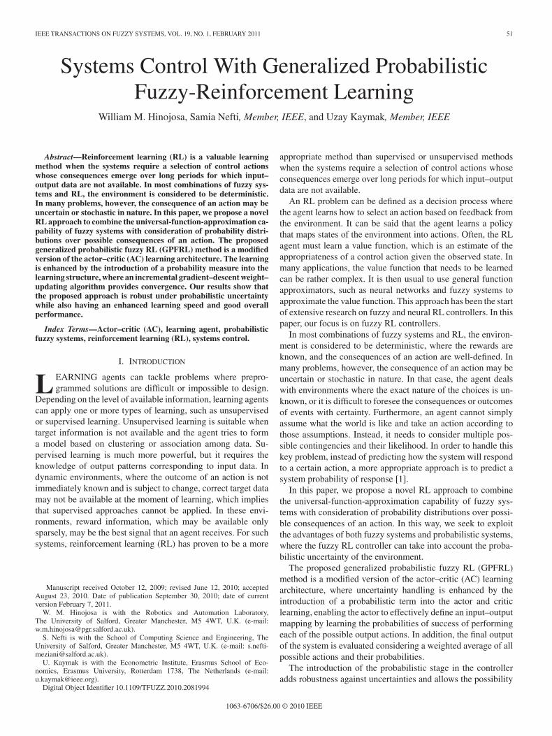
Fig. 1. AC architecture.

or AC techniques [10], [11]. Lin and Lin developed RL strategybased on fuzzy-adaptive-learning control network (FALCON-RL) method [12], Jouffe’s fuzzy-AC-learning (FACL) method[10], Lin’s RL-adaptive fuzzy-controller (RLAFC) method [11],and Wang’s fuzzy AC RL network (FACRLN) method [14].However, most of these algorithms fail to provide a way tohandle real-world uncertainty.

III. GENERALIZED PROBABILISTIC FUZZY REINFORCEMENT

LEARNING ARCHITECTURE

A. Actor–Critic

AC methods are a special case of temporal-difference (TD)methods [3], which are formed by two structures. The actor isa separate memory structure to explicitly represent the controlpolicy, which is independent of the value function, whose func-tion is to select the best control actions. The critic has the taskto estimate the value function, and it is called that way becauseit criticizes the control actions made by the actor. TD error de-pends also on the reward signal obtained from the environmentas a result of the control action. Fig. 1 shows the AC config-uration, where r represents the reward signal, r is the internalenhanced reinforcement signal, and a is the selected action forthe current system state.

B. Probabilistic Fuzzy Logic

Probabilistic modeling has proven to be a useful tool in manyengineering fields to handle random uncertainties, such as infinance markets [13], and in engineering fields, such as roboticcontrol systems [15], power systems [16], and signal process-ing [17]. As probabilistic methods and fuzzy techniques arecomplementary to process uncertainties [18], [19], it is a valu-able job to endow the FLS with probabilistic features. The in-tegration of probability theory and fuzzy logic has also beenstudied in [20].

HINOJOSA et al.: SYSTEMS CONTROL WITH GENERALIZED PROBABILISTIC FUZZY-REINFORCEMENT LEARNING 53

PFL systems work in a similar way as regular fuzzy-logicsystems and encompass all their parts: fuzzification, aggrega-tion, inference, and defuzzification; however, they incorporateprobabilistic modeling, which improve the stochastic model-ing capability like in [21], who applied it to solve a function-approximation problem and a control robotic system, showinga better performance than an ordinary FLS under stochastic cir-cumstances. Other PFS applications include classification prob-lems [22] and financial markets analysis [1].

In GPFRL, after an action ak ∈ A = {a1 , a2 , . . . , an}, is exe-cuted by the system, the learning agent performs a new observa-tion of the system. This observation is composed by a vector ofinputs that inform the agent about external or internal conditionsthat can have a direct impact on the outcome of a selected action.These inputs are then processed using Gaussian-membershipfunctions according to

Left shoulder: μLi (t) =

{1, if xi ≤ cL

e−(1/2)((xi (t)−cL )/σL )2

, otherwise

Center MFs: μCi (t) = e−(1/2)((xi (t)−cC )/σC )2

Right shoulder: μRi (t) =

{e−(1/2)((xi (t)−cR )/σR )2

, if xi ≤ cR

1, otherwise

(1)

where μ{L,C,R}i is the firing strength of input xi , i =

{1, 2, . . . , l} is the input number, L, C, and R specify the typeof membership function used to evaluate each input, xi is thenormalized value of input i, c{L,C,R} is the center value of theGaussian-membership function, and σ{L,C,R} is the standarddeviation for the corresponding membership function.

We consider a PFL system composed of a set of followingrules.

Rj : If x1 is Xh1 . . . xi is Xh

i . . ., and xl is Xhl , then y is a1

with a probability of success of ρj1 , . . ., ak with a probabilityof success of ρjk , and an with a probability of success of ρjn .where Rj is the jth rule of the rule base, Xh

i is the hth linguisticvalue for input i, and h = {1, 2, . . . , qi}, where qi is the totalnumber of membership functions for input xi . Variable y denotesthe output of the system, and ak is a possible value for y, withk = {1, 2, . . . , n} being the action number and n being the totalnumber of possible actions that can be executed. The probabilityof this action to be successful is ρjk , where j = {1, 2, . . . ,m}is the rule number, and m is the total number of rules. Thesesuccess probabilities ρjk are the normalization of the s-shapedweights of the actor, evaluated at time step t, and are defined by

ρjk (t) =S [wjk (t)]∑n

k=1 S [wjk (t)](2)

where S is an s-shaped function given by

S [wjk (t)] =1

1 − e−wj k (t) (3)

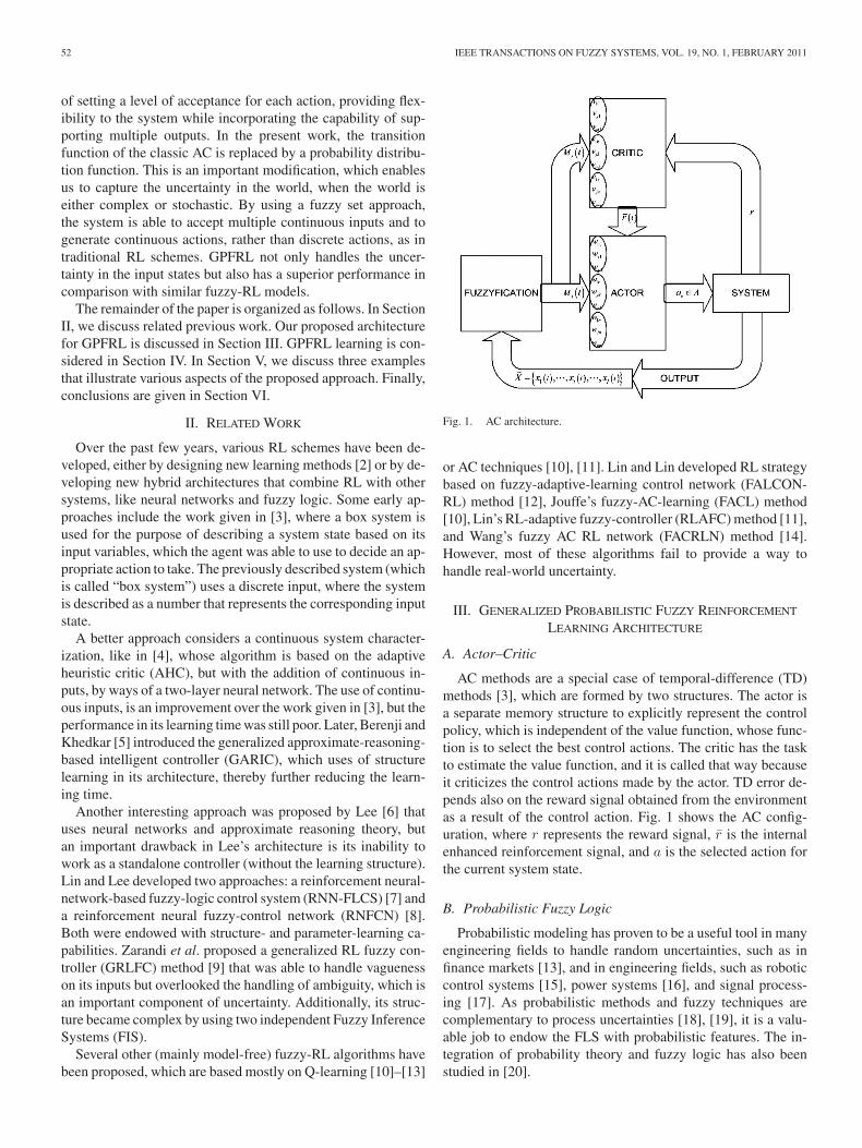
and wjk (t) is a real-valued weight that maps rule j with actionk at a time step t. The FIS structure can be seen in Fig. 2.

The total probability of success of performing action ak con-siders the effect of all individual probabilities and combines

Fig. 2. FIS scheme.

them using a weighted average, where Mj are all the conse-quents of the rules, and Pk (t) is the probability of success ofexecuting action ak at time step t, which is defined as follows:

Pk (t) =

∑mj=1 Mj (t) · ρjk (t)∑m

j=1 Mj (t). (4)

Choosing an action merely considering Pk (t) will lead toan exploiting behavior. In order to create a balance, Lee [6]suggested the addition of a noise signal with mean zero and aGaussian distribution. The use of this signal will force the systeminto an explorative behavior, where different from optimumactions are selected for all states; thus, a more accurate input–output mapping is created at the cost of learning speed. In orderto maximize both accuracy and learning speed, an enhancednoise signal is proposed. This new signal is generated by astochastic noise generator defined by

ηk = N (0, σk ) (5)

where N is a random-number-generator function with a Gaus-sian distribution, mean zero, and a standard deviation σk , whichis defined as follows:

σk =1

1 + e[2pk (t)] . (6)

The stochastic noise generator uses the prediction of eventualreinforcement pk (t), as shown in (11), as a damping factorin order to compute a new standard deviation. The result is anoise signal, which is more influential at the beginning of theruns, boosting exploration, but quickly becomes less influentialas the agent learns, thereby leaving the system with its defaultexploitation behavior.

The final output will be a weighted combination of all actionsand their probabilities, as shown in (7), where �a is a vector of


the final outputs

�a =n∑

k=1

�Ak × (Pk + ηk ) (7)

IV. GENERALIZED PROBABILISTIC FUZZY

REINFORCEMENT LEARNING

The learning process of a GPFRL is based on an AC RLscheme, where the actor learns the policy function, and the criticlearns the value function using the TD method simultaneously.This makes possible to focus on online performance, whichinvolves finding a balance between exploration (of unchartedenvironment) and exploitation (of the current knowledge).

Formally, the basic RL model consists of the following:1) a set of environment state observations O;2) a set of actions A;3) a set of scalar “rewards” r.In this model, an agent interacts with a stochastic environment

at a discrete, low-level time scale. At each discrete time step t,the environment acquires a set of inputs xi ∈ X and generates anobservation o (t) of the environment. Then, the agent performsand action, which is the result of the weighted combination ofall the possible actions ak ∈ A, where A is a discrete set ofactions. The action and observation events occur in sequence,o (t) , a (t) , o (t + 1) , a (t + 1) , . . .. This succession of actionsand observations will be called experience. In this sequence,each event depends only on those preceding it.

The goal in solving a Markov decision process is to find away of behaving, or policy, which yields a maximal reward [23].Formally, a policy is defined as a probability distribution forpicking actions in each state. For any policy π : s × A → [0, 1]and any state s ∈ S, the value function of π for state s is definedas the expected infinite-horizon discounted return from s, giventhat the agent behaves according to π

V π (s) = Eπ

{rt+1 + γrt+2 + γ2rt+3 + · · · |st = s

}(8)

where γ is a factor between 0 and 1 used to discount futurerewards. The objective is to find an optimal policy, π∗, whichmaximizes the value V π (s) of each state s. The optimal valuefunction, i.e., V ∗, is the unique value function corresponding toany optimal policy.

RL typically requires an unambiguous representation of statesand actions and the existence of a scalar reward function. For agiven state, the most traditional of these implementations wouldtake an action, observe a reward, update the value function, andselect, as the new control output, the action with the highestexpected value in each state (for a greedy-policy evaluation).The updating of the value function is repeated until convergenceis achieved. This procedure is usually summarized under policyimprovement iterations.

The parameter learning of the GPFRL system includes twoparts: the actor-parameter learning and the critic-parameterlearning. One feature of the AC learning is that the learningof these two parameters is executed simultaneously.

Given a performance measurement Q (t), and a minimum de-sirable performance Qmin , we define the external reinforcement

signal r as follows:

r ={

0 ∀Q (t) ≥ Qmin > 0−1 ∀0 ≤ Q (t) < Qmin .

(9)

The internal reinforcement, i.e., r, which is expressed in (10),is calculated using the TD of the value function between suc-cessive time steps and the external reinforcement

rk (t) = r (t) + γpk (t) − pk (t − 1) (10)

where γ is the discount factor used to determine the proportionof the delay to the future rewards, and the value function pk (t)is the prediction of eventual reinforcement for action ak and isdefined as

pk (t) =m∑

j=1

Mj (t) · vjk (t) (11)

where vjk is the critic weight of the jth rule, which is describedby (13).

A. Critic Learning

The goal of RL is to adjust correlated parameters in order tomaximize the cumulative sum of the future rewards. The role ofthe critic is to estimate the value function of the policy followedby the actor. The TD error, is the TD of the value functionbetween successive states. The goal of the learning agent is totrain the critic to minimize the error-performance index, whichis the squared TD error Ek (t), and is described as follows:

Ek (t) =12r2k (t). (12)

Gradient–descent methods are among the most widely usedof all function-approximation methods and are particularly well-suited to RL [24] due to its guaranteed convergence to a localoptimum under the usual stochastic approximation conditions.In fact, gradient-based TD learning algorithms that minimizesthe error-performance index has been proved convergent in gen-eral settings that includes both on-policy and off-policy learn-ing [25].

Based on the TD error-performance index (12), the weightsvjk of the critic are updated according to equations (13)–(19)through a gradient–descent method and the chain rule [26]

vjk (t + 1) = vjk (t) − β∂Ek (t)∂vjk (t)

. (13)

In (13), 0 < β < 1 is the learning rate, Ek (t) is the error-performance index, and vjk is the vector of the critic weights.


Rewriting (13) using the chain rule, we have

vjk (t + 1) = vjk (t) − β∂Ek (t)∂rk (t)

· ∂rk (t)∂pk (t)

· ∂pk (t)∂vjk (t)

(14)

∂Ek (t)∂rk (t)

= rk (t) (15)

∂rk (t)∂pk (t)

= γ (16)

∂pk (t)∂vjk (t)

= Mj (t) (17)

vjk (t + 1) = vjk (t) − βγrk (t) · Mj (t) (18)

vjk (t + 1) = vjk (t) − β′rk (t) · Mj (t) . (19)

In (19), 0 < β′ < 1 is the new critic learning rate.

B. Actor Learning

The main goal of the actor is to find a mapping between theinput and the output of the system that maximizes the perfor-mance of the system by maximizing the total expected reward.We can express the actor value function λk (t) according to

λk (t) =m∑

j=1

Mj (t) · ρjk (t) . (20)

Equation (20) represents a component of a mapping froman m-dimensional input state derived from x (t) ∈ R

m to an-dimensional state ak ∈ R

n .Then, we can express the performance function Fk (t) as

Fk (t) = λk (t) − λk (t − 1) . (21)

Using the gradient–descent method, we define the actor-weight-updating rule as follows:

wjk (t + 1) = wjk (t) − α∂Fk (t)∂wjk (t)

(22)

where 0 < α < 1 is a positive constant that specifies the learningrate of the weight wjk . Then, applying the chain rule to (22),we have

∂Fk (t)∂wjk (t)

=∂Fk (t)∂λk (t)

· ∂λk (t)∂ρjk (t)

· ∂ρjk (t)∂wjk (t)

(23)

∂Fk (t)∂wjk (t)

= Mj (t) · ρ2jk (t) · e−wj k (t)

× [ρjk (t) − 1] ·m∑

j=1

S [wjk (t)] . (24)

Hence, we obtain

wjk (t + 1) = wjk (t) − α · Mj (t) · ρ2jk (t)

× e−wj k (t) · [ρjk (t) − 1] ·m∑

j=1

S [wjk (t)]

(25)

Equation (25) represents the generalized weight-update rule,where 0 < α < 1 is the learning rate.

Fig. 3. Cart–pole balancing system.

V. EXPERIMENTS

In this section, we consider a number examples regardingour proposed RL approach. First, we consider the control of asimulated cart–pole system. Second, we consider the control ofa dc motor. Third, we consider a complex control problem formobile-robot navigation.

A. Cart–Pole Balancing Problem

In order to assess the performance of our approach, we usea cart–pole balancing system. This model was used to compareGPFRL (for both discrete and continuous actions) to the originalAHC [3], and other related RL methods.

For this case, the membership functions (i.e., centers andstandard deviations) and the actions are preselected. The task ofthe learning algorithm is to learn the probabilities of success ofperforming each action for every system state.

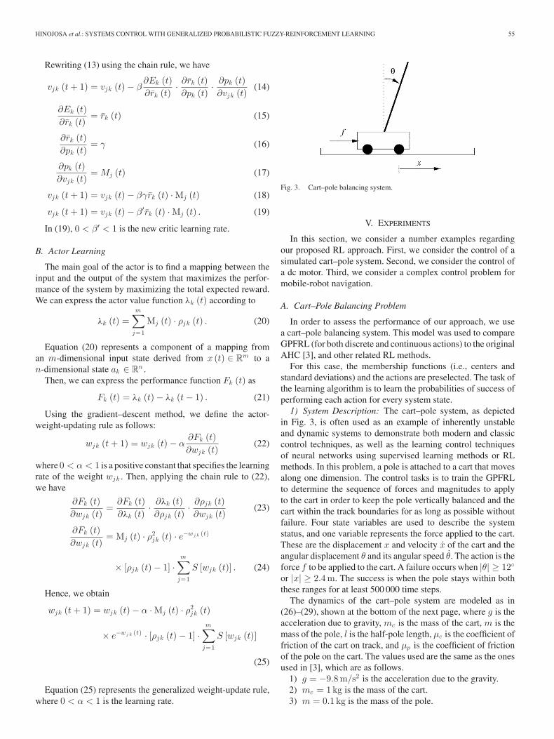
1) System Description: The cart–pole system, as depictedin Fig. 3, is often used as an example of inherently unstableand dynamic systems to demonstrate both modern and classiccontrol techniques, as well as the learning control techniquesof neural networks using supervised learning methods or RLmethods. In this problem, a pole is attached to a cart that movesalong one dimension. The control tasks is to train the GPFRLto determine the sequence of forces and magnitudes to applyto the cart in order to keep the pole vertically balanced and thecart within the track boundaries for as long as possible withoutfailure. Four state variables are used to describe the systemstatus, and one variable represents the force applied to the cart.These are the displacement x and velocity x of the cart and theangular displacement θ and its angular speed θ. The action is theforce f to be applied to the cart. A failure occurs when |θ| ≥ 12◦

or |x| ≥ 2.4m. The success is when the pole stays within boththese ranges for at least 500 000 time steps.

The dynamics of the cart–pole system are modeled as in(26)–(29), shown at the bottom of the next page, where g is theacceleration due to gravity, mc is the mass of the cart, m is themass of the pole, l is the half-pole length, μc is the coefficient offriction of the cart on track, and μp is the coefficient of frictionof the pole on the cart. The values used are the same as the onesused in [3], which are as follows.

1) g = −9.8m/s2 is the acceleration due to the gravity.2) mc = 1kg is the mass of the cart.3) m = 0.1 kg is the mass of the pole.


TABLE IPARAMETERS USED FOR THE CART–POLE RL ALGORITHM

4) l = 0.5m is the half-pole length.5) μc = 0.0005 is the coefficient of friction of the cart on the

track.6) μp = 0.000002 is the coefficient of friction of the pole on

the cart.These equations were simulated by the Euler method using a

time step of 20 ms (50 Hz).One of the important strengths of the proposed model is its ca-

pability of capturing and dealing with the uncertainty in the stateof the system. In our particular experiment with the cart–poleproblem, this may be caused by uncertainty in sensor readingsand the nonlinearity inherent to the system.

To avoid the problem generated by x = 0 in the simulationstudy, we use (30), as described in [27]

f ={

μNsgn (x) , x = 0μNsgn (Fx) , x = 0.

(30)

Table I shows the selected parameters for our experiments,where α is the actor learning rate, β is the critic learning rate,τ is the time step in seconds, and γ is the TD discount factor.The learning rates were selected based on a sequence of exper-iments as shown in the next section. The time step is selectedto be equal to the standard learning rate used in similar studies,and the discount factor was selected based on the basic criteriathat for values of γ close to zero. The system is almost onlyconcerned with the immediate consequences of its action. Forvalues approaching one, future consequences become a moreimportant factor in determining optimal actions. In RL, we aremore concerned in the long-term consequences of the actions;therefore, the selected value for γ is chosen to be 0.98.

2) Results: Table II shows the probabilities of success ofapplying a positive force to the cart for each system state. Theprobability values that are shown in Table II are the valuesobtained after a complete learning run. It can be observed thatvalues close to 50% are barely “visited” system states that canultimately be excluded, which reduces the number of fuzzyrules. This can also be controlled by manipulating the value ofthe stochastic noise generator, which can be set either to forcean exploration behavior, increase the learning time, or force an

TABLE IIPROBABILITIES OF SUCCESS OF APPLYING A POSITIVE FORCE TO THE CART FOR

EACH SYSTEM STATE

exploitation behavior, which will ensure a fast convergence, butwill result in fewer states being visited or “explored.”

We used the pole balancing problem with the only purposeof comparing our GPFRL approach to other RL methods. Sut-ton and Barto [3] proposed an AC learning method, which iscalled AHC, and was based on two single-layer neural networksaimed to control an inverted pendulum by performing a dis-cretization of a 4-D continuous input space, using a partition ofthese variables with no overlapping regions and with not anygeneralization between subspaces. Each of these regions con-stitutes a box, and a Boolean vector indicates in which box thesystem is. Based on this principle, the parameters that modelthe functions are simply stored in an associated vector, therebyproviding a weighting scheme. For large and continuous statespaces, this representation is intractable (curse of dimensional-ity). Therefore, some form of generalization must be incorpo-rated in the state representation. AHC algorithms are good attackling credit-assignment problems by making use of the criticand eligibility traces. In this approach, correlations betweenstate variables were difficult to embody into the algorithm, thecontrol structure was excessively complex, and suitable resultsfor complex and uncertain systems could not be obtained.

Anderson [4] further realized the balancing control for aninverted pendulum under a nondiscrete state by an AHC al-gorithm, which is based on two feed-forward neural networks.In this work, Anderson proposed a divided state space into fi-nite numbers of subspaces with no generalization between sub-spaces. Therefore, for complex, and uncertain systems a suitabledivision results could not be obtained, correlations between statevariables were difficult to embody into the algorithm, the con-trol structure was excessively complex, and the learning processtook too many trials for learning.

Lee [6] proposed a self-learning rule-based controller, whichis a direct extension of the AHC described in [3] using a fuzzy

θ =g sin θ + cos θ

[(−f − mlθ2 sin θ + μcsgn (x) /(mc + m)

]− (μp θ/ml)

l [(4/3) − (m cos2 θ/(mc + m)](26)

x =f + ml

[θ2 sin θ − θ cos θ

]− μcsgn (x)

mc + m(27)

θ (t + 1) = θ (t) + Δθ (t) (28)

x (t + 1) = x (t) + Δx (t) (29)


partition rather than the box system to code the state and twosingle-layer neural networks. Lee’s approach is capable of work-ing on both continues inputs (i.e., states) and outputs (i.e., ac-tions). However, the main drawback of this implementation isthat as a difference with the classic implementation in whichthe weight-updating process act as a quality modification dueto the bang–bang action characteristic (the resulting action isonly determined by the sign of the weight), in Lee’s, it acts asan action modificator. The internal reinforcement is only ableto inform about the improvement of the performance, which isnot informative enough to allow an action modification.

The GARIC architecture [5] is an extension of ARIC [28],and is a learning method based on AHC. It is used to tune thelinguistic label values of the fuzzy-controller rule base. This rulebase is previously designed manually or with another automaticmethod. The critic is implemented with a neural network and theactor is actually an implementation of a fuzzy-inference system(FIS). The critic learning is classical, but the actor learning, likethe one by Lee [6], acts directly on action magnitudes. Then,GARIC-Q [29] extends GARIC to derive a better controllerusing a competition between a society of agents (operating byGARIC), each including a rule base, and at the top level, ituses fuzzy Q-learning (FQL) to select the best agent at eachstep. GARIC belong to a category of off-line training systems(a dataset is required beforehand). Moreover, they do not havea capability of structure learning and it needs a large number oftrials to be tuned. A few years later, Zarandi et al. [9] modifiedthis approach in order to handle vagueness in the control states.This new approach shows an improvement in the learning speed,but did not solve the main drawbacks of the GARIC architecture.While the approach presented by Zarandi et al. [9] is able tohandle vagueness on the input states, it fails to generalize it inorder to handle uncertainty.

In supervised learning, precise training is usually not avail-able and is expensive. To overcome this problem, Lin andLee [30], [31] proposed an RNN-FLCS, which consists of twofuzzy neural networks (FNNs); one performs a fuzzy-neuralcontroller (i.e., actor), and the other stands for a fuzzy-neuralevaluator (i.e., critic). Moreover, the evaluator network providesinternal reinforcement signals to the action network to reducethe uncertainty faced by the latter network. In this scheme, us-ing two networks makes the scheme relatively complex and itscomputational demand heavy. The RNN-FLCS can find propernetwork structure and parameters simultaneously and dynam-ically. Although the topology structure and the parameters ofthe networks can be tuned online simultaneously, the num-ber and configuration of membership functions for each in-put and output variable have to be decided by an expert inadvance.

Lin [12] proposed an FALCON-RL, which is based on theFALCON algorithm [32]. The FALCON-RL is a type of FNN-based RL system (like ARIC, GARIC, and RNN-FLCS) thatuses two separate five-layer perceptron networks to fulfill thefunctions of actor and critic networks. With this approach, thetopology structure and the parameters of the networks can betuned online simultaneously, but the number and configurationof membership functions for each input and output variable

have to be decided by an expert in advance. In addition, thearchitecture of the system is complex.

Jouffe [10] investigated the continuous and discrete actionsby designing two RL methods with function-approximation im-plemented using FIS. These two methods, i.e., FACL and FQL,are both based on dynamic-planning theory while making useof eligibility traces to enhance the speed of learning. These twomethods merely tuned the parameters of the consequent part ofa FIS by using reinforcement signals received from the envi-ronment, while the premise part of the FIS was fixed during thelearning process. Therefore, they could not realize the adaptiveestablishment of a rule base, limiting its learning performance.Furthermore, FACL and FQL were both based on dynamic-programming principles; therefore, system stability and perfor-mance could not be guaranteed.

Another approach based on function approximation is theRLAFC method, which was proposed by Lin [11]; here, theaction-generating element is a fuzzy approximator with a setof tunable parameters; moreover, Lin [11] proposed a tuningalgorithm derived from the Lyapunov stability theory in orderto guarantee both tracking performance and stability. Again inthis approach, the number and configuration of the membershipfunctions for each input and output variable have to be decidedby an expert in advance. It also presents the highest number offuzzy rules of our studies and a very complex structure.

In order to solve the curse of the dimensionality problem,Wang et al. [14] proposed a new FACRLN based on a fuzzy-radial basis function (FRBF) neural network. The FACRLN useda four-layer FRBF neural network that is used to approximateboth the action value function of the actor and the state-valuefunction of the critic simultaneously. Moreover, the FRBF net-work is able to adjust its structure and parameters in an adaptiveway according to the complexity of the task and the progress inlearning. While the FACRLN architecture shows an excellentlearning rate, it fails to capture and handle the system inputuncertainties while presenting a very complex structure.

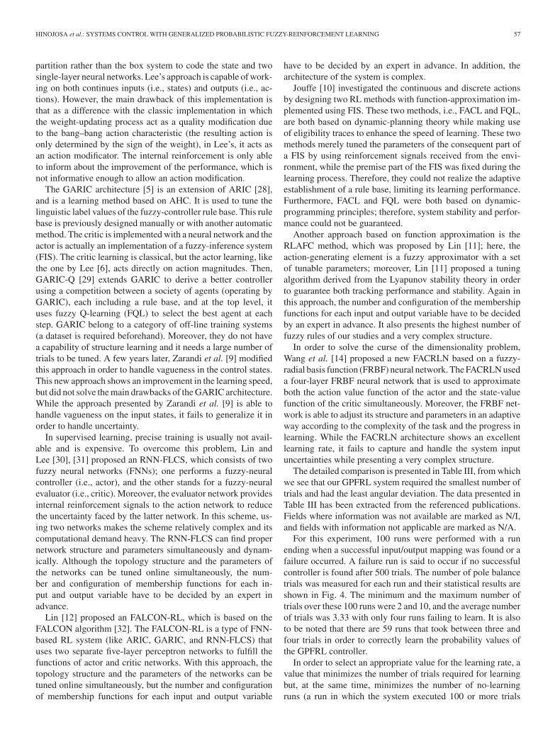
The detailed comparison is presented in Table III, from whichwe see that our GPFRL system required the smallest number oftrials and had the least angular deviation. The data presented inTable III has been extracted from the referenced publications.Fields where information was not available are marked as N/I,and fields with information not applicable are marked as N/A.

For this experiment, 100 runs were performed with a runending when a successful input/output mapping was found or afailure occurred. A failure run is said to occur if no successfulcontroller is found after 500 trials. The number of pole balancetrials was measured for each run and their statistical results areshown in Fig. 4. The minimum and the maximum number oftrials over these 100 runs were 2 and 10, and the average numberof trials was 3.33 with only four runs failing to learn. It is alsoto be noted that there are 59 runs that took between three andfour trials in order to correctly learn the probability values ofthe GPFRL controller.

In order to select an appropriate value for the learning rate, avalue that minimizes the number of trials required for learningbut, at the same time, minimizes the number of no-learningruns (a run in which the system executed 100 or more trials


TABLE IIILEARNING METHOD COMPARISON ON THE CART–POLE PROBLEM

Fig. 4. Trials distribution over 100 runs.

Fig. 5. Actor learning rate; alpha versus number of failed runs.

without success), a set of tests were performed and their resultsare depicted in Figs. 5–8. In there graphs, the solid black linerepresents the actual results, while the dashed line is a second-order polynomial trend line. In Figs. 5 and 6, it can be observedthat the value of alpha does not have a direct impact on thenumber of failed runs (which is in average 10%). It has, however,more impact on the learning speed, where there is no significanceincrease on the learning speed for a value higher than 45. Forthese tests, the program executed the learning algorithm 22times, each time consisting of 100 runs, from which the averagewas taken.

For the second set of tests, the values of beta were changed(see Figs. 7 and 8) while keeping alpha at 45. It can be observedthat there is no significant change in the amount of failed runsfor beta values under 0.000032. With beta values over this, thenumber of nonlearning runs increases quickly. Contrarily, forvalues of beta below 0.000032, there is no major increase on thelearning rate.

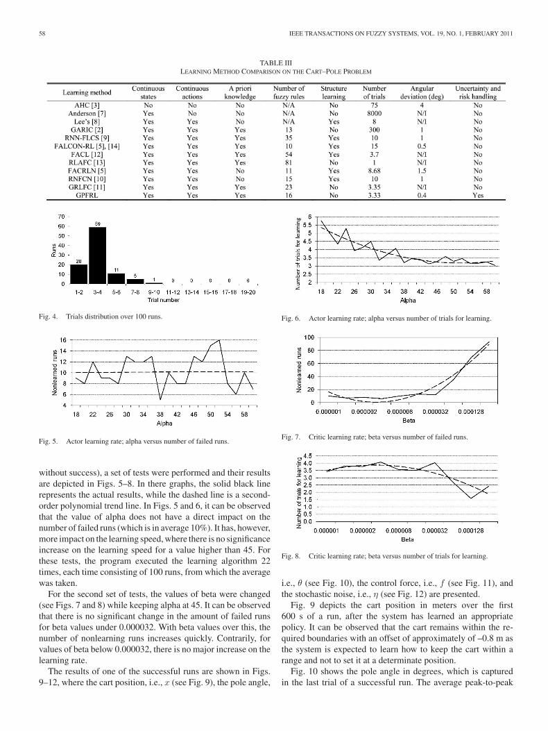
The results of one of the successful runs are shown in Figs.9–12, where the cart position, i.e., x (see Fig. 9), the pole angle,

Fig. 6. Actor learning rate; alpha versus number of trials for learning.

Fig. 7. Critic learning rate; beta versus number of failed runs.

Fig. 8. Critic learning rate; beta versus number of trials for learning.

i.e., θ (see Fig. 10), the control force, i.e., f (see Fig. 11), andthe stochastic noise, i.e., η (see Fig. 12) are presented.

Fig. 9 depicts the cart position in meters over the first600 s of a run, after the system has learned an appropriatepolicy. It can be observed that the cart remains within the re-quired boundaries with an offset of approximately of –0.8 m asthe system is expected to learn how to keep the cart within arange and not to set it at a determinate position.

Fig. 10 shows the pole angle in degrees, which is capturedin the last trial of a successful run. The average peak-to-peak


Fig. 9. Cart position at the end of a successful learning run.

Fig. 10. Pole angle at the end of a successful learning run.

Fig. 11. Applied force at the end of a successful learning run.

Fig. 12. Stochastic noise.

angle was calculated to be around 0.4◦, thus outperforming theperformance of previous works. In addition, it can be notedthat this value oscillates around an angle of 0◦, as this can beconsidered the most-stable position due to the effect of gravity.Therefore, it can be said that the system successfully learns howto keep the pole around this value.

Fig. 11 shows the generated forces that push the cart in eitherdirection. This generated force is a continuous value that rangesfrom 0 to 10 and is a function of the combined probability ofsuccess for each visited state. As expected, this force is thrilledaround 0, thus resulting in no average motion of the cart in eitherdirection and, thus, keeping it within the required boundaries.

Fig. 13. Motor with load attached.

Finally, Fig. 12 shows the stochastically generated noise,which is used to add exploration/exploitation behavior to thesystem. This noise is generated by the stochastic noise genera-tor described by (5) and (6). In this case, a small average valueindicates that preference is given to exploitation rather than ex-ploration behavior, as expected at the end of a learning trial. Therange of the generated noise depends on the value of the stan-dard deviation σk , which varies over the learning phase, thusgiving a higher priority to exploration at the beginning of thelearning and an increased priority to exploitation as the value ofthe prediction of eventual reinforcement pk (t) increases.

B. DC-Motor Control

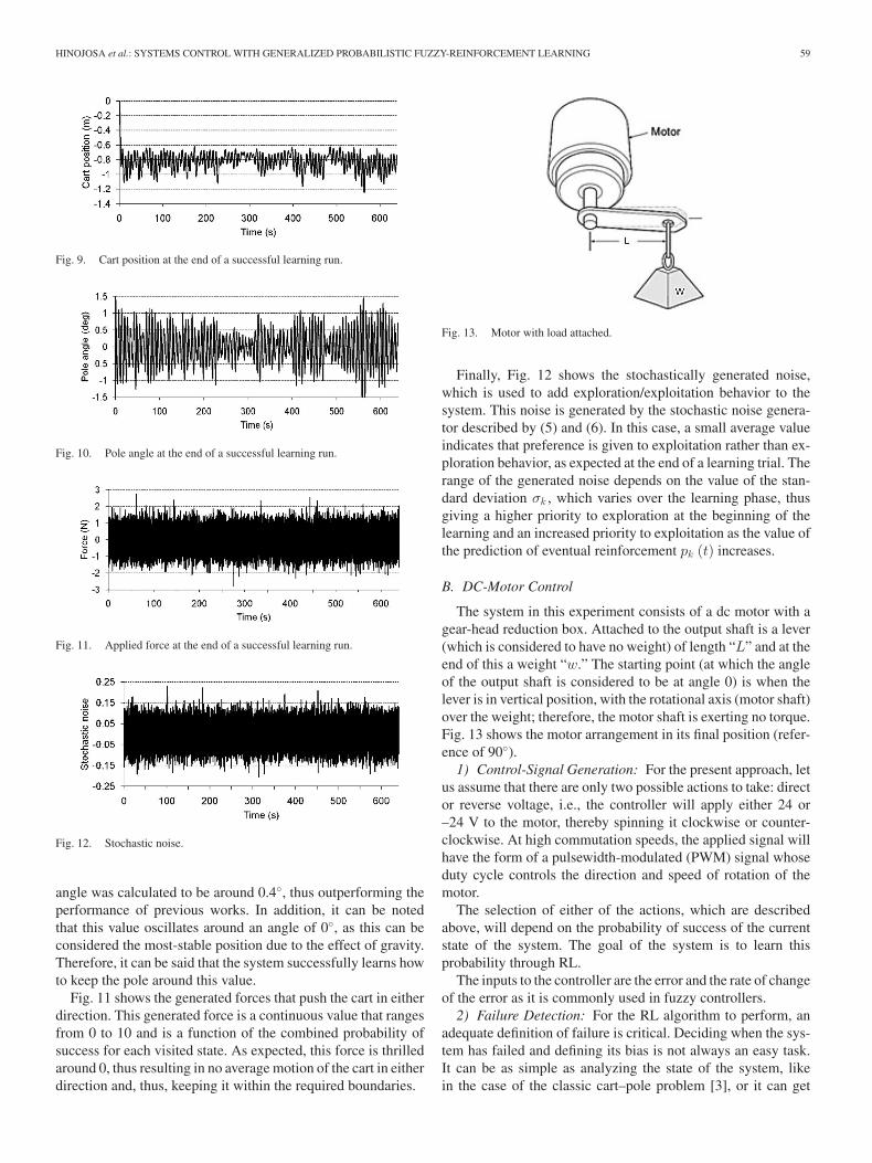
The system in this experiment consists of a dc motor with agear-head reduction box. Attached to the output shaft is a lever(which is considered to have no weight) of length “L” and at theend of this a weight “w.” The starting point (at which the angleof the output shaft is considered to be at angle 0) is when thelever is in vertical position, with the rotational axis (motor shaft)over the weight; therefore, the motor shaft is exerting no torque.Fig. 13 shows the motor arrangement in its final position (refer-ence of 90◦).

1) Control-Signal Generation: For the present approach, letus assume that there are only two possible actions to take: director reverse voltage, i.e., the controller will apply either 24 or–24 V to the motor, thereby spinning it clockwise or counter-clockwise. At high commutation speeds, the applied signal willhave the form of a pulsewidth-modulated (PWM) signal whoseduty cycle controls the direction and speed of rotation of themotor.

The selection of either of the actions, which are describedabove, will depend on the probability of success of the currentstate of the system. The goal of the system is to learn thisprobability through RL.

The inputs to the controller are the error and the rate of changeof the error as it is commonly used in fuzzy controllers.

2) Failure Detection: For the RL algorithm to perform, anadequate definition of failure is critical. Deciding when the sys-tem has failed and defining its bias is not always an easy task.It can be as simple as analyzing the state of the system, likein the case of the classic cart–pole problem [3], or it can get


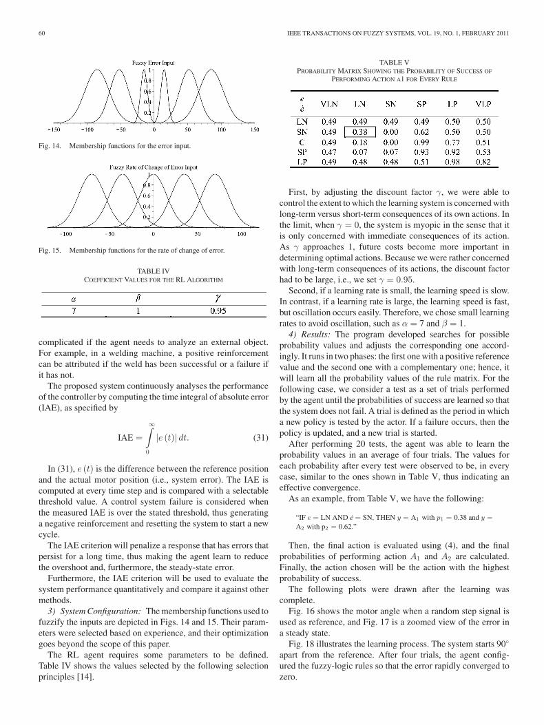
Fig. 14. Membership functions for the error input.

Fig. 15. Membership functions for the rate of change of error.

TABLE IVCOEFFICIENT VALUES FOR THE RL ALGORITHM

complicated if the agent needs to analyze an external object.For example, in a welding machine, a positive reinforcementcan be attributed if the weld has been successful or a failure ifit has not.

The proposed system continuously analyses the performanceof the controller by computing the time integral of absolute error(IAE), as specified by

IAE =

∞∫0

|e (t)| dt. (31)

In (31), e (t) is the difference between the reference positionand the actual motor position (i.e., system error). The IAE iscomputed at every time step and is compared with a selectablethreshold value. A control system failure is considered whenthe measured IAE is over the stated threshold, thus generatinga negative reinforcement and resetting the system to start a newcycle.

The IAE criterion will penalize a response that has errors thatpersist for a long time, thus making the agent learn to reducethe overshoot and, furthermore, the steady-state error.

Furthermore, the IAE criterion will be used to evaluate thesystem performance quantitatively and compare it against othermethods.

3) System Configuration: The membership functions used tofuzzify the inputs are depicted in Figs. 14 and 15. Their param-eters were selected based on experience, and their optimizationgoes beyond the scope of this paper.

The RL agent requires some parameters to be defined.Table IV shows the values selected by the following selectionprinciples [14].

TABLE VPROBABILITY MATRIX SHOWING THE PROBABILITY OF SUCCESS OF

PERFORMING ACTION A1 FOR EVERY RULE

First, by adjusting the discount factor γ, we were able tocontrol the extent to which the learning system is concerned withlong-term versus short-term consequences of its own actions. Inthe limit, when γ = 0, the system is myopic in the sense that itis only concerned with immediate consequences of its action.As γ approaches 1, future costs become more important indetermining optimal actions. Because we were rather concernedwith long-term consequences of its actions, the discount factorhad to be large, i.e., we set γ = 0.95.

Second, if a learning rate is small, the learning speed is slow.In contrast, if a learning rate is large, the learning speed is fast,but oscillation occurs easily. Therefore, we chose small learningrates to avoid oscillation, such as α = 7 and β = 1.

4) Results: The program developed searches for possibleprobability values and adjusts the corresponding one accord-ingly. It runs in two phases: the first one with a positive referencevalue and the second one with a complementary one; hence, itwill learn all the probability values of the rule matrix. For thefollowing case, we consider a test as a set of trials performedby the agent until the probabilities of success are learned so thatthe system does not fail. A trial is defined as the period in whicha new policy is tested by the actor. If a failure occurs, then thepolicy is updated, and a new trial is started.

After performing 20 tests, the agent was able to learn theprobability values in an average of four trials. The values foreach probability after every test were observed to be, in everycase, similar to the ones shown in Table V, thus indicating aneffective convergence.

As an example, from Table V, we have the following:

“IF e = LN AND e = SN, THEN y = A1 with p1 = 0.38 and y =A2 with p2 = 0.62.”

Then, the final action is evaluated using (4), and the finalprobabilities of performing action A1 and A2 are calculated.Finally, the action chosen will be the action with the highestprobability of success.

The following plots were drawn after the learning wascomplete.

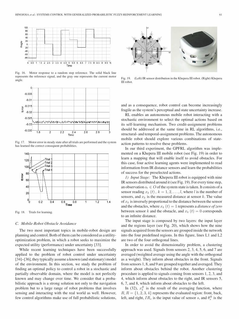
Fig. 16 shows the motor angle when a random step signal isused as reference, and Fig. 17 is a zoomed view of the error ina steady state.

Fig. 18 illustrates the learning process. The system starts 90◦

apart from the reference. After four trials, the agent config-ured the fuzzy-logic rules so that the error rapidly converged tozero.


Fig. 16. Motor response to a random step reference. The solid black linerepresents the reference signal, and the gray one represents the current motorangle.

Fig. 17. Motor error in steady state after all trials are performed and the systemhas learned the correct consequent probabilities.

Fig. 18. Trials for learning.

C. Mobile-Robot Obstacle Avoidance

The two most important topics in mobile-robot design areplanning and control. Both of them can be considered as a utility-optimization problem, in which a robot seeks to maximize theexpected utility (performance) under uncertainty [33].

While recent learning techniques have been successfullyapplied to the problem of robot control under uncertainty[34]–[36], they typically assume a known (and stationary) modelof the environment. In this section, we study the problem offinding an optimal policy to control a robot in a stochastic andpartially observable domain, where the model is not perfectlyknown and may change over time. We consider that a proba-bilistic approach is a strong solution not only to the navigationproblem but to a large range of robot problems that involvessensing and interacting with the real world as well. However,few control algorithms make use of full probabilistic solutions,

Fig. 19. (Left) IR sensor distribution in the Khepera III robot. (Right) KheperaIII robot.

and as a consequence, robot control can become increasinglyfragile as the system’s perceptual and state uncertainty increase.

RL enables an autonomous mobile robot interacting with astochastic environment to select the optimal actions based onits self-learning mechanism. Two credit-assignment problemsshould be addressed at the same time in RL algorithms, i.e.,structural- and temporal-assignment problems. The autonomousmobile robot should explore various combinations of state-action patterns to resolve these problems.

In our third experiment, the GPFRL algorithm was imple-mented on a Khepera III mobile robot (see Fig. 19) in order tolearn a mapping that will enable itself to avoid obstacles. Forthis case, four active learning agents were implemented to readinformation from IR distance sensors and learn the probabilitiesof success for the preselected actions.

1) Input Stage: The Khepera III robot is equipped with nineIR sensors distributed around it (see Fig. 19). For every time step,an observation ot ∈ O of the system state is taken. It consists of asensor reading xk (t) , k = 1, 2, . . . , l, where l is the number ofsensors, and xk is the measured distance at sensor k. The valueof xk is inversely proportional to the distance between the sensorand the obstacles, where xk (t) = 1 represents a distance of zerobetween sensor k and the obstacle, and xk (t) = 0 correspondsto an infinite distance.

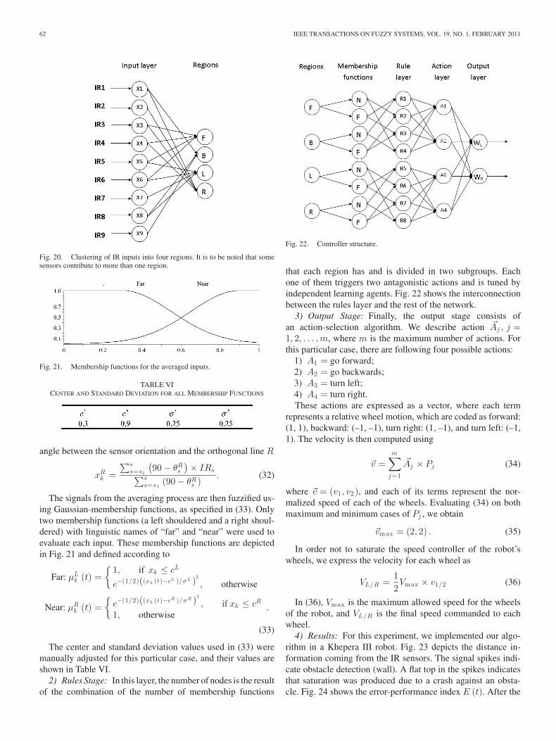
The input stage is composed by two layers: the input layerand the regions layer (see Fig. 20), which shows how the ninesignals acquired from the sensors are grouped inside the networkinto the four predefined regions. In this figure, lines L1 and L2are two of the four orthogonal lines.

In order to avoid the dimensionality problem, a clusteringapproach was used. Signals from sensors 2, 3, 4, 5, 6, and 7 areaveraged (weighted average using the angle with the orthogonalas a weight). They inform about obstacles in the front. Signalsfrom sensors 1, 8, and 9 are grouped together and averaged. Theyinform about obstacles behind the robot. Another clusteringprocedure is applied to signals coming from sensors 1, 2, 3, and4, which inform about obstacles to the right, and IR sensors 5,6, 7, and 8, which inform about obstacles to the left.

In (32), xRk is the result of the averaging function, where

R,R = {1, 2, 3, 4} represents the evaluated region: front, back,left, and right, IRs is the input value of sensor s, and θR

s is the


Fig. 20. Clustering of IR inputs into four regions. It is to be noted that somesensors contribute to more than one region.

Fig. 21. Membership functions for the averaged inputs.

TABLE VICENTER AND STANDARD DEVIATION FOR ALL MEMBERSHIP FUNCTIONS

angle between the sensor orientation and the orthogonal line R

xRk =

∑ss=s1

(90 − θR

s

)× IRs∑s

s=s1(90 − θR

s ). (32)

The signals from the averaging process are then fuzzified us-ing Gaussian-membership functions, as specified in (33). Onlytwo membership functions (a left shouldered and a right shoul-dered) with linguistic names of “far” and “near” were used toevaluate each input. These membership functions are depictedin Fig. 21 and defined according to

Far: μLk (t) =

{1, if xk ≤ cL

e−(1/2)((xk (t)−cL )/σL )2

, otherwise

Near: μRk (t) =

{e−(1/2)((xk (t)−cR )/σR )2

, if xk ≤ cR

1, otherwise.

(33)

The center and standard deviation values used in (33) weremanually adjusted for this particular case, and their values areshown in Table VI.

2) Rules Stage: In this layer, the number of nodes is the resultof the combination of the number of membership functions

Fig. 22. Controller structure.

that each region has and is divided in two subgroups. Eachone of them triggers two antagonistic actions and is tuned byindependent learning agents. Fig. 22 shows the interconnectionbetween the rules layer and the rest of the network.

3) Output Stage: Finally, the output stage consists ofan action-selection algorithm. We describe action �Aj , j =1, 2, . . . ,m, where m is the maximum number of actions. Forthis particular case, there are following four possible actions:

1) A1 = go forward;2) A2 = go backwards;3) A3 = turn left;4) A4 = turn right.These actions are expressed as a vector, where each term

represents a relative wheel motion, which are coded as forward:(1, 1), backward: (–1, –1), turn right: (1, –1), and turn left: (–1,1). The velocity is then computed using

�v =m∑

j=1

�Aj × Pj (34)

where �v = (v1 , v2), and each of its terms represent the nor-malized speed of each of the wheels. Evaluating (34) on bothmaximum and minimum cases of Pj , we obtain

�vmax = (2, 2) . (35)

In order not to saturate the speed controller of the robot’swheels, we express the velocity for each wheel as

VL/R =12Vmax × v1/2 (36)

In (36), Vmax is the maximum allowed speed for the wheelsof the robot, and VL/R is the final speed commanded to eachwheel.

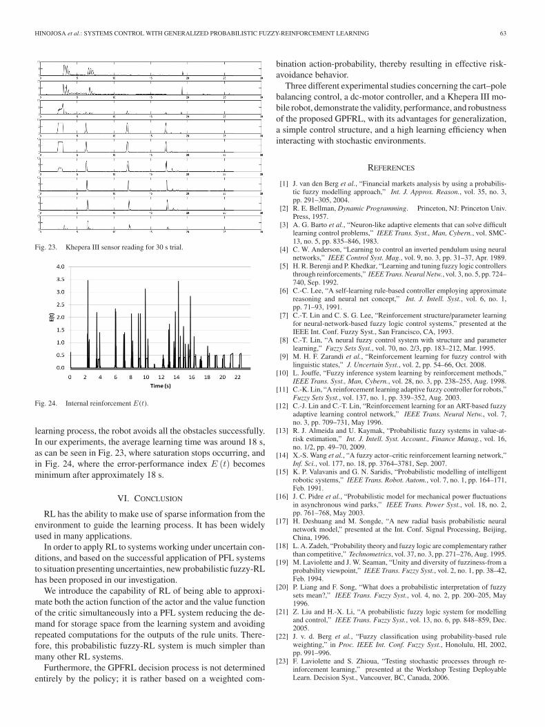
4) Results: For this experiment, we implemented our algo-rithm in a Khepera III robot. Fig. 23 depicts the distance in-formation coming from the IR sensors. The signal spikes indi-cate obstacle detection (wall). A flat top in the spikes indicatesthat saturation was produced due to a crash against an obsta-cle. Fig. 24 shows the error-performance index E (t). After the


Fig. 23. Khepera III sensor reading for 30 s trial.

Fig. 24. Internal reinforcement E(t).

learning process, the robot avoids all the obstacles successfully.In our experiments, the average learning time was around 18 s,as can be seen in Fig. 23, where saturation stops occurring, andin Fig. 24, where the error-performance index E (t) becomesminimum after approximately 18 s.

VI. CONCLUSION

RL has the ability to make use of sparse information from theenvironment to guide the learning process. It has been widelyused in many applications.

In order to apply RL to systems working under uncertain con-ditions, and based on the successful application of PFL systemsto situation presenting uncertainties, new probabilistic fuzzy-RLhas been proposed in our investigation.

We introduce the capability of RL of being able to approxi-mate both the action function of the actor and the value functionof the critic simultaneously into a PFL system reducing the de-mand for storage space from the learning system and avoidingrepeated computations for the outputs of the rule units. There-fore, this probabilistic fuzzy-RL system is much simpler thanmany other RL systems.

Furthermore, the GPFRL decision process is not determinedentirely by the policy; it is rather based on a weighted com-

bination action-probability, thereby resulting in effective risk-avoidance behavior.

Three different experimental studies concerning the cart–polebalancing control, a dc-motor controller, and a Khepera III mo-bile robot, demonstrate the validity, performance, and robustnessof the proposed GPFRL, with its advantages for generalization,a simple control structure, and a high learning efficiency wheninteracting with stochastic environments.

REFERENCES

[1] J. van den Berg et al., “Financial markets analysis by using a probabilis-tic fuzzy modelling approach,” Int. J. Approx. Reason., vol. 35, no. 3,pp. 291–305, 2004.

[2] R. E. Bellman, Dynamic Programming. Princeton, NJ: Princeton Univ.Press, 1957.

[3] A. G. Barto et al., “Neuron-like adaptive elements that can solve difficultlearning control problems,” IEEE Trans. Syst., Man, Cybern., vol. SMC-13, no. 5, pp. 835–846, 1983.

[4] C. W. Anderson, “Learning to control an inverted pendulum using neuralnetworks,” IEEE Control Syst. Mag., vol. 9, no. 3, pp. 31–37, Apr. 1989.

[5] H. R. Berenji and P. Khedkar, “Learning and tuning fuzzy logic controllersthrough reinforcements,” IEEE Trans. Neural Netw., vol. 3, no. 5, pp. 724–740, Sep. 1992.

[6] C.-C. Lee, “A self-learning rule-based controller employing approximatereasoning and neural net concept,” Int. J. Intell. Syst., vol. 6, no. 1,pp. 71–93, 1991.

[7] C.-T. Lin and C. S. G. Lee, “Reinforcement structure/parameter learningfor neural-network-based fuzzy logic control systems,” presented at theIEEE Int. Conf. Fuzzy Syst., San Francisco, CA, 1993.

[8] C.-T. Lin, “A neural fuzzy control system with structure and parameterlearning,” Fuzzy Sets Syst., vol. 70, no. 2/3, pp. 183–212, Mar. 1995.

[9] M. H. F. Zarandi et al., “Reinforcement learning for fuzzy control withlinguistic states,” J. Uncertain Syst., vol. 2, pp. 54–66, Oct. 2008.

[10] L. Jouffe, “Fuzzy inference system learning by reinforcement methods,”IEEE Trans. Syst., Man, Cybern., vol. 28, no. 3, pp. 238–255, Aug. 1998.

[11] C.-K. Lin, “A reinforcement learning adaptive fuzzy controller for robots,”Fuzzy Sets Syst., vol. 137, no. 1, pp. 339–352, Aug. 2003.

[12] C.-J. Lin and C.-T. Lin, “Reinforcement learning for an ART-based fuzzyadaptive learning control network,” IEEE Trans. Neural Netw., vol. 7,no. 3, pp. 709–731, May 1996.

[13] R. J. Almeida and U. Kaymak, “Probabilistic fuzzy systems in value-at-risk estimation,” Int. J. Intell. Syst. Account., Finance Manag., vol. 16,no. 1/2, pp. 49–70, 2009.

[14] X.-S. Wang et al., “A fuzzy actor–critic reinforcement learning network,”Inf. Sci., vol. 177, no. 18, pp. 3764–3781, Sep. 2007.

[15] K. P. Valavanis and G. N. Saridis, “Probabilistic modelling of intelligentrobotic systems,” IEEE Trans. Robot. Autom., vol. 7, no. 1, pp. 164–171,Feb. 1991.

[16] J. C. Pidre et al., “Probabilistic model for mechanical power fluctuationsin asynchronous wind parks,” IEEE Trans. Power Syst., vol. 18, no. 2,pp. 761–768, May 2003.

[17] H. Deshuang and M. Songde, “A new radial basis probabilistic neuralnetwork model,” presented at the Int. Conf. Signal Processing, Beijing,China, 1996.

[18] L. A. Zadeh, “Probability theory and fuzzy logic are complementary ratherthan competitive,” Technometrics, vol. 37, no. 3, pp. 271–276, Aug. 1995.

[19] M. Laviolette and J. W. Seaman, “Unity and diversity of fuzziness-from aprobability viewpoint,” IEEE Trans. Fuzzy Syst., vol. 2, no. 1, pp. 38–42,Feb. 1994.

[20] P. Liang and F. Song, “What does a probabilistic interpretation of fuzzysets mean?,” IEEE Trans. Fuzzy Syst., vol. 4, no. 2, pp. 200–205, May1996.

[21] Z. Liu and H.-X. Li, “A probabilistic fuzzy logic system for modellingand control,” IEEE Trans. Fuzzy Syst., vol. 13, no. 6, pp. 848–859, Dec.2005.

[22] J. v. d. Berg et al., “Fuzzy classification using probability-based ruleweighting,” in Proc. IEEE Int. Conf. Fuzzy Syst., Honolulu, HI, 2002,pp. 991–996.

[23] F. Laviolette and S. Zhioua, “Testing stochastic processes through re-inforcement learning,” presented at the Workshop Testing DeployableLearn. Decision Syst., Vancouver, BC, Canada, 2006.


[24] C. Baird, “Reinforcement learning through gradient descent,” Ph.D. dis-sertation, School of Comput. Sci., Carnegie Mellon Univ., Pittsburgh, PA,1999.

[25] R. S. Sutton et al., “Fast gradient-descent methods for temporal-differencelearning with linear function approximation,” in Proc. 26th Int. Conf.Mach. Learn., Montreal, QC, Canada, 2009, pp. 993–1000.

[26] L. Baird and A. Moore, “Gradient descent for general reinforcement learn-ing,” in Proc. Adv. Neural Inf. Process. Syst. II, 1999, pp. 968–974.

[27] H. Yu et al., “Tracking control of a peddulum-driven cart–pole under-actuated system,” presented at the IEEE Int. Conf. Syst., Man, Cybern.,Montreal, QC, Canada, 2007.

[28] H. R. Berenji, “Refinement of approximate reasoning-based controllers byreinforcement learning,” presented at the 8th Int. Workshop Mach. Learn.,San Francisco, CA, 1991.

[29] H. R. Berenji, “Fuzzy Q-learning for generalization of reinforcementlearning,” presented at the 5th IEEE Int. Conf. Fuzzy Syst., New Orleans,LA, 1996.

[30] C.-T. Lin and C. S. G. Lee, “Reinforcement structure/parameter learningfor neural-network-based fuzzy logic control systems,” IEEE Trans. FuzzySyst., vol. 2, no. 1, pp. 46–63, Feb. 1994.

[31] C.-T. Lin and C. S. G. Lee, “Neural-network-based fuzzy logic control anddecision system,” IEEE Trans. Comput., vol. 40, no. 12, pp. 1320–1336,Dec. 1991.

[32] C.-T. Lin et al., “Fuzzy adaptive learning control network with on-lineneural learning,” Fuzzy Sets Syst., vol. 71, no. 1, pp. 25–45, Apr. 1995.

[33] S. Thrun. (2000) Probabilistic algorithms in robotics. AI Mag.[34] J. Pineau, “Point-based value iteration: An any time algorithm for

POMDPs,” presented at the Int. Joint Conf. Artif. Intell., Acapulco,Mexico, 2003.

[35] P. Poupart and C. Boutilier, “VDCBPI: An approximate scalable algorithmfor large POMDPs,” presented at the Advances Neural Inform. Process.Syst., Vancouver, BC, Canada, 2004.

[36] N. Roy et al., “Finding approximate POMDP solutions through beliefcompression,” J. Artif. Intell. Res., vol. 23, no. 1, pp. 1–40, Jan. 2005.

William M. Hinojosa received the B.Sc. degree inscience and engineering, with a major in electronicengineering, the Engineer degree in electrical andelectronics, with a major in industrial control, fromthe Pontificia Universidad Catolica del Peru, Lima,Peru, in 2002 and 2003, respectively, and the M.Sc.degree in robotics and automation in 2006 from TheUniversity of Salford, Salford, Greater Manchester,U.K., where he is currently working toward the Ph.D.degree in advanced robotics.

Since September 2003, he has been with the Cen-ter for Advanced Robotics, School of Computing, Science, and Engineering,The University of Salford. Since 2007, he has been a Lecturer in mobile roboticswith the University of Salford and the Ecole Superieure des Technologies In-dustrielles Avancees, Biarritz, France. He has authored or coauthored a bookchapter for Humanoid Robots (InTech, 2009). His current research interests arefuzzy systems, neural networks, intelligent control, cognition, reinforcementlearning, and mobile robotics.

Mr. Hinojosa is member of the European Network for the Advancement ofArtificial Cognitive Systems, Interaction, and Robotics.

Samia Nefti (M’04) received the M.Sc. degree inelectrical engineering, the D.E.A. degree in indus-trial informatics, and the Ph.D. degree in roboticsand artificial intelligence from the University of ParisXII, Paris, France, in 1992, 1994, and 1998, respec-tively.

In November 1999, she joined the Liverpool Uni-versity, Liverpool, U.K., as a Senior Research Fellowengaged with the European Research Project Occu-pational Therapy Internet School. Afterwards, shewas involved in several projects with the European

and U.K. Engineering and Physical Sciences Research Council, where she wasconcerned mainly with model-based predictive control, modeling, and swarmoptimization and decision making. She is currently an Associate Professor ofcomputational intelligence and robotics with the School of Computing Scienceand Engineering, The University of Salford, Greater Manchester, U.K. Her cur-rent research interests include fuzzy- and neural-fuzzy clustering, neurofuzzymodeling, and cognitive behavior modeling in the area of robotics.

Mrs. Nefti is a Full Member of the Informatics Research Institute, a Char-tered Member of the British Computer Society, and a member of the IEEEComputer Society. She is a member of the international program committees ofseveral conferences and is an active member of the European Network for theAdvancement of Artificial Cognition Systems.

Uzay Kaymak (S’94–M’98) received the M.Sc. de-gree in electrical engineering, the Degree of Char-tered Designer in information technology, and thePh.D. degree in control engineering from the DelftUniversity of Technology, Delft, The Netherlands, in1992, 1995, and 1998, respectively.

From 1997 to 2000, he was a Reservoir Engineerwith Shell International Exploration and Production.He is currently a Professor of economics and com-puter science with the Econometric Institute, ErasmusUniversity, Rotterdam, The Netherlands.

Systems Control With Generalized Probabilistic Fuzzy-Reinforcement Learning

Documents

Transcript of Systems Control With Generalized Probabilistic Fuzzy-Reinforcement Learning